DPRIETI Discussion Paper Series 20-E-002

Meritocracy and Its Discontent:Long-run Effects of Repeated School Admission Reforms

TANAKA, MariHitotsubashi University

NARITA, YusukeRIETI

MORIGUCHI, ChiakiHitotsubashi University

The Research Institute of Economy, Trade and Industryhttps://www.rieti.go.jp/en/

1

RIETI Discussion Paper Series 20-E-002

January 2020

Meritocracy and Its Discontent: Long-run Effects of Repeated School Admission Reforms1

TANAKA, Mari NARITA, Yusuke MORIGUCHI, Chiaki

Hitotsubashi University Yale University Hitotsubashi University

and Research Institute of Economy, Trade and Industry

Abstract

We study the impacts of changing school admissions systems in higher education. To do so, we take advantage of

the world’s first known implementation of nationally centralized admissions and its subsequent reversals in early

twentieth-century Japan. This centralization was designed to make admissions more meritocratic, but we find that

meritocracy came at the cost of threatening equal regional access to higher education and career advancement.

Specifically, in the short run, the meritocratic centralization led students to make more inter-regional and risk-taking

applications. As high ability students were located disproportionately in urban areas, however, increased regional

mobility caused urban applicants to supplant rural applicants from higher education. Moreover, these impacts were

persistent: four decades later, compared to the decentralized system, the centralized system continued to increase the

number of urban-born elites (e.g., top income earners) relative to rural-born ones.

Keywords: Elite Education, Centralized vs Decentralized Admissions, Matching Algorithms, Strategic Behavior,

Regional Mobility, Universal Access, Persistent Effects

JEL Classification: I20, N30, N40, O20

1The authors are grateful for helpful comments and suggestions by Discussion Paper seminar participants at RIETI.

We thank Kentaro Fujioka for assisting in data collection, Hidehiko Ichimura and Yasuyuki Sawada for sharing a

part of the Japanese Personnel Inquiry Records data, and an extensive list of students for research assistance. Yeon-

Koo Che, Pat Kline, Chris Walters, and seminar participants at Berkeley, Stanford, Rice, and the NBER provided

helpful feedback. We gratefully acknowledge financial support from The Council on East Asian Studies at Yale

University and Hitotsubashi University IER Joint Usage and Research Center Grant (FY 2018).

The RIETI Discussion Papers Series aims at widely disseminating research results in the form of

professional papers, with the goal of stimulating lively discussion. The views expressed in the papers are

solely those of the author(s), and neither represent those of the organization(s) to which the author(s)

belong(s) nor the Research Institute of Economy, Trade and Industry.

1 Introduction

College and school admission processes vary across time and places. For example, Americancollege admissions use a decentralized system where each college makes its own admissionsoften based on opaque evaluation criteria. In contrast, China’s public college admissionsillustrate a regionally-integrated, single-application, and single-offer system using a trans-parent admission criterion. How do different admissions institutions affect students’ behaviorand future professional careers?

This paper studies the short- and long-run consequences of making school admissionsmeritocratic and centralized. We do so by combining a series of natural experiments inhistory, newly assembled historical data, and a game-theoretic model. Our theoretical andempirical investigations reveal the pros and cons of centralized meritocratic admissions, espe-cially a tradeoff between meritocracy and equal regional access to selective higher educationand career achievements.

Our empirical setting is the first known transition from decentralized to nationally-centralized school admissions. At the end of the 19th century, to modernize its highereducation system, the Japanese government set up elite national schools (high schools orcolleges) that served as an exclusive entry point to the most prestigious tertiary education(Yoshino, 2001a,b; Takeuchi, 2011). These schools later produced many of the most in-fluential members of the society, including several Prime Ministers, Nobel Laureates, andfounders of global companies like Toyota. Acceptance into these schools was merit-based,using annual entrance examinations. Initially, the government let each school run its ownexam and admissions based on exam scores, similar to many of today’s decentralized K-12and college admissions. The schools typically held exams on the same day so that eachapplicant could apply for only one school. Similar restrictions on the number of applicationsexist today in the college admission systems of Italy, Japan, Nigeria, and the UK.

At the turn of the 20th century, the government introduced a centralized system in orderto improve the quality of incoming students. In the new system, applicants were allowedto rank multiple schools in the order of their preference and take a single unified exam.1

Given their preferences and exam scores, each applicant is assigned to a school (or noneif unsuccessful) based on a computational algorithm. The algorithm was a mix of the so-called Immediate Acceptance (Boston) algorithm and Deferred Acceptance algorithm witha meritocracy principle imposed upfront. To the best of our knowledge, this instance isthe first recorded, nation-wide use of any matching algorithm.2 Furthermore, for reasons

1As shown later, the defining feature of the centralized system is not the use of a single unified exam, butto allow applicants to list multiple schools.

2The earliest known large-scale use of the Boston algorithm is the assignment of medical residents to

2

detailed below, the government later re-decentralized and re-centralized the system severaltimes, producing multiple natural experiments for studying the consequences of the differentsystems.

We exploit these bidirectional institutional changes to identify the impacts of the mer-itocratic centralization. We first use a stylized theoretical model to predict the impacts ofcentralization on application behavior and admissions. Consistent with the stated goal ofcentralization, we confirm that the centralized system produces more meritocratic schoolseat allocations. Our model also predicts that centralization would cause applicants to ap-ply to more selective schools and make more inter-regional applications, increasing regionalmobility. These theoretical results guide our empirical analysis.

For constructing the dataset for our analysis, we newly digitalized several historicalsources. From Government Gazettes and administrative documents by the Ministry ofEducation, we assemble data on applicants, their applications, and birth prefectures for1898-1930. We combine this data with a complete administrative list of entrants by school,year, and birth prefecture, using the Higher School Student Registers published annually byeach school. To our knowledge, these documents have not been used in economics research.

We first find that meritocratic centralization had large short-run effects on both appli-cation behavior and enrollment outcomes. First, consistent with the theoretical predictions,centralization caused stark strategic responses in application behavior. In particular, strate-gic incentives in the centralized system led both urban and rural applicants to more frequentlyrank the most selective school first.3 Second, the centralized system caused a greater numberof high-ability applicants from urban areas to be admitted to schools in rural areas, oftenafter being rejected by their first choice schools. As a result, urban high-achievers crowdedout rural applicants; the number of entrants to any national elite school coming from theurban area increases by about 10% during centralization.4

Historical documents suggest that this distributional consequence upset rural schools andcommunities. Partly as a result of such rural discontents, the government went back and forthbetween decentralized and centralized systems, finally settling for a decentralized scheme.This series of bidirectional reforms enables us to identify the causal effects of centralizationmore precisely than a usual, single policy change would.

hospitals in New York City in the 1920s (Roth, 1990). The oldest known national use of the DeferredAcceptance algorithm is the National Resident Matching Program (NRMP) in the 1950s (Roth, 1984). SeeAbdulkadiroğlu and Sönmez (2003) for the details of these algorithms in school admission contexts.

3We use the nomenclature of “urban” and “rural” schools, but note that “rural” schools were located inregional cities rather than in the countryside. See Section 2 for more details.

4It is also empirically true that the centralized system made a greater number of rural applicants applyto and enter urban schools. The centralized system thus increased regional mobility across the country. Buttheir net effects are such that urban high-achievers crowded out rural applicants.

3

Most importantly, we find that centralization had lasting impacts on students’ career out-comes. Since the centralized system is designed to be more meritocratic and high-achievingstudents are disproportionately located in urban areas, centralization is expected to let urbanareas disproportionately gain school access relative to rural areas. Our short-run analysisconfirms this expectation. This result motivates us to compare long-term career outcomes ofurban- and rural-born individuals by each cohort’s exposure to the centralized system. Thecareer outcome data come from the two editions of the Japanese Personnel Inquiry Records(JPIR) published in 1934 and 1939, more than thirty years after the first episode of mer-itocratic centralization. The JPIR is an equivalent of Who’s Who in Japan that providesa list of highly distinguished individuals (e.g., high-income earners, national medal recipi-ents, high-ranking government officials) along with their personal information. We provideextensive investigations about the quality of this long-term outcome data.5

Our difference-in-differences estimates suggest persistent effects of centralization. Almostfour decades later, relative to the decentralized system, the centralized system produced agreater number of top income earners, prestigious medal recipients, and other elite profes-sionals who came from urban areas compared to rural areas. Quantitatively, the numberof urban-born career elites increased by 10-20% for the cohorts exposed to the centralizedadmissions. We also obtain suggestive evidence that, in the long run, the centralized systemincreased the number of career elites residing in urban areas in their middle age relativeto those residing in rural areas. The design of admission systems therefore affects the geo-graphical origins and destinations of highly educated and skilled individuals, also known as“upper-tail human capital” (Mokyr, 2005), which is an important determinant of economicgrowth (Glaeser, 2011; Moretti, 2012; Autor, 2019).

In total, the impacts of centralization highlight an equity-meritocracy tension, both in theshort- and long-run. On the one hand, the centralized system achieved the goal of rewardingapplicants with higher academic performance. On the other hand, this meritocracy came atthe cost of urban applicants dominating rural applicants. This distributional effect turnedout to be persistent after decades.

Our analysis sheds light on the causal impacts of selective admission systems, contributingto the literature on their effects on application behavior, regional mobility, and applicants’academic achievement and welfare (Abdulkadiroğlu et al., 2006, 2009, 2017; Calsamiglia etal., 2010; Avery et al., 2014; Pallais, 2015; Machado and Szerman, 2017; Hafalir et al., 2018;

5We find that the data covers a large fraction of the national population of elites (e.g., 53% of the top 0.01%income earners) by comparing our data with national statistics. We also find no systematic variation in thesampling rates across prefectures, consistent with our assumption that sample selection bias is uncorrelatedwith the prefecture-cohort variation we use. Dell and Parsa (2019) also use the Japanese Personnel InquiryRecords in their analysis.

4

Carvalho et al., 2019; Grenet et al., 2019; Knight and Schiff, 2019).6 While these priorstudies focus on the short-run effects, we estimate the long-run effects by taking advantageof bidirectional, repeated policy changes in history. This use of bidirectional policy changesechoes other studies with similar identification strategies (Niederle and Roth, 2003; Reddingand Sturm, 2008).7 With its interest in long-run effects, this paper also relates to studies ofthe long-term effects of educational resources (Duflo, 2001; Currie and Moretti, 2003; Meghirand Palme, 2005; Oreopoulos, 2006; Pischke and Von Wachter, 2008). These studies focus onthe effects of expanding resources (such as school constructions and compulsory educationextensions), while we investigate the effects of changing resource allocation mechanisms giventhe fixed amount of resources. This zero-sum nature of school seats allocation induces anequity concern, sharing much in common with ongoing policy discussions on affirmativeactions (Arcidiacono and Lovenheim, 2016) and meritocratic college admissions.8 Finally,this paper belongs to the broad literature on the effects of expanding school choice andcompetition (Hoxby, 2007).

From a broader historical perspective, this paper relates to the literature that uses histori-cal data to understand the emergence and evolution of resource allocation mechanisms (Greif,1993; Kranton and Swamy, 2008; Börner and Hatfield, 2017; Donna and Espín-Sánchez, 2018)and to a limited literature that investigates the long-term effects of such mechanisms (Dell,2010; Bleakley and Ferrie, 2014, 2016). Our analysis is also related to Bai and Jia (2016),who examine political consequences of the abolition of a meritocratic elite recruitment system(i.e., civil service exam) in early twentieth-century China. While they focus on the short-run effects on revolution participation, we study the long-run consequences of introducing ameritocratic school admissions system on career trajectories.

The next section provides historical and institutional backgrounds. Section 3 developstheoretical predictions, which we test in Section 5 using data described in Section 4. Section 5examines the short-term impacts of school admissions reforms, while Section 6 analyzes theirlong-term impacts. Finally, Section 7 summarizes our findings, discusses their limitations,and outlines future directions.

6Other studies measure the effects of selective schools conditional on a particular admission system (Daleand Krueger, 2002; Altonji et al., 2012; Dobbie and Fryer, 2013; Hastings et al., 2013; Pop-Eleches andUrquiola, 2013; Deming et al., 2014; Lucas and Mbiti, 2014; Kirkeboen et al., 2016; Beuermann et al., 2018;Abdulkadiroglu et al., 2019; Zimmerman, 2019).

7In addition to these empirical studies, several papers theoretically compare admission mechanisms withdifferent degrees of centralization and choice based on their effects on application behavior and welfare(Haeringer and Klijn, 2009; Pathak and Sönmez, 2013; Che and Koh, 2016; Chen and Kesten, 2017; Hafaliret al., 2018; Shorrer, 2019).

8See also Kamada and Kojima (2015) and Agarwal (2017) for discussions about regional inequality inother matching markets.

5

2 Background

2.1 College Admissions around the World

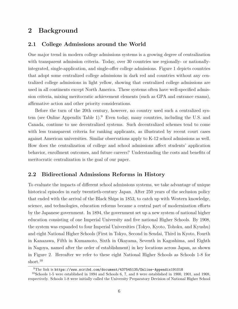
One major trend in modern college admissions systems is a growing degree of centralizationwith transparent admission criteria. Today, over 30 countries use regionally- or nationally-integrated, single-application, and single-offer college admissions. Figure 1 depicts countriesthat adopt some centralized college admissions in dark red and countries without any cen-tralized college admissions in light yellow, showing that centralized college admissions areused in all continents except North America. These systems often have well-specified admis-sion criteria, mixing meritocratic achievement elements (such as GPA and entrance exams),affirmative action and other priority considerations.

Before the turn of the 20th century, however, no country used such a centralized sys-tem (see Online Appendix Table 1).9 Even today, many countries, including the U.S. andCanada, continue to use decentralized systems. Such decentralized schemes tend to comewith less transparent criteria for ranking applicants, as illustrated by recent court casesagainst American universities. Similar observations apply to K-12 school admissions as well.How does the centralization of college and school admissions affect students’ applicationbehavior, enrollment outcomes, and future careers? Understanding the costs and benefits ofmeritocratic centralization is the goal of our paper.

2.2 Bidirectional Admissions Reforms in History

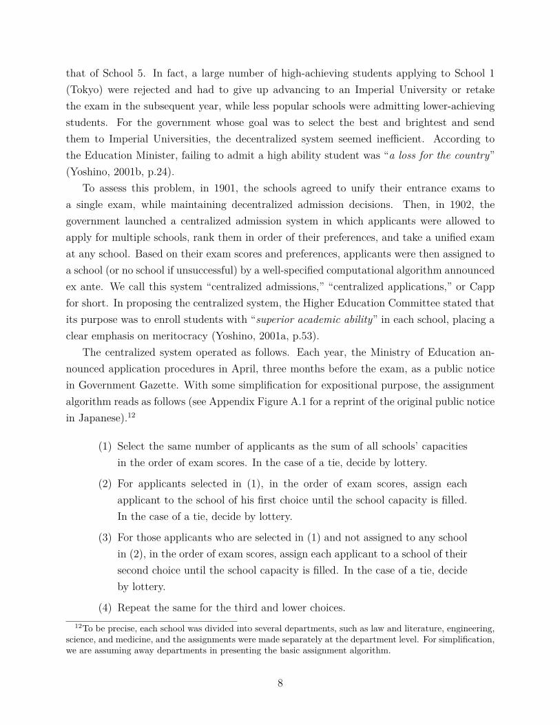
To evaluate the impacts of different school admissions systems, we take advantage of uniquehistorical episodes in early twentieth-century Japan. After 250 years of the seclusion policythat ended with the arrival of the Black Ships in 1853, to catch up with Western knowledge,science, and technologies, education reforms became a central part of modernization effortsby the Japanese government. In 1894, the government set up a new system of national highereducation consisting of one Imperial University and five national Higher Schools. By 1908,the system was expanded to four Imperial Universities (Tokyo, Kyoto, Tohoku, and Kyushu)and eight National Higher Schools (First in Tokyo, Second in Sendai, Third in Kyoto, Fourthin Kanazawa, Fifth in Kumamoto, Sixth in Okayama, Seventh in Kagoshima, and Eighthin Nagoya, named after the order of establishment) in key locations across Japan, as shownin Figure 2. Hereafter we refer to these eight National Higher Schools as Schools 1-8 forshort.10

9The link is https://www.scribd.com/document/437545135/Online-Appendix19101810Schools 1-5 were established in 1894 and Schools 6, 7, and 8 were established in 1900, 1901, and 1908,

respectively. Schools 1-8 were initially called the University Preparatory Devision of National Higher School

6

Schools 1-8 served as an exclusive entry point to Imperial Universities (the most presti-gious form of tertiary education). Virtually all graduates of Schools 1-8 were admitted tothese universities without further selection well into the 1920s. Imperial University gradu-ates were also partially or wholly exempted from the Higher Civil Service Examinations andother selective national qualification exams to become high-ranking administrators, diplo-mats, judges, and physicians (Amano, 2007). As a result, entering Schools 1-8 was consid-ered equivalent to obtaining a passport into the elite class. In fact, Schools 1-8 are knownto have produced highly distinguished and socially influential individuals, including severalPrime Ministers, Nobel Laureates, world-leading mathematicians, renowned novelists, andthe founders of global companies like Toyota. To apply to these schools, one must be maleaged 17 or older and have completed a five-year middle school.11 As Schools 1-8 admittedfewer than 2,300 students each year throughout 1900–1930, they constituted less than 0.5%of the cohort of males aged 17.

The admission to Schools 1-8 was merit-based and determined by annual entrance exams.Initially, the government took a laissez-faire approach and let each school administer its ownexam and admissions. Schools 1-8 typically held their exams on the same day so thateach applicant could only apply to one school. Following the convention in the literature(Che and Koh, 2016; Hafalir et al., 2018), we call this system “decentralized admissions,”“decentralized applications,” or Dapp for short. The single choice aspect of Dapp capturesan essential feature of decentralization, which incentivizes each applicant to self-select intoan appropriate school by comparing the selectivity of schools with his own standing.

Among the eight schools, School 1 in Tokyo was considered by far the most prestigiousdue to its location in the capital and geographical proximity to Tokyo Imperial University(today’s University of Tokyo). The next most prestigious was School 3 in Kyoto. By contrast,located in a remote southwest region, Schools 5 and 7 were considered the least prestigiousamong all schools. Consequently, the schools differed substantially in their popularity andselectiveness (Takeuchi, 2011, Chapter 2). For example, the acceptance rate (i.e., the shareof admitted applicants in all applicants) of School 1 (Tokyo) was always much lower than

(kan-ei koutou gakkou daigaku yoka) in 1894–1916 and were renamed National Higher School (kan-ei koutougakkou) in 1917. Despite the growing demand for national higher education, due to fiscal constraints, thenumber of National Higher Schools remained constant until 1918. From 1918 to 1925, the number of NationalHigher Schools gradually increased from 8 to 25, but Schools 1-8 remained the most distinguished among all25 schools. In addition to Schools 1-8, there was a quasi-national school, Yamaguchi Higher School, whichwas established in 1894, discontinued in 1904, and re-established in 1918. The number of higher educationinstitutions increased after 1918, as the government permitted not only national but also local public andprivate higher schools and universities. In our empirical analyses, we control for the number of nationalhigher schools as well as other higher education institutions.

11The eligibility was changed in 1919 to males aged 16 or older who have completed the fourth year ofmiddle school.

7

that of School 5. In fact, a large number of high-achieving students applying to School 1(Tokyo) were rejected and had to give up advancing to an Imperial University or retakethe exam in the subsequent year, while less popular schools were admitting lower-achievingstudents. For the government whose goal was to select the best and brightest and sendthem to Imperial Universities, the decentralized system seemed inefficient. According tothe Education Minister, failing to admit a high ability student was “a loss for the country”(Yoshino, 2001b, p.24).

To assess this problem, in 1901, the schools agreed to unify their entrance exams toa single exam, while maintaining decentralized admission decisions. Then, in 1902, thegovernment launched a centralized admission system in which applicants were allowed toapply for multiple schools, rank them in order of their preferences, and take a unified examat any school. Based on their exam scores and preferences, applicants were then assigned toa school (or no school if unsuccessful) by a well-specified computational algorithm announcedex ante. We call this system “centralized admissions,” “centralized applications,” or Cappfor short. In proposing the centralized system, the Higher Education Committee stated thatits purpose was to enroll students with “superior academic ability” in each school, placing aclear emphasis on meritocracy (Yoshino, 2001a, p.53).

The centralized system operated as follows. Each year, the Ministry of Education an-nounced application procedures in April, three months before the exam, as a public noticein Government Gazette. With some simplification for expositional purpose, the assignmentalgorithm reads as follows (see Appendix Figure A.1 for a reprint of the original public noticein Japanese).12

(1) Select the same number of applicants as the sum of all schools’ capacitiesin the order of exam scores. In the case of a tie, decide by lottery.

(2) For applicants selected in (1), in the order of exam scores, assign eachapplicant to the school of his first choice until the school capacity is filled.In the case of a tie, decide by lottery.

(3) For those applicants who are selected in (1) and not assigned to any schoolin (2), in the order of exam scores, assign each applicant to a school of theirsecond choice until the school capacity is filled. In the case of a tie, decideby lottery.

(4) Repeat the same for the third and lower choices.12To be precise, each school was divided into several departments, such as law and literature, engineering,

science, and medicine, and the assignments were made separately at the department level. For simplification,we are assuming away departments in presenting the basic assignment algorithm.

8

Written more than a century ago in natural language, the rules were described with math-ematical precision. Observe that the above method imposes meritocracy up front in whichonly top-scoring applicants were considered for admission regardless of their preferences (Step(1)). This step selects only applicants who would be admitted by any school under the SerialDictatorship (Deferred Acceptance) algorithm, one of the most widely used algorithms intoday’s college and selective K-12 admissions. These applicants are then assigned to one ofSchools 1-8 using the Immediate Acceptance (Boston) algorithm (Steps (2) to (4)). Thisalgorithm is therefore a variant of the Immediate Acceptance algorithm with a meritocracyconstraint, making it closer to the Serial Dictatorship (Deferred Acceptance) algorithm. Tothe best of our knowledge, this is the world’s first recorded nation-wide use of a matchingalgorithm.13

This institutional innovation was short-lived, however. Due to political and administra-tive reasons, the government switched back to Dapp (with a unified exam) in 1908. Thegovernment then continued to oscillate between decentralization and centralization, reintro-ducing Capp in 1917, moving back to Dapp (with a unified exam) in 1919, reinstitutingCapp (with major modifications of allowing applicants to list at most two schools) in 1926,and finally settling down to Dapp (with separate exams) in 1928. In a space of thirty years,therefore, there were three periods of centralized admissions: first in 1902–1907, next in1917–1918, and finally in 1926–1927.

According to historical studies, these repeated policy changes were the results of intensebargaining between the Ministry of Education, who pushed for centralization to advancemeritocracy, and the Council of School Principals, who preferred decentralization to protectschool autonomy and regional interests (Yoshino, 2001a,b; Takeuchi, 2011; Amano, 2017).We exploit this series of bidirectional policy changes to identify the impacts of centralizationon the selection of students and their career outcomes.14

3 Theory

To guide our empirical investigation, we develop a model to predict the impacts of central-ization on application behavior and assignment. We first confirm that centralized admissions(Capp) was indeed designed to make the school seat allocation more meritocratic compared

13See Appendix A.1 for the actual admission outcomes in 1917 under the above centralized algorithm.14These historical episodes are well known among historians of Japanese education, who provide detailed

institutional accounts (e.g., Yoshino, 2001a,b; Takeuchi, 2011; Amano, 2017). The preceding studies, how-ever, are mostly descriptive and qualitative. An important exception is Miyake (1998, 1999), who examinesregional variations in access to higher schools and compares the number of higher school students per pop-ulation across prefectures. Building on these studies, we combine a formal model and quasi-experimentalresearch design to identify the causal effects of admission reforms.

9

to decentralized admissions (Dapp). Our model also has two predictions about applicationbehavior. First, a greater number of applicants apply to the most popular school underCapp than under Dapp. Second, applicants make more inter-regional applications underCapp relative to Dapp, thus breaking the “local monopoly” of each school in its local area.

A school admission problem is (S, I, q, (ti)i∈I ,�) where S = {s1, . . . , sm} is the set ofschools while I = {i1, . . . , in} is the set of students. Motivated by our empirical setting,schools’ common priority order over students is based on test scores (ti)i∈I ∈ Rn

+ (the higherthe better). Without loss of generality, sort students so that tij > tik if j < k. We alsoassume that all students are acceptable for any school, which, in our institutional setting,is true conditional on the pool of eligible applicants. A capacity vector is q = (qs1 , . . . , qsm)

where qs is the number of students school s can accommodate. The profile of student (strict)reported preferences is �= (�i1 , . . . ,�in) defined over S∪{o} where o is the outside option.Let Pi denote the set of all possible preference relations for student i. P = ×i∈IPi is the setof all preference profiles. Let �, �′ and so on denote students’ reported preference profiles.

The outcome of a school admission problem is a matching ν : I → S∪I where ν(i) meansthe school that admits student i (or no assignment if ν(i) = i) with the following properties.

• ν(i) 6∈ S =⇒ ν(i) = i for every i ∈ I, and

•∣∣ν−1(s)

∣∣ ≤ qs for every s ∈ S.

A mechanism is a systematic procedure that determines a matching for each reported prefer-ence profile. Formally, it is a function µ : P → M where M denotes the set of all matchings.Let µs(�) denote the set of students assigned to s in mechanism µ for reported preferenceprofile �. Let µC be the Capp mechanism introduced in Section 2.

We compare mechanisms with a thought experiment where the same set of applicants withthe same true preferences and test scores participate in different mechanisms. Applicantsmay change their preference reports, depending on which mechanism they participate in.The set of schools and their capacities are assumed to stay constant. Index each school seatby j = 1, . . . , k ≡

∑i∈S qi. Let tµ(�)(j) be the test score of the student assigned to seat j

under mechanism µ for preference profile �. tµ(�)(j) = 0 if no student is assigned to seat j.Let Fµ(�) be the cumulative distribution of test scores among assigned students under anymechanism µ for preference profile �, defined as

Fµ(�)(t) =

∣∣{j ∈ {1, . . . , k} | tµ(�)(j) ≤ t}∣∣

k

for all t ∈ R+.

10

As should be the case given the official goal of centralization, Capp is more meritocraticthan any other mechanism, especially Dapp, in that Capp induces a first-order-stochastic-dominance improvement of the test score distribution among admittees.

Proposition 1. For any school admission problem and any mechanism µ, we have FµC(�)(t) ≤Fµ(�′)(t) for all t ∈ R+ and �,�′∈ P .

This fact implies that the worst test score among assigned students under Capp is weaklybetter than that under any other mechanism, including Dapp. Proposition 4 in AppendixA further shows that in terms of the test score distribution, Capp is as meritocratic as thepossibly most meritocratic mechanism, i.e., the Serial Dictatorship or Deferred Acceptancemechanism.

To derive additional predictions about applicant behavior, we need to impose more struc-tures on the model. We consider a model with two schools s1 and s2 with capacities q1 andq2, respectively, and any number of applicants. Each applicant takes an action under eachmechanism. Under Capp, for example, each applicant submits a preference list �i. UnderDapp, each applicant applies to a school. The mechanism then uses these actions to obtain amatching. This procedure induces a strategic form game, 〈I, (Ai)i∈I ,�o〉. The set of playersis the set of applicants I. The action space of each applicant is Ai. Under Capp, this is theset of all possible preference relations Pi over schools. Under Dapp, this is the set of schoolsS = {s1, s2}. The outcome is evaluated through the true preferences �o= (�o

i1, . . . ,�o

in).Take any mechanism as given. Let A−i denote the set of possible strategy profiles for

all applicants except applicant i. Let i denote remaining unassigned. We define a stochasticdominance relation, denoted sd(�o

i ), on the set of actions Ai as follows: Upon enumeratingS ∪ {i} from best to worst according to �o

i , we define

ai sd(�oi ) a

′i ⇐⇒

t∑l=1

pil(ai, a−i) ≥t∑

l=1

pil(a′i, a−i) for all t and a−i ∈ A−i

where pil(ai, a−i) is the probability that applicant i gets assigned to the l-th best option inS ∪ {i} according to �o

i if he plays action ai, given action profile a−i of other applicants.We say that strategy ai is a dominant strategy if we have ai sd(�o

i ) a′i for all a′i ∈ Ai. This

notation allows us to obtain the following result.

Proposition 2. Suppose that every applicant (1) prefers s1 over s2 and (2) submits thetrue preference whenever it is a dominant strategy. Then the number of applicants whoapply to the most popular school s1 is weakly larger under centralized admissions than underdecentralized admissions.

11

Intuitively, Capp would cause applicants to give a shot at the most prestigious and selectiveschool since Capp gives applicants a chance of acceptance by lower-choice schools afterrejected by the first-choice school.

To obtain the final theoretical prediction, assume that each applicant lives in a school’slocal area. Let nj be the number of students from school sj’s area. Assume the cardinalutility of applicant i from school s to be Uis = Us + V ∗ 1{i is from s’s area}. Applicantscannot observe their test scores when submitting their preferences, which is the case in ourempirical setting. Assume that each applicant believes that every applicant’s test score isindependent and identically distributed, i.e., t ∼iid F (t) for some distribution F . Definep(n, q) as the probability of being one of the top q applicants among n applicants as per i.i.dtest scores, i.e., p(n, q) = min{ q

n, 1} ∗ 1{n > 0}.

As above, Dapp induces strategic form game (I, (Ai)i∈I , (Ui)i∈I). The set of players andthe action space remain the same. The outcome is now evaluated accordingly to cardi-nal utility. Define Ui(.) as the expected payoff of player i at the application stage, i.e.,Ui(ai, a−i) = p(n̄ai , qai) ∗ Uiai if he plays action ai, given action profile a−i of other appli-cants, where n̄a =

∑j∈I 1{aj = a}. A strategy vector a = (a1, . . . , an) is an equilibrium if for

each applicant i ∈ I and each strategy a′i ∈ Ai, we have Ui(a) ≥ Ui(a′i, a−i). An equilibrium

(a1, . . . , an) is called a symmetric equilibrium if ai = aj for all i and j from the same area.We make the following assumptions for the rest of this section:

A1. Every applicant prefers s1 over s2.

A2. Applicants play a symmetric equilibrium, which is assumed to exist.

wj denotes the number of applicants assigned to school sj while wjk denotes the numberof applicants assigned to school sj who come from school sk’s area. Define the proportion ofassigned applicants assigned to their local school as

w11 + w22

w1 + w2

.

Proposition 3. Under assumptions A1 and A2, for sufficiently large V , the proportion ofassigned applicants assigned to their local school is higher under Dapp than under Capp.

Capp therefore reduces the number of local entrants born in the school’s prefecture. Ourempirical investigation starts with testing whether these theoretical predictions hold in thedata.

12

4 Data

To analyze short-run effects of centralization, we collect data on applications, enrollments,and other outcomes by digitalizing several administrative and non-administrative sources.

First, we collect data on the number of applicants and their first choice schools for 1898-1930 from multiple sources: Government Gazettes for 1902; letters exchanged between theMinistry of Education and the Tokyo Imperial University for 1903 and 1904; Yoshino (2001a)for 1907; the Investigation Records of Higher School Entrance Examinations by the Ministryof Education for 1917,1918 and 1927; and the Ministry of Education Yearbook for otheryears (except 1905, 1906, and 1926 for which there are no data). Because the InvestigationRecords of Higher School Entrance Examinations contain more detailed data for 1916 and1917, we collect the number of applicants by their first-choice school, birth prefecture, andthe prefecture of their middle school, for these two years. Birth prefecture is defined by theprefecture of legal domicile registered in Japan’s official family registry system. We includeapplicants born in all 47 prefectures (excluding colonies) in Japan and exclude foreign-bornapplicants.

Second, we newly collect data on the number of entrants (i.e., admitted applicants) byschool, year, and birth prefecture from 1898 to 1930. We use the number of freshmen as aproxy for the number of entrants.15 We collect the number of freshmen by birth prefecture,using the Higher School Student Registers published annually by each school. We includeonly freshman born in 47 prefectures in Japan, excluding foreign-born students and studentsborn in colonies.

Third, we collect data on the number of middle school graduates by year, school type(public or private), and prefecture (defined by the location of middle school) from 1897 to1930, using the Ministry of Education Yearbook. We use these data to control for the supplyof potential applicants as well as the general education level. We also control for the numbersof national, public, and private higher schools by prefecture that were established in additionto Schools 1-8 starting in 1919, using the same source.

Finally, we compute a measure of the geographical mobility of applicants and entrants.Since the finest geographical unit of observation is a prefecture, we define the distancebetween an applicant’s birth prefecture and the school of his first choice by a direct (straight-line) distance between the capital of the birth prefecture and the capital of the prefecturein which the school was located. Similarly, the distance between an entrant’s middle schooland one of Schools 1-8 he was admitted to is defined by a direct distance between the two

15Strictly speaking, the number of freshman may differ from the number of entrants due to dropouts andholdovers.

13

prefectural capitals determined by the prefectural locations of the middle school and theSchool 1-8. The distance data are from the Geospatial Information Authority of Japan.Descriptive statistics of main variables are summarized in Appendix Table A.2.

5 Short-run Impacts

5.1 Strategic Responses by Applicants

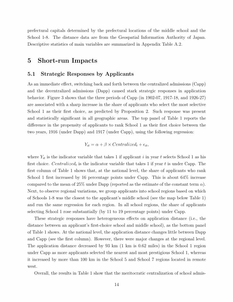
As an immediate effect, switching back and forth between the centralized admissions (Capp)and the decentralized admissions (Dapp) caused stark strategic responses in applicationbehavior. Figure 3 shows that the three periods of Capp (in 1902-07, 1917-18, and 1926-27)are associated with a sharp increase in the share of applicants who select the most selectiveSchool 1 as their first choice, as predicted by Proposition 2. Such response was presentand statistically significant in all geographic areas. The top panel of Table 1 reports thedifference in the propensity of applicants to rank School 1 as their first choice between thetwo years, 1916 (under Dapp) and 1917 (under Capp), using the following regression:

Yit = α + β × Centralizedt + εit,

where Yit is the indicator variable that takes 1 if applicant i in year t selects School 1 as hisfirst choice. Centralizedt is the indicator variable that takes 1 if year t is under Capp. Thefirst column of Table 1 shows that, at the national level, the share of applicants who rankSchool 1 first increased by 16 percentage points under Capp. This is about 64% increasecompared to the mean of 25% under Dapp (reported as the estimate of the constant term α).Next, to observe regional variations, we group applicants into school regions based on whichof Schools 1-8 was the closest to the applicant’s middle school (see the map below Table 1)and run the same regression for each region. In all school regions, the share of applicantsselecting School 1 rose substantially (by 11 to 19 percentage points) under Capp.

These strategic responses have heterogeneous effects on application distance (i.e., thedistance between an applicant’s first-choice school and middle school), as the bottom panelof Table 1 shows. At the national level, the application distance changes little between Dappand Capp (see the first column). However, there were major changes at the regional level.The application distance decreased by 93 km (1 km is 0.62 miles) in the School 1 regionunder Capp as more applicants selected the nearest and most prestigious School 1, whereasit increased by more than 100 km in the School 5 and School 7 regions located in remotewest.

Overall, the results in Table 1 show that the meritocratic centralization of school admis-

14

sions induced a greater number of applicants around the nation to rank the most prestigiousschool in Tokyo first and encouraged applicants to make more long-distance applications.As a result, the competition to enter School 1 became even more intense under the cen-tralized system. Appendix Figure A.2 depicts changes in the competitiveness of Schools1-8, measured by the ratio of the number of applicants who select the school as their firstchoice (hereafter first-choice applicants) to the number of entrants to the school. During theperiods of centralized admissions, the ratio spiked at School 1 (Tokyo), increased modestlyat School 3 (Kyoto), and declined sharply at the rest of the schools. For instance, at thesecond introduction of Capp in 1917, School 1 attracted 12 times more first-choice applicants(4,428 in total) than its capacity (361 seats). This implies that only a small fraction of thefirst-choice applicants were admitted to School 1, leaving hundreds of high-scoring applicantsrejected by School 1.

5.2 Regional Mobility in Enrollment

The centralized assignment rule allows high-scoring applicants from the urban area to beadmitted to lower-choice schools, even after being rejected by their first choice.16 As a result,the centralized system is associated with a sharp and discontinuous increase in enrollmentdistance, especially in the first two periods of Capp.17 Figure 4 shows this by plotting theaverage enrollment distance (i.e., the distance between an entrant’s birth prefecture and theschool he entered).

This increase in regional mobility is also visible as a sharp reduction in the number of“local” entrants (defined by entrants who entered schools in their birth prefectures). Weestimate the following regression for each school s separately:

Ypt = β1 × Centralizedt × 1{school s is located in prefecture p}

+ β2 × Centralizedt × 1{school s is 1-100 km away from prefecture p}

+ β3 × Centralizedt × 1{school s is 101-300 km away from prefecture p}

+Xpt + γt + γp + εpt,

where Ypt is the number of entrants born in prefecture p who entered school s in year t.16Recall that under the meritocratic algorithm discussed in Section 2, even for a not-so-selective school,

first-choice applicants will be rejected if their scores are below the threhold and second-choice applicantswith sufficiently high scores will be admitted in their place.

17The centralized mechanism used in the third period of Capp in 1926-27 was qualitatively different fromthat in the first and second periods. Because the number of national higher schools increased from 8 in 1918to 25 by 1926, the schools were divided into two groups and applicants were allowed to choose and rank atmost two schools (one school per group) in 1926-27.

15

Centralizedt is the indicator variable that takes 1 if the system was centralized in yeart. 1{school s is 1-100 km away from prefecture p} is the indicator variable that takes 1 ifschool s is not located in, but within 100 km from prefecture p. Xpt controls for observablecharacteristics of prefecture p and year t, including the number of middle school graduatesfrom prefecture p in year t and the number of higher schools other than School 1-8 inprefecture p in year t. γt and γp are year and prefecture fixed effects.

Capp reduces the number of local entrants born in the school’s prefecture, as shown inTable 2. The coefficients of 1{school s is located in prefecture p} are significantly negativefor all schools. Column 1 shows that the number of School 1 entrants born in Tokyo Pre-fecture declined by 28 under Capp from the average of 103 entrants under Dapp, or a 27%reduction. Most affected was School 7 (where the number of local entrants declined by 49%),while least affected was School 8 (with a decline of 17%). Schools 4-7 experienced reductionsin the number of entrants born not only from the school’s prefecture but also from surround-ing prefectures. In other words, centralization weakened the local monopoly power of eachschool by creating a national market for higher education, consistent with Proposition 3.These results are robust to whether or not to control for prefecture characteristics (resultsavailable upon request).

5.3 Meritocracy vs Equal Regional Access

As established above, centralization reduced the number of applicants who were admittedto their local schools. Then who gained more school seats under the centralized system?Figure 5a plots the change in the number of entrants to Schools 1-8 from Dapp to Capp bybirth prefecture (where blue colors indicate decreases and red colors indicate increases). Thefigure shows that most of the western and northern prefectures lost school seats, while TokyoPrefecture (around School 1) and its surrounding area gained school seats under Capp.

Figure 5b depicts the time evolution of the share of entrants to Schools 1-8 who were bornin the Tokyo area defined as prefectures located within 100 km from Tokyo (see AppendixFigure A.3). The share of Tokyo-area born entrants rose significantly during the years ofcentralization.

More formally, Table 3 compares the effects of Capp on Tokyo-area born entrants and

16

locally-born entrants, by estimating the following equation for each school s:

Ypt = β1 × Centralizedt × 1{prefecture p is Tokyo}

+ β2 × Centralizedt × 1{prefecture p is 1-100 km away from Tokyo}

+ β3 × Centralizedt × 1{prefecture p is 101-300 km away from Tokyo}

+ β4 × Centralizedt × 1{school s is located in prefecture p}

+ β5 × Centralizedt × 1{school s is 1-100 km away from prefecture p}

+ β6 × Centralizedt × 1{school s is 101-300 km away from prefecture p}

+Xpt + γt + γp + εpt,

where Ypt is the number of entrants born in prefecture p who entered school s in year t.Column 1 of Table 3 shows that the number of Tokyo-area-born students admitted to anyof Schools 1-8 increased by 23 under Capp, indicating a 10% increase from the averageof 226 under Dapp. The school-by-school estimates in columns 2-9 reveal that this effectcomes mainly from Tokyo-area born students entering less selective rural schools (Schools4-8).18 In other words, the net effect of Capp is such that the increased inter-regionalapplications caused high-achieving students residing mainly in the Tokyo area to crowd outlower-achieving, rural-born students from their local schools.

5.4 Political Economy of School Admission Reforms

The short-term impacts of centralization highlight a meritocracy-equity tradeoff. On the onehand, the centralized admissions made the school seat allocation more meritocratic, enablinghigh-ability students to enter one of the elite national higher schools even if they failed atentering the most selective one. On the other hand, this meritocracy came at the expenseof equal regional access to higher education, as high-achieving urban applicants dominatedrural applicants.

This meritocracy-equity tradeoff was one of the main reasons why the government wentback and forth between the centralized and decentralized systems. In this section, we brieflydiscuss why centralization was implemented three times (in 1902–07, 1917–18, and 1926–27)and why it was short-lived each time.

Historical evidence indicates that the repeated policy changes were the results of intensebargaining between the Ministry of Education (MOE), who pushed for centralization toadvance meritocracy, and the Council of School Principals (CSP), who preferred decentral-

18The results remain almost the same whether we control for observable prefecture characteristics or not(a table available upon request).

17

ization to protect school autonomy and regional interests of rural schools and communities(Yoshino, 2001a,b; Takeuchi, 2011; Amano, 2007).

When centralizing the school admissions, the MOE repeatedly emphasized the impor-tance of enrolling only the best and brightest to the national higher education system. Theproblem of the decentralized system was that the ability of admitted students varied widelyacross schools depending on the school’s selectiveness.19 With a striking clarity, the Ministerof Education criticized the decentralized system as follows (Education Times No.1146, p.21,published in February 15, 1917):

“[Under the decentralized system] among applicants rejected by School 1 andSchool 3, which attract a large number of high ability applicants, there are manyapplicants whose academic performance is superior to that of applicants admittedto other rural schools. (...) Namely, hundreds of applicants with sufficiently highacademic ability to enter rural schools are idly wasting another year [to retakethe exam]. This is not only a pity for them, but also a loss for the country.”

To maximize the quality of admitted students, the MOE proposed to centralize admis-sions, in which all applicants would take a single unified exam on the same date, all examsheets would be sent to a central exam committee and graded by a single person per questionto ensure fairness, and applicants would be admitted in the order of their exam scores.20

The Council of School Principals strongly opposed to the idea of centralization, however.First of all, the principals deemed it as an intrusion on their power and autonomy.21 Second,the CSP argued that the centralized system was disadvantageous to rural schools in both thequality of entrants and the quality of match between schools and entrants. According to theCSP, under the centralized system, urban schools were able to enroll all the best students,because applicants in all areas tended to rank urban schools as their first choice. As aresult, rural schools lost the most talented students in their local areas who used to enterrural schools under decentralized admissions.22 Moreover, after reviewing the admissionresults of 1917 (the first year of the second centralization period), the CSP found that, inthe prefectures where rural schools were located, the number of middle-school graduates

19Education Times (Kyouiku Jihou) No. 609, p.40, March 15, 1902; No.610, p.29, March 25, 1902; No.1141,pp.17-18, December 25, 1916; No.1146, pp.21, February 15, 1917; No.1151, pp.12-13, April 5, 1917.

20Education Times No. 609, p.40, March 15, 1902; No.610, p.29, March 25, 1902; No.1141, pp.17-18,December 25, 1916.

21Education Times No. 1143, p.21, January 15, 1917; Yoshino (2001b), p.30.22“A Proposal Regarding a Revision of the Entrance Examination Rules” by the CSP submitted to the

MOE in 1906, reprinted in Compendium of Higher Schools, Volume 3: Education (Kyusei Koutou GakkouZensho: Kyouiku-hen), pp.605-607.

18

admitted not only to their local higher school, but also to any higher schools, declinedconsiderably compared to the previous three years under decentralized admissions.23

The CSP further complained that under the centralized system, rural schools must admita sizable number of reluctant and unmotivated students who came to the school as a fallbackoption (“A Proposal Regarding a Revision of the Higher School Entrance Examination Rules”by the CSP submitted to the MOE in 1906):

“Students who entered the school of their second choice or below can never dispela thought that they had to enter that school because of their exam results. Asa result, they are unmotivated to study and have no loyalty to their school.Especially, in those schools that enroll many students who chose the school astheir fourth or fifth choice, these students often have adverse effects on the generalquality of education.”

This was upsetting to rural schools as well as rural communities, as they typically donatedmuch resource when inviting a higher school to their prefectures (Takeuchi (2011), p.56 andpp.106-107).

Finally, the administrative cost of implementing the centralized system was always aserious concern. Both MOE officials and the school principals repeatedly pointed out thedifficulty of grading thousands of exam sheets by a small number of people in a short periodof time and assign these applicants to schools according to the algorithm. Certainly, time andlabor costs of implementing the centralized admissions in the absence of modern computersand photocopying technologies was high.

Reflecting on these issues underlying the unusual series of centralization and its abolitions,a noted historian writes as follows (Takeuchi (2011), p.121):

“Urban applicants “overwhelm” rural applicants by applying for rural schools asfallback options. Urban applicants rob rural applicants of opportunities that wereonce open to them. This ruins the meaning of building national higher schoolsacross the nation.”

This equity-meritocracy tradeoff was one of the reasons why the government oscillated be-tween decentralized and centralized systems, finally settling down to the decentralized systemin 1928.

23Investigative Records of Higher School Entrance Examinations in 1917, p.40, published by the MOE;Education Times No. 1190, p.18, May 5, 1918.

19

5.5 Other Institutional Changes

Before moving on to long-term effects, we discuss potential threats to our analysis, especiallywhether changes in other institutional factors could explain away our short-run results. Ouranalysis takes the timing of the reforms as exogenous, which raises a few concerns. The firstconcern is that if there were simultaneous reforms in middle schools, it could affect applicationbehavior. Second, if there were capacity changes at Schools 1-8 that were correlated with theadmission reforms, it could influence application behavior and enrollment outcomes. Thefinal concern is that if the capacity of School 1 increased relative to the capacity of otherschools with the admission reforms, this could explain our findings on application behavior.

We investigate these concerns and confirm that time-series changes in the number ofmiddle school graduates, the total number of entrants to Schools 1-8, and the share ofentrants to School 1 in all entrants are not correlated with centralization periods (columns1-3 in Appendix Table A.3). In columns 4 and 5, we also verify that the number of applicantsas well as the level of competitiveness (measured by the number of entrants divided by thenumber of applicants) do not move systematically with introductions of Capp. In addition, ifthe probability of unsuccessful applicants retaking the exam in subsequent years changes withthe admission reforms, this may also affect our results. As shown in column 6, however, wefind that the average age of entrants does not change with the introductions of centralization.

A potential concern with the above robustness analysis is that the insignificant resultsin Appendix Table A.3 may be due to a small sample size (the number of observationsis around 30). Yet, using the same empirical specification, we find that centralization issignificantly correlated with our main outcome variables (the share of applicants to School1, the enrollment distance, and the share of entrants who were born in the Tokyo area), asshown in columns 7-9 of Appendix Table A.3. Taken together, these results suggest that it isunlikely that our findings are driven by institutional changes other than the school admissionreforms.

Finally, another concern is that the centralization reform introduced not only the meri-tocratic assignment algorithm, but also the unified entrance exam that applicants can takein any of the school locations. The estimated impacts of centralization may be confoundedby the integration of entrance exams and more flexible exam location choices. To investigatethis issue, we analyze how key outcomes change from 1900 to 1901, during which the govern-ment also introduced a single entrance exam that applicants are allowed to take anywherewhile the assignment method remained unchanged (decentralized). Figures 3 and 4 showthat the institutional change between 1900 and 1901 induced little changes in applicationand enrollment patterns. The estimated impacts of centralization are therefore likely due tothe meritocratic assignment algorithm, not other confounders like the content and location

20

of entrance exams.

6 Long-run Impacts

6.1 Long-run Outcome Data

To assess longer-term effects, we use the Japanese Personnel Inquiry Records (JPIR) pub-lished in 1939 as our main data source.24 The JPIR is an equivalent of Who’s Who in Japan,which compiles a highly selective list of distinguished individuals such as high-income earn-ers, imperial medal recipients, top business managers, elite professionals, high-ranking politi-cians, bureaucrats, and military personnels.25 In total, the 1939 JPIR lists 55,742 individualsor 0.15% of the adult Japanese population of that time. In selecting these individuals, theJPIR uses a variety of sources, including the directory of banks and companies, the govern-ment personnel directory, the directory of Japanese notables, and the directory of industrialassociations board members.26

To capture the effects of the first period of the centralized admission system in 1902–1907,we use the cohorts born in 1880–1894, who turned 17 years old (the age eligible for appli-cation) in 1897–1911. The cohorts born in 1880–1894 were 45 to 59 years old in 1939.27

The number of individuals listed in the JPIR in each of these cohorts is about 1,800. Weuse the following information from the JPIR data for each individual: full name, birth date,birth prefecture,28 residing prefecture, final education29, occupational titles and positions,the name of the employer (if applicable), the medal for merit and the court rank awarded(if any), and the amount of national income tax and corporate tax paid.

We define the following (mutually non-exclusive) groups of elites as subsets of JPIR-listedindividuals: (1) top 0.01% and 0.05% income earners,30 (2) medal recipients (individuals

24Digital images of the Japanese Personnel Inquiry Records (Jinji Koushin-roku) are publicly available atthe National Diet Library Digital Collections.

25The JPIR also lists the imperial and peerage families, but they are excluded from our data as we focuson career elites in our analysis.

26The directory of banks and companies includes a list of all directors of banks and companies whose capitalis 300,000 yen or above. The government personnel directory provides a complete list of politicians, militarypersonnels, and civil servants in national and local governments, including Imperial University professors.The directory of Japanese notables includes high tax payers defined by individuals who paid more than 50yen of income tax or more than 80 yen of business tax.

27The average life expectancy at age 20 for males born in 1880–1900 was about 40 years.28The JPIR obtained information about birth date and prefecture from the official family registry system

administered by local governments.29Because final education is typically a university, we are unable to observe which higher school these

individuals attended.30The threshold income tax payments for the top 0.01% and 0.05% income earners are 9,967 yen and

2,385 yen, respectively. For example, 9,967 yen of income tax payment is equivalent to around 50,000 yen

21

who received either the medal of the Fifth Order of Merit or above, or the court rank of theJunior Fifth Rank or above, excluding military personnels),31 (3) professionals (individualswhose occupation is either physician, engineer, lawyer, or scholar), (4) professors at ImperialUniversities (individuals whose occupation is either professor or associate professor at one ofthe Imperial Universities), and (5) managers (individuals employed in a private sector witha positive amount of income or corporate tax payment). Descriptive statistics in AppendixTable A.2 show that these categories are highly selective groups of career elites. For instance,the average number of the top 0.05% income earners per cohort per prefecture is fewer than5 and the total number for the whole country per cohort is just 230. These categoriesencompass social, economic, political, and cultural definitions of career elites, or “upper-tailhuman capital” of the society (Mokyr, 2005).

We use these data to count the number of elites in each group by birth prefecture andcohort. These counts allow us to conduct a difference-in-differences analysis that compareslong-term career outcomes of urban- and rural-born individuals by each cohort’s exposureto the centralized system.

Assessing the Coverage and Bias of the Data

Since the JPIR data is not exhaustive administrative data, we are concerned about potentialsample selection bias. For top income earners and Imperial University professors, we cancompute the exact sampling rates by comparing the number of individuals in the JPIRagainst complete counts reported in government statistics.32 We find that the samplingrates are decent even by modern standards: 53% and 39% for the top 0.01% and top 0.05%income earners, respectively, and 70% for Imperial University professors. Consistent with thenature of the JPIR, which lists only distinguished individuals, the sampling rates increasewith the income level (Appendix Figure A.4).

Sample selection bias becomes a problem for our difference-in-differences analysis only ifthe difference in sampling rates between urban and rural areas changes with cohorts’ exposure

of taxable income. The mean household income in 1936 is estimated to be about 900 yen (Yazawa, 2004).The top 0.01% income group earned about 3% of national income in the 1930s, indicating a high degreeof income concentration at the top of income distribution comparable to that of the U.S. during the sameperiod (Moriguchi and Saez, 2006, 2008).

31In the Japanese honor system, the medals for merit and the court ranks were conferred on individualsin recognition of their exceptional public service or distinguished merit. The medals had 8 grades from theFirst Order of Merit (the highest honor) to the Eighth Order of Merit (the lowest honor), and the courtranks had 16 ranks from Senior First Rank (the highest) to Junior Eighth Rank (the lowest). The highestorders and ranks were awarded mostly to top-ranking military officers, bureaucrats, and politicians, but asmall number of private individuals such as top corporate executives received the Fourth and Fifth Ordersof Merit (Ogawa, 2009).

32The number of high income earners are reported in the Tax Bureau Yearbook, and the number ofImperial University professors are reported in the Ministry of Education Yearbook.

22

to the centralized admission system. To assess this possibility, we examine the prefecture-level JPIR sampling rates for top income earners. As Appendix Figure A.5 shows, the numberof JPIR-listed individuals and the complete count from tax statistics are highly correlated,with similar sampling rates across prefectures. This result provides further support forthe quality of the JPIR data. Even so, one potential concern is that Imperial Universitygraduates might have a higher likelihood of being sampled by the JPIR even after controllingfor the income level. However, we find no positive correlation between the sampling ratesof top income earners in the JPIR data and the numbers of Imperial University graduatesacross prefectures (see Appendix Table A.4). This series of findings suggests that possiblesample selection bias in the JPIR data is unlikely to drive our empirical results.

Finally, we collect and control for a set of time-varying prefecture characteristics. Tocontrol for demographical changes, we collect prefecture-level birth populations for the co-horts born in 1886–1894 from the population census and estimate birth populations for thecohorts born in 1880-1885 using age-specific population data available in 1876-1894. To con-trol for local economic conditions, we take prefecture-level manufacturing GDP estimates in1874, 1890, 1909, and 1925 from Tangjun et al. (2009) and interpolate them linearly for eachprefecture. To control for changes in middle schools, we collect the number of middle schoolgraduates in each prefecture in the year when the cohort became age 16.

6.2 Regional Disparity in Producing Career Elites

We estimate the long-run impacts of the centralized school admissions (Capp), by conductinga difference-in-differences analysis by birth cohorts and birth areas. The key idea behindour empirical strategy is that applicants born in the Tokyo area should experience a greatergain in entering Schools 1-8 under Capp relative to Dapp, since the centralized system isdesigned to be more meritocratic and high-achieving students are disproportionately locatedin urban areas. Figure 5 and Table 3 confirm this expectation. We exploit this differentialgain in school access to compare the career outcomes of individuals born inside and outsidethe Tokyo area by the cohort’s exposure to Capp. If admission to Schools 1-8 increases one’schance of becoming a career elite, we should observe a greater number of elites born insidethe Tokyo area for the cohorts exposed to Capp.

We estimate a difference-in-differences specification as follows:

Ypt = β × Centralizedt × Urbanp + γp + γt + εpt,

where Ypt is the number of elites listed in the JPIR defined above in cohort t born inprefecture p. Centralizedt is the binary variable that takes 1 if cohort t turned 17 during

23

Capp (1902–1907), Urbanp is the indicator variable that takes 1 if prefecture p is in the Tokyoarea. The prefecture fixed effects γp capture any systematic difference in career outcomesacross prefectures that do not vary across cohorts. The cohort fixed effects γt control forcommon shocks that affect career outcomes in all prefectures as well as secular time trends.To allow for serial correlation of εpt within prefecture over time, we cluster the standarderrors at the prefecture level.33

We define Centralizedt as a binary indicator, as the simplest proxy for the intensity ofexposure to Capp. In reality, however, a nontrivial number of unsuccessful applicants retookthe exam at age 18 and beyond.34 As a result, the cohorts who turned age 17 in 1899–1901were partially and increasingly exposed to Capp (as they might have taken the exam in1902), the cohorts who turned age 17 in 1902–1904 were fully exposed to Capp, and thecohorts who turned age 17 in 1905–1907 were partially and decreasingly exposed to Capp(as they might have taken the exam in 1908), and the intensity of exposure drops to zerofor the cohorts who turned age 17 in 1908. For this reason, we provide a robustness checkby dropping the cohorts who were also partially exposed to Dapp below.

We first check whether the number of Imperial University graduates born inside theTokyo area increased for the cohorts exposed to Capp. Since all Schools 1-8 graduates wereautomatically admitted to an Imperial University during this period, the areas that producedmore Schools 1-8 entrants should produce more Imperial University graduates. Figure 6 (a)compares the average number of Imperial University graduates who were born in prefecturesinside and outside the Tokyo area by cohorts (represented by their birth year plus 17 on thehorizontal axis). In these and subsequent plots, we color cohorts according to their intensityof exposure to Capp as described above. Figure 6 (b) confirms that the urban-rural differencein the number of Imperial University graduates rises as the intensity of exposure to Cappincreases. The difference then falls after the end of Capp in 1908. Column 1 in Table 4shows that the difference-in-difference estimate is positive and statistically significant.

Our main results are presented in Figure 6 (c)–(h) and Table 4 columns 2-7. Figure 6(c)–(h) show difference-in-differences plots that compare the number of the top 0.05% incomeearners, professionals (physicians, engineers, lawyers, and scholars), and medal recipients (theFifth Order of Merit or the Junior Fifth Rank and above) who were born inside and outsidethe Tokyo area by the cohort’s exposure to Capp. Across all elite categories, the plots show

33Bertrand et al. (2004) evaluate approaches to deal with serial correlation within each cross-sectional unitin panel data. They suggest that clustering the standard errors on each cross-section unit performs well insettings with 50 or more cross-section units, as in our setting.

34According to the limited data available, out of all Schools 1-8 entrants in 1903, 63% graduated middleschool in the same year, 29% graduated in the previous year, 6% graduated two years before, and 1%graduated three years before.

24

that the difference between the Tokyo area and the rest grows larger as the intensity ofexposure to Capp increases, and then drops sharply after the end of Capp in 1908.

Table 4 columns 2-7 show that the long-run effects of the centralized admissions are eco-nomically and statistically significant. Panel A controls only for cohorts and prefecture fixedeffects. Panel B additionally controls for time- and cohort-varying prefecture characteristics(i.e., cohort birth population, the number of primary schools, the number of middle schoolgraduates, prefecture-level manufacturing GDP). The coefficients fall slightly in magnitudeafter adding control variables, but remain statistically significant. For the cohorts exposed toCapp, the number of career elites born inside the Tokyo area (compared to those born outsidethe Tokyo area) increases by 23% for the top 0.05% income earners, 36% for the top 0.01%income earners, 19% for managers, and 11% for professionals, 44% for Imperial Universityprofessors, and 35% for medal recipients (in Panel B).35 Panels C and D show that the effectsare symmetric with respect to the direction of the admission reforms, i.e., the change fromDapp to Capp and the change from Capp to Dapp produce quantitatively similar effects ofthe opposite sign. These results suggest that almost four decades after its implementation,the centralized admission system had lasting effects on the career trajectories of students.

The above results are robust to alternative specifications. First, the above analysisassumes that the cohorts who turned age 17 in 1902–1907 are fully exposed to Capp whilethe rest of the cohorts are fully exposed to Dapp. Even when we drop the cohorts whoare heavily exposed to both Capp and Dapp (i.e., cohorts who became age 17 in 1901 and1907) from the sample, we still find qualitatively the same results with higher statisticalsignificance (see Appendix Table A.5).

Second, we test if the assumption of parallel pre-event trends holds. Appendix Table A.6verifies that the differences in pre-event trends between the areas of comparison are smalland statistically insignificant for all of our outcome variables.

Another potential threat to our identification strategy is that there may be some age-specific trends in the number of JPIR-listed elites that differ across regions and covary withthe cohort-region variation we use. Specifically, the number of observations in the 1939 JPIRdata peaks at around the cohort who were 51 years old in 1939 (corresponding to the cohortwho turned age 17 in 1905) and gradually falls for younger and older cohorts, suggestingthat there are certain ages at which individuals are more likely to be listed in the JPIR.Such age effects may generate different trends in the number of elites born in the Tokyoand other areas, due, for example, to differences in population size across these areas. To

35For professionals, as shown in Appendix Table A.8, even if we look at each occupation separately (i.e.,scholars, physicians and lawyers, engineers), the results remain similar, but with lower precision due tosmaller sample size. The last column of Appendix Table A.8 further shows that a similar result holds forhigh-ranking government officials.

25

address this concern, we use the earlier edition of the JPIR published in 1934, construct theprefecture-cohort level data for the same cohorts used in our main analysis (but observed 5years earlier), and conduct similar regression analyses. The results in Appendix Table A.7confirm that our key results remain qualitatively the same even if we use the 1934 JPIRdata.

Finally, we conduct placebo tests to examine if the results are driven by other factorssuch as the sample selection of the JPIR or changes in cohort populations. Column 5confirms that the urban-rural difference in the cohort’s birth populations do not changesignificantly with the cohort’s exposure to Capp. As an additional placebo test, we also lookat unrelated career outcomes. Among the elites listed in the JPIR, we expect that landlords(defined as individuals whose occupational titles includes landlord, but excluding managersand professionals) are least likely to be affected by the introduction of Capp as receivinghigher education was not a typical pathway to becoming a landlord. As shown in column 4of Table 5, the estimated effect of Capp on the number of landlords is small and statisticallyinsignificant. .

Understanding the Mechanism behind the Long-run Impacts

Next, we explore potential mechanisms through which centralization affect career outcomes.First, in columns 1 and 2 of Table 5, we test if centralization, which caused substantial inter-regional mobility in the short-run outcomes, increased the geographical mobility of elitesin a long run. Somewhat surprisingly, the results indicate that it did not: The urban-ruraldifference in the fraction of elites whose residing prefectures differ from their birth prefecturesdid not significantly increase under Capp. We find similar results when we use the distancebetween an elite’s birth prefecture and his residing prefecture as an alternative measure oflong-run mobility. This result suggests that, even though a greater number of students bornin the Tokyo area entered rural schools under Capp, most of them might have returned tothe Tokyo area when pursuing their careers.

We also test whether centralization affected the urban-rural gap in the quality of Schools1-8 entrants (in addition to its quantity). As a quality measure, we use the ratio of thenumber of Imperial University graduates listed in the JPIR to the total number of Schools1-8 entrants when the cohort became age 17. We hypothesize that if the quality of entrantsis higher, then a larger fraction of them would be selected into the JPIR in their adulthoods.The estimated coefficients in column 3 are negative and insignificant. Our main results inTable 4 are therefore likely driven by an increase in the quantity, but not the quality, ofSchools 1-8 entrants from urban areas (relative to those from rural areas) under Capp.

26

Geographical Destinations of Career Elites

Having established that the centralized admission system affected the geographic originsof highly educated individuals, we now ask how it affected their geographic destinations.While the former is about regional inequality in educational opportunities, the latter isabout regional inequality in the supply of highly skilled human capital, which potentiallyaffects both regional and aggregate economic growth and inequality. If a greater numberof students who were born in the Tokyo area and admitted to rural schools under Cappeventually returned to the Tokyo area for their subsequent careers, we should observe agreater number of elites living in the Tokyo area for the cohorts exposed to Capp. To testthis hypothesis, we change the outcome variables by re-defining the prefecture (p) from birthprefecture to residing prefecture and estimate the equation with the same specification.

Table 6 shows positive effects of Capp on the urban-rural gap in the number of resid-ing elites, although some of the coefficients come with large standard errors and are notstatistically significant. For the cohorts exposed to Capp relative to Dapp, the number ofelites living in the Tokyo area in their middle age (compared to those living outside theTokyo area) increases by 16% for Imperial University graduates, 13% for professionals, and23% for medal recipients (Panel B). These results suggest that the centralized system likelyintensified the concentration of career elites in urban areas relative to rural areas in the longrun.

7 Conclusion

The design of school admissions persistently impacts the geography of career elites. We revealthis fact by looking at the world’s first recorded use of nationally centralized admissions andits subsequent abolitions in early twentieth-century Japan. While centralization was designedto make the school seat allocations more meritocratic, there turns out to be a tradeoff betweenmeritocracy and equal regional access to higher education and career success. In line with atheoretical prediction, the meritocratic centralization led students to apply to more selectiveschools and make more inter-regional applications. As high ability students were locateddisproportionately in urban areas, however, centralization caused urban applicants to crowdout rural applicants from advancing to higher education. Most importantly, these impactspersisted in the long run: Several decades later, the meritocratic centralization increased thenumber of high income earners, medal recipients, and other elite professionals born in urbanareas relative to those born in rural areas.

Though our study uses the admission reforms unique to Japan, the implications of our

27

study might be relevant for other contexts. For instance, distributional consequences of cen-tralized admissions may be a reason why many countries continue to use seemingly inefficientdecentralized college admissions. Methodologically, the use of natural experiments in historymay be also valuable for studying the long-run effects of market designs in other areas, suchas housing, labor, and health markets.

It is the multiple bidirectional policy changes in history that allow us to measure the long-run effects. The disadvantage of using historical events, however, is the limited availabilityof data. The ideal way to alleviate the data concerns would be to use modern administrativedata. For example, one may imagine linking administrative tax return data and schooldistrict data to measure the long-run effects of school choice reforms in the past few decades.Such an effort would be a fruitful complement to our historical study.

28

ReferencesAbdulkadiroglu, Atila, Joshua D Angrist, Yusuke Narita, and Parag A Pathak, “Breaking Ties:

Regression Discontinuity Design Meets Market Design,” 2019.

Abdulkadiroğlu, Atila and Tayfun Sönmez, “School Choice: A Mechanism Design Approach,” Amer-ican Economic Review, 2003, 93, 729–747.

, Nikhil Agarwal, and Parag A. Pathak, “The Welfare Consequences of Coordinated School Assign-ment: Evidence from the NYC High School Match,” American Economic Review, 2017.

, Parag A. Pathak, Alvin E. Roth, and Tayfun Sönmez, “Changing the Boston School ChoiceMechanism,” 2006. Working Paper.

, , and , “Strategy-proofness versus Efficiency in Matching with Indifferences: Redesigning the NewYork City High School Match,” American Economic Review, 2009, 99(5), 1954–1978.

Agarwal, Nikhil, “Policy Analysis in Matching Markets,” American Economic Review, 2017, 107 (5),246–50.

Altonji, Joseph G, Erica Blom, and Costas Meghir, “Heterogeneity in Human Capital Investments:High School Curriculum, College Major, and Careers,” Annual Review of Economics, 2012, 4 (1), 185–223.

Amano, Ikuo, Social History of Examination (In Japanese), Heibon-sha, 2007.

, Imperial Universities: Elite Factory in Modern Japan (In Japanese), Chuou-kouron-shinsha, 2017.

Arcidiacono, Peter and Michael Lovenheim, “Affirmative Action and the Quality-fit Trade-off,” Jour-nal of Economic Literature, 2016, 54 (1), 3–51.

Autor, David, “Work of the Past, Work of the Future,” in “Richard T. Ely Lecture given at Annual Meetingof American Economics Association, Atlanta, GA, January,” Vol. 4 2019.

Avery, Christopher, Soohyung Lee, and Alvin E Roth, “College Admissions as Non-Price Competi-tion: The Case of South Korea,” 2014. Working Paper.

Bai, Ying and Ruixue Jia, “Elite Recruitment and Political Stability: the Impact of the Abolition ofChina’s Civil Service Exam,” Econometrica, 2016, 84 (2), 677–733.

Bertrand, Marianne, Esther Duflo, and Sendhil Mullainathan, “How Much Should We TrustDifferences-in-differences Estimates?,” Quarterly Journal of Economics, 2004, 119 (1), 249–275.

Beuermann, Diether, C Kirabo Jackson et al., “Do Parents Know Best?: The Short and Long-RunEffects of Attending The Schools that Parents Prefer,” 2018. NBER Working Paper No. 24920.

Bleakley, Hoyt and Joseph Ferrie, “Land Openings on the Georgia Frontier and the Coase Theorem inthe Short and Long Run,” 2014. Working Paper.

and , “Shocking Behavior: Random Wealth in Antebellum Georgia and Human Capital AcrossGenerations,” Quarterly Journal of Economics, 2016, 131 (3), 1455–1495.

29

Börner, Lars and John William Hatfield, “The Design of Debt-Clearing Markets: Clearinghouse Mech-anisms in Preindustrial Europe,” Journal of Political Economy, 2017, 125 (6), 1991–2037.

Calsamiglia, Caterina, Guillaume Haeringer, and Flip Kljin, “Constrained School Choice: An Ex-perimental Study,” American Economic Review, 2010, 100(4), 1860–74.

Carvalho, José Raimundo, Thierry Magnac, and Qizhou Xiong, “College Choice, Selection andAllocation Mechanisms: A Structural Empirical Analysis,” Quantitative Economics, 2019.

Che, Yeon-Koo and Youngwoo Koh, “Decentralized College Admissions,” Journal of Political Economy,2016, 124 (5), 1295–1338.

Chen, Yan and Onur Kesten, “Chinese College Admissions and School Choice Reforms: A TheoreticalAnalysis,” Journal of Political Economy, 2017, 125 (1), 99–139.

Currie, Janet and Enrico Moretti, “Mother’s Education and the Intergenerational Transmission ofHuman Capital: Evidence from College Openings,” Quarterly Journal of Economics, 2003, 118 (4),1495–1532.

Dale, Stacy Berg and Alan B Krueger, “Estimating the Payoff to Attending a More Selective College:An Application of Selection on Observables and Unobservables,” Quarterly Journal of Economics, 2002,117 (4), 1491–1527.

Dell, Melissa, “The Persistent Effects of Peru’s Mining Mita,” Econometrica, 2010, 78 (6), 1863–1903.

and Sahar Parsa, “Managerial Talent and Economic Performance: Evidence from Discontinuities inDouglas MacArthur’s Economic Purge,” 2019. Working Paper.

Deming, David, Justine Hastings, Thomas Kane, and Douglas Staiger, “School Choice, SchoolQuality and Postsecondary Attainment,” American Economic Review, 2014, 104(3), 991–1013.

Dobbie, Will and Roland G. Fryer, “The Impact of Attending a School with High-Achieving Peers:Evidence from the New York City Exam Schools,” American Economic Journal: Applied Economics,2013.

Donna, Javier and José-Antonio Espín-Sánchez, “The Illiquidity of Water Markets: Efficient Institu-tions for Water Allocation in Southeastern Spain,” Available at SSRN 2667654, 2018.

Duflo, Esther, “Schooling and Labor Market Consequences of School Construction in Indonesia: Evidencefrom an Unusual Policy Experiment,” American Economic Review, 2001, 91 (4), 795–813.

Glaeser, Edward, Triumph of the City, Pan, 2011.

Greif, Avner, “Contract Enforceability and Economic Institutions in Early Trade: The Maghribi Traders’Coalition,” American Economic Review, 1993, pp. 525–548.

Grenet, Julien, Yinghua He, and Dorothea Kübler, “Decentralizing Centralized Matching Markets:Implications from Early Offers in University Admissions,” 2019. Working Paper.

30

Haeringer, Guillaume and Flip Klijn, “Constrained School Choice,” Journal of Economic Theory, 2009,144, 1921–1947.

Hafalir, Isa, Rustamdjan Hakimov, Dorothea Kuebler, and Morimitsu Kurino, “College Admis-sions with Entrance Exams: Centralized versus Decentralized,” Journal of Economic Theory, 2018.

Hastings, Justine, Christopher Neilson, and Seth Zimmerman, “Are Some Degrees Worth Morethan Others? Evidence from College Admission Cutoffs in Chile,” 2013. Working Paper.

Hoxby, Caroline M, The Economics of School Choice, University of Chicago Press, 2007.

Kamada, Yuichiro and Fuhito Kojima, “Efficient Matching under Distributional Constraints: Theoryand Applications,” American Economic Review, 2015, 105 (1), 67–99.

Kirkeboen, Lars, Edwin Leuven, and Magne Mogstad, “Field of Study, Earnings, and Self-Selection,”Quarterly Journal of Economics, 2016, 131, 1551–1552.

Knight, Brian and Nathan Schiff, “Reducing Frictions in College Admissions: Evidence from the Com-mon Application,” 2019.

Kranton, Rachel and Anand V Swamy, “Contracts, Hold-up, and Exports: Textiles and Opium inColonial India,” American Economic Review, 2008, 98 (3), 967–89.

Lucas, Adrienne and Isaac Mbiti, “Effects of School Quality on Student Achievement: DiscontinuityEvidence from Kenya,” American Economic Journal: Applied Economics, 2014, 6(3), 234–263.

Machado, Cecilia and Christiane Szerman, “Centralized Admissions and the Student-College Match,”2017. Working Paper.

Meghir, Costas and Marten Palme, “Educaitonal Reform, Ability, and Family Background,” AmericanEconomic Review, 2005, 95(1), 414–424.

Miyake, Sono, “Regional Difference in Access to Higher Schools during the Late Meiji Era (in Japanese),”Socio-Cultural Studies of Education, 1998, 5, 35–52.

, “Regional Difference in Attaining High Academic Career: From an Analysis of Higher School Enrollmentin Taisho Era (in Japanese),” Bulletin of the Graduate School of Education at Kyoto University, 1999.

Mokyr, Joel, “Long-Term Economic Growth and the History of Technology,” in “Handbook of economicgrowth,” Vol. 1, Elsevier, 2005, pp. 1113–1180.

Moretti, Enrico, The New Geography of Jobs, Houghton Mifflin Harcourt, 2012.

Moriguchi, Chiaki and Emmanuel Saez, “The Evolution of Income Concentration in Japan, 1886-2002:Evidence from Income Tax Statistics,” 2006. NBER Working Paper 12558.

and , “The Evolution of Income Concentration in Japan, 1886–2005: Evidence from Income TaxStatistics,” Review of Economics and Statistics, 2008, 90 (4), 713–734.

31

Niederle, Muriel and Alvin E Roth, “Unraveling Reduces Mobility in a Labor Market: Gastroenterologywith and without a Centralized Match,” Journal of Political Economy, 2003, 111 (6), 1342–1352.

Ogawa, Kenji, Sociology of the Medals (in Japanese), Shoyo Shobo; Kyoto, 2009.

Oreopoulos, Philip, “Estimating Average and Local Average Treatment Effects of Education When Com-pulsory Schooling Laws Really Matter,” American Economic Review, 2006, 96 (1), 152–175.

Pallais, Amanda, “Small Differences That Matter: Mistakes in Applying to College,” Journal of LaborEconomics, 2015, 33 (2), 493–520.

Pathak, Parag A. and Tayfun Sönmez, “School Admissions Reform in Chicago and England: ComparingMechanisms by Their Vulnerability to Manipulation,” American Economic Review, 2013, 103(1), 80–106.

Pischke, Jörn-Steffen and Till Von Wachter, “Zero Returns to Compulsory Schooling in Germany:Evidence and Interpretation,” Review of Economics and Statistics, 2008, 90 (3), 592–598.

Pop-Eleches, Cristian and Miguel Urquiola, “Going to a Better School: Effects and Behavioral Re-sponses,” American Economic Review, 2013, 103(4), 1289–1324.

Redding, Stephen J and Daniel M Sturm, “The Costs of Remoteness: Evidence from German Divisionand Reunification,” American Economic Review, 2008, 98 (5), 1766–97.

Roth, Alvin E., “The Evolution of the Labor Market for Medical Interns and Residents: A Case Study inGame Theory,” Journal of Political Economy, 1984, 92, 991–1016.

, “New Physicians: A Natural Experiment in Market Organization,” Science, 1990, 250, 1524–1528.

Shorrer, Ran, “Simultaneous Search: Beyond Independent Successes,” 2019. Working Paper.

Takeuchi, Hiroshi, The Glory and Baffle of Educational Elites (in Japanese), Kodansha, 2011.

Tangjun, Yuan, Settsu Tokihiko, Jean-Pascal Bassino, and Kyoji Fukao, “Gross Prefectural Do-mestic Product and Industrial Structure in Pre-war Japan [in Japanese],” 2009. Working Paper.

Yazawa, Hirotake, Income Distribution and Family Economics in Modern Japan (in Japanese), TokyoBook Center, 2004.

Yoshino, Takehiro, “Entrance Examination of Higher Schools in the Early Taisho Period (in Japanese),”Keio University Studies in Sociology, Psychology, and Education, 2001, (53), p.19–31.

, “Entrance Examination of Higher Schools in the Meiji Period (in Japanese),” Keio University Studiesin Sociology, Psychology, and Education, 2001, (52), p.51–62.

Zimmerman, Seth D, “Elite Colleges and Upward Mobility to Top Jobs and Top Incomes,” AmericanEconomic Review, 2019, 109 (1), 1–47.

32

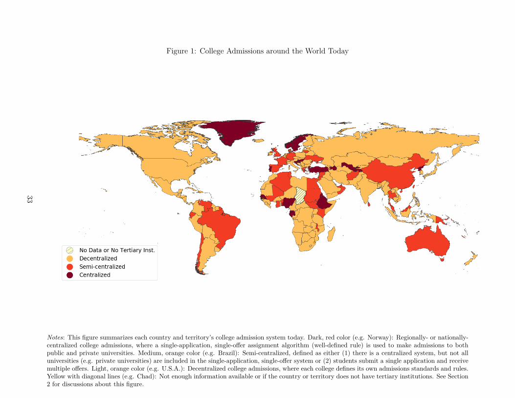
Figure 1: College Admissions around the World Today

Notes: This figure summarizes each country and territory’s college admission system today. Dark, red color (e.g. Norway): Regionally- or nationally-centralized college admissions, where a single-application, single-offer assignment algorithm (well-defined rule) is used to make admissions to bothpublic and private universities. Medium, orange color (e.g. Brazil): Semi-centralized, defined as either (1) there is a centralized system, but not alluniversities (e.g. private universities) are included in the single-application, single-offer system or (2) students submit a single application and receivemultiple offers. Light, orange color (e.g. U.S.A.): Decentralized college admissions, where each college defines its own admissions standards and rules.Yellow with diagonal lines (e.g. Chad): Not enough information available or if the country or territory does not have tertiary institutions. See Section2 for discussions about this figure.

33

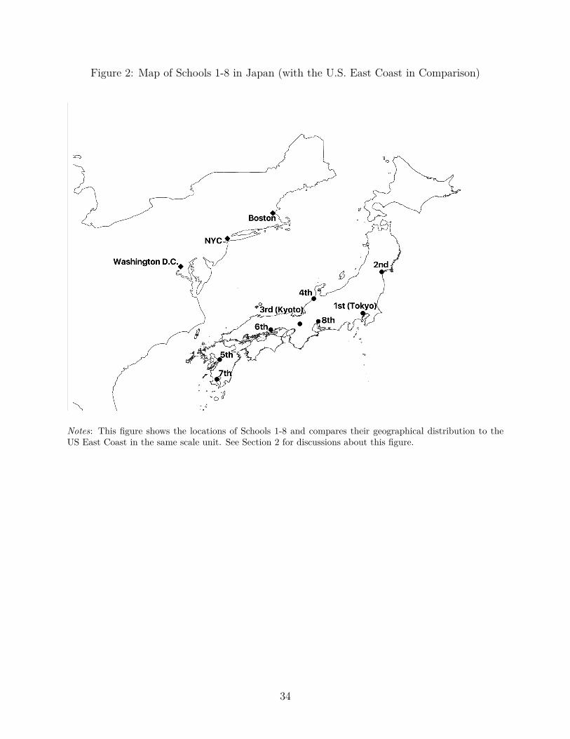
Figure 2: Map of Schools 1-8 in Japan (with the U.S. East Coast in Comparison)

Notes: This figure shows the locations of Schools 1-8 and compares their geographical distribution to theUS East Coast in the same scale unit. See Section 2 for discussions about this figure.

34

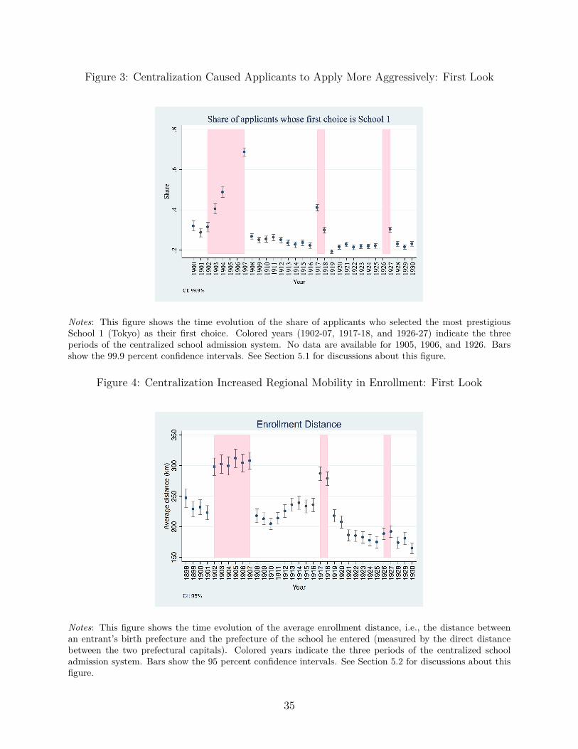
Figure 3: Centralization Caused Applicants to Apply More Aggressively: First Look

Notes: This figure shows the time evolution of the share of applicants who selected the most prestigiousSchool 1 (Tokyo) as their first choice. Colored years (1902-07, 1917-18, and 1926-27) indicate the threeperiods of the centralized school admission system. No data are available for 1905, 1906, and 1926. Barsshow the 99.9 percent confidence intervals. See Section 5.1 for discussions about this figure.

Figure 4: Centralization Increased Regional Mobility in Enrollment: First Look

Notes: This figure shows the time evolution of the average enrollment distance, i.e., the distance betweenan entrant’s birth prefecture and the prefecture of the school he entered (measured by the direct distancebetween the two prefectural capitals). Colored years indicate the three periods of the centralized schooladmission system. Bars show the 95 percent confidence intervals. See Section 5.2 for discussions about thisfigure.

35

Table 1: Centralization Caused Applicants Across the Country to Apply More Aggressively

Dependent var Select School 1 as First Choice

Centralized 0.159*** 0.192*** 0.151*** 0.146*** 0.128 0.168*** 0.180*** 0.166*** 0.114***(0.0106) (0.00924) (0.0329) (0.0232) (0.0646) (0.0245) (0.0336) (0.0136) (0.00786)

Constant 0.248*** 0.494*** 0.169*** 0.0892*** 0.178** 0.107*** 0.184*** 0.0813** 0.127*(0.0717) (0.0437) (0.0357) (0.0162) (0.0373) (0.0185) (0.0218) (0.00991) (0.0508)

Sample region All S1 Region S2 Region S3 Region S4 Region S5 Region S6 Region S7 Region S8 RegionObservations 20,913 6,505 2,555 3,248 1,266 2,730 2,276 615 1,718Dependent var Application Distance

Centralized -2.534 -92.88*** 10.95 2.080 -15.74 128.0*** 46.52** 145.4** -25.57(23.22) (2.888) (24.65) (5.482) (22.92) (23.11) (13.91) (21.27) (18.64)

Constant 226.2*** 231.7*** 289.7*** 158.8*** 166.7* 252.6*** 294.1*** 218.0* 154.2*(15.74) (16.43) (79.51) (28.11) (56.94) (42.52) (51.54) (70.94) (48.89)

Sample region All S1 Region S2 Region S3 Region S4 Region S5 Region S6 Region S7 Region S8 RegionObservations 20,913 6,505 2,555 3,248 1,266 2,730 2,276 615 1,718

Notes: In the first panel, we estimate the effects of centralization on the propensity of an applicant to selectthe most prestigious school (School 1) as his first choice, using the applicant-level data in 1916 (under thedecentralized system) and 1917 (under the centralized system). The prefecture-level application data areavailable only for these two years. We group applicants into “school regions” based on which school (amongSchools 1-8) is nearest to the applicant’s middle school in 1916, where “nearest” is defined by the distancebetween the prefectural capitals. The following map shows the locations of the eight school regions. Thesecond panel measures the effects on the application distance between an applicant’s first-choice school andmiddle school. Standard errors are clustered at the prefecture level. ***, **, and * mean significance at the1%, 5%, and 10% levels, respectively. See Section 5.1 for discussions about this table.

36

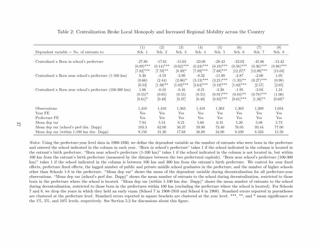
Table 2: Centralization Broke Local Monopoly and Increased Regional Mobility across the Country

(1) (2) (3) (4) (5) (6) (7) (8)Dependent variable = No. of entrants to: Sch. 1 Sch. 2 Sch. 3 Sch. 4 Sch. 5 Sch. 6 Sch. 7 Sch. 8

Centralized x Born in school’s prefecture -27.80 -17.61 -15.63 -23.08 -28.43 -23.02 -45.86 -13.42(0.89)*** (0.14)*** (0.62)*** (0.24)*** (0.19)*** (0.56)*** (0.36)*** (0.86)***[7.82]*** [7.70]** [8.39]* [7.89]*** [7.68]*** [12.27]* [12.98]*** [15.03]

Centralized x Born near school’s prefecture (1-100 km) 0.30 -3.19 -3.99 -9.32 -11.99 -2.87 -2.00 1.05(0.66) (2.44) (2.06)* (3.13)*** (3.21)*** (1.33)** (0.27)*** (0.98)[0.53] [1.38]** [1.03]*** [2.64]*** [3.18]*** [1.02]*** [2.57] [2.65]

Centralized x Born near school’s prefecture (100-300 km) 1.06 -0.10 -0.16 -0.21 -3.30 -1.95 -3.03 1.24(0.55)* (0.65) (0.55) (0.55) (0.91)*** (0.84)** (0.78)*** (1.06)[0.61]* [0.49] [0.37] [0.40] [0.83]*** [0.61]*** [1.26]** [0.69]*

Observations 1,410 1,410 1,363 1,410 1,363 1,363 1,269 1,034Year FE Yes Yes Yes Yes Yes Yes Yes YesPrefecture FE Yes Yes Yes Yes Yes Yes Yes YesMean dep var 7.94 5.54 6.21 5.68 6.31 5.20 5.08 5.73Mean dep var (school’s pref dur. Dapp) 103.3 62.00 56.37 59.90 73.40 76.05 93.44 77.00Mean dep var (within 1-100 km dur. Dapp) 9.150 21.20 17.68 26.88 34.90 8.439 8.333 15.50

Notes: Using the prefecture-year level data in 1900-1930, we define the dependent variable as the number of entrants who were born in the prefectureand entered the school indicated in the column in each year. “Born in school’s prefecture” takes 1 if the school indicated in the column is located inthe entrant’s birth prefecture. “Born near school’s prefecture (1-100 km)” takes 1 if the school indicated in the column is not located in, but within100 km from the entrant’s birth prefecture (measured by the distance between the two prefectural capitals). “Born near school’s prefecture (100-300km)” takes 1 if the school indicated in the column is between 100 km and 300 km from the entrant’s birth prefecture. We control for year fixedeffects, prefecture fixed effects, the lagged number of public and private middle school graduates in the prefecture, and the number of higher schoolsother than Schools 1-8 in the prefecture. “Mean dep var” shows the mean of the dependent variable during decentralization for all prefecture-yearobservations. “Mean dep var (school’s pref dur. Dapp)” shows the mean number of entrants to the school during decentralization, restricted to thoseborn in the prefecture where the school is located. “Mean dep var (within 1-100 km dur. Dapp)” shows the mean number of entrants to the schoolduring decentralization, restricted to those born in the prefectures within 100 km (excluding the prefecture where the school is located). For Schools7 and 8, we drop the years in which they held an early exam (School 7 in 1908-1910 and School 8 in 1908). Standard errors reported in parenthesesare clustered at the prefecture level. Standard errors reported in square brackets are clustered at the year level. ***, **, and * mean significance atthe 1%, 5%, and 10% levels, respectively. See Section 5.2 for discussions about this figure.

37

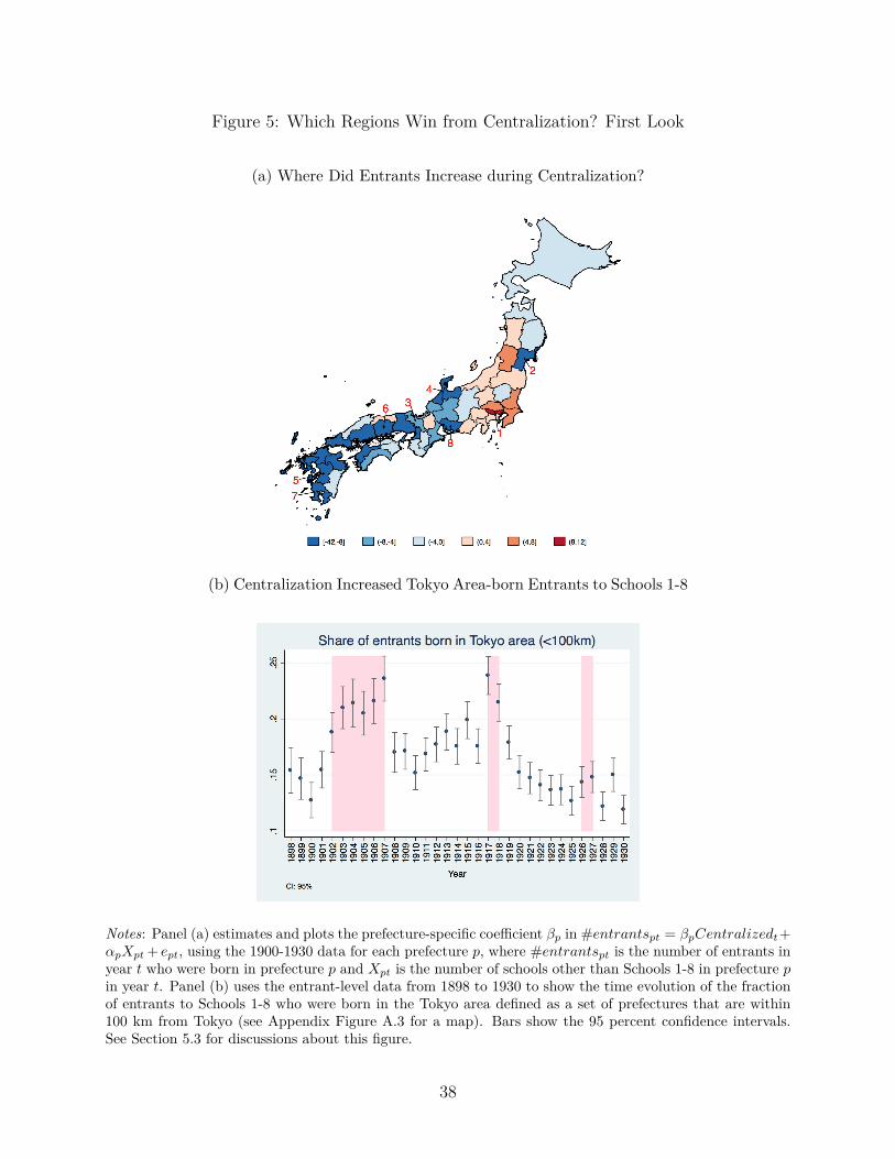
Figure 5: Which Regions Win from Centralization? First Look

(a) Where Did Entrants Increase during Centralization?

(b) Centralization Increased Tokyo Area-born Entrants to Schools 1-8

Notes: Panel (a) estimates and plots the prefecture-specific coefficient βp in#entrantspt = βpCentralizedt+αpXpt + ept, using the 1900-1930 data for each prefecture p, where #entrantspt is the number of entrants inyear t who were born in prefecture p and Xpt is the number of schools other than Schools 1-8 in prefecture pin year t. Panel (b) uses the entrant-level data from 1898 to 1930 to show the time evolution of the fractionof entrants to Schools 1-8 who were born in the Tokyo area defined as a set of prefectures that are within100 km from Tokyo (see Appendix Figure A.3 for a map). Bars show the 95 percent confidence intervals.See Section 5.3 for discussions about this figure.

38

Table 3: Which Regions Win from Centralization?

(1) (2) (3) (4) (5) (6) (7) (8) (9)Dependent variable = No. of entrants to: All schools Sch. 1 Sch. 2 Sch. 3 Sch. 4 Sch. 5 Sch. 6 Sch. 7 Sch. 8

Centralized x Born in Tokyo prefecture 9.11 0.34 2.54 7.06 3.41 10.21 6.87 19.87(2.68)*** (0.31) (1.74) (0.53)*** (0.31)*** (1.69)*** (0.49)*** (1.34)***[20.37] [3.19] [3.34] [2.32]*** [1.89]* [2.09]*** [2.96]** [3.42]***

Centralized x Born near Tokyo prefecture (1-100 km) 13.14 0.52 0.96 2.05 0.12 0.87 0.46 0.37(2.17)*** (0.60) (0.36)** (0.45)*** (0.34) (0.43)** (0.46) (0.66)[3.79]*** [0.51] [0.26]*** [0.65]*** [0.38] [0.30]*** [0.46] [0.34]

Centralized x Born near Tokyo prefecture (100-300 km) 3.91 0.91 1.67 -0.02 0.60 1.36 1.15 0.13(3.75) (0.46)* (0.78)** (0.89) (0.34)* (0.59)** (0.48)** (0.52)[2.16]* [0.37]** [0.44]*** [0.89] [0.38] [0.35]*** [0.36]*** [0.70]

Centralized x Born in school’s prefecture -27.80 -17.41 -15.14 -22.81 -28.16 -22.08 -47.82 -13.42(0.89)*** (0.17)*** (0.58)*** (0.90)*** (0.21)*** (0.36)*** (0.40)*** (1.13)***[7.82]*** [7.66]** [8.38]* [8.43]** [7.60]*** [12.18]* [13.02]*** [14.57]

Centralized x Born near school’s prefecture (1-100 km) 0.30 -3.91 -3.76 -9.07 -11.70 -1.91 -1.69 1.03(0.66) (2.48) (1.96)* (3.15)*** (3.21)*** (1.30) (0.27)*** (1.01)[0.53] [1.44]** [1.02]*** [2.81]*** [3.17]*** [0.88]** [2.52] [2.47]

Centralized x Born near school’s prefecture (100-300 km) 1.06 -0.34 -0.37 -0.69 -3.02 -1.17 -2.50 0.26(0.55)* (0.75) (0.51) (0.43) (0.92)*** (0.68)* (0.82)*** (0.37)[0.61]* [0.51] [0.35] [0.49] [0.76]*** [0.52]** [1.18]** [0.63]

Observations 1,410 1,410 1,410 1,363 1,410 1,363 1,363 1,222 1,034Year FE Yes Yes Yes Yes Yes Yes Yes Yes YesPref FE Yes Yes Yes Yes Yes Yes Yes Yes YesMean dep var 45.26 7.94 5.54 6.21 5.68 6.31 5.20 5.02 5.73Mean dep var (Tokyo pref dur. Dapp) 199.9 103.3 27.15 11.00 14.40 6.100 9.474 12.00 20.39Mean dep var (within 1-100 km from Tokyo pref. dur. Dapp) 26.38 9.150 6.733 1.246 2.867 0.767 1.254 1.618 3.250

Notes: This table uses the prefecture-year level data in 1900-1930. In column (1), the dependent variable is the number of students from birthprefecture p who entered one of Schools 1-8 in year t. In columns (2)–(10), the dependent variable is the number of students from birth prefecturep who entered the school indicated in the column in year t. For Schools 7 and 8, we drop the years in which they held an early exam (School 7 in1908-1910 and School 8 in 1908). We control for prefecture fixed effects, year fixed effects, the lagged number of public and private middle schoolgraduates in the prefecture and the number of higher schools other than Schools 1-8 in the prefecture. “Born in Tokyo prefecture” takes 1 if in theentrant’s birth prefecture is Tokyo prefecture. “Born near Tokyo prefecture (1-100 km)” takes 1 if the entrant’s birth prefecture is different fromTokyo prefecture, but within 100 km from it. “Born near Tokyo prefecture (100-300 km)” takes 1 if the entrant’s birth prefecture is between 100 kmand 300 km from Tokyo prefecture. Refer to the notes for Table 2 for the definitions of “Born in school’s prefecture,” “Born near school’s prefecture(1-100 km)”, and “Born near school’s prefecture (100-300 km).” “Mean dep var” shows the mean of the dependent variable during decentralization forall prefecture-year observations. “Mean dep var (Tokyo pref dur. Dapp)” shows the mean number of entrants to the school during decentralization,restricted to those born in Tokyo prefecture. “Mean dep var (within 1-100 km from Tokyo pref. dur. Dapp)” shows the mean number of entrantsto the school during decentralization, restricted to those born in the prefectures within 100 km from Tokyo prefecture (excluding Tokyo prefecture).Standard errors reported in parentheses are clustered at the prefecture level. Standard errors reported in square brackets are clustered at the yearlevel. ***, **, and * mean significance at the 1%, 5%, and 10% levels, respectively. See Section 5.3 for discussions about this figure.

39

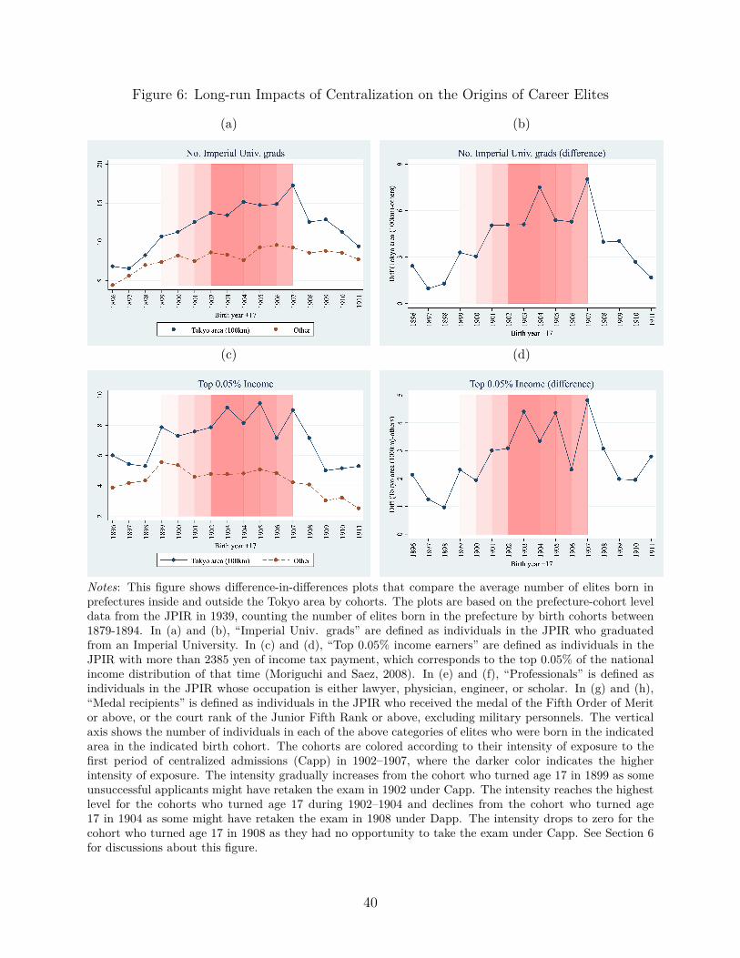
Figure 6: Long-run Impacts of Centralization on the Origins of Career Elites

(a) (b)

(c) (d)

Notes: This figure shows difference-in-differences plots that compare the average number of elites born inprefectures inside and outside the Tokyo area by cohorts. The plots are based on the prefecture-cohort leveldata from the JPIR in 1939, counting the number of elites born in the prefecture by birth cohorts between1879-1894. In (a) and (b), “Imperial Univ. grads” are defined as individuals in the JPIR who graduatedfrom an Imperial University. In (c) and (d), “Top 0.05% income earners” are defined as individuals in theJPIR with more than 2385 yen of income tax payment, which corresponds to the top 0.05% of the nationalincome distribution of that time (Moriguchi and Saez, 2008). In (e) and (f), “Professionals” is defined asindividuals in the JPIR whose occupation is either lawyer, physician, engineer, or scholar. In (g) and (h),“Medal recipients” is defined as individuals in the JPIR who received the medal of the Fifth Order of Meritor above, or the court rank of the Junior Fifth Rank or above, excluding military personnels. The verticalaxis shows the number of individuals in each of the above categories of elites who were born in the indicatedarea in the indicated birth cohort. The cohorts are colored according to their intensity of exposure to thefirst period of centralized admissions (Capp) in 1902–1907, where the darker color indicates the higherintensity of exposure. The intensity gradually increases from the cohort who turned age 17 in 1899 as someunsuccessful applicants might have retaken the exam in 1902 under Capp. The intensity reaches the highestlevel for the cohorts who turned age 17 during 1902–1904 and declines from the cohort who turned age17 in 1904 as some might have retaken the exam in 1908 under Dapp. The intensity drops to zero for thecohort who turned age 17 in 1908 as they had no opportunity to take the exam under Capp. See Section 6for discussions about this figure.

40

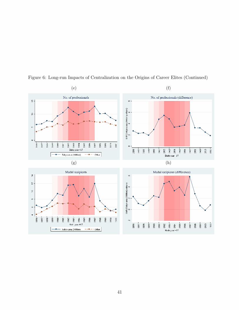
Figure 6: Long-run Impacts of Centralization on the Origins of Career Elites (Continued)

(e) (f)

(g) (h)

41

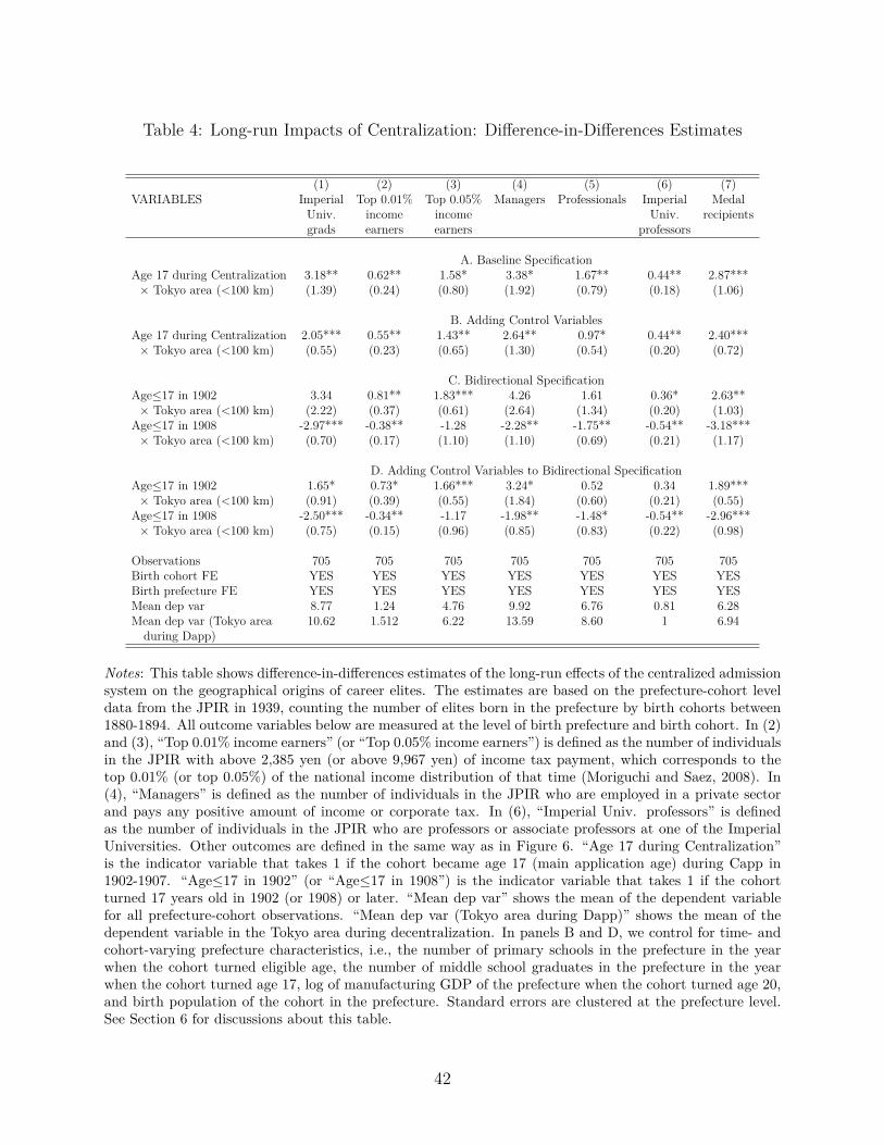
Table 4: Long-run Impacts of Centralization: Difference-in-Differences Estimates

(1) (2) (3) (4) (5) (6) (7)VARIABLES Imperial Top 0.01% Top 0.05% Managers Professionals Imperial Medal

Univ. income income Univ. recipientsgrads earners earners professors

A. Baseline SpecificationAge 17 during Centralization 3.18** 0.62** 1.58* 3.38* 1.67** 0.44** 2.87***× Tokyo area (<100 km) (1.39) (0.24) (0.80) (1.92) (0.79) (0.18) (1.06)

B. Adding Control VariablesAge 17 during Centralization 2.05*** 0.55** 1.43** 2.64** 0.97* 0.44** 2.40***× Tokyo area (<100 km) (0.55) (0.23) (0.65) (1.30) (0.54) (0.20) (0.72)

C. Bidirectional SpecificationAge≤17 in 1902 3.34 0.81** 1.83*** 4.26 1.61 0.36* 2.63**× Tokyo area (<100 km) (2.22) (0.37) (0.61) (2.64) (1.34) (0.20) (1.03)

Age≤17 in 1908 -2.97*** -0.38** -1.28 -2.28** -1.75** -0.54** -3.18***× Tokyo area (<100 km) (0.70) (0.17) (1.10) (1.10) (0.69) (0.21) (1.17)

D. Adding Control Variables to Bidirectional SpecificationAge≤17 in 1902 1.65* 0.73* 1.66*** 3.24* 0.52 0.34 1.89***× Tokyo area (<100 km) (0.91) (0.39) (0.55) (1.84) (0.60) (0.21) (0.55)

Age≤17 in 1908 -2.50*** -0.34** -1.17 -1.98** -1.48* -0.54** -2.96***× Tokyo area (<100 km) (0.75) (0.15) (0.96) (0.85) (0.83) (0.22) (0.98)

Observations 705 705 705 705 705 705 705Birth cohort FE YES YES YES YES YES YES YESBirth prefecture FE YES YES YES YES YES YES YESMean dep var 8.77 1.24 4.76 9.92 6.76 0.81 6.28Mean dep var (Tokyo area 10.62 1.512 6.22 13.59 8.60 1 6.94during Dapp)

Notes: This table shows difference-in-differences estimates of the long-run effects of the centralized admissionsystem on the geographical origins of career elites. The estimates are based on the prefecture-cohort leveldata from the JPIR in 1939, counting the number of elites born in the prefecture by birth cohorts between1880-1894. All outcome variables below are measured at the level of birth prefecture and birth cohort. In (2)and (3), “Top 0.01% income earners” (or “Top 0.05% income earners”) is defined as the number of individualsin the JPIR with above 2,385 yen (or above 9,967 yen) of income tax payment, which corresponds to thetop 0.01% (or top 0.05%) of the national income distribution of that time (Moriguchi and Saez, 2008). In(4), “Managers” is defined as the number of individuals in the JPIR who are employed in a private sectorand pays any positive amount of income or corporate tax. In (6), “Imperial Univ. professors” is definedas the number of individuals in the JPIR who are professors or associate professors at one of the ImperialUniversities. Other outcomes are defined in the same way as in Figure 6. “Age 17 during Centralization”is the indicator variable that takes 1 if the cohort became age 17 (main application age) during Capp in1902-1907. “Age≤17 in 1902” (or “Age≤17 in 1908”) is the indicator variable that takes 1 if the cohortturned 17 years old in 1902 (or 1908) or later. “Mean dep var” shows the mean of the dependent variablefor all prefecture-cohort observations. “Mean dep var (Tokyo area during Dapp)” shows the mean of thedependent variable in the Tokyo area during decentralization. In panels B and D, we control for time- andcohort-varying prefecture characteristics, i.e., the number of primary schools in the prefecture in the yearwhen the cohort turned eligible age, the number of middle school graduates in the prefecture in the yearwhen the cohort turned age 17, log of manufacturing GDP of the prefecture when the cohort turned age 20,and birth population of the cohort in the prefecture. Standard errors are clustered at the prefecture level.See Section 6 for discussions about this table.

42

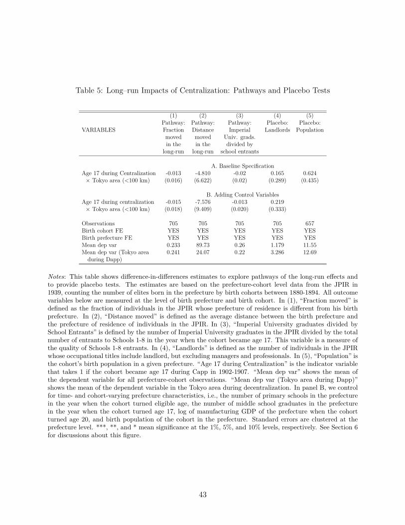
Table 5: Long–run Impacts of Centralization: Pathways and Placebo Tests

(1) (2) (3) (4) (5)Pathway: Pathway: Pathway: Placebo: Placebo:

VARIABLES Fraction Distance Imperial Landlords Populationmoved moved Univ. grads.in the in the divided by

long-run long-run school entrants

A. Baseline SpecificationAge 17 during Centralization -0.013 -4.810 -0.02 0.165 0.624× Tokyo area (<100 km) (0.016) (6.622) (0.02) (0.289) (0.435)

B. Adding Control VariablesAge 17 during centralization -0.015 -7.576 -0.013 0.219× Tokyo area (<100 km) (0.018) (9.409) (0.020) (0.333)

Observations 705 705 705 705 657Birth cohort FE YES YES YES YES YESBirth prefecture FE YES YES YES YES YESMean dep var 0.233 89.73 0.26 1.179 11.55Mean dep var (Tokyo area 0.241 24.07 0.22 3.286 12.69during Dapp)

Notes: This table shows difference-in-differences estimates to explore pathways of the long-run effects andto provide placebo tests. The estimates are based on the prefecture-cohort level data from the JPIR in1939, counting the number of elites born in the prefecture by birth cohorts between 1880-1894. All outcomevariables below are measured at the level of birth prefecture and birth cohort. In (1), “Fraction moved” isdefined as the fraction of individuals in the JPIR whose prefecture of residence is different from his birthprefecture. In (2), “Distance moved” is defined as the average distance between the birth prefecture andthe prefecture of residence of individuals in the JPIR. In (3), “Imperial University graduates divided bySchool Entrants” is defined by the number of Imperial University graduates in the JPIR divided by the totalnumber of entrants to Schools 1-8 in the year when the cohort became age 17. This variable is a measure ofthe quality of Schools 1-8 entrants. In (4), “Landlords” is defined as the number of individuals in the JPIRwhose occupational titles include landlord, but excluding managers and professionals. In (5), “Population” isthe cohort’s birth population in a given prefecture. “Age 17 during Centralization” is the indicator variablethat takes 1 if the cohort became age 17 during Capp in 1902-1907. “Mean dep var” shows the mean ofthe dependent variable for all prefecture-cohort observations. “Mean dep var (Tokyo area during Dapp)”shows the mean of the dependent variable in the Tokyo area during decentralization. In panel B, we controlfor time- and cohort-varying prefecture characteristics, i.e., the number of primary schools in the prefecturein the year when the cohort turned eligible age, the number of middle school graduates in the prefecturein the year when the cohort turned age 17, log of manufacturing GDP of the prefecture when the cohortturned age 20, and birth population of the cohort in the prefecture. Standard errors are clustered at theprefecture level. ***, **, and * mean significance at the 1%, 5%, and 10% levels, respectively. See Section 6for discussions about this figure.

43

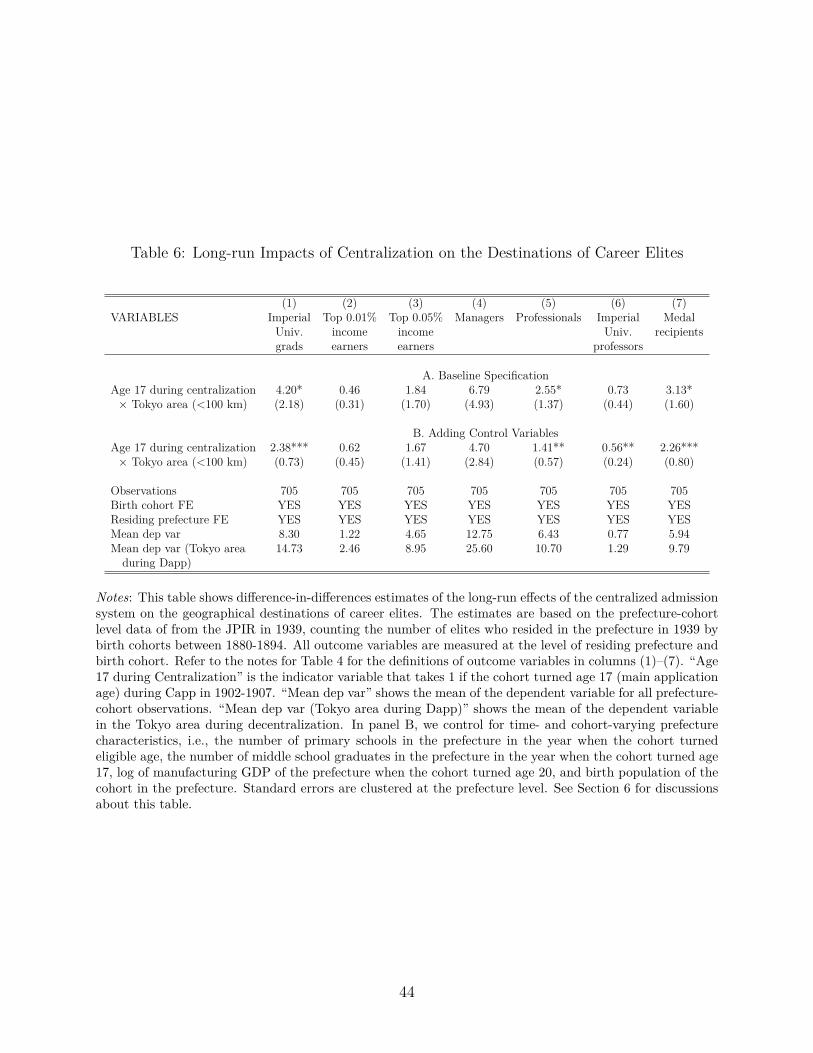
Table 6: Long-run Impacts of Centralization on the Destinations of Career Elites

(1) (2) (3) (4) (5) (6) (7)VARIABLES Imperial Top 0.01% Top 0.05% Managers Professionals Imperial Medal

Univ. income income Univ. recipientsgrads earners earners professors

A. Baseline SpecificationAge 17 during centralization 4.20* 0.46 1.84 6.79 2.55* 0.73 3.13*× Tokyo area (<100 km) (2.18) (0.31) (1.70) (4.93) (1.37) (0.44) (1.60)

B. Adding Control VariablesAge 17 during centralization 2.38*** 0.62 1.67 4.70 1.41** 0.56** 2.26***× Tokyo area (<100 km) (0.73) (0.45) (1.41) (2.84) (0.57) (0.24) (0.80)

Observations 705 705 705 705 705 705 705Birth cohort FE YES YES YES YES YES YES YESResiding prefecture FE YES YES YES YES YES YES YESMean dep var 8.30 1.22 4.65 12.75 6.43 0.77 5.94Mean dep var (Tokyo area 14.73 2.46 8.95 25.60 10.70 1.29 9.79during Dapp)

Notes: This table shows difference-in-differences estimates of the long-run effects of the centralized admissionsystem on the geographical destinations of career elites. The estimates are based on the prefecture-cohortlevel data of from the JPIR in 1939, counting the number of elites who resided in the prefecture in 1939 bybirth cohorts between 1880-1894. All outcome variables are measured at the level of residing prefecture andbirth cohort. Refer to the notes for Table 4 for the definitions of outcome variables in columns (1)–(7). “Age17 during Centralization” is the indicator variable that takes 1 if the cohort turned age 17 (main applicationage) during Capp in 1902-1907. “Mean dep var” shows the mean of the dependent variable for all prefecture-cohort observations. “Mean dep var (Tokyo area during Dapp)” shows the mean of the dependent variablein the Tokyo area during decentralization. In panel B, we control for time- and cohort-varying prefecturecharacteristics, i.e., the number of primary schools in the prefecture in the year when the cohort turnedeligible age, the number of middle school graduates in the prefecture in the year when the cohort turned age17, log of manufacturing GDP of the prefecture when the cohort turned age 20, and birth population of thecohort in the prefecture. Standard errors are clustered at the prefecture level. See Section 6 for discussionsabout this table.

44

A Appendix

A.1 Verifying the Centralized Assignment Algorithm

To see whether actual school assignments are consistent with the above algorithm, AppendixTable A.1 presents the number of admitted applicants (to the Department of Law andLiterature in each school) and their exam scores by their school preference order. Observethat, in the prestigious Schools 1 (Tokyo) and 3 (Kyoto), all seats were filled with applicantswho ranked these schools first. Both the maximum and minimum exam scores of School 1entrants were the highest among all schools, indicating that School 1 was the most selective,followed by School 3, School 4, and School 2, in that order. By contrast, Schools 5 and 7admitted a sizable number of students who ranked the school third or lower, because theydid not have a sufficient number of high-scoring applicants who placed these schools at thetop of their preferences. Students who were admitted to the school of their third choice orbelow are not necessarily low ability students. For example, the highest-score entrant toSchool 7 (with the score of 450) was the applicant admitted to his third choice after failingto enter Schools 1 and 3 by a narrow margin.

A.2 Additional Theoretical Results

Let µI be the mechanism that selects a matching based on the following Student-ProposingDeferred Acceptance or Serial Dictatorship algorithm.

• Step 1. Each student i proposes to her most-preferred school. Each school s holds topqs students and rejects the rest. If less than qs students proposed, then it holds all thestudents that proposed to s.

• Step k. Any student who was rejected at step k − 1 makes a new proposal to hismost-preferred school that has not yet rejected him. If no acceptable choices remain,she makes no proposal. Each school holds its most-preferred qs students to date andrejects the rest. If less than qs students proposed, then it holds all the students whoproposed to s.

• The algorithm terminates when there are no more rejections. Each student is assignedto the school that holds her in the last step.

Motivated by the fact that Schools 1-8 are prestigious public schools with no significantcompetitors, we assume that every student prefers Schools 1-8 over the outside option.

45

Assumption 1. s �i o for all i ∈ I and s ∈ S.

Under this assumption, µI and Capp are partially equivalent in the following sense.

Proposition 4. For any school choice problem with Assumption 1, ∪s∈SµCs (�) = ∪s∈Sµ

Is(�′)

for all �,�′∈ P .

This result says that the same students are assigned to schools under Capp and DA, whichis the most meritocratic mechanism we can design. This result holds regardless of applicantbehavior.

A.3 Proofs

Proof of Proposition 1. As mentioned in step 1 of Capp, school seats are assigned toapplicants i1, . . . , ik under µC , i.e., ∪s∈Sµ

Cs (�) = {i1, . . . , ik} and ∪j∈{1,...,k}{tµC(�)(j)} =

{ti1 , . . . , tik}. Let ∪s∈Sµs(�′) = {ij1 , . . . , ijl} with l ≤ k, j1 < . . . < jl and {j1, . . . , jl} ⊆{1, . . . , n}. This gives ∪j∈{1,...,k}{tµ(�′)(j)} = {tij1 , . . . , tijl ,∪

k−li=1{0}}. Since ti1 ≥ tij1 ,...,

til ≥ tijl , we have that∣∣{j ∈ {1, . . . , k} | tµC(�)(j) ≤ t}

∣∣ ≤ ∣∣{j ∈ {1, . . . , k} | tµ(�′)(j) ≤ t}∣∣

so that

FµC(�)(t) =

∣∣{j ∈ {1, . . . , k} | tµC(�)(j) ≤ t}∣∣

k≤

∣∣{j ∈ {1, . . . , k} | tµ(�′)(j) ≤ t}∣∣

k= Fµ(�′)(t).

Therefore, we have that FµC(�)(t) ≤ Fµ(�′)(t) for all t ∈ R+ and �,�′∈ P .

Proof of Proposition 2. The proposition follows from a lemma below.

Lemma 1. (a) Under Capp, submitting the true preference is a dominant strategy.

(b) Under Dapp, there is no dominant strategy.

Proof of Lemma 1. Suppose, without loss of generality, for applicant i s1 �oi s2 �o

i i where i

denotes remaining unassigned.Part (a). Under Capp, applicant i has four strategies available: reporting s1 as first choiceand s2 as second, denoted ai (=�o

i ); reporting s2 as first choice and s2 as second choice,denoted a′i; and reporting a single school as top choice, either s1 or s2. Fix any a−i ∈ A−i.We have to show that reporting ai is a dominant strategy for applicant i.

Notice that reporting a single school as top choice is not a dominant strategy since it isdominated by reporting that school as first choice and the other school as second because

2∑k=1

pik(ai, a−i) >2∑

k=1

pik(s1, a−i) and2∑

k=1

pik(a′i, a−i) >

2∑k=1

pik(s2, a−i)

46

Now we show that ai dominates a′i. First, only top k students are assigned a school, thatimplies if a student is unassigned under µC(ai, a−i), he would be unassigned under µC(a′i, a−i)

as well i.e. pi3(ai, a−i) = pi3(a′i, a−i). Therefore,

2∑k=1

pik(ai, a−i) =2∑

k=1

pik(a′i, a−i)

.Second, if the student gets s2 by reporting s1 as first choice, it is clear that he cannot get

s1 by reporting s2 as first choice because in that case he would be assigned s2 in the secondstep of Capp. Therefore,

pi1(ai, a−i) ≥ pi1(a′i, a−i)

.Therefore we have that ai is a dominant strategy.

Part (b). Under Dapp, applicant i has two strategies available: applying to s1, denotedai, and applying to s2, denoted a′i. Fix any any a−i ∈ A−i. Notice that pi2(ai, a−i) =

pi1(a′i, a−i) = 0.

ai is not a dominant strategy since in the case a−i is such that all students apply to s1,(note that applicant i is one of the top q1 students with a positive probability) we have that,

2∑k=1

pik(ai, a−i) = pi1(ai, a−i) < 1 = pi2(a′i, a−i) =

2∑k=1

pik(a′i, a−i)

.a′i is not a dominant strategy either since in the case a−i is such that all students apply tos2, pi1(ai, a−i) = 1 and therefore, ai sd(�o

i ) a′i.

Proof of Proposition 3.

Lemma 2. Under assumption A1, for sufficiently large V , all applicants apply to their localschools in any symmetric equilibrium under Dapp.

Proof of Lemma 2. First, we show that for sufficiently large V , none of the following sym-metric equilibrium survive: (i) all applicants apply to s1, (ii) all applicants apply to s2, and(iii) applicants from s1’s area apply to s2 while those from s2’s area apply to s1.Case (i). Applicants from school 2’s area apply to s1 if p(n1 + n2, q1) ∗ U1 ≥ U2 + V . ForV > (p(n1+n2, q1)∗U1)−U2, therefore, all applicants applying to s1 cannot be a symmetricequilibrium.

47

Case (ii). All applicants applying to s2 cannot be an equilibrium since this requiresUi1 < p(n1 + n2, q2) ∗ Ui2, but we assume that Ui1 ≥ Ui2.Case (iii). Suppose applicants from s1’s area apply to s2 while those from s2’s area applyto s1. It must be that the case that, for applicants from s1’s area: p(n1, q2) ∗ U2 ≥ p(n2 +

1, q1)∗ (U1+V ). While for applicants from s2’s area: p(n2, q1)∗U1 ≥ p(n1+1, q2)∗ (U2+V ).For sufficiently large V , this cannot be a symmetric equilibrium.

Now we show that, for large enough V , all students applying to their local schools isindeed a symmetric equilibrium. For applicants from school 1’s area to apply to s1, it mustbe the case that p(n1, q1) ∗ (U1 + V ) ≥ p(n2 +1, q2) ∗U2. For applicants from school 2’s areato apply to s2, p(n2, q2) ∗ (U2 + V ) ≥ p(n1 + 1, q1) ∗ U1 must hold. Since the left hand sidesof both the inequalities are increasing in V , the equilibrium conditions hold for sufficientlylarge V .

From Lemma 2, under assumptions A1 and A2, we know that under Dapp applicants applyto their locals schools. Therefore, the expected proportion of assigned applicants assignedto their local school under Dapp is 1 (the highest).

Proof of Proposition 4. As mentioned in step 1 of Capp, school seats are assigned to appli-cants i1, . . . , ik under µC , i.e., ∪s∈Sµ

Cs (�) = {i1, . . . , ik} for all �∈ P . Under assumption

1, any student ik′ with k′ > k will be rejected at some step of the Student-Proposing De-ferred Acceptance Algorithm. Assumption 1 therefore implies that the top k students areassigned to some school under µI , i.e., ∪s∈Sµ

Is(�′) = {i1, . . . , ik} for all �′∈ P . Therefore,

∪s∈SµCs (�) = ∪s∈Sµ

Is(�′) = k for all �,�′∈ P .

48

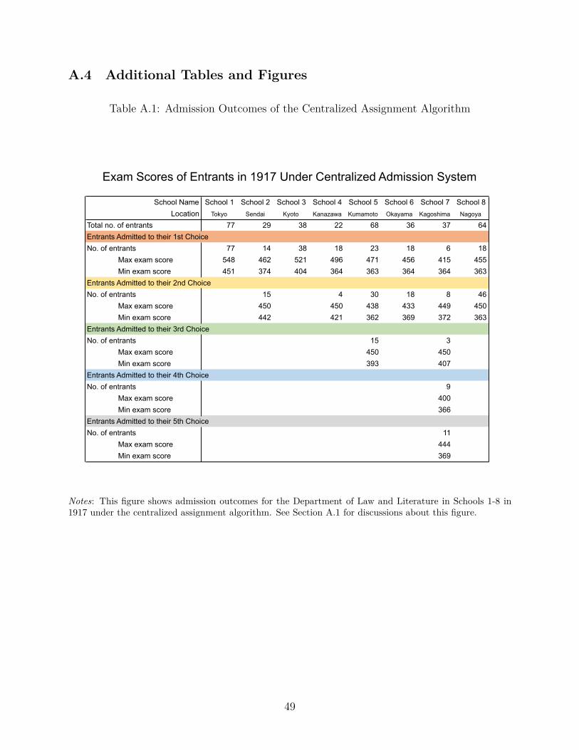
A.4 Additional Tables and Figures

Table A.1: Admission Outcomes of the Centralized Assignment Algorithm

Exam Scores of Entrants in 1917 Under Centralized Admission System

School Name School 1 School 2 School 3 School 4 School 5 School 6 School 7 School 8Location Tokyo Sendai Kyoto Kanazawa Kumamoto Okayama Kagoshima Nagoya

Total no. of entrants 77 29 38 22 68 36 37 64Entrants Admitted to their 1st ChoiceNo. of entrants 77 14 38 18 23 18 6 18

Max exam score 548 462 521 496 471 456 415 455Min exam score 451 374 404 364 363 364 364 363

Entrants Admitted to their 2nd ChoiceNo. of entrants 15 4 30 18 8 46

Max exam score 450 450 438 433 449 450Min exam score 442 421 362 369 372 363

Entrants Admitted to their 3rd ChoiceNo. of entrants 15 3

Max exam score 450 450Min exam score 393 407

Entrants Admitted to their 4th ChoiceNo. of entrants 9

Max exam score 400Min exam score 366

Entrants Admitted to their 5th ChoiceNo. of entrants 11

Max exam score 444Min exam score 369

Notes: This figure shows admission outcomes for the Department of Law and Literature in Schools 1-8 in1917 under the centralized assignment algorithm. See Section A.1 for discussions about this figure.

49

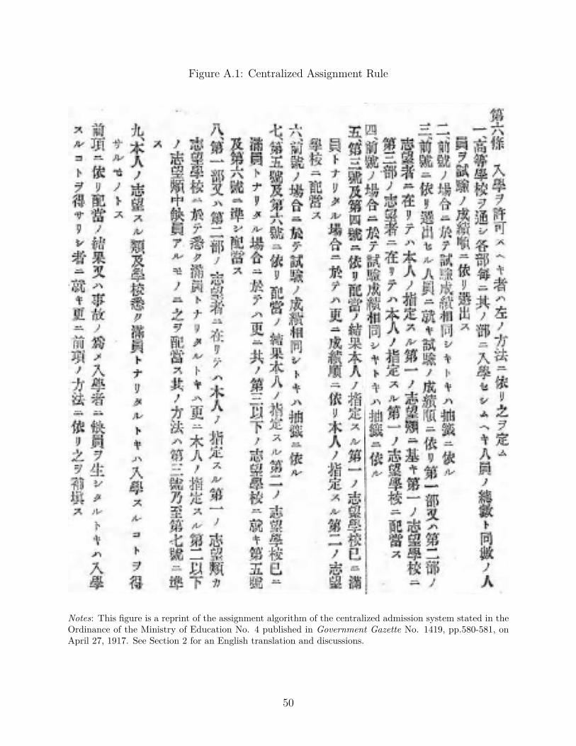
Figure A.1: Centralized Assignment Rule

Notes: This figure is a reprint of the assignment algorithm of the centralized admission system stated in theOrdinance of the Ministry of Education No. 4 published in Government Gazette No. 1419, pp.580-581, onApril 27, 1917. See Section 2 for an English translation and discussions.

50

Table A.2: Summary Statistics

Variable Mean Std. Dev. Median NYear level data on short-run outcomesTotal number of applicants to Schools 1–8 10613 4221 9997 28Share of applicants choosing School 1 as first choice 0.314 0.097 0.274 28Total number of entrants to Schools 1–8 1821 227 1919 31Applicant level data on short-run outcomesDistance between middle school prefecture and the school applied as first choice (km) 224.88 272.03 117 20913Applying to School 1 as first choice 0.33 0.47 0 20913Entrant level data on short-run outcomesDistance between birth prefecture and the school entered (km) 226.8 258.65 139 66193Entering the nearest school from birth prefecture 0.49 0.5 0 66193Born in Tokyo prefecture 0.09 0.29 0 66193Born in Tokyo area (7 prefectures within 100 km from Tokyo) 0.17 0.38 0 66193Prefecture-year level data on short-run outcomesNo. of entrants to Schools 1-8 45.06 37.45 34 1469No. of entrants to School 1 7.88 14.11 5 1469No. of entrants to School 2 5.5 10.4 2 1469No. of entrants to School 3 6.19 10.34 3 1421No. of entrants to School 4 5.64 9.91 3 1469No. of entrants to School 5 6.27 14.2 1 1422No. of entrants to School 6 5.19 11.8 2 1421No. of entrants to School 7 5.03 12.99 2 1328No. of entrants to School 8 5.67 12.45 2 1093No. of public middle school graduates 415.38 350.01 299 1410No. of private middle school graduates 118.49 435.12 0 1410No. of national higher schools other than Schools 1-8 0.13 0.43 0 1469Prefecture-cohort level data on long-run outcomesNo. of all Imperial University graduates 8.77 7.81 7 705No. of people earning top 0.01% level of income 1.24 2.06 1 705No. of people earning top 0.05% level of income 4.76 6.97 3 705No. of managers in private sector paying a positive amount of tax 13.25 16.34 7 705No. of scholars, physicians, lawyers, and engineers 6.76 6.11 5 705No. of Imperial University professors 0.81 1.18 0 705No. of civilians receiving medal of Order of Fifth Class and above 6.28 5.03 5 705

Notes: This table provides summary statistics of variables used in the empirical analysis. The sample period for year level data is from 1900 to 1930.The sample period for applicant level data is during 1916 and 1917. The sample period for entrant level data and prefecture level data for short-runoutcomes is from 1900 to 1930. The information on the school “entrants” is based on the first year students in the schools. The long-run outcomevariables are based on the prefecture-cohort level data from the JPIR in 1939, counting the number of elites born in the prefecture by birth cohortsbetween 1880-1894. See Sections 4 and 6 for discussions about this table.

51

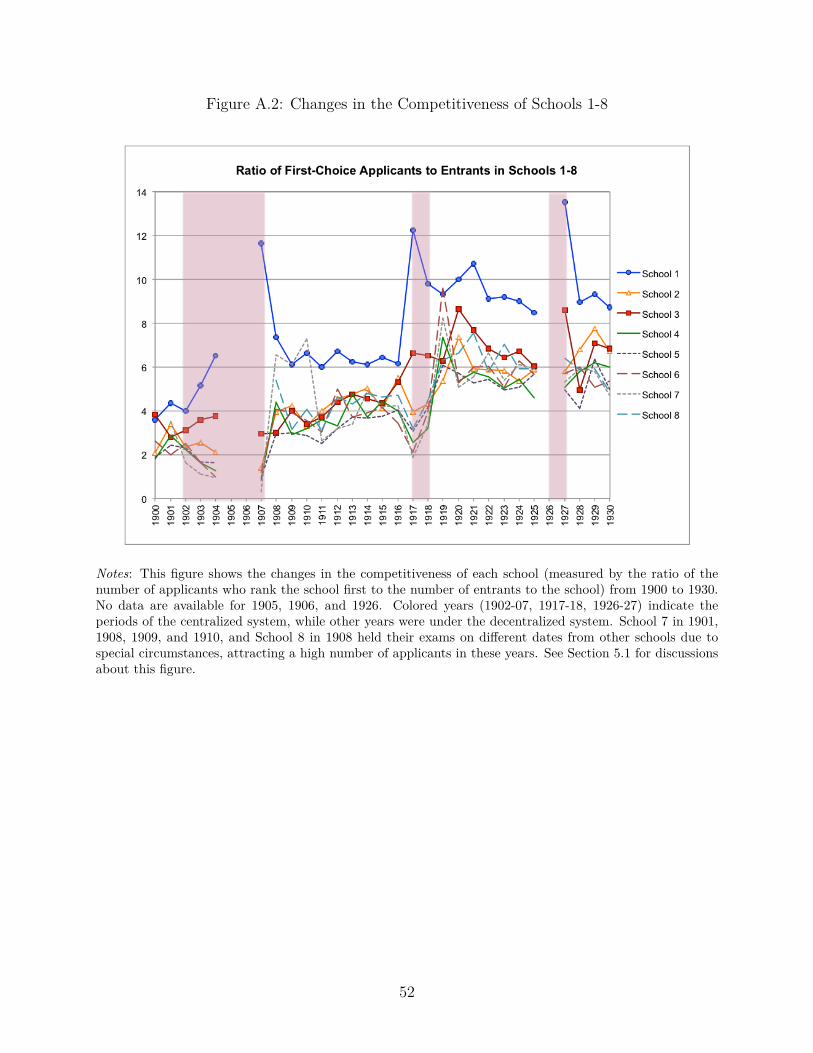
Figure A.2: Changes in the Competitiveness of Schools 1-8

Notes: This figure shows the changes in the competitiveness of each school (measured by the ratio of thenumber of applicants who rank the school first to the number of entrants to the school) from 1900 to 1930.No data are available for 1905, 1906, and 1926. Colored years (1902-07, 1917-18, 1926-27) indicate theperiods of the centralized system, while other years were under the decentralized system. School 7 in 1901,1908, 1909, and 1910, and School 8 in 1908 held their exams on different dates from other schools due tospecial circumstances, attracting a high number of applicants in these years. See Section 5.1 for discussionsabout this figure.

52

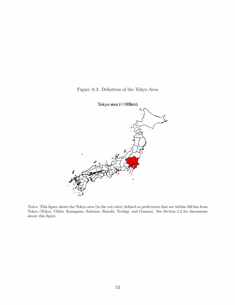
Figure A.3: Definition of the Tokyo Area

Notes: This figure shows the Tokyo area (in the red color) defined as prefectures that are within 100 km fromTokyo (Tokyo, Chiba, Kanagawa, Saitama, Ibaraki, Tochigi, and Gunma). See Section 5.2 for discussionsabout this figure.

53

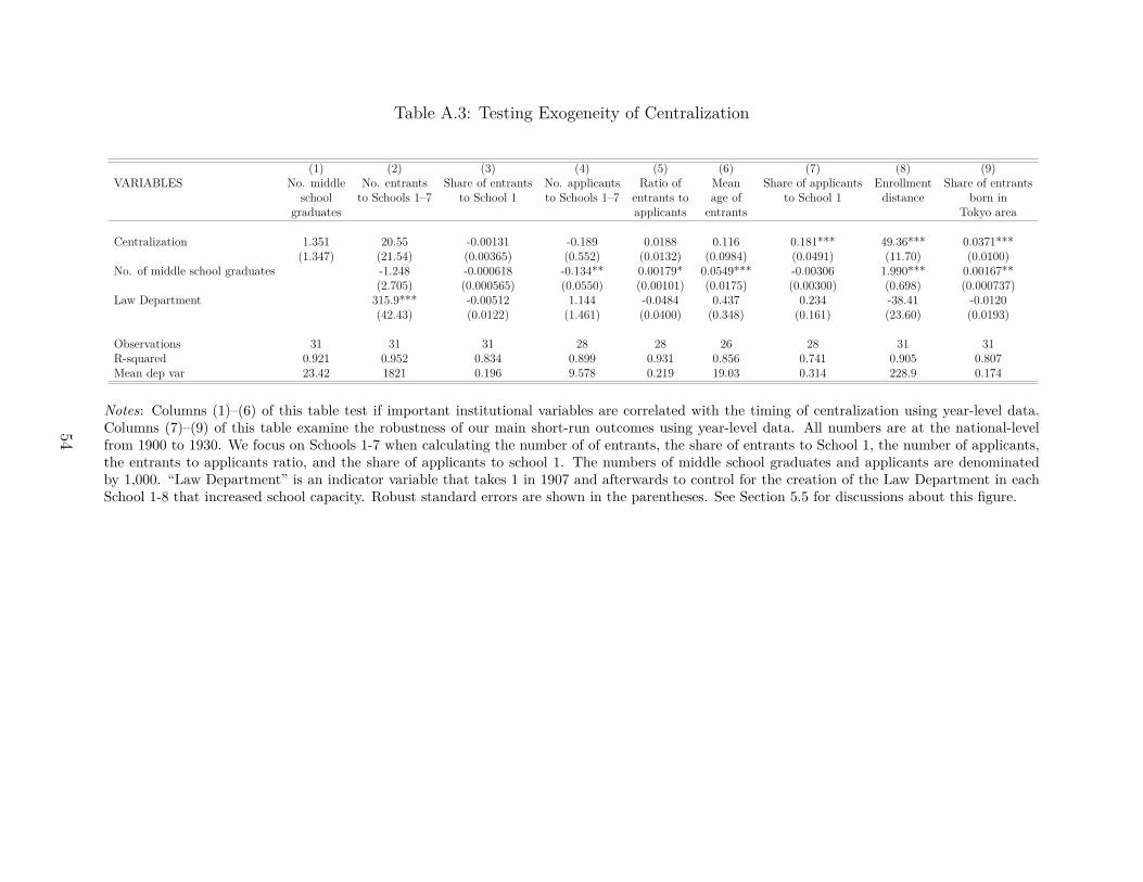
Table A.3: Testing Exogeneity of Centralization

(1) (2) (3) (4) (5) (6) (7) (8) (9)VARIABLES No. middle No. entrants Share of entrants No. applicants Ratio of Mean Share of applicants Enrollment Share of entrants

school to Schools 1–7 to School 1 to Schools 1–7 entrants to age of to School 1 distance born ingraduates applicants entrants Tokyo area

Centralization 1.351 20.55 -0.00131 -0.189 0.0188 0.116 0.181*** 49.36*** 0.0371***(1.347) (21.54) (0.00365) (0.552) (0.0132) (0.0984) (0.0491) (11.70) (0.0100)

No. of middle school graduates -1.248 -0.000618 -0.134** 0.00179* 0.0549*** -0.00306 1.990*** 0.00167**(2.705) (0.000565) (0.0550) (0.00101) (0.0175) (0.00300) (0.698) (0.000737)

Law Department 315.9*** -0.00512 1.144 -0.0484 0.437 0.234 -38.41 -0.0120(42.43) (0.0122) (1.461) (0.0400) (0.348) (0.161) (23.60) (0.0193)

Observations 31 31 31 28 28 26 28 31 31R-squared 0.921 0.952 0.834 0.899 0.931 0.856 0.741 0.905 0.807Mean dep var 23.42 1821 0.196 9.578 0.219 19.03 0.314 228.9 0.174

Notes: Columns (1)–(6) of this table test if important institutional variables are correlated with the timing of centralization using year-level data.Columns (7)–(9) of this table examine the robustness of our main short-run outcomes using year-level data. All numbers are at the national-levelfrom 1900 to 1930. We focus on Schools 1-7 when calculating the number of of entrants, the share of entrants to School 1, the number of applicants,the entrants to applicants ratio, and the share of applicants to school 1. The numbers of middle school graduates and applicants are denominatedby 1,000. “Law Department” is an indicator variable that takes 1 in 1907 and afterwards to control for the creation of the Law Department in eachSchool 1-8 that increased school capacity. Robust standard errors are shown in the parentheses. See Section 5.5 for discussions about this figure.

54

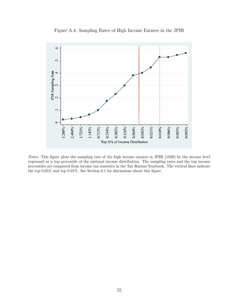
Figure A.4: Sampling Rates of High Income Earners in the JPIR

Notes: This figure plots the sampling rate of the high income earners in JPIR (1939) by the income levelexpressed as a top percentile of the national income distribution. The sampling rates and the top incomepercentiles are computed from income tax statistics in the Tax Bureau Yearbook. The vertical lines indicatethe top 0.05% and top 0.01%. See Section 6.1 for discussions about this figure.

55

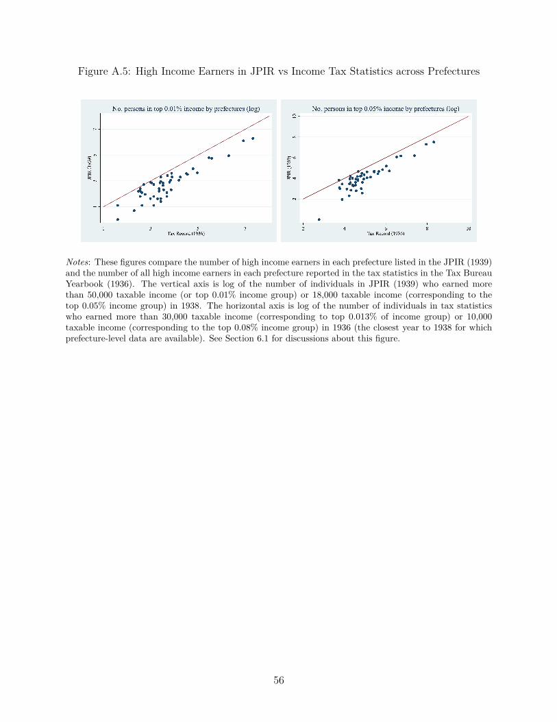
Figure A.5: High Income Earners in JPIR vs Income Tax Statistics across Prefectures

Notes: These figures compare the number of high income earners in each prefecture listed in the JPIR (1939)and the number of all high income earners in each prefecture reported in the tax statistics in the Tax BureauYearbook (1936). The vertical axis is log of the number of individuals in JPIR (1939) who earned morethan 50,000 taxable income (or top 0.01% income group) or 18,000 taxable income (corresponding to thetop 0.05% income group) in 1938. The horizontal axis is log of the number of individuals in tax statisticswho earned more than 30,000 taxable income (corresponding to top 0.013% of income group) or 10,000taxable income (corresponding to the top 0.08% income group) in 1936 (the closest year to 1938 for whichprefecture-level data are available). See Section 6.1 for discussions about this figure.

56

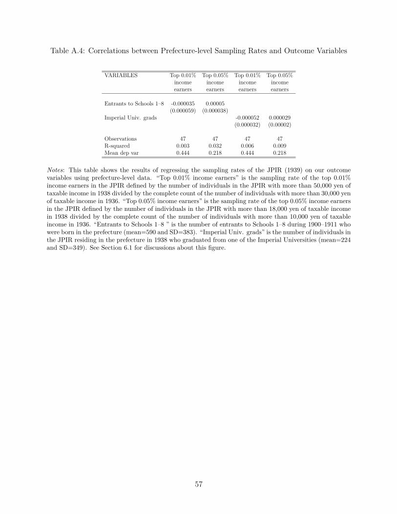
Table A.4: Correlations between Prefecture-level Sampling Rates and Outcome Variables

VARIABLES Top 0.01% Top 0.05% Top 0.01% Top 0.05%income income income incomeearners earners earners earners

Entrants to Schools 1–8 -0.000035 0.00005(0.000059) (0.000038)

Imperial Univ. grads -0.000052 0.000029(0.000032) (0.00002)

Observations 47 47 47 47R-squared 0.003 0.032 0.006 0.009Mean dep var 0.444 0.218 0.444 0.218

Notes: This table shows the results of regressing the sampling rates of the JPIR (1939) on our outcomevariables using prefecture-level data. “Top 0.01% income earners” is the sampling rate of the top 0.01%income earners in the JPIR defined by the number of individuals in the JPIR with more than 50,000 yen oftaxable income in 1938 divided by the complete count of the number of individuals with more than 30,000 yenof taxable income in 1936. “Top 0.05% income earners” is the sampling rate of the top 0.05% income earnersin the JPIR defined by the number of individuals in the JPIR with more than 18,000 yen of taxable incomein 1938 divided by the complete count of the number of individuals with more than 10,000 yen of taxableincome in 1936. “Entrants to Schools 1–8 ” is the number of entrants to Schools 1–8 during 1900–1911 whowere born in the prefecture (mean=590 and SD=383). “Imperial Univ. grads” is the number of individuals inthe JPIR residing in the prefecture in 1938 who graduated from one of the Imperial Universities (mean=224and SD=349). See Section 6.1 for discussions about this figure.

57

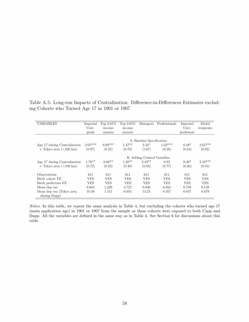
Table A.5: Long-run Impacts of Centralization: Difference-in-Differences Estimates exclud-ing Cohorts who Turned Age 17 in 1901 or 1907

VARIABLES Imperial Top 0.01% Top 0.05% Managers Professionals Imperial MedalUniv. income income Univ. recipientsgrads earners earners professors

A. Baseline SpecificationAge 17 during Centralization 3.05*** 0.69*** 1.47** 3.34* 1.63*** 0.48* 2.65***× Tokyo area (<100 km) (0.97) (0.24) (0.70) (1.67) (0.58) (0.24) (0.93)

B. Adding Control VariablesAge 17 during Centralization 1.76** 0.60** 1.28** 2.43** 0.83 0.46* 2.10***× Tokyo area (<100 km) (0.72) (0.23) (0.48) (0.94) (0.77) (0.26) (0.55)

Observations 611 611 611 611 611 611 611Birth cohort FE YES YES YES YES YES YES YESBirth prefecture FE YES YES YES YES YES YES YESMean dep var 8.684 1.229 4.727 9.830 6.682 0.750 6.149Mean dep var (Tokyo area 10.38 1.411 6.054 13.25 8.357 0.857 6.679during Dapp)

Notes: In this table, we repeat the same analysis in Table 4, but excluding the cohorts who turned age 17(main application age) in 1901 or 1907 from the sample as these cohorts were exposed to both Capp andDapp. All the variables are defined in the same way as in Table 4. See Section 6 for discussions about thistable.

58

Table A.6: Pre-event Trends Are Parallel

VARIABLES Imperial Top 0.01% Top 0.05% Managers Professionals Imperial MedalUniv. income income Univ. recipientsgrads earners earners professors

A. Baseline SpecificationTokyo area (< 100 km) 0.189 -0.017 0.073 0.224 0.202 0.019 0.178× Time trend (0.445) (0.065) (0.303) (0.478) (0.239) (0.082) (0.253)

B. Adding Control VariablesTokyo area (< 100 km) -0.054 -0.041 -0.112 -0.003 0.079 -0.017 0.050× Time trend (0.108) (0.050) (0.121) (0.167) (0.069) (0.033) (0.094)

Observations 470 470 470 470 470 470 470Birth cohort FE YES YES YES YES YES YES YESBirth prefecture FE YES YES YES YES YES YES YESMean dep var 5.023 1.209 4.151 7.070 3.994 0.381 4.402Mean dep var (Tokyo area 6.471 1.286 5.457 9.986 5.486 0.500 5.329during Dapp)

Notes: This table tests if there are differences in pre-event trends between urban and rural areas in thedifference-in-differences analysis in Table 4. The estimates are based on the birth-prefecture-cohort leveldata compiled from the JPIR in 1939, which includes cohorts born in 1874-1883 who turned age 17 (mainapplication age) in 1891-1900. This table runs the following regression:

Ypt = β × Timetrendt × Urbanp + αp + αt + εpt,

where Timetrendt is defined as the cohort’s birth year minus 1870 (the linear time trend). All the othervariables are defined in the same way as in Table 4. See Section 6 for discussions about this figure.

Table A.7: Using the JPIR in 1934

(1) (2) (3) (4) (5) (6) (7)VARIABLES Imperial Top 0.01% Top 0.05% Managers Professionals Imperial Medal

Univ. income income Univ. recipientsgrads earners earners professors

Age 17 during Centralization 1.68** 0.46* 1.63** 1.30*** 1.17** 0.15 1.40*× Tokyo area (<100 km) (0.64) (0.24) (0.72) (0.42) (0.56) (0.17) (0.76)

Observations 705 705 705 705 705 705 705Birth cohort FE YES YES YES YES YES YES YESBirth prefecture FE YES YES YES YES YES YES YESMean dep var 4.790 0.810 3.635 3.216 3.281 0.468 3.933Mean dep var (Tokyo area 5.683 1.111 6.175 5.063 4.175 0.587 4.524during Dapp)

Notes: In this table, we repeat the same analysis as in Table 4 Panel B, but alternatively using the datafrom JPIR published in 1934. In the 1934 JPIR, we observe the cohorts born in 1880–1894 when they are40 to 54 years old. Sampling rates in the 1934 JPIR for top income earners are similar to those in the 1939JPIR: 51% and 40% for top 0.01% and top 0.05% income earners. All the variables are defined in the sameway as in Table 4. See Section 6 for discussions about this table.

59

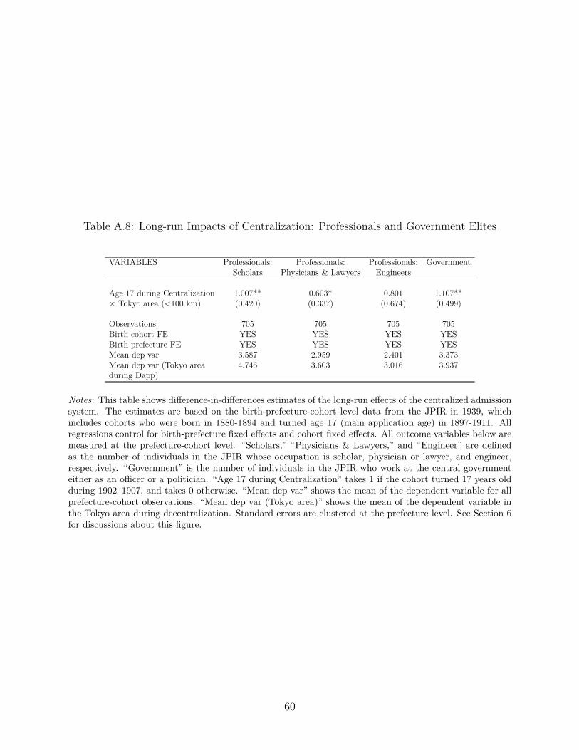
Table A.8: Long-run Impacts of Centralization: Professionals and Government Elites

VARIABLES Professionals: Professionals: Professionals: GovernmentScholars Physicians & Lawyers Engineers

Age 17 during Centralization 1.007** 0.603* 0.801 1.107**× Tokyo area (<100 km) (0.420) (0.337) (0.674) (0.499)

Observations 705 705 705 705Birth cohort FE YES YES YES YESBirth prefecture FE YES YES YES YESMean dep var 3.587 2.959 2.401 3.373Mean dep var (Tokyo area 4.746 3.603 3.016 3.937during Dapp)

Notes: This table shows difference-in-differences estimates of the long-run effects of the centralized admissionsystem. The estimates are based on the birth-prefecture-cohort level data from the JPIR in 1939, whichincludes cohorts who were born in 1880-1894 and turned age 17 (main application age) in 1897-1911. Allregressions control for birth-prefecture fixed effects and cohort fixed effects. All outcome variables below aremeasured at the prefecture-cohort level. “Scholars,” “Physicians & Lawyers,” and “Engineer” are definedas the number of individuals in the JPIR whose occupation is scholar, physician or lawyer, and engineer,respectively. “Government” is the number of individuals in the JPIR who work at the central governmenteither as an officer or a politician. “Age 17 during Centralization” takes 1 if the cohort turned 17 years oldduring 1902–1907, and takes 0 otherwise. “Mean dep var” shows the mean of the dependent variable for allprefecture-cohort observations. “Mean dep var (Tokyo area)” shows the mean of the dependent variable inthe Tokyo area during decentralization. Standard errors are clustered at the prefecture level. See Section 6for discussions about this figure.

60