Local unitary transformation, long-range quantum entanglement,wave function renormalization, and topological order

Xie Chen,1 Zheng-Cheng Gu,2 and Xiao-Gang Wen1

1Department of Physics, Massachusetts Institute of Technology, Cambridge, Massachusetts 02139, USA2Kavli Institute for Theoretical Physics, University of California, Santa Barbara, CA 93106, USA

(Dated: Jul., 2010)

Two gapped quantum ground states in the same phase are connected by an adiabatic evolutionwhich gives rise to a local unitary transformation that maps between the states. On the otherhand, gapped ground states remain within the same phase under local unitary transformations.Therefore, local unitary transformations define an equivalence relation and the equivalence classesare the universality classes that define the different phases for gapped quantum systems. Sincelocal unitary transformations can remove local entanglement, the above equivalence/universalityclasses correspond to pattern of long range entanglement, which is the essence of topological order.The local unitary transformation also allows us to define a wave function renormalization scheme,under which a wave function can flow to a simpler one within the same equivalence/universalityclass. Using such a setup, we find conditions on the possible fixed-point wave functions where thelocal unitary transformations have finite dimensions. The solutions of the conditions allow us toclassify this type of topological orders, which generalize the string-net classification of topologicalorders. We also describe an algorithm of wave function renormalization induced by local unitarytransformations. The algorithm allows us to calculate the flow of tensor-product wave functionswhich are not at the fixed points. This will allow us to calculate topological orders as well assymmetry breaking orders in a generic tensor-product state.

Contents

I. Introduction – new states beyond symmetrybreaking 1

II. Short-range and long-range quantumentanglement 3

III. Quantum phases and local unitary evolutions 3

IV. Topological order is a pattern of long-rangeentanglement 5

V. The LU evolutions and quantum circuits 5

VI. Symmetry breaking orders and symmetryprotected topological orders 6

VII. Local unitary transformation and wavefunction renormalization 7

VIII. Wave function renormalization and aclassification of topological order 8A. Quantum states on a graph 8B. The structure of entanglement in a fixed-point

wave function 9C. The first type of wave function renormalization 10D. The second type of wave function

renormalization 12E. The fixed-point wave functions from the

fixed-point gLU transformations 13

IX. Simple solutions of the fixed-point conditions 15A. Unimportant phase factors in the solutions 15B. N = 1 loop state 15C. N = 1 string-net state 16D. An N = 2 string-net state – the Z3 state 17

X. A classification of time reversal invarianttopological orders 17

XI. Wave function renormalization for tensorproduct states 18A. Motivation 18B. Tensor product states 19C. Renormalization algorithm 19

1. Step 1: F-move 192. Step 2: P-move 203. Complications: corner double line 21

XII. Applications of the renormalization fortensor product states 21A. Renormalization on square lattice 22B. Ising symmetry breaking phase 23C. Z2 topological ordered phase 24

XIII. Summary 25

Appendix: Equivalence relation betweenquantum states in the same phase 26

References 28

I. INTRODUCTION – NEW STATES BEYONDSYMMETRY BREAKING

According to the principle of emergence, the rich prop-erties and the many different forms of materials originatefrom the different ways in which the atoms are orderedin the materials. Landau symmetry-breaking theory pro-vides a general understanding of those different ordersand resulting rich states of matter.1,2 It points out thatdifferent orders really correspond to different symmetries

arX

iv:1

004.

3835

v2 [

cond

-mat

.str

-el]

28

Jul 2

010

2

in the organizations of the constituent atoms. As a mate-rial changes from one order to another order (i.e., as thematerial undergoes a phase transition), what happensis that the symmetry of the organization of the atomschanges.

For a long time, we believed that Landau symmetry-breaking theory describes all possible orders in materials,and all possible (continuous) phase transitions. However,in last twenty years, it has become more and more clearthat Landau symmetry-breaking theory does not describeall possible orders. After the discovery of high Tc super-conductors in 1986,3 some theorists believed that quan-tum spin liquids play a key role in understanding highTc superconductors4 and started to introduce variousspin liquids.5–9 Despite the success of Landau symmetry-breaking theory in describing all kinds of states, the the-ory cannot explain and does not even allow the existenceof spin liquids. This leads many theorists to doubt thevery existence of spin liquids. In 1987, in an attempt toexplain high temperature superconductivity, an infraredstable spin liquid – chiral spin state was discovered,10,11

which was shown to be perturbatively stable and exist asquantum phase of matter (at least in a large N limit).At first, not believing Landau symmetry-breaking the-ory fails to describe spin liquids, people still wanted touse symmetry-breaking to describe the chiral spin state.They identified the chiral spin state as a state that breaksthe time reversal and parity symmetries, but not the spinrotation symmetry.11 However, it was quickly realizedthat there are many different chiral spin states that haveexactly the same symmetry, so symmetry alone is notenough to characterize different chiral spin states. Thismeans that the chiral spin states contain a new kind oforder that is beyond symmetry description.12 This newkind of order was named13 topological order.72

The key to identify (and define) new orders is to iden-tify new universal properties that are beyond the localorder parameters and long-range correlations used in theLandau symmetry breaking theory. Indeed, new quan-tum numbers, such as ground state degeneracy12, thenon-Abelian Berry’s phase of degenerate ground states13

and edge excitations15, were introduced to character-ize (and define) the different topological orders in chi-ral spin states. Recently, it was shown that topologicalorders can also be characterized by topological entan-glement entropy.16,17 More importantly, those quantitieswere shown to be universal (ie robust against any localperturbation of the Hamiltonian) for chiral spin states.13

The existence of those universal properties establishes theexistence of topological order in chiral spin states.

Near the end of 1980’s, the existence of chiralspin states as a theoretical possibility, as well astheir many amazing properties, such as fractionalstatistics,10,11 spin-charge separation,10,11 chiral gaplessedge excitations,15 were established reliably, at least inthe large N -limit introduced in Ref. 26. Even non-Abelian chiral spin states can be established reliably inthe largeN -limit.18 However, it took about 10 years to es-

tablish the existence of a chiral spin state reliably withoutusing large N -limit (based on an exactly soluble modelon honeycomb lattice).19

Soon after the introduction of chiral spin states, exper-iments indicated that high-temperature superconductorsdo not break the time reversal and parity symmetries. Sochiral spin states do not describe high-temperature super-conductors. Thus the theory of topological order becamea theory with no experimental realization. However, thesimilarity between chiral spin states and fractional quan-tum Hall (FQH) states allows one to use the theory oftopological order to describe different FQH states.20 Justlike chiral spin states, different FQH states all have thesame symmetry and are beyond the Landau symmetry-breaking description. Also like chiral spin states, FQHstates have ground state degeneracies21 that depend onthe topology of the space.13,20 Those ground state de-generacies are shown to be robust against any pertur-bations. Thus, the different orders in different quantumHall states can be described by topological orders, andthe topological order does have experimental realizations.

The topology dependent ground state degeneracy, thatsignal the presence of topological order, is an amazingphenomenon. In FQH states, the correlation of any lo-cal operators are short ranged. This seems to imply thatFQH states are “short sighted” and they cannot knowthe topology of space which is a global and long-distanceproperty. However, the fact that ground state degeneracydoes depend on the topology of space implies that FQHstates are not “short sighted” and they do find a wayto know the global and long-distance structure of space.So, despite the short-range correlations of any local oper-ators, the FQH states must contain certain hidden long-range correlation. But what is this hidden long-rangecorrelation? This will be one of the main topic of thispaper.

Since high Tc superconductors do not break the timereversal and parity symmetries, nor any other latticesymmetries, some people concentrated on finding spinliquids that respect all those symmetries and hopingone of those symmetric spin liquids hold the key to un-derstand high Tc superconductors. Between 1987 and1992, many symmetric spin liquids were introduced andstudied.5–9,22–25 The excitations in some of constructedspin liquids have a finite energy gap, while in others thereis no energy gap. Those symmetric spin liquids do notbreak any symmetry and, by definition, are beyond Lan-dau symmetry-breaking description.

By construction, topological order only describes theorganization of particles or spins in a gapped quantumstate. So the theory of topological order only applies togapped spin liquids. Indeed, we find that the gappedspin liquids do contain nontrivial topological orders24

(as signified by their topology dependent and robustground state degeneracies) and are described by topo-logical quantum field theory (such as Z2 gauge theory)at low energies. One of the simplest topologically or-dered spin liquids is the Z2 spin liquid which was first

3

introduced in 1991.23,24 The existence of Z2 spin liquidas a theoretical possibility, as well as its many amazingproperties, such as spin-charge separation,23,24 fractionalmutual statistics,24 topologically protected ground statedegeneracy,24 were established reliably (at least in thelarge N -limit introduced in Ref. 26). Later, Kitaev in-troduced the famous toric code model which establishesthe existence of the Z2 spin liquid reliably without usinglarge N -limit.27 The topologically protected degeneracyof the Z2 spin liquid was used to perform fault-tolerantquantum computation.

The study of high Tc superconductors also leads tomany gapless spin liquids. The stability and the exis-tence of those gapless spin liquid were in more doubtsthan their gapped counterparts. But careful analysis incertain large N limit do suggest that stable gapless spinliquids can exist.26,28,29 If we do believe in the existenceof gapless spin liquids, then the next question is how todescribe the orders (ie the organizations of spins) in thosegapless spin liquids. If gapped quantum state can containnew type of orders that are beyond Landau’s symmetrybreaking description, it is natural to expect that gaplessquantum states can also contain new type of orders. Buthow to show the existence of new orders in gapless states?

Just like topological order, the key to identify new or-ders is to identify new universal properties that are be-yond Landau symmetry description. Clearly we can nolonger use the ground state degeneracy to establish theexistence of new orders in gapless states. To show theexistence of new orders in gapless states, a new univer-sal quantity – projective symmetry group (PSG) – wasintroduced.30 It was argued that (some) PSGs are robustagainst any local perturbations of the Hamiltonian thatdo not change the symmetry of the Hamiltonian.28–31 Sothrough PSG, we establish the existence of new orderseven in gapless states. The new orders are called quan-tum order to indicate that the new orders are relatedto patterns of quantum entanglement in the many-bodyground state.32

II. SHORT-RANGE AND LONG-RANGEQUANTUM ENTANGLEMENT

What is missed in Landau theory so that it fails todescribe those new orders? What is the new feature inthe organization of particles/spins so that the resultingorder cannot be described by symmetry?

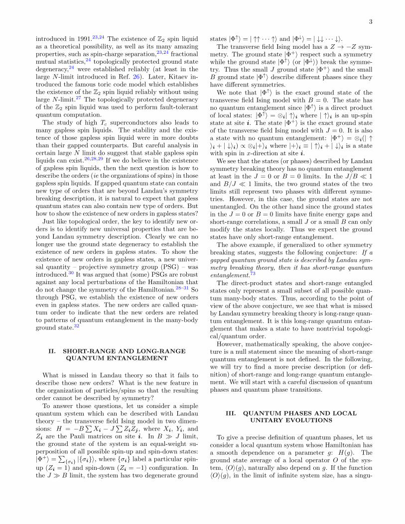
To answer those questions, let us consider a simplequantum system which can be described with Landautheory – the transverse field Ising model in two dimen-sions: H = −B

∑Xi − J

∑ZiZj , where Xi, Yi, and

Zi are the Pauli matrices on site i. In B � J limit,the ground state of the system is an equal-weight su-perposition of all possible spin-up and spin-down states:|Φ+〉 =

∑{σi} |{σi}〉, where {σi} label a particular spin-

up (Zi = 1) and spin-down (Zi = −1) configuration. Inthe J � B limit, the system has two degenerate ground

states |Φ↑〉 = | ↑↑ · · · ↑〉 and |Φ↓〉 = | ↓↓ · · · ↓〉.The transverse field Ising model has a Z → −Z sym-

metry. The ground state |Φ+〉 respect such a symmetrywhile the ground state |Φ↑〉 (or |Φ↓〉) break the symme-try. Thus the small J ground state |Φ+〉 and the smallB ground state |Φ↑〉 describe different phases since theyhave different symmetries.

We note that |Φ↑〉 is the exact ground state of thetransverse field Ising model with B = 0. The state hasno quantum entanglement since |Φ↑〉 is a direct productof local states: |Φ↑〉 = ⊗i| ↑〉i where | ↑〉i is an up-spinstate at site i. The state |Φ+〉 is the exact ground stateof the transverse field Ising model with J = 0. It is alsoa state with no quantum entanglement: |Φ+〉 = ⊗i(| ↑〉i + | ↓〉i) ∝ ⊗i|+〉i where |+〉i ≡ | ↑〉i + | ↓〉i is a statewith spin in x-direction at site i.

We see that the states (or phases) described by Landausymmetry breaking theory has no quantum entanglementat least in the J = 0 or B = 0 limits. In the J/B � 1and B/J � 1 limits, the two ground states of the twolimits still represent two phases with different symme-tries. However, in this case, the ground states are notunentangled. On the other hand since the ground statesin the J = 0 or B = 0 limits have finite energy gaps andshort-range correlations, a small J or a small B can onlymodify the states locally. Thus we expect the groundstates have only short-range entanglement.

The above example, if generalized to other symmetrybreaking states, suggests the following conjecture: If agapped quantum ground state is described by Landau sym-metry breaking theory, then it has short-range quantumentanglement.73

The direct-product states and short-range entangledstates only represent a small subset of all possible quan-tum many-body states. Thus, according to the point ofview of the above conjecture, we see that what is missedby Landau symmetry breaking theory is long-range quan-tum entanglement. It is this long-range quantum entan-glement that makes a state to have nontrivial topologi-cal/quantum order.

However, mathematically speaking, the above conjec-ture is a null statement since the meaning of short-rangequantum entanglement is not defined. In the following,we will try to find a more precise description (or defi-nition) of short-range and long-range quantum entangle-ment. We will start with a careful discussion of quantumphases and quantum phase transitions.

III. QUANTUM PHASES AND LOCALUNITARY EVOLUTIONS

To give a precise definition of quantum phases, let usconsider a local quantum system whose Hamiltonian hasa smooth dependence on a parameter g: H(g). Theground state average of a local operator O of the sys-tem, 〈O〉(g), naturally also depend on g. If the function〈O〉(g), in the limit of infinite system size, has a singu-

4

larity at gc for some local operators O, then the systemdescribed by H(g) has a quantum phase transition atgc. After defining phase transition, we can define whentwo quantum ground states belong to the same phase:Let |Φ(0)〉 be the ground state of H(0) and |Φ(1)〉 be theground state of H(1). If we can find a smooth path H(g),0 ≤ g ≤ 1 that connect the two Hamiltonian H(0) andH(1) such that there is no phase transition along thepath, then the two quantum ground states |Φ(0)〉 and|Φ(1)〉 belong to the same phase. We note that “con-nected by a smooth path” define an equivalence relationbetween quantum states. A quantum phase is an equiv-alence class of such equivalence relation. Such an equiv-alence class is called an universality class.

If |Φ(0)〉 is the ground state of H(0) and in the limitof infinite system size all excitations above |Φ(0)〉 have agap, then for small enough g, we believe that the systemsdescribed by H(g) are also gapped.33 In this case, we canshow that, the ground state of H(g), |Φ(g)〉, is in thesame phase as |Φ(0)〉, for small enough g, ie the average〈O〉(g) is a smooth function of g near g = 0 for any localoperator O.34 After scaling g to 1, we find that:

If the energy gap for H(g) is finite for all g in thesegment [0, 1], then there is no phase transitionalong the path g.

In other words, for gapped system, a quantum phasetransition can happen only when energy gap closes34 (seeFig. 1).74 Here, we would like to assume that the reverseis also true: a closing of the energy gap for a gapped statealways induces a phase transition. Or more precisely

If two gapped states |Φ(0)〉 and |Φ(1)〉 are in thesame phase, then we can always find a family ofHamiltonian H(g), such that the energy gap forH(g) are finite for all g in the segment [0, 1], and|Φ(0)〉 and |Φ(1)〉 are ground states of H(0) andH(1) respectively.

The above two boxed statements imply that two gappedquantum states are in the same phase |Φ(0)〉 ∼ |Φ(1)〉 ifand only if they can be connected by an adiabatic evolu-tion that does not close the energy gap.

Given two states, |Φ(0)〉 and |Φ(1)〉, determining theexistence of such a gapped adiabatic connection can behard. We would like to have a more operationally practi-cal equivalence relation between states in the same phase.Here we would like to show that two gapped states |Φ(0)〉and |Φ(1)〉 are in the same phase, if and only if they arerelated by a local unitary (LU) evolution. We definea local unitary(LU) evolution as an unitary operationgenerated by time evolution of a local Hamiltonian for afinite time. That is,

|Φ(1)〉 ∼ |Φ(0)〉 iff |Φ(1)〉 = T [e−i∫ 10dg H(g)]|Φ(0)〉 (1)

where T is the path-ordering operator and H(g) =∑iOi(g) is a sum of local Hermitian operators. Note

s

E

s

E

s

E

s

E

∆∆

ε

(a)

(c)

(b)

(d)

FIG. 1: (Color online) Energy spectrum of a gapped sys-tem as a function of a parameter s in the Hamiltonian. (a,b)For gapped system, a quantum phase transition can happenonly when energy gap closes. (a) describes a first order quan-tum phase transition (caused by level crossing). (b) describesa continuous quantum phase transition which has a contin-uum of gapless excitations at the transition point. (c) and(d) cannot happen for generic states. A gapped system mayhave ground state degeneracy, where the energy splitting be-tween the ground states vanishes when system size L → ∞:limL→∞ ε = 0. The energy gap ∆ between ground and excitedstates on the other hand remains finite as L→ ∞.

that H(g) is in general different from the adiabatic pathH(g) that connects the two states.

First, assume that two states |Φ(0)〉 and |Φ(1)〉 are inthe same phase, therefore we can find a gapped adia-batic path H(g) between the states. The existence of agap prevents the system to be excited to higher energylevels and leads to a local unitary evolution, the Quasi-adiabatic Continuation as defined in Ref. 34, that mapsfrom one state to the other. That is,

|Φ(1)〉 = U |Φ(0)〉, U = T [e−i∫ 10dg H(g)] (2)

The exact form of H(g) is given in Ref. 33,34 and will bediscussed in more detail in Appendix.

On the other hand, the reverse is also true: if twogapped states |Φ(0)〉 and |Φ(1)〉 are related by a local uni-tary evolution, then they are in the same phase. Since|Φ(0)〉 and |Φ(1)〉 are related by a local unitary evolution,

we have |Φ(1)〉 = T [e−i∫ 10dg H(g)]|Φ(0)〉. Let us introduce

|Φ(s)〉 = U(s)|Φ(0)〉, U(s) = T [e−i∫ s0dg H(g)]. (3)

Assume |Φ(0)〉 is a ground state of H(0), then |Φ(s)〉 isa ground state of H(s) = U(s)HU†(s). If H(s) remainslocal and gapped for all s ∈ [0, 1], then we have found anadiabatic connection between |Φ(0)〉 and |Φ(1)〉.

First, let us show that H(s) is a local Hamiltonian.Since H is a local Hamiltonian, it has a form H =

∑iOi

where Oi only acts on a cluster whose size is ξ. ξ is calledthe range of interaction of H. We see that H(s) has aform H(s) =

∑iOi(s), where Oi(s) = U(s)OiU

†(s). To

5

show that Oi(s) only acts on a cluster of a finite size,

we note that for a local system described by H(g), thepropagation velocities of its excitations have a maximumvalue vmax. Since Oi(s) can be viewed as the time evo-

lution of Oi by H(t) from t = 0 to t = s, we find that

Oi(s) only acts on a cluster of size ξ + ξ + svmax,34,35

where ξ is the range of interaction of H. Thus H(s) areindeed local Hamiltonian.

If H has a finite energy gap, then H(s) also have afinite energy gap for any s. As s goes for 0 to 1, theground state of the local Hamiltonians, H(s), goes from|Φ(0)〉 to |Φ(1)〉. Thus the two states |Φ(0)〉 and |Φ(1)〉belong to the same phase. This completes our argumentthat states related by a local unitary evolution belong tothe same phase.

Thus through the above discussion, we show that

Two gapped ground states,75 |Φ(0)〉 and |Φ(1)〉,belong to the same phase if and only if they arerelated by a local unitary evolution (1).

A more detailed and more rigorous discussion of thisequivalence relation is given in Appendix A, where ex-act bounds on locality and transformation error is given.

The relation (1) defines an equivalence relation be-tween |Φ(0)〉 and |Φ(1)〉. The equivalence classes ofsuch an equivalence relation represent different quantumphases. So the above result implies that the equivalenceclasses of the LU evolutions are the universality classesof quantum phases for gapped states.

IV. TOPOLOGICAL ORDER IS A PATTERN OFLONG-RANGE ENTANGLEMENT

Using the LU evolution, we can obtain a more precisedescription (or definition) of short-range entanglement:

A state has only short-range entanglement if andonly if it can be transformed into an unentangledstate (ie a direct-product state) through a local uni-tary evolution.

If a state cannot be transformed into an unentangledstate through a LU evolution, then the state has long-range entanglement. We also see that

All states with short-range entanglement cantransform into each other through local unitaryevolutions.

Thus all states with short-range entanglement belong tothe same phase. The local unitary evolutions we con-sider here do not have any symmetry. If we require cer-tain symmetry of the local unitary evolutions, states withshort-range entanglement may belong to different sym-metry breaking phases, which will be discussed in sectionVI.

(a)

(b)

l...

Ui

1 2

FIG. 2: (Color online) (a) A graphic representation of aquantum circuit, which is formed by (b) unitary operationson patches of finite size l. The green shading represents acausal structure.

Since a direct-product state is a state with trivial topo-logical order, we see that a state with a short-range en-tanglement also has a trivial topological order. Thisleads us to conclude that a non-trivial topological or-der is related to long-range entanglement. Since twogapped states related by a LU evolution belong to thesame phase, thus two gapped states related by a localunitary evolution have the same topological order. Inother words,

Topological order describes the equivalent classesdefined by local unitary evolutions.

Or more pictorially, topological order is a pattern oflong-range entanglement. In Ref. 36, it was shown thatthe “topologically non-trivial” ground states, such as thetoric code,27 cannot be changed into a “topologically triv-ial” state such as a product state by any unitary locality-preserving operator. In other words, those “topologicallynon-trivial” ground states have long-range entanglement.

V. THE LU EVOLUTIONS AND QUANTUMCIRCUITS

The LU evolutions introduced here is closely relatedto quantum circuits with finite depth. To define quan-tum circuits, let us introduce piece-wise local unitaryoperators. A piece-wise local unitary operator has aform Upwl =

∏i Ui where {Ui} is a set of unitary op-

erators that act on non overlapping regions. The sizeof each region is less than some finite number l. Theunitary operator Upwl defined in this way is called apiece-wise local unitary operator with range l. A quan-tum circuit with depth M is given by the product of Mpiece-wise local unitary operators (see Fig. 2): UMcirc =

U(1)pwlU

(2)pwl · · ·U

(M)pwl . In quantum information theory, it

is known that finite time unitary evolution with localHamiltonian (LU evolution defined before) can be sim-ulated with constant depth quantum circuit and vice-verse. Therefore, the equivalence relation eqn. (1) can beequivalently stated in terms of constant depth quantumcircuits:

|Φ(1)〉 ∼ |Φ(0)〉 iff |Φ(1)〉 = UMcirc|Φ(0)〉 (4)

6

where M is a constant independent of system size. Be-cause of their equivalence, we will use the term “LocalUnitary Transformation” to refer to both local unitaryevolution and constant depth quantum circuit in general.

The LU transformation defined through LU evolution(1) is more general. It can be easily generalized to studytopological orders and quantum phases with symmetries(see section VI).30,37 The quantum circuit has a moreclear and simple causal structure. However, the quantumcircuit approach breaks the translation symmetry. So itis more suitable for studying quantum phases that do nothave translation symmetry.

In fact, people have been using quantum circuits toclassify many-body quantum states which correspond toquantum phases of matter. In Ref. 38, the local uni-tary transformations described by quantum circuits wasused to define a renormalization group transformationsfor states and establish an equivalence relation in whichstates are equivalent if they are connected by a local uni-tary transformation. Such an approach was used to clas-sify 1D matrix product states. In Ref. 39, the local uni-tary transformations with disentanglers was used to per-form a renormalization group transformations for states,which give rise to the multi-scale entanglement renormal-ization ansatz (MERA) in one and higher dimensions.The disentanglers and the isometries in MERA can beused to study quantum phases and quantum phase tran-sitions in one and higher dimensions. Later in this paper,we will use the quantum circuit description of LU trans-formations to classify 2D topological orders through clas-sifying the fixed-point LU transformations.

VI. SYMMETRY BREAKING ORDERS ANDSYMMETRY PROTECTED TOPOLOGICAL

ORDERS

In the above discussions, we have defined phases with-out any symmetry consideration. The H(g) or Upwl inthe LU transformation does not need to have any sym-metry and can be sum/product of any local operators. Inthis case, two Hamiltonians with an adiabatic connectionare in the same phase even if they may have different sym-metries. Also, all states with short-range entanglementbelong to the same phase (under the LU transformationsthat do not have any symmetry).

On the other hand, we can consider only Hamiltoni-ans H with certain symmetries and define phases as theequivalent classes of symmetric local unitary transforma-tions:

|Ψ〉 ∼ T(e− i

∫ 10dg H(g)

)|Ψ〉 or |Ψ〉 ∼ UMcirc|Ψ〉

where H(g) or UMcirc has the same symmetries as H. Wenote that the symmetric local unitary transformation in

the form T(e− i

∫ 10dg H(g)

)always connect to the identity

transformation continuously. This may not be the casefor the transformation in the form UMcirc. To rule out that

g1

2g

2g

SRE

LRE 1 LRE 2

SB−SRE 1

SY−SRE 1

SB−LRE 1 SB−LRE 2

SB−SRE 2

SY−SRE 2

SB−LRE 3

SY−LRE 1 SY−LRE 2 SY−LRE 3

1g(a) (b)

FIG. 3: (Color online) (a) The possible phases for a Hamil-tonian H(g1, g2) without any symmetry. (b) The possiblephases for a Hamiltonian Hsymm(g1, g2) with some symme-tries. The shaded regions in (a) and (b) represent the phaseswith short range entanglement (ie those ground states canbe transformed into a direct product state via a generic LUtransformations that do not have any symmetry.)

possibility, we define symmetric local unitary transforma-tions as those that connect to the identity transformationcontinuously.

The equivalent classes of the symmetric LU transfor-mations have very different structures compared to thoseof LU transformations without symmetry. Each equiva-lent class of the symmetric LU transformations is smallerand there are more kinds of classes, in general.

Fig. 3 compares the structure of phases for a systemwithout any symmetry and a system with some symme-try in more detail. For a system without any symme-try, all the short-range-entangled (SRE) states (ie thoseground states can be transformed into a direct productstate via a generic LU transformations that do not haveany symmetry) are in the same phase (SRE in Fig. 3(a)).On the other hand, long range entanglement (LRE) canhave many different patterns that give rise to differenttopological phases (LRE 1 and LRE 2 in Fig. 3(a)).The different topological orders usually give rise to quasi-particles with different fractional statistics and fractionalcharges.

For a system with some symmetries, the phase struc-ture can be much more complicated. The short-range-entangled states no longer belong to the same phase,since the equivalence relation is described by more spe-cial symmetric LU transformations:(A) States with short range entanglement belong to dif-ferent equivalent classes of the symmetric LU transfor-mations if they have different broken symmetries. Theycorrespond to the symmetry-breaking (SB) short-range-entanglement phases SB-SRE 1 and SB-SRE 2 in Fig.3(b). They are Landau’s symmetry breaking states.(B) States with short range entanglement can belong todifferent equivalent classes of the symmetric LU trans-formations even if they do not break any symmetry ofthe system. (In this case, they have the same symme-try.) They correspond to the symmetric (SY) short-range-entangled phases SY-SRE 1 and SY-SRE 2 in Fig.3(b). We say those states have symmetry protected topo-logical orders. Haldane phase40 and Sz = 0 phase of spin-

7

FIG. 4: (Color online) A finite depth quantum circuit cantransform a state |Φ〉 into a direct-product state, if and only ifthe state |Φ〉 has no long-range quantum entanglement. Here,a dot represents a site with physical degrees of freedom. Avertical line carries an index that label the different physicalstates on a site. The presence of horizontal lines between dotsrepresents quantum entanglement.

1 chain are examples of states with the same symmetrywhich belong to two different equivalent classes of sym-metric LU transformations (with parity symmetry).37,41

Band and topological insulators42–47 are other examplesof states that have the same symmetry and at the sametime belong to two different equivalent classes of symmet-ric LU transformations (with time reversal symmetry).

Also, for a system with some symmetries, the long-range-entangled states are divided into more classes(more phases):(C) Symmetry breaking and long range entanglement canappear together in a state, such as SB-LRE 1, SB-LRE 2,etc in Fig. 3(b). The topological superconducting statesare examples of such phases.48,49

(D) Long-range-entangled states that do not break anysymmetry can also belong to different phases such asthe symmetric long-range-entanglement phases SY-LRE1, SY-LRE 2, etc in Fig. 3(b). The many differentZ2 symmetric spin liquids with spin rotation, transla-tion, and time-reversal symmetries are examples of thosephases.30,50,51 Some time-reversal symmetric topologi-cal orders were also called topological Mott-insulators orfractionalized topological insulators.52–57

VII. LOCAL UNITARY TRANSFORMATIONAND WAVE FUNCTION RENORMALIZATION

After defining topological order as the equivalentclasses of many-body wave functions under LU transfor-mations, we like to ask: how to describe (or label) thedifferent equivalent classes (ie the different topologicalorders or patterns of long-range entanglement)?

One simple way to do so is to use the full wave func-tion which completely describe the different topologicalorders. But the full wave functions contain a lot of non-universal short-range entanglement. As a result, such alabeling scheme is a very inefficient many-to-one labelingscheme of topological orders. To find a more efficient oreven one-to-one labeling scheme, we need to remove thenon-universal short-range entanglement.

As the first application of the notion of LU transfor-mation, we would like to describe a wave function renor-malization group flow introduced in Ref. 58,39. The wavefunction renormalization can remove the short-range en-

FIG. 5: (Color online) A piece-wise local unitary transforma-tion can transform some degrees of freedom in a state Φ〉 intoa direct product. Removing/adding the degrees of freedomin the form of direct product defines an additional equiva-lence relation that defines the topological order (or classes oflong-range entanglement).

tanglement and simplify the wave function. In Ref. 58,the wave function renormalization for string-net states isgenerated by the following two basic moves

Φ

(ji l

k)

=δijΦ

(i

)(5)

Φ

(l

mi

j k

)=∑n

F jim∗

lk∗n∗Φ

(ji

knl

)(6)

(Note that the definition of the F-tensor in Ref. 58 isslightly different from the definition in this paper.) Thetwo basic moves can generate a generic wave functionrenormalization which can reduce the string-net wavefunctions to very simple forms.17,58 Later in Ref. 39, thewave function renormalization for generic states was dis-cussed in a more general setting, and was called MERA.The two basic string-net moves (5) and (6) correspond tothe isometry and the disentangler in MERA respectively.In the MERA approach, the isometries and the disentan-glers are applied in a layered fashion, while in the string-net approach, the two basic moves can be applied arbi-trarily. In this section, we will follow the MERA setupto describe the wave function renormalization. Later inthis paper, we will follow the string-net setup to studythe fixed-point wave functions.

Note that we can use a LU transformation U to trans-form some degrees of freedom in a state into direct prod-uct (see Fig. 5). We then remove those degrees of free-dom in the form of direct product. Such a procedure doesnot change the topological order. The reverse process ofadding degrees of freedom in the form of direct prod-uct also does not change the topological order. We callthe local transformation in Fig. 5 that changes the de-grees of freedom a generalized local unitary (gLU) trans-formation. It is clear that a generalized local unitarytransformation inside a region A does not change the re-duced density matrix ρA for the region A. This is thereason why we say that (generalized) local unitary trans-formations cannot change long-range entanglement andtopological order. Similarly, the addition or removal ofdecoupled degrees of freedom to or from the Hamilto-nian, H ↔ H ⊗ Hdp, will not change the phase of theHamiltonian (ie the ground states of H and H⊗Hdp are

8

region A

region A

U

P

(b)

U

U

(a)

FIG. 6: (Color online) (a) A gLU transformation U acts inregion A of a state |Φ〉, which reduces the degree freedom inregion A to those contained only in the support space of |Φ〉in region A. (b) U†U = P is a projector that does not changethe state |Φ〉.

in the same phase), if those degrees of freedom form a di-rect product state (ie the ground state of Hdp is a directproduct state).

Let us define the gLU transformation U more carefullyand in a more general setting. Consider a state |Φ〉. LetρA be the reduced density matrix of |Φ〉 in region A. ρAmay act in a subspace of the total Hilbert space VA inregion A, which is called the support space V spA of regionA. The dimension Dsp

A of V spA is called support dimensionof region A. Now the Hilbert space VA in region A can bewritten as VA = V spA ⊕ V

spA . Let |ψi〉, i = 1, ..., Dsp

A be a

basis of this support space V spA , |ψi〉, i = DspA + 1, ..., DA

be a basis of V spA , where DA is the dimension of VA, and|ψi〉, i = 1, ..., DA be a basis of VA. We can introducea LU transformation Ufull which rotates the basis |ψi〉to |ψi〉. We note that in the new basis, the wave func-tion only has non-zero amplitudes on the first Dsp

A basis

vectors. Thus, in the new basis |ψi〉, we can reduce therange of the label i from [1, DA] to [1, Dsp

A ] without losingany information. This motivates us to introduce the gLUtransformation as a rotation from |ψi〉, i = 1, ..., DA to

|ψi〉, i = 1, ..., DspA . The rectangular matrix U is given by

Uij = 〈ψi|ψj〉. We also regard the inverse of U , U†, asa gLU transformation. A LU transformation is viewedas a special case of gLU transformation where the de-grees of freedom are not changed. Clearly U†U = P andUU† = P ′ are two projectors. The action of P does notchange the state |Φ〉 (see Fig. 6(b)).

We note that despite the reduction of the degrees offreedom, a gLU transformation defines an equivalent rela-tion. Two states related by a gLU transformation belongto the same phase. The renormalization flow induced bythe gLU transformations always flows within the samephase.

VIII. WAVE FUNCTION RENORMALIZATIONAND A CLASSIFICATION OF TOPOLOGICAL

ORDER

As an application of the wave function renormalization,in this section, we will study the structure of fixed-pointwave functions under the wave function renormalization,which will lead to a classification of topological order(without any symmetry).

We note that as wave functions flow to a fixed point,the gLU transformations in each step of the renormal-ization also flow to a fixed point. So instead of study-ing fixed-point wave functions, here, we will study thefixed-point gLU transformations. For this purpose, weneed to fix the renormalization scheme. In the following,we will discuss a renormalization scheme motivated bythe string-net wave function.58 After we specify a properwave function renormalization scheme, then the fixed-point wave function is simply the wave function whose“form” does not change under the wave function renor-malization.

Since those fixed-point gLU transformations do notchange the fixed-point wave function, their actions on thefixed-point wave function do not depend on the order ofthe actions. This allows us to obtain many conditionsthat gLU transformations must satisfy. From those con-ditions, we can determine the forms of allowed fixed-pointgLU transformations. This leads to a general descriptionand a classification of topological orders and their corre-sponding fixed-point wave functions.

The renormalization scheme that we will discuss wasfirst used in Ref. 58 to characterize the scale invariantstring-net wave function. It is also used in Ref. 17 to sim-plify the string-net state in a region, which allows us tocalculate the entanglement entropy of the string-net stateexactly. A similar approach was used in Ref. 59 to showquantum-double/string-net wave function to be a fixed-point wave function and its connection to 2D MERA.39 Inthe following, we will generalize those discussions by notstarting with string-net wave functions. We just try toconstruct local unitary transformations at a fixed point.We will see that the fixed-point conditions on the gLUtransformations lead to a mathematical structure that issimilar to the tensor category theory – the mathematicalframework behind the string-net states.

A. Quantum states on a graph

Since the wave function renormalization may changethe lattice structure, we will consider quantum states de-fined on a generic trivalence graph G: Each edge hasN + 1 states, labeled by i = 0, ..., N (see Fig. 7). Weassume that the index i on the edge admits an one-to-onemapping ∗: i → i∗ that satisfies (i∗)∗ = i. As a result,the edges of the graph are oriented. The mapping i→ i∗

corresponds to the reverse of the orientation of the edge(see Fig. 8). Each vertex also has physical states, labeled

9

α=

β

γ

λ

v1,...,N

k

j

i=0,...,N

n

ml

FIG. 7: A quantum state on a graphG. There areN+1 stateson each edge which are labeled by l = 0, ..., N . There are Nv

states on each vertex which are labeled by α = 1, ..., Nv.

i i*

FIG. 8: The mapping i → i∗ corresponds to the reverse ofthe orientation of the edge

by α = 1, ..., Nv (see Fig. 7).

Each labeled graph (see Fig. 7) corresponds to a stateand all the labeled graphs form an orthonormal basis.Our fixed-point state is a superposition of those basis

states: |Φfix〉 =∑

all conf. Φfix

( ) ∣∣∣∣ ⟩.

Here we will make an important assumption about thefixed-point wave function. We will assume that the fixed-point wave function is “topological”: two labeled graphshave the same amplitude if the two labeled graphs canbe deformed into each other continuously on the planewithout the vertices crossing the links. For example

ψfix

11

2

2

0

1

0

0

1 2

= ψfix

1

21

2 10

1

0

2

0

. Due to

such an assumption, the topological orders studied in thispaper may not be most general.

We also assume that all the fixed-point states on eachdifferent graphs to have the same “form”. This assump-tion is motivated by the fact that during wave functionrenormalization, we transform a state on one graph to astate on a different graph. The “fixed-point” means thatthe wave functions on those different graphs are all deter-mined by the same collection of the rules, which definesthe meaning of having the same “form”. However, thewave function for a given graph can have different totalphases if the wave function is calculated by applying therules in different orders. Those rules are noting but thefixed-point gLU transformations.

B. The structure of entanglement in a fixed-pointwave function

Before describing the wave function renormalization,let us examine the structure of entanglement of a fixed-point wave function. First, let us consider a fixed-pointwave function Φfix on a graph. We examine the wave

α= 1,...,Νijk

β

γ

λ

ml

k

j

i

n

FIG. 9: A quantum state on a graph G. If the three edgesof a vertex are in the states i, j, and k respectively, then thevertex has Nijk states, labeled by α = 1, ..., Nijk. Note theorientation of the edges are point towards to vertex. Alsonote that i→ j → k runs anti-clockwise.

function on a patch of the graph, for example, βα

ji

lm

k

.

The fixed-point wave function Φfix

(β

αji

lm

k)

(only the

relevant part of the graph is drawn) can be viewed as a

function of α, β,m: ψijkl,Γ(α, β,m) = Φfix

(β

αji

lm

k)

if

we fix i, j, k, l and the indices on other part of the graph.(Here the indices on other part of the graph is summa-rized by Γ.) As we vary the indices Γ on other part ofgraph (still keeping i, j, k, and l fixed), the wave func-tion of α, β,m, ψijkl,Γ(α, β,m), may change. All thoseψijkl,Γ(α, β,m) form a linear space of dimension Dijkl∗ .Dijkl is an important concept that will appear later. Wenote that the two vertices α and β and the link m forma region surrounded by the links i, j, k, l. So we will callthe dimension-Dijkl∗ space the support space Vijkl∗ andDijkl∗ the support dimension for the state Φfix on theregion surrounded by the fixed boundary state i, j, k, l.

Similarly, we can define Dijk as the support dimension

of the Φfix

(α

kji)

on a region bounded by links i, j, k.

Since the region contains only a single vertex α with Nvphysics states, we have Dijk ≤ Nv. We can use a lo-cal unitary transformation on the vertex to reduce therange of α to 1, ..., Nijk where Nijk = Dijk. In the restof this paper, we will implement such a reduction. So,the number of physical states on a vertex depend on thephysical states of the edges that connect to the vertex.If the three edges of a vertex are in the states i, j, and krespectively, then the vertex has Nijk states, labeled byα = 1, ..., Nijk (see Fig. 9). Here we assume that

Nijk = Njki. (7)

We note that in the fixed-point wave function

Φfix

(β

αji

lm

k)

, the number of choices of α, β,m is

Nijkl∗ =∑Nm=0Njim∗Nkml∗ . Thus the support dimen-

sion Dijkl∗ satisfies Dijkl∗ ≤ Nijkl∗ . Here we will makean important assumption – the saturation assumption:

10

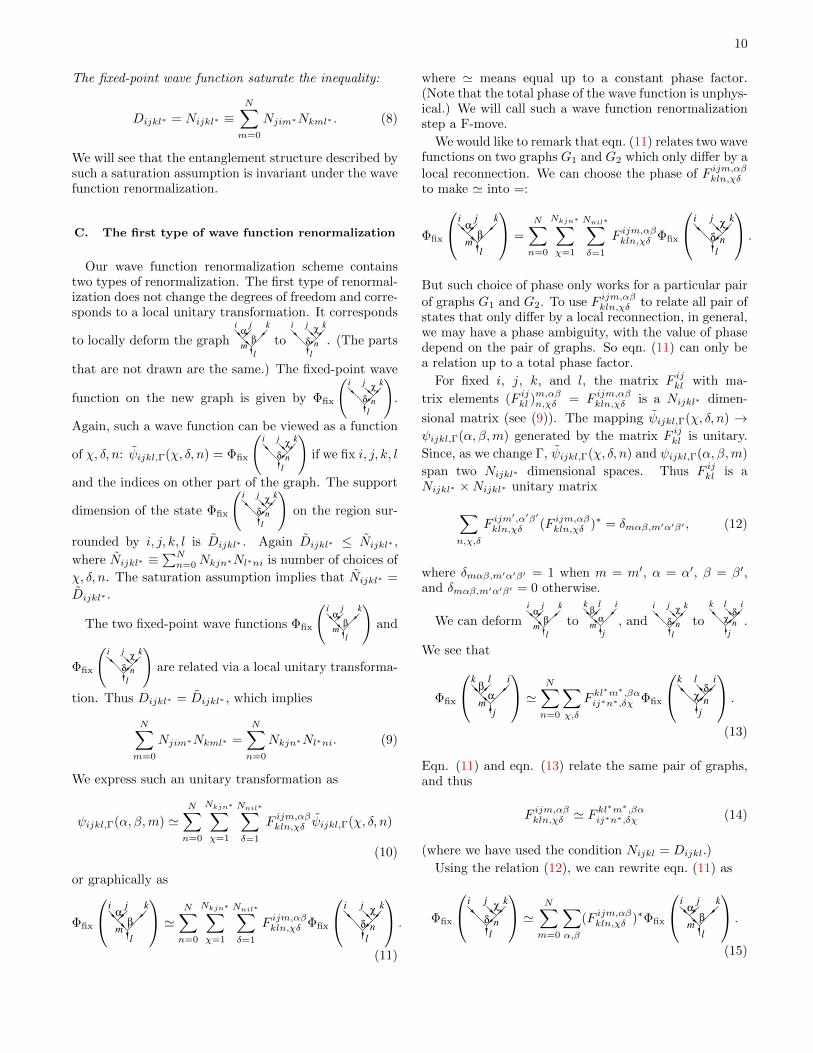
The fixed-point wave function saturate the inequality:

Dijkl∗ = Nijkl∗ ≡N∑m=0

Njim∗Nkml∗ . (8)

We will see that the entanglement structure described bysuch a saturation assumption is invariant under the wavefunction renormalization.

C. The first type of wave function renormalization

Our wave function renormalization scheme containstwo types of renormalization. The first type of renormal-ization does not change the degrees of freedom and corre-sponds to a local unitary transformation. It corresponds

to locally deform the graph βα

ji

lm

k

to δ

χi j k

l

n . (The parts

that are not drawn are the same.) The fixed-point wave

function on the new graph is given by Φfix

(δ

χi j k

l

n

).

Again, such a wave function can be viewed as a function

of χ, δ, n: ψijkl,Γ(χ, δ, n) = Φfix

(δ

χi j k

l

n

)if we fix i, j, k, l

and the indices on other part of the graph. The support

dimension of the state Φfix

(δ

χi j k

l

n

)on the region sur-

rounded by i, j, k, l is Dijkl∗ . Again Dijkl∗ ≤ Nijkl∗ ,

where Nijkl∗ ≡∑Nn=0Nkjn∗Nl∗ni is number of choices of

χ, δ, n. The saturation assumption implies that Nijkl∗ =

Dijkl∗ .

The two fixed-point wave functions Φfix

(β

αji

lm

k)

and

Φfix

(δ

χi j k

l

n

)are related via a local unitary transforma-

tion. Thus Dijkl∗ = Dijkl∗ , which implies

N∑m=0

Njim∗Nkml∗ =

N∑n=0

Nkjn∗Nl∗ni. (9)

We express such an unitary transformation as

ψijkl,Γ(α, β,m) 'N∑n=0

Nkjn∗∑χ=1

Nnil∗∑δ=1

F ijm,αβkln,χδ ψijkl,Γ(χ, δ, n)

(10)

or graphically as

Φfix

βα

ji

lm

k ' N∑

n=0

Nkjn∗∑χ=1

Nnil∗∑δ=1

F ijm,αβkln,χδ Φfix

δ

χi j k

l

n

.

(11)

where ' means equal up to a constant phase factor.(Note that the total phase of the wave function is unphys-ical.) We will call such a wave function renormalizationstep a F-move.

We would like to remark that eqn. (11) relates two wavefunctions on two graphs G1 and G2 which only differ by a

local reconnection. We can choose the phase of F ijm,αβkln,χδto make ' into =:

Φfix

βα

ji

lm

k =

N∑n=0

Nkjn∗∑χ=1

Nnil∗∑δ=1

F ijm,αβkln,χδ Φfix

δ

χi j k

l

n

.

But such choice of phase only works for a particular pair

of graphs G1 and G2. To use F ijm,αβkln,χδ to relate all pair ofstates that only differ by a local reconnection, in general,we may have a phase ambiguity, with the value of phasedepend on the pair of graphs. So eqn. (11) can only bea relation up to a total phase factor.

For fixed i, j, k, and l, the matrix F ijkl with ma-

trix elements (F ijkl )m,αβn,χδ = F ijm,αβkln,χδ is a Nijkl∗ dimen-

sional matrix (see (9)). The mapping ψijkl,Γ(χ, δ, n) →ψijkl,Γ(α, β,m) generated by the matrix F ijkl is unitary.

Since, as we change Γ, ψijkl,Γ(χ, δ, n) and ψijkl,Γ(α, β,m)

span two Nijkl∗ dimensional spaces. Thus F ijkl is aNijkl∗ ×Nijkl∗ unitary matrix

∑n,χ,δ

F ijm′,α′β′

kln,χδ (F ijm,αβkln,χδ )∗ = δmαβ,m′α′β′ , (12)

where δmαβ,m′α′β′ = 1 when m = m′, α = α′, β = β′,and δmαβ,m′α′β′ = 0 otherwise.

We can deform βα

ji

lm

k

toβ

α

k l

j

i

m , and δ

χi j k

l

n to χδ

k l

j

i

n .

We see that

Φfix

βα

k l

j

i

m

' N∑n=0

∑χ,δ

F kl∗m∗,βα

ij∗n∗,δχ Φfix

χδ

k l

j

i

n

.

(13)

Eqn. (11) and eqn. (13) relate the same pair of graphs,and thus

F ijm,αβkln,χδ ' Fkl∗m∗,βαij∗n∗,δχ (14)

(where we have used the condition Nijkl = Dijkl.)

Using the relation (12), we can rewrite eqn. (11) as

Φfix

δ

χi j k

l

n

' N∑m=0

∑α,β

(F ijm,αβkln,χδ )∗Φfix

βα

ji

lm

k .

(15)

11

We can also express Φfix

(δ

χi j k

l

n

)as

Φfix

δ

χi j k

l

n

' N∑m=0

∑α,β

F jkn,χδl∗i∗m∗,βαΦfix

βα

ji

lm

k(16)

using the relabeled eqn. (11). So we have

(F ijm,αβkln,χδ )∗ ' F jkn,χδl∗i∗m∗,βα. (17)

Since the total phase of the wave function is unphysical,

the total phase of F ijm,αβkln,χδ can be chosen arbitrarily. We

can choose the total phase of F ijm,αβkln,χδ to make

(F ijm,αβkln,χδ )∗ = F jkn,χδl∗i∗m∗,βα. (18)

If we apply eqn. (18) twice, we reproduce eqn. (14). Thuseqn. (14) is not independent and can be dropped.

From the graphic representation (11), We note that

F ijm,αβkln,χδ = 0 when (19)

Njim∗ < 1 or Nkml∗ < 1 or Nkjn∗ < 1 or Nnil∗ < 1.

When Njim∗ < 1 or Nkml∗ < 1, the left-hand-side of

eqn. (11) is always zero. Thus F ijm,αβkln,χδ = 0 whenNjim∗ <1 or Nkml∗ < 1. When Nkjn∗ < 1 or Nnil∗ < 1, wavefunction on the right-hand-side of eqn. (11) is always

zero. So we can choose F ijm,αβkln,χδ = 0 when Nkjn∗ < 1or Nnil∗ < 1.

The F-move (11) maps the wave functions on two dif-ferent graphs through a local unitary transformation.Since we can locally transform one graph to anothergraph through different paths, the F-move (11) must sat-isfy certain self consistent condition. For example the

graph χβ

αji

p

nm

lk

can be transformed toδ

γφ

ji

qs

p

lk

through

two different paths; one contains two steps of local trans-formations and the other contains three steps of localtransformations as described by eqn. (11). The two pathslead to the following relations between the wave func-tions:

Φfix

χβ

αji

p

nm

lk '∑

q,δ,ε

Fmkn,βχlpq,δε Φfix

ε

δαji

p

qm

lk ' ∑

q,δ,ε;s,φ,γ

Fmkn,βχlpq,δε F ijm,αεqps,φγ Φfix

δ

γφ

ji

qs

p

lk , (20)

Φfix

χβ

αji

p

nm

lk '∑

t,η,ϕ

F ijm,αβknt,ηϕ Φfix

ϕη

χ

ji

n

t

p

lk ' ∑

t,η,ϕ;s,κ,γ

F ijm,αβknt,ηϕ Fitn,ϕχlps,κγ Φfix

γ

κ

ηji

st

p

lk

'∑

t,η,κ;ϕ;s,κ,γ;q,δ,φ

F ijm,αβknt,ηϕ Fitn,ϕχlps,κγ F

jkt,ηκlsq,δφ Φfix

δ

γφ

ji

qs

p

lk . (21)

The consistence of the above two relations leads a condi-tion on the F tensor.

To obtain such a condition, let us fix i, j, k, l, p,

and view Φfix

χβ

αji

p

nm

lk as a function of α, β, χ,m, n:

ψ(α, β, χ,m, n) = Φfix

χβ

αji

p

nm

lk. As we vary indices

on other part of graph, we obtain different wave func-tions ψ(α, β, χ,m, n) which form a dimension Dijklp∗

space. In other words, Dijklp∗ is the support dimensionof the state Φfix on the region α, β, χ,m, n with bound-ary state i, j, k, l, p fixed (see the discussion in sectionVIII B). Since the number of choices of α, β, χ,m, n isNijklp∗ =

∑m,nNjim∗Nkmn∗Nlnp∗ , we have Dijklp∗ ≤

Nijklp∗ . Here we require a similar saturation conditionas in (8):

Nijklp∗ = Dijklp∗ (22)

12

Similarly, the number of choices of δ, φ, γ, q, s in

Φfix

δ

γφ

ji

qs

p

lk is also Nijklp∗ . Here we again assume

Dijklp∗ = Nijklp∗ , where Dijklp∗ is the support dimension

of Φfix

δ

γφ

ji

qs

p

lk on the region bounded by i, j, k, l, p.

So the two relations (20) and (21) can be viewed astwo relations between a pair of vectors in the two Dijklp∗

dimensional vector spaces. As we vary indices on otherpart of graph (still keeping i, j, k, l, p fixed), each vectorin the pair can span the full Dijklp∗ dimensional vectorspace. So the validity of the two relations (20) and (21)implies that

∑t

Nkjt∗∑η=1

Ntin∗∑ϕ=1

Nlts∗∑κ=1

F ijm,αβknt,ηϕ Fitn,ϕχlps,κγ F

jkt,ηκlsq,δφ

= e iθF

Nqmp∗∑ε=1

Fmkn,βχlpq,δε F ijm,αεqps,φγ . (23)

which is a generalization of the famous pentagon iden-tity (due to the extra constant phase factor e iθF ). Wewill call such a relation projective pentagon identity. Theprojective pentagon identity is a set of nonlinear equa-

tions satisfied by the rank-10 tensor F ijm,αβkln,χδ and θF . Theabove consistency relation is equivalent to the require-ment that the local unitary transformations described byeqn. (11) on different paths all commute with each otherup to a total phase factor.

D. The second type of wave functionrenormalization

The second type of wave function renormalization doeschange the degrees of freedom and corresponds to a gen-eralized local unitary transformation. One way to im-plement the second type renormalization is to reduce

i

a

bcγβ

α

j k

toλ

i

j k

(the part of the graph that is not

drawn is unchanged):

Φfix

i

a

bcγβ

α

j k

' Nijk∑λ=1

F abc,αβγijk,λ Φfix

λ

i

j k

.

(24)

But we can define a simpler second type renormaliza-

tion, by noting that

i

a

bcγβ

α

j k

can be reduced tok

β j

i

αi’

ji j

k k k

i’ jii’i

FIG. 10: A “triangle” graph can be transformed into a “tad-pole” via two steps of the first type of wave function renor-malization (ie two steps of local unitary transformations).

via the first type of renormalization steps (see Fig. 10),which are local unitary transformations. In the simplified

second type renormalization, we want to reducek

β j

i

αi’

to i , so that we still have a trivalence graph. This re-quires that the support dimension Dii′∗ of the fixed-point

wave function Φfix

k

β j

i

αi’

is given by

Dii′∗ = δii′ . (25)

This implies that

Φfix

k

β j

i

αi’

' δii′Φfix

i

β j

i

α

k

. (26)

The simplified second type renormalization can now bewritten as (since Dii∗ = 1)

Φfix

i

β j

i

α

k

' P kj,αβi Φfix

(i

). (27)

We will call such a wave function renormalization step a

P-move.59 Here P kj,αβi satisfies

∑k,j

Nkii∗∑α=1

Nj∗jk∗∑β=1

P kj,αβi (P kj,αβi )∗ = 1 (28)

and

P kj,αβi = 0, if Nkii∗ < 1 or Nj∗jk∗ < 1. (29)

The condition (28) ensures that the two wave functionson the two sides of eqn. (27) have the same normalization.We note that the number of choices for the four indices(j, k, α, β) in P kj,αβi must be equal or greater than 1:

Di =∑j,k

Nii∗kNjk∗j∗ ≥ 1. (30)

13

Notice that

Φfix

i

β j

i

α

k

' ∑m,λ,γ

F jj∗k,βα

i∗i∗m∗,λγΦfix

(i

j

mγ λ

i

)

'∑

m,λ,γ,l,ν,µ

F jj∗k,βα

i∗i∗m∗,λγFi∗mj,λγm∗i∗l,νµΦfix

m

i il

µ

ν

(31)

Using eqn. (27) and its variation

Φfix

m

i il

µ

ν

' P lm,µνi∗ Φfix

(i

). (32)

we can rewrite eqn. (31) as

e iθP1P kj,αβi =∑

m,λ,γ,l,ν,µ

F jj∗k,βα

i∗i∗m∗,λγFi∗mj,λγm∗i∗l,νµP

lm,µνi∗

(33)

which is a condition on P kj,αβi .

More conditions on F ijm,αβkln,χδ and P kj,αβi can be ob-tained by noticing that

Φfix

αβ

i

j

η

m

p

k

l

' N∑n=0

∑χ,δ

F ijm,αβkln,χδ Φfix

χδ

i

j

η k

n

l

p ,

(34)

which implies that

P jp,αηi δimΦfix

βi

l

k

'∑n,χ,δ

F ijm,αβkln,χδ Pjp,χηk∗ δknΦfix

δi k

l

. (35)

We find

e iθP2P jp,αηi δimδβδ =

Nkjk∗∑χ=1

F ijm,αβklk,χδ Pjp,χηk∗

for all k, i, l satisfying Nkil∗ > 0. (36)

E. The fixed-point wave functions from thefixed-point gLU transformations

In the last section, we discussed the conditions that

a fixed-point gLU transformation (F ijm,αβkln,γλ , Pkj,αβi ) must

satisfy. After finding a fixed-point gLU transformation

(F ijm,αβkln,γλ , Pkj,αβi ), in this section, we are going to discuss

how to calculate the corresponding fixed-point wave func-tion Φfix from the solved fixed-point gLU transformation

(F ijm,αβkln,γλ , Pkj,αβi ).

First we note that, using the two types of wave func-tion renormalization introduced above, we can reduce

any graph to i . So, once we know Φfix

(i

), we

can reconstruct the full fixed-point wave function Φfix onany connected graph.

Let us assume that

Φfix

(i

)= Ai = Ai

∗(37)

Here Ai satisfy

Ai = Ai∗,

∑i

Ai(Ai)∗ = 1. (38)

The condition∑iA

i(Ai)∗ = 1 is simply the normal-ization condition of the wave function. The condition

Ai = Ai∗

come from the fact that the graph i can be

deformed into the graph i on a sphere.

To find the conditions that determine Ai, let us firstconsider the fixed-point wave function where the index on

a link is i: Φfix(i,Γ) = Φfix

(iΓ

), where Γ are indices

on other part of graph. We note that the graph iΓ

can be deformed into the graphi

Γon a sphere. Thus

Φfix

(iΓ

)= Φfix

(i

Γ

). Using the F-moves and

the P-moves, we can reducei

Γto i :

Φfix

(iΓ

)= Φfix

(i

Γ

)' f(i,Γ)Φfix

(i

)(39)

We see that

Φfix

(i

)= Ai 6= 0 (40)

for all i. Otherwise, any wave function with i-link willbe zero.

To find more conditions on Ai, we note that

Φfix

λj

i

m

γ

' Pmj,γλi Φfix

(i

)= Pmj,γλi Ai.

(41)

14

By rotatingλ

j

i

m

γby 180◦, we can show that Pmj,γλi Ai '

Pm∗i∗,λγ

j∗ Aj or

Pmj,γλi Ai = e iθA1Pm∗i∗,λγ

j∗ Aj . (42)

We also note that

Φfix

j

α β

i

k

' ∑m,λ,γ

F ijk∗,αβ

j∗im,λγΦfix

λj

i

m

γ

. (43)

This allows us to show

Φθikj,αβ = e iθ′∑m,λ,γ

F ijk∗,αβ

j∗im,λγPmj,γλi Ai (44)

where

Φθikj,αβ ,≡ Φfix

j

α β

i

k

Φθikj,αβ = e iθA2Φθkji,αβ ,

Φθikj,αβ = 0, if Nikj = 0. (45)

The condition Φθikj,αβ ' Φθkji,αβ comes from the fact that

the graph

j

α β

i

kand the graph

k

α βji

can be deformed

into each other on a sphere.Also, for any given i, j, k, α that satisfy Nkji > 0, the

wave function Φfix

(α

ji

k

Γ

)must be non-zero for some

Γ, where Γ represents indices on other part of the graph.Then after some F-moves and P-moves, we can reduce

αj

i

k

Γ tok

α βji

. So, for any given i, j, k, α that sat-

isfy Nkji > 0, Φfix

(k

α βji

)is non-zero for some β.

Since such a statement is true for any choices of ba-sis on the vertex α, we find that for any given i, j, k, αthat satisfy Nkji > 0 and for any non-zero vector vα,∑α vαΦfix

(k

α βji

)is non-zero for some β. This means

that the matrix Mkji is invertible, where Mkji is a matrix

whose elements are given by (Mkji)αβ = Φfix

(k

α βji

).

Let us define det[Φfix

(k

α βji

)]= det(Mkji), we find

that

det[Φfix

k

α βji

] = det[Φθkji,αβ ] 6= 0. (46)

The above also implies that

Nkji = Ni∗j∗k∗ . (47)

The conditions eqns. (38, 42, 44, 45) allow us to deter-mine Ai (and Φθikj,αβ).

From eqn. (45), we see that relation Φfix

(j

α β

i

k

)=

Φfix

(k

α βji

)leads to some equations for F ijm,αβkln,γλ ,

P kj,αβi , and Ai. More equations for F ijm,αβkln,γλ , P kj,αβi , and

Ai, can be obtained by using the relations

Φfix

n

i j

mkl

δ χ

β

α

= Φfix

n

α j

m i

χ

δβl

k

= Φfix

l

i

kδ

α

χ

βn

m

j , (48)

from the tetrahedron rotation symmetry58,61 and

Φfix

n

i j

mkl

δ χ

β

α

'∑γλ

F ijm∗,αβ

kln,γλ Φfix

n

δ

l

λ

ji k

χ

γ

n

'∑γλ,pσε

F ijm∗,αβ

kln,γλ F ln∗i∗,δλ

nlp∗,σε Φfix

pk

χ

γ

n

n

σ

jl ε

'∑γλ,pσε

F ijm∗,αβ

kln,γλ F ln∗i∗,δλ

nlp∗,σε Ppl∗,σεn Φfix

jk

χ

γn

=∑γλ,pσε

F ijm∗,αβ

kln,γλ F ln∗i∗,δλ

nlp∗,σε Ppl∗,σεn Φθkjn∗,γχ. (49)

It is not clear if eqn. (48) and eqn. (49) will lead to newindependent equations or not. In the following discus-sions, we will not include eqn. (48) and eqn. (49). Wefind that, at least for simple cases, the equations withouteqn. (48) and eqn. (49) are enough to completely deter-mine the solutions.

To summarize, the conditions (9, 30, 47, 12, 18, 23, 33,36, 40, 38, 42, 44, 45, 46) form a set of non-linear equa-

tions whose variables are Nijk, F ijm,αβkln,γλ , P kj,αβi , Ai, and

(θF , θP1, θP2). Finding Nijk, F ijm,αβkln,γλ , P kj,αβi , and Ai

that satisfy such a set of non-linear equations correspondsto finding a fixed-point gLU transformation that has anon-trivial fixed-point wave function. So the solutions

(Nijk, Fijm,αβkln,γλ , P

kj,αβi , Ai) give us a characterization of

topological orders. This may lead to a classification oftopological order from the local unitary transformationpoint of view.

15

IX. SIMPLE SOLUTIONS OF THEFIXED-POINT CONDITIONS

In this section, let us find some simple solutions of thefixed-point conditions (9, 30, 47, 12, 18, 23, 33, 36, 40, 38,42, 44, 45, 46) for the fixed-point gLU transformations

(Nijk, Fijm,αβkln,γλ , P

kj,αβi ) and the fixed-point wave function

Ai.

A. Unimportant phase factors in the solutions

Formally, the solutions of the fixed-point conditionsare not isolated. They are parameterized by several con-tinuous phase factors. In this section, we will discuss theorigin of those phase factors. We will see that those dif-ferent phase factors do not correspond to different statesof matter (ie different equivalence classes of gLU trans-formations). So after removing those unimportant phasefactors, the solutions of the fixed-point conditions areisolated (at least for the simple examples studied here).

We notice that, apart from two normalization condi-

tions, all of the fixed-point conditions are linear in P kj,αβi

and Ai. Thus if (F ijm,αβkln,γλ , Pkj,αβi , Ai) is a solution, then

(F ijm,αβkln,γλ , e iφ1P kj,αβi , e iφ2Ai) is also a solution. How-

ever, the two phase factors e iφ1,2 do not lead to differentfixed-point wave functions, since they only affect the to-tal phase of the wave function and are unphysical. Thus

the total phases of P kji and Ai can be adjusted. We can

use this degree of freedom to set, say, P 00,110 ≥ 0 and

A0 > 0.Similarly the total phase of F ijm,αβkln,γλ is also unphysical

and can be adjusted. We have used this degree of free-dom to reduce eqn. (17) to eqn. (18). But this does not

totally fix the total phase of F ijm,αβkln,γλ . The transforma-

tion F ijm,αβkln,γλ → −Fijm,αβkln,γλ does not affect eqn. (18). We

can use such a transformation to set the real part of a

non-zero component of F ijm,αβkln,γλ to be positive.The above three phase factors are unphysical. How-

ever, the fixed-point solutions may also contain phasefactors that do correspond to different fixed-point wavefunctions. For example, the local unitary transfor-

mation e iθl0Ml0 does not affect the fusion rule Nijk,

where Ml0 is the number of links with |l0〉-state and|l∗0〉-state. Such a local unitary transformation changes

(F ijm,αβkln,γλ , Pkj,αβi , Ai) and generates a continuous family

of the fixed-point wave functions parameterized by θl0 .Those wave functions are related by local unitary trans-formations that continuously connect to identity. Thus,those fixed-point wave functions all belong to the samephase.

Similarly, we can consider the following local unitary

transformation |α〉 →∑β U

(i0j0k0)αβ |β〉 that acts on each

vertex with states |i0〉, |j0〉, |k0〉 on the three edges con-necting to the vertex. Such a local unitary transforma-

tion also does not affect the fusion rule Nijk. The new lo-

cal unitary transformation changes (F ijm,αβkln,γλ , Pkj,αβi , Ai)

and generates a continuous family of the fixed-point wave

functions parameterized by the unitary matrix U(i0j0k0)αβ .

Again, those fixed-point wave functions all belong to thesame phase.

In the following, we will study some simple solutions ofthe fixed-point conditions. We find that, for those exam-ples, the solutions have no addition continuous parame-ter apart from the phase factors discussed above. Thissuggests that the solutions of the fixed-point conditionscorrespond to isolated zero-temperature phases.

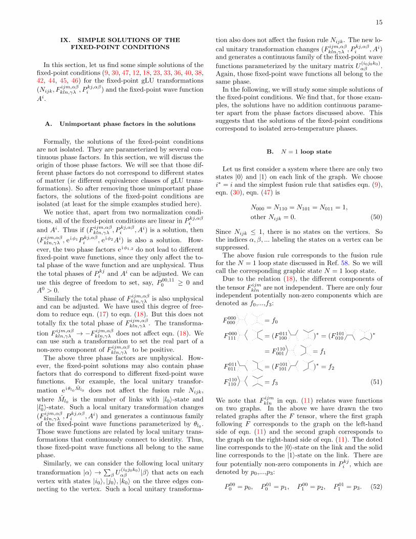
B. N = 1 loop state

Let us first consider a system where there are only twostates |0〉 and |1〉 on each link of the graph. We choosei∗ = i and the simplest fusion rule that satisfies eqn. (9),eqn. (30), eqn. (47) is

N000 = N110 = N101 = N011 = 1,

other Nijk = 0. (50)

Since Nijk ≤ 1, there is no states on the vertices. Sothe indices α, β, ... labeling the states on a vertex can besuppressed.

The above fusion rule corresponds to the fusion rulefor the N = 1 loop state discussed in Ref. 58. So we willcall the corresponding graphic state N = 1 loop state.

Due to the relation (18), the different components of

the tensor F ijmkln are not independent. There are only fourindependent potentially non-zero components which aredenoted as f0,...,f3:

F 000000 = f0

F 000111 = (F 011

100 )∗ = (F 101010 )∗

= F 110001 = f1

F 011011 = (F 101

101 )∗ = f2

F 110110 = f3 (51)

We note that F ijmkln in eqn. (11) relates wave functionson two graphs. In the above we have drawn the tworelated graphs after the F tensor, where the first graphfollowing F corresponds to the graph on the left-handside of eqn. (11) and the second graph corresponds tothe graph on the right-hand side of eqn. (11). The dotedline corresponds to the |0〉-state on the link and the solidline corresponds to the |1〉-state on the link. There are

four potentially non-zero components in P kji , which aredenoted by p0,...,p3:

P 000 = p0, P 01

0 = p1, P 001 = p2, P 01

1 = p3. (52)

16

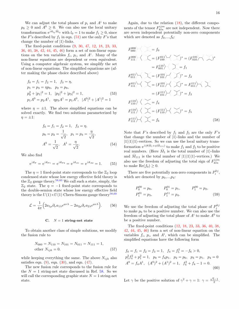
We can adjust the total phases of pi and Ai to makep0 ≥ 0 and A0 ≥ 0. We can also use the local unitary

transformation e iθl0Ml0 with l0 = 1 to make f1 ≥ 0, sincethe F ’s described by f1 in eqn. (51) are the only F ’s thatchange the number of |1〉-links.

The fixed-point conditions (9, 30, 47, 12, 18, 23, 33,36, 40, 38, 42, 44, 45, 46) form a set of non-linear equa-tions on the ten variables fi, pi, and Ai. Many of thenon-linear equations are dependent or even equivalent.Using a computer algebraic system, we simplify the setof non-linear equations. The simplified equations are (af-ter making the phase choice described above)

f0 = f1 = f2 = 1, f3 = η,

p1 = p3 = ηp0, p2 = p0,

p20 + |p1|2 = 1, |p2|2 + |p3|2 = 1, (53)

p1A0 = p2A

1, ηp3A1 = p1A

0, |A0|2 + |A1|2 = 1

where η = ±1. The above simplified equations can besolved exactly. We find two solutions parameterized byη = ±1:

f0 = f1 = f2 = 1, f3 = η,

p0 = p2 =1√2, p1 = p3 =

η√2,

A0 =1√2, A1 =

η√2. (54)

We also find

e iθF = e iθP1 = e iθP2 = e iθA1 = e iθA2 = 1. (55)

The η = 1 fixed-point state corresponds to the Z2 loopcondensed state whose low energy effective field theory isthe Z2 gauge theory.58,60 We call such a state, simply, theZ2 state. The η = −1 fixed-point state corresponds tothe double-semion state whose low energy effective fieldtheory is the U(1)×U(1) Chern-Simons gauge theory58,60

L =1

4π

(2a1µ∂νa1λε

µνλ − 2a2µ∂νa2λεµνλ). (56)

C. N = 1 string-net state

To obtain another class of simple solutions, we modifythe fusion rule to

N000 = N110 = N101 = N011 = N111 = 1,

other Nijk = 0. (57)

while keeping everything the same. The above Nijk alsosatisfies eqn. (9), eqn. (30), and eqn. (47).

The new fusion rule corresponds to the fusion rule forthe N = 1 string-net state discussed in Ref. 58. So wewill call the corresponding graphic state N = 1 string-netstate.

Again, due to the relation (18), the different compo-

nents of the tensor F ijmkln are not independent. Now thereare seven independent potentially non-zero componentswhich are denoted as f0,...,f6:

F 000000 = f0

F 000111 = (F 011

100 )∗ = (F 101010 )∗

= F 110001 = f1

F 011011 = (F 101

101 )∗ = f2

F 011111 = (F 101

111 )∗ = F 111011

= (F 111101 )∗ = f3

F 110110 = f4

F 110111 = (F 111

110 )∗ = f5

F 111111 = f6 (58)

Note that F ’s described by f1 and f5 are the only F ’sthat change the number of |1〉-links and the number of|1〉|1〉|1〉-vertices. So we can use the local unitary trans-

formation e i (θM1+φM111) to make f1 and f5 to be positivereal numbers. (Here M1 is the total number of |1〉-links

and M111 is the total number of |1〉|1〉|1〉-vertices.) We

also use the freedom of adjusting the total sign of F ijmklnto make Re(f0) ≥ 0.

There are five potentially non-zero components in P kji ,which are denoted by p0,...,p4:

P 000 = p0, P 01

0 = p1, P 001 = p2,

P 011 = p3, P 11

1 = p4. (59)

We use the freedom of adjusting the total phase of P kjito make p0 to be a positive number. We can also use thefreedom of adjusting the total phase of Ai to make A0 tobe a positive number.

The fixed-point conditions (12, 18, 23, 33, 36, 40, 38,42, 44, 45, 46) form a set of non-linear equation on thevariables fi, pi, and Ai, which can be simplified. Thesimplified equations have the following form

f0 = f1 = f2 = f3 = 1, f4 = f25 = −f6 > 0,

p21f

24 + p2

1 = 1, p0 = f4p1, p2 = p0, p3 = p1, p4 = 0

A0 = f4A1, (A0)2 + (A1)2 = 1, f2

4 + f4 − 1 = 0.(60)

Let γ be the positive solution of γ2 + γ = 1: γ =√

5−12 .

17

We see that f5 =√γ. The above can be written as

f0 = f1 = f2 = f3 = 1, f4 = −f6 = γ, f5 =√γ,

p0 = p2 =γ

γ2 + 1, p1 = p3 =

1

γ2 + 1, p4 = 0,

A0 =γ

γ2 + 1, A1 =

1

γ2 + 1. (61)

We also find

e iθF = e iθP1 = e iθP2 = e iθA1 = e iθA2 = 1. (62)

The fixed-point state corresponds to the N = 1string-net condensed state58 whose low energy effectivefield theory is the doubled SO(3) Chern-Simons gaugetheory.60

D. An N = 2 string-net state – the Z3 state

The above simple examples correspond to non-orientable string-net states. Here we will give an exampleof orientable string-net state. We choose N = 2, 0∗ = 0,1∗ = 2, 2∗ = 1, and

N000 = N012 = N120 = N201 = N021 = N102 = N210

= N111 = N222 = 1. (63)

The above Nijk satisfies eqn. (9), eqn. (30), and eqn. (47).Due to the relation (18), the different components of

the tensor F ijmkln are not independent. There are eightindependent potentially non-zero components which aredenoted as f0,...,f7:

F 000000 = f0

F 000111 = (F 011

200 )∗ = F 120002

= (F 202020 )∗ = f1

F 000222 = (F 022

100 )∗ = (F 101010 )∗

= F 210001 = f2

F 011011 = F 022

022 = (F 101202 )∗

= (F 202101 )∗ = f3

F 011122 = (F 101

121 )∗ = F 112021

= (F 112102 )∗ = f4

F 022211 = (F 202

212 )∗ = F 221012

= (F 221201 )∗ = f5

F 112210 = (F 120

221 )∗ = (F 210112 )∗

= F 221120 = f6

F 120110 = (F 210

220 )∗ = f7 (64)

There are nine potentially non-zero components in P kji ,which are denoted by p0,...,p8:

P 000 = p0, P 01

0 = p1, P 020 = p2, P 00

1 = p3, P 011 = p4,

P 021 = p5, P 00

2 = p6, P 012 = p7, P 02

2 = p8. (65)

Using the transformations discussed in section IX B, wecan fix the phases of f1, f2, f6, and p0 to make thempositive.

The fixed-point conditions (12, 18, 23, 33, 36, 40, 38,42, 44, 45, 46) form a set of non-linear equation on thevariables fi, pi, and Ai, which can be solved exactly. Af-ter fixing the phases using the transformations discussedin section IX B, we find only one solution

fi = 1, i = 0, 1, ..., 7,

pi =1√3, i = 0, 1, ..., 8,

A0 = A1 = A2 =1√3. (66)

We also find

e iθF = e iθP1 = e iθP2 = e iθA1 = e iθA2 = 1. (67)

The fixed-point state corresponds to the Z3 string-netcondensed state58 whose low energy effective field theoryis the U(1)× U(1) Chern-Simons gauge theory50,58

L =1

4π

(3a1µ∂νa2λε

µνλ + 3a2µ∂νa1λεµνλ), (68)

which is the Z3 gauge theory.We note that all the above simple solutions also satisfy

the standard pentagon identity, although we solved theweaker projective pentagon identity. It is not clear ifwe can find non-trivial solutions that do not satisfy thestandard pentagon identity.

X. A CLASSIFICATION OF TIME REVERSALINVARIANT TOPOLOGICAL ORDERS

There are several ways to define time reversal operationfor the graphic states. The simplest one is given by

T : Φ(Γ)→ Φ∗(Γ) (69)

where Γ represents the labels on the vertices and linkswhich are not changed under T . (This corresponds tothe situation where the different states on the links andthe vertices are realized by different occupations of scalarbosons.) For such a time reversal transformation, T 2 = 1and the real solutions of the fixed-point conditions (9,30, 47, 12, 18, 23, 33, 36, 40, 38, 42, 44, 45, 46) giveus a classification of time reversal invariant topologicalorders in local spin systems. Note that the time reversalinvariant topological orders are equivalent class of localorthogonal transformations that connect to the identitytransformation continuously.

18

Different real solutions (Nijk, Fijm,αβkln,γλ , P

kj,αβi , Ai) of

the fixed-point conditions do not always correspondto different time reversal invariant topological orders.The solutions differ by some unimportant phase factors(which are ±1 signs) correspond to the same topologicalorder.

To understand the above result, we noticethat, from the structure of the fixed-point condi-

tions, if (F ijm,αβkln,γλ , Pkj,αβi , Ai) is a solution, then

(ηFFijm,αβkln,γλ , ηPP

kj,αβi , ηAA

i) is also a solution, whereηF = ±1, ηP = ±1, and ηA = ±1. However, the threephase factors ηF , ηP , and ηA do not lead to differentfixed-point wave functions, since they only affect thetotal phase of the wave function and are unphysical.

On the other hand, the fixed-point solutions may alsocontain phase factors that do correspond to differentfixed-point wave functions. For example, the local or-

thogonal transformation e iπMl0 does not affect the fu-sion rule Nijk, where Ml0 is the number of links with|l0〉-state and |l∗0〉-state. Such a local orthogonal trans-

formation changes (F ijm,αβkln,γλ , Pkj,αβi , Ai) and generates a

discrete family of the fixed-point wave functions.Similarly, we can consider the following local orthog-

onal transformation |α〉 →∑β O

(i0j0k0)αβ |β〉 that acts

on each vertex with states |i0〉, |j0〉, |k0〉 on the threeedges connecting to the vertex. Such a local orthogo-nal transformation also does not affect the fusion ruleNijk. The new local orthogonal transformation changes

(F ijm,αβkln,γλ , Pkj,αβi , Ai) and generates a family of the fixed-

point wave functions parameterized by the orthogonal

matrix O(i0j0k0)αβ .

Now the question is that do those solutions related bylocal orthogonal transformations have the same time re-versal invariant topological order or not. We know thattwo gapped wave functions have the same time reversalinvariant topological order if and only if they can be con-nected by local orthogonal transformation that connectsto identity continuously. It is well known that an orthog-onal matrix whose determinant is −1 does not connect toidentity. Thus it appears that local orthogonal transfor-mations some times can generate different time reversalinvariant topological orders.

However, when we use the equivalent classes of localorthogonal transformations to define time reversal in-variant topological orders, we not only assume the localorthogonal transformations to connect to identity con-tinuously, we also assume that we can expand the lo-cal Hilbert spaces (say by increasing the range of theindices i and α that label the states on the edges andthe vertices). The local orthogonal transformations canact on those enlarged Hilbert spaces and can connect toidentity in those enlarged Hilbert spaces. Even when alocal orthogonal transformation cannot be deformed intoidentity in the original Hilbert space, it can always be de-formed into identity continuously in an enlarged Hilbertspace. Thus two real wave functions related by a localorthogonal transformation always have the same time re-

versal invariant topological order.

For example, an orthogonal matrix

(1 00 −1

)that acts

on states |0〉 and |1〉 does not connect to identity withinthe space of two by two orthogonal matrices. However,we can embed the above orthogonal matrix into a threeby three orthogonal matrix that acts on |0〉, |1〉, and |2〉:1 0 0

0 −1 00 0 −1

. Such a three by three orthogonal matrix

does connect to identity within the space of three by threeorthogonal matrices. This completes our argument thatall local orthogonal transformations can connect to iden-tity continuously at least in an enlarged Hilbert space.

So, after factoring out the unimportant phase factorsdiscussed above, the real solutions of the fixed-point con-ditions may uniquely correspond to time reversal invari-ant topological orders. The four types of real solutionsdiscussed in the last section are examples of four differenttime reversal invariant topological orders.

For the N = 1 loop states and the N = 1 string-netstate, we only have two states on each link. In this case,we can treat the two states as the two states of an electronspin. The time reversal transformation now becomes

T : c0|0〉+ c1|1〉 → −c∗1|0〉+ c∗0|1〉 (70)

on each link. For such a time reversal transformationT 2 = −1. The two N = 1 loop states and the N = 1string-net state are not invariant under such an time-reversal transformation.

XI. WAVE FUNCTION RENORMALIZATIONFOR TENSOR PRODUCT STATES

A. Motivation

Once the fixed-point states have been identified andthe labeling of topological orders has being found, wethen face the next important issue: given a genericground state wave function of a system, how to iden-tify the topological orders in the state? In other words,

how to calculate the data (Nijk, Fijm,αβkln,γλ , P

kj,αβi , Ai) that

characterize the topological orders from a generic wavefunction?

One way to address the above issue is to have a generalrenormalization procedure which flows other states in thesame phase to the simple fixed-point state so that we canidentify topological order from the resulting fixed-pointstate. That is, we want to find a local unitary transfor-mation which removes local entanglement and gets rid ofunnecessary degrees of freedom from the state. How tofind the appropriate unitary transformation for a specificstate is then the central problem in this renormalizationprocedure. Such a procedure for one dimensional tensorproduct states(TPS) (also called matrix product states)has been given in Ref. 38. Here we will propose a method

19

to renormalize two dimensional TPS, where nontrivialtopological orders emerge. The basic idea is to use thegLU transformation discussed in section VII. Note that,through the gLU transformation, we can reduce the num-ber of labels in a region A to the minimal value withoutloosing any quantum information (see Fig. 6). This isbecause the gLU transformation is a lossless projectioninto the support space of the state in the region A. Byperforming such gLU transformations on overlapping re-gions repeatedly (see Fig. 2a), we can reduce a genericwave function to the simple fixed-point form discussedabove. It should be noted that any state reducible inthis way can be represented as a MERA39.

In the following, we will present this renormalizationprocedure for two dimensional TPS where we find amethod to calculate the proper gLU transformations.The tensor product states are many-body entangledquantum states described with local tensors. By mak-ing use of the entanglement information contained in thelocal tensors, we are able to come up with an efficientalgorithm to renormalize two dimensional TPS.

This algorithm can be very useful in the study of quan-tum phases. Due to the efficiency in representation, TPShas found wide application as variational ansatz states inthe studies of quantum many-body systems62–68. Sup-pose that in a variational study we have found a set oftensors which describe the ground state of a two dimen-sional many-body Hamiltonian and want to determinethe phase this state belongs to. We can apply our renor-malization algorithm to this tensor product state, whichremoves local entanglement and flows the state to itsfixed point. By identifying the kind of order present inthe fixed-point state, we can obtain the phase informa-tion for the original state.

In this section, we will give a detailed description ofthe algorithm and in the next section we will present itsapplication to some simple (but nontrivial) cases. Thestates we are concerned with have translational symme-try and can be described with a translational invarianttensor network. To be specific, we discuss states on ahexagonal lattice. Generalization to other regular lat-tices is straight-forward.

B. Tensor product states

Consider a two-dimensional spin model on a hexagonallattice with one spin (or one qudit) living at each vertex.The Hilbert space of each spin is D-dimensional. Thestate can be represented by assigning to every vertex aset of tensors T iαβγ , where i labels the local physical di-mension and takes value from 1 to D. α, β, γ are innerindices along the three directions in the hexagonal lat-tice respectively. The dimension of the inner indices is d.Note that the figures in this note are all sideviews withinner indices in the horizontal plane and the physical in-dices pointing in the vertical direction, if not specifiedotherwise. The wave function is given in terms of these

FIG. 11: (Color online) Left: Tensor T representing a 2Dquantum state on hexagonal lattice. i is the physical index,α, β, γ are inner indices. Right: a tensor product state whereeach vertex is associated with a tensor. The inner indices ofthe neighboring tensors connect according to the underlyinghexagonal lattice.

tensors by

|ψ〉 =∑

i1,i2,...im...

tTr(T i1T i2 ...T im ...)|i1i2...im...〉 (71)

where tTr denotes tensor contraction of all the connectedinner indices on the links of the hexagonal lattice.

A renormalization procedure of quantum states is com-posed of local unitary transformations and isometry mapssuch that the state flows along the path |ψ(0)〉, |ψ(1)〉,|ψ(2)〉,...and finally towards a fixed point |ψ∞〉. With thetensor product representation, flow of states correspondsto a flow of tensors T (0), T (1), T (2)... We will give thedetailed procedure of how the tensors are mapped fromone step to the next in the following section.

C. Renormalization algorithm

In one round of renormalization, we start from tensorT (n), do some operation to it which corresponds to localunitary transformations on the state, and map T (n) toT (n+1). The whole procedure can be broken into twoparts: the F-move and the P move, in accordance withthe two steps introduced in the previous section.

1. Step 1: F-move

In the F-move, we take a configuration in the ten-

sor network and map it to a configuration by doing a

local unitary operation. We will see that the tensor prod-uct representation of a state leads to a natural way ofchoosing an appropriate unitary operation for the renor-malization of the state.

In order to do so, first we define the double tensor Tof tensor T as

Tα′β′γ′,αβγ =∑i

(T iα′β′γ′)∗ × T iαβγ (72)

20

FIG. 12: (Color online) Double tensor T represented as twolayers of tensor T with the physical indices contracted. Thegray layer is the lower layer.

FIG. 13: (Color online) F-move in the renormalization proce-dure: (1) combining double tensors T1 and T2 on neighboringsites into a single double tensor T (2)Splitting double tensor Tinto tensor T (3) SVD decomposition of tensor T into tensorsTa and Tb.

Graphically the double tensor T is represented by twolayers of tensor T with the physical indices connected.The tensor T giving rise to the same double tensor T isnot unique. Any tensor T ′ which differs from T by anunitary transformation U on physical index i gives thesame T as U and U† cancels out in the contraction of i.On the other hand, an unitary transformation on i is theonly degree of freedom possible, i.e. any T ′ which givesrise to the same T as T differs from T by a unitary oni. Therefore, in the process of turning a tensor T into adouble tensor T and then split it again into a differenttensor T ′, we apply a non-trivial local unitary operationon the corresponding state. A well designed way of split-ting the double tensor will give us the appropriate unitarytransformation we need, as we show below.

F-move has the following steps. First, construct dou-ble tensors for two neighboring sites on the lattice andcombine them into a single double tensor with 8 innerindices.

Tα′β′δ′ε′,αβδε =∑γ′,γ

T1,α′β′γ′,αβγ × T2,δ′ε′γ′,δεγ (73)

Note that with respect to the bipartition of indices

α′β′δ′ε′ and αβδε, T is Hermitian

Tα′β′δ′ε′,αβδε = (Tαβδε,α′β′δ′ε′)∗ (74)

and positive semidefinite. Therefore it has a spectraldecomposition with positive eigenvalues {λj ≥ 0}. The

corresponding eigenvectors are {T j}

Tα′β′δ′ε′,αβδε =∑j

λj

(T jα′β′δ′ε′

)∗× T jαβδε (75)

This spectral decomposition lead to a special way of de-composing double tensor T into tensors. Define a rank 8tensor T (as shown in Fig. 13 after step 2) as follows:

T lmnrαβδε =∑j

√λj

(T jlmnr

)∗× T jαβδε (76)

T has four inner indices α, β, δ, ε of dimension d and fourphysical indices l,m, n, r also of dimension d which arein the direction of α, β, δ, ε respectively. As {T j} form

an orthonormal set, it is easy to check that T gives riseto double tensor T. Going from T1 and T2 to T , we haveimplemented a local unitary transformation on the phys-ical degrees of freedom on the two sites, so that in T thephysical indices and the inner indices represent the sameconfiguration. In some sense, we are keeping only thephysical degrees of freedom necessary for entanglementwith the rest of the system while getting rid of thosethat are only entangled within this local region. Now wedo a singular value decomposition of tensor T in the di-rection orthogonal to the link between T1 and T2 and Tis decomposed into tensors Ta and Tb.

T lmnrαβδε =∑λ

T lna,αδλ × Tmrb,βελ (77)

This step completes the F-move. Ideally, this step shouldbe done exactly so we are only applying local unitaryoperations to the state. Numerically, we keep some largebut finite cutoff dimension for the SVD step, so this stepis approximate.

On a hexagonal lattice, we do F-move on the chosenneighboring pairs of sites (dash-circled in Fig. 14), sothat the tensor network is changed into a configurationshown by thick dark lines in Fig. 14. Physical indicesare omitted from this figure. Now by grouping togetherthe three tensors that meet at a triangle, we can mapthe tensor network back into a hexagonal lattice, with1/3 the number of sites in the original lattice. This isachieved by the P-move introduced in the next section.

2. Step 2: P-move

Now we contract the three tensors that meet at a tri-angle together to form a new tensor in the renormalizedlattice as shown in the first step in Fig. 15

T Iαβγ =∑δελ

Tnra,αδε × T lmb,βλδ × Tpqc,γελ (78)

21

FIG. 14: Original hexagonal lattice (gray line) and renormal-ized lattice (black line) after F-move has been applied to theneighboring pairs of sites circled by dash line.

FIG. 15: (Color online) P-move in the renormalization pro-cedure: (1) contracting three tensors that meet at a triangle

Ta, Tb, Tc to form a new tensor T (1) on one site of the renor-malized hexagonal lattice. (2)constructing the double tensor

T(1) from T (1) so that we can start to do F-moves again.

where I is the physical index of the new tensor which in-cludes all the physical indices of Ta, Tb, Tc: l,m, n, r, p, q.Note that in the contraction, only inner indices are con-tracted and the physical indices are simply group to-gether.

Constructing the double tensor T from T , we get therenormalized double tensor on the new hexagonal latticewhich is in the same form as T1,T2 and we can go backagain and do the F-move.

3. Complications: corner double line

One problem with the above renormalization algorithmis that, instead of having one isolated fixed-point tensorfor each phase, the algorithm has a continuous familyof fixed points which all correspond to the same phase.Consider a tensor with structure shown in Fig. 16. Thetensor is a tensor product of three parts which includeindices {α, β, i1}, {γ, δ, i2}, {ε, λ, i3} respectively. It canbe shown that this structure remains invariant under therenormalization flow. Therefore, any tensor of this struc-ture is a fixed point of our renormalization flow. However,it is easy to see that the state it represents is a tensorproduct of loops around each plaquette, which can bedisentangled locally into a trivial product state. There-fore, the states all have only short-range entanglementand correspond to the topologically trivial phase. The

FIG. 16: (Color online) The corner double line tensor whichis a fixed point of the renormalization algorithm. The threegroups of indices {α, β, i1}, {γ, δ, i2}, {ε, λ, i3}, are entangledwithin each group but not between the groups.

trivial phase has then a continuous family of fixed-pointtensors. This situation is very similar to that discussed inRef. 37,69. We will keep the terminology and call such atensor a corner double line tensor. Not only does cornerdouble line tensor complicate the situation in the trivialphase, it leads to a continuous family of fixed points inevery phase. It can be checked that the tensor productof a corner double line with any other fixed-point tensoris still a fixed-point tensor. The states they correspondto differ only by small loops around each plaquette andrepresent the same topological order. Therefore any sin-gle fixed-point tensor gets complicated into a continuousclass of fixed-point tensors. In practical application of therenormalization algorithm, in order to identify the topo-logical order of the fixed-point tensor, we need to get ridof such corner double line structures. Due to their sim-ple structure, this can always be done, as discussed inthe next section.

XII. APPLICATIONS OF THERENORMALIZATION FOR TENSOR PRODUCT

STATES

Now we present some examples where our algorithmis used to determine the phase of a tensor product state.The algorithm can be applied both to symmetry breakingphases and topological ordered phases. In the study ofsymmetry breaking/topological ordered phases, supposethat we have obtained some tensor product descriptionof the ground state of the system Hamiltonian. We canthen apply our algorithm to the tensors, flow them to thefixed point, and see whether they represent a state in thesymmetry breaking phase/topological ordered phase or atrivial phase.

For system with symmetry/topological order related togauge symmetry, it is very important to keep the sym-metry/gauge symmetry in the variational approach toground state and search within the set of tensors thathave this symmetry/gauge symmetry70. The resultingtensor will be invariant under such symmetries/gaugesymmetries, but the state they correspond to may havedifferent orders. In the symmetry breaking case, thestate could have this symmetry or could spontaneousbreak it. In the topological ordered phase, the state

22

FIG. 17: (Color online) Renormalization procedure on squarelattice part 1: (1) decomposing double tensor T into tensor

T (2) SVD decomposition of T in two different directions,resulting in tensors Ta, Tb and Tc, Td respectively.

could have nontrivial topological order or be just triv-ial. Our algorithm can then be applied to decide whichis the case. In order to correctly determine the phase forsuch symmetric tensors, it is crucial that we maintain thesymmetry/gauge symmetry of the tensor throughout ourrenormalization process. We will discuss in detail twocases: the Ising symmetry breaking phase and the Z2

topological ordered phase. For simplicity of discussionand to demonstrate the generality of our renormalizationscheme, we will first introduce the square lattice versionof the algorithm. All subsequent applications are carriedout on square lattice. (Algorithm on a hexagonal latticewould give qualitatively similar result, though quantita-tively they might differ, e.g. on the position of criticalpoint.)

A. Renormalization on square lattice

Tensor product states on a square lattice are repre-sented with one tensor T iαβγδ on each vertex, where i isthe physical index and αβγδ are the four inner indicesin the up,down,left,right direction respectively. We willassume translational invariance and require the tensor tobe the same on every vertex. The renormalization pro-cedure is be a local unitary transformation on the statewhich flows the form of the tensor until it reaches thefixed point. It is implemented in the following steps.First, we form the double tensor T from tensor T

Tα′β′γ′δ′,αβγδ =∑i

(T iα′β′γ′δ′

)∗ × T iαβγδThen do the spectral decomposition of positive operatorT into

Tα′β′γ′δ′,αβγδ =∑j

λj

(T jα′β′γ′δ′

)∗× T jαβγδ

FIG. 18: Original square lattice (gray line) and renormalizedlattice (black line) after the operations in Fig. 17 has beenapplied. Physical indices of the tensors are not drawn here.

FIG. 19: (Color online) Renormalization procedure on squarelattice part 2: (1) combining four tensors that meet at asquare into a single tensor (2) constructing a double tensorfrom it.

and form a new tensor T lmnrαβγδ

T lmnrαβγδ =∑j

√λj

(T jlmnr

)∗× T jαβγδ

l,m,n,r are physical indices in the up, down, left, rightdirections respectively. This is illustrated in step 1 ofFig. 17. This step is very similar to the second step inthe F-move on hexagonal lattice. Next we do SVD de-composition of tensor T . For vertices in sublattice A wedecompose between the up-right and down-left directionas shown in step 2 of Fig. 17. For vertices in sublat-tice B we decompose between the up-left and down-rightdirection as shown in step 3 of Fig. 17.

T lmnrαβγδ =∑λ

T lra,αδλ × Tmnb,βγλ

T lmnrαβγδ =∑λ

T lrc,αδλ × Tmnb,βγλ

After the decomposition, the original lattice (gray linesin Fig. 18) is transformed into the configuration shownby thick dark lines in Fig. 18. Physical indices are omit-ted from this figure. If we now shrink the small squares,we get a tensor product state on a renormalized squarelattice. Fig. 19 shows how this is done.

In step 1, we contract the four tensors that meet at a

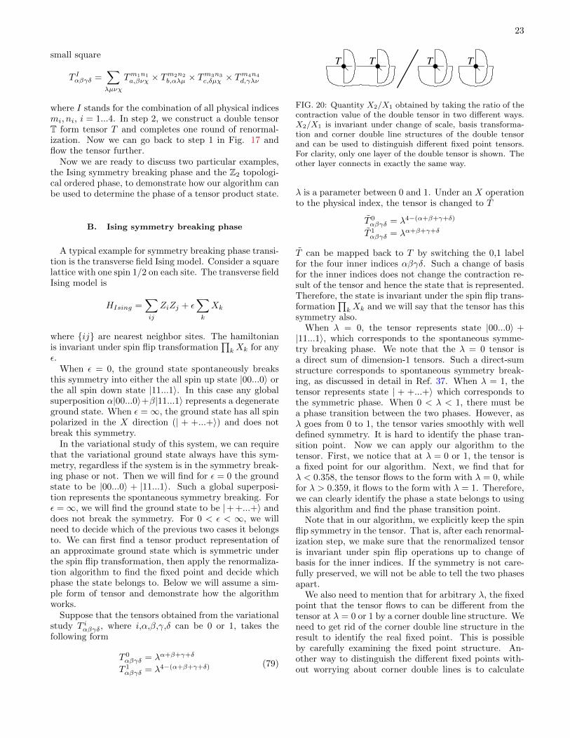
23

small square

T Iαβγδ =∑λµνχ

Tm1n1

a,βνχ × Tm2n2

b,αλµ × Tm3n3

c,δµχ × Tm4n4

d,γλν

where I stands for the combination of all physical indicesmi, ni, i = 1...4. In step 2, we construct a double tensorT form tensor T and completes one round of renormal-ization. Now we can go back to step 1 in Fig. 17 andflow the tensor further.

Now we are ready to discuss two particular examples,the Ising symmetry breaking phase and the Z2 topologi-cal ordered phase, to demonstrate how our algorithm canbe used to determine the phase of a tensor product state.

B. Ising symmetry breaking phase

A typical example for symmetry breaking phase transi-tion is the transverse field Ising model. Consider a squarelattice with one spin 1/2 on each site. The transverse fieldIsing model is

HIsing =∑ij

ZiZj + ε∑k

Xk

where {ij} are nearest neighbor sites. The hamiltonianis invariant under spin flip transformation

∏kXk for any

ε.When ε = 0, the ground state spontaneously breaks

this symmetry into either the all spin up state |00...0〉 orthe all spin down state |11...1〉. In this case any globalsuperposition α|00...0〉+β|11...1〉 represents a degenerateground state. When ε =∞, the ground state has all spinpolarized in the X direction (| + +...+〉) and does notbreak this symmetry.

In the variational study of this system, we can requirethat the variational ground state always have this sym-metry, regardless if the system is in the symmetry break-ing phase or not. Then we will find for ε = 0 the groundstate to be |00...0〉 + |11...1〉. Such a global superposi-tion represents the spontaneous symmetry breaking. Forε =∞, we will find the ground state to be |+ +...+〉 anddoes not break the symmetry. For 0 < ε < ∞, we willneed to decide which of the previous two cases it belongsto. We can first find a tensor product representation ofan approximate ground state which is symmetric underthe spin flip transformation, then apply the renormaliza-tion algorithm to find the fixed point and decide whichphase the state belongs to. Below we will assume a sim-ple form of tensor and demonstrate how the algorithmworks.

Suppose that the tensors obtained from the variationalstudy T iαβγδ, where i,α,β,γ,δ can be 0 or 1, takes thefollowing form

T 0αβγδ = λα+β+γ+δ

T 1αβγδ = λ4−(α+β+γ+δ) (79)

T TT T

FIG. 20: Quantity X2/X1 obtained by taking the ratio of thecontraction value of the double tensor in two different ways.X2/X1 is invariant under change of scale, basis transforma-tion and corner double line structures of the double tensorand can be used to distinguish different fixed point tensors.For clarity, only one layer of the double tensor is shown. Theother layer connects in exactly the same way.

λ is a parameter between 0 and 1. Under an X operationto the physical index, the tensor is changed to T

T 0αβγδ = λ4−(α+β+γ+δ)

T 1αβγδ = λα+β+γ+δ

T can be mapped back to T by switching the 0,1 labelfor the four inner indices αβγδ. Such a change of basisfor the inner indices does not change the contraction re-sult of the tensor and hence the state that is represented.Therefore, the state is invariant under the spin flip trans-formation

∏kXk and we will say that the tensor has this

symmetry also.When λ = 0, the tensor represents state |00...0〉 +|11...1〉, which corresponds to the spontaneous symme-try breaking phase. We note that the λ = 0 tensor isa direct sum of dimension-1 tensors. Such a direct-sumstructure corresponds to spontaneous symmetry break-ing, as discussed in detail in Ref. 37. When λ = 1, thetensor represents state | + +...+〉 which corresponds tothe symmetric phase. When 0 < λ < 1, there must bea phase transition between the two phases. However, asλ goes from 0 to 1, the tensor varies smoothly with welldefined symmetry. It is hard to identify the phase tran-sition point. Now we can apply our algorithm to thetensor. First, we notice that at λ = 0 or 1, the tensor isa fixed point for our algorithm. Next, we find that forλ < 0.358, the tensor flows to the form with λ = 0, whilefor λ > 0.359, it flows to the form with λ = 1. Therefore,we can clearly identify the phase a state belongs to usingthis algorithm and find the phase transition point.

Note that in our algorithm, we explicitly keep the spinflip symmetry in the tensor. That is, after each renormal-ization step, we make sure that the renormalized tensoris invariant under spin flip operations up to change ofbasis for the inner indices. If the symmetry is not care-fully preserved, we will not be able to tell the two phasesapart.

We also need to mention that for arbitrary λ, the fixedpoint that the tensor flows to can be different from thetensor at λ = 0 or 1 by a corner double line structure. Weneed to get rid of the corner double line structure in theresult to identify the real fixed point. This is possibleby carefully examining the fixed point structure. An-other way to distinguish the different fixed points with-out worrying about corner double lines is to calculate

24

FIG. 21: (Color online) X2/X1 for tensors (79) under therenormalization flow. As the number of RG steps increases,the transition in X2/X1 becomes sharper and finally ap-proaches a step function at fixed point. The critical pointis at λc = 0.358.

some quantities from the fixed-point tensors that are in-variant with the addition of corner double lines. Wealso want the quantity to be invariant under some triv-ial changes to the fixed point, such as a change in scaleT → ηT or the change of basis for physical and innerindices. One such quantity is given by the ratio of X2

and X1 defined as X1 =(∑

α′γ′,αγ Tα′α′γ′γ′,ααγγ)2

, and

X2 =∑α′β′γ′δ′,αβγδ Tα′α′γ′δ′,ααγδ × Tβ′β′δ′γ′,ββδγ . Fig.

20 gives a graphical representation of these two quanti-ties. In this figure, only one layer of the double tensor isshown. The other layer connects in the exactly the sameway. It is easy to verify that X2/X1 is invariant under thechange of scale, basis transformation and corner doublelines.

We calculate X2/X1 along the renormalization flow.The result is shown in Fig. 21. At the λ = 0 fixedpoint, X2/X1 = 0.5 while at λ = 1, X2/X1 = 1. As weincrease the number of renormalization steps, the transi-tion between the two fixed points becomes sharper andfinally approaches a step function with critical point atλc = 0.358. Tensors with λ < λc belongs to the symme-try breaking phase while tensors with λ > λc belongs tothe symmetric phase.

C. Z2 topological ordered phase

The algorithm can also be used to study topologicalorder of quantum states. In this section, we will demon-strate how the algorithm works with Z2 topological order.

Consider again a square lattice but now with one spin1/2 per each link. A simple Hamiltonian on this latticewith Z2 topological order can be defined as

HZ2=∑p

∏i∈p

Xi +∑v

∏j∈v

Zj

where p means plaquettes and i ∈ p is all the spin 1/2saround the plaquette and v means vertices and j ∈ v isall the spin 1/2s connected to the vertex. The groundstate wave function of this Hamiltonian is a fixed-pointwave function and corresponds to the N = 1 loop statewith η = 1 as discussed in the previous section.

The ground state wave function has a simple tensorproduct representation. For simplicity of discussion wesplit every spin 1/2 into two and associate every vertex

with four spins. The tensor T ijklαβγδ,Z2has four physical

indices i, j, k, l = 0, 1 and three inner indices α, β, γ, δ =0, 1.

T ijklijkl,Z2= 1, if mod(i+ j + k + l, 2) = 0

all other terms being 0

It can be checked that TZ2 is a fixed-point tensor of ouralgorithm. This tensor has a Z2 gauge symmetry. If weapply Z operation to all the inner indices, where Z maps0 to 0 and 1 to −1, the tensor remains invariant as onlyeven configurations of the inner indices are nonzero inthe tensor.

Consider then the following set of tensor parameterizedby g

T ijklijkl = gi+j+k+l, if mod(i+ j + k + l, 2) = 0all other terms being 0

(80)

At g = 1, this is exactly TZ2and the corresponding state

has topological order. At g = 0, the tensor representsa product state of all 0 and we denote the tensor as T0.At some critical point in g, the state must go througha phase transition. This set of tensors are all invariantunder gauge transformation ZZZZ on their inner indicesand the tensor seems to vary smoothly with g. One wayto detect the phase transition is to apply our algorithm.We find that, at g > gc, the tensors flow to TZ2 , whileat g < gc, the tensors flow to T0. We determine gc to bebetween 0.804 ∼ 0.805. As this model is mathematicallyequivalent to two dimensional classical Ising model wherethe transition point is known to great accuracy, we com-pare our result to that result and find our result to bewithin 1% accuracy (gc = 0.8022). Again in the renor-malization algorithm, we need to carefully preserve theZ2 gauge symmetry of the tensor so that we can correctlydetermine the phase of the states.

The fixed-point tensor structure might also be compli-cated by corner double line structures, but it is alwayspossible to identify and get rid of them. Similarly, wecan calculate the invariance quantity X2/X1 to distin-guish the two fixed points. X2/X1 = 1 for TZ2

whileX2/X1 = 0.5 for T0. The result is plotted in Fig. 22 andwe can see that the transition in X2/X1 approaches astep function after a large number of steps of RG, i.e. atthe fixed point. The critical point is at gc = 0.804. Forg < gc, the tensor belongs to the trivial phase, while forg > gc, the tensor belongs to the Z2 topological orderedphase.

25

FIG. 22: (Color online) X2/X1 for tensors (80) under therenormalization flow. As the number of RG steps increases,the transition in X2/X1 becomes sharper and finally ap-proaches a step function at fixed point. The critical pointis at gc = 0.804.

Our algorithm can also be used to demonstrate thestability of topological order against local perturbation.As is shown in Ref. 70, local perturbations to the Z2

Hamiltonian correspond to variations in tensor that donot break the Z2 gauge symmetry. We picked tensorsin the neighborhood of TZ2

which preserve this gaugesymmetry randomly and applied our renormalization al-gorithm (gauge symmetry is kept throughout the renor-malization process). We find that as long as the variationis small enough, the tensor flows back to TZ2

, up to a cor-ner double line structure. This result shows that the Z2

topological ordered phase is stable against local pertur-bations.

XIII. SUMMARY

In this paper, we discuss a defining relation betweenlocal unitary transformation and quantum phases. Weargue that two gapped states are related by a local uni-tary transformation if and only if the two states belongto the same quantum phase.

We can use the equivalent classes of local unitary trans-formations to define “patterns of long range entangle-ment”. So the patterns of long range entanglement cor-respond to universality classes of quantum phases, andare the essence of topological orders.32

As an application of this point of view of quantumphases and topological order, we use the generalized lo-cal unitary transformations to generate a wave functionrenormalization, where the wave functions flow withinthe same universality class of a quantum phase (or thesame equivalent class of the local unitary transforma-tions). In other words, the renormalization flow of a wavefunction does not change its topological order.

Such a wave function renormalization allows us to clas-

sify topological orders, by classifying the fixed-point wavefunctions and the associated fixed-point local unitarytransformations.

First, we find that the fixed-point local uni-tary transformations are described by the data

(Nijk, Fijm,αβkln,χδ , P

kj,αβi ) that satisfy

Nijk = Njki = Nk∗j∗i∗ ≥ 0,

N∑j,k=0

Nii∗kNjk∗j∗ ≥ 1,

N∑m=0

Njim∗Nkml∗ =

N∑n=0

Nkjn∗Nl∗ni, (81)

(F ijm,αβkln,χδ )∗ = F jkn,χδl∗i∗m∗,βα,∑n,χ,δ

F ijm′,α′β′

kln,χδ (F ijm,αβkln,χδ )∗ = δmαβ,m′α′β′ ,

∑t

Nkjt∗∑η=1

Ntin∗∑ϕ=1

Nlts∗∑κ=1

F ijm,αβknt,ηϕ Fitn,ϕχlps,κγ F

jkt,ηκlsq,δφ

= e iθF

Nqmp∗∑ε=1

Fmkn,βχlpq,δε F ijm,αεqps,φγ , (82)

e iθP1P kj,αβi =∑

m,λ,γ,l,ν,µ

F jj∗k,βα

i∗i∗m∗,λγFi∗mj,λγm∗i∗l,νµP

lm,µνi∗ ,

e iθP2P jp,αηi δimδβδ =

Nkjk∗∑χ=1

F ijm,αβklk,χδ Pjp,χηk∗

for all k, i, l satisfying Nkil∗ > 0. (83)

[see eqns. (9, 30, 47 12, 18, 23, 33, 36)]. From the data

(Nijk, Fijm,αβkln,χδ , P

kj,αβi ) we can further find out the fixed-

point wave function by solving the following equationsfor Ai, i = 0, ..., N :

Ai = e iθAAi∗6= 0,

∑i

Ai(Ai)∗ = 1,

Pmj,γλi Ai = e iθA1Pm∗i∗,λγ

j∗ Aj ,

Φθikj,αβ = e iθ′∑m,λ,γ

F ijk∗,αβ

j∗im,λγPmj,γλi Ai,

Φθikj,αβ = e iθA1Φθkji,αβ ,

Φθikj,αβ = 0, if Nikj = 0,

det(Φθikj,αβ) 6= 0. (84)

[see eqns. (40, 38, 42, 44, 45, 46)].

The combined data (Nijk, Fijm,αβkln,χδ , P

kj,αβi , Ai) that

satisfy the conditions (81), (82), (83) and (84) classifya large class of topological orders. We see that the prob-lem of classifying a large class of topological orders be-comes the problem of solving a set of non-linear algebraicequations (81), (82), (83), and (84).

26

The combined data (Nijk, Fijm,αβkln,χδ , P

kj,αβi , Ai) that

satisfy the conditions (81), (82), (83), and (84) also clas-sify a large class of time reversal invariant topologicalorders, if we restrict ourselves to real solutions. The so-lutions related by local orthogonal transformations all be-long to the same phase, since the local orthogonal trans-formations always connect to identity if we enlarge theHilbert space.

We like to point out that we cannot claim that the

solutions (Nijk, Fijm,αβkln,χδ , P

kj,αβi , Ai) classify all topolog-

ical orders since we have assumed that the fixed-pointlocal unitary transformations are described by tensorsof finite dimensions. It appears that chiral topologicalorders, such as quantum Hall states, are described bytensors of infinite dimensions.

We note that the data (Nijk, Fijm,αβkln,χδ , P

kj,αβi , Ai) just

characterize different fixed-point wave functions. It isnot guaranteed that the different data will represent dif-ferent topological orders. However, for the simple so-lutions discussed in this paper, they all coincide withstring-net states, where the topological properties, suchas the ground state degeneracy, number of quasiparti-cle types, the quasiparticle statistics etc, were calculatedfrom the data. From those topological properties, weknow that those different simple solutions represent dif-

ferent topological orders. Also (F ijm,αβkln,χδ , Pkj,αβi , Ai) are

real for the simple solutions discussed here. Thus theyalso represent topological orders with time reversal sym-metry. (Certainly, at the same time, they represent stabletopological orders even without time reversal symmetry.)

We also like to point out that our description of fixed-point local unitary transformations is very similar to thedescription of string-net states. However, the conditions(81), (82), (83), and (84) on the data appear to be weakerthan (or equivalent to) those58 on the string-net data.So the fixed-point wave functions discussed in this papermay include all the string-net states (in 2D).

Last, we present a wave function renormalizationscheme, based on the gLU transformations for genericTPS. Such a wave function renormalization always flowswithin the same phase (or within the same equivalenceclass of LU transformations). It allows us to determinewhich phase a generic TPS belongs to by studying the re-sulting fixed-point wave functions. We demonstrated theeffectiveness of our method for both symmetry break-ing phases and topological ordered phases. We find thatwe can even use tensors that do not break symmetryto describe spontaneous symmetry breaking states: if astate described by a symmetric tensor has a spontaneoussymmetry breaking, the symmetric tensor will flow to afixed-point tensor that has a form of direct sum.

We would like to thank I. Chuang, M. Hastings, M.Levin, F. Verstraete, Z.-H. Wang, Y.-S. Wu, S. Bravyifor some very helpful discussions. XGW is supported byNSF Grant No. DMR-0706078. ZCG is supported inpart by the NSF Grant No. NSFPHY05-51164.

Appendix: Equivalence relation between quantumstates in the same phase

In section III and section IV, we argued about theequivalence relation between gapped quantum groundstates in the same phase. We concluded that two statesare in the same phase if and only if they can be connectedby local unitary evolution or constant depth quantum cir-cuit:

|Φ(1)〉 ∼ |Φ(0)〉 iff |Φ(1)〉 = T [e−i∫ 10dg H(g)]|Φ(0)〉

|Φ(1)〉 ∼ |Φ(0)〉 iff |Φ(1)〉 = UMcirc|Φ(0)〉

Now we want to make these arguments more rigorous,by stating clearly what is proved and what is conjectured,and by giving precise definition of two states being thesame, the locality of operators, etc. We will show theequivalence in the following steps:

1. if two gapped ground states are in the same phase,then they are connected by local unitary evolution

2. a gapped ground state remains in the same phaseunder local unitary evolution

3. a local unitary evolution can be simulated by aconstant depth quantum circuit and vice-verse.

(All these discussions can be generalized to the case

where the system has certain symmetries. H(g) and Ucircused in the equivalence relation will then have the samesymmetry as the system Hamiltonian H.)

First, according to the definition in section III, twostates |Φ(0)〉 and |Φ(1)〉 are in the same phase if we canfind a family of local Hamiltonians H(g), g ∈ [0, 1] with|Φ(g)〉 being its ground state such that the ground stateaverage of any local operator O, 〈Φ(g)|O|Φ(g)〉 changessmoothly from g = 0 to g = 1. Here we allow a more gen-eral notion of locality for the Hamiltonian33 and requireH(g) to be a sum of local operators HZ(g):

H(g) =∑Z∈Z

HZ(g) (85)

where HZ(g) is a Hermitian operator defined on a com-pact region Z.

∑Z∈Z sums over a set Z of regions. The

set Z contains regions that differ by translations. Theset Z also contains regions with different sizes. However,HZ(g) approaches zero exponentially as the size of theregion Z approaches infinity. Or more precisely, for allsites u in the lattice∑

Z∈Z,Z3u‖HZ(g)‖ |Z| exp(µdiam(Z)) = O(1) (86)

for some positive constant µ. Here∑Z∈Z,Z3u sums over

all regions in the set Z that cover the site u, ‖...‖ denotesoperator norm, |Z| is the cardinality of Z, and diam(Z)is the diameter of Z. Therefore, instead of being exactlyzero outside of a finite region, the interaction terms canhave an exponentially decaying tail.

If |Φ(0)〉 and |Φ(1)〉 are gapped ground states of H(0)and H(1), then we assume that for all 〈Φ(g)|O|Φ(g)〉 to

27

be smooth, H(g) must remain gapped for all g. If H(g)closes gap for some gc, then there must exist a local op-erator O such that 〈Φ(g)|O|Φ(g)〉 has a singularity atgc. We call the gapped H(g) an adiabatic connectionbetween two states in the same phase.

The existence of an adiabatic connection gives rise toa local unitary evolution between |Φ(0)〉 and |Φ(1)〉. Aslight modification of Lemma 7.1 in Ref. 33 gives that

Theorem 1 Let H(g) be a differentiable family of lo-cal Hamiltonians and |Φ(g)〉 be its ground state. Ifthe excitation gap above |Φ(g)〉 is larger than some fi-

nite value ∆ for all g, then we can define H(g) =i∫dtF (t)exp(iH(g)t) (∂gH(g)) exp(−iH(g)t), such that

|Φ(1)〉 = T [e−i∫ 10dg H(g)]|Φ(0)〉.

where F (t) is a function which has the following proper-

ties: 1. The fourier transform of F (t), F (ω) is equal to

−1/ω for |ω| > ∆. 2. F (ω) is infinitely differentiable.

3. F (t) = −F (−t). Under this definition, H(g) is local(almost) and satisfies∥∥∥[HZ(g), OB

]∥∥∥ ≤ h′(dist(Z,B)) |Z|∥∥∥HZ(g)

∥∥∥ ‖OB‖(87)

where OB is any operator supported on site B, dist(Z,B)is the smallest distance between B and any site in Z, andh′(l) is a function which decays faster than any negativepower of l. [...] denotes commutator of two operators.This is called the quasi-adiabatic continuation of states.

Therefore, we can show that if |Φ(0)〉 and |Φ(1)〉 arein the same phase, then we can find a local (as de-

fined in (87)) Hamiltonian HZ(g) such that |Φ(1)〉 =

T [e−i∫ 10dg H(g)]|Φ(0)〉. In other words, states in the same

phase are equivalent under local unitary evolution.Note that here we map |Φ(0)〉 exactly to |Φ(1)〉. There

is another version of quasi-adiabatic continuation34,where the mapping is approximate. In that case, HZ(g)can be defined to have only exponentially small tail out-side of a finite region instead of a tail which decays faster

than any negative power. T [e−i∫ 10dg H(g)]|Φ(0)〉 will not

be exactly the same as |Φ(1)〉, but any local measurementon them will give approximately the same result.

Next we want to show that the reverse is also true.Suppose that |Φ(0)〉 is the gapped ground state of alocal Hamiltonian H(0), H(0) =

∑Z HZ(0) and each

HZ(0) is supported on a finite region Z. Apply a lo-

cal unitary evolution generated by H(s) to |Φ(0)〉 andtake it to |Φ(g)〉, g = 0 ∼ 1, |Φ(g)〉 = Ug|Φ(0)〉, where

Ug = T [e−i∫ g0ds H(s)]. |Φ(g)〉 is then ground state of

H(g) = UgH(0)U†g =∑Z UgHZ(0)U†g =

∑Z HZ(g).

Under unitary transformation Ug the spectrum of H(0)doesn’t change, therefore H(g) remains gapped. To showthat H(g) also remains local, we use the Lieb-Robinsonbound derived in Ref. 33, which gives

‖[HZ(g), OB ]‖ =∥∥[UgHZ(0)U†g , OB

]∥∥≤ h(dist(Z,B)) |Z| ‖HZ(0)‖ ‖OB‖

where h(l) decays faster than any negative power of l.Therefore, HZ(g) remains local up to a tail which decaysfaster than any negative power. H(g) then forms a localgapped adiabatic connection between |Φ(0)〉 and |Φ(1)〉.

To detect for phase transition, we must check whetherthe ground state average value of any local operator O,〈Φ(g)|O|Φ(g)〉, has a singularity or not. 〈Φ(g)|O|Φ(g)〉 =〈Φ(0)|U†gOUg|Φ(0)〉. Using the Lieb-Robinson bound

given in Ref. 33, we find U†gOUg remains local (in thesense of (87)) and evolves smoothly with g. Therefore,〈Φ(g)|O|Φ(g)〉 changes smoothly. In fact, becauseH(g) isdifferentiable, the derivative of 〈Φ(g)|O|Φ(g)〉 to any or-der always exists. Therefore, there is no singularity in theground state average value of any local operator O and|Φ(0)〉 and |Φ(1)〉 are in the same phase. We have henceshown that states connected with local unitary evolutionare in the same phase.

This completes the equivalence relation stated in (1).The definition of locality is slightly different in differentcases, so there is still some gap in the equivalence rela-tion. However, we believe that the equivalence relationshould be valid with a slight generalization of the defini-tion of locality.

Lastly, we want to show that the equivalence relationis still valid if we use constant depth quantum circuitinstead of local unitary evolution. This is true becausewe can always simulate a local unitary evolution using aconstant depth quantum circuit and vice-verse.

To simulate a local unitary evolution of the form

T [e−i∫ 10dg H(g)], first divide the total time into small seg-

ments δt such that T [e−i∫ (m+1)δtmδt dg H(g)] ' e−iδtH(mδt).

H(mδt) =∑Z HZ(mδt). The set of local opera-

tors {HZ(mδt)} can always be divided into a finitenumber of subsets {HZi1

(mδt)}, {HZi2(mδt)}... such

that elements in the same subset commute with eachother. Then we can do Trotter expansion and approx-imate e−iδtH(mδt) as e−iδtH(mδt) '

(U (1)U (2)...

)n, where

U (1) =∏i e−iδtH

Zi1/n

, U (2) =∏i e−iδtH

Zi2/n

... Each

term in U (1), U (2) commute, therefore they can be im-plement as a piece-wise local unitary operator. Puttingthese piece-wise local unitary operators together, we havea quantum circuit which simulates the local unitary evo-lution. The depth of circuit is proportional to n× (1/δt).It can be shown that to achieve a simulation with con-stant error, a constant depth circuit would suffice71.

On the other hand, to simulate a constant depth

quantum circuit Ucirc = U(1)pwlU

(2)pwl...U

(2)pwl, where U

(k)pwl =∏

i U(k)i with a local unitary evolution, we can define the

time dependent Hamiltonian as H(t) =∑iH

(k)i , such

that for (k − 1)δt < t < kδt, eiH(k)i δt = U

(k)i . It is easy

to check that T [e−i∫Mδt0

dg H(g)] = Ucirc. The simulationtime needed isMδt. We can always choose a finite δt such

that∥∥∥H(k)

i

∥∥∥ is finite and the evolution time is finite.

We have shown that constant depth quantum circuitand local unitary evolution can simulate each other. The

28

equivalence relation (1) can therefore also be stated in terms of constant depth circuit as in (4).

1 L. D. Landau, Phys. Z. Sowjetunion 11, 26 (1937).2 V. L. Ginzburg and L. D. Landau, Zh. Ekaper. Teoret. Fiz.

20, 1064 (1950).3 J. G. Bednorz and K. A. Mueller, Z. Phys. B 64, 189

(1986).4 P. W. Anderson, Science 235, 1196 (1987).5 G. Baskaran, Z. Zou, and P. W. Anderson, Solid State

Comm. 63, 973 (1987).6 I. Affleck and J. B. Marston, Phys. Rev. B 37, 3774 (1988).7 D. S. Rokhsar and S. A. Kivelson, Phys. Rev. Lett. 61,

2376 (1988).8 I. Affleck, Z. Zou, T. Hsu, and P. W. Anderson, Phys. Rev.

B 38, 745 (1988).9 E. Dagotto, E. Fradkin, and A. Moreo, Phys. Rev. B 38,

2926 (1988).10 V. Kalmeyer and R. B. Laughlin, Phys. Rev. Lett. 59, 2095

(1987).11 X.-G. Wen, F. Wilczek, and A. Zee, Phys. Rev. B 39,

11413 (1989).12 X.-G. Wen, Phys. Rev. B 40, 7387 (1989).13 X.-G. Wen, Int. J. Mod. Phys. B 4, 239 (1990).14 E. Witten, Comm. Math. Phys. 121, 351 (1989).15 X.-G. Wen, Phys. Rev. B 43, 11025 (1991).16 A. Kitaev and J. Preskill, Phys. Rev. Lett. 96, 110404

(2006).17 M. Levin and X.-G. Wen, Phys. Rev. Lett. 96, 110405

(2006).18 X.-G. Wen, Phys. Rev. Lett. 66, 802 (1991).19 A. Y. Kitaev, Ann. Phys. (N.Y.) 321, 2 (2006).20 X.-G. Wen and Q. Niu, Phys. Rev. B 41, 9377 (1990).21 F. D. M. Haldane and E. H. Rezayi, Phys. Rev. B 31, 2529

(1985).22 G. Kotliar and J. Liu, Phys. Rev. B 38, 5142 (1988).23 N. Read and S. Sachdev, Phys. Rev. Lett. 66, 1773 (1991).24 X.-G. Wen, Phys. Rev. B 44, 2664 (1991).25 P. A. Lee and N. Nagaosa, Phys. Rev. B 45, 5621 (1992).26 J. B. Marston and I. Affleck, Phys. Rev. B 39, 11538

(1989).27 A. Y. Kitaev, Ann. Phys. (N.Y.) 303, 2 (2003).28 W. Rantner and X.-G. Wen, Phys. Rev. B 66, 144501

(2002).29 M. Hermele, T. Senthil, M. P. A. Fisher, P. A. Lee, N. Na-

gaosa, and X.-G. Wen, Phys. Rev. B 70, 214437 (2004).30 X.-G. Wen, Phys. Rev. B 65, 165113 (2002).31 X.-G. Wen and A. Zee, Phys. Rev. B 66, 235110 (2002).32 X.-G. Wen, Physics Letters A 300, 175 (2002).33 S. Bravyi, M. Hastings, and S. Michalakis, (2010),

arXiv:1001.0344.34 M. B. Hastings and X.-G. Wen, Phys. Rev. B 72, 045141

(2005).35 E. H. Lieb and D. W. Robinson, Commun. Math. Phys.

28, 251 (1972).36 S. Bravyi, M. B. Hastings, and F. Verstraete, Phys. Rev.

Lett. 97, 050401 (2006); arXiv:quant-ph/060312137 Z.-C. Gu and X.-G. Wen, Phys. Rev. B 80, 155131 (2009),

arXiv:0903.1069.38 F. Verstraete, J. I. Cirac, J. I. Latorre, E. Rico, and M. M.

Wolf, Phys. Rev. Lett. 94, 140601 (2005)

39 G. Vidal, Phys. Rev. Lett. 99, 220405 (2007); G. Vidal,(2009), arXiv:0912.1651.

40 F. D. M. Haldane, Physics Letters A 93, 464 (1983).41 F. Pollmann, E. Berg, A. M. Turner, and M. Oshikawa

(2009), arXiv:0909.4059.42 C. Kane and E. Mele, Phys. Rev. Lett. 95, 226801 (2005),

cond-mat/0411737.43 B. A. Bernevig and S.-C. Zhang, Phys. Rev. Lett. 96,

106802 (2005), cond-mat/0504147.44 C. Kane and E. Mele, Phys. Rev. Lett. 95, 146802 (2005),

cond-mat/0506581.45 J. E. Moore and L. Balents, Phys. Rev. B 75, 121306

(2007), cond-mat/0607314.46 L. Fu, C. Kane, and E. Mele, Phys. Rev. Lett. 98, 106803

(2007), cond-mat/0607699.47 X.-L. Qi, T. Hughes, and S.-C. Zhang (2008),

arXiv:0802.3537.48 N. Read and D. Green, Phys. Rev. B 61, 10267 (2000).49 W.-H. Ko, P. A. Lee, and X.-G. Wen, Phys. Rev. B 79,

214502 (2009).50 S.-P. Kou, M. Levin, and X.-G. Wen, Phys. Rev. B 78,

155134 (2008).51 S.-P. Kou and X.-G. Wen, Phys. Rev. B 80, 224406 (2009).52 S. Raghu, X.-L. Qi, C. Honerkamp, S.-C. Zhang, Phys.

Rev. Lett., 100, 156401 (2008), arXiv:0710.0030.53 Y. Zhang, Y. Ran, and A. Vishwanath (2009),

arXiv:0904.0690.54 D. A. Pesin and L. Balents, (2009), arXiv:0907.2962.55 B.-J. Yang and Y. B. Kim, (2010), arXiv:1004.4630.56 J. Maciejko, X.-L. Qi, A. Karch, and S.-C. Zhang, (2009),

arXiv:1004.3628.57 B. Swingle, M. Barkeshli, J. McGreevy, and T. Senthil,

(2009), arXiv:1005.1076.58 M. Levin and X.-G. Wen, Phys. Rev. B 71, 045110 (2005).59 M. Aguado and G. Vidal, Phys. Rev. Lett. 100, 070404

(2008), arxiv:0712.0348; R. Koenig, B. W. Reichardt, andG. Vidal, Phys. Rev. B 79, 195123 (2009).

60 M. Freedman, C. Nayak, K. Shtengel, K. Walker, andZ. Wang, Ann. Phys. (NY) 310, 428 (2004).

61 Seung-Moon Hong, (2009) arXiv:0907.2204.62 A. Gendiar, N. Maeshima, and T. Nishino, Prog. Theor.

Phys. 110, 691 (2003).63 Y. Nishio, N. Maeshima, A. Gendiar, and T. Nishino

(2004), arXiv:cond-mat/0401115.64 N. Maeshima, J. Phys. Soc. Jpn. 73, 60 (2004).65 F. Verstraete and J. I. Cirac (2004), arXiv:cond-

mat/0407066.66 F. Verstraete, J.I. Cirac, V. Murg, Adv. Phys. 57,143

(2008)67 Z.-C. Gu, M. Levin, and X.-G. Wen Phys. Rev. B 78,

205116 (2008), arXiv:0806.3509.68 H. C. Jiang, Z. Y. Weng, and T. Xiang, Phys. Rev. Lett.

101, 090603 (2008).69 M. Levin and C. P. Nave, Phys. Rev. Lett. 99, 120601

(2007).70 Xie Chen, Bei Zeng, Zheng-Cheng Gu, Isaac L. Chuang,

Xiao-Gang Wen, (2010), arXiv:1003.1774.71 S. Lloyd, Science 23 Vol. 273. no. 5278, pp. 1073 (1996).

29

72 The name “topological order” is motivated by the low en-ergy effective theory of the chiral spin states, which is atopological quantum field theory.14.

73 The conjecture is for symmetry breaking states with finiteenergy gaps. However, it is unclear whether it is possible tofind a definition of “short range quantum entanglement” tomake the conjecture valid for gapless symmetry breakingstates.

74 For each Hamiltonian, we can introduce an algebra of local

operators. If the energy gap for H(g) is finite for all g in thesegment [0, 1], Ref. 34 show that the algebra of local oper-ators for different g’s are isomorphic to each other at lowenergies, using a quasi-adiabatic continuation of quantumstates.

75 A state is called a gapped state if there exist a local Hamil-tonian such that the state is the gapped ground state ofthe Hamiltonian.