Biogeosciences, 11, 6827–6840, 2014

www.biogeosciences.net/11/6827/2014/

doi:10.5194/bg-11-6827-2014

© Author(s) 2014. CC Attribution 3.0 License.

Local spatial structure of forest biomass and its consequences for

remote sensing of carbon stocks

M. Réjou-Méchain1, H. C. Muller-Landau2, M. Detto2, S. C. Thomas3, T. Le Toan4, S. S. Saatchi5, J. S. Barreto-Silva6,

N. A. Bourg7, S. Bunyavejchewin8, N. Butt9,10, W. Y. Brockelman11, M. Cao12, D. Cárdenas13, J.-M. Chiang14, G.

B. Chuyong15, K. Clay16, R. Condit2, H. S. Dattaraja17, S. J. Davies18, A. Duque19, S. Esufali20, C. Ewango21, R. H.

S. Fernando22, C. D. Fletcher23, I. A. U. N. Gunatilleke20, Z. Hao24, K. E. Harms25, T. B. Hart26, B. Hérault27, R.

W. Howe28, S. P. Hubbell2,29, D. J. Johnson16, D. Kenfack30, A. J. Larson31, L. Lin12, Y. Lin14, J. A. Lutz32,

J.-R. Makana33, Y. Malhi9, T. R. Marthews9, R. W. McEwan34, S. M. McMahon35, W. J. McShea7, R. Muscarella36,

A. Nathalang11, N. S. M. Noor23, C. J. Nytch37, A. A. Oliveira38, R. P. Phillips16, N. Pongpattananurak39,

R. Punchi-Manage40, R. Salim23, J. Schurman3, R. Sukumar17, H. S. Suresh17, U. Suwanvecho11, D. W. Thomas41,

J. Thompson37,42, M. Uríarte36, R. Valencia43, A. Vicentini44, A. T. Wolf28, S. Yap45, Z. Yuan24, C. E. Zartman44, J.

K. Zimmerman37, and J. Chave1

1Laboratoire Evolution et Diversité Biologique, UMR5174 CNRS, Université Paul Sabatier, 31062 Toulouse, France2Smithsonian Tropical Research Institute, Apartado Postal 0843-03092 Balboa, Ancon, Panama3University of Toronto, Faculty of Forestry, Toronto, Canada4Centre d’Etudes Spatiales de la Biosphère, UMR5126 CNRS, CNES, Université Paul Sabatier, IRD, 31401 Toulouse, France5Jet Propulsion Laboratory, California Institute of Technology, Pasadena, CA 91109, USA6Instituto Amazónico de Investigaciones Científicas SINCHI, Avenida Vásquez Cobo entre calles 15 y 16, Leticia,

Amazonas, Colombia7Conservation Ecology Center Smithsonian Conservation Biology Institute National Zoological Park 1500 Remount Rd.,

Front Royal, VA 22630, USA8National Parks, Wildlife and Plant Conservation Department, Research Office, Chatuchak, Bangkok 10900, Thailand9Environmental Change Institute, School of Geography and the Environment, University of Oxford, Oxford OX1 3QY, UK10ARC Centre of Excellence for Environmental Decisions, School of Biological Sciences, The University of Queensland, St.

Lucia, 4072, Australia11Ecology Lab, Bioresources Technology Unit, 113 Science Park, Paholyothin Road, Khlong 1, Khlongluang, Pathum Thani

12120, Thailand12Key Laboratory of Tropical Forest Ecology, Xishuangbanna Tropical Botanical Garden, Chinese Academy of Sciences,

Kunming 650223, China13Instituto Amazónico de Investigaciones Científicas SINCHI, Calle 20 No. 5 -44. Bogotá, Colombia14Department of Life Science, Tunghai University, Taichung 40704, Taiwan15Department of Botany and Plant Physiology, University of Buea, PO Box 63, Buea, Cameroon16Department of Biology, Indiana University, Jordan Hall, 1001 East Third Street, Bloomington, IN 47405, USA17Center for Ecological Sciences, Indian Institute of Science, Bangalore 560012, India18Center for Tropical Forest Science, Smithsonian Institution Global Earth Observatory, Smithsonian Tropical Research

Institute, P.O. Box 37012, Washington, DC 20012, USA19Departamento de Ciencias Forestales, Universidad Nacional de Colombia, Sede Medellín. Calle 59A No 63-20, Medellín,

Colombia20Department of Botany, Faculty of Science, University of Peradeniya, Peradeniya, Sri Lanka21Centre de Formation et de Recherche en Conservation Forestière (CEFRECOF), Wildlife Conservation Society, Kinshasa,

DR Congo22Royal Botanical Garden, Peradeniya, Sri Lanka23Forest Research Institute Malaysia (FRIM), 52109 Kepong, Selangor, Malaysia

Published by Copernicus Publications on behalf of the European Geosciences Union.

6828 M. Réjou-Méchain et al.: Spatial sampling of forest biomass

24State Key Laboratory of Forest and Soil Ecology, Institute of Applied Ecology, Chinese Academy of Sciences, Shenyang

110164, China25Department of Biological Sciences, Louisiana State University, Baton Rouge, LA 70803, USA26Project TL2, Kinshasa, DR Congo27Cirad, UMR Ecologie des Forêts de Guyane (EcoFoG), Campus Agronomique, BP701, 97310 Kourou, French Guiana28Department of Natural and Applied Sciences, University of Wisconsin-Green Bay, Green Bay, WI 54311, USA29Department of Ecology and Evolutionary Biology, University of California, Los Angeles, CA 90095, USA30CTFS-Arnold Arboretum Office, Harvard University, 22 Divinity Avenue, Cambridge, MA 02138, USA31Department of Forest Management, College of Forestry and Conservation, The University of Montana, Missoula, MT

59812, USA32Wildland Resources Department, Utah State University, 5230 Old Main Hill, Logan, UT 84322-5230, USA33Wildlife Conservation Society – DRC Program, Kinshasa, DR Congo34Department of Biology, University of Dayton, Dayton, OH 45469-2320, USA35Smithsonian Tropical Research Institute & Smithsonian Environmental Research Center, Edgewater, Maryland, USA36Department of Ecology, Evolution & Environmental Biology, Columbia University, New York, NY, USA37Department of Environmental Science, University of Puerto Rico, Box 70377, Rio Piedras, San Juan, 00936-8377, Puerto

Rico38Departamento de Ecologia, Instituto de Biociências, Universidade de São Paulo, 04582050 São Paulo, Brazil39Department of Conservation, Faculty of Forestry, Kasetsart University, Bangkok, Thailand40Department of Ecosystem Modelling, University of Göttingen, Göttingen, Germany41Department of Botany and Plant Pathology, Oregon State University, Corvallis, OR 97331, USA42Centre for Ecology & Hydrology, Edinburgh, Bush Estate, Penicuik, Midlothian, Scotland EH26 0QB, UK43Escuela de Ciencias Biológicas, Pontificia Universidad Católica del Ecuador, Apartado 17-01-2184, Quito, Ecuador44Instituto Nacional de Pesquisas da Amazônia – Manaus, AM, Brazil45Institute of Biology University of the Philippines Diliman, Quezon City 1101, Philippines

Correspondence to: M. Réjou-Méchain (maxime.rejou@gmail.com)

Received: 31 March 2014 – Published in Biogeosciences Discuss.: 22 April 2014

Revised: 28 October 2014 – Accepted: 7 November 2014 – Published: 8 December 2014

Abstract. Advances in forest carbon mapping have the po-

tential to greatly reduce uncertainties in the global carbon

budget and to facilitate effective emissions mitigation strate-

gies such as REDD+ (Reducing Emissions from Deforesta-

tion and Forest Degradation). Though broad-scale mapping

is based primarily on remote sensing data, the accuracy of

resulting forest carbon stock estimates depends critically on

the quality of field measurements and calibration procedures.

The mismatch in spatial scales between field inventory plots

and larger pixels of current and planned remote sensing prod-

ucts for forest biomass mapping is of particular concern, as

it has the potential to introduce errors, especially if forest

biomass shows strong local spatial variation. Here, we used

30 large (8–50 ha) globally distributed permanent forest plots

to quantify the spatial variability in aboveground biomass

density (AGBD in Mg ha−1) at spatial scales ranging from

5 to 250 m (0.025–6.25 ha), and to evaluate the implications

of this variability for calibrating remote sensing products us-

ing simulated remote sensing footprints. We found that local

spatial variability in AGBD is large for standard plot sizes,

averaging 46.3 % for replicate 0.1 ha subplots within a sin-

gle large plot, and 16.6 % for 1 ha subplots. AGBD showed

weak spatial autocorrelation at distances of 20–400 m, with

autocorrelation higher in sites with higher topographic vari-

ability and statistically significant in half of the sites. We fur-

ther show that when field calibration plots are smaller than

the remote sensing pixels, the high local spatial variability in

AGBD leads to a substantial “dilution” bias in calibration pa-

rameters, a bias that cannot be removed with standard statis-

tical methods. Our results suggest that topography should be

explicitly accounted for in future sampling strategies and that

much care must be taken in designing calibration schemes if

remote sensing of forest carbon is to achieve its promise.

1 Introduction

Forests represent the largest aboveground carbon stock in the

terrestrial biosphere, and deforestation, forest degradation,

and regrowth are globally important carbon fluxes (Pan et al.,

2011). Our ability to predict future atmospheric CO2 concen-

trations or to implement effective carbon emission mitiga-

tion strategies (e.g. REDD+; Agrawal et al., 2011) is limited

by the accuracy of forest carbon stock estimates. The global

Biogeosciences, 11, 6827–6840, 2014 www.biogeosciences.net/11/6827/2014/

M. Réjou-Méchain et al.: Spatial sampling of forest biomass 6829

monitoring of forest carbon stocks has thus come to the fore

of the research agenda, with important implications in eco-

nomics, policy and conservation (Gibbs et al., 2007).

Aboveground carbon stock estimates based on field inven-

tories and on remote sensing approaches have led to sub-

stantial progress in mapping broad-scale forest carbon stocks

(Asner et al., 2010; Baccini et al., 2012; Malhi et al., 2006;

Saatchi et al., 2011). However, such carbon maps have sub-

stantial uncertainties (Mitchard et al., 2014). The most com-

mon approach to quantifying forest carbon stocks at regional

and national scales is to first stratify the area of interest, and

then to assign to each stratum a mean carbon density value

estimated from ground measurements. This approach inher-

ently overlooks extensive spatial variation in carbon density

within strata, including variation related to forest degrada-

tion and regrowth, both crucial components of forest carbon

fluxes (Harris et al., 2012; Lewis et al., 2009). Thus, recent

studies have moved from classification approaches involv-

ing a discrete number of forest types toward approaches en-

compassing continuous spatial variation in forest structure

and carbon density, often utilizing space-based and airborne

sensing of vegetation (Asner et al., 2010, 2013; Goetz and

Dubayah, 2011; Wulder et al., 2012).

Active remote sensing tools such as light detection and

ranging (lidar) and synthetic aperture radar (SAR) are cur-

rently the best candidates for forest carbon mapping at broad

spatial scales. One forthcoming spaceborne mission is of

particularly interest, the P-band radar BIOMASS mission

(scheduled for launch in 2020; Le Toan et al., 2011), as it

will provide estimates of aboveground carbon and its annual

changes in the world’s forests. The products from this in-

strument will have a relatively coarse resolution (200 m) and

will rely on ground data to train their inversion models and

to evaluate the results. Hence, the quality of the resulting

BIOMASS forest carbon map will depend crucially on the

accuracy and suitability of the field data used.

The quality of a field-based model calibration and re-

sulting products depends fundamentally on how well forest

biomass density in pixels is represented by the field data. In

space-based remote sensing of forest biomass, sensor foot-

prints are often many times larger than field plots (Baccini

et al., 2007). If forest biomass is uniform within pixel-sized

areas, this mismatch in sample area will have little impact on

calibration; however, if there is substantial local spatial vari-

ability in biomass, then small calibration plots will have large

sampling errors. In general, as the sampling area decreases,

the variability associated with any field biomass estimate in-

creases, as does the associated sampling error. In addition,

the remote sensing field of view often differs from the field-

based view as a result of geolocalization errors, the conver-

sion of a circular or ellipsoidal footprint into a square pixel,

and the mismatch between the forest components measured

in-situ and observed by the sensors. Side-looking radar ob-

servation is a typical example of such spatial mismatch with

field-based tree stem measurements (Villard and Le Toan,

2014) and remote sensing of canopy structure versus field-

based tree stem measurements is a common source of spatial

mismatch in high-resolution remote sensing products (Mas-

caro et al., 2011). Such spatial mismatches may consider-

ably increase errors during the model training and evaluation

steps. There is thus a need to quantify these errors and test

strategies to address them.

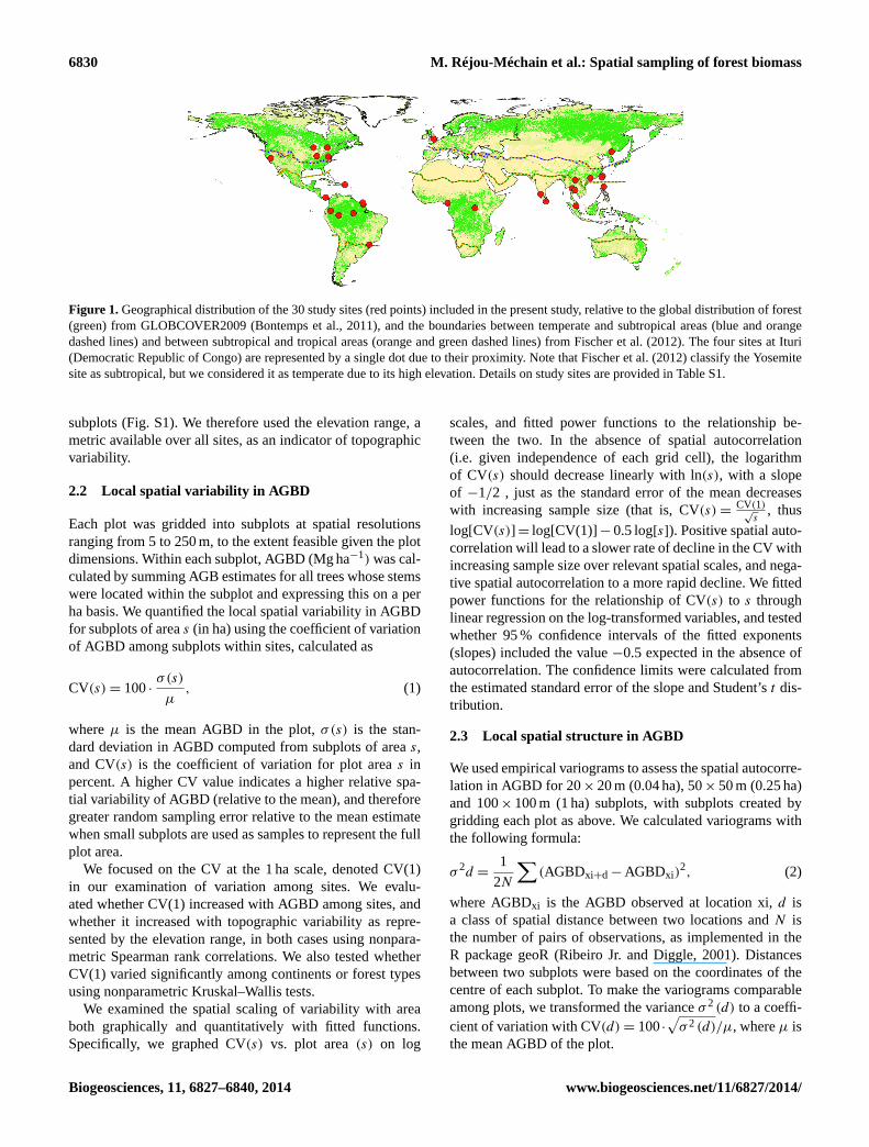
Here, we analysed spatially explicit forest census data

from a global network of 30 large permanent plots (8–50 ha)

in natural forests (Condit, 1998; Losos and Leigh, 2004)

to quantify local variation in aboveground biomass density

(AGBD) and explore its consequences for calibrating large-

footprint remote sensing products (≥ 0.5 ha) with field data

for smaller plots (Fig. 1; Table S1). Using these very large

plots, we address three questions. (1) What is the local vari-

ability in AGBD for the most commonly used plot sizes,

how does this variability scale with the area sampled, and

how does it differ among sites, forest types, and continents?

(2) Does local AGBD variability exhibit significant spatial

structure (e.g. aggregation) and, if so, what is that struc-

ture (strength, spatial scales)? (3) What are the implications

of the observed AGBD variability for the accuracy of re-

mote sensing calibration equations when calibration plots

are smaller than sensor footprints, and for different statisti-

cal procedures?

2 Material and methods

2.1 Field data

We used measurements in 30 large forest plots across three

continents (8–50 ha each; Fig. 1, Table S1). In 28 of the

plots, all free-standing trees ≥ 1 cm dbh (diameter measured

at 130 cm above the ground or 50 cm above buttresses)

were mapped, tagged, and identified taxonomically (Con-

dit, 1998). In two additional plots, only trees ≥ 10 cm in dbh

were included (Table S1). Trees < 10 cm dbh generally con-

tribute less than 5 % of the total aboveground biomass (AGB)

in mature tropical forests (Chave et al., 2003). AGB of each

individual stem was estimated using regression models based

on the measured individual diameter and the wood-specific

gravity assigned to that species and site, or site-specific al-

lometric equations (details in Table S1). We only used data

for free-standing woody stems, and excluded lianas from

our analyses for the few sites where these were censused.

Lianas usually represent less than 5 % of the total AGB (e.g.

Schnitzer et al., 2012).

Elevation ranges were computed for each site based on

5–20 m elevation maps generated from either field survey

measurements (Condit, 1998) or high-resolution airborne li-

dar (in Paracou, Nouragues and Haliburton). Among 19 for-

est plots where elevation maps were available, the eleva-

tion range showed a strong and significant correlation with

the mean of the standard deviation of elevation within 1 ha

www.biogeosciences.net/11/6827/2014/ Biogeosciences, 11, 6827–6840, 2014

6830 M. Réjou-Méchain et al.: Spatial sampling of forest biomass

Figure 1. Geographical distribution of the 30 study sites (red points) included in the present study, relative to the global distribution of forest

(green) from GLOBCOVER2009 (Bontemps et al., 2011), and the boundaries between temperate and subtropical areas (blue and orange

dashed lines) and between subtropical and tropical areas (orange and green dashed lines) from Fischer et al. (2012). The four sites at Ituri

(Democratic Republic of Congo) are represented by a single dot due to their proximity. Note that Fischer et al. (2012) classify the Yosemite

site as subtropical, but we considered it as temperate due to its high elevation. Details on study sites are provided in Table S1.

subplots (Fig. S1). We therefore used the elevation range, a

metric available over all sites, as an indicator of topographic

variability.

2.2 Local spatial variability in AGBD

Each plot was gridded into subplots at spatial resolutions

ranging from 5 to 250 m, to the extent feasible given the plot

dimensions. Within each subplot, AGBD (Mg ha−1) was cal-

culated by summing AGB estimates for all trees whose stems

were located within the subplot and expressing this on a per

ha basis. We quantified the local spatial variability in AGBD

for subplots of area s (in ha) using the coefficient of variation

of AGBD among subplots within sites, calculated as

CV(s)= 100 ·σ(s)

µ, (1)

where µ is the mean AGBD in the plot, σ(s) is the stan-

dard deviation in AGBD computed from subplots of area s,

and CV(s) is the coefficient of variation for plot area s in

percent. A higher CV value indicates a higher relative spa-

tial variability of AGBD (relative to the mean), and therefore

greater random sampling error relative to the mean estimate

when small subplots are used as samples to represent the full

plot area.

We focused on the CV at the 1 ha scale, denoted CV(1)

in our examination of variation among sites. We evalu-

ated whether CV(1) increased with AGBD among sites, and

whether it increased with topographic variability as repre-

sented by the elevation range, in both cases using nonpara-

metric Spearman rank correlations. We also tested whether

CV(1) varied significantly among continents or forest types

using nonparametric Kruskal–Wallis tests.

We examined the spatial scaling of variability with area

both graphically and quantitatively with fitted functions.

Specifically, we graphed CV(s) vs. plot area (s) on log

scales, and fitted power functions to the relationship be-

tween the two. In the absence of spatial autocorrelation

(i.e. given independence of each grid cell), the logarithm

of CV(s) should decrease linearly with ln(s), with a slope

of −1/2 , just as the standard error of the mean decreases

with increasing sample size (that is, CV(s)=CV(1)√s

, thus

log[CV(s)]= log[CV(1)]− 0.5 log[s]). Positive spatial auto-

correlation will lead to a slower rate of decline in the CV with

increasing sample size over relevant spatial scales, and nega-

tive spatial autocorrelation to a more rapid decline. We fitted

power functions for the relationship of CV(s) to s through

linear regression on the log-transformed variables, and tested

whether 95 % confidence intervals of the fitted exponents

(slopes) included the value −0.5 expected in the absence of

autocorrelation. The confidence limits were calculated from

the estimated standard error of the slope and Student’s t dis-

tribution.

2.3 Local spatial structure in AGBD

We used empirical variograms to assess the spatial autocorre-

lation in AGBD for 20× 20 m (0.04 ha), 50× 50 m (0.25 ha)

and 100× 100 m (1 ha) subplots, with subplots created by

gridding each plot as above. We calculated variograms with

the following formula:

σ 2d =1

2N

∑(AGBDxi+d−AGBDxi)

2, (2)

where AGBDxi is the AGBD observed at location xi, d is

a class of spatial distance between two locations and N is

the number of pairs of observations, as implemented in the

R package geoR (Ribeiro Jr. and Diggle, 2001). Distances

between two subplots were based on the coordinates of the

centre of each subplot. To make the variograms comparable

among plots, we transformed the variance σ 2 (d) to a coeffi-

cient of variation with CV(d)= 100 ·√σ 2 (d)/µ, where µ is

the mean AGBD of the plot.

Biogeosciences, 11, 6827–6840, 2014 www.biogeosciences.net/11/6827/2014/

M. Réjou-Méchain et al.: Spatial sampling of forest biomass 6831

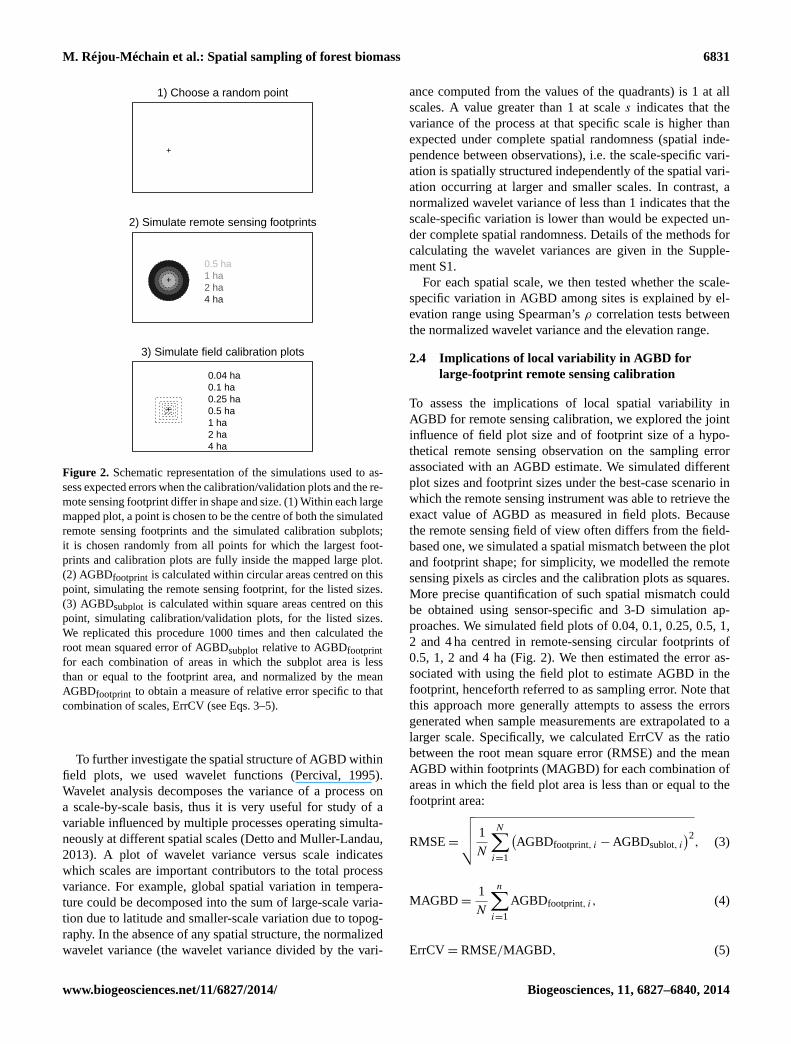
1) Choose a random point

+

2) Simulate remote sensing footprints

+

0.5 ha1 ha2 ha4 ha

3) Simulate field calibration plots

+

0.04 ha0.1 ha0.25 ha0.5 ha1 ha2 ha4 ha

Figure 2. Schematic representation of the simulations used to as-

sess expected errors when the calibration/validation plots and the re-

mote sensing footprint differ in shape and size. (1) Within each large

mapped plot, a point is chosen to be the centre of both the simulated

remote sensing footprints and the simulated calibration subplots;

it is chosen randomly from all points for which the largest foot-

prints and calibration plots are fully inside the mapped large plot.

(2) AGBDfootprint is calculated within circular areas centred on this

point, simulating the remote sensing footprint, for the listed sizes.

(3) AGBDsubplot is calculated within square areas centred on this

point, simulating calibration/validation plots, for the listed sizes.

We replicated this procedure 1000 times and then calculated the

root mean squared error of AGBDsubplot relative to AGBDfootprint

for each combination of areas in which the subplot area is less

than or equal to the footprint area, and normalized by the mean

AGBDfootprint to obtain a measure of relative error specific to that

combination of scales, ErrCV (see Eqs. 3–5).

To further investigate the spatial structure of AGBD within

field plots, we used wavelet functions (Percival, 1995).

Wavelet analysis decomposes the variance of a process on

a scale-by-scale basis, thus it is very useful for study of a

variable influenced by multiple processes operating simulta-

neously at different spatial scales (Detto and Muller-Landau,

2013). A plot of wavelet variance versus scale indicates

which scales are important contributors to the total process

variance. For example, global spatial variation in tempera-

ture could be decomposed into the sum of large-scale varia-

tion due to latitude and smaller-scale variation due to topog-

raphy. In the absence of any spatial structure, the normalized

wavelet variance (the wavelet variance divided by the vari-

ance computed from the values of the quadrants) is 1 at all

scales. A value greater than 1 at scale s indicates that the

variance of the process at that specific scale is higher than

expected under complete spatial randomness (spatial inde-

pendence between observations), i.e. the scale-specific vari-

ation is spatially structured independently of the spatial vari-

ation occurring at larger and smaller scales. In contrast, a

normalized wavelet variance of less than 1 indicates that the

scale-specific variation is lower than would be expected un-

der complete spatial randomness. Details of the methods for

calculating the wavelet variances are given in the Supple-

ment S1.

For each spatial scale, we then tested whether the scale-

specific variation in AGBD among sites is explained by el-

evation range using Spearman’s ρ correlation tests between

the normalized wavelet variance and the elevation range.

2.4 Implications of local variability in AGBD for

large-footprint remote sensing calibration

To assess the implications of local spatial variability in

AGBD for remote sensing calibration, we explored the joint

influence of field plot size and of footprint size of a hypo-

thetical remote sensing observation on the sampling error

associated with an AGBD estimate. We simulated different

plot sizes and footprint sizes under the best-case scenario in

which the remote sensing instrument was able to retrieve the

exact value of AGBD as measured in field plots. Because

the remote sensing field of view often differs from the field-

based one, we simulated a spatial mismatch between the plot

and footprint shape; for simplicity, we modelled the remote

sensing pixels as circles and the calibration plots as squares.

More precise quantification of such spatial mismatch could

be obtained using sensor-specific and 3-D simulation ap-

proaches. We simulated field plots of 0.04, 0.1, 0.25, 0.5, 1,

2 and 4 ha centred in remote-sensing circular footprints of

0.5, 1, 2 and 4 ha (Fig. 2). We then estimated the error as-

sociated with using the field plot to estimate AGBD in the

footprint, henceforth referred to as sampling error. Note that

this approach more generally attempts to assess the errors

generated when sample measurements are extrapolated to a

larger scale. Specifically, we calculated ErrCV as the ratio

between the root mean square error (RMSE) and the mean

AGBD within footprints (MAGBD) for each combination of

areas in which the field plot area is less than or equal to the

footprint area:

RMSE=

√√√√ 1

N

N∑i=1

(AGBDfootprint, i −AGBDsublot, i

)2, (3)

MAGBD=1

N

n∑i=1

AGBDfootprint, i, (4)

ErrCV= RMSE/MAGBD, (5)

www.biogeosciences.net/11/6827/2014/ Biogeosciences, 11, 6827–6840, 2014

6832 M. Réjou-Méchain et al.: Spatial sampling of forest biomass

where N is the number of simulations (1000 per combi-

nation), AGBDfootprint,i is the AGBD within the remote-

sensing footprint (i.e. the circle) for the ith simulation, and

AGBDsubplot,i is the AGBD within the field subplot for that

simulation. Five of our plots (the Haliburton plot and the

four Ituri plots) were too small to accommodate a circular

4 ha footprint and were thus not included in the calculation

of ErrCV at this scale.

To illustrate how this sampling error propagates into

AGBD maps, we then fitted calibration equations from the

combination of simulated remote sensing pixels and field cal-

ibration plots. For this exercise, we simulated square remote

sensing pixels of 4 ha, thus mimicking the expected resolu-

tion of the BIOMASS mission’s future products (Le Toan et

al., 2011). Given the size of our field plots, we were able to

simulate 60 such pixels (i.e. two pixels per plot for 30 plots).

Within each simulated pixel, we assumed that a single ran-

domly located field plot was available for calibration, for area

of 0.01, 0.04, 0.25, 0.5, 1 or 2 ha (i.e. 60 calibration plots, one

per 4 ha pixel). For each field plot scale we calculated the co-

efficients of an ordinary least squares (OLS) linear regression

between the AGBD estimated in the calibration subplots of a

given area and the simulated pixels. We changed the location

of the subplots in each plot a thousand times and averaged

the regression coefficients for each subplot size.

It is well-established in the statistical literature that ran-

dom error in the independent variable, such as that which

results from sampling error in field plots, leads to systematic

underestimation of the OLS regression slope, a bias referred

to as attenuation or regression dilution (Fuller, 1987). This

phenomenon is easily understood as the OLS slope β is cal-

culated as β = σ 2(X,Y )/σ 2(X), where σ 2(X,Y ) is the co-

variance ofX and Y and σ 2(X) is the variance ofX. IfW is a

measure ofX with measurement error (that is,W =X+εX),

then σ 2(W) > σ 2(X) (Mcardle, 2003). Hence, the estimate

of β tends to zero as the measurement error in X increases to

infinity, a phenomenon referred to as the dilution bias.

Several methods have been proposed to correct for this

bias (Carroll and Ruppert, 1996; Frost and Thompson, 2000;

Smith, 2009). The method of moments estimator (Carroll and

Ruppert, 1996; Fuller, 1987) assumes that a corrected slope,

βMM, could be calculated from the observed slope, β, using

a reliability ratio, Rr, with

βMM =β

Rr

, (6)

where

Rr =σ 2(W)− σ 2(εX)

σ 2(W). (7)

To estimate σ 2(εX), the variance of the sampling error in

X, we generated new estimates of X (here the AGBD of

calibration plots) by bootstrapping over 0.01 ha (10× 10 m)

subplots the calibration plot (i.e. 100 bootstrapped values

for each of the 60 calibration plots). The reliability ratio

Rr was estimated using the intraclass correlation coefficient

(ICC), an accurate proxy forRr (Frost and Thompson, 2000),

considering the bootstrapped values as repeated measures

grouped by calibration plot units. ICC was estimated through

a one-way analysis of variance of repeated measures con-

sidering the calibration plots as a factor. This approach was

called “within subplot Rr”. We also carried out a second reli-

ability study based on additional subplots (i.e. replicates) es-

tablished randomly inside the 4 ha pixels (in Supplement S2).

We evaluated two alternatives to OLS that have the poten-

tial to produce less bias in calibration equations. First, the

reduced major axis (RMA) regression minimizes the sum of

squared distances both horizontally (accounting for the error

in X) and vertically (accounting for the error in Y ). Second,

the nonparametric Theil–Sen estimator, also known as Sen’s

slope estimator or the single median method, is the median

of all the slopes determined by all pairs of observations. Both

methods have been proposed as preferred alternatives to OLS

in remote sensing studies (Cohen et al., 2003; Fernandes and

Leblanc, 2005; Mitchard et al., 2013; Ryan et al., 2012).

All analyses were performed using R version 3.0.2 (R De-

velopment Core Team, 2013). The R code for the analyses is

available on request from the first author.

3 Results

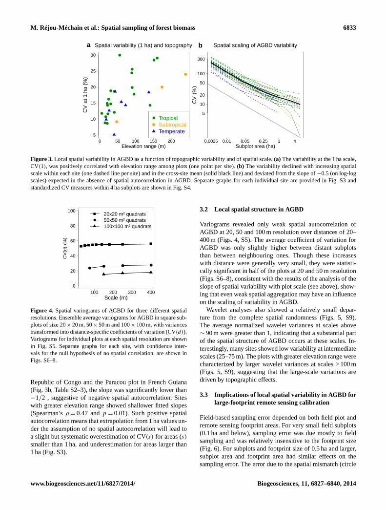
3.1 Local spatial variability in AGBD

The coefficient of variation for AGBD at the 1 ha scale,

CV(1), varied among sites (n= 30) from 5.1 (Haliburton,

Canada) to 29.9 % (Palanan, Philippines), with a mean of

16.6 %, and a median of 15.2 % (Table S2). The best pre-

dictor of variation in CV(1) among plots was within-plot

elevation range, that is, the difference between the highest

and lowest elevation (Spearman’s ρ= 0.70 and p < 10−4;

Fig. 3a). Thus, topographic variability, represented in the

analyses by elevation range across the plot, explained con-

siderable variation in AGBD variability among sites at the

1 ha scale. In contrast, CV(1)was not significantly correlated

with mean AGBD (Spearman’s correlation test, p = 0.15),

and did not differ significantly among forest types (tropical,

subtropical and temperate; Kruskal–Wallis test; p = 0.47)

or among continents (Kruskal–Wallis test; p = 0.18). Asian

tropical field plots tended to show higher biomass variabil-

ity than other tropical field plots (median CV(1) of 24.4 and

14.3 % respectively), consistent with their higher average to-

pographical variability (median elevation range of 90 m for

Asian tropical plots and 24 m for tropical non-Asian plots).

Regressing the logarithm of CV(s) against ln(s), we found

that in 15 of 30 sites the slope was significantly greater (less

negative) than−1/2, suggesting significantly positive spatial

autocorrelation in AGBD at the scales investigated. In con-

trast, in only two sites, the Ituri Edoro 1 plot in Democratic

Biogeosciences, 11, 6827–6840, 2014 www.biogeosciences.net/11/6827/2014/

M. Réjou-Méchain et al.: Spatial sampling of forest biomass 6833

a Spatial variability (1 ha) and topography b Spatial scaling of AGBD variability

●

●

●

●

●

●

●

●

●

●

●

●

●●

●

●

●

●●

●

0 50 100 150 2005

10

15

20

25

30

Elevation range (m)

CV

at 1

ha

(%)

● TropicalSubtropicalTemperate

Subplot area (ha)

CV

(%

)

5

10

20

50

100

300

0.0025 0.01 0.05 0.25 1 4

Figure 3. Local spatial variability in AGBD as a function of topographic variability and of spatial scale. (a) The variability at the 1 ha scale,

CV(1), was positively correlated with elevation range among plots (one point per site). (b) The variability declined with increasing spatial

scale within each site (one dashed line per site) and in the cross-site mean (solid black line) and deviated from the slope of −0.5 (on log-log

scales) expected in the absence of spatial autocorrelation in AGBD. Separate graphs for each individual site are provided in Fig. S3 and

standardized CV measures within 4 ha subplots are shown in Fig. S4.

100 200 300 4000

20

40

60

80

100

Scale (m)

●● ● ●

CV

(d)

(%)

●

20x20 m² quadrats50x50 m² quadrats100x100 m² quadrats

Figure 4. Spatial variograms of AGBD for three different spatial

resolutions. Ensemble average variograms for AGBD in square sub-

plots of size 20× 20 m, 50× 50 m and 100× 100 m, with variances

transformed into distance-specific coefficients of variation (CV(d)).

Variograms for individual plots at each spatial resolution are shown

in Fig. S5. Separate graphs for each site, with confidence inter-

vals for the null hypothesis of no spatial correlation, are shown in

Figs. S6–8.

Republic of Congo and the Paracou plot in French Guiana

(Fig. 3b, Table S2–3), the slope was significantly lower than

−1/2 , suggestive of negative spatial autocorrelation. Sites

with greater elevation range showed shallower fitted slopes

(Spearman’s ρ= 0.47 and p = 0.01). Such positive spatial

autocorrelation means that extrapolation from 1 ha values un-

der the assumption of no spatial autocorrelation will lead to

a slight but systematic overestimation of CV(s) for areas (s)

smaller than 1 ha, and underestimation for areas larger than

1 ha (Fig. S3).

3.2 Local spatial structure in AGBD

Variograms revealed only weak spatial autocorrelation of

AGBD at 20, 50 and 100 m resolution over distances of 20–

400 m (Figs. 4, S5). The average coefficient of variation for

AGBD was only slightly higher between distant subplots

than between neighbouring ones. Though these increases

with distance were generally very small, they were statisti-

cally significant in half of the plots at 20 and 50 m resolution

(Figs. S6–8), consistent with the results of the analysis of the

slope of spatial variability with plot scale (see above), show-

ing that even weak spatial aggregation may have an influence

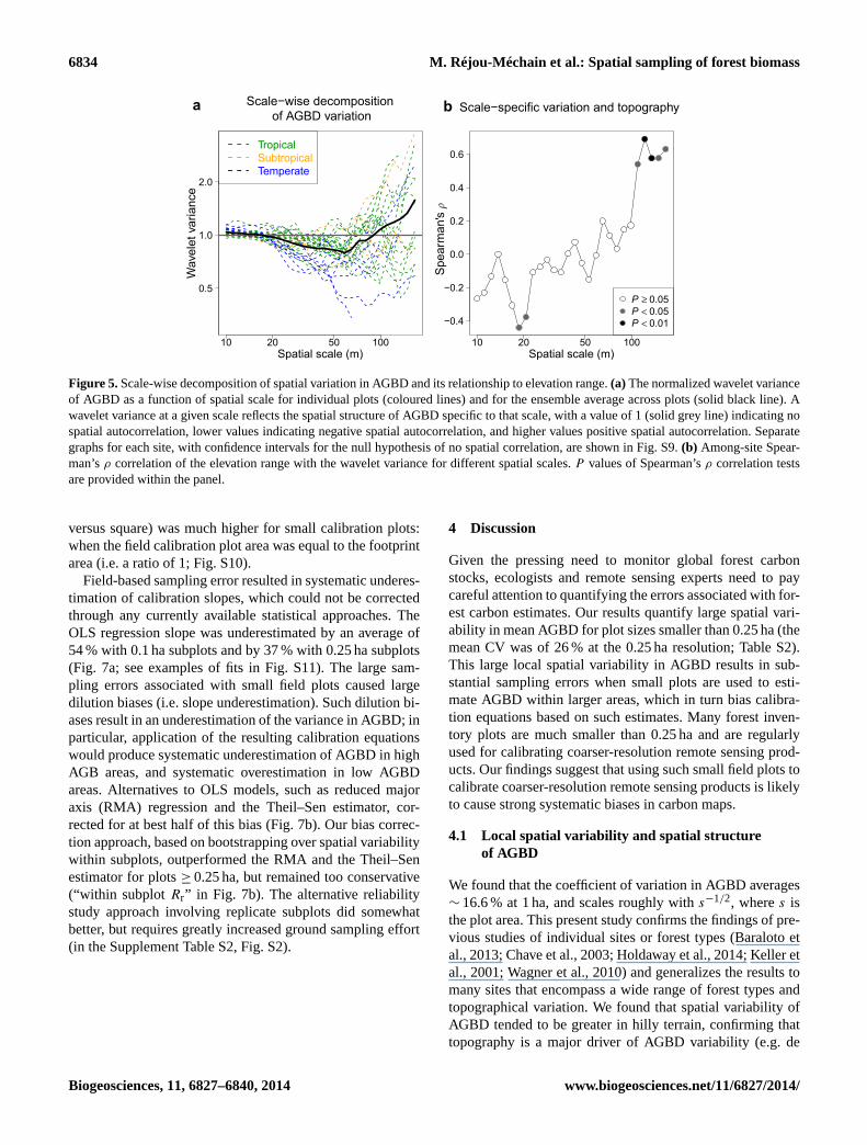
on the scaling of variability in AGBD.

Wavelet analyses also showed a relatively small depar-

ture from the complete spatial randomness (Figs. 5, S9).

The average normalized wavelet variances at scales above

∼ 90 m were greater than 1, indicating that a substantial part

of the spatial structure of AGBD occurs at these scales. In-

terestingly, many sites showed low variability at intermediate

scales (25–75 m). The plots with greater elevation range were

characterized by larger wavelet variances at scales > 100 m

(Figs. 5, S9), suggesting that the large-scale variations are

driven by topographic effects.

3.3 Implications of local spatial variability in AGBD for

large-footprint remote sensing calibration

Field-based sampling error depended on both field plot and

remote sensing footprint areas. For very small field subplots

(0.1 ha and below), sampling error was due mostly to field

sampling and was relatively insensitive to the footprint size

(Fig. 6). For subplots and footprint size of 0.5 ha and larger,

subplot area and footprint area had similar effects on the

sampling error. The error due to the spatial mismatch (circle

www.biogeosciences.net/11/6827/2014/ Biogeosciences, 11, 6827–6840, 2014

6834 M. Réjou-Méchain et al.: Spatial sampling of forest biomass

a Scale−wise decomposition of AGBD variation

b Scale−specific variation and topography

10 20 50 100

0.5

1.0

2.0

Spatial scale (m)

Wav

elet

var

ianc

e

TropicalSubtropicalTemperate

●

●

●

●

●●●

10 20 50 100

−0.4

−0.2

0.0

0.2

0.4

0.6

Spatial scale (m)

Spe

arm

an's

rho

●

●

P ≥ 0.05P < 0.05P < 0.01

ρ

Figure 5. Scale-wise decomposition of spatial variation in AGBD and its relationship to elevation range. (a) The normalized wavelet variance

of AGBD as a function of spatial scale for individual plots (coloured lines) and for the ensemble average across plots (solid black line). A

wavelet variance at a given scale reflects the spatial structure of AGBD specific to that scale, with a value of 1 (solid grey line) indicating no

spatial autocorrelation, lower values indicating negative spatial autocorrelation, and higher values positive spatial autocorrelation. Separate

graphs for each site, with confidence intervals for the null hypothesis of no spatial correlation, are shown in Fig. S9. (b) Among-site Spear-

man’s ρ correlation of the elevation range with the wavelet variance for different spatial scales. P values of Spearman’s ρ correlation tests

are provided within the panel.

versus square) was much higher for small calibration plots:

when the field calibration plot area was equal to the footprint

area (i.e. a ratio of 1; Fig. S10).

Field-based sampling error resulted in systematic underes-

timation of calibration slopes, which could not be corrected

through any currently available statistical approaches. The

OLS regression slope was underestimated by an average of

54 % with 0.1 ha subplots and by 37 % with 0.25 ha subplots

(Fig. 7a; see examples of fits in Fig. S11). The large sam-

pling errors associated with small field plots caused large

dilution biases (i.e. slope underestimation). Such dilution bi-

ases result in an underestimation of the variance in AGBD; in

particular, application of the resulting calibration equations

would produce systematic underestimation of AGBD in high

AGB areas, and systematic overestimation in low AGBD

areas. Alternatives to OLS models, such as reduced major

axis (RMA) regression and the Theil–Sen estimator, cor-

rected for at best half of this bias (Fig. 7b). Our bias correc-

tion approach, based on bootstrapping over spatial variability

within subplots, outperformed the RMA and the Theil–Sen

estimator for plots ≥ 0.25 ha, but remained too conservative

(“within subplot Rr” in Fig. 7b). The alternative reliability

study approach involving replicate subplots did somewhat

better, but requires greatly increased ground sampling effort

(in the Supplement Table S2, Fig. S2).

4 Discussion

Given the pressing need to monitor global forest carbon

stocks, ecologists and remote sensing experts need to pay

careful attention to quantifying the errors associated with for-

est carbon estimates. Our results quantify large spatial vari-

ability in mean AGBD for plot sizes smaller than 0.25 ha (the

mean CV was of 26 % at the 0.25 ha resolution; Table S2).

This large local spatial variability in AGBD results in sub-

stantial sampling errors when small plots are used to esti-

mate AGBD within larger areas, which in turn bias calibra-

tion equations based on such estimates. Many forest inven-

tory plots are much smaller than 0.25 ha and are regularly

used for calibrating coarser-resolution remote sensing prod-

ucts. Our findings suggest that using such small field plots to

calibrate coarser-resolution remote sensing products is likely

to cause strong systematic biases in carbon maps.

4.1 Local spatial variability and spatial structure

of AGBD

We found that the coefficient of variation in AGBD averages

∼ 16.6 % at 1 ha, and scales roughly with s−1/2, where s is

the plot area. This present study confirms the findings of pre-

vious studies of individual sites or forest types (Baraloto et

al., 2013; Chave et al., 2003; Holdaway et al., 2014; Keller et

al., 2001; Wagner et al., 2010) and generalizes the results to

many sites that encompass a wide range of forest types and

topographical variation. We found that spatial variability of

AGBD tended to be greater in hilly terrain, confirming that

topography is a major driver of AGBD variability (e.g. de

Biogeosciences, 11, 6827–6840, 2014 www.biogeosciences.net/11/6827/2014/

M. Réjou-Méchain et al.: Spatial sampling of forest biomass 6835

ErrCV in AGBD (%)

Footprint area (ha)

48.7

28.9

14.7

6.6

50.2

31.1

18.3

10.8

4.6

51.4

32.8

20.7

13.8

8

3.3

52.6

34.4

22.9

16.6

11.5

6.5

2.4

(22.1−77.1)

(11.4−45.6)

(5.8−23)

(3.3−10.1)

(22.3−78.5)

(11.4−48.4)

(6.1−28.6)

(4.1−16.6)

(2.1−7.5)

(23−79.8)

(12.1−50.6)

(6.6−36.3)

(4.4−25.6)

(2.5−14.9)

(1.4−5.2)

(24.1−83.6)

(14.9−56.1)

(10.1−45.4)

(7.2−36.1)

(5.2−26.4)

(2.9−14.4)

(1−3.8)

48.7

6.6

50.2

10.8

4.6

51.4

13.8

8

3.3

52.6

16.6

11.5

6.5

2.4

(22.1−77.1)

(3.3−10.1)

(22.3−78.5)

(4.1−16.6)

(2.1−7.5)

(23−79.8)

(4.4−25.6)

(2.5−14.9)

(1.4−5.2)

(24.1−83.6)

(7.2−36.1)

(5.2−26.4)

(2.9−14.4)

(1−3.8)

0.5 1 2 4

0.04

0.1

0.25

0.5

1

2

4

Sub

plot

are

a (h

a)

10

20

30

40

50

Figure 6. Expected sampling errors when the calibration/validation

plots and the remote sensing footprint differ in shape and size. The

remote sensing footprint is assumed circular, and subplots are as-

sumed to be square to simulate the spatial mismatch between the

remote sensing signal and the calibration plot (Fig. 2). The mean

ErrCV in AGBD estimates across all sites (n= 30) is both given

within the figure and illustrated by colours, and the range of ErrCV

across sites is given in parentheses below the mean.

Castilho et al., 2006; Detto et al., 2013). This is an important

finding given that 23 % of the world’s forests are on hilly

terrain (Table S4). This result suggests that forest biomass

maps in hilly areas have larger uncertainties, and that forest

plot sampling designs should take topography into account

(see below).

We found no other systematic differences in AGBD vari-

ability among continents, among forest types or with mean

AGBD. The higher AGBD variability found in our tropi-

cal Asian study sites compared with other tropical sites was

probably due to their larger topographic variability. This find-

ing is no accident of our study locations; remaining old-

growth tropical forests in Asia are disproportionately located

in topographically complex terrain, more so than on other

continents (Table S4), probably because these areas have dis-

proportionately escaped human disturbance.

Approximately half of the sites individually exhibited sta-

tistically significant spatial autocorrelation in AGBD. De-

composition of the variance in AGBD at different spatial

scales using wavelet analyses confirmed spatial aggregation

at scales > 100 m, and the role of topography in explaining

aggregation at these scales (Fig. 5b). These results suggest

that the weak spatial autocorrelation found in many plots

is due to broad-scale topographic differences. In a previous

scale-wise analysis of a 5000 ha area of moist tropical forest,

Detto et al. (2013) likewise found strong wavelet coherence

between canopy height (a proxy for AGBD) and topography

at scales of 100–800 m. These scale-specific results are con-

sistent with prior literature (reviewed in Detto et al., 2013)

documenting how forest structure and biomass vary with to-

pography (de Castilho et al., 2006; McEwan et al., 2011; Va-

lencia et al., 2009).

In most plots, the wavelet analyses also revealed that spa-

tial variability specific to scales of 25–75 m was lower (i.e.

more uniformly distributed) than expected by chance. We

hypothesize that this pattern may be associated with neigh-

bourhood competition and gap-phase dynamics. That is, the

forest can be thought of as a mosaic of patches of differ-

ent age, reflecting time since the last disturbance (e.g. major

treefall), with patch age strongly influencing AGBD (Moor-

croft et al., 2001). Within such patches, biomass variation

is reduced by the common time since disturbance, and also

because local competition may cause large trees to be more

evenly spaced than would be expected by chance (Lutz et al.,

2013). This local uniformity is overlaid on the larger-scale

topographic variation, and is evident only through scale-wise

wavelet analyses that separate the two.

4.2 Field sampling error and remote sensing of

carbon stocks

We showed that when field plots were very small (0.1 ha and

below), the sampling error was due mostly to the contribution

from field sampling, and was relatively insensitive to foot-

print area. Hence, with relatively high-resolution pixels such

as in the Landsat (30 m) or ICESat/GLAS (Ice, Cloud, and

land Elevation Satellite/Geoscience Laser Altimeter System)

(∼ 70 m) products, sampling errors are likely to be very high

if smaller plots are used or if spatial mismatches between

the field and the sensor signal occur. This is because most

of the AGBD variability is at the local scale so that a small

difference between the areas sampled in the ground and by

the sensor generates a large error. This is well illustrated by

our finding that the error was much lower for large calibra-

tion plots even when the same ratio of calibration plot area

to footprint area was maintained (Fig. S10). This reflects de-

creasing edge-to-area ratios for larger areas, which also pro-

vide other advantages for larger plots (see also Mascaro et

al., 2011; Zolkos et al., 2013).

Our analyses show that the field-sampling strategy may re-

sult in a serious bias in model calibration of remote sensing

products. When this bias is present, inversion models return

AGBD values that are regressed to the mean of the calibra-

tion plots (Fig. 7a), and thus underestimate the true spatial

AGBD variance. For instance, in a recent study that used

112 circular 0.13 ha plots to calibrate L-band radar prod-

ucts (Carreiras et al., 2012), the slope of an OLS regression

was found to be underestimated by 86 % and the final AGBD

map displayed a much lower variance than the map produced

by Saatchi et al. (2011). The dilution bias is independent of

the number of calibration plots; it depends only on the sam-

pling error associated with these plots, which is determined

largely by plot size. Though the mean AGBD of the cali-

bration plots is inherently correctly predicted (Fig. 7a), the

www.biogeosciences.net/11/6827/2014/ Biogeosciences, 11, 6827–6840, 2014

6836 M. Réjou-Méchain et al.: Spatial sampling of forest biomass

a Dilution bias b OLS corrections and alternatives

200 300 400 500 600

200

300

400

500

600

AG

BD

4−

ha p

ixel

(M

g.ha

−1)

AGBD subplot (Mg.ha−1)

True slope

0.1 ha (slope bias: 54%)0.25 ha (37%)1 ha (16%)2 ha (7%)

Subplot area:

Mean AGBD

0.0 0.5 1.0 1.5 2.0

0.4

0.6

0.8

1.0

Est

imat

ed s

lope

Subplot area (ha)

True slopeOLS (Within subplot Rr)RMATheil−Sen OLS non corrected

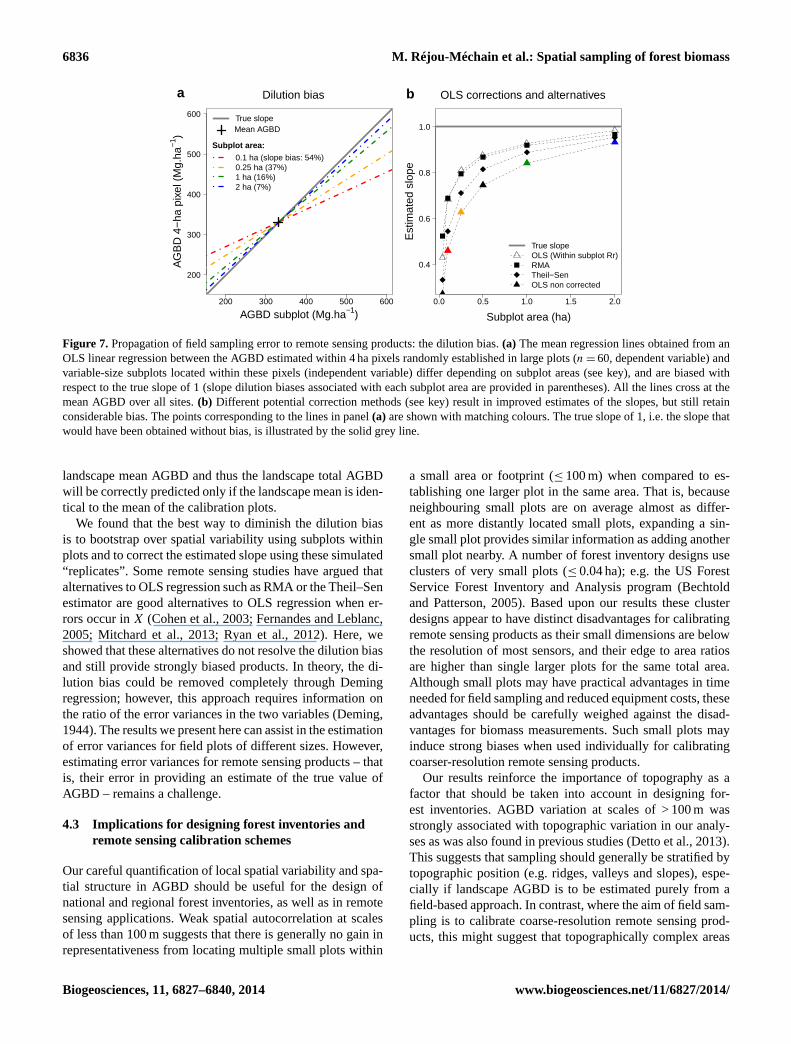
Figure 7. Propagation of field sampling error to remote sensing products: the dilution bias. (a) The mean regression lines obtained from an

OLS linear regression between the AGBD estimated within 4 ha pixels randomly established in large plots (n= 60, dependent variable) and

variable-size subplots located within these pixels (independent variable) differ depending on subplot areas (see key), and are biased with

respect to the true slope of 1 (slope dilution biases associated with each subplot area are provided in parentheses). All the lines cross at the

mean AGBD over all sites. (b) Different potential correction methods (see key) result in improved estimates of the slopes, but still retain

considerable bias. The points corresponding to the lines in panel (a) are shown with matching colours. The true slope of 1, i.e. the slope that

would have been obtained without bias, is illustrated by the solid grey line.

landscape mean AGBD and thus the landscape total AGBD

will be correctly predicted only if the landscape mean is iden-

tical to the mean of the calibration plots.

We found that the best way to diminish the dilution bias

is to bootstrap over spatial variability using subplots within

plots and to correct the estimated slope using these simulated

“replicates”. Some remote sensing studies have argued that

alternatives to OLS regression such as RMA or the Theil–Sen

estimator are good alternatives to OLS regression when er-

rors occur in X (Cohen et al., 2003; Fernandes and Leblanc,

2005; Mitchard et al., 2013; Ryan et al., 2012). Here, we

showed that these alternatives do not resolve the dilution bias

and still provide strongly biased products. In theory, the di-

lution bias could be removed completely through Deming

regression; however, this approach requires information on

the ratio of the error variances in the two variables (Deming,

1944). The results we present here can assist in the estimation

of error variances for field plots of different sizes. However,

estimating error variances for remote sensing products – that

is, their error in providing an estimate of the true value of

AGBD – remains a challenge.

4.3 Implications for designing forest inventories and

remote sensing calibration schemes

Our careful quantification of local spatial variability and spa-

tial structure in AGBD should be useful for the design of

national and regional forest inventories, as well as in remote

sensing applications. Weak spatial autocorrelation at scales

of less than 100 m suggests that there is generally no gain in

representativeness from locating multiple small plots within

a small area or footprint (≤ 100 m) when compared to es-

tablishing one larger plot in the same area. That is, because

neighbouring small plots are on average almost as differ-

ent as more distantly located small plots, expanding a sin-

gle small plot provides similar information as adding another

small plot nearby. A number of forest inventory designs use

clusters of very small plots (≤ 0.04 ha); e.g. the US Forest

Service Forest Inventory and Analysis program (Bechtold

and Patterson, 2005). Based upon our results these cluster

designs appear to have distinct disadvantages for calibrating

remote sensing products as their small dimensions are below

the resolution of most sensors, and their edge to area ratios

are higher than single larger plots for the same total area.

Although small plots may have practical advantages in time

needed for field sampling and reduced equipment costs, these

advantages should be carefully weighed against the disad-

vantages for biomass measurements. Such small plots may

induce strong biases when used individually for calibrating

coarser-resolution remote sensing products.

Our results reinforce the importance of topography as a

factor that should be taken into account in designing for-

est inventories. AGBD variation at scales of > 100 m was

strongly associated with topographic variation in our analy-

ses as was also found in previous studies (Detto et al., 2013).

This suggests that sampling should generally be stratified by

topographic position (e.g. ridges, valleys and slopes), espe-

cially if landscape AGBD is to be estimated purely from a

field-based approach. In contrast, where the aim of field sam-

pling is to calibrate coarse-resolution remote sensing prod-

ucts, this might suggest that topographically complex areas

Biogeosciences, 11, 6827–6840, 2014 www.biogeosciences.net/11/6827/2014/

M. Réjou-Méchain et al.: Spatial sampling of forest biomass 6837

should best be avoided to minimize sampling errors associ-

ated with local spatial variability. However, the gain from

reducing such sampling errors would have to be weighed

against the potential to bias the calibration sample if forests

in topographically complex areas differ systematically in the

relationship between remote sensing signals and AGBD.

The best way to avoid the dilution bias is to use cali-

bration plots covering entire remote sensing pixels. For re-

mote sensing tools with a resolution on the order of 4 ha,

such as the planned BIOMASS mission, it is realistic to in-

vest in a network of similarly sized field calibration plots.

Though such field sampling is expensive, it would greatly

improve the basis for mapping forest biomass, and its cost

would remain small compared with the investment in the

satellite itself. An alternative is to use a two-step approach

in which a coarse-resolution remote sensing product is cal-

ibrated against a higher-resolution remote sensing product

itself calibrated with field plots. For instance, airborne li-

dar may retrieve forest carbon stocks with an error of ca.

10–15 % at 1 ha resolution (Mascaro et al., 2011; Zolkos et

al., 2013). This compares favourably with errors from purely

field-based estimates for 1 ha and smaller plots (Fig. 3). Er-

rors in lidar-based estimates are expected to be even lower

for larger areas, as random errors average out (Mascaro et

al., 2011). Baccini and Asner (2013) found that using wall-

to-wall airborne lidar AGBD estimates to calibrate a 500 m

resolution MODIS product led to much less error than us-

ing nested AGBD estimates from GLAS footprints (60–75 m

resolution). This shows that even if the operational cost asso-

ciated with lidar coverage is high, the use of lidar technology

has the potential to greatly reduce the errors during the cal-

ibration step. In this case, care must be taken that errors are

carefully and appropriately propagated through the two-stage

calibration to the final map (Asner et al., 2013).

Future research should integrate the results of this study

with information on other sources of error in order to as-

sess the relative importance of field sampling errors to forest

carbon estimation and make appropriate recommendations.

Other important sources of error in forest carbon estimates

include field measurement errors (Flores and Coomes, 2011;

Larjavaara and Muller-Landau, 2013), biomass allometries

(Chave et al., 2014, 2004; Molto et al., 2013), data cleaning

procedures (Muller-Landau et al., 2014), and wood carbon

content (Thomas and Martin, 2012). At the scale of forest in-

ventories and calibration schemes, a major source of error is

the uneven and nonrandom distribution of plots at broad spa-

tial scales, an outstanding problem in the tropics where, for

example, the central Amazon, the central Congo Basin, and

swamp forests all remain insufficiently sampled.

5 Conclusions

Accurate measurements of forest carbon stocks are critical to

reduce uncertainties in the global carbon budget and for the

REDD (Reducing Emissions from Deforestation and Forest

Degradation) programme. However, uncertainty associated

with forest carbon maps remains poorly quantified (but for

notable exceptions see Asner et al., 2013; Gonzalez et al.,

2010; Mermoz et al., 2014). In this paper, we used a large-

scale global data set to illustrate that high local spatial vari-

ability in AGBD leads to large sampling errors when plots

of standard sizes (e.g. 0.1, 0.25, 1 ha) are used to estimate

AGBD over larger areas (e.g. 4 ha, the expected resolution

of BIOMASS products). We also show that remote sensing

estimates of biomass density that rely on field data for cal-

ibration may be highly biased if such field-sampling errors

are large. Such biases have previously been ignored by the

remote sensing community and, as we show, can only be par-

tially corrected by available statistical tools. Overall, our re-

sults strongly suggest that calibration of coarse-resolution re-

mote sensing products to estimate forest carbon would bene-

fit greatly from more investment in large forest plots that are

large enough to encompass entire pixels. We hope that this

contribution will stimulate further work on the propagation

of field sampling errors to remote sensing products and that

future studies will pay more careful attention to field sam-

pling and calibration strategies.

The Supplement related to this article is available online

at doi:10.5194/bg-11-6827-2014-supplement.

Acknowledgements. We thank E. T. A. Mitchard, G. P. As-

ner and an anonymous reviewer for useful comments and

suggestions on our work. We are also grateful to all the

people, institutions, foundations, and funding bodies that

have contributed to the collection of the large plot data sets

(http://www.ctfs.si.edu/group/Partners/Forest+Plot+Institutions),

including the staff members and central office of the Amacayacu

National Natural Park of Colombia, NSF support for the Luquillo

LTER program and EU FP7 support through the ROBIN project

for Jill Thompson. We sincerely thank Erika Gonzalez and

Sandeep Pulla for their help with analyses for the SCBI and

Mudumalai plots, respectively. Financial support for the analyses

presented here was provided by the CNES (postdoctoral grant

to M. Réjou-Méchain), the National Science Foundation (DEB

#1046113), and two Investissement d’Avenir grants managed by

Agence Nationale de la Recherche (CEBA: ANR-10-LABX-25-01;

TULIP: ANR-10-LABX-0041).

Edited by: M. Williams

www.biogeosciences.net/11/6827/2014/ Biogeosciences, 11, 6827–6840, 2014

6838 M. Réjou-Méchain et al.: Spatial sampling of forest biomass

References

Agrawal, A., Nepstad, D., and Chhatre, A.: Reducing emissions

from deforestation and forest degradation, Annu. Rev. Env. Re-

sour., 36, 373–396, 2011.

Asner, G. P., Powell, G. V. N., Mascaro, J., Knapp, D. E.,

Clark, J. K., Jacobson, J., Kennedy-Bowdoin, T., Balaji, A.,

Paez-Acosta, G., Victoria, E., Secada, L., Valqui, M., and

Hughes, R. F.: High-resolution forest carbon stocks and emis-

sions in the Amazon, P. Natl. Acad. Sci., 107, 16738–16742,

doi:10.1073/pnas.1004875107, 2010.

Asner, G. P., Mascaro, J., Anderson, C., Knapp, D. E., Martin, R.

E., Kennedy-Bowdoin, T., Breugel, M. van, Davies, S., Hall, J.

S., Muller-Landau, H. C., Potvin, C., Sousa, W., Wright, J., and

Bermingham, E.: High-fidelity national carbon mapping for re-

source management and REDD+, Carbon Balance and Manage-

ment, 8, 1–14, doi:10.1186/1750-0680-8-7, 2013.

Baccini, A. and Asner, G. P.: Improving pantropical forest carbon

maps with airborne LiDAR sampling, Carbon Management, 4,

591–600, 2013.

Baccini, A., Friedl, M. A., Woodcock, C. E., and Zhu, Z.: Scaling

field data to calibrate and validate moderate spatial resolution

remote sensing models, Photogramm. Eng. Rem. S., 73, 945–

954, 2007.

Baccini, A., Goetz, S. J., Walker, W. S., Laporte, N. T., Sun, M.,

Sulla-Menashe, D., Hackler, J., Beck, P. S. A., Dubayah, R.,

Friedl, M. A., Samanta, S., and Houghton, R. A.: Estimated

carbon dioxide emissions from tropical deforestation improved

by carbon-density maps, Nature Climate Change, 2, 182–185,

doi:10.1038/nclimate1354, 2012.

Baraloto, C., Molto, Q., Rabaud, S., Hérault, B., Valencia, R.,

Blanc, L., Fine, P. V. A., and Thompson, J.: Rapid Simultaneous

Estimation of Aboveground Biomass and Tree Diversity Across

Neotropical Forests: A Comparison of Field Inventory Methods,

Biotropica, 45, 288–298, doi:10.1111/btp.12006, 2013.

Bechtold, W. A. and Patterson, P. L.: The enhanced forest inven-

tory and analysis program: national sampling design and estima-

tion procedures, US Department of Agriculture Forest Service,

Southern Research Station, available at: http://www.srs.fs.usda.

gov/pubs/gtr/gtr_srs080/gtr_srs080 (last access: 18 September

2013), 2005.

Bontemps, S., Defourny, P., Van Bogaert, E., Arino, O.,

Kalogirou, V., and Ramos Perez, J.: GLOBCOVER

2009 Products Description and validation Report, avail-

able at: http://due.esrin.esa.int/globcover/LandCover2009/

GLOBCOVER2009_Validation_Report_2.2.pdf (last access: 5

December 2014), 2011.

Carreiras, J. M. B., Vasconcelos, M. J., and Lucas, R.

M.: Understanding the relationship between aboveground

biomass and ALOS PALSAR data in the forests of Guinea-

Bissau (West Africa), Remote Sens. Environ., 121, 426–442,

doi:10.1016/j.rse.2012.02.012, 2012.

Carroll, R. J. and Ruppert, D.: The Use and Misuse of Orthogo-

nal Regression in Linear Errors-in-Variables Models, The Ameri-

can Statistician, 50, 1–6, doi:10.1080/00031305.1996.10473533,

1996.

Chave, J., Condit, R., Lao, S., Caspersen, J. P., Foster, R. B., and

Hubbell, S. P.: Spatial and temporal variation of biomass in a

tropical Forest: results from a large census plot in Panama, J.

Ecol., 91, 240–252, 2003.

Chave, J., Condit, R., Aguilar, S., Hernandez, A., Lao, S., and Perez,

R.: Error propagation and scaling for tropical forest biomass es-

timates, P. T. Royal Soc. B, 359, 409–420, 2004.

Chave, J., Réjou-Méchain, M., Búrquez, A., Chidumayo, E., Col-

gan, M. S., Delitti, W. B. C., Duque, A., Eid, T., Fearnside, P.

M., Goodman, R. C., Henry, M., Martínez-Yrízar, A., Mugasha,

W. A., Muller-Landau, H. C., Mencuccini, M., Nelson, B. W.,

Ngomanda, A., Nogueira, E. M., Ortiz-Malavassi, E., Pélissier,

R., Ploton, P., Ryan, C. M., Saldarriaga, J. G. and Vieilledent,

G.: Improved allometric models to estimate the aboveground

biomass of tropical trees, Glob. Change Biol., 20, 3177–3190

doi:10.1111/gcb.12629, 2014.

Cohen, W. B., Maiersperger, T. K., Gower, S. T., and Turner, D.

P.: An improved strategy for regression of biophysical variables

and Landsat ETM+ data, Remote Sens. Environ., 84, 561–571,

doi:10.1016/S0034-4257(02)00173-6, 2003.

Condit, R.: Tropical Forest Census Plots: Methods and Results from

Barro Colorado Island, Panama and a Comparison with Other

Plots, Springer, Berlin, Germany, 211 pp., 1998.

De Castilho, C. V., Magnusson, W. E., de Araújo, R. N. O., Luizão,

R. C. C., Luizão, F. J., Lima, A. P., and Higuchi, N.: Variation

in aboveground tree live biomass in a central Amazonian Forest:

Effects of soil and topography, Forest Ecol. Manag., 234, 85–96,

doi:10.1016/j.foreco.2006.06.024, 2006.

Deming, W. E.: Statistical adjustment of data, New York,

available at: http://www.maa.org/publications/maa-reviews/

statistical-adjustment-of-data (last access: 21 August 2014),

1944.

Detto, M. and Muller-Landau, H. C.: Fitting ecological process

models to spatial patterns using scalewise variances and moment

equations, The American Naturalist, 181, E68–E82, 2013.

Detto, M., Muller-Landau, H. C., Mascaro, J., and Asner, G. P.:

Hydrological Networks and Associated Topographic Variation as

Templates for the Spatial Organization of Tropical Forest Vegeta-

tion, PLoS ONE, 8, e76296, doi:10.1371/journal.pone.0076296,

2013.

Fernandes, R. and Leblanc, S.: Parametric (modified least

squares) and non-parametric (Theil–Sen) linear regressions

for predicting biophysical parameters in the presence of

measurement errors, Remote Sens. Environ., 95, 303–316,

doi:10.1016/j.rse.2005.01.005, 2005.

Fischer, G., Nachtergaele, F. O., Prieler, S., Teixeira, E., Tóth,

G., Velthuizen, H., Verelst, L., and Wiberg, D.: Global Agro-

Ecological Zones (GAEZ v3. 0), Laxenburg, Austria: Interna-

tional Institute for Applied Systems Analysis, 2012.

Flores, O. and Coomes, D. A.: Estimating the wood density of

species for carbon stock assessments, Methods in Ecology and

Evolution, 2, 214–220, doi:10.1111/j.2041-210X.2010.00068.x,

2011.

Frost, C. and Thompson, S. G.: Correcting for Regression Dilution

Bias: Comparison of Methods for a Single Predictor Variable, J.

R. Stat. Soc. A Sta., 163, 173–189, 2000.

Fuller, W. A.: Measurement error models, John Wiley, New York,

440 pp., 1987.

Gibbs, H. K., Brown, S., Niles, J. O., and Foley, J. A.: Monitor-

ing and estimating tropical forest carbon stocks: making REDD

a reality, Environ. Res. Lett., 2, 045023, doi:10.1088/1748-

9326/2/4/045023, 2007.

Biogeosciences, 11, 6827–6840, 2014 www.biogeosciences.net/11/6827/2014/

M. Réjou-Méchain et al.: Spatial sampling of forest biomass 6839

Goetz, S. and Dubayah, R.: Advances in remote sensing technol-

ogy and implications for measuring and monitoring forest carbon

stocks and change, Carbon Management, 2, 231–244, 2011.

Gonzalez, P., Asner, G. P., Battles, J. J., Lefsky, M. A., Waring,

K. M., and Palace, M.: Forest carbon densities and uncertain-

ties from Lidar, QuickBird, and field measurements in California,

Remote Sens. Environ., 114, 1561–1575, 2010.

Harris, N. L., Brown, S., Hagen, S. C., Saatchi, S. S., Petrova, S.,

Salas, W., Hansen, M. C., Potapov, P. V., and Lotsch, A.: Baseline

map of carbon emissions from deforestation in tropical regions,

Science, 336, 1573–1576, doi:10.1126/science.1217962, 2012.

Holdaway, R. J., McNeill, S. J., Mason, N. W., and Carswell, F. E.:

Propagating Uncertainty in Plot-based Estimates of Forest Car-

bon Stock and Carbon Stock Change, Ecosystems, 17, 627–640,

doi:10.1007/s10021-014-9749-5, 2014.

Keller, M., Palace, M., and Hurtt, G.: Biomass estimation in the

Tapajos National Forest, Brazil: Examination of sampling and

allometric uncertainties, Forest Ecol. Manag., 154, 371–382,

doi:10.1016/S0378-1127(01)00509-6, 2001.

Larjavaara, M. and Muller-Landau, H. C.: Measuring Tree Height:

A Quantitative Comparison of Two Common Field Methods in

a Moist Tropical Forest, Methods in Ecology and Evolution, 4,

793–801, doi:10.1111/2041-210X.12071, 2013.

Lewis, S. L., Lloyd, J., Sitch, S., Mitchard, E. T. A., and Laurance,

W. F.: Changing ecology of tropical forests: evidence and drivers,

Annual Review of Ecology, Evolution, and Systematics, 40, 529–

549, doi:10.1146/annurev.ecolsys.39.110707.173345, 2009.

Losos, E. C. and Leigh, E. G.: The growth of a tree plot network,

Tropical Forest Diversity and Dynamism: Findings from a Large-

Scale Plot Network, 3–7, 2004.

Lutz, J. A., Larson, A. J., Freund, J. A., Swanson, M. E.,

and Bible, K. J.: The Importance of Large-Diameter Trees

to Forest Structural Heterogeneity, PLoS ONE, 8, e82784,

doi:10.1371/journal.pone.0082784, 2013.

Malhi, Y., Wood, D., Baker, T. R., Wright, J., Phillips, O. L.,

Cochrane, T., Meir, P., Chave, J., Almeida, S., Arroyo, L.,

Higuchi, N., Killeen, T. J., Laurance, S. G., Laurance, W. F.,

Lewis, S. L., Monteagudo, A., Neill, D. A., Vargas, P. N., Pitman,

N. C. A., Quesada, C. A., Salomão, R., Silva, J. N. M., Lezama,

A. T., Terborgh, J., Martínez, R. V., and Vinceti, B.: The regional

variation of aboveground live biomass in old-growth Amazonian

forests, Glob. Change Biol., 12, 1107–1138, doi:10.1111/j.1365-

2486.2006.01120.x, 2006.

Mascaro, J., Detto, M., Asner, G. P., and Muller-Landau, H.

C.: Evaluating uncertainty in mapping forest carbon with

airborne LiDAR, Remote Sens. Environ., 115, 3770–3774,

doi:10.1016/j.rse.2011.07.019, 2011.

Mcardle, B. H.: Lines, models, and errors: Regression in the field,

Limnol. Oceanogr., 48, 1363–1366, 2003.

McEwan, R. W., Lin, Y.-C., Sun, I.-F., Hsieh, C.-F., Su, S.-H.,

Chang, L.-W., Song, G.-Z. M., Wang, H.-H., Hwong, J.-L., Lin,

K.-C., Yang, K.-C., and Chiang, J.-M.: Topographic and biotic

regulation of aboveground carbon storage in subtropical broad-

leaved forests of Taiwan, Forest Ecol. Manag., 262, 1817–1825,

doi:10.1016/j.foreco.2011.07.028, 2011.

Mermoz, S., Le Toan, T., Villard, L., Réjou-Méchain, M., and

Seifert-Granzin, J.: Biomass assessment in the Cameroon sa-

vanna using ALOS PALSAR data, Remote Sens. Environ., 155,

109–119, doi:10.1016/j.rse.2014.01.029, 2014.

Mitchard, E. T. A., Meir, P., Ryan, C. M., Woollen, E. S., Williams,

M., Goodman, L. E., Mucavele, J. A., Watts, P., Woodhouse,

I. H., and Saatchi, S. S.: A novel application of satellite radar

data: measuring carbon sequestration and detecting degradation

in a community forestry project in Mozambique, Plant Ecology

& Diversity, 6, 159–170, doi:10.1080/17550874.2012.695814,

2013.

Mitchard, E. T. A., Feldpausch, T. R., Brienen, R. J. W., Lopez-

Gonzalez, G., Monteagudo, A., Baker, T. R., Lewis, S. L., Lloyd,

J., Quesada, C. A., Gloor, M., ter Steege, H., Meir, P., Alvarez,

E., Araujo-Murakami, A., Aragão, L. E. O. C., Arroyo, L., Ay-

mard, G., Banki, O., Bonal, D., Brown, S., Brown, F. I., Cerón,

C. E., Chama Moscoso, V., Chave, J., Comiskey, J. A., Cornejo,

F., Corrales Medina, M., Da Costa, L., Costa, F. R. C., Di Fiore,

A., Domingues, T. F., Erwin, T. L., Frederickson, T., Higuchi,

N., Honorio Coronado, E. N., Killeen, T. J., Laurance, W. F.,

Levis, C., Magnusson, W. E., Marimon, B. S., Marimon Junior,

B. H., Mendoza Polo, I., Mishra, P., Nascimento, M. T., Neill, D.,

Núñez Vargas, M. P., Palacios, W. A., Parada, A., Pardo Molina,

G., Peña-Claros, M., Pitman, N., Peres, C. A., Poorter, L., Pri-

eto, A., Ramirez-Angulo, H., Restrepo Correa, Z., Roopsind, A.,

Roucoux, K. H., Rudas, A., Salomão, R. P., Schietti, J., Silveira,

M., de Souza, P. F., Steininger, M. K., Stropp, J., Terborgh, J.,

Thomas, R., Toledo, M., Torres-Lezama, A., van Andel, T. R.,

van der Heijden, G. M. F., Vieira, I. C. G., Vieira, S., Vilanova-

Torre, E., Vos, V. A., Wang, O., Zartman, C. E., Malhi, Y., and

Phillips, O. L.: Markedly divergent estimates of Amazon for-

est carbon density from ground plots and satellites, Global Ecol.

Biogeogr., 23, 935–946, doi:10.1111/geb.12168, 2014.

Molto, Q., Rossi, V., and Blanc, L.: Error propagation in biomass

estimation in tropical forests, Methods in Ecology and Evolution,

4, 175–183, doi:10.1111/j.2041-210x.2012.00266.x, 2013.

Moorcroft, P. R., Hurtt, G. C., and Pacala, S. W.: A method for

scaling vegetation dynamics: the ecosystem demography model

(ED), Ecol. Monogr., 71, 557–586, 2001.

Muller-Landau, H. C., Detto, M., Chisholm, R. A., Hubbel,

S. P., and Condit, R.: Detecting and projecting changes

in forest biomass from plot data, in: Forests and Global

Change, edited by: Coomes, D. A. and Burslem, D., 381–

415, available at: http://books.google.fr/books?hl=fr&lr=

&id=QHdYAgAAQBAJ&oi=fnd&pg=PA381&dq=detecting+

and+projecting+changes+biomass+condit+detto&ots=

HSziWpN2aa&sig=nufRDPI5gMMHYibmapP2b_4-4Yc

(last access: 22 December 2013), 2014.

Pan, Y., Birdsey, R. A., Fang, J., Houghton, R., Kauppi, P. E., Kurz,

W. A., Phillips, O. L., Shvidenko, A., Lewis, S. L., and Canadell,

J. G.: A large and persistent carbon sink in the world’s forests,

Science, 333, 988–993, 2011.

Percival, D. P.: On estimation of the wavelet variance, Biometrika,

82, 619–631, doi:10.1093/biomet/82.3.619, 1995.

R Development Core Team: R: A language and environment for

statistical computing, Vienna, Austria, 2013.

Ribeiro Jr., P. J. and Diggle, P. J.: geoR: A package for geostatistical

analysis, R News, 1, 14–18, 2001.

Ryan, C. M., Hill, T., Woollen, E., Ghee, C., Mitchard, E., Cas-

sells, G., Grace, J., Woodhouse, I. H., and Williams, M.: Quanti-

fying small-scale deforestation and forest degradation in African

woodlands using radar imagery, Glob. Change Biol., 18, 243–

257, doi:10.1111/j.1365-2486.2011.02551.x, 2012.

www.biogeosciences.net/11/6827/2014/ Biogeosciences, 11, 6827–6840, 2014

6840 M. Réjou-Méchain et al.: Spatial sampling of forest biomass

Saatchi, S. S., Harris, N. L., Brown, S., Lefsky, M., Mitchard,

E. T. A., Salas, W., Zutta, B. R., Buermann, W., Lewis, S.

L., Hagen, S., Petrova, S., White, L., Silman, M., and Morel,

A.: Benchmark map of forest carbon stocks in tropical regions

across three continents, P. Natl. Acad. Sci., 108, 9899–9904,

doi:10.1073/pnas.1019576108, 2011.

Schnitzer, S. A., Mangan, S. A., Dalling, J. W., Baldeck, C. A.,

Hubbell, S. P., Ledo, A., Muller-Landau, H., Tobin, M. F.,

Aguilar, S., and Brassfield, D.: Liana abundance, diversity, and

distribution on Barro Colorado Island, Panama, PloS one, 7,

e52114, doi:10.1371/journal.pone.0052114, 2012.

Smith, R. J.: Use and misuse of the reduced major axis

for line-fitting, Am. J. Phys. Anthropol., 140, 476–486,

doi:10.1002/ajpa.21090, 2009.

Thomas, S. C. and Martin, A. R.: Carbon Content of Tree Tissues:

A Synthesis, Forests, 3, 332–352, doi:10.3390/f3020332, 2012.

Le Toan, T., Quegan, S., Davidson, M. W. J., Balzter, H., Pail-

lou, P., Papathanassiou, K., Plummer, S., Rocca, F., Saatchi,

S., Shugart, H., and Ulander, L.: The BIOMASS mission:

Mapping global forest biomass to better understand the ter-

restrial carbon cycle, Remote Sens. Environ., 115, 2850–2860,

doi:10.1016/j.rse.2011.03.020, 2011.

Valencia, R., Condit, R., Muller-Landau, H. C., Hernandez,

C., and Navarrete, H.: Dissecting biomass dynamics in a

large Amazonian forest plot, J. Trop. Ecol., 25, 473–482,

doi:10.1017/S0266467409990095, 2009.

Villard, L. and Le Toan, T.: Relating P-band SAR intensity to

biomass for tropical dense forests in hilly terrain: γ0 or t0?,

IEEE journal of selected topics in applied earth observations and

remote sensing, in press, doi:10.1109/JSTARS.2014.2359231,

2014.

Wagner, F., Rutishauser, E., Blanc, L., and Herault, B.: Effects

of plot size and census interval on descriptors of forest struc-

ture and dynamics, Biotropica, 42, 664–671, doi:10.1111/j.1744-

7429.2010.00644.x, 2010.

Wulder, M. A., White, J. C., Nelson, R. F., Næsset, E., Ørka,

H. O., Coops, N. C., Hilker, T., Bater, C. W., and Gob-

akken, T.: Lidar sampling for large-area forest character-

ization: A review, Remote Sens. Environ., 121, 196–209,

doi:10.1016/j.rse.2012.02.001, 2012.

Zolkos, S. G., Goetz, S. J., and Dubayah, R.: A meta-

analysis of terrestrial aboveground biomass estimation using

lidar remote sensing, Remote Sens. Environ., 128, 289–298,

doi:10.1016/j.rse.2012.10.017, 2013.

Biogeosciences, 11, 6827–6840, 2014 www.biogeosciences.net/11/6827/2014/