Local probe investigations of the electronic phase diagrams of ...
125
-
Upload
khangminh22 -
Category
Documents
-
view
0 -
download
0
Transcript of Local probe investigations of the electronic phase diagrams of ...

Local probe investigations of theelectronic phase diagrams of iron
pnictides and chalcogenides
DISSERTATIONzur Erlangung des akademischen Grades
Doctor rerum naturalium(Dr. rer. nat.)
vorgelegt
der Fakultät Mathematik und Naturwissenschaftender technischen Universität Dresden
von
Diplom-Physiker Philipp Materne
geboren am 07.03.1987 in Dresden
1. Gutachter: Prof. Dr. Hans-Henning Klauÿ
2. Gutachter: Prof. Dr. Joachim Wosnitza
Eingereicht am 27.04.2015
Disputation am 24.09.2015
Die Dissertation wurde in der Zeit von August 2011 bis April 2015im Institut für Festkörperphysik angefertigt.

2
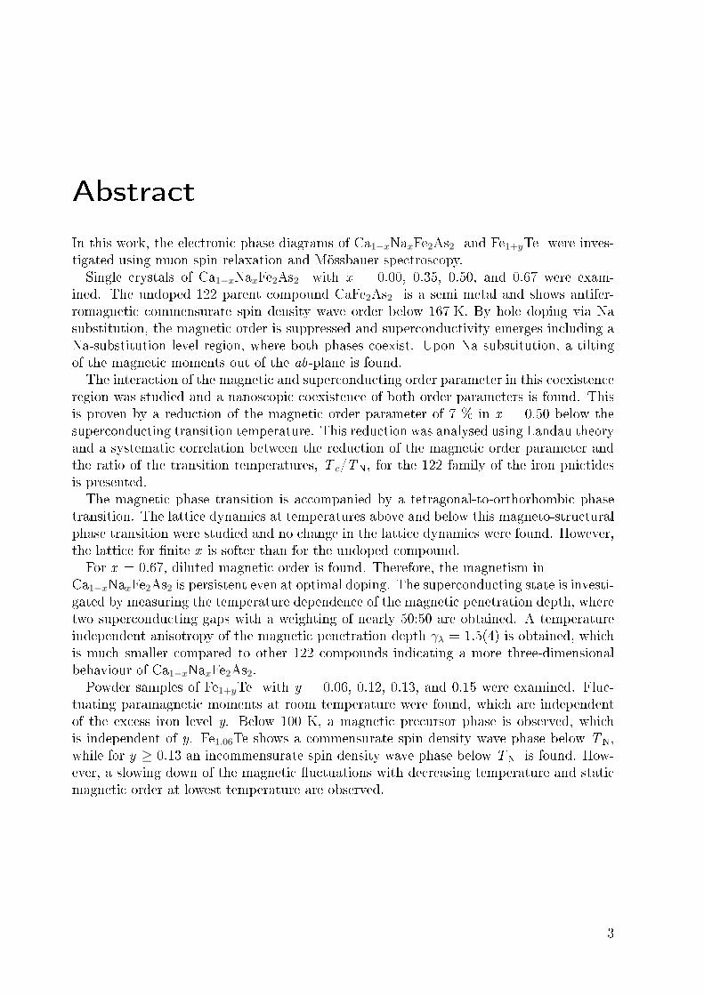
Abstract
In this work, the electronic phase diagrams of Ca1−xNaxFe2As2 and Fe1+yTe were inves-tigated using muon spin relaxation and Mössbauer spectroscopy.Single crystals of Ca1−xNaxFe2As2 with x = 0.00, 0.35, 0.50, and 0.67 were exam-
ined. The undoped 122 parent compound CaFe2As2 is a semi metal and shows antifer-romagnetic commensurate spin density wave order below 167 K. By hole doping via Nasubstitution, the magnetic order is suppressed and superconductivity emerges including aNa-substitution level region, where both phases coexist. Upon Na substitution, a tiltingof the magnetic moments out of the ab-plane is found.The interaction of the magnetic and superconducting order parameter in this coexistence
region was studied and a nanoscopic coexistence of both order parameters is found. Thisis proven by a reduction of the magnetic order parameter of 7 % in x = 0.50 below thesuperconducting transition temperature. This reduction was analysed using Landau theoryand a systematic correlation between the reduction of the magnetic order parameter andthe ratio of the transition temperatures, T c/TN, for the 122 family of the iron pnictidesis presented.The magnetic phase transition is accompanied by a tetragonal-to-orthorhombic phase
transition. The lattice dynamics at temperatures above and below this magneto-structuralphase transition were studied and no change in the lattice dynamics were found. However,the lattice for nite x is softer than for the undoped compound.For x = 0.67, diluted magnetic order is found. Therefore, the magnetism in
Ca1−xNaxFe2As2 is persistent even at optimal doping. The superconducting state is investi-gated by measuring the temperature dependence of the magnetic penetration depth, wheretwo superconducting gaps with a weighting of nearly 50:50 are obtained. A temperatureindependent anisotropy of the magnetic penetration depth γλ = 1.5(4) is obtained, whichis much smaller compared to other 122 compounds indicating a more three-dimensionalbehaviour of Ca1−xNaxFe2As2.Powder samples of Fe1+yTe with y = 0.06, 0.12, 0.13, and 0.15 were examined. Fluc-
tuating paramagnetic moments at room temperature were found, which are independentof the excess iron level y. Below 100 K, a magnetic precursor phase is observed, whichis independent of y. Fe1.06Te shows a commensurate spin density wave phase below TN,while for y ≥ 0.13 an incommensurate spin density wave phase below TN is found. How-ever, a slowing down of the magnetic uctuations with decreasing temperature and staticmagnetic order at lowest temperature are observed.
3

In dieser Arbeit wurden die elektronischen Phasendiagramme von Ca1−xNaxFe2As2 andFe1+yTe mit Hilfe der Myonspinrelaxations- und Mössbauerspektroskopie untersucht.Einkristalle von Ca1−xNaxFe2As2 mit x = 0.00, 0.35, 0.50 und 0.67 wurden untersucht.
Das undorierte 122-System CaFe2As2 ist ein Halbmetal und zeigt eine antiferromagnetischeSpindichtewelle unterhalb von 167 K. Substituiert man Ca durch Na, werden Löcher in dasSystem eingebracht. Die magnetische Ordnung wird mit steigendem Na-Anteil unterdrücktund Supraleitung tritt auf. Dabei existiert ein Na-Substitutionslevelbereich, in welchemMagnetismus und Supraleitung koexistieren. Desweiteren wurde ein herausdrehen dermagnetischen Momente aus der ab-Ebene als Funktion von x beobachtet.Die Wechselwirkung des magnetischen mit dem supraleitenden Ordnungsparameter in
der Koexistenzregion wurde untersucht und nanoskopische Koexistenz der beiden Ord-nungsparameter wurde gefunden. Dies konnte durch eine Reduktion des magnetischenOrdnungsparameteres um 7 % in x = 0.50 unterhalb der supraleitenden Ordnungstemper-atur gezeigt werden. Diese Reduktion wurde mit Hilfe der Landautheorie untersucht undes wurden systematische Korrelationen zwischen der Reduktion des magnetischen Ord-nungsparamteres und dem Verhältnis der Übergangstemperaturen, T c/TN, in der 122-Familie der Eisenpniktide gefunden.Der magnetische Phasenübergang wird von einem strukturellen Phasenübergang be-
gleitet. Die Gitterdynamik wurde bei Temperaturen oberhalb und unterhalb diesesmagneto-elastischen Phasenübergangs untersucht. Es wurden keine Änderungen in derGitterdynamik festgestellt. Jedoch konnte festgestellt werden, dass das Gitter für endlichex weicher ist als für das undotierte System.Für x = 0.67 wurde festgestellt, dass der Magnetismus im Ca1−xNaxFe2As2-System
auch noch bei optimaler Dotierung zu nden ist. In der supraleitenden Phase wurdedie Temperaturabghängigkeit der magnetischen Eindringtiefe untersucht und es wurdenzwei supraleitende Bandlücken gefunden. Die Anisotropie der magnetischen Eindringtiefeist temperaturunabhängig und mit γλ = 1.5(4) wesentlich kleiner als in anderen 122-Verbindungen, was für eine erhöhte Dreidimensionalität in Ca1−xNaxFe2As2 spricht.Pulverproben von Fe1+yTe mit y = 0.06, 0.12, 0.13 und 0.15 wurden untersucht. Es
wurden uktuierende paramagnetische Momente bei Raumtemperatur gefunden, welcheunabhängig vom Überschusseisenlevel y sind. Unterhalb von 100 K wurde eine magnetischeVorgängerphase gefunden, welche unabhängig von y ist. Mit fallender Temperatur wurdeeine Verlangsamung der magnetischen Fluktuationen festgestellt, welche in einer statischenmagnetischen Ordnung bei tiefen Temperaturen münden.
4
Contents
1. Introduction 9
2. Muon spin relaxation 11
2.1. Muon properties . . . . . . . . . . . . . . . . . . . . . . . . . . . . . . . . . 112.2. Muon production . . . . . . . . . . . . . . . . . . . . . . . . . . . . . . . . 122.3. Muon implantation . . . . . . . . . . . . . . . . . . . . . . . . . . . . . . . 132.4. Muon decay . . . . . . . . . . . . . . . . . . . . . . . . . . . . . . . . . . . 132.5. Experimental setup . . . . . . . . . . . . . . . . . . . . . . . . . . . . . . . 132.6. Interaction of the muon with the sample . . . . . . . . . . . . . . . . . . . 15
2.6.1. Static relaxation . . . . . . . . . . . . . . . . . . . . . . . . . . . . 172.6.2. Dynamic relaxation . . . . . . . . . . . . . . . . . . . . . . . . . . . 182.6.3. Magnetic order . . . . . . . . . . . . . . . . . . . . . . . . . . . . . 19
2.7. µSR in type-II superconductors . . . . . . . . . . . . . . . . . . . . . . . . 21
3. Mössbauer spectroscopy 29
3.1. Introduction . . . . . . . . . . . . . . . . . . . . . . . . . . . . . . . . . . . 293.2. The Mössbauer eect . . . . . . . . . . . . . . . . . . . . . . . . . . . . . . 293.3. Recoilless fraction . . . . . . . . . . . . . . . . . . . . . . . . . . . . . . . . 303.4. Temperature dependence of the recoilless fraction and second-order Doppler
eect . . . . . . . . . . . . . . . . . . . . . . . . . . . . . . . . . . . . . . . 333.5. Mössbauer eect in a solid . . . . . . . . . . . . . . . . . . . . . . . . . . . 353.6. Hyperne interaction . . . . . . . . . . . . . . . . . . . . . . . . . . . . . . 37
3.6.1. Electric interaction . . . . . . . . . . . . . . . . . . . . . . . . . . . 373.6.2. Magnetic hyperne interaction . . . . . . . . . . . . . . . . . . . . . 41
3.7. Experimental set up and measurement principle . . . . . . . . . . . . . . . 43
4. Iron-based superconductors 45
4.1. From SDW to SC . . . . . . . . . . . . . . . . . . . . . . . . . . . . . . . . 49
5. Mössbauer and muon spin relaxation spectroscopy of Ca1−xNaxFe2As2 53
5.1. The system Ca1−xNaxFe2As2 . . . . . . . . . . . . . . . . . . . . . . . . . . 535.2. Experimental details . . . . . . . . . . . . . . . . . . . . . . . . . . . . . . 545.3. Magnetic-susceptibility measurements . . . . . . . . . . . . . . . . . . . . . 555.4. Results and discussion . . . . . . . . . . . . . . . . . . . . . . . . . . . . . 56
5.4.1. Magnetic order in Ca1−xNaxFe2As2 . . . . . . . . . . . . . . . . . . 565.4.2. Landau theory of order-parameter coexistence . . . . . . . . . . . . 665.4.3. Magneto-structural phase transition . . . . . . . . . . . . . . . . . . 715.4.4. Optimally doped Ca0.33Na0.67Fe2As2 . . . . . . . . . . . . . . . . . . 74
5
Contents
5.5. Summary and conclusion . . . . . . . . . . . . . . . . . . . . . . . . . . . . 78
6. Mössbauer and muon spin relaxation spectroscopy of Fe1+yTe 83
6.1. Properties of Fe1+yTe . . . . . . . . . . . . . . . . . . . . . . . . . . . . . . 836.2. Experimental details . . . . . . . . . . . . . . . . . . . . . . . . . . . . . . 896.3. Results and discussion . . . . . . . . . . . . . . . . . . . . . . . . . . . . . 89
6.3.1. Mössbauer spectroscopy results . . . . . . . . . . . . . . . . . . . . 896.3.2. Muon spin relaxation results . . . . . . . . . . . . . . . . . . . . . . 96
6.4. Summary - The magnetic phase diagram of Fe1+yTe . . . . . . . . . . . . . 103
7. Conclusion 107
A. Momentum displacement operator 109
List of Figures 111
List of Tables 113
Bibliography 115
6
Abbreviations and symbols
AFM antiferromagnetic, antiferromagnet, antiferromagnetismARPES angle resolved photo-emission spectroscopy
B = µ0H magnetic eldBCS Bardeen-Cooper-SchrieerBhf magnetic hyperne eld
CDW charge densitiy waveδC chemical shift
DFT density functional theoryDOS density of statesEF Fermi energy
EFG electric eld gradientη asymmetry parameter of the electric quadrupole interaction
ER recoil energyf i muon spin precession frequency on site if recoilless fraction
FeChn iron-chalcogenFePn iron-pnictogenFS Fermi surfaceg gyromagnetic ratio
Γnat natural line width Γnat = 4.7 neV (for 57Fe)γλ magnetic penetration depth anisotropy
GKT Gauss-Kubo-ToyabeLKT Lorentz-Kubo-ToyabeLPD London penetration depthλL longitudinal muon spin relaxation rateλL transversal muon spin relaxation rate
µSR muon spin relaxationM e eective vibrating massPM paramagneticT c superconducting transition temperatureθD Debye temperatureθ angle between the magnetic hyperne eld and the principal axis of the EFG
TN Néel, magnetic transition temperatureT onset
N highest temperature with a nite magnetic volume fractionT 100%
N highest temperature with a magnetic volume fraction of 100 %T χN magnetic transition temperature determined
by magnetic susceptibility measurementsSC superconductor, superconducting, superconductivity
SDW spin density waveV mag magnetic volume fractionVzz z -component of the principal axis of the EFG
7

c speed of light c = 299792458 m/se elementary charge e = 1.602176565 ·10−19 A·sγµ gyromagnetic ratio of the muon γµ = 2π · 135.5342(5)MHz/T~ Planck constant ~ = 6.62606957 ·10−34 J·skB Boltzman constant kB = 1.3806488(13) ·10−23 J/KµB Bohr magneton µB = 9.27400968(20) ·10−24 J/TµP magnetic moment of the proton µP = 1.410606743(33) ·10−26 J/Tme electron mass me = 510.998928(11) keV/c2
mp proton mass mp = 938.272046(21) MeV/c2
τµ mean lifetime of the muon τµ = 2.19703(4) µs
8

1. Introduction
"It's a neural-net processor. It thinks and learns like we do. It's superconducting at room
temperature." - Tarissa Dyson about the central processing unit of a terminator [1].Room-temperature superconductivity - what is the reality in James Cameron's Termi-
nator 2, is still a dream of the future in the real world.But lets take a step back. Everything started with the discovery of a vanished resis-
tivity in metallic mercury below 4.2 K by Heike Kamerlingh Onnes in 1911, who wasrewarded with the Nobel Prize in physics in 1913. From this starting point, one majorgoal of the basic research was and is to nd a compound, which is superconducting atroom temperature. As time was passing by, the superconducting transition temperaturein conventional superconductors increased to T c = 39 K in MgB2, which was discoveredin 2001 [2]. The term conventional superconductivity is not well-dened in the literature,but is usually associated with phonon-mediated superconductivity, which can be describedby the famous Bardeen-Cooper-Schrieer (BCS) theory. The BCS-theory was publishedin 1957 and describes the formation of a coherent ground state out of electron pairs withopposite spin and momenta [3]. Bardeen, Cooper, and Schrieer were awarded with theNobel Prize in physics in 1972 for their theory. With the discovery of the cuprate su-perconductors in 1986 by Bednorz and Müller, who where rewarded with the Nobel Prizein physics in 1987, T c raised up to 153 K [4], which is up to now the highest achievedsuperconducting transition temperature. Superconductivity in cuprates is found in closeproximity to magnetic order: The antiferromagnetic order in the parent compounds areat least as important as the high T c, as magnetic moments were seen as deleterious tothe superconductivity in earlier times. The cuprates are unconventional superconductors.Unfortunately, a complete theory of unconventional superconductivity is still lacking upto now.With the discovery of the iron pnictides in 2008 [5], a new class of high-temperature su-
perconductors was identied. This class takes the proximity of magnetic order and super-conductivity to its extremes, as under certain conditions superconductivity and magneticorder coexisting in the same phase competing for the same electronic states at the Fermisurface. The understanding of this coexistence phase as well as of the high-temperaturesuperconductivity in general in these compounds is an important topic in contemporarycorrelated-electron physics.Therefore, studying this crossover from magnetic order to superconductivity with fo-
cus on the phase boundary between both orders is crucial for an understanding of thehigh-temperature superconductivity in the iron-based superconductors and for unconven-tional superconductivity in general. A combined study of macroscopic techniques and localmagnetic probes will give further insight in the electronic properties of these compounds.In this work, I examined Ca1−xNaxFe2As2 and Fe1+yTe using muon spin relaxation and
Mössbauer spectroscopy to study the pure magnetic and superconducting phases as well
9

1. Introduction
as the coexistence region. For a better understanding of the experiments, the principle ofboth techniques is given. Muon spin relaxation spectroscopy is described in Sec. 2 withfocus on magnetic order and superconductivity. Mössbauer spectroscopy is described inSec. 3 with focus on magnetic order and lattice dynamics. In Sec. 4, a short introductionto the physics of iron pnictides and chalcogenides is given. In Sec. 5 and 6, the relevantproperties of both investigated systems are presented followed by the results of the muonspin relaxation and Mössbauer spectroscopy experiments. In Sec. 7, I summarize my workand give an outlook.
10
2. Muon spin relaxation
Muon spin relaxation, usually abbreviated as µSR, is an experimental technique, which isused to study in particular magnetic and superconducting properties in condensed-mattersystems. The µSR technique uses a 100 % spin-polarized muon beam to investigate theelectronic properties of solid states. This chapter is organized in the following way: rstly,basic properties of the muon are described. Secondly, important experimental details arediscussed. Thirdly, the interaction of the muon with the sample is discussed with focus onsystems with magnetic order and/or superconductivity.
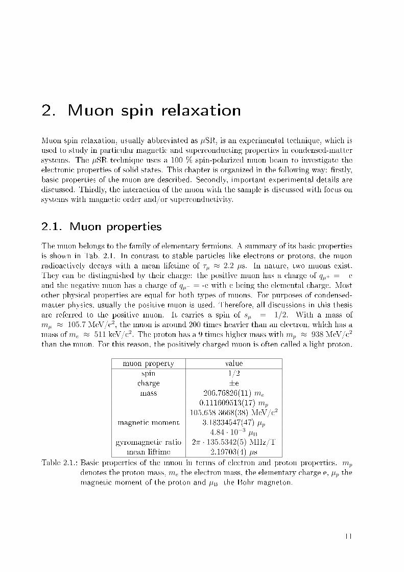
2.1. Muon properties
The muon belongs to the family of elementary fermions. A summary of its basic propertiesis shown in Tab. 2.1. In contrast to stable particles like electrons or protons, the muonradioactively decays with a mean lifetime of τµ ≈ 2.2 µs. In nature, two muons exist.They can be distinguished by their charge: the positive muon has a charge of qµ+ = +eand the negative muon has a charge of qµ− = -e with e being the elemental charge. Mostother physical properties are equal for both types of muons. For purposes of condensed-matter physics, usually the positive muon is used. Therefore, all discussions in this thesisare referred to the positive muon. It carries a spin of sµ = 1/2. With a mass ofmµ ≈ 105.7 MeV/c2, the muon is around 200 times heavier than an electron, which has amass of me ≈ 511 keV/c2. The proton has a 9 times higher mass with mp ≈ 938 MeV/c2
than the muon. For this reason, the positively charged muon is often called a light proton.
muon property valuespin 1/2charge ±emass 206.76826(11) me
0.111609513(17) mp
105.658 3668(38) MeV/c2
magnetic moment 3.18334547(47) µp
4.84 · 10−3 µBgyromagnetic ratio 2π · 135.5342(5) MHz/T
mean liftime 2.19703(4) µsTable 2.1.: Basic properties of the muon in terms of electron and proton properties. mp
denotes the proton mass, me the electron mass, the elementary charge e, µp themagnetic moment of the proton and µB the Bohr magneton.
11
2. Muon spin relaxation
2.2. Muon production
Positive muons can be produced using a high-energy proton beam. In a synchrotron orcyclotron, protons will be accelerated to energies of E > 500 MeV and then directed ona target (usually carbon or beryllium). Via proton-proton (p-p) and proton-neutron (p-n)interactions in the target, positively charged pions π+ are produced via the reactions
p+ p→ π+ + d,
p+ p→ π+ + p+ n, (2.1)
p+ n→ π+ + n+ n,
with deuterion d. The positive pion decays after a mean lifetime of τπ+ ≈ 26 ns via
π+ → µ+ + νµ (2.2)
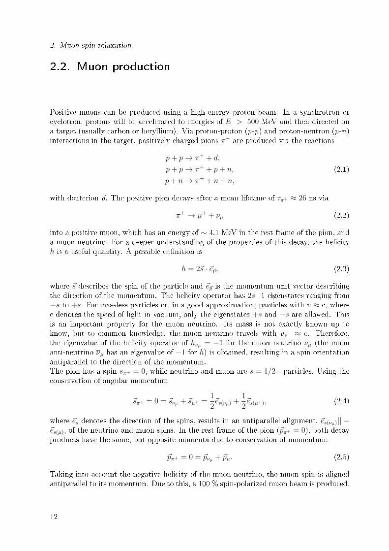
into a positive muon, which has an energy of ∼ 4.1 MeV in the rest frame of the pion, anda muon-neutrino. For a deeper understanding of the properties of this decay, the helicityh is a useful quantity. A possible denition is
h = 2s · ep, (2.3)
where s describes the spin of the particle and ep is the momentum unit vector describingthe direction of the momentum. The helicity operator has 2s+1 eigenstates ranging from−s to +s. For massless particles or, in a good approximation, particles with v ≈ c, wherec denotes the speed of light in vacuum, only the eigenstates +s and −s are allowed. Thisis an important property for the muon neutrino. Its mass is not exactly known up toknow, but to common knowledge, the muon neutrino travels with v ν ≈ c. Therefore,the eigenvalue of the helicity operator of hνµ = −1 for the muon neutrino νµ (the muonanti-neutrino νµ has an eigenvalue of +1 for h) is obtained, resulting in a spin orientationantiparallel to the direction of the momentum.The pion has a spin sπ+ = 0, while neutrino and muon are s = 1/2 - particles. Using theconservation of angular momentum
sπ+ = 0 = sνµ + sµ+ =1
2es(νµ) +
1
2es(µ+), (2.4)
where es denotes the direction of the spins, results in an antiparallel alignment, es(νµ)|| −es(µ), of the neutrino and muon spins. In the rest frame of the pion (pπ+ = 0), both decayproducts have the same, but opposite momenta due to conservation of momentum:
pπ+ = 0 = pνµ + pµ. (2.5)
Taking into account the negative helicity of the muon neutrino, the muon spin is alignedantiparallel to its momentum. Due to this, a 100 % spin-polarized muon beam is produced.
12

2.3. Muon implantation
2.3. Muon implantation
The muon enters the sample with a kinetic energy E kin of ∼ 4.1 MeV. E kin is reduced to 2-3 keV within 10−10−10−9 s due to ionization eects and electron scattering. After another10−13s, the kinetic energy is reduced to a few hundred eV due to inelastic collisions with theatoms as well as through the creation of short-lived and unstable muonium states. As themuon is positively charged, it is repulsed by the also positively charged nuclei. Therefore,the muon tend to move to the minima of the electrostatic potential and come to restat these interstitial sites. The muon interacts with the electrostatic potential leading tothe so-called host-lattice relaxation, which changes the lattice constants by a few %. Aftercoming to rest, the muon still has its initial spin polarisation, as the thermalization processis rapid and only electrostatic interactions occur.
2.4. Muon decay
The positive muon decays into a positron and two neutrinos with a mean lifetime ofτµ ≈ 2.2 ms via
µ+ → e+ + νe + νµ (2.6)
into a positron e+, an electron neutrino νe and a muon anti-neutrino νµ. The kineticenergy of the positron varies up to a maximum energy of ≈ 52.83 MeV, depending on themomenta of the neutrinos. Positrons with the highest energies emerge, if the momentumof the positron is opposite to the momenta of the two neutrinos. As the helicity of bothneutrinos is dierent (hνµ = +1 and hνe = −1), their spins are aligned antiparallel andadding up to zero. Therefore, muon and positron spin are pointing in the same direction.Due to the parity violation of the weak interaction, only chiral right-handed positrons(he+= +1) are produced. Thus, the momentum of the muon is parallelly aligned to thespin direction. This causes an anisotropic distribution of the positron emission, as thepositron is predominantly emitted along the muon spin direction. This distribution canbe described by calculating the probability dW of the emission of a positron with energydε in the solid angle dΩ using [6]
d2W (ε, φ)
dε dΩ=
3− 2ε
2πτµε2[1− 1− 2ε
3− 2εcos(φ)
], (2.7)
where ε=E kin/Emax is the normalized positron energy, τµ the mean life time of themuon and φ the angle between the muon spin and the momentum of the emitted positron.Integration over all energies leads to the anisotropic emission probability [6]
dW (φ)
dΩ=
1
4πτµ
[1 +
1
3cos(φ)
]. (2.8)
2.5. Experimental setup
There are, in principle, two types of setups for a µSR experiment: Continuous wave (CW)and pulsed muon sources. The former technique is used at the Paul Scherrer Institute
13
2. Muon spin relaxation
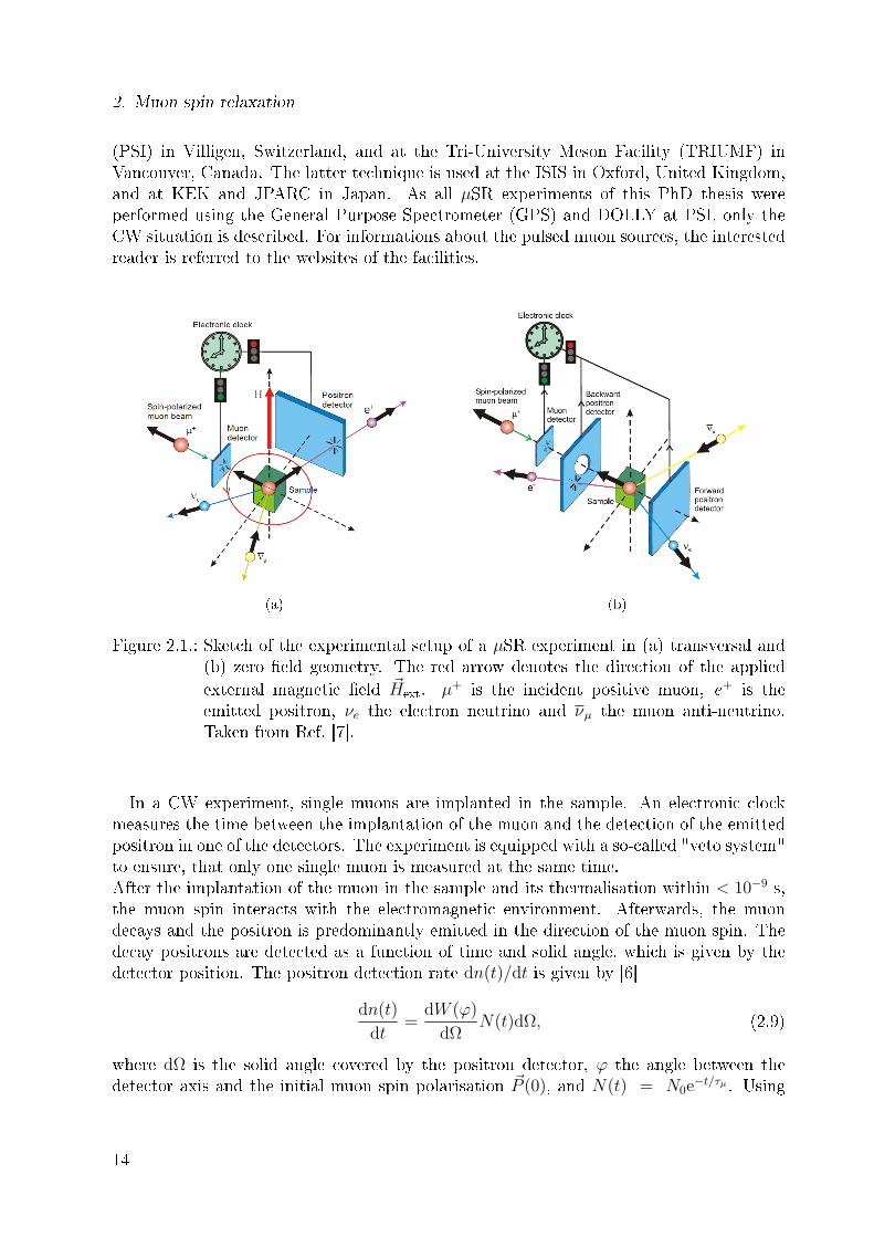
(PSI) in Villigen, Switzerland, and at the Tri-University Meson Facility (TRIUMF) inVancouver, Canada. The latter technique is used at the ISIS in Oxford, United Kingdom,and at KEK and JPARC in Japan. As all µSR experiments of this PhD thesis wereperformed using the General Purpose Spectrometer (GPS) and DOLLY at PSI, only theCW situation is described. For informations about the pulsed muon sources, the interestedreader is referred to the websites of the facilities.
(a) (b)
Figure 2.1.: Sketch of the experimental setup of a µSR experiment in (a) transversal and(b) zero eld geometry. The red arrow denotes the direction of the appliedexternal magnetic eld Hext. µ+ is the incident positive muon, e+ is theemitted positron, νe the electron neutrino and νµ the muon anti-neutrino.Taken from Ref. [7].
In a CW experiment, single muons are implanted in the sample. An electronic clockmeasures the time between the implantation of the muon and the detection of the emittedpositron in one of the detectors. The experiment is equipped with a so-called "veto system"to ensure, that only one single muon is measured at the same time.After the implantation of the muon in the sample and its thermalisation within < 10−9 s,the muon spin interacts with the electromagnetic environment. Afterwards, the muondecays and the positron is predominantly emitted in the direction of the muon spin. Thedecay positrons are detected as a function of time and solid angle, which is given by thedetector position. The positron detection rate dn(t)/dt is given by [6]
dn(t)
dt=
dW (φ)
dΩN(t)dΩ, (2.9)
where dΩ is the solid angle covered by the positron detector, φ the angle between thedetector axis and the initial muon spin polarisation P (0), and N(t) = N0e
−t/τµ . Using
14

2.6. Interaction of the muon with the sample
Eq. (2.8) and Eq. (2.9), the detection rate is given by [6]
dn(t)
dt=
1
4πτµ
1 +
1
3P (t)eµΩ
N(t)dΩ, (2.10)
where eµΩ is the unit vector pointing from the muon to the detector and, therefore, P (t)eµΩis the projection of the muon spin polarisation in this direction.To extract the time-dependent asymmetry of the muon decay, the normalized dierence
in the detection rate of dierent detectors i,j is needed and is given by
A(t) =ddtni(t)− d
dtnj(t)
ddtni(t) +
ddtnj(t)
. (2.11)
3
4
2
1
1+ WEP
WEDL
sampleX
Figure 2.2.: Sketch of the GPS and DOLLY spectrometer. The detector pairs 3,4 and2,1 as well as the implemented magnets WEP and WEDL are shown, wherethe arrows denote the direction of the magnetic eld. The chosen muon spindirection, which is 45 rotated from the muon beam direction, is shown.
The detector arrangement at GPS is shown in Fig 2.2 with the detector pairs 3,4 and2,1. By counting the number of positrons, which are measured in a time-interval [tn, tn+1]after the muon implantation, a time histogram is recorded with tN = n∆t, n=1, 2, 3,... and ∆t is the time resolution of the detector. The time dependence of the positrondetection rate is described by these time histograms.The asymmetry for two opposite detectors can be calculated using Eq. (2.11) and is
given byA(t) = A0P (t)eµΩ, (2.12)
where A0 = A(0) is the maximum asymmetry. By analysing the asymmetry A(t), onecan study the time evolution of the muon spin polarisation, P (t), in the sample, which isdetermined by the interaction of the muon spin with its electromagnetic environment.In practice, there are experimental limitations. The maximum asymmetry is usually
smaller than the theoretically expected 1/3 due to, for example, a nite solid angle.
2.6. Interaction of the muon with the sample
As the muon has a spin of 1/2, it does not couple to electric eld gradients. Therefore,the spin Hamiltonian of the muon is determined by dipole-dipole and Fermi-contact inter-
15

2. Muon spin relaxation
actions. The Hamiltonian, which describes the magnetic interaction of the muon with itselectromagnetic environment, is given by
H = Hdipol +Hhf = −γµ~2µ0
4π
∑i
γJi
3[riSµ
]·[riJi
]r5i
− SµJir3i
+∑i
AiSµJi, (2.13)
where the rst term describes the dipole-dipole interaction of the muon spin with nuclearand electronic magnetic moments γJi~Ji. The second term describes the Fermi-contactinteraction with conduction electrons, if the electrons have a non-zero magnetization atthe muon site. γµ denotes the gyromagnetic ratio of the positive muon and γJi of the spinJi. ri is the position vector connecting the muon spin Sµ and Ji. Ai denotes the hypernecoupling constant between the muon spin and the spin Ji.Under the assumption, that the perturbation of the electronic system of the solid state
due to the muon is negligible small, the Hamiltonian can be written in a mean-eld ap-proximation:
H = −γµ~Sµ
~µ0
4π
∑i
γJi
ri[ri ⟨Ji⟩
]r5i
− ⟨Ji⟩r3i
+1
~γµ
∑i
Ai ⟨Ji⟩
= −γµ~Sµ
[Bdip + Bhf
](2.14)
= −γµ~SµBloc.
This approximation is valid for magnetic materials, where the magnetic exchange inter-action of electronic magnetic moments is much larger than the dipole-dipole interaction ofthe muon with an electronic moment. For an understanding of the mean-eld Hamiltonian,it is necessary to know the local magnetic eld Bloc at the muon site.In solids, the local magnetic eld at the muon stopping site is a function of space and
time B(r, t). The space dependence is based on disorder and the dipole interaction ofthe muon spin with randomly oriented nuclear moments. It causes a dephasing of themuon spin precession. The time dependence is based on magnetic uctuations and muondiusion and results in a relaxation of the muon spin polarisation to thermal equilibrium.The muons randomly stop at interstitial sites. As a result, the measured asymmetry
and consequently P (t) is an ensemble average of the spatial variation of Bloc. Instead ofusing the spatial variation of Bloc, P (t) can be calculated using a nite distribution of themagnetic elds n(Bloc) [8]:
P (t) =
∫P ′(Bloc, t)n(Bloc)dBloc, (2.15)
where P ′(Bloc, t) denotes the local muon spin polarisation. In the following chapters, thecases of static and dynamic magnetic eld distributions as well as muon spin relaxation in
16
2.6. Interaction of the muon with the sample
magnetically ordered systems are discussed.
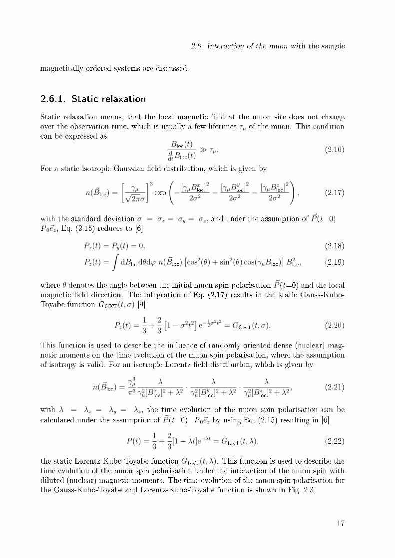
2.6.1. Static relaxation
Static relaxation means, that the local magnetic eld at the muon site does not changeover the observation time, which is usually a few lifetimes τµ of the muon. This conditioncan be expressed as
Bloc(t)ddtBloc(t)
≫ τµ. (2.16)
For a static isotropic Gaussian eld distribution, which is given by
n(Bloc) =
[γµ√2πσ
]3exp
(− [γµB
xloc]
2
2σ2− [γµB
yloc]
2
2σ2− [γµB
zloc]
2
2σ2
), (2.17)
with the standard deviation σ = σx = σy = σz, and under the assumption of P (t=0) =P0ez, Eq. (2.15) reduces to [6]
Px(t) = Py(t) = 0, (2.18)
Pz(t) =
∫dBlocdθdφ n(Bloc)
[cos2(θ) + sin2(θ) cos(γµBloc)
]B2loc, (2.19)
where θ denotes the angle between the initial muon spin polarisation P (t=0) and the localmagnetic eld direction. The integration of Eq. (2.17) results in the static Gauss-Kubo-Toyabe function GGKT(t, σ) [9]
Pz(t) =1
3+
2
3
[1− σ2t2
]e−
12σ2t2 = GGKT(t, σ). (2.20)
This function is used to describe the inuence of randomly oriented dense (nuclear) mag-netic moments on the time evolution of the muon spin polarisation, where the assumptionof isotropy is valid. For an isotropic Lorentz eld distribution, which is given by
n(Bloc) =γ3µπ3
λ
γ2µ[Bxloc]
2 + λ2· λ
γ2µ[Byloc]
2 + λ2· λ
γ2µ[Bzloc]
2 + λ2, (2.21)
with λ = λx = λy = λz, the time evolution of the muon spin polarisation can becalculated under the assumption of P (t=0)=P0ez by using Eq. (2.15) resulting in [6]
P (t) =1
3+
2
3[1− λt]e−λt = GLKT(t, λ), (2.22)
the static Lorentz-Kubo-Toyabe function GLKT(t, λ). This function is used to describe thetime evolution of the muon spin polarisation under the interaction of the muon spin withdiluted (nuclear) magnetic moments. The time evolution of the muon spin polarisation forthe Gauss-Kubo-Toyabe and Lorentz-Kubo-Toyabe function is shown in Fig. 2.3.
17

2. Muon spin relaxation
0 2 4 6 8 100.0
0.2
0.4
0.6
0.8
1.0
muo
n sp
in p
olar
izat
ion P
(t)
time ( s)
= = 3 MHz
= = 0.1 MHz
Figure 2.3.: Gauss-Kubo-Toyabe (black) and Lorentz-Kubo-Toyabe (red) function for re-laxation rates of 0.1 MHz (dashed line) and 3 MHz (straight line).
2.6.2. Dynamic relaxation
Dynamic muon spin relaxation is caused by, e.g., muon diusion or uctuations of theinternal magnetic eld. This non-static behaviour can be modelled by the strong-collisionapproximation [9]. The muons experience a uctuation of the magnetic eld B after acharacteristic time τc, or the magnetic eld uctuates with a frequency of ν = 1/τc,respectively. In the strong-collision model, the magnetic eld values before and after theuctuation are treated as independent, which corresponds to a rst-order Markov process[9]. Before the rst uctuation, the muons experience a static eld B0 and hence thetime evolution of the muon spin polarisation exhibits a static depolarisation PS(t). Theprobability of observing no uctuation after a time t is given by [9]
p0(t) = e−tτcPS(t). (2.23)
The probability of having one uctuation at a time t∈(0,t ') is given by [9]
p1(t) =1
τc
∫ ∞
0
dt′ e−t−t′τc
tPS(t− t′)e−t′τcPS(t) (2.24)
and of n uctuations at a time t∈(0,t ') by [9]
pn(t) =1
τc
∫ t
0
dt′ pn−1(t− t′)e−t′τcPS(t). (2.25)
Consequential, the time evolution of the muon spin polarisation including all possibleuctuation channels is given by [9]
P (t) =∞∑n
pn(t). (2.26)
This expression can be evaluated for any internal eld distribution resulting in the dy-namic Kubo-Toyabe function. For an isotropic Gaussian eld distribution with a standard
18

2.6. Interaction of the muon with the sample
deviation σ, slow uctuations, στc ≫ 1, lead to an exponentially damped 1/3 - tail with adamping rate λ = 2/3τc. In the limit of fast uctuations, στc ≪ 1, an overall exponentialdepolarisation,
P (t) = e−λτc , λ = 2σ2τc (2.27)
is obtained.
2.6.3. Magnetic order
Assuming an ideal crystal lattice, long-range commensurate magnetic order of electronicmoments creates a well-dened nite magnetic eld at the muon site, which can be de-scribed by n(Bloc) = δ(B0 − Bloc) with the Dirac delta function δ(B). Applying this elddistribution n(Bloc) on Eq. (2.15) results in a general expression for the relaxation and,therefore, the time evolution of the muon spin polarisation is given by [6]
P (t) = cos2(θ) + sin2(θ) cos(γµB0t). (2.28)
For an isotropic internal-eld distribution, P(t) can be expressed by
P (t) =1
3+
2
3cos(γµB0t), (2.29)
after averaging over all spatial directions θ. This is, for example, the case in a powdersample.In real systems a distribution of local elds is often found. For an isotropic Lorentz
distribution
n(Bloc) =γ3µπ3
λ
γ2µ[Bxloc]
2 + λ2· λ
γ2µ[Byloc]
2 + λ2· λ
γ2µ[Bzloc]
2 + λ2, (2.30)
with λ = λx = λy = λz, Eq. (2.15) gives [10]
P (t) =1
3+
2
3
cos(2πfµt)−
λ
2πfµsin(2πfµt)
e−λt, (2.31)
with 2π × fµ = γµ|B0|. For λ/2πfµ ≪ 1, Eq. (2.31) reduces to
P (t) =1
3+
2
3cos(2πfµt)e
−λt, (2.32)
which is a commonly used equation to analyse the time evolution of the muon spin polar-isation in magnetically ordered systems.For an ideal commensurate magnetic structure, one value of B loc is expected. In con-
trast, for an incommensurate magnetic structure, any number of magnetically inequivalentmuon sites is possible. Assuming a periodical eld modulation, e.g. a spin-density wave,results in B = Bmax cos(qr), where Bmax is the maximum magnetic eld, q the wave vectorand r the position vector. This eld modulation results in the magnetic eld distribution
19

2. Muon spin relaxation
[11]
n(B) =2
π
1√B2max −B2
, (2.33)
which is the so-called Overhauser form of the spin density wave. Applying this eld distri-bution to Eq. (2.15) gives the corresponding time evolution of the muon spin polarisation
P (t) =1
3+
2
3J0(γµBmaxt), (2.34)
where J0 is the 0 th-order Bessel function. P(t) has the same structure as in the case ofstatic commensurate magnetic order. Only the form of the oscillation is dierent, whichis illustrated in Fig. 2.4. The sinusoidal oscillation shows no damping, while the Bessel-oscillation shows a strong damping.
0 2 4 6 8-0.4
-0.2
0.0
0.2
0.4
0.6
0.8
1.0
muo
n sp
in p
olar
izat
ion P
(t)
time ( s)
(a)
0 2 4 6 8
0.0
0.2
0.4
0.6
0.8
1.0
muo
n sp
in p
olar
isat
ion P
(t)
time ( s)
F8
(b)
Figure 2.4.: time evolution of the muon spin polarisation P(t) with a sinusoidal (black)or Bessel (red) oscillation for the undamped (a) and damped (b) case. Theexponential relaxation in (b) has a relaxation rate λ = 0.5 MHz.
In single crystals, the situation is dierent, as the local eld has a xed, yet arbitraryorientation. A useful approach is to introduce variable parameters a1 and a2 as well as aphase ϕ leading to the expression [6]
P (t) = a1 + a2 cos(2πfµt+ ϕ)e−λt, (2.35)
where a1 and a2 are not connected in a simple way.P(t) for the case of N magnetically inequivalent muon stopping sites can be expressed
by
P (t) =N∑i
pia1,i cos(2πfµ,it+ ϕ)e−λT,it + a2,ie−λL,it
, (2.36)
where pi denotes the occupation probability of the dierent muons site with∑N
i pi = 1.The exponential damping of the tail a2 is modeled by the (longitudinal) exponential damp-ing rate λL. This exponential damping is, however, a result of dynamic magnetic elductuations.
20

2.7. µSR in type-II superconductors
It is possible with µSR to determine the magnetic volume fraction of a sample. In atemperature region, where not 100 % of the sample is magnetically ordered, a certainamount of the muons show a depolarisation of P(t) due to the interaction of the muonspin with randomly oriented nuclear magnetic moments only. The rest of the muonsstops in sample volumes, which are magnetically ordered and, therefore, P(t) shows adepolarisation following Eq. (2.36). To separate this signal fractions, the following equationcan be used:
P (t) =Vmag
N∑i
pia1,i cos(2πfµ,it+ ϕ)e−λT,it + a2,ie
−λL,it
+ [1− Vmag]GGKT(t, σnm), (2.37)
where V mag denotes the magnetic volume fraction and dense nuclear moments are assumed.Another possibility to measure the magnetic volume fraction is to apply a weak external
transverse eld BTF. P(t) then is given by
P (t) = Vmaga1 + a2 cos(2πfµ)e
−λt+ [1− Vmag] cos(γµBTFt). (2.38)
Muons, which stop in a paramagnetic sample volume interact with the external magneticeld and, therefore, perform a precession with a frequency 2π × fTF = γµBTF. Muons,which stop in a magnetically ordered sample volume only experience the internal local eldB loc, if BTF ≪ B loc. Consequently, the magnetic volume fraction is given by the relativeamount of muons precessing with a frequency f TF.
2.7. µSR in type-II superconductors
As described in Sec. 2.6, µSR is a suitable tool to measure the shape of the magnetic elddistribution inside a sample. This can be used to investigate the Shubnikov phase of atype-II superconductor.By applying an external magnetic eld B ext with B c1< B ext < B c2 at temperatures belowthe superconducting transition temperature, T c, a vortex lattice is formed. B c1 is thelower and B c2 the upper critical eld of the superconductor. The Gibbs free energy Gs
for the case of an inhomogeneous superconductor, e.g. including spatial variation of thesuperconducting order parameter, |ψ(r)|2, in an applied magnetic eld Bext is given by
Gs[ψ, A] = Gn+α|ψ(r)|2+β
2|ψ(r)|4+ 1
2µ0
∣∣∣Bext − Bi
∣∣∣2+ 1
2ms
∣∣∣[−i~∇ − qsA]ψ∣∣∣2 , (2.39)
where the Gibbs free energy is a functional of ψ and the vector potential A. qs is thecharge and ms the mass of the superconducting charge carriers. Gn denotes the Gibbs
free energy of the normal state. The term 12µ0
∣∣∣Bext − Bi
∣∣∣2 describes the energy, which is
needed to expel the magnetic eld from the superconductor up to a residual eld of Bi.This energy is maximal in the case of the Meissner-phase (Bi = 0). Minimizing the Gibbs
21
2. Muon spin relaxation
free energy functional with respect to ψ∗ results in the rst Ginzburg-Landau equation
αψ(r) + β|ψ(r)|2ψ(r) + 1
2ms
∣∣∣[−i~∇ − qsA]ψ∣∣∣2 = 0. (2.40)
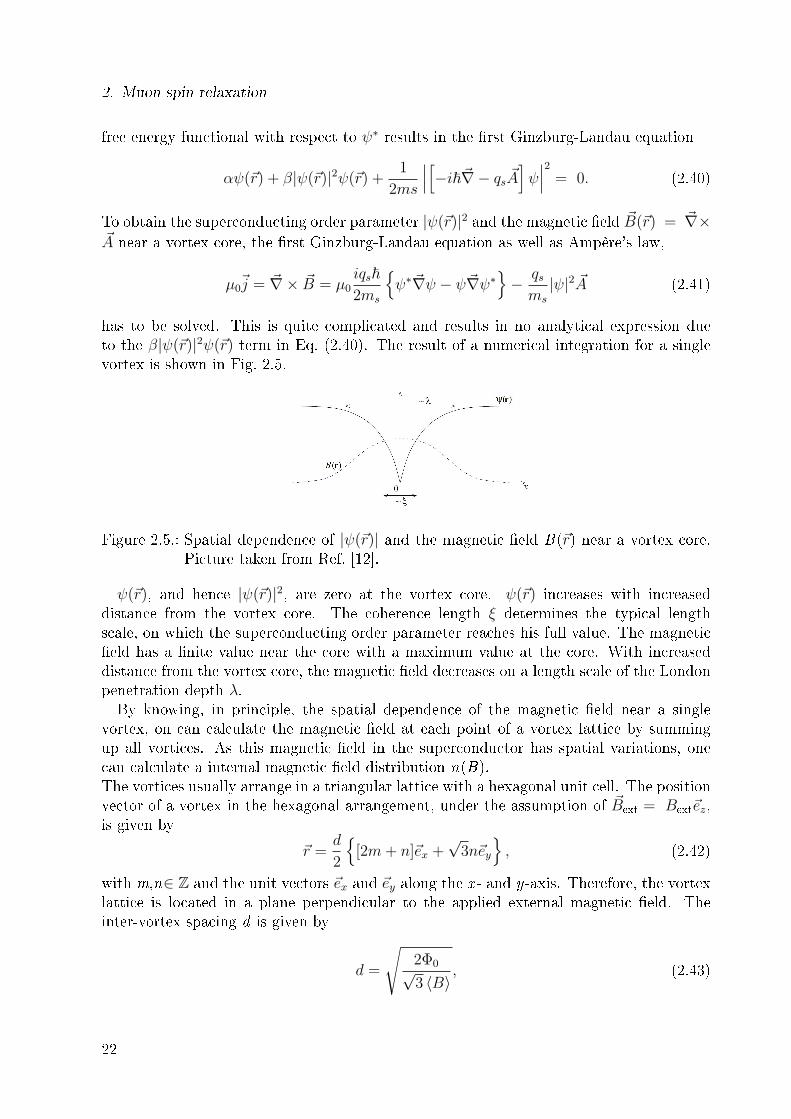
To obtain the superconducting order parameter |ψ(r)|2 and the magnetic eld B(r) = ∇×A near a vortex core, the rst Ginzburg-Landau equation as well as Ampère's law,
µ0j = ∇ × B = µ0iqs~2ms
ψ∗∇ψ − ψ∇ψ∗
− qsms
|ψ|2A (2.41)
has to be solved. This is quite complicated and results in no analytical expression dueto the β|ψ(r)|2ψ(r) term in Eq. (2.40). The result of a numerical integration for a singlevortex is shown in Fig. 2.5.
Figure 2.5.: Spatial dependence of |ψ(r)| and the magnetic eld B(r) near a vortex core.Picture taken from Ref. [12].
ψ(r), and hence |ψ(r)|2, are zero at the vortex core. ψ(r) increases with increaseddistance from the vortex core. The coherence length ξ determines the typical lengthscale, on which the superconducting order parameter reaches his full value. The magneticeld has a nite value near the core with a maximum value at the core. With increaseddistance from the vortex core, the magnetic eld decreases on a length scale of the Londonpenetration depth λ.By knowing, in principle, the spatial dependence of the magnetic eld near a single
vortex, on can calculate the magnetic eld at each point of a vortex lattice by summingup all vortices. As this magnetic eld in the superconductor has spatial variations, onecan calculate a internal magnetic eld distribution n(B).The vortices usually arrange in a triangular lattice with a hexagonal unit cell. The positionvector of a vortex in the hexagonal arrangement, under the assumption of Bext = Bextez,is given by
r =d
2
[2m+ n]ex +
√3ney
, (2.42)
with m,n∈ Z and the unit vectors ex and ey along the x - and y-axis. Therefore, the vortexlattice is located in a plane perpendicular to the applied external magnetic eld. Theinter-vortex spacing d is given by
d =
√2Φ0√3 ⟨B⟩
, (2.43)
22

2.7. µSR in type-II superconductors
where ⟨B⟩ denotes the average local magnetic eld and Φ0 the magnetic ux quantum.The magnetic eld can be calculated using the Fourier expansion:
Bz(r) = ⟨B⟩∑G
e−iGrBG(λ, ξ), (2.44)
where G denotes the reciprocal lattice vector and is given by
G =2π
d
mex −
1√3[m+ 2n]ey
, (2.45)
with m,n ∈ Z. Applying this calculations on a single crystal transforms the coordinatesystem from Fourier to real space like (x,y,z )T 7−→ (a,b,c)T with the crystallographic a-, b-,and c-axis. Then r denotes the position vector, as described in Eq. (2.42), in the ab-plane,which is perpendicular to the applied external eld Bext = Bextez, which is applied alongthe crystallographic c-axis. BG(λ, ξ) are the corresponding Fourier coecients. For smallapplied elds, B c1 < B ext ≪ B c2, and λab ≫ ξab, BG(λ, ξ) is given by [13]
BG(λ, ξ) =e−
12ξ2abG
2
1 +G2λ2ab, (2.46)
including a Gaussian cut-o, which is introduced to suppress the divergence of B z(r)for r → 0. Taking the eld-dependence of the order parameter into account, Eq. (2.46)becomes [14, 15]
BG(λ, ξ) =e−
12
ξ2abG2
1−b
1 +G2λ2
ab
1−b
(2.47)
with the reduced eld b = ⟨B⟩ /Bc2.
The probability distribution n(B) inside the Shubnikov phase for a perfect ux-linelattice can be calculated from the known spatial variation of the internal magnetic eldB0(r) using
n0(B) =
∫dr3 δ(B −B0(r))∫
dr3, (2.48)
where δ(x) is the Dirac delta function and is shown in Fig. 2.6.
The corresponding time evolution of the muon spin polarisation with Bext = Bextez andP (0) = ex is given by
Px(t) =
∫ ∞
0
dB n(B) cos(γµBt). (2.49)
Vortex disorder
The ideally (unperturbed) ux-line lattice results in a magnetic eld distribution, whichis described by Eq. (2.48) with a periodic eld B0(r). In a non-perfect vortex lattice with
23

2. Muon spin relaxation
Figure 2.6.: Spatial dependence of the magnetic eld and magnetic eld distribution P(B)for an ideal hexagonal vortex lattice, calculated by using Eq. (2.47) and (2.48),respectively. λ = 50 nm, ξ = 20 nm, ⟨B⟩ = 246.8 mT, b = 0.3, and d = 69.5 nmare used. Picture taken from [16].
random perturbations of the ux-lines, the magnetic eld is given by
B(r) = B0(r) + δB(r), (2.50)
with the eld perturbation δB(r), which results in a general expression for the magneticeld distribution [17]
n(B) =
∫dr3 p(B −B0(r); r)∫
dr3=
∫dr3 p(δB(r); r)∫
dr3, (2.51)
where p(δB(r); r) is the probability to nd the deviation δB at the position r. As B0(r) is aperiodic function of the ux-line lattice, one may replace the dependence of p(B−B0(r); r)from r by a dependence of the periodic eld value, which leads to [17]
n(B) =
∫dr3 p(B −B0(r);B0(r))∫
dr3. (2.52)
For small perturbations, i.e., B ≈ B0, Eq. (2.52) becomes
n(B) =
∫dr3 p(B −B0(r);B(r))∫
dr3. (2.53)
This equation can be expressed in a more enlightening way [17]:
n(B) =
∫dδB p(δB(r);B(r)) n0(B − δB). (2.54)
24

2.7. µSR in type-II superconductors
Therefore, for small perturbations δB, the magnetic eld distribution n(B) is given by aconvolution of the unperturbed magnetic eld distribution n0(B) of the perfect ux-linelattice with a function, which describes the perturbation of the vortices. For the case ofrandomly weak perturbed vortices, the function p(δB(r);B(r)) is approximated with aGaussian distribution [17],
p(δB,B) =1√
2πσ(B)exp
(−1
2
δB2
σVD(B)2
), (2.55)
with a eld-dependent standard deviation σVD(B) due to the vortex disorder. This leadsto the magnetic eld distribution
n(B) =1√
2πσVD(B)
∫d(δB) n0(B − δB)exp
(−1
2
δB2
σVD(B)2
)(2.56)
which is a convolution of the unperturbed magnetic eld distribution with a Gaussianlydistributed perturbation. The time evolution of the muon spin polarisation P(t) and themagnetic eld distribution n(B) are connected via a Fourier transformation. Using theproperty of the Fourier transformation, that the Fourier transform of any convolution isthe product of the Fourier transformations of the original functions, under the assumptionof a eld-independent σ(B), P(t) is given by
Px(t) = e−12σ2VDt
2
∫ ∞
0
dB n0(B) cos(γµBt). (2.57)
with Bext = Bextez and P (0) = ex (as in Eq. (2.49)).
To investigate Px(t), it is often assumed, that n(B) is a sum of N Gaussian distributions[16], which leads to
Px(t) =N∑i
pi · cos(γµBit+ φ) · e−
12σ2i t
2· e−
12σ2VDt
2
e−12σ2Nt
2
, (2.58)
where σVD is the relaxation rate due to the vortex disorder. σN is the relaxation rate dueto the dipole-dipole interaction of the muon spin with randomly oriented nuclear moments.pi is the weighting of the N single Gaussian distributions with
∑Ni pi = 1 and φ the initial
phase of the muon beam. B i is the rst moment and σi the relaxation rate of the ithGaussian component. The corresponding magnetic eld distribution is given by
n(B) =1√2π
N∑i
piσiexp
(−γ2µ
[⟨B⟩ − Bi]2
2σ2i
), (2.59)
with the rst moment ⟨B⟩. By analysing the time evolution of the muon spin polarisation inthe superconducting state using Eq. (2.58), the total magnetic eld distribution is obtained.
25
2. Muon spin relaxation
The rst moment of this distribution is given by
⟨B⟩ =N∑i
piBi (2.60)
and the second moment by [16]
⟨∆B2⟩t =N∑i
pi
[σiγµ
]2+ [Bi − ⟨B⟩]2
. (2.61)
This second moment is composed of the second moment of the magnetic eld distributionas well as contributions from the vortex disorder and the nuclear magnetic moments [16]:
⟨∆B2⟩t = ⟨∆B2⟩+[σVDγµ
]2+
[σNγµ
]2. (2.62)
The contribution from the nuclear magnetic moments can be measured at temperaturesabove the superconducting transition temperature. Unfortunately, it is not possible toseparate ⟨∆B2⟩ and σ2
VD/γ2µ in the course of a multi-Gaussian analysis of P(t). Taking
into account, that the second moment ⟨∆B2⟩ is related to the magnetic penetration depthby [13]
1
λ2=
√⟨∆B2⟩C
, (2.63)
λ can be calculated using the approximation σVD = β/λ2 [16]:
λ =
[1
C
γ2µ + Cβ2
γ2µ ⟨∆B2⟩t − σ2N
]0.25. (2.64)
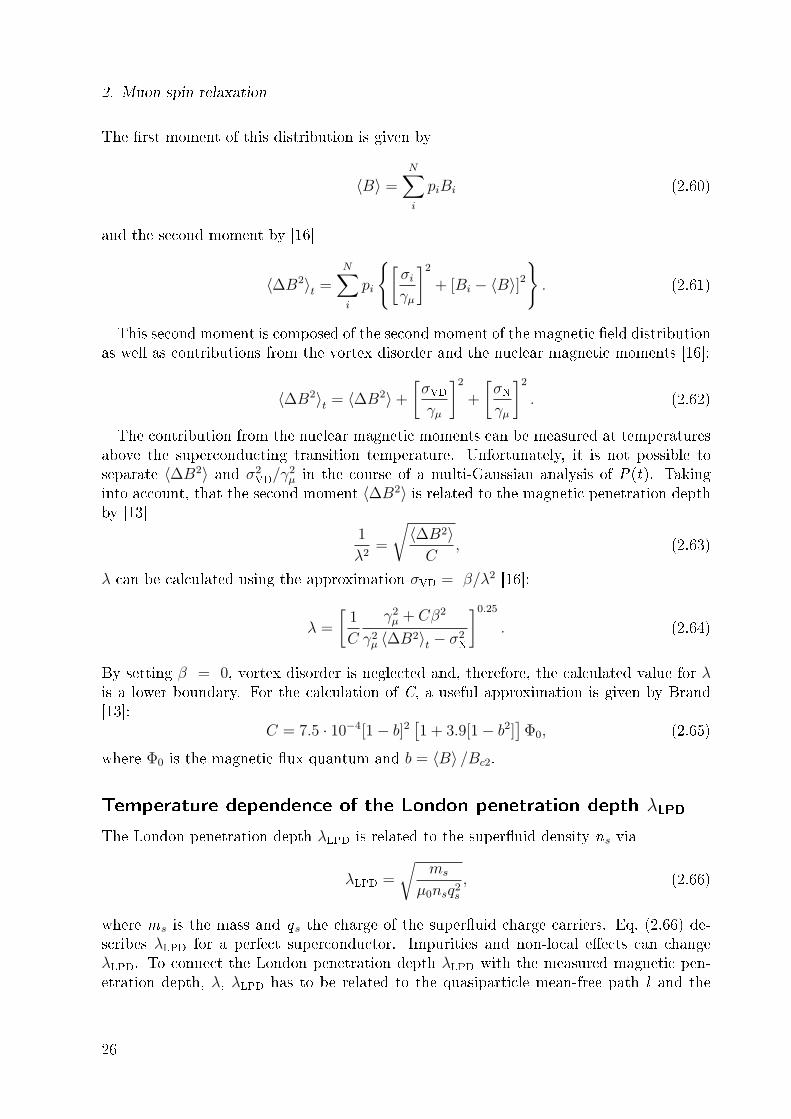
By setting β = 0, vortex disorder is neglected and, therefore, the calculated value for λis a lower boundary. For the calculation of C, a useful approximation is given by Brand[13]:
C = 7.5 · 10−4[1− b]2[1 + 3.9[1− b2]
]Φ0, (2.65)
where Φ0 is the magnetic ux quantum and b = ⟨B⟩ /Bc2.
Temperature dependence of the London penetration depth λLPD
The London penetration depth λLPD is related to the superuid density ns via
λLPD =
√ms
µ0nsq2s, (2.66)
where ms is the mass and qs the charge of the superuid charge carriers. Eq. (2.66) de-scribes λLPD for a perfect superconductor. Impurities and non-local eects can changeλLPD. To connect the London penetration depth λLPD with the measured magnetic pen-etration depth, λ, λLPD has to be related to the quasiparticle mean-free path l and the
26

2.7. µSR in type-II superconductors
coherence length ξ. In the clean local (or London) limit with λLPD ≫ l ≫ ξ, λLPD andλ are of equal value. This limit is valid for high-temperature superconductors [18]. Inthe dirty local limit, taking impurity scattering into account, with λLPD ≫ l ≈ ξ, themeasured λ is enhanced compared to λLPD and is given by [19]
λ = λLPD
√1 +
ξ
l, (2.67)
which is appropriate for alloy superconductors [18]. In the extreme dirty limit with l ≪ ξ,the measured magnetic penetration depth is given by [19]
λ = λLPD
√ξ
l. (2.68)
Non-local eects occur for ξ ≫ λLPD. They are described within the phenomenologicalPipard model. The enhancement is given by [19]
λ ≈[λ2LPDξ
] 13 . (2.69)
Therefore, the real values of the magnetic penetration depth λmay dier from λLPD. Apartfrom that, informations about the size, the number and the symmetry of the supercon-ducting gaps can be obtained by the temperature dependence of λ(T ). The temperaturedependence of the magnetic penetration depth λ can be calculated for a single isotropicgap ∆(T ) by [19]
λ2(0)
λ2(T )= 1− 2
∫ ∞
∆(t)
dE
[−∂nF(E)
∂E
]E√
E2 −∆2(T )= 1 +D(∆, T ), (2.70)
where nF(E) is the Fermi-Dirac distribution and E√E2−∆2(T )
is the density of states. In
general, no analytical expression for the temperature dependence of the superconductinggap is speciable. ∆(T ) can be calculated by self-consistently solving the gap equation
∫ ∞
0
dE
tanh(
12kBT
√E2 +∆2
)√E2 +∆2
− 1
Etanh
(E
2kBTc
) = 0, (2.71)
with Boltzmann's constant kB and the superconducting transition temperature T c. Al-ternatively, an appropriate approximation can be used, which is, for example, given by[20]
∆(T ) = 1.76∆(0) tanh
(1.82
[1.018
Tc − T
T
]0.51). (2.72)
27

2. Muon spin relaxation
For numerical convenience, the integral in Eq. (2.70) may be approximated by [21]
D(∆, T ) = −2
∫ ∞
∆(T )
dE
[−∂nF∂E
]E√
E2 −∆2(T )
≈[cosh
(∆(T )
2kBT
)]−2√π∆(T )
8kBT+
1
1 + π∆(T )8kBT
. (2.73)
Eq. (2.70) describes the dependence of the magnetic penetration depth from one singlesuperconducting gap. Multiband superconductors such as MgB2 or the iron pnictides mayhave more than one gap, and theses gaps may have dierent sizes. In this case, the tem-perature dependence of the dierent gaps should be calculated using the Eliashberg theory[20]. In the limit of non-interacting bands, however, one can treat the superconductinggaps within a phenomenological α model [2022]
λ2(0)
λ2(T )= w[1−D(∆1, T )]− [1− w] · [1−D(∆2, T )], (2.74)
where w is a phenomenological weighting factor of the two gaps. D(∆i, T ) is given byEq. (2.73) and ∆(T ) by Eq. (2.72).
28
3. Mössbauer spectroscopy
3.1. Introduction
The recoil energy-free nuclear resonance uorescence spectroscopy, which is often calledMössbauer spectroscopy, was discovered by Rudolph Mössbauer who received the physicsNobel price in 1961 [23]. The Mössbauer spectroscopy technique uses the transition be-tween an excited and the ground state of a nucleus to investigate the electromagneticproperties of its environment. The most often used nucleus, also exclusively in this thesis,is 57Fe. Therefore, the theoretical descriptions in this chapter are referred to 57Fe.This chapter is organized in the following way: First, a semi-classical description of theresonance absorption (Sec. 3.2) is given followed by a quantum mechanical treatment(Sec. 3.3-3.5). Secondly, the hyperne interaction of the nucleus with its electromagneticenvironment is discussed in Sec. 3.6.
3.2. The Mössbauer eect
The energy of a free 57Fe nucleus in the rst excited state, before the emission of a photon,is given by
Ei = Ees +p2
2M, (3.1)
where Ees denotes the energy of the excited spin 32
− state, p the momentum and M themass of the 57Fe nucleus. The energy of a 57Fe nucleus after the emission of a photon isgiven by
Ef = Egs +
[p− ~kγ
]22M
, (3.2)
where Egs denotes the energy of the spin 12
− ground state and kγ the momentum of thephoton. Therefore, the energy Eγ of the emitted photon can be calculated by using theEq. (3.1) and (3.2):
Eγ = Ei − Ef := ~ω = ~ω0 + ~kγp
M− ~2k2
2M, (3.3)
with Ees −Egs = ~ω0 = 14.4 keV. The absorption of a photon can be treated analogously,leading to
Eγ = Ei − Ef := ~ω = ~ω0 + ~kγp
M+
~2k2
2M. (3.4)
29
3. Mössbauer spectroscopy
In the rest frame of the nucleus, the energy of the photon is given by
Eγ = ~ω0 ±~2k2γ2M︸ ︷︷ ︸ER
(3.5)
and is shifted by the recoil energy ER compared to the bare transition energy ~ω0. There-fore, the nucleus, which absorbs the photon, will gain ER. This results in a separation ofthe two transition lines (absorption and emission) by 2ER.A nuclear state has an energy uncertainty Γnat, which is connected to its mean lifetime τover
Γnat · τ = ~. (3.6)
The ground state is stable and hence τ → 0, which results in Γnat → 0. Therefore,the energy of the ground state is well-dened. The excited 3
2
−-state has mean life-time ofτ = 141 ns corresponding to Γnat= 4.7 neV. Hence, the energy is not well-dened, butLorentz distributed [24]:
P (E)dE =Γ
2π
1
[E − Ees]2 +Γ2
4
dE, with∫P (E)dE = 1, (3.7)
where Ees denotes the energy of the excited state.The absorption of an emitted photon is possible, if there is a sucient overlap of thetransition lines, which is the case, if 2ER ≤ Γ. The separation of the two energy bands is2ER ≈ 3.9 meV , which is ≈ 1.2 · 106 Γnat [25]. As a consequence, resonance absorptionis not possible in free nuclei (as well as in gases and liquids).In the case of a solid state, the recoil energy can be partitioned into
ER = Etranslation + Evibration. (3.8)
The translational part refers to the linear momentum, which is transferred to the wholelattice system due to the strong bonding of the nucleus in the lattice. This chemical bondscorrespond to a binding energy of typically 10 eV and are much larger than the recoilenergy [25]. Therefore, the nucleus can not recoil alone. Instead, the whole lattice has torecoil together. As the mass of the lattice system, M lattice, is much larger then the massof a free nucleus M, E translation << Γnat. Thus, E translation is negligible. The vibrationalpart describes the excitation of phonons. For resonance absorption, no phonon excitationshould take place. The recoilless fraction f describes the probability of a zero-phononprocess (the phonon system remains unchanged). Therefore, in a solid state, resonanceemission and absorption of a photon can only take place, if f>0.
3.3. Recoilless fraction
The Mössbauer eect is based on the probability of a recoil-free absorption of a photon.Therefore, it is necessary to know this probability, which is called recoilless fraction f.The simplest model system to describe the oscillation excitations of the nucleus is the
30

3.3. Recoilless fraction
harmonic oscillator. Without any loss of generality, the harmonic oscillator is chosen tobe one-dimensional. The corresponding Hamiltonian is
H =p2
2m+
1
2mω2x2, (3.9)
where x denotes the position operator and p the momentum operator. The Hamiltoniancan be described in the second quantization formalism by introducing the annihilationoperator a and the creation operator a†:
a =
√mω
2~
x+
i
mωp
and a† =
√mω
2~
x− i
mωp
. (3.10)
Both operators are connected to x and p via
x =
√~
2mω
a† + a
and p = i
√~mω2
a† − a
. (3.11)
The harmonic oscillator Hamiltonian in second quantization is given by
H = ~ωa†a+
1
2
. (3.12)
The particle number operator n is dened as
n = a†a (3.13)
and has the eigenstates (Fock states) |n⟩, which are also eigenstates of the Hamiltonian:
H |n⟩ = En |n⟩ , n ∈ N. (3.14)
An arbitrary excited state |n⟩ can be created out of the ground state |0⟩ by applying thecreation operator n times:
|n⟩ = 1√n!
[a†]n |0⟩ . (3.15)
These states form a complete orthonormal set. A coherent (or Glauber) state |α⟩ can beconstructed as a superposition of all Fock states |n⟩ and is dened as [26]
|α⟩ = e−12|α|2∑n
αn
√n!
|n⟩, α ∈ C, (3.16)
and hence has an indenite number of phonons. The coherent state is fully described by thecomplex number α and is the state, which shows the most resemblance with the classicalharmonic oscillator states. For further information the interested reader is referred to thebook "Coherent States in Quantum Physics" of Jean-Pierre Gazeau [27].
31
3. Mössbauer spectroscopy
Recoilless fraction
A nucleus, which is in the ground state |0⟩ with a momentum ~k′, absorbs a photon, whichhas a momentum ~k. The momentum of the nucleus after the absorption of the photonis ~ [k + k′] due to momentum conservation. The ground state |0⟩ is no eigenstate to themomentum operator p (or k) and thus has to be expanded in an orthonormal basis set |k′⟩:
|0⟩ =∑k′
|k′⟩ ⟨k′|0⟩. (3.17)
The nal state |F ⟩ of the nucleus after the absorption of the photon is given by
|F ⟩ =∑k′
|k′ + k⟩ ⟨k′|0⟩. (3.18)
The corresponding displacement operator to |k⟩ is eikx, which is proven in Appendix A.Applying the displacement operator on an arbitrary state |k′⟩ gives
eikx |k′⟩ = |k′ + k⟩ (3.19)
and, therefore, the nal state is given by
|F ⟩ =∑k′
|k′ + k⟩ ⟨k′|0⟩ = eikx |0⟩ , (3.20)
which is no eigenstate of the Hamiltonian. Expanding |F ⟩ in the complete set of eigenstates|n⟩ gives
|F ⟩ =∑n
|n⟩ ⟨n|F ⟩ =∑n
|n⟩ ⟨n| eikx |0⟩. (3.21)
The probability P(|n⟩), to nd the nucleus in the state |n⟩ after the absorption of a photon,is given by
P (|n⟩) =∣∣⟨n| eikx |0⟩∣∣2 . (3.22)
The recoilles fraction f of the Mössbauer eect is then the probability of the nucleus toremain in the ground state |0⟩ after the absorption of the photon:
f = P (|0⟩) =∣∣⟨0| eikx |0⟩∣∣2 . (3.23)
As mentioned earlier, eikx is a displacement operator. In general, a unitary displacementoperator D(α) is dened as
D(α) = eαa†−α∗a α ∈ C. (3.24)
Therefore, eikx can be expressed in terms of a† and a, using Eq. (3.11), by
ikx = αa† − α∗a, α = ik
√~
2Mω, (3.25)
32
3.4. Temperature dependence of the recoilless fraction and second-order Doppler eect
whereM denotes the mass of the nucleus. As eikx is a displacement operator, the generatednal state |F ⟩ is a coherent state:
eikx |0⟩ = eαa†−α∗a |0⟩ = |α⟩ = e−
12|α|2∑n
αn
√n!
|n⟩. (3.26)
Applying Eq. (3.26) to Eq. (3.23), the recoilless fraction f is given by
f =
∣∣∣∣∣⟨0| e− 12|α|2∑n
αn
√n!
|n⟩
∣∣∣∣∣2
⟨ni|nj⟩=δij−−−−−−→ f = e−|α|2 . (3.27)
α is determined in Eq. (3.25) and, therefore, f can be expressed by
f = e−|α|2 = exp
(− ~k2
2Mω
). (3.28)
Using the property of the harmonic oscillator, that the average kinetic energy is one halfof the total energy, and that the oscillator stays in the ground state |n = 0⟩ during therecoilless transition, the average squared displacement ⟨x2⟩ can be determined by
1
2Mω ⟨x2⟩ = 1
2
1
2~ω
→ ⟨x2⟩ = ~2Mω
, (3.29)
which leads to the well-known expression for the recoilless fraction
f = e−k2⟨x2⟩. (3.30)
3.4. Temperature dependence of the recoilless fraction
and second-order Doppler eect
The lifetime of the excited state is τ ≈ 10−7 s, while the time of a lattice vibrationis of the order of tlattice ≈ 10−13 s. Therefore, the average velocity ⟨v⟩ and the averagedisplacement ⟨u⟩ of the oscillating nucleus is zero. However, ⟨u2⟩ and ⟨v2⟩ are non-zeroand given by [25]
⟨u2⟩ = ~2M
∫dω
1
ωcoth
(1
2
~ωkBT
)g(ω) (3.31)
and
⟨v2⟩ = 3~M
∫dω ω coth
(1
2
~ωkBT
)g(ω), (3.32)
where M denotes the mass of the nucleus and g(ω) the phonon densitiy of states (DOS).To calculate ⟨u2⟩ and ⟨v2⟩, g(ω) has to be approximated. A useful model for the phonon
33

3. Mössbauer spectroscopy
DOS is the Debye model, which leads to
⟨u2⟩ = 3~2
4MkBθD
1 + 4
[T
θD
]2 ∫ θD/T
0
x
ex − 1dx
(3.33)
⟨v2⟩ = 9kBθD8M
1 + 8
[T
θD
]4 ∫ θD/T
0
x3
ex − 1dx
. (3.34)
Temperature dependence of the recoilless fraction
The temperature dependence of the recoilless fraction can be calculated by insertingEq. (3.33) in Eq. (3.30), which leads to
f(T ) = exp
(− 3ER
2kBθD
1 + 4
[T
θD
]2 ∫ θD/T
0
x
ex − 1dx
), (3.35)
where ER denotes the recoil energy, kB Boltzmann's constant, and θD the Debye temper-ature. However, f (T ) can be directly calculated by applying the coherent state formalismof the harmonic oscillator to excited states, as it was shown by Bateman et al., resultingin Eq. (3.35) [28]. Eq. (3.35) shows, that the recoilless fraction increases with decreasingtemperature, but is always f < 1, even in the theoretical case of zero temperature. Thisis illustrated in Fig. 3.1 for typical values of θD.
0 50 100 150 200 2500.0
0.2
0.4
0.6
0.8
1.0
D=200 Kf (T)
temperature (K)
D=300 K
D=100 K
Figure 3.1.: Temperature dependence of the recoilless fraction f (T ) for Debye temperaturesθD = 100-300 K.
Second-order Doppler eect
The nucleus vibrates with a mean-squared velocity ⟨v2⟩, as described in Eq. (3.32), whichleads to a modulation of the frequency of the emitted or absorbed photon. By applyingEinstein's special theory of relativity, the frequency modulation in the laboratory referenceframe is given by
ω = ω0
√1− v2
c2
1− cos(ϑ)vc
, (3.36)
34
3.5. Mössbauer eect in a solid
where v denotes the velocity of the nucleus, c the speed of light and ϑ the angle betweenthe photon direction and the velocity direction of the nucleus. Under the assumption ofv ≪ c, Eq. (3.36) can be expanded as
ω = ω0
1 +
v
ccos(ϑ)− v2
2c2+ . . .
. (3.37)
The term ω0
1 + v
ccos(ϑ)
describes the rst-order Doppler eect, which is used to modu-
late the frequency of the photon in a Mössbauer spectroscopy experiment. The term−ω0v2
2c2
describes the frequency modulation due to the time dilatation and is called second-orderDoppler shift.The average velocity ⟨v⟩ of the nucleus is zero, so the rst-order Doppler eect vanishes.Consequently, Eq. (3.37) becomes
⟨∆ω⟩ = ⟨ω − ω0⟩ = −ω0⟨v2⟩2c2
or δR = ⟨∆E⟩ = −E0⟨v2⟩2c2
. (3.38)
The temperature dependence of the second-order Doppler shift δR(T ) is determined bythe temperature dependence of the mean-squared velocity ⟨v2⟩, which is described byEq. (3.34), and leads to
δR(T ) = − 9
16
kBEγ
Me c2
θD + 8T
[T
θD
]3 ∫ θD/T
0
x3
ex − 1dx
=− 9
16
kBMe c
θD + 8T
[T
θD
]3 ∫ θD/T
0
x3
ex − 1dx
(3.39)
where the rst equation computes the result in terms of energies and the second equationin terms of velocities. M e denotes the eective vibrating mass and E γ the transitionenergy between the excited and ground state (for 57Fe: 14.4 keV).
3.5. Mössbauer eect in a solid
As described on a classical level in Sec. 3.2, the energy transfer by the emission or absorp-tion of a photon by a nucleus in a solid is negligible. A quantum mechanical derivation ofthis property is given in this chapter. Let the lth nucleus be displaced from its equilibriumposition r0 by a distance u(l) due to the thermal motion of the nucleus, which leads to theposition rl = r0 + u(l). The nucleus undergoes a transition from the initial state |i⟩ tothe nal state |f⟩ by the emission of a photon with the momentum ~k. As the nucleus isbound in the lattice, the lattice may undergo a transition from the initial phonon state |ni⟩to the nal phonon state |nf⟩. The nuclear force, which causes the transition |i⟩ → |f⟩,is extremely short-ranged. The bonding forces in a lattice are weak, but long-ranged,compared to the nuclear force. Therefore, these two processes can be treated indepen-dently. As the nuclear transition is independent from the displacement of the nucleus, itwill be neglected in the further treatment and focused on the phonon transition. Similar
35
3. Mössbauer spectroscopy
to Eq. (3.22), the probability of a phonon transition of the lattice after the emission of aphoton by the nucleus is given by
p(nf , ni) =∣∣∣⟨nf |eikrl|ni⟩
∣∣∣2 , with∑f
p(nf , ni) = 1. (3.40)
To calculate the transition energies, a sum rule is derived [29]. It is assumed for the furthertreatment, that the interactions between the atoms are independent from their velocitiesand depend on their positions only. Calculating the commutator of the lattice Hamiltonianwith eikrl gives [
H, eikrl]=
[p
2m, eikrl
]= ekrl
~2k2
2m+
~km
ˆp
, (3.41)
as the kinetic energy operator is the only operator not commuting with ekrl . m is the massof the lth nucleus. The double commutator is then given by[[
H, eikrl], e−ikrl
]= −~2k2
m= −2ER. (3.42)
Taking into account the properties of sum rules [30], Lipkin's sum rule is derived [25, 29]:∑f
[Ef − Ei]p(nf , ni) = ER, (3.43)
where Ef and Ei are the energies of the states nf and ni and ER is the recoil energy of afree nucleus. Eq. (3.43) describes the average energy of all transitions between the phononstates nf and ni. There is a nite probability p(nf=i, ni) for a transition, where no energyis transferred from the nucleus to the lattice, and therefore Ef = Ei. This probability issimilar to the recoilless fraction f in Eq. (3.23). All other transitions cause a recoil. Thereis a nite probability of transitions with recoil, where the transferred energy is greaterthan the recoil energy ER. Therefore, by allowing to excite higher frequency modes of thephonon spectra, the probability p(nf=i, ni) of the zero-energy-transfer transition increasesto maintain the average recoil energy ER. To clarify this fact, an idealized example inthe form of a two-level system is given. Let the phonon system be in the state |n0⟩ thatcan be excited in the state |n1⟩, where the corresponding energies are E0 and E1 withE1 − E0 > ER. Applying this to Eq. (3.43) gives
ER =∑f
[Ef − Ei]p(nf , ni) =1∑
f=0
[Ef − E0]p(nf , n0)
= [E0 − E0]p(n0, n0) + [E1 − E0]p(n1, n0)
= [E1 − E0]p(n1, n0) (3.44)
36

3.6. Hyperne interaction
and, therefore, the probability to excite the phonon to the state |n1⟩ is given by
p(n1, n0) =ER
E1 − E0
< 1, E1 − E0 > ER . (3.45)
Using∑
f p(nf , ni) = 1, the probability of a transition with zero energy transfer (|n0⟩ →|n0⟩) is given by
p(n0, n0) = 1− ER
E1 − E0
. (3.46)
By increasing the energy of the excited phonon mode E1, the probability p(n0, n0) increases,which leads to an increased Mössbauer eect.
In the Debye approximation, p(ni, ni) is given by [29]
p(ni, ni) = exp(−3
2
~2k2
2mkBθD
), (3.47)
where m is the mass of the nucleus emitting or absorbing the photon, ~k the momentumof the photon, kB Boltzmann's constant and θD the Debye temperature.
3.6. Hyperne interaction
The nucleus interacts with its electromagnetic environment. The corresponding Hamiltonoperator is given by
Hhf = Hel +HZ
=
∫ρ(r)Φ(r) d3r − µB, (3.48)
where the former term describes the energy of the nuclear charge distribution in the electricpotential of its surrounding. The latter term describes the interaction of the nuclearmagnetic moment with a magnetic eld.
3.6.1. Electric interaction
To calculate Hel, it is useful to perform a Taylor expansion of the electric potential aroundr = 0 resulting in
Φ(r) = Φ(r′) |r′=0 +r[∇′Φ(r′)
]r′=0
+1
2
r∇′
[r∇′Φ(r′)
]r′=0
+ . . . . (3.49)
37
3. Mössbauer spectroscopy
Therefore, Hel can be written as
Hel =
∫ρ(r)
Φ(r′) |r′=0 +r
[∇′Φ(r′)
]r′=0
+1
2
r∇′
[r∇′Φ(r′)
]r′=0
d3r (3.50)
=
∫ρ(r)Φ(0)d3r︸ ︷︷ ︸=E0=ZeΦ(0)
+
∫ρ(r)r
[∇′Φ(r′)
]r′=0
d3r︸ ︷︷ ︸=E1
+
∫ρ(r)
1
2
r∇′
[r∇′Φ(r′)
]r′=0
d3r︸ ︷︷ ︸
=E2
by neglecting terms of the order of O(∇3) and higher.E0 is the Coulomb energy of a point charge and hence constant. It contributes to thepotential energy of the lattice, but can be neglected for the further treatment of thehyperne interactions.E1 describes the dipole interaction of the electric dipole moment of the nuclear chargedistribution with an electric eld E = −∇Φ. The nuclear states have a dened parity,i.e. |ψ(r)|2 = |ψ(−r)|2. Therefore, the static electric dipole moment of the nucleus hasto be zero and E1 vanishes.E2 is the so-called quadrupole term. By adding a nutritious zero, E2 can be written as
E2 =1
6
∑i,j
Φij
∫d3r ρ(r)
[3rirj − δij r
2]+ δijΦij
∫d3r r2ρ(r)
, (3.51)
with
Φij =
(∂2Φ
∂ri ∂rj
)0
. (3.52)
This expression can be simplied in the principal axis system of the electric potential:
E2 =1
6
∫d3r ρ(r)r2
3∑i
Φii +1
6
3∑i
Φii
∫d3r ρ(r)
[3r2i − r2
]. (3.53)
The z -axis is chosen in a way, that Φzz has the highest absolute value of the componentsof Φii. With ∫
d3r ρ(r)r2 = Ze ⟨r2⟩ (3.54)
and3∑i
Φii = ∆Φ(0) = −ρ(0)ε0
(3.55)
as well as the denition of the nuclear quadrupole moment
eQii =
∫d3r ρ(r)
[3r2i − r2
], (3.56)
38
3.6. Hyperne interaction
Eq. (3.53) can be written as
E2 = −Ze
6ε0ρ(0) ⟨r2⟩︸ ︷︷ ︸
= monopole shift
+e
6
3∑i
ViiQii︸ ︷︷ ︸= quadrupole interaction
. (3.57)
Center shift
The monopole shift is composed of two eects. One has nuclear origin and depends on theaverage squared radius ⟨r2⟩. In the case of 57Fe, the excited spin 3
2
− state has a smaller ⟨r2⟩value than the spin 1
2
− ground state [24]. This eect depends only on the main quantumnumber. Therefore, it is independent of the other interactions and results in a constantshift of the spectra. The second eect is based on the nite probability density of thes-electrons at the nucleus. The center shift δ is dened as the dierence of the monopoleshift of source (S) and absorber (A) and can be calculated using
δ =Ze2c
6ε0~ω0
|ψA(0)|2 − |ψS(0)|2
[⟨r2es⟩ − ⟨r2gs⟩
]︸ ︷︷ ︸<0
, (3.58)
with the electronic charge density at the nucleus −e|ψ(0)|2, the average squared radius⟨r2⟩ and the unperturbed transition energy ~ω0 between excited (es) and ground state(gs). Therefore, the center shift depends on the used radioactive source. In this thesis, δis given against α-Fe.The temperature dependence of the center shift is the sum of the temperature-
independent chemical shift δC and a temperature-dependent contribution δR(T ) (in Debye-approximation) due to the second-order Doppler shift (see section 3.4 for more details)
δ(T ) = δC + δR(T ), (3.59)
δR(T ) = − 9
16
kBMe c
θD + 8T
[T
θD
]3 ∫ θD/T
0
x3
ex − 1dx
(3.60)
whereMe denotes the eective mass of the 57Fe atom, c the speed of light, kB Boltzmann'sconstant, and θD the Debye-temperature [24].
Quadrupole interaction
The quadrupole interaction describes the interaction of the nuclear quadrupole momenteQii with an electric eld gradient Vii = Φii − 1
3∆Φ. As Vii is traceless, two parameter are
sucient to describe the system: Vzz, which is chosen to be
Vzz ≥ Vyy ≥ Vxx, (3.61)
39

3. Mössbauer spectroscopy
and the asmmetry parameter η, which is dened as
η =Vxx − Vyy
Vzz. (3.62)
The classical expression in Eq. (3.57) can be transformed, using the Wigner-Eckhart-theorem, into the form
Hel =eQzzVzz
4I [2I − 1]
3I2z − I2 +
η
2
[I2+ + I2−
], (3.63)
with nuclear spin operator I and the displacement operators I+ and I−.
40
3.6. Hyperne interaction
3.6.2. Magnetic hyperne interaction
The interaction of a magnetic eld B with a magnetic moment µ can be described by theZeeman-Hamilton operator
HZ = −µB = −γIB, (3.64)
where γ = g µN~ denotes the gyromagnetic ratio with µN being the nuclear magneton and g
the Landé factor. By choosing, without any loss of generality, B = Bz ez, the eigenvaluesof the Hamilton operator HZ can be obtained by computing the expectation value
⟨HZ⟩ = EZ
= ⟨I,m| − µzBz|I,m⟩ (3.65)
= −γBz~m,
where m is the magnetic quantum number. Therefore, the magnetic eld breaks thedegeneracy in m and leads to [2I+1] substates.
The magnetic moment of the excited state is µes = -0.153(4) µN and of the groundstate µgs = +0.0903(7) µN [31]. Therefore, as both magnetic moments are not equal, eighttransitions between the excited and ground state are possible. Taking into account thedipole selection rules (∆m = ±1, 0), only six transitions are allowed.
The magnetic eld at the nucleus is given by
B = Bloc + Bel, (3.66)
where Bloc denotes the so-called "local eld" due to an applied external eld. This con-tribution is neglected in the further treatment of the magnetic eld, as no external eldswere applied in this work. The second term describes the electronic contribution and isgiven by [24]
Bel = −gelµ0µB∑i
1
4π
lir3i
+1
4π
[sir3i
− 3ri[siri]
r5i
]+
2
3δ(ri)si)
, (3.67)
where µB denotes the Bohr magneton, gel the electronic Landé factor, li the angularmomentum, and si the spin of the ith electron at a position vector ri. The rst termdescribes the so-called orbital eld due to the orbital momentum of unpaired electrons.The second term describes the dipole-dipole interaction of the magnetic moment of thenucleus with the total spin magnetic moment of the valence electrons. The third termis the Fermi contact term and describes the nite spin density of the s-electrons at thenucleus.
41

3. Mössbauer spectroscopy
Combined electric and magnetic hyperne interaction
The Hamiltonian for the combined electric and magnetic interaction is given by [24]
Hhf =eQzzVzz
4I [2I − 1]
3I2z − I2 +
η
2
[I2+ + I2−
]− g
µN~B
I+e
−iΦ + I−e+iΦ
2sin(θ) + Iz cos(θ)
, (3.68)
using Eq. (3.63) and Eq. (3.64). Φ denotes the polar angle and θ the azimuth angle betweenthe principal axis of the EFG and the magnetic hyperne eld. Calculating the transitionmatrix elements is more dicult, compared to the bare electric or magnetic interaction,due to the non-diagonal structure of the Hamiltonian. The corresponding eigenstates ofHhf are mixed states of the bare m substates and can be calculated by diagonalizing Hhf.This calculations were performed by using the MöSSFIT-software [32]. The hyperneinteractions are summarized in Fig. 3.2.
Figure 3.2.: Inuence of the hyperne interactions on the energy levels of the excited spin3/2 state and the spin 1/2 ground state (top row) and the corresponding Möss-bauer spectra (lower row). I denotes the nuclear spin and mI the magneticquantum number. (a) Bare transition without any hyperne interaction. (b)Change of the energy levels of both states due to the isomer shift. (c) Splittingof the excited state in two degenerated sub states due to the interaction of thenuclear spin with an electric eld gradient. (d) The interaction of the nuclearspin with a magnetic eld breaks the degeneracy in m and leads to [2I+1] substates. Due to the dipole selection rules, only six transitions are allowed. (e)Combined magnetic and electric hyperne interaction.
42
3.7. Experimental set up and measurement principle
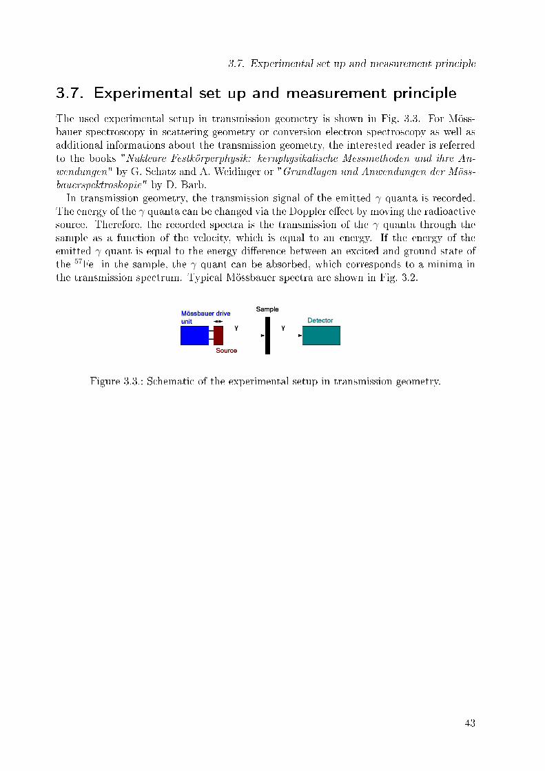
3.7. Experimental set up and measurement principle
The used experimental setup in transmission geometry is shown in Fig. 3.3. For Möss-bauer spectroscopy in scattering geometry or conversion electron spectroscopy as well asadditional informations about the transmission geometry, the interested reader is referredto the books "Nukleare Festkörperphysik: kernphysikalische Messmethoden und ihre An-
wendungen" by G. Schatz and A. Weidinger or "Grundlagen und Anwendungen der Möss-
bauerspektroskopie" by D. Barb.In transmission geometry, the transmission signal of the emitted γ quanta is recorded.
The energy of the γ quanta can be changed via the Doppler eect by moving the radioactivesource. Therefore, the recorded spectra is the transmission of the γ quanta through thesample as a function of the velocity, which is equal to an energy. If the energy of theemitted γ quant is equal to the energy dierence between an excited and ground state ofthe 57Fe in the sample, the γ quant can be absorbed, which corresponds to a minima inthe transmission spectrum. Typical Mössbauer spectra are shown in Fig. 3.2.
Figure 3.3.: Schematic of the experimental setup in transmission geometry.
43
3. Mössbauer spectroscopy
44

4. Iron-based superconductors
Iron-based superconductors such as Th7Fe3, U6Fe, and Lu2Fe3Si5 with superconductingtransition temperatures of T c = 1.8 K, 3.9 K, and 6.1 K, respectively, are known forover 50 years [3335]. However, beginning with the discovery of superconductivity inLaO1−xFxFeAs with a superconducting transition temperature of T c = 26 K in 2008 [5]the expression iron-based superconductors refers mainly to this class of high-temperaturesuperconductors, namely the iron pnictides respectively iron chalcogenides.The phase diagram of LaO1−xFxFeAs is shown in Fig. 4.1. The parent compound
Figure 4.1.: Phase diagram of LaO1−xFxFeAs. The spin density wave (SDW) magneticorder as well as the tetragonal-to-orthorhombic phase transition is suppressedas a function of F doping and superconductivity emerges. Taken from Ref. [36].
LaOFeAs shows a tetragonal-to-orthorhombic phase transition at T S = 156 K and a sub-sequent long-range antiferromagnetic spin density wave (SDW) order below TN = 138 K[36, 37]. This is one of the most important dierences between the iron pnictides and thelong-known Fe-based superconductors such as U6Fe, where the iron is non-magnetic. Themagnetic order as well as the structural phase transition in LaO1−xFxFeAs are suppressedas a function of the F doping [36]. Superconductivity emerges close to or after the sup-pression of the magnetic order. This suggests a competition of the superconducting andmagnetically ordered ground states. Measurements of the phonon density of states usinginelastic neutron scattering methods as well as linear-response calculations showed, that aphonon mediation of the superconductivity can be ruled out [38, 39]. This indicates an un-
45

4. Iron-based superconductors
conventional pairing mechanism, e.g. via magnetic uctuations due to the close proximityof superconductivity and magnetism [40].LaO1−xFxFeAs represents one example of several structural modications of the iron
pnictides and chalcogenides. The rst commonality among this Fe-based compounds isthe iron-pnictogen (FePn) respectively iron-chalcogen (FeChn) layer, which is shown fordierent families in Fig. 4.2. In the "1111" family, the FePn layer is separated by rare-earth-
Figure 4.2.: Crystal structure of iron-based superconductors. From left to right the dier-ent "families" including the highest superconducting transition temperatureT c: 1111, 122, 111 and 11. Taken from Ref. [41].
oxygen layers. In the "122" family, alternating FePn layers are separated by alkaline-earthmetal layers. In the "111" family, the alkaline metal is located in the FePn plane. In the"11" family, no separation of the FeChn layers is present.In this work, I studied Ca1−xNaxFe2As2 and Fe1+yTe. For this reason, I will give a
short overview about the 122 and 11 family. A more detailed description of the propertiesof Ca1−xNaxFe2As2 and Fe1+yTe is given in the corresponding chapters (Sec. 5 and 6).For information about the 1111 and 111 iron pnictides as well as additional informationsabout the 122 iron pnictides and 11 iron chalcogenids, the interested reader is referred tothe reviews of Lumsden and Christianson [41], Johnston [42], Johrendt [43], Hirschfeld et
al. [44], and Stewart [45].The so-called "122" compounds are one class of the recently discovered iron-based super-
conductors. In 1980, Pster and Nargosen reported the successful growth of single crystalsof ternary transition-metal arsenides [48]. They prepared the ternary arsenides AET 2As2(AE = Ca, Sr, Ba, and T = Cr, Fe, Co, Ni, Cu). These compounds form in the tetragonalThCr2Si2 structure with the space group I 4/mmm. They consist of edge-sharing TAs4tetrahedra forming a TAs plane, which is separated by AE atoms.The superconducting Fe-based 122 compounds can be summarized by the chemical for-
mula AE 1−xAx(Fe1−yT yAs1−zPz )2 with the alkaline-earth metals AE (= Ca, Sr, Ba), thealkaline metals A (= Na, K, Rb, Cs), and the transition metals T (= Co, Ni, Rh, Ru,Mn). The undoped AEFe2As2 compounds show antiferromagnetic (π, 0) spin density waveorder with TN = 140 K (Ba [49]), 205 K (Sr [50]), and 170 K (Ca [49, 51]). The magneticphase transition is accompanied by a tetragonal-to-orthorhombic phase transition. The or-thorhombic phase has the space group Fmmm and is characterized by the structural orderparameter δ = (a-b)/(a+b), which is the orthorhombic splitting of the crystallographic
46
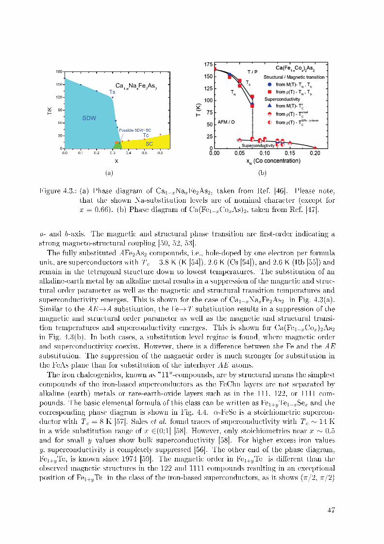
(a) (b)
Figure 4.3.: (a) Phase diagram of Ca1−xNaxFe2As2, taken from Ref. [46]. Please note,that the shown Na-substitution levels are of nominal character (except forx = 0.66). (b) Phase diagram of Ca(Fe1−xCoxAs)2, taken from Ref. [47].
a- and b-axis. The magnetic and structural phase transition are rst-order indicating astrong magneto-structural coupling [50, 52, 53].The fully substituted AFe2As2 compounds, i.e., hole-doped by one electron per formula
unit, are superconductors with T c = 3.8 K (K [54]), 2.6 K (Cs [54]), and 2.6 K (Rb [55]) andremain in the tetragonal structure down to lowest temperatures. The substitution of analkaline-earth metal by an alkaline metal results in a suppression of the magnetic and struc-tural order parameter as well as the magnetic and structural transition temperatures andsuperconductivity emerges. This is shown for the case of Ca1−xNaxFe2As2 in Fig. 4.3(a).Similar to the AE→A substitution, the Fe→T substitution results in a suppression of themagnetic and structural order parameter as well as the magnetic and structural transi-tion temperatures and superconductivity emerges. This is shown for Ca(Fe1−xCox)2As2in Fig. 4.3(b). In both cases, a substitution level regime is found, where magnetic orderand superconductivity coexist. However, there is a dierence between the Fe and the AEsubstitution. The suppression of the magnetic order is much stronger for substitution inthe FeAs plane than for substitution of the interlayer AE atoms.The iron chalcogenides, known as "11"-compounds, are by structural means the simplest
compounds of the iron-based superconductors as the FeChn layers are not separated byalkaline (earth) metals or rare-earth-oxide layers such as in the 111, 122, or 1111 com-pounds. The basic elemental formula of this class can be written as Fe1+yTe1−xSex and thecorresponding phase diagram is shown in Fig. 4.4. α-FeSe is a stoichiometric supercon-ductor with T c = 8 K [57]. Sales et al. found traces of superconductivity with T c ∼ 14 Kin a wide substitution range of x ∈(0;1] [58]. However, only stoichiometries near x ∼ 0.5and for small y values show bulk superconductivity [58]. For higher excess-iron valuesy, superconductivity is completely suppressed [56]. The other end of the phase diagram,Fe1+yTe, is known since 1974 [59]. The magnetic order in Fe1+yTe is dierent than theobserved magnetic structures in the 122 and 1111 compounds resulting in an exceptionalposition of Fe1+yTe in the class of the iron-based superconductors, as it shows (π/2, π/2)
47

4. Iron-based superconductors
Figure 4.4.: Phase diagram of Fe1+yTe1−xSex. Taken from Ref. [56]
SDW order [60].
Figure 4.5.: Generic phase diagram of the iron pnictides. Taken from Ref. [61].
A generic phase diagram for the iron pnictides is shown in Fig. 4.5 [61]. Starting froman antiferromagnetically ordered parent compound, such as LaOFeAs or BaFe2As2, themagnetic order is suppressed and superconductivity emerges by hole or electron doping.However, also isovalent doping such as Fe→Ru or As→P substitution, as well as applica-tion of hydrostatic pressure can cause the suppression of magnetic order and appearanceof superconductivity. Remarkably, a region in the phase diagram appears, where bothmagnetic order and superconductivity are present. One possibility is, that both phases areseparated as it is the case in LaO1−xFxFeAs or Ba1−xKxFe2As2 [62]. A second possibilityis a coexistence on a nanoscopic scale as in SmO1−xFxFeAs with superconducting domainswith a size of the superconducting coherence length [63, 64]. A third possibility is a ho-mogeneous superconducting state coexisting with a homogeneous magnetic order as it was
48

4.1. From SDW to SC
found in Ba1−xNaxFe2As2 [65]. This implies, that the same electrons at the Fermi surfaceare both superconducting and magnetically ordered. Local probes such as muon spin re-laxation or Mössbauer spectroscopy are necessary to decide, which type of coexistence ispresent.
4.1. From SDW to SC
For a deeper understanding of the superconductivity in the iron-based superconductorsit is crucial to understand the development of the superconducting state out of the spindensity wave state of the parent compounds AEFe2As2. The subsequent description of thisdevelopment can easily applied to the other families of the iron-based superconductors.The 122 parent compounds CaFe2As2 , SrFe2As2, and BaFe2As2 reveal electrical resistiv-
ity values of 0.1-1 mΩcm indicating semi-metallic behaviour [49, 66, 67]. For comparison,metals exhibit electrical resistivities of 1 − 10 µΩcm, which are 2-3 orders of magnitudesmaller. These 122 compounds are multi-band materials with ve Fe 3d bands crossing theFermi energy [43, 44]. In the non-magnetic state, two or more hole bands near (0,0) andtwo electron pockets near (0,π) and (π,0) cross the Fermi level in the unfolded Brillouinzone. Therefore, two electron and at least two hole Fermi surfaces (FS) are present. Aschematic FS is shown in Fig. 4.6. These multiple FSs with a high density of states (DOS)at the FS, N (EF), and enable various possibilities of electronic ordering, such as SDW,charge-density wave (CDW), or superconductivity [6870].
Figure 4.6.: (a) Schematic FeAs lattice showing the 1-Fe unit cell (green a × a) andthe 2-Fe unit cell (blue
√2a × a
√2). (b) Fermi surface topology in
the unfolded BZ (1-Fe unit cell) with an antiferromagnetic ordering vectorQAFM = (π, 0) = Γ → X. The blue arrow denotes the folding vector (π, π).(c) Fermi surface topology in the folded BZ (2-Fe unit cell) with an antifer-romagnetic ordering vector QAFM = (π, π) = Γ → M . Picture taken fromRef. [44].
CaFe2As2 , SrFe2As2, and BaFe2As2 show magnetic order below with the respectivetransition temperatures TN = 170 K [49, 51], 205 K [50], and 140 K [49]. The iron
49
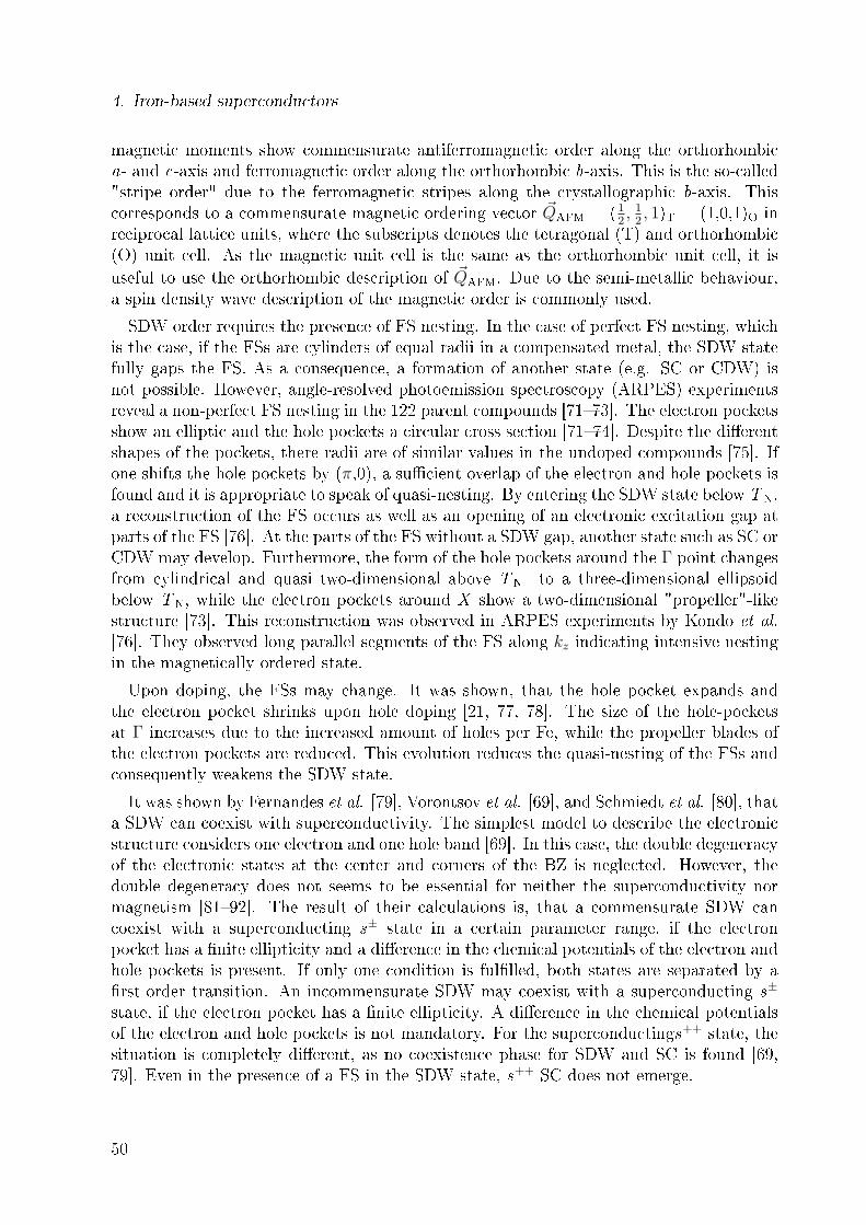
4. Iron-based superconductors
magnetic moments show commensurate antiferromagnetic order along the orthorhombica- and c-axis and ferromagnetic order along the orthorhombic b-axis. This is the so-called"stripe order" due to the ferromagnetic stripes along the crystallographic b-axis. Thiscorresponds to a commensurate magnetic ordering vector QAFM = (1
2, 12, 1)T = (1,0,1)O in
reciprocal lattice units, where the subscripts denotes the tetragonal (T) and orthorhombic(O) unit cell. As the magnetic unit cell is the same as the orthorhombic unit cell, it isuseful to use the orthorhombic description of QAFM. Due to the semi-metallic behaviour,a spin density wave description of the magnetic order is commonly used.
SDW order requires the presence of FS nesting. In the case of perfect FS nesting, whichis the case, if the FSs are cylinders of equal radii in a compensated metal, the SDW statefully gaps the FS. As a consequence, a formation of another state (e.g. SC or CDW) isnot possible. However, angle-resolved photoemission spectroscopy (ARPES) experimentsreveal a non-perfect FS nesting in the 122 parent compounds [7173]. The electron pocketsshow an elliptic and the hole pockets a circular cross section [7174]. Despite the dierentshapes of the pockets, there radii are of similar values in the undoped compounds [75]. Ifone shifts the hole pockets by (π,0), a sucient overlap of the electron and hole pockets isfound and it is appropriate to speak of quasi-nesting. By entering the SDW state below TN,a reconstruction of the FS occurs as well as an opening of an electronic excitation gap atparts of the FS [76]. At the parts of the FS without a SDW gap, another state such as SC orCDW may develop. Furthermore, the form of the hole pockets around the Γ point changesfrom cylindrical and quasi two-dimensional above TN to a three-dimensional ellipsoidbelow TN, while the electron pockets around X show a two-dimensional "propeller"-likestructure [73]. This reconstruction was observed in ARPES experiments by Kondo et al.
[76]. They observed long parallel segments of the FS along kz indicating intensive nestingin the magnetically ordered state.
Upon doping, the FSs may change. It was shown, that the hole pocket expands andthe electron pocket shrinks upon hole doping [21, 77, 78]. The size of the hole-pocketsat Γ increases due to the increased amount of holes per Fe, while the propeller blades ofthe electron pockets are reduced. This evolution reduces the quasi-nesting of the FSs andconsequently weakens the SDW state.
It was shown by Fernandes et al. [79], Vorontsov et al. [69], and Schmiedt et al. [80], thata SDW can coexist with superconductivity. The simplest model to describe the electronicstructure considers one electron and one hole band [69]. In this case, the double degeneracyof the electronic states at the center and corners of the BZ is neglected. However, thedouble degeneracy does not seems to be essential for neither the superconductivity normagnetism [8192]. The result of their calculations is, that a commensurate SDW cancoexist with a superconducting s± state in a certain parameter range, if the electronpocket has a nite ellipticity and a dierence in the chemical potentials of the electron andhole pockets is present. If only one condition is fullled, both states are separated by arst-order transition. An incommensurate SDW may coexist with a superconducting s±
state, if the electron pocket has a nite ellipticity. A dierence in the chemical potentialsof the electron and hole pockets is not mandatory. For the superconductings++ state, thesituation is completely dierent, as no coexistence phase for SDW and SC is found [69,79]. Even in the presence of a FS in the SDW state, s++ SC does not emerge.
50
4.1. From SDW to SC
In summary, there is an eective "attraction" between the SDW and the superconduct-ing s± state resulting in a coexistence region for certain parameters, while an eective"repulsion" is present for s++ SC resulting in no coexistence.
51
4. Iron-based superconductors
52
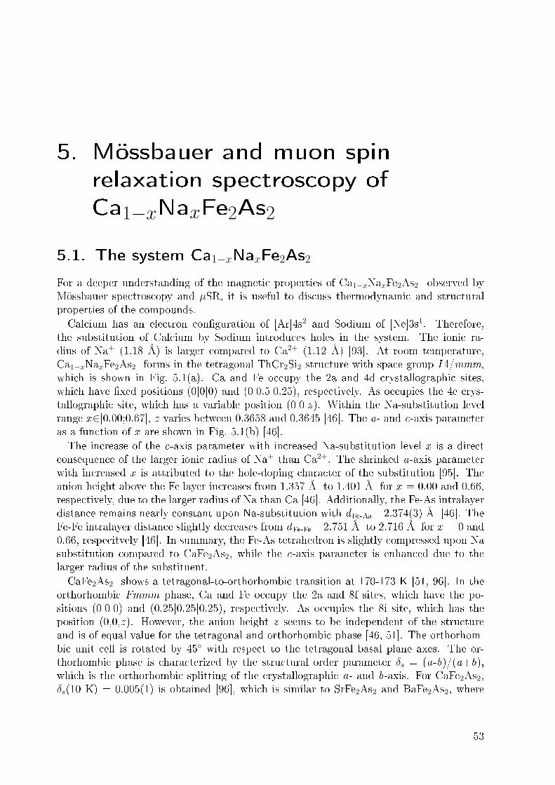
5. Mössbauer and muon spin
relaxation spectroscopy of
Ca1−xNaxFe2As2
5.1. The system Ca1−xNaxFe2As2
For a deeper understanding of the magnetic properties of Ca1−xNaxFe2As2 observed byMössbauer spectroscopy and µSR, it is useful to discuss thermodynamic and structuralproperties of the compounds.Calcium has an electron conguration of [Ar]4s2 and Sodium of [Ne]3s1. Therefore,
the substitution of Calcium by Sodium introduces holes in the system. The ionic ra-dius of Na+ (1.18 Å) is larger compared to Ca2+ (1.12 Å) [93]. At room temperature,Ca1−xNaxFe2As2 forms in the tetragonal ThCr2Si2 structure with space group I 4/mmm,which is shown in Fig. 5.1(a). Ca and Fe occupy the 2a and 4d crystallographic sites,which have xed positions (0|0|0) and (0|0.5|0.25), respectively. As occupies the 4e crys-tallographic site, which has a variable position (0|0|z ). Within the Na-substitution levelrange x∈[0.00;0.67], z varies between 0.3658 and 0.3645 [46]. The a- and c-axis parameteras a function of x are shown in Fig. 5.1(b) [46].The increase of the c-axis parameter with increased Na-substitution level x is a direct
consequence of the larger ionic radius of Na+ than Ca2+. The shrinked a-axis parameterwith increased x is attributed to the hole-doping character of the substitution [95]. Theanion height above the Fe layer increases from 1.357 Å to 1.401 Å for x = 0.00 and 0.66,respectively, due to the larger radius of Na than Ca [46]. Additionally, the Fe-As intralayerdistance remains nearly constant upon Na-substitution with dFe-As= 2.374(3) Å [46]. TheFe-Fe intralayer distance slightly decreases from dFe-Fe= 2.751 Å to 2.716 Å for x = 0 and0.66, respecitvely [46]. In summary, the Fe-As tetrahedron is slightly compressed upon Nasubstitution compared to CaFe2As2, while the c-axis parameter is enhanced due to thelarger radius of the substituent.CaFe2As2 shows a tetragonal-to-orthorhombic transition at 170-173 K [51, 96]. In the
orthorhombic Fmmm phase, Ca and Fe occupy the 2a and 8f sites, which have the po-sitions (0|0|0) and (0.25|0.25|0.25), respectively. As occupies the 8i site, which has theposition (0,0,z ). However, the anion height z seems to be independent of the structureand is of equal value for the tetragonal and orthorhombic phase [46, 51]. The orthorhom-bic unit cell is rotated by 45 with respect to the tetragonal basal plane axes. The or-thorhombic phase is characterized by the structural order parameter δs = (a-b)/(a+b),which is the orthorhombic splitting of the crystallographic a- and b-axis. For CaFe2As2,δs(10 K) = 0.005(1) is obtained [96], which is similar to SrFe2As2 and BaFe2As2, where
53
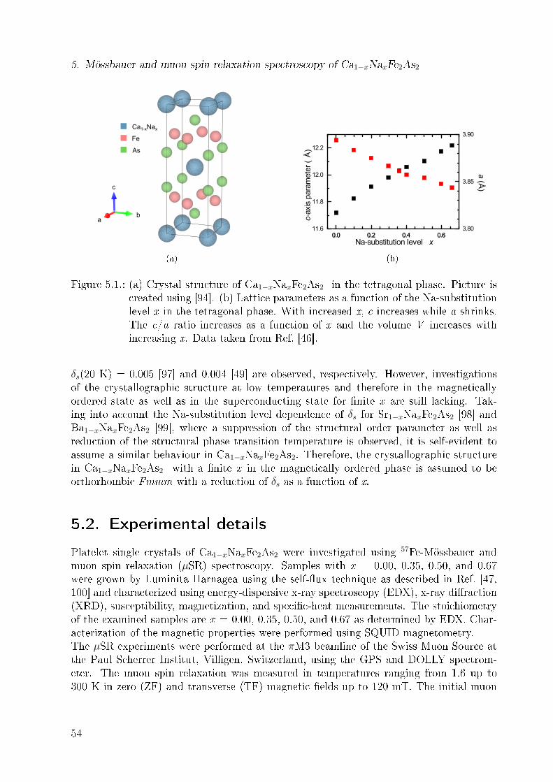
5. Mössbauer and muon spin relaxation spectroscopy of Ca1−xNaxFe2As2
c
b
a
Fe
As
Ca1-xNax
ab
c
(a)
0.0 0.2 0.4 0.611.6
11.8
12.0
12.2
Na-substitution level x
c-ax
is p
aram
eter
(Å
)
0.0 0.2 0.4 0.63.80
3.85
3.90
a (Å)
(b)
Figure 5.1.: (a) Crystal structure of Ca1−xNaxFe2As2 in the tetragonal phase. Picture iscreated using [94]. (b) Lattice parameters as a function of the Na-substitutionlevel x in the tetragonal phase. With increased x, c increases while a shrinks.The c/a ratio increases as a function of x and the volume V increases withincreasing x. Data taken from Ref. [46].
δs(20 K) = 0.005 [97] and 0.004 [49] are observed, respectively. However, investigationsof the crystallographic structure at low temperatures and therefore in the magneticallyordered state as well as in the superconducting state for nite x are still lacking. Tak-ing into account the Na-substitution level dependence of δs for Sr1−xNaxFe2As2 [98] andBa1−xNaxFe2As2 [99], where a suppression of the structural order parameter as well asreduction of the structural phase transition temperature is observed, it is self-evident toassume a similar behaviour in Ca1−xNaxFe2As2. Therefore, the crystallographic structurein Ca1−xNaxFe2As2 with a nite x in the magnetically ordered phase is assumed to beorthorhombic Fmmm with a reduction of δs as a function of x.
5.2. Experimental details
Platelet single crystals of Ca1−xNaxFe2As2 were investigated using 57Fe-Mössbauer andmuon spin relaxation (µSR) spectroscopy. Samples with x = 0.00, 0.35, 0.50, and 0.67were grown by Luminita Harnagea using the self-ux technique as described in Ref. [47,100] and characterized using energy-dispersive x-ray spectroscopy (EDX), x-ray diraction(XRD), susceptibility, magnetization, and specic-heat measurements. The stoichiometryof the examined samples are x = 0.00, 0.35, 0.50, and 0.67 as determined by EDX. Char-acterization of the magnetic properties were performed using SQUID magnetometry.The µSR experiments were performed at the πM3 beamline of the Swiss Muon Source atthe Paul Scherrer Institut, Villigen, Switzerland, using the GPS and DOLLY spectrom-eter. The muon spin relaxation was measured in temperatures ranging from 1.6 up to300 K in zero (ZF) and transverse (TF) magnetic elds up to 120 mT. The initial muon
54

5.3. Magnetic-susceptibility measurements
spin polarization was rotated by ≈ -45 with respect to the z -direction determined byTF-µSR. I measured the x = 0.35 and 0.50 samples, Hemke Maeter measured the samplewith x = 0.67 and Hubertus Luetkens measured the sample with x = 0.00. The µSR datawas analysed using the MUSRFIT software [101].I performed the Mössbauer spectroscopy (MBS) experiments together with Til Goltz andSirko Kamusella at the Institut für Festkörperphysik, TU Dresden, in transmission geom-etry in a temperature range between 4.2 and 300 K using a CryoVac Konti IT cryostat.As a γ-source, 57Co in Rhodium matrix was used. For the MBS experiments, the singlecrystals were cleaved to ensure sucient transmission of the γ-beam. This was necessary,as the γ-radiation was nearly 100 % absorbed in the case of uncleaved crystals due to itslarge thicknesses. The data were analysed using the MOESSFIT software [32].In µSR and MBS experiments, the single crystals were aligned with the crystallographicc-axis along the γ-/muon-beam direction.
5.3. Magnetic-susceptibility measurements
0 50 100 150 200 250 300-0.2
0.0
0.2
0.4
0.6
0.8
1.0
1.2
1.4
TN
TN
0Hext= 1T||ab x = 0.00 x = 0.35 x = 0.50 x = 0.67M
/H (1
0-3 e
mu
/ mol
*G)
temperature (K)
TN
(a)
0 10 20 30 40 50
-1.2
-1.0
-0.8
-0.6
-0.4
-0.2
0.0
x=0.35 x=0.50 x=0.67
4V
temperature (K)
0Hext= 2mT||ab
FC
ZFC
(b)
Figure 5.2.: Temperature dependence of the magnetic susceptibility of Ca1−xNaxFe2As2(with x = 0.00, 0.35, 0.50, and 0.67). The measurements were performed atapplied elds of (a) 1 T and (b) 2 mT parallel to the ab-plane. T χ
N = 167 K,143 K, and 119 K for x = 0.00, 0.35, and 0.50, respectively, are the magnetictransition temperatures determined by the magnetic susceptibility measure-ments. Zero (ZFC) and eld-cooled (FC) measurements show superconductiv-ity in parts of the sample (x = 0.35, T c = 17 K) and bulk superconductivity(x = 0.50 and 0.67 with T c = 17 K and 34 K, respectively).
Magnetic-susceptibility measurements in an applied eld of 1 T parallel to the ab-planeare shown in Fig. 5.2(a). For x = 0.00, 0.35, and 0.50, a nearly linear decrease of themagnetic susceptibility is observed in the paramagnetic region, which is found also formany other iron-based supercondcutors [102104]. The kinks at 167 K (x = 0.00), 143 K(x = 0.35), and 119 K (x = 0.50) indicate the magnetic transition temperature T χ
N. Forx = 0.67, a nearly linear decrease of the magnetic susceptibility is also observed above thesuperconducting transition temperature T c = 34 K. The slope of the decrease changes at≈ 150 K. This change may be attributed to the onset of antiferromagnetic uctuations.
55

5. Mössbauer and muon spin relaxation spectroscopy of Ca1−xNaxFe2As2
Magnetic-susceptibility measurements in an applied eld of 2 mT parallel to the ab-planeare shown in Fig. 5.2(b). For x = 0.35, below 17 K a broad superconducting transitionoccurs. As the diamagnetic shielding is not fully developed, only parts of the sample showsuperconductivity. For x = 0.50, a two-step superconducting transition occurs. Below34 K, a slightly negative magnetic susceptibility is measured, which indicates a supercon-ducting phase in a small volume of the sample. Below 17 K, a broad second transitionoccurs, where bulk superconductivity is formed resulting in the full superconducting re-sponse. For the further treatment of the x = 0.50 sample, 17 K will be considered asthe superconducting transition temperature. This two-step behaviour as well as the broadtransition indicates an inhomogeneous sample. The sample with x = 0.67 shows bulksuperconductivity below 34 K. The sharp transition indicates a homogeneous sample.
5.4. Results and discussion
5.4.1. Magnetic order in Ca1−xNaxFe2As2
ZF-µSR spectra for x = 0.00, 0.35, and 0.50 are shown in Fig. 5.3 for both detector pairs3,4 and 2,1. To analyse the ZF time spectra, the function
P (t) =Vmag
2∑i=1
pia1,i cos(2πfµ,it+ ϕ)e−λT,it + a2,ie
−λL,it
+ [1− Vmag]GGKT(t, σnm) (5.1)
with two magnetically inequivalent muon stopping sites was used. V mag denotes the mag-netic volume fraction (MVF), λT the transverse and λL the longitudinal relaxation rate,f µ the muon spin precession frequency, and GGKT(t, σnm) the static Gauss-Kubo-Toyabefunction.In the paramagnetic temperature regime, a weak Gauss-Kubo-Toyabe damping of P(t) is
observed caused by the dipole-dipole interaction of the muon spin with randomly orienteddense nuclear magnetic moments in absence of ordered electronic moments for all investi-gated stoichiometries. The obtained relaxation rates are σnm = 0.067 MHz, 0.052 MHz,and 0.074 MHz for x = 0.00, 0.35, and 0.50, respectively. TF-µSR experiments wereperformed by applying a magnetic eld of 5 mT perpendicular to the initial muon spinpolarization to study the temperature dependence of the magnetic volume fraction. Todescribe the magnetic phase transition, two temperatures are dened. T onset
N is dened asthe highest temperature with a nite V mag. T 100%
N is dened as as the highest temperaturewith V mag = 100 % = 1. The resulting temperature dependence of the magnetic volumefraction is shown in Fig. 5.4.T onset
N , T 100%N , and∆T = T onset
N - T 100%N , which are obtained by analysing the temperature
dependence of the magnetic volume fraction, are summarized in Tab. 5.1.A reduction of the magnetic transition temperatures with increased Na-substitution level
is observed. Additionally, ∆T = T onsetN - T 100%
N increases with increased Na-substitutionlevel, which is caused by the higher degree of disorder in the Na-substituted systemscompared to CaFe2As2 in combination with an increased gradient of the TN(x ) curve
56

5.4. Results and discussion
-0.5
0.0
0.5
1.0
0.0
0.2
0.4
0.6
0.8
1.0
x=0.00 190 K 1.6 K
detector pair 21
muon spin polarization P
(t)
detector pair 34
x=0.35 250 K 5 K
0.00 0.05 0.10 0.15 0.200.0
0.5
1.0
x=0.50 250 K 5 K
muo
n sp
in p
olar
izat
ion P
(t)
time ( s)
0 2 4 60.0
0.2
0.4
0.6
0.8
1.0
time ( s)
-0.5
0.0
0.5
1.0
0.0
0.2
0.4
0.6
0.8
1.0
Figure 5.3.: Time evolution of the muon spin polarization for representative temperaturesin the paramagnetic and magnetically ordered temperature regime for x = 0.00(upper row), 0.35 (middle row), and 0.50 (lower row). The measurements wereperformed using detector pair 3,4 (left column) and 2,1 (right column). SeeSec. 2.5 for more details of the experimental setup. Lines are best ts toEq. (2.37). Please note the dierent time scales.
57

5. Mössbauer and muon spin relaxation spectroscopy of Ca1−xNaxFe2As2
0 20 40 60 80 100 120 140 160 1800.0
0.2
0.4
0.6
0.8
1.0 x = 0.00 ( SR) x = 0.35 ( SR) x = 0.50 ( SR) x = 0.35 (MBS) x = 0.50 (MBS)
mag
netic
vol
ume
fract
ion
temperature (K)
120 160 200
0.15
0.30
w (m
m/s
)T (K)
Figure 5.4.: Temperature and Na-substitution level dependence of the magnetic volumefraction for x = 0.00, 0.35, and 0.50. A reduction of the onset of the magneticordering temperature as well as a broadening of the phase transition is ob-served with increased Na-substitution level. The onset of the magnetic orderis determined by i) the appearance of a well-dened muon spin precession inthe µSR experiments and ii) an abrupt increase of the paramagnetic linewidthw, which is shown in the inset, in the Mössbauer spectroscopy.
with increasing x.
In the magnetically ordered temperature regime, the detector pairs 3,4 and 2,1 studydierent muon spin components. Analysing detector pair 3,4 studies the muon spin com-ponent perpendicular to the crystallographic c-axis. In the magnetically ordered state, twomagnetically inequivalent muon (A, B) sites are obtained. This is consistent with calcu-lations by Yuri Pashkevich [105], who found two magnetically inequivalent muon stoppingsites. The calculations were performed at SrFe2As2 in the Fmmm structure using a mod-ied Thomas-Fermi approach, which results in the muon stopping sites (0.00|0.00|0.20)and (0.19|0.19|0.40), where the former is the main muon site A. The two muon sites showa temperature and Na-substitution level independent occupation ratio of PA:PB= 80:20as it is found in BaFe2As2 [106]. In SrFe2As2, an occupation ration of PA:PB= 70:30 isobserved [50]. This indicates, that the muon stopping sites in SrFe2As2 may be slightlydierent from those in BaFe2As2 and CaFe2As2. However, it is self-evident due to the samestructure to assume, that the muon stopping sites in CaFe2As2 and BaFe2As2 are not com-pletely dierent from those in SrFe2As2 and only small corrections to the two calculatedpositions occur. For x = 0.00, the signal fraction corresponding to muons stopping at siteA show a well-dened sinusoidal oscillation below 167 K. This indicates static long-rangecommensurate magnetic order. The signal fraction corresponding to muons stopping atsite B show an exponential relaxation below 167 K and a well-dened sinusoidal oscillationbelow 60 K. This indicates a broad eld distribution at temperatures between 60 K and167 K at the muon stopping site B suppressing a coherent oscillation of the muon spins,which is contrary to the observations in BaFe2As2, where two well-dened sinusoidal os-cillation frequencies are obtained at all temperatures below TN [106]. Below 60 K, the
58

5.4. Results and discussion
x T 100%N T onset
N ∆T = T onsetN - T 100%
N
0.00 163(2) K 167(2) K 4(4) K0.35 140(3) K 161(2) K 21(5) K0.50 80(3) K 125(3) K 45(6) K
Table 5.1.: Summary of the magnetic transition temperatures obtained by Mössbauer(MBS), TF- and ZF-muon spin relaxation experiments, of the investigatedCa1−xNaxFe2As2 compounds with x = 0.00, 0.35, and 0.50. T onset
N denotesthe temperature, where magnetic order starts to develop and a nite magneticvolume fraction is observed. T 100%
N denotes the temperature, where a mag-netic volume fraction of 100 % is observed. The obtained magnetic transitiontemperatures by both techniques for x = 0.35 and 0.50 are equal within errorbars.
two precession frequencies have a temperature independent ratio of f A/f B = 1.9. Thetemperature dependence of f A is shown in Fig. 5.5(a) with f A(T→0) = 52.0 MHz.
0 20 40 60 80 100 120 140 1600
10
20
30
40
50
60
x = 0.00 x = 0.35
prec
essi
on fr
eque
ncy
(MH
z)
temperature (K)
0
2
4
6
8
10
12 magnetic hyperfine field (T)
(a)
0 20 40 60 80 100 1200
5
10
15
20
25
30
prec
essi
on fr
eque
ncy
(MH
z)
temperature (K)
x = 0.50
0
2
4
6
magnetic hyperfine field (T)
0 20 4026
28
T(K)
f A (M
Hz)
(b)
Figure 5.5.: Temperature dependence of the magnetic order parameter for (a) x = 0.00and 0.35 and (b) x = 0.50 including best order parameter ts according toEq. (5.2). For reasons of clarity, only frequency f A, which corresponds tothe 80 % occupation probability, is shown. The Mössbauer hyperne eld in5.5(b) is the average value of the Gaussian-distributed hyperne eld with onestandard deviation as error bar. The inset in 5.5(b) shows the low-temperatureregime, where superconductivity occurs below T c = 17 K.
For x = 0.35 and 0.50, two well-dened sinusoidal precession frequencies withtemperature-independent ratios of f A/f B ≈ 4 and 8, respectively, are observed belowT onsetN . The temperature dependencies of the corresponding f A are shown in Figs. 5.5(a)
and 5.5(b). A reduction of the muon spin precession frequency and, therefore, of the mag-netic order parameter with increased Na-substitution level is observed. Additionally, thedamping of the muon spin oscillation increases with increased Na-substitution level, whichcan be seen in the ZF time spectra in Fig. 5.3. This indicates a broader eld distributionat the muon site, which is consistent with a higher degree of disorder due to the Na sub-stitution. The magnetic-susceptibility measurements, which were introduced in Sec. 5.3,
59
5. Mössbauer and muon spin relaxation spectroscopy of Ca1−xNaxFe2As2
prove a superconducting phase in parts of the sample volume (x = 0.35) or in the wholesample volume (x = 0.50). To study the interaction of the magnetic and superconductingorder parameter, f A is analysed using a temperature-dependent phenomenological orderparameter (M ) t of the form [107]
M(T ) =M(T = 0) ·[1−
(T
TN
)α]β(5.2)
above and below the superconducting transition temperature T c = 17 K for x = 0.35 and0.50. For x = 0.35, a t to Eq.(5.2) above T c for f A(T ) represents the data in the wholetemperature range with f A(T→0) = 39.3 MHz. Therefore, no interaction between themagnetic and superconducting order parameter is detectable.For x = 0.50, the muon spin precession frequency is reduced by approximately 7 %
below 17 K with f A(T→T c) = 27.5 MHz. As both order parameters compete for the sameelectrons at the Fermi surface, this reduction of the magnetic order parameter proves themicroscopic coexistence of magnetic order and superconductivity. Both order parametersare weakly coupled compared to Ba1−xNaxFe2As2, where a reduction of the muon spinprecession frequency and, therefore, of the magnetic order parameter of ≈ 65 % is observed[65]. A theoretical study of the order parameter interaction is presented in Sec. 5.4.2.Analysing detector pair 2,1 studies the muon spin component parallel to the crystal-
lographic c-axis. Down to lowest temperatures, most parts of the signal shows a Gauss-Kubo-Toyabe depolarization. Only a small fraction of muons experiencing a fast exponen-tial damping corresponding to a loss in the asymmetry respectively a fast depolarization.This fast depolarization increases with increased Na-substitution level, which can be seenin the ZF time spectra in Fig. 5.3. For x = 0.00, no dierence in the ZF time spectra and,therefore, no loss in the asymmetry is observed. In contrast, for x = 0.35 and 0.50 a fastdepolarization of 5 % and 35 % of the signal is observed, respectively. Taking into accountthe well-dened muon spin precession seen in detector pair 3,4 and the mainly Gauss-Kubo-Toyabe depolarization in detector pair 2,1, one can conclude, that the magneticeld at the muon site points essentially in the direction of the crystallographic c-axis withan increased magnetic eld component in the ab-plane as a function of the Na-substitutionlevel. This is consistent with Fe moments located in the ab-plane and a tilting out of theab-plane as a function of the Na-substitution level. Additionally, no change in the timespectra for x = 0.50 below 50 K is observed, and, hence, a spin reorientation below thesuperconducting transition temperature can be ruled out as a possible origin of the 7 %reduction of the muon spin precession frequency below T c.The Na-substitution dependence of the muon spin precession-frequency ratio. f A/f B
changes from 1.9 to 4 and 8 for x = 0.00, 0.35, and 0.50, respectively. This change ismore drastic compared to other 122 compounds. In the following, rst the undoped 122compounds are discussed and afterwards the eect of Na and K doping. The ionic radii andelectronic conguration of the alkaline (earth) metals used in 122 compounds are shownin Fig. 5.6. The c-axis parameter increases nearly linear as a function of the ionic radius.Ca is the smallest and Cs the largest ion [93]. As a consequence, the crystallographic c-
axis is shortest for CaFe2As2 [46] and longest for CsFe2As2 [54]. However, only CaFe2As2,SrFe2As2, and BaFe2As2 show magnetic order, while NaFe2As2, KFe2As2, RbFe2As2, and
60
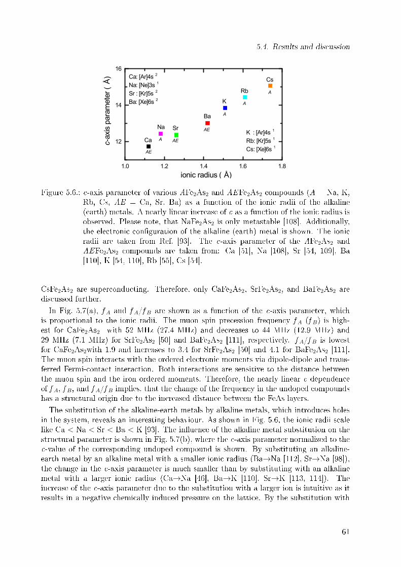
5.4. Results and discussion
1.0 1.2 1.4 1.6 1.8
12
14
16
A
A
A
A
AE
AE
AE
K : [Ar]4s 1
Rb: [Kr]5s 1
Cs: [Xe]6s 1
c-ax
is p
aram
eter
(Å
)
ionic radius ( Å)
Ca
Sr
Ba
K
Rb
Cs
Na
Ca: [Ar]4s 2
Na: [Ne]3s 1
Sr : [Kr]5s 2
Ba: [Xe]6s 2
Figure 5.6.: c-axis parameter of various AFe2As2 and AEFe2As2 compounds (A = Na, K,Rb, Cs, AE = Ca, Sr, Ba) as a function of the ionic radii of the alkaline(earth) metals. A nearly linear increase of c as a function of the ionic radius isobserved. Please note, that NaFe2As2 is only metastable [108]. Additionally,the electronic conguration of the alkaline (earth) metal is shown. The ionicradii are taken from Ref. [93]. The c-axis parameter of the AFe2As2 andAEFe2As2 compounds are taken from: Ca [51], Na [108], Sr [54, 109], Ba[110], K [54, 110], Rb [55], Cs [54].
CsFe2As2 are superconducting. Therefore, only CaFe2As2, SrFe2As2, and BaFe2As2 arediscussed further.
In Fig. 5.7(a), f A and f A/f B are shown as a function of the c-axis parameter, whichis proportional to the ionic radii. The muon spin precession frequency f A (f B) is high-est for CaFe2As2 with 52 MHz (27.4 MHz) and decreases to 44 MHz (12.9 MHz) and29 MHz (7.1 MHz) for SrFe2As2 [50] and BaFe2As2 [111], respectively. f A/f B is lowestfor CaFe2As2with 1.9 and increases to 3.4 for SrFe2As2 [50] and 4.1 for BaFe2As2 [111].The muon spin interacts with the ordered electronic moments via dipole-dipole and trans-ferred Fermi-contact interaction. Both interactions are sensitive to the distance betweenthe muon spin and the iron ordered moments. Therefore, the nearly linear c dependenceof f A, f B, and f A/f B implies, that the change of the frequency in the undoped compoundshas a structural origin due to the increased distance between the FeAs layers.
The substitution of the alkaline-earth metals by alkaline metals, which introduces holesin the system, reveals an interesting behaviour. As shown in Fig. 5.6, the ionic radii scalelike Ca < Na < Sr < Ba < K [93]. The inuence of the alkaline metal substitution on thestructural parameter is shown in Fig. 5.7(b), where the c-axis parameter normalized to thec-value of the corresponding undoped compound is shown. By substituting an alkaline-earth metal by an alkaline metal with a smaller ionic radius (Ba→Na [112], Sr→Na [98]),the change in the c-axis parameter is much smaller than by substituting with an alkalinemetal with a larger ionic radius (Ca→Na [46], Ba→K [110], Sr→K [113, 114]). Theincrease of the c-axis parameter due to the substitution with a larger ion is intuitive as itresults in a negative chemically induced pressure on the lattice. By the substitution with
61
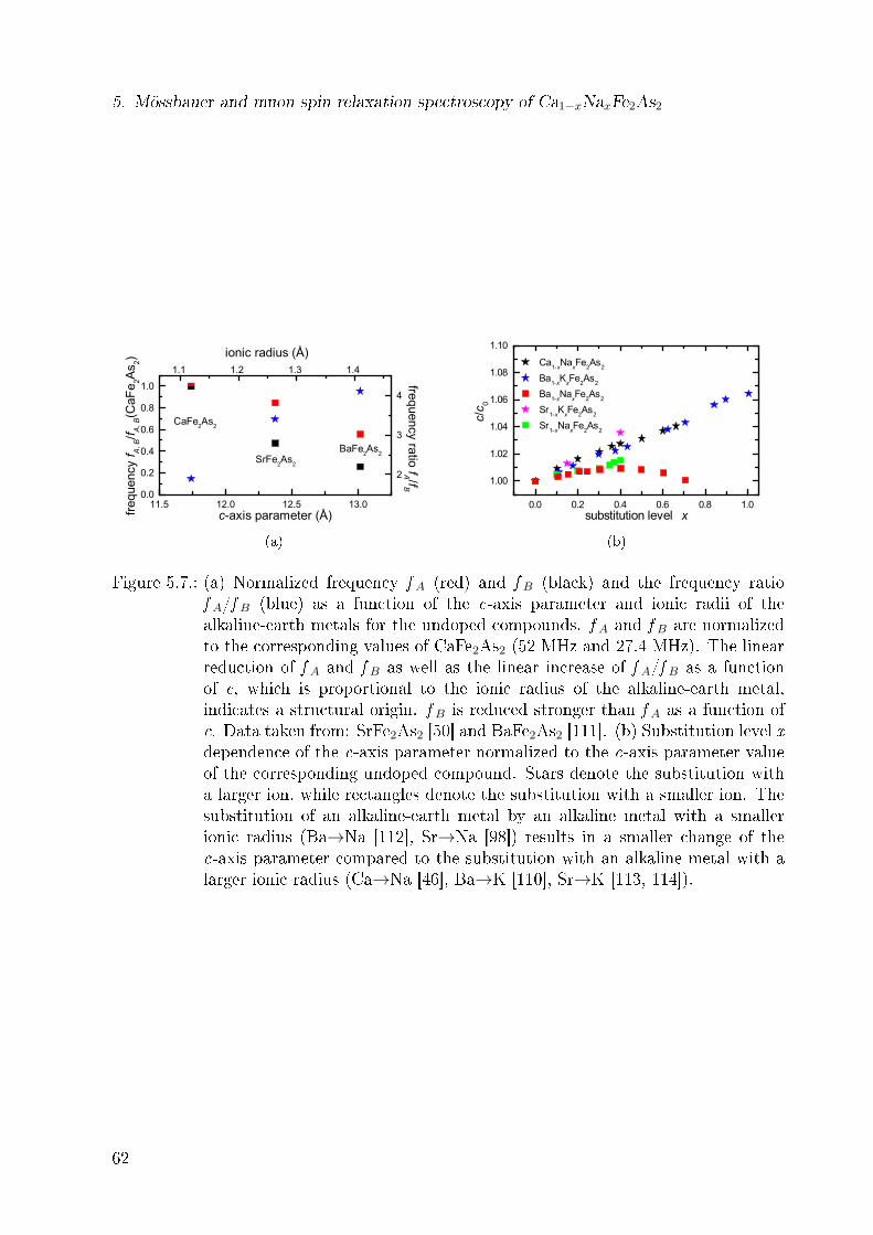
5. Mössbauer and muon spin relaxation spectroscopy of Ca1−xNaxFe2As2
11.5 12.0 12.5 13.00.0
0.2
0.4
0.6
0.8
1.0
BaFe2As2SrFe2As2
frequ
ency
f A, B
/f A, B
(CaF
e 2As 2)
c-axis parameter (Å)
CaFe2As2
1.1 1.2 1.3 1.4
ionic radius (Å)
2
3
4
frequency ratio fA /fB
(a)
0.0 0.2 0.4 0.6 0.8 1.0
1.00
1.02
1.04
1.06
1.08
1.10
Ca1-xNaxFe2As2
Ba1-xKxFe2As2
Ba1-xNaxFe2As2
Sr1-xKxFe2As2
Sr1-xNaxFe2As2
c/c 0
substitution level x
(b)
Figure 5.7.: (a) Normalized frequency f A (red) and f B (black) and the frequency ratiof A/f B (blue) as a function of the c-axis parameter and ionic radii of thealkaline-earth metals for the undoped compounds. f A and f B are normalizedto the corresponding values of CaFe2As2 (52 MHz and 27.4 MHz). The linearreduction of f A and f B as well as the linear increase of f A/f B as a functionof c, which is proportional to the ionic radius of the alkaline-earth metal,indicates a structural origin. f B is reduced stronger than f A as a function ofc. Data taken from: SrFe2As2 [50] and BaFe2As2 [111]. (b) Substitution level xdependence of the c-axis parameter normalized to the c-axis parameter valueof the corresponding undoped compound. Stars denote the substitution witha larger ion, while rectangles denote the substitution with a smaller ion. Thesubstitution of an alkaline-earth metal by an alkaline metal with a smallerionic radius (Ba→Na [112], Sr→Na [98]) results in a smaller change of thec-axis parameter compared to the substitution with an alkaline metal with alarger ionic radius (Ca→Na [46], Ba→K [110], Sr→K [113, 114]).
62
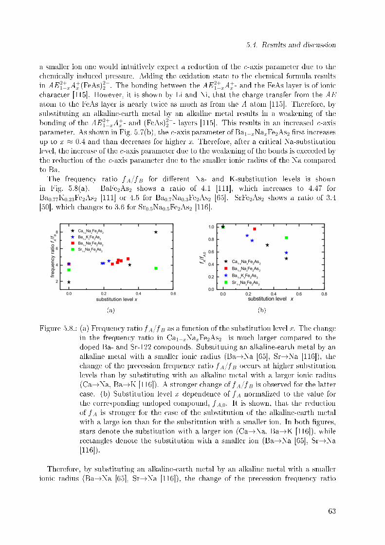
5.4. Results and discussion
a smaller ion one would intuitively expect a reduction of the c-axis parameter due to thechemically induced pressure. Adding the oxidation state to the chemical formula resultsin AE 2+
1−xA+x (FeAs)
2−2 . The bonding between the AE 2+
1−xA+x - and the FeAs layer is of ionic
character [115]. However, it is shown by Li and Ni, that the charge transfer from the AEatom to the FeAs layer is nearly twice as much as from the A atom [115]. Therefore, bysubstituting an alkaline-earth metal by an alkaline metal results in a weakening of thebonding of the AE 2+
1−xA+x - and (FeAs)2−2 - layers [115]. This results in an increased c-axis
parameter. As shown in Fig. 5.7(b), the c-axis parameter of Ba1−xNaxFe2As2 rst increasesup to x ≈ 0.4 and than decreases for higher x. Therefore, after a critical Na-substitutionlevel, the increase of the c-axis parameter due to the weakening of the bonds is exceeded bythe reduction of the c-axis parameter due to the smaller ionic radius of the Na comparedto Ba.The frequency ratio f A/f B for dierent Na- and K-substitution levels is shown
in Fig. 5.8(a). BaFe2As2 shows a ratio of 4.1 [111], which increases to 4.47 forBa0.77K0.23Fe2As2 [111] or 4.5 for Ba0.7Na0.3Fe2As2 [65]. SrFe2As2 shows a ratio of 3.4[50], which changes to 3.6 for Sr0.5Na0.5Fe2As2 [116].
0.0 0.2 0.4 0.6
2
4
6
8 Ca1-x
NaxFe
2As
2
Ba1-x
KxFe
2As
2
Ba1-x
NaxFe
2As
2
Sr1-x
NaxFe
2As
2
frequ
ency
ratio
f A/f B
substitution level x
(a)
0.0 0.2 0.4 0.6 0.80.0
0.2
0.4
0.6
0.8
1.0
f A/f A
,0
Ca1-xNaxFe2As2
Ba1-xNaxFe2As2
Ba1-xKxFe2As2
Sr1-xNaxFe2As2
substitution level x
(b)
Figure 5.8.: (a) Frequency ratio f A/f B as a function of the substitution level x. The changein the frequency ratio in Ca1−xNaxFe2As2 is much larger compared to thedoped Ba- and Sr-122 compounds. Substituting an alkaline-earth metal by analkaline metal with a smaller ionic radius (Ba→Na [65], Sr→Na [116]), thechange of the precession frequency ratio f A/f B occurs at higher substitutionlevels than by substituting with an alkaline metal with a larger ionic radius(Ca→Na, Ba→K [116]). A stronger change of f A/f B is observed for the lattercase. (b) Substitution level x dependence of f A normalized to the value forthe corresponding undoped compound, f A,0. It is shown, that the reductionof f A is stronger for the case of the substitution of the alkaline-earth metalwith a large ion than for the substitution with a smaller ion. In both gures,stars denote the substitution with a larger ion (Ca→Na, Ba→K [116]), whilerectangles denote the substitution with a smaller ion (Ba→Na [65], Sr→Na[116]).
Therefore, by substituting an alkaline-earth metal by an alkaline metal with a smallerionic radius (Ba→Na [65], Sr→Na [116]), the change of the precession frequency ratio
63
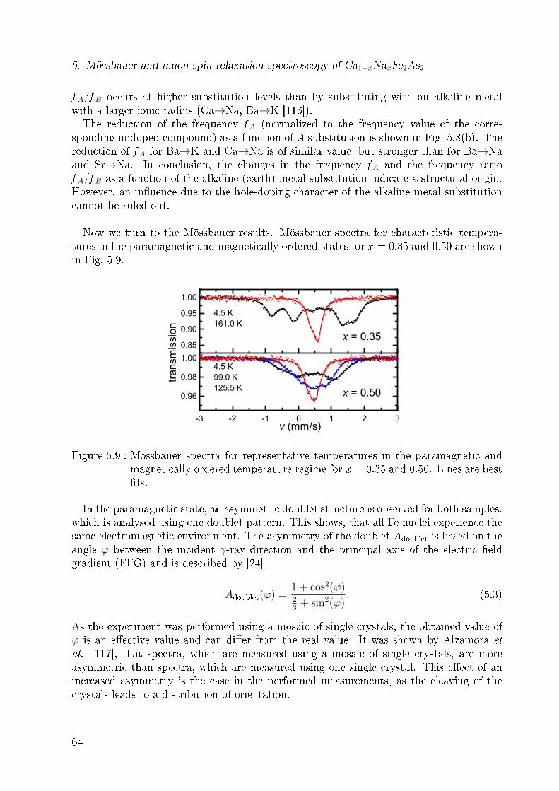
5. Mössbauer and muon spin relaxation spectroscopy of Ca1−xNaxFe2As2
f A/f B occurs at higher substitution levels than by substituting with an alkaline metalwith a larger ionic radius (Ca→Na, Ba→K [116]).The reduction of the frequency f A (normalized to the frequency value of the corre-
sponding undoped compound) as a function of A substitution is shown in Fig. 5.8(b). Thereduction of f A for Ba→K and Ca→Na is of similar value, but stronger than for Ba→Naand Sr→Na. In conclusion, the changes in the frequency f A and the frequency ratiof A/f B as a function of the alkaline (earth) metal substitution indicate a structural origin.However, an inuence due to the hole-doping character of the alkaline metal substitutioncannot be ruled out.
Now we turn to the Mössbauer results. Mössbauer spectra for characteristic tempera-tures in the paramagnetic and magnetically ordered states for x = 0.35 and 0.50 are shownin Fig. 5.9.
-3 -2 -1 0 1 2 3
0.96
0.98
1.00
v (mm/s)
4.5 K99.0 K125.5 K x = 0.50
0.85
0.90
0.95
1.00
trans
mis
sion
4.5 K161.0 K
x = 0.35
Figure 5.9.: Mössbauer spectra for representative temperatures in the paramagnetic andmagnetically ordered temperature regime for x = 0.35 and 0.50. Lines are bestts.
In the paramagnetic state, an asymmetric doublet structure is observed for both samples,which is analysed using one doublet pattern. This shows, that all Fe nuclei experience thesame electromagnetic environment. The asymmetry of the doublet Adoublet is based on theangle φ between the incident γ-ray direction and the principal axis of the electric eldgradient (EFG) and is described by [24]
Adoublet(φ) =1 + cos2(φ)23+ sin2(φ)
. (5.3)
As the experiment was performed using a mosaic of single crystals, the obtained value ofφ is an eective value and can dier from the real value. It was shown by Alzamora et
al. [117], that spectra, which are measured using a mosaic of single crystals, are moreasymmetric than spectra, which are measured using one single crystal. This eect of anincreased asymmetry is the case in the performed measurements, as the cleaving of thecrystals leads to a distribution of orientation.
64
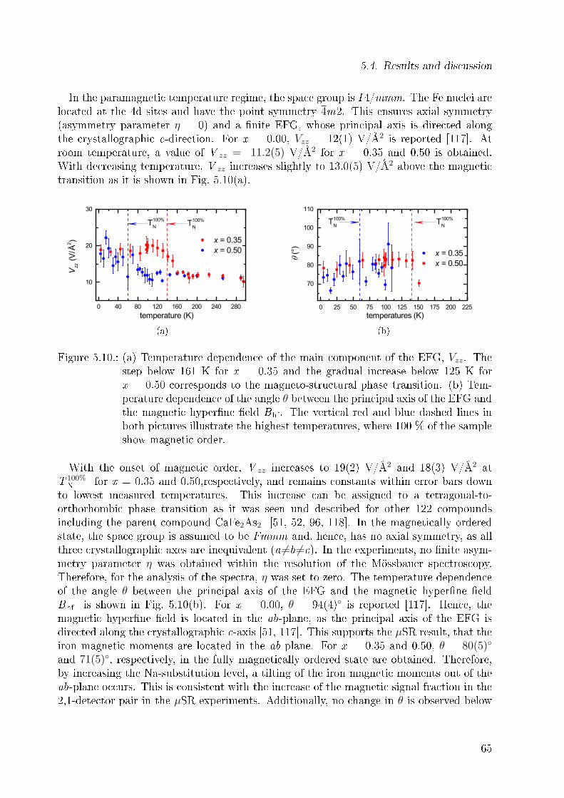
5.4. Results and discussion
In the paramagnetic temperature regime, the space group is I 4/mmm. The Fe nuclei arelocated at the 4d sites and have the point symmetry 4m2. This ensures axial symmetry(asymmetry parameter η = 0) and a nite EFG, whose principal axis is directed alongthe crystallographic c-direction. For x = 0.00, Vzz = 12(1) V/Å2 is reported [117]. Atroom temperature, a value of V zz = 11.2(5) V/Å2 for x = 0.35 and 0.50 is obtained.With decreasing temperature, V zz increases slightly to 13.0(5) V/Å2 above the magnetictransition as it is shown in Fig. 5.10(a).
0 40 80 120 160 200 240 280
10
20
30
x = 0.35 x = 0.50
T100%N
Vzz
(V/Å
2 )
temperature (K)
T100%N
(a)
0 25 50 75 100 125 150 175 200 225
70
80
90
100
110
x = 0.35 x = 0.50
temperatures (K)
(°)
T100%
N T100%N
(b)
Figure 5.10.: (a) Temperature dependence of the main component of the EFG, Vzz. Thestep below 161 K for x = 0.35 and the gradual increase below 125 K forx = 0.50 corresponds to the magneto-structural phase transition. (b) Tem-perature dependence of the angle θ between the principal axis of the EFG andthe magnetic hyperne eld Bhf. The vertical red and blue dashed lines inboth pictures illustrate the highest temperatures, where 100 % of the sampleshow magnetic order.
With the onset of magnetic order, V zz increases to 19(2) V/Å2 and 18(3) V/Å2 atT 100%
N for x = 0.35 and 0.50,respectively, and remains constants within error bars downto lowest measured temperatures. This increase can be assigned to a tetragonal-to-orthorhombic phase transition as it was seen und described for other 122 compoundsincluding the parent compound CaFe2As2 [51, 52, 96, 118]. In the magnetically orderedstate, the space group is assumed to be Fmmm and, hence, has no axial symmetry, as allthree crystallographic axes are inequivalent (a =b =c). In the experiments, no nite asym-metry parameter η was obtained within the resolution of the Mössbauer spectroscopy.Therefore, for the analysis of the spectra, η was set to zero. The temperature dependenceof the angle θ between the principal axis of the EFG and the magnetic hyperne eldBhf is shown in Fig. 5.10(b). For x = 0.00, θ = 94(4) is reported [117]. Hence, themagnetic hyperne eld is located in the ab-plane, as the principal axis of the EFG isdirected along the crystallographic c-axis [51, 117]. This supports the µSR result, that theiron magnetic moments are located in the ab-plane. For x = 0.35 and 0.50, θ = 80(5)
and 71(5), respectively, in the fully magnetically ordered state are obtained. Therefore,by increasing the Na-substitution level, a tilting of the iron magnetic moments out of theab-plane occurs. This is consistent with the increase of the magnetic signal fraction in the2,1-detector pair in the µSR experiments. Additionally, no change in θ is observed below
65
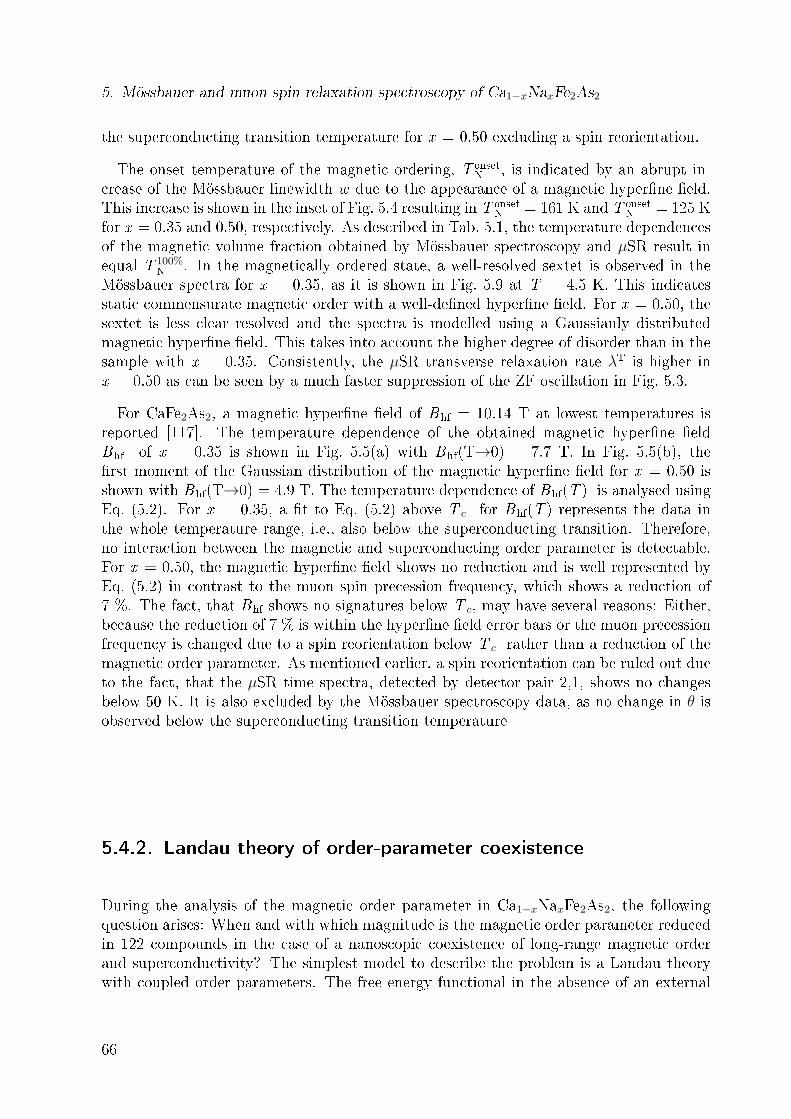
5. Mössbauer and muon spin relaxation spectroscopy of Ca1−xNaxFe2As2
the superconducting transition temperature for x = 0.50 excluding a spin reorientation.
The onset temperature of the magnetic ordering, T onsetN , is indicated by an abrupt in-
crease of the Mössbauer linewidth w due to the appearance of a magnetic hyperne eld.This increase is shown in the inset of Fig. 5.4 resulting in T onset
N = 161 K and T onsetN = 125 K
for x = 0.35 and 0.50, respectively. As described in Tab. 5.1, the temperature dependencesof the magnetic volume fraction obtained by Mössbauer spectroscopy and µSR result inequal T 100%
N . In the magnetically ordered state, a well-resolved sextet is observed in theMössbauer spectra for x = 0.35, as it is shown in Fig. 5.9 at T = 4.5 K. This indicatesstatic commensurate magnetic order with a well-dened hyperne eld. For x = 0.50, thesextet is less clear resolved and the spectra is modelled using a Gaussianly distributedmagnetic hyperne eld. This takes into account the higher degree of disorder than in thesample with x = 0.35. Consistently, the µSR transverse relaxation rate λT is higher inx = 0.50 as can be seen by a much faster suppression of the ZF oscillation in Fig. 5.3.
For CaFe2As2, a magnetic hyperne eld of Bhf = 10.14 T at lowest temperatures isreported [117]. The temperature dependence of the obtained magnetic hyperne eldBhf of x = 0.35 is shown in Fig. 5.5(a) with Bhf(T→0) = 7.7 T. In Fig. 5.5(b), therst moment of the Gaussian distribution of the magnetic hyperne eld for x = 0.50 isshown with Bhf(T→0) = 4.9 T. The temperature dependence of Bhf(T ) is analysed usingEq. (5.2). For x = 0.35, a t to Eq. (5.2) above T c for Bhf(T ) represents the data inthe whole temperature range, i.e., also below the superconducting transition. Therefore,no interaction between the magnetic and superconducting order parameter is detectable.For x = 0.50, the magnetic hyperne eld shows no reduction and is well represented byEq. (5.2) in contrast to the muon spin precession frequency, which shows a reduction of7 %. The fact, that Bhf shows no signatures below T c, may have several reasons: Either,because the reduction of 7 % is within the hyperne eld error bars or the muon precessionfrequency is changed due to a spin reorientation below T c rather than a reduction of themagnetic order parameter. As mentioned earlier, a spin reorientation can be ruled out dueto the fact, that the µSR time spectra, detected by detector pair 2,1, shows no changesbelow 50 K. It is also excluded by the Mössbauer spectroscopy data, as no change in θ isobserved below the superconducting transition temperature
5.4.2. Landau theory of order-parameter coexistence
During the analysis of the magnetic order parameter in Ca1−xNaxFe2As2, the followingquestion arises: When and with which magnitude is the magnetic order parameter reducedin 122 compounds in the case of a nanoscopic coexistence of long-range magnetic orderand superconductivity? The simplest model to describe the problem is a Landau theorywith coupled order parameters. The free energy functional in the absence of an external
66

5.4. Results and discussion
eld is given by [70, 119121]
F [ψ, M ] =
∫d3r
α
2|ψ(r)|2 + β
4|ψ(r)|4 + γ
2|∇ψ(r)|2 + d
2|ψ(r)|2|M(r)|2
+a
2|M(r)|2 + b
4|M(r)|4 + g
2|∇M(r)|2
, (5.4)
where ψ(r) is the superconducting and M(r) the magnetic order parameter. ψ(r) is com-plex and described by an amplitude and a phase, while M(r) is a real three componenttensor of rst order. Following the common approaches, α and a are described as
a = a0[T − TN0] , a0 > 0; (5.5)
α = α0[T − Tc0] , α0 > 0, (5.6)
where TN0 denotes the bare magnetic and Tc0 the bare superconducting transition tem-perature. The bare transition temperature describes the decoupled case. Tc0 < TN0 isassumed for the further treatment being the case in all 122 compounds, which are knownat the time of writing of this thesis. This determines, that the bare magnetic transitiontemperature is equal to the measured magnetic transition temperature, TN0 = TN. Thesuperconducting transition temperature, Tc, which is measured in an experiment, mightbe reduced in the presence of magnetic order and, therefore, Tc ≤ Tc0. To ensure, thatthe free energy has a denite minimum, β > 0, b > 0 and d > −
√bβ are required. All
interactions between the magnetic and superconducting order parameter are put into theterm
d
2|ψ(r)|2|M(r)|2. (5.7)
A negative d corresponds to a strengthening of both order parameters due to their interac-tion. This eect might be possible, but is beyond the scope of this discussion. Therefore,to ensure an order parameter competition, d is set to be strictly positive. Assuming thespatial homogeneity of both order parameters results in a vanishing of the gradient termsin Eq. (5.4). Minimizing the free energy functional with respect to ψ∗ and M gives
0 = αψ + β|ψ|2ψ + d|M |2ψ, (5.8)
0 = aM + b|M |2ψ + d|ψ|2M. (5.9)
This system of equations has the following solutions resulting in dierent phases dependingon the values of the parameters. The paramagnetic and normal conducting phase corre-spond to ψ = 0 and M = 0 with a, α > 0. The magnetic and normal conductingphase is given by ψ = 0 and M2 = −a/b with a < 0 and αb > ad. The paramagneticand superconducting phase corresponds to ψ = −α/β and M = 0 with α < 0 andaβ > αd.
67

5. Mössbauer and muon spin relaxation spectroscopy of Ca1−xNaxFe2As2
The solution of coexistence of both order parameters is given by
|ψ|2 =− αb− ad
bβ − d2, αb < ad; (5.10)
M2 =− aβ − αd
bβ − d2, aβ < αd, (5.11)
if the coupling is suciently small and fulls the equation bβ − d2 > 0. The conditionsαb < ad and aβ < αd are a result of |ψ|2 and M2 being real. At Tc, where |ψ|2 = 0,Eq. (5.10) reduces to
|ψ(Tc)|2 = 0 = α(Tc)b− a(Tc)d = α0b[Tc − Tc0]− a0d[Tc − TN], (5.12)
which results in an expression for the measured and bare superconducting transition tem-perature as a function of each other,
Tc =α0bTc0 − a0dTNα0b− a0d
, (5.13)
Tc0 =aod
α0bTN +
[1− a0d
α0b
]Tc, (5.14)
and the magnetic transition temperature. The temperature dependence of the magneticorder parameter in the coexistence region, using Eqs. (5.5), (5.6), (5.11) and (5.14) as wellas basic maths, is consequently given by
M2co(T ) =
1
bβ − d2
[α0d− a0β]T +
[a0β − a0
bd2]TN −
[1− a0d
α0b
]Tc
, (5.15)
for T ≤ Tc ≤ TN. As the magnetic order parameter decreases below T c with decreasingtemperature, the rst derivative of Eq. (5.15) must obey
dM2
dT> 0, (5.16)
leading to the condition α0d > a0β. To investigate the reduction of the magnetic orderparameter in the coexistence region, the ratio of M2
co and M20 at a given T ≤ Tc ≤ TN
is calculated:
M2co
M20
(T ) =1
bβ − d2
T
TN − T
[α0
a0bd− bβ
]+
TNTN − T
[bβ − d2
]− TcTN − T
[α0
a0bd− d2
]. (5.17)
68
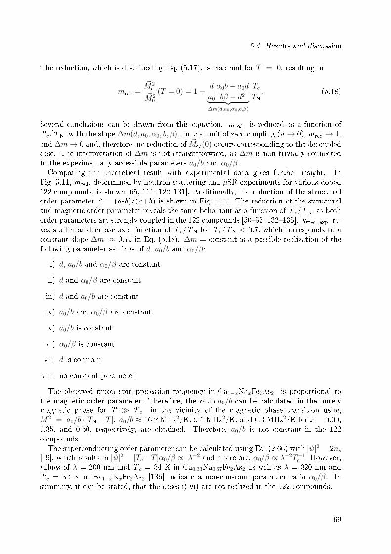
5.4. Results and discussion
The reduction, which is described by Eq. (5.17), is maximal for T = 0, resulting in
mred =M2
co
M20
(T = 0) = 1− d
a0
α0b− a0d
bβ − d2︸ ︷︷ ︸∆m(d,a0,α0,b,β)
TcTN. (5.18)
Several conclusions can be drawn from this equation. mred is reduced as a function ofT c/TN with the slope ∆m(d, a0, α0, b, β). In the limit of zero coupling (d → 0), mred → 1,and ∆m→ 0 and, therefore, no reduction of Mco(0) occurs corresponding to the decoupledcase. The interpretation of ∆m is not straightforward, as ∆m is non-trivially connectedto the experimentally accessible parameters a0/b and α0/β.Comparing the theoretical result with experimental data gives further insight. In
Fig. 5.11, mred, determined by neutron scattering and µSR experiments for various doped122 compounds, is shown [65, 111, 122131]. Additionally, the reduction of the structuralorder parameter S = (a-b)/(a+b) is shown in Fig. 5.11. The reduction of the structuraland magnetic order parameter reveals the same behaviour as a function of T c/TN, as bothorder parameters are strongly coupled in the 122 compounds [5052, 132135]. mred, exp re-veals a linear decrease as a function of T c/TN for T c/TN < 0.7, which corresponds to aconstant slope ∆m ≈ 0.75 in Eq. (5.18). ∆m = constant is a possible realization of thefollowing parameter settings of d, a0/b and α0/β:
i) d, a0/b and α0/β are constant
ii) d and α0/β are constant
iii) d and a0/b are constant
iv) a0/b and α0/β are constant
v) a0/b is constant
vi) α0/β is constant
vii) d is constant
viii) no constant parameter.
The observed muon spin precession frequency in Ca1−xNaxFe2As2 is proportional tothe magnetic order parameter. Therefore, the ratio a0/b can be calculated in the purelymagnetic phase for T ≫ T c in the vicinity of the magnetic phase transition usingM2 = a0/b · [TN− T ]. a0/b ≈ 16.2 MHz2/K, 9.5 MHz2/K, and 6.3 MHz2/K for x = 0.00,0.35, and 0.50, respectively, are obtained. Therefore, a0/b is not constant in the 122compounds.The superconducting order parameter can be calculated using Eq. (2.66) with |ψ|2 = 2ns
[19], which results in |ψ|2 = [Tc−T ]α0/β ∝ λ−2 and, therefore, α0/β ∝ λ−2T−1c . However,
values of λ = 200 nm and T c = 34 K in Ca0.33Na0.67Fe2As2 as well as λ = 320 nm andT c = 32 K in Ba1−xKxFe2As2 [136] indicate a non-constant parameter ratio α0/β. Insummary, it can be stated, that the cases i)-vi) are not realized in the 122 compounds.
69

5. Mössbauer and muon spin relaxation spectroscopy of Ca1−xNaxFe2As2
a0/b shows a linear decrease with increased doping level and hence can be approximatedby ax0/b
x = a00/b0 [1 - ∆(a/b)], where a00 and b
0 denote the corresponding parameter for theundoped magnetic compounds. For Ca1−xNaxFe2As2, ∆(a/b) = −20(2)×x, with the Na-substitution level x∈[0.00;0.67]. The linearity of the doping dependence of α0/β ∝ λ−2T−1
c
cannot be proven for the Ca1−xNaxFe2As2-series, as only λ values for x = 0.50 and 0.67are available in the literature. For the doped BaFe2As2 compounds, more data is avail-able. It can be shown, using the data published by Prozorov and Kogan [137] that α0/βshows a linear doping dependence similar to a0/b. Hence, it can be approximated usingα0/β = α0
0/β0 × ∆(α0/β), where α0
0 and β0 denote the corresponding parameter for theundoped superconducting compounds. ∆(α0/β) is a linear function of the doping levelx. However, due to the similar properties in the 122 compounds, it is assumed, that thedoping dependence of a0/b and α0/β is always of linear type for each doping series. Thislinear doping dependence indicate a constant coupling d (case vii) in the 122 compounds.In Fig. 5.11, it is visible, that no reduction of the magnetic order parameter occurs for
0.0 0.2 0.4 0.6 0.8 1.00.0
0.2
0.4
0.6
0.8
1.0structural order parameter:
Ba1-xKxFe2As2 Ba(Fe1-xRhx)2As2
Ba(Fe1-xCox)2As2
magnetic order parameter: Ca1-xNaxFe2As2
Ba1-xNaxFe2As2 Ba1-xKxFe2As2 Ba(Fe1-xRhx)2As2 Ba(Fe1-xRux)2As2 Ba(Fe1-xNix)2As2 Ba(Fe1-xCox)2As2
M2 C
o/M2 0 (
T =
0), S
2 Co/S
2 0 (T
= 0)
Tc/TN
Figure 5.11.: Magnetic (M ) and structural (S ) order parameter reduction as a functionof T c/TN. M co and S co denote the order parameter in the coexistence re-gion, while M 0 and S 0 denote the bare order parameter. The solid linecorresponds to Eq. (5.18). Data taken from Refs. Ba1−xNaxFe2As2 [65],Ba1−xKxFe2As2 [111, 122, 123], Ba(Fe1−xRux)2As2 [124], Ba(Fe1−xRhx)2As2[125, 126], Ba(Fe1−xNix)2As2 [127], and Ba(Fe1−xCox)2As2 [125, 128131].
0 < T c/TN ≈ 0.1. This has several reasons. For T c/TN ≈ 0, due to the experimental
70

5.4. Results and discussion
resolution, a reduction of the order parameter may not be resolved. Additionally, thecompounds may not show bulk superconductivity, but only in parts of the sample. Thisis, e. g., the case for Ca0.65Na0.35Fe2As2, where only parts of the volume are supercon-ducting and no reduction of the magnetic order parameter is observed. Also, it is dicultto determine M (T→0) in the presence of a superconducting phase due to the reductionof the magnetic order parameter in the coexistence region. For the majority of the lit-erature data, only M (T c) is available and used in Fig. 5.11. The resulting error can beestimated by the described µSR experiment on Ca0.50Na0.50Fe2As2. M (T c) = 27.5 MHzand M co(T → 0) = 26 MHz are obtained by the experiment, while M (T → 0) = 28 MHz iscalculated using Eq. (5.2). The reduction is than given by M co(T → 0)/M (T c) ≈ 5 % andM co(T → 0)/M (T → 0)≈ 7 %. The corresponding reduction of the magnetic order param-eter is than given by M 2
co(T → 0)/M 2(T c) ≈ 0.89 and M 2co(T → 0)/M 2(T → 0) ≈ 0.86.
The dierence between both reduction values is ≈ 3.5 %, which is of the order of the dotsize in Fig. 5.11. This approximation is appropriate, if M (T → 0) ≈ M (T c), which is thecase for T c/TN ≪ 1. For T c/TN → 1, M (T → 0) ≈ M (T c) is not secured. In this case,M (T c) < M (T → 0) and, hence, mred is overestimated. Therefore, the limitations ofthe data extraction cannot explain the systematic deviations of the data from Eq. (5.18)in the range 0.7 . T c/TN < 1. This indicates a change of the slope in Eq. (5.18), whichcan be consistently described with case vii: For T c/TN < 0.7, a similar coupling strengthd ≈ constant of the magnetic and superconducting order parameter results in ∆m = con-stant. With increasing T c/TN, ∆m changes for T c/TN > 0.7 and hence the constantvalue of d is changed. However, if T c ≈ TN, higher order terms in M and ψ may have tobe considered.In summary, a qualitative description of the reduction of the magnetic order parameter
in the coexistence region as a function of T c/TN is given. For a quantitative treatmentof the problem with Landau theory, the parameters α and a have to be calculated usinga microscopic theory. This would also put the argumentation about the similar couplingstrength of the superconducting and magnetic order parameter in the 122 compounds ona more robust basis.
5.4.3. Magneto-structural phase transition
When a nucleus absorbs a photon, the phonon system remains unchanged with a proba-bility f, where f is the recoilless fraction. This probability depends on the phonon spectra.Therefore, by analysing f, informations about the phonon spectra can be obtained. Asdescribed in Sec. 3.4, the temperature dependence of f in Debye approximation is givenby
f = exp
(− 3ER
2kBθD
1 + 4
[T
θD
]2 ∫ θD/T
0
x
ex − 1dx
), (5.19)
with the recoil energy ER, Boltzmann's constant kB and the Debye temperature θD. Inthe Mössbauer experiments, the area of the total spectrum A and the baseline I0 areextracted from the Mössbauer spectra. The quantity AN = A/I0 is proportional tof [138]. Therefore, by analysing the temperature dependence of AN , the temperaturedependence of f can be obtained, but statements about absolute values of f cannot be
71

5. Mössbauer and muon spin relaxation spectroscopy of Ca1−xNaxFe2As2
made. f is then given byf = CAN(T ), (5.20)
where C is a positive constant. The temperature dependence of AN(T ), normalized to thevalue AN(T = 4.2 K), for x = 0.35, 0.50, and 0.67 is shown in Fig. 5.12(a). For x = 0.35and 0.50, AN(T )/AN(4.2K) is well-described by Eq. (5.20) in the fully magnetically orderedstate as well as in the paramagnetic state. The step at 161 K for x = 0.35 and the gradualincrease between 60 K and 125 K is attributed to the splitting of former overlappingtransition lines due to the magnetic phase transition, which leads to an increase of theeective absorption area [24, 139]. Debye temperatures of θPMD = 200(32) K and 203(12) Kas well as θAFMD = 208(16) K and 219(28) K for x = 0.35 and 0.50, respectively, are obtained.For x = 0.67, Eq. (5.20) describes AN(T )/AN(4.2 K) for all investigated temperatures .The obtained Debye temperatures θD are summarized in Tab. 5.2.
x θPMD /K θAFMD /K0.00 272 2710.35 200(32) 208(16)0.50 203(12) 219(28)0.67 213(6)
Table 5.2.: Debye temperatures θD obtained using Eq. (5.19) above (PM) and below (AFM)the magnetic phase transition. Data for x = 0.00 are taken from Ref. [140]
The Debye temperatures θPMD and θAFMD do not change within error bars at the phasetransition. This shows, that the lattice dynamics does not change at the magneto-structuralphase transition. Additionally, θD is constant for all nite x. Therefore, the latticedynamics is independent of the Na-substitution level in the investigated substitution range0.35 ≤ x ≤ 0.67. In contrast to the undoped compound, CaFe2As2 with θD = 270 K,the lattice is softer [140] . Therefore, the lattice dynamics change between the undopedcompound x = 0 and the investigated Na-substitution range 0.35 ≤ x ≤ 0.67.To further study the properties of the magneto-structural phase transition, the temper-
ature dependence of the center shift δ is analysed. δ is a measure for the electron densityat the Fe nucleus. Comparing the room temperature values of δ, a Na-substitution levelindependent value of δ = 0.40(1) mm/s for x = 0.35, 0.50, and 0.67 is observed. Theundoped compound shows an isomer shift of δ = 0.43 mm/s [117]. Therefore, the electrondensity at the Fe nucleus is increased upon Na substitution. As described in Sec. 3.6.1, thetemperature dependence of the center shift, which is shown in Fig. 5.12(b), is the sum ofthe temperature-independent chemical shift δC and a temperature-dependent contributionδR(T ) due to the second-order Doppler shift,
δ(T ) = δC + δR(T ), (5.21)
δR(T ) = − 9
16
kBMe c
θD + 8T
[T
θD
]3 ∫ θD/T
0
x3
ex − 1dx
,
where Me denotes the eective vibrating mass of the 57Fe atom. The chemical shift is
72

5.4. Results and discussion
0.5
1.0
AN(T
) / A
N(4
.2 K
)
x = 0.35
0.5
1.0x = 0.50
0 50 100 150 200 250 300
0.5
1.0x = 0.67
temperature (K)
(a)
0 50 100 150 200 250 3000.340.360.380.400.420.440.460.480.500.520.540.560.58
x = 0.35 x = 0.50
x = 0.67 ( shiftet by -0.05 mm/s)
(mm
/s)
temperature (K)
TonsetN
TonsetN
(b)
Figure 5.12.: (a) Temperature dependence of the relative recoilless fractionAN(T )/AN(4.2 K) including best ts following Eq. (5.19). (b) Tem-perature dependence of the center shift. The solid lines are a t in theparamagnetic temperature regime and the dashed lines are a t in themagnetically ordered temperature regime using Eq. (5.21) with θD = 200 Kand 203 K for x = 0.35 and 0.50, respectively. The deviation from δPM(T )corresponds to the magneto-structural transition, which causes a change inthe electron density at the nucleus. For x = 0.67, δ is shifted by -0.05 mm/sfor illustration purposes.
calculated using δC = δ(0) − δR(0).To study the inuence of the magneto-structural phase transition on the center shift,
its temperature dependence is analysed. Analysing δ(T ) in the paramagnetic state with axed θD, which is obtained by Eq. (5.20), gives δPM(T ) and M PM
e and δPMC can be calcu-lated. δPM(T ) reveals similar behaviour for both samples leading to δPMC = 0.61(3) mm/sand δPMC = 0.60(1) mm/s for x = 0.35 and 0.50. The eective vibrating mass has, withinerror bars, the same value M PM
e = 60(1) u for both samples, which is slightly enhancedcompared to the 57 u of a free 57Fenucleus due to the bonding of the nucleus in the crystallattice. Applying the resultant temperature dependence δPM(T ) to the full temperaturerange, one can see, that systematic deviations from the behaviour in the paramagneticstate occur below the magneto-structural phase transition.Analysing the magnetically ordered state (AFM) with the same θD as in the para-
magnetic state, δAFM(T ) is obtained and MAFMe and δAFMC can be calculated. MAFM
e
has the same value as in the paramagnetic state. Therefore, M e= MAFMe = M PM
e isdened. This constant M e indicates no signicant change in the bonding of the nu-cleus due to the magneto-structural phase transition. Values of δAFMC = 0.57(1) mm/s andδAFMC = 0.56(1) mm/s are obtained for x = 0.35 and 0.50, respectively.Both δPM(T ) and δAFM(T ) have the same temperature dependence due to the same
θD and M e and only vary in the values of δC. The experimental data is described byδPM(T ) at temperatures above 161 K and 125 K and by δAFM(T ) at temperatures below100 K and 60 K for x = 0.35 and 0.50, respectively. Therefore, a change of δC occurin this intermediate temperature regime. δPMC is reduced to δAFMC = 0.57(1) mm/s and0.56(1) mm/s for x = 0.35 and 0.50, respectively. These reductions in the chemical shifts
73

5. Mössbauer and muon spin relaxation spectroscopy of Ca1−xNaxFe2As2
correspond to an increase of the electron density at the nucleus [24]. The origin of thechange of the electron density at the nucleus can be the structural and/or the magneticphase transition. The change from a tetragonal to an orthorhombic structure changes thelattice parameters and hence the volume of the unit cell, which may change the chemicalshift [24]. An increase of the volume and, hence, an increase of the Fe-As distance resultsin a decrease of the electron density at the nucleus corresponding to an increased δC [140].This behaviour is, for example, observed in non-magnetic FeSe, which shows an increase ofδC of 0.006(1) mm/s at the tetragonal-to-orthorhombic phase transition [141]. A magneticphase transition may change the chemical shift, as it was observed in metallic iron atthe Curie temperature, where no structural phase transition occurs [142]. The reductionof δC in metallic iron due to the magnetic phase transition is ≈ 0.3 mm/s [142]. Thisindicates, that the origin of the change of the chemical shifts is of both magnetic andstructural nature. However, Mössbauer measurements on the undoped compound showeither no change [117], an increase [140] or a decrease [143] of the chemical shift. Themeasurements on samples with x > 0 indicate, that a reduction of the isomer shift at themagneto-structural phase transition of CaFe2As2 is the most probable case. For x = 0.67,the temperature dependence of δ(T ) can be properly described by Eq. (5.21) and a valueof δC= 0.56(1) mm/s was obtained. Therefore, no signs of a magnetic or structural phasetransition were obtained.
5.4.4. Optimally doped Ca0.33Na0.67Fe2As2
-2 -1 0 1 20.90
0.92
0.94
0.96
0.98
1.00
1.02
trans
mis
sion
v (mm/s)
4.5 K295 K
(a)
0 2 40.0
0.2
0.4
0.6
0.8
1.0
muo
n sp
in p
olar
izat
ion P
(t)
time ( s)
100 K 4.2 K
(b)
Figure 5.13.: (a) Mössbauer spectra and (b) µSR time spectra in the paramagnetic andsuperconducting phase.
For Ca0.33Na0.67Fe2As2, magnetic susceptibility measurements evidence bulk supercon-ductivity below T c = 34 K, as shown in Fig. 5.2(b). Mössbauer experiments whereperformed at temperatures below 60 K and above 151 K. The Mössbauer spectra, whichare shown in Fig. 5.13(a) exhibit an asymmetric doublet structure with V zz= 10.3(2) V/Å2
at 295 K. Vzz remains constant within error bars down to lowest temperatures excludinga structural phase transition. This Vzzvalue is ≈ 8 % smaller than for x = 0.35 and 0.50.Therefore, the deviation form the perfect FeAs4 tetrahedron is smaller for x = 0.67. How-ever, the superconducting transition is sensitive to the distortion of this tetrahedron and
74

5.4. Results and discussion
-1.0
-0.5
0.0
0.5
1.0
0Hext=11.8 mT||ab
-1.0
-0.5
0.0
0.5
1.0
1 2 3 4
-1.0
-0.5
0.0
0.5
1.0
d) 1.6 Kc) 14.1 Ka) 38.2 K b) 29.2 K
muo
n sp
in p
olar
izat
ion P
(t)
time ( s)1 2 3 4
time ( s)1 2 3 4
time ( s)1 2 3 4
-1.0
-0.5
0.0
0.5
1.0
0Hext=11.8 mT||c
muon spin polarization P
(t)
time ( s)
Figure 5.14.: TF-µSR spectra for x = 0.67 with µ0Hext=11.8 mT∥ab (upper row) andµ0Hext=11.8 mT∥c (lower row) for temperatures above and below the super-conducting transition temperature, T c = 34 K. The small Gaussian dampingin spectrum (a) is attributed to the dipole-dipole interaction of the muon spinwith randomly oriented dense nuclear moments. The additional damping inspectra (b)-(d) is caused by the formation of a vortex lattice in the supercon-ducting state and the associated internal magnetic eld distribution n(B). Itis clearly visible, that the damping of the muon precession is stronger in theµ0Hext = 11.8 mT∥c case.
75

5. Mössbauer and muon spin relaxation spectroscopy of Ca1−xNaxFe2As2
0 10 20 30 400
5
10
15
20
25
30 specific heat SR
ab
-2 ~
<B
2 >0.5 (
m-2)
temperature (K)
11.2
11.4
11.6
11.8
12.0
<B> (m
T)
0Hext = 11.8 mT||c-axis
(a)
0 10 20 30 400
5
10
15
-2 c ~
<B
2 >0.5 (
m-2)
temperature (K)
11.2
11.3
11.4
11.5
11.6
11.7
11.8
11.9
0Hext = 11.8 mT||ab-plane
<B> (m
T)
(b)
Figure 5.15.: Temperature dependence of the magnetic penetration depths (a) λ−2ab (T ) and
(b) λ−2c (T ), which are proportional to the superuid density, and the av-
erage magnetic eld determined by TF-µSR. The reduction of the averagemagnetic eld is caused by the diamagnetic shielding of the superconductingstate. The solid line is the best t with a phenomenological α model [20].The dashed line illustrates the temperature dependence of λ−2 obtained byspecic-heat measurements with the parameter ∆1 = 2.35 meV, ∆2 = 7.5meV, W(∆1) = 0.75 and λ(0) = 210 nm [100, 144].
T c is enhanced for less distorted tetrahedra [145].The broadening of the Mössbauer spectra below 60 K cannot be explained by neither
an increase of Vzz nor an increase of the linewidth w. Therefore, this broadening indicatesthe existence of small magnetic elds, which were modelled using a Gaussian distributionwith the rst moment ⟨B⟩ = 0. The standard deviation of this Gaussian distribution isconstant within error bars σ(B) = 2.2(1) T above Tc and decreases in the superconductingphase to 1.7(1) T at 4.2 K. This indicates a competition between magnetism and super-conductivity. Additionally, the spectra are nearly symmetric below 60 K and an angleθ = 55(5) between the principal axis of the EFG and the magnetic hyperne eld, whichis close to the magic angle, is obtained. ZF µSR experiments, which were measured fortemperatures below 40 K and above 75 K, down to 5 K are shown in Fig. 5.3. The timeevolution of the muon spin polarization exhibit a Gauss-Kubo-Toyabe depolarization above75 K excluding any electronic magnetic order. Below 40 K, a weak exponential relaxationproves short-range magnetic order in small volume fractions with a MVF < 20 %. Bycombining both local probes, the onset temperature of the magnetic order is estimated tobe 60 < T onset
N < 75 K. However, room-temperature Mössbauer measurements as well asthe sharp superconducting transition observed via magnetic-susceptibility measurementsindicate a homogeneous sample. This indicates, that the weak magnetism is diluted anddisordered and persistent even in the optimal doping regime, as it was seen in other ironpnictides. [36, 63, 146]For an investigation of the superconducting phase (T c = 34 K), TF-µSR measurements
were performed in external magnetic elds of µ0Hext = 11.8 mT perpendicular and par-allel to the crystallographic c-axis. The magnetic eld was applied at T>T c and thecorresponding time evolution of the muon spin polarization is shown in Fig. 5.14(a). The
76
5.4. Results and discussion
damping above T c is caused by the dipole-dipole interaction of the muon spin with ran-domly oriented dense nuclear moments. Subsequent cooling of the sample in the externaleld with µ0Hc1 < µ0Hext < µ0Hc2 below the superconducting transition tempera-ture causes the formation of a vortex lattice. The superconducting signal fraction is fullydamped after 2-3 µs and ≈ 18 % residual signal fraction is still oscillating with a preces-sion frequency equal to the applied eld at times t > 3 µs. Identifying this ≈18 % signalfraction with the MVF obtained by ZF-µSR measurements, which is of equal value, show,that the internal magnetic elds are small compared to the 11.8 mT applied eld.The vortex lattice and the associated magnetic eld distribution n⊥,∥c(B) causes an
additional Gaussian damping. The corresponding time evolution of the muon spin polar-ization is shown in Fig. 5.14(b-d). Measuring the magnetic eld distribution within thevortex lattice, the magnetic penetration depth can be obtained via Eq. (2.63). The result-ing temperature dependence of the inverse squared magnetic penetration depth, λ−2(T ),is shown in Fig. 5.15(a) and Fig. 5.15(b) together with the rst moment ⟨B⟩ of the in-ternal magnetic eld distribution n⊥,∥c(B). ⟨B⟩ shows a reduction due to the diamagneticshielding below the superconducting transition. For µ0Hext=11.8 mT∥c, ⟨B⟩ increases atlowest temperatures, which is unexpected in the superconducting phase. The eect maybe caused by eld induced magnetism [147149], vortex disorder [147], or a decrease of thespin susceptibility, which is concealed by the diamagnetic shielding [150, 151].λ−2(T ) is modelled using the phenomenological α model including two independent
superconducting gaps with s-wave symmetry [20]. The results are shown in Tab. 5.3. Theobtained values for the larger superconducting energy gap are in reasonable agreement withrecent ARPES and specic-heat measurements on single crystals from the same batchwith the same composition [77, 100]. Using the measurements with µ0Hext∥c, the in-plane penetration depth λab(0)= 194(17) nm can be directly calculated. For µ0Hext∥ab,contributions from both λac and λbc are measured. Let λe be the measured magneticpenetration depth for the case µ0Hext∥ab, and is given by λe=
√λacλbc [152]. Assuming
λa ≈ λb and using λab =√λaλb, λac =
√λaλc and λbc =
√λbλc, a value for λc can
be estimated using λc = λ2eff/λab, where a value of λc(0)= 280(46) nm is obtained. Asdisorder in the vortex lattice would articially reduce the penetration depth due to thebroadening of n(B), λab and λc describe strictly lower limits only (and λ−2 an upper limit).
∆1(0)/meV ∆2(0)/meV w(∆1) λ(0)/nmµ0Hext⊥c 0.57(8) 6.7(1.3) 0.49(4) 280(46)µ0Hext∥c 0.8(3) 6(1) 0.46(8) 194(17)
ARPES [77] 2.3 7.8spec. heat [100, 144] 2.35 7.5 0.75 [100] 210(10) [144]
Table 5.3.: Superconducting gap and penetration depth values obtained by a phenomeno-logical α model analysis of λ−2 for an applied external eld parallel and per-pendicular to the crystallographic c-axis. ∆i(0) denotes the zero temperaturevalues of the gaps. w(∆1) and w(∆2)=1-w(∆1) are the corresponding weightingfactors. λ(0) denotes the zero temperature penetration depth.
Therefore, the obtained values for the magnetic penetration depths are reduced com-
77
5. Mössbauer and muon spin relaxation spectroscopy of Ca1−xNaxFe2As2
pared to the values obtained by, e.g. specic-heat experiments. To illustrate this ef-fect, the temperature dependence of λ−2
spec. heat(T ) with the corresponding parameters(∆1 = 2.35 meV, ∆2 = 7.5 meV, w(∆1) = 0.75, and λ(0) = 210 nm) obtained byspecic-heat measurements [100, 144] is plotted in Fig. 5.15(a). It is clearly visible, thatλ−2spec. heat(T ) < λ−2
µSR(T ) for T < T c. This underestimation of the magnetic penetra-tion depth in the µSR experiments may result in a dierent temperature dependence ofλ−2(T ) and, therefore, in dierent gap sizes and weighting factors. Additionally, Johnstonet al. considered the interband coupling of the superconducting bands and found an in-termediate coupling strength [100]. The α model here used considers two non-interactingsuperconducting bands, which may also explain the dierent parameter values. However,taking into account the limitation of magnetic-penetration-depth measurements via µSRexperiments and the used α model, the obtained parameter for ∆1(0), ∆2(0), w(∆1) andλ(0) are in reasonable agreement with the values obtained by ARPES and specic-heatexperiments.The magnetic-penetration-depth anisotropy can be calculated under the assumption of
λa ≈ λb by [136]
γλ =λcλab
. (5.22)
The temperature-independent value of γλ = 1.5(4) is the smallest observed among the122-pnictides [100], where values of 2 at Tc are obtained, which increase to 6 at 1 K[153], indicating a more three-dimensional behaviour in Ca0.33Na0.67Fe2As2. This result isconsistent with the temperature-independent value of γ = 1.85(5) for the anisotropy of theupper critical elds [154].
5.5. Summary and conclusion
In conclusion, 57Fe-Mössbauer spectroscopy and muon spin relaxation experiments wereperformed to study the electronic phase diagram of Ca1−xNaxFe2As2 resulting in an up-dated phase diagram, which are shown in Figs. 5.16 and 5.17. The investigated sampleshave the Na-substitution levels x = 0.00, 0.35, 0.50, and 0.67. Upon Na substitution, themagnetic order is suppressed. For x = 0.00, a sharp magnetic transition is observed with a4 K temperature dierence between the onset of the magnetic order at 163 K and the fullyordered state at 167 K. This temperature dierence increases to 21 K and 45 K while theonset temperatures are reduced to 161 K and 125 K for x = 0.35 and 0.50, respectively.The magnetic hyperne eld Bhf and the muon spin precession frequency, which are mea-sures for the magnetic order parameter, are reduced as a function of x. This is shown inFig. 5.16 together with the x -dependence of the angle between Bhf and the principal-axisof the EFG, θ. The decrease of θ as a function of x indicates a tilting of the the orderedmagnetic moments out of the ab-plane. For x = 0.35, no reduction of the magnetic orderparameter below the superconducting transition temperature is observed. In contrast, forx = 0.50, a reduction of the muon spin precession frequency of 7 % below T c is observed.This originates in the competition of the superconducting and magnetic order parameter,as both states compete for the same electrons at the Fermi surface. In both x = 0.35and 0.50, the coexistence of magnetic order and superconductivity is proven. For a deeper
78
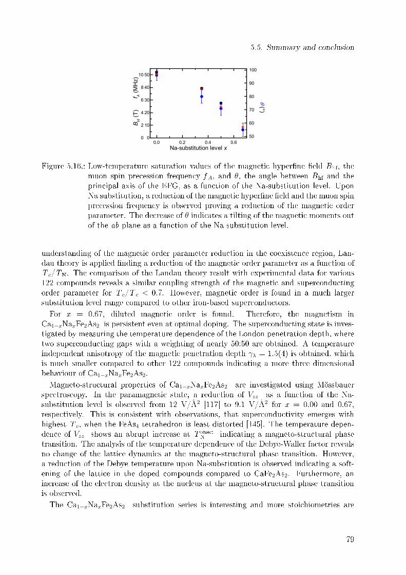
5.5. Summary and conclusion
0.0 0.2 0.4 0.60
10
20
30
40
50
Na-substitution level x
f A (M
Hz)
50
60
70
80
90
100
(°)0
2
4
6
8
10
Bhf (T
)
Figure 5.16.: Low-temperature saturation values of the magnetic hyperne eld Bhf, themuon spin precession frequency f A, and θ, the angle between Bhf and theprincipal axis of the EFG, as a function of the Na-substitution level. UponNa substitution, a reduction of the magnetic hyperne eld and the muon spinprecession frequency is observed proving a reduction of the magnetic orderparameter. The decrease of θ indicates a tilting of the magnetic moments outof the ab-plane as a function of the Na-substitution level.
understanding of the magnetic order parameter reduction in the coexistence region, Lan-dau theory is applied nding a reduction of the magnetic order parameter as a function ofT c/TN. The comparison of the Landau theory result with experimental data for various122 compounds reveals a similar coupling strength of the magnetic and superconductingorder parameter for T c/T c < 0.7. However, magnetic order is found in a much largersubstitution level range compared to other iron-based superconductors.For x = 0.67, diluted magnetic order is found. Therefore, the magnetism in
Ca1−xNaxFe2As2 is persistent even at optimal doping. The superconducting state is inves-tigated by measuring the temperature dependence of the London penetration depth, wheretwo superconducting gaps with a weighting of nearly 50:50 are obtained. A temperatureindependent anisotropy of the magnetic penetration depth γλ = 1.5(4) is obtained, whichis much smaller compared to other 122 compounds indicating a more three dimensionalbehaviour of Ca1−xNaxFe2As2.Magneto-structural properties of Ca1−xNaxFe2As2 are investigated using Mössbauer
spectroscopy. In the paramagnetic state, a reduction of Vzz as a function of the Na-substitution level is observed from 12 V/Å2 [117] to 9.1 V/Å2 for x = 0.00 and 0.67,respectively. This is consistent with observations, that superconductivity emerges withhighest T c, when the FeAs4 tetrahedron is least distorted [145]. The temperature depen-dence of Vzz shows an abrupt increase at T onset
N indicating a magneto-structural phasetransition. The analysis of the temperature dependence of the Debye-Waller factor revealsno change of the lattice dynamics at the magneto-structural phase transition. However,a reduction of the Debye temperature upon Na-substitution is observed indicating a soft-ening of the lattice in the doped compounds compared to CaFe2As2. Furthermore, anincrease of the electron density at the nucleus at the magneto-structural phase transitionis observed.The Ca1−xNaxFe2As2 substitution series is interesting and more stoichiometries are
79

5. Mössbauer and muon spin relaxation spectroscopy of Ca1−xNaxFe2As2
0.0 0.1 0.2 0.3 0.4 0.5 0.60
20406080
100120140160180
TNonset
TN100 %
Tctem
pera
ture
(K)
Na-substitution level x
SDW
SC
PM
Figure 5.17.: Phase diagram of Ca1−xNaxFe2As2 obtained by µSR, Mössbauer spec-troscopy, and magnetic susceptibility measurements. T onset
N is the highesttemperature with a nite magnetic volume fraction. T 100%
N is the high-est temperature, where 100 % of the sample volume shows magnetic order.Mössbauer spectroscopy and µSR measurements result in equal values forT onset
N and T 100%N within error bars. T c is the superconducting transition
temperature. Above T onsetN , a paramagnetic (PM) phase is observed. Below
T 100%N , a antiferromagnetic spin density wave (SDW, red) is found. Below
T c, superconductivity (SC, blue) is found. The blue-red striped area marksthe coexistence region of magnetic order and superconductivity with 100 %magnetic volume fraction. At optimal doping, diluted magnetism is foundbelow T onset
N coexisting with superconductivity.
80

5.5. Summary and conclusion
needed to study the x -dependence of the frequency ratio f A/f B as well as the suppressionof the magnetic order for x > 0.00. This would also answer the question, at which x
the long-range magnetic order is changed to the diluted magnetism observed at optimaldoping. Additionally, the determination of the low-temperature crystallographic structureof Ca1−xNaxFe2As2 for nite x is necessary to prove the assumption of a Fmmm phase.
81
5. Mössbauer and muon spin relaxation spectroscopy of Ca1−xNaxFe2As2
82
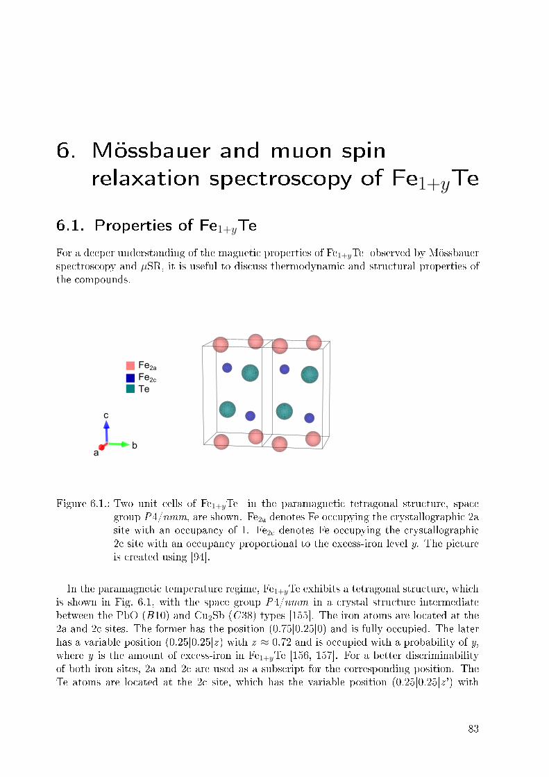
6. Mössbauer and muon spin
relaxation spectroscopy of Fe1+yTe
6.1. Properties of Fe1+yTe
For a deeper understanding of the magnetic properties of Fe1+yTe observed by Mössbauerspectroscopy and µSR, it is useful to discuss thermodynamic and structural properties ofthe compounds.
b
c
a
Fe2a
Fe2c
Te
ab
c
Figure 6.1.: Two unit cells of Fe1+yTe in the paramagnetic tetragonal structure, spacegroup P4/nmm, are shown. Fe2a denotes Fe occupying the crystallographic 2asite with an occupancy of 1. Fe2c denotes Fe occupying the crystallographic2c site with an occupancy proportional to the excess-iron level y. The pictureis created using [94].
In the paramagnetic temperature regime, Fe1+yTe exhibits a tetragonal structure, whichis shown in Fig. 6.1, with the space group P4/nmm in a crystal structure intermediatebetween the PbO (B10) and Cu2Sb (C38) types [155]. The iron atoms are located at the2a and 2c sites. The former has the position (0.75|0.25|0) and is fully occupied. The laterhas a variable position (0.25|0.25|z ) with z ≈ 0.72 and is occupied with a probability of y,where y is the amount of excess-iron in Fe1+yTe [156, 157]. For a better discriminabilityof both iron sites, 2a and 2c are used as a subscript for the corresponding position. TheTe atoms are located at the 2c site, which has the variable position (0.25|0.25|z ') with
83

6. Mössbauer and muon spin relaxation spectroscopy of Fe1+yTe
Figure 6.2.: Temperature dependence of the specic heat, Cp(T ), of Fe1+yTe for variousexcess-iron levels y. For y = 0.06, a sharp rst-order phase transition is ob-served at 70 K. By increasing y, the transition temperature decreases to 57 Kat y = 0.11. For y = 0.13, a λ-shaped peak at 57 K and a rst-order peak at46 K are observed. Fe1.15Te shows a λ-shaped peak at 63 K. Pictures takenfrom Ref. [155].
84

6.1. Properties of Fe1+yTe
z ' ≈ 0.28 and is fully occupied [156, 157]. The lattice parameters a and c decrease withincreased amount of excess-iron y [157].In the magnetically ordered phase for y ≤ 0.11, the crystallographic structure changes
from tetragonal to monoclinic. This low-temperature phase has the space group P21/m[155, 156]. For y ≥ 0.12, the crystallographic structure in the magnetically ordered phaseis orthorhombic with the space group Pmmn [155, 156].The temperature dependence of the specic heat Cp(T ) is shown in Fig. 6.2 for various
excess-iron levels y. Fe1.06Te shows a sharp rst-order like peak at 70 K, which is identiedwith the magneto-structural phase transition [155]. By increasing the amount of the excess-iron y, the transition temperature is suppressed to 57 K for Fe1.11Te [155]. The behaviourchanges for y ≥ 0.12, where two distinct phase transitions occur. For Fe1.13Te, a λ-shapedpeak at 57 K and a rst-order peak at 46 K is observed. The peak at higher temperaturescan be identied with the magnetic phase transition, while the peak at lower temperaturescorresponds to the tetragonal-to-orthorhombic phase transition [155], which is uncommonamong the iron pnictides and chalcogenides, where usually the structural phase transitionoccurs at the same or higher temperatures than the magnetic phase transition. Fe1.15Teshows a λ-shaped peak at 63 K, which is identied with the magnetic phase transition[155].The temperature dependence upon cooling and heating of the magnetic-susceptibility,
χ, measured in an applied eld of 100 mT in eld-cooled condition, is shown in Fig. 6.3(a)for various excess-iron levels [156]. By increasing y, the magnitude of χ increases due tothe magnetic moment of the excess-iron supporting results from DFT calculations [158].The temperature dependence of χ for Fe1.11Te shows a small thermal hysteresis. Thisindicates the rst-order character of the phase transition. A broader thermal hysteresiswas observed for Fe1.12Te and Fe1.13Te. This indicates two consecutive phase transitions.For y ≥ 0.14, no thermal hysteresis was observed, which is a sign for a continuous phasetransition.The temperature dependence of the normalized resistance R/R300K for y = 0.11, 0.12,
0.13, 0.14, and 0.15 is shown in Fig. 6.3(a). For y = 0.11, 0.12, and 0.13, a metallic be-haviour is observed below the phase transition. In contrast, the resistance of samples withy = 0.14 and 0.15 increases below the phase transition. This behaviour can be also seenin the temperature dependence of the resistivity, which is shown in Fig. 6.3(b). Resistivityvalues of the order of mΩ cm indicate semi-metallic behaviour [156]. For y = 0.11, athermal hysteresis is observed. For y = 0.12 and 0.13, a broadened thermal hysteresis isobserved and for y = 0.14 and 0.15 no thermal hysteresis is observed. Therefore, resistivityand magnetic-susceptibility measurements show similar behaviour in the excess-iron leveldependence of the thermal hysteresis [156].The rst studies of the magnetic low-temperature phase were of theoretical nature.
DFT calculations by Subedi et al. predict an electronic structure, which is similar tothose of the iron pnictides [60]. This includes strong (π,0) Fermi surface nesting resultingin a large SDW gap. However, neutron-scattering experiments [157, 159] and ARPESmeasurements [160] reveal a dierent behaviour. The obtained magnetic and electronicstructure is shown in Figs. 6.4(a) and 6.4(b). In contrast to the 122 compounds, which showa collinear antiferromagnetic order with a propagation vector (π, 0), neutron-scatteringexperiments evidenced a (δπ,δπ) bicollinear antiferromagnetic ordering, which is rotated
85
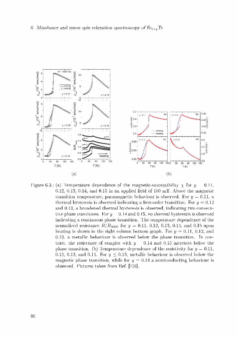
6. Mössbauer and muon spin relaxation spectroscopy of Fe1+yTe
(a) (b)
Figure 6.3.: (a) Temperature dependence of the magnetic-susceptibility χ for y = 0.11,0.12, 0.13, 0.14, and 0.15 in an applied eld of 100 mT. Above the magnetictransition temperature, paramagnetic behaviour is observed. For y = 0.11, athermal hysteresis is observed indicating a rst-order transition. For y = 0.12and 0.13, a broadened thermal hysteresis is observed, indicating two consecu-tive phase transitions. For y = 0.14 and 0.15, no thermal hysteresis is observedindicating a continuous phase transition. The temperature dependence of thenormalized resistance R/R300K for y = 0.11, 0.12, 0.13, 0.14, and 0.15 uponheating is shown in the right column bottom graph. For y = 0.11, 0.12, and0.13, a metallic behaviour is observed below the phase transition. In con-trast, the resistance of samples with y = 0.14 and 0.15 increases below thephase transition. (b) Temperature dependence of the resistivity for y = 0.11,0.12, 0.13, and 0.14. For y ≤ 0.13, metallic behaviour is observed below themagnetic phase transition, while for y = 0.14 a semiconducting behaviour isobserved. Pictures taken from Ref. [156].
86
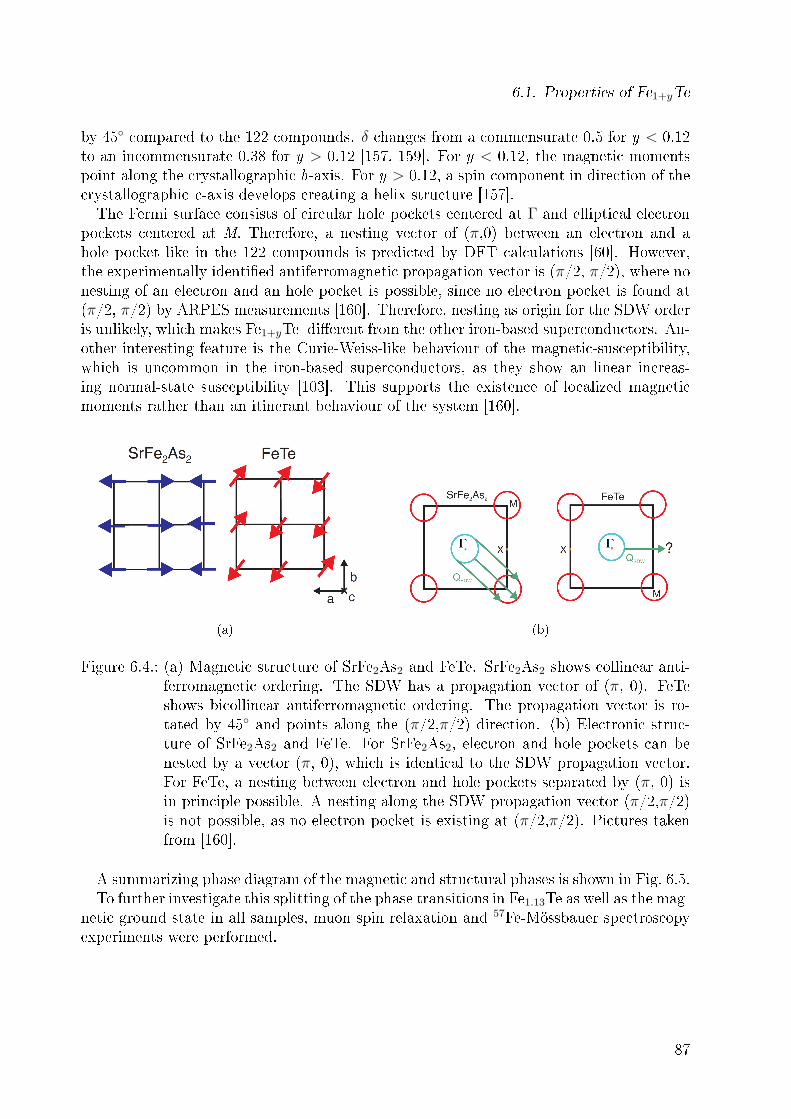
6.1. Properties of Fe1+yTe
by 45 compared to the 122 compounds. δ changes from a commensurate 0.5 for y < 0.12to an incommensurate 0.38 for y > 0.12 [157, 159]. For y < 0.12, the magnetic momentspoint along the crystallographic b-axis. For y > 0.12, a spin component in direction of thecrystallographic c-axis develops creating a helix structure [157].The Fermi surface consists of circular hole pockets centered at Γ and elliptical electron
pockets centered at M. Therefore, a nesting vector of (π,0) between an electron and ahole pocket like in the 122 compounds is predicted by DFT calculations [60]. However,the experimentally identied antiferromagnetic propagation vector is (π/2, π/2), where nonesting of an electron and an hole pocket is possible, since no electron pocket is found at(π/2, π/2) by ARPES measurements [160]. Therefore, nesting as origin for the SDW orderis unlikely, which makes Fe1+yTe dierent from the other iron-based superconductors. An-other interesting feature is the Curie-Weiss-like behaviour of the magnetic-susceptibility,which is uncommon in the iron-based superconductors, as they show an linear increas-ing normal-state susceptibility [103]. This supports the existence of localized magneticmoments rather than an itinerant behaviour of the system [160].
(a) (b)
Figure 6.4.: (a) Magnetic structure of SrFe2As2 and FeTe. SrFe2As2 shows collinear anti-ferromagnetic ordering. The SDW has a propagation vector of (π, 0). FeTeshows bicollinear antiferromagnetic ordering. The propagation vector is ro-tated by 45 and points along the (π/2,π/2) direction. (b) Electronic struc-ture of SrFe2As2 and FeTe. For SrFe2As2, electron and hole pockets can benested by a vector (π, 0), which is identical to the SDW propagation vector.For FeTe, a nesting between electron and hole pockets separated by (π, 0) isin principle possible. A nesting along the SDW propagation vector (π/2,π/2)is not possible, as no electron pocket is existing at (π/2,π/2). Pictures takenfrom [160].
A summarizing phase diagram of the magnetic and structural phases is shown in Fig. 6.5.To further investigate this splitting of the phase transitions in Fe1.13Te as well as the mag-
netic ground state in all samples, muon spin relaxation and 57Fe-Mössbauer spectroscopyexperiments were performed.
87

6. Mössbauer and muon spin relaxation spectroscopy of Fe1+yTe
0.04 0.06 0.08 0.10 0.12 0.140
20
40
60
80
100
120
tem
pera
ture
T(K
)
excess Fe level y
ICSDWPmmn
paramagneticP4/nmm
CSDWP21/m
unknown phase
magnetic phaseP4/nmm
Figure 6.5.: Phase diagram of Fe1+yTe composed out of data from specic heat [155],magnetic-susceptibility [156], and x-ray diraction [156] measurements as wellas neutron-scattering experiments [157, 159]. The high-temperature phaseconsists of a paramagnetic phase with tetragonal structure. For y < 0.11, thelow-temperature phase consists of a commensurate spin density wave (SDW)phase and a monoclinic structure. For y > 0.12, two phase transitions occur.The transition at higher temperatures is followed by a complicated magneticphase and a tetragonal structure. The low-temperature phase shows an in-commensurate SDW state and an orthorhombic structure.
88

6.2. Experimental details
6.2. Experimental details
Powder samples with the compositions Fe1.06Te, Fe1.12Te, Fe1.13Te, and Fe1.15Te were suc-cessfully synthesised by Cevriye Koz at the Max-Planck-Institut für Chemische Physikfester Stoe in Dresden. For details of the synthesis see Ref. [161].µSR experiments were performed on samples of Fe1.06Te, Fe1.12Te, and Fe1.13Te with
≈ 150 mg sample mass for each composition. The experiments were performed at the πM3beamline of the Swiss Muon Source at the Paul Scherrer Institut, Villigen, Switzerland,using the GPS spectrometer. The muon spin relaxation was measured in temperaturesranging from 5 up to 300 K in zero (ZF), longitudinal (LF) and transverse (TF) eldgeometry using external magnetic elds up to 400 mT. The µSR data were analysed usingthe MUSRFIT software [101].I performed the Mössbauer spectroscopy (MBS) experiments for Fe1.06Te, Fe1.13Te, and
Fe1.15Te at the Institut für Festkörperphysik, TU Dresden, in transmission geometry ina temperature range between 4.2 and 300 K using a CryoVac Konti IT cryostat. As aγ-source, 57Co in rhodium matrix was used. The dierent compositions were preparedwith ≈ 50 mg sample mass. To ensure a homogeneous distribution of the powder in thesample holder, ethanol was used. The data were analysed using the MOESSFIT software[32].
6.3. Results and discussion
6.3.1. Mössbauer spectroscopy results
Paramagnetic high-temperature phase
The room-temperature Mössbauer spectra for all compositions are shown in Fig 6.6(a).They show a slightly asymmetric doublet structure, which indicates the absence of magneticorder. The asymmetry of the doublet A is based on the angle φ between the incident γ-raydirection and the principal axis of the electric eld gradient (EFG) and is described by
A(φ) =1 + cos2(φ)23+ sin2(φ)
. (6.1)
As the experiment was performed using powder samples, one would expect an asymmetryof A = 1 due to the averaging over all angles φ. In the analysing process, there are twopossibilities to model an asymmetry of one: 1) Averaging over all angles φ or 2) settingthe angle φ to a value of arccos(1/
√3) ≈ 54.7, which is called the magic angle. As it is
shown in Fig 6.6(a), a small asymmetry is observed at room temperature. These deviationfrom A = 1 can be explained by a texture eect, which occurs, when the crystallites inthe powder are not spherical but consist of small platelets. This platelets arrange in a notfully randomized orientation resulting in an eective angle φe deviating from the magicangle corresponding to A = 1. The obtained angles are φe =56(1) and hence only dierby < 3 % from the magic angle supporting a small texture eect.The Fe atoms are located at the 2a and 2c sites, which have the point symmetries
89

6. Mössbauer and muon spin relaxation spectroscopy of Fe1+yTe
4m2 and 4mm. This ensures axial symmetry (asymmetry parameter η = 0) and a niteEFG at each iron site. The principal axis of EFG2a and EFG2c are directed along thecrystallographic c-axis.
-2 -1 0 1 2
0.90
0.95
1.00
1.05
1.10
Fe1.06Te Fe1.13Te Fe1.15Te
trans
mission
v (mm/s)
(a)
0 20 40 600.00
0.05
0.10
0.15 Fe1.06Te Fe1.13Te Fe1.15Te
n(Vzz)
Vzz (V/Å2)
(b)
Figure 6.6.: (a) Mössbauer spectra of Fe1.06Te, Fe1.13Te, and Fe1.15Te at room tempera-ture. The transmission of Fe1.06Te and Fe1.13Te is shifted by 0.10 and 0.05,respectively, for illustration purposes. (b) Distribution n(Vzz) extracted fromthe room temperature Mössbauer spectra.
The Mössbauer spectra at room temperature are analysed using a doublet pattern anisomer shift δ and the z -component of the EFG, Vzz. As there are two crystallographicinequivalent iron sites, where only the 2a site is fully occupied and the 2c site is partiallyoccupied, at least two dierent EFGs are expected. Therefore, a distribution of Vzz val-ues is assumed. The probability distribution n(Vzz) was obtained by using a maximum-entropy method, which is included in the MOESSFIT software [32]. The result is shownin Fig. 6.6(b) and shows two features at Vzz = 20(1) V/Å2 and 42(1) V/Å2. The rstis a peak with the majority of the spectral weight of the probability distribution. Thesecond is a broad shoulder for y = 0.06 and 0.13, which turns into a well-dened peak fory = 0.15. By increasing the amount of excess-iron, spectral weight is shifted from the peakat 20 V/Å2 to the feature at 42 V/Å2. Analysing the spectral weight of the two features,one can extract the relative intensity of the two features at 20 V/Å2(42 V/Å2), which are0.91 (0.09), 0.85 (0.15), and 0.80 (0.20) for y = 0.06, 0.13, and 0.15 respectively. To relatethe two peaks to the two dierent iron sites, one has to take into account the propertiesof the 2a and 2c iron sites. The 2a site is fully occupied and the 2c site is occupied with aprobability given by the amount of excess-iron y. Therefore, the total amount of iron in thesystem is 1+y with y
1+yand 1
1+ybeing the relative amount of iron on the 2a and 2c sites.
Applying this to the investigated samples, relative amounts of 0.94 (0.06), 0.88 (0.12), and0.87 (0.13) for y = 0.06, 0.13, and 0.15, respectively, for the iron 2a (2c) site would beexpected. Comparing this relative amounts of iron with the relative intensities of the twofeatures in n(Vzz) gives reasonable agreements for y = 0.06 and 0.13. For y = 0.15, theagreement is moderate, which can be explained by the higher degree of disorder due to thelarge amount of excess-iron in the system. In addition, the 2a site is directly located on thetetragonal lattice, while the 2c site is located between the FeTe tetrahedrons. Therefore,one would expect a higher EFG for the 2c than for the 2a site. Due to this reasons, the
90
6.3. Results and discussion
peak at 20 V/Å2 is identied with iron occupying the 2a site and the peak at 42 V/Å2
with the 2c site and hence the system contains two inequivalent iron sites.For further analysis in the paramagnetic temperature regime, two doublet patterns are
used to investigate the measured Mössbauer spectra. A set of hyperne parameters δ andVzz is assigned to each doublet pattern corresponding to the two iron sites 2a and 2c withthe same relative intensities as obtained by the analysis of n(Vzz). At room-temperature,the obtained values of Vzz,2a are 17.2(6) V/Å2, 18.4(1) V/Å2, and 17.2(6) V/Å2, whilethe second pattern has values of Vzz,2c = 32(1) V/Å2, 38(1) V/Å2, and 36(2) V/Å2 fory = 0.06, 0.13, and 0.15, respectively. This values are in good agreement with the moregeneral approach of the distribution n(Vzz). With decreasing temperature, Vzz,2a increasesslightly to values of 19.6(3) V/Å2, 21.0(3) V/Å2, and 20.5(5) V/Å2, while Vzz,2c increasesto 40(1) V/Å2, 39.3(9) V/Å2, and 40(1) V/Å2 for y = 0.06, 0.13, and 0.15 at T ≈ 80 K,respectively. Vzz was xed for temperatures below 80 K to reduce the number of freeparameters in the magnetically ordered phase.The temperature dependence of the center shift δ is shown in Figs. 6.7(a), 6.7(b), and
6.7(c). Both center shifts δ2a and δ2c are of equal value within error bars in the paramag-netic temperature regime. Values of 0.472(5) mm/s, 0.482(5) mm/s, and 0.479(5) mm/s areobtained at room temperature for y = 0.06, 0.13, and 0.15, which increase to 0.60(2) mm/s,0.614(5) mm/s, and 0.62(2) mm/s at ≈ 80 K, respectively. For y = 0.06, δ2a and δ2c areof equal value in the magnetically ordered state. With decreasing temperature, the isomershift increases to a value of δ2a,2c = 0.63(1) mm/s at 4.2 K.For y = 0.13 and 0.15 a splitting below 80 K is visible. With δ2a = 0.69(3) mm/s
and δ2a = 0.67(3) mm/s the a site center shifts are smaller than δ2c = 0.79(2) mm/s andδ2c = 0.74(3) mm/s at 4.2 K, respectively. Therefore, the s-electron density at the nucleusis higher for the 2a site than for the 2c site. However, the electron density of the 1s-,2s-, and 3s-electrons is nearly constant [24]. In contrast, the 3d -electrons can screen the4s-electrons. A more itinerant behaviour of the 3d -electrons results in a reduced screeningof the 4s-electrons and, therefore, an increased electron density at the nucleus. I.e., the 2asite shows a more itinerant behaviour than the 2c site, which supports results from DFTcalculations [158].
Magnetic low-temperature phase
The onset temperature of the magnetic ordering, T onsetN , is dened as the temperature, at
which the Mössbauer linewidth, w, shows an abrupt increase due to the appearance of amagnetic hyperne eld. The Mössbauer spectra in the magnetically ordered temperatureregime are analysed using two subspectra. Each subspectrum contains a set of hyperneparameters: δ, Vzz, w and the magnetic hyperne eld Bhf. The centers shifts are δ2a andδ2c and their temperature dependence is shown in Figs. 6.7(a), 6.7(b), and 6.7(c). Vzz wasxed in the magnetically ordered state to its value at ≈ 80 K. First, the magnetic hyperneelds at the 2a and 2c sites are analysed using a maximum-entropy method. The resultof this rst and most general analysis is, that the magnetic hyperne eld at the 2c siteshows a Gaussian distribution. Taking into account the small relative intensity of the 2cpattern and to reduce the amount of parameters, it is convenient to analyse Bhf at the 2c
91

6. Mössbauer and muon spin relaxation spectroscopy of Fe1+yTe
0 25 50 75 290 300
0.56
0.58
0.60
0.62
0.64
0.66
(T)
temperature (K)
Fe1.06Te
(a)
0 25 50 75 290 300
0.50
0.55
0.60
0.65
0.70
0.75
0.80
Fe2a
Fe2c
FePM (T
)
temperature (K)
Fe1.13Te
(b)
0 25 50 75 300
0.50
0.55
0.60
0.65
0.70
0.75
0.80
Fe2a
Fe2c
FePM
(T)
temperature (K)
Fe1.15Te
(c)
Figure 6.7.: Temperature dependence of the center shift δ(T ) of (a) Fe1.06Te, (b) Fe1.13Te,and (c) Fe1.15Te. For Fe1.06Te, both δ2a and δ2c are of equal value over thewhole temperature range. For Fe1.13Te and Fe1.15Te, both δ2a and δ2c are ofequal value and denoted as FePM in the paramagnetic temperature regime. Inthe magnetically ordered state, δ2a and δ2c have dierent values.
92

6.3. Results and discussion
site with a magnetic hyperne eld, which is Gauss-distributed:
n(Bhf) =1√2πσ
exp
(−1
2
[B −B2c]2
σ2
), (6.2)
with the rst moment B2c and the standard deviation σ. The magnetic eld distribu-tion at site 2a was determined by maximum entropy at all temperatures. The resultingdistributions at 4.2 K are shown in Figs. 6.8(a), 6.8(b), and 6.8(c).
0 2 4 6 8 10 12 14 16 18 20 22 24 26 28 30
0.0
0.1
0.2
0.3
0.4
n 2a(B)
B (T)
Fe1.06Te4.2 K
(a)
0 2 4 6 8 10 12 14 16 18 20 22 24 26 28 30
0.00
0.05
0.10
0.15
0.20
n 2a(B)
B (T)
Fe1.13Te4.2 K
(b)
0 2 4 6 8 10 12 14 16 18 20 22 24 26 28 30
0.00
0.05
0.10
0.15
n 2a(B)
B (T)
Fe1.15Te4.2 K
(c)
Figure 6.8.: Magnetic eld distribution n2a(B) of Fe1+yTe with y = 0.06, 0.13, and 0.15at 4.2 K. The red line in (a) shows the Gaussian magnetic eld distribution ofthe excess-iron for y = 0.06 (scaled for comparison purposes).
Magnetic order in Fe1.06Te
The Mössbauer spectrum at 4.2 K is shown in Fig. 6.9, where a well-resolved sextet struc-ture is visible, which is a sign for a well-dened Bhf-value. The temperature dependence ofthe magnetic volume fraction is shown in Fig. 6.10(b) together with results from TF-µSRmeasurements, which are discussed in Sec. 6.3.2. Below 72 K, static magnetic order isobserved by Mössbauer spectroscopy, while µSR detects magnetic order up to ≈ 100 K.At 65 K, the magnetic volume fraction approaches 100 %. The 5 % non-magnetic samplefraction measured by µSR is attributed to muons stopping outside the sample (e.g. the
93

6. Mössbauer and muon spin relaxation spectroscopy of Fe1+yTe
-6 -4 -2 0 2 4 6
0.86
0.88
0.90
0.92
0.94
0.96
0.98
1.00
1.02
Fe1.06Te Fe1.13Te (x2) Fe1.15Te (x2)
trans
mission
v (mm/s)
Figure 6.9.: Mössbauer spectra at 4.2 K of Fe1+yTe with y = 0.06, 0.13, and 0.15 includingbest ts. The absorption for y = 0.13 and 0.15 is doubled for illustrationpurposes.
cryostat). The magnetic hyperne eld at both Fe sites are of equal value within errorbars within the investigated temperature range, as it is shown in Fig 6.10(a). The mag-netic eld distribution at the 2a site at 4.2 K shows a peak at ≈ 11 T. In Fig. 6.8(a), themagnetic eld distribution at the 2a site and the Gaussian eld distribution at the 2c site(scaled for comparison purposes) is plotted and both are virtually congruent. Therefore,I conclude, that both Fe sites show the same magnetic properties within the resolution ofthe Mössbauer spectroscopy. The Gaussian behaviour of both magnetic hyperne elds in-stead of a Lorentzian is attributed to the disorder introduced by the excess-iron comparedto a theoretical FeTe compound.
0 20 40 600
2
4
6
8
10
12
14
16
18
Fe1.06Te: Fe2a
Fe2c
mag
netic
hyp
erfin
e fie
ld (T
)
temperature (K)
(a)
0 20 40 60 80 1000.0
0.5
1.0
Fe1.06Te: SR MBS
mag
netic
vol
ume
fract
ion
temperature (K)
(b)
Figure 6.10.: (a) Temperature dependence of the average magnetic hyperne eld of themagnetic eld distribution at the 2a site as well as the temperature depen-dence of the rst moment of the Gaussian magnetic eld distribution at the2c site for Fe1.06Te. (b) Temperature dependence of the magnetic volumefraction determined by Mössbauer spectroscopy and TF-µSR.
94

6.3. Results and discussion
Magnetic order in Fe1.13Te and Fe1.15Te
The Mössbauer spectra of Fe1.13Te and Fe1.15Te at 4.2 K are shown in Fig. 6.9. They showa less-clear resolved sextet structure compared to Fe1.06Te. This can be explained by eithera magnetic eld distribution or magnetically inequivalent Fe sites or both. The magneticeld distributions of the 2a site at 4.2 K are shown in Figs. 6.8(b) and 6.8(c). They show arectangular shape consistent with the result in Ref. [162]. Blachowski et al. expanded themagnetic eld distribution in terms of Fourier coecients, which requires a periodic andpiecewise continuous distribution. This may be a too strong constriction of the possibleshape of the magnetic eld distribution. Maximum entropy determines the most proba-ble distribution without any restrictions of the shape of the distribution. Furthermore,the rectangular shape is comparable with a broadened incommensurate spin-density waveshape suggested by neutron-scattering experiments [157]. The temperature dependence of
0 10 20 30 40 50 60 70 80024681012141618
Fe1.13Te: Fe2a
Fe2c
mag
entic
hyp
erfin
e fie
ld (T
)
temperature (K)
(a)
0 20 40 60 80 100 120 1400.0
0.5
1.0Fe1.12Te:
SRFe1.13Te:
MBS SR
mag
netic
vol
ume
fract
ion
temperature (K)
(b)
Figure 6.11.: (a) Temperature dependence of the average magnetic hyperne eld of themagnetic eld distribution at the 2a site as well as the temperature depen-dence of the rst moment of the Gaussian magnetic eld distribution at the2c site of y = 0.13. (b) Temperature dependence of the magnetic volume frac-tion determined by Mössbauer spectroscopy and TF-µSR for Fe1+yTe withy = 0.12 and 0.13.
the average value of the magnetic eld distribution at the 2a site as well as the rst momentof the Gauss-distributed magnetic hyperne eld at the 2c site is shown in Figs. 6.11(a)and 6.12(a). At temperatures slightly below the magnetic transition temperature, bothBhf, 2a and Bhf, 2c are of equal value within error bars. For Fe1.13Te, a splitting occurs be-low the structural phase transition at 46 K supporting the strong magneto-elastic couplingscenario in this compounds [155, 156, 163]. For Fe1.15Te, a splitting is obtained down tolowest temperatures, but the onset of the splitting cannot be determined due to the lackof data points between 4.2 K and 50 K. It should be expected at 45 K, where Rössler etal. report the structural transition temperature [155].The temperature dependence of the magnetic volume fraction is shown in Fig. 6.11(b)
together with results from TF-µSR-measurements, which are discussed in Sec. 6.3.2. Möss-bauer spectroscopy measurements show magnetic order below 70 K and 85 K and 100 %magnetic volume fraction below 60 K for y = 0.13 and 0.15, respectively. TF-µSR-
95
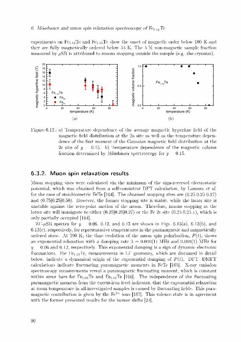
6. Mössbauer and muon spin relaxation spectroscopy of Fe1+yTe
experiments on Fe1.12Te and Fe1.13Te show the onset of magnetic order below 100 K andthey are fully magnetically ordered below 55 K. The 5 % non-magnetic sample fractionmeasured by µSR is attributed to muons stopping outside the sample (e.g. the cryostat).
0 20 40 60 8002468101214161820
Fe1.15Te: Fe2a
Fe2c
mag
netic
hyp
erfin
e fie
ld (T
)
temperature (K)
(a)
0 20 40 60 800.0
0.5
1.0
mag
netic
vol
ume
fract
ion
temperature (K)
Fe1.15Te
(b)
Figure 6.12.: a) Temperature dependence of the average magnetic hyperne eld of themagnetic eld distribution at the 2a site as well as the temperature depen-dence of the rst moment of the Gaussian magnetic eld distribution at the2c site of y = 0.15. b) Temperature dependence of the magnetic volumefraction determined by Mössbauer spectroscopy for y = 0.15.
6.3.2. Muon spin relaxation results
Muon stopping sites were calculated via the minimum of the sign-reversed electrostaticpotential, which was obtained from a self-consistent DFT calculation, by Lamura et al.
for the case of stoichiometric FeTe [164]. The obtained stopping sites are (0.25|0.25|0.27)and (0.75|0.25|0.50). However, the former stopping site is stable, while the latter site isunstable against the zero-point motion of the muon. Therefore, muons stopping at thelatter site will immigrate to either (0.25|0.25|0.27) or the Fe 2c site (0.25|0.25|z ), which isonly partially occupied [164].ZF-µSR spectra for y = 0.06, 0.12, and 0.13 are shown in Figs. 6.13(a), 6.13(b), and
6.13(c), respectively, for representative temperatures in the paramagnetic and magneticallyordered state. At 290 K, the time evolution of the muon spin polarization, P(t), showsan exponential relaxation with a damping rate λ = 0.040(1) MHz and 0.068(1) MHz fory = 0.06 and 0.12, respectively. This exponential damping is a sign of dynamic electronicuctuations. For Fe1.13Te, measurements in LF geometry, which are discussed in detailbelow, indicate a dynamical origin of the exponential damping of P(t). DFT+DMFTcalculations indicate uctuating paramagnetic moments in FeTe [165]. X-ray emissionspectroscopy measurements reveal a paramagnetic uctuating moment, which is constantwithin error bars for Fe1.03Te and Fe1.12Te [166]. The independence of the uctuatingparamagnetic moment from the excess-iron level indicates, that the exponential relaxationat room temperature in all investigated samples is caused by uctuating elds. This para-magnetic contribution is given by the Fe2+ ions [167]. This valence state is in agreementwith the former presented results for the isomer shifts [24].
96

6.3. Results and discussion
0 1 2 3 40.0
0.2
0.4
0.6
0.8
1.0
290 K Fe1.06Te 5 K
muo
n sp
in p
olar
izat
ion P
(t)
time ( s)
(a)
0 1 2 3 40.0
0.2
0.4
0.6
0.8
1.0
290 K Fe1.12Te 5 K
muo
n sp
in p
olar
izat
ion P
(t)
time ( s)
(b)
0 2 4 6 80.0
0.2
0.4
0.6
0.8
1.0
100 K Fe1.13Te 5 K
muo
n sp
in p
olar
izat
ion P
(t)
time ( s)
(c)
Figure 6.13.: Time evolution of the muon spin polarization P(t) at temperatures above andbelow the magnetic transition temperatures of 65 K for (a) Fe1.06Te, 55 Kfor (b) Fe1.12Te, and (c) Fe1.13Te, respectively. Solid lines are best ts usingEq. (6.3).
97

6. Mössbauer and muon spin relaxation spectroscopy of Fe1+yTe
Magnetic order in Fe1+yTe
µSR measurements in TF geometry in an applied eld of 5 mT were performed at tempera-tures between 5 K and 300 K for Fe1.06Te, Fe1.12Te, and Fe1.13Te. The resulting temperaturedependence of the magnetic volume fraction is shown in Figs. 6.10(b) and 6.11(b). A non-zero magnetic volume fraction is obtained for temperatures below 100-110 K. By reducingthe temperature, the magnetic volume fraction increases until it reaches nearly 100 % at65 K for Fe1.06Te, at 55 K for Fe1.12Te and at 60 K for Fe1.13Te. The small amount ofnon-magnetic volume fraction arises from muons stopping inside the sample holder.ZF measurements in the magnetic phase below ≈ 100 K show two signal fractions cor-
responding to two magnetically inequivalent muon stopping sites. The time evolution ofthe muon spin polarization is analysed using the function
P (t) = VmagAosc
[2
3Gosc(fµ, t)e
−λT,osct +1
3e−λL,osct
]+ VmagAnonosc
[2
3e−λT,nonosct +
1
3e−λL,nonosct
]+ [1− Vmag] e
−λPMt, (6.3)
similar to Eq. (2.37) with the magnetic volume fraction Vmag, the transversal relaxationrates λT and the longitudinal relaxation rates λL. Gosc(fµ, t) denotes an oscillation functionas a function of time t and the muon spin precession frequency fµ. The paramagnetic sig-nal fraction is modelled using a simple exponential relaxation function with a temperatureindependent relaxation rate λPM. The two magnetically inequivalent muon stopping sitesare occupied with probabilities of Aosc and Anonosc under the condition Aosc+ Anonosc = 1.The occupation probability Aosc has temperature-independent values of 0.96, 0.80, and0.76 for Fe1.06Te, Fe1.12Te, and Fe1.13Te, respectively. However, the 2/3-part (see Sec. 2.6.3for more details about the origin of the 2/3 signal fraction) of both magnetic signals, Aosc
and Anonosc, are fully damped within the rst 20 ns of P(t). This strong damping indicatesa higher degree of disorder in the system due to the excess-iron resulting in transversalrelaxation rates of the order of a few hundred MHz. This high damping caused experi-mental diculties, as the the time resolution of the spectrometer was of the order of 1 ns.Therefore, high statistic measurements were needed resulting in long measurement times.As the beamtime at the PSI was highly limited for Fe1.06Te and Fe1.12Te, only the mostimportant temperatures were investigated by means of ZF-µSR. For Fe1.13Te, more beamtime was available resulting in more ZF data points. To analyse the form of the relaxationin this rst 20 ns of P(t), dierent relaxation functions with and without an oscillationare used and the coecients of determination of the resultant ts are compared. Thesecoecients are a measure for the quality of the analysis as a function of the sample sizeand the number of parameters. The most probable result is the following. The oscillationfunction Gosc(fµ, t) is a cosine for Fe1.06Te, which is identied with long-range commensu-rate magnetic order. The oscillation frequency at 5 K is obtained as fµ= 168(10) MHz,which corresponds to a eld of B = 197(12) mT at the muon stopping site. This is in goodagreement with measurements at Fe1.03Te and Fe1.087Te, where values of 210 mT [168] and197(11) mT [164] are reported. For Fe1.12Te and Fe1.13Te, Gosc(fµ, t) is best described by
98

6.3. Results and discussion
a 0 th-order Bessel function, which is identied with long-range incommensurate magneticorder. The oscillation frequency at 5 K is obtained as fµ= 73(6) MHz, which correspondsto a eld of B = 86(7) mT at the muon stopping site. Muons, stopping at the site de-scribed by Anonosc, show no coherent oscillation of the muon spins. This is consistent witha very broad internal magnetic eld distribution at this muon stopping site preventing acoherent oscillation of the muon spins.As a consequence of this strong static damping, after 20 ns only the 1/3-tail parts of
the signal are observed. The ZF spectra at 5 K, which are shown in Figs. 6.13(a), 6.13(b)and 6.13(c), show an exponential relaxation of the 1/3-tail, which is caused by magneticeld uctuations. Above 70 K, where TF-µSR measurements show a magnetic volumefraction below 15 %, both λLs are of the same order of magnitude as the relaxation rate ofthe paramagnetic volume fraction, λPM. Both λL increase between 60 K and 70 K due toenhanced low-frequency magnetic uctuations above the magnetic transition temperature.In the fully ordered state, both λLs decreases, which indicates a slowing down of the elductuations and a more static internal eld distribution.Taking into account the two dierent muon sites proposed by DFT calculations [164],
the two signal fractions can be interpreted in the following way: The Aosc-signal fractionis identied with muons stopping at a stable site (0.25|0.25|0.27) where they experiencelong-range magnetic order. The Anonosc-signal fraction is identied with muons stopping ata metastable site (0.75|0.25|0.50), which successfully move to a stable site. This movementresults in a broad internal eld distribution experienced by the muon, which prevents acoherent oscillation of the muon spin. This results in an exponential relaxation of the muonspin polarization. The reduction of the Aosc-signal fraction as a function of the excess-ironlevel is attributed to the higher degree of disorder in the system, which results in a broadereld distribution.
0 2 4 6 80.0
0.2
0.4
0.6
0.8
1.0
300 K 80 K 62.5 Km
uon
spin
pol
ariz
atio
n P
(t)
time ( s)
Fe1.13Te, 30 mT, LF
(a)
0 2 4 6 80.0
0.2
0.4
0.6
0.8
62.5 K 50 K 5 K
Fe1.13Te, 30 mT, LF
muo
n sp
in p
olar
izat
ion P
(t)
time ( s)
(b)
Figure 6.14.: Temperature dependence of the time evolution of the muon spin polarizationof Fe1.13Te in an applied longitudinal eld (LF) of 30 mT. Solid lines are bestts to Eq. (6.4).
To further investigate the dynamics in Fe1.13Te, µSR experiments in LF geometry inelds up to 400 mT at various temperatures between 5 K and 300 K were performed.The time evolution of the muon spin polarization in an applied LF of 30 mT is shown inFigs. 6.14(a) and 6.14(b) for various temperatures in the paramagnetic and magnetically
99
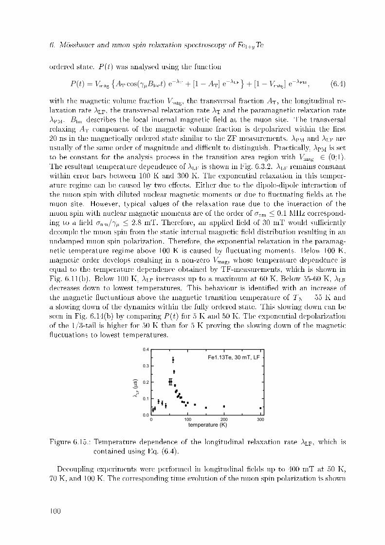
6. Mössbauer and muon spin relaxation spectroscopy of Fe1+yTe
ordered state. P(t) was analysed using the function
P (t) = VmagAT cos(γµBloct) e
−λT + [1− AT] e−λLF
+ [1− Vmag] e
−λPM , (6.4)
with the magnetic volume fraction Vmag, the transversal fraction AT, the longitudinal re-laxation rate λLF, the transversal relaxation rate λT and the paramagnetic relaxation rateλPM. Bloc describes the local internal magnetic eld at the muon site. The transversalrelaxing AT component of the magnetic volume fraction is depolarized within the rst20 ns in the magnetically ordered state similar to the ZF measurements. λPM and λLF areusually of the same order of magnitude and dicult to distinguish. Practically, λPM is setto be constant for the analysis process in the transition area region with Vmag ∈ (0;1).The resultant temperature dependence of λLF is shown in Fig. 6.3.2. λLF remains constantwithin error bars between 100 K and 300 K. The exponential relaxation in this temper-ature regime can be caused by two eects. Either due to the dipole-dipole interaction ofthe muon spin with diluted nuclear magnetic moments or due to uctuating elds at themuon site. However, typical values of the relaxation rate due to the interaction of themuon spin with nuclear magnetic moments are of the order of σnm ≤ 0.1 MHz correspond-ing to a eld σnm/γµ ≤ 2.8 mT. Therefore, an applied eld of 30 mT would sucientlydecouple the muon spin from the static internal magnetic eld distribution resulting in anundamped muon spin polarization. Therefore, the exponential relaxation in the paramag-netic temperature regime above 100 K is caused by uctuating moments. Below 100 K,magnetic order develops resulting in a non-zero Vmag, whose temperature dependence isequal to the temperature dependence obtained by TF-measurements, which is shown inFig. 6.11(b). Below 100 K, λLF increases up to a maximum at 60 K. Below 55-60 K, λLFdecreases down to lowest temperatures. This behaviour is identied with an increase ofthe magnetic uctuations above the magnetic transition temperature of TN = 55 K anda slowing down of the dynamics within the fully ordered state. This slowing down can beseen in Fig. 6.14(b) by comparing P(t) for 5 K and 50 K. The exponential depolarizationof the 1/3-tail is higher for 50 K than for 5 K proving the slowing down of the magneticuctuations to lowest temperatures.
0 100 200 3000.0
0.1
0.2
0.3
0.4
LF (
s)
temperature (K)
Fe1.13Te, 30 mT, LF
Figure 6.15.: Temperature dependence of the longitudinal relaxation rate λLF, which iscontained using Eq. (6.4).
Decoupling experiments were performed in longitudinal elds up to 400 mT at 50 K,70 K, and 100 K. The corresponding time evolution of the muon spin polarization is shown
100
6.3. Results and discussion
in Figs. 6.16(a), 6.16(b), and 6.16(c), respectively. The ZF-spectrum at 100 K shows a fastdepolarization from P(t = 0) = 1.00 to P(t = 20 ns) = 0.85 due to the static magnetic orderin parts of the sample volume. This fast depolarization is quenched by applying an externallongitudinal eld of 100 mT. This indicates, that the internal eld is small compared tothe applied external eld. Empirical experience shows, that the internal eld is around1/10 of the applied external eld, which decouples the muon spin from the internal-elddistribution. Therefore, the internal eld at the muon site is ≈ 10 mT. The time evolutionof the muon spin polarization for applied longitudinal elds of 100 mT and 400 mT is equaland shows an exponential relaxation with a relaxation rate of λ100K,400mT = 0.08(1) MHz.This provides evidence for uctuating elds at the muon site at 100 K. The ZF spectrum at70 K shows a fast depolarization from P(t = 0) = 1.0 to P(t = 20 ns) = 0.8 due to the staticmagnetic order in parts of the sample volume. The enlarged reduction of the polarizationby 20 %, compared to the 15 % at 100 K, indicates an increased volume fraction showingstatic order. This fast depolarization is quenched by applying an external longitudinaleld of 100 mT similar to the LF measurements at 100 K indicating a similar internaleld at the muon stopping site for both temperatures. Additionally, no change in P(t)at applied longitudinal elds between 100 mT and 400 mT is observed. At both appliedelds, an exponential relaxation with a relaxation rate of λ70K,400mT = 0.32(1) MHz isobserved, which is enhanced compared to λ100 K indicating an increase of the magnetic elductuations. The ZF spectrum at 50 K shows a fast depolarization from P(t = 0) = 1.00to P(t = 20 ns) = 0.33 due to the static magnetic order in 100 % of the sample volume.By applying an external longitudinal eld of 400 mT, the amplitude of the fast relaxationis reduced resulting in P(t = 20 ns) = 0.6. This indicates, that the internal eld at themuon stopping site is of the order of the external eld. This is in good agreement withthe internal magnetic eld of 86(7) mT obtained by ZF measurement. The exponentialrelaxation rate at 400 mT has a value of λ50K,400mT = 0.8(1) MHz. This indicates thepresence of magnetic uctuations slightly below the magnetic transition temperature of55 K.
101

6. Mössbauer and muon spin relaxation spectroscopy of Fe1+yTe
0 2 4 6 8-0.2
0.0
0.2
0.4
0.6
0.8
1.0
0 mT 20 mT 100 mT 400 mT
muo
n sp
in p
olar
izat
ion P
(t)
time ( s)
Fe1.13Te, 50 K, LF
(a)
0 2 4 6 80.0
0.2
0.4
0.6
0.8
1.0
0 mT 20 mT 100 mT 400 mT
Fe1.13Te, 70 K, LF
muo
n sp
in p
olar
izat
ion P
(t)
time ( s)
(b)
0 2 4 6 80.0
0.2
0.4
0.6
0.8
1.0
0 mT 20 mT 100 mT 400 mT
Fe1.13Te, 100 K, LF
muo
n sp
in p
olar
izat
ion P
(t)
time ( s)
(c)
Figure 6.16.: Field dependence of the time evolution of the muon spin polarization at50 K, 70 K, and 100 K in external longitudinal elds up to 400 mT. Theexponential relaxation at 400 mT indicates uctuating magnetic elds at themuon stopping site.
102

6.4. Summary - The magnetic phase diagram of Fe1+yTe
6.4. Summary - The magnetic phase diagram of
Fe1+yTe
The phase diagram of Fe1+yTe was studied in detail by 57Fe-Mössbauer and muon spinrelaxation spectroscopy. The results of the investigations are summarized and illustrated inFig. 6.17, which is a modication of the phase diagram (Fig. 6.5) presented at the beginningof Sec. 6.1. At room temperature, an exponential relaxation of the muon spin polarizationis observed for y = 0.06, 0.12, and 0.13. µSR-measurements in longitudinal eld geometryfor y = 0.13 prove, that this exponential relaxation is caused by uctuating elds atthe muon stopping site. This is in agreement with recent x-ray emission spectroscopymeasurements observing a paramagnetic uctuating moment, which is constant withinerror bars for Fe1.03Te and Fe1.12Te [166]. DFT+DMFT calculations provide evidencefor uctuating paramagnetic moments in FeTe which are of the order of the observedparamagnetic moments by x-ray emission spectroscopy in Fe1.03Te and Fe1.14Te [165, 166].This indicate, that the uctuating paramagnetic moments are independent of the excess-iron level. This implies, that mostly the iron atoms occupying the 2a site contribute tothe uctuating paramagnetic moment, as in FeTe the occupation of the 2c site is zero.The magnetic transition temperatures, obtained by Mössbauer spectroscopy and muon
spin relaxation experiments, are summarized in Tab. 6.1
Fe1+yTe T 100%N T onset
N
Fe1.06Te 65(2) 100(5) µSR65(1) 72(2) MBS
Fe1.12Te 55(1) 110(5) µSRFe1.13Te 60(1) 100(5) µSR
60(1) 80(5) MBSFe1.15Te 60(5) 85(5) MBS
Table 6.1.: Summary of the magnetic transition temperatures, obtained by Mössbauer(MBS) and muon spin relaxation (µSR) experiments, of the investigated com-pounds with y = 0.06, 0.12, 0.13 and 0.15. T onset
N denotes the highest tempera-ture with a nite magnetic volume fraction, which corresponds to the tempera-ture, where the Mössbauer linewidth shows an abrupt increase. T 100%
N denotesthe highest temperature, where a magnetic volume fraction of 100 % is observed.
These T 100%N values are in good agreement with the magnetic transition temperatures
obtained by macroscopic measurements (magnetic-susceptibility, specic heat, resistivity)and neutron-scattering experiments [156, 157, 159]. The discrepancy in T onset
N betweenMössbauer spectroscopy and µSR experiment originates in the dierent resolutions of bothmethods, as the µSR is able to detect smaller magnetic moments than the Mössbauerspectroscopy.A magnetic precursor state is found for temperatures below 100 K. The onset of this
precursor state is independent of the excess-iron level and characterized by an increase ofthe magnetic volume fraction from 0 at 100 K to 100 % at T 100%
N . For temperatures belowT onset
N , a coherent sinusoidal oscillation of the muon spin as well as a well-resolved sextet
103

6. Mössbauer and muon spin relaxation spectroscopy of Fe1+yTe
0.04 0.06 0.08 0.10 0.12 0.140
20
40
60
80
100
120
TNonset, MBS
TN100%, MBS
TNonset, SR
TN100%, SR
tem
pera
ture
T(K
)
excess Fe level y
ICSDWPmmn
paramagneticP4/nmm
CSDWP21/m
unknown phase magnetic phaseP4/nmm
magnetic precursor phase
Figure 6.17.: Phase diagram of Fe1+yTe composed out of data taken from Ref. [155157,159, 165, 166, 168] as well as 57Fe-Mössbauer spectroscopy and muon spinrelaxation experiments. The high-temperature phase consists of a param-agnetic phase with tetragonal structure including uctuating paramagneticmoments, which are independent of the excess-iron level. The colour code isred for static internal magnetic elds and green for uctuating elds at themuon site corresponding to static and uctuating magnetic moments. Thetransitions temperatures obtained by MBS and µSR experiments are illus-trated as T onset
N and T 100%N , where the former denotes the onset of magnetic
order and the latter the temperature, where the magnetic volume fractionreaches 100 %. A magnetic precursor phase, which is independent of theexcess-iron level, is found for temperatures below 100 K. For y < 0.11, thelow-temperature phase consists of a commensurate spin density wave (SDW)phase and a monoclinic structure. For y > 0.12, two phase transitions occur.The transition at higher temperatures shows a complicated magnetic phaseand a tetragonal structure. The low-temperature phase shows an incommen-surate SDW state and an orthorhombic structure. A slowing down of themagnetic uctuations is observed in the magnetically ordered state belowTN .
104
6.4. Summary - The magnetic phase diagram of Fe1+yTe
in the fully magnetically ordered state is observed for y = 0.06. This proves long-rangecommensurate magnetic order, which is consistent with the commensurate SDW foundby neutron-scattering experiments [157, 159]. µSR measurements on y = 0.12 and 0.13observe a coherent oscillation of the muon spin, which is modelled with a 0 th-order Besselfunction indicating long-range incommensurate magnetic order. Mössbauer spectroscopymeasurements on y = 0.13 and 0.15 show a rectangular eld distribution. These results fory = 0.12, 0.13, and 0.15 are consistent with the magnetic structure obtained by neutron-scattering experiments, where an incommensurate SDW is found [157, 159]. Furthermore,a slowing down of the eld uctuations at the muon stopping sites in the fully magneticallyordered state is observed. Therefore, the paramagnetic high-temperature phase is moredynamic than the magnetically ordered low-temperature phase.The magnetic structure in Fe1.13Te at temperatures below the magnetic and above the
structural phase transition is still unclear. To solve this problem with Mössbauer spec-troscopy, high-quality single crystals instead of powder are necessary.
105
6. Mössbauer and muon spin relaxation spectroscopy of Fe1+yTe
106
7. Conclusion
In this work, the magnetic and superconducting properties of two specic series of ironpnictides and chalcogenides were studied using muon spin relaxation and Mössbauer spec-troscopy.In Ca1−xNaxFe2As2, the focus of interest was set to the crossover from magnetic order
to superconductivity. Using local magnetic probes and samples with the Na-substitutionlevels x = 0.00, 0.35, 0.50, and 0.67, an updated phase diagram is derived. It was found,that the magnetic order is suppressed as a function of x and is persistent even at high-est achievable Na-substitution levels, where a superconducting transition temperature ofT c = 34 K at x = 0.67 is observed. The suppression of the magnetic order is accompaniedby a tilting of the magnetic moments out of the ab-plane as a function of x. For x = 0.50,a reduction of the magnetic order parameter below T c is observed proving, together witha magnetic volume fraction of 100 % and a full diamagnetic signal, the coexistence ofmagnetic order and superconductivity in the same sample volume. The magnitude of thereduction of the magnetic order parameter is explained using Landau theory. Using theLandau theory, a clear correlation between the reduction of the magnetic order parameterin the superconducting state and the ratio of the ordering temperatures, T c/TN, could bequantitatively described. Further investigations of the lattice dynamics reveal no changeof the phonon system at the magneto-structural phase transition. However, a softening ofthe lattice for nite x compared to the undoped compound is found.In the optimally doped sample (x = 0.67) with T c = 34 K, diluted magnetism is foundcoexisting with the superconducting phase. Analysing the temperature dependence of themagnetic penetration depth results in two superconducting gaps showing the multi-bandcharacter of the iron pnictides.In Fe1+yTe, the focus of interest was set to examine the unusual behaviour, that the
magnetic phase transition temperature is higher than the structural transition temperature,which is unique among the iron pnictides and chalcogenides. The type of the magneticorder changes from a commensurate to an incommensurate spin density wave as a functionof the excess iron level y. In contrast, an y-independent magnetic precursor phase below100 K is found. This is surprising, as T 100%
N , which is the highest temperature where 100 %of the sample show magnetic order, changes as a function of y. Additionally, uctuatingparamagnetic moments at room temperature are observed. Upon cooling, the uctuationrate decreases and a static magnetic phase is found at lowest temperatures.This work shows, that the understanding of the interplay between magnetism and su-
perconductivity is crucial. Some specic questions were answered, but new question wereraised. The most important question is connected to the undoped and fully doped com-pounds of the 122 iron pnictides. By increasing the c-axis parameter from CaFe2As2 toCsFe2As2 and, therefore, increasing the FeAs interlayer distance, the magnetic order issuppressed and superconductivity emerges. The rst question is, if this change in the
107

7. Conclusion
electronic ground state is just based on the structure due to the increased c-axis parame-ter and, therefore, an increased FeAs interlayer distance or if the reduced electron count,because of the hole doping character of the alkaline-earth metal to alkaline metal substi-tution, is also important. The second question is, if this general trend of the change in theground state due to the increased c-axis parameter can also be applied to the doped 122compounds. The consequential question is, if it is possible to control the suppression ofthe magnetic order parameter down to a certain value, where the magnetic order is weakenough to mediate the Cooper pairing, just by changing the c-axis parameter. To answerthis question, further experiments together with theoretical studies are necessary.Room temperature superconductivity is still in the distant future, but a step in the right
direction is done to remove the ction out of the science ction.
108
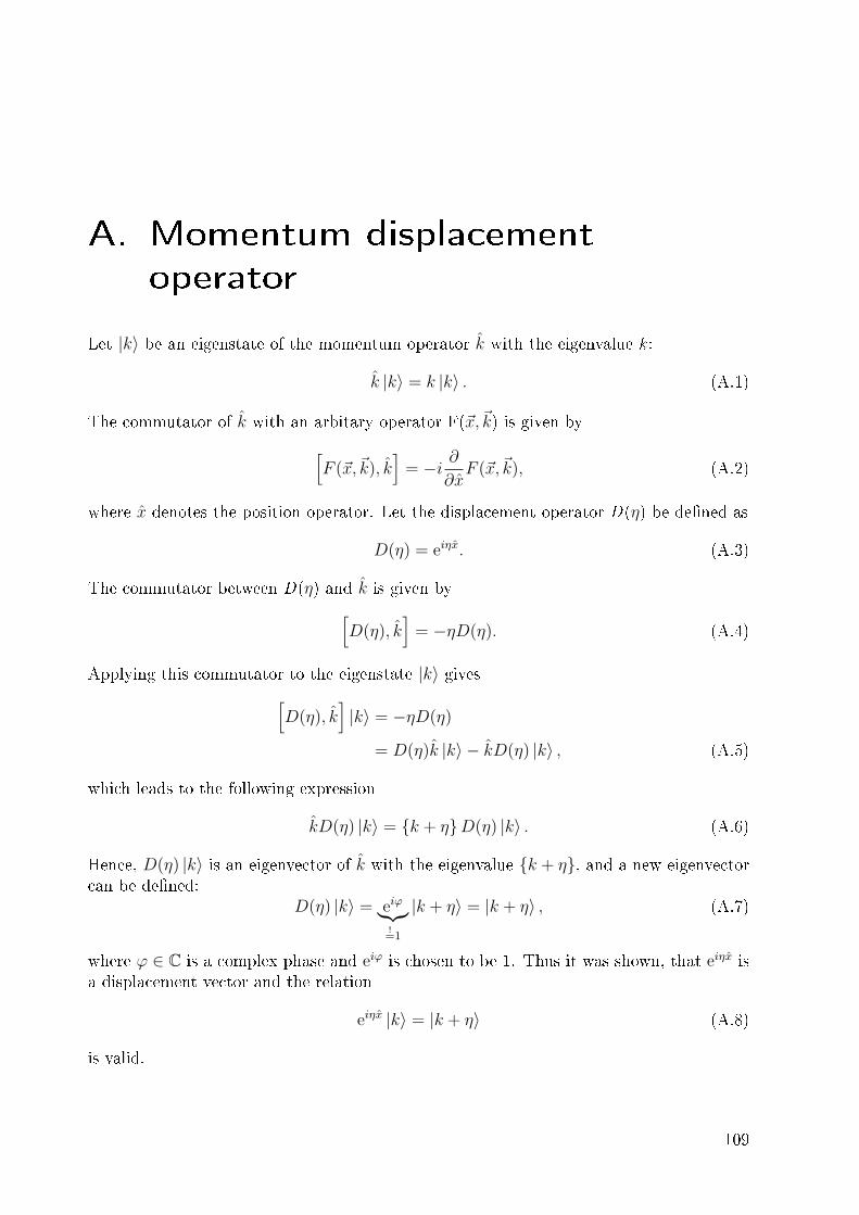
A. Momentum displacement
operator
Let |k⟩ be an eigenstate of the momentum operator k with the eigenvalue k :
k |k⟩ = k |k⟩ . (A.1)
The commutator of k with an arbitary operator F(x, k) is given by[F (x, k), k
]= −i ∂
∂xF (x, k), (A.2)
where x denotes the position operator. Let the displacement operator D(η) be dened as
D(η) = eiηx. (A.3)
The commutator between D(η) and k is given by[D(η), k
]= −ηD(η). (A.4)
Applying this commutator to the eigenstate |k⟩ gives[D(η), k
]|k⟩ = −ηD(η)
= D(η)k |k⟩ − kD(η) |k⟩ , (A.5)
which leads to the following expression
kD(η) |k⟩ = k + ηD(η) |k⟩ . (A.6)
Hence, D(η) |k⟩ is an eigenvector of k with the eigenvalue k + η, and a new eigenvectorcan be dened:
D(η) |k⟩ = eiφ︸︷︷︸!=1
|k + η⟩ = |k + η⟩ , (A.7)
where φ ∈ C is a complex phase and eiφ is chosen to be 1. Thus it was shown, that eiηx isa displacement vector and the relation
eiηx |k⟩ = |k + η⟩ (A.8)
is valid.
109
A. Momentum displacement operator
110

List of Figures
2.1. Experimental setup for ZF and TF-eld µSR . . . . . . . . . . . . . . . . . 142.2. Experimental setup of the GPS spectrometer, PSI . . . . . . . . . . . . . . 152.3. Time evolution of the muon spin polarisation with Gauss-Kubo-Toyabe and
Lorentz-Kubo-Toyabe damping . . . . . . . . . . . . . . . . . . . . . . . . 182.4. time evolution of the muon spin polarisation with sinusoidal and Bessel
oscillation . . . . . . . . . . . . . . . . . . . . . . . . . . . . . . . . . . . . 202.5. Spatial dependence of |ψ(r)| and the magnetic eld B(r) near a vortex core 222.6. Spatial dependence of the magnetic eld and magnetic eld distribution for
an ideal hexagonal vortex lattice . . . . . . . . . . . . . . . . . . . . . . . . 24
3.1. Temperature dependence of the recoilless fraction f (T ) for Debye tempera-tures θD = 100-300 K. . . . . . . . . . . . . . . . . . . . . . . . . . . . . . 34
3.2. Combined magnetic and electrical hyperne interactions and the corre-sponding Mössbauer spectra . . . . . . . . . . . . . . . . . . . . . . . . . . 42
3.3. Schematic of the experimental setup in transmission geometry . . . . . . . 43
4.1. Phase diagram of LaO1−xFxFeAs . . . . . . . . . . . . . . . . . . . . . . . 454.2. Crystal structure of iron-based superconductors . . . . . . . . . . . . . . . 464.3. Phase diagram of Ca1−xNaxFe2As2 and Ca(Fe1−xCoxAs)2 . . . . . . . . . 474.4. Phase diagram of Fe1+yTe1−xSex . . . . . . . . . . . . . . . . . . . . . . . . 484.5. Generic phase diagram of the iron pnictides . . . . . . . . . . . . . . . . . 484.6. Schematic FeAs lattice and Fermi surface topology . . . . . . . . . . . . . 49
5.1. Crystal structure of Ca1−xNaxFe2As2 in the tetragonal phase and latticeparameters . . . . . . . . . . . . . . . . . . . . . . . . . . . . . . . . . . . . 54
5.2. Temperature dependence of the magnetic susceptibility of Ca1−xNaxFe2As2 555.3. Time evolution of the muon spin polarization for representative tempera-
tures in the paramagnetic and magnetically ordered temperature regime forx = 0.00 , 0.35 and 0.50 . . . . . . . . . . . . . . . . . . . . . . . . . . . . 57
5.4. Temperature and Na-substitution level dependence of the magnetic volumefraction for x = 0.00, 0.35, and 0.50 . . . . . . . . . . . . . . . . . . . . . . 58
5.5. Temperature dependence of the magnetic order parameter for x = 0.00,0.35, and 0.50 . . . . . . . . . . . . . . . . . . . . . . . . . . . . . . . . . . 59
5.6. c-axis parameter of various 122 compounds . . . . . . . . . . . . . . . . . . 615.7. Frequency and frequency ratio for the undoped 122 compounds and normal-
ized c-axis parameter as a function of doping . . . . . . . . . . . . . . . . . 625.8. Frequency ratio and reduction of the frequency as a function of doping . . 63
111

List of Figures
5.9. Mössbauer spectra for representative temperatures in the paramagnetic andmagnetically ordered temperature regime for x = 0.35 and 0.50 . . . . . . 64
5.10. Temperature dependence of Vzz and θ . . . . . . . . . . . . . . . . . . . . 655.11. Magnetic and structural order parameter reduction as a function of T c/TN 705.12. Temperature dependence of the relative recoilless fraction and the center shift 735.13. Mössbauer spectra and µSR time spectra in the paramagnetic and super-
conducting phase . . . . . . . . . . . . . . . . . . . . . . . . . . . . . . . . 745.14. TF-µSR spectra for x = 0.67 . . . . . . . . . . . . . . . . . . . . . . . . . . 755.15. Temperature dependence of the magnetic penetration depth . . . . . . . . 765.16. Na-substitution level dependence of the magnetic hyperne eld, the muon
spin precession frequency as well as the the angle between the magnetichyperne eld and the principal axis of the EFG . . . . . . . . . . . . . . . 79
5.17. Phase diagram of Ca1−xNaxFe2As2 obtained by µSR, Mössbauer spec-troscopy, and magnetic-susceptibility measurements . . . . . . . . . . . . . 80
6.1. Crystallographic structure of Fe1+yTe . . . . . . . . . . . . . . . . . . . . . 836.2. Temperature dependence of the specic heat . . . . . . . . . . . . . . . . . 846.3. Temperature dependence of the magnetic-susceptibility, normalized resis-
tance and resistivity . . . . . . . . . . . . . . . . . . . . . . . . . . . . . . 866.4. Magnetic and electronic structure of SrFe2As2 and FeTe . . . . . . . . . . . 876.5. Phase diagram of Fe1+yTe . . . . . . . . . . . . . . . . . . . . . . . . . . . 886.6. Mössbauer spectra of Fe1.06Te, Fe1.13Te, and Fe1.15Te at room temperature
and the corresponding distribution n(Vzz) . . . . . . . . . . . . . . . . . . 906.7. Temperature dependence of the center shift δ(T ) of Fe1.06Te, Fe1.13Te, and
Fe1.15Te . . . . . . . . . . . . . . . . . . . . . . . . . . . . . . . . . . . . . 926.8. Magnetic eld distribution n2a(B) of Fe1.06Te, Fe1.13Te, and Fe1.15Te . . . . 936.9. Mössbauer spectra at 4.2 K of Fe1.06Te, Fe1.13Te, and Fe1.15Te . . . . . . . 946.10. Temperature dependence of the magnetic hyperne eld and magnetic vol-
ume fraction for Fe1.06Te . . . . . . . . . . . . . . . . . . . . . . . . . . . . 946.11. Temperature dependence of the magnetic hyperne eld and magnetic vol-
ume fraction for Fe1.13Te and Fe1.15Te . . . . . . . . . . . . . . . . . . . . . 956.12. Temperature dependence of the magnetic hyperne eld and magnetic vol-
ume fraction for Fe1.15Te . . . . . . . . . . . . . . . . . . . . . . . . . . . . 966.13. Time evolution of the muon spin polarization P(t) at temperatures above
and below the magnetic transition temperatures for Fe1.06Te, Fe1.12Te, andFe1.13Te . . . . . . . . . . . . . . . . . . . . . . . . . . . . . . . . . . . . . 97
6.14. Temperature dependence of the time evolution of the muon spin polarizationof Fe1.13Te in an applied longitudinal eld of 30 mT . . . . . . . . . . . . . 99
6.15. Temperature dependence of the longitudinal relaxation rate λLF . . . . . . 1006.16. Field dependence of the time evolution of the muon spin polarization at
50 K, 70 K, and 100 K in external longitudinal elds up to 400 mT . . . . 1026.17. Updated magnetic phase diagram of Fe1+yTe containing the Mössbauer and
muon spin relaxation spectroscopy results . . . . . . . . . . . . . . . . . . . 104
112
List of Tables
2.1. Basic properties of the muon in terms of electron and proton properties . . 11
5.1. Summary of the magnetic transition temperatures for x = 0.00, 0.35, and0.50 . . . . . . . . . . . . . . . . . . . . . . . . . . . . . . . . . . . . . . . 59
5.2. Debye temperatures θD for x = 0.00, 0.35, 0.50, and 0.67 . . . . . . . . . . 725.3. Superconducting gap and penetration depth values for x = 0.67 . . . . . . 77
6.1. Summary of the magnetic transition temperatures for Fe1+yTe . . . . . . . 103
113
List of Tables
114

Bibliography
[1] J. Cameron and W. Wisher, Terminator 2: Judgement Day, 1991.
[2] S. L. Bud'ko, G. Lapertot, C. Petrovic, C. E. Cunningham, N. Anderson, and P. C.Caneld, Phys. Rev. Lett. 86, 1877 (2001).
[3] J. Bardeen, L. N. Cooper, and J. R. Schrieer, Phys. Rev. 108, 1175 (1957).
[4] C. W. Chu, L. Gao, F. Chen, Z. J. Huang, R. L. Meng, and Y. Y. Xue, Nature 365,323 (1993).
[5] Y. Kamihara, T. Watanabe, M. Hirano, and H. Hosono, J. Am. Chem. Soc. 130,3296 (2008).
[6] A. Schenck, Muon spin rotation spectroscopy (CRC Press, 1985).
[7] J. Sonier, TRIUMF Web Sites (2001).
[8] P. D. de Réotier and A Yaouanc, J. Phys. Condens. Matter 9, 9113 (1997).
[9] R. S. Hayano, Y. J. Uemura, J. Imazato, N. Nishida, T. Yamazaki, and R. Kubo,Phys. Rev. B 20, 850 (1979).
[10] M. Larkin, Y. Fudamoto, I. Gat, A. Kinkhabwala, K. Kojima, G. Luke, J. Merrin,B. Nachumi, Y. Uemura, M. Azuma, T. Saito, and M. Takano, Physica B 289-290,153 (2000).
[11] A. Overhauser, J. Phys. Chem. Solids 13, 71 (1960).
[12] C. Timm, Lecture: theory of superconductivity.
[13] E. H. Brandt, Phys. Rev. B 37, 2349 (1988).
[14] J. E. Sonier, J. H. Brewer, and R. F. Kie, Rev. Mod. Phys. 72, 769 (2000).
[15] T. M. Riseman, J. H. Brewer, K. H. Chow, W. N. Hardy, R. F. Kie, S. R. Kre-itzman, R. Liang, W. A. MacFarlane, P. Mendels, G. D. Morris, J. Rammer, J. W.Schneider, C. Niedermayer, and S. L. Lee, Phys. Rev. B 52, 10569 (1995).
[16] A. Maisuradze, R. Khasanov, A. Shengelaya, and H. Keller, J. Phys. Condens. Mat-ter 21, 075701 (2009).
[17] E. Brandt, J. Low Temp. Phys. 73, 355 (1988).
[18] D. Cardwell and D. Ginley, Handbook of superconducting materials, Bd. 1 (Instituteof Physics, 2003).
[19] M. Tinkham, Introduction to Superconductivity, Dover Books on Physics Series(Dover Publications, Incorporated, 2012).
[20] A. Carrington and F. Manzano, Physica C 385, 205 (2003).
115
Bibliography
[21] D. V. Evtushinsky, D. S. Inosov, V. B. Zabolotnyy, M. S. Viazovska, R. Khasanov,A. Amato, H.-H. Klauss, H. Luetkens, C. Niedermayer, G. L. Sun, V. Hinkov, C. T.Lin, A. Varykhalov, A. Koitzsch, M. Knupfer, B. Büchner, A. A. Kordyuk, and S. V.Borisenko, N. J. Phys. 11, 055069 (2009).
[22] A. A. Golubov, A. Brinkman, O. V. Dolgov, J. Kortus, and O. Jepsen, Phys. Rev.B 66, 054524 (2002).
[23] R. L. Mössbauer, German, Z. Phys. 151, 124 (1958).
[24] D. Barb, Grundlagen und Anwendungen der Mössbauerspektroskopie (Berlin,Akademie-Verlag, 1980).
[25] D.-P. Y. Yi-Long Chen, Mössbauer eect in lattice dynamics (WILEY-VCH, 2007).
[26] R. J. Glauber, Phys. Rev. 131, 2766 (1963).
[27] J. Gazeau, Coherent states in quantum physics (Wiley, 2009).
[28] D. S. Bateman, S. K. Bose, B. DuttaRoy, and M. Bhattacharyya, Am. J. Phys. 60,829 (1992).
[29] H. J. Lipkin, Ann. Phys. 18, 182 (1962).
[30] S. Wang, Phys. Rev. A 60, 262 (1999).
[31] G. Schatz and A. Weidinger, Nukleare Festkörperphysik: kernphysikalische Mess-
methoden und ihre Anwendungen, Teubner-Studienbücher: Physik (Teubner, 1997).
[32] S. Kamusella, MoessFit: A Free Framework for 57Fe Mössbauer Data Analysis, (pri-vate communication).
[33] B. Matthias, V. Compton, and E. Corenzwit, J. Phys. Chem. Solids 19, 130 (1961).
[34] B. Chandrasekhar and J. Hulm, J. Phys. Chem. Solids 7, 259 (1958).
[35] H. F. Braun, Phys. Lett. A 75, 386 (1980).
[36] H. Luetkens, H.-H. Klauss, M. Kraken, F. J. Litterst, T. Dellmann, R. Klingeler, C.Hess, R. Khasanov, A. Amato, C. Baines, M. Kosmala, O. J. Schumann, M. Braden,J. Hamann-Borrero, N. Leps, A. Kondrat, G. Behr, J. Werner, and B. Büchner, Nat.Mater. 8, 305 (2009).
[37] H.-H. Klauss, H. Luetkens, R. Klingeler, C. Hess, F. J. Litterst, M. Kraken, M. M.Korshunov, I. Eremin, S.-L. Drechsler, R. Khasanov, A. Amato, J. Hamann-Borrero,N. Leps, A. Kondrat, G. Behr, J. Werner, and B. Büchner, Phys. Rev. Lett. 101,077005 (2008).
[38] A. D. Christianson, M. D. Lumsden, O. Delaire, M. B. Stone, D. L. Abernathy, M.A. McGuire, A. S. Sefat, R. Jin, B. C. Sales, D. Mandrus, E. D. Mun, P. C. Caneld,J. Y. Y. Lin, M. Lucas, M. Kresch, J. B. Keith, B. Fultz, E. A. Goremychkin, andR. J. McQueeney, Phys. Rev. Lett. 101, 157004 (2008).
[39] L. Boeri, O. V. Dolgov, and A. A. Golubov, Phys. Rev. Lett. 101, 026403 (2008).
[40] I. Mazin and J. Schmalian, Physica C 469, 614 (2009).
116

Bibliography
[41] M. D. Lumsden and A. D. Christianson, J. Phys. Condens. Matter 22, 203203(2010).
[42] D. C. Johnston, Adv. Phys. 59, 803 (2010).
[43] D. Johrendt, J. Mater. Chem. 21, 13726 (2011).
[44] P. J. Hirschfeld, M. M. Korshunov, and I. I. Mazin, Rep. Prog. Phys. 74, 124508(2011).
[45] G. R. Stewart, Rev. Mod. Phys. 83, 1589 (2011).
[46] K. Zhao, Q. Q. Liu, X. C. Wang, Z. Deng, Y. X. Lv, J. L. Zhu, F. Y. Li, and C. Q.Jin, Phys. Rev. B 84, 184534 (2011).
[47] L. Harnagea, S. Singh, G. Friemel, N. Leps, D. Bombor, M. Abdel-Haez, A. U. B.Wolter, C. Hess, R. Klingeler, G. Behr, S. Wurmehl, and B. Büchner, Phys. Rev. B83, 094523 (2011).
[48] M. Psterer and G. Nagorsen, Z. Naturforsch. B 35 (1980).
[49] M. Rotter, M. Tegel, D. Johrendt, I. Schellenberg, W. Hermes, and R. Pöttgen,Phys. Rev. B 78, 020503 (2008).
[50] A. Jesche, N. Caroca-Canales, H. Rosner, H. Borrmann, A. Ormeci, D. Kasinathan,H. H. Klauss, H. Luetkens, R. Khasanov, A. Amato, A. Hoser, K. Kaneko, C. Krell-ner, and C. Geibel, Phys. Rev. B 78, 180504 (2008).
[51] A. I. Goldman, D. N. Argyriou, B. Ouladdiaf, T. Chatterji, A. Kreyssig, S. Nandi,N. Ni, S. L. Bud'ko, P. C. Caneld, and R. J. McQueeney, Phys. Rev. B 78, 100506(2008).
[52] Q. Huang, Y. Qiu, W. Bao, M. A. Green, J. W. Lynn, Y. C. Gasparovic, T. Wu,G. Wu, and X. H. Chen, Phys. Rev. Lett. 101, 257003 (2008).
[53] A. Cano, M. Civelli, I. Eremin, and I. Paul, Phys. Rev. B 82, 020408 (2010).
[54] K. Sasmal, B. Lv, B. Lorenz, A. M. Guloy, F. Chen, Y.-Y. Xue, and C.-W. Chu,Phys. Rev. Lett. 101, 107007 (2008).
[55] Z. Bukowski, S. Weyeneth, R. Puzniak, J. Karpinski, and B. Batlogg, Physica C470, Supplement 1, Proceedings of the 9th International Conference on Materialsand Mechanisms of Superconductivity, S328 (2010).
[56] M. Bendele, P. Babkevich, S. Katrych, S. N. Gvasaliya, E. Pomjakushina, K. Conder,B. Roessli, A. T. Boothroyd, R. Khasanov, and H. Keller, Phys. Rev. B 82, 212504(2010).
[57] F.-C. Hsu, J.-Y. Luo, K.-W. Yeh, T.-K. Chen, T.-W. Huang, P. M. Wu, Y.-C. Lee,Y.-L. Huang, Y.-Y. Chu, D.-C. Yan, and M.-K. Wu, Proc. Natl. Acad. Sci. 105,14262 (2008).
[58] B. C. Sales, A. S. Sefat, M. A. McGuire, R. Y. Jin, D. Mandrus, and Y.Mozharivskyj, Phys. Rev. B 79, 094521 (2009).
[59] D. Fruchart, P. Convert, P. Wolfers, R. Madar, J. Senateur, and R. Fruchart, Mater.Res. Bull. 10, 169 (1975).
117
Bibliography
[60] A. Subedi, L. Zhang, D. J. Singh, and M. H. Du, Phys. Rev. B 78, 134514 (2008).
[61] D. N. Basov and A. V. Chubukov, Nat. Phys. 7, 272 (2011).
[62] J. T. Park, D. S. Inosov, C. Niedermayer, G. L. Sun, D. Haug, N. B. Christensen,R. Dinnebier, A. V. Boris, A. J. Drew, L. Schulz, T. Shapoval, U. Wol, V. Neu, X.Yang, C. T. Lin, B. Keimer, and V. Hinkov, Phys. Rev. Lett. 102, 117006 (2009).
[63] A. J. Drew, C. Niedermayer, P. J. Baker, F. L. Pratt, S. J. Blundell, T. Lancaster,R. H. Liu, G. Wu, X. H. Chen, I. Watanabe, V. K. Malik, A. Dubroka, M. Rossle,K. W. Kim, C. Baines, and C. Bernhard, Nat. Mater. 8, 310 (2009).
[64] S. Sanna, R. De Renzi, G. Lamura, C. Ferdeghini, A. Palenzona, M. Putti, M.Tropeano, and T. Shiroka, Phys. Rev. B 80, 052503 (2009).
[65] H. Maeter, G. Pascua, H. Luetkens, J. Knolle, S. Aswartham, S. Wurmehl, G. Behr,B. Büchner, Z. Shermadini, K. Sedlak, A. Amato, R. Moessner, I. Eremin, and H.-H.Klauss, arXiv 1210.6881v1 (2012).
[66] G Wu, H Chen, T Wu, Y. L. Xie, Y. J. Yan, R. H. Liu, X. F. Wang, J. J. Ying, andX. H. Chen, J. Phys. Condens. Matter 20, 422201 (2008).
[67] G. F. Chen, Z. Li, J. Dong, G. Li, W. Z. Hu, X. D. Zhang, X. H. Song, P. Zheng,N. L. Wang, and J. L. Luo, Phys. Rev. B 78, 224512 (2008).
[68] D. Singh, Physica C 469, 418 (2009).
[69] A. B. Vorontsov, M. G. Vavilov, and A. V. Chubukov, Phys. Rev. B 81, 174538(2010).
[70] M. G. Vavilov, A. V. Chubukov, and A. B. Vorontsov, Sup. Sci. Technol. 23, 054011(2010).
[71] G. Liu, H. Liu, L. Zhao, W. Zhang, X. Jia, J. Meng, X. Dong, J. Zhang, G. F. Chen,G. Wang, Y. Zhou, Y. Zhu, X. Wang, Z. Xu, C. Chen, and X. J. Zhou, Phys. Rev.B 80, 134519 (2009).
[72] M. Neupane, P. Richard, Y.-M. Xu, K. Nakayama, T. Sato, T. Takahashi, A. V.Federov, G. Xu, X. Dai, Z. Fang, Z. Wang, G.-F. Chen, N.-L. Wang, H.-H. Wen,and H. Ding, Phys. Rev. B 83, 094522 (2011).
[73] C. Liu, T. Kondo, N. Ni, A. D. Palczewski, A. Bostwick, G. D. Samolyuk, R.Khasanov, M. Shi, E. Rotenberg, S. L. Bud'ko, P. C. Caneld, and A. Kaminski,Phys. Rev. Lett. 102, 167004 (2009).
[74] R. Gonnelli, M. Tortello, D. Daghero, P. Pecchio, S. Galasso, V. Stepanov, Z.Bukowski, N. Zhigadlo, J. Karpinski, K. Iida, and B. Holzapfel, English, J. Su-percond. Nov. Magn. 26, 1331 (2013).
[75] S. Avci, O. Chmaissem, D. Y. Chung, S. Rosenkranz, E. A. Goremychkin, J. P.Castellan, I. S. Todorov, J. A. Schlueter, H. Claus, A. Daoud-Aladine, D. D.Khalyavin, M. G. Kanatzidis, and R. Osborn, Phys. Rev. B 85, 184507 (2012).
[76] T. Kondo, R. M. Fernandes, R. Khasanov, C. Liu, A. D. Palczewski, N. Ni, M.Shi, A. Bostwick, E. Rotenberg, J. Schmalian, S. L. Bud'ko, P. C. Caneld, and A.Kaminski, Phys. Rev. B 81, 060507 (2010).
118

Bibliography
[77] D. V. Evtushinsky, V. B. Zabolotnyy, L. Harnagea, A. N. Yaresko, S. Thirupathaiah,A. A. Kordyuk, J. Maletz, S. Aswartham, S. Wurmehl, E. Rienks, R. Follath, B.Büchner, and S. V. Borisenko, Phys. Rev. B 87, 094501 (2013).
[78] C. Liu, G. D. Samolyuk, Y. Lee, N. Ni, T. Kondo, A. F. Santander-Syro, S. L.Bud'ko, J. L. McChesney, E. Rotenberg, T. Valla, A. V. Fedorov, P. C. Caneld,B. N. Harmon, and A. Kaminski, Phys. Rev. Lett. 101, 177005 (2008).
[79] R. M. Fernandes, D. K. Pratt, W. Tian, J. Zarestky, A. Kreyssig, S. Nandi, M. G.Kim, A. Thaler, N. Ni, P. C. Caneld, R. J. McQueeney, J. Schmalian, and A. I.Goldman, Phys. Rev. B 81, 140501 (2010).
[80] J. Schmiedt, P. M. R. Brydon, and C. Timm, Phys. Rev. B 89, 054515 (2014).
[81] T. A. Maier, S. Graser, D. J. Scalapino, and P. J. Hirschfeld, Phys. Rev. B 79,224510 (2009).
[82] A. V. Chubukov, M. G. Vavilov, and A. B. Vorontsov, Phys. Rev. B 80, 140515(2009).
[83] R. Thomale, C. Platt, J. Hu, C. Honerkamp, and B. A. Bernevig, Phys. Rev. B 80,180505 (2009).
[84] V. Cvetkovic and Z. Tesanovic, Europhys. Lett. 85, 37002 (2009).
[85] F. Wang, H. Zhai, Y. Ran, A. Vishwanath, and D.-H. Lee, Phys. Rev. Lett. 102,047005 (2009).
[86] C. Platt, C. Honerkamp, and W. Hanke, N. J. Phys. 11, 055058 (2009).
[87] S. Raghu, X.-L. Qi, C.-X. Liu, D. J. Scalapino, and S.-C. Zhang, Phys. Rev. B 77,220503 (2008).
[88] J. Lorenzana, G. Seibold, C. Ortix, and M. Grilli, Phys. Rev. Lett. 101, 186402(2008).
[89] P. M. R. Brydon and C. Timm, Phys. Rev. B 79, 180504 (2009).
[90] M. D. Johannes and I. I. Mazin, Phys. Rev. B 79, 220510 (2009).
[91] I. Eremin and A. V. Chubukov, Phys. Rev. B 81, 024511 (2010).
[92] I. I. Mazin and M. D. Johannes, Nat. Phys. 5, 141 (2009).
[93] R. D. Shannon, Acta Crystallogr. Sec. A 32, 751 (1976).
[94] K. Momman and F. Izumi, VESTA3 for three-dimensional visualization of crystal,
volumetric and morphology data, 2011.
[95] P. M. Shirage, K. Miyazawa, H. Kito, H. Eisaki, and A. Iyo, Appl. Phys. Express1, 081702 (2008).
[96] N. Ni, S. Nandi, A. Kreyssig, A. I. Goldman, E. D. Mun, S. L. Bud'ko, and P. C.Caneld, Phys. Rev. B 78, 014523 (2008).
[97] J. Zhao, W. Ratcli, J. W. Lynn, G. F. Chen, J. L. Luo, N. L. Wang, J. Hu, andP. Dai, Phys. Rev. B 78, 140504 (2008).
[98] R. Cortes-Gil and S. J. Clarke, Chem. Mater. 23, 1009 (2011).
119

Bibliography
[99] R. Cortes-Gil, D. R. Parker, M. J. Pitcher, J. Hadermann, and S. J. Clarke, Chem.Mater. 22, 4304 (2010).
[100] S. Johnston, M. Abdel-Haez, L. Harnagea, V. Grinenko, D. Bombor, Y. Krupskaya,C. Hess, S. Wurmehl, A. U. B. Wolter, B. Büchner, H. Rosner, and S.-L. Drechsler,Phys. Rev. B 89, 134507 (2014).
[101] A. Suter and B. Wojek, Phys. Procedia 30, 69 (2012).
[102] S. Aswartham, M. Abdel-Haez, D. Bombor, M. Kumar, A. U. B. Wolter, C. Hess,D. V. Evtushinsky, V. B. Zabolotnyy, A. A. Kordyuk, T. K. Kim, S. V. Borisenko,G. Behr, B. Büchner, and S. Wurmehl, Phys. Rev. B 85, 224520 (2012).
[103] R. Klingeler, N. Leps, I. Hellmann, A. Popa, U. Stockert, C. Hess, V. Kataev, H.-J.Grafe, F. Hammerath, G. Lang, S. Wurmehl, G. Behr, L. Harnagea, S. Singh, andB. Büchner, Phys. Rev. B 81, 024506 (2010).
[104] G. M. Zhang, Y. H. Su, Z. Y. Lu, Z. Y. Weng, D. H. Lee, and T. Xiang, Europhys.Lett. 86, 37006 (2009).
[105] Y. G. Pashkevich, private communication.
[106] A. A. Aczel, E. Baggio-Saitovitch, S. L. Budko, P. C. Caneld, J. P. Carlo, G. F.Chen, P. Dai, T. Goko, W. Z. Hu, G. M. Luke, J. L. Luo, N. Ni, D. R. Sanchez-Candela, F. F. Tafti, N. L. Wang, T. J. Williams, W. Yu, and Y. J. Uemura, Phys.Rev. B 78, 214503 (2008).
[107] R. Scheuermann, E. Roduner, G. Engelhardt, H.-H. Klauss, and D. Herlach, Phys.Rev. B 66, 144429 (2002).
[108] M. Gooch, B. Lv, K. Sasmal, J. Tapp, Z. Tang, A. Guloy, B. Lorenz, and C. Chu,Physica C 470, Supplement 1, Proceedings of the 9th International Conferenceon Materials and Mechanisms of Superconductivity, S276 (2010).
[109] M. Tegel, M. Rotter, V. Weiÿ, F. M. Schappacher, R. Pöttgen, and D. Johrendt, J.Phys. Condens. Matter 20, 452201 (2008).
[110] M. Rotter, M. Pangerl, M. Tegel, and D. Johrendt, Angew. Chem. Int. Ed. 47, 7949(2008).
[111] E. Wiesenmayer, H. Luetkens, G. Pascua, R. Khasanov, A. Amato, H. Potts, B.Banusch, H.-H. Klauss, and D. Johrendt, Phys. Rev. Lett. 107, 237001 (2011).
[112] S. Avci, J. M. Allred, O. Chmaissem, D. Y. Chung, S. Rosenkranz, J. A. Schlueter, H.Claus, A. Daoud-Aladine, D. D. Khalyavin, P. Manuel, A. Llobet, M. R. Suchomel,M. G. Kanatzidis, and R. Osborn, Phys. Rev. B 88, 094510 (2013).
[113] G. Sun, D. Sun, M. Konuma, P. Popovich, A. Boris, J. Peng, K.-Y. Choi, P. Lem-mens, and C. Lin, J. Supercond. Nov. Magn. 24, 1773 (2011).
[114] Y. Qi, X. Zhang, Z. Gao, Z. Zhang, L. Wang, D. Wang, and Y. Ma, Physica C 469,717 (2009).
[115] Y. Li and J. Ni, Solid State Commun. 151, 446 (2011).
120

Bibliography
[116] T. Goko, A. A. Aczel, E. Baggio-Saitovitch, S. L. Bud'ko, P. C. Caneld, J. P. Carlo,G. F. Chen, P. Dai, A. C. Hamann, W. Z. Hu, H. Kageyama, G. M. Luke, J. L. Luo,B. Nachumi, N. Ni, D. Reznik, D. R. Sanchez-Candela, A. T. Savici, K. J. Sikes,N. L. Wang, C. R. Wiebe, T. J. Williams, T. Yamamoto, W. Yu, and Y. J. Uemura,Phys. Rev. B 80, 024508 (2009).
[117] M. Alzamora, J. Munevar, E. Baggio-Saitovitch, S. L. Bud'ko, N. Ni, P. C. Caneld,and D. R. Sánchez, J. Phys. Condens. Matter 23, 145701 (2011).
[118] D. Kasinathan, A. Ormeci, K. Koch, U. Burkhardt, W. Schnelle, A. Leithe-Jasper,and H. Rosner, N. J. Phys. 11, 025023 (2009).
[119] H. Suhl, J. L. Com. Metals 62, 225 (1978).
[120] T. K. Kopec and J. Klamut, Phys. Status Solidi B 137, 73 (1986).
[121] R. M. Fernandes and J. Schmalian, Phys. Rev. B 82, 014521 (2010).
[122] C. R. Rotundu, W. Tian, K. C. Rule, T. R. Forrest, J. Zhao, J. L. Zarestky, andR. J. Birgeneau, Phys. Rev. B 85, 144506 (2012).
[123] S. Avci, O. Chmaissem, E. A. Goremychkin, S. Rosenkranz, J.-P. Castellan, D. Y.Chung, I. S. Todorov, J. A. Schlueter, H. Claus, M. G. Kanatzidis, A. Daoud-Aladine, D. Khalyavin, and R. Osborn, Phys. Rev. B 83, 172503 (2011).
[124] M. G. Kim, D. K. Pratt, G. E. Rustan, W. Tian, J. L. Zarestky, A. Thaler, S. L.Bud'ko, P. C. Caneld, R. J. McQueeney, A. Kreyssig, and A. I. Goldman, Phys.Rev. B 83, 054514 (2011).
[125] A. Kreyssig, M. G. Kim, S. Nandi, D. K. Pratt, W. Tian, J. L. Zarestky, N. Ni, A.Thaler, S. L. Bud'ko, P. C. Caneld, R. J. McQueeney, and A. I. Goldman, Phys.Rev. B 81, 134512 (2010).
[126] P. Wang, Z. M. Stadnik, J. Zukrowski, A. Thaler, S. L. Bud'ko, and P. C. Caneld,Phys. Rev. B 84, 024509 (2011).
[127] H. Luo, R. Zhang, M. Laver, Z. Yamani, M. Wang, X. Lu, M. Wang, Y. Chen, S. Li,S. Chang, J. W. Lynn, and P. Dai, Phys. Rev. Lett. 108, 247002 (2012).
[128] S. Nandi, M. G. Kim, A. Kreyssig, R. M. Fernandes, D. K. Pratt, A. Thaler, N. Ni,S. L. Bud'ko, P. C. Caneld, J. Schmalian, R. J. McQueeney, and A. I. Goldman,Phys. Rev. Lett. 104, 057006 (2010).
[129] P. Marsik, K. W. Kim, A. Dubroka, M. Rössle, V. K. Malik, L. Schulz, C. N. Wang,C. Niedermayer, A. J. Drew, M. Willis, T. Wolf, and C. Bernhard, Phys. Rev. Lett.105, 057001 (2010).
[130] A. D. Christianson, M. D. Lumsden, S. E. Nagler, G. J. MacDougall, M. A. McGuire,A. S. Sefat, R. Jin, B. C. Sales, and D. Mandrus, Phys. Rev. Lett. 103, 087002(2009).
[131] D. K. Pratt, M. G. Kim, A. Kreyssig, Y. B. Lee, G. S. Tucker, A. Thaler, W. Tian,J. L. Zarestky, S. L. Bud'ko, P. C. Caneld, B. N. Harmon, A. I. Goldman, andR. J. McQueeney, Phys. Rev. Lett. 106, 257001 (2011).
121
Bibliography
[132] T. Yildirim, Physica C 469, Superconductivity in Iron-Pnictides, 425 (2009).
[133] S. E. Hahn, Y. Lee, N. Ni, P. C. Caneld, A. I. Goldman, R. J. McQueeney, B. N.Harmon, A. Alatas, B. M. Leu, E. E. Alp, D. Y. Chung, I. S. Todorov, and M. G.Kanatzidis, Phys. Rev. B 79, 220511 (2009).
[134] R. Mittal, S. K. Mishra, S. L. Chaplot, S. V. Ovsyannikov, E. Greenberg, D. M.Trots, L. Dubrovinsky, Y. Su, T. Brueckel, S. Matsuishi, H. Hosono, and G. Gar-barino, Phys. Rev. B 83, 054503 (2011).
[135] L. Chauvière, Y. Gallais, M. Cazayous, A. Sacuto, M. A. Méasson, D. Colson, andA. Forget, Phys. Rev. B 80, 094504 (2009).
[136] R. Khasanov, D. Evtushinsky, A. Amato, H.-H. Klauss, H. Luetkens, C. Nieder-mayer, B. Büchner, G. Sun, C. Lin, J. Park, D. Inosov, and V. Hinkov, Phys. Rev.Lett. 102, 187005 (2009).
[137] R. Prozorov and V. G. Kogan, Rep. Prog. Phys. 74, 124505 (2011).
[138] R. Housley, N. Erickson, and J. Dash, Nucl. Instrum. and Methods 27, 29 (1964).
[139] G. Lang, Nucl. Instrum. Methods 24, 425 (1963).
[140] Z. Li, X. Ma, H. Pang, and F. Li, J. Phys. Condens. Matter 23, 255701 (2011).
[141] A. Blachowski, K. Ruebenbauer, J. Zukrowski, J. Przewoznik, K. Wojciechowski,and Z. Stadnik, J. All. Comp. 494, 1 (2010).
[142] R. S. Preston, Phys. Rev. Lett. 19, 75 (1967).
[143] A. Blachowski, K. Ruebenbauer, J. ukrowski, K. Rogacki, Z. Bukowski, and J.Karpinski, Phys. Rev. B 83, 134410 (2011).
[144] M. Abdel-Haez, P. J. Pereira, S. A. Kuzmichev, T. E. Kuzmicheva, V. M. Pudalov,L. Harnagea, A. A. Kordyuk, A. V. Silhanek, V. V. Moshchalkov, B. Shen, H.-H.Wen, A. N. Vasiliev, and X.-J. Chen, Phys. Rev. B 90, 054524 (2014).
[145] S. A. J. Kimber, A. Kreyssig, Y.-Z. Zhang, H. O. Jeschke, R. Valenti, F. Yokaichiya,E. Colombier, J. Yan, T. C. Hansen, T. Chatterji, R. J. McQueeney, P. C. Caneld,A. I. Goldman, and D. N. Argyriou, Nat. Mater. 8, 471 (2009).
[146] C. Bernhard, A. J. Drew, L. Schulz, V. K. Malik, M. Rössle, C. Niedermayer, T.Wolf, G. D. Varma, G. Mu, H.-H. Wen, H. Liu, G. Wu, and X. H. Chen, N. J. Phys.11, 055050 (2009).
[147] J. E. Sonier, W. Huang, C. V. Kaiser, C. Cochrane, V. Pacradouni, S. A. Sabok-Sayr, M. D. Lumsden, B. C. Sales, M. A. McGuire, A. S. Sefat, and D. Mandrus,Phys. Rev. Lett. 106, 127002 (2011).
[148] R. Khasanov, A. Maisuradze, H. Maeter, A. Kwadrin, H. Luetkens, A. Amato, W.Schnelle, H. Rosner, A. Leithe-Jasper, and H.-H. Klauss, Phys. Rev. Lett. 103,067010 (2009).
[149] T. J. Williams, A. A. Aczel, E. Baggio-Saitovitch, S. L. Bud'ko, P. C. Caneld,J. P. Carlo, T. Goko, H. Kageyama, A. Kitada, J. Munevar, N. Ni, S. R. Saha, K.Kirschenbaum, J. Paglione, D. R. Sanchez-Candela, Y. J. Uemura, and G. M. Luke,Phys. Rev. B 82, 094512 (2010).
122

Bibliography
[150] K. Yosida, Phys. Rev. 110, 769 (1958).
[151] T. Goltz, V. Zinth, D. Johrendt, H. Rosner, G. Pascua, H. Luetkens, P. Materne,and H.-H. Klauss, Phys. Rev. B 89, 144511 (2014).
[152] S. L. Thiemann, Z. Radovi¢, and V. G. Kogan, Phys. Rev. B 39, 11406 (1989).
[153] R. Prozorov, M. Tanatar, R. Gordon, C. Martin, H. Kim, V. Kogan, N. Ni, M.Tillman, S. Bud'ko, and P. Caneld, Physica C 469, 582 (2009).
[154] N. Haberkorn, B. Maiorov, M. Jaime, I. Usov, M. Miura, G. F. Chen, W. Yu, andL. Civale, Phys. Rev. B 84, 064533 (2011).
[155] S. Röÿler, D. Cherian, W. Lorenz, M. Doerr, C. Koz, C. Curfs, Y. Prots, U. K.Röÿler, U. Schwarz, S. Elizabeth, and S. Wirth, Phys. Rev. B 84, 174506 (2011).
[156] C. Koz, S. Röÿler, A. A. Tsirlin, S. Wirth, and U. Schwarz, Phys. Rev. B 88, 094509(2013).
[157] E. E. Rodriguez, C. Stock, P. Zajdel, K. L. Krycka, C. F. Majkrzak, P. Zavalij, andM. A. Green, Phys. Rev. B 84, 064403 (2011).
[158] L. Zhang, D. J. Singh, and M. H. Du, Phys. Rev. B 79, 012506 (2009).
[159] W. Bao, Y. Qiu, Q. Huang, M. A. Green, P. Zajdel, M. R. Fitzsimmons, M. Zh-ernenkov, S. Chang, M. Fang, B. Qian, E. K. Vehstedt, J. Yang, H. M. Pham, L.Spinu, and Z. Q. Mao, Phys. Rev. Lett. 102, 247001 (2009).
[160] Y. Xia, D. Qian, L. Wray, D. Hsieh, G. F. Chen, J. L. Luo, N. L. Wang, and M. Z.Hasan, Phys. Rev. Lett. 103, 037002 (2009).
[161] S. Röÿler, D. Cherian, S. Harikrishnan, H. L. Bhat, S. Elizabeth, J. A. Mydosh,L. H. Tjeng, F. Steglich, and S. Wirth, Phys. Rev. B 82, 144523 (2010).
[162] A. Blachowski, K. Ruebenbauer, P. Zajdel, E. E. Rodriguez, and M. A. Green, J.Phys. Condens. Matter 24, 386006 (2012).
[163] I. Paul, Phys. Rev. Lett. 107, 047004 (2011).
[164] G. Lamura, T. Shiroka, P. Bonfà, S. Sanna, F. Bernardini, R. De Renzi, R. Viennois,E. Giannini, A. Piriou, N. Emery, M. R. Cimberle, and M. Putti, J. Phys. Condens.Matter 25, 156004 (2013).
[165] Z. P. Yin, K. Haule, and G. Kotliar, Nat. Mater. 10, 932 (2011).
[166] H. Gretarsson, A. Lupascu, J. Kim, D. Casa, T. Gog, W. Wu, S. R. Julian, Z. J. Xu,J. S. Wen, G. D. Gu, R. H. Yuan, Z. G. Chen, N.-L. Wang, S. Khim, K. H. Kim,M. Ishikado, I. Jarrige, S. Shamoto, J.-H. Chu, I. R. Fisher, and Y.-J. Kim, Phys.Rev. B 84, 100509 (2011).
[167] Y. Liu, R. K. Kremer, and C. T. Lin, Sup. Sci. Technol. 24, 035012 (2011).
[168] R. Khasanov, M. Bendele, A. Amato, P. Babkevich, A. T. Boothroyd, A. Cervellino,K. Conder, S. N. Gvasaliya, H. Keller, H.-H. Klauss, H. Luetkens, V. Pomjakushin,E. Pomjakushina, and B. Roessli, Phys. Rev. B 80, 140511 (2009).
123

Danksagung
Ich möchte allen danken, die mich während der Promotion begleitet und diese damit über-haupt auch erst möglich gemacht haben.Da wäre an aller erster Stelle der Doktorvater Prof. Hans-Henning Klauÿ zu nennen,
in dessen Arbeitsgruppe diese Arbeit durchgeführt wurde. Die Arbeit in und mit derArbeitsgruppe war im Allgemeinen ausgesprochen angenehm, was sich dentiv positivausgewirkt hat, da ich mich immer gefreut habe, ans Institut zu kommen. Da wären zunennen: Hemke Maeter, Johannes Spehling, Til Goltz, Sirko Kamusella, Nicolas Yeche,Mathias Dörr und Rajib Sarkar. Desweiteren danke ich Elke Wachsmuth für die Hilfe beiall den nichtwissenschaftlichen Dingen, mit denen ich mich so rumplagen musste, sowieden angenehmen Gesprächen. Das gleiche gilt für Marion Malkoc für die Hilfe beim GRK1621. Und Hubertus Luetkens für die Hilfestellungen bei den µSR-Messreisen. Es hatimmer ausgesprochen viel Spaÿ gemacht, ihn am PSI zu besuchen.Desweiteren danke ich Prof. Wosnitza für die vollkommen unkomplizierte Übernahme
der Tätigkeit als Zweitgutachter.Und ich danke meiner Familie und meinen Freunden für die Unterstützung während
der Promotion. Auch wenn die Fragen "Wann bist du denn fertig?" und "Was machstdu nachher?," welche in regelmäÿigen Zweitagesabständen aufkamen, ab und zu auch maletwas nervig waren. Aber so hatte ich direkt einen zusätzlichen Grund, schneller fertig zuwerden.Last but not least möchte ich der Bierstube danken, auch wenn sie das Ende meiner Pro-
motion nicht mehr erleben kann. Es gab einfach keinen besseren Ort, um nach Feierabendetwas abzuspannen oder um physikalische Probleme in entspannter Athmosphäre bei ein,zwei oder auch acht Bier zu diskutieren. Dazu gehören auch die üblichen Verdächtigen derMontagsrunde.
124
Versicherung
Hiermit versichere ich, dass ich die vorliegende Arbeit ohne unzulässige Hilfe Dritter undohne Benutzung anderer als der angegebenen Hilfsmittel angefertigt habe; die aus fremdenQuellen direkt oder indirekt bernommenen Gedanken sind als solche kenntlich gemacht.Die Arbeit wurde bisher weder im Inland noch im Ausland in gleicher oder hnlicher Formeiner anderen Prfungsbehrde vorgelegt. Die vorliegende Dissertation wurde am Institutfür Festköperphysik der Technischen Universität Dresden unter der wissenschaftlichen Be-treuung von Herrn Professor Dr. Hans-Henning Klauÿ angefertigt. Ich erkenne hiermit diePromotionsordnung der Fakultät Mathematik und Naturwissenschaften der TechnischenUniversität Dresden vom 23.2.2011 an.
Dresden, den 27. April 2015
125