Journal of Geodynamics 38 (2004) 355–374

Local hydrology, the Global Geodynamics Project andCHAMP/GRACE perspective: some case studies

M. Llubesa,∗, N. Florschb, J. Hindererc,d, L. Longuevergneb, M. Amalvictc

a LEGOS/CNES/CNRS, 18 avenue Edouard Belin, 31401 Toulouse Cedex 9, Franceb UMR 7619 “Sisyphe”, UPMC, 4 Place Jussieu, 75252 Paris Cedex 05, France

c EOST-IPGS (UMR 7516 CNRS/ULP), 5 rue Descartes, 67084 Strasbourg Cedex, Franced NASA GSFC Greenbelt, MD 20771, USA

Received 5 January 2004; received in revised form 23 June 2004; accepted 9 July 2004

Abstract

We first quantify the influence of aquifers on gravity variations by considering local, regional and continentalscales. We show that locally only the direct attraction of the underlying aquifer has to be taken into account. Atcontinental (or global scales), the underground water masses act by direct attraction (due to the earth curvature),loading flexure and potential redistribution. We show that at the intermediate regional scale (saying a few kilometresto a few hundreds of kilometres), groundwater contributions can be neglected in practice. Afterwards, we illustratethe difficulties in tackling the local hydrological context by studying comparatively the geological and hydrogeo-logical surroundings of three European Global Geodynamics Project (GGP) superconducting gravimeter stations(Strasbourg, Moxa, and Vienna). Finally, it appears clearly that hydrological variability and cycle characterisationsconstitute the up-to-date challenge while studying gravity variations in a large spectral range. That is why, gravityis used to quantify hydrological transfers, and overall when seeking for small signals from the Earth’s deep interioror other environmental signals (atmosphere, oceans) where groundwater influence can be seen as a disturbance.© 2004 Elsevier Ltd. All rights reserved.

1. Introduction

The gravimetry research community gathered within the Global Geodynamics Project (GGP) is inter-ested in temporal variations of the Earth’s gravity field and by the associated geodetic aspects, through

∗ Corresponding author. Tel.: +33 5 6133 2862; fax: +33 5 6125 3505.E-mail address:muriel.llubes@notos.cst.cnes.fr (M. Llubes).

0264-3707/$ – see front matter © 2004 Elsevier Ltd. All rights reserved.doi:10.1016/j.jog.2004.07.015

356 M. Llubes et al. / Journal of Geodynamics 38 (2004) 355–374

the combination of data from superconducting gravimeters (SGs), with a variable geographic distributionover the Earth. Several disciplines and topics are involved; the synthesis paper in EOS byCrossley et al.(1999)describes, in a comprehensive overview, the various GGP challenges.

At the same time, new satellite gravity missions with low altitude satellites—typically 400 km for theCHAMP and GRACE missions—are dedicated to the study of the gravity field from space, and to itstemporal variations. Such studies are helping to renew interest in gravimetry as a fundamental tool forthe study of the Earth. This is due to the implications of high quality gravity information for large set ofphenomena, involving modifications in the density distribution inside the Earth or in the surface layers(oceans, atmosphere, and hydrosphere) that produce measurable variations from periods of hours to years.

It is meaningful to ask how to inter-compare gravity data from ground-based measurements and fromspace, particularly the observations provided by the recently launched gravity satellites. In geodesy, thevertical displacements of the crust are phenomenologically associated with variations of the gravity field(geometrical coupling). The hydrological problem has to be addressed as soon as we are interested inmeasuring surface gravity variations or crustal displacements (Mangiaroti et al., 2001) that appear nearthe accuracy limit of available instruments (gravimeters and positioning system with geodetic quality).Hydrology is in fact a prime target of the new satellite missions dedicated to the study of gravimetry(CHAMP and GRACE), the main objective being the observation of water storage variations (Rodell andFamiglietti, 1999; Velicogna et al., 2001), identified from space from the induced attraction and flexuraleffects. From other points of view, the hydrological loading constitutes a “parasite signal”, e.g. in the studyof vertical movements induced by tectonic stresses (Van Dam et al., 2001a,b), for the study of deep originphenomena (motions and dynamics of the core) or when the aim is to interconnect gravimetric stations(establishment of a fundamental gravimetric network). Second, the study of gravity field variations allowsus to estimate some hydrogeological parameters (e.g. efficient porosity) at a meso-scale that is not easilyaccessible from the ground alone.

In this paper, we first review several theoretical aspects concerning the influence of an aquifer ongravity, then we give a brief description of the hydrogeological environment for three European stationsof the GGP, pointing out the very large variability of these environments and the need to improve thehydrogeological and hydrological studies around the SGs or stations with repeated measurements byabsolute gravimeters.

2. The effect of aquifer variability on gravity

The analysis of space and time variations of parameters such as run-off, precipitation and groundwaterlevels involves a wide diversity in the characteristic scales which are involved in hydrology (Skoien etal., 2003; Neuman and Di Frederico, 2003). To study the effects of an aquifer on gravity, it is useful todistinguish three different scales:

• a local scale, for water masses located at distances up to 1–10 km, denoted L1;• a regional scale, located in a ring between the local limit L1 and a more distant limit L2 (typically

several 100 km). As we will see, the water enclosed in this area has a minimal influence on the gravityfield at the current instrument level sensitivity, either by direct attraction influence or flexure;

• a global – or at least continental – scale, where only the water masses beyond the L2 limit are takeninto account, because they will have a perceptible effect on the observations.

M. Llubes et al. / Journal of Geodynamics 38 (2004) 355–374 357

2.1. Local scale, L1

We first consider the first scale in stake (for distances to the station less than L1 = 1 or 10km), byestimating the direct local attraction effect. It is shown later that the flexure and mass redistribution effectsare negligible at this scale and hence have not to be addressed here.

To take into account the existence of underground water stored immediately beneath the gravimeter, asimple model based on a centred cylinder with a radiusr, a thicknesst and whose upper limit would beat depthd, can be used. We obtain for the attraction contribution:

g = 2πGρw

[t +

√d2 + r2 −

√(d + t)2 + r2

](1)

while r becomes large compared tot andd, this quantity quickly tends to the classical Bouguer’s contri-bution corresponding to a horizontal and homogeneous layer (a sheet)

gBouguer= 2πGρwt

In other words, the termgBouguer− g, relative to an horizontal ring beyond the distancer, becomesrapidly negligible asr increases, and there is little error in assigning the effect of local attraction togBougueras a first (and good) approximation.

When considering a more generic layer with a variable thicknesst(x, y), described by two interfaces,upper and lower limitsz1(x, y) andz2(x, y), their heights being defined from a reference levelh0 (abovethe irregular layer), we can write the induced attraction using the formula given byParker (1972):

FT(gz) = 2πGe|k|h0

∞∑n=1

(− |k|)n−1

n!FT[ρ(zn1 − zn2)] (2)

where FT is the Fourier transform of the quantity in square brackets [],G the constant of gravitation,kthe spatial wave number, andρ is the density in kg m−3.

Even with this general formalism, the model of the Bouguer layer clearly shows that only water massesclose to the gravimeter will have an influence, at least as long asz1 >Z1 andz2 <Z2 (these quantities beingreferenced to a local and plane level, withz-axis pointing down), because the attraction of such a layer isnecessary smaller than the attraction of a layer with a maximum thickness ofZ2 − Z1, which is equal to2Gρw(Z2 − Z1).

In a more general manner, the attraction of water masses can be estimated by direct numerical integrationif the underground distribution is known but too complex to be approximated by elementary models.

The Bouguer sheet attraction corresponds to 41.9Gal for each meter of water (no matter wherelocated). However, referring to the variation of a piezometric level, one must take into account theeffective porosityΦ that describes the effective volume of movable fluid into the porous medium. Hence,if h is the variation of a piezometric level, the induced variation of gravity, (assuming a water densityclose to 1) isg= 2000GΦh as expressed in the International System. For most aquifers, porosityvaries from a few percent to 30%, at least as far as superficial geology is concerned. Taking as a typicalexample a 10% porosity (assumingΦ = 0.1), the variationh of a piezometric level (in m) induces agravity variation of aboutg= 4h (in Gal).

Nevertheless, we must not consider the piezometric level, this quantity being the most easily accessiblein boreholes, because it is not fully representative of the entire water column. Also important is soil

358 M. Llubes et al. / Journal of Geodynamics 38 (2004) 355–374

moisture, i.e. the water contained in the vadose zone that has not yet reached the free aquifer table orthat has not disappeared by evapo-transpiration at the soil surface or through plants. Hence, a thoroughevaluation of the phenomenon needs to consider all the water in transit from the surface to the water table,and to quantify that contained in the vadose zone, where capillary phenomena act.

2.2. Medium and large scales, L2

We consider now the computations related to water masses located at distances between L1 and L2(medium or regional scale) or larger than L2 continental or global scale). The formalism commonly usedin the study of ocean loading can be adapted here; it assumes a surface layer described with surfacedensity values. Using this approach, the station location is supposed to be at the same altitude as thissurface layer (or within it), and hence does not involve the attraction of local water masses that, in a morerealistic model, are located above or below the gravimeter. As far as only water masses are concerned(neglecting redistribution processes), two attraction effects can be distinguished. One concerns the watermasses directly beneath the gravimeter, that can be modelled by using a Bouguer infinite plate model (orrefined Parker’s model) as given above. As we have seen, the remote attraction contribution of such a layercan be neglected, while the remote loading effect (flexure and mass redistribution) of such a horizontallayer is unrealistic and has to be replaced by a formalism including the Earth’s surface curvature. Thissecond and new part becomes significant when the distance to the station is large (much more than 1 or10 km). Let us now estimate the magnitude of this remote contribution as a function of the scale.

To manage with these “regional” (L1–L2) and global (>L2) scales, we make use of the classical loadingformalism, as usually done in ocean loading computations. It takes into account the direct Newtonianattraction, depending on the curvature of the Earth – which puts water masses greatly beneath the instru-ment – the free air effect caused by the flexure of the crust and mantle, and finally the effect of massesredistribution associated to the deformation generated by this load. The recent results obtained for theoceanic loading problem and for the various stations of GGP show a good agreement between the com-puted results and the gravimetric observations (Baker and Bos, 2003; Boy et al., 2003). The discrepancyseems to be linked with errors in the oceanic models themselves, because the rheology of the crust isexpected to have only a very slight influence.

The contributions of remote water masses can be computed by using two different ways: either inthe spectral domain, by using spherical harmonic functions (Wahr et al., 1998) as for global Earth dy-namics, or choosing a convolution formalism which uses a Green’s function (seeFarrell, 1972). Thelatter is the method of choice for the computation with loads of limited extension (e.g.Van Dam et al.,2001a,b); this approach is therefore more practical for the hydrological loading. Green’s functions forradial displacement and gravity effect are:

u(α) = a

me

∞∑n=0

h′nPn(cosα) γ(α) = g

me

∞∑n=0

(n + 2h′n − (n + 1)k′

n)Pn(cosα) (3)

whereα is the angular distance between the load and the instrumental station, “a” the radius of the Earth,me its mass,g the mean gravity at the surface andPn the Legendre polynomials of degreen. h′

n andk′n

are load Love numbers of degreen, computed by the integration of the equations of elasto-gravitation(e.g.Alterman et al., 1959; Pagiatakis, 1990); these numbers are computed for a stratified Earth modelsuch as PREM (Dziewonski and Anderson, 1981).

M. Llubes et al. / Journal of Geodynamics 38 (2004) 355–374 359

Using the functions in Eq.(3) (that do not include the local attraction term, but both flexure andredistribution effects), the hydrological loading is easy to compute with a convolution algorithm. Thisleads to an estimate of either the induced gravity variation, or the radial displacement—which of coursecontributes to the variation of gravity, but which is accessible separately by precise positioning techniquessuch as GPS, VLBI or SLR.

More precisely, these two quantities are given by:

(θ, λ) = ρw

∫∫Ω

GF (α) × H(θ′, λ′) dS′ (4)

whereθ andλ are the coordinates of the station,ρw is the water density, GF(α) is the Green’s function ofinterest, andH(θ′, λ′) represents the height of the applied load on the elementary surface element dS′, atlocationθ′, λ′.

To estimate the magnitude of these terms, one uses a load defined by a centred homogeneous shell ofwater (of angular radiusα), normalised thickness 1 m, and computes the induced effects as a function ofangle alpha, that finally leads us to propose values and meanings for the distance L2.

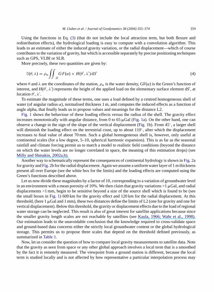
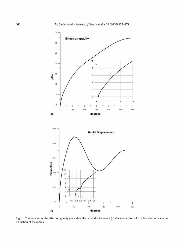
Fig. 1 shows the behaviour of these loading effects versus the radius of the shell. The gravity effectincreases monotonically with angular distance, from 0 to 65Gal (Fig. 1a). On the other hand, one canobserve a change in the sign of the slope of the vertical displacement (Fig. 1b). From 45, a larger shellwill diminish the loading effect on the terrestrial crust, up to about 110, after which the displacementincreases to final value of about 70 mm. Such a global homogeneous shell is, however, only useful atcontinental scales (for a low degree, 5–10, spherical harmonic expansion). This is as far as the seasonalrainfall and climate forcing permit us to match a model to realistic field conditions (beyond the distanceon which the water levels are no longer correlated in space, the meaning of this estimation drops) (seeMilly and Shmakin, 2002a,b).

Another way to schematically represent the consequences of continental hydrology is shown inFig. 2afor gravity andFig. 2b for the radial displacement. Again we assume a uniform water layer of 1 m thicknesspresent all over Europe (see the white box for the limits) and the loading effects are computed using theGreen’s functions described above.

Let us now divide these magnitudes by a factor of 10, corresponding to a variation of groundwater levelin an environment with a mean porosity of 10%. We then claim that gravity variations >1Gal, and radialdisplacements >1 mm, begin to be sensitive beyond a size of the source shell which is found to be (seethe small boxes inFig. 1) 600 km for the gravity effect and 120 km for the radial displacement. At thisthreshold, (here 1Gal and 1 mm), these two distances define the limits of L2 (one for gravity and one forvertical displacement). Below this threshold, the gravity or displacement effects due to the load of regionalwater storage can be neglected. This result is also of great interest for satellite applications because sincethe smaller gravity length scales are not reachable by satellites (seeKaula, 1966; Wahr et al., 1998).Our estimation leads to the unavoidable conclusion that the knowledge required to cross-validate spaceand ground-based data concerns either the strictly local groundwater content or the global hydrologicalstorage. This permits us to propose three scales that depend on the threshold defined previously, assummarized inTable 1.

Now, let us consider the question of how to compare local gravity measurements to satellite data. Notethat the gravity as seen from space or any other global approach involves a local term that is a smoothedby the fact it is remotely measured. The viewpoint from a ground station is different, because the localterm is studied locally and is not affected by how representative a particular interpolation process may

360 M. Llubes et al. / Journal of Geodynamics 38 (2004) 355–374

Fig. 1. Computation of the effect on gravity (a) and on the radial displacement (b) due to a uniform 1 m thick shell of water, asa function of the radius.

M. Llubes et al. / Journal of Geodynamics 38 (2004) 355–374 361

Fig. 2. Gravity change (inGal) (a) and radial displacement (in mm) (b) caused by an hypothetical water table of continentalsize (the white box) in Europe of 1 m thickness.

be. One can compare this to the difficulty of interpolating a rapidly varying function from its smoothedform.

A possible scheme to compare gravity space data to ground-based data, based on signals originatingfrom hydrology, could be similar to the following:

(1) take the global or smoothed water storage data as derived from space techniques (above Kaula’slimit), and re-estimating (by convolution) the gravity contribution of water masses variations butputting a “hole” at the station location to cancel the local contribution seen from space. Let “S” bethis quantity,

(2) estimate, by using station gauges (piezometers, soil moisture probes, evapo-transpiration models. . .)the total amount of underground water, and calculate the corresponding local gravity contribution,say “GW”,

(3) add together S + GW, and compare to gravity residuals (gravity observations corrected for the usualknown signals such as solid and ocean tides, atmospheric pressure, pole motion and instrumentaldrift) as given by superconducting or absolute gravimeters.

362 M. Llubes et al. / Journal of Geodynamics 38 (2004) 355–374

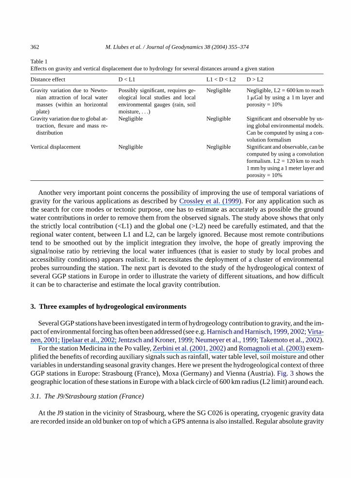
Table 1Effects on gravity and vertical displacement due to hydrology for several distances around a given station

Distance effect D < L1 L1 < D < L2 D > L2

Gravity variation due to Newto-nian attraction of local watermasses (within an horizontalplate)

Possibly significant, requires ge-ological local studies and localenvironmental gauges (rain, soilmoisture,. . .)

Negligible Negligible, L2 = 600 km to reach1Gal by using a 1 m layer andporosity = 10%

Gravity variation due to global at-traction, flexure and mass re-distribution

Negligible Negligible Significant and observable by us-ing global environmental models.Can be computed by using a con-volution formalism

Vertical displacement Negligible Negligible Significant and observable, can becomputed by using a convolutionformalism. L2 = 120 km to reach1 mm by using a 1 meter layer andporosity = 10%

Another very important point concerns the possibility of improving the use of temporal variations ofgravity for the various applications as described byCrossley et al. (1999). For any application such asthe search for core modes or tectonic purpose, one has to estimate as accurately as possible the groundwater contributions in order to remove them from the observed signals. The study above shows that onlythe strictly local contribution (<L1) and the global one (>L2) need be carefully estimated, and that theregional water content, between L1 and L2, can be largely ignored. Because most remote contributionstend to be smoothed out by the implicit integration they involve, the hope of greatly improving thesignal/noise ratio by retrieving the local water influences (that is easier to study by local probes andaccessibility conditions) appears realistic. It necessitates the deployment of a cluster of environmentalprobes surrounding the station. The next part is devoted to the study of the hydrogeological context ofseveral GGP stations in Europe in order to illustrate the variety of different situations, and how difficultit can be to characterise and estimate the local gravity contribution.

3. Three examples of hydrogeological environments

Several GGP stations have been investigated in term of hydrogeology contribution to gravity, and the im-pact of environmental forcing has often been addressed (see e.g.Harnisch and Harnisch, 1999, 2002; Virta-nen, 2001; Ijpelaar et al., 2002; Jentzsch and Kroner, 1999; Neumeyer et al., 1999; Takemoto et al., 2002).

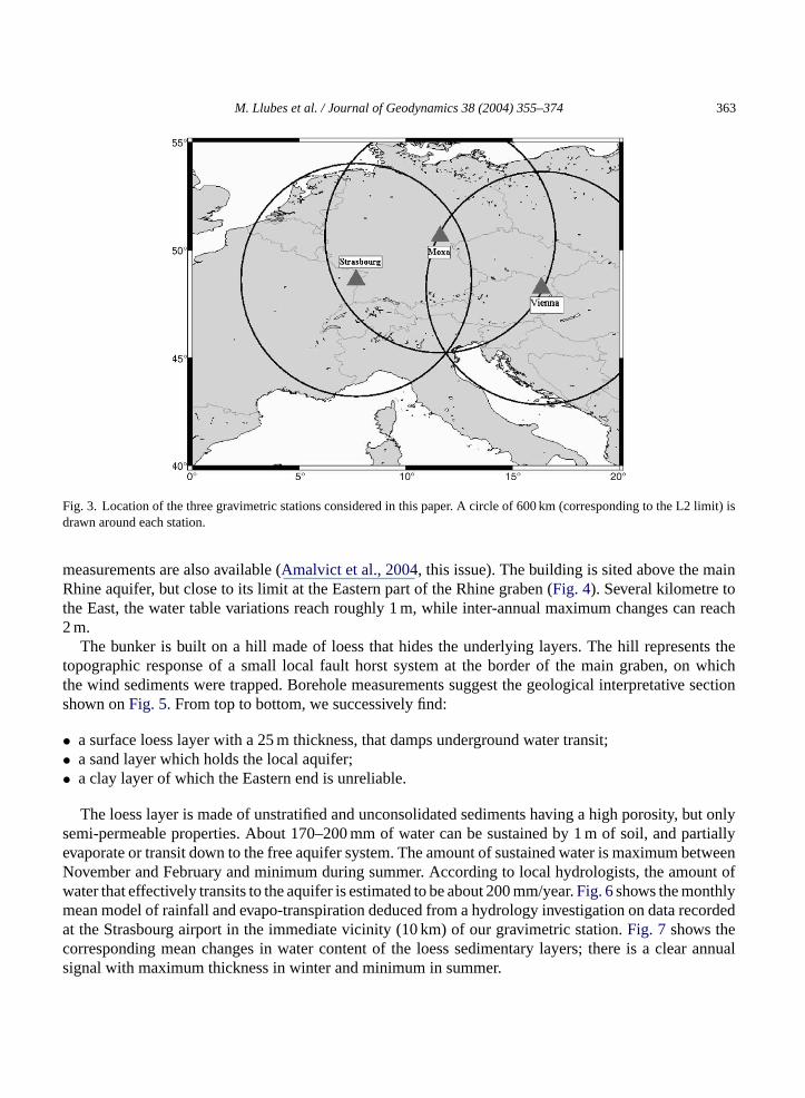
For the station Medicina in the Po valley,Zerbini et al. (2001, 2002)andRomagnoli et al. (2003)exem-plified the benefits of recording auxiliary signals such as rainfall, water table level, soil moisture and othervariables in understanding seasonal gravity changes. Here we present the hydrogeological context of threeGGP stations in Europe: Strasbourg (France), Moxa (Germany) and Vienna (Austria).Fig. 3shows thegeographic location of these stations in Europe with a black circle of 600 km radius (L2 limit) around each.

3.1. The J9/Strasbourg station (France)

At the J9 station in the vicinity of Strasbourg, where the SG C026 is operating, cryogenic gravity dataare recorded inside an old bunker on top of which a GPS antenna is also installed. Regular absolute gravity

M. Llubes et al. / Journal of Geodynamics 38 (2004) 355–374 363

Fig. 3. Location of the three gravimetric stations considered in this paper. A circle of 600 km (corresponding to the L2 limit) isdrawn around each station.

measurements are also available (Amalvict et al., 2004, this issue). The building is sited above the mainRhine aquifer, but close to its limit at the Eastern part of the Rhine graben (Fig. 4). Several kilometre tothe East, the water table variations reach roughly 1 m, while inter-annual maximum changes can reach2 m.

The bunker is built on a hill made of loess that hides the underlying layers. The hill represents thetopographic response of a small local fault horst system at the border of the main graben, on whichthe wind sediments were trapped. Borehole measurements suggest the geological interpretative sectionshown onFig. 5. From top to bottom, we successively find:

• a surface loess layer with a 25 m thickness, that damps underground water transit;• a sand layer which holds the local aquifer;• a clay layer of which the Eastern end is unreliable.

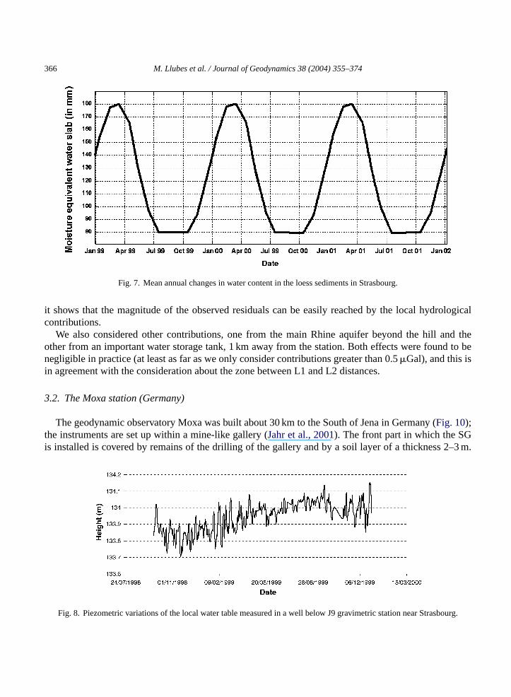
The loess layer is made of unstratified and unconsolidated sediments having a high porosity, but onlysemi-permeable properties. About 170–200 mm of water can be sustained by 1 m of soil, and partiallyevaporate or transit down to the free aquifer system. The amount of sustained water is maximum betweenNovember and February and minimum during summer. According to local hydrologists, the amount ofwater that effectively transits to the aquifer is estimated to be about 200 mm/year.Fig. 6shows the monthlymean model of rainfall and evapo-transpiration deduced from a hydrology investigation on data recordedat the Strasbourg airport in the immediate vicinity (10 km) of our gravimetric station.Fig. 7 shows thecorresponding mean changes in water content of the loess sedimentary layers; there is a clear annualsignal with maximum thickness in winter and minimum in summer.

364 M. Llubes et al. / Journal of Geodynamics 38 (2004) 355–374

Fig. 4. Delimitation of the water table of the Rhine alluvium, in the vicinity of the J9 gravimetric station, North–West ofStrasbourg (France).

A piezometer sited in a well within the bunker continuously records the local water table level (Fig. 8)within the sandy layer. Due to the topography, the water surface lies above the Rhine aquifer, runsindependently of it and discharges at the hillside. The level range is found to be clearly compatible withthe estimation above. Due to the lack of soil moisture data, we estimate the amount of gravity changesthat results from the ground water content by using simple models or by studying correlations betweengravity and water table levels.

The observed gravity variations show a good correlation with the water table level variations, and leadsto an approximate linear dependence of 20Gal m−1, an with an uncertainty of 4Gal between maximumand minimum values. This corresponds to a porosity of 40%, which is probably an overestimate. Thiscan be due to the fact that local variations and continental ones are correlated through seasonal coherentvariations: both crustal flexure and local water attraction act in the same direction, increasing gravitywhen the water level increases.Fig. 9b (thick line) shows the gravity prediction due to the local watertable using this admittance value.

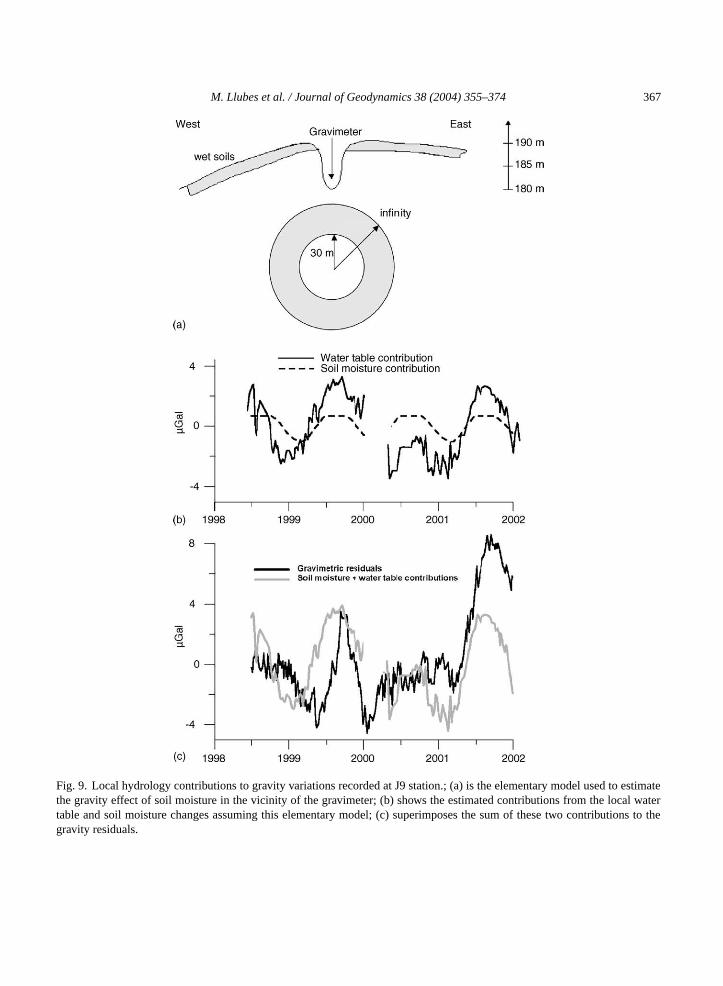
As noted above, to estimate the soil moisture contribution in the lack of any data is not straightforward.Another difficulty arises from the complex topography and background just around the gravimeter.Fig. 9ashows a simple model used for the computation of the gravity attraction due to soil moisture; the upperpart is a section view indicating the 10 m deep location of the gravimeter below the surrounding top soillayers and the bottom part gives the geometry of the model. To first order, the equivalent water layersimulating the soil moisture trapped in the surficial loess terrains is modelled by two half cylinders (one

M. Llubes et al. / Journal of Geodynamics 38 (2004) 355–374 365

Fig. 5. Geological section of the Hausbergen hill (around J9 gravimetric station).

at a mean height of 190 m to the East, the other at 185 m to the West) of internal radius 30 m and extendingto infinity.

Using this model to compute the attraction due to soil moisture leads to a value of about 1.5Galpeak to peak for this contribution (see dotted line inFig. 9b). Finally, the sum of these two terms issuperimposed to the observed gravity residuals onFig. 9c. Even if the curve agreement is not perfect,

Fig. 6. Monthly mean model for rainfall and evapo-transpiration in Strasbourg (Entzheim airport values).

366 M. Llubes et al. / Journal of Geodynamics 38 (2004) 355–374

Fig. 7. Mean annual changes in water content in the loess sediments in Strasbourg.

it shows that the magnitude of the observed residuals can be easily reached by the local hydrologicalcontributions.

We also considered other contributions, one from the main Rhine aquifer beyond the hill and theother from an important water storage tank, 1 km away from the station. Both effects were found to benegligible in practice (at least as far as we only consider contributions greater than 0.5Gal), and this isin agreement with the consideration about the zone between L1 and L2 distances.

3.2. The Moxa station (Germany)

The geodynamic observatory Moxa was built about 30 km to the South of Jena in Germany (Fig. 10);the instruments are set up within a mine-like gallery (Jahr et al., 2001). The front part in which the SGis installed is covered by remains of the drilling of the gallery and by a soil layer of a thickness 2–3 m.

Fig. 8. Piezometric variations of the local water table measured in a well below J9 gravimetric station near Strasbourg.

M. Llubes et al. / Journal of Geodynamics 38 (2004) 355–374 367

Fig. 9. Local hydrology contributions to gravity variations recorded at J9 station.; (a) is the elementary model used to estimatethe gravity effect of soil moisture in the vicinity of the gravimeter; (b) shows the estimated contributions from the local watertable and soil moisture changes assuming this elementary model; (c) superimposes the sum of these two contributions to thegravity residuals.

368 M. Llubes et al. / Journal of Geodynamics 38 (2004) 355–374

Fig. 10. Topographic map in the vicinity of the Moxa (Germany) station.

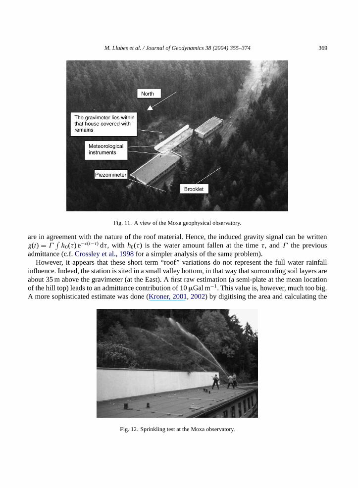
This station is also equipped with rain and water table gauges (50 m deep), and classical meteorologicalprobes (Fig. 11).

As shown byKroner (2001, 2002), significant hydrological effects in gravity occur at Moxa making adetailed analysis necessary. Most of the rainfall drains into a local stream, but the surrounding forest is veryhumid and the soil and the weathering layer can probably retain a significant amount of water. A sprinklingtest has been done to estimate the possible signal due to water within the roof area that consists of drillingrubble (Kroner, 2001, 2002). This experiment sprayed onto the roof of the building a total amount of waterequivalent to a 4 cm thick layer that run-off more or less quickly (Fig. 12). It induced a 1.2Gal gravitysignal (a corresponding admittance can be estimated as 30Gal m−1 compared to 42Gal m−1 that is thestandard Bouguer value. Because the instrument involves two spheres in levitation, a differential signalhas also been observed, as expected, and reaches 0.05Gal that seems to be in agreement with a cylindermodel of stored water on the roof of the station.

This experiment shows that at least the material over the roof behaves asonepossible source of rainfallwater storage. It also permits us to estimate the characteristic time of residence of the water on the roofthat is very useful to convert rainfall quantities into gravimetric signal including the final leakage to thestream (although it relies on a strong simplification of the local topology). It is possible to model thissystem by considering a “roof reservoir” of surface (A) (that is instantaneously filled) where the waterleaks through a permeable medium of surface (a), thickness (L) and permeability (K) (seeFig. 13). Theconservation law plus Darcy’s law leads to a solutionh(t) = h0e−c(t−t0), wherec=AK/aL (andt0 is theinitial time of filling). Although rainfall immediately succeeded the experiment, it was possible to obtaina first insight to parametersc= 6.5× 10−4 s−1 (time constant = 2 h and 30 min) andK= 10−2 m s−1 that

M. Llubes et al. / Journal of Geodynamics 38 (2004) 355–374 369

Fig. 11. A view of the Moxa geophysical observatory.

are in agreement with the nature of the roof material. Hence, the induced gravity signal can be writteng(t) = Γ

∫h0(τ) e−c(t−τ) dτ, with h0(τ) is the water amount fallen at the timeτ, andΓ the previous

admittance (c.f.Crossley et al., 1998for a simpler analysis of the same problem).However, it appears that these short term “roof” variations do not represent the full water rainfall

influence. Indeed, the station is sited in a small valley bottom, in that way that surrounding soil layers areabout 35 m above the gravimeter (at the East). A first raw estimation (a semi-plate at the mean locationof the hill top) leads to an admittance contribution of 10Gal m−1. This value is, however, much too big.A more sophisticated estimate was done (Kroner, 2001, 2002) by digitising the area and calculating the

Fig. 12. Sprinkling test at the Moxa observatory.

370 M. Llubes et al. / Journal of Geodynamics 38 (2004) 355–374

Fig. 13. Schematic description of a model of water discharge in schist debris; (A) is the “roof reservoir” (that is instantaneouslyfilled) where the water leaks through a permeable medium of surface (a), thickness (L) and permeability (K).

gravity effect of the rectangular areas. An estimation of the effect of about 2Gal m−1 for each hillsideassuming a change in water filled pore volume of 10% was obtained. In addition it would need to takeinto account the changes below the gravimeter horizon.

When observing the ground water level record versus that of gravity, from 28/04/2000 to 05/05/2000, itbecomes clear that these two signals are anti-correlated (Kroner, 2001, 2002), so the groundwater recharge(of the near-surface layer) coincides with a decrease of the gravity signal. Although the admittance changesfrom one event to the following (and the water level probe is only representative of the valley bottom), itis fully compatible with the value estimated above, between 5 and 15Gal m−1.

3.3. The Vienna station (Austria)

The Austrian superconducting gravimeter which is supported by the Institute for Meteorology andGeophysics lies in the centre of the city of Vienna, on the hillside just above the Danube River. Rainfalland soil moisture data are monitored in the park close to the gravity station (Fig. 14). The geologicalcontext consists in basin that evolved from the beginning of Miocene, as a pull-apart feature involvingseveral sedimentary episodes, until the end of Pliocene. It ended by an inversion of the tectonic conditionsthat raised the Danube basin (Decker, 1996). The various tertiary deposits show high lateral variability.The inner geomorphology is complex and consists of several local aquifers that are hard to distinguish andcharacterise. Because most of the sediments are consolidated, the mean vertical permeability is low, whilethe Danube recent sediment dynamical porosity reaches about 10%.Fig. 15summarises the geologicalsection. Although the sandy soil around the instrument can accommodate a free aquifer of significantsize, the deeper groundwater could be confined.

Sudden summer thunderstorm rainfalls form the main meteorological water contribution. An increasecan also be observed in November, while the evapo-transpiration is minimum. Because the gravimeterarea is horizontal and flat, rather high frequency gravity variations are expected. Since 1996, the cityof Vienna has managed a protective policy to prevent flooding, and the banks of the Danube have beenreinforced. A system of hydraulic pump stabilises the piezometric levels over a large extent of the WestDanube aquifer.

M. Llubes et al. / Journal of Geodynamics 38 (2004) 355–374 371

Fig. 14. Map of Vienna (Austria) showing the location of the superconducting gravimeter.

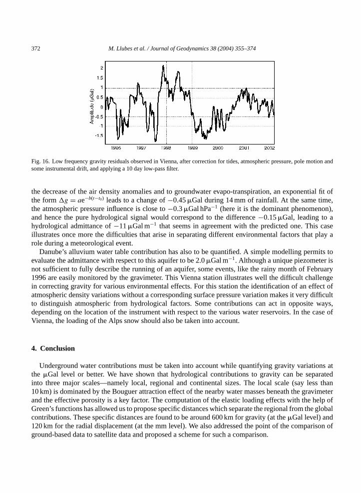
After correction for the usual known signals (solid and ocean tides, atmospheric pressure, pole motionand instrumental drift) and low-pass filtering the residuals at 10 days, the long-time gravity residualsexhibit a seasonal feature which decreases since 1999 (Fig. 16). By comparison, when considering shortperiod records, one observes a remarkable correspondence between big rainfalls and gravity changes inwhich the gravity variations occur before the rainfall itself.Meurers (2000, 2001)has interpreted this as aredistribution of atmospheric masses (vertical density changes due to water condensation) during storms,without pressure change. A few hours after the stormy event, air masses stabilise and the gravity recoversits initial level.

The atmospheric and hydrological contributions are difficult to differentiate during such events, andit is not easy to determine whether a theoretical groundwater admittance value of−12Gal m−1, asderived from a elementary geometric calculation, could be applied. Assuming that the main part of thesummer rainfall evaporates quickly, and that the slow increase in gravity after the storm is due only to

Fig. 15. Geological section of the Danube hillside in the vicinity of the gravimeter.

372 M. Llubes et al. / Journal of Geodynamics 38 (2004) 355–374

Fig. 16. Low frequency gravity residuals observed in Vienna, after correction for tides, atmospheric pressure, pole motion andsome instrumental drift, and applying a 10 day low-pass filter.

the decrease of the air density anomalies and to groundwater evapo-transpiration, an exponential fit ofthe formg = ae−b(t−t0) leads to a change of−0.45Gal during 14 mm of rainfall. At the same time,the atmospheric pressure influence is close to−0.3Gal hPa−1 (here it is the dominant phenomenon),and hence the pure hydrological signal would correspond to the difference−0.15Gal, leading to ahydrological admittance of−11Gal m−1 that seems in agreement with the predicted one. This caseillustrates once more the difficulties that arise in separating different environmental factors that play arole during a meteorological event.

Danube’s alluvium water table contribution has also to be quantified. A simple modelling permits toevaluate the admittance with respect to this aquifer to be 2.0Gal m−1. Although a unique piezometer isnot sufficient to fully describe the running of an aquifer, some events, like the rainy month of February1996 are easily monitored by the gravimeter. This Vienna station illustrates well the difficult challengein correcting gravity for various environmental effects. For this station the identification of an effect ofatmospheric density variations without a corresponding surface pressure variation makes it very difficultto distinguish atmospheric from hydrological factors. Some contributions can act in opposite ways,depending on the location of the instrument with respect to the various water reservoirs. In the case ofVienna, the loading of the Alps snow should also be taken into account.

4. Conclusion

Underground water contributions must be taken into account while quantifying gravity variations atthe Gal level or better. We have shown that hydrological contributions to gravity can be separatedinto three major scales—namely local, regional and continental sizes. The local scale (say less than10 km) is dominated by the Bouguer attraction effect of the nearby water masses beneath the gravimeterand the effective porosity is a key factor. The computation of the elastic loading effects with the help ofGreen’s functions has allowed us to propose specific distances which separate the regional from the globalcontributions. These specific distances are found to be around 600 km for gravity (at theGal level) and120 km for the radial displacement (at the mm level). We also addressed the point of the comparison ofground-based data to satellite data and proposed a scheme for such a comparison.

M. Llubes et al. / Journal of Geodynamics 38 (2004) 355–374 373

The second part of this paper was devoted to three case studies (Strasbourg, France; Moxa, Germanyand Vienna, Austria) concerning the hydrological impact on gravity in Europe with the help of SGs andenvironmental data such as rainfall, evapo-transpiration, piezometric level and soil moisture models. Inall three cases, even if the gravity residuals can be partly attributed to hydrology because of similaritiesin the observations and models, the problem has been shown to be difficult, due at least in part to the lackof the adequate environmental data.

Satellite missions dedicated to observing gravity will provide water content at a global scale withaccuracy better than any ground hydrological dataset, but they will not provide suitable data at localscale. To build an integrated understanding of groundwater contributions to gravity at ground-basedstations such as GGP, detailed hydrogeological studies must be undertaken and environmental parametersmonitored with a suitable resolution, both in time and space. Although these problems may sometimesappear less attractive than some others, they generally require significant investment that is fully relevantto separate different gravity variations and finally analyse and understand them. A special attention mustbe paid to monitor the unsaturated zone. These tasks are especially necessary to clean the gravity signalsfrom environmental forcing and must be considered in the retrieval of other, more subtle, signals. Weare thinking here of those linked to possible core dynamics or other environmental signals of oceanicor atmospheric origin in a period range from a few minutes (during rainfalls) to secular scale includingseasonal effects.

Acknowledgements

We want to acknowledge Corinna Kroner who kindly allowed us to include some figures for thestation Moxa, and has also re-read a part of the text. We also thank Bruno Meurers for providing us withuseful figures for the Vienna station. We are grateful to David Crossley who gently accepted to read themanuscript and to correct it. This work had been supported by French ACI “Observation de la Terre”program.

References

Alterman, Z., Jarosch, H., Pekeris, C.L., 1959. Oscillation of the Earth. Proc. R. Soc., London A 252, 80–95.Amalvict, M., Hinderer, J., Rosat, S., Rogister, Y., Makinen, J., 2004. Long term and seasonal gravity changes at the Strasbourg

station and their relation to crustal deformation, J. Geod. 38, 343–353.Baker, T.F., Bos, M.S., 2003. Validating Earth and ocean tide models using tidal gravity measurements. Geophys. J. Int. 152,

468–485.Boy, J.P., Llubes, M., Hinderer, J., Florsch, N., 2003. A comparison of ocean tide loading models using superconducting

gravimeter data. J. Geophys. Res. 108, B4, 2193, doi:10.1029/2002JB002050.Crossley, D., Xu, S., van Dam, T., 1998. Comprehensive analysis of 2 years of data from Table Mountain Colorado. In: Proceedings

of the 13th International Symposium on Earth Tides, Brussels, July 1997, Royal Observatory of Brussels, pp. 659–668.Crossley, D., Hinderer, J., Casula, G., Francis, O., Hsu, H.-T., Imanishi, Y., Jentzsch, G., Kaarianen, J., Merriam, J., Meurers,

B., Neumeyer, J., Richter, B., Shibuya, K., Sato, T., van Dam, T., 1999. Network of superconducting gravimeters benefits anumber of disciplines. Trans. Am. Geophys. U. 80, 121–126.

Decker, K., 1996. Miocene tectonics at the Alpine–Carpathian junction and the evolution of the Vienna Basin. Mitt. Ges. Geol.Bergbaustud.Osterr. Vienna 41, 33–44.

Dziewonski, A.M., Anderson, D.L., 1981. Preliminary reference Earth model. Phys. Earth Planet. Int. 25, 297–356.

374 M. Llubes et al. / Journal of Geodynamics 38 (2004) 355–374

Farrell, W.E., 1972. Deformation of the Earth by surface loads. Rev. Geophys. 10, 761–797.Harnisch, M., Harnisch, G., 1999. Hydrological influences in the registrations of superconducting gravimeters. BIM 131,

10161–10170.Harnisch, M., Harnisch, G., 2002. Seasonal variations of hydrological influences on gravity measurements at Wettzell. BIM 137,

10849–10861.Ijpelaar, R., Troch, P., Warderdam, P., Stricker, H., Ducarme, B., 2002. Detecting hydrological signals in time series of in situ

gravity measurements. BIM 135, 10837–10838.Jahr, T., Jentzsch, G., Kroner, C., 2001. The geodynamic observatory Moxa/Germany: instrumentation and purposes. J. Geod.

Soc. Jpn. 47 (1), 34–39.Jentzsch, G., Kroner, C., 1999. Environmental effects on the gravity vectorq short overview. BIM 131, 10107–10112.Kaula, W.M., 1966. Theory of satellite geodesy. Blaisdell, Waltham, p. 140.Kroner, C., 2001. Hydrological effects on gravity at the geodynamic observatory Moxa. J. Geod. Soc. Jpn. 47 (1), 353–358.Kroner, C., 2002. Zeitliche Variationen des Erdschwerefeldes und ihre Beobachtung mit einem supraleitenden Gravimeter im

Geodynamischen Observatorium Moxa. Professorial dissertation, Institut fur Geowissenschaften, FSU Jena.Mangiaroti, S., Cazenave, A., Soudarin, L., Cretaux, J.F., 2001. Annual vertical motions predicted from surface mass redistribution

and observed by space geodesy. J. Geophys. Res. 106 (B3), 4277–4291.Meurers, B., 2000. Gravitational effect of atmospheric processes in SG gravity data. BIM 133, 10395–10402.Meurers, B., 2001. Tidal and non-tidal gravity variations in Vienna—a five years’ SG record. J. Geod. Soc. Jpn. 47, 392–397.Milly, P.C.D., Shmakin, A.B., 2002a. Global modeling of land water and energy balances, Part I: the land dynamics (LaD) model.

J. Hydrometeorol. 3, 283–299.Milly, P.C.D., Shmakin, A.B., 2002b. Global modeling of land water and energy balances, Part II: land characteristic contributions

to spatial variability. J. Hydrometeorol. 3, 301–310.Neuman, S., Di Frederico, V., 2003. Multifaceted nature of hydrogeologic scaling and its interpretation. Rev. Geophys. 41 (3),

1014, doi:10.1029/2003RG000130.Neumeyer, J., Barthelmes, F., Wolf, D., 1999. Estimates of environmental effects in superconducting gravimeters. BIM 131,

10153–10160.Parker, R.L., 1972. The rapid calculation of potential anomalies. Geophys. J. R. Astron. Soc. 31, 447–455.Pagiatakis, S.D., 1990. The response of a realistic Earth to ocean tide loadings. Geophys. J. Int. 103, 541–560.Rodell, M., Famiglietti, J.S., 1999. Detectability of variations in continental water storage from satellite observations of the time

dependent gravity field. Water Resour. Res. 35 (9), 2705–2723.Romagnoli, Zerbini, S., Lago, L., Richter, B., Simon, D., Domenichini, F., Elmi, C., Ghirotti, M., 2003. Influence of soil

consolidation and thermal expansion effects on height and gravity variations. J. Geodyn., 521–539.Skoien, J., Bloeschl, G., Western, A., 2003. Characteristic space scales and timescales in hydrology. Water Resour. Res. 39 (10),

1304, doi:10.1029/2002WR001736.Takemoto, S., Fukuda, Y., Higashi, T., Ogasawara, S., Abe, M., Dwipa, S., Kusuma, S., Andan, A., 2002. Effect of groundwater

changes on SG observations in Kyoto and Bandung. BIM 135, 10839–10844.Van Dam, T., Wahr, J., Milly, P.C.D., Shmakin, A.B., Blewitt, G., Lavallee, D., Larson, K.M., 2001a. Crustal displacements due

to continental water loading. Geophys. Res. Lett. 28 (4), 651–654.Van Dam, T., Wahr, J., Milly, P., Francis, O., 2001b. Gravity changes due to continental water storage. J. Geodet. Soc. Jpn. 47,

249–254.Velicogna, I., Wahr, J., Van den Dool, H., 2001. Can surface pressure be used to remove atmospheric contributions from GRACE

data with sufficient accuracy to recover hydrological signals? J. Geophys. Res. 106 (B8), 16,415–16,434.Virtanen, H., 2001. Hydrological studies at the gravity station Metsahovi, Finland. J. Geodet. Soc. Jpn. 47 (1), 328–333.Wahr, J., Molenaar, M., Bryan, F., 1998. Time variability of the Earth’s gravity field: hydrological and oceanic effects and their

possible detection using GRACE. J. Geophys. Res. 103 (B12), 30205–30229.Zerbini, S., Richter, B., Negusini, M., Romagnoli, C., Simon, D., Domenichini, F., Schwahn, W., 2001. Height and gravity

variations by continuous GPS, gravity and environmental parameter observations in the Southern Po Plain, near Bologna,Italy. Earth Planet. Sci. Lett. 192 (3), 267–279.

Zerbini, S., Negusini, M., Romagnoli, C., Domenichini, F., Richter, B., Simon, D., 2002. Multi-parameter continuous observationsto detect ground deformation and to study environmental variability impacts. Global Planet. Changes 34, 37–58.