Liquidity on the Rise - Too Much Money Chasing Too Few Goods

HOHENHEIMER

DISKUSSIONSBEITRÄGE

Liquidity on the Rise - Too Much Money Chasing Too Few Goods

von

Ansgar Belke, Wim Kösters,

Martin Leschke und Thorsten Polleit

Nr. 237/2004

Institut für Volkswirtschaftslehre (520)

Universität Hohenheim, 70593 Stuttgart

ISSN 0930-8334

ECB Observer No 6: Liquidity on the rise

2

ECB OBSERVER www.ecb-observer.com

Analyses of the monetary policy of the European System of Central Banks

Liquidity on the rise – too much money chasing too few goods

No 6

2 February 2004

Prof. Dr. Ansgar Belke Universität Hohenheim

[email protected]

Prof. Dr. Wim Kösters Ruhr-Universität Bochum

[email protected]

Prof. Dr. Martin Leschke Universität Bayreuth

[email protected]

Honorary Prof. Dr. Thorsten Polleit1 Barclays Capital, Frankfurt and

Hochschule für Bankwirtschaft, Frankfurt [email protected]

________________________

1 NOTE: Thorsten Polleit works in the European economics department of Barclays Capital. His contribution to this document represents his personal views, which do not necessarily correspond to the views of the firm.


3

CONTENT Introduction Part 1: A case against ECB FX market interventions 1.1 A case against ECB FX market interventions 1.2 Exchange rate manipulation – an instrument to fight low growth? 1.3 Impact of euro exchange rate moves on euro area GDP and inflation Part 2: “Price gaps” and US inflation 2.1 The theory of price gaps 2.2 Estimating US consumer price inflation with price gaps 2.3 Conclusions Part 3: Price gaps and euro area inflation 3.1 Price gaps based on M3, trend money and Divisia-aggregates 3.2 Estimating consumer price inflation with various price gaps 3.3 Conclusions Part 4: ECB policy and euro inflation outlook 4.1 Monetary policy in the last six months 4.2 “Deflating deflation fears” 4.3 Euro area inflation forecast Appendix A.1. Schedules for the meetings of the ECB Governing Council in 2004 A.2. ECB OBSERVER – recent publications A.3. ECB OBSERVER – objectives and approach A.4. ECB OBSERVER – team members


4

SUMMARY Part 1: A case against ECB FX market interventions We argue against ECB FX market interventions. Our most important considerations are: (1) To support the US dollar against the euro, the ECB would have to pursue an expansionary policy, thereby causing inflation to rise in the future. (2) Empirical evidence shows that appreciations of the euro exchange rate do not cause the negative effects on (German) exports that are widely put forward as an argument for an ECB intervention. (3) Assuming forward-looking market agents, monetary policy cannot influence the real exchange rate – which is the relevant variable for ex-ports – at will and on a systematic basis. (4) FX market interventions run the risk of becoming de-stabilising. (5) Reducing economic incentives to bring about structural reforms and process and product innovations, thereby damages growth and thus employment in the euro area. Part 2: “Price gaps” and US inflation Empirical analyses on the relationship between money and inflation in the US suggest that the so-called “price gap” – that is the stock of money which has not yet been absorbed by increases in output and prices – has considerably power for explaining US consumer price inflation; “money matters,” even in the US. However, the income velocities of monetary aggregates do not show a “deterministic trend stationarity”. As a result, the US Federal Reserve (Fed) cannot – like, for in-stance, the ECB – make its interest rate decisions solely dependent on money growth. A careful interpretation of the current US monetary developments suggests that inflation is going to acceler-ate (slightly) going forward; deflationary tendencies are not discernible from the point of view of monetary conditions. Part 3: “Price gaps” and euro area inflation In the euro area, the price gap on the basis of M3 is an inflation indicator par excellence; it outper-forms alternative indicators such as, for instance, the output gap, the exchange rate and unem-ployment. The price gap M3 is particularly useful when it is calculated on the basis of the trend path of M3. Alternative specifications such “Divisia” monetary aggregates are no better than M3 for inflation-forecasting exercises. Against this background it would be rational for the ECB to focus on the price gap M3 (“monetary analysis”) rather than other indicators (“economic analy-sis”) when setting rates. That said, the bank’s decision to downgrade the role of M3 in its policy, as happened in the last strategy revision, is hard to understand. The actual price gap M3 indicates considerable inflation potential: the liquidity built up would be sufficient to increase the euro area price level by around 7.0% on a persistent basis. Part 4: ECB rate and euro inflation outlook Money and credit supply in the euro area suggests a need for higher central bank interest rates to reduce (the increase in) the price gap M3; it is hard to see that currently prevailing real short-term interest rates will be compatible with low inflation. It is unlikely that the excess liquidity, which has been built up in the past, will be fully absorbed by higher production. On the basis of our forecast model, euro area inflation will start to rise, being, on average, 2.1% in 2004 and 2.2% in 2005. – In particular, we see the risk that excess liquidity in the US as well as in the euro area could cause, in a first wave, asset price inflation (on the stock, bond and housing markets) before driving up consumer prices. The inevitable correction of such a development could prove highly costly as far as output and employment are concerned, and thus warrants attention by monetary policy makers. This is why we conclude: “Too much money is chasing too few goods.”


5

Zusammenfassung

Teil 1: Argumente gegen EZB-Devisenmarktinterventionen Wir sprechen uns gegen Devisenmarktinterventionen aus. Unsere wichtigsten Argumente sind: (1) Eine Schwächung des Euro zu Gunsten des US-Dollar würde eine noch expansivere Geldpolitik der EZB erfordern, die die Preisstabilität gefährdet. (2) Empirische Erkenntnisse zeigen, dass Wechselkursaufwertungen nicht die negativen Folgen auf die (deutschen) Exporte ausüben, wie allgemein behauptet wird. (3) Die EZB kann den (entscheidenden) realen Wechselkurs nicht ziel-gerecht und systematisch beeinflussen. (4) Devisenmarktinterventionen bergen das Risiko, desta-bilisierende Effekte auf den Märkten auszulösen. (5) Geldpolitische Interventionen zur Schwä-chung des Euro könnten die Anreize reduzieren, Strukturreformen sowie Produkt- und Prozessin-novationen voranzutreiben, die dann den Wachstumspfad und die Beschäftigungslage schädigen.

Teil 2: “Price gaps” und die US-Inflation Empirische Untersuchungen zur Beziehung zwischen Geldmenge und Inflation in den USA zei-gen, dass die „Preislücke“ – d. h. der in der Vergangenheit aufgebaute und noch nicht durch Out-put- und/oder Preissteigerungen abgebaute Geldüberschuss – einen ganz erheblichen Beitrag leis-tet, um die Inflation der amerikanischen Konsumentenpreise zu erklären: Es gilt „Money Mat-ters“. Allerdings erweisen sich die Umlaufgeschwindigkeiten der US-Geldmengen häufig als nicht „trendstabil“. Dadurch kann die US Notenbank ihre Politik nicht – wie es etwa der EZB möglich ist – unmittelbar an der Geldmengenentwicklung ausrichten. – Eine vorsichtige Interpre-tation der aktuellen US-Geldmengenentwicklungen deutet auf einen (leichten) Anstieg der Inflati-on in der Zukunft hin; deflationären Tendenzen sind in den USA nicht zu erkennen.

Teil 3: “Price gaps” und die Euroraum-Inflation Die Preislücke auf Basis der Geldmenge M3 erweist sich als überragender Inflationsindikator im Euroraum; sie „outperformed“ alternative Indikatoren wie z. B. das „Output Gap“, den Wechsel-kurs und die Arbeitslosigkeit. Als besonders aussagekräftiger Inflationsindikator erweist sich die Preislücke, wenn sie auf Basis ihres „Trendverlauf“ errechnet wird. Alternative Spezifikationen, wie etwa zinsgewichtete Geldmengenaggregate („Divisia-Aggregate“), sind der M3-Preislücke nicht überlegen. Vor diesem Hintergrund wäre es für die EZB rational, ihre Geldpolitik verstärkt an der M3-Preislücke („Monetäre Analyse“) auszurichten und die Bedeutung anderer Variablen („wirtschaftliche Analyse“) zurückzustufen. Daher erscheint auch die „Strategierevision“ vom 8. Mai 2003 als wenig nachvollziehbar. – Die aktuelle M3-Preislücke zeigt ein beträchtliches Infla-tionspotenzial: Die aufgelaufene Liquidität reicht aus, das Preisniveau im Euroraum dauerhaft um etwa 7,0 Prozent anzuheben.

Teil 4: EZB-Geldpolitik und Inflationsausblick Die Geld- und Kreditexpansion im Euroraum legt Zinsanhebungen nahe, um die Expansion der M3-Preislücke abzubremsen; eine Situation, in der der Realzins mehr oder weniger Null Prozent beträgt, kann nicht beibehalten werden, ohne letztlich die Inflation anzuheizen. Schon heute er-scheint es unwahrscheinlich, dass der Geldüberschuss durch einen Anstieg der Produktion (voll-ständig) absorbiert wird. Auf Basis unseres Prognosemodells errechnen wir eine jahresdurch-schnittliche Inflation in Höhe von 2,1 Prozent in 2004 und 2,2 Prozent in 2005. – Im aktuellen Umfeld besteht dies- und jenseits des Atlantiks die akute Gefahr, dass der Geldmengenüberschuss eine (weitere) „Asset Price Inflation“ auf den Vermögensmärkten (Aktien, Bonds, Häuser etc.) speisen wird, deren unausweichliche Korrektur mit beträchtlichen Output- und Beschäftigungs-verlusten verbunden sein kann. Daher auch unsere Schlussfolgerung: „Too much money is chasing too few goods”.


6

Introduction There are obvious signs of an economic recovery in the major economies around the world. In the US, economic growth is likely to be well above the potential rate this year after an already above-potential expansion in 2003. In the euro area, expectations of economic expansion towards the po-tential rate of 2.0% in 2004 seem realistic. The Japanese economy seems set to expand at positive rates this year. Moreover, the majority of Asian countries appear to have embarked on a fairly ro-bust growth path. However, there are challenges ahead that may have the potential to spoil the party.

Challenges ahead. – The question that has increasingly attracted attention is: Are there risks that a further strengthening of the euro exchange rate might derail the still fragile euro area economic recovery? And if so, shall a case be made for ECB FX market intervention to weaken the euro, e.g. prevent it from appreciating further vis-à-vis third currencies? Moreover, there is hardly any doubt about the fact that monetary policy has been immensely expansionary. In the US and the euro area, central banks have lowered (real) short-term rates to historic lows. This, in turn, has contributed to the high growth rates of monetary aggregates. At the same time, how-ever, strong growth of money supply has been assigned relatively little attention by monetary pol-icy makers. So, the second question is: What are the consequences of the monetary expansion seen in recent years for future inflation?

In this report we aim to address these two questions. In addition, we present, as always, our inflation forecast for the euro area for the coming 12 months.

Against FX market interventions. – In view of the unfolding discussion about the need for ECB FX market interventions, we put forward a number of strong arguments against any such policy. First, in view of the monetary overhang in the euro area that already exists, an FX market intervention to weaken the euro vis-à-vis the US dollar would require the ECB to in-crease the money supply even further, thereby increasing inflation. Second, there is no convincing evidence that the central bank will be able to influence the real exchange rate – the de facto rele-vant variable – according to its own design. And third, the consequences of the exchange rate moves seen so far certainly do not make a case for “market failure,” which could be used to argue for government intervention.

“Money matters”. – We analyse the role monetary expansion plays for inflation by the concept of “price gaps,” that is the supply of money which has built up in the past and has not yet been absorbed by either output gains and/or price increases. As far as the euro area is concerned, we find strong statistical evidence that the “M3 price gap” is a key driver for future inflation. That said, there is a strong rationale for the ECB to focus on M3 when setting interest rates. Even in the US we find that money price gaps play an important role in explaining inflation. In contrast to the euro area, however, the velocities of US monetary aggregates do not exhibit a deterministic trend path, which might limit the indication quality of monetary aggregates for monetary policy.

ECB will have to raise interest rates. – Looking at money and credit growth in the euro area, we conclude that a forward-looking monetary policy would require the ECB to raise interest rates to slow the growth of M3. It is unlikely that a build up in excess liquidity will be fully absorbed by output gains. That said, inflation is unlikely to slow down as is widely expected. In fact, our model suggests that under current conditions, inflation will be 2.1% in 2004 and rise to 2.2% in 2005. We see the biggest risk that excess liquidity in the US as well as in the euro area could cause, in a first wave, “asset price inflation” (on stock, bond and housing markets) before driving up consumer prices. The inevitable correction of such a development could prove highly costly as far as output and employment are concerned and thus warrants attention by monetary policy makers.


7

Part 1: A case against FX market intervention CONTENT: 1.1 Weakening the euro exchange rate would increase inflation. 1.2 Further considerations. 1.3 Impact of euro exchange rate moves on euro area GDP and inflation. SUMMARY: There are a number of strong arguments against ECB FX market intervention. First, in view of the already monetary overhang in the euro area, an FX market intervention to weaken the euro vis-à-vis the US dollar would require the ECB to increase the money supply even further, thereby increasing inflation. Second, there is no convincing evidence that the central bank will be able to influence the real exchange rate – the de facto relevant variable – according to its own design. And third, the consequences of the exchange rate moves so far do not make a case for “market failure” which could argue for government intervention. 1.1 Weakening the euro exchange rate would increase in-

flation Low growth, low inflation and a seemingly relentless appreciation of the euro exchange rate: surely it is time for the European Central bank (ECB) to cut rates?2Declining borrowing costs, for instance, could support investment spending, induce positive wealth effects and, ulti-mately, increase output and employment. Lower rates might also reduce the euro area’s short-term interest rate differential vis-à-vis the US, thereby slowing – or even reversing – the sin-gle currency’s appreciation. The case for monetary policy easing seems to be compelling in-deed. However, the effectiveness of monetary policy and, most importantly, monetary devel-opments, argue in favour of the ECB refraining from cutting rates any further.

To start with, monetary policy can only impact output and employment if it produces “surprise” inflation; that is, it delivers inflation that is higher than originally expected. Only then will monetary policy exert an influence on real prices and thus output. However, adept market agents (that is those who form their expectations according to the model of “rational expectations”) will anticipate such a policy action and adjust prices accordingly. In doing so, the outcome of an expansionary policy would not only be ineffective but also sub-optimal: output and employment would remain unchanged while inflation would rise. Given that the ECB has a mandate to deliver stable and low inflation, inducing surprise inflation is not an option. And rightly so: the high costs of inflation argue against a monetary policy trading off inflationary concerns against the promise of growth benefits. With this in mind, it is interest-ing to note that in formulating monetary policy, little attention is currently paid to the growth rate of the money supply. Admittedly, the relationship between money growth and inflation from quarter to quarter and year to year is not easy to understand, yet this is the time frame within which policymakers generally operate. As such, money may not be a particularly use-ful guide for short-term policymaking. However, there is strong empirical evidence that over two or more years, broad money inflation may still be largely determined by the long-run growth rate of the money supply. This finding serves as a reminder that ignoring money growth for too long may be unwise.

In recent years, excess liquidity in the euro area – that is, the stock of money that has yet to be absorbed by output and inflation – has built to a level sufficient to push the price level up by more than 7%. Experience suggests that excess liquidity will ultimately show up in higher prices, be it at the consumer-price level or, as is more likely, in the current low-growth environment, in “asset price inflation”. Both types of inflation would be detrimental to the

________________________

2 See in this context also ECB Observer, “10 Argumente gegen eine Euro-US-Dollar-Wechselkurs-manipulation”, 11 December, 2003 (www.ecb-observer.com).


8

creation of sustainable output and employment expansion. In fact, the overly generous liquid-ity provision is actually the key argument against any ECB FX market intervention in favour of the US dollar (see Box 1.1).

Box. 1.1. – FX market intervention and the ensuing liquidity effect

In this box we provide an example on how FX market interventions to support the euro vis-à-vis the US dollar would affect liquidity in the euro area. Let us assume the ECB has provided the euro area banking sector with a monetary base of €100. With the latter, the banking sector is in a position to increase the amount of money and credit to the non-bank sector via “multiple money creation”. If the ECB would intervene in the FX market to weaken the euro versus the US dollar, the bank would have to buy US dollars – in our example, say to the amount of a euro equivalent of €10. The US dollar would be re-corded on the asset side of the ECB’s balance sheet (1a). Such a transaction, however, would involve providing the money market with a euro monetary base (that is central bank money) for the same amount (1b), which would be recorded on the liability side of the bank’s balance sheet.

Assets Balance sheet of the ECB Liabilities Securities 100 Banks’ minimum reserves 100 (1a) US dollar +10 Free bank liquidity (1b) +10

As a result, the euro area banking sector’s free liquidity would increase which, in turn, increases its capacity to expand money and credit supply. A higher amount of money and credit, however, might run counter to the cen-tral bank’s intention to control liquidity to keep inflation at the envisaged path. A decline in money market rates, which can be expected to be associated with the increase in bank liquidity, may counteract upward pres-sure on the external value of the currency. With M3 growth running well above the envisaged path, however, liquidity in the euro area is already much higher than desired, which would render any such operation undesir-able. In a case where the ECB would try to “neutralise” the liquidity-enhancing intervention effect, it would have to take recourse to restrictive open market operations (or simply raise interest rates). Under such a policy, the bank would have to sell securities to the market, thereby reducing the monetary base. The reverse expansionary open market operation would very likely eliminate the preceding effect on the exchange rate, if there were any.

Such market intervention would require the ECB to pursue an expansionary policy – ie,

increasing the already very high level of excess money: the ECB would have to buy US dol-lars against issuing euro, thus lowering rates further. Such a shift in policy emphasis towards the exchange rate would thus conflict with the bank’s primary objective, which is maintaining price stability. Moreover, it is highly questionable whether the ECB would be able to influ-ence the exchange rate according to its own design.

Economic literature has often detected destabilising effects from intervention. Interven-ing within a narrow band of the equilibrium rate is likely to increase the chances of creating persistent instability. Unfortunately, the likelihood of meeting equilibrium is relatively re-mote. Experience shows that intervention increases the probability of stability only when the rate is clearly misaligned. An additional, and perhaps more striking argument against inter-vention, is that the factors driving the direction and intensity of exchange rate moves – that is, for instance, expected growth and capital returns – are beyond the reach of monetary policy: apart from the price level it is hard to see how monetary policy can have a systematic impact on the variables which are usually held responsible for exchange rate levels (see Box 1.2).

ECB monetary policy in the euro area is, by all measures, already highly expansionary, suggesting that it is questionable whether inflation will fall to below the ECB’s 2.0% ceiling on a consistent basis. As a result, the bank’s already loose monetary policy stance makes FX market intervention neither feasible nor compatible with the bank’s policy target – all the more so as empirical evidence shows that the trend of euro area inflation is driven by excess


9

liquidity, and that the impact of the exchange rate on inflation is largely temporary. As such, it is rational for monetary policy to look more closely at money growth trends rather than ex-change rate fluctuations when setting rates. Lastly, it should be stressed that the onus is on na-tional governments to improve the euro area’s growth perspectives by speeding up and inten-sifying the reform process – a factor that is no doubt at the heart of the euro area’s disappoint-ing growth performance. 1.2 Exchange rate manipulation – an instrument to fight

low growth? In the last weeks, the euro rushed from one all time high to another. Since November 2003, the euro has re-valued in terms of the effective trade-weighted exchange rate in the midst of January by around five percent while the euro has appreciated by even ten percent in bilateral terms vis-à-vis the dollar since December 2003. This clear upward trend was interrupted only briefly when some members of the ECB council intervened verbally from January 12 on in favour of a lower euro (“brutal revaluation of the euro”). Except this brief episode, the ECB president Trichet has strictly stuck to his clear confession to refrain from FX interventions and interest rates cuts in order to weaken the strong euro. Although, for instance, the Federal As-sociation of German Industry and some euro area politicians like the Belgian finance minister Didier Reynders already assess a euro exchange rate vis-à-vis the dollar of 1.20 to 1.30 as a threat and a bottom line for interventions, Trichet’s position deserves our support. A bulk of forceful arguments speak against interventions on the FX markets and/or against efforts to in-fluence the euro-dollar exchange rate indirectly via euro interest rate cuts as the next step fol-lowing pure rhetoric. We would like to base these arguments on the main insight that the re-cent strength of the euro cannot be attributed to a strong performance of the euro area econ-omy but on the weak US dollar, i.e. the US twin deficit combined with currently extremely low interest rates.

Besides the fact that German politics and interest groups loudly complained also about an undervalued dollar exchange rate of the euro around two years ago, it should also be taken into account (1) that dollars have to be bought in a massive and continuous fashion even in order to keep the euro-dollar exchange rate on a constant lower level. This would fuel euro area inflation, (2) that the exchange rate of 1.18 dollar per euro which has already been called a bottom line and a threat for German exporters closely corresponds to the starting exchange rate at the birth date of European Economic and Monetary Union in 1999, and (3) that a high-valued euro implies significant terms-of-trade gains for the euro area. This essentially means that the imported raw materials and intermediate goods become cheaper for euro area resi-dents. This effect partly compensates euro area firms like Lufthansa, Puma, Metro or Adidas (which import heavily from the US or from those Asian countries with a peg to the US dollar) for the price increase of their exports.3 Hence, a deterioration of the terms-of-trade in the wake of a devaluation of the euro results in a further reduced scope for wage policy in the euro area. In the following, we present ten most forceful arguments against the two possible options for the ECB in order to weaken the euro - FX Interventions or euro interest rate cuts.

________________________

3 On average, an appreciation of the euro vis-à-vis the dollar by ten percent on average tends to diminish the returns of a German DAX enterprise by five percent. This kind of calculation leads to the nowadays popular derivation of “bottom lines” for the euro exchange rate. In order to become more immune against the appreciation of the euro vis-à-vis the dollar, some firms like Volkswagen and EADS even consider a shift towards more purchases of intermediate goods in the dollar area. Also the German Telekom profits from the weak dollar because the interest burden on its dollar debt is shrinking.


10

Point 1: From a transatlantic perspective: if at all, there is a need for up-ward instead of downward adjustment of the euro

The recent pattern (if it) persists that the currencies of the UK, Asia and other emerg-ing markets are effectively pegged to the dollar has mainly two implications: 1) Most of the counterpart for the future current account adjustment of the US would be forced on the euro area. 2) A further large move in the bilateral dollar/euro rate will be needed before the dollar can get even close to a level that would produce a sizeable adjustment in the US current ac-count into the desired direction. In view of the risks which are connected with the U.S. twin deficit also for the euro area, an appreciation of the euro would be not only in the US but also in the euro area interest. Interventions on the FX market in order to weaken the euro and to strengthen the dollar at the same time do not make any sense from this point of view. Point 2: An appreciation of the euro does generally not lead to the often feared devastating effects on the German export industry.

The argument that an overvalued currency from the perspective of leads to a loss of in-ternational competitiveness is anything but new. It can be refuted rather easily if one asks which exactly are the areas in which Germany is in fact lacking competitiveness. A consider-able number of eminent economists blame Germany’s dismal economic performance in recent years on a lack of external competitiveness. They claim that the country entered EMU at too high a nominal exchange rate, to which it is now irrevocably locked. The only solution to this predicament, so the argument goes, is a slow and painful internal devaluation of the real ex-change rate.

At the same time, however, export data tell an entirely different story. German real ex-ports of goods and services grew at an annual average rate of 6¾% in 1999-2002, signifi-cantly stronger than exports in France (5.2%), Italy (2.9%), Spain (5.6%) or the Netherlands (3.9%). According to the OECD, Germany gained considerable market share in its foreign markets in 1999-2002, while France, Italy, and Spain lost market shares. This means: Ger-many is quite competitive in certain foreign trade-oriented branches. This competitiveness manifests itself in a relatively high robustness vis-à-vis euro appreciations. Strong export per-formance against the odds could be explained by a successful focus on up-market goods and services, characterised by high income and low price elasticities (see, e.g., Porsche), effective marketing, and heavy emphasis on close customer relations. The latter factor is especially im-portant for vertically integrated global companies. During the 1990s, many German compa-nies acquired foreign production facilities, and they are now supplying inputs to these facto-ries from their home base. Clearly, these exports within the same firm are much less price and cost sensitive than exports to outside customers.

The (since ten years) comparably low growth rates of real GDP in Germany are defi-nitely not the result from a lack of external competitiveness. Instead, failure to explain Ger-many’s economic weakness with either a lack of external competitiveness or restrictive mac-roeconomic policies points to a lack of “internal” competitiveness as the main problem. One important implication of our analysis is that the appreciation of the euro may not have the widely expected devastating effect on German exports. Given their past experience, German companies may be more capable to deal with a deterioration of their price competitiveness than some of their euro area competitors. Hence, countries that in the past have more strongly relied on improved price competitiveness to boost growth and employment than Germany may feel more affected by euro appreciation. If this argument holds, the gap in growth be-tween Germany and France, which benefited from larger gains in cost competitiveness in the


11

past, could narrow in the future – even without an artificial weakening of the euro by the ECB.

In addition, one has to take into account that lower volumes of exports of goods and services have recently been more than compensated by higher exports within the euro area. For instance, more than 50 percent of Germany’s exports are of the intra-EU type but only about 12 percent are determined for the US.4 Finally, the world economic climate and, thus, the world demand for imports from the euro area are recovering these days. Both aspects might dominate the effects of the euro appreciation on euro zone total exports. Point 3: The real exchange rate of the euro cannot be influenced perma-nently and durably by changes of the nominal exchange rate

Does it make good economic sense to apply exchange rate policy to compensate for the euro area-specific bad growth performance in view of the structural character of unem-ployment in the current member countries of the euro area? Besides some problems of fine-tuning and of a controlled implementation of a devaluation via an expansive monetary policy one has to take into account above all that there is no higher probability that wage-negotiating parties do submit themselves to indirect reductions of their real wages via devaluations of the home currency than to direct wage decreases. Empirical evidence for Western Europe insinu-ates that the often maintained implicit assumption of exchange rate illusion of the wage-negotiating parties is in the medium to the long term untenable and not warranted. In the long term, nominal exchange rate movements do not lead to changes of the real exchange rate.

If additionally imported inflation as in the past leads to higher wage demands, the prospects for European unemployment become even more gloomy. A spiral of devaluations and wage increases and an unforeseeable variability of the (real) exchange rate are the conse-quences. This scenario often goes along with periods of excessive speculation which have the potential to harm the economy because the speculation waves hamper a sound calculation by the export oriented firms. Point 4: Rational expectations speak against a systematic real impact of a devaluation of the euro – in search for the euro “bottom line”

The efficiency of pro-active monetary and exchange rate policy in fighting low eco-nomic growth can be severely questioned by the theory of rational expectations. According to the latter, devaluations do not represent an instrument which can be used in a systematic and repeated fashion in order to efficiently fight weak economic growth. Under rational expecta-tions, i.e. watchful actors which hare capable of learning, a prolonged period of price stability presupposes a credible and steady monetary policy. If monetary authorities are in breach of their commitment to keep a stable price level by frequent interventions, actors will tend to change their expectations immediately.

The credibility of the central bank begins to sway and can only be restored under the condition of significant output and employment costs. If monetary policy is used only once to serve devaluation purposes, the possibility of a repeated successful use of this instrument has become smaller since such interventions are anticipated, for instance, in wage contracts. The wage discipline of the wage negotiating parties tends to get weaker if these parties can as a rule reckon with a bailout via a devaluation of the home currency in times of lower interna-tional competitiveness. Empirical evidence indicates for Western Europe that the implicit as-sumption of exchange rate illusion of the wage-negotiating parties cannot be corroborated in ________________________

4 For the above arguments see in detail Gros et al. (2003). However, one has to add one fifth of total exports which is directed towards countries outward the US which peg their currencies to the US dollar.


12

the longer term: nominal exchange rate movements do not result in changes of the real ex-change rate in the long run. Hence, any exchange rate policy which is backed by discretionary monetary policy runs the risk of triggering additional destabilizing real effects and of durably modifying the functioning and the dynamics of the economy.

From this perspective, it cannot be excluded that the most recent euro appreciation was largely determined by speculation about the future ECB policy itself. The markets seem to be willing to test the "bottom line" of the central bank: Does the ECB intervene at rate of 1.30, 1.40 or 1.50? A clear and credible commitment by the ECB not to intervene in the FX market would probably be the means to calm down the FX markets and to stop the upward trend of the euro (Belke and Polleit, 2003). Point 5: Devaluations initiated by pro-active monetary policy tend to pre-vent the necessary structural adjustment

Devaluations of the home currency induced by monetary policy tend to prevent or at least contribute to a delay of necessary structural adjustments in the euro area and especially in Germany. A massive devaluation initially improves the international price competitiveness significantly but renders product and process innovations a less pressing issue than without the devaluation (see also our point 2). Moreover, there is no sufficient pressure any more to-wards structural adjustment on labour and product markets. With an eye on the by now well-known structural character of European unemployment this seems to be a quite important ca-veat. In contrast, the credible absence of interventions or of a monetary policy geared to the exchange rate forces entrepreneurs and politicians to enact the necessary adjustments. Espe-cially in the case of negative supply shocks, one should refrain from accommodating devalua-tions which at best alleviate the short term symptoms of low growth in Europe. Pro-active de-valuations significantly lower the incentives to break open encrusted structures on labour and product markets and, thus, prospects for growth and employment. Point 6: Structural reforms are more effective than devaluations anyway

It has often been argued in the past that problems of international competitiveness aris-ing from the cartelisation of labour markets can be eliminated much easier if the necessary macroeconomic adjustment takes place via the exchange rate than via wages. From this per-spective, the devaluation of the euro represents a substitute for wage restraint and structural reforms. However, there are some pieces of evidence available from history which prove ex-actly the contrary. For instance, it is by now clear that the positive employment impacts with-out additional inflation claimed for the UK and Italy after their exit from the European Mone-tary System (EMS) in 1992 cannot be traced back to the massive devaluations of the respec-tive currencies. Rather, these effects were induced by policy reforms which took effect simul-taneously with the exit of the Italian lira and the British pound from the EMS. Hence, in em-pirical studies investigating the efficiency of exchange rate movements in terms of employ-ment, the extent of reform has to be modelled as an explaining variable which is endogenous with regard to the choice of the exchange rate system. Then it will immediately become clear that structural reforms and not, as often maintained, pro-active devaluations of the respective home currency are the most efficient way towards more growth and employment. Hence, the euro exchange rate cannot be regarded as an important short-term oriented instrument to pre-vent path-dependence in unemployment in the presence of negative shocks.


13

Point 7: The demand for euro area exports and the size of country-specific market shares is relatively inelastic to exchange rate movements.

The impacts of exchange rate movements on foreign trade of the euro area tend to be rather small (see also point 2). One of the reasons is that the recent experience with large ex-change rate swings in Europe and the US has once again shown that there is a lot of 'pricing to market'. Firms fix local prices even in the face of large exchange rate changes.5 This implies that quantities react little to exchange rates, but profits much more: firms produce and export more or less the same amount. Hence, the same should be valid for the benefits from devalua-tions of the euro. The positive employment impacts to be expected from a devaluation in the exporting goods industry are, thus, small as well. From an empirical point of view and ab-stracting from all other negative effects of a policy of euro devaluation – extremely large de-valuations are necessary in order to raise relatively small employment effects. Finally, the real effectiveness of exchange rate variations is by definition basically restricted to country-specific shocks. Since problems of international competitiveness within the euro area are branch and region-specific, it is difficult to see why changes in the nominal euro exchange rate should be a solution for these problems which differ from branch to branch and from re-gion to region. Point 8: Exchange rate volatility induced by FX interventions has damaging effects on the real economy.

If nominal wages are rigid, it is entirely possible that flexible exchange rates lead to more flexibility of real wages which cannot be reached, for instance, with a fixed exchange rate regime. However, this can be interpreted as an advantage only if the exchange rate change is determined within a system of completely flexible exchange rates. Only in this case exchange rate movements are induced by disturbances and shocks on labour markets and cushion the home economy against these shocks. However, if exchange rate movements are not caused by labour market shocks but instead by policy fine-tuning and dirty-floating they tend to cause additional problems in the real economy instead of alleviating employment problems.

Moreover, in those countries which are most negatively affected by the comparative advantage of the devaluing countries – in the years 1992/93 Germany and France were the worst affected –political reactions cannot be ruled out which are geared against cross-border market integration and, thus, towards more protectionism. Again there is a historical example for this. For instance, Germany and France at times even questioned the Single European market in the wake of the 1992/93 EMS turbulences. Finally, there might be a negative im-pact of increasing interest rates in European capital markets which hare caused by a diminish-ing credibility of the authorities (i.e., an increasing risk premium) and a loss of reputation of the devaluating currency, the euro. Point 9: One-sided political interests of certain pressure groups are the driving forces behind the request for a euro devaluation.

The stylised fact that currency depreciations only have a small direct macroeconomic impact on growth and employment in the export branch and are counter-productive in the me-dium and the long run, is supported by the mainstream of economists but is stubbornly re-________________________

5 However, this is not so in the case of some German firms which do not appear to be flexible enough and, in-stead of cutting local prices in the destination country, prefer to complain about an overvalued dollar ex-change rate of the euro.


14

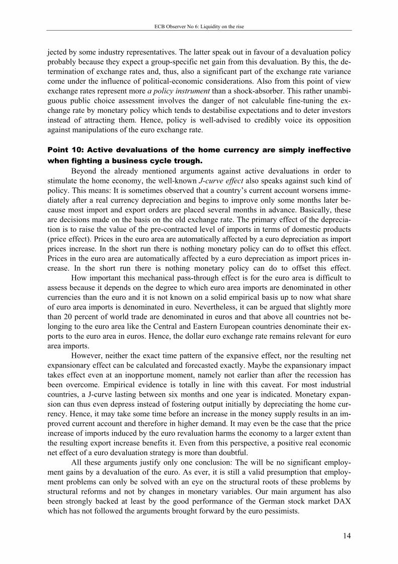
jected by some industry representatives. The latter speak out in favour of a devaluation policy probably because they expect a group-specific net gain from this devaluation. By this, the de-termination of exchange rates and, thus, also a significant part of the exchange rate variance come under the influence of political-economic considerations. Also from this point of view exchange rates represent more a policy instrument than a shock-absorber. This rather unambi-guous public choice assessment involves the danger of not calculable fine-tuning the ex-change rate by monetary policy which tends to destabilise expectations and to deter investors instead of attracting them. Hence, policy is well-advised to credibly voice its opposition against manipulations of the euro exchange rate. Point 10: Active devaluations of the home currency are simply ineffective when fighting a business cycle trough.

Beyond the already mentioned arguments against active devaluations in order to stimulate the home economy, the well-known J-curve effect also speaks against such kind of policy. This means: It is sometimes observed that a country’s current account worsens imme-diately after a real currency depreciation and begins to improve only some months later be-cause most import and export orders are placed several months in advance. Basically, these are decisions made on the basis on the old exchange rate. The primary effect of the deprecia-tion is to raise the value of the pre-contracted level of imports in terms of domestic products (price effect). Prices in the euro area are automatically affected by a euro depreciation as import prices increase. In the short run there is nothing monetary policy can do to offset this effect. Prices in the euro area are automatically affected by a euro depreciation as import prices in-crease. In the short run there is nothing monetary policy can do to offset this effect.

How important this mechanical pass-through effect is for the euro area is difficult to assess because it depends on the degree to which euro area imports are denominated in other currencies than the euro and it is not known on a solid empirical basis up to now what share of euro area imports is denominated in euro. Nevertheless, it can be argued that slightly more than 20 percent of world trade are denominated in euros and that above all countries not be-longing to the euro area like the Central and Eastern European countries denominate their ex-ports to the euro area in euros. Hence, the dollar euro exchange rate remains relevant for euro area imports.

However, neither the exact time pattern of the expansive effect, nor the resulting net expansionary effect can be calculated and forecasted exactly. Maybe the expansionary impact takes effect even at an inopportune moment, namely not earlier than after the recession has been overcome. Empirical evidence is totally in line with this caveat. For most industrial countries, a J-curve lasting between six months and one year is indicated. Monetary expan-sion can thus even depress instead of fostering output initially by depreciating the home cur-rency. Hence, it may take some time before an increase in the money supply results in an im-proved current account and therefore in higher demand. It may even be the case that the price increase of imports induced by the euro revaluation harms the economy to a larger extent than the resulting export increase benefits it. Even from this perspective, a positive real economic net effect of a euro devaluation strategy is more than doubtful.

All these arguments justify only one conclusion: The will be no significant employ-ment gains by a devaluation of the euro. As ever, it is still a valid presumption that employ-ment problems can only be solved with an eye on the structural roots of these problems by structural reforms and not by changes in monetary variables. Our main argument has also been strongly backed at least by the good performance of the German stock market DAX which has not followed the arguments brought forward by the euro pessimists.


15

The retarding effect of the most recent appreciation of the euro will most probably be felt not earlier than in the midst of 2004 since until then the hedging operations of the euro area firms will be effective and the world economic climate will continue its recovery in the next months. According to the macroeconometric models of the ECB, it may well be that the five percent effective appreciation of the euro will lower euro area GDP by 0.7 percent within a year. However, avoiding this pessimistic scenario is a challenge to the flexibility of euro area entrepreneurs and unions and, due to the expectations of increasing euro area inflation, not primarily for the ECB. The ECB cannot do anything against the weak dollar anyway since the latter has its main origin in the US and not in the euro area as shown above. Hence, the most recent verbal interventions by Mr. Trichet will only be able to slow down the apprecia-tion of the euro but not to stop it. And why at all should the ECB take care of the fact that the euro is not weak any more but slightly above its long-term average? Seen on the whole, thus, it would be inadequate to give the most recent exchange rate movement similar attention within monetary policy circles as it was the case in the public discussions during the last weeks. It seems as if some euro area interest groups try to take peoples’ attention away from other problems. Seen on the whole, the ECB should not narrow its focus on the euro exchange rate. References Belke, A. (2003): Maastricht - Implications of a Centralized Monetary and Currency Policy for Employment in

Europe, in: Addison, J.T., Welfens, P.J. (eds.), Labor Markets and Social Security - Wage Costs, Social Se-curity Financing and Labor Market Reforms in Europe, Springer, Berlin et al., 2nd ed., pp. 195 - 245.

Belke, A. (2001): Wechselkursschwankungen, Außenhandel und Arbeitsmärkte: Neue theoretische und empiri-sche Analysen im Lichte der Europäischen Währungsunion, Wirtschaftswissenschaftliche Beiträge 183, Physica, Heidelberg.

Belke, A., Gros, D. (2002): Designing EU-US Monetary Relations: The Impact of Exchange Rate Variability on Labor Markets on Both Sides of the Atlantic, in: The World Economy, Vol. 25, pp. 789 - 813.

Belke, A., Polleit, T. (2003): ECB Staat Machteloos Tegen Hoge Euro, in: Het Financieele Dagblad, November 22.

Gros, D., Jimeno, J.F., Mayer, T., Thygesen, N., Ubide, A. (2003): Adjusting to Leaner Times, 5th Annual Report of the CEPS Macroeconomic Policy Group, Centre for European Policy Studies, Brussels.

Krugman, P.R., Obstfeld, M. (2003): International Economics – Theory and Policy, 6th ed., Pearson.

1.3 Impact of euro exchange rate moves on euro area GDP and inflation

Some stylised facts In view of the relentlessly appreciating euro vis-à-vis third currencies, there is growing con-cern that a “strong euro” could actually harm, if not derail, the still fragile economic recovery in the euro area. In fact, it is feared that a rising (real effective) euro exchange rate would ul-timately dampen domestic production by making euro area exports of goods and services less competitive in world markets. Indeed, net trade (exports less imports) as a percentage of GDP has been growing since the early 1990s and stood at slightly above 3% in Q3 03. That said, net trade, which can be expected to be influenced by FX market developments, has become a non-negligible contribution to euro area output (see Figure 1.3.1).


16

Figure 1.3.1 – Euro area net trade, exports and imports and the real exchange rate, Q1 1977 to Q3 2003

(a) Net trade as percentage of GDP in the euro area (b) Euro area real GDP growth (RS) and real effective euro exchange rate (LS)

-1

0

1

2

3

4

-1

0

1

2

3

4

77 79 81 83 85 87 89 91 93 95 97 99 01 03

-.20

-.15

-.10

-.05

.00

.05

.10

.15

-.02

-.01

.00

.01

.02

.03

.04

.05

77 79 81 83 85 87 89 91 93 95 97 99 01 03

D4LNEURDS (LS) D4LNEGDPR (RS)

(c) Euro area export growth and real effective euro ex-

change rate

-.20

-.15

-.10

-.05

.00

.05

.10

.15

-.20

-.15

-.10

-.05

.00

.05

.10

.15

1980 1985 1990 1995 2000

D4LNEURDS D4LNEEX

(d) Euro area import growth and real effective euro ex-change rate

-.20

-.15

-.10

-.05

.00

.05

.10

.15

-.20

-.15

-.10

-.05

.00

.05

.10

.15

1980 1985 1990 1995 2000

D4LNEIM D4LNEURDS

Source: ECB; own calculations. Figure 1.3.1 (b) shows the annual growth rate of euro area GDP and the real effective euro exchange rate (REER) in percent for the period Q1 77 to Q3 03. A simple cross-correlation analysis reveals that exchange rate changes tend to lead GDP growth by seven quarters. Here, the correlation coefficient reaches its maximum of 0.32. Even though the correlation coeffi-cient is relatively low by statistical standards, it nevertheless suggests that an appreciating REER has been accompanied by an increase in real production after a time lag of around two years.6

Figure 1.3.1 (c) and (d) show the annual changes of exports and imports and the REER of the euro for the period Q1 77 to Q3 03. A cross-correlation analysis indicates that changes in the REER seem to lead export growth by around two quarters; here, the correlation coefficient reaches its maximum of -0.45; thus export growth was negatively (positively) associated with an appreciating (depreciating) REER half a year earlier. Changes in the REER lead import growth by around eight quarters (here, the correlation coefficient reaches its maximum of 0.34). Obviously, imports have responded positively (negatively) to an appreciating (depreci-ating) exchange rate with a noticeable time lag.

________________________

6 It should be noted that the correlation coefficient does not imply any causality between the variables but merely shows the degree of association between the two variables.


17

Transmission channels In view of the actual developments, we are most interested in finding out something about the consequences that movements in the REER could be expected to have on (1) exports (EX) and imports (IM), that is net trade (NX = EX – IM), and thus real GDP and (2) consumer price inflation in the euro area in terms of both direction and intensity. The stylised facts out-lined above have already provided some intuition as far as the reaction of economic variables to movements in the REER are concerned. From a theoretical point of view, one would expect the following relations: (1) An appreciation (depreciation) of the REER can be expected to exert a negative (positive)

impact on exports, thereby dampening (increasing) GDP growth. At the same time, how-ever, we have to take into account that an appreciation (depreciation) of the REER in-creases (lowers) the import volume, which would argue for a dampening (expansionary) effect on GDP. Whereas a change in the REER can be expected to have a relatively pre-dictable effect on the import volume, however, we have note that the value of imports (that is the price of imported goods translated into domestic currency) is also dependent on the REER. That said, net trade will rise (decline) in response to a depreciation (appre-ciation) of the REER only if the “Marshall-Lerner” condition holds:

10 >+⇔> IMEXREERNX ηη That is, for instance, net trade will rise only in response to a depreciation of the REER if the sum of the export elasticity ( EXη ) and import elasticity ( IMη ) exceeds one. Whether this is the case, however, is an empirical question – which we will answer below.

(2) If import prices decline (rise) as a response to an appreciating (depreciating) REER, one might expect that domestic inflation will ultimately be lowered (increased). This, in turn, might well induce a positive (negative) “real balance effect” which stimulates (dampens) domestic demand and thus production. This transmission process would thus imply that the REER change-induced import price changes would ultimately translate into domestic consumer prices.

The models To test the responsiveness of NX, real GDP growth and inflation in the euro area to changes in REER, we applied a simple vector autoregressive (VAR) model.7 After running various model specifications, the statistics argued for putting trust in a 6x6 VAR system which con-tains the following variables: euro area real GDP, net trade as a percentage of real GDP, do-mestic consumer price inflation, the short-term nominal interest rate, the euro REER and im-port price inflation. Besides these endogenous variables, the world real GDP, US consumer price inflation, the US 3-month money market rate and world commodity prices entered the model as exogenous variables in order to control for world market, e.g. business cycle, condi-

________________________

7 See also, for instance, Openness, imperfect exchange rate pass-through and monetary policy, Smets, F., Wouters, R., ECB Working Paper No. 128, March 2002. In our approach we follow Vector Autoregressive Models: Specification, Estimation, Inference, and Forecasting, Canova, F., in Handbook of Applied Econo-metrics, Vol. I Macroeconomics, Pesaran, H., Wickens, M. (eds.), that the presence of non-stationarities of the variables does not require the transformation of the VAR into a VECM form for meaningful economic in-ference to be carried out.


18

tions.8 In line with various other studies9, the impulse-response functions of the endogenous variables were identified by using a Cholseki decomposition. We run the model for two time periods, that is Q1 77 to Q4 99 (Model I) and Q1 77 to Q4 02 (Model II). Results of Model I Figure 1.3.2 shows the impulse-response functions of the VAR model for the period Q1 77 to Q4 99. The graphs show how a variable responds over time (that is, quarters) following a one-off change (“shock”) in the REER. The solid lines represent the response of the variable under review, the dotted lines stand for two times the standard error of the estimate, respectively. In the following, we highlight the major findings of the model10: We find that a 10% appreciation of the REER leads to a decline in real GDP growth of

0.6% after four quarters (see Figure 1.3.2 (a)). The negative impulse is thus relatively pro-nounced. The dampening impact on growth following an appreciation seems to be persis-tent rather than temporary in nature, as the impulse-response function reveals.

The response of net trade as a percentage of GDP to an appreciation of the REER is de-picted in Figure 1.3.2 (b). Net trade as a percentage GDP declines by 0.7% until three quarters in response to a 10% appreciation of the REER. However, the negative effect seems to be temporary rather than persistent; it peters out until 10 quarters.

The impact of an appreciation of the REER on euro area consumer price inflation is shown in Figure 1.3.2 (c). Following a 10% appreciation of the REER, the inflation rate would decline by 0.8 percentage points until five quarters. In fact, this is a fairly small re-action to a REER move.11 The dampening effect on inflation declines somewhat over time and stabilises at around 0.2 percentage points.

Figure 1.3.2 (d) shows the impact of an appreciation of the REER on the short-term inter-est rate. As can be seen, the rate declines by 1.2 percentage points until five quarters fol-lowing a 10% appreciation of the REER. (Of course, this particular impulse-response function reflects the central bank(s) policy behaviour in the past.)

Figure 1.3.2 (e) shows the reaction of the REER to a shock of its own (which shall not be interpreted here). Figure 1.3.2 (d) shows the reaction of import price inflation. Initially, a 10% appreciation of the REER leads to a very pronounced decline of import price infla-tion of 6 percentage points after three quarters. However, this dampening effect is re-versed after 7-13 quarters, where import price inflation rises, before the effect peters out in the negative territory.

________________________

8 We also experimented with the US real GDP as an exogenous variable. The results, however, did not show any major differences to the model including world real GDP.

9 See, for instance, Monetary policy shocks: what have we learned and to what end? Christiano, L., Ei-chenbaum, M., Evans C., Handbook for Macroeconomics, Taylor and Woodford (eds.), North Holland, 1999.

10 We outline the response of the variables under review to a 10% appreciation of the REER, which we calcu-lated on the basis of the non-standardised VAR estimation results.

11 Note, the impulse-response function shows the change in the fourth logarithm in the consumer price index (inflation). So a change in the fourth logarithm of consumer prices represent a percentage change in inflation: Following a 10% appreciation of the REER, an inflation rate of 4.5% (that is the average for the period under review) would decline by just 0.8 percentage points to 4.46%. Note that the maximum correlation coefficient between changes in the REER and consumer price inflation is just -0.24 in the period under review.


19

Figure 1.3.2. – Impulse-response functions for a one-off shock in the REER (Model I)

-.003

-.002

-.001

.000

.001

.002

-.003

-.002

-.001

.000

.001

.002

2 4 6 8 10 12 14 16 18 20

(a) Response of LNEGDPR to LNEURDS

-.3

-.2

-.1

.0

.1

.2

-.3

-.2

-.1

.0

.1

.2

2 4 6 8 10 12 14 16 18 20

(b) Response of ENETGDP to LNEURDS

-.003

-.002

-.001

.000

.001

.002

-.003

-.002

-.001

.000

.001

.002

2 4 6 8 10 12 14 16 18 20

(c) Response of D4LNECPI to LNEURDS

-.5

-.4

-.3

-.2

-.1

.0

.1

.2

.3

-.5

-.4

-.3

-.2

-.1

.0

.1

.2

.3

2 4 6 8 10 12 14 16 18 20

(d) Response of IE3M to LNEURDS

-.02

-.01

.00

.01

.02

.03

.04

-.02

-.01

.00

.01

.02

.03

.04

2 4 6 8 10 12 14 16 18 20

(e) Response of LNEURDS to LNEURDS

-.02

-.01

.00

.01

-.02

-.01

.00

.01

2 4 6 8 10 12 14 16 18 20

(f) Response of D4LNEIMP to LNEURDS

Response to Cholesky One S.D. Innovations ± 2 S.E.

Source: ECB; Thomson Financials; Bloomberg; own calculations. Period: Q1 77 to Q4 99. Endogenous vari-ables: euro area real GDP, net trade as a percentage of real GDP, domestic consumer price inflation, the short-term nominal interest rate, the euro REER and import price inflation; exogenous variables: world real GDP, US consumer price inflation, the US 3-month money market rate and world commodity prices. All variables in loga-rithms, except for net trade and interest rates. Lag length: 3 quarters. The x-axis shows the number of quarters following the “shock”, the y-axis shows the response of the variable under review, respectively.


20

Results of Model II Model II contains the same variables but was run for the period Q1 77 to Q4 02 (see Figure 1.3.3). The impulse-response functions confirm, in general, the results from Model I. How-ever, three findings need highlighting. First, in the extended sample period real GDP no longer shows a negative reaction to an appreciation of the REER as it did in Model I. In fact, the reaction is now slightly positive, eg, close to zero. Secondly, the reaction of net trade be-comes a little more pronounced with the negative effect being persistent rather than temporary in nature. Thirdly, the decline of the short-term interest rate in response to an appreciation of the REER is no longer as strong as indicated in Model I and, moreover, is reversed after 11 quarters. This finding might indicate a noticeable change in the monetary policy regime since the beginning of EMU when compared to the earlier period. Summary The results of our simple VAR models support the widely held notion that an appreciation of the REER leads to a decline in euro area net trade (as predicted by the “Marshall-Lerner” condition”). Moreover, an appreciation of the REER seems to induce a dampening effect on consumer price inflation (for this result, at least initially, import price inflation seems to play an important role). However, the impact is much less than one may expect. The reaction of real GDP growth to an appreciating REER is not that clear: for the period Q1 77 to Q4 99 the effect is clearly negative; for the period Q1 77 to Q4 02, however, it is seems more or less zero. The results might thus allow two conclusions: Firstly, there might be some reason to ex-pect that the latest appreciation of the euro exchange rate vis-à-vis third currencies will not be that negative in terms of its potential consequences on euro area GDP growth: foreign trade is not the only, and certainly not the most important, variable in determining output expansion in the euro area. And secondly, a further rising REER might not turn out to be as beneficial for consumer price inflation as one might expect, because consumer price inflation is obviously not dominantly driven by changes in the REER.


21

Figure 1.3.3. – Impulse-response functions for a one-off shock in the REER (Model II)

-.0015

-.0010

-.0005

.0000

.0005

.0010

.0015

-.0015

-.0010

-.0005

.0000

.0005

.0010

.0015

2 4 6 8 10 12 14 16 18 20

Response of LNEGDPR to LNEURDS

-.25

-.20

-.15

-.10

-.05

.00

.05

.10

-.25

-.20

-.15

-.10

-.05

.00

.05

.10

2 4 6 8 10 12 14 16 18 20

Response of ENETGDP to LNEURDS

-.0025

-.0020

-.0015

-.0010

-.0005

.0000

.0005

.0010

-.0025

-.0020

-.0015

-.0010

-.0005

.0000

.0005

.0010

2 4 6 8 10 12 14 16 18 20

Response of D4LNECPI to LNEURDS

-.3

-.2

-.1

.0

.1

.2

.3

.4

-.3

-.2

-.1

.0

.1

.2

.3

.4

2 4 6 8 10 12 14 16 18 20

Response of IE3M to LNEURDS

-.01

.00

.01

.02

.03

.04

-.01

.00

.01

.02

.03

.04

2 4 6 8 10 12 14 16 18 20

Response of LNEURDS to LNEURDS

-.020

-.015

-.010

-.005

.000

.005

.010

-.020

-.015

-.010

-.005

.000

.005

.010

2 4 6 8 10 12 14 16 18 20

Response of D4LNEIMP to LNEURDS

Response to Cholesky One S.D. Innovations ± 2 S.E.

Source: ECB; Thomson Financials; Bloomberg; own calculations. Period: Q1 77 to Q4 02. Endogenous vari-ables: euro area real GDP, net trade as a percentage of real GDP, domestic consumer price inflation, the short-term nominal interest rate, the euro REER and import price inflation; exogenous variables: world real GDP, US consumer price inflation, the US 3-month money market rate and world commodity prices. All variables in loga-rithms, except for net trade and interest rates. Lags: 3 quarters. The x-axis shows the number of quarters follow-ing the “shock”, the y-axis shows the response of the variable under review, respectively.


22

Part 2: “Price gaps” and US inflation CONTENT: 2.1 The theory of “price gaps”. 2.2 Estimating US consumer price inflation with “price gaps”. 2.3 Conclusions and outlook. SUMMARY: Growth rates of US monetary aggregates, in both nominal and real terms, have been buoyant in recent years. In view of historic standards, it seems fair to say that there is no indication that deflationary pres-sure would be discernible emerging from the monetary front. This impression is confirmed by our long time ho-rizon analyses on the role monetary aggregates have for US inflation. We find that “money price gaps” have, in most cases, very valuable information for future changes in inflation; in some cases the money price gaps even outperform the output gap as an indicator variable for US consumer price inflation. In view of the latest devel-opments, inflation in the US can be expected, if anything, to pick up only slightly in the coming quarters. 2.1 The theory of “price gaps” Inflation is always and everywhere a monetary phenomenon. In the long run, an excess crea-tion of money is bound to lead to inflation. In the short run, however, the links between money and inflation may not be as tight. In recent years, monetary aggregates have declined in importance in monetary policy in many countries. This might be attributable to two inter-related factors. In many countries the demand functions for money have been found unstable, at least over the short to medium term. Most importantly, this development has been accom-panied by monetary policies having become rather short-term oriented in terms of policy ac-tions. As a consequence, the more long-term signals of monetary aggregates often no longer play a prominent role in implementing monetary policies. After the immensely expansionary policies pursued in the US – and, of course, various other countries – is seems worthwhile re-visiting the question of how much information monetary aggregates contain in explaining in-flation.

Figure 2.1.1 shows the annual expansion rates of the official US monetary aggregates, namely M1, M2, M2ST (M2 minus short-term deposits) and M3, in nominal and real terms for the period Q1 69 to Q3 03. As can be seen, the more narrowly defined aggregates M1 and M2ST have been quite volatile in the period under review (see Figure 2.1.1 (a) and (c)). As can be seen, since the mid-1990s the trend of the expansion rates of these aggregates has been pointing upwards. Also, the more broadly defined money aggregates M2 and M3, which have exhibited a less volatile growth pattern, have embarked on a rather pronounced growth path since the mid-1990s (Figure 2.1.1 (b) and (d)).

To analyse the information content of the stock of money, we will use the well-known “transaction equation”: (1) PYVM ⋅=⋅ , where M = is the stock of money, V = the velocity of money, Y = real output and P = price level. Equation (1) simply says that the stock of money, multiplied by the number of times a money unit is used for financing purposes, equals the real output valued with its price level. Equation (1) allows the presentation of the concept of the P-star model, which provides a theoretical reasoning to establish a link between money (growth) and the (change in) price level. To start with, the actual price level is:

(3) yvmp −+= .


23

Figure 2.1.1. – Growth rates of US money (nominal and real), Q1 69 to Q3 03 (a) M1

-.10

-.05

.00

.05

.10

.15

.20

-.10

-.05

.00

.05

.10

.15

.20

68 70 72 74 76 78 80 82 84 86 88 90 92 94 96 98 00 02

Nominal Real

(b) M2

-.08

-.04

.00

.04

.08

.12

.16

-.08

-.04

.00

.04

.08

.12

.16

68 70 72 74 76 78 80 82 84 86 88 90 92 94 96 98 00 02

Nominal Real

(c) M2 minus short-term deposits (ST)

-.2

-.1

.0

.1

.2

.3

.4

-.2

-.1

.0

.1

.2

.3

.4

68 70 72 74 76 78 80 82 84 86 88 90 92 94 96 98 00 02

Nominal Real

(d) M3

-.08

-.04

.00

.04

.08

.12

.16

-.08

-.04

.00

.04

.08

.12

.16

68 70 72 74 76 78 80 82 84 86 88 90 92 94 96 98 00 02

Nominal Real

Source: Bloomberg; own calculations. Annual growth rates are represented by fourth differences of log levels. Real growth rates are nominal growth rates minus increase in consumer prices. The long-term price level can be formalised as: (4) *** yvmp −+= . The difference between equations (3) and (4) is the so-called price gap: (5) )*(*)(* yyvvpp −+−=− . The price gap ( *)pp − consists of (i) the liquidity gap *)( vv − and (ii) the output gap

)*( yy − . If, for instance, actual output exceeds potential (y* < y) and actual velocity equals the long-term equilibrium (v = v*), the actual price level can be expected to rise in the future. For the relationship between the price gap and the “real money gap”, see Box 1.

Gerlach and Svensson (2000) assume the following dynamic relation between the infla-tion rate and the price gap, which will be used in the following analyses:

(6) ttt

*t

*tt uz)pp(pp +∆+−∆+∆=∆ −−−− 1111 ,


24

where tp∆ is the change in the price level, *tp 1−∆ is the one period lag change of the equilib-

rium price level; tz∆ represents the lagged change of an exogenous “cost push shock” vari-able that influences the price level as well; the latter is assumed to have only temporary ef-fects. Equation (6) implies that inflation is modelled in an error correction framework. Includ-ing the equilibrium price level allows the capture of additional inflationary pressure in the case where the price gap remains constant whereas the speed with which the equilibrium and actual price levels change (in response to an increase in money supply) differs.

Box 1. P-star, real money gap and nominal money gap and the reference value The “real money gap” is closely affiliated with the so-called P-star model. The actual “real money holdings” are defined as actual money supply, m, less actual price level, p: (1) pmmreal −= , The real equilibrium real money holding is: (2) *pmm*

real −= , where p* is the equilibrium price level. The difference between equations (1) and (2) is the real money gap, which represents nothing other than the price gap with a negative sign: (3) *)pp(*pp*)pm()pm(mm *

realreal −−=+−=−−−=− . Against the backdrop of these findings, it is easy to show that a simple comparison between actual money growth and the reference value – as defined by the ECB – might lead to misleading policy signals as monetary expansions, which occurred in the past and will have a bearing on future prices, are systematically neglected. Using a more formal approach, the equilibrium price level is: (4) *y*vm*p T −+= , where Tm is the envisaged money supply growth as determined by the reference value concept. The deviation between the actual and equilibrium price level is: (5) *)pp()mm(*)y*vm(yvm*pp TT −+−=−+−−+=− . The deviation of the actual from the envisaged price level can be explained by the deviation of actual from the envisaged stock of money and the price gap (or, alternatively, the negative real money gap). Only if the price gap is zero, does it make sense to base monetary policy decisions on the reference value concept. See: Gerlach, S., Svensson, L. E. O., Money and inflation in the euro area: a case for monetary indicators? BIS Working Paper No 98, 2000.

There are two main methods for calculating the price gap, namely (i) estimating a long-

run demand function for money in which the price gap is the residual of the equation and (ii) estimating the equilibrium values of output and velocity which are then used to calculate the price gap according to equation (5).12 In the following analysis, we will make use of the sec-________________________

12 Estrella and Mishkin suggest assuming that velocity in the current period is unkown, but the optimal predic-tion of velocity can be adequately characterised by an ARIMA model: 11 −− ++∆=∆ tttt ßvv εεα , where tv∆ is the change in velocity and tε denotes a white noise term. The optimal predictor of the change in velocity


25

ond approach. To this end, we will apply the Hodrick-Prescott-Filter (HP-Filter) to both time series’ output and velocity.

The actual and trend velocities of various US monetary aggregates, CPI inflation and the respective price gaps are depicted in Figure 2.1.2. The velocity of money is simply calculated by dividing nominal GDP by the respective monetary aggregate. Starting at the end of the 1960s, the velocities of M1, M2, M2ST and M3 increased sharply (Figure 2.1.2 (a), (b) and (d)). In this context it should be noted that the existence of a stable monetary demand function does not necessarily imply that velocity follows a smooth trend-stationary path. In fact, veloc-ity may well have a stochastic trend. For instance, if the demand for money is interest-rate sensitive (that is a measure of opportunity cost of money holdings), the velocity of money may prove to be quite volatile indeed if fluctuations in the opportunity costs of money hold-ings are pronounced.13

Figure 2.1.2. – Velocity of money, price gaps and CPI inflation, Q1 68 to Q3 03 (a) M1 velocity, actual and trend

1.5

1.6

1.7

1.8

1.9

2.0

2.1

2.2

2.3

1.5

1.6

1.7

1.8

1.9

2.0

2.1

2.2

2.3

68 70 72 74 76 78 80 82 84 86 88 90 92 94 96 98 00 02

Actual M1 velocity Trend M1 velocity

(b) M1 price gap and CPI inflation

-.08

-.04

.00

.04

.08

.12

.16

-.08

-.04

.00

.04

.08

.12

.16

68 70 72 74 76 78 80 82 84 86 88 90 92 94 96 98 00 02

M1 price gap CPI inflation

(c) M2 velocity, actual and trend

.45

.50

.55

.60

.65

.70

.75

.80

.45

.50

.55

.60

.65

.70

.75

.80

68 70 72 74 76 78 80 82 84 86 88 90 92 94 96 98 00 02


(d) M2 price gap and CPI inflation

-.08

-.04

.00

.04

.08

.12

.16

-.08

-.04

.00

.04

.08

.12

.16

68 70 72 74 76 78 80 82 84 86 88 90 92 94 96 98 00 02


Source: Bloomberg; own calculations. – Legend: Velocity of money is calculated as logarithm of nominal GDP minus logarithm of the stock of money. – Trend velocity is calculated by applying the HP-Filter (h = 1600) to actual velocity. – The price gap is calculated according to the P-star model, where a HP-Filter was applied to ac-tual real GDP to estimate potential GDP. – CPI inflation is the fourth differences of the logarithm of the US con-sumer price index.

is then: 11 −− +∆=∆ ttt ßvv εα . See Estrella, A., Mishkin, F. S. (1997), Is there a role for monetary aggregates in the conduct of monetary policy?, in: Journal of Monetary Economics, 40 (2), pp. 279 – 304.

13 The monetarist theory of money demand, for instance, assumes that the velocity of money (that is the recip-rocal of money holdings) is not a constant variable but rather a stable function of various factors such as, for instance, the (expected) permanent income, bond and equity returns, etc.


26

Figure 2.1.2. – Velocity of money, price gaps and CPI inflation, Q1 68 to Q3 03 (cont’d) (e) M3 velocity, actual and trend

.15

.20

.25

.30

.35

.40

.45

.50

.55

.15

.20

.25

.30

.35

.40

.45

.50

.55

68 70 72 74 76 78 80 82 84 86 88 90 92 94 96 98 00 02


(f) M3 price gap and CPI inflation

-.08

-.04

.00

.04

.08

.12

.16

-.08

-.04

.00

.04

.08

.12

.16

68 70 72 74 76 78 80 82 84 86 88 90 92 94 96 98 00 02


(g) MZM velocity, actual and trend

0.5

0.6

0.7

0.8

0.9

1.0

1.1

1.2

1.3

0.5

0.6

0.7

0.8

0.9

1.0

1.1

1.2

1.3

75 77 79 81 83 85 87 89 91 93 95 97 99 01 03

Actual MZM velocity Trend MZM velocity

(h) MZM price gap and CPI inflation

-.15

-.10

-.05

.00

.05

.10

.15

-.15

-.10

-.05

.00

.05

.10

.15

75 77 79 81 83 85 87 89 91 93 95 97 99 01 03

MZM price gap CPI inflation

(i) M2ST velocity, actual and trend

0.7

0.8

0.9

1.0

1.1

1.2

1.3

0.7

0.8

0.9

1.0

1.1

1.2

1.3

75 77 79 81 83 85 87 89 91 93 95 97 99 01 03

Actual M2ST velocity Trend M2ST velocity

(j) M2ST price gap and CPI inflation

-.15

-.10

-.05

.00

.05

.10

.15

-.15

-.10

-.05

.00

.05

.10

.15

75 77 79 81 83 85 87 89 91 93 95 97 99 01 03

M2ST price gap CPI inflation

Source: Bloomberg; own calculations. – Legend: Velocity of money is calculated as logarithm of nominal GDP minus logarithm of the stock of money. – Trend velocity is calculated by applying the HP-Filter (h = 1600) to actual velocity. – The price gap is calculated according to the P-star model, where a HP-Filter was applied to ac-tual real GDP to estimate potential GDP. – CPI inflation is the fourth differences of the logarithm of the US con-sumer price index.


27

2.2 Estimating inflation with price gaps In the following section, we will make an attempt to identify the role price gaps – as outlined over previous pages – play in forecasting US consumer price inflation. As a first step, we de-termined the order of integration of the variables under review (not shown here). After that, we took a closer look at the role price gaps – calculated on the basis of (1) M1, (2) M2, (3) M2ST and (4) M3 – play in future US consumer price inflation. We apply bi-variate Granger causality (C. W. J. Granger (1969)) tests. Secondly, we specify error correction models for predicting US consumer price inflation. Re (1): M1 price gap and inflation To analyse the information content of the M1 price gap for predicting future inflation (and vice versa), we applied bi-variate Granger causality tests for the M1 price gap and the quar-terly change in US inflation. The optimal lag lengths were determined by way of calculating a simple bi-variate VAR model. The Akaike information criterion (AKIC) suggested a lag of eight quarters, the Schwarz information criterion (SCIC) of five, and Hannan-Quinn informa-tion criterion (HQIC) of six quarters. The results are shown in the tables below. Except for a lag of eight quarters, the null hypothesis that the M1 price gap does not Granger cause future changes in inflation can be rejected. Granger causality tests, Q1 70 to Q3 03 Null Hypothesis (lag = 5 quarters): Obs F-Statistic Probability

Change in inflation does not Granger Cause M1 price gap 130 0.82513 0.53419 M1 price gap does not Granger Cause change in inflation 3.60757 0.00449 Null Hypothesis (lags: 6 quarters): Obs F-Statistic Probability

Change in inflation does not Granger Cause M1 price gap 129 0.94366 0.46678 M1 price gap does not Granger Cause change in inflation 3.39151 0.00405 Null Hypothesis (lags = 7 quarters): Obs F-Statistic Probability

Change in inflation does not Granger Cause M1 price gap 128 0.90517 0.50521 M1 price gap does not Granger Cause change in inflation 2.61684 0.01530 Null Hypothesis (lag = 8 quarters) Obs F-Statistic Probability

Change in inflation does not Granger Cause M1 price gap 127 1.05547 0.39965 M1 price gap does not Granger Cause change in inflation 1.81751 0.08119


28

Tab. 2.12. – Change in US inflation and M1 price gap, Q1 72 to Q3 03

Variable Coefficient Std. Error t-Statistic Prob. C -0.000846 0.000443 -1.910213 0.0585

D1D4LNCPI(-3) 0.146257 0.066012 2.215593 0.0286 D1D4LNCPI(-4) -0.330196 0.062790 -5.258737 0.0000

D4LNOIL 0.005863 0.001454 4.030959 0.0001 D4LNCRB 0.010183 0.004409 2.309522 0.0226

LNOG 0.185395 0.030690 6.040993 0.0000 LNM1PG(-1) 0.036059 0.015970 2.257920 0.0258

D1D4LNPM1(-1) 0.050243 0.025121 2.000052 0.0478 DUM811 -0.015073 0.004949 -3.045841 0.0029

R-squared 0.617143 Mean dependent var -0.000159 Adjusted R-squared 0.591619 S.D. dependent var 0.007504 S.E. of regression 0.004795 Akaike info criterion -7.775213 Sum squared resid 0.002759 Schwarz criterion -7.575691 Log likelihood 510.5012 F-statistic 24.17911 Durbin-Watson stat 2.050271 Prob(F-statistic) 0.000000

Legend: Numbers in brackets represent the number of lagged quarters. ln = loga-rithm, d1 = first difference, d4 = fourth difference. – Test statistics: LM(1) = 0.07[0.76], LM(4) = 2.05[0.09], ARCH(1) = 3.04[0.08], ARCH(4) = 1.66[0.16], WHITE = 1.39[0.16], RESET(1) = 0.89[0.36], RESET(2) = 0.48[0.62].

Figure 4. – M1 price gap and US CPI inflation, actual and estimated

(a) Change in inflation, actual, fitted and residual

-.015

-.005

.005

.015

.00

.01

.02

.03

72 74 76 78 80 82 84 86 88 90 92 94 96 98 00 02

Residual Actual Fitted

(b) Change in inflation, estimate and actual

-.012

-.008

-.004

.000

.004

.008

.012

-.012

-.008

-.004

.000

.004

.008

.012

95 96 97 98 99 00 01 02 03

Estimate Actual

Source: Bloomberg, Thomson Financials; own estimates. Fig. 4 (a) according to the regression shown in Tab. 2. Fig. 4 (b) represents an “out-of-sample” estimate, estimated on the basis of the equation shown in Tab. X for the period Q1 72 to Q4 94. Re (2): M2 price gap and inflation The results of the Granger causality tests for the M2 price gap and changes in future inflation (and vice versa) are shown in the tables below. The Akaike information criterion (AKIC) suggested a lag of six quarters, the Schwarz information criterion (SCIC) and Hannan-Quinn information criterion (HCIC) of five quarters, respectively. The null hypothesis that the M2 price gap does not have an impact on future inflation is rejected for all lag specifications. In-flation, in turn, has no additional information for the future price gap.


29

Granger causality tests (Q1 70 to Q3 03) Null Hypothesis (lag = 5 quarters): Obs F-Statistic Probability

Change in inflation does not Granger cause M2 price gap 130 1.62043 0.15980

M2 price gap does not Granger cause change in inflation 8.98665 2.9E-07 Null Hypothesis (lag = 6 quarters): Obs F-Statistic Probability

Change in inflation does not Granger cause M2 price gap 130 1.1402 0.3435 M2 price gap does not Granger cause change in inflation 7.4154 9.9E-07 Null Hypothesis (lag = 8 quarters):

Null Hypothesis: Obs F-Statistic Probability

Change in inflation does not Granger cause M2 price gap 127 0.83849 0.57077 M2 price gap does not Granger cause change in inflation 4.56406 8.0E-05

Tab. 3 shows the estimation of the change in inflation on the basis of lagged inflation (d1d4lnCPI); the oil price (d4lnoil); commodity prices (d4lnCRB); the M2 price gap (lnM2PG); the equilibrium price level (d1d4lnpM2) and the unemployment ratio (d1lnU) for the period Q4 71 to Q3 03. The loading coefficient of the M2 price gap, lagged by three quar-ters, proves to be highly significant at standard levels. The output gap, in turn, proved to be insignificant. Figure 5 (a) shows the actual, fitted and residual of the regression. We also es-timated the equation for the period Q1 72 to Q1 94 and, on the basis of these results, esti-mated the change in inflation for the period Q1 95 to Q3 03 (“out-of-sample”; results are not shown here). Figure 5 (b) shows the actual and forecast change in CPI inflation. As can be seen, the equation explains the change in inflation fairly well.

Tab. 3. – Change in US inflation and M2 price gap, Q4 71 to Q3 03 Variable Coefficient Std. Error t-Statistic Prob.

C -0.001314 0.000407 -3.227434 0.0016 D1D4LNCPI(-1) -0.245489 0.074925 -3.276475 0.0014 D1D4LNCPI(-2) -0.331251 0.070359 -4.708032 0.0000 D1D4LNCPI(-4) -0.388644 0.063752 -6.096228 0.0000

D4LNOIL 0.010725 0.001397 7.675869 0.0000 D4LNCRB(-2) 0.021285 0.005688 3.742092 0.0003 D4LNCRB(-3) -0.013676 0.005552 -2.463245 0.0152 LNM2PG(-3) 0.289868 0.029639 9.779963 0.0000

D1D4LNPM2(-1) 0.144869 0.044008 3.291920 0.0013 D1D4LNPM2(-2) 0.168040 0.042345 3.968389 0.0001

D1LNU(-3) -0.030766 0.010552 -2.915744 0.0043 D1LNU(-4) -0.031897 0.010029 -3.180455 0.0019


Legend: Numbers in brackets represent the number of lagged quarters. ln = loga-rithm, d1 = first difference, d4 = fourth difference. – Test statistics: LM(1) = 2.96[0.09], LM(4) = 1.96[0.10], ARCH(1) = 1.02[0.31], ARCH(4) = 1.57[0.19], WHITE = 1.41[0.09], RESET(1) = 0.07[0.78], RESET(2) = 0.265[0.77], CHOW(1989-Q4) = 1.81[0.06].


30

Figure 5. – M2 price gap, US CPI inflation, actual and estimated


-.012

-.004

.004

.012

.00

.01

.02

.03

72 74 76 78 80 82 84 86 88 90 92 94 96 98 00 02


(b) Actual and estimate change in inflation

-.006

-.004

-.002

.000

.002

.004

.006

-.006

-.004

-.002

.000

.002

.004

.006

95 96 97 98 99 00 01 02 03 04

Actual Estimate

Source: Bloomberg, Thomson Financials; own estimates. Fig. 5(a) according to the regression shown in Tab. 3. Fig. 5 (b) represents an “out-of-sample” estimate, estimated on the basis of the equation shown in Tab. X for the period Q1 72 to Q4 94. Re (3): M2ST price gap and inflation The monetary aggregate M2ST was calculated by subtracting short-term deposits from the stock of M2. The Granger causality tests, AKIC and HQIC suggest an optimal lag structure of eight quarters and the SCIC of four quarters. The tests results are shown in the tables below. For lags 2, 3 and 6 the null that the M2ST price gap does not Granger-cause the change in in-flation can be rejected. For lags 1, 4, 5, 7 and 8, the results are inconclusive. In no case does the change of inflation help to predict the M2ST price gap. Granger causality tests (Q1 70 to Q3 03) Null Hypothesis (lag = 4 quarters): Obs F-Statistic Probability

D1D4LNCPI does not Granger Cause LNM2STPG 134 3.38472 0.01149 LNM2STPG does not Granger Cause D1D4LNCPI 6.66742 6.8E-05 Null Hypothesis (lag = 6 quarters): Obs F-Statistic Probability

D1D4LNCPI does not Granger Cause LNM2STPG 132 2.09626 0.05861 LNM2STPG does not Granger Cause D1D4LNCPI 7.85476 3.9E-07 Null Hypothesis (lag = 8 quarters): Obs F-Statistic Probability

D1D4LNCPI does not Granger Cause LNM2STPG 130 2.74480 0.00833 LNM2STPG does not Granger Cause D1D4LNCPI 4.29482 0.00015

Tab. 4 shows the estimation of the change in inflation on the basis of lagged inflation (d1d4lnCPI); the oil price (d4lnoil); commodity prices (d4lnCRB); the M2ST price gap (lnM2STPG), lagged by one quarter; the equilibrium price level (d1d4lnpM2ST) and the un-employment ratio (d1lnU) for the period Q4 71 to Q3 03. The loading coefficient of the M2ST price gap, lagged by three quarters, proves to be highly significant at standard levels. The output gap proved to be significant with a three quarter lag. Figure 5 (a) shows the actual, fitted and residual of the regression. We also estimated the equation for the period Q1 72 to Q1 94 and, on the basis of these results, estimated the change in inflation for the period Q1 95 to Q3 03 (“out-of-sample”; results are not shown here). Figure 5 (b) shows the actual and forecast change in CPI inflation. As can be seen, the equation explains the change in inflation fairly well.


31

Tab. 4. – Change in US inflation and M2STprice gap, Q4 71 to Q3 03

Variable Coefficient Std. Error t-Statistic Prob. C -0.000483 0.000399 -1.211094 0.2281

D1D4LNCPI(-4) -0.517473 0.063763 -8.115620 0.0000 D4LNOIL 0.007526 0.001203 6.257109 0.0000 LNOG(-3) 0.163147 0.031378 5.199385 0.0000

LNM2STPG(-3) 0.086667 0.011919 7.271480 0.0000 D1D4LNPM2ST(-1) 0.072566 0.016017 4.530671 0.0000

D1LNU -0.025916 0.009088 -2.851471 0.0051 DUM861 -0.013797 0.004490 -3.073004 0.0026 DUM821 -0.017983 0.004646 -3.870641 0.0002


Legend: Numbers in brackets represent the number of lagged quarters. ln = loga-rithm, d1 = first difference, d4 = fourth difference. – Test statistics: LM(1) = 0.01[0.98], LM(4) = 2.49[0.05], ARCH(1) = 1.57[0.21], ARCH(4) = 0.86[0.50], WHITE = 1.290[0.18], RESET(1) = 0.88[0.35], RESET(2) = 0.52[0.60].

Figure 6. M2ST price gap, US CPI inflation, actual and estimated


-.012

-.004

.004

.012

.00

.01

.02

.03

70 72 74 76 78 80 82 84 86 88 90 92 94 96 98 00 02



-.012

-.008

-.004

.000

.004

.008

.012

-.012

-.008

-.004

.000

.004

.008

.012

95 96 97 98 99 00 01 02 03

Estimate Actual

Source: Bloomberg, Thomson Financials; own estimates. – Fig. X (a) according to the regression shown in Tab. X. Fig. X (b) represents an “out-of-sample” estimate, estimated on the basis of the equation shown in Tab. X for the period Q1 72 to Q4 94. Re (4): M3 price gap and inflation The tables below show the results of bi-variate Granger causality tests for the M3 price gap and the change in US inflation. The optimal lag lengths were determined by way of calculat-ing a simple bi-variate VAR model. The AIC, SC and HC suggest a lag of four quarters, re-spectively. We also conducted the tests for two and six quarters. For all lag lengths, the null hypothesis that the M3 price gap does not Granger-cause future changes in inflation can be re-jected. Changes in inflation do not seem to be of significant help in predicting future M3 price gaps.


32

Granger causality tests (Q1 70 to Q3 03) Null Hypothesis (lag= 2 quarters): Obs F-Statistic Probability

Change in inflation does not Granger cause M3 price gap 135 0.36157 0.69728 M3 price gap does not Granger cause change in inflation 8.63690 0.00030 Null Hypothesis (lag = 4 quarters): Obs F-Statistic Probability

Change in inflation does not Granger cause M3 price gap 134 0.14955 0.96289 M3 price gap does not Granger cause change in inflation 5.88973 0.00022 Null Hypothesis (lag = 6 quarters): Obs F-Statistic Probability

Change in inflation does not Granger cause M3 price gap 132 0.13416 0.99165 M3 price gap does not Granger cause change in inflation 4.64931 0.00028

Tab. 4 shows the estimation of the change in inflation on the basis of lagged inflation (d1d4lnCPI); the oil price (d4lnoil); commodity prices (d4lnCRB); the M3 price gap (lnM3PG); the equilibrium price level (d1d4lnpM3) and the unemployment ratio (d1lnU) for the period Q4 71 to Q3 03. Again, the loading coefficient of the M3 price gap, lagged by three quarters, proves to be highly significant at standard levels. The output gap and the equilibrium price level, in turn, proved to be insignificant. Figure 5 (a) shows the actual, fitted and resid-ual of the regression. We also estimated the equation for the period Q1 72 to Q1 94 and, on the basis of these results, estimated the change in inflation for the period Q1 95 to Q3 03 (“out-of-sample”; results are not shown here). Figure 5 (b) shows the actual and forecast change in CPI inflation. With the exception of 1995-1996, the equation seems to explain the change in inflation fairly well.

Tab. 4. – Change in US inflation and M3 price gap, Q4 71 to Q3 03 Variable Coefficient Std. Error t-Statistic Prob.

C -0.001466 0.000428 -3.429071 0.0008 D1D4LNCPI(-1) -0.204689 0.078413 -2.610400 0.0102 D1D4LNCPI(-2) -0.228518 0.072928 -3.133482 0.0022 D1D4LNCPI(-4) -0.381436 0.064315 -5.930746 0.0000

D4LNOIL 0.008021 0.001455 5.514135 0.0000 D4LNCRB(-1) 0.012506 0.004146 3.016674 0.0031 LNM3PG(-3) 0.237593 0.030811 7.711329 0.0000

D1LNU -0.032667 0.010294 -3.173377 0.0019 D1LNU(-1) -0.027201 0.010910 -2.493282 0.0141 D1LNU(-3) -0.023107 0.011146 -2.073139 0.0404 D1LNU(-4) -0.035177 0.010750 -3.272251 0.0014

R-squared 0.666437 Mean dependent var -7.66E-05 Adjusted R-squared 0.637681 S.D. dependent var 0.007527 S.E. of regression 0.004531 Akaike info criterion -7.873150 Sum squared resid 0.002381 Schwarz criterion -7.626803 Log likelihood 510.9450 F-statistic 23.17603 Durbin-Watson stat 1.780253 Prob(F-statistic) 0.000000

Legend: Numbers in brackets represent the number of lagged quarters. ln = loga-rithm, d1 = first difference, d4 = fourth difference. – Test statistics: LM(1) = 4.00[0.05], LM(4) = 2.45[0.05], ARCH(1) = 1.23[0.27], ARCH(4) = 1.93[0.11], WHITE = 1.00[0.47], RESET(1) = 2.20[0.14], RESET(2) = 2.86[0.06], CHOW(1989-Q4) = 1.07[0.39]. CHOW(1994-Q4) = 1.13[0.35].


33

Figure 7. – M3 price gap, US CPI inflation, actual and estimated


-.012

-.004

.004

.012

.00

.01

.02

.03

72 74 76 78 80 82 84 86 88 90 92 94 96 98 00 02



-.015

-.010

-.005

.000

.005

.010

.015

-.015

-.010

-.005

.000

.005

.010

.015

95 96 97 98 99 00 01 02 03

Estimate Actual

Source: Bloomberg, Thomson Financials; own estimates. Fig. X (a) according to the regression shown in Tab. X. Fig. X (b) represents an “out-of-sample” estimate, estimated on the basis of the equation shown in Tab. X for the period Q1 72 to Q4 94. 2.3 Conclusions and outlook Our analyses reveal that the price gaps, calculated on the basis of various US monetary aggre-gates, contain valuable (complementary) information for explaining/forecasting US consumer price inflation. These findings suggest that even for central banks that adjust their rates to on-going economic developments, such as the US Fed, monitoring money growth has its value. It should be noted in this context that the critical variables are the velocities of the stock of monetary aggregates: as things stand it appears difficult to identify a deterministic (trend) sta-tionarity of the income velocities under review. As a result, US monetary policy cannot base its interest rate decisions (solely) on changes in the stock of monies.

Figure 8. – Interest rate spread and change in the velocity of M3, Q1 80 to Q3 03

-8.0

-4.0

0.0

4.0

8.0

Mar-80 Mar-84 Mar-88 Mar-92 Mar-96 Mar-00 Mar-04-8.0

-6.0

-4.0

-2.0

0.0

2.0

4.0

6.0

8.0Spread 10-years minus 1-year M2

Data source: Bloomberg; own estimates.


34

Since the mid-1990s, the velocity of broadly defined monetary aggregates – such as M2 and M3 – have been declining substantially. These developments have de facto “neutralised” the relatively high growth rates of money supply as far as its impact on output and/or inflation is concerned. Given the already high amount of money outstanding, however, a reversal of that trend – namely a substantial increase in the velocity of money – could pose serious infla-tionary potential. Such a risk, however, is hard to measure at this juncture. Based on a con-tinuation of the latest income velocity trends, it seems that a further increase in money supply would have unfavourable effects for future US consumer price inflation. Such an increase might be triggered by a continuation of the steep yield curve as suggested by Figure 8.


35

Part 3: “Price gaps” and euro area inflation CONTENT: 1.1 Price gaps based on M3, trend money and Divisia-aggregates in the euro area. 1.2 Empirical evaluation: various monetary aggregates and inflation in the euro area. 1.3 Conclusions. SUMMARY: A growing number of monetary economists do not put trust in the inflation-indicator quality of monetary aggregates in terms of future inflation. In order to forecast or steer inflation, they recommend the ECB increasingly rely on non-monetary indicators such as the output gap, and changes in the employment rate, wages, the oil price index, and so on. We would not deny that these variables might have some impact on con-sumer price changes. However, we would like to stress: in the euro area, money outperforms all these variables, and – general speaking – in all currency areas where long-term money demand is stable. In this part of the re-port, we calculate “price gaps” based on M3, trend money M3 and various Divisia-aggregates and test the indi-cator function of the different price gaps (real money gaps) for euro area inflation. We will show that M3 and trend money M3 have a greater impact on inflation compared to the output gap and other variables. 3.1 “Price gaps” based on M3, trend money and Divisia-

aggregates Since the work of John Maynard Keynes, money demand is usually specified as a function of real actual output and the opportunity costs of holding money. The Keynesian money demand theory stresses three motives of holding money: (i) the transaction motive, (ii) the precaution-ary motive, and (iii) the speculative motive. The speculative stance assumes that, if interest rates are low (high), money is a more (less) attractive store of wealth compared to bonds. As a result, the demand for speculative balances is assumed to be negatively related to interest rates. James Tobin and William Baumol later developed theories of optimal portfolios, show-ing that the demand for transaction balances is also related to the interest rate: as interest rates rise (decline), the opportunity cost of holding transaction balances will rise (decline). As a re-sult, the demand for holding money for financing transactions is also assumed to be nega-tively related to the opportunity cost of money holdings.

Milton Friedman developed a model for money demand based on a general theory of as-set demand. According to Friedman, money demand, like the demand for any other asset, should be specified as a function of wealth and the returns of a wide range of alternative asset classes. The prominent factors in the Friedman money demand function are: (i) the (expected) permanent income which represents the (expected) long-run average of current and future in-come, (ii) the utility of holding money (the expected return on money), (iii) expected bond and stock returns and (iv) the expected inflation. Friedman favours assigning the indicator function for monetary policy to broadly defined monetary aggregates. He argues that changes in aggregates such as, for instance, M2 and M3, would be, in the long run, dominated by changes in permanent income rather than (fluctuations and/or swings in) interest rates. As-suming a stable demand function for money, the growth rate of money aggregates would thus provide indications of future inflation.

The traditional wisdom that inflation is always and everywhere a monetary phenome-non, as Friedman put it, and can be controlled by the growth rate of a broadly defined mone-tary aggregate, is based on several arguments: (i) Changes in the stock of broad money reflect changes in M1 – the stock of payment –

and changes in the velocity of M1; (ii) A broad money aggregate reflects banks’ credit expansion to non-banks and the expan-

sion in the stock of wealth; and


36

(iii) The path of the velocity of a broad aggregate (long-run money demand respectively) should move in a predictable way.

As a result, steering money growth can control future inflation. However, new theoretical and empirical work does not support this kind of policy advice: the linkage between money and prices seems to be evident only for countries with high (double digit) inflation rates. In coun-tries with low (single digit) inflation rates, by contrast, money growth tends to lose its useful-ness as a predictor of future inflation. Other variables like the output gap, and cost-push vari-ables, are widely seen as playing the dominant role in predicting and controlling inflation. The ECB’s decision to downgrade the monetary pillar is in line with this new line of research – even though there is a great deal of work that has found M3 money to have a great impact on prices when measured through the “price gap”, eg, the “real money gap”.14

Figure 1 (i) shows growth of the M3 price gap (M3-PG) for the period Q1 80 to Q3 03.15 As can be seen, the price gap has been increasing markedly since 2001, indicating a (strong) rise in future inflation. However, given the fact that money demand is also a function of inter-est rates, the increase in the M3 price gap may be attributed to portfolio shifts rather than re-flecting excessive money expansion in the past, endangering future price stability. For in-stance, the consequences of 11 September 2001, financial market volatility and an increase in investor risk aversion, might have increased demand for M3.

Figure 1. – M3-PG price gap based on M3 (i) M3 price gap

-.008

-.004

.000

.004

.008

.012

1980 1985 1990 1995 2000

(ii) M3 trend price gap

-.002

.000

.002

.004

.006

.008

.010

1980 1985 1990 1995 2000

Source: ECB; own estimates.

To circumvent the problem of (short-term) distortions in the indicator quality of M3 due to changes in the opportunity cost of money holdings, one might use the “M3 trend price gap” (M3T-PG) as an inflation indicator. Such an aggregate can easily be built by filtering the ac-tual M3 time series (by using, for instance, the Hodrick-Prescott-Filter with smoothing pa-

________________________

14 For an explanation of the price gap, see part 2 of this report. In this section, the price gap was defined as the sum of the output gap (OG), ie, the four-quarter-average-log-difference real GDP minus potential GDP, and the “liquidity gap”, that, is the four-quarter-average-log-difference between actual liquidity M3 minus real GDP (corrected by the falling trend of M3-velocity). To put if differently, the real money gap is the four-quarter average log difference between real money and potential output (corrected by the falling trend of M3 velocity).

15 M3 is taken from the balance sheet. We have eliminated the structural breaks caused by the German unifica-tion (1990, Q2, + 3.3 %) and by the euro area enlargement when Greece adopted the euro in Jan 01 (+ 2.63 %). We constructed shock-free time series of M3 and real GDP. These series were the basis to build trend money M3T and potential GDP Y* by using the Hodrick-Prescott Filter (smoothing parameter λ = 1600 for quarterly data)


37

rameter λ = 1600 for quarterly data). Figure 1 (ii) shows the growth rate of M3T-PG. As can be seen, the growth rate of M3T-PG runs much more smoothly since the 1990s when com-pared to the behaviour of the actual M3 price gap. Like the M3-PG, however, M3T-PG ap-pears to have drifted higher since 2001, signalling inflationary pressure going forward.

In view of these findings, M3’s interest rate sensitivity might pose a non-negligible problem for ECB monetary policy. This is because one would expect that, in response to a change in opportunity costs of holding money, different components of M3 would react dif-ferently, thereby leading to distortions in the indicator quality of M3. Thus, it might be advis-able for policy makers to focus on so-called “Divisia-aggregates”. Synthetic Divisia-aggregates integrate the price of alternative assets, eg, their returns, into the stock of money (see Box 1).

Box 1. – Divisia-M3 Aggregates such as M3 in the euro area are the simple sum of their components, eg: M3 = a1 M1 + a2 (M3 – M1) with a1 = a2 = 1. In contrast, the underlying idea of Divisia-M3 is that the spread between the interest rate on an alternative asset and the rate of return of the M3 component is a proper indicator for the price of the component and, therefore, of its liquidity. A Divisia-M3 might be defined in terms of the growth rate as follows: (1) ∆ Divisia-M3 = w’1 ∆Μ1 + w’2 ∆(Μ3 − Μ1) , where the weights w’1 and w’2 are a moving average of the

variables w1 and w2 with: (2) w1 = u1 M1 / (u1 M1 + u2 (M3-M1)) and w2 = u2 (M3 – M1) / (u1 M1 + u2 (M3-M1)) with (3) u1 = (R – 0) / (1 + R) and u2 = (R – r) / (1 + R). We assume that the interest rate of M1-components is zero and the interest rate of the M3–M1 components is r. This interest rate r is assumed to be identical with the rate of return of M3 calculated by Seitz. If R is the rate of 10-year bonds, the annual growth rates of Divisia-M3 (dDM3) and M3 (dM3) are shown in the graph below.

0

0.02

0.04

0.06

0.08

0.1

0.12

0.14

1981

:1

1982

:2

1983

:3

1984

:4

1986

:1

1987

:2

1988

:3

1989

:4

1991

:1

1992

:2

1993

:3

1994

:4

1996

:1

1997

:2

1998

:3

1999

:4

2001

:1

2002

:2

2003

:3

dDM3

dM3

Even though our method for calculating Divisia-M3 is quite simple and contains assumptions that do not live up to reality (that is, for instance, M1 interest rate is slightly above zero, M3 can be separated in more than two components etc.), the behaviour of our Divisia-aggregates (that is their growth rates) is nearly identical with the growth rates of the Divisia-aggregates calculated by Stracca (2001) in a much more sophisticated manner. See: Does Liquidity matter? Properties of a synthetic Divisia monetary aggregate in the euro area, Livio Stracca, ECB Working Paper No. 79, 2001.


38

The relevant opportunity cost of an M3 component is the difference between the interest

rate of an alternative asset and the own rate of M3 components. This, however, leaves open what the relevant alternative interest rate is. Because this is not clear we build Divisia-aggregates and the corresponding price gaps upon four alternative interest rates: (i) the short-term interest rate (3 months), (ii) the maximum of the short-term interest rate (3 months) and the bond rate (10 years), (iii) the maximum of the short-term interest rate (3 months), the bond rate (10 years), and the

equity rate16, and (iv) a rate built of a mix of alternative interest rates (50 % short-term interest rate, 40% bond

rate and 10 % equity rate). Figure 2 (a) to (d) shows the corresponding real money gaps.

Figure 2. – Price gaps based on Divisia-aggregates (a) PG-DM3-1: Price gap based on Divisia-M3-

aggregate with maximum of 3 month interest rate and 10 year bond rate as the reference rate

-.008

-.004

.000

.004

.008

.012

.016

1980 1985 1990 1995 2000

(b) PG-DM3-2: Price gap based on Divisia-M3-aggregate with maximum of 3 month interest rate and

10 year bond rate as the reference rate

-.008

-.004

.000

.004

.008

.012

1980 1985 1990 1995 2000

(c) PG-DM3-3: Price gap based on Divisia-M3-aggregate with maximum of 3 month rate, 10 year interest rate and equity rate as the reference rate

-.008

-.004

.000

.004

.008

.012

1980 1985 1990 1995 2000

(d) PG-DM3-4: Price gap based on Divisia-M3-aggregate with 50 % short-term interest rate, 40%

bond rate and 10 % equity rate, as the reference rate

-.008

-.004

.000

.004

.008

.012

.016

1980 1985 1990 1995 2000

Data source: ECB; own estimates.

________________________

16 The equity rate is the growth rate of the trend of euro stoxx index. The trend is built by using the Hodrick-Prescott Filter with smoothing parameter λ = 1600 for quarterly data.


39

In view of the alternative opportunity costs, we will define four different Divisia price gaps for the euro area. All four real money gaps, which were calculated on alternative Divisia-aggregates, do not differ very much from one another, and they all point to a marked expan-sion of the real money overhang since 2001, which, so far, peaked in Q2 03. Figure 3 shows the correlation coefficients between all six real money gaps. Three facts stand out. First, the Divisia price gaps are highly correlated with one another. Second, the price gap based on M3 is relatively highly correlated with the Divisia price gaps, especially with PG-DM3-3. Third, the real money gap based on trend money (PG-M3T) appears to behave quite differently when compared to the other price gaps. In the next section we will compare the validity of all the six real money gaps as predictors of future inflation.

Figure 3. – Correlations among the price gaps PG-M3 PG-M3T PG-DM3-1 PG-DM3-2 PG-DM3-3 PG-DM3-4 PG-M3 1 PG-M3T 0.646 1 PG-DM3-1 0.827 0.660 1 PG-DM3-2 0.874 0.688 0.991 1 PG-DM3-3 0.930 0.702 0.940 0.971 1 PG-DM3-4 0.875 0.685 0.980 0.990 0.980 1

Data source: ECB; own estimates. 3.2 Estimating inflation with various price gaps In this section we compare the validity of different real money gaps in the euro area. We ana-lyse the influence of money on inflation, on the basis of a model presented in previous ECB Observer reports. We regress quarterly changes to the annual change in the euro zone con-sumer price index (DD4LNP) on to: - a constant (C), - dummies to correct structural breaks and outliers (DUM), - quarterly differences to the annual change (log diff.) in oil prices (DD4LNOIL), - quarterly differences to the annual change (log diff.) in the Euro-US dollar exchange

rate (DD4LNEUROUSD), - quarterly differences to the output gap (DLNOG), - quarterly differences to the price gap (DLNPG), - lagged quarterly differences to the annual change (log diff.) in the price level

(DD4LNP). According to the price gaps presented in the previous section we test six different mod-

els in order to find out which of the price gaps has a valid impact on inflation. The results are shown in Figure 4. In model M-1 the (growth rate of the) price gap is based on M3, the PG in model M-2 is based on trend money (M3T). The models M-3, M-4, M-5 and M-6 contain the (growth rates of the) PGs based on the Divisia-aggregates PG-DM3-1, PG-DM3-2, PG-DM3-3 and PG-DM3-4. The models M-1# and M-2# contain the same PGs as the models M-1 and M-2 but here the sample starts with 1986 (Q1).


40

Figure 4. – Estimations based on different real money gaps Dependent Variable: D4DLNP. – Method: Least Squares. – Sample 1982:2-2003:3. – Observations: 86. – # in-dicates: Sample 1986:1 2003:3. – Observations: 71. Variable M-1 M-2 M-3 M-4 M-5 M-6 M-1# M-2# C -0.0008

(-2.21) -0.0012 (-2.82)

-0.0006 (-1.37)**

-0.0006 (-1.51)**

-0.0006 (1.66)**

-0.0006 (-1.47)**

-0.0009 (-2.12)**

-0.0017 (-3.51)

DUM(1980,1-1987,4) -0.0025 (-4.39)

0.0025 (-4.42)

-0.0022 (-3.53)

-0.0022 (-3.68)

-0.0024 (-4.02)

-0.0023 (-3.73)

-0.0025 (-2.92)

0.0041 (-4.37)

DUM(1992,3-1992,4) -0.0046 (-3.17)

-0.0041 (-2.88)

-0.0038 (-2.48)

-0.0037 (-2.47)

-0.0038 (-2.54)

-0.0036 (-2.40)

-0.0045 (-3.09)

-0.0039 (-2.79)

DUM(2001,2) 0.0091 (4.53)

0.0076 (3.95)

0.0088 (4.15)

0.0089 (4.24)

0.0090 (4.40)

0.0089 (4.26)

0.0091 (4.44)

0.0075 (4.00)

DUM(2001,3) -0.0059 (-2.90)

-0.0065 (-3.29)

-0.0064 (-3.03)

-0.0063 (-3.04)

-0.0063 (-3.08)

-0.0064 (-3.06)

-0.0058 (-2.86)

-0.0063 (-3.31)

DUM(2002,2) -0.0087 (-4.07)

-0.0084 (-4.05)

-0.0082 (-3.70)

-0.0084 (-3.82)

-0.0088 (-4.03)

-0.0083 (-3.79)

-0.0083 (-3.83)

-0.0081 (-3.96)

DD4LNOIL 0.0048 (4.41)

0.0047 (4.42)

0.0049 (4.32)

0.0048 (4.28)

0.0049 (4.52)

0.0049 (4.40)

0.0046 (4.08)

0.0043 (4.04)

DD4LNEUROUSD(-1) -0.0173 (-4.56)

-0.0158 (-4.27)

-0.0171 (-4.29)

-0.0173 (-4.38)

-0.0174 (-4.51)

-0.0175 (-4.44)

-0.0176 (-4.29)

-0.0148 (-3.85)

DLNOG(-1) 0.2806 (2.61)

0.1273 (1.31)**

0.1730 (1.64)**

0.1856 (1.76)*

0.2040 (1.96)*

0.1887 (1.79)*

0.2959 (2.57)

0.1314 (1.32)**

DLNPG(-1) 0.2926 (3.77)

0.4308 (4.21)

0.1703 (2.53)

0.1974 (2.79)

0.2333 (3.29)

0.1916 (2.85)

0.2954 (3.43)

0.6177 (4.50)

DD4LNP(-1) 0.1868 (2.66)

0.1932 (2.81)

0.2008 (2.74)

0.1994 (2.74)

0.1938 (2.71)

0.1968 (2.71)

0.1864 (2.47)

0.2093 (2.94)

DD4LNP(-3) 0.1185 (1.69)**

0.1733 (2.54)

0.1604 (2.21)

0.1571 (2.18)

0.1440 (2.03)

0.1549 (2.15)

0.1479 (1.91)*

0.2051 (2.89)

DD4LNP(-4) -0.2302 (-3.12)

-0.1694 (-2.32)

-0.2002 (2.58)

-0.2046 (2.67)

-0.2026 (-2.69)

-0.2014 (-2.63)

-0.2560 (-2.94)

-0.1962 (-2.42)

Adjusted R2 0.708 0.720 0.680 0.685 0.696 0.687 0.701 0.733

LM Test F-statistic (4 lagged)

1.535 1.478 0.683 0.951 1.561 1.078 0.295 1.056

Jarque-Bera 0.418 0.516 0.623 0.661 0.674 0.642 0.671 0.950

White Test F-statistic 0.994 1.415 1.062 1.057 1.021 1.049 0.823 1.193

Arch Test F-statistic (4 lagged)

1.029 1.373 1.281 1.176 0.985 1.128 1.119 1.009

* not significant on a 5 % level

** not significant on a 10 % level t-values in parenthesis


Figure 4 shows that all (changes in the growth rates of the) price gaps are at least signifi-cant on a 5% level and all have the expected sign. That said, the real money overhang has a statistically significant impact on inflation. Moreover, compared to the (changes in the growth rates of the) output gaps, money seems to have a greater influence on inflation measured through the price gap. Moreover, if one looks at the coefficients and t-values of the different price gaps and at the adjusted r-squared of the corresponding models, it becomes obvious that M3 is much more valid than Divisia-aggregates. The exception is M3T, which seems to be more appropriate than M3: the (changes in the growth rate of the) price gap PG-M3T has a greater impact on inflation than PG-M3. It should also be noted that if one puts both PGs in one regression RMG-M3 would become insignificant. This finding suggests that trend money M3T “outperforms” M3.

Before drawing further (normative) conclusions from these results, we want to test the stability of the models M-1 and M-2. First, we analyse whether the price gaps (based on M3 and M3T) will loose their validity when the phase of relatively high inflation rates from 1980 to 1985 is eliminated. So we run both regression models from the starting point 1986 (Q1).


41

The new models M-1# and M-2# in Figure 2 show that the validity of the price gaps would not decline when the period of high inflation rates is eliminated. The coefficient and t-value of DLNPG-M3T even rises. Second, we want to take a look at the “estimated recursive coeffi-cients” of both the output gaps and the price gaps of the models M-1 and M-2. Figure 5 shows the results.

Figure 5. – Estimated recursive coefficients

Model M-1 Model M-2 Recursive coefficient of DLNOG(-1)

-1.5

-1.0

-0.5

0.0

0.5

1.0

1.5

86 88 90 92 94 96 98 00 02

± 2 S.E.

Recursive coefficient of DLNOG(-1)

-1.5

-1.0

-0.5

0.0

0.5

1.0

1.5

86 88 90 92 94 96 98 00 02

± 2 S.E.

Recursive coefficient of DLNPG(-1)

-1.5

-1.0

-0.5

0.0

0.5

1.0

1.5

86 88 90 92 94 96 98 00 02

± 2 S.E.

Recursive coefficient of DLNPG(-1)

-1.5

-1.0

-0.5

0.0

0.5

1.0

1.5

86 88 90 92 94 96 98 00 02

± 2 S.E.


The coefficient paths of the (growth rate of the) price gaps run pretty constant over time.

There is no indication that the impact of the real money gap has lost its influence on inflation over the last 15 years. The impact of money, especially trend money, on prices appears to be higher in the euro area than ever before. In contrast, the influence of the output gap is much smaller, even though it has been increasing slightly since 1993.

3.3 Conclusion There appears to be a growing number of analyses in the field of monetary policy that claim central banks should no longer pay attention to monetary aggregates when setting interest rates. In fact, they recommend monetary policy should focus on indicators such as the oil price, the exchange rate, or the output gap for forming a view about future inflation. Would it be rational for the ECB to follow these recommendations and, as a consequence, weaken the role of the monetary pillar even further? Our analysis suggests the very opposite. We find that the most important variable influencing inflation in the euro area is the M3 price gap, espe-cially when trend money M3 is taken as the monetary aggregate under review. The claim that


42

the linkage between money and prices vanishes when inflation is low does not hold true for the euro area. The message in a low inflation environment – which also implies that the vola-tility of inflation tends to decline – is that it would be rational for the ECB to increasingly fo-cus on a less erratic monetary aggregate. That said, trend money M3 and its price gap, respec-tively, remain important variables in providing indicators for future inflation in the euro area.

Synthetic aggregates like Divisia-M3 aggregates, which consider opportunity cost and the degree of alternative asset classes’ degree of liquidity do not provide better indicators for future inflation. These aggregates do not outperform simple sum aggregates such as the stock of M3. These aggregates, nevertheless, should be monitored in addition to M3, but they should certainly not replace M3. The decision of the ECB to choose a wide simple sum ag-gregate, therefore, does not appear unwise at all. In the view of our analysis, however, it is ra-tional to pay (much more) attention to the trend of money M3 in order to estimate future infla-tion and to keep inflation rates low in the long term. Against his background it is hard to un-derstand why the ECB de facto downgraded the role of money in its 8 May strategy revision.


43

Part 4: ECB policy and euro inflation outlook CONTENT: 1.1 Monetary policy in the last six months. 1.2 “Deflating deflation fears”. 1.3 Euro area infla-tion forecast. SUMMARY: Since December 2002, the ECB’s rate cuts appear to have been largely motivated by the de-cline in HICP inflation and short-term business cycle considerations. The medium- to long-term inflation indica-tors, such as the “real money gap”, did not play an important role in the bank’s decisions. In the euro area, de-flationary pressure is not discernible. Liquidity is very high with the real money gap having risen to more than 6%, representing substantial inflation potential. Bank loan expansion, despite having declined since Q3 00, does not suggest any supply side restrictions but seems to be in line with the cyclical position of the euro area. In view of the already very high money overhang and our inflation forecasts of 2.1% for 2003 and 2.2% for 2004 a fur-ther easing would deteriorate the price stability outlook in the euro area. In the current economic environment, further monetary policy easing could run the risk of causing asset price inflation and reducing the economic in-centives to bring about structural reforms in the euro area. 4.1 Monetary policy in the last six months In the last six months, ECB interest rates have remained unchanged from the last cut on 5 June 2003, which brought official central bank rates to an all-time low in the euro area in both nominal and real terms (see Figure 4.1.1 (a)). Real short-term interest rates, as represented by the 3-month money market rates, were already below the real expansion rate of the economy in Q3 03 and Q 03 (see Figure 4.1.1 (b)), suggesting, especially when viewed from an histori-cal perspective, a very expansionary monetary policy.

Figure 4.1.1. – ECB official and money market rates in percent (a) Nominal and real 3-months rates

-2.0

0.0

2.0

4.0

6.0

8.0

10.0

12.0

14.0

16.0

1980-1 1983-4 1987-3 1991-2 1995-1 1998-4 2002-3-2.0

0.0

2.0

4.0

6.0

8.0

10.0

12.0

14.0

16.0Real Nominal

(b) Real 3-mths rate and real GDP (q/q, annualised)

-4.0

-2.0

0.0

2.0

4.0

6.0

8.0

10.0

1980-1 1983-4 1987-3 1991-2 1995-1 1998-4 2002-3-4.0

-2.0

0.0

2.0

4.0

6.0

8.0

10.0Real 3-mths rate Real GDP growth

Data source: ECB; Bloomberg; own calculations. The real rate was calculated by subtracting consumer price inflation from the nominal yield.

Since June 2001, annual M3 growth has been 7.4% on average, an expansion rate nearly

twice as high as the 4.5% reference value considered compatible with price stability (see Fig-ure 4.1.2 (a)). In the last 12 months, M3 expansion has been a remarkable 7.9%. Of course, portfolio shifts (driven, for instance, by a high degree of investor risk aversion) may have contributed to excessive money growth. However, the historic low (real) central bank rates can be expected to have fuelled money creation to a large extent given the negative interest rate elasticity of the M3 demand function.


44

There should be no doubt about the fact that there is presently significantly more liquidity in the euro area than is needed to finance non-inflationary economic growth. For instance, the M3 price gap – as a prominent measure of excess liquidity – stands currently at more than 7.0%, implying that excess money could finance an increase of the euro area price level by that amount (see Figure 4.1.2 (b)). The excess money has been “neutralised” so far by the ac-tual velocity of money having fallen below its trend value (see Figure 4.1.2 (c)).

Figure 4.1.2 – Monetary trends in the euro area

(a) M3 growth and reference value in percent

0.0

2.0

4.0

6.0

8.0

10.0

12.0

Jan-90 Mar-92 May-94 Jul-96 Sep-98 Nov-00 Jan-030.0

2.0

4.0

6.0

8.0

10.0

12.0Annual rate 6-months, annualised Reference value

(b) “Nominal“ and “real money gap” in percent

-2.0

0.0

2.0

4.0

6.0

8.0

10.0

Dec-98 Dec-99 Dec-00 Dec-01 Dec-02

-2.0

0.0

2.0

4.0

6.0

8.0

10.0Nominal M3 gap Real M3 gap

(c) Velocity of M3, 1980-Q1 to 2003-Q3

0.28

0.30

0.32

0.34

0.36

0.38

0.40

0.42

0.44

1980:1 1983:1 1986:1 1989:1 1992:1 1995:1 1998:1 2001:1

(d) Bank loan growth to non-banks in percent

-2.0

0.0

2.0

4.0

6.0

8.0

10.0

12.0

14.0

1980-1 1983-4 1987-3 1991-2 1995-1 1998-4 2002-3-2.0

0.0

2.0

4.0

6.0

8.0

10.0

12.0

14.0Nominal Real

Data source: ECB, Bloomberg, Thomson Financial; own calculations. Real growth rates = nominal growth rates minus annual change of the consumer price index.

As far as bank credit is concerned, the growth of loans extended to firms and private

households in the euro area (both in nominal and real terms) seems to have bottomed out (see Figure 4.1.2 (d)). A decline in stock market volatility, shrinking credit spreads and improved economic perspectives support this interpretation (see Figure 4.1.3). Even during the cyclical slowdown, credit expansion remained relatively robust, having been developed more or less in line with the long-term average. In this context it should be noted that the decline in bank loan growth, which began in 2000, did not, according to our analysis, suggest supply-side re-strictions, which have overly dampening money production.17

Contrasting the monetary developments with the ECB’s actual policy stance could sug-gest that the bank has put a much stronger focus on immediate cyclical rather than medium- to long-term inflationary forces. Such a constellation might have been brought about by the banks monetary policy revision on 8 May, 2003. In particular, the de facto “shifting of the pil-lars” has increased the scope for discretionary policy action, especially so as the formerly ________________________

17 See ECB Observer No. 5, Challenges to the ECB, 8 July 2003.


45

“rule binding” represented by the first pillar has been diminished considerably. The stock of M3, which formerly played a prominent role, has been downgraded to an information vari-able: “The monetary analysis mainly serves as a means of cross-checking, from a medium- to long-term perspective, the short- to medium-term indications coming from economic analysis”.18 This change in weights assigned to the strategy pillars should certainly increase the claims for a more business-cycle oriented monetary policy.

Figure 4.1.3. – Stock market and bond future prices

(a) Stock market volatility

0.0

10.0

20.0

30.0

40.0

50.0

60.0

Jan-92 Jan-94 Jan-96 Jan-98 Jan-00 Jan-02 Jan-040.0

10.0

20.0

30.0

40.0

50.0

60.0

VDAX VIX

(b) US yield spreads

-200.0

0.0

200.0

400.0

600.0

800.0

Jan-99 Jan-00 Jan-01 Jan-02 Jan-03 Jan-04

-200.0

0.0

200.0

400.0

600.0

800.0

AAA A BBB B BB+

Data source: Bloomberg; own calculations. – Legend: VDAX = volatility of the DAX, VIX = volatility of the S&% 500. – Credit spreads in basis points.

Figure 4.1.4. – Stock market and bond future prices

(a) Stock market prices

0.0

200.0

400.0

600.0

800.0

1000.0

1200.0

1400.0

1600.0

1800.0

Jan-80 Aug-82 Mar-85 Oct-87 May-90 Dec-92 Jul-95 Feb-98 Sep-00 Apr-030.0

200.0

400.0

600.0

800.0

1000.0

1200.0

1400.0

1600.0

1800.0US Euro area Japan

(b) Bond future prices

90.0

100.0

110.0

120.0

130.0

140.0

150.0

Jan-90 Sep-91 May-93 Jan-95 Sep-96 May-98 Jan-00 Sep-01 May-03

Bund Treasury

Data source: Bloomberg; own calculations. – January 1980 = 100 for the stock markets, July 1990 for bonds.

“Too much money chasing too few goods” does not only imply a risk to consumer price

stability but may also cause asset price inflation in various asset markets, in particular stock and bond markets. In the past, stock markets and, albeit to a lesser extent, bond markets, have already shown price increases well above the rate usually identified with price stability (see Figure 4.1.4). Three inter-related factors may be responsible for why excess money could continue to exert upward pressure on the prices of these assets. First, a heightened degree of risk aversion could induce market agents to place excess liquidity in financial market assets, such as stocks and bonds, rather than investing in new projects. Second, the expectation of further ECB monetary policy easing should suggest further gains to be made from investing in the bond market, bidding up asset prices. Third, the latest decline in stock market valuations

________________________

18 ECB press release, The ECB’s monetary policy strategy, 8 May, 2003 (www.ecb.int).


46

has translated into an increase in real money supply: whereas stock prices have declined markedly, the stock of money outstanding has remained unaffected. As are a result, the in-crease in real money supply is likely to translate (at least in part) into an even stronger asset price increase. This process should, of course, be strongly supported by the continuation of an overly generous money supply growth. A potential increase in asset prices to levels well above “fundamental value” might cause destabilising effects once a price correction ensues, which, in turn, could affect the financial sector stability negatively. 4.2 “Deflating the deflation fears” Six months ago, deflation fears had become a major concern among central banks and the public at large. In our latest report we wrote: “In view of the latest monetary developments, a money supply shortage, or an obvious bank loan growth restraint, which argues for down-ward pressure on the euro area price level in the periods to come, is certainly not discerni-ble.” Only in recent months have deflation fears seem to have retreated.

The term deflation implies a persistent decline in the economy’s overall price level, con-sisting of prices of current production and prices of the already existing stock of wealth (hous-ing, real estate, equities etc). However, such a development has not been observed at any point in time: the annual rise in consumer prices, representing central banks’ target variable, in the euro area as well as in the US, has continued to expand at positive rates (see Figure 4.2.1 (a)).

Figure 4.2.1. – Inflation, oil price and CRB-future prices (a) Inflation in the US, Japan and the euro area

-4.0

0.0

4.0

8.0

12.0

16.0

20.0

24.0

Jan-50 Jan-58 Jan-66 Jan-74 Jan-82 Jan-90 Jan-980.0

4.0

8.0

12.0

16.0

20.0

24.0

28.0

32.0

36.0

40.0

44.0Oil (RS)USAEuro areaJapan

(b) CRB-futures prices

160.0

180.0

200.0

220.0

240.0

260.0

280.0

300.0

320.0

340.0

Feb-74 Feb-78 Feb-82 Feb-86 Feb-90 Feb-94 Feb-98 Feb-02

Data source: Thomson Financial, Bloomberg; own calculations.

It seems to be the concurrence of relatively low inflation and subdued economic activity

that might have provoked widespread deflationary fears. To find evidence as to whether defla-tionary expectations are gaining ground among many market participants it seems worthwhile to take a look at the price action in financial markets, as this might provide a relatively objec-tive assessment of prevailing inflation expectations.

To start with, market agents’ inflation expectations as measured, for instance, by the “break-even” inflation have been edging up in recent months (see Figure 4.1.2). However, they have remained positive and relatively closely linked to central banks’ (implied) price stability promises. In contrast to the widely expressed deflation concerns, therefore, markets have expected average inflation over the coming years to remain positive, eg, to follow the central bank’s envisaged inflation targets.


47

In addition, the developments of price action in the commodity markets, represented by the CRB-Future prices (see Figure 4.3.1 (b)), which can also be assumed to be priced on a forward-looking basis, have not, at any point, indicated signs of a period of sustained falling prices. On the contrary, commodity prices have risen markedly since the beginning of 2002, a development that could suggest that inflation, rather than deflation concerns, might currently be on market agents’ minds.

Figure 4.3.2. – Break-even inflation and real interest rates of long-term government bonds

(d) Euro area break-even inflation

0.0

0.5

1.0

1.5

2.0

2.5

3.0

Oct-98 Oct-99 Oct-00 Oct-01 Oct-02 Oct-030.0

0.5

1.0

1.5

2.0

2.5

3.0

OATi25July2009 OATi25July2029 OATie25July2012

(b) US break-even

0.0

0.5

1.0

1.5

2.0

2.5

3.0

Jan-99 Mar-00 May-01 Jul-02 Sep-030.0

0.5

1.0

1.5

2.0

2.5

3.0

TSY INFL 3 7/8% 15Jan2009TSY INFL 3 7/8% 15April2029TSY INFL 3.0% 15Jan2012

(c) Euro area real yields

0.0

0.5

1.0

1.5

2.0

2.5

3.0

3.5

4.0

Oct-98 Oct-99 Oct-00 Oct-01 Oct-02 Oct-03

0.0

0.5

1.0

1.5

2.0

2.5

3.0

3.5

4.0

OATi25July2009 OATi25July2029 OATie25July2012

(d) US real yields

0.0

1.0

2.0

3.0

4.0

5.0

Sep-98 Sep-99 Sep-00 Sep-01 Sep-02

0.

1.

2.

3.

4.

5.

TSY INFL 3 7/8% 15Jan2009TSY INFL 3 7/8% 15April2029TSY INFL 3.0% 15Jan2012

Data source: Bloomberg; own calculations.

A look at inflation-linked bonds reveals that the decline of nominal interest rates can be

explained by a decline in real interest rates rather than inflation expectations (see Figure 4.3.2 (a) and (b)). This suggests that market agents appear to have lowered their long-term growth expectations rather than having lost confidence in average future inflation following the path promised by central banks. This confidence certainly rests on the generally held belief that central banks have the ability – and willingness – to expand money supply at will, thereby preventing any unwanted downward movement in the price level.

The discussion about potential deflation concerns was, of course, to a large extent driven by conflicting theories of what determines an economy’s price level. On the one hand, there is the notion that the output gap should be held responsible. This line of theoretical reasoning rests on a more Keynesian thinking. On the other hand, there is a school of thought in which the price level is ultimately set by money supply, taking reference to Milton Friedman’s Monetarist theory.

As far as the euro area is concerned, there appears to be convincing empirical evidence that inflation, eg, the change in the price level, is driven by money supply as measured by the “real money gap”. In view of the latest monetary developments, a money supply shortage or


48

an obvious bank loan-growth restraint which argues for downward pressure on the euro area price level in periods to come, is certainly not discernible.

4.3 Euro area inflation forecast To estimate euro area inflation we took advantage of the “price gap” (see earlier ECB Ob-server reports for details of the model applied). Here, we regressed quarterly changes to the annual change in the euro area consumer price index (DDLNCPI) on to (i) quarterly changes to the annual change in the price gap of M3 (DDLN4PLM3, gliding four-quarter average), (ii) quarterly changes to the annual change in the output gap (DDLN4OG, gliding four-quarter average), (iii) quarterly changes to the annual change in oil prices (DDLNOIL), (iv) quarterly changes to the annual change in the EUR/USD exchange rate (DDLN4EUROUSD), gliding four-quarter average), and (v) lagged quarterly changes to the annual change in the price level (DDLNCPI).

Figure 4.3.1. – Euro area inflation for the period Q1 01 to Q4 05

2.22.1

0.0

0.5

1.0

1.5

2.0

2.5

3.0

3.5

4.0

2001:1 2002:1 2003:1 2004:1 2005:10.0

0.5

1.0

1.5

2.0

2.5

3.0

3.5

4.0

Actual Estimate / forecast

Source: Please see the explanations in part 3 of this report. – Grey shaded area: forecast period. – The numbers represent the average annual increase in the HICP. – The dotted lines represent 2 standard errors of the estimate.

Figure 4.3.1 shows actual inflation for the euro area for the period Q1 01 to Q1 03 and

forecast inflation for the period Q1 04 to Q4 05. The forecast rests on the following assump-tions: (i) potential euro area output growth is 1.9% in 2004 and 2.0% in 2005; (ii) oil price amounts to US$29 in Q4 03, US$28 in Q1 04 and US$27 thereafter, (iii) EUR/USD 1.25 in Q4 03 and 1.20 thereafter, (iv) annual output growth is assumed to be 1.8% in 2004 and 2.0% in 2005; (v) annual M3 growth declining from 7.0% in Q4 03 to 5.5% in Q3 04, remaining at 5.0% throughout 2005. On the basis of these assumptions, the model predicts inflation to amount to 2.1% in 2004 and 2.2% in 2005.

The likely continuation of relatively subdued economic expansion, unsatisfactory per-formance of labour markets in numerous euro area countries, strained public finances and a “cost push”-driven slowdown in current inflation will continue to pose a challenging envi-ronment for ECB monetary policy in the quarters ahead. Moreover, the widely expected real economic recovery is most likely to remain vulnerable for quite some time. The potential emerge of negative shocks, such as growing geopolitical tensions and an unexpected sharp


49

upward movement in the oil price, could easily put the sustainability of improving economic conditions in doubt. Moreover, a rising euro exchange rate against the US dollar will also put pressure on the bank to ease monetary policy further.

In view of the environment outlined above, a further monetary policy easing can be ex-pected to lead to a (further) deterioration of the inflation outlook in the euro area. Most impor-tantly, the case for such an increasingly short term-oriented monetary policy can hardly be backed by sufficient theoretical or empirical evidence. First, money policy actions are accom-panied by de facto unknown “time-lags”. Thus, interest rate cuts in response to the current business cycle and inflation fluctuations could run the risk of destabilising the economy going forward. Second, experience suggests that the effectiveness of monetary policy on real output is presumably via an increase in (unexpected) inflation. In view of the costs associated with inflation, such a policy is hardly recommendable.

Moreover, a continuation of an expansionary monetary policy might reduce the eco-nomic incentives to bring about structural reform in both the private and public sector. A low-ering of the economy’s costs of capital as a result of lower central bank rates might reduce the economic incentives for firms to bring about product and process innovations. Moreover, de-clining yields could lead to lower funding costs, making it less pressing for governments’ budget policies to reduce spending and step up reform efforts. This, in turn, could lead to ce-menting rather than solving inefficiencies. A potential lack of structural reform could be det-rimental to generating positive growth expectations, translating into a continuation of weak growth and, as a result, further pressure on the ECB to lower rates even further.


50

APPENDIX


51

A.1. – Schedules for the meetings of the Governing Council and General Council of the ECB and related press conferences 2004

Governing Council General Council Press Conferences

8 January 8 January

22 January

5 February 5 February

19 February

4 March 4 March

18 March 18 March

1 April 1 April

22 April

6 May (Finland) 6 May

19 May (Wednesday)

3 June 3 June

17 June 17 June

1 July 1 July

22 July

5 August

2 September 2 September

16 September 16 September

7 October (Belgium) 7 October

21 October

4 November 4 November

18 November

2 December 2 December

16 December 16 December Source: ECB.


52

A.2. – ECB OBSERVER – recent publications Number Title and content Date of publication No. 6 Liquidity on the rise

Content: 1. A case against ECB FX market interventions. – 2. “Price gaps” and US inflation. – 3. “Price gaps” and euro area inflation. – 4. ECB rate and euro inflation outlook.

2 February 2004

No. 5 Challenges to ECB credibility Content: 1. Fundamentals of ECB credibility. – 2. ECB strategy re-view – increasing the bank's open flank. – 3. Uncertainty – pressure for easier monetary policy. – 4. ECB policy review and outlook.

8 July 2003

No. 4 International coordination of monetary policies – challenges, concepts and consequences Content: 1. International coordination of monetary policies. – 2. Does the ECB follow the Fed? – 3. Stock prices – a special challenge for monetary policy. – 4. ECB monetary policy review and outlook.

19 December 2002

No. 3 The Fed and the ECB – why and how policies differ Content: 1. The US Federal Reserve System and the European System of Central Banks – selected issues under review. – 2. The reaction functions of the US Fed and ECB. – 3. The influence of monetary pol-icy on consumer prices. – 4. ECB rate policy and euro area inflation perspectives.

24 June 2002

No. 2 Can the ECB do more for growth? Content: 1. Should the ECB assign a greater role to growth? – 2. Government finances and ECB policy – a discussion of the European Stability and Growth Pact. – 3. “Price gap” versus reference value concept. – 4. Assessment of current ECB policy and outlook.

19 November 2001

No. 1 Inflationsperspektiven im Euro-Raum Content: 1. Warum die EZB-Geldpolitik glaubwürdig ist. – 2. EZB-Strategie – Stabilitätsgarant oder überkommenes Regelwerk? – 3. Stabilitätsrisiken der Osterweiterung. – 4. Zinspolitik der EZB in 2001 und 2002.

17 April 2001


53

A.3. – ECB OBSERVER – objectives and approach The objective of ECB OBSERVER is to analyse and comment on the conceptual and opera-tional monetary policy of the European System of Central Banks (ESCB). ECB OBSERVER analyses focus on the potential consequences of past and current monetary policy actions for the future real and monetary environment in the euro area. The analyses aim to take into ac-count insights from monetary policy theory, institutional economics and capital market theory and are supplemented by quantitative methods. The results of the analyses are made public to a broad audience with the aim of strengthening and improving interest in and understanding of ECB monetary policy. ECB publishes its analyses in written form on a semi-annual basis.


54

ECB OBSERVER – team members

www.ecb-observer.com

Professor Dr. Ansgar Belke, born 28 March 1965. 1991 Diploma in Economics, University of Münster; 1995 Ph.D. in Economics, University of Bochum; 1997 Research Fellow at the Center for Economic Research, Tilburg/Netherlands, Visitor at the Centre for European Policy Studies, Brussels; 2000 Ha-bilitation in Economics and Econometrics, University of Bochum; 2000 Visiting professor (C4) at the University of Essen, 2000 Full Professor of Economics, University of Vienna (C4); since 2001: Full Professor of Economics (C4), Head of ‘Research Center for European Integration’, and board member ‘Eastern Europe Center’, University of Hohenheim; since 2004: Research Fellow at the Institute for the Study of Labour (IZA), Bonn. Fields of interest: International Macroeconomics, Monetary Economics, European Integration, Venture Capital Finance. Publications in journals such as North American Jour-nal of Economics and Finance, Open Economies Review, Public Choice, Scottish Journal of Political Economy, World Economy. Referee for journals like European Economic Review, Open Economies Review, Public Choice, and for the German Science Foundation, Volkswagen Foundation, German Economic Association, FEMISE Network (Forum Euro-Mediterranéen des Instituts Economiques). Presentations at international conferences such as 'Annual Econometric Society European Meeting', ‘European Economic Association Congress', 'International Seminar on Macroeconomics (EEA and NBER)'. E-mail: [email protected].

Professor Dr. Martin Leschke, born on 2 March 1962 in Oberhausen, Germany. From 1983 to 1989 studied economics at the Westfälische Wilhelms-University. From 1989 to 1993 assistant to professor-ship for economics, specialising in monetary economics (professor Dr. Manfred Borchert). Dissertation in 1993 at the University of Münster. 1994 research fellowship at the Center for Study of Public Choi-ce, George Mason University, Fairfax, VA, USA (sponsored by DFG). Habilitation in 1998. From 1999 to February 2002 assistant professor at the University of Münster. Since March 2002, professor-ship of economics at the University of Bayreuth. Research focus: money theory and monetary policy, European integration, institutional economics, macro-economic issues. E-mail: [email protected].

Professor Dr. Wim Kösters, born on 26 November 1942 in Greven, Germany. From 1963 to 1968 stud-ied economics at the Westfälische Wilhelms-Universität Münster. From 1968 to 1969 stipendium at the Florida State University and Harvard University. From 1969 to 1982 assistant to Prof. Dr. Hans K. Schneider in Münster and Cologne. Dissertation in 1972 at the University in Münster. Habilitation in 1982 at the Universität in Cologne. From 1982 to 1991 Professor of macroeconomics at the University of Münster. Since 1991 professorship in theoretical economics I (Jean Monnet professorship) at the Ruhr-University Bochum. Memberships: Council for Economic and Social Policy – Verein für Social-politik, Working Group International Economic Relations and Working Council German Domestic Market of the List Association, Working Group Economic Policy and Development, Working Group Europe Policy and Science of the Konrad Adenauer-Stiftung, Brussels Initiative, Latin America Centre of the University of Münster (corresponding), Presidium of the Working Group European Integration, European Community Studies Association/USA. Research focus: monetary theory and monetary pol-icy, macro-economics and stabilisation policy, labour market theory and policy, integration theory and policy with a special emphasis on monetary integration, international trade policy. E-mail: [email protected].

Dr. Thorsten Polleit, born 4 December 1967 in Münster, Germany. From 1988 to 1993 studied eco-nomics at the Westfälische Wilhelms-Universität Münster. 1995 dissertation with Professor Dr. Man-fred Borchert, professorship for monetary economics, specialising in monetary theory and policy. From 1997 to March 1998 ABN AMRO (Deutschland) AG, Frankfurt, Institutional Investor Equity Advi-sory. From April 1998 to September 2000 Chief Economist (Germany) at ABN AMRO (Deutschland) AG and ABN AMRO Asset Management GmbH. Since October 2000 at Barclays Capital in the Eco-nomics and Strategy Division. Since the end of 2002, he is a member of the Handelsblatt / Wall Street Journal Europe sponsored ECB Shadow Council. Responsibilities: German and euro zone economics, ECB monetary policy; EU Covered Bond Research. Thorsten is active in the fields of financial market and monetary policy theory research. In March 2003, he was appointed Honorary Professor at the Hochschule für Bankwirtschaft, Frankfurt, lecturing Monetary and Financial Market Economics. Re-search focus: monetary theory and policy, and capital market theory. E-mail: [email protected].

I

DISKUSSIONSBEITRÄGE AUS DEM

INSTITUT FÜR VOLKSWIRTSCHAFTSLEHRE

DER UNIVERSITÄT HOHENHEIM

Nr. 184/2000 Hans Pitlik, Günther Schmid und Harald Strotmann, Politökonomische Bestimmungsgründe

der Umverteilung im Länderfinanzausgleich 1979-1990 – Theorie und empirische Überprüfung

Nr. 185/2000 André Casajus, Weak Isomorphisms of Extensive Games Nr. 186/2000 Björn Frank, Hans Pitlik and Steffen Wirth, Expert Opinion Leaders‘ Impact on Voter

Turnout Nr. 187/2000 Heinz-Peter Spahn, Zinsparität und Geldpolitik – Der Euro im Sog der Dollar-Zinsen Nr. 188/2000 Gerhard Wagenhals, Anreiz- und Verteilungswirkungen der Steuerreform 2000 Nr. 189/2000 Hans Pitlik, Economic Freedom, Policy Volatility, and Growth in Developing Countries Nr. 190/2000 Ansgar Belke and Rainer Fehn, Institutions and Structural Unemployment; Do Capital-

Market Imperfections Matter? Nr. 191/2000 Vincent Merlin and Jörg Naeve, Implementation of Social Choice Functions via Demanding

Equilibria Nr. 192/2001 Ansgar Belke, Too Big to Fail – Bankenkonkurs, „Bailout“ und Wählerstimmenkalkül Nr. 193/2001 Heinz-Peter Spahn, On the theory of interest-rate policy Nr. 194/2001 Gerhard Wagenhals, Incentive and Redistribution Effects of the „Karlsruher Entwurf zur

Reform des Einkommensteuergesetzes“ Nr. 195/2001 Ansgar Belke and Daniel Gros, Designing EU-US Atlantic Monetary Relations: Exchange Rate

Variability and Labor Markets Nr. 196/2001 Hans Pitlik and Steffen Wirth, Do Crises Promote the Extent of Economic Liberalization? An

Empirical Test Nr. 197/2001 Ansgar Belke and Rainer Fehn, Neil Foster, Venture Capital Investment and Labor Market

Performance: A Panel Data Analysis Nr. 198/2001 Ansgar Belke and Martin Hebler, Towards a European Social Union: Impacts on Labor Markets in

the Acceding CEECs Nr. 199/2001 Michael Ahlheim, Ökosteuern - Idee und Wirklichkeit Nr. 200/2002 Ansgar Belke, Carsten Eppendorfer und Jens Michael Heine, Zur Bedeutung unterschiedlicher

Finanzmarktstrukturen für den geldpolitischen Transmissionsprozess in der EWU Nr. 201/2002 Ansgar Belke and Leo Kaas, The Impact of Exchange Rate Volatility on Labor Markets: Europe versus United States

IINr. 202/2002 Michael Ahlheim, Project Appraisal and the Reclamation of Disturbed Landscapes Nr. 203/2002 Heinz-Peter Spahn, Vermögensmärkte, Investitionen und Beschäftigung. Ein Rückblick auf die keynesianische Phase im angebotstheoretischen Konzept des

Sachverständigenrates Nr. 204/2002 Ansgar Belke and Daniel Gros, Monetary Integration in the Southern Cone: Mercosur Is Not Like the EU? Nr. 205/2002 Ralph Setzer, Dollarisierung für Argentinien? Nr. 206/2002 Ansgar Belke und Martin Hebler, Euroisierung der mittel- und osteuropäischen EU-

Beitrittskandidaten - ein alternativer Weg in die Währungsunion? Nr. 207/2002 Michael Ahlheim, Umweltkapital in Theorie und politischer Praxis Nr. 208/2002 Katja Hölsch and Margit Kraus, European Schemes of Social Assistance: An Empirical Analysis of

Set-Ups and Distributive Impacts Nr. 209/2002 Ansgar Belke und Frank Baumgärtner, Fiskalische Transfermechanismen und asymmetrische

Schocks in Euroland Nr. 210/2002 Ansgar Belke and Jens M. Heine, Specialisation Patterns and the Synchronicity of Regional

Employment Cycles in Europe Nr. 211/2002 Ansgar Belke, Does the ECB Follow the FED? Nr. 212/2002 Katja Hölsch, The Effect of Social Transfers in Europe: An Empirical Analysis Using Generalised

Lorenz Curves Nr. 213/2002 Ansgar Belke, EU Enlargement, Exchange Rate Variability and Labor Market Performance Nr. 214/2003 Ansgar Belke, Wim Kösters, Martin Leschke and Thorsten Polleit, International Coordination of

Monetary Policy – An Analysis of the Monetary Policy of the European System of Central Banks, Frankfurt

Nr. 215/2003 Ulrich Schwalbe, Die Airtours / First Choice Entscheidung Ökonomische Grundlagen und wettbewerbspolitische Konsequenzen Nr. 216/2003 Ansgar Belke, Rainer Fehn and Neil Foster, Does Venture Capital Investment Spur Employment

Growth? – Further Evidence Nr. 217/2003 Oliver Frör, Using Stated Preference Methods for Biodiversity Valuation. A critical analysis Nr. 218/2003 Ansgar Belke und Dirk Kruwinnus, Erweiterung der EU und Reform des EZB-Rats: Rotation versus

Delegation Nr. 219/2003 Katja Hölsch and Margit Kraus, Poverty Alleviation and the Degree of Centralisation in European

Schemes of Social Assistance Nr. 220/2003 Walter Piesch, Ein Überblick über einige erweiterte Gini-Indices Eigenschaften, Zusammenhänge, Interpretationen Nr. 221/2003 Ansgar Belke, Hysteresis Models and Policy Consulting Nr. 222/2003 Ansgar Belke and Daniel Gros, Does the ECB Follow the FED? Part II September 11th and the Option Value of Waiting Nr. 223/2003 Ansgar Belke and Matthias Göcke, Monetary Policy (In-) Effectiveness under Uncertainty Some Normative Implications for European Monetary Policy

III Nr. 224/2003 Walter Piesch, Ein Vorschlag zur Kombination von P – und M – Indices in der Disparitätsmessung Nr. 225/2003 Ansgar Belke, Wim Kösters, Martin Leschke and Thorsten Polleit, Challenges to ECB Credibility Nr. 226/2003 Heinz-Peter Spahn, Zum Policy-Mix in der Europäischen Währungsunion Nr. 227/2003 Heinz-Peter Spahn, Money as a Social Bookkeeping Device From Mercantilism to General Equilibrium Theory Nr. 228/2003 Ansgar Belke, Matthias Göcke and Martin Hebler, Institutional Uncertainty and European Social

Union: Impacts on Job Creation and Destruction in the CEECs. Nr. 229/2003 Ansgar Belke, Friedrich Schneider, Privatization in Austria and other EU countries: Some theoretical

reasons and first results about the privatization proceeds. Nr. 230/2003 Ansgar Belke, Nilgün Terzibas, Die Integrationsbemühungen der Türkei aus ökonomischer Sicht. Nr. 231/2003 Ansgar Belke, Thorsten Polleit, 10 Argumente gegen eine Euro-US-Dollar-

Wechselkursmanipulation Nr. 232/2004 Ansgar Belke, Kai Geisslreither and Daniel Gros, On the Relationship Between Exchange Rates and

Interest Rates: Evidence from the Southern Cone Nr. 233/2004 Lars Wang, IT-Joint Ventures and Economic Development in China- An Applied General

Equilibrium Analysis Nr. 234/2004 Ansgar Belke, Ralph Setzer, Contagion, Herding and Exchange Rate Instability – A Survey Nr. 235/2004 Gerhard Wagenhals, Tax-benefit microsimulation models for Germany: A Survey Nr. 236/2004 Heinz-Peter Spahn, Learning in Macroeconomics and Monetary Policy: The Case of an Open Economy Nr. 237/2004 Ansgar Belke, Wim Kösters, Martin Leschke and Thorsten Polleit, Liquidity on the Rise – Too Much Money Chasing Too Few Goods

Liquidity on the Rise - Too Much Money Chasing Too Few Goods

Documents

Transcript of Liquidity on the Rise - Too Much Money Chasing Too Few Goods