Seediscussions,stats,andauthorprofilesforthispublicationat:https://www.researchgate.net/publication/225180990

LipschitzianRegularityOfMinimizersForOptimalControlProblemsWithControl-AffineDynamics

ArticleinAppliedMathematicsandOptimization·April2000

DOI:10.1007/s002459911013·Source:CiteSeer

CITATIONS

38

READS

12

2authors,including:

Someoftheauthorsofthispublicationarealsoworkingontheserelatedprojects:

MathematicalModelingandControlofInfectiousDiseasesViewproject

TheCapeVerdeInternationalDaysonMathematics2017Viewproject

DelfimF.M.Torres

UniversityofAveiro

342PUBLICATIONS4,775CITATIONS

SEEPROFILE

AllcontentfollowingthispagewasuploadedbyDelfimF.M.Torreson01December2016.

Theuserhasrequestedenhancementofthedownloadedfile.Allin-textreferencesunderlinedinbluearelinkedtopublicationsonResearchGate,lettingyouaccessandreadthemimmediately.

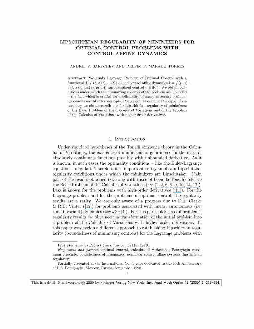
LIPSCHITZIAN REGULARITY OF MINIMIZERS FOR

OPTIMAL CONTROL PROBLEMS WITH

CONTROL-AFFINE DYNAMICS

ANDREI V. SARYCHEV AND DELFIM F. MARADO TORRES

Abstract. We study Lagrange Problem of Optimal Control with a

functional∫

b

aL (t, x (t) , u (t)) dt and control affine dynamics x = f (t, x)+

g (t, x) u and (a priori) unconstrained control u ∈ IRm. We obtain con-ditions under which the minimizing controls of the problem are bounded– the fact which is crucial for applicability of many necessary optimal-ity conditions, like, for example, Pontryagin Maximum Principle. As acorollary we obtain conditions for Lipschitzian regularity of minimizersof the Basic Problem of the Calculus of Variations and of the Problemof the Calculus of Variations with higher-order derivatives.

1. Introduction

Under standard hypotheses of the Tonelli existence theory in the Calcu-lus of Variations, the existence of minimizers is guaranteed in the class ofabsolutely continuous functions possibly with unbounded derivative. As itis known, in such cases the optimality conditions – like the Euler-Lagrangeequation – may fail. Therefore it is important to try to obtain Lipschitzianregularity conditions under which the minimizers are Lipschitzian. Mainpart of the results obtained (starting with those of Leonida Tonelli) refer tothe Basic Problem of the Calculus of Variations (see [1, 2, 6, 8, 9, 10, 14, 17]).Less is known for the problems with high-order derivatives ([11]). For theLagrange problem and for the problems of optimal control, the regularityresults are a rarity. We are only aware of a progress due to F.H. Clarke& R.B. Vinter ([12]) for problems associated with linear, autonomous (i.e.time-invariant) dynamics (see also [4]). For this particular class of problems,regularity results are obtained via transformation of the initial problem intoa problem of the Calculus of Variations with higher order derivatives. Inthis paper we develop a different approach to establishing Lipschitzian regu-larity (boundedness of minimizing controls) for the Lagrange problems with

1991 Mathematics Subject Classification. 49J15, 49J30.Key words and phrases. optimal control, calculus of variations, Pontryagin maxi-

mum principle, boundedness of minimizers, nonlinear control affine systems, lipschitzianregularity.

Partially presented at the International Conference dedicated to the 90th Anniversaryof L.S. Pontryagin, Moscow, Russia, September 1998.

1

This is a draft. Final version c© 2000 by Springer-Verlag New York, Inc. Appl Math Optim 41 (2000) 2, 237–254.

2 ANDREI V. SARYCHEV AND DELFIM F. MARADO TORRES

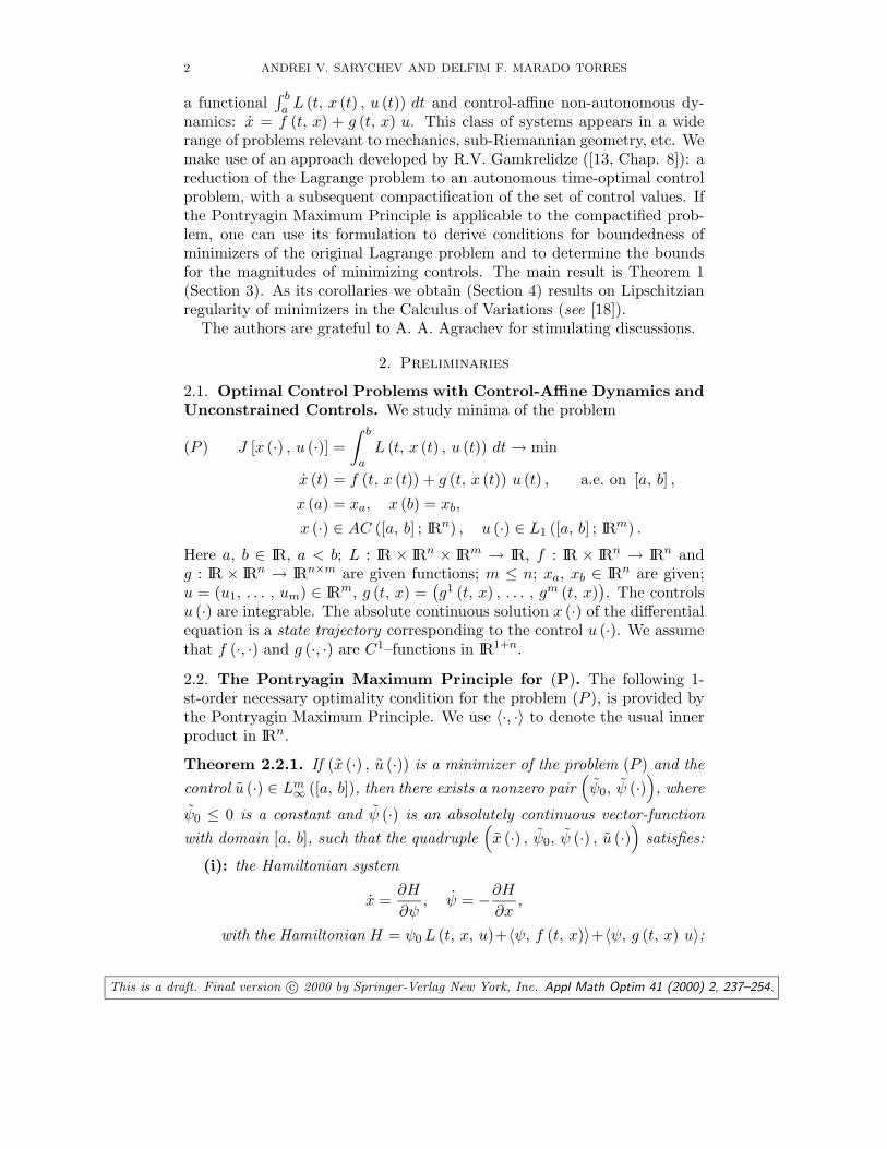
a functional∫ ba L (t, x (t) , u (t)) dt and control-affine non-autonomous dy-

namics: x = f (t, x) + g (t, x) u. This class of systems appears in a widerange of problems relevant to mechanics, sub-Riemannian geometry, etc. Wemake use of an approach developed by R.V. Gamkrelidze ([13, Chap. 8]): areduction of the Lagrange problem to an autonomous time-optimal controlproblem, with a subsequent compactification of the set of control values. Ifthe Pontryagin Maximum Principle is applicable to the compactified prob-lem, one can use its formulation to derive conditions for boundedness ofminimizers of the original Lagrange problem and to determine the boundsfor the magnitudes of minimizing controls. The main result is Theorem 1(Section 3). As its corollaries we obtain (Section 4) results on Lipschitzianregularity of minimizers in the Calculus of Variations (see [18]).

The authors are grateful to A. A. Agrachev for stimulating discussions.

2. Preliminaries

2.1. Optimal Control Problems with Control-Affine Dynamics andUnconstrained Controls. We study minima of the problem

J [x (·) , u (·)] =

∫ b

aL (t, x (t) , u (t)) dt → min(P )

x (t) = f (t, x (t)) + g (t, x (t)) u (t) , a.e. on [a, b] ,

x (a) = xa, x (b) = xb,

x (·) ∈ AC ([a, b] ; IRn) , u (·) ∈ L1 ([a, b] ; IRm) .

Here a, b ∈ IR, a < b; L : IR × IRn × IRm → IR, f : IR × IRn → IRn andg : IR × IRn → IRn×m are given functions; m ≤ n; xa, xb ∈ IRn are given;u = (u1, . . . , um) ∈ IRm, g (t, x) =

(

g1 (t, x) , . . . , gm (t, x))

. The controlsu (·) are integrable. The absolute continuous solution x (·) of the differentialequation is a state trajectory corresponding to the control u (·). We assumethat f (·, ·) and g (·, ·) are C1–functions in IR1+n.

2.2. The Pontryagin Maximum Principle for (P). The following 1-st-order necessary optimality condition for the problem (P ), is provided bythe Pontryagin Maximum Principle. We use 〈·, ·〉 to denote the usual innerproduct in IRn.

Theorem 2.2.1. If (x (·) , u (·)) is a minimizer of the problem (P ) and the

control u (·) ∈ Lm∞ ([a, b]), then there exists a nonzero pair

(

ψ0, ψ (·))

, where

ψ0 ≤ 0 is a constant and ψ (·) is an absolutely continuous vector-function

with domain [a, b], such that the quadruple(

x (·) , ψ0, ψ (·) , u (·))

satisfies:

(i): the Hamiltonian system

x =∂H

∂ψ, ψ = −

∂H

∂x,

with the Hamiltonian H = ψ0 L (t, x, u)+〈ψ, f (t, x)〉+〈ψ, g (t, x) u〉;

This is a draft. Final version c© 2000 by Springer-Verlag New York, Inc. Appl Math Optim 41 (2000) 2, 237–254.

LIPSCHITZIAN REGULARITY FOR OPTIMAL CONTROL PROBLEMS 3

(ii): the maximality condition

H(

t, x (t) , ψ0, ψ (t) , u (t))

= M(

t, x (t) , ψ0, ψ (t))

=

= supu∈IRm

H(

t, x (t) , ψ0, ψ (t) , u)

for almost all t ∈ [a, b].

Definition 1. A quadruple(

x (·) , ψ0, ψ (·) , u (·))

in which ψ0, ψ (·) are as

in Theorem 2.2.1, u (·) is integrable and satisfies the conditions (i) and (ii)of Theorem 2.2.1, is called extremal for the problem (P ). The control u (·)

is called an extremal control. An extremal(

x (·) , ψ0, ψ (·) , u (·))

is called

normal if ψ0 6= 0 and abnormal if ψ0 = 0. We call u (·) abnormal extremal

control if it corresponds to an abnormal extremal(

x (·) , 0, ψ (·) , u (·))

.

2.3. The Pontryagin Maximum Principle for Autonomous TimeOptimal Control Problems and Constrained Controls. An autonomoustime optimal problem is

T → min(2.1)

subject to

x (t) = F (x (t) , u (t)) , a.e. t ∈ [a, T ] ,

x (·) ∈ AC ([a, T ] ; IRn) , u (·) ∈ L∞ ([a, T ] ; U) ,

x (a) = xa, x (T ) = xT .

Here F (·, ·) is a continuous function on IRn+m, and has continuous partialderivatives with respect to x. The control u (·), defined on [a, T ], takes itsvalues in U ⊂ IRm, and is a measurable and bounded function. The follow-ing first-order necessary condition – the Pontryagin Maximum Principle –holds for any minimizer of the problem (details can be found, for example,in [13]). There are plenty of generalizations and modifications of the Pon-tryagin Maximum Principle. For example a Pontryagin Maximum Principleunder less restrictive assumptions for smoothness of data, can be found in[5] or [16].

Theorem 2.3.1. Let (x (·) , u (·)) be a solution of the time-optimal prob-

lem (2.1). Then there exists a nonzero absolutely continuous function ψ (·)satisfying:

• the Hamiltonian system

x =∂H (x, ψ, u)

∂ψ, ψ = −

∂H (x, ψ, u)

∂x,

with corresponding Hamiltonian H (x, ψ, u) = 〈ψ, F (x, u)〉;

This is a draft. Final version c© 2000 by Springer-Verlag New York, Inc. Appl Math Optim 41 (2000) 2, 237–254.

4 ANDREI V. SARYCHEV AND DELFIM F. MARADO TORRES

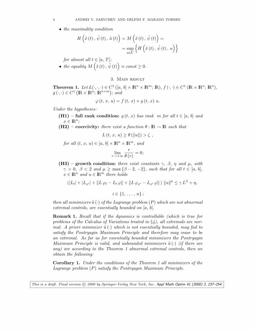
• the maximality condition

H(

x (t) , ψ (t) , u (t))

= M(

x (t) , ψ (t))

=

= supu∈U

{

H(

x (t) , ψ (t) , u)}

for almost all t ∈ [a, T ];

• the equality M(

x (t) , ψ (t))

≡ const ≥ 0.

3. Main result

Theorem 1. Let L(·, ·, ·) ∈ C1 ([a, b] × IRn × IRm; IR), f (·, ·) ∈ C1 (IR × IRn; IRn),g (·, ·) ∈ C1

(

IR × IRn; IRn×m)

; and

ϕ (t, x, u) = f (t, x) + g (t, x) u.

Under the hypotheses:

(H1) – full rank condition: g (t, x) has rank m for all t ∈ [a, b] andx ∈ IRn;

(H2) – coercivity: there exist a function θ : IR → IR such that

L (t, x, u) ≥ θ (‖u‖) > ζ ,

for all (t, x, u) ∈ [a, b] × IRn × IRm, and

limr→+∞

r

θ (r)= 0;

(H3) – growth condition: there exist constants γ, β, η and µ, withγ > 0, β < 2 and µ ≥ max {β − 2, −2}, such that for all t ∈ [a, b],x ∈ IRn and u ∈ IRm there holds

(|Lt| + |Lxi | + ‖L ϕt − Lt ϕ‖ + ‖L ϕxi − Lxi ϕ‖ ) ‖u‖µ ≤ γ Lβ + η,

i ∈ {1, . . . , n} ;

then all minimizers u (·) of the Lagrange problem (P ) which are not abnormalextremal controls, are essentially bounded on [a, b].

Remark 1. Recall that if the dynamics is controllable (which is true forproblems of the Calculus of Variations treated in §4), all extremals are nor-mal. A priori minimizer u (·) which is not essentially bounded, may fail tosatisfy the Pontryagin Maximum Principle and therefore may cease to bean extremal. As far as for essentially bounded minimizers the PontryaginMaximum Principle is valid, and unbounded minimizers u (·) (if there areany) are according to the Theorem 1 abnormal extremal controls, then weobtain the following:

Corollary 1. Under the conditions of the Theorem 1 all minimizers of theLagrange problem (P ) satisfy the Pontryagin Maximum Principle.

This is a draft. Final version c© 2000 by Springer-Verlag New York, Inc. Appl Math Optim 41 (2000) 2, 237–254.

LIPSCHITZIAN REGULARITY FOR OPTIMAL CONTROL PROBLEMS 5

Remark 2. We may impose stronger but technically simpler forms of as-sumption (H3) in Theorem 1. Under these conditions Theorem 1 loosessome generality, but sometimes, for a given problem, these conditions areeasier to verify. For example they can be: (in increasing order of simplicityand in decreasing order of generality)

[L (‖ϕt‖ + ‖ϕxi‖) + ‖ϕ‖ (|Lt| + |Lxi | )] ‖u‖µ ≤ γ Lβ + η;

L (‖ϕt‖ + ‖ϕxi‖) + ‖ϕ‖ (|Lt| + |Lxi | ) ‖u‖µ ≤ γ Lβ + η;

‖ϕt‖ + ‖ϕxi‖ + |Lt| + |Lxi | ≤ γ Lβ′

+ η, β′ < 1.

It is easy to see why (H3) follows from any of these conditions. It is enoughto notice that

‖L ϕt − Lt ϕ‖ + ‖L ϕxi − Lxi ϕ‖ ≤

≤ L (‖ϕt‖ + ‖ϕxi‖) + ‖ϕ‖ (|Lt| + |Lxi | ) ;

and that 0 ≥ max {β − 2, −2}.

Remark 3. The result of Theorem 1 admits a generalization for Lagrangeproblems with dynamics which is nonlinear in control. It will be addressedin a forthcoming paper.

3.1. Proof of the Theorem. We begin with an elementary observation.

Remark 4. It suffices to prove Theorem 1 in the special case where in (H2)we put ζ = 0. Indeed, minimization of

∫ b

aL (t, x (t) , u (t)) dt

under conditions in (P ) is equivalent to∫ b

a(L (t, x (t) , u (t)) − ζ) dt → min

since the difference of the integrands is constant.

Remind that everywhere below the notation ϕ (t, x, u) stands for f (t, x)+g (t, x) u.

3.1.1. Reduction to a time optimal problem. The following idea of trans-forming the variational problem into a time-optimal control problem andsubsequent compactification of the control set has been used earlier by R.V.Gamkrelidze ([13, Chap. 8]) to prove some existence results. We introducea new time variable

τ (t) =

∫ t

aL (θ, x(θ), u(θ)) dθ, t ∈ [a, b],

This is a draft. Final version c© 2000 by Springer-Verlag New York, Inc. Appl Math Optim 41 (2000) 2, 237–254.

6 ANDREI V. SARYCHEV AND DELFIM F. MARADO TORRES

which is a strictly monotonous absolutely continuous function of t, for anypair (x(t), u (t)) satisfying x (t) = ϕ (t, x (t) , u (t)). Obviously τ (b) = T

coincides with the value of the functional of the original problem. As far as

dτ(t)

dt= L (t, x(t), u(t)) > 0,

then τ (·) admits a monotonous inverse function t(·) defined on [0, T ], suchthat

dt

dτ(τ) =

1

L (t(τ), x (t(τ)) , u(t(τ))).

Notice that the inverse function t (·), is also absolutely continuous. Obvi-ously

dx (t(τ))

dτ=

dx (t(τ))

dt

dt(τ)

dτ=

ϕ (t(τ), x (t(τ)) , u (t(τ)))

L (t(τ), x (t(τ)) , u(t(τ))).(3.1)

Taking τ as a new time variable, considering t(τ) and z(τ) = x (t(τ)) ascomponents of state trajectory and v(τ) = u(t(τ)) as the control, we cantransform the problem (P ) into the following form

T −→ min(3.2)

t(τ) =1

L (t(τ), z(τ), v(τ))

z(τ) =ϕ (t(τ), z(τ), v(τ))

L (t(τ), z(τ), v(τ))

,(3.3)

v : IR → IRm

t(0) = a , t(T ) = b

z(0) = xa , z(T ) = xb

.(3.4)

3.1.2. Compactification of the space of admissible controls. So far the newcontrol variable takes its values in IRm and a priori control v(τ) can beunbounded. This unboundedness is kind of fictitious as far as the set

{(

1

L (t, z, v),ϕ (t, z, v)

L (t, z, v)

)

: v ∈ IRm

}

,

is bounded under the hypotheses (H1) and (H2). This set (for fixed (t, z) ∈IR x IRn) is not closed, but becomes compact if we add to it the point (0, 0) ∈IR x IRn which corresponds to the ’infinite value’ of the control v ∈ IRm. Theset

E(t, z) = {(0, 0)} ∪

{(

1

L (t, z, v),ϕ (t, z, v)

L (t, z, v)

)

: v ∈ IRm

}

,

can be represented as a homeomorphic image of the m-dimensional sphereSm ≈ IRm. This homeomorphism is defined in a standard way: we fix apoint w ∈ Sm, called north pole, and consider the stereographic projection

π : Sm\ {w} → IRm.(3.5)

This is a draft. Final version c© 2000 by Springer-Verlag New York, Inc. Appl Math Optim 41 (2000) 2, 237–254.

LIPSCHITZIAN REGULARITY FOR OPTIMAL CONTROL PROBLEMS 7

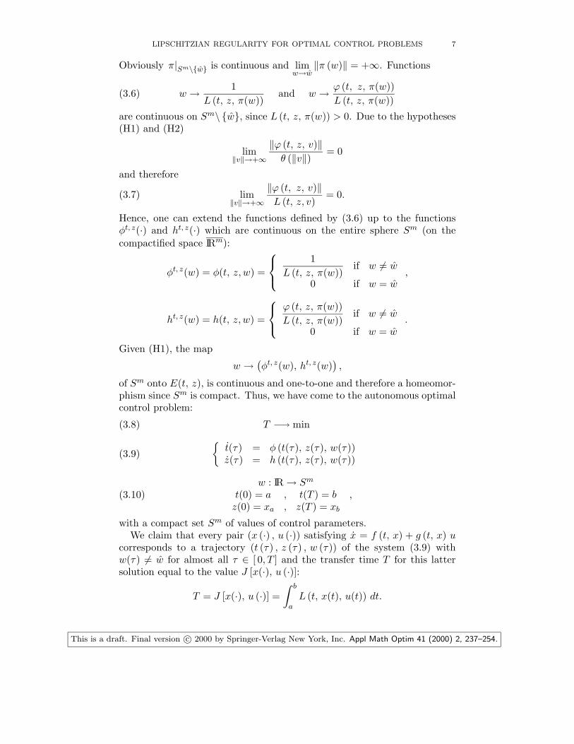
Obviously π|Sm\{w} is continuous and limw→w

‖π (w)‖ = +∞. Functions

w →1

L (t, z, π(w))and w →

ϕ (t, z, π(w))

L (t, z, π(w))(3.6)

are continuous on Sm\ {w}, since L (t, z, π(w)) > 0. Due to the hypotheses(H1) and (H2)

lim‖v‖→+∞

‖ϕ (t, z, v)‖

θ (‖v‖)= 0

and therefore

lim‖v‖→+∞

‖ϕ (t, z, v)‖

L (t, z, v)= 0.(3.7)

Hence, one can extend the functions defined by (3.6) up to the functionsφt, z(·) and ht, z(·) which are continuous on the entire sphere Sm (on thecompactified space IRm):

φt, z(w) = φ(t, z, w) =

1

L (t, z, π(w))if w 6= w

0 if w = w,

ht, z(w) = h(t, z, w) =

ϕ (t, z, π(w))

L (t, z, π(w))if w 6= w

0 if w = w

.

Given (H1), the map

w →(

φt, z(w), ht, z(w))

,

of Sm onto E(t, z), is continuous and one-to-one and therefore a homeomor-phism since Sm is compact. Thus, we have come to the autonomous optimalcontrol problem:

T −→ min(3.8)

{

t(τ) = φ (t(τ), z(τ), w(τ))z(τ) = h (t(τ), z(τ), w(τ))

(3.9)

w : IR → Sm

t(0) = a , t(T ) = b

z(0) = xa , z(T ) = xb

,(3.10)

with a compact set Sm of values of control parameters.We claim that every pair (x (·) , u (·)) satisfying x = f (t, x) + g (t, x) u

corresponds to a trajectory (t (τ) , z (τ) , w (τ)) of the system (3.9) withw(τ) 6= w for almost all τ ∈ [ 0, T ] and the transfer time T for this lattersolution equal to the value J [x(·), u (·)]:

T = J [x(·), u (·)] =

∫ b

aL (t, x(t), u(t)) dt.

This is a draft. Final version c© 2000 by Springer-Verlag New York, Inc. Appl Math Optim 41 (2000) 2, 237–254.

8 ANDREI V. SARYCHEV AND DELFIM F. MARADO TORRES

Indeed we may define (t (τ) , z (τ) , w (τ)) setting

t (τ) − an inverse function to τ (t) =

∫ t

aL (θ, x(θ), u(θ)) dθ,

z(τ) = x (t(τ)) , w(τ) = π−1 (u(t(τ))) ,

0 ≤ τ ≤ T = J [x(·), u (·)] ,

where π−1(·) is the mapping inverse to (3.5). Function z(·) is absolutelycontinuous since it is a composition of an absolutely continuous function withanother strictly monotonous absolutely continuous function t (τ). Functionw(·) is measurable because π−1(·) is a continuous function, u(·) is measurableand t(·) is a strictly monotonous absolutely continuous function. We alreadyknow that

dt (τ)

dτ=

1

L (t(τ), z(τ), π (w(τ))),

dz (τ)

dτ=

ϕ (t (τ) , z(τ), π (w(τ)))

L (t(τ), z(τ), π (w(τ))),

and w(τ) 6= w for almost all τ ∈ [ 0, T ], since u (·) has finite values almosteverywhere and t (·) is strictly monotonous.

We shall show now that every solution of (3.9), with w(τ) 6= w a.e.,results from this correspondence. Taking the absolutely continuous functionτ(t), a ≤ t ≤ b, which is the inverse of the strictly monotonous, absolutelycontinuous function t(τ), 0 ≤ τ ≤ T , we set

{

x(t) = z (τ(t))u (t) = π (w (τ (t)))

, a ≤ t ≤ b.

The curve x (·) defined in this way is absolutely continuous (because z(·) andτ(·) are absolutely continuous and τ(·) is strictly monotonous) and satisfiesthe boundary conditions

x(a) = xa and x(b) = xb.

The function u (·) is measurable because π (·) is continuous, w (·) is measur-able and τ (·) is continuous and monotonous. Also

∫ b

a‖u (t)‖ dt =

∫ b

a‖π (w (τ (t)))‖ dt =

=

∫ T

0

∥

∥

∥

∥

π (w (τ))

L (t(τ), z(τ), π (w(τ)))

∥

∥

∥

∥

dτ .

As far as the latter integrand is bounded due to the coercivity condition, weconclude that u (·) is integrable on [a, b]. Differentiating x (t) with respectto t, we conclude that

dx (t)

dt=

dz (τ(t))

dt=

dz (τ(t))

dτ

dτ(t)

dt= ϕ (t, x (t) , u (t))

This is a draft. Final version c© 2000 by Springer-Verlag New York, Inc. Appl Math Optim 41 (2000) 2, 237–254.

LIPSCHITZIAN REGULARITY FOR OPTIMAL CONTROL PROBLEMS 9

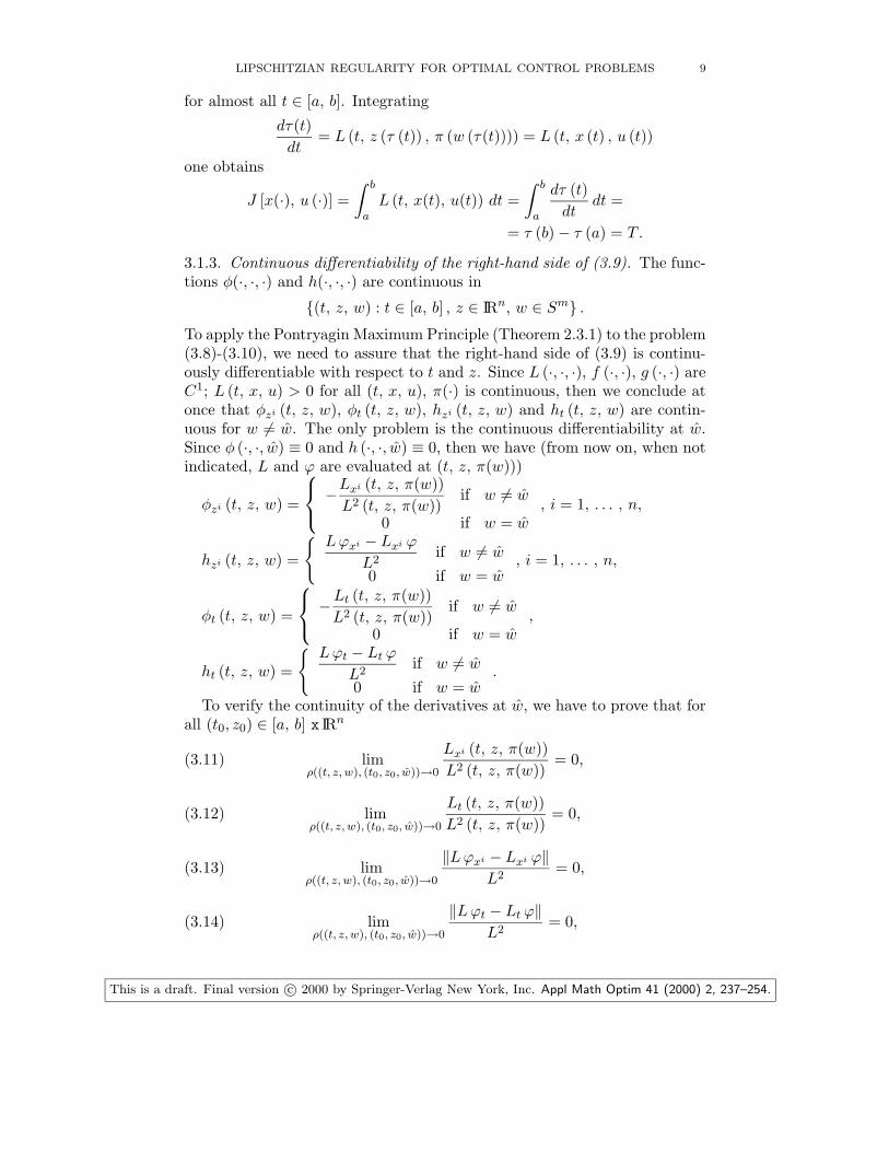
for almost all t ∈ [a, b]. Integrating

dτ(t)

dt= L (t, z (τ (t)) , π (w (τ(t)))) = L (t, x (t) , u (t))

one obtains

J [x(·), u (·)] =

∫ b

aL (t, x(t), u(t)) dt =

∫ b

a

dτ (t)

dtdt =

= τ (b) − τ (a) = T .

3.1.3. Continuous differentiability of the right-hand side of (3.9). The func-tions φ(·, ·, ·) and h(·, ·, ·) are continuous in

{(t, z, w) : t ∈ [a, b] , z ∈ IRn, w ∈ Sm} .

To apply the Pontryagin Maximum Principle (Theorem 2.3.1) to the problem(3.8)-(3.10), we need to assure that the right-hand side of (3.9) is continu-ously differentiable with respect to t and z. Since L (·, ·, ·), f (·, ·), g (·, ·) areC1; L (t, x, u) > 0 for all (t, x, u), π(·) is continuous, then we conclude atonce that φzi (t, z, w), φt (t, z, w), hzi (t, z, w) and ht (t, z, w) are contin-uous for w 6= w. The only problem is the continuous differentiability at w.Since φ (·, ·, w) ≡ 0 and h (·, ·, w) ≡ 0, then we have (from now on, when notindicated, L and ϕ are evaluated at (t, z, π(w)))

φzi (t, z, w) =

−Lxi (t, z, π(w))

L2 (t, z, π(w))if w 6= w

0 if w = w

, i = 1, . . . , n,

hzi (t, z, w) =

{

L ϕxi − Lxi ϕ

L2if w 6= w

0 if w = w, i = 1, . . . , n,

φt (t, z, w) =

−Lt (t, z, π(w))

L2 (t, z, π(w))if w 6= w

0 if w = w

,

ht (t, z, w) =

{

L ϕt − Lt ϕ

L2if w 6= w

0 if w = w.

To verify the continuity of the derivatives at w, we have to prove that forall (t0, z0) ∈ [a, b] x IRn

limρ((t, z, w), (t0, z0, w))→0

Lxi (t, z, π(w))

L2 (t, z, π(w))= 0,(3.11)

limρ((t, z, w), (t0, z0, w))→0

Lt (t, z, π(w))

L2 (t, z, π(w))= 0,(3.12)

limρ((t, z, w), (t0, z0, w))→0

‖L ϕxi − Lxi ϕ‖

L2= 0,(3.13)

limρ((t, z, w), (t0, z0, w))→0

‖L ϕt − Lt ϕ‖

L2= 0,(3.14)

This is a draft. Final version c© 2000 by Springer-Verlag New York, Inc. Appl Math Optim 41 (2000) 2, 237–254.

10 ANDREI V. SARYCHEV AND DELFIM F. MARADO TORRES

where ρ (·, ·) is a distance defined on [a, b] x IRnxSm. We shall see that

(3.11), (3.12), (3.13) and (3.14) are true under our hypotheses.Let N (t, z, π(w)) denote any of numerators in (3.11)–(3.14). From the

growth condition (H3), we obtain that, for all t ∈ [a, b], x ∈ IRn and u ∈ IRm,

‖N (t, x, u)‖ ≤ γ Lβ (t, x, u) ‖u‖−µ + η ‖u‖−µ .

As long as 2 − β > 0, one concludes

‖N (t, z, π(w))‖

L2 (t, z, π(w))≤ γ

‖π(w)‖−µ

L2−β (t, z, π(w))+ η

‖π(w)‖−µ

L2 (t, z, π(w)).

Since by (H2)1

L (t, z, π(w))≤

1

θ (‖π(w)‖), then

‖N (t, z, π(w))‖

L2 (t, z, π(w))≤ γ

‖π(w)‖−µ

θ2−β (‖π(w)‖)+ η

‖π(w)‖−µ

θ2 (‖π(w)‖).

If we recall that

lim‖π(w)‖→+∞

‖π(w)‖

θ (‖π(w)‖)= 0,

−µ ≤ 2 − β ∧ −µ ≤ 2 ∧ 2 − β > 0, then we obtain

limρ((t, z, w), (t0, z0, w))→0

‖N (t, z, π(w))‖

L2 (t, z, π(w))= 0,

which proves the equalities (3.11), (3.12), (3.13) and (3.14).

3.1.4. Pontryagin Maximum Principle and Lipschitzian Regularity. Let (x (·) , u (·))be a minimizer of the original problem (P ) and

(

t (·) , z (·) , w (·))

the corre-spondent minimizer for the time-optimal problem (3.8)-(3.10) with w (τ) 6=w almost everywhere. Applying Pontryagin’s Maximum Principle to thetime-minimal problem (3.8)-(3.10), we conclude that there exists absolutely

continuous functions on [0, T ]

λ : IR → IR, p : IR → IRn,

where T denotes the minimal time for the problem (3.8)-(3.10) and p (τ) isa row covector, not vanishing simultaneously, satisfying:

i): the Hamiltonian system{

λ (τ) = −Ht (t (τ) , z (τ) , λ (τ) , p (τ) , w (τ))p (τ) = −Hz (t (τ) , z (τ) , λ (τ) , p (τ) , w (τ))

with the Hamiltonian

H(t, z, λ, p, w) = λ φ (t, z, w) + 〈p, h (t, z, w)〉 ;

ii): the maximality condition

0 ≤ c = supw∈Sm

{

λ (τ) φ(

t (τ) , z (τ) , w)

+⟨

p (τ) , h(

t (τ) , z (τ) , w)⟩

}

(3.15)

This is a draft. Final version c© 2000 by Springer-Verlag New York, Inc. Appl Math Optim 41 (2000) 2, 237–254.

LIPSCHITZIAN REGULARITY FOR OPTIMAL CONTROL PROBLEMS 11

a.e.= λ (τ) φ

(

t (τ) , z (τ) , w (τ))

+⟨

p (τ) , h(

t (τ) , z (τ) , w (τ))⟩

,(3.16)

where c is a constant, z(τ) = x(

t(τ))

and w(τ) = π−1(

u(t(τ)))

.

We shall prove now that, under the hypotheses of the theorem, c must bepositive. Recall that

φ(t, z, w) =1

L (t, z, π(w)), h(t, z, w) =

ϕ (t, z, π(w))

L (t, z, π(w))

almost everywhere. In fact, if c = 0, then (3.15) implies (after a substitutionv = π (w)) that

supv∈IRm

{

λ (τ) +⟨

p (τ) , f(

t (τ) , z (τ))⟩

+⟨

p (τ) g(

t (τ) , z (τ))

, v⟩

L(

t (τ) , z (τ) , v)

}

vanishes for almost all τ ∈[

0, T]

. This obviously implies

p (τ) g(

t (τ) , z (τ))

≡ 0.(3.17)

At the same time, since L is positive, λ (τ) +⟨

p (τ) , f(

t (τ) , z (τ))⟩

mustbe non-positive. Then, since a finite value for v implies a finite value forL

(

t (τ) , z (τ) , v)

, one concludes

λ (τ) +⟨

p (τ) , f(

t (τ) , z (τ))⟩

= 0 a.e.(3.18)

The following proposition tell us that (3.17) and (3.18) imply that u (·) isan abnormal extremal control for (P ).

Proposition 1. If the equalities (3.17) and (3.18) hold then the quadruple(

x (·) , ψ0, ψ (·) , u (·))

defined as

(z (τ (·)) , 0, p (τ (·)) , v (τ (·))) ,

where τ (·) is the inverse function of t (·), is an abnormal extremal for theproblem (P ).

Proof. The respective Hamiltonian for the problem (3.8)-(3.10) equals

H (t, z, λ, p, v) =λ + 〈p, f (t, z)〉 + 〈p g (t, z) , v〉

L (t, z, v).

We have to verify the conditions (i) and (ii) of the Theorem 2.2.1 for the

quadruple(

x (·) , 0, ψ (·) , u (·))

defined in the formulation of the Proposi-

tion. Let us introduce the abnormal Hamiltonian

H = 〈ψ, f (t, x)〉 + 〈ψ, g (t, x) u〉 .

Direct computation shows

˙x (t) =d

dt{z (τ (t))} = ˙τ (t) ˙z (τ (t)) ;

This is a draft. Final version c© 2000 by Springer-Verlag New York, Inc. Appl Math Optim 41 (2000) 2, 237–254.

12 ANDREI V. SARYCHEV AND DELFIM F. MARADO TORRES

˙z (τ (t)) =f (t, x (t)) + g (t, x (t)) u (t)

L (t, x (t) , u (t));

˙τ (t) = L (t, x (t) , u (t))

and hence ˙x (t) = f (t, x (t)) + g (t, x (t)) u (t). Also

˙ψi (t) =

d

dtpi (τ (t)) = ˙τ (t)

˙pi (τ (t)) .

Obviously ψ(·) is absolutely continuous as a composition of the absolutelycontinuous function p(·) with the absolutely continuous monotonous func-tion τ(·). For all i = 1, . . . , n

˙pi (τ) = −∂H

∂zi = −〈p(τ), f

xi(t(τ), z(τ))〉+〈p(τ), gxi(t(τ), z(τ)) v(τ)〉

L(t(τ), z(τ), v(τ))+

+(λ(τ)+〈p(τ), f(t(τ), z(τ))〉+〈p(τ), g(t(τ), z(τ)) v(τ)〉)L

xi(t(τ), z(τ), v(τ))L2(t(τ), z(τ), v(τ))

.

The second addend vanishes by virtue of (3.17)-(3.18) and therefore

˙ψi (t) = −

⟨

ψ (t) , fxi (t, x (t))⟩

−⟨

ψ (t) , gxi (t, x (t)) u (t)⟩

=

= −∂H

∂xi,

so that (i) is fulfilled. On the other side,⟨

ψ (t) , g (t, x (t)) u (t)⟩

= 〈p (τ (t)) , g (t, z (τ (t))) u (t)〉 ≡ 0,

and therefore⟨

ψ (t) , f (t, x (t)) + g (t, x (t)) u (t)⟩

=⟨

ψ (t) , f (t, x (t))⟩

does not depend in u, so the maximality condition (ii) is fulfilled trivially(or abnormally).

This proves that vanishing c corresponds to an abnormal extremal controlof the problem (P ). Thus, for minimizers which are not abnormal extremalcontrols, there holds c > 0. From (3.15) we obtain

0 < ca.e.=

λ(τ) +⟨

p(τ), ϕ(

t(τ), z(τ), v (τ))⟩

L(

t(τ), z(τ), v (τ)) ⇒

⇒ L(

t(τ), z(τ), v(τ))

= c−1(

λ(τ) +⟨

p(τ), ϕ(

t(τ), z(τ), v (τ))⟩

)

.

Let∣

∣

∣λ (τ)

∣

∣

∣≤ M and ‖p (τ)‖ ≤ M on

[

0, T]

.

Then for any fixed τ ∈[

0, T]

L(

t(τ), z(τ), v(τ))

≤ c−1M(

1 +∥

∥ϕ(

t(τ), z(τ), v(τ))∥

∥

)

This is a draft. Final version c© 2000 by Springer-Verlag New York, Inc. Appl Math Optim 41 (2000) 2, 237–254.

LIPSCHITZIAN REGULARITY FOR OPTIMAL CONTROL PROBLEMS 13

and hence

θ (‖v(τ)‖)∥

∥ϕ(

t(τ), z(τ), v(τ))∥

∥

≤L

(

t(τ), z(τ), v(τ))

∥

∥ϕ(

t(τ), z(τ), v(τ))∥

∥

≤

≤ c−1M1 +

∥

∥ϕ(

t(τ), z(τ), v(τ))∥

∥

∥

∥ϕ(

t(τ), z(τ), v(τ))∥

∥

(3.19)

for almost all τ ∈[

0, T]

. The last term of this inequality can be ma-

jorized by 2 c−1 M if∥

∥ϕ(

t(τ), z(τ), v(τ))∥

∥ ≥ 1. From the growth condition(H2), and from the fact that g (t, x) has full column rank, it follows that

lim‖u‖→+∞

‖ϕ (t, x, u)‖ = +∞ and from the linearity of ϕ (t, x, u) with respect

to u

lim‖v(τ)‖→+∞

θ (‖v(τ)‖)∥

∥ϕ(

t(τ), z(τ), v(τ))∥

∥

= +∞.

Hence one can find r0 such that ∀ r ≥ r0:

∥

∥ϕ(

t(τ), z(τ), r)∥

∥ ≥ 1 andθ (r)

∥

∥ϕ(

t(τ), z(τ), r)∥

∥

≥ 2 c−1 M .

Therefore for (3.19) to be satisfied there must be

‖v(τ)‖ ≤ r0.

The proof is now complete: v (·) = π (w (·)) must be essentially bounded (by

r0) on[

0, T]

, that is, u (·) = v (τ (·)) is essentially bounded on [a, b]. 2

4. Applications to the Calculus of Variations

4.1. Basic problem of the Calculus of Variations. The following resultis an immediate Corollary of the Theorem 1.

Theorem 2. Let L(·, ·, ·) be continuously differentiable on IR x IRnx IRn,

a, b ∈ IR (a < b) and xa, xb ∈ IRn. Consider the Basic problem of theCalculus of Variations:

J [x(·)] =

∫ b

aL (t, x(t), x(t)) dt −→ min(4.1)

x(a) = xa , x(b) = xb.

Under the hypotheses:

(H1) – coercivity: there is a function θ : IR → IR such that

L (t, x, u) ≥ θ (‖u‖) > ζ, ζ ∈ IR,

for all (t, x, u) ∈ IR1+n+n, and

limr→+∞

r

θ (r)= 0;

This is a draft. Final version c© 2000 by Springer-Verlag New York, Inc. Appl Math Optim 41 (2000) 2, 237–254.

14 ANDREI V. SARYCHEV AND DELFIM F. MARADO TORRES

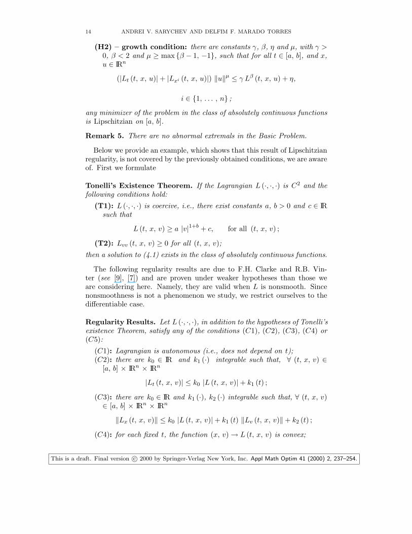
(H2) – growth condition: there are constants γ, β, η and µ, with γ >

0, β < 2 and µ ≥ max {β − 1, −1}, such that for all t ∈ [a, b], and x,u ∈ IRn

(|Lt (t, x, u)| + |Lxi (t, x, u)|) ‖u‖µ ≤ γ Lβ (t, x, u) + η,

i ∈ {1, . . . , n} ;

any minimizer of the problem in the class of absolutely continuous functionsis Lipschitzian on [a, b].

Remark 5. There are no abnormal extremals in the Basic Problem.

Below we provide an example, which shows that this result of Lipschitzianregularity, is not covered by the previously obtained conditions, we are awareof. First we formulate

Tonelli’s Existence Theorem. If the Lagrangian L (·, ·, ·) is C2 and thefollowing conditions hold:

(T1): L (·, ·, ·) is coercive, i.e., there exist constants a, b > 0 and c ∈ IRsuch that

L (t, x, v) ≥ a |v|1+b + c, for all (t, x, v) ;

(T2): Lvv (t, x, v) ≥ 0 for all (t, x, v);

then a solution to (4.1) exists in the class of absolutely continuous functions.

The following regularity results are due to F.H. Clarke and R.B. Vin-ter (see [9], [7]) and are proven under weaker hypotheses than those weare considering here. Namely, they are valid when L is nonsmooth. Sincenonsmoothness is not a phenomenon we study, we restrict ourselves to thedifferentiable case.

Regularity Results. Let L (·, ·, ·), in addition to the hypotheses of Tonelli’sexistence Theorem, satisfy any of the conditions (C1), (C2), (C3), (C4) or(C5):

(C1): Lagrangian is autonomous (i.e., does not depend on t);(C2): there are k0 ∈ IR and k1 (·) integrable such that, ∀ (t, x, v) ∈

[a, b] × IRn × IRn

|Lt (t, x, v)| ≤ k0 |L (t, x, v)| + k1 (t) ;

(C3): there are k0 ∈ IR and k1 (·), k2 (·) integrable such that, ∀ (t, x, v)∈ [a, b] × IRn × IRn

‖Lx (t, x, v)‖ ≤ k0 |L (t, x, v)| + k1 (t) ‖Lv (t, x, v)‖ + k2 (t) ;

(C4): for each fixed t, the function (x, v) → L (t, x, v) is convex;

This is a draft. Final version c© 2000 by Springer-Verlag New York, Inc. Appl Math Optim 41 (2000) 2, 237–254.

LIPSCHITZIAN REGULARITY FOR OPTIMAL CONTROL PROBLEMS 15

(C5): Lvv (t, x, v) > 0 and there exist a constant k0 such that ∀ (t, x, v) ∈[a, b] × IRn × IRn

∥

∥L−1vv (t, x, v) (Lx (t, x, v) − Lvt (t, x, v) − Lvx (t, x, v) v)

∥

∥ ≤

≤ k0

(

‖v‖2+b + 1)

,

where b is the positive constant that appears in the coercivity condition(T1) of Tonelli’s existence theorem;

then every minimizer of the basic problem of the Calculus of Variations (4.1)is Lipschitzian.

Notice that (C1) is a particular case of condition (C2). The growthconditions (C3) and (C5) are generalizations of classical conditions obtainedrespectively by Tonelli–Morrey and Bernstein (Loc. cit.).

Now we provide an example of a functional which possesses a minimizer,for which no one of the conditions (C1)–(C5) is applicable, while Theorem2 is.

Example. Let us consider the following problem (n = 1):

J [x (·)] =

∫ 1

0

[

(

x4 + 1)3

e(x4+1) (t+π

2−arctan x)

]

dt → min(4.2)

x (0) = x0, x (1) = x1.

Denoting L (t, x, v) =(

v4 + 1)3

e(v4+1) (t+π

2−arctan x), we conclude

Lvv (t, x, v) =

[

132v6 + 36v2

(v4 + 1)2+

(

96v6

v4 + 1+ 12v2

)

(

t +π

2− arctanx

)

+

+16v6(

t +π

2− arctanx

)2]

L (t, x, v) .

Tonelli’s theorem guarantees existence of a minimizer x (·) ∈ AC for theproblem (4.2) as long as:

• L (·, ·, ·) ∈ C2;• For all (t, x, v) ∈ [0, 1] × IR × IR we have:

L (t, x, v) >(

v4 + 1)3

≥ v4 + 1 > 0;

• Lvv (t, x, v) ≥ 0.

The assumptions of the Theorem 2 are also verifiable with θ (r) = r4 + 1,

β =3

2, µ =

1

2, γ = 2 and η = 0. Indeed:

Lt (t, x, v) =(

v4 + 1)

L (t, x, v) , Lx (t, x, v) = −v4 + 1

1 + x2L (t, x, v) ,

This is a draft. Final version c© 2000 by Springer-Verlag New York, Inc. Appl Math Optim 41 (2000) 2, 237–254.

16 ANDREI V. SARYCHEV AND DELFIM F. MARADO TORRES

(|Lx (t, x, v)| + |Lt (t, x, v)|) |v|1/2 ≤ 2(

|v|4)1/8

(

v4 + 1)

L (t, x, v) <

< 2(

v4 + 1)9/8

L (t, x, v) = 2(

v4 + 1)33/8

e(v4+1) (t+π

2−arctan x) <

< 2(

v4 + 1)36/8

e3/2 (v4+1) (t+π

2−arctan x) = 2L3/2 (t, x, v) .

Theorem 2 guarantees then, that all the minimizers of this functional areLipschitzian.

As we shall see now, none of the conditions (C1) − (C5) is applicable tothis example. Indeed:

1. The Lagrangian depends explicitly on t and so the condition (C1) fails.

2. If (C2) were true, one might concludeLt (t, x, v)

L (t, x, v)≤ k0 +

k1 (t)

L (t, x, v),

which in our case implies

v4 + 1 ≤ k0 +k1 (t)

L (t, x, v),

an inequality which fails for v sufficiently large.3. For (C3) to hold, we should have for v > 0, x = 0 and some t

|Lx (t, 0, v)|

v7/2 L (t, 0, v)≤

k0

v7/2+ k1 (t)

|Lv (t, 0, v)|

v7/2 L (t, 0, v)+

k2 (t)

v7/2 L (t, 0, v);

as far as

Lv (t, x, v) =

[

12 v3

v4 + 1+ 4v3

(

t +π

2− arctan x

)

]

L (t, x, v) ,

one obtains the inequality

v4 + 1

v7/2≤

k0

v7/2+ k1 (t)

12 v3

v4+1+ 4 v3

(

t + π2

)

v7/2+

k2 (t)

v7/2 L (t, 0, v)

which fails for v sufficiently large.4. (C4) isn’t true either: if we fix t and v we come to the function x −→

C3 eC (B−arctan x) which is not convex: its second derivative equals

2 x + C

(1 + x2)2C4 eC (B−arctan x)

which is not sign-definite.5. Finally (C5) fails, since we have Lvv (t, x, v) = 0 for example for v = 0.

This is a draft. Final version c© 2000 by Springer-Verlag New York, Inc. Appl Math Optim 41 (2000) 2, 237–254.

LIPSCHITZIAN REGULARITY FOR OPTIMAL CONTROL PROBLEMS 17

4.2. Variational problems with higher order derivatives. Let us con-sider now the problem of the Calculus of Variations with higher-order deriva-tives:

∫ b

aL

(

t, x(t), x(t), . . . , x(m)(t))

dt −→ min(4.3)

x(a) = x0a x(b) = x0

b...

...

x(m−1)(a) = xm−1a x(m−1)(b) = xm−1

b .

(4.4)

We use the notation Wk,p (k = 1, . . . ; 1 ≤ p ≤ ∞) for the class of functionswhich are absolutely continuous with their derivatives up to order k−1 andhave k-th derivative belonging to Lp. Existence of minimizers for problem(4.3)-(4.4) in the class Wm,1 ([a, b] , IRn), will follow from classical existenceresults, if we impose that L (t, x0, . . . , xm) is convex with respect to xm

(see [3]). One can put a question of whether every minimizer x (·) ∈ Wm,1

has essentially bounded m−th derivative, i.e. belongs to Wm,∞. A studyof higher-order regularity has been done in 1990 by F.H. Clarke and R.B.Vinter in [11], where they deduced a condition of the Tonelli-Morrey-type:

‖Lxi(t, x0, . . . , xm)‖ ≤γ (|L (t, x0, . . . , xm)| + ‖xm‖) +

+ η (t) r (x0, . . . , xm) ,

with i = 0, . . . , m − 1, γ being a constant, η an integrable function, r alocally bounded function. Once again, we are able to derive from our mainresult a condition of a new type also for this case.

Theorem 3. Provided that: for all t ∈ [a, b] and x0, . . . , xm ∈ IRn thefunction (t, x0, . . . , xm) → L (t, x0, . . . , xm) is continuously differentiableand the following conditions hold

(H1) – coercivity: there is a function θ : IR → IR and a constant ζ

such that

L (t, x0, . . . , xm) ≥ θ (‖xm‖) > ζ,

and limr→+∞

r

θ (r)= 0;

(H2) – growth condition: for some constants γ, β, η and µ with γ >

0, β < 2 and µ ≥ max {β − 1, −1}

(|Lt| + ‖Lxi‖) ‖xm‖µ ≤ γ Lβ + η, i ∈ {0, . . . , m − 1} ;(4.5)

then all minimizers x (·) ∈ Wm,1 ([a, b], IRn) of the variational problem(4.3)-(4.4) belong to the class Wm,∞ ([a, b], IRn).

Remark 6. There are no abnormal extremals for problem (4.3)-(4.4).

Some corollaries can be easily derived.

This is a draft. Final version c© 2000 by Springer-Verlag New York, Inc. Appl Math Optim 41 (2000) 2, 237–254.

18 ANDREI V. SARYCHEV AND DELFIM F. MARADO TORRES

Corollary 2. Any minimizer x (·) of the functional

J [x (·)] =

∫ b

aL

(

x(m) (t))

dt → min ,

x (·) ∈ Wm,1 ([a, b] , IRn) ,

under the conditions (4.4), is contained in the space Wm,∞ ([a, b] , IRn), pro-vided L (·) is continuously differentiable; and for all xm ∈ IRn and someconstants ξ ∈ IR and α ∈ ]1, +∞[, L (xm) ≥ ‖xm‖α + ξ.

For m = 1 there exists a much stronger result, than this latter corollary:if m = 1 and L is autonomous, L = L (x, x), coercive and convex in x,then all the minimizers of the problem belong to W1,∞ (condition (C1) of’Regularity Results’ ). The question of whether it can be generalized onto the

case of higher-order functionals L(

x, x, . . . , x(m))

remained open till recenttime. It has been shown in [15] that autonomous higher-order functionalsnot only may possess minimizers belonging to Wm,1\W1,∞ but also exhibitthe Lavrentiev phenomenon: their infimum in Wm,1 can be strictly less thanthe one in Wm,∞.

References

1. Ambrosio L, Ascenzi O, Buttazzo G (1989) Lipschitz regularity for min-imizers of integral functionals with highly discontinuous integrands. JMath Anal Appl 142:301-316

2. Bernstein S (1912) Sur les quations du calcul des variations. Ann SciEcole Norm Sup 3:431-485

3. Cesari L (1983) Optimization Theory and Applications. Springer-Verlag, New York

4. Cheng C, Mizel VJ (1996) On the Lavrentiev phenomenon for optimalcontrol problems with second-order dynamics. SIAM J Control Opti-mization 34:2172-2179

5. Clarke FH (1976) The Maximum Principle under minimal hypotheses.SIAM J Control and Optimization 14:1078-1091

6. Clarke FH (1985) Existence and Regularity in the Small in the Calculusof Variations. J Differential Equations 59:336-354

7. Clarke FH (1989) Methods of Dynamic and Nonsmooth Optimization.SIAM, Philadelphia

8. Clarke FH, Loewen PD (1989) Variational problems with Lipschitzianminimizers. Ann Inst Henri Poincar, Anal Nonlinaire 6:185-209

9. Clarke FH, Vinter RB (1985) Regularity properties of solutions to thebasic problem in the calculus of variations. Trans Amer Math Soc289:73-98

10. Clarke FH, Vinter RB (1986) Regularity of Solutions to VariationalProblems with Polynomial Lagrangians. Bull Polish Acad Sci 34:73-81

11. Clarke FH, Vinter RB (1990) A regularity theory for variational prob-lems with higher order derivatives. Trans Amer Math Soc 320:227-251

This is a draft. Final version c© 2000 by Springer-Verlag New York, Inc. Appl Math Optim 41 (2000) 2, 237–254.

LIPSCHITZIAN REGULARITY FOR OPTIMAL CONTROL PROBLEMS 19

12. Clarke FH, Vinter RB (1990) Regularity properties of optimal controls.SIAM J Control and Optimization 28:980-997

13. Gamkrelidze RV (1978) Principles of Optimal Control Theory. PlenumPress, New York

14. Morrey CB (1966) Multiple integrals in the Calculus of Variations.Springer, Berlin

15. Sarychev AV (1997) First and Second-Order Integral Functionals ofthe Calculus of Variations Which Exhibit the Lavrentiev Phenomenon.Journal of Dynamical and Control Systems 3:565-588

16. Sussmann HJ (1994) A strong version of the Maximum Principle underweak hypotheses. Proc 33rd IEEE Conference on Decision and Control,Orlando 1950-1956

17. Tonelli L (1915) Sur une mthode directe du calcul des variations. RendCirc Mat Palermo 39:233-264

18. Torres DM (1997) Lipschitzian Regularity of Minimizers in the Calculusof Variations and Optimal Control (in Portuguese). MSc thesis, UnivAveiro, Portugal

Dep. of Mathematics, Univ. of Aveiro, 3810 Aveiro, Portugal

E-mail address: ansar@mat.ua.pt

E-mail address: delfim@mat.ua.ptURL: http://www.mat.ua.pt/cotg

This is a draft. Final version c© 2000 by Springer-Verlag New York, Inc. Appl Math Optim 41 (2000) 2, 237–254.