This article was downloaded by:[HEAL-Link Consortium]On: 23 April 2008Access Details: [subscription number 772810551]Publisher: Taylor & FrancisInforma Ltd Registered in England and Wales Registered Number: 1072954Registered office: Mortimer House, 37-41 Mortimer Street, London W1T 3JH, UK

International Journal of ComputerMathematicsPublication details, including instructions for authors and subscription information:http://www.informaworld.com/smpp/title~content=t713455451

LINEAR NEURAL NETWORK TRAININGALGORITHMS FOR REAL-WORLD BENCHMARKPROBLEMSK. Goulianas a; M. Adamopoulos; S. Katsavounis b; Ch. FRAGAKIS b; C. C.Tsouros ba Department of Informatics, Technological Educational Institute of Thessaloniki,Greece.b Faculty of Engineering, Aristotle University of Thessaloniki, Greece.

Online Publication Date: 01 January 2002To cite this Article: Goulianas, K., Adamopoulos, M., Katsavounis, S., FRAGAKIS,

Ch. and Tsouros, C. C. (2002) 'LINEAR NEURAL NETWORK TRAINING ALGORITHMS FOR REAL-WORLDBENCHMARK PROBLEMS', International Journal of Computer Mathematics, 79:11, 1149 - 1167To link to this article: DOI: 10.1080/00207160213945URL: http://dx.doi.org/10.1080/00207160213945

PLEASE SCROLL DOWN FOR ARTICLE

Full terms and conditions of use: http://www.informaworld.com/terms-and-conditions-of-access.pdf

This article maybe used for research, teaching and private study purposes. Any substantial or systematic reproduction,re-distribution, re-selling, loan or sub-licensing, systematic supply or distribution in any form to anyone is expresslyforbidden.

The publisher does not give any warranty express or implied or make any representation that the contents will becomplete or accurate or up to date. The accuracy of any instructions, formulae and drug doses should beindependently verified with primary sources. The publisher shall not be liable for any loss, actions, claims, proceedings,demand or costs or damages whatsoever or howsoever caused arising directly or indirectly in connection with orarising out of the use of this material.

Dow

nloa

ded

By:

[HE

AL-

Link

Con

sorti

um] A

t: 22

:35

23 A

pril

2008

Intern. J. Computer Math., 2002, Vol. 79(11), pp. 1149–1167

LINEAR NEURAL NETWORK TRAININGALGORITHMS FOR REAL-WORLD BENCHMARK

PROBLEMS

K. GOULIANASa, M. ADAMOPOULOSa,b, S. KATSAVOUNISc Ch. FRAGAKISc

and C. C. TSOUROSc

aDepartment of Informatics, Technological Educational Institute of Thessaloniki, Greece;bDepartment of Informatics, University of Macedonia, Thessaloniki, Greece;

cFaculty of Engineering, Aristotle University of Thessaloniki, Greece

(Received 22 June 2001; In final form 1 July 2001)

This paper describes the Adaptive Steepest Descent (ASD) and Optimal Fletcher-Reeves (OFR) algorithms for linearneural network training. The algorithms are applied to well-known pattern classification and function approximationproblems, belonging to benchmark collection Proben1. The paper discusses the convergence behavior andperformance of the ASD and OFR training algorithms by computer simulations and compares the results withthose produced by linear-RPROP method.

Keywords: Neural nets; Training algorithms; Iterative methods

C.R. Categories: I.5.1, I.2.6, G.1.3

1 INTRODUCTION

Linear feedforward neural network architectures have been proved capable of solving sys-

tems of linear equations [2, 5–7, 14, 15], and pattern classification problems [8]. Most of

these applications use LMS and Batch-LMS training [4, 17, 18], and require a selection

of appropriate parameters by the user, executed with a trial-and-error process. In real

world problems, it is essential to consider learning methods with a good average perfor-

mance. This paper describes some methods that have been shown to accelerate the conver-

gence of the learning phase, and that do not require the choice of critical parameters, like the

learning rate or the momentum. A simple two-layer feedforward neural network with linear

neuron functions is studied. Batch-LMS training is extended to implement steepest descent

algorithms, like the Adaptive Steepest Descent (ASD) and the Optimal Fletcher-Reeves

(OFR) algorithm. The performance of these algorithms is compared to linear-RPROP

training [9], a technique for optimizing the backpropagation training [10, 11], which uses

ISSN 0020-7160 print; ISSN 1029-0265 online # 2002 Taylor & Francis LtdDOI: 10.1080=0020716021000030684

Dow

nloa

ded

By:

[HE

AL-

Link

Con

sorti

um] A

t: 22

:35

23 A

pril

2008

a fixed update size not influenced by the magnitude of the gradient. Instead, only the sign of

the derivative is used to find the proper update direction. Those three methods are applied to

well-known benchmarks from the Proben1 collection. Proben1 contains data from the UCI

repository of machine learning databases for 9 pattern classification problems and 3 function

approximation problems. The 9 pattern classification problems are the following: cancer (a

dataset for diagnosis of breast cancer, originally obtained from the University of Wisconsin

Hospital, Madison, from Dr. William H. Wolberg), card (a dataset for approval or non-ap-

proval of a credit card to a customer), diabetes (a dataset for diagnosis of diabetes of Pima

Indians), gene (a dataset for detection of intron/exon boundaries in nucleotide sequences),

glass (a dataset for classification of glass types), heart (a dataset for heart disease predic-

tion), horse (a dataset for prediction of the fate of a horse that has a colic), soybean (a da-

taset for recognition of 19 diseases of soybeans), and thyroid (a dataset for diagnosis of

thyroid hyper- or hypofunction). The 3 function approximation problems are the following:

building (a dataset for prediction of energy consumption in a building), flare (a dataset for

prediction of sonar flares), and hearta (the analogue version of the heart disease diagnosis

problem). All the datasets are partitioned into training, validation, and test set, while the size

of the training, validation, and test set data files is 50%, 25%, and 25% respectively. Since

results may vary for different partitionings, Proben1 contains three different permutations of

each dataset. For instance, the problem cancer is available in three datasets cancer1, can-

cer2, and cancer3, which differ only in the ordering of the patterns. Validation set is

used as a pseudo test set in order to evaluate the quality of the network during training, a

method called cross-validation, which avoids overfitting, a problem created when many

training examples are available causing the loss of much of the regularities needed for

good generalization [13]. The method used for cross-validation is early stopping

[1, 12, 16], where training proceeds until a minimum of the error on validation set (and

not the training set) is reached.

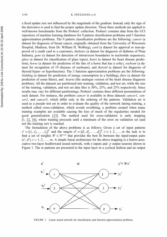
The formulation of the above problems is as follows: Given a set of input patterns

xi ¼ ½xi1; xi

2; . . . ; xin�

T and the targets di ¼ ½di1; di

2; . . . ; dip�

T; i ¼ 1; 2; . . . ;m the task is to

find a set of weights W 2 <n�p that provides the best fit between the input/output pairs

ðxi; diÞ; i ¼ 1; 2; . . . ;m. A simple linear architecture for the above mapping is a hetero-asso-

ciative two-layer feedforward neural network, with n inputs and p output neurons shown in

Figure 1. The m patterns are presented to the input layer in a cyclical fashion and an output

FIGURE 1 Linear neural network for classification and function approximation problems.

1150 K. GOULIANAS et al.

Dow

nloa

ded

By:

[HE

AL-

Link

Con

sorti

um] A

t: 22

:35

23 A

pril

2008

yi ¼ ½ yi1; yi

2; . . . ; yip�

T is generated. The goal is to minimize the mean square error, or the cost

function

EðW Þ ¼Xp

j¼1

Eðw jÞ ¼1

2

Xp

j¼1

Xm

i¼1

ðdij yi

jÞ2¼

1

2

Xm

i¼1

Xp

j¼1

dij

Xn

k¼1

xikw

jk

!2

¼1

2X TW D�� ��2

ð1Þ

With X ¼ ½x1; x2; . . . ; xm�, and D ¼ ½d1; d2; . . . ; dm�;w j the weight vector of the jth output

neuron, and E(w j) its cost function. Using a general gradient approach, any minimum of the

cost function in Eq. (1) must satisfy HEðW Þ ¼ X ðX TW DÞ ¼ 0, which can be rewritten as

XX TW ¼ XD ð2Þ

or the equivalent system BW ¼ C with B ¼ XX T;B 2 <n�n and C ¼ XD;C 2 <n. Equation

(2) consists of p systems of normal equations, with B ¼ XX T positive definite and symmetric.

The solution of systems (2) for a non-singular matrix X T with m n, gives the unique least

mean square solution W ¼ XþD with Xþ ¼ ðXX TÞ1X the Moore-Penrose generalized

inverse [3].

The cost functions E(w j) defined in (1) are quadratic in the weights w j and for m n they

define convex hyper-paraboloidal surfaces with a single minimum, the global minimum, the

solutions of Eq. (2), which are unique, since the Hessian matrix of E(w j) at

w j;H2Eðw jÞ ¼ XX T is positive definite.

Since the mean squared error defined in (1) depends on the number of output coefficients,

and on the range of the output values used, Prechelt [8] suggests the use of the squared error

percentage, a normalization of these factors, as follows:

EðW Þ ¼Xp

j¼1

E w j� �

¼ 100 �ðomax ominÞ

m � p

Xp

j¼1

Xm

i¼1

dij yi

j

� �2

ð3Þ

with omin and omax to be the minimum and maximum value of output coefficients, p the num-

ber of output nodes, and m the number of patterns in the dataset.

The material is organized as follows. In Section 2 we simulate the ASD and OFR

algorithm with the above architecture and discuss convergence issues for obtaining estimates

of the optimal solution. In Section 3, we compare the performance of the ASD and OFR

training algorithm with linear-RPROP in the solution of the pattern classification and

function approximation benchmarking problems. Finally, in Section 4, we draw some final

conclusions.

2 ASD AND OFR METHODS FOR LINEAR NEURAL NETWORK TRAINING

With zero or random in [0:01, 0.01] initial weights wjk; j ¼ 1; 2; . . . ; p; k ¼ 1; 2; . . . ; n the

train set patterns xi ¼ ½xi1; xi

2; . . . ; xin�

T; i ¼ 1; 2; . . . ;m are presented to the network in a

NEURAL NET TRAINING 1151

Dow

nloa

ded

By:

[HE

AL-

Link

Con

sorti

um] A

t: 22

:35

23 A

pril

2008

cyclical fashion. Thus, with the presentation of the ith pattern, the outputs yðtþ1;iÞj ;

j ¼ 1; 2; . . . ; p; will be

yðtþ1;iÞj ¼ wðt;jÞxi ¼

Xn

k¼1

wðt;jÞk xi

k ð4Þ

with ðt þ 1; iÞ the step i of the training cycle t þ 1. Delta Rule is applied, and the discrepancy

between desired and calculated output dij and y

ðtþ1;iÞj , for every pattern i, i ¼ 1; 2; . . . ;m and

output neuron j, j ¼ 1; 2; . . . ; p is

eðtþ1;iÞj ¼ di

j yðtþ1;iÞj ð5Þ

We define the batch error dðtþ1Þk for every input neuron k, k ¼ 1; 2; . . . ; n to be

dðtþ1Þk ¼

Xm

i¼1

eðtþ1;iÞj xi

k ¼Xm

i¼1

dij y

ðtþ1;iÞj

� �xi

k ð6Þ

or in a matrix-vector form

dðtþ1Þ¼Xm

i¼1

eðtþ1;iÞj xi ¼

Xm

i¼1

dij y

ðtþ1;iÞj

� �xi ð7Þ

and the adaptive learning rate aðtþ1Þk as

aðtþ1Þk ¼

dðtþ1Þk dðtþ1Þ

k

dðtþ1Þk X TXdðtþ1Þ

k

ð8Þ

2.1 The Adaptive Steepest Descent (ASD) Method

The connection update after the presentation of all the training set patterns xi; i ¼ 1; 2; . . . ;m

at training cycle t þ 1, could have the form

wðtþ1;jÞk ¼ w

ðt;jÞk þ aðtþ1Þ

k

Xm

i¼1

ðdij y

ðtþ1;iÞj Þxi

k

¼ wðt;jÞk þ

dðtþ1Þdðtþ1Þ

dðtþ1ÞX TXdðtþ1Þ

Xm

i¼1

dij

Xn

q¼1

wðt;jÞq xi

q

!xi

k

¼ wðt;jÞk þ

dðtþ1Þdðtþ1Þ

dðtþ1ÞCdðtþ1Þ

Xm

i¼1

cik

Xn

q¼1

wðt;jÞq bi

q

!ð9Þ

with k ¼ 1; 2; . . . ; n and bkq; ci

k the corresponding elements of B and C, as defined in (2).

The operation of the ANN in Figure 1 using ASD method with the adaptive learning

rate aðtþ1Þk defined in (2) simulates the Adaptive Steepest Descent Method. Proof can be

found in [2].

1152 K. GOULIANAS et al.

Dow

nloa

ded

By:

[HE

AL-

Link

Con

sorti

um] A

t: 22

:35

23 A

pril

2008

2.2 The Optimal Fletcher-Reeves (OFR) Method

We define bðtþ1Þ to be

bðtþ1Þ¼

dðtþ1Þdðtþ1Þ

dðtÞdðtÞð10Þ

and the connection update after the presentation of all the training set patterns

xi; i ¼ 1; 2; . . . ;m at training cycle t þ 1, has the form

wðtþ1;jÞk ¼ w

ðt;jÞk þ aðtþ1Þ

k

Xm

i¼1

dij y

ðtþ1;iÞj

� �xi

k þ bðtþ1ÞDwðt;jÞk

¼ wðt;jÞk

dðtþ1Þdðtþ1Þ

dðtÞCdðtÞXm

i¼1

dij

Xn

q¼1

wðt;jÞq xi

q

!xi þ

dðtþ1Þdðtþ1Þ

dðtÞdðtÞDw

ðt;jÞk

¼ wðt;jÞk þ

dðtþ1Þdðtþ1Þ

dðtþ1ÞCdðtþ1Þ

Xm

i¼1

cik

Xn

q¼1

wðt;jÞq bi

q

!þdðtþ1Þdðtþ1Þ

dðtÞdðtÞDw

ðt;jÞk ð11Þ

with k ¼ 1; 2; . . . ; n and bkq; ci

k the corresponding elements of B and C, as defined in (2). The

operation of the ANN in Figure 1 using OFR method with the adaptive learning rate aðtþ1Þk

defined in (2) simulates the Optimal Fletcher-Reeves Method.

3 EXPERIMENTAL STUDY

In order to check the performance and the convergence behavior of the proposed algorithm

the benchmark problems used were taken from the Proben1 benchmark set, with the standard

Proben1 benchmarking rules. The error measures reported include: the training set error

(mean and standard deviation of minimum squared error percentage on training set, reached

at any time during training), validation set error (mean and standard deviation of minimum

squared error percentage on validation set, reached at any time during training), test set error

(mean and standard deviation of minimum squared error percentage on test set, at point of

minimum validation set error), and the test set classification error (i.e. the percentage of in-

correctly classified examples). For the classification problems, winner-takes-all method was

used to determine the classification, i.e. the output with the highest activation designates the

class, while in approximation problems, a threshold of 0.3 was used in the output, and the

network accepts an output as 0, if it is below 0.3, and as 1, if it is above 0.7. In order to

measure the training time, we also report the number of epochs used, the number of relative

epochs, i.e. the epochs needed to reach the minimum validation error, and the connection

traversals. One stopping criterion is the loss of generality. The generalization loss at epoch

t is defined as the relative increase of the validation squared error percentage over the mini-

mum so far in percent

GLðtÞ ¼ 100 �EvaðtÞ

mint0�t

Evaðt0Þ 1

0@

1A ð12Þ

NEURAL NET TRAINING 1153

Dow

nloa

ded

By:

[HE

AL-

Link

Con

sorti

um] A

t: 22

:35

23 A

pril

2008

and the algorithm stops as the generalization loss exceeds a threshold a ¼ 5. Another stop-

ping criterion is the training progress, defined in terms of a training strip. A training strip of

length k is a sequence of k epochs, and the training progress is how much is the average train-

ing error during the strip larger than the minimum error during the strip

PkðtÞ ¼ 1000 �

Pt02kkþ1���t Etrðt

0Þ

k � mint02kkþ1���t Etrðt0Þ 1

� �ð13Þ

Since training involves some kind of random generalization, in order to make reliable state-

ments about the performance of the three algorithms, we used 20 runs on each problem, for

each one of the three datasets. The data reported include the mean and standard deviation of

the above error and training measures for these 20 runs, along with generalization loss at end

of training.

The results of ASD and OFR training of the linear network in Figure 1 with the classifica-

tion and approximation problems, are compared to linear-RPROP, with the following

parameters used by Prechelt [8]: nþ ¼ 1:2; n ¼ 0:5; D0 2 0:005 � � � 0:02; Dmax ¼ 50;Dmin ¼ 0, and initial weights randomly chosen in ½0:01; 0:01�.

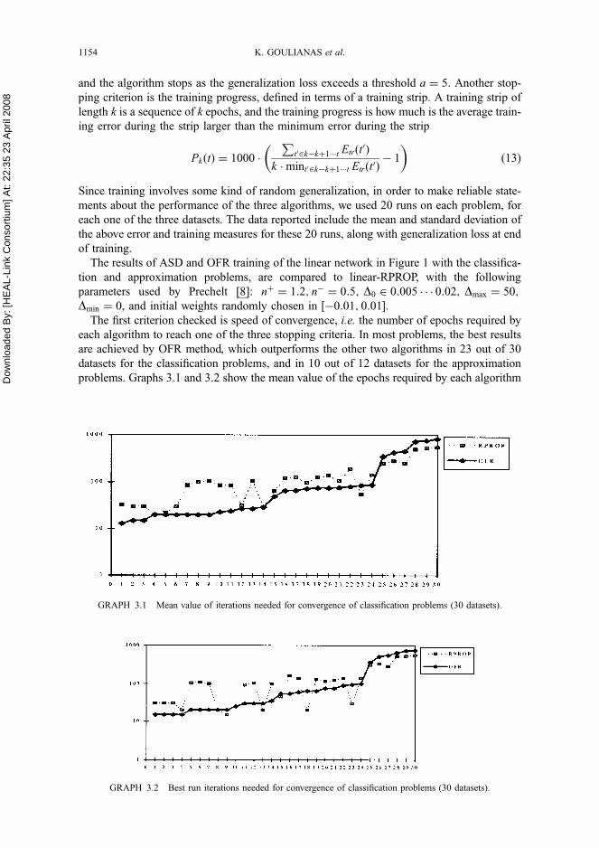
The first criterion checked is speed of convergence, i.e. the number of epochs required by

each algorithm to reach one of the three stopping criteria. In most problems, the best results

are achieved by OFR method, which outperforms the other two algorithms in 23 out of 30

datasets for the classification problems, and in 10 out of 12 datasets for the approximation

problems. Graphs 3.1 and 3.2 show the mean value of the epochs required by each algorithm

GRAPH 3.1 Mean value of iterations needed for convergence of classification problems (30 datasets).

GRAPH 3.2 Best run iterations needed for convergence of classification problems (30 datasets).

1154 K. GOULIANAS et al.

Dow

nloa

ded

By:

[HE

AL-

Link

Con

sorti

um] A

t: 22

:35

23 A

pril

2008

TA

BL

EII

I.1

Res

ult

sfo

rC

lass

ifica

tion

Pro

ble

ms.

Epo

chs

Rel

eva

nt

epo

chs

Connec

tion

trave

rsals

Tra

inin

gse

ter

ror

Va

lid

ati

on

set

erro

rTes

tse

ter

ror

Tes

tse

tcl

ass

ific

ati

on

Gen

era

lity

loss

Pro

ble

mM

eth

od

mea

nst

dev

mea

nst

dev

mea

nst

dev

mea

nst

dev

mea

nst

dev

mea

nst

dev

mea

nst

dev

mea

nst

dev

Can

cer1

RP

RO

P8

51

47

31

88

51

42

0.7

50

.01

20

.21

0.1

21

8.6

10

.13

15

.15

0.5

00

.18

0.2

8A

SD

40

02

31

40

02

0.7

40

.00

20

.20

0.0

01

8.6

30

.00

16

.09

0.0

00

.16

0.0

1O

FR

20

19

02

01

20

.74

0.0

02

0.0

70

.04

18

.61

0.0

51

5.7

90

.39

0.8

30

.28

Can

cer2

RP

RO

P8

42

36

31

98

42

31

8.7

10

.18

20

.56

0.1

02

2.0

30

.19

19

.03

0.4

51

.12

2.6

8A

SD

50

03

01

50

01

8.6

50

.00

20

.51

0.0

02

2.0

20

.01

18

.39

0.0

00

.13

0.0

1O

FR

24

41

10

24

41

8.6

40

.00

20

.47

0.0

22

2.1

40

.03

18

.94

0.1

30

.37

0.0

8

Can

cer3

RP

RO

P8

51

47

31

88

51

42

0.7

50

.01

20

.21

0.1

21

8.6

10

.13

15

.15

0.5

00

.18

0.2

8A

SD

48

22

10

48

22

0.4

30

.00

18

.70

0.0

02

0.3

40

.01

17

.66

0.2

50

.46

0.0

3O

FR

23

51

35

23

52

0.4

30

.01

18

.75

0.0

32

0.2

80

.07

16

.88

0.2

80

.33

0.1

6

Car

d1

RP

RO

P6

49

27

56

49

9.8

30

.01

8.9

30

.14

10

.67

0.2

01

3.7

10

.74

4.1

91

.23

AS

D8

83

13

08

83

10

.04

0.0

18

.21

0.0

11

0.4

70

.01

13

.95

0.0

05

.08

0.0

6O

FR

49

13

13

04

91

31

0.0

50

.07

28

.20

0.0

11

0.4

60

.01

13

.95

0.0

05

.90

0.8

6

Car

d2

RP

RO

P5

51

92

46

55

19

8.3

80

.35

10

.76

0.2

41

4.9

30

.26

19

.37

0.3

84

.38

1.4

9A

SD

23

14

21

12

31

48

.32

0.0

09

.71

0.0

11

3.6

70

.03

19

.77

0.0

05

.02

0.0

4O

FR

85

30

19

08

53

08

.34

0.0

39

.71

0.0

11

3.7

20

.02

19

.77

0.0

05

.59

0.7

7

Car

d3

RP

RO

P1

04

11

45

13

10

41

19

.47

0.0

08

.39

0.1

01

2.6

00

.21

14

.60

0.6

51

.75

1.1

9A

SD

15

84

26

11

58

49

.64

0.0

07

.68

0.0

11

2.3

40

.01

15

.45

0.2

95

.05

0.0

4O

FR

76

35

20

27

63

59

.65

0.0

47

.67

0.0

11

2.3

40

.03

15

.51

0.4

25

.69

0.8

1

Dia

bet

es1

RP

RO

P1

03

15

85

19

10

31

52

0.3

40

.01

22

.58

0.0

32

4.0

60

.09

38

.65

0.6

00

.19

0.1

6A

SD

30

01

00

30

02

0.3

20

.00

22

.54

0.0

02

4.0

20

.00

38

.54

0.0

00

.54

0.0

1O

FR

20

18

02

01

20

.31

0.0

02

2.5

10

.00

23

.89

0.0

13

7.5

00

.00

0.8

80

.04

Dia

bet

es2

RP

RO

P1

00

16

99

16

10

01

62

1.0

50

.01

20

.87

0.0

62

4.2

90

.08

37

.31

0.7

80

.02

0.0

3A

SD

30

01

50

30

02

1.0

30

.00

20

.71

0.0

02

3.9

80

.00

35

.94

0.0

00

.16

0.0

1O

FR

20

01

11

20

02

1.0

20

.00

20

.72

0.0

02

4.1

60

.09

36

.38

0.7

20

.22

0.0

2

Dia

bet

es3

RP

RO

P106

11

35

8106

11

20.4

00.0

123.0

30.1

422.6

40.1

737.0

61.2

42.5

50.5

7A

SD

25

03

02

50

20

.38

0.0

02

2.8

70

.01

22

.04

0.0

13

3.7

40

.47

3.7

00

.03

OF

R2

78

30

27

82

0.3

90

.01

22

.89

0.0

12

2.0

30

.01

33

.28

0.5

33

.65

0.2

2

Gen

e1R

PR

OP

30

01

86

30

02

1.4

80

.00

25

.55

0.0

52

5.0

30

.04

39

.06

0.6

00

.24

0.2

0A

SD

19

22

01

92

21

.48

0.0

02

4.7

30

.10

24

.46

0.0

64

0.7

00

.68

3.5

20

.43

OF

R2

02

20

20

22

1.4

80

.00

24

.74

0.0

82

4.5

30

.07

40

.66

0.6

63

.46

0.3

4

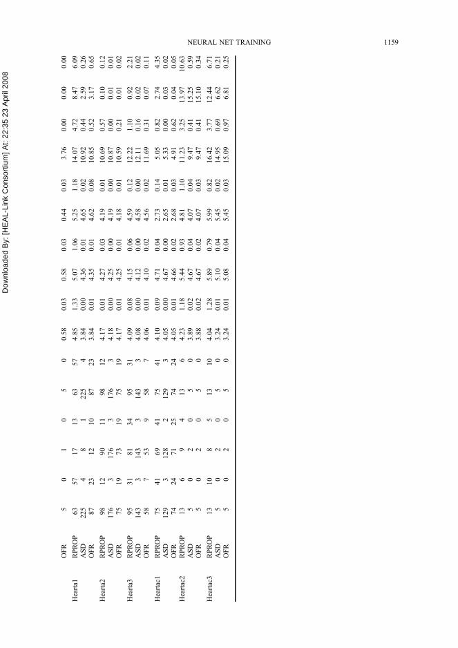
NEURAL NET TRAINING 1155

Dow

nloa

ded

By:

[HE

AL-

Link

Con

sorti

um] A

t: 22

:35

23 A

pril

2008

TA

BL

EII

I.1

(co

nti

nued

)

Epo

chs

Rel

eva

nt

epo

chs

Connec

tion

trave

rsals

Tra

inin

gse

ter

ror

Va

lid

ati

on

set

erro

rTes

tse

ter

ror

Tes

tse

tcl

ass

ific

ati

on

Gen

era

lity

loss

Pro

ble

mM

eth

od

mea

nst

dev

mea

nst

dev

mea

nst

dev

mea

nst

dev

mea

nst

dev

mea

nst

dev

mea

nst

dev

mea

nst

dev

Gen

e2R

PR

OP

30

01

95

30

02

1.6

20

.00

25

.20

0.0

32

4.9

90

.04

39

.74

0.5

00

.15

0.0

9A

SD

15

02

01

50

21

.62

0.0

02

4.5

40

.10

24

.54

0.0

94

1.1

40

.58

2.7

50

.39

OF

R1

50

20

15

02

1.6

20

.00

24

.54

0.1

12

4.5

70

.11

41

.05

0.7

72

.75

0.4

5

Gen

e3R

PR

OP

30

01

85

30

02

1.8

80

.00

24

.33

0.0

52

5.3

70

.07

41

.93

0.6

40

.21

0.2

0A

SD

15

03

01

50

21

.88

0.0

02

4.0

10

.08

24

.88

0.0

84

2.3

70

.41

1.4

50

.32

OF

R1

50

30

15

02

1.8

80

.00

24

.00

0.0

62

4.8

60

.06

42

.50

0.3

41

.50

0.2

6

Gla

ss1

RP

RO

P1

24

14

24

51

24

14

8.8

40

.01

9.7

10

.07

10

.13

0.1

24

7.6

73

.05

3.7

50

.69

AS

D1

57

34

41

15

73

8.8

00

.00

9.9

50

.01

9.7

70

.01

47

.17

0.0

01

.65

0.0

6O

FR

75

14

29

87

51

48

.79

0.0

29

.86

0.0

89

.80

0.1

14

3.3

02

.07

3.6

81

.95

Gla

ss2

RP

RO

P3

39

16

33

39

8.7

50

.16

10

.27

0.1

61

0.3

00

.14

55

.91

2.3

96

.19

1.0

9A

SD

25

07

02

50

8.6

20

.01

10

.54

0.0

11

0.3

70

.01

54

.72

0.0

05

.40

0.1

4O

FR

13

35

01

33

8.7

00

.11

10

.59

0.0

21

0.4

80

.01

52

.83

0.0

06

.16

0.9

7

Gla

ss3

RP

RO

P1

24

22

26

12

12

42

28

.72

0.0

29

.36

0.0

51

1.1

80

.20

60

.77

4.1

32

.03

0.5

5A

SD

18

23

46

21

82

38

.67

0.0

09

.41

0.0

01

0.9

40

.01

56

.60

0.0

01

.36

0.0

4O

FR

66

22

28

76

62

28

.68

0.0

69

.41

0.0

31

1.0

10

.07

56

.31

1.2

64

.07

4.4

0

Hea

rt1

RP

RO

P1

38

15

49

91

38

15

11

.19

0.0

11

3.2

50

.06

14

.31

0.0

52

1.0

80

.41

1.2

20

.55

AS

D1

61

21

60

21

61

21

1.2

10

.00

13

.13

0.0

01

4.1

30

.00

20

.43

0.0

00

.01

0.0

1O

FR

75

17

69

15

75

17

11

.19

0.0

21

3.1

10

.02

14

.08

0.0

22

0.4

80

.13

0.0

60

.06

Hea

rt2

RP

RO

P1

89

24

16

82

61

89

24

11

.67

0.0

21

2.2

10

.02

13

.53

0.0

31

6.5

00

.22

0.1

50

.11

AS

D2

16

32

15

32

16

31

1.6

60

.00

12

.22

0.0

01

3.6

00

.00

16

.52

0.0

00

.00

0.0

0O

FR

81

23

72

23

81

23

11

.64

0.0

21

2.2

20

.01

13

.63

0.0

41

6.5

40

.10

0.0

70

.08

Hea

rt3

RP

RO

P1

41

13

85

48

14

11

31

1.1

10

.00

10

.73

0.0

61

6.4

00

.11

23

.18

0.9

00

.42

0.4

8A

SD

18

72

13

72

18

72

11

.11

0.0

01

0.6

10

.00

16

.27

0.0

02

2.6

10

.00

0.0

90

.02

OF

R8

72

15

71

08

72

11

1.0

90

.01

10

.56

0.0

21

6.2

50

.04

22

.68

0.3

20

.58

0.3

2

Hea

rtc1

RP

RO

P1

20

27

82

40

12

02

71

0.2

00

.15

9.6

20

.12

16

.47

0.6

42

0.0

00

.97

0.8

21

.40

AS

D1

55

01

55

01

55

01

0.1

80

.00

9.6

10

.00

16

.00

0.0

02

0.0

00

.00

0.0

00

.00

OF

R6

61

34

41

86

61

31

0.1

60

.01

9.5

70

.03

16

.04

0.0

71

9.4

40

.66

0.4

00

.25

Hea

rtc2

RP

RO

P9

66

12

61

69

66

11

1.7

80

.93

16

.58

0.4

36

.66

0.9

83

.79

1.9

05

.38

2.2

5A

SD

17

00

28

11

70

01

1.2

30

.00

16

.54

0.0

16

.15

0.0

13

.23

0.6

62

.87

0.0

4O

FR

72

19

22

27

21

91

1.2

20

.01

16

.53

0.0

46

.22

0.1

02

.46

0.4

93

.41

0.4

1

Hea

rtc3

RP

RO

P2

06

13

22

06

11

.12

0.6

21

3.9

90

.35

13

.21

0.4

11

3.7

51

.44

8.3

13

.33

1156 K. GOULIANAS et al.

Dow

nloa

ded

By:

[HE

AL-

Link

Con

sorti

um] A

t: 22

:35

23 A

pril

2008

AS

D2

42

50

24

21

0.4

40

.06

13

.12

0.0

31

2.0

80

.02

15

.44

0.6

66

.06

0.5

3O

FR

20

05

02

00

10

.33

0.0

21

3.1

10

.03

12

.09

0.0

31

5.7

20

.54

8.7

50

.50

Ho

rse1

RP

RO

P3

06

13

43

06

11

.30

0.2

01

5.5

50

.24

12

.87

0.3

32

6.2

02

.60

6.2

50

.64

AS

D3

22

50

32

21

1.2

50

.05

15

.21

0.0

41

2.7

60

.05

26

.49

1.2

35

.59

0.3

6O

FR

29

25

02

92

11

.10

0.0

71

5.2

00

.05

12

.75

0.0

42

6.9

51

.09

6.8

40

.82

Ho

rse2

RP

RO

P3

27

14

33

27

8.9

00

.21

15

.73

0.2

71

7.3

40

.50

36

.50

1.3

15

.60

0.9

6A

SD

60

01

51

60

08

.36

0.0

11

5.6

80

.02

16

.62

0.0

63

5.8

00

.54

5.2

20

.13

OF

R2

73

13

12

73

8.4

40

.06

15

.69

0.0

31

6.6

60

.08

35

.51

0.5

16

.82

1.3

1

Ho

rse3

RP

RO

P2

27

92

22

71

0.7

30

.42

15

.43

0.2

81

5.2

40

.34

31

.87

1.8

25

.89

0.9

0A

SD

25

17

12

51

10

.26

0.0

31

5.3

30

.04

15

.13

0.0

53

3.2

00

.67

5.3

00

.29

OF

R2

00

71

20

01

0.2

41

0.0

31

5.3

10

.04

15

.13

0.0

53

3.4

90

.75

6.0

60

.35

Soy

bea

n1

RP

RO

P5

43

15

42

05

15

43

15

0.6

50

.00

0.9

80

.00

1.1

60

.00

9.5

70

.32

0.2

60

.11

AS

D1

19

82

01

19

82

01

19

82

00

.67

0.0

00

.96

0.0

01

.15

0.0

09

.35

0.1

80

.00

0.0

1O

FR

82

17

48

02

81

82

17

40

.67

0.0

00

.96

0.0

01

.15

0.0

19

.20

0.2

80

.07

0.0

8

Soy

bea

n2

RP

RO

P4

91

18

47

42

84

91

18

0.8

00

.00

0.8

10

.00

1.0

50

.00

4.1

20

.00

0.0

50

.04

AS

D1

01

31

51

01

21

51

01

31

50

.82

0.0

00

.82

0.0

01

.07

0.0

04

.12

0.0

00

.00

0.0

1O

FR

72

85

47

18

54

72

85

40

.82

0.0

00

.82

0.0

11

.07

0.0

14

.12

0.0

00

.06

0.0

9

Soy

bea

n3

RP

RO

P5

18

20

49

83

45

18

20

0.7

80

.00

0.9

60

.00

1.0

40

.00

7.0

90

.13

0.0

40

.03

AS

D1

12

82

51

12

82

51

12

82

50

.80

0.0

00

.96

0.0

01

.02

0.0

06

.53

0.1

80

.00

0.0

1O

FR

75

96

07

52

60

75

96

00

.79

0.0

00

.96

0.0

11

.03

0.0

16

.59

0.3

10

.09

0.1

3

Thy

roid

1R

PR

OP

24

65

02

43

51

24

65

03

.91

0.0

13

.95

0.0

24

.08

0.0

26

.53

0.0

30

.03

0.0

3A

SD

81

01

18

10

11

81

01

14

.03

0.0

04

.17

0.0

04

.22

0.0

06

.56

0.0

00

.01

0.0

1O

FR

34

61

21

34

41

20

34

61

21

3.9

70

.04

4.0

50

.09

4.1

30

.08

6.5

50

.02

0.0

10

.01

Thy

roid

2R

PR

OP

25

14

02

48

39

25

14

04

.10

0.0

13

.68

0.0

23

.86

0.0

26

.38

0.0

00

.05

0.0

5A

SD

91

41

09

13

10

91

41

04

.23

0.0

03

.81

0.0

03

.99

0.0

06

.38

0.0

00

.01

0.0

1O

FR

45

31

10

45

21

10

45

31

10

4.1

70

.04

3.7

70

.04

3.9

50

.04

6.3

80

.00

0.0

10

.01

Thy

roid

3R

PR

OP

28

06

52

75

67

28

06

54

.01

0.0

13

.48

0.0

14

.19

0.0

17

.23

0.0

20

.05

0.0

3A

SD

90

47

90

37

90

47

4.1

60

.00

3.6

50

.00

4.3

30

.00

7.1

70

.00

0.0

20

.01

OF

R4

24

12

64

22

12

54

24

12

64

.08

0.0

63

.56

0.0

64

.25

0.0

57

.22

0.0

60

.02

0.0

2

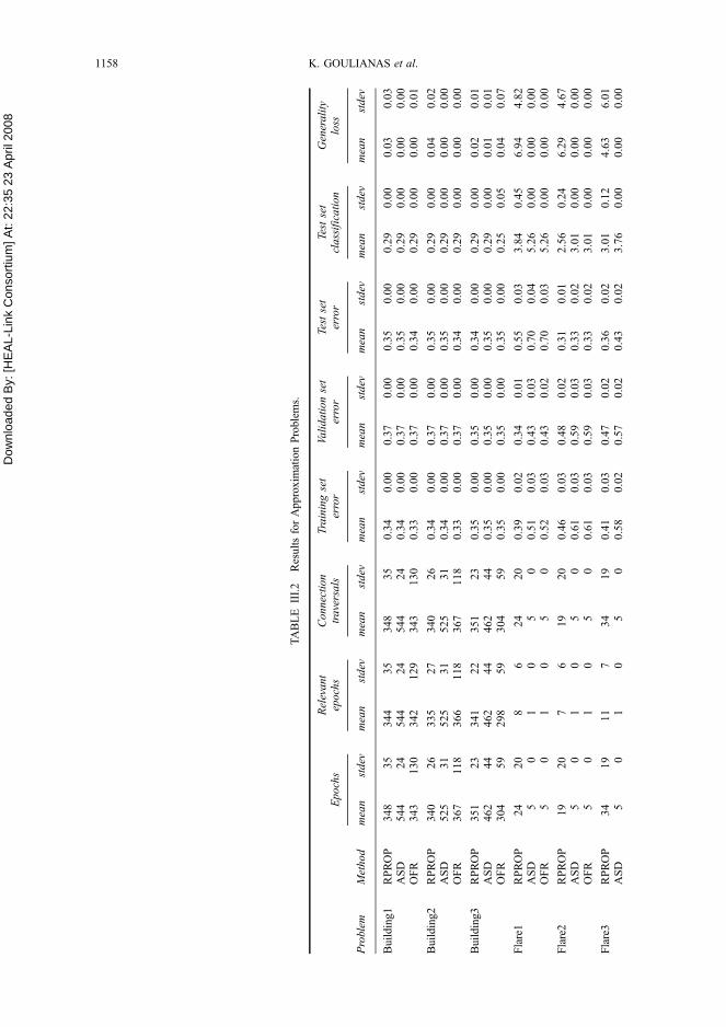
NEURAL NET TRAINING 1157

Dow

nloa

ded

By:

[HE

AL-

Link

Con

sorti

um] A

t: 22

:35

23 A

pril

2008

TA

BL

EII

I.2

Res

ult

sfo

rA

pp

rox

imat

ion

Pro

ble

ms.

Ep

och

sR

elev

ant

epoch

sC

on

nec

tio

ntr

ave

rsals

Tra

inin

gse

ter

ror

Va

lid

ati

on

set

erro

rTes

tse

ter

ror

Tes

tse

tcl

ass

ific

ati

on

Gen

era

lity

loss

Pro

ble

mM

eth

od

mea

nst

dev

mea

nst

dev

mea

nst

dev

mea

nst

dev

mea

nst

dev

mea

nst

dev

mea

nst

dev

mea

nst

dev

Buil

din

g1

RP

RO

P3

48

35

34

43

53

48

35

0.3

40

.00

0.3

70

.00

0.3

50

.00

0.2

90

.00

0.0

30

.03

AS

D5

44

24

54

42

45

44

24

0.3

40

.00

0.3

70

.00

0.3

50

.00

0.2

90

.00

0.0

00

.00

OF

R3

43

13

03

42

12

93

43

13

00

.33

0.0

00

.37

0.0

00

.34

0.0

00

.29

0.0

00

.00

0.0

1

Buil

din

g2

RP

RO

P3

40

26

33

52

73

40

26

0.3

40

.00

0.3

70

.00

0.3

50

.00

0.2

90

.00

0.0

40

.02

AS

D5

25

31

52

53

15

25

31

0.3

40

.00

0.3

70

.00

0.3

50

.00

0.2

90

.00

0.0

00

.00

OF

R3

67

11

83

66

11

83

67

11

80

.33

0.0

00

.37

0.0

00

.34

0.0

00

.29

0.0

00

.00

0.0

0

Buil

din

g3

RP

RO

P3

51

23

34

12

23

51

23

0.3

50

.00

0.3

50

.00

0.3

40

.00

0.2

90

.00

0.0

20

.01

AS

D4

62

44

46

24

44

62

44

0.3

50

.00

0.3

50

.00

0.3

50

.00

0.2

90

.00

0.0

10

.01

OF

R3

04

59

29

85

93

04

59

0.3

50

.00

0.3

50

.00

0.3

50

.00

0.2

50

.05

0.0

40

.07

Fla

re1

RP

RO

P2

42

08

62

42

00

.39

0.0

20

.34

0.0

10

.55

0.0

33

.84

0.4

56

.94

4.8

2A

SD

50

10

50

0.5

10

.03

0.4

30

.03

0.7

00

.04

5.2

60

.00

0.0

00

.00

OF

R5

01

05

00

.52

0.0

30

.43

0.0

20

.70

0.0

35

.26

0.0

00

.00

0.0

0

Fla

re2

RP

RO

P1

92

07

61

92

00

.46

0.0

30

.48

0.0

20

.31

0.0

12

.56

0.2

46

.29

4.6

7A

SD

50

10

50

0.6

10

.03

0.5

90

.03

0.3

30

.02

3.0

10

.00

0.0

00

.00

OF

R5

01

05

00

.61

0.0

30

.59

0.0

30

.33

0.0

23

.01

0.0

00

.00

0.0

0

Fla

re3

RP

RO

P3

41

91

17

34

19

0.4

10

.03

0.4

70

.02

0.3

60

.02

3.0

10

.12

4.6

36

.01

AS

D5

01

05

00

.58

0.0

20

.57

0.0

20

.43

0.0

23

.76

0.0

00

.00

0.0

0

1158 K. GOULIANAS et al.

Dow

nloa

ded

By:

[HE

AL-

Link

Con

sorti

um] A

t: 22

:35

23 A

pril

2008

OF

R5

01

05

00

.58

0.0

30

.58

0.0

30

.44

0.0

33

.76

0.0

00

.00

0.0

0

Hea

rta1

RP

RO

P6

35

71

71

36

35

74

.85

1.3

35

.07

1.0

65

.25

1.1

81

4.0

74

.72

8.4

76

.09

AS

D2

25

48

12

25

43

.84

0.0

04

.36

0.0

14

.65

0.0

21

0.9

20

.44

2.5

90

.26

OF

R8

72

31

21

08

72

33

.84

0.0

14

.35

0.0

14

.62

0.0

81

0.8

50

.52

3.1

70

.65

Hea

rta2

RP

RO

P9

81

29

01

19

81

24

.17

0.0

14

.27

0.0

34

.19

0.0

11

0.6

90

.57

0.1

00

.12

AS

D1

76

31

76

31

76

34

.18

0.0

04

.25

0.0

04

.19

0.0

01

0.8

70

.00

0.0

10

.01

OF

R7

51

97

31

97

51

94

.17

0.0

14

.25

0.0

14

.18

0.0

11

0.5

90

.21

0.0

10

.02

Hea

rta3

RP

RO

P9

53

18

13

49

53

14

.09

0.0

84

.15

0.0

64

.59

0.1

21

2.2

21

.10

0.9

22

.21

AS

D1

43

31

43

31

43

34

.08

0.0

04

.12

0.0

04

.58

0.0

01

2.1

10

.16

0.0

20

.02

OF

R5

87

53

95

87

4.0

60

.01

4.1

00

.02

4.5

60

.02

11

.69

0.3

10

.07

0.1

1

Hea

rtac

1R

PR

OP

75

41

69

41

75

41

4.1

00

.09

4.7

10

.04

2.7

30

.14

5.0

50

.82

2.7

44

.35

AS

D1

29

31

28

21

29

34

.05

0.0

04

.67

0.0

02

.65

0.0

15

.33

0.0

00

.03

0.0

2O

FR

74

24

71

25

74

24

4.0

50

.01

4.6

60

.02

2.6

80

.03

4.9

10

.62

0.0

40

.05

Hea

rtac

2R

PR

OP

13

69

41

36

4.2

31

.18

5.4

40

.93

4.8

11

.10

11

.23

3.2

51

3.9

71

0.6

3A

SD

50

20

50

3.8

90

.02

4.6

70

.04

4.0

70

.04

9.4

70

.41

15

.25

0.5

9O

FR

50

20

50

3.8

80

.02

4.6

70

.02

4.0

70

.03

9.4

70

.41

15

.10

0.3

4

Hea

rtac

3R

PR

OP

13

10

85

13

10

4.0

41

.28

5.8

90

.79

5.9

90

.82

16

.42

3.7

71

2.4

46

.71

AS

D5

02

05

03

.24

0.0

15

.10

0.0

45

.45

0.0

21

4.9

50

.69

6.6

20

.21

OF

R5

02

05

03

.24

0.0

15

.08

0.0

45

.45

0.0

31

5.0

90

.97

6.8

10

.25

NEURAL NET TRAINING 1159

Dow

nloa

ded

By:

[HE

AL-

Link

Con

sorti

um] A

t: 22

:35

23 A

pril

2008

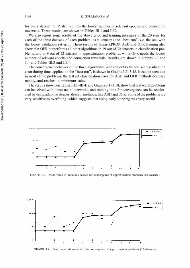
for every dataset. OFR also requires the lowest number of relevant epochs, and connection

traversals. These results, are shown in Tables III.1 and III.2.

We also report some results of the above error and training measures of the 20 runs for

each of the three datasets of each problem, as it concerns the ‘‘best run’’, i.e. the one with

the lowest validation set error. These results of linear-RPROP, ASD and OFR training also

show that OFR outperforms all other algorithms in 19 out of 30 datasets in classification pro-

blems, and in 9 out of 12 datasets in approximation problems, while OFR needs the lowest

number of relevant epochs and connection traversals. Results, are shown in Graphs 3.3 and

3.4 and Tables III.3 and III.4.

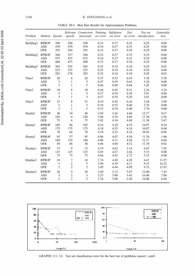
The convergence behavior of the three algorithms, with respect to the test set classification

error during time, applied on the ‘‘best run’’, is shown in Graphs 3.5–3.18. It can be seen that

in most of the problems, the test set classification error for ASD and OFR methods decrease

rapidly, and reaches its minimum value.

The results shown on Tables III.1–III.4, and Graphs 3.1–3.18, show that real world problems

can be solved with linear neural networks, and training time for convergence can be acceler-

ated by using adaptive steepest descent methods, like ASD and OFR. Some of the problems are

very sensitive to overfitting, which suggests that using early stopping was very useful.

GRAPH 3.3 Mean value of iterations needed for convergence of approximation problems (12 datasets).

GRAPH 3.4 Best run iterations needed for convergence of approximation problems (12 datasets).

1160 K. GOULIANAS et al.

Dow

nloa

ded

By:

[HE

AL-

Link

Con

sorti

um] A

t: 22

:35

23 A

pril

2008

TA

BL

EII

I.3

Bes

tR

un

Res

ult

sfo

rC

lass

ifica

tio

nP

roble

ms.

Pro

ble

mM

eth

od

Epo

chs

Rel

eva

nt

epoch

sC

on

nec

tio

ntr

ave

rsa

lsTra

inin

gse

ter

ror

Va

lid

ati

on

set

erro

rTes

tse

ter

ror

Tes

tse

tcl

ass

ific

ati

on

Gen

era

lity

loss

Can

cer1

RP

RO

P1

05

79

10

52

0.7

52

0.0

31

8.4

51

4.3

70

.38

AS

D4

02

34

02

0.7

42

0.1

91

8.6

31

6.0

90

.17

OF

R2

09

20

20

.75

20

.01

18

.54

16

.67

1.3

0

Can

cer2

RP

RO

P9

54

39

51

8.6

62

0.3

82

1.9

51

7.8

20

.72

AS

D5

03

15

01

8.6

52

0.5

12

2.0

21

8.3

90

.13

OF

R3

01

03

01

8.6

62

0.4

42

2.1

91

8.9

70

.32

Can

cer3

RP

RO

P1

00

49

10

02

0.4

41

8.4

82

0.3

91

6.0

91

.23

AS

D5

02

15

02

0.4

21

8.7

02

0.3

41

7.8

20

.50

OF

R3

51

13

52

0.4

21

8.7

12

0.2

91

7.2

40

.54

Car

d1

RP

RO

P4

52

84

59

.86

8.6

41

0.6

71

3.9

56

.24

AS

D8

01

38

01

0.0

68

.19

10

.46

13

.95

5.0

3O

FR

55

13

55

10

.05

8.1

91

0.4

41

3.9

55

.21

Car

d2

RP

RO

P2

01

52

08

.48

10

.07

14

.85

19

.77

6.5

6A

SD

22

52

12

25

8.3

29

.70

13

.65

19

.77

5.0

1O

FR

65

19

65

8.3

59

.69

13

.70

19

.77

5.1

0

Car

d3

RP

RO

P1

15

23

11

59

.48

8.1

61

2.2

31

3.9

54

.45

AS

D1

55

27

15

59

.64

7.6

71

2.3

51

5.7

05

.00

OF

R7

52

47

59

.68

7.6

81

2.2

71

6.2

85

.06

Dia

bet

es1

RP

RO

P110

87

110

20.3

322.5

123.9

638.5

40.2

7A

SD

30

10

30

20

.32

22

.54

24

.01

38

.54

0.5

5O

FR

20

82

02

0.3

12

2.5

02

3.8

73

7.5

00

.91

Dia

bet

es2

RP

RO

P100

97

100

21.0

320.7

524.3

438.0

20.0

3A

SD

30

15

30

21

.03

20

.71

23

.99

35

.94

0.1

7O

FR

20

10

20

21

.02

20

.71

24

.20

35

.94

0.2

4

Dia

bet

es3

RP

RO

P105

33

105

20.4

022.8

322.5

037.5

03.2

2A

SD

25

32

52

0.3

82

2.8

62

2.0

53

4.3

83

.73

OF

R3

03

30

20

.39

22

.88

22

.03

33

.33

3.7

0

Gen

e1R

PR

OP

30

13

30

21

.48

25

.45

25

.01

39

.34

0.6

5A

SD

20

22

02

1.4

82

4.5

22

4.3

64

1.7

44

.38

OF

R1

52

15

21

.48

24

.63

24

.48

40

.48

3.8

2

Gen

e2R

PR

OP

30

16

30

21

.62

25

.15

24

.91

38

.59

0.3

2A

SD

15

21

52

1.6

22

4.3

42

4.5

04

0.9

83

.58

OF

R1

52

15

21

.62

24

.38

24

.49

42

.12

3.3

8

NEURAL NET TRAINING 1161

Dow

nloa

ded

By:

[HE

AL-

Link

Con

sorti

um] A

t: 22

:35

23 A

pril

2008

TA

BL

EII

I.3

(co

nti

nued

)

Pro

ble

mM

eth

od

Epo

chs

Rel

eva

nt

epo

chs

Co

nn

ecti

on

trave

rsals

Tra

inin

gse

ter

ror

Va

lid

ati

on

set

erro

rTes

tse

ter

ror

Tes

tse

tcl

ass

ific

ati

on

Gen

era

lity

loss

Gen

e3R

PR

OP

30

93

02

1.8

82

4.2

02

5.2

84

0.2

30

.77

AS

D1

53

15

21

.88

23

.91

24

.85

42

.62

1.8

9O

FR

15

31

52

1.8

82

3.9

02

4.7

54

2.6

21

.96

Gla

ss1

RP

RO

P1

40

18

14

08

.84

9.5

91

0.3

24

9.0

64

.87

AS

D1

60

45

16

08

.80

9.9

49

.75

47

.17

1.7

9O

FR

90

34

90

8.7

89

.73

9.6

34

3.4

03

.88

Gla

ss2

RP

RO

P2

01

42

08

.95

9.9

31

0.3

35

4.7

25

.45

AS

D2

57

25

8.6

21

0.5

11

0.3

65

4.7

25

.61

OF

R1

55

15

8.5

81

0.5

21

0.4

65

2.8

38

.71

Gla

ss3

RP

RO

P1

40

18

14

08

.71

9.2

41

1.0

26

0.3

83

.33

AS

D1

85

43

18

58

.67

9.4

01

0.9

55

6.6

01

.44

OF

R1

00

28

10

08

.61

9.3

61

0.9

55

6.6

03

.38

Hea

rt1

RP

RO

P1

35

39

13

51

1.1

81

3.1

51

4.3

62

2.1

71

.82

AS

D1

60

15

91

60

11

.21

13

.12

14

.13

20

.43

0.0

2O

FR

60

52

60

11

.18

13

.07

14

.06

20

.43

0.1

1

Hea

rt2

RP

RO

P1

60

13

71

60

11

.67

12

.18

13

.51

16

.52

0.1

7A

SD

22

02

20

22

01

1.6

61

2.2

21

3.6

01

6.5

20

.00

OF

R5

54

45

51

1.6

41

2.2

01

3.5

91

6.5

20

.33

Hea

rt3

RP

RO

P1

30

34

13

01

1.1

01

0.5

91

6.5

62

3.4

81

.42

AS

D1

90

13

51

90

11

.11

10

.61

16

.27

22

.61

0.1

2O

FR

65

52

65

11

.09

10

.53

16

.21

22

.17

0.7

0

Hea

rtc1

RP

RO

P1

25

17

12

51

0.1

69

.44

17

.45

22

.67

2.1

9A

SD

15

51

55

15

51

0.1

89

.60

16

.00

20

.00

0.0

0O

FR

75

24

75

10

.14

9.5

11

6.0

41

8.6

70

.74

Hea

rtc2

RP

RO

P3

01

53

01

1.8

71

5.8

06

.08

2.6

75

.31

AS

D1

70

27

17

01

1.2

31

6.5

26

.14

4.0

02

.99

OF

R9

52

69

51

1.2

31

6.3

96

.27

1.3

34

.01

Hea

rtc3

RP

RO

P2

01

12

01

0.6

61

3.2

41

2.6

41

6.0

01

2.7

2A

SD

20

52

01

0.5

51

3.0

61

2.0

81

6.0

05

.19

OF

R2

05

20

10

.32

13

.05

12

.06

16

.00

9.1

7

Ho

rse1

RP

RO

P2

51

42

51

1.4

31

5.1

81

2.9

12

7.4

75

.60

AS

D3

05

30

11

.29

15

.13

12

.70

26

.37

5.4

5O

FR

25

52

51

1.2

41

5.1

01

2.7

32

6.3

75

.45

1162 K. GOULIANAS et al.

Dow

nloa

ded

By:

[HE

AL-

Link

Con

sorti

um] A

t: 22

:35

23 A

pril

2008

Ho

rse2

RP

RO

P2

01

22

09

.36

15

.18

17

.48

35

.16

9.6

5A

SD

60

15

60

8.3

81

5.6

31

6.6

13

5.1

65

.14

OF

R3

01

33

08

.41

15

.65

16

.68

35

.16

6.4

5

Ho

rse3

RP

RO

P1

59

15

11

.01

14

.71

15

.33

30

.77

9.0

8A

SD

25

52

51

0.2

41

5.2

21

5.0

03

4.0

75

.88

OF

R2

07

20

10

.23

15

.25

15

.12

32

.97

6.3

7

Soy

bea

n1

RP

RO

P5

25

48

65

25

0.6

50

.98

1.1

68

.82

0.2

2A

SD

11

70

11

70

11

70

0.6

70

.96

1.1

59

.41

0.0

0O

FR

73

57

28

73

50

.67

0.9

61

.14

9.4

10

.01

Soy

bea

n2

RP

RO

P5

20

48

45

20

0.8

00

.81

1.0

54

.12

0.1

1A

SD

10

35

10

35

10

35

0.8

20

.82

1.0

74

.12

0.0

0O

FR

65

56

30

65

50

.82

0.8

11

.05

4.1

20

.02

Soy

bea

n3

RP

RO

P5

55

54

85

55

0.7

80

.96

1.0

37

.06

0.0

4A

SD

11

00

11

00

11

00

0.8

00

.96

1.0

26

.47

0.0

0O

FR

74

57

39

74

50

.79

0.9

41

.02

6.4

70

.00

Thy

roid

1R

PR

OP

29

02

87

29

03

.91

3.9

64

.08

6.5

60

.01

AS

D8

15

81

48

15

4.0

34

.17

4.2

26

.56

0.0

2O

FR

55

55

48

55

53

.88

3.8

73

.99

6.5

60

.03

Thy

roid

2R

PR

OP

31

02

97

31

04

.08

3.6

53

.82

6.3

80

.14

AS

D9

30

92

99

30

4.2

23

.81

3.9

96

.38

0.0

2O

FR

37

03

70

37

04

.10

3.6

73

.83

6.3

80

.00

Thy

roid

3R

PR

OP

34

03

37

34

04

.02

3.4

84

.19

7.2

20

.05

AS

D9

15

91

59

15

4.1

63

.64

4.3

27

.17

0.0

0O

FR

51

05

03

51

03

.98

3.4

64

.16

7.2

80

.07

NEURAL NET TRAINING 1163

Dow

nloa

ded

By:

[HE

AL-

Link

Con

sorti

um] A

t: 22

:35

23 A

pril

2008

GRAPHS 3.5, 3.6 Test set classification error for the best run of problems cancer1, card1.

TABLE III.4 Best Run Results for Approximation Problems.

Problem Method EpochsRelevantepochs

Connectiontraversals

Trainingset error

Validationset error

Testset error

Test setclassification

Generalityloss

Building1 RPROP 390 390 390 0.33 0.37 0.35 0.29 0.00ASD 470 470 470 0.34 0.37 0.35 0.29 0.00OFR 395 394 395 0.33 0.37 0.34 0.29 0.00

Building2 RPROP 360 357 360 0.33 0.37 0.35 0.29 0.06ASD 475 475 475 0.34 0.37 0.35 0.29 0.00OFR 480 475 480 0.33 0.37 0.34 0.29 0.00

Building3 RPROP 305 295 305 0.35 0.34 0.34 0.29 0.03ASD 525 525 525 0.35 0.34 0.34 0.29 0.00OFR 285 278 285 0.35 0.34 0.34 0.29 0.03

Flare1 RPROP 20 6 20 0.37 0.32 0.54 3.38 5.38ASD 5 1 5 0.47 0.39 0.65 5.26 0.00OFR 5 1 5 0.46 0.40 0.64 5.26 0.00

Flare2 RPROP 10 8 10 0.44 0.45 0.31 2.26 5.34ASD 5 1 5 0.57 0.54 0.30 3.01 0.00OFR 5 1 5 0.57 0.54 0.29 3.01 0.00

Flare3 RPROP 55 8 55 0.39 0.45 0.36 3.38 3.09ASD 5 1 5 0.54 0.55 0.40 3.76 0.00OFR 5 1 5 0.53 0.54 0.40 3.76 0.00

Hearta1 RPROP 40 10 40 3.94 4.26 4.60 12.17 8.67ASD 220 6 220 3.84 4.34 4.69 11.30 2.96OFR 75 6 75 3.82 4.34 4.68 11.30 3.67

Hearta2 RPROP 105 86 105 4.16 4.20 4.19 10.87 0.34ASD 175 175 175 4.18 4.25 4.18 10.87 0.00OFR 70 64 70 4.16 4.23 4.18 10.43 0.06

Hearta3 RPROP 95 57 95 4.06 4.07 4.56 11.30 1.06ASD 140 139 140 4.08 4.11 4.58 12.17 0.04OFR 50 48 50 4.06 4.06 4.52 11.30 0.02

Heartac1 RPROP 15 9 15 4.19 4.63 3.14 6.67 7.85ASD 125 125 125 4.05 4.67 2.66 5.33 0.00OFR 75 75 75 4.04 4.62 2.72 5.33 0.00

Heartac2 RPROP 10 7 10 3.74 4.49 4.28 6.67 11.97ASD 5 2 5 3.90 4.59 4.11 9.33 16.32OFR 5 2 5 3.89 4.64 4.09 9.33 15.91

Heartac3 RPROP 20 9 20 2.89 5.12 5.07 12.00 7.43ASD 5 2 5 3.23 5.00 5.43 16.00 7.04OFR 5 2 5 3.24 5.00 5.44 16.00 6.84

1164 K. GOULIANAS et al.

Dow

nloa

ded

By:

[HE

AL-

Link

Con

sorti

um] A

t: 22

:35

23 A

pril

2008

GRAPHS 3.7, 3.8 Test set classification error for the best run of problems diabetes1, gene1.

GRAPHS 3.9, 3.10 Test set classification error for the best run of problems glass1, heart1.

GRAPHS 3.11, 3.12 Test set classification error for the best run of problems heartac1, horse1.

NEURAL NET TRAINING 1165

Dow

nloa

ded

By:

[HE

AL-

Link

Con

sorti

um] A

t: 22

:35

23 A

pril

2008

4 CONCLUSIONS

In this paper we discussed a linear neural network design and implementation for solving

pattern classification and function approximation problems, taken by the Proben1 benchmark

collection. Batch-LMS neural network training rule is modified in order to lead to Adaptive

GRAPHS 3.13, 3.14 Test set classification error for the best run of problems soybean1, thyroid1.

GRAPHS 3.15, 3.16 Test set classification error for the best run of problems building1, flare1.

GRAPHS 3.17, 3.18 Test set classification error for the best run of problems hearta1, heartac1.

1166 K. GOULIANAS et al.

Dow

nloa

ded

By:

[HE

AL-

Link

Con

sorti

um] A

t: 22

:35

23 A

pril

2008

Steepest Descent (ASD) and Optimal Fletcher-Reeves (OFR) methods. These methods have

been shown to accelerate the convergence of the learning phase, and they do not require the

choice of critical parameters, like the learning rate or the momentum. When these methods

are applied to real-world benchmarking problems, they produce adequate solutions, although

they use a linear neural network architecture. They guarantee fast network convergence, gen-

erating a Least Square Solution, and they have good convergence properties. An extension of

the presented architecture could be used, introducing multilayer networks with sigmoidal hid-

den nodes. Such an architecture has been tested by Prechelt [8], who used one-hidden and

two-hidden layer networks, with various numbers of hidden nodes, and linear-RPROP train-

ing. The results of these architectures for some problems were worse than those obtained

using linear networks, and the tendency to overfit was much higher than for linear networks,

which suggests that introducing non-linearity is not an improvement.

References

[1] Amari, S., Murata, N., Muller, K. R., Finke, M. and Yang, H. (1995) Asymptotic statistical theory of overtrainingand cross-validation, METR 95-06; Department of Mathematical Engineering and Information Physics,University of Tokyo, Hongo 7-3-1, Bunkyo-ku, Tokyo 113, Japan.

[2] Goulianas, K., Adamopoulos, M. and Margaritis, K. G. (1997) Structured artificial neural networks for fast batchLMS algorithms, Neural, Parallel and Scientific Computations 5(4), 549–562.

[3] Golub, G. H. and Van Loan, C. F. (1983) Matrix Computations (The Johns Hopkins University Press, Baltimore,MD).

[4] Hassoun, M. H. (1995) Fundamentals of Artificial Neural Networks (The MIT Press, Cambridge, MA).[5] Luo Zhi-Quan (1991) On the convergence of the LMS algorithm with adaptive learning rate for linear

feedforward networks, Neural Computation 3, 226–245.[6] Margaritis, K. G., Adamopoulos, M., Goulianas, K. and Evans, D. J. (1994) Artificial neural networks and

iterative linear algebra methods, Parallel Algorithms and Applications 3, 31–44.[7] Polycarpou, M. and Ioannou, P. (1992) Learning and convergence analysis of neural-type structured networks,

IEEE Transactions on Neural Networks 3(1), 39–50.[8] Prechelt Lutz (1994) Proben1 – A Set of Neural Network Benchmark Problems and Benchmarking Rules,

Technical Report, Universitat Karlsruhe 21/94.[9] Riedmiller, M. and Braun, H. (1993) A direct adaptive method for faster backpropagation learning: the RPROP

algorithm, Proceedings of the IEEE International Conference on Neural Networks, San Fransisco, CA, April1993, IEEE.

[10] Rumelhart, D. E., Hinton, G. E. and Williams, R. J. (1986) Learning internal representation by error propagation.In: Rumelhart, D. E. and McClelland, J. (eds.), Parallel Distributed Processing I (MIT Press, Cambridge, MA).

[11] Rumelhart, D. E. and McClelland, J. (1986) Parallel Distributed Processing: Explorations in the Microstructureof Cognition (MIT Press, Cambridge, MA).

[12] Sarle, W. S. (1995) Stopped training and other remedies for overfitting, Proceedings of the 27th Symposium onthe Interface of Computing Science and Statistics, pp. 352–360.

[13] Stuart, G., Bienenstock, E. and Doursat, R. (1992) Neural networks and the bias/variance dilemma, NeuralComputation 4, 1–58.

[14] Wang, L. X. and Mendel, J. M. (1991) Three-dimensional structured networks for matrix equation solving, IEEETransactions on Computers 40(12), 1337–1346.

[15] Wang, L. X. and Mendel, J. M. (1992) Parallel structured networks for solving a wide variety of matrix algebraproblems, Journal of Parallel and Distributed Computing 14, 236–247.

[16] Wang, C., Venkatesh, S. S. and Judd, J. S. (1994) Optimal stopping and effective machine complexity in learning,NIPS6, 303–310.

[17] Widrow, B. and Hoff, M. E. Jr. (1960) Adaptive switching circuits, IRE Western Electric Show and ConventionRecord, Part 4, 96–104.

[18] Widrow, B. and Lehr, M. (1990) 30 years of adaptive neural networks: perceptron, madaline and back-propagation, Proceedings of the IEEE 78(9), 1415–1442.

NEURAL NET TRAINING 1167