Linear Differential Games and High Precision Attitude Stabilization of Spacecrafts With Large...

0

Linear Differential Games and High PrecisionAttitude Stabilization of Spacecrafts With Large

Flexible Elements

Georgi V. Smirnov1, Anna D. Guerman2 and Susana Dias3

1University of Minho2University of Beira Interior

3University of PortoPortugal

1. Introduction

Space mission success depends on adequate attitude control system performance. Highprecision pointing control design for flexible spacecraft with large appendages requires specialcare (Yamada & Yoshikawa, 1996; Nagashio, 2010). Many linear control schemes such asLQR, LQG, QFT, H∞, and μ-synthesis have been used to guarantee robust stability againstboth vibrations and parameter uncertainties. Future advanced space missions will involvecontrol system design techniques with novel architectures, technologies, and algorithms. Nextgeneration of microcomputers will allow one to use more sophisticated control algorithms.Pontryagin’s theory of linear differential games (Pontryagin, 1981) is a natural tool to solvelocal stabilization problems under conditions of uncertainty. The corresponding mathematicalmodel involves a linear differential equation

x = Ax− u + v, (1)

with two control parameters u ∈ P and v ∈ Q belonging to bounded sets. One can choosethe control u so as to bring the point x into the terminal set S , while the term v representsthe disturbances caused by the model uncertainties, vibration of flexible elements, and stateestimation errors. Differential games of stabilization (Smirnov, 2002) have some characteristicfeatures that distinguish them from other differential games. Namely, the terminal set Sshould be invariant (see Sec. 3). Moreover, the zero equilibrium position of the lineardifferential equation

x = Ax, (2)

is assumed to be asymptotically stable. Equation (2) can be obtained applying standard linearstabilization techniques to the control system under consideration. The trajectories of theclosed-loop system

x = Ax + v, (3)

subject to the disturbance v, approach a limit set Ω and not tend to zero. The aim of thedifferential game approach is to construct a smaller invariant set S ⊂Ω, to bring the trajectoryx(t) into S , and to maintain it there.

19

https://www.researchgate.net/publication/246531953_Introduction_to_the_Theory_of_Differential_Inclusions?el=1_x_8&enrichId=rgreq-da1d106a1c5dec820285f3e13790e45e-XXX&enrichSource=Y292ZXJQYWdlOzIyMTkxMDgyMjtBUzo5OTI5NzcyMjg5NjM5OEAxNDAwNjg1ODMwODg0

https://www.researchgate.net/publication/285100793_Linear_differential_games_of_pursuit?el=1_x_8&enrichId=rgreq-da1d106a1c5dec820285f3e13790e45e-XXX&enrichSource=Y292ZXJQYWdlOzIyMTkxMDgyMjtBUzo5OTI5NzcyMjg5NjM5OEAxNDAwNjg1ODMwODg0

2 Advances in Spacecraft Technologies

The idea to use differential game methods to solve stabilization problems with uncertaintiesis not new (see (Gutman & Leitmann, 1975a; Gutman & Leitmann, 1975b), for example).However, the previous studies are based on Lyapunov functions (Gutman, 1979) or solutionsto the Hamilton-Jacobi-Isaacs-Bellman equation (Isaacs, 1965; Kurzhanski & Varaiya, 2002;Mitchell et al., 2005). In this chapter we discuss theoretical and computational aspectsof differential games of stabilization considered in the framework of Pontryagin’sapproach. Theoretically both approaches are equivalent (Kurzhanski & Melnikov, 2000). But,from the computational point of view, the geometric language of Pontryagin’s method(alternating integral, support functions, etc.) proves more efficient in constructing thestabilizing control than the approach based on Lyapunov functions or the solution toHamilton-Jacobi-Isaacs-Bellman equation. Since a local stabilization problem is considered,linear model (1) suffices to adequately describe the system behaviour. Although the dynamicsis linear, the approach itself is based on the usage of nonlinear methods such as convexanalysis and nonlinear programming.This chapter is organized in the following way. First we give a short introduction to the theoryof linear differential games and describe numerical methods developed for the alternatingintegral approximation. We also address the problem of construction of a minimal invariantset. Next, we apply the developed techniques to the problem of high precision attitudestabilization of spacecrafts with large flexible elements.

2. Mathematical background

Throughout this chapter we denote the set of real numbers by R and the usual n-dimensionalspace of vectors x = (x1, . . . , xn), where xi ∈ R, i = 1,n, by Rn. The inner product of two vectorsx and y in Rn is expressed by

〈x,y〉 = x1y1 + . . . + xnyn.

The norm of a vector x ∈ Rn is defined by ‖x‖ = 〈x, x〉1/2. Let A be a linear operator from Rn

to Rm. If A is an m× n real matrix corresponding to the linear operator A (we use the samesymbol), then the transposed matrix A∗ corresponds to the adjoint operator. The unit linearoperator from Rn to Rn will be denoted by In. We denote the unit ball in Rn by Bn:

Bn = {x ∈ Rn | ‖x‖ ≤ 1}.

Let C ⊂ Rn. The distance function d(·,C) : Rn → R is defined by

d(x,C) = inf{‖x− c‖ | c ∈ C}, x ∈ Rn.

Let λ ∈ R. Then put by definition

λC = {λc | c ∈ C}.

For two sets C1 and C2 in Rn their sum is defined by

C1 + C2 = {c1 + c2 | c1 ∈ C1, c2 ∈ C2}.

A set C ⊂ Rn is said to be convex if λx + (1− λ)y ∈ C whenever x ∈ C, y ∈ C, and λ ∈ [0,1].From definition it follows that an intersection of any number of convex sets is a convex set,and if C1 ⊂ Rn, C2 ⊂ Rn are convex, and α1 and α2 are real numbers, then the set α1C1 + α2C2is convex. Let C ⊂ Rn. The intersection of all convex sets containing C is called the convexhull of C and is denoted by coA.


https://www.researchgate.net/publication/245346036_Correction_to_Uncertain_dynamical_systems--A_Lyapunov_min-max_approach?el=1_x_8&enrichId=rgreq-da1d106a1c5dec820285f3e13790e45e-XXX&enrichSource=Y292ZXJQYWdlOzIyMTkxMDgyMjtBUzo5OTI5NzcyMjg5NjM5OEAxNDAwNjg1ODMwODg0

Linear Differential Games and High PrecisionAttitude Stabilization of Spacecrafts With Large Flexible Elements 3

All convex sets C ⊂ Rn considered in this chapter are assumed to be symmetric, i.e., C = −C.This family is enough for our goals. The function S(·,C) : Rn → R defined by

S(ϕ,C) = sup{〈x, ϕ〉 | x ∈ C}is called the support function of C. The distance function can be expressed via supportfunction:

d(x,C) = sup{〈x, ϕ〉 − S(ϕ,C) | ϕ ∈ Bn}. (4)

Moreover, the support function allows one to express the inclusion x ∈ C in an analytical form.Namely, x ∈ C if and only if 〈x, ϕ〉 ≤ S(ϕ,C) for all ϕ ∈ Bn.Another description of a compact convex set C can be obtained in terms of the Minkowskifunction. A point x ∈ C if and only if μ(x,C) ≤ 1, where

μ(x,C) = inf{t > 0 | t−1x ∈ C}is the Minkowski function of the set C.Let C1 and C2 be convex sets in Rn. The Minkowski difference of these sets is defined by

C1∗− C2 = {c | c + C2 ⊂ C1}.

If C1 is convex and closed and C2 is compact, then C1∗− C2 is closed and convex. It is easy to

see that the following relations hold

(C1∗− C2) + C2 ⊂ C1,

and(C1 + C2)

∗− C2 = C1.

Moreover if C3 is compact and convex, then we have

(C1∗− C2) + C3 ⊂ (C1 + C3)

∗− C2.

The Hausdorff distance between two sets C1, C2 ⊂ Rn is defined as

h(C1,C2) = min{h ≥ 0 | C1 ⊂ C2 + hBn, C2 ⊂ C1 + hBn}.

A set-valued map F : Rn → Rm with compact values is called continuous at x0 ∈ Rn if for anyε > 0 there exists δ > 0 such that h(F(x), F(x0)) < ε, whenever x ∈ x0 + δBn.Let F : [a,b] → Rn be a set-valued map with compact convex values. Its Riemann integral∫ b

a F(t)dt is defined as a limit in the sense of the Hausdorff distance of the integral sums∑k F(ξk)(tk+1− tk), where a = t0 < t1 < . . . < tN = b, is a partition of the interval [a,b] and ξk ∈[tk, tk+1]. The integral exists whenever F is continuous at all points of the interval. Moreover,it coincides with the set of all integrals of integrable selections f (t) ∈ F(t)

∫ b

aF(t)dt =

{∫ b

af (t)dt | f (t) ∈ F(t), t ∈ [0, T]

}

(see (Castaing & Valadier, 1977)) and

S(

ϕ,∫ b

aF(t)dt

)=

∫ b

aS(ϕ, F(t))dt

for all ϕ ∈ Rn. This equality allows one to compute integrals of set-valued maps.

425Linear Differential Games and High PrecisionAttitude Stabilization of Spacecrafts With Large Flexible Elements


3. Linear differential games of pursuit

Differential games are control problems in a conflict situation. For example, if one aircraftpursuits another one we have such a situation. The dynamics of the system is described by adifferential equation depending on two control parameters

x = f (x,u,v), u ∈ P, v ∈ Q.

One player controls the parameter u and the other one controls the parameter v. The aim ofthe first player is to drive the system to a terminal set S while the aim of the second player is toavoid this event. The solution to this problem consists in determination of functions u = u(x)and v = v(x), known as strategies (Krasovski & Subbotin, 1987), guaranteeing

1. the fastest arrival to the terminal set S for the first player;

2. the latest arrival to the terminal set S for the second player.

In this form the problem is extremely involved because the functions u(x) and v(x) canbe discontinuous and the differential equation x = f (x,u(x),v(x)) may have no solution inthe classical sense. This difficulty can be overcome introducing the concept of Pontryagin’sε-strategy. The differential game is considered as a pursuit game or an evasion game.In the first case we identify ourself with the first player. At the initial moment of time t0 thesecond player communicates to the first player a number ε0 > 0 and his control v(t) defined inthe time interval [t0, t0 + ε0]. The first player uses this information to choose his own controlu(t), t ∈ [t0, t0 + ε0]. Next, at the moment of time t1 = t0 + ε0 the second player communicatesto the first player a number ε1 > 0 and his control v(t) defined in the time interval [t1, t1 + ε1].The first player uses this information to choose his control u(t), t ∈ [t1, t1 + ε1], and so on.In the case of evasion games we identify ourself with the second player and the first onecommunicates us numbers εk > 0 and controls u(t), t ∈ [tk, tk + εk].Here we study only pursuit games for linear control systems

x = Ax− u + v (5)

and without the objective to reach the terminal set S in an optimal time. Our aim is to finishthe game in a time T not necessarily optimal. The sets P and Q are assumed to be compact andconvex. The terminal set S is closed and convex. Moreover, the number ε from the definitionof the ε-strategy is assumed to be fixed.

Differential games of stabilization have some characteristic features that distinguish themfrom other differential games. Namely, the terminal set S should be invariant, i.e., if x0 ∈ S ,then for any control v(t) ∈ Q there should exist a control u(t) ∈ P such that it maintains thetrajectory x(t, x0,u(·),v(·)) in the set S . There are many possibilities to formalize the conceptof invariance. We say that a set S is ε-invariant if the following inclusion holds

ΛεS +Qε ⊂ S + Pε. (6)

Here we use the notations

Λε = eεA, Pε =∫ ε

0etAPdt, and Qε =

∫ ε

0etAQdt. (7)



Let x ∈ S and v(t) ∈ Q, t ∈ [0,ε], be an admissible disturbance. After a change of variable inintegrals (7) we obtain

Pε =∫ ε

0e(ε−t)APdt and Qε =

∫ ε

0e(ε−t)AQdt (8)

From (6) and (8) we see that there exists an admissible control u(t) ∈ Q, t ∈ [0,ε] such that

x(ε) = eεAx−∫ ε

0e(ε−t)Au(t)dt +

∫ ε

0e(ε−t)Av(t)dt ∈ S ,

i.e., starting at S we always return to it after time ε.The zero equilibrium position of the linear differential equation

x = Ax, (9)

is assumed to be asymptotically stable. This implies that there exists a positive definitesymmetric matrix V satisfying the Lyapunov equation

VA + A∗V = −In.

If α > 0 is sufficiently large and ε is sufficiently small, then the ellipsoid αE, where

E = {x | 〈x,Vx〉 ≤ 1} (10)

is ε-invariant.

Consider the sets Ik ⊂ Rn defined by I0 = S ,

Ik+1 = (Ik + Pε)∗− Qε, k = 0, N − 1.

The sets Ik are known as Pontryagin alternating sums. Fix T > 0 and set ε = T/N. The limitof the Pontryagin alternating sums as N goes to infinity,

IT = limN→∞

IN ,

is called Pontryagin alternating integral. The inclusion Λεx ∈ Ik+1 implies that for anyadmissible disturbance v(t) ∈ Q, t ∈ [0,ε], there exists an admissible control u(t) ∈ Q, t ∈ [0,ε]such that

x(ε) = eεAx−∫ ε

0e(ε−t)Au(t)dt +

∫ ε

0e(ε−t)Av(t)dt ∈ Ik.

By induction we see that if ΛNε x ∈ IN , then the game can be finished in time Nε, i.e., that the

first player can choose an ε-strategy in order to guarantee the inclusion x(Nε) ∈ I0 = S . Theset

FT = e−TAIT

is known as Pontryagin-Pshenichnyj pursuit operator and consists of all initial points x0 suchthat the game starting from x0 can be finished in time less than or equal to T independentlyon the ε-strategy of the second player. Instead of the Pontryagin alternating sums we shalluse the Pontryagin-Pshenichnyj pursuit ε-operators defined by F0 = S ,

Fk = F kε (S), k = 0, N, (11)



where

Fε(C) = Λ−1ε

((C + Pε)

∗− Qε

).

If the set Fk is ε-invariant (see (6)), then the set Fk+1 is also invariant. Indeed, from theinclusion

ΛεFk +Qε ⊂ Fk + Pε,

we have

Fk ⊂ Λ−1ε

((Fk + Pε)

∗− Qε

)= Fk+1. (12)

This implies

ΛεFk+1 +Qε =

((Fk + Pε)

∗− Qε

)+Qε ⊂ Fk + Pε ⊂ Fk+1 + Pε.

Therefore the operators Fk form a monotone family, provided that the terminal set S isε-invariant.To construct an absorbing family of Pontryagin-Pshenichnyj operators, suppose that theterminal set is strictly invariant, i.e.,

Λε(S + E) +Qε ⊂ S + Pε,

where the ellipsoid E satisfies the inclusion ΛεE ⊂ E (see (10)). The strict invariance of Simplies the inclusion S + E ⊂ Fε(S). Observe that

Λε(Fε(S) + E) +Qε = ((S + Pε)∗− Qε) + ΛεE +Qε) ⊂ S + Pε + E ⊂ Fε(S) + Pε.

From this we obtainS + 2E ⊂ Fε(S) + E ⊂ F2

ε (S).By induction we have S + kE ⊂ F k

ε (S). Therefore⋃

k≥0F kε (S) = Rn.

4. Computational aspects

To numerically compute the pursuit operator and the stabilizing control, the considered setsshould be approximated by polyhedrons. In this section we briefly present the computationalgeometry tools necessary for this purpose.Fix two sets of unit vectors {ϕm}M

m=1 and {ξl}Ll=1. An exterior polyhedral approximation, C,

of a convex compact set C ⊂ Rn is given by

C ⊂ C = {x | 〈ϕm, x〉 ≤ S(ϕm,C), m = 1, M},

and an interior polyhedral approximation, C, of a convex compact set C ⊂ Rn is given by

C ⊃ C = co{(μ(ξl ,C))

−1ξl | l = 1, L}

.

We shall use the notations σm = S(ϕm,C) and μl = μ(ξl ,C) for the values of the supportfunction and of the Minkowski function, respectively. The vectors σ = (σ1, . . . ,σM) andμ = (μ1, . . . ,μL) define the exterior and interior approximations of a compact convex set C.We say that the exterior and interior approximations are consistent if the following conditionsare satisfied:



1. 〈ξl , ϕm〉 ≤ μlσm, for all l = 1, L and m = 1, M,

2. for any l = 1, L there exists m(l) such that 〈ξl , ϕm(l)〉 = μlσm(l),

3. for any m = 1, M there exists l(m) such that 〈ξl(m), ϕm〉 = μl(m)σm.

If exterior and interior descriptions σ = (σ1, . . . ,σM) and μ = (μ1, . . . ,μL) are not consistent,they can be made consistent using one of adjustment operators μ → Aσ(μ) and σ → Aμ(σ)defined by

Aσ(μ) = (σ1(μ), . . . ,σM(μ)), σm(μ) = maxl=1,L

μ−1l 〈ξl , ϕm〉

and

Aμ(σ) = (μ1(σ), . . . ,μL(σ)), μl(σ) =

⎛⎜⎝ min

m=1,M〈ξl ,ϕm〉>0

σm

〈ξl , ϕm〉

⎞⎟⎠−1

.

Let C1 and C2 be two convex compact sets, and let σ(C1) and σ(C2) be the vectors definingtheir exterior approximations. Since S(ϕ,C1 + C2) = S(ϕ,C1) + S(ϕ,C2), it is natural to definethe exterior approximation vector σ(C1 + C2) for the sum as

σ(C1 + C2) = σ(C1) + σ(C2).

The evaluation of the approximation for the Minkowski difference C1∗− C2 is more involved.

The point is that the difference of support functions S(ϕ,C1)− S(ϕ,C2) may be not a supportfunction of a convex set and some correction is needed. This correction is done using theinterior description. Namely, we set

σ(C1∗− C2) =Aσ(Aμ(σ(C1)− σ(C2))).

If the vectors {ϕm}Mm=1 and {ξl}L

l=1 form rather fine meshes in the unite sphere, the aboveexterior approximations of the sum and the Minkowski difference given by

{x | 〈x, ϕm〉 ≤ σm(C1 + C2), m = 1, M}and

{x | 〈x, ϕm〉 ≤ σm(C1∗− C2), m = 1, M}

tend to C1 + C2 and C1∗− C2, respectively, as M and L go to infinity. Some estimates for the

precision of the approximations can be found in (Polovinkin et al., 2001).The approximation of the set ΛC, where Λ : Rn → Rn is a linear operator, is based on thefollowing property of support functions:

S(ϕ,ΛC) = S(Λ∗ϕ,C) = ‖Λ∗ϕ‖S(

Λ∗ϕ

‖Λ∗ϕ‖ ,C)

and is computed as

S(ϕm,ΛC) = ‖Λ∗ϕm‖S(

ϕλ(m),C)

,

where the vector ϕλ(m) satisfies the condition∥∥∥∥ϕλ(m) −Λ∗ϕm

‖Λ∗ϕm‖∥∥∥∥ = min

m′=1,M

∥∥∥∥ϕm′ − Λ∗ϕm

‖Λ∗ϕm‖∥∥∥∥ .



Now, consider the problem of a minimal invariant set construction. Let P ⊂ Rn and Q ⊂ Rn

be convex compact sets, and let Λ : Rn → Rn be a linear operator. The condition of a convexset S invariance,

ΛS +Q⊂ S + P , (13)

in terms of support functions takes the form

S(ϕ,ΛS) + S(ϕ,Q) ≤ S(ϕ,S) + S(ϕ,P), for all ϕ, ‖ϕ‖ = 1. (14)

We say that an invariant set S is minimal, if for any S′ ⊂ S , S′ = S , we have ΛS′ + Q ⊂S′ + P . Note that the minimal invariant set may be not unique and that the intersection oftwo invariant sets may be not invariant. Indeed, consider the following example in R2. LetΛ = 1

2 I2, P = co{(0,2), (0,−2)}, and Q = co{(1,1), (1,−1), (−1,1), (−1,−1)}. It is easy to seethat any set Sa = {(x, ax) | x ∈ [−2,2]}, a ∈ [−1,1], is minimal invariant. The intersectionSa1 ∩ Sa2 = {0}, a1 = a2, is not invariant.To restrict the set of invariant sets, we introduce the following definition. Put

r(S) = min{r > 0 | S ⊂ rBn}.

An invariant set S is said to be r-minimal, if for any S′ satisfying r(S′)< r(S), we have ΛS′+Q ⊂ S′ + P . In the previous example a unique r-minimal invariant set is co{(1,0), (−1,0)}.Note that in general the r-minimality does not define a unique invariant set, as it is clear fromthe following example. Set

Λ =12

(0 1−1 0

),

P = co{(0,1), (0,−1)}, and Q = co{(1,1), (1,−1), (−1,1), (−1,−1), (0,2), (0,−2)}. It is easyto see that the sets S1 = 2B2 and S1 = co{(1,0), (−1,0), (0,1), (0,−1)} are both r-minimalinvariant.Although the property of r-minimality does not define a unique invariant set, it is quitesuitable from the practical point of view.We developed the following algorithm to compute a minimal invariant set. Let S0 be aninvariant set. (Recall that in the case of a differential game of stabilization there always existsan invariant ellipsoid (see Sec. 3).) Then we obtain an interior approximation of S0 described

by a vector μ(0) = (μ(0)1 , . . . ,μ(0)

L ) and set S0 = co{±(μ(0)

1 )−1ξ1, . . . ,±(μ(0))−1L ξL

}. Let δ > 0.

The current invariant set Sk is successively shrunk going through the vectors ξl , l = 1, L, andconsidering the sets

S lk = co

{±(μ(0)

1 )−1ξ1, . . . ,±(μ(0)l + δ)−1ξl , . . . ,±(μ(0)

L )−1ξL

}.

If the set S lk is invariant, we put Sk+1 = S l

k. After passing through all vectors ξl , l = 1, L, thealgorithm turns to the vector ξ1. The algorithm stops if none of the modified sets S l

k, l = 1, L,is invariant. This algorithm is very simple and efficient. However, in general, it does not leadto a r-minimal invariant sets.The problem of r-minimal invariant set construction is more involved and can be solved usingnonlinear programming techniques. The invariance condition (14) implies that the vector σr =(σr

1, . . . ,σrM) giving the external description of a r-minimal invariant set has to be a solution to



the following linear programming problem

r→min,

‖Λ∗ϕm‖σλ(m) + qm ≤ σm + pm, m = 1, M,

0≤ σm ≤ r, m = 1, M,

where pm = S(ϕm,P), qm = S(ϕm,Q), and σm, m = 1, M, and r are the unknown variables.Unfortunately the solution to this problem is not unique and a vector σ, solving the problem,may be not a vector of a support function values. For this reason it is necessary to use innerapproximations for the invariant set and solve the following nonlinear programming problem

r→min,

maxl=1,L

〈μ−1l Λξl , ϕm〉+ qm ≤ max

l=1,L〈μ−1

l ξl , ϕm〉+ pm, m = 1, M,

0≤ μ−1l ≤ r, l = 1, L,

with the variables μl , l = 1, L, and r.A very important issue is the stabilizing control u construction. Assume that the currentposition of the system xk belongs to the set FN−k. To determine the stabilizing control u(t)defined on the interval [kε, (k + 1)ε] we numerically solve the optimal control problem

d(

eεAxk −∫ ε

0e(ε−t)Au(kε + t)dt +

∫ ε

0e(ε−t)Av(kε + t)dt,FN−k−1

)→min,

u(kε + t) ∈ P.

The distance function is calculated using representation (4) and the control u(t), t ∈ [kε, (k +1)ε], is considered to be a piece-wise constant function, u(t) = uj, t ∈ [(k − j/J)ε, (k − (j +1)/J)ε], j = 0, J − 1. Approximating the set P by a polyhedron, we get the linear programmingproblem

r→min⟨eεA − ε

J

J

∑j=1

eε(1−j/J)Auj +∫ ε

0e(ε−t)Av(kε + t)dt, ϕm

⟩− S(ϕm,FN−k−1) ≤ r, m = 1, M

〈uj, ϕm〉 ≤ S(ϕm, P), m = 1, M, j = 1, J.

Here uj, j = 1, J, and r are the unknown variables. This problem can be solved using thesimplex-method or an interior-point method. Since the difference between the problems onthe adjacent time intervals is rather small, the solution uj, j = 1, J, obtained at the momentt = kε can be used as an initial point to solve the linear programming problem on the nexttime interval.

5. Robust Pontryagin-Pshenichnyj operator

At the instant t = kε the disturbance v(t) defined on the interval [kε, (k + 1)ε], needed toconstruct the control u(t), t ∈ [kε, (k + 1)ε], is not available. For this reason we use thedisturbance v(t) defined on the interval [(k− 1)ε,kε]. It turns out that this can cause seriousproblems and the construction of the Pontryagin-Pshenichnyj operator should be modified inorder to overcome them. To clarify this issue we need some notations. Let T(x0) be such that



x0 ∈FT(x0) and x0 ∈ Ft, t < T(x0). By u(t,v(t− ε), x0) denote the control u(t), t∈ [kε, (k+ 1)ε],computed using the disturbance v(t) defined on the interval [(k− 1)ε,kε], and by u(t,v(t), x0)denote the control u(t), t ∈ [kε, (k + 1)ε], computed using the disturbance v(t) defined on theinterval [kε, (k + 1)ε]. The corresponding solutions of system (5) we denote by

X−ε(x0) = eεAx0 −∫ ε

0e(ε−t)Au(t,v(t− ε), x0)dt +

∫ ε

0e(ε−t)Av(t)dt

andXε(x0) = eεAx0 −

∫ ε

0e(ε−t)Au(t,v(t), x0)dt +

∫ ε

0e(ε−t)Av(t)dt.

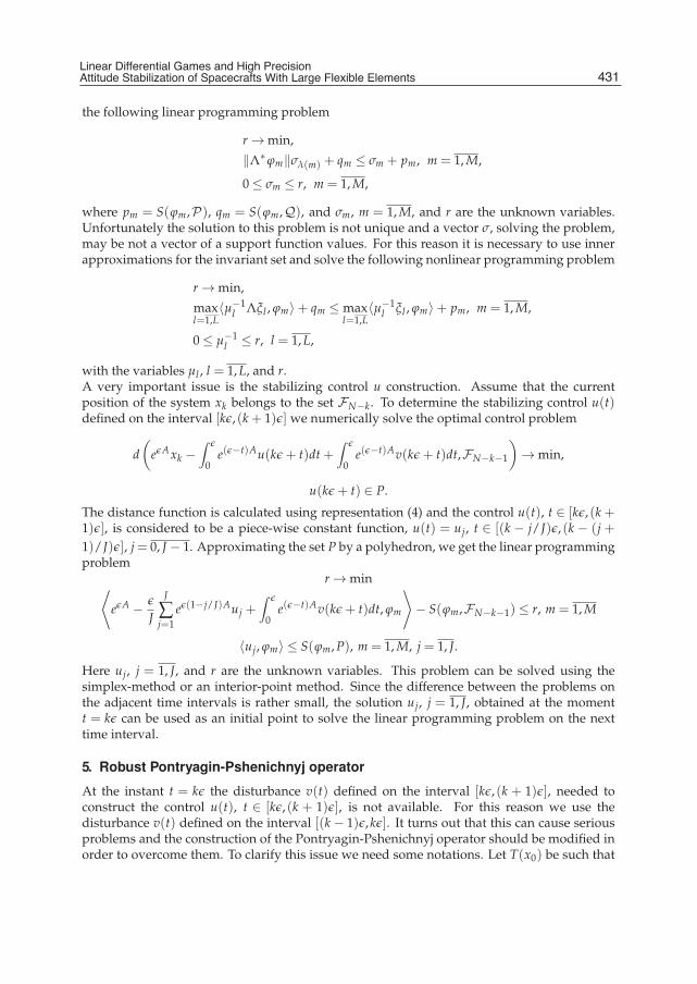
The controls u(t,v(t− ε), x0) and u(t,v(t), x0), t ∈ [kε, (k + 1)ε], are constructed to minimizethe distances d(X−ε(x0),FT(x0)−ε) and d(Xε(x0),FT(x0)−ε), respectively. It turns out that,in general, in the first case the trajectory rapidly zigzags in the vicinity of the equilibriumposition and in the second case its behaviour is more regular.Consider the following example. The control system

x = −βx− αx− u + v, |u| ≤ umax, |v| ≤ vmax (15)

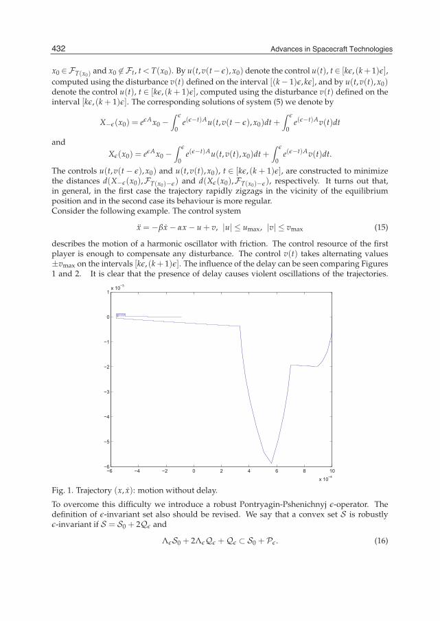
describes the motion of a harmonic oscillator with friction. The control resource of the firstplayer is enough to compensate any disturbance. The control v(t) takes alternating values±vmax on the intervals [kε, (k+ 1)ε]. The influence of the delay can be seen comparing Figures1 and 2. It is clear that the presence of delay causes violent oscillations of the trajectories.

−6 −4 −2 0 2 4 6 8 10

x 10−4

−6

−5

−4

−3

−2

−1

0

1x 10−3

Fig. 1. Trajectory (x, x): motion without delay.

To overcome this difficulty we introduce a robust Pontryagin-Pshenichnyj ε-operator. Thedefinition of ε-invariant set also should be revised. We say that a convex set S is robustlyε-invariant if S = S0 + 2Qε and

ΛεS0 + 2ΛεQε +Qε ⊂ S0 + Pε. (16)



−5 0 5 10

x 10−4

−7

−6

−5

−4

−3

−2

−1

0

1

2

3x 10−3

Fig. 2. Trajectory (x, x): motion with delay.

This definition implies the inclusion

ΛεS +Qε ⊂ (S ∗− 2Qε) + Pε. (17)

The robust Pontryagin-Pshenichnyj ε-operator is defined by G0 = S ,

Gk = Gkε (S), k = 0, N, (18)

where

Gε(C) = Λ−1ε

(((C ∗− 2Qε

)+ Pε

) ∗− Qε

).

If x0 ∈ Gk+1 and we choose the control u(t,v(t− ε), x0) to guarantee the inclusions X−(ε, x0) ∈Gk

∗− 2Qε, then we have

Xε(x0) = eεAx0 −∫ ε

0e(ε−t)Au(t,v(t− ε), x0)dt +

∫ ε

0e(ε−t)Av(t− ε)dt

−∫ ε

0e(ε−t)Av(t− ε)dt +

∫ ε

0e(ε−t)Av(t)dt ∈

(Gk

∗− 2Qε

)+ 2Qε ⊂ Gk. (19)

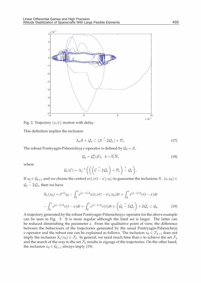
A trajectory generated by the robust Pontryagin-Pshenichnyj ε-operator for the above examplecan be seen in Fig. 3. It is more regular although the limit set is larger. The latter canbe reduced diminishing the parameter ε. From the qualitative point of view, the differencebetween the behaviours of the trajectories generated by the usual Pontryagin-Pshenichnyjε-operator and the robust one can be explained as follows. The inclusion x0 ∈ Fk+1 does notimply the inclusion Xε(x0) ∈ Fk. In general, we need much time than ε to achieve the set Fkand the search of the way to the set Fk results in zigzags of the trajectories. On the other hand,the inclusion x0 ∈ Gk+1 always imply (19).



−1 −0.8 −0.6 −0.4 −0.2 0 0.2 0.4 0.6 0.8 1

x 10−3

−0.01

−0.008

−0.006

−0.004

−0.002

0

0.002

0.004

0.006

0.008

0.01

Fig. 3. Trajectory (x, x): motion generated by the robust Pontryagin-Pshenichnyj ε-operator.

6. High precision attitude stabilization of spacecrafts with large flexible elements

Satellites with flexible appendages are modelled by hybrid systems of differential equations

x = f (x, g(y, y, y),u), (20)

y = G(x, x, x,y), (21)

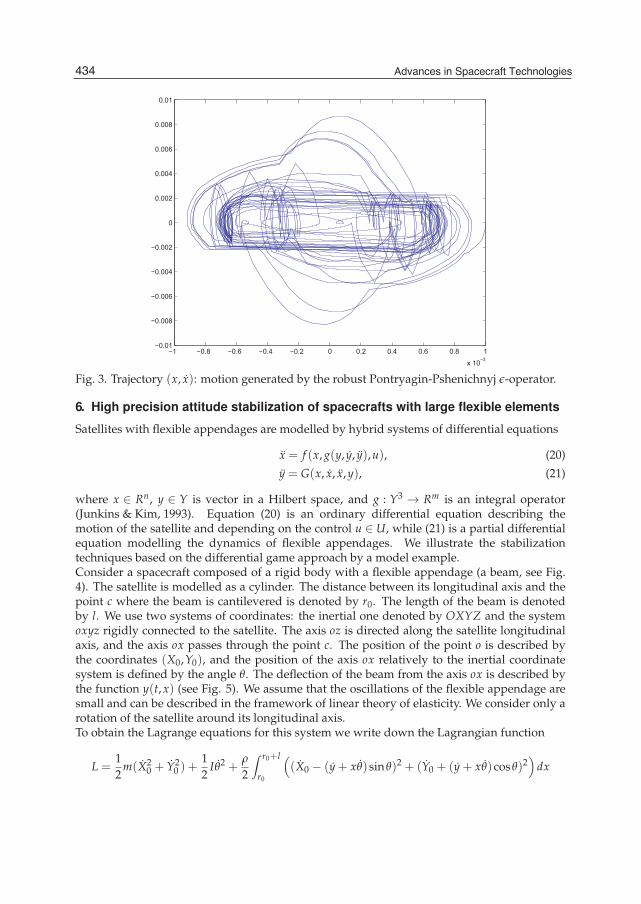
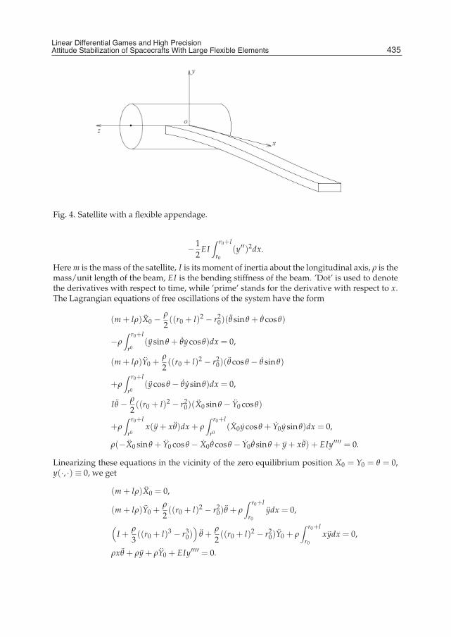
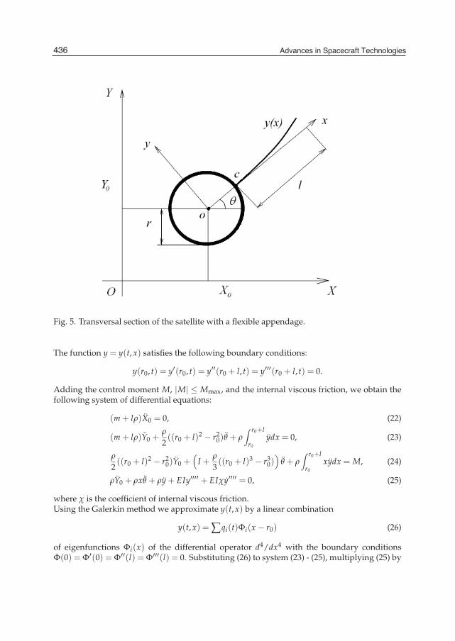
where x ∈ Rn, y ∈ Y is vector in a Hilbert space, and g : Y3 → Rm is an integral operator(Junkins & Kim, 1993). Equation (20) is an ordinary differential equation describing themotion of the satellite and depending on the control u ∈ U, while (21) is a partial differentialequation modelling the dynamics of flexible appendages. We illustrate the stabilizationtechniques based on the differential game approach by a model example.Consider a spacecraft composed of a rigid body with a flexible appendage (a beam, see Fig.4). The satellite is modelled as a cylinder. The distance between its longitudinal axis and thepoint c where the beam is cantilevered is denoted by r0. The length of the beam is denotedby l. We use two systems of coordinates: the inertial one denoted by OXYZ and the systemoxyz rigidly connected to the satellite. The axis oz is directed along the satellite longitudinalaxis, and the axis ox passes through the point c. The position of the point o is described bythe coordinates (X0,Y0), and the position of the axis ox relatively to the inertial coordinatesystem is defined by the angle θ. The deflection of the beam from the axis ox is described bythe function y(t, x) (see Fig. 5). We assume that the oscillations of the flexible appendage aresmall and can be described in the framework of linear theory of elasticity. We consider only arotation of the satellite around its longitudinal axis.To obtain the Lagrange equations for this system we write down the Lagrangian function

L =12

m(X20 + Y2

0 ) +12

Iθ2 +ρ

2

∫ r0+l

r0

((X0 − (y + xθ)sinθ)2 + (Y0 + (y + xθ)cosθ)2

)dx



Fig. 4. Satellite with a flexible appendage.

−12

EI∫ r0+l

r0

(y′′)2dx.

Here m is the mass of the satellite, I is its moment of inertia about the longitudinal axis, ρ is themass/unit length of the beam, EI is the bending stiffness of the beam. ’Dot’ is used to denotethe derivatives with respect to time, while ’prime’ stands for the derivative with respect to x.The Lagrangian equations of free oscillations of the system have the form

(m + lρ)X0 − ρ

2((r0 + l)2 − r2

0)(θ sinθ + θ cosθ)

−ρ∫ r0+l

r0(ysinθ + θycosθ)dx = 0,

(m + lρ)Y0 +ρ

2((r0 + l)2 − r2

0)(θ cosθ − θ sinθ)

+ρ∫ r0+l

r0(ycosθ − θysinθ)dx = 0,

Iθ − ρ

2((r0 + l)2 − r2

0)(X0 sinθ − Y0 cosθ)

+ρ∫ r0+l

r0x(y + xθ)dx + ρ

∫ r0+l

r0(X0ycosθ + Y0ysinθ)dx = 0,

ρ(−X0 sinθ + Y0 cosθ − X0 θ cosθ − Y0 θ sinθ + y + xθ) + EIy′′′′ = 0.

Linearizing these equations in the vicinity of the zero equilibrium position X0 = Y0 = θ = 0,y(·, ·) ≡ 0, we get

(m + lρ)X0 = 0,

(m + lρ)Y0 +ρ

2((r0 + l)2 − r2

0)θ + ρ∫ r0+l

r0

ydx = 0,

(I +

ρ

3((r0 + l)3 − r3

0))

θ +ρ

2((r0 + l)2 − r2

0)Y0 + ρ∫ r0+l

r0

xydx = 0,

ρxθ + ρy + ρY0 + EIy′′′′ = 0.



Fig. 5. Transversal section of the satellite with a flexible appendage.

The function y = y(t, x) satisfies the following boundary conditions:

y(r0, t) = y′(r0, t) = y′′(r0 + l, t) = y′′′(r0 + l, t) = 0.

Adding the control moment M, |M| ≤ Mmax, and the internal viscous friction, we obtain thefollowing system of differential equations:

(m + lρ)X0 = 0, (22)

(m + lρ)Y0 +ρ

2((r0 + l)2 − r2

0)θ + ρ∫ r0+l

r0

ydx = 0, (23)

ρ

2((r0 + l)2 − r2

0)Y0 +(

I +ρ

3((r0 + l)3 − r3

0))

θ + ρ∫ r0+l

r0

xydx = M, (24)

ρY0 + ρxθ + ρy + EIy′′′′ + EIχy′′′′ = 0, (25)

where χ is the coefficient of internal viscous friction.Using the Galerkin method we approximate y(t, x) by a linear combination

y(t, x) = ∑qi(t)Φi(x− r0) (26)

of eigenfunctions Φi(x) of the differential operator d4/dx4 with the boundary conditionsΦ(0) = Φ′(0) = Φ′′(l) = Φ′′′(l) = 0. Substituting (26) to system (23) - (25), multiplying (25) by



0 50 100 150 200 250−4

−2

0

2

4x 10−4

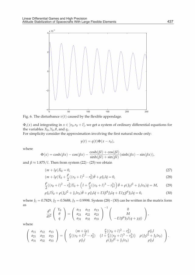
Fig. 6. The disturbance v(t) caused by the flexible appendage.

Φi(x) and integrating in x ∈ [r0,r0 + l], we get a system of ordinary differential equations forthe variables X0,Y0,θ, and qi.For simplicity consider the approximation involving the first natural mode only:

y(t) = q(t)Φ(x− r0),

where

Φ(x) = cosh(βx)− cos(βx)− cosh(βl) + cos(βl)sinh(βl) + sin(βl)

(sinh(βx)− sin(βx)),

and β ≈ 1.875/l. Then from system (22) - (25) we obtain

(m + lρ)X0 = 0, (27)

(m + lρ)Y0 +ρ

2((r0 + l)2 − r2

0)θ + ρJ1lq = 0, (28)

ρ

2((r0 + l)2 − r2

0)Y0 +(

I +ρ

3((r0 + l)3 − r3

0))

θ + ρ(J2l2 + J1lr0)q = M, (29)

ρJ1lY0 + ρ(J2l2 + J1lr0)θ + ρJ3lq + EIβ4 J3lq + EIχβ4 J3lq = 0, (30)

where J1 = 0.7829, J2 = 0.5688, J3 = 0.9998. System (28) - (30) can be written in the matrix formas

d2

dt2

⎛⎝ Y0

θq

⎞⎠ =

⎛⎝ a11 a12 a13

a21 a22 a23a31 a32 a33

⎞⎠−1 ⎛

⎝ 0M

−EIβ4 J3l(q + χq)

⎞⎠ ,

where⎛⎝ a11 a12 a13

a21 a22 a23a31 a32 a33

⎞⎠ =

⎛⎝ (m + lρ) ρ

2 ((r0 + l)2 − r20) ρJ1l

ρ2 ((r0 + l)2 − r2

0)(

I + ρ3 ((r0 + l)3 − r3

0))

ρ(J2l2 + J1lr0)ρJ1l ρ(J2l2 + J1lr0) ρJ3l

⎞⎠ .



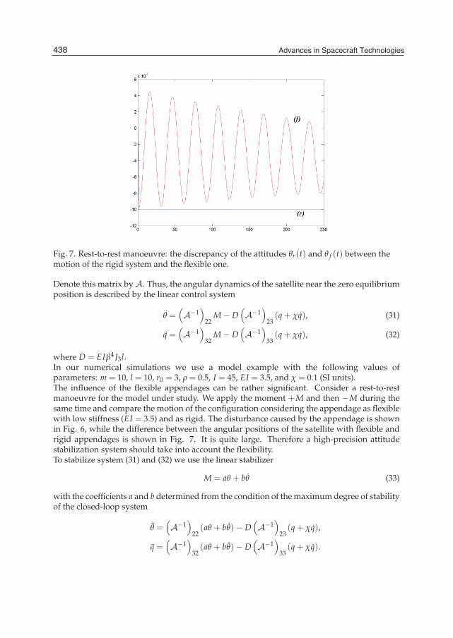
Fig. 7. Rest-to-rest manoeuvre: the discrepancy of the attitudes θr(t) and θ f (t) between themotion of the rigid system and the flexible one.

Denote this matrix byA. Thus, the angular dynamics of the satellite near the zero equilibriumposition is described by the linear control system

θ =(A−1

)22

M− D(A−1

)23(q + χq), (31)

q =(A−1

)32

M− D(A−1

)33(q + χq), (32)

where D = EIβ4 J3l.In our numerical simulations we use a model example with the following values ofparameters: m = 10, l = 10, r0 = 3, ρ = 0.5, I = 45, EI = 3.5, and χ = 0.1 (SI units).The influence of the flexible appendages can be rather significant. Consider a rest-to-restmanoeuvre for the model under study. We apply the moment +M and then −M during thesame time and compare the motion of the configuration considering the appendage as flexiblewith low stiffness (EI = 3.5) and as rigid. The disturbance caused by the appendage is shownin Fig. 6, while the difference between the angular positions of the satellite with flexible andrigid appendages is shown in Fig. 7. It is quite large. Therefore a high-precision attitudestabilization system should take into account the flexibility.To stabilize system (31) and (32) we use the linear stabilizer

M = aθ + bθ (33)

with the coefficients a and b determined from the condition of the maximum degree of stabilityof the closed-loop system

θ =(A−1

)22(aθ + bθ)− D

(A−1

)23(q + χq),

q =(A−1

)32(aθ + bθ)− D

(A−1

)33(q + χq).



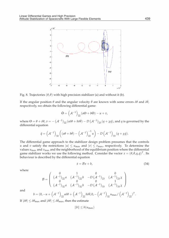
Fig. 8. Trajectories (θ, θ) with high precision stabilizer (a) and without it (b).

If the angular position θ and the angular velocity θ are known with some errors δθ and δθ,respectively, we obtain the following differential game:

Θ =(A−1

)22(aΘ + bΘ)− u + v,

where Θ = θ + δθ, v = −(A−1)22 (aδθ + bδθ)− D

(A−1)23 (q + χq), and q is governed by the

differential equation

q =(A−1

)32

((aθ + bθ)−

(A−1

)−1

22u)− D

(A−1

)33(q + χq).

The differential game approach to the stabilizer design problem presumes that the controlsu and v satisfy the restrictions |u| ≤ umax and |v| ≤ vmax, respectively. To determine thevalues umax and vmax and the neighborhood of the equilibrium position where the differentialgame stabilizer works we use the following method. Consider the vector x = (θ, θ,q, q)T . Itsbehaviour is described by the differential equation

x = Bx + b, (34)

where

B =

⎛⎜⎜⎝

0 1 0 0(A−1)22 a

(A−1)22 b −D

(A−1)23

(A−1)23 χ

0 0 0 1(A−1)32 a

(A−1)32 b −D

(A−1)33

(A−1)33 χ

⎞⎟⎟⎠

andb = (0,−u +

(A−1

)22

aδθ +(A−1

)22

bδθ,0,−(A−1

)32

umax/(A−1

)22)T .

If |δθ| ≤ δθmax and |δθ| ≤ δθmax, then the estimate

‖b‖ ≤ b(umax)



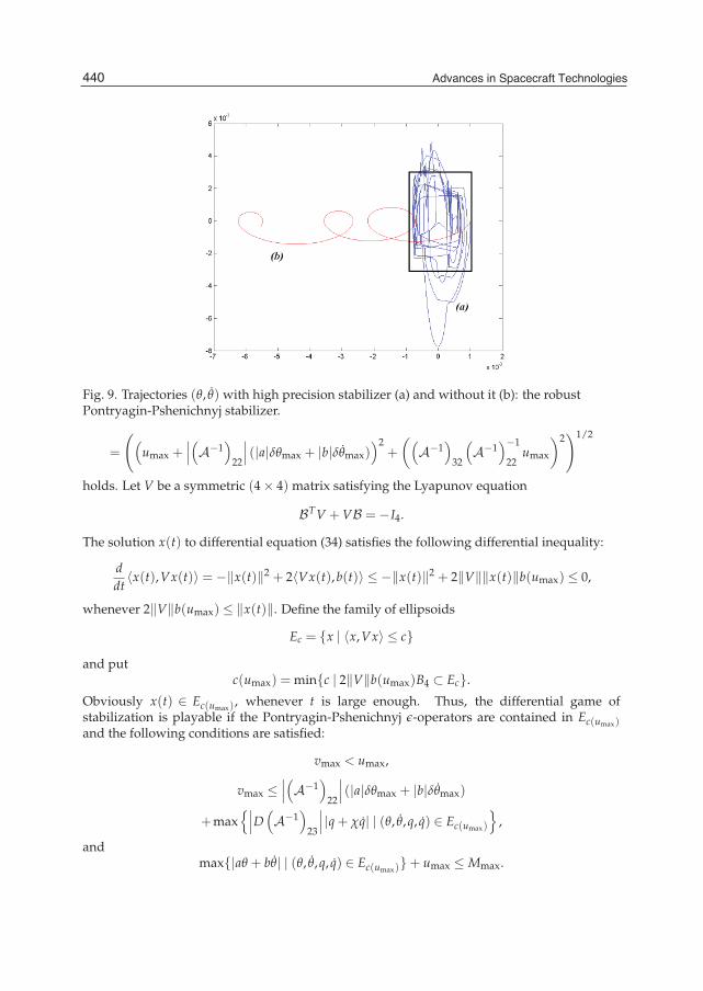
Fig. 9. Trajectories (θ, θ) with high precision stabilizer (a) and without it (b): the robustPontryagin-Pshenichnyj stabilizer.

=

((umax +

∣∣∣(A−1)

22

∣∣∣ (|a|δθmax + |b|δθmax))2

+

((A−1

)32

(A−1

)−1

22umax

)2)1/2

holds. Let V be a symmetric (4× 4) matrix satisfying the Lyapunov equation

BTV + VB = −I4.

The solution x(t) to differential equation (34) satisfies the following differential inequality:

ddt〈x(t),Vx(t)〉 = −‖x(t)‖2 + 2〈Vx(t),b(t)〉 ≤ −‖x(t)‖2 + 2‖V‖‖x(t)‖b(umax) ≤ 0,

whenever 2‖V‖b(umax) ≤ ‖x(t)‖. Define the family of ellipsoids

Ec = {x | 〈x,Vx〉 ≤ c}and put

c(umax) = min{c | 2‖V‖b(umax)B4 ⊂ Ec}.

Obviously x(t) ∈ Ec(umax), whenever t is large enough. Thus, the differential game ofstabilization is playable if the Pontryagin-Pshenichnyj ε-operators are contained in Ec(umax)and the following conditions are satisfied:

vmax < umax,

vmax ≤∣∣∣(A−1

)22

∣∣∣ (|a|δθmax + |b|δθmax)

+max{∣∣∣D(

A−1)

23

∣∣∣ |q + χq| | (θ, θ,q, q) ∈ Ec(umax)

},

andmax{|aθ + bθ| | (θ, θ,q, q) ∈ Ec(umax)}+ umax ≤ Mmax.



Typical trajectories generated by a linear feed-back and by a high-precision stabilizer withthe Pontryagin-Pshenichnyj ε-operator and the robust Pontryagin-Pshenichnyj ε-operator,respectively, are shown in Fig. 8 and 9. (The disturbance v in the numerical simulations isa periodic function.) The differential game method of stabilization yields significantly smallerlimit set (marked by box) than the simple linear stabilizer (33).

7. Conclusion

We present here a new approach to stabilization of mechanical systems with uncertaintiesin parameters and/or state data. This approach considers the perturbations caused by theseuncertainties as an evader control in a linear pursuit differential game. We describe the generaltheoretical basis and the numerical algorithms for implementation of the described differentialgame stabilizer. Estimates for the amplitude of the evader control should be obtained for anyspecific case of control system using its mechanical properties.We consider here an application of the suggested method to the stabilization problem fora satellite with large flexible appendages. The estimates for the evader control caused byuncertainties are deduced applying the method of Lyapunov functions. We construct ahigh-precision stabilizer using the differential game approach and the above estimates forthe evader control.The principal advantage of the suggested method is that, to achieve a high-precisionstabilization, it requires only the satellite attitude data and does not need any estimation forthe flexible elements’ state and/or unknown system parameters.

8. Acknowledgments

This research is supported by the Portuguese Foundation for Science and Technologies(FCT), the Portuguese Operational Programme for Competitiveness Factors (COMPETE), thePortuguese National Strategic Reference Framework (QREN), and the European RegionalDevelopment Fund (FEDER).

9. References

[Castaing & Valadier, 1977] Castaing, C. & Valadier, M. (1977). Convex Analysis and MeasurableMultifunctions, Lect. Notes in Math., n. 580, Springer-Verlag.

[Gutman, 1979] Gutman, S. (1979). Uncertain Dynamical Systems: A Lyapunov Min-MaxApproach, IEEE Transactions on Automatic Control, Vol. 24, No. 3, 437-443.

[Gutman & Leitmann, 1975a] Gutman, S. & Leitmann, G. (1975). On a Class of LinearDifferential Games, Journal of Optimization Theory and Applications, Vol. 17, No. 5-6,511522.

[Gutman & Leitmann, 1975b] Gutman, S. & Leitmann, G. (1975). Stabilizing Control forLinear Systems with Bounded Parameter and Input Uncertainty, Proceedings of the 7thIFIP Conference on Optimization Techniques, Nice, France, Springer-Verlag, Berlin.

[Isaacs, 1965] Isaacs, R. (1965). Differential Games, John Wiley and Sons, New York.[Junkins & Kim, 1993] Junkins, J. L. & Kim, Y. (1993). Introduction to dynamics and control of

flexible structures, American Institute of Aeronautics and Astronautics, Washington DC.[Krasovski & Subbotin, 1987] Krasovski, N.N.& Subbotin, A.I. (1987). Game-Theoretical

Control Problems, Springer-Verlag, New York.[Kurzhanski & Melnikov, 2000] Kurzhanski, A. & Melnikov, N. (2000). On the Problem





of Control Synthesis: the Pontryagin Alternating Integral and the Hamilton-JacobiEquation, Sbornik: Mathematics, Vol. 191, 849-881.

[Kurzhanski & Varaiya, 2002] Kurzhanski, A. & Varaiya, P. (2002). On Reachability underUncertainty, SIAM J. Control optimization, Vol. 41, No. 1, 181-216.

[Mitchell et al., 2005] Mitchell, I. M.; & Bayen, A. & Tomlin, C. (2005). Time-DependentHamilton-Jacobi Formulation of Reachable Sets for Continuous Dynamic Games, IEEETransactions on Automatic Control, Vol. 50, No. 7, 947-957.

[Nagashio, 2010] Nagashio, T.; Kida, T.; Ohtani, T. & Hamada, Y. Design and Implementationof Robust Symmetric Attitude Controller for ETS-VIII Spacecraft, Control EngineeringPractice (in press).

[Polovinkin et al., 2001] Polovinkin, E.; Ivanov, G.; Balashov, M.; Konstantinov, R.; & Khorev,A. (2001). An Algorithm for the Numerical Solution of Linear Differential Games,Sbornik: Mathematics, Vol. 192, 1515-1542.

[Pontryagin, 1981] Pontryagin, L. (1981). Linear Differential Games of Pursuit, Mathematics ofthe USSR-Sbornik, Vol. 40, 285-303.

[Pshenichnyj, 1969] Pshenichnyj, B. (1969). The structure of differential games, Sov. Math.Dokl. Vol. 10, 70-72.

[Smirnov, 2002] Smirnov, G. (2002) Introduction to the Theory of Differential Inclusions, GraduateStudies in Mathematics, vol. 41, American Mathematical Society, Providence.

[Yamada & Yoshikawa, 1996] Yamada, K. & Yoshikawa, S. (1996). Adaptive Attitude Controlfor an Artificial Satellite with Mobile Bodies, Journal of Guidance, Control and Dynamics,Vol. 19, No. 4, 948-953.


https://www.researchgate.net/publication/222422831_Design_and_implementation_of_robust_symmetric_attitude_controller_for_ETS-VIII_spacecraft?el=1_x_8&enrichId=rgreq-da1d106a1c5dec820285f3e13790e45e-XXX&enrichSource=Y292ZXJQYWdlOzIyMTkxMDgyMjtBUzo5OTI5NzcyMjg5NjM5OEAxNDAwNjg1ODMwODg0



https://www.researchgate.net/publication/268537926_The_structure_of_differential_games?el=1_x_8&enrichId=rgreq-da1d106a1c5dec820285f3e13790e45e-XXX&enrichSource=Y292ZXJQYWdlOzIyMTkxMDgyMjtBUzo5OTI5NzcyMjg5NjM5OEAxNDAwNjg1ODMwODg0

https://www.researchgate.net/publication/268537926_The_structure_of_differential_games?el=1_x_8&enrichId=rgreq-da1d106a1c5dec820285f3e13790e45e-XXX&enrichSource=Y292ZXJQYWdlOzIyMTkxMDgyMjtBUzo5OTI5NzcyMjg5NjM5OEAxNDAwNjg1ODMwODg0





Linear Differential Games and High Precision Attitude Stabilization of Spacecrafts With Large...

Documents

Transcript of Linear Differential Games and High Precision Attitude Stabilization of Spacecrafts With Large...