Linac Coherent Light Source (LCLS) Design Study Report
400
• SLAC-R-521 UC-414 Linac Coherent Light Source (LCLS) Design Study Report The LCSL Design Study Group SEP 2 3 OSTI April 1998 Prepared for the Department of Energy under contract number DE-AC03-76SF00515 by Stanford Linear Accelerator Center, Stanford University, Stanford, California. Printed in the United States of America. Available from National Technical Information Services, US Department of Commerce, 5285 Port Royal Road, Springfield, Virginia, 22161. MASTER pr DWTTO9UTION OF THIS DOCUM©iT « UMUMRS©
-
Upload
khangminh22 -
Category
Documents
-
view
5 -
download
0
Transcript of Linac Coherent Light Source (LCLS) Design Study Report
•
SLAC-R-521
UC-414
Linac Coherent Light Source(LCLS)
Design Study Report
The LCSL Design Study Group SEP 2 3
OSTI
April 1998
Prepared for the Department of Energy under contract number DE-AC03-76SF00515 by StanfordLinear Accelerator Center, Stanford University, Stanford, California. Printed in the United States ofAmerica. Available from National Technical Information Services, US Department of Commerce,5285 Port Royal Road, Springfield, Virginia, 22161.
MASTER prDWTTO9UTION OF THIS DOCUM©iT « UMUMRS©

This document, and the material and data contained therein, was developed undersponsorship of the United States Government. Neither the United States nor theDepartment of Energy, nor the Leiand Stanford Junior University, nor their employees, northeir respective contractors, subcontractors, or their employees, makes any warranty,express or implied, or assumes any liability of responsibility for accuracy, completeness orusefulness of any information, apparatus, product or process disclosed, or represents thatits use will not infringe privately owned rights. Mention of any product, its manufacturer,or suppliers shall not, nor is intended to imply approval, disapproval, or fitness for anyparticular use. A royalty-free, nonexclusive right to use and disseminate same for anypurpose whatsoever, is expressly reserved to the United States and the University

DISCLAIMER
Portions of this document may beillegible in electronic image products.
Images are produced from the bestavailable original document.

L C L S D E S I G N S T U D Y R E P O R T
The LCLS Design Study GroupStanford Linear Accelerator Center, Stanford, California, USA
J. Arthur, K. Bane, V. Bbaradwaj, G. Bowden, R. Boyce, R. Can, J. Clendenin,W. Corbett, M. Cornacchia (Design Study Group Leader), T. Cremer, P. Emma,A. Fasso, C. Field, A. Fisher, R. Gould, R. Hettel, J. Humphrey, K. Ko,T. Kotseroglou, Z. Li, D. Martin, B. McSwain, R. Miller, C. Ng, H.-D. Nuhn,D. Palmer, M. Pietryka, S. Rokni, R. Ruland, J. Schmerge, J. Sheppard, R. Tatchyn,V. Vylet, D. Walz, R. Warnock, H. Winick, M. Woodley, A. Yeremian, R. Yotam,F. Zimmerman
University of California, Los Angeles, California, USA
C. Pellegrini, J. Rosenzweig
Lawrence Livermore National Laboratory, Livermore, California, USA
L. Bertolini, K. van Bibber, L. Griffith, M. Libkind, R. Moore, E.T. Scharlemann
Los Alamos National Laboratory, Los Alamos, New Mexico, USA
S. Schriber, R. Sheffield
Lawrence Berkeley National Laboratory, Berkeley, California, USA
W. Fawley, K. Halbach, D. Humphries, K.-J. Kim, S. Lidia, R. Schlueter, M. Xie
European Synchrotron Radiation Facility, Grenoble, France
A. Freund
University of Rochester, Rochester, New York, USA
D. Meyerhofer
INFN, University of Milan, Milan, Italy
L. Serafini
Deutsches Elektronen-Synchrotron, Hamburg, Germany
T. limberg
L I S T O F C O N T R I B U T O R S •

This page(s) is (are) intentionally left blank.
L C L S D E S I G N S T U D Y R E P O R T
Acknowledgements
The concept and the feasibility of an x-ray FEL is based on the theoretical and experimental
work of many people. We are indebted to those scientists and engineers who prepared the ground
for this Design Study. A special thanks is due to the LCLS Study Group, led by Herman Winick,
that conducted the first exploratory and design studies of an x-ray FEL based on the SLAC linac
following the 1992 SLAC Workshop on Fourth-Generation Sources, where the concept was
introduced by Claudio Pellegrini.
The Design Study has benefited greatly from comments and suggestions made during
reviews. We are grateful to the members of the LCLS Design Review Committee whose
members were: Joe Bisognano (Chairman), Han Ben-Zvi, Alex Chao, Bill Colson, Gary Deis,
Efim Gluskin, Hank Hsieh, Gerd Materlik, Joachim Pflueger, Marc Ross, and Ross Schlueter.
Previous reviews included an early LCLS review chaired by Dan Ben-Zvi and an undulator
review chaired by Efim Gluskin. Their comments and suggestions proved to be very useful, and
some of them are incorporated in the Design.
We thank Terry Anderson (cover design), Frank Cebulski (technical editing), Ruth McDunn
(production), Berah McSwain (project administration), and Thelma Walker (administration) for
their valuable contribution to this report.
A C K N O W L E D G E M E N T S *

This page(s) is (are) intentionally left blank.

Preface
The Stanford Linear Accelerator Center (SLAC), in collaboration with Los Alamos
National Laboratory, Lawrence Livermore National Laboratory, and the University of
California at Los Angeles, is proposing to build a Free-Electron-Laser (FEL) R&D facility
operating in the self-amplified spontaneous emission (SASE) mode in the wavelength range
1.5-15 A. This FEL, called "Linac Coherent Light Source" (LCLS), utilizes the SLAC linac
and produces sub-picosecond pulses of short wavelength x-rays with very high peak
brightness and full transverse coherence.
Until about the 1960s x-rays were obtained from Roentgen tubes. After the first
observation of synchrotron radiation [1] and the evolution of cyclic electron synchrotrons and
then storage rings for high energy physics applications, it was realized that these accelerators
could be exploited as much more intense x-ray sources. Storage ring synchrotron light
sources have now evolved through three generations. The first-generation sources utilized
radiation from storage rings built for high-energy physics purposes. These included Tantalus
at the University of Wisconsin, ACO and DCI at LURE, SPEAR and PEP at SLAC, DORIS
and PETRA at DESY, Adone at Frascati, VEPP-2M and VEPP-3 in Novosibirsk, and CESR
at Cornell. Initially only bending magnet radiation was used and experiments were carried
out parasitically during high-energy physics runs. The second-generation machines were
purpose built, but still initially used bending magnet radiation. The first round of second-
generation sources included the SOR-ring in Tokyo, the SRS at Daresbury, Aladdin in
Wisconsin, the Photon Factory at KEK, and the NSLS at Brookhaven. Eventually, insertion
devices were added to these facilities, but only in limited number because, in most cases, the
magnet lattice did not include a large number of straight sections.
The rapid growth in demand for synchrotron radiation and the successful implementation
of wiggler and undulator insertion devices on first- and second-generation sources led to the
need for third-generation facilities. These are characterized by a lower electron beam
emittance (emittance is the product of the beam transverse size and divergence) and a larger
number of straight sections for insertion devices. Presently operating third-generation sources
include the ALS and APS in the USA; the SRRC in Taiwan; Super-ACO and the ESRF in
France; Elettra in Italy; PLS in Korea; MAX II in Sweden; and SPring-8 in Japan. The lower
electron beam emittance of these rings, typically of the order of a 5-10 nm-rad compared with
-100 nm-rad in earlier sources, results in higher radiation brightness, particularly from
undulators, and transversely coherent (i.e., diffraction-limited) radiation at wavelengths
longer than ~ 50 nm.
. L C L S D E S I G N S T U D Y R E P O R T
Three workshops have been held to discuss fourth-generation light sources, the first at
SLAC in 1992 [2], the second at the ESRF [3] in 1996, and a third at APS in 1997. The
LCLS was first proposed [4] at the SLAC workshop, leading to several years of continued
refinement of the design by a multi-institutional study group. At the ESRF workshop, a
consensus developed that short wavelength free electron lasers driven by linear accelerators
are the most promising path for the increasing number of applications where high brightness,
coherence, and short bunches are important. A similar view was expressed by the 1997
Synchrotron Radiation Light Source Working Group [5] (the Birgeneau/Shen Panel) of the
Basic Energy Sciences Advisory Committee of the Department of Energy. This report
recognizes that "fourth-generation x-ray sources...will in all likelihood be based on the free
electron laser concepts. If successful, this technology could yield improvements in brightness
by many orders of magnitude."
In 1996 a team was formed to produce a detailed design for the LCLS. One of the goals
of this Design Study is to show that advances in the technology of electron sources and linear
accelerators, as well as improved understanding in the physics of transporting and
compressing high brightness beams, are such that an electron beam can be created of
sufficiently high quality to drive a single pass free-electron laser operating at wavelengths
down to ~ 1.5 A in the SASE mode. In this mode, the FEL radiation is created by inducing a
longitudinal bunch density modulation at the optical wavelength in a single pass of the
electron beam through a long undulator, without the need for high reflectivity mirrors to form
an optical cavity, as is used in longer wavelength FEL oscillators. The lack of mirrors
adequate to form an optical cavity now limits FEL oscillators to wavelengths longer than
-2000 A.
A free-electron laser has all the characteristics of a fourth-generation source: brightness
several orders of magnitude greater than presently achieved in third-generation sources, full
transverse coherence, and sub-picosecond long pulses. The technologies needed to achieve
this performance are those of bright electron sources, of acceleration systems capable of
preserving the brightness of the source, and of undulators capable of meeting the magnetic
and mechanical tolerances that are required for operation in the SASE mode.
Starting in FY1998, the first two-thirds of the SLAC linac will be used for injection into
the B factory. This leaves the last third free for acceleration to 15 GeV. The LCLS takes
advantage of this opportunity, opening the way for the next generation of synchrotron light
sources with largely proven technology and cost effective methods.
The LCLS uses an rf photoinjector as the source of electrons. In this device, developed at
LANL, the cathode is placed in the accelerating field of a radio-frequency cavity. A laser,
shining on the cathode, expels electrons that are rapidly accelerated in the rf field, minimizing
emittance growth due to space charge effects. Photoinjectors have been recognized as the
most effective method of achieving very bright and short electron pulses, and their
v i • P R E F A C E
L C L S D E S I G N S T U D Y R E P O R T
technology has made great progress in recent years. The LCLS makes full use of these
advances.
To achieve design performance it is essential that acceleration occur with minimal
longitudinal and transverse emittance dilution. Here, the LCLS will exploit the research and
progress in the technology and accelerator physics of linear colliders that have produced the
tools and knowledge that now find a remarkable application in the realization of fourth-
generation light sources. SLAC, a leading laboratory in this research, and the first laboratory
to have constructed and operated a linear collider, the SLC (SLAC Linear Collider), is in an
ideal position to apply this linear collider technology to a free electron laser.
As a consequence of the enormous growth of synchrotron light sources over the last
20 years, insertion devices have reached a very high level of performance. The LCLS
undulator is a state-of-the art device that is capable of meeting the specifications demanded
by the design.
The LCLS would create a photon beam of unprecedented brightness, coherence, and
beam power, far surpassing anything available in third-generation sources today. Design
goals are a brightness of 1.2 x 1033 photons/(s mm2 mrad2 0.1% bandwidth), a peak power of
9 GW, and sub-picosecond pulse duration. The remarkable features of this facility promise
unparalleled potential for the development of completely new capabilities, such as non-linear
dynamics, as well as for extending existing fields of study into new dimensions.
Organization of this Design Study Report
In this report, the Design Team has established performance parameters for all the major
components of the LCLS and developed a layout of the entire system. Chapter 1 is the
Executive Summary. Chapter 2 (Overview) provides a brief description of each of the major
sections of the LCLS, from the rf photocathode gun, through the experimental stations and
electron beam dump. Chapter 3 describes the scientific case for the LCLS. Chapter 4
provides a review of the principles of the FEL physics that the LCLS is based on, and
Chapter 5 discusses the choice of the system's physical parameters. Chapters 6 through 10
describe in detail each major element of the system. Chapters 11 through 13 respectively
cover undulator controls, mechanical alignment, and radiation issues.
Several technical challenges that are crucial to achieving the LCLS's performance goals
have received serious attention during the study. Among the most important of these are:
(1) the generation and preservation of very low emittance and low momentum spread during
acceleration; (2) the understanding of the SASE mechanism and the conditions required for it;
(3) the conceptual development and design of a very long undulator; and (4) the control and
utilization of radiation at extremely high power densities. These issues are addressed in
Chapter 6 through 10.
P R E F A C E
L C L S D E S I G N S T U D Y R E P O R T
A research and development program that will provide further support and confirmation
of the design has been formulated, and plans are being made to implement this program in the
next 2 years. Construction could begin in FY2001. Concurrent with the Design Study, further
work is being carried out to document the eventual applications of the LCLS.
Reference
1 J.P. Brewett, Phys. Rev, 69 (1946) 87.
2 Proceedings of the Workshop on Fourth-generation Sources, February 24-27, 1992. M.Comacchia.
3 Proceedings of the 10th ICFA Beam Dynamics Panel Workshop on Fourth-generation LightSources, Grenoble, January 22-25,1996.
4 C. Pellegrini, Proceedings of the Workshop on Fourth-generation Sources, pp. 376-384,February 24-27,1992. M. Comacchia and H, Winick, eds., SSRL 92/02.
5 Report of the Basic Energy Sciences Advisory Committee, Synchrotron Radiation Light SourceWorking Group, October 8-9, 1997.
P R E F A C E

Table of Contents
1 Executive Summary1.1 Introduction 1-1
1.2 The Scientific Case 1-3
1.3 FEL Physics and Simulations • 1-3
1.4 The Injector 1-4
1.5 Acceleration and Compression 1-4
1.6 TheUndulator 1-5
1.7 Undulator-to-Experimental Area 1-6
1.8 Take-off Optics and Beamline Layout 1-7
1.9 Instrumentation andControls. 1-7
1.10 Alignment 1-8
1.11 Radiation Protection 1-8
1.12 Basic Parameters 1-9
1.13 Estimated Costs, Proposed Schedule, and Project Execution 1-10
2 Overview2.1 Introduction 2-1
2.2 Principle of Operation 2-1
2.3 Overall Layout 2-2
2.4 Performance Characteristics 2-3
2.5 The Photoinjector 2-5
2.6 Compression and Acceleration 2-6
2.7 TheUndulator 2-6
2.8 The X-ray Optics and Experimental Areas 2-6
2.9 Applications of the LCLS 2-7
2.10 Summary 2-8
2.11 References 2-8
L C L S D E S I G N S T U D Y R E P O R T
The Scientific CaseTechnical Synopsis 3-1
3.1 History of Scientific Interest in X-ray Free Electron Lasers 3-1
3.2 Unique Features of X-ray FEL Radiation 3-3
3.2.1 Fundamental Quantum Mechanics 3-5
3.2.2 Atomic, Molecular, and Plasma Physics 3-6
3.2.3 Chemical Physics 3-7
3.2.4 Condensed Matter Physics and Materials Science 3-7
3.2.5 Biology 3-8
3.3 The Role of the LCLS 3-9
3.4 References 3-9
FEL PhysicsTechnical Synopsis 4-1
4.1 Introduction 4-1
4.1.1 Spontaneous Radiation from the LCLS Undulator 4-3
4.2 FEL Radiation 4-7
4.3 References 4-11
FEL Parameters and PerformanceTechnical Synopsis 5-1
5.1 Introduction 5-1
5.2 Parameter Optimization 5-2
5.3 Electron Beam Focusing 5-4
5.3.1 Lattice Design Criteria 5-5
5.3.2 Focusing Method (Lattice) 5-5
5.3.3 Optimum Beam Size 5-6
5.3.4 Tolerable Beta-Function Modulation Amplitude.. 5-7
5.4 Undulator Sections 5-9
5.5 Parameter Sensitivities 5-9
5.6 Temporal Structure of Laser Power 5-11
5.7 Effect of Deviations from the Ideal Electron Trajectory 5-12
5.7.1 Undulator Steering and Corrector Description 5-12
5.7.2 Magnetic Field Errors 5-12
5.7.3 Trajectory and Error Control Requirement from Simulations 5-12
5.7.4 Magnetic Field Error Tolerances 5-13
5.7.5 Steering Algorithm 5-13
5.7.6 Steering Error Tolerance 5-14
5.7.7 Optimum Steering Station Separation 5-14
5.7.8 Undulator Matching Tolerances 5-16
2 * T A B L E O F C O N T E N T S

L C L S D E S I G N S T U D Y R E P O R T
5.8 Emission of Spontaneous Radiation 5-16
5.8.1 Average Energy Loss 5-16
5.8.2 Energy Spread Increase 5-17
5.8.3 Emittance Increase ; 5-18
5.9 Output Power Control 5-18
5.9.1 Peak Current .' 5-18
5.9.2 Phase Shifter at Saturation 5-19
5.10 Initial Phase Space Distribution (Coupling to Linac Simulation Results) 5-19
5.10.1 Transverse Halo 5-20
5.11 Optical Klystron 5-20
5.12 Summary 5-21
5.13 References 5-21
PhofoinjectorTechnical Synopsis 6-1
6.1 Electron Source 6-2
6.1.1 RF Photocathode Gun 6-2
Gun Description 6-2
Field Balance 6-3
Symmetrization 6-4
Emittance Compensation 6-5
Summary of Experimental Results at ATF 6-5
Photocathode 6-7
RF System 6-7
Emittance Compensating Solenoid 6-8
Beamline 6-8
Vacuum System 6-8
6.1.2 Laser System 6-9
System Description 6-10
Temporal Pulse Shaping 6-13
Fourier Relay Optics 6-14
Spatial Pulse Shaping 6-14
Frequency Conversion 6-15
Grazing Incidence 6-15
Stability of Laser Pulse 6-16
Diagnostics 6-18
6.1.3 Choice of Laser System 6-21
6.2 Linac 0 6-24
6.2.1 Comments on Emittance Compensation 6-24
6.2.2 System Description 6-26
6.2.3 Emittance Compensation in Linac 0 6-27
6.3 References 6-30
T A B L E O F C O N T E N T S

L C L S D E S I G N S T U D Y R E P O R T
AcceleratorTechnical Synopsis 7-1
7.1 Introduction and Overview 7-1
7.2 Compression and Longitudinal Dynamics 7-3
7.2.1 Bunch Compression Overview 7-3
7.2.2 Parameters 7-5
7.2.3 Longitudinal Wakefields and Non-linearities 7-7
Geometric Wakefields 7-7
Resistive Wall Wakefields 7-8
7.2.4 Beam Jitter Sensitivities 7-11
7.2.5 Energy Management and Overhead 7-12
7.3 Transverse Linac Beam Dynamics 7-13
7.3.1 The LO Linac 7-14
7.3.2 TheLl Linac 7-14
7.3.3 The L2 Linac 7-16
7.3.4 The L3 Linac 7-19
7.4 Design of the Second Bunch Compressor 7-21
7.4.1 Overview and Parameters 7-21
7.4.2 Momentum Compaction 7-23
7.4.3 Incoherent Synchrotron Radiation (ISR) 7-24
7.4.4 Coherent Synchrotron Radiation (CSR) 7-24
Unshielded Radiation 7-24
Shielded Radiation . 7-26
Transverse Forces 7-28
Calculations with a Transient Model 7-29
7.4.5 Resistive Wall Longitudinal Wakefields in the Bends 7-31
7.4.6 Beam Size, Aperture and Field Quality 7-32
7.4.7 Tuning and Correction 7-32
7.5 Design of the First Bunch Compressor 7-33
7.5.1 Overview and Parameters 7-33
7.5.2 Beam Size, Aperture, and Field Quality 7-34
7.5.3 Tuning and Correction 7-35
7.6 Beam Transport Lines 7-36
7.6.1 Low-Energy Dog Leg 7-36
Parameters 7-37
Beam Size, Aperture, and Field Quality .'. 7-38
Tuning and Correction 7-38
7.6.2 High-Energy Dog Leg 7-39
Parameters ; 7-40
Beam Size, Aperture, and Field Quality 7-41
Tuning and Correction 7-41
Coherent Radiation 7-41
4 * T A B L E O F C O N T E N T S

L C L S D E S I G N S T U D Y R E P O R T
7.7 Instrumentation, Diagnostics, and Feedback 7-42
7.7.1 Transverse Emittance Diagnostics.... 7-42
EDO Emittance Station 7-44
EDI Emittance Station 7-44
L2-ED Emittance Station 7-44
BC2-ED Emittance Station 7-45
L3-ED Emittance Station 7-45
ED2 Emittance Station 7-45
7.7.2 Bunch Length Diagnostics 7-45
7.7.3 Beam Energy Spread Diagnostics 7-47
DL1 Energy Spread Diagnostics 7-47
BC1 Energy Spread Diagnostics 7-47
BC2 Energy Spread Diagnostics 7-48
DL2 Energy Spread Diagnostics 7-48
7.7.4 Orbit and Energy Monitors and Feedback Systems 7-48
Orbit Feedback Systems 7-48
Energy Feedback Systems 7-49
7.8 The Wake Functions for the SLAC Linac 7-49
7.8.1 Introduction 7-49
7.8.2 The Calculated Wakefields for the SLAC Linac 7-50
7.8.3 Discussion 7-51
7.8.4 Confirmations 7-54
7.8.5 Resistive Wall Wakefields 7-54
7.8.6 The Impedance Due to the Roughness of the Iris Surface 7-56
7.9 Summary of Dilution Effects 7-57
7.9.1 Transverse Emittance Dilution 7-57
7.9.1 Final Energy Spread 7-58
7.10 References 7-59
8 UndulatorTechnical Synopsis 8-1
8.1 Overview 8-2
8.1.1 Introduction 8-2
8.1.2 Undulator Design Summary 8-2
Introduction 8-2
Design Concept History 8-3
The Undulator 8-3
Strong Focusing 8-5
Undulator Tolerances 8-7
Undulator Construction 8-7
Mechanical, Thermal, and Geophysical Engineering 8-8
T A B L E O F C O N T E N T S

L C L S D E S I G N S T U D Y R E P O R T
8.2 Undulator Magnetic Design ....8-9
8.2.1 Design of Undulator Segments 8-9
Basic Considerations , 8-9
Correcting Local Field Errors 8-10
Initial Sorting Model and Results 8-11
Use of Shims to Correct Field Errors 8-15
8.2.2 End Design of Undulator Segments 8-15
8.3 Undulator Mechanical Design 8-17
8.3.1 Mechanical and Thermal Design 8-17
Introduction 8-17
Piers 8-18
Motors 8-20
Girder 8-21
Thermal Considerations 8-23
Vibration of the Girder , 8-24
Dimensional Stability 8-24
Magnet Support 8-25
Conclusions 8-30
8.3.2 Electron Beam Collimation and Vacuum Chamber Design 8-30
Beam Parameters Used in These Calculations 8-30
Permanent Magnet Material 8-30
Undulator Vacuum Chamber 8-32
Beam Strikes at the Entrance to the Vacuum Chamber 8-32
Beam Strikes Inside the Undulator 8-33
Adjustable Collimators to Protect Undulator and Vacuum Chamber 8-35
Fixed Aperture Protection Collimators 8-36
Vacuum Chamber Surface Roughness 8-37
8.4 Undulator Vacuum System 8-37
8.4.1 System Requirements and Description 8-37
8.4.2 Gas Load and Vacuum Pressure 8-39
8.4.3 Thermal Considerations 8-42
8.5 Alignment and Trajectory Control '. 8-42
8.5.1 Introduction 8-42
8.5.2 Undulator Beam Based Alignment 8-43
Introduction 8-44
Simulation Results 8-47
Sensitivities 8-56
Summary 8-57
8.5.3 The Singular Value Decomposition (SVD) Technique 8-57
Description 8-57
Simulation Results 8-59
Summary 8-61
6 * T A B L E O F C O N T E N T S

L C L S D E S I G N S T U D Y R E P O R T
8.6 Beam Diagnostics 8-61
8.6.1 RF Cavity BPMs 8-61
Review of BPM Technology 8-62
Evaluation of BPM Options for the LCLS 8-63
LCLS Stripline BPM 8-64
LCLS Microwave Cavity BPM 8-65
Parameters of the LCLS BPM Cavity 8-68
Microwave Cavity Beam Impedance 8-68
Microwave Cavity Signal Processing 8-70
8.6.2 Carbon Wire BPMs 8-71
Beam Position Measurement 8-71
Beam Emittance Measurements 8-74
8.6.3 The Combined Electron and Photon Beam Diagnostic 8-75
8.6.4 Wire Position Monitors 8-77
8.7 Wakefield Effects in the Undulator 8-77
8.7.1 Introduction 8-77
8.7.2 Wakefield Induced Beam Degradation 8-78
8.7.3 The Resistive Wall Wakefields 8-80
8.7.4 The Effect of Flange Gaps, Pumping Slots, and Bellows 8-81
8.7.5 The Effect of Wall Surface Roughness 8-82
8.7.6 The Effects of the Expected Bunch Shape 8-84
8.7.7 Conclusion 8-84
8.8 Ion Effects 8-85
8.8.1 Introduction 8-85
8.8.2 Ionization Processes 8-85
8.8.3 Emittance Dilution 8-87
8.8.4 Conclusion 8-89
8.9 References 8-89
Undulator-to-Experimental AreaTechnical Synopsis 9-1
9.1 Transport System 9-1
9.2 Shielding Enclosures 9-4
9.3 Beam Lines and Experimental Stations 9-5
9.3.1 Experimental Beam Lines 9-5
9.3.2 The Long Beam Line 9-6
9.3.3 Experimental Stations 9-8
9.4 Experimental Hall 9-9
9.5 References 9-9
T A B L E O F C O N T E N T S
L C L S D E S I G N S T U D Y R E P O R T
10 Take-off Optics and Beam Line LayoutsTechnical Synopsis 10-1
10.1 Coherent Radiation 10-2
10.2 Spontaneous Radiation Calculations 10-8
10.2.1 Spectral-angular Radiation Profiles 10-10
10.2.2 Far-field Spontaneous Radiation Peak Power Density 10-18
10.3 Bremsstrahlung Calculations 10-20
10.3.1 Bremsstrahlung from Halo 10-20
10.3.2 Gas Bremsstrahlung 10-24
10.3.3 Muons 10-25
10.3.4 Future Work: Other Radiation Sources 10-25
10.4 Optical System 10-26
10.4.1 Differential Pumping Section 10-28
10.4.2 X-ray Slits (Collimators) 10-30
10.4.3 Personnel Protection System Beam Stoppers 10-33
10.4.4 Absorption cell 10-34
10.4.5 Mirrors 10-39
10.4.6 Crystals 10-44
10.5 Beam Line Optical Instrumentation 10-46
10.6 References 10-47
11 Instrumentation and ControlsTechnical Synopsis 11-1
11.1 Control System 11-2
11.2 Undulator Control 11-4
11.2.1 Undulator Elements 11-4
11.2.2 Mover Mechanism 11-5
11.2.3 Stepping Motor Controllers and Position Potentiometers 11-5
11.2.4 The Wire Position Monitor System 11-6
11.2.5 The Beam Position Monitors 11-7
11.2.6 Control System Layout 11-7
11.3 Beam Line Electronics and Controls 11-10
11.3.1 X-ray Optics and Experimental Stations 11-10
11.3.2 Control System Objectives 11-10
11.3.3 Control System Layout 11-10
11.3.4 Motion Controls 11-11
11.3.5 Photon Beam Stabilization at the Sample 11-11
11.3.6 Timing System 11-13
11.4 Personnel Protection 11-16
11.5 Machine Protection :. 11-20
8 * T A B L E O F C O N T E N T S

L C L S D E S I G N S T U D Y R E P O R T
12 AlignmentTechnical Synopsis 12-1
12.1 Surveying Reference Frame 12-2
12.1.1 Network Design Philosophy 12-3
12.1.2 Network Lay-Out ! 12-5
Linac Network „ 12-5
Undulator Network 12-5
Transport Line/Experimental Area Network 12-6
12.1.3 Alignment Coordinate System 12-6
12.1.4 Network Survey 12-7
12.1.5 Data Analysis and Data-Flow 12-9
12.2 Lay out Description Reference Frame 12-9
12.2.1 Lattice Coordinate System 12-9
12.2.2 Tolerance Lists 12-10
12.2.3 Relationship between Coordinate Systems 12-10
12.3 Fiducializing Magnets 12-10
12.4 Absolute Positioning 12-10
12.4.1 Undulator Absolute Positioning 12-11
Undulator Anchor Hole Layout Survey 12-11
Pre-alignment of Girder Supports and Magnet Movers 12-11
Absolute Quadrupole Positioning 12-12
Quality Control Survey .....12-12
12.4.2 Transport Line and Experimental Area Absolute Positioning 12-12
12.5 Relative Alignment 12-12
12.5.1 Relative Undulator Alignment 12-12
Introduction 12-12
Relative Quadrupole Positioning 12-12
Undulator Alignment 12-13
12.5.2 Linac Smoothing 12-13
Purpose of Linac Smoothing 12-13
Linac Straightness Measurement Procedure 12-14
12.5.3 Relative Alignment of Transport Line and Experimental Area
Components 12-15
12.6 Undulator Monitoring System 12-15
12.7 References 12-15
T A B L E O F C O N T E N T S

L C L S D E S I G N S T U D Y R E P O R T
13 Radiation IssuesTechnical Synopsis 13-1
13.1 Radiation Concerns Downstream of the Undulator 13-1
13.2 Radiation Issues in the Undulator 13-1
13.2.1 Introduction 13-1
13.2.2 Beam Scattering on the Residual Gas 13-2
13.2.3 Spontaneous Radiation 13-2
13.2.4 Bremsstrahlung from Halo on Collimators 13-5
Normal Incidence 13-5
Grazing Angle Incidence 13-6
13.2.5 Induced Activity 13-8
13.3 References 13-9
A Parameter TablesTable Description
1 Beam Tracking A-l
2 Parameter Summary A-2
3 Gun Laser A-3
4 Injector - rf Photocathode Gun A-4
5 Injector - Accelerator A-5
6 Injector - Dogleg A-6
7 General Linac Parameters A-8
8 Linac-1 A-9
9 Bunch Compressor-1 A-l 1
10 Linac-2 A-13
11 Bunch Compressor-2..... A-15
12 Linac-3 A-17
13 Linac to Undulator Transport A-19
14 Undulator A-21
15 FEL A-25
16 Electron Beam Dump A-27
17 X-ray Optics A-28
1 0 • T A B L E O F C O N T E N T S

ExecutiveSummary
1.1 Introduction
The Stanford Linear Accelerator Center, in collaboration with Los Alamos National
Laboratory, Lawrence Livermore National Laboratory, and the University of California at
Los Angeles, is proposing to build a Free-Electron-Laser (FEL) R&D facility operating in the
wavelength range 1.5-15 A. This FEL, called the "Linac Coherent Light Source" (LCLS),
utilizes the SLAC linac and produces sub-picosecond pulses of short wavelength x-rays with
very high peak brightness and full transverse coherence.
Starting in FY 1998, the first two-thirds of the SLAC linac will be used for injection into
the B factory. This leaves the last one-third free for acceleration to 15 GeV. The LCLS takes
advantage of this opportunity, opening the way for the next generation of synchrotron light
sources with largely proven technology and cost effective methods. This proposal is
consistent with the recommendations of the Report of the Basic Energy Sciences Advisory
Committee (Synchrotron Radiation Light Source Working Group, October 18-19, 1997). The
report recognizes that "fourth-generation x-ray sources...will in all likelihood be based on the
free electron laser concepts. If successful, this technology could yield improvements in
brightness by many orders of magnitude." This Design Study, the authors believe, confirms
the feasibility of constructing an x-ray FEL based on the SLAC linac. Although this design is
based on a consistent and feasible set of parameters, some components require more research
and development to guarantee the performance. Given appropriate funding, this R&D phase
can be completed in 2 years.
This Executive Summary provides a brief description of the LCLS. A layout of the LCLS
is shown in Fig. 1.1-1. The facility is comprised of the following main elements:
a. A photoinjector and a short linac, where a bright electron beam is generated and
accelerated to 150 MeV.
b. The main linear accelerator, consisting of the last one-third of the SLAC 3 km linac,
where the electron bunch is compressed and accelerated to 14.3 GeV.
c. The transport system to the undulator.
d. The undulator, where the electrons emit FEL and spontaneous radiation .
e. The undulator-to-experimental area transport line.
f. The take-off optics and experimental stations.

L C L S D E S I G N S T U D Y R E P O R T
The LCLS(Lfnac Coherent Light Source)
RF Gun
LinacO-
Unad
Linac 2Existing Linac
Linac 3
PhotonBeam Lines
B Factory Rings1-96
6360A1
Figure 1.1-1. Layout of the Linac Coherent Light Source.
A photoinjector will be used to generate a bright electron beam. A bunch of electrons will
go through two magnetic compressors that will reduce its length from 10 ps to 280 fs during
acceleration to 14.3 GeV. After acceleration to 14.3 GeV, the beam goes through a transport
system to a 100 m long undulator, where the FEL radiation is generated and channeled to an
experimental area. The transport system and the undulator area use an existing tunnel that
presently houses the SLAC Final Focus Test Beam (FFTB).
The projected peak brightness of the produced FEL radiation is 10 orders of magnitude
above existing radiation sources. Accompanying this FEL radiation, and independent of the
lasing action, the peak spontaneous radiation brightness that will be produced has high
bandwidth, comes in sub-picosecond long pulses, and is four orders of magnitude above
existing sources. This leap in performance is possible because of major technical advances in
some of the experimental tools of high-energy physics and synchrotron radiation. These are
the development of photoinjectors, the acceleration and compression without degradation of
very high brightness electron beams in linear colliders, and the progress in undulator design
and its error control. In the LCLS all these technologies converge to produce a scientific tool
of extraordinary performance.
1 - 2 • E X E C U T I V E S U M M A R Y

L C L S D E S I G N S T U D Y R E P O R T
1.2 The Scientific Case
An FEL operating in the hard x-ray region, such as the LCLS, will produce radiation with
unique qualities. The peak brightness will exceed that produced by today's brightest
synchrotrons by more than 10 orders of magnitude, an advance similar to that of the
synchrotron over a 1960s laboratory x-ray tube. In addition, the FELs sub-picosecond pulse
length will be two orders of magnitude shorter than a synchrotron pulse, and the FEL pulse
will be highly coherent.
Given the revolutionary properties of the LCLS, accurate projection of its scientific
applications is difficult. Nevertheless, major advances can be anticipated in many fields of
research, exploiting the short pulse, high brightness and coherence of the FEL. These include
fundamental quantum mechanics phenomena using entangled multi-photon states, and atomic
physics studies that measure photon interactions with core atomic electrons well into the
nonlinear regime. In molecular and plasma physics, ionization and dissociation processes
under extremely high-intensity electromagnetic fields will be studied. In chemistry, the x-ray
FEL has great potential as a monitor of surface chemical reactions using x-ray fluorescence or
photoelectron spectroscopy. In condensed matter science, the brightness of the FEL will be
used to apply standard x-ray techniques to sub-micron samples, and to record the signals in
less than 1 picosecond. The coherence will allow interference techniques, such as photon
correlation spectroscopy, to become powerful tools for studying dynamics in condensed
matter. In addition, the FEL should allow the development of completely new ways to study
condensed matter, based on nonlinear x-ray interactions. In biology, the sub-picosecond time
scale of the FEL pulse will make it possible to observe dynamical interactions between large
molecules in some extremely interesting systems.
All of these advances will require much development of detectors, optics, and timing
techniques. The LCLS will provide a wonderful tool for carrying out this development, and
will be the door that opens into a new world of science.
1.3 FEL Physics and Simulations
Theoretical and computational studies led to a selection of the accelerator and FEL
parameters. An exhaustive study was carried out of the sensitivity of the FEL radiation to
changes in the values of accelerator parameters and beam characteristics and to unavoidable
imperfections of the magnetic elements, alignment, and electron beam monitoring.
The focusing of the electron beam in the undulator plays an important role in the
production of the FEL radiation. The LCLS undulator optics has been optimized in terms of
its focusing lattice and strength. The electron optics consists of FODO cells, with a cell length
of 4.32 m. Focusing is obtained by placing permanent magnet quadrupoles in the
interruptions of the undulator sections. Each interruption is 23.5 cm long, and also includes
focusing quadrupoles, beam position monitors, and vacuum ports. The correction of the
electron orbit is obtained by a small lateral displacement (up to 0.5 mm) of the quadrupoles.
E X E C U T I V E S U M M A R Y • 1 -3

L C L S D E S I G N S T U D Y R E P O R T
Simulations indicate that the FEL radiation saturates at a length of -90 m. The proposed
LCLS undulator has a magnetic length of 100 m, as it is a requirement that the FEL operate in
the saturation regime. This fact not only gives the maximum output power, but also reduces
the pulse-to-pulse fluctuations of the radiation.
1.4 The Injector
The injector for the LCLS is required to produce a single 150 MeV bunch of ~1 nC and
-100 A peak current at a repetition rate of 120 Hz with a normalized rms transverse emittance
of ~1 n mm-mrad. The required emittance is about a factor of two lower than has been
achieved to date. The design employs a solenoidal field near the cathode of a specially
designed rf laser-driven gun which allows the initial emittance growth due to space charge to
be almost completely compensated by the end of the injection linac (Linac 0). Spatial and
temporal shaping of the laser pulse striking the cathode can reduce the compensated
emittance even further. Following the injection linac, the geometric emittance simply damps
linearly with energy growth. PARMELA simulations show that this design will produce the
desired normalized emittance. In addition to low emittance, there are two additional
electron-beam requirements that are challenging—the timing and intensity stabilities must
have rms values of 0.5 ps and 1% respectively. The desired laser-pulse energy stability will
be achieved by stabilizing the pumping laser for the amplifiers and by operating the second
amplifier in saturation. Although additional R&D is planned to improve the projected
performance of the photoinjector, confidence in the present design is based on the
performance of existing systems. PARMELA accurately simulates the measured performance
of low emittance rf photoinjectors operating near the emittance level of the LCLS. Laser
systems have been employed in high-energy physics experiments with timing stability—with
respect to the accelerated electron beam—that is within a factor of two of the value required
here.
1.5 Acceleration and Compression
In order for the FEL to operate in the saturation regime with a 100 m long undulator, a
high electron peak current in a small transverse and longitudinal emittance is required. For
the LCLS operating at 1.5 A, the design values are a peak current of 3.4 kA with a transverse
normalized emittance of 1.5 n mm-mrad at 14.3 GeV. This value is 50% higher than is
provided by the photoinjector and includes a safety margin against emittance dilution effects.
Since the rf photocathode gun produces 1 nC in a length of 3 ps rms, corresponding to a peak
current of 100 A, the bunch has to be compressed by a factor of about 50 before it enters the
undulator. The compressors consist of a series of magnetic chicanes, arranged and located
such that the non-linearities in the compression and acceleration process (longitudinal
wakefields, rf curvature, and second order momentum compaction) are partially cancelled. An
optimum choice of parameters compensates the correlated energy spread after the final
compression and desensitizes the system to phase and charge variations. The energy of the
1 - 4 • E X E C U T I V E S U M M A R Y

. L C L S D E S I G N S T U D Y R E P O R T
first compressor is 280 MeV. The choice of energy for the first compressor is set by the need
to minimize space charge effects at the lower energy end, while the upper limit is set by the
desire to compress the bunch early in the linac to ease transverse wakefields. In the first
compressor, the bunch length shrinks from lmm to 390 /m (rms values). The energy of the
second compressor, 6 GeV, was chosen as an optimum between the conflicting requirements
of longitudinal emittance dilution due to synchrotron radiation effects and longitudinal
wakefields. The design of the second compressor is set by the need to reduce coherent
synchrotron radiation effects, which are most pronounced for short bunches. Since the energy
spread generated by the coherent synchrotron radiation is correlated along the bunch, its
effect on the transverse emittance is compensated by introducing a double chicane and optical
symmetry to cancel longitudinal-to-transverse coupling. The coherent synchrotron radiation
effect on the beam was calculated both in the steady state and transient regime. In the former,
the radiation force is supposed to vanish in between bends. In the transient regime the effect
of the transition between bends is included, and found to be important. With the double
chicane compensating scheme,. the emittance growth in the LCLS, due to coherent
synchrotron radiation, is only 3-5%.
Simulations have also been made which calculate emittance dilution effects in the linac
due to transverse wakefields and anomalous momentum dispersion, each of which arise with
component misalignments. These simulations include realistic correction techniques and
successfully demonstrate the level of transverse emittance preservation required.
1.6 The Undulator
After reviewing several possible magnet designs, a planar Halbach hybrid type was
adopted, with a period of 3 cm and a fixed 6 mm magnetic gap. The focusing of the electron
beam is obtained with a FODO separated function lattice, with quadrupole focusing
permanent magnets placed between segments of the undulator. Each segment contains 64
periods and is 1.92 m long. The poles are made of vanadium permendur, and the magnets that
drive them are made of NdFeB. The separation between segments is 23.5 cm long. This free
space will house the focusing quadrupoles, beam position monitors, and vacuum ports. The
quadrupoles are also used to correct the trajectory by moving them transversely. The electron
beam trajectory is required to be straight to within 5 /an over a field gain length (11.7 m) to
achieve adequate overlap of the electron and photon beams. It is shown that this specification,
presently beyond state-of-the-art mechanically, can be achieved with electron beam-based
techniques. A suspended wire and mechanical actuator feedback will be used to maintain
alignment at the micron level. A small amount of tapering is required to compensate for the
small energy loss due to the emission of radiation and to resistive wall effects.
Each undulator section is supported by a girder. A pier supports the ends of two girders,
with the quadrupole magnets and other components, such as Beam Position Monitors (BPMs)
and vacuum ports, located between the girders.
E X E C U T I V E S U M M A R Y • 1 -5
L C L S D E S I G N S T U D Y R E P O R T
The BPMs are the primary system for measuring the transverse electron beam position in
the undulator. The BPMs must have the ability to detect relative changes in position of 1 /an
at the operating charge of 1 nC. After a review of several BPM technologies, it was decided
that a microwave cavity type of detector can provide sub-micron resolution and micron level
absolute accuracy, and this is the non-intercepting monitor choice for the LCLS. Carbon
wires will be used for emittance measurements and to measure simultaneously the electron
and photon beams' position and size.
Because of the small chamber radius, wakefield effects have to be taken into account in
the design. The resistive wall effects can be made small by plating the stainless steel vacuum
chamber with copper. It has been estimated that the roughness of the inside pipe surface can
cause a momentum spread increase and interfere with the FEL dynamics if it is greater than
about 100 nm. With some R&D effort, this value is achievable.
1.7 Undulator-to-Experimental Area
The primary function of the undulator-to-experimental area is to deflect the electron beam
away from the radiation exiting the undulator, dump it, and then pass the radiation on through
a high-vacuum system of spectral-angular filters and beam lines. This system is required to
transport either the spontaneous or coherent photons to the experimental end station, while
suppressing as much as possible the transmission of the bremsstrahlung component and any
secondary noise generated by it. After the beam has exited the undulator, it will be
intercepted by an absorption cell, whose purpose is to attenuate the power to levels
manageable with conventional optics and to provide a continuous transition to power
densities at which meaningful research on the interaction of LCLS radiation pulses with
matter can proceed.
The coherent FEL light (820 eV-8200 eV in the fundamental and up to about 25 keV in
the third harmonic) will be spectrally and angularly separated from the spontaneous radiation
(extending out to beyond 1 MeV) by an absorption cell, by mirrors or crystals, and by a pair
of horizontally/vertically tunable x-ray slits. Two beam lines, one based on crystal take-off
optics and the other on mirrors, will deliver photons to experimental end stations. The
bremsstrahlung, a concern for both personnel safety and experimental signal-to-noise quality,
will be absorbed by stoppers following line-of-sight impact with a mirror or crystal, while the
thermal neutrons created by this interaction will be contained with a lead/polyethylene shield
wall.
As a future alternative to the absorption cell and the initial location of the experimental
hall, siting for a long beam line (up to 780 m) has been assessed as a means of reducing the
beam's power density without diluting its brightness.
1 - 6 • E X E C U T I V E S U M M A R Y

L C L S D E S I G N S T U D Y R E P O R T
1.8 Take-off Optics and Beamline Layout
Accurate theoretical understanding and modeling of the source properties of the coherent
and spontaneous components are required for the design, operation, support, and
interpretation of scientific experiments. The properties of the radiation emitted from an ideal
source are well understood, and detailed calculations of the spectral-angular flux and power
density distributions have been carried out. More refined source studies and simulations based
on departures of the LCLS components and the electron bunch from their ideal parameters
will be undertaken as part of the R&D program.
Detailed modeling of the bremsstrahlung gamma flux entering the experimental area has
also been carried out and determined to be controllable with standard shielding techniques.
The primary elements in the x-ray optical system are: Differential Pumping Sections
(DPSs), x-ray slits, an absorption cell, mirrors, and crystals. The DPSs provide windowless
in-vacuum transport and ultra high vacuum environment. Phase-space filtering of the
radiation will be accomplished with two sets of horizontal and vertical slits. The absorption
cell, designed for variable attenuation of the coherent radiation, will operate with a suitable
gas or, alternatively, a liquid. The mirrors, operating at extreme grazing incidence, will
provide low-pass spectral filtering and beam deflection. The crystal optics, applicable to
wavelengths < 3-5 A, will employ low-Z materials and asymmetrically cut geometries to
minimize absorbed energy density. In addition to the primary optics, special instruments and
components need to be developed for both beam diagnostics and selected scientific
experiments.
A basic theme underlying the x-ray optics design study has been, and remains, the lack of
knowledge regarding the interaction of extremely high peak power levels of radiation pulses
with matter. The LCLS will provide the opportunity for experimental studies that will lead to
optimal instrumentation and experimental design.
1.9 Instrumentation and Controls
The control system of the LCLS consists of three separate systems. The control system
currently running the SLAC facility will control and monitor the operation of the
photocathode gun and accelerator systems up to the undulator. A workstation will control and
monitor the operation of the undulator systems. Another workstation will control and monitor
the operation of the x-ray optics and the acquisition of data from the detectors.
The undulator control system includes movers of the 1.9 m segments and steering
magnets, the monitoring of the position of the undulator segments with wire position monitors
and the acquisition of the beam position monitors.
Most of the LCLS x-ray experiments require synchronization of the experimental station's
equipment with the electron beam. The electron beam, in turn, is phased to the 476 MHz of
the SLAC master clock. Temporal jitter between the RF and the beam must be specified to be
E X E C U T I V E S U M M A R Y • 1 - 7

L C L S D E S I G N S T U D Y R E P O R T
less than 0.5 ps. For those experiments that require synchronization with an external laser
pulse, the timing system is designed to assure that the synchronization between the user laser
and the FEL x-ray pulses have a timing jitter better than 1 ps for time delays of +/-1 ns, and
better than 1 ns for time delays of +/-10 ms.
1.10 Alignment
The alignment network design philosophy is based on a 3-D design, now widely used in
high precision metrology. The network consists of three parts: the linac, undulator, and
transport line/experimental area. Since the linac exists already, the network does not need to
support construction survey and alignment but will only provide tie-points during the linac
straightening (smoothing)-procedure. The undulator network's geometry is dictated by the
tunnel and machine layout. The geometry should permit observation of each target point from
at least three different stations. A triplet of monuments is placed in the tunnel cross section.
The transport line/experimental area network will be constructed and established like the
undulator network, with the only difference that each cross section will have only two
monuments.
The alignment coordinate system will be a Cartesian right handed system, with the origin
placed where the present SLC origin is (Linac Station 100). The instrumentation for the
network observation will be a laser tracker/Total Station combination. The laser tracker will
be used for position and the Total Station for angle accuracy. The alignment tolerances in the
linac tunnel are achievable with an established laser technique.
The undulator requirements are somewhat tighter. Free-stationed laser trackers, oriented
to at least four neighboring points, are used for absolute position measurements. The
trajectory in the undulator is determined by a string of quadrupoles, supported by magnet
movers. For the beam-based algorithm to converge, 100 fan initial placement accuracy of the
quadrupoles is required. Laser tracker measurements and hydrostatic level information will
provide the required positional accuracy.
The position tolerances of transport line and experimental area components are
achievable with standard absolute alignment procedures. A relative alignment is not required.
1.11 Radiation Protection
The radiation concerns fall into three distinct areas: radiation safety, radiation
background in experiments, and machine protection. The study covers these concerns in the
region downstream of the undulator, since the linac will be taken care of by the existing
radiation protection system.
The effect of scattering of the electron beam on the residual gas of the undulator was
computed, and no degradation of the undulator is expected from this source of radiation. The
photon deposition due to spontaneous emission in the undulator was calculated and does not
cause a problem. The effectiveness of the undulator protection collimators was found to be
1 - 8 • E X E C U T I V E S U M M A R Y

L C L S D E S I G N S T U D Y R E P O R T
very good. The emission due to gas bremsstrahlung was estimated using an analytical fonnula
and found to be controllable. Computational estimates of the muon dose rates behind the
concrete and iron shielding have been made. All these studies indicate that the radiation is
quite manageable.
The dose rates due to induced activity were calculated. With the expected low level of
beam loss and activation in the undulator, the resulting personnel exposures are expected to
be very low.
1.12 Basic Parameters
Table 1.12-1 lists some of the basic parameters of the LCLS electron beam, of the
undulator, and of the FEL performance at the shortest operating photon wavelength.
Table 1.12-1. LCLS electron beam
Parameters
Electron beam energy
Emittance
Peak current
Energy spread (uncorrelated)
Energy spread (correlated)
Bunch length
Undulator period
Number of undulator periods
Undulator magnetic length
Undulator field
Undulator gap
Undulator parameter, K
FEL parameter,/?
Field gain length
Repetition rate
Saturation peak power
Peak brightness
Average brightness
parameters.
Value
14.35
1.5
3,400
0.02
0.10
67
3
3,328
99.8
1.32
6
3.7
4.7 x 10"
11.7
120
9
1.2 xlO3 2—1.2x10"
4.2 x 10²¹—4.2 x 10²²
Units
GeV
i m m mrad, rms
A
%, rms
%, rms
fsec, rms
cm
m
Tesla
mm
m
Hz
GW
Photons/(s mm2 mrad2 0.1% bandwidth)
Photons/(s mm2 mrad2 0.1% bandwidth)
E X E C U T I V E S U M M A R Y • 1 - 9

L C L S D E S I G N S T U D Y R E P O R T
1.13 Estimated Costs, Proposed Schedule, and ProjectExecution
The most general expression of the estimated fabrication costs for the Linear Coherent
Light Source (LCLS) has been "from $75M to $100M." This conservative and broad range in
the estimated costs reflects the fact that LCLS R&D has not yet been completed. On the other
hand, preliminary cost estimates have been prepared, and these estimates indicate that the
LCLS fabrication costs should be on the order of $85M, assuming a two-station experimental
facility. In addition to fabrication costs, the LCLS project includes $9.9M in R&D costs and
$5M in pre-fabrication engineering costs, for a total project cost on the order of $99.9M.
The LCLS has been proposed as a 3-year capital equipment fabrication project with a
start date at the beginning of FY2001. To accomplish this fabrication schedule, R&D
activities will be conducted in FY 1999 and FY 2000 and pre-fabrication engineering in
FY 2000. With these schedules, commissioning of the major systems would begin in FY 2004
and continue for two quarters. Research and Development using the two experimental stations
would be scheduled starting in April 2004.
The LCLS project will be managed by the Stanford Synchrotron Radiation Laboratory
(SSRL) division of the Stanford Linear Accelerator Center (SLAC). Formal collaboration
will include, but not be limited to, other divisions of SLAC, the High Energy Physics and
Accelerator Technology Group of the Lawrence Livermore National Laboratory (LLNL), the
Los Alamos Neutron Science Center (LANSC) of the Los Alamos National Laboratory
(LANL), and the Particle Beam Physics Laboratory at the University of California, Los
Angeles (UCLA).
It is expected that the National Environmental Protection Act (NEPA) determination will
be an Environmental Assessment (EA), with an outcome of a Finding of No Significant
Impact (FONSI). Because the EA process takes 6 months or more, this effort will begin in
early FY 2000.
1 - 1 0 • E X E C U T I V E S U M M A R Y
Overview
2.1 Introduction
The SLAC linac presently accelerates electrons to 50 GeV for colliding beams
experiments (the SLAC Linear Collider, SLC) and for nuclear and high-energy physics
experiments on fixed targets. In the near future, the first two-thirds of the 3 km linac will be
used to inject electrons and positrons in the soon-to-be-completed PEP-IIB Factory. The last
one-third of the linac will be available for the production of an up to 16 GeV electron beam.
The design discussed in this paper uses this electron beam to create a Free-Electron Laser
(FEL), the Linac Coherent Light Source (LCLS), capable of delivering coherent radiation of
unprecedented characteristics at wavelengths as short as 1.5 A. The LCLS is based on the
Self-Amplified Spontaneous Emission (SASE) principle. The SASE mode of operation was
first proposed in [1,2] and analyzed for short wavelength FELs in [3]. In the SASE mode of
operation, high power transversely coherent, electromagnetic radiation is produced from a
single pass of a high peak current electron beam through a long undulator. SASE eliminates
the need for optical cavities, which are difficult to build in the x-ray spectral region.
However, the resulting requirements on the electron beam peak current, emittance, and
energy spread are very stringent and, until recently, difficult to achieve. The LCLS makes use
of up-to-date technologies developed for the SLAC Linear Collider Project and the next
generation of linear colliders, as well as the progress in the production of intense electron
beams with radio-frequency photocathode guns. These advances in the creation, compression,
transport and monitoring of bright electron beams make it possible to base the next (fourth)
generation of synchrotron radiation sources on linear accelerators rather than on storage rings.
These new sources will produce coherent radiation orders of magnitude greater in peak power
and peak brightness than the present third-generation sources. Such a large increase in
brightness, coupled with the very short pulse duration, will open new and exciting research
possibilities in chemistry, physics, biology and other applied sciences. The concept of an
x-ray FEL based on the SLAC Linac and a photocathode injector [4] was proposed in 1992
[5,6,7]. This proposal was followed by a period of studies [8] until, in 1996, a Design Study
was initiated that will form the basis of a formal construction proposal.
2.2 Principle of Operation
As described in Chapter 4, lasing action is achieved in an FEL when a high brightness
electron beam interacts with an intense light beam while travelling through a periodic

L C L S D E S I G N S T U D Y R E P O R T
magnetic field. Under the right conditions, the longitudinal density of the electron beam
becomes modulated at the wavelength of the light. When this occurs, electrons contained in a
region shorter than an optical wavelength emit synchrotron radiation coherently; i.e., the
intensity of the light emitted is proportional to the square of the number of electrons
cooperating, rather than increasing only linearly with the number of electrons, as is the case
with normal synchrotron radiation. The increasing light intensity interacting with the electron
beam passing through the magnetic field enhances the bunch density modulation, further
increasing the intensity of the light. The net result is an exponential increase of radiated
power ultimately reaching about ten orders of magnitude above conventional undulator
radiation.
The main ingredients of an FEL are a high-energy electron beam with very high
brightness (i.e., low emittance, high peak current, small energy spread) and a periodic
transverse magnetic field, such as produced by an undulator magnet. Electrons bent in a
magnetic field emit synchrotron radiation in a sharp forward cone along the instantaneous
direction of motion of the electron, and hence the electric field of this light is predominantly
transverse to the average electron beam direction. In most present FELs the light from many
passes of the electron beam through the undulator is stored in an optical cavity formed by
mirrors. Many of these FELs work in the IR range and some have been extended to the UV
range. Extending these devices to shorter wavelengths poses increasing difficulties due
primarily to the lack of good reflecting surfaces to form the optical cavity mirrors at these
shorter wavelengths. It has recently become possible to consider another path to shorter
wavelength, down to the Angstrom range. This new class of FEL achieves lasing in a single
pass of a high brightness electron bunch through a long undulator by a process called Self-
Amplified Spontaneous Emission (SASE). No mirrors are used. This is the path proposed for
the LCLS.
The LCLS reaches the Angstrom range with this approach with a high energy
(14.3 GeV), high peak current (3.4 kA), low emittance (1.5 n mm mrad), small energy spread
(0.02%) electron beam passing through a long (100 m) undulator magnet. The spontaneous
radiation emitted in the first part of this long undulator, travelling along with the electrons,
builds up as the bunch-density modulation begins to take place during a single pass, resulting
in an exponential increase in the emitted light intensity until saturation is reached. Usually
this occurs after about 10 exponential field gain lengths.
2.3 Overall Layout
Figure 23-1 shows the layout of the proposed facility. Note the hexagonal shape of the
soon-to-be-completed PEP-II B Factory electron-positron collider that uses the first 2 km of
the Linear Accelerator as the injector. The last 1 km of the linac is used by the LCLS.
2-2 • O V E R V I E W

L C L S D E S I G N S T U D Y . R E P O R T
The LCLS(Linac Coherent Light Source)
RF Gun •
Linac 0 -
Unad
Linac 2Existing Linac
Linac 3Bunch Compressor 1
PhotonBeam Lines
B Factory Rings
Figure 2.3-1 . Layout of the Linac Coherent Light Source.
1-966360A1
A new injector consisting of a gun and a short linac is used to inject an electron beam into
the last kilometer of the SLAC linac. With the addition of two stages of magnetic bunch
compression, it emerges with the energy of 14.3 GeV, a peak current of 3,400 A, and a
normalized emittance of 1.5 /rmm-mrad. A transfer line takes the beam and matches it to the
entrance of the undulator. The 100 m long undulator will be installed in the runnel that
presently houses the Final Focus Test Beam Facility. After exiting the undulator, the electron
beam is deflected onto a beam dump, while the photon beam enters the experimental areas.
2.4 Performance Characteristics
Table 2.4-1 lists some of the basic parameters of the LCLS electron beam, of the
undulator, and of the FEL performance at the shortest operating photon wavelength.
Figure 2.4-1 shows the peak and average brightness as a function of photon energy. The
LCLS is designed to be tunable in the photon wavelength range 1.5-15 A, corresponding to
4.5-14.3 GeV electron energy.
O V E R V I E W • 2-3

L C L
Table 2.4-1. LCLS electron
Parameters
Electron beam energy
Emittance
Peak current
Energy spread (uncorrelated)
Energy spread (correlated)
Bunch length
Undulator period
Number of undulator periods
Undulator magnetic length
Undulator field
Undulator gap
Undulator parameter, K
FEL parameter, p
Field gain length
Repetition rate
Saturation peak power
Peak brightness
Average brightness
S D E S I G N S T U D
beam parameters.
Value
14.35
1.5
3,400
0.02
0.10
67
3
3,328
99.8
1.32
6
3.7
4.7 x 10⁴
11.7
120
9
1.2 x lO 3 2 - !^ x 10"
4.2 x VP-A2 x 1022
Y R E P O R T
Units
GeV
n mm mrad, rms
A
%, rms
%, rms
fsec, rms
cm
m
Tesla
mm
m
Hz
GW
Photons/(s mm2 mrad2 0.1% bandwidth)
Photons/(s mm2 mrad2 0.1% bandwidth)
The curves for the presently operating third-generation facilities indicate that the
projected peak brightness of the LCLS FEL radiation would be about ten orders of magnitude
greater than currently achieved. Also note that the peak spontaneous emission alone
(independent of the laser radiation) is four orders of magnitude greater than in present
sources. This, coupled with sub-picosecond pulse length, makes the LCLS a unique source
not only of laser, but also of spontaneous radiation. This spontaneous radiation is also
transversely coherent at wavelengths of 6 A and longer.
2 - 4 • O V E R V I E W

L C L S D E S I G N S T U D Y R E P O R T
Wavelength (run)124.0 12.4 154 0.124 0.0124
W IO36
1 0 3 3 -
E 1031-
\
\
1025
102 3
I 1021
CD
s1 1 ° 1 9
toI 1017
Wavelength (nm)124.0 12.4 1.24 0.124 0-0124
1 1 1
. -••* 'DESYTTF-FEL
LCLS ••••
t i
.SLACX LCLS
ESRF/APS7GeV — . > .
(max) \
_ ALS1-2 GeVUoWato re^—^
/NSLS ^~^f^
1 1 1
APS 6-8 GeVWgglers
\i i
<; 10-3 10"2 10"' 10° 101 102 103 °- KT3 10"2 10"1 10° 101 102 103
wt Photon Energy (kev) M Photon Energy (kev)
Figure 2 . 4 - 1 . Average and peak brightness calculated for the LCLS and for other facilities operatingor under construction.
2.5 The Photoinjector
The design goal of radio-frequency photocathode guns currently under development at
various laboratories is a 3 ps (rms) long beam of 1 nC charge with a normalized rms
emittance of 1 n mm-mrad.
In a radio-frequency photocathode gun, electrons are emitted when a laser beam strikes
the surface of a cathode [9]. The extracted electrons are accelerated rapidly (to 7 MeV) by the
field of a radio-frequency cavity. The rapid acceleration reduces the increase in beam
emittance that would be caused by the space charge field. The variation of phase space
distribution along the bunch, caused by the varying transverse space charge field along the
bunch, is compensated with an appropriate solenoidal focusing field [10].
The laser will have a YAG-pumped Ti: sapphire amplifier operating at 780 nm that will be
frequency tripled (3rd harmonic). Very restrictive conditions are required for the
reproducibility of the laser energy and timing. Stable FEL operation requires a pulse-to-pulse
energy jitter of better than 1% and a pulse-to-pulse phase stability of better than 0.5 ps (rms).
These tight tolerances are needed to ensure optimum compression conditions.
O V E R V I E W • 2-5

L C L S D E S I G N S T U D Y R E P O R T
2.6 Compression and Acceleration
The purpose of the compressors is to reduce the bunch length, thereby increasing the peak
current to the 3,400 A required to saturate the LCLS. Accelerating the beam off the crest of
the rf waveform in the linac creates an energy-phase correlation that can be used by a chicane
to shorten the bunch by appropriate energy-path length dependence. It is preferable to utilize
two, rather than one, chicane. This reduces the sensitivity of the final bunch length to the
phase jitter in the photocathode laser timing [11]. The rms length of the bunch emitted from
the cathode is 1 mm (3 ps). After compression, the bunch shortens to 0.02 mm.
The choice of energies of the various compression stages is the result of an optimization
that takes into account beam dynamics effects, the most relevant ones being the space charge
forces in the early acceleration stage, the wakefields induced by the electromagnetic
interaction of the beam with the linac structure [12], and the coherent synchrotron radiation
emitted by a short bunch [13]. With all dynamic effects included, the simulations [14]
indicate that the emittance dilution up to the entrance of the undulator should be less than
50%.
From the linac exit a transport system carries the beam to the entrance of the undulator.
2.7 The Undulator
Several candidate undulator types were evaluated, including pure permanent magnet
helical devices, superconducting bifilar solenoids, and hybrid planar devices.
Superconducting devices require more investment and resources than were available for this
study, though they may offer a good solution. A hybrid device has a stronger field, and,
therefore, a shorter length, than a pure permanent magnet device. It also offers superior error
control. The advantage of a pure permanent magnet system is that it allows superposition of
focusing fields. Since the focusing quadrupoles can be placed in the interruptions and need
not envelop the undulator, this property of pure permanent magnet undulators is not critical.
The other choice is between a planar and a helical undulator. Helical devices offer a
shorter gain length to reach saturation, but are less understood than planar devices,
particularly in terms of magnetic errors, a crucial factor in the SASE x-ray situation.
Measurements of the magnetic field are also difficult. A planar hybrid undulator was chosen
for this design for its superior control of magnetic errors and simplicity of construction and
operation. The magnetic length of the undulator is 99.8 m, its period is 3 cm, and the pole-to-
pole gap is 6 mm.
2.8 The X-ray Optics and Experimental Areas
After leaving the undulator, the electron beam, carrying an average power of 1.6 kW, will
be dumped into a shielding block by a sequence of downward-deflecting permanent magnets,
while the PEL radiation will be transported downstream to the experimental areas. The design
2 - 6 • O V E R V I E W

L C L S D E S I G N S T U D Y R E P O R T
envisages the construction of two experimental stations in one hutch. To cover the spectral
range of the LCLS, both specular (for the full spectral range) and crystal (for wavelengths
shorter than 4.5 A) optics will be employed. In the initial operation, it is expected that the
high peak power and power density will inhibit the utilization of the full FEL flux with
conventional focusing and transport optics. On the other hand, there will be a unique
opportunity to study the effect of high peak power density on materials and optical elements,
thereby opening the path to the full exploitation of the radiation in the LCLS and in future
FEL facilities. Consequently, a system will be designed that allows intensity of the radiation
to be varied from the level of current third-generation facilities up to the maximum LCLS
intensity. This will be achieved by introducing a gas attenuation cell into the path of the FEL
radiation. Further reduction factors can be obtained on the beam line optics and
instrumentation by operating their crystal or specular optical elements at very low grazing-
incidence angles. It is also possible, as a future extension of the LCLS, to construct a long
beam line (-800 m) to reduce the power density without lowering the brightness.
2.9 Applications of the LCLS
The 67 fs (rms) pulses from the LCLS would provide the means for pump/probe x-ray
structural studies on a sub-picosecond time scale. Synchronization with external optical lasers
should be possible at the picosecond level, and more precise, sub-picosecond synchronization
could be achieved by using diffracting crystal optics to split the x-ray pulse into pump and
delayed probe pulses. Similar pulse-splitting techniques could be used for time-correlation
studies of fast fluctuations in a sample. On a slower time scale, the spatial coherence and
pulsed nature of the beam would make time-correlation spectroscopy a powerful technique in
the x-ray region. Even intermediate range order fluctuations near the glass transition could be
measured, thus providing critical microscopic information about one of the least understood
phenomena in condensed matter science.
The 9 GW peak power would make possible non-linear x-ray optical studies of a variety
of atomic and solid-state phenomena, including exciton and polariton coherent motions. The
spatial coherence of the beam would allow focusing down to sub-micron dimensions,
producing tremendous peak electromagnetic fields. While the coherent FEL radiation would
be monochromatic, the LCLS would also produce a broadband (1-300 keV) pulse of
radiation, incoherent but quite intense and having a sub-picosecond pulse duration. This
spontaneous radiation could be used for ultra-fast Laue crystallography. Structures could be
derived for very small or unstable samples. The hard x-ray phase-contrast tomographic and
holographic imaging techniques pioneered at NSLS and ESRF can provide three-dimensional
microscopic images of low-absorption organic and biological materials, which could be
produced on biologically and physically important time scales with the coherent LCLS
radiation. Similar phase-sensitive techniques could enhance protein crystallography, leading
to the determination of presently intractable structures.
O V E R V I E W • 2-7

L C L S D E S I G N S T U D Y R E P O R T
2*10 Summary
In summary, this report describes the design of an x-ray Free-Electron Laser operating on
the single pass SASE principle. The FEL uses the unique capability of the SLAC linear
accelerator to create an intense electron beam of low emittance and a long undulator to
produce high brightness coherent radiation down to about 1.5 A. Theory and computations
indicate that the peak brightness from such a device would be about ten orders of magnitude
greater than currently achievable in third-generation synchrotron radiation sources. Such
performance, coupled with the very short bunch length (67 fsec nns) and full transverse
coherence, would allow the exploration of new horizons in material science, structural
biology, and other disciplines.
2.11 References
1 R. Bonifacio, C. Pellegrini, L.M Narducci, Opt. Commun. "Collective instabilities and high gainregime in a free-electron laser," Vol. 50, No. 6 (1985); J.B. Murphy, C. Pellegrini, "Generation ofhigh intensity coherent radiation in the soft x-ray and VUV regions," Jour. Opt. Soc. ofAmeri.B2, 259 (1985).
2 Ya. S. Derbenev, A.M. Kondratenko, and E.L. Saldin, Nuclear Instruments and Methods, A193,415 (1982).
3 K.-J. Kim et al, "Issues in storage ring design for operation of high gain FELs," Nucl. Instr. andMeth in Phys. Res. A239, 54 (1985); K.-J. Kim, "Three-dimensional analysis of coherentamplification and self-amplified spontaneous emission in free-electron lasers," Phys. Rev. LettersVol. 57, 1871 (1986); C. Pellegrini, "Progress towards a soft x-ray FEL," Nucl. Instr. and Meth.in Phys. Res. A272, 364 (1988).
4 R.L. Sheffield, "Photocathode rf guns," in Physics of Particle Accelerators, AIP Vol. 184,pp.1500-1531, M. Month and M. Dienes, eds. (1992).
5 C. Pellegrini, "A 4 to 0.1 nm FEL based on the SLAC linac," in Workshop on Fourth-GenerationLight Sources, SSRL Report 92/02, pp. 364-375, M. Comacchia and H. Winick, eds. (1992)
6 Ibid, K.-J. Kim, "Estimates of SASE power in the short wavelength region," pp. 315-324.
7 Ibid., W. Barletta, A. Sessler and L. Yu, "Using the SLAC two-mile accelerator for powering anFEL," pp. 376-384.
8 R. Tatchyn, J. Arthur, M. Baltay, K. Bane, R. Boyce, M. Cornacchia, T. Cremer, A. Fisher, S.-J.Hahn, M. Hernandez, G. Loew, R. Miller, W.R. Nelson, H.-D. Nuhn, D. Palmer, J. Paterson, T.Raubenheimer, J. Weaver, H. Wiedemann, H. Winick, C. Pellegrini, G.Travish, E.T.Schariemann, S. Caspi, W. Fawley, K. Halbach, K.-J. Kim, R. Schlueter, M. Xie, D. Meyerhofer,R. Bonifacio, L. De Salvo, "Research and development toward a 4.5-1.5 A Linac Coherent LightSource (LCLS) at SLAC," Proc. ofFEL95, New York, NY 8/21-25/95; Nucl. Instr. & Method, inPhys Res., A375 (1996) pp. 274-283.
9 R.L. Sheffield, "Photocathode rf guns," in Physics of Particle Accelerators, AIP Vol. 184,pp. 1500-1531, M. Month and M. Dienes, eds. (1992).
10 B. Carlsten, "New photoelectric injector design for the Los Alamos National Laboratory XUVaccelerator," Nucl. Inst. and Meth. in Phys. Res., A285 (1989) 313.
11 T.O. Raubenheimer, "Electron beam acceleration and compression for short wavelength FELs,"Nucl. Instrum. Meth. in Phys. Res. A358, 40 (1995).
2 - 8 • O V E R V I E W

L C L S D E S I G N S T U D Y R E P O R T
12 See, for example, A. Chao, "Physics of Coherent Beam Instabilities" in High EnergyAccelerators, Ch. 2, J. Wiley & Sons, eds., New-York, 1993.
13 Ya. S. Derbenev et al., "Microbunch radiative head-tail interaction," DESY Report TESLA 95-05,Sept. 1995.
14 R. Assmann et al., "LIAR-A computer program for linear accelerator simulations," SLAC/AP-103, Oct. 1996.
O V E R V I E W • 2-9

The Scientific Case
TECHNICAL SYNOPSIS
An FEL operating in the hard x-ray region, such as the LCLS, will produce radiation
with unique qualities. The peak brightness will exceed that produced by today's brightest
synchrotrons by more than 10 orders of magnitude, an advance similar to that of the
synchrotron over a 1960s laboratory x-ray tube. In addition, the FEL's sub-picosecond pulse
length will be two orders of magnitude shorter than a synchrotron pulse, and the FEL pulse
will be highly coherent.
Given the revolutionary properties of the LCLS, accurate projection of its scientific
applications is difficult. Nevertheless, major advances can be anticipated in many fields of
research, exploiting the short pulse, short wavelength, and high intensity of the FEL. These
include fundamental quantum mechanics phenomena using entangled multi-photon states,
and atomic physics studies that measure photon interactions with core atomic electrons well
into the nonlinear regime. In molecular and plasma physics, ionization and dissociation
processes under extremely high-intensity electromagnetic fields will be studied. In chemistry,
the x-ray FEL has great potential as a monitor of surface chemical reactions using x-ray
fluorescence or photoelectron spectroscopy. In condensed matter science, the brightness of
the FEL will be used to apply standard x-ray techniques to sub-micron samples, and to
record the signals in less than 1 picosecond. The coherence will allow interference
techniques such as photon correlation spectroscopy to become powerful tools for studying
dynamics in condensed matter. In addition, the FEL should allow the development of
completely new ways to study condensed matter, based on nonlinear x-ray interactions. In
biology, the sub-picosecond time scale of the FEL pulse will make it possible to observe
dynamical interactions between large molecules in some extremely interesting systems.
3.1 History of Scientific Interest in X-ray Free ElectronLasers
In the mid-1960s the new Stanford Linear Accelerator offered a great leap in accelerator
capability, and provided a boost to the rapidly growing field of particle physics. At that time
x-ray physics was a stable, mature field, with a solid theoretical base and standardized
instrumentation. (The x-rays considered here are hard x-rays, with wavelengths shorter than
about 15 A. This is the region of the spectrum that will be affected by the LCLS.) Though
essential to crystallography and materials analysis, the x-ray field had not changed much for

L C L S D E S I G N S T U D Y R E P O R T ._
many years, and great future development did not seem likely. Nevertheless, during the
intervening 30 years the capability of x-ray sources has increased far more than that of
particle accelerators, and x-ray physics has witnessed an explosion of new techniques and
applications. The key to this huge change has been the development of synchrotron radiation
from high-energy electron storage rings.
The scientific capabilities of synchrotron x-ray sources are reflected in the fact that in the
US nine such facilities are operated with a collective annual funding level of about $200
million. Several thousand scientists per year make use of these facilities for their research
programs, which range from fundamental physics to materials science to biology and
medicine to environmental science. Now, with the LCLS, the Stanford Linear Accelerator can
be used to drive an x-ray source whose capabilities outshine those of a modern synchrotron
source by nearly as much as the synchrotron does the 1960s laboratory source.
Advances in accelerator technology have been the driving forces in the progress toward
brighter synchrotron sources, with scientific applications developing in response to the
availability of new sources. The rate of improvement in source capability has been
tremendous: for 30 years x-ray source brightness has been increasing exponentially with a
doubling time of about 10 months. A modern synchrotron source is eleven orders of
magnitude brighter than a 1960s laboratory x-ray source. Seldom if ever in history (perhaps
only in the field of visible laser optics) has a scientific discipline seen its tools change so
dramatically within the active life of a single generation of scientists. Such change makes it
very difficult to predict the future. No one foresaw the huge impact on biomedical research
that has come from synchrotron-based EXAFS and protein crystallography, though these
techniques had been developed previously using laboratory sources. The new source
capability made them qualitatively and unexpectedly more powerful. This history indicates
that it should be very difficult to predict the eventual applications of the LCLS, a source more
than ten orders of magnitude brighter than today's synchrotron source.
Nevertheless, recently there has been much speculation about the future of synchrotron
radiation. A first workshop on "Fourth-Generation Light Sources," at SLAC in 1992 [1],
concentrated almost exclusively on accelerator technology rather than applications. This
workshop served to alert the scientific community to the possibilities for x-ray FELs driven
by linacs, including the SLAC linac. It is interesting to note that a workshop earlier in 1992
on "Applications of X-ray Lasers" [2] did not mention FEL sources at all; only conventional
lasers were considered. The SLAC workshop directly stimulated the first workshops on
scientific applications of x-ray FELs [3,4]. The next "Fourth-Generation Light Sources"
workshop, in 1996 at the ESRF [5], included sessions on both sources and applications. The
discussions convinced nearly all the participants that linac FELs would be the most effective
machines for continuing to improve the performance of x-ray sources, and in particular,
would provide the only route to a diffraction-limited hard x-ray source. Subsequent
workshops at DESY in 1996 [6,7] and APS in 1997 [8] have assumed that future fourth-
3 - 2 • T H E S C I E N T I F I C C A S E

L C L S D E S I G N S T U D Y R E P O R T
generation x-ray user facilities will be based on linac FELs, and have attempted to foresee the
new science that these sources will bring. These workshops form the basis for the ideas
presented below.
3.2 Unique Features of X-ray FEL Radiation
Intrinsic to the short-wavelength FEL process are several features which give unique
and useful attributes to the radiation that is produced. Because of the difficulty of creating an
optical cavity at x-ray wavelengths, a high-gain, single-pass FEL design is used. This implies
a very short, high-energy electron pulse (compressed to achieve high peak current) producing
a similarly short but very intense FEL radiation pulse. The radiation has a relatively short
longitudinal coherence length (limited by the number of undulator periods within a few gain
lengths), but complete transverse coherence. The undulator is a high-K device, and so in
addition to the FEL radiation, it produces a spontaneous radiation spectrum rich in higher
harmonics. Fig. 3.2-1 shows a calculation of the LCLS radiation spectrum with FEL
operation at 1.5 A, and Table 3.2-1 gives some descriptive parameters for the beam.
Compared with existing x-ray sources, it has three truly unique aspects:
• The FEL peak intensity and peak brightness are both many orders of magnitude
higher than can be produced by any other source (see Fig. 3.2-2). Even the average
brightness, though limited by the low repetition rate of the linac, is still orders of
magnitude higher than the brightest synchrotron radiation.
• The sub-picosecond pulse length is orders of magnitude shorter than can be achieved
with a synchrotron. There exist x-ray sources with comparable pulse lengths (plasma
sources and inverse Compton scattering sources), but they have very much lower
brightness.
• The FEL radiation has full transverse coherence (it is diffraction limited). In addition,
the degeneracy parameter (photons per coherence volume in phase space) is many
orders of magnitude greater than one. Only at the longest wavelengths can some
synchrotron sources approach the diffraction limit, and no source has a degeneracy
parameter much greater than one.
In addition to these features of the FEL radiation, the high-energy spontaneous radiation
offers attractive characteristics. The spectrum of this radiation extends to nearly 1 MeV;
above about 100 keV it is far brighter than any synchrotron radiation.
T H E S C I E N T I F I C C A S E • 3 - 3

L C L S D E S I G N S T U D Y R E P O R T
10 *4
10 •+
,- 10
9pxtanscus9pectnxr)
10
10
15
14o
10* t
4-10
(x2)
10'
10 9
+ 108
1 10
Photon energy (keV)100 1IVfeV 1000
3
s10 £10 -2-
Figure 3.2-1. LCLS peak flux spectrum, with FEL radiation at 1.5 A. The first harmonic FELamplification is saturated. There is also some amplification of the third harmonic, butthis is far from saturation, and is likely to be further reduced by magnet and beamerrors. (3300 periods, K = 3.7, E = 14.35 GeV, 120 Hz rep rate)
Several recent international workshops have discussed the scientific applications of FEL
x-ray sources. The following summary has been distilled from the two most recent workshops
[7,8]. Many of the techniques mentioned are already in use, or at least proof-of-principle
experiments have been done. An attempt has been made to try to project the impact of an FEL
source on the future importance of these techniques. However, experience with synchrotron
sources indicates that accurate projections are very difficult to make. It is also certain that,
once it is available, the FEL source will stimulate the development of completely new
techniques, the importance of which is extremely difficult to predict.
3-4 T H E S C I E N T I F I C C A S E

L C L S D E S I G N
Table 3.2-1. Calculated characteristics of the
Parameter
FEL wavelength
FEL bandwidth (<£>£)
Pulse duration (FWHM)
Pulse length (FWHM)
Peak coherent power
Peak coherent power density
FEL energy/pulse
Peak brightness
FEL photons/pulse
FEL photons/second
Degeneracy parameter
Peak EM field (unfocused)
Average FEL power
Average FEL brightness
Transverse size of FEL beam (FWHM)
Divergence of FEL beam (FWHM)
Peak power of spontaneous radiation
S T U D Y R E P O R T
LCLS radiation.
Value
1.5
0.002
233
67
9
1.5 x 10'2
2.6
1.2 x 10"
2 x 10¹²
2.4 x 10'4
3.3 x 10⁹
3.4 x 10'°
0.31
4.2 x 10²²
78
1
81
Unit
A
fs
urn
GW
W/mm2
mJ
Photons/(s mm2 mrad2 0.1% bandwidth)
V/m
W
Photons/(s mm2 rarad2 0.1 % bandwidth)
urn
prad
GW
3.2.1 Fundamental Quantum Mechanics
Nonlinear scattering of the high-brightness FEL beam could be used to produce large
numbers of entangled multi-photon states, which could be used to study correlation effects
such as the Bell inequality. It would be advantageous to use x-rays for experiments of this
type, rather than optical photons, because the high quantum efficiency of x-ray detectors
would make it easier to keep track of every photon.
The ability to create intense, short-wavelength electric field patterns using an x-ray FEL
would be useful for atom-interferometry experiments. FEL standing wave interference
patterns could be used as beam splitters and mirrors for the atom beams. This is achieved
today with visible lasers; using the FEL would allow these optics to be created with shorter
periods, allowing larger scattering angles for the atom beams, and thereby giving the
interferometry experiments much higher sensitivity.
T H E S C I E N T I F I C C A S E • 3 - 5

L C L S D E S I G N S T U D Y R E P O R T
If the full peak power of the x-ray EEL were focused into a submicron spot, the peak
electric field could approach 1015 V/m. This value is high enough to be interesting for tests of
quantum electrodynamics.
Wavelength (nm)124.0 12.4 1.24 0.124 0.0124
- * SLAC•• L C L S
U 1035
I 103 3-
E 1031
CJJ
I 1029
_• 1027
I 1025
1
m1I
Wavelength (nm)124.0 12.4 1.24 0.124 0.0124
1021 -
1I 10,19 -
10° 101 102 103101
"1
-
-
-
-
t I
-•**DESYTTF-FEL
LCLS .- -• 'spont.(TOOm)
I I
..SLAC*~ LCLS
--"" -...
ESRF/APS7 GeV ^Undulalof X(max) \
ALS 1-2 GeVUndulators^. ^
/NSLSXr^JS^5
/1 I I
APS 6-8 GeVWigglws
^ \
\1 1
10" 10- 10" 10° 101 102 103
Photon Energy (kev) Photon Energy (kev)
Figure 3.2-2. LCLS average brightness and peak brightness compared with some other sources.
3.2.2 Atomic, Molecular, and Plasma Physics
The extremely high peak brightness of an EEL x-ray source offers the chance to extend
the study of photon interactions with core atomic electrons well into the nonlinear regime.
This area cannot be explored using existing sources, since synchrotrons lack the intensity to
produce such multi-photon excitations, and atomic x-ray lasers, while intense, are constrained
by low repetition rates and lack tunability. The new experimental capability would provide
tests of theoretical analysis that go beyond the dipole approximation. For example, it would
allow tests of nonlinear processes such as core-resonant ionization in helium, and adiabatic
stabilization [9], in which, under certain conditions, transition rates are predicted to decrease
with increasing intensity.
In the area of molecular physics, the high brightness and short pulses of the EEL source
would contribute to better understanding of ionization and dissociation processes by
controlling them coherently. Chemical reactions in the time domain with pump/probe
techniques could also be studied.
3 - 6 * T H E S C I E N T I F I C C A S E

L C L S D E S I G N S T U D Y R E P O R T
The plasma physics community is very excited about the ability of an FEL x-ray source
to greatly extend their studies of the interactions between matter and extremely high-power-
density electromagnetic fields. This would allow new tests of the scaling properties of nano-
plasma multiple ionization, and inner-shell excitations.
3.2.3 Chemical Physics
With its very high brightness, the x-ray FEL has the potential to become the universal
monitor of surface chemical reactions, using x-ray fluorescence or XPS as the system probe.
This application has the ability to fully characterize the kinetics (reactants, products, and
rates) of surface reactions. The feasibility of the scheme has been demonstrated using a
simple model system at the APS; the x-ray FEL will allow the technique to be fully
developed and to realize its full potential.
By using the x-ray pulse as a probe beam, a fast-pulse optical laser can be used to set up
femtosecond-resolution structural dynamics studies. Local structure would be obtained by
EXAFS, and global structure would be obtained via diffraction measurements. Again, the
intensity of the FEL allows both dilute and complex systems to be analyzed.
Finally, one can expect that x-ray FEL sources will eventually be developed which have
sub-femtosecond time resolution, which would allow probing the next level of temporal
dynamics in atomic systems.
3.2.4 Condensed Matter Physics and Materials Science
The characteristic distances important for studies of condensed materials typically range
from micrometers down to Angstroms, and the typical interaction energy runs from about
1 eV down to 1 //eV (corresponding to interaction times in the femtosecond to nanosecond
range). These values match very well with the characteristic length and time scales of an
x-ray FEL pulse:-Angstrom wavelength with coherence length of many micrometers, and
pulse duration measured in femtoseconds.
In addition, the brightness is much higher than that produced by any other x-ray source.
This feature will allow a large number of standard x-ray techniques to be applied to smaller
samples, and to record the relevant signal in less time. Examples include surface scattering
studies of very small samples, diffraction from samples in very high pulsed magnetic fields,
time-resolved studies of crack propagation, diffraction from materials undergoing shock wave
distortion, diffraction from single grains in complex polycrystalline materials, studies of
critical phenomena, and scattering studies of laser pulse-induced charge modulations in
materials [10]. One large class of experiments that can take advantage of the x-ray FEL are
those involving x-ray photon correlation spectroscopy (XPCS) [11]. This technique today is
limited by source brightness to studying length scales larger than 100 nm and time scales
longer than 1 ms. Both the length and time limits could be reduced by orders of magnitude
with an x-ray FEL. In particular, time scales shorter than 1 ps could be probed, allowing the
T H E S C I E N T I F I C C A S E • 3 - 7

L C L S D E S I G N S T U D Y R E P O R T
XPCS technique to complement energy-resolved inelastic x-ray scattering techniques. Initial
FEL designs, such as the LCLS, are particularly suited for XPCS measurements in the ps-ns
time range. This range is complementary to that covered by the neutron spin echo technique,
which is now being used to study the dynamics of the glass transition. The vastly higher
brightness of the FEL source would allow experiments to be performed in much less time and
with much smaller samples.
In addition to these extensions of existing techniques, the x-ray FEL should allow the
development of some completely new ways to study condensed matter. Some of these new
techniques will most likely involve the high degeneracy of the FEL photon state. By analogy
with visible laser science, one can envision gaining higher spectroscopic resolution through
multi-photon excitations, or nonlinear interactions between the FEL x-rays and synchronized
visible laser pulses [12]. If suitable resonances can be identified, x-ray photon echo
experiments could provide a new sensitive probe of internal fields in materials.
The very high peak power of the x-ray FEL could also be used to induce desired
permanent changes in materials. For example, a spatial interference pattern created from the
FEL radiation could have enough intensity to carve a high-quality Fresnel optic into a smooth
block of material. The focused FEL beam could also be used to create small holes
(microexplosioris) deep inside a sample.
3.2.5 Biology
Structural biologists wish to determine the atomic structures and to observe the dynamical
interactions between large molecules (mass between 5 kDa and 5 x 10⁶ kDa). The dynamical
time scales of interest are typically microseconds or longer, but for some extremely
interesting systems (e.g., photosynthetic reaction centers, light-harvesting complexes,
photosystem n, and light sensors such as photoactive yellow protein and bacteriorhodopsin)
the interesting time scale can be as short as a few femtoseconds.
The high brightness of the x-ray FEL would allow structures to be determined using very
small samples. It should be possible to study two-dimensionally ordered crystals (e.g.,
membrane proteins), which are notoriously hard to crystallize in three-dimensions and which
are both numerous and of keen biological interest. In addition to conventional
crystallographic techniques, it might be possible to exploit the spatial coherence of the FEL
radiation to get structural information holographically.
The short time structure of the FEL pulse could be used to probe sample dynamics on a
femtosecond to nanosecond time scale. There is interest in both time correlation studies of
thermal fluctuations, and pump-probe relaxation studies (using as a pump either an external
synchronized laser or the FEL x-ray pulse itself).
The issue of sample damage due to the radiation must be resolved in order for these
concepts to lead to practical techniques. At this point too little is known about the damage
that FEL pulses will cause in biological samples. From the power density involved, one
3 - 8 • T H E S C I E N T I F I C C A S E
L C L S D E S I G N S T U D Y R E P O R T
would expect significant damage, yet the very short period of the FEL pulse might very well
allow scattering information to be collected before damage becomes apparent. For static
structure measurements, irreversible damage to the sample is not necessarily a problem, so
long as the structure information is retrieved first, in snapshot fashion. The damage issue may
be more problematic for dynamical measurements in which the sample must remain
undamaged for a longer time. Experiments are needed with high-power, very fast x-ray pulses
in order to understand this issue.
3.3 The Role of the LCLS
For the above applications to be realized, much needs to be learned about the interaction
between x-ray FEL radiation and matter. This cannot be learned using today's radiation
sources: a recent workshop convened to address this issue [13] concluded that all existing
laser and synchrotron sources fail by at least three orders of magnitude in frequency or power
density to duplicate the conditions of an x-ray FEL. As mentioned in Section 32, the basic
interactions between atoms and electromagnetic fields with the strength of the FEL radiation
are not well understood. It is not known exactly what kind of damage this radiation will cause
in solid samples, or how best to moderate its intensity.
Thus the first scientific contribution of the LCLS will be to provide an understanding of
the interactions between very intense, very high frequency electromagnetic radiation and
matter. In the process of gaining this understanding, many technical issues must be addressed,
such as fast, high dynamic range detectors, high-power optics, and precise synchronization
with external probes. These techniques and knowledge can then be used to explore the many
other FEL applications mentioned above. It is very likely that as experience with the LCLS
grows, further advances in accelerator science will lead to greater control over the FEL
radiation. It may become possible to produce even shorter x-ray pulses, energy-chirped
pulses, or pulses with special polarization states. All of these will lead to new applications.
Ultimately, it is likely that the US will decide to invest in an FEL x-ray light source user
facility. The scientific utility of such a source, and its planning and design, will be greatly
influenced by the LCLS operating experience. Just as were the early synchrotron sources of
the 1970s, the LCLS is in a sense a door, opening into a wide new world of scientific
applications.
3.4 References1 M. Cornacchia and H. Winick, eds., "Workshop on Fourth-Generation Light Sources," SSRL
Report 92/02 (1992).
2 Richard London, Dennis Mathews, and Szymon Suckewer, eds., "Applications of X-Ray Lasers,"LLNL (1992).
3 W. Spicer, J. Arthur, and H. Winick, eds., "Workshop on Scientific Applications of ShortWavelength Coherent Light Sources," SLAC Report 414 (1992).
T H E S C I E N T I F I C C A S E • 3 - 9

L C L S D E S I G N S T U D Y R E P O R T
4 J. Arthur, G. Materlik, and H. Winick, eds., "Workshop on Scientific Applications of CoherentX-Rays," SIAC Report 437 (1994).
5 J.-L. Laclare, ed., "4th Generation Light Sources," ESRF (1996).
6 J. Schneider, ed. "X-Ray Free Electron Laser Applications," DESY (1996).
7 G. Materlik, ed., "A Superbrilliant X-Ray Laser Facility," DESY (1997).
8 M. Knotek, J. Arthur, E. Johnson, and F. Dylla, eds., "Workshop on Scientific Opportunities forFourth-Generation Light Sources," in preparation at APS.
9 M. Gavrila and J. Shertzer, "Two-electron atoms in superintense radiation fields: dichotomy andstabilization," Phys. Rev. A53, 3431 (1996).
16 For elaboration of these applications, see Ref. 7.
11 S. Brauer, et al., Phys. Rev. Lett. 74,2010 (1995); G. Grubel, ed., "Perspectives on X-Ray PhotonCorrelation Spectroscopy," ESRF (1996).
12 K. Namikawa, "X-ray parametric scattering stimulated by an intense laser field," contribution toRef. 4 (1994).
13 R. Tatchyn and J. Arthur, eds., "Workshop on Interactions of High Intensity LCLS RadiationPulses with Matter," SLAC (1997).
3 - 1 0 • T H E S C I E N T I F I C C A S E
FEL Physics
TECHNICAL SYNOPSIS
The physics of the x-ray FEL is described. The chapter first presents a review of the
historical and technological developments of the Free Electron Laser that led to proposals to
operate an FEL in the large gain regime, starting from the spontaneous radiation noise,
without using an optical cavity. In this mode, called "Self-Amplified-Spontdneous-Emission "
(SASE), losing is produced in a single pass of an electron beam with high phase-space
density through a long undulator, eliminating the need for optical cavities, which are difficult
to build in the soft x-ray or x-ray spectral region.
A discussion of the spontaneous radiation produced in the LCLS undulator then
introduces the concepts and formulae for the radiation intensity, the number of photons
produced per electron, brightness, and peak power. The spontaneous radiation is emitted
incoherently, and thus its power increases only linearly with the number of electrons. To
increase the peak brightness, one can either increase the electron current or the number of
photons produced per electron. An FEL does the latter by increasing the number of photons
per electron by many orders of magnitude. This is achieved by microbunching the electrons
at the optical wavelength of the radiation. The electron beam interacts with the electric field
of the radiation. This interaction produces an electron energy modulation which modifies the
electron trajectory in such a way as to produce bunching at the scale of the radiation
wavelength. For this collective instability to occur, several conditions must be satisfied and a
parameter of paramount importance is the electron density in phase space.
4.1 Introduction
An x-ray laser offers a unique way to explore the structure of matter at the atomic and
molecular scale. Among the various schemes proposed to reach this wavelength region, the
free-electron laser (FEL), operating without mirrors in a self-amplified spontaneous emission
(SASE) mode [1,2], offers a favorable scaling law [3]. It has also been shown [4] that by
utilizing state-of-the-art linear accelerators and electron sources, it is possible to build an x-
ray SASE FEL, and this has led to two major proposals to build a SASE x-ray FEL, one at
SLAC [5], the other at DESY [6]. The SASE x-ray FEL can produce subpicosecond long,
high peak power, transversely coherent, photon pulses, with peak brightness about 10 orders
of magnitude larger than that obtainable at storage ring based synchrotron radiation sources,
the best sources available today. This promises a real breakthrough in the use of photons to

L C L S D E S I G N S T U D Y R E P O R T
explore matter. The SLAC and DESY proposals are the culmination of many years of
theoretical and experimental work on the generation of radiation from relativistic electron
beams, going back to the 1950s. The first generators of coherent electromagnetic (EM)
radiation from free-electron beams were the microwave tubes; their development received a
strong push during World War EL Microwave tubes use slow wave structures, which limit
their operation mainly to long wavelengths, in the centimeter region. FELs were developed
from the work on free-electron beams. Motz [7] showed in 1951 that an electron beam
propagating through an undulator magnet can be used to amplify radiation. The Ubitron, a
microwave tube developed in 1960 by Philips [8], is quite similar to the FEL. Theoretical
work on the FEL was done in the 1960s and 1970s by Palmer [9], Robinson [10] and Csonka
[11].
During the 1960s the research on the generation of short wavelength coherent radiation
turned mainly in the direction of atomic and molecular lasers, and optical resonators. While
extremely successful in the infrared, visible, and ultraviolet regions, these lasers have limited
tunability, and this line of development does not permit them to reach the x-ray region. The
use of electron beams and FELs is an alternative when atomic and molecular lasers and
microwave tubes cannot be used.
Madey in 1971 [12] analyzed again the possibility of exchanging energy between free
electrons and electromagnetic radiation in the small gain regime, using a quantum theoretical
approach, and he and coworkers followed this work with successful experimental
demonstration of an FEL amplifier [13] at 10 /m, and of an oscillator [14]. This very
important step led over the following years to a large interest in FELs, and the successful
construction and operation of many FEL oscillators, at wavelengths from the far IR to the
near UV. These FEL oscillators operate starting from spontaneous synchrotron radiation
(sometimes called noise), and in the small signal gain regime. Soon afterward, additional
theoretical work showed that there is also a large gain regime, based on the existence of an
exponentially growing solution for the equations describing the interaction of the
electromagnetic field and the electron beam, this is called FEL collective instability [15]. (For
a review of the FEL collective instability theory see Murphy and Pellegrini [16] and
Bonifacio et al. [17].) This work led to the first proposal to operate an FEL in the large gain
regime, starting from the spontaneous synchrotron radiation noise, without using an optical
cavity, a SASE FEL. In the SASE mode, lasing is produced in a single pass of a high phase-
space density electron beam through a long undulator, eliminating the need for optical
cavities, which are difficult to build in the soft x-ray or x-ray spectral regions.
The analysis of the FEL in the 1-dimensional (1-D) case has led to a simple theory of the
FEL collective instability, which describes most of the EEL physics with one single
parameter [18]. The extension of the FEL theory to three dimensions, including the effect of
diffraction and optical guiding [19], has been another important step toward a full
understanding of the physics of this system. The combination of the 1-D theory of the
4 - 2 • F E L P H Y S I C S

L C L S D E S I G N S T U D Y R E P O R T
collective instability and of the 3-D diffraction effects allows us to obtain a simple scaling
law of a SASE-FEL with wavelength, showing a weak dependence of the gain on wavelength
[4]. Using this analysis it is possible to show that to reach short wavelengths one needs to
attain a large six-dimensional electron beam phase-space density and to provide additional
focusing in the undulator. In fact, the requirements on the electron beam's peak current,
emittance, and energy spread are very stringent, and until recently, difficult to satisfy. This
situation has been changed by the recent development of high-brightness radio frequency
photocathode electron guns [20], and the progress in accelerating and compressing low
emittance beams without spoiling their brightness, resulting from the work on linear colliders
[21]. As a result, there is now the possibility to make a major extension of FEL operation,
from the shortest wavelength yet achieved (240 nm) to 0.1 nm [22].
The theory on which the x-ray SASE-FEL has been developed over many years, but the
experimental data to support it are few and incomplete. One characteristic of a SASE-FEL is
that the output intensity is proportional to the initial random bunching of the electron beam at
the FEL frequency. The output intensity will thus fluctuate from shot to shot [23]. These
intensity fluctuations and their distribution, as well as the exponential gain, are important to a
full understanding of the SASE-FEL. Very large gain in the SASE mode has so far been
observed in the centimeter to millimeter waves [24], and in the medium infrared (IR) at Los
Alamos [25]. Recently, gain in the near IR has been observed at Orsay [26], Brookhaven
[27], and UCLA [28]. The intensity distribution function has been previously measured for
spontaneous undulator radiation [29], with no amplification and long bunches, and more
recently for amplified radiation and a short bunch length at UCLA [28]. Large gain (>105)
and intensity fluctuations at 12 /an, using a 2 m long undulator, have been measured recently
in a UCLA-LANL experiment [30]. All these results are in agreement with the FEL theory as
described in the next sections.
4.1.1 Spontaneous Radiation from the LCLS Undulator
The LCLS is an outstanding source of coherent radiation in the x-ray region even if one
neglects the FEL action. For this reason, the spontaneous undulator radiation produced in the
LCLS undulator is discussed first. The beam and undulator parameters used are given in
Table 4.1-1 and form the baseline design parameters of this report.
When an electron beam traverses an undulator, it emits electromagnetic (EM) radiation at
the wavelength
A r=^(l+J?2/2) /2j '2 (4.1.1)
and at harmonic wavelengths. Au is the undulator period, ymc2 the beam energy, and
K = ecBuAu/2nmc2 is the vector potential normalized to me2. A plot of wavelength versus
beam energy is given in Fig. 4.1-1.
F E L P H Y S I C S • 4 -3

L C L S D E S I G N
Table 4 .1-1 . Main LCLS parameters.
Parameter
Beam energy
Beam emittance, normalized, rms
Bunch charge
Peak current
Pulse duration, rms
Repetition rate
Undulator period
Undulator parameter, K
Number of periods
P-function in undulator
Radiation wavelength
FEL parameter, p
Cooperation length L,;
S T U D Y R E P O R T
Value
14.35
1.5
0.95
3.4
67
120
3.0
3.7
3328
18
1.5
4.7 x 1CT1
51
Unit
GeV
mm-mrad
nC
kA
fsec
Hz
cm
m
A
nm
14.0
£ 12.0
Sj IO.O
c
_e* 8.0
lJJ 6.0
tca
Jj 4.02.0
0.0
-
\
• \
-
^ -
1
5.0 20.010.0 15.0
Energy, GeV
Figure 4.1-1 . Radiation wavelength as a function of the electron energy.
The width of the radiation line (bandwidth) at the fundamental wavelength is related to
the number of undulator periods iV,, [16] by
(4.1.2)0)
4 - 4 • F E L P H Y S I C S

L C L S D E S I G N S T U D Y R E P O R T
The undulator is an extended linear source, but the coherent part of the radiation, withinthe bandwidth (Eq. 4.1.2), can be approximately described as an equivalent source at theundulator center, with angular aperture
and an effective source radius
w =—J——-—-. (4.1.4)An v 2
Notice that the product,
= 4". (4-1.5)
gives the minimum phase space for a diffraction limited photon beam. For a planar undulator,the intensity of the radiation emitted on axis and at the wavelength /Jr(Eq. 4.1.1) per unitfrequency and solid angle is approximately
• = Ng—y2 - FMK), (4.1.6)dcodQ. c (1 +if2/2)2 '
where F, (*) = {/, (if*/4(1 +if*/2))-• / , (£*/4(1 + K*/2))}. The coherent intensity isobtained by multiplying Eq. 4.1.6 by the solid angle corresponding to Eq. 4.1.3 and thebandwidth (Eq. 4.1.2). Dividing this intensity by the photon energy, the coherent intensitycan be written as the number of coherent photons per electron, within the solid angle nd \(Eq. 4.1.3) and bandwidth A<o\<o (Eq. 4.1.2), as
Npk=na——2—F?{K), (4.1.7)
where a is the fine structure constant. For a value K - 3.7, Nph« 2.2 x 10"2 photons/electron.For an electron beam with Ne,av electrons per second, the number of photons per second isobtained from Eq. 4.1.7 as
(4.1.8)
The photon phase space density, i.e., the beam average brightness in a frequencybandwidth 10'3, is obtained from N^ (Eq. 4.1.7), the normalized electron beam emittance £„
F E L P H Y S I C S • 4 -5
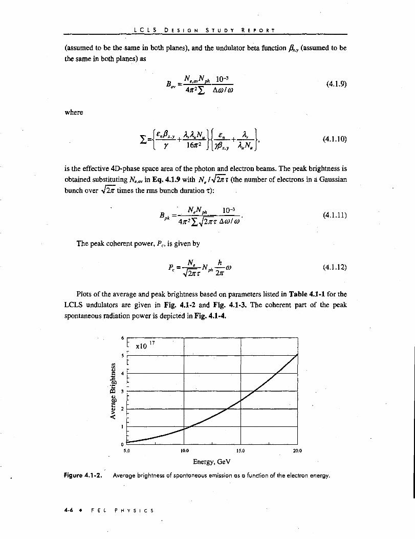
L C L S D E S I G N S T U D Y R E P O R T
(assumed to be the same in both planes), and the undulator beta function fi^y (assumed to be
the same in both planes) as
4;r22 Aala(4.1.9)
where
(4.1.10)
is the effective 4D-phase space area of the photon and electron beams. The peak brightness is
obtained substituting Ne>av in Eq. 4.1.9 with Ne I-Jinx (the number of electrons in a Gaussian
bunch over V2# times the rms bunch duration x):
• w, 10-3
(4.1.11)
The peak coherent power, Pc, is given by
_ Ne (4.1.12)
Plots of the average and peak brightness based on parameters listed in Table 4.1-1 for the
LCLS undulators are given in Fig. 4.1-2 and Fig. 4.1-3. The coherent part of the peak
spontaneous radiation power is depicted in Fig. 4.1-4.
'trffl 3U6J>
: x i o 1 7
-
•
-
/
5.0 2 0 . 010.0 15.0
Energy, GeV
Figure 4.1-2. Average brightness of spontaneous emission as a function of the electron energy.
4 - 6 * F E L P H Y S I C S

L C L S D E S I G N S T U D Y R E P O R T
2.50
2.00
60 1-50
BO
S 1.000 -
O.S0
0.00
- X1028
-
•
-
/
5.0 20.010.0 15.0
Energy, GeV
Figure 4.1-3. Peak brightness of spontaneous emission as a function of electron energy.
Peak
Coh
eren
t Pow
er, k
W -
-
•
•
5.0 10.0 15.0
Energy, GeV
20.0
Figure 4.1-4. Coherent component of the peak power of spontaneous radiation as a function ofelectron energy.
4.2 FEL Radiation
To increase the peak brightness for a given wavelength, either the electron current or the
number of photons produced per electron can be increased. An FEL achieves the second goal
by increasing the number of photons per electron by many orders of magnitude.
In the latter case, many electrons, say Ne, are all grouped within a small fraction of a
wavelength. The total intensity would then be the single particle intensity times N}, and the
number of photons per electron would be increased by a factor Ne. In practical cases, the
electrons are in a bunch much longer than the radiation wavelength, and their position
distribution on a scale of K is completely random: As a result, the radiation fields emitted by
F E L P H Y S I C S 4-7
L C L S D E S I G N S T U D Y R E P O R T
different electrons have a random relative phase, the total intensity is proportional to Ne, andthe number of photons per electrons is still given by Eq. 4.1.7. Taking advantage of acollective instability of the electron beam-EM radiation field-undulator system, the number ofphotons emitted per electron can be increased. This instability works as follows:
1. The electron beam interacts with the electric field of the radiation; the electric fieldis perpendicular to the direction of propagation of the beam (the undulator axis), andis parallel to the wiggling (transverse) velocity of the electrons produced by theundulator magnet, of amplitude K/y, the interaction produces an electron energymodulation, on the scale Xr.
2. The electron energy modulation modifies the electron trajectory in the undulator, insuch a way to produce bunching of the electrons at the scale h.
3. Electrons bunched within a wavelength emit radiation in phase, thus producing alarger intensity. The larger intensity leads to more energy modulation and morebunching, leading to exponential growth of the radiation until saturation is reached.
The FEL instability has been discussed in detail in the literature. Here are summarizedsome of the most important results for the FEL physics in a planar undulator. For thecollective instability to occur there are several conditions that must be satisfied. Theseconditions depend on the FEL parameter [18],
P- (4.2.1)
and on the beam emittance, e. cou =2nc/Au is the frequency associated with the undulatorperiodicity;
lis the beam plasma frequency; neis the electron density; re is the classical electron radius. TheFEL parameter characterizes the instability, giving the instability inverse growth rate, orpower gain length, which, in the 1-D approximation, is
and the saturation power
Psa,=PheamEbeamte> (4-2-4)
4 - 8 * F E L P H Y S I C S
L C L S D E S I G N S T U D Y R E P O R T
where lbeam is the beam current, and Ebeam the beam energy. Saturation occurs after about 20gain lengths. The conditions for the 1-D approximation to be valid are:
1. Beam emittance smaller than or on the order of the wavelength.
en<j;r, (4-2.5)
2. Beam energy spread smaller than the FEL parameter.
OE/E<p, (4.2.6)
3. Gain length shorter than the radiation Rayleigh range;
LC<LR, (4.2.7)
where the Rayleigh range is defined in terms of the radiation beam radius, w, andthe wavelength by n w2 = XtLR.
4. Slippage, Nu Kr, is much smaller than the bunch length ot,
NuAr«a,. (4.2.8)
Condition 1 says that for the instability to occur the electron beam must match theangular and transverse phase-space characteristics of the radiation emitted by one electron intraversing the undulator (Eqs. 4.13, 4.1.4, 4.1.5). Notice that for wavelengths in theAngstrom region this condition cannot be met at present by storage-ring-based synchrotronradiation sources, but it can be satisfied by electron beams produced by a linac fed by a radiofrequency laser-driven electron guns (photoinjectors), as will be discussed in the followingsections.
Condition 2 limits the beam energy spread to a value such that the width of thespontaneous radiation line is not increased, and Landau damping does not reduce the growthrate. Condition 3 requires that the beam produce more radiation than is lost throughdiffraction. Conditions 1 and 3 both depend on the beam radius and the radiation wavelength,and are not independent. If they are satisfied, diffraction and three-dimensional effects are notimportant, and the one-dimensional model can be used with good approximation. In the caseof the LCLS system, Condition 1 is not satisfied and, as a result, the gain length is about afactor of two larger than what predicted by the 1-D model. Condition 4 is well satisfied in theLCLS case, where the slippage is 5 //m, and the bunch length is 70 /an (fwhm).
If, as it is the case in SASE, there is no input electromagnetic field at the undulatorentrance, radiation is still emitted when the longitudinal distribution of the electron beam is
F E L P H Y S I C S • 4 - 9

L C L S D E S I G N S T U D Y R E P O R T
non-uniform, and has a Fourier component b(cor)at <or=2nclXr. This quantity can be
written as
b(o)r)=— T e 2 « W * r , (4.2.9)
and is called the bunching parameter. zm is the initial electron position at the time t = 0, when
the electron bunch enters the undulator.
The amplitude of the electromagnetic field is then proportional to b(G}r), and the intensity
is proportional to \b((Dr)\2. If the bunch length, o , , is much larger than the resonant
wavelength, An and the beam is generated from a thermionic cathode or from a photocathode,
the bunching parameter, &(ffiO, and thus the amplitude and the intensity of the
electromagnetic field are stochastic quantities characterized by a distribution function, which
is determined by the random initial longitudinal electron distribution. The dependence of
\b(o)r)\2 on the number of electrons is <IKo>r)l2> = Ne(l+F(cor)Ne), where F(eor) is the bunch
form factor. The intensity term, quadratic in Ne, is called the Coherent Spontaneous Emission
(CSE). For ai»XTi as in the case of the LCLS, and for a regular charge distribution,
F(car)Nf «1. Thus, this term can be neglected in the LCLS case. For a long undulator, the
electromagnetic field will grow exponentially along the undulator axis, z, with growth rate,
1/LG, and the intensity, /, will grow as
f (4.2.10)
until saturation is reached. Since the initial bunching is a random quantity, the intensity will
vary each time a bunch is sent through the undulator. The average value of the saturation
power is still given by Eq. 4.2.4 and the line width by 1/NU, as in the case of the spontaneous
radiation. If the full line width is detected, the distribution of intensities can be reached by a
gamma function [23].
(4.2.11)
with a relative standard deviation given by \lsM , where the quantity M, which can be
described as the number of degrees of freedom of the photon system, is
<4.2.12,
where Lc is the cooperation length, Q<* the solid angle defined by the detector, and Clc the
coherent solid angle. When the observed frequency spread is larger than the FEL line, the
4 - 1 0 • F E L P H Y S I C S

L C L S D E S I G N S T U D Y R E P O R T
cooperation length is Lc =-2L0(ArlXu), the slippage in one field gain length. In the LCLS
case, and assuming Cl* = Clc, M » 166 and the relative standard deviation of the intensity
distribution is expected to be about 7.7%.
The possibility of operating an FEL in the short wavelength region follows from the
favorable scaling laws for this system [3]. To obtain and discuss the FEL scaling laws let us
write the FEL parameter, p, using two quantities, the electron beam emittance, e, and the
longitudinal brightness, BL , to characterize the electron beam. The longitudinal brightness is
defined as
(4-2.13)
where GE/E is the rms relative energy spread. The quantity in the denominator of Eq. 4.2.13is the beam longitudinal phase-space area. The conditions for the validity of the 1-D model,
Eq. 4.2.5, 4.2.6, 4.2.7, must all be satisfied assuming OEIE-plkl,en = k2Ar/4n . The last
condition, Eq. 4.2.7, on the optical focusing can be shown to follow from the other two.
Using these conditions, the FEL parameter can be written in terms of longitudinal brightness,
P = TTBL, (4.2.14)
To obtain a value of p of the order of 5 x 10"4, the minimum compatible with a practical
undulator, a longitudinal brightness of the order of 1000 A is needed. This value has been
exceeded in photoinjector electron sources [30]. The scaling law Eq. 4.2.13 does not depend
directly on the radiation wavelength, but only indirectly through the requirements, as given in
Eq. 4.2.6. This weak dependence of the FEL scaling law on the radiation wavelength is an
important property, and can be used to develop an x-ray FEL. The simple analysis discussed
here can be used for an initial design of an x-ray FEL. More detailed calculations, including
effects like diffraction and undulator errors, must be performed to predict the system
performance. See Chapter 5.
4.3 References
1 J.B. Murphy and C. Pellegrini, Nuclear Instruments and Methods, 159 (1985); J. B. Murphy andC. Pellegrini, J. Opt. Soc. Am., B2, 259 (1985).
2 Ya. S. Derbenev, A.M. Kondratenko, and E.L. Saldin, Nuclear Instruments and Methods, A193,415 (1982).
3 C. Pellegrini, Nucl. Instr. andMeth. A272,364 (1988).
4 C. Pellegrini, Proc. of the Workshop on IV Generation Light Sources, M.Cornacchia andH. Winick, eds., SSRL Report 92-02, p. 364 (1992).
F E L P H Y S I C S • 4 - 1 1

L C L S D E S I G N S T U D Y R E P O R T
5 M. Cornacchia, "Performance and design concepts of free-electron laser operating in the x-rayregion," Proc. SPIE, Vol. 2998, p. 2-14, Free-Electron-Laser Challenges, P.G. O'Shea andH.E. Bennett, eds.
6 J. Rossbach et al., Nuclear Instruments and Methods A375,269 (1996).
7 J. Motz, J. Appl. Phys., 22, 527 (1951); H. Motz, W. Thon and R. N. Whitehurst, J. Appl. Phys.24,826 (1953); H. Mote and M. Nakamura, Ann. Phys. 7,84 (1959).
8 R.M. Philips, IRE lans. Electron Devices, 7,231 (1960).
9 R.V. Palmer, / . Appl. Phys., 43,3014 (1972).
10 K.W. Robinson, Nuclear Instruments and Methods A239,111 (1985).
11 P. Csonka, Part. Ace. 8,225 (1978).
12 J.M.J. Madey, / . Appl. Phys., 42,1906 (1971).
13 L.R. Elias, W.M. Fairbank, J.M.J. Madey, H.A. Schwettman and T.I. Smith, Phys. Rev. Lett. 36,717 (1976).
14 D.A.G. Deacon, L.R. Elias, J.M.J. Madey, G. J. Ramian, H.A. Schwettman and T.I. Smith, Phys.Rev. Lett. 8; 892 (1977).
15 N.M. Kroll, Phys. Quantum Electron. 5, 115 (1978); P. Sprangle and R.A. Smith, NRL Memo-Report 4033 (1979); D. B. McDermott and T. C. Marshall, Phys. Quantum Electron. 7, 509(1980); A. Gover and P. Srangle, IEEE J. Quantum Electron. QE-17, 1196 (1981); G. Dattolietal, IEEE J. Quantum Electron. QE-17, 1371 (1981); R. Bonifacio, C. Pellegrini, andL. Narducci, Opt. Commun., 50, 373 (1984); J.B. Murphy, C. Pellegrini and R. Bonifacio, Opt.Comm. 53, 197 (1985); J. Gea-Banacloche, G.T. Moore and M. Scully, SPIE 453, 393 (1984);P. Sprangle, CM. Tang and C.W. Roberson, Nucl. Instr. and Meth. A239, 1 (1985); E. Jerby andA. Gover, IEEE J. Quantum Electron. QE-21, 1041 (1985); R. Bonifacio, F. Casagrande andC. Pellegrini, Opt. Comm. 61,55 (1987).
16 J. B. Murphy and C. Pellegrini, "Introduction to the Physics of FELs," in Laser Handbook,Vol. 6, W.B. Colson, C. Pellegrini, and A. Renieri, eds., North Holland, (1990).
17 R. Bonifacio et al, La Rivistadel Nuovo Cimento, Vol. 13, N. 9, (1990).
18 J.B. Murphy, C. Pellegrini and R. Bonifacio, Opt. Comm. 53,197 (1985).
19 G. T. Moore, Nuclear Instruments and Methods A239, 19 (1985); E. T. Scharlemann,A. M. Sessler, and J. S. Wurtele, Phys. Rev. Lett., 54 1925 (1985); M. Xie and D.A.G. Deacon,Nuclear Instruments and Methods A250,426 (1986); K.-J. Kim, Phys. Rev. Lett. 57, 1871 (1986);L.-H. Yu, S. Krinsky and R. Gluckstern, Phys. Rev. Lett. 64,3011 (1990).
20 R. L. Sheffield, "Photocathode RF Guns," in Physics of Particle Accelerators, AIP, V01.184,p. 1500, M. Month and M. Dienes, eds., (1989).
21 K. Bane, "Wakefield Effects in a Linear Collider," AIP Conf. Proc, vol. 153, p. 971 (1987); J.Seeman et al., "Summary of Emittance Control in the SLC Linac," US Particle AcceleratorConference, IEEE Conf. Proc. 91CH3038-7, p. 2064 (1991); M. Ross et al, "Wire Scanners forBeam Size and Emittance Measurements at the SLC," US Particle Accelerator Conference, IEEEConf. Proc. 91CH3038-7, p. 1201 (1991); J. Seeman et al., "Multibunch Enery and SpectrumControl in the SLC High Energy Linac," US Particle Accelerator Conference, IEEE Conf. Proc.91CH3038-7, p. 3210 (1991); T. Raubenheimer, "The Generation and Acceleration of LowEmittance Flat Beams for Future Linear Colliders," SLAC Report 387 (1991).
22 Workshop on Fourth Generation Light Sources, SSRL Report 92/02, 639 pages, M. Comacchiaand H. Winick, eds.; Ibid., C. Pellegrini, p.364.; Ibid., K.J. Kim, p. 315.; Ibid., W. Barletta, A.Sessler and L. Yu, p.376-84; C. Pellegrini et al., Nucl. Instr. and Meth. 341, 326 (1Q94); G.Travish et al., Nucl. Instr. and Meth. A358, 60 (1995).
4 - 1 2 • . F E L P H Y S I C S
L C L S D E S I G N S T U D Y R E P O R T
23 R. Bonifacio et al., Phys. Rev. Lett. 73, 70 (1994); K.-J. Kim, "Noise and Fluctuations in SASEFELs," to be published in Proc. of the 1996 FEL Conf, Rome (1996); E l . Saldin, E.A.Schneidmiller, and M.V. Yurkov, "Statistical properties of Radiation from VUV and X-ray Free-Electron Laser," DESY rep. TESLA-FEL 97-02, (1997).
24 T. Orzechowski et al., Phys. Rev. Lett. 54, 889 (1985); D. Kirkpatrick, Nuclear Instruments andMethods A285, 43 (1989); J. Gardelle, J. Labrouch, and J.L. Rullier, Phys. Rev. Lett. 76, 4532(1996).
25 R. Sheffield, J. Goldstein, and D. Nguyen, Proc. SPIE LASE97 Conf., San Jose, California,p. 2988. (1997).
26 R. Prazeres et al., Phys. Rev. Lett. 78, 2124 (1997).
27 I. Benzvi, private communication.
28 M.C. Teich, T. Tanabe, T.C. Marshall, and J. Galayda, Phys. Rev. Letter, 65, 3393 (1990).
29 M. Hogan et al., "Measurements of High Gain and Intensity Fluctuations in a SASE FEL," Phys.Rev. Lett., 80, 289 (1998)
30 M. Hogan, R. Sheffield, et al., private communication.
F E L P H Y S I C S • 4 -13
FEL Parameters andPerformance
TECHNICAL SYNOPSIS
The FEL theory outlined in Chapter 4 is strictly valid in the one-dimensional
approximation. The FEL parameter optimization and performance characterizations that are
described in Chapter 5 are based on three-dimensional theory and computer models. The
investigation led to a selection of the best parameters and to a study of the sensitivity to
changes in values of accelerator components and beam characteristics and to unavoidable
imperfections in the settings of the beam characteristics, magnetic and mechanical
components and electron beam monitoring. The focusing of the electron beam plays an
important role in the production of the FEL radiation. The LCLS undulator optics has been
optimized in terms of its focusing lattice and strength. The electron optics consists ofFODO
cells, with a cell length of 4.32 m. Focusing is obtained by placing permanent magnet
quadrupoles in the interruptions of the undulator sections. Each interruption is 23.5 cm long,
and also includes beam position monitors and vacuum ports. The correction of the electron
orbit is obtained by a small lateral displacement of the quadrupoles; the total movement is
0.5 mm with a resolution ofJ/jm. Simulations indicate that the FEL radiation saturates at a
length of -90 m. The proposed LCLS undulator has a magnetic length of 100 m, since it is a
requirement that the FEL operate in the saturation regime. This fact not only gives the
maximum output power, but also reduces the pulse-to-pulse fluctuations of the radiation.
The possibility of changing (i.e., lowering) the output power was investigated. This may-
be desirable if the peak power on the sample is excessive and if required for experimental
purposes. The reduction in power, by either reducing the electron current or by increasing
the beam emittance, is accompanied by an increase in fluctuations of the output power due to
fluctuations in the beam characteristics from pulse-to-pulse, since the FEL no longer
operates in the saturation regime. For this reason, the best way to reduce the output power is
by placing an FEL absorption cell in the path of the radiation, as discussed in Chapter 10.
5.1 Introduction
The FEL theory outlined in Chapter 4 is strictly valid in the one-dimensional
approximation. Although a three-dimensional theory has been developed [1,2,6,7] and allows
us to study the effect of parameters like energy spread, emittance, and diffraction. The effects
of magnet errors, misalignment, and lumped alternating gradient focusing can not be treated
analytically. For this reason, after one has used the 3-D theory to search and optimize the

L C L S D E S I G N S T U D Y R E P O R T
fundamental parameters of an EEL, the most important tools for a subsequent and more
precise study and optimization are the computer simulation codes. There is no single code at
present that can handle all the perturbations that can affect performance. Simulations for this
design report used the 3-D codes GINGER [3] (time dependent), FRED-3D [4] (magnet error
analysis, beam position control), and TDA3D [5] (effects of lumped focusing). The codes
GINGER and FRED-3D were developed about 10 years ago at LLNL for the ELF
experiment. They have been extensively cross-checked with experimental results from ELF
and are under full control of the author. TDA3D, originally conceived and implemented at
MIT, was developed during the last 8 years. This section describes the simulations and the
process that led to the selection of the parameter and the sensitivity of the performance to
deviations from optimum operating conditions. This section is organized as follows:
• Section 5.2 describes the method used in the analysis.
• Section 5.3 and 5.4 describe the process that led to the choice of the focusing
system in the undulator.
• Section 5.5 discusses the sensitivity of the performance to various parameters.
• Section 5.6 describes the structure of the FEL radiation.
• Section 5.7 describes the effect of deviation from the ideal electron orbit.
• Section 5.8 discusses the effect of the emission of the spontaneous radiation on
the FEL dynamics.
• Section 5.9 considers ways to control the output power.
• Section 5.10 discusses a realistic beam distribution, as delivered from the linear
accelerator.
• Section 5.11 discusses an optical klystron configuration, a method suggested to
shorten the undulator.
The LCLS parameters are listed in Appendix A.
5.2 Parameter Optimization
The design of the LCLS FEL configuration greatly benefited from an analytical function
of a few independent parameters describing FEL physics in the exponential gain regime,
based on 3-D FEL theory developed between 1985 and 1995. In 1985, K.-J. Kim developed a
dispersion relation which included betatron oscillations [1]. However, this equation did not
take all the effects into account and could not be solved. In 1989 L.H. Yu, S. Krinsky and
R.L. Gluckstern [6] derived the complete dispersion relation from the Vlasov-Maxwell
equations, and solved it for a parabolic electron distribution (waterbag model). They were the
first to discover the scaling property of the solution i.e., that the gain length is a universal
5 - 2 • F E L P A R A M E T E R S A N D P E R F O R M A N C E

_ _ _ _ _ _ _ _ _ L C L S D E S I G N S T U D Y R E P O R T
function of three dimensionless variables (emittance-to-wavelength ratio, scaled electronfocusing strength, and scaled electron-energy spread) and a dimensionless scaling parameter.
In 1992, Y.H. Chin, K.-J. Kim and M. Xie [7] solved the dispersion relation for aGaussian distribution. M. Xie expressed the scaling function • in 1995 asF(TJ& V? VJ-LGJD/LG = 1/(1+1J), fitted a 19-parameter polynomial to the function 7) andpublished its coefficients [2]
La and LGJD are the three and one-dimensional gain length, respectively. The 19 fitcoefficients, a,, are shown in Table 5.2-1.
T a b l e 5 . 2 - 1 . Fit coeff icients.
0.45
an
0.95
a2
0.57
a,2
3
a3
0.55
an
5.4
a4
1.6
an
0.7
a5
3
ais
1.9
a<s
2
aie
1140
a?
0.35
an
2.2
ag
2.9
»u
2.9
a.
2.4
a19
3.2
aio
51
The scaling parameters express the deviation from the 1-D condition due to diffraction,emittance, r]e and energy spread, r\y:
LC,W . _LG,W 4KEn _ LG,W
n d r • t J s : ; V d « : rLR LK XTy K E
Using the 1-D gain length
and the total peak beam power
pb.pk =
the peak power at saturation, P^,, can be approximated:
Psat=l.6p(^)pb,pk (5.2.3)
F E L P A R A M E T E R S A N D P E R F O R M A N C E • 5 - 3

[ C I S D E S I G N S T U D Y R E P O R T
The results of the fit formula have been checked against 3-D simulation codes and are in
excellent agreement. Practical limits exist for a number of parameters g (undulator gap)
£ 6 mm, E < 15 GeV, /^ < 3400 A, aE > 0.0002 and Lu > 100 m.
This report uses the terms "slice emittance," "projected emittance," and "nominal
emittance" to characterize the normalized emittance of the LCLS electron beam. The need for
different emittance definitions comes from the fact that electromagnetic fields, produced by
space charge, chamber impedance, and coherent synchrotron radiation, create a dependence
of the transverse position of the beam centroid on its longitudinal position within the bunch
while the local electron density remains unaffected.
The total phase space distribution integrated over the entire bunch along the longitudinal
axis is characterized by the term "projected emittance" and will generally increase during
beam transport while the electron density at a given bunch location is likely to stay constant.
During the FEL interaction, inside the LCLS undulator, electrons that are further apart
then one slippage distance, LsUp = Nu-Ar, will not interact with each other. To understand the
production of FEL radiation, it is therefore useful to introduce the term "slice emittance," as
the emittance of the phase space distribution integrated over a distance Lslip along the bunch
inside the undulator. For the LCLS, simulations and analytical calculations indicate that the
increase in slice emittance during beam transport will be negligible. The fact that different
slices at different positions in the bunch will arrive with relative transverse offset to each
other effects overall beam brightness but not peak FEL radiation power.
Expected lower limits of projected emittance and slice emittance are being reduced as gun
and beam transport R&D efforts progress. In order to have a fixed working number for
component design and simulations, the LCLS design team decided early on to work with a
"nominal emittance." The nominal emittance was set to a value of 1.5 /rmm mrad, close to
what is expected as projected emittance at the entrance of the undulator. Its use in FEL
calculation constitutes a worst case scenario for the FEL saturation length.
A planar hybrid undulator is assumed; this choice is discussed and justified in Chapter 8.
Within the above constraints, the optimum operating point (Table 5.2-2) can be found using
the fit-formula. Table 5.2-2 lists the parameters that were found to be optimal for the
proposed range of LCLS operations.
5.3 Electron Beam Focusing
As the electron beam is transported through the undulator, transverse focusing is applied
to keep the beam size approximately constant. A planar undulator focuses in the plane
perpendicular to the wiggle motion only (in this report, called x-plane, since the undulator, as
shown in Chapter 8, has a horizontal field). The focusing strength can be expressed by
specifying the "natural" beta-function of the focusing system that is intrinsic to an undulator
made of parallel poles
5 - 4 • F E L P A R A M E T E R S A N D P E R F O R M A N C E

L C L S D E S I G N S T U D Y R E P O R T
KK. (5.3.1)
Table 5.2-2.
Parameter
E
K
Kg
Bw
K
OsJE
Basic LCLS parameters
Value
4.54
15
0.03
6
1.32
3.71
2.0
3400
0.00068
at limits of operational range.
Value
14.35
1.5
0.03
6
1.32
3.71
1.5
3400
0.00021
Unit
GeV
Am
mm
T
mm mrad
A
By appropriately shaping the pole faces, half the focusing can be directed into the wiggle
plane. This type of constant focusing in both planes is called Ted-Pole Focusing [4].
PWy = PT V I . (5.3.2)
The amount of focusing that can be obtained this way is often smaller than required for
optimum FEL performance, especially for high energy and short wavelength applications.
5.3.1 Lattice Design Criteria
The criteria that led to the selection of the average /^-function, cell spacing, and
quadrupole strength were established by first determining the optimum value of the average
/^-function, and, after that, the maximum tolerable amplitude of the modulation of the
/2-function. See Fig. 5.3-1.
5.3.2 Focusing Method (Lattice)
A focusing system stronger than that given by Ted-Pole focusing can be obtained with
external quadrupole fields. Possible lattice choices are two (FODO), three (Triplet), or more
quadrupole magnets per unit cell. A FODO lattice was selected based on simplicity of design
and on the cost-related desire to keep the number of magnets and associated instrumentation
small. With quadrupole focusing, the /^-function is no longer independent of z and its
variation along z, known as the modulation amplitude, defined as
Wx,ylPx,y = iPx,y,m*x-Px,y,™*)lPx,y> causes the beam envelope to vary also. Ted
Scharlemann [4] observed that quadrupole focusing introduces an oscillation in the
longitudinal phase of the electrons with respect to the ponderqmotive potential well, while
F E L P A R A M E T E R S A N D P E R F O R M A N C E • 5 - 5
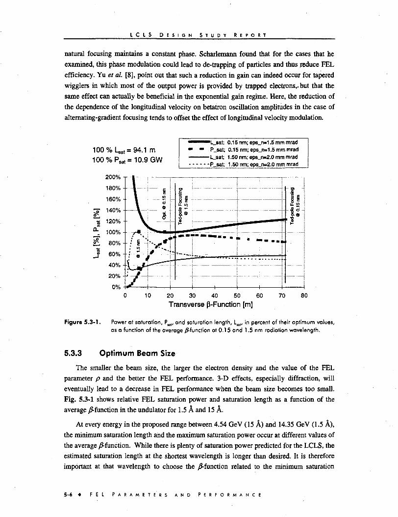
L C L S D E S I G N S T U D Y R E P O R T
natural focusing maintains a constant phase. Scharlemann found that for the cases that he
examined, this phase modulation could lead to de-trapping of particles and thus reduce FEL
efficiency. Yu et al. [8], point out that such a reduction in gain can indeed occur for tapered
wigglers in which most of the output power is provided by trapped electrons,, but that the
same effect can actually be beneficial in the exponential gain regime. Here, the reduction of
the dependence of the longitudinal velocity on betatron oscillation amplitudes in the case of
alternating-gradient focusing tends to offset the effect of longitudinal velocity modulation.
100100
%%Rsat =
94.1 m10.9 GW
•"•"••™L.sat; 0.15 nm; eps_n=1.5 mm rnrad• • P_sat; 0.15nm;eps_n=1.5mmmrad— — — L_sat; 1.50 nm; eps_n=2.0 mm mrad
P_sat; 1.50 nm; eps_n=2.0 mm mrad
Figure 5.3-1.
20 30 40 50 60
Transverse p-Function [m]70 80
Power at saturation, P ,, and saturation length, LMt, in percent of their optimum values,as a function of the average ^function at 0.15 and 1.5 nm radiation wavelength.
5.3.3 Optimum Beam Size
The smaller the beam size, the larger the electron density and the value of the FEL
parameter p and the better the FEL performance. 3-D effects, especially diffraction, will
eventually lead to a decrease in FEL performance when the beam size becomes too small.
Fig. 5.3-1 shows relative FEL saturation power and saturation length as a function of the
average /^-function in the undulator for 1.5 A and 15 A.
At every energy in the proposed range between 4.54 GeV (15 A) and 14.35 GeV (1.5 A),
the minimum saturation length and the maximum saturation power occur at different values of
the average ^-function. While there is plenty of saturation power predicted for the LCLS, the
estimated saturation length at the shortest wavelength is longer than desired. It is therefore
important at that wavelength to choose the /5-function related to the minimum saturation
5 - 6 • F E L P A R A M E T E R S A N D P E R F O R M A N C E
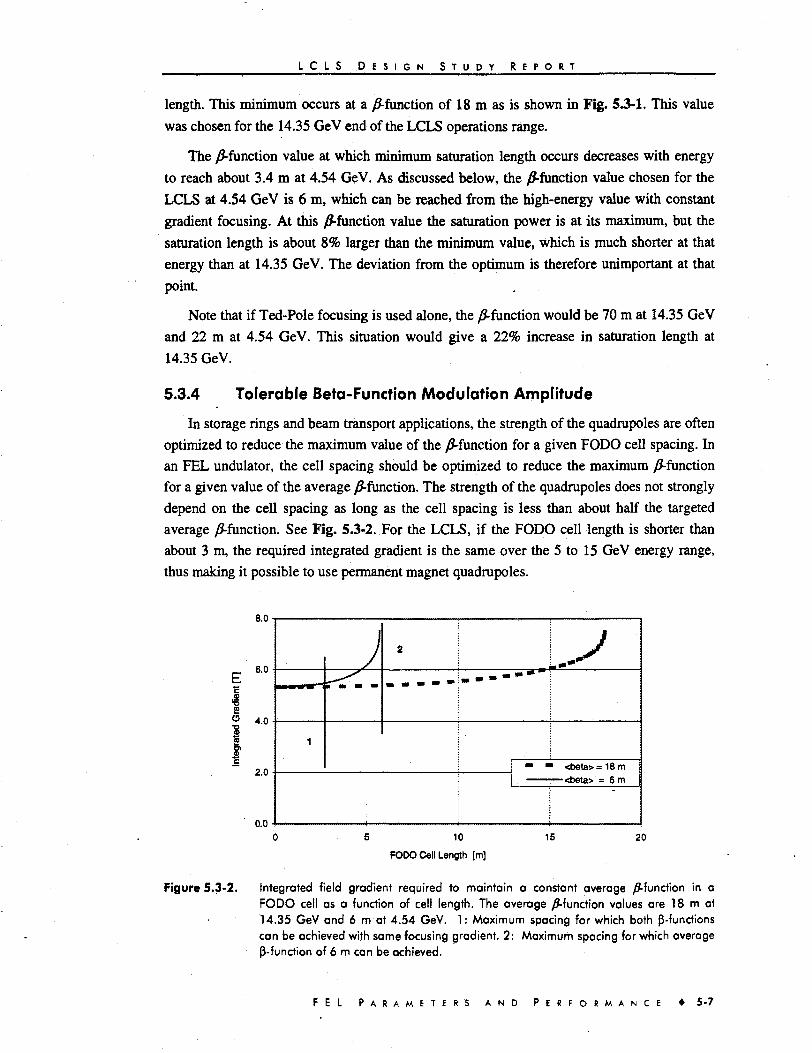
L C L S D E S I G N S T U D Y R E P O R T
length. This minimum occurs at a /^-function of 18 m as is shown in Fig. 53-1. This value
was chosen for the 14.35 GeV end of the LCLS operations range.
The ^-function value at which minimum saturation length occurs decreases with energy
to reach about 3.4 m at 4.54 GeV. As discussed below, the ^-function value chosen for the
LCLS at 4.54 GeV is 6 m, which can be reached from the high-energy value with constant
gradient focusing. At this /^-function value the saturation power is at its maximum, but the
saturation length is about 8% larger than the minimum value, which is much shorter at that
energy than at 14.35 GeV. The deviation from the optimum is therefore unimportant at that
point.
Note that if Ted-Pole focusing is used alone, the /^-function would be 70 m at 14.35 GeV
and 22 m at 4.54 GeV. This situation would give a 22% increase in saturation length at
14.35 GeV.
5.3.4 Tolerable Beta-Function Modulation Amplitude
In storage rings and beam transport applications, the strength of the quadrupoles are often
optimized to reduce the maximum value of the /S-function for a given FODO cell spacing. In
an FEL undulator, the cell spacing should be optimized to reduce the maximum /^-function
for a given value of the average yS-function. The strength of the quadrupoles does not strongly
depend on the cell spacing as long as the cell spacing is less than about half the targeted
average /5-function. See Fig. 5.3-2. For the LCLS, if the FODO cell length is shorter than
about 3 m, the required integrated gradient is the same over the 5 to 15 GeV energy range,
thus making it possible to use permanent magnet quadrupoles.
8.0
EI1
Figure 5.3-2.
4.0
2.0
0.0
)
— » • ! • 1
1
2 i
am m' <beta>=18m—<bela> = 6m
I
10
FODO Cell Length [m]
15 20
Integrated field gradient required to maintain a constant average /^-function in aFODO cell as a function of cell length. The average /^function values are 18 m at14.35 GeV and 6 m at 4.54 GeV. 1: Maximum spacing for which both p-functionscan be achieved with same focusing gradient. 2: Maximum spacing for which average|3-function of 6 m can be achieved.
F E L P A R A M E T E R S A N D P E R F O R M A N C E • 5 - 7

L C L S D E S I G N S T U D Y R E P O R T
For longer cell lengths, the quadrupole strength would have to be adjusted to keep the
/^-functions at their optimum values. The ^function modulation amplitude increases with the
FODO cell length (see Fig. 53-3). The largest cell spacing possible for a given value of the
average /9-function is I^obfPxy wi*h a phase advance of 90 degrees per cell and a
modulation amplitude of about 141%. Small modulation amplitudes could be achieved with
small FODO cell lengths but at the expense of shorter quadrupoles with stronger quadrupole
gradients, more magnets, and higher overall cost. Long FODO cell lengths are desirable. The
question of the maximum allowable FODO cell length can only be answered by computer
simulations. The effect of ^-function modulation on FEL performance was studied with a
version of the TDA3D code as presently maintained at DESY [9]. This version allows the
possibility of using lumped focusing optics [10]. The TDA3D analysis carried out so far
predicts that the effect of /^-function modulation will be rather small. At the largest cell length
that would still allow to obtain the optimum /9-function at the low energy end, the increase in
saturation length is a few percent at 14.35 GeV (with a yS-modulation < 30 %) and slightly
above 10% at 4.54 GeV (^modulation ~ 140%). As pointed out above, the increase of
saturation length at the lower energy is not as critical, since at that operating point the
saturation length is about one-third of the length of the undulator. Based on these
considerations, a 4 m cell length was chosen, which still permits us to obtain an average
/S-function of 6.3 m at 4.54 GeV with permanent magnet quadrupoles. If one uses permanent
magnet quadrupoles, as proposed in Chapter 8, the lack of tunability increases the saturation
length at the longer wavelength end by about 8%. Here, however, the gain length is so much
shorter as to make this not a serious consequence. One additional point to consider is that
strong quadrupole focusing causes the longitudinal velocity of the electrons to change as they
execute betatron oscillations away from the axis. This effect is negligible for the LCLS.
FODO Cell Length [m]
Figure 5.3-3. /J-fundion modulation amplitude for an average /S-function of 18 m at 14.35 GeV and6.3 m at 4.54 GeV as a function of FODO cell spacing. 1: Maximum spacing forwhich both yS-functions can be achieved with same focusing gradient. 2: Maximumspacing for which average ^-function of 6.3 m/rad can be achieved.
5-8 • F E L P A R A M E T E R S A N D P E R F O R M A N C E

L C L S D E S I G N S T U D Y R E P O R T
5.4 Undulator Sections
The LCLS undulator design uses a modular layout. Identical short sections are combined
to form the 100 m device. Analytical studies and computer simulations found the effect of
separations on FEL performance to be small [11]. See Table 5.4-1.
Table 5.4-1 summarizes the FRED-3D simulations for the LCLS: L ^ increases by 6.5 m
when a total of 5.17 m of drifts is inserted, each 23.5 cm long. The increase in actual
undulator length needed to saturate is therefore only 1.33 m. Separations have to be designed
to allow the electron bunches to slip an integral number of wavelengths behind the
electromagnetic wave. This can be accomplished by choosing the correct length for the drift
space [an integral multiple of Xu (1 + K2 12), which is 23.5 cm for the LCLS] or by adding a
phase shifter that corrects the slippage for a separation of different length. The LCLS design
now includes 23.5 cm long separations between undulator sections. The section length (half
FODO cell) was chosen to be 1.92 m (64 periods) so that every quadrupole of the 4.32 m
FODO cell lattice, together with beam position monitors, orbit correctors and other
components, will fit into the separations.
Table 5 . 4 - 1 . Results from two "error-free" FRED-3D runs simulating 4.32 m long undulator section
separated by drift sections, 1 mm and 23.5 cm of length, respectively.
Separation Length
0.001m
0.235 m
Total Inserted Drift to Saturation
0.022 m
5.170 m
94.5 m
101m
P«*
14 GW
13.2 GW
5.5 Parameter Sensitivities
Table 5.5-1 shows the sensitivities of the saturation power and length to various FEL
parameters at 1.5 A (14.35 GeV). Notice the strong sensitivities of the saturation length to
peak current and normalized emittance. Fig. 5.5-1 shows how peak current can be traded
against normalized emittance when keeping the saturation length constant.
F E L P A R A M E T E R S A N D P E R F O R M A N C E • 5 - 9

Table 5.5-1.
APsJPsa,
AV^
APsol/Psal
APmIPsa
Aaulau
AP IP
WX,ylP>
APsJPsal
Ay/y
APsJPsa,AOy fCy
APsJPsm
*ejem
AP^IP^,
I C L S
LCLS sensitivities
- 1 8
— A Q
9' —n s
- 20
0 E S
to input
1 G N S T
parameters.
u o Y R E
ALsa!ILsal_
AL^IL^
Aau/au
ALsat ILm
Af5Xy 1 Pxy
ALsJLsal
Ay/y
ALsat/Lsm
AaYlar
ALsJLsat
ALsal /Lsa
P O R T
= -0.5
- no
8000
1 1.5
e,, / [mm mrad]
Figure 5.5-1 . Peak current vs. normalized emittance at constant saturation length.
2.5
5 - 1 0 • F E L P A R A M E T E R S A N D P E R F O R M A N C E

L C L S D E S I G N S T U D Y R E P O R T
5.6 Temporal Structure of Laser Power
Figure 5.6-1 shows the simulation results obtained with the time-dependent computer
code GINGER. Self-Amplified Spontaneous Emission [12,13] relies on longitudinal electron
density fluctuations (shot-noise bunching). Regions where the initial bunching is larger
produce more radiation, thus accelerating the lasing process. Due to slippage during the
transport through the undulator, those regions will expand to build spikes on the scale of
2nLc =4/zLGAr/Al< [14]. The time-dependent simulations clearly show this phenomenon.
For the LCLS, the spike structure length is of the order of 0.3 /an at 1.5 A wavelength and
5 fm at 15 A.
Avg. Field Power vs. Z
1.E+11
i.E+10 r
T i m e I f s )
Figure 5 . 6 - 1 . FEl output power pattern along the bunch
F E L P A R A M E T E R S A N D P E R F O R M A N C E • 5-11

L C L S D E S I G N S T U D Y R E P O R T
5.7 Effect of Deviations from the Ideal Electron Trajectory
This section discusses the sensitivity of the FEL performance on the imperfections of the
electron orbit in the undulator.
5.7.1 Undulator Steering and Corrector Description
As shown in detail in Chapter 8, the design of the undulator is a planar NdFeB hybrid
structure with 1.5 cm long undulator poles (i.e., 3 cm period lengths) and a full gap height of
6 mm. 64 undulator periods form a 1.92 m long segment Segments are separated by 23.5 cm
long gaps that accommodate electron beam position monitors as well as 12 cm long
permanent magnet quadrupoles with a gradient of 45.5 T/m. The quadrupoles are used for
two purposes, electron beam focusing and steering. Steering is achieved by adjusting the
quadrupoles' x and y positions with stepper motor based systems that allow a total movement
of 0.5 mm with a step size of 1 /an. The undulator is built from 52 segments resulting in a
total length of 111.825 m, of which 99.84 m is magnet length.
5.7.2 Magnetic Field Errors
One of the most significant sources of FEL performance reduction comes from errors in
the on-axis magnetic field of the undulator as well as from dipole components of transversely
misaligned quadrupoles. In an ideal magnetic field, the electron beam would execute a
sinusoidal movement in the plane perpendicular to the undulator field axis. Error fields can
arise from (1) iron pole, permanent magnet, and quadrupole positioning/orientation errors,
(2) permanent magnet strength and global/local easy-axis misorientation errors, and (3) iron
non-uniformities, including saturation effects. Symmetric field errors AB/_z) are perpendicular
to the midplane and give a horizontal angular displacement to the beam. Antisymmetric field
errors are parallel to the midplane, causing vertical beam steering. Positioning errors of the
magnetic structure or variations of the period length give rise to systematic phase errors. If
the electron beam is misaligned with respect to the undulator magnetic structure or if the
undulator segments are not coaxial with the beam steering, errors can also arise.
5.7.3 Trajectory and Error Control Requirement from Simulations
The effect of magnet errors on the FEL performance has been studied with the FRED-3D
simulation code on the NERSC computer systems at LLNL and LBNL. FRED-3D simulates
the interaction between the electron beam and the optical field in the undulator. The effects of
random pole-to-pole errors in the undulator magnetic field on the centroid motion of the
electron beam and on the relative electron-to-radiation phase are included. In each half-
period, a transverse momentum increment corresponding to the magnetic field error at that
magnetic pole is added to the motion of each particle. The field errors are chosen from a
truncated Gaussian distribution. The rms fractional field error and the truncation level are
specified as input parameters. Since FRED-3D does not handle lumped quadrupoles or
quadrupole misalignments, quadrupole focusing is implemented as distributed constant
5 - 1 2 • F E L P A R A M E T E R S A N D P E R F O R M A N C E

L C L S D E S I G N S T U D Y R E P O R T
gradient focusing. The error field amplitudes from quadrupole misalignments were assumed
to be of the same order as the simulated pole-to-pole errors. To estimate the width of the
distribution of saturation length and saturation power, a number of different simulation runs
were done each with a different set of seed numbers for the generation of magnet errors,
initial particle, and seed laser field distribution.
5.7.4 Magnetic Field Error Tolerances
The residual random walk of the electron beam generated by field errors reduces the
overlap between the electron and photon beams and also causes dephasing of the electrons
with respect to the FEL ponderomotive potential wells. Simulation results shown in Fig. 5.7-1
were obtained with FRED-3D using error-free trajectory corrections spaced 2 m apart. They
indicate a threshold in the sensitivity of the saturation length to rms magnet errors. Below an
rms distribution of about 0.1%, magnet errors have little or no influence on saturation length.
Above the threshold, saturation length increases with error amplitude; therefore, the rms
magnet error is specified to 0.1 %.
B5(0
w"35
Figure 5.7-1.
2.50
2.00
1.50-
1.00 -
0.50-
0.00
0.05 0.1 0.15
RMS Magnet Error [%]
0.2 0.25
Saturation length as a function of the rms of the magnet error distribution. The lineconnects the data points.
5.7.5 Steering Algorithm
The random walk can be partially corrected in FRED-3D by introducing "steering
stations," at which the position of the electron beam is measured and a transverse momentum
kick is applied to steer the electron beam onto the axis of the next steering station. The
position measurement is assumed to be imperfect, with specifiable errors in the accuracy with
which the beam position monitors are aligned and the accuracy with which they can measure
F E L P A R A M E T E R S A N D P E R F O R M A N C E • 5 - 1 3

L C L S D E S I G N S T U D Y R E P O R T
the beam position. The positions of steering stations along the undulator axis and the
magnitude of the steering errors are inputs to the code. FRED-3D code uses a point-to-point
correction steering algoritum.
5.7.6 Steering Error Tolerance
A steering correction that is imprecise because of misalignment errors in the beam
position monitors, noise in the processing electronic, or corrector resolution, may reduce the
FEL performance. Fig. S.7-2 shows the effect of four different rms steering error amplitudes
on LCLS output power as result of simulations. For the 1.5 A case (14.35 GeV) with 5 m
steering station separation, the absolute reading accuracy of the beam position monitors
should be better than 5 /an.
f5o
11I
Figure 5.7-2.
2.50
2.00
1.50
1I 1.00c 0.50-
0.00
A—*=£- 3 micron steering error
• S micron steering error
10 micron sterring error
-15 micron steering error
0.05 0.1 0.15 0.2 0.25
RMS Magnet Error [%]
Saturation length as a function of the rms of the distribution of the magnet errors at1.5 A. In the simulation the orbit was corrected with steering magnets placed 5 mapart.
5.7.7 Optimum Steering Station Separation
If the steering errors become significant, the steering process can degrade as well as
improve performance. Fig. 5.7-3 and Fig. 5.7-4 show saturation length and saturation power,
respectively, as a function of steering station separation for the 1.5 A (14.35 GeV), as
obtained with the FRED-3D simulations.
5 - 1 4 • F E L P A R A M E T E R S A N D P E R F O R M A N C E

L C L S D E S I G N S T U D Y R E P O R T
k
atio
n.
Sat
urR
el.
1.20
1.00
0.80
0.60
0.40
0.20
0.00
2 micron steering error
5 micron steering error
10 micron steering error
0 10 20 30
Steering Station Separation [m]
40
Figure 5.7-3. Effect of the separation between steering stations on the saturation power at 1.5 A. Therms of the magnet error distribution is 0.1 %.
2.50
2.00 -
rr0.50 -
0.00
- 2 micron steering error
- 5 micron steering error
• 10 micron steering error
10 20 30
Steering Station Separation [m]
40
Figure 5.7-4. Dependence of the saturation length on the separation between steering stations at1.5 A. The rms of the magnet error distribution is 0.1%.
Close to optimum performance can be expected if the steering station separation is
smaller than 15 m. The trajectory correction process becomes insufficient for larger spacings.
For shorter spacing the effect of very large steering errors can reduce the performance. The
distance between steering stations should be larger than 4-5 m when the inaccuracy in
F E L P A R A M E T E R S A N D P E R F O R M A N C E • 5 - 1 5

L C L S D E S I G N S T U D Y R E P O R T
determining the electron orbit (due to finite beam position monitor resolution and residual
calibration errors) is of the order of 5-10 /an. If the monitors' accuracy is better or equal than
2 fan, then the separation between correctors could be as close as 2 m. This result also yields
the tolerance for the deviation from perfect overlap between the electron and photon beams at
those stations. Although this absolute accuracy seems difficult to achieve, it will be shown in
Section 8.5 that it is obtainable with a beam-based alignment technique.
5.7.8 Undulator Matching Tolerances
The match of the electron trajectory at the entrance and end of each undulator section can
be done by adding a series of %, Vi and XA period long undulator blocks before the first and
after the last period of a 4.32 m long section. The "matching sections," which are off
resonance, do not contribute to lasing but will add a small phase shift, which reduces the
space of the actual separation by a few millimeters. Estimates based on beam size arguments
indicate that position and angle errors of about 5 /an and 1 yurad, respectively, should not
effect FEL performance. These tolerances can be achieved with state-of-the-art
instrumentation (see Section 7.7).
5.8 Emission of Spontaneous Radiation
Due to the rather large value of the undulator parameter, K, synchrotron radiation from
the electron beam in the FEL undulator not only occurs at the resonant frequency and its
harmonics but over a wide continuous spectrum of frequencies. As long as micro-bunching
can be neglected, the total peak synchrotron power radiated by a bunch is given by [15]
pk. (5.8.1)
The power from spontaneous radiation grows linearly along the undulator up to
Psporu =80 GW after 100 m at 1.5 A. This is more than eight times as much as can be
expected for the fundamental peak of the coherent FEL radiation. While this large amount of
incoherent radiation by itself makes the LCLS the brightest x-ray source available, it is
undesirable when the LCLS is to be tuned for FEL lasing. Not only can it cause problems for
the x-ray optics, but it also reduces the average electron energy, increases the incoherent
energy spread and emittance, and adds extra heat load to components that might be installed
along the undulator for diagnostics and beam filtering purposes. The detrimental effects on
the electron beam need to be taken into account during FEL simulations, but the present
computer codes are not yet prepared to handle them.
5.8.1 Average Energy Loss
The average energy loss A<y> from spontaneous synchrotron radiation for each electron
is
5 - 1 6 * F E L P A R A M E T E R S A N D P E R F O R M A N C E
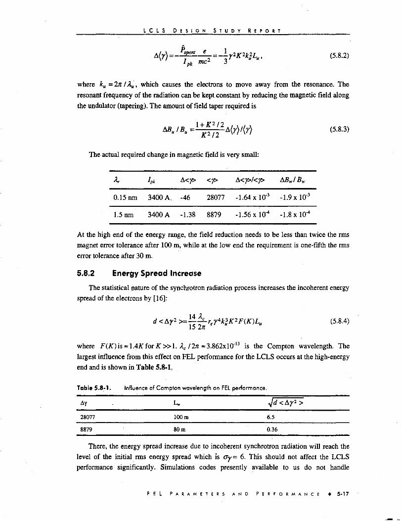
L C L S D E S I G N S T U D Y R E P O R T
Ipk rmP- 3(5.8.2)
where ku=2x/Au, which causes the electrons to move away from the resonance. Theresonant frequency of the radiation can be kept constant by reducing the magnetic field alongthe undulator (tapering). The amount of field taper required is
(5.8.3)
The actual required change in magnetic field is very small:
K
0.15 nm
1.5 nm
1*
3400 A.
3400 A
A<y>
-46
-1.38
<y>
28077
8879
A<y>/<y>
-1.64 xl(T3
-1.56 xlO"4
ABWI Bw
-1.9 xHT3
-1.8 xlO"4
At the high end of the energy range, the field reduction needs to be less than twice the rmsmagnet error tolerance after 100 m, while at the low end the requirement is one-fifth the rmserror tolerance after 30 m.
5.8.2 Energy Spread Increase
The statistical nature of the synchrotron radiation process increases the incoherent energyspread of the electrons by [16]:
d < Ay* >=±i^rer4k2K2F{K)Lu (5.8.4)15 2n
where F(K)\s~\AK fox K » 1 . Xc I2n =3.862xl013 is the Compton wavelength. Thelargest influence from this effect on FEL performance for the LCLS occurs at the high-energyend and is shown in Table 5.8-1.
Table 5.8-1.
AY
28077
8879
Influence of Compton wavelength on
U,
100 m
80 m
FEL performance
Jd < Ay2 >
6.5
0.36
There, the energy spread increase due to incoherent synchrotron radiation will reach thelevel of the initial rms energy spread which is ay = 6. This should not affect the LCLSperformance significantly. Simulations codes presently available to us do not handle
F E L P A R A M E T E R S A N D P E R F O R M A N C E • 5 - 1 7

L C L S D E S I G N S T U D Y R E P O R T
spontaneous synchrotron radiation, but a 1-D code was recently developed at DESY to studythis effect. Running this code with the LCLS parameters showed no reduction in performance[17].
5.8.3 Emittance Increase
Spontaneous synchrotron radiation can cause an increase in rms beam emittance if theradiation occurs at a location with a finite dispersion function [18]. The dispersion functionoriginates in the undulator, is of the order of the wiggle amplitude (~1 /an), and has anegligible effect on the emittance.
5.9 Output Power Control
For applications that use the x-rays produced by the FEL, it is important that the outputpower levels be controllable (see Chapter 10). The feasibility of changing the output powerby varying the peak current or by the use of a magnetic phase shifter was studied. Theconclusion is that neither method is promising. For this reason, a gas absorption cell after theFEL undulator will be used for this purpose.
5.9.1 Peak Current
By changing peak current, either by reducing the amount of charge per pulse or byincreasing the pulse length, one can control (reduce) the FEL production over many orders ofmagnitude. Unfortunately, this action not only reduces the saturation power, but it alsoincreases the saturation length. For reasons of cost optimization, the undulator will bedesigned to be not much longer than the expected saturation length at the highest achievablepeak current. Reduction of the peak current at the highest energy (and shortest wavelength)will move the saturation point beyond the end of the undulator. The FEL output will then bedetermined by the exponential gain regime, resulting in much higher pulse-to-pulsevariations. According to the 1-D FEL theory, the derivative of the peak power with respect tothe peak current dPsmldlpk =(1 + z/(3LG))Psat 11pk in the exponential gain regime. Thesensitivities can be defined as
AP IP 4" / * = • ? (5-9.1)
fpk APZ/PZ _ t , 1 z
Pz= l + ~ (5.9.2)
In the exponential gain regime, the sensitivity to fluctuations in peak current increases, asdo the sensitivities to fluctuations in normalized emittance and energy spread. The relativesensitivities as obtained from GINGER simulations at 1.5 A are shown in Table 5.9-1.
5 - 1 8 • F E L P A R A M E T E R S A N D P E R F O R M A N C E

L C L S D E S I G N S T U D Y R E P O R T
Table 5.9-1 . Sensitivities of LCLS performance to electron beam parameters at the end of the 100 mlong undulator in the exponential gain regime (at Z/LQ « 11.3 for lpk = 1500 A) andat saturation (1^ = 3400 A).
Sensitivity at 1=3400 A Sensitivity at 1=1500 A
Saturation Exponential Gain Regime
.= 1.8
=0.2
The above numbers are larger than those predicted by the 1-D formula, i.e., 1.3 compared
to 1.8 at saturation and 4.8 compared to 6.4 at z/Lc « 11.3. With the expected pulse-to-pulse
jitter of the electron beam that is provided by the linac A/p* /IPk ~ 10-20%, AEn/En ~ 5%,
Aa/ar<l0'5, the x-ray power jitter will be large when operating at saturation but will be
unacceptable when operating in the exponential gain regime. The peak current therefore may
not be a suitable variable for controlling FEL output power. The implications of Table 5.9-1
are that the output power at saturation is expected to fluctuate by 20-36%, due mostly to
fluctuations in peak current. This fluctuation adds (quadratically) to the natural fluctuations of
the SASE process (7.7%; see Section 4.2).
5.9.2 Phase Shifter at Saturation
Another method of controlling output power was suggested, which makes use of the
relative stability at saturation by changing the relative position between the electron beam and
the electromagnetic wave. This could be implemented by installing a chicane after the
saturation point of the undulator. The interaction with the electromagnetic field in a second
short undulator after the chicane would accelerate the electrons by an amount determined by
the phase shift, thus reducing the power of the photon beam. The computed effect is small.
Even the 1-D simulations predict about one order of magnitude of output power reduction.
This would come at a cost of a 20% increase in undulator length. Thus, this is not a
recommended technique for lowering the output power.
5.10 Initial Phase Space Distribution (Coupling to LinacSimulation Results)
Various simulation codes are being used to simulate the development of the electron
phase space from the gun cathode to the end of the linac. Due to these simulations, which are
described elsewhere in this document, transverse and longitudinal phase space distributions of
F E L P A R A M E T E R S A N D P E R F O R M A N C E • 5 - 1 9

L C L S D E S I G N S T U D Y R E P O R T
macro-particles are available at various positions of the system. Phase-space distributions at
the entrance to the undulator can, to some extent, be used to load the particles for the 3-D
FEL simulation codes. The longitudinal scale at which the gun and linac simulation codes
work (1000-10 fjra) is very different from the scale at which the FEL simulation codes
operate (1.5-0.00015 /an). While linac simulations consider the entire length of the bunch,
for the FEL simulations only transverse and momentum distributions over slices of the order
of the slippage length, XrNu, are relevant. On the other hand, linac simulations for the LCLS
use less than one macro-particle per optical wavelength, while FEL simulations need
hundreds if not thousands of particles per optical wavelength, appropriately spaced
longitudinally to avoid artificial numerical bunching. Particle seeding for FEL codes based on
linac simulation distribution can be done by generating a phase distribution of macro-particles
from the macro-particles in bunch slices taken at various positions along the bunch. If the
linac simulation is only done in longitudinal distribution, the amount of information that can
be extracted is very limited. The following section describes effects related to the initial phase
space distributions.
5.10.1 Transverse Halo
The effect of transverse halo on FEL performance has been studied with FRED-3D using
a model distribution composed of two Gaussian distributions. The total number of
macro-particles was distributed on the core Gaussian distribution with nominal emittance and
on a halo Gaussian distribution with a 10 times larger emittance. The simulation was done for
various ratios of particle numbers between the two distributions. There was no detrimental
effect of the FEL process due to the presence of the halo, provided the core current remains
unchanged.
5.11 Optical Klystron
The great length of the LCLS undulator makes it very desirable to find a mechanism that
would shorten the undulator. The suggestion to use an optical klystron configuration has been
put forward. The undulator could be converted into an optical klystron by splitting it in two
parts and inserting a dispersive section. In the first part the interaction between the electron
beam and the emerging electromagnetic wave imprints an energy modulation on the electron
beam that is transformed into a spatial modulation in the dispersive section. The bunching
created by the dispersive section increases the coherent emission of radiation in the second
part of the undulator. The theory of the high-gain optical klystron [19] indicates that the
effect is strongly dependent on the initial energy spread and that the condition A j /) « p
must be fulfilled. For the 1.5 A, the energy spread condition is violated: A> ly » p/2, and
no improvement of performance can be expected with an optical klystron. This was
confirmed by computer simulations, which indicate that the reduction of saturation length can
be significant for very small values of energy spread but that the effect vanishes as energy
spread approaches the expected value of A}/? =2x10-*.
5 - 2 0 • F E L P A R A M E T E R S A N D P E R F O R M A N C E

L C L S D E S I G N S T U D Y R E P O R T
5.12 Summary
The operating parameters have been optimized by an analysis a three-dimensional
algorithm and by computer simulations. The results of the study are that the FEL design
objectives are reachable with a 100 m long undulator, and with the beam characteristics given
in Chapter 2, Table 2.4-1, and in Appendix A (parameter list). A study of the effect of the
electron beam optics on the FEL. performance led to the choice of the FODO lattice cell
length and the quadrupole strength. The sensitivity of the FEL performance to the main
undulator and electron beam parameters was studied, and from this, tolerances for the pole-to-
pole magnetic field variations and for the electron beam characteristics were derived.
5.13 References
1 K.-J. Kim, "Three-dimensional analysis of coherent amplification and self-amplified spontaneousemission in free electron lasers," Phys. Rev. Letters, 57, p.1871, 1986.
2 M. Xie, "Design Optimization for an X-ray Free Electron Laser Driven by SLAC Linac," LBLPreprint No-36038,1995, also, IEEE Proceedings for Pac95, No. 95CH3584,183, 1996.
3 W.M. Fawley, "An Informal Manual for GINGER and its Post-Processor XPLOTGIN", LBID-2141, December 1995. CBP Tech. Note 104, UC-414.
4 E.T. Scharlemann, "Wiggle plane focusing in linear undulators," J. Appl. Phys., 58(6), pp. 2154-2161,1985.
5 T.M. Tran, J. Wurtele, "TDA3D", Computer Phys. Commun., 54, pp. 263-272,1989.
6 L.H. Yu, S. Krinsky, and R.L. Gluckstern, "Calculation of Universal Function for Free-Electron-
Laser Gain," Phys. Rev. Lett. 64, 3011 (1990).
7 Y.H. Chin, K.-J. Kim, M. Xie, "Three-Dimensional Free Electron Laser Theory IncludingBetatron Oscillations," LBL-32329, May 1992 49pp and Phys. Rev, A46, 6662 (1992).
8 L.H. Yu, S. Krinsky, R.L. Gluckstern, J.B.J. van Zeijts, "Effect of wiggler errors on free-electron-laser gain." Phys. Rev. A, 45,1163,1992
9 B.Faatz, DESY, private communication. 1997.
10 G.Travish and LRosenzweig, "Numerical Studies of Strong Focusing in Planar Undulators," inProceedings of the 1993 Particle Accelerator Conference, Washington D.C., 2, pp. 1548-1550,1993.
11 K.-J. Kim, "Undulator Interruption in High-Gain Free-Electron Lasers", LBNL report no. F6,August 1997.
12 R.Bonifacio, CPellegrini, and L.Narducci, "Collective instabilities and high gain regime in a freeelectron laser," Opt. Commun., 50(6), 1985.
13 J.Murphy and CPellegrini, "Generation of high intensity coherent radiation in the soft x-ray andVUV regions," J. Opt. Soc. Am. B2, 259,1985.
14 R. Bonifacio et. al, "Spectrum, Temporal Structure, and Fluctuations in a High-Gain Free-Electron Laser Starting from Noise," Phys. Rev. Let., 73(1), p.70, 1994.
15 K.-J. Kim, "Characterization of Synchrotron Radiation," in X-RAY DATA BOOKLET, K. Kirz et.al, ed., April 1986, LBNL PUB-490 Rev.
F E L P A R A M E T E R S A N D P E R F O R M A N C E • 5 - 2 1

L C L S D E S I G N S T U D Y R E P O R T
16 S. Reiche, in Proceedings of the 1997 Workshop, "Towards X-Ray Free Electron Lasers," atLake Garda, Italy, 1997.
17 S. Reiche, private communication.
18 P.Emma and R.Brinkmann, "Emittance Dilution Through Coherent Energy Spread Generation inBending Systems," in Proceedings of the 1997 Particle Accelerator Conference (PAC97),Vancouver, B.C., Canada, SLAC-PUB-7554. May 12-16,1997.
19 R. Bonifacio, R. Corsini, and P. Pierini, "Theory of the high-gain optical klystron," Phys. Rev. A,45(6), pp. 4091-4096,1992.
5 - 2 2 • F E L P A R A M E T E R S A N D P E R F O R M A N C E

Photoinjector
TECHNICAL SYNOPSIS
The injector for the LCLS is required to produce a single 150 MeV bunch of ~1 nC and
-100 A peak current at a repetition rate of 120 Hz with a normalized rms transverse
emittance of ~1 nmm-mrad. The required emittance is about a factor of two lower than has
been achieved to date. The design employs a solenoidal field near the cathode of a specially
designed rf gun which allows the initial emittance growth due to space charge to be almost
completely compensated by the end of the booster linac (Linac 0). Spatial and temporal
shaping of the laser pulse striking the cathode can further reduce the compensated emittance.
Following the booster linac, the geometric emittance simply damps linearly with energy
growth. PARMELA simulations show that this design will produce the desired normalized
emittance.
In addition to low emittance, there are two additional electron-beam requirements that
pose a challenge: the timing and intensity stabilities should have an rms sigma of < 0.5 ps
and < 1%, respectively. For an rf photoinjector, these parameters are determined principally
by the laser system. Commercial laser oscillators are available with a timing stability of
0.5 ps. The laser system described here uses feedback loops to maintain this stability in the
amplification and pulse shaping stages. The desired laser-pulse energy tolerance is achieved
by stabilizing the pumping laser for the amplifiers and by operating the second amplifier in
saturation. RF systems with a phase stability ofO.Sps are already routine for the SLC.
Although additional R&D is planned to improve the projected performance of the
photoinjector, confidence in the present design is based on the performance of existing
systems. PARMELA simulates the measured performance of low-emittance rf photoinjectors
operating near the emittance level desired. Laser systems have been employed in high energy
physics experiments with timing stability—with respect to the accelerated electron beam—
that is within a factor of two of the value required. The photoinjector is divided
geographically between the electron source—consisting of an rf gun and laser system—and
the booster accelerator. However, to produce the minimal transverse emittance at high
energy, the photoinjector as a whole is treated as one unit.

L C L S D E S I G N S T U D Y R E P O R T
6.1 Electron Source
The electron source for the LCLS consists of a high-gradient 1.6 cell S-band rf gun with a
copper photocathode illuminated by intense optical pulses at 260 nm provided by a Nd:YAG-
pumped Tirsapphire laser system whose fundamental frequency is tripled.
For the LCLS, the electron source must produce a nominal 1 nC pulse with low
transverse and longitudinal emittances at a pulse repetition rate of up to 120 Hz. The required
1 arms emittance for the nominal charge is <1 # mm-mrad. A significant part of the overall
emittance produced by the source is expected to be contained in the spatial and temporal halo
of the pulse, which can be removed downstream of the photoinjector, if desired, with
scrapers.
To meet the emittance requirements, the optical spot size at the cathode has a radius of
-1 mm, the pulse duration has an rms sigma of ~3 ps, and the rf field at the cathode is
130-150 MV/m.
6.1.1 RF Photocathode Gun
A 1.6 cell low-emittance S-band rf photocathode gun has been designed by the
BNL/SLAC/UCLA rf gun collaboration for x-ray FEL applications [1]. The parameters for
this gun as applied to the LCLS are listed in Table 6.1-1. The prototype of this design is now
installed at the Brookhaven Accelerator Test Facility (ATF). A modified version is installed
at the Gun Test Facility at SLAC. Initial measurements at BNL of the gun performance are
very encouraging. (See Section 6.1.6, Summary of Experimental Results at ATF.)
Gun Description
The 1.6 cell rf gun design is based on the original 1.5 cell gun designed at BNL [2]. To
minimize emittance growth due to the Ez component of the TMllO mode, the gun has been
symmetrized. The original BNL zero-mode-suppressed side-coupling has been replaced by
side-coupling rf into the full cell only. This does not completely suppress the zero mode.
Since there is no direct rf coupling from the waveguide to the half cell, the cell-to-cell
coupling between the two cells has been improved by increasing the iris size, which also
increases the mode separation between the zero and /r-modes. This arrangement allows for
more precise field balancing during tuning. To provide more rf focusing and decrease the
peak field on the cell-to-cell iris, the half-cell length has been slightly increased.
A cross section of the rf gun is shown in Fig. 6.1-1. There are two identical coupling
ports in the full cell, located 180° apart. The rf waveguide is connected to one port. A vacuum
pump is connected to the second port. For diagnostic purposes, an rf monitoring loop is also
located in the second port. The photocathode is located in the geometric center of the end
plate of. the half-cell. The end plate is removable to facilitate installation of cathode material
other than Cu by implantation or by using an insert. As with the original BNL gun, the laser
6-2 • P H O T O I N J E C T O R

L C L S D E S I G N S T U D Y R E P O R T
beam can be brought to the cathode either along the axis of the gun or at a grazing incidence
through the 72° side port (not shown in the figure).
Table 6.1-1. Photoinjector Gun Parameters"
Parameter
Cathode material
Usable diameter of cathode
Quantum efficiency
Nominal extraction field
Charge per bunch
Peak current*1
Beam energy at gun exit0
Energy spread at exit0
RF frequency
Bunch repetition rate
RF pulse duration
RF peak power
Number of cells
Length
Value
Cu (or possibly Mg)
12 mm
1(T5 at 260 nm
140 MV/ra
- i n C
-100 A
-7MeV
0.2% rms
2856 MHz
120 Hz
3-4 jjsee
15 MW
1.6
0.168 m
a. Definitions and clarifications. The term "rms" after units indicates a i d value; both the terms"FWHM" (full-width at half-maximum) and "HWHM" (half-width at half-maximum) are used. Thelaser produces "pulses" and the gun produces "bunches."
b. Assumes the laser pulse temporal profile is uniform. If Gaussian, then / = Q/[(2x)"2 *<%], or in thiscase about 130 A.
c. The beam energy is quoted for 130 MV/m extraction field and initial phase of 54° with respect to thecrest of the rf.
Electric field maps for the gun were obtained with SUPERFISH. The ;r-mode fields are
shown in Fig. 6.1-2.
Field Balance
Because of the deleterious effects of space charge on the beam emittance, it is important
to accelerate the beam as rapidly as possible within the gun itself. Field balance tuning is
accomplished using the observed mode separation measured during cold testing. Nonetheless,
simulatians indicate that the transverse emittance decreases as the field increases until about
140 MV/m on the cathode surface.
P H O T O I N J E C T O R • 6-3

L C L S D E S I G N S T U D Y R E P O R T
Figure 6.1-1. Cross section of rf gun. The rf coupler is the top coupler shown here. The bottom portis for the adjustable short and vacuum pump. The electron beam exits to the right.
V>/ii
tin
7-978311*3
Figure 6.1-2. /r-mode field lines for the rf gun obtained with SUPERFISH.
Symmetrization
The emittance growth due to multipole modes of Ez (dominated by the dipole mode) in a
gun cavity with a conventional asymmetric rf coupler is estimated to contribute
>1 ^•mm-mrad to the transverse emittance [3]. Any residual dipole mode in the symmetrized
gun can be minimized by proper tuning of the adjustable short [4]. This is accomplished
during cold testing by measuring the dipole field directly using a needle rotation technique
[5]. The same procedure was used to determine that resistive coupling of the waveguide
results in a lower dipole component before symmetrization than capacitive coupling. After
6-4 • P H O T O I N J E C T O R

L C L S D E S I G N S T U D Y R E P O R T
symmetrization, the effect of the dipole component on the transverse emittance is estimated to
be on the order of 0.1 ;r mm-mrad or less.
Emittance Compensation
Until the energy of the beam is high enough to eliminate the effects of space charge [6],
such effects can result in significant and unacceptable emittance growth. Since the beam
diameter is relatively large and the initial acceleration is rapid, the charge from the gun during
initial acceleration undergoes something like laminar flow. Under these conditions, the effect
of space charge on the transverse emittance of a thin longitudinal slice of the bunch is
minimal, and consequently for a single slice the initial emittance is approximately preserved.
However, space charge has a significant effect on the shape of the phase space as the bunch
progresses through the gun, especially in the first half-cell when the beam energy is lowest.
These space charge effects in the center of an electron bunch are significantly greater than at
the edges. Consequently, the transverse phase space of the various slices of the bunch evolve
differently such that the integrated emittance of the bunch undergoes significant growth.
In 1989 Carlsten [7] pointed out that by simply placing a solenoidal field at the proper
location at the gun one can reverse the evolution of the phase space such that at a later point
downstream, the individual phase spaces of the various slices in the bunch will momentarily
be aligned. If this point of alignment occurs at sufficiently high beam energy, then the
integrated normalized emittance will be frozen at close to its initial value. Experimentally this
realignment of the phase space of the individual longitudinal slices was recently confirmed
[8]. The emittance-compensating scheme for this photoinjector is described in Section 6.2,
Linac 0.
Summary of Experimental Results at ATF
The beamline at the Accelerator Test Facility (ATF) at BNL consists of a 1.6 cell rf gun
with emittance compensating solenoid plus two SLAC-type 3 m sections. The distance from
the cathode to the input coupler of the first 3 m section is 0.9 m. The electron beam energy for
all beam studies is 40 MeV. Interference with the rf coupler at the gun forces the center of the
compensating solenoid to be placed about 5 cm downstream of the optimum position. The
laser beam is operated with a longitudinal Gaussian profile (10 ps FWHM) and a uniform
transverse profile. It is incident on the cathode at 72° with compensation for the anamorphic
magnification and the time slew. Both Cu and Mg cathodes have been tried, but the Mg
cathodes have limited the field at the cathode to about 80 MV/m because of excessive rf
breakdown.
The normalized rms emittance for a 1 nC bunch after compensation has been measured at
the ATF to be 2.5 n mm-mrad at 30 MeV [9]. The "slice" emittance (the emittance of a
transverse slice of the bunch that is significantly thinner than the overall bunch length) was
<1.5 n mm-mrad. For these ATF measurements, the emittance compensating solenoid was not
at its optimal position, and the intensity of the distribution of the laser pulse was uniform
P H O T O I N J E C T O R • 6-5
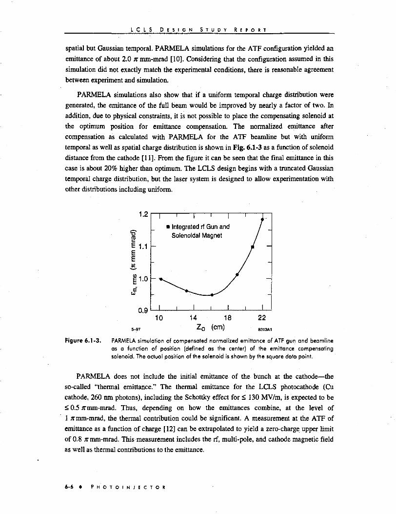
L C L S D E S I G N S T U D Y R E P O R T
spatial but Gaussian temporal. PARMELA simulations for the ATF configuration yielded an
emittance of about 2.0 ;r mm-mrad [10]. Considering that the configuration assumed in this
simulation did not exactly match the experimental conditions, there is reasonable agreement
between experiment and simulation.
PARMELA simulations also show that if a uniform temporal charge distribution were
generated, the emittance of the full beam would be improved by nearly a factor of two. In
addition, due to physical constraints, it is not possible to place the compensating solenoid at
the optimum position for emittance compensation. The normalized emittance after
compensation as calculated with PARMELA for the ATF beamline but with uniform
temporal as well as spatial charge distribution is shown in Fig. 6.1-3 as a function of solenoid
distance from the cathode [11]. From the figure it can be seen that the final emittance in this
case is about 20% higher than optimum. The LCLS design begins with a truncated Gaussian
temporal charge distribution, but the laser system is designed to allow experimentation with
other distributions including uniform.
1.2
•o2EE
(0 1.0
0.9
' Integrated rf Gun andSolenoidal Magnet
I
10
5-97
14 18Z o (cm)
22
8313A1
Figure 6.1-3. PARMELA simulation of compensated normalized emittance of ATF gun and beamlineas a function of position (defined as the center) of the emittance compensatingsolenoid. The actual position of the solenoid is shown by the square data point.
PARMELA does not include the initial emittance of the bunch at the cathode—the
so-called "thermal emittance." The thermal emittance for the LCLS photocathode (Cu
cathode, 260 nm photons), including the Schottky effect for < 130 MV/m, is expected to be
< 0.5 it mm-mrad. Thus, depending on how the emittances combine, at the level of
1 n mm-mrad, the thermal contribution could be significant. A measurement at the ATF of
emittance as a function of charge [12] can be extrapolated to yield a zero-charge upper limit
of 0.8 n mm-mrad. This measurement includes the rf, multi-pole, and cathode magnetic field
as well as thermal contributions to the emittance.
6-6 • P H O T O I N J E C T O R
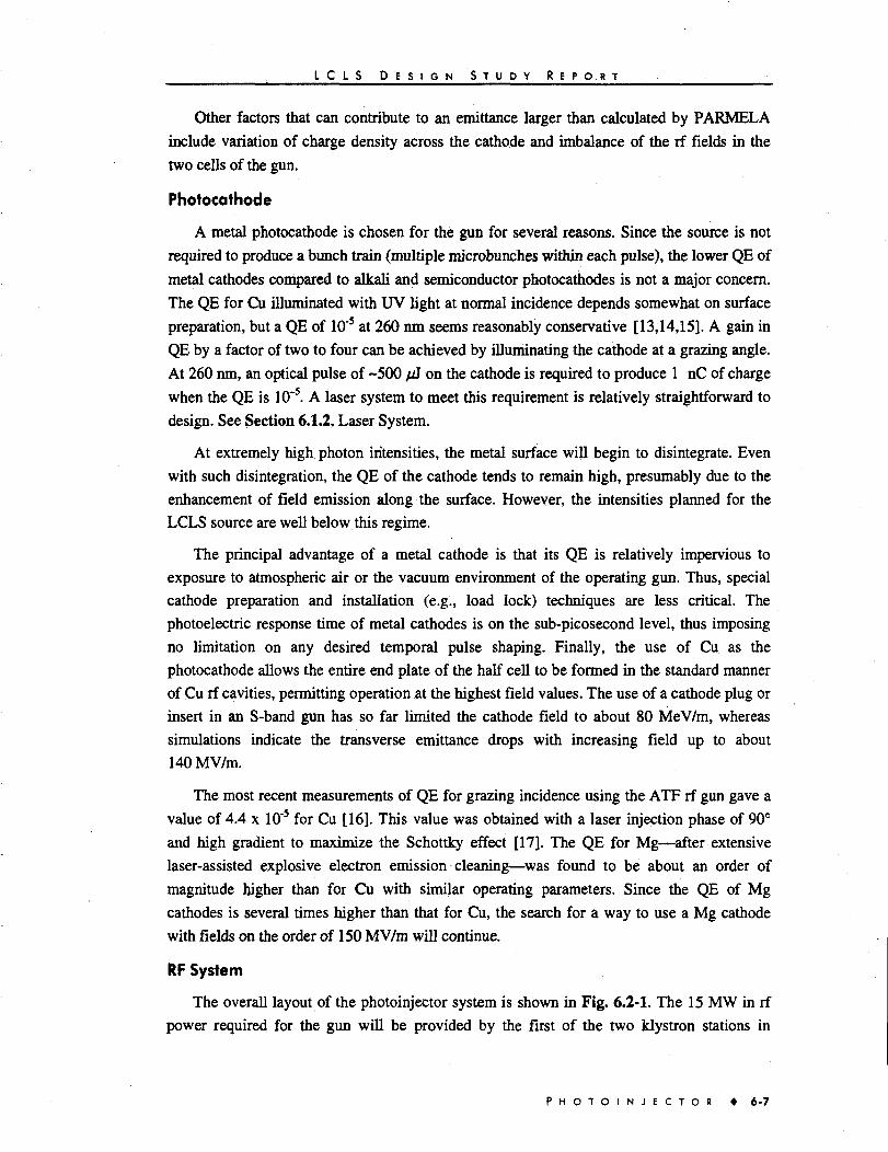
I C L S D E S I G N S T U D Y R E P O R T .
Other factors that can contribute to an emittance larger than calculated by PARMELA
include variation of charge density across the cathode and imbalance of the rf fields in the
two cells of the gun.
Photocathode
A metal photocathode is chosen for the gun for several reasons. Since the source is not
required to produce a bunch train (multiple microbunches within each pulse), the lower QE of
metal cathodes compared to alkali and semiconductor photocathodes is not a major concern.
The QE for Cu illuminated with UV light at normal incidence depends somewhat on surface
preparation, but a QE of 10"5 at 260 nm seems reasonably conservative [13,14,15]. A gain in
QE by a factor of two to four can be achieved by illuminating the cathode at a grazing angle.
At 260 nm, an optical pulse of -500 / J on the cathode is required to produce 1 nC of charge
when the QE is 10~5. A laser system to meet this requirement is relatively straightforward to
design. See Section 6.1.2, Laser System.
At extremely high photon intensities, the metal surface will begin to disintegrate. Even
with such disintegration, the QE of the cathode tends to remain high, presumably due to the
enhancement of field emission along the surface. However, the intensities planned for the
LCLS source are well below this regime.
The principal advantage of a metal cathode is that its QE is relatively impervious to
exposure to atmospheric air or the vacuum environment of the operating gun. Thus, special
cathode preparation and installation (e.g., load lock) techniques are less critical. The
photoelectric response time of metal cathodes is on the sub-picosecond level, thus imposing
no limitation on any desired temporal pulse shaping. Finally, the use of Cu as the
photocathode allows the entire end plate of the half cell to be formed in the standard manner
of Cu rf cavities, permitting operation at the highest field values. The use of a cathode plug or
insert in an S-band gun has so far limited the cathode field to about 80 MeV/m, whereas
simulations indicate the transverse emittance drops with increasing field up to about
140MV/m.
The most recent measurements of QE for grazing incidence using the ATF rf gun gave a
value of 4.4 x 10'5 for Cu [16]. This value was obtained with a laser injection phase of 90°
and high gradient to maximize the Schottky effect [17]. The QE for Mg—after extensive
laser-assisted explosive electron emission cleaning—was found to be about an order of
magnitude higher than for Cu with similar operating parameters. Since the QE of Mg
cathodes is several times higher than that for Cu, the search for a way to use a Mg cathode
with fields on the order of 150 MV/m will continue.
RF System
The overall layout of the photoinjector system is shown in Fig. 6.2-1. The 15 MW in rf
power required for the gun will be provided by the first of the two klystron stations in
P H O T O I N J E C T O R • 6-7

L C L S D E S I G N S T U D Y R E P O R T
Linac 0. The rf phase and amplitude out of this station will be adjusted for the gun without
the use of a high-power phase shifter or attenuator for the gun, thus avoiding the associated
instabilities.
Emittance Compensating Solenoid
For emittance compensation, a solenoid with precisely defined field symmetry and
positioning will be used at the gun exit. An identical compensation magnet with current flow
in the opposite sense will be used to null the magnetic field at the cathode.
The specific solenoid design incorporates several pancake assemblies, each assembly
consisting of a pancake coil, a steel flux straightener, a steel flux return, an aluminum
alignment tube, a coil spacer, a flux return to coil shim, a ceramic flux straightener spacer, a
recessed ceramic yoke-to-flux straightener spacer, and a spacer and compression wave spring.
Conventional manufacturing techniques using molded coils will not accommodate the
required flux straightener position accuracy, therefore the straighteners are positioned
independently of the coil positioning. The axial positioning and stability requirement of
±25 /jm is met by precisely locating the axis of each of the flux straighteners with respect to
the yoke bore by the use of a precision ground aluminum tube. Alignment and survey
fiducials will be pinned to the gun side of the steel flux return plate. Precision bronze
bushings will be located on either side of the solenoid flux return bore axis. The entire
solenoid assembly will be suspended off these- two bushings in the solenoid flux return by
steel pins. An additional pin in the bottom face of the solenoid gun plate will permit the
kinematic location of the gun solenoid assembly. The solenoid will be pinned to an aluminum
cradle, which will be suspended off the floor by struts with thermal expansion coefficient
matched to the gun and linac support system.
Beamline
A diagnostic section of about 0.75 m will separate the entrance of Linac 0 from the exit of
the rf gun. This drift section will contain two vacuum isolation valves and the following
instrumentation: beam position monitor (BPM), current monitor, Faraday cup, profile screen,
and steering magnets.
Vacuum System
After brazing and before final tuning, the rf gun will undergo a 450°C vacuum bakeout in
the Klystron Department's vacuum bakeout facility. This procedure removes excess hydrogen
absorbed by the vacuum surfaces of the rf gun during brazing. A 20 1/s ion pump will be
located in the rf waveguide near the gun rf input coupler and another near the opposite port.
The gun vacuum is separated by the rest of the rf waveguide by rf windows. A third ion pump
of 2201/s will be located just downstream of the emittance compensating solenoid. Together
these three pumps provide a pressure of ~5 x 10"10 Torr at the gun with the field gradient at
6-8 • P H O T O I N J E C T O R
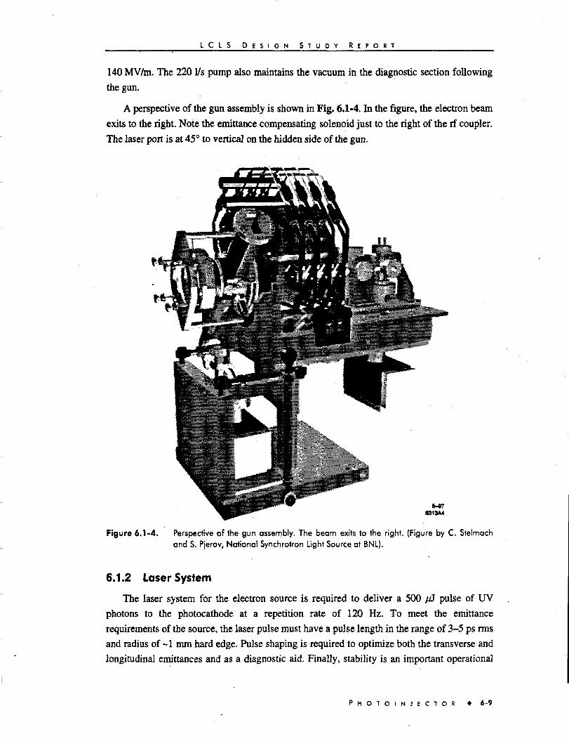
L C L S D E S I G N S T U D Y R E P O R T
140 MV/m. The 2201/s pump also maintains the vacuum in the diagnostic section following
the gun.
A perspective of the gun assembly is shown in Fig. 6.1-4. In the figure, the electron beam
exits to the right. Note the emittance compensating solenoid just to the right of the rf coupler.
The laser port is at 45° to vertical on the hidden side of the gun.
6-978313A4
Figure 6.1-4. Perspective of the gun assembly. The beam exits to the right. (Figure by C. Stelmachand S. Pjerov, National Synchrotron Light Source at BNL).
6.1.2 Laser System
The laser system for the electron source is required to deliver a 500 fd pulse of UV
photons to the photocathode at a repetition rate of 120 Hz. To meet the emittance
requirements of the source, the laser pulse must have a pulse length in the range of 3-5 ps rms
and radius of ~1 mm hard edge. Pulse shaping is required to optimize both the transverse and
longitudinal emittances and as a diagnostic aid. Finally, stability is an important operational
P H O T O I N J E C T O R • 6-9
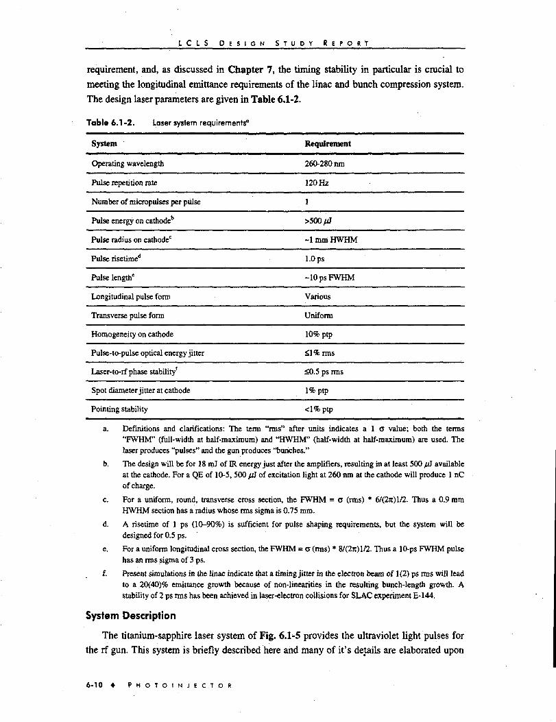
L C L S D E S I G N S T U D Y R E P O R T
requirement, and, as discussed in Chapter 7, the timing stability in particular is crucial to
meeting the longitudinal emittance requirements of the linac and bunch compression system.
The design laser parameters are given in Table 6.1-2.
Table 6 .1-2. Laser system requirements0
System
Operating wavelength
Pulse repetition rate
Number of micropulses per pulse
Pulse energy on cathodeb
Pulse radius on cathode0
Pulse risetimed
Pulse length'
Longitudinal pulse form
Transverse pulse form
Homogeneity on cathode
Pulse-to-pulse optical energy jitter
Laser-to-rf phase stability*
Spot diameter jitter at cathode
Pointing stability
Requirement
260-280 nm
120 Hz
1
>500j«J
- l m m H W H M
1.0 ps
-lOpsFWHM
Various
Uniform
10% ptp
£l%rms
<0.5 ps rms
1% ptp
<1% ptp
a. Definitions and clarifications: The term "rms" after units indicates a 1 o value; both the terms"FWHM" (full-width at half-maximum) and "HWHM" (half-width at half-maximum) are used. Thelaser produces "pulses" and the gun produces "bunches."
b. The design will be for 18 mJ of IR energy just after the amplifiers, resulting in at least 500 pS availableat the cathode. For a QE of 10-5,500 /jj of excitation light at 260 nm at the cathode will produce 1 nCof charge.
c. For a uniform, round, transverse cross section, die FWHM = a (rms) * 6/(2JI)1/2. Thus a 0.9 mmHWHM section has a radius whose rms sigma is 0.75 mm.
d. A risetime of 1 ps (10-90%) is sufficient for pulse shaping requirements, but the system will bedesigned for 0.5 ps.
e. For a uniform longitudinal cross section, the FWHM = o (rms) * 8/(2n)l/2. Thus a 10-ps FWHM pulsehas an rms sigma of 3 ps.
f. Present simulations in the linac indicate that a timing jitter in the electron beam of 1(2) ps rms will leadto a.20(40)% emittance growth because of non-linearities in the resulting bunch-length growth. Astability of 2 ps rms has been achieved in laser-electron collisions for SLAC experiment E-144.
System Description
The titanium-sapphire laser system of Fig. 6.1-5 provides the ultraviolet light pulses for
the rf gun. This system is briefly described here and many of it's details are elaborated upon
6 - 1 0 • P H O T O I N J E C T O R

. L G L S D E S I G N S T U D Y R E P O R T
in subsequent sections. A CW, frequency-doubled, diode-pumped Nd:YAG laser provides
energy in the green (532 run) to pump the CW mode-locked Ti:sapphire oscillator, which
delivers a continuous train of 10 nJ, 100 fs FWHM pulses that repeat at 119 MHz. By using
this frequency, the 24th subharmonic of the linac's 2856-MHz rf, timing of the laser pulse is
locked to the phase of the rf in the linac and rf gun. This question of timing is discussed in
detail below. The wavelength is tuned to 780 nm, which after the amplification is frequency
tripled to 260 nm to provide a suitable wavelength for the photocathode of the gun. With the
possible exception of the pulse stability requirements at 119 MHz, oscillators of this type are
commercially available (e.g., Coherent's Mira or Spectra-Physics' Tsunami with modification
to 119 MHz).
A Pockels cell and polarizer are used to gate single pulses, at 120 Hz, from the 119 MHz
pulse train. The selected pulses are then amplified by two Tirsapphire crystals, both
configured as 4-pass "bow-tie" amplifiers [18]. Both are pumped by a single Q-switched,
doubled Nd.YAG laser that can produce a 120 Hz train of 3 ns pulses (again a commercial
laser, such as Coherent's Infinity). The pump output is stabilized. Fourier-relay optics (see
below), beginning with a primary aperture between the two amplifiers and continuing to the
final optics platform next to the gun, are used to maintain a good transverse mode while
efficiently filling the pumped volume of the Ti:sapphire crystals.
In amplifiers for picosecond and especially sub-picosecond pulses, the peak power must
be limited to avoid optical damage and nonlinearities. This system uses chirped pulse
amplification [19] to keep the peak power in the amplifier small. The large bandwidth of the
Ti.sapphire oscillator enables it to produce the 0.1 ps pulse desired for pulse shaping. The
dispersion of a grating pair can then stretch the pulse to hundreds of picoseconds, so that the
peak power is reduced to avoid nonlinearities and damage during amplification. Different
wavelengths take different optical paths through the diffraction gratings. The resulting space,
tune and wavelength correlations are then used to stretch—or compress—the pulse. After
amplification, the process can be reversed to compress the pulse to the original or any greater
width. The large bandwidth of the Ti:sapphire oscillator also allows us to shape the pulse in
time (using Fourier-transform pulse shaping, as discussed later). The final shape at the system
output can be readily altered under computer control. Fig. 6.1-5 includes the pulse shaper and
stretcher after the oscillator and a compressor after the amplifier. An additional low-power
compressor after the oscillator is used as a diagnostic for the pulse shaper. It compresses the
pulses from the 119 MHz train that are not selected by the Pockels-cell gate, and a cross-
correlator using a portion of the oscillator light can then probe the resulting pulse shape.
After the second amplifier, the transverse shape of the pulse is modified from Gaussian to
uniform to better match the requirements for obtaining a low emittance from the gun. Next,
two crystals triple the frequency of the light to a wavelength of 260 nm. The flattened pulse
also improves efficiency and uniformity in this harmonic-generation process.
P H O T O I N J E C T O R • 6-11

L C L S D E S I G N S T U D Y R E P O R T
c w , Diode-Pumped,Doubled Nd:YAG—
SW, 532 nrn
Stretcher CW, Mode-Locked,TirSapphire Oscillator—
100 Is pulses © 119 MHz,1 W, 10nJ/pulse, 780nm
Photooiode
Joule+CCD
12 pJ
Joule+CCD
Q-Switched,Doubled Nd:YAG—
8 ns pulses 6 120 Hz,160 mJ/pulse, 532 nm
W2«
Poll10% Trim
~ 1
30 ns |Delay1
Integrate&Hold
1 +HV
Pulser Pockels
$i 1/2
^ ^
PrimaryAperture
18 mj
|
CrossCorrelator
VacuumSpatial Filter
j Photodiode
i|Joule+CCD| |Joule+CCD|
SpatialFlattener
10 pS
Compressor
ASF22Oct97
Figure 6.1-5. The drive laser for the rf photocathode electron gun for the LCLS. The thick lines showthe main beam path, the closely spaced, dashed lines indicate diagnostic beams, andthe widely spaced, dashed lines are pump beams.
6-12 • P H O T O I N J E C T O R

I C L S D E S I G N S T U D Y R E P O R T
Finally, the beam is transported through an evacuated tube to an optics platform next tothe gun. Because of the long transport tube, the last image plane of the Fourier-relay opticalsystem has a spot size that is too small for the photocathode. The image is magnified onto aplane with a circular aperture that slightly trims the edge of the beam. Since this aperture issubsequently imaged onto the photocathode, the illuminated region of the photocathode isprecisely defined without jitter. The imaging includes compensation (discussed below) for thetemporal and spatial distortion caused by grazing incidence onto the photocathode.
The energy management of the laser system is as follows: transmission through thespatial flattener -50%, through the compressor -50%, through the frequency tripling stage-25%, and through the optical transport to the gun -50%. Consequently, starting with 18 mJafter the second amplifier, the required 500 / J is delivered to the cathode.
The factors that entered into the choice of a CW Nd:YAG-pumped Tksapphire oscillatorcombined with a Q-switched Nd:YAG pumped Tksapphire amplifier laser system are givenin Section 6.1.3.
Temporal Pulse Shaping
The spatial and temporal shape of the optical (and thus also the electron) pulse isnominally Gaussian. Simulations indicate that an emittance-compensated beam at the exit ofthe injector will have a lower transverse emittance if uniform temporal and spatialdistributions of charge are extracted at the photocathode. However, following the beamdownstream through the linacs and compressors, present simulations indicate that the bunchlength at the entrance to the undulator for a beam with an initial uniform temporal shape ismore sensitive to timing jitter than for an initial Gaussian shape. It is likely that anintermediate shape will in the end prove optimal. Since an experimental variation of the pulseshape will be needed to establish the final operating configuration, the capability to shape(including a uniform shape) the temporal profile of the laser pulse is built into the system.
Temporal shaping of the optical pulse will be accomplished through the well-establishedtechnique of frequency domain pulse shaping [20]. This technique takes advantage of thelarge bandwidth of ultrafast laser pulses. The bandwidth of a laser pulse is determined by theFourier transform of its electric field
£(fi))= jdtEtfe™' . (6.1.1)
For a laser pulse with an intensity envelope
I(t) = Ioe'V) , (6.1.2)
the power spectrum is
P H O T O I N J E C T O R • 6-13

L C L S D E S I G N S T U D Y R E P O R T
J , (6.1.3)
where A® = 2/t is the bandwidth of the pulse. The shorter the pulse the larger the spectral
bandwidth. The frequency spectrum is dispersed in space between a pair of diffraction
gratings separated by a pair of lenses. By using relay imaging between the gratings, no
dispersion is introduced in the pulse. A spatially resolved amplitude and/or phase mask at the
dispersion plane modifies the Fourier transform of the laser pulse and permits any pulse shape
allowed by the bandwidth to be produced. In principle, a square pulse with a rise time equal
to the pulse duration of the original compressed pulse can be produced. In Fig. 6.1-5 pulse
shaping is accomplished in a pair of gratings before the amplifier sections. This arrangement
reduces the possibility of damage to the pulse shaping optics. The pulse shape will
subsequently be modified by the gain properties of the amplifiers and the frequency
conversion process. Thus, the Fourier transform produced in the pulse shaping gratings must
take these changes into account. To accomplish this, the amplitude and/or phase masks will
be made with computer-addressable liquid crystal optics [21]. In this case, the single shot
pulse duration measurement will allow immediate feedback on the mask configuration, which
can then be modified to produce the desired pulse shape. Thus, the effects of frequency
conversion and gain shaping will be readily taken into account, and it will be relatively
simple to change the pulse shape if another is found to be advantageous.
Fourier Relay Optics
A technique known as Fourier relay imaging combines relay imaging, in which lenses
relay an image of an aperture to each pass through an amplifier Ti:sapphire crystal or
harmonic-generation crystal, and filtering of the beam's spatial Fourier transform. This
approach can maintain a clean transverse mode and improve pointing stability, while also
achieving better utilization of the pump energy. Initially, the oscillator beam is trimmed in an
aperture. At each step a lens of focal length/! is placed a distance f\ after one of the image
planes. The Fourier transform is formed at the focus/] beyond the lens, where higher spatial
harmonics are removed by a pinhole. A second lens with focal length fz then recollimates the
beam (with magnification/2 lf\) and forms the relay image at a distance 2(fi +/2) from the
previous image plane. Similar imaging takes place at the harmonic-generation crystals, and
finally an image of the aperture is relayed to the photocathode to define the area of
photoemission.
Spatial Pulse Shaping
To shape the pulse in space, a position-dependent attenuation will be applied to the beam
[22]. Relay imaging must be used after the flattening to limit diffraction. However, the
repeated filtering of the spatial Fourier transform limits the steepness of any uniform pulse at
the output, and so Fourier filtering is not used after the spatial shaper. Also, the initial
6 - 1 4 • P H O T O I N J E C T O R

L C L S D E S I G N S T U D Y R E P O R T
flattening is lossy, and so the system must have sufficient gain. On the other hand, harmonic
generation can be more efficient with a uniform intensity across the beam.
Frequency Conversion
The -780 nm pulses will be frequency tripled to -260 nm in a pair of frequency
conversion crystals using a Type E-Type II tripling scheme [23]. This scheme is called a
polarization mismatch scheme because the beam is detuned from optimal in the first crystal to
allow efficient conversion to the third harmonic in the second. In Type II doubling, the beam
is typically incident with a polarization angle of 45° with respect to the e- and o-axes. For
polarization mismatch, the beam is polarized at 35° with respect to the o-axis, allowing
approximately 50% conversion to the second harmonic. The unconverted fundamental beam
is mixed with the converted beam in the second crystal. Frequency conversion efficiencies in
excess of 50% to the third harmonic have been measured with picosecond 1 /urn laser pulses.
A pair of BBO crystals with phase matching angles of 42° and 54° respectively will be
discussed. The cautious estimates of Fig. 6.1-5 assume a day-to-day tripling efficiency of
25%, although twice this efficiency should be achievable.
Because of the intensity and wavelength dependence of the frequency conversion process,
one has to be concerned about the pulse distortion during conversion. If the pulse is
temporally and spatially uniform (a cylindrical slug), the frequency conversion will maintain
the pulse shape. Under these conditions, the frequency conversion efficiency can be
optimized. Frequency conversion will also sharpen the edges due to the nonlinearity of the
process. On the other hand, a non-uniform shape will be distorted upon frequency conversion.
This must be accounted for in the generation of the pulse shape. In addition, any structure on
the pulse—ripples in time or space—are likely to grow during the conversion process, again
due to the non-linearity [24]. This means that the constraints on the spatial and temporal
uniformity before conversion will be more severe than those required at the photocathode.
Grazing Incidence
In the rf photocathode guns being developed by the Brookhaven-SLAC-UCLA
collaboration, the laser is incident on the photocathode at near-grazing incidence (72° from
the normal at Brookhaven's ATF). When ajc-polarized beam is incident on the photocathode
(so that the electric field is nearly normal to the surface), photoemission from metals is
enhanced by up to a factor of three over emission at normal incidence. In addition, there is no
need to insert a laser mirror directly downstream from the gun, right next to the electron-
beam path, where it is an obstacle and a source of wakefields.
However, a circular laser beam incident at a grazing angle illuminates an elliptical spot
on the cathode, and, if the spot is millimeters across, the side closer to the laser entry will
emit picoseconds earlier than the other side. Corrections for both of these effects are needed
to minimize emittance. To compensate for the elliptical spot, the last relay of the beam in
Fig. 6.1-5, from the final image plane to the cathode, uses a pair of cylindrical lenses, to
P H O T O I N J E C T O R • 6-15

L C L S D E S I G N S T U D Y R E P O R T
apply different magnifications horizontally and vertically and so illuminate a circular area.
Alternatively, a suitable prism pair can also provide this compensation.
The time slew can be corrected by reflection from a grating or by transmission through an
echelon (a staircase of fused-silica plates) in order to add a time delay varying across the
beam. By placing the grating in the beam near the final image plane, the time delay is
correlated with the position across the cathode. Since gratings are lossy in the ultraviolet, care
must be taken to make the beam size large enough on the grating to avoid damage.
Stability of Laser Pulse
Putse-fo-Pulse Timing
The LCLS design places several strict requirements on laser stability and reproducibility.
One of these is pulse-to-pulse timing jitter of the bunch with respect to the rf phase driving
the gun and rf accelerating sections. Because of the rf acceleration process in Linac 1, any
timing (phase) change at the gun affects the energy slew along the bunch which in turn
changes the bunch compression in the subsequent chicane. The energy of the bunch is also
affected, which changes the arrival time at Linac 2. The original timing error may in some
cases be canceled in the second linac and chicane, but because of the nonlinearities in the
compression process, the average bunch length is increased in all cases. Since the peak
current varies inversely as the bunch length, the net effect may lead to a serious degradation
of FEL performance beginning at the level of a timing jitter of about 1 ps rms. For this
reason, a criterion of 0.5 ps rms is adopted for the LCLS. Almost all of the jitter of the laser
system originates in the laser oscillator, and this criterion has been met by the stabilization
techniques incorporated in advanced commercial oscillators such as those planned for LCLS.
In the design of the laser system presented here, the timing is stabilized twice. Refer to
Fig. 6.1-6. First, a measurement is made of the laser oscillator output phase with respect to
the accelerator rf phase where the rf is provided by a coupler in the accelerator rf main drive
line. The phase error signal, which is first passed through a low-pass filter and then amplified,
is used to drive a piezo stage on which the end mirror of the laser oscillator is mounted. The
oscillator incorporates a passive mode-locker (using Kerr lens or Fabry-Perot saturable
absorber mode-locking techniques), while the lock to the external rf reference is done by
tuning the length of the oscillator cavity. Thus the length of the cavity, which is initially set
up to match a fraction of the accelerator frequency, can be continuously adjusted to lock the
phase of the subsequent laser pulses to the rf. The bandwidth of the method is estimated to be
of the kilohertz range. The timing is then restabilized external to the laser oscillator. A prism
is mounted on a piezo stage with a fast motor (e.g., a picomotor from New Focus Inc.) which
acts as a delay for the laser pulses. As shown in the figure, this delay system uses the same
phase error signal as the piezo stage internal to the oscillator, but it could equally well be
made to use the measured phase error signal of either the electrons or the laser with respect to
the rf, both of which are shown in the figure.
6-16 • P H O T O I N J E C T O R

[ C I S D E S I G N S T U D Y R E P O R T
The piezo and motor would be computer controlled and would account for all the slow
drifts in the laser optical path length or timing drifts in the rf system. In a recent high-energy
physics experiment, timing stabilization of a laser pulse with respect to the electron beam has
been demonstrated at the level of 2 ps using similar techniques.
faster Generator476 MHz
Accelerator RF Main Drive Line
\ Laser timing/phase shifter
[irt
119 MHz
Picosecond Timingo F Stability
Laser Oscillator Cavity
SpectrumAnalyzer
Long termTiming Stability
SamplingScope
Pulseselection
PockelsCell
Laser AMPChain
PulseCompression
Sample and HoldPhase Measurement
ELECTRON PHASE w.r.t. RF
Ix24
AMP
A / D
Sample and Hold Phase MeasurementELECTRON PHASE w.r.t. LASER
Electrooptic Single PulsePhase Measurement
R F G U N
K|ystron I Optical Transport [
electrons
0—*•
Figure 6.1-6. Timing stabilization schematic.
Pulse Duration
Like timing jitter, the stability of the pulse duration is important for LCLS performance.
The pulse duration should fluctuate by no more than the allowable timing jitter. A stable
oscillator is again essential. A technique for further control takes advantage of the phase and
P H O T O I N J E C T O R • 6-17

L C L S D E S I G N S T U D Y R E P O R T
amplitude masks used to shape the pulse in time. If the bandwidth of the oscillator pulse is
wider than that transmitted by the masks, so that the masks are illuminated almost uniformly,
then fluctuations in the oscillator width do not affect the final pulse width or shape, which is
determined only by the masks and the pulse compressor following the amplifiers.
Optical Energy
The optical energy per pulse should be held constant to the level of 1% rms or less as
indicated in Table 6.1-2. This requirement is set by the stability required of the x-ray laser
beam. Harmonic generation can compound the difficulty of this criterion, since 1% stability
in the third harmonic would require 0.3% stability in the fundamental. Since it is difficult to
make a clean Pockels cell trim of a broadband pulse without affecting its temporal shape, the
gain is stabilized by using laser diode pumping in the oscillator; by careful control of the
beam mode and its pointing through the amplifiers through Fourier relay imaging; and by a
combination of feedback loops to stabilize the amplifier pumping to maintain the UV energy
at the gun.
To stabilize the pumping, the relatively long upper-state lifetime of Tirsapphire (3.2 /&) is
used to keep the total pump energy constant on a pulse-by-pulse basis. To accomplish this,
10% of the pump beam will be delayed by a 30 ns optical path (the delay chosen to be the
minimum necessary to adjust the Pockels cell HV) and used to trim the pumping of the
Thsapphire for a given primary pulse by up to ±5%. Since the pump has a narrow bandwidth,
it is easily trimmed by the Pockels cell shown in Fig. 6.1-5.
To correct for long-term drift in the UV pulse energy as monitored at the gun, a software
feedback loop will adjust the set point in the primary feedback loop that stabilizes the
amplifier pump energy.
Spot Size and Position
To carefully and reproducibly control the distribution of space charge in the gun for
optimal emittance, the laser must maintain a 1% variation in the diameter of the laser spot on
the photocathode with a centroid location that varies by no more than 1% of the diameter.
Position stability can be achieved by trimming the edge of the beam with a circular aperture
placed on the final relay plane before the gun; this aperture is then imaged onto the
photocathode. A Gaussian beam could still have fluctuations in the position of the centroid
within the aperture, but with the uniform pulse shape preferred for LCLS, pointing jitter does
not cause any change in cathode illumination (as long as the jitter does not leave any part of
the beam-trimming aperture unilluminated).
Diagnostics
The laser system is designed with an integral diagnostic beam. (See Fig. 6.1-5.) This
beam is used to monitor the shot-to-shot amplifier gain and also is used for diagnosing the
pulse shape of the UV pulse to be incident on the photocathode. To obtain the diagnostic
6-18 • P H O T O I N J E C T O R

L C L S D E S I G N S T U D Y R E P O R T
beam (lighter line in the figure), a Pockels cell and polarizer are used to gate a second
oscillator pulse that follows the primary pulse by tens of nanoseconds. The diagnostic pulse
makes only one pass through each of the amplifiers. A photodiode measures its energy at each
stage to check the gain. The unstretched (100 fs) diagnostic pulse is then cross correlated with
the UV output pulse (3-10 ps) to measure the pulse shape.
Cross-correlation Pulse Shape
The advantage of using a diagnostic beam for a cross-correlation measurement of the UV
pulse shape is that the diagnostic beam retains the original -100 fs duration of the seed beam
and so provides a comparable temporal resolution. A cross-correlation provides more
information than an auto-correlation because the latter cannot distinguish temporal
asymmetries. The diagnostic pulse will be chosen to arrive at a cross-correlator at the same
time as a fraction of the primary pulse picked off by a beam splitter. There are a number of
techniques for measuring the cross-correlation of an infrared and UV pulse. It is anticipated
that a single-shot polarization-gating cross-correlator [25] will be used. This will generate a
third-order intensity cross-correlation of the -100 fs, 800 nm IR pulse and the -10 ps UV
pulse. If the IR pulse is used as the gating pulse, the measured pulse shape is that of the UV
pulse with a temporal resolution of approximately 100 fs. The two pulses are incident nearly
colinearly on a nonlinear optic. The UV pulse to be detected is incident on a spatially
resolving detector through crossed polarizers. In the absence of a gating pulse, no UV light is
detected. Between the polarizers there is a Kerr medium, such as a thin piece of fused silica.
When the gate pulse is incident on the Kerr medium, it acts as in instantaneous waveplate
which allows the portion of the UV pulse passing through the same space-time location to
pass through the crossed polarizers and be detected. By choosing the crossing angle, detector
and crystal size, and appropriate probe beam energy, the pulse duration can be measured with
a resolution approaching the 100 fs duration of the gate pulse.
The effect of the pulse shaping on the low-energy IR pulse will also be measured using
cross-correlation. In this case, all of the pulses (other than the primary pulse) from the
119 MHz train out of the shaper-stretcher are selected. After recompression, their shape is
measured in the cross-correlator shown in Fig. 6.1-5 in the low-energy area. From the
diagnostic beam picked off before the shaper-stretcher (lighter line in the figure), all of the
119 MHz train not selected as the diagnostic pulse is used as the gate pulse. Because both
beams entering this cross-correlator are 119 MHz trains (except for the 120 pulses per second
selected by the Pockels cells), it can use a simpler swept time delay to scan the overlap of the
pulse trains, rather than the single-shot approach of the output cross-correlator where
different time delays occur at different spatial locations.
Energy
The energy will be monitored using joulemeter probes in combination with calibrated
pick-offs at several points in the system: after each amplifier stage, after each harmonic
P H O T O I N J E C T O R • 6-19

L C L S D E S I G N S T U D Y R E P O R T
conversion, and just before the beam enters the rf gun's vacuum to strike the photocathode.
These checks allow simple monitoring of amplifier and harmonic-generation efficiency.
Spatial Shape
The spatial shape of the beam on the photocathode can be monitored by picking off a
fraction of the beam near the final (cylindrical) lenses and the window leading into the gun. A
CCD (without the usual protective glass cover, since it would block the UV laser light),
placed at the pick-off image plane (optically the same distance away as the cathode but
physically located outside the high-radiation area using an imaging fiber optic relay) and at
the same angle to the beam as the cathode surface, would then image the beam spot. Typical
CCDs are 4 to 9 mm wide, a good match for the spot needed on the cathode. For a grazing
angle on the cathode, it is preferable to get a CCD on a printed circuit board rather than in a
camera body since the body does not permit the correct angle. Alternatively, the UV could be
incident on a fluorescing surface at the correct angle, and a CCD camera could record the
visible glow; however, the response may be somewhat less uniform than that of a direct hit on
the CCD. Other CCDs check the beam's transverse mode after each amplifier and at each
harmonic-generation step.
Stability of Spot Centroid
The same camera at the gun can measure the stability of the spot centroid on the
photocathode. A digital frame grabber can record the video image, calculate the centroid
location, and keep statistics on its stability. For each laser pulse, the centroid can be
calculated to better than one pixel, which is typically 8 to 13 //m, about 1% of a typical
1 m-diameter beam. The mean and standard deviation can be calculated with even higher
accuracy.
Timing Jitter
Most of the timing jitter is introduced in the laser oscillator. To measure it, some light is
picked off with a fast photodiode just after the oscillator, as shown in Fig. 6.1-6. Such diodes
are available with rise times down to 7 ps. Jitter can be measured in the time domain using a
repetitive-trace sampling oscilloscope triggered by the rf of the gun. After taking many
samples, the timing jitter broadens the rising edge of the pulse, which the scope can measure
directly, limited to 2-3 ps resolution. In the frequency domain, the same photodiode pulse can
be the input to a spectrum analyzer. The timing jitter can be determined from the differences
of this spectrum at high and low harmonics using well known techniques [26]. Finally one
can mix this diode signal with rf (as already done for control of the end mirror piezo of the
oscillator). The phase error (DC) can then be measured with an ordinary oscilloscope, studied
in a spectrum analyzer to identify possible noise sources with narrow frequencies, and
ultimately recorded by the accelerator control system.
A measurement of the laser pulse jitter with respect to the arrival of the electron beam
itself is also possible at a BPM or resonant cavity in the beam-line near the gun exit. In a
6-20 • P H O T O I N J E C T O R

. L C L S D E S I G N S T U D Y R E P O R T
similar fashion the timing jitter of the electron beam itself with the rf can be also estimated as
shown in Fig. 6.1-6.
6.1.3 Choice of Laser System
Table 6.1-3 lists four options for the basic laser system that have been considered. The
rationale behind these options can be found using the data of Table 6.1-4. Neither Nd:YAG
nor Nd:YLF laser systems are suitable as oscillators for the sort of shaped pulses that are
desired, since a medium with a bandwidth that can support rise times below 1 ps is required.
On the other hand, Nd:glass can support the rise time and so provide a suitable oscillator, but
it does not support the 120 Hz repetition rate needed for the amplifier. To achieve both short
pulses and a high repetition rate, Option 1 rums to a Tirsapphire amplifier coupled to a
1.05 //m Nd:glass oscillator. However, this wavelength is on the edge of the Tirsapphire band
which results in inefficient amplification.
Table 6.1-3". Laser element options.
Option Element Comments
1 Oscillator CW mode-locked Nd:glass
Oscillator Pump CW diode laser
Amplifier Tksapphire
Amplifier Pump Frequency-doubled, flash-lamp-pumped, Q-switched, Nd:YAG or Nd:YLFlaser
2 Oscillator CW mode-locked CnLiSAF
Oscillator Pump CW diode laser
Amplifier Ti:Sapphire
Amplifier Pump Frequency-doubled, flash-lamp-pumped, Q-switched, Nd:YAG or Nd:YLFlaser
Oscillator
Oscillator Pump
Amplifier
Amplifier Pump
CW mode-locked CnLiSAF
CW diode laser
CnLiSAF
Several pulsed diode lasers
4 Oscillator CW mode-locked Tksapphire
Oscillator Pump Frequency-doubled CW Nd:YAG laser pumped by several diode lasers
Amplifier Tksapphire
Amplifier Pump Frequency-doubled, Q-switched, NdrYAG or Nd: YLF laser
The desired wavelength can be obtained by frequency tripling of Ti:sapphire, which has a
gain maximum at 790 ran. This leads to Option 4, in which Ti:sapphire is used for both
oscillator and amplifier. Ti.-sapphire's main disadvantage is the need for large external pump
lasers. The oscillator is the only one of the four that is not pumped by a compact diode laser.
P H O T O I N J E C T O R • 6-21

L C L S D E S I G N S T U D Y R E P O R T
Instead, a CW, frequency-doubled, diode-pumped Nd:YAG or Nd:YLF is used to transform
diode-laser light into green. As a pulsed amplifier, Ti:sapphire is limited by its short upper-
state lifetime: energy must be pumped in within a few microseconds from when it will be
used for amplification. For this application, flashlamps and diode lasers are impractical;
instead, a Q-switched (~1 ns), doubled, flashlamp-pumped Nd:YAG or Nd:YLF is used.
The other two options make use of CnLiSAF (short for Cr:LiSr AlFg), the newest of these
gain media. It supports a short pulse and lasers at a wavelength that is compatible with
frequency tripling and with amplification by Ti: sapphire. The wavelength on the cathode is
slightly longer (280 vs. 260 nm) than that of the other options, and so will have a reduced
quantum efficiency. However, the peak emission of LiSAF occurs at 830 nm, and Time-
Bandwidth Products may be able to make an oscillator with a somewhat shorter wavelength
than their nominal 850 nm ± 10 nm. The CnLiSAF oscillator is compatible with diode
pumping. Because the upper-state lifetime (67 pts) is longer than that of Ti:sapphire (but still
short compared to the Nd media), the amplifier could be pumped either by a flash-lamp or by
a bar of laser diodes. This is the only amplifier on the list without a substantial external
pump, and so would be the most compact of the four.
Table 6.1-4. Laser data.
Parameter
Lasing wavelength(s) [nm]
Wavelength needed [nm]
Harmonic required for gun
Gun wavelength [nm]
Pump bands [nm]
Fluorescent lifetime [ps]
Thermal conductivity1" [vv/mJf ]
Thermal diffusivityb [cm2/s]
Oscillator power [mW]
Oscillator pulse duration0 [ps]
Max amplifier rep rate [Hz]
Nd:YAG
1064
1064
4
266
750, 810
230
13
0.046
>100
18
-100
Nd:YLF
1053,1047
1053
4
263
750, 810
480
6
200
8
-100
Nd:Glassa
1054
1054
4
263
750, 810
290
1.19
0.0063
>50
0.15
-5
TkSapphire
670-1070
780
3
260
440-580
3.2
42
0.15
1000
<0.1-60
lOO4
CnLiSAF
780-920
840
3
280
440,560-690
67
3.09
0.02
>25
0.075
a. Phosphate glass, Hoya LHG-5.b. At 300 K.c. For a Lightwave or Time-Bandwidth Products diode-pumped, CW mode-locked oscillator, except for
Tirsapphire, which is pumped by a diode-pumped, doubled Nd:YAG (or an argon-ion) laser and cansupport various pulse widths. This duration is also typical of what can be supported by an amplifier.
d. Depends on rep rate of pump laser. 100 Hz is typical for a flash-lamp-pumped, Q-switched, doubledNd:YAG, while rates above 1 kHz (but with correspondingly lower energies per pulse) can be obtainedwith a CW arc-lamp-pumped, doubled, Q-switched Nd:YAG.
6-22 • P M O T O I N J E C T O R
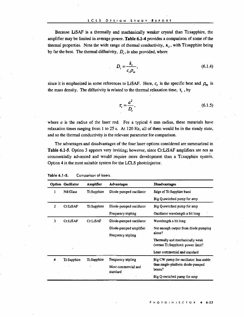
L C L S D E S I G N S T U D Y R E P O R T
Because LiSAF is a thermally and mechanically weaker crystal than Ti:sapphire, the
amplifier may be limited in average power. Table 6.1-4 provides a comparison of some of the
thermal properties. Note the wide range of thermal conductivity, Kt, with Ti:sapphire being
by far the best. The thermal diffusivity, Dt, is also provided, where
(6.1.4)
since it is emphasized in some references to LiSAF. Here, ct is the specific heat and pm is
the mass density. The diffusivity is related to the thermal relaxation time, tt , by
a (6.1.5)
where a is the radius of the laser rod. For a typical 4 mm radius, these materials have
relaxation times ranging from 1 to 25 s. At 120 Hz, all of them would be in the steady state,
and so the thermal conductivity is the relevant parameter for comparison.
The advantages and disadvantages of the four laser options considered are summarized in
Table 6.1-5. Option 3 appears very inviting; however, since CnLiSAF amplifiers are not as
commercially advanced and would require more development than a Ti:sapphire system,
Option 4 is the most suitable system for the LCLS photoinjector.
Table 6.
Option
1
2
1-5. Comparison of lasers.
Oscillator
Nd:Glass
CnLiSAF
Amplifier
TirSapphire
TirSapphire
Advantages
Diode-pumped oscillator
Diode-pumped oscillator
Frequency tripling
Disadvantages
Edge of TirSapphire band
Big Q-switched pump for amp
Big Q-switched pump for amp
Oscillator wavelength a bit long
CnLiSAF CnLiSAF Diode-pumped oscillator
Diode-pumped amplifier
Frequency tripling
Wavelength a bit long
Not enough output from diode pumpingalone?
Thermally and mechanically weak(versus TirSapphire): power limit?
Least commercial and standard
Ti:Sapphire Ti:Sapphire Frequency tripling
Most commercial andstandard
Big CW pump for oscillator less stablethan single-platform diode-pumpedboxes?
Big Q-switched pump for amp
P H O T O I N J E C T O R • 6-23

L C L S D E S I G N S T U D Y R E P O R T
6.2 Linac 0
6.2.1 Comments on Emittance Compensation
The beam will exit the electron gun with an energy of ~7 MeV. As explained in
Section 6.1, Emittance Compensation, the transverse emittance will already have grown
significantly, and is susceptible to additional growth. To maintain the high brightness of the
beam as extracted from the photocathode, emittance compensation will be employed to
minimize the integrated emittance of the beam at high energy [27]. Simulations with
PARMELA indicate that at 150 MeV, space-charge effects in the downstream drift and low-
energy dog leg are negligible.
Emittance compensation in photoinjectors has been subjected to an extensive analytical
treatment by Serafini and Rosenzweig [28]. The evolution of the beam dynamics for the
photoinjector can be described in four stages:
1. From the cathode to the end of the gun (i.e., to the second iris).
2. The drift space from the gun to the end of the gun solenoid.
3. The remaining drift space after the solenoid.
4. The following booster accelerator (Linac 0).
In each stage, the dominant forces acting on the beam—space charge, rf, and magnetic
field—can be analyzed to understand their effect on the correlated emittance. The analysis is
only valid in the regime for which four-dimensional laminarity holds. To provide optimal
emittance compensation, it has been shown that these forces should be arranged to match the
beam to the invariant envelope (IE). The conditions for satisfying the IE are analogous to
those for Brillouin flow—in fact identical in the absence of an rf accelerating field.
In the first stage, especially in the half-cell of the gun where the beam energy is still low,
the beam radius will expand rapidly due to the intense space-charge forces. However, since
laminarity is maintained, the resulting increase in the transverse emittance will be highly
correlated with axial position within the beam pulse. In fact, a given thin, longitudinal slice
will be expected to maintain its original uncorrelated (thermal) emittance. A sharp rise in the
magnetic field just after the cathode (which in turn requires the gun solenoid to be very close
to the cathode) and a strong accelerating gradient are essential to minimize the growth in
beam size.
In the second stage, the evolution of the beam size and emittance is reversed by the gun
solenoid. The solenoidal field must be strong enough to transform the diverging beam into
one that is convergent, overcoming as well the divergent kick received by the beam on exiting
the rf field, but not so strong as to destroy the laminarity of the beam. The laminarity is
irretrievably destroyed when particle paths cross, creating an uncorrelated group of particles
6-24 • P H O T O I N J E C T O R

L C L S D E S I G N S T U D Y R E P O R T
commonly described as a halo. Since the charge density at the temporal and spatial edges of
the pulse varies rapidly between the nominal value and zero, some beam crossover is
inevitable. Beam crossover in general can be minimized by two techniques: (1) use of a
uniform charge distribution at the cathode; and (2) use of a gentle convergence in stages 2
and 3.
Before describing stage 3, it is useful to state the desired condition for stage 4. In the
booster accelerator, the goal is to have the beam match the IE, for which case the phase-space
angle (in configuration space), 6 =)o'/o , is invariant with respect to the beam current and
equal to -f, and remains invariant during acceleration while the beam size and transverse
emittance adiabatically damp. (The prime refers to differentiation with respect to the axial
coordinate z.) Ideally, this process continues until the beam energy is high enough that the
space-charge forces can be ignored. In principle, a completely compensated integrated
emittance can be reached, that is, the original uncorrelated (thermal) emittance can be
restored and maintained.
The IE requires the beam be slightly convergent at the beginning of the booster
accelerator. This convergence is provided by the rf kick the beam receives at the entrance to
the booster accelerator if at the end of the drift the beam envelope is at a waist. A relatively
gentle waist is required to minimize crossover. To achieve the IE condition, the emittance
compensating solenoid must be confined to the gun area and adjusted to match at least one
longitudinal slice to the IE at the entrance of the booster accelerator. Those slices that are
slightly mismatched will undergo oscillations in the linac that will be damped as y ~i/2.
For specific photoinjector designs, simulations with PARMELA have been used to
confirm the general validity of this analytical approach [29]. Thus the analytical approach
promises to provide the guidance that will permit more rapid convergence with simulations to
a photoinjector design having minimum emittance.
The discussion above assumes continuous acceleration in a booster accelerator until
150 MeV is reached. But in fact four separate accelerating sections will be used. If two
sections are placed very close together, then presumably the increase in beam size and thus
also emittance between the two sections will be minimal and the beam will still be
approximately matched in the second section. However, it is possible not only to eliminate
the small deterioration of the beam between sections, but even to improve it by placing
another solenoid at the exit of a section followed by an appropriate drift. If this drift is
treated in a manner similar to stages 2 and 3 discussed above, then in fact the new waist at the
entrance to the second section will be smaller, and the resulting emittance of the beam
matched to the IE in the following sections will be lower than otherwise. In principle, one can
treat each of the three drift spaces between accelerating sections in this manner.
For a non-uniform temporal charge distribution at the cathode, rms emittance matching
provides perhaps the closest match for the largest portion of the beam [30]. For rms emittance
P H O T O I N J E C T O R • 6-25

L C L S D E S I G N S T U D Y R E P O R T
matching, the solenoidal field is adjusted to match a longitudinal slice close to one sigma in
the charge distribution to the IE. Since the motion of the other slices around the IE is stable,
one obtains an emittance correction that is optimum even though the correction for some
slices will not result in the real emittance minimum.
This discussion assumes that the initial solenoid is placed so that the axial field extends
from z « M2 to z = (7/4)/L Moving the solenoid downstream along the axis will allow the
beam to expand more than it would otherwise, resulting in beam oscillations. It is important
to keep the amplitude of these oscillations small, since whenever the beam oscillations leave
the linear (i.e., perturbative) regime, anharmonic components are introduced in the plasma
frequency (i.e., the frequency becomes dependent on the beam size) making it more difficult
to correct the emittance for the mismatched slices [31].
6.2.2 System Description
Linac 0 consists of four SLAC-type 3-m S-band accelerator sections, associated
solenoids, and necessary drift sections with diagnostics. It is preceded by the rf gun and
diagnostic section (see Section 6.1.1, RF Photocathode Gun) and followed by a second
diagnostic section and an achromatic bend system (the low-energy dog leg) and associated
instrumentation that brings the beam into Linac 1 (see Section 7.6.1, Low-Energy Dog Leg).
The overall layout of the photoinjector system is shown in Fig. 6.2-1. The overall length of
the photoinjector from the photocathode to the last accelerator section output flange is
15.8 m, including 4 drift sections of 75,47,105, and 105 cm respectively.
The rf distribution system is also shown in Fig. 6.2-1. Two unSLEDed 5045 klystrons are
required, one to power the gun and the first two 3 m sections and the other for the last two
3 m sections. As shown in the figure, high power rf phase shifters and attenuators will allow
the rf phase and amplitude for the rf gun and the first two 3 m sections to be controlled
independently.
Streak camera, screen,BPM, Toroid
BPM, current mon,Faraday cup, screen
BPM,profilemonitor
Matching & Diagnostics'E scraper
Mainlinac
Beam stopperToroid
\ Wire scanner
Screen
4-978253A1
X Vac valves
IS Solenoid
Attenuator
Phase Shifter
Figure 6.2-1. Overall layout of the LCLS pbotoinjector showing the rf gun, Linac 0, and the low-energy dog leg, with drift sections and diagnostics indicated.
6-26 • P H O T O I N J E C T O R

L C L S D E S I G N S T U D Y R E P O R T
The nearest klystron stations to the photoinjector are K20-3 and K20-4. Since these
klystrons will not be used by PEP-II, they can be rerouted to the LCLS photoinjector using
penetrations P20-5 and P20-7 respectively. In the future, should these stations need to be
restored to the 50-GeV linac, two of the downstream stations which will be permanently
liberated by the LCLS chicane installations can be moved with modest effort to be near
penetrations P20-8 and P20-9 and rectangular waveguide (RWG) of a reasonable length
installed to feed the rf gun and Linac 0.
The gun solenoid is 20 cm in length and is located 19.8 cm downstream of the
photocathode as shown in Fig. 6.1-3. Two linac solenoids, each 70 cm in length, are located
at the end of accelerating sections 2 and 3 respectively.
The beamline diagnostics upstream of Linac 0 are described in Section 6.1.1, Beamline.
In Linac 0, after each accelerator section there will be a BPM, a current monitor, and a
screen. In addition, between the second and third sections, an X-band cavity will be placed
alongside a-ceramic gap in the beamline. The charge-normalized rf intensity generated in this
cavity as an electron bunch passes can be used as an aid in minimizing the bunch length [32].
The beamline diagnostics downstream of Linac 0 are described in Section 7.7, Transverse
Emittance Diagnostics.
6.2.3 Emittance Compensation in Linac 0
Emittance growth in the photoinjector from the rf gun through the end of Linac 0 has
been studied using PARMELA simulations. The electric field map of the gun was obtained
with SUPERFISH and directly used in PARMELA. SUPERFISH was also used to simulate
the fields in the traveling-wave accelerating sections, and space harmonics were calculated to
be used in PARMELA. RF fields were assumed to be cylindrically symmetric, which seems
to be a reasonable assumption since, as discussed in Section 6.1.1, Symmetrization, the
dipole rf fields which are normally dominant in an rf gun will be largely eliminated in this
gun.
A magnetic field map for the solenoid magnets at the gun was produced using POISSON
and passed to PARMELA. The air core solenoids between the accelerator sections are
represented with single coils with appropriate strength to accurately represent the magnetic
field from each. The magnetic and electric fields in the gun and accelerator region were
adjusted to minimize the normalized emittance at 150 MeV. The peak electric field at the
cathode is 150 MV/m. The laser pulse is injected 57° ahead of the peak.
In the first two 3-m sections, where the gradient is 7 MV/m, a 1.5% energy spread for the
full beam is introduced to help in emittance compensation by placing the centroid of the beam
-5° ahead of the rf crest. This energy spread is removed in the last two 3 m sections, where
the gradient is 17 MeV/m, by phasing the rf such that the beam is slightly behind the crest.
P H O T O I N J E C T O R • 6-27

L C L S D E S I G N S T U D Y R E P O R T
The magnetic field in the emittance compensation solenoid at the gun is slightly less than
3 kG with an effective length of ~20 cm, while the solenoid between the accelerating sections
is slightly greater than 3 kG with an effective length of 70 cm.
The edge of the laser spot at the cathode will have a radius of -0.9 mm. The spot size is
dictated by trying to balance the effects of space charge and rf on emittance growth in the gun
itself. At the entrance to the third 3 m section, the beam energy is ~50 MeV so that space
charge effects are much reduced. On the other hand, the rf field gradient in this section is
more than double that of the previous two sections, so for this reason the beam radius is
purposely reduced—using a solenoid between the second and third 3 m sections—in order to
more nearly balance the space charge and rf effects on emittance growth.
The transverse charge distribution at the cathode is assumed to be uniform, but the
temporal shape will be a Gaussian with an rms sigma of 4.4 ps truncated at ±2 sigma,
resulting in an overall rms length of 3.8 ps. The use of a truncated Gaussian rather than a
uniform distribution is dictated by the beam dynamics of the downstream linac and
compressor systems. See Chapter 7.
A summary of the beam parameters at the end of Linac 0 based on PARMELA
simulations using the input parameters given in Table 62-1 is shown in Table 6.2-2. The
beam distribution predicted by PARMELA under these same conditions is shown in
Fig. 6.2-2.
Table 6.2-1 . Input Parameters for PARMELA Simulation.
Parameter
Bunch charge at cathode
Longitudinal charge distribution at cathode
Transverse charge distribution at cathode
Equivalent rms bunch length at cathode
Bunch radius at cathode
Peak rf field at cathode
injection phase
Gradient of accelerator sections 1 and 2
. Gradient of accelerator sections 3 and 4
Strength of gun solenoid
Strength of linac solenoids
Value
1.1 nC
Truncated Gaussian
Uniform
3.8 ps
0.9 mm HWHM
150MV/m
57° ahead of rf peak
7MeV/m
17 MeV/m
-3150G
-3300G
6 - 2 8 • P . H O T O I N J E C T O R
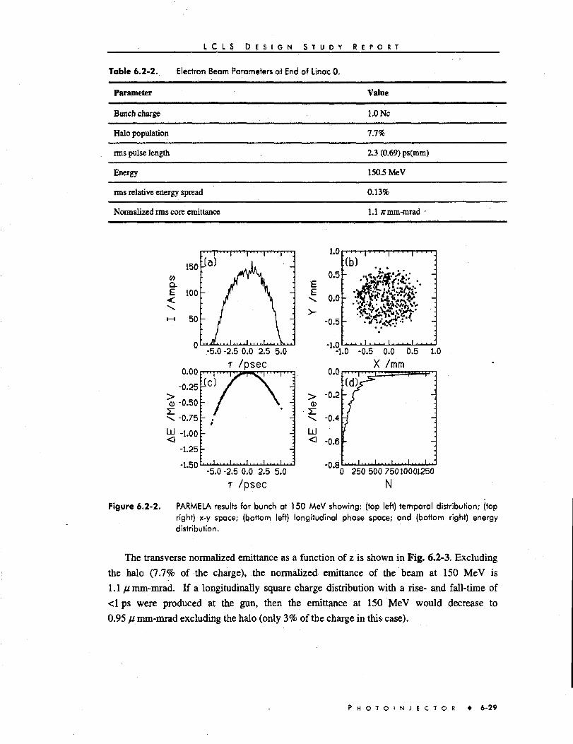
L C L S D E S I G N S T U D Y
Table 6.2-2. Electron Beam Parameters at End of Linac 0.
Parameter
Bunch charge
Halo population
rms pulse length
Energy
ims relative energy spread
Nonnalized rms core emittance
R E P O R T
Value
1.0 Nc
7.7%
2.3 (0.69) ps(mm)
150.5 MeV
0.13%
1.1 ffmm-mrad -
££
50
0
0.00
-5.0 -2.5 0.0 2.5 5.0
T /psec-1.0 -0.5 0.0 0.5 1.
X /mmo
-1.50-5.0 -2.5 0.0 2.5 5.0
T /psec
-0.80 250 500 75010001250
N
Figure 6.2-2. PARMELA results for bunch at 150 MeV showing: (top left) temporal distribution; (topright) x-y space; (bottom left) longitudinal phase space; and (bottom right) energydistribution.
The transverse normalized emittance as a function of z is shown in Fig. 6.2-3. Excluding
the halo (7.7% of the charge), the normalized emittance of the beam at 150 MeV is
1.1 //mm-mrad. If a longitudinally square charge distribution with a rise- and fall-time of
<1 ps were produced at the gun, then the emittance at 150 MeV would decrease to
0.95 [l mm-mrad excluding the halo (only 3% of the charge in this case).
P H O T O I N J E C T O R • 6-29

L C L S D E S I G N S T U D Y R E P O R T
CO
s&a
Figure 6.2-3.
15
33
Normalized emiftance (solid line) and rms beam size (dashed line) along the beamlinefrom the cathode (s=0) to 150 MeV at the end of Linac 0. The step at s~16 m is a7.7% halo cut (in simulation only).
6.3 References
1 D.T. Palmer**al., SPIE2522 (1995) 514.
2 K. Batchelor et al., Proceedings of the 2nd European Particle Accelerator Conference, EditionsFrontieres (1990), p. 541.
3 D.T. Palmer et al, Proc. of the 1995 Particle Accelerator Conference (1995), p. 982. In thisreference it is pointed out that the dipole emittance term has been suppressed by an order ofmagnitude to the level of 0.1 n mm-mrad, implying that in the unsymmetrized case the dipoleemittance term would be 1 n mm-mrad. See also B. Dwersteg et ai, "RF Gun design for theTESLA VUV Free Electron Laser," contributed to FEL '96, August 26-31, 1996, Rome, Italy.
4 In the case of the symmetrized gun being used at BNL, no significant dipole mode was found. Inthis case the adjustable short is used for diagnostic purposes only.
5 D.T. Palmer et al., Proc. of the 1995 Particle Accelerator Conference (1995), p. 982.
6 For the LCLS injector, energies above 150 MeV are taken to be high enough to eliminate theeffects of space charge. See Section 6.2.1.
7 B.E. Carlsten, Nucl. Instrum. andMeth. A 285 (1989) 313.
8 X. Qiu et al., Phys. Rev. Lett. 76 (1996) 3723.
9 I. Ben-Zvi (BNL), private communication (1997).
10 D.T. Palmer, "Emittance Studies of the BNL/SLAC/UCLA 1.6 cell Photocathode rf Gun,"contributed to the 17th IEEE Particle Accelerator Conference, Vancouver, B.C., Canada, May12-16, 1997.
11 D.T. Palmer et al., "Experimental Results of a Single Emittance Compensation SolenoidalMagnet", SLAC-PUB-7421, (May 1997), presented at the 17th IEEE Particle AcceleratorConference, Vancouver, B.C., Canada, May 12 -16,1997.
12 D.T. Palmer, "Emittance Studies of the BNL/SLAC/UCLA 1.6 cell Photocathode Gun," SLAC-PUB-7422 (May 1977), presented at the 17th IEEE Particle Accelerator Conference, Vancouver,B.C., Canada, May 12 -16,1997.
13 T. Srinivasan-Rao et al.,J. Appl. Phys. 69 (1991) 3291.
6-30 • P H O T O I N J E C T O R

L C L S D E S I G N S T U D Y R E P O R T •
14 P. Davis et al., Proc. of the 1993 Particle Accelerator Conference, p. 2976.
15 E. Chevallay et al., Nucl. Instrum. and Meth. A 340 (1994) 146.
16 D. Palmer, SLAC, private communication (1997).
17 The crest of the rf is defined as zero phase.
18 The gain per pass in Ti:sapphire amplifiers is sufficient to get from 1 nJ to a few mJ in eight (8)passes. For example, see S. Backus et al., Opt. Lett. 20 (1995) 2000.
19 P. Maine et al., IEEE J. Quantum Electron. QE-24 (1988) 398.
20 A.M. Weiner et al., J. Opt. Soc. B 5 (1988) 1563.
21 A.M. Weiner et al., Opt. Lett. 15 (1990) 326.
22 B.M. Van Wonterghem et al., Proc. of the Conference on Laser Coherence Control, SPIE 1870(1993) 64.
23 R.S. Craxton, Opt. Commun. 34 (1980) 474.
24 For ultrafast laser pulses, the effects of group velocity walkoff and nonlinear phase effects mustbe considered when designing the conversion stage.
25 H.-S. Albrecht et al., Appl. Opt. 32 (1993) 6659.
26 M.J.W. Rodwell et al. Opt. Lett. 11 (1986) 638; and M.J.W. Rodwell et al., IEEE J. QuantumElectronics 25 (1989) 817; also T. Kotseroglou et al, Nucl. Instrum. and Meth. A 383 (1996)309.
27 For the LCLS injector, energies above 150 MeV are taken to be high energy.
28 L. Serafini and J.B. Rosenzweig, Phys. Rev. E 55 (1997) 7565. A shorter version of this papermay be found in L. Serafini, "Overview on Production and Dynamics of High BrightnessBeams," presented at the IFCA Workshop on Nonlinear and Collective Phenomena in BeamPhysics, Arcidosso, IT, September 1-6,1996.
29 J.L. Coacolo et al., Proc. of the 1996 European Accelerator Conference, p. 1289.
30 L. Serafini, UCLA, private communication (March 1997).
31 Ibid., Serafmi.
32 R.H. Miller, "Proposed Bunch Monitor," SLAC TN-63-65 (1965).
P H O T O I N J E C T O R • 6-31

Accelerator
TECHNICAL SYNOPSIS
In order for the FEL to operate in the saturation regime with a 100 m long undulator, a
high electron peak current in a small transverse and longitudinal emittance is required. For
the LCLS operating at 1.5 A, the design values are a peak current of 3.4 kA with a transverse
normalized emittance of 1.5 it mm-mrad at 14,3 GeV. Since the rf photocathode gun can
produce 1 nC in a length of 3 psec rms, corresponding to a peak current of 100 A, the bunch
has to be compressed by a factor of about 30 before it enters the undulator. The compressors
consist of a series of magnetic chicanes, arranged and located such that the non-linearities in
the compression and acceleration process (longitudinal wakefields, rf curvature, and second
order momentum compaction) are partially cancelled. An optimum choice of parameters
compensates the correlated energy spread after the final compression and desensitizes the
system to phase and charge variations. The energy of the first compressor is 280 MeV. The
choice of energy for the first compressor is set by the need to minimize space charge effects at
the lower energy end, while the upper limit is set by the desire to compress the bunch early in
the linac to ease transverse wakefields. In the first compressor, the bunch length shrinks from
1 mm to 390 /urn rms. The second compressor produces a 20 pun bunch. The energy of the
second compressor, 6 GeV, was chosen as an optimum between the conflicting requirements
of longitudinal emittance dilution due to synchrotron radiation effects and longitudinal
wakefields. The design of the second compressor is set by the need to reduce coherent
synchrotron radiation effects, which is most pronounced for short bunches. Since the energy
spread generated by the coherent synchrotron radiation is correlated along the bunch, its
effect on the transverse emittance is compensated by introducing a double chicane and
optical symmetry to cancel longitudinal-to-transverse coupling. With the double chicane
compensating scheme, the emittance growth in the LCLS, due to coherent synchrotron
radiation, is expected to be 3-5%. Simulations have also been made which calculate
emittance dilution effects in the linac due to transverse wakefields and anomalous momentum
dispersion, each of which arise with component misalignments. These simulations include
realistic correction techniques and successfully demonstrate the level of transverse emittance
preservation required.
7.1 Introduction and Overview
In order to reach photon power saturation in a reasonable length undulator, a high
electron peak current is required. For a 1.5 A LCLS with transverse normalized emittances of
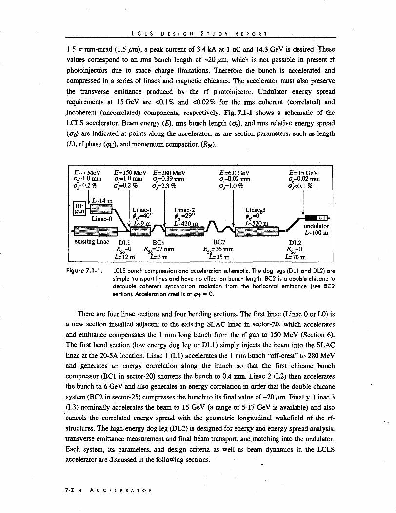
I C L S D E S I G N S T U D Y R E P O R T
1.5 /rmm-mrad (1.5 //m), a peak current of 3.4 kA at 1 nC and 14.3 GeV is desired. These
values correspond to an rms bunch length of -20 /im, which is not possible in present rf
photoinjectors due to space charge limitations. Therefore the bunch is accelerated and
compressed in a series of linacs and magnetic chicanes. The accelerator must also preserve
the transverse emittance produced by the rf photoinjector. Undulator energy spread
requirements at 15 GeV are <0.1% and <0.02% for the rms coherent (correlated) and
incoherent (uncorrelated) components, respectively. Fig. 7.1-1 shows a schematic of the
LCLS accelerator. Beam energy (£), rms bunch length (<xz), and rms relative energy spread
(as) are indicated at points along the accelerator, as are section parameters, such as length
(L), rf phase (^f), and momentum compaction (R56).
E~l MeVo-1.0 mm
£=150 MeV £=280 MeVa =1.0 mm 0^=0.39 mm
£=6.0 GeVoz~0.02 mm
°£=15 GeVOj-0.02 mm^ 0 1 %
RFgun Linac-1
°
iexisting linac
Linac-2
L~420m
Linac53
L~520m undulatorL~100m
BC1#,,=27 mm
JO
i=3m
BC2/?56=36 mm
1=35 m
DL2
V°£=70 m
Figure 7.1-1. LCLS bunch compression and acceleration schematic. The dog legs (DLl and DL2) aresimple transport lines and have no effect on bunch length. BC2 is a double chicane todecouple coherent synchrotron radiation from the horizontal emittance (see BC2section). Acceleration crest is at prf = 0.
There are four linac sections and four bending sections. The first linac (Linac 0 or L0) is
a new section installed adjacent to the existing SLAC linac in sector-20, which accelerates
and emittance compensates the 1 mm long bunch from the rf gun to 150 MeV (Section 6).
The first bend section (low energy dog leg or DLl) simply injects the beam into the SLAC
linac at the 20-5A location. Linac 1 (LI) accelerates the 1 mm bunch "off-crest" to 280 MeV
and generates an energy correlation along the bunch so that the first chicane bunch
compressor (BC1 in sector-20) shortens the bunch to 0.4 mm. Linac 2 (L2) then accelerates
the bunch to 6 GeV and also generates an energy correlation in order that the double chicane
system (BC2 in sector-25) compresses the bunch to its final value of -20 /im. Finally, Linac 3
(L3) nominally accelerates the beam to 15 GeV (a range of 5-17 GeV is available) and also
cancels the correlated energy spread with the geometric longitudinal wakefield of the rf-
structures. The high-energy dog leg (DL2) is designed for energy and energy spread analysis,
transverse emittance measurement and final beam transport, and matching into the undulator.
Each system, its parameters, and design criteria as well as beam dynamics in the LCLS
accelerator are discussed in the following sections.
7-2 A C C E L E R A T O R

L C L S D E S I G N S T U D Y R E P O R T
7.2 Compression and Longitudinal Dynamics
To achieve the high peak current and small energy spread in the undulator, the bunch
must be compressed in a series of magnetic chicanes. These are arranged and located such
that non-linearities in the compression and acceleration process (longitudinal wakefields, rf
curvature, and second order momentum compaction) are partially canceled. With a careful
arrangement of compression and acceleration parameters, the bunch compression process can
be made more linear, which reduces the minimum bunch length achievable. An optimum
choice of parameters compensates the correlated energy spread after final compression and
desensitizes the system to phase and charge variations.
7.2.1 Bunch Compression Overview
The bunch is compressed by accelerating with an off-crest rf phase, thereby introducing a
correlated energy spread along the bunch. This process is followed by a bending section with
linear path length dependence on particle energy. The final energy (£/•) of a particle, which is
at axial position z,- with respect to bunch center, after nominal acceleration from £,o to EJQ at
an rf phase <p0 (crest at q>o = 0 and q>0 * ;r/2) is given by
1 J COS^0
with A<p as a phase error and X the rf wavelength. The relative energy deviation after
acceleration, Sf = (£/ -EfO)/E/o, is then
Ei0 I cos{(p0 +A<p)-{2nZi/A)sm{<p0 +A<p) \ , , . „
EfQ
where Si s (£, -£ , 0 ) /£ /o represents small injection energy deviations scaled to the final
energy. Wakefields are ignored and it is assumed that zt« Allx. From the approximate linear
energy dependence, coefficient is defined as
Ef0
After a bending section with path length dependence, /?56, where z/ = zi + Rs6Sf, the final
bunch length, &zf, and energy spread, o$f, are functions of the initial bunch length, aZj, and
energy spread, as,, (assuming {ziSj} = 0).
A C C E L E R A T O R • 7-3
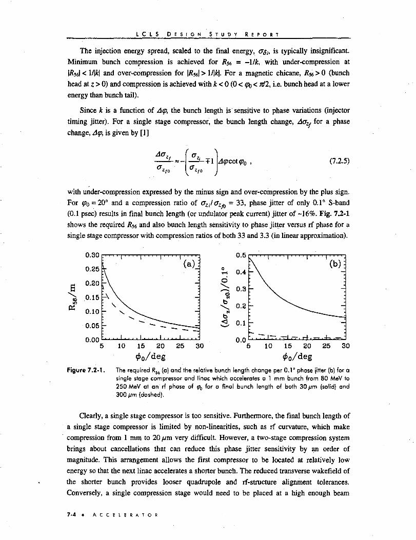
L C L S D E S I G N S T U D Y R E P O R T
The injection energy spread, scaled to the final energy, as,, is typically insignificant.
Minimum bunch compression is achieved for R$f, = —Ilk, with under-compression at
|/?56| < l/|fc| and over-compression for |/?56| > l/|fc|. For a magnetic chicane, Rse > 0 (bunch
head at z > 0) and compression is achieved with it < 0 (0 < <fo < nil, i.e. bunch head at a lower
energy than bunch tail).
Since k is a function of A<p, the bunch length is sensitive to phase variations (injector
timing jitter). For a single stage compressor, the bunch length change, AaZf for a phase
change, Aq>, is given by [1]
Aa,•+1 (7.2.5)
with under-compression expressed by the minus sign and over-compression by the plus sign.
For <po = 20° and a compression ratio of aZilaZfi = 33, phase jitter of only 0.1° S-band
(0.1 psec) results in final bunch length (or undulator peak current) jitter of -16%. Fig. 7.2-1
shows the required Rs6 and also bunch length sensitivity to phase jitter versus rf phase for a
single stage compressor with compression ratios of both 33 and 3.3 (in linear approximation).
to
0.30
0.25
0.20
0.15
0.10
0.05
0.0010 15 20 25 30 10 15 20 25 30
Figure 7.2-1.
0o/degThe required RS6 (a) and the relative bunch length change per 0.1° phase jitter (b) for asingle stage compressor and linac which accelerates a 1 mm bunch from 80 MeV to250 MeV at an rf phase of % for a final bunch length of both 30 jum (solid) and300 fim (dashed).
Clearly, a single stage compressor is too sensitive. Furthermore, the final bunch length of
a single stage compressor is limited by non-linearities, such as rf curvature, which make
compression from 1 mm to 20 //m very difficult. However, a two-stage compression system
brings about cancellations that can reduce this phase jitter sensitivity by an order of
magnitude. This arrangement allows the first compressor to be located at relatively low
energy so that the next linac accelerates a shorter bunch. The reduced transverse wakefield of
the shorter bunch provides looser quadrupole and rf-structure alignment tolerances.
Conversely, a single compression stage would need to be placed at a high enough beam
7-4 • A C C E L E R A T O R

L C L S D E S I G N S T U D Y R E P O R T
energy so that space charge forces are not significant for a 20 pm bunch. This system
prolongs the acceleration of a long bunch (~1 mm) through more linac, which tightens
alignment tolerances. For these reasons, a two-stage compressor is used.
The linear relations for a two-stage bunch compression system are similarly expressible.
For a first linac which accelerates from Eo to E\ at rf phase q>i followed by a first compressor
with /?56 = a\, then a second linac which accelerates from E\ to E% at rf phase <pi followed by
a second compressor with /?56 = 02, the final bunch length, azv and energy spread, 0$ , are
approximately
a **J[(l+alki)(l+a2k2)+a2klEi/E2]2<rl+[a1(l+a2k2)EQ/E1 +a2E0/E2]
2cl ,(7.2.6)
In this case, os0 is the relative energy spread at injection to the first linac (at energy £0)
and crZo is the initial bunch length there. Note, k\ is a function of the rf phase and initial and
final energies of Linac 1 as in Eq. 7.2.3. The value for &2, however, depends on the total
phase error, which may have contributions from both Linac 1 and Linac 2.
2
It appears that the above relationships can be used to find a minimum final bunch length
sensitivity to injection phase jitter, A<(>\. In fact, longitudinal wakefields, rf curvature, and
second order path length dependence, T^, complicate these calculations sufficiently to
invalidate this simple linear model. The above relationships can help to understand
sensitivities, but the optimum stability is best found with a complete computer simulation that
includes all non-linearities (see Section 7.2.3).
7.2.2 Parameters
The final design parameters for the LCLS two-stage bunch compression system are
summarized graphically in Fig. 7.1-1 and numerically in Table 7.2-1 below.
A string of three linacs and two chicane sections are used to compress a 1 mm rms bunch
at 150 MeV to 20 fim at 15 GeV. The final bunch is slightly under compressed, so it is
actually possible to compress it even further. However, many severe challenges arise with a
shorter bunch, such as coherent synchrotron radiation in BC2 (see Section 7.4) and resistive
wall and vacuum chamber roughness wakefields in the undulator (see Section 8.7). These
effects can quickly become intolerable as the bunch further shortens. Therefore the final
compression is limited to no less than ~20 //m rms. This achieves the 3.4 kA peak current
required and yet allows management of these micro-bunch limitations. A longer bunch is also
A C C E L E R A T O R • 7-5

t C L S D E S I G N S T U D Y R E P O R T
operationally possible if the transverse "slice" emittance achieved is less than 1.5 ;rmm-mrad
(e.g., 35 //m at 1.1 *rmm-mrad, see Fig. 5.5-1).
Table 7.2-1 . LCLS bunch compression and acceleration parameters per beamline section.
Beamline
Linac 1
BC1
Linac 2
BC2
Linac 3
GeV
0.15
0.28
0.28
6.0
6.0
GeV
0.28
0.28
6.0
6.0
15.0
mm
1
1
0.39
0.39
0.02
mm
1
0.39
0.39
0.02
0.02
r0.2
2.3
2.3
1.1
1.1
OS-out
2.3
2.3
1.1
1.1
<0.1
<Prt
deg
40
—
29
—
0
mm
—
27.0
—
35.5
—
For this ultra-relativistic beam, the bunch length cannot change through a linac
(excluding L0), and the energy spread does not significantly change through the chicanes.
Phase and current jitter tolerances are described in Section 7.2.4.
The first compression is from 1 mm to 390 jum. This is near the limit set by non-
linearities due to 7566 and S-band rf. A shorter bunch is possible, but larger energy tails are
generated at 15 GeV. This choice, for the parameters of Table 7.2-1, also best minimizes
final bunch length sensitivity to injector timing jitter. Finally, the chosen value of 390 pm
also optimally scales the longitudinal wakefield in Linac 2 so that a cancellation is established
between the Linac 2 wake and the non-linearities (rf curvature and r566) of the Linac 1/BC1
pair. The parameters are not a unique solution but represent a workable set. A qualitative
summary of the effects of changes to the critical compression parameters is listed in
Table 72-2. The two /?56 values are not considered free parameters here since their values
depend on rf phases and other factors.
The lower limit on the choice for BC1 energy is set by space charge forces of the shorter
bunch with 280 MeV at a safe energy. The upper limit is set by the desire to initially
compress the bunch early in the linac to ease transverse wakefields. The chosen energy of
280 MeV also desensitizes the system to injector timing jitter and is a practical solution for
LI, which consists of three 3-meter S-band sections at an rf phase of 40° and a gradient of
19 MV/m. The location (energy) of BC2 is set by the need to produce a very small energy
spread at 15 GeV. This involves a balance between the longitudinal geometric wakefield in
L3 (scales with Linac 3 length) and the S-z correlation just after BC2. Simulations with BC2
at the 6 GeV location (described below) produce the required beam conditions at 15 GeV.
Other factors, including synchrotron radiation, are discussed in more detail in Section 7.4
(BC2) and Section 7.5 (BC1).
7-6 • A C C E L E R A T O R

L G L S D E S I G N S T U D Y R E P O R T
Table 7,2-2. Bunch Compression Parameter Trade-Offs: A qualitative summary of the effects of
changes to the bunch compression parameters. Only limitations are noted. An
"increase" of rf phase, f, refers to moving farther off rf crest and 0^ is the
intermediate bunch length (after BC1).
Parameter Increase Parameter Decrease Parameter
az = 390 pm • Insufficient L2 wake compensation for
L1/BC1 non-linearities.
• Can increase timing jitter sensitivity.
• Reach BC1 compression limit—bunch begins to
fold over itself.
• Can increase timing jitter sensitivity.
| = 40° • Increased LI & L2 energy spread.
• Inefficient acceleration.
• Increased rf curvature non-linearity.
• Increased BC1 strength and Ae due to coherent
synchrotron radiation (CSR).
29° * Energy spread too large for cancellation
with L3 wake.
• Inefficient acceleration.
• Energy spread too small—over-compensated
with L3 wake.
• Increased BC2 strength and CSR Ae.
E = 280 MeV * Longer LI—> stronger LI transverse
wakes and increased LI Ae.
• Can increase timing jitter sensitivity.
• Smaller kl—> increase BC1 chicane strength
and CSR Ae.
> Increased space charge forces.
• Increase BC2 Ae due to incoherent
synchrotron radiation or must lengthen
BC2.
• Shorter L3—> insufficient L3 wake for
L2 energy spread compensation.
• Longer L3—> L3 wake too large— over-
compensation of L2 energy spread.
• Shorter L2—> insufficient L2 wake
compensation for L1/BC1 non-linearities.
7.2.3 Longitudinal Wakefields and Non-linearities
Geometric Wakefields
In this section the asymptotic longitudinal geometric wakefield is used in a full tracking
simulation. A more detailed description of the wakefields for the SLAC S-band accelerating
structures as well as a justification for the use of the asymptotic wake is given in Section 7.8.
The simulation [2] includes non-linearities such as 7566, longitudinal geometric wakefields of
the rf-structures, and sinusoidal rf curvature and proceeds from the LCLS injector to the
undulator entrance. Transverse effects do not generally couple back into the longitudinal
plane and so are ignored here. The simulation also ignores space charge effects since the
compression process takes place at energies above 150 MeV.
Figure 7.2-2 shows the longitudinal phase space, energy distributions, and axial (z)
distributions at various points in the compression process. The longitudinal phase space at
150 MeV used in the simulations is similar in both distributions and correlation to the output
of space-charge dominated injector simulations using PARMELA [3], The input beam used is
gaussian cut at ±2(7in energy and axially with a 1 mm rms bunch length and 0.2% rms energy
spread (after cuts) at 10 MeV and a bunch population of 6.3xl09 (after cuts). The axial
distribution is a truncated gaussian, in order to minimize final bunch length sensitivity to
injector timing jitter (see Section 7.2.4). Simulations using an initial uniform distribution
A C C E L E R A T O R 7-7

L C L S D E S I G N S T U D Y R E P O R T
show more severe sensitivities to jitter by up to a factor of three. This choice represents a
compromise between jitter sensitivity and transverse emittance compensation in the injector.
As Fig. 7.2-2 shows, the compression process has been arranged so that non-linearities
such as rf-curvature and wakefield effects cancel, leaving a flat energy profile at 15 GeV. The
final rms bunch length is 18 fim with >3.4 kA of peak beam current all along the bunch. Long
tails exist in the energy distribution (shown at bottom right of Fig. 72-2). The core of the
beam, however, has an rms energy spread of 0.035% with 85% of the particles contained
within a ±0.15% energy window. The remaining 15% of the beam has been cut out of
Fig. 7.2-3 (15 GeV) to show the core beam more clearly while all particles are shown in
Fig. 7.2-2. Note, the incoherent component of the final energy spread at any particular slice
of the bunch core is <0.01 % rms.
Figure 7.2-4 shows a progression of longitudinal phase space, on a fixed scale, through
each compressor. The S-band rf and TS66 quadratic curvature of L1/BC1 can be seen in
Fig. 7.2-4(a-b). Wakefields in L2 produce mostly a quadratic curvature see in (c). Some of
the curvature is cancelled by the T566 of BC2, but the tail of the bunch (right side) is over-
compressed (see 6 GeV S-z plot of Fig. 7.2-2) leading to the large spike in the z-distribution
of Fig. 7.2-3 (upper right). Finally, the longitudinal wakefield of L3 flattens most of the
coherent energy spread into the core distribution of Fig. 7.2-3 (lower right). This is a critical
cancellation which provides the narrow energy spread and depends on the strength of the
longitudinal wakefield in L3, the rf phase of L2, and the bunch length in L2.
Calculations of the longitudinal wakefield for the micro-bunch in L3 are believed to be
accurate to -10% (see Section 7.8). In order to allow for this potential error in the magnitude
of the wakefield, the compression systems require a range over which it may be tuned. To
demonstrate the tuning range required, a simulation was also run where the wakefield in L3
was arbitrarily scaled up by a factor of 1.5 and the BC2 /?56 and L2 rf phase were re-tuned.
For this extreme case, the bunch length and energy spread at the end of L3 are still
recoverable to the conditions of Fig. 7.2-3. The re-tuning produces an increase of the L2 rf
phase (29°-»34°: farther off crest) and decreased BC2 R56 (35.5 mm—>28.2 mm: a weaker
chicane). Note, this is a desirable condition since a higher bunch charge will also increase the
L3 wakefield, but the BC2 chicane bends are then reduced in strength. A weakened chicane
matches a higher bunch charge, and the effects of coherent synchrotron radiation in BC2 are
then, for small changes, nearly independent of charge.
Resistive Wall Wakefields
In addition to geometric longitudinal wakefields, the micro-bunch in L3 and beyondexperiences a longitudinal resistive wall wakefield which also introduces a coherent energyspread along the bunch. For the linac and transport lines leading up to the undulator, this is asmall effect and is described in detail in Section 7.8. The rms relative energy spread inducedby the resistive wall effect in the accelerator and the transport lines prior to the undulator isexpected to be ~0.02% (see Fig. 7.8-6). The associated transverse wakefields areinsignificant.
7-8 • A C C E L E R A T O R
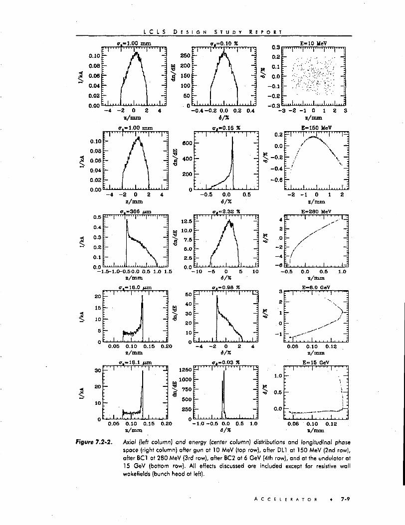
L C L S D E S I G N S T U D Y R E P O R T
1.00 mm g«=0.10
0.00
0.5
0.4
0.3
0.2
0.1
n n
. I , , , . , M 1r1"! ""1—
'- '
'-
'—•.... 1 , . . . 1
= 3 8 6 f u n. . . | . . . , | . . . . | . . L J .
- :
^\. i
... i.... i., .Y..;-1.5-1.0-0.50.0 0.5 1.0 1.5
z/mm
20
15
10
5
0
:• • I
: |
a. -18.01
fun• r '
. i . . j0.05 0.10 0.15
z/mm0.20
A1 " ' 1':
. . . . 1 .i-0.4-0.2 0.0 0.2 0.4
6/Xgj-0.15
12.5
10.0
7.5
5.0
2.5n n
g,=2.32 %E l " ' " 1 1 ' ' ' ' 1 ' '
r / \
% i i hi
1:
—.—.
111=0
6/%10
!
50
40
30
20
10
g4-0.98 %r1 '
Mill
-'—
I I Vz
i 1
11
i
(T
ill
J
- 4 - 2
10 -—
g4=0.03
" I 1 " 1
V M
%' 1"
11. II1 f
0.3
0.2
0.10.0
-0.1-0.2-0.3
E=10:""l""r
11
11
1
i-
iMeV Jl lip
11
11
1
•Us .';':.- :
*'•• ? V *. -
. . . 1 . . . , ! . . . ;- 3 - 2 - 1 0 1
z /mm2 3
0.2
0.0
-0 .2
-0 .4
-0 .6
E=
:— /: /— /
—.
—
:".!.... 1.
150 MeV
—
\ in, -
—
. . ! . . . . I . . . . T . :- 2 - 1 0 1
z/ram
4
2
0
-2
-4
- 6
:—
\-: /- /L./I 1
E=280• | • • •
. 1 . , ,
MeVi ' • •;. u
-4• 11 • i ri1 11
1 . . , , IT=
-0.5 0.0 0.5z/ram
6.0 GeV
1.0
0.0B 0.10 0.12z/mm
1.0
0.5
0.0
E=15
—
: . T 7 7 . " f ,
GeV
. -
\t
. . . i . . . :0.05 0.10 0.15
z/mm0.20 -1.0 -0.5 0.0 0.5 1.0
6/%0.08 0.10 0.12
z/mm
Figure 7.2-2. Axiol (left column) ond energy (center column) distributions and longitudinal phasespace (right column) after gun at 10 MeV (top row), after DLl at 150 MeV (2nd row),after BC1 at 280 MeV (3rd row), after BC2 at 6 GeV (4th row), and at the undulator at15 GeV (bottom row). All effects discussed are included except for resistive wallwakefields (bunch head at left).
A C C E L E R A T O R 7-9
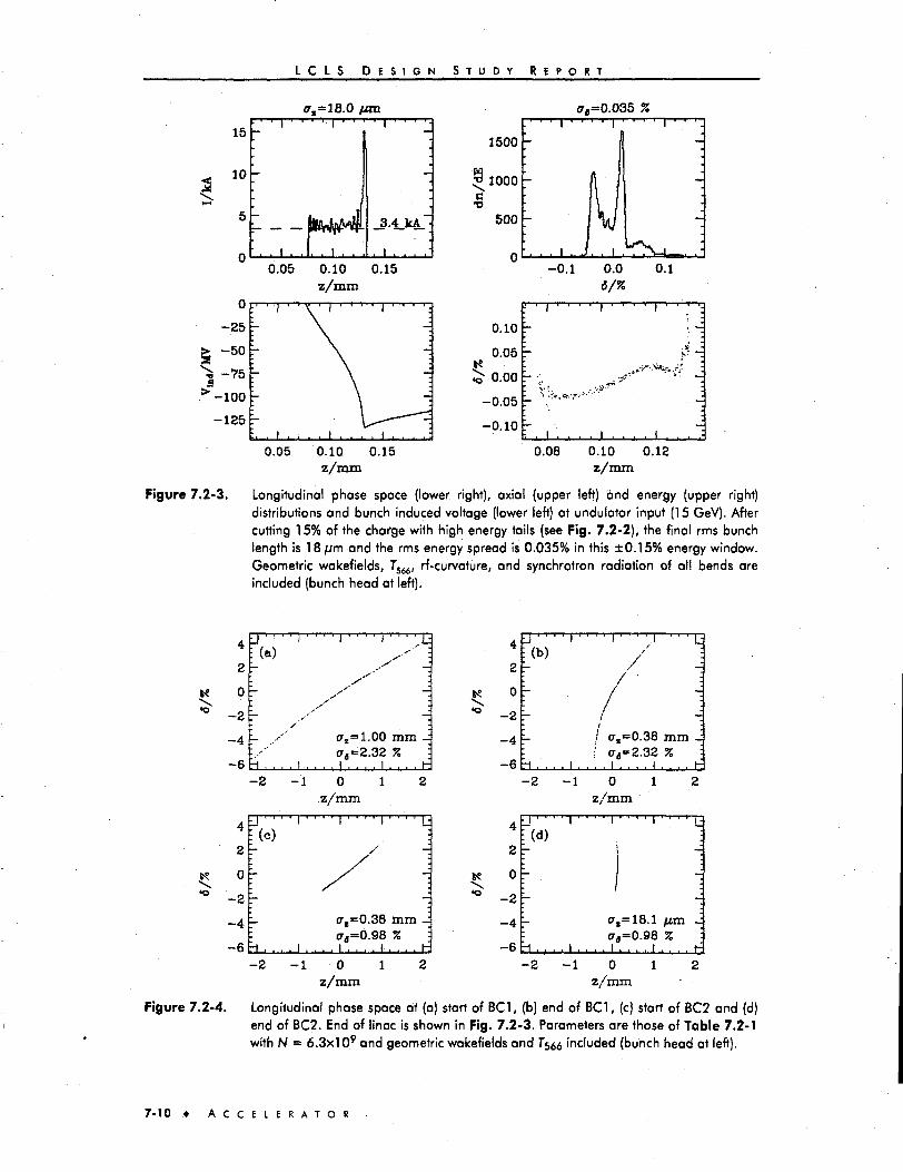
L C L S D E S I G N S T U D Y R E P O R T
15
10
5
n
-
-
• i 1
=18
1
. 0 A
4
an-
-
_3.4_kA_"
. 1 . . . .'
ct=*0.035
0.05 0.10 0.15z/mm
0.05 0.10 0.15z/mm
0.10 r
0.05
5- o.oo-0.05
-0.10
:' ' 1
[
', . 1
' I
V'''*
• ( • • • ' .
^ / ]-
, \ . . . . ' •
0.08 0.10 0.12z/mm
Figure 7.2-3. Longitudinal phase space (lower right), axial (upper left) and energy (upper right)distributions and bunch induced voltage (lower left) at undulator input (15 GeV). Aftercutting 15% of the charge with high energy tails (see Fig. 7.2-2), the final rms bunchlength is 18 fim and the rms energy spread is 0.035% in this ±0.15% energy window.Geometric wakefields, TS64, rf-curvature, and synchrotron radiation of all bends areincluded (bunch head at left).
4
2
0
- 2
- 4
- 6
r
r
ri . .- 2
4
2
0
- 2
- 4
- 6
r
rt , . .- 2
' I • ' ' ' I ' '
. 1 . . . . I . .
-1 0z/mm
• I ' ' • • I ' •
y
/
' 1
.00
.32I1
1 1
(Tx=0.38cr,,=0.98
. 1 . . . . 1 . . . . 1-1 0
z/mm1
1 I'M-i
-imm -
. . . . h2
1 1 L
- •
-i
-imm -
. . . h2
4
2
&? 0
10 - 2
- 4
- 6
4
2
^ 0
* - 2
- 4
- 6
-
'-
h . .- 2
-_\ • •
r
'-
- 2
1 1 I '
. . I .
- 1
. , I .
- 1
. . , I . . .
/
/
I
i at=0.i cd=2
. . . I . . .0
z/mm• • • I • • '
.1
3832
11
' 1
£ r , = 0 . 9 8. . . 1 . , . . I
0z/mm
1
mm -% :. . , . f
2
1 ' " L
-;
-;
-ifj,m -
. . . t -
2
Figure 7.2-4. Longitudinal phase space at (a) start of BC1, (b) end of BC1, (c) start of BC2 and (d)end of BC2. End of linac is shown in Fig. 7.2-3. Parameters are those of Table 7.2-1with N - 6.3x10⁹ and geometric wakefields and Ts66 included (bunch head at left).
7-10 • A C C E L E R A T O R

L C L S D E S I G N S T U D Y R E P O R T
7.2.4 Beam Jitter Sensitivities
Although it has been optimized, the two-stage compressor is still quite sensitive to beam
phase and bunch population jitter. Fig. 7.2-5 shows the peak current (/ «= l/<%) variation
versus relative bunch population, AN/No, and timing (phase), T, jitter at the injector.
Table 7.2-3 lists tolerances for rf phases, chicane bend power supplies and energy jitter for
LI, L2, BC1 and BC2. Each tolerance corresponds to a 10% rms bunch length variation.
These tolerances represent jitter that is too fast to be corrected with feedback.
0.30
0.25
0.20
0.15
0.10
0.05
0.00
- 4
-
: 1 . .
- 2 0AN/N0 /?
<d)
i - 0 "*. . i . . . . i . . .
2rB
' 1 ' '
. 1 . .
4
' ' I :
-;
. . 1 i
Figure 7.2-5.
- 4 - 2 0 2 4AN/N0 /%
Relative peak undulator current, I/IQ, and FWHM relative energy spread versus bunchpopulation jitter, 4N/N0 , and timing jitter, 7, at injector (No = 6.3x10⁹, /0 " 3-5 kA,<7zo = 1 8 pm). Geometric wakefields, T^ and rf-curvature are all included.
The pulse-to-pulse rf phase tolerances per linac are quite tight. However, the common
mode phase tolerance for the entire system is an order of magnitude looser. The gun timing
jitter tolerance of 0.8 psec rms has been optimized assuming a gaussian axial distribution at
the gun cut at ±2<j(see top of Fig. 7.2-2). When new compression parameters are set up for a
uniform gun distribution, however, the best timing jitter tolerances found are more than a
factor of two tighter than for the gaussian case.
A C C E L E R A T O R 7-n

L C L S D E S I G N S T U D Y R E P O R T
Table 7.2-3. Individual tolerances to provide <10% bunch length (or peak current) jitter. Timingjitter with a gaussian distribution is assumed for the quadratic x sensitivity where amean bunch length increase of 7% is also produced. All other sensitivities are linear.The LI rf phase tolerance increases to 0.64° when the beam energy at BC1 is heldconstant (e.g., using a feedback system).
Parameter
LI rf phase
L2rfphase
LI, L2, L3 common rf phase
BC1 chicane bend supply
BC2 1st chicane supply
BC2 2nd chicane supply
LI final energy jitter
L2 final energy jitter
Gun timing jitter
Initial bunch population jitter
Symbol
An
AC
A f l « A B = AG
ABl/Bl
AB21/B21
AB22IB22
AEXIE\
AE2IE2
X
AN/N
Unit
deg
deg
deg
%
%
%
%
%
psec
%
nns Tolerance
0.14
0.13
0.8
0.24
0.70
4.80
0.28
0.52
0.80
2.9
7.2.5 Energy Management and Overhead
Each linac section must operate with several spare klystrons to accommodate their
inevitable failure rate (except LI, which operates on just one klystron). Table 7.2-4 lists, for
each LCLS linac section, the total number of klystrons potentially available, Ng, the number
of klystrons held in reserve, NR, the maximum rf phase anticipated (a worst case estimate to
include a tuning range), | $ m a x ' the average energy gain per klystron, {AE)K, the beam
loading energy loss, AEB, and the resulting maximum energy achievable, £max, (assuming an
injection energy, £,).
Table 7.2-4. Energy monagement parameters for the three linac sections. The average energy gainis based on 19.3 MV/m and all existing linac structure lengths and also includes theshortening of two 3-meter LI sections and removal of three BC2 sections and the 20-5A section.
Linac
LI
L2
L3
1
34
45
0
4
5
ifima*
deg
45
34
0
MeV
192
230
228
MeV
1
30
63
GeV
0.15
0.28
6.00
GeV
0.285
5.97
15.1
7-12 A C C E L E R A T O R

L C L S D E S I G N S T U D Y R E P O R T
The maximum energy achievable per linac is calculated using
B . (7.2.8)
where the beam loading is based on a bunch population of 6.3 x 10⁹, LCLS bunch lengths,
and a nominal rf accelerating gradient of 19.3 MV/m. For the average energy gain
calculation, all existing linac structure lengths are used allowing for the required shortening
of two 3 meter LI sections and the removal of both the 20-5A section and the three 3 meter
sections for BC1. Note, the rf phases used here are larger than nominal to provide some
tuning range, and still a reasonable 12% of available klystrons are held in reserve.
These calculations include the necessary modifications of the existing SLAC linac (BC1
and BC2 insertions) which will eliminate four klystrons. This will nullify 910 MeV of
unloaded energy gain. Other accelerating structure modifications and removals (DL1
insertion, LI quadrupole additions and L2 wire scanners) will forego another 150 MeV for a
total loss of 1.06 GeV of unloaded energy gain (with respect to the pre-LCLS linac). For
future non-LCLS linac operation this energy is not easily recovered; however, the maximum
energy available is still within ~1 GeV of the pre-LCLS bnac maximum energy of -50 GeV.
7.3 Transverse Linac Beam Dynamics
The LCLS accelerator is composed of four separate S-band linac sections (L0, LI, L2,
and L3) each of which require individual lattice designs in order to best minimize transverse
emittance dilution due to transverse wakefields and momentum dispersion, both of which are
generated through component misalignments. Each section has its own particular beam
parameters which motivate the optical design of that linac. For example, a large beam energy
spread and short bunch length suggest weak focusing with large quadrupole spacing.
Table 73-1 summarizes the four linacs and their various beam parameters. The final energy
of L3 is also variable from 5 to 17 GeV through appropriate phasing and rf power. The rf
phase angles of the various linacs as well as motivations for the length of each linac section
are discussed in the section on bunch compression and longitudinal dynamics.
Table 7 . 3 - 1 . Beam parameters of the four separate S-band linac sections at ~ 1 9 MV/m.
Beam Parameter
Initial energy
Final energy
Active linac length
rf phase (crest at 0)
Initial rms energy spread
Final rms energy spread
rms bunch length
Unit
GeV
GeV
m
deg
%
%
mm
L0
0.007
0.150
12
variable
0.2
0.2
1.0
LI
0.150
0.280
9
40
0.2
2.3
1.0
L2
0.280
6.0
420
29
2.3
1.1
0.39
L3
6.0
5-17
523
0
1.1
<0.1
0.020
A C C E L E R A T O R • 7-13

L C L S D E S I G N S T U D Y R E P O R T
7.3.1 The LO Linac
A description of the LO linac is given in Chapter 6. LO provides the initial acceleration
and transverse emittance compensation from the if gun. It is a new beamline constructed
parallel to the existing SLAC linac in sector-20 displaced approximately 1 meter horizontally.
It is composed of four 3 meter acceleration sections that need no quadrupole magnets. It is a
space charge dominated system. Following LO is an adjustable matching section and a
transverse emittance diagnostic section, EDO (see Section 7.7.1 and Fig. 7.6-1). The first dog
leg, DL1 (see Section 7.6.1), then bends the beam onto the main SLAC linac axis and into the
LI linac section at the 20-5A location. The existing 3 meter rf-section there is removed to
provide space for DL1 injection.
7.3.2 The LI Linac
LI initiates the compression process by accelerating off crest, thereby generating the
necessary energy-z correlation so the first chicane, BC1, will compress the bunch. LI is
composed of three existing 3 meter linac structures 20-5B, 20-5C, and 20-5D (20-5A is
removed in order to inject). Because of the large rf phase angle and the long bunch, the rms
energy spread in LI rapidly increases from 0.2 to 2.3%. Therefore, both dispersion and
transverse wakefields are potential emittance dilution mechanisms. At this energy, however,
space charge forces are insignificant.
To choose the best focusing lattice for LI, several lattice designs have been simulated
using LIAR [4], This computer program calculates the transverse emittance dilution along a
linac and includes both longitudinal and transverse wakefields, random quadrupole, BPM,
and rf-structure misalignments and the dispersion these generate. It also provides various
steering algorithms. Three different quadrupole spacing schemes were simulated where the
betatron phase advance per cell was varied from 15° to 90° in 15° steps for each spacing
scheme (18 total lattices simulated).
The three LI lattice types are as follows:
1. Cut off -18 cm from the ends of first two 3 m rf-sections so that one quadrupole-BPM-steering pair set is inserted between sections. The quadrupole spacing is then3 m.
2. Same as 1 above, but also add two "wrap-around" quadrupoles (QWs) per 3 msection. (A "wrap-around" quadrupole is a large bore magnet that is installed aroundthe outside of the rf-structure.) In this case, no further BPMs or steering coils can beadded at the QWs. The quadrupole spacing is 1 m.
3. Same as 2 above, but with four rather than two QWs (maximum physical densityallowed on one 3 m section). The quadrupole spacing is 0.6 m.
The simulations use 300 //m rms random quadrupole, BPM, and rf-structure transverse
misalignments (with gaussian distributions). These are pessimistic conditions in order to
7-14 • A C C E L E R A T O R

. L C L S D E S I G N S T U D Y R E P O R T
optimize the lattice. The same 10 seeds were then run for each lattice and one-to-one steering
was applied at each BPM. In all cases, BPMs and steering-coils are only placed between
rf-sections—where they will actually fit. The results of these simulations are listed in
Table 73-2.
Because there can be no BPMs at the new QWs, the increased quadrupole density and
weaker focusing does not significantly improve emittance dilution. The results are similar
enough to adapt the simplest lattice (type-1) which requires no QWs. In fact, beam-based
alignment techniques in the SLAC linac are presently used to align quadrupoles and BPMs to
-100 pm rms [5]. Fig. 7.3-1 shows horizontal emittance growth versus phase advance/cell
with and without transverse wake effects for lattice type-1. Error bars are the error on the
mean over the 10 seeds. Beta-functions and beamline layout are shown in Fig. 7.3-2 for the
type-1 lattice at the chosen 757cell.
Included in Fig. 7.3-2 and following LI is the BCl bunch compressor chicane (see
Section 7.5). BCl is followed by a second four-wire transverse emittance diagnostic section
(EDI, see Section 7.7.1), which is included in order to measure and correct the inevitable
dispersion errors of the BCl chicane.
Table 7.3-2. LIAR simulations for LI over 10 seeds for the three different lattice types and conditionsdescribed above. The standard deviation over the 10 seeds is also listed.
Simulation Results
{AeJ Co) ± rms
(Aey/eo) ± nns
Optimal phase advance/cell
Unit
%
%
deg
Lattice Type-1
8.4 ± 2.6
3.5 ±1.1
75
Lattice Type-2
5.6 ± 2.3
5.1 ±2.0
15
Lattice Type-3
4.4 ±1.4
4.5 ±1.7
15
'zr i30
fc«
Figure 7.3-1.
40 60 80 100
Horizontal relative emittance growth versus phase advance/celi for LI type-1 latticeover 10 seeds (solid: wakes-ON, dash: wakes-OFF). Quadrupole, BPM, and rf-structure misalignments of 300 pm rms were used as well as one-to-one steering.Vertical emittance behavior is similar.
A C C E L E R A T O R 7-15

L C L S D E S I G N S T U D Y R E P O R T
o —
0.10
- 0.05
— 0.00
0 U (I If I) U I!Figure 7.3-2. Lattice functions along LI (S < 37 m) and through the BC1 chicane and EDI emittance
diagnostic section (S > 37 m) for type-1 spacing described above (one quadrupole per3-meters) at a phase advance of 757cell. Wire scanners indicated by small circles on
" schematic at bottom.
7.3.3 The L2 Linac
The energy spread is large (1-2%) over the entire 430 meter length of L2, and the bunch
is only partially compressed making L2 the most problematic linac section with respect to
emittance dilution. The L2 linac begins at the 20-7A location and ends at 24-8D. The lattice
choice for L2 was made, as in the case of LI, using the computer code LIAR and varying the
phase advance per cell and the quadrupole spacing. Several spacing schemes were tested
including (1) the existing 12-meter spacing, (2) a 6 meter spacing over the full L2 length, and
(3) a 6 meter spacing for the first 60 meters followed by a 12 meter spacing. Although the
shorter quadrupole spacing in the first 60 meters reduced the wakefield induced emittance
growth by approximately a factor of two, the reduction was not large enough compared with
the increased scale (cost) of modifications required. Furthermore, well tested and very
effective emittance correction techniques are also possible and are described below.
Using LIAR to study emittance correction schemes, it was found that even though the L2
emittance growth can easily reach 100%, localized trajectory bumps can be used to restore the
emittance to just 5-10% dilution. Fig. 7.3-3 shows the emittance dilution, without corrections
applied, versus phase advance per cell for the existing 12-meter quadrupole spacing over the
length of L2. The minimum emittance growth occurs near 707cell (more clearly when the
vertical emittance is included), yet the growth, for these misalignments, is still nearly 100% in
each plane if no further correction is attempted. Fig. 7.3-4 shows the beta functions through
the L2 linac at 70° per cell and a 12 meter quadrupole spacing. Four wire scanners are
indicated at the end of L2 as small circles on the schematic. These are used to measure the L2
output emittance as the correction bumps are empirically optimized. This trajectory-based
emittance correction scheme is similar to that used in the SLAC linac for SLC operations [6].
7 - 1 6 • A C C E L E R A T O R

L C L S D E S I G N S T U D Y R E P O R T
Simulations of trajectory-based emittance corrections are performed using LIAR. Betatron
oscillations ("bumps"), which are -300 meters long and of 100-300 fim peak amplitude, are
used to empirically minimize the measured emittance in both planes. Beam position and
angle, per plane, are varied near the beginning of L2 (end of sector-20) to optimize
emittances at the end of L2. Oscillations are terminated with an orbit controlling feedback
system near the end of L2 (end of sector-23).
Figure 7.3-3.
20 40 60 80 100
Horizontal relative emittance growth versus phase advance/cell for L2 and 12-meterquadrupole spacing over 10 seeds (solid: wakes ON, dash: wakes OFF). Quadrupole,BPM, and rf-strudure misalignments of 300 fjm rms were used as well as one-to-onesteering (no bumps applied). Vertical emittance growth (not shown) is similar, resultingin a minimum near 70°/cell.
<&.
Figure 7.3-4.
500
i \ i r I I i i i i i i i i mBeta-functions along L2 at 70°/cell phase advance and 12-meter quadrupole spacing.Small circles on bottom schematic are wire scanners for emittance measurement afterL2 (L2-ED).
A C C E L E R A T O R 7-17
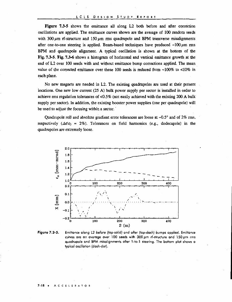
L C L S D E S I G N S T U D Y R E P O R T
Figure 7.3-5 shows the emittance all along L2 both before and after correction
oscillations are applied. The emittance curves shown are the average of 100 random seeds
with 300/im rf-structure and 150/im rms quadrupole and BPM transverse misalignments
after one-to-one steering is applied. Beam-based techniques have produced -100 jum rms
BPM and quadrupole alignment. A typical oscillation is shown at the bottom of the
Fig. 7.3-5. Fig. 7.3-6 shows a histogram of horizontal and vertical emittance growth at the
end of L2 over 100 seeds with and without emittance bump corrections applied. The mean
value of the corrected emittance over these 100 seeds is reduced from -100% to <I0% in
each plane.
No new magnets are needed in L2. The existing quadrupoles are used at their present
locations. One new low current (25 A) bulk power supply per sector is installed in order to
achieve rms regulation tolerances of <0.5% (not easily achieved with the existing 200 A bulk
supply per sector). In addition, the existing booster power supplies (one per quadrupole) will
be used to adjust the focusing within a sector.
Quadrupole roll and absolute gradient error tolerances are loose at -0.5° and of 2% rms,
respectively (_Ad£Q = 2%). Tolerances on field harmonics (e.g., dodecapole) in the
quadrupoles are extremely loose.
Figure 7.3-5.
. . . . . . . .
i . . . . i
300 400
Emittance along L2 before (top-solid) and after (top-dash) bumps applied. Emittancecurves are an average over 100 seeds with 300 pm rf-structure and 150/jm rmsquadrupole and BPM misalignments after l-to-1 steering. The bottom plot shows atypical oscillation (dash-dot).
7-18 A C C E L E R A T O R

L C L S D E S I G N S T U D Y R E P O R T
BEFORE CORR: <AcJt/6 l0)=97% BEFORE CORR: <A£y /ey 0)=90%
20
15
10
5
0
~L
i
"i — i — i — .(a)-
0 50 100 150 300 250 300
20
15
10
5
0
20
15
10
5
n
AFTER
— r
\
1 1
CORR:
.... 1 . . .
. , , 1 . . .
(A€I/ert>-4.6%1''
1..
1 1(b)"
-_
. . i i •
0 50 100 150 200 250 300
AFTER CORR:
10
" i — r
50 100 150 200 250 300L I I LL. L I J J j J_,
0 50 100 150 200 250 300
AFigure 7.3-6. Histogram of horizontal (left) and vertical (right) emittance growth along L2 for a 12-
meter quadrupole spacing and 707cell over TOO seeds with (top plots) and without(bottom plots) erhittance "bump" corrections applied. On overage, the growth isreduced from -100% to <10%.
7.3.4 The L3 Linac
The L3 linac begins at 25-4A and ends at the end of sector-30. Eleven 3 meter sections
from 25-lA to 25-3D are removed to install the long BC2 bunch compressor chicanes (25-lC
does not exist). The short bunch of 20 ptm in L3 effectively eliminates transverse wakefields
as an emittance dilution mechanism, and the rms energy spread shrinks from 1.1% down to
<0.1% due to the strong longitudinal wakefield of the short bunch. In this case the dominant
emittance dilution mechanism is due to momentum dispersion generated by quadrupole and
BPM misalignments. This suggests a weak focusing. LIAR simulations were run for L3 using
the existing SLAC linac 12 meter quadrupole spacing but varying the phase advance per cell
over the set 20°, 30°, 40°, 60° and 90°. Fig. 7.3-7 shows the horizontal relative emittance
growth versus phase advance per cell for L3 with and without transverse wakefield effects.
This clearly demonstrates the weak transverse wakefield due to the extremely short bunch
in L3. Large quadrupole, BPM, and rf-structure misalignments of 300 (im rms were used as
well as a one-to-one steering algorithm and the nominal undulator energy of 15 GeV.
A C C E L E R A T O R 7-19

L C L S D E S I G N S T U D Y R E P O R T
fc?
otu
Figure 7.3-7.
135
100
75
50
25
n
—
— / /
— //
—
— s>'
—
—
—
, , . . 1 . . , , :
20 40 60 60 100
Horizontal relative emittance growth versus phase advance/cell for L3 and 12-meterquadrupole spacing over 10 seeds (solid: wakes ON, dash: wakes OFF). Quadrupole,BPM, and rf-structure misalignments of 300 /Jm rms were used as well as one-to-onesteering (no bumps applied). Vertical emittance growth (not shown) is similar. Thephase chosen is 307cell.
A phase advance per cell of 30° is chosen for L3 since it is near the minimum emittance
dilution and also optimizes the phase advance separation of the existing sector-28 wire
scanners for the best x and y emittance resolution. The first and last wires will be relocated to
set each wire-to-wire separation at 1.5 cells, or 45° (see Section 7.7.1). Beta-functions and
beamline layout are shown in Fig. 73-8 for 307cell.
I I I I I I I I I I I I I I M M T TFigure 7.3-8. Beta-functions along L3 at a phase advance of 30°/cell. Four existing sector-28 wire
scanners are indicated on the schematic (L3-ED: first and last relocated for optimumemittance resolution).
7-20 A C C E L E R A T O R

L C L S D E S I G N S T U D Y R E P O R T
7.4 Design of the Second Bunch Compressor
The second bunch compressor (BC2) is discussed here before the first compressor (BC1)
because the beam dynamics through it are more complex than in BC1. BC2 is a pair of
magnetic chicanes designed to introduce the energy dependence of a particle's path length
(Az= RS6$E/EQ) needed to compress a 400 fan bunch to 20jum. Many designs were
considered, but the simplicity of a four-dipole magnetic chicane is attractive because it
(1) introduces no net beamline bend angle, (2) generates no chromaticity or high order
dispersion (rectangular bends), since it contains no quadrupole magnets, and (3) allows
simple tuning of the momentum compaction, i?56, with a single power supply.
The high energy and short bunch demand a chicane design where synchrotron radiation
generated within the bends does not significantly dilute the emittance. Furthermore, energy
independent space charge forces within the dipoles [7] need to be insignificant and the
chicane length should be minimized so that the number of removed linac accelerating sections
is small. An optimized parameter set has been chosen with a 6 GeV double chicane motivated
by synchrotron radiation effects and linac longitudinal beam dynamics simulations. This
system will replace the 11 existing 3 meter rf-sections in sector-25 at 25-1, 25-2 and 25-3
(25-1C does not exist).
7.4.1 Overview and Parameters
The chicane design is set by the need to reduce transverse emittance dilution due to
coherent synchrotron radiation (CSR) in the bends, which is most pronounced for short
bunches. Since the energy spread generated by CSR is coherent along the bunch, its effect on
the transverse emittance can be compensated by introducing a double chicane and optical
symmetry to cancel the longitudinal-to-transverse coupling [8]. The symmetry is formed by
two consecutive chicanes of unequal strength with four quadrupole magnets between them to
establish a - I horizontal transfer matrix between chicane centers (as well as between paired
chicane bends). The compensation may be optimized empirically by varying chicane
strengths while holding the sum of the squares of the two chicane bend angles constant
(maintains compression). The compensation is described below. Fig. 7.4-1 is a schematic of a
bunched beam traversing the double chicane compressor. The design also minimizes
emittance dilution due to incoherent synchrotron radiation (ISR). The parameters in
Table 7.4-1 describe the final BC2 design.
Motivations and quantitative arguments for the choices of these parameters are described
in the following sections. Results of longitudinal beam dynamics simulations have been used
to set the incoming BC2 bunch length at -400 //m rms. The bunch length after BC2 is
adjustable using the /?s6of BC2 and the rf phase of L2. A nominal rms final bunch length of
20 //m is used throughout the following descriptions (unless otherwise noted). In order to
allow non-LCLS linac operation, and to ease dipole field quality tolerances (see
Section 7.4.7), the center two dipoles per chicane will be placed on remotely moveable
horizontal stages. With the dipoles switched off, the two BC2 (and the BC1) chicanes can
A C C E L E R A T O R • 7-21

L C L S D E S I G N S T U D Y R E P O R T
then be straightened out. The maximum horizontal beamline excursion at each chicane center
is equal to the maximum dispersion, 77max, listed in the table.
on—[p- LKHHHD IT—
Figure 7.4-1 . Schematic of beam in the double chicane bunch compressor.
Table 7.4-1. Parameters of 2nd bunch compressor
Parameter
Beam energy
Initial rms bunch length
Final rms bunch length
Rms incoming relative energy spread (at 6 GeV)
Net momentum compaction
Net second order momentum compaction
Total system length
Physical length of each dipole magnet
Drift between first two and last two dipoles (per chicane)
Drift between center two dipoles
Bend angle for each of 1st four dipoles
Bend angle for each of last four dipoles
Magnetic field for each of 1st four dipoles
Magnetic field for each of last four dipoles
Maximum dispersion in chicane-1 center
Maximum dispersion in chicane-2 center
Emittance dilution due to ISR
Emittance dilution due to CSR (no shielding)
rms ISR relative energy spread (at 6 GeV)
rms CSR relative energy spread (at 6 GeV)
Linac 3 rf phase delay per unit /?» change
double chicane, BC2.
Symbol
E
<V
OS
* 5 6
7*566
Aotal
LB
AL
ALC
Iftll
l%2l
IBll
\B2\
*7l-max
%-max
A£m/£Q
4«CSR/£0
<%R
<7<5cSR
d<p/dRi(>
Unit
GeV
ftm
/jm
%
mm
mm
m
m
m
m
deg
deg
kG
kG
m
m
%
%
vr4
10-4
deg/mm
Value
6.0
390
20
1.07
35.5
-53.3
34.7
1.500
3.350
0.500
3.420
1.303
7.964
- 3.034
0.290
0.110
1.4
-5
0.1
-2.4
1.72
7-22 « A C C E L E R A T O R -

L C L S D E S I G N S T U D Y R E P O R T
Figure 7.4-2 shows the dispersion and beta functions through the BC2 chicanes. Dipole
magnets with names used in the text are shown at the bottom of the figure. The plot and other
calculations are made for a net /?56 of 35.5 mm (R56-i = 31.0 mm, R56.2 = 4.5 mm).
"ft.
60
40
20
1
h \• i
. s- i• i
—
• /
/
. 1480
\ i
A
•J
t
_ , |
i
i
s
I
\s
' 1
\\
V
V
, 1490
i ( (
/
\ /
\ - /
- ^ \
-x ^1 1 1
I—I s
1 1
__ _ -
~ \\\/
/, 1
500(lli)
Vx
/ s\ •
• —
1...
• ' 1 '
/
/ /
— T
, . 1 ,510
- • /
/
V
/
/\
-
/I -1 •
/ —
, 1 -520
u.
0.3
0.2
0.1
0.0
i rus
Figure 7.4-2. Dispersion and beta functions through BC2 double chicane for Ri6 = 35.5 mm.Magnet names are shown at bottom with wire scanners as small circles. The two smallquadrupoles (CQ21 and CQ22) are for dispersion correction and are nominally off.
7.4.2 Momentum Compaction
The momentum compaction (/?56) of two consecutive chicanes made up of rectangular
bend magnets is positive (bunch head at z > 0) and is the sum of R& values of each single
chicane. For ultra-relativistic electrons and small bend angles, the net /?56 of the double
chicane is given in Eq. 7.4.1 where the symbol definitions are taken from Table 7.4-1.
^56 = • hi + 0B2 (7.4.1)
Free parameters are bend lengths, angles, and drift lengths. The required R^ is
determined from the desired end-of-linac bunch length and energy spread, and the rf phase of
L2, which is chosen through longitudinal dynamics simulations as described in Section 7.2.3.
The second order momentum compaction (T^) of a rectangular bend chicane (no quadrupole
magnets) is Ts^ - -37?56/2 [9]. From Eq. 7.4.1 the ratio of the two bend angles is clearly
adjustable while maintaining the necessary total R$6. This provides an empirical correction
"knob" for the minimization of transverse emittance effects from CSR (as described below in
Section 7.4.4).
A beam delay must also be accounted for in the rf phase of L3 as the beam path length
increases through a four-dipole chicane with bend angles dg.
For the double chicane, the approximation at right of Eq. 7.4.2 is accurate to within 0.1°
S-band phase over the full /?56 range of 0 to 50 mm. The L3 rf ph'ase needs to be delayed, with
A C C E L E R A T O R 7-23

L C L S D E S I G N S T U D Y R E P O R T
respect to the chicane-off phase, by d(p/dR56« rik » 1.727mm (or 61.1° with the nominal /?56value for BC2).
TJZAS AK
cos#B
^ 5 6
X(7.4.2)
7.4.3 Incoherent Synchrotron Radiation (ISR)
Transverse emittance dilution will occur if significant energy spread is generatedanywhere in the chicane. Synchrotron radiation within the dipoles generates energy spread,which breaks the linear achromaticity of the chicane and therefore dilutes the horizontalemittance. Using a typical symmetric beta function through a single chicane with itsmaximum, y nax, at start and end of the chicane and its minimum, /J^in, in the middle (seeFig. 7.4-2), and using symbols defined in Table 7.4-1, then
P max = 2/? min = ALB +2AL + ALC. (7.4.3)
The additive ISR emittance dilution [ 10] can then be approximated (A el £Q «1) by
- (8x10-* m2 . G e V - V ^ f e + 0>n)4AL+6LB+**- . (7.4.4)
2LB
The parameters of Table 7.4-1 are chosen such that the relative ISR emittance growth is1.4%. This is entirely determined by the first chicane since 6B2 <9B\- This incoherent energyspread is generated through a random process and therefore cannot be corrected.
7.4.4 Coherent Synchrotron Radiation (CSR)
Unshielded Radiation
For very short bunches, coherent synchrotron radiation can dilute the horizontalemittance by similarly generating energy spread in the dipoles. In this case, however, theenergy spread is correlated along the bunch and not a random process. For an rms bunchlength az, dipole length L$, bend radius R (=Lg/^g) and N electrons per bunch, the CSR-induced relative rms energy spread per dipole for a gaussian bunch under steady-stateconditions, is [11]
where re is the classical electron radius and yis the Lorentz energy factor. This is valid for adipole magnet where metallic vacuum chamber radiation shielding is not significant (i.e., fora full vertical vacuum chamber height h which satisfies [12]
7 - 2 4 • A C C E L E R A T O R

L C L S D E S I G N S T U D Y R E P O R T
h » {nojRf1* E hc . (7.4.6)
Since the bunch length shortens through the chicane, the energy spread induced at each
dipole increases, with the final dipole generating the most significant energy spread (the
bunch length is virtually constant in the first and last dipoles—see Fig. 7.4-4). The rms
horizontal emittance after a single chicane can be written as
Ax = j R16(s)^-ds , Ax'= J R^{s)^-ds ,to* as i as
/p] + <Ax2XAx'2)-<AxAx'>2 (7.4.7)
{e0 + As f ,
Here Ri6(s) and R26(s) are the standard transfer matrix elements from point s to end of
chicane, fi (=Anax) and o. are the nominal Twiss parameters at the end of the chicane, and SQ
and e are the initial and final rms horizontal emittances. The change in centroid coordinates,
Ax and Ax', pertain to a single longitudinal bunch slice. Their second moments (e.g., (Ax2))
are ensemble averages over the entire bunch, and ^ i s the Courant-Snyder invariant (see
Eq. 7.7.1). In unshielded, steady-state conditions, where (Ax2)(Ax'2) = (AxAx1)2, the
relative emittance growth for just the last bend of a single chicane, using Eq. 7.4.5 and
Eq. 7.4.7 and a constant gaussian bunch length, is
with £ff ( s yeo) introduced to represent the initial normalized (invariant) emittance.
For a single chicane with parameters of the first chicane in Table 7.4-1 and the full
20 fim final compression occurring in that one chicane, the CSR emittance growth of
Eq. 7.4.8 is ~70%. The chicane could be made twice as long but the emittance dilution is still
too large. To arrive at the final double chicane design, a single chicane is chosen based on a
-2% ISR emittance growth, and then a second identical chicane is added with reduced bend
angles and separating optics to approximately cancel the net CSR emittance increase.
The cancellation can be understood by imagining an electron which looses energy inside
the nth dipole (n = 1...4) of chicane-1. In this steady-state model, the energy loss depends
only on the axial position of the electron within the bunch. Fig. 7.4-3 (solid curve) shows this
wakefield voltage (energy variation) along the bunch. The calculation was made using a
computer program [13] which calculates the CSR steady-state wakefields in bends, including
radiation shielding effects, for a gaussian bunch.
A C C E L E R A T O R • 7-25

L C L S D E S I G N S T U D Y R E P O R T
I
100
75
50
25
-25
: - • i • • • • i • • • • i
— /
L - "J/^- v h/h.-0.5 / 'v /
17 . 1 . . . . 1 . . . . t
' ' ' ' 1 *
yi/hc-7.i
\
\
V
* ' • i ' ' ;
—
—
—
<. . i . --4 -2
Figure 7.4-3. Coherent radiation steady-state wake per 2K bend (R = 19.4 m, (Tz = 30 /Jm,hc = 5.6 mm) for both shielded (dash: h/hc = 0.5) and unshielded (solid: h/hc >> 1)coherent radiation of a gaussion bunch. The bunch head is at z > 0 and V > 0represents energy loss.
Due to the energy loss, the electron receives an additional horizontal kick, with respect to
an on-energy electron, in the nth bend. This same electron, with its unchanged relative axial
position, will again loose energy in the nth bend of chicane-2, but due to the - I matrix
between paired bend, the shorter bunch in chicane-2, and the arrangement of the relative
strengths of the two chicanes, the net horizontal kick at the end of the system is zero. This
assumes the electron does not shift axially with respect to the remainder of the bunch as
would occur in the case of over-compression (>90° phase space rotation) or a non-linear
phase space transformation. In order to estimate the effect over the entire system, a computer
program is used to generate the steady-state CSR energy spread of Eq. 7.4.5 in each l/10th
slice of each dipole magnet. The horizontal position and angle of the particles are mapped to
the end of the second chicane. The bunch is allowed to linearly compress along the way from
390 m to 20 pm. The relative emittance increase, CSR energy spread, bunch length, and
horizontal dispersion function are plotted in Fig. 7.4-4.
This steady-state calculation ignores field transients, and the CSR forces are assumed to
vanish between bends. The net emittance increase is 0.3%. More thorough calculations of the
CSR-induced emittance dilution have been made using the DESY "WAKE" code [14] (see
below, "Calculations with a Transient Model") which result in an emittance growth of 3-5%.
Shielded Radiation
If a small vertical vacuum chamber height, h, is used in the bends which does not satisfy
Eq. 7.4.6, the CSR induced energy spread may be reduced. Fig. 7.4-3 shows the coherent
radiation wakefield voltage for a 30 /im bunch through a bend with R = 19.4 m both with and
without radiation shielding. Here the vacuum chamber is modeled as parallel plates.
7-26 A C C E L E R A T O R
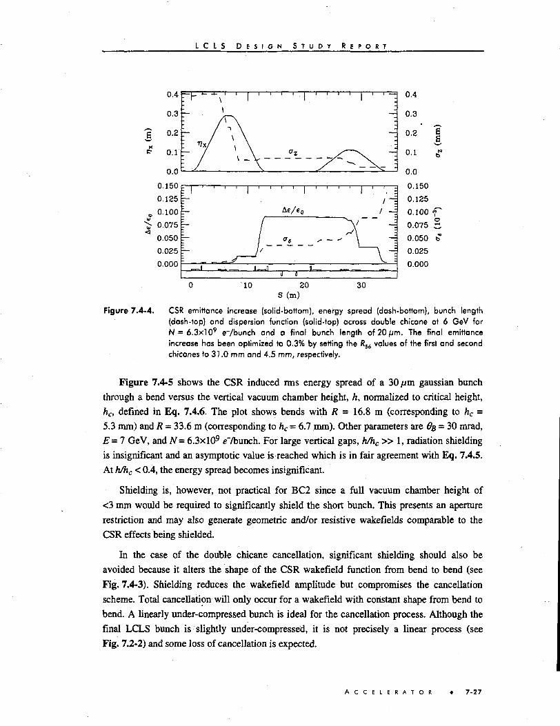
L C L S D E S I G N S T U D Y R E P O R T
I
0.0
0.150
0.125
0.100
0.075
0.050
0.025
0.000
I 1 • ' ' ' 1 ' •
1 | r]
L
(
U
>±-
II
' '
y —
Hi . •
' ' 1 ' '. :
0.0
0.150
0.125
0.100
0.075
0.050
0.025
0.000
10 20 30S (m)
Figure 7.4-4. CSR emittance increase {solid-bottom), energy spread (dash-bottom), bunch length(dash-top) and dispersion function (solid-top) across double chicane at 6 GeV forN = 6.3x10⁹ e~/bunch and a final bunch length of 20 pm. The final emittanceincrease has been optimized to 0.3% by setting the RS6 values of the first and secondchicanes to 31.0 mm and 4.5 mm, respectively.
Figure 7.4-5 shows the CSR induced rms energy spread of a 30 pm gaussian bunch
through a bend versus the vertical vacuum chamber height, h, normalized to critical height,
hc, defined in Eq. 7.4.6. The plot shows bends with R = 16.8 m (corresponding to hc =
5.3 mm) and R = 33.6 m (corresponding to hc = 6.7 mm). Other parameters are $B = 30 mrad,
E = 7 GeV, and iV= 6.3xlO9 eTbunch. For large vertical gaps, h/hc » 1, radiation shielding
is insignificant and an asymptotic value is reached which is in fair agreement with Eq. 7.4.5.
At h/hc < 0.4, the energy spread becomes insignificant.
Shielding is, however, not practical for BC2 since a full vacuum chamber height of
<3 mm would be required to significantly shield the short bunch. This presents an aperture
restriction and may also generate geometric and/or resistive wakefields comparable to the
CSR effects being shielded.
In the case of the double chicane cancellation, significant shielding should also be
avoided because it alters the shape of the CSR wakefield function from bend to bend (see
Fig. 7.4-3). Shielding reduces the wakefield amplitude but compromises the cancellation
scheme. Total cancellation will only occur for a wakefield with constant shape from bend to
bend. A linearly under-compressed bunch is ideal for the cancellation process. Although the
final LCLS bunch is slightly under-compressed, it is not precisely a linear process (see
Fig. 7.2-2) and some loss of cancellation is expected.
A C C E L E R A T O R 7-27

L C L S D E S I G N S T U D Y R E P O R T
30 -
CO
O
•ob
20 -
10 -
0
- '
—
V J1
1 < 1 <
i :^ ^ - •"• ' -
-
1 1
1 I
1 I
1 1
I 1
1 1
0 4h/hc
8
Figure 7.4-5. CSR-induced rms energy spread per bend versus vertical vacuum chamber height, h,normalized to critical height, hc. Curves for both R=16.8 m, hc=5.3 mm (dash) andR=33.6 m, hc=6.7 mm (solid) are shown. Horizontal lines nearest asymptotic valuesare from Eq. 7.4.5.
The /?56 of the BC2 chicanes is also intended to be adjustable to allow for correction of
the longitudinal phase space of the linac output beam and to provide control of the final
bunch length. A tuning range of 20 to 50 mm should easily allow for uncertainties in the
longitudinal wakefields of the 20//m bunch. Fig. 7.4-6 shows the variation of several
parameters over a large R& range. The end-of-system CSR emittance increase, "CSRend>" has
been minimized (steady-state) at the operational point (R$6 = 35.5 mm). It is not plotted
beyond this point since the bunch begins to over-compress at Rse,« 37 mm and destroys the
cancellation. The scan was made keeping the ratio of the two bend angles constant (~2.6)
which is not precisely the optimal CSR cancellation ratio for different Rs6 values.
Transverse Forces
A transverse force or "centripetal force" is described by Derbenev and Shiltsev [15]
which originates from radiation of trailing particles and depends on the local charge density
along the bunch. The maximum force takes place at the center of the bunch and its effect on
transverse emittance is estimated in the reference. This estimate predicts an emittance growth
of « 1 % for the worst case (last dipole of chicane-2 where bunch is shortest).
7-28 • A C C E L E R A T O R

L C L S D E S I G N S T U D Y R E P O R T
o01
0 10 20 30 40 50 60R5e / m m
O
CO
0 10 20 30 40 50 60R56 / m m
. , . . i , , . .-
0 10 20 30 40 50 60R56 /mm
0 10 20 30 40 50 60R56 /mm
Figure 7.4-6. For the BC2 double chicane, the variation of (a) CSR and ISR emittance increase, (b)final bunch length, (c) dipole magnetic fields, and (d) horizontal dispersion in chicanecenters, all as a function of the net R56 at 6 GeV [di/6^2.6). The label "CSRmax"indicates emittance between chicanes, whereas "CSRend" indicates emittance increaseat BC2 system end (no shielding).
Calculations with a Transient Model
More complete calculations of the CSR effects on the bunch through BC2 have been
made using a computer code written at DESY [16]. The code is a time domain treatment that
includes the field transients at entrance and exit of the bends, the x-z correlation in the beam
at high dispersion points, the space charge forces, and longitudinal as well as transverse
forces. The bunch is composed of N (=301) 5 fjm sub-bunches each with a 30 fJm vertical
extent, and the double chicane, including the - I quadrupoles, is split into 100 beamline
segments. Fig. 7.4-7 shows the dispersion function and the CSR relative energy spread
calculated using both the steady-state [$E/£O(SS)] model and this transient model
The total rms CSR energy spread generated to the end of BC2 (end of last dipole) using
the transient model is 2.5X10"4 while the steady-state model predicts a lower value of
1.6X10"4. Furthermore, in the transient model, energy spread is generated between the bends
as well as in the bends, whereas the steady-state model only provides for energy spread
generation within the bends. Clearly, the emittance growth should be evaluated using the
more complete, transient model, so that the contributions from these "drift" sections are
included in the emittance dilution estimates. In addition, the CSR wakefield function is not of
constant shape in this model, and the non-linear aspects of the compression process are
included (e.g., TSM). This provides a more realistic evaluation of the transverse emittance
growth.
A C C E L E R A T O R 7-29

L C L S D E S I G N S T U D Y R E P O R T
0.25
0.20
0.15
0.10
0.05
0.0030
0.30
0.25
0.20
0.15
0.10
0.05
0.00
Figure 7.4-7. The dispersion function (dash-dot) and the CSR rms energy spread generated in theBC2 double chicane using the transient (dash) and the steady-state (solid) models.
Fig. 7.4-8 shows the transverse phase space, with and without CSR effects, 1 meter
downstream of the last BC2 bend. The points on the plot show the centroid position of each
of the 301 longitudinal slices. In this calculation, the axial bunch distribution prior to BC1 is
gaussian.
The nominal beam (without CSR effects) is represented as a large-solid ellipse. With
CSR effects, each longitudinal slice (301) has this same phase space ellipse but displaced
according to its centroid position (points). The equivalent ellipse of the slice centroids,
including their different charges, is shown as a small-solid ellipse. The area of this small
ellipse is the rms emittance produced by CSR for a zero-emittance input beam (the additive
component—As in Eq. 7.4.7). The final equivalent ellipse produced by combining the
nominal beam and the slice centroids is shown as the large-dashed ellipse. The transverse
distribution functions are, in general, no longer gaussian, but they can be described by the
second moments of their distributions. In this representation the emittance which is calculated
is the rms value. Here the relative rms emittance dilution is 14% for an initial rms emittance
of 1 mm-mrad.
This 14% emittance growth can be further improved by choosing optimal input beta
functions through BC2. The minimal emittance impact is obtained by setting the nominal beta
and alpha functions (large-solid ellipse of Fig. 7.4-8) to those of the CSR-generated beam
(small-solid ellipse)^—see Eq. 7.4.7 with £ = 1. In this case the beta functions through the
BC2 become somewhat asymmetric, but not unreasonably so, and the emittance dilution
drops to 6%. A further reduction can be realized by removing the linear component of the (xz)
and (x'z) correlation. This is possible since energy, S, and z are also linearly related, and
therefore a small spatial and angular "dispersion" adjustment can be used to reduce the
emittance growth to just 3.5%.
7-30 A C C E L E R A T O R

L C L S D E S I G N S T U D Y R E P O R T
cd
x
5.0
2.5
0.0
-2.5
-5.0
- ' ' ' ' 1 ' ' ' '
r ^• y^G
1 ' ' ' I ' ' ' ' -
—
- 4 0 -20 0 20 40
xFigure 7.4-8. Transverse (bending plane) phase space after BC2. The various ellipses are: nominal
beam (large-solid), additive CSR beam (small-solid), arid total beam after CSR effectsand 14% emittance growth (large-dashed). Points are the centroid positions of thelongitudinal slices.
Calculations with a uniform bunch distribution (rather than a gaussian) produce similar
results: 20% emittance dilution without optimal beta, 5% with optimal beta, and 3% with
dispersion correction and optimal beta functions. Calculations have yet to be done which
include the precise bunch distribution of Fig. 7.2-2 (plot of row-3, column-1).
7.4.5 Resistive Wall Longitudinal Wakefields in the Bends
Longitudinal resistive wall wakefields in the BC2 vacuum chambers also induce energy
spread which may dilute the emittance. The rms relative energy spread generated in a
cylindrical vacuum chamber of length L, radius a, and conductivity <7is (see section 7.8.5)
(0.22)e2cNL
n2aEaf(7.4.9)
where ZQ (=377 Q) is the free space impedance. Note, Eq. 7.4.9 is for a long, gaussian
bunch—see Section 7.8.5. For parameters of Table 7.4-1 using aluminum (cr= 3.6xlO7
Q-inr1) and a = 15 mm through the final bend, where the bunch length is 20 jum, the rms
energy spread is ~4xlO~6 which is more than an order of magnitude smaller than the CSR
energy spread generated in this final bend. Stainless steel, on the other hand, will generate
five times this value and should be avoided. The other bends generate much less energy
spread.
A C C E L E R A T O R 7-31
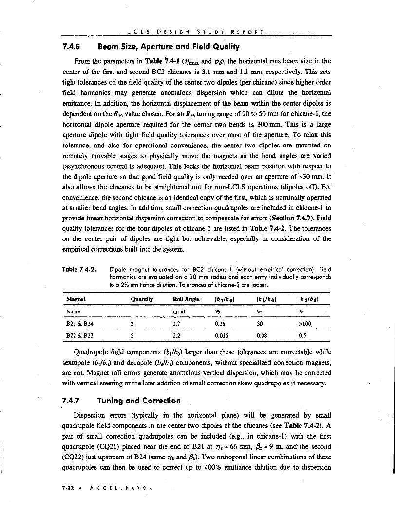
L C L S D E S I G N S T U D Y R E P O R T . .
7.4.6 Beam Size, Aperture and Field Quality
From the parameters in Table 7.4-1 (7]msx and <7<y), the horizontal rms beam size in the
center of the first and second BC2 chicanes is 3.1 mm and 1.1 mm, respectively. This sets
tight tolerances on the field quality of the center two dipoles (per chicane) since higher order
field harmonics may generate anomalous dispersion which can dilute the horizontal
emittance. In addition, the horizontal displacement of the beam within the center dipoles is
dependent on the R^ value chosen. For an /?«tuning range of 20 to 50 mm for chicane-1, the
horizontal dipole aperture required for the center two bends is 300 mm. This is a large
aperture dipole with tight field quality tolerances over most of the aperture. To relax this
tolerance, and also for operational convenience, the center two dipoles are mounted on
remotely movable stages to physically move the magnets as the bend angles are varied
(asynchronous control is adequate). This locks the horizontal beam position with respect to
the dipole aperture so that good field quality is only needed over an aperture of ~30 mm. It
also allows the chicanes to be straightened out for non-LCLS operations (dipoles off). For
convenience, the second chicane is an identical copy of the first, which is nominally operated
at smaller bend angles. In addition, small correction quadrupoles are included in chicane-1 to
provide linear horizontal dispersion correction to compensate for errors (Section 7.4.7). Field
quality tolerances for the four dipoles of chicane-1 are listed in Table 7.4-2. The tolerances
on the center pair of dipoles are tight but achievable, especially in consideration of the
empirical corrections built into the system.
Table 7.4-2. Dipole magnet tolerances for BC2 chicane-1 (without empirical correction). Fieldharmonics are evaluated on a 20 mm radius and each entry individually correspondsto a 2% emittance dilution. Tolerances of chicane-2 are looser.
Magnet
Name
B21&B24
B22&B23
Quantity
2
2
Roll Angle
mrad
1.7
2.2
%
0.28
0.016
l*2/»«l
%
30.
0.08
\b4lbo\
%
>100
0.5
Quadrupole field components (bi/b0) larger than these tolerances are correctable while
sextupole (b2/b0) and decapole (bjb^) components, without specialized correction magnets,
are not. Magnet roll errors generate anomalous vertical dispersion, which may be corrected
with vertical steering or the later addition of small correction skew quadrupoles if necessary.
7.4.7 Tuning and Correction
Dispersion errors (typically in the horizontal plane) will be generated by small
quadrupole field components in the center two dipoles of the chicanes (see Table 7.4-2). A
pair of small correction quadrupoles can be included (e.g., in chicane-1) with the first
quadrupole (CQ21) placed near the end of B21 at T]x»66 mm, px"9 m, and the second
(CQ22) just upstream of B24 (same T)x and fix). Two orthogonal linear combinations of these
quadrupoles can then be used to correct up to 400% emittance dilution due to dispersion
7 - 3 2 • A C C E L E R A T O R

L C L S D E S I G N S T U D Y R E P O R T
errors. Since the dispersive beam size at these quadrupoles is 7]xcr$- 700 pm and the betatron
beam size is much smaller at {fix,y£x,y)^12 ** 30//m, these quadrupoles have little effect on the
final beta functions. The specifications for these correction quadrupoles are given in
Table 7.4-3 and their locations are shown in Fig. 7.4-2.
Table 7.4-3. Dispersion correction quadrupoles for BC2 chicane-1 for horizontal emittancecorrection of up to 400% (with 1 % step size control).
Maximum Pole-Tip Field
kG
1.1
Quantity
2
Step Size
kG
0.06
Pole Radius
mm
50
Length
m
0.1
The four main dipoles of each chicane will be powered in series by one power supply so
that field regulation tolerances can be loosened (see Table 7.2-3). The two chicane supplies
are then used in two separate non-linear combinations to orthogonally control the net i?56 and
the CSR emittance compensation. Trim coils should be included in each BC2 main dipole for
compensation of magnet-to-magnet construction errors in the dipole field strengths. This will
also allow some horizontal steering. In addition, vertical dipole correctors (2 per chicane) will
be included to facilitate vertical steering.
7.5 Design of the First Bunch Compressor
7.5.1 Overview and Parameters
Like the second compressor, the first bunch compressor (BC1) is also an adjustable
magnetic chicane. It performs an initial bunch compression from 1 mm to -400 pm. The
longer bunch and lower energy allow for a much shorter and simpler design than BC2, and
the complexity of a double chicane is not required. The tools developed for the design of BC2
were used to choose a 2.8-meter long chicane for BC1 as outlined below in Table 7.5-1. The
dispersion and beta functions through the BC1 chicane are shown in Fig. 7.5-1.
Emittance growth and energy spread through BC1 due to incoherent synchrotron
radiation are completely negligible. Emittance growth due to CSR is 5% using the transient
model (see Section 7.4.4) and 2% using the steady-state model. If the dipole vacuum
chambers are 12 mm in height, the shielding effect reduces the emittance growth to <2%.
The rf phase delay in L2 introduced by the BC1 chicane is given by the approximation at
right of Eq. 7.4.2, which is accurate to within 0.2° S-band phase over the full R56 range of 0
to 35 mm. The L2 rf phase is delayed by d<p/dR56 ~ nil = 1.727mm (or 46.4° with the
nominal /?56).
A C C E L E R A T O R • 7-33
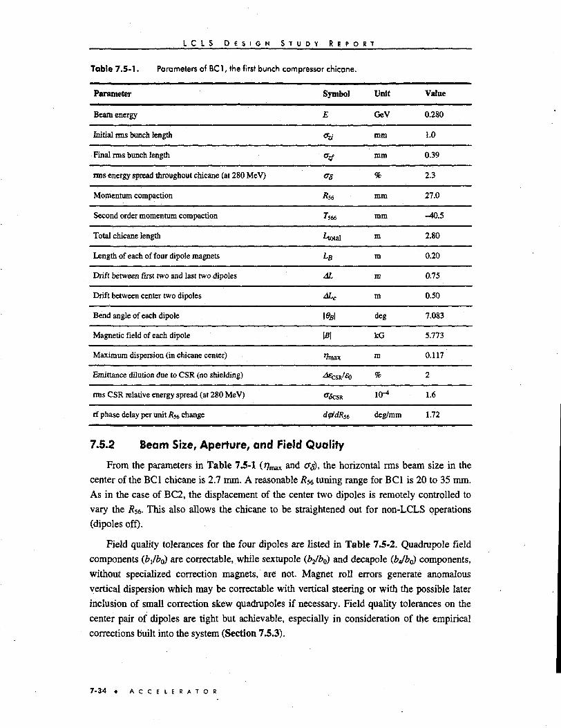
L C L S D E S I G N
Table 7 .5-1 . Parameters of BCl, the first bunch
Parameter
Beam energy
Initial rms bunch length
Final rms bunch length
iros energy spread throughout chicane (at 280 MeV)
Momentum compaction
Second order momentum compaction
Total chicane length
Length of each of four dipole magnets
Drift between first two and last two dipoles
Drift between center two dipoles
Bend angle of each dipole
Magnetic field of each dipole
Maximum dispersion (in chicane center)
Emittance dilution due to CSR (no shielding)
rms CSR relative energy spread (at 280 MeV)
rf phase delay per unit RS6 change
S T U D Y R E P O
compressor chicane.
Symbol
E
<?zi
°*<*s
*56
7-566
Aotal
LB
AL
ALC
\eB\
'/max
°<SCSR
d<p/dR56
R T
Unit
GeV
mm
mm
%
mm
mm
m
m
m
m
deg
kG
m
%
icr*
deg/mm
Value
0.280
1.0
0.39
2.3
27.0
-40.5
2.80
0.20
0.75
0.50
7.083
5.773
0.117
2
1.6
1.72
7.5.2 Beam Size, Aperture, and Field Quality
From the parameters in Table 7.5-1 ( max a nd 0£)> the horizontal rms beam size in the
center of the BCl chicane is 2.7 mm. A reasonable /?56 tuning range for BCl is 20 to 35 mm.
As in the case of BC2, the displacement of the center two dipoles is remotely controlled to
vary the RS6. This also allows the chicane to be straightened out for non-LCLS operations
(dipoles off).
Field quality tolerances for the four dipoles are listed in Table 7.5-2. Quadrupole field
components (bx/b0) are correctable, while sextupole (b2/b0) and decapole (Jbjb^) components,
without specialized correction magnets, are not. Magnet roll errors generate anomalous
vertical dispersion which may be correctable with vertical steering or with the possible later
inclusion of small correction skew quadrupoles if necessary. Field quality tolerances on the
center pair of dipoles are tight but achievable, especially in consideration of the empirical
corrections built into the system (Section 7.5.3).
7 - 3 4 « A C C E L E R A T O R

L C L S D E S I G N S T U D Y R E P O R T
S (m) 40 410.00
S 3 S » m S S
Figure 7.5-1. Dispersion and beta functions through BC1 chicane. Energy spread wire is "WS11".The two quadrupoles CQ11 and CQ12 are for dispersion correction and nominallyoff.
7.5.3 Tuning and Correction
Dispersion errors (typically horizontal) are generated by quadrupole field components in
the center dipoles of BC1 (Table 7.5-2). As in BC2, a pair of small correction quadrupoles
are included with the first one (CQ11) placed near the end of Bl 1 at i]x~ 10 mm, flx => 2.6 m,
and the second (CQ12) just upstream of B4 (same r\x and J5X). Two orthogonal linear
combinations of these quadrupoles can then be used to correct up to 400% emittance dilution
due to dispersion errors. Since the dispersive beam size at these quadrupoles is T)x<J8a
230 iiva. and the betatron beam size is much smaller at (fix^s^y)^2 = 70 /urn, these quadrupoles
have little effect on beta functions. The specifications for these two correction quadrupoles
are given in Table 7.5-3 and their locations are shown in Fig. 7.5-1.
Table 7.5-2. Dipole magnet tolerances for BC1. Field harmonics are evaluated on a 10 mm radiusand each entry individually corresponds to a 2% emittance dilution.
Magnet
Name
B11&B14
B12&B13
Table 7.5-3. Dispersion400% (2%
Maximum Pole-Tip Field
kG
1.1
Quantity Roll Angle
mrad
2 3.7
2 4.8
correction quadrupolesstep siie control).
Quantity
2
l»l/»0l
%
0.5
0.04
for BC1 for horizontal <
l»2/*il
%
10.
0.1
jmittance
Step Size Pole Radius
kG
0.08
mm
50
%
>100
0.3
correction of up to
Length
m
0.1
A C C E L E R A T O R 7-35

L C L S D E S I G N S T U D Y R E P O R T
The dipoles are powered in series with a single main power supply so that regulation
tolerances can be loosened (Table 7.2-3). Trim coils will also be included in each BC1 main
dipole so that compensation can be made for magnet-to-magnet construction variations in the
dipole field strength. This will also allow some horizontal steering. In addition, vertical dipole
correctors will be included to allow vertical steering.
7.6 Beam Transport Lines
This section discusses the two beam transport lines. The first is a low-energy dog leg
(DL1) used to transport the electrons from the injector into the main linac. The second is the
high-energy dog leg (DL2) used for L3 to undulator transport and energy and energy spread
analysis. The DL2 beamline also horizontally displaces the undulator axis from that of the
main linac in order to protect the undulator from potential beam halo and dark current.
7.6.1 Low-Energy Dog Leg
The function of the low-energy dog leg (DL1) is to transport the 150 MeV electron beam
from the new injector linac (L0) into the existing linac. While it is possible to design the dog
leg as a first bunch compression stage, this necessitates a large incoming correlated energy
spread of 1-2%, and the chromaticity of the quadrupole magnets within the dog leg, required
for a linear achromat, generate large second order dispersion which needs sextupole
compensation. Due to this, and also the need for /?56 tuning (not natural in a dog leg), DL1 is
designed as a simple transport line. Its design requirements are:
• Provides a horizontal beamline inflection of ~1 meter over a few meters distance
• Should not alter the bunch length (i.e., should be isochronous)
• Should introduce no significant transverse emittance dilution
The inflection may also be made in the vertical plane or a rolled plane. However, there is
no strong motivation to do so. A simple system that satisfies these conditions is composed of
two dipole magnets of opposite strength separated by a +1 optical transformer (seven
quadrupoles) to produce a linear achromat. The dipoles are rectangular bends.
The momentum compaction, /?s6, of such a system, for ultra-relativistic electrons and
small angles, is
(7.6.1)
where 6B and L% are the bend angle and length of each dipole, respectively. A 4 meter long
beamline with 14° bends provides the ~1 meter inflection, and 20 cm long dipoles produce an
i?56 of-4 mm. Therefore, an extreme electron which is off energy by 1% will move axially by
just 40 jum, which is small compared to the 1 mm rms bunch length. The effect of the second
order momentum compaction, rs66, is even less. Note, the incoming relative rms energy
7 - 3 6 • A C C E L E R A T O R
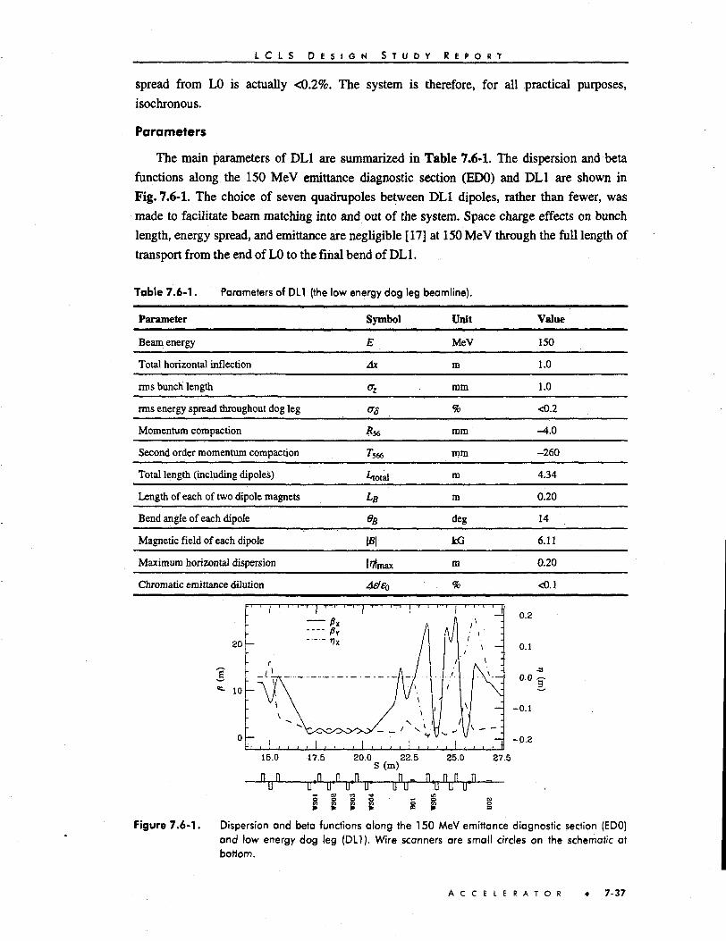
L C L S D E S I G N S T U D Y R E P O R T
spread from LO is actually <0.2%. The system is therefore, for all practical purposes,
isochronous.
Parameters
The main parameters of DLl are summarized in Table 7.6-1. The dispersion and beta
functions along the 150 MeV emittance diagnostic section (EDO) and DLl are shown in
Fig. 7.6-1. The choice of seven quadrupoles between DLl dipoles, rather than fewer, was
made to facilitate beam matching into and out of the system. Space charge effects on bunch
length, energy spread, and emittance are negligible [17] at 150 MeV through the full length of
transport from the end of LO to the final bend of DLl.
Table 7.6-1. Parameters of DLl
Parameter
Beam energy
Total horizontal inflection
rms bunch length
rms energy spread throughout dog leg
Momentum compaction
Second order momentum compaction
Total length (including dipoles)
Length of each of two dipole magnets
Bend angle of each dipole
Magnetic field of each dipole
Maximum horizontal dispersion
Chromatic emittance dilution
(the low energy dog leg
Symbol
£
Ax
°zOS
*56
7-566
^total
OB
mI'/tmax
AdSQ
beamline).
Unit
MeV
m
mm
%
mm
mm
m
m
deg
kG
m
. %
Value
150
1.0
1.0
<0.2
-4.0
-260
4.34
0.20
14
6.11
0.20
<0.1
20
-0 .1
-0.2
15.0 17.5 20.0 22.5 25.0 27.5S (m)
n n ,n n n n , n. n n _n „u U" U" U" U" O "U U U"
Figure 7.6-1. Dispersion and beta functions along the 150 MeV emittance diagnostic section (EDO)and low energy dog leg (DLl). Wire scanners are small circles on the schematic aibottom.
A C C E L E R A T O R 7-37

L C L S D E S I G N S T U D Y R E P O R T .
Beam Size, Aperture, and Field Quality
The horizontal beam size in DL1 reaches a peak value of -400 pna with the vertical size
at -150 /an. A 25 mm full aperture is, therefore, completely adequate. The large dispersion in
the DL1 quadrupoles and the strong bends set fairly tight tolerances on field quality and
gradient errors. Tables 7.6-2 and 7.6-3 list dipole and quadrupole magnet tolerances in DLL
Table 7.6-2. Dipole magnet tolerances for DL1. Field harmonics are evaluated on a 10 mm radiusand each entry individually corresponds to a 2% emittance dilution.
Magnet
Name
B01 and B02
Table 7.6-3.
Magnet
Name
QL01-07
Quantity
2
Quadrupole magnet 1radius and each entry
Quantity
7
Roll Angle | * i / * o l
mrad %
17 0.068
l*2/*0l
%
2.25
tolerances for DLL Field harmonics are evaluatedindividually corresponds to a 2% emittance dilution
Roll Angle M & i / * i l
mrad %
3 0.2
l*2/*ll
%
3
l*4/*0l
%
>100
on a 10 mm
l»s/*il
%
>100
The most challenging of these tolerances are the quadrupole content in the bends, \bi/bo\,
and the absolute gradient errors of the quadrupoles, \Abx/b\\. Although six of the seven
quadrupoles will be powered in series, their gradients may differ slightly due to construction
errors. The tolerance of <0.2% is difficult to achieve. The effect on the beam, however, is the
generation of linear dispersion. This can easily be tuned out empirically by including two
small correction quadrupoles in the DL1 design. Failure to meet the tolerances on the
quadrupole content in the bends results in a beta function mismatch (since the dispersion is so
small in the bends). This mismatch can be compensated with matching quadrupoles in front of
the DLL Quadrupole alignment tolerances are ~400 //m and do not present a significant
challenge, and dipole field errors (not listed) are correctable with steering coils.
Tuning and Correction
The dominant error which will likely arise in DL1 is anomalous linear dispersion which
will dilute the horizontal emittance. Quadrupole field strength errors are the most likely
cause. Two small correction quadrupoles on separate power supplies separated by ~90° of
betatron phase advance will be used in appropriate linear combinations to generate orthogonal
dispersion correction knobs. The emittance can be measured in the diagnostic section
following BC1 (BC1 can be switched off if necessary) and will be minimized with the
orthogonal knobs sequentially.
7-38 • A C C E L E R A T O R

L C L S D E S I G N S T U D Y R E P O R T
7.6.2 High-Energy Dog Leg
The requirements for beam transport to the LCLS undulator are fairly simple. The
transport line must:
• Include bends to introduce precise energy and energy spread measurement
capability without generating significant CSR or other transverse emittance
dilution effects.
• Include precise transverse emittance diagnostics for final verification/tuning prior
to undulator.
• Provide adjustable undulator-input matching for the various beam energies
desired.
• Not alter the bunch length (must be isochronous).
• Make use of existing FFTB tunnel and components wherever possible, as long as
the design or performance of the transport line is not compromised.
Energy and energy spread diagnostics are built into a four dipole horizontal inflector
beamline (DL2) where the first bend is located just inside the beginning of the existing Final
Focus Test Beam (FFTB) housing. Primarily to meet the small energy spread measurement
capability, a doublet of Chasman-Green [18] type cells is used. A cell consists of a dipole pair
sandwiching a quadrupole triplet. The horizontal dispersion function in the center of each cell
reaches a maximum, while the horizontal beta function converges towards a minimum. A
horizontal wire scanner here is capable of measuring an rms energy spread of 0.02% at
15 GeV with a nominal betatron beam size contribution of only 5% (see Section 7.7.3).
The Chasman-Green type cells are also advantageous since they introduce very little path
length energy dependence and generate minimal transverse emittance dilution due to
incoherent synchrotron radiation. The net system forms a 4-dipole dog leg (DL2) which
displaces the beamline horizontally by 0.9 m. The net momentum compaction for the 4-dipole
system, similar to DL1, is given by
Bends of $g= 1.3° and L# = 2.62 m produce a net momentum compaction of /?s6of
-0.9 mm which is, for a worst case energy spread of -0.1%, isochronous (<1 jum axial
position shift per 0.1% energy deviation). The emittance dilution due to incoherent
synchrotron radiation at 15 GeV is insignificant (<0.1%).
In order to include a high resolution relative energy spectrometer which is insensitive to
incoming linac orbit jitter, the centers of the Chasman-Green cells are separated by a unity
optical transformer (+1). The signals from two BPMs, one placed at the maximum dispersion
point in each cell, are subtracted to eliminate all incoming orbit jitter and enhance the relative
energy signal (the dispersion is of opposite sign in the two cells—see Fig. 7.6-2). With a
A C C E L E R A T O R • 7 -39
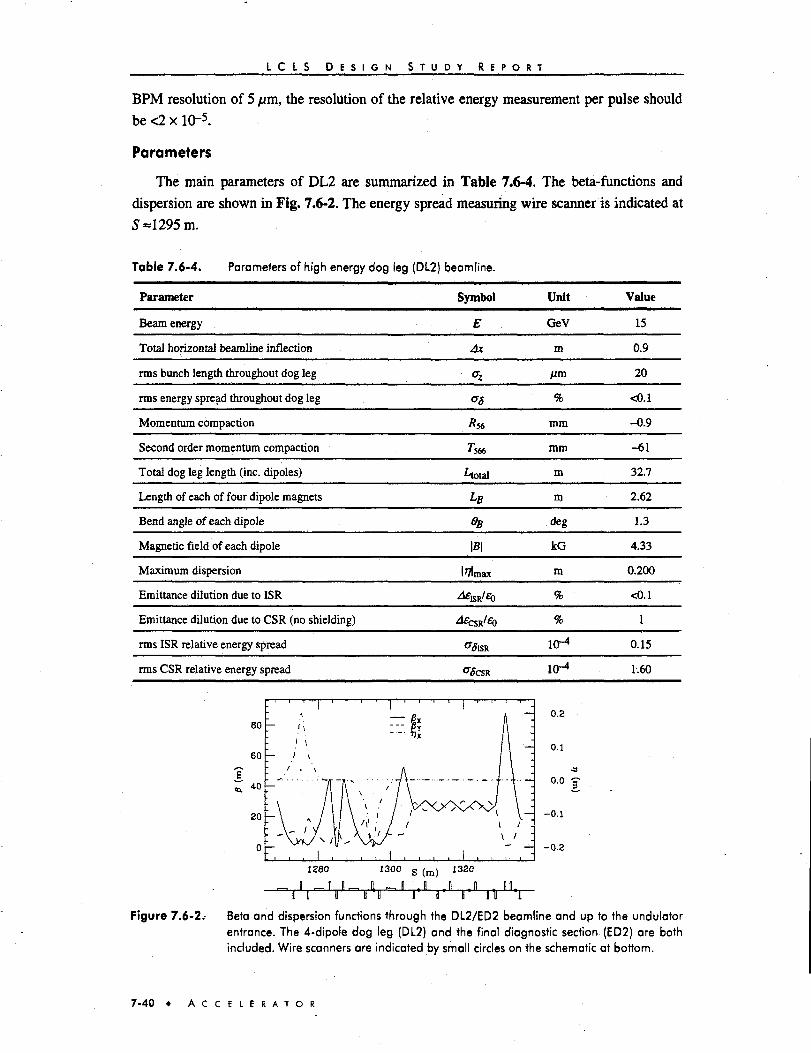
L C L S D E S I G N S T U D Y R E P O R T
BPM resolution of 5 pm, the resolution of the relative energy measurement per pulse shouldbe <2 x 10⁻⁵.
Parameters
The main parameters of DL2 are summarized in Table 7.6-4. The beta-functions and
dispersion are shown in Fig. 7.6-2. The energy spread measuring wire scanner is indicated at
S=1295m.
Table 7.6-4. Parameters of high energy dog
Parameter
Beam energy
Total horizontal beamline inflection
rms bunch length throughout dog leg
rms energy spread throughout dog leg
Momentum compaction
Second order momentum compaction
Total dog leg length (inc. dipoles)
Length of each of four dipole magnets
Bend angle of each dipole
Magnetic field of each dipole
Maximum dispersion
Emittance dilution due to ISR
Emittance dilution due to CSR (no shielding)
rms ISR relative energy spread
rms CSR relative energy spread
leg (DL2) beamline.
Symbol
E
Ax
°z<*8
*56
7*566
Aotal
%
\B\
I'Tlmax
^ C S R ' 3 )
°&SR
°<foiR
Unit
GeV
m
j im
%
mm
mm
m
m
deg
kG
m
%
%
10"4
1<H
Value
15
0.9
20
<0.1
-0.9
-61
32.7
2.62
1.3
4.33
0.200
<0.1
1
0.15
1.60
— 0.2
- 0.1
- 0.0
— -0 .1
- -0 .2
II X
Figure 7.6-2. Beta and dispersion functions through the DL2/ED2 beamline and up to the undulatorentrance. The 4-dipole dog leg (DL2) and the final diagnostic section (ED2) are bothincluded. Wire scanners are indicated by small circles on the schematic at bottom.
7 - 4 0 • A C C E L E R A T O R

L C L S D E S I G N S T U D Y R E P O R T
Beam Size, Aperture, and Field Quality
The horizontal beam size in DL2 reaches a peak value of ~200 /an (for a worst case
coherent energy spread of 0.1%) with the vertical size at -30 /an. A 25 mm full aperture is,
therefore, completely adequate. The large dispersion in the DL2 quadrupoles sets fairly tight
tolerances on field quality and gradient errors. Tables 7.6-5 and 7.6-6 list dipole and
quadrupole magnet tolerances in DL2.
Table 7.6-5. Dipole magnet tolerances for DL2. Field harmonics are evaluated on a 10 mm radiusand each entry individually corresponds to a 2% emittonce dilution.
Magnet
Name
B31-34
Table 7.6-6.
Magnet
Name
Quantity
4
Quadrupole magnet 1radius and each erjtry
Quantity
QL31-33, QL37-39 6
QL34-36 3
Roll Angle
mrad
18
l*i/*ol%
0.38
l»2/*0l
%
35
l*4/*0l
%
>100
tolerances for DL2. Field harmonics are evaluated on a 10 mmindividually corresponds to a 2% emittance dilution.
Roll Angle
mrad
2.7
16
\Abxlbx\
%
0.5
0.7
l*2/»ll
%
10
50
I&5/61I
%
>100
>100
The most challenging of these tolerances are the absolute gradient errors of the six
QL31-33, QL37-39 quadrupoles, \Ab\lb\\. Although these six magnets will be powered in
series, their gradients may differ slightly due to construction errors. The tolerance of <0.5% is
not trivially achievable. The effect on the beam, however, is the generation of linear
dispersion. This can easily be tuned out empirically by including two small correction
quadrupoles in the DL2 design. Quadrupole alignment tolerances are ~500 /an and do not
present a significant challenge, and dipole field errors (not listed) are correctable with
steering coils.
Tuning and Correction
The dominant error which will likely arise in DL2 is anomalous linear dispersion which
will dilute the horizontal emittance. Quadrupole field strength errors are the most likely
cause. Two small correction quadrupoles on separate power supplies separated by -90° of
betatron phase advance will be used in appropriate linear combinations to generate orthogonal
dispersion correction knobs. The emittance can be measured in the ED2 diagnostic section
following DL2 and will be minimized with the orthogonal knobs sequentially.
Coherent Radiation
Since the bunch length is constant over DL2, the symmetry, as in the case of the BC2
double chicane, also cancels the ~20% CSR horizontal emittance dilution which arises
between bend pairs (<rz = 20 //m). The emittance growth is calculated using both the transient
A C C E L E R A T O R • 7-41

I C I S D E S I G N S T U D Y R E P O R T
model computer code (see Section 7.4.4) and the steady-state approximation. The transient
calculation results in an emittance growth of 1%, whereas the steady state is 0.1%. The CSR
rms energy spread induced is fairly large at 1.6 x 1(H, but the allowable coherent energy
spread FEL chirp tolerance is nearly an order of magnitude larger (1 x 10~3). Fig. 7.6-3
shows the "steady state" (ss) and the transient modeled energy spread along with the
horizontal emittance growth (steady state) due to CSR through the DL2 beamline for a 20 //m
bunch.
o
•(
o
6
X
0.2
0.1
0.0
-0.1
-0.2
•
—
-
— *<•
•
—
•
-
01 1
. ' >
——1
1 '
1 .
1 \
/ • \
V
_ • _ ' _ - • — V 4 - ^
, , , 1I 10
ffi 111
1 . .'.
•• "
(7 (SS)
1 III Z
III
1. ' ' '
^ " '
N
\
\
m
• i '
'
i
ui
—
—
—
_:
-—
S (m)
Figure 7.6-3. The induced rms energy spread ("steady-state": solid, "transient": dash) and horizontalemittance growth (dots) due to CSR along the DL2 high energy dog leg for a 20 jJtnrms gaussian bunch. The horizontal dispersion function (dash-dot) and DL2 beamlineschematic are also shown.
7.7 Instrumentation, Diagnostics, and Feedback
Critical to the preservation of the transverse emittance and the generation of a low-energy
spread micro-bunch are the precise measurement techniques and correction schemes used to
initially commission and maintain the machine. The LCLS accelerator has many phase space
diagnostics and correction schemes built into the design. In most cases the relevant beamline
is specifically designed to enhance the performance of these critical diagnostics.
7.7.1 Transverse Emittance Diagnostics
There are six different transverse emittance diagnostic stations distributed along the
LCLS accelerator of which five are new installations (the existing sector-28 station [19] will
be slightly modified). In four of these cases the emittance measurement is accomplished with
four consecutive wire scanners placed along the beamline with appropriate phase advance
between scanners to optimize resolution. (Only three scanners are necessary with four used to
improve resolution and provide redundancy.) This also allows non-invasive emittance
measurements to be made during normal machine operation. To save space, the emittance
7 - 4 2 • A C C E L E R A T O R

L C L S D E S I G N S T U D Y R E P O R T
measurement following BC2 consists of a single wire scanner placed at a beam waist
(&x,y - 0) and upstream quadrupole magnets are used to vary the beam size at the scanner.
The emittance measurement stations and their parameters are summarized below in
Table 7.7-1.
Table 7.7-1. Transverse emittance measurement stations along the LCLS {y£o = 1 /^rn).
Location
Following L0
Following BC1
AttheendofLinac2
Following BC2
Sector-28 in Iinac 3
Prior to undulator
StationName
EDO
EDI
L2-ED
BC2-ED
L3-ED
ED2
Energy(GeV)
0.150
0.280
5.5-6.0
6.0
9.9-11.7
15.0
(pm)
67
52
28-63
49
42-58
30
Oy(fim)
67
52
32-65
48
42-58
30
No. ofScanners
4
4
4
1
4
4
Existing
No
No
No
No
Yes
No
The energy range of a diagnostic station listed in Table 7.7-1 (e.g., L2-ED) indicates the
scanners are separated by accelerator sections. A range of beam sizes in the table represents
the minimum and maximum over the four scanners. The EDO, EDI and ED2 stations listed in
Table 7.7-1 are dedicated, non-accelerating emittance diagnostic stations designed to produce
identical beam sizes in x and y at all scanners; the betatron phase advance between wires is set
to the optimal value for a four-scanner station (45°). These three sections are shown
schematically in Figs. 7.6-1 (EDO), 7.3-2 (EDI), and 7.6-2 (ED2) with small circles
indicating wire scanner locations on the beamline schematics. The scanners are separated by
quadrupole doublets, with an upstream matching section. For four scanners, this 45°
separation minimizes emittance resolution sensitivity to incoming beta function errors.
Fig. 7.7-1 shows the emittance measurement resolution for the four wire systems of EDO,
EDI or ED2 (solid) versus the phase of an incoming beta-mismatch with a large amplitude of
£= 1.5, as defined in Eq. 7.7.1. The subscripted parameters represent the ideal matched beam
and the non-subscripted parameters are the perturbed beam.
(7.7.1)
For comparison, the same resolution sensitivity to mismatch phase is plotted (dash) for
the existing linac sector-28 four-wire system of the SLC. A modified SLC system is also
shown (dots)—(see L3-ED description below). The single scanner relative beam size
resolution used here is 5%. The average emittance measurement resolution (for g= 1.5) for
an optimally designed system (6.7%) is nearly a factor of 2 better than that (11%) of a system
where wire scanners are a latter addition to an existing optical design (as in the case of the
A C C E L E R A T O R • 7-43

L C L S D E S I G N S T U D Y R E P O R T
sector-28 system). The resolution at the worst case phase is nearly three times better. The
equal beam sizes at each scanner in both x and y may also help reduce systematic errors of the
measurement and simplify the measurement interpretation (i.e., beam is matched when all
wires show equal beam size).
6? 15 -
100 150
/cleg
Figure 7.7-1. Emittance resolution versus beta-mismatch phase for a C, = 1.5 and beam sizeresolution of 5%. Resolution is shown for the EDO/ED 1/ED2 sections (solid), the existingSLC sector-28 system (dash) and a modified sector-28 for SLC (dots). Lines are theaverage resolution.
EDO Emittance Station
The EDO station (see schematic of Fig. 7.6-1) is used to confirm and optimize the
emittance of the injector system. It is a resolution optimized four-wire system as shown in
Fig. 7.7-1, which is minimally sensitive to incoming beta-function errors. For the nominal
emittance of 1 mm-mrad at 150 MeV, the rms beam size is identically 67 pm at each wire in
both planes.
EDI Emittance Station
The EDI station (Fig. 7.3-2) is placed directly after BCl. It is crucial for the
measurement and empirical correction of dispersion errors generated in BCl. The BCl
chicane can also be completely switched off to help isolate the different errors of BCl, LI,
and DLL Like EDO, EDI is a dedicated emittance measurement section. At 280 MeV a
52 ftm beam size exists at each wire in both planes.
L2-ED Emittance Station
The L2 linac is the most sensitive to orbit variation (note large growth in Fig. 73-3) and
therefore can be expected to require frequent, perhaps daily, emittance optimization. The
L2-ED station is placed at the end of L2 (Fig. 7.3-4). It is a space-constrained, four-scanner
7 - 4 4 • A C C E L E R A T O R

L C L S D E S I G N S T U D Y R E P O R T
station with non-optimal phase advance and an expected emittance resolution of -10%. This
section will be used primarily to empirically minimize the wakefield emittance dilution of L2.
BC2-ED Emittance Station
The BC2-ED station is a single wire ("WS26" in Fig. 7.4-2) included to-provide some
separation of BC2 dilution effects from those of the first half of L3. The quadrupoles used to
measure the emittance are, however, upstream of BC2 and therefore may not provide the most
ideal measurement since the beta functions will vary through BC2 as the measurement
progresses (see Eq. 7.4.7). The L3-ED (sector-28) scanners may also be used to monitor BC2
dilution effects.
L3-ED Emittance Station
The L3-ED station (Fig. 7.3-8) is composed of four existing sector-28 wire scanners. The
linac optics, however, change somewhat in this area for LCLS operation and therefore a small
modification to the existing scanner locations is called for. The first sector-28 scanner will be
moved upstream by one cell (24 meters) and the last scanner will be moved downstream by
one cell. The LCLS optics then provides nearly 45° per plane between scanners. In fact, the
statistical resolution for the SLC optical configuration is also marginally improved
(Fig. 7.7-1: dots). The rms beam sizes are not identical at each wire; however, the phase
advance between scanners provides optimal statistical measurement resolution. The L3-ED
station will be used primarily to guide BC2 dispersion and CSR corrections. Emittance
dilution occurring within L3 (see Fig. 7.3-7) is expected to be very small due to the short
bunch there.
ED2 Emittance Station
A final emittance measurement section (Fig. 7.6-2) is included just upstream of the
undulator entrance. This section will be used to make precise adjustments to the final
horizontal and vertical beta functions (using quadrupoles QM33-36 of Fig. 7.6-2) and to
confirm and optimize the final emittance immediately before the undulator. This emittance
measurement section is also necessary to diagnose potential emittance dilution arising in DL2
through dispersion errors or CSR. Like EDO and EDI, ED2 is a dedicated emittance
measurement section, but with a 30 jum beam size at each wire in both planes at 15 GeV.
7.7.2 Bunch Length Diagnostics
The beam current delivered to the LCLS undulator is a critical parameter. It is determined
by both the charge accelerated and the final bunch length achieved by the two bunch
compressors. To optimize the compression, the bunch length needs to be measured before and
after BC1 and BC2. In addition, once the bunch compressors are set up, a bunch length
feedback system will be advantageous in the stabilization of the compressors. These feedback
systems have not yet been designed.
A C C E L E R A T O R • 7-45

L C L S D E S I G N S T U D Y R E P O R T
The bunch lengths of interest are approximately 1000, 400, and 20 pm rms (10, 4, and
0.2 psec full width, respectively). Measuring 10 psec accurately using a streak camera is
straightforward. The 4 psec measurement is more challenging but still feasible. Direct
measurement of the 0.2 psec bunch is problematic. Bunch length monitors [20] designed to
use coherent synchrotron radiation (CSR) have demonstrated fast, non-invasive
measurements in the LCLS regime. They, however, provide a relative bunch length
measurement. Absolute bunch length requires an understanding of the frequency spectrum of
the radiation, the various component attenuation functions, and the CSR process.
For the LCLS accelerator, CSR detectors are used as the basic bunch length monitors,
and their outputs are calibrated using a streak camera for the 10 and 4 psec ranges and using a
"zero-phasing technique" [21] for the 0.2 psec range. The zero-phasing technique employs an
rf system at a zero-crossing angle to generate a correlated energy spread. The transverse beam
size can then be measured in a dispersive region to extract the bunch length. In the LCLS, the
L3 linac is used as the rf system. The measurement is invasive and performed infrequently to
calibrate or cross-check the CSR detectors. The micro-bunch is transported to the energy
spread measuring wire scanner in DL2 with a +90° L3 rf phase (zero crossing producing no
acceleration in L3). The measurement is then repeated at a -90° rf phase. The bunch length is
then given by the average of the two energy spread values.
* 4xEf-L.
Here X is the rf wavelength (105 mm), £,• is the L3 injection energy (6 GeV), iy is the L3
final energy obtained when the L3 rf phase is at crest (15 GeV), and <7<?(±9o°) are the two
energy spread measurements at +90° and -90°.
Results of a measurement using this method are simulated in Fig. 7.7-2, including
wakefields, and demonstrate that it can be used to measure the absolute bunch length with an
accuracy of a few percent. A 55 /*m FWHM bunch length generates FWHM energy spread
values of 0.31% (-90°) and 0.67% (+90°) which, when used in Eq. 7.72, reproduce the
55 fjm bunch length to within 1 fim. Statistical resolution is dependent on the wire scanner
used and should be 5-10%. The horizontal FWHM beam size at the DL2 energy spread wire
associated with these conditions is ~1 mm. The less invasive CSR monitor is then directly
calibrated.
7 - 4 6 • A C C E L E R A T O R

L C L S D E S I G N S T U D Y R E P O R T
\
•o
300
200
100
-
-
- 4
O -
1
0
- l
-
— z ••
' ' ' | ' ' * " { " ' * ' | " " ' '6mm = 0.315%
-
,1-
- 2 0 2 'd/%
. j . . . . ( . . .
\
tI
T :
. i . . . . i . . •
0.00 0.05 .z/mm
300
200
100
-
-
I -4
1
0
~l
-
— 2 1 —
L3 rf off 0rf=+9O°
....... |.... |... .&nmt = 0.145% :-
—
J. . 1
w u
300
200
100
. . . . | . . . . | . . . . | . . . .: 6TWWI = 0 - 8 7 « :
- -
— —
r . r t , •- 2 0 2 4 - 4 - 2 0 2 4
d/% . <5/%• I • • • • . j • • .
i -
t \ :
. i . . . . i . . •
1
0
- 1
. • i • • - •• i • -
I \\
'• • " " " ' ~ " * ~ \ •
• . 1 . . ^ . I . .
0.00 0.05 0.00 0.05z/mm z/mm
Figure 7.7-2. Simulated zero-phasing technique for absolute bunch length measurement of 56 pmFWHM. Top row of plots are energy distribution after DL2 at 6 GeV for -90°, rf-off,and +90° in L3 (no acceleration in all cases). Bottom row are longitudinal phase spacefor these same cases.
7.7.3 Beam Energy Spread Diagnostics
DLl Energy Spread Diagnostics
The energy spread measurement in DLl is made with a single wire scanner located
between the two dipoles of DLl at the point where the horizontal dispersion function reaches
a value of ^ = -126 mm with a horizontal beta function of /?x=3.7 m (see "WS05" of
Fig. 7.6-1). For the nominal emittance and nominal energy spread of cr$~ 0.2% at 150 MeV,
the betatron beam size is 113//m, but the dispersive size is 252 /urn. This produces a
systematic energy spread measurement error of 10% (see Eq. 7.7.3). The statistical error
depends on the wire scanner and should be 5-10%.
— 1 < 10% (7.7.3)
BCl Energy Spread Diagnostics
The energy spread measurement in BCl is made with a single wire scanner located in the
center of the chicane at a point where the horizontal dispersion function is TJX = 117 mm and
the horizontal beta function converges towards a minimum of fix= 1.4 m (see "WS11" of
Fig. 7.5-1). For the nominal emittance and nominal energy spread of a j = 2.3% at 280 MeV,
A C C E L E R A T O R 7-47

L C L S D E S I G N S T U D Y R E P O R T
the betatron beam size is 50 //m, but the dispersive size is 2700//m. This produces no
systematic error in the energy spread measurement.
BC2 Energy Spread Diagnostics
The energy spread measurement in BC2 is also made with a single wire scanner located
in the center of the first chicane at a point where the horizontal dispersion function is
TJX = 290 mm and the beta function converges towards a minimum of fix - 6.5 m (see "WS25"
of Fig. 7.4-2). For the nominal emittance and nominal energy spread of O£= 1.1% at 6 GeV,
the betatron beam size is 24 /mi, but the dispersive size is 3200 jum. As in the case of BC1,
this produces no systematic error in the energy spread measurement.
DL2 Energy Spread Diagnostics
The energy spread measurement in DL2 is made with a single wire scanner located where
the dispersion function is ^ = 1 7 8 mm and the beta function converges towards a minimum
of fix = 4 m (see first wire scanner of Fig. 7.6-2). For the nominal emittance and an rms
energy spread of eg- 0.02%, the betatron beam size is 12 /urn, but the dispersive size is a
measurable 36 fim. The total beam size is then 38 //m, and a horizontal wire scanner produces
an energy spread measurement accuracy of 5% at 15 GeV.
7.7.4 Orbit and Energy Monitors and Feedback Systems
Orbit Feedback Systems
Orbit feedback systems will be placed at the entrance of the L2 linac, the L3 linac and at
the undulator entrance. As at the SLC [22], these systems will each be composed of -10 x and
y BPMs preceded by a set of two horizontal and two vertical fast dipole corrector magnets
controlled by a microprocessor based cascaded feedback system. The cascade algorithm
isolates each feedback system such that the systems do not all respond to the same orbit
change.
In order to control transverse orbit variations to better than 1/10 of the beam size, the
BPM resolutions for the three systems described above need to be 50 jam, 20 ftm and 10 fim,
respectively (decreasing with increasing energy). Orbit variations which occur at frequencies
below -10 Hz will be stabilized. Faster variations cannot be damped significantly and will
need to be identified at the source. Additional orbit control systems (e.g., in the L0 linac) are
addressed in Chapter 6 or not yet identified.
Transverse vibrations of quadrupole magnets will generate orbit variations which, if fast
enough, will not be damped by feedback systems. Tolerance calculations in L2 (strongest
quadrupole gradients) indicate that uncorrelated random vibrations of all 35 L2 quadrupoles
at the level of 400 run rms will generate orbit centroid fluctuations in the undulator which are
6% of the beam size there (6% of 30 /an). Measurements in the SLC indicate that existing
linac magnet vibrations are <250 nm [23] with the highest frequency content at 59 Hz and
7 - 4 8 • A C C E L E R A T O R

L C L S D E S I G N S T U D Y R E P O R T
10 Hz driven by cooling water. These observed vibrations are small enough to limit undulator
orbit centroid jitter to well below the goal of 20% of its nominal beam size.
Energy Feedback Systems
Energy feedback systems will be placed at each bending system (DL1, BC1, BC2, and
DL2). A single BPM or group of BPMs placed at a high dispersion point will be used to
determine energy variations, and upstream rf phases will be used to stabilize the energy. A
group of klystron phases will be used to control the energy while maintaining the correlated
energy spread such that compression variations are not induced. Similar systems have been
successfully tested at SLC [24].
The DL1 Energy Feedback System consists of at least 3 BPMs—one placed inside QL01,
another in QL07, and a third near QL04 (see Fig. 7.6-1). With this simple system, energy
variations can be distinguished from betatron oscillations, and the large dispersion at the
QL01 and QL07 BPMs (195 mm) produces a relative energy resolution of 5< 1 x 10"4 with
20 fjtm resolution BPMs.
The BC1 Energy Feedback System consists of 3 BPMs—one placed at the center of the
chicane and at least two more beyond the chicane in the EDI diagnostic section (see
Fig. 7.3-2). The large dispersion (117 mm) at the chicane center should produce a relative
energy resolution of S< 2 x 10~4 with a 20 jum resolution BPM.
The BC2 Energy Feedback System consists of 2 BPMs—one placed at the center of each
BC2 chicane. Since the 2x2 transfer matrix between chicane centers is - I (see Fig. 7.4-1)summing these two x BPM readings will exactly cancel any betatron oscillation signal leaving
only an energy variation signal. The large nominal dispersion in the two chicanes (290 mm
and 110 mm, respectively) should produce a relative energy resolution of <?= 7 x 10~5 with
two 20 jum resolution BPMs.
The DL2 Energy Feedback System consists of 2 BPMs—one placed at QL32 and another
at QL38 (see Fig. 7.6-2). Since the 2 x 2 transfer matrix between these quadrupoles is +1,
differencing these two x BPM readings will cancel any betatron signal leaving only the
energy signal. The large nominal dispersion in the two quadrupoles (200 mm) should produce
a relative energy resolution of <5= 7 x 10~5 with two 20 //m resolution BPMs.
In all cases above, the energy resolution exceeds that necessary for the compression
system tolerances (see Table 7.2-3).
7.8 The Wake Functions for the SLAC Linac
7.8.1 Introduction
Obtaining wake functions for the SLAC linac structure that are sufficiently accurate to be
used in beam dynamics studies for bunches as short as 20 jjm (rms) is not an easy task. It
requires an accurate knowledge of the impedance of the structure over a large frequency
A C C E L E R A T O R • 7-49

L C L S D E S I G N S T U D Y R E P O R T
range, which is difficult to obtain both by means of frequency domain and time domain
calculations. Direct time-domain integration, using a computer program such as the MAFIA
module T2 [25], needs a very large mesh and hence prohibitive amounts of computer time.
Even then, errors will tend to accumulate in the results. The approach actually employed, uses
a frequency-domain calculation applied to a simplified model of the linac structure, an
approach which also has its difficulties. The wake functions obtained are the wake fields
excited by a point charge, as a function of distance behind that charge. By performing a
convolution over the bunch, the wake fields left by a bunch of arbitrary shape can be
obtained.
A SLAC structure is 3 m long; it consists of 84 cells. It is a constant gradient structure,
and both the cavity radius and the iris radius gradually become smaller (the change in iris
radius is 0.5%/cell) along the length of each structure. In our calculations each SLAC
constant gradient structure is broken into five pieces. Each piece is represented by a periodic
model with an average iris radius, and the rounded iris profiles are replaced by rectangular
ones. The wake fields for the five models are obtained and then averaged to obtain wake
functions to represent an entire structure. Questions as to the accuracy and applicability of the
calculated wake functions concern primarily:
• The accuracy of the periodic calculations themselves
• Transient effects and effects at the ends of a structure
• The fact that the irises vary in the real structure
• The effects of resistivity/roughness of the iris surface
7.8.2 The Calculated Wakefields for the SLAC Linac
The wakefields for the SLAC linac structure were first calculated many years ago [26].
The methods and results presented here are essentially the same, though there are some
changes in the details (see, for details, where these methods are applied to the NLC X-band
structure [27] and the SBLC S-band structure [28]). To obtain the wake fields for each of the
representative periodic models, are several hundred mode frequencies and loss factors are
obtained using computer programs that employ mode-matching techniques. The accuracy of
these calculations is not easy to assess. The density of modes obtained is one consistency
check, and good agreement is found.
The high-frequency contribution to the impedances is obtained employing the so-called
"Sessler-Vainsteyn optical resonator model" [29,30]. It is a simple model that combines the
Poynting flux at the iris due to the beam with the diffraction due to light at the edges of a
periodic array of circular mirrors. It yields the expected high-frequency dependence of the
impedance; e.g., the real part of the longitudinal impedance varies with frequency as of3'2.
Fig. 7.8-1 shows the real part of the longitudinal impedance, averaged over frequency bins,
for the geometry of cell 45 (a in the plot is the iris radius). The dashed curve is the Sessler-
Vainsteyn prediction. At the higher frequencies the agreement is seen to be quite good. As a
7 - 5 0 • A C C E L E R A T O R

L C L S D E S I G N S T U D Y R E P O R T
dipole example, the real part of the longitudinal dipole impedance, averaged over frequency
bins, for the geometry of cell 45 is plotted in Fig. 7.8-2, with the dashed curve again giving
the Sessler-Vainsteyn prediction. There appears to be a 15% systematic difference between
the two results at high frequencies, probably due to the approximate nature of the Sessler-
Vainsteyn model. The agreement, however, is acceptable for our requirements.
The longitudinal wakefield of the 5 representative cells—cells 1, 23, 45, 65, and 84—is
given in Fig. 7.8-3, and the average (with the end cells weighted by one half), representing
the whole structure, is given by the dashes. One important consistency check is that for each
model structure, the longitudinal wakefield at the origin must satisfy [31]
(7.8.1)
with Zo = 377 £2 and a the iris radius. In all cases the computed values are low, but in no case
by more than 4%. Similarly, the transverse wakefield of the representative cells is given in
Fig. 7.8-4, and the average, again representing the whole structure, is given by the dashes.
The transverse wakefield of the representative cells must satisfy Eq. 7.8.2 [26]. In all cases
the agreement is within 1-2%.
^ £ (7.8.2)net
7.8.3 Discussion
The calculated wakefields are asymptotic wakefields in that they apply only after the
beam has traversed a critical number of cells A^t. For a gaussian bunch, for the total loss
obtained using only the asymptotic wake functions to be within a few percent of the loss
when transient effects are also included, requires that
(7.8.3)
with a > 0.5, p the structure cell length, and oz the bunch length. The transient region is
largest for short bunches. In the LCLS the bunch is shortest after the second bunch
compressor where az = 20 fan. Taking, in addition, a = 1 cm and p = 3.5 cm, that NCTn ~ 70,
which represents about 80% of the length of one structure or 0.4% of the length of the third
linac. In most of the SLAC linac the 3-m structures are combined in groups of four, with
nearly no extra space in between them; the groups of four are separated by about 20 cm of
beam tube, and every 100 m there is an extra 4 m of beam tube. With this arrangement, after
the.end of the structures, the wakefields generated by the beam do not have a chance to return
to their initial conditions, except partially at the 3% of the structures that follow the 4 m gaps.
A C C E L E R A T O R • 7-51

L C L S D E S I G N S T U D Y R E P O R T
Therefore, using the asymptotic wakefields to represent the entire SLAC linac, and ignoring
the transient effects, should result in very little error even for a 20 jLtm bunch.
103 _
*f 102 -
—
•
• • ' 1 • • • • 1 •
N
—
, , , , 1 , , , , 1 ,
' • • | • • • • | • • • •
-
, , , 1 , , , , 1 . , , ,200 400 600 800 1000
Figure 7.8-1 . The real part of the longitudinal impedance, averaged over frequency bins, for thegeometry of cell 45. The Sessler-Vainsteyn prediction is given by the dashed curve.
10
200 400We) 2
600 800 1000
Figure 7.8-2. . The real part of the longitudinal dipole impedance, averaged over frequency bins, forthe geometry of cell 45. The Sessler-Vainsteyn prediction is given by the dashed curve.
7 - 5 2 4 A C C E L E R A T O R

L C L S D E S I G N S T U D Y R E P O R T
400
300
a
. . . . . . . . . . . . .
Figure 7.8-3. The longitudinal wakefieid of representative cells in the SLAC structure (solid curves).The average represents the whole structure (the dashes).
BBa>
0.0 2.0
Figure 7.8-4. The transverse (dipole) wakefieid of representative cells in the SLAC structure (solidcurves). The average represents the whole structure (the dashes).
There are four other effects that can be important for short bunches: (1) The so-called
"catch-up distance" effect: If the head of the beam generates a wakefieid at a certain position
in the linac, due to causality the tail does not feel the effect until a distance ~0 .5a 1loz,
which in this case is 2.5 m, later. Since this is a small fraction of the 516 meters of
accelerating structure after the second compressor, this effect should not be important. (2) For
at < aly, which in this case is 0.3 fim, the impedance drops dramatically. Since the
minimum bunch length is 20 ftm, this effect should also not. be important for the LCLS.
A C C E L E R A T O R 7-53
L C L S D E S I G N S T U D Y R E P O R T
(3) The effect of the resistivity of the iris surface is shown, in the following section, not to be
a significant effect for the LCLS accelerator. (4) The effect of the roughness of the iris
surface will be discussed in Section 7.8-6.
Finally, it should be noted that the above estimates all assume that the bunch is gaussian,
which it is not. The real bunch shape is rather rectangular with spikes, which have a rms
length on the order of a few microns, at the tail of the distribution. The Fourier transform of
such a bunch shape reaches to higher frequencies than the gaussian approximation, and
therefore the short bunch effects will become somewhat more pronounced than estimated
above. However, even with this consideration, the calculated wake functions will accurately
represent the wakefield effects in the linac for the LCLS project.
7.8.4 Confirmations
There have been confirmations, both theoretical and by measurement, of the calculated
SLAC wake functions and, more recently, of the similarly calculated wake functions for the
NLC and the DESY-SBLC linac. All the comparisons, however, have been done for bunch
lengths significantly larger than the 20 /an of interest here. As to theoretical comparisons, the
calculated SLAC wake functions have been confirmed, for gaussian bunches down to
az = 0.5 mm, using the time domain program TBCI [32]. A time domain program exists that
seems to be able to obtain accurate results for short bunches in accelerating structures [33].
For the case of a 100 |im bunch in the NLC structure, the results of this program, as well as
those of a frequency domain program [34], agree with our frequency domain results to within
7%.
As to confirmation by measurement, in the SLC linac the total wakefield-induced energy
loss [35] and more recently the wakefield-induced voltage of a bunch [36] have been shown
to agree quite well, for bunch lengths down to 0.5 mm. Also, in the ASSET test facility, the
short range transverse wakefield of a 0.5 mm bunch in the NLC structure has been measured,
and the results agree quite well with the calculated results [37].
7.8.5 Resistive Wall Wakefields
In addition to geometric wakefields, the micro-bunch in L3 and beyond experiences a
longitudinal resistive wall (RW) wakefield which may also introduce a coherent energy
spread along the bunch [38]. For a bunch with gaussian axial distribution which is much
longer then the characteristic length, SQ,
(7.8.4)
the rms relative energy spread, <7<jRW, induced in a smooth cylindrical chamber of radius, a,
and conductivity, c, is
7 - 5 4 • A C C E L E R A T O R

L C L S D E S I G N S T U D Y R E P O R T
< T J R W = ( 0 . 2 2 >e2cNL
(7.8.5)
The 172 3-meter copper accelerating structures that make up most of the length of L3 are
each composed of 84 cavities. A model of three such cavities is shown in Fig. 7.8-5.
Figure 7.8-5. Model of the geometry of three cavities (of 84) of one SLAC 3-meter acceleratingsection. The dimensions used are: a = 11.6 mm, b =41 .3 mm, d = 35.0 mm, andg= 29.2 mm. The iris radius, a, actually decreases from 13.1 to 9.1 mm along thesection. The mean is used here.
The large radius (b) segments of the structures are not "seen" by the bunch and therefore
contribute nothing. For copper ( a = 5.9 x 10⁷ Q^nr 1) and iV=6 .3x 109 er per bunch, the
RW relative rms energy spread at ymc2 =15 GeV is 0.01%. Note, this is for a gaussian bunch
which is long compared to *o (Eq. 7.8.4). To more accurately estimate the RW energy spread
generated along the entire beamline from BC2 exit to undulator entrance, including non-
accelerating sections, the beamline is broken into three discrete sections of significantly small
radius (Table 7.8-1). The remaining sections (-120 m) have much larger radii (40-400 mm)
and are ignored here.
Table 7.8-1. The three main beamline sections which transport the micro-bunch and contribute to aresistive wall wakefield energy spread generated between BC2 and the undulatorentrance.
Beamline Section
linac 3 rf-stnictures (iris a)
Iinac 3 non-accelerating chambers
Iinac-to-undulator beamline
Material
Copper
Stainless Steel
Aluminum
Conductivity
Q-J-m-1
5.9X10⁷
0.14xl07
3.6X10⁷
Radius
mm
11.6
12.7
12.7
Length
m
87
60
100
fim
23
85
29
The 60 meters of 1-inch diameter stainless steel are distributed along Linac 3 as
quadrupole/BPM chambers, and other short non-accelerating sections including 12 meters
beyond sector-30 in the beam switchyard. The aluminum sections will be new chambers that
A C C E L E R A T O R 7-55

L C L S D E S I G N S T U D Y R E P O R T
follow the large radius beam switchyard sections and make up the chamber for the DL2
section. For all of these sections, the bunch (20jum) is shorter than the characteristic length
SQ. The RW energy spread of the short-bunch (cr/srjOl) is calculated using the Green's
function wakefield [39],
* { •IJ
(7.8.6)
of a short bunch which is convoluted with the bunch distribution of Fig. 12-3. This estimate
ignores the frequency dependence of the conductivity. The results for each of the three
sections of Table 7.8-1 are shown in Fig. 7.8-6. For this bunch distribution (shown on
arbitrary vertical scale as solid curve in the figure), the total rms RW energy spread generated
by all three sections is 2.5 x 1CT4 (with respect to the mean), which is a factor of 4 below the
chirp tolerance (~1 x 10~3). If the linear component of the energy spread is removed (-0.5° rf
phase increase in L2), this is reduced to 1.7 x 10"4.
U.UYO
0.050
0.025
*° 0.000
-0.025
-0.050
• • • • j
V./r~ "•>
\ \
V N
- •-!-. '_
. . . . 1
• • • • ( • •
^ —
X ' I TS.- ''
s s '•»
• ' I
Jr
* N\
\. . f
// /
< •
' ' 1
/;
/ • '
/ • '
/
/
/
. . 1
. . . . ,
<?<( Cu)=>
a,( SS)=ff»( Al)=
•s
//
/
. . . 1
0.710"4
1.610"*0.7-10"4 '2.5-10~*~!
_
—
-
20 40 60 80 100 ISO
Figure 7.8-6. Resistive wall wakefield of a 1 nC bunch after convolution with the axial distribution(solid, arbitrary vertical scale) of Fig. 7.2-3. The energy spread at 15 GeV is generatedby the beamline sections described in Table 7.8-1. The total RW rms relative energyspread (with respect to mean) is 2.5x10"4 which can be reduced to 1.7x10~* when thelinear component is removed.
7.8.6 The Impedance Due to the Roughness of the Iris Surface
The wakefields due to the surface roughness of a tube have been recently estimated [40].
The energy spread generated by the longitudinal wakefield is correlated along the bunch and
is much more critical in the undulator with its small tube radius. The effect as it pertains to
7 - 5 6 • A C C E L E R A T O R
I C I S D E S I G N S T U D Y R E P O R T
the accelerator is briefly described here. A more thorough discussion is taken up in
Section 8.7.
The effect of roughness is important primarily after the second bunch compressor, where
the beam is shortest. From causality it is seen that the wakefield effect experienced by the
beam in the accelerator structure can only be due to the 12 mm radius irises. The length of
accelerating structure after the second compression is ~520 m; the fraction of the period that
is the iris length is 0.167; therefore, the effective length for this calculation is 86 m. For a
1 nC, 20//m rms gaussian bunch and a surface roughness of 0.15 /an [41] we find a
correlated rms energy spread of as = 0.06% at 14.3 GeV. However, the bunch distribution is
closer to uniform than gaussian (see Fig. 7.2-3). This reduces the rms energy spread to a
tolerable -0.02%. The transverse wakefields generated by the rough surface are negligible
(see also Section 8.7).
7.9 Summary of Dilution Effects
7.9.1 Transverse Emittance Dilution
The overwhelming majority of emittance dilution mechanisms occurring in the
accelerator produce an immediate 'correlated' emittance growth such that the mean transverse
position of each bunch slice is altered, but the local electron density remains nearly unaltered;
the projected emittance is changed but the slice emittance is not. The degree of preservation
of this correlation through the entire accelerator has not, at this time, been studied in
sufficient detail to predict its full impact on FEL performance. Whether the emittance is
correlated or not has different implications for the brightness and the saturation length. A
correlated emittance growth effects the brightness whereas an increase in the slice emittance
effects both brightness and saturation length. Detailed multi-particle tracking studies are
needed to quantify this issue.
Simulations of transverse emittance dilution throughout the various accelerator sections
have been presented in the preceding sections. A summary is presented here of the
accelerator 'emittance budget'. Included in this budget are estimates of the emittance
measurement resolution and correction capabilities of each system. For example, if the
emittance after BC1 is increased through the generation of anomalous momentum dispersion,
then the EDI wire scanners are used to measure the emittance so that it can be empirically
minimized using the CQ11 and CQ12 quadrupole pair in BC1. The correction is ultimately
limited by the measurement resolution which is conservatively assumed (from SLC
experience) to be de/eo ~ 10%. If the emittance is measured 5 times in each minimization
scan the final resolution should be ~(10%)/V5 ~ 4%. This represents the approximate
minimum emittance dilution achievable after optimization, assuming full correction is
possible. Table 7.9-1 lists the emittance budget based on these estimates and other
uncorrectable dilution components.
A C C E L E R A T O R • 7-57
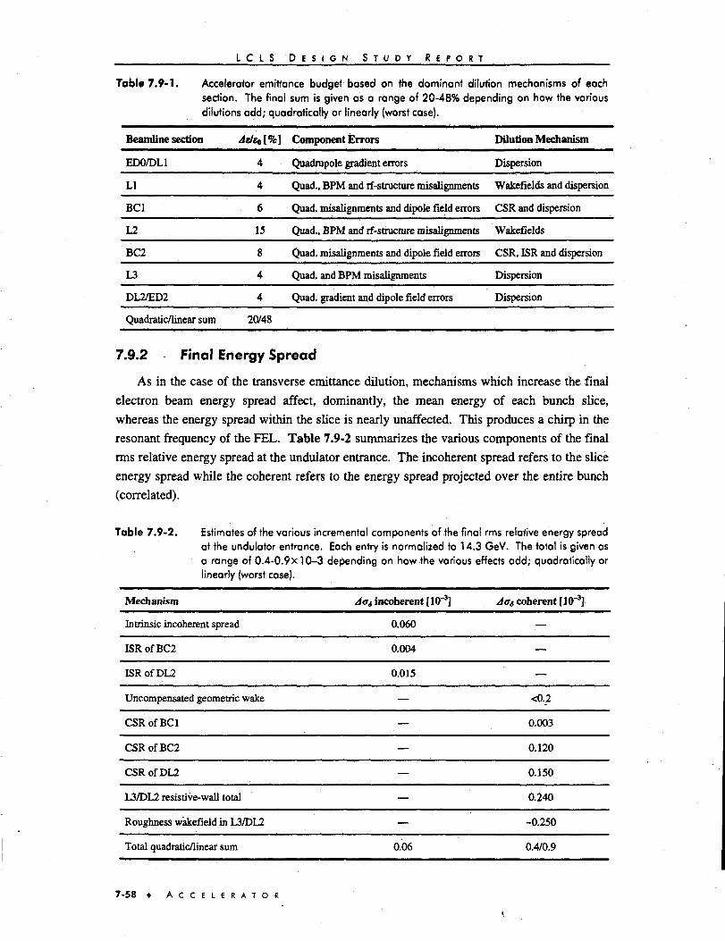
L C L S D E S I G N S T U D Y R E P O R T
Table 7.9-1. Accelerator emittance budget based on the dominant dilution mechanisms of eachsection. The final sum is given as a range of 20-48% depending on how the variousdilutions add; quadratically or linearly (worst case).
Beamline section
ED0/DL1
LI
BC1
L2
BC2
L3
DL2/ED2
Quadratic/linear sum
4
4
6
15
8
4
4
20/48
Component Errors
Quadrupole gradient errors
Quad., BPM and if-structure misalignments
Quad, misalignments and dipole field errors
Quad., BPM and rf-structure misalignments
Quad, misalignments and dipole field errors
Quad, and BPM misalignments
Quad, gradient and dipole field errors
Dilution Mechanism
Dispersion
Wakefields and dispersion
CSR and dispersion
Wakefields
CSR, ISR and dispersion
Dispersion
Dispersion
7.9.2 Final Energy Spread
As in the case of the transverse emittance dilution, mechanisms which increase the final
electron beam energy spread affect, dominantly, the mean energy of each bunch slice,
whereas the energy spread within the slice is nearly unaffected. This produces a chirp in the
resonant frequency of the FEL. Table 7.9-2 summarizes the various components of the final
rms relative energy spread at the undulator entrance. The incoherent spread refers to the slice
energy spread while the coherent refers to the energy spread projected over the entire bunch
(correlated).
Table 7.9-2. Estimates of the various incremental components of the final rms relative energy spreadat the undulator entrance. Each entry is normalized to 14.3 GeV. The total is given asa range of 0.4-0.9x10⁻³ depending on how the various effects add; quadratically orlinearly (worst case).
Mechanism
Intrinsic incoherent spread
ISRofBC2
ISRofDL2
Uncompensated geometric wake
CSRofBCl
CSR of BC2
CSRofDL2
13JDL2 resistive-wall total
Roughness wakefield in L3/DL2
Total quadratic/linear sum
Jos incoherent [10"3]
0.060
0.004
0.015
—
—
—
—
—
—
0.06
Aas coherent [10~3]
—
—
—
<0.2
0.003
0.120
0.150
0.240
-0.250
0.4/0.9
7-58 A C C E L E R A T O R

I C L S D E S I G N S T U D Y R E P O R T
7.10 References
1 K. L. Bane et al., "Electron Transport of a Linac Coherent Light Source (LCLS) Using the SLACLinac," Proceedings of the 1993 Part. Accel. Conf., Washington, DC, 1993.
2 The simulation was performed using the computer code "LITRACK" written by K.L. Bane.
3 Dian Yeremian, private communication.
4 R. Assmann et al., "LIAR-A New Program for the Modeling and Simulation of LinearAccelerators with High Gradients and Small Emittances," 18th International linac Conference,Geneva, Switzerland, August, 1996.
5 C.E. Adolphsen et al, "Beam-Based Alignment Technique for the SLC Linac," Proceedings ofthe 1989 Part. Accel. Conf., Chicago, IL, 1989.
6 J.T. Seeman et al., T h e Introduction of Trajectory Oscillations to Reduce Emittance Growth inthe SLC Linac," 15th International Conf. on High Energy Accelerators, Hamburg, Germany,July 1992.
7 B. E. Carlsten and T. O. Raubenheimer, "Emittance Growth of Bunched Beams in Bends," Phys.Rev. £57:1453(1995).
8 P. Emma and R. Brinkmann, "Emittance Dilution Through Coherent Energy Spread Generationin Bending Systems," Proceedings of the 1997 Part. Accel. Conf., Vancouver, BC, Canada, 1997.
9 F. Zirnmennann, "Longitudinal Single Bunch Dynamics and Synchrotron Radiation Effects inthe Bunch Compressor," NLC-Note-3, SLAC, October 1994.
10 T. O. Raubenheimer et al., "Chicane and Wiggler Based Bunch Compressors for Future LinearColliders," SLAC-PUB-6119, May 1993.
11 Ya. S. Derbenev et al., "Microbunch Radiative Tail-Head Interaction," DESY, Sep. 1995.
12 R. L. Wamock, "Shielded Synchrotron Radiation and Its Effect on Very Short Bunches," SLAC-PUB-5375, November 1990.
13 The computer code was written by R. Wamock at SLAC.
14 T. Limberg, "Emittance Growth in the LCLS due to Coherent Synchrotron Radiation," internalnote, Oct. 1997.
15 Ya. S. Derbenev and V.D. Shiltsev, "Transverse Effects of Microbunch Radiative Interaction,"SLAC-PUB-7181, Fermilab-TM-1974, May 1996.
16 M. Dohlus, T. Limberg, "Emittance Growth due to Wake Fields on Curved Bunch Trajectories,"presented at XVIII International Free Electron Laser Conference (Rome, 1996); DESY printTESIA-FEL 96-13.
17 Confirmed withPARMELA calculations performed by Dian Yeremian, Dec. 1997.
18 R. Chasman, K. Green, E. Rowe, IEEE Trans., NS-22,1765 (1975).
19 M.C. Ross et al, "Wire Scanners for Beam Size and Emittance Measurements at the SLC,"Proceedings of the 1991 Part. Accel. Conf., San Francisco, CA, 1991.
20 D X Wang, "Electron Beam Instrumentation Techniques Using Coherent Radiation,"Proceedings of the 1997 Part. Accel. Conf., Vancouver, BC, Canada, 1997.
21 DX. Wang, "Measuring Longitudinal Distribution and Bunch Length of Femtosecond Buncheswith RF Zero-Phasing Method," Proceedings of the 1997 Part. Accel. Conf., Vancouver, BC,Canada, 1997.
A C C E L E R A T O R • 7-59
L C L S D E S I G N S T U D Y R E P O R T
22 T. Himel et al, "Adaptive Cascaded Beam-Based Feedback at the SLC," Proceedings of the1993 Part. Accel. Conf., Washington, DC, 1993.
23 J. L. Turner et al., "Vibration Studies of the Stanford Linear Accelerator," Proceedings of the1995 Part. Accel. Conf., Dallas, TX, 1995.
24 G.S. Abrams et al., *Tast Energy and Energy Spectrum Feedback in the SLC Linac,"Proceedings of the 1987 Part. Accel. Conf., Washington, DC, 1987.
25 The MAFIA collaboration, User Guide, CST GmbH, Darmstadt, Germany.
26 K. Bane and P. Wilson, Proceedings of the 11th Int. Conf. on High Energy Accelerators, CERN(Birkhuser Verlag, Basel, 1980), p. 592.
27 K. Bane, SLAC-NLC-Note 9, February 1995, and in "Zeroth-order Design Report for the NextLinear Collider," SLAC Report 474, p. 367, May 1996.
28 "The Short Range Wake Fields in the SBLC Linac," K. Bane, et al, DESY-M-97-02, Jan. 1997.
29 E.Keil, Nucl.Instr.Meth. 700,419(1972). .
30 K.L Bane, SLAC-NLC-Note 9, February 1995, and in "Zeroth-order Design Report for the NextLinear Collider," SLAC Report 474, p. 367, May 1996.
31 R. Gluckstem, Phys. Rev D, 29, 2780 (1989).
32 "Verification of the SLC Wake Potentials," SLAC/AP-001, Jan. 1983.
33 A. Novokhatskii and A. Mosnier, "Short Bunch Wake Potentials for a Chain of TESLACavities," DAPNIA-SEA-96-08, Nov. 1996.
34 K. Yokoya, private communication.
35 K.L. Bane et al., "Measurements of the Longitudinal Phase Space in the SLC Linac," SLAC-PUB-5255, May 1990.
36 K.L. Bane et al., "Measurement of the Longitudinal Wakefield and the Bunch Shape in theSLAC Linae," SLAC-PUB-7536, May 1997.
37 C. Adolphsen, et al., report in preparation.
38 O. Napoly and O. Henry, "The Resistive-Pipe Wake Potentials for Short Bunches," ParticleAccelerators, Vol. 35, pp. 235-247,1991.
39 K.L.F. Bane and M. Sands, "The Short-Range Resistive Wall Wakefields," Contributed to MicroBunches: A Workshop on the Production, Measurement and Applications of Short Bunches ofElectrons and Positrons in Linacs and Storage Rings, Upton, L.I., New York, September 28-30,1995.
40 K.L. Bane et al., "Estimate of the Impedance Due to Wall Surface Roughness," SLAC-PUB-7514, May 1997.
41 D. Walz, private communication.
7 - 6 0 • A C C E L E R A T O R
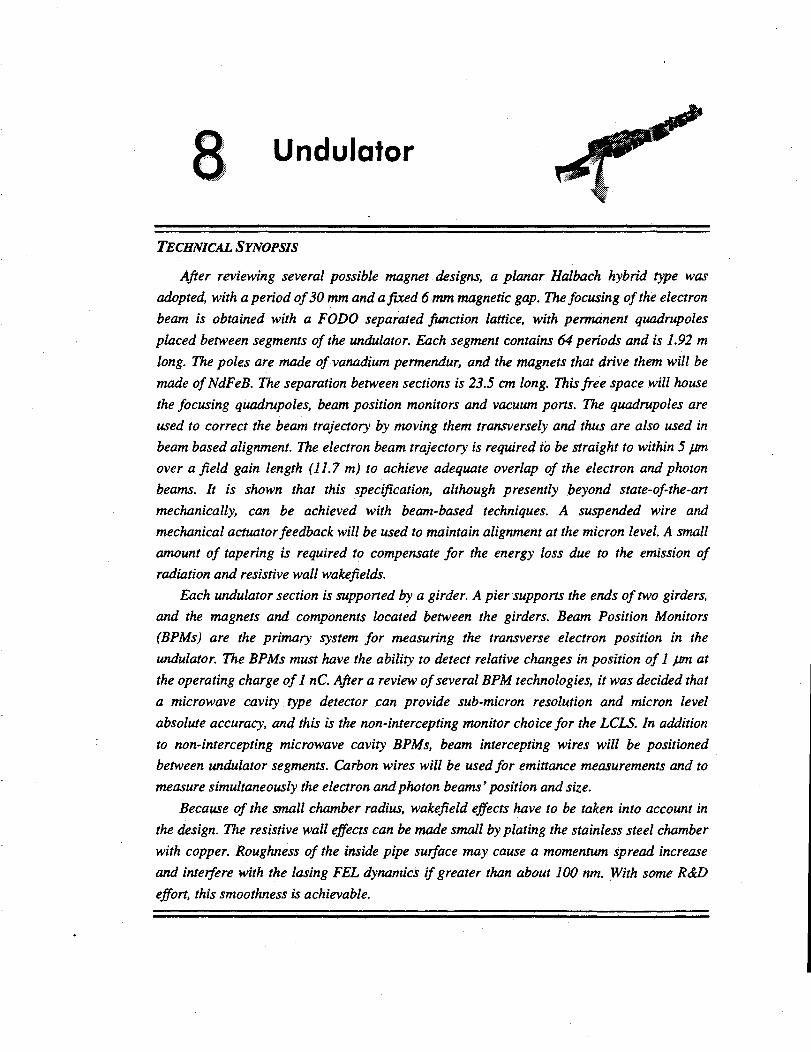
Undulator
TECHNICAL SYNOPSIS
After reviewing several possible magnet designs, a planar Halbach hybrid type was
adopted, with a period of 30 mm and a fixed 6 mm magnetic gap. The focusing of the electron
beam is obtained with a FODO separated function lattice, with permanent quadrupoles
placed between segments of the undulator. Each segment contains 64 periods and is 1.92 m
long. The poles are made of vanadium permendur, and the magnets that drive them will be
made ofNdFeB. The separation between sections is 23.5 cm long. This free space will house
the focusing quadrupoles, beam position monitors and vacuum ports. The quadrupoles are
used to correct the beam trajectory by moving them transversely and thus are also used in
beam based alignment. The electron beam trajectory is required to be straight to within 5 fjm
over afield gain length (11.7 m) to achieve adequate overlap of the electron and photon
beams. It is shown that this specification, although presently beyond state-of-the-art
mechanically, can be achieved with beam-based techniques. A suspended wire and
mechanical actuator feedback will be used to maintain alignment at the micron level. A small
amount of tapering is required to compensate for the energy loss due to the emission of
radiation and resistive wall wakefields.
Each undulator section is supported by a girder. A pier supports the ends of two girders,
and the magnets and components located between the girders. Beam Position Monitors
(BPMs) are the primary system for measuring the transverse electron position in the
undulator. The BPMs must have the ability to detect relative changes in position of 1 pm at
the operating charge ofl nC. After a review of several BPM technologies, it was decided that
a microwave cavity type detector can provide sub-micron resolution and micron level
absolute accuracy, and this is the non-intercepting monitor choice for the LCLS. In addition
to non-intercepting microwave cavity BPMs, beam intercepting wires will be positioned
between undulator segments. Carbon wires will be used for emittance measurements and to
measure simultaneously the electron and photon beams' position and size.
Because of the small chamber radius, wakefield effects have to be taken into account in
the design. The resistive wall effects can be made small by plating the stainless steel chamber
with copper. Roughness of the inside pipe surface may cause a momentum spread increase
and interfere with the losing FEL dynamics if greater than about 100 nm. With some R&D
effort, this smoothness is achievable.

L C L S . D E S I G N S T U D Y R E P O R T
8.1 Overview
8.1.1 Introduction
In a single pass EEL operating in the SASE regime, exponential gain of the coherent
radiation intensity is predicted by theory and power saturation is achieved in about ten gain
lengths. An FEL operating at saturation will have a more stable radiation output, a feature
considered essential by the experimental users of the LCLS. The task of the undulator design
is to achieve saturation in a real device in a length not significantly larger than an ideal
undulator.
A planar Halbach hybrid undulator with fifty-two segments has been chosen. Each
segment is 1.92 m long and is separated from its neighbors by a gap of 23.5 cm for focusing,
trajectory control, beam position and vacuum components. This gives a total undulator length
of 112 m. Section 8.2 outlines the undulator magnetic field optimization. Section 8.3.1describes the mechanical design of the undulator. Stray radiation-bremsstrahlung and the
direct electron beam hits-can damage the undulator by catastrophic single strike effects and
by changing the magnetization of the permanent magnet material over longer periods of time.
The effects of radiation demagnetization have been shown to be mitigated by thermally
stabilizing the magnetic material. Protection of the undulator from errors in the incoming
beam trajectory can be met by standard beam collimator designs and is described in
Section 8.3.2. The undulator vacuum system is fairly straightforward and is described in
Section 8.4. To ensure overlap of the radiation field with the electron beam traversing the
undulator, an alignment tolerance of 5 |im over a gain length (11.7 m) is required. Mechanical
survey cannot meet this requirement. A beam based alignment system that will be used to
achieve this tolerance is described in Section 8.5.2. After the initial undulator setup a
measurement and feedback system will be needed to maintain the beam trajectory. The BPM
system for measuring the trajectory is described in the Section 8.6. In order to allow and
correct for ground motions—vibrations, tides, diurnal thermal effects etc.—the undulator
magnets will incorporate a Wire Position Monitor (WPM) system. This system is also
described in Section 8.6. In addition, Section 8.6 describes the carbon wire position and
emittance diagnostic and the combined electron/photon position diagnostic. To achieve the
high undulator fields needed for the LCLS FEL, the pole tip gap is set to 6 mm. The small
bore of the beam pipe needed to fit into this gap necessitates careful consideration of resistive
wall wakefields and the effects of surface roughness. These effects are extensively discussed
in Section 8.7. Finally Section 8.8 considers the effects of ions generated by the electron
beam passing through the undulator vacuum.
8.1.2 Undulator Design Summary
Introduction
The LCLS undulator is made of a permanent-magnet hybrid array with 30 mm period and
6 mm gap. It is designed to take a 233 fsec (fwhm), 1 nC pulse of electrons at 4.5-14.3 GeV
8-2 • U N D U I A T O R
L C L S D E S I G N S T U D Y R E P O R T
and microbunch the pulse with 15-1.5 A period, and to cause the microbunches to radiate
coherently at 15-1.5 A. A device that will achieve these performance goals with a magnet
length that is not excessively greater than the 94 m saturation length of an ideal undulator has
been designed.
The design includes the undulator proper, the termination of the undulator at separations
between segments, and quadrupple magnets, which are used for focusing, trajectory
corrections and beam-based alignment. It also requires the measurement of the fields of
fabricated components, and the design of shimming strategies to achieve desired tolerances.
Design Concept History
Several undulator options were studied and a plane polarizing design that uses hybrid
permanent magnet technology was chosen. Optical klystron style dispersive sections in the
undulator allow the energy-modulated bunch to become spatially modulated, but this
approach is ruled out because of the LCLS energy spread. (See Chapter 5.)
Superconducting DC and warm-pulsed bifilar helical electromagnetic undulators were
considered, but were thought to be costly, complicated, difficult to hold to mechanical
tolerances and to provide with steering corrections. Access to the beampipe completely
surrounded by undulator would be impaired. The technological complications of going to a
superconducting magnet design and the resultant R&D required argue against that approach.
Besides the bifilar helix, there are permanent magnet helical undulator concepts, both
with permanent magnets only (twistor designs) and with hybrid structures. These do not offer
short periods like the electromagnet devices, and are as costly and complex as the plane
polarizing devices. A pure permanent magnet plane polarizing undulator would work for the
LCLS, but it would have a longer period than a hybrid device because the field is weaker for
a given gap. Also, errors are harder to control in the pure permanent magnet design. Such a
design might have the advantage that steering and focusing fields could be superimposed by
electromagnets surrounding the undulator. As a result of the above considerations, a hybrid
permanent magnet design was chosen.
The Undulator
The undulator is a standard Halbach hybrid design [1]. The undulator will have 1.92 m,
64 period segments, with a ferromagnetic field clamp at the end of each segment. The poles
will be vanadium permendur, and the magnets that drive them will be NdFeB. The NdFeB
will be heat treated after it is magnetized at temperatures as high as 125"C in order to stabilize
the material against radiation damage. It will also be exposed to demagnetizing fields, which
also stabilizes the material by demagnetizing marginal domains. In the mechanical design,
each pole will have one single block of magnet material attached to it, and it will also receive
flux from the neighboring poles' magnets, through a small longitudinal gap that is imposed in
the design to prevent mechanical stackup. The mechanical design is described in Section 8.3.
U N D U L A T O R • 8-3

I C L S D E S I G N S T U D Y R E P O R T
Ultra-smooth beampipe with 0.25 in OD (6.35 mm) is already commercially available. Ifmanufacturing of a 6 mm ultra-smooth beampipe proofs to be costly, the 6.35 mm diameterpipe can be drawn into an oval to fit the 6 mm gap. (Wakefields are not significantly affectedby such a modification.)
Each end of the girder will be supported by a pier, and a separation of 23.5 cm will beallowed between undulator segments, to allow the electrons to fall behind the photon beam byone photon wavelength. The separation will be used for diagnostics, and for focusingcorrector magnets. The undulator sections can be mounted on high precision movers, if it isnecessary to control their positions using feedback.
The separation between two sections of the FEL undulator is given by the condition that,as the electron and the photon waves travel the distance Zsqn the phase between the two wavesadvances by A(j>= 2tc A time t is required for the electron to travel the distance z and A<j> isgiven by:
(8.1.1)vz
In the separation, where the velocity of the electron, vz, is constant:
f = z / c £ = z( l- l /2> 2) /c (8.1.2)
so that:
2n~kzsep[\-(\-\l2f)] = 7CzsepIXrf (8.1.3)
and Zsep will be given by:
fAf^±^ 2 (8.1.4)
In the LCLS case, zsep = 23.76 cm for K = 3.71, and undulator period h = 30 mm. zsepisindependent of K, the radiation wavelength, and independent of electron energy. Theelectron's velocity vz is not constant in the undulator or at the end of the undulator, so a moreexact separation must be calculated numerically. The termination of the magnetic field shouldbe done with a ferromagnetic field clamp in a manner that causes the least loss of resonantwiggles (see Section 8.2.2).
As the electron beam travels down the undulator, it loses energy to radiation( 4 « -0.16% at 14.3 GeV), and wakefields ( 4 = -0 .1% at 14.3 GeV). Beampipe roughnesscauses energy spread of the order of 0.05% rms over the core of the electron bunch. Thiseffect is not as well understood as the first two. Because of the loss of electron energy, the
8-4 • U N D U L A T O R

L C L S D E S I G N S T U D Y R E P O R T
electrons move outside the potential well established by the radiation field. To offset these
effects, it is necessary to taper the undulator. A purely mechanical gap taper for SE ~ -0 .3%
would require a gap increase of about 15 //m over 100 m.
Two other types of tapering can be used. One is fixed (to account for SE ~ -0.3%) to
offset the radiation and resistive wall effects that are considered well understood. The second
is variable (up to SE ~ -0.15%) to allow some realtime adjustability for wakefield effects that
are less well understood.
The variable taper is achieved by recalling that the magnetic field strength varies as
cosh(2^x/AB) across the gap. If the beam is off-center horizontally, it experiences a greater
magnetic field strength than when it is on-center. Therefore a taper can be achieved by
moving modules of the undulator so that the beam is off-center at the beginning and on-center
at the end. A displacement of 136 /an is required to achieve SE ~ -0.15% at 14.3 GeV.
Strong Focusing
Simulations of the LCLS show that strong focusing must be added to the undulator lattice
to maintain a small beam diameter; natural focusing would give a beta function length of
about 70 m; optimal focusing occurs with a beta function of less than 20 m. The LCLS design
energy ranges from 4.5 to 14.3 GeV. Optimum focusing at all energies can be obtained by
focusing with variable permanent magnet quadrupoles or electromagnetic quadrupoles. As
was shown in Chapter 5, this flexibility is not required, since the optimum beta function at
14.3 GeV, is not far off the optimum for 4.5 GeV. For this reason, permanent magnet
quadupoles are used.
Segment separations allow for a separated function FODO lattice. See Fig. 8.1-1. The
smallest beta-function (6 m) is at 4.5 GeV. This implies that the FODO cell length needs to be
less than 6 m (see Chapter 5). The LCLS design nominally adopts a 1.92 m (64 periods)
undulator segment length with a BPM and corrector in each separation between segments.
Simulations show that this spacing meets the requirements for beam-based alignment.
i BPM
! ] - •
Figure 8.1-1.
undutator| 11
A schematic side view of the undulator structure, showing the FODO lattice withseparations between 1.92 m undulator sections for diagnostics, focusing correctors,and vacuum ports. The undulator magnets are mounted on aluminum girders whosetemperature is stabilized.
The quadrupole magnets serve two other functions. They are used in the initial alignment
to establish a straight-line trajectory. They will be moved mechanically on vertical and
horizontal slides to correct the trajectory to approximate a straight line. See Section 8.3 for a
U N D U L A T O R 8-5

L C L S D E S I G N S T U D Y R E P O R T
more detailed description. They are also used as run time correctors; they will be moved
transversely to offset small trajectory errors that are detected by the BPM systems. See
Section 8.5 for details.
To be less vulnerable to electronic drifts in the BPM signals, it is preferable to place the
BPMs on the undulator girders, so that their positions are tracked and corrected by the WPM
system (see Section 8.6.4). They would still move on x-y stages, but now relative to a non-
drifting frame of reference.
The quadrupole focusing magnets are made using permanent magnets. Assuming a field
gradient of 50 T/m over a length of 10 cm, a 200 /an motion would result in a 40 /an
deflection at a BPM that is 2 m downstream. In addition to errors caused by the non-zero field
integrals of the undulators, errors caused by the earth's field need also to be corrected. A 1 G
environmental field would cause a 14.3 GeV beam to deflect by 8 /an every 2 m. The
quadrupole correction system can control this easily.
The fields inside a Halbach "orange slice" pure permanent magnet quadrupole (see
Fig. 8.1-2) are given to leading order by [1]:
iBy =n
n )cosrxr2 [
fe]sinful (8.1.5)
where z — x + /y = re10, M is the number of "orange slices", rx is the radius of the bore, and r2
is the outer radius. In the case where M - 4:
_2Brr(r2-rx) (8.1.6)
The field gradient will therefore be:
dBQ 2Br(r2-r:)
dr n rxr2
(8.1.7)
Figure 8.1-2. Cross-sectional views of Halbach (left) and Panofsky (right) pure permanent magnetquadrupole focusing corrector magnets. The arrows show the direction ofmagnetization in blocks of permanent magnet material.
8-6 • U N D U L A T O R

L C L S . D E S I G N S T U D Y R E P O R T
A gradient of 50 T/m is far below the maximum achievable with a pure permanent
magnet design and a simple quadrupole design with four trapezoidal pole pieces of NdFeB
2.7 cm outer radius and a 1 cm bore will suffice. See Fig. 8.1-2. The LCLS is insensitive to
higher harmonics of the magnetic field.
Undulator Tolerances
For large scales, such as the length of an undulator segment, the principle that governs the
tolerances is that the emitted radiation meets the resonance condition, so that it can create
coherent electron bunching. Errors that cause off-resonance radiation should be no larger than
the resonance width defined by the energy spread of the electron beam, which is 0.02% at
14.3 GeV, and 0.068% at 4.5 GeV. For small scales, such as the length of one period of the
undulator, simulations show that random magnetic field errors are tolerable up to
£Bmw/Bmax< 0.1%, beyond which there is a degradation of the FEL gain according to
FRED-3D. See Chapter 5 for details. This tolerance corresponds to a local period error of
35 yum, or a local gap error of 7 fsa. These tight tolerances can be met with standard
machining and assembly and magnetic shimming techniques. See Fig. 8.1-3.
Figure 8.1-3. Left: Top view of undulator, showing shims on poles and small gaps between poleassemblies. Shims may also be applied to the gapside faces of the NdFeB. Right: Endview of undulator, showing NdFeB overlapping vanadium permendur pole pieces. Thefield of the undulator is horizontal, so that the radiation is vertically polarized.
It is possible to order magnets with AB/Bms < 0.5%, and an angular error of 0.5° from the
nominal easy axis, but 1.0%, 1° magnets are much less costly. For pure permanent magnet
devices, computerized sorting techniques can reduce undulator field errors by a factor of
about 5 over those in a randomly assembled undulator. The same reduction factor is expected
with a hybrid structure [2]. Since magnetic sorting and shimming will be used to get to 0.1%
s the looser tolerances are probably acceptable. See Section 8.2.1 for details.
Undulator Construction
The undulator pole assembly comprises vanadium permendur poles with an NdFeB
magnet closely attached to one face, as shown in Fig. 8.1-3. The NdFeB magnet opposite the
other face will be separated from the pole by a small gap, in order to prevent mechanical
stackup error. This is not ideal magnetically, as it can lead to some direct fields from the
NdFeB reaching the gap. But by keeping the separation to 50 fm, these fields are small.
U N D U L A T O R 8-7
L C L S D E S I G N S T U D Y R E P O R T
Even with precision machining, sorting of magnets, tight specifications, and precise
assembly, measurable field errors are expected. A standard Hall probe can, in principle, be
used to measure fields in the Tesla range with 20 //T (0.2 Gauss) resolution [3]. Each pole
will be shimmed to minimize the trajectory and photon resonance errors. A coordinate
measuring machine with 0.8 mm absolute positioning accuracy over a volume of 1.2 m x 1 m
x 0.6 m [4] is available and has been fitted with a temperature-compensated Hall probe
(calibration drift = 80 ppm/K). This will enable the magnetic field to be characterized
precisely.
The effect of placing small shims on the ends of the pole pieces away from the gap,
which lowers the field in the gap by a few Gauss, has been modeled. Magnets with 1%
(125 Gauss) individual magnetization errors can be sorted to lower the effective undulator
field errors to 0.2% (25 Gauss). These errors are well within the range of the shimming
strategy. A desirable feature of the shimming strategy is that the effect is local to one pole,
with little fanout. Thin ferromagnetic shims may also be placed on the gapside faces of the
NdFeB magnets to control phase errors.
The phase shake tolerance is given byA0<ay l(y<J?>p) [5], where p- 0.00047 is the
1-FEL parameter for the LCLS at 14.3 GeV. Thus, a phase shake tolerance of 14.4°, which is
easy to meet, is likely to make phase shimming unnecessary. Also, field shimming of poles
with thin strip shims may be labor intensive, so a tuning screw approach, that is more labor
efficient, will be developed.
Detailed design of the undulator has been carried out using the AMPERES 3-D magnet
modeling code [6]. These simulations show us that the vanadium permendur poles should be
25-30 mm wide (parallel to gap) 5 mm thick, and 30 mm tall (normal to gap). The NdFeB
should be 35-40 mm wide, 10 mm thick (longitudinally), and 35 mm tall. It might be possible
to reduce these dimensions somewhat if significant economies could be achieved.
Each segment of the undulator will have to have careful termination of the field, with the
goal of keeping as many undulations of the trajectory on resonance as possible. A field clamp
will control the fields of the undulator in the separation between segments. A preliminary
design for this termination is given in Section 8.2.2.
Mechanical, Thermal, and Geophysical Engineering
The LCLS undulator will be placed in the existing FFTB facility at SLAC. The first third
of the tunnel for the undulator is underground; the last two-thirds are in an above ground
heavily shielded concrete structure. The substrate throughout is a continuous slab of miocene
sandstone. In the range below 100 Hz, there is cultural and ocean-generated vibration, but at
the top of existing sand/epoxy composite FFTB piers, the measured amplitude of these
vibrations is less than 50 nm.
Diurnal thermal movements of the tunnel outside the hillside can be as much as
100/an/day, but they can be reduced by isolating the tunnel with trenches cut into the
8-8 • U N D U L A T O R
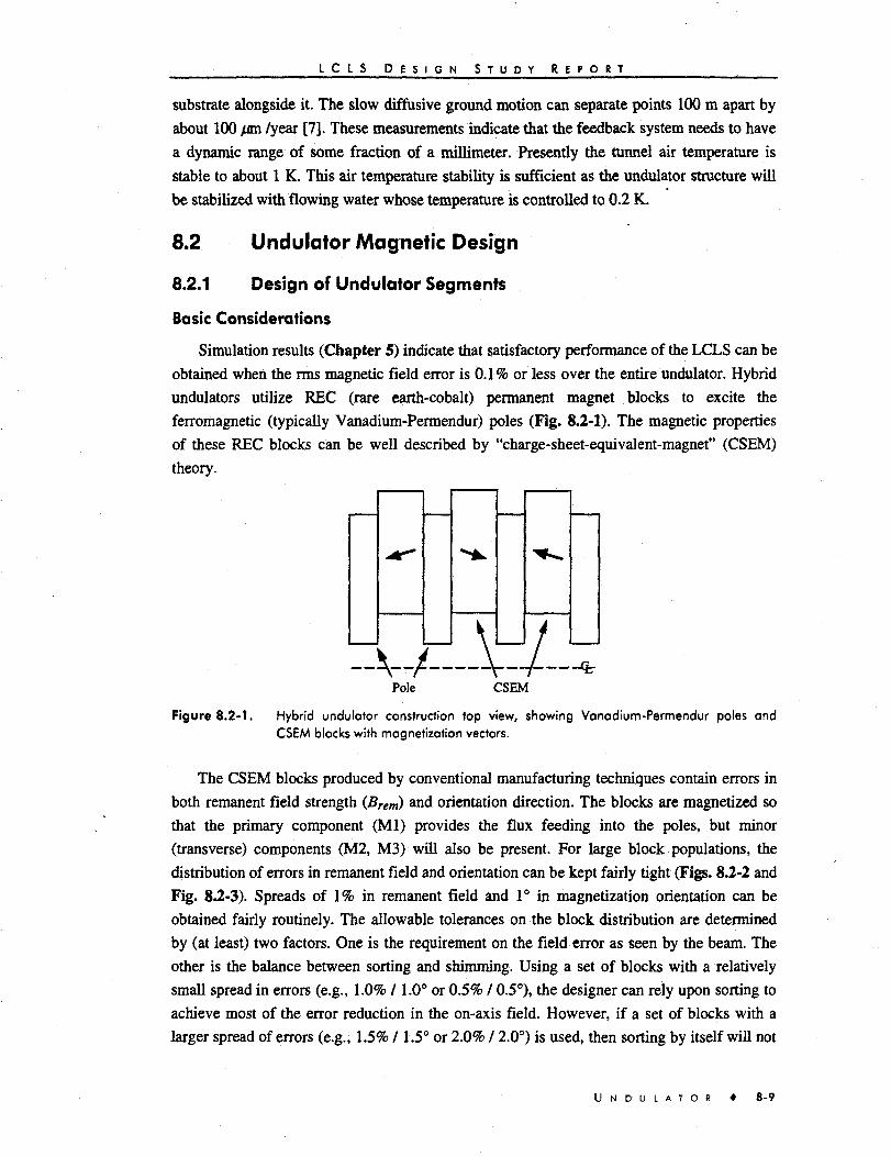
L C L S D E S I G N S T U D Y R E P O R T
substrate alongside it. The slow diffusive ground motion can separate points 100 m apart by
about 100 /an /year [7]. These measurements indicate that the feedback system needs to have
a dynamic range of some fraction of a millimeter. Presently the tunnel air temperature is
stable to about 1 K. This air temperature stability is sufficient as the undulator structure will
be stabilized with flowing water whose temperature is controlled to 0.2 K.
8.2 Undulator Magnetic Design
8.2.1 Design of Undulator Segments
Basic Considerations
Simulation results (Chapter 5) indicate that satisfactory performance of the LCLS can be
obtained when the rms magnetic field error is 0.1% or less over the entire undulator. Hybrid
undulators utilize REC (rare earth-cobalt) permanent magnet blocks to excite the
ferromagnetic (typically Vanadium-Permendur) poles (Fig. 8.2-1). The magnetic properties
of these REC blocks can be well described by "charge-sheet-equivalent-magnet" (CSEM)
theory.
Pole CSEM
Figure 8.2-1. Hybrid undulator construction top view, showing Vanadium-Permendur poles andCSEM blocks with magnetization vectors.
The CSEM blocks produced by conventional manufacturing techniques contain errors in
both remanent field strength (Brem) and orientation direction. The blocks are magnetized so
that the primary component (Ml) provides the flux feeding into the poles, but minor
(transverse) components (M2, M3) will also be present. For large block populations, the
distribution of errors in remanent field and orientation can be kept fairly tight (Figs. 8.2-2 and
Fig. 8.2-3). Spreads of 1% in remanent field and 1° in magnetization orientation can be
obtained fairly routinely. The allowable tolerances on the block distribution are determined
by (at least) two factors. One is the requirement on the field error as seen by the beam. The
other is the balance between sorting and shimming. Using a set of blocks with a relatively
small spread in errors (e.g., 1.0% / 1.0° or 0.5% / 0.5°), the designer can rely upon sorting to
achieve most of the error reduction in the on-axis field. However, if a set of blocks with a
larger spread of errors (e.g., 1.5% / 1.5° or 2.0% / 2.0°) is used, then sorting by itself will not
U N D U L A T O R 8-9

L C L S D E S I G N S T U D Y R E P O R T
be able to reduce the errors to a tolerable level. In that case, ferromagnetic shims must be
carefully placed to shunt flux away from the beam axis and, hence, to reduce the field error.
This process is usually iterative, and is very labor-intensive. For a very long device, it may be
less expensive to purchase better blocks than to purchase more hours of labor.
-°-02-0.015-0.01-0.005 0
mm °01 ....0015
0.020.015
0.010 0.005
-o.oi0005
_ -0.0150.02 -0.02
Figure 8.2-2. Distribution of magnetization components in a simulated block population.
-0.02 -0.015 -0.01 -0.005 0 0.005 0.01 0.015 0.02
M2rnFigure 8.2-3. Distribution of transverse magnetization components in the block distribution.
Correcting Local Field Errors
The CSEM blocks possess magnetization errors as described above, which lead to errors
in the field seen by the electron beam. Deviations in the magnitude of the primary component
(Ml) yield pole-to-pole excitation errors, while minor components of the magnetization (M2,
M3) can be seen by the beam as normal and skew multipole fields [8]. Thus, the primary
8-10 • U N D U L A T O R
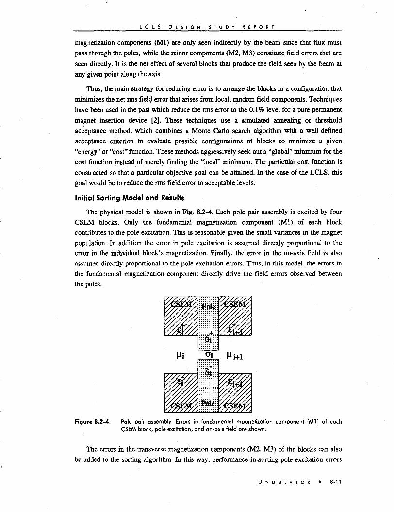
L C L S D E S I G N S T U D Y R E P O R T
magnetization components (Ml) are only seen indirectly by the beam since that flux must
pass through the poles, while the minor components (M2, M3) constitute field errors that are
seen directly. It is the net effect of several blocks that produce the field seen by the beam at
any given point along the axis.
Thus, the main strategy for reducing error is to arrange the blocks in a configuration that
minimizes the net rms field error that arises from local, random field components. Techniques
have been used in the past which reduce the rms error to the 0.1% level for a pure permanent
magnet insertion device [2]. These techniques use a simulated annealing or threshold
acceptance method, which combines a Monte Carlo search algorithm with a well-defined
acceptance criterion to evaluate possible configurations of blocks to minimize a given
"energy" or "cost" function. These methods aggressively seek out a "global" minimum for the
cost function instead of merely finding the "local" minimum. The particular cost function is
constructed so that a particular objective goal can be attained. In the case of the LCLS, this
goal would be to reduce the rms field error to acceptable levels.
Initial Sorting Model and Results
The physical model is shown in Fig. 8.2-4. Each pole pair assembly is excited by four
CSEM blocks. Only the fundamental magnetization component (Ml) of each block
contributes to the pole excitation. This is reasonable given the small variances in the magnet
population. In addition the error in pole excitation is assumed directly proportional to the
error in the individual block's magnetization. Finally, the error in the on-axis field is also
assumed directly proportional to the pole excitation errors. Thus, in this model, the errors in
the fundamental magnetization component directly drive the field errors observed between
the poles.
Figure 8.2-4. Pole pair assembly. Errors in fundamental magnetisation component (Ml) of eachCSEM block, pole excitation, and on-axis field are shown.
The errors in the transverse magnetization components (M2, M3) of the blocks can also
be added to the sorting algorithm. In this way, performance in .sorting pole excitation errors
U N D U L A T O R • 8-11

L C L S D E S I G N S T U D Y R E P O R T
can be traded off with sorting skew and normal field components generated directly from thepermanent magnet blocks themselves. This is done by constructing two independent costfunctions and combining them linearly.
This model neglects higher order contributions to the field error. These othercontributions arise from a variety of sources—differential permeability effects in the poles,transverse magnetization components contributing to pole excitation, exact 3-D distributionof the magnetic field, etc. A better sorting model would try to include these effects. However,the current model should give a reasonable initial solution to magnet block placement. Higherorder errors as well as errors in the final mechanical assembly will always be present, and willbe corrected by shimming.
To construct the pole pair excitation error cost function, the following definitions aremade:
C * = ( A f l ) f - ( M ) (8.2.1)
is the error in the magnetization for an individual block (+ -) bordering the ith pole pair,where <M> is the average magnetization for the entire block population,
S± =e± -\-e± (8 2 2")
is the error in the excitation of the ith upper (+) or lower (-) pole, and
^ f ; (8.2.3)
is the relative error in the on-axis field.
The construction of the direct field error cost function is similar. It is observed that thereis no fundamental magnetization in the transverse directions of the ideal device, so that theentire transverse magnetization components (M2 and M3) are errors. The net error in a giventransverse component is simply the sum of magnetization components of the upper and lowerblocks, normalized by the average magnetization of the blocks.
The total cost function used in the sorting process is the total variance of the on-axis fielderror, including a weighting factor (or),
Total Cost =[ttX(o« *O t) + ( l -«)£( / / , • *Mi)h (8-2.4)
where the summations are over the total number (N) of block or pole pairs in the sort, and
Total C o s t = [ a 2 > i * Ot /N) + 5 > £ *Mi /#)]/<<* + D (8-2-5)
is the measure of the relative direct field error at the ith block pair.
8 - 1 2 • U N D U L A T O R

L C L S D E S I G N S T U D Y R E P O R T
A weighting factor (0 < a < 1) can be used to balance the relative contribution betweenpole excitation and direct field error effects to the final cost function. For example, by placinga larger emphasis upon the direct field error cost function (or < 1/2), these effects can bereduced while somewhat enhancing the pole excitation errors. Without any other information,however, the most straightforward method is to assume equal contributions from both costfunction components (a= 1/2).
For this calculation the total magnet population is comprised of 2000 blocks, which canbe used to feed N = 1000 pole pairs or 500 periods. Thus, sorting is done for a length (15 m),which is somewhat longer than a gain length (11.7 m). Such a long section of the device issorted all at once in order to improve the resulting rms error in the field. The extra blocks areutilized to form a "bull pen." These blocks are then excluded from the final device, or re-usedin other segments of the device. This technique improves the final quality of the devicewithout incurring significant additional material costs.
In this case, the sorting is done with a block population possessing a nearly uniformdistribution in remanent field strength (Brem = <M>) with average value of 1.25T, a uniformdistribution in azimuthal angle, and a Gaussian distribution in inclination angle (seeFig. 8.2-2 and Fig. 8.2-3).
The total cost function is calculated during the sorting process. Fig. 8.2-5 and Fig. 8.2-6show the individual cost function values for each pole or block pair. Summing these values,the net variance in the error components is calculated. From this, the relevant rms relativeerrors averaged over the entire gain length as well as individual pole and block pair errors canbe derived.
o.ooi1
le-100 100 200 300 400 500 600 700 800 900 1000
Pole Position
Figure 8.2-5. Pole pair excitation error cost function (oj * oj) versus pole pair position {/), before(triangles) and after (asterisks) sorting, for N = 1000 and <M> = 1.25T.
U N D U L A T O R 8-13

L C L S D E S I G N S T U D Y R E P O R T
0.001
le-080 100 200 300 400 500 600 700 800 900 1000
Block Position
Figure 8.2-6. Direct field error cost function (^ * fi-j versus block pair position (i), before (triangles)and after (asterisks) sorting, for N = 1000 and <M> = 1.25T.
The net rms relative error in the pole pair excitation before sorting is approximately
0.66%. After sorting, that figure drops to 0.075%. The net rms relative direct field error
before sorting is approximately 1.4%, dropping to 0.11% after sorting. Using a different
weighting factor (a= 1/4) equalizes both sets of errors to 0.1% after sorting.
If instead of a magnet population that had a 1.0% spread in magnetization strength and a
1.0° spread in inclination angle, a set with spreads in strength and orientation of 1.5% and
1.5° respectively had been used, then after sorting the relative pole excitation error would be
approximately 0.12% and the relative direct field error would be approximately 0.16%. Even
after readjusting the weighting factor to balance these values (approximately 0.14%), the
design specifications would be not met. Extensive additional shimming would then be
necessary.
Looking at the individual values of the two components of the total cost function the
magnitude of the local error can be calculated. After sorting the maximum value of the cost
function for the pole pairs (Fig. 8.2-2) is seen to be approximately 8 x 10"6, corresponding to
a 35 G error in excitation between upper and lower poles. The maximum value of the direct
field cost function (Fig. 8.2-3) is approximately 1 x 10'5 after sorting, corresponding to a
40 G error in the transverse field components between upper and lower blocks.
The actual results will be even better because the large number of magnets needed by the
•LCLS can be binned into groups with smaller variances. Binning will be done according to
magnetization strength. The ideal bin might be 1024 magnets, corresponding to four modules.
This arrangement improves the variance of the pool from which the sorting is done, with the
consequent improvement in the sort result. The undulator will be built with a small
mechanical adjustment of the gap, so that the mean field amplitude can be corrected, thus
taking out the difference between the bins. The total range of gap variation would be on the
8-14 • U N D U L A T O R

L C L S D E S I G N S T U D Y R E P O R T
order of 10s of microns. This will be combined with tapering, which is needed to keep the
electron beam on-resonance, as explained in Section 8.1.2. Instead of keeping the mean field
amplitude constant, it would be graded linearly; each module being 0.3%/52 = 0.0057%
weaker than the previous one. The tapering will be done by forcing the mean of the sort to be
different from the mean of the randomly arranged magnets. This works, but only a small
difference can be achieved before the error magnitude increases excessively. The total range
of gaps required for tapering is about 50 /an.
Use of Shims to Correct Field Errors
As a final correction to the fields, ferromagnetic shims may also be employed. These can
be used to "neutralize" field strengths of the order of several Gauss. The exact placement of
the shims depends upon the type of error. Pole excitation can be decreased slightly by placing
the shim on the exterior surface of the pole piece. Transverse magnetization errors in the
blocks can be decreased by placing shims on the surface of the individual block.
For the magnitude of the errors described above, shimming may be entirely unnecessary
because the required field tolerances can be attained by sorting through a population of
magnet blocks with tight tolerances. Sorting can reduce the initial rms error by an order of
magnitude and the design specifications can be obtained. Relaxing the tolerances on the
magnets will result in larger errors that may then need correction. However, the process of
field measurement, fabricating and placing shims, field re-measurement, etc., is extremely
labor- and time-intensive. It may be more desirable to eliminate much of that effort by using a
block population with tighter tolerances from the start.
8.2.2 End Design of Undulator Segments
The end design concept is based on a normalized pole scalar potential distribution that
provides a maximum number of regular periods while avoiding unacceptable end steering
effects. The normalized scalar potentials of the poles in the uniform interior of the wiggler are
+1,-1,+1,-1, etc. A desirable truncation scheme is . . .+1,-1, +1,-1, +1/2,0. This distribution
provides rapid termination and no net end steering effect.
Abrupt termination of a hybrid (permanent magnet material and steel poles) results in
relatively little net integrated steering field but has the disadvantage of a skewed scalar
potential distribution in the last several poles of the structure and thus a reduction in the
performance of the device.
By altering the quantities of the permanent magnet (P.M.) material between the last few
poles of the device, it is possible to approach the desired scalar potential distribution
previously described. A 3-D boundary element code was used to model a hybrid end
structure. A 2-D cross-section of the upper half of this structure is shown in Fig. 8.2-7.
An additional section of P.M. material along with a shunt plate is shown to the right of
pole 0 in Fig. 8.2-7. This provides an independent excitation parameter to control the steering
excitation of pole 0. This shunt plate is sufficiently thick so that it is in an unsaturated
U N D U L A T O R • 8-15

L C L S D E S I G N S T U D Y R E P O R T
condition and acts as a field clamp that reduces the fringe fields extending beyond the end of
the structure to the right Beyond the shunt plate to the right as shown also in Fig. 8.2-7 are
two magnetically detached shield plates which further reduce the fringe fields of the structure.
Preliminary 3-D calculations show less than 10 G fields at 2 cm beyond the center of pole 0.
NdFeB magnets
Vanadium permendur poles
poleindex
Shunt plate IShields
midplane » beam axis
Figure 8.2-7.
cutout for beam pipe
Cross-section of end structure with reduced P.M. material between poles 0 and 1 andincreased material at pole 2.
The midplane field results are shown in the graph of Fig. 8.2-8. This graph includes the
By field on the midplane of the device and the first and second integrals of the field, which
give the beam steering and trajectories. This preliminary design shows: (1) good peak-to-peak
uniformity leading up to the last pole of the device, and (2) small steering first integral and
rapid termination of the fields beyond the steering pole. By adjusting the P.M. quantities in
the structure, the net first integral can be brought arbitrarily close to zero to eliminate the end
steering.
15000
se 1OOO0e
I 5000
\
I-A-rv-
\ j
rf> •• / /'\\\ t
r\%>- .-_ t — —-"
E
0
u -5000
I0 -10000r
-150000 0.5 1 1.5 2 2.5 3 3.5 4 4.5 5 5.5 6 6.5 7 7.5 8 8.5 9 9.5 10
2 (em)
| By(G.) mi(By)(G-cnn) - 2nd lnt{By)(G-cm'g) (x 1.0) I
Figure 8.2-8. Graph of By with first and second integrals of By which give the steering field andnormalized beam trajectory. The horizontal axis is z (cm).
8-16 • U N D U L A T O R

L C I S D E S I G N S T U D Y R E P O R T '
8.3 Undulator Mechanical Design
8.3.1 Mechanical and Thermal Design
Introduction
The 100 m long undulator is made up of 52 nominally 2.16 m sections. Each 2.16 m
section consists of 1.92 meters of permanent magnets and monitors (BPMs and WPMs)
supported by a girder. The remaining 0.235 m located between adjacent girders contains a
focusing corrector magnet and miscellaneous non-magnet components. A pier supports the
end of each girder and the magnet and components located between the girders. Fig. 8.3-1
shows the layout of the components.
Focusing corrector
Sub-nodule
Motor; Beam tube
Girder
Pier!
Figure 8.3-1 . Layout of girders and undulator components - basic 1.92 m section.
Physics considerations for successful operation dictates that the maximum position
deviation of the undulator segments relative to each other not exceed 100 fim horizontally and
500 /an vertically. The ability to perform real time global alignment of the girders and the
absence of real time control of the sub-components of each girder section translates to a
condition where most of the 100/500 fna stability tolerance can be allocated to the girder
assemblies. After subtracting for global alignment tolerances, the remaining tolerance must be
budgeted between machining tolerances, magnet assembly tolerances, and alignment
tolerances within a girder.
There are 64 periods per girder. The period is 30 mm with a tolerance of 35 /an. The
horizontal pole gap is 6 mm with a tolerance of 7 jum. The gap between poles and magnets
U N D U L A T O R 8-17

L C L S D E S I G N S T U D Y R E P O R T
should be a minimum. In the girder design, the effects of heat loads, vibration, and ground
motion are considered. Each of these will be covered in detail in this section.
The focusing corrector located between adjacent girders is a 120 mm long permanent
magnet. These magnets must be aligned horizontally and vertically (perpendicular to the
beam axis) within 100 /an. The positioning of these magnets is not critical with respect to
axial position and angular alignment. The alignment of the sub-modules on the girder and the
global alignment of the girders are described in Chapter 12.
Piers
The piers are monolithic structures with center-to-center spacings of 2.16 m. The ends of
each girder are supported by adjacent piers. The piers will also support components located
between the girders. The height of the piers will be determined by the elevation of the
electron beam above the floor and the dimensions of the individual components making up
the magnet support system. The result will be a pier on the order 1 m high.
The capability of motors to adjust the position of the girders (in five degrees of freedom)
in real time permits corrections to be made for dimensional changes in the piers due to
thermal conditions and positional changes due to geophysical motions. Currently the plan
does not call for motor control in the z-axis, but if necessary, it can be implemented. The
ability to correct for slow (on the order of hours, days or longer) changes in the dimensions
and position of the piers up to 1 mm eliminates the need for high global stability of the
girders.
Concrete piers have several advantages. The most obvious is that they are the least costly.
Aside from the cost of the raw material, the use of concrete permits in-situ fabrication and
eliminates one step associated with other alternatives; the concrete "pots" itself into the hole
made in the sandstone ground structure.
Often associated with concrete are large values for shrinkage and swelling. In the case of
the undulator, the initial shrinkage and the slow changes that take place over days, weeks or
longer are not important. The total magnitude can be accommodated by the girder movers is
the only relevant factor.
Although there are many factors affecting the behavior of concrete (e.g., mix ratio, water
ratio, curing conditions) the following shrinkage and strain information is typical of a broad
range of conditions. Shrinkage decreases rapidly with time. Based on total shrinkage at 20
years:
• 14—34% of the shrinkage occurs in 2 weeks
• 40-80% of the shrinkage occurs in 3 months
• 66-85% of the shrinkage occurs in 1 year
A typical number for strain at 1 month is 40 /an/m and at 5 years 100 /an/m (these values
are linear strains). Thus between 1 month and 4 years the strain is 60 fjva/m. Assuming the
8-18 • U N D U L A T O R

L C L S D E S I G N S T U D Y R E P O R T
concrete shrinks 75% of its total lifetime value before alignment begins at 1 year, the strain
becomes 25 //m/m between 1 and 5 years.
Shrinking and swelling due to changes in humidity should be very small after initial
curing. Moisture would only be an issue if the concrete were stored "in water," in which case
significant swelling would be experienced over even 1 month. However, this is not the case.
Concrete also exhibits a change in strength over time. Considering the exceptionally low
loads, and that concrete attains 70% of its strength within 28 days and 90% of its strength
within 3 months, the issue of strength is irrelevant. The bottom line is that concrete appears to
be an acceptable material for construction of the piers.
An alternative to concrete is Anorad Corporation's Anocast®, which is a sand-epoxy
composite used for the FFTB piers. According to the manufacturer, this polymer/granite sand
composite exhibits excellent vibration damping, structural rigidity, and thermal stability.
However, their comparisons are with metal structures used in machine tool design. It is not
clear whether there is actually an advantage over concrete piers in the undulator design.
Table 8.3-1 compares useful properties of concrete and Anocast®.
Table 8 .3 -1 . Properties of concrete and Anocast®.
Property
Density (lb/in3)
Modulus of Elasticity (psi x 10~6)
Poisson's Ratio
Tensile Strength (psi)
Compressive Strength (psi)
Shear Strength (psi)
Coefficient of Thermal Expansion (x 10%)
Thermal Conductivity (BTU/hr-ft-F)
Heat Capacity (BTU/lbm-F)
Concrete(a)
0.09
2.5-4.5
—
—
1,000-10,000
200-2,000
6.0-8.0
0.54-0.70
0.20
Anocast
0.084
4.5
0.24
4,200
17,000
3,000
7.0
1.08
0.27
(a) Properties vary with mix ratios, age and moisture.
A negative aspect to Anocast® is its relative high overall cost—material, fabrication,
shipping (it is factory fabricated), and installation. Because Anocast® piers would be factory-
fabricated, they require potting into the hole in the sandstone ground structure.
Due to the low aspect ratio of the piers (length to width on the order of two to four),
deformation of the pier due to vibration is not an issue. Analysis has shown that the amplitude
of vibration of the girders is very small even when no damping is associated with the pier.
Therefore damping is not a critical factor in the choice of pier material. The coefficient of
U N D U L A T O R 8-19

L C L S D E S I G N S T U D Y R E P O R T
thermal expansion is basically the same for both concrete and Anocast®. Therefore, thermal
expansion does not appear to be a factor in choosing one material over the other. The strength
of Anocast® is clearly greater than concrete, but the total loading on the piers is very low and
is therefore not a factor in choosing one material over the other.
The advantage of Anocast® is that its properties are more uniformly controlled and known
than concrete, and SLAC has had positive experience with it and less satisfactory experiences
with concrete for support structures. However, the modest tolerances associated with the piers
combined with the lack of definitive reasons for the use of Anocast® make concrete the most
likely candidate. Therefore, the baseline design calls for concrete piers unless mitigating
factors are discovered, e.g., the cost of Anocast® piers can be greatly reduced by recycling the
38 Anocast® piers that will be removed from FFTB facility.
The design of the pier is the same, and dimensional changes will occur as a result of
diurnal temperature cycles of the ground and air inside the tunnel regardless of whether
concrete or Anocast® is chosen. The diurnal changes in temperature are slow, and induced
motions of the girders can be corrected by the girder control motors, provided that the
motions are less than the range of the control system. In the system envisioned, the control
motor-mechanisms will have a range of 1 mm.
To eliminate the diurnal temperature cycles associated with the ground, it is only
necessary for the piers to extend 1-2 feet below the concrete floor [9]. Given that the piers
should be set into the sandstone ground structure, the piers will extend on the order of 2 feet
below the floor level or more as required to reach the sandstone. The piers will be isolated
from the concrete floor.
If the total height of a pier is 1.5 m and the coefficient of thermal expansion is
7.0 x 10"6/°F (this is equivalent to 7.0 /um/m/°F), the thermal expansion (or contraction) of a
pier length for a 5°F change in temperature is 52 /an. This magnitude is small relative to the
capability of the motors to make corrections to the position of the girders. At the same time,
temperature stabilization of the tunnel environment to within 5°F is a reasonable requirement.
Motors
Motors will be coupled to the girders using a system of cams as outlined in "Precision
Magnet Movers for the Final Focus Test Beam" [10]. This system has been shown to be
capable of providing sub-micron resolution and stability. Step size and gearing can be
adjusted to obtain a resolution commensurate with the positioning tolerances required while
minimizing the time per move.
The magnets will be mounted on five eccentric cams (see Fig. 8.3-2), which are driven by
stepping motors and harmonic drive gear reduction units. The stepping motors have
200 steps/turn, the harmonic drives 100:1 gear ratios, and the cam an eccentricity of 1 mm,
for a net resolution of 10 steps///m. Rotation of the five cams controls pitch, yaw, roll, x, and
y motion. A kinematic algorithm is used to control the motors. All five motors have to move
8-20 • U N D U L A T O R

L C L S D E S I G N S T U D Y R E P O R T
to correct an error in any of these degrees of freedom. These stepping motors are energized
only when they are to be moved, so as not to create unwanted heat. Each motor dissipates
about 10 W in motion. If, on average, one motor is running at a time, only this 10 W has to be
removed from the system.
Figure 8.3-2.
Girder
End view of the undulator magnet and mover showing three of the cams on one end ofthe girder (there are two on the other end) and the wire position monitors (upper leftand right). The beampipe is 6 mm OD stainless steel tube.
The strongback for each 1.92 meter section of magnets will be a hollow, square tube
girder with nominal dimensions of 8 x 8 x 0.375 inches. Figure 8.3-3 shows the cross section.
Each girder will be supported kinematically as described in the preceding section.
Deformation of the girder resulting from thermal effects can not be corrected by any means.
Therefore the temperature of the girder must be maintained within a tolerance range
sufficiently narrow to preclude such deformation. A worse case estimate of the effects of
thermal distortion indicates that 30 jum stability can be obtained with ±0.5°F temperature
control of the girder. This is coarse control even compared with off-the-shelf technology.
Temperature control of the girder can be obtained by two methods:
• The tunnel's environment is maintained within the necessary tolerance and the net
flow of heat to and from the girder is nulled by forced convective heat transfer.
• The girders are manufactured with water cooling tubes and the net flow of heat to
and from the girder is nulled by conductive heat transfer.
There are two strong reasons for the use of water-cooling to stabilize the temperature of
the girders. Conductive heat transfer has a much stronger effect than convective heat transfer,
and the accurate control of water temperature is much simpler and less costly than the control
of air temperature. Therefore, each girder will be designed with four (possibly eight) water-
cooling tubes running its length. The water in these tubes is set to the desired operating
temperature (near ambient temperature) of the girder and acts as a sink for heat loads.
U N D U L A T O R 8-21

L C L S D E S I G N S T U D Y R E P O R T
AluminumExtrusion
Cooling Tube
Figure 8.3-3. Cross section of the strong back girder.
Three alternatives for fabrication of the girders were considered:
• Single extruded girder with integral cooling tubes
• Four extruded plates with integral cooling tubes that are bolted together
• Four cast plates with machined cooling tubes that are bolted together
Other alternatives include soldered or brazed cooling tubes, or the use of high thermal
conductivity pastes. These were eliminated because they either limited the choice of
materials, because they exhibited poorer thermal conduction, or because of their complexity.
The optimum material for the girder is non-magnetic and one that has a maximum ratio of
coefficient of thermal conduction to coefficient of thermal expansion. Table 8.3-2 lists
several commercially available materials.
Table 8.3-2. Coefficient of thermal conduction or thermal expansion for copper, bronze, andaluminum.
Material
Copper (OFC)
Bronze (90% Cu-10% Zn)
Aluminum (1100)
k
(btu/hr-ft2-°F)
226
109
128
a
(1/°F) (x 106)
9.8
10.2
13.1
k/a
(btu/hr-ft2-°F) (x 106)
23.1
10.7
9.8
The LCLS design uses aluminum. The lower density for aluminum helps reduce the
amplitude of vibration. The fact that the ratio of k/a is not optimized for aluminum has been
shown not to affect the distortion of the girder beyond acceptable limits.
Cast aluminum tooling plate material (e.g., MIC-6, Alca Plus, and K-100S) is designed to
provide excellent dimensional stability. The negatives to the use of this material include the
cost of machining cooling channels and the potentially negative effects of bolting plates
together. Stresses are generated during bolting, and bolted connections have poor shear
characteristics. Also, the heat transfer in an xy-section of a girder is limited by the thermal
contact resistance at the connections when individual plates make up the girder.
8-22 • U N D U L A T O R

L C L S D E S I G N S T U D Y R E P O R T
The use of extruded plates with integral cooling tubes eliminates the need for machining
cooling channels. However, the negatives associated with bolting them together still remain.
A single extruded girder with integral cooling tubes is the preferred alternative from the
standpoint of simplicity and optimum heat transfer. However, the extrusion process does have
the potential to induce internal stresses that may lead to dimensional instability. This potential
problem can be eliminated by well-designed post-extrusion heat treatment. In the extreme
case, the extrusions can be heat treated to their annealed condition, in which case there are
little if any residual stresses. For annealed aluminum (e.g., T1100) the tensile strength is
13,000 psi, and the yield strength is 5,000 psi, which are more than adequate, given the low
stresses (240 psi max) that will be encountered. Therefore, the baseline design includes
extruded aluminum girders with integral cooling tubes. Initial straightness of a girder is not
critical because the magnets will be aligned relative to each other, not relative to the girder.
The error budget allows 10 fan for machining, 20 /an for assembly, and 45 fan for
thermal distortion, for a sum in quadratures of 50 fan rms. This conforms favorably with the
global position tolerance for the undulator which is 100 fan horizontally and 500 fan
vertically.
Three mechanisms are known that can potentially affect distortion of the girder. The
following three mechanisms are treated more fully below:
• Heat loads resulting in differential thermal expansion of the girder
• Vibration of the girder
• Dimensional instability of the girder
Thermal Considerations
Heat sources in the tunnel may transfer heat to or from the girder. The design of the
support mechanism for the girder, in which conduction is limited by line contact, precludes
conduction as one of the transfer mechanisms for this heat. Heat is conducted along the z-axis
strut, but this can be controlled by the choice of dimensions and materials, or by attaching the
strut close to a cooling tube. This leaves convection and radiation as the two mechanisms of
heat transfer between the tunnel and the girder.
Counteracting the heat transfer between the tunnel and the girder is the heat transfer
between the cooling water and the girder. The high thermal conductivity of aluminum
combined with the large heat capacity for cooling water provides an excellent temperature
controlling mechanism. The limiting factor on this mechanism is the thermal contact
resistance between the water and the wall of the cooling tube. Regardless, this mechanism
dominates all other heat transfer mechanisms of concern.
Because vibration is another mechanism by which the girder can distort, it is important
that the flow of water within the cooling tubes not be a source of excitation. If necessary, this
U N D U L A T O R • 8-23

L C L S D E S I G N S T U D Y R E P O R T
can be accomplished by limiting the Reynolds number to avoid both transition and turbulent
flow, i.e., the flow is laminar.
Vibration of the Girder
A finite element model was used to determine the effect of ground motion on the
vibration of the girder. In this model the magnets were assumed to be assembled into sub-
modules and the sub-modules mounted to the girder. The weight of the sub-modules (base
plates and magnets) was accounted for by increasing the density of the top of the girder
proportionally. The model included an end cap on each open end of the girder. This is
necessary in order to obtain bending-like first and second modes. Without the end caps, the
square tube has lower frequency modes associated with skewing (parallelogram-like motion)
which are undesirable. The first and second modes are first-order bending modes at 49 and
60 Hz. The next lowest mode is a twist mode at 118 Hz. The girder can be tuned to shift the
60 Hz mode, if desired.
A dynamic random response analysis was run using: (1) a photo sensitive detector (PSD)
input of 1.038 x 10¹⁹g2/Hz, from 0.1 to 100 Hz as the input simultaneously in the transverse
and vertical directions (based on SLAC data); (2) the first four modes; and (3) a damping
coefficient of 2%. The rms or apparent displacement for a point at the center of the top edge
of the girder relative to the girder supports is 1.7 x 10"6 /an. Clearly, vibration will not be a
problem.
Another positive effect of small vibration amplitude is that the transfer of energy due to
water flow in the turbulent regime will probably cause little additional vibration. If true, then
the cooling water in the girder can flow in the turbulent regime thereby decreasing the
thermal resistance and increasing the heat transfer dramatically.
Dimensional Stability
The last and most difficult mechanism that may affect distortion of a girder is
dimensional stability. Marschall and Maringer [11] describe the causes of dimensional
instabilities that can affect precision hardware. The problem at hand is less difficult than the
problems described in the literature because the girders will not experience oscillating loads
or large changes in temperature, and stresses will always be small. There cannot be any
change in loading of the girders after alignment because that, in itself, would change the
shape of the girder. The requirement of accurate temperature control should eliminate stress
relieving due to thermal cycling. The maximum stress in the girders has been calculated at
1.66 N/mm2 (240 psi), excluding local stresses at the points of support, for a girder supported
at its ends. This is very low. The corresponding maximum deflection in the girder is 86 /an
(0.0034 inch).
Microcreep can potentially cause distortion of the girders at low stress levels over long
periods of time. This effect can involve both short-range (on a molecular level) and long-
range (usually associated with fabrication processes) internal stresses. The key to controlling
8-24 • U N D U L A T O R

L C L S D E S I G N S T U D Y R E P O R T
microcreep is the removal of internal stresses from the system prior to final alignment and
removal of factors that cause stress relaxation after alignment. Appropriate heat treatment as a
final step in the processing of the girder is very important to minimize internal stresses. The
avoidance of thermal cycling and mechanical exercising helps prevent stress relaxation.
Quantitative measures of stability are obtained from experiment. There does appear,
however, to be a stress below which significant microcreep will not occur over substantial
time periods. At 30°C (85°F) for 356-T6 aluminum that stress is on the order of 5,000 psi and
for 6061-T6 aluminum it is on the order of 6,000 psi. These values are more than an order of
magnitude greater than the maximum stress expected in the girders. The most conservative
approach, short of an experiment to verify the dimensional stability of the material used
(including the manufacturing processes), is to use the desired material in the annealed
condition that will have minimal internal stresses.
Magnet Support
There are 64 periods per girder. Each half-period consists of two magnet/pole units, and
each unit consists of one NdFeB permanent magnet and one vanadium permendur pole. The
baseline design has the magnets assembled into sub-modules of 8 periods or 16 half-periods.
There are two reasons for choosing 8 periods per sub-module versus 16 periods, the next
larger integral division of 64. There is no active cooling of the base plates for the sub-
modules, and keeping the dimensions of the sub-modules small translates to less deformation
of the base plates by temperature gradients. Also, the tolerances of the fabrication processes
are a function of the size of the parts. Doubling the size of the sub-module causes an
unwanted increase in the fabrication tolerance.
The bases for the sub-modules are made from aluminum tooling plate with machined
index features. Fig. 8.3-4 shows the following features of the base:
• Lands—The lands fulfill two purposes. Each pair, such as "left land #1" and "left
land #2", form the vertical support for each pole. The profile of the top surfaces
of all lands will have a tolerance of 5 /mi. The tops of these lands form the
secondary datum for each magnet/pole unit.
The rear faces of each pair of lands provide two of the three datum points of the
primary datum (the third datum point will be discussed later). The magnet of each
magnet/pole unit will index on these rear faces. The absolute position of the rear
faces will have a tolerance of 13 /mi, which translates to a tolerance on the period
of 13 tan (± 6.5 //m).
• Gap spacer—The gap spacer sets the spacing between left and right poles, and
controls the transverse offset. It is the tertiary datum. The tolerance on the width
. of the gap spacer is 7 /an, and the tolerance on the transverse offset is 13 /an. A
temporary mechanism will be used to apply a force to the outside edge of the
pole, thereby insuring that it is butted against the gap spacer.
U N D U I A T O R • 8-25

L C L S D E S I G N S T U D Y R E P O R T
Vertical clamping screw hole—The base incorporates clearance holes for vertical
clamping screws. These holes will align with tapped holes in the poles. The
screws create the reaction force to counter the moment couple caused by the
attraction of left and right magnet/pole units. These holes are purposely placed
outboard as far as possible relative to the undulators centerline to maximize their
effectiveness and minimize their effect on the magnetic field.
Magnet glue holes—One or more holes (three shown in Fig. 8.3-4) penetrate the
thickness of the base plates under each magnet. These holes are used to inject
glue into the gap between the base plates and the magnets. Machined "dams"
may be incorporated to facilitate proper glue distribution.
Kinematic features—Not shown in Fig. 8.3-4 are the machined features required
to kinematically mount the sub-modules to the girders.
Alignment features—Not shown in Fig. 8.3-4 are the machined features that may
be required to mount alignment hardware.
Gap spacer
Hear faces of lands
Vertical clamping serf* holes
Left land t\
Base plate
Figure 8.3-4. Base for the sub-modules.
Fig. 8.3-5 shows a sub-module base plate with the vertical supports and top spacer blocks
attached. The top spacer blocks have axial locating tabs spaced identical to the axial spacing
of the lands on the base plates. These tabs form the third datum point of the primary datum.
8-26 • U N D U L A T O R

L C L S D E S I G N S T U D Y R E P O R T
Glue holes
Figure 8.3-5. Sub-module bose plate with vertical supports and top spacer blocks.
The design allows sufficient space adjacent to the final position of the magnet/pole units
to permit the units to be slid into position from the side. The units finally come to rest on and
against the lands, against the tabs of the top spacer blocks, and against the gap spacer. In their
final position there is a small gap between each magnet and the top spacer block. Holes
through the top spacer block provide access for injecting glue into the gap between each
magnet and the top spacer block.
Initially the top spacer blocks must be aligned relative to the lands on the base plate and
consequently to each other. This alignment may be accomplished with a coordinate
measuring machine (CMM). Fig. 8.3-6 shows a sub-module with a half-period (left and right
magnet/pole units) installed. The temporary mechanisms used to force the pole against the
gap spacer are not shown.
Fig. 8.3-7 shows a complete sub-module without kinematic mounting and alignment
features. The current design calls for the use of both screws and glue to secure the
magnet/pole units. Both are used because screws are superior in tension or compression, and
glue is superior in shear. A detailed study of the assembly process will determine the final
choice of technologies.
U N D U L A T O R 8-27

L C L S D E S I G N S T U D Y R E P O R T
Figure 8.3-6. Sub-module with a half-period (left and right magnet/pole units) installed.
Figure 8.3-7. Complete sub-module without kinematic mounting and alignment features.
8-28 • U N D U L A T O R
L C L S D E S I G N S T U D Y R E P O R T
Following is a list of some of the salient features of the conceptual design:
• Each pole is aligned to its corresponding magnet using a jig. In this process
strong magnetic forces hold the pole and the magnet together. The arrangement
of the magnet/pole units in the final configuration will cause these forces to be
nulled. Therefore, glue is used to form a fillet bond between the pole and magnet
of each unit. The gap between the magnet and pole is zero.
• During the installation of the first left and right magnet/pole units, an axial force
is applied to insure that each unit is indexed correctly against its primary datum.
When a subsequent magnet/pole unit is installed, strong magnetic forces pull it
toward the adjacent magnet/pole unit. The resultant of this magnetic force lies
within the triangle of the three primary datum points, thus creating a stable
configuration during assembly.
• CNC control during the machining processes insures that the half-period length is
maintained without build-up along the length of the sub-module.
• The axial gap between adjacent magnet/pole units is determined by the accuracy
to which the magnets and pole thickness are ground, and the accuracy to which
the primary datum points are located. A gap of 50 ±25 fim is reasonable to
expect.
• The vertical gap between two poles is controlled at the bottom by the dimension
of the gap spacer. The gap at the top is also a function of the perpendicularity of
the inside edge of the pole to the bottom edge of the pole, which sits on the
secondary datum. Corrections for this error can be made by "magnetic"
shimming.
• While the vertical clamping screw provides restraint against the moment couple
that wants to rotate the magnet/pole units around the gap spacer, the glue acts as
the axial restraint mechanism. The glue is a positive mechanism for this restraint,
unlike the vertical clamping screws that generate frictional forces. The glue
eliminates the concern that the magnet/pole units may be accidentally knocked
out of alignment.
• The assembly of the magnet/pole units into the sub-module does not require the
use of a CMM, although it may be used to verify the correct assembly and to
inspect the magnetic field.
• BPMs are attached to the downstream end of each girder.
• WPMs are attached to both ends of each girder.
U N D U L A T O R • 8-29

L C L S D E S I G N S T U D Y R E P O R T
Conclusions
No show stoppers were identified with respect to the mechanical and thermal design of
the LCLS undulator. The tolerances for alignment of the magnets into sub-modules is within
the limits of precision machining. The level of stability that is required can be met with
careful attention to the temperature control and material processing in conjunction with active
alignment of the girders. The LCLS design satisfies all these requirements.
8.3.2 Electron Beam Collimation and Vacuum Chamber Design
This section analyzes the vacuum chamber and magnetic material with regard to the need
for protection from accidental electron beam losses and discusses the vacuum chamber
surface roughness limits.
Beam Parameters Used in These Calculations
It is of vital importance to fully understand the consequences of primary electron beam
exposure to the undulator. Of greatest concern is the behavior of the permanent magnet
material and that of the undulator vacuum chamber. The following electron beam parameters
(at injection into the undulator) and geometric dimensions were used in the analysis:
Beam Energy Eo = 5-15 GeV, with 14.3 GeV being the most desirable
Bunch Charge Q - 1 nC (with the desire to increase to 2 nC in the future)
.-. N = 0.625 x 10!0 e/bunch
Repetition Rate Pulse Repetition Rate, PRR < 120 Hz
Average Power Pav <, 1.8 kW
Beam Size <r~32 /an
Magnet Gap g = 6.0 mm
Vacuum Chamber OD = 6.0 mm
ID = 5.0 mm = 0.97 inch
.-. Wall thickness t = 0.50 mm s 0.020 inch
Permanent Magnet Material
The material used for this analysis is neodymium-iron-boron (NdFeB) (2-14-1) with the
following material properties:
Modulus of Elasticity E = 1.5 x 10n N/m2 s 21.74 x 10⁶ psi
Poisson Ratio v = 0.3
Tensile Strength am = 80 N/mm2 = 11,600 psi
Coefficient of Thermal Expansion Oh = 3.4 x 10"6/°C
a2 *-4.8xl0"*/°C
.-. E ail = 74 psi/°C; E a± = 104 psi/°C
Specific Gravity p = 7.4 to 7.5 g/cm3
Specific Heat c = 0.11 cal/(g°C) m 0.46 Ws/(g°C)
8-30 • U N D U L A T O R

L C L S D E S I G N S T U D Y R E P O R T
Based on composition values and atomic weights of the constituents, the radiation length,
atomic number, and material critical energy of the material are: Xo = 11.54 g/cm2;
X<//?~1.55cm; Z~29; £^~17.3 MeV. The minimum ionization loss is
dE/dx = E,/Xo -1.5 MeV/(g/cm2). Note: these values very closely match those of copper.
For a square hit up front with no shower multiplicity (i.e., n<«~> =1) , the normalized
power deposition is P' ~1.35 W/cm. For the highest envisioned incident beam energy of
17 GeV, shower maximum of the electromagnetic cascade occurs at a depth of Tmax~6 Xo =
9.2 cm, and the maximum shower multiplicity is n ^ - 1 2 0 (from Rossi, High Energy
Particles). Consequently, the maximum normalized power deposition is P^ = P'Ylmax
-160 W/cm.
First, the exposure at the undulator entrance where the assumed Gaussian distributed
beam has a predicted transverse size of <T= 32 /an is estimated. Assuming a uniform particle
distribution inside 0 < r £ <r, a heat source term after folding in a double-convoluted
Gaussian is defined as 5 = CP'/Ab -165 x 103 W/cm3, where C -0.4 to reflect the double
convoluted Gaussian, and Ab - o 2n -16.5 x 10³ W/cm3. For a specific heat capacity of
pc = 3.43 Ws/(cm3oC), the temperature rise per pulse (RF-bunch) for pulse repetition rate
(PRR) = 120 Hz is
= 40°C/pulse. (8.3.1)
The consequential thermal stresses are proportional to the product of the coefficient of
thermal expansion a and the modulus of elasticity E:
athoc EaAT. (8.3.2)
Numerically <7,h is ~ 4100 psi (-0.35 oj/r) for a fully restrained body. Since this is near a
surface, actual stresses are somewhat lower. This should not present any structural challenge
to the magnetic material, even for repeated exposures. At T^ the effective transverse beam
size increases to <% -220 //m (from Monte Carlo simulations for copper and scaling.). Using
rimax = 120, the heat source term is S-40kW/cm3, and the resulting single pulse
temperature rise is AT ~100°C/pulse.
Somewhat higher temperatures are actually observed short of T ^ , at a depth of - 3.5 to
4XO for Eo = 15 GeV, since the increase in the transverse shower has not yet caught up with
the rapidly increasing shower multiplicity. At 4 Xo, aeff is -130 /an and II<e~>is ~ 83. The
resulting effective heat source term is 54 xo ~82kW/cm3, the temperature rise per pulse is
(8.3.3)
and the consequential thermal stress rise is of the order of o/A ~ 21,000 psi (~ 1.8 a UJ ) .
U N D U L A T O R • 8-31

L C L S D E S I G N S T U D Y R E P O R T
The permanent magnet material must therefore be protected from direct hits by the
electron beam. The material is a powder-metallurgical product and is quite brittle, i.e., has
very low ductility, and exposure to one pulse might fracture it. Independent of structural
concerns, temperature changes of this magnitude would cause permanent changes in the
remanent magnetic field which are not acceptable.
Since the magnetic material has atomic properties very similar to copper, neither copper
nor materials with similar or higher atomic number are suitable as primary collimator
materials. The primary material must be protected by a low-Z material like titanium.
Undulator Vacuum Chamber
There are two distinctly different beam exposure scenarios for the undulator vacuum
chamber. The first is direct e'-beam exposure at the entrance to the undulator with the
momentum vector approximately parallel to the undulator and vacuum chamber axis (this
assumes that no collimator is in place). The second exposure scenario results from excessive
beam deflection inside the undulator resulting in the beam impinging at shallow angles onto
the vacuum chamber. Selection of an appropriate material for the vacuum chamber creates
tradeoffs between physics performance, survival during direct primary beam exposure, and
ease of manufacture, and thus economics. Physics performance dictates a chamber material of
low electrical resistivity, at least on the inside surface to keep the resistive wall wake function
at acceptable levels. Materials like copper and aluminum are good choices.
Long term survival against direct hits by the e'-beam requires a low-Z material with good
strength and endurance characteristics. Titanium and some of its alloys, as well as some
aluminum alloys, are good choices. Since the undulator and its vacuum chamber are ~ 100 m
long, the chamber needs to be built in segments (anticipated modular length -2.16 m) and
joined by vacuum flanges and bellows. All of the materials mentioned above are technically
feasible to use, but they also present fabrication, installation, and economic challenges.
Copper, aluminum, titanium, and stainless steel were evaluated for possible use as vacuum
chamber material. Stainless steel is the final choice, and an analysis of its performance for the
two exposure criteria is presented below. Cost effective manufacturing, ease of installation,
and maintenance for ultra-high vacuum make stainless steel a first choice, but at the expense
of high electrical resistivity. This handicap can be compensated by surface coating with a low
resistivity material.
Beam Strikes at the Entrance to the Vacuum Chamber
Using the minimum ionization loss and no shower multiplicity ( I I ( ' ) = 1), the power
deposition at normal incidence to the chamber is
P'= (-/7dE/dx) Nxl.6xlO"19PRR =11.6xlO6xO.625xlO'0xl.6xl0-1 9xl20 =
using dE/dx for iron to approximate stainless steel.
8 - 3 2 • U N D U L A T O R

L C L S D E S I G N S T U D Y R E P O R T
Next, again assuming a Gaussian beam intensity distribution with a -32 fjm, and also
assuming a uniform intensity in the radial interval 0 < r < a, the heat source term becomes S
-17 kW/cm3. The temperature rise per single rf-bunch follows as AT- 17 x 103/(4 x 120)
~35°C. The resulting thermal stresses are o,h -12,500 psi for a fully restrained body. Thin-
walled tubing and beam exposure near the surface (inside or outside) will remove some of
these restraints and thereby reduce the magnitude of these stresses at the expense of increased
elastic strain. The endurance limit for the type of stainless steel used for vacuum chamber
tubing (300 Series) is Ofe -38,000 psi, and there would be no problem for this level of beam
exposure. Even the yield strength of ay -30,000 psi is significantly above the exposure stress,
and no plastic, permanent deformations would occur.
Beam Strikes Inside the Undulator
Once inside the undulator, the electron beam can experience additional deflections. Based
on alignment considerations for both the undulator and the quadrupoles, it is desirable to have
a dynamic range of ± 500 /an at each magnet mover. For an assumed maximum quadrupole
gradient of 45 T/m and an effective magnetic length of leff = 12 cm, the maximum kick angle
becomes 50 //rad. The present design value of the center-to-center module length is 2.16 cm.
The deflection at the end of one modular section is therefore 108 //m. The vacuum chamber
inside diameter is 5.0 mm. It can readily be shown that six consecutive maximum kicks will
amount to a deflection of -2.3 mm and the beam could strike the following module vacuum
chamber wall with a maximum angle of 6 -300 //rad (see Fig. 8.3-8). The shortest
longitudinal distance, /,, over which the 2<rcore of the incident Gaussian distribution could
strike the vacuum chamber is then /, = 2a/0 = 21.3 cm s 13 Xo for stainless steel with 1 Xo
-1.66 cm. Similarly, the shortest distance of the momentum vector traversing the vacuum
chamber wall is I, = t/&= 167 cm = 100 Xo. This means that every conceivable e" energy
envisioned for the undulator reaches the peak of the electromagnetic cascade inside the
vacuum chamber wall, and also, with the exception of particles scattered out of the wall in the
transverse direction, the chamber wall is almost a complete absorber of the cascade.
Examining the region of shower maximum where the normalized power deposition varies
little (dP/dT - 0) and using the longitudinal interval of 7 ^ ± 1 Xo = 4.5 to 6.5 Xo = 3.3 cm,
Monte Carlo simulations using the EGS code, show that -0.23 Pav is absorbed in this region.
The volume element defined by 2aand ± 1 Xo is a "skewed" ellipsoid, and after folding in a
double convoluted Gaussian, the expected power deposition is P4.5-6.5X0 ~ ^-23 CPav = 0.23
x 0.4 x 1.8 x 103 - 165 W. Let Ao be the average transverse increase in o at the depth
location of the, ellipsoid; then the two axes are (/; + 2Ao~ /, -21.5 cm) and (2a + 2Ao~ 0.27
cm). The effective volume of the ellipsoid is then V = A^ h - [(/, + 2Ao) (2o + 2Ao) rf4] 2X0
~ [21.5 x 0.27^/4] 2 x 1.66 x 300x 106 -4.54 x 103cm3.
Before arriving at a heat source term 5, allowance has to be made for transverse leakage
of shower particles out of the chamber wall. Monte Carlo calculations of a beam impinging in
the center of a thin-walled stainless steel tube of similar wall thickness (1.27 mm) with the
momentum vector parallel to the tube axis have been made. These resulted in volumetric
U N D U L A T O R • 8-33

L C L S D E S I G N S T U D Y R E P O R T
power deposition values approximately a factor of 3-5 lower than those found for a semi-
infinite medium of the same material (Eo was 50 GeV and a = 100 //m for the tube and 200
//m for the semi-infinite medium). Then P4.5.6.5X0 ~40 W. The heat source term for
assumed uniformly distributed heat sources is then
and the temperature rise per pulse for stainless steel with pc = 4 Ws/(cm3oC) is
te = 5 e # /(pcPRR) - 20° C.
•SKEWED"ELLIPSOID
300/»rodl»ns
2V = 6 4 ^ ^ ^ l,=S4xl0's/300xl0'6 = 0.213m « 13 Xo
lt=500xl0"s/300xl0"s = 1.667m « lOOXo
Figure 8.3-8. Model of accidental exposure of vacuum chamber to electron beam.
The consequential thermal stress spike in a fully restrained body would be about
Oth ~6600 psi. Since a thin-walled tube is not very restrained, actual stresses would be even
lower. Both pulse temperature rise and thermal stress are very modest; and one could
comfortably manage even 2nC per pulse.
Next the steady state conditions when the beam is accidentally "parked" on the chamber
for a long time are evaluated. The effective power is converted into a heat load per unit length
based on the distance of impingement, /,-. Then P'eff = P^k - 40/21.5 ~2W/cm. Assume a
hypothetical heat sink at K= 180° from the line source. Then the azimuthal conduction heat
flux in the tube is q" = P'eff lit = 2/(2JC0.050) ~ 20 W/cm2. Ignoring natural convection and
thermal radiation losses for the moment, the maximum temperature difference over K, i.e., 5=
rn= 0.864 cm and for a thermal conductivity of k = 0.165 W/(cm2oC/cm) is AT = q"cS Ik = 20
x 0.864 /0.165 -105 °C. This difference is modest, and to first approximation, a uniform
temperature can be assumed for heat rejection by thermal radiation over the entire surface of
the longitudinal section of chamber under consideration. The radiation heat flux is then
q" = P^ Ind - 2/(0.06/t) ~ 1.06W/cm2. For stainless steel tubing, thermal emissivity is e
8 -34 * U N D U L A T O R

L C L S D E S I G N S T U D Y R E P O R T
-0.1 of black body. Solving the Stefan-Boltzmann equation for black body radiation to an
ambient temperature Ta -300 K = 27°C for the surface temperature of the tubing,
" *UA =1345K = 1072°C.
Even if one factored in a small reduction due to the contribution of natural convection,
steady state temperatures of this magnitude are too high for the stainless steel chamber and
they are disastrous for the adjacent permanent magnet material. Such an errant beam
condition must be detected in a reasonable time, and beam delivery to the undulator
temporarily interrupted.
In addition to stainless steel, three other potential magnet vacuum chamber materials were
analyzed. Aluminum was found to comfortably withstand the consequences of single rf-bunch
hits; but for continuous exposure to a 1.8 kW beam, the steady state temperature exceeds the
melting point. OFE copper was found to be able to take individual bunch hits but was
marginal for repeated exposure at the same location; i.e., single bunch thermal stresses were
modestly above the endurance limit. Continuous beam exposure resulted in steady state
temperatures near the melting point, and this material is not suitable for a vacuum chamber.
Early detection of errant beam would remove this handicap for both copper and aluminum. A
proposed ceramic (AI2O3) vacuum chamber concept has also been analyzed. Single pulse
temperature and stress rises were modest, and the steady state temperature was well within
the capability of this material. When compared to stainless steel, neither of these materials
were cost effective; and the ceramic presented additional engineering challenges.
In summary, the proposed stainless steel vacuum chamber can comfortably accept
missteered beam pulses inside the undulator and will not suffer any damage for c > 32 /ztn
and Pav = 1.8 kW. However, a continuous beam exposure must be detected and beam delivery
terminated before significant temperature increases in the chamber and adjacent magnetic
material occur.
Adjustable Collimators to Protect Undulator and Vacuum Chamber
The analysis of various collimator concepts resulted in selection of a jaw design with
multiple materials. For many reasons, such as fabrication, water-cooling, compactness, etc., it
is still highly desirable to use copper as the primary power absorber material. For fully
annealed OFE copper to withstand the exposure to a very large number of pulses, the cyclic
thermal stresses should not exceed -5000 to 6000 psi. Working backwards, the effective
transverse beam size for an assumed Gaussian distributed beam should be a> 50//m at the
beam entrance face of a copper collimator jaw where n<e~) = 1 . But the transverse beam size
at that location is a - 38 /an. To guarantee long term survival of the copper, the transverse
beam size must be increased. Using a spoiler of a lower Z material with appropriate
mechanical properties is a simple and passive method of achieving this goal. In the past a
titanium alloy (Ti-6 A/-4V) has been successfully used for this purpose. Modeling with the
Monte Carlo code EGS resulted in a minimum spoiler thickness of -0.3 Xo. However, after
this thickness, II <e~> >1, which increases the minimum beam size for the copper block.
U N D U L A T O R • 8-35

L C L S D E S I G N S T U D Y R E P O R T
Moreover, the region of the highest power density and therefore temperature rise for the beam
energies of interest and for copper is at a depth of ~3 Xo. Since there is significant shower
multiplicity to that depth without a commensurate transverse spread of the beam, the
minimum size of the beam needs to increase to C ~160 /an at the front face of the jaw. A
spoiler of thickness -1 Xo ( s 3.77 cm) will do the job. The shower multiplicity in.the titanium
alloy at that depth is n<e~> ~6. The effective heat source term is S1Xo ~ 4500 W/cm3, the
resulting single pulse temperature rise for the standard beam parameters is ATpuise ~11°C, and
the consequential thermal stress rise is o,h ~3100 psi <0£w- At a depth of 3 Xo (i.e., 1 Xo Ti +
2 Xo Cu), n<e"> is ~ 45 and <% is ~ 310 /an. Then the heat source term becomes
S3Xo -9 kW/cm3, ATpute ~22°C, and a,h ~6200 psi -o©^. This is acceptable for long term
operation. The spoiler thickness can be increased even more, but it would be at the expense of
more power deposition in the titanium jaw, which has poor thermal conductivity. The Ti-slab
can be mechanically attached directly to the entrance face of the copper block.
The steady state power deposition in 1 Xo of Ti is P -6 W and can be conducted into the
copper. The copper block needs to be water-cooled. To completely attenuate and absorb a
17 GeV cascade shower, a total jaw length of ~30 Xo is recommended. However, most of the
power has been absorbed after -15 Xo, and one could switch to a higher Z material at that
depth and keep the assembly compact. The recommendation is to have a jaw composed of
1 Xo m 3.77 cm Ti-6A/-4V followed by 14 Xo Cu s 20.23 cm and completed with 15 Xo
W = 5.16 cm for a total length of 30 Xo = 27.2 cm s 10.7 inch. Here W stands for preferably
W-26 Re or a free-machining tungsten composite with good ductility. The transverse size
should be of the order of 8 cm x 8 cm. Only the copper section of the jaw would be water-
cooled. A flow rate of ~0.5 to 1 gpm is recommended. Such jaws could be mounted to
standard SLAC collimator designs with only minor modifications.
Fixed Aperture Protection Collimators
Since the undulator represents such a large investment and is the centerpiece of the whole
LCLS, it is prudent to back up the adjustable collimators with an additional fixed aperture
protection collimator just ahead of the entrance to the undulator. Such a collimator could be
made of copper or even tungsten (if space were at a premium), would not have to be water-
cooled, and would be a sacrificial device since exposure to primary beam would be an
accidental occurrence. The aperture of the collimator would need to be less than the inside
diameter of the vacuum chamber (ID = 4.57 mm), and its length should be 25 to 30 Xo (~36 to
44 cm) with sufficient transverse size to shadow all of the undulator structure. Its presence
would also reduce exposure of the undulator to scattered radiation from the many possible
sources in the e"-beam transport system.
Additional fixed aperture collimators need to be placed in the transport system at strategic
locations for equipment protection reasons. They should be patterned after the FFTB
protection collimator design and either can be copper if <r> 50 /an or must have a titanium
(like Ti-6A/-4V) insert in locations where a< 50 /an.
8-36 • U N D U L A T O R
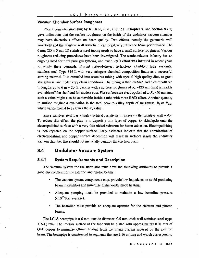
L C L S D E S I G N S T U D Y R E P O R T
Vacuum Chamber Surface Roughness
Recent computer modeling by K. Bane, et al., (ref. [51], Chapter 7, and Section 8.7.5)
gave indications that the surface roughness on the inside of the undulator vacuum chamber
may have deleterious effects on beam quality. Two effects, namely the geometric wall
wakefield and the resistive wall wakefield, can negatively influence beam performance. The
6 mm OD x 5 mm ID stainless steel tubing needs to have a small surface roughness. Various
roughness-reducing procedures have been investigated. The semiconductor industry has an
ongoing need for ultra pure gas systems, and much R&D effort was invested in recent years
to satisfy these demands. Present state-of-the-art technology identified fully austenitic
stainless steel Type 316-L with very stringent chemical composition limits as a successful
starting material. It is extruded into seamless tubing with special high quality dies, to great
straightness, and under very clean conditions. The tubing is then cleaned and electropolished
in lengths up to 6 m s 20 ft. Tubing with a surface roughness of Ra -125 nm (rms) is readily
available off the shelf and for modest cost. Rat surfaces are electropolished to Ra ~50 nm, and
such a value might also be achievable inside a tube with more R&D effort. Another quantity
in surface roughness evaluation is the total peak-to-valley depth of roughness, R, or R^,
which varies from 4 to 12 times the Ra value.
Since stainless steel has a high electrical resistivity, it increases the resistive wall wake.
To reduce this effect, the plan is to deposit a thin layer of copper (> skindepth) onto the
electropolished surface with a very thin nickel substrate for better adhesion. Electropolishing
is then repeated on the copper surface. Early estimates indicate that the combination of
electropolishing and copper surface deposition will result in surfaces inside the undulator
vacuum chamber that should not materially degrade the electron beam.
8.4 Undulator Vacuum System
8.4.1 System Requirements and Description
The vacuum system for the undulator must have the following attributes to provide a
good environment for the electron and photon beams:
• The vacuum system components must provide low impedance to avoid producing
beam instabilities and minimize higher-order mode heating.
• Adequate pumping must be provided to maintain a low beamline pressure
(<10'7Torr average).
• The beamline must provide an adequate aperture for the electron and photon
beams.
The LCLS beampipe is a 6 mm outside diameter, 0.5 mm thick wall stainless steel (type
316-L) tube. The interior surface of the tube will be plated with approximately 0.01 mm of
OFE copper to minimize Ohmic heating from the image current induced by the electron
beam. The beampipe is constructed in segments that are 2.16 m long and which correspond to
U N D U L A T O R • 8-37

L C L S D E S I G N S T U D Y R E P O R T
the undulator magnet segments. The beampipe segments are constructed from type 316-L
stainless steel to minimize the magnetization of the heat-affected zone at the welds. After
welding, each beampipe section will be annealed to completely de-magnetize the welds.
Vacuum processing of the vacuum tubes section will consist of baking at 800°C for a
minimum of 4 hours.
Between undulator segments there are 23.5 cm gaps where vacuum pumping, beam
steering, and diagnostic components are located. The undulator segments with the 23.5 cm
gaps are repeated over the 112 m long device. A typical segment gap is shown in Fig. 8.4-1.
2 Lps Ion Pump
Quadrupole/Corrector Magnet
BPM
-23.5 cr
Figure 8.4-1. Undulator segment gap with vacuum and magnet components.
Between each undulator segment, there is an RF shielded bellows module. The purpose
of the bellows is to provide flexibility for ease of installation of adjacent segments of the
beampipe and to account for any minor length changes due to temperature fluctuations. A
cross-section of the LCLS bellows module is shown in Fig. 8.4-2. Since space is tight,
vacuum pumping of the beampipe is accomplished within the bellows module. A 2 liter/sec
noble diode ion pump is mounted on one of the bellows end flanges. Pumping occurs through
ten 1-mm diameter holes in the beampipe. Conductance losses through the module decreases
the actual pumping speed to approximately 1 liter/sec.
The sliding RF fingers within the bellows are fabricated from a thin wall type 316-L
stainless steel tube. The ends of the tube have 0.15 mm slits, which allow the tube to flex
radially and provide spring force to maintain contact with the adjacent tubes. The tube slits
are plated with 0.01 mm thick silver. The contacting surfaces of the adjacent tubes are plated
with 0.01 mm thick rhodium. The combination of the relatively soft silver and the hard
rhodium provide a sliding surface with both good lubricity and good electrical conductivity.
The flanges in the vacuum system are raised face type using a "VAT" style seal. The
VAT seal is a commercially available, silver-plated, soft copper gasket. The gasket has a
raised bead around the inside diameter of the beam tube, which is crushed between the
flanges. The raised bead acts as both the vacuum seal and the RF seal across the flanged joint.
8-38 • U N D U L A T O

L C L S D E S I G N S T U D Y R E P O R T
•Vocuum Pumping Port 5mm ID Beam Tube
Rhodium Plated Stub
Figure 8.4-2.
• Axial Restraints
Bellows module cross-section.
8.4.2 Gas Load and Vacuum Pressure
In general, accelerator beampipes are conductance limited. In the case of the undulator
vacuum system, this problem is extreme. It turns out that the amount of pumping at 2.16 m
intervals has little effect on the average system pressure. This can be demonstrated with a
simple calculation. Assuming a constant gasload along the length of the beampipe and
considering the symmetry of the vacuum system, the average beampipe pressure is calculated
analytically using the following equation:
(8.4.1)
where Pav, average pressure, Torr
q, H2 gasload = 1 x 10"u Torr-liter/sec-sq cm
p, perimeter = ;r(0.5 cm) = 1.57 cm
L, half-length of cell = 108 cm
C, beampipe conductance = 0.0269 liter/sec
S, pumping speed
Assuming a pumping speed of 1 liter/sec, the average pressure is 2.27 x 10"8 Torr. If the
pumping speed is increased to 10 liter/sec, the average pressure decreases to 2.11 x 10'8 Torr
(only a 7.6% improvement). From this, it can be seen that minimizing the gasload has a much
greater effect on beampipe pressure than does pumping speed. The gasload within the
U N D U L A T O R • 8-39

L C L S D E S I G N S T U D Y R E P O R T
undulator vacuum system comes from two processes, thermal desorption and photo-
desorption. Thermal desorption is common to all types of vacuum systems; it is the heat-
stimulated release of gas constituents adsorbed on the walls of the system. Photo-desorption is
the outgassing that occurs due to synchrotron radiation hitting the walls of the beampipe and
desorbing gas molecules. Good thermal desorption data exists for UHV processed copper
plated stainless steel from the PEP-II project [12,13]. Typically, q, = 5 x 10"13 Torr-liter/sec-
sq cm (@ T = 20°C) after a 800°C bake for 4 hours. Since the undulator vacuum system is
expected to operate at 20 °C, this value will be used.
Photodesorption is a little harder to estimate. The undulator produces 90 GW of total
power. A worst case estimate would be that 100 GW hits the walls of the vacuum system.
Converting power to photon flux:
PSRtf(6.242xl0l5keV/j)= — (8.4.2)
•photon
where Nf photon flux = photons/sec
PSR, synchrotron radiation power = 100 x 109 Watts
t, pulse length = 100 x 10"15 sec
/ pulse frequency = 120 sec'1
Ephoton, average photon energy = 200 keV/photon
Nyfor the undulator is 3.74 x 10¹³ photons/sec. The distribution of the photon flux is
assumed to increase linearly along the length of the vacuum system as shown in Fig. 8.4-3.
100
Figure 8.4-3. Undulator photon flux profile.
8-40 • U N D U L A T O R

L C L S D E S I G N S T U D Y R E P O R T
The photo-desorption gasload is calculated as follows:
qp = Ay7(2.83*10-20Torr-l/molecule) (8.4.3)
where qp, photo-desorption gasload = Torr-liter/sec
f], photo-desorption rate = molecules/photon
Photo-desorption of copper and stainless steel beam tubes were investigated in the past.
Brookhaven National Laboratory conducted studies for the PEP-II Project, determining the
values of T] with respect to flux [14]. The photon flux for the undulator vacuum system is in
fact quite low, so, realistically, photon scrubbing will not occur during the lifetime of the
machine. From the Brookhaven results, it has been determined that an 77 = 5 x 10~3
molecules/photon is appropriate for design purposes. Using this value, the photo-desorption
profile is calculated and is shown along with the calculated thermal desorption profile in
Fig. 8.4-4.
Using the desorption profiles, a vacuum pressure profile for the 100 m long undulator
vacuum system is calculated using VACCALC [15], a pipeline pressure computer code. The
entire undulator beampipe is modeled using discrete pipeline segments. Each segment is
defined by its length (m), conductance (liters/sec), gasload (nTorr-liter/sec), and pumping
speed (liter/sec). All values for conductance, gasload and pumping speed are calculated for
"hydrogen." Fig. 8.4-5 shows the pressure profile along the length of the undulator vacuum
system, with its average pressure being 1.06 x 10"9 Torr (1 nTorr). This is well below the
design requirement of 10"7 Torr.
(x10-12)
l/sec
-cr
Tor
r-G
aslo
ad (
1 .£.
1.0
0.8
0.6
0.4
0.2
0
1 l • i ' i
-
^ i I . I . I
1 i '
-
• i .
3-988360A2
20 40 60Z (m)
80 100
Figure 8.4-4. Undulator thermal and photo-desorption profiles.
U N D U L A T O R 8-41

L C L S D E S I G N S T U D Y R E P O R T
Hill!1
1 ---v-s-i! J ! j | l i ! ; j ! j » ! i J i j j jS^ l l i J i l If II i ( ! i ! j ! i; II i! |i
Mm
Himrrrn
Figure 8.4-5. LCLS vacuum pressure profile.
8.4.3 Thermal Considerations
As described above, 100 GW of synchrotron radiation power strikes the walls of the
beampipe. However, the pulse length of the photons is 100 x 10"15 sec and the frequency of
the pulse is 120 Hz. Therefore, the total power absorbed by the entire 112 m of beampipe is
1.2 Watts. With such a low level of incident power, there is no need to actively cool the
vacuum chamber.
8.5 Alignment and Trajectory Control
8.5.1 Introduction
FEL simulations show that transverse displacement as well as phase slippage between the
electron and radiation beams have to be kept small and to very high tolerances (see
Section 5.7). While the radiation beam, once generated coaxially with the electron beam path,
will propagate in a straight line, the path of the electron beam can be changed by magnetic
fields. The strongest magnetic field component acting on the beam is the undulator field itself.
The ideal undulator field will cause the beam path to undergo undulation with very small
amplitudes that average to zero over one 3 cm long undulator period, thus keeping the
electron beam on a straight line.
Deviations from the ideal field will cause the average beam position to move away from a
straight line onto a random walk trajectory. These deviations or field errors can only partially
be corrected by field shimming techniques. Another contribution to random walk can come
from transverse misalignment of the focusing quadrupoles. While undulator field errors will
cause random walk mostly in one plane, quadrupole misalignment will produce a wander in
two planes.
Random walk trajectories need to be controlled by correcting the beam path using
electron beam position monitors from which the trajectory's deviation from a straight line can
8-42 • U N D U L A T O R

L C L S D E S I G N S T U D Y R E P O R T
be obtained. While state-of-the-art electron beam position monitors offer excellent position
resolution, their absolute position information is comparatively poor. A level of absolute
alignment would be required that is beyond what present technology can do.
Beam-based alignment with variable electron energy offers a solution to this problem.
Without putting very tight tolerances on absolute physical BPM alignment, the technique
provides information about BPM position and BPM gain errors that can be used to correct the
readings so that the electron beam trajectory deviation from a straight line can be measured
down to a few microns. See Section 8.5.2.
The beam-based alignment procedure will be used infrequently to provide and update
BPM calibration data. Continuous beam trajectory correction will be applied based on the
calibration data. The methods considered include point-to-point steering with high spatial
frequency components or a method (based on the linear algebra "Singular Value
Decomposition" or SVD technique) that allows limiting the spatial frequency components
and the maximum kick angles. All methods include trajectory measurements in one or more
shots and trajectory correction in subsequent shots.
The point-to-point technique effectively uses one corrector (i.e., permanent quadrupole
position) at a time to steer the beam to the calibrated center of the next position monitor. In
the LCLS, correctors (movable quadrupoles) and monitors will be positioned next to each
other. In the presence of large calibration errors, small spacings between subsequent
correctors can lead to large kick angles that will eventually increase FEL saturation length.
For practical reasons, the spacing between monitor/corrector stations is much larger than
an undulator pole or period. While the kicks produced by quadrupole misalignments can be
eliminated, the random walk amplitude between two stations can only be minimized to some
degree. The residual amplitude will depend on the field error amplitude, the monitor/corrector
station separation and, to some extent, the steering algorithm.
Section 8.5.2 describes the initial trajectory control using undulator beam-based
alignment. Section 8.5.3 describes trajectory control based on the Singular Value
Decomposition (SVD) technique.
8.5.2 Undulator Beam Based Alignment
The electron trajectory within the LCLS undulator needs to be straight to a high degree of
accuracy so that the undulator radiation overlaps efficiently within each gain length of the
undulator. This condition requires a trajectory straightness of ~5 //m over a 10-meter length
of undulator. This level is very difficult to achieve with tunnel component survey alignment
techniques. For this reason, an empirical beam-based alignment technique that uses beam
position monitor (BPM) readings as a function of large, deliberate variations in the electron
energy has been developed. The measurements are analyzed and then converted to
(1) quadrupole magnet transverse position corrections, (2) BPM offset corrections, and
(3) adjustments of the incoming beam position and angle at the undulator entrance (initial
U N D U L A T O R • 8-43

L C I S D E S I G N S T U D Y R E P O R T
launch conditions). The alignment procedure is repeated 2-3 times in succession for the
initial machine startup, and then reapplied only once per few weeks or months as necessary.
Between these infrequent applications a simple steering technique will be used for daily
trajectory control, and a fast feedback system will maintain the trajectory down to a time scale
of seconds. This section discusses primarily the alignment procedure that is applied during
the initial machine commissioning.
Introduction
The readback of the ith BPM, which measures the centroid of the transverse position of
the electron bunch at location s,- along the beamline, can be written as
m, = (8.5.1)
where 6j is the kick angle at point j (j<i) due to a transversely misaligned quadrupole magnet
or dipole field error upstream of BPM-i, Cy is the transfer coefficient which maps a beam
angle at point j to a position at point i, and b( is the readback offset (mechanical and/or
electrical) of the ith BPM. The initial launch conditions are ignored for now (more on this
below). This is described graphically in Fig. 8.5-1.
Figure 8.5-1. Schematic of an electron trajectory for the nominal beam energy (AE= 0) and for amuch lower energy (AE < 0). The undulator induced oscillations of the centraltrajectory are not shown.
The kick angles in the figure are represented as dipoles; however, they are completely
equivalent to either quadrupole magnets with transverse displacements or to field errors of the
undulator dipoles or both. The quadrupole focusing within the undulator is not explicitly
.shown in the figure, but is represented mathematically in the transfer coefficient, Cy.
Since the kick angles, 9j, are inversely proportional to beam momentum, p, whereas the
BPM offsets, £>/, are independent of momentum, then variations of the beam energy
(momentum) can be used to measure both parameters simultaneously. This is demonstrated
by substituting a dipole field error, ABj, (equivalent to a quadrupole misalignment) for 9jt and
explicitly showing the momentum dependence of Eq. 8.5.1
8-44 • U N D U L A T O R

L C L S D E S I G N S T U D Y R E P O R T
Pk j=\(8.5.2)
Here / is the dipole length, e is the electron charge (the subscript k on momentum and
BPM readback is introduced to indicate different values of beam momentum). The transfer
coefficients, Cy<p*)> in general also include a momentum dependence, except in the case of no
quadrupole focusing. As a simple example, this no-quadrupole case is graphically represented
in Fig. 8.5-2 as a linear dependence of m,- on lip plus an offset, £>,-. The measurement then
reduces to a line-fit where the slope is equal to the summation term in Eq. 8.5.2 and the offset
is equal to -£,-. The general case, including quadrupole focusing, is similar but does not
appear as the simple line-fit shown.
15 GeV/c 10 GeV/c 5 GeV/c
Figure 8.5-2. Graphical representation of Eq. 8.3.2. The BPM readback is linear with 1/p and has aslope equal to the summation term and an offset equal to -b,-. The plot is linear only ifthe Cjj elements are momentum independent (e.g., no focusing). This linear case isshown as a simple example.
The solutions are obtained more effectively in a linear fit using all BPMs and energies
simultaneously. A matrix expression for this linear system is given in Eq. 8.5.3. Here the
elements PtJ (k) = eCtjPk are the scaled momentum dependent transfer coefficients which map
theyth field error to the ith BPM. AT BPMs, N kicks, and two different momenta (k = 1,2) are
also indicated.
-1 0 - 0 Pn(l) 0 ••• 0
0 -1 - 0 P21(l) PnQ) ••• 0Ith\
mm"hi
p-1
0
0 ••0 ••
-1 ••
• —:• 0
• 0
Pn(2) 0 00
0 0
h
AB2£
(8.5.3)
U N D U L A T O R 8-45

L C L S D E S I G N S T U D Y R E P O R T
There is a large number of dipoles along the undulator (~6600) and therefore too many todetermine. Because of this, the fact that the simulated BPM readbacks contain contributionsfrom the dipole field errors is ignored and the BPM data is fit to quadrupole magnetmisalignments and BPM offsets only. Therefore, any BPM readback sensitivity to energychange will be identified as upstream quadrupole offsets, and the determined quadrupolemisalignments (in the bend plane) will necessarily be biased in order to best cancel the netdipole error (real localized dipole errors plus quadrupole misalignment). The quality of thiscancellation is examined in the simulation section described below. The non-bend plane hasno dipoles, and therefore the determined quadrupole positions will not be biased (unlessdipole roll errors or other stray magnetic fields exist). This is a significant advantage for theenergy scan technique where all bend fields, without explicit knowledge of their source, areapproximately canceled by biasing the final quadrupole positions to remove trajectorysensitivity to energy variations.
To write Eq. 8.5.3 explicitly in terms of quadrupole misalignments, ABjl is replaced bythe quadrupole magnet misalignment, AXJ, and Pijik) by
Py;(k) -> [1 - Q(x (kW/i (k)-Q>x(k)R&(k), .. (8.5.4)
where Qn(k) and j2/21(£) are the thick-lens transfer matrix elements across they'th quadrupolemagnet evaluated at the kth momentum, and RuHk) and Ri^Kk) (=Qj) are the position-to-position and angle-to-position, respectively, transfer matrix elements from the exit of theythquadrupole to the zth BPM and are also evaluated at the kth momentum. Note, a thin lensquadrupole of pole-tip field B, radius r, and length / has a focal length/= rplBle. The rightside of Eq. 8.5.4 reduces to -Cfj(k)/f, where the minus sign indicates that a horizontallyfocusing quadrupole (1/f < 0) which is displaced in the positive direction (Ax > 0) will kickthe beam in the positive direction.
In practice, the linear system of Eq. 8.5.3 is solved by imposing "soft-constraints" on thesolutions to stabilize the system. The inclusion of the soft-constraints is equivalent toincluding the additional known information that the quadrupole and BPM offsets are zero towithin -1 fim. The constraints are not hard limits but rather weight the normalized residual fiterror (x2) such that the solutions do not wander out to large values over long distances [16].Eq. 8.5.5 shows the standard least-squares minimization where additional "soft-constraints"are included for the BPM and the quadrupole offsets (last two terms).
imik ~
7=1(8.5.5)
8-46 • U N D U L A T O R

L C L S D E S I G N S T U D Y R E P O R T
The BPM and quadrupole offsets are weighted by their respective soft-constraints, ax and ofc
(=1 /an in the simulations to follow). The solutions are then found in the standard way where
the gradient of x2 with respect to the solutions is set to zero.
By ignoring the initial launch conditions of the beam at the entrance to the undulator in
Eq. 8.5.3 the reference line for the determined BPM and quadrupole misalignments (&,• and
AxJ) is defined as the incoming position and angle of the beam. When Eq. 8.53 has been
solved, N values of b and Ax are available. A best line fit (initial position and angle) from
these data is used to adjust the launch conditions (with steering dipoles prior to the undulator)
so that the quadrupole and BPM offset corrections will not systematically follow these initial
erroneous launch conditions. On the next application of the procedure, the launch conditions
should be much closer to the axis defined by the initial BPM and quadrupole positions (the
initial tunnel survey).
The advantage of scanning the beam energy, compared with scanning quadrupole field
strengths, is that the energy scanned BPM data are sensitive to all bending fields whether due
to quadrupole misalignments, undulator dipole errors or other stray fields such as the earth's
field. By using these field-sensitive data, the solutions obtained provide the best minimization
of all bending by biasing the quadrupole positions slightly offset with respect to the beam
centroid. The net effect is to produce minimal erroneous bending within the undulator. Given
dipole errors and other stray fields, this produces a much straighter trajectory than is
obtainable by varying quadrupole field strengths, which is also inconvenient for permanent
magnet quadrupoles.
Simulation Results
Simulations have been run for the entire beam-based alignment algorithm, from initial
rough steering through final precision alignment. The simulations use 48 quadrupoles and 48
BPMs, where quadrupoles are separated by 2.16 m (center-to-center) and have a field
gradient of 48 T/m and length of 12 cm. One BPM is located at the upstream face of each
quadrupole. A conservative set of statistical and systematic errors is included in the
simulations as summarized in Table 8.5-1. The sensitivities of the final results to the input
errors are studied in the next section.
The "correlated" BPM and quadrupole offsets (misalignments) define a random walk path
where the expectation value of the square of the misalignment, (x2), is related linearly to its
distance, L, from the undulator entrance [17]. This treatment approximates the long undulator
survey "wander" error arising over 100 meters. In this case, an rms of 100 pm per 10 meter
length, or ~300 pm over 100 meters is used. The BPMs and quadrupoles both follow the
same random walk plus an additional 50 ^im rms "uncorrelated" component (applied to both
BPMs and quadrupoles separately). Two adjacent elements are therefore misaligned with
respect to each other by V2 x 50 urn = 70 um rms. Over longer distances the relative
misalignment increases.
U N D U L A T O R • 8-47
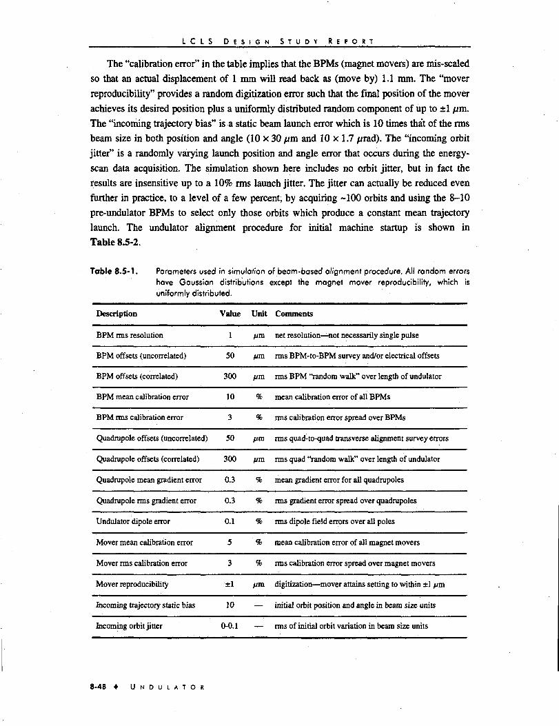
L C L S D E S I G N S T U D Y R E P O R T
The "calibration error" in the table implies that the BPMs (magnet movers) are mis-scaled
so that an actual displacement of 1 mm will read back as (move by) 1.1 mm. The "mover
reproducibility" provides a random digitization error such that the final position of the mover
achieves its desired position plus a uniformly distributed random component of up to ±1 ftm.
The "incoming trajectory bias" is a static beam launch error which is 10 times that of the rms
beam size in both position and angle (10 x 30 fim and 10 x 1.7 find). The "incoming orbit
jitter" is a randomly varying launch position and angle error that occurs during the energy-
scan data acquisition. The simulation shown here includes no orbit jitter, but in fact the
results are insensitive up to a 10% rms launch jitter. The jitter can actually be reduced even
further in practice, to a level of a few percent, by acquiring -100 orbits and using the 8-10
pre-undulator BPMs to select only those orbits which produce a constant mean trajectory
launch. The undulator alignment procedure for initial machine startup is shown in
Table 8.5-2.
Table 8.5-1. Parameters used in simulation of beam-based alignment procedure. All random errorshave Gaussian distributions except the magnet mover reproducibility, which isuniformly distributed.
Description
BPM rms resolution
BPM offsets (uncorrelated)
BPM offsets (correlated)
BPM mean calibration error
BPM rms calibration error
Quadrupole offsets (uncorrelated)
Quadrupole offsets (correlated)
Quadrupole mean gradient error
Quadrupole rms gradient error
Undulator dipole error
Mover mean calibration error
Mover rms calibration error
Mover reproducibility
Incoming trajectory static bias
Incoming orbit jitter
Value
1
50
300
10
3
50
300
0.3
0.3
0.1
5
3
±1
10
0-0.1
Unit
fim
pm
(im
%
%
fan
fim
%
%
%
%
%
fim
—
—
Comments
net resolution—not necessarily single pulse
rms BPM-to-BPM survey and/or electrical offsets
rms BPM "random walk" over length of undulator
mean calibration error of all BPMs
rms calibration error spread over BPMs
rms quad-to-quad transverse alignment survey errors
rms quad "random walk" over length of undulator
mean gradient error for all quadrupoles
rms gradient error spread over quadrupoles
rms dipole field errors over all poles
mean calibration error of all magnet movers
rms calibration error spread over magnet movers
digitization—mover attains setting to within ±1 pm
initial orbit position and angle in beam size units
rms of initial orbit variation in beam size units
8-48 • U N D U L A T O R

L C L S D E S I G N S T U D Y R E P O R T
The initial step is to reduce the field strength of the 2nd bunch compressor chicane bends
so as to increase the bunch length in the undulator to ~ 150 fim. This will alleviate transverse
resistive wall wakefields as a source of systematic error which may otherwise be quite strong
when large trajectory excursions occur during the alignment procedure. The transverse
geometric wakefields increase with a longer bunch, but are still weak with a 150 //m bunch
length.
Figure 8.5-3 shows the specific quadrupole and BPM misalignments used in the
simulation with respect to a line defined by the pre-undulator beamline axis (as are all figures
in this section unless otherwise noted). Both the correlated and uncorrelated misalignment
components are included (see Table 8.5-1).
The resultant, un-steered horizontal and vertical beam trajectory through the undulator is
shown in Fig. 8.5-4 (prior to step-1). The true orbit is shown (as in the plots to follow) every
12.5 cm along the undulator (every 8th dipole of 6624). The BPM readbacks (diamonds) are,
in practice, the only known quantities at this point. The first correction (step-1) is to adjust
the launch based on the first 10 BPMs in the undulator which are used in a best fit to an
incoming betatron oscillation (see dashed line in first 20 meters of Fig. 8.5-4). Table 8.5-3shows the initial launch conditions for this simulation both before and after the step-1
correction.
Table 8.5-2. Beam-based undulator alignment procedure. Beam energy is 14.3 GeV unlessotherwise noted.
Step#
0
1
2
3
4
5
6
7
8
Description
Adjust the 2nd bunch compressor chicane for a -150 j/m electron bunch length tominimize transverse wakefields in the undulator
Adjust the launch using best position and angle fit to 1st 10 BPMs
Apply weighted steering to reduce (not zero) both the absolute BPM readings (-f 50fim) and the applied mover changes {-i-50 ftm)
Save -100 sets of BPM readings for each of 5,10, and 14.3 GeV beam energieswhile scaling upstream magnets to new energy each time
Run BPM data through analysis program to determine BPM and quadrupoleoffsets (select from data sets to minimize orbit jitter)
Adjust launch position and angle to remove determined linear component of BPMand quadrupole offsets
Set quadrupole movers to new positions and correct BPM offsets
Steer offset-corrected BPM readings to approximately zero using a minimumnumber of magnet movers
Repeat steps 3-7 until peak BPM readings at 4.5 GeV are <-50 fim
time/hr
0.5
0.1
0.2
3
0.1
0.1
0.1
0.2
3.5/ iteration
U N D U I A T O R 8-49
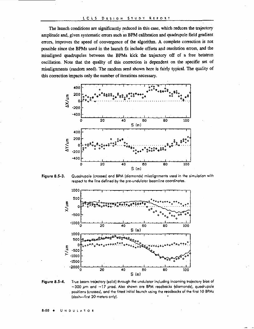
L C L S D E S I G N S T U D Y R E P O R T
The launch conditions are significantly reduced in this case, which reduces the trajectoryamplitude and, given systematic errors such as BPM calibration and quadrupole field gradienterrors, improves the speed of convergence of the algorithm. A complete correction is notpossible since the BPMs used in the launch fit include offsets and resolution errors, and themisaligned quadrupoles between the BPMs kick the trajectory off of a free betatronoscillation. Note that the quality of this correction is dependent on the specific set ofmisalignments (random seed). The random seed shown here is fairly typical. The quality ofthis correction impacts only the number of iterations necessary.
20 40 60 80 100
£
>-<
400
200
o'-200
-400
i • • •
-
1
•
|
s (m)' 1
« • • * %oo
. . 1 . .
1 . . . . 1
* * • * " * • *
20 40 60 80 100
S Cm)Figure 8.5-3. Quadrupole (crosses) and BPM (diamonds) misalignments used in the simulation with
respect to the line defined by the pre-undulator beamline coordinates.
1000
i#^^^
-200040 60
S Cm)80 100
Figure 8.5-4. True beam trajectory (solid) through the undulator including incoming trajectory bias of~300 jJm and —17 /;rad. Also shown are BPM readbacks (diamonds), quadrupolepositions (crosses), and the fitted initial launch using the readbacks of the first 10 BPMs(dash—first 20 meters only).
8-50 • U N D U L A T O R

Table 8.5-3.
L C L
Initial launchcorrection.
Launch Parameter
<*>
<*')
<y>
W>
S D E S I G N S T U D Y R E
conditions at undulator entrance
Before Step-1
320 pm
16.0 prad
283 pm
18.0 prad
P O R T
before and after step-1 launch
After Step-1
73/um
5.4 prad
13 pm
4.9prad
Step 2 involves a weighted steering procedure using the undulator quadrupole magnet
movers. The absolute readings of the BPMs are minimized with respect to a 50 jum weighting
and the magnet mover changes are simultaneously minimized with respect to a 50 /urn
weighting. Without this weighting the magnet movers can move more than 1 mm in order to
exactly zero each BPM reading which, due to the large BPM offsets, is an unnecessary
steering accuracy at this early stage. With the weighting included, the movers change by
~50 fim which is sufficient to correct the large trajectory deviations of Fig. 8.5-4. Fig. 8.5-5shows the trajectory after the Step 2 weighted steering is applied.
1000
£a.
E
>-
-1000100
(m)Figure 8.5-5. True beam trajectory (solid) at 14.3 GeV after application of Step 2 weighted steering.
The BPM read bocks (diamonds) and the applied magnet mover changes have beenminimized with respect to a 50 jjm weighting. The post-steering absolute quadrupolepositions (crosses) are also shown.
These 14.3 GeV BPM data are saved and the energy is then lowered to 10 GeV by
switching off klystrons in the last part of the linac. The fields of the magnets upstream of the
undulator are scaled to the new energy, and any beam position differences upstream of the
undulator, with respect to the 14.3 GeV orbit, are manually corrected until the launch position
at 10 GeV is within ±3 m of that at 14.3 GeV. Note that any beam angle difference at the
undulator entrance will not be detectable with the BPMs upstream of the undulator. However,
U N D U L A T O R 8-51

L C L S D E S I G N S T U D Y R E P O R T
this angle will eventually be properly incorporated into a correction of the transverse position
of the first undulator quadrupole. Fig. 8.5-6 shows the trajectory at 10 GeV while Fig. 8.5-7
shows the trajectory at 4.5 GeV. No changes are made to the undulator components during
the energy scan. Only the pre-undulator trajectory is adjusted, if necessary, to maintain a
constant beam position.
Since the fields of the magnets upstream of the undulator will be scaled to the lower
energies, the beta functions at the undulator entrance will be constant during the procedure. In
addition, the undulator focusing is accomplished with permanent magnet quadrupoles.
Therefore a betatron-mismatch, with respect to the energy dependent periodic beta functions
of the undulator FODO lattice, will propagate through the undulator at the lower beam
energies. In the worst case (4.5 GeV) the beam size will beat at twice the betatron frequency
reaching a peak rms size of -80 fim as compared to the 50 [xm beam size of the 4.5 GeV
periodic beta functions. This worst case beat in beam size should have no significant effect on
the alignment procedure.
1000
500
0
-500
-1000
1000
500
0
-500
-1000
20 40 60 80 100
-
_
1 . .
. . . 1 . .
s• • 1 • •
. . 1 . .
(m)
1 . . . . 1 . . . . 120 40 B0 80 100
S (m)Figure 8.5-6. True beam trajectory (solid) at 10 GeV. BPM readbacks (diamonds) and quadrupole
positions (crosses) are also shown. These BPM readings are saved for analysis.
With the 5, 10, and 14.3 GeV BPM readback data saved, the analysis program is run
which calculates BPM offsets and quadrupole magnet positions with respect to the Step 1
corrected incoming beam position and angle. Fig. 8.5-8 shows the calculated quadrupole
offsets as well as the true offsets (used in the simulation). The fine structure of the calculated
offsets agree well with the true offsets. The values differ, however, by a straight line, which is
due to both (1) the Step 1 corrected launch bias and (2) the correlated component of the BPM
and quadrupole offset errors. The best line fitted to the calculated BPM and the quadrupole
offsets is also shown. The slope and offset of the best line fit is used to readjust the initial
launch position and angle at the undulator entrance.
8-52 • U N D U L A T O R
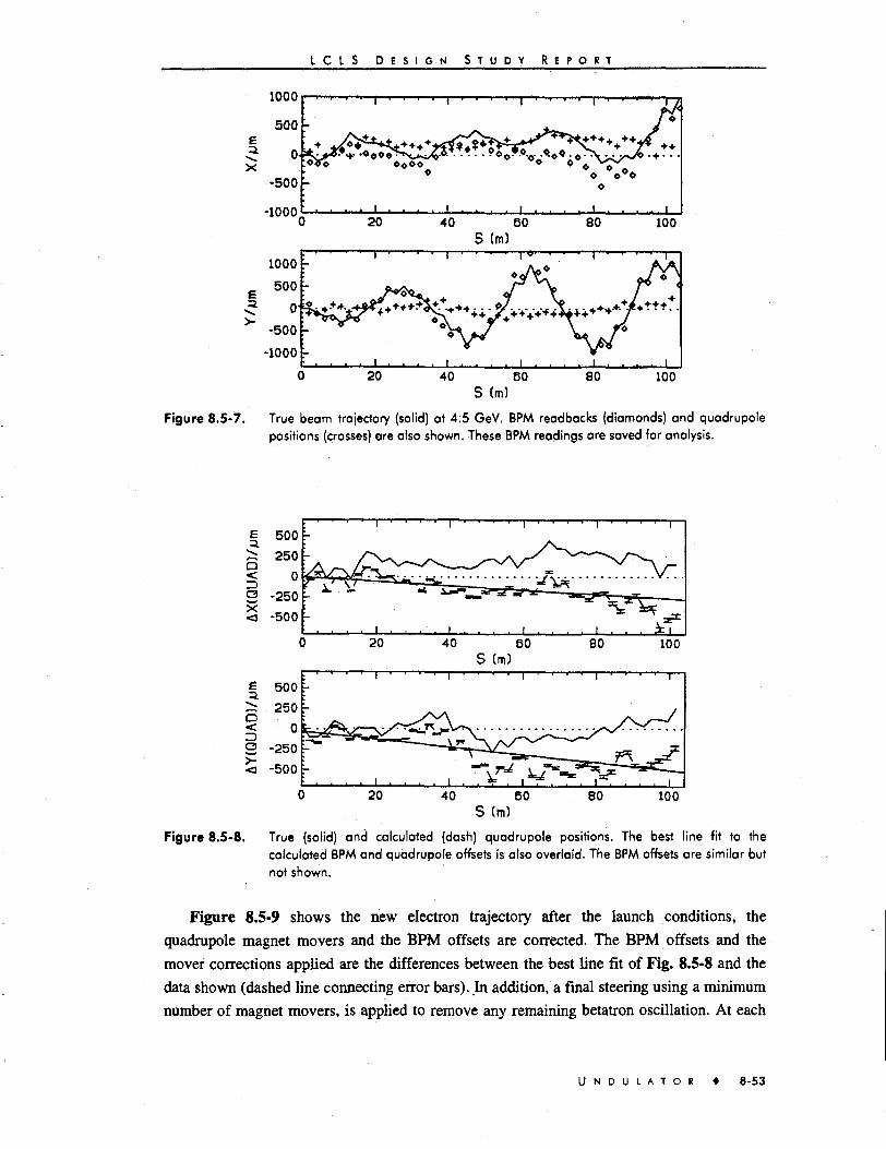
L C L S D E S I G N S T U D Y R E P O R T
20 40 60S (m)
80 100
2
>-
1000
500
0
-500
-1000
. 1 . 1 . . . .
\
1
20 40 60S (m)
80 100
Figure 8.5-7. True beam trajectory (solid) at 4.5 GeV. BPM readbacb (diamonds) and quadrupolepositions (crosses) are also shown. These BPM readings are saved for analysis.
80 100S (m)
Figure 8.5-8. True (solid) and calculated (dash) quadrupole positions. The best line fit to thecalculated BPM and quadrupole offsets is also overlaid. The BPM offsets are similar butnot shown.
Figure 8.5-9 shows the new electron trajectory after the launch conditions, the
quadrupole magnet movers and the BPM offsets are corrected. The BPM offsets and the
mover corrections applied are the differences between the best line fit of Fig. 8.5-8 and the
data shown (dashed line connecting error bars)..In addition, a final steering using a minimum
number of magnet movers, is applied to remove any remaining betatron oscillation. At each
U N D U L A T O R 8-53

L C L S D E S I G N S T U D Y R E P O R T
stage the real magnet mover limitations (calibration errors and reproducibility errors) and
BPM errors (calibration and resolution) are incorporated.
The linear component which remains in the Fig. 8.5-9 trajectory is due to the correlated
quadrupole and BPM offsets (random walk of initial tunnel survey). Since these offsets are
due dominantly to the difference between the line defined by the linac beamline axis and the
slightly different line established by the undulator beamline, the alignment procedure
inevitably launches the electrons straight down the undulator vacuum chamber which
presumably follows these correlated tunnel survey errors. The true trajectory shown in
Fig. 8.5-9 is then actually the most desired trajectory where a slight change in beam position
and angle at the undulator entrance is used to launch the electron beam down the center of the
undulator. The tiny dispersion generated by this slight position and angle change is
completely negligible, especially in consideration of the <0.02 % nns relative energy spread.
Figure 8.5-10 shows the same data as in Fig. 8.5-9 except that the linear component of
the true orbit has been removed in order to show more clearly the straightness of the
trajectory. Fig. 8.5-11 shows this linear-corrected view of the final trajectories after a second
iteration of Steps 3-7 is applied. The rms of the electron trajectory over the length of the
undulator with respect to a straight line achieves a value of ~3 m. Finally, Fig. 8.5-12 shows
the final quadrupole magnet mover settings after the two iterations have been completed. The
final alignment correction requires magnet mover settings with an rms value of ~ 100 jum.
. . . . I . . . . I . . . . I . . . . I . . . . I
300200100
0-100-200-300
3 20
. . . . . i . .
40
• ' i '
. . 1 .
s
+
(m)
+ +
60
i
+
i .
80
• • t •
•4- +
. . 1 . .
100
• 1
. . 1
20 40 60S (m)
80 100
Figure 8.5-9. True beam trajectory (solid) at 14.3 GeV after one iteration of Steps 1-7. BPMreadbacks (diamonds) and quadrupole positions (crosses) are also shown. Thetrajectory is fairly straight but does not necessarily follow the line established by thelinac axis. This is due to the correlated BPM and quadrupole misalignments (randomwalk of the initial tunnel survey).
8-54 • U N D U L A T O R

L C L S D E S I G N S T U D Y R E P O R T
£=2.
X
ea.-•»>-
200
100
o
-100
-200(
100
o.
-100
-200)
)
}
20
• i •
+
. i .
20
* + +
40
* • • *•f
. . . i .40
++
s
+
s
60(m)
+4-
. . 1 . . .
60(m)
4-
80
i +
+ 4-
. 1 . . .80
i
4*
100
f
4 *
. 1100
Figure 8.5-10. True beam trajectory (solid) at 14.3 GeV, with linear component removed, after oneiteration of Steps 1-7. BPM readbacks (diamonds) and quadrupole positions (crosses)are also shown. The quadrupole positions are shown in the same linear-correctedcoordinates of the true orbit. The true beam trajectories with respect to a straight lineover the undulator length (for this first pass correction) has rms values of*rms = 7.9 pm, y r m s = 11.7 pm and peak values of xpk = 18pm, yp|< = 36 pm.
!
60
40
20
0
-20
-40
-
s i
•• 4> 4-
14-
4
4 +
• •
. 1 . .
' • 1
4* + *
4>!
4
1 4
4- 4-
4 •
1
80 100
100
Figure 8.5-11. True beam trajectory (solid) at 14.3 GeV, with linear component removed, after twoiterations of Steps 3-7. BPM readbacks (diamonds) and quadrupole positions (crosses)are also shown. Quadrupole positions are shown in the same linear-correctedcoordinates of the true orbit. The true beam trajectories with respect to a straight lineover the undulator length has rms values of x r m s = 3.1 /urn, y r r ns = 2.9 /im and peakvalues of Xp|< = 6.8 pm, ypk = 6.6 pm.
U N D U L A T O R 8-55

L C L S D E S I G N S T U D Y R E P O R T
200
100
0
-100
-200
200
100
0
-100
-200
1 1 . . . j
. . . . 1 . .
0 20
n piJ. i . .
• •• i •
x| nJLT
. . i .40
• i •
. . . . _ J
.
u
. . . J . .
.-s-v^-. y j . . . .
60S(m)
. . i . .
• • i • •
. . 1 . .
80
• i • •
Si
J
. . i100
1
20 40 60S (m)
80 100
Figure 8.5-12. Final quadrupole magnet mover settings after two iterations of the alignmentprocedure. The movers are initially set to zero prior to the alignment procedure (x rms
= 88A<m, y r r n s = 105 (im).
Sensitivities
The sensitivities of the final rms trajectory straightness to the simulation input errors are
summarized in Table 8.5-4. A new simulation is run using the input errors listed in
Table 8.5-1 except that for each run a different error is doubled. The first row summarizes the
simulation shown in detail above, and every following row represents a new simulation where
the noted error has been doubled with respect to Table 8.3-1.
Table 8.5-4. Sensitivities of the final rms trajectory straightness (in fim) to the simulation input errors.All errors are those of Table 8.3-1 unless noted at left in which cose that error hasbeen doubled. The random seed used is unchanged for purposes of comparison.
Input Error Varied
All errors of Table 8.1-1
2 fim BPM resolution
0.2 % rms dipole errors
100 fira uncorrelated BPM & quadrupole offsets
0.6 % quadrupole gradient errors (mean & rms)
Mover reproducibility error ±2 //m
Incoming trajectory bias = 20 x (rms beam size)
Rms incoming orbit jitter = 0.1 x (rms beam size)
1st Iteration [fim]
•*rms yrms
7.9
8.8
8.8
12.3
8.5
8.3
8.2
8.4
11.7
9.3
9.3
18.8
15.1
12.7
13.0
11.5
2nd Iteration
^rms I
3.1
5.2
3.4
3.6
3.2
3.3
2.7
5.3
[fim]
• 'rms
2.9
4.2
2.8
5.0
3.2
6.1
3.9
3.3
8 - 5 6 • U N D U L A T O R

L C L S D E S I G N S T U D Y R E P O R T
All errors are returned to original values for each new run except for the noted error. As
the table shows, two iterations of the alignment procedure renders the algorithm fairly
insensitive to the precise beamline errors. A third iteration (not shown) will, in most cases,
reduce the rms trajectory to <3 //m in both planes. This is certainly true for the case of
100 ftm BPM and quadrupole misalignments.
Summary
A final electron trajectory of 3 /mi rms with respect to a straight line over the length of
the LCLS undulator is achievable using energy scanned beam-based alignment. Therefore,
prior to the alignment procedure, BPM and quadrupole uncorrelated misalignments of 100 /<m
rms plus 300 /rai rms correlated misalignments are tolerable for the LCLS undulator. Effects
such as BPM and magnet mover calibration errors, quadrupole field gradient errors, and
dipole field errors are included in a detailed simulation that demonstrates this level can be
achieved with high confidence. Only one random seed is presented here as an example.
However, many seeds have also been run with similar success. In some cases a third iteration
is necessary in order to achieve the 3 fim rms. However, the second iteration still achieves 5 -
6 //m rms, which is nearly adequate. An estimated time of 8-12 hrs is required to accomplish
the alignment. The procedure will likely be required every 1-3 months.
8.5.3 The Singular Value Decomposition (SVD) Technique
Description
The primary task of the trajectory control system is to provide run-time correction of the
beam position as it wanders from the aligned trajectory described in Section 8.5.2. The
simulations here determines the optimum spacing of BPMs and correctors for LCLS
conditions, based on an assumed magnitude of field error that causes trajectory error. The
result is that a BPM and a corrector every 2 m gives acceptable trajectory control, which is
the same interval required for initial alignment. Depending on the actual field errors, the
results can be scaled linearly. Based on the 2 Gauss field error figure, the dipole kick is
JBdl 2G-m . .G=± = = 4//rad
Bp 5x l0 5 G-/n
for a meter of undulator.
In the computer simulation, random dipole kicks of 2 /arad rms every 0.5 m are used to
perturb the electron beam trajectory. The random kick distribution is truncated at 3 a. All
calculations are performed in a single plane. No fast pulse-to-pulse studies were made.
Computer simulations of the trajectory control system are based on first-order particle
transport calculations. Initially, a beamline file is specified containing quadrupoles, dipole
kick locations, and BPM locations. Undulator field perturbations are neglected. The
quadrupoles are modeled as thick lens devices with no fringe fields. For 360° phase advance
U N D U L A T O R • 8-57
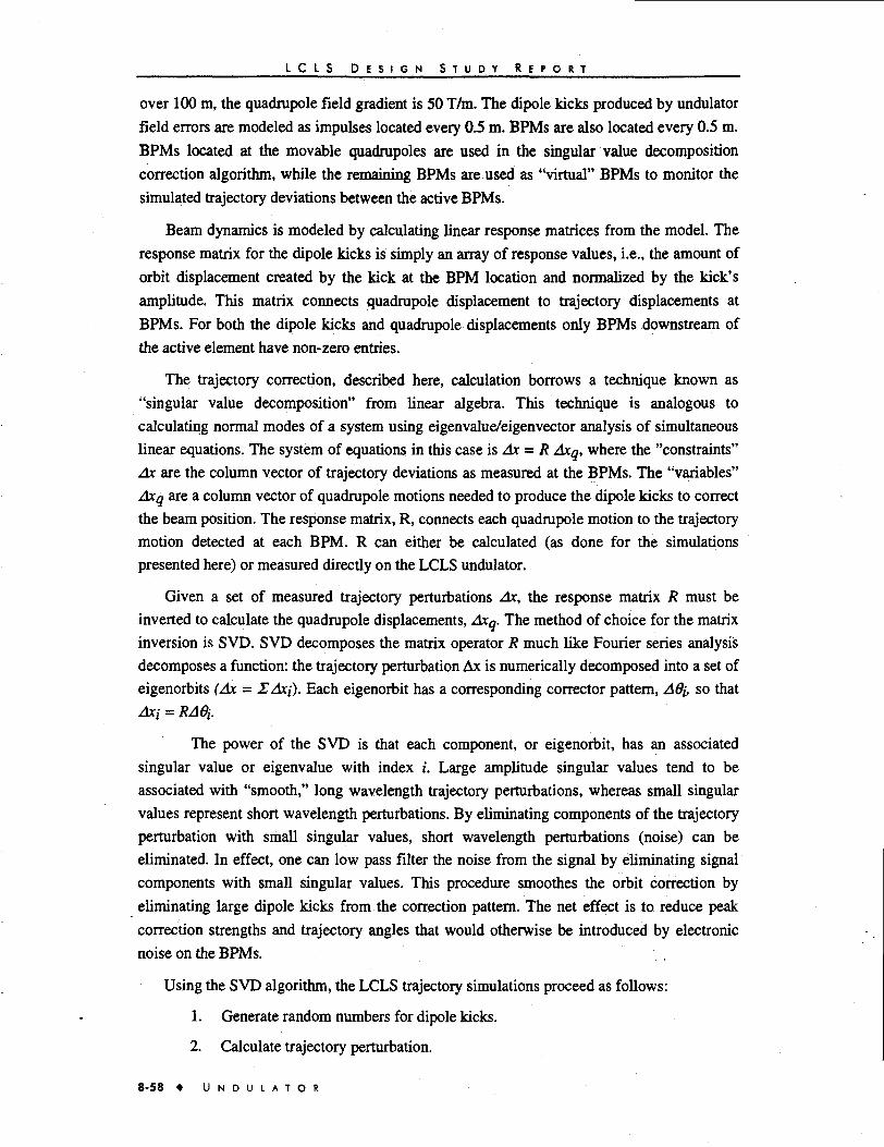
L C I S D E S I G N S T U D Y R E P O R T
over 100 m, the quadrupole field gradient is 50 T/m. The dipole kicks produced by undulator
field errors are modeled as impulses located every 0.5 m. BPMs are also located every 0.5 m.
BPMs located at the movable quadrupoles are used in the singular value decomposition
correction algorithm, while the remaining BPMs are used as "virtual" BPMs to monitor the
simulated trajectory deviations between the active BPMs.
Beam dynamics is modeled by calculating linear response matrices from the model. The
response matrix for the dipole kicks is simply an array of response values, i.e., the amount of
orbit displacement created by the kick at the BPM location and normalized by the kick's
amplitude. This matrix connects quadrupole displacement to trajectory displacements at
BPMs. For both the dipole kicks and quadrupole displacements only BPMs downstream of
the active element have non-zero entries.
The trajectory correction, described here, calculation borrows a technique known as
"singular value decomposition" from linear algebra. This technique is analogous to
calculating normal modes of a system using eigenvalue/eigenvector analysis of simultaneous
linear equations. The system of equations in this case is Ax = R Axq, where the "constraints"
Ax are the column vector of trajectory deviations as measured at the BPMs. The "variables"
Axq are a column vector of quadrupole motions needed to produce the dipole kicks to correct
the beam position. The response matrix, R, connects each quadrupole motion to the trajectory
motion detected at each BPM. R can either be calculated (as done for the simulations
presented here) or measured directly on the LCLS undulator.
Given a set of measured trajectory perturbations Ax, the response matrix R must be
inverted to calculate the quadrupole displacements, Axq. The method of choice for the matrix
inversion is SVD. SVD decomposes the matrix operator R much like Fourier series analysis
decomposes a function: the trajectory perturbation Ax is numerically decomposed into a set of
eigenorbits (Ax = EAxi). Each eigenorbit has a corresponding corrector pattern, Adi so that
Ax( =
The power of the SVD is that each component, or eigenorbit, has an associated
singular value or eigenvalue with index i. Large amplitude singular values tend to be
associated with "smooth," long wavelength trajectory perturbations, whereas small singular
values represent short wavelength perturbations. By eliminating components of the trajectory
perturbation with small singular values, short wavelength perturbations (noise) can be
eliminated. In effect, one can low pass filter the noise from the signal by eliminating signal
components with small singular values. This procedure smoothes the orbit correction by
eliminating large dipole kicks from the correction pattern. The net effect is to reduce peak
correction strengths and trajectory angles that would otherwise be introduced by electronic
noise on the BPMs.
Using the SVD algorithm, the LCLS trajectory simulations proceed as follows:
1. Generate random numbers for dipole kicks.
2. Calculate trajectory perturbation.
8 - 5 8 • U N D U L A T O R

[ C I S D E S I G N S T U D Y R E P O R T
3. Add random noise to BPM readback values.
4. Calculate quadrupole motions to correct trajectory.
5. Discrete quantization of quadrupole motions.
6. Calculate corrected orbit.
7. Accumulate statistics.
Simulation results are based on statistical analysis of many sets of random dipole kicks to
perturb the electron beam trajectory. One thousand random machines were used for these
results. The pertinent simulation parameters used for the LCLS are:
• Dipole kicks: 2 jurad rms, 3 a truncation
• BPM noise: 2 jim rms, 3 a truncation
• Quadrupole position setting errors: +/-0.125nm (discrete quantization)
Simulation Results
Figure 8.5-13 shows an example of a single random electron beam trajectory through the
undulator transport line, including BPM noise. The trajectory executes random drift-kick-
drift-kick motion through the beamline. Because of the weak focusing effect from the FODO
structure, the rms trajectory displacement, calculated for many machine seeds, does not
proceed as, <JN with N the number of dipole kicks.
Figure 8.5-14 shows the standard deviation over many random seeds of corrected beam
trajectories with BPMs and quadrapole movers placed after every 1.92 m section of undulator
(2.155 m on center). The BPMs are located at the null points in the standard deviation plots.
It is clear from the plot that the trajectory control at the BPMs is down to the noise level
(2 /an rms in this case). The rms" quadrupole displacements required to correct the beam
trajectory are on the order of 27 /an. For this example, all of the singular values were used to
correct the orbit. The effect of eliminating singular values (eigenvectors) from the correction
algorithm is demonstrated below.
Fig. 8.5-14 also shows the standard deviation of the corrected electron beam trajectory
when all quadrupole movers are used, but only half the BPMs (4.31 m on center). In this case,
the peak rms trajectory displacement reaches 3.5 /an between BPMs, and the rms quadrupole
motions required to correct the orbit are about 20 jura. For both cases (BPM at 2 m, BPM at
4 m) the quantized quadrupole motion of 250 nm does not cause a problem. If the undulator
field errors are increased from the 2 Gauss value cited above, the peaks of the rms trajectory
displacements scale linearly. For instance, in the case with BPMs every 4 m the peak rms
trajectory displacements are 3, 6, 9, and 12 /an for field errors of 2, 4, 6, and 8G,
respectively.
U N D U L A T O R • 8-59

L C L S D E S I G N S T U D Y R E P O R T
40 60z-posrriON(m)
Figure 8.5-13. Example of a single random electron beam trajectory through the undulator transportline, including BPM noise.
BPM every 4m
20 40 60Z-POSIT)ON(ro)
80 100
Figure 8.5-14. Standard deviation over many random seeds of corrected beam trajectories with BPMsand quadrupole movers placed after every 2 m (smaller amplitude curve) and 4 m(larger amplitude curve). The threshold is due to a random BPM detection error of2 fJm rms that is build into the simulation.
Figure 8.5-15 shows a plot of the average of the rms trajectory displacements, taken over
the length of the 100 m undulator, for 1000 machine seeds as a function of the number of
singular values used for the trajectory correction. In this case, BPMs were used every 2 m. By
reducing the number of singular values, noise introduced by the BPMs is effectively filtered
out. Also indicated in this plot is the average of the rms corrector strengths, taken over the
length of the 100 m undulator, as a function of the number of singular values used by the
trajectory correction algorithm. Note that even as the number of singular values is reduced,
the statistical deviation of the electron beam orbit from the central axis remains roughly
8-60 • U N D U L A T O R

L C L S D E S I G N S T U D Y R E P O R T
constant until only about half of the singular values are used. At the same time, the rms
quadrupole displacements decrease by about 20%. Although the displacement of the electron
beam trajectory at the BPMs is slightly relaxed, large deviations occur between BPMs as the
number of singular values is reduced.
15
10BPM
, READINGS QUADRUPOLE MOTIONS
50
-40
- 3 0 !
- 2 0 :
- 1 0 '
10 15 20 25
NUMBER OF SINGULAR VALUES
30 35 40
Figure 8.5-15.
Summary
Plot of the average of the rms trajectory displacements, taken over the length of theTOO m undulator, for 1000 machine seeds as a function of the number of singularvalues used for the trajectory correction.
The method of singular value decomposition (SVD) of the corrector-to-BPM response
matrix for trajectory control in the LCLS looks satisfactory. The SVD control algorithm is
presently used for trajectory control on many storage rings and on various sections of the
SLC linac. The trajectory control algorithm is easy to implement from a control system
interface point of view. Another redeeming feature of SVD is the robustness of the solution as
the number of singular values is reduced: the control algorithm can be used as a software
filter to reduce the effects of noise. Weighting of individual BPMs and correctors is also
possible. It should be noted that the success of the trajectory control depends on the
quadrupole mover and BPMs being located near each other. If the movers and BPMs are
"interlaced" (every 2 m for instance), then large trajectory excursions and trajectory angles
can occur.
8.6 Beam Diagnostics
8.6.1 RF Cavity BPMs
The Beam Position Monitor (BPM) system is the primary system for measuring the
transverse position of the electron beam in the LCLS. The instrument must provide these
measurements with exceptional accuracy through every phase of FEL operation:
commissioning, problem resolution, user operation, and facility improvement. The BPM
U N D U L A T O R 8-61

L C L S D E S I G N S T U D Y R E P O R T
system is used to maintain co-linearity of the electron and photon beams, within 5 jum rms
over any 10m length with 14.3 GeV electrons. However, the absolute accuracy of the BPM
system is not the basis of the alignment system. The initial survey errors of BPM detectors are
held to better than 50 pm. So as to contribute little to the total position error, the accuracy of
individual BPMs was specified, with respect to their external fiducials, at less than 25 fjm.
This includes all error factors: mechanical, electronic, and electronic drift. Each BPM must
have the ability to detect relative changes in position of 1.0//m at the nominal operating
charge of 1 nC bunches.
These requirements placed on the BPM system are stringent, but within the forefront of
position measurement technology. The structure of the electron beam is 1 nC bunches,
nominally rectangularly distributed along the direction of travel (z-axis), with
FWHMZ = 70 /an. The bunch repetition rate is 120 Hz. Each BPM station shall provide single
shot position measurements on any bunch in both x and y planes, and a beam intensity
measurement. The requirements of the LCLS BPM system are shown in Table 8.6-1.
Table 8.6-1. LCLS BPM performance requirements.
Operational Mode
Position accuracy (with respect to local externalfiducials)
Position resolution
Current accuracy
Current resolution
Data collection/ local memory number of points
Single shot, any bunch, x & y planes
A<25//m
S< l.Oftm/ 1 nC (10//m/0.1 nC)
2% (0.05 nC - 2.5 nC)
0.1%
104 point FIFO memory with acquisition enable
Review of BPM Technology
Several BPM technologies, including both intercepting and non-intercepting methods,
were evaluated against the LCLS requirements. The expected performance of Non-
Intercepting BPM technologies is summarized in Table 8.6-2. Four of the technologies (U)
don't meet the LCLS design specifications, while two do (D).
Intercepting monitors were also considered because of the high absolute accuracy that a
mechanical drive/hard stop assembly can provide. Intercepting monitors would be inserted
infrequently, to obtain an absolute position calibration. The offsets of the non-intercepting
monitors would then be measured and applied as corrections in the database. The intercepting
monitors which were considered for the LCLS are shown in Table 8.6-3.
8-62 • U N D U L A T O R

Table 8.6-2.
Wall CurrentMonitor (U)
Stripline (U)
MicrowaveAperture (U)
Cavity (U)
Stripline (D)
Cavity (D)
Table 8.6-3.
Fluorescentscreen
Transitionradiation
Wire scanner
L C L S D E S I G N S T U D Y R i P O R T
Evaluation of BPM technologies for LCLS (non-intercepting).
Device Parameters Accuracy Estimatedof Center Resolution
z = 6 mm, RB =2 Q, Moderate 0.2 //m/nC
z = 9mm,Z o = Moderate 0.25 //m/nC40 Q,g = 0.125 (~50//m)
3.0 x 1.5 mm slot to Good 0.1/on/nCwaveguide. Unproved
fe = 7.0 mm Good 1 //m/nCz = 2.8 mm
z = 40 mm, Moderate 0.25 /fin/nCZo = 50Q ( -50 / t o )
((•ID = 60 mm Excellent - 5 GHzz = 5.0mm (~5//m)
OperatingFrequency
>lGHz
- 2-5 GHz
> 50 GHz
- 3 2 GHz
-0.5-2 GHz
- 5 GHz
Evaluation of BPM technologies for LCLS (intercepting).
Device Accuracy of ResolutionParameters Center
Doped crystal - 1 fjm Unproven.(YAG, Csl) Suffers from
saturation.
Conducting foil Fair. Optics Unprovedchange inradiation.
7 -20 /an Good 5-10//mcarbon wire (- 10/an)
OperatingRegime
0.5-1.0 //m
~30//m
Bremsstrahlung22-39 MeV
Issues
Ferrite saturation.
Strips on ceramiccylinder
Operates abovechamber cutoff.HOM errors.
fo near chambercutoff. Low Q
Good technicalmaturity
Robust design,
TMoio mode.
•
Issues
Superposed photonand e" beams.
Competingundulator radiation
Proventechnology.
Evaluation of BPM Options for the LCLS
The BPM design approach for the LCLS may incorporate both intercepting and non-
intercepting monitors, if a single variety cannot meet every requirement. The monitors will be
located within the 23.5 cm long drift spaces between sections of the undulator. The regions
within the undulator considerably restrict the BPM mechanics that can be built, and present
other complications. For example, in the case of the Wall Current Monitor (WCM), its ferrite
cannot be allowed inside the undulator. For any of the monitors, vacuum feedthroughs within
the undulator can only be accommodated with difficulty. Monitors such as the aperture
monitor or multi-aperture monitor [18], which operate on Bethe hole radiation, must have
U N D U L A T O R 8-63

L C L S D E S I G N S T U D Y R E P O R T
small apertures, and as such are strongly influenced by higher order modes. The cavity
monitor within the undulator, with beam pipe apertures nearly the size of the resonator end
plates, would have low Q. In addition, the relative compactness of any of these "within
undulator" structures raises the operating frequency, contributing to signal cable losses and
higher component costs. These factors argue in favor of locating BPM structures in the drift
spaces.
BPM structures in the drift regions offer superior performance with fewer design
restrictions. Of those investigated, three monitor types meet or nearly meet the LCLS
requirements: The cavity structure [19,20,21] can be built to meet the design requirements.
An absolute accuracy of ~ 5 /an results from the natural symmetry which is achieved in a
circularly machined component. The stripline design [22] also meets many of the
requirements, while approaching the accuracy requirement. A four-electrode stripline within
the undulator has been studied extensively. Wire scanners could be used in a few locations to
check the accuracy of center of the non-intercepting monitors.
LCLS Stripline BPM
An LCLS stripline detector, consisting of four longitudinal strips, 8 mm long and 2 mm
wide, plated to a 10 mm long ceramic section of beam tube, was designed to fit within the
undulator. The strips may be plated to either the inner or outer surfaces of the ceramic. In the
latter case, the electromagnetic fields of the beam readily penetrate the ceramic, producing
signal current on the strips. Position sensitivity occurs because of the non-symmetrical image
current distribution on the strips. Each of the two strip configurations offers particular
advantages. For the internally plated strips, less ceramic is exposed to the beam, diminishing
the possibility that static charges accumulate on the insulator. (In either configuration, the
ceramic is lightly coated with ~ 0.5 M£i/square resistive material to drain the charge). The
externally plated strips have the considerable advantage that feedthrough connections are not
required, reducing cost, complexity, and potential vacuum leaks. If feedthroughs are used,
they would be simple wires, fired into the "green" ceramic tube.
The strip characteristic impedance (Zo) must be well controlled to minimize accuracy of
center error. The strip impedance is entirely governed by the transverse geometry of the strip
and its associated ground, a shield that occupies a larger radial space than the beam tube
alone. Optimal performance is obtained when the strip length is AJ4 at the selected processing
frequency, the chosen frequency to be a strong beam current component. In the LCLS, the
spectrum of beam current is constant from DC to - 2 THz; not an optimizable parameter. The
stripline frequency response is broad and low Q. An operating frequency of 2.4 GHz is
desirable, because convolution of the detector and long haul cable response is peaked, and
very low cost communication components are available at 2.4 GHz.
The stripline detector, as with every detector under consideration for the LCLS, produces
very high peak voltages. In the stripline design, the high voltage problem has been addressed.
First, the plating geometry of the upstream end can be designed to be dispersive at the higher
8-64 • U N D U L A T O R
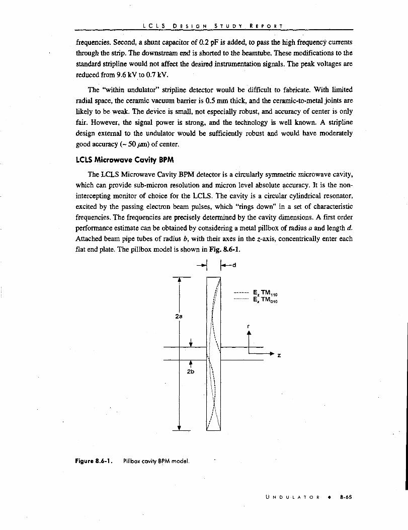
L C L S D E S I G N S T U D Y R E P O R T
frequencies. Second, a shunt capacitor of 0.2 pF is added, to pass the high frequency currents
through the strip. The downstream end is shorted to the beamtube. These modifications to the
standard stripline would not affect the desired instrumentation signals. The peak voltages are
reduced from 9.6 kV to 0.7 kV.
The "within undulator" stripline detector would be difficult to fabricate. With limited
radial space, the ceramic vacuum barrier is 0.5 mm thick, and the ceramic-to-metal joints are
likely to be weak. The device is small, not especially robust, and accuracy of center is only
fair. However, the signal power is strong, and the technology is well known. A stripline
design external to the undulator would be sufficiently robust and would have moderately
good accuracy (~ 50 /an) of center.
LCLS Microwave Cavity BPM
The LCLS Microwave Cavity BPM detector is a circularly symmetric microwave cavity,
which can provide sub-micron resolution and micron level absolute accuracy. It is the non-
intercepting monitor of choice for the LCLS. The cavity is a circular cylindrical resonator,
excited by the passing electron beam pulses, which "rings down" in a set of characteristic
frequencies. The frequencies are precisely determined by the cavity dimensions. A first order
performance estimate can be obtained by considering a metal pillbox of radius a and length d.
Attached beam pipe tubes of radius b, with their axes in the z-axis, concentrically enter each
flat end plate. The pillbox model is shown in Fig. 8.6-1.
-H
2a
I
2b
E 2 T M 1 1 0
Figure 8.6-1. Pillbox cavity BPM model.
U N D U L A T O R 8-65
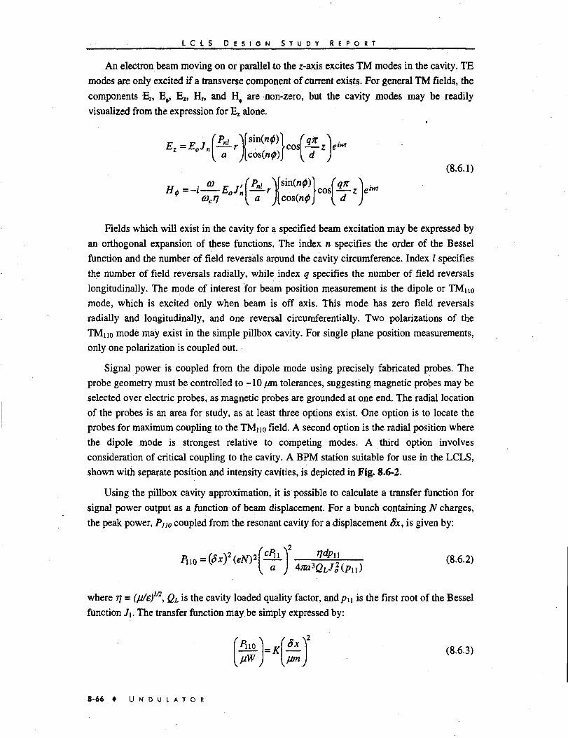
L C L S D E S I G N S T U D Y R E P O R T
An electron beam moving on or parallel to the z-axis excites TM modes in the cavity. TE
modes are only excited if a transverse component of current exists. For general TM fields, the
components Er, E , E2, Hr, and H0 are non-zero, but the cavity modes may be readily
visualized from the expression for Ez alone.
= E" "[ a ilcos(n0J d J(8.6.1)
m Jp, ^ sinCM< M (nir \Hp =— i-
i
Fields which will exist in the cavity for a specified beam excitation may be expressed by
an orthogonal expansion of these functions. The index n specifies the order of the Bessel
function and the number of field reversals around the cavity circumference. Index / specifies
the number of field reversals radially, while index q specifies the number of field reversals
longitudinally. The mode of interest for beam position measurement is the dipole or TMUo
mode, which is excited only when beam is off axis. This mode has zero field reversals
radially and longitudinally, and one reversal circumferentially. Two polarizations of the
TMno mode may exist in the simple pillbox cavity. For single plane position measurements,
only one polarization is coupled out.
Signal power is coupled from the dipole mode using precisely fabricated probes. The
probe geometry must be controlled to ~10 /an tolerances, suggesting magnetic probes may be
selected over electric probes, as magnetic probes are grounded at one end. The radial location
of the probes is an area for study, as at least three options exist. One option is to locate the
probes for maximum coupling to the TMuo field. A second option is the radial position where
the dipole mode is strongest relative to competing modes. A third option involves
consideration of critical coupling to the cavity. A BPM station suitable for use in the LCLS,
shown with separate position and intensity cavities, is depicted in Fig. 8.6-2.
Using the pillbox cavity approximation, it is possible to calculate a transfer function for
signal power output as a function of beam displacement. For a bunch containing N charges,
the peak power, Pn0 coupled from the resonant cavity for a displacement Sx, is given by:
Pm = {8xf (eAO'f^I-T . £% , (8-6.2)
where rj - {/j/e)m, QL is the cavity loaded quality factor, widpu is the first root of the Bessel
function 7i. The transfer function may be simply expressed by:
(8.6.3)
8-66 • U N D U L A T O R

L C L S D E S I G N S T U D Y R E P O R T
Figure 8.6-2. High accuracy/high resolution microwave cavity BPM. Dimensions are in mm.
Various investigators [23,24] have measured or calculated the coefficient K, reporting
values between 4.0 and 7.0. Measurements made by Shintake [21] in the FFTB indicate the
coefficient to be - 4, resulting in a calculated position resolution of 5 nm.
The accuracy to which the BPM cavity is machined limits the precision of the electrical
center. Using diamond turning on ultra-precision lathes, mechanical tolerances of a few
microns can be achieved. However, even a perfectly machined cavity is limited in accuracy
because of the presence of a symmetrical excitation of the cavity [25]. The desired TMn0
mode is not the dominant cavity mode, and must compete with two lower frequency modes.
The TEni mode exists at a lower frequency, but only if d/a>2. This situation is readily
prevented. The remaining lower mode is the TMOio, which is excited with beam on or off
axis. This dominant mode is significantly stronger than the dipole mode. This loss of
precision is the primary research issue which must be addressed for a cavity monitor, and at
least two techniques [26] are known—symmetry discrimination and frequency discrimination.
The former involves canceling the large amplitude TMoio signal, which is present on all
output ports of the cavity, using a hybrid junction. This "common mode" cancellation, taken
alone, is not expected to be sufficient to provide the required suppression. Frequency
discrimination using narrow-band receiver techniques will also be used. This method is
fundamentally limited, however, by the fact that the cavity is shock excited by a single bunch.
The cavity responds producing the strong dominant (TMoio) mode, which contains finite
spectral density at the signal (TMn0) frequency, at which the receiver is tuned. This
phenomenon can be improved but not eliminated by increasing the Q of the cavity [21].
U N D U L A T O R 8-67

L C L S D E S I G N S T U D Y R E P O R T
Schnell [25] has estimated the required rejection of the beam-induced common mode
signal. To obtain a position resolution of 5* from a circular cylindrical cavity of radius a, the
rejection factor must exceed the ratio of the power in the two modes. The ratio is given by:
(8.6.4)
The level of common mode rejection (frequency discrimination) provided by the cavity is
given by:
0)1CMRRf=Qm\l ^2-I (8.6.5)
where Quo is the loaded cavity quality factor in the dipole mode, and fiW<flbio = 1-6 is the
ratio of the mode frequencies. The rejection available from symmetry discrimination is a
function of imperfections in the cavity and hybrid junction fabrication, with the junction
believed to dominate. Because of the small fractional bandwidth, advantage can be taken of
tuning. This second factor is conservatively taken to be CMRRS = 0.02.
Parameters of the LCLS BPM Cavity
A cavity operating frequency of 6 GHz is under consideration for the LCLS BPM. This is
well below the beam tube cutoff (35.1 GHz) frequency, therefore reducing corruption by
beam higher order modes. The selected frequency is not so low as to make the cavity very
large, where machining tolerances proportional to radius would dominate. This operating
frequency is independent of the SLAC accelerating frequency and its harmonics. There is no
advantage to operating there, but the decided disadvantage of man-made electromagnetic
interference. At 6 GHz, the radius of the position cavity is 28.5 mm, and the power ratio
PuofPoio = 79 dB. Taking Qm = 2000, then CMRRf= 62 dB, and with CMRRS = 34 dB, the
total rejection is adequate. While position resolution improves with operating frequency, the
price to performance ratio of microwave components at 6 GHz (C-band) is favorable [21],
generally increasing with increasing frequency. Consideration of other operating frequencies
between 6 GHz and 25 GHz is an appropriate R&D effort.
The parameters and performance of the microwave cavity BPM are summarized in
Table 8.6-4.
Microwave Cavity Beam Impedance
The microwave BPM cavities remove real signal power from the passing bunch, and as
such are a small, but not insignificant, source of beam impedance. The impedance of a single
cavity has been estimated using analytical and numerical methods. Because the bunches are
very short (cr/a < .018), the diffraction model [27,28,29] of the high-frequency impedance of
a cavity is used. According to the model, the longitudinal impedance varies as cSm, and the
8-68 • U N D U L A T O R

L C L S D E S I G N S T U D Y R E P O R T
transverse impedance as ofV2. The loss factors, it, for a single cavity are calculated by
integrating the impedances over the bunch spectrum, and are shown in Table 8.6-5. The
BPMs make a noticeable contribution to the machine's total longitudinal loss.
Table 8.6-4. Parameters and performance of microwave cavity BPM.
Parameter
Cavity radius
Cavity height
Beam pipe radius (inner)
Frequency TM1I0
(R/Q)TM1]0
Shunt impedance (RSH) TMOIO
Vom into 50 Q TMHo
Absolute position accuracy (Ax)
Position resolution (&)
Peak electric field aT = 20 fjm
q = lnC r = 0 oz = 40 /fln
Performance
a = 28.5 mm
d = 5mm
b = 2.5 mm
6 GHz
8.4 Q
27.5 kQ
15//V/nm/nC
-10 fm
< ljura
7.7 MV/m
5.3 MV/m
Table 8.6-5. Cavity BPM beam impedances and wakefields.
Impedance
Longitudinal loss factor fe;/(o)
Transverse loss factor kx(d)
Longitudinal loss factor kt(d) TMoio (only)
Longitudinal impedance <J=50 GHz)
Energy spread cr5
Emittance Growth Ae/e
az = 20.0 yum (cr= 66.7 fs) g = 5 mm ay=2.94xlO4 5,= 1.5mm-mr /?=18i
Wakefield
37.1 V/pC
342V/pam
0.6 V/pC
(14.8 +i 14.8) Q.
0.0255%
0.00242
= 2.5 mm N=109/e Ncav = 104 £=14.3GeVn L=100m JCO = 100//m
The numerical simulation code MAFIA was used to confirm the loss factors and to
calculate the wakefields. The energy spread and emittance growth were calculated with the
equations in this section, using the parameter values listed at the bottom of Table 8.6-5. The
number of cavities Ncav is taken as 104, allowing for two cavities in each of 52 locations. This
assumes one two-plane position sensitive cavity at each location, with a similar intensity
cavity. The intensity cavities produce a significant additional impedance, each cavity
producing far more signal power (~ 4 W) than required. A lower impedance source of the
intensity signals is possible, consisting of a slot-coupled pickup, with more than one
U N D U L A T O R • 8-69

L C L S D E S I G N S T U D Y R E P O R T
symmetrically placed slot, coupled by a single vacuum feedthrough. Its signal must then be
filtered using an external cavity, which does not interact with the beam.
Microwave Cavity Signal Processing
The BPM signal processor produces digital position and intensity information by
demodulating the signals produced by the two cavities. Each measurement plane requires two
output ports. The number of outputs from each cavity would be the subject of study, which
would consider the dominant mode issue and possible mode suppression methods, against the
value of obtaining both planes from a single cavity. The output ports may be either
waveguide or coaxial line. Waveguide coupling to the cavity is accomplished by machined
rectangular slots in the cavity circumference, the shorter edge parallel to the beam direction.
The waveguides are actually machined from the same metal block as the cavity, and form a
"Magic-Tee," which rejects the dominant (3.7 GHz) common mode. The waveguide approach
preserves absolute accuracy because the entire structure is machined to micron level
tolerances. Coaxial line coupling is better suited to a low frequency cavity, but allows more
degrees of freedom, and higher mechanical tolerance accumulations. By connecting the
coaxial lines to machined pins, which are held in place by precision ceramic bushings,
excellent tolerances can also be achieved. In the proposed design, opposing coaxial outputs
feed the difference arms of a hybrid coupler. This difference output is transmitted by low-loss
coaxial cable to the electronics area, a maximum of 70 m away.
The difference signal is a tone burst at 6 GHz, of amplitude 6 //V/nm/nC (rms), with an e-
folding time of 30 ns. This duration can be extended somewhat by weakening the cavity
coupling, noting that the cavity is the highest Q device in the system. The signal is filtered to
attenuate the strong mode at 3.7 GHz, and attenuated as necessary by a binary controlled
attenuator. Small signals suffer only residual attenuation and are amplified. The amplifier is
protected by a passive diode limiter. Attached to the position cavity, the intensity or
"reference" cavity, operating at 6 GHz in the monopole mode, provides the phase reference
signal. The phase reference signal is proportional to beam intensity and is provided as an
output. The position and reference signals are filtered to reject power in all undesired modes,
and then mixed to a suitable Intermediate Frequency (IF) using a Local Oscillator (LO). For a
small fractional bandwidth, the IF should be several times the information bandwidth. A
particularly poor choice for the LO would be 4.85 GHz, since the strong 3.7 GHz mode
becomes the image, translated directly into an 1150 MHz IF. An IF in the range 500 MHz is
preferable, with an LO at 6.5 GHz.
The LO is synthesized using a signal from the reference cavity and an independent
oscillator. This added step causes the IF operating frequency to equal that of the independent
oscillator and be essentially constant. The oscillator is itself synthesized from a stable crystal
oscillator using a Direct Digital Synthesizer (DDS) and Phase-Locked Loop (PLL) multiplier.
Such a solution provides broad frequency coverage for in situ frequency response testing,
calibration in the presence of beam, and low phase noise. In the absence of beam, the
reference cavity signal will be provided by a crystal oscillator, which is injection locked to
8-70 • U N D U L A T O R

L C L S D E S I G N S T U D Y R t r o n
the beam frequency when beam is present. Fig. 8.6-3 shows a block diagram of the detection
scheme.
DC-50MHZ
Figure 8.6-3. BPM analog signal processing scheme.
Calibration circuitry provides the capability to inject the same or different frequencies
into the position and intensity inputs. The connections are made near the receiver inputs with
directional couplers. The calibration procedure can be completed while beam is present by
operating at a frequency offset. The calibration sources can also be un-powered to avoid
isolation problems. Finally, the raw cavity signals can be monitored at the directional
couplers. These are designed with sufficient isolation not to affect the normal diagnostic
operation.
Because the position and reference signals are (approximately) the impulse responses of
two different filters, the detected difference will contain a phase precession. To circumvent
the problem, In-Phase and Quadrature (I&Q) detection is applied. Using I&Q, phase
synchronization is not required, and the system is immune to phase delay changes in cables
and components. The low frequency information on each I and Q line is captured by a Track-
and-Hold amplifier, and is digitized with 12-bit precision. A computer then calculates the
position using the two numbers. Many of the sources of amplitude and phase error can be
measured, updated, and compensated after digitization. This approach follows a modern trend
[30] in signal processing toward error compensation in software, rather than extensive
adjustment of the analog electronics to zero out these errors.
8.6.2 Carbon Wire BPMs
Beam Position Measurement
To test the alignment of the electron beam in the undulator, fine wires can be used as
electron beam targets. They would be positioned between undulator segments, would be used
as needed, perhaps daily, and must not interfere with the beam when not in use. The optimum
number of stations for alignment may be affected by their use also as emittance diagnostics.
Wire scanners are standard tools of accelerator instrumentation. In cases where beam
heating is severe, the wire of choice is made of carbon. At the final focus in SLD and at the
U N D U L A T O R 8-71

L C L S D E S I G N S T U D Y R E P O R T
FFTB, carbon filaments seem to withstand the heating of spots of 2 /an x 2 /an (rms width
x rms width) for 1010 electrons per pulse. Thus a round spot of 31 /an would not be a threat.
There is even more experience with tungsten wires. It is estimated that they should withstand
beams up to 15% of the intensity limit of carbon, so the LCLS beam is well within the range
of tungsten. A degree of caution should be exercised, because heavily used tungsten wires
have shown susceptibility to failure in 120 Hz operation. This is associated with arcing at
their support points. Although a solution is not yet in hand, trials of alternative support
designs are being made. Alternative materials, for example silicon carbide, are also being
tested.
Various techniques have been used to detect a signal from the beam overlap with the
wire. The most robust and successful is detection of the Bremsstrahlung gamma rays. Their
1/e spectrum is emitted in a cone of half angle about \ly (y is the Lorentz factor). In some
cases a better signal is obtained from the Bremsstrahlung electrons well below beam energy.
This, of course, requires that they are forced out of the beam pipe by a magnetic field. In
either case, beam line components can make it difficult to access the raw signal, and
sometimes only the tail of an electromagnetic shower can be used. With the tungsten radiation
length less than 2% of that of carbon, its Bremsstrahlung signal is much stronger, while a
different type of signal also becomes accessible. This is the yield of delta rays, of about
1 MeV and at right angles to the beam, that is used in numerous places at SLC and FFTB.
Although it requires a thin window in the vacuum pipe, it can be used when the straight-
ahead Bremsstrahlung signal is not available. From a carbon fiber, however, this process is
normally too weak to be useful.
Finally, secondary emission (of electrons of 1 eV and above) has been used with carbon
and other materials. Because of the large rf noise accompanying the beam, the charge signal
is collected in a shaping amplifier with a shaping time of several microseconds, giving time
for the bipolar rf noise to die away. Several systematic effects have been encountered. For the
short SLC pulses, the electric dipole induced at the surface of the wire has the effect of
suppressing secondary emission from an electron beam (and enhancing it from a positron
beam). The higher energy electrons, often called <$-rays, are still ejected. A further problem
was encountered at the SLC final focus, but never resolved. When the spot width decreased
below roughly 5 /an rms, for 5 x 10⁹per pulse, the signal became unstable and unrepeatable.
However, the technique evidently is applicable within the LCLS parameters.
Since a tungsten wire could be thinner than a carbon filament while still maintaining a
larger signal for beam measurement, one could expect to use a 7.5 or 10 j/m diameter wire as
against the available 34 jum for carbon. Fibers are normally mounted spanning the prongs of a
fork. Common fork materials are Macor, alumina, or aluminum. In the former cases the
surfaces are rendered slightly conducting to bleed away any charge buildup. A typical wire
span is in the range of 2 cm. Somewhat shorter lengths, more suitable to LCLS, are probably
safe: for carbon fibers, one must be careful to avoid relative movement or vibration on the
prongs beyond the 1 % fiber strain limit.
8-72 • U N D U L A T O R

L C L S D E S I G N S T U D Y R E P O R T
The beam will be multiply scattered by the filament. Whatever fraction is intercepted, say
25%, would have an rms scattering angle of about 12 /ffad from a 34 /an carbon fiber. For a
10 /an tungsten wire these numbers would become 7% at 55 /a:ad. The mean fractional energy
lost through Bremsstrahlung by the part of the beam penetrating the carbon would be 3 x 10'5,
or 2 x 10'3 for tungsten.
In operation, a Gaussian curve would be fitted to the pulse-by-pulse signals from a scan.
From SLC experience, the uncertainty on the location of the center of the fit would be in the
range of 2% of the width, or better than a micron. However, a careful evaluation of the quoted
SLC error bars has not been done. The most serious issue affecting accuracy will certainly be
the systematics of the exact location of the target wires, and for this reason tungsten is
favored. The center of the thinner wire can be located more accurately, approximately as the
ratio of the diameters.
Since the wires are difficult to see even under good conditions, it is assumed that they
will not be surveyed directly in the vacuum tank. Instead, after attaching them, the lab work
would include measuring their positions relative to a fiducial on the holder structure, but
outside the vacuum. This probably has to be done optically, since touching the wires is
generally counter-productive. An accuracy of about 2 //m would be budgeted for this work,
and it would be a challenge for the 34 /an carbon material. Repeatability at this level has,
however, been achieved for thinner wires. It is clear that the process of fiducialization would
have to be built into the design from the beginning. The external fiducial would have to be
surveyed relative to the beam-line monument system, probably relying on Invar or fused
silica spacers, and optical systems.
The mechanisms to move the forks on or off the beam line would have a total motion of
one or two cm. Stages that accomplish this in 1 fim or 5 /an steps are readily obtained. (Steps
of 5 /an would be fine enough for spot sizes down to 10 /an rms.) SLAC usually has a
redundant direct read-back of the position using an LVDT. This is hardly an absolute location
measurement, but can give an accurate offset relative to a stop. If an absolute readback is
necessary, grating-based optical encoders can be used. The design will be dominated by
systematic concerns. For instance, between two materials, a typical difference in expansion
coefficients might be 10"5 per °C. For a mechanism length of 30 cm and a 1°C temperature
excursion, the differential motion would be 3 /an. A smooth beam pipe aperture for FEL
operation could be mounted on the same mechanism as the wire-fork. This would increase the
length of motion of the linear stages by perhaps two centimeters.
In summary, the most difficult problems facing a thin-wire-based technique for beam
alignment are the same problems as face all techniques. Surveying and aligning the position
monitors within <5 /an relative to a straight line, and maintaining long term dimensional
stability, will require careful engineering.
U N D U L A T O R • 8-73

L C L S D E S I G N S T U D Y R E P O R T
Beam Emittance Measurements
Carbon wire scanners can be used to measure the horizontal and vertical emittance of the
electron beam; these could be the same systems as the carbon wire BPMs or the combined
photon/electron diagnostics. Wire scanners near the end of the undulator will permit
observation and correction of emittance dilution (e.g., that caused by wakefields) generated
within the undulator. The wires measure the transverse beam size, which is used to calculate
the emittance, if there are at least three independent measurements of the beam size per plane
and these three are separated by an appropriate betatron phase advance. An array of wire
scanners placed toward the end of the undulator will provide precision, redundancy, and
energy adaptability in undulator emittance measurements.
For an emittance measurement, a minimum of three measurements per plane are required
because of the three independent parameters {£, fi, or) necessary to describe the second central
moments of the electron beam phase space per plane ((x2), (x'2), (xc*)). To transform these
beam size measurements into phase space parameters requires that they span the space
adequately. This condition is optimally set when the wire-to-wire separation is tdN in
betatron phase advance, where N is the number of wire scanners. For the minimum, N = 3, the
optimal separation is 60°. To provide redundancy in the measurement (for increased precision
and backup for failed wires), N - 4 and an optimal separation of 45° are used. The
configuration described here is for one plane. The other plane should be similarly configured.
With permanent magnet focusing, the betatron phase advance per cell, Ay, of the
undulator lattice is energy dependent. At 5 GeV it is Ay/ ~ 45°. This is nearly ideal for four
wires when one wire is placed at each of the last four cells (4.32 m or every other quadrupole)
with the last wire at the end of the undulator. Fig. 8.6-4 shows the locations of the wires and
their various groupings for 5,10, and 15 (or 14.3) GeV beams. The 5 GeV grouping of wires
is indicated as wires 5A, 5B, 5C and 5D. At 15 GeV A^ « 13° and a wire every three cells
provides 3Ay/~ 40°. For this case, the last two wires, 5Dsl5D and 5A=15C, already exist
from the 5 GeV case. By adding one wire at 6 (15B) and one at 9 cells (15A) upstream of the
last wire, the 15 GeV case is also fully covered. At 10 GeV Ay/ ~ 21°), or other intermediate
energies, using the last three wires (10A, 10B and IOC) located for 15 GeV provides
3Ay/ ~ 63°, which is nearly ideal for N = 3. Redundancy is included by using any of the other
two 5 GeV wires (5B and/or 5C) 21° away, when necessary. This 6-wire array then covers all
energies adequately. The other transverse plane may be covered by adding another set of 6
scanners slipped by one-half cell upstream, or by designing each scanner to measure both
planes. In the latter case the beam size is smaller for one plane than the other, especially at
5 GeV (by a factor of 1.45). For alignment purposes about five more wires per plane are
added every 3 cells (13 m) extending from near the undulator entrance toward these emittance
wires.
8-74 • U N D U L A T O R

I C L S D E S I G N S T U D Y R E P O R T
*- beginning
"""1 ± / ^^^^H
15A
Figure 8.6-4.
; of undulator
TfTMSFWM
Proposed
10A15B
locations
<-ccll-»
(4.32 m)
(up-arrows)
•
of
5A10B15C
undulator
end
5B
wire
of undulator j
5C 5D « •IOC ^15D * •
scanners for optimal
5 GeV10 GeV15 GeV
emittancemeasurement at 5-15 GeV. The last 9.5 cells of 26 in the undulator are shown. Wiregroupings for the three energies are labeled A-C or A-D with an energy prefix of 5, 10or 15 GeV.
8.6.3 The Combined Electron and Photon Beam Diagnostic
The trajectory control techniques described in Section 8.5.2 assume that the FEL photon
beam will overlap with the LCLS electron beam if the electron beam forms a straight line. A
technique to verify the electron and photon beams overlap directly is also desirable. This
technique is described here.
The proposal is to insert a 10-30 jum wire, probably carbon, into the beampipe. When it is
struck by the electron beam, bremsstrahlung will be generated, which can be detected at the
end of the undulator. When it is struck by the photon beam, photons will be diffracted at a
large angle by the polycrystalline wire, and can be detected using a PIN diode or similar solid
state detector. Powder diffraction from a polycrystalline carbon wire can be used to select a
narrow bandwidth of photon energy or the FEL fundamental energy, 8.3 keV (1.5 A), can be
chosen. The carbon wire would have to be mounted on a movable x-y stage, and there would
have to be wires in both horizontal and vertical orientations. This apparatus can be used to
measure the electron and photon beam sizes, to verify overlap of electron and photon beams
and for rough beam alignment. One carbon wire monitor every 10 m, or about one per gain
length is sufficient for LCLS needs (see Section 8.62).
If this apparatus were to be used for rough beam alignment, the procedure would be as
follows. It is presumed that a beam of spontaneous radiation is launched in a straight line
from the first segment of the undulator. The task would then be to steer the electron beam at a
point downstream so that it overlaps this first photon beam. This could be done by observing
the electron and photon beams in separate positions, finding the sensitivity of the electron
beam to steering, and calculating the best steering for overlap. The process would then be
repeated for the next monitor downstream.
The spontaneous radiation at the 1.5 A fundamental has a characteristic transverse size
given by arad = a} + X^L, reflecting the electron beam size (31 jum rms radius) plus the
photon beam divergence. At a distance L = 10 m, this size is 38 /an, and at 100 m it is 70 /m.
The FEL beam divergence is smaller, only 0.74 /aad at the end of the undulator, so its beam
size is dominated by the electron beam size. On axis, the FEL power is expected to be greater
than the spontaneous power only after about 7 gain lengths. Sweeping a 20-30 //m carbon
U N D U L A T O R • 8-75
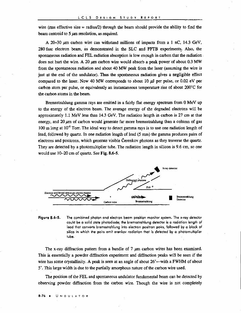
L C L S D E S I G N S T U D Y R E P O R T
wire (rms effective size = radius/2) through the beam should provide the ability to find the
beam centroid to 5 fan resolution, as required.
A 20-30 /an carbon wire can withstand millions of impacts from a 1 nC, 14.3 GeV,
280fsec electron beam, as demonstrated in the SLC and FFTB experiments. Also, the
spontaneous radiation and FEL radiation absorption is low enough in carbon that the radiation
does not hurt the wire. A 20 /an carbon wire would absorb a peak power of about 0.3 MW
from the spontaneous radiation and about 40 MW peak from the laser (assuming the wire is
just at the end of the undulator). Thus the spontaneous radiation gives a negligible effect
compared to the laser. Now 40 MW corresponds to about 10 fjJ per pulse, or 0.02 eV per
carbon atom per pulse, or equivalently an instantaneous temperature rise of about 200°C for
the carbon atoms in the beam.
Bremsstrahlung gamma rays are emitted in a fairly flat energy spectrum from 0 MeV up
to the energy of the electron beam. The average energy of the degraded electrons will be
approximately 1.1 MeV less than 14.3 GeV. The radiation length in carbon is 27 cm at that
energy, and 20 /an of carbon would generate far more bremsstrahlung than a column of gas
100 m long at 10"6 Torr. The ideal way to detect gamma rays is to use one radiation length of
lead, followed by quartz. In one radiation length of lead (5 mm) the gamma produces pairs of
electrons and positrons, which generate visible Cerenkov photons as they traverse the quartz.
They are detected by a photomultiplier tube. The radiation length in silicon is 9.6 cm, so one
would use 10-20 cm of quartz. See Fig. 8.6-5.
X-ray detector
Diffracted photons ^
^ 2 5 . 8 °
Electron and broad spectrum photon beams
• lAA'UOV^- • Bremsstrahlung• Detector
Carbon wire Bremsstrahlung
Figure 8.6-5. The combined photon and electron beam position monitor system. The x-ray detectorcould be a solid state photodiode; the bremsstrahlung detector is a radiation length oflead that converts bremsstrahlung into electron positron pairs, followed by a block ofsilica in which the pairs emit erenkov radiation that is detected by a photomultipliertube.
The x-ray diffraction pattern from a bundle of 7 /an carbon wires has been examined.
This is essentially a powder diffraction experiment and diffraction peaks will be seen if the
wire has some crystallinity. A peak is seen at an angle of about 26°—with a FWHM of about
5°. This large width is due to the partially amorphous nature of the carbon wire used.
The position of the FEL and spontaneous undulator fundamental beam can be detected by
observing powder diffraction from the carbon wire. Though the wire is not completely
8-76 • U N D U L A T O R
L C L S D E S I G N . S T U D Y R E P O R T
crystalline or powder-like, the x-ray diffraction tests at SSRL have shown that these wires
have enough of a graphite-like polycrystalline character to give an easily observable powder
pattern. It is expected that heating in the electron and x-ray beams would increase the
crystallinity of a wire.
The strongest graphite powder reflection of 1.5 A radiation occurs at a 25.8° scattering
angle. A limited-aperture detector set at this angle would signal when the carbon wire
intercepts and scatters the undulator fundamental radiation (near the beginning of the
undulator) or the FEL radiation (farther down the undulator where the FEL intensity is
dominant). If operation at a different FEL wavelength is desired, it would be necessary to
move the powder diffraction detector to a different angle. Practical constraints on this angle
would probably limit the utility of this beam-location technique to wavelengths shorter than
6 A. The optimal detector would be a small silicon avalanche diode, which could be moved
inside a wedge-shaped vacuum chamber annex to set the scattering angle.
8.6.4 Wire Position Monitors
The LCLS proposes to detect and correct diurnal, thermal, and ground motions with a
system that was successfully implemented on the FFTB [31]. Two wires will be suspended
inside hollow chambers that run the length of the undulator. The chambers are fixed to the
undulator magnets; one end of the wire runs over a pulley and is tensioned by a fixed hanging
weight. The exact shape of the curve described by the wire is not a catenary, but is distorted
by imperfections in the wire at the micron level. However, a wire suspended this way is very
stable. Using optical LED and split photodiode position sensors, the WPM system is capable
of resolving changes in the position of the wire with submicron resolution.
8.7 WaIcefield Effects in the Undulator
8.7.1 Introduction
When the electron beam moves through the undulator it will excite longitudinal and
transverse wakefields due to the resistance and the discontinuities in the beam tube wall. Let
us assume that the wall geometry is cylindrically symmetric. Then the longitudinal
(monopole) wakefield will generate an energy loss and an increase in energy spread
independent of the beam orbit, and the transverse (dipole) wakefield will generate an
emittance growth that does depend on the orbit. It is, however, important to recognize that
the forces due to the wakefields are correlated with longitudinal position. Assuming the
bunch is composed of many slices at different longitudinal positions, the wakefields affect
only the centroid values of the slices—i.e., the average energy and the average position of the
slices in, respectively, the longitudinal and the transverse case. The distributions of the slices
about their centroids are not affected.
The critical issues concerning the electron beam with respect to wakefield effects in the
undulator are:
U N D U L A T O R • 8-77

L C L S D E S I G N S T U D Y R E P O R T
• The absolute value of the maximum relative energy deviation of a bunch "slice"
(slippage length: -0.5 /an) with respect to the mean of the whole bunch generated
over the length of the undulator at 14.3 GeV should be less than -0.1%. This
tolerance is derived from GINGER simulations.
• The dilution of the "projected" emittance (emittance projected over the entire
bunch) should not exceed -10%.
• The mean energy loss over the undulator, including radiation losses, will
determine the necessary taper of the magnetic fields of the undulator dipoles.
Since undulator wakefields have very little effect on the "slice" energy spread and the "slice"
emittance, these tolerances are not considered here.
In this report the longitudinal and transverse wakefield effects on the LCLS beam during
its time in the undulator are estimated to see how well these conditions are satisfied. Note
that the beam dynamics and wakefield concepts that are presented are thoroughly discussed,
with equations in [28].
8.7.2 Wakefield Induced Beam Degradation
In the longitudinal case the wake function for a Gaussian bunch, from which the average
wake (also known as the loss factor) (W^ and the rms deviation of the wake with respect to
the mean, (W ),™ (the units are V/C/m) are derived, is first obtained. Then the wakefield
induced energy loss is given by
e2NL(Wz)
E
with N the number of particles in the bunch, L the length of travel, and E the beam energy.
The rms energy spread, with respect to the mean, becomes
( 8 . 7 . 2 )
In the transverse case the average of the transverse wakefield of a Gaussian bunch (Wx)
(here in units of V/C/m2) is first obtained. The focusing lattice in the undulator is a FODO
type with a phase advance of 137cell at 14.3 GeV, and therefore a smooth focusing analysis
is appropriate. First, to study the effect of injection jitter, the wake function is applied to
obtain the projected emittance growth due to a betatron oscillation in the undulator. The
offset at the end of the undulator, averaged over the bunch, can be written as
iv) (8.7.3)
8-78 • U N D U L A T O R
L C L S D E S I G N S T U D Y R E P O R T
with xo the initial offset, ft the beta function, and v the strength parameter (as long as it is
small). The strength parameter is given by x
= ^ - • (8-7.4)
The relative emittance growth, if it is small, is then given by
Ae xlv^y(8.7.5)
with y the energy factor and % the normalized emittance. If the beam tube wall is not
perfectly straight and aligned then even if the beam does not undergo betatron oscillations the
projected emittance can grow. However, unlike in the case of injection jitter, since this error
is a static error some correction can usually be performed to reduce the effect. The
misalignment errors are divided into two types, those that are uncorrelated to each other and
those that are correlated. In the former category suppose the wakefield generating object is
composed of Mp equal, randomly misaligned pieces. Then the emittance growth will again be
approximately given by Eq. 8.7.5, but with x0 replaced by the rms misalignment of the pieces
divided by the factor Mpin. For correlated errors, the largest effect, for a given misalignment
amplitude, is when the misalignment varies as cos{zlp), and the results are the same as given
in Eq. 8.7.5, but with xo representing the misalignment amplitude. If the oscillation
frequency of the misalignments differs from the betatron wave number by Ak then the effect
on emittance decreases according to sinc2(AkL).
The above effects are due to a resonance term in the equation of motion. But there is
normally also a bounded, non-resonance term. For example, consider the case where the
beam's trajectory follows the magnetic focusing axis in the undulator, but this axis is not
aligned with the axis of the impedance generating objects. In this case the projected
emittance of the beam will grow and then again decrease within the undulator. Even though
the final emittance growth in the LCLS undulator due to this effect is small, there may be a
tolerance for bunch emittance growth anywhere within the undulator. In such a case this
effect will set a tolerance for the alignment of the wakefield generating axis with respect to
the magnetic axis. For this example, the maximum emittance growth is given by Eq. 8.7.5,
with Xo the distance between the two axes and with v = 2e2AT(Wt)/?2/£.
In the calculations below, the following bunch and machine properties are considered:
total charge of 1 nC, rms bunch length az = 20 nva, normalized emittance e# - 1.0 mm-mrad
(the undiluted emittance is used for a conservative estimate), and energy E = 14.3 GeV. The
length of the undulator is L = 112 m and the average focusing beta function is fi = 18 m. Note
that in reality the bunch shape is not Gaussian, and to obtain a more accurate result one would
need to use the real bunch shape in the calculations. The results given in this report should
serve as reasonable estimates. The generators of wakefields considered are the wall
U N D U L A T O R • 8-79
L C L S D E S I G N S T U D Y R E P O R T
resistance of the beam tube, the flange gaps, the pumping slots, and the bellows. The effect
of the beam position monitors (BPM's) is discussed in Section 8.5. Finally, the effects of
wall surface roughness are considered.
8.7.3 The Resistive Wall Wakefields
The beam tube inside the undulator is made of stainless steel or stainless steel plated with
copper. It is of circular cross-section and has a radius of a = 2.5 mm. The normal formulas
for the resistive wall wakefields are valid only if ojso > 1, with the characteristic distance
(8.7.6)
where Zo = 377 ft and a is the conductivity of the metal. For stainless steel (SS) a =
1.7 x 10⁶Q~1-m~1, for copper (Cu) it is 60 x 106 JT'-nf'. Therefore, for the beam tube with
SS s0 = 27 ftm, with Cu s0 = 8 /an. Thus, in either case, since az ~ 20 fim, the normal formulas
should be valid. The average of the longitudinal wakefield of a Gaussian bunch is given by
(8.7.7)
with r(3/4) « 1.23, and the rms is given by (WJ^ a (\.02)(Wz). Combined with Eq. 8.7.1this gives (d) = 0.34% for stainless steel and 0.06% for copper, and similar results for the
induced rms energy spread. The effects of the more realistic, non-Gaussian bunch
distribution, and also the general case for OJSQ < 1, are discussed in Section 8.7.6. Here the
resistive-wall loss and spread are both smaller than that of the Gaussian case examined above.
For the transverse case
. (-7 V/2
with T(l/4) ~ 3.63. Combined with Eq. 8.7.4 it is seen that v is 0.58 and 0.10 for the SS and
Cu cases, respectively. For an extreme 100 //m oscillation (e.g. random pulse-to-pulse jitter
which is not correctable) the emittance growth is 260% for SS and 8% in the case of Cu.
As to the effects of static errors, it is noted first that the beam tube is composed of 52
equal pieces. With uncorrelated, random misalignments with an rms of 100 /an, the emittance
growth will be a factor of 52 less than given above. Or, conversely, the misalignment
tolerance for 10% emittance growth, assuming copper is used, is 800 /on. For a correlated,
cosine variation of misalignments of amplitude 100 pra the emittance growth is approximated
by the above jitter results multiplied by smc2(AkL), where Ak is the deviation from the
betatron wave number of the wall oscillation wave number. Finally, if the static emittance
8-80 • U N D U L A T O R
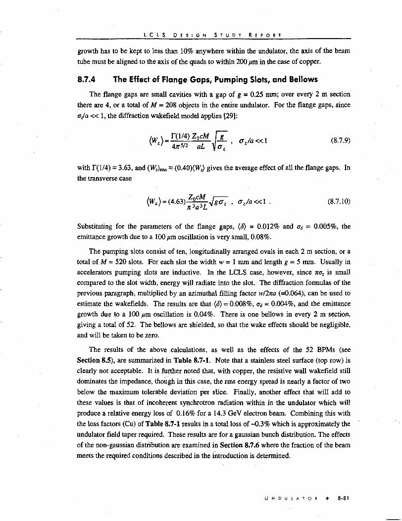
- L C L S D E S I G N S T U D Y R E P O R T
growth has to be kept to less than 10% anywhere within the undulator, the axis of the beamtube must be aligned to the axis of the quads to within 200 //m in the case of copper.
8.7.4 The Effect of Flange Gaps, Pumping Slots, and Bellows
The flange gaps are small cavities with a gap of g = 0.25 mm; over every 2 m sectionthere are 4, or a total of M = 208 objects in the entire undulator. For the flange gaps, sinceaja « 1, the diffraction wakefield model applies [29]:
with T(l/4) ~ 3.63, and (WXB* ~ (0A0)(W£ gives the average effect of all the flange gaps. Inthe transverse case
oz/a«\ . (8.7.10)7iiaiL
Substituting for the parameters of the flange gaps, (S) = 0.012% and a& = 0.005%, theemittance growth due to a 100 /an oscillation is very small, 0.08%.
The pumping slots consist of ten, longitudinally arranged ovals in each 2 m section, or atotal of M = 520 slots. For each slot the width w - 1 mm and length g = 5 mm. Usually inaccelerators pumping slots are inductive. In the LCLS case, however, since %az is smallcompared to the slot width, energy will radiate into the slot. The diffraction formulas of theprevious paragraph, multiplied by an azimuthal filling factor wl2na (=0.064), can be used toestimate the wakefields. The results are that (S) = 0.008%, as = 0.004%, and the emittancegrowth due to a 100 ftm oscillation is 0.04%. There is one bellows in every 2 m section,giving a total of 52. The bellows are shielded, so that the wake effects should be negligible,and will be taken to be zero.
The results of the above calculations, as well as the effects of the 52 BPMs (seeSection 8.5), are summarized in Table 8.7-1. Note that a stainless steel surface (top row) isclearly not acceptable. It is further noted that, with copper, the resistive wall wakefield stilldominates the impedance, though in this case, the rms energy spread is nearly a factor of twobelow the maximum tolerable deviation per slice. Finally, another effect that will add tothese values is that of incoherent synchrotron radiation within in the undulator which willproduce a relative energy loss of 0.16% for a 14.3 GeV electron beam. Combining this withthe loss factors (Cu) of Table 8.7-1 results in a total loss of -0.3% which is approximately theundulator field taper required. These results are for a gaussian bunch distribution. The effectsof the non-gaussian distribution are examined in Section 8.7.6 where the fraction of the beammeets the required conditions described in the introduction is determined.
U N D U L A T O R • 8-81

L C L S D E S I G N S T U D Y R E P O R T
Table 8.7-1. The total longitudinal and transverse wakefield effects, for a gaussian axial distribution,due to the various types of objects in the LCLS undulator. Given are the averageenergy loss, (8), the rms energy spread, Op and the relative correlated emittancegrowth, Aele^, of a 100 //m betatron oscillation.
Type of Objects
Resistive Wall (SS)
Resistive Wall (Cu)
Flange Gaps
Pumping Slots
BPMs
<<5>/%
0.340
0.060
0.012
0.008
0.027
Oil%
0.350
0.060
0.005
0.004
0.010
Js/sof%
260
8
0.08
0.04
0.39
8.7.5 The Effect of Wall Surface Roughness
In a recent paper the impedance due to a rough metallic surface is estimated [32]. The
calculation procedure was to find first the low frequency impedance (the inductance) of a
small bump on a smooth beam pipe surface, and then to use averaging to obtain the effect of a
random distribution of bumps. Some of these results are reproduced here.
At low frequencies the longitudinal impedance of a small perturbation on the wall of a
cylindrical tube is inductive and can be written as
(8.7.11)€n2a2
with co the frequency, r the size of the perturbation, a the beam pipe radius, and L the
effective inductance; / is a form factor which equals 1 when the perturbation is a small,
shallow hole of radius r [33]. The impedance of various shapes of perturbations was
investigated numerically. Some results are reproduced in Table 8.7-2. (Note that the
definition of/used here is slightly different from that used in [32].) Given are the inductance
L of: (1) a hemisphere with radius r, (2) a half cube with width w and length / both equal, and
height h = w/2, (3) a post with w = / = hN%, rotated by 45°, (4) a wedge with base dimensions
w = I and height h = w/2, and (5) a cube with w - I = h. The absolute dimensions were
chosen so that all have base area sr2, with r = 0.5 mm. Also given is the form factor/when
comparing to a shallow hole of radius r = 0.5 mm. The longitudinal and transverse profiles of
the objects are sketched below the table.
It is noted that the impedance of a bump is much larger than that of an equivalent-sized
hole. Also, from the first 4 examples in Table 8.7-2, it is seen that for objects that are of
similar size, the form factor/can vary by a large factor, in this case by a factor three to four.
The fifth example demonstrates a roughly quadratic dependence on height. In the report it is
also shown that when two cubes are longitudinally aligned, if they are separated by a distance
>h then the effect is about twice the single cube result.
8-82 • U N D U L A T O R

L C L S D E S I G N S T U D Y R E P O R T
Table 8.7-2.
Case
Results for 5 selected objects, whose longitudinal and transverse profiles are sketchedbelow. All have base areas JO2, with r = 0.5 mm. Given is the inductance L, and theform factor/when comparing to a shallow hole with radius r = 0.5 mm.
MpH]
Hemisphere (analytical) 0.13
Half Cube
Rotated Post
Wedge
Cube
0.33
0.08
0.15
1.41
/
4.7
12.1
2.9
5.3
50.8
longi.
trans.LJ
Without knowing the microstructure at the beam tube surface, an accurate estimate of the
roughness impedance cannot be obtained. To obtain a rough estimate, however, let us assume
that the tube is covered by a random set of bumps. In the longitudinal case (not treated in
132]) the shape of the induced voltage is given by the derivative of the bunch shape.
Therefore, the average energy loss is near zero. The wakefield rms for a gaussian bunch,
according to this model, is
Zoc rfa(8.7.12)
with r the typical size of the bumps, / a form factor, and a the surface filling factor of the
bumps. In Eq. 8.7.12 it is assumed that the average base area of a bump is 7cr2.
In the transverse case, the shape of the wakefield is the same as the shape of the bunch.
For a gaussian bunch the average wake becomes
Zoc rfaJo,
(8.7.13)
Let us assume that typically the form factor/= 5 and the surface filling factor a = 0.5. Then
to keep the rms energy spread o& < 0.05% implies that the allowable bump size r < 40 nm. Or
transversely to keep the emittance growth due to a 100 j*m oscillation to less than 10%
requires that the bump size r < 100 nm. These required levels of smoothness would be
difficult to achieve.
The microstructure of a metallic surface depends on the manufacturing and machining
method used to create the surface. With state-of-the-art manufacturing methods the necessary
U N D U L A T O R 8-83
L C L S D E S I G N S T U D Y R E P O R T
tolerance can be achieved. For example (see Section 8.2.6), using a die to extrude a stainless
steel tube, a variation on the order of 75 nm can be achieved. This surface roughness can be
improved upon by electro-polishing. This process is followed by deposition of a 1 /mi layer
of copper, which may result in an even smoother surface. A model of the final product a
surface with 150 nm wide, smooth bumps, with an elliptical longitudinal profile, with semi-
minor axis (the depth) of 75 nm and semi-major (longitudinal) axis of 200 nm is used. On top
of these bumps there are many smaller bumps with a typical size that may be significantly
smaller than 40 nm. The effect of both types of bumps to give a$ < 0.05% and, for a 100 m
oscillation, As/so » 2% is estimated. Clearly these estimates are only approximate. More
study is needed both in the questions of what the undulator tube surface actually might look
like and, more fundamentally, the correctness of the rough surface impedance model. Trying
to answer these questions is an ongoing research project.
8.7.6 The Effects of the Expected Bunch Shape
The fact that the bunch shape is not gaussian will affect the above results, primarily in the
longitudinal case. The actual bunch distribution, except at the head and the tail, is rather
constant. Therefore, the longitudinal effect, since it depends on the derivative of the
distribution, will be very small over the core of the bunch but very large at the head and the
tail. Fig. 8.7-1 shows the roughness wakefield and the resistive wall wakefield (for the
general case without the limit: OJSQ > 1) generated by 1 nC over the length of the 112 meter
undulator. The axial bunch distribution used here,,/(z), from Fig. 7.2-3, is also overlaid on an
arbitrary scale. The chamber surface is copper and the roughness amplitude is r = 100 nm.
Other parameters of Eq. 8.7.12 are a = 0.5, a = 2.5 mm, / = 5 and E= 14.3 GeV. The
fraction of the electron beam with an energy change of less than ±0.1%, with respect to the
mean, over the length of the undulator, is 55%. According to GINGER simulations, if the
energy of a bunch slice deviates by more than 0.1% from the synchronous energy over the
length of the undulator, the saturation length starts to increase. The mean energy loss is
(<5) ~ -0.016% and the rms spread, with respect to the mean, is a» ~ 0.034%. This may be
improved by further flattening the axial distribution through optimization of the compression
parameters, and/or by advanced beam pipe surface preparation techniques, both of which are
continuing research efforts.
8.7.7 Conclusion
Using copper-plated stainless steel for the LCLS undulator beam tube will meet the
tolerance limits both in increased correlated energy spread and in projected emittance growth.
The implications of slice energy deviation and projected emittance increase are twofold. One
effect is a decrease in beam brightness, which with the numbers discussed in the previous
sections, will be small in the LCLS (see also Section 10.1), where this point is discussed in
more detail). The other issue that was investigated is the effect of a slice energy deviation on
the FEL dynamics (see Section 8.7.6). The consequence of this effect is that 55% of the beam
is within tolerance of 0.1%, as shown in Fig. 8.7-1. Thus 45% of the*beam may experience a
8-84 • U N D U L A T O R
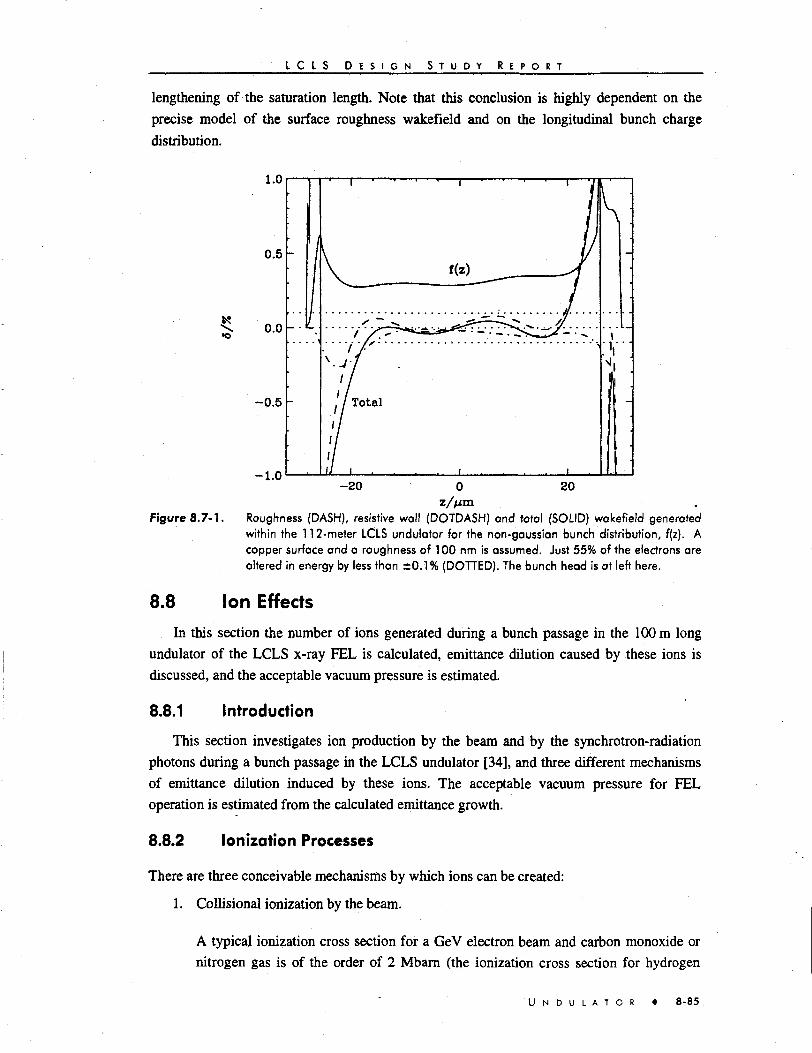
L C I S D E S I G N S T U D Y R E P O R T
lengthening of the saturation length. Note that this conclusion is highly dependent on the
precise model of the surface roughness wakefield and on the longitudinal bunch charge
distribution.
1.0
0.5 -
0.0 - • c
-0.5 -
-1.0
-
-
7r"i"f' '•
7A Total
iJ i . . . . i . . . . i
\
\
-I
- 2 0 20
Figure 8.7-1. Roughness (DASH), resistive wall (DOTDASH) and total (SOLID) wakefield generatedwithin the 112-meter LCLS undulator for the non-gaussian bunch distribution, f(z). Acopper surface and a roughness of TOO nm is assumed. Just 55% of the electrons arealtered in energy by less than ±0.1 % (DOTTED). The bunch head is at left here.
8.8 Ion Effects
In this section the number of ions generated during a bunch passage in the 100 m long
undulator of the LCLS x-ray FEL is calculated, emittance dilution caused by these ions is
discussed, and the acceptable vacuum pressure is estimated.
8.8.1 Introduction
This section investigates ion production by the beam and by the synchrotron-radiation
photons during a bunch passage in the LCLS undulator [34], and three different mechanisms
of emittance dilution induced by these ions. The acceptable vacuum pressure for FEL
operation is estimated from the calculated emittance growth.
8.8.2 lonization Processes
There are three conceivable mechanisms by which ions can be created:
1. Collisional ionization by the beam.
A typical ionization cross section for a GeV electron beam and carbon monoxide or
nitrogen gas is of the order of 2 Mbarn (the ionization cross section for hydrogen
U N D U L A T O R 8-85
L C L S D E S I G N S T U D Y R E P O R T
molecules would be approximately 10 times smaller). The 2-Mbarn cross section
translates into an ion line density of about
hmb*-1 ] - 5Nbp[nTorr] (8.8.1)
at the end of the bunch, or 320 ions per meter for a pressure of 10 nTorr and
Nb=6.3 109 electrons per bunch.
2. Ionization by incoherent synchrotron radiation.
The ionization cross section of 8-keV photons for typical elements is about 100 barn
[35]. Even though the number of photons at 1.5 A is three orders of magnitude higher
than the number of electrons, this cross section is so much smaller than the
collisional-ionization cross section that the photoionization at Angstrom wavelengths
can be neglected in comparison.
In addition to the photons emitted at the first (and higher) FEL harmonic
wavelengths, a broad spontaneous photon spectrum extends to much lower energies,
where the photoionization cross section is considerably higher. Below about 100 eV
the photoionization cross section becomes comparable to, and may even exceed by up
to a factor of 5, the cross section for collisional ionization.
From Figure 6 in Ref. [34], illustrating the spontaneous photon spectrum, and from
Fig. 8.8-1, showing its low-energy part, it is estimated that, at the end of the
undulator, there are about 6 x 10!0 photons per bunch with energies below 1 keV, and
fewer than 5 x 10⁹ photons whose energy is below 100 eV. Thus, the number of low-
energetic photons is about equal to the number of electrons in the bunch. With an rms
opening angle of 10-20 /ffad for the spontaneous radiation (and an even wider
opening angle at low photon energies), the photoionization processes occur on
average far away from the beam orbit. Therefore, considering the small number of
low-energy photons, the ions are assumed to be produced by photo-ionization form a
diffuse halo, whose effect on the beam is negligible compared with that of the much
denser ion cloud produced by collisional ionization inside the beam.
3. Tunneling ionization in the coherent laser field.
Up to frequencies of the order
co, =ceE/yJ2mec2I (8.8.2)
the tunnel effect is determined simply by the instantaneous value of the electric field
[36,37]. In Eq. 8.8.2, the parameter E is the electric field, me the electron mass, and /
the ionization potential. The peak electric field of the laser pulse can be roughly
estimated from the equation
8-86 • U N D U L A T O R

L C L S D E S I G N S T U D Y R E P O R T
2Nrhv(8.8.3)
and is found to be about 85 GV/m. Somewhat arbitrarily using / ~ 20 eV, the
threshold frequency is (D,~ 1016 s"1, which is very low compared to the FEL frequency
O) ~ 1019 s"1. This means that the standard formula for static tunneling ionization does
not apply here. To determine if the coherence of the FEL X-rays is important, the
photon density is calculated as
fly = •«7.2xl024m-3, (8.8.4)
which implies that in a sphere with a radius equal to the Bohr radius ao (ao ~ 0.5 A) on
average there are only 1.2 x 10'6 photons at any given time during the pulse. It is thus
legitimate to consider the photons as incoherent [38], in which case, as seen under
point 2, their contribution to the ionization is insignificant.
10'
total spectral flux at undulotor exit, integrated over all angles
first harmonic energy = 8.3 keV
100 200 300 400 500 600 700 800 900 1000
Er (eV)
Figure 8.8-1. Number of photons per 0.03 % frequency interval and per bunch passage at the endof the LCLS undulator; the spontaneous flux increases linearly along the undulator.
8.8.3 Emittance Dilution
Ions could dilute the bunch emittance in various ways: first, the ions induce a tune shift
across the bunch which could lead to filamentation and to an effective increase in the
transverse emittance; second, the electrons or, third, the ions generated by the bunch head can
excite the bunch tail and cause a beam break-up instability.
U N D U L A T O R 8-87

L C L S D E S I G N S T U D Y R E P O R T
Pessimistically assuming that all electrons originating in the ionization process are
dispersed and lost before the end of the bunch (using this assumption, which is not fulfilled
for the LCLS, the actual tune shift will be overestimated), one can estimate the ion-induced
shift in betatron phase advance between head and tail of the bunch at the end of the undulator:
A m & / A A (885)" TOviOt + Gj)
Using an ion line density A^m as expected for collisional ionization, Eq. 8.8.1, the phase shift
is Ay/Xiy~ 4 x 10'6 rad for 1 nTorr and 4 x 10"4 rad for 100 nTorr. Significant emittance growth
due to filamentation would be expected only for an average pressure exceeding 100 //Torr,
for which the phase shift approaches 1 rad.
Since, different from the situation in most other accelerators, the bunch length in the
LCLS is shorter than the transverse beam size, the electrons do not escape from the bunch
during its passage, but the electrons generated by the head will still affect the trailing
particles. The resulting emittance growth can be estimated from a first-order perturbation
expansion, in analogy to the treatment in [39]:
A.,. "vU'Afe, (,,6)
where y describes the amplitude of an initial vertical perturbation of the form yb°(s,z) =
ycos(s/fi +<t>)sirih(6>,z+6) with©,. = [4Nbrel3-j2noxoy(ox +<ry)]1A, where s is the
longitudinal position along the beam line, and z denotes the longitudinal position of a particle
with respect to the bunch center. Inserting numbers, ffltcris ~ 0.3. Exactly the same expression
with the subindices x and y interchanged applies to the horizontal case, and, by symmetry, it
yields the same emittance growth. Inserting numbers and assuming an ion density as in
Eq. 8.8.1, Eq. 8.8.6 is rewritten as
Aiysy )[m] - 4 x 10~19 - M (p [nTorr])2. (8.8.7)\°y)
For a huge perturbation, y «10<7y, one finds that the emittance growth becomes significant
when the pressure approaches 10"* Torr, which is almost five orders of magnitude higher than
the anticipated operating pressure.
In principle, not only the electrons but also the ions themselves could drive an instability,
even though the ions do not move during the beam passage. This could happen when the
bunch is tilted and the ions generated by the head are offset with respect to the tail. Especially
important is the case when the ion force drives the beam tail in resonance with the betatron
motion. As an example, due to the acceleration in the SLAC linac, the beams in the SLC arcs
8 - 8 8 • U N D U L A T O R
L C L S D E S I G N S T U D Y R E P O R T
usually exhibit a significant energy spread that is correlated with the longitudinal position
along the bunch. At locations with vertical dispersion, the beam is tilted vertically with
respect to the forward direction. Since the vertical dispersion in each achromat of the arc
propagates exactly like a betatron oscillation, ions generated by the head then drive the tail in
resonance. This effect, in fact, sets the tolerance on the acceptable arc vacuum pressure [40].
In the case of the LCLS, effects of this type are unlikely to be important because the
horizontal design dispersion in the undulator is small. The peak dispersion is only about
7)x=duku/x = 1.26 urn so that any perturbation involving energy variation and dispersion
will be very small compared with the transverse beam size. 9U = 132 /zrad is the maximum
deflection angle during the wiggle motion.
8.8.4 Conclusion
In this section, the number of ions generated during a bunch passage in the LCLS
undulator and their effect on the beam emittance is established. The ionization of the residual
gas due to .the coherent x-rays and, from the viewpoint of beam dynamics, also the ionization
due to the lower-energetic spontaneous photons were found to be insignificant compared with
the collisional ionization by the beam. There is not a tight tolerance on the vacuum pressure
in the LCLS undulator. Even a pressure as high as 1 //Torr would still appear to be perfectly
acceptable.
8.9 References
1 K. Halbach, "Physical and Optical Properties of Rare Earth Cobalt Magnets," Nucl. Inst. &Methods 187, p. 109 (1981).
2 S. Lidia and R. Carr, "Faster Magnet Sorting with a Threshold Acceptance Algorithm," Review ofScientific Instruments, V66 N2:1865-1867 (1995).
3 Group 3 Technology Ltd. model DTM 130 Teslameter.
4 Leitz Enhanced Accuracy Model PMM 12-10-6 Coordinate Measuring Machine.
5 Faatz et al, "Study of the Undulator Specifications for the VUV-FEL at the TESLA TestFacility," Nucl. Inst. & Methods A393, p. 380 (1997).
6 Integrated Engineering Software Inc., Winnepeg, Canada
7 "Zero Order Design Report for the Next Linear Collider," Appendix C, SIAC Report 474, LBNLPublication 5424, UCRL-ID-124161.
8 D. Humphries, et al., "A Multiple Objective Sorting Algorithm for the ALS Insertion Devices,"in the Proceedings of the Fifth International Conference on Synchrotron RadiationInstrumentation, Woodbury, NY (1994).
9 Eckhart and Drake, "Analysis of Heat and Mass Transfer"
10 Nucl. Inst. & Methods A 368, p. 579-592 (1996).
11 "Dimensional Instability: An Introduction," Battelle Memorial Institute (1977).
12 A. Berman, "Vacuum Engineering, Calculations, Formulas, and Solved Exercises," AcademicPress (1992).
U N D U L A T O R • 8-89

L C L S D E S I G N S T U D Y R E P O R T
13 D. Behne, "Outgassing Test Results from PEP-II Standard Straight Section Vacuum Chambers,"(1997).
14 C. Forester, et al., "Photon Stimulated Desorption (PSD) Measurements of Welded Copper BeamChambers for the PEP-II Asymetric B-Factory," 4th European Particle Accelerator Conference(1994).
15 M. Sullivan, "A Method for Calculating Pressure Profiles in Vacuum Pipes," PEP-II AP NoteNo. 6-94 (1994).
16 P. Emma, "Beam Based Alignment of Sector 1 of the SLC Linac," SLAC-PUB-5787 (1992).
17 This misalignment component was suggested by Chris Adolphsen.
18 D. A. Goldberg and G. R. Lambertson, "Dynamic Devices: A Primer on Pickups and Kickers,"American Institute of Physics, p.537 (1992).
19 W. Schnell, et al., "CLIC Beam Position Monitor Developments," CERN SU92-33(DI) (1992).
20 J.P.H. Sladen, I. Wilson, and W. Wuensch, "Measurement of the Precision of a CLIC BeamPosition Monitor," CERN CUCNote 189 (1993).
21 T. Shintake, private communication. (1997).
22 LCLS Preliminary Design Review ,(1996).
23 Ronald Lorenz, "RF Beam Position Monitors for the TESLA Test Facility," IEEE PAC, p. 2325(1993).
24 S.C. Hartman, T. Shintake, and N. Akasaka, "Nanometer Resolution BPM Using Damped SlotResonator," SLAC-PUB-95-6908 (1995).
25 W. Schnell, "Common-Mode Rejection in Resonant Microwave Position Monitors for LinearColliders," CERN-LEP-RF/88-4, CUCNote 70 (1988).
26 D. Martin, "LCLS Beam Position Monitor Design Notes," unpublished.
27 G. Dome, "Wake Potentials of a Relativistic Point Charge Crossing a Beam-Pipe Gap: AnAnalytical Approximation," IEEE Transactions on Nuclear Science, Vol. NS-32, No. 5 (1985).
28 A. Chao, "Physics of Collective Beam Instabilities in High Energy Accelerators," John Wiley(1993).
29 Karl Bane and Matthew Sands, "Wakefields of Very Short Bunches in an Accelerating Cavity,"Particle Accelerators, Vol. 25, pp. 73-95 (1990).
30 G. Roberto Aiello, "SLAC PEP-II BPM Design Manual," seehttp://www.slac.stanford.edii/~aiello.
31 G. Bowden, P. Holik, S.R. Wagner, G. Heimlinger, and R. Settles Nucl. Instr.&Methods A368, p.579 (1996).
32 K. Bane, C.-K. Ng, A. Chao, "Estimate of the Impedance due to Wall Surface Roughness,"SLAC-PUB-7514 (1997).
33 S. Kurennoy, "On the Coupling Impendance of a Hole or Slot," Part. Ace. 39, 1 (1992)
34 R. Tatchyn, et al., "Research and Development Toward a 4.5-1.5 A Linac Coherent Light Source(LCLS) at SLAC," SLAC-PUB-95-6994 (1995).
35 D.E. Cullen et al., "Tables and Graphs of Photon-Interaction Cross Sections from 10 eV to 100GeV Derived from the LLNL Evaluated Photon Data Library (EPDL)," Lawrence LivermoreNational Laboratory, UCRL-504000-Vol.6-Rev.4-Pt .A (1989).
8-90 • U N D U L A T O R

L C L S D E S I G N S T U D Y R E P O R T
36 L.V. Keldysh, "Ionization in the field of a strong electromagnetic wave," Soviet Physics JETP,Vol. 20, no. 5 (1965).
37 T. Raubenheimer, private communication (1997).
38 P. Chen, private communication (1997).
39 T.O. Raubenheimer and F. Zimmermann, "A Fast Beam-Ion Instability in Linear Acceleratorsand Storage Rings," Physical Review E, Vol. 52,5, pp. 5487-5498 and SLAC-PUB-6740 (1995).
40 P. Emma, T. Raubenheimer, F. Zimmermann, "Emittance Dilution by Ions in the SLC Arcs,"Proc. of the Fourth European Accelerator Conference (EPAC 94), World Scientific, Vol. 2, p.1162 (1995), and SLAC-PUB-6522 (1994).
U N D U L A T O R • 8-91

9 Undulator-to-Experimental Area
TECHNICAL SYNOPSIS
The primary Junction of the undulator-to-experimental area is to deflect the electron
beam away from the radiation exiting the undulator, dump it, and then pass the radiation on
through a high-vacuum system of spectral-angular filters and beam lines. The electron beam
is then dumped. The radiation is passed on through a system of spectral-angular filters whose
function is to transport either the spontaneous or coherent photons to the experimental end
station and suppress, as much as possible, the transmission of the bremsstrahlung component
and any secondary noise generated by it. After the beam has exited the undulator, an
absorption cell intercepts the radiation; its purpose is to attenuate the power to levels
manageable with conventional optics and to provide a continuous transition to power
densities at which meaningful research on the interaction of LCLS-type pulses with matter
can proceed. The coherent FEL radiation will be separated from the spontaneous radiation
by the absorption cell, by spectral and angular filters made of mirrors or crystals, and by
horizontally/vertically tunable x-ray slits. The bremsstrahlung radiation, a concern for both
personnel safety and experimental noise, will be absorbed by a mirror or a crystal, while the
thermal neutrons created by this interaction will be stopped by a lead/polyethylene shield
wall.
The spectral range of the coherent FEL line (820 eV-8200 eV in the fundamental and up
to about 25 keV in the 3rd harmonic) requires the use of both crystal and specular optics to
transmit and process the radiation for experimental applications.
The absorption cell is used to vary the output power of the radiation. Alternatively, a long
beam line (780 m long) could be built to reduce the beam's power density without diluting its
brightness. One of its major advantages would be that the reduced power density would allow
conventional optics to be installed in hutches far downstream from the undulator exit and
employed to control the output power density in a continuous fashion. The Experimental Hall
will consist, initially, of one crystal and one mirror beamline.
9.1 Transport System
The radiation emanating from the undulator may be broadly classified into three
categories: (1) the coherent spectral lines (the FEL fundamental and its harmonics); (2) the
ordinary spontaneous undulator spectrum; and (3) a very broad bremsstrahlung and
secondary-particle spectrum consisting of gamma rays, neutrons, muons, and other particles
with energies bounded by the operating energy of the LCLS (4.5-14.3 GeV). All three types
L C L S D E S I G N S T U D Y R E P O R T
of radiation emerge more or less co-terminously with the high-energy electron bunch that
drives their production. The primary function of the undulator-to-experimental area beamline
is to deflect the electron beam away from the (predominantly neutral) radiation into a beam
dump, and then pass the radiation on through a system of spectral-angular filters whose
function is to transport either the spontaneous or coherent undulator photons to the
experimental end stations while suppressing, as much as possible, the transmission of the
bremsstrahlung component and any secondary noise generated by it.
Apart from their role in performing these general functions, a number of the details of the
LCLS optical system and components shown in Fig. 9.1-1 are also determined by the
necessity of handling the unprecedented peak power densities of the coherent light. The basic
components (shown schematized in Fig. 9.1-2), as well as their functions and layout, can be
assessed from this perspective.
The LCLS will generate coherent radiation in the fundamental over the range of 820 eV-
8.2 keV. This necessitates the unobstructed transport of the radiation (i.e., with no normal-
incidence barriers or windows) from the undulator exit out to the experimental
instrumentation and samples. Furthermore, since the net power absorbed by a number of the
components that intersect the LCLS x-rays at extreme grazing incidence is very sensitive to
surface contamination, all such vacuum-sensitive components must be bracketed by
differential pumping sections featuring large isolation ratios. The goal of the design is to
maintain, on the average, Ultra High Vacuum (UHV) environments (i.e., <10"9 Torr) in the
bracketed regions. The most critical optical element is the absorption cell. Its primary
purpose is basically twofold: (1) to attenuate the LCLS power to levels manageable by
ordinary optics, and (2) to provide a continuous transition to power densities at which
meaningful research on the interaction of LCLS-type pulses with matter can proceed. Indeed,
the cell itself constitutes an appropriate physical system for performing initial studies of this
type. An alternative means for controlling the power density, a long beam line, has also been
considered, and a brief account of some of the details is given in Section 9.3.2.
An important option for various experimental applications is the possibility of separating,
or suppressing, the spontaneous radiation with respect to the coherent line spectrum. In the
layout of Fig. 9.1-2, spectral-angular filtering function is performed by: (1) the absorption
cell itself, (2) the take-off mirrors or crystals, and (3) by the horizontally/vertically tunable x-
ray slits. In particular, the first slit-pair has been located just upstream of the absorption cell,
allowing the suppression of the long-wavelength part of the spontaneous spectrum. This is
expected to enhance the control of scattering experiments performed in the absorption cell, as
well as to provide an upstream half of a long collimator whose downstream part consists of a
similar set of slits at the entrance to the experimental area. In this regard, both the slits and the
absorption cell can be considered as high-pass spectral filters. In particular, if the absorption
cell is very effective at the LCLS fundamental, it can transmit most of (the high-energy part
of) the spontaneous spectrum on to the experimental area. The mirrors downstream of the
second set of slits provide the complementary function of low-pass filtering. Since, as is
9 - 2 • U N D U L A T O R - T O - E X P E R I M E N T A L A R E A

L C L S D E S I G N S T U D Y R E P O R T
shown below, the spontaneous radiation spectrum can extend out to more than 1 MeV, the
mirrors, in conjunction with the absorption cell and the slits, can approximately isolate and
deliver selected FEL harmonics to experiments requiring them. In an analogous sense, the
crystal take-off optics can be viewed as a spectral-angular bandpass filter, but with a
substantially sharper response.
Research Yard(plan view)
Bldg 103
LCLS Experimental Bldg Crystal
Experimental Hutch
Crystal Beam Line
I i i i i I i I i i I i i i I I i i i i II I f f I r I i i |
3 10 20 metersFFTB Tunnel
Undulator
Absorption Cell Enclosure
FFTBBeamDump/Shield
9-978347A9
Figure 9.1-1. LCLS undubtor-to-experimental area layout in the SLAC Research Yard.
Finally, the primary bremsstrahlung radiation cone and its derivatives, generated by the
collimators upstream of the undulator and the undulator vacuum, present a potential concern
both for personnel safety and for experimental incursion (via detector and instrumentation
noise). In view of its high average spectral energy, bremsstrahlung noise will co-propagate
with any undulator radiation until it hits a medium with an adequately short extinction depth.
In the system of Fig. 9.1-1, this may be either a mirror or a crystal. The impact will, in
general, impulsively excite an intense thermal neutron field that will decay with a time
constant on the order of milliseconds. To suppress any possible interference with LCLS
experiments operating over similar time intervals, the layout includes a lead/polyethylene
shield wall between the crystal and specular take-off optics tanks and the experimental end
stations. Since both beam lines pass through this wall at off-axis angles and via small
U N D U L A T O R . T O - E X P E R I M E N T A L A R E A • 9 - 3

L C L S D E S I G N S T U D Y R E P O R T
apertures, the suppression of this source of interference by the wall is expected to be very
effective.
£-978347A8
Figure 9.1-2.
r0 4 5 meters
Detailed layout (elevation view) of electron beam dump line and the x-ray optics systemcomponents in the LCLS undulator-to-experimental area. 1-undulator exit; 2-electronbeam dump magnets; 3-vacuum valve; 4-Differential Pumping Section (DPS); 5-verticalx-ray slits; 6-horizontal x-ray slits; 7-absorption cell; 8-absorption cell radiationenclosure; 9-beam shutter; 10-mirror tank; 11-crystal tank; 12-crystal beam line endstation; 13-specular beam line end station.
9.2 Shielding Enclosures
The space for the undulator and the x-ray transport line is provided by the existing FFTB
tunnel enclosure [1]. This structure is sufficiently long and wide to allow installation of the
112 meter long undulator without major facility modifications. The shielding structures,
designed to protect against radiation generated by dumping the 50 GeV FFTB beam, consist
of: (1) 1.2 m thick concrete tunnel walls and a i m thick ceiling; (2) an FFTB dump shield
consisting of an 8 m x 8 m concrete and steel bunker surrounding the dump core; and (3) a
22 m long iron muon shield extending past the downstream wall of the FFTB dump
enclosure. Under the FFTB experimental protocols, the FFTB tunnel and beam dump facility
shielding allows routine operation of 50 GeV beams with ~1010 e7pulse, at 10 Hz, or an
average power of Pav~800W. By special arrangement this can be increased to 30 Hz, or
Pav~2500 W. At the nominal e"-beam parameters of <15 GeV and Pav~1800 W, operation
will consequently not present any requirements beyond those already satisfied for FFTB
operation. Despite this basic compatibility, modifications to the dump system design to
handle the lower (4.5-14.3 GeV) beam energies will be required, and selected initial
recalculations of the existing dump and shielding structures for the new parameters have
already been performed.
9 - 4 • U N D U L A T O R - T O - E X P E R I M E N T A L A R E A

L C L S D E S I G N S T U D Y R E P O R T
Apart from the revised dump design, the major new shielding structures required for the
LCLS are associated with the transport of high-power bremsstrahlung and X-through-y
radiation into the x-ray transport line and on through a vacuum pipe running through the
FFTB dump structure and into the contiguous Experimental Hall. The additional structures
are: (1) a radiation enclosure for the absorption cell located in the FFTB tunnel; and (2) a
shielded experimental hutch located in the Experimental Hall. The primary functions of the
added structures are: (1) personnel protection, (2) shielding of experimental detectors from
bremsstrahlung-generated radiation, or (3) both.
The absorption cell enclosure is intended to shield the area around the absorption cell
from bremsstrahlung-generated noise radiation, enabling detectors to be placed and operated
in close proximity to the cell. The performance of the conceptual design, consisting of lead
and polyethylene bricks arranged to form a rectangular enclosure (see Fig. 9.1-2), has not, as
yet, been rigorously calculated. An optimal configuration for this structure will be developed
as part of continuing LCLS R&D.
The hutch in the Experimental Hall will have a construction similar to the hutches
employed on the beamlines on SPEAR [2], but probably with somewhat thicker lead
shielding. A singular aspect of the hutch design—the shield wall separating the mirror and
crystal tanks from the experimental station area—is motivated by the time structure of the
electron beam. Due to the sub-picosecond duration of the electron bunches, both the
bremsstrahlung and the x-rays will strike the solid mirror or crystal surfaces more-or-less
simultaneously with a peak fluence far exceeding that on existing synchrotron storage ring
beam lines. For FEL gains substantially below saturation, or otherwise with the absorption
cell strongly attenuating the fully saturated output, the incoming bremsstrahlung pulse may
contain substantially more energy than the pulse, and the resulting thermal neutron flux that it
will generate may interfere with experimental signals picked up immediately following the
pulse. The primary function of the shield wall is, consequently, to suppress the transport of
thermal neutron flux from the mirror/crystal tank area to the experimental stations.
9.3 Beam Lines and Experimental Stations
9.3.1 Experimental Beam Lines
The spectral range of the coherent line output (820 eV - 8200 eV in the fundamental and
up to about 25 keV in the 3rd harmonic) necessitates the use of both crystal and specular
optics to transmit and process the radiation for experimental applications. The natural spectral
partition is to use crystal optics for wavelengths <3-5 A and specular or transmissive optics
over the complete range (i.e., reflective and refractive optics over the 800 eV-25 keV range
and diffractive specular optics for wavelengths >5 A). This natural emphasis on the two
spectral regimes has led to the current minimal allocation of two experimental beam lines to
the experimental hutch. Since the use of specular reflective and diffractive optics generally
requires operation at extreme grazing incidence with long dispersion lengths in the x-ray
U N D U L A T ' O R - T O - E X P E R I M E N T A L A R E A • 9 - 5

L C L S D E S I G N S T U D Y R E P O R T
range, the specular line has been assigned a length of -15 ra. This should permit the
implementation of sufficiently high resolution monochromators, as well as focusing optics of
sufficiently high demagnification. The crystal optics beam line, which will operate with
beams deflected at much larger angles to the undulator axis (see Section 10.4.6), is
correspondingly shorter.
As described in Section 10.4.5, the angle of incidence on the mirrors in the long beam
line will nominally lie in the 0.0001-0.0005 rad range. If at least two reflectors are used, the
net angle of deflection away from the undulator axis will lie in the 0.0004-0.002 rad range.
At a distance of 15 meters, the corresponding net deflection of the beam from the undulator
axis will be in the 6-30 mm range. If additional deflection is required, extra mirror tanks or
mirrors can be added to provide additional tandem reflections. Alternatively, should line-of-
sight propagation be required, the mirrors and crystal elements in the two tanks can be moved
out of the beam's way, providing a direct path to the rear hutch wall.
Apart from the nominal spectral ranges of the two beam lines, it is noted that the longer
line provides low pass filtering via its mirrors, which is also a potentially useful function for
experiments in the <3-5 A range (e.g., those requiring harmonic suppression). This condition
can be realized by operating the crystal tank in tandem with the mirrors. Clearly, should
additional reflections be required, the longer beam line could also be used for this purpose,
with the appropriate crystal instrumentation mounted in a suitable location between the
crystal tank and the downstream hutch wall. An additional attribute of this line is sufficient
space to install additional optics for spatial or temporal processing of the radiation pulses
(e.g., beam expanders or beam splitters, delay lines, etc.). Finally, its -15 m length provides
additional flexibility for spectral/angular separation of the spontaneous SR spectrum from the
coherent FEL lines and the installation of experimental equipment to utilize this radiation.
9.3.2 The Long Beam Line
The peak power density of the x-ray beam leaving the undulator is many orders of
magnitude higher than that currently handled by existing optical methods and technologies.
To provide a continuous variation of this parameter from maximum down to conventional
values at the experimental stations (which are located at distances of approximately 35 m and
50 m from the undulator exit), the present system design incorporates a gas (or liquid)
absorption cell. Alternatively, a "long" beam line could also be used to reduce the beam's
power density by allowing it to spread out over a substantially increased area via natural
divergence. A major advantage of this approach is that the reduced power density would
allow conventional optics to be installed in hutches far downstream from the undulator exit
and employed to either further reduce the power density or to increase it, in a controlled way,
to levels corresponding to its diffraction-limited waist.
9 - 6 • U N D U L A T O R - T O - E X P E R I M E N T A L A R E A

L C L S D E S I G N S T U D Y R E P O R T
Possible site ofExperimental hall
9-978347A6
Figure 9.3-1. Topographical view of SLAC displaying LCLS long beamline layout options.
Fortunately, less intrusive options are available. The most attractive of these is a simple
extension of the x-ray beam line along the linac machine slope beyond the aforementioned
two experimental stations. Such a beamline would cross the SLAC Central Research Yard
above ground and eventually encounter a hill bordering the SSRL access road at a distance of
-115 m from the FFTB dump. A small diameter tunnel would have to be bored and a short
section of the access road elevated. The local topography is such that the beam trajectory
would approach the top surface of the hill to within ~8 meters at a distance of ~335 meters
from the proposed exit of the undulator. This location can readily accommodate an
experimental hutch that would be partially buried in the ground, but would be near an access
road and utilities. The tunnel could be extended even farther underneath an adjacent hill and
would eventually surface at an ultimate distance of ~780 meters from the end of the
undulator. This site is encumbered by access to utilities, but is otherwise very suitable for a
research enclosure. Figs. 9.3-1 and 9.3-2 display a topographical map and a vertical cross
sectional contour along the proposed siting route of the beam's nominal axis.
To obtain estimates of cost and effort associated with the above options, a firm
specializing in micro tunneling was contacted. Their assessment was that such a tunnel would
be a routine construction and that no special challenges are foreseen. Depending on the
specific boring equipment used, the minimum diameter of such a tunnel would be either
~3/4m or -1.1 m for the two hutch locations, respectively. The difference comes from the
different boring methods that would be used. The longer and larger diameter tunnel would be
driven using a laser guided boring head, which has great pointing accuracy. Either tunnel
would have a liner installed to keep soil and water out. The estimated lapse times to construct
such a tunnel to the two hutch locations would be -1 month and -2 months, respectively.
U N D U I A T O R - T O - E X P E R I M E N T A I A R E A 9-7
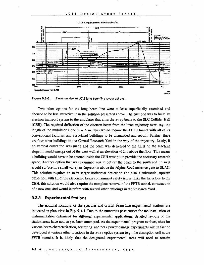
L C L S D E S I G N S T U D Y R E P O R T
335
305
275
245
215
185
1551C
Hi
g
itsi
End oi
LCLS Long Beamline Elevation Profile
1
mDump
— /
4-I—
100 1500
xtoontal Distero from St 100
625' •
mmmmmmmm
•V 1
1
2000
B < •350'AMSL
—27? AM
i Exparimi
^r—^?p"e
Start _ _nl»IH«H >
2500
^-
»lantor Slow
3000
0-2727279*
—\—\
——V-Q. ^
IBB ILOUaka^H^
13600
8
if: R July 17/87
> * Draviins by: 6. PUulta
•ui
EiMrtmamaiHail
. Ava. Slf^f
\
_ i .
4000
M 7>M7«tO
Figure 9 .3 -2 . Elevation view of LCLS long beamline layout options.
Two other options for the long beam line were at least superficially examined and
deemed to be less attractive than the solution presented above. The first one was to build an
electron transport system to the undulator that aims the x-ray beam to the SLC Collider Hall
(CEH). The required deflection of the electron beam from the linac trajectory over, say, the
length of the undulator alone is -15 m. This would require the FFTB tunnel with all of its
conventional facilities and associated buildings to be dismantled and rebuilt. Further, there
are four other buildings in the Central Research Yard in the way of the trajectory. Lastly, if
no vertical correction was made and the beam was delivered to the CEH on the machine
slope, it would emerge out of the west wall at an elevation -12 m above the floor. This means
a building would have to be erected inside the CEH west pit to provide the necessary research
space. Another option that was examined was to deflect the beam to the south and up so it
would surface in a small valley or depression above the Alpine Road entrance gate to SLAC.
This solution requires an even larger horizontal deflection and also a substantial upward
deflection with all of the associated beam containment safety issues. Like the trajectory to the
CEH, this solution would also require the complete removal of the FFTB tunnel, construction
of a new one, and would interfere with several other buildings in the Research Yard.
9.3.3 Experimental Stations
The nominal locations of the specular and crystal beam line experimental stations are
indicated in plan view in Fig. 9.1-1. Due to the numerous possibilities for the installation of
instrumentation optimized for different experimental applications, detailed layouts of the
station areas have not, as yet, been attempted. As the experimental program evolves, sites for
various beam-characterization, scattering, and peak power damage experiments will in fact be
developed at various other locations in the x-ray optics system (e.g., the absorption cell in the
FFTB tunnel). It is likely that the designated experimental areas will need to remain
9 - 8 4 U N D U I A T O R - T O - E X P E R I M E N T A L A R E A

L C L S D E S I G N S T U D Y R E P O R T
'flexible" in this sense, with each experiment or class of experiments resulting in a different
layout of instrumentation, detectors, shielding, and data acquisition protocols.
9.4 Experimental Hall
The function of the Experimental Hall is to contain the shielded experimental hutch and
to provide access to it from a controlled environment. Related functions include the
establishment of climate control to reduce the effect of outside temperature variations on the
optical and experimental system components and the provision of utility and communications
support for workers. The design laid out in Fig. 9.1-1 was based on securing a hutch space of
maximal length without interfering with any of the adjacent buildings in the Research Yard.
The dimensions of the hall are 10 m wide x 5.8 m high x 27 m long, providing a total floor
space of ~2700 m2. The 10 m width allows for approximately a 2 m wide walkway between
the building and hutch walls toward the downstream end of the hall, with a substantially
larger floor area located between the hutch and building walls in proximity to the FFTB beam
dump. This rather narrow floor area can be used for placement of electronic racks and data
acquisition and control computers. Depending on the location of access doors to the hutch,
the remaining floor space could be used for preparing samples and queuing of experimental
equipment.
In continuing design studies, possibilities for extending the length and width of the
Experimental Hall, possibly by removing or merging with adjacent buildings, will be pursued.
9.5 References
1 S. H. Rokni, E. C. Benson, D. L. Burke, T. M. Jenkins, J. C. Liu, G. Nelson, W. R. Nelson, H. E.Smith, P. Tenenbaum, V. Vylet, D. R. Walz, "Radiation protection systems for the Final FocusTest Beam at SLAC," Health Physics 71(5), 786 (1996); SLAC-PUB 6784.
2 H. Winick, "Synchrotron Radiation Sources, Research Facilities, and Instrumentation," inSynchrotron Radiation Research, H. Winick and S. Doniach, eds., Plenum Press, New York,1980, p. 27.
U N D U I A T O R - T O - E X P E R I M E N T A L A R E A • 9 - 9

Take-off Optics andBeam Line Layouts
TECHNICAL SYNOPSIS
The coherent output of the LCLS features peak output powers in the 10 GW range,
average powers on the order of 1 W, spectral bandwidths on the order of 0.1%, full
transverse coherence, and pulse lengths of approximately 300 fs. The peak brightness of the
LCLS can attain values in thel^—lO34 (ph/s,mm2 jnr2, 1%BW) range. A comprehensive set
of calculations of the spontaneous spectral flux has been carried out in the far-field
approximation. The spectral distributions and peak power densities associated with both the
coherent and spontaneous LCLS beams have been calculated and archived for use in optical
instrumentation and experimental design. The peak on-axis power density of the spontaneous
radiation, approximately 1013 W/cm2 for 15 GeV operation, is approximately only one
hundred times smaller than that of the coherent line, which due to its full transverse
coherence can, in principle, be focused (at 1.5 A) to an approximate limit of 1025 W/cm2.
The bremsstrahlung flux, generated by scattering off in-vacuum molecules and various
upstream collimators and optical elements, is of concern both for personnel safety and the
maintenance of a low-noise experimental environment. Detailed modeling of the
bremsstrahlung gamma flux entering the experimental area has been carried out. The
modeling has determined that this gamma flux is controllable with standard shielding
techniques. Time-domain modeling of the conversion of the bremsstrahlung into thermal
neutron flux and the associated design optimization of the experimental hutch shield wall and
experimental areas will be continued as part of the x-ray optics design effort.
The layout of the initial optical system, dedicated to transporting and processing the
above species of radiation, has been designed to satisfy two basic requirements. First, it will
provide diagnostic capabilities for analyzing the output in the initial stages of the facility's
operation. Second, it will provide a nominal set of spectral-angular filtering capabilities for
supporting a flexible range of exploratory experiments. These capabilities include low-
resolution high-pass, low-pass, and band-pass filtering, as well as one high-resolution
monochromator. The transport system and optical beam lines will utilize windowless in-
vacuum transport for the radiation, and specially designed shutters and stoppers for
personnel and facility protection.
The primary elements in the x-ray transport and optical beam line systems are:
Differential Pumping Sections (DPSs), x-ray slits, an absorption cell, mirrors, and crystals.
The establishment of windowless in-vacuum transport, as well as Ultra High Vacuum (UHV)
environments for selected beam line optics, will be realized with the DPSs. These components
provide up to five orders of magnitude of vacuum isolation by blocking line-of-sight

L C L S D E S I G N S T U D Y R E P O R T
molecular flow with electron-based ionizing and magnetic-deflection-based trapping
mechanisms. Spatial and angular phase-space filtering of the radiation will be provided by
two sets of horizontally and vertically oriented slits. Both the slit apertures and angles of
incidence will be individually adjustable, allowing operation in either a normal-incidence or
grazing-incidence mode.
The absorption cell, designed for variable attenuation of the coherent radiation, will
operate by emitting streams of high-pressure xenon, or an alternative gas, onto the radiation
axis. Since the present design has been based on calculations valid for weak-field
radiation/matter interactions, it is anticipated that more detailed studies of such interactions
in the strong-field regime of the LCLS will need to be performed for the development of an
optimized design. The mirrors, utilized for low-pass filtering and beam deflection, are
designed to operate at extreme grazing incidence to dilute the incoming power density of the
reflected light. In order to keep the absorbed energy density below the activation threshold of
various damage mechanisms, the mirror surfaces must be polished down to roughness in the
1-2 A range and kept free of contaminants during operation.
For crystal optics, energy-absorption calculations indicate that very thin, low-Z materials
should be used at large angles of incidence in order to minimize the absorbed energy.
Alternatively, the incidence angle could be reduced by using asymmetrically cut samples. In
either case, diamond, and perhaps beryllium, appear to be optimal choices with regard to
weak-field calculations, although here too there is no experimental data and little theoretical
knowledge of how they will behave in the parameter regime of the LCLS. In addition to the
primary optics, special instruments and components will need to be developed in support of
the beam diagnostics and selected scientific experiments. In the first case, for example,
calorimeters, spectrometers, and other instruments (e.g., Michelson interferometers) will be
required to characterize or profile the phase-space parameters of the LCLS pulses. In the
second case, extending or tailoring the source parameters of the coherent light will be
necessary. For example, beam splitters and time-delay lines will be required to support time-
domain correlation experiments; pulse compressors may be required for the study of ultra-
fast phenomena; and microfocusing of the beam to power densities orders of magnitude in
excess of those in the raw x-ray beam will be desirable for coherent imaging and nonlinear
physics investigations.
10.1 Coherent Radiation
A basic theme underlying the design and development of the x-ray optical system
components and instrumentation listed above has been, and remains, the lack of theoretical
and experimental knowledge regarding the interaction of the radiation pulses with matter. In
view of the fact that the initial designs of critical components such as the mirrors and
absorption cell have been predicated on physical data and techniques valid in the weak-field
regime, it is anticipated that an intensive theoretical and experimental R&D program for
investigating the interaction of LCLS-type radiation pulses with matter will be required to
1 0 - 2 • T A K E - O F F O P T I C S A N D B E A M L I N E L A Y O U T S

L C L S D E S I G N S T U D Y R E P O R T
provide understanding and control of the physical factors necessary for optimal
instrumentation and experimental design. Indeed, it is expected that the first use of the x-ray
system will be to investigate such interactions using the optical elements and materials
initially in place.
The characteristics of the coherent line spectrum of the LCLS operating in the SASE
mode have been studied extensively, both theoretically and numerically
[1,2,3,4,5,6,7,8,9,10,11,12]. The results are typically condensed into tabulations or graphs of
the peak power, brightness, transverse/longitudinal coherence, and the temporal/spectral
structure of the output pulses as explicit or implicit functions of the electron beam and
undulator parameters. Many if not all, of the cited investigations idealize or restrict the FEL
system being studied in various ways. The primary ones include: (1) the representation of
beams and interaction regions in spaces of reduced dimension; (2) restriction to the dynamics
of the exponential gain process without a comprehensive or realistic model of startup noise;
(3) an emphasis on the realistic characteristics of startup noise and their propagation using
simplified linearized models of the electron beam and its bunching dynamics; (4) the use of
simplified analytical models to represent actual insertion device fields; (5) the use of
simplified electron beam phase space and field models; and (6) restriction to selected regimes
of the FEL gain process, such as the onset and evolution of saturation. In many instances,
analytical treatments are used to provide nominal or initial estimates of selected output
parameters, followed ultimately by deferral to computer simulations that are perceived to be
more realistic.
For purposes of optical design and the reliable calculation of the propagation of radiation
through the optical system, a comprehensive quantitative description of its phase-space
parameters is required. This description naturally takes into account the statistical and
coherence properties of the radiation field [13], providing a convenient set of parameters
whose spatial-angular and spectral-temporal propagation through linear systems can be
calculated with the aid of well-known analytical techniques, e.g., the van Cittert-Zernicke
[14] and Wiener-Khintchine [15] Fourier-transform relations.
The first-order coherence properties of the LCLS pulses [16] are expressible in terms of
the source brightness B [photons/(sec mm2 mr2 0.1 %BW)], and the closely related degeneracy
parameter, 8. The brightness, whose propagation through linear systems can also be
calculated using well-known analytical formalisms [17], can be defined as the photon energy
density in phase space,
B= Nph°'/Ot . (10.1.1)Wee(r/f)
Here Npho, is the number of photons, Ox is .the standard deviation of the pulse's duration,
ex(=axox')and £y(=oyoy-) are the total transverse emittances, Of is the standard deviation
of the bandwidth, and / i s the mean photon frequency. If the wakefield effects, discussed in
T A K E - O F F O P T I C S A N D B E A M L I N E L A Y O U T S • 1 0 - 3

L C L S D E S I G N S T U D Y R E P O R T
Section 8.7, cause the slices along the bunch to differ in their average transverse location ex,
ey and energy spread, Of, should be replaced by the larger values of projected emittance and
energy spread. The corresponding degeneracy parameter is defined as the photon number per
phase space mode volume,
S=-(XllfNphot _
= BAc
(10.1.2)
where X is the mean photon wavelength and c the speed of light. In numerical terms,
^ ^ x l O " 2 5 ^ ! ^ ] ) 3 ! } . For a fully transversely coherent source, Qn)2exe =(>l/2)2, resulting
in the simplified expression <5 = Nphot I2naf. As stressed by Coisson [18], Scan be used as an
index to assess the probability of collective, or stimulated, photon/electron beam interactions
(with the probability approaching 1 for S»\). When expressed as the density of photons in
the real-space volume associated with a single phase-space mode, S can be contrasted with
the particle density of the material the pulse is interacting with to gauge the relative
expectation of collective and multi-photon processes.
Using these definitions, the basic radiation parameters of the LCLS can be summarized
on the basis of results from the aforementioned theoretical studies and numerical simulations.
A graphical representation of the temporal and spectral characteristics of a short interval of an
LCLS-type radiation pulse at saturation is shown in Fig. 10.1-1. A simplified analysis of the
evolution of SASE from startup noise into lineshapes similar to the ones depicted can be
found in the references (e.g., Saldin et al.). Due to its origin in shot noise, the temporal output
consists of peaks of random phase and amplitude, with the average peak width corresponding
to ~0.05NuX-G.\NuX , where Nu is the number of undulator periods. Nominal parameters
corresponding to the SLAC LCLS operating at 1.5 A and 15 A are listed in Table 10.1-1.
9-978347A12
0.8 1.6Time (fs)
— (X2.56) r
51.E+11 t
,?1.E+090.145 0.150 0.155
Wavelength (nm)Figure 10.1-1. Temporal (a, left) and spectral jb, right) features of the saturated output of a 30 m
1.5 A SASE FEL. The abscissa of b) is divided into 256 bins.
1 0 - 4 • T A K E - O F F O P T I C S A N D B E A M L I N E L A Y O U T S

L C L S D E S I G N S T U D Y
Table 10.1-1. Optical and source parameters of the LCLS.Undulator period Ay=3 cm.
Parameter
Radiation wavelength [A]
Norm, emittance ye [mm-mrad]
Electron energy [GeV]
Peak current [A]
Bunch duration [fs, FWHM]
Peak spontaneous power [GW]
Peak coherent power(a) [GW]
Average coherent power [W]
Energy/pulse [mJ]
Coherent photons/pulse (xlO12)
Approximate bandwidth (BW) [%]
Peakbrightness(c)(xl032)
Peak degeneracy parameter [xlO9]
Average brightness(c) (xlO21)
Transverse size \jm, FWHM] (d)
Divergence angle [/zrad, FWHM](d)
Spontaneous fundamental opening angle [pmd, FWHM]
Spontaneous fundamental transverse size [yUm,FWHM]
Peak Power Density [W/mm2](d) (xlO12)
Peak Field [V/m](d)(xl010)
R E P O R T
Undulator K=3.71.
1.5
1.5
14.35
3400
277
81
9
0.31
2.5
1.9
0.1
12
3.3
40
78
1
4.9
82
1.88
3.8
N u =3328 periods.
Value
15
2.0
4.54
3400
277
5
11
0.35
0.64
23
0.1
1.48
412
4.9
93
8
15.5
131
1.62
3.3
a. Output fully transversely coherent
b. At 120 Hz rep rate.
c. Photons/s/mm2/mrad2/0.1%BW.
d. At exit of undulator.
An important aspect of the temporal structure of the LCLS is that the full pulse is
effectively partitioned into a sequence of contiguous, causally non-overlapping intervals of
length Lsiip =NuAr (referred to in the FEL literature as "slippage" lengths). In the LCLS
pulse at 15 GeV, for example, there are approximately 140 such intervals. Due to the physical
independence of each interval, its coherent radiation mode must also be considered fully
independent of the others. Under the assumed ideal conditions that each such interval of the
LCLS bunch travels and emits along exactly the same axis, is characterized by the same
statistics, and has the same mean energy, its mean (peak) brightness and degeneracy
parameters will be equal to those of the full pulse. In general, however, there may be a
substantial variation of the mean radiation and phase space parameters, as well as of their
T A K E - O F F O P T I C S A N D B E A M L I N E L A Y O U T S • 1 0 - 5

L C L S D E S I G N S T U D Y R E P O R T
higher statistical moments, from interval to interval. This may result in an increased (average)
mode volume, or a decreased amount of photon energy per mode. For example, if the
longitudinal density profile of the electron bunch is strongly non-uniform, the amount of gain
saturation within each interval may vary with the local density. Other possibilities may
include changes in the mean electron beam energy (and thereby of the emitted photon energy
by twice the relative amount) from interval to interval, as well of the average transverse
position and angle. Under these conditions, it becomes critical to distinguish between the two
limiting cases where the variation of the statistical moments from interval to interval is:
1) random, or "uncorrelated"; and 2) dependent, or "correlated," with respect to z.
Each of these limiting cases requires a basically different description of the source
characteristics, corresponding to the distinction drawn in the statistical literature between
"frequency" versus "time" series [19]. In the random case, the phase space probability
distributions of the entire beam can be trivially derived form the corresponding distributions
of the individual sub-bunches. The statistical moments of the entire bunch are then obtained
by averaging the powers of the parameters in question with the distributions of the whole
bunch.
In the second case, while the same procedure can also be formally applied, it also
becomes critical to describe the correlation, or functional dependence, of the statistical
moments of the individual bunch intervals with respect to z. This can be straightforwardly
accomplished by calculating, for example, the autocorrelation of each statistical moment over
the entire bunch as a function of z. If the mean energy of each sub-bunch decrease
monotonically versus z (as in the case of the "chirp" induced in the electron bunch by linac
wakefields), a knowledge of this dependence can be exploited for designing optics for
temporally compressing the LCLS output [20]. More generally, the existence of such "chirps"
in the transverse phase space parameters are also of extreme interest, as they can influence the
design of instrumentation for experimental applications, as well as the interpretation of
experimental results.
A representation of LCLS peak and average brightness contrasted with other quasi-
coherent x-ray or SR sources is shown in Fig. 10.1-2. The maximum values (dashed curves)
assume homogeneous and smooth temporal and spectral lineshapes, as well as diffraction-
limited transverse outputs. Due to the idealized nature of these assumptions, the brightness is
displayed as a range in anticipation of realistic factors that could ultimately lessen the
maximum value. In addition to the one discussed above, these could include: (1) spectral
broadening effects due to non-linearities in the gain process (dilution of A^<«); (2) actual
mode structures more complex than the one evidenced in current analytical theories (increase
of phase-space volume); and (3) correlated and uncorrelated energy spreads in the beam
greater than those assumed in current simulations (dilution of A pfto,).
1 0 - 6 • T A K E - O F F O P T I C S A N D B E A M L I N E L A Y O U T S

L C L S D E S I G N S T U D Y R E P O R T
Wavelength (nm)124.0 12.4 1.24 0.124 0.0124
Wavelength (nm)124.0 12.4 1.24 0.124 0.0124
1
-
-
-
-
I
- ' * * DESYTTF-FEL
LCLSspont
ALS1-2GeVUndulators^—«,
/ N S L S X1
I i
i i i
„ SLAC^^& LCLS
-
ESRF/APS7GeV _Undulator x(max) \
\ _S. APS 6-8 GeV
> Wigglers
^ -
I I I
103 10" 10" 10" 10° 101 10z
Photon Energy (kev) Photon Energy (kev)
Figure 10.1-2. Comparative peak and average brightness curves contrasting the LCLS with otherfacilities operating or under construction.
Combined coherent and spontaneous output flux of the LCLS based on the parameters
listed in Table 10.1-1 is shown in Fig. 10.1-3. Peak and average flux values corresponding to
120-Hz operation of the SLAC linac are marked on the opposing ordinates. The spontaneous
curve is normalized to the electron beam /and a fixed undulator K value of 3.71. For this
value the spontaneous spectrum is seen to extend well beyond the 50th harmonic, whereas the
expected output of the third coherent harmonic is up to two orders of magnitude weaker than
the fundamental. The nominal FWHM opening angle of the ith coherent FEL peak is of the
same order of size as the opening angle, % r , of the ith spontaneous radiation harmonic,
(10.1.3)
and at least a factor JJN^ smaller than that of the remaining spontaneous background. In
view of the fact that the total spontaneous power can match or greatly exceed the total
coherent power, it is of interest to rigorously calculate and contrast the power and power
density of both. These calculations are described in the following section.
T A K E - O F F O P T I C S A N D B E A M L I N E L A Y O U T S • 1 0 - 7

L C L S D E S I G N S T U D Y R E P O R T
10"+
m
* <xN/3300)
10"+
101s+
Sat OutputRange
1st mHarmonic
• ^ 0.92 keV(G 4.8 GeV)
^ 8.3 teV(* 14.35 GeV)
3rd FELHarmonic
Spontaneous Spectrum
• • • • • " ! • • • • • • • !1 10
e[keVJ/£ t [keV]
Figure 10.1-3. LCLS spontaneous versus coherent spectral flux (N=number of periods; K=3.71;0.92 keV < e, < 8.3 keV; linac pulise frequency 120 Hz).
Two observations concerning the full transverse coherence of the FEL spectral line
radiation are in order. First, it is (in principle) admissible to consider focusing the beam down
to a diffraction-limited waist of the scale of X. Although the practical obstacles to attaining
this level of focusing are formidable, especially toward the short end of the wavelength scale,
a systematic effort starting with the longest wavelengths would prove to be a worthwhile
R&D effort. Second, the saturated transverse coherence could activate scattering or
threshhold damage effects during propagation through non-homogeneous materials by
significantly enhancing local electric field amplitudes via the mechanism of near-field
diffraction. The investigation of this potentially significant effect is also a subject for
continuing numerical and experimental R&D.
10.2 Spontaneous Radiation Calculations
The long transverse LCLS undulator can emit a characteristic synchrotron radiation (SR)
spectrum with a total peak (and average) power an order of magnitude or more greater than
the coherent line power (see Table 10.1-1). As depicted in Fig. 10.1-2, this radiation,
distributed about the forward direction of the coherent FEL line, can contain on-axis
harmonics out to the >1 MeV range. Due to its broad spectrum and high power, the
spontaneous SR can be either useful or nocuous. In the first case it could be used for novel
experiments requiring broadband spontaneous radiation with an ultra-short-pulse time
structure, while in the second instance it can interfere with experiments designed to utilize the
coherent FEL line. In view of this, the capability of processing and separating, either
1 0 - 8 • T A K E - O F F O P T I C S A N D B E A M L I N E L A Y O U T S
L C L S D E S I G N S T U D Y R E P O R T
spectrally or angularly, the spontaneous SR from the FEL line(s) is clearly of critical
importance to the operation and scientific utility of the LCLS. This, in turn, necessitates a
quantitative spectral-angular description of the SR spectrum.
In view of the limited available time and other resources, the calculations for the present
study were restricted in a number of ways. First, the far-field limit of the general classical
expression for the spectral-angular flux distribution, as described elsewhere [21,22], was
employed. Although not as general as the more realistic near-field calculations that will
eventually need to be performed in support of future experimental applications, the use of the
simplified (and thereby substantially more rapid) far-field algorithms has: (1) provided a
conservative description of the power density distribution for optical design purposes (i.e., the
actual near-field spectra will be spectrally and angularly more diluted [23]), and (2) permitted
an initial comprehensive mapping of the LCLS's spontaneous spectral-angular parameter
space. Second, a zero-emittance source with a zero energy spread was assumed. Again, this
may be justified for the following reasons: (1) the zero-emittance assumption is
approximately realistic in the long-wavelength limit of the LCLS fundamental (at ~800 eV);
(2) for the relatively small emittance of the LCLS beam, which is only a factor of four greater
than the diffraction-limited emittance at 8.3 keV, longitudinal and transverse phase-space
corrections to the peak spectral flux numbers can be easily factored in, using simple analytical
expressions [24]; and (3) the calculated peak values represent the maximum attainable flux
density, which provides a conservative referent for optical design purposes. Finally, a
continuous undulator structure with no field errors was assumed. Again, this resulted in
maximal estimates for the spectral flux density, which were of primary relevance to the
present design study. In the real-life case, however, the presence of undulator field errors,
together with the electron beam's realistic phase space parameters, can cause substantial
deviations of the real spectrum from ideality, particularly at harmonic energies well above the
fundamental. To illustrate this, in Fig. 10.2-1 an equivalent-K wiggler spectrum [25] has been
superimposed on the ideal integrated spectrum of the LCLS. To first order, the effects of
undulator errors and beam emittance will tend to wash out the undulator's harmonic peaks in
the region around and above the wiggler's critical energy, bringing it into approximate
agreement with the high end of the wiggler's rolloff. With the availability of more realistic
modeling calculations, these discrepancies could, to a certain extent, be used to establish
information about the undulator's and electron beam's departures from ideality [26,27].
In continuing R&D efforts on the LCLS project, the calculations we report here will be
extended in a number of ways. First, the unrestricted formalism for the spectral-angular flux
density will be used to calculate realistic flux distributions for the fundamental and selected
higher harmonics at distances representative of the actual locations of the experimental end
stations. Second, the effects of the electron beam's phase space parameters will be factored
into the spontaneous radiation model. Third, provisions will be made for including
discontinuous undulator structures with realistic field errors into the source simulations.
Fourth, polarization profiles incorporating realistic beam and undulator parameters will be
T A K E - O F F O P T I C S A N D B E A M L I N E L A Y O U T S • 1 0 - 9

L C L S D E S I G N S T U D Y R E P O R T
calculated for the fundamental and lower-order harmonics. Finally, if required, the
calculations will be extended to elliptically polarizing field structures.
Most of the present calculations were carried out either on SSRL's mainframe computer
or on the Cray computers at the NERSC facility at LBNL. The data files have been archived
at SSRL. In the following sections selected results of these calculations are summarized.
. i—|...^:..:..:.J.:.
....„.„....;.....„;.....;...!..;..;..;
..4.4.4..J..J.
[•——! {—+--1--J"}-*.j < j 1—I—J—»-•J-i - i »——•——•--•--»-*-i l : i i i l i i
f f~4+• *.-..+
10
Undulator Harmonic Number
Figure 10.2-1. Equivalent-K (K=3.67) wiggler spectrum superimposed on an angle-integratedspectrum of the LCLS undulator.
10.2.1 Spectral-angular Radiation Profiles
The basic far-field geometry employed for a spectral-angular description of the
spontaneous SR emitted by the LCLS is shown in Fig. 10.2-2. The target areas are circular or
annular regions centered on the axis of the undulator. The dimensions of the regions are given
in angular units normalized to the particle beam's Lorentz contraction factor y and the
undulator deflection parameter K via the parametery* = } /(l + K2/2)0-5. In these units, the
quantity y*Q [rad] represents the angular radius of the far-field distribution for arbitrary
values of y, which is the primary spectral tuning parameter of the LCLS. In particular, the
radius y*8=l, emphasized by the heavy black circle, represents the contour containing
approximately 85% of the emitted spontaneous power. The small solid circular area in the
center of Fig. 10.2-2 represents the FWHM angular diameter of the spontaneous SR
fundamental. This diameter, which is of the same order of size as the angular diameter of the
fundamental FEL line, also contains all the higher spontaneous (odd) SR harmonics. In
Fig. 10.2-3 the peak spectral flux integrated over the solid central aperture is plotted versus
harmonic number. This spectrum is seen to consist primarily of the odd on-axis harmonics
with only a small fraction of the off-axis even harmonic flux appearing at large harmonic
1 0 - 1 0 • T A K E - O F F . O P T I C S A N D B E A M L I N E L A Y O U T S
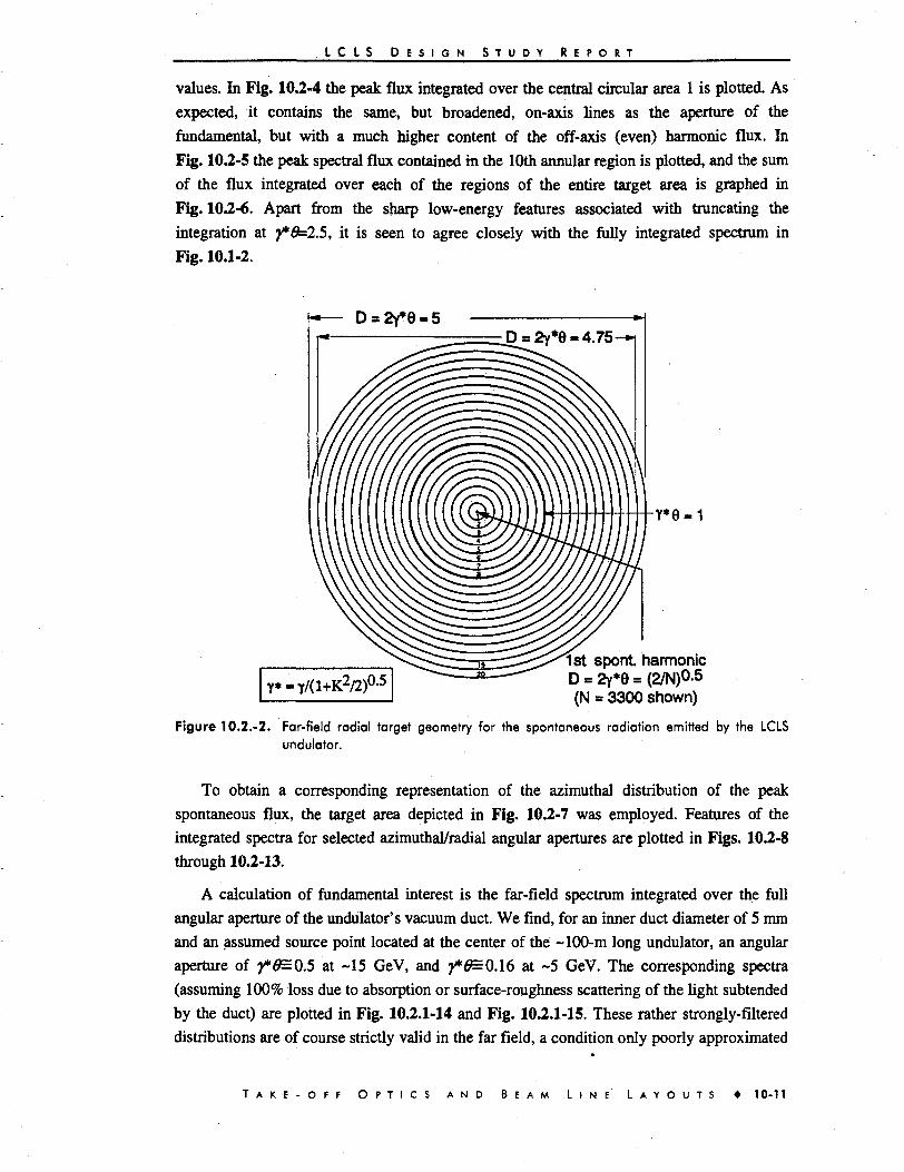
L C L S D E S I G N S T U D Y R E P O R T
values. In Fig. 10.2-4 the peak flux integrated over the central circular area 1 is plotted. As
expected, it contains the same, but broadened, on-axis lines as the aperture of the
fundamental, but with a much higher content of the off-axis (even) harmonic flux. In
Fig. 10.2-5 the peak spectral flux contained in the 10th annular region is plotted, and the sum
of the flux integrated over each of the regions of the entire target area is graphed in
Fig. 10.2-6. Apart from the sharp low-energy features associated with truncating the
integration at y*(h2.5, it is seen to agree closely with the fully integrated spectrum in
Fig. 10.1-2.
Y*0-1
1st spont. harmonicD = 2y*8 = (2/N)0.5(N = 3300 shown)
Figure 10.2.-2. Far-field radial target geometry for the spontaneous radiation emitted by the LCLSundulator.
To obtain a corresponding representation of the azimuthal distribution of the peak
spontaneous flux, the target area depicted in Fig. 10.2-7 was employed. Features of the
integrated spectra for selected azimuthal/radial angular apertures are plotted in Figs. 10.2-8
through 10.2-13.
A calculation of fundamental interest is the far-field spectrum integrated over the full
angular aperture of the undulator's vacuum duct. We find, for an inner duct diameter of 5 mm
and an assumed source point located at the center of the ~100-m long undulator, an angular
aperture of y* 6=0.5 at -15 GeV, and 7* ^ 0 . 1 6 at ~5 GeV. The corresponding spectra
(assuming 100% loss due to absorption or surface-roughness scattering of the light subtended
by the duct) are plotted in Fig. 10.2.1-14 and Fig. 10.2.1-15. These rather strongly-filtered
distributions are of course strictly valid in the far field, a condition only poorly approximated
T A K E - O F F O P T I C S A N D B E A M L I N E L A Y O U T S • 1 0 - 1 1

L C L S D E S I G N S T U D Y R E P O R T
by the present geometry of the LCLS (see Fig. 9.1-1). However, in the event of the
development of an ultra-long LCLS beam line (see Section 932) their relative accuracy will
be considerably improved. Prior to such a development, realistic distributions spectrally
filtered by the undulator's vacuum duct will need to be computed with a more valid near-field
radiation formalism (see Section 10.2).
810*
710"-
od
srIo
610*
510
10
310*
2 10*
1 10"
+—t—•—•:;—.*.—4.—i
±=i=*=l
.4...,
:i:
„_*.._;...
-t—t
E~jn~*™4" 4—i—i.!.X——i—i—
v.H4>.»>»-»...».4*.>^—4—; :—.;——I—^...4 j—;...«.—;—4.—j 4—4—«
• • • • •
T-"T—5—t—>.—y [—;—4-—I—"-—4—1—+—i 4—i—!—i i—i—
•!••-•••"<•—• • t - - ! •••••••-•••-
..J..™ .{.„. .
=f
20 30
Harmonic Number
40
Figure 10.2-3. LCLS spontaneous flux distribution integrated over the FWHM aperture of thefundamental.
8 10*
7 10*
00 6 10f
CO9 5 10
S 4 10w-
2 10".
1 10w-
0-
..J.....!....i..,.l.—'....1 ;....i_..j.
. .4.—j.. . .* » 4.—1 4 (.....—..j.—4...,
I • • . . I , , .
:i"l"":""i""t"""":i":!i"!"t""fc":i""i""i"!!i""i"!"n"i"~!"~t:"r~":~!i!!"i":
::::±::±:::fcn:~x::::i:::±:::!n:::n::x::::j:::±::nnn:::n±:±:::-•j-—j""|.~.j. ^-.—^..^.».).».».».>—.j....^.....t.....»-.^..>.)....^..-t..J...»..^...j...-
••••; 4—j....^—; 4—;—j....^ ^....j...
-*-•!--+•• ..4.—4....+.—I- »™2""£
10 20 30Harmonic Number
40
Figure 10.2-4. Spontaneous LCLS flux distribution integrated over a small aperture near the axis.
1 0 - 1 2 • T A K E - O F F O P T I C S A N D B E A M L I N E L A Y O U T S
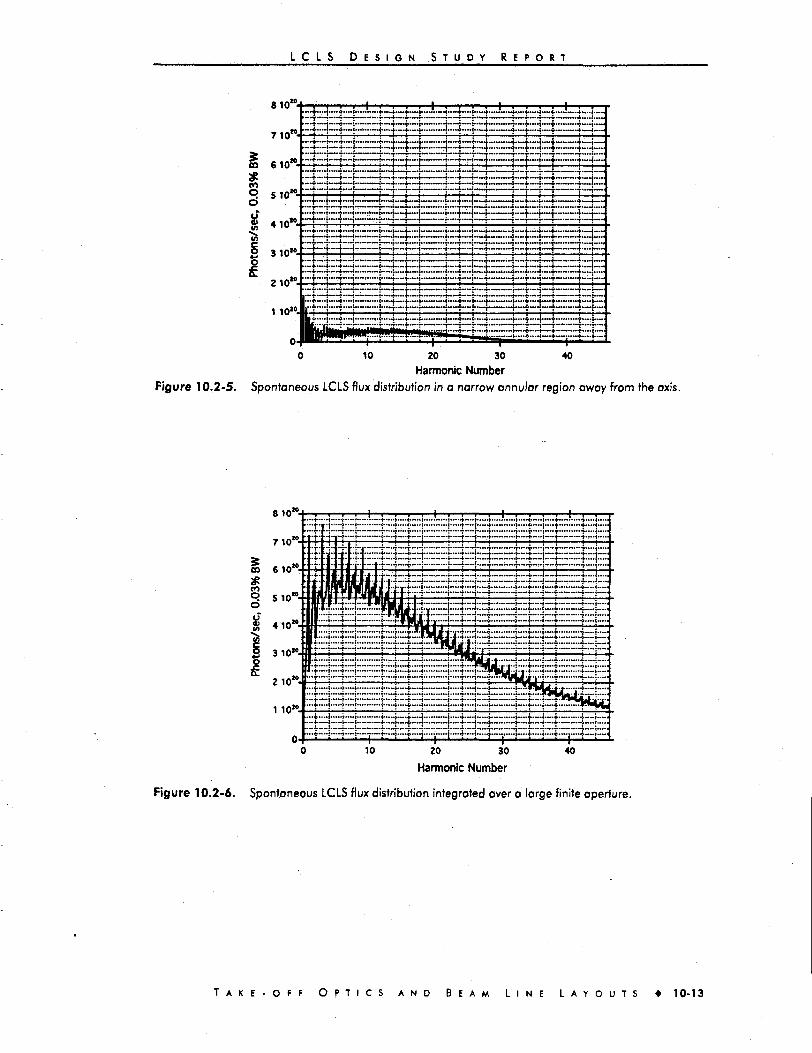
L C L S D E S I G N S T U D Y R E P O R T
810
I -j •• -4—«j««+.«....«4«~ j
20 30 40
Harmonic Number
Figure 10.2-5. Spontaneous LCLS flux distribution in a narrow annular region away from the axis.
••-J—*i—•
.......f.....^....^..«.f"""*"i—*4'">j'»«>-"—»
,i.....i,i-.r,r,.;i-.,ni-TT,i,...J .i
....,_...r::3.........,...t...;:::::;QE:
10 'Li—i.-i-i i-4....j.....i j"4:-i-..i _j j : j. ]'T^
-*- •+•-4—i-
10 20 30
Harmonic Number
40
Figure 10.2-6. Spontaneous LCLS flux distribution integrated over a large finite aperture.
T A K E - O F F O P T I C S A N D B E A M L I N E L A Y O U T S • 10-13

L C L S D E S I G N S T U D Y R E P O R T
A<|> a J I / 2 0 - H / • » - .
- • = 0
Figure 10.2-7. Far-field radial/azimuthal target geometry for the spontaneous radiation emitted by theLCLS undulator.
1 1010-
iCOqd
810". -
6 10". -
410*.
2 10"- •
—f—1
._i__j_._!__.
Jw.i.«-A....J.
-i-f-t-t-t"i [-•-- t -T -T~ : • - •
•f-i—i-"f~-
-f-r
._.^™+.._(...,
-t-t-H-.—i—(.—>—i..
-I—!•—>—'
"i"-t"tTt"rt-i-f-T-t
• ! • : • • • ;..+—t.-H..~4—i—+_..i—(.• • • • • t i i
. . . 1 . . . ] . .,..4....i™4...4....|—|™..j..4™j..-4...
! 4 t—-i J. j J.*...j.-.-^—
; ; : : i : ! : : i :
10 20 30
Harmonic Number40
Figure 10.2-8. Spontaneous LCLS flux distribution integrated over 0 . 0 < Y * 6 < 0 . 5 and 0<(|><Jt/20.
1 0 - 1 4 • T A K E - O F F O P T I C S A N D B E A M L I N E L A Y O U T S

L C L S D E S I G N S T U D Y R E P O R T
810"
Id
H+r-l-rH-t-f-H, ( , t [ t ! j j j , ,
•i^.^....j—:—;—4.—i—v—i—A-—;•..-!• I • I : : • • i : • ! • !
41 o'"+|-i—•-+-i~
2 1 0 " . •
t 7 1 t ,—[-—f—|—j—j—
20
Harmonic Number
Figure 10.2-9. Spontaneous LCLS flux distribution integrated over 0.0<7*6<0.5 and 9jc/20«|><7t/2.
1 10™
20 30
Harmonic Number40
Figure 10.2-10. Spontaneous LCLS flux distribution integrated over over 0 .5<7*6< l and 0<<|)<7t/20.
T A K E - O F F O P T I C S A N D B E A M L I N E L A Y O U T S • 10-15

L C L S D E S I G N S T U D Y R E P O R T
110™-
I
: : : : : : ; : ! ; : : :
10 20 30Harmonic Number
Figure 10.2-11. Spontaneous LCLS flux distribution integrated over over O.5<7*0<1 and9n/20«t)<7:/2.
....4....J...4...4...4...4.......4.........
H—i—t—j.—t—i—.»—j.—i—i—4—.
TT i j i i0 10 20 30
Harmonic Number
Figure 10.2-12. Spontaneous LCLS flux distribution integrated over over 1 <Y*8<2.5 and 0 « | > < J I / 2 0 .
1 0 - 1 6 • T A K E - O F F O P T I C S A N D B E A M L I N E L A Y O U T S

L C L S D E S I G N S T U D Y R E P O R T
1 10*
810"-~4~
I ! I I I I ! I 1 ! ! i I l l l l l l l l l
4 4 - 4 4 - 4 - 4 - 4 4 - 4 O - 4 - 4 - 4 - I - U -^4^4*™f—^•^••"j""t""h*H"''4"**^*"i""'h"*f"'i"^*"t"'4''W*"'4*"*i""
xiiprd 6io".-H-~i~4-
4 1 0 '
44444-i-U-U
—j.—1—1—1_ ^.—1—j.—1—1—*——1—j-~j—1—|—|.-
-t-r-t-t-t-r-f-r
• • i^ ^ 4
• i^H.t...^.>..
44• i •
4 4 4_| !__i I L4....L.4..4..
i ' ' ' ' ' ' ' '
:—1 f t I 1—1 r 1 j r , . , . . .-4"*j** i it""i""t i-~4—~.—[••••<•'"4 ••••i"—+""j"»'j""4"'M-'
J...I i L _ i _ | L_j L. i ! L L...1.™ : 1 f : ~ ! " : T : ™ : T_i j i i v.,
0 10 20 30
Harmonic Number
Figure 10.2-13. Spontaneous LCLS flux distribution integrated over over 1<Y*8<2.5 and
9;t/20«|><7i/2.
8 10*
710*
610*
4 10™-
310".
2 10".
1 10™.
0
T T 1 T ~ T I T I I i T I T T T I I I T • t * . . ,w — . . » - • £ . . . . • • — • — . . . • . . . ; •••••£ • • — • " — " J — - J - — - * J — - « - — • — — - £ — - j . — — . - - - j - - - j - — • ' „ . _ ,
—-?-•}—-}-"> ^—j—.j—» J...H...4..4 4.—4—4-—§ f-j-
:t:lj:t:::::t:;::::t,,..,_.;i.L . . . . . . . . . A . . * ^ . . . . . . . . . ^ . . * » % . . * • w . . « • > * . . . . . . . . ^ « . . • « • . . «
_— _ _.__ . __ _ T_ ._ ._ J . _ _ _ __ _ ._ . _._.Xmu-iJn.II.........H.—.i....i...••!..•.«.—>[.».n.—X....t..-•-•.«^....1 H>X.»«I . . • . . ] ! .i...«,T J...^|...*J M M t L.. .t™J™. 2 til.*....;—..*...2....:™I....;"... 2 L-«
^....^»....^......^..........^..^;.....m.^....^.....
20 30
Harmonic Number
40
Figure 10.2-14. Spontaneous far-field LCLS flux distribution integrated, over the angular aperture of the
LCLS undulator's vacuum duct at ~ 1 5 GeV.
T A K E - O F F O P T I C S A N D B E A M L I N E L A Y O U T S • 10-17

L C L S D E S I G N S T U D Y R E P O R T
BIO".
710*.
»..-;—j..,.,. >....),_t—1 >-_<-.»—, > • • • • , • • • • ,
— . { .H.^* •«• |> «..J«..^< •~>|*»*4> —™*l « W « W ^ « M | W " • ' «• • f" ••••*•«*> «-•
20 30Harmonic Number
Figure 10.2-15. Spontaneous far-field LCLS flux distribution integrated over the angular aperture of theLCLS undulator's vacuum duct at ~5 GeV.
10.2.2 Far-field Spontaneous Radiation Peak Power Density
To estimate the spontaneous power density distribution at a fundamental wavelength of
1.5 A, the total power contained in each circular or annular region of Fig. 10.2-2 was
calculated by integrating the spectrum associated with the region versus harmonic energy.
The curve connecting the corresponding values of power is plotted in solid black in
Fig. 10.2-16. The integral of this curve is plotted versus y*0 as the monotonically increasing
dashed line. As can be independently verified with simple analytical approximations [24,28]
the asymptotic value of the power density represents the total emitted spontaneous power.
The calculations have been done out to the 46th harmonic. The average power density over
each region is calculated by dividing the total power in that region by the corresponding
circular or annular area. The resulting power density values are connected by the
monotonically decreasing curve.
For reference, the peak coherent output power of the LCLS and its output power density
at a distance of 10 meters from the undulator exit are marked on the ordinate by arrows in
Fig. 10.2-16. Note that the peak spontaneous power density is only two orders of magnitude
smaller than the coherent power density. This is explained by the large number of additional
odd harmonics that exit along the same axis as the spontaneous fundamental. As noted in
Section 10.1, however, the power density in the coherent raw beam represents a lower limit
with respect to that attainable by additional focusing. If we assume that focusing down to the
theoretical diffraction limit can be attained, the upper limit on the attainable peak power
density of the LCLS will lie well in excess of 1Q25 W/cm2 as shown in Fig. 10.2-16.
Fig. 10.2-17 shows these curves and data points with the additional designation of this critical
limiting point.
1 0 - 1 8 • T A K E - O F F O P T I C S A N D B E A M L I N E L A Y O U T S
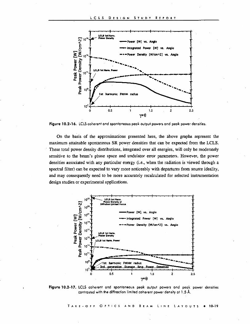
L C L S D E S I G N S T U D Y R E P O R T
1 ' 1A1!
<
> V)H* " io"+1 * 7
« in9..
LCLS 1«t Harm.Pemr Owwlly
•+•
——Power [W] vs. Angle
•••-Integrated Power [W] vs. Angle
—* -Power Density [W/cmA2] vs. Angle
LCLS 1«t Ham. Power
Figure 10.2-16. LCLS coherent and spontaneous peak output powers and peak power densities.
On the basis of the approximations presented here, the above graphs represent the
maximum attainable spontaneous SR power densities that can be expected from the LCLS.
These total power density distributions, integrated over all energies, will only be moderately
sensitive to the beam's phase space and undulator error parameters. However, the power
densities associated with any particular energy (i.e., when the radiation is viewed through a
spectral filter) can be expected to vary more noticeably with departures from source ideality,
and may consequently need to be more accurately recalculated for selected instrumentation
design studies or experimental applications.
LCLS 1»t Harm.Poww Density at
DMration Umitod Focui
-Power [W] vs. Angle
•Integrated Power [W] vs. Angle
— •—Power Density [W/cm*2] vs. Angle
Figure 10.2-17. LCLS coherent and spontaneous peak output powers and peak power densities
contrasted with the diffraction limited coherent power density at 1.5 A.
T A K E - O F F O P T I C S A N D B E A M L I N E L A Y O U T S • 10-19

L C L S D E S I G N S T U D Y R E P O R T
10.3 Bremsstrahlung Calculations
The radiation concerns related to the LCLS project fall into three distinct areas:
• Radiation safety
• Radiation background in experiments
• Machine protection
In each of these areas one or more of the following radiation sources needs to be
considered:
• Bremsstrahlung from beam/halo interactions with beamline components
• Gas bremsstrahlung
• Synchrotron radiation
• Neutrons
• Muons
• Induced activity
• Secondary electrons and positron
In this section we are concerned with radiation effects in the areas downstream of the
undulator, taking into account any relevant radiation source, located upstream, inside, or
downstream of the undulator. Potentially all sources listed above can contribute to the
radiation background in experiments. Machine protection mainly concerns possible radiation
damage to mirrors and collimators that will intercept the spontaneous synchrotron radiation
accompanying the laser beam proper. The radiation safety items include shielding, beam
containment system (BCS), and personnel protection system (PPS). Since the LCLS electron
beam power will be comparable to that of the FFTB, the existing enclosure and dump
shielding as well as PPS and BCS should be adequate without major modifications. New
designs of the three safety items are only required for the optics enclosure and experimental
hutch downstream of the electron beam dump. The ultimate goal is to have sufficiently
accurate estimates of radiation and their effects. Initial modeling of some of the dominant
sources has been completed, and the status of the calculations is summarized in the text
below. More comprehensive calculations, as described below, will be continued in the future.
10.3.1 Bremsstrahlung from Halo
Forward-directed bremsstrahlung can be produced by the interaction of the electron beam
halo with the protection collimators upstream of the undulator, with the undulator, and
possibly other beamline components downstream. Using the Monte Carlo transport code
FLUKA [29], one particular scenario has been simulated. In this case electrons are assumed
to hit the vacuum chamber at a very grazing angle near the undulator exit. The beam line
layout was simplified to a cylindrical-slab geometry, as represented schematically (not to
scale) in Fig. 103-1. Due to its length, the geometry in this figure is broken into two parts,
1 0 - 2 0 • T A K E - O F F O P T I C S A N D B E A M L I N E L A Y O U T S

L C L S D E S I G N S T U D Y R E P O R T
starting in the top left corner. The front face of the undulator (b) is the origin of longitudinal
coordinates describing the position of important components. In these simulations most of the
components are symmetrical relative to the beam line axis (shown as a dashed line). The two
sets of vertical and horizontal collimators (f) present their plane surfaces to the beam under a
very small angle and were therefore simulated in greater detail. The extent of the geometry in
the radial direction around the beam pipe is very constrained up to the experimental hutch (o).
Particles exceeding this radial limit are killed in order to save computation time, because they
have an extremely low probability of reaching one of the three scoring regions (n) in the
experimental hutch.
The high electron energy and the long distance between the undulator and the
experimental hutch (more than 30 m) require long computing times in order to achieve
sufficient statistics. Fig. 103-2 shows the poor dose score obtained behind a 20-cm thick lead
dump at the end of the line after simulating 106 histories, despite very high cutoffs and leading
particle biasing.
To improve statistics, importance biasing was implemented setting the relative
importances as a function of distance from the source based on the scored energy deposition
in the wall of the vacuum chamber (Fig. 10.3-3 and 10.3-4). The new result, corresponding to
5xl05 histories, is shown in Fig. 10.3-5. The dose on the front side of the same dump is
shown in Fig. 10.3-6.
100m
a-coHmatorsb-undulatorc - beam pipe wafld-undttetorende - cohfeei coflbfwtof
f-horizontal & verticalplane collimators
9 - attenuation chamberh - concrete shield of dumpI - Iron shielding of dumpj-dump cavity
k -l-SrrwnteadshWdof
optical hutchm - bremswahUmg dumpn - scoring regionso • optical hutch
Figure 1 0 . 3 - 1 . Features of the bremsstrahlung source/propagation model of the LCLS from the
undulator to the experimental area.
T A K E - O F F O P T I C S A N D B E A M L I N E L A Y O U T S • 10-21

L C L S D E S I G N S T U D Y R E P O R T
-1410
c
1 10-15
I «r»&A.
S3O
< * - r -
<> _ o
' t ' ' 1
80 1000 30 40 80
Figure 10.3-2 Tissue dose as a function of distance from the beam axis at the end of the experimentalhutch, behind the electron beam dump. Only leading particle biasing wasimplemented.
IE
I03
!
0 1000 2000 3000Distance from the end of the undulator (cm)
Figure 10.3-3. Energy absorbed per unit length in the vacuum chomber wall as a function of distancefrom the end of the undulator.
1 0 - 2 2 • T A K E - O F F O P T I C S A N D B E A M L I N E L A Y O U T S

L C L S D E S I G N S T U D Y R E P O R T
P10J
10° r-
r1
10-i _
10,-30 1000 2000 3000
Distance from the end of the undulator (cm)Figure 10.3-4. Relative region importances assigned as a function of distance from the end of the
undulator.
10,-14
Ii1I
10,-15
10-16
10-17
10,-18
10,-1920 40 60 80
Radial distance from beam axis (cm)100
Figure 10.3-5. Tissue dose as a function of distance from the beam axis at the end of the experimentalhutch, behind the dump. Leading particle biasing, windows and importance biasingwere implemented.
T A K E - O F F O P T I C S A N D B E A M L I N E L A Y O U T S • 1 0 - 2 3

L C L S D E S I G N S T U D Y R E P O R T
I•r-tO
c
I5 10 16
Radial distance from beam axis (cm)20
Figure 10.3-6. Tissue dose as a function of distance from the beam axis at the exit of the FFTB dumpshielding. Leading particle biasing, windows, and importance biasing wereimplemented.
In future work, calculations will be extended to include bremsstrahlung from collimators
upstream of the undulator.
10.3.2 Gas Bremsstrahlung
Gas bremsstrahlung will arise from beam interactions with the residual gas over a straight
portion of the beamline, starting near the end of the dogleg and comprising the undulator. A
length of about 130 m was considered. This is indeed a unique situation, since gas
bremsstrahlung is normally supposed to be an issue only in the straight sections of electron
storage rings. However, while on one hand the 0.1 /zA current of the LCLS electron beam
will be about a factor of 106 smaller than that found in storage rings, on the other hand the
assumed maximal residual pressure (10"7 Torr) will be 100-1000 times larger and the length
of the straight section will also be larger by two orders of magnitude. In addition, the electron
energy will be approximately two-to-three times that of existing high-energy storage rings
(dose from gas bremsstrahlung increases with more than the second power of energy). Based
on a number of Monte Carlo simulations, Ferrari et ah, [30] proposed an analytical formula to
•calculate dose rates from gas bremsstrahlung as a function of distance, length of the straight
section, air pressure, electron beam current, and electron energy. A simple extrapolation of
this formula would give 5 rem/h in the optical enclosure. However, it is not obvious that the
formula can be applied to the LCLS situation, i.e., extrapolated to such extreme straight
section lengths and energies. A full Monte Carlo simulation is planned in the near future.
1 0 - 2 4 • T A K E - O F F O P T I C S . A N D B E A M L I N E L A Y O U T S

L C L S D E S I G N S T U D Y R E P O R T
10.3.3 Muons
The 15 GeV electron beam terminating in the beam dump will be a non-negligible source
of muons. Preliminary estimates of muon dose rates behind the concrete and iron shielding of
the FFTB beam dump were done with the MUON89 code written by W.R. Nelson [31].
Approximately 6 m of iron shielding, in addition to the existing FFTB dump shield, would be
needed to bring the dose rate in the forward direction to 6 mrem/h, assuming that the beam
power is 3 kW. These estimates were confirmed by another simple method described by
Sullivan [32]. If the beam is directed, or deflected sufficiently in the downward direction, the
narrow maximum of the muon beam might emerge from the FFTB dump shield already
underground, in which case its shielding would be a lesser problem.
The MUON89 program, however, was designed for simple assessment of accelerator
shielding and is not suited for complex geometries. These could be investigated in the future
using the Monte Carlo code MUCARLO [33]. Another possibility is to couple two codes,
letting MUON89 or MUCARLO do the muon production and FLUKA the transport.
10.3.4 Future Work: Other Radiation Sources
Besides personnel protection issues in experimental hutches, transport of synchrotron
radiation is of interest for machine protection. A series of collimators will be inserted in the
LCLS photon beam line in order to eliminate as much as possible the spontaneous
synchrotron radiation from the useful laser beam. To minimize local heating, such collimators
will consist of slabs of an approximately cuboid shape tilted at a very grazing angle, and will
be coated with a very smooth and thin layer of gold. The energy deposition in such a thin
layer must be calculated. However, it will be necessary to implement in FLUKA reflection
and refraction properties of low-energy x-rays in addition to the existing normal interactions
at the level of a single atom.
To estimate neutron generation in the beam dump and other beamline components, we
plan to exploit the recently improved capability of FLUKA to simulate the whole
electromagnetic cascade, including photonuclear reactions, in any nucleus at all energies [34].
Accurate assessment of the neutron field, including thermal neutrons, is needed for both
personnel protection and experimental background.
Fluence and spectra of secondary electrons and positrons in experimental apparatus can
be readily obtained in FLUKA calculations concerning bremsstrahlung and other sources.
FLUKA also was used to assess activation of the undulator material and can be used for this
purpose in other beamline components.
Finally, the pulsed structure of the LCLS beam will require a study of the time
development of each component of the background fields. In principle, FLUKA can be used
to carry out such an analysis, but the task is expected to be demanding on staff and computer
resources.
T A K E - O F F O P T I C S A N D B E A M L I N E L A Y O U T S • 1 0 - 2 5

L C L S D E S I G N S T U D Y R E P O R T
10.4 Optical System
The x-ray optics system provides the interface between the LCLS undulator and the
experimental stations, and performs a number of critical functions, selected representations of
which are schematized in Fig. 10.4-1. This diagram, which depicts those functions that are
incorporated in the present design in solid blocks and a number of those that can be added
subsequently in dashed outline, provides a convenient basis for a general description of the
optical system and its components (see Fig. 10.4-2).
± ±Included in 1997design study
Not included Calorimetry
< [Spectrometry L
J PhaseSp'ace "j_; Profilometry ;
FEUParticle Beam Science
HighPeak
PowerControl
- f Calorimetry \-
{Spe
phase SpaceI Profilometry
PhotonBeam
Normalization and Source ControlFeedbacWFeedthrough
X-Ray Optics
• • To•*• Detectors,- » . Controlers
t!
X-Ray Science
Figure. 10.4-1. Functional diagram of the experimental and diagnostic capabilities of the LCLS x-rayoptics system.
EXPERIMENTAL H A U
FFTBSHIEUVBEAM DUMP
G«» AttenuationCell
LONG BEAMUNE AXIS
S«c«on
E ) SRCoKm«K«/Slit»
I SeamStopper
Figure 10.4-2. Schematic layout of LCLS x-ray optics system components. Drawing not to scale.
1 0 - 2 6 • T A K E - O F F O P T I C S A N D B E A M L I N E L A Y O U T S

L C L S D E S I G N S T U D Y R E P O R T
A convenient starting point is to take account of the high peak power of the LCLS pulses
and the potential damage they can cause. During the course of the design study, this led to the
assessment of two alternative ways of mitigating this problem: (1) a long beam line, and
(2) an absorption cell. The cell, chosen both for reasons of economy and for the immediate
opportunity it will afford for studying the interactions of FEL radiation pulses with matter,
will also provide readily controllable attenuation of the intensity from maximum down to
levels at which conventional diagnostic and experimental instrumentation, as well as
experimental samples, can be safely illuminated. This will enable the systematic study of both
the onset and overall extent of high peak power effects, a major initial goal of the LCLS
experimental program.
The following capabilities provided by the optical system are in the critical area of
spectral-angular filtering. For convenience, they may be classified into low-pass, high-pass,
and band-pass categories for the spectrum, and into equivalent aperture filters for the beam's
spatial and angular phase-space parameters. The two slit systems located upstream of the
absorption cell and downstream of the FFTB dump are designed to perform both spectral and
phase-space filtering functions. Operated together, they constitute a long and ultra-precise
collimator with an angular aperture adjustable down to a value of zero. Individually, they can
also be used as (spatial) apertures and high-pass spectral filters. One particularly important
application of these capabilities will be the separation of the (off-axis) spontaneous spectrum
from the coherent line by reflection and absorption, a critical prerequisite for selected
scattering experiments (e.g., in the absorption cell). In normal operation, the slits will also
pass the high-energy part of the spontaneous radiation, which propagates co-axially with the
FEL line. The separation of these two spectra can be accomplished with the basic low-pass
filtering component, the mirror. The corresponding (spectral/angular) bandpass filtering
function can be provided either by a (natural) crystal located in the crystal tank or by
multilayer reflectors in the mirror tank.
Due to the perceived importance of certain scattering and diffraction-based experiments
currently performed in the hard x-ray range at SSRL and elsewhere, one high-resolution
crystal monochromator, similar to the ones currently employed at SSRL for one of the
experimental end stations, will be provided. This will enable experiments of current interest
to be extrapolated to the new source parameters and then referenced to the broad base of data
and experience available at SSRL.
As indicated in Fig. 10.4-1, no optical means for (1) controlling the polarization,
(2) microfocusing, and (3) tailoring of the spatial and temporal parameters of the radiation
pulses were included in the present design. These are, however, critical capabilities for
important classes of experiments, and their implementation will be pursued in future phases
of the LCLS x-ray optics experimental program.
In the initial phase of the LCLS experimental program, perhaps the most critical function
of the x-ray optics system will be to provide diagnostic capabilities for the light emitted by
the undulator. Due to the availability of the absorption cell, these functions will be able to be
T A K E - O F F O P T I C S A N D B E A M L I N E L A Y O U T S • 1 0 - 2 7

L C L S D E S I G N S T U D Y R E P O R T
performed with conventional instrumentation. For example, analysis of the radiation spectrum
can be carried out by a crystal spectrometer in the <5 A range and by a reflection-grating
spectrometer at longer wavelengths. Calorimetry will be performed by conventional
instruments, which can either be purchased and adapted, or designed and fabricated at SLAC.
Phase-space diagnostics will be executed with suitable interference-based,
spectrophotometric, or spatial/temporal scanning/recording techniques.
In view of the enormous peak powers and electric fields emitted by the undulator, damage
to the specular beam line components (the slits and mirrors) is expected to be exacerbated by
. surface contamination, particularly by adsorbates forming irregular surfaces or otherwise by
those inducing a reflectivity drop at the angle and energy of the incoming radiation.
Suppression or prevention of these effects will involve maintaining an Ultra High Vacuum
(UHV) environment in the slit and mirror chambers, as well as providing capabilities for in
situ surface cleaning. A further requirement, in view of the 820-8200 eV range of the LCLS
fundamental, is the necessity for line-of-sight optics through to the experimental stations
(operation without windows). These requirements, as well as the vacuum isolation of the
absorption cell from the optics transport line, will be accomplished by suitably designed
Differential Pumping Sections (DPSs).
10.4.1 Differential Pumping Section
The provision for windowless (line-of-sight) radiation transport through the LCLS x-ray
optics system will be accomplished with conventionally implemented vacuum pumping at all
locations generating non-negligible gas loads and by special Differential Pumping Sections
(DPSs) bracketing all the chambers in which Ultra High Vacuum (UHV) environments need
to be maintained. The DPS chosen for this task [35] develops a large isolation ratio across its
length by effectively suppressing the "straight-through" molecular flux propagating along the
axis of its line-of-sight aperture. This flux component, which is usually the limiting factor in
the effective conductance of straight-through ducts, is blocked by generating a high-density
electron cloud along a section of the duct volume. The electrons, generated, trapped, and
accumulated by a structure similar to that of a conventional ion pump, ionize the propagating
molecules, allowing them to be deflected and trapped on getters or duct walls by various
well-known mechanisms [36]. A drawing of a typical pump structure (omitting the external
magnet) is shown in Fig. 10.4-3. The performance of the pump in isolating N2 ambient
pressures is shown in Fig. 10.4-4. In continuing the x-ray optics engineering studies, we will
optimize the DPS design for adequate pumping of the noble (and other) gases that may be
employed in the x-ray transport and optics systems.
1 0 - 2 8 • T A K E - O F F O P T I C S A N D B E A M L I N E L A Y O U T S

L C L S D E S I G N S T U D Y R E P O R T
Adapter Nipple Differential Pump(Magnet removed)
Throttle Tubes: Carry inserts withapertures up to 8 x 12 mm.The apertures are usually sizedto provide 1 mm clearance on allsides of the x-ray beam. Aperturescan be different sizes at the twoends of the pump.
4.5 CF Flange(Both ends)
Varian HViConnector
Adapter Cross
6 7 5 . 2.75 CF Flange
(Both ends)
J _Clear-Aperture Cenlerfine
Uil. Mounting Holes:0.32" dia. (4 places)
-0.63"-18.00'--21.00"- 8.00"-
Target Ball Socket,(4 places)
i I Clear-Aperture Centerline i-g
-a-""I
»-978M7A1S
. „ „ Clear-Aperture Centerline to1 -50 Mounting Bar Bottom Surface
4.5 CF Flange(2 places)
• 4.25".
2.77"
2.77"
Figure 10.4-3. Differential pump chamber and connecting flange geometry.
XIA Differential Pump Projection: DP-01
10-8
ICOCOCD
10"9
_ i i 11n i i j i i 1 1 i i i i j i i i i i n i j r i 1 1 i m
-Conductances: 15 cm Long x (shown dimensions-Exit Pump Speed: 50 l/s, Pumping N2
Bkg P (Torr)I Output P (Torr) ( 5.0 mm)- — Output P (Torr) ( 7.5 mm)
Output P (Torr) (10.0 mm)
o.tier10
o
10"11
Background Pressure -
i i i mill i i i mil l i i MI i i i in
1 0 -89-978347A14
1 0 -7 1Q-6 1 0 -5Input Pressure (Torr)
10-4
Figure 10.4-4. Projected differential pump performance curves for N2 versus aperture diameter.
Aperture length 15 cm.
T A K E - O F F O P T I C S A N D B E A M L I N E L A Y O U T S • 10-29

L C L S D E S I G N S T U D Y R E P O R T
10.4.2 X-ray Slits (Collimators)
At 15 GeV the x-ray beam entering the x-ray optics transport system following the beam
dump consists of an intense coherent EEL line with an FWHM angular divergence of ~1 /aad
(-9 /ffad at 5 GeV) surrounded by a broad spontaneous distribution with an FWHM angular
width of -100 /ffad (-310 //rad at 5 GeV). For particular experimental applications, the low
energy spontaneous radiation can constitute a noise source and needs to be removed. For
other applications, removal of the full off-axis spectrum may be required. These
considerations have led to the introduction of the two-slit-pair system shown in Fig. 9.1-2.
The first slit-pair is located just upstream of the absorption cell so that low energy
spontaneous radiation can be filtered out for scattering experiments located at the cell. The
second slit-pair, located -15 m farther downstream, can also be used as an independent
aperture, or combined with the first slit-pair to provide an angular collimator with an
extremely small acceptance, providing a broad range of spectral-angular filtering options,
including the delivery of quasi-monochromatic beams. As will become clear from the energy-
loading calculations presented below, an additional, equally important function of the slits
(when operated with suitable ancillary collimators) will be to protect the mirrors from
excessive peak power damage stemming from transient beam jitter.
The configuration of each slit-pair is schematized in Fig. 10.4-5. The basic strategy is to
control both the minimal aperture of each slit (ddv or ddh), as well as the angles of incidence
presented to the off-axis x-rays—tan'^duv-ddvl/L) or tan'^duh-ddJ/L). The basic structure of
each slit segment (jaw) consists of a low-Z substrate to minimize bremsstrahlung propagation,
coated with a high-Z material to maximize reflectivity at a given incidence angle (which in
the present design is assumed to be greater than the critical angle). The nominal materials
considered for our initial design studies were Al and Au. For the actual structure we propose
to use a modified version of an existing SLC collimator design as presently employed in the
SLAC beam switchyard for collimator C-0 and momentum slit SL-2 [37]. The modification
will replace the existing jaws, which have curved surfaces, with the geometry of Fig. 10.4-5.The most recent jaw design assumes a 0.5-m long block of Al heat-treated for exceptional
dimensional stability. The collirnating surface will be lapped flat to a low surface roughness
of 50-100 nm (rms). The high-Z material will be deposited onto this surface to a thickness of
a few-to-several Lim and polished. Although average power deposition will be modest and
cooling by thermal radiation appears acceptable, the jaws will nevertheless be water-cooled
for optimal dimensional stability during operation. In the existing chamber design, the jaws
are remotely adjustable by means of stepper motors and can be differentially adjusted to
control duv, ddV, dUh, and d^, as well as the average vertical and horizontal midplanes of the
slits. A maximal incidence-angle range of -0-1.5 mrad is envisaged, and the minimum
aperture size will be variable from 0 to >1 cm.
1 0 - 3 0 • T A K E - O F F O P T I C S A N D B E A M L I N E L A Y O U T S

L C L S D E S I G N S T U D Y R E P O R T
X-RAYS Vertical
HorizontalSlits
iow-Zsubstrate
high-Zcoating
Figure 10.4-5. LCLS x-ray slit configuration. Detailed geometry of facets not shown. Gap dimensionsduv- ddv duh< ddh independently adjustable.
Although the average x-ray beam power deposited into the jaws through the reflecting
surfaces is.expected to be quite small, the total cross section of the spontaneous radiation at
both slit locations will be significantly larger than the upstream slit apertures duv and duh. This
means that not only can one or more of the slits absorb most of the spontaneous x-ray power
during operation, but that most of it will impact the jaws' upstream faces at normal or near-
normal incidence. As calculated in Section 10.2, the spontaneous peak power density at
normal incidence can attain off-axis values within three orders of magnitude of that of the
coherent spectral line, which brings the peak power densities anticipated for the jaws to levels
at which little or no experimental data exist. Similar peak power levels in the high-Z
reflecting material (assuming ~99% reflectivity) can be expected for scenarios where the
LCLS coherent spectral line impacts the jaw surface, whether due to jitter or for other
reasons. For illustration, a list of characteristic absorption lengths for five high-through-low-Z
materials is shown for selected LCLS harmonic energies in Table 10.4-1. Based on the
tabulated values, energy absorption data for a block of tungsten were calculated and are listed
in Table 10.4-2. The peak power absorption value, after folding in a double-convoluted
Gaussian angular distribution, was found to be ~3 x 10¹³ W/cm3 for the coherent LCLS
fundamental. At this level of power loading, the total absorbed energy per pulse is high
enough to bring the temperature near to the melting range of tungsten. Should the incidence
angle attain substantially larger values (e.g., by the coherent striking one of the slit jaws'
upstream faces), the energy absorption could approach catastrophic values. For this reason,
additional protective apertures will be incorporated into the final slit assembly designs.
For the spontaneous harmonics, the total absorbed energy density per pulse is, even in
this worst-case limit, small enough to result in relatively safe temperature increases when
averaged over sufficiently long intervals of time. On the other hand, since for both the
T A K E - O F F O P T I C S A N D B E A M L I N E L A Y O U T S • 1 0 - 3 1

L C L S D E S I G N S T U D Y R E P O R T
fundamental and spontaneous radiation the absorbed energy is deposited in a time interval too
short for thermalization and diffusion processes to evolve, energy removal may proceed via
mechanisms that could induce alternative types of irreversible damage in the jaw materials.
Although there is some evidence of survival of mirrors exposed to very high specific power
densities from alternative sources, the processes that take place in the temporal and spectral
regimes of the LCLS [38] are still very poorly understood and more experimental and
theoretical studies will be needed.
Table 10.4-1. Normal-incidence 1/e absorption lengths (in \im) for W, Cu, Ti, Al, and C versus LCLSharmonic photon energy.
e-beam energy
[GeV]
5
5
5
5
5
15
15
15
15
15
15
15
15
15
15
15
15
15
15
15
15
15
15
15
15
15
Harmonic #
l<a)
3
5
7
9
l(a)
3
5
7
9
11
13
15
17
19
21
23
25
27
29
31
33
37
41
45
N/A
Photon Energy
fkeV]
0.825
2.475
4.125
5.775
7.425
8.25
24.75
41.25
57.75
74.25
90.75
107.25
123.75
140.25
156.75
173.25
1810.75
206.25
222.75
2310.25
255.75
272.25
305.25
339.25
371.25
500
W
0.108
0.195
0.592
1.36
2.57
3.36
13.9
53.2
128
54.9
91.8
141
203
280
369
473
590
720
861
1014
1176
1348
1711
2086
2470
3969
Cu
0.528
0.922
3.59
9.93
17.8
23.7
60
252
637
1227
1984
2837
3721
4584
5395
6140
6817
7433
7985
8491
8955
9383
10150
10830
11450
13480
Ti
0.245
4.11
16.4
4.69
9.95
11.9
259
1095
2650
4737
6994
9138
11040
12680
14080
15280
16330
17260
18090
18850
19550
20210
21410
22500
23520
27040
Al
2
2.86
11.4
210.4
60.7
82.4
1987
6969
12590
16990
20130
22420
24200
25670
26940
28070
29120
30090
31020
31910
32760
33590
35190
36730
38210
43630
C
1.24
210.1
136
378
809
1108
13880
21320
24620
26780
28500
30020
31410
32700
33920
35090
36200
37260
38290
39280
40230
41160
42930
44600
46180
51690
a. fundamental
1 0 - 3 2 • T A K E - O F F O P T I C S A N D B E A M L I N E L A Y O U T S
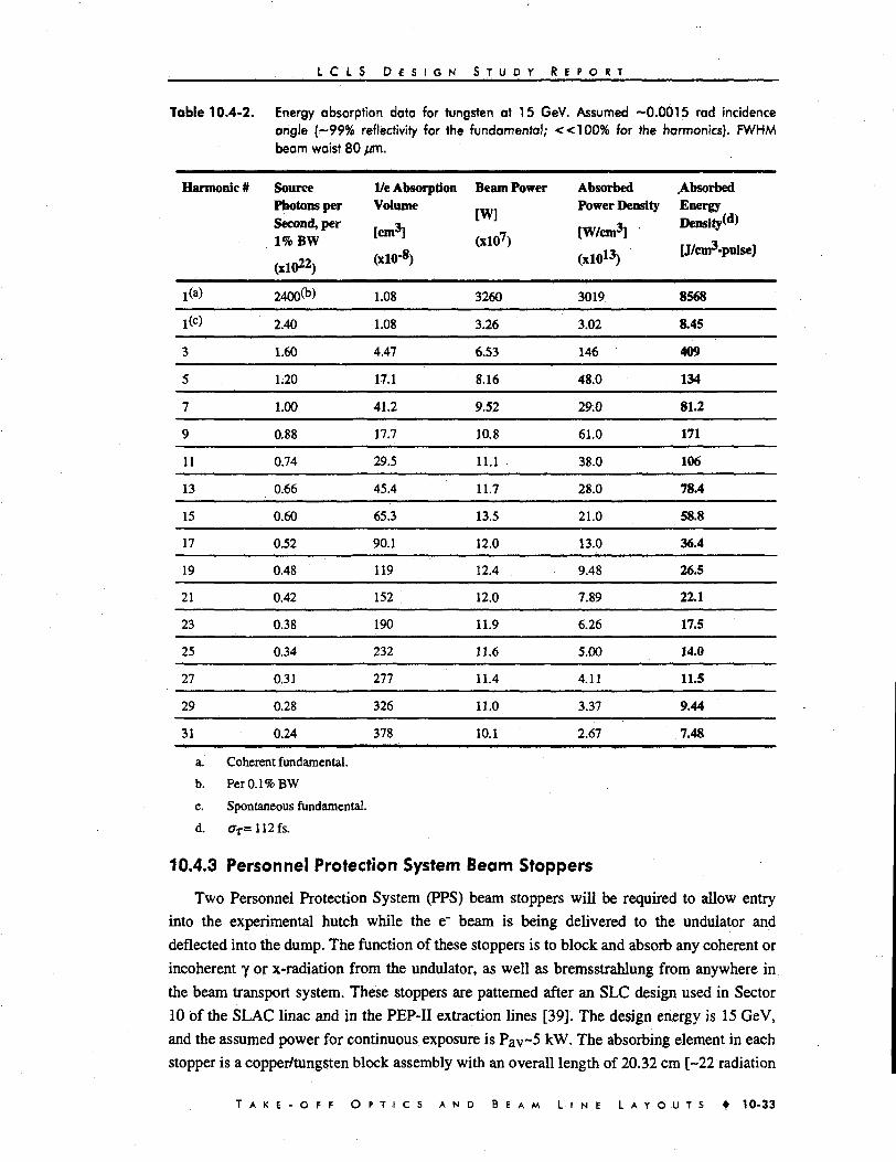
L C L S D t s i G N S T U O Y R E P O R T
Toble 10.4-2. Energy absorption data for tungsten at 15 GeV. Assumed ~0.0015 rad incidenceangle (~99% reflectivity for the fundamental; <<100% for the harmonics). FWHMbeam waist 80 //m.
Harmonic # SourcePhotons perSecond, per1%BW
(xlO22)
1/e Absorption Beam PowerVolume [ W ]
t C m 3 ] (xlO7)
Absorbed .AbsorbedPower Density Energy
Density<d>[W/cm3]
(xlO13)[J/cnr'-pulse]
l(a)
l(c)
3
5
7
9
11
13
15
17
19
21
23
25
27
29
31
2400^)
2.40
1.60
1.20
1.00
0.88
0.74
0.66
0.60
0.52
0.48
0.42
0.38
0.34
0.31
0.28
0.24
1.08
1.08
4.47
17.1
41.2
17.7
29.5
45.4
65.3
90.1
119
152
190
232
277
326
378
3260
3.26
6.53
8.16
9.52
10.8
11.1
11.7
13.5
12.0
12.4
12.0
11.9
11.6
11.4
11.0
10.1
3019
3.02
146
48.0
29.0
61.0
38.0
28.0
21.0
13.0
9.48
7.89
6.26
5.00
4.11
3.37
2.67
8568
8.45
409
134
81.2
171
106
78.4
58.8
36.4
26.5
22.1
17.5
14.0
11.5
9.44
7.48
a. Coherent fundamental.
b. Per 0.1% BW
c. Spontaneous fundamental.
d. crT=112fs.
10.4.3 Personnel Protection System Beam Stoppers
Two Personnel Protection System (PPS) beam stoppers will be required to allow entry
into the experimental hutch while the e" beam is being delivered to the undulator and
deflected into the dump. The function of these stoppers is to block and absorb any coherent or
incoherent y or x-radiation from the undulator, as well as bremsstrahlung from anywhere in
the beam transport system. These stoppers are patterned after an SLC design used in Sector
10 of the SLAC linac and in the PEP-II extraction lines [39]. The design energy is 15 GeV,
and the assumed power for continuous exposure is Pav~5 kW. The absorbing element in each
stopper is a copper/tungsten block assembly with an overall length of 20.32 cm [-22 radiation
T A K E - O F F O P T I C S A N D B E A M L I N E L A Y O U T S t 1 0 - 3 3

L C L S D E S I G N S T U D Y R E P O R T
lengths (Xo)]. The beam first encounters the 3.7 Xo long Cu section. The remaining 12.3 Xo
are provided by a block of free-machining tungsten (tungsten content - 90%, p ~ 17 g/cm^)
which is brazed to the Cu. The shower maximum of the electromagnetic cascade for 12-15
GeV occurs at a depth of 5.5-5.7 Xo. A built-in burn-through monitor is located at that z-
depth. It consists of a pair of cavities separated by a Cu diaphragm. The first cavity is
pressurized with dry N2- Its return line contains a pressure switch with the trip level set to
15 psig. Should excessive beam power be deposited in the stopper block, the diaphragm will
perforate, allowing the N2 to escape into the second cavity, which is open to atmospheric
conditions on the outside. The pressure switch will interrupt beam delivery within 2-3 linac
pulses. The transverse dimensions of the stopper block are 3.16 cm wide x 2.9 cm high. The
minimum radial attenuation distances are then, respectively, 3.5 Xo and 3.1 X o in the Cu
section and 7.7 Xo and 7.1 XQ in the free-machining tungsten. This is more than adequate to
attenuate the radial shower.
The absorber block can be vertically inserted or removed from the beam channel by
means of a remotely controlled air cylinder. The block has a water-cooled heat sink attached
to the top surface, which allows continuous and safe dissipation of up to 5 kW of beam
power.
A third stopper will be installed which is essentially an ordinary pneumatic valve with no
special heat-removal provisions. It is intended for protective insertion when the linac is
running in an ultra-low peak or average current mode, for which the average radiation power
is on the order of milliwatts or less.
10.4.4 Absorption cell
Attenuation of the coherent pulses of the LCLS can be accomplished by passage through
a gaseous, solid, or liquid medium. The nominal LCLS design is for a gas cell operated with
high pressure puff valves to introduce the absorbing gas into the path of the coherent FEL
photons (see Fig. 10.4-6, left). The axial dimensions of the chamber and the number of valve
nozzles must be adequate or numerous enough to allow a sufficient thickness of the gas to
provide four or more orders of magnitude of attenuation over the full range of the LCLS
fundamental energy (820 eV-8.2 keV). The combined axial and transverse dimensions are
determined by the requirement of maintaining an average vessel pressure of <0.0075 Torr,
corresponding to the Knudsen-through-molecular flow regimes [40]. This pressure, which
(for N2) is sufficiently low to be reduced to < 10"6 Torr by the differential pumping sections
bracketing the chamber [35], will be determined primarily by: (1) the average volume of gas
introduced into the chamber per puff, (2) its average pressure, (3) the axial conductance out
of the gas cell, (4) the chamber volume, (5) the puff valve repetition rate, and (6) the capacity
of the primary pump(s) connected directly to the chamber. A set of valve and vacuum
parameters for the absorption cell representing maximal loading conditions is listed in
Table 10.4-3. Initial design calculations show that the gas absorption will be able to support
1 0 - 3 4 • T A K E - O F F O P T I C S A N D B E A M L I N E L A Y O U T S

L C L S D E S I G N S T U D Y R E P O R T
initial operation of the LCLS at 120 Hz. Additional R&D will be required to optimize
performance of the pump for alternative gases [36] and nozzle geometries.
Although no comprehensive simulations of the interaction of the LCLS pulses with
candidate absorbing media have as yet been undertaken, the operation of the gas cell in the
weak-field (linear) regime using xenon as an absorber has been calculated for reference. In
Fig. 10.4-7 the absolute attenuation of x-rays through xenon for four given
pressure x tg [Torr-cm] products is plotted from 800 to 25000 eV. The curves indicate that a
7500 Torr Xe gas jet with tg - 1 cm would provide an attenuation factor of -1O4 for an input
intensity at which the absorption mechanisms are essentially unimolecular and linear. With
suitable design and a sufficiently low pulse repetition rate, the loading of the vacuum system
by the required amount of gas should be maintainable at acceptable levels.
PUFFVALVE LIQUID Ga
NOZZLE
X-RAYS,
fast- shutter
liquid..-•' stream
reservoirto pump
Figure 10.4-6. Schematized gas (left) and liquid (right) nozzle configurations for the LCLS absorptioncell.
Table 10.4-3. Absorption cell valve and vacuum parameters. Valve orifice width 250 jim; tg=lcm;gas jet height l m m .
Parameter
Valve Rep Rate [Hz]
Valve Pressure [Torr]
Particles/Puff
Chamber Pump Capacity [1/s]
Gas Load Q [Torr-ys]
Average Pressure [Torr]
120
7500
6.65 x 10¹⁷
1800
2.25
1.25 x 10'3
Value
12
7500
6.65 x 10¹⁷
1800
0.225
1.25 x 10⁻⁴
An alternative system with a substantially smaller vacuum loading effect could be based
on a liquid metal, such as gallium [41,42]. As schematized in Fig. 10.4-6 (right), the surface
T A K E - O F F O P T I C S A N D B E A M L I N E L A Y O U T S • 1 0 - 3 5

L C L S D E S I G N S T U D Y R E P O R T
area of a liquid stream exposed to the vacuum could, with proper reservoir and baffle design,
be kept small even with the use of continuous pumping, while the time-averaged vacuum
loading could be further reduced with suitably designed rotating beam shutters. In Fig. 10.4-8
a set of attenuation curves is plotted over the 800-25000 eV range for three values of tj. A jet
with a thickness controllable over a range of 0.1-1 mm, could evidently provide effective
attenuation over the entire fundamental-through-3rd-harmonic range of the LCLS.
0.01
-SQOO&Tofr-em10000 Tor-cm
IIo
-*•*••»—SOOQTdrr-ern™;?-
p -
10 •18
1000Photon Energy [eV]
Figure 10.4-7. Weak-field attenuation curves for xenon.
c 0.01o(0
c
— 0.5 mm0.4mm---0.01 mm
1000 104
Photon Energy (eV]
Figure 10.4-8. Weak-field attenuation curves for gallium.
As a third option, an attenuator system based on movable foils could also be employed
[20]. Such a system would be destructive, and would probably need to employ synchronized
1 0 - 3 6 • T A K E - O F F O P T I C S A N D B E A M L I N E L A Y O U T S

L C L S D E S I G N S T U D Y R E P O R T
shutters bracketing the foil to capture debris and inhibit contamination of the vacuum system.
Relatively frequent access to the absorption cell to replace the obliterated absorbing material
would also be required.
The absorption cell will be used for initial studies of scattering of the LCLS pulses by
absorbing media. The chamber design, predicated on the initial use of xenon, includes ports
for line-of-sight fluorescence detection, as well for the introduction of external magnetic and
electric fields. Due to its location inside the FFTB tunnel, provisions for a detector shielding
enclosure has been included (see Fig. 9.1-2).
A basic question, at this point is how the actual LCLS pulses, whose intensity and
degeneracy parameters lie well outside the regime of weak-field interactions, will interact
with candidate absorbing media. To resolve this question to the degree at which a satisfactory
prediction of the absorption cell's performance vis-a-vis its linear absorption characteristics
can be made, a number of physical processes, parameters, and effects must first be
theoretically analyzed, understood, and calculated. The primary parameters are the cross
sections of the various scattering and energy conversion processes encountered by the
radiation (see Fig. 10.4-9). At the field strengths of the LCLS, absorption mechanisms that
are ordinarily negligible for weak fields can become activated [43] and grow strong enough to
significantly influence the total absorption cross section. Potentially prominent ones include:
(1) multi-photon absorption or ionization, and (2) field (tunneling) ionization. A second set of
critical parameters includes the time constants associated with the various absorption and
scattering processes. Here a distinction is usually drawn between processes taking place at the
individual molecular level and those involving collective interactions. Again, the high field
strength and degeneracy parameter of the LCLS can complicate a quantitative assessment.
For example, if the spatial density of coherent photons is of the order of the absorber's atomic
density, it may be necessary to treat some or all of the ordinarily independent absorption
mechanisms as collective phenomena. In view of these and other complexities, the question of
how well various gaseous or liquid absorbers will attenuate the LCLS pulses in contrast to
weak-field radiation will probably be ultimately answerable only with actual experimental
measurements. Notwithstanding this, the curves presented in this section may be regarded, for
purposes of coarse estimation, as lower bounds on the actual (unimolecular) absorptivities,
primarily due to the activation of additional scattering mechanisms that are inoperable in the
weak-field regime.
Regarding the propagation of the pulses through the absorbing medium, in addition to the
above-mentioned cross sections, the dynamics and characteristic time constants of the
dominant energy-conversion channels in the absorbing medium must be known. In a broad
discussion of the physical interactions representative of a gas or liquid absorber, it is useful to
refer to six fundamental time constants: (1) Aticus, the temporal interval between LCLS
pulses (for 120 Hz operation, J«LCLS =8.33 ms); (2) ^uise, the FWHM temporal pulse length
(-233 fs); (3) t^ke, the FWHM temporal length of the average random spike contained in the
full FEL pulse (-0.25 fs); (4) TBL, the time constant associated with the fastest (electronic)
T A K E - O F F O P T I C S A N D B E A M L I N E L A Y O U T S • 1 0 - 3 7

L C L S D E S I G N S T U D Y R E P O R T
scattering, absorption, or ionization mechanisms (e.g., resonant scattering, single and multiple
photon ionization, tunneling ionization, multiple-photon scattering, etc.); (5) TF, the
characteristic duration of fluorescence processes; and (6) TA, the time constant of the longest
(collective) energy-conversion and thermodynamic processes in the medium (e.g.,
thermalization, charge neutralization, relaxation back to equilibrium, etc.). In general, the
relations Xspate< )uise<47LCLS and TEL<*F<TA will apply. An additional characteristic parameter
relevant to operation with a gas or liquid jet, is the flow velocity, which, if high enough, can
re-establish a locally neutral and equilibrated absorbing medium by the time of arrival of the
subsequent pulse.
spontaneousbeam
coherentbeam
(vertical) (horizontal)
siits Tabsorption ceil
\ Y V \
Figure 10.4-9. Energy-conversion and scattering channels for radiation passing through an absorbing
medium.
For an assumed static medium, the propagation of the LCLS pulses through the
absorption cell can be represented as in Fig. 10.4-10. A fundamental question to be resolved
for scientific experiments or pulse metrology utilizing the cell is the effect of its various
scattering and absorption processes on the temporal shape and the longitudinal and transverse
coherence of the pulses. Although to first order it can be assumed that there will be an
unscattered (as well as elastically scattered) fraction of photons [44] that will retain their
incoming coherence properties, an accurate quantitative estimate of this fraction may, for
various regimes of LCLS parameter space, be difficult to obtain [45]. Additionally, non-linear
absorption mechanisms may substantially modulate the photons' temporal distribution. For
example, apart from the non-linearities associated with high fields, those that collectively
saturate, or "use up" available electronic transitions can subject the downstream part of the
pulse to stronger absorptivities than its upstream end [46]. Finally, if the interval ATUCLS
becomes too short, the overall model for propagation will acquire additional complexity due
to the fact that the medium's state will bear the imprint of preceding pulses.
10-38 • T A K E - O F F O P T I C S A N D B E A M L I N E L A Y O U T S

L C L S D E S I G N S T U D Y R E P O R T
V)
CDI
I \, \% \
I V
i \
LCLS Pulse Train
i f EL
; \
J
J \1 \t \ r
1 \, Vi V
I \
8.33 16.66 25 33.33t[ms]
Figure 10.4-10. Response of a (static) gaseous (or liquid) medium to LCLS pulses. The FWHM widths %,tf, and tA (not drawn to scale) represent the medium's characteristic electronic,fluorescence, and equilibration time constants. tA here is assumed to be < -icis-
10.4.5 Mirrors
From the output parameters listed in Table 10.1-1 it can be estimated that a coherent
photon pulse at normal incidence can deposit of the order of 10-100 eV per atom for
absorptivities [47] and penetration depths typical of solid state materials in the x-ray range.
This level of energy loading, which is high enough to enhance the probability of irreversible
lattice damage, can pose a serious problem for optical elements that are expected to handle
more than a small number of pulses over their lifetimes.
A natural way of trying to accomplish this is by decreasing the angle of incidence, $h
with respect to the optical surface. This will not only dilute the power density inversely with
6i but the density of damage sites as well, compounding the effective improvement in the
optic's longevity. Should the required 0t prove to be impermissibly small, a configuration of
equal-# multiple reflectors, as shown in Fig. 10.4-11, could be used to increase the total
reflection angle, $r, to an acceptable value.
Figure 1 0 . 4 - 1 1 . Tandem-grazing-incidence reflector geometry. Rm is the reflectivity and
complex index of refraction of the mth reflector.the
T A K E - O F F O P T I C S A N D B E A M L I N E L A Y O U T S • 10-39

L C L S D E S I G N S T U D * R E P O R T
To assess the ultimate effectiveness of this approach, it is first necessary to analyze how
the distribution of deposited energy varies with $ and the material parameters of the optic in
question. Assuming an approximately equal absorption of energy in each reflector in
Fig. 10.4-11 (Rm=R-l for all m), a convenient expression for the absorbed energy density in
terms of the relevant optical parameters of the photon beam and reflecting medium, is easily
derived [20]:
J]A[eV/atom] =_ * peak e. n-R (10.4.1)
Here P ^ is the peak coherent power (Table 10.1-1), a? is the standard deviation of the
temporal pulse length, q is the electronic charge in MKS units, Dw [cm] is the beam diameter
at the optic, 4>[cm] *s the l/e penetration depth of the light into the material in a direction
normal to the surface, and # [cm"3] is the atomic density of the material. Since it is known
from first principles that the probability of lattice disruption will be high when the deposited
energy density is on the order of 1 eV/atom, our aim is to determine if parameters for grazing-
incidence reflection can be found for which T]A«l.
To establish this, the parameter if? needs to be quantitatively investigated as a function of
$i and the optical constants of the reflecting material. Following conventional analysis [48],
we define the TM and TE reflectivities
mpHti*etPy+kM > 2 ( i 0 + > ) 2 + j f c 2
and
-R P(C0Sflc0tflp) + P= KTM —— ———. (1 U.4.3)
p2(cos di cot 0( + p)2 + k2
Here
p = J^Tsin2^ - 25+^(sin2^ - 2S)2 + 4k21, (10.4.4)
and S and k axe, the decremental components of the complex index of
refraction n = 1 — 6 + ik. For this study, it is convenient to identify the "critical angle" 6ic,
the incidence angle for which sin 6 fc ~6 =(2<5)1/2. At this angle, the use of higher-Z
reflecting materials generally improves the reflectivity, since <? increases with Z and RTEOM)
generally increases for # < #«.. At the same time, since there is interest in the smallest feasible
incidence angles, there is also interest in the behavior of RTE(TM) for # « 6ic. Inserting this
condition into (Eq 10.4.2) and (Eq. 10.4.3) and expanding, gives [49]
1 0 - 4 0 • T A K E - O F F O P T I C S A N D B E A M L I N E L A Y O U T S

L C L S D E S I G N S T U D Y R E P O R T
(10.4.5)
which reveals the dependence of the reflectivity on the ratio k/Sia this limit. Since this ratio
drops rapidly for low-Z materials, for certain values of photon energy and 6i, the optimum
power loading performance may shift from high-Z to low-Z materials [50].
For the present study, the polarization of the incident light has been set to TE under the
assumption that it may be less conducive to the initiation of peak-field damage mechanisms
than TM. Fig. 10.4-12 shows the reflectivities of three candidate reflecting materials: an Au
(high-Z), Ni (medium-Z), and Be (low-Z) in for three representative values of the LCLS'
coherent fundamental and -3rd harmonic lines (900 eV, 8500 eV, and 30000 eV). The
physical constants for the calculations were generated using the recently installed
XREFLECTION utility at SSRL [51]. As expected, the 3 db rolloff angle at each energy
increases with Z.
Next, denoting the wavelength of the incident radiation by X, and taking 6p = Xp/47lk ,
J]A (Eq. 10.4.1) is plotted versus 6{ for the same set of materials and photon energies, in
Fig. 10.4-13. The curves clearly exhibit the aforementioned interplay between the atomic
number Z, 0j, and n as a function of photon energy. Thus, while Be is seen to offer superior
performance at energies >2.6 keV, its performance at 1 keV is greatly inferior to that of the
higher-Z materials. The selection of materials and mirror parameters for the LCLS can
proceed on the basis of the information shown in Figs. 10.4-12 and 10.4-13. Selecting, e.g.,
T]A < 0.01, a criterion suggested by earlier experimental work at SSRL [52], for example, an
Au-coated mirror with $-0.0001 for energies <3 keV, and a Be-coated reflector with
$-0.0005 for all energies >3 keV may be selected. The general result is that, for acceptable
power-loading performance, the optimal Z of the materials utilized for the specular optics
(slits, mirrors, diffraction gratings, etc.) on the LCLS beam lines will depend on the spectral
regime in which they operate.
The theoretical results arrived at need to be integrated with a number of practical
considerations in developing a mirror design. First, due to the high power and peak fields of
the LCLS pulses, the issue of surface roughness is of paramount importance. As it is clear
from Eq. 10.4.1 and the performance graphs, even a minor degradation of R (which decreases
exponentially with the square of rms roughness) can drive r]A rapidly to values in excess of 1.
Thus, not only does the selected mirror material need to exhibit acceptable power loading
performance in the ideal limit, but it must also be polishable down to rms roughnesses in the
range of 1-3 A. Second, the value of 0/ will define, for a given Dw, the required length of the
mirror, in this respect the mirror length will be quite sensitive to the actual value of rjA at
which the mirror is operated. Thus, in order to avoid the use of extremely long mirrors (e.g.,
>1 m) it will be important to identify and utilize those high-Z materials that exhibit the least
amount of damage over time. Finally, for similar reasons, the use of materials with surfaces
T A K E - O F F O P T I C S A N D B E A M L I N E L A Y O U T S • 1 0 - 4 1
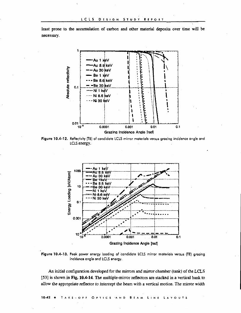
L C L S D E S I G N S T U D Y R E P O R T
least prone to the accumulation of carbon and other material deposits over time will be
necessary.
3ri
0.1
0.01
•Au 1 kjeV-Au 8.6JkeV•Au3o|<eVBe1 kjeV
•Be8.6JkeV-Be 30 iteV
-NJ 1 ktfVNi 8.6 |ceVNi30keV
0.0001 0.001 0.01
Grazing Incidence Angle fracfl
0.1
Figure 10.4-12. Reflectivity (TE) of candidate LCLS mirror materials versus grazing incidence angle andLCLS energy.
_ 1000—Au t key
nn.:».M»..« »
•=• 10
i5
I>> °'1<D
0.001
10
Au30k6V
• • • Be 8.6 kjeV
Ni 1 keV|
---Ni30keV
0.0001 0.001 0.01
Grazing Incidence Angle [rad]
0.1
Figure 10.4-13. Peak power energy loading of candidate LCLS mirror materials versus (TE) grazingincidence angle and LCLS energy.
An initial configuration developed for the mirrors and mirror chamber (tank) of the LCLS
[53] is shown in Fig. 10.4-14. The multiple-mirror reflectors are stacked in a vertical bank to
allow the appropriate reflector to intercept the beam with a vertical motion. The mirror width
1 0 - 4 2 • T A K E - O F F O P T I C S A N D B E A M L I N E L A Y O U T S

L C L S D E S I G N S T U D Y R E P O R T
(shown as a nominal 4 cm) allows a large degree of mitigative redundancy against surface
damage by repeated vertical displacements. The length L of each facet is determined by the
value of $i utilized for its particular reflector. Provisions for UHV pumping and in situ
cleaning [54], which may prove to be critical to the practical longevity of the reflectors, are
included. For illustrative purposes, a set of nominal mirror dimensions and mirror bank
parameters is listed below in Table 10.4-4. Evidently, facet length will be a sensitive
parameter for higher-Z reflecting materials, and the initial design parameters of the mirror
enclosure may need to be revised, or additional enclosures added, to accommodate multiple
reflectors.
Vertical Translation
In-SituCleaning Access
u Vacuum PumpingAccess
Reflected Photons(@ 12|)
Figure 10.4-14. LCLS mirror chamber geometry.
Table 10.4-4. LCLS mirror bank parameters. Dw~100 mm.
Mirror
Material
Beryllium
Gold
Energy Range
3-30 keV
<3keV
m
1
2
L[m]
0.25
1
$[rad]
0.0004
0.0001
0rfrad]
0.0004
0.0004
[eV/atom]
6-0.12
200
In view of the importance of specular reflection, fundamental areas of investigation
include the theory and modeling of the interaction of ultra-intense, ultra-short x-ray pulses
with matter [45]. Such studies, coupled with selected experimental investigations, are needed
to shed light on a number of physical effects with the potential of inducing damage. These
include radiation field/surface interactions versus surface roughness and surface
contaminants; radiation/surface interactions as a function of polarization; photoemissive
T A K E - O F F O P T I C S A N D B E A M L I N E L A Y O U T S • 1 0 - 4 3

L C L S D E S I G N S T U D Y R E P O R T
surface stresses induced by radiation pulses; and bulk and surface ionization-related damage
effects. Regarding the mirror tank and the mirrors, engineering R&D will be required for the
ongoing identification and study of alternative mirror materials with optimal properties, the
development of adequate in situ cleaning processes for those that are selected, and the
fabrication, polishing, and testing of prototypes.
10.4.6 Crystals
In view of the broad-based scientific case developed over the last 4 years for an x-ray
FEL [55,56,57,58], the use of crystals and crystal-based instrumentation will undoubtedly
prove to be critical to the ultimate productivity of the LCLS. Depending on the unit cell
structure of the material and its lattice spacing, a number of candidates can efficiently diffract
LCLS radiation in the <3-5 A wavelength range, for which a broad depth of experience has
been acquired at storage ring SR and other facilities over the last 20 years. In recent years in
particular, the development of established techniques for crystal-based instrumentation design
[59] has been brought to a state of reliable maturity at 3rd and earlier-generation SR facilities
[60,61,62]. Singular enhancements in practical crystal performance have been brought about
by two relatively recent technological advancements: (1) the development of perfect (mosaic-
free) Si and C crystals, and (2) the introduction of cooling techniques that can operate
diamond crystals at temperatures at which the sensitivity of lattice distortion to heat loading is
drastically minimized [63]. Given the evident promise of crystal technology for LCLS
applications, it is important to assess whether or not the unprecedented peak power densities
of the LCLS could be expected to inhibit its use.
Assuming a crystal cut to a thickness equal to its extinction depth, te [64], and using a set
of simple conservative assumptions to obtain an estimate of power and energy loading. The
assumptions are: (1) the angles of incidence of the radiation (with respect to the surface
plane) are large enough to enforce negligible reflection; (2) on the average, the diffracted
beams travel through approximately the same distance in the material as the Oth order beam;
and (3) on average, the absorption depth, tA, for the diffracted beams is the same as for the
incoming beam. Under these conditions, an expression for the energy loading of the crystal
material (in eV/atom), analogous to Eq. 10.4-1, is straighforwardly derived:
(10.4.6)
Table 10.4-5 shows selected physical constants [63] and TJA for various crystal plane
orientations for Be, C, and Si. The lower absorptivities of the lower-Z materials result in
substantially lower energy loading, in fact down to levels comparable to those that were
presumed marginal for the mirror materials in Section 10.4-5. On the other hand, even at
1.5 A, it is evident that carbon (i.e., diamond), ostensibly the material of choice, is beginning
1 0 - 4 4 • T A K E - O F F O P T I C S A N D B E A M L I N E L A Y O U T S
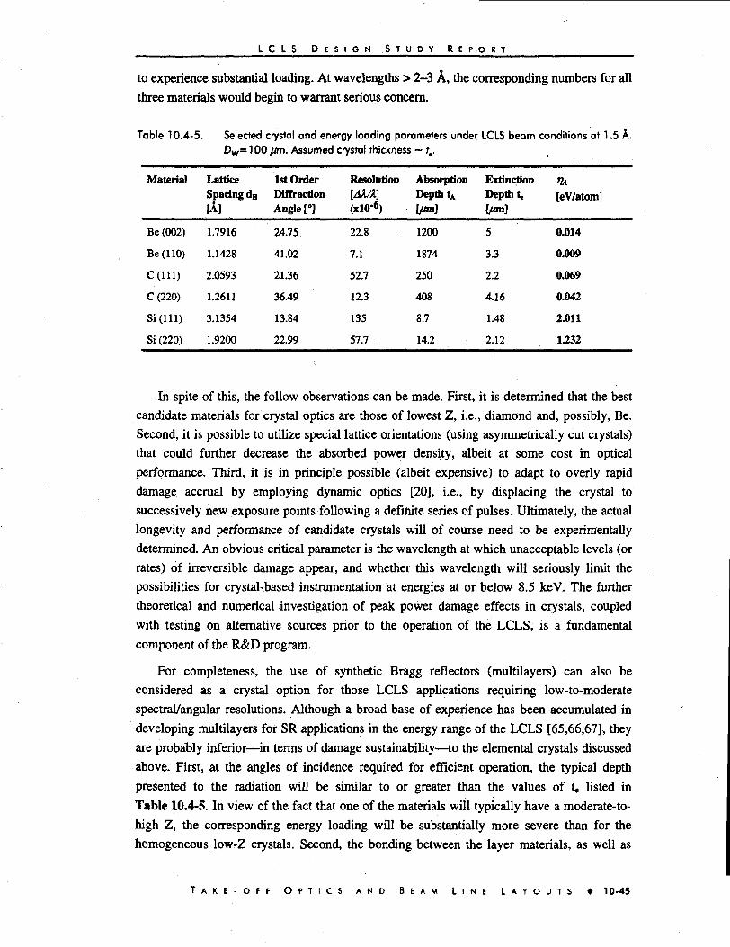
L C L S D E S I G N S T U D Y R E P O R T
to experience substantial loading. At wavelengths > 2-3 A, the corresponding numbers for all
three materials would begin to warrant serious concern.
Table 10.4-5. Selected crystal and energy loading parameters under LCLS beam conditions at 1.5 A.Dw= 100 ftm. Assumed crystal thickness ~ tt.
Material
Be (002)
Be (110)
C( l l l )
C (220)
Si (111)
Si (220)
LatticeSpacing dH
lA]
1.7916
1.1428
2.0593
1.2611
3.1354
1.9200
1st OrderDiffractionAngle [°]
24.75
41.02
21.36
36.49
13.84
22.99
Resolution[AM](xW6)
22.8
7.1
52.7
12.3
135
57.7
AbsorptionDepth tA
turn]
1200
1874
250
408
8.7
14.2
ExtinctionDepth t,turn]
5
3.3
2.2
4.16
1.48
2.12
1A.
feV/atom]
0.014
0.009
0.069
0.042
2.011
1.232
In spite of this, the follow observations can be made. First, it is determined that the best
candidate materials for crystal optics are those of lowest Z, i.e., diamond and, possibly, Be.
Second, it is possible to utilize special lattice orientations (using asymmetrically cut crystals)
that could further decrease the absorbed power density, albeit at some cost in optical
performance. Third, it is in principle possible (albeit expensive) to adapt to overly rapid
damage accrual by employing dynamic optics [20], i.e., by displacing the crystal to
successively new exposure points following a definite series of pulses. Ultimately, the actual
longevity and perfonnance of candidate crystals will of course need to be experimentally
determined. An obvious critical parameter is the wavelength at which unacceptable levels (or
rates) of irreversible damage appear, and whether this wavelength will seriously limit the
possibilities for crystal-based instrumentation at energies at or below 8.5 keV. The further
theoretical and numerical investigation of peak power damage effects in crystals, coupled
with testing on alternative sources prior to the operation of the LCLS, is a fundamental
component of the R&D program.
For completeness, the use of synthetic Bragg reflectors (multilayers) can also be
considered as a crystal option for those LCLS applications requiring low-to-moderate
spectral/angular resolutions. Although a broad base of experience has been accumulated in
developing multilayers for SR applications in the energy range of the LCLS [65,66,67], they
are probably inferior—in terms of damage sustainability—to the elemental crystals discussed
above. First, at the angles of incidence required for efficient operation, the typical depth
presented to the radiation will be similar to or greater than the values of U listed in
Table 10.4-5. In view of the fact that one of the materials will typically have a moderate-to-
high Z, the corresponding energy loading will be substantially more severe than for the
homogeneous low-Z crystals. Second, the bonding between the layer materials, as well as
T A K E - O F F O P T I C S A N D B E A M L I N E L A Y O U T S • 1 0 - 4 5
L C L S D E S I G N S T U D Y R E P O R T
their internal homogeneities are, on the average, substantially poorer than in perfect crystals,
leading to the acceleration of damage mechanisms [68]. Finally, the disparity between the
bulk and surface properties of the substrate (which would almost certainly need to be a low-Z
material such as Be or C) and the multilayer constituents could also be expected to contribute
to the activation or exacerbation of irreversible damage processes. Nonetheless, the exposure
of multilayers to the LCLS pulses is of inherent interest, and the operation and investigation
of multilayers at the LCLS is expected to become a continuing R&D activity.
10.5 Beam Line Optical Instrumentation
The beam line optical instrumentation may be classified into two categories:
(1) conventional instrumentation, intended for operation in conjunction with the absorption
cell; and (2) instruments and components specially designed or developed to handle the peak
power density of the coherent light. Each of these may be further subdivided according on the
spectral range that is involved (see Section 9.3.1). In category (1), custom-designed or
commercially available monochromators, spectrometers, interferometers and calorimeters can
be employed, both to perform beam diagnostics and to support initial experiments. The
second category of instrumentation, which will be developed as experience with the
unprecedented x-ray power densities is acquired, will be designed both for particular
experimental applications, as well as to further control and enhance the spectral-angular,
temporal, polarization, and coherence properties of the LCLS beam [20]. The design of such
components (e.g., monochromators, interferometers, beam splitters, etc.) is expected to
present both significant challenges and opportunities. For example, the diffraction-limited
transverse source volume of the LCLS should allow the development of simple
monochromator configurations in which the beam source serves as the entrance aperture. At
the same time, special care may need to be exerted in the use of diffraction gratings in the
specular wavelength regime (>3-5 A). For example, their ordinarily sharp-featured grooves
may need to be made smooth to mitigate against high edge-field effects, and the usual
transverse orientation of the grooves with respect to the light may need to be switched to a
conical diffraction geometry. As another example, the development of microfocusing optics
[52,69] aimed at approaching the diffraction-limited waist size is an extremely challenging
goal, which if pursued diligently enough, could substantially extend the range of scientific
applications at the LCLS. Due to potential damage effects and the extreme brevity of the
radiation pulses [70], special techniques such as transverse or longitudinal beam expansion
and compression, spectral filtering, or novel elements such as multi-phase or dynamical
optics, may need to be developed to attain the desired spectral profiles, resolving powers, and
efficiencies. Current and projected R&D activities in this area include: (1) theoretical and
computer investigations of short-pulse effects, instrumentation concepts and systems; and
(2) demonstration experiments on optical components to investigate limiting effects related to
coherence, specular and interfacial scattering, and peak power damage. A number of valid
experiments in these areas could be initiated at emerging longer-wavelength FEL or plasma
x-ray laser facilities [55,71,72].
1 0 - 4 6 • T A K E - O F F O P T I C S A N D B E A M L I N E L A Y O U T S

L C L S D E S I G N S T U D Y R E P O R T
10.6 References
1 K.-J. Kim, "Three Dimensional Analysis of Coherent Amplification and Self-AmplifiedSpontaneous Emission in Free-Electron Lasers," Phys. Rev. Lett. 57(13), 1871 (1986).
2 J. B. Murphy, C. Pellegrini, "Introduction to the Physics of the Free Electron Laser," in Frontiersof Particle Beams, M. Month, S. Turner, eds., Lecture Notes in Physics No. 296, H. Araki et al.,eds., Springer-Verlag, Berlin, 1988, pp. 163-212.
3 Y. H. Chin, K.-J. Kim, M. Xie, "Three dimensional theory of the small-signal high-gain free-electron laser including betatron oscillations," Phys. Rev. A, 46(10), 6662 (1992).
4 R. Bonifacio, L. DeSalvo, P. Pierini, N. Piovella, C. Pellegrini, "Spectrum, temporal structureand fluctuations in a high gain free electron laser starting from noise," Phys. Rev. Lett. 73(1), 70(1994).
5 W. M. Fawley, "Output characteristics of SASE-driven short wavelength FEL's," SPIEProceedings 2988, 98 (1997).
6 R. Bonifacio, F. Casagrande, "Instability threshold, quantum initiation and photo statistics inhigh-gain free electron lasers," Nucl. Instrum. Meth. A237, No. 1-2,168 (1985).
7 R. L. Gluckstern, H. Okamoto, S. Krinsky, "Saturation of a high gain FEL," Proceedings of the1993 Particle Accelerator Conference, IEEE Cat. No.93CH3279-7, vol. 2,1545 (1993).
8 H. P. Freund, "Nonlinear theory of short-wavelength free-electron lasers," Phys. Rev. E 52(5),part B, 5401 (1995).
9 L.H. Yu, C. M. Hung, D. Li, S. Krinsky, "Scaling function for free-electron-laser gain includingalternating-gradient focusing," Phys. Rev. E51(l), 813 (1995).
10 M. Xie, "Design optimization for an X-ray free electron laser driven by SLAC linac,"Proceedings of the 1995 Particle Accelerator Conference, IEEE Cat. No.95CH35843, vol. 1, 183(1995).
11 Nuhn, H.-D. et al., "Alignment and magnet error tolerances for the LCLS X-ray FEL," ibid., p.231.
12 E. L. Saldin, E. A. Schneidemiller, M. V. Yurkov, "Statistical Properties of Radiation from VUVand X-ray Free Electron Laser," DESY Technical Note TESLA-FEL 97-02, April 1997.
13 J. W. Goodman, Statistical Optics, John Wiley & Sons, New York, 1985.
14 L. Mandel, E. Wolf, Optical Coherence and Quantum Optics, Cambridge University Press, 1995,ch. 4.
15 M. Born, E. Wolf, Principles of Optics, Pergamon Press, Oxford, 1975, ch. 10.
16 R. Tatchyn, J. Arthur, "Phase Space and Coherence Properties of an X-ray FEL Source," inpreparation.
17 K.-J. Kim, "A New Formulation of Synchrotron Radiation Optics Using the WignerDistribution," SPIE Proceedings 582, 2 (1986).
18 R. Coisson, "Some Remarks on Coherence and Degeneracy," in Proceedings of the Workshop onPEP as a Synchrotron Radiation Source, SSRL Report 88/06.
19 N. Wiener, Generalized Harmonic Analysis, and Tauberian Theorems, M.I.T. Press, Cambridge,Mass., 1966, pp. 57 et ff.
20 R. Tatchyn, "LCLS Optics: Technological Issues and Scientific Opportunities," in Proceedings ofthe Workshop on Scientific Applications of Short Wavelength Coherent Light Sources, SLACReport 414; SLAC-PUB 6064, March 1993.
21 J. D. Jackson, Classical Electrodynamics, John Wiley & Sons, New York, 1975, ch. 14.
T A K E - O F F O P T I C S A N D B E A M L I N E L A Y O U T S • 1 0 - 4 7
L C L S D E S I G N S T U D Y R E P O R T
22 R. Tatchyn. A. D. Cox, S. Qadri, "Undulator Spectra: Computer Simulations and Modeling,"SPIE Proceedings, 552,47(1986).
23 R. Walker, "Near field effects in off-axis undulator radiation," Nucl. Instrum. Meth. A267, 537(1988).
24 K.-J. Kim, "X-ray Sources," in Center for X-ray Optics X-ray Data Booklet, D. Vaughan, ed.,LBNL PUB-490 rev., April 1986, pp. 4-1-4-17.
25 R. Tatchyn, "Simple approximations to transverse wiggler spectra integrated over finite aperturesin the wiggle plane," Nucl. Instrum. Meth. A336, no. 1-2,361 (1993).
26 R. J. Dejus, I. Vasserman, E. R. Moog, E. Gluskin, "Phase errors and predicted spectralperformance of a prototype undulator," Rev. Sci. Instrum. 66(2), pL 2,1875 (1995).
27 Yu. M. Nikitina, J. Pflueger, "Influence of magnetic field errors on the spectrum of the PETRAundulator," 10th National Synchrotron Radiation Conference (SR'94). Held: Novosibirsk, Russia11-15 July 1994. Nucl. Instrum. Meth. A359, no.1-2, 89(1995).
28 J. D. Jackson, Classical Electrodynamics, John Wiley & Sons, New York, 1975, pp.677-678.
29 A. Fass6 et al., "FLUKA92," Proc. ofSARE-1, Santa Fe Jan. 11-15, 1993, Ed. A. Palounek, LosAlamos LA-12835-C (1994), p. 134.
30 A. Ferrari, M. Pelliccioni, P.R. Sala, "Estimation of fluence rate and absorbed dose rate due togas bremsstrahlung from electron storage rings," Nucl. Instrum. Meth. B83, no. 4,518 (1993).
31 W.R. Nelson; Y. Namito, Computer code MUON83.MORTRAN, SLAC Radiation PhysicsDept., 1981.
32 A. H. Sullivan, "A Guide to Radiation and Radioactivity Levels near High Energy ParticleAccelerators," Nucl. Tech. Publishing, 1992.
33 L.P. Keller, "Muon background in a 1.0 TeV Linear Collider," SLAC-PUB 6385, 1993.
34 A. Fassd, A. Ferrari, P.R. Sala, "Total Giant Resonance Photonuclear Cross Sections for LightNuclei: a Database for the FLUKA Monte Carlo Transport Code," presented at SATIF-3, Sendai,12-13 May 1997.
35 Differential Pump DP-01, XHA X-ray Instrumentation Associates, Mountain View, CA 94043.
36 J. F. O'Hanlon, A User's Guide to Vacuum Technology, John Wiley & Sons, New York, 1980.
37 D. R. Walz, A. McFarlane, E. Lewandowsky, J. Zabdyr, "Momentum Slits, Collimators, andMasks in the SLC," Proceedings IEEE 1989 Particle Accelerator Conference, IEEE Catalog #89CH2669-0, 553 (1989); SLAC-PUB 4965.
38 R. Tatchyn, G. Materlik, A. Freund, J. Arthur, eds., Proceedings of the SLAC/DESY InternationalWorkshop on the Interactions of Intense Sub-Picosecond X-ray Pulses with Matter, SLAC,Stanford, CA, Jan. 23-24, 1997, in preparation.
39 D. Walz, "Beam Stopper for PEP II Injection," SLAC Memorandum, Sept. 28,1994.
40 S. Dushman, Scientific Foundations of Vacuum Technique, John Wiley, New York, 1941.
41 E. H. Kawamoto et al., "X-ray reflectivity study of the surface of liquid gallium," Phys. Rev. B47(11), 6847 (1993).
42 D. H. Bilderback, C. Henderson, J. White, R. K. Smither, G. A. Forster, "Undulator HeatLoading Studies on X-ray Monochromators Cooled With Liquid Gallium," Rev. Sci. Instrum.60(7), 1973 (1989).
43 K. C. Kulander, M. Lewenstein, "Multiphoton and Strong-Field Processes," in Atomic,Molecular, & Optical Physics Handbook, G. W. F. Drake, ed., American Institute of Physics,Woodbury, New York, 1996, p. 828 et ff.
1 0 - 4 8 • T A K E - O F F O P T I C S A N D B E A M L I N E L A Y O U T S

L C L S D E S I G N S T U D Y R E P O R T
44 R. P. Feynman, Quantum Mechanics and Path Integrals, McGraw-Hill, New York, [ 1965]).
45 R. More, "Interaction Experiments with Advanced Photon Sources," presented at theSLAC/DESY International Workshop on the Interactions of Intense Sub-Picosecond X-ray Pulseswith Matter, SLAC, Stanford, CA, Jan. 23-24,1997.
46 R. H. Pantell and H. E. Puthoff, Fundamentals of Quantum Electronics, Wiley, New York, 1961.
47 B. L. Henke, "Low Energy X-ray Interactions: Photoionization, Scattering, Specular and BraggReflection," AIP Conference ProceedingsWo. 75,146(1981).
48 G. Fowles, Introduction to Modern Optics, Holt, Rinehart, and Winston, New York, 1975.
49 R. Tatchyn, T. Cremer, "Optical cavity versus electron beam requirements for the operation of a1.5 A LCLS in a regenerative amplifier mode," Nucl. Instrum. Meth. A375, no. 1-3,345 (1996).
50 M. Howells, "X-ray Gabor Holography," presented at the SLAC/DESY International Workshopon the Interactions of Intense Sub-Picosecond X-ray Pulses with Matter, SLAC, Stanford, CA,Jan. 23-24, 1997.
51 T. Cremer and R. Tatchyn, "XREFLECTION: A New Graphical Database and Optics SimulationUtility at SSRL," SSRL Newsletter, Fall 1996.
52 R. Tatchyn, P. Csonka, H. Kilic, H. Watanabe, A. Fuller, M. Beck, A. Toor, J. Underwood, andR. Catura, "Focusing of undulator light at SPEAR with a lacquer-coated mirror to power
densities of 109 watts/cm2," SPIE Proceedings No. 733, 368-376(1986).
53 R. Tatchyn, P. Pianetta, "X-ray beam lines and beam line components for the SLAC LinacCoherent Light Source (LCLS)," Proceedings of the 1993 International Conference on ParticleAccelerators, Washington, DC, Mayl7-20, 1993, IEEE Cat. No.93CH3279-7, vol. 2, pp. 1536-1539.
54 T. Koide, T. Shidara, K. Tanaka, A. Yagishita, S. Sato, "In situ dc oxygen-discharge cleaningsystem for optical elements," Rev. Sci. Instrum. 60(7), 2034 (1989).
55 R. Brinkmann, G. Materlik, J. Rossback, A. Wagner, eds., "Conceptual Design of a 500 GeVe+e- Linear Collider with Integrated X-ray Laser Facility," DESY 97-048, (1997).
56 J. Arthur, G. Materlik, H. Winick, eds., Proceedings of the Workshop on Scientific Applicationsof Coherent X-rays, SLAC-437.
57 J. Arthur, G. Materlik, R. Tatchyn, H. Winick, "The LCLS: a fourth-generation light source usingthe SLAC linac," Rev. Sci. Instrum. 66(2), pt. 2,1987(1995).
58 B. H. Wiik et ah. International Workshop on "X-ray Free Electron Laser Applications," (Copiesof Transparencies), Sept. 16-17, 1996, DESY, Hamburg, Germany.
59 T. Matsushita, H. Hashizume, "X-ray monochromators," in Handbook on Synchrotron Radiation,North-Holland, Amsterdam, 1983, pp. 261-314.
60 L. E. Berman, "Preserving the high source brightness with x-ray beam line optics," Rev. Sci.Instrum. 66(2), no. 2, pt. 2, 2041(1995).
61 J. Arthur, "Experience with microchannel and pin-post water cooling of silicon monochromatorcrystals," Optical Engineering 34(2), no.2,441(1995).
62 G. Grubel, J. Als-Nielsen, A. K. Freund, "The TROIKA beamline at ESRF," J. Phys. TV, Colloq.(France), 4(C9), 27(1994).
63 A. Freund, "Crystal Optics for the LCLS," presented at the SLAC/DESY International Workshopon the Interactions of Intense Sub-Picosecond X-ray Pulses with Matter, SLAC, Stanford, CA,Jan. 23-24,1997.
64 L. H. Schwartz, J. B. Cohen, Diffraction from Materials, Springer-Verlag, Berlin, 1987.
T A K E - O F F O P T I C S A N D B E A M L I N E L A Y O U T S • 1 0 - 4 9
L C L S D E S I G N S T U D Y R E P O R T
65 D. H. Bilderback, B. M. Lairson, T. W. Barbee, Jr., G. E. Ice, C. J. Sparks, Jr., "Design of doublyfocusing, tunable (5-30 keV), wide bandpass optics made from layered syntheticmicrostructures," Nucl. Instrum. Meth. 208, no. 1-3, 251 (1983).
66 D. Boyers, A. Ho, Q. Li, M. Piestrup, M. Rice, R. Tatchyn, "Tests of variable-band multilayersdesigned for investigating optimal signal-to-noise versus artifact signal ratios in dual-energydigital subtraction angiography (DDSA) imaging systems," Nucl. Instrum. Meth. A346 3, 565(1994).
67 E. Ziegler, "Multilayers for high heat load synchrotron applications," Optical Engineering 34(2),445 (1995).
68 E. J. Gray, L. V. Knight, B. J. Peterson, J. M. Thome, T. W. Barbee, Jr., A. Toor, "Laser plasmadamage to multilayer mirrors," SPIE Proceedings 831,136 (1988).
69 A. Snigirev, V. Kohn, I. Snigireva, A. Lengeler, "A compound refractive lens for focusing high-energy X-rays," Nature 384(6604), 49 (1996).
70 S. A. Akhmanov, V. A. Vysloukh, A. S. Chirkin, Optics of Femtosecond Laser Pulses,Y. Atanov, tr., American Institute of Physics, New York, 1992.
71 E. D. Johnson, "Scientific opportunities for FEL amplifier based VUV and X-ray research," Nucl.Instrum. Meth. A358, 544 (1995).
72 P. Celliers, F. Weber, L. B. Da Silva, T. W. Barbee, Jr., S. Mrowka, J. Trebes, "X-ray laserinterferometry experiments at LLNL," AIP Conference Proceedings 332,549 (1994).
1 0 - 5 0 • T A K E - O F F O P T I C S A N D B E A M L I N E L A Y O U T S

Instrumentationand Controls
TECHNICAL SYNOPSIS
The control system for the LCLS consists of three separate systems. (A) The control
system currently running the SLAC facility will control and monitor the operation of the
photocathode gun and accelerator systems up stream to the undulator. (B) A workstation will
control and monitor the operation of the undulator systems. These systems include:
(1) Undulator segments and steering magnets alignment and stabilization movers. The motion
controls and movers of the undulator segments need to operate over a limited range
of+/- 0.5 mm with a resolution ttf 10 jjm. The undulator segments will be mounted on five
cam-movers (x, y, roll, pitch, and yaw). The motion controls and movers of the undulator
steering correctors need to operate over a limited range of +/-0.5 mm with a position
resolution of 1 fan. (2) Wire Position Monitors (WPMs) that monitor the mechanical position
of the undulator segments and their mechanically attached beam position monitors. The
WPMs are designed to detect position changes with a resolution of 1 fJm over a range of
+/-1 mm. To keep the undulator segments in their proper position requires that the signals
from the WPMs will be processed on-line, and then fed back to the segment movers' stepper
motors in the form of the number of steps to move and the direction in which to move.
(3) Beam Position Monitors (BPMs) that operate with high stability, low drift, low
impedance, and high resolution (1 fan or better). The beam trajectories measured by the
electron BPM signals will be processed on-line, and then fed back to the steering magnets
movers. (4) Beam intercepting position monitors. (C) Another workstation will control and
monitor the operation of the x-ray optics and the acquisition of data from the detectors. The
x-ray optics and experiment controls have two major objectives. One objective is to provide
local control of the x-ray optical elements. The x-ray optics includes the take-off mirror(s),
the crystal monochromator, collimators, a gas attenuation cell, and possibly filters. The
second objective is to provide local control of the experimental stations and the experiment
data collection equipment. The equipment includes optical tables, adjustable slits, sample
positioners, calorimeters and detectors with their associated high-speed electronics.
Most of the LCLS x-ray experiments require synchronization of the experimental stations
equipment with the electron beam. The electron beam, in turn, is phased to the 476 MHz of
the SLAC master clock Temporal jitter between the RF and the beam is specified to less than
0.5 ps. A timing system is designed to assure that the synchronization between experiment
lasers and the FEL x-ray (External Pulse Class of experiments) have jitter better than 1 ps
for time delays of +/-1 ns and better than 1 nsfor time delays of +/-IOms.

L C L S D E S I G N S T U D Y R E P O R T
11.1 Control System
The LCLS operation will be controlled by three separate systems: (1) the photocathode-
gun and accelerator controls; (2) the undulator controls; and (3) the x-ray optics and the
experimental stations controls.
1. Since part of the SLAC Linac will be used as the LCLS accelerator, the controlsystem currently running the SLAC facility will be used to operate the LCLSsystems up stream to the undulator. Systems, such as the RF photocathode gun, theaccelerator, the beam steering, as well as access to the FFTB tunnel will becontrolled and monitored from the SLAC Main Control Center (MCC). Touch-panelconsoles located in the MCC provide the human interface to the machine hardware.For commissioning and maintenance purposes, additional control terminals will bebuilt into the electronics racks in the LCLS support buildings. Control of the systemshardware and the acquisition of data from the sensors and diagnosticsinstrumentation in the FFTB tunnel will be done by a CAMAC based system that isan extension of the existing SLAC control structure. Some of the LCLS specificdiagnostics may be implemented in VME or VXI crates, and integrated into theexisting SLC/PEP-II control structure via EPICS. EPICS is presently used at SLACin subsystems of the PEP-II accelerator (RF system and longitudinal feedback).
2. The undulator will be operated from the LCLS Experimental Hall (see Fig. 11.1-1).A workstation will control and monitor the operation of the undulator systems.These include undulator segments and steering magnets alignment movers, WirePosition Monitors, Beam Position Monitors, and Beam-Intercepting PositionMonitors. The undulator controls are described in Section 11.2. Control of thehardware and acquisition of data from the sensors and diagnostics instrumentationwill be done by CAMAC and/or VXI-based systems. The workstation will include aPCI-based Interconnect Highway Driver that will be linked through a fiber-opticscable to CAMAC or VXI Interconnect Crate Controllers. The workstation will alsobe linked to the SLAC network. This link will allow communications with the SLCcomputer and with other control consoles.
3. Operation of the x-ray optics and experimental stations will be done from the LCLSExperimental Hall (see Fig. 11.1-1). Another workstation will control and monitorthe operation of the x-ray optics and the acquisition of data from the detectors. It willcontrol the mirror and crystal monochromator movers, optical tables, adjustable slits,a gas attenuation cell, sample positioners, calorimeters, and detectors. The x-rayoptics and experiment controls are described in Section 11.3. Control of thehardware, and acquisition of data from the detectors and diagnostics instrumentationwill be done by a CAMAC and/or VXI-based systems. The workstation will includea PCI-based Interconnect Highway Driver that will be linked through a fiber-opticscable to CAMAC or VXI Interconnect Crate Controllers. The workstation will also
1 1 - 2 • I N S T R U M E N T A T I O N A N D C O N T R O L S

L C L S D E S I G N S T U D Y R E P O R T
be linked to the SLAC network. This will allow communications with the SSRLnetwork and with other control consoles.
rL
8
1 II
11
&
N,
io> o>
o o * • on
ii
i si
18l
Figure 11 .1 -1 . Schematic layout for the LCLS controls.
The Interconnect is specifically designed to facilitate synchronous data acquisition over a
distributed area while maintaining the time coherency of the data. It operates over a wide
I N S T R U M E N T A T I O N A N D C O N T R O L S • 1 1 - 3

L C L S . D E S I G N S T U D Y R E P O R T
range of sampling rates and throughputs as well as collects data from a number of modular
standard I/O chassis including VXI, CAMAC, and VME. The implementation of the
Interconnect is based on 125 MHz bit-serial technology and a protocol that provides
throughputs up to 10 Mbytes/second. For short distances (up to 5 m) a coaxial cable can be
used. For longer distances, or where good isolation is required, a fiber optic link is supported.
Fiber optic links up to 2 km between nodes are available. The Interconnect is designed as a
single master (host) with up to 126 addressable slave nodes or I/O chassis. Similar
configurations using workstations with Alpha CPUs and Grand Interconnect are used by all
the SSRL beam lines.
Relevant acronyms are defined in Table 11.1-1.
Table 11.1-1. Acronyms.
Acronym Description
CAMAC Computer Automated Measurement and Control is an IEEE-standard (583). CAMAC is widelyused in SLAC (SLC, PEP n, etc.) and other laboratories.
EPICS Experimental Physics and Industrial Control System is used and supported by a number ofuniversities and DOE laboratories (ANL, LANL, LBNL, CEBAF, TJNAF, and SLAC). EPICSis a set of software tools and applications developed for the purpose of controlling particleaccelerators and large experiments.
VME Versa Module Eurocard is an IEEE-standard (1014). VME has become one of the most popularbus standards in use today. It is widely used in industrial, commercial, and militaryapplications.
VXI VMEbus extension for Instrumentation is an IEEE-standard (1155). VXI has gained broadsupport from the major instrumentation manufacturers and is becoming a widely acceptedstandard.
11.2 Undulator Control
11.2.1 Undulator Elements
The LCLS undulator will be comprised of 1.92 m long sections of a 3-cm-period, planar-.
hybrid-Halbach design. A separation of 23.5 cm between sections of the undulator will
accommodate a 12 cm long permanent magnet focusing corrector, an electron Beam Position
Monitor (BPM), a beam intercepting position monitor, and vacuum ports. The undulator will
include 52 segments supported on piers spaced every 2.16 m. Atop the piers will be mounted
movers to align each end of an undulator segment and to align the steering quadrupole
magnets. The electron beam position monitors will mechanically be attached, in a fixed
manner, to each upstream undulator segment, so that the electrical center of the BPM remains
closely aligned to the magnetic center of the undulator segment. The position of the undulator
segments, as well as the BPMs attached to them, will be actively stabilized by the Wire
Position Monitor (WPM) system. The steering correctors will sit on movers attached to the
piers, and the BPM system will actively stabilize their position. The position of the steering
n - 4 • I N S T R U M E N T A T I O N A - N D C O N T R O L S

^ _ L C L S D E S I G N S T U D Y R E P O R T
correctors will not be monitored by the WPM system, even though the piers may move due to
ground motions and temperature changes.
The basic specification for alignment and stabilization is that the beam trajectory must be
straight to within 5 fan over the field gain length (-10 m). Achieving this requires that:
(1) The WPMs that monitor the position of the undulator segments and attached BPMs have a
resolution of 1 yum; (2) The undulator segments and attached BPMs be aligned and stabilized
by motion controls and movers with a position resolution of 10 fims; and (3) The steering
correctors be aligned and stabilized by motion controls and movers with a position resolution
of 1 fan.
A WPM system will be installed along the undulator. The system will include two
parallel stretched wires; one on each side of the undulator, with the WPMs mechanically
coupled to the undulator segments. The WPM system will provide information about changes
in the position of the undulator elements relative to the position of the two reference wires.
11.2.2 Mover Mechanism
The movers are needed for the initial alignment process of each undulator segment and
steering magnet as well as for their mechanical repositioning should the magnets drift beyond
acceptable amounts. The motion controls and the movers of the undulator segments
(including the mechanically attached BPMs) need to operate over a limited range of ±0.5 mm,
with a position resolution of 10 /an. The movers are designed to respond to environmental
changes or disturbances that occur over extended periods, but not to those that occur
sporadically and last a few seconds or less. The undulator segments will be mounted on five-
cam movers (x, y, roll, pitch, and yaw), and each motion will be driven by a stepper motor.
The mover design is similar to the movers used in the FFTB and the SLC final focus. These
movers have a positional accuracy of ± 5 /an and an incremental positioning precision of
-0.5 fim under loads of several tons for all 5 degrees of freedom.
The motion controls and the movers of the undulator steering correctors need to operate
over a limited range of ±0.5 mm, with a position resolution of 1 /on. The correctors will be
mounted on x-y slides with no roll motion.
11.2.3 Stepping Motor Controllers and Position Potentiometers
Stepping motors will drive each camshaft through a "harmonic drive" gearbox. The
motors will run in "full step," and the gearboxes will have a gear ratio of 100:1. This will
provide a resolution of 0.1 fxm for a full transverse range of ±0.5 mm. The undulator control
computer will calculate the number of steps and the direction that each motor needs to take.
Stepper Motor Control (SMC) commands will be sent out to the drivers in the form of the
number of steps needed and direction to move. Currently the movers controls design is based
on a CAMAC system and SLAC SLC-type motor drivers. The final design may use a VXI-
based system and commercially available stepper motor drivers. Single turn, high precision
N S T R U M E N T A T I O N A N D C O N T R O L S • 1 1 - 5
L C L S D E S I G N S T U D Y R E P O R T
rotary potentiometers will be fixed to each cam at the end opposite to the stepping motor. The
potentiometers will be used to determine the undulator segment midrange position and to
check that a motor is responding correctly to the number of steps that it has been commanded
to move.
11.2.4 The Wire Position Monitor System
The mechanical position of each undulator segment and attached beam position monitor
will be monitored by the WPM system. The operation of the WPM system is based on the
detection of the position of two parallel stretched wires, one on each side of the undulator.
Each wire is suspended inside an evacuated pipe under tension from a weight, and is not
coupled or in contact with any part of the undulator. High resolution WPMs will be
mechanically coupled to undulator segments, such that a movement of an undulator segment
will cause its attached WPMs to move with respect to the two wires. Conceptually, a WPM
consists of a U-shaped bracket with a light emitting diode on one side and a split silicon
photo-diode on the other side. The split photo-diode outputs will be connected to a
differential amplifier. The stretched wire runs between the emitting diode and the split photo-
diode, casting a shadow on the split photo-diode. If the WPM is off-axis relative to the wire,
the split photo-diode will produce a differential output signal. The signal amplitude depends
on the distance of the shadow from the split diode center, and its polarity depends on the split
diode that has the greater shadow. When the diode is centered about the wire, the output of
the two sides of the split photo-diode is the same and the differential amplifier output is zero.
Each WPM is composed of a pair of sensors. One sensor measures the displacement from the
wire in the X direction and the other sensor measures the displacement in the Y direction. The
WPMs are designed to detect position changes with a resolution of 1 pm or better over a
range of ±1 mm. Four WPMs will be coupled to each undulator segment to detect the position
of the two parallel stretched wires. This will be sufficient to determine changes in the
horizontal and vertical positions as well as possible changes in the roll, pitch, and yaw of the
magnet's orientation. A total of 208 WPMs will be required to monitor the position of all the
52 undulator segments and BPMs attached to them.
As mentioned above, the WPM system does not determine the absolute position of the
undulator magnets, but rather their relative position. The WPM system detects changes in the
alignment of the undulator segments with respect to the wire position. These are changes
from the absolute positioning that was established when the alignment was originally
established. To fully stabilize the undulator segments may necessitate a system that monitors
changes in the position of the stretched wires. To keep the undulator segments and the BPMs
in their proper position requires that the signals from the WPMs be processed on-line, and
then fed back to the movers' stepper motors in the form of the number of steps to move and
the direction in which to move.
1 1 - 6 • I N S T R U M E N T A T I O N A N D C O N T R O L S
L C L S D E S I G N S T U D Y R E P O R T
11.2.5 The Beam Position Monitors
The undulator steering magnets, beam position monitors, and carbon wire scanners wiU
be installed in the 23.5 cm gaps between the undulator segments. The BPMs will be attached
mechanically, in a fixed manner, to the undulator segments. The BPMs need to operate with
high stability, low drift, low impedance, and high resolution (1 /mi or better). The beam
trajectories measured by the electron BPM signals will be processed on-line, and then fed
back to the steering magnets movers, in the form of the number of steps and direction of
motion. Ten carbon wire scanners will be spaced equally along the undulator. The motion
controls and movers of the carbon wire scanners need to operate over a range of
approximately 1 cm, with a position resolution of 1 /nn or better. The repeatability of the
motion of the scanners will be monitored by using LVDTs or optical encoders that will be
mechanically fixed to the scanner's motion mechanism.
11.2.6 Control System Layout
A workstation will control and monitor the operation of the undulator systems. The
systems include: undulator segments and steering magnets alignment movers; wire position
monitors; beam position monitors; beam-intercepting position monitors; and ion pumps (see
Fig. 11.2-1). Control of the hardware and acquisition of data from the sensors and diagnostics
instrumentation will be done by CAMAC and/or VXI-based systems. The workstation will
include a PCI-based Interconnect Highway Driver that will be linked through a fiber-optic
cable to CAMAC or VXI crate controllers. The workstation will also be linked to the SLAC
network. This link will allow communications with the SLC computer and with other control
consoles.
The undulator will be operated from the LCLS Experimental Hall (see Fig. 11.2-2). The
BPM and WPM processing electronics (head amplifiers), stepper motor controls, and the
control crates will be installed in Building 406.
I N S T R U M E N T A T I O N A N D C O N T R O L S • 1 1 - 7

SEGMENT*1
d ) ( b (b ( b ( b ({) ( b ( b
2.16 M < —
9 . 10
PER
ty " < t > <t> •C3
a5'3
REPRESENTATION OF ONE SEGMENT
UNOUIATOR SEGMENT
O
z
>zD
noz
c
6"
Ca.c_aonO3
MOVER WIRE POSITION MONITORS
PI I ( P2 ) ( P3 } ( P4 ) I PS
irSTEERMQ CORRECTOR BEAM POSITIONMONITORS
VACUUMSYSTEM
MOVER^ ^ H « _ » • unwvcn i _ SBPM -. p WIRE SCANNERS - p KDNPUMP -
TBNS TBNS TBN8 TBNS TBNS
LVDT1
LVDT2
1
1
0
az
co
COMPONENT
BPMMOVER 8TEPPER MOTORPOTENTIOMETERWPM
LVOTWIRE 8CANNERWIRE SCANNER STEPPER-MOTOR
TOTALFOR
SEGMENT
1774
TOTALFOR
UNDULATOR
62364364208
2010*
20
* EQUALLY SPACED ALONGTHEUNOULATOR
LEGEND:BPM .BEAM POSITION MONITORIP . I O N PUMPLVDT-LINEAR VARIABLE
DIFFERENTIAL TRANSFORMERM .STEPPER MOTORP .POSITION POTENTIOMETERWPM .WIRE POSITION MONITOR
T - TOP ELECTRODEB . BOTTOM ELECTRODEN - NORTH ELECTRODE8 - SOUTH ELECTRODE
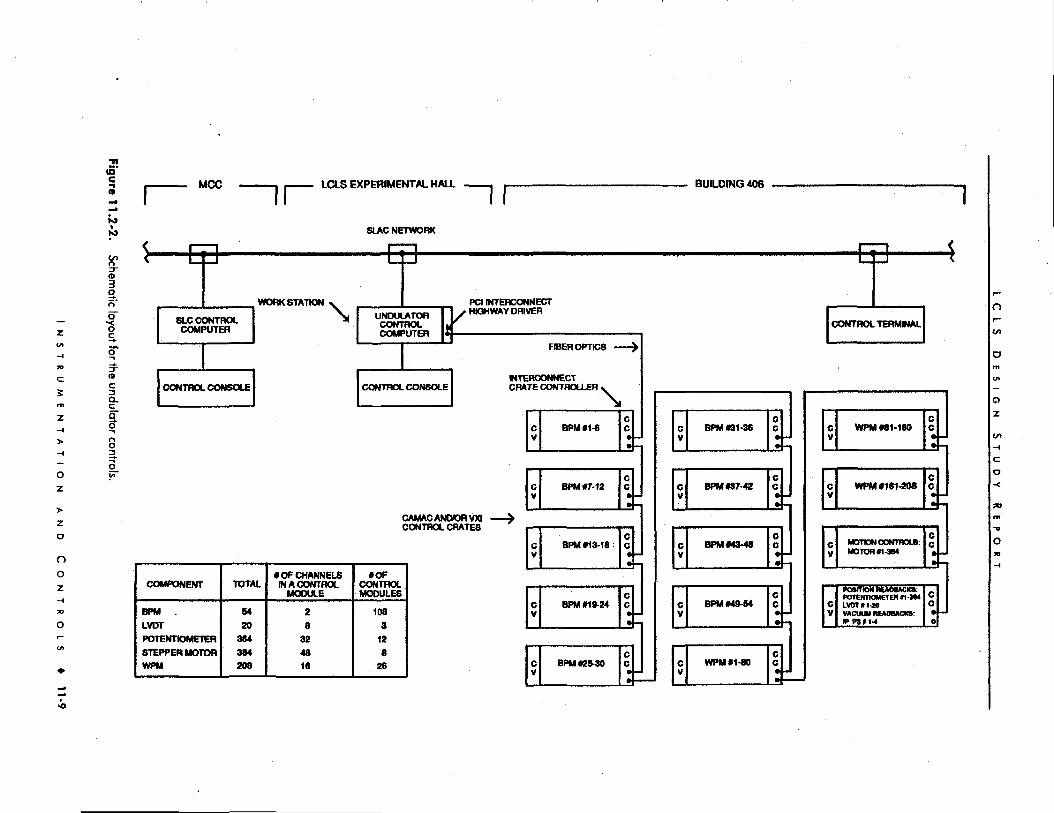
ID.c MCC LCLS EXPERIMENTAL HALL BUILDING 406
SLAC NETWORK
0
aWORKSTATION
SLC CONTROLCOMPUTER
(DC
a.a"3"
8•3
\ UNDULATORCONTROLCOMPUTER
PCI INTERCONNECT• HIGHWAY DRIVER
FIBER OPTIC8
CONTROL CONSOLE CONTROL CONSOLEINTERCONNECTCRATE CONTROLLER
oz>zo
OOz
CAMACANDORVXICONTROL CRATES
COMPONENT
BPM .
LVDT
POTENTIOMETER
STEPPER MOTOR
WPM
TOTAL
5420
384
384208
# OF CHANNELSIN A CONTROL
MODULE
2
83248IS
#OFCONTROLMODULES
1083
128
26
\
cV
BPM #1-6CC••
CV
BPM#7-1ZCC••
CV
BPM #13-18CC
•
CV
BPM #19-24CC
•
CV
BPM #25-30CC••
CONTROL TERMINAL
CV
BPM #31-36CC••
CV
BPM #37-42CC••
CV
BPM #43-480C
•
CV
BPM #49-54CC
•
CV
WPM #1-80CC••
cV
WPM #81-160CC
•
CV
WPM #161-208CC••
ni—
v>
D
Oz
co
cV
MOTION CONTROLS:MOTOR # 1-384
CC••
cV
POSITION REA08ACKS:POTtNTlOMETEH f l -9MLVOTft-MVACUUM REAOBACKS:PPW1-4
c•O
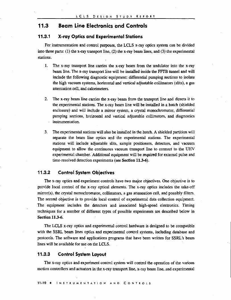
L C L S D E S I G N S T U D Y R E P O R T
11.3 Beam Line Electronics and Controls
11.3.1 X-ray Optics and Experimental Stations
For instrumentation and control purposes, the LCLS x-ray optics system can be divided
into three parts: (1) the x-ray transport line, (2) the x-ray beam lines, and (3) the experimental
stations.
1. The x-ray transport line carries the x-ray beam from the undulator into the x-raybeam line. The x-ray transport line will be installed inside the FFTB tunnel and willinclude the following diagnostic equipment: differential pumping sections to isolatethe high vacuum systems, horizontal and vertical adjustable collimators (slits), a gasattenuation cell, and calorimeters.
2. The x-ray beam line carries the x-ray beam from the transport line and directs it tothe experimental stations. The x-ray beam line will be installed in a hutch (shieldedenclosure) and will include a mirror system, a crystal monochromator, differentialpumping sections, horizontal and vertical adjustable collimators, and diagnosticsinstrumentation.
3. The experimental stations will also be installed in the hutch. A shielded partition willseparate the beam line optics and the experimental stations. The experimentalstations will include adjustable slits, sample positioners, detectors, and vacuumequipment to allow the continuous vacuum transport line to connect to the UHVexperimental chamber. Additional equipment will be required for external pulse andtime-resolved detection experiments (see Section 11.3-6).
11.3.2 Control System Objectives
The x-ray optics and experiment controls have two major objectives. One objective is to
provide local control of the x-ray optical elements. The x-ray optics includes the take-off
mirror(s), the crystal monochromator, collimators, a gas attenuation cell, and possibly filters.
The second objective is to provide local control of experimental data collection equipment.
The equipment includes the detectors and associated high-speed electronics. Timing
techniques for a number of different types of possible experiments are described below in
Section 11.3-6.
The LCLS x-ray optics and experimental control hardware is designed to be compatible
with the SSRL beam lines optics and experimental control systems, including database and
protocols. The software and applications programs that have been written for SSRL's beam
lines will be available for use on the LCLS.
11.3.3 Control System Layout
The x-ray optics and experiment control system will control the operation of the various
motion controllers and actuators in the x-ray transport line, x-ray beam line, and experimental
1 1 - 1 0 • I N S T R U M E N T A T I O N A N D C O N T R O L S

L C L S D E S I G N S T U D Y R E P O R T
stations. A functional layout of the x-ray optics motion and actuator controls is shown in
Fig. 113-1. The optics and experiment control system will be installed in the LCLS
Experimental Hall. A workstation will control and monitor the operation of the x-ray optics
and the acquisition of data from the detectors. It will control the operation of the mirror and
crystal monochromator movers, optical tables, adjustable slits, a gas attenuation cell, sample
positioners, calorimeters, and detectors. Control of the hardware and acquisition of data from
the sensors and diagnostics instrumentation will be done by a CAMAC and/or VXI based
system(s). The workstation will include a PCI-based Interconnect Highway Driver that will
be linked through a fiber-optics cable to CAMAC or VXI interconnect crate controllers (see
Fig. 113-2).
11.3.4 Motion Controls
The x-ray transport line, x-ray beam line, and the experimental stations include systems
such as adjustable collimators, mirror optics, crystal optics, and adjustable slits. To operate
these systems requires position control and position readback. The design goals, such as
positioning accuracy, position encoder linearity and resolution, and processing electronics
resolution, differ from mover to mover. They strongly depend on the mechanical design like
the motor gear ratio and the position encoder range of travel.
The mechanical position will be measured directly with linear variable differential
transformers (LVDTs). LVDTs were chosen for their resolution (essentially determined by
the number of bits in the read-out ADC and the LVDT range of travel), their linearity
(<0.15%), and their ease of use.
The x-ray optics and experiment control computer will calculate the number of steps and
directions that each motor needs to take. Stepper Motor Control (SMC) commands will be
sent out to the drivers in a form of the number of steps and direction to move. Currently the
movers controls design is based on a CAMAC system and SLAC SLC-type motor drivers.
The final design may use a VXI based system and commercially available stepper motor
drivers.
11.3.5 Photon Beam Stabilization at the Sample
Experiments that require irradiation of a fixed sample point (e.g., diffraction from an
individual microstructure) may require the stable positioning of the beam to within a fraction
of its diameter. Factors contributing to positional beam jitter or drift at the sample plane
might include the following: (1) power supply and other component fluctuations in the gun-
to-undulator system, (2) vibration or positional drift in the linac and undulator structures, and
(3) vibration or positional drift of the x-ray optics system components. For factors
contributing to beam motion that have sufficiently long time constants, detection of jitter or
drift and their stabilization may be accomplished with suitable detectors providing feedback
to any of the upstream LCLS system elements that govern beam position and attitude.
I N S T R U M E N T A T I O N A N D C O N T R O L S • 1 1 - 1 1

c3 EXPERIMENTAL STATICNS - X-fiAY BEAN LINE X-RAY TRANSPORT LINE H
Oz
zo
ooz
c
d5'Q
-
X
3o
o5'DQCLOQ.ao"
8
ySMU <OJETMLE ansriL
P C I T i n g TABLE SLITS BTIC TABLEMIRHR MUET/CU
uwvtm OPTICS auiMns
CAS HfATTENUATIDN MUETME
CEIL OUKDCIS CHLIMUR
D-H
S M U NUSTMUrniTine ttex
tWDCNT
PIE2DH0T0R
P1E2D LINEAR
LVOT
TOTAL
50
2
t
13
LEGEND:
LVDT . LIWAR VARIABLEOIFFaENTIAL TRANSFTOO
H s STEPPER MDTTRP « PIEZO LINEARPM • PIE2O MTIDRPV • PUFF VALVEVA . VALVE ACTUlTtR

L C L S D E S I G N S T U D Y R E P O R T
Detection of positional and attitudinal jitter or drift can be accomplished with non-
destructive photon beam position monitors of the type used on SPEAR, or with, for example,
a beam splitter directing part of the (suitably attenuated) radiation to a position sensitive
detector (PSD) array in proximity to the experimental location. The detector signal can be fed
back to positional/angular controllers in the mirror or crystal tanks. The control system for
accomplishing this will need to be based on algorithms that can correlate the observed beam
drift with the required corrective motion(s) or current(s) of the upstream elements. Operation
of the full photon beam stabilization system, which will need to be under the control of the
experimenter, can be incorporated into the control network schematized in Fig. 113-2.
LCLS EXPERIMENTAL HALL
SLAC NETWORK
WORKSTATION
\ mcKTAND OPTICSCONTROL •COMPUTER
PCI INTERCONNECTHIGHWAY DRIVER
FBEfi OPTICS >
CONTROL CONSOLE
cV
MOTION CONTROLSMOTOR #1-4»LVDTI1-13PlEZOti
cc••
CAMACANDORVX)CONTROL CRATES
cV
EXPERIMENTCONTROL
CC
•
cV
DATAACQUISITION
CC•0
Figure 11.3-2. Schematic layout for the x-ray optics and the experimental stations controls.
11.3.6 Timing System
Most LCLS x-ray experiments require synchronization of the experimental stations'
equipment with the electron beam. The electron beam, in turn, is phased to the 476 MHz of
the SLC master clock. Temporal jitter between the RF and the beam is specified to less than
0.5 ps rms.
To minimize the jitter of the 476 MHz timing pulses at the LCLS experiment stations, the
RF signal needs to be derived from the SLC RF system at a location as close as possible to
the LCLS Experimental Hall. The timing pulses used currently at the FFTB facility are
derived from the linac RF at sector 30 (the end of the linac), optically modulated, and
transferred by an optical fiber link to the FFTB building 407B (a distance of -600 m). There,
they are demodulated to electrical pulses. This 476 MHz RF signal is divided in frequency as
necessary to generate the various triggers. An optical fiber cable is used because it is less
I N S T R U M E N T A T I O N A N D C O N T R O L S • n o 3

L C L S D E S I G N S T U D Y R E P O R T
sensitive to environmental changes (e.g., temperature changes) than coaxial cables. For the
short link between building 407B and the LCLS Experimental Hall (~50 m) a temperature-
stabilized heliax coaxial cable should be sufficient.
The following are the timing requirements and techniques for three types of LCLS x-ray
experiments: (1) split pulse, (2) external pulse, and (3) time-resolved detection.
1. Split pulse (x-ray probe/probe) experiments are planned for the study of fastcorrelations in solids, liquids, glasses, phonons, and phase transition dynamics. Thetechnique is based on splitting the LCLS x-ray pulse with a x-ray beam splitter intotwo parts. One part hits the sample directly and the other hits the sample after anadjustable delay of 0-1 ns (see Fig. 11.3-3(A)). With this technique the time delay iscreated in the experimental hutch, with high precision. Nevertheless, the activatingwindow for the detectors has to be synchronized with the FEL 120 Hz source anddelayed accordingly.
2. External pulse (x-ray or laser pump/x-ray probe) experiments are designed for thestudy of structures of transient states and relaxation of excitations. This techniqueutilizes an external optical laser as the pumping source and the FEL x-ray beampulse as the probe. The required triggering range for the external laser is from-10 ms to +10 ms. This class of experiments requires that the synchronizationbetween the user laser and the FEL x-ray beam have a timing jitter better than 1 psfor time delays of ± 1 ns, and better than 1 ns for time delays of ± 10 ms. (seeFig. 11 J-3(B)).
3. Time-resolved detection experiments are planned for the study of relaxationphenomena. This class of experiments also requires that the synchronization betweenthe user laser and the FEL x-ray beam have a timing jitter of approximately 1 ps fortime delays in the 1 ns range (see Fig. 11.3-3(C)).
1 1 - 1 4 • I N S T R U M E N T A T I O N A N D C O N T R O L S

L C L S D E S I G N S T U D Y R E P O R T
LCLSX-RAYS
(A) • -
Sample
X-RAYBEAM
SPUTTER
Delay(0-1 NS)
SPLIT PLUSE
(B)
LCLS X-RAYS
Sample
User Laser—•
oDelay
(-10 MS to+10 MS)
EXTERNAL PLUSE
Sample
(C)
User Laser- L
'elector
Delay(-1 MS to +1 MS)
TIME RESOLVED DETECTION
Figure 11.3-3. LCLS experiments timing techniques.
The operation of the external-pulse (laser pump/x-ray probe) timing system is an
important factor in experiments such as those described above. A schematic of the system is
shown in Fig. 11.3-4. The requisite wide triggering range is achieved by using a pulse
selection stage. The main components of the pulse selection stage are two polarizers, a
Pockels cell, an HV pulser, and a pulse delay unit. The pulse delay unit 120 Hz input trigger
is synchronized with the laser oscillator (119 MHz). Therefore, the selection of any laser
pulse can be done by setting the pulse delay unit's digital delay. The laser oscillator produces
very narrow light pulses (-10 fs) every -8 ns. To select a given laser pulse requires that it
pass the Pockels cell while the cell is pulsed by the high voltage pulser. A pulse width of 6 ns
assures that only one laser pulse is selected at a time. The fine synchronization between the x-
rays and the user laser is achieved by the delay stage. The delay stage consists of a prism that
is installed on a stepper motor controlled translation stage and two mirrors. The position of
the prism determines the light travel time through the delay stage. A translation stage with a
linear motion of -33 cm and resolution of 1 /an provides a total delay of 2 ns.
I N S T R U M E N T A T I O N A N D C O N T R O L S • 1 1 - 1 5
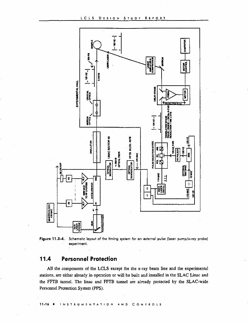
L C L S D E S I G N S T U D Y R E P O R T
Figure 11.3-4. Schematic layout of the timing system for an external pulse (laser pump/x-ray probe)
experiment.
11.4 Personnel Protection
All the components of the LCLS except for the x-ray beam line and the experimental
stations, are either already in operation or will be built and installed in the SLAC Linac and
the FFTB tunnel. The linac and FFTB tunnel are already protected by the SLAC-wide
Personnel Protection System (PPS).
11-16 • I N S T R U M E N T A T I O N A N D C O N T R O L S

L C L S D E S I G N S T U D Y R E P O R T
The radiation protection system in place in the FFTB includes the following:
(1) shielding, (2) Beam Containment System (BCS), and (3) PPS.
1. The radiation protection system is designed to shield personnel working inside theFFTB tunnel from radiation which could be generated by other beams in the switchyard, and to protect personnel outside the FFTB enclosure from potential radiationgenerated during the LCLS operation.
2. The BCS prevents the accelerated beams from diverging from the desired channel,and exceeding levels of energy and intensity that may cause excessive radiation inoccupied area. The FFTB BCS already in place consists of the following: (1) deviceswhich limit the incoming average beam power to 2.4 kW (current monitors 13,14,and 15); (2) devices which limit normal beam loss so that the radiation level outsidethe tunnel shielding is less than 1 mrem/hr (current monitors 16 and 17 and long ionchambers); (3) protection collimators which ensure that errant beams do not escapecontainment; and (4) ion chambers and water flow switches which protectcollimators, stoppers and dumps. The beam power on the D2 dump is limited to15 kW and is protected by ion chambers IC104A and IC104B. The beam stoppersST60 and ST61 are protected by ion chambers IC 65 and IC66. The FFTB BCS willbe modified and used for the LCLS (see Fig. 11.4-1).
Te ToR*p AM* BipolarMonitor Avtl
ISKI I I I
Beam Switch Yard
knChlmUf
Figure 11 .4 -1 . Layout of the beam containment system (not to scale).
3. The PPS already in place in the FFTB tunnel is designed to protect personnel fromradiation and electrical hazards. The function of the system is to preventunauthorized access into the tunnel where there is the potential for beam and/orelectrical hazards. It is also designed to prevent the radiation dose or dose rate fromexceeding the radiation design criteria inside the tunnel when access is permitted, oroutside the tunnel during the LCLS operation.
The FFTB PPS is composed of beam stoppers, an entry module, a search/reset system,
and emergency buttons. The system is controlled from the SLAC Main Control Center
(MCC). It allows beam stoppers to be opened only after the tunnel has been searched and
I N S T R U M E N T A T I O N A N D C O N T R O L S • 1 1 - 1 7

L C L S D i s i C N S T U D Y R E P O R T
secured and is in the No Access state. Access to the tunnel is permitted by the PPS only if all
the beam stoppers (D2, ST60, and ST61) are closed.
Radiation safety inside the tunnel is insured by the following: beam dump D2 and beam
stoppers ST60 and ST61; a Burn Through Monitor (BTM) installed up stream of the muon
shielding; and several Beam Shut-Off Ion Chambers (BSOICs) installed down stream of the
muon shielding inside the tunnel. This system prevents the beam from striking the muon
shield and shuts the beam off if radiation levels inside the tunnel exceed the allowed limit. An
additional BTM is installed behind the FFTB dump, and several BSOICs are installed outside
the tunnel to monitor the radiation levels outside the FFTB shielding.
The x-ray beam line and the two experiment stations will be installed in a shielded hutch.
The hutch will be designed to contain all radiation background so that the dose rates outside
the hutch are acceptable when photons from the FEL are inside the hutch. Access to the hutch
will be controlled by a Hutch Protection System (HPS) modeled after existing SSRL hutches.
The key parts of the HPS are the access door, photon stoppers, and search/reset system. The
HPS allows either physical access or permission to direct beam into the hutch. It contains the
logic circuits that govern the sequence of access operations based on the status of the
stoppers. It also captures or releases the hutch door keys, acknowledges completion of a
search, and keys the experiment enclosure on-line or off-line.
The LCLS HPS will control the operation of four photon stoppers. The system will allow
the photon stoppers to be opened (go on-line) only if the hutch has been searched and
secured, and the hutch door key is captured in the HPS panel. Access to the hutch is permitted
only if all photon stoppers are closed. Stoppers MM1, IS1, and IS2 will be installed inside the
FFTB tunnel, and stopper MM2 will be installed in the hutch. Stoppers MM1, IS 1, and IS2
are designed to protect personnel from radiation generated by the FEL. The MM2 stopper is
designed to protect personnel from scattered radiation generated from the interaction of the
electron beam on the main dump (see Fig. 11.4-1). Table 11.4-1 lists possible PPS violations
and system responses.
Table 11.4-1. PPS violation and response.
1. FFTB tunnel Any FFTB tunnel security fault, while dump D2 and stoppers ST60 and ST61 are notsecurity fault closed, will shut-off the LCLS beam, close FFTB stoppers, turn off the electrical hazards.
2. Inside tunnel These BSOICs continuously monitor the radiation inside the tunnel. If the detectedBSOICs trip radiation level exceeds the preset limit, the PPS will shut-off the LCLS, SLC, and the A
Beam. The BSOICs interlocks are by-passed when the FFTB tunnel is in the No Accessstate.
3. Outside tunnel These BSOICs continuously monitor the radiation outside the tunnel. If the detectedBSOICs trip radiation level exceeds the preset limit, the PPS will shut-off the LCLS beam and close the
beam stoppers.
4. HPS security Any HPS security fault while the hutch photon stoppers and the FFTB beam stoppers arefault not closed will shut-off the LCLS beam and close the hutch and FFTB stoppers.
1 1 - 1 8 • I N S T R U M E N T A T I O N A N D C O N T R O L S
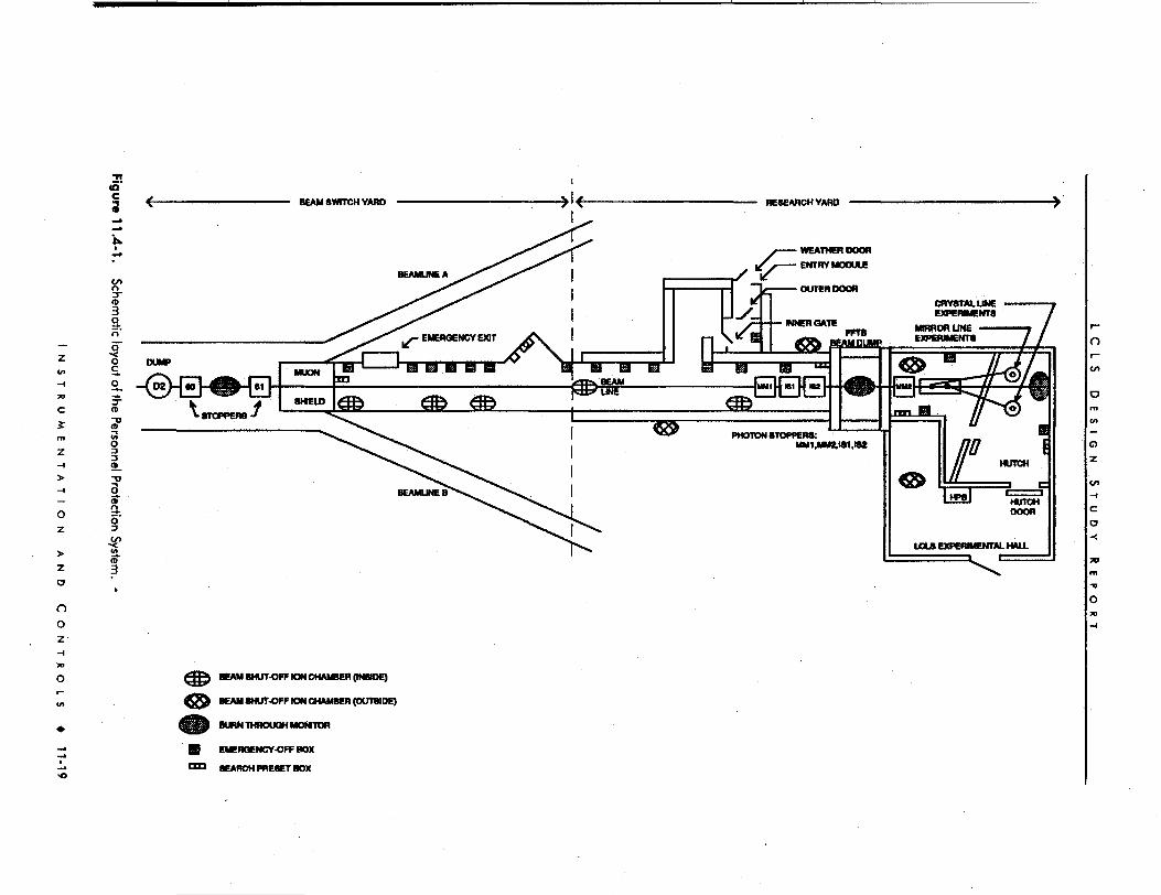
(O
c
c5
Oz
zD
noz
5"
O
O_
35"a5'
n
oz
co
BEAM SHUT-OFF ION CHAMBER (INSIDE)
BEAM SHUT-OFF ION CHAMBER (OUTSIDE)
BURN THROUQH MONITOR
EMERGENGV-OFFBOX
SEARCH PRESET BOX

L C L S D E S I G N S T U D Y R E P O R T
11.5 Machine Protection
A Machine Protection System (MPS) is designed to protect the LCLS components. The
three primary functions of the MPS are to protect: (1) the integrity of the vacuum system;
(2) the proper cooling of the water cooled components; and (3) the LCLS components from
damage resulting from errant steering of the electron beam.
1. The MPS will control and monitor the operation of vacuum components such asdifferential pumping sections, ion gauges, ion pumps, and isolation valves.
2. The MPS will monitor temperature sensors and water flow switches that insure thatthe magnets, collimators, stoppers, x-ray mirror, and monochromator crystals aresufficiently cooled.
3. Ionization chambers and long ion chambers capable of detecting average radiationare currently installed in the FFTB tunnel. If the average rate of beam loss is foundto be sufficient to threaten machine components, the beam repetition rate isautomatically reduced. In addition, a pulse-to-pulse comparator system measures thebeam current. The operation of the pulse-to-pulse comparator is based on measuringthe beam current in two locations. The signal from a toroid at the beam's finaldestination (beam dump) is compared with that from a toroid at the beginning of thearea being protected. If the comparison on a pulse-to-pulse basis shows a beam lossgreater than some specified amount the beam is automatically turned off.
The LCLS MPS will consist of two separate systems. One system will protect the LCLS
components up stream to the undulator and the second system will protect the components of
the undulator, the transport line, the x-ray beam line, and the experimental stations. The first
system will be operated from the SLAC MCC, and the second system will be operated from
the LCLS Experimental Hall. The two control systems will be interfaced to provide vacuum
and thermal interlocks to protect the LCLS accelerator and the x-ray beam line from the
following: (1) accidental exposure to atmospheric pressure; and (2) accidental interruption of
the Low Conductivity Water (LCW) to water-cooled components. Status signals such as
vacuum and LCW faults as well as permits to open or close isolation valves will be shared by
both systems.
The existing FFTB MPS control panels are installed in building 406. These controls will
be modified to protect the LCLS components in the tunnel. The undulator-to-experimental
stations MPS control panels will be installed in the Experimental Hall. This system will
include a Programmable Logic Controller (PLC) and control panels. A typical PLC consists
of processor (CPU) and Input/Output (I/O) modules. Most of SSRL beam lines' MPS use
PLCs. The undulator-to-experimental stations component layout is given in Fig. 11.5-1.
1 1 - 2 0 • I N S T R U M E N T A T I O N - A N D C O N T R O L S
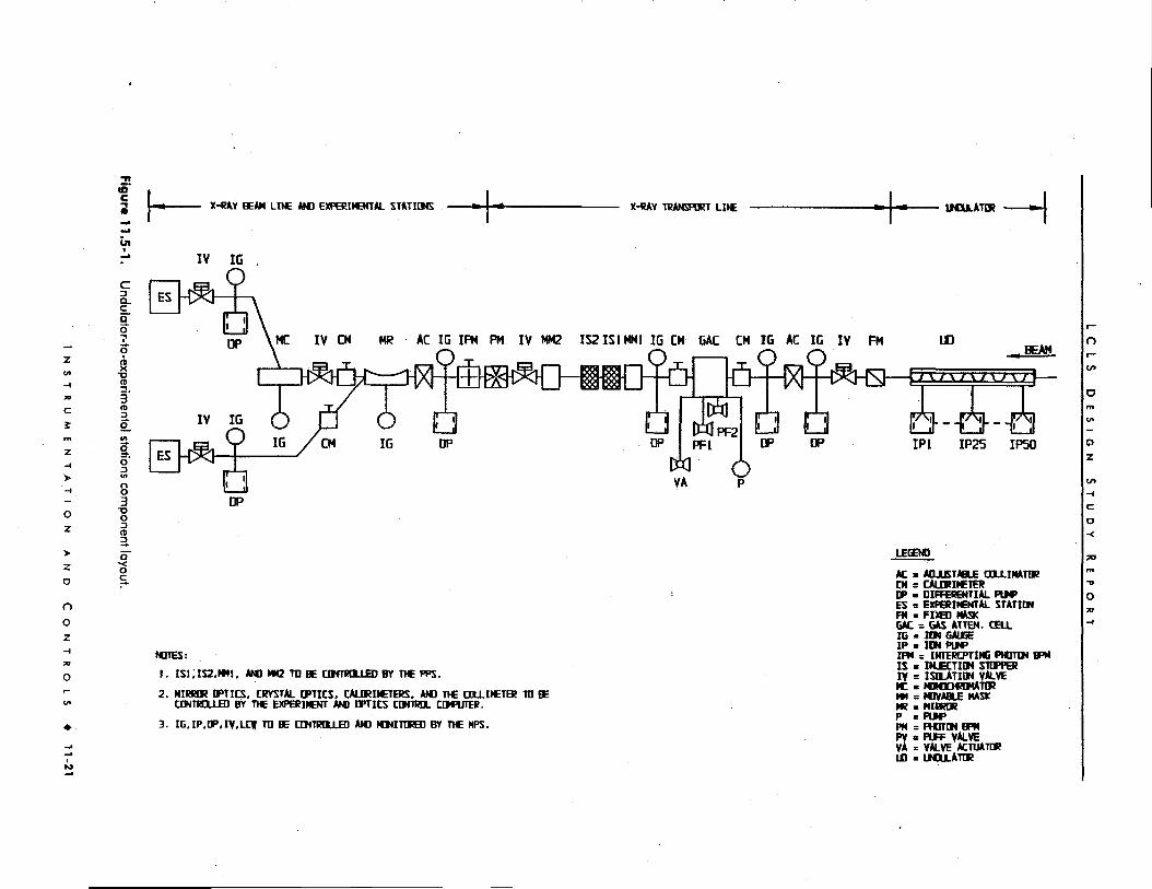
cX-RAY BEAM LINE AM) EXPERIMENTAL STATIONS X-RAY TRANSPORT LINE 1HJU.ATO? H
IV IG
oz
zo
ooz
8•oo3
Q
C
-z
-\3D
c
m
Z
cQ.cQ
3"-to
S?
(t
3"(Atatio
3
ES
ES
MR AC IG IPM PM IV W O IS2ISIMMI IG CM GAC CM IG AC IG IV FM
NOTES:
1 . I S i ; i S 2 . M M l , AM) MM2 TD BE CDNTKLLED BY THE PPS.
2 . MIRROR OPTICS. CRYSTAL OPTICS, CALORIMETERS. AND THE COLLIMETB! TD BECONTROLLED BY THE EXPERIMENT AND OPTICS CONTROL CCWUTEI?.
3 . I G . I P . O P . I V . L C f TO BE CONTROLLED AMD MTMITORED BY THE NPS.
DP
UDBEAM n
W WWW
IP1 IP25 IP50 Oz
ca
LEGEND
AC > ADJUSTABLE caxiHATDRCM s CALORIMETERDP - DIFFERENTIAL PIM>ES = EXPERIMENTAL STATIONFM > FIXED MASKGAC = CAS ATTEN. CELLIG • ION GAUGEIP • ION PltPIPM = INTERCPTING PHOTON BPMIS = INJECTION STOPPERIV = ISOLATION VALVEMC > MONXHROMATD?MM = MOVABLE MASKMR * MIRRORP * PIK>PM = PHOTON BPMPV s PUFF VALVEVA «= VALVE ACTUATORUD - UNDULATDR
Alignment
TECHNICAL SYNOPSIS
This section describes the procedures and methods used to position the LCLS components
with their required accuracy. The network design philosophy is based on a 3-D design, now
widely used in high precision metrology. The network consists of 3 parts: the linac,
undulator, and transport line/experimental area networks. Since the linac exists already, the
linac network does not need to support construction survey and alignment, but rather will
only provide tie-points during the linac straightening (smoothing) procedure. The undulator
network's geometry is dictated by the tunnel and machine layout. The geometry should permit
observation of each target point from at least three different stations. A triplet of monuments
is placed in the tunnel cross section. The Transport Line/Experimental Area Network will be
constructed and established like the undulator network, with the only difference that each
cross section will have only two monuments.
The alignment coordinate system will be a Cartesian right handed system, with the origin
placed where the present SLC origin is (Linac Station 100). The instrumentation for the
network observation will be a laser tracker/Total Station combination. The laser tracker will
be used for position, and the total station for angle accuracy.
The alignment tolerances in the linac and transfer line tunnels are achievable with
established techniques. The undulator requirements are somewhat tighter. The trajectory in
the undulator is determined by a string of quadrupoles, supported by magnet movers. For the
beam-based algorithm to converge, 100 jum initial placement accuracy is required. Laser
tracker measurements supported by hydrostatic level observations will provide the required
positional accuracy. The positional stability of the undulator will be monitored using a
hydrostatic level system in the vertical dimension and a stretched wire based system in the
horizontal dimension.

L C L S D E S I G N S T U D Y R E P O R T
12.1 Surveying Reference Frame
Horizontal position differences between the projection of points on the geoid1 or a best
fitting local ellipsoid and those on a local tangential plane are not significant for a project of
the size the LCLS. Hence, it is not necessary to project original observations like angles and
distances into the local planar system to arrive at planar rectangular coordinates [1].
In the vertical plane, however, the curvature of the earth needs to be considered (see
Fig. 12.1-1). Since leveling is done with respect to gravity, the reference surface is the geoid.
Because of the relatively small area of the LCLS project, one can substitute the non-
parametric geoid with a locally best fitting sphere or spheroid. Table 12.1-1 shows the
projection differences between a tangential plane, a sphere, and an ellipsoid as a function of
the distance from the coordinate system's origin. Notice that for distances as short as 20 m the
deviation between plane and sphere is already 0.03 mm (see Table 12.1-1).
Plane
Ellipsoid
Sphere
Figure 12.1-1. Effect of earth curvature.
Table 12.1 - 1 . Curvature correction
Distance, R, [m]
20
50
100
1000
Sphere, H$, [m]
0.00003
0.00020
0.00078
0.07846
Spheroid, HE , [m]
0.00003
0.00016
0.00063
0.06257
The Geoid is the reference surface described by gravity; it is the equipotential surface at mean sealevel that is everywhere normal to the gravity vector. Although it is a more regular figure than theearth's surface, it is still irregular due to local mass anomalies that cause departures of up to 150 mfrom the reference ellipsoid. As a result, the geoid is nonsymmetric and its mathematical descriptionnonparametric, rendering it unsuitable as a reference surface for calculations. It is, however, thesurface on which most survey measurements are made, as the majority of survey instruments are setup with respect to gravity.
The reference ellipsoid is the regular figure that most closely approximates the shape of the earth,and is therefore widely used in astronomy and geodesy to model the earth. Being a regularmathematical figure, it is the surface on which calculations can be made.
12-2 • A L I G N M E N T

L C l S D E S I G N S T U D Y R E P O R T _ _ _ _
12.1.1 Network Design Philosophy
The global alignment tolerance, the relatively weak links between machine sections, and
advances in surveying make it possible to forego the traditional design of a two-tiered
network hierarchy covering the whole machine. Instead, each machine section can be
considered independent, only connected by tunnel networks. A two-tiered approach will only
become necessary if a remote experiment is added to the project and at that time needs to be
connected to the undulator. Omitting a primary network not only removes many constraints
for component placement, since fewer lines-of-sight need to be maintained, but also presents
a significant reduction in alignment costs.
Traditionally, forced centered2 "2 + 1 - D" triangulation and trilateration techniques3 were
used to measure the tunnel networks. However, a 3-D "free stationing4" approach does not
require forced-centered instrument set-ups, thus eliminating the need for set-up hardware and
their systematic error contributions. Removable heavy-duty metal tripods, translation stages,
CERN sockets, and optical plummets are not needed (see Fig. 12.1-2). The network design
still must consider other systematic error effects, especially lateral refraction.5 Another
important consideration is the target reference system. Its design becomes less difficult with
free stationing since there are only targets and not instruments. Accordingly, a 3-D design
will be used, which is now quite common in high precision metrology. This approach is
centered on a 1.5 inch6 sphere. Different targets can be incorporated into the sphere in such a
way that the position of the target is invariant to any rotation of the sphere. At SLAC, designs
Forced centering refers to a specific instrument mount. This type of mounting system, whether vendorspecific or independent, allows the exchange of instruments on a station without losing themeasurement point, i.e., all instruments are by mechanical "force" set up in exactly the sameposition. However, experience has shown that even the best of these forced centering systems has ao of about 50-100 /im. Unfortunately, the forced-centering system contributed error is not random.Since a whole set of measurements is usually completed from a slightly offset position, this errorbehaves mostly systematically. No efficient method is known to determine the offset vector. Theseerrors, vertical refraction, and lateral refraction are the biggest contributors to the systematic errorbudget in surveying engineering,
2 + 1 - D refers to the fact that because of mechanical problems in the forced-centering hardware,three-dimensional networks were usually split into separate horizontal (2-D) and vertical (1-D)networks. Both networks were established, measured and analyzed separately.
Rather than setting up the instrument over a known point, the instrument's position is flexible andchosen only following considerations of geometry, line of sight, and convenience. To determine theinstrument position, at least three points, whose coordinates are already known or are part of anetwork solution, need to be included in the measurements.
Lateral refraction is caused by horizontal stationary temperature gradients. In a tunnel environment,the tunnel wall is often warmer than the air. This creates vertical stable temperature layers withgradients of only a few hundredth of a degree Celsius per meter. If one runs a traverse close to atunnel wall on one side only, the systematic accumulation of the effect can be significant; e.g., duringthe construction of the channel tunnel, a control measurement using gyro theodolites revealed thatafter about 4 km they had already veered about 0.5 m off the desigji trajectory.
The diameter of the 1.5 in. sphere is equivalent to 3.81 cm.
A L I G N M E N T • 12-3

L C L S D E S I G N S T U D Y R E P O R T
have been developed to incorporate theodolite targets (see Fig. 12.1-3), photogrammetric
reflective targets, as well as glass and air corner cubes (see Fig. 12.1-4) into the sphere.
Receptacles for the spheres, which are usually referred to as "nests" or "cups," have been
designed to accommodate different functions. TJNAF has a very suitable design for nests to
be grouted into the floor, and designs are available at SLAC for cups tack-welded onto
magnets, for mounting cups on wall brackets and for a "centered" removable mounting placed
into tooling ball bushings (see Fig. 12.1-5).
Figure 12.1-2. Forced centered set-up at SLAC.
Figure 12.1 -3 . Sphere mounted theodolite target.
12-4 • A L I G N M E N T

L C L S D E S I G N S T U D Y R E P O R T
Figure 12.1-4. Sphere mounted glass and air reflectors.
Figure 12.1-5. Sphere receptacles: floor, component, and wall bracket fixed mount versions,removable centered version.
12.1.2 Network Lay-Out
The LCLS network consists of three parts: the linac network, the undulator network, and
the transport line/experimental area network.
Linac Network
The linac network serves a different purpose than the other networks. Since the linac
already exists, the linac network does not need to support construction survey and alignment,
but rather will only provide local tie-points during the linac straightening (smoothing)
procedure.
Undulator Network
The undulator network's overall geometry is dictated by the tunnel geometry, machine
layout and the fact that the free stationing method requires a greater number of reference
points. The geometry should also permit observing each target point from at least three
different stations. The reference points can be of two different hierarchical classes. The
A L I G N M E N T • 12-5

L C L S D E S I G N S T U D Y R E P O R T
second order points, or tie points, mainly serve to connect the orientation of free stationed
instruments. In addition the first order points provide the geometric reference during machine
installation; they are the equivalent of traditional traverse points or monuments. The
following sketch (Fig. 12.1-6) shows a typical section of the layout. A triplet of monuments is
placed in the tunnel cross section at the position of each corrector magnet. One monument
will be placed close to the corrector magnet on the floor, the second one mounted at
instrument height to the aisle wall, and the third monument mounted to the back wall also at
instrument height.
-100 m
0 Floor-Mounted®
I •Wall-Mounted 0
Figure 12.1-6. Undulator network layout.
Transport Line/Experimental Area Network
Initially, the project will only include an experimental area directly down-stream of the
undulator. This network will be constructed and established similar to the undulator network,
the only difference being that each cross section will have only two monuments. These
monuments will be mounted to the walls at instrument height.
12.1.3 Alignment Coordinate System
The alignment coordinate system will be a Cartesian right-handed system. The origin is
placed at the linac Station 100 (in analogy to the SLC coordinate system). There will be no
monument at the origin; it is purely a virtual point. The Y-axis assumes the direction of the
gravity vector at the origin but with opposite sign. The Z-axis is in the direction of the linac,
and the X-axis is perpendicular to both the Y and Z-axes. The signs are defined by the right-
handed rule (see Fig. 12.1-7).
12-6 • A L I G N M E N T
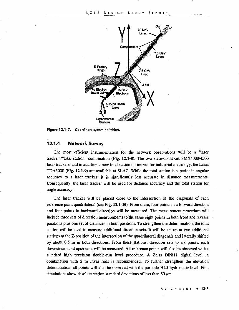
L C L S D E S I G N S T U D Y R E P O R T
B FactoryRings
.__•• T o ElectronV; Beam
ExperimentalStations
Figure 12.1-7. Coordinate system definition.
. • J \ l.
12.1.4 Network Survey
The most efficient instrumentation for the network observations will be a "laser
tracker'V'total station" combination (Fig. 12.1-8). The two state-of-the-art SMX4000/4500
laser trackers, and in addition a new total station optimized for industrial metrology, the Leica
TDA5000 (Fig. 12.1-9) are available at SLAC. While the total station is superior in angular
accuracy to a laser tracker, it is significantly less accurate in distance measurements.
Consequently, the laser tracker will be used for distance accuracy and the total station for
angle accuracy.
The laser tracker will be placed close to the intersection of the diagonals of each
reference point quadrilateral (see Fig. 12.1-10). From there, four points in a forward direction
and four points in backward direction will be measured. The measurement procedure will
include three sets of direction measurements to the same eight points in both front and reverse
positions plus one set of distances in both positions. To strengthen the determination, the total
station will be used to measure additional direction sets. It will be set up at two additional
stations at the Z-position of the intersection of the quadrilateral diagonals and laterally shifted
by about 0.5 m in both directions. From these stations, direction sets to six points, each
downstream and upstream, will be measured. All reference points will also be observed with a
standard high precision double-run level procedure. A Zeiss DiNill digital level in
combination with 2 m invar rods is recommended. To further strengthen the elevation
determination, all points will also be observed with the portable HL5 hydrostatic level. First
simulations show absolute station standard deviations of less than 80 //m.
A L I G N M E N T • 12-7

L C L S D E S I G N S T U D Y R E P O R T
Figure 12.1 -8. SMX laser tracker.
s j te l stMimt tot Musts ial msifeiogf)
Figure 12.1-9. Leica TDA5000 total station.
12-8 • A L I G N M E N T

L C L S D E S I G N S T U D Y R E P O R T
Total Station Laser Tracker
Figure 12.1-10. Observation plan.
12.1.5 Data Analysis and Data-Flow
To reduce the data from the measurements as described above, special software is
required. This type of analysis software is based on the photogrammetric bundle approach.
Since a photogrammetric sensor is arbitrarily oriented in space, not only its translational
parameters but also its rotational orientation parameters must be treated as unknowns and
become part of the solution. With traditional trilateration/triangulation-based analysis
software, however, pitch and roll are supposed to be oriented to gravity, and yaw is expressed
as a function of translations. Additionally, the traditional software assumes that the instrument
is centered on a point to which sufficient measurements have been taken. This analysis
approach does not work well with free stationing, and does not work at all with present
generation laser trackers, since they cannot be oriented directly to gravity.
To reduce errors stemming from transcription of data, the data-flow should be automated.
The suggested instruments support direct connection to field computers. The fully automated
data-flow should extend from field computers through data analysis to data storage.
Measurements with any type of instrument will be guided by software based on rigid
procedures running on field data logging computers. The data logging software will also pre-
analyze the measurements, and will try to determine and flag possible outliers before the
measurement set-up is broken down. This method combined with an automated data-flow will
greatly reduce errors and improve measurement consistency and reliability.
12.2 Lay-out Description Reference Frame
12.2.1 Lattice Coordinate System
The LCLS lattice is designed in a right-handed beam following coordinate system, where
the positive y-axis is perpendicular to the design plane, the z-axis is pointing in the beam
direction and perpendicular to the y-axis, and the x-axis is perpendicular to both the y and
z-axes.
A L I G N M E N T • 12-9

L C L S D E S I G N S T U D Y R E P O R T
12.2.2 Tolerance Lists
The relative positioning tolerances aB Cy, <TZ of the undulator segments, BPMs, and
quadrupoles are listed in Table 12.2-1. The undulator is oriented such that the x-axis is in the
direction of the magnetic field.
Table 12.2-1. LCLS positioning tolerances.
Relative alignment between segments
Global straightness of undulator
Linac straightness
Quadrupole ab initio
100
300
n/a
100
bum]
500
500
n/a
100
[mr]
1
2
n/a
n/a
ojz
[pm/m]
n/a
100/10
150/15
n/a
12.2.3 Relationship between Coordinate Systems
The relationship between the surveying and lattice coordinate systems is given by the
building design and machine layout parameters. The result is a transformation matrix
(rotations and translations).
12.3 Fiducializing Magnets
The correct fiducialization of magnets is as important as their correct alignment since an
error in either task will affect the particles' trajectory and cannot be distinguished from each
other. Fiducialization can be accomplished either through opto-mechanical and opto-electrical
measurements or by using fixtures, which refer to a magnet's reference features. Detailed
descriptions can be found in the literature [2].
The most demanding task is the quadrupole positioning. With a total error budget of
100 /dm, the fiducialization should be done to about 25 />m to accommodate a 90 juin
alignment error. The quadrupoles will have tooling plates attached which reference fiducials
to the magnets' axes. To find the magnetic axes, the preferred method is the vibrating wire
method. A Coordinate Measurement Machine (CMM) will be used to relate the wire position
to the fiducials.
The undulator fiducialization will be carried out on a CMM from physical measurements
and verified using Hall probes mounted to the CMM probe head.
12.4 Absolute Positioning
Common to all parts of the machine, free-stationed laser trackers, oriented to at least four
neighboring points, are used for the absolute positioning measurements. The tracking
12-10 • A L I G N M E N T

L C L S D E S I G N S T U D Y R E P O R T
capabilities of these instruments will significantly facilitate the control of any alignment
operation (moving components into position).
12.4.1 Undulator Absolute Positioning
Undulator Anchor Hole Layout Survey
During the anchor layout survey, the anchor hole positions for the girder supports are
marked on the piers. Fabricating a standard template including all anchor holes at one girder
end, thus significantly reducing the number of individual layout pointings, will be needed. A
total station from one free-stationed position can locate and position the template with only
two pointings. Before the holes are marked, the location of the template should be checked
from a second station. In the sequences of work, the last station can then serve for the n+1
girder as its first station. Specialized software is required to improve the efficiency and
reliability of this task.
Pre-alignment of Girder Supports and Magnet Movers
The undulator girders will be supported by motorized adjustment systems sitting directly
on top of concrete piers. The motorized adjustment systems are based on the Bowden
camshaft design. Two individually controlled camshaft pairs and two single camshafts
provide 5 degrees of freedom per girder. The cam shaft design does not compromise the
rigidity of the supports and, consequently, does not show a resonance in an undesirable
frequency range. This mover system comes in two horizontal slices. The bottom piece
consists of a mounting plate, which holds the shafts and stepping motors. The top part is
integrated into the girder by mounting the kinematic cams to the girder. The girder is held
onto the shafts by gravity or, if necessary, loaded by springs.
To accommodate easy installation, the bottom parts of the movers, set to mid range, have
to be aligned relative to each other. The required relative position tolerance of these,
however, is fairly loose, since the two axes cams are only paired with a single axis cam. On
the other hand, to retain as much magnet mover range as possible, the bottom part of the
magnet movers should be within 0.5 mm of their nominal positions.
To facilitate placing a pedestal such that its top is within 0.5 mm of its nominal position,
a widely used method can be used. Here, the base plate of the bottom part of a mover is
mounted to the pier by four standoff screws, which are grouted/epoxied into the concrete. The
vertical/horizontal pre-alignment of the base plate is accomplished by the following sequence
of steps. (1) After the four bolts are epoxied into the concrete, a nut with a washer on top is
screwed onto each bolt. These nuts are set to their nominal heights by a simple level
operation. (2) Next the base plate is set on the nuts, and a set of washers and nuts is then
screwed on the bolts to fasten it down. However, the top nuts remain only hand tight at this
point. (3) Next, the elevation and tilts of the base plate are set by adjusting the position of the
lower nuts, and subsequently checked with a level with respect to local benchmarks. (4) Then
a total station with a "free station Bundle" software package is used to determine the
A L I G N M E N T • 12-n

L C L S D E S I G N S T U D Y R E P O R T .
horizontal offset and to simultaneously double-check the vertical offset of the base plate from
its nominal position. (5) Finally, the base plate is moved into horizontal alignment using a
clamp-on adjustment fixture (push-push screw arrangement), and the nuts are tightened to the
prescribed torque. To vibrationally stiffen the set-up, the space between the pier and the base
plate should be filled with non-shrinking grout after the alignment has been confirmed.
Once the pedestal is positioned, the bottom part of its magnet mover is mounted and
aligned following the same procedures as described in the previous paragraph.
Absolute Quadrupole Positioning
After the lower part of the magnet mover assembly is mounted and aligned, the
components can be installed. Since the magnet mover parts have a defined geometrical
relationship to the magnetic axes of the quadrupoles and undulator segments, the installation
will place these components to within 0.5 mm. In preparation for the relative alignment, the
position of the quadrupoles will be mapped and adjusted using a laser tracker in reference to
adjacent network points. Absolute position accuracy relative to the network points of about
100 /an can be achieved.
Quality Control Survey
Once the above set is completed, the components will be mapped. If the positional
residuals exceed the tolerance, a second iteration can be "jump started" by using the quality
control map to quantify the position corrections, which need to be applied. If a second
iteration be necessary, a new quality control survey is required after completion of the
alignment process.
12.4.2 Transport Line and Experimental Area Absolute Positioning
The absolute positioning of these components will follow the same procedures as
described above.
12.5 Relative Alignment
12.5.1 Relative Undulator Alignment
Introduction
The trajectory is determined by a string of quadrupoles and BPMs. The quadrupoles are
supported by magnet movers and can be moved to permit beam-based alignment. For the
beam-based alignment algorithm to converge, a 100 /an ab initio placement is required.
Taking fiducialization errors into account, these magnets need to be aligned to 90 /an. The
BPMs, taking fiducializatiori and acquisition error into account, need to be aligned to 80 /an.
Relative Quadrupole Positioning
The absolute position alignment of the quadrupoles is refined by repeating the same
process with the important difference, however, that measurements to a quadrupole are taken
12-12 • A L I G N M E N T
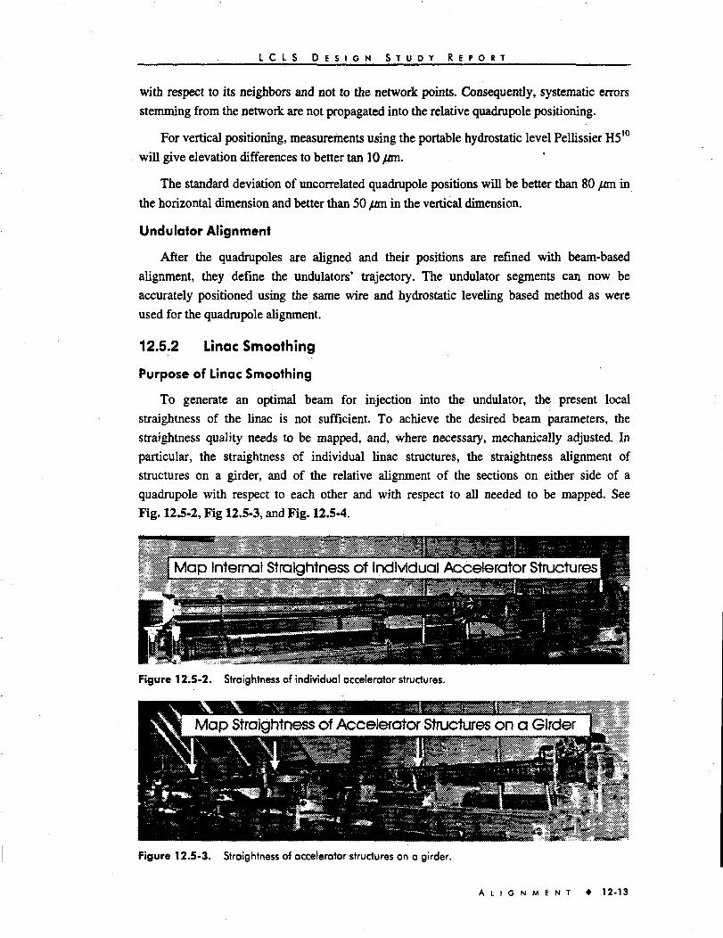
L C L S D E S I G N S T U D Y R E P O R T
with respect to its neighbors and not to the network points. Consequently, systematic errors
stemming from the network are not propagated into the relative quadrupole positioning.
For vertical positioning, measurements using the portable hydrostatic level Pellissier H510
will give elevation differences to better tan 10 fan.
The standard deviation of uncorrelated quadrupole positions will be better than 80 //m in
the horizontal dimension and better than 50 /an in the vertical dimension.
Undulator Alignment
After the quadrupoles are aligned and their positions are refined with beam-based
alignment, they define the undulators' trajectory. The undulator segments can now be
accurately positioned using the same wire and hydrostatic leveling based method as were
used for the quadrupole alignment.
12.5.2 Linac Smoothing
Purpose of Linac Smoothing
To generate an optimal beam for injection into the undulator, the present local
straightness of the linac is not sufficient. To achieve the desired beam parameters, the
straightness quality needs to be mapped, and, where necessary, mechanically adjusted. In
particular, the straightness of individual linac structures, the straightness alignment of
structures on a girder, and of the relative alignment of the sections on either side of a
quadrupole with respect to each other and with respect to all needed to be mapped. See
Fig. 12.5-2, Fig 12.5-3, and Fig. 12.5-4.
I Map Internal Straightness of Individual Accelerator Structures
Figure 12.5-2. Straightness of individual accelerator structures.
Map Straightness of Accelerator Structures
Figure 12.5-3. Straightness of accelerator structures on a girder.
A L I G N M E N T • 12-13

L C L S D E S I G N S T U D Y R E P O R T
^ l l p . V ^ I Retattve Alignment ppg^gQ
Figure 12.5-4. Relative straightness alignment of accelerator structures and an associated quadrupole.
Linac Straightness Measurement Procedure
Because of the required resolution, reliability and the large amount of work (about 1 km
of beam line), the task is best performed with a system that does not require an operator to
point and adjust micrometers. It also should allow on-line data logging. A laser system
developed by Hamar [3] will be used. The instrument generates two laser light planes by
bouncing a laser beam off rotating mirrors. The two light planes are truly perpendicular to
each other. The flatness or wobble-induced error of each light plane is specified as 5 fiiad,
which is well below the straightness specification at maximum distance. The light source
would be set up about the middle between two quadrupoles, offset horizontally and vertically
such that the light planes clear all beam line components. This set-up versus a set-up at an
endpoint reduces the length of the line-of-sight to about 5 m, thus greatly lessening the effects
of potential refraction and air turbulence on the light beam. After bucking in the light planes
both horizontally and vertically to two points on the measured object, intermediate offsets, for
example, between the accelerator structure and the light planes, are measured with a photo-
sensitive-detector (PSD) attached to an offset arm. The detector is linked to an interface box
by a cable, which can be as long as 15 m. The interface box provides a serial link to a data
logger. To measure the offsets, the offset arm is held against the accelerator structure
sequentially in both planes. To determine the perpendicular offset, the alignment technician
will arc the arm. While the arm is being arced, the light position is continuously read out and
stored. Software will then determine the perpendicular offset by finding the smallest read-out
value. Since the PSD measurement range is limited to about 8 mm, the arm will be adjustable
in length. To avoid errors due to the adjustability, the adjustment length will be monitored by
an electronic dial gauge, which also reports its reading to the data logging software. The total
straightness measurement error budget is expected to be below 75 fim.
The relative alignment of a linac quadrupole in relation to its adjacent accelerator sections
will be determined analogously. However, since these quadrupoles are not fiducialized and
also do not have any precision reference surfaces, the offset will be measured to their BPMs
instead. Each BPM has a cylindrical body, which is inserted between the poles with a very
close fit, and protrudes from the poles on either side of the magnet. The BPM is expected to
reference the magnet's axis to about 100 //m. The adjustment range of the offset arm will be
12-14 • A L I G N M E N T
L C L S D E S I G N S T U D Y R E P O R T
sufficiently dimensioned to allow the same arm to measure both BPMs and accelerator
structure offsets.
12.5.3 Relative Alignment of Transport Line and Experimental AreaComponents
The position tolerances of these components will be achieved during the absolute
alignment step. A relative alignment is not required.
12.6 Undulator Monitoring System
In the vertical dimension, a hydrostatic leveling system cloned after ESRF's HLS will
accurately monitor relative and global vertical position changes. Four sensors per girder are
required. To eliminate temperature effects on the hydrostatic leveling results, any vertical
deviations from a plane of the water runs must be avoided. This condition is guaranteed using
the "half-filled" pipe approach. Assuming four sensors per girder, a total of about 88 sensors
will be required.
Since there is no natural absolute reference in the horizontal plane, some kind of artificial
local reference needs to be created as is done by stretched wires. Two wires, one on either
side of the undulator sections/magnets will provide the straight-line reference. Inductive
sensors will provide wire position information. The system is modeled after the Panofsky
wire system used in the original installation of SLAC's A beam. Test measurements have
shown sub-micron resolution and better than 10 pm stability.
12.7 References
1 R. Ruland, Magnet Support and Alignment, in H. Winick, Editor, Synchrotron RadiationSources-A Primer, pp. 274 - 304.
2 R. Ruland, "Setting Reference Targets," in Proceedings of the CERN Accelerator School on"Magnetic Measurements and Alignment," Capri, 1997, in print.
3 Hamar Lasersystems, Model L-723 Triple Scan® Laser with Model A-517 Scan Target.
A L I G N M E N T • 12-15

Radiation Issues
TECHNICAL SYNOPSIS
The radiation concerns related to the LCLS fall into three distinct areas: radiation safety,
radiation background in experiments, and machine protection. This chapter covers these
concerns in the region downstream of the undulator, since the linac will be taken care of by
the existing system. The effect of gas scattering on the residual gas of the undulator was
computed, and no degradation of the undulator is expected from this source of radiation. The
photon deposition due to spontaneous emission in the undulator was calculated and does not
cause a problem. The effectiveness of the undulator protection collimators was found to be
very good. The emission due to gas bremsstrahlung was estimated with an analytical formula.
Computational estimates of the muon dose rates behind the concrete and iron shielding have
been made. All these studies indicate that the radiation is quite manageable. The dose rates
due to induced activity were calculated and with the expected low level of beam loss in the
undulator, the activation of the unit, and the resulting personnel exposure, are expected to be
very low.
13.1 Radiation Concerns Downstream of the Undulator
Radiation concerns downstream of the undulator have been extensively discussed in
Section 10.3, Bremsstrahlung Calculations.
13.2 Radiation Issues in the Undulator
13.2.1 Introduction
The 100 m long undulator will be located partly underground in the tunnel of the SLAC
linac, and partly in a less heavily shielded enclosure which is presently occupied by the Final
Focus Test Beam experiment (FFTB). While the linac and the Beam Switchyard are shielded
with more than 12 m of concrete and earth, the FFTB enclosure shield is only 1.2 m thick
laterally, and 1 m thick on the roof. However, since the LCLS electron beam power will be
comparable to that of the FFTB, the existing shielding should be adequate. As far as the
undulator section of the LCLS project is concerned, the existing Personnel Protection System
(PPS) and Beam Containment System (BCS) can be used with little modification. The
radiation issues that need to be studied relate therefore more to machine protection, such as

L C L S D E S I G N S T U D Y R E P O R T
radiation damage to the permanent magnets, than to radiation safety. Assessment of potential
radiation sources and relevant effects are described in the following sections.
13.2.2 Beam Scattering on the Residual Gas
The beam pipe inside the undulator will be very long (100 m) and will have a very small
diameter (5 mm). Therefore, beam electrons scattered by the residual gas, although in a very
forward direction, have a good chance to hit the vacuum chamber wall and could in principle
contribute to the dose absorbed by the permanent magnets. The usual condensed history
transport implemented in most electron-photon Monte Carlo codes could not be applied to
this problem. Therefore, the single scattering algorithm [1] of the Monte Carlo radiation
transport code FLUKA [2] was activated in these calculations. Cylindrical-slab geometry was
assumed in order to achieve better statistics.
Similar to the more familiar problem of gas bremsstrahlung [3], the low density of the
residual gas (at a pressure of 10"6 Torr) does not allow a direct simulation. Therefore,
calculations were performed at higher gas pressures and the results were extrapolated to the
actual gas density. The interaction of beam particles with gas was initiated more than 100 m
up stream of the start of the undulator.
Since the energy deposited in the undulator by the scattered particles is not uniformly
distributed throughout the unit, the appropriate choice of scoring bin is important. In each
simulation, the dose was scored for different bin sizes. Results show no dependence on the
choice of the bin size along the incident beam axis, but a strong dependence on the radial bin
size, due to the large dose gradient. The results also show that for radial bin sizes of less than
0.01 cm a plateau is reached. Thus, a correcting factor depending on bin size was established.
For a bin size of 1 cm, the correction factor is more than 20. However, most of the
simulations were performed with a bin radial size of 0.2 cm, corresponding to a correction
factor of 2.7. Fig. 13.2-1 shows the deposited dose at 10"3 Torr for the 2 mm thick shell
(radial bin) closest to the beam axis along 60 m of the undulator length with an upper limit of
2.5 x 10'15 Gy (2.5 x 10"13 rad) per incident electron. At 10"6 Torr, the dose rate is reduced by a
factor 1000, but when corrected for the bin size it reaches 7 x 10¹⁸ Gy (7 x 10'16rad) per
incident electron. Assuming a bunch intensity of 1 nC per pulse, 120 Hz, 9 months of
operation per year, and an "up-time" of 80%, the estimated dose to the innermost shell of the
LCLS undulator is less than 102 Gy (104 rad) per year.
At this radiation level no degradation of the undulator is expected from scattering of the
beam off the residual gas in the beam pipe.
13.2.3 Spontaneous Radiation
Spontaneous synchrotron radiation will be emitted in a cone with a larger angle than the
laser beam, and its total power will be of the same order. Its angular and energy distribution is
rather complex. A source user code was written for FLUKA to sample photons from energy-
1 3 - 2 • R A D I A T I O N I S S U E S

L C L S D E S I G N S T U D Y R E P O R T
angle distributions. The total number of low energy photons in a cone of half-aperture
85 urad is 3 x 1024 per second (peak value).
V
"8
|
a
0 1000 2000 3000 4000 5000 6000Distance from the beginning of the undulator (cm)
Figure 13.2-1. Dose along the undulator from scattering of a 15 GeV electron from air at10"3Torr.
To simplify the problem, the source was assumed to be pointlike (a conservative
assumption) and located at the entrance of an undulator 100 m long. Fig. 13.2-2 shows the
spectrum of photons scored as they hit the wall of the vacuum chamber.
0.05
i3
0.0* -
0.03 -
§
ft
so
8
0.02 -
0.01 -
0.0060 100 150 200
Photon energy (keV)250
Figure 13.2-2. Spontaneous emission synchrotron radiation: scored spectrum of photons hitting thevacuum chamber wall inside the undulator. The peaks correspond to differentharmonics.
R A D I A T I O N I S S U E S • 1 3 - 3

L C L S D E S I G N S T U D Y R E P O R T
Variance reduction techniques (splitting) were used for photon transport, due to the
strong attenuation of low energy photons in iron. The dose scored in a very thin superficial
layer of the undulator material is shown in Fig. 13.2-3 as a function of distance along the
undulator. Fig. 13.2-4 shows the radial attenuation.
The maximum estimated dose per year, taking into account a duty factor of 1.2 x 10u
(120 Hz, pulse duration 10"13 seconds), was 2 x 10³ Gy (2 x 10⁵ rad). Averaging over a radial
layer 1 cm thick, one would obtain a dose 10 times lower.
10000
5000 -
cu
I
2 0 0 0
1000 -
600 -
200 -
1005000
. . . . I . . . . I , . . . I , . . .6000 7000 8000 9000
Distance from front end of the undulator10000
Figure 13.2-3. Longitudinal dose distribution due to spontaneous synchrotron radiation in a layer0.1 mm thick inside the undulator.
10000 p—r
5 0 0 0
0.
a>09o
Q
0.4 0.6 0.8 1.0 1.2
Radial distance from the beam axis (cm)
Figure 13.2-4. Radial dose distribution due to spontaneous synchrotron radiation inside the undulator.
1 3 - 4 • R A D I A T I O N I S S U E S
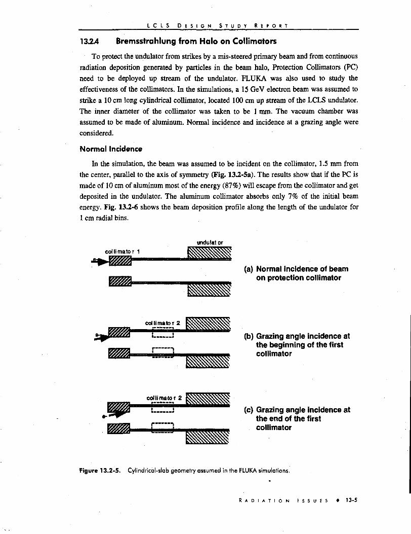
L C L S D E S I G N S T U D Y R E P O R T
13.2.4 Bremsstrahlung from Halo on Collimators
To protect the undulator from strikes by a mis-steered primary beam and from continuous
radiation deposition generated by particles in the beam halo, Protection Collimators (PC)
need to be deployed up stream of the undulator. FLUKA was also used to study the
effectiveness of the collimators. In the simulations, a 15 GeV electron beam was assumed to
strike a 10 cm long cylindrical collimator, located 100 cm up stream of the LCLS undulator.
The inner diameter of the collimator was taken to be 1 mm. The vacuum chamber was
assumed to be made of aluminum. Normal incidence and incidence at a grazing angle were
considered.
Normal Incidence
In the simulation, the beam was assumed to be incident on the collimator, 1.5 mm from
the center, parallel to the axis of symmetry (Fig. 13.2-5a). The results show that if the PC is
made of 10 cm of aluminum most of the energy (87%) will escape from the collimator and get
deposited in the undulator. The aluminum collimator absorbs only 7% of the initial beam
energy. Fig. 13.2-6 shows the beam deposition profile along the length of the undulator for
1 cm radial bins.
undulat or
collimator 1
(a) Normal incidence of beamon protection collimator
col li mate r 2
...J
'. J
(b) Grazing angle incidence atthe beginning of the firstcollimator
collimator 2
(c) Grazing angle incidence atthe end of the firstcollimator
Figure 13.2-5. Cylindrical-slab geometry assumed in the FLUKA simulations.
R A D I A T I O N I S S U E S • 13-5

L C L S D E S I G N S T U D Y R E P O R T
When corrected for the bin size effect, the dose rate deposited in the innermost shell of
the undulator from such a scenario will reach 2.2 x 10"9 Gy (2.2 x 10'7 rad) per incident
electron.
When the collimator is assumed to be made of high-Z material, the electromagnetic
shower fully develops in the collimator, which thus protects the undulator from continuous
deposition of energy due to particles in the beam halo. Fig. 13.2-7 shows the energy
deposition profile in a 10 cm long tungsten collimator. In this scenario 99% of the energy of
the incident beam is absorbed in the PC. It should be pointed out that tungsten would not
withstand strikes with the direct beam; therefore, a combination of low-Z material acting as a
spoiler followed by a high-Z absorber may be needed for an efficient protection collimator.
1000 2000 3000 4000 5000Distance Along the Undulator (cm)
6000
Figure 13.2-6. Dose along the undulator for a 15GeV beam normally incident on an aluminumcollimator 10 cm long.
Grazing Angle Incidence
In the simulation, the beam was assumed to strike the inside of the tungsten collimator,
1 cm from the front face, at an angle of incidence of 10 mrad (Fig. 13.2-5b). The results show
that the undulator would receive 51% of the initial beam energy. When a similar collimator is
added 80 cm down stream of the first PC (20 cm up stream of the undulator) the second unit
absorbs part of the energy escaping from the first PC. The energy deposited in the undulator
for the same scenario would reduce from 51% to 26%. Fig. 13.2-8 shows the radiation
deposited in the first 10 cm length of the undulator where the largest radiation deposition is
expected in the two cases of one and two collimators.
1 3 - 6 • R A D I A T I O N I S S U E S

L C L S D E S I G N S T U D Y R E P O R T
10-7 =r1 5
I1SLO
a10r lO
-
rnr
—
="o--
llJll 11 1
1
o
1
o
1
1
o
1
o
1
1
o
1
o
1
0
t
1
1
mil
i i
-
inn-
LLU
-
* 1
0 2 4 6 8Depth Inside the Collimator (cm)
10
Figure 13.2-7. Dose profile inside the tungsten collimator for a normally incident 15 GeV electronbeam.
Itt
3
8.
V01OQ
100 120 U0 160 180Distance along the undulator (cm)
200
Figure 13.2-8. Energy deposition in the first 100 cm of the undulator, for a 15 GeV electron incidentat a grazing angle (10 |irad) on a tungsten collimator. The beam is assumed to strikethe first collimator at 1 cm from its front face. One and two collimator cases areshown.
In another calculation the beam was assumed to strike the inside of the first tungsten
collimator, 9 cm from the front face (Fig. 13.2-5c). Results show that the undulator receives
77% of the energy in the beam. Addition of a second PC would reduce the deposited energy
to 28%. The dose per electron deposited in the undulator for the one and two collimator cases
R A D I A T I O N I S S U E S • 1 3 - 7
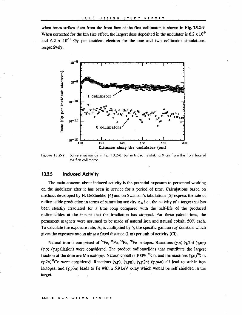
L C L S D E S I G N S T U D Y R E P O R T
when beam strikes 9 cm from the front face of the first collimator is shown in Fig. 13.2-9.
When corrected for the bin size effect, the largest dose deposited in the undulator is 6.2 x 10'9
and 6.2 x 10"n Gy per incident electron for the one and two collimator simulations,
respectively.
10"
"8 ,n-910"
S2213
Vft
10-12
1
• 1
: *
7-
' • 1 ' • ' ' 1 ' '
collimator '
2 collimators'
. . 1 . . . . 1 . .
1 • 1 • ' ' " 1 ' ' ' ' :
« :
. . 1 . . . . 1 . . . .100 120 140 160 180
Distance along the undulator (cm)200
Figure 13.2-9. Same situation as in Fig. 13.2-8, but with beams striking 9 cm from the front face ofthe first collimator.
13.2.5 Induced Activity
The main concern about induced activity is the potential exposure to personnel working
on the undulator after it has been in service for a period of time. Calculations based on
methods developed by H. DeStaebler [4] and on Swanson's tabulations [5] express the rate of
radionuclide production in terms of saturation activity As, i.e., the activity of a target that has
been steadily irradiated for a time long compared with the half-life of the produced
radionuclides at the instant that the irradiation has stopped. For these calculations, the
permanent magnets were assumed to be made of natural iron and natural cobalt, 50% each.
To calculate the exposure rate, As is multiplied by y, the specific gamma ray constant which
gives the exposure rate in air at a fixed distance (1 m) per unit of activity (Ci).
Natural iron is comprised of ^Fe, 56Fe, 57Fe, 58Fe isotopes. Reactions (y,n) (y,2n) (y,np)
(y.p) (y.spallation) were considered. The product radionuclides that contribute the largest
fraction of the dose are Mn isotopes. Natural cobalt is 100% 59Co, and the reactions (y,n)58Co,
(y,2n)57Co were considered. Reactions (y,p), (y,pn), (y,p2n) (y,p4n) all lead to stable iron
isotopes, and (y,p3n) leads to Fe with a 5.9 keV x-ray which would be self shielded in the
target.
1 3 - 8 • R A D I A T I O N I S S U E S

L C L S D E S I G N S T U D Y R E P O R T
The total exposure rate from an activated magnet immediately after shut-down is
conservatively estimated to be 5 mR hr"' W*1 at 1 m. The exposure is dominated by a
0.8 MeV gamma from 58Co with a half-life of 71 days. Monte Carlo simulations of Armstrong
et al. [6] on a free electron laser wiggler result in exposure rates of 3-3.5 mR/hr for an
average beam loss of 1 W/m compared to 5 mR hr ~x W 1 calculated above.
Personnel exposure from radioactive components in the beam line is of concern mainly
around beam dumps, targets, or collimators where the entire beam or a large fraction of the
beam is dissipated continuously. At the dose rates calculated above, and with the expected
low level of beam losses in the undulator, the activation of the unit and resulting personnel
exposure are expected to be very low.
13.3 References
1 A. Fass6, A. Ferrari, J. Ranft, P.R. Sala, "An update about FLUKA," Proc. ofSARE-2, GenevaOct. 9-11,1995, Ed. G.R. Stevenson, CERN TIS, RP/97,05 (1997), p. 169.
2 A. Fasso et al., "FLUKA92," Proc. of SARE-J, Santa Fe, NM, Jan. 11-15, 1993, Ed. A.Palounek, Los Alamos LA, 12835, C (1994), p. 134.
3 A. Ferrari, M. Pelliccioni, P.R. Sala, Nucl. Inst. Meth. B83,518 (1993).
4 H. DeStaebler, "Photon-Induced Residual Activity," SLAC-TN-6392 (1963).
5 W.P. Swanson, "Radiological Safety Aspects of the Operation of Electron Linear Accelerators,"IAEA Technical Report Series No. 188 (1979).
6 T.W. Armstrong et al., "Predictions of Induced Radioactivity in Free Electron Laser Wiggler dueto 80- and 180- MeV Electron Beam Loss," IEEE Nucl. Sci.
R A D I A T I O N I S S U E S • 1 3 - 9

Parameter Tables
1. Beam Tracking
Values at section exit
Injector -RF Photocathode Gun
injector -Accelerator
injector - Dogleg
L1NAC-1
Bunch Compressor-}
UNAC-2
Bunch Compressor-2
LINAC-3
LlNACtoUndulatorTransport
Parameters used inFEL Simulations
«
r»]
0.2
14
26
39
41
471
506
1093
1161
Energy
[GeV]
0.007
0.15
0.15
0.28
0.28
6.00
6.00
14.35
14.35
Emitt.
Growth*
I*]
4
4
6
15
8
4
4
Norm.
Eraitt.
{mmmrad]
1.00
1.04
1.08
1.14
1.29
1.37
1.41
1.45
1.50
Slice
[%)
0.01
0.005
0.013
0.0006
0.012
0.005
0.006
0.02
Inieasity
Loss
[*]
0.0
0.0
0.0
0.5
0.0
0.5
0.0
0.0
Halo*
Oiarge
CnCJ
1
1
1
1
0.995
0.995
0.990
0.990
0.990
RMS
Bunch L.
[mm]
1
1
1
0.39
0.39
0.020
0.020
0.020
Peak
Current
IA}
87
87
87
87
220
220
3560
3560
3560
3400
•Relative to the initial emittance.
''Beam Halo will not contribute to FEL process.

L C L S D E S I G N S T U D Y R E P O R T
2. Parameter Summary
Injector Beamline
Cathode material
Energy at gun
Energy at end of dogleg
Normal transverse rms emittance
Linac
Energy at first compressor
Energy at second compressor
Energy after linac
Norm, transverse rms emittance after linac
Undulator
Undulator type
Magnet material
Undulator period A,,
Full gap
Maximum field
Undulator parameter K
Number of periods Nu
Total length L«
rms magnet error AB
Charge at undulator
Radiation wavelength \
Energy E
Peak current at undulator entrance
rms bunch length LB
rms bunch length xB
Average p-function
X-ray Optics
Number of coherent photons per pulse
Peak photon flux
Peak brightness
Average brightness -
Units
metal (Cu or possibly Mg)
7
150
1.00
280
6
14.35
1.45
MeV
MeV
nmmmrad
MeV
GeV
GeV
it mm mrad
planar hybrid undulator
NdFeB
30
6
1.32
3.71
3328
112.3
0.10
0.947
15
4.54
3400
20
67
6
22.5
80.7
0.12
0.42
mm
mm
T
m%
nC
1.5
14.35
3400
20
67
18
2.0
7.1
1.2
4.2
Units
AGeV
A
\im
fs
m/rad
1012 Photons/pulse
1024 Photons/s
1O33 Photons/s/mm2/mr2/.l%
1022 Photons/s/mm2/mrad2/.l
Peak spontaneous power per pulse 81 GW
A - 2 • P A R A M E T E R T A B L E S
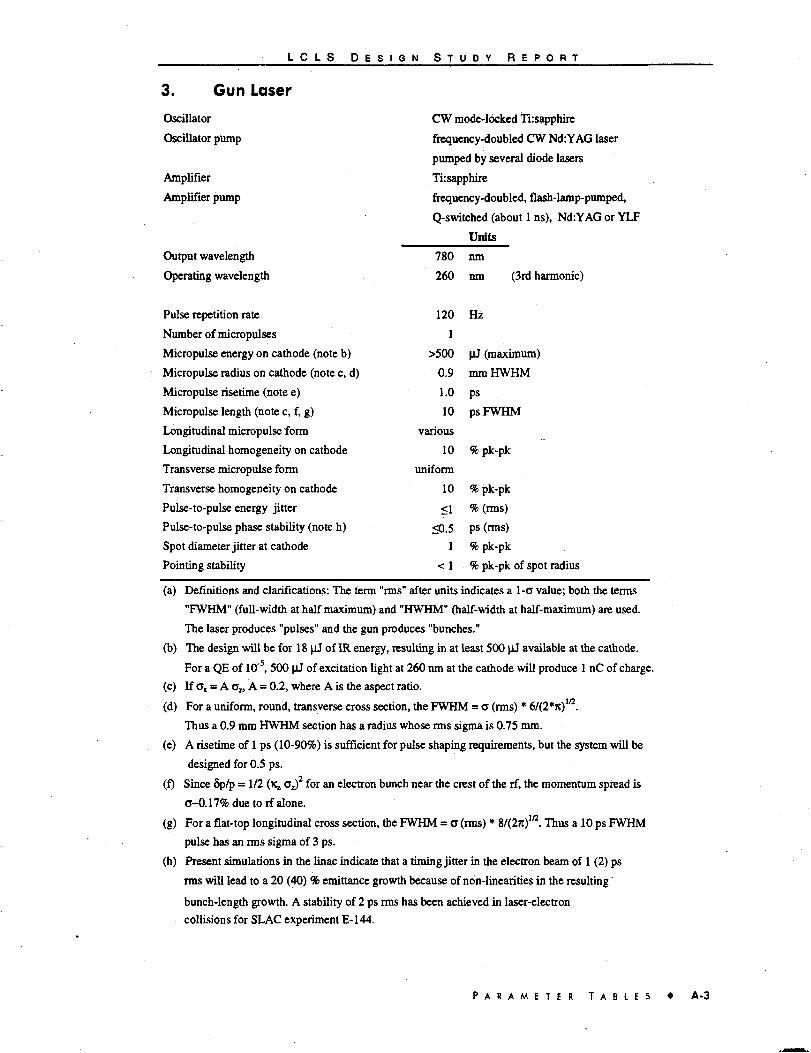
L C L S D E S I G N S T U D Y R E P O R T
3. Gun Laser
Oscillator
Oscillator pump
Amplifier
Amplifier pump
Output wavelength
Operating wavelength
Pulse repetition rate
Number of micropulses
Micropulse energy on cathode (note b)
Micropulse radius on cathode (note c, d)
Micropulse risetime (note e)
Micropulse length (note c, f, g)
Longitudinal micropulse form
Longitudinal homogeneity on cathode
Transverse micropulse form
Transverse homogeneity on cathode
Pulse-to-pulse energy jitter
Pulse-to-pulse phase stability (note h)
Spot diameter jitter at cathode
Pointing stability
CW mode-locked Ti:sapphire
frequency-doubled CW Nd:YAG laser
pumped by several diode lasers
Ti: sapphire
frequency-doubled, flash-lamp-pumped,
Q-switched (about 1 ns), Nd:YAG or YLF
Units
780 nm
260 nm (3rd harmonic)
120 Hz
1
>500 (iJ (maximum)
0.9 mm HWHM
1.0 ps
10 ps FWHM
various
10 % pk-pk
uniform
10 % pk-pk
<1 % (rms)
<0.5 ps (rms)
1 % pk-pk
< 1 % pk-pk of spot radius
(a) Definitions and clarifications: The term "rms" after units indicates a l-o value; both the terms
"FWHM" (full-width at half maximum) and "HWHM" (half-width at half-maximum) are used.
The laser produces "pulses" and the gun produces "bunches."
(b) The design will be for 18 ^J of IR energy, resulting in at least 500 \iJ available at the cathode.
For a QE of 10'5, 500 (iJ of excitation light at 260 nm at the cathode will produce 1 nC of charge.
(c) If ax = A oE, A = 0.2, where A is the aspect ratio.
(d) For a uniform, round, transverse cross section, the FWHM = a (rms) * 6/(2*n)1/2.
Thus a 0.9 mm HWHM section has a radius whose rms sigma is 0.75 mm.
(e) A risetime of 1 ps (10-90%) is sufficient for pulse shaping requirements, but the system will be
designed for 0.5 ps.
(f) Since 8p/p = 1/2 fe cz)2 for an electron bunch near the crest of the rf, the momentum spread is
0-0.17% due to rf alone.
(g) For a flat-top longitudinal cross section, the FWHM = o (rms) * %l(2n)m. Thus a 10 ps FWHM
pulse has an rms sigma of 3 ps.
(h) Present simulations in the linac indicate that a timing jitter in the electron beam of 1 (2) ps
rms will lead to a 20 (40) % emittance growth because of non-linearities in the resulting
bunch-length growth. A stability of 2 ps rms has been achieved in laser-electron
collisions for SLAC experiment E-144.
P A R A M E T E R T A B L E S A-3
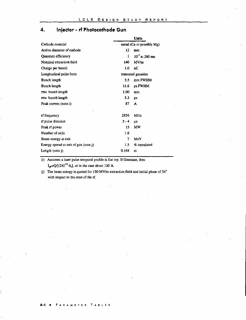
L C L S D E S I G N S T U D Y R E P O R T
4. Injector • rf Photocathode Gun
Units
Cathode material
Active diameter of cathode
Quantum efficiency
Nominal extraction field
Charge per bunch
Longitudinal pulse form
Bunch length
Bunch length
rms bunch length
rms bunch length
Peak current (note i)
rf frequency
rf pulse duration
Peak rf power
Number of cells
Beam energy at exit
Energy spread at exit of gun (note j)
Length (note j)
metal (Cu or possibly Mg)
12 mm
1 10"5 at 260 ran
140 MV/m
1.0 nC
truncated gaussian
3.5 mmFWHM
11.6 psFWHM
1.00 mm
3.3 ps
87 A
2856 MHz
3 - 4 us
15 MW
1.6
7 MeV
1.5 % correlated
0.168 m
(i) Assumes a laser pulse temporal profile is flat top. If Gaussian, then
Ipk=Q/t(2Jt)!/2 o j , or in the case about 130 A.
(j) The beam energy is quoted for 130 MV/m extraction field and initial phase of 54°
with respect to the crest of the rf.
A - 4 • P A R A M E T E R T A B L E S
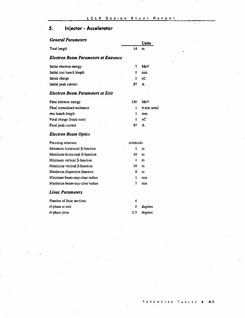
L C L S D E S I G N S T U D Y R E P O R T
Units
5. Injector - Accelerator
General Parameters
Total length 14 m
Electron Beam Parameters at Entrance
Initial electron energy
Initial rras bunch length
Initial charge
Initial peak current
Electron Beam Parameters at Exit
Final electron energy
Final normalized emittance
rras bunch length
Final charge (beam core)
Final peak current
Electron Beam Optics
Focusing structure
Minimum horizontal p-function
Maximum horizontal ^-function
Minimum vertical p-function
Maximum vertical P-function
Maximum dispersion function
Minimum beam-stay-clear radius
Maximum beam-stay-clear radius
Linac Parameters
Number of linac sections 4
rf-phase at exit 0 degrees
rf-phase jitter 0.5 degrees
71
1
87
150
1
1
1
87
MeVmmnC
A
MeV
nmm mrad
mm
nC
A
solenoids
1
10
1
10
0
1
7
m
m
m
mm
mm
mm
P A R A M E T E R T A B L E S A-5

L C L S D E S I G N S T U D Y R E P O R T
6. Injector - Dogleg
General Parameters
Dogleg type
R56
Transverse offset
Total length
Electron Beam Parameters at Entrance
Energy
Initial normalized emittance
Initital total energy spread
Initial slice energy spread
Initial rms bunch length
Initial charge
Initial peak current
Longitudinal brightness
Location after cathode
Electron Beam Quality Reduction
Intensity loss
Mean emittance growth dslt^^
Electron Beam Parameters at Exit
Energy
Final normalized emittance
Final total energy spread
Final slice energy spread
Final rms bunch length
Final charge
Final peak current
Longitudinal brightness
Electron Beam Optics
Minimum horizontal P-function
Maximum horizontal p-function
Minimum vertical p-function
Maximum vertical P-function
Maximum dispersion function
Units
2 dipole dogleg
-4
1.0
12
e150
1
0.20
0.01
1
1
87
mm
m
m
MeV
Jt mm mrad
%
%
mm
nC
A
5900 A
14.2 m
0.00
4.0
150
1.04
0.20
0.01
1
1
87
5900
2
30
2
20
0.2
%
%
MeV
it mm mrad
%
%
mm
nC
A
A
m
m
m
m
m
A - 6 • P A R A M E T E R T A B L E S
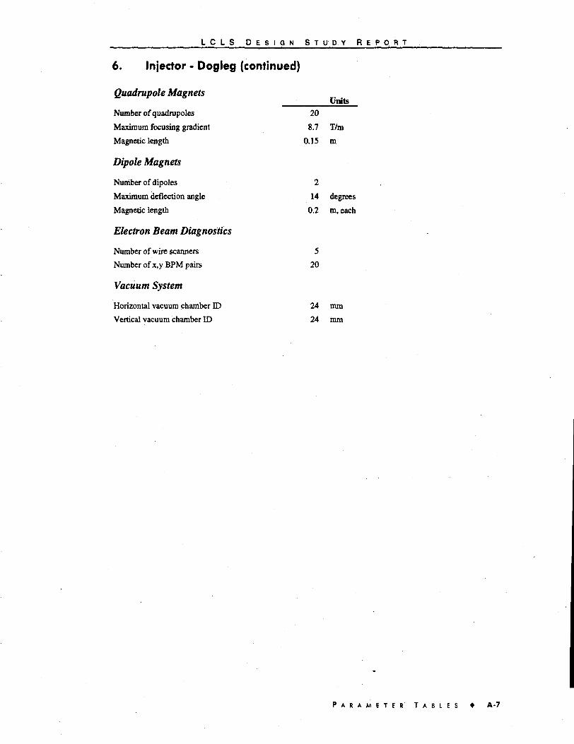
L C L S D E S I G N S T U D Y R E P O R T
6. Injector - Dogleg (continued)
Quadrupole MagnetsUnits
Number of quadrupoles
Maximum focusing gradient
Magnetic length
Dipole Magnets
Number of dipoles
Maximum deflection angle
Magnetic length
Electron Beam Diagnostics
Number of wire scanners
Number of x,y BPM pairs
Vacuum System
Horizontal vacuum chamber ID
Vertical vacuum chamber ID
20
8.7
0.15
2
14
0.2
5
20
24
24
T/mm
degrees
m,each
mm
mm
P A R A M E T E R T A B L E S • A - 7

L C L S D E S I G N S T U D Y R E P O R T
7. General Linac Parameters
rf frequency
Acceleration gradient
Active length of section
Q
Shunt impedance
Iris diameter
Klystron type
Peak rf power
Mean rf power
Units
2856 MHz
19 MV/m
3 m
13000-14000
53-60 MQ/in
26.2 -19.1 mm
5045
60 MW, 130 MW SLED
45 kW
A - 8 • P A R A M E T E R T A B L E S

L C L S D E S I G N S T U D Y R E P O R T
8. Linac-1
General ParametersUnits
Total length
Electron Beam Parameters at Entrance
Initial electron energy
Initial normalized emittance
Initital total energy spread
Initial slice energy spread
Initial nns bunch length
Initial charge
Initial peak current
Longitudinal brightness
Location after cathode
Electron Beam Quality Reduction
Intensity loss
Mean emittance growth bzlt&iuuKt
Electron Beam Parameters at Exit
Final electron energy
Final normalized emittance
Final total energy spread
Final slice energy spread
Final rms bunch length
Final charge
Final Peak current
Longitudinal brightness
Focusing structure
Mean cell length
Minimum horizontal (J-function
Maximum horizontal f$-function
Minimum vertical f}-function
Maximum vertical ^-function
Maximum dispersion function
Phase advance per cell
Beam-stay-clear radius
12.375
150
1.04
0.20
0.01
1
1
87
5900
26.2
0
3.8
280
1.08
2.30
0.005
1
1
87
5900
FODO
6
3
10
3
10
0
75
11.6
m
MeV
Ji mm mrad
%
%
mmnC
A
A
m
%
%
MeV
Jt mm mrad
%
%
mm
nC
A
A
m
m/rad
m/rad
m/rad
m/rad
m
degrees
mm
P A R A M E T E R T A B L E S • A - 9
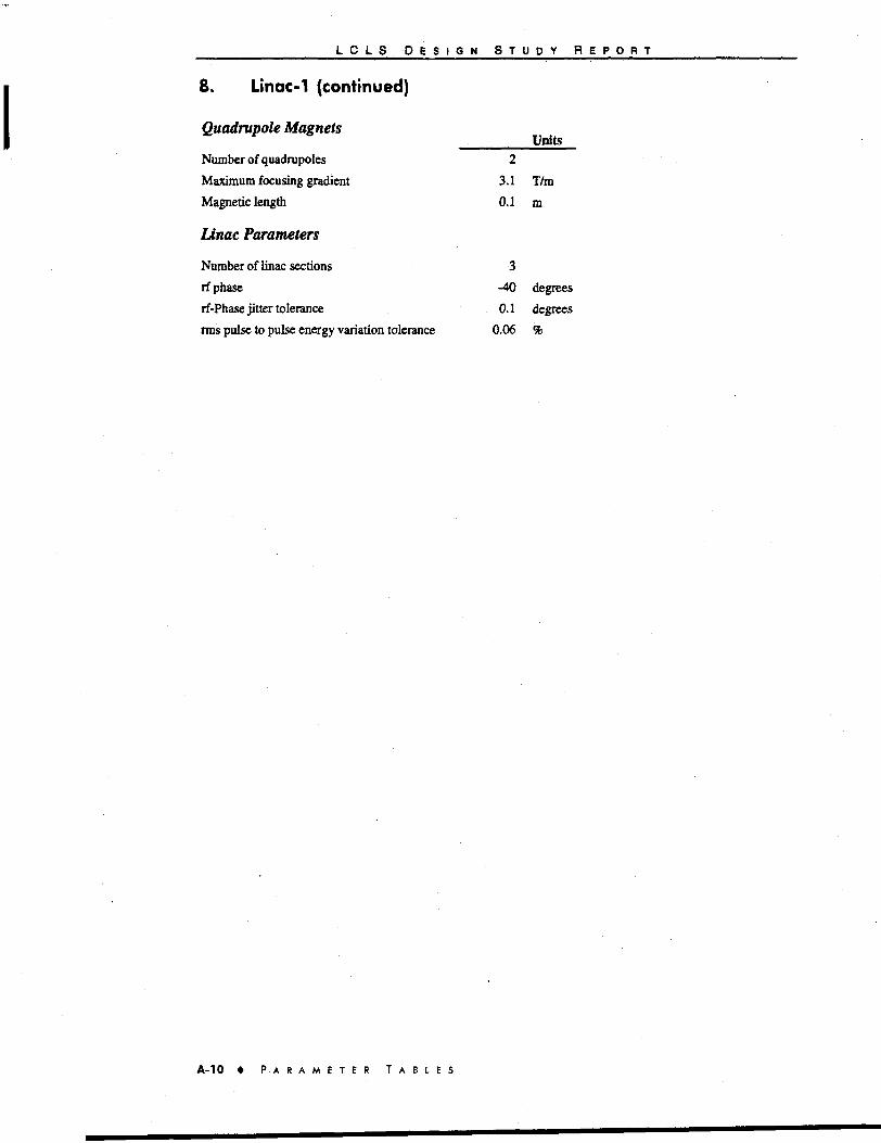
L C L S D E S I G N S T U D Y R E P O R T
8. Linac-1 (continued)
Quadrupole MagnetsUnits
Number of quadrupoles
Maximum focusing gradient
Magnetic length
Linac Parameters
Number of linac sections
if phase
rf-Phase jitter tolerance
rms pulse to pulse energy variation tolerance
2
3.1
0.1
3
-40
0.1
0.06
T/m
m
degrees
degrees
%
A - 1 0 • P A R A M E T E R T A B L E S

L C L S D E S I G N S T U D Y R E P O R T
9. Bunch Compressor-!
General ParametersUnits
Compressor type
R56
Transverse offset
Total length
Electron Beam Parameters at Entrance
Energy
Initial normalized emittance
InititaJ total energy spread
Initial slice energy spread
Initial rms bunch length
Initial charge
Initial peak current
Longitudinal brightness
Location after cathode
Electron Beam Quality Reduction
Intensity loss
Mean emittance growth A£/£En(ran«
Electron Beam Parameters at Exit
Energy
Final normalized emittance
Final total energy spread
Final slice energy spread
Final rms bunch length
Final charge
Final peak current
Longitudinal brightness
Electron Beam Optics
Minimum horizontal p-function
Maximum horizontal p-function
Minimum vertical |3-function
Maximum vertical P-function
Maximum dispersion function
Beam-stay-clear radius
4 dipole chicane
27
117
2.8
280
1.08
2.3
0.005
1
1
87
5900
38.5
0.5
5.6
280
1.14
2.3
0.013
0.39
0.995
220
5851
1.4
2.8
1.4
2.6
0.117
>30
mm
nun
m
MeV
71 mm mrad
%
%
mm
hC
A
A
m
%
%
MeV
7t mm rorad
%
%
mm
nC
A
A
m
m
m
m
m
mm
P A R A M E T E R T A B L E S A - 1 1
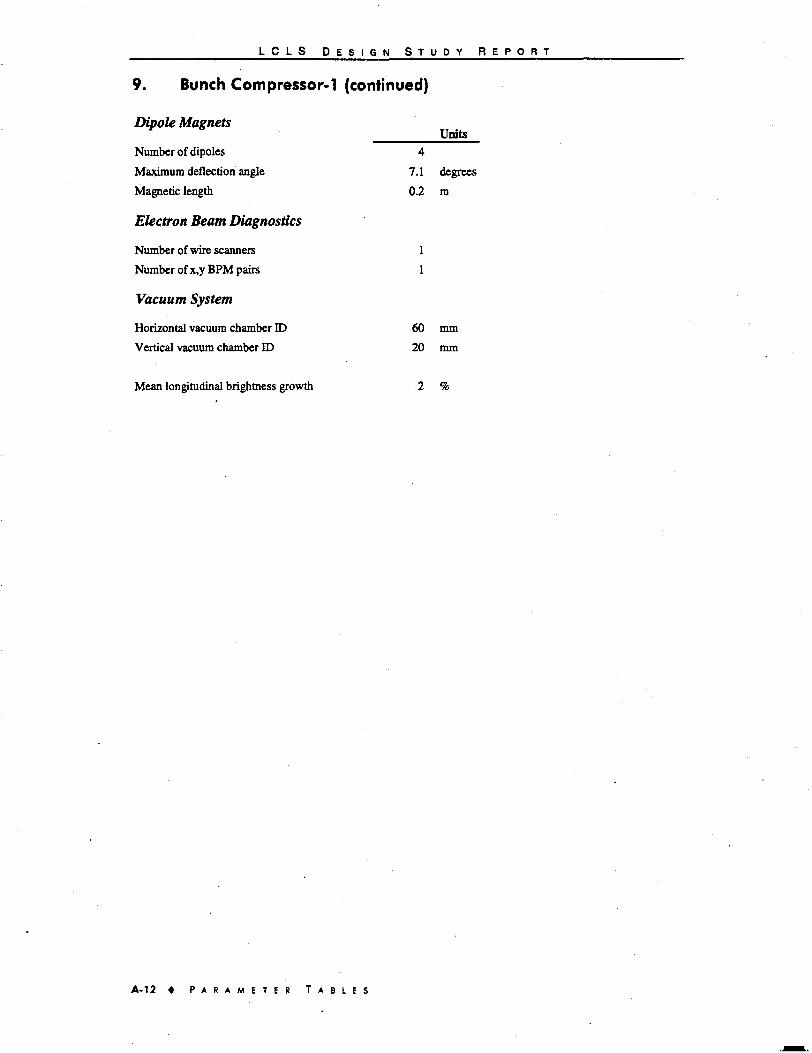
L C L S D E S I G N S T U D Y R E P O R T
9. Bunch Compressor-1 (continued)
Dipole Magnets
Number of dipoles
Maximum deflection angle
Magnetic length
Electron Beam Diagnostics
Number of wire scanners
Number of x,y BPM pairs
Vacuum System
Horizontal vacuum chamber ID
Vertical vacuum chamber ID
4
7.1
0.2
1
1
60
20
Units
degrees
m
mm
mm
Mean longitudinal brightness growth
A - 1 2 • P A R A M E T E R T A B L E S

L C L S D E S I G N S T U D Y R E P O R T
10. Linac-2
General Parameters
Total length
Electron Beam Parameters at Entrance
Initial electron energy
Initial normalized emittance
Initital total energy spread
Initial slice energy spread
Initial rms bunch length
Initial charge
Initial peak current
Longitudinal brightness
Location after cathode
Electron Beam Quality Reduction
Intensity loss
Mean emittance growth teJtEmnace
Electron Beam Parameters at Exit
Final electron energy
Final normalized emittance
Final total energy spread
Final slice energy spread
Final rms bunch length
Final charge
Final peak current
Longitudinal brightness
Electron Beam Optics
Focusing structure
Mean cell length
Minimum horizontal { -function
Maximum horizontal (J-function
Minimum vertical f}-function
Maximum vertical ^-function
Maximum dispersion function
Phase advance per cell
Beam-stay-clear radius
Units430 m
280
1.14
2.3
0.013
0.39
0.995
220
5900
41
0.0
13.2
6
1.29
1.0
0.0006
0.39
0.995
220
5800
FODO
25
10
47
10
44
0
70
11.6
MeV
Tcmmmrad
%
%
mm
nC
A
A
m
%%
GeV
71 mm mrad
%
%
mm
nC
A
A
mm
mm
m
mdegrees
mm
P A R A M E T E R T A B L E S A - 1 3

L C L S D E S I G N S T U D Y R E P O R T
10. Linac-2 (continued)
Quadrupole MagnetsUnits
Number of quadrupoles
Maximum focusing gradient
Magnetic length
linac Parameters
Number of linac sections
rf-compression phase
rms rf-phase jitter tolerance
rms pulse to pulse energy variation tolerance
35
17.5
0.1
133
-29
1
0.15
T/m
m
degrees
degrees
%
A - 1 4 • P A R A M E T E R T A B L E S

L C L S D E S I G N S T U D Y R E P O R T
11. Bunch Compressor-2
General Parameters
Compressor type
R56
Transverse offset
Total length
Electron Beam Parameters at Entrance
Electron energy
Initial normalized emittance
Initital total energy spread
Initial slice energy spread
Initial rms bunch length
Initial charge
Initial peak current
Longitudinal brightness
Location after cathode
Electron Beam Quality Reduction
Intensity loss
Mean emittance growth A£/£EUIU«X
Electron Beam Parameters at Exit
Energy
Final normalized emittance
Final total energy spread
Final slice energy spread
Final rms bunch length*
Final charge
Final peak current
Longitudinal brightness
Electron Beam Optics
Minimum horizontal P-function
Maximum horizontal P-function
Minimum vertical P-function
Maximum vertical P-function
Maximum dispersion function
Units
double 4 dipole chicane
36
0.29
35
?
6.01.29
1.0
0.0006
0.39
0.995
220
5800
471
0.5
6.2
6.0
1.37
1.01
0.012
0.020
0.990
3560
5765
17
35
17
35
0.29
mm
m
m
GeV
% mm mrad
%
%
mm
nC
A
A
m
%
%
GeV
7C mm mrad
%
%
mm
nC
A
A
m
m
m
m
m
•Starts to get difficult to quantify due to increasing non-linearities of correlations.
P A R A M E T E R T A B L E S A - 1 5

L C L S D E S I G N S T U D Y R E P O R T
11. Bunch Compressor-2 (continued)
Dipole Magnets
Number of dipoles
Maximum deflection angle
Magnetic length
Electron Beam Diagnostics
Number of wire scanners
Number of x,y BPM pairs
Vacuum System
Horizontal vacuum chamber ID
Vertical vacuum chamber ID
8
3.4/1.3
1.5
2
10
80
30
Units
degrees
m
mm
mm
Mean longitudinal brightness growth
A - 1 6 • P A R A M E T E R T A B L E S

L C L S D E S I G N S T U D Y R E P O R T
12. Linac-3
General Parameters
Total length
Electron Beam Parameters at Entrance
Initial electron energy
Initial normalized emittance
Initital total energy spread
Initial slice energy spread
rms bunch length
Initial charge
Peak current
Longitudinal brightness
Location after cathode
Electron Beam Quality Reduction
Intensity loss
Mean emittance growth Ae/ea^a,,,*
Electron Beam Parameters at Exit
Final electron energy
Final normalized emittance
Final total energy spread
Final slice energy spread
Final rms bunch length
Final charge
Final peak current
Longitudinal brightness
Electron Beam Optics
Focusing structure
Mean cell length
Minimum horizontal P-function
Maximum horizontal P-function
Minimum vertical P-function
Maximum vertical P-function
Maximum dispersion function
Phase advance per cell
Beam-stay-clear radius
587.5
6.0
1.37
1.0
0.012
0.020
0.990
3560
5800
506.0
0
2.9
14.35
1.41
0.10
0.005
0.020
0.990
3560
5700
FODO
25
32
68
33
72
0
30
11.6
Units
m
GeV
nmmmrad
%
%
mm
nC
A
A
m
Units
%
%
GeV
7t mm mrad
%
%
mm
nC
A
A
mm
m
m
mm
degrees
mm
P A R A M E T E R T A B L E S A - 1 7

L C L S D E S I G N S T U D Y R E P O R T
12. Linac-3 (continued)
Quadrupole MagnetsUnits
Number of quadruples
Maximum focusing gradient
Magnetic length
Linac Parameters
Number of linac sections
rf-compression phase
rms rf-phase jitter (typical)
rms bunch to bunch energy variation (typical)
46
18.7
0.1
188
0
2
0.05
T/m
m
degrees
degrees
%
A - 1 8 • P A R A M E T E R T A B L E S
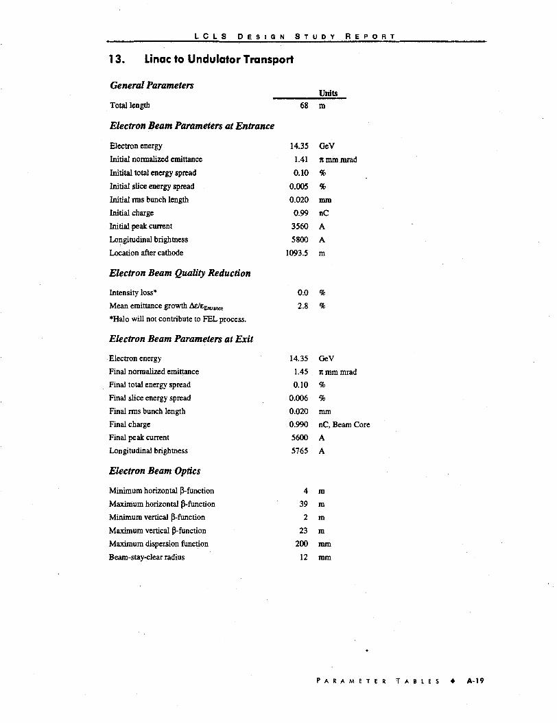
L C L S D E S I G N S T U D Y R E P O R T
13. Linac to Undulator Transport
General Parameters
Total length
Electron Beam Parameters at Entrance
Electron energy
Initial normalized emittance
Initital total energy spread
Initial slice energy spread
Initial rms bunch length
Initial charge
Initial peak current
Longitudinal brightness
Location after cathode
Electron Beam Quality Reduction
Intensity loss*
Mean emittance growth Ae/ea^,,^
•Halo will not contribute to FEL process.
Electron Beam Parameters at Exit
Electron energy
Final normalized emittance
Final total energy spread
Final slice energy spread
Final rms bunch length
Final charge
Final peak current
Longitudinal brightness
68
14.35
1.41
0.10
0.005
0.020
0.99
3560
5800
1093.5
0.0
2.8
14.35
1.45
0.10
0.006
0.020
0.990
5600
5765
Units
m
GeV
Jt mm mrad
%
%
mm
nC
A
A
m
%
%
GeV
Jt mm mrad
%
%
mm
nC, Beam Core
A
A
Electron Beam Optics
Minimum horizontal p-function
Maximum horizontal ^-function
Minimum vertical p-function
Maximum vertical (3-function
Maximum dispersion function
Beam-stay-clear radius
39m
m2 m
23 m
200 mm
12 mm
P A R A M E T E R T A B L E S A - 1 9

^ _ _ L C L S D E S I G N S T U D Y R E P O R T
13. Linac to Unduiator Transport (continued)
Quadrupole MagnetsUnits
Number of quadrupoles
Maximum focusing gradient
Magnetic length
Dogleg
R56
T566
Dogleg type
Number of dipoles
Maximum deflection angle
Magnetic length
Transverse
Diagnostics
Number of wire stations for e
Number of wire stations for Ap/p
Number of x,y BPM pairs
Collimatpr
Number of collimators
Collimator bore
21
78
0.46
-0.9
-61
T/m
m
mm
mm
4 dipole dogleg
4
1.3
2.62
90
1-4
1
21
4
1.2
degrees
m
cm
mm
A - 2 0 • P A R A M E T E R T A B L E S

L C L S D E S I G N S T U D Y R E P O R T
14. Undulator
Undulator PropertiesUnits
Overall length, including separations
Undulator magnet length
Start location after cathode
Undulator type
Magnet material
Permeable material
undulator period A
Full gap g
Undulator field B m
Undulator parameter K
a. (K/2)
Number of periods per segment
Number of segments
Separation between segments
Segment magnet length
Number of periods Nu
Wiggle plane
Electron Beam Optics
Focusing method
Focusing scheme
Quadrupole length
Quadrupole type
Cell length
Quadrupole gradient
111.825 m
99.84 m
1161 m
planar hybrid undulator
NdFeB
40 mm x 10 mm x 30 mm
Va Permendur
36 mm x S mm x 25 mm
30 mm
6 mm
1.32 T
3.71
2.62
64
52
0.235 m
1.92 m
3328
vertical
separated function
FODO
12 cm
permanet magnet
4.32 m
45.5 T/m
P A R A M E T E R T A B L E S A - 2 1
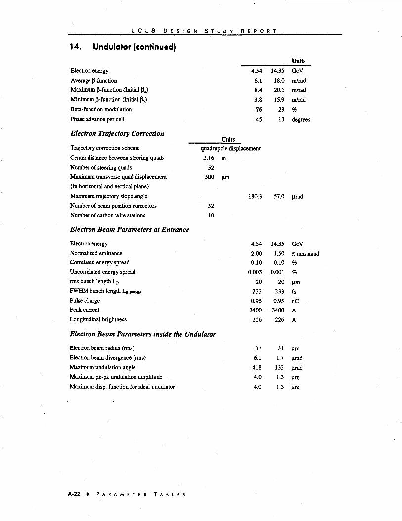
L C L S D E S I G N S T U D Y R E P O R T
14. Undulator (continued)
Electron energy
Average (J-function
Maximum ^-function (Initial px)
Minimum ^-function (Initial Py)
Beta-function modulation
Phase advance per cell
Electron Trajectory Correction
Trajectory correction scheme
Center distance between steering quads
Number of steering quads
Maximum transverse quad displacement
(In horizontal and vertical plane)
Maximum trajectory slope angle
Number of beam position correctors
Number of carbon wire stations
Electron Beam Parameters at Entrance
Electron energy
Normalized emittance
Correlated energy spread
Uncorrelated energy spread
rms bunch length LB
FWHM bunch length LBiFWHM
Pulse charge
Peak current
Longitudinal brightness
Electron Beam Parameters inside the Undulator
Electron beam radius (rms)
Electron beam divergence (rms)
Maximum undulation angle
Maximum pk-pk undulation amplitude
Maximum disp. function for ideal undulator
4.54
6.1
8.4
3.8
76
45
Units
quadrupole displacement
2.16 m
52
500 Jim
52
10
Units
14.35 GeV
18.0 m/rad
20.1 m/rad
15.9 m/rad
23 %
13 degrees
180.3 57.0 urad
4.54
2.00
0.10
0.003
20
233
0.95
3400
226
37
6.1
418
4.0
4.0
14.35
1.50
0.10
0.001
20
233
0.95
3400
226
31
1.7
132
1.3
1.3
GeVn mm mrad
%
%
Hmfs
nC
A
A
(im
lirad
Ltrad
|xmfun
A - 2 2 • P A R A M E T E R T A B L E S

L C L S D E S I G N S T U D Y R E P O R T
14. Undulator (continued)
Vacuum System
Vacuum chamber height OD
Vacuum chamber wall thickness
Vacuum chamber material
Bunch frequency co=27ic/LB
Skin depth
Maximum inner surface roughness
Beam pipe straightness
Vacuum pressure
Expected Radiation Dose per Year
Rad. to damge mag. face AB/Br=l %
* 1 Gy -1 J/kg = 100 rad
Miscellaneous
Tunnel Temperature Stability
Und. Water Systems Temp. Stability
Units
6 mm
0.5 mm
copper plated stainlesss steel
6.8 lo'V
64 nm
100 nm
200 \un I m
< 10'7 mbar
4 kGy*
100 kGy*
1
0.1
K
K
Electron energy
Static Electron Beam Tolerances at Entrance
Electron energy
Peak current
Maximum.correlated rms energy spread
Maximum uncorrelated rms energy spread
Horizontal and vertical P matching
Maximum horizontal and vertical r\
Maximum horizontal and vertical TJ'
Maximum slice emittance
Maximum projected emittance
Maximum beam position displacement
Maximum beam angle
Pulse-to-Pulse Electron Beam Tolerances at Entrance
Electron energy
Peak current
Maximum correlated energy spread
Maximum uncorrelated energy spread
Pulse-to-pulse positional stability (rms)
Pulse-to-pulse angular stability (rms)
Units
4.54 14.35 GeV
0.05
20
0.001
0.0007
2
0.188
0.031
2.0
2.5
36.9
6.1
0.05
20
0.001
0.0007
7.4
1.2
0.05 %
20 %
0.001
0.0002
2 %
0.500 m
0.028
1.5 K mm mrad
2.0 Jt mm mrad
31.0 |im
1.7 Lirad
0.05 %
20 %
0.001
0.0002
6.2 p.m
0.3 urad
P A R A M E T E R T A B L E S A - 2 3

L C L S D E S I G N S T U D Y R E P O R T
14. Undulator (continued)
Radiation wavelength X,
Electron energy E
Y
Normalized electron beam emittance £„
Initial charge
Longitudinal pulse form
Transverse pulse form
rms bunch length LB
FWHM bunch length LB>FWHM
Units
Peak current
Uncorrelated rms Ap/p
Correlated Ap/p.
Longitudinal brightness: lpk/(2jc)woy
Cooperation length Lc
Slippage length L ^
FEL parameter p
Rayleigh length zR
Power gain length LQ
Field gain length LE
Peak saturation power PMt
Saturation length L ^
Energy of first harmonic
15
4.54
8879
2.00
0.95
flat-top
gaussian
20
67
70
233
3400
0.068
0.2
226
182
1145
4992
13
5.7
1.8
3.7
11
32.2
-48
100
0.82
1.5
14.35
28077
1.50
0.95
flat-top
gaussian
20
67
70
233
3400
0.021
0.1
226
51
322
499.2
4.7
40
5.8
11.7
9
94.2
-100
100
8.2
AGeV
rcmmmrad
nC
(im
fs
(im
fs
A
%
%
A
nm
nm
nm
io-4
m
m
m
GW
m
m
m
keV
A - 2 4 • P A R A M E T E R T A B L E S

L C L S D E S I G N S T U D Y R E P O R T
15. FEL
Radiation wavelength \
Electron energy E
y
Normalized electron beam emittance e,,
Initial charge
Longitudinal pulse form
Transverse pulse form
rms bunch length LB
FWHM bunch length L B F W H M
^B.FWHM
Peak current
Uncorrelated rms Ap/p
Correlated Ap/p
Longitudinal brightness: LJ/(2JC)V4or
Cooperation length Lc
2nLc
Slippage length L ^
FEL parameter p
Rayleigh length ZR
Power gain length LQ
Field gain length LE
Peak saturation power P^,
Saturation length L^,
Energy of first harmonic
Units
15
4.54
8879
2.00
0.95
flat-top
gaussian
20
67
70
233
3400
0.068
0.2
226
182
1145
4992
13
5.7
1.8
3.7
11
32.2
-48
100
0.82
1.5
14.35
28077
1.50
0.95
flat-top
gaussian
20
67
70
233
3400
0.021
0.1
226
51
322
499.2
4.7
40
5.8
11.7
9
94.2
-100
100
8.2
AGeV
it mm mrad
nC
\im
fs
\xmfs
A
%
%
A
nm
nm
nm
lO4
m
m
m
GW
m
m
m
keV
P A R A M E T E R T A B L E S A - 2 5

L C L S D E S I G N S T U D Y R E P O R T
15. FEL (continued)
FEL Radiation
Average saturation power
Energy per pulse
Number of coherent photons per pulse
Peak photon flux
Peak brightness
Average brightness
Instantaneous photon energy spread
Integrated photon energy spread
FEL fund, trans, beam size
FEL fund, trans, beam divergence
Spontaneous Radiaton
Peak spontaneous power per pulse
Average spontaneous power
Energy loss from spont. radiation
Rel. energy loss from spont. radiation
AE/E induced by spont. radiation
Spont. fund, trans, beam size
Spont. fund, trans, beam divergence
Units
0.36
3.0
22
81
1.2
0.42
0.14
0.42
37
3.2
8.1
0.27
0.0023
0.050
< 0.02 %
52
6.2
0.31
2.6
2.0
7.1
12
4.2
0.05
0.21
31
0.38
81
2.7
0.023
0.16
<0.02
33
2.0
W
mJ
1012 Photons/pulse
1024 Photons/s
1032 Photons/(s mm2 mr2.1%)
1022 Photons/(s mm2 mr2.1%)
%
%
\un|irad
GW
W
GeV
%
%
\im
urad
A - 2 6 • P A R A M E T E R T A B L E S

L C L S D E S I G N S T U D Y R E P O R T
16. Electron Beam Dump
General Parameters
Total length
Electron Beam Parameters at Entrance
Electron energy
Initial normalized emittance
Correlated energy spread
Uncorrelated energy spread
Initial rms bunch length
Initial charge
Initial peak current
Longitudinal emittance
Longitudinal brightness
Location after cathode
Electron Beam Optics
Minimum horizontal p-function
Maximum horizontal |3-function
Minimum vertical ^-function
Maximum vertical P-function
Dipole Magnets
Magnet type
Number of dipoles
Maximum deflection angle
Units10 m
14.35
1.50
0.10
0.05
0.024
0.95
3400
40
104
1273.788
4
39
23
2
GeVit mmmrad
%
%
mmnCA
MeVmm
A
m
m/rad
m/rad
m/rad
m/rad
permanent magnet
6
-4.5 degrees
P A R A M E T E R T A B L E S A - 2 7

L C L S D E S I G N S T U D Y R E P O R T
17. X-ray Optics
Radiation Source ParametersUnits
Radiation wavelength \
Macropulse rep rate
Number of micropulses/macropulse
rms Pulse duration
FWHM Pulse duration
Peak 1st FEL harmonic power
Energy/FEL pulse
Number of photons/FEL pulse
FWHM source size (electron)
FWHM source divergence (electron)
FWHM FEL mode & mode src. size (photon)
FWHM FEL mode & mode src. div. (photon)
1st harmonic rms FEL Rayleigh waist
1st harmonic FEL Rayleigh length
1st harm, homogeneous bandwidth a
1st harm, inhom. (z-corr.) bandwidth A
Peak 1st FEL harm, power density (@ 10m)
Peak 1st FEL harmonic field (@ 10m)
Peak spontaneous power
Time-averaged spontaneous power
90% total power bandwidth
FWHM sponL source size (photon)
FWHM spont source div. (photon)
15
120
1
67
232
11
3.0
22
93
15
93
8.1
37
5.7
0.14
0.42
7.0
2.3
8
0.3
-0.006
-131
-15.5
1.5
120
1
67
232
9
2.6
2.0
78
4.3
78
1.0
31
40
0.05
0.21
15
3.4
81
2.7
-0.025
82
4.9
AHz
fs
fs
109W
mJ
1012
\xm(irad
Hm(TEM00)
Urad (TEMOO)
|im
m
%
%
1011 W/mm2
1010V/m
GW
W
keV
pm (far field)
prad (far field)
A - 2 8 • P A R A M E T E R T A B L E S

L C L S D E S I G N S T U D Y R E P O R T
17. X-ray Optics (continued)
Absorption CellLength DTU*
1st differential pumping section
1st x-ray slit pair
2nd differential pumping aection
Absorption Cell
3rd differential pumping section
Near-FFTB X-ray Optics
4th differential pumping section
2nd x-ray slit pair
5th differential pumping section
Mirror tank
6th differential pumping section
Crystal tank
7th differential pumping section
Specular Optics Beamline
Crystal Optics Beamline
Long Beam line X'Ray Optics
End station (Option 1)
End station (Option 2)
1.1
2.7
1.1
1.2
1.1
Length
1.1
2.2
1.1
0.9
1.1
0.44
1.1
Length
Length
Length
n/a
n/a
mm
m
m
m
mm
m
m
m
m
ra
14.8
16.9
18.7
19.9
20.8
DTU*
31.5
33.4
35.3
36.8
38.0
39.0
40.0
DTU*
DTU*
DTU*
335.0
780.0
m
m
mm
m
m
m
m
m
m
m
m
m
m
* Distance to Undulator
P A R A M E T E R T A B L E S A - 2 9