Limited liability, strategic default and bargaining power
48
Working Paper Series Limited liability, strategic default and bargaining power Mirco Balatti, Carolina López-Quiles Disclaimer: This paper should not be reported as representing the views of the European Central Bank (ECB). The views expressed are those of the authors and do not necessarily reflect those of the ECB. No 2519 / January 2021
-
Upload
khangminh22 -
Category
Documents
-
view
0 -
download
0
Transcript of Limited liability, strategic default and bargaining power

Working Paper Series Limited liability, strategic default and bargaining power
Mirco Balatti, Carolina López-Quiles
Disclaimer: This paper should not be reported as representing the views of the European Central Bank (ECB). The views expressed are those of the authors and do not necessarily reflect those of the ECB.
No 2519 / January 2021
Abstract
In this paper we examine the effects of limited liability on mortgage dynamics. Whilethe literature has focused on default rates, renegotiation, or loan rates individually,we study them together as equilibrium outcomes of the strategic interaction betweenlenders and borrowers. We present a simple model of default and renegotiationwhere the degree of limited liability plays a key role in agents’ strategies. Wethen use Fannie Mae loan performance data to test the predictions of the model.We focus on Metropolitan Statistical Areas that are crossed by a State border inorder to exploit the discontinuity in regulation around the borders of States. Aspredicted by the model, we find that limited liability results in higher default ratesand renegotiation rates. Regarding loan pricing, while the model predicts higherinterest rates for limited liability loans, we find no such evidence in the Fannie Maedata. We further investigate this by using loan application data, which containsthe interest rates on loans sold to private vs public investors. We find that privateinvestors do price in the difference in ex-ante predictable default risk for limitedliability loans.
JEL codes: D10, E40, G21, R20, R30
Keywords: lender recourse, mortgage contracts, debt repudiation, renegotiation, discon-
tinuity.
ECB Working Paper Series No 2519 / January 2021 1

Non-technical summary
The rise of household debt before the financial crisis combined with high default rates
was a root cause of the Great Recession and highlighted the role of consumer finance for the
macroeconomy. Mortgage debt, in particular, constitutes two-thirds of US household total
debt. Outstanding mortgage amounts declined substantially during the Great Recession,
but have since reached new historical highs.
While there are several factors that determine the rate of mortgage default, such as
adverse economic shocks that leave households unable to honour their debt, default may
also be a voluntary choice, commonly referred to as strategic default. One particular
aspect the household may consider before choosing to default is whether there is limited
or full liability in place. Under limited liability, the lender is not allowed to seize the
household’s assets after default.
Limited liability constitutes the legal protection of a stakeholder’s liabilities beyond a
fixed sum. In the context of loans, and in particular of mortgage contracts, limited liability
implies a fixed limit on the borrower’s obligations, which amounts to the handover of the
mortgaged property. In the absence of limited liability, the borrower is liable for the
repayment of the full loan amount, and the lender is entitled to seize the borrower’s
personal assets.
In contrast to the literature, which has studied several effects of limited liability indi-
vidually, we analyse default decisions, renegotiation and loan pricing together. These are,
in fact, equilibrium outcomes of the strategic interaction between lenders and borrowers.
To this end, we first develop a simple model of default and renegotiation where the degree
of limited liability plays a key role in agents’ strategies. Borrowers who can afford to pay
the loan may choose to default if their mortgage is underwater. Limited liability encour-
ECB Working Paper Series No 2519 / January 2021 2

ages this behaviour since borrowers can walk away from their debt more easily. In turn,
lenders may be inclined to offer renegotiated loan prices to these borrowers, as they know
under limited liability they would not be able to recover more than the foreclosure value
of the home. Borrowers thus have greater bargaining power over lenders under limited
liability. These interactions also have an effect on loan prices, as the expected value of
each loan will depend on the equilibrium of this game. Thus, the model provides three
main predictions. First, limited liability leads to higher default rates. Second, lenders
renegotiate more under limited liability. Lastly, loan prices are higher for limited liability
loans.
We then use Fannie Mae loan performance data to test the predictions of the model. We
exploit the difference in regulation in different States. In particular, we limit our analysis
to Metropolitan Statistical Areas (MSAs) that are crossed by a State border, where one
side has limited liability laws in place and the other does not. This allows us to isolate the
effect of limited liability on loan outcomes, as other factors such as economic shocks are
expected to be the same within each MSA. As predicted by the model, we find that limited
liability results in higher default and renegotiation rates. Regarding loan pricing, while
the model predicts higher interest rates for limited liability loans, we find no such evidence
in the Fannie Mae data. We further investigate this by using loan application data from
the Home Mortgage Disclosure Act (HMDA) database, which contains the interest rates
on loans sold to private and public purchasers. We find that private investors do price
in the difference in ex-ante predictable default risk for limited liability loans, while their
public counterparts, such as Fannie Mae, do not. This has important policy implications,
as it imposes price distortions in a multi-trillion dollar market.
ECB Working Paper Series No 2519 / January 2021 3
1 Introduction
The rise of household indebtedness before the financial crisis combined with high default
rates was a root cause of the Great Recession and underlined the importance of consumer
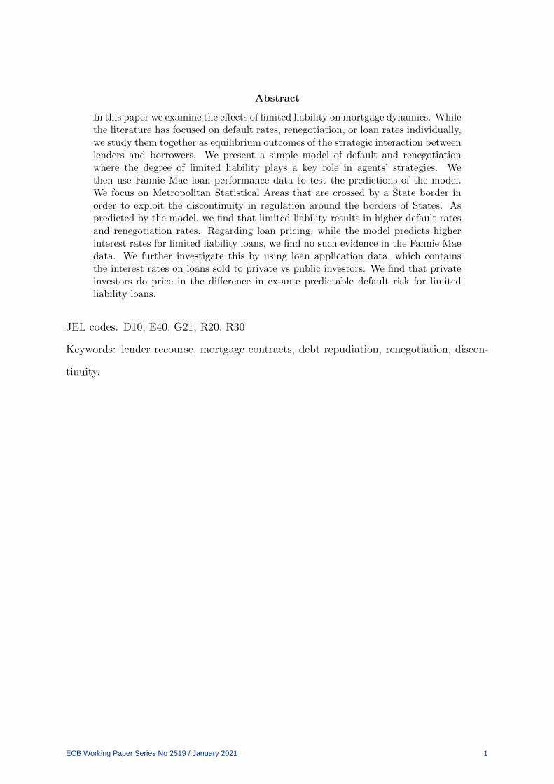
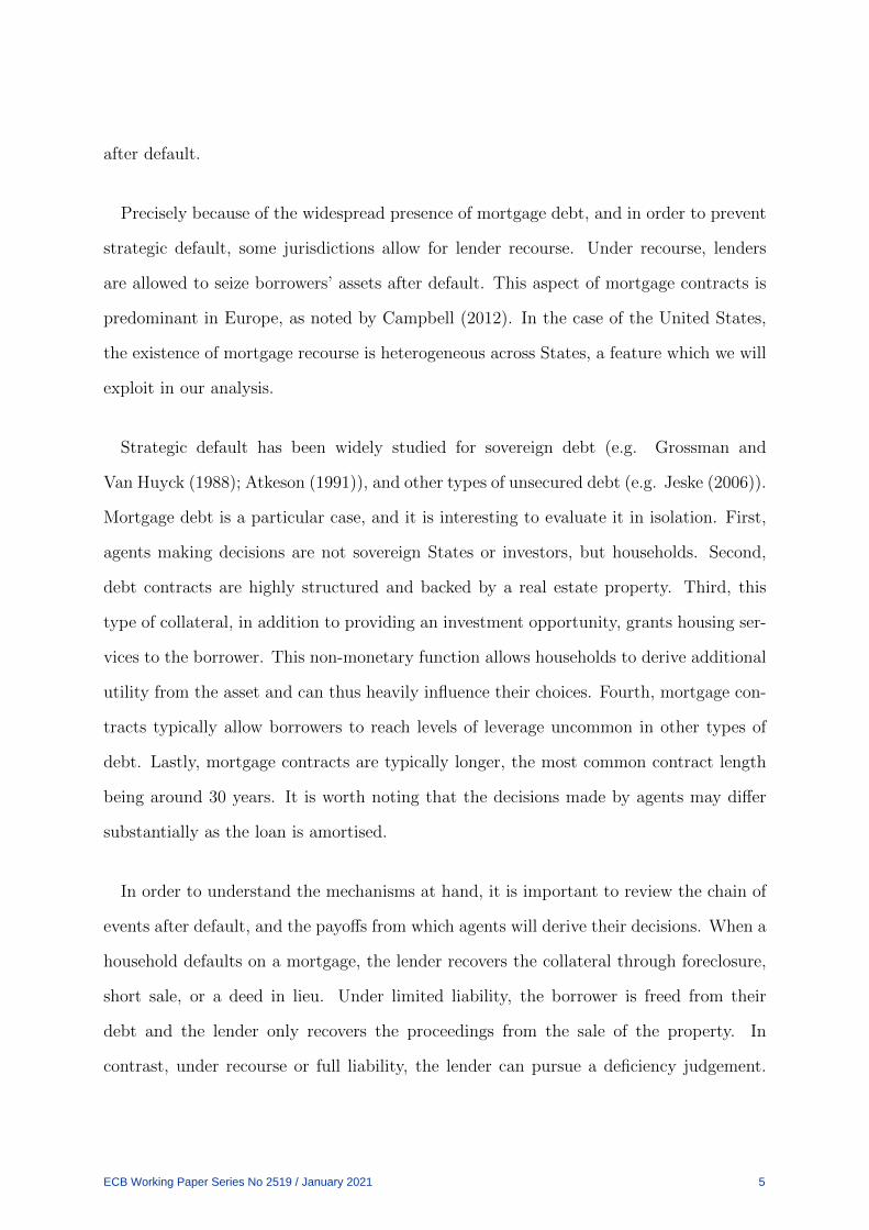
finance for the macroeconomy. Mortgage debt, in particular, constitutes two-thirds of
US household total debt, as shown in Figure 1. Outstanding mortgage amounts declined
substantially during the Great Recession, but have since reached new historical highs.
Figure 1: US households debt
Notes: Share of mortgage and other debt types as a percentageof total household debt. Total US outstanding mortgage amountin trillion US dollars. Source: New York Fed Consumer CreditPanel/Equifax and authors own calculations, 2003-2019.
While there are several factors that determine the rate of mortgage default, such as
adverse economic shocks that leave households unable to honour their debt, default may
also be a voluntary choice, commonly referred to as strategic default. One particular
aspect the household may consider before choosing to default is whether there is limited
in place. Under limited liability, the lender is not allowed to seize the household’s assets
ECB Working Paper Series No 2519 / January 2021 4
after default.
Precisely because of the widespread presence of mortgage debt, and in order to prevent
strategic default, some jurisdictions allow for lender recourse. Under recourse, lenders
are allowed to seize borrowers’ assets after default. This aspect of mortgage contracts is
predominant in Europe, as noted by Campbell (2012). In the case of the United States,
the existence of mortgage recourse is heterogeneous across States, a feature which we will
exploit in our analysis.
Strategic default has been widely studied for sovereign debt (e.g. Grossman and
Van Huyck (1988); Atkeson (1991)), and other types of unsecured debt (e.g. Jeske (2006)).
Mortgage debt is a particular case, and it is interesting to evaluate it in isolation. First,
agents making decisions are not sovereign States or investors, but households. Second,
debt contracts are highly structured and backed by a real estate property. Third, this
type of collateral, in addition to providing an investment opportunity, grants housing ser-
vices to the borrower. This non-monetary function allows households to derive additional
utility from the asset and can thus heavily influence their choices. Fourth, mortgage con-
tracts typically allow borrowers to reach levels of leverage uncommon in other types of
debt. Lastly, mortgage contracts are typically longer, the most common contract length
being around 30 years. It is worth noting that the decisions made by agents may differ
substantially as the loan is amortised.
In order to understand the mechanisms at hand, it is important to review the chain of
events after default, and the payoffs from which agents will derive their decisions. When a
household defaults on a mortgage, the lender recovers the collateral through foreclosure,
short sale, or a deed in lieu. Under limited liability, the borrower is freed from their
debt and the lender only recovers the proceedings from the sale of the property. In
contrast, under recourse or full liability, the lender can pursue a deficiency judgement.
ECB Working Paper Series No 2519 / January 2021 5

A deficiency judgement is a ruling through which the lender calculates the difference
between the mortgage balance outstanding and the amount recovered through the sale
of the collateral. Should the sale of the collateral not be enough to cover the mortgage
balance, the lender is entitled to claim the difference from the borrower.
This paper relates to two bodies of literature. The first one exploits different legislative
discontinuities around State borders to study several aspects of limited liability and its
effect on different market outcomes. Some papers have focused on the effect of limited
liability on loan origination. Pence (2006) studies loan origination volumes through the
difference in the size of loans on recourse and non-recourse States and finds that non-
recourse loans are smaller on average. Curtis (2014) finds that lender-friendly foreclosure
is associated with an increase in subprime originations, but has less effect on the prime
market. Li and Oswald (2017) leverage on the abolition of deficiency judgements in the
State of Nevada in 2009 and find that it led to a decline in equilibrium loan sizes and
approval rates. Some other papers have studied the effect of limited liability on loan rates
and housing prices. Meador (1982) finds that States with judicial foreclosure exhibit lower
interest rates on loans. Pennington-Cross and Ho (2008) inquire whether laws intending
to reduce predatory lending behaviour have an effect on loan rates. Their results suggest
that these laws have only a modest effect on loan prices. Mian et al. (2015) use judicial
requirements for foreclosures across States as an instrument for foreclosures and find
that higher foreclosure rates lead to a decline in house prices, residential investments
and consumer demand. Another set of papers is concerned with forbearance and loan
modifications. Gerardi et al. (2013) find that laws designed to protect borrowers delay
but do not prevent foreclosure. Conditional on a loan being underwater, these laws do not
increase the probability of cure. Collins et al. (2011) test the extent to which distressed
mortgage borrowers benefit from different types of State foreclosure polices. They find
that judicial foreclosure proceedings and foreclosure prevention initiatives are associated
ECB Working Paper Series No 2519 / January 2021 6

with modest increases in loan modification rates. Finally, another group of papers focus
on the effect of different legislation on default rates. Ghent and Kudlyak (2011) compare
recourse and non-recourse States and find higher mortgage default rates in the latter.
Chan et al. (2016) examine how factors affecting mortgage default spill over to other credit
markets. They find that, while non-recourse mortgage laws increase mortgage default,
they are associated with lower credit card default. Gianinazzi et al. (2019) investigate
default behaviour in Europe, where all mortgages have lender recourse and conclude that
many households default when the value of the house is greater than the outstanding
mortgage balance. They find this result puzzling because it is suboptimal. The authors
rationalise it by arguing that, under recourse, the fear of a decline in house prices pushes
these households to anticipate their default decision, thereby ‘leaving money on the table’.
While these papers focus on individual aspects on limited liability, one contribution of
this paper is to encompass default, renegotiation and loan pricing in an integrated setting.
We consider this an important aspect, as these elements are all equilibrium outcomes of
the strategic interaction between borrowers and lenders, which we show in our model.
The second strand of the literature this paper relates to deals with discrepancies between
Government-Sponsored Enterprises (GSEs) and the private market. Most notably, Hurst
et al. (2016) find that despite large regional variation in predictable default risk, GSE
mortgage rates for otherwise identical loans do not vary spatially. In contrast, they find
that the private market does set interest rates which vary with local risk. In this regard,
Dagher and Sun (2016) find similar results for credit supply by exploiting an exogenous
cutoff in loan eligibility to GSE guarantees. They find that judicial requirements reduce
the supply of credit only for jumbo loans, which are ineligible for GSE guarantees.
In this paper we connect these two strands of the literature by analysing default and
renegotiation choices by borrowers and lenders, as well as loan pricing, and to highlight
the difference in pricing between private and public investors.
ECB Working Paper Series No 2519 / January 2021 7
In addition, this paper is related to the theoretical literature that studies debt and
renegotiation, of which the closest papers are Hart and Moore (1998) and Bester (1994).
Some other papers have studied mortgage contracts and default decisions through the lens
of a dynamic heterogeneous agents model in general equilibrium. Some examples of such
models are Kaplan et al. (2017) and Guren et al. (2018). Guren et al. (2018) investigate the
interaction of adjustable and fixed-rate mortgage contracts with monetary policy. Kaplan
et al. (2017) propose a life-cycle model of housing decisions with both idiosyncratic and
aggregate shocks. Their goal is to replicate the macroeconomic dynamics observed in
the data during the Great Recession. These papers focus exclusively on non-recourse
mortgages.
In what follows, we present a model of debt renegotiation where the strategic choices of
lenders and borrowers depend on the extent to which recourse is enforced. In the model,
both house prices and the income of the borrower are stochastic. In some states of the
world, the household has enough income to pay their mortgage, whereas in other states of
the world it does not. Likewise, in some states of the world, the house value is higher than
the mortgage amount, i.e. the household has positive equity, whereas in other states of
the world the house value is lower, i.e. the mortgage is underwater. Households who can
afford to meet their payments, but whose mortgage is underwater, may find it optimal
to default, in particular on instances where it is unlikely that they will be liable with
their personal assets after default. Lenders who know this may find it optimal to offer
these households a renegotiated mortgage price in order to prevent them from walking
away from their obligations. At the same time, the price of these loans will reflect these
mechanisms.
We test the predictions of this model exploiting the difference in mortgage laws in
different US States. We focus on Metropolitan Statistical Areas that are crossed by a
State border, where one State has limited liability laws in place while the other does
ECB Working Paper Series No 2519 / January 2021 8

not. Using Fannie Mae loan performance data we find, as predicted by the model, that
default rates are higher for lower levels of lender recourse, and so are renegotiation rates.
However, one result is at odds with our model: there appears to be no significant difference
in the interest rate charged on loans across State borders. Importantly, this finding adds
to the notion that GSEs do not appropriately price regional differences in the likelihood
of default, as pointed out by Hurst et al. (2016). We further investigate this by using
loan application data from loans that were sold to private and public buyers. We find
a statistically and economically significant difference in loan rates in the private market,
as opposed to the findings on GSE pricing. We hence advance to the debate on the
differences in pricing between private and public entities by including its interaction with
limited liability.
These results have non-negligible economic and policy implications. Since observable
differences in local mortgage regulation yield different ex-ante predictable default risk, the
lack of price discrimination implies mispricing by GSEs. This is an important distortion in
a multi-trillion dollar market. The GSE’s single rate policy across jurisdictions generates
inefficiencies, which is a cost to taxpayers. On the contrary, private investors of securitised
loans are less subject to such costs. In addition, friendly borrowing conditions can increase
demand for homes in limited liability jurisdictions, which could generate divergence in
house prices across States.
In sum, this paper contributes to the literature along several dimensions. First, we
add to the theoretical literature by modelling limited liability explicitly. Furthermore, we
incorporate it as a key parameter defined on a continuum, which allows us to identify
the different equilibria of the game for different degrees of enforcement of limited liability
law. Other features of the model, such as stochastic income and house prices enhance
its richness and permit a better characterisation of the equilibria in different states of
the world. This is needed to formalise pricing of mortgages theoretically, taking into
ECB Working Paper Series No 2519 / January 2021 9

account the propensity of default and renegotiation observed in equilibrium, as well as
the expected values of household income and house prices. We thus also contribute to the
empirical literature, which has studied default and renegotiation individually in partial
equilibrium by using this model as a guide for the empirical testing of its implications.
The conclusions of the model are non-trivial. Ex-post, i.e. once a mortgage contract
is sealed, the bargaining power given to borrowers by limited liability intuitively points
to higher default and renegotiation. Yet, ex-ante lenders know the limited liability law
and could be expected to adjust their strategies accordingly, via higher prices or ex-
ante commitment to a lower renegotiation propensity in order to disincentivise strategic
default. The model suggests that equilibrium pricing should be different but does not
point to less renegotiation offering, as in this setting it would represent a non-credible
threat.
While the data confirms model predictions regarding default and renegotiation, we find
mispricing of ex-ante known strategic default risk in GSEs. This represents an additional
dimension of inefficiencies in GSEs, previously unknown in the literature. We therefore
also contribute to the literature that has studied loan pricing by GSEs by highlighting
the lack of differential pricing along a regulatory dimension.
The rest of the paper is organised as follows. Section 2 proposes a simple model of
the strategic interactions between lenders and borrowers and outlines the optimal rates
of default, renegotiation, and loan prices. Section 3 describes the data and explains
the identification strategy. Section 4 lays out the results for the empirical tests of the
model predictions and elaborates on the loan pricing difference between private and public
investors. Finally, Section 5 concludes.
ECB Working Paper Series No 2519 / January 2021 10

2 The Model
This model draws from Bester (1994) model of debt renegotiation with collateral, where
we incorporate lender recourse. There are two time periods t = {0, 1}. Consider a house-
hold who wants to buy a house. The house has a purchase price R in period 0. In period
1, the house changes value stochastically to R(s), where s ∈ {sH , sL} denotes the state of
the world. We assume sH realises with probability n, and sL with probability 1− n. The
household has no initial wealth so it borrows an amount M = R to purchase the property.
In t = 1, the household will have to pay an amount P equal to the principal plus some
non-negative interest, so P ≥ M . In period t = 1 the household receives an exogenous
income, which can be either high, YH , with probability p, or low, YL with probability 1−p.
There is asymmetric information about the realisation of income, but the market value
of the house in t = 1 is public information. All distributions are public information, so
the bank knows the probability that YH or YL realise, that is, it knows p. Asymmetric
information implies that the lender cannot write a contract contingent on income.
In the event of default, the bank can choose to foreclose the property, which yields a
return of ΦR(s) (where Φ < 1 represents the recovery rate considering foreclosure costs),
or to renegotiate the payment price, offering an alternative payment P ′.
If the bank chooses to foreclose the property, and in order to model the mortgage
recourse laws outlined in the previous section, we assume that after foreclosure, there is
a judge ruling about the deficiency judgement, which can entitle the bank to seize the
household’s income for the difference between the amount owed, P , and the amount re-
covered in foreclosure, ΦR(s). We assume the judge rules for a deficiency judgement with
probability λ. The limited liability case, or non-recourse, is the nested case where the
ECB Working Paper Series No 2519 / January 2021 11

parameter λ = 0, i.e. the law rules out deficiency judgements.
It is clear that in the event of a low income realisation, the household is forced to de-
fault. With a high income realisation, however, the household may default strategically.
Then, the right to foreclose, together with the extent of lender recourse play an important
role in incentivising payment by the high income household.
To sum up, a debt contract specifies a payment amount P , and entitles the lender
to seize the borrower’s personal assets (income) with exogenous probability λ. Lender
recourse is a threat that may induce the high income household to pay. At the same time,
the extent of lender recourse will affect the incentives for the lender to renegotiate and
offer a lower payment price. This is because, under limited liability, i.e. non-recourse, by
not renegotiating the bank may be committing to an ex post inefficient outcome. This
happens when the foreclosure value of the property is lower than the potential renegotiated
payment P ′. It is therefore interesting to consider the following game in t = 1:
ECB Working Paper Series No 2519 / January 2021 12

Figure 2: Game in t = 1
Nature
Household
default
(YL − P ′ +R(s),P ′ −M)
r
Nature
(YL,ΦR(s)−M)
1− λ
(max{YL − (P − ΦR(s)), 0},ΦR(s) +min{(P − ΦR(s)), YL} −M)
λ
1− r
1− p
Household
(YH − P ′ +R(s),P ′ −M)
r
Nature
(YH ,ΦR(s)−M)
1− λ
(max{YH − (P − ΦR(s)), 0},ΦR(s) +min{(P − ΦR), YH} −M)
λ
1− r
d
(YH − P +R(s),P −M)
1− d
p
Bank
where p denotes the probability of high income, d denotes the probability with
which the household chooses to default, r denotes the probability with which the bank
chooses to renegotiate the payment amount, and λ indicates the probability of a deficiency
judgement. The dotted area indicates the information set of the bank in the second stage.
It observes that the household has defaulted, but it doesn’t know whether this default
was strategic, i.e. whether the household has high income. The payoffs of the household
and the bank are reported below the ending nodes, respectively.
In order to simplify the game and to focus on the most interesting parts of the mech-
anism, we make the following assumptions about the relative values of the parameters:
Assumption 1. YH > P > YL. The household can only afford the mortgage payment
amount if it receives a high realisation of income.
ECB Working Paper Series No 2519 / January 2021 13
This assumption places the model in the interesting case where some households are
financially unable to meet their obligations.
Assumption 2. ΦR(s) < YL. The foreclosure value of the house is lower than the
low realisation of income in all states of the world s.
This assumption yields the interesting case where the bank would be able to recover
more by renegotiating than by foreclosing the property.
Assumption 3. P − ΦR(s) > YL. The low income household cannot afford the
deficiency judgement for all s.
From the assumption that YH > P it is clear that YH > P − ΦR(s), i.e. the high in-
come household can always afford the deficiency judgement. If the low income household
could also pay the deficiency judgement, i.e. if YL > P − ΦR(s), then the asymmetry of
information around the realisation of income would be irrelevant to the bank’s decision to
renegotiate because it would get the same expected return whether the household has high
or low income. We impose P −ΦR(s) > YL in order to focus on the more interesting case
where asymmetric information about the borrower’s realisation of income, together with
the fact that the low income household cannot pay the deficiency judgement, introduces
an interesting mechanism for the renegotiation of the price.
Corollary 1. P ′ = YL. The renegotiated price is equal to the low realisation of
income.
It is clear that if P ′ > YL, the low income household cannot afford the renegotiated
price, and will pay at most YL, so the renegotiation price must be equal to the low real-
ization of income.
In order to characterise the equilibria of the game, it is important to note two cases:
ECB Working Paper Series No 2519 / January 2021 14

whether P < R(s), i.e. the household has positive equity on the mortgage, or P > R(s),
i.e. the mortgage is underwater.
Assumption 4. R(sL) < P < R(sH). The values of the house in different states of
the world are such that the repayment price of the mortgage falls between them. That is,
the low value of the house is lower than the price of the mortgage, while the high value of
the house is higher, i.e. the mortgage is underwater when sL realises.
In the case of positive equity, i.e. state sH , the equilibria of this game imply no default
and no renegotiation. The borrower would not find it optimal to give up the house when
they can afford the mortgage, given that the house value is higher than the payment
amount unless it gets a renegotiation offer. In turn, the lender would not find it optimal
to renegotiate if they know this is the case. In fact, by choosing r = 0 the lender can
guarantee that the borrower will choose d = 0 since for the high income household
YH − P +R(sH) > YH − λ(P − ΦR(sH))
where the inequality comes from the fact that λ ∈ [0, 1] and P < R(sH).
In sum, r = 0 is a dominant strategy for the lender, independently of λ, in which case
only the low income household defaults.
In state sL, when the mortgage is underwater, one can show that the dominant strategy
is not to default if YH realises, i.e. d = 0 unless
λ ≤ P −R(sL)
P − ΦR(sL)(1)
In this case, the lender will choose r = 1 if
YL ≥ ΦR(sL) + λ[(1− p)YL + p(P − ΦR(sL))], i.e.
λ ≤ YL − ΦR(sL)
p(P − ΦR(sL)) + (1− p)YL(2)
ECB Working Paper Series No 2519 / January 2021 15

Alternatively, the lender will choose r = 0 if
YL ≤ ΦR(sL) + λ[(1− p)YL + p(P − ΦR(sL))], i.e.
λ ≥ YL − ΦR(sL)
p(P − ΦR(sL)) + (1− p)YL(3)
In the case where (2) holds with equality (and therefore (3) as well), the lender will
first observe the borrower’s strategy, and choose r = 0 if d = 0, or mix r ∈ (0, 1) if d = 1.
Proposition 1. If P < R(s) there is a unique pure strategy equilibrium with d = 0
and r=0 independently of λ. If P > R(s) the is a pure strategy equilibrium when condition
(1) and (2) are satisfied with strict inequality with d = 1 and r = 0, while if (1) and (3)
are satisfied with strict inequality, the equilibrium is given by d = 1 and r = 1; therefore,
when (1) is satisfied with strict inequality and (3) is satisfied with equality, any r ∈ (0, 1)
and d = 1 is an equilibrium, and when (1) is satisfied with equality and (3) is satisfied
with strict inequality, any d ∈ (0, 1) and r = 1 is an equilibrium.
The equilibria of this game will therefore depend on the value of λ and the relative
position of thresholds (1) and (2) when they hold with equality. Figure 3 provides a
graphical representation of the equilibria as a function of λ when when (1) > (2). As can
be seen, for high values of λ, there is no default or renegotiation in equilibrium. This is
because high lender recourse imposes too high a cost for the high income household to
default, as it may risk a deficiency judgement. Knowing this, the lender chooses to not
renegotiate. As lender recourse decreases, the borrower starts facing higher incentives to
default, as the risk of a deficiency judgement is lower. When (1) holds with equality, there
is no renegotiation and the borrower mixes between default and repayment. For values
of lambda between (1) and (2), it is optimal for the household to default, as the risk of
a deficiency judgement is below the threshold, but it is still not optimal for the lender
ECB Working Paper Series No 2519 / January 2021 16

to renegotiate, as the expected payoff from doing so continues to be lower than that of
renegotiating. This is because, for the lender, the probability of a deficiency judgement is
still high enough such that in expectation they would recover more from the judgement
than from the low renegotiated price YL. For λ below (2), the incentive for renegotiation
kicks in for the lender, as the probability of a deficiency judgement is too low and hence the
renegotiated price is higher than the expected recovery value from a foreclosed property.
Equilibria for the cases where (1) < (2) and (1) = (2) can be found in Appendix A. In
all cases, the equilibria with default and renegotiation appear as λ decreases. Hence, the
testable implication is that default and renegotiation are higher in non-recourse States.
We will test this in the next Section.
Figure 3: Equilibria when (1) > (2) as a function of λ
We now turn to the pricing decision by the bank. With bank competition, a risk-
neutral bank will set a repayment price P in t = 0 so as to set the expected value of
the game in t = 1 equal to zero. The bank knows the value of λ, and it anticipates the
equilibrium of the game for each state of the world. Hence, there are three cases:
ECB Working Paper Series No 2519 / January 2021 17

First, when λ > (1), the bank knows that under any realisation of the house value, it
is always optimal for the high income household not to default. It therefore anticipates
the equilibrium where d = 0 and r = 0. The expected value of the game is then
(1− p)[Φ(nRH + (1− n)RL) + λYL −M
]+ p(P −M) = 0 (4)
so
Pλ>(1) =(1− p)p
[M − Φ(nRH + (1− n)RL)− λYL
]+M (5)
Second, when (1) > λ > (2), the bank anticipates that the household will default if
the low house value realises. Therefore the expected value of the game is
n[(1− p)[ΦRH + λYL −M ] + p(P −M)
]+(1− n)
[(1− p)[ΦRL + λYL −M ] + p[ΦRL + λP −M ]
]= 0
(6)
so
P(1)>λ>(2) =(1− p)p
[M − λYL − nΦRH − (1− n)ΦRL]
n+ (1− n)λ
+M − φRL
n+ (1− n)λ
(7)
Third, when λ < (2), the bank anticipates that under the low realisation of the house
value the household will default, and it also finds it optimal to renegotiate, that is, d = 1
and r = 1. The expected value of the game is then
n[(1− p)[ΦRH + λYL −M ] + p(P −M)
]+(1− n)[YL −M ] = 0
(8)
so
Pλ<(2) =(1− p)p
[M − ΦRH − λYL] +M
n+
(1− n)
np[M − YL] (9)
ECB Working Paper Series No 2519 / January 2021 18

It can be shown that P is decreasing in λ in all cases, that is, that for higher lender
recourse, mortgage rates are lower.
This model outlines the mechanism we want to highlight and provides testable impli-
cations. Namely, that for higher levels of lender recourse, underwater borrowers default
at a higher rate even when they have the means to pay for their mortgage. Lenders are
incentivised to renegotiate the price of the mortgage in cases where lender recourse is
low, as is the case in limited liability States. Loan prices therefore should reflect this.
However, as we will see in the next Section, Government Sponsored Enterprises such as
Fannie Mae, do not set loan prices differently across jurisdictions with different levels of
lender recourse. The fact that in the US most mortgages are bought by GSEs, which
are government-guaranteed, implies that in the end this deadweight loss is borne by the
taxpayer. We now turn to empirically verify the relationship between recourse laws and
mortgage prices, default probabilities, and renegotiation.
3 Data and Methodology
3.1 Fannie Mae Single Family Loan Database
This database contains acquisition data from all the mortgage loans acquired by Fannie
Mae, together with monthly performance data of said loans. Acquisition data includes
variables such as the seller name, original unpaid balance, original loan term, origination
date, original loan-to-value (LTV) ratio, original debt-to-income (DTI) ratio, borrower
credit score (FICO score), loan purpose, property type and mortgage insurance percent
and type. Performance data includes variables such as current interest rate, current
unpaid balance, loan age, remaining months to maturity, delinquency status, last paid
instalment date, foreclosure date, foreclosure costs, asset recovery costs and other costs,
taxes, net sale proceeds and other proceeds and principal forgiveness amount. Location
data of the property is also available. In particular, the State, the Metropolitan Statistical
Area (MSA) and the 3-digit Zip code are reported. Data is available on a monthly basis
ECB Working Paper Series No 2519 / January 2021 19

from 2004 to 2016.
We focus exclusively on purchase loans for principal home, to abstract from the dif-
ference in default incentives that may be present for mortgage loans used for investment
purposes. We consider a loan to have defaulted once it is over 90 days delinquent, as is
standard in the literature. However, we note that our results are robust to other definitions
of default.1
3.2 Home Mortgage Disclosure Act Database
The Home Mortgage Disclosure Act (HMDA) Database contains the universe of all
mortgage loan applications filed by reporting banks in the United States. Banks are
obliged to report if their balance sheet size is above a certain threshold. The information
on each application includes loan characteristics such as the loan amount and the purpose
of the loan (purchase, refinance or home improvement); borrower and co-borrower char-
acteristics such as income, race and gender; and characteristics of the property such as its
geographical location (Metropolitan Statistical Area, census tract, State, ...), occupancy
and type of dwelling (single-family, multifamily, ...).
In addition, the database includes information about whether the loan was granted or
not, and the reasons for denial where applicable.
We use this database to explore the differences in the characteristics of the demand for
loans, as well as lenders’ willingness to lend conditional on loan characteristics between
recourse and non-recourse States.
1For instance, we consider a loan to have defaulted if it has been delinquent for over 90 days at anypoint in time and has not gone back to current status in the 12 months prior to the end of its reportinglife, i.e. no recovery in the 12 months prior to it being sold to a third party, foreclosed or otherwisefinalised. Another definition, used by Ghent and Kudlyak (2011), considers a loan to have defaultedwhen it is terminated by short sale, deed in lieu or REO sale.
ECB Working Paper Series No 2519 / January 2021 20

This data is available on a yearly basis from 2004 to 2016.
3.3 Federal Housing Finance Agency database
In order to assert the value of the collateral of each mortgage at each point in time, we
use House Price Indices from the Federal Housing Finance Agency. They are estimates
using all transactions of sold houses in a given period and 3-digit ZIP code. These data
are used to estimate the current value of the property and the current equity value of the
mortgage owner.
Following the literature, we compute the market price of a house at time t as follows:
Pt = P0HPItHPI0
(10)
where P0 is the purchase price of the house at the time it was acquired by the borrower,
and HPItHPI0
is the growth of the Housing Price Index in the period between the home
purchase (time 0) and the present time.
3.4 Identification
Our identification strategy consists of comparing mortgage loans of homes located in
recourse and non-recourse States over their life cycle in order to understand the effect of
different regulations on different outcomes.
In order to exploit the discontinuity around the border of recourse and non-recourse
States, we focus on Metropolitan Statistical Areas that are crossed by a State border.
First, let us define what an MSA is:
The United States Office of Management and Budget (OMB) delineates metropoli-
tan and micropolitan statistical areas according to published standards that are
applied to Census Bureau data. The general concept of a metropolitan or mi-
cropolitan statistical area is that of a core area containing a substantial pop-
ulation nucleus, together with adjacent communities having a high degree of
ECB Working Paper Series No 2519 / January 2021 21
economic and social integration with that core.
United States Census Bureau.
Mortgages in the same MSA are arguably exposed to the same economic shocks since
MSAs are delineated by definition to encompass geographical areas that are ‘economi-
cally and socially integrated’. Households on either side of such borders are expected to
be exposed to the same economic shocks, so a difference in our variables of interest can
be interpreted as stemming from the difference in borrower liability.
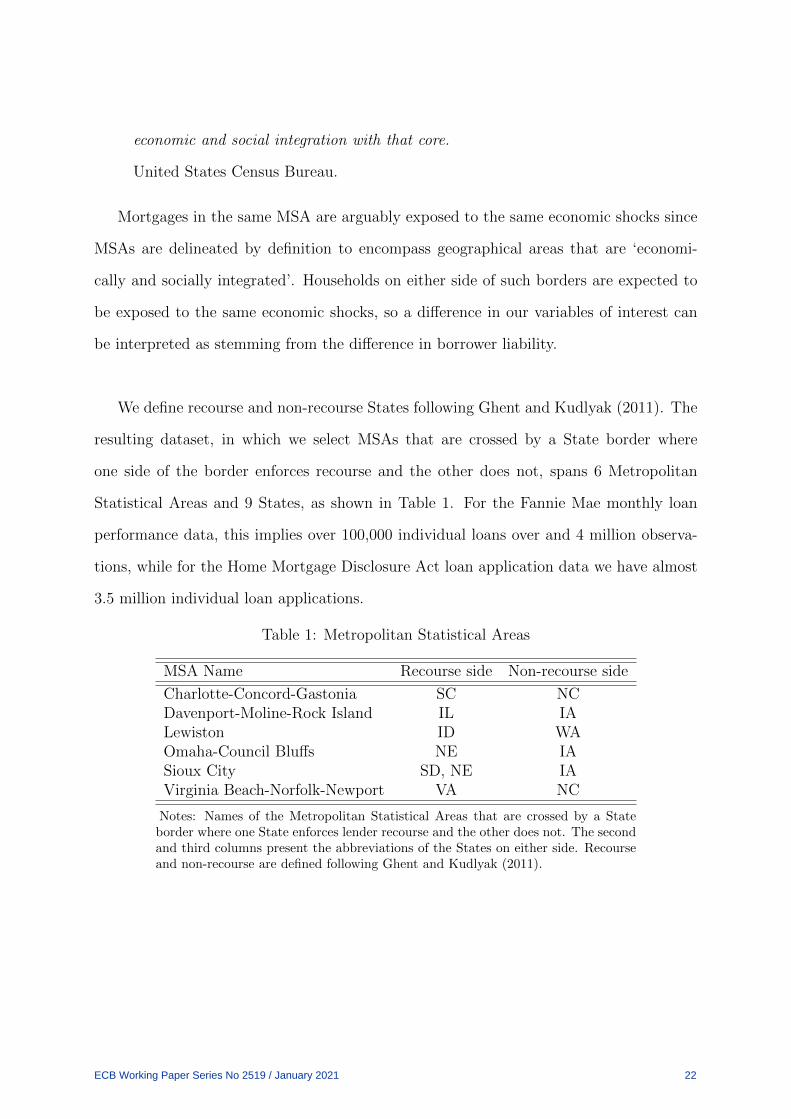
We define recourse and non-recourse States following Ghent and Kudlyak (2011). The
resulting dataset, in which we select MSAs that are crossed by a State border where
one side of the border enforces recourse and the other does not, spans 6 Metropolitan
Statistical Areas and 9 States, as shown in Table 1. For the Fannie Mae monthly loan
performance data, this implies over 100,000 individual loans over and 4 million observa-
tions, while for the Home Mortgage Disclosure Act loan application data we have almost
3.5 million individual loan applications.
Table 1: Metropolitan Statistical Areas
MSA Name Recourse side Non-recourse side
Charlotte-Concord-Gastonia SC NCDavenport-Moline-Rock Island IL IALewiston ID WAOmaha-Council Bluffs NE IASioux City SD, NE IAVirginia Beach-Norfolk-Newport VA NC
Notes: Names of the Metropolitan Statistical Areas that are crossed by a Stateborder where one State enforces lender recourse and the other does not. The secondand third columns present the abbreviations of the States on either side. Recourseand non-recourse are defined following Ghent and Kudlyak (2011).
ECB Working Paper Series No 2519 / January 2021 22

4 Empirical Analysis
4.1 Testing the Model predictions: the pricing puzzle
In this section we use the Fannie Mae Single Family Loan Performance database to test
the predictions from the model. Table 2 shows the mean values for some key variables,
separated by recourse and non-recourse, together with the p-values for the two-sided t-test
of whether they are statistically different from each other.
Table 2: Descriptive Statistics
Non-recourse Recourse p-value
Variables at originationRate of default (%) 3.24 2.15 <.001Loan Amount ($) 196,477 181,003 <.001Credit Score 750.9 755.6 <.001Interest Rate (%) 4.85 4.84 .06Debt-to-income (%) 33.46 33.83 <.001Loan-to-value (%) 80.32 80.01 <.001
Current variablesCurrent Balance ($) 170,202 157,804 <.001Current Interest Rate (%) 4.98 4.97 <.001Market Price ($) 250,118 227,611 <.001Months to Maturity 311 310 <.001
N. of loans 48,406 51,892 .N. of observations 2,044,322 2,174,763 .
Notes: Loan amount, current balance and market price are in US dollaramounts, interest rate, current interest rate, debt-to-income (DTI) and loan-to-value (LTV) are reported as percentages. DTI is calculated as the ratiobetween the borrower’s total monthly obligations and their stable monthlyincome. Credit score is the FICO score. Source: Fannie Mae Single FamilyLoan Database, Federal Housing Finance Agency and authors own calcula-tions, 2004-2016.
We consider a loan to have defaulted, as is standard in the literature, when it has
delinquency status for longer than 3 months. Default rates are higher in non-recourse
States, as predicted by the model, while interest rates at origination are not statistically
different across jurisdictions. This is puzzling, as one would expect the higher risk of
default to be reflected on prices. We will explore this more formally in the course of
ECB Working Paper Series No 2519 / January 2021 23

this section. Credit scores are lower on average on the non-recourse side of the border.
While this difference is statistically significant, it is not economically significant as the
magnitude of the difference is only 5 points in the FICO score. One may worry that
there is self-selection into purchasing a house on either side of the border. Lower quality
borrowers may choose to live on the non-recourse side of the border since they expect
they may need to default with higher probability. This would bias our results. However,
this small difference in the credit score is reassuring that borrower quality is similar on
either side of the border.
In addition, Debt-to-income ratios are also very similar. Debt-to-income ratios are a
good way to measure the likelihood of default of a household, as it measures the strain
that their debt places on their finances. The fact that these ratios are similar across
jurisdictions, together with our use of the discontinuity around the border which ensures
similar exposure to economic shocks, indicates that households can be expected to be
able to meet their financial obligations with similar probability. This relates to the model
along parameter p, that is, the probability that the household will receive a low income
realisation and not be able to meet their payments. Furthermore, Loan-to-value ratios
seem to also be similar across jurisdictions, and very close to the regulatory soft limit of
80%. We call this a soft limit because banks are allowed to issue loans for more than 80%
of the value of the property, but in order to do so, they must meet additional requirements,
which makes 80% the effective limit for a wide majority of loans. Overall, it appears that
most variables are similar in recourse and non-recourse States, which allows us to compare
these loans and draw conclusions on the relevant variables of interest.
Next, we formally test the model predictions using different regressions. First, the
model predicts that default rates should be higher in non-recourse States. We test this
using the following Logit regression:
ECB Working Paper Series No 2519 / January 2021 24
LD = β0 + β1DNR + β3Xi,t + εi,t (11)
where LD denotes the log odds of default, DNR is a dummy variable that takes value
1 if the house is located in a non-recourse State and 0 otherwise, and Xi,t is the set of
control variables. Control variables include the credit score of the borrower, the remain-
ing loan term, the debt-to-income ratio of the borrower, the loan’s current outstanding
balance and the market price of the property.
Second, the model shows that, when faced with a delinquent borrower, the bank must
choose whether to renegotiate the loan payment or let the household default. The model
predicts that the bank chooses to renegotiate with lower probability as λ decreases. That
implies that we should expect lower levels of renegotiation, conditional on the borrower
being delinquent, in non-recourse States. We test the difference in renegotiation rates
between recourse and non-recourse States, conditional on the loan being more than 3
months delinquent, which is consistent with the standard definition of default used in the
literature. The Logit regression in this case reads:
LM = β0 + β1DNR + β3Xi,t + εi,t (12)
where LM denotes the log odds of loan modification and the rest of the variables are
defined as in the previous regression.
Finally, the model prediction is that prices should be higher on non-recourse States,
owing to the higher level of ex-ante predictable risk. We run an OLS regression to test
for the difference in loan prices at origination:
ratei,t = β0 + β1DNR + β3Xi,t + εi,t (13)
where ratei,t is the interest rate agreed in the initial terms, and Xi,t are a set of con-
ECB Working Paper Series No 2519 / January 2021 25
trol variables. The control variables, in this case, are the credit score of the borrower, the
initial loan term and the debt to income ratio of the borrower at origination.
Table 3 shows the results from these regressions. Columns 1-4 report Logit coefficient
estimates in odds ratios to facilitate the comparison and interpretation of the relative
probability of default and renegotiation between recourse and non-recourse States. Val-
ues above (below) unity indicate a positive (negative) relation between the independent
variable and the likelihood of default or renegotiation. As shown in Column 2, default
rates are higher in non-recourse States, as predicted by the model. In terms of magni-
tude, borrowers in non-recourse States are around 42% more likely to default on their
mortgage.2 Column 4 shows that the probability of loan renegotiation is 28% higher in
non-recourse States. This result is also in line with the model’s predictions.
Moving on to pricing, Column 8 shows a puzzling result: the difference in the interest
rate between recourse and non-recourse loans is economically negligible at less than 1bp.
In addition, the sign of this difference is the opposite of what is predicted in the model.
In a regression specification with no time or MSA fixed effects, we find that this difference
is not statistically significant. Recalling that these results come from Fannie Mae’s loan
performance data, they provide evidence of an additional dimension of mispricing by
GSEs. In addition to Hurst et al. (2016), who find that GSEs do not correctly price
regional risk, we show that such enterprises do not take into account ex-ante predictable
non-recourse risk. In order to shed light on this issue, in the next section we take a step
2These results are qualitatively robust if we only use the cross-section of loans rather than the fullpanel. In the baseline, we opt to use a period by period approach to account for time spent in delinquencyand possibility of cure. This also allows including running variables as controls, such as house price, inline with the model.
ECB Working Paper Series No 2519 / January 2021 26

back and use the HMDA dataset to evaluate loan prices at the loan application stage,
where data is available also for the private sector.
Table 3: Regression Results
Logit - odds ratios OLS(1) (2) (3) (4) (5) (6)
VARIABLES Default Default Renegotiation Renegotiation Interest Rate Interest Rate
DNR 1.474*** 1.416*** 1.268*** 1.282*** 0.009** -0.008***(0.084) (0.079) (0.092) (0.095) (0.004) (0.003)
Credit Score 0.982*** 0.990*** -0.002***(<.001) (0.001) (<.001)
Months to Maturity 1.004*** 1.037*** 0.003***(0.001) (0.001) (<.001)
DTI 1.051*** 1.030*** 0.002***(0.002) (0.003) (<.001)
Current Balance 1.000*** 1.000***(<.001) (<.001)
Market Price 0.999*** 0.999***(<.001) (<.001)
Observations 4,052,363 3,436,163 3,650,449 3,124,426 100,298 98,617R-squared 0.859 0.904Pseudo R2 0.149 0.250 0.053 0.396
MSA FE YES YES YES YES YES YESTime FE YES YES YES YES YES YES
Heteroskedasticity robust standard errors in parentheses*** p<0.01, ** p<0.05, * p<0.1
Notes: Columns 1-4 report Logit coefficient estimates in odds ratios to facilitate the comparison and interpretation of the relativeprobability of default and modification between recourse and non-recourse States. Values above (below) unity indicate a positive(negative) relation between the independent variable and the likelihood of default or modification. The standard errors reportedin parentheses for the Logit regressions are computed via Delta method to match the odds ratio coefficients. Columns 5-6 reportOLS estimates estimated using observations at origination only. Source: Fannie Mae Single Family Loan Database, FederalHousing Finance Agency and authors own calculations, 2004-2016.
4.2 Understanding loan pricing
In this section we focus on loan applications data in order to examine whether there are
differences in loan demand, loan origination, and loan sales that could explain the pricing
puzzle outlined in the previous section.
ECB Working Paper Series No 2519 / January 2021 27
4.2.1 Loan origination and sale
Table 4 shows the mean values for some key variables in the HMDA Dataset, separated
by recourse and non-recourse, together with the p-values for the two-sided t-test of whether
they are statistically different from each other.
Both origination rates and sales to third parties are higher in recourse States. The
average income of the applicant is higher in non-recourse States, whereas the median
income is equal across jurisdictions, indicating the presence of outliers. Loan amounts
of all received applications, as well as those of accepted loans, are significantly different
in statistical terms, but are very similar in economic terms, differing by roughly $1,500.
Importantly though, loan-to-income ratios of all applications as well as of originated loans
are significantly higher in recourse States. The loan-to-income ratio is a measure of the
burden that the loan repayment poses on the borrowers’ payment capacity, hence higher
loan-to-income is associated with a higher risk of default. The fact that recourse States
display higher loan-to-income ratios of granted loans may indicate that lenders are more
willing to take on risk in recourse States because they have a higher recovery ratio given
that they can seize the borrowers’ personal assets in the event of default.
ECB Working Paper Series No 2519 / January 2021 28

Table 4: HMDA
Non-recourse Recourse p-value
All ApplicationsAnnual income of applicant ($) 84,723 80,846 <.001Median annual income ($) 67,000 67,000 .Loan amount ($) 151,716 153,358 <.001Loan-to-income 2.055 2.155 <.001
Originated LoansAnnual income of applicant ($) 89,592 84,430 <.001Median income ($) 72,000 71,000 .Loan amount ($) 157,237 155,573 <.001Loan-to-income 2.012 2.101 <.001Loan acceptance rate (%) 54.04 55.27 <.001Sold to 3rd party (%) 67.39 68.83 <.001
N. of observations 1,370,430 2,013,317 .
Notes: Income and loan amounts are in US dollars. Loan-to-income is the ratioof the loan amount over the annual income of the applicant. The acceptance rateis the percentage of loan applications that were granted. Loans sold to 3rd partiesreflect the percentage of granted loans that were sold to a 3rd party in the naturalyear in which the loan was originated. Source: Home Mortgage Disclosure ActDatabase and authors own calculations, 2004-2016.
First, we focus on the characteristics of loan applications, as well as on the lenders’
willingness to lend given the applications it receives on either side of the border.
The distribution of income of applications is depicted in Figure 4. There are no
significant differences in the distribution of income of applicants on either side of the
border. We can therefore conclude that any differences in the probability to originate a
loan are due to differences in limited liability.
Figure 5 illustrates the differences in reasons for denial. The most common reason
for denial is the credit history of the borrower in both types of States. The second most
frequent reason in recourse States is the debt-to-income ratio, followed by the value of
the collateral (the real estate property). Notably, this order is reversed in non-recourse
States, indicating that collateral value is more important to lenders in States with limited
liability. This is intuitive since limited liability implies that the lender may be limited
in how much they can recover from the borrower in case of default, making the value of
ECB Working Paper Series No 2519 / January 2021 29

Figure 4: Income distributions
Notes: Distributions of yearly income is US Dollars at the loan application stagesplit by recourse and non-recourse States. Source: Home Mortgage DisclosureAct Database and authors own calculations, 2004-2016.
ECB Working Paper Series No 2519 / January 2021 30
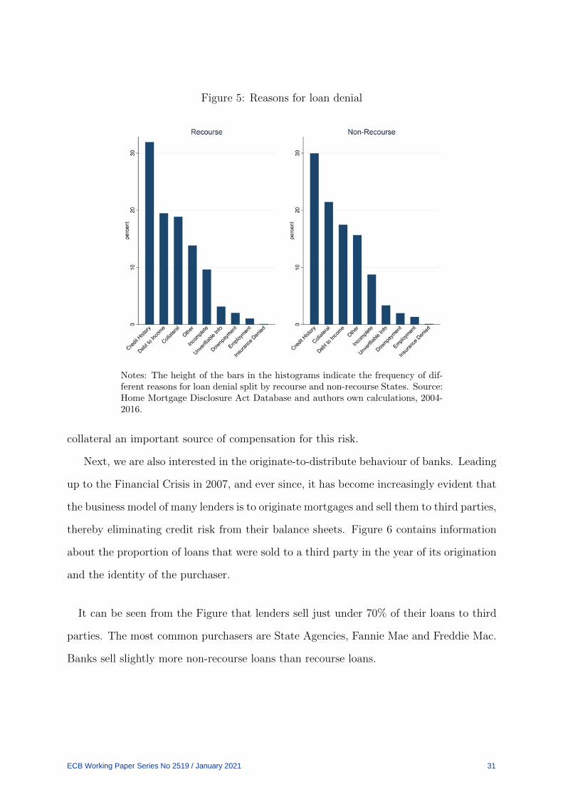
Figure 5: Reasons for loan denial
Notes: The height of the bars in the histograms indicate the frequency of dif-ferent reasons for loan denial split by recourse and non-recourse States. Source:Home Mortgage Disclosure Act Database and authors own calculations, 2004-2016.
collateral an important source of compensation for this risk.
Next, we are also interested in the originate-to-distribute behaviour of banks. Leading
up to the Financial Crisis in 2007, and ever since, it has become increasingly evident that
the business model of many lenders is to originate mortgages and sell them to third parties,
thereby eliminating credit risk from their balance sheets. Figure 6 contains information
about the proportion of loans that were sold to a third party in the year of its origination
and the identity of the purchaser.
It can be seen from the Figure that lenders sell just under 70% of their loans to third
parties. The most common purchasers are State Agencies, Fannie Mae and Freddie Mac.
Banks sell slightly more non-recourse loans than recourse loans.
ECB Working Paper Series No 2519 / January 2021 31
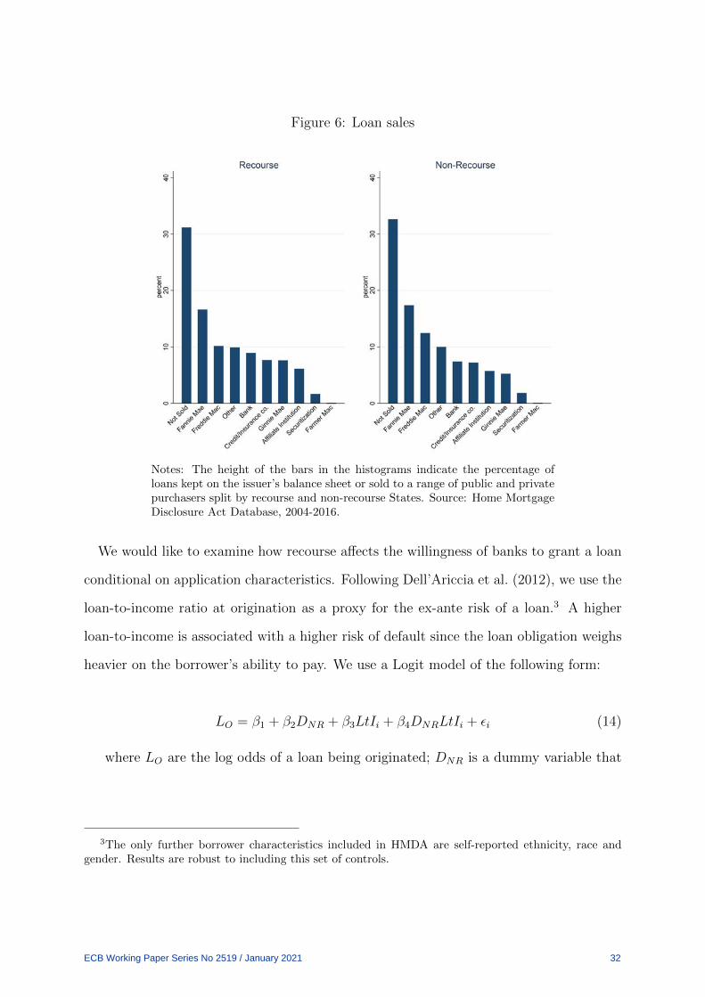
Figure 6: Loan sales
Notes: The height of the bars in the histograms indicate the percentage ofloans kept on the issuer’s balance sheet or sold to a range of public and privatepurchasers split by recourse and non-recourse States. Source: Home MortgageDisclosure Act Database, 2004-2016.
We would like to examine how recourse affects the willingness of banks to grant a loan
conditional on application characteristics. Following Dell’Ariccia et al. (2012), we use the
loan-to-income ratio at origination as a proxy for the ex-ante risk of a loan.3 A higher
loan-to-income is associated with a higher risk of default since the loan obligation weighs
heavier on the borrower’s ability to pay. We use a Logit model of the following form:
LO = β1 + β2DNR + β3LtIi + β4DNRLtIi + εi (14)
where LO are the log odds of a loan being originated; DNR is a dummy variable that
3The only further borrower characteristics included in HMDA are self-reported ethnicity, race andgender. Results are robust to including this set of controls.
ECB Working Paper Series No 2519 / January 2021 32
takes value 1 if the property is located in a non-recourse State and 0 otherwise, LtIi
is the loan-to-income ratio of application i. β4 is then the regression coefficient for the
interaction term between the non-recourse dummy and the loan-to-income ratio.
We also run a Logit model of the same form to assess the difference in the probability
of selling a loan to a third party:
LS = β1 + β2DNR + β3LtIi + β4DNRLtIi + εi,t (15)
where LS are the log odds of a loan being sold.
Table 5 shows the results of these regressions. The interpretation of interaction terms in
Logit regression needs careful consideration. First, it is worth noting that the regression
results are expressed in terms of log odds. While Logit models are linear in log odds,
they are not linear in other metrics such as probabilities. We want to be able to interpret
the results of these regressions in terms of the difference in the probability of originating
a loan between recourse and non-recourse, conditional on the ex-ante risk of the loan as
proxied by the loan-to-income ratio. This probability difference will therefore depend on
the different values of the model variables. Furthermore, the interaction term is composed
by a categorical variable and a continuous variable, so in order to interpret the results, it
will be necessary to evaluate the coefficient at different levels of loan-to-income.4
4While we follow Dell’Ariccia et al. (2012) in the use of loan-to-income as a key variable to measurethe riskiness of a mortgage, results are comparable if we use income instead.
ECB Working Paper Series No 2519 / January 2021 33
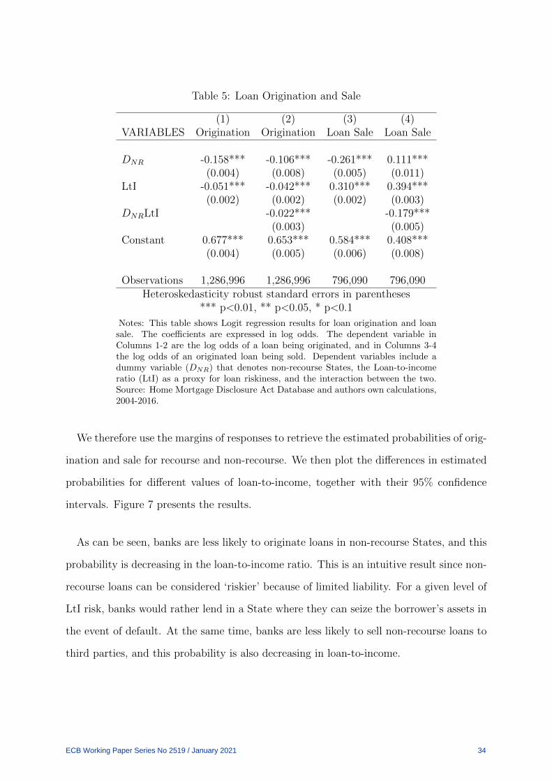
Table 5: Loan Origination and Sale
(1) (2) (3) (4)VARIABLES Origination Origination Loan Sale Loan Sale
DNR -0.158*** -0.106*** -0.261*** 0.111***(0.004) (0.008) (0.005) (0.011)
LtI -0.051*** -0.042*** 0.310*** 0.394***(0.002) (0.002) (0.002) (0.003)
DNRLtI -0.022*** -0.179***(0.003) (0.005)
Constant 0.677*** 0.653*** 0.584*** 0.408***(0.004) (0.005) (0.006) (0.008)
Observations 1,286,996 1,286,996 796,090 796,090Heteroskedasticity robust standard errors in parentheses
*** p<0.01, ** p<0.05, * p<0.1
Notes: This table shows Logit regression results for loan origination and loansale. The coefficients are expressed in log odds. The dependent variable inColumns 1-2 are the log odds of a loan being originated, and in Columns 3-4the log odds of an originated loan being sold. Dependent variables include adummy variable (DNR) that denotes non-recourse States, the Loan-to-incomeratio (LtI) as a proxy for loan riskiness, and the interaction between the two.Source: Home Mortgage Disclosure Act Database and authors own calculations,2004-2016.
We therefore use the margins of responses to retrieve the estimated probabilities of orig-
ination and sale for recourse and non-recourse. We then plot the differences in estimated
probabilities for different values of loan-to-income, together with their 95% confidence
intervals. Figure 7 presents the results.
As can be seen, banks are less likely to originate loans in non-recourse States, and this
probability is decreasing in the loan-to-income ratio. This is an intuitive result since non-
recourse loans can be considered ‘riskier’ because of limited liability. For a given level of
LtI risk, banks would rather lend in a State where they can seize the borrower’s assets in
the event of default. At the same time, banks are less likely to sell non-recourse loans to
third parties, and this probability is also decreasing in loan-to-income.
ECB Working Paper Series No 2519 / January 2021 34

Figure 7: Differences in probability of Origination and Sale
Notes: The solid line plots the difference in the probability of origination andsale between recourse and non-recourse States for different levels of loan-to-income ratios (a proxy of the riskiness of the loan). The dashed lines trace the95% confidence intervals. Source: Home Mortgage Disclosure Act Databaseand authors own calculations, 2004-2016.
4.2.2 Interest rate on sold loans
One of the striking results from Table 3 is that for loans bought by Fannie Mae, the
interest rate at origination does not differ between recourse and non-recourse loans. Given
that non-recourse loans are expected to have a lower recovery rate in the event of default,
one could expect the interest rate for these loans to be higher. We ask whether the fact
that the interest rate at origination does not differ across jurisdictions for loans that were
sold to Fannie Mae is due to the fact that banks anticipated they would sell this loans to
a third party and therefore did not have an incentive to price in their risk. To this end,
we use the HMDA loan application database to test whether loans that were not sold to
a third party were priced differently, conditional on observables.
ECB Working Paper Series No 2519 / January 2021 35

While the loan application data does not include the interest rate of each loan, banks
report the spread between the rate charged for a given loan and the average interest rate
that a loan with similar characteristics would have in the market. Banks must report the
spread (difference) between the annual percentage rate (APR) and the applicable average
prime offer rate if the spread is equal to or greater than 1.5 percentage points for first-lien
loans. Due to this, there is a selection issue on the spread variable: we do not observe the
spread if it is lower than the reporting threshold. In order to overcome this issue, some
papers in the literature, for instance Pennington-Cross and Ho (2008), have applied the
Heckman two-stage procedure for selection correction to this dataset. Hence, we run the
following Probit regression:
Yi = δXi + ui (16)
where Yi takes value 1 if the spread of loan application i is observed (i.e. if the
spread is greater than 1.5 percentage points), and Xi is a set of variables that influence
the probability of the spread being above the reporting threshold. We use all available
borrower information in Xi, which includes income and dummy variables for self-reported
race and gender.
We then use δ̂ to compute the inverse Mills ratio, λ(Xδ̂) = φ(Xδ̂)
Φ(Xδ̂), and it to different
second stage regressions in order to answer different questions. First, we examine the
difference in the spread between recourse and non-recourse States using the following
regression:
spreadi = β0 + β1DNR + γλ(Xδ̂) + εi (17)
where DNR takes value 1 for non-recourse loans and 0 otherwise. Then, we ask whether
the spread is higher for loans that are sold to third parties, and whether this differs across
jurisdictions. The regression reads:
ECB Working Paper Series No 2519 / January 2021 36
spreadi = β0 + β1DNR + β2DSold + β3DNRDSold + γλ(Xδ̂) + εi (18)
where DSold takes value 1 for loans that were sold to third parties and 0 otherwise and
DNRDSold is an interaction term of both dummy variables.
Hurst et al. (2016) show that public agencies such as Fannie Mae and Freddie Mac
are less efficient at pricing mortgage loan risk than the private market. They argue
that this price difference leads to cross subsidisation from low risk mortgages to high
risk mortgages. We explore whether this issue extends to the difference in risk between
recourse and non-recourse loans in the following way:
spreadi = β0 + β1DNR + β2DPrivate + β3DNRDPrivate + γλ(Xδ̂) + εi (19)
where DPrivate takes value 1 for loans that were sold to private buyers (securitisation
agencies, commercial banks, insurance companies, funds...) and 0 for loans that were sold
to public buyers (Fannie Mae, Freddie Mac, Ginnie Mae and Farmer Mac).
The results of these regressions are laid out in Table 6. Regression 17 is shown in
Column 1. The loan spread is significantly lower in non-recourse States which is a sur-
prising result. We are interested, however, in whether there is a significant difference in
loan pricing for loans that were sold to third parties, and among those, whether there is a
difference between private and public buyers. Column 2 presents the results of Regression
18. The constant term implies that the average spread of a recourse loan that was kept
by the bank is around 6.7%. The coefficient of DNR captures the difference in the interest
rate between non-recourse and recourse for unsold loans. The interest rate on unsold
loans is 24bp lower for non-recourse loans. The coefficient for DSold equals the difference
between sold and kept loans in recourse States. It implies that, among recourse loans, the
spread is around 5bp lower for those that were sold. The coefficient for the interaction
term DNRDSold is equivalent to a difference-in-differences estimator. It represents the
ECB Working Paper Series No 2519 / January 2021 37
difference in the spread between recourse and non-recourse loans for loans that were sold.
The fact that it is positive and statistically significant indicates that in the market for
loan sales the spread is higher for non-recourse mortgages. This result is intuitive, since
non-recourse implies a higher rate of default as predicted by the theoretical model, and
shown empirically in the previous section. We note that there may be an endogeneity
issue in interacting DNR and DSold, as we have shown before that non-recourse loans are
less likely to be sold to third parties than their recourse counterparts.
This phenomenon is further investigated in Column 3, where the pool of sold loans
is split between private and public buyers, as outlined in regression 19. The coefficient
for DPrivate indicates the difference between loans sold to private and public agents in
recourse States. The estimate of this difference is almost 200bp, which is an order of
magnitude higher than the DSold coefficient in Column 1. This implies that most of the
variation in the spread of sold loans is driven by pricing behaviour of private investors.
The coefficient for the interaction term DNRDPrivate is also positive and statistically
significant. It means that for non-recourse loans, private purchasers demand a higher
spread than public agencies. This suggests that private markets price in the higher risk
associated with non-recourse loans (or limited liability) to a greater extent than their
public counterparts. We conclude from this analysis that banks do charge significantly
higher interest rates on non-recourse loans when selling the loan to a private third party,
while loans bought by Fannie Mae seem to have the same interest rate at origination, as
was shown in Table 2. These results are in contrast with Hurst et al. (2016), who find
that interest rates do not vary across recourse and non-recourse States for both private
and public loans.
ECB Working Paper Series No 2519 / January 2021 38

Table 6: Heckman Regression Results
(1) (2) (3)EQUATION VARIABLES spread spread spread
Second Stage DNR -0.085*** -0.242*** -0.006(0.008) (0.013) (0.025)
DSold -0.052***(0.011)
DNRDSold 0.266***(0.017)
DPrivate 1.978***(0.021)
DNRDPrivate 0.222***(0.032)
Constant 6.722*** 6.731*** 4.913***(0.047) (0.048) (0.123)
First Stage Income -0.002*** -0.002*** -0.002***(0.000) (0.000) (0.000)
Female 0.051*** 0.051*** 0.040***(0.002) (0.002) (0.004)
Native -0.014 -0.014 -0.082***(0.015) (0.015) (0.030)
Asian -0.149*** -0.149*** -0.046***(0.008) (0.008) (0.014)
Black 0.339*** 0.339*** 0.314***(0.003) (0.003) (0.005)
Hawaiian 0.051*** 0.051*** 0.049(0.017) (0.017) (0.031)
Constant -1.363*** -1.363*** -2.112***(0.002) (0.002) (0.004)
Observations 3,072,488 3,072,488 2,897,723Standard errors in parentheses
*** p<0.01, ** p<0.05, * p<0.1
Notes: This table shows the first and second stage of the two-step Heckmanprocedure for selection correction. The first stage is a Probit regression wherethe probability of being selected depends on borrower observables. We includeas selection variables the borrower’s income, gender, and race. The inverse Millsratio is computed from the first stage and is used in the second stage regressionas an independent variable together with other explanatory variables. DNR isa dummy variable that takes value 1 for non-recourse States and 0 for recourseStates, DSold is a dummy variable that takes value 1 for loans that were sold an0 for loans that were kept by the bank, DPrivate is a dummy variable for loansthat were sold to a private entity and 0 for loans that were sold to a publicenterprise (GSE). Standard errors are corrected to account for the two-stepprocedure. Source: Home Mortgage Disclosure Act Database and authors owncalculations, 2004-2016.
ECB Working Paper Series No 2519 / January 2021 39
5 Conclusion
The rise of household indebtedness before the Financial Crisis combined with high
default rates was a root cause of the Great Recession and underlined the role of consumer
finance for the macroeconomy. Mortgage debt in particular, constitutes two-thirds of US
household total debt, and it currently follows an increasing trend.
While there are several factors that determine the rate of mortgage default, such as
adverse economic shocks that leave households unable to honour their debt, default may
also be a voluntary choice, commonly referred to as strategic default. One particular
aspect the household may consider before choosing to default is whether there is limited
liability in place. Under limited liability, the lender is not allowed to seize the household’s
assets after default. On the contrary, under lender recourse, the lender is allowed to claw
back the borrower’s assets after default.
While the literature has analysed the consequences of limited liability, such as default
rates, loan renegotiation or forbearance, and interest rates in isolation, we embody all
these features in our analysis as equilibrium outcomes of the strategic interaction between
borrowers and lenders.
We use a model of default and renegotiation to highlight the mechanisms at hand, and
we test them empirically by exploiting the difference in legislation across US States. We
do this by comparing loans for houses situated in Metropolitan Statistical Areas that are
crossed by a State border, where one State enforces lender recourse and the other does
not. Given than MSAs are defined by the US Census Bureau as a core area containing a
substantial population nucleus, together with adjacent communities having a high degree
of economic and social integration with that core’, we argue that borrowers on either
side of the border are exposed to the same economic shocks, and the difference in their
ECB Working Paper Series No 2519 / January 2021 40
behaviour towards their mortgage loans can be thought to stem exclusively from the
presence or absence or limited liability.
In the model, both house prices and the income of the borrower are stochastic. In some
states of the world, the household has enough income to pay their mortgage, whereas in
other states of the world it does not. Likewise, in some states of the world, the house
value is higher than the mortgage amount, i.e. the household has positive equity, whereas
in other states of the world the house value is lower, i.e. the mortgage is underwater.
Households who can afford to meet their payments, but whose mortgage is underwater,
may find it optimal to default, in particular on instances where it is unlikely that they
will be liable with their personal assets after default. Lenders who know this may find it
optimal to offer these households a renegotiated mortgage price in order to prevent them
from walking away from their obligations. At the same time, the price of these loans will
reflect these mechanisms. Loan rates are expected to be higher under limited liability,
because of the higher ex-ante predictable default and renegotiation risk, and the lower
recovery rate for the lender after default.
These predictions are confirmed by the data. In fact, non-recourse loans are around
42% more likely to default, and 28% more likely to receive a renegotiation offer. However,
while the model predicts that loan rates should be higher for non-recourse loans (as they
have a higher expected default rate), loan performance data from Fannie Mae does not
confirm this. This lack of price differentiation has been noted in the literature, for instance
by Hurst et al. (2016). They note that Government-Sponsored Enterprises (GSEs) fail
to appropriately price in regional differences in ex-ante predictable default risk. In this
paper, regional risk is expected to be the same within each MSA, as they are by definition
integrated economic areas. However, we still find a lack of price differentiation on the side
of GSEs, which fail to account for the risk of default and renegotiation brought about
by the difference in legislation. We test this by using additional data from the Home
ECB Working Paper Series No 2519 / January 2021 41

Mortgage Disclosure Act (HMDA) in order to compare the interest rates on loans that
were sold to private investors vs GSEs, for recourse and non-recourse States. We find
that the difference in default risk implied by different recourse laws is indeed priced into
loans that are securitised by private investors. Overall, rates on non-recourse loans sold
to private investors are around 22bp higher than their recourse counterparts.
These results overall speak to the distortions imposed by the differences in limited
liability across States, together with the heterogeneity of public and private market par-
ticipants. Given the size of the market and the importance of mortgages in households’
balance sheets, our findings have important macroeconomic implications. Further theoret-
ical research should fill the gap in how these mechanisms interact in general equilibrium.
ECB Working Paper Series No 2519 / January 2021 42

Appendix A: Equilibria under different relative values
of thresholds (1) and (2)
Figure 8a shows the same graphic representation for the case when (1) < (2). In this
case, for values of λ weakly greater or smaller than the threshold, the above logic still
holds. However, for values between (1) and (2), the household would find it optimal
not to default, so the lender would not renegotiate. For λ = (1), the borrower would
mix between defaulting and repaying. If it defaults, then the lender would mix between
renegotiating or not. The same logic holds when λ = (1) = (2), which is represented in
figure 8b.
(a) (1) < (2) (b) (1) = (2)
Figure 8: Equilibria for different relative values of (1) and (2)
ECB Working Paper Series No 2519 / January 2021 43

References
Atkeson, A. (1991). International lending with moral hazard and risk of repudiation.
Econometrica, pages 1069–1089.
Bester, H. (1994). The role of collateral in a model of debt renegotiation. Journal of
money, credit and banking, 26(1):72–86.
Campbell, J. Y. (2012). Mortgage market design. Review of Finance, 17(1):1–33.
Chan, S., Haughwout, A., Hayashi, A., and Van der Klaauw, W. (2016). Determinants of
mortgage default and consumer credit use: the effects of foreclosure laws and foreclosure
delays. Journal of Money, Credit and Banking, 48(2-3):393–413.
Collins, J. M., Lam, K., and Herbert, C. E. (2011). State mortgage foreclosure policies
and lender interventions: Impacts on borrower behavior in default. Journal of Policy
Analysis and Management, 30(2):216–232.
Curtis, Q. (2014). State foreclosure laws and mortgage origination in the subprime. The
Journal of Real Estate Finance and Economics, 49(3):303–328.
Dagher, J. and Sun, Y. (2016). Borrower protection and the supply of credit: Evidence
from foreclosure laws. Journal of Financial Economics, 121(1):195–209.
Dell’Ariccia, G., Igan, D., and Laeven, L. (2012). Credit Booms and Lending Standards:
Evidence from the Subprime Mortgage Market. Journal of Money, Credit and Banking,
44:367–384.
Gerardi, K., Lambie-Hanson, L., and Willen, P. S. (2013). Do borrower rights improve bor-
rower outcomes? evidence from the foreclosure process. Journal of Urban Economics,
73(1):1–17.
ECB Working Paper Series No 2519 / January 2021 44

Ghent, A. C. and Kudlyak, M. (2011). Recourse and residential mortgage default: evi-
dence from us states. Review of Financial Studies, 24(9):3139–3186.
Gianinazzi, V., Pelizzon, L., and Plazzi, A. (2019). Residential mortgage defaults and
positive equity: Lessons from europe. Working Paper.
Grossman, H. I. and Van Huyck, J. B. (1988). Sovereign debt as a contingent claim: Ex-
cusable default, repudiation, and reputation. American Economic Review, 78(5):1088–
1097.
Guren, A. M., Krishnamurthy, A., and McQuade, T. J. (2018). Mortgage design in an
equilibrium model of the housing market. NBER.
Hart, O. and Moore, J. (1998). Default and renegotiation: A dynamic model of debt.
Quarterly Journal of Economics, 113(1):1–41.
Hurst, E., Keys, B. J., Seru, A., and Vavra, J. (2016). Regional redistribution through
the us mortgage market. American Economic Review, 106(10):2982–3028.
Jeske, K. (2006). Private international debt with risk of repudiation. Journal of political
Economy, 114(3):576–593.
Kaplan, G., Mitman, K., and Violante, G. L. (2017). The housing boom and bust: Model
meets evidence. NBER.
Li, W. and Oswald, F. (2017). Recourse and residential mortgages: The case of nevada.
Journal of Urban Economics, 101:1–13.
Meador, M. (1982). The effects of mortgage laws on home mortgage rates. Journal of
Economics and Business, 34(2):143–148.
Mian, A., Sufi, A., and Trebbi, F. (2015). Foreclosures, house prices, and the real economy.
The Journal of Finance, 70(6):2587–2634.
ECB Working Paper Series No 2519 / January 2021 45
Pence, K. M. (2006). Foreclosing on opportunity: State laws and mortgage credit. Review
of Economics and Statistics, 88(1):177–182.
Pennington-Cross, A. and Ho, G. (2008). Predatory lending laws and the cost of credit.
Real Estate Economics, 36(2):175–211.
ECB Working Paper Series No 2519 / January 2021 46

Acknowledgements We are grateful to Chris Brooks, Michael Clements, Russell Cooper, Juan José Dolado, Matteo Escudé, Nadia Kappou, David K. Levine, Ramón Marimón, Steven Ongena, Giorgio Primiceri, Rafael Repullo, Paul Voß, and various seminar participants at EUI, ICMA Centre at the Henley Business School, and at the 2019 EDP Jamboree in UCLouvain for useful comments and suggestions. We also thank the Editorial Board of the ECB Working Paper Series, as well as an anonymous referee. The views expressed are our own and do not necessarily reflect those of the European Central Bank or the Eurosystem. Mirco Balatti European Central Bank, Frankfurt am Main, Germany; ICMA Centre, Henley Business School, Reading, United Kingdom; email: [email protected] Carolina López-Quiles European Central Bank, Frankfurt am Main, Germany; European University Institute, Florence, Italy; email: [email protected]
© European Central Bank, 2021
Postal address 60640 Frankfurt am Main, Germany Telephone +49 69 1344 0 Website www.ecb.europa.eu
All rights reserved. Any reproduction, publication and reprint in the form of a different publication, whether printed or produced electronically, in whole or in part, is permitted only with the explicit written authorisation of the ECB or the authors.
This paper can be downloaded without charge from www.ecb.europa.eu, from the Social Science Research Network electronic library or from RePEc: Research Papers in Economics. Information on all of the papers published in the ECB Working Paper Series can be found on the ECB’s website.
PDF ISBN 978-92-899-4519-6 ISSN 1725-2806 doi:10.2866/502561 QB-AR-21-010-EN-N