LIMITED COMMITMENT MODELS OF THE LABOUR MARKET

LIMITED COMMITMENT MODELS OF THE LABOR MARKET

JONATHAN P. THOMAS TIM WORRALL

CESIFO WORKING PAPER NO. 2109 CATEGORY 4: LABOUR MARKETS

OCTOBER 2007

An electronic version of the paper may be downloaded • from the SSRN website: http://www.SSRN.com/abstract=1019236 • from the RePEc website: www.RePEc.org

• from the CESifo website: Twww.CESifo-group.org/wp T

CESifo Working Paper No. 2109


Abstract We present an overview of models of long-term self-enforcing labor contracts in which risk sharing is the dominant motive for contractual solutions. A base model is developed which is sufficiently general to encompass the two-agent problem central to most of the literature, including variable hours. We consider two-sided limited commitment and look at its implications for aggregate labor market variables. We consider the implications for empirical testing and the available empirical evidence. We also consider the one-sided limited commitment problem for which there exists a considerable amount of empirical support.

JEL Code: E32, J41.

Keywords: labor contracts, self-enforcing contracts, unemployment, business cycle.

Jonathan P. Thomas Management School and Economics

William Robertson Building University of Edinburgh

50 George Square Edinburgh EH8 9JY

United Kingdom [email protected]

Tim Worrall School of Economic and Management

Studies Chancellor’s Building

Keele University Keele ST5 5BG United Kingdom

[email protected] September 2007 We gratefully acknowledge the financial support of the Economic and Social Research Council (Research Grant:RES-000-23-0865). We also thank Jim Malcomson, Leena Rudanko and Dongyun Shin for helpful comments on an earlier draft and the participants of the workshop on “The theory and empirics of risk sharing” at the Toulouse School of Economics, September 2007. The usual caveats apply.

1. INTRODUCTION

In this paper we consider long-term risk-sharing1 labor contracts under limitedcommitment. Firms and workers are allowed to sign, or implicitly agree to, contingentcontracts but also to renege on these contracts when it is to their advantage. That is tosay, there are no courts to enforce contracts and low mobility or “lock-in” costs. We firstdevelop a general framework for analyzing contracts in this class of repeated interac-tions. The logic of these contracts follows that of repeated games, in that a party calledupon to sacrifice current utility to maintain the insurance is prepared to do so in antic-ipation of receiving reciprocal benefits in the future. However in general first-best risksharing cannot be achieved, and it is what happens in the second best contracts which isof particular interest. What then follows is a selective overview of the existing literaturethat considers both the implications for empirical testing and summaries the availableempirical evidence.

The study of long-term labor contracts with limited commitment is important be-cause other standard models of the labor market cannot easily account for observed pat-terns in the data. The data typically show that real wages are only weakly correlated withproductivity or even mildly countercyclical. Hours on the other hand are found to bequite strongly positively correlated with productivity. To match this observed pattern inthe data using standard real business cycle models requires a very high intertemporalelasticity of substitution for labor supply that is not supported by estimates from microdata. Recently Shimer (2005) has suggested that standard search models under-predictthe volatilities of vacancies and unemployment because of the flexibility of wage re-sponses to productivity under Nash bargaining unless implausibly large shocks for pro-ductivity are assumed. We therefore consider some of the available empirical evidenceon whether these puzzles might be resolved within the limited commitment labor con-tracting model.

We start by developing a basic two-agent (worker-firm) model in which either agentcan quit the relationship at any time either at a positive or zero cost. The agents agreeinitially to a contingent sequence of wages (and potentially a termination rule) whichsatisfies certain incentive or participation constraints. The outside environment is sum-marized by the evolution of the respective outside options for the two agents. The basiccharacterization of second-best contracts can then be applied to specific models, andwe do this to summaries the existing theoretical work in the area. In the development ofthe model we do not use the dynamic programming framework that is usually employedfor this environment, but instead show that the model can be solved by using local vari-ational arguments, thus avoiding the need to establish a number of technical propertiesof value functions.

1Thus we do not consider the other much analyzed motive for contracting, namely to protect relationshipspecific investments from opportunistic behavior. For a discussion of this, see MacLeod (2007).

1

JONATHAN P. THOMAS AND TIM WORRALL

Although the basic characterizations of the second-best contracts have been knownfor some time, in the second part of the paper we consider how the outside options of theagents can be made endogenous in search equilibrium models or competitive modelswith perfect labor mobility. There has been a recent upsurge of interest in applicationsof this type of model to macroeconomics, and of testing of the model particularly in theone-sided limited commitment case where workers are mobile but firms can commit.We summaries the main findings of the literature and the empirical evidence which isgenerally very supportive of the one-sided model.

2. A GENERAL MODEL OF LIMITED COMMITMENT

This section considers a general model of limited commitment. We first derive theimplications of optimum contracting in a simple model with fixed hours in Section 2.1and consider the empirical test of the model given in Macis (2006). The remaining sub-sections then consider various extensions of the basic model. Section 2.2 considers themodification of the model when hours are variable and reports on the results of Beaudry& DiNardo (1995) on the implied negative correlation between hours and wages. Sec-tion 2.3 discuses the role of ex ante or up-front payments between the worker and thefirm and Section 2.4 examines the some further implications of quitting or renegingcosts.

2.1. A baseline model

The model is as follows.2 There is an infinite horizon, t = 1,2,3 . . .∞. Workers arerisk-averse with per-period twice differentiable utility function u(c), u′ > 0,u′′ < 0, wherec ≥ 0 is the income/consumption of the single good received within the period; crucially,it is assumed that they cannot make capital market transactions, so the only possibilityfor consumption smoothing across states of nature or over time arises if the firm pro-vides insurance. There is no disutility of work, but hours are fixed so that workers areeither employed or unemployed (although we relax the assumption of fixed hours be-low). The firm is assumed to be risk-neutral. We consider a single match between oneworker and one firm,3 and for the moment we do not need to fill in the details of theoutside environment. There is perfect information within the match. We suppose thatoutput at time t within this match is z(st ) ≥ 0, where st is the current state of nature.4 Thestate of nature st follows a time-homogeneous Markov process, with finite state space S,and initial distribution p over S, and from state s state r ∈ S is reachable next period with

2A description of a general limited commitment model of risk sharing can be found in Ljungqvist & Sar-gent (2004, Chapter 20).

3That is we shall treat contracts between each firm and worker separately. The case where contracts withdifferent workers cannot be treated separately is studied in Martins, Snell & Thomas (2005) and Snell &Thomas (2006) and discussed briefly in Section 2.4.

4We do not identify the state of nature directly with productivity, z, as it may be that other firms facedifferent productivity shocks, and so the outside options will not be determined by the match productivity.

2


transition probability: πsr ≥ 0. Let ht := (s1, s2, . . . , st ) be the history at t . Workers andfirms discount the future with common discount factor β ∈ (0,1).

At the start of date 1, after the initial state s1 is observed,5 the firm offers the worker acontract (wt (ht ))T

t=1 = ((w1(s1), w2(s1, s2), w3(s1, s2, s3), . . .)), where wt (ht ) ≥ 0 is the wageat t after history ht , and T > 1 is the (random) date at which the contract is terminated.6

The within period timing is as follows. At the start of each period, both agents observethe current state of nature, st . At this point either party can quit and take their outsideoption. Otherwise, they trade at the agreed terms, in which case the value of output z(st )is realized, and the firm then makes a wage payment according to the contract. (Thuswe do not allow, for example, for the firm to renege on its wage payment after the workerhas contributed to output.) The value (discounted utility) of the outside option for theworker and firm respectively is denoted by χw (s) and χ f (s) in state s.7

Let Vt (ht ) denote the continuation utility from t onwards from the contract (as-suming it does not terminate at t ):

(1) Vt (ht ) := u(wt (ht ))+E

[T−1∑

t ′=t+1βt ′−t u(wt ′(ht ′))+βT−tχw (sT ) | ht

],

where E denotes expectation. Likewise the firm’s continuation profit is

(2) Πt (ht ) := z (st )−wt (ht )+E

[T−1∑

t ′=t+1βt ′−t (z (st ′)−wt ′(ht ′))+βT−tχ f (sT ) | ht

].

The contract is said to be self-enforcing if the following hold for all dates t , T −1 ≥ t ≥ 1,and for all positive probability ht (with initial state s1):

Vt (ht ) ≥χw (st )−Cw ,(3)

Πt (ht ) ≥χ f (st )−C f ,(4)

5If matches also start at later dates, the characterization developed below, which depends only on thestate prevailing at the time the contract starts, is the same.

6So that at t = T , after observing the current state st , the partnership dissolves and both agents get theiroutside options. T is a random variable (a stopping time) so that the length of the contract will in generaldepend on the history of shocks. At this level of generality, termination must be allowed for as there may beno continuation values that satisfy participation constraints.

7In much of the existing literature it is assumed that competition among firms drives profits to zero fromnew matches so χ f = 0. Even with competition, if other inputs such as capital were included in the firm’sprofits, then the participation constraint for the firm would require that it covers capital costs. This wouldmake the firm’s outside option state dependent if say, the interest rate varied with the state. See Calmès(2007) for a model including a fixed capital component where the outside options of competitive firms arestate dependent. Further, although in a more general model outside options may not be a function of thecurrent state only, in most models where the outside option is endogenous, as considered in Section 3, thepayoff from a new contract, and hence the outside option, will only depend on the current state.

3


where C f and Cw are respective directly incurred quitting/mobility costs for the firm andworker.8 Inequality (3) is the worker’s participation constraint that says that at any pointin the future the contract must offer at least what a worker can get by quitting, net ofquitting costs, while (4) is the corresponding constraint for the firm.9 We assume thatχw (s)−Cw > u(0)/(1−β) so that if a feasible contract exists it will pay positive wages atsome point.

We shall be interested in constrained efficient contracts, that is to say contracts whichare self-enforcing and are not Pareto-dominated by any other self-enforcing contracts.Efficient contracts can thus be found as the solutions to the following problem:

Problem A max(wt (ht ))T

t=1

Π1 (h1)

subject to (3), (4), and

(5) V1 (h1) ≥ V̄1.

The term V̄1 measures how much utility the worker gets from the relationship, and asthis is varied across feasible values (i.e. values for which self-enforcing contract exist), allefficient contracts are traced out.10

LEMMA 1: In an efficient contract in which the firm’s (worker’s) participation con-straint is slack at t +1, wages cannot fall (rise) between t and t +1.

PROOF: Suppose we are at ht , and suppose that the firms’s participation constraintat t +1 in some state s is not binding. By assumption the contract is not terminated att +1 (otherwise the constraint would trivially bind). Consider, starting from the optimalcontract, reshuffling wages between t , and t + 1 in state s, to backload them (assumewt > 0). Increase the wage at t +1 after state s by a small amount ∆, and cut the wage att by x so as to leave the worker indifferent; do not change the contract otherwise:

πst sβu′ (wt+1(ht , s))∆−u′ (wt (ht )) x ' 0.

This backloading satisfies all worker participation constraints since the worker’s utilityrises at t +1, and so even if her constraint were binding, it will not be violated; at t her

8Either party can initiate termination, but both suffer the costs. We assume that these are also incurred ifthe contract is terminated by agreement (i.e. at t = T ), so they are costs which cannot be avoided on matchbreak-up. It would also be equivalent in these circumstances to factor these costs directly into outsideoptions. See Section 2.4 for discussion of alternative assumptions.

9It is also possible to introduce hiring costs for the firm. The contract dynamics do not depend onwhether there are hiring costs (unlike quitting costs which may potentially affect the contract dynamics,see Section 2.4 below), but apply as soon as a relationship is established. Thus if the firm incurs hiring coststo establish a relationship, to judge the profitability of the relationship it would have to subtract them fromwhatever surplus it makes once the relationship is established in the manner to be described.

10The issue of existence of solutions to this problem for feasible V̄1 is standard in this environment.

4


constraint holds as her utility is unchanged, and likewise it is unchanged earlier sinceutility is held constant over the two periods. The change in profits (viewed from ht ) is

−πst sβ∆+x '−πst sβ∆+ πst sβu′ (wt+1(ht , s))∆

u′ (wt (ht )),

which is positive for ∆ small enough if

(6)u′ (wt+1(ht , s))

u′ (wt (ht ))> 1.

If (6) holds (so that wages are falling), then the backloading would raise profits at t , sothe firm’s participation constraint would hold at t , and at t +1 by assumption the firm’sparticipation constraint is slack, so a small change to the wage will not violate it. Thusall constraints are satisfied by this change, and profits have increased, contrary to theoptimality of the original contract. So (6) cannot hold: marginal utility growth cannotbe positive, or equivalently, wages cannot fall. By a symmetric argument if the worker’sparticipation constraint is slack at t +1, then wages cannot rise between t and t +1. 2

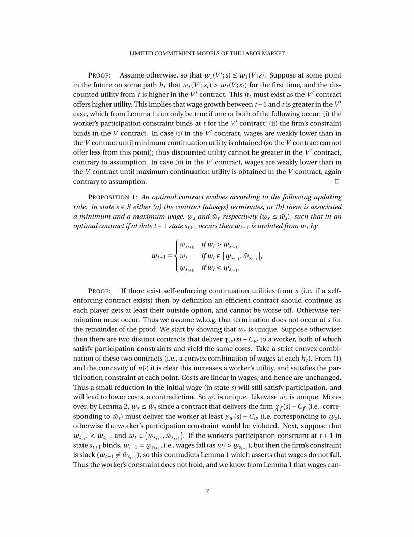
The proof of this lemma is illustrated in Figure 1. In the figure wages at date t ,wt are plotted against wages at date t + 1, wt+1 in some state s. Plotted in the figureare a worker’s indifference curve and two of the firm’s iso-profit lines (the dashed lines).Utility increases toward the North-East of the diagram and profits increase toward theSouth-West. The slope of the indifference curve where it crosses the 45° line is βπst ,s ,the discounted probability of reaching the state s at date t + 1 from state st at date t ,and this is just equal to the slope of the firm’s iso-profit lines. Consider first a contractwhere wages are at a point like A in Figure 1. As point A is above the 45° line the wageis falling, wt > wt+1. If the firm’s participation constraint does not bind at date t + 1then it would be possible to adjust wages along the indifference curve in the directionof equalizing wages and move to a higher iso-profit line. As wt+1 is increased this willrelax the worker’s participation constraint at date t +1 in state s and for a small changein wages it will not violate the firm’s participation constraint at date t + 1 as this wasassumed to be slack. Thus at any point like A an improvement in the contract can befound and hence we can conclude that wages cannot be falling if the firm’s constraintis slack. It is however, clear that a similar argument cannot necessarily be applied at apoint like B, below the 45° line, where wages are rising. Although a movement along theindifference curve toward equality of wages will raise profits, reducing wt+1 may violatethe worker’s participation constraint at date t +1. Thus we have the intuitive result thatwages will rise only if the worker’s participation constraint is binding and fall only if thefirm’s participation constraint is binding.

Next, we need to characterize more precisely what happens to the wage when oneof the participation constraints binds. First, let

(wt (V̄1; s)

)Tt=1 be a constrained efficient

contract in Problem A starting from state s1 = s. This must deliver precisely V̄1 to the

5


A

B

w t+1

w t

45°

Figure 1: ILLUSTRATION OF LEMMA 1

worker, otherwise we can cut the period 1 wage without violating the worker’s constraint,thus increasing profits.11 We define

¯ws := w1(χw (s)−Cw ; s), i.e. the period 1 wage spec-

ified by an optimal contract starting in state s which delivers exactly the worker’s netoutside option, V̄1 = χw (s)−Cw . It must be unique by a simple convexity argument (seebelow). A key observation is the following: it must be optimal at any date t in state sto set wt =

¯ws whenever Vt (ht ) = χw (s)−Cw . This follows from the fact that the future

distribution over states depends only on s, and that the continuation contract must itselfbe optimal (otherwise replacing the continuation contract by a lower cost one which de-livered the same continuation utility would reduce the initial costs but satisfy all partici-pation constraints). Thus,

¯ws is the wage in state s at any t if the participation constraint

is binding. Similarly define w̄s to be the period 1 wage specified by an optimal contractstarting in state s which delivers profits of exactly χ f (s)−C f .

It can then be established that if an optimal contract offers a continuation higherutility, then it must offer a higher first period wage:

LEMMA 2: If V ′ >V , then w1(V ′; s) > w1(V ; s).

11Provided w1 > 0; otherwise, since it is assumed that the outside option dominates zero consumption forever, it is easily shown that there must be a point in the future at which wt > 0 and the worker’s constraint isnot binding, so wages can be cut at this point instead.

6


PROOF: Assume otherwise, so that w1(V ′; s) ≤ w1(V ; s). Suppose at some pointin the future on some path ht that wt (V ′; st ) > wt (V ; st ) for the first time, and the dis-counted utility from t is higher in the V ′ contract. This ht must exist as the V ′ contractoffers higher utility. This implies that wage growth between t−1 and t is greater in the V ′

case, which from Lemma 1 can only be true if one or both of the following occur: (i) theworker’s participation constraint binds at t for the V ′ contract; (ii) the firm’s constraintbinds in the V contract. In case (i) in the V ′ contract, wages are weakly lower than inthe V contract until minimum continuation utility is obtained (so the V contract cannotoffer less from this point); thus discounted utility cannot be greater in the V ′ contract,contrary to assumption. In case (ii) in the V ′ contract, wages are weakly lower than inthe V contract until maximum continuation utility is obtained in the V contract, againcontrary to assumption. 2

PROPOSITION 1: An optimal contract evolves according to the following updatingrule. In state s ∈ S either (a) the contract (always) terminates, or (b) there is associateda minimum and a maximum wage,

¯ws and w̄s respectively (

¯ws ≤ w̄s), such that in an

optimal contract if at date t +1 state st+1 occurs then wt+1 is updated from wt by

wt+1 =

w̄st+1 if wt > w̄st+1 ,

wt if wt ∈[

¯wst+1 , w̄st+1

],

¯wst+1 if wt <

¯wst+1 .

PROOF: If there exist self-enforcing continuation utilities from s (i.e. if a self-enforcing contract exists) then by definition an efficient contract should continue aseach player gets at least their outside option, and cannot be worse off. Otherwise ter-mination must occur. Thus we assume w.l.o.g. that termination does not occur at s forthe remainder of the proof. We start by showing that

¯ws is unique. Suppose otherwise:

then there are two distinct contracts that deliver χw (s)−Cw to a worker, both of whichsatisfy participation constraints and yield the same costs. Take a strict convex combi-nation of these two contracts (i.e., a convex combination of wages at each ht ). From (1)and the concavity of u(·) it is clear this increases a worker’s utility, and satisfies the par-ticipation constraint at each point. Costs are linear in wages, and hence are unchanged.Thus a small reduction in the initial wage (in state s) will still satisfy participation, andwill lead to lower costs, a contradiction. So

¯ws is unique. Likewise w̄s is unique. More-

over, by Lemma 2,¯ws ≤ w̄s since a contract that delivers the firm χ f (s)−C f (i.e., corre-

sponding to w̄s) must deliver the worker at least χw (s)−Cw (i.e. corresponding to¯ws),

otherwise the worker’s participation constraint would be violated. Next, suppose that

¯wst+1 < w̄st+1 and wt ∈

(¯wst+1 , w̄st+1

). If the worker’s participation constraint at t + 1 in

state st+1 binds, wt+1 =¯wst+1 , i.e., wages fall (as wt >

¯wst+1 ), but then the firm’s constraint

is slack (wt+1 6= w̄st+1 ), so this contradicts Lemma 1 which asserts that wages do not fall.Thus the worker’s constraint does not hold, and we know from Lemma 1 that wages can-

7


not rise. Likewise as wt < w̄st+1 the worker’s constraint cannot bind, and wages cannotfall. Thus for wt ∈

(¯wst+1 , w̄st+1

), wages remain constant. Next suppose that wt ≤

¯wst+1 .

Then if the worker’s constraint does not hold (Vt+1 > χw (st+1)−Cw ), by Lemma 1 wagescannot rise, so wt+1 ≤

¯wst+1 . However, Vt+1 > χw (st+1)−Cw would imply by Lemma 2

(comparing with the contract that delivers χw (st+1)−Cw ) that wt+1 >¯wst+1 , a contradic-

tion. So the constraint binds and wt+1 =¯wst+1 . A symmetrical argument establishes that

wt+1 = w̄st+1 if wt > w̄st+1 . 2

Thus wages evolve in a simple fashion: they remain constant unless this takes thewage outside the interval of efficient wages

[¯ws , w̄s

]for the current state, in which case

the wage changes by the minimum amount needed to bring it into this interval. This isa very intuitive resolution of the desire of the worker to smooth earnings and the needto self-enforce the contract. It is important to remember however, that the endpoints ofthe intervals are determined optimally and do not simply reflect feasibility. For example,it may be feasible to pay a wage lower than

¯ws and meet the worker’s participation con-

straint by offering increased wages further in the future. It will not however, be optimalto do so as this would introduce further undesirable variability in future wages. It shouldalso be noted that although the wage intervals

[¯ws , w̄s

]are history independent, the op-

timal wage contract will not be independent of history. However, once an endpoint ofan interval is hit, say at date t , then the only relevant part of the history ht is the stateat date t , st , and previous history ht−1 becomes irrelevant. The only thing remaining tobe determined is the initial wage, w1(s1). This will be determined by V̄1 in Problem A,and this can in turn be thought of as depending on the bargaining strengths of the twoparties or the initial outside options of the two parties. By varying the initial wage allpossible splits of the joint surplus will be traced out.12

The state-dependent wage intervals[

¯ws , w̄s

]will in general depend on all the pa-

rameters of the model including the worker’s preferences and the stochastic process forproductivity. However, the outside options and the quitting and mobility costs Cw andC f , will also play a crucial role in the determination of these interval endpoints. We willprovide the more specific assumptions in various models as we encounter them. In thefirst paper to analyze a problem of this type, Thomas & Worrall (1988), it is assumed thatCw and C f are zero, and if a worker reneges, thereafter she can find work only at the spotmarket wage, where because of competition among firms, the wage equals current pro-ductivity z(st ) (which is assumed to be a common shock across all firms). Similarly, ifa firm reneges it is assumed it can hire at the spot market rate. This may be motivatedas follows. Suppose there are, in addition to infinitely-lived workers and firms, at eachdate m workers and n firms, n > m, who live for only one period. Since there is no en-forcement mechanism and no mobility costs, the one-period-lived agents trade at thespot market wage. The infinitely-lived agents are competitive and thus treat these spot

12For an intuitive derivation of a version of this proposition, including a discussion of when terminationoccurs, see Malcomson (1999).

8

LIMITED COMMITMENT MODELS OF THE LABOUR MARKET

market wages as given. This is then in line with reputation models of repeated games,and corresponds to the most severe credible punishment. It requires that when an agentreneges she is observed by everyone else, and once she has reneged she has proved her-self unreliable and no one will sign a contract with her again. Likewise for a firm whichhas reneged in the past. The implication is that a worker who reneges will receive a con-sumption stream equal to productivity at each date, and so χw (s) equals the discountedexpected utility generated by this stream.

The most direct testing of the implications of this two-sided model is by Macis(2006), using longitudinal, matched employer-employee data on a large sample of Italianworkers employed at firms in the manufacturing sector.13 He tests a number of impli-cations of the model. A first implication, which follows from Lemma 2 that the wage

¯ws will be increasing in the outside option of the working. Assuming that these outsideopportunities can be proxied by the unemployment rate and with some additional re-strictions on the model,14 the updating rule implies that controlling for current outsideopportunities and other worker characteristics, the current wage will respond negativelyto the initial unemployment rate (when the contract was entered into), and the best andworst unemployment rates since the contract started.15 Macis finds that all three un-employment rates (initial, best and worst matter, providing some support for the modeland suggesting that both the worker’s and the firm’s outside option constraints matter. Itshould however be noted that Grant (2003) also used the highest unemployment rate in asimilar analysis of U.S. data, and found less evidence for its significance, while Devereux& Hart (2007) find it to be either insignificant or largely incorrectly signed in U.K. data.16

A second implication of the model is that “cohort effects”—differences betweenwages for different entry cohorts within a firm—will tend not to persist. The wage inter-vals will be cohort independent, so that a large change in outside opportunities shouldeliminate any differences if all cohorts need to “renegotiate” (have binding self-enforcingconstraints). Consistent with this, Macis finds that the correlation between the unem-ployment rate prevailing at the time of hiring and current wages declines with tenure. Afurther test is based on the following observation: if a worker’s wage rose between t −1and t , then according to the model she is constrained at t . This implies an asymmetric re-

13It should be noted that it is difficult to distinguish the limited commitment hypothesis from that ofefficient incomplete contracts to overcome hold-up when there are exogenous switching costs (MacLeod& Malcomson (1993); see also Malcomson (1997)). The latter can also however rationalise rigid nominalcontracts, something that the risk-sharing approach cannot.

14See Macis (2006) for details.15This extends the testing approach of Beaudry & DiNardo (1991) in the one-sided commitment case,

which is discussed in Section 3.2 below, where only the lowest unemployment rate since the contract startedshould be relevant.

16Grant (2003) finds maximum unemployment to matter in a basic individual fixed effects specification,but not if year and tenure dummies are included (whereas the effect of minimum unemployment is largelyrobust to these additions; see Section 3.2).

9


sponse to changes in outside options. Suppose first that unemployment rises in the nextperiod between t and t +1 so that the worker’s outside option worsens. This should relaxthe constraint, and certainly a small change should not imply that the firm’s constraintbinds, so the wage will be unchanged; a larger rise in unemployment will however causethe firm’s constraint to bind and the wage to fall. On the other hand, if unemploymentfalls, the improvement in the worker’s outside option will further tighten the constraint,pushing up the wage, even if this change is small. This is what Macis finds in the data.However the prediction should also work in the opposite direction when wages fall be-tween t −1 and t , so that the firm’s constraint can be assumed to be binding, but in thiscase small increases in unemployment at t +1 (which should further tighten the firm’sconstraint) do not appear to reduce wages.

Two further implications are also considered by Macis. First an implication of ourassumptions is that market conditions before the start of the contract have no effect onthe contracted wage. This is what Macis finds in the data and this provides some evi-dence against models where contracts to new workers must match those already givento incumbents. Secondly he considers worker heterogeneity in terms of their mobilitycosts. He finds evidence that high wage earners have contracts that are more responsiveto market conditions than low wage earners. This would be consistent with the model ifit is assumed that high wage earners have lower mobility costs and hence grater outsideopportunities.

2.2. Introducing variable hours

The baseline model presented above is important in understanding the behaviorof wages as the insurance motive partially disassociates wages from productivity. It iscommonly observed in many countries that labor market fluctuations are characterizedby large procyclical variations in hours, but far smaller variations in wages. It has beensuggested that the insurance provided in wage contracts can help explain this (Rosen(1985), Azariadis (1975)). Abowd & Card (1987) and Boldrin & Horvath (1995) have testedthe implicit contract model of full insurance against the spot market alternative and havefound some weak support for the contracting hypothesis over the alternative.

In order to address the behavior of both wages and hours in the limited commit-ment model this subsection shows how the baseline model presented above can be ex-tended to allow for joint determination of wages and hours within the contract.17 In thiscase a contract will specify not only a profile for wages (wt (ht ))T

t=1 but also a profile forhours worked (Ht (ht ))T

t=1. It is assumed that the worker has per-period twice differen-tiable strictly concave utility function u(c, H) where work is disliked, so uH < 0. It will fur-ther be assumed that leisure is a normal good so that the Engel curve for hours worked isdownward sloping. As before it is assumed that workers cannot engage in capital market

17See also Malcomson (1999).

10


transactions so that consumption is equal to earnings, c(ht ) = w(ht )H(ht ). The contin-uation utilities are defined analogously to equations (1) and (2) but with the per-periodpayoffs of the worker and the firm are replaced by u(ct (ht ), H(ht )) and z(st )H(ht )−ct (ht )respectively. The self-enforcing constraints are then still given by equations (3) and (4)and constrained efficient contracts can be found by solving

Problem A′ max(ct (ht ),Ht (ht ))T

t=1

Π1 (h1)

subject to (3), (4), and (5). Again if matches start at a later date the characterization isexactly the same as it depends only on the state in which the match is initiated.

The first thing to note about the solution to Problem A′ is that hours will be chosenefficiently so that for every history18

(7) − uH (ct (ht ), Ht (ht ))

uc (ct (ht ), Ht (ht ))= z(st ).

To see this consider a pure intratemporal reallocation of consumption and hours thatleaves profits unchanged. That is consider a change in consumption of ∆c and a changein hours ∆H such that ∆c = z∆H . The net effect on utility is approximately uc (c, H)∆c +uH (c, H)∆H = (uc (c, H)z +uH (c, H))∆H . Thus if −uH /uc < z a small decrease in hours,∆H < 0 would raise utility and if −uH /uc > z a small increase in hours would raise utility.Hence at the optimum (7) must hold. The reason why this condition holds is that the self-enforcing constraints are concerned only with the intertemporal allocation and thus donot interfere with the efficient intratemporal allocation of hours.19

It is further possible to find the updating rule analogous to Proposition 1. To do thiswe define the marginal utility of consumption

(8) λt (ht ) = uc (ct (ht ), Ht (ht )).

Associated with each state st+1 is an interval[

¯λst+1 , λ̄st+1

]and the updating rule for λ is

given by

(9) λt+1 =

λ̄st+1 if λt > λ̄st+1 ,

λt if λt ∈[

¯λst+1 , λ̄st+1

],

¯λst+1 if λt <

¯λst+1 .

Here λ̄st+1 is the value of λ which delivers the exactly the worker’s outside option and

¯λst+1 is the value that delivers the firm’s outside option. The initial value of λ will be de-

18This was first pointed out in Beaudry & DiNardo (1995).19If there were also a moral hazard or adverse selection problem then (7) would not hold and in general

there would be an interaction between the intratemporal and intertemporal allocation problems.

11


termined by the bargaining strength or initial outside options of the parties as reflectedby V̄1 in equation (5).20 It is easy to see that if hours are fixed then λ̄st+1 = u′(

¯wst+1 ) and

¯λst+1 = u′(w̄st+1 ).

To consider the contractual solution for the path of wages and hours, first considerthe following two equations

uc (c, H) =λ(10)

−uH (c, H) =λz.(11)

The solutions to the two equations (10) and (11) are the Frisch-type demand functionsc(λ, z) and H(λ, z).21 It is easy to check that provided leisure is a normal good, the hoursfunction H(λ, z) is increasing in λ and z. The intuition is that a decrease in λ holdingz fixed, and hence holding the marginal rate of substitution constant, is a pure posi-tive income effect and therefore, because leisure is normal, leads to a decrease in hoursworked. Equally, an increase in productivity holding the marginal utility of consump-tion, λ, fixed leads to a substitution effect and therefore an increase in hours worked.It can also be checked that the function c(λ, z) is decreasing in λ provided consump-tion is normal.22 In the limited commitment contractual solution, consumption andhours satisfy equations (10) and (11) where at each history consumption equals earn-ings, ct (ht ) = wt (ht )Ht (ht ), and λt (ht ) satisfies equation (8) and follows the updatingrule given by equation (9). It follows from the equation of earnings and consumption,that provided consumption is normal, the contractual wage rate w(λ, z) is decreasing inλ and z.23

The implications of the model have been considered and tested by Beaudry & Di-Nardo (1995). Consider first the case of complete insurance so that λ is fixed and deter-mined by the initial bargaining position at the time the contract is begun. This may varyfrom worker to worker. Thus workers who enter the contract with a better bargainingposition (lower λ) will in any given state (and hence productivity z) have higher wagerates and lower hours. Looking at a cross section of workers therefore it is to be expected

20Here λ is the inverse of the multiplier on inequality (5) in Problem A′. Thus a lower value of λ corre-sponds to a greater bargaining strength for the worker. See Sigouin (2004) for a derivation of the updatingrule in the case of separable preferences.

21These are Frisch-type as Frisch demand functions are derived by keeping the marginal utility of wealthconstant and where the marginal rate of substitution equals the real wage (see below).

22The effect of an increase in z on consumption is ambiguous and depends on whether the marginal utilityof consumption increases or decreases with hours worked (i.e. on the sign of ucH ): if utility is separable,consumption is independent of z for a fixed λ.

23This is easy to see if utility is separable in consumption and hours worked: with z fixed an increasein λ increases the marginal disutility of labor from equation (11) and hence the hours worked. Equally anincrease in λ increases the marginal utility of consumption so that consumption or earnings is decreased.Since hours are increased it follows that the wage rate falls. A separable formulation for preferences is usedby Sigouin (2004) in his search model (see Section 3.1 below).

12


that hours are negatively related to wage rates. This is to be contrasted with the standardintertemporal model of labor supply. In that model equations (10) and (11) apply withz = w and withλdetermined by an Euler equation of the formλt = (1+rt )βE[λt+1] wherert is the interest rate on borrowing and lending. Since the standard intertemporal modelof labor supply allows the worker to self-insure through borrowing and lending, earningsneed not equal consumption and therefore it follows directly from equation (11) with zreplaced by the wage rate w that the Frisch labor supply function H(λ, w) is increasing inw holding λ fixed provided only that the marginal disutility of work is increasing. This isthe intertemporal substitution effect that as wages rise more hours of work are suppliedso that wages and hours should be positively associated holding the marginal utility ofwealth fixed. Of course λ will not in general be constant over time and therefore thelong-run elasticity of wages on hours will depend on the evolution of λ.

Beaudry & DiNardo (1995) also consider the implications of the case where the par-ticipation constraints are binding in some states. Depending on the history of statesany individual worker may have any λt (ht ) ∈ [

¯λst , λ̄st ] for a given state and productivity

z(st ). This has three important effects. First although different workers initially em-ployed at different dates may have different λs, as soon as both workers are constrainedin a particular state (or the firm is constrained for both workers), their λs will be equal-ized and therefore they will have the same wages and hours in subsequent periods. Thusthe cross-sectional variation in wages and hours across employees should be lower withincreasing tenure. Second, for any worker who is constrained following an increase inproductivity, there will be a decrease in λ and two offsetting effects: the hours workedwill increase because of the increase in productivity but the decrease in λ will offset thisand tend to reduce hours worked. Similarly the wage rate will rise because of the de-crease in λ but fall because of the increase in productivity. Thus the model will predictan ambiguous or weak effect of changes in productivity on hours and wage rates. Thirdly,for workers with different starting points the change in λ experienced by different work-ers will be different. Therefore the consequent growth rates in wages and hours will varyacross workers of different tenure.

In testing the relationship between hours and wages Beaudry & DiNardo (1995) usean instrumental variable approach. They use the implications of the limited commit-ment solution and exploit both variations due to time of entry into a job and cross-sectional variation in on the job wage growth associated with different cohorts (iden-tified by time of entry into a job). Thus they use time of entry dummy variables and yearof entry cross-year dummies to instrument for wage growth. Using the Panel Study ofIncome Dynamics (PSID) 1976–1989 for male heads of household Beaudry & DiNardo(1995) estimate the relationship between hours and wages according to the equation

∆ ln H j ,τ+t =α1∆ ln w j ,τ+t +α2∆ ln z j ,k,τ+t +α3∆X j ,τ+t +ε j ,τ+t .

13


Hours, H j ,τ+t measure annual hours at date τ+ t of worker j hired in year τ, X j ,τ+t mea-sures marital and union status and ε j ,τ+t is the error term. The wage rates, w j ,τ+t aremeasured in two alternative ways, either as an annual average or as the reported “pointin time” estimate from the survey information. The productivity term z j ,k,τ+t is decom-posed into industry specific terms (k denotes the industry), and a quadratic experienceand tenure profile for each worker. The equation is estimated in log differences to ac-count for worker specific productivity differences at the time of hiring.

They find a statistically significant negative relationship between hours and wages.The test of the validity of their instrumental variable approach shows that typically theinstruments for productivity are not only affecting hours through their effect on wages.However when Beaudry & DiNardo restrict data either to non-union contracts or by ex-cluding workers that have recently switched jobs they find that for these subsets theover-identification restrictions are rejected less frequently while the coefficient α1 re-mains significantly negative. This offers strong evidence in support of what the limitedcommitment contracting model would predict. It is however, important to recall that asmentioned above this model is not testing against an alternative. Thus unless assump-tions are made about the long-run intertemporal elasticity of substitution this cannot betaken as evidence against the spot market model. When the estimates for α1 are com-bined with the results of Beaudry & DiNardo (1991) (discussed below in Section 3.2) thissuggests that a 1% reduction in unemployment would lead to a 3–4% increase in thewage rate and therefore a reduction in hours worked of between one-half and one per-cent absent changes in productivity. This combination would seem to give quite plausi-ble estimates for the change in hours.

2.3. Up-front wage payments

In the absence of any participation constraints on the firm or worker it is withoutloss of generality to assume that wage payments are made ex post once the state is real-ized. However, Gauthier, Poitevin & Gonzáez (1997) have pointed out that in the pres-ence of participation constraints, ex ante or up-front payments might be used to helprelax the participation constraints and achieve greater risk sharing. For example, sup-pose that the worker is getting relatively low expected discounted utility from the con-tract (relative to the outside option values), then she will be tempted to renege in somestates and the wage must be kept relatively high in these states to meet the participationconstraint. If the worker makes an up-front payment to the firm, this can relax the partic-ipation constraints as then the firm can pay a high wage ex post to meet the participationconstraint whilst still paying on average a lower net wage. Of course this introduces a fur-ther self-enforcing constraint as the firm might be tempted to simply take the up-frontpayment and renege when called upon to make the reverse payment.

To analyze this case in more detail it is necessary to be more specific on how theup-front payments affect the outside options of the firm and the worker. To do this sup-

14


pose that we return to the case where hours are fixed and assume for simplicity that thecosts C f and Cw are zero. Furthermore assume that the outside options χ f and χw aredetermined by the value of trading on the spot market as explained above. Let y denotethe value of the up-front payment made from the worker to the firm. We assume thatthis could be negative in which case the up-front payment is made by the firm. The con-tract will then specify at up-front payment contingent on the history up to that date inaddition to the wage payment. The continuation utilities are as defined in equations (1)and (2) but with w(ht )− y(ht−1) replacing w(ht ). Let V a

s denote the worker’s expecteddiscounted utility of trading on the spot market forever. This is defined recursively by

V as = u(zs)+β∑

rπsr V a

r .

Let the expected discounted utility from the contract be defined by

Vt (ht−1, s) = u(w(ht−1, s)− y(ht−1))+β∑rπsr Vt+1(ht−1, s,r ),

Πt (ht−1, s) = zs + y(ht−1)−w(ht−1, s)+β∑rπsrΠt+1(ht−1, s,r ).

Then because the expected payoff to the firm from trading on the spot market is zero,the analogues of the self-enforcing constraints (3) and (4) are

Vt (ht−1, s) ≥ u(zs − y(ht−1))+β∑rπsr V a

r =V as + [u(zs − y(ht−1))−u(zs)],(3′)

Πt (ht−1, s) ≥ y(ht−1).(4′)

Allowing for up-front payments, however, introduces additional ex ante participationconstraints. These require that

Es[Vt (ht−1, s) | ht−1] ≥ Es[V as | ht−1],(12)

Es[Πt (ht−1, s) | ht−1] ≥ 0(13)

at every date and history. It can be seen that if say, y(ht−1) > 0 so that the worker makesan up-front payment, then the firm’s ex post participation constraints become morestringent whereas the worker’s ex post participation constraints are relaxed.

There are some implications of the up-front payment for the contractual solution.Lemmas 1 and 2 continue to apply but where the wage payment is considered as thetotal wage payment w(ht−1, s)− y(ht−1). Proposition 1, however, requires some modi-fication. It can be seen that the worker will make an up-front payment when she getsrelatively little ex ante gain from the contract in order to relax the ex post participationconstraints. Conversely the firm will make an up-front payment when it gets relativelylittle gain from the contract. Since the updating rule of Proposition 1 is determined bythe ex post participation constraints this means that the new updating rule will depend

15


on past history through the up-front payment. For example suppose the worker makesan up-front payment but that the state moves to one very favorable to the worker. Thenin the next period the worker might have be in a strong position in the contract and thefirm may be making an up-front payment next period. Thus in general the consumptionlevels at which the ex post constraints are binding will depend on the up-front paymentsmaking the updating rule itself history dependent. It is difficult to characterize the solu-tion further without imposing more structure on the model.24

An extreme case, where the firm can fully commit, so that it faces no participationconstraints (a case we analyze in Section 3.2 below), does lead to a stark conclusion. Inthis case the worker can make an up-front payment sufficient to relax the ex post par-ticipation constraints. Effectively the worker gives a bond to the firm which she wouldforfeit if she were to renege. This will improve risk sharing and can allow full efficiencyto be achieved. The use of up-front payments of this type is not frequently observed inpractice and may be subject to legal restriction and therefore we shall ignore up-frontpayments in what follows.25

2.4. More on quitting costs

Much of the literature assumes that quitting costs are zero (e.g., Thomas & Worrall(1988), Beaudry & DiNardo (1991)) although the search models described below in Sec-tion 3.1 implicitly assume there is a cost to quitting as new matches cannot be madeimmediately. The basic theory considered in Section 2.1 allows for termination costs(C f ,Cw ) which are assumed to be incurred by both parties whenever either party termi-nates the relationship and goes for its outside option. With this assumption the termina-tion costs can be simply incorporated into the outside options or whenever terminationis mutually agreed. If, however, there is a direct cost to reneging on an agreement overand above necessary economic costs, for example, because of psychic, legal or reputa-tion costs, then such costs cannot be simply factored into the outside options and it isnecessary to slightly modify the previous characterization.26 In particular, the termina-tion rule is less straightforward. Suppose the direct costs to reneging are pi , i = w, f(these could be made state-dependent) and ignore the costs C f ,Cw considered earlier

24The discussion of ex ante payments has been generalized by Dubois, Jullien & Magnac (2007) who allowfor formal payments contingent on a set of events which is a subset of the set of states. In the case whereonly one event can be identified, the formal contract is equivalent to the single ex ante payment of Gauthieret al. (1997).

25If savings are introduced into the model than savings can fulfill a similar role and obviate the need forup-front payments (except at the initial date). For a model where this is true in a limited commitmentenvironment see Ligon, Thomas & Worrall (2000).

26A similar argument would apply if there were some enforced compensation on contract breach, as it isonly the cost to the reneger that matters. If however there are enforced costs on break-up, such as redun-dancy payments (i.e., that are incurred even if it is agreed to terminate the relationship), then these shouldbe factored into the outside options.

16


(or factor them into the outside options χi (st )). The self-enforcing constraints become

Vt (ht ) ≥χw (st )−pw ,

Πt (ht ) ≥χ f (st )−p f .

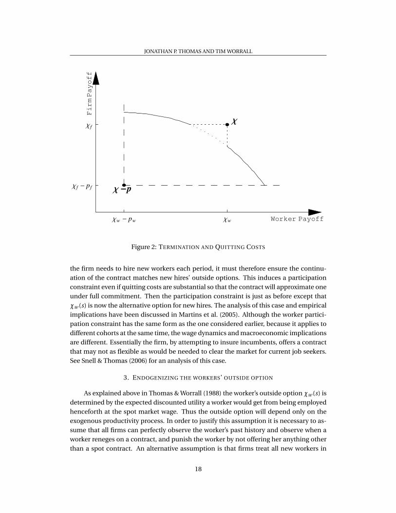
Suppose that after observing the current state at t , the Pareto-frontier conditional onthe relationship continuing is calculated. That is, consider self-enforcing agreementsfrom state st which do not terminate immediately and calculate the frontier from theirpayoffs. If it is the case that (χw (st ),χ f (st )) lies inside this frontier then termination isinefficient and cannot occur in any efficient agreement, since by definition there is anon-terminating self-enforcing contract which could be followed instead of terminationand which would be better for both parties. If however (χw (st ),χ f (st )) lies above thefrontier, then termination may or may not be efficient depending on the past historyof states. This case is illustrated in Figure 2 which depicts the frontier conditional oncontinuation and the outside options point χ(st ) = (χw (st ),χ f (st )) for some particularstate st . In this case, the overall frontier for this state is composed of the non-dominatedpoints from the set of the frontier conditional on non-termination plus (χw (st ),χ f (st )).As can be seen from Figure 2 there can be no agreement that corresponds to a divisionof the payoffs on the dotted part of the no-termination frontier as this would be domi-nated by termination. In particular, if there were such an agreement on the dotted partof the no-termination frontier then the parties would agree to termination. This wouldlead to to an improvement for both firm and worker and would be better that eitherparty quitting as it would avoid the quitting or reneging costs. On the other hand if theupdating rule were to put the division of the payoffs along the solid section of the no-termination frontier, then although termination will be better for one party, it will notbe a Pareto-improvement. Hence termination will not be agreed and the agreement willbe supported by the quitting or reneging costs which will prevent parties from unilater-ally defaulting. Thus the implication of allowing for quitting or reneging costs is that theoptimality of termination may now depend on the previous history, and so we lose thesimple termination rule of Proposition 1.27

Another issue arises if the firm employs many workers and that rather than deal-ing with each employee bilaterally, as we have assumed so far, an employer is requiredto treat every employee in the same way. Furthermore, suppose that this restriction ap-plies even to subsequent hires, so that they must be paid the same as incumbents fromthe point they join. That is a worker hired after history hτ must be offered the contin-uation of the original contract: (wτ(hτ), wτ+1(hτ, sτ+1), wτ+2(hτ, sτ+1, sτ+2), . . .). Provided

27This discussion assumes that side-payments are not possible. However, if side-payments were feasible itmay be that after observing st the contract specifies termination plus a payment from one agent to another,and the penalties pi may support this to an extent (for example, the firm will be prepared to transfer up top f ). In this case instead of a single point (χw ,χ f ) being added to set of payoffs, a curve through (χw ,χ f )determined by the trade-off of the side payments between the two agents will be added.

17


Χ

Χ-p

Worker Payoff

FirmPayoff

Χw - pw Χw

Χf - pf

Χf

Figure 2: TERMINATION AND QUITTING COSTS

the firm needs to hire new workers each period, it must therefore ensure the continu-ation of the contract matches new hires’ outside options. This induces a participationconstraint even if quitting costs are substantial so that the contract will approximate oneunder full commitment. Then the participation constraint is just as before except thatχw (s) is now the alternative option for new hires. The analysis of this case and empiricalimplications have been discussed in Martins et al. (2005). Although the worker partici-pation constraint has the same form as the one considered earlier, because it applies todifferent cohorts at the same time, the wage dynamics and macroeconomic implicationsare different. Essentially the firm, by attempting to insure incumbents, offers a contractthat may not as flexible as would be needed to clear the market for current job seekers.See Snell & Thomas (2006) for an analysis of this case.

3. ENDOGENIZING THE WORKERS’ OUTSIDE OPTION

As explained above in Thomas & Worrall (1988) the worker’s outside option χw (s) isdetermined by the expected discounted utility a worker would get from being employedhenceforth at the spot market wage. Thus the outside option will depend only on theexogenous productivity process. In order to justify this assumption it is necessary to as-sume that all firms can perfectly observe the worker’s past history and observe when aworker reneges on a contract, and punish the worker by not offering her anything otherthan a spot contract. An alternative assumption is that firms treat all new workers in

18


the same way, irrespective of whether or not they have reneged on a previous contract.According to this view, when a worker quits a firm, she can look for a new job offeringas much insurance as in the contract from which she just quit. If however, workers andfirms could move costlessly to other contracts then no non-spot contracts could be sus-tained.28 Therefore it will be necessary to assume either that there are other frictionssuch as search costs in the labor market, or that firms can commit to contracts. We dealwith each of these in turn.

3.1. Search frictions

In this section we discuss two papers (Sigouin (2004), Rudanko (2006)) which em-bed the above model into a matching framework to analyze the association of certainvariables with aggregate productivity. Both argue that the two-sided limited commit-ment model performs better than full commitment models and other versions such asspot contracts, one-sided limited commitment or continuous bargaining. Sigouin (2004)allows hours, but not employment, to vary, while Rudanko (2006) allows employmentand vacancies to vary. However in both of these matching models there is also the pos-sibility of an unemployment spell before a new contract is found, so the outside optionχw (s) is less than the utility from a new contract.

Sigouin (2004) develops the model with variable hours by allowing the outside op-tion χw (s) to be determined by contracts offered by other firms, rather than on a spotmarket as in the Thomas-Worrall model. He assumes however, that if a worker quitsfrom one firm she faces a probability of not being matched with a new firm (even thoughif matching does occur, it happens without a delay) and being unemployed.29 This issufficient to drive a potential wedge between what a worker can get by remaining inthe contract and what is available by quitting, and allows for some insurance to be sus-tained. Then χw (s) is determined by what a worker would get by quitting and waiting fora job; because of competition between firms a new job yields the worker the maximumsurplus from a self-enforcing contract; however the worker may be unlucky and sufferunemployment, so this is also factored into χw (s).

28This assertion assumes that the surplus split in state s from a new contract is always the same. Otherwisequitters could be punished effectively by starting a new contract so that the other agent gets all the surplusfrom the relationship. For example, in the Thomas-Worrall model this would imply that punishments areas severe as consignment to trading on the spot marker, so the same set of contracts are self-enforcing.

29There is no cost to posting a vacancy, but only a fixed fraction of the unemployed are able to make amatch, or rather, to ‘see’ wage offers (i.e. they are nor directly matched, but are able to enter into a contract,whereas the unlucky ones cannot). This implies that the unemployment rate does not vary. Essentially heposits a matching function where the matching or “seeing” probability does not depend on the numberof vacancies but only on the number seeking work. Moreover, although each entrepreneur can only matchwith a single worker, there are more entrepreneurs than workers so that competition between entrepreneursfor the fraction of unemployed workers who can see offers drives profits down to zero.

19


Each worker has a total time endowment which is normalized to one, and can sup-ply up to this amount to a single firm at any date. The productivity per hour workedis z(st ) at time t , which is common to all firms. However there is also a match specificshock, which can reduce productivity to zero (where it remains). If this happens, thematch is dissolved. A worker has separable preferences at t given by

Et

∞∑j=t

β j−t[

ln(c j )+B(1−η)−1 (

1−H j)1−η] ,

where c j is consumption and H j is hours supplied at time j . With separable preferencesthe updating rule of (9) in Section 2.2 implies that each state s ∈ S is associated minimumand maximum earnings,

¯Ws and W̄s (

¯Ws ≤ W̄s), such that earnings are kept constant if

possible and otherwise move by the smallest amount to¯

Ws or W̄s . In addition earningsand hours satisfy equation (7) that the marginal rate of substitution equals the marginalproduct. With the separable specification of preference given above, it follows that

(wt+1Ht+1)B (1−Ht+1)−η = z (st ) .

Notice that under a full commitment contract with these preferences a risk-neutral firmwill stabilize total earnings while hours will vary procyclically with productivity (accord-ing to the intertemporal elasticity of labor supply described above). This leads to the(counterfactual, given the very weak empirical correlation) conclusion that the wage rateis perfectly negatively correlated with hours supplied. On the other hand under a spot la-bor contract, where the wage is always equal to productivity z(st ), these preferences havethe property that income and substitution effects of a wage change cancel out (assumingthat all income is labor income and there are no taxes, and maintaining the assumptionof no borrowing/saving). In this case hours do not vary at all with the wage or produc-tivity (this contradicts the positive correlation between hours and productivity typicallyfound in the data).

As described in Section 2.2 the situation will, however, be somewhat different whenthere are enforcement constraints, and the result is a mixing of the above two extremes.For relatively small changes in productivity (and assuming that earnings are not alreadyup against the constraint that tightens) such that wt Ht ∈ [

¯Wst+1 ,W̄st+1 ], so neither con-

straint is binding with strictly positive shadow value, the rule says that earnings stay con-stant, so there is no income effect, and hours change with productivity according to theintertemporal elasticity of supply. On the other hand, if the change is large enough thata constraint binds, then earnings change and there will be an income effect which re-duces to an extent the change in hours. For example, a large increase in productivitymay imply only a small increase in hours if earnings rise substantially, so the wage will

20


also rise.30 In this case there is a positive correlation. The overall effect may then be thatthe correlation is very weak, in accordance with the evidence.

Rudanko (2006) also embeds the basic model in a model of search. She addressesissues recently raised by Shimer (2005) who argues that the Mortensen-Pissarides modelcannot account for the magnitude of unemployment and vacancy fluctuations withoutassuming an unrealistically high volatility in productivity. Hall (2005) argues that someform of wage rigidity may be sufficient to solve this puzzle. The Sigouin model holdsunemployment and vacancies fixed, so cannot address these issues. Rudanko looks atdifferent versions of a contracting model in a directed search model of the labor market,following Moen (1997), rather than the random matching model typically used in thisliterature. The model has similarities with the Sigouin model in that match specific pro-ductivity is composed (as the product of) a common (economy wide) component andmatch component that is unity initially, but transits to an absorbing state of 0 with afixed probability each period. As in Sigouin, when this occurs, the match dissolves andthe worker looks for a new job. Likewise there are a large number of risk-neutral en-trepreneurs operating under constant returns to scale. (Unlike Sigouin, however, hoursare fixed, although in the US the extensive margin is more important in accounting fortotal hours variation than the intensive one.) The model is one of competitive search:At the start of each period, after observing the current aggregate productivity level, firmscan choose to post an offer of a wage contract, but have to pay a cost k for keeping avacancy open. Worker search can be directed to a particular wage contract σ. There isa matching function defined as follows: if there is a measure Nu of unemployed agentssearching for σ and measure Nv of vacancies offering σ, the measure of matches takingplace this period is given by a Cobb-Douglas matching function

m(Nu , Nv ) = K Nαu N 1−α

v

where 0 < K < 1 and 0 < α < 1. Defining θ = Nv /Nu to be the vacancy unemploymentratio (“labor market tightness”), the probability that a worker finds a contract σ this pe-riod is m(θ) := m(Nu , Nv )/Nu , and the corresponding probability for an entrepreneur isq(θ) := m(Nu , Nv )/Nv . Thus the payoff to a worker from searching for σ is

µ (θ(z))Vσ(z)+ (1−µ (θ(z))

)Vu(z)

where Vσ(z) is the discounted worker utility from finding a job with contract σ, whileVu(z) is the corresponding utility from being unemployed, where both are functions ofthe prevailing aggregate state z. Vu(z) is the discounted utility from consuming the un-employment benefit today and searching again tomorrow. Likewise Vσ(z) is just the ex-pression given in the original model for contract utility with a stochastic termination

30This depends on how [¯

Wst+1 ,W̄st+1 ] varies with zt+1 but Sigouin shows through numerical simulationsthat the intuition will be correct in many situations.

21


added, at which point the worker gets Vu(z ′) if z ′ is the current state as she is unem-

ployed for a period and then has to seek a new job. The firm’s profit per job will dependon the probability that a job is filled, q(θ), and equals q (θ(z))Fσ(z)− k where Fσ(z) isthe discounted profit from σ achieved if a match occurs and where k is the vacancy costwhich must be incurred whether or not a match is made. With competition amongstentrepreneurs, this profit is driven to zero in equilibrium. The self-enforcing constraintsspecify that a worker cannot gain by leaving the contract, which requires that continua-tion utility must not be below Vu(z ′) (the worker is unemployed for at least a period), andagain that the continuation profits of the entrepreneur are non-negative. In addition, forequilibrium to obtain it must be the case that there is no other contract that could beoffered which would offer greater profits, where the corresponding θ will equate the re-turns to workers from searching in either market.31 As in Sigouin, the model endogenizesthe worker’s outside option so that it depends on what she would get by starting a newcontract, but again the risk of unemployment (here it will last at least one period) is asufficient deterrent to allow non-spot contracts to be sustained.

The model is calibrated to U.S. data, and the volatilities of real wages and of thevacancy/unemployment ratio are analyzed. Not surprisingly, if there is commitment inthe wage contract then wages vary too little with productivity (only new matches are re-sponsible for any variability). The model only comes close to matching the respectiveempirical correlations of the wage and the vacancy/unemployment ratio with produc-tivity in the two-sided limited commitment model if the replacement ratio is around80%, which is considerably higher than usually assumed (although Rudanko argues thatthis is not necessarily an unreasonable number). Intuitively, to get the wage to vary suf-ficiently, the worker’s outside option constraint must bind sufficiently frequently; thisrequires workers to be relatively indifferent between working and not working.32

3.2. One-sided limited commitment

We next consider the influential paper by Beaudry & DiNardo (1991) (hereafter BD91).They develop a model of labor contracting where a risk-neutral firm offers insurance torisk-averse employees, but there is no worker commitment and unlike the search modelsconsidered above a worker who quits can immediately start work elsewhere (perfect mo-bility). In terms of our model above, they assume that C f =∞ (firm commitment) andCw = 0 with χw (st ) given by the utility from starting a new job (perfect labor mobility).We derive their basic characterization, which is a generalization of Holmstrom (1983)who considered a two-period model. We then describe the other ingredients of their

31Rudanko shows that only a single contract is ever offered to new matches in equilibrium. Moreover, itis equivalent to a model with undirected search in which a weighted Nash product of surpluses (relative to(Vu (z) ,0)) is maximized, with weights proportional to the exponents in the matching function, i.e., α and1−α. So the competitive search framework appears not to be crucial to the results.

32The model actually does better as risk aversion tends to zero; this may be taken as support for the typeof hold-up model analyzed by MacLeod & Malcomson (1993).

22


model which lead to empirically testable predictions, and finally we discuss the empir-ical evidence. Their work is particularly important for two reasons. First, they providestrong evidence in favor of the perfect mobility model. Secondly, the paper addresseshow wages respond to unemployment levels over the business cycle. There is a volumi-nous literature that examines how real wages respond to contemporaneous movementsin unemployment which generally has not found a very strong relationship, but the re-sults in BD91 suggest that this literature may have been looking at the wrong businesscycle variable. If one looks at the lowest unemployment rate since a worker started a job,this appears to show a much stronger effect.33

Given that C f = ∞, we can treat the value of w̄s derived in Section 2.1 as beinginfinite. (Alternatively, we can just ignore the firm’s constraint in all the above arguments,so Lemma 1 directly asserts that wages cannot fall, etc.). Thus the intervals for efficientwages become [

¯ws ,∞). The ratchet nature of wages follows from Proposition 1: wt+1 =

¯wst+1 if wt <

¯wst+1 , and otherwise wt+1 = wt . To pin down the values for the

¯ws , we need

to specify the process for χw (st ) and how the contractual surplus is split between workerand firm.

BD91 assume that there are a large number of identical firms and workers, withnew workers entering each period to replenish the labor force, replacing workers whodie.34 It is assumed further that because firms operate under constant returns to scale,competition for workers drives profits for a new worker to zero, so any surplus goes tothe worker. A worker who quits a firm can immediately seek employment with anotherfirm. Moreover the only source of uncertainty is the common shock to productivity eachperiod. What this implies is that χw (st ), the utility of the worker’s outside option, equalsthe utility from an optimal contract which generates zero profits.35 Given the updatingrule, it is then possible to calculate the initial wage of a contract starting in state s forwhich discounted expected wages and discounted expected productivity are equal. Thismust therefore be

¯ws .

What is perhaps surprising at first glance is how it is possible to offer any insur-ance at all when the worker can quit and restart the contract at a different firm, without

33As before we assume that workers do not engage in capital market transactions. This is not an innocuousassumption when the insurance offered by the contract is partial as the workers may wish to supplementthe insurance through borrowing even when the capital market is imperfect. A two-period model that doesconsider access to imperfect capital markets is Haltiwanger & Waldman (1986). In their model where work-ers learn their true productivity in the second period, they are able to show wages offer some insurance inthe second period, rising if either high or low productivity is revealed. They show that this may help explainthe positive correlation between experience and compensation in the absence of changes in productivity asa result of experience.

34BD91 also have firm death, but we shall abstract from this in the exposition that follows.35BD91 express the worker’s participation constraint equivalently as the fact that the contract must never

offer strictly positive profits, looking forward from any point—if it did then the worker would be bid away.

23


any penalty.36 Normally in repeated game models of cooperation players are induced totake short-term sub-optimal actions (such as paying out on insurance) by the promiseof long-term rewards relative to reneging on this, which yields termination. But here aworker who quits is able to immediately start a new contract with a different firm so thatwhenever productivity is such that the contract demands a sacrifice by the worker, theworker can quit. The resolution of this apparent paradox is that contracts require thatworkers initially receive a wage below productivity. Thus workers are effectively makingtransfers firms in the early periods of the contract. These early transfers are compen-sated by the likelihood of wages above productivity as wages will tend to increase overtime.37,38

In order to get testable restrictions, it is necessary to link the productivity level inthe theoretical model to an observable variable. Notice that the optimal wage contractdepends only on the productivity process—a very convenient feature. Moreover the la-bor market must always clear, since at the point of hiring there are no restrictions onwages. However when productivity is high, the wage and expected utility for a new en-trant is high. BD91 posit an alternative sector in which a worker could be employedwhich is subject to a (fixed) decreasing returns technology. Thus a new entrant to thelabor market faces a choice between a period in the alternative sector and then gettinga contract, versus getting a contract in the original sector right away (by constructionof the equilibrium, once a worker has a contract, the option of moving to the alterna-tive sector will offer the same as a new contract, and so is always weakly dominated dueto the participation constraint). In equilibrium workers will be indifferent (there are al-ways some workers employed in the alternative sector) so a high wage in the originalsector must positively related to a high wage in the alternative sector and hence low lev-els of employment in the alternative sector (because of decreasing returns). BD91 equatea low level of employment in the alternative sector with low unemployment rate in theeconomy and hence conclude that a low level of unemployment will be associated withhigher wages in the current and subsequent periods.39

BD91 conclude, then, that with no worker commitment (perfect mobility), wherethe worker is free to quit at any point, the wage follows a ratchet like process, risingwhenever the labor market is tighter than hitherto (since the worker joined the firm), butstaying constant otherwise; hence the current wage is determined by the tightest labor

36In fact this intuition is correct in the two-sided case where the firm could also terminate the relationshipcostlessly. In the Sigouin and Rudanko models discussed above, there is the possibility of unemployment ifa worker quits, and this is sufficient to support non-trivial contracts.

37This issue has been explored by Krueger & Uhlig (2006) in a general risk sharing context where bothparties to the contract are risk-averse.

38The feature that workers initially receive wages below productivity with a rising wage profile is of coursereminiscent of the agency models where rising wages provide incentives for effort, see e.g. Lazear (1981).

39It is tempting to interpret the alternative sector as leisure or some sort of household production, al-though the decreasing returns to total labor input makes this interpretation difficult.

24


market during a worker’s tenure. Tightness of the labor market is measured by how lowthe unemployment rate is. In testing, this perfect mobility model does better than twoalternatives: a spot market model in which current unemployment determines wages,and a full commitment model in which unemployment at the time of hiring is the de-termining factor. In the spot market model, wages are determined solely by the value ofa worker’s current marginal product, in the full commitment contracting model, wagesare constant but the level is determined by the worker’s outside opportunity at the pointat which she joins the firm. Beaudry & DiNardo (1991) test these three models againsteach other on U.S. data (PSID/Current Population Survey (CPS)). Perhaps surprisingly,the latter model appears to perform much better than the other two, which we describein more detail:

Commitment: a binding contract is signed when the worker joins a firm. Becausethe worker is risk-averse, the risk-neutral firm acts as an insurance company, completelystabilizing wages. (This results from our above general model by imposing Cw =∞, sothat

¯ws = −∞.) In equilibrium workers will be offered a fixed wage contract (where the

wage will equal the expected discounted value of a worker’s productivity so firms makezero profits). The wage will be fixed at a level corresponding to conditions at the pointthe worker joins the firm—it equals the best estimate of a worker’s lifetime productivity,and under the assumed productivity process this will depend only on her productivity atthis point, which is, as explained above, proxied by the unemployment rate, Ut , at thatpoint.

Spot market contract: no long-term contract is possible, so this implies that wt =z(st ). (If a firm offered say a fixed wage contract, then whenever the wage was less thanz(st ) the worker could just walk away, and go to another firm, while if the wage wasgreater than z(st ) the firm could sack the worker.) Thus wages fluctuate with z(st ) whichis proxied by Ut .

The general model can be expressed as follows: the natural log of the real wage forworker j at time τ+ t for a worker who started the job at time τ satisfies:

ln w j ,τ+t =α1X j ,τ+t +α2C (τ, t )+ε j ,τ+t

where X j ,τ+t is a vector of individual variables40, α1 is the vector of coefficients on thesevariables, ε j ,τ+t is an error term, and α2 is the coefficient on the business cycle (i.e.,unemployment) variable, with the 3 possibilities for the business cycle variable C (τ, t )

40For individual characteristics, BD91 used experience, experience squared, how much schooling, jobtenure, and dummies for industry, region, race, union status, marriage, and metropolitan area (SMSA).

25


being:

C (τ, t ) =

Uτ+t spot market model

Uτ fully binding contract

min{Uτ+k ,k = 0,1, . . . , t } non-binding on worker

where the unemployment rate is denoted by U , with Uτ the rate prevailing at the start ofthe job and Uτ+t the rate at time τ+ t where t denotes tenure with the employer.

The results are striking. In some specifications41 in which all three variables are in-cluded, the coefficient on the minimum unemployment rate is the only correctly signed(i.e., negative) significant one (PSID, no fixed effects), and in all specifications it is muchlarger than the other coefficients, implying that a 1% drop in the minimum unemploy-ment rate (e.g., from 4% to 3%) leads to an increase in current wages of between 3% and8%.

The implications for our understanding of real wage cyclicality are considerable.Typically studies have looked at how wages respond to contemporaneous unemploy-ment movements. For example, using the PSID for men over the period of 1968–69 to86–87, Solon, Barsky & Parker (1994) found that a one percentage point reduction of theunemployment rate leads to a rise in the real wage rate of workers who stayed in theirjobs by 1.2 percent (movers appear to be subject to greater procyclical wage movements).Similar estimates are found in Shin (1994) and Devereux (2001). BD91’s results suggestthat the response of wages to the minimum unemployment rate is substantially larger.On the other hand, as argued in Grant (2003), because the minimum unemployment ratedoes not actually vary as much as contemporaneous unemployment (consider a workerwhose minimum value occurred early in a job spell), minimum unemployment may notexplain very much of the variability of aggregate wages over the business cycle.

Several recent empirical studies have largely confirmed the robustness of BD91’smain empirical findings over different periods and using different datasets, that the min-imum rate of unemployment since hiring is a statistically important determinant of thecurrent wage of an individual (McDonald & Worswick 1999, Grant 2003, Shin & Shin2007, Devereux & Hart 2007). Both Grant (2003), and Devereux & Hart (2007), however,find more of a role for the current unemployment rate than did BD91. Grant (2003) ex-tends BD91’s analysis (using six cohorts from the National Longitudinal Surveys) to coverthe time period 1966 to 1998. He finds that the significance and importance of minu isbroadly robust with respect to the addition of fixed time dummies (to rule out any ef-fects coming through macroeconomic variables, and thus the coefficient on minu is es-timated only through variation across individuals in each year), of tenure dummies (tocapture nonlinear tenure effects), a tenure-unemployment interaction term (to capturetenure effects that vary over the business cycle), and using sub-samples selected on the

41See Table 2 of their paper.

26


basis of age, and sex. As mentioned, however, current unemployment levels also havesome explanatory power.

A somewhat different methodology was adopted by Shin & Shin (2007), using thePSID for the period 1974–91, which includes one business cycle more than BD91. Theyrun the BD91 regressions over the whole period and get very similar results—but as Grantdoes, they also find more significant results for contemporaneous unemployment.42,43

They also estimate a complementary econometric model, only using the current unem-ployment rate as a business cycle regressor, but look for asymmetric effects of tight labormarkets. Thus they split a job history into periods of tightening and loosening labormarkets, and subdivide the former category into two sub-categories, when unemploy-ment is falling but above its minimum for the current job, and when it is below the min-imum. Tenure is measured with considerable error in the PSID; thus a mismeasurementin tenure may lead to an incorrect value for minu, used in BD91’s estimation, whereashere it will lead to the respective periods when unemployment is falling but below orrespectively above the historical minimum, to be measured incorrectly. It is argued thatthe former is more likely to be problematical. The results are that most of the wage ad-justment occurs in periods when the unemployment rate falls below the historical mini-mum level observed since the start of the current job in accordance with the perfect mo-bility model (according to the model, wages should be constant in other periods): Forthe sample of male household heads, the estimated coefficient on the unemploymentrate is -0.026 (i.e., a one percentage point reduction in the unemployment rate is asso-ciated with a 2.64 percent rise in real wages). The coefficient on unemployment whenit is falling but not below the historical minimum is much smaller at -.0076, but not sig-nificant. For periods of contraction, the coefficient is smaller and insignificant. So againthere is a strong confirmation of the perfect mobility model. They also confirm the find-ings of other studies that the wages of job stayers are procyclical, but less so than thoseof movers.

42In comparing their estimates with those of Grant, it is interesting to note that the PSID sample has ahigher average age than the National Longitudinal Survey of Youth used by Grant except for the NLSY OlderMen. Estimates in Table 2 of Grant (2003) show that the effect of the minimum unemployment rate oncurrent wages dominates those of the other unemployment variables more in the NLSY “Older Men” cohortthan in “Young Men” or “Women,” and the “Older Men” results are closest to the PSID estimates. Thissuggests that the BD91 model may work better for older workers.

43Shin & Shin (2007) include a trend, which might matter as the period studied has a generally risingunemployment rate, so that the a job’s minimum unemployment rate is negatively correlated with timeelapsed since the date at which the minimum is attained; as wages are rising omitting this trend mightoverstate the effect of the minimum unemployment rate. However it makes little difference, as one wouldanticipate from Grant’s analysis with time dummies. Likewise, to rule out nonlinear effects of tenure theyfind that the addition a squared tenure term does not matter to the worker fixed effect model (although itdoes to the no-fixed effects specification); again this confirms Grant’s findings.

27


4. CLOSING COMMENTS

We presented an overview of models of self-enforcing labor contracts in which risksharing is the dominant motive for contractual solutions. A basic two-agent (firm-worker)model was developed which is sufficiently general to encompass the problem consid-ered in most of the literature. We have shown how the solution can be characterizedusing local variational arguments and therefore avoided the need to establish more com-plex technical properties of optimum value functions. We have considered how the out-side option of the worker is made endogenous in competitive or search markets andconsidered some of the implications for aggregate hours and wages and productivityand what empirical support exists for the model. The broad conclusion is that the self-enforcing contractual model does help explain some of the observed empirical regular-ities better than a spot market or full commitment alternatives. There is fairly strongsupport from a variety of sources and data of the one-sided limited commitment modelwhere workers outside options are determined competitively.

There remain some issues for further study. A weakness of the empirical tests hasbeen to discriminate against alternative assumptions of capital market imperfections,such as credit constraints for employees, or alternative contracting explanations basedon hold-up rather than risk aversion. The general success of the empirical method how-ever suggests that it will be useful to explore whether the model can help explain ob-served patterns in wages at the firm level where it is typically found that larger firms payhigher wages and fast growing firms pay lower wages. An approach along these linescombining contracts with firm credit constraints can be found in Michelacci & Quadrini(2005).

28


REFERENCES

Abowd, J. M. & Card, D. (1987), ‘Intertemporal labor supply and long-term employmentcontracts’, American Economic Review 77(1), 50–68.

Azariadis, C. (1975), ‘Implicit contracts and underemployment equilibria’, Journal of Po-litical Economy 83(6), 1183–1202.

Beaudry, P. & DiNardo, J. (1991), ‘The effect of implicit contracts on the movement ofwages over the business-cycle - evidence from micro data’, Journal of Political Econ-omy 99(4), 665–688.

Beaudry, P. & DiNardo, J. (1995), ‘Is the behavior of hours worked consistent with implicitcontract theory?’, Quarterly Journal of Economics 110(3), 743–768.

Boldrin, M. & Horvath, M. (1995), ‘Labor contracts and business cycles’, Journal of Polit-ical Economy 103(5), 972–1004.

Calmès, C. (2007), ‘Self-enforcing labour contracts and macroeconomic dynamics’, In-ternational Advances in Economic Research 13(2), 200–213.

Devereux, P. J. (2001), ‘The cyclicality of real wages within employer-employee matches’,Industrial Labor Relations Review 54(4), 835–850.

Devereux, P. J. & Hart, R. A. (2007), ‘The spot market matters: Evidence on implicit con-tracts from Britain’, Scottish Journal of Political Economy . Forthcoming.

Dubois, P., Jullien, B. & Magnac, T. (2007), Formal and informal risk sharing in LDCs:Theory and empirical evidence, IZA Discussion Papers 2842, Institute for the Studyof Labor (IZA).

Gauthier, C., Poitevin, M. & Gonzáez, P. (1997), ‘Ex ante payments in self-enforcing risk-sharing contracts’, Journal of Economic Theory 76(1), 106–144.

Grant, D. (2003), ‘The effect of implicit contracts on the movement of wages over thebusiness cycle: Evidence from national longtitudinal surveys’, Industrial and LaborRelations Review 56(3), 393–408.

Hall, R. E. (2005), ‘Employment fluctuations with equilibrium wage stickiness’, AmericanEconomic Review 95(1), 50–65.

Haltiwanger, J. & Waldman, M. (1986), ‘Insurance and labor market contracting: An anal-ysis of the capital market assumption’, Journal of Labor Economics 4(3), 355–75.

Holmstrom, B. (1983), ‘Equilibrium long-term labor contracts’, Quarterly Journal of Eco-nomics 98(3), 23–54.

Krueger, D. & Uhlig, H. (2006), ‘Competitive risk sharing contracts with one-sided com-mitment’, Journal of Monetary Economics 53(7), 1661–1691.

29


Lazear, E. (1981), ‘Agency, earnings profiles, productivity, and hours restrictions’, Ameri-can Economic Review 71(4), 606–620.

Ligon, E., Thomas, J. P. & Worrall, T. (2000), ‘Mutual insurance, individual savings andlimited commitment’, Review of Economic Dynamics 3(2), 216–246.

Ljungqvist, L. & Sargent, T. J. (2004), Recursive Macroeconomic Theory, second edn, MITPress.

Macis, M. (2006), Wage dynamics and insurance. Mimeo, University of Chicago.

MacLeod, W. B. (2007), ‘The three solitudes in contract: Law, data and theory’, ScottishJournal of Political Economy . Forthcoming.

MacLeod, W. B. & Malcomson, J. M. (1993), ‘Investments, hold-up, and the form of mar-ket contracts’, American Economic Review 83(4), 811–847.

Malcomson, J. M. (1997), ‘Contracts, hold-up, and labor markets’, Journal of EconomicLiterature 35(4), 1916–1957.

Malcomson, J. M. (1999), Individual employment contracts, in O. Ashenfelter & D. Card,eds, ‘Handbook of Labor Economics’, Vol. 3, Elsevier, chapter 35, pp. 2291–2372.

Martins, P., Snell, A. & Thomas, J. P. (2005), ‘Wage dynamics, cohort effects, and limitedcommitment models’, Journal of the European Economic Association 3(2–3), 350–359.

McDonald, J. T. & Worswick, C. (1999), ‘Wages, implicit contracts, and the business cycle:Evidence from Canadian micro data’, Journal of Political Economy 107(4), 884–892.

Michelacci, C. & Quadrini, V. (2005), Financial markets and wages, NBER Working Papers11050, National Bureau of Economic Research, Inc.

Moen, E. R. (1997), ‘Competitive search equilibrium’, Journal of Political Economy105(2), 385–411.

Rosen, S. (1985), ‘Implicit contracts: A survey’, Journal of Economic Literature23(3), 1144–1175.

Rudanko, L. (2006), Labor market dynamics under long-term wage contracting and in-complete markets. Mimeo, University of Chicago.

Shimer, R. (2005), ‘The cyclical behavior of equilibrium unemployment and vacancies’,American Economic Review 95(1), 25–49.

Shin, D. (1994), ‘Cyclicality of real wages among young men’, Economics Letters46(2), 137–142.

30


Shin, D. & Shin, K. (2007), ‘Why are the wages of job stayers procyclical?’, MacroeconomicDynamics 11. Forthcoming.

Sigouin, C. (2004), ‘Self-enforcing employment contracts and business cycle fluctua-tions’, Journal of Monetary Economics 51(2), 339–373.

Snell, A. & Thomas, J. P. (2006), Labour contracts, equal treatment and wage-unemployment dynamics, CESifo Working Paper No. 1835, CESifo Munich.

Solon, G., Barsky, R. & Parker, J. A. (1994), ‘Measuring the cyclicality of real wages: howimportant is composition bias?’, Quarterly Journal of Economics 109(1), 1–26.

Thomas, J. P. & Worrall, T. (1988), ‘Self-enforcing wage contracts’, Review of EconomicStudies 55(4), 541–554.

31

CESifo Working Paper Series for full list see Twww.cesifo-group.org/wp T (address: Poschingerstr. 5, 81679 Munich, Germany, [email protected])

___________________________________________________________________________ 2044 Annika Alexius and Bertil Holmlund, Monetary Policy and Swedish Unemployment

Fluctuations, July 2007 2045 Axel Dreher, Jan-Egbert Sturm and Jakob de Haan, Does High Inflation Cause Central

Bankers to Lose their Job? Evidence Based on a New Data Set, July 2007 2046 Guglielmo Maria Caporale and Luis A. Gil-Alana, Long Run and Cyclical Dynamics in

the US Stock Market, July 2007 2047 Alessandro Balestrino, It is a Theft but not a Crime, July 2007 2048 Daniel Becker and Michael Rauscher, Fiscal Competition in Space and Time: An

Endogenous-Growth Approach, July 2007 2049 Yannis M. Ioannides, Henry G. Overman, Esteban Rossi-Hansberg and Kurt

Schmidheiny, The Effect of Information and Communication Technologies on Urban Structure, July 2007

2050 Hans-Werner Sinn, Please Bring me the New York Times – On the European Roots of

Richard Abel Musgrave, July 2007 2051 Gunther Schnabl and Christian Danne, A Role Model for China? Exchange Rate

Flexibility and Monetary Policy in Japan, July 2007 2052 Joseph Plasmans, Jorge Fornero and Tomasz Michalak, A Microfounded Sectoral

Model for Open Economies, July 2007 2053 Vesa Kanniainen and Panu Poutvaara, Imperfect Transmission of Tacit Knowledge and

other Barriers to Entrepreneurship, July 2007 2054 Marko Koethenbuerger, Federal Tax-Transfer Policy and Intergovernmental Pre-

Commitment, July 2007 2055 Hendrik Jürges and Kerstin Schneider, What Can Go Wrong Will Go Wrong: Birthday

Effects and Early Tracking in the German School System, July 2007 2056 Bahram Pesaran and M. Hashem Pesaran, Modelling Volatilities and Conditional

Correlations in Futures Markets with a Multivariate t Distribution, July 2007 2057 Walter H. Fisher and Christian Keuschnigg, Pension Reform and Labor Market

Incentives, July 2007 2058 Martin Altemeyer-Bartscher, Dirk T. G. Rübbelke and Eytan Sheshinski, Policies to

Internalize Reciprocal International Spillovers, July 2007

2059 Kurt R. Brekke, Astrid L. Grasdal and Tor Helge Holmås, Regulation and Pricing of

Pharmaceuticals: Reference Pricing or Price Cap Regulation?, July 2007 2060 Tigran Poghosyan and Jakob de Haan, Interest Rate Linkages in EMU Countries: A

Rolling Threshold Vector Error-Correction Approach, July 2007 2061 Robert Dur and Klaas Staal, Local Public Good Provision, Municipal Consolidation,

and National Transfers, July 2007 2062 Helge Berger and Anika Holler, What Determines Fiscal Policy? Evidence from

German States, July 2007 2063 Ernesto Reuben and Arno Riedl, Public Goods Provision and Sanctioning in Privileged

Groups, July 2007 2064 Jan Hanousek, Dana Hajkova and Randall K. Filer, A Rise by Any Other Name?

Sensitivity of Growth Regressions to Data Source, July 2007 2065 Yin-Wong Cheung and Xing Wang Qian, Hoarding of International Reserves: Mrs

Machlup’s Wardrobe and the Joneses, July 2007 2066 Sheilagh Ogilvie, ‘Whatever Is, Is Right’?, Economic Institutions in Pre-Industrial

Europe (Tawney Lecture 2006), August 2007 2067 Floriana Cerniglia and Laura Pagani, The European Union and the Member States:

Which Level of Government Should Do what? An Empirical Analysis of Europeans’ Preferences, August 2007

2068 Alessandro Balestrino and Cinzia Ciardi, Social Norms, Cognitive Dissonance and the

Timing of Marriage, August 2007 2069 Massimo Bordignon, Exit and Voice. Yardstick versus Fiscal Competition across

Governments, August 2007 2070 Emily Blanchard and Gerald Willmann, Political Stasis or Protectionist Rut? Policy

Mechanisms for Trade Reform in a Democracy, August 2007 2071 Maarten Bosker and Harry Garretsen, Trade Costs, Market Access and Economic

Geography: Why the Empirical Specification of Trade Costs Matters, August 2007 2072 Marco Runkel and Guttorm Schjelderup, The Choice of Apportionment Factors under

Formula Apportionment, August 2007 2073 Jay Pil Choi, Tying in Two-Sided Markets with Multi-Homing, August 2007 2074 Marcella Nicolini, Institutions and Offshoring Decision, August 2007 2075 Rainer Niemann, The Impact of Tax Uncertainty on Irreversible Investment, August

2007

2076 Nikitas Konstantinidis, Gradualism and Uncertainty in International Union Formation,

August 2007 2077 Maria Bas and Ivan Ledezma, Market Access and the Evolution of within Plant

Productivity in Chile, August 2007 2078 Friedrich Breyer and Stefan Hupfeld, On the Fairness of Early Retirement Provisions,

August 2007 2079 Scott Alan Carson, Black and White Labor Market Outcomes in the 19th Century

American South, August 2007 2080 Christian Bauer, Paul De Grauwe and Stefan Reitz, Exchange Rates Dynamics in a

Target Zone – A Heterogeneous Expectations Approach, August 2007 2081 Ana Rute Cardoso, Miguel Portela, Carla Sá and Fernando Alexandre, Demand for

Higher Education Programs: The Impact of the Bologna Process, August 2007 2082 Christian Hopp and Axel Dreher, Do Differences in Institutional and Legal

Environments Explain Cross-Country Variations in IPO Underpricing?, August 2007 2083 Hans-Werner Sinn, Pareto Optimality in the Extraction of Fossil Fuels and the

Greenhouse Effect: A Note, August 2007 2084 Robert Fenge, Maximilian von Ehrlich and Matthias Wrede, Fiscal Competition,

Convergence and Agglomeration, August 2007 2085 Volker Nitsch, Die Another Day: Duration in German Import Trade, August 2007 2086 Kam Ki Tang and Jie Zhang, Morbidity, Mortality, Health Expenditures and

Annuitization, August 2007 2087 Hans-Werner Sinn, Public Policies against Global Warming, August 2007 2088 Arti Grover, International Outsourcing and the Supply Side Productivity Determinants,

September 2007 2089 M. Alejandra Cattaneo and Stefan C. Wolter, Are the Elderly a Threat to Educational

Expenditures?, September 2007 2090 Ted Bergstrom, Rod Garratt and Damien Sheehan-Connor, One Chance in a Million:

Altruism and the Bone Marrow Registry, September 2007 2091 Geraldo Cerqueiro, Hans Degryse and Steven Ongena, Rules versus Discretion in Loan

Rate Setting, September 2007 2092 Henrik Jacobsen Kleven, Claus Thustrup Kreiner and Emmanuel Saez, The Optimal

Income Taxation of Couples as a Multi-Dimensional Screening Problem, September 2007

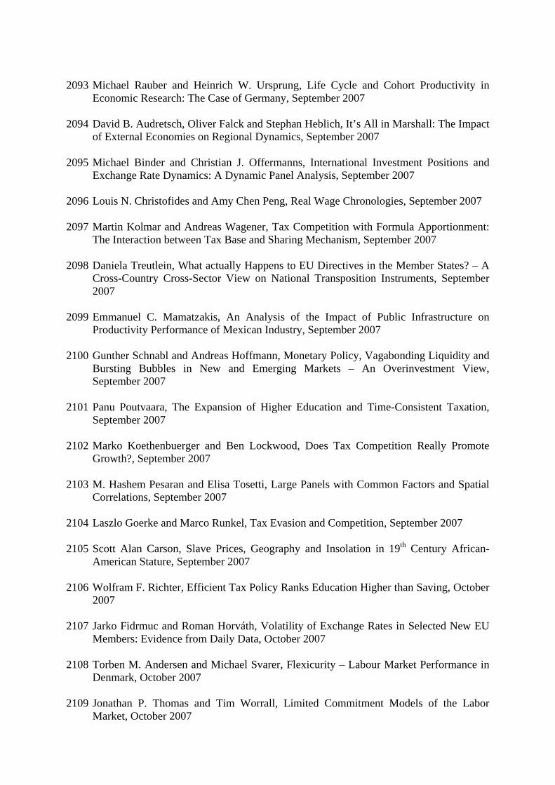
2093 Michael Rauber and Heinrich W. Ursprung, Life Cycle and Cohort Productivity in

Economic Research: The Case of Germany, September 2007 2094 David B. Audretsch, Oliver Falck and Stephan Heblich, It’s All in Marshall: The Impact

of External Economies on Regional Dynamics, September 2007 2095 Michael Binder and Christian J. Offermanns, International Investment Positions and

Exchange Rate Dynamics: A Dynamic Panel Analysis, September 2007 2096 Louis N. Christofides and Amy Chen Peng, Real Wage Chronologies, September 2007 2097 Martin Kolmar and Andreas Wagener, Tax Competition with Formula Apportionment:

The Interaction between Tax Base and Sharing Mechanism, September 2007 2098 Daniela Treutlein, What actually Happens to EU Directives in the Member States? – A

Cross-Country Cross-Sector View on National Transposition Instruments, September 2007

2099 Emmanuel C. Mamatzakis, An Analysis of the Impact of Public Infrastructure on

Productivity Performance of Mexican Industry, September 2007 2100 Gunther Schnabl and Andreas Hoffmann, Monetary Policy, Vagabonding Liquidity and

Bursting Bubbles in New and Emerging Markets – An Overinvestment View, September 2007

2101 Panu Poutvaara, The Expansion of Higher Education and Time-Consistent Taxation,

September 2007 2102 Marko Koethenbuerger and Ben Lockwood, Does Tax Competition Really Promote

Growth?, September 2007 2103 M. Hashem Pesaran and Elisa Tosetti, Large Panels with Common Factors and Spatial

Correlations, September 2007 2104 Laszlo Goerke and Marco Runkel, Tax Evasion and Competition, September 2007 2105 Scott Alan Carson, Slave Prices, Geography and Insolation in 19th Century African-

American Stature, September 2007 2106 Wolfram F. Richter, Efficient Tax Policy Ranks Education Higher than Saving, October

2007 2107 Jarko Fidrmuc and Roman Horváth, Volatility of Exchange Rates in Selected New EU

Members: Evidence from Daily Data, October 2007 2108 Torben M. Andersen and Michael Svarer, Flexicurity – Labour Market Performance in

Denmark, October 2007 2109 Jonathan P. Thomas and Tim Worrall, Limited Commitment Models of the Labor

Market, October 2007

LIMITED COMMITMENT MODELS OF THE LABOUR MARKET

Documents

Transcript of LIMITED COMMITMENT MODELS OF THE LABOUR MARKET