LIGHTLY REINFORCED WALLS SUBJECTED TO SEISMIC EXCITATIONS. INTERPRETATION OF

CAMUS 2000-1 AND 2000-2 DYNAMIC TESTS

N. ILE Unité de Recherche de Génie Civil,

National Institute of Applied Mechanics of Lyon, 20, Av. Albert Einstein, 69621, Villeurbanne, France

J.M. REYNOUARD

Unité de Recherche de Génie Civil, National Institute of Applied Mechanics of Lyon,

20, Av. Albert Einstein, 69621, Villeurbanne, France

In this paper is presented a study of the inelastic seismic performance of two 5-storey reinforced concrete wall specimens, which were tested in the context of the CAMUS 2000 program. The structure has been sized and detailed following the French PS92 code. To investigate the simplifying assumptions made in design, a 3-D refined non-linear analysis was conducted. Particular aspects of the behaviour of the two tested specimens are presented and then test results are compared with numerical predictions. The experimental-analytical comparisons not only demonstrate the accuracy of the time-history analysis model, but also allow obtaining more detailed information about the behaviour of the specimen when it is subjected to seismic excitation. The significant effect of degradation of the stiffness and strength of the wall suggests that it is always important that design procedures are derived from numerical modelling and experimental observations. Keywords: lightly RC wall, bi-directional seismic loading, 3-D finite element analysis, shaking-table test. 1. Introduction The seismic behaviour of RC wall structures, designed and detailed to develop a ductile flexural plastic hinge at the base (ductile walls) has been the subject of extended research. A wide literature is available on this subject (e.g. [State-of-the-Art, 1982], [Vulcano et al., 1988], [Elnashai et al., 1990], [Kabeyasawa et al.,1996], [Paulay, 1997], [Chiou, et al., 2003]). As a direct consequence of these studies the behaviour of ductile walls is nowadays fairly well understood and code provisions give detailed guidelines to the designer. Despite the large research effort of the last three decades, very little attention has been paid to the seismic behaviour of lightly reinforced RC walls.

RC bearing walls with limited reinforcement ratio are commonly used in France and some central European countries for building structures. In wall structures, where masonry is generally not used for partitioning, the wall arrangement is redundant when compared to the structural demand. In this kind of structure the design procedure allows

the wall to go inelastic and develop cracking and/or plastic hinges at any location along its height. Slender walls may be designed in this way as lightly reinforced walls, the flexural reinforcement being curtailed in accordance with the bending moment diagram.

Within the French CAMUS (Conception et analyse du comportement des murs porteurs sous séisme) [Bisch and Coin, 1998] and European TMR (Training and Mobility of Researchers) [TMR, 2003] projects, shaking table tests on RC wall structures in different situations (fixed or not to the shaking table, placed on a layer of sand, with different reinforcement ratio) have been performed. The data provided by these experimental programs have been used not only to validate numerical models integrated into FE codes [Mazars, 1998], [Faria et al., 2002], [Fischinger et al., 2002], [Ilker et al., 2006], but also to improve existing design methods [Bisch and Coin 1998]. Moreover, “large lightly reinforced walls” have been introduced in the relevant provisions of EN1998 [CEN, 2004].

It should be noted that in these previous research programs, only loadings in one direction (in the plane of the walls) were applied. In real structures, such walls are likely to be loaded in the out-of-plane direction as well, and the question arises as to how such walls behave under combined in-plane and out-of-plane loading. Furthermore, the majority of wall structures are irregular, so the validation of design codes requires tests on asymmetric specimens.

A new research programme (CAMUS 2000) was launched in 1998 with the aim of investigating two aspects of the behaviour of lightly reinforced concrete walls, which are used as the main lateral load resisting system:

• the influence of a simultaneous acceleration perpendicular to the wall plane, and • the influence of torsion on the behaviour of the wall

As a part of this program, two scaled (1/3) models representative of 5 storey reinforced concrete buildings have been tested on the major Azalee shaking table of Commissariat à l’Energie Atomique CEA (France) in the Saclay Nuclear Centre. The first structure (CAMUS 2000-1) has been subjected to horizontal bi-directional excitations. Two identical shear walls in one direction and a steel bracing system in the orthogonal direction provided structural stiffness and strength. The second structure (CAMUS 2000-2) was made of two RC walls with different rectangular sections, while in the orthogonal direction the same steel bracing system was used. Although only in-plane excitation was applied to this specimen, a torsion response was generated by the fact that the centre of stiffness was eccentric with respect to the centre of mass. The CAMUS 2000-2 specimen was tested on the 24th and 25th of April and CAMUS 2000-1 specimen on the 13th and 14th of June, 2002.

First, pre-test 3-D nonlinear analyses of the structural response of these specimens were performed at the end of 2001. Then, at the end of 2002, after the test results became available, the same mathematical model as in the pre-test analyses was used, only the value of some material parameters have been changed, based on the results of laboratory tests. This paper presents some particular aspects of the behaviour of the tested specimens and then compares test results with post-test numerical predictions based on a refined and detailed 3-D thin shell representation of the geometry of the walls. Comparing numerical and experimental results gives great help in verifying the numerical models and understanding the behaviour of the test specimens more clearly. In the section that follows, a brief summary of the design background is first provided in order to familiarize the reader with the CAMUS 2000 program.

2. Design of the Test Specimens 2.1 Design of the CAMUS 2000-1 Specimen The objective of the CAMUS 2000-1 test has been examination of the influence of bi-directional seismic excitations on the inelastic behaviour of in-plane regular wall structures. As compared to the uni-directional case, bi-directional seismic excitation generates higher axial force in a wall and consequently, more damage is to be expected when bi-directional effects are considered.

To study these effects, the test specimen has been designed as lightly reinforced and has been subjected to two horizontal uncorrelated accelerograms in the X and Y directions (Figure 1). Since the research is more oriented towards knowledge of the behaviour of lightly reinforced walls, there was no need to deduce the dimensions of the specimens directly from a reference building. However, it was considered as necessary that the general characteristics of the specimen can be found in a real building. A first choice was made with the number of stories: five stories were considered as representative of the current situation in France. It was also necessary to select a priori the value of the scale factor, as additional masses are necessary when reduction is operated from reasonable sizes. To represent correctly the behaviour of reinforced concrete in the inelastic domain, there is no choice but keeping stress and strain levels in the specimen similar to those obtained in a real structure in a similar situation. Then, the accelerations

should be kept constant, the supported mass varies with 2λ and the time with λ , where

λ is the scale factor. Hence, additional masses are necessary to compensate the lack of

mass induced by the reduction factor (the volume of concrete varies with3λ ) and to keep the chosen level of mean compressive stress. The scale factor was selected so that the wall thickness in the specimen be practically built with micro-concrete and thin rebars, the mechanical characteristics of which being reasonably comparable to those of a material used in a real construction. Based on the previous experience acquired in the CAMUS program, a scale factor of 1/3 has been chosen. With this scale factor, the wall thickness was taken as 6 cm (corresponding to a thickness of 18 cm in a real building) and the storey height was 90 cm (corresponding to 2,70 m in a real building).

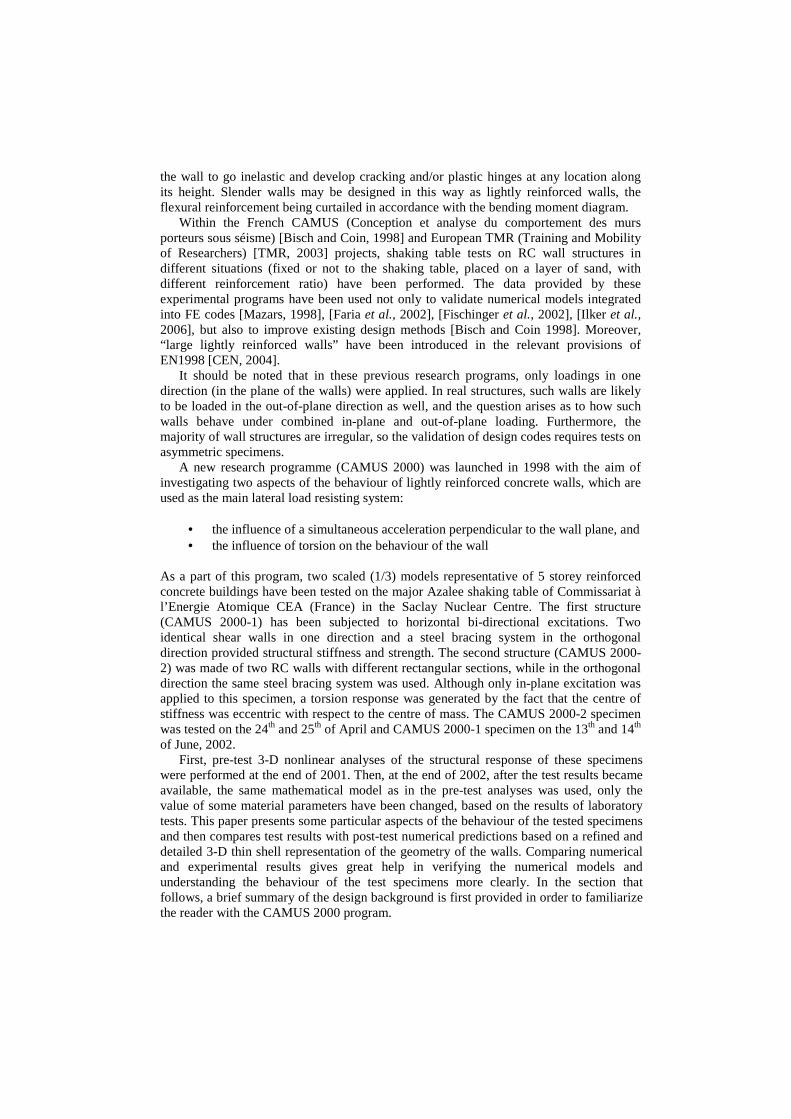
For the definition of the maximum seismic action, due consideration has been given to the specimen’s strength in the perpendicular direction of the walls. As a matter of fact, this strength is that of the composite steel – concrete bracing system in the Y direction, which was defined at the beginning of the previous CAMUS research programs [Bisch and Coin, 1998]. With a PS92 [REGLES, 1995] specified seismic action as defined by the NICE S1 PS92 design spectrum, the specimen has been designed for a peak ground acceleration (PGA) of about 0.51g, corresponding to a ratio α/q (where α is the magnification factor applied to the reference signal and q is the behaviour factor) equal to 0.55. The values of α and q were determined by the energy equivalence method, given the ultimate strains accepted in steel and concrete. The calculated value of α was 2.05, with an associated value of q equal to 3.73 [Bisch and Coin, 2002]. The flexural reinforcement associated to this value of α/q, has been determined considering the existence of possible higher values for the tensile and compressive axial force in each wall, due to the flexure perpendicular to the walls plane. To enforce a predominantly flexural behaviour with nearly horizontal cracking all along the walls height, the flexural reinforcement has been optimised in each quarter of each level. Figure 2 indicates the flexural reinforcement distribution as well as the reinforcement ratio at the base of each storey. Closed stirrups

with 3 mm diameter at 45 mm spacing were placed around the bar layers from the wall base to below the third floor. In the upper part of the structure only open U-shaped stirrups at 45 mm spacing were used. Verification under shear force indicated that the amplified designed shear is less than the design shear strength without reinforcement, so the specimen has no horizontal shear reinforcement. In a real construction, however, a minimum amount of horizontal reinforcement is especially required for exterior (façade) walls, where temperature, shrinkage or other actions, can produce high tensile stresses due to restrains on the imposed deformations.

The specimen is composed of two parallel 5-floor RC walls without openings, linked together by 6 square floors, the reinforced concrete footing being anchored to the shaking table (Figure 2). The walls are each 5.10 m height, 1.70 m long and 6 cm thick. They were cast in order to reproduce the construction joints, just above the middle of each floor. All the floors are 1.70 m long 1.70 m wide and 21 cm thick. The wall footing is 2.10 m wide, 0.60 m high and 10 cm thick. Additional mass was added to the upper and lower part of each floor (excepting the first floor) as well as on the walls at mid-height of each level, to simulate the gravity load compatible with the vertical stress values commonly found at the base of this type of structure, which is about 1.6 MPa. This level is in direct relation with the span between two walls and approximately corresponds to a 6.5 m span in a real construction. For the most part, the additional mass was supported on prefabricated concrete floors that can be removed and reused after test. For this reason, they are not monolithic with the wall, being fixed to the wall by dowels. The steel bracing system stabilising the structure in the direction perpendicular to the walls is shown in (Figure 1). It is designed in such a way that it does not interfere with the in-plane bending behaviour of the walls and only the horizontal load perpendicular to the walls plane is transferred to it. Four steel bars acting in tension and compression connect the lateral bracing system of two different storeys. Each part of the structure, the wall, floor, and basement was cast separately and assembled on the shaking table.

Front view Section 1 - 1

Fig.1. Steel bracing system for CAMUS 2000-1 and CAMUS 2000-2 specimens (Dimensions in centimetres).

X

Y

1 1

X

Y

X

Y

1 1

Side view Front view Reinforcement

Fig. 2. General scheme of the CAMUS 2000-1 specimen (Dimensions in meters).

2.2 Design of the CAMUS 2000-2 Specimen The objective of the CAMUS 2000-2 test has been examination of the influence of general torsion about the vertical axis, which can induce a torsional distortion of the wall, simultaneous to the in-plane movement. Torsional behaviour is created by the fact that the centre of stiffness is eccentric with respect to the centre of mass. This was obtained by decreasing the length of one wall to 1.30 m (instead of 1.70 m) and increasing the length of the other wall to 2.10 m. Additional masses were installed on the small wall to compensate to the deficit of mass on its side and to keep the centre of mass in the middle of the specimen width. Under these conditions, the eccentricity between the centre of stiffness and the centre of mass is about 0.51 m.

As in the case of the previous CAMUS 2000-1 specimen, it was considered as necessary that the general characteristics of the specimen can be deduced from elements, which can be found in a real building. So, again five stories have been considered as representative of the current situation in France, and a scale factor of 1/3 has been chosen.

In the case of CAMUS 2000-2 specimen, it was decided to design the walls so that they have possible lattice behaviour due to the shear force in the first level. Using a simplified tri-dimensional analysis and assuming a simple lattice mode in the smaller wall and a double lattice mode in the other one (as a consequence of a different slenderness and different levels of static compression), a higher value of α/q was selected at 1.41. This led to a value of α equal to 4.53 and a behaviour factor q equal to 3.21. The design made the two walls have different length and very different reinforcement ratio (Figure 3), but very similar ultimate bending moment capacity. Closed stirrups with 3 mm diameter were used at a spacing of 60 mm from the wall base to below the third floor,

while in the upper part of the structure only open U-shaped stirrups at 45 mm spacing were used. The steel bracing system stabilising the structure in the direction perpendicular to the walls was the same as that used in the case of CAMUS 2000-1 specimen (Figure 2). The compressive stresses due to permanent vertical loads are respectively 2.2 MPa and 1.3 MPa, which although quite different, remain within the usual range of stresses in such type of buildings.

Long wall (210 cm x 6 cm) Short wall (130 cm x 6 cm) Fig. 3. General scheme of the CAMUS 2000-2 specimen (Dimensions in centimetres).

3. Seismic Action Both specimens were tested on the AZALEE shaking table, in the CEA facilities, which allows for testing up to 100 ton models under three-directional excitations. The input signals have been derived from the normalized elastic spectrum S1 defined in the French seismic design code [REGLES, 1995]. This spectrum was modified to take into account

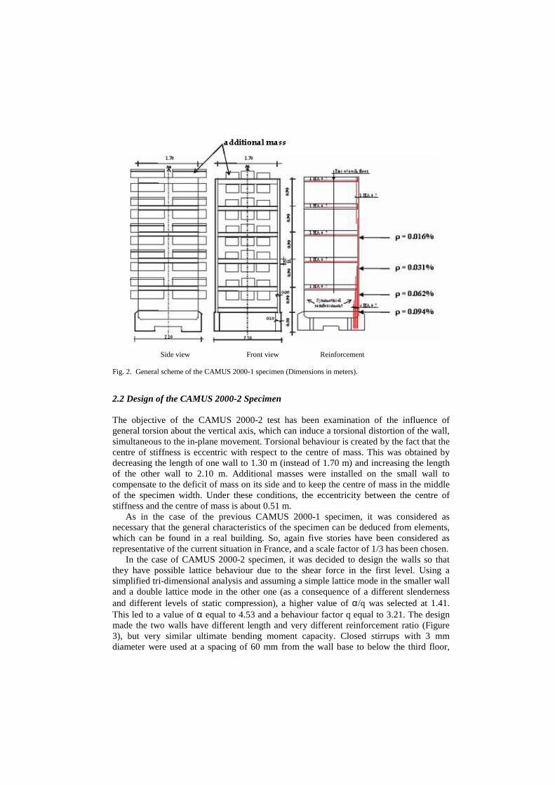
the reduction factor λ on periods and then it was multiplied by the nominal acceleration an = 2.5 m/s2. Finally, two artificial uncorrelated accelerograms (along the directions parallel and perpendicular to the walls plane) were generated so as to match the elastic response spectrum (with 5% viscous damping). Figure 4 shows the artificial accelerograms and the corresponding acceleration response spectra compared with the modified elastic spectrum S1.

The CAMUS 2000-1 specimen was subjected to increasing horizontal artificial accelerations along the directions parallel and perpendicular to the walls plane (Figure 5). The following PGA levels of the uncorrelated input signals were applied during the test in both directions: 0.15g, 0.40g, 0.55g, and 0.65g.

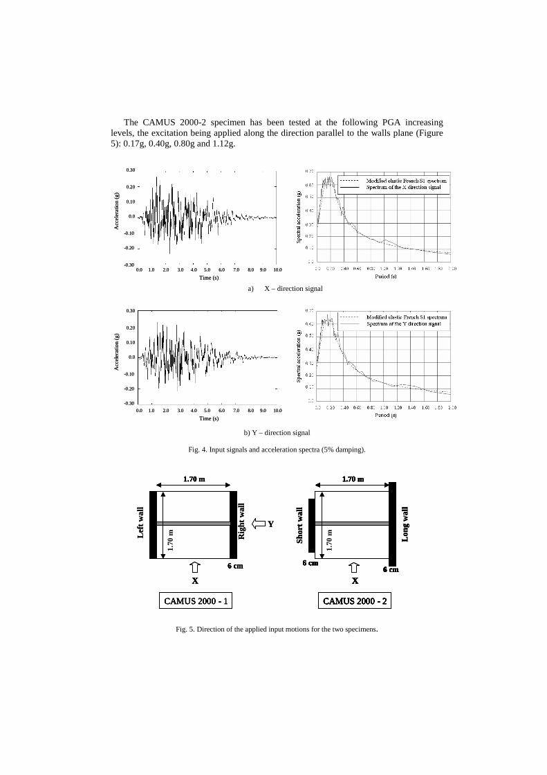
The CAMUS 2000-2 specimen has been tested at the following PGA increasing levels, the excitation being applied along the direction parallel to the walls plane (Figure 5): 0.17g, 0.40g, 0.80g and 1.12g.

a) X – direction signal

b) Y – direction signal

Fig. 4. Input signals and acceleration spectra (5% damping).

Fig. 5. Direction of the applied input motions for the two specimens.

0.30

0.20

0.10

0.0

-0.10

-0.20

-0.300.0 1.0 2.0 3.0 4.0 5.0 6.0 7.0 8.0 9.0 10.0

Acc

ele

ratio

n (g

)

Time (s)

0.30

0.20

0.10

0.0

-0.10

-0.20

-0.300.0 1.0 2.0 3.0 4.0 5.0 6.0 7.0 8.0 9.0 10.0

Acc

ele

ratio

n (g

)

Time (s)

0.30

0.20

0.10

0.0

-0.10

-0.20

-0.30

0.0 1.0 2.0 3.0 4.0 5.0 6.0 7.0 8.0 9.0 10.0

Acc

ele

ratio

n (g

)

Time (s)

0.30

0.20

0.10

0.0

-0.10

-0.20

-0.30

0.0 1.0 2.0 3.0 4.0 5.0 6.0 7.0 8.0 9.0 10.0

Acc

ele

ratio

n (g

)

Time (s)

1.70 m

1.70

m

CAMUS 2000 - 1

6 cm

X

Y

Rig

ht w

all

Lef

tw

all

1.70 m

1.70

m

CAMUS 2000 - 1

6 cm

X

Shor

t w

all

Lon

g w

all

1.70 m

1.70

m

CAMUS 2000 - 2

6 cm6 cm

X

1.70 m

1.70

m

CAMUS 2000 - 2

6 cm6 cm

X

1.70 m

1.70

m

CAMUS 2000 - 1

6 cm

X

Y

Rig

ht w

all

Lef

tw

all

1.70 m

1.70

m

CAMUS 2000 - 1

6 cm

X

Shor

t w

all

Lon

g w

all

1.70 m

1.70

m

CAMUS 2000 - 2

6 cm6 cm

X

1.70 m

1.70

m

CAMUS 2000 - 2

6 cm6 cm

X

Shor

t w

all

Lon

g w

all

1.70 m

1.70

m

CAMUS 2000 - 2

6 cm6 cm

X

1.70 m

1.70

m

CAMUS 2000 - 2

6 cm6 cm

X

1.70 m

1.70

m

CAMUS 2000 - 2

6 cm6 cm

X

1.70 m

1.70

m

CAMUS 2000 - 2

6 cm6 cm

X

4. Instrumentation The instrumentation was conceived to record the motion of the shaking table and the global and local behaviour of the specimens. Sixty four measurement channels were available during each test, but only the most important ones are described in this part. The instrumentation consisted mainly in:

• measurement of the table acceleration in the X, Y and vertical directions. • measurement of the absolute displacements at the different floors relative to a

fixed vertical beam, in the X and Y directions, with displacement sensors (LVDTs). The floor horizontal displacements relative to the wall base were deduced directly from these measurements.

• measurement of the horizontal (in the X and Y directions) and vertical accelerations at different floor levels.

• measurement of the vertical elongation between two floors with 900 mm long vertical transducers.

• measurement of the strain of the reinforcing bars with strain gages fixed on the reinforcement bars at the level of the construction joints.

More detailed information about the instrumentation used for these tests can be found in [Sollogoub and Queval, 2002]. 5. Particular Aspects of the Behaviour of the Specimens 5.1 Axial Force Previous experimental and numerical studies on lightly reinforced walls subjected to in-plane uni-directional loading [Bisch and Coin, 1998], [Ile et al., 2002] have underlined the importance of the variation of the dynamic axial force. A first cause of this phenomenon is the extension mode due to bending: at maximum horizontal deflection, the neutral axis is at its maximum distance from the centre of the wall cross-section, the raising of masses is maximum, and the dynamic variation of the axial force is a tensile force; the frequency of this vertical motion is two times that of the horizontal movement. The second reason of this phenomenon relies on the excitation of the first natural vertical mode of the system: at crack closure, when concrete recovers its stiffness, compression forces strongly increase and these shocks excite the vertical vibration mode of the system (shaking table + specimen). It is to be noted that the variation of the axial force affects the value of the maximum bending moment, as these two parameters act together to determine the ultimate state of strain in the wall. Therefore, axial force variation has to be taken into account in design. In conclusion of the previous CAMUS research [Fouré and Vié, 2002a], the following principle has been proposed in order to introduce the axial force in design:

• In a first phase, the design is made with the static value of the axial force N0 and the corresponding value of the ultimate bending moment Mult. The extreme strains at the section level are εa and εb, where εa stands for the tensile steel strain and εb for the compressive concrete strain. At least one of these two strains represents an ultimate strain corresponding to a limit state of the reinforced

concrete section. For lightly reinforced walls with low axial compression, this limit state generally corresponds to the code specified value εau = 10 x 10-3 .

• In a second phase, the variation ±∆N of the axial force is considered. With the

assumption that the curvature is constant, a new limit state is found, corresponding to M’ult = Mult + ∆M and to the extreme strains εa + ∆εG and εb + ∆εG (∆εG being the neutral axis translation due to the variation of the axial force). If the compressive strain in concrete is excessive ( > 3.5x10-3), either the width of the wall is increased, or the concrete is confined. If the tensile strain in the steel bars is excessive, the reinforcement area has to be increased.

The range of variation in the axial force is difficult to know a priori because it depends

on the vertical response of the structure and mainly on the vertical accelerations. However, until further information from extensive parametric studies is available, the following formula for estimating the axial force variation has been proposed and accepted in the relevant provisions of EN1998 [CEN, 2004]:

∆Nmax = ± λN0, (1) where λ depends on the soil type and on the ratio TA/0.5TF, TA being the horizontal vibration period and TF the vertical vibration period of the structure.

Since the CAMUS 2000-1 specimen is subjected to bi-directional loading, the overturning moment perpendicular to the walls induces a compression axial force in one wall and a tensile axial force in the other. The total axial force variation in each wall is then given by the superposition of the dynamic axial force due to the in-plane bending and of the axial force due to the out-of-plane loading. Based on previous experimental results on lightly reinforced walls, and taking into account the uncertainty of the dynamic axial force variation, design has assumed λ = 0.8. According to the two design combinations rules, Sx + 0.3Sy and Sy + 0.3Sx (where Sx and Sy are action effects), the maximum axial force (Nr) due to the out-of-plane loading in each wall has been calculated. Its design value is equal to ±198 KN. The total variation of the axial force in each wall is then given by: ∆Nmax = ± λN0 ± Nr = ± 343 KN (N0 = 180.7 KN) (2) This large variation (almost double the permanent load) indicates that different states of cracking from one wall to another are to be expected, leading to different lengthening of their neutral axes and asymmetric behaviour of the specimen.

In the case of the CAMUS 2000-2 specimen, because of the difference in length between the two walls, the change in the position of the neutral axis due to cracking makes different vertical uplift of the two walls (for the same horizontal displacement). This induces a state of deformation perpendicular to the walls plane corresponding to general flexure in this direction, which excites the corresponding eigenmode. It itself creates a complementary axial force variation due to the global overturning moment. So, again, the total axial force variation in each wall is given by the superposition of the dynamic axial force due to the in-plane bending and of the axial force due to the out-of-plane loading.

5.2 Torsional Stiffness of the Floors Due to the asymmetric behaviour of the walls in both experiments, at each level of the construction the rotations of the wall sections are not the same and rotation of the floors about a vertical axis is involved in the behaviour. At each level, the floors are then able to transfer a bending moment, from one wall to the other. It is to be noted, however, that the thickness of the floors (21cm) was determined in order to provide the necessary floor strength under additional masses. This value is much higher than in real construction. Since the usual thickness of floors is about 18 cm in a normal building, taking into account a scale factor of 3, the thickness of the specimens’ floors should have been 6 cm. Hence, the stiffness of the floors is much higher in the specimen than in a normal situation, and the twist rotation is then expected to be much lower in the tests than in the case of a normal building.

It is clear that axial force effects as well as redistribution of forces due to the evolution of stiffness of the walls are completely nonlinear and cannot be adequately represented in a standard linear elastic model. One aim of the nonlinear time history analysis was to verify these design assumptions and to obtain more detailed information about the behaviour of the specimen. 6. Modelling Approach The numerical analyses have been performed using the general-purpose finite element program CASTEM 2000 developed at CEA-Saclay, France [Millard, 1993]. To predict the inelastic seismic response with sufficient accuracy, due care has been given to create detailed models of the two specimens, taking into account the necessary geometric characteristics, construction details, and boundary conditions. An example of the 3-D finite element meshes used in the analyses is reported in Figure 6. Since in-plane as well as out-of-plane behaviour of the walls need to be analysed, layered thin shell discrete Kirchoff triangles (DKT) are used to represent the two walls and the slabs. The shaking table is modelled with solid eight-node brick elements, while four-node shell elements are used to model the steel I-shaped bracing system. Discrete modelling is adopted to represent the reinforcement through the use of two-node truss-bar elements. The structure is assumed fully restrained at all nodes along the base of the shear wall. During previous tests on CAMUS specimens [Sollogoub et al., 2000], it was observed that the specimen oscillation have induced vertical and rocking displacements on the shaking table, leading to significant reductions of the corresponding natural frequencies. In these conditions, the shaking table itself (in terms of mass) and their external supports (in terms of stiffness) had to be included into the numerical model. Owing to its high stiffness, the finite elements representing the shaking-table base were assumed to remain elastic and almost infinitely rigid. The total mass of the shaking-table (25 000 kg) was uniformly distributed to these finite elements. The vertical rods supporting the shaking-table were simulated with four elastic vertical bars, the axial stiffness of each bar being equal to 215 MN/m, as suggested by experimenters [Combescure, 2002]. Perfect bond was assumed to exist between concrete and reinforcement. Therefore, nodes of bar and concrete coincide, without interface elements. The possibility of non-linear material behaviour was specified for all wall concrete and reinforcing bar-elements, while the behaviour of the foundation and bracing system was considered as elastic. Assuming a 2.5% critical damping factor (close to the measured damping value) for the first and second vibration modes, the

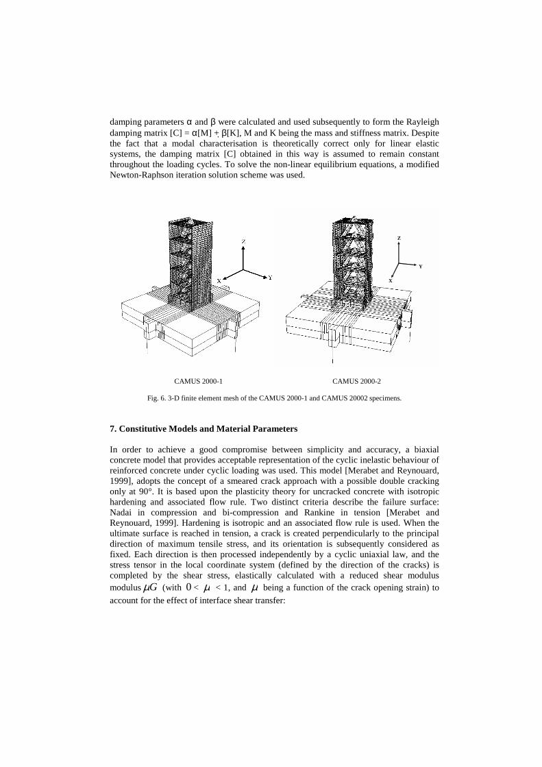
damping parameters α and β were calculated and used subsequently to form the Rayleigh damping matrix [C] = α[M] + β[K], M and K being the mass and stiffness matrix. Despite the fact that a modal characterisation is theoretically correct only for linear elastic systems, the damping matrix [C] obtained in this way is assumed to remain constant throughout the loading cycles. To solve the non-linear equilibrium equations, a modified Newton-Raphson iteration solution scheme was used.

CAMUS 2000-1 CAMUS 2000-2

Fig. 6. 3-D finite element mesh of the CAMUS 2000-1 and CAMUS 20002 specimens. 7. Constitutive Models and Material Parameters In order to achieve a good compromise between simplicity and accuracy, a biaxial concrete model that provides acceptable representation of the cyclic inelastic behaviour of reinforced concrete under cyclic loading was used. This model [Merabet and Reynouard, 1999], adopts the concept of a smeared crack approach with a possible double cracking only at 90°. It is based upon the plasticity theory for uncracked concrete with isotropic hardening and associated flow rule. Two distinct criteria describe the failure surface: Nadai in compression and bi-compression and Rankine in tension [Merabet and Reynouard, 1999]. Hardening is isotropic and an associated flow rule is used. When the ultimate surface is reached in tension, a crack is created perpendicularly to the principal direction of maximum tensile stress, and its orientation is subsequently considered as fixed. Each direction is then processed independently by a cyclic uniaxial law, and the stress tensor in the local coordinate system (defined by the direction of the cracks) is completed by the shear stress, elastically calculated with a reduced shear modulus modulus Gµ (with 0 < µ < 1, and µ being a function of the crack opening strain) to

account for the effect of interface shear transfer:

X

Y

Z

X

Y

Z

µ = 0.4 ……………………..if εcr- εres- εtm ≤ 2 εtm

µ = 0 ……………………….if εcr- εres- εtm ≥ 2 εtm

µ = 0 and σ12 = 0…………...if εcr- εres- εtm ≥ 4 εtm

where:

εcr - total strain εres - residual strain after unloading in compression εtm - crack opening strain σ12 – shear stress

The behaviour of a point initially under tension, which completely cracks prior to

undergoing a reverse loading in compression, is illustrated in Figure 7. Similar laws describe the case of an initial compressed point or that of a point, which has not totally cracked under a reverse loading. The model has been described in detail and verified elsewhere [Ile and Reynouard, 2000], [Ile et al., 2002]. Its validity has been demonstrated by using it to predict the behaviour of shear walls with different span-to-height ratio under monotonic, cyclic and dynamic loading conditions for which experimental observation was available.

10

E

f t

E0

εcm

2

9

45

1STRAIN

STRESSfc

-fc

E2

-ft

PF

11

12

1εtm

7

8

E3

6 3

1 - Elastic tension2 - Crack opening3, 8 Crack closing4 - Nonlinear compression5, 11 - Damaged unloading, E2 ≠ E0

6 - Damaged unloading. Modulus = E1

7 - Reopening of crack9 - Reloading: Linear compression10 - Softening behaviour in compression12 - Elastic tension with resistance f’c < ft

Fig. 7. Uniaxial model: point initially in tension.

For steel, a cyclic model that can take into account the Bauschinger effect and buckling of reinforcing bars has been adopted (Figure 8). The monotonic backbone curve is characterised by an initial linear branch followed by a plateau and hardening up to failure. The cyclic behaviour is described by the formulation proposed by Giuffré and Pinto and implemented by Menegoto and Pinto [1973]. For ratio between the length L and

the diameter D of the steel bar less or equal to 5, the compression curve is similar to the tensile one and no buckling effect is observed. For L/D ratios greater than 5, modifications are introduced in the model and the inelastic buckling effect is accounted for (Figure 8b). A detailed description of the steel constitutive law can be found in [Guedes et al., 1994]. a) cyclic behaviour without buckling b) cyclic behaviour with buckling

Fig. 8. Numerical model for steel under cyclic loading.

The concrete for the specimens is a C20 microconcrete. The concrete characteristics were checked by the usual compressive and splitting tests on 160 mm diameter cylinders prior to the testing program. They exhibited an unexpected compressive over strength. The compressive strength, tensile strength and modulus of elasticity were found from the average of test results [Fouré and Vié, 2002b] to be 34 MPa, 2.7 MPa and 25 000 MPa, respectively. These values were used in the analytical computations. Based on other simulation studies on the seismic behaviour of lightly reinforced walls [Ile et al., 2002], an initial value of 0.4 for the post-cracking parameter µ was assumed in the analysis. No

confinement effect of the stirrups on the compression strength has been considered, due to the very low percentage of transverse steel reinforcement.

The finite element model and the assigned non-linear material properties can be improved by modelling the bond-slip interaction between the steel bars and concrete through the use of special contact elements, interposed between steel and concrete elements. If such elements are used in conjunction with the smeared modelling of cracks, they can only reflect the trend of the variation of steel and concrete stresses along the bar, to which such contact elements are connected. Local variation between cracks is unaccounted for, since location of individual cracks cannot be accurately predicted by the smeared crack model. Moreover, for smeared cracking it is computationally more efficient to assume perfect bond between steel and concrete and account implicitly for the effect on bond-slip on the average stresses and strains in concrete, through appropriate modification of the properties of concrete. This later approach was adopted in this study. So, tension stiffening was superimposed to the tension softening following a simple approach proposed by Feenstra and de Borst [1995]. The descending branch of the concrete tensile

E

b x E

σσσσ

εεεε

σσσσ = f(εεεε)

Er

εεεε0εεεε5

γγγγsbc x E

ξξξξ0000.... (ε(ε(ε(ε0000−−−−εεεερρρρ))))2222

ξξξξ1111.... (ε(ε(ε(ε0000−−−−εεεερρρρ ))))1111

((((εεεεr ,,,, σσσσr))))1111

(ε(ε(ε(ε0 0 0 0 ,,,, σσσσ0))))1111((((εεεεr ,,,, σσσσr))))0000((((εεεεr ,,,, σσσσr))))2222

(ε(ε(ε(ε0 0 0 0 ,,,, σσσσ0))))2222

(ε(ε(ε(ε0 ,,,, σσσσ0))))0000

E0 E0

Eh

Eh

σσσσ

εεεε

R(ξξξξ1111 ))))

R(ξξξξ2 ))))σσσσ = f(εεεε)

ξξξξ0000.... (ε(ε(ε(ε0000−−−−εεεερρρρ))))2222

ξξξξ1111.... (ε(ε(ε(ε0000−−−−εεεερρρρ ))))1111

((((εεεεr ,,,, σσσσr))))1111

(ε(ε(ε(ε0 0 0 0 ,,,, σσσσ0))))1111((((εεεεr ,,,, σσσσr))))0000((((εεεεr ,,,, σσσσr))))2222

(ε(ε(ε(ε0 0 0 0 ,,,, σσσσ0))))2222

(ε(ε(ε(ε0 ,,,, σσσσ0))))0000

E0 E0

Eh

Eh

σσσσ

εεεε

R(ξξξξ1111 ))))

R(ξξξξ2 ))))σσσσ = f(εεεε)

E

b x E

σσσσ

εεεε

σσσσ = f(εεεε)σσσσ = f(εεεε)

Er

εεεε0εεεε5

γγγγsbc x E

E

b x E

σσσσ

εεεε

σσσσ = f(εεεε)σσσσ = f(εεεε)

Er

εεεε0εεεε5

γγγγsbc x E

ξξξξ0000.... (ε(ε(ε(ε0000−−−−εεεερρρρ))))2222

ξξξξ1111.... (ε(ε(ε(ε0000−−−−εεεερρρρ ))))1111

((((εεεεr ,,,, σσσσr))))1111

(ε(ε(ε(ε0 0 0 0 ,,,, σσσσ0))))1111((((εεεεr ,,,, σσσσr))))0000((((εεεεr ,,,, σσσσr))))2222

(ε(ε(ε(ε0 0 0 0 ,,,, σσσσ0))))2222

(ε(ε(ε(ε0 ,,,, σσσσ0))))0000

E0 E0

Eh

Eh

σσσσ

εεεε

R(ξξξξ1111 ))))

R(ξξξξ2 ))))σσσσ = f(εεεε)

ξξξξ0000.... (ε(ε(ε(ε0000−−−−εεεερρρρ))))2222

ξξξξ1111.... (ε(ε(ε(ε0000−−−−εεεερρρρ ))))1111

((((εεεεr ,,,, σσσσr))))1111

(ε(ε(ε(ε0 0 0 0 ,,,, σσσσ0))))1111((((εεεεr ,,,, σσσσr))))0000((((εεεεr ,,,, σσσσr))))2222

(ε(ε(ε(ε0 0 0 0 ,,,, σσσσ0))))2222

(ε(ε(ε(ε0 ,,,, σσσσ0))))0000

E0 E0

Eh

Eh

σσσσ

εεεε

R(ξξξξ1111 ))))

R(ξξξξ2 ))))σσσσ = f(εεεε)

ξξξξ0000.... (ε(ε(ε(ε0000−−−−εεεερρρρ))))2222

ξξξξ1111.... (ε(ε(ε(ε0000−−−−εεεερρρρ ))))1111

((((εεεεr ,,,, σσσσr))))1111

(ε(ε(ε(ε0 0 0 0 ,,,, σσσσ0))))1111((((εεεεr ,,,, σσσσr))))0000((((εεεεr ,,,, σσσσr))))2222

(ε(ε(ε(ε0 0 0 0 ,,,, σσσσ0))))2222

(ε(ε(ε(ε0 ,,,, σσσσ0))))0000

E0 E0

Eh

Eh

σσσσ

εεεε

R(ξξξξ1111 ))))

R(ξξξξ2 ))))σσσσ = f(εεεε)

ξξξξ0000.... (ε(ε(ε(ε0000−−−−εεεερρρρ))))2222

ξξξξ1111.... (ε(ε(ε(ε0000−−−−εεεερρρρ ))))1111

((((εεεεr ,,,, σσσσr))))1111

(ε(ε(ε(ε0 0 0 0 ,,,, σσσσ0))))1111((((εεεεr ,,,, σσσσr))))0000((((εεεεr ,,,, σσσσr))))2222

(ε(ε(ε(ε0 0 0 0 ,,,, σσσσ0))))2222

(ε(ε(ε(ε0 ,,,, σσσσ0))))0000

E0 E0

Eh

Eh

σσσσ

εεεε

R(ξξξξ1111 ))))

R(ξξξξ2 ))))σσσσ = f(εεεε)

ξξξξ0000.... (ε(ε(ε(ε0000−−−−εεεερρρρ))))2222

ξξξξ1111.... (ε(ε(ε(ε0000−−−−εεεερρρρ ))))1111

((((εεεεr ,,,, σσσσr))))1111

(ε(ε(ε(ε0 0 0 0 ,,,, σσσσ0))))1111((((εεεεr ,,,, σσσσr))))0000((((εεεεr ,,,, σσσσr))))2222

(ε(ε(ε(ε0 0 0 0 ,,,, σσσσ0))))2222

(ε(ε(ε(ε0 ,,,, σσσσ0))))0000

E0 E0

Eh

Eh

σσσσ

εεεε

R(ξξξξ1111 ))))

R(ξξξξ2 ))))σσσσ = f(εεεε)

ξξξξ0000.... (ε(ε(ε(ε0000−−−−εεεερρρρ))))2222

ξξξξ1111.... (ε(ε(ε(ε0000−−−−εεεερρρρ ))))1111

((((εεεεr ,,,, σσσσr))))1111

(ε(ε(ε(ε0 0 0 0 ,,,, σσσσ0))))1111((((εεεεr ,,,, σσσσr))))0000((((εεεεr ,,,, σσσσr))))2222

(ε(ε(ε(ε0 0 0 0 ,,,, σσσσ0))))2222

(ε(ε(ε(ε0 ,,,, σσσσ0))))0000

E0 E0

Eh

Eh

σσσσ

εεεε

R(ξξξξ1111 ))))

R(ξξξξ2 ))))σσσσ = f(εεεε)

E

b x E

σσσσ

εεεε

σσσσ = f(εεεε)σσσσ = f(εεεε)

Er

εεεε0εεεε5

γγγγsbc x E

σσσσ = f(εεεε)σσσσ = f(εεεε)

Er

εεεε0εεεε5

γγγγsbc x E

stress-strain behaviour was approximated by a straight-line function, the corresponding

ultimate compressive straintmε being equal to 1.5 x 10-3.

The nominal steel yield stress used in designing the walls was 500 MPa. Actual yielding stresses are given in Table 1 along with other data measured from tests on the bars [Fouré and Vié, 2002b]. It can be observed that the 4.5 mm diameter bar has unexpected high yielding stress and very low ductility. For this, the bond between steel and reinforcement is insured by very small variations of steel diameter, while the remaining bars are ribbed high bond bars. It is to be noted here that small diameter bars had to be used in the scaled model. For these bars, it was not possible in the production process to obtain higher ductility than that indicated in Table 1.

Table 1. Steel properties

Diameter φ (mm)

Type Yield stress fy

Failure stress fr

Strain at fr εgt

4.5 With diameter variation

664 MPa 733 MPa 2.2%

8 High bond 563 MPa 617 MPa 3.8% 10 High bond 562 MPa 629 MPa 8.7%

To represent the material property of the three different reinforcing bars, the measured

value of the yield stress, failure stress and strain at failure was directly used. To describe the cyclic behaviour of the reinforcing steel in compression, L/D ratio was set equal to 13. 8. Comparison with Experimental Results The comparison of the numerical time history results with the experimental records is one important step in confirming the accuracy of the modelling approach. Numerical results also allow to verify design assumptions and to extend the limited experimental database of seismic wall behaviour with analytical data. The experimental bending moments, shear forces and axial forces have been computed with the absolute accelerations given by the accelerometers and the estimation of the masses of each floor. Due to the fact that the structure is highly hyperstatic the experimental internal forces in each wall were difficult to estimate. Based on the assumption that the RC floors can transfer only torsion and no bending (due to the high out-of-plane flexibility in bending of the walls), the measurement channels used during the test allowed determining with sufficient accuracy only horizontal (shear) and normal (axial) forces in each wall, [Combescure et al., 2002]. The experiment could also indicate the total bending moment at different levels for the whole specimen, but the values of the bending moment in each wall, which are important, were however not measured. Since the numerical model can indicate individual bending moment at specified locations in each wall, its usefulness in investigating the wall behaviour is obvious. In the numerical analysis, all the seismic signals applied to the specimens were considered in chronological order.

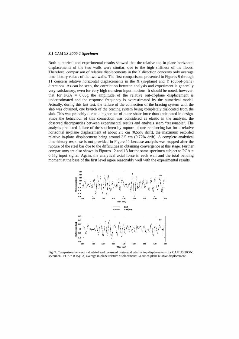
8.1 CAMUS 2000-1 Specimen Both numerical and experimental results showed that the relative top in-plane horizontal displacements of the two walls were similar, due to the high stiffness of the floors. Therefore, comparison of relative displacements in the X direction concerns only average time history values of the two walls. The first comparisons presented in Figures 9 through 11 concern relative horizontal displacements in the X (in-plane) and Y (out-of-plane) directions. As can be seen, the correlation between analysis and experiment is generally very satisfactory, even for very high transient input motions. It should be noted, however, that for PGA = 0.65g the amplitude of the relative out-of-plane displacement is underestimated and the response frequency is overestimated by the numerical model. Actually, during this last test, the failure of the connection of the bracing system with the slab was obtained, one branch of the bracing system being completely dislocated from the slab. This was probably due to a higher out-of-plane shear force than anticipated in design. Since the behaviour of this connection was considered as elastic in the analysis, the observed discrepancies between experimental results and analysis seem “reasonable”. The analysis predicted failure of the specimen by rupture of one reinforcing bar for a relative horizontal in-plane displacement of about 2.5 cm (0.55% drift), the maximum recorded relative in-plane displacement being around 3.5 cm (0.77% drift). A complete analytical time-history response is not provided in Figure 11 because analysis was stopped after the rupture of the steel bar due to the difficulties in obtaining convergence at this stage. Further comparisons are also shown in Figures 12 and 13 for the same specimen subject to PGA = 0.55g input signal. Again, the analytical axial force in each wall and the total bending moment at the base of the first level agree reasonably well with the experimental results. Fig. 9. Comparison between calculated and measured horizontal relative top displacements for CAMUS 2000-1 specimen - PGA = 0.15g: A) average in-plane relative displacement; B) out-of-plane relative displacement.

2.50 3.00 3.50 4.00 4.50 5.00 5.50 6.00 6.50

0.40

0.30

0.20

0.10

0.0

-0.10

-0.20

-0.30

-0.40

Time (sec.)

Dis

plac

emen

t (cm

)

A)

2.50 3.00 3.50 4.00 4.50 5.00 5.50 6.00 6.50

0.60

0.40

0.20

0.0

-0.20

-0.40

-0.60

Time (sec.)

Dis

plac

emen

t (cm

)

B)

TestAnalysis

2.50 3.00 3.50 4.00 4.50 5.00 5.50 6.00 6.50

0.40

0.30

0.20

0.10

0.0

-0.10

-0.20

-0.30

-0.40

Time (sec.)

Dis

plac

emen

t (cm

)

A)

2.50 3.00 3.50 4.00 4.50 5.00 5.50 6.00 6.50

0.40

0.30

0.20

0.10

0.0

-0.10

-0.20

-0.30

-0.40

Time (sec.)

Dis

plac

emen

t (cm

)

A)

2.50 3.00 3.50 4.00 4.50 5.00 5.50 6.00 6.50

0.60

0.40

0.20

0.0

-0.20

-0.40

-0.60

Time (sec.)

Dis

plac

emen

t (cm

)

B)

2.50 3.00 3.50 4.00 4.50 5.00 5.50 6.00 6.50

0.60

0.40

0.20

0.0

-0.20

-0.40

-0.60

Time (sec.)

Dis

plac

emen

t (cm

)

B)

TestAnalysisTestAnalysis

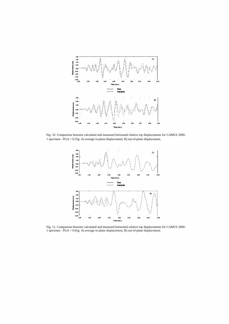
Fig. 10. Comparison between calculated and measured horizontal relative top displacements for CAMUS 2000-1 specimen - PGA = 0.55g: A) average in-plane displacement; B) out-of-plane displacement. Fig. 11. Comparison between calculated and measured horizontal relative top displacements for CAMUS 2000-1 specimen - PGA = 0.65g: A) average in-plane displacement; B) out-of-plane displacement.

TestAnalysis

Time (sec.)

2.00 2.50 3.00 3.50 4.00 4.50 5.00 5.50 6.00 6.50

2.00

1.00

0.50

-0.50

-1.00

-2.00

Dis

pla c

emen

t(c m

)

0.00

-1.50

1.50

A)

2.00 2.50 3.00 3.50 4.00 4.50 5.00 5.50 6.00 6.50

3.00

2.00

1.00

-1.00

-2.00

-3.00

Dis

plac

emen

t(cm

)

0.00

Time (sec.)

B)

TestAnalysisTestAnalysis

Time (sec.)

2.00 2.50 3.00 3.50 4.00 4.50 5.00 5.50 6.00 6.50

2.00

1.00

0.50

-0.50

-1.00

-2.00

Dis

pla c

emen

t(c m

)

0.00

-1.50

1.50

A)

Time (sec.)

2.00 2.50 3.00 3.50 4.00 4.50 5.00 5.50 6.00 6.50

2.00

1.00

0.50

-0.50

-1.00

-2.00

Dis

pla c

emen

t(c m

)

0.00

-1.50

1.50

A)

2.00 2.50 3.00 3.50 4.00 4.50 5.00 5.50 6.00 6.50

3.00

2.00

1.00

-1.00

-2.00

-3.00

Dis

plac

emen

t(cm

)

0.00

Time (sec.)

B)

2.00 2.50 3.00 3.50 4.00 4.50 5.00 5.50 6.00 6.50

3.00

2.00

1.00

-1.00

-2.00

-3.00

Dis

plac

emen

t(cm

)

0.00

Time (sec.)

B)

TestAnalysis

Time (sec.)

1.00 1.50 2.00 2.50 3.00 3.50 4.00 4.50 5.00

4.00

3.00

1.00

-1.00

-2.00

-3.00

Dis

pla c

emen

t(c

m)

0.00

2.00

A)

3.00

2.00

1.00

-1.00

-3.00

-4.00

Dis

plac

emen

t(cm

)

0.00

Time (sec.)

1.00 1.50 2.00 2.50 3.00 3.50 4.00 4.50 5.00

-2.00

B)

TestAnalysisTestAnalysis

Time (sec.)

1.00 1.50 2.00 2.50 3.00 3.50 4.00 4.50 5.00

4.00

3.00

1.00

-1.00

-2.00

-3.00

Dis

pla c

emen

t(c

m)

0.00

2.00

A)

Time (sec.)

1.00 1.50 2.00 2.50 3.00 3.50 4.00 4.50 5.00

4.00

3.00

1.00

-1.00

-2.00

-3.00

Dis

pla c

emen

t(c

m)

0.00

2.00

A)

3.00

2.00

1.00

-1.00

-3.00

-4.00

Dis

plac

emen

t(cm

)

0.00

Time (sec.)

1.00 1.50 2.00 2.50 3.00 3.50 4.00 4.50 5.00

-2.00

B)3.00

2.00

1.00

-1.00

-3.00

-4.00

Dis

plac

emen

t(cm

)

0.00

Time (sec.)

1.00 1.50 2.00 2.50 3.00 3.50 4.00 4.50 5.00

-2.00

B)

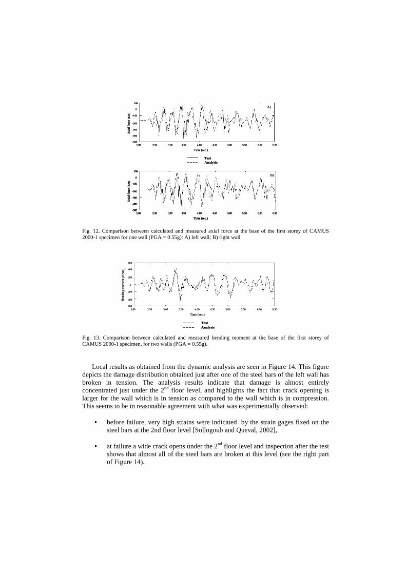
Fig. 12. Comparison between calculated and measured axial force at the base of the first storey of CAMUS 2000-1 specimen for one wall (PGA = 0.55g): A) left wall; B) right wall.

Fig. 13. Comparison between calculated and measured bending moment at the base of the first storey of CAMUS 2000-1 specimen, for two walls (PGA = 0.55g).

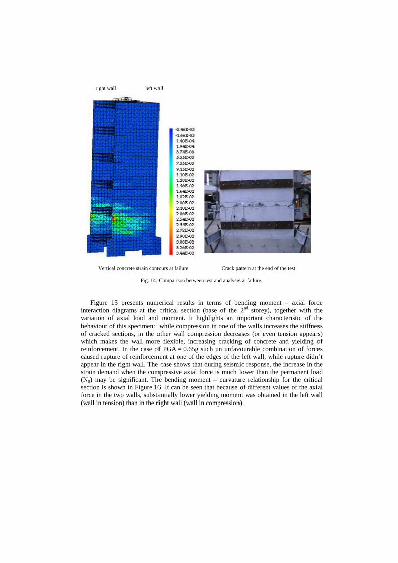
Local results as obtained from the dynamic analysis are seen in Figure 14. This figure

depicts the damage distribution obtained just after one of the steel bars of the left wall has broken in tension. The analysis results indicate that damage is almost entirely concentrated just under the 2nd floor level, and highlights the fact that crack opening is larger for the wall which is in tension as compared to the wall which is in compression. This seems to be in reasonable agreement with what was experimentally observed:

• before failure, very high strains were indicated by the strain gages fixed on the steel bars at the 2nd floor level [Sollogoub and Queval, 2002],

• at failure a wide crack opens under the 2nd floor level and inspection after the test

shows that almost all of the steel bars are broken at this level (see the right part of Figure 14).

TestAnalysis

Time (sec.)

2.00 2.50 3.00 3.50 4.00 4.50 5.00 5.50 6.00 6.50

100

0

-200

-300

-500

Axi

al f

orce

(K

N)

-400

-100

A)

Time (sec.)

2.00 2.50 3.00 3.50 4.00 4.50 5.00 5.50 6.00 6.50

100

0

-200

-300

-500

Axi

al fo

rce

( KN

)

-400

-100

B)

TestAnalysis

Time (sec.)

2.00 2.50 3.00 3.50 4.00 4.50 5.00 5.50 6.00 6.50

100

0

-200

-300

-500

Axi

al f

orce

(K

N)

-400

-100

A)

Time (sec.)

2.00 2.50 3.00 3.50 4.00 4.50 5.00 5.50 6.00 6.50

100

0

-200

-300

-500

Axi

al f

orce

(K

N)

-400

-100

A)

Time (sec.)

2.00 2.50 3.00 3.50 4.00 4.50 5.00 5.50 6.00 6.50

100

0

-200

-300

-500

Axi

al fo

rce

( KN

)

-400

-100

B)

Time (sec.)

2.00 2.50 3.00 3.50 4.00 4.50 5.00 5.50 6.00 6.50

100

0

-200

-300

-500

Axi

al fo

rce

( KN

)

-400

-100

B)

Time (sec.)

2.00 2.50 3.00 3.50 4.00 4.50 5.00 5.50 6.00 6.50

100

0

-200

-300

-500

Axi

al fo

rce

( KN

)

-400

-100

B)

TestAnalysis

Time (sec.)

2.00 2.50 3.00 3.50 4.00 4.50 5.00 5.50 6.00 6.50

600

400

200

400Be n

ding

mom

ent (

KN

m)

600

200

0

TestAnalysis

Time (sec.)

2.00 2.50 3.00 3.50 4.00 4.50 5.00 5.50 6.00 6.50

600

400

200

400Be n

ding

mom

ent (

KN

m)

600

200

0

right wall left wall

Vertical concrete strain contours at failure Crack pattern at the end of the test

Fig. 14. Comparison between test and analysis at failure.

Figure 15 presents numerical results in terms of bending moment – axial force

interaction diagrams at the critical section (base of the 2nd storey), together with the variation of axial load and moment. It highlights an important characteristic of the behaviour of this specimen: while compression in one of the walls increases the stiffness of cracked sections, in the other wall compression decreases (or even tension appears) which makes the wall more flexible, increasing cracking of concrete and yielding of reinforcement. In the case of PGA = 0.65g such un unfavourable combination of forces caused rupture of reinforcement at one of the edges of the left wall, while rupture didn’t appear in the right wall. The case shows that during seismic response, the increase in the strain demand when the compressive axial force is much lower than the permanent load (N0) may be significant. The bending moment – curvature relationship for the critical section is shown in Figure 16. It can be seen that because of different values of the axial force in the two walls, substantially lower yielding moment was obtained in the left wall (wall in tension) than in the right wall (wall in compression).

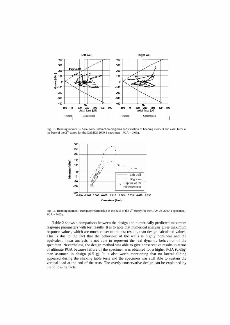
Fig. 15. Bending moment – Axial force interaction diagrams and variation of bending moment and axial force at the base of the 2nd storey for the CAMUS 2000-1 specimen - PGA = 0.65g.

Fig. 16. Bending moment–curvature relationship at the base of the 2nd storey for the CAMUS 2000-1 specimen -PGA = 0.65g.

Table 2 shows a comparison between the design and numerically predicted maximum response parameters with test results. It is to note that numerical analysis gives maximum response values, which are much closer to the test results, than design calculated values. This is due to the fact that the behaviour of the walls is highly nonlinear and the equivalent linear analysis is not able to represent the real dynamic behaviour of the specimen. Nevertheless, the design method was able to give conservative results in terms of ultimate PGA because failure of the specimen was obtained for a higher PGA (0.65g) than assumed in design (0.51g). It is also worth mentioning that no lateral sliding appeared during the shaking table tests and the specimen was still able to sustain the vertical load at the end of the tests. The overly conservative design can be explained by the following facts:

-400

-300

-200

-100

0

100

200

300

400

-100 0 100 200 300 400 500Axial force [kN]

Mom

ent

[kN

m]

Left wall

N0-400

-300

-200

-100

0

100

200

300

400

-100 0 100 200 300 400 500Axial force [kN]

N0

rupture

-400

-300

-200

-100

0

100

200

300

400

-100 0 100 200 300 400 500kN]

]Right wall

N0-400

-300

-200

-100

0

100

200

300

400

-100 0 100 200 300 400 500kN]

N0

Traction Traction CompressionCompression

-400

-300

-200

-100

0

100

200

300

400

-100 0 100 200 300 400 500Axial force [kN]

Mom

ent

[kN

m]

Left wall

N0-400

-300

-200

-100

0

100

200

300

400

-100 0 100 200 300 400 500Axial force [kN]

N0

rupture

-400

-300

-200

-100

0

100

200

300

400

-100 0 100 200 300 400 500kN]

]Right wall

N0-400

-300

-200

-100

0

100

200

300

400

-100 0 100 200 300 400 500kN]

N0

Traction Traction CompressionCompression

-0.010 -0.005 0.000 0.005 0.010 0.015 0.020 0.025 0.030

Curvature (1/m)

300

250

200

150

100

50

0

-50

-100

-150

Mom

ent

(kN

m)

x

-0.010 -0.005 0.000 0.005 0.010 0.015 0.020 0.025 0.030

300

250

200

150

100

50

0

-50

-100

-150

x

Left wall

Right wallRupture of thereinforcement

x

-0.010 -0.005 0.000 0.005 0.010 0.015 0.020 0.025 0.030

Curvature (1/m)

300

250

200

150

100

50

0

-50

-100

-150

Mom

ent

(kN

m)

x

-0.010 -0.005 0.000 0.005 0.010 0.015 0.020 0.025 0.030

300

250

200

150

100

50

0

-50

-100

-150

x

Left wall

Right wallRupture of thereinforcement

x

Left wall

Right wallRupture of thereinforcement

x

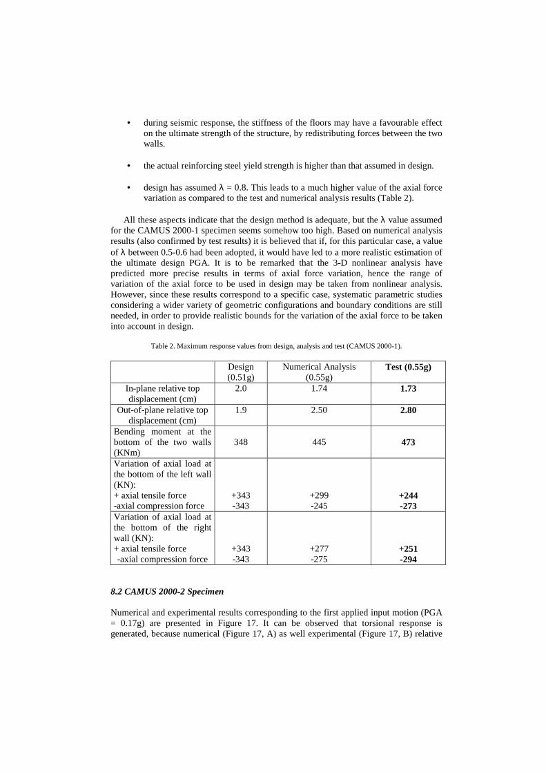
• during seismic response, the stiffness of the floors may have a favourable effect on the ultimate strength of the structure, by redistributing forces between the two walls.

• the actual reinforcing steel yield strength is higher than that assumed in design.

• design has assumed λ = 0.8. This leads to a much higher value of the axial force

variation as compared to the test and numerical analysis results (Table 2).

All these aspects indicate that the design method is adequate, but the λ value assumed for the CAMUS 2000-1 specimen seems somehow too high. Based on numerical analysis results (also confirmed by test results) it is believed that if, for this particular case, a value of λ between 0.5-0.6 had been adopted, it would have led to a more realistic estimation of the ultimate design PGA. It is to be remarked that the 3-D nonlinear analysis have predicted more precise results in terms of axial force variation, hence the range of variation of the axial force to be used in design may be taken from nonlinear analysis. However, since these results correspond to a specific case, systematic parametric studies considering a wider variety of geometric configurations and boundary conditions are still needed, in order to provide realistic bounds for the variation of the axial force to be taken into account in design.

Table 2. Maximum response values from design, analysis and test (CAMUS 2000-1).

Design (0.51g)

Numerical Analysis (0.55g)

Test (0.55g)

In-plane relative top displacement (cm)

2.0 1.74 1.73

Out-of-plane relative top displacement (cm)

1.9 2.50 2.80

Bending moment at the bottom of the two walls (KNm)

348

445

473

Variation of axial load at the bottom of the left wall (KN): + axial tensile force -axial compression force

+343 -343

+299 -245

+244 -273

Variation of axial load at the bottom of the right wall (KN): + axial tensile force -axial compression force

+343 -343

+277 -275

+251 -294

8.2 CAMUS 2000-2 Specimen Numerical and experimental results corresponding to the first applied input motion (PGA = 0.17g) are presented in Figure 17. It can be observed that torsional response is generated, because numerical (Figure 17, A) as well experimental (Figure 17, B) relative

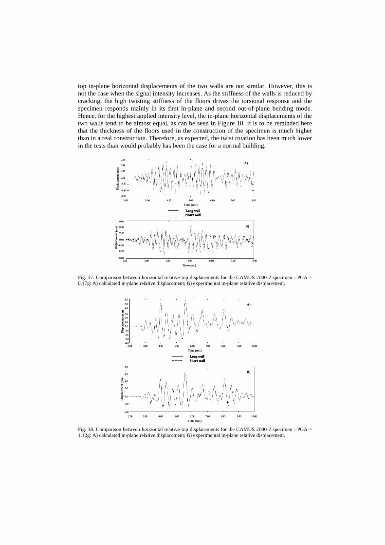
top in-plane horizontal displacements of the two walls are not similar. However, this is not the case when the signal intensity increases. As the stiffness of the walls is reduced by cracking, the high twisting stiffness of the floors drives the torsional response and the specimen responds mainly in its first in-plane and second out-of-plane bending mode. Hence, for the highest applied intensity level, the in-plane horizontal displacements of the two walls tend to be almost equal, as can be seen in Figure 18. It is to be reminded here that the thickness of the floors used in the construction of the specimen is much higher than in a real construction. Therefore, as expected, the twist rotation has been much lower in the tests than would probably has been the case for a normal building.

Fig. 17. Comparison between horizontal relative top displacements for the CAMUS 2000-2 specimen - PGA = 0.17g: A) calculated in-plane relative displacement; B) experimental in-plane relative displacement.

Fig. 18. Comparison between horizontal relative top displacements for the CAMUS 2000-2 specimen - PGA = 1.12g: A) calculated in-plane relative displacement; B) experimental in-plane relative displacement.

Long wallShort wall

Time (sec.)

2.00 3.00 4.00 5.00 6.00 7.00 8.00

0.40

0.20

-0.20

-0.40

-0.60

Dis

p lac

eme n

t(cm

)

0.00

A)0.60

Time (sec.)

0.60

0.40

0.20

-0.20

-0.40

-0.60

Dis

plac

emen

t(c

m)

0.00

B)

2.00 3.00 4.00 5.00 6.00 7.00 8.00

Long wallShort wallLong wallShort wall

Time (sec.)

2.00 3.00 4.00 5.00 6.00 7.00 8.00

0.40

0.20

-0.20

-0.40

-0.60

Dis

p lac

eme n

t(cm

)

0.00

A)0.60

Time (sec.)

0.60

0.40

0.20

-0.20

-0.40

-0.60

Dis

plac

emen

t(c

m)

0.00

B)

2.00 3.00 4.00 5.00 6.00 7.00 8.00

Long wallShort wall

Time (sec.)

Time (sec.)

2.00 3.00 4.00 5.00 6.00 7.00 8.00 9.00 10.00

5.0

3.0

-2.0

-4.0

Dis

pla c

emen

t (cm

)

0.0

6.0

4.0

2.0

1.0

-3.0

-1.0

A)

2.00 3.00 4.00 5.00 6.00 7.00 8.00 9.00 10.00

6.0

-2.0

-4.0

Dis

pla c

emen

t (cm

)

0.0

8.0

4.0

2.0

B)

Long wallShort wallLong wallShort wall

Time (sec.)

Time (sec.)

2.00 3.00 4.00 5.00 6.00 7.00 8.00 9.00 10.00

5.0

3.0

-2.0

-4.0

Dis

pla c

emen

t (cm

)

0.0

6.0

4.0

2.0

1.0

-3.0

-1.0

A)

2.00 3.00 4.00 5.00 6.00 7.00 8.00 9.00 10.00

6.0

-2.0

-4.0

Dis

pla c

emen

t (cm

)

0.0

8.0

4.0

2.0

B)

During the last test, measured data indicated a maximum average drift of about 1.34%, while the numerically predicted value is around 1.25%. Failure was obtained in the long wall by the opening of a wide horizontal crack and rupture of the reinforcement at the first level (at the bottom of the wall). The short wall has suffered less damage, as it is much more flexible. As can be seen from Figure 19, the analysis results agree well with the observed behaviour, failure of the specimen being predicted in the long wall and at the base of the 1st level, by rupture of the extreme reinforcement. Fig. 19. Bending moment – Axial force interaction diagrams and variation of bending moment and axial force at the base of the 1st storey for the CAMUS 2000-2 specimen - PGA = 1.12g.

Table 3 shows a comparison between the design and numerically predicted maximum response parameters with test results. As in the case of the previous specimen, numerical analysis gives maximum response values that are much closer to test results than to design calculated values. It is to be noted however that again, the out-of-plane displacement is underestimated by the analysis due to the nonlinear behaviour of the transverse bracing system.

Table 3. Maximum response values from design, analysis and test (CAMUS 2000-2).

Design (1.13g)

Numerical Analysis (1.12g)

Test (1.12g)

Short wall In-plane relative top displacement (cm)

3.6

5.87

5.79

Long wall In-plane relative top displacement (cm)

2.3

5.45

6.34

Out-of-plane relative top displacement (cm)

0.55

0.92

1.81

Bending moment at the bottom of the two walls

(KNm)

671

793

1033

-600 -400 -200 0 200 400 600

600

400

200

0

-600

-400

-200Mo

me

nt [

kNm

]

Axial force [kN]

N0

-300 -200 -100 0 100 200 300 400 500 600

800

400

200

0

-600

-400

-200M

om

ent

[kN

m]

Axial force [kN]

N0

600

-800

Traction Compression Traction Compression

rupture

Short wall Long wall

-600 -400 -200 0 200 400 600

600

400

200

0

-600

-400

-200Mo

me

nt [

kNm

]

Axial force [kN]

N0-600 -400 -200 0 200 400 600

600

400

200

0

-600

-400

-200Mo

me

nt [

kNm

]

Axial force [kN]

N0

-300 -200 -100 0 100 200 300 400 500 600

800

400

200

0

-600

-400

-200M

om

ent

[kN

m]

Axial force [kN]

N0

600

-800

-300 -200 -100 0 100 200 300 400 500 600

800

400

200

0

-600

-400

-200M

om

ent

[kN

m]

Axial force [kN]

N0

600

-800

Traction Compression Traction Compression

rupture

Short wall Long wall

9. Conclusions This paper has described some particular aspects of the behaviour of two lightly reinforced wall specimens subjected to seismic excitation. The significant effect of the wall degradation on the stiffness and strength of the wall suggests that it is always important that design procedures are derived from numerical modelling and experimental observations. This is due to the fact that axial force effects, as well as re-distribution of forces due to the evolution of stiffness of the walls, are completely nonlinear and cannot be adequately represented in a standard linear elastic model. The experimental-analytical comparisons not only demonstrate the accuracy of the 3-D time-history analysis model, but also allow obtaining more detailed information about the behaviour of the specimen when it is subjected to more complex loading conditions. The numerical model however requires a refined and realistic description of the geometry of the wall and of its reinforcement and detailed cyclic constitutive models of the material behaviour. Its principal advantage relative to the macro models lies in the fact that the mechanical properties of each constituent element of the wall are based on the actual local behaviour of materials, and due to this the interaction between axial force, flexure and shear is directly taken into account. Below, the most significant issues of this paper are reiterated:

• In the case of the first specimen, it has been shown that bi-directional excitation can importantly increase the strain demand of reinforced concrete walls with limited reinforcement, mainly because of increasing the variation of the axial force. During seismic response, high tension strains are to be expected and failure can happen by rupture of reinforcement in tension. Low-ductility “non-standard” steel is thus unsuitable for seismic application.

• In the case of the second specimen, even though the thickness of the floors is

much higher than in a real construction, the torsional stiffness of the floors may play an important role in the spreading of the shear force between the walls and in the ultimate strength of the structure.

• When compared to test results, the design method has given good results as

concerns the maximum accelerations. However, the maximum displacements are notably underestimated and the method is not able to give precise values of the variation of the axial force. Based on nonlinear numerical analysis results (also confirmed by test results), for the particular case of CAMUS 2000-1 specimen, the dynamic component of the wall axial force may be taken as 50% of the axial force in the wall due to gravity loads present in the seismic design situation. This is a confirmation of the relevant provisions of EN1998 [CEN, 2004] for additional dynamic axial forces to be taken into account in the ULS verification of the lightly reinforced wall for flexure with axial load.

Since this study was concerned with a particular case, it is clear that more systematic

and parametric studies considering a wider variety of geometric configurations and boundary conditions will be required to establish definite criteria for efficient design of lightly reinforced walls. Based on the results obtained in this study, it appears to be possible to investigate behaviour trends for a wider variety of configurations than is practically possible to study experimentally.

Acknowledgement This research was financed by the Civil Works Program (French Ministries of Equipment and National Education), CEA (French Atomic Energy Commission), FFB (French National Federation of Housing), EDF (French Electricity Utility) and EC (European Commission). References Bisch, P. and Coin, A. [1998] “The CAMUS research,” Proc. of the Eleventh European

Conference on Earthquake Engineering, Paris, CD-ROM, Vol. 2, 150p. Bisch, P. and Coin, A [2002] “The CAMUS 2000 research,” Proc. of the Twelfth

European Conference on Earthquake Engineering, London, CD-ROM, 10p. CEN [2004] “European Standard EN1998-1:2004 Eurocode 8: Design of structures for

earthquake resistance. Part 1: General rules, seismic actions and rules for buildings,” Brussels.

Chiou, Y.J., Mo, Y.L., Hsiao, F.P., Liou, Y.W. and Sheu, M.S. [2003] “Experimental and Analytical Studies on Large-Scale Reinforced Concrete Framed Shear Walls” ACI Special Publication, Vol. 211, pp. 201-222.

Combescure, D. [2002] “Principaux résultats d’essais, recalage des modèles et analyses post essais,” Projet CAMUS 2000 Rapport final, Vol. 5, Section 3, Paris, (in French), 161p.

Combescure, D., Queval, J.C., Chaudat, T. and Sollogoub P. [2002] “ Seismic Behaviour of Non Symmetric R/C Bearing Walls Specimen with Torsion. Experimental Results and Non Linear Numerical Modelling,” Proc. of the Twelfth European Conference on Earthquake Engineering, London, CD-ROM, 9p.

Elnashai, A., Pilakoutas, K. and Ambraseys, N. [1990] “Experimental behaviour of reinforced concrete walls under earthquake loading,” Earthquake Engineering and Structural Dynamics, 19, pp. 389-407.

Faria, R., Pouca, N.V. and Delgado, R. [2002] “Seismic Behaviour of a R/C Wall: Numerical Simulation and Experimental Validation,” Journal of Earthquake Engineering, Vol. 6, No. 4, pp. 473-498.

Feenstra, P. and de Borst, R. [1995] “Constitutive Model for Reinforced Concrete,” Journal of Engineering Mechanics, Vol. 121, No. 5, pp. 587-595.

Fischinger, M., Isacovic, T. and Kante, P. [2002] “CAMUS 3 International Benchmark, Report on Numerical Modeling, Blind Prediction and Post-Experimental Calibrations,” IKPIR Report EE – 1/02, University of Ljubljana, ISBN 951-6167-45-6, 118p.

Fouré, B. and Vié, D. [2002a] “Etude de l’effort normal dynamique,” Projet CAMUS 2000 Rapport final, Vol. 12, Section 5: Document 2, (in French), 60p.

Fouré, B and Vié, D. [2002b] “Document 1: Contrôles de fabrication des maquettes,” Projet CAMUS 2000 Rapport final, Vol. 11, Section 5: Etudes CEBTP, (in French), 41p.

Guedes, J., Pégon, P., Pinto, A.V. [1994] “A Fibre/Timoshenko Beam Element in CASTEM 2000,” Special Publication Nr. I.94.31, Joint Research Centre, 55p.

Ile, N. and Reynouard, J. M. [2000] “Non-linear analysis of reinforced concrete shear wall under earthquake loading,” Journal of Earthquake Engineering, Vol. 4, No. 2, pp. 183-213.

Ile, N., Reynouard, J.M. and Georgin, J.F. [2002] “Non-linear Response and Modelling of RC Walls Subjected to Seismic Loading,” ISET Journal of Earthquake Technology, Vol. 39, No. 1-2, 20p.

Ilker, K., Ahmet, Y and Polat G. [2005] “Numerical Simulation of Dynamic Shear wall tests: A Benchmark Study,” Computers & Structures, No. 84 [2006], pp. 549-562.

Kabeyasawa, T., Ohkubo, T. and Nakamura, Y. [1996] “Tests and Analysis of Hybrid Wall Systems,” Proc. of the Eleventh World Conference on Earthquake Engineering, Paper No. 470, Acapulco, Mexico, 8p.

Mazars, J. [1998] “French advanced research on structural walls: An overview on recent seismic programs,” Proc. of the Eleventh European Conference on Earthquake Engineering, Invited Lectures, Paris, pp. 21-41.

Menegoto, M. and Pinto, P. [1973] “Method of analysis of cyclically loaded reinforced concrete plane frames including changes in geometry and non-elastic behaviour of elements under combined normal force and bending,” IABSE Symposium on resistance and ultimate deformability of structures acted on by well-defined repeated loads, Final report, Lisbon, 328p.

Merabet O. & Reynouard, J.M. [1999] “Formulation d’un modèle elasto-plastique fissurable pour le béton sous chargement cyclique, ” Contract Study EDF/DER, Final Report, No.1/943/002, URGC-Structures, National Institute for Applied Sciences, Lyon, (in French), 84 p.

Millard, A. [1993] ”CASTEM 2000, Manuel d’utilisation,” Report CEA-LAMS No. 93/007, Saclay, France, (in French).

Paulay, T. [1997] “Seismic Torsional Effects on Ductile Structural Wall Systems,” Journal of Earthquake Engineering, Vol. 1, No. 4, pp. 721-745.

REGLES PS 92 [1995] “Règles de construction parasismique, Règles PS applicables aux bâtiments, dites Règles PS 92,” Norme Française, AFNOR, 217p.

“State-of-the-art report on finite element analysis of reinforced concrete” [1982] ASCE special publication, New York, N.Y., 553p.

Sollogoub, P., Combescure, D., Queval J-C. and Chaudat, T. [2000] “In Plane Seismic Behaviour of Several 1/3rd Scaled R/C Bearing Walls – Testing and Interpretation Using Non-Linear Numerical Modelling,” Proc. of the Twelfth World Conference on Earthquake Engineering, Auckland, 9p.

Sollogoub, P., and Queval J-C. [2002] “Essais (CEA),” Projet CAMUS 2000 Rapport final, Vol. 6, Section 4, Paris, (in French), 35p.

TMR [2003] “Training and Mobility of Researchers,” www.cordis.lu/tmr/home.html Vulcano, A., Bertero, V.V. and Colotti, V. [1988] “Analytical Modeling of R/C structural

walls,” Proc. of the Ninth World Conference on Earthquake Engineering, Vol.6, Tokyo-Kyopto, Japan, pp. 41-46.