Levy walk patterns in the foraging movements of spider monkeys (Ateles geoffroyi
25
1 2 Lévy walk patterns in the foraging movements of 4 spider monkeys ( Ateles geoffroyi ) 6 GABRIEL RAMOS-FERNÁNDEZ ()), JOSÉ LUIS MATEOS, OCTAVIO MIRAMONTES, GERMINAL COCHO 8 Departamento de Sistemas Complejos, Instituto de Física, Universidad Nacional Autónoma de México, Ciudad Universitaria, México 01000 D.F. México. 10 HERNÁN LARRALDE Centro de Ciencias Físicas, Universidad Nacional Autónoma de México, Av. Universidad 12 s/n, Col. Chamilpa, Cuernavaca 62210 Morelos, México. BÁRBARA AYALA -OROZCO 14 Department of Environmental Studies, University of California, Santa Cruz, CA, 95064. 16 Current address: Pronatura Península de Yucatán. Calle 17 #188A x 10, Col. García Ginerés. Mérida Yucatán 97070 México. 18 [email protected] FAX: 52 999 925 3787 20 Telephone: 52 999 920 4647 22
Transcript of Levy walk patterns in the foraging movements of spider monkeys (Ateles geoffroyi
1
2
Lévy walk patterns in the foraging movements of4
spider monkeys (Ateles geoffroyi)6
GABRIEL RAMOS-FERNÁNDEZ ()), JOSÉ LUIS MATEOS, OCTAVIO MIRAMONTES, GERMINAL
COCHO8
Departamento de Sistemas Complejos, Instituto de Física, Universidad Nacional Autónoma
de México, Ciudad Universitaria, México 01000 D.F. México.10
HERNÁN LARRALDE
Centro de Ciencias Físicas, Universidad Nacional Autónoma de México, Av. Universidad12
s/n, Col. Chamilpa, Cuernavaca 62210 Morelos, México.
BÁRBARA AYALA-OROZCO14
Department of Environmental Studies, University of California, Santa Cruz, CA, 95064.
16
Current address: Pronatura Península de Yucatán. Calle 17 #188A x 10, Col. García
Ginerés. Mérida Yucatán 97070 México.18
FAX: 52 999 925 378720
Telephone: 52 999 920 464722
2
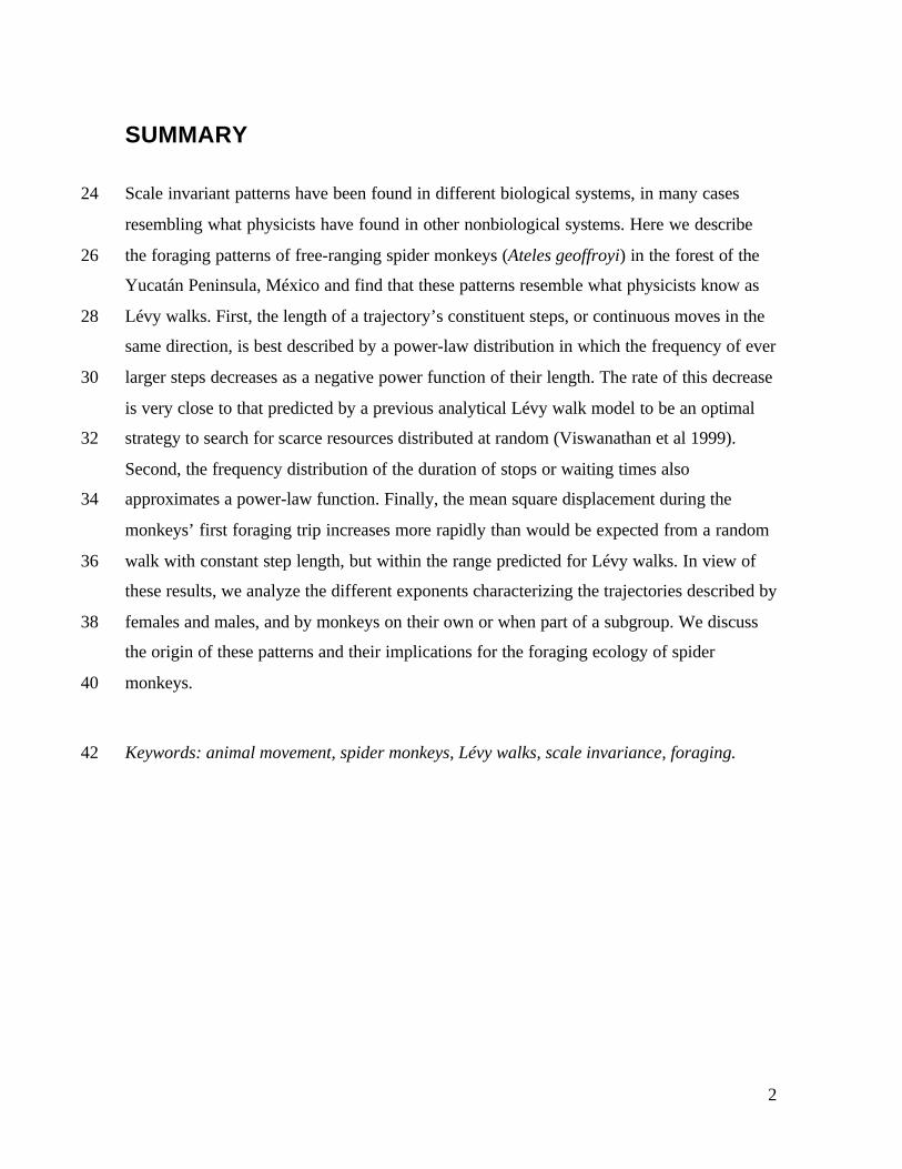
SUMMARY
Scale invariant patterns have been found in different biological systems, in many cases24
resembling what physicists have found in other nonbiological systems. Here we describe
the foraging patterns of free-ranging spider monkeys (Ateles geoffroyi) in the forest of the26
Yucatán Peninsula, México and find that these patterns resemble what physicists know as
Lévy walks. First, the length of a trajectory’s constituent steps, or continuous moves in the28
same direction, is best described by a power-law distribution in which the frequency of ever
larger steps decreases as a negative power function of their length. The rate of this decrease30
is very close to that predicted by a previous analytical Lévy walk model to be an optimal
strategy to search for scarce resources distributed at random (Viswanathan et al 1999).32
Second, the frequency distribution of the duration of stops or waiting times also
approximates a power-law function. Finally, the mean square displacement during the34
monkeys’ first foraging trip increases more rapidly than would be expected from a random
walk with constant step length, but within the range predicted for Lévy walks. In view of36
these results, we analyze the different exponents characterizing the trajectories described by
females and males, and by monkeys on their own or when part of a subgroup. We discuss38
the origin of these patterns and their implications for the foraging ecology of spider
monkeys.40
Keywords: animal movement, spider monkeys, Lévy walks, scale invariance, foraging.42
3
INTRODUCTION44
Understanding how pattern and variability changes with the scale of analysis is one of the
main goals of ecological research (Levin 1992). Ideally, one would like to extrapolate46
findings in one scale of analysis to another. This may be achieved by simplifying the
problem at one scale, finding an expression that its main features without unnecessary48
detail and then using this expression to extrapolate to larger scales. Thus, the diffussion
approximation to individual animal movements, where an individual is assumed to move at50
random as if it was a Brownian particle, has been successfully applied to predict large-scale
features of the population such as its rate of spatial dispersal (Turchin 1998).52
In some cases, universal scaling relationships which describe the same pattern at different54
scales have been found in biological systems (rev. in Gisiger 2001). Fractal geometry,
where spatial patterns show statistically similar patterns over several orders of magnitude in56
the scale of observation, has been succesful in describing patterns of aggregation of
resources (Ritchie and Olff 2000) and even in predicting the different relationships that58
should exist between body size and home range in different species (Haskell et al. 2002).
60
Here we describe the movement patterns of individual spider monkeys (Ateles geoffroyi) in
the wild and find that they resemble what physicists have long recognized as Lévy walks.62
These walks show spatial scale invariance in the length of constituent steps and temporal
scale invariance in the duration of intervals between steps. Similar movement patterns have64
already been found in the foraging flights of wandering albatrosses (Diomedea exulans;
Viswanathan et al. 1996). The same authors developed an analytical model suggesting that66
Lévy walks are an optimal strategy for finding randomly distributed, scarce resources
(Viswanathan et al. 1999).68
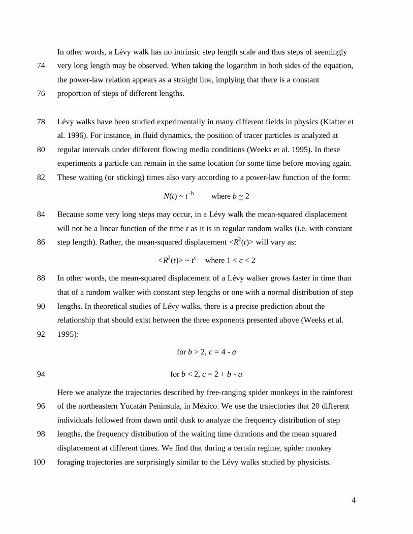
In a Lévy walk (Schlesinger et al. 1993), the length of each successive step (x) varies70
according to a power-law function of the form:
N(x) ~ x−a where 2 < a < 372
4
In other words, a Lévy walk has no intrinsic step length scale and thus steps of seemingly
very long length may be observed. When taking the logarithm in both sides of the equation,74
the power-law relation appears as a straight line, implying that there is a constant
proportion of steps of different lengths.76
Lévy walks have been studied experimentally in many different fields in physics (Klafter et78
al. 1996). For instance, in fluid dynamics, the position of tracer particles is analyzed at
regular intervals under different flowing media conditions (Weeks et al. 1995). In these80
experiments a particle can remain in the same location for some time before moving again.
These waiting (or sticking) times also vary according to a power-law function of the form:82
N(t) ~ t−b where b ~ 2
Because some very long steps may occur, in a Lévy walk the mean-squared displacement84
will not be a linear function of the time t as it is in regular random walks (i.e. with constant
step length). Rather, the mean-squared displacement <R2(t)> will vary as:86
<R2(t)> ~ tc where 1 < c < 2
In other words, the mean-squared displacement of a Lévy walker grows faster in time than88
that of a random walker with constant step lengths or one with a normal distribution of step
lengths. In theoretical studies of Lévy walks, there is a precise prediction about the90
relationship that should exist between the three exponents presented above (Weeks et al.
1995):92
for b > 2, c = 4 - a
for b < 2, c = 2 + b - a94
Here we analyze the trajectories described by free-ranging spider monkeys in the rainforest
of the northeastern Yucatán Peninsula, in México. We use the trajectories that 20 different96
individuals followed from dawn until dusk to analyze the frequency distribution of step
lengths, the frequency distribution of the waiting time durations and the mean squared98
displacement at different times. We find that during a certain regime, spider monkey
foraging trajectories are surprisingly similar to the Lévy walks studied by physicists.100
5
We then use this finding as a tool to explore the possible variations in trajectories with102
regard to the grouping behavior of spider monkeys. This species forms temporary
aggregations that vary in size and composition throughout the day, which have been104
suggested to occur in response to the variation in food availability (Klein and Klein 1977;
Symington 1987, 1988). The trajectories described by lone individuals could then be106
different to those described by individuals in a subgroup, as they probably represent
different strategies for finding or exploiting known food patches. In addition, male spider108
monkeys occupy larger home ranges, and travel farther per day and in larger subgroups
than females (Symington 1987; Ramos-Fernández and Ayala-Orozco 2002) a difference110
that may reflect different space use strategies (Wrangham 2000). Therefore we analyzed the
Lévy walk parameters separately in the trajectories of lone and grouped individuals as well112
as in those of females and males.
114
METHODS
Study site and animals116
Data were collected in in the area of forest surrounding the Punta Laguna lake (2 km x 0.75
km), in the Yucatán Peninsula, México (20o38' N, 87o38' W, 14 m elevation). This region is118
characterized by seasonally dry tropical climate, with mean annual temperature of about
25oC and mean annual rainfall around 1500 mm, 70% of which is concentrated between120
May and October. The main forest fragment near the lake consists or 60 hectares of
medium semi-evergreen forest. This is in turn surrounded by secondary successional forest122
about 30-40 years old in an area of 5000 hectares recently declared as a protected area, the
Otoch Ma'ax Yetel Koh Sanctuary. Spider monkeys use both of these vegetation types,124
although they spend more than 70% of their daily time and every night in the medium
forest (Ramos-Fernández and Ayala-Orozco 2002). Trails were cut throughout the fragment126
of medium forest and through part of the successional forest. In these trails, trees and other
landmarks were used to make accurate maps of this area. Visibility conditions were very128
good as monkeys used the canopy at heights from 5 to 25 m. More details about the study
site can be found in Ramos-Fernández and Ayala-Orozco (2002).130
6
Two study groups, occupying 0.95 and 1.66 km2 of forest, respectively, have been studied132
continuously since January, 1997. One group (5 female and 3 male adults as of 1999) was
habituated to human presence before the study began and the other (15 female and 6 male134
adults as of 1999) was habituated during 1997. All monkeys were identified by facial marks
and other unique features. Adults were defined by their size and darker faces, and in the136
case of males, for their fully descended testes. All monkeys could be reliably identified by
the end of 1997.138
Data collection
Data reported here were collected between September through December 1999. On 20 days140
during that period, a different known adult was chosen as the focal subject and followed by
at least two observers from dusk until dawn, taking an instantaneous sample of its location,142
activity and subgroup size and composition every 5 minutes. The location was estimated
visually by two observers to the nearest 5 m with respect to landmark trees or paths. In all144
cases a landmark was closer than 50 m from the position of the monkey.
Data analysis146
Trajectories were analyzed according to the methods outlined by Turchin (1998). The
trajectory of each focal monkey consisted of a sequence of paired coordinates, one pair for148
each 5 minute interval where an instantaneous sample had been recorded. A step was
defined as an interval in which any or both of the coordinates in two consecutive samples150
differed. The length of each step was the linear distance separating the position at two
consecutive samples. In some cases, observers lost sight of the focal animal for a number of152
sample intervals. Steps were not calculated for those intervals but only for those in which
the position was known for two consecutive five-minute samples. The frequency154
distribution of step lengths was analyzed using a bin size of 10 m. The log-log plot of this
distribution was used to calculate the relationship that produced the best fit using a least-156
square method.
158
Wating times were calculated from the number of samples in which the focal animal did
not change position. The frequency distribution of waiting times was analyzed using a bin160

7
size of one interval (5 minutes). The log-log transform of this distribution was used to
calculate the relationship producing the best fit using a least-square method.162
Squared displacements were calculated by measuring, for each individual separately, the164
length of a line joining its location in the first sample of the day and its location at different
times thereafter. The mean-squared displacement was obtained by averaging all squared166
displacements accross all individuals for a given time of day. From this mean-squared
displacement a maximum was obtained around 1030 hours, which then decreased as168
monkeys consistently began approaching their starting point, in some cases returning to it at
noon and in most cases returning to it at dusk (see Figure 4). The mean-squared170
displacement from 0630 to 1030 was then taken to be a period in which most of the
individuals moved away from their starting point. For this period only, a log-log plot was172
produced and a line adjusted by the least-square method.
174
Turning angles were calculated by substracting the absolute angle (with respect to the east-
west axis and in a counterclockwise direction) of each step from the absolute angle of the176
previous step. A frequency distribution of turning angles was thus produced, using a bin
size of 10 degrees.178
The regression slopes for the Lévy walk distribution of trajectories of lone vs. grouped180
individuals and females vs. males were compared using an F test for regression slopes
(Sokal and Rohlf 1994).182
RESULTS
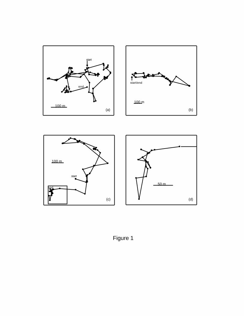
The observed daily trajectories of spider monkeys are made up of steps of variable length.184
Three examples of these trajectories are shown in Figure 1(a-c). One important property of
Lévy walks is that they show self-similarity accross different spatial scales. Indeed, when186
we close in on a region of one of these trajectories, a qualitatively similar pattern as in the
large scale appears (Figure 1d).188
Figure 1
8
The frequency distribution of step lengths of all trajectories together shows a wide range of190
variation (Figure 2a). The data can be fitted better to a power-law function (Figure 2b; r2 =
0.89) than to an exponential one (r2 = 0.79). The value of the exponent in the negative192
power-law equation fitted to the data is a = 2.18.
194
Figure 2196
The frequency distribution of waiting times of all trajectories together also shows a wide
degree of varation. Before traveling again, spider monkeys may stop for as little as 10198
minutes or for as much as 2 hours (Figure 3). The log-log plot of the data is fit well by a
negative power-law function with an exponent b = 1.7 (r2 = 0.86).200
Figure 3202
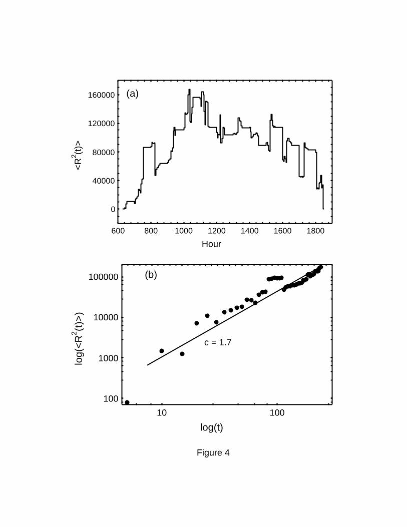
The squared displacement in many of the individuals analyzed shows a common pattern:204
monkeys tend to get away from their sleeping site for a few hours in the morning, before
coming back to the origin at noon or staying in the vicinity, normally coming back to the206
same sleeping site shortly before sunset. Some individuals, especially males, did not return
to the same sleeping site at the end of the day. Close inspection of the mean-squared208
displacement of all individuals shows a maximum at around 1030 hours (Figure 4a). A log-
log plot of the data for the period between 0630 and 1030 only, when all individuals were210
getting away from the origin, adjusts to a line with a slope of 1.7 (r2 = 0.87), as would be
expected in a Lévy walk (Figure 4b).212
Figure 4214
The fact that spider monkeys travel back to their sleeping sites, as well as the fact that they216
sometimes use the same routes for going away from and returning to their sleeping site (for
example, see Figure 1b), implies that some persistence should exist in the direction of218
9
consecutive steps. Figure 5 shows the distribution of turning angles between successive
steps. This distribution is far from being uniform, being centered around zero. However, at220
a large enough time scale, this persistence is not expected to affect the scaling relations
between the mean-squared displacement and time.222
Figure 5224
Spider monkeys change subgroup several times during a day, so the trajectory described by226
one individual in one complete day includes some steps traveled on its own and others
when in a subgroup. When analyzing the distribution of lengths for these steps separately,228
the value of the exponent is different: as = 1.50 (r2 = 0.80) for solitary individuals and ag =
2.12 (r2 = 0.89) for individuals in groups (Figure 6). An F test comparing the two regression230
slopes shows a significant difference (F = 5.72, P < 0.05). Considering the fact that the
number of samples in each category are different, monkeys travel a higher proportion of232
long trajectories when on their own than when part of a subgroup (Figure 6).
234
Figure 6236
We also analyzed the distribution of travel lengths separately for females and males. Figure
7 shows that both are described by power laws with exponents af = 2.11 for females and am238
= 1.47 for males. It is males who travel a higher proportion of long trajectories than
females.240
DISCUSSION
We have presented evidence showing that the daily movements of spider monkeys242
resemble what physicists know as Lévy walks, i.e. random walks with power-law scaling in
the length of their constituent steps. Waiting times, or the duration of intervals without244
movement, also show power-law scaling. As expected from theoretical studies of Lévy
walks, the mean-squared displacement increases faster in time than in other random walks246
such as a Brownian random walk (Schlesinger et al. 1993).
10
248
In support of this interpretation, there is an agreement between all three exponents, as
would be predicted from theoretical studies of Lévy walks (Weeks et al. 1995):250
for b < 2, c = 2 + b - a
which, substituting the observed values of each exponent, yields the following prediction252
for the value of c:
for b = 1.7 < 2254
c = 2 + 1.7 – 2.18 = 1.52
A value that is close to the observed value of 1.7. In other words, there is an agreement256
between different properties of the observed trajectories during this time lapse, such that
they can accurately be described as Lévy walks.258
Lévy walks differ in fundamental ways from other types of random walks, such as260
Brownian random walks, which have been used in most models of animal foraging
(Turchin 1998). As mentioned before, the mean-squared displacement after a time t is262
larger for Lévy walks than for other random walks (Weeks et al. 1995). In the period
between 0630 and 1030, when spider monkeys normally spend two or three hours foraging264
away from their sleeping sites (Ramos-Fernández, personal observations), the mean-
squared displacement increases faster than in a Brownian random walk.266
However, there are certain regularities in the trajectories analyzed here that would not allow268
us to label them as “pure” Lévy walks. After 1030 hours spider monkeys tend to stop
traveling away from their sleeping sites and on most ocassions return to them before sunset.270
Also, the shape of their home range, which circles a lake (e.g. see Figure 1c), implies that
sometimes a monkey will use the same route to go in one direction and return in the272
opposite direction. The idea that monkeys are actually following a route of some sort is
suggested by the fact that two consecutive steps tend to be given in a similar direction, as274
shown in the distribution of turning directions, which is centered around zero.
276
11
Interpretation of these results hinges on the crucial question of the cues that spider monkeys
use for finding food sources. Feeding on the fruit from 50 to 150 species of trees (van278
Roosmalen and Klein 1987; Ramos-Fernández and Ayala-Orozco 2002), each with its own
phenological pattern, spider monkeys clearly face the problem of exploiting an extremely280
variable resource. Lévy walks could represent a foraging search strategy, in which the
movements of spider monkeys are guided by the odour and visual cues they detect from the282
existing ripe fruit in fruiting trees. Alternatively, the patterns reported here could be the
result of the knowledge based on memory that spider monkeys could have about the284
location of fruiting trees.
286
Little is known about what animals in general know about the location of food sources (rev.
in Boinski and Garber, 2000). Experimental evidence suggests that wild capuchin monkeys288
(Cebus apella) visit the closest food sources more often than would be expected on the
basis of “random search” null models (Janson 1998). Also, they appear to use straighter290
lines than would be expected if they were only searching with no memory of where they
had found food in the past. If spider monkeys have a similar kind of spatial knowledge292
about the past location of food, then the patterns that we report here may not represent
“random” searches at all, but the result of more directed travel between known food294
sources.
296
However, the null models developed by Janson (1998) as an expectation of travel with no
spatial knowledge assume either a constant step length and arbitrary changes in direction or298
a constant travel direction until finding a food source. In the results we report here, spider
monkeys are in fact including some very long steps in their foraging trajectories. If this is a300
common pattern in tree-dwelling monkeys, then a more appropriate null model for foarging
with no memory should include visits to farther, unknown food sites. This, in Janson’s302
(1998) study, would make it more difficult to distinguish between observed and expected
visiting frequencies.304
It is possible that spider monkeys travel in Lévy walks in order to exploit these unknown306
sources of food more efficiently. Viswanathan et al. (1999) have shown that a Lévy walker
12
visiting a number of randomly distributed foraging sites will visit more new sites and revisit308
less previously visited sites than a Brownian random walker traveling the same total
distance. This is because the long steps in a Lévy walk quickly take the forager to more310
distant sites, making it less likely that it will walk on its own steps again. In this study, the
value for the exponent a in the distribution of step lengths is close to the optimum of a = 2312
predicted by Viswanathan et al (1999) for foragers searching for randomly and sparsely
distributed food sources.314
Lévy walk foraging patterns could also be the result of the distribution of fruiting trees316
themselves. In an extensive study on several species of tropical trees in different sites
around the world, Condit et al. (2000) found highly aggregated distribution patterns for318
most of the species, showing graphs of density of neighbors as a function of distance that
look strikingly similar to those described by power-law functions. Also, Solé and Manrubia320
(1995) report self similar distributions of tree gaps (and thereby sites available for
establishment of many new individual trees) in a tropical forest in Panamá. It is possible322
that at any given time, the fruiting trees where spider monkeys can feed are distributed in a
scale-invariant, fractal manner. Thus, the long steps in the Lévy walks could be those given324
between patches of a given fruiting tree, while shorter steps would be given while foraging
within a patch. Clearly, more information on the spatial distribution of the spider monkeys’326
food resources is required to clarify this issue.
328
Because spider monkeys are important seed dispersers for several tree species, in reality
there could exist a bidirectional relationship between their foraging patterns and the330
distribution of trees. By foraging and dispersing seeds in such a pattern, spider monkeys
might favor, in the long run, a self similar distribution of the very same trees on which they332
feed. A similar positive feedback between foraging behavior and the distribution of
resources was found by Seabloom and Reichman (2001) in a simulation model of gopher –334
grass interaction. By restricting their movements to their defended territories, gophers
disturbed areas where more grass could grow on the following season, therefore increasing336
habitat patchiness, which increased the foraging efficiency of gophers in the long run.
Westcott and Graham (2000) report a long-tailed distribution in the distance traveled by a338
13
tropical flycatcher (Myonectes oleaginus) continuously after feeding. Based on the times of
digestion for the seeds of different species, the authors derive the expected shape of seed340
shadows for different species, which also look very similar to power laws.
342
Another consequence of foraging in a Lévy walk pattern is that previously visited food
sources may be revisited after long periods of time, favoring the ripening of more fruit344
before the next visit. Such “harvesting” of resources was suggested by Janson (2000) to be
one of the reasons why animals foraging on scarce patches of food would not necessarily346
visit the closest one in the most optimal route. Perhaps the temporal dimension of the Lévy
walk patterns reported here is as important as the spatial one.348
We have found that the Lévy walks of females and males are different. Males have a larger350
proportion of long trajectories than females. This is consistent with the fact that male spider
monkeys range over wider areas and travel further per day than females (Symington, 1987;352
Ramos-Fernández and Ayala-Orozco 2002). While males range over the whole territory of
their group, females seem to restrict most of their time to a portion of it (Ramos-Fernández,354
personal observation). At the boundaries of their group’s territory, males form coalitions
that engage in very aggressive encounters with neighboring males (Symington 1987;356
Ramos-Fernández, personal observations). In view of these results, the fact that the Lévy
walks of males contain more long steps than those of females is consistent with their358
different space use strategies.
360
Finally, we have found a different value of the power-law exponent for the length
distribution of steps given by lone monkeys as for those given by monkeys when part of a362
subgroup. In particular, monkeys on their own seem to travel a higher proportion of long
steps compared to short ones. One of the cited benefits of group foraging has been an364
improvement on the likelihood that the group would find food patches which an individual
on its own would not find (Krebs and Davies 1993). If spider monkeys do not have366
knowldege of the location of food sources, they could still find more fruting trees when
traveling in a subgroup than when alone. The same argument applies if spider monkeys368
have knowledge about the location of fruiting trees: if they can share information on the

14
known location of resources (Boinski and Garber 2000) it would seem logical that a370
subgroup would find more fruiting trees than a single individual, therefore decreasing the
proportion of long steps.372
The origin of the grouping pattern of spider monkeys has led to some discussion374
(Symington 1990; Wrangham 2000, in chimpanzees and spider monkeys). An intriguing
possibility is that, in a hypothetical ancestor with stable grouping patterns, a Lévy walk376
foraging pattern increased the chances of separating from the rest of the group when
foraging on scarce resources. In a group of n Lévy walkers, the probability that individuals378
will remain near the origin (or cross each other’s path if they all start together at the same
spot) is greatly reduced compared to a group of n Brownian walkers (Larralde et al 1992).380
Favored by the decrease in feeding competition offered by Lévy walks, social behaviors
that maintained group membership even in the absence of visual contact would then382
develop, leading to the fission-fusion grouping pattern that we see today.
384
ACKNOWLEDGEMENTS
The authors are truly grateful to Eulogio and Macedonio Canul, who provided invaluable386
assistance in the field by locating the study subgroups and collecting data. Laura Vick and
David Taub initiated the study of spider monkeys in Punta Laguna. Fieldwork was financed388
by a graduate scholarship from the National Council for Science and Technology
(CONACYT, Mexico) and by grants from the Wildlife Conservation Society, the National390
Commission for the Knowledge and Use of Biodiversity (CONABIO, Mexico), the
Mexican Fund for the Conservation of Nature (FMCN) and the Turner Foundation. Data392
analysis and manuscript preparation was financed by CONACYT project 32453-E and
DGAPA project IN-111000, as well as a visiting scholarship (Cátedra Tomás Brody) from394
the Complex Systems Department at the Physics Institute, National Autonomous University
of México. These observations were performed in compliance with the Mexican396
Environment Protection Law (LGEEPA).
15
REFERENCES398
Boinski S and Garber P. 2000. On the move: how and why animals travel in groups. University of Chicago Press.
Condit R., Ashton PS, Baker P, Bunyavejchewin S, Gunatilleke S, Gunatilleke N, Hubbel SP, Foster RB, Itoh A,400LaFrankie JV, Seng Lee H, Losos E, Manokaran N, Sukumar R and Yakamura T. 2000. Spatial patterns in the distribution
of tropical tree species. Science 288: 1414--1418.402Gisiger T. 2001. Scale invariance in biology: coincidence or footprint of a universal mechanism? Biol. Rev. 76: 161--209.
Haskell J.P., Ritchie M.E. and Olff H. 2002. Fractal geometry predicts varying body size scaling relationships for404mammal and bird home ranges. Nature 418: 527--530.
Janson CH. 1998. Experimental evidence for spatial memory in foraging wild capuchin monkeys (Cebus apella). Anim406Behav 55: 1229--1243.
Janson CH. 2000. Spatial movement strategies: theory, evidence and challenges. Ch. 7 in: Boinski S and Garber P. (Eds).408On the move: how and why animals travel in groups. University of Chicago Press, pp 165--203.
Jones R.E. 1977. Movement patterns and egg distribution in cabbage butterflies. J Anim Ecol 45: 195--212.410Klafter J., Schlesinger M.F. and Zumofen G. 1996. Beyond Brownian motion. Phyisics Today 49(2): 33--39.
Klein LL. and Klein DJ. 1977. Feeding behavior of the Colombian spider monkey. In: Clutton-Brock, T.H. (ed) Primate412Ecology. Academic Press, London, pp 153--181.
Krebs JR and Davies NB. 1993. An introduction to behavioural ecology. Blackwell, London.414Larralde H, Trunfio P, Havlin S, Stanley HE and Weiss GH. 1992. Territory covered by N diffusing particles. Nature
355:423--426.416Levin S.A. 1992. The problem of pattern and scale in ecology. Ecology 73(6): 1943--1967.
Ramos-Fernández G. and Ayala-Orozco B. 2002. Population size and habitat use of spider monkeys in Punta Laguna,418México. In: Laura K. Marsh (Ed). Primates in fragments: ecology and conservation. Plenum/Kluwer Press, New York.
Ritchie M.E. and Olff H. 2000. Spatial scaling laws yield a synthetic theory of biodiversity. Nature 400: 557--560.420van Roosmalen MGM. and Klein LL. 1987. The spider monkeys, Genus Ateles. In: Mittermeier RA and Rylands AB
(eds). Ecology and Behavior of Neotropical Primates . World Wide Fund, Washington, pp 455--537.422Schlesinger M.F., Zaslavsky G.M. and Klafter J. 1993. Strange Kinetics. Nature 363: 31--37.
Seabloom EW and Reichman OJ. 2001. Simulation models of the interaction between herbivore strategies, social behavior424and plant community dynamics. Am Nat 157: 76--96.
Sokal RR and Rohlf FJ. 1994. Biometry. 3d ed. Freeman, New York.426Solé RV and Manrubia SC. 1995. Are rain forests self-organized in a critical state? J Theor Biol 173: 31--40.
Symington, MM. 1987. Ecological and social correlates of party size in the black spider monkey, Ateles paniscus chamek .428Ph D. thesis, Princenton University.
Symington M.M. 1988. Food competition and foraging party size in the black spider monkey (Ateles paniscus chamek).430Behaviour 105:117--134.
Symington M.M. 1990. Fission-Fusion Social Organization in Ateles and Pan. Int J Primatol 11, p. 47--61.432Turchin P. 1998. Quantitative analysis of movement. Sinauer, Massachusetts.
Viswanathan GM, Afanasyev V, Buldyrev SV, Murphy EJ, Prince PA and Stanley HE. 1996. Lévy flight search patterns434of wandering albatrosses. Nature 381: 413--415.
Viswanathan GM, Buldyrev SV, Havlin S, da Luz MGE, Raposo EP and Stanley HE. 1999. Optimizing the success of436random searches. Nature 401: 911--914.

16
Weeks E.R., Solomon T.H., Urbach J.S. and Swinney H.L. 1995. Observation of anomalous diffusion and Lévy flights.438In: Schlesinger M.F., Zaslavsky G.M. and Frisch U. (Eds) Lévy flights and related topics in Physics . Springer, Berlin, pp
51--71440Westcott DA and Graham DL. 2000. Patterns of movement and seed dispersal of a tropical frugivore. Oecologia 122:
249--257.442Wrangham R.W. 2000. Why are male chimpanzees more gregarious than mothers? A scramble competition hypothesis.
In: Kappeler P. (ed). Primate Males: causes and consequences of variation in group composition. Cambridge University444Press., pp 248--258.
446

17
FIGURE LEGENDS448
Figure 1 Daily trajectories of spider monkeys. (a) and (b) adult females. (c) adult male,
with the section of the trajectory within the lower-left square amplified in (d). Note that450
some individuals, like the adult female in (b), returned to sleep close to where they started
their daily travel.452
Figure 2 Distribution of the number of 5-minute intervals N(x) during which spider454
monkeys traveled a distance of x meters. A total of 841 five-minute intervals from 20 adult
individuals are included. The insert (b) shows the log-log plot of the same data. A power-456
law relationship fits the data with r2 = 0.89. The estimated value of the exponent is -2.18.
458
Figure 3 Distribution of waiting times in the trajectories of spider monkeys. The figure
shows the log-log plot of the number of intervals N(t) with duration t. The relationship is fit460
by a power-law function with an estimated value of the exponent of -1.7 (r2 = 0.86).
462
Figure 4 Squared displacement in the trajectories of spider monkeys. (a) the mean squared
displacement across all individual trajectories at different times of day. Note that there is a464
maximum at 1030 hours. (b) log-log plot of the mean squared displacement observed from
0630 to 1030 hours. The relationship is well fit by a power-law function with an estimated466
value for the exponent of 1.7 (r2 = 0.87).
468
Figure 5 Circular distribution plot of the turning angle between consecutive steps. Shown
is the number of times that two consecutive steps in the trajectories differed by the degrees470
shown. Note that the distribution peaks around zero.
472
Figure 6 Distance traveled by spider monkeys when alone and in groups. Shown is a log-
log plot of the number N(x) of five-minute intervals in which a lone adult spider monkey474
traveled a distance x. For monkeys traveling alone, a total of 156 five-minute intervals are
included. A power-law relationship fits the data with r2 = 0.8. The estimated value of the476
exponent is -1.50. For monkeys traveling in a group, a total of 685 five-minute intervals are
18
included. A power-law relationship fits the data with r2 = 0.89. The estimated value of the478
exponent is -2.12.
480
Figure 7 Distance traveled by female and male spider monkeys. Shown is a log-log plot of
the number N(x) of continuous trajectories traveled by adult spider monkeys without482
stopping, for a distance of x meters. For 14 females, a total of 604 five-minute intervals
were analyzed. A power-law relationship fits the data with r2 = 0.9. The estimated value of484
the exponent is -2.11. For 7 males, a total of 237 five-minute intervals were analyzed. A
power-law relationship fits the data with r2 = 0.93. The estimated value of the exponent is -486
1.47.
488
100 m
end
start
(a)
100 m
start/end
(b)
100 m
start
end
(c)
50 m
(d)
Figure 1
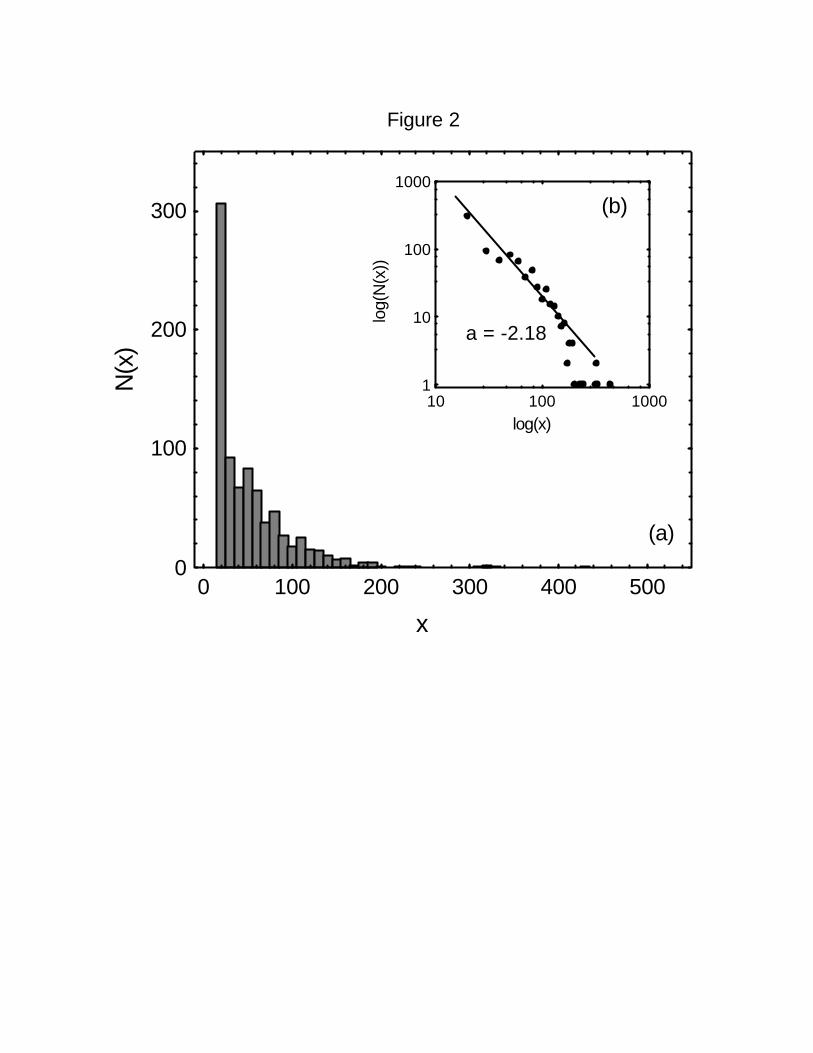
Figure 2
x
N(x
)
0
100
200
300
0 100 200 300 400 500
log(x)
log(
N(x
))1
10
100
1000
10 100 1000
(a)
(b)
a = -2.18
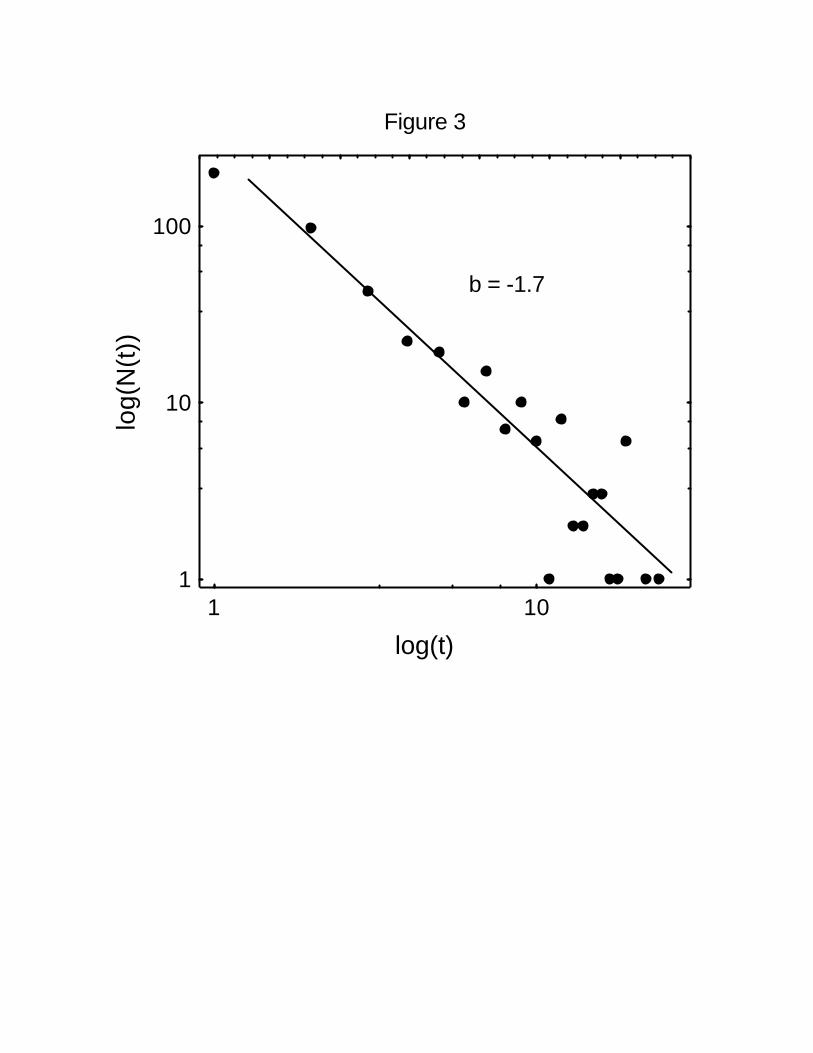
Figure 3
log(t)
log(
N(t
))
1
10
100
1 10
b = -1.7
Hour
<R2 (t)
>
0
40000
80000
120000
160000
600 800 1000 1200 1400 1600 1800
(a)
log(t)
log(
<R2 (t
)>)
100
1000
10000
100000
10 100
c = 1.7
(b)
Figure 4
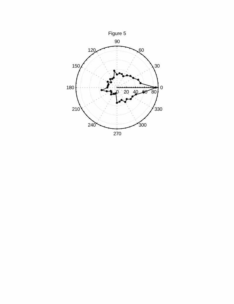
Figure 5
0 20 40 60 800
30
60
90
120
150
180
210
240
270
300
330
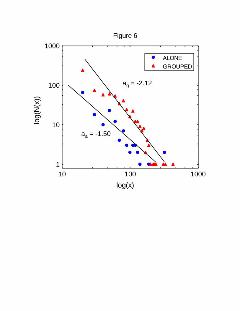
Figure 6
log(x)
log(
N(x
))
1
10
100
1000
10 100 1000
ALONEGROUPED
ag = -2.12
aa = -1.50
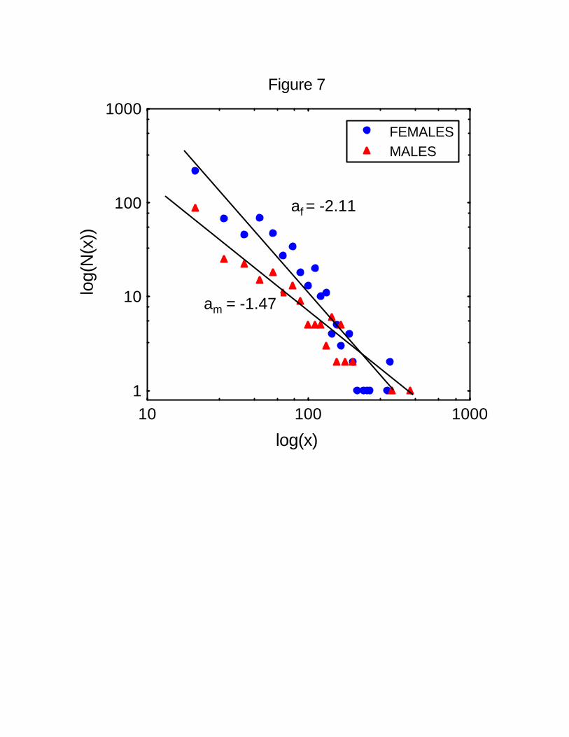
Figure 7
log(x)
log(
N(x
))
1
10
100
1000
10 100 1000
FEMALESMALES
af = -2.11
am = -1.47