Working Paper No. 743

Investment, Financial Markets, and Uncertainty

by

Philip Arestis University of Cambridge

University of the Basque Country Levy Economics Institute of Bard College

Ana Rosa González

University of the Basque Country

Óscar Dejuán University of Castilla-La Mancha

December 2012

The Levy Economics Institute Working Paper Collection presents research in progress by Levy Institute scholars and conference participants. The purpose of the series is to disseminate ideas to and elicit comments from academics and professionals.

Levy Economics Institute of Bard College, founded in 1986, is a nonprofit, nonpartisan, independently funded research organization devoted to public service. Through scholarship and economic research it generates viable, effective public policy responses to important economic problems that profoundly affect the quality of life in the United States and abroad.

Levy Economics Institute

P.O. Box 5000 Annandale-on-Hudson, NY 12504-5000

http://www.levyinstitute.org

Copyright © Levy Economics Institute 2012 All rights reserved

ISSN 1547-366X

1

ABSTRACT

This paper provides a theoretical explanation of the accumulation process, which accounts for

the developments in the financial markets over the recent past. Specifically, our approach is

focused on the presence of correlations between physical and financial investment, and how the

latter could affect the former. In order to achieve this objective, two assets are considered:

equities and bonds. This choice permits us to account for two extreme alternative possibilities:

taking risk in the short run with unknown profits, or undertaking a commitment to the long run

with known yields. This proposal also accounts for the influence of the cost of external finance

and the impact of financial uncertainty, as proxied by the interest rate in the former case and the

exchange rate in the latter case; thereby utilizing the Keynesian notion of conventions in the

determination of investment. The model thus formulated is subsequently estimated by applying

the difference GMM and the system GMM in a panel of 14 OECD countries from 1970 to 2010.

Keywords: Accumulation; Financial Markets; Conventions; Uncertainty; Keynesian Economics

JEL Classifications: B22, C23, E22

2

1. INTRODUCTION1

The development of the financial sector ever since the financial liberalization process, which

started in the early 1970s, and the great evolution of financial investment through this period

suggest that serious consideration of this complex phenomenon is in order. This should enable

one to extend the Keynesian investment function, which does not fully account for the links

between financial elements and the real economy. In this context, we may note that over the

period since the beginning of financial liberalization in the early 1970s, the majority of the

Organisation for Economic Co-operation and Development (OECD) countries have experienced

an increase in their profit shares, while at the same time a slowing down of the rhythm of

accumulation of physical assets has taken place. Both phenomena depict a controversial

relationship, since from a theoretical point of view, the higher profit shares could be interpreted

as an increase in the amount of internal resources available for investment. However, this higher

amount of internal funds has not promoted the expected acceleration of the path of capital

accumulation.

At first sight, this could demonstrate the extent of financial investment crowding out

physical investment (Stockhammer 2004a). It is thereby crucial to study the inverse relationship

between profits and capital accumulation because the conflict that emerges has important

consequences for effective demand and long-run growth. Specifically, firms have to decide

between two options: 1) acquiring capital goods like machinery, equipment, and vehicles, which

generates demand in the current period and also influences the production of the economy,

thereby creating employment and wealth for future generations; or, 2) promoting financial

investment, which permits entrepreneurs to obtain rapidly short-run speculative gains without

worrying about the long run. The preference for one kind of investment over the other displays

evidence of the conflict between managers and shareholders inside firms. This is so since the

behavior of the first group is directed to maximizing profits in the short run, while the second

group prefers to pay more attention to the long run.

The increasing importance of financial activities also exerts another effect on

accumulation via uncertainty. The development of financial activities, which has permitted the

appearance of new activities and financial assets without a strong regulation of them, has

1 This contribution was put together when Ana Rosa González was a visitor at the Department of Land Economy,University of Cambridge from September 2011 to September 2012. It relates to Ana Rosa González’s PhD thesis.

3

boosted speculation, thereby promoting the creation of financial bubbles. According to this

view, an increase in uncertainty means that businessmen face difficulties in their attempt to

foresee the future, which is less predictable now. The inclusion of uncertainty in our explanation

of the accumulation process in mature capitalist economies enables the possibility of utilizing

the Keynesian notion of conventions, which helps businessmen in their investment decisions.

The main novelty of our contribution is the special attention paid to the impact of

financial markets and the presence of uncertainty, introduced explicitly in the model by means

of a set of variables, which as far as we know, have not been accounted for previously in the

investment relationship. Moreover, the theoretical proposition as postulated in this research is

subsequently investigated empirically in a sample of 14 OECD economies over the period

1970–2010. We employ the difference GMM (generalized method of moments) and the system

GMM for this purpose, which permits us to account for the presence of common determinants in

the postulated dynamic phenomenon and in the case of different open economies.

The remainder of this contribution is organized as follows. The foundations of the

proposed investment function are presented in Section 2. The testable hypothesis is clarified and

discussed in Sections 3 and 4. Section 5 deals with the econometric techniques employed for the

purpose of the estimated relationships. In Section 6, we describe the data utilized. The derived

results are discussed in Section 7. Finally, concluding remarks are provided in Section 8.

2. INVESTMENT WITH LABOR CONSTRAINTS

We begin with the Kaleckian investment function with labor constraints as presented by Ryoo

and Skott (2008) and Skott and Zipperer (2010). This approach accounts for the effect of this

constraint on the accumulation pace of mature economies.2 It portrays the rate of accumulation,

g (which is equivalent to I/K, where I is investment and K capital stock), as a linear function of

the capacity utilization, u, the profit share, π, and the rate of employment, e, as shown in

equation (1):

euKIg 3210/ (1)

where u is measured by the output/capital ratio.3

2 See, also, Skott (1989) and Stockhammer (2004b).3 We may note that equation (1) is rooted in the model developed by Dutt (1984) and Bhaduri and Marglin (1990),

and is based on the expression: 210/ uKIg , where the symbols are as in equation (1). Further

consideration of this function is provided in Dutt (2011).

4

Skott and Zipperer (2010) consider as the main feature of mature economies the

relevance of employment in order to determine the rate of accumulation. According to this view,

increasing employment rates are perceived as a signal by firms for a need of higher profit shares

in order to maintain their rate of accumulation. Specifically, high levels of employment promote

the conflict between workers and firms, and favor the former group, which at the end of the day

depresses animal spirits. Moreover, the existence of this labor constraint could generate an

indirect and negative effect on accumulation when the economy is close to full employment.

This is so since contractionary economic policies could be implemented in order to slow down

economic growth. However, at first sight, the analysis of the empirical data questions this

premise because increasing involuntary unemployment has been the general trend observed in

the majority of the European economies since 1960 (Nickell and Nunziata 2002). In this sense,

decreasing rates of employment could be understood by firms as a negative signal of the market,

since they expect a reduction of future demand in view of the newly unemployed workers.

Nevertheless, this negative impact does not take place due to the existence of hysteresis in this

market. This has allowed the development of a labor constraint in economies where the normal

conditions of the labor market are far from full employment (DiNardo and Moore 1999).

However, equation (1) ignores the role of the normal rate of capacity utilization, which

is considered as exogenously determined. From a Kaleckian standpoint (Amadeo 1986; Dutt

1997), this normal rate is considered as a key element in the investment decision, due to the fact

that accumulation dynamics are driven by the gap between the current rate of capacity

utilization and the normal one, which is an endogenous element. Excess capacity has an

influence not only in the short run, but also in the long run. According to this view, firms

maintain idle capacity in normal conditions due to the presence of uncertainty, which compels

them to have excess capacity to respond to unexpected increases in demand (Lavoie, Rodríguez,

and Seccareccia 2004). An alternative explanation of the presence of deviations between the

current capacity utilization rate and its normal level is provided by Dallery and van Treeck

(2011), which introduces two different targets: desired capacity utilization, and desired

profitability. In the context of the latter contribution, firms prefer working in order to satisfy

their objective of profitability instead of their capacity utilization target.

5

3. THE RELEVANCE OF THE REAL RATE OF INTEREST AND UNCERTAINTY TO

INVESTMENT

The investment model described in equation (1) needs to be widened by considering the impact

of the real long-term interest rate, i, as other contributors suggest (Ryoo and Skott 2008,

Stockhammer and Grafl 2010). Ceteris paribus, we can expect that entrepreneurs postpone their

new investment projects under the presence of an increasing cost of external finance. However,

if expectations about demand growth are powerful enough, demand and the rate of interest can

move in parallel; and the final effect of the rate of interest on accumulation could be positive

(Radcliffe Report 1957).4 In periods of boom, investment is high despite upward movements in

the rate of interest because businessmen expect strong increases in demand and profitability,

which compensate for the increase in the cost of external resources. In recessions, investment is

almost nil despite the possibility of a negative real rate of interest, due to pessimistic

expectations about demand. The latter induces entrepreneurs to maintain more idle capacity than

usual, and also to postpone new investment projects to avoid default due to lower profits, which

does not permit the repayment of their loans.

Moreover, variations in the rate of interest must be considered, since they provoke an

income redistribution process between rentiers and firms, which affects consumption and

eventually accumulation. Keynes (1936) considers the long-term interest rate as a conventional

phenomenon, in the sense that it is not determined entirely by the monetary authorities, but it

also incorporates the expectations of the market about future monetary policy. According to this

notion, there is room to emphasize businessmen’s expectations about long-run interest rates,

which permit the inclusion of their predictions about the cost of externally financing new

investment projects. Instead of considering only the real long-term rate of interest and assuming

the conventional level of this variable exogenously determined, our proposal includes the

deviation of the real long-term interest rate from its conventional level. As a result, the

accumulation relationship (1) can be written as in (2):

dieuKIg 43210/ (2)

4 Hein and Ochsen (2003) provide evidence for the US over the period 1983–95 that supports the propositionmentioned in the text. Although in this particular situation the effect of the rate of interest on accumulation could bepositive, in general terms, the existence of an inverse relationship between these variables has been demonstratedby using the Kaldorian/Robinsonian framework (Lavoie 1995; Hein 2007).

6

where the symbols are as in (1) with the exception of di, which stands for the deviation of the

long-term real rate of interest from its conventional level.

However, equation (2) needs to take on board uncertainty. This is so since uncertainty

influences accumulation in view of the fact that investment frequently entails very specific

capital goods, implying that sunk costs change. A depressing effect on accumulation also

emerges in view of the possibility of postponing the decision to invest in order to search for

better information, which would make it easier to decide. The presence of uncertainty has been

emphasized in view of the financial crisis of August 2007, and particularly after some events

like the collapse of several investment banks in the United States and the development of

housing bubbles in countries like Spain. This experience also highlights that agents are far away

from having rational expectations and probability cannot be considered as a proper way to

forecast the evolution of the economic system. Investment is depressed by the presence of

uncertainty, in view of the assumption of a non-ergodic world, where there is no possibility of

forecasting the future based on the past by using mathematical tools. According to this

formulation, businessmen cannot predict profitability or expected demand and ignore what

might modify the environment where they have to take their decisions and invest (Davidson

1991). Keynes (1936) introduces animal spirits, which prompt entrepreneurs to invest in the

current period rather than wait and invest in the future.5 However, this feature, which makes

attractive the notion of animal spirits, is at the same time its Achilles’ heel because they could

be easily disappointed by the presence of uncertainty in the economy due to the fact that they

are based on subjective factors. The inclusion of uncertainty in the previous accumulation

function produces equation (3):

VdieuKIg 543210/ (3)

where the variables are as before with the exception of V, which stands for uncertainty.

4. INVESTMENT IN A FINANCIALIZED ECONOMY AND EXPECTATIONS

There are studies that examine the impact of financialization on accumulation: Hein (2007),

Ryoo and Skott (2008), and Stockhammer (2004a) are the most important in this respect. These

contributions share common theoretical explanations with the Bhaduri and Marglin (1990)

investment function. However, there are differences between them regarding the way in which

5Keynes (1936) relates animal spirits with whim, sentiment, digestion, nerves, and hysteria of entrepreneurs.

7

the financial elements are introduced. Stockhammer (2004a) proxies financialization by the

ratio of interest and dividend income to the value added of the non-financial business sector.

Hein (2007) introduces the ratio debt to capital, while Ryoo and Skott (2008) compute the ratios

debt to capital and retained earnings to capital. However, and as we argue below, our approach

studies investment as the relationship between physical investment and its two traditional

alternatives, bonds and equities. Clearly, this is a different explanation from the one offered by

the above-mentioned studies. Moreover, our proposal also accounts for the incidence of

uncertainty.

The starting point of our theoretical explanation is the investment function as in equation

(3) above. However, we modify it in two ways. First, we include businessmen’s expectations

about the future development of the economy and the notion of conventions as the tool that

businessmen use in their investment-decisions to account for an uncertain world. Second, we

adapt the model to two of the characteristic features of a financialized economy, i.e., a relevant

financial market and alternative financial assets.

4.1. The Role of Expectations and Conventions

According to the Keynesian literature, the investment decision has to be taken in a context

characterized by the presence of uncertainty and the absence of perfect information. In this

uncertain world, there is no room to apply probability as the ultimate way to predict the

expected values of economic variables (Davidson 1991). However, subjective elements (animal

spirits and expectations) occupy an exceptional position. Our contribution, in an attempt to

overcome the impossibility of knowing the future, introduces businessmen’s expectations that

relate to several aspects. The latter are: 1) aggregate demand, which is the engine of the model;

2) capacity utilization, which is the most important indicator of the level of economic activity

and give the opportunity to model expectations about future demand; 3) a proxy of financial

uncertainty, which accounts for expectations about the exchange rate; and 4) the stock market,

whose development gives a new kind of business opportunity.

Our model assigns an important role to the acceleration principle, which accounts for

expectations about future aggregate demand, y. These expectations are crucial in order to

determine the effective demand of the economy, via investment, employment, and consumption.

However, the presence of uncertainty prevents businessmen from predicting expected demand

precisely, so they can only approximate it by considering some stability in the current economic

8

situation and have to consider current aggregate demand as a proxy of expected demand.

Additionally, and in terms of the framework as in equation (4), we have to complete the role of

expectations about demand by utilizing the notion of the normal rate of capacity utilization. As

a result, we include as another determinant of accumulation the deviation between effective

capacity utilization and its “normal” rate, du, since entrepreneurs normally desire to have some

idle capacity in order to deal with unexpected increases in demand. Introducing these elements

in equation (3), the investment function is summarized as in expression (4):

Vdieduyg 6543210 (4)

where the symbols are as in equation (3) with the exception of, y, which stands for expected

demand, and du, which is the deviation of capacity utilization from its conventional level.6

Furthermore, our approach accounts for the uncertainty that emanates from the

international markets by considering the exchange rate, and substitutes the generic variable, V,

by the deviation between the current exchange rate and its conventional level, dr. In economics,

the power of expectations is strong, in the sense that in some cases expectations can be self-

fulfilling prophecies (Keynes 1936; Merton 1968). A common feature of capitalist economies is

their openness to international trade, so our model takes on board the real exchange rate as a

proxy of uncertainty, since its impact is important not only for the financial markets, but also for

the goods market. However, the impact that emanates from the exchange rate could have an

ambiguous effect on accumulation. Assuming negative expectations about the future value of

the currency, i.e., businessmen expect losses in its value, there would be a negative effect on

investment to the extent that they rely on imports of capital goods. The negative expectations

about the future value of the currency could also depress accumulation indirectly via

unfavorable expectations for inflation and future interest rates. At the same time, though, a

falling exchange rate favors exports, which provides incentives to invest and sell goods in the

international markets.

6This deviation and those that appear throughout the text are defined as shown immediately below:

*

*1,

1,

ti

tid

where is the effective rate of the variable (rate of capacity utilization in this particular case) and * is its normalor conventional rate (e.g., normal rate of capacity utilization). The calculation of this discrepancy permits us tointroduce the presence of uncertainty regarding to the variable that is computed in each deviation.

9

Accounting for deviations between the real exchange rate and its conventional level as a

way to cope with uncertainty, the investment function becomes as in (5):

drdieduyg 6543210 (5)

where the symbols are as before with the exception of dr, which stands for the deviation

between the exchange rate and its conventional level.

4.2. Introducing the Financial Sector

The great development of finance in general over the period of our investigation requires special

attention paid to it for the problem at hand. This requirement is even more important in view of

the failure of the New Consensus Macroeconomics, which ignores the role of money and

financial markets in a context where the presence of links between the real and the financial

sectors of the economy is unquestionable (Arestis 2009). Specifically, the growth of profits,

which did not provoke an acceleration of the accumulation of physical assets, provides the

rationale for investigating the possibility of a negative relationship between capital

accumulation and its main financial alternatives; namely, equities and the US bonds.

The development of the stock market is a clear signal that the role of “equities” as an

important financial asset should be seriously considered. This particular asset gives the

possibility of revising investors’ long-run obligations in a short-run horizon. In this way,

businessmen can rescue some of their invested funds when mistakes are evident in their

decisions. It should be said, though, that the counterpart of this advantage is that the yields of

this investment are unknown. We assume a negative impact of stock markets on accumulation in

view of the presence of several financial crises over the recent past (the European crisis in 1992,

the Asian crisis in 1997, the dot-com bubble in 2001, and the financial crisis in August 2007).

This portrays the development of financial bubbles that adds more uncertainty and instability to

the economy. This kind of phenomena makes evident the preference of capital flows for

speculative and financial activities rather than for productive ones; the reason is of course that

they permit rapid capital gains without involving obligations in the long run.7 This relevant and

controversial role of the stock market is enhanced in the current globalized economy where,

more generally speaking, capital movements are huge.8 Keynes (1936) points to a positive effect

7 This assumption differs from the relevant one of Brainard and Tobin (1968, 1977). The latter points to a positiverelationship between both elements, since the stock market is an alternative source of finance.8 In terms of gross domestic product (GDP) the volume of financial transactions is 70 times greater than the currentworld GDP, while in the mid–1990s it was around 25 times (see Fundación Ideas 2010). It is, thus, not surprising

10

of the stock market on accumulation, due to the fact that this market gives the opportunity to

revise businessmen’s commitments when their expectations about future profitability fail.

Keynes (1936) also suggests a negative relationship under the presence of financial bubbles

where the role of animal spirits becomes stronger. In order to account for these possibilities, our

proposed model includes a new explanatory variable, which is built as a deviation between the

stock market index and its conventional level. The latter permits us to consider at the same time

the evolution of the stock market and businessmen’s expectations about its development. The

presence of expectations plays a key role in the majority of economic affairs, but this role is

even stronger in the particular case of the stock market, where the decisions that are focused on

the achievement of capital gains through speculation have to be made rapidly and they are not

always based upon objective and mathematical elements of calculation (Keynes 1936). The

inclusion of this deviation emphasizes the role of expectations, which makes it possible to

consider the choice between productive and financial investments and the presence of

uncertainty related to the latter.

Regarding the US bond market, its relative and traditional safety consideration makes it

interesting to include in our analysis. This would enable us to consider the risk aversion of some

entrepreneurs, and specifically, study the presence of a depressing effect of non-risky financial

investments with known yields on risky physical investment. Despite the high volume of US

public debt,9 US bonds are safe for several reasons: 1) the US public sector has never defaulted;

2) the fiscal pressure of this economy is low, which would permit the possibility of tax increases

to finance its public deficit;10 and 3) this high rate of public indebtedness is due to the

expansionary policy after the crisis of August 2007.

In view of these arguments, we proceed to include the yield of the US Treasury long-

term bonds in our investment equation, in order to analyze a possible relationship between

physical investment—that is, a commitment to the long run with uncertain results—and this

particular financial investment, whose yields are known at the point of making the investment

decision. Our approach assumes a negative effect of the US bond yields on accumulation, due to

that the Tobin tax is considered to contain the enormous speculative capital flow movements (Tobin 1978; Arestisand Sawyer 1997; Brondolo 2011).9The International Monetary Fund estimates the volume of US public debt as 99.33 percent of GDP in 2011 (IMF2010).10The tax to revenue ratio in the US in 2010 was 24.8 percent, the third lowest in the OECD countries, while theaverage of the EU-27 was around 39.3 percent (OECD 2011).

11

businessmen’s expectation that it is more attractive to invest some of their profits in public debt

with a low risk than to start with a new risky project with unknown yields.

Introducing the impact of stock markets and yields of US long-term bonds and retaining

the assumed linear specification, our theoretical premise is captured as follows:

rbdSdrdieduyg 876543210 (6)

where βi are the coefficients that are to be estimated, with β0 being the intercept, and ξ is a

random error term. All the variables are as in equation (6) with the exception of dS, which

stands for the deviation of the stock market index from its conventional level, and rb, which is

the US Treasury bond interest rate.11

5. ECONOMETRIC ANALYSIS

We employ the panel data technique (Baltagi 2006) for the following two reasons. First, we

choose the panel data technique to account for the presence of common characteristics among

the countries in our sample. This effect cannot be ignored due to the existence of correlations

between the unobserved heterogeneity and the explanatory variables (Baltagi 1995).12 Second,

panel data analysis permits a prediction of the behavior of individuals more precisely than other

techniques, since it studies particular individual cases and uses this information to make

predictions. In other words, this method utilizes acquired knowledge from past experience for

prediction purposes (Hsiao and Mountain 1994).

In order to test our theoretical propositions, two techniques are applied: the linear

generalized method of moments (GMM), i.e., difference GMM and the system GMM. The latter

improves the results obtained with the former technique because the system GMM increases the

efficiency of the estimators under additional conditions, i.e., the presence of persistence

(autocorrelation and individual effects) through time (Alonso-Borrego and Arellano 1996). Both

techniques are suitable since the relationship under consideration is a dynamic one. Following

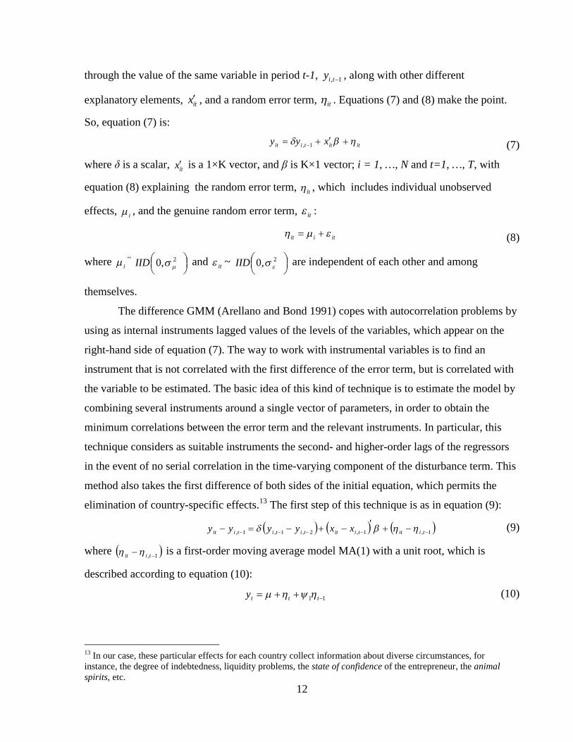
Baltagi (2006), this relationship shows how a variable in period t, say ity , could be explained

11 The subsequent extensions of the basic model proposed in equation (1) permit us to obtain an extended version ofthe Post-Keynesian investment function, where the inclusion of expectations about the development of severalvariables, especially in the case of financial elements, is relevant due to the presence of uncertainty, which emergesfrom different sources. However, our proposal does not include a deviation of the US Treasury bond yields in orderto account for uncertainty and expectations, since this particular asset is not considered risky and volatile.12 In other words, this technique accounts for the effects that provoke the same influence on each individual case inperiod t (individual effects) and those effects that differ from each individual case but are constant through thewhole period (temporary effects).

12

through the value of the same variable in period t-1, , 1i ty , along with other different

explanatory elements, ítx , and a random error term, it . Equations (7) and (8) make the point.

So, equation (7) is:

itíttiit xyy 1, (7)

where δ is a scalar, ítx is a 1×K vector, and β is K×1 vector; i = 1, …, N and t=1, …, T, with

equation (8) explaining the random error term, it , which includes individual unobserved

effects, i , and the genuine random error term, it :

itiit (8)

where i~

2,0 IID and it ~

2,0 IID are independent of each other and among

themselves.

The difference GMM (Arellano and Bond 1991) copes with autocorrelation problems by

using as internal instruments lagged values of the levels of the variables, which appear on the

right-hand side of equation (7). The way to work with instrumental variables is to find an

instrument that is not correlated with the first difference of the error term, but is correlated with

the variable to be estimated. The basic idea of this kind of technique is to estimate the model by

combining several instruments around a single vector of parameters, in order to obtain the

minimum correlations between the error term and the relevant instruments. In particular, this

technique considers as suitable instruments the second- and higher-order lags of the regressors

in the event of no serial correlation in the time-varying component of the disturbance term. This

method also takes the first difference of both sides of the initial equation, which permits the

elimination of country-specific effects.13 The first step of this technique is as in equation (9):

1,1,2,1,1,

tiittiittititiit xxyyyy (9)

where 1, tiit is a first-order moving average model MA(1) with a unit root, which is

described according to equation (10):

11 ttty (10)

13 In our case, these particular effects for each country collect information about diverse circumstances, forinstance, the degree of indebtedness, liquidity problems, the state of confidence of the entrepreneur, the animalspirits, etc.

13

where 1 is the estimated coefficient, E(yt)=, and ηt is a random variable with E(ηt)=0 and

Var(ηt)=σ2.

The presence of endogeneity among the explanatory variables and the existence of

correlation between the error term and the lagged dependent variable compel the application of

instrumental variables. Specifically, the moment conditions, which are used by difference

GMM, are shown in equations (11) and (12):

01,, tiitstiyE (11)

01,, tiitstixE (12)

for 2s ; Tt ,...,1

Under the presence of autocorrelation and individual effects through time, lagged values

could not be adequate instruments for the model in differences. In order to account for this

problem, and improve the efficiency of the GMM estimators, Arellano and Bover (1995) and

Blundell and Bond (1998) have developed the system GMM, which computes the equation in

differences, as shown in (9), and also adds an equation in levels as shown in equation (13):

itíttiiit xyy 1,(13)

where i captures fixed effects. The equation in levels considers as instruments the lagged

differences of the regressors, while the regression in differences utilizes the same instruments as

in the difference GMM technique. Equation (13) shows how ity is a function of i , and it is

correlated with the compound error, it . The presence of country-specific effects disappears by

first-differencing, but it is kept in the equation in levels. The instruments for the regression in

differences are those that are used in the difference GMM estimator. In the case of the equation

in levels, the relevant instruments are the lagged differences of the variables. The system GMM

utilizes the equation in levels and tries to find instruments that are correlated with 1ity but not

with i —instead of dropping i with the model in differences. Equations (14) and (15) show

the moment conditions considered by this technique:

0, iitstiyE (14)

0, iitstixE (15)

for 2s ; Tt ,...,1

14

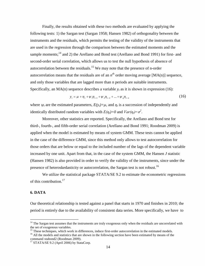
Finally, the results obtained with these two methods are evaluated by applying the

following tests: 1) the Sargan test (Sargan 1958; Hansen 1982) of orthogonality between the

instruments and the residuals, which permits the testing of the validity of the instruments that

are used in the regression through the comparison between the estimated moments and the

sample moments;14 and 2) the Arellano and Bond test (Arellano and Bond 1991) for first- and

second-order serial correlation, which allows us to test the null hypothesis of absence of

autocorrelation between the residuals.15 We may note that the presence of n-order

autocorrelation means that the residuals are of an nth order moving average [MA(n)] sequence,

and only those variables that are lagged more than n periods are suitable instruments.

Specifically, an MA(n) sequence describes a variable yt as it is shown in expression (16):

ntqtttty ...2211(16)

where t are the estimated parameters, E(yt)=, and ηt is a succession of independently and

identically distributed random variables with E(ηt)=0 and Var(ηt)=σ2.

Moreover, other statistics are reported. Specifically, the Arellano and Bond test for

third-, fourth-, and fifth-order serial correlation (Arellano and Bond 1991; Roodman 2009) is

applied when the model is estimated by means of system GMM. These tests cannot be applied

in the case of the difference GMM, since this method only allows to test autocorrelation for

those orders that are below or equal to the included number of the lags of the dependent variable

increased by one unit. Apart from that, in the case of the system GMM, the Hansen J statistic

(Hansen 1982) is also provided in order to verify the validity of the instruments, since under the

presence of heteroskedasticity or autocorrelation, the Sargan test is not robust.16

We utilize the statistical package STATA/SE 9.2 to estimate the econometric regressions

of this contribution.17

6. DATA

Our theoretical relationship is tested against a panel that starts in 1970 and finishes in 2010; the

period is entirely due to the availability of consistent data series. More specifically, we have to

14 The Sargan test assumes that the instruments are truly exogenous only when the residuals are uncorrelated withthe set of exogenous variables.15 These techniques, which work in differences, induce first-order autocorrelation in the estimated models.16 All the models and statistics that are shown in the following section have been estimated by means of thecommand xtabond2 (Roodman 2009).17 STATA/SE 9.2 (April 2006) by StataCorp.

15

start with the 1970 data because of several reasons: 1) the data on dwelling and gross fixed

capital formation are only provided since 1970 for some of the countries included in our sample;

2) there isn’t much homogenous information about financial variables, like stock market indices

before this time—in fact, this lack of availability of data compels us to include only five

indices;18 and 3) the statistics about capacity utilization began to be published during the 1960s

and we could only find consistent series since 1970. Our sample includes the following

countries: Australia, Austria, Belgium, Canada, Denmark, France, Germany, Italy, the

Netherlands, Norway, Spain, Sweden, the UK, and the US.

The majority of the data come from the AMECO databank, where there is available and

consistent annual data series for the countries under consideration. AMECO is published by the

European Commission’s Directorate General for Economic and Financial Affairs and offers

annual macroeconomic information on a great number of variables.19

The OECD database “Business Tendency and Consumer Opinion Surveys” compiles

capacity utilization information. However, the quarterly Australian series are provided by the

Australian Chamber of Commerce and Industry (“ACCI Westpac Survey of Industrial Trends”)

and the monthly US data by the Federal Reserve website (“G.17 Industrial Production and

Capacity Utilization, Capacity Utilization: Total Industry”). In all of these cases, the annual

average capacity utilization is calculated by using four-quarterly data, except for the US, where

the annual time series is the average value of the twelve observations.

Regarding the financial variables, the main source of data is Wren Investment Advisers

website. This databank provides the annual US Treasury long-term bond yields, the AXS, and

the FTSE indices that cover the whole period. Other sources are also used: Deutsche

Bundesbank, which publishes annual DAX series; Standard & Poor’s, which provides daily

observations of the Standard & Poor’s index since 1989, with previous monthly data available

on the IESE Business School of the University of Navarra website. Finally, Bolsa de Madrid

18 We may note that the development of stock markets is included in our model through the evolution of the DAXindex for all the European economies except for the UK, where FTSE is more relevant, and IGBM for Spain. In thecase of the US and Canada, the relevant index is the Standard & Poor’s, and AXS is computed for Australia.19 The lack of statistics on business capital stock in this databank compels us to calculate the dependent variable ofour model, business accumulation rate, in the following way:

11

t

bt

t

tpr

tt

K

I

K

DGFCFg

where g is the business rate of accumulation, GFCFpr is the private gross fixed capital formation in the privatesector, D accounts for dwellings, Ib is the business investment, and K is the capital stock in the total economy.

16

offers daily information of the IGBM index since 2003, and the IESE Business School of the

University of Navarra provides annual observations for the rest of the period under

consideration. For those financial variables for which there is no annual information available,

we have had to convert the daily or monthly data provided in annual time series by calculating

the average value.

7. EMPIRICAL EVIDENCE

First, the absence of unit roots in our panel was checked by means of several unit root tests. For

this purpose, we have employed the Im, Pesaran, and Shin (2003) tests, which consider an

individual unit root process. We also apply the Levin, Lin, and Chu (2002) test and the Harris

and Tzavalis (1999) test. All of them assume a common unit process, although the Harris–

Tzavalis (1999) test considers that the number of time periods under consideration is fixed.

Apart from that, we also utilize the Fisher-augmented Dickey–Fuller (Choi 2001) test and the

Fisher–Phillips–Perron (Choi 2001) test, which were applied to the observations of each

variable as a set by assuming an individual unit root process. The results of these tests confirm

the lack of a unit root test, which is required to avoid spurious regressions.20

We utilize two lags of each variable for estimation purposes, since there are considerable

delays in the investment process due to the fact that new investment projects require some time

between the investment decision and when the new equipment begins to produce. This time

horizon is enough to capture the investment delay, as has been demonstrated by other studies—

as for example Bean (1981), where a lag structure of three quarters and a delay of seven

quarters is found, and Evans (1967) where five and six quarter lags are empirically established.

All the conventional levels of the included variables are defined by using the Hodrick

and Prescott (1980) filter, which allows for the construction of businessmen’s expectations

based on the trends of the variables employed. Specifically, this filter isolates the trend and the

cyclical components that form a particular time series, and works by minimizing the square of

the deviations from the trend and by penalizing changes in the acceleration of the trend of the

time series.21

20 The results of these tests are not reported in the paper but are available from the authors upon request.21 The Hodrick and Prescott (1980) filter that captures the trend of the variable is compatible with the notion ofconventions, since according to Keynes (1936), the conventional level has to collect the most important values ofthe variable in the past, which moreover, individuals expect to be maintained for the near future. The originalnotion of conventions gives room for the idea that the belief in a future situation similar to the current one could be

17

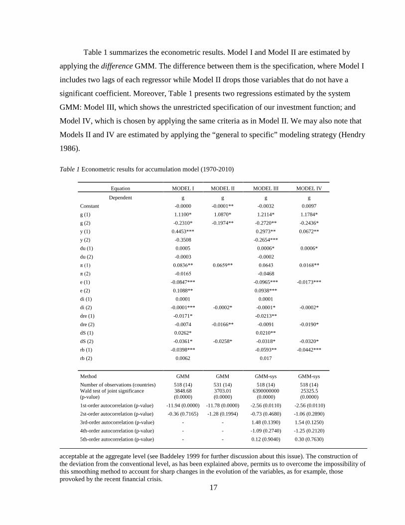
Table 1 summarizes the econometric results. Model I and Model II are estimated by

applying the difference GMM. The difference between them is the specification, where Model I

includes two lags of each regressor while Model II drops those variables that do not have a

significant coefficient. Moreover, Table 1 presents two regressions estimated by the system

GMM: Model III, which shows the unrestricted specification of our investment function; and

Model IV, which is chosen by applying the same criteria as in Model II. We may also note that

Models II and IV are estimated by applying the “general to specific” modeling strategy (Hendry

1986).

Table 1 Econometric results for accumulation model (1970-2010)

Equation MODEL I MODEL II MODEL III MODEL IV

Dependent g g g g

Constant -0.0000 -0.0001** -0.0032 0.0097

g (1) 1.1100* 1.0870* 1.2114* 1.1784*

g (2) -0.2310* -0.1974** -0.2720** -0.2436*

y (1) 0.4453*** 0.2973** 0.0672**

y (2) -0.3508 -0.2654***

du (1) 0.0005 0.0006* 0.0006*

du (2) -0.0003 -0.0002

π (1) 0.0836** 0.0659** 0.0643 0.0168**

π (2) -0.0165 -0.0468

e (1) -0.0847*** -0.0965*** -0.0173***

e (2) 0.1088** 0.0938***

di (1) 0.0001 0.0001

di (2) -0.0001*** -0.0002* -0.0001* -0.0002*

dre (1) -0.0171* -0.0213**

dre (2) -0.0074 -0.0166** -0.0091 -0.0190*

dS (1) 0.0262* 0.0210**

dS (2) -0.0361* -0.0258* -0.0318* -0.0320*

rb (1) -0.0398*** -0.0593** -0.0442***

rb (2) 0.0062 0.017

Method GMM GMM GMM-sys GMM-sys

Number of observations (countries) 518 (14) 531 (14) 518 (14) 518 (14)Wald test of joint significance(p-value)

3848.68(0.0000)

3703.01(0.0000)

6390000000(0.0000)

25325.5(0.0000)

1st-order autocorrelation (p-value) -11.94 (0.0000) -11.78 (0.0000) -2.56 (0.0110) -2.56 (0.0110)

2st-order autocorrelation (p-value) -0.36 (0.7165) -1.28 (0.1994) -0.73 (0.4680) -1.06 (0.2890)

3rd-order autocorrelation (p-value) - - 1.48 (0.1390) 1.54 (0.1250)

4th-order autocorrelation (p-value) - - -1.09 (0.2740) -1.25 (0.2120)

5th-order autocorrelation (p-value) - - 0.12 (0.9040) 0.30 (0.7630)

acceptable at the aggregate level (see Baddeley 1999 for further discussion about this issue). The construction ofthe deviation from the conventional level, as has been explained above, permits us to overcome the impossibility ofthis smoothing method to account for sharp changes in the evolution of the variables, as for example, thoseprovoked by the recent financial crisis.

18

Sargan test (p-value) 487.37 (1.0000) 483.34 (1.0000) 502.57 (0.3970) 500.35 (0.424)

Hansen J test (p-value) - - 0.00 (1.0000) 1.30 (1.0000)

Instruments for levels:

Hansen J test (p-value) - - 0.00 (1.0000) 1.30 (1.0000)

Difference (p-value) - - 0.00 (1.0000) 0.00 (1.0000)

Instruments for exogenous variables:

Hansen J test (p-value) - - 0.00 (1.0000) 3.00 (1.0000)

Difference (p-value) - - 0.00 (1.0000) -1.70 (1.0000)

Note: *, **, and *** indicate statistical significance and rejection of the null at the 1, 5, and 10 percent significancelevels, respectively. Numbers in parentheses, in the case of the variables, show the lag(s) of the relevant variable.

The diagnostics/statistics that validate these econometric results are reported in the lower

part of Table 1. All the models reported in Table 1 reject the null hypothesis of the Wald test of

joint significance. The Wald test checks the value of the regressors by taking into account the

sample under consideration and, in the case of Table 1, provides for the acceptance of the

estimated parameters. The results of the Sargan test, which are provided in each case, validate

the instruments included in the estimated relationships. The Hansen J test is also applied to test

our instruments and the results reported permit us to accept the instruments considered.22

Finally, the autocorrelation between the residuals is examined, since this would indicate whether

we could use lags of the dependent and independent variables as suitable instruments. Those

relationships that are estimated by difference GMM (Models I and II), do not display first- and

second-order autocorrelation. Nevertheless, Models III and IV, which use the system technique,

reject the null hypothesis of absence of first-order autocorrelation; they fulfill, nonetheless, the

condition of absence of second- and higher-order autocorrelation. However, the presence of

first-order autocorrelation in a system GMM regression is not a problem. In fact, we can expect

the presence of this phenomenon since these models are built by applying differences to the

initial equation and the lagged variables to produce the equation in differences and the

instruments of the equation in levels (Arellano and Bond 1991). In this sense, the residuals of

the equation in differences are those that we need to examine seriously. The results of these tests

permit us to validate our estimations, which are described in greater detail in what follows.

To begin with the econometric results, the first column (Model I) reports a positive

impact of expected demand (0.4453) and profit shares in t-1 (0.0836) on accumulation. This

22 The Hansen J test has been applied in several ways: 1) Hansen J test of overidentification, which is applied to theinstruments as a group; 2) Hansen J test for the variables in levels; and 3) Hansen J test for those variables that areexogenous and have been used as instruments. In all of these, the null hypothesis is that the instruments are trulyexogenous.

19

unrestricted specification, which was estimated by difference GMM, also shows how a rise in

the cost of external finance in t-2 (-0.0001) and the presence of increasing uncertainty (-0.0171)

in the previous period dampen current investment. Moreover, an increase in the yield of the US

Treasury bonds exerts a negative and strong incidence on investment (-0.0398). This is so since

this increase makes it more attractive to invest in financial assets without risk, and indirectly,

since this increases the cost of external finance. This model also captures a double effect, which

comes from the stock market. Specifically, in the shorter horizon (t-1), there is a positive impact

(0.0262), which has to be interpreted according to Tobin’s q (Brainard and Tobin 1968, 1977).

However, the development of the stock exchange causes a stronger negative effect on

accumulation in t-2 (-0.0361), which is the one that prevails in the restricted models that we

discuss below. There is also evident a contradictory impact of the level of employment in the

case of Model I. The labor constraint dampens investment in t-1 (-0.0847), although high levels

of employment that are maintained through time can push demand and influence investment

positively (0.1088).

In the restricted version of this model (Model II), the key variable of the model is the

profit share (0.0659), which has the expected positive effect. A negative incidence emanates

from the stock market (-0.0258 in t-2). This version of the model also displays a negative effect

of the cost of external finance and the presence of uncertainty (-0.0002 and -0.0166,

respectively). However, the estimation of the model by means of the system GMM method,

which provides more efficient regressors, increases the number of significant variables in the

case of the restricted version. Model III, which considers two lags for each independent

variable, portrays a positive relationship between the rate of growth of GDP in t-1 and

investment (0.2973). Another variable, which accelerates capital accumulation, is deviations of

capacity utilization in t-1 (0.0006). However, all the financial elements have a negative effect on

accumulation. Specifically, increasing interest rates, rising values of the stock markets, and

higher US Treasury bond yields dampen accumulation by -0.0001, -0.0318, and -0.0593,

respectively. A positive influence of the stock market on investment is also found (0.0210),

which is consistent with the Tobin q model (Brainard and Tobin 1968, 1977). Model III also

shows a double and conflicting impact of the labor market: first, the labor constraint, which

depresses accumulation (-0.0965) is present in t-1; second, there is a positive impact (0.0938)

that arises from the level of employment in t-2. A high level of employment favors good

20

expectations about future demand. Finally, and as expected, the model shows an inverse

relationship between uncertainty and accumulation (-0.0213).

The last column displays the preferred estimation, since the independent variables are

significant, have the correct signs, and the model satisfies the basic statistical requirements

reported in Table 1. Model IV exhibits a positive impact of expectations about future demand

(0.0672), profit shares (0.0168), and deviation of capacity utilization on accumulation (0.0006).

However, this model gives a role to the labor constraint, which depresses investment according

to the theoretical hypothesis (-0.0173). This specification also reports a depressive effect of

interest rates (-0.0002) and bonds (-0.0442). As the theory suggests, uncertainty depresses new

investment (-0.0196). Deviations of the stock market index exert a remarkable negative effect

(-0.0380), which reinforces our hypothesis that the development of the stock market crowds out

physical investment. We may note that all these variables are lagged once, except for the

deviation of the exchange rate, interest rate, and the stock market, which are lagged two periods.

The econometric analysis undertaken supports the theoretical premise as elaborated in

Section 4. This study reinforces the idea that the core of the investment decision is the

accelerator term. As the theoretical framework of the paper suggests, there are two other

elements that accelerate the process of capital accumulation: profit shares and deviations of

capacity utilization. However, entrepreneurs’ expectations about future demand exert the

strongest positive impact on accumulation, since a weak effective demand does not encourage

businessmen to increase capacity even in the case that internal finance is available. The

incidence of profit shares is relevant, although the intensity of this effect is around a quarter of

the one that emerges from expectations about demand. In terms of capacity utilization, its

influence is not very strong, since only when the gap between effective capacity utilization and

its normal level is too big and maintained over a long period would it have an impact. It requires

that demand is systematically stronger than expected for new investment projects to be

undertaken. The negative effect of the labor market conditions is not most important. A negative

effect for the rate of interest is reported as it might be expected.

The econometric results reported in Table 1 produce an inverse effect of uncertainty, as

suggested by our theoretical framework. Its incidence is remarkable since the proxy of

uncertainty employed, the exchange rate, can affect accumulation through different channels,

i.e., international and monetary markets. A negative and strong influence of the stock market on

21

accumulation is also reported. This reinforces the idea of the presence of a kind of crowding-out

between financial and physical investment, which takes place in a financialized economy.

Finally, our study takes into account the US Treasury long-term bond yield as a way of

including the effect of a “safe haven.” The depressive effect of this financial investment is high

since an increase in these yields means, directly, an opportunity to obtain profits without risk,

and, indirectly, a rise in the cost of external finance that reduces the possibility of profitability of

a new project financed externally. The stronger impact of this variable in comparison with the

deviation of the interest rate is easily explained, since the long-term bond yields are capturing

partially the effect of the interest rates that agents have to face when they borrow external

resources. Specifically, an indebted public sector would have to increase the yields of its bonds

in order to attract capital flows, which theoretically induces hikes in the rest of the interest rates.

The importance of the US economy and the strong connections among the economies in the

global markets can explain why changes in US interest rates are often reflected in the interest

rates of the rest of the economies. This fact supports the previous conclusion, even in the case

that we compute just the yields that are provided by the US bond. This evidence is along the

lines portrayed by the Kaleckian and Kaldorian literature about growth and distribution, which

points to a negative effect of interest rates on accumulation (Lavoie 1995; Hein 2007).

Our findings have other implications in terms of the Post-Keynesian theory. On the one

hand, our estimated model is compatible with the Kaleckian view of the investment function,

since profits and the deviation of capacity utilization are key in the investment decision.

Moreover, the definition of the normal rate of capacity utilization based on the past also

supports the Kaleckian notion of the normal level of this element.23 On the other hand, the

negative effect that arises from the inclusion of the stock market contradicts Keynes’ (1936)

original writings and the Tobin q model (Brainard and Tobin 1968, 1977), which point to a

positive relationship between this particular financial market and investment in fixed assets. The

rejection of the Tobin q model, which is derived from our estimations, is in the same direction

of the conclusions reached by Medlen (2003).

23 See also Lavoie, Rodríguez, and Seccareccia (2004) for further discussion about the normal rate of capacityutilization in the Post-Keynesian literature and empirical evidence in the case of Canada.

22

8. CONCLUDING REMARKS

The purpose of this paper is the analysis of the accumulation path in capitalist economies, where

financial markets have become one of the fundamental pillars of the system, especially so after

the financialization process that began in the early 1970s. Although our contribution is rooted in

the basic Keynesian model, it is extended to account for the possibility of external finance

(interest rates) and two financial alternatives to invest in physical assets: bonds and equities. The

former is introduced through the US Treasury long-term bond yield and the latter through the

stock market. The inclusion of financial markets, which fits in well with the presence of

uncertainty, compels us to consider a proxy for this variable. The exchange rate is used for this

purpose.

In our theoretical framework, entrepreneurs’ expectations are built according to the

Keynesian notion of conventions, which helps to make the investment decision in a world

dominated by radical uncertainty. The idea of a conventional or normal level is also applied to

the variable that proxies the level of economic activity, i.e., capacity utilization, and permits the

creation of a deviation between the effective level and the conventional one. Specifically,

deviations of capacity utilization are justified on the premise that businessmen cannot predict

precisely expected demand and they decide to maintain idle capacity in normal conditions.

Moreover, the level of employment is considered as another indicator of the level of economic

activity, whose impact highlights the presence of labor constraints in the process of

accumulation and the existence of tensions between workers and firms, which could depress

business investment.

Our particular approach is tested econometrically by means of the difference GMM and

the system GMM techniques with a panel that collects annual information about 14 OECD

countries from 1970 to 2010. The empirical analysis points to the accelerator term as the main

explanatory element that exerts the strongest positive effect on investment. Accumulation is also

affected by the presence of equities and the impact of deviations between capacity utilization

and its normal level. Nevertheless, there is an inverse relationship between financial elements

(the US Treasury bonds and stock markets) and capital accumulation, which reinforces the

hypothesis of a conflict between physical and financial investment. Our model also highlights a

negative incidence of uncertainty on accumulation, since this phenomenon makes it more

difficult for businessmen to foresee the future. Finally, this study emphasizes how changes in

23

interest rates can affect investment. The estimated relationships confirm the theoretical

explanation of the accumulation process as presented in Section 4.

24

REFERENCES

Alonso-Borrego, C. and M. Arellano. 1996. “Symmetrically Normalized Instrumental-VariableEstimation Using Panel Data.” Journal of Business and Economic Statistics 17(1): 36–49.

Amadeo, E. 1986. “The Role of Capacity Utilization in Long-Period Analysis.” PoliticalEconomy 2(2): 147–85.

Arellano, M. and S. Bond. 1991. “Some Tests of Specification for Panel Data: Monte CarloEvidence and an Application to Employment Equations.” Review of Economic Studies58(2): 277–97.

Arellano, M. and O. Bover. 1995. “Another Look at the Instrumental Variable Estimation ofError-components Models.” Journal of Econometrics 68(1): 29–51.

Arestis, P. 2009. “New Consensus Macroeconomics and Keynesian Critique.” In E. Hein, T.Niechoj, and E. Stockhammer (Eds.), Macroeconomic Policies on Shaky Foundations:Wither Mainstream Macroeconomics? Marburg, Germany: Metropolis.

Arestis, P. and M. Sawyer. 1997. “How Many Cheers for the Tobin Financial Transaction Tax.”Cambridge Journal of Economics 21(6): 753–68.

Baddeley, M. 1999. “Keynes on Rationality, Expectations and Investment.” In C. Sardoni (Ed.),Keynes, Post Keynesianism and Political Economy: Essays in Honour of GeoffHarcourt, vol. III. London, UK: Routledge.

Baltagi, B. H. 1995. Econometric Analysis of Panel Data. Chichester, UK: Wiley.

———. 2006. “Panel Data Models.” In T. E. Mills and K. Patterson (Eds.), Palgrave Handbookof Econometrics, vol. I. New York, UK: Palgrave Macmillan.

Bean, C. R. 1981. “An Econometric Model of Manufacturing Investment in the UK.”Econometric Journal 91(361): 106–21.

Bhaduri, A. and S. Marglin. 1990. “Unemployment and the Real Wage: The Economic Basis forContesting Political Ideologies.” Cambridge Journal of Economics 14(4): 375–93.

Blundell, R. and S. Bond. 1998. “Initial Conditions and Moment Restrictionsin Dynamic Panel Data Models.” Journal of Econometrics 87(1): 115–43.

Brainard, W. C. and J. Tobin. 1968. “Pitfalls in Financial Model Building.” American EconomicReview 58(2): 99–122.

———. 1977. “Asset Markets and the Cost of Capital.” In B. Belassa and R. Nelson (Eds.),Economic Progress, Private Values and Public Policy: Essays in Honour of WilliamFellner, vol. I. New York, NY: North-Holland.

25

Brondolo, J. 2011. “Taxing Financial Transactions: An Assessment of AdministrativeFeasibility.” IMF Working Paper, WP/11/185. Washington DC: International MonetaryFund.

Choi, I. 2001. “Unit Root Tests for Panel Data.” Journal of International Money and Finance20(2): 249–72.

Dallery, T. and T. van Treeck. 2011. “Conflicting Claims and Equilibrium AdjustmentProcesses in a Stock-flow Consistent Macroeconomic Model.” Review of PoliticalEconomy 23(2): 189–211.

Davidson, P. 1991. “Is Probability Theory Relevant for Uncertainty? A Post KeynesianPerspective.” Journal of Economic Perspectives 5(1): 19–43.

DiNardo, J. and M. P. Moore. 1999. “The Phillips Curve is Back? Using Panel Data to Analyzethe Relationship between Unemployment and Inflation in an Open Economy.” NBERWorking Paper No. 7328. Cambridge, MA: National Bureau of Economic Research.

Dutt, A. K. 1984. “Stagnation, Income Distribution and Monopoly Power.” Cambridge Journalof Economics 8(1): 25–40.

———. 1997. “Equilibrium, Path Dependence and Hysteresis in Post-Keynesian Models.” In P.Arestis, G. Palma, and M. Sawyer (Eds.), Capital Controversy, Post-KeynesianEconomics and the History of Economic Thought: Essays in Honour of Geoff Harcourt.London, UK: Routledge.

———. 2011. “Growth and Income Distribution: A Post-Keynesian Perspective.” In E. Heinand E. Stockhammer (Eds.), A Modern Guide to Keynesian Macroeconomics andEconomic Policies. Cheltenham, UK: Edward Elgar.

Fundación Ideas. 2010. Impuestos Para Frenar La Especulación Financiera. Report, May,Madrid: Editado por Fundación IDEAS.

Evans, M. K. 1967. “A Study of Industry Investment Decisions.” Review of Economic Statistics53(1): 151–64.

Hansen, L. P. 1982. “Large Sample Properties of Generalized Method of Moments Estimators.”Econometrica 50(4): 1029–54.

Harris, R. D. F. and E. Tzavalis. 1999. “Inference for Unit Root in Dynamics Panels where theTime Dimension Is Fixed.” Journal of Econometrics 91(2): 201–26.

Hein, E. and C. Ochsen. 2003. “Regimes of Interest Rates, Income Equities, Savings andInvestment: A Kaleckian Model and Empirical Estimations for Some Advanced OECDEconomies.” Metroeconomica 54(4): 404–33.

———. 2007. “Interest, Debt, Distribution and Capital Accumulation in a Post-KaleckianModel.” Metroeconomica 58(2): 310–39.

26

Hendry, D. 1986. “Empirical Modelling in Dynamic Econometrics: the New-constructionSector.” Applied Mathematics and Computation 21: 1–36.

Hsiao, C. and D. C. Mountain. 1994. “A Framework for Regional Modeling and ImpactAnalysis: An Analysis of the Demand for Electricity by Large Municipalities in Ontario,Canada.” Journal of Regional Science 34(3): 361–85.

Hodrick, R. J. and E. C. Prescott. 1980. Postwar US Business Cycles: An EmpiricalInvestigation. Manuscript. Pittsburgh, PA: Carnegie-Mellon University.

IMF. 2010. World Economic Outlook Database, General Government Gross Debt. Percent ofGDP. Washington, DC: International Monetary Fund.

Im, K. S., M. H. Pesaran, and Y. Shin. 2003. “Testing for Unit Roots in Heterogeneous Panels.”Journal of Econometrics 115(1): 53–74.

Keynes, J. M. 1936. The General Theory of Employment, Interest and Money. London, UK:Macmillan.

Kiviet, J. F. 1995. “On Bias, Inconsistency, and Efficiency of Various Estimators in DynamicPanel Data Models.” Journal of Econometrics 68(1): 53–78.

Lavoie, M. 1995. “Interest Rates in Post-Keynesian Models of Growth and Distribution.”Metroeconomica 46(2): 146–77.

Lavoie, M., G. Rodríguez, and M. Seccareccia. 2004. “Similitudes and Discrepancies in Post-Keynesian and Marxist Theories of Investment: A Theoretical and EmpiricalInvestigation.” International Review of Applied Economics 18(2): 127–49.

Levin, A., C. F. Lin, and C. S. J. Chu. 2002. “Unit Root Test in Panel Data: Assymptotic andFinite-Sample Properties.” Journal of Econometrics 108(1): 1–24.

Medlen, C. 2003. “The Trouble with Q.” Journal of Post Keynesian Economics 25(4): 693–98.

Merton, R. K. 1968. Social Theory and Social Structure. New York, NY: Free Press.

Nickell, S. and L. Nunziata. 2002. “Unemployment in the OECD since the 1960s: What Do weKnow?” Paper Presented at the Unemployment Conference, London School ofEconomics, London, UK. May 27–28.

OECD. 2011. Revenue Statistics, 1965–2010, 2011 Edition. Paris, France: Organisation forEconomic Co-operation.

Radcliffe Report. 1957. Report of the Committee on the Working of the Monetary System.London, UK: Her Majesty’s Stationary Office, Cmd 827.

Roodman, D. 2009. “How to Do xtabond2: An Introduction to ‘Difference’ and ‘System’ GMMin Stata.” Stata Journal 9(1): 86–136.

27

Ryoo, S. and P. Skott. 2008. “Financialization in Kaleckian Economies with and without LaborConstraints.” Intervention 5(2): 357–86.

Sargan, J. 1958. “The Estimation of Economic Relationships Using Instrumental Variables.”Econometrica 26(3): 393–415.

Skott, P. 1989. “Effective Demand, Class Struggle and Cyclical Growth.” InternationalEconomic Review 30(1): 231–47.

Skott, P. and B. Zipperer. 2010. “An Empirical Evaluation of Three Post Keynesian Models.”Working Paper 2010-08. Amherst, MA: University of Massachusetts–AmherstDepartment of Economics.

Stockhammer, E. 2004a. “Financialisation and the Slowdown of Accumulation.” CambridgeJournal of Economics 28(5): 719–41.

———. 2004b. The Rise of Unemployment in Europe. Cheltenham, UK: Edward Elgar.

Stockhammer, E. and L. Grafl. 2010. “Financial Uncertainty and Business Investment.” Reviewof Political Economy 22(4): 551–68.

Tobin, J. 1978. “A Proposal for International Monetary Reform.” Eastern Economic Journal4(3–4): 153–59.