Level Set Gait Analysis for Synthesis and Reconstruction

G. Bebis et al. (Eds.): ISVC 2009, Part II, LNCS 5876, pp. 377–386, 2009. © Springer-Verlag Berlin Heidelberg 2009

Level Set Gait Analysis for Synthesis and Reconstruction

Muayed S. Al-Huseiny, Sasan Mahmoodi, and Mark S. Nixon

ISIS, School of Electronics and Computer Science, University of Southampton, UK {mssah07r,sm3,msn}@ecs.soton.ac.uk

Abstract. We describe a new technique to extract the boundary of a walking subject, with ability to predict movement in missing frames. This paper uses a level sets representation of the training shapes and uses an interpolating cubic spline to model the eigenmodes of implicit shapes. Our contribution is to use a continuous representation of the feature space variation with time. The experimental results demonstrate that this level set-based technique can be used reliably in reconstructing the training shapes, estimating in-between frames to help in synchronizing multiple cameras, compensating for missing training sample frames, and the recognition of subjects based on their gait.

1 Introduction

For almost all computer vision problems, segmentation plays an important role in higher level algorithm development. The fact that real world images are mostly com-plex, noisy and occluded makes the achievement of robust segmentation a serious challenge. Some of these difficulties can be tackled via the introduction of prior knowledge [1], due to its capacity to compensate for missing or misleading image information caused by noise, clutter or occlusion [2, 3]. Accordingly a robust gait prior shape should enable improved segmentation of walking subjects. By hitting this target, this paper clears the way to solve other related problems like synchronizing multiple cameras [4] and amenably estimating the temporally correlated prior shapes.

One of the earliest uses of prior knowledge in image segmentation was in the work by Cootes et al [5, 6], in which a Gaussian model was used to learn a set of training shapes represented by a set of corresponding points. Leventon et al [7] image segmen-tation approach uses geodesic active contour [8] guided by statistical prior shape cap-tured by PCA. By using the Chan and Vese [9] segmentation model, Tsai et al [10] modified the Leventon et al [7] approach to develop a prior shape segmentation for objects with linear deformations such as human organs in medical images. This ap-proach has shown success for a wide range of application specifically image segmen-tation tasks.

Human gait segmentation is inherently more challenging, because the deformation of shapes is non-Gaussian and because gait is self occluding. It is also periodic, and as such temporally coherent in terms of the shapes which are not equally likely at all times [2]. Two main directions under the title of statistical shape priors have been suggested and employed so far in order to deal with these issues.

Some authors suggest the use of kernel density [11] to decompose a shape’s deformation modes. The problem however with this approach is that the kernel is chosen regardless of how the data is distributed in feature space [12].

378 M.S. Al-Huseiny, S. Mahmoodi, and M.S. Nixon

An alternative is to use traditional linear PCA, accompanied with some mechanism to synthesize new shapes. In other words the PCA will be used to reduce the dimen-sionality, while the temporally dependent deformation will be handled by this me-chanism. In one early approach, Cremers [2] have developed a gait segmentation model based on Autoregressive (AR) systems as a mechanism to synthesize new shapes.

Motivated by the above, we describe a new approach to shape reconstruction which can reconstruct moving shapes in image sequence: the interpolation with cubic spline, and then application of our proposed method to estimate accurate shapes in a human gait sequences. So in the rest of the paper, section 2 explains the statistical shape model, section 3 deals with the interpolating cubic spline, the results and dis-cussions are presented in section 4 and finally the paper concludes in section 5.

2 Statistical Shape Model

This section describes the process of learning the training set shapes and then re-constructing the learned shapes. Principal Components Analysis (PCA) decomposi-tion is used to capture the main modes of variation that the shape undergoes over time, and to reduce dimensionality. Following Leventon [7], the boundaries of the n shapes with pixels each, constituting the training set, are embedded as the zero level sets of n signed distance functions (SDFs) using Fast Marching [13]-see Fig. 1 for illustration. These functions then form the set , , … , . The goal then is to build a statistical model from this set of shapes.

Fig. 1. Formation of SDFs of four training shapes out of 38 using Fast Marching. Also pro-jected beneath them the corresponding contours that represent their zero level sets.

The mean shape, µ is computed by averaging the elements over the set , i.e., ∑ ⁄ . Then the shapes’ variability is calculated by PCA. First, each shape is cen-tralized by subtracting the mean from to create the mean-offset maps . Next, n column vectors, ui, are formed by vertically stacking the columns of the ith

offset maps to generate n lexicographical column vectors. These vectors collective-ly define the shape-variability ( ) matrix S: u1,u2 , . . . .,un . (1)

Level Set Gait Analysis for Synthesis and Reconstruction 379

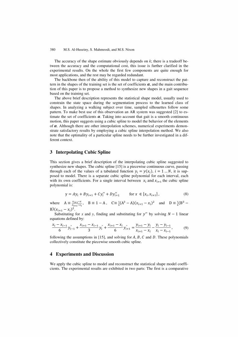
Eigenvalue decomposition is then employed to decompose the matrix ⁄ to its eigenvectors and eigenvalues as: 1 , (2)

where is an matrix whose column vectors represent the modes of variation (principal components) and is the diagonal matrix of the eigenvalues.

In order to reduce the computational burden, the eigenvectors of the (n << N) matrix are computed as: 1 , (3)

then the set of vectors: , (4)

must be normalized to become of unity length: , (5)

which in turn represent the eigenvectors of the matrix ⁄ [14], i.e. .

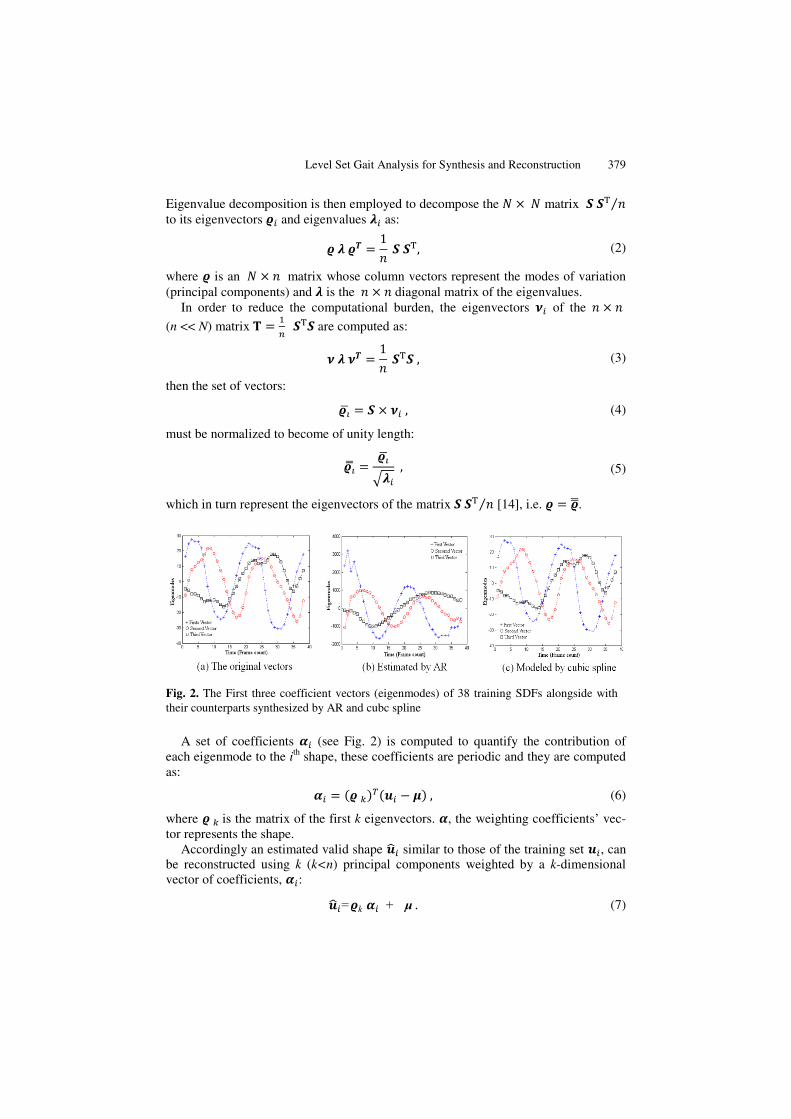
Fig. 2. The First three coefficient vectors (eigenmodes) of 38 training SDFs alongside with their counterparts synthesized by AR and cubc spline

A set of coefficients (see Fig. 2) is computed to quantify the contribution of each eigenmode to the ith shape, these coefficients are periodic and they are computed as: , (6)

where is the matrix of the first k eigenvectors. , the weighting coefficients’ vec-tor represents the shape.

Accordingly an estimated valid shape similar to those of the training set , can be reconstructed using k (k<n) principal components weighted by a k-dimensional vector of coefficients, :

= k + μ . (7)


The accuracy of the shape estimate obviously depends on k; there is a tradeoff be-tween the accuracy and the computational cost, this issue is further clarified in the experimental results. On the whole the first few components are quite enough for most applications, and the rest may be regarded redundant.

The backbone then of the ability of this model to capture and reconstruct the pat-tern in the shapes of the training set is the set of coefficients , and the main contribu-tion of this paper is to propose a method to synthesize new shapes in a gait sequence based on the training set.

The above brief description represents the statistical shape model, usually used to constrain the state space during the segmentation process to the learned class of shapes. In analyzing a walking subject over time, sampled silhouettes follow some pattern. To make best use of this observation an AR system was suggested [2] to es-timate the set of coefficients . Taking into account that gait is a smooth continuous motion, this paper suggests using a cubic spline to model the behavior of the elements of . Although there are other interpolation schemes, numerical experiments demon-strate satisfactory results by employing a cubic spline interpolation method. We also note that the optimality of a particular spline needs to be further investigated in a dif-ferent context.

3 Interpolating Cubic Spline

This section gives a brief description of the interpolating cubic spline suggested to synthesize new shapes. The cubic spline [15] is a piecewise continuous curve, passing through each of the values of a tabulated function , 1 … , it is sup-posed to model. There is a separate cubic spline polynomial for each interval, each with its own coefficients. For a single interval between and the cubic spline polynomial is: y for , , (8)

where A , B 1 A , C A A and D BB . Substituting for x and y, finding and substituting for by solving 1 linear

equations defined by:

6 ′′ 3 ′′ 6 ′′ , (9)

following the assumptions in [15], and solving for , , and . These polynomials collectively constitute the piecewise smooth cubic spline.

4 Experiments and Discussion

We apply the cubic spline to model and reconstruct the statistical shape model coeffi-cients. The experimental results are exhibited in two parts: The first is a comparative


application of AR system and the cubic spline to the shape model. This is aimed to test the performance of the proposed approach in comparison with AR and hence the suitability for use as gait segmentation prior shape model, this is quantified by the error function ℰ described below. The second part includes further tests to verify the robustness of the proposed approach in perceiving the evolution of the implicit shapes, namely by examining its ability to estimate the in-between shapes, by testing its adaptability to the lack of part of the training data, and finally by using the gener-ated model parameters in the recognition of subjects.

• Error Function ℰ : This measure is introduced to assess the accuracy of the estimated shape; the total number of erroneous pixels in the estimated shape is com-puted as follows: ℰ | | , (10)

where is the original shape defined by the training set, is its estimated counterpart. Initially the training set silhouettes are aligned with respect to their centre of gravi-

ty and the corresponding embedding SDFs are computed by applying the Fast March-ing technique [13] (see Fig. 1).

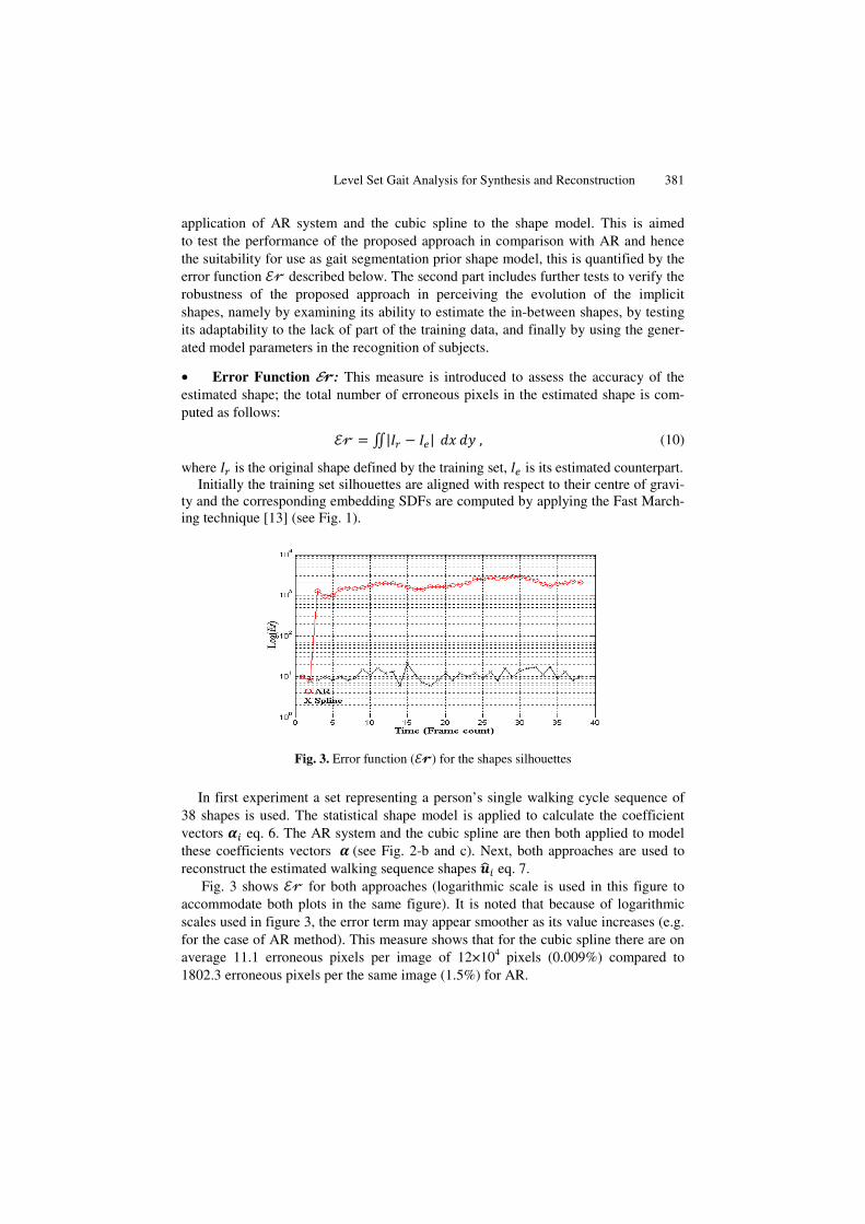
Fig. 3. Error function (ℰ ) for the shapes silhouettes

In first experiment a set representing a person’s single walking cycle sequence of 38 shapes is used. The statistical shape model is applied to calculate the coefficient vectors eq. 6. The AR system and the cubic spline are then both applied to model these coefficients vectors (see Fig. 2-b and c). Next, both approaches are used to reconstruct the estimated walking sequence shapes eq. 7.

Fig. 3 shows ℰ for both approaches (logarithmic scale is used in this figure to accommodate both plots in the same figure). It is noted that because of logarithmic scales used in figure 3, the error term may appear smoother as its value increases (e.g. for the case of AR method). This measure shows that for the cubic spline there are on average 11.1 erroneous pixels per image of 12×104 pixels (0.009%) compared to 1802.3 erroneous pixels per the same image (1.5%) for AR.


Fig. 4 contrasts these results, by showing some of the training sequence shapes alongside with their reconstructed counterparts. In the bottom row it is very easy to observe a filtering effect imposed by the AR system on the time series data, , this may be due to the fact that AR system acts as a recursive discrete time filter [16], and therefore affects the original data due to its intrinsic filtering properties, which ap-pears on the reconstructed shapes in the form of smoothening or even erasing the thin parts of the shapes, like the hands and the feet which in some cases result in invalid shapes like having twisted hands or feet. The middle row which shows the shapes reconstructed by the cubic spline look much more similar to the training set, and this is consistent with the outcome of the error measure ℰr.

Fig. 4. The estimation of the training shapes. Top row is a sample of the training sequence shapes of order (right to left): 1, 5, 10, 13, 21, 26, 28, 33 and 38. Middle row is the same shapes reconstructed by cubic spline. Bottom row is the shapes estimated by AR.

One final point worth mentioning is that AR is not self starting by nature, i.e. it de-pends on initial condition data that must be provided prior to the start of the recon-struction operation, and when such data is not available or inaccurate the subsequent reconstruction is poor, putting this in the context of segmentation this means that the segmentation of the first few frames must rely on an alternative technique, and that the overall segmentation depends on the accuracy of that alternative segmentation technique, this is of course in addition to the genuine shortcoming of the AR demon-strated by the results above. Comparing this with the cubic spline which demonstrated excellent reconstruction results and is self starting data sequence reconstruction tech-nique, the argument may be very strongly held towards using this approach proposed here in the gait prior shape segmentation model.

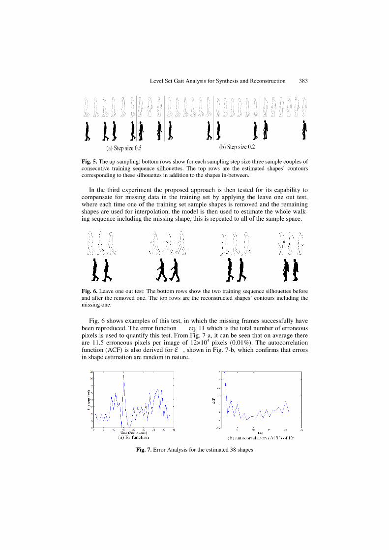
In the second experiment the approach proposed here is tested for its capability to estimate the transitional shapes in-between the successive training shapes, i.e. to up-sample the training data set. This has application in synchronizing multiple cameras. This is quite important because a large number of cameras placed in different locations, working with different sampling rates, produce unsynchronized footages. Up-sampling can numerically synchronize the captured frames by reconstructing in-between frames. Fig. 5 exhibits the subtle movements estimated by this approach us-ing two different sampling rates.

L

Fig. 5. The up-sampling: bottoconsecutive training sequencecorresponding to these silhoue

In the third experiment compensate for missing dawhere each time one of theshapes are used for interpoing sequence including the

Fig. 6. Leave one out test: Theand after the removed one. Thmissing one.

Fig. 6 shows examples obeen reproduced. The errorpixels is used to quantify thare 11.5 erroneous pixels pfunction (ACF) is also deriin shape estimation are rand

Fig. 7.

Level Set Gait Analysis for Synthesis and Reconstruction

om rows show for each sampling step size three sample couplee silhouettes. The top rows are the estimated shapes’ contoettes in addition to the shapes in-between.

the proposed approach is then tested for its capabilityata in the training set by applying the leave one out te training set sample shapes is removed and the remainolation, the model is then used to estimate the whole wamissing shape, this is repeated to all of the sample space

e bottom rows show the two training sequence silhouettes behe top rows are the reconstructed shapes’ contours including

of this test, in which the missing frames successfully hr function eq. 11 which is the total number of erronehis test. From Fig. 7-a, it can be seen that on average thper image of 12×104 pixels (0.01%). The autocorrelatived for ℰ , shown in Fig. 7-b, which confirms that errdom in nature.

Error Analysis for the estimated 38 shapes

383

es ofours

y to test, ning alk-e.

efore g the

have eous here tion rors


The impact of the number of eigenmodes used in the reconstruction and to es-timate missing shapes is assessed by performing the leave one out test to reconstruct missing frames by decreasing the number of eigenmodes iteratively, Fig. 8 shows the results of this experiment. As shown in this figure, by increasing the number of ei-genmodes, the reconstruction error decreases.

Fig. 8. The error function (Er) for estimating the 28th shape in the sequence with the number of eignemodes used in the estimation ranging from 1 to 37

In the fifth experiment the proposed approach is used for recognition based on the assumption that different subjects have different deformability coefficients i.e. α, hence the gait cycles of four different subjects are used in producing four different sets of α, for one of those subjects another test gait cycle different from the one used earlier is also used and the corresponding α is also produced. Next a distance meas-ure is defined as ∑ |α α | , where is the index over the coefficients, is a single period of walking cycle shapes, α and α are the coeffi-cients vectors for which the distance is computed and is the time variable.

This distance is employed and shown good results. This distance is used to choose the subject whose gait cycle coefficients have the least distance from those of the test gait cycle as the recognized one. Table 1 shows that the correct subject (the forth) has been identical with a ratio of 0.003%, that represent the distance for the correct sub-ject relative to the average distance for the incorrect ones.

Table 1. , calculated between the test subject’s set and four subjects’ sets, the correct subject is highlighted

Distance ( ) 1st subject 28992 2nd subject 25158 3rd subject 26722 4th subject 7868

5 Conclusions

This paper has introduced an interpolating cubic spline to better model walking sub-jects by modeling the time variation of the coefficients of the eigenvectors over one


walking cycle. This demonstrated better performance and accuracy over the autore-gressive system used in the literature for the same purpose. The technique proposed here succeeded in capturing the key variability modes which led to success in the re-construction of walking cycle shapes identical to the training set.

Our method presented here was also used successfully in reconstructing the in-between frames which did not exist in the initial training set and hence cleared the way for numerically synchronizing multiple cameras, an application which increa-singly vital with the rise in using monitoring cameras. The method proposed here was also tested for its tolerance to missing parts of the training set for which the technique proved robust.

Furthermore the present technique was employed in recognition by using the va-riability coefficients, which can be further improved by using the orthogonal basis functions such as Chebyshev moments as future work.

The technique proposed here demonstrates promising results and we therefore ex-pect it to be a very useful tool in other gait problem such as action identification and modeling/recognition for the curved path walking cycles in the gait challenge. The technique presented here can be easily applied in other applications, such as modeling the movement of moving objects, including animals.

References

1. Nixon, M.S., Aguado, A.: Feature Extraction & Image Processing, 2nd edn. Academic Press, London (2008)

2. Cremers, D.: Dynamical statistical shape priors for level set-based tracking. IEEE Trans. on PAMI 28(8), 1262–1273 (2006)

3. Mowbray, S.D., Nixon, M.S.: Extraction and recognition of periodically deforming objects by continuous, spatio-temporal shape description. In: Proc. IEEE Conf. on CVPR, vol. 2, pp. 895–901 (2004)

4. Prismall, S.P., Nixon, M.S., Carter, J.N.: Novel Temporal Views of Moving Objects for Gait Biometrics. In: Kittler, J., Nixon, M.S. (eds.) AVBPA 2003. LNCS, vol. 2688, Springer, Heidelberg (2003)

5. Cremers, D.: Statistical shape priors for level set segmentation. PAMM 7(1), 1041903–1041904 (2007)

6. Cootes, T.F., Taylor, C.J., Cooper, D.H., Graham, J.: Active Shape Models-Their Training and Application. Computer Vision and Image Understanding 61(1), 38–59 (1995)

7. Leventon, M.E., Grimson, W.E.L., Faugeras, O.: Statistical shape influence in geodesic ac-tive contours. In: Proc. IEEE Conf. on CVPR, pp. 316–323 (2000)

8. Caselles, V., Kimmel, R., Sapiro, G.: Geodesic Active Contours. International Journal of Computer Vision 22(1), 61–79 (1997)

9. Chan, T.F., Vese, L.A.: Active contours without edges. IEEE Trans. on Image Processing 10(2), 266–277 (2001)

10. Tsai, A., Yezzi Jr., A., Wells, W., Tempany, C., Tucker, D., Fan, A., Grimson, W.E., Willsky, A.: A shape-based approach to the segmentation of medical imagery using level sets. IEEE Trans. on Medical Imaging 22(2), 137–154 (2003)

11. Cremers, D., Osher, S., Soatto, S.: Kernel Density Estimation and Intrinsic Alignment for Shape Priors in Level Set Segmentation. International Journal of Computer Vision 69(3), 335–351 (2006)


12. Dambreville, S., Rathi, Y., Tannenbaum, A.: A Framework for Image Segmentation Using Shape Models and Kernel Space Shape Priors. IEEE Trans. on PAMI 30(8), 1385–1399 (2008)

13. Sethian, J.A.: A fast marching level set method for monotonically advancing fronts. Proc. of the National Academy of Sciences of the United States of America 93(4), 1591–1595 (1996)

14. Leventon, M.E.: Statistical models in medical image analysis, PhD Thesis, MIT (2000) 15. Press, W., Teukolsky, S., Vetterling, W., Flannery, B.: Numerical Recipes with Source

Code CD-ROM, The Art of Scientific Computing, 3rd edn. Cambridge University Press, Cambridge (2007)

16. Oppenheim, A., Schafer, R., Buck, J.: Discrete-Time Signal Processing, 2nd edn. Prentice Hall, Englewood Cliffs (1999)

Level Set Gait Analysis for Synthesis and Reconstruction

Documents

Transcript of Level Set Gait Analysis for Synthesis and Reconstruction