Lepton polarization asymmetries for $B \to K^* \ell^+ \ell^-$: A Model Independent approach

$: Lepton polarization asymmetries for $B \to K^* \ell^+ \ell^-$: A Model Independent approach$
arX

iv:h

ep-p

h/04

0816

4v2

4 F

eb 2

005

Preprint typeset in JHEP style - HYPER VERSION hep-ph/0408164

Lepton polarization asymmetries for B → K∗ℓ+ℓ

−:

A Model Independent approach

A. S. Cornell ∗

Korea Institute of Advanced Study, 207-43 Cheongryangri 2-dong,

Dongdaemun-gu, Seoul 130-722, Korea.

E-mail : [email protected]

Naveen Gaur

Department of Physics & Astrophysics

University of Delhi, Delhi - 110 007, India.

E-mail : [email protected]

Abstract:

In this work we shall derive expressions for the single and double lepton polarization asym-

metries for the exclusive decay B → K∗ℓ+ℓ−, using the most general model independent

effective Hamiltonian. We have conducted this study with this particular channel as it

has the highest branching ratio among the various purely leptonic and semi-leptonic de-

cay modes, making this mode particularly useful for studying physics beyond the SM. We

have also analyzed the effects on these polarization asymmetries, and hence the physics

underlying it, when complex phases are included in some of the Wilson coefficients.

Keywords: B-Physics, Rare Decays, Beyond Standard Model.

∗Present address: Yukawa Institute for Theoretical Physics, Kyoto University, Kitashirakawa Oiwake-

Cho, Sakyo-ku, Kyoto 606-8502, Japan.

http://arxiv.org/abs/hep-ph/0408164v2

http://jhep.sissa.it/stdsearch?keywords=B-Physics+Rare_Decays+Beyond_Standard_Model

Contents

1. Introduction 1

2. The Effective Hamiltonian 3

3. Lepton polarization asymmetries 5

4. Numerical analysis, Results and Discussion 10

A. Input parameters 19

B. Some Analytical Expressions 21

B.1 Parameterization of Form Factors 21

B.2 The unpolarized cross-section 21

1. Introduction

As more and more experimental data is produced by B-factories our quest for finding new

physics signatures in the various decay modes for low energy processes is increasing. The

sheer volume of literature studying the possible signatures of different supersymmetric (and

other) models in the context of B-meson decays evidences how promising a testing ground

these rare decays, induced by the flavour changing neutral current (FCNC) b → s, are.

Of the various hadronic, leptonic and semi-leptonic decays modes (based on the b → s

transition of the B-meson) the semi-leptonic decay modes are extremely significant as they

are theoretically cleaner, and hence very useful for testing various new physics models.

The semi-leptonic decay modes based on the quark level transition b → sℓ+ℓ− offer many

more observables associated with the final state lepton pair, such as the forward-backward

(FB) asymmetry, lepton polarization asymmetries etc. These additional observables could

prove to be very useful in testing the effective structure of these theories and hence the

underlying physics. For this reason many processes like B → π(ρ)ℓ+ℓ− [1], B → ℓ−ℓ+γ [2],

B → Kℓ+ℓ− [3] and the inclusive process B → Xsℓ+ℓ− [4–6] have been studied. But of

the various decay modes of the B-mesons based on the transition b → sℓ+ℓ− the exclusive

mode B → K∗ℓ+ℓ− is one of the more attractive due to it having the highest standard

model (SM) branching ratio. For this reason large numbers of observables in this decay

mode have been studied [7–11].

Previously Aliev et al. [8] studied the various single polarization asymmetries for this

decay mode, where they used the model independent approach earlier proposed by Fukae et

al. [5]. They were able to demonstrate that within the framework of a model independent

– 1 –

theory, constrained by the experimentally measured values of the B → K∗ℓ+ℓ− branch-

ing ratio, there existed regions where the possible new Wilson coefficients could generate

considerable departures from the SM. However, as pointed out in London et al. [12] some

of the single lepton polarization asymmetries may be too small to be observed, and hence

merely the single lepton polarization asymmetries may not provide a sufficient number of

observables to crosscheck the structure of the effective Hamiltonian. With this in mind

more observables are required.

Further to this there has been in the recent observations of the B → ππ and B → πK

decays hints of possible anomalies unexplainable within the SM [13, 14]. These anomalies

arise when we try to match the pattern of data from the B-factories with theory. The recent

Belle and BaBar data regarding the B → ππ mode can be easily explained by taking into

account the non-factorizable contributions. Note that the B → ππ channel is not greatly

effected by the electroweak (EW) penguin diagrams and therefore one can extract the

hadronic parameters from this by assuming isospin symmetry. Using the SU(3) flavour

symmetry we can determine the hadronic B → πK parameters from the relevant B → ππ

modes. As has been pointed out some time back by Buras et al. [13], which has been

revived in many later works [14], this procedure works very well and gives us a good match

between theory and experimental results as long as we are analyzing those modes which are

not greatly affected by the EW penguin diagrams. However, if we try to repeat the same

sort of exercise for modes like Bd → π0KS , which are dominated by EW penguins, then

there is a substantial disagreement between theory and experimental data [13]. Lately some

solutions of this “B → πK puzzle” are being tested and almost all of these propose EW

penguins which are sizably enhanced not only in magnitude but also in their CP-violating

phase, which can become as large as -90o. This proposal is a very interesting one and

can significantly affect many other decay modes. Rather detailed studies of this proposal

have been carried out by Buras et al. [13] leading to possible predictions of substantial

enhancements in the branching ratio of many leptonic and semi-leptonic decay modes,

which will soon be tested in B-factories. This sort of possibility forces us to consider the

option of what could be the possible changes expected in various kinematical observables,

such as the branching ratios, FB asymmetries and various polarization asymmetries, if some

of the Wilson coefficients had such a large phase (making them predominately imaginary).

Note that with this in mind we have analyzed this in an earlier work [15] for the inclusive

decay mode B → Xsℓ+ℓ−. In that study we estimated the variation in the polarization

asymmetries in the inclusive mode if the bsZ vertex were modified. In this work we also

explored the option of allowing some of the Wilson coefficients having large CP violating

phases. This sort of approach to finding the effects of extra phases in Wilsons on various

kinematical observables like branching ratio, partial width CP asymmetry, FB asymmetry

and single lepton polarization asymmetry in B → K∗ℓ+ℓ− have been followed in earlier

works [16]. In this current study we shall also try to analyze what effects there shall be on

the various polarization asymmetries in the B → K∗ℓ+ℓ− decay.

In this study we will work in a model independent framework by taking the most

general form of the effective Hamiltonian and then analyzing the effect on polarization

asymmetries if the Wilson coefficients (mainly the coefficients which correspond to vector

– 2 –

like interactions) have an extra phase. Keeping this eventual aim in mind, this paper shall

be organized as follows: In section 2 we shall introduce the most general form of the effective

Hamiltonian, obtaining (in terms of the forms factors for the B → K∗ transition) the matrix

element for the B → K∗ℓ+ℓ− decay and the unpolarized cross-section. In section 3 we shall

define and calculate the various single and double polarization asymmetries, followed in

section 4 with our numerical analysis. We shall also include a discussion of these results

and our conclusions in this final section.

2. The Effective Hamiltonian

We know, from the paper by Fukae et al. [5] that together with the terms proportional

to our conventionally defined C7 (written below as CSL and CBR for terms corresponding

to the standard −2msC7 and −2mbC7 terms respectively), C9 and C10 (which can be

redefined in terms of CLL and CLR) we have ten independent local four-Fermi interactions

which contribute to the FCNC transition b → sℓ+ℓ−;

Heff =αGF√

2πV ∗

tsVtb

[

CSL

(

siσµνqν

q2Lb

)

(

ℓγµℓ)

+ CBR

(

siσµνqν

q2Rb

)

(

ℓγµℓ)

+CLL (sLγµbL)(

ℓLγµℓL

)

+ CLR (sLγµbL)(

ℓRγµℓR

)

+CRL (sRγµbR)(

ℓLγµℓL

)

+ CRR (sRγµbR)(

ℓRγµℓR

)

+CLRLR (sLbR)(

ℓLℓR

)

+ CRLLR (sRbL)(

ℓLℓR

)

+CLRRL (sLbR)(

ℓRℓL

)

+ CRLRL (sRbL)(

ℓRℓL

)

+CT (sσµνb)(

ℓσµνℓ)

+ iCTE (sσµνb)(

ℓσαβℓ)

ǫµναβ

]

, (2.1)

where q represents the momentum transfer (q = pB − pK∗), L/R = (1 ∓ γ5)/2 and the

CX ’s are the coefficients of the four Fermi interactions. Among these there are four vector

type interactions (CLL, CLR, CRL and CRR), two of which contain contributions from the

SM Wilson coefficients. These two coefficients, CLL and CLR, can be written as;

CtotLL = C9 − C10 + CLL,

CtotLR = C9 + C10 + CLR. (2.2)

So CtotLL and Ctot

LR describe the sum of the contributions from the SM and new physics.

Eqn.(2.1) also contains four scalar type interactions (CLRLR, CRLLR, CLRRL and CRLRL)

and two tensor type interactions (CT and CTE).

We shall now follow the standard techniques, as seen in references [5, 7–9] of rendering

the quark level transition above to a matrix element which describes the exclusive process

B → K∗ℓ+ℓ−, that is, by parameterizing over the B and K∗ meson states in terms of

form factors. Using the form factor expressions derived in the paper by Ball et al. [17] we

express our hadronic matrix elements as;

〈K∗|s(1 ± γ5)b|B〉 = ∓2imK∗

mb(ǫ∗ · q)A0(s), (2.3)

– 3 –

〈K∗|siσµνqν(1 ± γ5)b|B〉 = −2ǫµνρσǫ∗νqρpσK∗T1(s) ± iT2(s)

[

ǫ∗µ(

m2B − m2

K∗

)

− (ǫ∗ · q)

(2pK∗ + q)µ

]

± iT3(s) (ǫ∗ · q)[

qµ − q2

m2B − m2

K∗

(2pK∗ + q)µ

]

,(2.4)

〈K∗|sγµ(1 ± γ5)b|B〉 = ǫµναβǫ∗νqαpβK∗

(

2V (s)

mB + mK∗

)

± iǫ∗µ (mB + mK∗) A1(s)

∓i (2pK∗ + q)µ (ǫ∗ · q) A2(s)

mB + mK∗

∓iqµ (ǫ∗ · q) 2mK∗

s(A3(s) − A0(s)) , (2.5)

〈K∗|sσµνb|B〉 = −iǫµναβ

[

T1(s)ǫ∗α (2pK∗ + q)β −

(

m2B − m2

K∗

)

q2{T1(s) − T2(s)} ǫ∗αqβ

+2 (ǫ∗ · q)

q2

{

T1(s) − T2(s) −q2

m2B − m2

K∗

T3(s)

}

pαK∗qβ

]

.

(2.6)

Note that the parameterization of these form factors can be found in Appendix B.1.

Using these form factor expressions our matrix element for the decay B → K∗ℓ+ℓ−

can be expressed as;

M(B → K∗ℓ+ℓ−) =αGF

4√

2πVtbV

∗ts

[

(

ℓγµℓ) {

Aǫµνρσǫ∗νqρpσK∗ + iBǫ∗µ + 2i C (pK∗)µ (ǫ∗.q)

}

+(

ℓγµγ5ℓ) {

E ǫµνρσǫ∗νqρpσK∗ + i F ǫ∗µ + 2i G pK∗µ (ǫ∗.q)

}

+i K(

ℓ ℓ)

(ǫ∗.q) + i M(

ℓγ5ℓ)

(ǫ∗.q)

+4iCT

(

ℓσµνℓ)

ǫµνρσ

{

− 2T1ǫ∗ρpσ

K∗ + N1ǫ∗ρqσ − N2(ǫ.q)p

ρK∗q

σ

}

+16CTE

(

ℓσµνℓ)

{

− 2T1ǫ∗µpν

K∗ + M1ǫ∗µqν − M2(ǫ.q)p

µK∗q

ν

}]

,

(2.7)

where;

A =(

CtotLL + CRL

) V (s)

mB + mK∗

− 4 (CSL + CBR)T1(s)

q2,

B =(

CRL + CRR − CtotLL − Ctot

LR

)

(mB + mK∗)A1 − 2 (CBR − CSL)T2(s)

q2

(

m2B − m2

K∗

)

,

C =(

CtotLL + Ctot

LR − CRL − CRR

) A2(s)

mB + mK∗

− 2 (CBR − CSL)1

q2

[

T2(s) +q2

(m2B − m2

K∗)T3(s)

]

,

D = 2(

CtotLL + Ctot

LR − CRL − CRR

) mK∗

q2(A3(s) − A0(s)) + 2 (CBR − CSL)

T3(s)

q2,

– 4 –

+(

CtotLL + Ctot

LR − CRL − CRR

)

+A2(s)

mB + mK∗

− 2 (CBR − CSL)1

q2

[

T2(s) +q2

(m2B − m2

K∗)T3(s)

]

E = 2(

CRR + CtotLR − Ctot

LL − CRL

) V (s)

(mB + mK∗),

F =(

CRR − CtotLR

)

(mB + mK∗)A1(s),

G =(

CRL + CtotLR − Ctot

LL − CRR

) A2(s)

(mB + mK∗),

H = 2(

CtotLR + CRL − Ctot

LL − CRR

) mK∗

q2(A3(s) − A0(s)) +

(

CRL + CtotLR − Ctot

LL − CRR

) A2(s)

(mB + mK∗),

K = 2 (CRLLR + CRLRL − CLRLR − CLRRL)mK∗

mbA0(s),

M = 2 (CLRRL + CRLLR − CLRLR − CRLRL)mK∗

mbA0(s),

N1 = −T1(s) +

(

m2B − m2

K∗

)

q2{T1(s) − T2(s)} ,

N2 =2

q2

[

T1(s) − T2(s) −q2

(m2B − m2

K∗)T3(s)

]

,

M1 = N1,

M2 = N2. (2.8)

Using the above expression we can calculate the unpolarized decay rate as;

dΓ

d s

(

B → K∗ℓ+ℓ−)

=G2

F α2

214π5mB|VtsV

∗tb|2 λ1/2

√

1 − 4m2ℓ

q2∆, (2.9)

where λ = 1 + m4K∗ + s2 − 2(mK∗ + s) − 2mK∗ s with mK∗ = mK∗/mB and s = s/m2

B . s

is the dilepton invariant mass. The function ∆ is defined in Appendix B.2.

3. Lepton polarization asymmetries

In order to now calculate the polarization asymmetries of both the leptons defined in the

effective four fermion interaction of Eqn.(2.1), we must first define the orthogonal vectors

S in the rest frame of ℓ− and W in the rest frame of ℓ+ (where these vectors are the

polarization vectors of the leptons). Note that we shall use the subscripts L, N and T to

correspond to the leptons being polarized along the longitudinal, normal and transverse

directions respectively [2, 4, 6, 8, 12].

SµL ≡ (0, eL) =

(

0,p−

|p−|

)

,

SµN ≡ (0, eN ) =

(

0,pK∗ × p−

|pK∗ × p−|

)

,

SµT ≡ (0, eT ) = (0, eN × eL) , (3.1)

W µL ≡ (0,wL) =

(

0,p+

|p+|

)

,

– 5 –

W µN ≡ (0,wN ) =

(

0,pK∗ × p+

|pK∗ × p+|

)

,

W µT ≡ (0,wT ) = (0,wN ×wL), (3.2)

where p+, p− and pK∗ are the three momenta of the ℓ+, ℓ− and K∗ particles respectively.

On boosting the vectors defined by Eqns.(3.1,3.2) to the c.m. frame of the ℓ−ℓ+ system only

the longitudinal vector will be boosted, whilst the other two vectors remain unchanged.

The longitudinal vectors after the boost will become;

SµL =

( |p−|mℓ

,Eℓp−

mℓ|p−|

)

,

W µL =

( |p−|mℓ

,− Eℓp−

mℓ|p−|

)

. (3.3)

The polarization asymmetries can now be calculated using the spin projector 12 (1 + γ5 6S)

for ℓ− and the spin projector 12 (1 + γ5 6W ) for ℓ+.

Equipped with the above expressions we now define the various single lepton and double

lepton polarization asymmetries. Firstly, the single lepton polarization asymmetries are

defined as [2, 4, 6, 8, 12];

P−x ≡

(

dΓ(Sx,Wx)ds + dΓ(Sx,−Wx)

ds

)

−(

dΓ(−Sx,Wx)ds + dΓ(−Sx,−Wx)

ds

)

(


ds

)

+(


ds

) ,

P+x ≡

(

dΓ(Sx,Wx)ds + dΓ(−Sx,Wx)

ds

)

−(

dΓ(Sx,−Wx)ds + dΓ(−Sx,−Wx)

ds

)

(


ds

)

+(


ds

) , (3.4)

where the sub-index x can be either L, N or T . P± denotes the polarization asymmetry of

the charged lepton ℓ±. Along the same lines we can also define the double spin polarization

asymmetries as [12];

Pxy ≡

(

dΓ(Sx,Wy)ds − dΓ(−Sx,Wy)

ds

)

−(

dΓ(Sx,−Wy)ds − dΓ(−Sx,−Wy)

ds

)

(

dΓ(Sx,Wy)ds +

dΓ(−Sx,Wy)ds

)

+(

dΓ(Sx,−Wy)ds +

dΓ(−Sx,−Wy)ds

) , (3.5)

where the sub-indices x and y can be either L, N or T .

The single lepton polarization asymmetries are then;

P(∓)L =

m2B

∆

√

1 − 4m2ℓ

s

[

± 8

3m4

B sλRe(A∗E) ∓ 4

3m2K∗

{

λ(1 − m2K∗ − s)Re(B∗G)

−(

λ + 12sm2K∗

)

Re(B∗F )}

± 4

3m2K∗

m2Bλ

{

m2BλRe(C∗G) + (1 − m2

K∗ − s)Re(F ∗C)}

+16

3m2K∗

mBmℓRe(B∗CT ){

2(

λ + 12sm2K∗

)

N1 + (m2K∗ + s − 1)

(

m2BλN2 + 24m2

K∗T1

)}

− 16mℓ

3m2K∗

m3BRe(C∗CT )λ

{

m2BλN2 + 2(m2

K∗ + s − 1)N1 + 8m2K∗T1

}

– 6 –

−256mℓ

3m3

BλT1 {Re(A∗CTE) ∓ Re(E∗CT )} − 4mℓ

m2K∗

mBλ{

sRe(H∗K) + (1 − s − m2K∗)

×m2BRe(G∗K) + Re(F ∗K)

}

∓ 64mℓ

3m2K∗

mBλ{

2(λ + 12sm2K∗)N1 + (m2

K∗ + s − 1)

×(

λm2BN2 + 24m2

K∗T1

)}

Re(F ∗CTE) ± 64mℓ

3m2K∗

λm3B

{

λm2BN2 + 2(m2

K∗ + s − 1)N1

+8m2K∗T1

}

Re(G∗CTE) − 2sλ

m2K∗

m2BRe(M∗K) − 64

3m2K∗

m2B

{

m2B sλ2m2

BN22

+16m2Bm2

K∗ sλT1N2 + 64m2K∗

(

λ + 3sm2K∗

)

T 21

}

]

, (3.6)

P(∓)N =

πm3B

√sλ

∆

√

1 − 4m2ℓ

s

[

± 2mBmℓ {Im(A∗F ) + Im(B∗E)} − 1

2m2K∗

{

m2Bλ (Im(K∗C) + Im(M∗G))

+(1 − s − m2K∗) (Im(K∗B) + Im(K∗F ))

}

+ 8m2Bπ

{

sN1 + (m2K∗ + s − 1)T1

}

Im(A∗CT )

+16T1 {2Im(C∗TEB) ± Im(C∗

T F )} − πmℓ

m2K∗

{

(m2K∗ + s − 1)Im(F ∗H) − 4m2

K∗Im(F ∗G)}

+m3B

mℓ

m2K∗

λIm(G∗H) ± 8mBmℓ

m2K∗

{

λm2BN2 + 2

(

m2K∗ + s − 1

)

N1 + 8m2K∗T1

}

Im(C∗TEK)

∓16m2B

{

N1s +(

m2K∗ + s − 1

)

T1

}

]

, (3.7)

P(∓)T =

πm2B

√sλ

∆

[

− 4m2BmℓRe(A∗B) ∓ mℓ

(

m2K∗ + s − 1

)

m2K∗ s

{

m2B s (Re(B∗H) − λRe(C∗H))

+(1 − s − m2K∗)m2

B (Re(G∗B) − λRe(C∗G)) + (Re(F ∗B) − λRe(F ∗C))}

− 16(

4m2ℓ + s

)

λ

s

×{

T1Re(B∗CT ) −(

sN1 + (m2K∗ + s − 1)T1

)

Re(A∗CTE)}

+

(

s − 4m2ℓ

)

2m2K∗ s

{

m2BλRe(K∗G)

+(1 − s − m2K∗)Re(F ∗K)

}

± 8m2B

s

(

sN1 + (m2K∗ + s − 1)T1

) {

m3B

(

s − 4m2ℓ

)

Re(C∗T E)

∓128m2BmℓT1Re(C∗

T CTE)}

± 16mB

sm2K∗

{

2(

8m2ℓ − s

)

m2K∗T1 + 2m2

ℓ

(

m2K∗ + s − 1

)

N1

+m2Bm2

ℓλN2

}

Re(C∗TEG) ∓ 16m3

Bm2ℓ

sm2K∗

{

m2BλN2 + 2

(

m2K∗ + s − 1

)

N1 + 8m2K∗T1

}

Re(MC∗TE)

]

.

(3.8)

And the double polarization asymmetries are;

PLL =1

∆

4m2B

3sm2K∗

[

(

2m2ℓ − s

)

{

m4B sm2

K∗λ|A|2 +1

2

(

λ + 12sm2K∗

)

|B|2 +m4

B

2λ2|C|2 + m2

B

×(

1 − s − m2K∗

)

λRe(B∗C)}

− 32m3B sm2

K∗mℓλT1Re(C∗T A) + 8mB smℓ

{

2(

λ + 12sm2K∗

)

N1

+(

m2K∗ + s − 1

) (

m2BλN2 + 24m2

K∗T1

)

Re(C∗TEB)

}

− 8m3B smℓλ

{

m2BλN2 + 2

(

m2K∗ + s − 1

)

N1

+8m2K∗T1

}

Re(C∗TEC) +

(

4m2ℓ − s

)

m2B sm2

K∗λ

{

m2B|E|2 +

|K|24

}

− 1

2

{(

λ + 12sm2K∗

)

– 7 –

−2m2ℓ

(

5λ + 24sm2K∗

)}

|F |2 − m4B

2λ

{

sλ − 2m2ℓ

(

5λ + 12sm2K∗

)}

|G|2 + m2Bλ

{

s(

m2K∗ + s − 1

)

×Re(F ∗G) − 2m2ℓ

(

5(

m2K∗ + s − 1

)

Re(G∗F ) − 3sRe(H∗F ))}

+ 3m2Bmℓλs {sRe(M∗H)

+m2B

(

1 − s − m2K∗

)

Re(M∗G) + Re(F ∗M)}

+3

4m2

B s2λ|M |2

+4m2B s

(

s − 4m2ℓ

) {

m4Bλ2N2

2 + 4(

λ + 12sm2K∗

)

N21 + 4

(

m2K∗ + s − 1

)

×(

m2BλN1N2 + 24sm2

K∗N1T1

)

+ 16m6B sm2

K∗λN2T1

}

|CT |2 + 256m6Bm2

K∗

{

sλ − 6m2ℓ

×(

λ + 2sm2K∗

)}

T 21 |CT |2 + 4m2

B

(

s − 8m2ℓ

) {

m4Bλ2N2

2 + 4(

λ + 12sm2K∗

)

N21 + 4

(

m2K∗ + s − 1

)

×(

m2BλN1N2 + 24sm2

K∗N1T1

)

+ 16m6B sm2

K∗λN2T1

}

|CTE |2 + 512m6Bm2

K∗

{

sλ − 6m2ℓ

×(

m2K∗ + s − 1

)}

T 21 |CTE |2

]

, (3.9)

PLN =1

∆

m2Bπ

m2K∗

√

λ

s

[

(

m2K∗ + s − 1

)

mℓ

{

m2B

(

sIm(H∗B) +(

1 − s − m2K∗

)

Im(G∗B))

+ Im(F ∗B)}

+λmℓm2B

{

m2B

(

sIm(C∗H) +(

1 − s − m2K∗

)

Im(C∗G))

+ Im(C∗F )}

+mB s

2

{

m2BλIm(C∗M)

+(

1 − s − m2K∗

)

Im(B∗M)}

+(

s − 4m2ℓ

) {

16mBT1Im(B∗CT ) + 16m3B

(

sN1 +(

m2K∗ + s − 1

)

T1

)

×Im(C∗TEA) +

mB

2

((

m2K∗ + s − 1

)

Im(F ∗K) − m2BλIm(G∗K)

)

+ 8m3B

×(

sN1 +(

m2K∗ + s − 1

)

T1

)

Im(E∗CT )}

+ 16mB

{(

2sm2K∗T1 + 2m2

ℓ

(

m2K∗ + s − 1

)

N1

+m2Bm2

ℓλN2

)

Im(C∗TEF ) + m2

Bm2ℓ

(

m2BλN2 + 2

(

m2K∗ + s − 1

)

N1 + 8m2K∗T1

)

((

m2K∗ + s − 1

)

Im(G∗CTE) + sIm(C∗TEH)

)}

+ 8m2Bmℓs

{

m2BλN2 + 2

(

m2K∗ + s − 1

)

N1

+8m2K∗T1

}

]

, (3.10)

PLT =1

∆

m2Bπ

m2K∗

√

λ

s

√

1 − 4m2ℓ

s

[

− 2m2Bm2

K∗mℓsRe(A∗F + B∗E + 8T1C∗T F ) +

mB s

2

{

m2Bλ (Re(K∗C)

−Re(M∗G)) +(

1 − s − m2K∗

)

(Re(B∗K) − Re(M∗F ))}

− 8m3Bm2

K∗ s{

sN1 +(

m2K∗ + s − 1

)

T1

}

× (Re(A∗CT ) − 2Re(C∗T E)) + 32mB sT1Re(B∗CTE) + m2

ℓ s{(

m2K∗ + s − 1

) (

|F |2 + m4Bλ|G|2

)

−2m2BλRe(F ∗G) + m2

B

(

m2K∗ + s − 1

)

sRe(F ∗H) − m4B sλRe(G∗H)

}

+ 8m2Bmℓs

{

m2BλN2

+2(

m2K∗ + s − 1

)

N1 + 8m2K∗T1

}

Re(K∗CTE) − 256m2Bmℓ

{

sN1 +(

m2K∗ + s − 1

)

T1

}

(

|CT |2 + 4|CTE |2)

+ 16m3B s

{

sN1 +(

m2K∗ + s − 1

)

T1

}

Re(C∗TEE)

]

, (3.11)

PNL =1

∆

m2Bπ

m2K∗

√

λ

s

[

−(

m2K∗ + s − 1

)

mℓ

{

m2B

(

sIm(H∗B) +(

1 − s − m2K∗

)

Im(G∗B))

+ Im(F ∗B)}

−λmℓm2B

{

m2B

(

sIm(C∗H) +(

1 − s − m2K∗

)

Im(C∗G))

+ Im(C∗F )}

− mB s

2

{

m2BλIm(C∗M)

+(

1 − s − m2K∗

)

Im(B∗M)}

+(

s − 4m2ℓ

) {

16mBT1Im(B∗CT ) + 16m3B

(

sN1 +(

m2K∗ + s − 1

)

T1

)

×Im(C∗TEA) +

mB

2

((

m2K∗ + s − 1

)

Im(F ∗K) − m2BλIm(G∗K)

)

− 8m3B

×(

sN1 +(

m2K∗ + s − 1

)

T1

)

Im(E∗CT )}

− 16mB

{(

2sm2K∗T1 + 2m2

ℓ

(

m2K∗ + s − 1

)

N1

– 8 –

+m2Bm2

ℓλN2

)

Im(C∗TEF ) + m2

Bm2ℓ

(

m2BλN2 + 2

(

m2K∗ + s − 1

)

N1 + 8m2K∗T1

)

((

m2K∗ + s − 1

)

Im(G∗CTE) + sIm(C∗TEH)

)}

+ 8m2Bmℓs

{

m2BλN2 + 2

(

m2K∗ + s − 1

)

N1

+8m2K∗T1

}

Im(C∗TEM)

]

, (3.12)

PNN =1

∆

2m2B

3sm2K∗

[

m4B

(

s − 4m2ℓ

)

m2K∗λ

(

s|A|2 + s|E|2 +1

2|K|2

)

−{

2(

λ + 12sm2K∗

)

m2K∗ + sλ

} (

|B|2

−m4Bλ|G|2

)

+ m2Bλ

(

s + 2m2ℓ

) {

m2Bλ|C|2 + 2

(

m2K∗ + s − 1

)

(Re(B∗C) − Re(F ∗G)) + |F |2}

−48mBmℓs{

m2BλN2 + 2

(

m2K∗ + s − 1

)

N1 + 8m2K∗T1

}{

m2BλRe(C∗CTE) −

(

m2K∗ + s − 1

)

×Re (B∗CTE)} + 2m2B sm2

ℓλ

(

m2B s|H|2 + 2Re(F ∗H) +

1

4

m2B

m2ℓ

|M |2)

+ 2m2Bλ

(

1 − s − m2K∗

)

×{(

2m2ℓ + s

)

Re(F ∗G) + 6sm2ℓRe(G∗H)

}

− 6mBmℓsλ{

m2B

((

m2K∗ + s − 1

)

Re(G∗M)

−sRe(H∗M)) − Re(M∗F )} + 8m2B s

(

s − 4m2ℓ

)

|CT |2{

m4Bλ2N2

2 + 16m2Bm2

K∗λT1N2

+192m4K∗T 2

1 + 4(

λ + 12sm2K∗

)

N21 + 4

(

m2K∗ + s − 1

) (

m2BλN2 + 24m2

K∗T1

)}

+32m2B s|CTE |2

{

λm2B

(

s + 8m2ℓ

) (

λm2BN2

2 + 16T1m2K∗T1N2

)

+ 19sm4K∗T 2

1 + 4(

8λm2ℓ

+s(

λ + 12sm2K∗

))

N21 + 4

(

m2K∗ + s − 1

) (

m2Bλ

(

s + 8m2ℓ

)

N2 + 24sm2K∗T1

)}

]

, (3.13)

PNT =4

∆

m2B

3m2K∗

√

1 − 4m2ℓ

s

[

m4B sλIm(E∗A) + 32m3

Bmℓλm2K∗T1 (2Im(A∗CTE) + Im(E∗CT ))

+λ{(

m2K∗ + s − 1

) (

m2BIm(G∗B) − Im(C∗F )

)

− Im(F ∗B) + m2BλIm(C∗G)

}

+4mBmℓ

{

2(

λ + 12sm2K∗

)

N1 +(

m2K∗ + s − 1

) (

m2BλN2 + 24m2

K∗T1

)}

Im(C∗T B)

+4m3Bmℓ

{

8λT1m2K∗ + m2

Bλ2N2 + 2λ(

m2K∗ + s − 1

)

N1

}

Im(C∗T C) +

3

2m2

B sλIm(K∗M)

+3m3Bmℓλ

{

m2B

(

sIm(K∗H) +(

1 − s − m2K∗

)

Im(K∗G))

+ Im(K∗F )}

+16mBmℓλ{

m2B

(

8m2K∗T1Im(C∗

TEG) + N2

(

m2BλIm(C∗

TEG) −(

m2K∗ + s − 1

))

N2

)

−2(

Im(C∗TEF ) − m2

B

(

m2K∗ + s − 1

)

Im(C∗TEG)

)}

+ 16m2B s

{

4(

λ + 12sm2K∗

)

N21 + m4

Bλ2

+192m2K∗T 2

1 + 4m2Bλ

(

m2K∗ + s − 1

)

N1N2 + 96(

m2K∗ + s − 1

)

T1N1 + 16λm2BT1N2

}

×Im(C∗TECT )

]

, (3.14)

PTL =1

∆

m2Bπ

sm2K∗

√

λ

s

√

1 − 4m2ℓ

s

[

2m2Bm2

K∗mℓsRe(A∗F + B∗E + 8T1C∗T F ) +

mB s

2

{

−m2Bλ (Re(K∗C)

−Re(M∗G)) −(

1 − s − m2K∗

)

(Re(B∗K) + Re(M∗F ))}

− 8m3Bm2

K∗ s{

sN1 +(

m2K∗ + s − 1

)

T1

}

× (Re(A∗CT ) − 2Re(C∗T E)) + 32mB sT1Re(B∗CTE) + m2

ℓ s{(

m2K∗ + s − 1

) (

|F |2 + m4Bλ|G|2

)

−2m2BλRe(F ∗G) + m2

B

(

m2K∗ + s − 1

)

sRe(F ∗H) − m4B sλRe(G∗H)

}

+ 8m2Bmℓs

{

m2BλN2

+2(

m2K∗ + s − 1

)

N1 + 8m2K∗T1

}

Re(K∗CTE) − 256m2Bmℓ

{

sN1 +(

m2K∗ + s − 1

)

T1

}

(

|CT |2 + 4|CTE |2)

− 16m3B s

{

sN1 +(

m2K∗ + s − 1

)

T1

}

Re(C∗TEE)

]

, (3.15)

– 9 –

PTN =4

∆

m2B

3m2K∗

√

1 − 4m2ℓ

s

[

3m4B sλIm(E∗A) + 32m3

Bmℓλm2K∗T1 (−2Im(A∗CTE) + Im(E∗CT ))

+λ{(

m2K∗ + s − 1

) (

m2BIm(G∗B) − Im(C∗F )

)

− Im(F ∗B) + m2BλIm(C∗G)

}

+4mBmℓ

{

2(

λ + 12sm2K∗

)

N1 +(

m2K∗ + s − 1

) (

m2BλN2 + 24m2

K∗T1

)}

Im(C∗T B)

+4m3Bmℓ

{

8λT1m2K∗ + m2

Bλ2N2 + 2λ(

m2K∗ + s − 1

)

N1

}

Im(C∗T C) +

3

2m2

B sλIm(K∗M)

+3m3Bmℓλ

{

m2B

(

sIm(K∗H) +(

1 − s − m2K∗

)

Im(K∗G))

+ Im(K∗F )}

+48mBmℓλ{

m2B

(

8m2K∗T1Im(C∗

TEG) + N2

(

m2BλIm(C∗

TEG) −(

m2K∗ + s − 1

))

N2

)

−2(

Im(C∗TEF ) − m2

B

(

m2K∗ + s − 1

)

Im(C∗TEG)

)}

+ 16m2B s

{

4(

λ + 12sm2K∗

)

N21 + m4

Bλ2

+192m2K∗T 2

1 + 4m2Bλ

(

m2K∗ + s − 1

)

N1N2 + 96(

m2K∗ + s − 1

)

T1N1 + 16λm2BT1N2

}

×Im(C∗TECT )

]

, (3.16)

PTT =2

3∆m2

B

[

λ(

s + 4m2ℓ

)

m4B|A|2 +

1

s

{

λs − 2(

λ + 12sm2K∗

)}

|B|2 +

(

2m2ℓ − s

)

sm2K∗

λm2B

{

λ|C|2

−2(

m2K∗ + s − 1

)

Re(B∗C)}

+ 128m3BmℓλT1Re(A∗CT ) + m2

Bλ(

s − 4m2ℓ

) (

−|E|2

+3

2m2K∗

|K|2)

+ 16mBmℓ

m2K∗

{

2(

λ − 12sm2K∗

)

N1 +(

m2K∗ + s − 1

) (

m2BλN2 − 24m2

K∗T1

)}

×Re(B∗CTE) − 32m3B

mℓλ

m2K∗

{

8m2K∗T1 + m2

BλN2 − 2λ(

m2K∗ + s − 1

)

N1

}

Re(C∗CTE)

+m4B

λ

m2K∗ s

{

λs − 2m2ℓ

(

5λ + 12sm2K∗

)}

|G|2 +

(

s − 10m2ℓ

)

λ

sm2K∗

{

|F |2 − 2m4B

(

m2K∗ + s − 1

)

Re(F ∗G)}

−12m2B

m2ℓλ

m2K∗

Re(F ∗H) + 6mBmℓλ

m2K∗

{

m2B

((

m2K∗ + s − 1

)

Re(M∗G) − sRe(H∗M))

− Re(M∗F )}

−3

2m2

B

λs

m2K∗

|M |2 + 8m2

B

sm2K∗

{(

4m2ℓ − s

) ((

λ + 12sm2K∗

)

sN21 + λ2m4

BN22 + 16sm2

K∗m2Bλ

)

+4(

4m2ℓ − s

) (

m2K∗ + s − 1

)

s(

λm2BN1N2 + 24m2

K∗N1T1

)

+ 64m2K∗

(

4m2ℓλ − 3m2

K∗ s2)

T 21

}

×|CT |2 + 32m2

B

sm2K∗

{

4((

λ + 12sm2K∗

)

s − 8m2ℓλ

)

sN21 − sλm2

BN2

(

8m2ℓ − s

) (

λN2 + 2m2K∗T1

)

−4m2B

(

8m2ℓ − s

) (

m2K∗ + s − 1

)

sλN1N2 + 64m2K∗

(

4λm2ℓ + 3m2

K∗ s2)

T 21 + 96

(

m2K∗ + s − 1

)

m2K∗

+s2N1T1

}

|CTE |2]

. (3.17)

4. Numerical analysis, Results and Discussion

In this final section we shall present the results of our numerical analysis. As such, the

input parameters which we have used, in order to calculate the various Wilson coefficients

defined in Eqn.(2.1), are listed in Appendix A. The value of C7 is fixed by the observation

of b → sγ. Note that this observation fixes the magnitude and not the sign of C7, we

have therefore choosen the SM predicted value C7 = −0.313. For C10 we have used the

– 10 –

0

1

2

3

4

5

-3 -2 -1 0 1 2 3

Br(B

→ K

* τ+ τ− ) ✕

107

CX

CLLCLRCRLCRR

CLRLR = CRLRLCRLLR = CLRRL

CTCTE

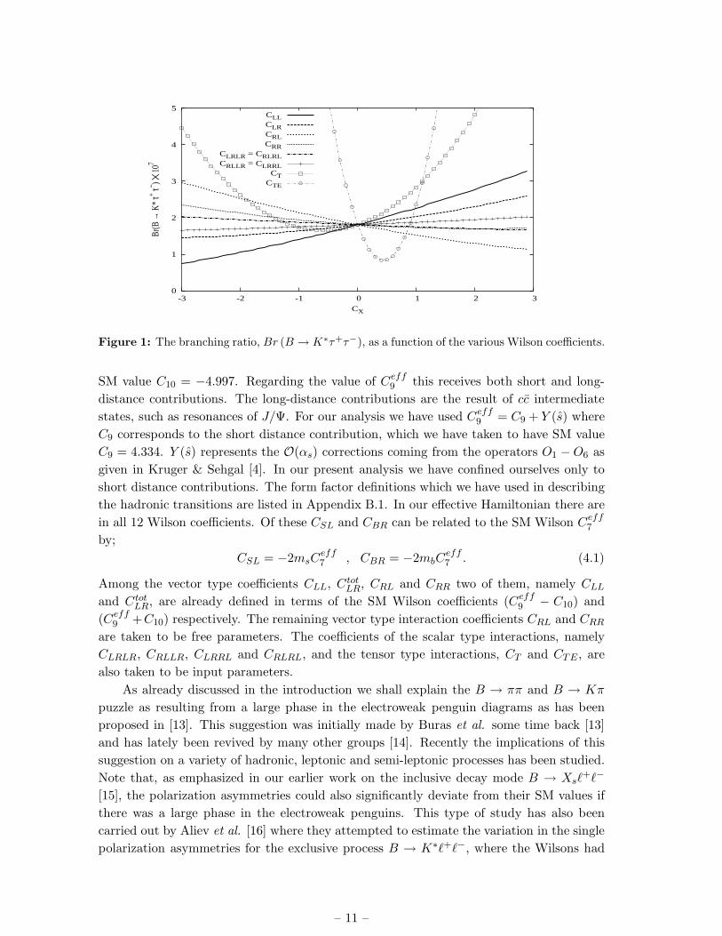
Figure 1: The branching ratio, Br (B → K∗τ+τ−), as a function of the various Wilson coefficients.

SM value C10 = −4.997. Regarding the value of Ceff9 this receives both short and long-

distance contributions. The long-distance contributions are the result of cc intermediate

states, such as resonances of J/Ψ. For our analysis we have used Ceff9 = C9 + Y (s) where

C9 corresponds to the short distance contribution, which we have taken to have SM value

C9 = 4.334. Y (s) represents the O(αs) corrections coming from the operators O1 − O6 as

given in Kruger & Sehgal [4]. In our present analysis we have confined ourselves only to

short distance contributions. The form factor definitions which we have used in describing

the hadronic transitions are listed in Appendix B.1. In our effective Hamiltonian there are

in all 12 Wilson coefficients. Of these CSL and CBR can be related to the SM Wilson Ceff7

by;

CSL = −2msCeff7 , CBR = −2mbC

eff7 . (4.1)

Among the vector type coefficients CLL, CtotLR, CRL and CRR two of them, namely CLL

and CtotLR, are already defined in terms of the SM Wilson coefficients (Ceff

9 − C10) and

(Ceff9 +C10) respectively. The remaining vector type interaction coefficients CRL and CRR

are taken to be free parameters. The coefficients of the scalar type interactions, namely

CLRLR, CRLLR, CLRRL and CRLRL, and the tensor type interactions, CT and CTE, are

also taken to be input parameters.

As already discussed in the introduction we shall explain the B → ππ and B → Kπ

puzzle as resulting from a large phase in the electroweak penguin diagrams as has been

proposed in [13]. This suggestion was initially made by Buras et al. some time back [13]

and has lately been revived by many other groups [14]. Recently the implications of this

suggestion on a variety of hadronic, leptonic and semi-leptonic processes has been studied.

Note that, as emphasized in our earlier work on the inclusive decay mode B → Xsℓ+ℓ−

[15], the polarization asymmetries could also significantly deviate from their SM values if

there was a large phase in the electroweak penguins. This type of study has also been

carried out by Aliev et al. [16] where they attempted to estimate the variation in the single

polarization asymmetries for the exclusive process B → K∗ℓ+ℓ−, where the Wilsons had

– 11 –

-0.4

-0.35

-0.3

-0.25

-0.2

-0.15

-0.1

-0.05

0

0.05

-3 -2 -1 0 1 2 3

<PLL

>

CX

CLLCLRCRLCRR


CTCTE

Figure 2: The double polarization asymmetry, PLL, as a function of the various Wilson coefficients,

where both τ leptons are longitudinally polarized.

some extra phase. Aliev et al. in their study of the single lepton polarization asymmetries

in the exclusive process B → K∗ℓ+ℓ− also emphasized the importance of the tensorial

interactions on various asymmetries [8]. They concluded that single polarization asym-

metries are very sensitive to scalar and tensor type interactions. In our earlier work [18]

we demonstrated the supersymmetric effects on various double polarization asymmetries

in B → K∗ℓ+ℓ−, where supersymmetry predicts the existence of scalar and pseudo-scalar

operators in the large tanβ region1 [19]. However, in this previous study we did not in-

clude the tensorial structures. In this current work we will use the most general form of the

effective Hamiltonian to study the effects on various polarization asymmetries. We shall

also include the extra possible phase from the electroweak penguin sector.

Note that in this paper these additional effects from the electroweak penguin sector,

which can give effective structures similar to those given in Eqn.(2.1) with coefficients CLL,

CLR, CRL and CRR, will all be given an additional phase. As already stated in section 2

two of these coefficients, namely CLL and CLR, can be parameterized in terms of C9 and

C10. Therefore we shall only consider effects of a new phase in the C10, CRL and CRR

coefficients. For this purpose we will parameterize these coefficients as;

C10 = |C10|eiφ10 , (4.2)

CRL = |CRL|eiφRL , (4.3)

CRR = |CRR|eiφRR . (4.4)

As the majority of our results involve the polarization asymmetries, listed in the pre-

vious section, which are dependent on the scaled invariant mass (s), it is experimentally

useful to consider the averaged values of these asymmetries. Therefore we shall present

1tanβ is the ratio of the vev’s of two Higgs bosons

– 12 –

0

0.01

0.02

0.03

0.04

0.05

0.06

0.07

0.08

-3 -2 -1 0 1 2 3

<PLN

>

CX

CLLCLRCRLCRR


CTCTE

Figure 3: The same as Figure (2), but for ℓ− longitudinal and ℓ+ normal.

-0.5

-0.4

-0.3

-0.2

-0.1

0

0.1

0.2

0.3

-3 -2 -1 0 1 2 3

<PLT

>

CX

CLLCLRCRLCRR


CTCTE

Figure 4: The same as Figure (2), but for ℓ− longitudinal and ℓ+ transverse.

only the averaged values of the polarization asymmetries in our results using the averaging

procedure defined as;

〈Pi〉 =

∫ (mB−mK∗ )2

4m2ℓ

PidΓ

dsds

∫ (mB−mK∗ )2

4m2ℓ

dΓ

dsds

. (4.5)

Our results are presented in a series of figures commencing with Figure (1) where we

have plotted the branching ratio of B → K∗τ+τ− as a function of the various Wilson

coefficients. In this plot we have constrained the value of the branching ratio to have an

upper bound Br(B → K∗τ+τ−) ≤ 5 × 10−7. As can be seen from this graph the largest

variation in the branching ratio corresponds to tensorial type interactions.

– 13 –

-0.09

-0.08

-0.07

-0.06

-0.05

-0.04

-0.03

-0.02

-0.01

0

-3 -2 -1 0 1 2 3

<PN

L>

CX

CLLCLRCRLCRR


CTCTE

Figure 5: The same as Figure (2), but for ℓ− normal and ℓ+ longitudinal.

-0.4

-0.3

-0.2

-0.1

0

0.1

0.2

0.3

0.4

-3 -2 -1 0 1 2 3

<PN

N>

CX

CLLCLRCRLCRR


CTCTE

Figure 6: The same as Figure (2), but for both leptons polarized in the normal direction.

Figures (2)-(10) represent the various double polarization asymmetries plotted as func-

tions of the various Wilson coefficients. In these plots we have assumed that all the Wilson

coefficients are real. In all cases we have varied the Wilson coefficients over a range of -3 to

3. It is also apparent that, as in the case of the branching ratio, the greatest variation of

the various double polarization asymmetries corresponds to the tensorial type interactions.

From the graphs of the polarization asymmetries we can also see substantial variations for

various other values of the Wilson coefficients. The major change is that produced in the

plots of < PLL >, < PLT >, < PNN >, < PNT >, < PTL >, < PTN > and < PTT >

where the respective asymmetry can even change sign for certain values of the Wilson co-

efficients! Note that in these plots we have only shown those asymmetries which are larger

than 10−3. As such the variations of CLL, CRL and CLR, in the respective asymmetries

for Figures (7) and (9), are not shown.

– 14 –

-0.03

-0.025

-0.02

-0.015

-0.01

-0.005

0

0.005

0.01

0.015

-3 -2 -1 0 1 2 3

<PN

T>

CX

CRRCLRLR = CRLRLCRLLR = CLRRL

CTCTE

Figure 7: The same as Figure (2), but for ℓ− normal and ℓ+ transverse.

-0.3

-0.2

-0.1

0

0.1

0.2

0.3

0.4

-3 -2 -1 0 1 2 3

<PTL

>

CX

CLLCLRCRLCRR


CTCTE

Figure 8: The same as Figure (2), but for ℓ− transverse and ℓ+ longitudinal.

Note in particular that the < PLL > in Figure (2) shows substantial dependence on

the CLR, CLRLR, CRLLR, CRR, CT and CTE coefficients in which the magnitude of the

asymmetry can change by more than 100%. Of major significance is that the tensorial

operators can even change the sign of this asymmetry. A very similar sort of behaviour is

exhibited by these Wilson coefficients for < PLN >, < PNL > and < PNT >, except here

in the case of < PLN > and < PNL > the sign of the asymmetry does not change. We can

also see in Figure (6) that for the case of < PNN > all the Wilson coefficients, with the

exception of CLL and CRL, predict a sign change.

These results prompt us to analyze the polarization asymmetries for the case where

the branching ratio of B → K∗τ+τ− remains close to the SM value. This sort of scenario

could tell us more about how the various Wilson coefficients affect various asymmetries

(as they are different quadratic functions of the Wilsons and hence carry independent sets

– 15 –

-0.01

-0.008

-0.006

-0.004

-0.002

0

0.002

0.004

0.006

-3 -2 -1 0 1 2 3

<PTN

>

CX

CRRCLRLR = CRLRLCRLLR = CLRRL

CTCTE

Figure 9: The same as Figure (2), but for ℓ− transverse and ℓ+ normal.

of information). This possibility has been presented in Figure (11), where we have also

restricted the branching ratio to the range 1 × 10−7 < Br(B → K∗τ+τ−) < 4 × 10−7.

From these graphs we observe that there can be substantial variation in the polarization

asymmetries even if the branching ratio is not substantially different from its SM value. As

can be seen from Figure (11) all the polarization asymmetries shows substantial variations.

Some of the asymmetries, in particular < PLL >, < PLT >, < PNN >, < PNT >, < PTL >,

< PTN > and < PTT > not only show variation in magnitude but even their sign changes.

Some asymmetries like < PNN >, < PTL > and < PTT > can change by more than an

order of magnitude, even if there is no major change in the branching ratio. Note that all

these asymmetries are most sensitive to tensorial structures in the effective Hamiltonian.

The next set of results we present includes the extra phase in the Wilson coefficients,

as stated in Eqns.(4.2), (4.3) and (4.4). In Figures (12) and (13) we have plotted integrated

polarization asymmetries as a function of the phase φ10. In Figure (12) we have used the

SM value C10 = 4.669. Note that we have only shown those asymmetries which vary with

the inclusion of φ10. In Figure (13) we have plotted the same variables but with an increase

in the magnitude of C10, namely we have chosen |C10| = 9. This value has been chosen

to correspond with the value calculated by Buras et al. [13] which they predict in order

to solve the B → ππ and B → Kπ puzzle. They say that C10 should be complex with a

magnitude almost twice that of its SM value with a phase which should make it almost

imaginary. As can be seen in both the Figures there is a substantial deviation as the phase,

φ10, is changed.

In Figure (14) we have plotted the correlations of various polarization asymmetries

and the branching ratio of B → K∗τ+τ−. In this plot we have varied the phase φRL in a

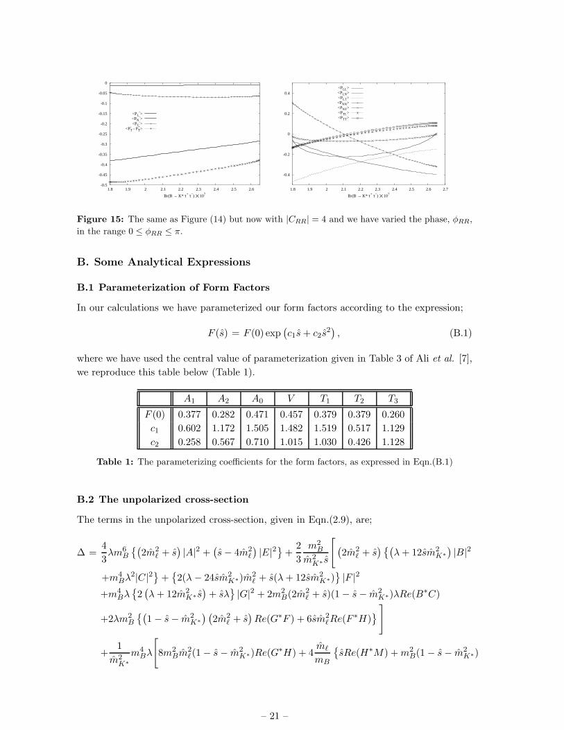
range of 0 ≤ φRL ≤ π. Finally in Figure (15) we have drawn the same sort of plot but for

CRR. As we can see from these graphs some of the polarization asymmetries can change

sign as we vary the phase of the CRL and CRR Wilsons.

For the numerical analysis the central values of the form factors given in Appendix

– 16 –

-0.3

-0.2

-0.1

0

0.1

0.2

0.3

0.4

0.5

-3 -2 -1 0 1 2 3

<PTT

>

CX

CLLCLRCRLCRR


CTCTE

Figure 10: The same as Figure (2), but for both leptons polarized in the transverse direction.

B.1 and [7] have been used. These form factors have substantial uncertainties associated

with them but as can be seen from the various plots we have shown that these polarization

asymmetries have substantial variations even if we restrict ourselves to a branching ratio

near the SM value. In fact some of the asymmetries can even change sign, as shown in

Figure (11). Although changing the form factor definition will change the quantitative

nature of these asymmetries (and the branching ratio) the qualitative nature of these

observables would remain the same (as the variations in the asymmetries is substantial

and hence even with uncertainties present in form factor definitions one can still draw

definite conclusions regarding the asymmetries).

Finally, in order to measure these various polarization asymmetries we must determine

how many BB pairs are required. Using the arguments given in [3, 20], experimentally an

observation of the polarization asymmetry of a decay with branching ratio B at a

nσ level to the required number of events is given by (i.e. the number of BB pairs);

N =n2

s1s2 B < Pij >(for double polarization asymmetries)

N =n2

s B < Pi >(for single polarization asymmetries) (4.6)

In the above equation s1, s2 and s are the efficiencies of detecting the state of polarization

of τ leptons. If we take s1(= s2 = s) to be 0.5 then the number of events required to

– 17 –

-0.4

-0.35

-0.3

-0.25

-0.2

-0.15

-0.1

-0.05

0

0.05

1 1.5 2 2.5 3 3.5 4



Br(B → K* τ+ τ−) ✕ 107

CLLCLRCRLCRR

CSCT

CTE

0.01

0.02

0.03

0.04

0.05

0.06

0.07

1 1.5 2 2.5 3 3.5 4



Br(B → K* τ+ τ−) ✕ 107

CLLCLRCRLCRR

CSCT

CTE

-0.5

-0.4

-0.3

-0.2

-0.1

0

0.1

0.2

0.3

1 1.5 2 2.5 3 3.5 4



Br(B → K* τ+ τ−) ✕ 107

CLLCLRCRLCRR

CSCT

CTE

-0.09

-0.08

-0.07

-0.06

-0.05

-0.04

-0.03

-0.02

-0.01

1 1.5 2 2.5 3 3.5 4



Br(B → K* τ+ τ−) ✕ 107

CLLCLRCRLCRR

CSCT

CTE

-0.4

-0.3

-0.2

-0.1

0

0.1

0.2

0.3

0.4

1 1.5 2 2.5 3 3.5 4



Br(B → K* τ+ τ−) ✕ 107

CLLCLRCRLCRR

CSCT

CTE

-0.03

-0.025

-0.02

-0.015

-0.01

-0.005

0

0.005

0.01

0.015

1 1.5 2 2.5 3 3.5 4



Br(B → K* τ+ τ−) ✕ 107

CLLCLRCRLCRR

CSCT

CTE

-0.3

-0.2

-0.1

0

0.1

0.2

0.3

1 1.5 2 2.5 3 3.5 4



Br(B → K* τ+ τ−) ✕ 107

CLLCLRCRLCRR

CSCT

CTE

-0.01

-0.008

-0.006

-0.004

-0.002

0

0.002

0.004

0.006

1 1.5 2 2.5 3 3.5 4



Br(B → K* τ+ τ−) ✕ 107

CLLCLRCRLCRR

CSCT

CTE

-0.4

-0.3

-0.2

-0.1

0

0.1

0.2

0.3

0.4

1 1.5 2 2.5 3 3.5 4



Br(B → K* τ+ τ−) ✕ 107

CLLCLRCRLCRR

CSCT

CTE

Figure 11: Plots of various integrated polarization asymmetries with Branching ratio of B →K∗τ+τ−. In above figures CS = CLRLR = CRLRL = CRLLR = CLRRL.

observe various asymmetries at the 3σ level would be2;

N =

(2 ± 1) × 108 for < PL >,< PN >,< PT >,

(8 ± 3) × 108 for < PLL >,< PLT >,

(5 ± 3) × 109 for < PLN >,< PNL >,

(8 ± 7.5) × 109 for < PNN >,< PTL >,< PTT >,

(2 ± 1.5) × 1010 for < PNT >,< PTN > .

(4.7)

The number of BB pairs required to observe these asymmetries might not be produced at

the present generation B-factories but future factories like LHCb and Super-B would be

able to measure these asymmetries.

The study of polarization asymmetries in B → K∗ℓ+ℓ− has also been done within

the model independent framework by Aliev et al. [8]. Their study of the single lepton

polarization asymmetries was done with real valued Wilsons. Our results agree with those

2here we are taking the efficiency of detecting the polarization state, including the efficiency of τ mea-

surement and detection of the polarization of τ . If τ detection efficiency is 80% and efficiency of detection

of its polarization state is 60% then the total efficiency of detecting τ in a particular polarization state is

0.8 × 0.6 ≈ 0.5.

– 18 –

they obtained with the exception of typographical errors in their expression of the normal

polarization asymmetries P±N .

The polarization asymmetries provide us a large number of observables which would

be very useful in determining the structure of the effective Hamiltonian; which in turn

could help us in discovering the structure of the underlying physics. The most general ef-

fective Hamiltonain for transitions based on b → s(d)ℓ+ℓ− quark level transition has twelve

Wilsons. If we consider all these Wilsons to be complex valued, this would result in 24

parameters and we would need at least 24 observables in order to fix all these parameters.

Of these the measurement of b → sγ can fix one of them, namely the magnitude of C7.

The observables which are presently at our disposal are the branching ratio and the FB

asymmetry. Along with these two one can construct six single lepton polarization asymme-

tries (three for each of the leptons) in addition one can have nine more double polarization

asymmetries. This would still leaves us with six more unconstrained parameters. This

number can be further restricted if we also construct the polarized FB asymmetries (which

would gives us 15 more observables, namely six single lepton polarization asymmetries and

nine double lepton polarization asymmetries). With this in mind a comprehensive study of

polarized FB asymmetries was done by Aliev et al. [10]. Inclusion of all these observables

would give us 33 observables with which to fix the 24 parameters. So even if some of our

observables are small we should still have sufficiently many observables to constrain the

value of our 24 parameters.

To summarize, the various polarization asymmetries show a strong dependence on

the scalar and tensorial interactions. Also the phase of the Wilson coefficients can give

substantial deviations in the polarization asymmetries. This is of great importance as

various polarization asymmetries have different bilinear combinations of Wilsons and hence

have independent information. Hence they can be very useful in not only estimating the

magnitude of the various Wilson coefficients but also in providing information regarding

their phases.

Acknowledgments

The authors would like to thank S. Rai Choudhury for the useful discussions during the

course of the work. The authors are also greatful to T. M. Aliev for some useful clarifica-

tions.

The work of NG was supported under SERC scheme of the Department of Science and

Technology (DST), India in project no. SP/S2/K-20/99. NG would like to thank KIAS,

Korea for their hospitality, where part of this work was also done.

A. Input parameters

|VtbV∗ts| = 0.0385 , α = 1

129

– 19 –

-0.8

-0.6

-0.4

-0.2

0

0.2

0.4

0.6

0.8

0 20 40 60 80 100 120 140 160 180

φ10

<PL->

<PN->

<PT->

<P-T - P+

T>

-0.3

-0.2

-0.1

0

0.1

0.2

0.3

0 20 40 60 80 100 120 140 160 180

φ10

<PLL><PLN><PLT><PNN><PNT><PTL><PTT>

Figure 12: The variation of the lepton polarization asymmetries as a function of the phase (in

degrees), φ10, of C10 where we have taken |C10| = 4.669.

-0.8

-0.6

-0.4

-0.2

0

0.2

0.4

0.6

0.8

0 20 40 60 80 100 120 140 160 180

φ10

<PL->

<PN->

<PT->

<P-T - P+

T>

-0.5

-0.4

-0.3

-0.2

-0.1

0

0.1

0.2

0.3

0.4

0 20 40 60 80 100 120 140 160 180

φ10


Figure 13: The same as Figure (12) but now taking |C10| = 9.

-0.8

-0.6

-0.4

-0.2

0

0.2

1 1.5 2 2.5 3 3.5

Br(B → K* τ+ τ−) ✕ 107

<PL->

<PN->

<PT->

<P-T - P+

T>

-0.4

-0.3

-0.2

-0.1

0

0.1

0.2

0.3

1 1.5 2 2.5 3 3.5

Br(B → K* τ+ τ−) ✕ 107


Figure 14: The polarization asymmetries as a function of the branching ratio varied across the

phase range 0 ≤ φRL ≤ π; where the magnitude of CRL is taken to be |CRL| = 4.

GF = 1.17 × 10−5 GeV−2 , ΓB = 4.22 × 10−13 GeV

mB = 5.3 GeV , mK∗ = 0.89 GeV , mb = 4.5 GeV

– 20 –

-0.5

-0.45

-0.4

-0.35

-0.3

-0.25

-0.2

-0.15

-0.1

-0.05

0

1.8 1.9 2 2.1 2.2 2.3 2.4 2.5 2.6

Br(B → K* τ+ τ−) ✕ 107

<PL->

<PN->

<PT->

<P-T - P+

T>

-0.4

-0.2

0

0.2

0.4

1.8 1.9 2 2.1 2.2 2.3 2.4 2.5 2.6 2.7

Br(B → K* τ+ τ−) ✕ 107


Figure 15: The same as Figure (14) but now with |CRR| = 4 and we have varied the phase, φRR,

in the range 0 ≤ φRR ≤ π.

B. Some Analytical Expressions

B.1 Parameterization of Form Factors

In our calculations we have parameterized our form factors according to the expression;

F (s) = F (0) exp(

c1s + c2s2)

, (B.1)

where we have used the central value of parameterization given in Table 3 of Ali et al. [7],

we reproduce this table below (Table 1).

A1 A2 A0 V T1 T2 T3

F (0) 0.377 0.282 0.471 0.457 0.379 0.379 0.260

c1 0.602 1.172 1.505 1.482 1.519 0.517 1.129

c2 0.258 0.567 0.710 1.015 1.030 0.426 1.128

Table 1: The parameterizing coefficients for the form factors, as expressed in Eqn.(B.1)

B.2 The unpolarized cross-section

The terms in the unpolarized cross-section, given in Eqn.(2.9), are;

∆ =4

3λm6

B

{(

2m2ℓ + s

)

|A|2 +(

s − 4m2ℓ

)

|E|2}

+2

3

m2B

m2K∗ s

[

(

2m2ℓ + s

) {(

λ + 12sm2K∗

)

|B|2

+m4Bλ2|C|2

}

+{

2(λ − 24sm2K∗)m2

ℓ + s(λ + 12sm2K∗)

}

|F |2

+m4Bλ

{

2(

λ + 12m2K∗ s

)

+ sλ}

|G|2 + 2m2B(2m2

ℓ + s)(1 − s − m2K∗)λRe(B∗C)

+2λm2B

{(

1 − s − m2K∗

) (

2m2ℓ + s

)

Re(G∗F ) + 6sm2ℓRe(F ∗H)

}

]

+1

m2K∗

m4Bλ

[

8m2Bm2

ℓ(1 − s − m2K∗)Re(G∗H) + 4

mℓ

mB

{

sRe(H∗M) + m2B(1 − s − m2

K∗)

– 21 –

×Re(G∗M) + Re(F ∗M)} + (s − 4m2ℓ )|K|2 + s|M |2

]

+16

3

1

m2K∗

{(

s − 4m2ℓ

)

|CT |2 + 4(

s + 8m2ℓ

)

|CTE|2}

×[

4(

λ + 12sm2K∗

)

N21 + λ2N2

2 − 4m2B(1 − s − m2

K∗)(

λN1N2 + m2K∗N1T1

)

+16m2Bm2

K∗λN2T1

]

+1024

3

m4B

s|CT |2T 2

1

[

2(

λ − 6m2K∗ s

)

m2ℓ + λs

]

+4096

3

m4B

s|CTE |2T 2

1

[

2m2ℓ

(

λ + 12sm2K∗

)

+ sλ]

. (B.2)

References

[1] S. R. Choudhury and N. Gaur, Phys. Rev. D 66, 094015 (2002) [hep-ph/0206128].

[2] S. Rai Choudhury, N. Gaur and N. Mahajan, Phys. Rev. D 66, 054003 (2002)

[hep-ph/0203041]; S. R. Choudhury and N. Gaur, hep-ph/0205076 ; E. O. Iltan and

G. Turan, Phys. Rev. D 61, 034010 (2000), [hep-ph/9906502]; G. Erkol and G. Turan Acta.

Phys. Pol. B 33, 1285, (2002) [hep-ph/0112115]; G. Erkol and G. Turan, Phys. Rev. D 65,

094029 (2002), [hep-ph/0110017]; T. M. Aliev, A. Ozpineci, M. Savci, Phys. Lett. B 520, 69

(2001), [hep-ph/0105279].

[3] S. R. Choudhury, A. S. Cornell, N. Gaur and G. C. Joshi, Phys. Rev. D 69, 054018 (2004)

[hep-ph/0307276] ; T. M. Aliev, V. Bashiry and M. Savci, hep-ph/0311294 ; T. M. Aliev,

M. K. Cakmak, A. Ozpineci and M. Savci, Phys. Rev. D 64, 055007 (2001)

[hep-ph/0103039].

[4] F. Kruger and L. M. Sehgal, Phys. Lett. B 380, 199 (1996), [hep-ph/9603237 ] ;

J. L. Hewett, Phys. Rev. D 53, 4964 (1996), [hep-ph/9506289].

[5] S. Fukae, C. S. Kim, T. Morozumi and T. Yoshikawa, Phys. Rev. D 59, 074013 (1999)

[hep-ph/9807254].

[6] S. Rai Choudhury, A. Gupta and N. Gaur, Phys. Rev. D 60, 115004 (1999)

[hep-ph/9902355]; S. Fukae, C. S. Kim and T. Yoshikawa, Phys. Rev. D 61, 074015 (2000)

[hep-ph/9908229]; D. Guetta and E. Nardi, Phys. Rev. D 58, 012001 (1998)

[hep-ph/9707371].

[7] A. Ali, P. Ball, L. T. Handoko and G. Hiller, Phys. Rev. D 61, 074024 (2000)

[hep-ph/9910221].

[8] T. M. Aliev, M. K. Cakmak and M. Savci, Nucl. Phys. B 607, 305 (2001) [hep-ph/0009133];

T. M. Aliev and M. Savci, Phys. Lett. B 481, 275 (2000) [hep-ph/0003188].

[9] G. Burdman, Phys. Rev. D 52, 6400 (1995) [hep-ph/9505352].

[10] T. M. Aliev, V. Bashiry and M. Savci, JHEP 0405, 037 (2004) [hep-ph/0403282].

[11] T. M. Aliev, A. Ozpineci, M. Savci and C. Yuce, Phys. Rev. D 66, 115006 (2002)

[hep-ph/0208128] ; T. M. Aliev, A. Ozpineci and M. Savci, Phys. Lett. B 511, 49 (2001)

[hep-ph/0103261] ; E. O. Iltan, G. Turan and I. Turan, J. Phys. G 28, 307 (2002)

[hep-ph/0106136] ; T. M. Aliev, A. Ozpineci and M. Savci, Nucl. Phys. B 585, 275 (2000)

– 22 –

http://xxx.lanl.gov/abs/hep-ph/0206128
























[hep-ph/0002061] ; T. M. Aliev, C. S. Kim and Y. G. Kim, Phys. Rev. D 62, 014026 (2000)

[hep-ph/9910501] ; T. M. Aliev and E. O. Iltan, Phys. Lett. B 451, 175 (1999)

[hep-ph/9804458] ; T. M. Aliev, C. S. Kim and M. Savci, Phys. Lett. B 441, 410 (1998)

[hep-ph/9804456].

[12] W. Bensalem, D. London, N. Sinha and R. Sinha, Phys. Rev. D 67, 034007 (2003)

[hep-ph/0209228] ; N. Gaur, hep-ph/0305242 ; A. S. Cornell and N. Gaur, JHEP 0309, 030

(2003) [hep-ph/0308132].

[13] A. J. Buras and R. Fleischer, Eur. Phys. J. C 16, 97 (2000) [hep-ph/0003323]. A. J. Buras,

R. Fleischer, S. Recksiegel and F. Schwab, Phys. Rev. Lett. 92, 101804 (2004)

[hep-ph/0312259] ; A. J. Buras, R. Fleischer, S. Recksiegel and F. Schwab, hep-ph/0402112

; A. J. Buras, F. Schwab and S. Uhlig, hep-ph/0405132 ; A. J. Buras, R. Fleischer,

S. Recksiegel and F. Schwab, Eur. Phys. J. C 32, 45 (2003) [hep-ph/0309012].

[14] T. Yoshikawa, Phys. Rev. D 68, 054023 (2003) [hep-ph/0306147]. M. Gronau and

J. L. Rosner, Phys. Lett. B 572, 43 (2003) [hep-ph/0307095]. M. Beneke and M. Neubert,

Nucl. Phys. B 675, 333 (2003) [hep-ph/0308039].

[15] S. Rai Choudhury, N. Gaur and A. S. Cornell, Phys. Rev. D 70 057501 (2004)

[hep-ph/0402273].

[16] F. Kruger and E. Lunghi, Phys. Rev. D 63, 014013 (2001) [hep-ph/0008210]. T. M. Aliev,

D. A. Demir and M. Savci, Phys. Rev. D 62, 074016 (2000) [hep-ph/9912525]. G. Erkol and

G. Turan, Nucl. Phys. B 635, 286 (2002) [hep-ph/0204219].

[17] P. Ball and V. M. Braun, Phys. Rev. D 58, 094016 (1998) [hep-ph/9805422].

[18] S. R. Choudhury, N. Gaur, A. S. Cornell and G. C. Joshi, Phys. Rev. D 68, 054016 (2003)

[hep-ph/0304084].

[19] S. R. Choudhury and N. Gaur, Phys. Lett. B 451, 86 (1999) [hep-ph/9810307].

[20] T. M. Aliev, V. Bashiry and M. Savci, arXiv:hep-ph/0409275.

– 23 –























Lepton polarization asymmetries for $B \to K^* \ell^+ \ell^-$: A Model Independent approach

Documents

Transcript of Lepton polarization asymmetries for $B \to K^* \ell^+ \ell^-$: A Model Independent approach