Learning to Transform Time Series with a Few Examples

Learning to Transform Time Serieswith a Few ExamplesAli Rahimi, Benjamin Recht, and Trevor Darrell

Abstract—We describe a semisupervised regression algorithm that learns to transform one time series into another time series given

examples of the transformation. This algorithm is applied to tracking, where a time series of observations from sensors is transformed

to a time series describing the pose of a target. Instead of defining and implementing such transformations for each tracking task

separately, our algorithm learns a memoryless transformation of time series from a few example input-output mappings. The algorithm

searches for a smooth function that fits the training examples and, when applied to the input time series, produces a time series that

evolves according to assumed dynamics. The learning procedure is fast and lends itself to a closed-form solution. It is closely related to

nonlinear system identification and manifold learning techniques. We demonstrate our algorithm on the tasks of tracking RFID tags

from signal strength measurements, recovering the pose of rigid objects, deformable bodies, and articulated bodies from video

sequences. For these tasks, this algorithm requires significantly fewer examples compared to fully supervised regression algorithms or

semisupervised learning algorithms that do not take the dynamics of the output time series into account.

Index Terms—Semisupervised learning, example-based tracking, manifold learning, nonlinear system identification.

Ç

1 INTRODUCTION

MANY fundamental problems in machine perception,computer graphics, and controls involve the transfor-

mation of one time series into another. For example, intracking, one transforms a time series of observations fromsensors to the pose of a target, one can generate computeranimation by transforming a time series representing themotions of an actor to vectorized graphics and, fundamen-tally, a controller maps a time series of measurements froma plant to a time series of control signals. Typically, suchtime series transformations are specified programmaticallywith application-specific algorithms. We present an alter-native: Algorithms that learn how to transform time seriesfrom examples. This paper demonstrates how nonlinearregression techniques, when augmented with a prior on thedynamics of their output, can transform a variety of timeseries with very few output examples.

Given enough input-output examples, nonlinear regres-

sion techniques can learn and represent any smooth

mapping using any sufficiently general family of functions

such as multilayer perceptrons or radial basis functions.

But, for many of the time series transformation applications

addressed here, traditional nonlinear regression techniques

require too many input-output examples to be of practical

use. To accommodate the dearth of available examples, our

algorithms utilize easy-to-obtain side information in theform of a prior distribution on the output time series.Utilizing this prior to regularize the output allows ouralgorithms to take advantage of “unlabeled,” examples, orexamples for which no output example is provided.

In tracking applications, the output time series representsthe motion of physical objects, so we expect that this timeseries will exhibit physical dynamics. We assume that alinear-Gaussian autoregressive model that roughly capturesthe dynamics of the output time series is a priori available. It isconvenient to specify these dynamics by hand, as is done inmuch of the tracking literature. Like nonlinear regressionmethods, our algorithms search for a smooth function that fitsthe given input-output examples. In addition, this function isalso made to map inputs to outputs that exhibit temporalbehavior consistent with the given dynamical model. Thesearch for this function is expressed as a joint optimizationover the labels of the unlabeled examples and a mapping in aReproducing Kernel Hilbert Space. We show empirically thatthe algorithms are not very sensitive to their parametersettings, including those of the dynamics model, so finetuning this model is often not necessary.

We demonstrate our algorithms with an interactivetracking system for annotating video sequences: The userspecifies the desired output for a few key frames in the videosequence and the system recovers labels for the remainingframes of the video sequence. The output examples are real-valued vectors that may represent any temporally smoothlyvarying attribute of the video frames. For example, to trackthe limbs of a person in a 1-minute-long video, only 13 framesof the video needed to be manually labeled with the positionof the person’s limbs. The estimated mapping between videoframes and the person’s pose is represented using radialkernels centered on the frames of the video sequence. Becausethe system can take advantage of unlabeled data, it can tracklimbs much more accurately than simple interpolation ortraditional nonlinear regression given the same number ofexamples. The very same algorithm can be used to learn to

IEEE TRANSACTIONS ON PATTERN ANALYSIS AND MACHINE INTELLIGENCE, VOL. 29, NO. 10, OCTOBER 2007 1759

. A. Rahimi is with Intel, 1100 NE 45th Street, 6th Floor, Seattle, WA98105. E-mail: [email protected].

. B. Recht is with the Center for the Mathematics of Information, CaliforniaInstitute of Technology, 1200 East California Blvd, MC126-93, Pasadena,CA 91125. E-mail: [email protected].

. T. Darrell is with the Computer Science and Artificial IntelligenceLaboratory, Massachusetts Institute of Technology, 32 Vassar Street, Room32-D512, Cambridge, MA 02139. E-mail: [email protected].

Manuscript received 21 Feb. 2006; revised 9 Sept. 2006; accepted 9 Oct. 2006;published online 3 Jan. 2007.Recommended for acceptance by S. Soatto.For information on obtaining reprints of this article, please send e-mail to:[email protected], and reference IEEECS Log Number TPAMI-0171-0206.Digital Object Identifier no. 10.1109/TPAMI.2007.1001.

0162-8828/07/$25.00 � 2007 IEEE Published by the IEEE Computer Society

track deformable contours like the contour of lips (repre-sented with a spline curve). The system is interactive, so theuser may specify additional examples to improve theperformance of the system where needed. Our method worksdirectly on the provided feature space, which in the case ofimages may be raw pixels, extracted silhouttes, or trackedcontours. No explicit representation or reasoning aboutocclusions or 3D is required in our approach. Our algorithmscan also be applied in nonvisual settings. We can learn totransform the voltages induced in a set of antennae by a RadioFrequency ID (RFID) tag to the position of the tag with onlyfour labeled examples.

Our main contribution is to demonstrate empirically thatfor a large variety of tracking problems, sophisticatedgenerative models and nonlinear filters that are prone tolocal minima are not needed. Instead, a few examples coupledwith very generic assumptions on the dynamics of the latentspace and simple quadratic optimization are sufficient. Wedemonstrate this by regularizing the output of a regressionalgorithm with a dynamical model. This results in a nonlinearsystem identification algorithm that, rather than estimatingan observation function that maps latent states to observa-tions, estimates a function that maps observations to latentstates. This affords us significant computational advantagesover existing nonlinear system identification algorithmswhen the observation function is invertible and the dynamicsare known, linear, and Gaussian. When the dimensionality ofeach output is lower than that of each observation, thisestimated function performs dimensionality reduction. Thus,our contribution is also a semisupervised manifold learningalgorithm that takes advantage of the dynamics of the low-dimensional representation.

2 RELATED WORK

This work is closely related to the problem of nonlineardimensionality reduction using manifold learning. Mani-fold learning techniques [1], [2], [3], [4], [5], [6] find low-dimensional representations that preserve geometric attri-butes high-dimensional observed points. To define theseattributes, these algorithms identify local neighborhoodsalong the manifold of observations by thresholding pair-wise distances in the ambient space. When the manifold issparsely sampled, neighboring points along the manifoldare difficult to identify and the algorithms can fail torecover any meaningful geometric attributes [7]. Ourapproach utilizes the time-ordering of data points to obviatethe need to construct neighborhoods. While we do rely onthe distance between pairs of points, these distances areused only to enforce the smoothness of the manifold.

Jenkins and Mataric [8] suggest artificially reducing thedistance between temporally adjacent points to provide anadditional hint to Isomap about the local neighborhoods ofimage windows. We take advantage of dynamics in the low-dimensional space to allow our algorithm to better estimatethe distance between pairs of temporally adjacent pointsalong the manifold. This requires only small enoughsampling over time to retain the temporal coherence betweenvideo frames, which is much less onerous than the samplingrate required to correctly estimate neighborhood relation-ships in traditional manifold learning algorithms. Varioussemisupervised extensions to manifold learning algorithmshave been proposed [9], [10], but these algorithms still do not

take advantage of the temporal coherence between adjacentsamples of the input time series.

Our technique is semisupervised in that it takes advantageof both labeled data (the input-output examples) andunlabeled data (the portions of the input time series withoutoutput examples). The semisupervised regression ap-proaches of [11] and [12] take into account the manifoldstructure of the data, but they also rely on estimates of theneighborhood structure and do not take advantage of thetime ordering of the data set. These semisupervised regres-sion methods are similar to our method in that they alsoimpose a random field on the low-dimensional representa-tion. The work presented here augments these techniques byintroducing the temporal dependency between outputsamples in the random field. It can be viewed as a specialcase of estimating the parameters of a continuous-valuedconditional random field [13] or a manifold learningalgorithm based on function estimation [14]. The algorithmsin this article are based on our earlier work [15]. Here, weprovide a simpler formulation of the problem along with avariant, a more thorough comparison against existingalgorithms, and some new tracking applications.

Nonlinear system identification seeks to recover theparameters of a generative model for observed data (see[16], [17], [18], [19] and references within). Typically, themodel is a continuous-valued hidden Markov chain, wherethe state transitions are governed by an unknown nonlinearstate transition function and states are mapped to observa-tions by an unknown nonlinear observation function. In thecontext of visual tracking, states are physical configurationsof objects and observations are frames of the video. Commonrepresentations for the observation function (such as RBF [16]or MLP [17]) require a great amount of storage, and find themaximum a posteriori estimate of the observation functionrequires optimization procedures that are prone to localoptima. Discrete dynamical models, such as HMMs, havealso been proposed [20]. Dynamic Textures [21] sidestepsthese issues by performing linear system identificationinstead, which limits it to linear appearance manifolds.

Like conditional random fields [13], the algorithms inthis paper learn a mapping in the reverse direction, fromobservations to states, though the states here are Gaussianrandom variables. Adopting an RBF representation for themapping results in an optimization problem that isquadratic in the latent states and the parameters of thefunction to estimate. This makes the problem computation-ally tractable, not subject to local minima and significantlyreduces the storage requirement in the case of very high-dimensional observations.

3 BACKGROUND: FUNCTION FITTING

We wish to learn a memoryless and time-invariant functionthat transforms each sample xt of an input time series X ¼fxtgTt¼1 to a sample yt of the output time series Y ¼ fytgTt¼1.The samples of X and Y are M and N-dimensional,respectively. We will let sets of vectors such as X ¼ fxtg alsodenote matrices that stack the vectors in X horizontally. In avisual tracking application, eachxt might represent the pixelsof an image, withM � 106, yt might be the joint angles of thelimbs of a person in the scene, with N � 20, and we wouldseek a transformation from images to joint angles. Functionfitting is the process of fitting a function f : RM !RN given a

1760 IEEE TRANSACTIONS ON PATTERN ANALYSIS AND MACHINE INTELLIGENCE, VOL. 29, NO. 10, OCTOBER 2007

set of input-output examples fxi; yig, with 0 � i � T . Scenar-ios where not all the ys are given are discussed later.

To find the best mapping f , one defines a loss functionover the space of functions using a loss V ðy; zÞ betweenoutput labels. Additionally, one may place a regularizer onf or on its parameters to improve stability [22], resulting inan optimization of the form

minf

XTi¼1

V ðfðxiÞ; yiÞ þ P ðfÞ: ð1Þ

The mapping f can take any form that is algorithmicallyconvenient, such as linear, polynomial, radial basis function(RBF), neural networks, or the nearest neighbors rule. In thispaper, we focus on the RBF representation, though otherrepresentations, such as nearest neighbors, also result insimple optimizations.

The Radial Basis Functions (RBF) form consists of aweighted sum of radial basis functions centered at prespe-cified centers fcjg1��J .

f�ðxÞ ¼XJj¼1

�jkðx; cjÞ: ð2Þ

Here, the parameters � of the function consist of vectors �j 2RN and k : RM �RM !R is a function of the euclideandistance between its arguments. When V in (1) is thequadratic loss, estimating � reduces to a least-squaresproblem since the output of f is linear in its parameters �.

3.1 Reproducing Kernel Hilbert Spaces

The theory of Reproducing Kernel Hilbert Spaces (RKHS)provides a guide for a stabilizer P and a set of basis functionsfor function fitting. Every positive definite kernel k :RM �RM !R defines an inner product on bounded func-tions whose domains is a compact subset of RN and whoserange isR [23]. This inner product is defined so that it satisfiesthe so-called reproducing property hkðx; �Þ; fð�Þi ¼ fðxÞ. Thatis, in the RKHS, taking the inner product of a function withkðx; �Þ evaluates that function at x. The norm k � k in thisHilbert space is defined in terms of this inner product in theusual way.

This norm favors smooth functions and will serve as thestabilizer P for function fitting. According to Mercer’stheorem [23], k has a countable representation on a compactdomain: kðx1; x2Þ ¼

P1i¼1 �i�iðx1Þ�iðx2Þ, where the func-

tions �i : RM ! R are linearly independent. Combiningthis with the reproducing property reveals that the set of �are a countable basis for the RKHS

fðxÞ ¼ hfð�Þ; kðx; �Þi ¼ fð�Þ;X1i¼1

�i�ið�Þ�iðxÞ* +

¼X1i¼1

�iðxÞ�ihfð�Þ; �ið�Þi ¼X1i¼1

�iðxÞci;ð3Þ

where ci ¼ �ihfð�Þ; �ið�Þi are the coefficients of f in the basisset defined by the �i.

The functions � are orthogonal under this inner product:By the reproducing property, we have �jðxÞ ¼ h�jð�Þ;kðx; �Þi ¼

P1i¼1 �iðxÞ�ih�jð�Þ; �ið�Þi. The �s form a basis, so

�j cannot be written as a linear combination of other �s. Thisimplies h�i; �ji ¼ �ij=�i or that the �s are orthonormal.

The norm of a function in the RKHS can therefore beexpressed in terms of its coefficients

kfk2k ¼ hf; fi ¼

X1i¼1

�ici;X1i¼1

�ici

* +

¼Xij

cicjh�i; �ji ¼Xi

c2i =�i:

ð4Þ

An RBF kernel kðx; x0Þ ¼ kðkx� x0kÞ has sinusoidalbases � [23], [24], so the norm kfk2

k penalizes thecoefficients the projection of f on sinusoids. When k is aGaussian kernel kðx0; xÞ ¼ expð�kx� x0k2=�2

kÞ, �i are posi-tive and decaying with increasing i. Thus, kfkk under thiskernel penalizes the high frequency content in f more thanthe low-frequency content, favoring smoother f’s [23], [24].

3.2 Nonlinear Regression with TikhonovRegularization on an RKHS

Since the RKHS norm for the Gaussian kernel favors smoothfunctions, we may use it as a stabilizer for function fitting. Wefit a multivariate function f ¼ ½f1ðxÞ . . . fNðxÞ� to data byapplying Tikhonov regularization to each scalar-valudedcomponent of f independently. Denoting the dth componentof each yi by ydi , the Tikhonov problem for each fd becomes

minfd

XTi¼1

V ðfdðxiÞ; ydi Þ þ �kkfdk2k: ð5Þ

The minimization is over the RKHS defined by the kernel kand �k is a scalar that controls the trade-off betweensmoothness and agreement with the training data.

Although the optimization (5) is a search over a functionspace, the Representer theorem states that its minimizer canbe represented as a weighted sum of kernels placed at eachxi [25]

fdðxÞ ¼XTi¼1

cdi kðx; xiÞ: ð6Þ

To see that the optimum of (5) must have this form, we show

that any solution containing a component that is orthogonal

to the space of functions spanned by this form must have

a greater cost according to (5) and, therefore, cannot be

optimal. Specifically, suppose the optimal solution has the

form f ¼ gþ h, with g having the form (6) and h nonzero and

orthogonal to all functions of the form (6), i.e., for all c,

hP

i¼1 cikð�; xiÞ; hi ¼ 0. By the reproducing property, we havePi cihðxiÞ ¼ 0 for all c, so hðxiÞ ¼ 0. Therefore, fðxiÞ ¼ gðxiÞ.

But, by the orthogonality of f and g, kfk2k ¼ kgk

2k þ khk

2k, so

kfk2k is strictly greater than kgk2

k, even though their corre-

sponding data terms are equal. Therefore, f cannot be

optimal.When V ðx; yÞ has the quadratic form ðx� yÞ2, we can use

the representer theorem to reduce (5) into a finite-dimensionalleast-squares problem in the coefficients of f . The optimalsolution given by (6) can be written in vector form as K0xc

d,where the ith component of the column vector Kx is kðx; xiÞ,cd is a column vector of coefficients, and 0 is the transposeoperator. The column vector consisting of fd evaluated atevery xi can be written as Kcd, where Kij ¼ kðxi; xjÞ. Usingthe reproducing property of the inner product, it can be seen

RAHIMI ET AL.: LEARNING TO TRANSFORM TIME SERIES WITH A FEW EXAMPLES 1761

that the RKHS norm of a functions of the form (6) iskfdk2

k ¼ cd0Kcd. Substituting these into (5) yields a finite-

dimensional least-squares problem in the coefficients of f

mincdkKcd � ydk2 þ �kcd

0Kcd: ð7Þ

One c is found, f can be evaluated at arbitrary points byevaluating the form (6).

4 SEMISUPERVISED NONLINEAR REGRESSION WITH

DYNAMICS

It is appealing to use fully supervised regression to learn amapping from the samples of the input time series to those ofthe output time series. But, for many of the applications weconsider here, obtaining adequate performance with thesetechniques has required supplying so many input-outputexamples that even straightforward temporal interpolationbetween the examples yields adequate performance. This isnot surprising since a priori most nonlinear regressionalgorithms take into account very little of the structure ofthe problem at hand. In addition, they ignore unlabeledexamples.

Taking advantage of even seemingly trivial additionalinformation about the structure of the problem cannot onlyimprove regression with supervised points, but also rendersunlabeled points informative, which in turn provides asignificant boost in the quality of the regressor. For example,explicitly enforcing the constraint that missing labels must bebinary and the regressor smooth, as in a transductive SVM[26], [27], [28], [29], results in performance gains over an SVMthat only makes the latter assumption [30].

To take advantage of missing labels, we augment the costfunctional for Tikhonov regularized function regressionwith a penalty function, S, over missing labels. The penaltyfunction S favors label sequences that exhibit plausibletemporal dynamics. Under this setting, semisupervisedlearning becomes a joint optimization over a function f andan output sequence Y. Let Z ¼ fzig, i 2 L be the set oflabeled outputs, where the index set L of input-outputexamples may index a subset of samples of the time seriesor may index additional out-of-sample examples.

The following optimization problem searches for anassignment to missing labels that is consistent with S, and asmooth function f that fits the labeled data:

minf;Y

XTi¼1

V ðfðxiÞ; yiÞ þ �lXi2L

V ðfðxiÞ; ziÞ

þ �sSðYÞ þ �kXNd¼1

kfdk2k:

ð8Þ

This cost functional adds two terms to the cost functional of(1). As before, the second term ensures that f fits the giveninput-output examples and the term weighted by �k favorssmoothness of f . The first term ensures that f also fits theestimated missing labels and the term weighted by �s favorssequences Y that adhere to the prior knowledge about Y. Thescalar �l allows points with known labels to have moreinfluence than unlabeled points.

We consider applications where the output time seriesrepresents the motion of physical objects. In many cases, alinear-Gaussian random walk process is a reasonable model

for the time evolution of the dynamical state of the object, sothe negative log likelihood of this process provides thepenalty function S. For simplicity, we assume that eachcoordinate of the object’s pose evolves independently of theother coordinates and that the state sequence S ¼ fstgt¼1��Tfor each coordinate evolves according to a chain of the form

st ¼ Ast�1 þ !t ð9Þ

A ¼1 �v 0

0 1 �a

0 0 1

264

375; ð10Þ

where the Gaussian random variable !t has zero mean anddiagonal covariance �!. These parameters, along with thescalars �v and �a specify the desired dynamics of the outputtime series. When describing the motion of an object, eachcomponent of st has an intuitive physical analog: The firstcomponent corresponds to a position, the second tovelocity, and the third to acceleration.

We would like to define S so that it favors output timeseries Y that adhere to the position component of theprocess defined by (9). Equation (9) defines a zero-meanGaussian distribution, pðSÞ, with

log pðSÞ¼k�1

2

XTt¼1

kst�Ast�1k2�!þ pðs0Þ ¼ k�

1

2s0Ts; ð11Þ

where k is a normalization constant, pðs0Þ is a Gaussianprior over the first time step, and T can be written as a blocktridiagonal matrix. Since pðSÞ is a zero-mean Gaussian pdf,marginalizing over the components of S not correspondingto position yields another zero-mean Gaussian distributionp1ðs1Þ, where s1 ¼ ½s1

1 � � � s1T �0 denotes the column vector

consisting of the first component of each st. The Schurcomplement of T over s1 gives the inverse covariance �1 ofp1ðs1Þ [31], and we get log p1ðs1Þ ¼ k1 � 1

2 s10�1s

1. To favortime series Y that adhere to these dynamics, we penalizeeach component yd ¼ ½yd1 � � � ydT � of Y, using log p1ðydÞ. Thisamounts to penalizing each component of Y with ðydÞ0�1y

d.We can substitute this quadratic form into the semisu-

pervised learning framework of (8). Letting V be thequadratic penalty function and defining zd ¼ fzdi gL as acolumn vector consisting of the dth component of thelabeled outputs, we get

minf;Y

XNd¼1

XTi¼1

�fdðxiÞ � ydi

�2

þ �lXi2L

�fdðxiÞ � zdi

�2

þ �kkfdk2k þ �s yd

� �0�1y

d:

ð12Þ

Because our choice of S decouples over each dimension ofY, the terms in the summation over d are decoupled, soeach term over d can be optimized separately

minfd;yd

XTi¼1

�fdðxiÞ � ydi

�2

þ �lXi2L

�fdðxiÞ � zdi

�2

þ �kkfdk2k þ �s yd

� �0�1y

d:

ð13Þ

This is an optimization over f , nested within an optimizationover yd, so the Representer theorem still applies. Letting theset I ¼ L [ f1 � � �Tg denote the index set of labeled andunlabeled data, the optimum fd has the RBF form


fdðxÞ ¼Xi2I

cdi kðx; xiÞ: ð14Þ

Note that, in contrast to fully supervised nonlinear regression,where kernels are only centered on labeled points, the kernelshere are centered on the labeled as well as the unlabeledpoints. This allows the function f to have larger support in theinput data space without making it overly smooth.

Substituting the RBF form (14) for f in (13) turns it into aquadratic problem in the coefficients of the RBF form andthe missing labels

mincd;ydkKT c

d � ydk2 þ �lkKLcd � zdk2

þ �kcd0Kcd þ �s yd

� �0�1y

d;ð15Þ

where K is the kernel matrix corresponding to labeled andunlabeled data, KT is the matrix consisting of the rows of Kthat correspond to the unlabeled examples, and KL is thekernel matrix consisting of the rows of K that correspond tothe labeled examples.

A simple way to perform this minimization is to rewritethe cost function (15) as a quadratic form plus a linear term

mincd;yd

cd

yd

" #0K0TKT þ �kKþ �lK0LKL �K0T

�KT Iþ �s�1

� �cd

yd

" #

þ �2�lK0Lz

d

0

" #0cd

yd

" #:

ð16Þ

The optima can be found by matrix inversion, but becausethe right-hand side of this inversion problem has a zeroblock, we can reduce the complexity of the inversion bysolving for c only. Denote by P the matrix that appears inthe quadratic term and partition it according to

P ¼ Pc Pcy

P0cy Py

� �:

Taking derivatives of the cost and setting to zero yields

Pcc Pcy

P0cy Pyy

� �cd

yd

� �¼ �lK

0Lz

d

0

� �:

Using the matrix inversion lemma yields a solution for theoptimal cd

cd� ¼ �l Pcc �PcyP�1yy P0cy

� ��1K0Lz

d: ð17Þ

Once these coefficients are recovered, labels can beestimated by evaluating f at various xs by evaluating theRBF form (14).

This algorithm is not very sensitive to the settings of the itsparameters, and usually works with default parametersettings. These parameters are �k, �l, �s, �v, �a, �!, and theparameters required to define the kernel kð�; �Þ. Since �s scales�!, it is subsumed by �!, which is diagonal, leaving us with atotal of seven parameters, plus the parameters of k (which isusually just a scalar). In [32], we present a variant based on anearest-neighbors representation of f that requires fewerparameters. The next section presents a variation based on theRBF form that eliminates one parameter. Sections 6 and 8provide some intuition to guide any manual parametertuning that may be necessary.

5 ALGORITHM VARIATION: NOISE-FREE EXAMPLES

The learning functional in the previous section does notrequire f to fit the given input-output examples exactly,allowing some noise to be present in the given outputlabels. But, if the given labels are accurate, we may requirethat f fit them exactly. This has the advantage ofeliminating the free parameter �l, which weights theinfluence of the labeled points.

An exact fit to the given examples can be enforced bymaking �l very large, but this makes the cost functionalpoorly conditioned. A better solution is to turn the secondterm into a set of constraints, resulting in the followingalternative to (8):

minf;Y

XTi¼1

V�fðxiÞ; yi

�þ �sSðYÞ þ �k

XNd¼1

kfdkv2; ð18Þ

s:t: fðxiÞ ¼ zi; 8i 2 L: ð19Þ

When V is quadratic, this reduces to minimizing aquadratic form subject to linear constraints

mincd;yd

cd

yd

" #0"K0TKT þ �kK �K0T�KT Iþ �s�1

#cd

yd

" #; ð20Þ

s:t: KLcd ¼ zd: ð21Þ

To solve for cd, partition again the matrix that appears in thequadratic term as

P ¼ Pcc Pcy

P0cy Pyy

� �:

Solving for the optimal yd and plugging back in yields aquadratic form in terms of the Schur complement of P,which we denote by H ¼ Pcc �PcyP

�1yy P0cy

mincd

�cd�0

Hcd ð22Þ

s:t: KLcd ¼ zd: ð23Þ

The optimal coefficients, derived in the Appendix, whichcan be found at http://computer.org/tpami/archives.htm,are given by

cd� ¼ H�1K0L�K0LH

�1KL��1

zd: ð24Þ

6 INTUITIVE INTERPRETATION

An informal understanding of these algorithms will behelpful in understanding when they will work and how totune their parameters. The optimization (8) simultaneouslyinterpolates the missing labels using S and fits a function f tomissing and given labels with Tikhonov regularization. Thiscan be better understood by regrouping the terms of (8)

. Function fitting. The data penalty terms fit f togiven and estimated labels. To see this, rewrite (8) as

minY�sSðYÞ þ

"minf

XTi¼1

V�fðxiÞ; yi

�

þ �lXi2L

V�fðxiÞ; zi

�þ �k

XNd¼1

kfdk2k

#:

ð25Þ


The inner optimization is Tikhonov regularizationand assigns a different weight to known labels andimputed labels.

. Interpolation. The optimization over Y implements asmoother over label trajectories that uses fðxiÞ asobservations andS as a prior. To see this, rewrite (8) as

minf�kXNd¼1

kfdk2k þ �l

Xi2L

V�fðxiÞ; zi

�

þ minY

XTi¼1

V ðfðxiÞ; yiÞ þ �sSðYÞ" #

:

ð26Þ

This nested smoothing operation corrects the outputof f at unlabeled points. This, in turn, guides thefunction fitting step.

The coupling between these two operations allows thealgorithm to learn the correct mapping in regions wherelabeled data is scarce. In those regions, the labels can beinferred by interpolating them from temporally adjacentknown outputs. This effect is starkly illustrated with theSensetable data set in the next section.

7 LEARNING TO TRACK FROM EXAMPLES WITH

SEMISUPERVISED LEARNING

This section exhibits the effectiveness of regularizing theoutput nonlinear regression when solving tracking pro-blems. The relationship to manifold learning algorithms isclarified with some synthetic examples. We then report ourexperiments in learning a tracker for RFID tags and oursequence annotation tool for labeling video sequences.Throughout this section, we show that a fully supervisednonlinear regression algorithm would require significantlymore examples to learn these operations.

The applications demonstrated here rely on the semi-supervised learning algorithm of Section 5, whichrequires the output time series to fit the input-outputexamples exactly. We use a Gaussian kernel kðx1; x2Þ ¼expð� 1

2 kx1 � x2k2=�2Þ , whose bandwidth parameter � is afree parameter of the algorithm. Section 8 provides someguidance in tuning the algorithm’s free parameters.

7.1 Synthetic Manifold Learning Problems

We first demonstrate the effectiveness of the semisupervisedlearning algorithm on a synthetic dimensionality reductionproblem where the task is to recover low-dimensionalcoordinates on a smooth 2D manifold embedded in R3. Thedata set considered here proves challenging for existingmanifold learning techniques, which estimate the neighbor-hood structure of the manifold based on the proximity ofhigh-dimensional points. Taking advantage of temporaldynamics, and a few points labeled with their low-dimen-sional coordinates, makes the problem tractable using ouralgorithm. To assess the importance of labeled points, we alsocompare against a semisupervised learning algorithm thatdoes not take temporal dynamics into account.

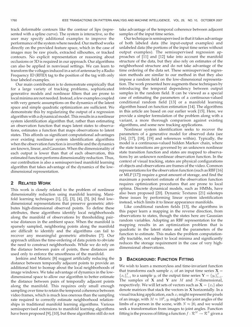
The high-dimensional data set is constructed by lifting arandom walk on a 2D euclidean patch toR3 via a smooth andinvertible mapping. See Figs. 1a and 1b. The task is to recoverthe projection function f : R3 !R2 to invert this lifting.

In this data set, the nearest neighbors inR3 of points nearthe region of near-self-intersection (the “neck”) will straddle

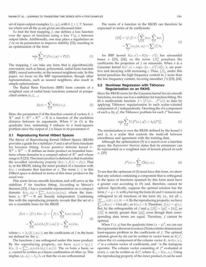
the neck, and the recovered neighborhood structure will notreflect the proximity of points on the manifold. This causesexisting manifold learning algorithms such as LLE [2],Isomap [1], and Laplacian Eigenmaps [3] to assign similarcoordinates to points that are in fact very far from each otheron the manifold. Isomap creates folds in the projection. SeeFig. 2a. Neither LLE nor Laplacian Eigenmaps producedsensible results, projecting the data to a straight line, evenwith denser sampling of the manifold (up to 7,000 samples)and with a variety of neighborhood sizes (from threeneighbors to 30 neighbors).

These manifold learning algorithms ignore labeled points,but the presence of labeled points does not make the recoveryof low-dimensional coordinates trivial. To show this, we alsocompare against Belkin and Nyogi’s graph Laplacian-basedsemisupervised regression algorithm [12], referred to here asBNR. Six points on the boundary of the manifold were labeledwith their ground truth low-dimensional coordinates.Figs. 2b and 2e show the results of BNR on this data set whenit operates on large neighborhoods. There is a fold in theresulting low-dimensional coordinates because BNR assignsthe same value to all points behind the neck. Also, therecovered coordinates are shrunk toward the center, becausethe Laplacian regularizer favors coordinates with smallermagnitudes. For smaller settings of the neighborhood size,the folding disappears, but the shrinking remains.1

It is also not sufficient to merely take temporal adjacencyinto account when building the neighborhood structure ofthe high-dimensional points. Figs. 2c and 2f show the resultof BNR when the neighborhood of each point includestemporally adjacent points. Including these neighbors doesnot improve the result.

Finally, Fig. 2d shows the result of Tikhonov regulariza-tion on an RKHS with quadratic loss (the solution of (5)applied to the high-dimensional points). This algorithm usesonly labeled points and ignores unlabeled data. Because allthe labeled points have the same y coordinates, Tikhonovregularization cannot generalize the mapping to the rest ofthe 3D shape.

Taking into account the temporal coherence between datapoints and the dynamics of the low-dimensional coordinatesalleviates these problems. Folding problems are alleviatedbecause our algorithm takes advantage of the time ordering ofdata points and the explicit dynamical model alleviates theshrinking toward zero by implicitly modeling velocity in thelow-dimensional trajectory. Fig. 1c shows the low-dimen-sional coordinates recovered by our algorithm. These valuesare close to the true low-dimensional coordinates.

We can also assess the quality of the learned function fon as-yet unseen points. Figs. 1d and 1e show a 2D gridspanning ½0; 5� � ½�3; 3� lifted by the same mapping used togenerate the training data. Each of these points in R3 ispassed through the recovered mapping f to obtain the2D representation shown in Fig. 1f. These projections fallclose to the true 2D location of these samples, implying thatf has correctly generalized an inverse for the true lifting.


1. In comparing the algorithm with Isomap, LLE, and LaplacianEigenmaps, we relied on source code available from the respective authors’Web sites. To compute eigenvalues and eigenvectors, we tried bothMATLAB’s EIGS routine and JDQR [33], a drop-in replacement for EIGS.We used our own implementation of BNR, but relied on the code suppliedby the authors to compute the Laplacian.

This synthetic experiment illustrates three features that

recur in subsequent experiments:

. While the kernel matrix K takes into account thesimilarity of the high-dimensional data points,explicitly taking into account the dynamics of thelow-dimensional process obviates the need to buildthe brittle neighborhood graph that is common inmanifold learning and semisupervised learningalgorithms.

. The assumed dynamics model does not need to bevery accurate. The true low-dimensional randomwalk used to generate the data set bounced off theboundaries of the rectangle ½0; 5� � ½�3; 3�, an effect

not modeled by a linear-Gaussian Markov chain.Nevertheless, the assumed dynamics of (9) aresufficient for recovering the true location of unla-beled points.

. The labeled examples do not need to capture all themodes of variation of the data. Despite the fact thatthe examples only showed how to transform pointswhose y coordinate is 2.5, our semisupervisedlearning algorithm learned the low-dimensionalcoordinate of points with any y-coordinate.

7.2 Learning to Track: Tracking with the Sensetable

The Sensetable is a hardware platform for tracking the position

of radio frequency identification (RFID) tags [35]. It consists of


Fig. 1. (a) The true 2D parameter trajectory. The six labeled points are marked with big blue triangles. The trajectory has 1,500 samples. In all ofthese plots, the color of each trajectory point is based on its y-value, with higher intensities corresponding to greater y-values. (b) Embedding of thepath via the lifting F ðx; yÞ ¼ ðx; jyj; sinð�yÞðy2 þ 1Þ�2 þ 0:3yÞ. (c) Recovered low-dimensional representation using our algorithm. The original data in(a) is recovered. (d) Even sampling of the rectangle ½0; 5� � ½�3; 3�. (e) Lifting of this rectangle via F . (f) Projection of (e) via the learned function f.The recovered locations are close to their 2D locations, showing that the inverse of F has been learned correctly.

10 antennae woven into a flat surface that is 30 cm on a side.As an RFID tag moves along the flat surface, analog-to-digitalconversion circuitry reports the strength of the RF signal fromthe RFID tag as measured by each antenna, producing a timeseries of 10 numbers. See Fig. 3a. The Sensetable has beenintegrated into various hardware platforms, such as a systemfor visualizing supply chains and the Audiopad [34], aninteractive disc jockey system.

We wish to learn to map the 10 signal strength measure-ments from the antennae to the 2D position of the RFID tag.Previously, a mapping was recovered by hand through anarduous reverse-engineering process that involved buildinga physical model of the inner-workings of the Sensetable and

resorting to trial and error to refine the resulting mappings[35]. Rather than reverse-engineering this device by hand, weshow that it is possible to recover this mapping with only fourlabeled examples and some unlabeled data points, eventhough the relationship between the tag’s position an theobserved measurements is highly oscillatory. Once it islearned, we can use the mapping to track RFID tags. Theprocedure we follow is quite general and can be applied to avariety of other hardware.

To collect the four labeled examples, the tag was placed oneach of the four corners of the Sensetable, the Sensetable’soutput was recorded. We collected unlabeled data bysweeping the tag on the Sensetable’s surface for about


Fig. 2. (a) Isomap’s recovered 2D coordinates for the data set of Fig. 1b. Errors in estimating the neighborhood relations at the neck of the manifoldcause the projection to fold over itself in the center. The neighborhood size was 10, but smaller neighborhoods produce similar results. (d) Fullysupervised algorithms, which do not take advantage of unlabeled points, cannot correctly recover the coordinates of unlabeled points because onlypoints at the edges of the shape are labeled. (b) Projection with BNR, a semisupervised regression algorithm, with neighborhood size of 10. Althoughthe structure is recovered more accurately, all the points behind the neck are folded into one thin strip. (e) BNR with neighborhood size of 3 prevents onlysome of the folding. Points are still shrunk to the center, so the low-dimensional values are not recovered accurately. (c) and (f) BNR as before, withtemporally adjacent points included in neighborhoods. There is no significant improvement over building neighborhoods using nearest neighbors only.

400 seconds, and down-sampled the result by a factor of 3 toobtain about 3,600 unlabeled data points. Fig. 3b shows theground truth trajectory of the RFID tag, as recovered by themanually reverse-engineered Sensetable mappings. The fourtriangles in the corners of the figure depict the location of thelabeled examples. The rest of the 2D trajectory was not madeavailable to the algorithm. Contrary to what one might hope,the output from each antenna of the Sensetable does not have astraightforward one-to-one relationship with a component ofthe 2D position. For example, when the tag is moved in astraight line from left to right, it generates oscillatory tracessimilar to those shown in Fig. 3c.

The four labeled points, along with the few minutes ofrecorded data were passed to the semisupervised learningalgorithm to recover the mapping. The algorithm took90 seconds to process this data set on a 3.2 Ghz Xeon machine.The trajectory is recovered accurately despite the complicatedrelationship between the 10 outputs and the tag position (seeFig. 4). The RMS distance to the ground truth trajectory isabout 1.3 cm, though the ground truth itself is based on thereverse engineered tracker and may be inaccurate. Fig. 4bshows the regions that are most prone to errors. The errors aregreatest outside the bounding box of the labeled points, butpoints near the center of the board are recovered very

accurately, despite the lack of labeled points there. Thisphenomenon is discussed in Section 6.

The recovered mapping from measurements to positionscan be used to track tags. Individual samples of 10 measure-ments can be passed to the recovered mapping f to recoverthe corresponding tag position, but because the Sensetable’soutput is noisy, the results must be filtered. Fig. 5 shows theoutput of a few test paths after smoothing using the assumeddynamics. The recovered trajectories match the patternstraced by the tag.

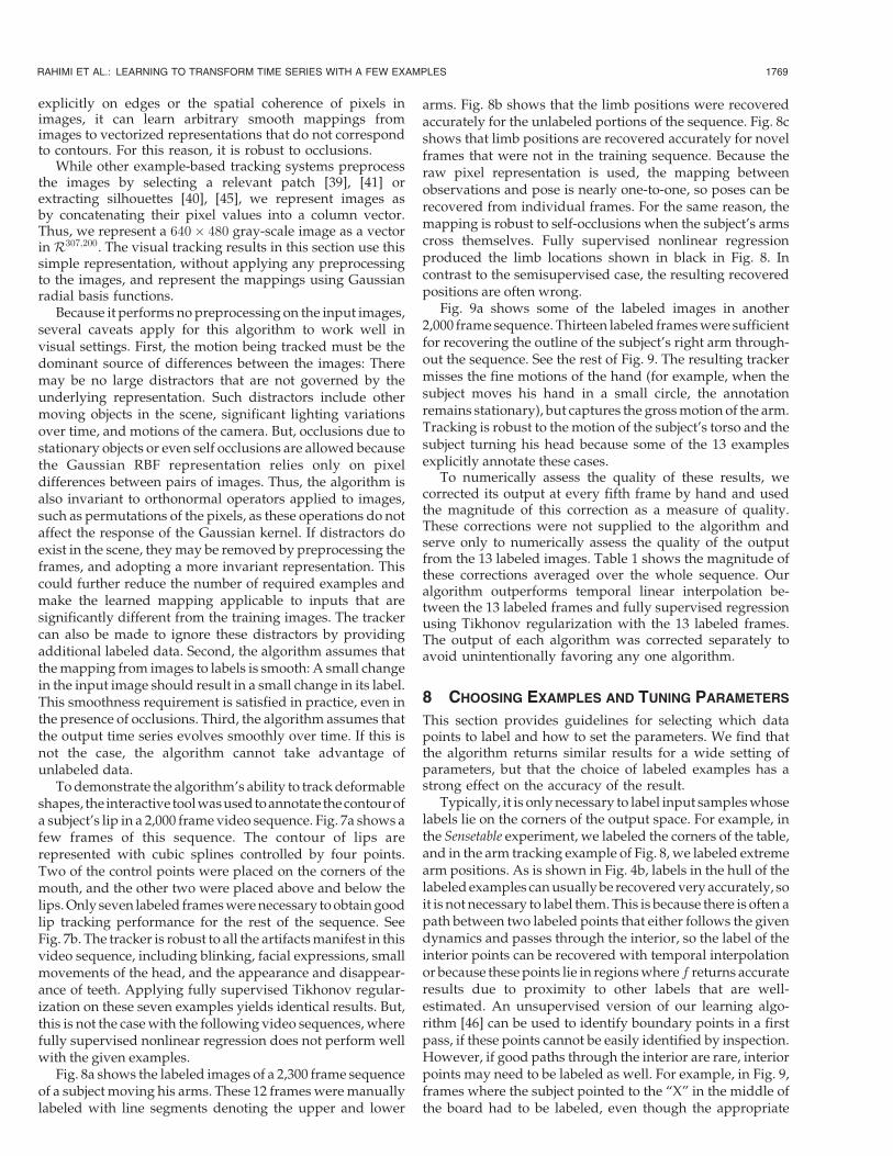
Unlabeled data and explicitly taking advantage of dy-namics is critical in this data set because the relationshipbetween signal strengths and tag positions is complex, andfew input-output examples are available. Thus, fully super-vised learning with Tikhonov regularization on an RKHS failsto recover the mapping. See Fig. 6a. Fig. 6b shows thetrajectory recovered by BNR with its most favorable para-meter setting for this data set. Fig. 6c shows the trajectoryrecovered by BNR when temporally adjacent neighbors arecounted as part of the adjacency graph when computing theLaplacian. As with the synthetic data set, there is severeshrinkage toward the mean of the labeled points and somefolding at the bottom and taking temporal adjacency intoaccount does not significantly improve the results.


Fig. 3. (a) A top view of the Sensetable, an interactive environment for tracking RFID tags. Users manipulate RFID tagged pucks and a projectoroverlays visual feedback on the surface of the table. Coils under the table measure the strength of the signals induced by RFID tags. Our algorithmrecovers a mapping from these signal strengths to the position of the tags. (b) The ground truth trajectory of the tag. The tag was moved aroundsmoothly on the surface of the Sensetable for about 400 seconds, producing about 3,600 signal strength measurement samples after downsampling.Triangles indicate the four locations where the true location of the tag was provided to the algorithm. The color of each point is based on its y-value,with higher intensities corresponding to higher y-values. (c) Samples from the antennae of the Sensetable over a six second period, taken over thetrajectory marked by large circles in (a).

Fig. 4. (a) The recovered tag positions match the original trajectory depicted in Fig. 3. (b) Errors in recovering the ground truth trajectory. Circlesdepict ground truth locations, with the intensity and size of each circle proportional to the euclidean distance between a point’s true position and itsrecovered position. The largest errors are outside the bounding box of the labeled points. Points in the center are recovered accurately, despite thelack of labeled points there.

7.3 Learning to Track: Visual Tracking

In this section, we demonstrate an interactive applicationwhere our algorithm helps a user quickly annotate everyframe of a video sequence with a low-dimensional represen-tation of a the scene given a few manually-labeled key frames.These labels are specified with an interactive graphical tool asa collection of vectorized drawing primitives, such as splinesand polylines. The output representation consists of thecontrol points of these drawing primitives. Given the videosequence and the labeled examples, our algorithm recoversthe control points for the unlabeled frames of the videosequence. If the user is not satisfied with the rendering ofthese control points, he can modify the labeling and rerun thealgorithm at interactive rates. The tool is demonstrated on alip tracking video where the user specifies the shape of thelips of a subject and two articulated body tracking experi-ments [36], [37], where the user specifies positions of thesubject’s limbs. The annotation tool is available online [38].

There is a rich body of work in learning visual trackersfrom examples using fully supervised regression algorithms.For example, relying on the nearest neighbors representation,Efros et al. [39] used thousands of labeled images of soccerplayers to recover the articulated pose of players in newimages and Shaknarovich et al. [40] used a database ofsynthetically rendered hands to recover the pose of hands.Relying on the RBF representation, El Gammal [41] recoveredthe deformation of image patches and Agarwal and Triggs[42] learned a mapping from features of an image to the poseof human bodies. In our case, the training sequence aresequential frames of a video, and taking advantage of thetemporal coherence between these frames allows us to takeadvantage of unlabeled examples, and greatly reduces theneed for labeled outputs.

Because it is interactive, our system is reminiscent ofrotoscoping tools [43], [44], which allow the user tointeractively adjust the output of contour trackers byannotating key frames. Since our algorithm does not rely


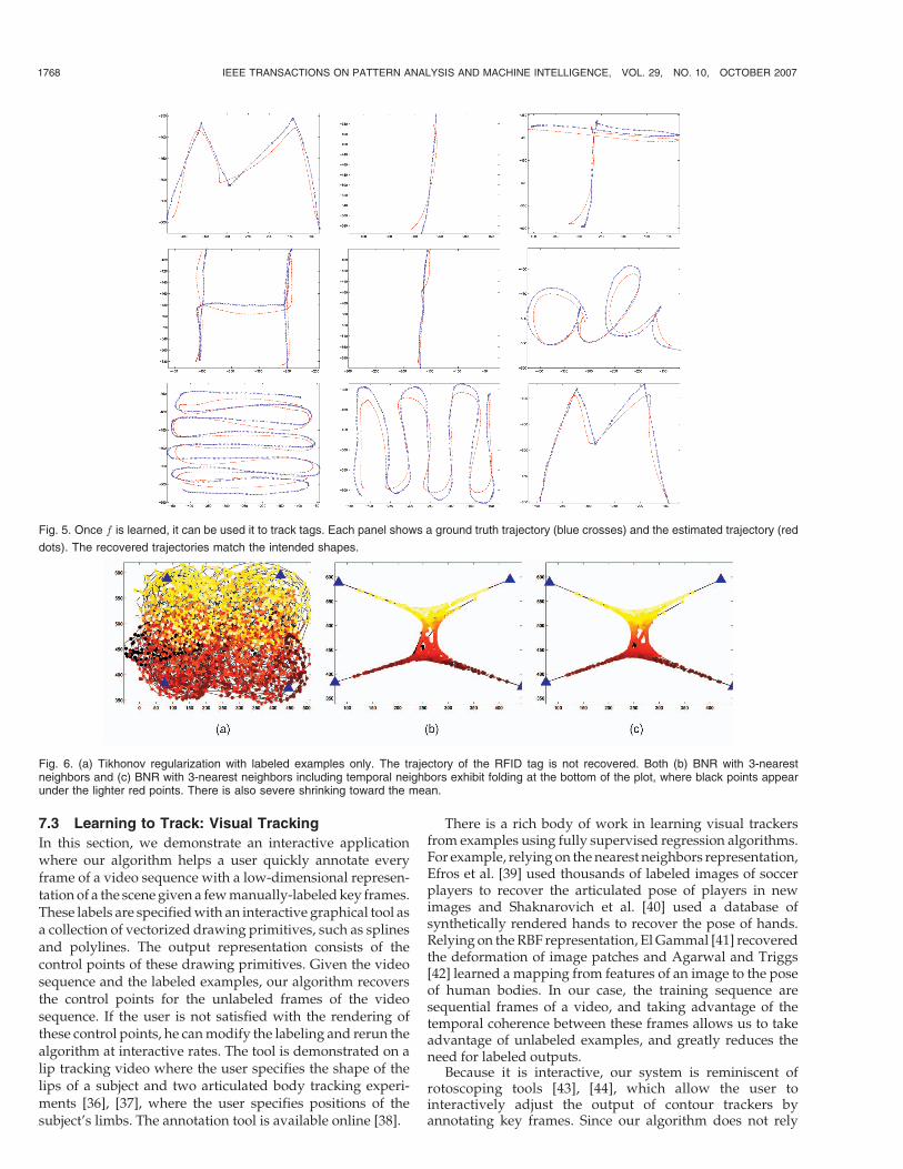
Fig. 5. Once f is learned, it can be used it to track tags. Each panel shows a ground truth trajectory (blue crosses) and the estimated trajectory (red

dots). The recovered trajectories match the intended shapes.

Fig. 6. (a) Tikhonov regularization with labeled examples only. The trajectory of the RFID tag is not recovered. Both (b) BNR with 3-nearestneighbors and (c) BNR with 3-nearest neighbors including temporal neighbors exhibit folding at the bottom of the plot, where black points appearunder the lighter red points. There is also severe shrinking toward the mean.

explicitly on edges or the spatial coherence of pixels inimages, it can learn arbitrary smooth mappings fromimages to vectorized representations that do not correspondto contours. For this reason, it is robust to occlusions.

While other example-based tracking systems preprocessthe images by selecting a relevant patch [39], [41] orextracting silhouettes [40], [45], we represent images asby concatenating their pixel values into a column vector.Thus, we represent a 640� 480 gray-scale image as a vectorin R307;200. The visual tracking results in this section use thissimple representation, without applying any preprocessingto the images, and represent the mappings using Gaussianradial basis functions.

Because it performs no preprocessing on the input images,several caveats apply for this algorithm to work well invisual settings. First, the motion being tracked must be thedominant source of differences between the images: Theremay be no large distractors that are not governed by theunderlying representation. Such distractors include othermoving objects in the scene, significant lighting variationsover time, and motions of the camera. But, occlusions due tostationary objects or even self occlusions are allowed becausethe Gaussian RBF representation relies only on pixeldifferences between pairs of images. Thus, the algorithm isalso invariant to orthonormal operators applied to images,such as permutations of the pixels, as these operations do notaffect the response of the Gaussian kernel. If distractors doexist in the scene, they may be removed by preprocessing theframes, and adopting a more invariant representation. Thiscould further reduce the number of required examples andmake the learned mapping applicable to inputs that aresignificantly different from the training images. The trackercan also be made to ignore these distractors by providingadditional labeled data. Second, the algorithm assumes thatthe mapping from images to labels is smooth: A small changein the input image should result in a small change in its label.This smoothness requirement is satisfied in practice, even inthe presence of occlusions. Third, the algorithm assumes thatthe output time series evolves smoothly over time. If this isnot the case, the algorithm cannot take advantage ofunlabeled data.

To demonstrate the algorithm’s ability to track deformableshapes, the interactive tool wasusedto annotate the contourofa subject’s lip in a 2,000 frame video sequence. Fig. 7a shows afew frames of this sequence. The contour of lips arerepresented with cubic splines controlled by four points.Two of the control points were placed on the corners of themouth, and the other two were placed above and below thelips. Only seven labeled frames were necessary to obtain goodlip tracking performance for the rest of the sequence. SeeFig. 7b. The tracker is robust to all the artifacts manifest in thisvideo sequence, including blinking, facial expressions, smallmovements of the head, and the appearance and disappear-ance of teeth. Applying fully supervised Tikhonov regular-ization on these seven examples yields identical results. But,this is not the case with the following video sequences, wherefully supervised nonlinear regression does not perform wellwith the given examples.

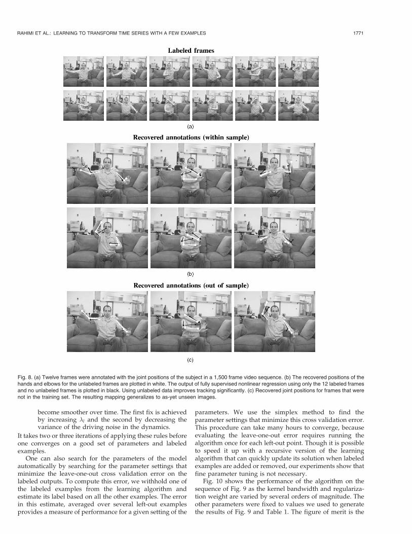
Fig. 8a shows the labeled images of a 2,300 frame sequenceof a subject moving his arms. These 12 frames were manuallylabeled with line segments denoting the upper and lower

arms. Fig. 8b shows that the limb positions were recoveredaccurately for the unlabeled portions of the sequence. Fig. 8cshows that limb positions are recovered accurately for novelframes that were not in the training sequence. Because theraw pixel representation is used, the mapping betweenobservations and pose is nearly one-to-one, so poses can berecovered from individual frames. For the same reason, themapping is robust to self-occlusions when the subject’s armscross themselves. Fully supervised nonlinear regressionproduced the limb locations shown in black in Fig. 8. Incontrast to the semisupervised case, the resulting recoveredpositions are often wrong.

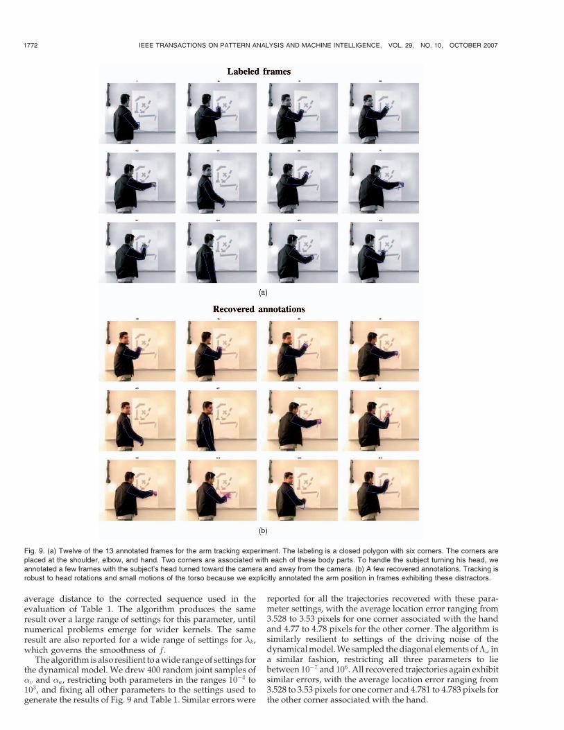
Fig. 9a shows some of the labeled images in another2,000 frame sequence. Thirteen labeled frames were sufficientfor recovering the outline of the subject’s right arm through-out the sequence. See the rest of Fig. 9. The resulting trackermisses the fine motions of the hand (for example, when thesubject moves his hand in a small circle, the annotationremains stationary), but captures the gross motion of the arm.Tracking is robust to the motion of the subject’s torso and thesubject turning his head because some of the 13 examplesexplicitly annotate these cases.

To numerically assess the quality of these results, wecorrected its output at every fifth frame by hand and usedthe magnitude of this correction as a measure of quality.These corrections were not supplied to the algorithm andserve only to numerically assess the quality of the outputfrom the 13 labeled images. Table 1 shows the magnitude ofthese corrections averaged over the whole sequence. Ouralgorithm outperforms temporal linear interpolation be-tween the 13 labeled frames and fully supervised regressionusing Tikhonov regularization with the 13 labeled frames.The output of each algorithm was corrected separately toavoid unintentionally favoring any one algorithm.

8 CHOOSING EXAMPLES AND TUNING PARAMETERS

This section provides guidelines for selecting which datapoints to label and how to set the parameters. We find thatthe algorithm returns similar results for a wide setting ofparameters, but that the choice of labeled examples has astrong effect on the accuracy of the result.

Typically, it is only necessary to label input samples whoselabels lie on the corners of the output space. For example, inthe Sensetable experiment, we labeled the corners of the table,and in the arm tracking example of Fig. 8, we labeled extremearm positions. As is shown in Fig. 4b, labels in the hull of thelabeled examples can usually be recovered very accurately, soit is not necessary to label them. This is because there is often apath between two labeled points that either follows the givendynamics and passes through the interior, so the label of theinterior points can be recovered with temporal interpolationor because these points lie in regions where f returns accurateresults due to proximity to other labels that are well-estimated. An unsupervised version of our learning algo-rithm [46] can be used to identify boundary points in a firstpass, if these points cannot be easily identified by inspection.However, if good paths through the interior are rare, interiorpoints may need to be labeled as well. For example, in Fig. 9,frames where the subject pointed to the “X” in the middle ofthe board had to be labeled, even though the appropriate


parameters of the shape of the arm for these frames lie in the

convex hull of the other labeled frames. In this video

sequence, to reach the “X” from a boundary point, thesubject’s arm followed a circuitous path through previously

unexplored interior regions of the board. Because this path

was neither very likely according to the dynamics model nor

near other points whose labels were recovered, we had to

explicitly label some points along it.The algorithm is insensitive to settings of the other

parameters up to several orders of magnitude and, typically,only the parameters of the kernel need to be tuned. Whenusing a Gaussian kernel, if the bandwidth parameter is toosmall, K becomes diagonal and all points are considered to bedissimilar. If the bandwidth parameter is too large, K has onein each entry and all points are considered to be identical. Weinitially set the kernel bandwidth parameter so that theminimum entry in K is approximately 0.1. Other parameters,including the scalar weights and the parameters of dynamics

are initially set to 1. After labeling a few boundary examples,we run the algorithm with this default set of parameters andadjust them or add new examples depending on the way inwhich the output falls short of the desired result. Some of thesymptoms and possible adjustments are:

. Boundary points are not correctly mapped: Theoutput may exhibit slight shrinkage toward thecenter. One way to fix this issue is to provide morelabels on the boundary. Another solution is toincrease �v and �a to under-damp the dynamics.

. All outputs take on the same value, except for abruptjumps at example points: This happens when thekernel bandwidth parameter is too small, causingthe algorithm to treat all points as being dissimilar.Increasing the bandwidth fixes this problem.

. Jittery outputs: If the recovered labels are not smoothover time, one can either force f to become smootheras a function of x or force the label sequence to


Fig. 7. (a) The contour of the lips was annotated in seven frames of a 2,000 frame video. The contour is represented using cubic splines, controlled byfour control points. The desired output time series is the position of the control points over time. These labeled points and first 1,500 frames were usedto train our algorithm. (b) The recovered mouth contours for various frames. The first three images show the labeling recovered for to unlabeled framesin the training set and the next two show the labeling for frames that did not appear in the training set. The tracker is robust to natural changes in lighting(i.e., the flicker of fluorescent lights), blinking, facial expressions, small movements of the head, and the appearance and disappearance of teeth.

become smoother over time. The first fix is achievedby increasing �l and the second by decreasing thevariance of the driving noise in the dynamics.

It takes two or three iterations of applying these rules beforeone converges on a good set of parameters and labeledexamples.

One can also search for the parameters of the modelautomatically by searching for the parameter settings thatminimize the leave-one-out cross validation error on thelabeled outputs. To compute this error, we withhold one ofthe labeled examples from the learning algorithm andestimate its label based on all the other examples. The errorin this estimate, averaged over several left-out examplesprovides a measure of performance for a given setting of the

parameters. We use the simplex method to find theparameter settings that minimize this cross validation error.This procedure can take many hours to converge, becauseevaluating the leave-one-out error requires running thealgorithm once for each left-out point. Though it is possibleto speed it up with a recursive version of the learningalgorithm that can quickly update its solution when labeledexamples are added or removed, our experiments show thatfine parameter tuning is not necessary.

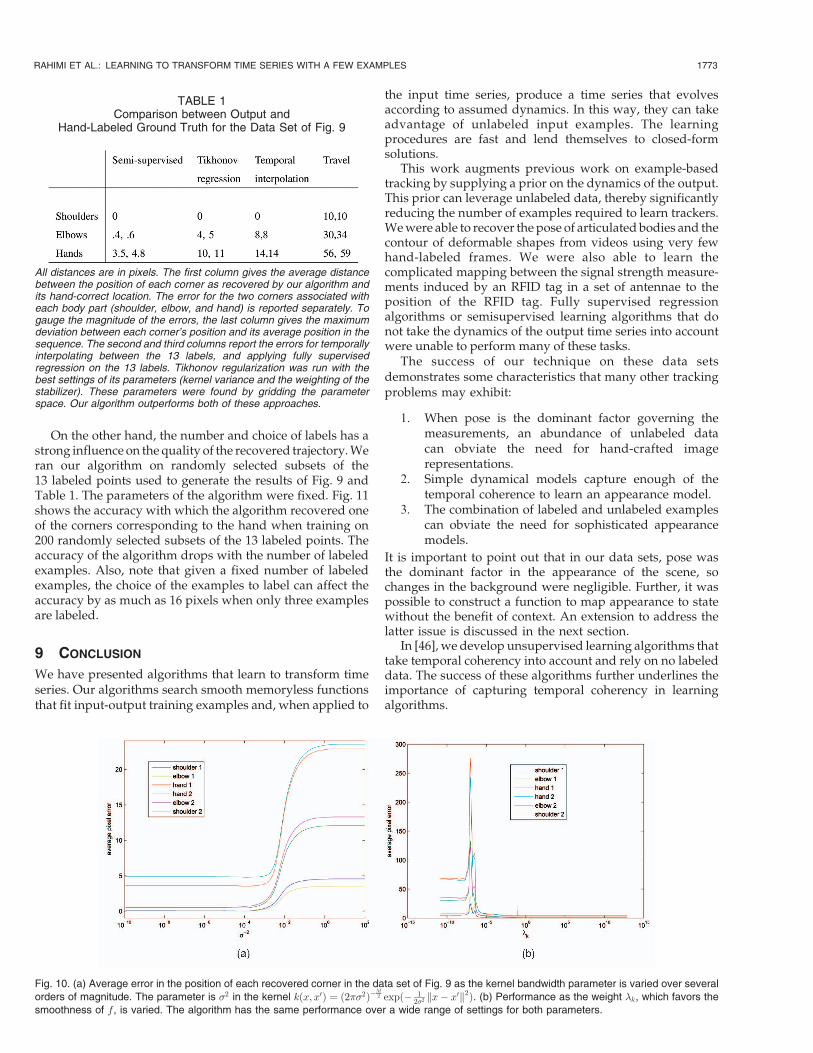
Fig. 10 shows the performance of the algorithm on thesequence of Fig. 9 as the kernel bandwidth and regulariza-tion weight are varied by several orders of magnitude. Theother parameters were fixed to values we used to generatethe results of Fig. 9 and Table 1. The figure of merit is the


Fig. 8. (a) Twelve frames were annotated with the joint positions of the subject in a 1,500 frame video sequence. (b) The recovered positions of thehands and elbows for the unlabeled frames are plotted in white. The output of fully supervised nonlinear regression using only the 12 labeled framesand no unlabeled frames is plotted in black. Using unlabeled data improves tracking significantly. (c) Recovered joint positions for frames that werenot in the training set. The resulting mapping generalizes to as-yet unseen images.

average distance to the corrected sequence used in theevaluation of Table 1. The algorithm produces the sameresult over a large range of settings for this parameter, untilnumerical problems emerge for wider kernels. The sameresult are also reported for a wide range of settings for �k,which governs the smoothness of f .

The algorithm is also resilient to a wide range of settings forthe dynamical model. We drew 400 random joint samples of�v and �a, restricting both parameters in the ranges 10�4 to103, and fixing all other parameters to the settings used togenerate the results of Fig. 9 and Table 1. Similar errors were

reported for all the trajectories recovered with these para-meter settings, with the average location error ranging from3.528 to 3.53 pixels for one corner associated with the handand 4.77 to 4.78 pixels for the other corner. The algorithm issimilarly resilient to settings of the driving noise of thedynamical model. We sampled the diagonal elements of �! ina similar fashion, restricting all three parameters to liebetween 10�7 and 106. All recovered trajectories again exhibitsimilar errors, with the average location error ranging from3.528 to 3.53 pixels for one corner and 4.781 to 4.783 pixels forthe other corner associated with the hand.


Fig. 9. (a) Twelve of the 13 annotated frames for the arm tracking experiment. The labeling is a closed polygon with six corners. The corners areplaced at the shoulder, elbow, and hand. Two corners are associated with each of these body parts. To handle the subject turning his head, weannotated a few frames with the subject’s head turned toward the camera and away from the camera. (b) A few recovered annotations. Tracking isrobust to head rotations and small motions of the torso because we explicitly annotated the arm position in frames exhibiting these distractors.

On the other hand, the number and choice of labels has astrong influence on the quality of the recovered trajectory. Weran our algorithm on randomly selected subsets of the13 labeled points used to generate the results of Fig. 9 andTable 1. The parameters of the algorithm were fixed. Fig. 11shows the accuracy with which the algorithm recovered oneof the corners corresponding to the hand when training on200 randomly selected subsets of the 13 labeled points. Theaccuracy of the algorithm drops with the number of labeledexamples. Also, note that given a fixed number of labeledexamples, the choice of the examples to label can affect theaccuracy by as much as 16 pixels when only three examplesare labeled.

9 CONCLUSION

We have presented algorithms that learn to transform timeseries. Our algorithms search smooth memoryless functionsthat fit input-output training examples and, when applied to

the input time series, produce a time series that evolvesaccording to assumed dynamics. In this way, they can takeadvantage of unlabeled input examples. The learningprocedures are fast and lend themselves to closed-formsolutions.

This work augments previous work on example-basedtracking by supplying a prior on the dynamics of the output.This prior can leverage unlabeled data, thereby significantlyreducing the number of examples required to learn trackers.We were able to recover the pose of articulated bodies and thecontour of deformable shapes from videos using very fewhand-labeled frames. We were also able to learn thecomplicated mapping between the signal strength measure-ments induced by an RFID tag in a set of antennae to theposition of the RFID tag. Fully supervised regressionalgorithms or semisupervised learning algorithms that donot take the dynamics of the output time series into accountwere unable to perform many of these tasks.

The success of our technique on these data setsdemonstrates some characteristics that many other trackingproblems may exhibit:

1. When pose is the dominant factor governing themeasurements, an abundance of unlabeled datacan obviate the need for hand-crafted imagerepresentations.

2. Simple dynamical models capture enough of thetemporal coherence to learn an appearance model.

3. The combination of labeled and unlabeled examplescan obviate the need for sophisticated appearancemodels.

It is important to point out that in our data sets, pose wasthe dominant factor in the appearance of the scene, sochanges in the background were negligible. Further, it waspossible to construct a function to map appearance to statewithout the benefit of context. An extension to address thelatter issue is discussed in the next section.

In [46], we develop unsupervised learning algorithms thattake temporal coherency into account and rely on no labeleddata. The success of these algorithms further underlines theimportance of capturing temporal coherency in learningalgorithms.


Fig. 10. (a) Average error in the position of each recovered corner in the data set of Fig. 9 as the kernel bandwidth parameter is varied over several

orders of magnitude. The parameter is �2 in the kernel kðx; x0Þ ¼ ð2��2Þ�M2 expð� 1

2�2 kx� x0k2Þ. (b) Performance as the weight �k, which favors the

smoothness of f, is varied. The algorithm has the same performance over a wide range of settings for both parameters.

TABLE 1Comparison between Output and

Hand-Labeled Ground Truth for the Data Set of Fig. 9

All distances are in pixels. The first column gives the average distancebetween the position of each corner as recovered by our algorithm andits hand-correct location. The error for the two corners associated witheach body part (shoulder, elbow, and hand) is reported separately. Togauge the magnitude of the errors, the last column gives the maximumdeviation between each corner’s position and its average position in thesequence. The second and third columns report the errors for temporallyinterpolating between the 13 labels, and applying fully supervisedregression on the 13 labels. Tikhonov regularization was run with thebest settings of its parameters (kernel variance and the weighting of thestabilizer). These parameters were found by gridding the parameterspace. Our algorithm outperforms both of these approaches.

10 FUTURE WORK

Several interesting directions remain to be explored. We

would like to apply the semisupervised learning algorithm

to more application areas, and to extend this work by

exploring various kernels that might provide invariance to

more distractors, more sophisticated dynamical models,

and an automatic way of selecting data points to label.In this work, the pose of the target was the only factor

governing the appearance of the target. This allowed us to usea simple Gaussian kernel to compare observations. to providemore invariance to distractors, we could either summarizeimages by a list of interest points and their descriptors, as in[42], or compute the similarity matrix with different kernels,as in [47] and references within. We would also like to explorean automatic way to select features by tuning the covariancematrix of the Gaussian kernel.

We have also assumed that a priori the components ofthe output evolve independently of each other. In somesettings, such as when tracking articulated objects in 3Dwith a weak-perspective camera, a priori correlationbetween the outputs becomes an important cue becausethe observation function is not invertible and pose can onlybe recovered up to a subspace from a single frame. Toaddress this issue, the data matching terms in the costfunction can be set to V ðfðxiÞ;HyiÞ, where H spans thissubspace. A correlated prior on Y would then allow thealgorithm to recover the best path within the subspace. Wehave not tried our algorithm on a data set where correlatedoutputs and one-to-many mappings are critical, but itwould be interesting to examine the benefits of theseadditions, and the use of other priors.

We provided some guidelines for choosing the inputsto label, but it would be interesting to let the systemguide the user’s choice of inputs to label via activelearning [48], [49], [50].

In the future, we hope to explore many other applicationareas. For example, we could learn to transform images tocartoon sequences, add special effects to image sequences,extract audio from muted video sequences, and drive videowith audio signals.

REFERENCES

[1] J.B. Tenenbaum, V. de Silva, and J.C. Langford, “A GlobalGeometric Framework for Nonlinear Dimensionality Reduction,”Science, vol. 290, no. 5500, pp. 2319-2323, 2000.

[2] S. Roweis and L. Saul, “Nonlinear Dimensionality Reduction byLocally Linear Embedding,” Science, vol. 290, no. 5500, pp. 2323-2326, 2000.

[3] M. Belkin and P. Niyogi, “Laplacian Eigenmaps for Dimension-ality Reduction and Data Representation,” Neural Computation,vol. 15, no. 6, pp. 1373-1396, 2003.

[4] D. Donoho and C. Grimes, “Hessian Eigenmaps: New LocallyLinear Embedding Techniques for Highdimensional Data,” Tech-nical Report TR2003-08, Dept. of Statistics, Stanford Univ., 2003.

[5] K. Weinberger and L. Saul, “Unsupervised Learning of ImageManifolds by Semidefinite Programming,” Proc. IEEE Conf.Computer Vision and Pattern Recognition, 2004.

[6] M. Brand, “Charting a Manifold,” Proc. Conf. Neural InformationProcessing Systems, 2002.

[7] M. Balasubramanian, E.L. Schwartz, J.B. Tenenbaum, V. de Silva,and J.C. Langford, “The Isomap Algorithm and TopologicalStability,” Science, vol. 295, no. 5552, 2002.

[8] O. Jenkins and M. Mataric, “A Spatio-Temporal Extension toIsomap Nonlinear Dimension Reduction,” Proc. Int’l Conf. MachineLearning, 2004.

[9] J. Ham, D. Lee, and L. Saul, “Learning High DimensionalCorrespondences from Low Dimensional Manifolds,” Proc. Int’lConf. Machine Learning, 2003.

[10] R. Pless and I. Simon, “Using Thousands of Images of an Object,”Proc. Conf. Computer Vision, Pattern Recognition, and Image Proces-sing, 2002.

[11] X. Zhu, Z. Ghahramani, and J. Lafferty, “Semi-SupervisedLearning Using Gaussian Fields and Harmonic Functions,” Proc.Int’l Conf. Machine Learning, 2003.

[12] M. Belkin, I. Matveeva, and P. Niyogi, “Regularization and Semi-Supervised Learning on Large Graphs,” Proc. 17th Ann. Conf.Computational Learning Theory, 2004.

[13] J. Lafferty, A. McCallum, and F. Pereira, “Conditional RandomFields: Probabilistic Models for Segmenting and Labeling Se-quence Data,” Proc. Int’l Conf. Machine Learning, pp. 282-289, 2001.

[14] A. Smola, S. Mika, B. Schoelkopf, and R.C. Williamson, “Regular-ized Principal Manifolds,” J. Machine Learning, vol. 1, pp. 179-209,2001.

[15] A. Rahimi, B. Recht, and T. Darrell, “Learning AppearanceManifolds from Video,” Proc. IEEE Conf. Computer Vision andPattern Recognition, 2005.

[16] Z. Ghahramani and S. Roweis, “Learning Nonlinear DynamicalSystems Using an EM Algorithm,” Neural Information ProcessingSystems (NIPS), pp. 431-437, 1998.

[17] H. Valpola and J. Karhunen, “An Unsupervised EnsembleLearning Method for Nonlinear Dynamic State-Space Models,”Neural Computation, vol. 14, no. 11, pp. 2647-2692, 2002.

[18] L. Ljung, System Identification: Theory for the User. Prentice-Hall,1987.

[19] A. Juditsky, H. Hjalmarsson, A. Benveniste, B. Delyon, L. Ljung, J.Sjoberg, and Q. Zhang, “Nonlinear Black-Box Models in SystemIdentification: Mathematical Foundations,” Automatica, vol. 31,no. 12, pp. 1725-1750, 1995.

[20] K.-C. Lee and D. Kriegman, “Online Learning of ProbabilisticAppearance Manifolds for Video-Based Recognition and Track-ing,” Proc. IEEE Conf. Computer Vision and Pattern Recognition, 2005.

[21] G. Doretto, A. Chiuso, and Y.W.S. Soatto, “Dynamic Textures,”Int’l J. Computer Vision, vol. 51, no. 2, pp. 91-109, 2003.

[22] O. Bousquet and A. Elisseeff, “Stability and Generalization,”Journal of Machine Learning Research, 2002.

[23] M.P.T. Evgeniou and T. Poggio, “Regularization Networks andSupport Vector Machines,” Advances in Computational Math., 2000.

[24] G. Wahba, “Spline Models for Observational Data,” Proc. SIAM,vol. 59, 1990.

[25] B. Scholkopf, R. Herbrich, A. Smola, and R. Williamson, “AGeneralized Representer Theorem,” Proc. Neural Networks andComputational Learning Theory, NeuroCOLT Technical Report NC-TR-00-081, 2000.

[26] V. Vapnik, Statistical Learning Theory. Wiley, 1998.[27] T. De Bie and N. Cristianini, “Convex Methods for Transduction,”

Proc. Conf. Neural Information Processing Systems, 2003.


Fig. 11. Average error in the position of one of the corners correspondingto the hand, as a function of the number of labeled examples used.Labeled examples were chosen randomly from a fixed set of 13 labeledexamples. Reducing the number of labels reduces accuracy. Also, thechoice of labels has a strong influence on the performance, asdemonstrated by the vertical spread of each column.

[28] T. Joachims, “Transductive Inference for Text Classification UsingSupport Vector Machines,” Proc. Int’l Conf. Machine Learning,pp. 200-209, 1999.

[29] K. Bennett and A. Demiriz, “Semi-Supervised Support VectorMachines,” Proc. Conf. Advances in Neural Information ProcessingSystems, pp. 368-374, 1998.

[30] R. Rifkin, G. Yeo, and T. Poggio, “Regularized Least SquaresClassification,” Proc. Conf. Advances in Learning Theory: Methods,Model and Applications, NATO Science Series III: Computer andSystems Sciences, vol. 190, 2003.

[31] T. Kailath, A.H. Sayed, and B. Hassibi, Linear Estimation. PrenticeHall, 2000.

[32] A. Rahimi, “Learning to Transform Time Series with a FewExamples,” PhD dissertation, Massachusetts Inst. of Technology,Computer Science and AI Lab, Cambridge, 2005.

[33] D. Fokkema, G. Sleijpen, and H. van der Vorst, “Jacobi-DavidsonStyle Qr and Qz Algorithms for the Reduction of Matrix Pencils,”SIAM J. Scientific Computing, vol. 20, no. 1, pp. 94-125, 1998.

[34] J. Patten, B. Recht, and H. Ishii, “Audiopad: A Tag-Based Interfacefor Musical Performance,” Proc. Conf. New Interfaces for MusicalExpression, 2002.

[35] J. Patten, H. Ishii, J. Hines, and G. Pangaro, “Sensetable: AWireless Object Tracking Platform for Tangible User Interfaces,”Proc. Conf. Human Factors in Computing Systems, 2001.

[36] H. Sidenbladh, M.J. Black, and D. Fleet, “Stochastic Tracking of 3DHuman Figures Using 2D Image Motion,” Proc. European Conf.Computer Vision, pp. 702-718, 2000.

[37] C. Bregler and J. Malik, “Tracking People with Twists andExponential Maps,” Proc. IEEE Conf. Computer Vision and PatternRecognition, 1998.

[38] A. Rahimi, “Spline Drawing Tool for MATLAB,” MIT CSAILhttp://people.csail.mit.edu/rahimi/splines/html, technicalreport, Aug. 2005.

[39] A.A. Efros, A.C. Berg, G. Mori, and J. Malik, “Recognizing Actionat a Distance,” Proc. Int’l Conf. Computer Vision, 2003.

[40] G. Shakhnarovich, P. Viola, and T. Darrell, “Fast Pose Estimationwith Parameter Sensitive Hashing,” Proc. Int’l Conf. ComputerVision, 2003.

[41] A.M. Elgammal, “Learning to Track: Conceptual Manifold Mapfor Closed-Form Tracking,” Proc. IEEE Conf. Computer Vision andPattern Recognition, pp. 724-730, 2005.

[42] A. Agarwal and B. Triggs, “3D Human Pose from Silhouettes byRelevance Vector Regression,” Proc. IEEE Conf. Computer Visionand Pattern Recognition, 2004.

[43] A. Agarwal, A. Hertzmann, and S.M.S.D.H. Salesin, “Keyframe-Based Tracking for Rotoscoping and Animation,” Proc. ACMSIGGRAPH, 2004.

[44] A. Agarwala, “Snaketoonz: A Semi-Automatic Approach to Creat-ing Cel Animation from Video,” Proc. Int’l Symp. Non-PhotorealisticAnimation and Rendering, http://www.agarwala.org/Pages/snaketoonz.html, 2002.

[45] K. Grauman and T. Darrell, “Fast Contour Matching UsingApproximate Earth Mover’s Distance,” Proc. IEEE Conf. ComputerVision and Pattern Recognition, 2004.

[46] A. Rahimi and B. Recht, “Estimating Observation Functions inDynamical Systems Using Unsupervised Regression,” Proc.Advances in Neural Information Processing Systems, 2006.

[47] K. Grauman and T. Darrell, “The Pyramid Match Kernel:Discriminative Classification with Sets of Image Features,” Proc.Int’l Conf. Computer Vision, 2005.

[48] N. Roy and A. McCallum, “Toward Optimal Active Learningthrough Sampling Estimation of Error Reduction,” Proc. IEEE Int’lConf. Machine Learning, pp. 441-448, 2001.

[49] G. Schohn and D. Cohn, “Less Is More: Active Learning withSupport Vector Machines,” Proc. IEEE Int’l Conf. Machine Learning,pp. 839-846, 2000.

[50] R. Yan, J. Yang, and A. Hauptmann, “Automatically LabelingVideo Data Using Multi-Class Active Learning,” Proc. Int’l Conf.Computer Vision, pp. 516-523, 2003.

[51] D.P. Bertsekas, A. Nedic, and A.E. Ozdaglar, Convex Analysis andOptimization. Athena Scientific, 2001.

Ali Rahimi received the BS degree in electricalengineering and computer science from theUniversity of California, Berkeley, in 1997, theMS degree in media arts and sciences from theMassachusetts Institute of Technology (MIT)Media Lab, and the PhD degree in electricalengineering and computer science from the MITComputer Science and AI Laboratory. He was amember of the research staff at Interval Re-search from 1997 to 1999, and is currently a

member of the research staff at the Intel Research lablet in Seattle,Washington.

Benjamin Recht received the BS degree fromthe University of Chicago in 2000, and the MS andPhD degrees from the Massachusetts Institute ofTechnology in 2002 and 2006, respectively. He iscurrently a postdoctoral fellow at the Center forthe Mathematics of Information at the CaliforniaInstitute of Technology. He was the recipient ofthe Cohen Prize from the University of ChicagoMathematics Department and was awarded anMIT Presidential Fellowship.

Trevor Darrell received the PhD degree and theSM degree from the Massachusetts Institute ofTechnology (MIT) Media Lab in 1996 and 1991,and the BSE degree while working at theGRASP Robotics Laboratory at the Universityof Pennsylvania in 1988. He is an associateprofessor of electrical engineering and computerscience at MIT. He leads the Vision InterfaceGroup at the Computer Science and ArtificialIntelligence Laboratory. His interests include

computer vision, interactive graphics, and machine learning. Prior tojoining the faculty of MIT he worked as a member of the research staff atInterval Research in Palo Alto, California, reseaching vision-basedinterface algorithms for consumer applications.

. For more information on this or any other computing topic,please visit our Digital Library at www.computer.org/publications/dlib.


Learning to Transform Time Series with a Few Examples

Documents

Transcript of Learning to Transform Time Series with a Few Examples