IEEE TMI-2014-0365

1

Abstract— Recently, multiple-atlas segmentation (MAS) has

achieved a great success in the medical imaging area. The key

assumption is that multiple atlases have greater chances of

correctly labeling a target image than a single atlas. However, the

problem of atlas selection still remains unexplored. Traditionally,

image similarity is used to select a set of atlases. Unfortunately,

this heuristic criterion is not necessarily related to the final

segmentation performance. To solve this seemingly simple but

critical problem, we propose a learning-based atlas selection

method to pick up the best atlases that would lead to a more

accurate segmentation. Our main idea is to learn the relationship

between the pairwise appearance of observed instances (i.e., a

pair of atlas and target images) and their final labeling

performance (e.g., using the Dice ratio). In this way, we select the

best atlases based on their expected labeling accuracy. Our atlas

selection method is general enough to be integrated with any

existing MAS method. We show the advantages of our atlas

selection method in an extensive experimental evaluation in the

ADNI, SATA, IXI, and LONI LPBA40 datasets. As shown in the

experiments, our method can boost the performance of three

widely used MAS methods, outperforming other learning-based

and image-similarity-based atlas selection methods.

Index Terms— Atlas selection, multi-atlas based segmentation,

feature selection, SVM rank

I. INTRODUCTION

ith the development of modern imaging techniques,

imaging-based studies become more and more

important in the medical science area. For example,

many neuroscience and clinical studies have investigated the

shapes of certain structures, such as hippocampus, for their

close relation to certain brain diseases, such as Alzheimer's

disease [1-6]. However, manual delineation of the structures

of interest is a tedious task, especially for the studies involving

large datasets. Therefore, the development of automatic

segmentation tools is critical to facilitate the current medical

imaging studies. A technique which has recently gained

Copyright © 2010 IEEE. Personal use of this material is permitted.

However, permission to use this material for any other purposes must be obtained from the IEEE by sending a request to pubs-permissions@ieee.org

Gerard Sanroma, Guorong Wu, Yaozong Gao and Dinggang Shen are with

the Department of Radiology and BRIC, University of North Carolina at Chapel Hill, USA (e-mail: gsanroma@gmail.com, grwu@med.unc.edu,

yzgao@cs.unc.edu, dgshen@med.unc.edu ).

Yaozong Gao is also with the Department of Computer Science, University of North Carolina at Chapel Hill, USA

Dinggang Shen is also with the Department of Brain and Cognitive

Engineering, Korea University, Seoul, Korea *Corresponding author

popularity is called multiple-atlas segmentation (MAS) [7-11].

It consists in segmenting an unknown target image by

transferring the labels from a population of annotated

exemplars (i.e., the atlases), through image registration. In the

atlas-based segmentation, we assume that, if two anatomical

structures have similar location and show similar intensity

appearance, they should bear similar label (or tissue type).

Since a population of atlases often encompasses large

anatomical variability, MAS has a greater chance of accurately

labeling a new target image with appropriate atlases than the

use of only a single atlas.

Two main steps are involved in MAS, namely, image

registration and label fusion. In the step of image registration,

each atlas is non-rigidly warped onto the target image with

non-linear registration methods [12-21]. Then, in the step of

label fusion, the labels from the registered atlases are

transferred onto the target image for producing the final result.

A critical step in label fusion is how to measure the fidelity of

each atlas or atlas patch in labeling the target image. The

simplest strategy, known as majority voting (MV), treats each

atlas equally by assigning each target location with the label

appearing most frequently [22, 23]. More advanced methods

use the appearance information of local image patches to

guide the label fusion. For example, the local-weighted voting

strategy (LWV) uses patch-wise similarity between the target

and each registered atlas to determine the voting weight [8].

Moreover, in order to alleviate the possible registration errors,

the non-local weighted voting strategy (NLWV) has also been

proposed to examine not only the same-location patches but

also the neighboring patches, thus improving both accuracy

and robustness of the labeling results [24, 25].

Essentially, MAS methods leverage the information from

multiple atlases to accommodate the possible complex

anatomical variations in the target images. However, their

performances highly depend on the set of atlases selected for

labeling each target image, since the inclusion of misleading

atlases will undermine the labeling performance. Most atlas

selection methods employ image similarity measures, such as

mutual information (MI) [26], to select suitable atlases. For

example, in [7], it is shown that the use of atlases selected

with the normalized MI leads to improved segmentation

performance, compared to the random selection of atlases. In

[27], authors selected the atlases based on the normalized MI

between the regions of interest (ROIs), containing the

structure to be segmented. More advanced methods used the

distance in the manifold, instead of the original Euclidean

space, to select the most similar atlases [11, 28]. However,

these manifold-distance-based methods simply used the

pairwise image similarity to learn the manifolds.

Learning to Rank Atlases for Multiple-Atlas

Segmentation

Gerard Sanroma, Guorong Wu, Yaozong Gao and Dinggang Shen*

W

IEEE TMI-2014-0365

2

All of the aforementioned atlas selection methods have two

limitations. Firstly, their selection accuracy highly depends on

the performance of the non-rigid registration algorithm in

aligning the atlases to the target image. Although we

eventually select only a small set of best atlases for labeling of

target image, we have to non-rigidly register all the atlases to

the target image for atlas selection, which is very time-

consuming. Secondly, image similarity (e.g., mutual

information) is a surrogate and indirect measure for atlas

selection, which is not closely related to the final labeling

performance for the target image.

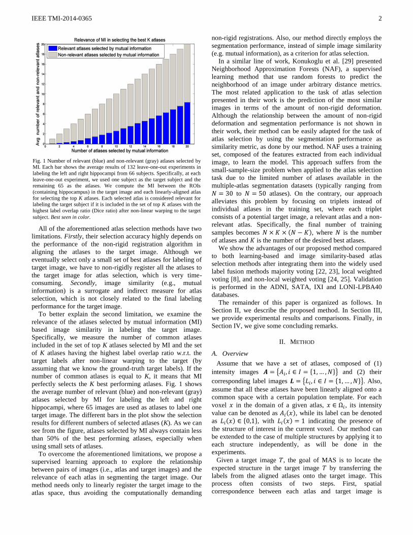
To better explain the second limitation, we examine the

relevance of the atlases selected by mutual information (MI)

based image similarity in labeling the target image.

Specifically, we measure the number of common atlases

included in the set of top K atlases selected by MI and the set

of K atlases having the highest label overlap ratio w.r.t. the

target labels after non-linear warping to the target (by

assuming that we know the ground-truth target labels). If the

number of common atlases is equal to K, it means that MI

perfectly selects the K best performing atlases. Fig. 1 shows

the average number of relevant (blue) and non-relevant (gray)

atlases selected by MI for labeling the left and right

hippocampi, where 65 images are used as atlases to label one

target image. The different bars in the plot show the selection

results for different numbers of selected atlases (K). As we can

see from the figure, atlases selected by MI always contain less

than 50% of the best performing atlases, especially when

using small sets of atlases.

To overcome the aforementioned limitations, we propose a

supervised learning approach to explore the relationship

between pairs of images (i.e., atlas and target images) and the

relevance of each atlas in segmenting the target image. Our

method needs only to linearly register the target image to the

atlas space, thus avoiding the computationally demanding

non-rigid registrations. Also, our method directly employs the

segmentation performance, instead of simple image similarity

(e.g. mutual information), as a criterion for atlas selection.

In a similar line of work, Konukoglu et al. [29] presented

Neighborhood Approximation Forests (NAF), a supervised

learning method that use random forests to predict the

neighborhood of an image under arbitrary distance metrics.

The most related application to the task of atlas selection

presented in their work is the prediction of the most similar

images in terms of the amount of non-rigid deformation.

Although the relationship between the amount of non-rigid

deformation and segmentation performance is not shown in

their work, their method can be easily adapted for the task of

atlas selection by using the segmentation performance as

similarity metric, as done by our method. NAF uses a training

set, composed of the features extracted from each individual

image, to learn the model. This approach suffers from the

small-sample-size problem when applied to the atlas selection

task due to the limited number of atlases available in the

multiple-atlas segmentation datasets (typically ranging from

to atlases). On the contrary, our approach

alleviates this problem by focusing on triplets instead of

individual atlases in the training set, where each triplet

consists of a potential target image, a relevant atlas and a non-

relevant atlas. Specifically, the final number of training

samples becomes ( ), where is the number

of atlases and is the number of the desired best atlases.

We show the advantages of our proposed method compared

to both learning-based and image similarity-based atlas

selection methods after integrating them into the widely used

label fusion methods majority voting [22, 23], local weighted

voting [8], and non-local weighted voting [24, 25]. Validation

is performed in the ADNI, SATA, IXI and LONI-LPBA40

databases.

The remainder of this paper is organized as follows. In

Section II, we describe the proposed method. In Section III,

we provide experimental results and comparisons. Finally, in

Section IV, we give some concluding remarks.

II. METHOD

A. Overview

Assume that we have a set of atlases, composed of (1)

intensity images { { }} and (2) their

corresponding label images { { }}. Also,

assume that all these atlases have been linearly aligned onto a

common space with a certain population template. For each

voxel in the domain of a given atlas, , its intensity

value can be denoted as ( ), while its label can be denoted

as ( ) { }, with ( ) indicating the presence of

the structure of interest in the current voxel Our method can

be extended to the case of multiple structures by applying it to

each structure independently, as will be done in the

experiments.

Given a target image , the goal of MAS is to locate the

expected structure in the target image by transferring the

labels from the aligned atlases onto the target image. This

process often consists of two steps. First, spatial

correspondence between each atlas and target image is

Fig. 1 Number of relevant (blue) and non-relevant (gray) atlases selected by MI. Each bar shows the average results of 132 leave-one-out experiments in

labeling the left and right hippocampi from 66 subjects. Specifically, at each

leave-one-out experiment, we used one subject as the target subject and the remaining 65 as the atlases. We compute the MI between the ROIs

(containing hippocampus) in the target image and each linearly-aligned atlas

for selecting the top K atlases. Each selected atlas is considered relevant for labeling the target subject if it is included in the set of top K atlases with the

highest label overlap ratio (Dice ratio) after non-linear warping to the target

subject. Best seen in color.

IEEE TMI-2014-0365

3

obtained by a non-rigid registration algorithm [12-14]. In this

way, we can obtain a set of registered atlases { },

along with a set of deformed label images { }. Second, a label fusion procedure is performed to determine the

label on each voxel of the target image by fusing the labels

from all registered atlases .

The accuracy of MAS largely depends on the ability of

selecting suitable atlases, i.e., atlases that are anatomically

similar to the target image. Therefore, atlas selection is a

critical issue, which affects not only to the labeling accuracy,

but also to the labeling speed. Although using a small subset

of atlases can lead to faster labeling, it can potentially lead to a

large inaccuracy since relevant information from other atlases

may be left out. On the other hand, using a large subset of

atlases can potentially increase the chance of including more

relevant atlases at the expenses of including more ambiguous

atlases and spending longer computational time. The most

common atlas selection strategy consists in using an image

similarity measurement such as mutual information (MI) [26]

to select the most similar atlases to the target image .

Although these image-similarity-based atlas selection methods

perform significantly better than random atlas selection [7],

the image similarity metric used is not directly related to the

final labeling performance. Mathematically, given a target

image and a set of atlases ( ), the whole process of MAS

can be formulated as:

( ) (1)

where is the resulting segmentation for the target image ,

and ( ) with selected index-set , is the subset of

selected atlases for segmenting the target image .

Dice ratio (DR) is widely used to measure the degree of

overlap between two segmentations, such as the

resulting/expected segmentation and the individual

segmentation of each registered atlas . It is defined as:

( ) ( )

( ) ( ) (2)

where ( ) denotes volume. Suppose that we know the

ground-truth label map for the target image, which we denote

as . We can use the Dice ratio between the ground-truth

target labels and each registered atlas labels (i.e., ( )),

to select the set of best atlases for the given target image ,

denoted as , where the set of best atlases satisfies the

following requirement:

( ) (

)

(3)

where the cardinality of the selected atlas set equals to ,

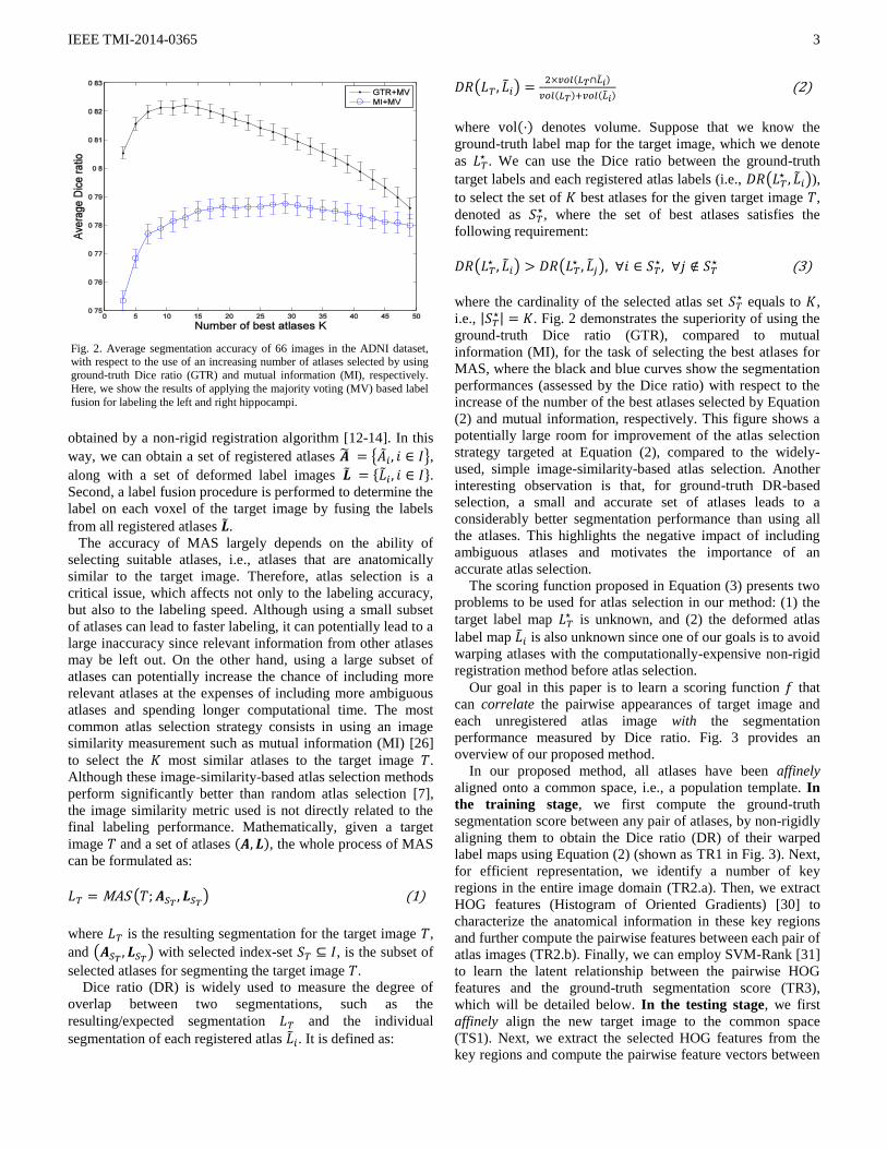
i.e., | | . Fig. 2 demonstrates the superiority of using the

ground-truth Dice ratio (GTR), compared to mutual

information (MI), for the task of selecting the best atlases for

MAS, where the black and blue curves show the segmentation

performances (assessed by the Dice ratio) with respect to the

increase of the number of the best atlases selected by Equation

(2) and mutual information, respectively. This figure shows a

potentially large room for improvement of the atlas selection

strategy targeted at Equation (2), compared to the widely-

used, simple image-similarity-based atlas selection. Another

interesting observation is that, for ground-truth DR-based

selection, a small and accurate set of atlases leads to a

considerably better segmentation performance than using all

the atlases. This highlights the negative impact of including

ambiguous atlases and motivates the importance of an

accurate atlas selection.

The scoring function proposed in Equation (3) presents two

problems to be used for atlas selection in our method: (1) the

target label map is unknown, and (2) the deformed atlas

label map is also unknown since one of our goals is to avoid

warping atlases with the computationally-expensive non-rigid

registration method before atlas selection.

Our goal in this paper is to learn a scoring function that

can correlate the pairwise appearances of target image and

each unregistered atlas image with the segmentation

performance measured by Dice ratio. Fig. 3 provides an

overview of our proposed method.

In our proposed method, all atlases have been affinely

aligned onto a common space, i.e., a population template. In

the training stage, we first compute the ground-truth

segmentation score between any pair of atlases, by non-rigidly

aligning them to obtain the Dice ratio (DR) of their warped

label maps using Equation (2) (shown as TR1 in Fig. 3). Next,

for efficient representation, we identify a number of key

regions in the entire image domain (TR2.a). Then, we extract

HOG features (Histogram of Oriented Gradients) [30] to

characterize the anatomical information in these key regions

and further compute the pairwise features between each pair of

atlas images (TR2.b). Finally, we can employ SVM-Rank [31]

to learn the latent relationship between the pairwise HOG

features and the ground-truth segmentation score (TR3),

which will be detailed below. In the testing stage, we first

affinely align the new target image to the common space

(TS1). Next, we extract the selected HOG features from the

key regions and compute the pairwise feature vectors between

Fig. 2. Average segmentation accuracy of 66 images in the ADNI dataset, with respect to the use of an increasing number of atlases selected by using

ground-truth Dice ratio (GTR) and mutual information (MI), respectively.

Here, we show the results of applying the majority voting (MV) based label

fusion for labeling the left and right hippocampi.

IEEE TMI-2014-0365

4

the new target image and each atlas (TS2). Finally, we

evaluate the potential segmentation performance of each atlas

by using the learned SVM-Rank model (TS3), and select the

best atlases for MAS according to the obtained scores (TS4).

The main intuition behind our approach is to learn the

relationships between affine registration errors (encoded in the

pairwise HOG features) and the final segmentation

performance (in terms of Dice ratio). Or, equivalently, we

learn which affine registration errors are critical in

determining the final segmentation performance after non-

rigid registration. To make our learning approach tractable, we

use a linear model for mapping the pairwise representations

obtained by the feature extraction process to our final score ,

as stated below:

( ) ( ) (4)

where ( ) is the vector of pairwise features derived from a

pair of images (TR2 in Fig. 3) and is the weighting vector

modeling the relationship between the pairwise features and

the ground-truth segmentation score (TR3 in Fig. 3). Each

element in this weighting vector measures the importance of a

particular pairwise feature in predicting the segmentation

score.

In the next two subsections, we will describe the process of

learning the weighting vector and computing the pairwise

features ( ), respectively. Table I shows a summary of the

notation used in the rest of the paper.

B. Learning the Relationships Between Pairwise Features

and Segmentation Score

Here, we focus on the computation of the weighting vector by assuming that we already have the pairwise features

between the images (which we will explain in Section II.C).

Consider an atlas in the training set as the target image, e.g.,

, , and the rest as the atlases, i.e., { }. According

to Equation (3), we focus on the separation between the set of

the best atlases, denoted as , and the rest (i.e.,

{ { }}). That is, we want to find the weighting vector

that satisfies the following inequalities:

( ) ( ) {

{ }} (5)

It is worth noting that ( ) denotes the features extracted

from a pair of linearly aligned intensity images without

applying any non-rigid registration between them. This type of

problem, in which we seek to satisfy certain order

relationships between pairs of elements ( ) with respect

to a given reference , is known as learning to rank and there

exist several algorithms in the literature aimed at solving this

problem [31-33]. We use SVM-Rank1 [31] because it has

1 we use the implementation in

http://olivier.chapelle.cc/primal/

Fig. 3 Overview of our proposed method. Training: TR1) computation of

ground-truth Dice ratio between each pair of atlas label maps after non-rigid

registration, TR2) computation of pairwise features from the key regions between each pair of atlas images after affine alignment, and TR3) learning

of the relationship between pairwise features and ground-truth DR. Testing:

TS1) affine alignment of the target image to the common space, TS2)

computation of pairwise features between the target and all the atlas images,

TS3) prediction of the segmentation performance by using the learned

model, and TS4) selection of atlases with the highest scores for multiple-atlas

segmentation.

TABLE I SUMMARY OF NOTATION

Symbol Description

( ) Intensity and label images of the -th atlas

( ) Intensity and label images of the -th atlas after non-

rigid warping to a particular target (

) Target intensity image, estimated label image (by

MAS) and ground-truth label image, respectively.

Index-set of the N atlases

Index to denote the atlas acting as target image in the training set

Scalar denoting the number of selected atlases to be

used for MAS

Set of indexes of the best atlases for segmenting

target image , according to ground-truth

Set of indexes of the best atlases for segmenting

target image

( ) Scoring function that maps a pair of affinely

registered images to their expected segmentation performance

Weighting vector learned by SVM-Rank

Vector with the HOG features extracted from -th image in the training set

Scalar denoting the total number of features

Vector with the -th pairwise feature from all atlas-target pairs in the training set

Vector with the ground-truth DR from all atlas-

target pairs in the training set

( ) Compact vector of pairwise features from a pair of

target and atlas images

Scalar denoting the size of the compact set of features

IEEE TMI-2014-0365

5

superior performance than other methods [34]. Accordingly,

we compute a set of constraints for each target image , to

constrain the pairs of atlases ( ) so that the -th atlas

should be ranked higher than the -th atlas according to their

ground-truth Dice ratios. Considering as the ground-truth

selection of the best atlases for segmenting the target image

, as defined in Equation (3), the set of specific constraints

for the target image can be now defined as follows:

{( ) |

{ { }}} (6)

where is the set of indices of the best atlases for

segmenting the target image , and ( ) means that the

-th atlas should be ranked higher than the -th atlas for

segmenting . By using the SVM-Rank, we pose this

problem as a constrained optimization problem, in which we

want to find the weighting vector that maximizes the

margin between the scores of the relevant and non-relevant

atlases. We can mathematically formulate it as:

‖ ‖ ∑

( )

( ) ( ) (7)

where the objective function represents a trade-off between a

regularization term and the margin size, controlled by the

parameter . The margin is dynamically set to , with

as the slack variable controlling the amount of margin

violation regarding each triplet ( ).

The constraints of Eq. (7) can be equivalently expressed as

– , where each

( ) – ( ) can be considered as an

individual training sample regarding the triplet ( ).

Therefore, the final number of training samples used by our

method becomes ( ), where is the number of

atlases and is the number of the desired best atlases. This

represents an advantage in the case of small training sets as is

usually the case in multiple-atlas segmentation. For example,

in the case of learning to select the best atlases from a

set of atlases, this would correspond to

training samples in our method.

As part of the training process, we need to perform ( ) pairwise non-rigid registrations between the atlases in

order to compute the constraints of Equation (6). It is worth

noting that this is done in the training stage, which will not

affect the speed of the testing stage.

C. Pairwise Feature Computation

As mentioned in Equation (4), our relevance score is a

function of the pairwise features between target image and

atlas image . In order to find a more compact and accurate

representation for describing the connection between and ,

the calculation of ( ) consists of three steps, namely, (1)

key region detection, (2) pairwise HOG computation, and (3)

feature selection, as detailed below one by one. It is worth

noting that we compute the pairwise features only after affine

registration, both in the training and testing stages. However,

the Dice ratio in the training stage (Section II.B) is computed

based on the non-rigid registration results, which essentially

reflects the goal of our approach to predict the segmentation

score based only on the affine registration results.

1) Key Region Detection

In MAS, the segmentation label at each point in the target

image is determined by the labels of the aligned atlases at that

point. Regions with high label variability, such as label

boundaries, are the source of most labeling errors. Therefore,

we use the appearance in these regions as cues to predict the

segmentation performance. Since we already know the label

information in the training set, we can obtain the set of

boundary locations ( ) from the label map , where

is the set of locations in the whole volume of the -th atlas.

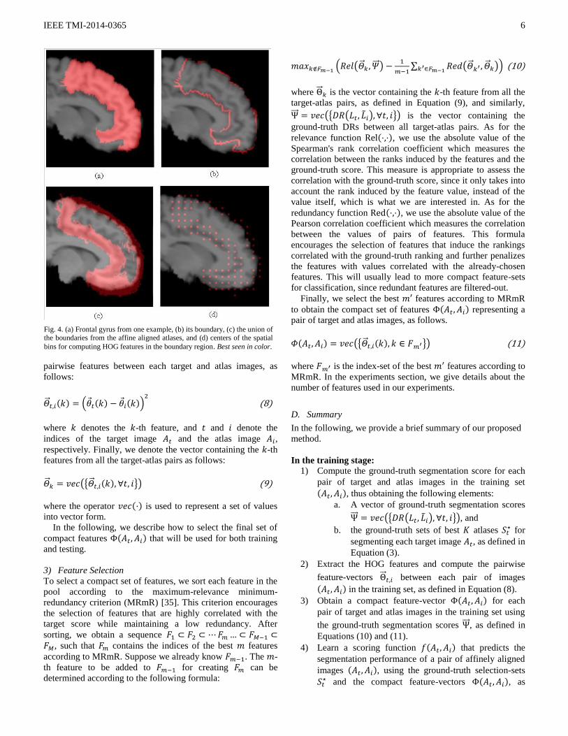
We further define the set of sensible locations as the union of

all boundary locations in all the training set, ⋃ ( ) .

Fig. 4 shows an example structure, its boundary, and the union

of all boundaries from all pre-registered atlases (with affine

transformation).

2) Pairwise HOG Computation

HOG descriptors provide a histogram of local edge

orientations in the image. Pairwise HOG features in our

method are computed as the squared differences of the HOG

features. Therefore, they convey information about edge

orientation differences after affine alignment. Intuitively, high

feature values at certain locations indicate large edge

discrepancy between the two images. Many works have

demonstrated that the registration accuracy depends on the

shape discrepancies between two images, while label fusion

performance (measured by the Dice score), depends on the

non-rigid registration accuracy along the boundaries of the

structures. Since HOG features are good indicators of the

shape discrepancies, then HOG features extracted in the

boundary regions provide useful clues to predict the final

segmentation performance.

We initially extract the HOG features from the whole

rectangular ROI containing the structure to be segmented. The

rectangular ROI is computed as the rectangular bounding box

containing the union of all the labels in the training set, and

then enlarged by 20 voxels on each side. Computation of the

HOG features establishes a partition of the ROI into spatial

bins, with each spatial bin containing the feature values of all

the orientation bins at that location. We concatenate the

features at spatial bins within a distance to the nearest

boundary point in , to construct a feature vector . We use

the locations of the spatial bin centers to compute the distance

to the boundary region. Overlaid on the intensity image, Fig. 4

(d) shows the centers of the selected bins in the boundary

region of Fig 4 (c). Note that the location of the selected HOG

features is fixed for all the images since it depends on the

union of boundaries in the whole training set. After this

process, for each individual image, we obtain a vector containing a number of selected HOG features in the

boundary region. We use the squared difference between the

features from the individual images to compute the pool of

IEEE TMI-2014-0365

6

pairwise features between each target and atlas images, as

follows:

( ) ( ( ) ( ))

(8)

where denotes the -th feature, and and denote the

indices of the target image and the atlas image ,

respectively. Finally, we denote the vector containing the -th

features from all the target-atlas pairs as follows:

({ ( ) }) (9)

where the operator ( ) is used to represent a set of values

into vector form.

In the following, we describe how to select the final set of

compact features ( ) that will be used for both training

and testing.

3) Feature Selection

To select a compact set of features, we sort each feature in the

pool according to the maximum-relevance minimum-

redundancy criterion (MRmR) [35]. This criterion encourages

the selection of features that are highly correlated with the

target score while maintaining a low redundancy. After

sorting, we obtain a sequence , such that contains the indices of the best features

according to MRmR. Suppose we already know . The -

th feature to be added to for creating can be

determined according to the following formula:

( ( )

∑ ( )

) (10)

where is the vector containing the -th feature from all the

target-atlas pairs, as defined in Equation (9), and similarly,

({ ( ) }) is the vector containing the

ground-truth DRs between all target-atlas pairs. As for the

relevance function ( ), we use the absolute value of the

Spearman's rank correlation coefficient which measures the

correlation between the ranks induced by the features and the

ground-truth score. This measure is appropriate to assess the

correlation with the ground-truth score, since it only takes into

account the rank induced by the feature value, instead of the

value itself, which is what we are interested in. As for the

redundancy function ( ), we use the absolute value of the

Pearson correlation coefficient which measures the correlation

between the values of pairs of features. This formula

encourages the selection of features that induce the rankings

correlated with the ground-truth ranking and further penalizes

the features with values correlated with the already-chosen

features. This will usually lead to more compact feature-sets

for classification, since redundant features are filtered-out.

Finally, we select the best features according to MRmR

to obtain the compact set of features ( ) representing a

pair of target and atlas images, as follows.

( ) ({ ( ) }) (11)

where is the index-set of the best features according to

MRmR. In the experiments section, we give details about the

number of features used in our experiments.

D. Summary

In the following, we provide a brief summary of our proposed

method.

In the training stage:

1) Compute the ground-truth segmentation score for each

pair of target and atlas images in the training set

( ), thus obtaining the following elements:

a. A vector of ground-truth segmentation scores

({ ( ) }), and

b. the ground-truth sets of best atlases for

segmenting each target image , as defined in

Equation (3).

2) Extract the HOG features and compute the pairwise

feature-vectors between each pair of images

( ) in the training set, as defined in Equation (8).

3) Obtain a compact feature-vector ( ) for each

pair of target and atlas images in the training set using

the ground-truth segmentation scores , as defined in

Equations (10) and (11).

4) Learn a scoring function ( ) that predicts the

segmentation performance of a pair of affinely aligned

images ( ), using the ground-truth selection-sets

and the compact feature-vectors ( ), as

Fig. 4. (a) Frontal gyrus from one example, (b) its boundary, (c) the union of the boundaries from the affine aligned atlases, and (d) centers of the spatial

bins for computing HOG features in the boundary region. Best seen in color.

IEEE TMI-2014-0365

7

defined in Section II.B.

In the testing stage:

1) Affinely align a new target image onto the common

space.

2) Extract HOG features from the affinely aligned target

image and obtain compact vectors of pairwise

features between the target image and all the atlases,

i.e., { ( ) }. 3) Determine the set of atlases ( ) with the highest

expected performance for segmenting target image ,

such that ( ) ( ) , and

| | .

4) Segment target image using the selected atlases

( ), as defined in Equation (1).

It is worth noting that we need to learn a different scoring

function ( ) for each different value of .

III. EXPERIMENTS

We have evaluated the performance of our atlas selection

method in four datasets, namely, ADNI2, SATA

3, IXI

4 and

LONI-LPBA405 [36] datasets. Segmentation performance is

assessed by the Dice ratio between the estimated

segmentations and the ground-truth label annotations.

In the ADNI, IXI and LONI-LPBA40 dataset we conducted

the following three pre-processing steps on all images: (1)

Skull stripping by a learning-based meta-algorithm [37]; (2)

N4-based bias field correction [38]; (3) ITK-based histogram

matching for normalizing the intensity range. We use non-

rigid registration with diffeomorphic demons [14] for both

ground-truth Dice ratio computation and multi-atlas

segmentation of new target images. The images in the SATA

dataset were already skull-stripped and their pairwise non-

rigid deformations were also provided. We use FLIRT [39] to

affinely align all atlases to a population image, prior to feature

extraction.

We perform our segmentation experiments by combining

different atlas selection methods with different label fusion

methods. Specifically, we use the following atlas selection

methods: (1) our proposed method, denoted as HSR (HOG

plus SVMRank), (2) a degraded version of our proposed

method that selects atlases according only to the distance

between the HOG features, denoted as HOG, and (3) a

baseline method which selects the best atlases by mutual-

information-based image similarity, denoted as MI. We also

include a comparison with the state-of-the-art Neighbourhood

Approximation Forests (NAF) method [29], which uses

random forests to predict the neighborhood in a population of

training samples under arbitrary similarity measurements.

The degraded version of our method for atlas selection (i.e.,

HOG) uses the squared differences between the pools of HOG

features from two images in order to select the best atlases.

2 http://www.adni-info.org/ 3

https://masi.vuse.vanderbilt.edu/workshop2013/index.

php/Main_Page 4 http://www.brain-development.org 5 http://www.loni.ucla.edu/Atlases/LPBA40

This can be expressed by the new scoring function ( )

∑ ( ( ) ( ))

, where ( ) and

( ) are the

-th features in the vectors of HOG features extracted from

the key regions of the target image and the atlas image ,

respectively. This scoring function corresponds to the sum of

local edge discrepancies between the atlas and the target

image and can be used as reference to elucidate the benefit of

the learning component in our method for effective atlas

selection.

NAF is a state-of-the-art learning-based method for

predicting neighborhoods given arbitrary distance metrics.

One of the applications of NAF is the prediction of the most

similar training images to a given testing one in terms of the

amount of non-rigid deformation necessary to align them.

Although there is no direct relationship between the amount of

deformation and the final segmentation performance, it is

straightforward to adapt NAF for the task of atlas selection. To

that end, we define the new ground-truth dissimilarity metric

between two training images and as ( ),

where ( ) is the ground-truth Dice ratio as defined in Eq.

(2). By using this dissimilarity measurement, selection by

NAF is directly motivated by the final segmentation

performance (as in our method). We use the implementation

provided by the authors6.

Segmentation experiments are run on each anatomical

structure independently. We use a region of interest containing

the anatomical structure to be segmented as input for the three

selection methods. All the methods use the affinely aligned

images as input. The three label fusion methods used are,

respectively, (1) majority voting (MV) [22, 23], (2) local

weighted voting (LWV) [8], and (3) non-local weighted voting

(NLWV) [24, 25]. MV-based label fusion assigns each target

voxel with the label occurring most frequently among all the

candidate atlas voxels. LWV- and NLWV-based label fusions

use the image patch similarity measure to estimate the local

relevance of each atlas patch to segment the target image. The

difference between LWV and NLWV is that LWV-based label

fusion only takes into account the corresponding atlas patches,

whereas NLWV-based label fusion searches similar patches

within a local neighborhood.

Each segmentation variant is named as ‘the atlas selection

method + the label fusion method’. This is, ‘MI+MV’

represents the segmentation variant using mutual information

for atlas selection and majority voting for label fusion.

In the ADNI, IXI and LONI-LPBA40 datasets, we conduct

5-fold cross-validation experiments. That is, we partition each

dataset into 5 subsets and, at each fold, we use the images in

one subset as the target images and all the images in the

remaining subsets as the atlases. In the SATA dataset, we use

the pre-defined training and testing sets.

A. Parameter Setting

HOG features have two parameters, namely, the number of

orientation bins and cell size (in voxels) of the spatial

bins. We found our method not very sensitive to the values of

these parameters. Since different structures often have

6 Source code available at

www.nmr.mgh.harvard.edu/~enderk/software.html

IEEE TMI-2014-0365

8

different sizes, setting these parameters to fixed values will

cause larger structures to generate an unnecessarily high

number of features. To trim the number of features to a

manageable size, we adaptively fix the HOG parameters and

to get a reasonable number ( ) of features. Specifically, we

start with and , and iteratively increase the cell

size and decrease the number of orientation bins until the

number of resulting features is less than or equal to , or we

reach the pre-defined values and . Therefore, the

final values for these two parameters are fixed for

each structure. The number of features, , is set to

in all experiments. The final size of the selected features as

used in all experiments is set to . The distance

threshold for selecting the features in the boundary regions is

set to . That is, we use only the HOG features inside the

boundary region. We set the parameters for the LWV- and

NLWV-based label fusion methods according to the values

given in [24].

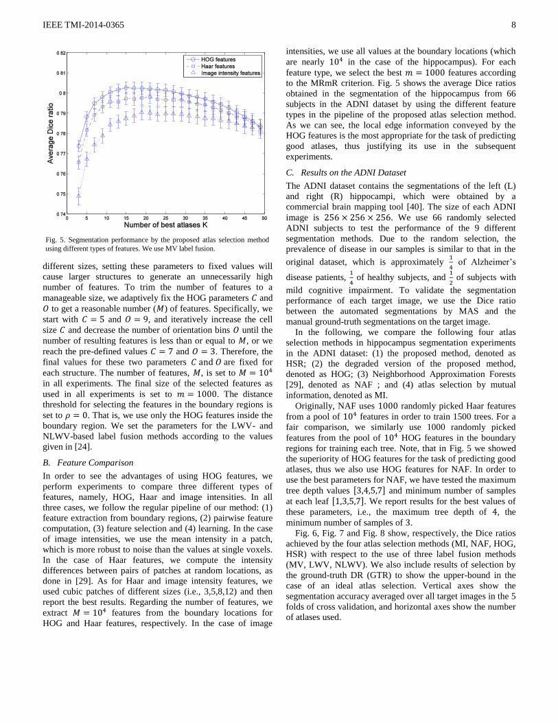
B. Feature Comparison

In order to see the advantages of using HOG features, we

perform experiments to compare three different types of

features, namely, HOG, Haar and image intensities. In all

three cases, we follow the regular pipeline of our method: (1)

feature extraction from boundary regions, (2) pairwise feature

computation, (3) feature selection and (4) learning. In the case

of image intensities, we use the mean intensity in a patch,

which is more robust to noise than the values at single voxels.

In the case of Haar features, we compute the intensity

differences between pairs of patches at random locations, as

done in [29]. As for Haar and image intensity features, we

used cubic patches of different sizes (i.e., 3,5,8,12) and then

report the best results. Regarding the number of features, we

extract features from the boundary locations for

HOG and Haar features, respectively. In the case of image

intensities, we use all values at the boundary locations (which

are nearly in the case of the hippocampus). For each

feature type, we select the best features according

to the MRmR criterion. Fig. 5 shows the average Dice ratios

obtained in the segmentation of the hippocampus from 66

subjects in the ADNI dataset by using the different feature

types in the pipeline of the proposed atlas selection method.

As we can see, the local edge information conveyed by the

HOG features is the most appropriate for the task of predicting

good atlases, thus justifying its use in the subsequent

experiments.

C. Results on the ADNI Dataset

The ADNI dataset contains the segmentations of the left (L)

and right (R) hippocampi, which were obtained by a

commercial brain mapping tool [40]. The size of each ADNI

image is . We use 66 randomly selected

ADNI subjects to test the performance of the 9 different

segmentation methods. Due to the random selection, the

prevalence of disease in our samples is similar to that in the

original dataset, which is approximately

of Alzheimer’s

disease patients,

of healthy subjects, and

of subjects with

mild cognitive impairment. To validate the segmentation

performance of each target image, we use the Dice ratio

between the automated segmentations by MAS and the

manual ground-truth segmentations on the target image.

In the following, we compare the following four atlas

selection methods in hippocampus segmentation experiments

in the ADNI dataset: (1) the proposed method, denoted as

HSR; (2) the degraded version of the proposed method,

denoted as HOG; (3) Neighborhood Approximation Forests

[29], denoted as NAF ; and (4) atlas selection by mutual

information, denoted as MI.

Originally, NAF uses randomly picked Haar features

from a pool of features in order to train 1500 trees. For a

fair comparison, we similarly use 1000 randomly picked

features from the pool of HOG features in the boundary

regions for training each tree. Note, that in Fig. 5 we showed

the superiority of HOG features for the task of predicting good

atlases, thus we also use HOG features for NAF. In order to

use the best parameters for NAF, we have tested the maximum

tree depth values [ ] and minimum number of samples

at each leaf [ ]. We report results for the best values of

these parameters, i.e., the maximum tree depth of , the

minimum number of samples of .

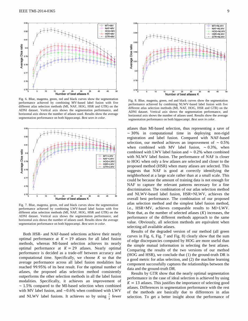
Fig. 6, Fig. 7 and Fig. 8 show, respectively, the Dice ratios

achieved by the four atlas selection methods (MI, NAF, HOG,

HSR) with respect to the use of three label fusion methods

(MV, LWV, NLWV). We also include results of selection by

the ground-truth DR (GTR) to show the upper-bound in the

case of an ideal atlas selection. Vertical axes show the

segmentation accuracy averaged over all target images in the 5

folds of cross validation, and horizontal axes show the number

of atlases used.

Fig. 5. Segmentation performance by the proposed atlas selection method

using different types of features. We use MV label fusion.

IEEE TMI-2014-0365

9

Both HSR- and NAF-based selections achieve their nearly

optimal performance at atlases for all label fusion

methods, whereas MI-based selection achieves its nearly

optimal performance at atlases. Nearly optimal

performance is decided as a trade-off between accuracy and

computational time. Specifically, we choose so that the

average performance across all label fusion modalities has

reached of its best result. For the optimal number of

atlases, the proposed atlas selection method consistently

outperforms the other selection methods in all the label fusion

modalities. Specifically, it achieves an improvement of

compared to the MI-based selection when combined

with MV label fusion, and when combined with LWV

and NLWV label fusions. It achieves so by using

fewer

atlases than MI-based selection, thus representing a save of

in computational time in deploying non-rigid

registration and label fusion. Compared with NAF-based

selection, our method achieves an improvement of

when combined with MV label fusion, , when

combined with LWV label fusion and when combined

with NLWV label fusion. The performance of NAF is closer

to HOG when only a few atlases are selected and closer to the

proposed method (HSR) when many atlases are selected. This

suggests that NAF is good at correctly identifying the

neighborhood at a large scale rather than at a small scale. This

could be because the amount of training data is not enough for

NAF to capture the relevant patterns necessary for a fine

discrimination. The combination of our atlas selection method

and NLWV-based label fusion, HSR+NLWV, achieves the

overall best performance. The combination of our proposed

atlas selection method and the simplest label fusion method,

i.e., HSR+MV, achieves comparable results to MI+LWV.

Note that, as the number of selected atlases ( ) increases, the

performance of the different methods approach to the same

value. Obviously, all selection methods are equivalent when

selecting all available atlases.

Results of the degraded version of our method (all green

curves in Fig. 6, Fig. 7 and Fig. 8) clearly show that the sum

of edge discrepancies computed by HOG are more useful than

the simple mutual information in selecting the best atlases.

Comparing the results of the two versions of our method

(HOG and HSR), we conclude that (1) the ground-truth DR is

a good metric for atlas selection, and (2) the machine learning

component successfully captures the relationships between the

data and the ground-truth DR.

Results by GTR show that the nearly optimal segmentation

performance in the case of ideal selection is achieved by using

atlases. This justifies the importance of selecting good

atlases. Differences in segmentation performance with the rest

of the methods are basically due to differences in atlas

selection. To get a better insight about the performance of

Fig. 6. Blue, magenta, green, red and black curves show the segmentation

performance achieved by combining MV-based label fusion with five

different atlas selection methods (MI, NAF, HOG, HSR and GTR) on the

ADNI dataset. Vertical axis shows the segmentation performance, and horizontal axis shows the number of atlases used. Results show the average

segmentation performance on both hippocampi. Best seen in color.

Fig. 7. Blue, magenta, green, red and black curves show the segmentation

performance achieved by combining LWV-based label fusion with five different atlas selection methods (MI, NAF, HOG, HSR and GTR) on the

ADNI dataset. Vertical axis shows the segmentation performance, and

horizontal axis shows the number of atlases used. Results show the average

segmentation performance on both hippocampi. Best seen in color.

Fig. 8. Blue, magenta, green, red and black curves show the segmentation

performance achieved by combining NLWV-based label fusion with five

different atlas selection methods (MI, NAF, HOG, HSR and GTR) on the

ADNI dataset. Vertical axis shows the segmentation performance, and horizontal axis shows the number of atlases used. Results show the average

segmentation performance on both hippocampi. Best seen in color.

IEEE TMI-2014-0365

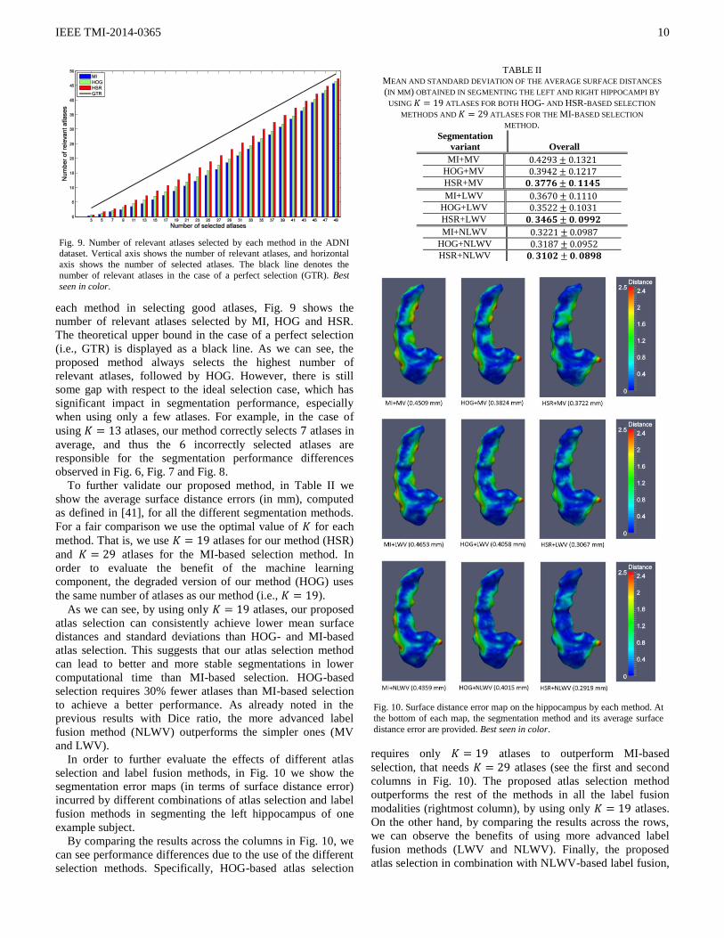
10

each method in selecting good atlases, Fig. 9 shows the

number of relevant atlases selected by MI, HOG and HSR.

The theoretical upper bound in the case of a perfect selection

(i.e., GTR) is displayed as a black line. As we can see, the

proposed method always selects the highest number of

relevant atlases, followed by HOG. However, there is still

some gap with respect to the ideal selection case, which has

significant impact in segmentation performance, especially

when using only a few atlases. For example, in the case of

using atlases, our method correctly selects atlases in

average, and thus the incorrectly selected atlases are

responsible for the segmentation performance differences

observed in Fig. 6, Fig. 7 and Fig. 8.

To further validate our proposed method, in Table II we

show the average surface distance errors (in mm), computed

as defined in [41], for all the different segmentation methods.

For a fair comparison we use the optimal value of for each

method. That is, we use atlases for our method (HSR)

and atlases for the MI-based selection method. In

order to evaluate the benefit of the machine learning

component, the degraded version of our method (HOG) uses

the same number of atlases as our method (i.e., ).

As we can see, by using only atlases, our proposed

atlas selection can consistently achieve lower mean surface

distances and standard deviations than HOG- and MI-based

atlas selection. This suggests that our atlas selection method

can lead to better and more stable segmentations in lower

computational time than MI-based selection. HOG-based

selection requires 30% fewer atlases than MI-based selection

to achieve a better performance. As already noted in the

previous results with Dice ratio, the more advanced label

fusion method (NLWV) outperforms the simpler ones (MV

and LWV).

In order to further evaluate the effects of different atlas

selection and label fusion methods, in Fig. 10 we show the

segmentation error maps (in terms of surface distance error)

incurred by different combinations of atlas selection and label

fusion methods in segmenting the left hippocampus of one

example subject.

By comparing the results across the columns in Fig. 10, we

can see performance differences due to the use of the different

selection methods. Specifically, HOG-based atlas selection

requires only atlases to outperform MI-based

selection, that needs atlases (see the first and second

columns in Fig. 10). The proposed atlas selection method

outperforms the rest of the methods in all the label fusion

modalities (rightmost column), by using only atlases.

On the other hand, by comparing the results across the rows,

we can observe the benefits of using more advanced label

fusion methods (LWV and NLWV). Finally, the proposed

atlas selection in combination with NLWV-based label fusion,

TABLE II MEAN AND STANDARD DEVIATION OF THE AVERAGE SURFACE DISTANCES

(IN MM) OBTAINED IN SEGMENTING THE LEFT AND RIGHT HIPPOCAMPI BY

USING ATLASES FOR BOTH HOG- AND HSR-BASED SELECTION

METHODS AND ATLASES FOR THE MI-BASED SELECTION

METHOD.

Segmentation

variant

Overall

MI+MV

HOG+MV

HSR+MV

MI+LWV

HOG+LWV

HSR+LWV

MI+NLWV

HOG+NLWV

HSR+NLWV

Fig. 10. Surface distance error map on the hippocampus by each method. At

the bottom of each map, the segmentation method and its average surface

distance error are provided. Best seen in color.

Fig. 9. Number of relevant atlases selected by each method in the ADNI dataset. Vertical axis shows the number of relevant atlases, and horizontal

axis shows the number of selected atlases. The black line denotes the

number of relevant atlases in the case of a perfect selection (GTR). Best

seen in color.

IEEE TMI-2014-0365

11

HSR+NLWV, achieves the overall lowest surface distance

errors, as can be seen in the bottom-right map.

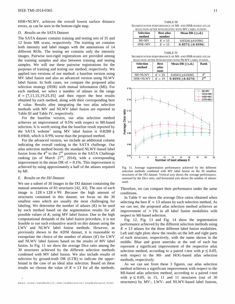
D. Results on the SATA Dataset

The SATA dataset contains training and testing sets of 35 and

12 brain MR scans, respectively. The training set contains

both intensity and label images with the annotations of 14

different ROIs. The testing set contains only the intensity

images. Pairwise non-rigid registrations are provided among

the training samples and also between training and testing

samples. We will use these pairwise registrations for the

purposes of training and testing our method, respectively. We

applied two versions of our method: a baseline version using

MV label fusion and also an advanced version using NLWV

label fusion. In both cases, we compare the proposed atlas

selection strategy (HSR) with mutual information (MI). For

each method, we select a number of atlases in the range

[ ] and then report the best results

obtained by each method, along with their corresponding best

value. Results after integrating the two atlas selection

methods with MV and NLWV label fusion are reported in

Table III and Table IV, respectively.

For the baseline version, our atlas selection method

achieves an improvement of with respect to MI-based

selection. It is worth noting that the baseline result reported by

the SATA website7 using MV label fusion is

, which is worse than the proposed method.

For the advanced version, we include an additional column

indicating the overall ranking in the SATA challenge. Our

atlas selection method boosts the standard NLWV-based label

fusion from the 4th

to the 2nd

position in the SATA Challenge

ranking (as of March 27th

, 2014), with a corresponding

improvement in the mean DR of . This improvement is

achieved by using approximately a half of the atlases required

by MI.

E. Results on the IXI Dataset

We use a subset of 30 images in the IXI dataset containing the

manual annotations of 83 structures [42, 43]. The size of each

image is . Because the high amount of

structures contained in this dataset, we focus on the 30

smallest ones which are usually the most challenging for

labeling. We determine the number of atlases (K) to be used

by each method based on the segmentation results for all

possible values of K, using MV label fusion. Due to the high

computational demands of the label fusion procedure, it is not

feasible to run such exhaustive search on this dataset using the

LWV and NLWV label fusion methods. However, as

previously shown in the ADNI dataset, it is reasonable to

extrapolate the choice of the number of atlases ( ) for LWV

and NLWV label fusions based on the results of MV label

fusion. In Fig. 11 we show the average Dice ratio among the

30 structures achieved by the different selection methods

combined with MV label fusion. We also include results of

selection by ground-truth DR (GTR) to indicate the upper-

bound in the case of an ideal atlas selection. Based on these

results we choose the value of for all the methods.

7

masi.vuse.vanderbilt.edu/submission/leaderboard.html

Therefore, we can compare their performance under the same

conditions.

In Table V we show the average Dice ratios obtained when

selecting the best atlases by each selection method. As

we can see, the proposed atlas selection method achieves an

improvement of in all label fusion modalities with

respect to MI-based selection.

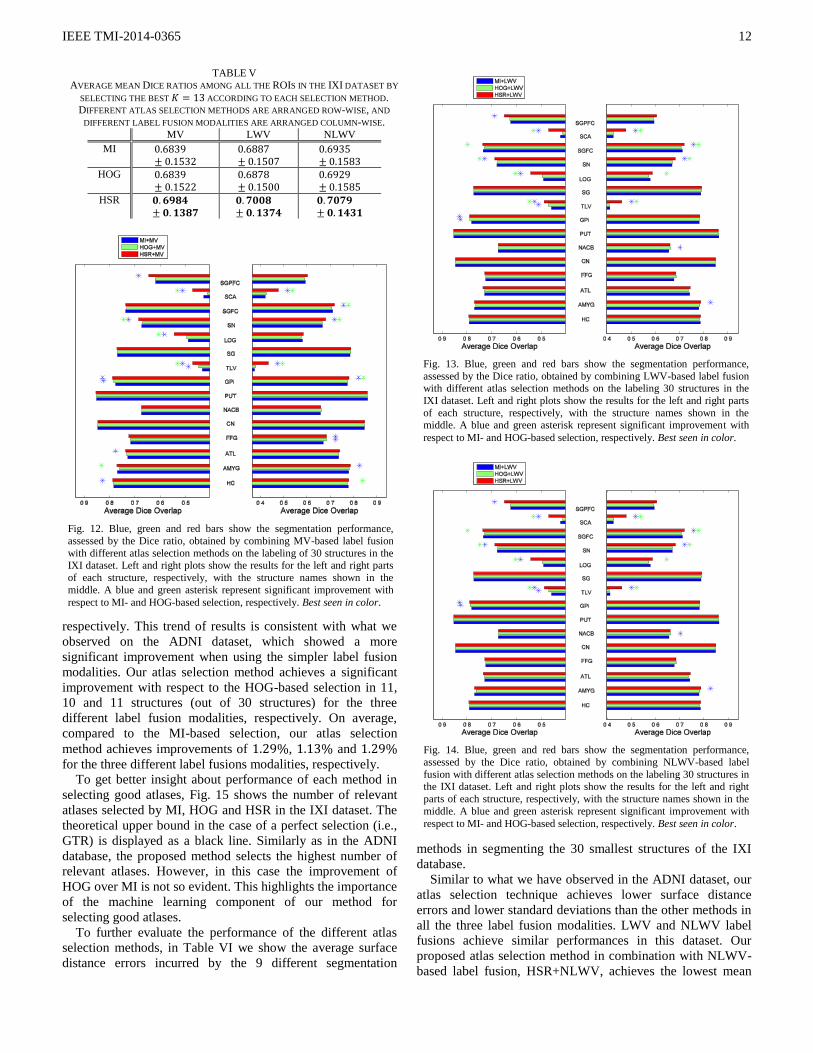
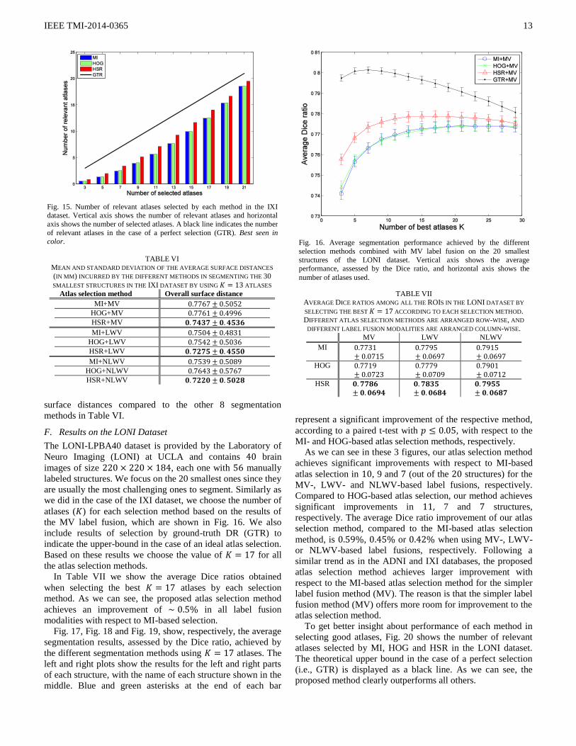
Fig. 12, Fig. 13 and Fig. 14 show the segmentation

performance achieved by the different selection methods using

atlases for the three different label fusion modalities.

Left and right plots show the results on the left and right parts

of each structure, respectively, with the name shown in the

middle. Blue and green asterisks at the end of each bar

represent a significant improvement of the respective atlas

selection method, according to a paired t-test with ,

with respect to the MI- and HOG-based atlas selection

methods, respectively.

As we can see from these 3 figures, our atlas selection

method achieves a significant improvement with respect to the

MI-based atlas selection method, according to a paired t-test

with , in 15, 11 and 11 structures (out of 30

structures) by MV-, LWV- and NLWV-based label fusions,

TABLE III

SEGMENTATION PERFORMANCE OF MI- AND HSR-BASED ATLAS

SELECTION AFTER INTEGRATING WITH MV LABEL FUSION.

Selection

method

Best atlas

number

Mean DR ( s.d.)

MI+MV ( ) HSR+MV ( )

TABLE IV

SEGMENTATION PERFORMANCE OF MI- AND HSR-BASED ATLAS

SELECTION AFTER INTEGRATING WITH NLWV LABEL FUSION.

Selection

method

Best

atlas

num

Mean DR ( s.d.) Rank

MI+NLWV ( ) 4th

HSR+NLWV ( ) 2nd

Fig. 11. Average segmentation performance achieved by the different selection methods combined with MV label fusion on the 30 smallest

structures of the IXI dataset. Vertical axis shows the average performance,

assessed by the Dice ratio, and horizontal axis shows the number of atlases

used.

IEEE TMI-2014-0365

12

respectively. This trend of results is consistent with what we

observed on the ADNI dataset, which showed a more

significant improvement when using the simpler label fusion

modalities. Our atlas selection method achieves a significant

improvement with respect to the HOG-based selection in 11,

10 and 11 structures (out of 30 structures) for the three

different label fusion modalities, respectively. On average,

compared to the MI-based selection, our atlas selection

method achieves improvements of , and

for the three different label fusions modalities, respectively.

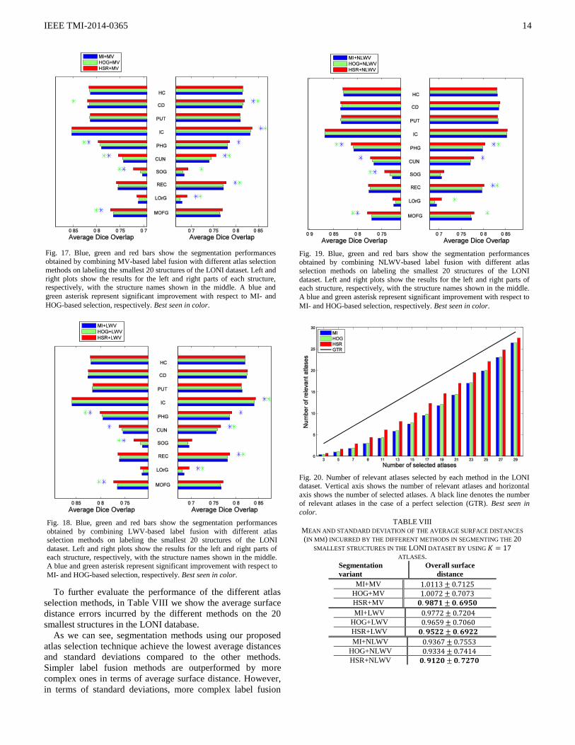
To get better insight about performance of each method in

selecting good atlases, Fig. 15 shows the number of relevant

atlases selected by MI, HOG and HSR in the IXI dataset. The

theoretical upper bound in the case of a perfect selection (i.e.,

GTR) is displayed as a black line. Similarly as in the ADNI

database, the proposed method selects the highest number of

relevant atlases. However, in this case the improvement of

HOG over MI is not so evident. This highlights the importance

of the machine learning component of our method for

selecting good atlases.

To further evaluate the performance of the different atlas

selection methods, in Table VI we show the average surface

distance errors incurred by the 9 different segmentation

methods in segmenting the 30 smallest structures of the IXI

database.

Similar to what we have observed in the ADNI dataset, our

atlas selection technique achieves lower surface distance

errors and lower standard deviations than the other methods in

all the three label fusion modalities. LWV and NLWV label

fusions achieve similar performances in this dataset. Our

proposed atlas selection method in combination with NLWV-

based label fusion, HSR+NLWV, achieves the lowest mean

TABLE V AVERAGE MEAN DICE RATIOS AMONG ALL THE ROIS IN THE IXI DATASET BY

SELECTING THE BEST ACCORDING TO EACH SELECTION METHOD.

DIFFERENT ATLAS SELECTION METHODS ARE ARRANGED ROW-WISE, AND

DIFFERENT LABEL FUSION MODALITIES ARE ARRANGED COLUMN-WISE.

MV LWV NLWV

MI

HOG

HSR

Fig. 12. Blue, green and red bars show the segmentation performance,

assessed by the Dice ratio, obtained by combining MV-based label fusion

with different atlas selection methods on the labeling of 30 structures in the

IXI dataset. Left and right plots show the results for the left and right parts

of each structure, respectively, with the structure names shown in the

middle. A blue and green asterisk represent significant improvement with

respect to MI- and HOG-based selection, respectively. Best seen in color.

Fig. 13. Blue, green and red bars show the segmentation performance,

assessed by the Dice ratio, obtained by combining LWV-based label fusion with different atlas selection methods on the labeling 30 structures in the

IXI dataset. Left and right plots show the results for the left and right parts

of each structure, respectively, with the structure names shown in the middle. A blue and green asterisk represent significant improvement with

respect to MI- and HOG-based selection, respectively. Best seen in color.

Fig. 14. Blue, green and red bars show the segmentation performance,

assessed by the Dice ratio, obtained by combining NLWV-based label

fusion with different atlas selection methods on the labeling 30 structures in the IXI dataset. Left and right plots show the results for the left and right

parts of each structure, respectively, with the structure names shown in the

middle. A blue and green asterisk represent significant improvement with

respect to MI- and HOG-based selection, respectively. Best seen in color.

IEEE TMI-2014-0365

13

surface distances compared to the other 8 segmentation

methods in Table VI.

F. Results on the LONI Dataset

The LONI-LPBA40 dataset is provided by the Laboratory of

Neuro Imaging (LONI) at UCLA and contains brain

images of size , each one with manually

labeled structures. We focus on the 20 smallest ones since they

are usually the most challenging ones to segment. Similarly as

we did in the case of the IXI dataset, we choose the number of

atlases ( ) for each selection method based on the results of

the MV label fusion, which are shown in Fig. 16. We also

include results of selection by ground-truth DR (GTR) to

indicate the upper-bound in the case of an ideal atlas selection.

Based on these results we choose the value of for all

the atlas selection methods.

In Table VII we show the average Dice ratios obtained

when selecting the best atlases by each selection

method. As we can see, the proposed atlas selection method

achieves an improvement of in all label fusion

modalities with respect to MI-based selection.

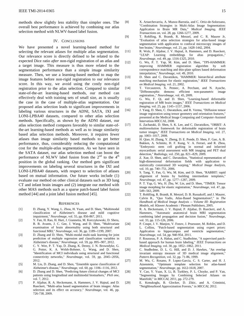
Fig. 17, Fig. 18 and Fig. 19, show, respectively, the average

segmentation results, assessed by the Dice ratio, achieved by

the different segmentation methods using atlases. The

left and right plots show the results for the left and right parts

of each structure, with the name of each structure shown in the

middle. Blue and green asterisks at the end of each bar

represent a significant improvement of the respective method,

according to a paired t-test with , with respect to the

MI- and HOG-based atlas selection methods, respectively.

As we can see in these 3 figures, our atlas selection method

achieves significant improvements with respect to MI-based

atlas selection in , 9 and (out of the structures) for the

MV-, LWV- and NLWV-based label fusions, respectively.

Compared to HOG-based atlas selection, our method achieves

significant improvements in 7 and structures,

respectively. The average Dice ratio improvement of our atlas

selection method, compared to the MI-based atlas selection

method, is , or when using MV-, LWV-

or NLWV-based label fusions, respectively. Following a

similar trend as in the ADNI and IXI databases, the proposed

atlas selection method achieves larger improvement with

respect to the MI-based atlas selection method for the simpler

label fusion method (MV). The reason is that the simpler label

fusion method (MV) offers more room for improvement to the

atlas selection method.

To get better insight about performance of each method in

selecting good atlases, Fig. 20 shows the number of relevant

atlases selected by MI, HOG and HSR in the LONI dataset.

The theoretical upper bound in the case of a perfect selection

(i.e., GTR) is displayed as a black line. As we can see, the

proposed method clearly outperforms all others.

Fig. 15. Number of relevant atlases selected by each method in the IXI dataset. Vertical axis shows the number of relevant atlases and horizontal

axis shows the number of selected atlases. A black line indicates the number

of relevant atlases in the case of a perfect selection (GTR). Best seen in

color.

TABLE VI MEAN AND STANDARD DEVIATION OF THE AVERAGE SURFACE DISTANCES

(IN MM) INCURRED BY THE DIFFERENT METHODS IN SEGMENTING THE 30

SMALLEST STRUCTURES IN THE IXI DATASET BY USING ATLASES

Atlas selection method Overall surface distance

MI+MV

HOG+MV

HSR+MV

MI+LWV

HOG+LWV

HSR+LWV

MI+NLWV

HOG+NLWV

HSR+NLWV

Fig. 16. Average segmentation performance achieved by the different

selection methods combined with MV label fusion on the 20 smallest

structures of the LONI dataset. Vertical axis shows the average performance, assessed by the Dice ratio, and horizontal axis shows the

number of atlases used.

TABLE VII AVERAGE DICE RATIOS AMONG ALL THE ROIS IN THE LONI DATASET BY

SELECTING THE BEST ACCORDING TO EACH SELECTION METHOD. DIFFERENT ATLAS SELECTION METHODS ARE ARRANGED ROW-WISE, AND

DIFFERENT LABEL FUSION MODALITIES ARE ARRANGED COLUMN-WISE.

MV LWV NLWV

MI

HOG

HSR

IEEE TMI-2014-0365

14

To further evaluate the performance of the different atlas

selection methods, in Table VIII we show the average surface

distance errors incurred by the different methods on the 20

smallest structures in the LONI database.

As we can see, segmentation methods using our proposed

atlas selection technique achieve the lowest average distances

and standard deviations compared to the other methods.

Simpler label fusion methods are outperformed by more

complex ones in terms of average surface distance. However,

in terms of standard deviations, more complex label fusion

Fig. 17. Blue, green and red bars show the segmentation performances obtained by combining MV-based label fusion with different atlas selection

methods on labeling the smallest 20 structures of the LONI dataset. Left and

right plots show the results for the left and right parts of each structure, respectively, with the structure names shown in the middle. A blue and

green asterisk represent significant improvement with respect to MI- and

HOG-based selection, respectively. Best seen in color.

Fig. 18. Blue, green and red bars show the segmentation performances

obtained by combining LWV-based label fusion with different atlas selection methods on labeling the smallest 20 structures of the LONI

dataset. Left and right plots show the results for the left and right parts of

each structure, respectively, with the structure names shown in the middle.

A blue and green asterisk represent significant improvement with respect to

MI- and HOG-based selection, respectively. Best seen in color.

Fig. 19. Blue, green and red bars show the segmentation performances obtained by combining NLWV-based label fusion with different atlas

selection methods on labeling the smallest 20 structures of the LONI

dataset. Left and right plots show the results for the left and right parts of each structure, respectively, with the structure names shown in the middle.

A blue and green asterisk represent significant improvement with respect to

MI- and HOG-based selection, respectively. Best seen in color.

Fig. 20. Number of relevant atlases selected by each method in the LONI dataset. Vertical axis shows the number of relevant atlases and horizontal

axis shows the number of selected atlases. A black line denotes the number

of relevant atlases in the case of a perfect selection (GTR). Best seen in

color.

TABLE VIII

MEAN AND STANDARD DEVIATION OF THE AVERAGE SURFACE DISTANCES

(IN MM) INCURRED BY THE DIFFERENT METHODS IN SEGMENTING THE 20

SMALLEST STRUCTURES IN THE LONI DATASET BY USING

ATLASES.

Segmentation

variant

Overall surface

distance

MI+MV

HOG+MV

HSR+MV

MI+LWV

HOG+LWV

HSR+LWV

MI+NLWV

HOG+NLWV

HSR+NLWV

IEEE TMI-2014-0365

15

methods show slightly less stability than simpler ones. The

overall best performance is achieved by combining our atlas

selection method with NLWV-based label fusion.

IV. CONCLUSIONS

We have presented a novel learning-based method for

selecting the relevant atlases for multiple atlas segmentation.

Our relevance score is directly defined to be related to the

expected Dice ratio after non-rigid registration of an atlas and

a target image. This measure is thus more related to the

segmentation performance than a simple image similarity

measure. Then, we use a learning-based method to map the

image features before non-rigid registration to our relevance

score. In this way, we avoid using the costly non-rigid

registration prior to the atlas selection. Compared to similar

state-of-the-art learning-based methods, our method can

effectively deal with training sets of small size, as is usually

the case in the case of multiple-atlas segmentation. Our

proposed atlas selection leads to significant improvements in

labeling various structures in the ADNI, SATA, IXI and

LONI-LPBA40 datasets, compared to other atlas selection

methods. Specifically, as shown by the ADNI dataset, our

atlas selection method compares favorably to similar state-of-

the-art learning-based methods as well as to image similarity

based atlas selection methods. Moreover, it requires fewer

atlases than image similarity based methods to get better

performance, thus, considerably reducing the computational

cost for the multiple-atlas segmentation. As we have seen in

the SATA dataset, our atlas selection method can boost the

performance of NLWV label fusion from the 2nd

to the 4th

position in the global ranking. Our method gets significant

improvements on labeling several structures in the IXI and

LONI-LPBA40 datasets, with respect to selection of atlases

based on mutual information. Our future works include (1)

evaluate our method on other clinical datasets such as 3D lung

CT and infant brain images and (2) integrate our method with

other MAS methods such as a sparse patch-based label fusion

method [44] and a joint label fusion method [45].

REFERENCES

[1] D. Zhang, Y. Wang, L. Zhou, H. Yuan, and D. Shen, "Multimodal

classification of Alzheimer's disease and mild cognitive impairment," NeuroImage, vol. 55, pp. 856-867, 2011.

[2] Y. Fan, H. Rao, H. Hurt, J. Giannetta, M. Korczykowski, D. Shera,

B. B. Avants, J. C. Gee, J. Wang, and D. Shen, "Multivariate examination of brain abnormality using both structural and

functional MRI," NeuroImage, vol. 36, pp. 1189--1199, 2007.

[3] D. Zhang and D. Shen, "Multi-modal multi-task learning for joint prediction of multiple regression and classification variables in

Alzheimer's disease," NeuroImage, vol. 59, pp. 895--907, 2012.

[4] C. Y. Wee, P. T. Yap, D. Zhang, K. Denny, J. N. Browndyke, G. G. Potter, K. A. Welsh-Bohmer, L. Wang, and D. Shen,

"Identification of MCI individuals using structural and functional

connectivity networks," NeuroImage, vol. 59, pp. 2045--2056, 2012.

[5] M. Liu, D. Zhang, and D. Shen, "Ensemble sparse classification of

Alzheimer's disease," NeuroImage, vol. 60, pp. 1106--1116, 2012. [6] D. Zhang and D. Shen, "Predicting future clinical changes of MCI

patients using longitudinal and multimodal biomarkers," PloS one,

vol. 7, 2012. [7] P. Aljabar, R. A. Heckemann, A. Hammers, J. V. Hajnal, and D.

Rueckert, "Multi-atlas based segmentation of brain images: Atlas

selection and its effect on accuracy," NeuroImage, vol. 46, pp. 726-738, 2009.

[8] X. Artaechevarria, A. Munoz-Barrutia, and C. Ortiz-de-Solorzano,

"Combination Strategies in Multi-Atlas Image Segmentation: Application to Brain MR Data," Medical Imaging, IEEE

Transactions on, vol. 28, pp. 1266-1277, 2009.

[9] T. Rohlfing, R. Brandt, R. Menzel, and C. R. Maurer Jr, "Evaluation of atlas selection strategies for atlas-based image

segmentation with application to confocal microscopy images of

bee brains," NeuroImage, vol. 21, pp. 1428-1442, 2004. [11] R. Wolz, P. Aljabar, J. V. Hajnal, A. Hammers, and D. Rueckert,

"LEAP: Learning embeddings for altas propagation.,"

NeuroImage, vol. 49, pp. 1316-1325, 2010. [12] G. Wu, P. T. Yap, M. Kim, and D. Shen, "TPS-HAMMER:

improving HAMMER registration algorithm by soft

correspondence matching and thin-plate splines based deformation interpolation," NeuroImage, vol. 49, 2010.

[13] D. Shen and C. Davatzikos, "HAMMER: hierarchical attribute

matching mechanism for elastic registration," IEEE Transactions on Medical Imaging, vol. 21, 2002.

[14] T. Vercauteren, X. Pennec, A. Perchant, and N. Ayache,

"Diffeomorphic demons: efficient non-parametric image registration.," NeuroImage, vol. 45, 2009.

[15] G. Wu, F. Qi, and D. Shen, "Learning-based deformable

registration of MR brain images," IEEE Transactions on Medical Imaging, vol. 25, pp. 1145--1157, 2006.

[16] J. Yang, D. Shen, C. Davatzikos, and R. Verma, "Diffusion tensor

image registration using tensor geometry and orientation features," presented at the Medical Image Computing and Computer-Assisted

Intervetion-MICCAI, 2008. [17] E. Zacharaki, D. Shen, S. K. Lee, and C. Davatzikos, "ORBIT: A

multiresolution framework for deformable registration of brain

tumor images," IEEE Transactions on Medical Imaging, vol. 27, pp. 1003--1017, 2008.

[18] H. Qiao, H. Zhang, Y. Zheng, D. E. Ponde, D. Shen, F. Gao, A. B.

Bakken, A. Schmitz, H. F. Kung, V. A. Ferrari, and R. Zhou, "Embryonic stem cell grafting in normal and infarcted

myocardium: serial assessment with MR imaging and PET dual

detection," Radiology, vol. 250, pp. 821--829, 2009. [19] Z. Xue, D. Shen, and C. Davatzikos, "Statistical representation of

high-dimensional deformation fields with application to

statistically constrained 3D warping," Medical Image Analysis, vol. 10, pp. 740--751, 2006.

[20] S. Tang, Y. Fan, G. Wu, M. Kim, and D. Shen, "RABBIT: rapid

alignment of brains by building intermediate templates," NeuroImage, vol. 47, pp. 1277--1287, 2009.

[21] P. T. Yap, G. Wu, H. Zhu, W. Lin, and D. Shen, "TIMER: Tensor

image morphing for elastic registration," NeuroImage, vol. 47, pp. 549--563, 2009.

[22] T. Rohlfing, R. Brandt, R. Menzel, D. B. Russakoff, and J. Maurer,

Calvin R., "Quo Vadis, Atlas-Based Segmentation?," in The Handbook of Medical Image Analysis -- Volume III: Registration

Models, ed: Kluwer Academic / Plenum Publishers, 2005.

[23] R. A. Heckemann, J. V. Hajnal, P. Aljabar, D. Rueckert, and A. Hammers, "Automatic anatomical brain MRI segmentation

combining label propagation and decision fusion," NeuroImage,

vol. 33, pp. 115-126, 2006. [24] P. Coupe, J. V. Manjon, V. Fonov, J. Pruessner, M. Robles, and D.

L. Collins, "Patch-based segmentation using expert priors:

Application to hippocampus and ventricle segmentation," NeuroImage, vol. 54, pp. 940-954, 2011.

[25] F. Rousseau, P. A. Habas, and C. Studholme, "A supervised patch-

based approach for human brain labeling," IEEE Transactions on Medical Imaging, vol. 30, pp. 1852--1862, 2011.

[26] C. Studholme, D. L. G. Hill, and D. J. Hawkes, "An overlap

invariant entropy measure of 3D medical image alignment," Pattern Recognition, vol. 32, pp. 71-86, 1999.

[27] M. Wu, C. Rosano, P. Lopez-Garcia, C. S. Carter, and H. J.

Aizenstein, "Optimum template selection for atlas-based segmentation," NeuroImage, pp. 1612-1618, 2007.

[28] Y. Cao, Y. Yuan, X. Li, B. Turkbey, P. L. Choyke, and P. Yan,

"Segmenting Images by Combining Selected Atlases on Manifold," in MICCAI, 2011, pp. 272-279.

[29] E. Konukoglu, B. Glocker, D. Zikic, and A. Criminisi,

"Neighbourhood Approximation Forests," in MICCAI, 2012.

IEEE TMI-2014-0365

16

[30] N. Dalal and B. Triggs, "Histograms of Oriented Gradients for

Human Detection," in International Conference on Computer Vision & Pattern Recognition, 2005, pp. 886-893.

[31] T. Joachims, "Optimizing search engines using clickthrough data,"

in Proceedings of the eighth ACM SIGKDD international conference on Knowledge discovery and data mining, 2002, pp.

133-142.

[32] Y. Freund, R. Iyer, R. E. Schapire, and Y. Singer, "An efficient boosting algorithm for combining preferences," J. Mach. Learn.

Res., vol. 4, pp. 933--969, 2003.

[33] C. J. C. Burges, R. Ragno, and Q. V. Le, "Learning to Rank with Nonsmooth Cost Functions," in NIPS, 2006.

[34] O. Chapelle and S. S. Keerthi, "Efficient algorithms for ranking

with SVMs," Inf. Retr., vol. 13, pp. 201--215, 2010. [35] H. Peng, F. Long, and C. Ding, "Feature Selection Based on

Mutual Information: Criteria of Max-Dependency, Max-

Relevance, and Min-Redundancy," IEEE Transactions on Pattern Analysis and Machine Intelligence, vol. 27, pp. 1226--1238, 2005.

[36] D. W. Shattuck, M. Mirza, V. Adisetiyo, C. Hojatkashani, G.

Salamon, K. L. Narr, R. A. Poldrack, R. M. Bilder, and A. W. Toga, "Construction of a 3D probabilistic atlas of human cortical

structures," NeuroImage, vol. 39, 2008.

[37] F. Shi, L. Wang, Y. Dai, J. H. Gilmore, W. Lin, and D. Shen, "LABEL: Pediatric brain extraction using learning-based meta-

algorithm," NeuroImage, vol. 62, 2012.

[38] N. J. Tustison, B. B. Avants, P. A. Cook, Y. Zheng, A. Egan, P. A. Yushkevich, and J. C. Gee, "N4ITK: Improved N3 Bias

Correction," IEEE Transactions on Medical Imaging, pp. 1310-1320, 2010.

[39] M. Jenkinson, P. Bannister, M. Brady, and S. Smith, "Improved

Optimization for the Robust and Accurate Linear Registration and Motion Correction of Brain Images," NeuroImage, vol. 17, pp. 825

- 841, 2002.

[40] Y.-Y. Hsu, N. Schuff, A.-T. Du, K. Mark, X. Zhu, D. Hardin, and M. W. Weiner, "Comparison of automated and manual MRI

volumetry of hippocampus in normal aging and dementia," Journal

of magnetic resonance imaging : JMRI, vol. 16, 2002. [41] G. Li, J. Nie, G. Wu, Y. Wang, D. Shen, and A. s. D. N. Initiative,

"Consistent reconstruction of cortical surfaces from longitudinal

brain MR images," NeuroImage, vol. 59, pp. 3805-20, 2012. [42] A. Hammers, C. H. Chen, L. Lemieux, R. Allom, S. Vossos, S. L.

Free, R. Myers, D. J. Brooks, J. S. Duncan, and M. J. Koepp,

"Statistical neuroanatomy of the human inferior frontal gyrus and probabilistic atlas in a standard stereotaxic space," Human Brain

Mapping, 2007.

[43] I. S. Gousias, D. Rueckert, R. A. Heckemann, L. E. Dyet, J. P. Boardman, A. D. Edwards, and A. Hammers, "Automatic

segmentation of brain MRIs of 2-year-olds into 83 regions of

interest.," NeuroImage, 2008. [44] D. Zhang, Q. Guo, G. Wu, and D. Shen, "Sparse Patch-Based

Label Fusion for Multi-Atlas Segmentation," in MBIA, Nice,

France, 2012. [45] G. Wu, Q. Wang, D. Zhang, F. Nie, and D. Shen, "A Generative

Probability Model of Joint Label Fusion for Multi-Atlas Based

Brain Segmentation," to appear in Medical Image Analysis, 2013.