Learning Processing A Beginner's Guide to Programming

Learning ProcessingA Beginner’s Guide to Programming Images, Animation, and Interaction

The Morgan Kaufmann Series in Computer Graphics

Learning Processing D!"#$% S&#''(!" Digital Modeling of Material Appearance J)%#$ D*+,$-, H*%%- R),&($#$+, and F+!".*#, S#%%#*" Mobile 3D Graphics with OpenGL ES and M3G K!+# P)%%#, T*(# A!+"#*, V#%%$ M#$//#"$", K#((* R*#($%!, and J!"# V!!+!%%! Visualization in Medicine B$+"&!+0 P+$#( and D#+1 B!+/2 Geometric Algebra for Computer Science: As Object-oriented Approach to Geometry L$* D*+,/, D!"#$% F*"/#3"$, and S/$4&$" M!"" Point-Based Graphics M !+1), G +*,, and H !",4$/$+ P '#,/$+ , E0#/*+, High Dynamic Range Imaging: Data Acquisition, Manipulation, and Display E+#1 R$#"&!+0, G+$5 W!+0, S)(!"/! P!//!"!#1, and P!)% D$6$7$8 Complete Maya Programming Volume II: An In-depth Guide to 3D Fundamentals, Geometry, and Modeling D !7#0 A. D. G *)%0 MEL Scripting for Maya Animators, Second Edition M!+1 R. W#%1#", and C&+#, K!2(#$+ Advanced Graphics Programming Using OpenGL T*( McR$-"*%0, and D!7#0 B%-/&$ Digital Geometry Geometric Methods for Digital Picture Analysis R$#"&!+0 K%$//$ and A2+#$% R*,$"'$%0 Digital Video and HDTV Algorithms and Interfaces C&!+%$, P*-"/*" Real-Time Shader Programming R *" F *,"$+ Complete Maya Programming: An Extensive Guide to MEL and the C ! ! API D !7#0 A. D. G *)%0

Texturing & Modeling: A Procedural Approach, ! ird Edition D!7#0 S. E6$+/, F. K$"/*" M),5+!7$, D!+9-" P$!8&$-, K$" P$+%#", and S/$7$" W*+%$- Geometric Tools for Computer Graphics P&#%#4 S8&"$#0$+ and D!7#0 H. E6$+%- Understanding Virtual Reality: Interface, Application, and Design W #%%#!( B. S &$+(!" and A %!" R. C +!#5 Jim Blinn’s Corner: Notation, Notation, Notation J #( B %#"" Level of Detail for 3D Graphics D!7#0 L)$61$, M!+/#" R$00-, J*"!/&!" D. C*&$", A(#/!6& V!+,&"$-, B$"3!(#" W!/,*", and R*6$+/ H)$6"$+ Pyramid Algorithms: A Dynamic Programming Approach to Curves and Surfaces for Geometric Modeling R*" G*%0(!" Non-Photorealistic Computer Graphics: Modeling, Rendering, and Animation T&*(!, S/+*/&*//$ and S/$'!" S8&%$8&/9$5 Curves and Surfaces for CAGD: A Practical Guid e, Fifth Edition G$+!%0 F!+#" Subdivision Methods for Geometric Design: A Constructive Approach J*$ W!++$" and H$"+#1 W$#($+ Computer Animation: Algorithms and Techniques R#81 P!+$"/ ! e Computer Animator’s Technical Handbook L-"" P*8*81 and J)0,*" R*,$6),& Advanced RenderMan: Creating CGI for Motion Pictures A"/&*"- A. A4*0!8! and L!++- G+#/2 Curves and Surfaces in Geometric Modeling: ! eory and Algorithms J $!" G !%%#$+

Andrew Glassner’s Notebook: Recreational Computer Graphics A"0+$9 S. G%!,,"$+ Warping and Morphing of Graphical Objects J*"!, G*($,, L)8#! D!+,!, B+)"* C*,/!, and L)#2 V$%&* Jim Blinn’s Corner: Dirty Pixels J #( B %#"" Rendering with Radiance: ! e Art and Science of Lighting Visualization G+$5 W!+0 L!+,*" and R*6 S&!1$,4$!+$ Introduction to Implicit Surfaces E0#/$0 by J )%$, B %**($"/&!% Jim Blinn’s Corner: A Trip Down the Graphics Pipeline J #( B %#"" Interactive Curves and Surfaces: A Multimedia Tutorial on CAGD A%-" R*819**0 and P$/$+ C&!(6$+, Wavelets for Computer Graphics: ! eory and Applications E +#8 J. S /*%%"#/2 , T *"- D. D $R*,$ , and D !7#0 H. S !%$,#" Principles of Digital Image Synthesis A"0+$9 S. G%!,,"$+ Radiosity & Global Illumination F+!".*#, X. S#%%#*" and C%!)0$ P)$8& Knotty: A B-Spline Visualization Program J*"!/&!" Y$" User Interface Management Systems: Models and Algorithms D !" R. O %,$" , Jr. Making ! em Move: Mechanics, Control, and Animation of Articulated Figures E0#/$0 by N *+(!" I. B !0%$+ , B +#!" A. B !+,1- , and D !7#0 Z $%/2$+ Geometric and Solid Modeling: An Introduction C&+#,/*4& M. H*''(!"" An Introduction to Splines for Use in Computer Graphics and Geometric Modeling R #8&!+0 H. B !+/$%, , J *&" C. B $!//- , and B +#!" A. B !+,1-

Learning ProcessingA Beginner’s Guide to Programming Images, Animation, and Interaction

Daniel Shiffman

AMSTERDAM • BOSTON • HEIDELBERG • LONDON NEW YORK • OXFORD • PARIS • SAN DIEGO

SAN FRANCISCO • SINGAPORE • SYDNEY • TOKYOMorgan Kaufmann Publishers is an imprint of Elsevier

Morgan Kaufmann Publishers is an imprint of Elsevier 30 Corporate Drive, Suite 400, Burlington, MA 01803, USA

Copyright © 2008, Elsevier Inc. All rights reserved.

Designations used by companies to distinguish their products are often claimed as trademarks or registered trademarks. In all instances in which Morgan Kaufmann Publishers is aware of a claim, the product names appear in initial capital or all capital letters. All trademarks that appear or are otherwise referred to in this work belong to their respective owners. Neither Morgan Kaufmann Publishers nor the authors and other contributors of this work have any relationship or a: liation with such trademark owners nor do such trademark owners confi rm, endorse, or approve the contents of this work. Readers, however, should contact the appropriate companies formore information regarding trademarks and any related registrations.

No part of this publication may be reproduced, stored in a retrieval system, or transmitted in any form or by any means—electronic, mechanical, photocopying, scanning, or otherwise—without prior written permission of the publisher.

Permissions may be sought directly from Elsevier’s Science & Technology Rights Department in Oxford, UK: phone: ( ! 44) 1865 843830, fax: ( ! 44) 1865 853333, E-mail: [email protected]. You may also complete your request online via the Elsevier homepage ( http://www.elsevier.com ) by selecting “ Support & Contact ” then “ Copyright and Permission ” and then “ Obtaining Permissions. ”

Library of Congress Cataloging-in-Publication Data Application submitted.

ISBN: 978-0-12-373602-4

For information on all Morgan Kaufmann publications, visit our Web site at www.mkp.com or www.books.elsevier.com

Typset by Charon Tec Ltd., A Macmillan Company (www.macmillansolutions.com).

Printed in the United States of America.

08 09 10 11 12 5 4 3 2 1

Contents

Acknowledgments viiIntroduction ix

Lesson 1: The Beginning 1 Chapter 1: Pixels 3 Chapter 2: Processing 17 Chapter 3: Interaction 31 Lesson 2: Everything You Need to Know 43 Chapter 4: Variables 45 Chapter 5: Conditionals 59 Chapter 6: Loops 81 Lesson 3: Organization 99 Chapter 7: Functions 101 Chapter 8: Objects 121 Lesson 4: More of the Same 139 Chapter 9: Arrays 141 Lesson 5: Putting It All Together 163 Chapter 10: Algorithms 165 Chapter 11: Debugging 191 Chapter 12: Libraries 195 Lesson 6: The World Revolves Around You 199 Chapter 13: Mathematics 201 Chapter 14: Translation and Rotation (in 3D!) 227 Lesson 7: Pixels Under a Microscope 253 Chapter 15: Images 255 Chapter 16: Video 275 Lesson 8: The Outside World 303 Chapter 17: Text 305 Chapter 18: Data Input 325 Chapter 19: Data Streams 357 Lesson 9: Making Noise 379 Chapter 20: Sound 381 Chapter 21: Exporting 397 Lesson 10: Beyond Processing 407 Chapter 22: Advanced Object-Oriented Programming 409 Chapter 23: Java 423 Appendix: Common Errors 439 Index 447

This page intentionally left blank

Acknowledgments In the fall of 2001, I wandered into the Interactive Telecommunications Program in the Tisch School of the Arts at New York University having not written a line of code since some early 80’s experiments in BASIC on an Apple II ! . ; ere, in a fi rst semester course entitled Introduction to Computational Media, I discovered programming. Without the inspiration and support of ITP, my home since 2001, this book would have never been written.

Red Burns, the department’s chair and founder, has supported and encouraged me in my work for the last seven years. Dan O’Sullivan has been my teaching mentor and was the fi rst to suggest that I try a course in Processing at ITP, giving me a reason to start putting together programming tutorials. Shawn Van Every sat next to me in the o: ce throughout the majority of the writing of this book, providing helpful suggestions, code, and a great deal of moral support along the way. Tom Igoe’s work with physical computing provided inspiration for this book, and he was particularly helpful as a resource while putting together examples on network and serial communication. And it was Clay Shirky who I can thank for one day stopping me in the hall to tell me I should write a book in the fi rst place. Clay also provided a great deal of feedback on early drafts.

All of my fellow computational media teachers at ITP have provided helpful suggestions and feedback along the way: Danny Rozin (the inspiration behind Chapters 15 and 16), Amit Pitaru (who helped in particular with the chapter on sound), Nancy Lewis, James Tu, Mark Napier, Chris Kairalla, and Luke Dubois. ITP faculty members Marianne Petit, Nancy Hechinger, and Jean-Marc Gauthier have provided inspiration and support throughout the writing of this book. ; e rest of the faculty and sta< at ITP have also made this possible: George Agudow, Edward Gordon, Midori Yasuda, Megan Demarest, Robert Ryan, John Duane, Marlon Evans, and Tony Tseng.

; e students of ITP, too numerous to mention, have been an amazing source of feedback throughout this process, having used much of the material in this book in trial runs for various courses. I have stacks of pages with notes scrawled along the margins as well as a vast archive of e-mails with corrections, comments, and generous words of encouragement.

I am also indebted to the energetic and supportive community of Processing programmers and artists. I’d probably be out of a job if it weren’t for Casey Reas and Benjamin Fry who created Processing . I’ve learned half of what I know simply from reading through the Processing source code; the elegant simplicity of the Processing language, web site, and IDE has made programming accessible and fun for all of my students. I’ve received advice, suggestions, and comments from many Processing programmers including Tom Carden, Marius Watz, Karsten Schmidt, Robert Hodgin, Ariel Malka, Burak Arikan, and Ira Greenberg. ; e following teachers were also helpful test driving early versions of the book in their courses: Hector Rodriguez, Keith Lam, Liubo Borissov, Rick Giles, Amit Pitaru, David Maccarella, Je< Gray, and Toshitaka Amaoka.

Peter Kirn and Douglas Edric Stanley provided extraordinarily detailed comments and feedback during the technical review process and the book is a great deal better than it would have been without their e< orts. Demetrie Tyler did a tremendous job working on the visual design of the cover and interior of this

book, making me look much cooler than I am. And a thanks to David Hindman, who worked on helping me organize the screenshots and diagrams.

I’d also like to thank everyone at Morgan Kaufmann/Elsevier who worked on producing the book: Gregory Chalson, Ti< any Gasbarrini, Je< Freeland, Danielle Monroe, Matthew Cater, Michele Cronin, Denise Penrose, and Mary James.

Finally, and most important, I’d like to thank my wife, Aliki Caloyeras, who graciously stayed awake whenever I needed to talk through the content of this book (and even when I felt the need to practice material for class) my parents, Doris and Bernard Shi< man; and my brother, Jonathan Shi< man, who all helped edit some of the very fi rst pages of this book, even while on vacation.

viii Acknowledgments

Introduction What is this book? ; is book tells a story. It is a story of liberation, of taking the fi rst steps toward understanding the foundations of computing, writing your own code, and creating your own media without the bonds of existing software tools. ; is story is not reserved for computer scientists and engineers. ; is story is for you.

Who is this book for? ; is book is for the beginner. If you have never written a line of code in your life, you are in the right place. No assumptions are made, and the fundamentals of programming are covered slowly, one by one, in the fi rst nine chapters of this book. You do not need any background knowledge besides the basics of operating a computer—turning it on, browsing the web, launching an application, that sort of thing.

Because this book uses Processing (more on Processing in a moment) , it is especially good for someone studying or working in a visual fi eld, such as graphic design, painting, sculpture, architecture, fi lm, video, illustration, web design, and so on. If you are in one of these fi elds (at least one that involves using a computer), you are probably well versed in a particular software package, possibly more than one, such as Photoshop, Illustrator, AutoCAD, Maya, After E< ects, and so on. ; e point of this book is to release you, at least in part, from the confi nes of existing tools. What can you make, what can you design if, instead of using someone else’s tools, you write your own? If this question interests you, you are in the right place.

If you have some programming experience, but are interested in learning about Processing , this book could also be useful. ; e early chapters will provide you with a quick refresher (and solid foundation) for the more advanced topics found in the second half of the book.

What is Processing ? Let’s say you are taking Computer Science 101, perhaps taught with the Java programming language. Here is the output of the fi rst example program demonstrated in class:

x Introduction

Traditionally, programmers are taught the basics via command line output:

1. TEXT IN ! You write your code as text. 2. TEXT OUT ! Your code produces text output on the command line. 3. TEXT INTERACTION ! ; e user can enter text on the command line to interact with the program.

; e output “ Hello, World! ” of this example program is an old joke, a programmer’s convention where the text output of the fi rst program you learn to write in any given language says “ Hello, World! ” It fi rst appeared in a 1974 Bell Laboratories memorandum by Brian Kernighan entitled “ Programming in C: A Tutorial. ”

; e strength of learning with Processing is its emphasis on a more intuitive and visually responsive environment, one that is more conducive to artists and designers learning programming.

1. TEXT IN ! You write your code as text. 2. VISUALS OUT ! Your code produces visuals in a window. 3. MOUSE INTERACTION ! ; e user can interact with those visuals via the mouse (and more as

we will see in this book!).

Processing ’s “ Hello, World! ” might look something like this:

Hello, Shapes!

; ough quite friendly looking, it is nothing spectacular (both of these fi rst programs leave out #3: interaction), but neither is “ Hello, World! ” However, the focus, learning through immediate visual feedback, is quite di< erent.

Processing is not the fi rst language to follow this paradigm. In 1967, the Logo programming language was developed by Daniel G. Bobrow, Wally Feurzeig, and Seymour Papert. With Logo, a programmer writes instructions to direct a turtle around the screen, producing shapes and designs. John Maeda’s Design By Numbers (1999) introduced computation to visual designers and artists with a simple, easy to use syntax.

Introduction xi

While both of these languages are wonderful for their simplicity and innovation, their capabilities are limited.

Processing , a direct descendent of Logo and Design by Numbers , was born in 2001 in the “ Aesthetics and Computation ” research group at the Massachusetts Institute of Technology Media Lab. It is an open source initiative by Casey Reas and Benjamin Fry, who developed Processing as graduate students studying with John Maeda.

“Processing is an open source programming language and environment for people who want to program images, animation, and sound. It is used by students, artists, designers, architects, researchers, and hobbyists for learning, prototyping, and production. It is created to teach fundamentals of computer programming within a visual context and to serve as a software sketchbook and professional production tool. Processing is developed by artists and designers as an alternative to proprietary software tools in the same domain.” — www.processing.org

To sum up, Processing is awesome. First of all, it is free. It doesn’t cost a dime. Secondly, because Processing is built on top of the Java programming language (this is explored further in the last chapter of this book), it is a fully functional language without some of the limitations of Logo or Design by Numbers . ; ere is very little you can’t do with Processing . Finally, Processing is open source. For the most part, this will not be a crucial detail of the story of this book. Nevertheless, as you move beyond the beginning stages, this philosophical principle will prove invaluable. It is the reason that such an amazing community of developers, teachers, and artists come together to share work, contribute ideas, and expand the features of Processing .

A quick surf-through of the processing.org Web site reveals this vibrant and creative community. ; ere, code is shared in an open exchange of ideas and artwork among beginners and experts alike. While the site contains a complete reference as well as a plethora of examples to get you started, it does not have a step-by-step tutorial for the true beginner. ; is book is designed to give you a jump start on joining and contributing to this community by methodically walking you through the fundamentals of programming as well as exploring some advanced topics.

It is important to realize that, although without Processing this book might not exist, this book is not a Processing book per se. ; e intention here is to teach you programming. We are choosing to use Processing as our learning environment, but the focus is on the core computational concepts, which will carry you forward in your digital life as you explore other languages and environments.

But shouldn’t I be Learning __________ ? You know you want to. Fill in that blank. You heard that the next big thing is that programming language and environment Flibideefl obidee. Sure it sounds made up, but that friend of yours will not stop talking about how awesome it is. How it makes everything soooo easy. How what used to take you a whole day to program can be done in fi ve minutes. And it works on a Mac. And a PC! And a toaster oven! And you can program your pets to speak with it. In Japanese!

Here’s the thing. ; at magical language that solves all your problems does not exist. No language is perfect, and Processing comes with its fair share of limitations and fl aws. Processing , however, is an excellent place to start (and stay). ; is book teaches you the fundamentals of programming so that you can apply them throughout your life, whether you use Processing , Java, Actionscript, C, PHP, or some other language.

xii Introduction

It is true that for some projects, other languages and environments can be better. But Processing is really darn good for a lot of stu< , especially media-related and screen-based work. A common misconception is that Processing is just for fi ddling around; this is not the case. People (myself included) are out there using Processing from day number 1 to day number 365 of their project. It is used for web applications, art projects in museums and galleries, and exhibits and installations in public spaces. Most recently, I used Processing to develop a real-time graphics video wall system ( http://www.mostpixelsever.com ) that can display content on a 120 by 12 foot (yes, feet!) video wall in the lobby of InterActive Corps ’ New York City headquarters.

Not only is Processing great for actually doing stu< , but for learning, there really isn’t much out there better. It is free and open source. It is simple. It is visual. It is fun. It is object-oriented (we will get to this later.) And it does actually work on Macs, PCs, and Linux machines (no talking dogs though, sorry).

So I would suggest to you that you stop worrying about what it is you should be using and focus on learning the fundamentals with Processing . ; at knowledge will take you above and beyond this book to any language you want to tackle.

Write in this book! Let’s say you are a novelist. Or a screenwriter. Is the only time you spend writing the time spent sitting and typing at a computer? Or (gasp) a typewriter? Most likely, this is not the case. Perhaps ideas swirl in your mind as you lie in bed at night. Or maybe you like to sit on a bench in the park, feed the pigeons, and play out dialogue in your head. And one late night, at the local pub, you fi nd yourself scrawling out a brilliant plot twist on a napkin.

Well, writing software, programming, and creating code is no di< erent. It is really easy to forget this since the work itself is so inherently tied to the computer. But you must fi nd time to let your mind wander, think about logic, and brainstorm ideas away from the chair, the desk, and the computer. Personally, I do all my best programming while jogging.

Sure, the actual typing on the computer part is pretty important. I mean, you will not end up with a life-changing, working application just by laying out by the pool. But thinking you always need to be hunched over the glare of an LCD screen will not be enough.

Writing all over this book is a step in the right direction, ensuring you will practice thinking through code away from the keyboard. I have included many exercises in the book that incorporate a “ fi ll in the blanks ” approach. (All of these fi ll in the blanks exercises have answers on the book’s Web site, http://www.learningprocessing.com, so you can check your work.) Use these pages! When an idea inspires you, make a note and write it down. ; ink of the book as a workbook and sketchbook for your computational ideas. (You can of course use your own sketchbook, too.)

I would suggest you spend half your time reading this book away from the computer and the other half, side by side with your machine, experimenting with example code along the way.

How should I read this book? It is best to read this book in order. Chapter 1, Chapter 2, Chapter 3, and so on. You can get a bit more relaxed about this after the end of Chapter 9 but in the beginning it is pretty important.

Introduction xiii

; e book is designed to teach you programming in a linear fashion. A more advanced text might operate more like a reference where you read bits and pieces here and there, moving back and forth throughout the book. But here, the fi rst half of the book is dedicated to making one example, and building the features of that example one step at a time (more on this in a moment). In addition, the fundamental elements of computer programming are presented in a particular order, one that comes from several years of trial and error with a group of patient and wonderful students in New York University’s Interactive Telecommunications Program ( “ ITP ” ) at the Tisch School of the Arts ( http://itp.nyu.edu ).

; e chapters of the book (23 total) are grouped into lessons (10 total). ; e fi rst nine chapters introduce computer graphics, and cover the fundamental principles behind computer programming. Chapters 10 through 12 take a break from learning new material to examine how larger projects are developed with an incremental approach. Chapters 13 through 23 expand on the basics and o< er a selection of more advanced topics ranging from 3D, to incorporating live video, to data visualization.

; e “ Lessons ” are o< ered as a means of dividing the book into digestible chunks. ; e end of a lesson marks a spot at which I suggest you take a break from reading and attempt to incorporate that lesson’s chapters into a project. Suggestions for these projects are o< ered (but they are really just that: suggestions).

Is this a textbook? ; is book is designed to be used either as a textbook for an introductory level programming course or for self-instruction.

I should mention that the structure of this book comes directly out of the course “ Introduction to Computational Media ” at ITP. Without the help my fellow teachers of this class (Dan O’Sullivan, Danny Rozin, Chris Kairalla, Shawn Van Every, Nancy Lewis, Mark Napier, and James Tu) and hundreds of students (I wish I could name them all here), I don’t think this book would even exist.

To be honest, though, I am including a bit more material than can be taught in a beginner level one semester course. Out of the 23 chapters, I probably cover about 18 of them in detail in my class (but make reference to everything in the book at some point). Nevertheless, whether or not you are reading the book for a course or learning on your own, it is reasonable that you could consume the book in a period of a few months. Sure, you can read it faster than that, but in terms of actually writing code and developing projects that incorporate all the material here, you will need a fairly signifi cant amount of time. As tempting as it is to call this book “ Learn to Program with 10 Lessons in 10 Days! ” it is just not realistic.

Here is an example of how the material could play out in a 14 week semester course.

Week 1 Lesson 1: Chapters 1–3



Week 4 Lesson 4: Chapter 9

Week 5 Lesson 5: Chapter 10–11

Week 6 Midterm! (Also, continue Lesson 5: Chapter 12)

xiv Introduction

Will this be on the test? A book will only take you so far. ; e real key is practice, practice, practice. Pretend you are 10 years old and taking violin lessons. Your teacher would tell you to practice every day. And that would seem perfectly reasonable to you. Do the exercises in this book. Practice every day if you can. Sometimes when you are learning, it can be di: cult to come up with your own ideas. ; ese exercises are there so that you do not have to. However, if you have an idea for something you want to develop, you should feel free to twist and tweak the exercises to fi t with what you are doing. A lot of the exercises are tiny little drills that can be answered in a few minutes. Some are a bit harder and might require up to an hour. Along the way, however, it is good to stop and work on a project that takes longer, a few hours, a day, or a week. As I just mentioned, this is what the “ lesson ” structure is for. I suggest that in between each lesson, you take a break from reading and work on making something in Processing . A page with project suggestions is provided for each lesson. All of the answers to all of the exercises can be found on this book’s web site. Speaking of which …

Do you have a web site? ; e Web site for this book is: http://www.learningprocessing.com ; ere you will fi nd the following things:

• Answers to all exercises in the book. • Downloadable versions of all code in the book. • Online versions of the examples (that can be put online) in the book. • Corrections of any errors in the book. • Additional tips and tutorials beyond material in the book. • Questions and comments page.

Since many of the examples in this book use color and are animated, the black and white, static screenshots provided in the pages here will not give you the whole picture. As you are reading, you can refer to the web site to view the examples running in your browser as well as download them to run locally on your computer.






Week 12 Final Project Workshop

Week 13 Final Project Workshop

Week 14 Final Project Presentations

Introduction xv

; is book’s web site is not a substitute for the amazing resource that is the o: cial Processing web site: http://www.processing.org . ; ere, you will fi nd the Processing reference, many more examples, and a lively forum.

Take It One Step at a Time ! e Philosophy of Incremental Development ; ere is one more thing we should discuss before we embark on this journey together. It is an important driving force behind the way I learned to program and will contribute greatly to the style of this book. As coined by a former professor of mine, it is called the “ philosophy of incremental development. ” Or perhaps, more simply, the “ one-step-at-a-time approach. ”

Whether you are a total novice or a coder with years of experience, with any programming project, it is crucial not to fall into the trap of trying to do too much all at once. Your dream might be to create the uber- Processing program that, say, uses Perlin noise to procedurally generate textures for 3D vertex shapes that evolve via the artifi cial intelligence of a neural network that crawls the web mining for today’s news stories, displaying the text of these stories onscreen in colors taken from a live video feed of a viewer in front of the screen who can control the interface with live microphone input by singing.

; ere is nothing wrong with having grand visions, but the most important favor you can do for yourself is to learn how to break those visions into small parts and attack each piece slowly, one at a time. ; e previous example is a bit silly; nevertheless, if you were to sit down and attempt to program its features all at once, I am pretty sure you would end up using a cold compress to treat your pounding headache.

To demonstrate, let’s simplify and say that you aspire to program the game Space Invaders (see: http://en.wikipedia.org/wiki/Space_Invaders ). While this is not explicitly a game programming book, the skills to accomplish this goal will be found here. Following our newfound philosophy, however, we know we need to develop one step at a time, breaking down the problem of programming Space Invaders into small parts. Here is a quick attempt:

1. Program the spaceship. 2. Program the invaders. 3. Program the scoring system.

Great, we divided our program into three steps! Nevertheless, we are not at all fi nished. ; e key is to divide the problem into the smallest pieces possible, to the point of absurdity, if necessary. You will learn to scale back into larger chunks when the time comes, but for now, the pieces should be so small that they seem ridiculously oversimplifi ed. After all, if the idea of developing a complex game such as Space Invaders seems overwhelming, this feeling will go away if you leave yourself with a list of steps to follow, each one simple and easy.

With that in mind, let’s try a little harder, breaking Step 1 from above down into smaller parts. ; e idea here is that you would write six programs, the fi rst being the simplest: display a triangle . With each step, we add a small improvement: move the triangle. As the program gets more and more advanced, eventually we will be fi nished.

xvi Introduction

1.1 Draw a triangle onscreen. ; e triangle will be our spaceship. 1.2 Position the triangle at the bottom of the screen. 1.3 Position the triangle slightly to the right of where it was before. 1.4 Animate the triangle so that it moves from position left to right. 1.5 Animate the triangle from left to right only when the right-arrow key is pressed. 1.6 Animate the triangle right to left when the left-arrow key is pressed.

Of course, this is only a small fraction of all of the steps we need for a full Space Invaders game, but it demonstrates a vital way of thinking. ; e benefi ts of this approach are not simply that it makes programming easier (which it does), but that it also makes “ debugging ” easier.

Debugging 1 refers to the process of fi nding defects in a computer program and fi xing them so that the program behaves properly. You have probably heard about bugs in, say, the Windows operating system: miniscule, arcane errors deep in the code. For us, a bug is a much simpler concept: a mistake. Each time you try to program something, it is very likely that something will not work as you expected, if at all. So if you start out trying to program everything all at once, it will be very hard to fi nd these bugs. ; e one-step-at-a-time methodology, however, allows you to tackle these mistakes one at a time, squishing the bugs.

In addition, incremental development lends itself really well to object-oriented programming , a core principle of this book. Objects, which will be introduced in Lesson 3, Chapter 8, will help us to develop projects in modular pieces as well as provide an excellent means for organizing (and sharing) code. Reusability will also be key. For example, if you have programmed a spaceship for Space Invaders and want to start working on asteroids, you can grab the parts you need (i.e., the moving spaceship code), and develop the new pieces around them.

Algorithms When all is said and done, computer programming is all about writing algorithms . An algorithm is a sequential list of instructions that solves a particular problem. And the philosophy of incremental development (which is essentially an algorithm for you, the human being, to follow) is designed to make it easier for you to write an algorithm that implements your idea.

As an exercise, before you get to Chapter 1, try writing an algorithm for something you do on a daily basis, such as brushing your teeth. Make sure the instructions seem comically simple (as in “ Move the toothbrush one centimeter to the left ” ).

Imagine that you had to provide instructions on how to accomplish this task to someone entirely unfamiliar with toothbrushes, toothpaste, and teeth. ; at is how it is to write a program. A computer is nothing more than a machine that is brilliant at following precise instructions, but knows nothing about the world at large. And this is where we begin our journey, our story, our new life as a programmer. We begin with learning how to talk to our friend, the computer.

1 ; e term “ debugging ” comes from the apocryphal story of a moth getting stuck in the relay circuits of one of computer scientist Grace Murray Hopper’s computers.

Introduction xvii

Some suggestions: • Do you do different things based on conditions? How might you use the words

“ if ” or “ otherwise ” in your instructions? (For example: if the water is too cold, increase the warm water. Otherwise, increase cold water.)

• Use the word “ repeat ” in your instructions. For example: Move the brush up and down. Repeat 5 times.

Also, note that we are starting with Step # 0. In programming, we often like to count starting from 0 so it is good for us to get used to this idea right o< the bat!

How to brush your teeth by ___________________________________________ Step 0. ___________________________________________________________ Step 1. ___________________________________________________________ Step 2. ___________________________________________________________ Step 3. ___________________________________________________________ Step 4. ___________________________________________________________ Step 5. ___________________________________________________________ Step 6. ___________________________________________________________ Step 7. ___________________________________________________________ Step 8. ___________________________________________________________ Step 9. ___________________________________________________________

Introductory Exercise: Write instructions for brushing your teeth.

Lesson OneThe Beginning

1 Pixels2 Processing3 Interaction

Pixels 3

1 Pixels “ A journey of a thousand miles begins with a single step. ” —Lao-tzu

In this chapter:– Specifying pixel coordinates. – Basic shapes: point, line, rectangle, ellipse. – Color: grayscale, “ RGB. ” – Color transparency.

Note that we are not doing any programming yet in this chapter! We are just dipping our feet in the water and getting comfortable with the idea of creating onscreen graphics with text-based commands, that is, “ code ” !

1.1 Graph Paper ; is book will teach you how to program in the context of computational media, and it will use the development environment Processing ( http://www.processing.org ) as the basis for all discussion and examples. But before any of this becomes relevant or interesting, we must fi rst channel our eighth grade selves, pull out a piece of graph paper, and draw a line. ; e shortest distance between two points is a good old fashioned line, and this is where we begin, with two points on that graph paper.

0

012345

Point B (4,5)

Point A(1,0)

x-axis

y-axis1 2 3 4

fi g. 1.1

Figure 1.1 shows a line between point A (1,0) and point B (4,5). If you wanted to direct a friend of yours to draw that same line, you would give them a shout and say “ draw a line from the point one-zero to the point four-fi ve, please. ” Well, for the moment, imagine your friend was a computer and you wanted to instruct this digital pal to display that same line on its screen. ; e same command applies (only this time you can skip the pleasantries and you will be required to employ a precise formatting). Here, the instruction will look like this:

line(1,0,4,5);

Congratulations, you have written your fi rst line of computer code! We will get to the precise formatting of the above later, but for now, even without knowing too much, it should make a fair amount of sense. We are providing a command (which we will refer to as a “ function ” ) for the machine to follow entitled “ line. ” In addition, we are specifying some arguments for how that line should be drawn, from point

4 Learning Processing

A (0,1) to point B (4,5). If you think of that line of code as a sentence, the function is a verb and the arguments are the objects of the sentence. ; e code sentence also ends with a semicolon instead of a period.

Verb Object Object

Draw a line from 0,1 to 4,5

fi g. 1.2

! !!

"

"

!(0,0)

(0,0)

y-axis y-axis

x-axis x-axis

Eighth grade Computer fi g. 1.3

; e key here is to realize that the computer screen is nothing more than a fancier piece of graph paper. Each pixel of the screen is a coordinate—two numbers, an “ x ” (horizontal) and a “ y ” (vertical)—that determine the location of a point in space. And it is our job to specify what shapes and colors should appear at these pixel coordinates.

Nevertheless, there is a catch here. ; e graph paper from eighth grade ( “ Cartesian coordinate system ” ) placed (0,0) in the center with the y-axis pointing up and the x-axis pointing to the right (in the positive direction, negative down and to the left). ; e coordinate system for pixels in a computer window, however, is reversed along the y -axis. (0,0) can be found at the top left with the positive direction to the right horizontally and down vertically. See Figure 1.3 .

Exercise 1-1: Looking at how we wrote the instruction for line “ line(1,0,4,5); ” how would you guess you would write an instruction to draw a rectangle? A circle? A triangle? Write out the instructions in English and then translate it into “ code. ”

English: ________________________________________________________________ _ Code: ______________________________________________________ ___________ English: ______________________________________________________ ___________ Code: ______________________________________________________ ___________ English: ______________________________________________________ ___________ Code: ______________________________________________________ ___________

Come back later and see how your guesses matched up with how Processing actually works.

Pixels 5

1.2 Simple Shapes ; e vast majority of the programming examples in this book will be visual in nature. You may ultimately learn to develop interactive games, algorithmic art pieces, animated logo designs, and (insert your own category here) with Processing , but at its core, each visual program will involve setting pixels. ; e simplest way to get started in understanding how this works is to learn to draw primitive shapes. ; is is not unlike how we learn to draw in elementary school, only here we do so with code instead of crayons. Let’s start with the four primitive shapes shown in Figure 1.4 .

Point Line Rectangle Ellipse fi g. 1.4

00 1 2 3 4

x-axis

y-axis

5 6 7 8 9

1234

Point (4,5);

x

56789

y

fi g. 1.5

For each shape, we will ask ourselves what information is required to specify the location and size (and later color) of that shape and learn how Processing expects to receive that information. In each of the diagrams below ( Figures 1.5 through 1.11), assume a window with a width of 10 pixels and height of 10 pixels. ; is isn’t particularly realistic since when we really start coding we will most likely work with much larger windows (10 # 10 pixels is barely a few millimeters of screen space). Nevertheless for demonstration purposes, it is nice to work with smaller numbers in order to present the pixels as they might appear on graph paper (for now) to better illustrate the inner workings of each line of code.

A point is the easiest of the shapes and a good place to start. To draw a point, we only need an x and y coordinate as shown in Figure 1.5 . A line isn’t terribly di: cult either. A line requires two points, as shown in Figure 1.6 .

fi g. 1.6

00 1 2 3 4

x-axis

y-axis

5 6 7 8 9

1234

Point B (8,3)

line (1,3,8,3);

56789

Point A (1,3)

yxPoint A

yxPoint B


00 1 2 3 4

x-axis

y-axis

5 6 7 8 9

1234

rectMode (CENTER);rect (3,3,5,5);

56789

center(3,3)

centerx

centery

widthheight

fi g. 1.8

00 1 2 3 4

x-axis

y-axis

5 6 7 8 9

1234 rect (2,3,5,4);

top leftx

Top left

top lefty

width

width

height

height56789

fi g. 1.7

Finally, we can also draw a rectangle with two points (the top left corner and the bottom right corner). ; e mode here is “ CORNERS ” (see Figure 1.9) .

Once we arrive at drawing a rectangle, things become a bit more complicated. In Processing , a rectangle is specifi ed by the coordinate for the top left corner of the rectangle, as well as its width and height (see Figure 1.7 ).

However, a second way to draw a rectangle involves specifying the centerpoint, along with width and height as shown in Figure 1.8 . If we prefer this method, we fi rst indicate that we want to use the “ CENTER ” mode before the instruction for the rectangle itself. Note that Processing is case-sensitive. Incidentally, the default mode is “ CORNER, ” which is how we began as illustrated in Figure 1.7 .

Pixels 7

Once we have become comfortable with the concept of drawing a rectangle, an ellipse is a snap. In fact, it is identical to rect( ) with the di< erence being that an ellipse is drawn where the bounding box 1 (as shown in Figure 1.11 ) of the rectangle would be. ; e default mode for ellipse( ) is “ CENTER ” , rather than “ CORNER ” as with rect( ) . See Figure 1.10 .

00 1 2 3 4 5 6 7 8 9

123456789

bottom right (8,7)

rectMode (CORNERS)rect (5,5,8,7);

top left (5,5)

top leftx

bottom right x

bottom right ytop left

y

fi g. 1.9

1 A bounding box of a shape in computer graphics is the smallest rectangle that includes all the pixels of that shape. For example, the bounding box of a circle is shown in Figure 1.11 .

0

0 1 2 3 4 5 6 7 8 9

1234 ellipseMode (CENTER);

ellipse (3,3,5,5);56789

ellipseMode (CORNER);ellipse (3,3,4,4);

0

0 1 2 3 4 5 6 7 8 9

123456789

ellipseMode (CORNERS);ellipse (5,5,8,7);

0

0 1 2 3 4 5 6 7 8 9

123456789

fi g. 1.10

It is important to acknowledge that in Figure 1.10 , the ellipses do not look particularly circular. Processing has a built-in methodology for selecting which pixels should be used to create a circular shape. Zoomed in like this, we get a bunch of squares in a circle-like pattern, but zoomed out on a computer screen, we get a nice round ellipse. Later, we will see that Processing gives us the power to develop our own


Triangle Arc Quad Curve fi g. 1.12

algorithms for coloring in individual pixels (in fact, we can already imagine how we might do this using “ point ” over and over again), but for now, we are content with allowing the “ ellipse ” statement to do the hard work.

Certainly, point, line, ellipse, and rectangle are not the only shapes available in the Processing library of functions. In Chapter 2, we will see how the Processing reference provides us with a full list of available drawing functions along with documentation of the required arguments, sample syntax, and imagery. For now, as an exercise, you might try to imagine what arguments are required for some other shapes (Figure 1.12):

triangle( ) arc( ) quad( ) curve( )

00 1 2 3 4

x-axis

y-axis

5 6 7 8 9

123456789

line(0,0,9,6); point(0,2); point(0,4); rectMode(CORNER); rect(5,0,4,3);

ellipseMode(CENTER);

ellipse(3,7,4,4);

Exercise 1-2: Using the blank graph below, draw the primitive shapes specifi ed by the code.

Circle’s bounding box

fi g. 1.11

Pixels 9

Exercise 1-3: Reverse engineer a list of primitive shape drawing instructions for the diagram below.

00 1 2 3 4

Note: There is more than one correct answer!

5 6 7 8 9

123456789

__________________________________________________________________

__________________________________________________________________

__________________________________________________________________

__________________________________________________________________

__________________________________________________________________

1.3 Grayscale Color As we learned in Section 1.2, the primary building block for placing shapes onscreen is a pixel coordinate. You politely instructed the computer to draw a shape at a specifi c location with a specifi c size. Nevertheless, a fundamental element was missing—color.

In the digital world, precision is required. Saying “ Hey, can you make that circle bluish-green? ” will not do. ; erefore, color is defi ned with a range of numbers. Let’s start with the simplest case: black and white or grayscale . In grayscale terms, we have the following: 0 means black, 255 means white. In between, every other number—50, 87, 162, 209, and so on—is a shade of gray ranging from black to white. See Figure 1.13 .

0 50 87 162 209 255 fi g. 1.13

Does 0–255 seem arbitary to you?

Color for a given shape needs to be stored in the computer’s memory. ; is memory is just a long sequence of 0’s and 1’s (a whole bunch of on or o< switches.) Each one of these switches is a


By adding the stroke( ) and fi ll( ) functions before the shape is drawn, we can set the color. It is much like instructing your friend to use a specifi c pen to draw on the graph paper. You would have to tell your friend before he or she starting drawing, not after.

; ere is also the function background( ) , which sets a background color for the window where shapes will be rendered.

Example 1-1: Stroke and fi ll

background(255); stroke(0); fill(150); rect(50,50,75,100);

stroke( ) or fi ll( ) can be eliminated with the noStroke( ) or noFill( ) functions. Our instinct might be to say “ stroke(0) ” for no outline, however, it is important to remember that 0 is not “ nothing ” , but rather denotes the color black. Also, remember not to eliminate both—with noStroke( ) and noFill( ) , nothing will appear!

Understanding how this range works, we can now move to setting specifi c grayscale colors for the shapes we drew in Section 1.2. In Processing , every shape has a stroke( ) or a fi ll( ) or both. ; e stroke( ) is the outline of the shape, and the fi ll( ) is the interior of that shape. Lines and points can only have stroke( ) , for obvious reasons.

If we forget to specify a color, Processing will use black (0) for the stroke( ) and white (255) for the fi ll( ) by default. Note that we are now using more realistic numbers for the pixel locations, assuming a larger window of size 200 # 200 pixels. See Figure 1.14.

rect(50,40,75,100);

fi g. 1.14

fi g. 1.15

bit , eight of them together is a byte . Imagine if we had eight bits (one byte) in sequence—how many ways can we confi gure these switches? ; e answer is (and doing a little research into binary numbers will prove this point) 256 possibilities, or a range of numbers between 0 and 255. We will use eight bit color for our grayscale range and 24 bit for full color (eight bits for each of the red, green, and blue color components; see Section 1.4).

The outline of the rectangle is black

The interior of the rectangle is white

The background color is gray.

Pixels 11

background(150);stroke(0);line(0,0,100,100);stroke(255);noFill();rect(25,25,50,50);

fi g. 1.17

Example 1-2: noFill ( )

background(255); stroke(0); noFill(); ellipse(60,60,100,100);

If we draw two shapes at one time, Processing will always use the most recently specifi ed stroke( ) and fi ll( ) , reading the code from top to bottom. See Figure 1.17 .

fi g. 1.16

Exercise 1-4: Try to guess what the instructions would be for the following screenshot.

__________________________________________________________________

__________________________________________________________________

__________________________________________________________________

__________________________________________________________________

__________________________________________________________________

__________________________________________________________________

__________________________________________________________________

__________________________________________________________________

nofi ll( ) leaves the shape with only an outline


1.4 RGB Color A nostalgic look back at graph paper helped us learn the fundamentals for pixel locations and size. Now that it is time to study the basics of digital color, we search for another childhood memory to get us started. Remember fi nger painting? By mixing three “ primary ” colors, any color could be generated. Swirling all colors together resulted in a muddy brown. ; e more paint you added, the darker it got.

Digital colors are also constructed by mixing three primary colors, but it works di< erently from paint. First, the primaries are di< erent: red, green, and blue (i.e., “ RGB ” color). And with color on the screen, you are mixing light, not paint, so the mixing rules are di< erent as well.

• Red ! green $ yellow • Red ! blue $ purple • Green ! blue $ cyan (blue-green) • Red ! green ! blue $ white • No colors $ black

; is assumes that the colors are all as bright as possible, but of course, you have a range of color available, so some red plus some green plus some blue equals gray, and a bit of red plus a bit of blue equals dark purple.

While this may take some getting used to, the more you program and experiment with RGB color, the more it will become instinctive, much like swirling colors with your fi ngers. And of course you can’t say “ Mix some red with a bit of blue, ” you have to provide an exact amount. As with grayscale, the individual color elements are expressed as ranges from 0 (none of that color) to 255 (as much as possible), and they are listed in the order R, G, and B. You will get the hang of RGB color mixing through experimentation, but next we will cover some code using some common colors.

Note that this book will only show you black and white versions of each Processing sketch, but everything is documented online in full color at http://www.learningprocessing.com with RGB color diagrams found specifi cally at: http://learningprocessing.com/color .

Example 1-3: RGB color

background(255); noStroke();

fill(255,0,0); ellipse(20,20,16,16);

fill(127,0,0); ellipse(40,20,16,16);

fill(255,200,200); ellipse(60,20,16,16);

Processing also has a color selector to aid in choosing colors. Access this via TOOLS (from the menu bar) ! COLOR SELECTOR. See Figure 1.19 .

fi g. 1.18

Bright red

Dark red

Pink (pale red).

Pixels 13

fi g. 1.19

fill(0,100,0); ______________________________________

fill(100); ______________________________________

stroke(0,0,200); ______________________________________

stroke(225); ______________________________________

stroke(255,255,0); ______________________________________

stroke(0,255,255); ______________________________________

stroke(200,50,50); ______________________________________

Exercise 1-6: What color will each of the following lines of code generate?

Exercise 1-5: Complete the following program. Guess what RGB values to use (you will be able to check your results in Processing after reading the next chapter). You could also use the color selector, shown in Figure 1.19 .

fill(________,________,________);

ellipse(20,40,16,16);

fill(________,________,________);

ellipse(40,40,16,16);

fill(________,________,________);

ellipse(60,40,16,16);

Bright blue

Dark purple

Yellow


1.5 Color Transparency In addition to the red, green, and blue components of each color, there is an additional optional fourth component, referred to as the color’s “ alpha. ” Alpha means transparency and is particularly useful when you want to draw elements that appear partially see-through on top of one another. ; e alpha values for an image are sometimes referred to collectively as the “ alpha channel ” of an image. It is important to realize that pixels are not literally transparent, this is simply a convenient illusion that is accomplished by blending colors. Behind the scenes, Processing takes the color numbers and adds a percentage of one to a percentage of another, creating the optical perception of blending. (If you are interested in programming “ rose-colored ” glasses, this is where you would begin.)

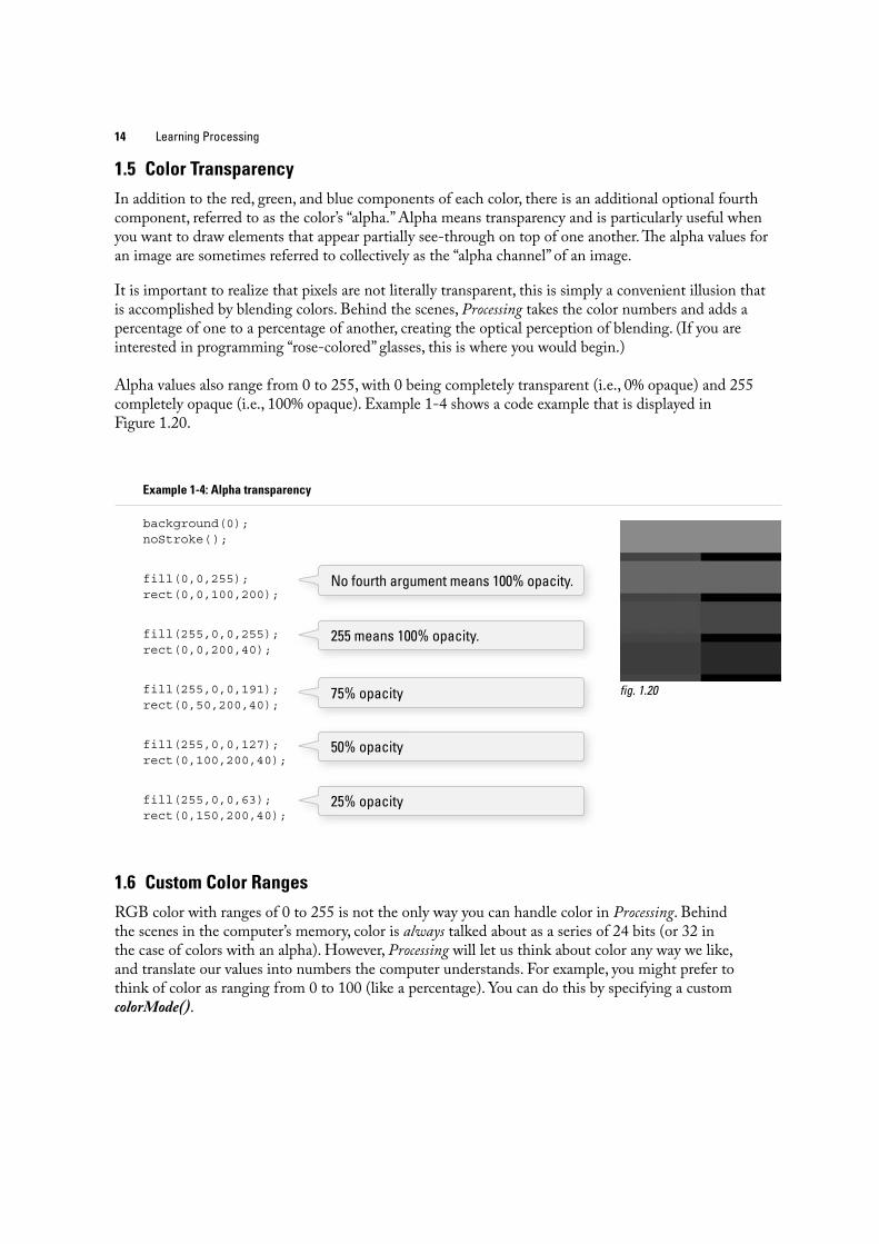
Alpha values also range from 0 to 255, with 0 being completely transparent (i.e., 0% opaque) and 255 completely opaque (i.e., 100% opaque). Example 1-4 shows a code example that is displayed in Figure 1.20 .

Example 1-4: Alpha transparency

background(0); noStroke( );

fill(0,0,255); rect(0,0,100,200);

fill(255,0,0,255); rect(0,0,200,40);

fill(255,0,0,191); rect(0,50,200,40);

fill(255,0,0,127); rect(0,100,200,40);

fill(255,0,0,63); rect(0,150,200,40);

1.6 Custom Color Ranges RGB color with ranges of 0 to 255 is not the only way you can handle color in Processing . Behind the scenes in the computer’s memory, color is always talked about as a series of 24 bits (or 32 in the case of colors with an alpha). However, Processing will let us think about color any way we like, and translate our values into numbers the computer understands. For example, you might prefer to think of color as ranging from 0 to 100 (like a percentage). You can do this by specifying a custom colorMode( ) .

fi g. 1.20

No fourth argument means 100% opacity.

255 means 100% opacity.

75% opacity

50% opacity

25% opacity

Pixels 15

colorMode(RGB,100);

; e above function says: “ OK, we want to think about color in terms of red, green, and blue. ; e range of RGB values will be from 0 to 100. ”

Although it is rarely convenient to do so, you can also have di< erent ranges for each color component: colorMode(RGB,100,500,10,255);

Now we are saying “ Red values go from 0 to 100, green from 0 to 500, blue from 0 to 10, and alpha from 0 to 255. ”

Finally, while you will likely only need RGB color for all of your programming needs, you can also specify colors in the HSB (hue, saturation, and brightness) mode. Without getting into too much detail, HSB color works as follows:

• Hue —The color type, ranges from 0 to 360 by default (think of 360° on a color “ wheel ” ). • Saturation —The vibrancy of the color, 0 to 100 by default. • Brightness —The, well, brightness of the color, 0 to 100 by default.

________________________________________ ________________________________________ ________________________________________ ________________________________________ ________________________________________ ________________________________________ ________________________________________ ________________________________________ ________________________________________

Exercise 1-7: Design a creature using simple shapes and colors. Draw the creature by hand using only points, lines, rectangles, and ellipses. ! en attempt to write the code for the creature, using the Processing commands covered in this chapter: point( ), lines( ), rect( ), ellipse( ), stroke( ) , and fi ll( ) . In the next chapter, you will have a chance to test your results by running your code in Processing.

With colorMode( ) you can set your own color range.


Example 1-5 shows my version of Zoog, with the outputs shown in Figure 1.21 .

Example 1-5: Zoog

ellipseMode(CENTER); rectMode(CENTER); stroke(0); fi ll(150); rect(100,100,20,100); fi ll(255); ellipse(100,70,60,60); fi ll(0); ellipse(81,70,16,32); ellipse(119,70,16,32); stroke(0); line(90,150,80,160); line(110,150,120,160);

; e sample answer is my Processing -born being, named Zoog. Over the course of the fi rst nine chapters of this book, we will follow the course of Zoog’s childhood. ; e fundamentals of programming will be demonstrated as Zoog grows up. We will fi rst learn to display Zoog, then to make an interactive Zoog and animated Zoog, and fi nally to duplicate Zoog in a world of many Zoogs.

I suggest you design your own “ thing ” (note that there is no need to limit yourself to a humanoid or creature-like form; any programmatic pattern will do) and recreate all of the examples throughout the fi rst nine chapters with your own design. Most likely, this will require you to only change a small portion (the shape rendering part) of each example. ; is process, however, should help solidify your understanding of the basic elements required for computer programs—Variables, Conditionals, Loops, Functions, Objects, and Arrays—and prepare you for when Zoog matures, leaves the nest, and ventures o< into the more advanced topics from Chapter 10 on in this book.

fi g. 1.21

Processing 17

2 Processing “ Computers in the future may weigh no more than 1.5 tons. ” —Popular Mechanics, 1949

“ Take me to your leader. ” —Zoog, 2008

In this chapter: – Downloading and installing Processing . – Menu options. – A Processing “ sketchbook. ” – Writing code. – Errors. – The Processing reference. – The “ Play ” button. – Your fi rst sketch. – Publishing your sketch to the web.

2.1 Processing to the Rescue Now that we conquered the world of primitive shapes and RGB color, we are ready to implement this knowledge in a real world programming scenario. Happily for us, the environment we are going to use is Processing , free and open source software developed by Ben Fry and Casey Reas at the MIT Media Lab in 2001. (See this book’s introduction for more about Processing ’s history.) Processing ’s core library of functions for drawing graphics to the screen will provide for immediate visual feedback and clues as to what the code is doing. And since its programming language employs all the same principles, structures, and concepts of other languages (specifi cally Java), everything you learn with Processing is real programming. It is not some pretend language to help you get started; it has all the fundamentals and core concepts that all languages have. After reading this book and learning to program, you might continue to use Processing in your academic or professional life as a prototyping or production tool. You might also take the knowledge acquired here and apply it to learning other languages and authoring environments. You may, in fact, discover that programming is not your cup of tea; nonetheless, learning the basics will help you become a better-informed technology citizen as you work on collaborative projects with other designers and programmers. It may seem like overkill to emphasize the why with respect to Processing . After all, the focus of this book is primarily on learning the fundamentals of computer programming in the context of computer graphics and design. It is, however, important to take some time to ponder the reasons behind selecting a programming language for a book, a class, a homework assignment, a web application, a software suite, and so forth. After all, now that you are going to start calling yourself a computer programmer at cocktail parties, this question will come up over and over again. I need programming in order to accomplish project X , what language and environment should I use? I say, without a shadow of doubt, that for you, the beginner, the answer is Processing . Its simplicity is ideal for a beginner. At the end of this chapter, you will be up and running with your fi rst computational design and ready to learn the fundamental concepts of programming. But simplicity is not where Processing


ends. A trip through the Processing online exhibition ( http://processing.org/exhibition/ ) will uncover a wide variety of beautiful and innovative projects developed entirely with Processing . By the end of this book, you will have all the tools and knowledge you need to take your ideas and turn them into real world software projects like those found in the exhibition. Processing is great both for learning and for producing, there are very few other environments and languages you can say that about.

2.2 How do I get Processing? For the most part, this book will assume that you have a basic working knowledge of how to operate your personal computer. ; e good news, of course, is that Processing is available for free download. Head to http://www.processing.org/ and visit the download page. If you are a Windows user, you will see two options: “ Windows (standard) ” and “ Windows (expert). ” Since you are reading this book, it is quite likely you are a beginner, in which case you will want the standard version. ; e expert version is for those who have already installed Java themselves. For Mac OS X, there is only one download option. ; ere is also a Linux version available. Operating systems and programs change, of course, so if this paragraph is obsolete or out of date, visit the download page on the site for information regarding what you need.

; e Processing software will arrive as a compressed fi le. Choose a nice directory to store the application (usually “ c:\Program Files\ ” on Windows and in “ Applications ” on Mac), extract the fi les there, locate the “ Processing ” executable, and run it.

Exercise 2-1: Download and install Processing.

2.3 The Processing Application ; e Processing development environment is a simplifi ed environment for writing computer code, and is just about as straightforward to use as simple text editing software (such as TextEdit or Notepad) combined with a media player. Each sketch ( Processing programs are referred to as “ sketches ” ) has a fi lename, a place where you can type code, and some buttons for saving, opening, and running sketches. See Figure 2.1 .

Stop New Export

SaveOpen

Type code here

Sketchname

Messagewindow

Run

fi g. 2.1

Once you have opened the example, click the “ run ” button as indicated in Figure 2.3 . If a new window pops open running the example, you are all set! If this does not occur, visit the online FAQ “ Processing won’t start! ” for possible solutions. ; e page can be found at this direct link: http://www.processing.org/faq/bugs.html#wontstart .

Exercise 2-2: Open a sketch from the Processing examples and run it.

Processing programs can also be viewed full-screen (known as “ present mode ” in Processing ). ; is is available through the menu option: Sketch ! Present (or by shift-clicking the run button). Present will not resize your screen resolution. If you want the sketch to cover your entire screen, you must use your screen dimensions in size( ) .

2.4 The Sketchbook Processing programs are informally referred to as sketches , in the spirit of quick graphics prototyping, and we will employ this term throughout the course of this book. ; e folder where you store your sketches is called your “sketchbook.” Technically speaking, when you run a sketch in processing , it runs as a local application on your computer. As we will see both in this Chapter and in Chapter 18, Processing also allows you to export your sketches as web applets (mini-programs that run embedded in a browser) or as platform-specifi c stand-alone applications (that could, for example, be made available for download).

Once you have confi rmed that the Processing examples work, you are ready to start creating your own sketches. Clicking the “ new ” button will generate a blank new sketch named by date. It is a good idea to “ Save as ” and create your own sketch name. (Note: Processing does not allow spaces or hyphens, and your sketch name cannot start with a number.)

fi g. 2.2

To make sure everything is working, it is a good idea to try running one of the Processing examples. Go to FILE ! EXAMPLES ! (pick an example, suggested: Topics ! Drawing ! ContinuousLines) as shown in Figure 2.2 .

fi g. 2.3

Processing 19


When you fi rst ran Processing , a default “ Processing ” directory was created to store all sketches in the “ My Documents ” folder on Windows and in “ Documents ” on OS X. Although you can select any directory on your hard drive, this folder is the default. It is a pretty good folder to use, but it can be changed by opening the Processing preferences (which are available under the FILE menu).

Each Processing sketch consists of a folder (with the same name as your sketch) and a fi le with the extension “ pde. ” If your Processing sketch is named MyFirstProgram , then you will have a folder named MyFirstProgram with a fi le MyFirstProgram.pde inside. ; e “ pde ” fi le is a plain text fi le that contains the source code. (Later we will see that Processing sketches can have multiple pde’s, but for now one will do.) Some sketches will also contain a folder called “ data ” where media elements used in the program, such as image fi les, sound clips, and so on, are stored.

Exercise 2-3: Type some instructions from Chapter 1 into a blank sketch. Note how certain words are colored. Run the sketch. Does it do what you thought it would?

2.5 Coding in Processing It is fi nally time to start writing some code, using the elements discussed in Chapter 1. Let’s go over some basic syntax rules. ; ere are three kinds of statements we can write:

• Function calls • Assignment operations • Control structures

For now, every line of code will be a function call. See Figure 2.4 . We will explore the other two categories in future chapters. Functions have a name, followed by a set of arguments enclosed in parentheses. Recalling Chapter 1, we used functions to describe how to draw shapes (we just called them “ commands ” or “ instructions ” ). ; inking of a function call as a natural language sentence, the function name is the verb ( “ draw ” ) and the arguments are the objects ( “ point 0,0 ” ) of the sentence. Each function call must always end with a semicolon. See Figure 2.5 .

Ends withsemi-colon

Arguments inparenthesesFunction

name

Line (0,0,200,200);

fi g. 2.4

We have learned several functions already, including background( ), stroke( ), fi ll( ), noFill ( ), noStroke( ), point( ), line( ), rect( ), ellipse( ), rectMode( ), and ellipseMode( ) . Processing will execute a sequence of functions one by one and fi nish by displaying the drawn result in a window. We forgot to learn one very important function in Chapter 1, however— size( ). size( ) specifi es the dimensions of the window you want to create and takes two arguments, width and height. ; e size( ) function should always be fi rst.

size(320,240); Opens a window of width 320 and height 240.

; ere are a few additional items to note.

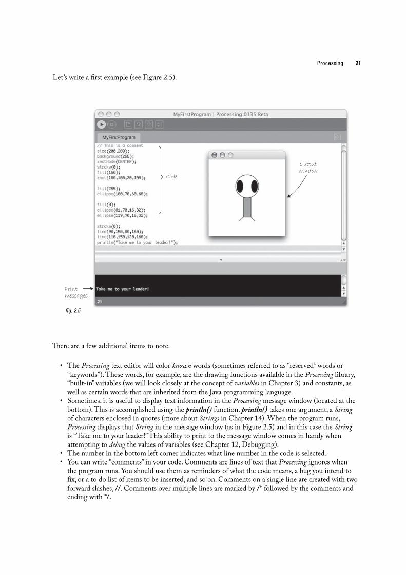
• The Processing text editor will color known words (sometimes referred to as “ reserved ” words or “ keywords ” ). These words, for example, are the drawing functions available in the Processing library, “ built-in ” variables (we will look closely at the concept of variables in Chapter 3) and constants, as well as certain words that are inherited from the Java programming language.

• Sometimes, it is useful to display text information in the Processing message window (located at the bottom). This is accomplished using the println( ) function. println( ) takes one argument, a String of characters enclosed in quotes (more about Strings in Chapter 14). When the program runs, Processing displays that String in the message window (as in Figure 2.5 ) and in this case the String is “ Take me to your leader! ” This ability to print to the message window comes in handy when attempting to debug the values of variables (see Chapter 12, Debugging).

• The number in the bottom left corner indicates what line number in the code is selected. • You can write “ comments ” in your code. Comments are lines of text that Processing ignores when

the program runs. You should use them as reminders of what the code means, a bug you intend to fix, or a to do list of items to be inserted, and so on. Comments on a single line are created with two forward slashes, // . Comments over multiple lines are marked by /* followed by the comments and ending with */ .

Let’s write a fi rst example ( see Figure 2.5 ).

Outputwindow

Code

Printmessages

fi g. 2.5

Processing 21


// ; is is a comment on one line /* ; is is a comment that spans several lines of code */

A quick word about comments. You should get in the habit right now of writing comments in your code. Even though our sketches will be very simple and short at fi rst, you should put comments in for everything. Code is very hard to read and understand without comments. You do not need to have a comment for every line of code, but the more you include, the easier a time you will have revising and reusing your code later. Comments also force you to understand how code works as you are programming. If you do not know what you are doing, how can you write a comment about it?

Comments will not always be included in the text here. ; is is because I fi nd that, unlike in an actual program, code comments are hard to read in a book. Instead, this book will often use code “ hints ” for additional insight and explanations. If you look at the book’s examples on the web site, though, comments will always be included. So, I can’t emphasize it enough, write comments!

// A comment about this code

line(0,0,100,100);

Exercise 2-4: Create a blank sketch. Take your code from the end of Chapter 1 and type it in the Processing window. Add comments to describe what the code is doing. Add a println( ) statement to display text in the message window. Save the sketch. Press the “ run ” button. Does it work or do you get an error?

2.6 Errors ; e previous example only works because we did not make any errors or typos. Over the course of a programmer’s life, this is quite a rare occurrence. Most of the time, our fi rst push of the play button will not be met with success. Let’s examine what happens when we make a mistake in our code in Figure 2.6 .

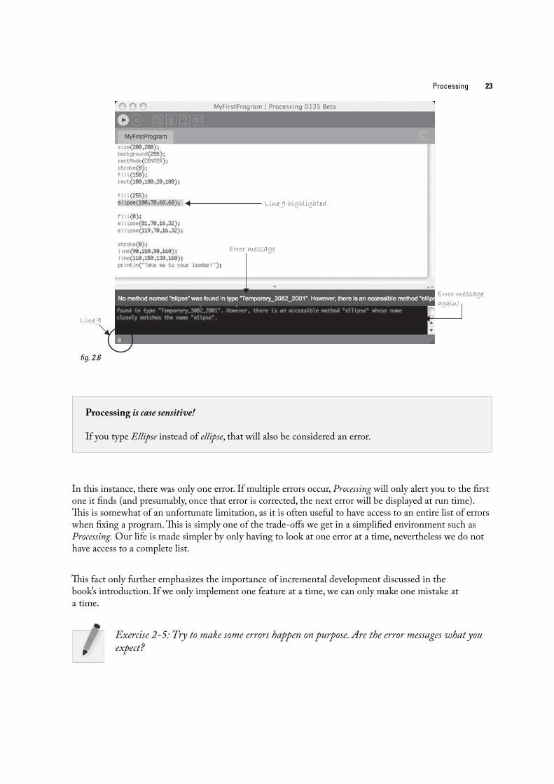
Figure 2.6 shows what happens when you have a typo— “ elipse ” instead of “ ellipse ” on line 9. If there is an error in the code when the play button is pressed, Processing will not open the sketch window, and will instead display the error message. ; is particular message is fairly friendly, telling us that we probably meant to type “ ellipse. ” Not all Processing error messages are so easy to understand, and we will continue to look at other errors throughout the course of this book. An Appendix on common errors in Processing is also included at the end of the book.

A hint about this code!

Processing 23

Line 9 highlighted

Line 9

Error message

Error messageagain!

fi g. 2.6

Processing is case sensitive!

If you type Ellipse instead of ellipse , that will also be considered an error.

In this instance, there was only one error. If multiple errors occur, Processing will only alert you to the fi rst one it fi nds (and presumably, once that error is corrected, the next error will be displayed at run time). ; is is somewhat of an unfortunate limitation, as it is often useful to have access to an entire list of errors when fi xing a program. ; is is simply one of the trade-o< s we get in a simplifi ed environment such as Processing. Our life is made simpler by only having to look at one error at a time, nevertheless we do not have access to a complete list.

; is fact only further emphasizes the importance of incremental development discussed in the book’s introduction. If we only implement one feature at a time, we can only make one mistake at a time.

Exercise 2-5: Try to make some errors happen on purpose. Are the error messages what you expect?


size(200,200); _______________________________________

background(); _______________________________________

stroke 255; ______________________________________ _

fill(150) ______________________________ _________

rectMode(center); _______________________________________

rect(100,100,50); _______________________________________

Exercise 2-6: Fix the errors in the following code.

2.7 The Processing Reference ; e functions we have demonstrated— ellipse( ), line( ), stroke( ) , and so on—are all part of Processing’s library. How do we know that “ ellipse ” isn’t spelled “ elipse ” , or that rect( ) takes four arguments (an “ x coordinate, ” a “ y coordinate, ” a “ width, ” and a “ height ” )? A lot of these details are intuitive, and this speaks to the strength of Processing as a beginner’s programming language. Nevertheless, the only way to know for sure is by reading the online reference. While we will cover many of the elements from the reference throughout this book, it is by no means a substitute for the reference and both will be required for you to learn Processing .

; e reference for Processing can be found online at the o: cial web site ( http://www.processing.org ) under the “ reference ” link. ; ere, you can browse all of the available functions by category or alphabetically. If you were to visit the page for rect( ) , for example, you would fi nd the explanation shown in Figure 2.7 .

As you can see, the reference page o< ers full documentation for the function rect( ) , including: • Name —The name of the function. • Examples —Example code (and visual result, if applicable). • Description —A friendly description of what the function does. • Syntax —Exact syntax of how to write the function. • Parameters —These are the elements that go inside the parentheses. It tells you what kind of data

you put in (a number, character, etc.) and what that element stands for. (This will become clearer as we explore more in future chapters.) These are also sometimes referred to as “ arguments. ”

• Returns —Sometimes a function sends something back to you when you call it (e.g., instead of asking a function to perform a task such as draw a circle, you could ask a function to add two numbers and return the answer to you). Again, this will become more clear later.

• Usage —Certain functions will be available for Processing applets that you publish online ( “ Web ” ) and some will only be available as you run Processing locally on your machine ( “ Application ” ).

• Related Methods —A list of functions often called in connection with the current function. Note that “ functions ” in Java are often referred to as “ methods. ” More on this in Chapter 6.

Processing 25

Processing also has a very handy “ fi nd in reference ” option. Double-click on any keyword to select it and go to to HELP ! FIND IN REFERENCE (or select the keyword and hit SHIFT ! CNTRL ! F).

Exercise 2-7: Using the Processing reference, try implementing two functions that we have not yet covered in this book. Stay within the “ Shape ” and “ Color (setting) ” categories.

Exercise 2-8: Using the reference, fi nd a function that allows you to alter the thickness of a line. What arguments does the function take? Write example code that draws a line one pixel wide, then fi ve pixels wide, then 10 pixels wide.

2.8 The “ Play ” Button One of the nice qualities of Processing is that all one has to do to run a program is press the “ play ” button. It is a nice metaphor and the assumption is that we are comfortable with the idea of playing animations,

fi g. 2.7


movies, music, and other forms of media. Processing programs output media in the form of real-time computer graphics, so why not just play them too?

Nevertheless, it is important to take a moment and consider the fact that what we are doing here is not the same as what happens on an iPod or TiVo. Processing programs start out as text, they are translated into machine code, and then executed to run. All of these steps happen in sequence when the play button is pressed. Let’s examine these steps one by one, relaxed in the knowledge that Processing handles the hard work for us.

Step 1. Translate to Java. Processing is really Java (this will become more evident in a detailed discussion in Chapter 23). In order for your code to run on your machine, it must fi rst be translated to Java code.

Step 2. Compile into Java byte code. ; e Java code created in Step 1 is just another text fi le (with the .java extension instead of .pde). In order for the computer to understand it, it needs to be translated into machine language. ; is translation process is known as compilation. If you were programming in a di< erent language, such as C, the code would compile directly into machine language specifi c to your operating system. In the case of Java, the code is compiled into a special machine language known as Java byte code. It can run on di< erent platforms (Mac, Windows, cellphones, PDAs, etc.) as long as the machine is running a “ Java Virtual Machine. ” Although this extra layer can sometimes cause programs to run a bit slower than they might otherwise, being cross-platform is a great feature of Java. For more on how this works, visit http://java.sun.com or consider picking up a book on Java programming (after you have fi nished with this one).

Step 3. Execution. ; e compiled program ends up in a JAR fi le. A JAR is a Java archive fi le that contains compiled Java programs ( “ classes ” ), images, fonts, and other data fi les. ; e JAR fi le is executed by the Java Virtual Machine and is what causes the display window to appear.

2.9 Your First Sketch Now that we have downloaded and installed Processing , understand the basic menu and interface elements, and have gotten familiar with the online reference, we are ready to start coding. As I briefl y mentioned in Chapter 1, the fi rst half of this book will follow one example that illustrates the foundational elements of programming: variables, arrays, conditionals, loops, functions, and objects . Other examples will be included along the way, but following just one will reveal how the basic elements behind computer programming build on each other.

; e example will follow the story of our new friend Zoog, beginning with a static rendering with simple shapes. Zoog’s development will include mouse interaction, motion, and cloning into a population of many Zoogs. While you are by no means required to complete every exercise of this book with your own alien form, I do suggest that you start with a design and after each chapter, expand the functionality of that design with the programming concepts that are explored. If you are at a loss for an idea, then just draw your own little alien, name it Gooz, and get programming! See Figure 2.8 .

Processing 27

Example 2-1: Zoog again

size(200,200); // Set the size of the window background(255); // Draw a black background smooth();

// Set ellipses and rects to CENTER mode ellipseMode(CENTER); rectMode(CENTER);

// Draw Zoog’s body stroke(0); fill(150); rect(100,100,20,100);

// Draw Zoog’s head fill(255); ellipse(100,70,60,60);

// Draw Zoog’s eyes fill(0); ellipse(81,70,16,32); ellipse(119,70,16,32);

// Draw Zoog’s legs stroke(0); line(90,150,80,160); line(110,150,120,160);

Let’s pretend, just for a moment, that you fi nd this Zoog design to be so astonishingly gorgeous that you just cannot wait to see it displayed on your computer screen. (Yes, I am aware this may require a fairly signifi cant suspension of disbelief.) To run any and all code examples found in this book, you have two choices:

• Retype the code manually. • Visit the book’s web site ( http://www.learningprocessing.com ), find the example by its number, and

copy/paste (or download) the code.

Certainly option #2 is the easier and less time-consuming one and I recommend you use the site as a resource for seeing sketches running in real-time and grabbing code examples. Nonetheless, as you start learning, there is real value in typing the code yourself. Your brain will sponge up the syntax and logic as you type and you will learn a great deal by making mistakes along the way. Not to mention simply running the sketch after entering each new line of code will eliminate any mystery as to how the sketch works.

You will know best when you are ready for copy /paste. Keep track of your progress and if you start running a lot of examples without feeling comfortable with how they work, try going back to manual typing.

fi g. 2.8

Zoog’s body.

Zoog’s head.

Zoog’s eyes.

Zoog’s legs.

The function smooth() enables “anti-aliasing” which smooths the edges of the shapes. no smooth() disables anti-aliasing.


Exercise 2-9: Using what you designed in Chapter 1, implement your own screen drawing, using only 2D primitive shapes— arc( ) , curve( ) , ellipse( ) , line( ) , point( ) , quad( ) , rect( ) , triangle( ) —and basic color functions— background( ) , colorMode( ) , fi ll( ) , noFill( ) , noStroke( ) , and stroke( ) . Remember to use size( ) to specify the dimensions of your window. Suggestion: Play the sketch after typing each new line of code. Correct any errors or typos along the way.

2.10 Publishing Your Program After you have completed a Processing sketch, you can publish it to the web as a Java applet. ; is will become more exciting once we are making interactive, animated applets, but it is good to practice with a simple example. Once you have fi nished Exercise 2-9 and determined that your sketch works, select FILE ! EXPORT.

Note that if you have errors in your program, it will not export properly, so always test by running fi rst!

A new directory named “ applet ” will be created in the sketch folder and displayed, as shown in Figure 2.9 .

fi g. 2.9

You now have the necessary fi les for publishing your applet to the web.

• index.html —The HTML source for a page that displays the applet. • loading.gif —An image to be displayed while the user loads the applet ( Processing will supply a

default one, but you can create your own). • zoog.jar —The compiled applet itself. • zoog.java —The translated Java source code (looks like your Processing code, but has a few extra

things that Java requires. See Chapter 20 for details.) • zoog.pde —Your Processing source.

Processing 29

To see the applet working, double-click the “ index.html ” fi le which should launch a page in your default web browser. See Figure 2.10 . To get the applet online, you will need web server space and FTP software (or you can also use a Processing sketch sharing site such as http://www.openprocessing.org ). You can fi nd some tips for getting started at this book’s web site.

fi g. 2.10

Exercise 2-10: Export your sketch as an applet. View the sketch in the browser (either locally or by uploading). 00002 00002

Interaction 31

3 Interaction “ Always remember that this whole thing was started with a dream and a mouse. ” —Walt Disney

“ ! e quality of the imagination is to fl ow and not to freeze. ” —Ralph Waldo Emerson

In this chapter: – The “ fl ow ” of a program. – The meaning behind setup( ) and draw( ) . – Mouse interaction. – Your fi rst “ dynamic ” Processing program. – Handling events, such as mouse clicks and key presses.

3.1 Go with the fl ow. If you have ever played a computer game, interacted with a digital art installation, or watched a screensaver at three in the morning, you have probably given very little thought to the fact that the software that runs these experiences happens over a period of time . ; e game starts, you save princess so-and-so from the evil lord who-zee-ma-whats-it, achieve a high score, and the game ends.

What I want to focus on in this chapter is that very “ fl ow ” over time. A game begins with a set of initial conditions: you name your character, you start with a score of zero, and you start on level one. Let’s think of this part as the program’s SETUP . After these conditions are initialized, you begin to play the game. At every instant, the computer checks what you are doing with the mouse, calculates all the appropriate behaviors for the game characters, and updates the screen to render all the game graphics. ; is cycle of calculating and drawing happens over and over again, ideally 30 or more times per second for a smooth animation. Let’s think of this part as the program’s DRAW .

; is concept is crucial to our ability to move beyond static designs (as in Chapter 2) with Processing .

Step 1. Set starting conditions for the program one time. Step 2. Do something over and over and over and over (and over … ) again until the program

quits.

Consider how you might go about running a race.

Step 1. Put on your sneakers and stretch. Just do this once, OK? Step 2. Put your right foot forward, then your left foot. Repeat this over and over as fast as

you can. Step 3. After 26 miles, quit.


What is a block of code?

A block of code is any code enclosed within curly brackets. { A block of code

}

Blocks of code can be nested within each other, too. { A block of code { A block inside a block of code }

}

; is is an important construct as it allows us to separate and manage our code as individual pieces of a larger puzzle. A programming convention is to indent the lines of code within each block to make the code more readable. Processing will do this for you via the Auto-Format option (Tools ! Auto-Format). Blocks of code will reveal themselves to be crucial in developing more complex logic, in terms of variables , conditionals , iteration , objects , and functions , as discussed in future chapters. For now, we only need to look at two simple blocks: setup( ) and draw( ) .

3.2 Our Good Friends, setup( ) and draw( ) Now that we are good and exhausted from running marathons in order to better learn programming, we can take this newfound knowledge and apply it to our fi rst “ dynamic ” Processing sketch. Unlike Chapter 2’s static examples, this program will draw to the screen continuously (i.e., until the user quits). ; is is accomplished by writing two “ blocks of code ” setup( ) and draw( ) . Technically speaking setup( ) and draw( ) are functions. We will get into a longer discussion of writing our own functions in a later chapter; for now, we understand them to be two sections where we write code.

Exercise 3-1: In English, write out the “ fl ow ” for a simple computer game, such as Pong. If you are not familiar with Pong, visit: http://en.wikipedia.org/wiki/Pong .

_______________________________________________________________ _______________________________________________________________ _______________________________________________________________ _______________________________________________________________

Interaction 33

Let’s look at what will surely be strange-looking syntax for setup( ) and draw( ) . See Figure 3.1 .

void setup() { // Initialization code goes here}

void draw() { // Code that runs forever goes here}

What’s this? What are these for?

Curly brackets open and close a block of code.

fi g. 3.1

void setup() { // Step 1a // Step 1b // Step 1c}

void draw() { // Step 2a // Step 2b}

Do once!

Skip to draw.

Loop over and over!

fi g. 3.2

Admittedly, there is a lot of stu< in Figure 3.1 that we are not entirely ready to learn about. We have covered that the curly brackets indicate the beginning and end of a “ block of code, ” but why are there parentheses after “ setup ” and “ draw ” ? Oh, and, my goodness, what is this “ void ” all about? It makes me feel sad inside! For now, we have to decide to feel comfortable with not knowing everything all at once, and that these important pieces of syntax will start to make sense in future chapters as more concepts are revealed.

For now, the key is to focus on how Figure 3.1 ’s structures control the fl ow of our program. ; is is shown in Figure 3.2 .

How does it work? When we run the program, it will follow our instructions precisely, executing the steps in setup( ) fi rst, and then move on to the steps in draw( ) . ; e order ends up being something like:

1a, 1b, 1c, 2a, 2b, 2a, 2b, 2a, 2b, 2a, 2b, 2a, 2b, 2a, 2b …

Now, we can rewrite the Zoog example as a dynamic sketch. See Example 3–1 .


Example 3-1: Zoog as dynamic sketch

void setup() { // Set the size of the window size(200,200); }

void draw() { // Draw a white background background(255);

// Set CENTER mode ellipseMode(CENTER); rectMode(CENTER);

// Draw Zoog's body stroke(0); fill(150); rect(100,100,20,100);

// Draw Zoog's head stroke(0); fill(255); ellipse(100,70,60,60);

// Draw Zoog's eyes fill(0); ellipse(81,70,16,32); ellipse(119,70,16,32);

// Draw Zoog's legs stroke(0); line(90,150,80,160); line(110,150,120,160); }

Take the code from Example 3-1 and run it in Processing. Strange, right? You will notice that nothing in the window changes. ; is looks identical to a static sketch! What is going on? All this discussion for nothing?

Well, if we examine the code, we will notice that nothing in the draw( ) function varies . Each time through the loop, the program cycles through the code and executes the identical instructions. So, yes, the program is running over time redrawing the window, but it looks static to us since it draws the same thing each time!

Exercise 3-2: Redo the drawing you created at the end of Chapter 2 as a dynamic program. Even though it will look the same, feel good about your accomplishment!

setup() runs fi rst one time. size() should always be fi rst line of setup() since Processing will not be able to do anything before the window size if specifi ed.

draw() loops continuously until you close the sketch window.

fi g. 3.3

Interaction 35

3.3 Variation with the Mouse Consider this. What if, instead of typing a number into one of the drawing functions, you could type “ the mouse’s X location ” or “ the mouse’s Y location. ”

line(the mouse's X location, the mouse's Y location, 100, 100);

In fact, you can, only instead of the more descriptive language, you must use the keywords mouseX and mouseY , indicating the horizontal or vertical position of the mouse cursor.

Example 3-2: mouseX and mouseY

void setup() { size(200,200);

}

void draw() { background(255);

// Body stroke(0); fill(175); rectMode(CENTER); rect(mouseX,mouseY,50,50); }

fi g. 3.4

An Invisible Line of Code

If you are following the logic of setup( ) and draw( ) closely, you might arrive at an interesting question: When does Processing actually display the shapes in the window? When do the new pixels appear?

_____________________________________________________

_____________________________________________________

_____________________________________________________

_____________________________________________________

_____________________________________________________

Exercise 3-3: Explain why we see a trail of rectangles if we move background( ) to setup( ) , leaving it out of draw( ) .

Try moving background()to setup() and see the difference! (Exercise 3–3)

mouseX is a keyword that the sketch replaces with the horizontal position of the mouse.mouseY is a keyword that the sketch replaces with the vertical position of the mouse.


We could push this idea a bit further and create an example where a more complex pattern (multiple shapes and colors) is controlled by mouseX and mouseY position. For example, we can rewrite Zoog to follow the mouse. Note that Zoog’s body is located at the exact location of the mouse ( mouseX, mouseY ), however, other parts of Zoog’s body are drawn relative to the mouse. Zoog’s head, for example, is located at ( mouseX, mouseY-30 ). ; e following example only moves Zoog’s body and head, as shown in Figure 3.5 .

Example 3-3: Zoog as dynamic sketch with variation

void setup() { size(200,200); // Set the size of the window smooth(); }

void draw() { background(255); // Draw a white background


// Draw Zoog's body stroke(0); fill(175); rect(mouseX,mouseY,20,100);

// Draw Zoog's head stroke(0); fill(255); ellipse(mouseX,mouseY-30,60,60);

On fi rst glance, one might assume the display is updated for every line of code that includes a drawing function. If this were the case, however, we would see the shapes appear onscreen one at a time. ; is would happen so fast that we would hardly notice each shape appearing individually. However, when the window is erased every time background( ) is called, a somewhat unfortunate and unpleasant result would occur: fl icker. Processing solves this problem by updating the window only at the end of every cycle through draw( ) . It is as if there were an invisible line of code that renders the window at the end of the draw( ) function.

void draw() { // All of your code // Update Display Window -- invisible line of code we don’t see }

; is process is known as double-bu" ering and, in a lower-level environment, you may fi nd that you have to implement it yourself. Again, we take the time to thank Processing for making our introduction to programming friendlier and simpler by taking care of this for us.

fi g. 3.5

Zoog’s head is drawn above the body at the location (mouseX, mouseY-30).

Zoog’s body is drawn at the location (mouseX, mouseY).

Interaction 37

// Draw Zoog's eyes fill(0); ellipse(81,70,16,32); ellipse(119,70,16,32);

// Draw Zoog's legs stroke(0); line(90,150,80,160); line(110,150,120,160); }

Exercise 3-4: Complete Zoog so that the rest of its body moves with the mouse.

mouseX $ 20mouseY $ 50

1st timethrough draw()

100 # 100 window20 75

25

50

50

90

2nd timethrough draw()

3rd timethrough draw()

pmouseX $ 20pmouseY $ 50mouseX $ 75mouseY $ 25

pmouseX $ 20pmouseY $ 50mouseX $ 50mouseY $ 90

fi g. 3.6

In addition to mouseX and mouseY , you can also use pmouseX and pmouseY . ; ese two keywords stand for the “ previous ” mouse X and mouse Y locations, that is, where the mouse was the last time we cycled through draw( ) . ; is allows for some interesting interaction possibilities. For example, let’s consider what happens if we draw a line from the previous mouse location to the current mouse location, as illustrated in the diagram in Figure 3.6 .

// Draw Zoog's eyes

fill(0);

ellipse(_______,_______ ,16,32);

ellipse(_______,_______ ,16,32);

// Draw Zoog's legs

stroke(0);

line(_______,_______,_______,_______);

line(_______,_______,_______,_______);

Exercise 3-5: Recode your design so that shapes respond to the mouse (by varying color and location).


• The absolute value of –2 is 2. • The absolute value of 2 is 2.

In Processing, we can get the absolute value of the number by placing it inside the abs( ) function, that is,

• abs( " 5) ! 5

! e speed at which the mouse is moving is therefore:

• abs( mouseX - pmouseX )

Update Exercise 3-7 so that the faster the user moves the mouse, the wider the drawn line. Hint: look up strokeWeight( ) in the Processing reference.

stroke(255);

_____________________________ (______________);

line(pmouse X ,pmouse Y ,mouse X ,mouse Y);

Example 3-4: Drawing a continuous line

void setup() { size(200,200); background(255); smooth(); }

void draw() { stroke(0); line(pmouse X ,pmouse Y ,mouse X ,mouse Y ); }

Exercise 3-6: Fill in the blank in Figure 3.6 .

fi g. 3.7

By connecting the previous mouse location to the current mouse location with a line each time through draw( ) , we are able to render a continuous line that follows the mouse. See Figure 3.7 .

Exercise 3-7: ! e formula for calculating the speed of the mouse’s horizontal motion is the absolute value of the di" erence between mouseX and pmouseX . ! e absolute value of a number is defi ned as that number without its sign:

Draw a line from previous mouse location to current mouse location.

Interaction 39

3.4 Mouse Clicks and Key Presses We are well on our way to creating dynamic, interactive Processing sketches through the use the setup( ) and draw( ) framework and the mouseX and mouseY keywords. A crucial form of interaction, however, is missing—clicking the mouse!

In order to learn how to have something happen when the mouse is clicked, we need to return to the fl ow of our program. We know setup( ) happens once and draw( ) loops forever. When does a mouse click occur? Mouse presses (and key presses) as considered events in Processing . If we want something to happen (such as “ the background color changes to red ” ) when the mouse is clicked, we need to add a third block of code to handle this event.

; is event “ function ” will tell the program what code to execute when an event occurs. As with setup( ) , the code will occur once and only once. ; at is, once and only once for each occurrence of the event. An event, such as a mouse click, can happen multiple times of course!

; ese are the two new functions we need: • mousePressed( ) —Handles mouse clicks. • keyPressed( ) —Handles key presses.

; e following example uses both event functions, adding squares whenever the mouse is pressed and clearing the background whenever a key is pressed.

Example 3-5: mousePressed( ) and keyPressed( )

void setup() { size(200,200); background(255); }

void draw() {

}

void mousePressed() { stroke(0); fill(175); rectMode(CENTER); rect(mouseX,mouseY,16,16); }

void keyPressed() { background(255); }

In Example 3-5, we have four functions that describe the program’s fl ow. ; e program starts in setup( ) where the size and background are initialized. It continues into draw( ) , looping endlessly. Since draw( ) contains no code, the window will remain blank. However, we have added two new functions: mousePressed( ) and

fi g. 3.8 Nothing happens in draw() in this example!

Whenever a user clicks the mouse the code written inside mousePressed() is executed.

Whenever a user presses a key the code written inside keyPressed() is executed.

keyPressed( ) . ; e code inside these functions sits and waits. When the user clicks the mouse (or presses a key), it springs into action, executing the enclosed block of instructions once and only once.

Exercise 3-8: Add “ background(255); ” to the draw( ) function. Why does the program stop working?

We are now ready to bring all of these elements together for Zoog. • Zoog’s entire body will follow the mouse. • Zoog’s eye color will be determined by mouse location. • Zoog’s legs will be drawn from the previous mouse location to the current mouse location. • When the mouse is clicked, a message will be displayed in the message window: “ Take me to your

leader! ”

Note the addition in Example 3–6 of the function frameRate( ). frameRate( ) , which requires an integer between 1 and 60, enforces the speed at which Processing will cycle through draw( ). frameRate (30) , for example, means 30 frames per second, a traditional speed for computer animation. If you do not include frameRate( ) , Processing will attempt to run the sketch at 60 frames per second. Since computers run at di< erent speeds, frameRate( ) is used to make sure that your sketch is consistent across multiple computers.

; is frame rate is just a maximum, however. If your sketch has to draw one million rectangles, it may take a long time to fi nish the draw cycle and run at a slower speed.

Example 3-6: Interactive Zoog

void setup() { // Set the size of the window

size(200,200); smooth(); frameRate(30) ;}

void draw() { // Draw a black background background(255);


// Draw Zoog's body stroke(0); fill(175); rect(mouseX,mouseY,20,100);

// Draw Zoog's head stroke(0); fill(255); ellipse(mouse X ,mouse Y -30,60,60);

fi g. 3.9

The frame rate is set to 30 frames per second.


Interaction 41

// Draw Zoog's eyes fill(mo useX,0,mouseY); ellipse(mouse X-19,mouseY-30,16,32); ellipse(mouse X + 19,mouse Y-30,16,32);

// Draw Zoog's legs stroke(0); line(mouse X-10,mouseY + 50,pmouse X-10,pmouseY + 60); line(mouse X + 10,mouse Y + 50,pmouse X + 10,pmouse Y + 60); }

void mousePressed() { println( "Take me to your leader! "); }

The legs are drawn according to the mouse location and the previous mouse location.

The eye color is determined by the mouse location.

Lesson One Project (You may have completed much of this project already via the exercises in Chapters 1–3. ! is project brings all of the elements together. You could either start from scratch with a new design or use elements from the exercises.)

Step 1. Design a static screen drawing using RGB color and primitive shapes.

Step 2. Make the static screen drawing dynamic by having it interact with the mouse. ; is might include shapes following the mouse, changing their size according to the mouse, changing their color according to the mouse, and so on.

Use the space provided below to sketch designs, notes, and pseudocode for your project.


Learning Processing A Beginner's Guide to Programming

Documents

Transcript of Learning Processing A Beginner's Guide to Programming