A Beginner's Guide I: A Visual Introduction to Dynamics

Chaos and Complexity Letters ISSN: 1556-3995

Volume 8, Number 2-3 © Nova Science Publishers, Inc.

A BEGINNER’S GUIDE TO THE NATURE

AND POTENTIALITIES OF DYNAMICAL

AND NETWORK THEORY

PART I: A VERY VERY BRIEF VISUAL INTRODUCTION

TO THE THEORY OF DYNAMICAL SYSTEMS

Frederick David Abraham1,2 and ©2010-2014

3,4

“Concerning things which mortals cannot perceive, only the gods know, but for we

mortals, only conjecture from sensory evidence [tekmaíresthai] is possible.”5

(Alcmaeon, circa 500 BC.)

“. . . a substantial part of the theory of organization will be concerned with properties

that are not intrinsic to the thing but are relational between observer and thing”6

(Ashby, 1962).

“General systems theory has taken its impetus from the excitement of discovering

larger and larger contexts, on the one hand, and a kind of microprobing into fine detail

within a system, on the other. Both of these activities are intrinsic to anthropology to the

extent that field work in living societies has been the basic disciplinary method. It is no

1 The author is the beginner, who invites others to share this introductory exploration. I minimize citations to those

that are my principal sources and serve as a gateway to the vast literature on these subjects. 2 [email protected], www.blueberry-brain.org Waterbury Center, VT, USA & Silliman University,

Philippines. 3 Except where other authors or publishers have previously copyrighted cited material or where internet sites have

presented non-copyrighted material cited herein. 4 This essay is a summary of some basic principles of dynamics that I mostly learned and redacted from my brother,

Ralph (Abraham & Shaw, 1982-88; 1987; 1992, 2005), updated with some of my own selection of additional

materials gleaned from various sources, especially from the worldwide web where great graphics and

interactive applets abound for those wishing to venture further. I have asked his supervision for this latest

redactive effort in order to minimize any errors or distortions. 5 Motto at beginning of Alcmaeon’s On Nature. The statement is my merge of commentary by Huffman (2013) and

Manetti (1993) based on Diels & Kranz (1951-4, 1972/2001). Alcmaeon’s theories on health were dynamic

(balance of multiple binary oppositions) and he was the first of the early Greek Enlightenment philosophers to

specify the brain as the locus of understanding. 6 ‘Thing’ is a subset [aka attractor] in the ‘product’ [aka state space] representing a set of interacting variables. This

quote hints not only of uncertainty in the observer, but also of the arbitrary nature of defining variables. It hints

of Korzybsky’s map-territory distinction (1931/1933), and the unity of science movement as well (Neurath et

al., 1938). These quotes suggest both the potentialities and limitations of systems theory and math-science.

Frederick David Abraham 2

revelation to any field- experienced anthropologist that everything is related to everything

else, or that whether the entire sociocultural setting can be studied in detail or not, it has

to be known in general outline.” Mead, 1973.

“Viewed against the background of the movement of thought from Kant through

Hegel to Marx, . . . conceptual substitution . . . [of] thought-figures are retained in

structural analogies. . . The system-environment relationship is thought out altogether in

accord with the model of a world constituted by transcendental consciousness. . . The

systems theorist finds a multiplicity of system-environment relationships in his object

domain. . .

“Systems theory lets cognitive acts, even its own, meld into the system’s

achievements of mastering complexity and thus takes away from knowledge any moment

of unconditionality.” (Habermas, 1995).

DYNAMICAL SYSTEMS

A dynamical system is, loosely speaking, a set of variables interacting over time. The

changes in these variables, their time series, can exhibit various patterns of behavior. If there

are reasonable regularities and smoothness in these patterns, they can be represented by

graphic methods and mathematical notation. The equations describing the changes over

time—usually ordinary differential equations (ODE’s) for the continuous time case, or

difference equations for the discrete time case— may contain nonlinear elements. These

empower the ability of such nonlinear models to describe not only point and cyclic activity

asymptotically but also are necessary (but not sufficient) conditions for the production of

‘deterministic chaotic’ activity as well—often known as chaos, chaotic attractors or strange

attractors. These nonlinear elements also are necessary for the production of dramatic shifts

in the temporal patterns generated by the systems—bifurcations.

2. THE VECTORFIELD

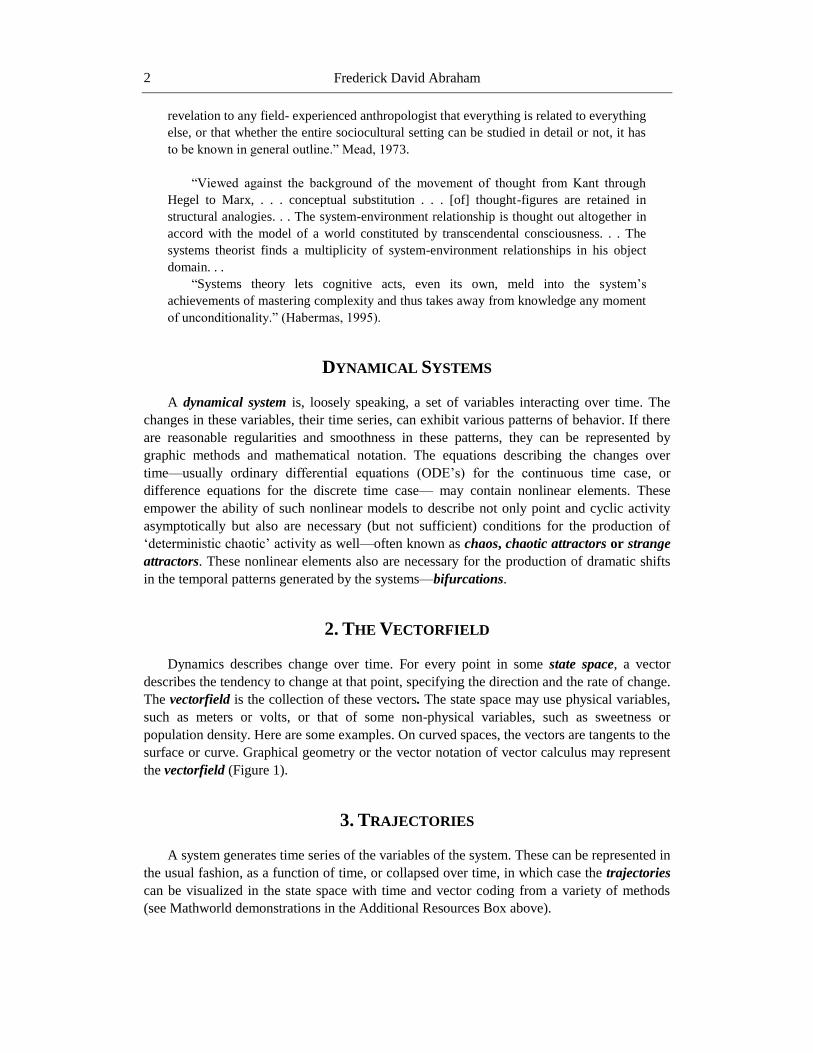
Dynamics describes change over time. For every point in some state space, a vector

describes the tendency to change at that point, specifying the direction and the rate of change.

The vectorfield is the collection of these vectors. The state space may use physical variables,

such as meters or volts, or that of some non-physical variables, such as sweetness or

population density. Here are some examples. On curved spaces, the vectors are tangents to the

surface or curve. Graphical geometry or the vector notation of vector calculus may represent

the vectorfield (Figure 1).

3. TRAJECTORIES

A system generates time series of the variables of the system. These can be represented in

the usual fashion, as a function of time, or collapsed over time, in which case the trajectories

can be visualized in the state space with time and vector coding from a variety of methods

(see Mathworld demonstrations in the Additional Resources Box above).

A Beginner’s Guide to the Nature and Potentialities of Dynamical and Network Theory 3

Figure 1a. Two-

dimensional

Vectorfield in a planar

state space.7

Figure 1b. 2D Vectorfield

for a spherical-surface state

space.6 (Tangential to

surface.)

Figure 1c. 3D

Velocity Vectorfield.

For the Couette

Stirrer. 8

Additional Resources:

http://www. falstad. com/vector/ Terrific interactive applets of 2D and 3D motion.

http://mathworld. wolfram. com/VectorField. html Article plus links to 4 demonstrations; needs

Mathematica Player 7 (easy download) for the interactive demonstration projects.

http://tutorial. math. lamar. edu/Classes/CalcIII/VectorFields. aspx Paul Dawkins’ class notes

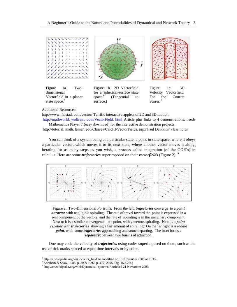
You can think of a system being at a particular state, a point in state space, where it obeys

a particular vector, which moves it to its next state, where another vector moves it along,

iterating for as many steps as you wish, a process called integration (of the ODE’s) in

calculus. Here are some trajectories superimposed on their vectorfields (Figure 2). 9

Figure 2. Two-Dimensional Portraits. From the left: trajectories converge to a point

attractor with negligible spiraling. The rate of travel toward the point is expressed in a

real component of the vectors, and the rate of spiraling is in the imaginary component.

Next to it is a similar convergence to a point, with generous spiraling. Next is a point

repellor with trajectories showing a fair amount of spiraling? On the far right is a saddle

point, with some trajectories approaching and some departing. The inset forms a

separatrix between two basins of attraction.

One may code the velocity of trajectories using codes superimposed on them, such as the

use of tick marks spaced at equal time intervals or by color.

7 http:/en.wikipedia.org/wiki/Vector_field As modified on 16 November 2009 at 01:15.

8 Abraham & Shaw, 1988, p. 30 & 1992, p. 472; 2005, Fig. 16.3.2.b.)

9 http://en.wikipedia.org/wiki/Dynamical_systems Retrieved 21 November 2009.

http://www.falstad.com/vector/

http://tutorial.math.lamar.edu/Classes/CalcIII/VectorFields.aspx

http://en.wikipedia.org/wiki/Dynamical_systems


Question: Can you draw a trajectory and indicate with tick marks where it is moving

faster and where it is moving slower?

Since trajectories are evolving in time, they constitute time series, and one may plotted

them as such, that is, as a function of time as well as in the state space representation. The

same holds true for the vectorfield, though that is not as commonly done.

Question: Can you draw a trajectory both in a state space and as a time series for a

periodic attractor?

4. BASIC ATTRACTORS

Trajectories may tend to some basic patterns, which are called attractors. Some of the

most basic types are fixed point (Figure 2, left two panels), periodic (cyclic), toroidal (with

irrational winding ratio, otherwise they would be periodic!), and chaotic, those being from

nearly cyclic (e. g., the Rössler Attractor) to nearly random.

Figure 3. Attractors for Prey-Predator Models (axes: density of each species). Left: Cyclic

Attractor with point Repellor (top), and Fixed-Point Attractor (bottom)10

. Below: Chaotic

Attractor for Prey-Predator with Two Habitats.11

10

Lotka, 1956, cover. 11

Schwinning at Schaffer's web site.


5. BASIC FEATURES REVEALED IN THE PORTRAIT:

ATTRACTORS, REPELLORS, SADDLES, INSETS, OUTSETS,

BASINS, SEPARATRICES

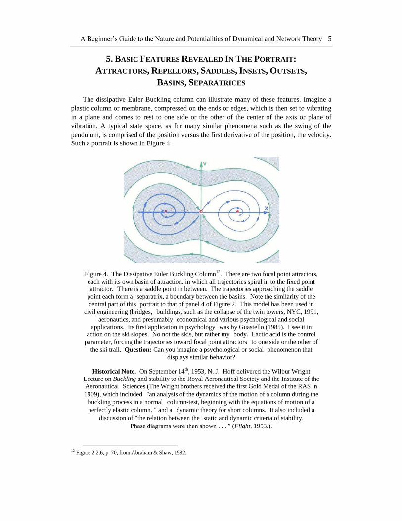
The dissipative Euler Buckling column can illustrate many of these features. Imagine a

plastic column or membrane, compressed on the ends or edges, which is then set to vibrating

in a plane and comes to rest to one side or the other of the center of the axis or plane of

vibration. A typical state space, as for many similar phenomena such as the swing of the

pendulum, is comprised of the position versus the first derivative of the position, the velocity.

Such a portrait is shown in Figure 4.

Figure 4. The Dissipative Euler Buckling Column12

. There are two focal point attractors,

each with its own basin of attraction, in which all trajectories spiral in to the fixed point

attractor. There is a saddle point in between. The trajectories approaching the saddle

point each form a separatrix, a boundary between the basins. Note the similarity of the

central part of this portrait to that of panel 4 of Figure 2. This model has been used in

civil engineering (bridges, buildings, such as the collapse of the twin towers, NYC, 1991,

aeronautics, and presumably economical and various psychological and social

applications. Its first application in psychology was by Guastello (1985). I see it in

action on the ski slopes. No not the skis, but rather my body. Lactic acid is the control

parameter, forcing the trajectories toward focal point attractors to one side or the other of

the ski trail. Question: Can you imagine a psychological or social phenomenon that

displays similar behavior?

Historical Note. On September 14th

, 1953, N. J. Hoff delivered the Wilbur Wright

Lecture on Buckling and stability to the Royal Aeronautical Society and the Institute of the

Aeronautical Sciences (The Wright brothers received the first Gold Medal of the RAS in

1909), which included “an analysis of the dynamics of the motion of a column during the

buckling process in a normal column-test, beginning with the equations of motion of a

perfectly elastic column. ” and a dynamic theory for short columns. It also included a

discussion of “the relation between the static and dynamic criteria of stability.

Phase diagrams were then shown . . . ” (Flight, 1953.).

12

Figure 2.2.6, p. 70, from Abraham & Shaw, 1982.


Other features were shown above in Section 3 Trajectories and Section 4 Basic

Attractors. The portrait here is to show that many features can be revealed in a portrait, which

technically includes or represents all possible trajectories of the system.

6. RESPONSE DIAGRAMS

We have established that a given dynamical model or system may provide different

patterns, portraits, system behaviors, from the interaction of its variables over time, and that

the differences in those patterns, while produced from the same mathematical equations, are

due to different values of the system's parameters. This property of being able to summarize

different system behaviors with one set of equations is one of the great offerings of

dynamics— parsimony. Besides depicting the behavior of the system as portraits in state

space, we can also map the territory occupied by each type of portrait in parameter space.

There are various terms one might use for these maps, such as the response diagram, the

bifurcation diagram, or the bifuration portrait. There are many ways to do this. Here is one

of the simplest for one of the most used and abused objects in dynamics, the cusp catastrophe

(Figure 5).

Figure 5. The Cusp Catastrophe13

. The state space is one-dimensional, a single variable.

The parameter space is two-dimensional. One usually represents them in their joint space

as in the upper part of the figure. This is the 3D Basin-Boundary Portrait of the system.

The vertical line shows the state space for one point in the parameter space. Its portraits

consist of the all the trajectories that move toward each of the point attractors (solid dots)

depending on which side of the repellor (open dot) is their initial state. The folded blanket

part of the surface shows the loci of the attractors (solid dots) for each point in the

parameter space (upper and lower layers in the folded part, and shows the loci of the

repellors (middle red-dotted layer). Outside the area of the fold, there is only one point

attractor, and no repellor. The projection to the bottom of the figure shows the response

diagram in the 2D parameter space, with the triangular area being the area where the

13

Figure from Abraham & Shaw, 1987, p. 583, with kind permission.


system has two attractors and one repellor, and the space outside showing the area where

there is only one attractor. Question: Can you see how these features generate the

hysteresis effect from systematically changing the parameters? Hint: As one decreases

the parameter from right to left, when entering the area of the fold, in which basin of

attraction is it? Likewise, when increasing the control parameter from left to right, in

which basin is it after the bifurcation from one to two point attractors?

The familiar figure for the logistic equation is another example. Question: Can you draw,

either by calculating and sketching by hand, by using a hand calculator, or by using a

spreadsheet on a computer, the response diagram for the logistic equation (the equation is

x(n+1) = λxn(1-xn), usually explored with real numbers such that 0<xo<1, 0<λ<4)?

7. BIFURCATIONS

A bifurcation occurs when there is a significant change in the portrait as some parameter

changes and passes through a threshold called the Bifurcation Point. For the cusp shown

above, the loci of the bifurcation points are given by the line outlining the tent-like area in the

parameter space (the lower part of Figure 5). As the parameters move into or out of this area,

a fold bifurcation occurs. The cusp thus is sometimes called a double fold. The diagram thus

can also be called a Bifurcation Diagram or map. If you did the exercise for the logistic map,

you probably discovered that the response diagram reveals a sequence of bifurcations, the

bifurcation sequence, for that equation. Exercise: try running the sequence going from λ =-2

to 4. You can check your result at http://www. hevanet.com/bradc/MiscMathStuff. htm where

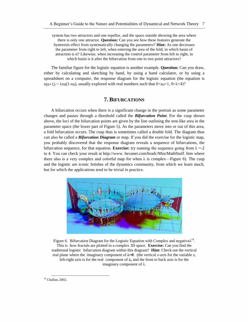
there also is a very complex and colorful map for when λ is complex—Figure 6). The cusp

and the logistic are iconic fetishes of the dynamics community, from which we learn much,

but for which the applications tend to be trivial in practice.

Figure 6. Bifurcation Diagram for the Logistic Equation with Complex and negativeλ14

.

This is how fractals are plotted in a complex 3D space. Exercise: Can you find the

traditional logistic bifurcation diagram within this diagram? Hint: Check out the vertical

real plane where the imaginary component of λ=0. (the vertical x-axis for the variable x,

left-right axis is for the real component of λ, and the front to back axis is for the

imaginary component of λ.

14

Chalfan, 2002.


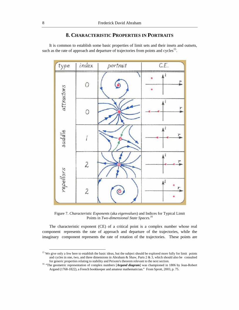
8. CHARACTERISTIC PROPERTIES IN PORTRAITS

It is common to establish some basic properties of limit sets and their insets and outsets,

such as the rate of approach and departure of trajectories from points and cycles15

.

Figure 7. Characteristic Exponents (aka eigenvalues) and Indices for Typical Limit

Points in Two-dimensional State Spaces.16

The characteristic exponent (CE) of a critical point is a complex number whose real

component represents the rate of approach and departure of the trajectories, while the

imaginary component represents the rate of rotation of the trajectories. These points are

15

We give only a few here to establish the basic ideas, but the subject should be explored more fully for limit points

and cycles in one, two, and three dimensions in Abraham & Shaw, Parts 2 & 3, which should also be consulted

for generic properties relating to stability and Peixoto's theorem relevant to the next section. 16

“The geometric representation of complex numbers [Argand diagram] was championed in 1806 by Jean-Robert

Argand (1768-1822), a French bookkeeper and amateur mathematician.” From Sprott, 2003, p. 75.


hyperbolic, that is, the real component is not equal to 0. The index is the dimension of the

outset of a critical point.

Figure 8. Characteristic Multipliers (aka eigenvalues or Floquet multipliers) for Limit

Cycles in Two-dimensional State Spaces. Note the unstable center (non-hyperbolic case)

in the bottom panel. The CM is never 0. Complex CMs exist for the three-dimensional

case; we omit them here and again urge consulting the works of Abraham & Shaw; also

Sprott. For an interesting application of complex CMs in 3D, see Duchesne (1993).17

9. STABILITY

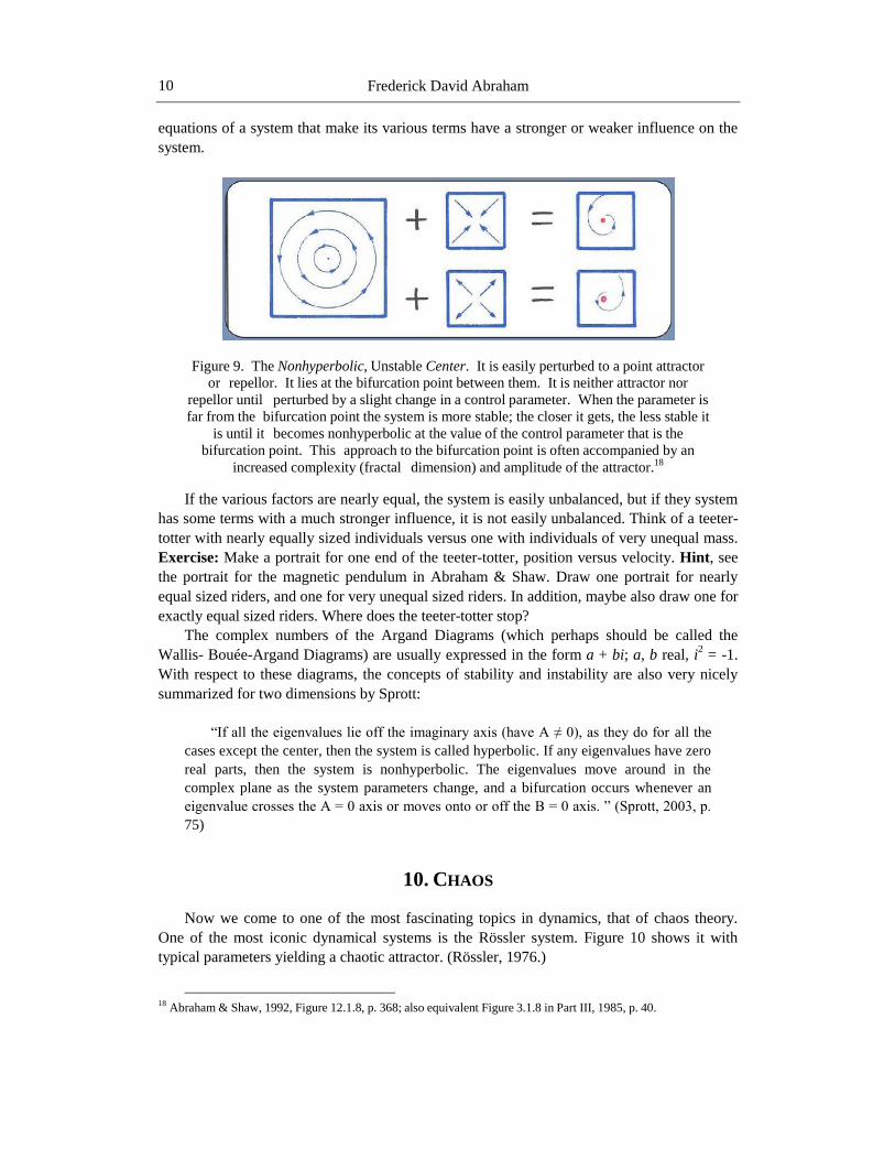
Abraham & Shaw describe a stable or unstable system by how it is affected by a

perturbation that is as an addition to the Vectorfield. For example, the center just mentioned,

is unstable, but their figure (Figure 9) shows how easily a perturbation can change the portrait

into a point attractor or repellor.

The generic properties that describe a stable system (Peixoto's theorem) summarize a

necessary and sufficient set of conditions for stability. However, these do not tell the story

about why there is stability and instability, which depends on the parameters within the

17

Abraham & Shaw, 1992, Figure 7.2.7. p. 243; also equivalent Figure 2.2.7, in Part II, 1984, p. 42.


equations of a system that make its various terms have a stronger or weaker influence on the

system.

Figure 9. The Nonhyperbolic, Unstable Center. It is easily perturbed to a point attractor

or repellor. It lies at the bifurcation point between them. It is neither attractor nor

repellor until perturbed by a slight change in a control parameter. When the parameter is

far from the bifurcation point the system is more stable; the closer it gets, the less stable it

is until it becomes nonhyperbolic at the value of the control parameter that is the

bifurcation point. This approach to the bifurcation point is often accompanied by an

increased complexity (fractal dimension) and amplitude of the attractor.18

If the various factors are nearly equal, the system is easily unbalanced, but if they system

has some terms with a much stronger influence, it is not easily unbalanced. Think of a teeter-

totter with nearly equally sized individuals versus one with individuals of very unequal mass.

Exercise: Make a portrait for one end of the teeter-totter, position versus velocity. Hint, see

the portrait for the magnetic pendulum in Abraham & Shaw. Draw one portrait for nearly

equal sized riders, and one for very unequal sized riders. In addition, maybe also draw one for

exactly equal sized riders. Where does the teeter-totter stop?

The complex numbers of the Argand Diagrams (which perhaps should be called the

Wallis- Bouée-Argand Diagrams) are usually expressed in the form a + bi; a, b real, i2

= -1.

With respect to these diagrams, the concepts of stability and instability are also very nicely

summarized for two dimensions by Sprott:

“If all the eigenvalues lie off the imaginary axis (have A ≠ 0), as they do for all the

cases except the center, then the system is called hyperbolic. If any eigenvalues have zero

real parts, then the system is nonhyperbolic. The eigenvalues move around in the

complex plane as the system parameters change, and a bifurcation occurs whenever an

eigenvalue crosses the A = 0 axis or moves onto or off the B = 0 axis. ” (Sprott, 2003, p.

75)

10. CHAOS

Now we come to one of the most fascinating topics in dynamics, that of chaos theory.

One of the most iconic dynamical systems is the Rössler system. Figure 10 shows it with

typical parameters yielding a chaotic attractor. (Rössler, 1976.)

18

Abraham & Shaw, 1992, Figure 12.1.8, p. 368; also equivalent Figure 3.1.8 in Part III, 1985, p. 40.


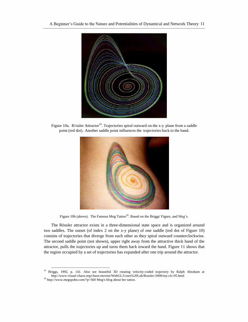
Figure 10a. Rӧssler Attractor19

. Trajectories spiral outward on the x-y plane from a saddle

point (red dot). Another saddle point influences the trajectories back to the band.

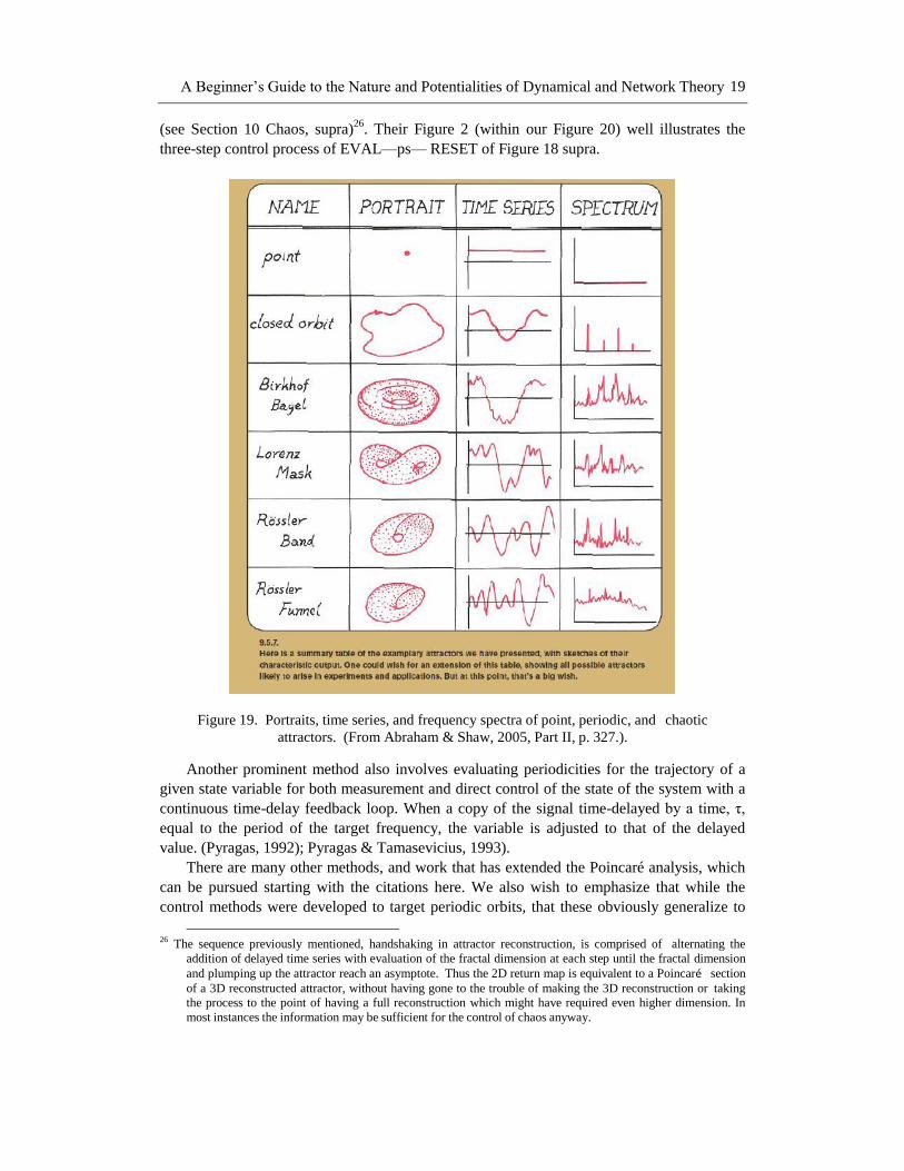
Figure 10b (above). The Famous Meg Tattoo20. Based on the Briggs' Figure, and Meg’s.

The Rössler attractor exists in a three-dimensional state space and is organized around

two saddles. The outset (of index 2 on the x-y plane) of one saddle (red dot of Figure 10)

consists of trajectories that diverge from each other as they spiral outward counterclockwise.

The second saddle point (not shown), upper right away from the attractive thick band of the

attractor, pulls the trajectories up and turns them back toward the band. Figure 11 shows that

the region occupied by a set of trajectories has expanded after one trip around the attractor.

19

Briggs, 1992, p. 141. Also see beautiful 3D rotating velocity-coded trajectory by Ralph Abraham at

http://www.visual-chaos.org/chaos-movies/WebGL/Lines%20Lab/Rossler-5000/my-clc-05.html 20

http://www.megspohn.com/?p=560 Meg/s blog about her tattoo.

http://www.visual-chaos.org/chaos-movies/WebGL/Lines%20Lab/Rossler-5000/my-clc-05.html

http://www.megspohn.com/?p=560


Figure 11. Expansion of a set of Trajectories in one turn around the attractor.21

.

Figure 12. Fractal Microstructure.22

.

Figure 12a (above). Poincaré Sections.

Perpendicular to the Rössler Band

Figure 12b. Lorenz Section

Perpendicular to the Poincaré Section.

Figure 12c. The Lorenz Section reveals the

pattern of the layering of the Rössler

Attractor.

Figure 12d. The Cantor Process.

Successive steps of decimating a line

illustrate the self- similarity across scale

evident in the chaotic attractor.

Middle-thirds decimation shown.

21

Abraham & Shaw, 1984, cover. 22

Abraham & Shaw, 1992, pp. 319-320.


This process leads to an infinitely layered thick surface as a fractal pattern which is

revealed when transected by planes, called Poincaré and Lorenz Sections (Figure 12).

The rate or strength of divergence of trajectories within and convergence to the attractor

are given by Lyapunov Exponents (characteristic exponents and multipliers), one exponent

for each dimension of a chaotic attractor, which comprise the Lyapunov Spectrum. Positive

exponents measure the rate of divergence while negative Lyapunov exponents measure the

rate of convergence. The absolute value of the negative exponents must exceed that of the

positive exponents or the trajectory would depart the space with the result of no attractor.

Often the largest positive exponent is reported rather than the whole spectrum to give a

quicker characterization the sensitivity to initial conditions, a defining feature of trajectories

of chaotic attractors. The exponents may be computed locally or globally for an attractor.

The Rössler system started life as a set of three ordinary differential equations, but there

are methods for reconstructing attractors and determining their fractal dimensions (the

degree to which the state space is occupied), and their Lyapunov Exponents from

experimental data using a handshaking combination of geometric reconstruction and numeric

computation of the fractal dimension. (See Abraham, 1997 for a brief review; Abarbanel,

1996; Kantz & Schreiber, 1997; Ott et al., 1994; and Sprott, 2003 for more complete details.)

The Equations for the Rössler System are:

dx/dt = – y – z; dy/dt = x + ay; dz/dt = b + z(x – c)

Rössler used a = b = 0. 2, c = 5.7, but now a = b = 0. 1, c = 14 are usually used.

Some Useful Links for the Rössler System

http://www. scholarpedia. org/article/Rossler_attractor

Christophe Letellier and Otto E. Rössler (2006), Scholarpedia, 1(10):1721. Shows and

gives the location of the two saddle points that organize the attractor. Shows attractor in

stereocopic view and in rotation for better visualization, and shows the folding into

layers. Gives the unimodal first-return map and the Lyapunov spectra. This is a

compulsory site.

http://en. wikipedia. org/wiki/R%C3%B6ssler_attractor Presents properties via

eigenvectors, Poincaré maps, and birucation diagrams.

http://chaos. wlu. edu/106/programs/rosslerdes. html Allows launch of an interactive

applet which allows one to choose parameters and runs two trajectories on each 2D

plane of the attractor.

http://demonstrations. wolfram. com/TheRosslerAttractor/ The Wolfram demonstrations

can be dramatic. They require download of the Mathematica Player. There is an

interactive applet allowing changing the three parameters, which produces static graphs

of time series for each dimension and the 3D attractor.

11. DYNAMICAL BIFURCATION THEORY

There are three basic types of bifurcations for the finite dimensional case: catatstrophic,

subtle, and explosive.

Catastrophic bifurcations, also called blue sky bifurcations, are those where a limit set

(attractor) appears or disappears. The best known example is the cusp (Figure 5.) where a


second point attractor entered or left the one-dimensional portrait as the control parameters

changed. Here is another example where a second periodic attractor appears or disappears.

Figure 13. Periodic Fold Catastrophe in 2D23

. Attractors (black), separatices (red), state

spaces (vertical planes), and the horizontal axis is the control parameter. As the control is

moved from left to right, a second periodic attractor appears; as it is moved from right to

left, it disappears. The inserts show the portraits at the ends of this sequence.

The horizontal red line i s the locus of the point repellors which are virtual separatrices

in the center of the attractors; they do not separate basins.

Figure 14. The Hopf Bifurcation24

. As the control parameter is changed from left to right,

the spiral point attractor (left) becomes a center at the bifurcation point (middle) and then

a periodic attractor with a repellor in its center (right) which continues to grow

parabolically as the parameter continues to increase. This subtle bifurcation is also called

the Poincaré-Andronov-Hopf Bifurcation, or Excitation.

23

Abraham & Shaw, 1987, p. 566.) 24

Abraham & Shaw, 1988, p. 172; 1992, p. 609; 2005, Figure 17.1.7, p. 495.


Subtle bifurcations are those where one attractor is transformed into one topologically

(qualitatively) different but gradually in the sense of initially being in a small epsilon

neighborhood of the previous attractor. Here is a prototypical subtle bifurcation. It was known

to Poincaré in 1885, analyzed by Hopf in 1942 for the couette stirring machine, and has had

numerous other applications such as the Van der Pol transmitter.

Explosive bifurcations involve a sudden large increase or decrease in the size of an

attractor, usually involving the disappearance of saddles or a change in heteroclinic

connections (saddle-to-saddle). They are varied and complex. Some are between point and

cycle, some between cycle and braid, some between cycle and chaos. Here is one in which

small chaotic attractors merge into a larger one, explosively and fractally smeared over time.

Figure 15. Ueda's Chaotic Explosion in 3D.25

The attractor is in the red area. Outside of it

are two saddles with homoclinic connections (from the saddle to itself). The chaotic

attractor in the center is a tangle organized around a saddle. Trajectories from the outer

saddles are attracted to the center saddle and, along with its own homoclinic connections,

form the inset to the center saddle. Then the outset of the central saddle makes

connections to the outer saddles, which are then part of the larger chaotic tangled

attractor. It is an explosive chaos-to- chaos attractor.

12. SELF-ORGANIZATION, NETWORKS, AND CONTROL THEORY

These topics are of paramount importance, but we mention only the minimum of ideas

leaving these topics for further exploration. Self-organization refers to the fact that one or

more control parameters of a system are a function of the state of the system and thus the

behavior of the system will change accordingly. The changes may be subtle or gradual, or if a

bifurcation point is passed, they may be dramatic, i.e., non-topologically equivalent.

25

Abraham & Shaw, 1988, p. 172; 1992, p. 609.


Figure 16. Self-Organization.

One can have multiple dynamical systems interconnected in various configurations,

which we have previously called complex dynamical systems when the systems are fairly

homogeneous in type. Complexity Theory may be consider as a superset of Systems Theory

extending some of the basic ideas to hybrid networks that may include continuous and

discrete systems of a greater variety than those of the nonlinear dynamical systems we have

been discussing here. There are many varieties of these, but the most generalized and versatile

of these include complex adaptive systems, agent-based systems, and scale free networks.

Here is a representation of a very simple network.

In our scheme, self-organization is simple conceptually, but allows for complex

outcomes. Self- organization is where a system can create changes, including bifurcations, by


influencing its own control-parameters (we could call that homoclinic self-organization), or

where its influence is mediated by its influence on other components in the network, with one

or more of those feeding back onto the control-parameters of the first referenced component

we might have designated (we might call that heteroclinic self-organization).

We believe that our definition of self-organization which is based on that of Abraham and

Shaw (1982) fits Ashby’s (1962) definition though it fits neither of his cases of self-

organization, that of either a changing evolution of connectivity among subsystems within a

network, or the evolution toward a ‘good’ organization of a system. That is, our definition

allows exploration of parameter space to investigate the various behaviors a system is capable

of without necessarily directing the system to a good or bad organization, leaving such

decisions to a posterior evaluations.

Intentional systems, in our view, include those that can navigate in parameter space and

state space (as depicted in the basin-boundary portrait—aka response diagram), and thus

induce bifurcations (Abraham, 1994a; Kugler et al., 1990; 1991). That is, such systems can

make choices among future attractors. This would seem to imply a self-awareness of at least

some aspects of both its state space and its parameter space, and maybe some of the whole

network, and perhaps of the network’s context (in which case the aware agent is both a part of

the system, and of its context). We very briefly discuss this paradox below.

Emergent properties of the network can flow from these self-organizational features. As

Goldstein (1999) puts it, emergence is “the arising of novel and coherent structures, patterns

and properties during the process of self-organization in complex systems.” Of course with

our definition, emergent simply means we, or nature, has not yet explored the whole of the

parameter space before, so we see system behaviors being realized for the first time. Figure 6

could be an example; Chalfan pushed the limits of the parameter space, and produced this

beautiful fractal (Figure 6) never before seen, at least to our knowledge. Rössler has also

pushed the logistic equation to new places, i.e., expanded the visibility of the state space.

Control of Chaos refers to the modification of the trajectory of a chaotic system in real

time. A small modification or series of modifications of the trajectory is made based on some

parameter of the attractor or the state of the system. Since the equations are usually unknown

for a real complex system, the parameters are measures on a reconstructed attractor (see 10.

Chaos, supra). Using these parameters, one can design systems to insure the evolution of the

system some toward some target subset of properties of its behavior, its attractors. Figure 18,

a revised version of the self-organizational Figure 16, outlines the process. The system may or

may not be considered intentional, but may, of course, reflect the intention of the designer, if

there be one (Ashby’s ‘good organization’, 1962).

Most of the theoretical developments have been concerned with taming unruly chaotic

behavior to more stable chaotic behavior, to regimes of periodic or near periodic behavior, or

to fixed point behavior. (Boccaletti et al., 2000; Ott, 2006).

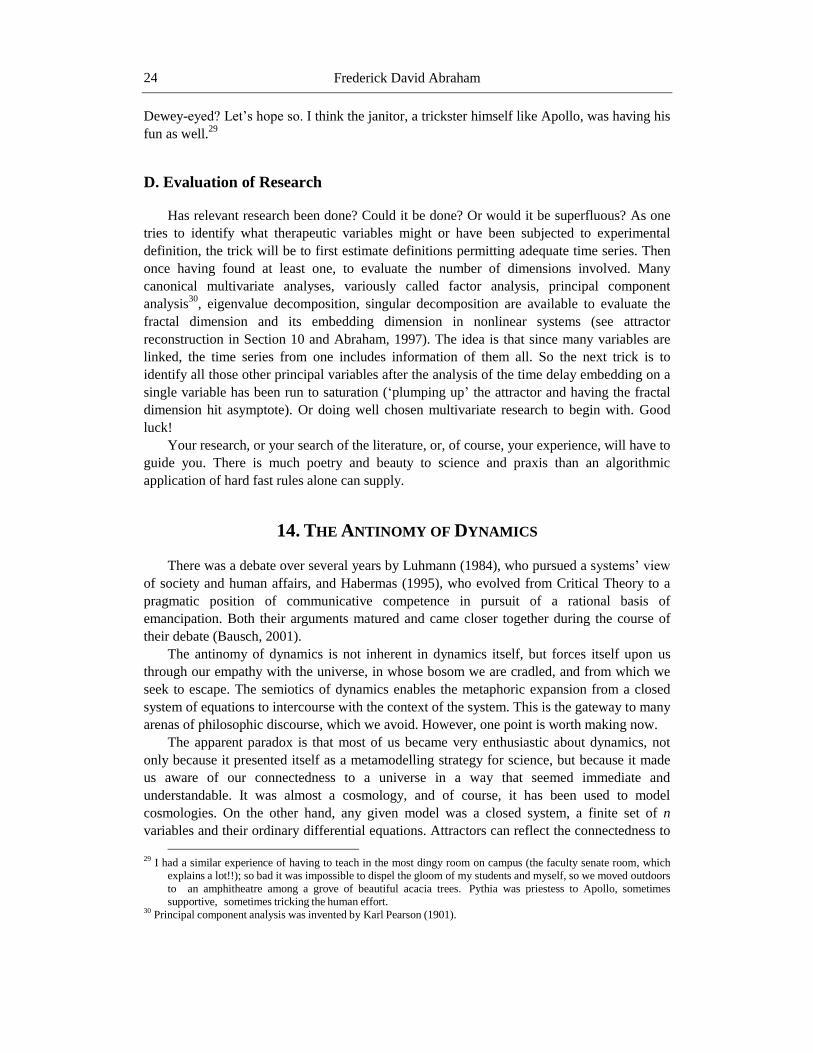
A chaotic attractor can be characterized not only by its portrait or time series, but by its

frequency spectrum (Figure 19). These frequency spectra reveal often some dominant

frequencies and a mess of lesser ones. While control theory has been around for a while, Ott,

Grebogi, and Yorke (1990) launched the contemporary exploitation of features of chaos to

attenuate, enhance, or optimize some constraints to chaos in complex systems, in short, to

sculpt more desirable system behaviors from the attractor. They start with a closer look at

those multiple frequencies (unstable periodic orbits, or UPO’s) comprising the chaotic

trajectories. They noted that UPO’s were of varying instability. Furthermore they exploit the


fact the unstable orbits occur ergodically in some sort of stochastic sequence, something like

states in symbolic dynamics. These properties allow the periodicities to be evaluated from

Poincaré sections of attractor reconstruction. A point representing an UPO to be targeted for

stabilization is a saddle point. Its inset is a stable manifold, a separatrix between two basins of

attraction, which is repelling. Its outset is an unstable manifold, which is attractive. Their

local properties can be measured with Lyapunov exponents (aka eigenvalues, characteristic

exponents; see Sections 8 Characteristic Properties of portraits, and 9 Stability, supra).

Parameters based on these can be used to move the trajectory closer to the stable

manifold. Pushing around these trajectories by small increments, by dint of the exponential

divergence of nearby trajectories in chaotic attractors (sensitivity to initial, i.e., nearby,

conditions), could move the trajectories to the desired positions and behaviors faster than

traditional linear methods. These adjustments are made when the trajectory approaches near a

point in the neighborhood of the UPO to be stabilized (clamped). In short, this OGY method

captures the trajectory in a range of frequencies close to the target frequency once it has

wandered close.

Chaos thus enables flexibility in switching among favorable targets. (Basccaletti et al.,

2000; Ott, 2006).)

Figure 18. Control of Chaos.

There have been many instantiations of the OGY theory and modifications of it,

including a magnetoelastic ribbon (Ditto et al., 1990) and quantum entanglement (Chaudhury

et al., 2009). One of the most intriguing to us, not only because it is a biological system,

isolated cardiac tissue (under chaos-inducing ouabain-epinephrine perfusion), but also

because of the clarity of their procedure in showing visualization of their Poincaré sections

(aka maps) and procedures (Garfinkel et al. 1992). They used electrical recording and

stimulation, and then constructed the Poincaré maps as return maps of the interheartbeat

intervals (In). This abbreviates the attractor reconstruction process to a single time-delay step


(see Section 10 Chaos, supra)26

. Their Figure 2 (within our Figure 20) well illustrates the

three-step control process of EVAL—ps— RESET of Figure 18 supra.

Figure 19. Portraits, time series, and frequency spectra of point, periodic, and chaotic

attractors. (From Abraham & Shaw, 2005, Part II, p. 327.).

Another prominent method also involves evaluating periodicities for the trajectory of a

given state variable for both measurement and direct control of the state of the system with a

continuous time-delay feedback loop. When a copy of the signal time-delayed by a time, τ,

equal to the period of the target frequency, the variable is adjusted to that of the delayed

value. (Pyragas, 1992); Pyragas & Tamasevicius, 1993).

There are many other methods, and work that has extended the Poincaré analysis, which

can be pursued starting with the citations here. We also wish to emphasize that while the

control methods were developed to target periodic orbits, that these obviously generalize to

26

The sequence previously mentioned, handshaking in attractor reconstruction, is comprised of alternating the

addition of delayed time series with evaluation of the fractal dimension at each step until the fractal dimension

and plumping up the attractor reach an asymptote. Thus the 2D return map is equivalent to a Poincaré section

of a 3D reconstructed attractor, without having gone to the trouble of making the 3D reconstruction or taking

the process to the point of having a full reconstruction which might have required even higher dimension. In

most instances the information may be sufficient for the control of chaos anyway.


target chaotic attractors as well, which are beneficial to many biological, social, ecological,

psychological systems, as well as physical and mechanical systems. Or as Sprott (2003,

p. 146) put it: “Sometimes it is desirable to use feedback to keep the orbits unstable (‘anti-

control’ of chaos.)” We might further suggest that optimizing to chaotic regimes of mid-

dimensional complexity makes for more creative and evolutionary processes (Alford &

Abraham, 2011; Krippner, Richards, & Abraham, 2014).

EVAL: The left upper panel A shows the results of

the system after progressing from a single frequency to

an alternating one and then onto chaos. Several

successive points (163-167) are identified which help to

identify the portrait revealed in the Poincaré (return) map

as that of a saddle (aka unstable fixed point), similar to

those shown in Figures 2 and 4 supra). The inset to the

saddle, the stable manifold, is a separatrix between two

basins of attraction is thus repelling; the outset (unstable

manifold) represents attraction.

ps: The left middle panel B shows that an unstable

point needs to be moved to a point on the stable manifold

close to the desired fixed point attractor of a single

periodicity, or near to it, on the identity line of being

equal going from any step n to step n+1. To do this

requires computation of the Lyapunov exponents (See

Sections 8 Characteristic Properties of portraits, and 9

Stability, supra.) Once these are determined, they can be

used to compute how much the interheartbeat interval

needs to be shortened, and a stimulus was given to

precede the next beat to accomplish it.

RESET: The implementation is indicated in the left

lower panel C. Above are results from one experiment:

time series left panel B; Poincaré map right panel E,

small dots for control off, large for control on. (From

their Figure 3).

Figure 20. Controlling Cardiac Chaos (Figures 2 and part of 3 from Garfinkel et al., 1992), by permission of Garfinkel).


13. PERSPECTIVES FOR PSYCHOTHERAPY

Here are just a few dynamical principles to evaluate regarding therapeutic practice.

A. Stability, Instability, and Bifurcation

One approach is to view the therapeutic process as one of trying to achieve a

transformation of certain aspects of self27

. A person with a partly dysfunctional attractor

within the self resists change despite maladaptive features due to certain advantages they

seem to provide’; collateral damage, side effects, so to speak. They can move to a bifurcation

point by some combination of learning and emotional adjustment. The source of this point of

view comes from the idea that the move toward the bifurcation point involves destabilizing

some aspects (attractors) of self by using any identified control parameters, getting near to the

bifurcation point, then bifurcating, and then stabilizing the new attractors, a process made

famous by Kurt Lewin’s ‘unfreeze-change-freeze’. (1947). See Section 9 and Figure 9.

Orsucci (2008, his Section 7), echoing Varela (1999), emphasizes that this is a continual

process, a sequence of instabilities and bifurcations: “constitutional instabilities are the norm

and not a nuisance to be avoided.” This happens many times during the course of therapy,

education, and a lifetime. Different authors and therapists approach this process

metaphorically, some with formal models, and some with research.

My friend Derek Paar refers to this process as ‘Noing” (saying no) and uses riddles to

seed it (Paar, 1993). When Croesus, King of Lydia, consulted his therapists at Delphi and

Amphiaraus about making war on Persia, they each replied ambiguously that to do so would

destroy a great empire. Pythia (the oracle at Delphi) also told him that he should beware when

a mule became lord of the Medes. Since it seemed impossible to Croesus for a mule to be a

ruler, he interpreted this to mean that he would prevail over the Persians. This was a

methaphorical trick taking advantage of Croesus’ literal-semiotic mind. It did not occur to

him that ‘mule’ could refer to Cyrus the Great, King of Persia. As a consequence, the great

empire that was destroyed was his own, not Persia. (Herodotus, I.55). The purpose of this

trickiness of Greek oracles has been interpreted as to reveal gods’ ill will toward humans,

(Manetti, 1993, chapter 2), but an alternative interpretation might be that these were lessons

in getting humans to think for themselves, to be self-organizational, rather than to trust rigid,

deterministic semiotic codes. I made a similar point in a mini-sermon about Eve that I gave at

a ceremony for psychology students at Silliman University (Abraham, 1997a). Terry Marks-

Tarlow has made a similar analysis of Pythia’s two sessions with Oedipus before and after his

solving the riddle of the Sphinx, a well-known story dramatized by Sophocles. She suggested

27

No term adequately served my purpose here. I considered terms such as behavior, personality, being (Maslow,

1999), and self-system, but Stanley Krippner and Ruth Richards kindly pointed out their shortcomings for most

of them. I conclude there is no adequate word to get to the idea that the self can be considered as a complex of

attractors in flux, some more stable and durable, some changing at different times and with varying degrees of

awareness. Probably the best perspective is that of neurological positivism introduced by Vandervert (1993),

elaborated by me and apparent in the works of sociologists (Schwalbe, 1991) and Baumeister & Bushman

(2011). “Neurological positivism regards phenomenology, brain, behavior, and environment as a holistic unity.

Their complex interaction over time can be regarded as a complex dynamical system, which we might call

mind. Attractors and other features of dynamical systems can represent processes of the mind.” (Abraham,

1994b)


a self-referential transition to a more abstract level of thought (Marks- Tarlow, 2014), which

is similar to my dynamical and Manetti’s semiotic approach.

Such divinations finally became more secular, and led to divination evolving into

discourse similar to that in the democratic polis. Another example also comes from Herodotus

(VII.141) again involving Pythia. Some Athenian representatives consulted her concerning a

Persian invasion, and were warned of disaster. The representatives refused the negative news

and demanded a second more favorable opinion from her, refusing to leave until she gave

them another answer, which she did. Her second and more complete reply led to open debate

at the assembly in Athens over military strategy, showing that not only could one negotiate

with the oracle, but that the oracle’s pronouncement also led to public discourse (Manetti,

1993, chapter 2). Thus in the history of semiotics in ancient Greece and modern

psychotherapy, there are many parallels which extol the place of the evolution of creativity

and self-organization, as we shall see next.

B. Mid-Dimensional Chaos and Creativity

Most attractors are or can be considered as chaotic, especially those in the social and

psychological domains. That implies that they exhibit both convergent and divergent

characteristics (Section 10). My colleagues and I have suggested that creative process operate

in a range of middle amounts of complexity reflecting a good balance of these convergent and

divergent tendencies (Abraham, 1996, 2007, Krippner et al., 2014, Richards, 2007 and several

authors therein; see also Guilford, 1953). In adequately defined attractors, these conditions

are reflected in mid-range fractal dimensions.

This thesis has two implications for psychotherapy. The first is that the bifurcations

within therapy will be best accomplished if these mid-dimensional conditions can be

established. The second is that a major goal of therapy should be to establish a creative mode

of life with flexibility, adaptability, some comfort with ambiguity, some comfort with

challenge, tolerance, self-organization, and self-actualization, empathy, etc. In short, these

goals are those emphasized in humanistic/existential psychology.

Since some of the changes are, at least in part, self-organizational, this means some

dynamics of keeping within certain ranges of mid-dimensional complexity could employ

some version of the control of chaos of Section 12; i.e., self-control.

Pauli had developed the exclusion principle before his collaboration with Jung and Jung

had already been developing his acausal principle from a patient’s dream about a scarab

beetle. Despite the apparent complexity of quantum mechanics, I would maintain that its

principles along with the lower dimensionality of the scarab dream and its related Egyptian

mythology represent mid-dimensionality environment paving the way for their creative

exploration of mind and matter. That is, many alternative explanations were excluded or

discarded on the way, probably a process similar to that described in the control of chaos (in

Section 12).28

28

See Burns, 2011, as one possibility for a start on this story. There is a wealth of other material available for those

not familiar with it.


C. Evaluation of Initial Conditions

In chaotic attractors we have seen that ‘sensitivity to initial conditions’ predicates that in

the near term, nearby trajectories tend to diverge. This fact can be relevant to therapy in two

ways. The first is that evaluating the very first interactions between therapist and client should

be performed carefully. I have another colleague, the Jungian, Michael Conforti (1999), for

whom this is all import, and who includes the acceptance or rejection of/by the client as

dependent on reading the nuances involved, and, if there is mutual acceptance, establishing

conditions for the work to follow based on the initial conditions of the first interview with the

client. The second is that it offers an alternative to changing system parameters to achieve

bifurcations, to resetting the trajectory to new initial conditions. Instead of nudging aspects,

parameters if you will, you find a different attractor-basin or different region within chaotic

attractors, and boldly try to move the client to it and proceed from there. As an example of

resetting initial conditions consider when Krishna tells his patient, Arjuna, to get a grip in

order to get him to self-organize (Bhagavad-Gita, II.38).

Linda Dennard (2008) provides my favorite example of that I think exemplifies all these

principles, and more, within an educational environment:

“In the first days of teaching at a university I would take an art print and tape it to the

barren walls of the classroom — in particular a room that was tiered like a medical school

arena — cold and clinical like an operating theatre. Over time, the paintings served to

generate dialogue which could then be related to the course’s topic, although that had not

been the original intent. More, the picture broke the boredom and sterility of the

classroom; remembering as I rolled out the scotch tape, that John Dewey deplored the

artificial space of the American classroom. Indeed, Dewey made a connection between

developing the capacity for self-governance and the existence of complex learning space

filled with the provocative effects of nature and art. . . Dewey felt American schools

were too much like bureaucratized, efficient prisons to be proper space for learning from

the experience of democracy (Dewey, 2005, p. 21).

“To finish the story, each night after class, the janitor would take down the print;

replacing it with a sign that said ‘no posting.’ Next class, the students would put up

another print, but leave the janitor’s sign in place. This went on until all the prints were

gone and the walls were papered with ‘no posting’ signs. The students were amused with

the determination of the maintenance staff to stay in control of the situation, as I realized

that the janitor had been a helpful, if unwitting, participant in an object lesson on the

adaptive dynamics of regulatory government. The lesson? Over time, the administration

of democracy endures even at the cost of emerging elements of a social system that may

actually transform the conditions that limit the evolution of democracy.”

So, Linda and her students consulted the oracle asking if putting posters up would

prevail, to which the oracle replied, “If you persist, the wall will be covered with posters.” So

they persisted only to discover that the posters that prevailed were those authorized by the

campus bureaucracy, that is, in the wrong basin of attraction! And she surmised, as did I

previously, that was a valuable educational experience. But did the students come away


Dewey-eyed? Let’s hope so. I think the janitor, a trickster himself like Apollo, was having his

fun as well.29

D. Evaluation of Research

Has relevant research been done? Could it be done? Or would it be superfluous? As one

tries to identify what therapeutic variables might or have been subjected to experimental

definition, the trick will be to first estimate definitions permitting adequate time series. Then

once having found at least one, to evaluate the number of dimensions involved. Many

canonical multivariate analyses, variously called factor analysis, principal component

analysis30

, eigenvalue decomposition, singular decomposition are available to evaluate the

fractal dimension and its embedding dimension in nonlinear systems (see attractor

reconstruction in Section 10 and Abraham, 1997). The idea is that since many variables are

linked, the time series from one includes information of them all. So the next trick is to

identify all those other principal variables after the analysis of the time delay embedding on a

single variable has been run to saturation (‘plumping up’ the attractor and having the fractal

dimension hit asymptote). Or doing well chosen multivariate research to begin with. Good

luck!

Your research, or your search of the literature, or, of course, your experience, will have to

guide you. There is much poetry and beauty to science and praxis than an algorithmic

application of hard fast rules alone can supply.

14. THE ANTINOMY OF DYNAMICS

There was a debate over several years by Luhmann (1984), who pursued a systems’ view

of society and human affairs, and Habermas (1995), who evolved from Critical Theory to a

pragmatic position of communicative competence in pursuit of a rational basis of

emancipation. Both their arguments matured and came closer together during the course of

their debate (Bausch, 2001).

The antinomy of dynamics is not inherent in dynamics itself, but forces itself upon us

through our empathy with the universe, in whose bosom we are cradled, and from which we

seek to escape. The semiotics of dynamics enables the metaphoric expansion from a closed

system of equations to intercourse with the context of the system. This is the gateway to many

arenas of philosophic discourse, which we avoid. However, one point is worth making now.

The apparent paradox is that most of us became very enthusiastic about dynamics, not

only because it presented itself as a metamodelling strategy for science, but because it made

us aware of our connectedness to a universe in a way that seemed immediate and

understandable. It was almost a cosmology, and of course, it has been used to model

cosmologies. On the other hand, any given model was a closed system, a finite set of n

variables and their ordinary differential equations. Attractors can reflect the connectedness to

29

I had a similar experience of having to teach in the most dingy room on campus (the faculty senate room, which

explains a lot!!); so bad it was impossible to dispel the gloom of my students and myself, so we moved outdoors

to an amphitheatre among a grove of beautiful acacia trees. Pythia was priestess to Apollo, sometimes

supportive, sometimes tricking the human effort. 30

Principal component analysis was invented by Karl Pearson (1901).


variables not declared in our models, but conjecturing about what those variables are might be

difficult. We can even compute the dimensionality (embedding dimension) of the state space,

and the fractal dimension of those attractors and we can reconstruct the attractors, but

identifying the unknown variables may remain elusive, especially when the coupling

constants to them are very weak. That is not the issue here, although it is one of long standing

on the philosophy of the interplay between observation and theory in science. Alcmaeon

proposed “the semiotic principal of conjecture: ‘The gods have immediate knowledge of

invisible and mortal things, but men must conjecture (techmaíresthai)’ [that is human

knowledge had to proceed] by evidence and conjecture.” (Manetti, p. 44).

What might be of interest is that, as Figure 16 depicts, from our conception of dynamical

systems, the parameters and context of the system may interact. The system is context

sensitive. Thus the paradox remains. The context become part of the system; a component of

the network which attempts to evade formalization, similar to the failure of axiomatic number

systems to behave without self-reference as Gӧdel’s (1992) incompleteness theorem showed.

Also it is similar to the Russell’s-Zermelo paradox of the set of all sets that are not members

of themselves and Russell’s theory of types (Russell, 1903), Quine’s response “. . . a

repudiation of our conceptual heritage . . . ” (1966, p. 11), and ‘type-free methods’ of dealing

with paradoxes (von Nuemann, 1925; Quine, 1967; Atkins, 2013). There is also a similarity

to Peirce’s semiotic triad, where context becomes a dynamic component (Irvine & Deutsch,

2014).

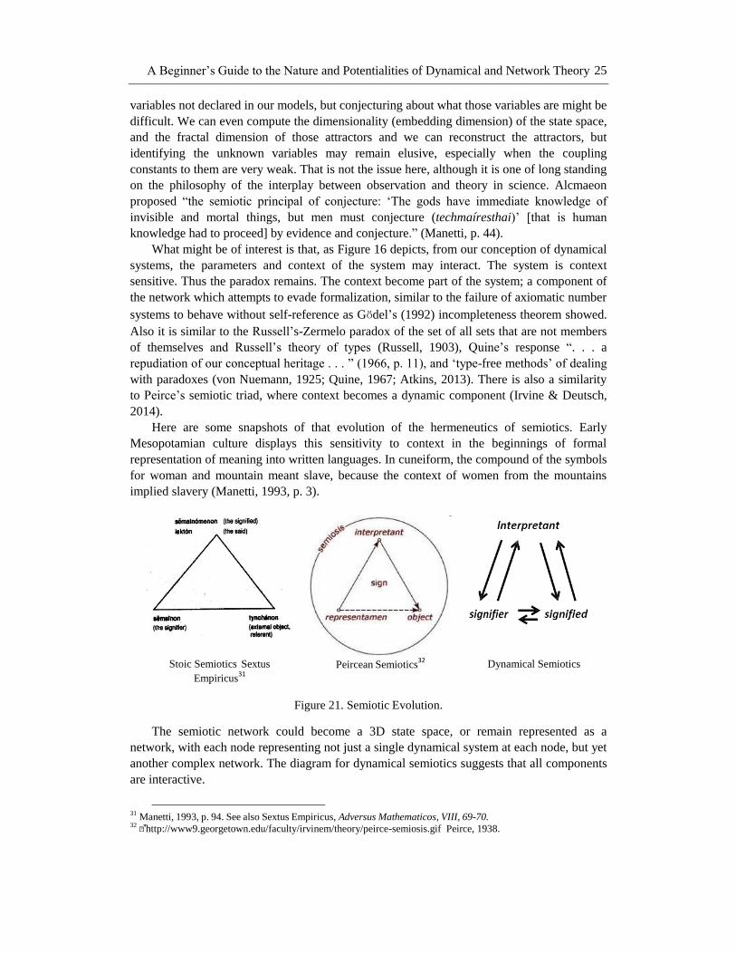
Here are some snapshots of that evolution of the hermeneutics of semiotics. Early

Mesopotamian culture displays this sensitivity to context in the beginnings of formal

representation of meaning into written languages. In cuneiform, the compound of the symbols

for woman and mountain meant slave, because the context of women from the mountains

implied slavery (Manetti, 1993, p. 3).

Stoic Semiotics Sextus

Empiricus31

Peircean Semiotics32

Dynamical Semiotics

Figure 21. Semiotic Evolution.

The semiotic network could become a 3D state space, or remain represented as a

network, with each node representing not just a single dynamical system at each node, but yet

another complex network. The diagram for dynamical semiotics suggests that all components

are interactive.

31

Manetti, 1993, p. 94. See also Sextus Empiricus, Adversus Mathematicos, VIII, 69-70. 32

http://www9.georgetown.edu/faculty/irvinem/theory/peirce-semiosis.gif Peirce, 1938.


If we consider semiotics as a meta-modelling strategy, that is, that language is used to

represent our view of the world, and dynamics as a meta-modelling strategy, then it follows

that we can represent semiotics dynamically (which Hardy, 1998, does; also Chandler, 2009;

and Sandararajan & Kim, 2011). Moreover, in turn, semiotics can treat dynamics as a

language. That is, semiotics can represent dynamics. Escher’s (1948) hands that draw each

other?

ACKNOWLEDGMENTS AND DEDICATION

We wish to acknowledge the intellectual and personal support from our diverse friends in

liberation science: Linda Alford, Jay Allen, Dick Bird, Linnea Carlson-Sabelli, Jerry

Chandler, Tina Champagne, Mike Cole, Allan Combs, Bill & Gail Corning, Linda Dennard,

Eva de Lourdes Edwards, Neil Edwards, Bob & Connie Eldridge, Mark Filippi, Doris

Fromberg, Martin & Pat Gardiner, Tom Gentry, David Gibson, Al Gilgen, Robert Gregson,

Sally Goerner, Christine Hardy, Gus & Vic Koehler, Stanley Krippner, David Loye, Tom

Malloy, Terry Marks-Tarlow, Frank Mosca, George Muhs, Judith Nagib, Rick Paar, Lothar

Pickenhain, Bob Porter, Karl Pribram, Paul Rapp, Hector Sabelli, Ruth Richards, Robin

Robertson, Henry & Carole Slucki, Meg Spohn, Clint Sprott, Carlos Torre, Karen VanderVen,

Norman Weinberger, Enrico Wensing, and Tobi Zausner, many of whom are members of the

Winter Chaos Conference and/or the Society for Chaos Theory in Psychology and the Life

Sciences.

Special thanks to Ralph Abraham, Alan Garfinkel, Stanley Krippner, Ruth Richards, and

Linda Alford for helpful comments and corrections, from copy edits to deep mathematical and

philosophical insights. This article started life in response to a request for a chapter for a book,

by Hector Sabelli, whose death rendered that project unfinished. I dedicate this article to

Hector, for his passion for dynamics and philosophy, but mostly, for his passion for human

rights and justice.

REFERENCES

Abarbanel, H. D. I. (1996). Analysis of observed chaotic data. New York: Springer-Verlag.

Abraham, F. D. (1994a). Chaos and dynamical navigation of the cognitive map. In S. L.

Macey, (Ed.), Encyclopedia of time. Hamden: Garland.

Abraham, F. D. (1994b). Chaos, bifurcations, & self-organization: Extensions of neurological

positivism and ecological psychology. Psychoscience, 1, 85-118. Also at:

http://www.goertzel.org/dynapsyc/1996/fred.html and http://www.blueberry-brain.org/

dynamics/np.htm

Abraham FD. (1996). The dynamics of creativity and the courage to be. In W Sulis and A

Combs (Eds.), Nonliner dynamics in human behavior. Singapore: World Scientific.

Abraham, F. D. (1997a). Sophia: The courage to become wise: Freedom responsibility, &

chaos. http://www.blueberry-brain.org/chaosophy/sophia.html

Abraham, F. D. (1997b). Nonlinear coherence in multivariate research: Invariants and the

reconstruction of attractors. Nonlinear Dynamics, Psychology & Life Science, 1, 7-34.


Abraham, F.D. (2007). Cyborgs, cyberspace, cybersexuality: The evolution of everyday

creativity. In R. Richards (Ed.), Everyday creativity and new views of human nature (pp.

241-259). Washington, DC: American Psychological Association.

Abraham, F. D. (2012). Dynamical concepts used in creativity and chaos. NeuroQuantology,

10(2), 177-182.

*Abraham, R. H., & Shaw, C. D. (1982). Dynamics: The geometry of behavior, Part I:

Periodic behavior. Santa Cruz: Aerial Press. Parts II, Chaotic behavior, 1984, III, Global

behavior, 1985, & IV, Bifurcation behavior, 1988. All four volumes were collected into a

second edition, Dynamics: The geometry of behavior, 1992, Redwood City: Addison-

Wesley. Since 2005 available as a CD, from Aerial Press.

Abraham, R. H., & Shaw, C. D. (1987). Dynamics: A visual introduction. In F. E. Yates

(Ed.), Self-organizing systems: The emergence of order. New York: Plenum

Alford, L., & Abraham, F. D. (2011). Aesthetics as a driving force for understanding a fractal

taxonomy, living systems, mind and engagement with the world. Paper presented at the

Winter Chaos Conference, March 18-20, 2011, New Haven, CT.

http://impleximundi.com/tiki-read_article.php?articleId=99

Ashby, W. R. (1945). The physical origin of adaptation by trial and error. Journal of General

Psychology, 32, 13-25.

Ashby, W. R. (1962). Principles of the self-organizing system. In H. Von Foerster & G. W.

Zopf, J. R. (Eds.), Principles of self-organization: Transactions of the University of

Illinois Symposium, 255-278. London: Pergamon. Reprinted 2004 in Classical Papers—

Principles of the self-organizing system, E:CO Special Double Issue, 6, 1-2, 102-126.

Atkins, A. Peirce's theory of signs". In E. N. Zalta (Ed.), The Stanford Encyclopedia of

Philosophy (Summer 2013 Edition), http://plato.stanford.edu/archives/sum2013/

entries/peirce-semiotics/

Baumeister, R. F., & B. J. Bushman, B. J. (2011). The self. In Social psychology and human

nature. 2nd ed. Belmont, CA: Cengage Learning. 57-96.

Bausch, K. (2001). The emerging consensus in social systems theory. New York: Plenum.

Bertalanffy, L. von (1950). An outline of general system theory. British Journal for the

Philosophy of Science, 1, 134-165.

Boccaletti, S., Grebogi, C., Lai, Y.-C., Mancini, H., & Maza, D. (2000). The control of chaos:

Theory and applications. Physics Reports, 329, 103-197.

Boyle, M., & Petersen, K. (2014). Markov processes in the context of symbolic dynamics. In

B. Marcus, K. Petersen, & T. Weissman (Eds.), Entropy of hidden Markov processes and

connections to dynamical systems. Cambridge: Cambridge University Press.

Briggs, J. (1992). Fractals: The patterns of chaos. New York: Simon & Schuster.

Burns, C. P. E. (2011). Wolfgang Pauli, Carl Jung, and the acausal connecting principle: A

case study in trandisciplinarity. http://www.metanexus.net/essay/wolfgang-pauli-carl-

jung- and-acausal-connecting-principle-case-study-transdisciplinarity.

Chalfan, B. (2002) http://www. hevanet. com/bradc/MiscMathStuff. html Retrieved 20

December 2009.

Chandler, J. L. R. (2009). An introduction to the perplex number system, Discrete Applied

Mathematics. 157, 2296-2309. https://www.academia.edu/3306860/Algebraic_

Chemistry_as_an_Application_of_the_Per plex_Number_System

Chaudhury, S., Smith, A., Anderson, B. E., Ghose, S. & Jessen, P. S. (2009). Quantum

signatures of chaos in a kicked top. Nature, 461, 768-771.


Conforti, M. (1999). Field, form, and fate: Patterns in mind, nature, and psyche. New

Orleans: Spring Journal.

Dennard, L. (2008). Legitimacy, Accountability and Policy Analysis: The Evolution of the

Administrative State. Chap. 4 in L. Dennard, K. A. Richardson, & G. Morçöl (Eds.),

Complexity and Policy Analysis: Tools and Concepts for Designing Robust Policies in a

Complex World, Volume 2. ISCE.

Dewey, J. (2005). Art as experience. Peregee Trade.

Diels, H. & W. Kranz, 1951-1954, Die Fragmente der Vorsokratiker, 7th

edition, Berlin:

Weidmann. English translation (1972/2001), by R. K. Sprague (Ed. & trans.), The older

sophists: A complete translation by several hands of the Fragments in Die Fragmente der

Vorsokratiker edited by Diels-Kranz with a new edition of Antiphon and of Euthydemus.

Columbia: University of South Carolina Press/Hackett.

Ditto, W. L., Rauseo, S. N., Spano, M. L. (1990). Experimental control of chaos. Physical

Review Letters, 65, 3211.

Duchesne, L. (1993). Using characteristic multiplier loci to predict bifurcation phenomena

and chaos―A tutorial. IEEE Transactions on Circuits and Systems―I: Fundamental

Theory and Applications, 40(10), 683-688. http://www. eecs. berkeley.edu/~chua/papers/

Duchesne93. pdf retrieved 24 December 2009.

Escher, M. C. (1948). Drawing Hands (lithograph). www..archive.com/archive/

E/escher_hands.jpg.html [4 July 2014]

Flight, 25 September 1953, The Wilbur Wright Lecture, p. 431. See: http://www. flightglobal.

com/pdfarchive/view/1953/1953%20-%201275. html

Garfinkel, A., Spano, M., Ditto, W., & Weiss, J. (1992). Controlling cardiac chaos. Science,

257, 1230-1235.

Gӧdel, K. (1992). On formally undecidable propositions of Principia Mathematica and

related systems, tr. B. Meltzer, with a comprehensive introduction by Richard

Braithwaite. Dover reprint of the 1962 Basic Books edition. First paper in 1931.

Goldstein, J. (1999). Emergence as a construct: History and issues. Emergence: Complexity

and Organization, 1 (1): 49-72.

Guilford, J. P. (1953). Creativity and its cultivation. New York: Harper & Row.

Guastello, S. J. (1985). Euler buckling in a wheelbarrow obstacle course: A catastrophe with

complex lag. Behavioral Science, 30, 204—212

Habermas, J. (1995). Excursus on Luhmann’s appropriation of the philosophy of the subject

through systems theory. In The philosophical discourse of modernity: Twelve lectures.

Cambridge: MIT Press.

Hardy, C. (1998). Networks of meaning. Westport: Praeger.

Herodotus Historiae. I.53 & I.55, VII.141. (2008-2013). Project Gutenberg Ebook of The

history of Herodotus, by Herodotus. G. D. Macaulay (trans.),

http://www.gutenberg.org/files/2707/2707-h/2707-h.htm

Huffman, C. (2013). Alcmaeon. In E. N. Zalta (Ed.), The Stanford Encyclopedia of

Philosophy (Summer 2013 Edition).

http://plato.stanford.edu/archives/sum2013/entries/alcmaeon

Irvine, A. D., & Deutsch, H. (2014). Russell’s paradox. In E. N. Zalta (Ed.), The Stanford

Encyclopedia of Philosophy (Summer 2014 Edition),

http://plato.stanford.edu/archives/fall2014/entries/russell-paradox/


Kantz, H. , & Schreiber, T. (1997). Nonlinear time series analysis. Cambridge: Cambridge.

Korzybski, A. (1931/1933). A non-Aristotelian system and its necessity for rigor in

mathematics and physics, paper at American Mathematical Society at the New Orleans,

Louisiana, meeting of the American Association for the Advancement of Science,

December 28, 1931. Reprinted in Science and Sanity, 1933, p. 747–61

Krippner, S. Richards, R., & Abraham, F. D. (2014). Creativity and chaos while waking and

dreaming. International Journal of Existential Psychology & Psychotherapy, 5(1), 18 –

26.

Kugler, P. N. , Shaw, R. E. , Vicente, K. J. , & Kinsella-Shaw, J. (1990). Inquiry into

intentional systems I: Issues in ecological physics. Psychological Research, 52, 98-121,

or Kugler, P. N. , Shaw, R. E. , Vicente, K. J. , & Kinsella-Shaw, J. (1991). The role of

attractors in the self-organization of intentional systems, in R. R. Hoffman & D. S.

Palermo (Eds.), Cognition and the symbolic processes. New York: Erlbaum.

Lewin, K. (1947). Frontiers of group dynamics: Concept, method and reality in social science,

social equilibria, and social change. Human Relations, 1, 5-41.

Lotka, A. J. (1925) Elements of physical biology. Baltimore: Williams & Wilkins. Reprinted

1956 by Dover as Elements of mathematical biology.

Luhmann, N. (1984). Soziale systeme. Frankfort am Main.

Manetti, G. (1993). Theories of the sign in classical antiquity. C. Richardson (trans.).

Bloomington: Indiana.

Marks-Tarlow, T. (2014). Myth, metaphor, and the evolution of self-awareness. International

Journal of Signs and Semiotic Systems, 3(1), 46-60.

Maslow, A. (1999). Toward a psychology of being, 3rd

ed. Wiley.

Mead, M. (1973). Changing styles of anthropological work. Annual Review of Anthropology,

2, 1-27.

Neurath, O., Carnap, R., & Morris C., (Eds.), (1938). International Encyclopedia of Unified

Science, 1. Chicago: Chicago.

Orsucci, F. (2008). Ethos in everyday action: Notes for a mindscape of bioethics. Chaos and

Complexity Letters, 3(2), 217-228.

Ott, E. (2006). Controlling chaos. Scholarpedia, 1(8):1699. doi:10.4249

Ott, E., Grebogi, C., & Yorke, J. A. (1990). Controlling chaos. Physical Review Letters, 64,

1196- 1199. Reprinted in Ott, Sauer, & Yorke, 1994.

*Ott, E., Sauer, T., & Yorke, J. A. (Eds.). (1994). Coping with chaos: Analysis of chaotic

data and the exploitation of chaotic systems. New York: Wiley.

Paar, D. W. (1993). Introducing confusion to create change. The Psychotherapy Patient, 8(1-

2).

Pearson, K. (1901): On lines and planes of closest fit to systems of points in space.

Philosophical Magazine, 2(11): 559–572. doi:10.1080/14786440109462720

Peirce, C. S. (1938). Writings on the general theory of signs. 1971, Mouton, The Hague, The

Netherlands.

Poincaré, H. (1881-1886). Mémoire sur les courbes définies par une équation différentielle.

Journal de Mathématiques pures et appliquées (3), 7, 375-422; 8, 251-296; (4), 1, 167-

244; 2, 151-217. Also in Œuvres, 1, 3-44, 44-84, 90-161, 167-222.

Poincaré, H. (1892, 1893, 1899). Les méthodes nouvelles de la mécanique céleste, Vols 1-3.

Gauthiers-Villars, Paris. Also at: https://archive.org/details/lesmthodesnouv001poin


(English translation edited by D. Goroff, published by the American Institute of Physics,

New York, 1993.)

Pyragas, K. (1992). Continuous control of chaos by self-controlling feedback. Physics Letters

A, 170, 421.

Pyragas, K., & Tamasevicius, T. (1993). Experimental control of chaos by delayed self-

control feedback Physics Letters A, 180, 99.

Quine, W.V.O. (1966). The ways of paradox and other essays. New York: Random House.

Quine, W.V.O. (1967). Set theory and its logic. Harvard: Belknap Press.

Rapp, P. E. (1994). A guide to dynamical analysis. Integrative Physiological and Behavioral

Science, 29, 311-327.

Richards, R. (Ed.). (2007). Everyday creativity and new views of human nature). Washington,

DC: American Psychological Association.

Rössler, O. E. (1976), Different types of chaos in two simple differential equations,

Zeitschrift für Naturforsch A, 31, 1664-1670.

Russell, B. (1903). The principles of mathematics. Cambridge: Cambridge. Pp. 523–528.

Schwalbe, M. L. (1991). The autogenesis of the self. Journal for the Theory of Social

Behavior, 21, 269-295.

Schwinning, S. Predator-prey model with habitat selection. At Bill Schaffer’s web site:

http://bill. srnr. arizona. edu/cool/newswkpx. html §8. Retrieved 22 November 2009.

Sundararajan, L. , & Kim, C. (2011). Beyond I-you-me: An empirically supported

formulation of the triadic self. The American Sociologist, DOI 10. 1007/s12108-010-

9117-7. http://www. springerlink. com/content/48q53lp6m2p62835/

Smith, L. (2007). Chaos: A very short introduction. New York: Oxford.

*Sprott, J. C. (2003). Chaos and time-series analysis. Oxford: Oxford & NY.

Thompson, J. M. T., & Stewart, H. B. (1986). Nonlinear dynamics and chaos. New York:

Wiley.

Vandervert, L.R. (1993). Neurological positivism's evolution of mathematics. The Journal of

Mind and Behavior, 14, 277-288.

Varela, F. J. (1999). The specious present: A neurophenomenology of time consciousness. In

J. Petitot, F. J. Varela, B. Pachoud, J-M. Roy (Eds.), Naturalizing phenomenology. 266-

314. Stanford.

von Neumann, J. (1925). An axiomatization of set theory. In J. van Heijenoort (Ed.), From

Frege to Gödel. Cambridge26 and London: Harvard. Ppp, 393–413.

A Beginner's Guide I: A Visual Introduction to Dynamics

Documents

Transcript of A Beginner's Guide I: A Visual Introduction to Dynamics