arX

iv:0

909.

5216

v2 [

stat

.ML]

5 J

an 2

010

1

Learning Gaussian Tree Models: Analysis of ErrorExponents and Extremal Structures

Vincent Y. F. Tan,Student Member, IEEE,Animashree Anandkumar,Member, IEEE,Alan S. Willsky, Fellow, IEEE.

Abstract—The problem of learning tree-structured Gaussiangraphical models from independent and identically distributed(i.i.d.) samples is considered. The influence of the tree structureand the parameters of the Gaussian distribution on the learningrate as the number of samples increases is discussed. Specifically,the error exponent corresponding to the event that the estimatedtree structure differs from the actual unknown tree structure ofthe distribution is analyzed. Finding the error exponent reducesto a least-squares problem in the very noisy learning regime.In this regime, it is shown that the extremal tree structure thatminimizes the error exponent is the star for any fixed set ofcorrelation coefficients on the edges of the tree. If the magnitudesof all the correlation coefficients are less than 0.63, it is also shownthat the tree structure that maximizes the error exponent is theMarkov chain. In other words, the star and the chain graphsrepresent the hardest and the easiest structures to learn in theclass of tree-structured Gaussian graphical models. This resultcan also be intuitively explained by correlation decay: pairs ofnodes which are far apart, in terms of graph distance, are unlikelyto be mistaken as edges by the maximum-likelihood estimator inthe asymptotic regime.

Index Terms—Structure learning, Gaussian graphical models,Gauss-Markov random fields, Large deviations, Error exponents,Tree distributions, Euclidean information theory.

I. I NTRODUCTION

Learning of structure and interdependencies of a largecollection of random variables from a set of data samplesis an important task in signal and image analysis and manyother scientific domains (see examples in [1]–[4] and refer-ences therein). This task is extremely challenging when thedimensionality of the data is large compared to the numberof samples. Furthermore, structure learning of multivariatedistributions is also complicated as it is imperative to findthe right balance between data fidelity and overfitting the datato the model. This problem is circumvented when we limit thedistributions to the set of Markov tree distributions, which havea fixed number of parameters and are tractable for learning [5]and statistical inference [1], [4].

The problem of maximum-likelihood (ML) learning of aMarkov tree distribution from i.i.d. samples has an elegantsolution, proposed by Chow and Liu in [5]. The ML tree

The authors are with Department of Electrical Engineering and Computer Sci-ence and the Stochastic Systems Group, Laboratory for Information and Deci-sion Systems, Massachusetts Institute of Technology. Email:{vtan, animakum,willsky}@mit.edu.

This work is supported in part by a AFOSR through Grant FA9550-08-1-1080,in partby a MURI funded through ARO Grant W911NF-06-1-0076 and in part under a MURIthrough AFOSR Grant FA9550-06-1-0324. Vincent Tan is also supported by A*STAR,Singapore.

This work was presented in part at the Allerton Conference on Communication,Control, and Computing, Monticello, IL, Sep 2009.

structure is given by the maximum-weight spanning tree(MWST) with empirical mutual information quantities as theedge weights. Furthermore, the ML algorithm isconsistent[6],which implies that the error probability in learning the treestructure decays to zero with the number of samples availablefor learning.

While consistency is an important qualitative property, thereis substantial motivation for additional and more quantitativecharacterization of performance. One such measure, which weinvestigate in this theoretical paper is the rate of decay oftheerror probability,i.e., the probability that the ML estimate ofthe edge set differs from the true edge set. When the errorprobability decays exponentially, the learning rate is usuallyreferred to as theerror exponent, which provides a carefulmeasure of performance of the learning algorithm since alarger rate implies a faster decay of the error probability.

We answer three fundamental questions in this paper. (i)Can we characterize the error exponent for structure learningby the ML algorithm for tree-structured Gaussian graphicalmodels (also called Gauss-Markov random fields)? (ii) Howdo the structure and parametersof the model influence theerror exponent? (iii) What are extremal tree distributions forlearning, i.e., the distributions that maximize and minimizethe error exponents? We believe that our intuitively appealinganswers to these important questions provide key insightsfor learning tree-structured Gaussian graphical models fromdata, and thus, for modeling high-dimensional data usingparameterized tree-structured distributions.

A. Summary of Main Results

We derive the error exponent as the optimal value of theobjective function of a non-convex optimization problem,which can only be solved numerically (Theorem 2). To gainbetter insights into when errors occur, we approximate theerror exponent with a closed-form expression that can beinterpreted as the signal-to-noise ratio (SNR) for structurelearning (Theorem 4), thus showing how the parameters ofthe true model affect learning. Furthermore, we show that dueto correlation decay, pairs of nodes which are far apart, interms of their graph distance, are unlikely to be mistaken asedges by the ML estimator. This is not only an intuitive result,but also results in a significant reduction in the computationalcomplexity to find the exponent – fromO(dd−2) for exhaus-tive search andO(d3) for discrete tree models [7] toO(d) forGaussians (Proposition 7), whered is the number of nodes.

We then analyze extremal tree structures for learning, givena fixed set of correlation coefficients on the edges of the tree.

2

Our main result is the following: Thestar graph minimizes theerror exponent and if the absolute value of all the correlationcoefficients of the variables along the edges is less than 0.63,then theMarkov chain also maximizes the error exponent(Theorem 8). Therefore, the extremal tree structures in termsof the diameter arealso extremal trees for learning Gaussiantree distributions. This agrees with the intuition that theamount of correlation decay increases with the tree diameter,and that correlation decay helps the ML estimator to betterdistinguish the edges from the non-neighbor pairs. Lastly,we analyze how changing the size of the tree influences themagnitude of the error exponent (Propositions 11 and 12).

B. Related Work

There is a substantial body of work on approximate learningof graphical models (also known as Markov random fields)from data e.g. [8]–[11]. The authors of these papers usevarious score-based approaches [8], the maximum entropyprinciple [9] or ℓ1 regularization [10], [11] as approximatestructure learning techniques. Consistency guarantees intermsof the number of samples, the number of variables andthe maximum neighborhood size are provided. Information-theoretic limits [12] for learning graphical models have alsobeen derived. In [13], bounds on the error rate for learning thestructure of Bayesian networks were provided but in contrastto our work, these bounds are not asymptotically tight (cf.Theorem 2). Furthermore, the analysis in [13] is tied to theBayesian Information Criterion. The focus of our paper is theanalysis of the Chow-Liu [5] algorithm as anexact learningtechnique for estimating the tree structure and comparingerror rates amongst different graphical models. In a recentpaper [14], the authors concluded that if the graphical modelpossesses long range correlations, then it is difficult to learn.In this paper, we in fact identify the extremal structures anddistributions in terms of error exponents for structure learning.The area of study in statistics known ascovariance selec-tion [15], [16] also has connections with structure learningin Gaussian graphical models. Covariance selection involvesestimating the non-zero elements in the inverse covariancematrix and providing consistency guarantees of the estimatein some norm,e.g. the Frobenius norm in [17].

We previously analyzed the error exponent for learningdiscrete tree distributions in [7]. We proved that for everydiscrete spanning tree model, the error exponent for learning isstrictly positive, which implies that the error probability decaysexponentially fast. In this paper, we extend these results toGaussian tree models and derive new results which are bothexplicit and intuitive by exploiting the properties of Gaussians.The results we obtain in Sections III and IV are analogous tothe results in [7] obtained for discrete distributions, althoughthe proof techniques are different. Sections V and VI containnew results thanks to simplifications which hold for Gaussiansbut which do not hold for discrete distributions.

C. Paper Outline

This paper is organized as follows: In Section II, we statethe problem precisely and provide necessary preliminarieson

learning Gaussian tree models. In Section III, we derive anexpression for the so-called crossover rate of two pairs ofnodes. We then relate the set of crossover rates to the errorexponent for learning the tree structure. In Section IV, weleverage on ideas from Euclidean information theory [18]to state conditions that allow accurate approximations of theerror exponent. We demonstrate in Section V how to reducethe computational complexity for calculating the exponent. InSection VI, we identify extremal structures that maximize andminimize the error exponent. Numerical results are presentedin Section VII and we conclude the discussion in Section VIII.

II. PRELIMINARIES AND PROBLEM STATEMENT

A. Basics of Undirected Gaussian Graphical Models

Undirected graphical modelsor Markov random fields1

(MRFs) are probability distributions that factorize accordingto given undirected graphs [3]. In this paper, we focus solelyon spanning trees(i.e., undirected, acyclic, connected graphs).A d-dimensional random vectorx = [x1, . . . , xd]

T ∈ Rd issaid to beMarkov on a spanning treeTp = (V, Ep) withvertex (or node) setV = {1, . . . , d} and edge setEp ⊂

(V2

)

if its distribution p(x) satisfies the (local) Markov property:p(xi|xV\{i}) = p(xi|xnbd(i)), where nbd(i) := {j ∈ V :(i, j) ∈ Ep} denotes the set of neighbors of nodei. Wealso denote the set of spanning trees withd nodes asT d,thus Tp ∈ T d. Since p is Markov on the treeTp, itsprobability density function (pdf) factorizes according to Tp

into node marginals{pi : i ∈ V} and pairwise marginals{pi,j : (i, j) ∈ Ep} in the following specific way [3] given theedge setEp:

p(x) =∏

i∈V

pi(xi)∏

(i,j)∈Ep

pi,j(xi, xj)

pi(xi)pj(xj), (1)

We assume thatp, in addition to being Markov on the spanningtreeTp = (V, Ep), is a Gaussian graphical modelor Gauss-Markov random field(GMRF) with known zero mean2 andunknown positive definite covariance matrixΣ ≻ 0. Thus,p(x) can be written as

p(x) =1

(2π)d/2|Σ|1/2 exp

(−1

2xTΣ

−1x

). (2)

We also use the notationp(x) = N (x;0,Σ) as a shorthandfor (2). For Gaussian graphical models, it is known that thefill-pattern of the inverse covariance matrixΣ−1 encodes thestructure ofp(x) [3], i.e., Σ−1(i, j) = 0 if and only if (iff)(i, j) /∈ Ep.

We denote the set of pdfs onRd by P(Rd), the set ofGaussian pdfs onRd by PN (Rd) and the set of Gaussiangraphical models which factorize according to some tree inT d as PN (Rd, T d). For learning the structure ofp(x) (orequivalently the fill-pattern ofΣ−1), we are provided with aset ofd-dimensional samplesxn := {x1, . . . ,xn} drawn fromp, wherexk := [xk,1, . . . , xk,d]

T ∈ Rd.

1In this paper, we use the terms “graphical models” and “Markov randomfields” interchangeably.

2Our results also extend to the scenario where the mean of the Gaussian isunknown and has to be estimated from the samples.

3

B. ML Estimation of Gaussian Tree Models

In this subsection, we review the Chow-Liu ML learningalgorithm [5] for estimating the structure ofp given samplesxn. DenotingD(p1||p2) := Ep1

log(p1/p2) as the Kullback-Leibler (KL) divergence [19] betweenp1 and p2, the MLestimate of the structureECL(x

n) is given by the optimizationproblem3

ECL(xn) := argmin

Eq :q∈PN (Rd,T d)

D(p || q), (3)

where p(x) := N (x;0, Σ) and Σ := 1/n∑n

k=1 xkxTk is the

empirical covariance matrix. Given p, and exploiting the factthatq in (3) factorizes according to a tree as in (1), Chow andLiu [5] showed that the optimization for the optimal edge setin (3) can be reduced to a MWST problem:

ECL(xn) = argmax

Eq :q∈PN (Rd,T d)

∑

e∈Eq

I(pe), (4)

where the edge weights are theempirical mutual informationquantities[19] given by4

I(pe) = −1

2log

(1− ρ2e

), (5)

and where theempirical correlation coefficientsare given byρe = ρi,j := Σ(i, j)/(Σ(i, i)Σ(j, j))1/2. Note that in (4), theestimated edge setECL(x

n) depends onn and, specifically, onthe samples inxn and we make this dependence explicit. Weassume thatTp is a spanning tree because with probability 1,the resulting optimization problem in (4) produces a spanningtree as all the mutual information quantities in (5) will be non-zero. IfTp wereallowed to be aproper forest(a tree that is notconnected), the estimation ofEp will be inconsistent becausethe learned edge set will be different from the true edge set.

C. Problem Statement

We now state our problem formally. Given a set of i.i.d.samplesxn drawn from an unknown Gaussian tree modelpwith edge setEp, we define the error event that the set of edgesis estimated incorrectly as

An := {xn : ECL(xn) 6= Ep}, (6)

whereECL(xn) is the edge set of the Chow-Liu ML estimator

in (3). In this paper, we are interested tocomputeand subse-quentlystudythe error exponentKp, or the rate that the errorprobability of the eventAn with respect to thetrue modelpdecays with the number of samplesn. Kp is defined as

Kp := limn→∞

− 1

nlogP(An), (7)

assuming the limit exists and whereP is the product probabil-ity measure with respect to the true modelp. We prove that thelimit in (7) exists in Section III (Corollary 3). The value ofKp

for different tree modelsp provides an indication of the relativeease of estimating such models. Note that both theparametersandstructureof the model influence the magnitude ofKp.

3Note that it is unnecessary to impose the Gaussianity constraint onq in (3).We can optimize overP(Rd, T d) instead ofPN (Rd, T d). It can be shownthat the optimal distribution is still Gaussian. We omit the proof for brevity.

4Our notation for the mutual information between two random variablesdiffers from the conventional one in [19].

@@@

@@ �

��

��

w

w w w

we′ /∈ EP

e ∈ Path(e′; EP )

?

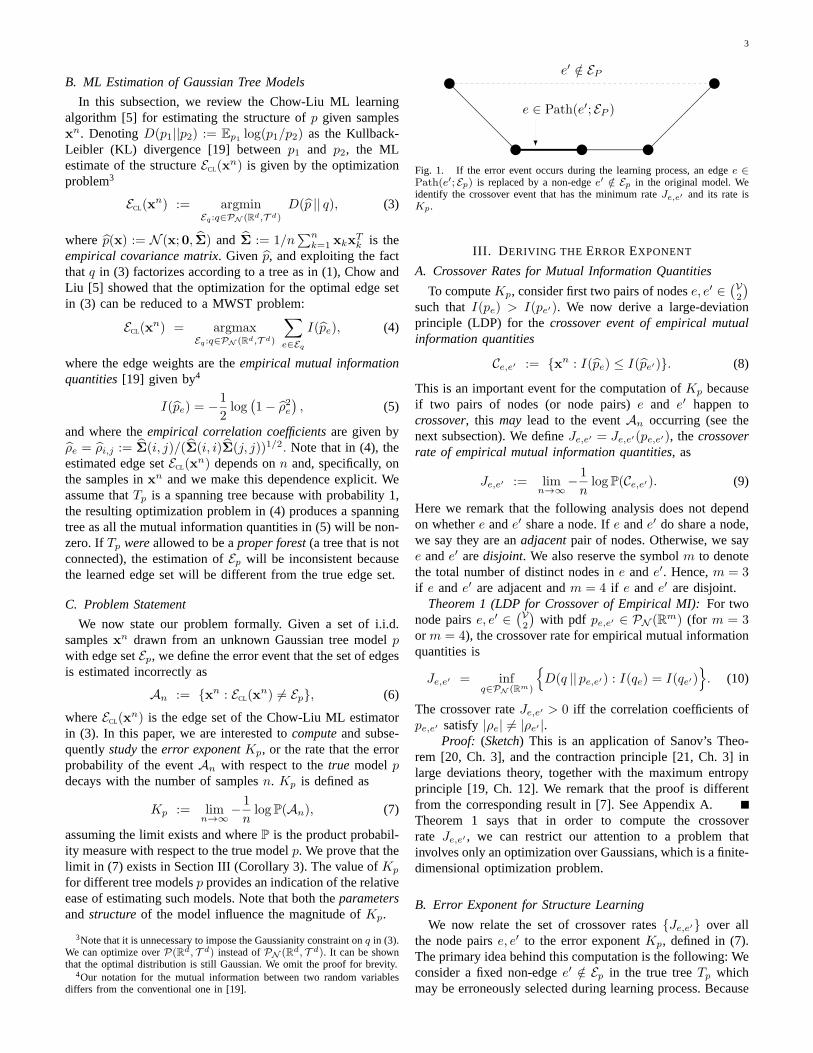
Fig. 1. If the error event occurs during the learning process, an edgee ∈Path(e′; Ep) is replaced by a non-edgee′ /∈ Ep in the original model. Weidentify the crossover event that has the minimum rateJe,e′ and its rate isKp.

III. D ERIVING THE ERROREXPONENT

A. Crossover Rates for Mutual Information Quantities

To computeKp, consider first two pairs of nodese, e′ ∈(V2

)

such thatI(pe) > I(pe′). We now derive a large-deviationprinciple (LDP) for thecrossover event of empirical mutualinformation quantities

Ce,e′ := {xn : I(pe) ≤ I(pe′)}. (8)

This is an important event for the computation ofKp becauseif two pairs of nodes (or node pairs)e and e′ happen tocrossover, this may lead to the eventAn occurring (see thenext subsection). We defineJe,e′ = Je,e′(pe,e′), thecrossoverrate of empirical mutual information quantities, as

Je,e′ := limn→∞

− 1

nlogP(Ce,e′). (9)

Here we remark that the following analysis does not dependon whethere ande′ share a node. Ife ande′ do share a node,we say they are anadjacentpair of nodes. Otherwise, we saye ande′ aredisjoint. We also reserve the symbolm to denotethe total number of distinct nodes ine ande′. Hence,m = 3if e ande′ are adjacent andm = 4 if e ande′ are disjoint.

Theorem 1 (LDP for Crossover of Empirical MI):For twonode pairse, e′ ∈

(V2

)with pdf pe,e′ ∈ PN (Rm) (for m = 3

or m = 4), the crossover rate for empirical mutual informationquantities is

Je,e′ = infq∈PN (Rm)

{D(q || pe,e′) : I(qe) = I(qe′)

}. (10)

The crossover rateJe,e′ > 0 iff the correlation coefficients ofpe,e′ satisfy |ρe| 6= |ρe′ |.

Proof: (Sketch) This is an application of Sanov’s Theo-rem [20, Ch. 3], and the contraction principle [21, Ch. 3] inlarge deviations theory, together with the maximum entropyprinciple [19, Ch. 12]. We remark that the proof is differentfrom the corresponding result in [7]. See Appendix A.Theorem 1 says that in order to compute the crossoverrate Je,e′ , we can restrict our attention to a problem thatinvolves only an optimization over Gaussians, which is a finite-dimensional optimization problem.

B. Error Exponent for Structure Learning

We now relate the set of crossover rates{Je,e′} over allthe node pairse, e′ to the error exponentKp, defined in (7).The primary idea behind this computation is the following: Weconsider a fixed non-edgee′ /∈ Ep in the true treeTp whichmay be erroneously selected during learning process. Because

4

of the global tree constraint, this non-edgee′ must replacesome edge along its unique path in the original model. We onlyneed to consider a single such crossover event becauseKp willbe larger if there are multiple crossovers (see formal proofin [7]). Finally, we identify the crossover event that has theminimum rate. See Fig. 1 for an illustration of this intuition.

Theorem 2 (Exponent as a Crossover Event [7]):The er-ror exponent for structure learning of tree-structured Gaussiangraphical models, defined in (7), is given as

Kp = mine′ /∈Ep

mine∈Path(e′;Ep)

Je,e′ , (11)

wherePath(e′; Ep) ⊂ Ep is the unique path joining the nodesin e′ in the original treeTp = (V, Ep).This theorem implies that thedominant error tree[7], whichis the asymptotically most-likely estimated error tree under theerror eventAn, differs from the true treeTp in exactly oneedge. Note that in order to compute the error exponentKp

in (11), we need to compute at mostdiam(Tp)(d−1)(d−2)/2crossover rates, wherediam(Tp) is the diameter ofTp. Thus,this is a significant reduction in the complexity of computingKp as compared to performing an exhaustive search overall possible error events which requires a total ofO(dd−2)computations [22] (equal to the number of spanning trees withd nodes).

In addition, from the result in Theorem 2, we can deriveconditions to ensure thatKp > 0 and hence for the errorprobability to decay exponentially.

Corollary 3 (Condition for Positive Error Exponent):Theerror probabilityP(An) decays exponentially,i.e., Kp > 0iff Σ has full rank andTp is not a forest (as was assumed inSection II).

Proof: See Appendix B for the proof.The above result provides necessary and sufficient condi-

tions for the error exponentKp to be positive, which impliesexponential decay of the error probability inn, the number ofsamples. Our goal now is to analyze the influence of structureand parameters of the Gaussian distributionp on themagnitudeof the error exponentKp. Such an exercise requires a closed-form expression forKp, which in turn, requires a closed-formexpression for the crossover rateJe,e′ . However, the crossoverrate, despite having an exact expression in (10), can only befound numerically, since the optimization is non-convex (dueto the highly nonlinear equality constraintI(qe) = I(qe′)).Hence, we provide an approximation to the crossover rate inthe next section which is tight in the so-called very noisylearning regime.

IV. EUCLIDEAN APPROXIMATIONS

In this section, we use an approximation that only con-siders parameters of Gaussian tree models that are “hard”for learning. There are three reasons for doing this. Firstly,we expect parameters which result in easy problems to havelarge error exponents and so the structures can be learnedaccurately from a moderate number of samples. Hard problemsthus lend much more insight into when and how errors occur.Secondly, it allows us to approximate the intractable problemin (10) with an intuitive, closed-form expression. Finally, such

an approximation allows us to compare the relative ease oflearning various tree structures in the subsequent sections.

Our analysis is based on Euclidean information theory [18],which we exploit to approximate the crossover rateJe,e′ andthe error exponentKp, defined in (9) and (7) respectively. Thekey idea is to impose suitable “noisy” conditions onpe,e′ (thejoint pdf on node pairse ande′) so as to enable us to relax thenon-convex optimization problem in (10) to a convex program.

Definition 1 (ǫ-Very Noisy Condition):The joint pdf pe,e′on node pairse and e′ is said to satisfy theǫ-very noisycondition if the correlation coefficients one and e′ satisfy||ρe| − |ρe′ || < ǫ.By continuity of the mutual information in the correlationcoefficient, given any fixedǫ and ρe, there exists aδ =δ(ǫ, ρe) > 0 such that|I(pe)− I(pe′)| < δ, which means thatif ǫ is small, it is difficult to distinguish which node paireor e′ has the larger mutual information given the samplesx

n.Therefore the ordering of the empirical mutual informationquantitiesI(pe) and I(pe′) may be incorrect. Thus, ifǫ issmall, we are in the very noisy learning regime, where learningis difficult.

To perform our analysis, we recall from Verdu [23, Sec. IV-E] that we can bound the KL-divergence between two zero-mean Gaussians with covariance matricesΣe,e′ + ∆e,e′ andΣe,e′ as

D(N (0,Σe,e′ +∆e,e′)||N (0,Σe,e′))≤‖Σ−1

e,e′∆e,e′‖2F4

,

(12)where‖M‖F is the Frobenius norm of the matrixM. Fur-thermore, the inequality in (12) is tight when the perturbationmatrix ∆e,e′ is small. More precisely, as the ratio of the

singular valuesσmax(∆e,e′ )

σmin(Σe,e′ )tends to zero, the inequality in

(12) becomes tight. To convexify the problem, we also performa linearization of the nonlinear constraint set in (10) aroundthe unperturbed covariance matrixΣe,e′ . This involves takingthe derivative of the mutual information with respect to thecovariance matrix in the Taylor expansion. We denote thisderivative as∇Σe

I(Σe) where I(Σe) = I(N (0,Σe)) isthe mutual information between the two random variables ofthe Gaussian joint pdfpe = N (0,Σe). We now define thelinearized constraint setof (10) as the affine subspace

L∆(pe,e′) := {∆e,e′ ∈ Rm×m : I(Σe) + 〈∇ΣeI(Σe),∆e〉

= I(Σe′) + 〈∇Σe′I(Σe′),∆e′〉}, (13)

where∆e ∈ R2×2 is the sub-matrix of∆e,e′ ∈ Rm×m (m =3 or 4) that corresponds to the covariance matrix of the nodepair e. We also define theapproximate crossover rateof e ande′ as the minimization of the quadratic in (12) over the affinesubspaceL∆(pe,e′) defined in (13):

Je,e′ := min∆e,e′∈L∆(pe,e′ )

1

4‖Σ−1

e,e′∆e,e′‖2F . (14)

Eqn. (14) is aconvexifiedversion of the original optimizationin (10). This problem is not only much easier to solve, butalso provides key insights as to when and how errors occurwhen learning the structure. We now define an additional

5

w

w w

w@@@@

@ �����

p p p p p p p p p p p p p p p p p p p p p p p p p p p p p p p p p p p p pp p p p p p p p p p p p p p p p p p p p p p p pp p pp p p

p p pp p p

p p pp p p

p p pp p p

x1

x2 x3

x4

ρ1,2

ρ2,3

ρ3,4

(1,4) not dominant

Either (1,3) or (2,4)dominates

Fig. 2. Illustration of correlation decay in a Markov chain.By Lemma 5(b),only the node pairs(1, 3) and (2, 4) need to be considered for computingthe error exponentKp. By correlation decay, the node pair(1, 4) will not bemistaken as a true edge by the estimator because its distance, which is equalto 3, is longer than either(1, 3) or (2, 4), whose distances are equal to 2.

information-theoretic quantity before stating the Euclideanapproximation.

Definition 2 (Information Density):Given a pairwise jointpdf pi,j with marginalspi and pj , the information densitydenoted bysi,j : R2 → R, is defined as

si,j(xi, xj) := logpi,j(xi, xj)

pi(xi)pj(xj). (15)

Hence, for each pair of variablesxi andxj , its associated in-formation densitysi,j is a random variable whose expectationis the mutual information ofxi andxj , i.e., E[si,j ] = I(pi,j).

Theorem 4 (Euclidean Approx. of Crossover Rate):The approximate crossover rate for the empirical mutualinformation quantities, defined in (14), is given by

Je,e′ =(E[se′ − se])

2

2Var(se′ − se)=

(I(pe′)− I(pe))2

2Var(se′ − se). (16)

In addition, the approximate error exponent correspondingtoJe,e′ in (14) is given by

Kp = mine′∈Ep

mine∈Path(e′;Ep)

Je,e′ . (17)

Proof: The proof involves solving the least squares prob-lem in (14). See Appendix C.We have obtained a closed-form expression for the approxi-mate crossover rateJe,e′ in (16). It is proportional to the squareof the difference between the mutual information quantities.This corresponds to our intuition – that ifI(pe) and I(pe′)are relatively well separated (I(pe) ≫ I(pe′)) then the rateJe,e′ is large. In addition, the SNR is also weighted by theinverse variance of the difference of the information densitiesse−se′ . If the variance is large, then we are uncertain about theestimateI(pe)− I(pe′), thereby reducing the rate. Theorem 4illustrates howparametersof Gaussian tree models affect thecrossover rate. In the sequel, we limit our analysis to the verynoisy regime where the above expressions apply.

V. SIMPLIFICATION OF THE ERROREXPONENT

In this section, we exploit the properties of the approximatecrossover rate in (16) to significantly reduce the complexityin finding the error exponentKp to O(d). As a motivatingexample, consider the Markov chain in Fig. 2. From ouranalysis to this point, it appears that, when computing theapproximate error exponentKp in (17), we have to considerall possible replacements between the non-edges(1, 4), (1, 3)and(2, 4) and the true edges along the unique paths connecting

−0.4 −0.2 0 0.2 0.4 0.6 0.80

0.005

0.01

0.015

0.02

0.025

ρe′

App

roxi

mat

e C

ross

over

Rat

e

ρ

e=0.2

ρe=0.4

ρe=0.6

−1 −0.5 0 0.5 10

0.005

0.01

0.015

0.02

0.025

ρe

1

App

roxi

mat

e C

ross

over

Rat

e

ρcrit

ρe

2

=0.2

ρe

2

=0.4

ρe

2

=0.6

−1 −0.5 0 0.5 10

0.005

0.01

0.015

0.02

0.025

ρe

App

roxi

mat

e C

ross

over

Rat

e

ρcrit

ρe′=0.1

ρe′=0.2

ρe′=0.3

Fig. 3. Illustration of the properties ofJ(ρe, ρe′ ) in Lemma 5.J(ρe, ρe′ )is decreasing in|ρe′ | for fixed ρe (top) and J(ρe1 , ρe1ρe2 ) is increasingin |ρe1 | for fixed ρe2 if |ρe1 | < ρcrit (middle). Similarly, J(ρe, ρe′ ) isincreasing in|ρe| for fixed ρe′ if |ρe| < ρcrit (bottom).

these non-edges. For example,(1, 3) might be mistaken as atrue edge, replacing either(1, 2) or (2, 3).

We will prove that, in fact, to computeKp we can ignorethe possibility that longest non-edge(1, 4) is mistaken as atrue edge, thus reducing the number of computations for theapproximate crossover rateJe,e′ . The key to this result isthe exploitation ofcorrelation decay, i.e., the decrease in theabsolute value of the correlation coefficient between two nodesas thedistance(the number of edges along the path betweentwo nodes) between them increases. This follows from theMarkov property:

ρe′ =∏

e∈Path(e′;Ep)

ρe, ∀e′ /∈ Ep. (18)

For example, in Fig. 2,|ρ1,4| ≤ min{|ρ1,3|, |ρ2,4|} andbecause of this, the following lemma implies that(1, 4) isless likely to be mistaken as a true edge than(1, 3) or (2, 4).

It is easy to verify that the crossover rateJe,e′ in (16)dependsonly on the correlation coefficientsρe andρe′ and notthe variancesσ2

i . Thus, without loss of generality, we assume

6

that all random variables have unit variance (which is stillunknown to the learner) and to make the dependence clear, wenow write Je,e′ = J(ρe, ρe′). Finally defineρcrit := 0.63055.

Lemma 5 (Monotonicity ofJ(ρe, ρe′)): J(ρe, ρe′), derivedin (16), has the following properties:

(a) J(ρe, ρe′) is an even function of bothρe andρe′ .(b) J(ρe, ρe′) is monotonicallydecreasingin |ρe′ | for fixed

ρe ∈ (−1, 1).(c) Assuming that|ρe1 | < ρcrit, then J(ρe1 , ρe1ρe2) is

monotonicallyincreasingin |ρe1 | for fixed ρe2 .(d) Assuming that|ρe| < ρcrit, then J(ρe, ρe′) is monoton-

ically increasingin |ρe| for fixed ρe′ .

See Fig. 3 for an illustration of the properties ofJ(ρe, ρe′).Proof: (Sketch) Statement (a) follows from (16). We prove

(b) by showing that∂J(ρe, ρe′)/∂|ρe′ | ≤ 0 for all |ρe′ | ≤ |ρe|.Statements (c) and (d) follow similarly. See Appendix D forthe details.

Our intuition about correlation decay is substantiated byLemma 5(b), which implies that for the example in Fig. 2,J(ρ2,3, ρ1,3) ≤ J(ρ2,3, ρ1,4), since |ρ1,4| ≤ |ρ1,3| due toMarkov property on the chain (18). Therefore,J(ρ2,3, ρ1,4)

can be ignored in the minimization to findKp in (17). Interest-ingly while Lemma 5(b) is a statement about correlation decay,Lemma 5(c) states that the absolute strengths of the correlationcoefficients also influence the magnitude of the crossover rate.

From Lemma 5(b) (and the above motivating example inFig. 2), finding the approximate error exponentKp nowreduces to finding the minimum crossover rate only overtriangles((1, 2, 3) and(2, 3, 4)) in the tree as shown in Fig. 2,i.e., we only need to considerJ(ρe, ρe′) for adjacentedges.

Corollary 6 (Computation ofKp): Under the very noisylearning regime, the error exponentKp is

Kp = minei,ej∈Ep,ei∼ej

W (ρei , ρej ), (19)

where ei ∼ ej means that the edgesei and ej are adjacentand the weights are defined as

W (ρe1 , ρe2) :=min{J(ρe1 , ρe1ρe2), J(ρe2 , ρe1ρe2)

}. (20)

If we carry out the computations in (19) independently, thecomplexity isO(d degmax), wheredegmax is the maximumdegree of the nodes in the tree graph. Hence, in the worstcase, the complexity isO(d2), instead ofO(d3) if (17) isused. We can, in fact, reduce the number of computations toO(d).

Proposition 7 (Complexity in computingKp): The approx-imate error exponentKp, derived in (17), can be computed inlinear time (d− 1 operations) as

Kp = mine∈Ep

J(ρe, ρeρ∗e), (21)

where the maximum correlation coefficient on the edgesadjacent toe ∈ Ep is defined as

ρ∗e := max{|ρe| : e ∈ Ep, e ∼ e}. (22)

Proof: By Lemma 5(b) and the definition ofρ∗e, we obtainthe smallest crossover rate associated to edgee. We obtain the

approximate error exponentKp by minimizing over all edgese ∈ Ep in (21).Recall thatdiam(Tp) is the diameter ofTp. The computationof Kp is reduced significantly fromO(diam(Tp)d

2) in (11)to O(d). Thus, there is a further reduction in the complexityto estimate the error exponentKp as compared to exhaustivesearch which requiresO(dd−2) computations. This simplifi-cation only holds for Gaussians under the very noisy regime.

VI. EXTREMAL STRUCTURES FORLEARNING

In this section, we study the influence of graph structure onthe approximate error exponentKp using the concept of cor-relation decay and the properties of the crossover rateJe,e′ inLemma 5. We have already discussed the connection betweenthe error exponent and correlation decay. We also proved thatnon-neighbor node pairs which have shorter distances are morelikely to be mistaken as edges by the ML estimator. Hence, weexpect that a treeTp which contains non-edges with shorterdistances to be “harder” to learn (i.e., has a smaller errorexponentKp) as compared to a tree which contains non-edgeswith longer distances. In subsequent subsections, we formalizethis intuition in terms of the diameter of the treediam(Tp),and show that the extremal trees, in terms of their diameter,are also extremal trees for learning. We also analyze the effectof changing the size of the tree on the error exponent.

From the Markov property in (18), we see that for aGaussian tree distribution, the set of correlation coefficientsfixed on the edges of the tree, along with the structureTp, aresufficient statistics and they completely characterizep. Notethat this parameterization neatly decouples the structurefromthe correlations. We use this fact to study the influence ofchanging the structureTp while keeping the set of correlationson the edges fixed.5 Before doing so, we provide a review ofsome basic graph theory.

A. Basic Notions in Graph Theory

Definition 3 (Extremal Trees in terms of Diameter):Assume thatd > 3. Define theextremal treeswith d nodes interms of the tree diameterdiam : T d → {2, . . . , d− 1} as

Tmax(d) :=argmaxT∈T d

diam(T ), Tmin(d) :=argminT∈T d

diam(T ),

(23)Then it is clear that the two extremal structures, thechain(where there is a simple path passing through all nodes andedges exactly once) and thestar (where there is one centralnode) have the largest and smallest diameters respectively, i.e.,Tmax(d) = Tchain(d), andTmin(d) = Tstar(d).

Definition 4 (Line Graph):The line graph [22] H of agraphG, denoted byH = L(G), is one in which, roughlyspeaking, the vertices and edges ofG are interchanged. Moreprecisely,H is the undirected graph whose vertices are theedges ofG and there is an edge between any two verticesin the line graph if the corresponding edges inG have acommon node,i.e., are adjacent. See Fig. 4 for a graphGand its associated line graphH.

5Although the set of correlation coefficients on the edges is fixed, theelements in this set can be arranged in different ways on the edges of thetree. We formalize this concept in (24).

7

w w

w

w

w w

e1 e2

e3

e4 e5 @@@

@@

@@

@@@w w

w

w

w

1

2

3

4

5

(a) (b)

Fig. 4. (a): A graphG. (b): The line graphH = L(G) that corresponds toG is the graph whose vertices are the edges ofG (denoted asei) and thereis an edge between any two verticesi andj in H if the corresponding edgesin G share a node.

B. Formulation: Extremal Structures for Learning

We now formulate the problem of finding the best and worsttree structures for learning and also the distributions associatedwith them. At a high level, our strategy involves two distinctsteps. Firstly and primarily, we find thestructureof the optimaldistributions in Section VI-D. It turns out that the optimalstructures that maximize and minimize the exponent are theMarkov chain (under some conditions on the correlations) andthe star respectively and these are the extremal structuresinterms of the diameter. Secondly, we optimize over thepositions(or placement) of the correlation coefficients on the edges ofthe optimal structures.

Let ρ := [ρ1, ρ2, . . . , ρd−1] be a fixed vector of feasible6

correlation coefficients,i.e., ρi ∈ (−1, 1) \ {0} for all i. Fora tree, it follows from (18) that ifρi’s are the correlationcoefficients on the edges, then|ρi| < 1 is a necessary andsufficient condition to ensure thatΣ ≻ 0. Define Πd−1

to be the group of permutations of orderd − 1, henceelements inΠd−1 are permutations of a given ordered setwith cardinalityd− 1. Also denote the set of tree-structured,d-variate Gaussians which have unit variances at all nodes andρ as the correlation coefficients on the edges in some orderasPN (Rd, T d;ρ). Formally,

PN (Rd, T d;ρ) :={p(x)=N (x;0,Σ)∈PN (Rd, T d) :

Σ(i, i) = 1, ∀ i ∈ V, ∃πp ∈ Πd−1 : σEp= πp(ρ)

}, (24)

whereσEp:= [Σ(i, j) : (i, j) ∈ Ep] is the length-(d−1) vector

consisting of the covariance elements7 on the edges (arrangedin lexicographic order) andπp(ρ) is the permutation ofρaccording toπp. The tuple(Tp,πp,ρ) uniquely parameterizesa Gaussian tree distribution with unit variances. Note thatwecan regard the permutationπp as a nuisance parameter forsolving the optimization for the best structure givenρ. Indeed,it can happen that there are differentπp’s such that the errorexponentKp is the same. For instance, in a star graph, allpermutationsπp result in the same exponent. Despite this, weshow that extremal treestructuresare invariant to the specificchoice ofπp andρ.

For distributions in the setPN (Rd, T d;ρ), our goal is tofind the best (easiest to learn) and the worst (most difficultto learn) distributions for learning. Formally, the optimization

6We do not allow any of the correlation coefficient to be zero becauseotherwise, this would result inTp being a forest.

7None of the elements inΣ are allowed to be zero becauseρi 6= 0 forevery i ∈ V and the Markov property in (18).

problems for the best and worst distributions for learning aregiven by

pmax,ρ := argmaxp∈PN (Rd,T d;ρ)

Kp, (25)

pmin,ρ := argminp∈PN (Rd,T d;ρ)

Kp. (26)

Thus,pmax,ρ (resp.pmin,ρ) corresponds to the Gaussian treemodel which has the largest (resp. smallest) approximate errorexponent.

C. Reformulation as Optimization over Line Graphs

Since the number of permutationsπ and number of span-ning trees are prohibitively large, finding the optimal distri-butions cannot be done through a brute-force search unlessdis small. Our main idea in this section is to use the notionof line graphs to simplify the problems in (25) and (26). Insubsequent sections, we identify the extremal tree structuresbefore identifying the precise best and worst distributions.

Recall that the approximate error exponentKp can beexpressed in terms of the weightsW (ρei , ρej ) between twoadjacent edgesei, ej as in (19). Therefore, we can write theextremal distribution in (25) as

pmax,ρ = argmaxp∈PN (Rd,T d;ρ)

minei,ej∈Ep,ei∼ej

W (ρei , ρej ). (27)

Note that in (27),Ep is the edge set of a weighted graph whoseedge weights are given byρ. Since the weight is between twoedges, it is more convenient to consider line graphs defined inSection VI-A.

We now transform the intractable optimization problemin (27) over the set of trees to an optimization problem overall the set of line graphs:

pmax,ρ = argmaxp∈PN (Rd,T d;ρ)

min(i,j)∈H,H=L(Tp)

W (ρi, ρj), (28)

andW (ρi, ρj) can be considered as an edge weight betweennodesi and j in a weighted line graphH. Equivalently, (26)can also be written as in (28) but with theargmax replacedby anargmin.

D. Main Results: Best and Worst Tree Structures

In order to solve (28), we need to characterize the set of linegraphs of spanning treesL(T d) = {L(T ) : T ∈ T d}. This hasbeen studied before [24, Theorem 8.5], but the setL(T d) isnonetheless still very complicated. Hence, solving (28) directlyis intractable. Instead, our strategy now is to identify thestructurescorresponding to the optimal distributions,pmax,ρ

andpmin,ρ by exploiting the monotonicity ofJ(ρe, ρe′) givenin Lemma 5.

Theorem 8 (Extremal Tree Structures):The tree structurethat minimizes the approximate error exponentKp in (26)is given by

Tpmin,ρ= Tstar(d), (29)

for all feasible correlation coefficient vectorsρ with ρi ∈(−1, 1) \ {0}. In addition, if ρi ∈ (−ρcrit, ρcrit) \ {0} (where

8

w

w

w

w

w

ρe3

ρe1ρe2ρe4 w w w w w

ρe1 ρe2 ρe3 ρe4

(a) (b)

Fig. 5. Illustration for Theorem 8: The star (a) and the chain(b) minimizeand maximize the approximate error exponent respectively.

ρcrit = 0.63055), then the tree structure that maximizes theapproximate error exponentKp in (25) is given by

Tpmax,ρ= Tchain(d), (30)

Proof: (Idea) The assertion thatTpmin,ρ= Tstar(d)

follows from the fact that all the crossover rates for the stargraph are the minimum possible, henceKstar ≤ Kp. SeeAppendix E for the details.See Fig. 5. This theorem agrees with our intuition: for the stargraph, the nodes are strongly correlated (since its diameteris the smallest) while in the chain, there are many weaklycorrelated pairs of nodes for the same set of correlationcoefficients on the edges thanks to correlation decay. Hence,it is hardest to learn the star while it is easiest to learn thechain. It is interesting to observe Theorem 8 implies that theextremal tree structuresTpmax,ρ

and Tpmin,ρare independent

of the correlation coefficientsρ (if |ρi| < ρcrit in the caseof the star). Indeed, the experiments in Section VII-B alsosuggest that Theorem 8 may likely be true for larger rangesof problems (without the constraint that|ρi| < ρcrit) but thisremains open.

The results in (29) and (30) do not yet provide the completesolution topmax,ρ andpmin,ρ in (25) and (26) since there aremany possible pdfs inPN (Rd, T d;ρ) corresponding to a fixedtree because we can rearrange the correlation coefficients alongthe edges of the tree in multiple ways. The only exception isif Tp is known to be a star then there is only one pdf inPN (Rd, T d;ρ), and we formally state the result below.

Corollary 9 (Most Difficult Distribution to Learn):TheGaussian pmin,ρ(x) = N (x;0,Σmin,ρ) defined in (26),corresponding to the most difficult distribution to learnfor fixed ρ, has the covariance matrix whose uppertriangular elements are given asΣmin,ρ(i, j) = ρi ifi = 1, j 6= 1 and Σmin,ρ(i, j) = ρiρj otherwise. Moreover,if |ρ1| ≥ . . . ≥ |ρd−1| and |ρ1| < ρcrit = 0.63055,then Kp corresponding to the star graph can be writtenexplicitly as a minimization over only two crossover rates:Kpmin,ρ

= min{J(ρ1, ρ1ρ2), J(ρd−1, ρd−1ρ1)}.Proof: The first assertion follows from the Markov

property (18) and Theorem 8. The next result followsfrom Lemma 5(c) which implies thatJ(ρd−1, ρd−1ρ1) ≤J(ρk, ρkρ1) for all 2 ≤ k ≤ d− 1.In other words,pmin,ρ is astar Gaussian graphical model withcorrelation coefficientsρi on its edges. This result can alsobe explained by correlation decay. In a star graph, since thedistances between non-edges are small, the estimator in (3)ismore likely to mistake a non-edge with a true edge. It is often

w

w

w@

@@@�

���

ρ1,2 ρ2,3

ρ1,2ρ2,31 3

2

Fig. 6. If |ρ1,2| < |ρ2,3|, then the likelihood of the non-edge(1, 3)replacing edge(1, 2) would be higher than if|ρ1,2| = |ρ2,3|. Hence, theweightW (ρ1,2, ρ2,3) is maximized when equality holds.

g

w

g

w

g

wi

j

k ρi,k ρ∗i,k

e = (i, j)

6SubtreeTp′

TreeTp

6

?Fig. 7. Illustration of Proposition 11.Tp = (V, Ep) is the original treeande ∈ Ep. Tp′ = (V ′, Ep′ ) is a subtree. The observations for learning thestructurep′ correspond to the shaded nodes, the unshaded nodes correspondto unobserved variables.

useful in applications to compute the minimum error exponentfor a fixed vector of correlationsρ as it provides a lowerbound of the decay rate ofP(An) for any tree distributionwith parameter vectorρ. Interestingly, we also have a resultfor the easiest tree distribution to learn.

Corollary 10 (Easiest Distribution to Learn):Assume thatρcrit > |ρ1| ≥ |ρ2| ≥ . . . ≥ |ρd−1|. Then, the Gaussianpmax,ρ(x) =N (x;0,Σmax,ρ) defined in (25), correspondingto the easiest distribution to learn for fixedρ, has the covari-ance matrix whose upper triangular elements areΣmax,ρ(i, i+

1) = ρi for all i = 1, . . . , d− 1 andΣmax,ρ(i, j) =∏j−1

k=i ρkfor all j > i.

Proof: The first assertion follows from the proof ofTheorem 8 in Appendix E and the second assertion from theMarkov property in (18).In other words, in the regime where|ρi| < ρcrit, pmax,ρ isa Markov chain Gaussian graphical model with correlationcoefficients arranged in increasing (or decreasing) order on itsedges. We now provide some intuition for why this is so. Ifa particular correlation coefficientρi (such that|ρi| < ρcrit)is fixed, then the edge weightW (ρi, ρj), defined in (20), ismaximized when|ρj | = |ρi|. Otherwise, if |ρi| < |ρj | theevent that the non-edge with correlationρiρj replaces the edgewith correlationρi (and hence results in an error) has a higherlikelihood than if equality holds. Thus, correlationsρi andρj that are close in terms of their absolute values should beplaced closer to one another (in terms of graph distance) forthe approximate error exponent to be maximized. See Fig. 6.

E. Influence of Data Dimension on Error Exponent

We now analyze the influence ofchangingthe sizeof thetree on the error exponent,i.e., adding and deleting nodes andedges while satisfying the tree constraint and observing sam-ples from the modified graphical model. This is of importancein many applications. For example, insequentialproblems, thelearner receives data at different times and would like to updatethe estimate of the tree structure learned. Indimensionalityreduction, the learner is required to estimate the structureof a smaller model given high-dimensional data. Intuitively,

9

learning only a tree with a smaller number of nodes is easierthan learning the entire tree since there are fewer ways forerrors to occur during the learning process. We prove this inthe affirmative in Proposition 11.

Formally, we start with a d-variate Gaussianp ∈PN (Rd, T d;ρ) and consider a d′-variate pdf p′ ∈PN (Rd′

, T d′

;ρ′), obtained by marginalizingp over a subsetof variables andTp′ is the tree8 associated to the distributionp′. Henced′ < d andρ′ is a subvector ofρ. See Fig. 7. In ourformulation, the only available observations are those sampledfrom the smaller Gaussian graphical modelp′.

Proposition 11 (Error Exponent of Smaller Trees):Theapproximate error exponent for learningp′ is at least that ofp, i.e., Kp′ ≥ Kp.

Proof: Reducing the number of adjacent edges to a fixededge(i, k) ∈ Ep as in Fig. 7 (wherek ∈ nbd(i)\{j}) ensuresthat the maximum correlation coefficientρ∗i,k, defined in (22),does not increase. By Lemma 5(b) and (17), the approximateerror exponentKp does not decrease.Thus, lower-dimensional models are easier to learn if the set ofcorrelation coefficients is fixed and the tree constraint remainssatisfied. This is a consequence of the fact that there are fewercrossover error events that contribute to the error exponent Kp.

We now consider the “dual” problem of adding a new edgeto an existing tree model, which results in a larger tree. We arenow provided with(d+ 1)-dimensional observations to learnthe larger tree. More precisely, given ad-variate tree Gaussianpdf p, we consider a(d+ 1)-variate pdfp′′ such thatTp is asubtree ofTp′′ . Equivalently, letρ := [ρe1 , ρe2 , . . . , ρed−1

] bethe vector of correlation coefficients on the edges of the graphof p and letρ′′ := [ρ, ρnew] be that ofp′′.

By comparing the error exponentsKp and Kp′′ , we canaddress the following question: Given a new edge correlationcoefficient ρnew, how should one adjoin this new edge tothe existing tree such that the resulting error exponent ismaximized or minimized? Evidently, from Proposition 11, itisnot possible to increase the error exponent by growing the treebut can we devise a strategy to place this new edge judiciously(resp. adversarially) so that the error exponent deteriorates aslittle (resp. as much) as possible?

To do so, we say edgee containsnodev if e = (v, i) andwe define the nodes in the smaller treeTp

v∗min := argminv∈V

maxe∈Ep

{|ρe| : e contains nodev}. (31)

v∗max := argmaxv∈V

maxe∈Ep

{|ρe| : e contains nodev}. (32)

Proposition 12 (Error Exponent of Larger Trees):Assumethat |ρnew| < |ρe| ∀ e ∈ Ep. Then,(a) The difference between the error exponentsKp − Kp′′

is minimizedwhen Tp′′ is obtained by adding toTp anew edge with correlation coefficientρnew at vertexv∗min

given by (31) as a leaf.

8Note thatTp′ still needs to satisfy the tree constraint so that the variablesthat are marginalized out are not arbitrary (but must be variables that form thefirst part of a node elimination order [3]). For example, we are not allowedto marginalize out the central node of a star graph since the resulting graphwould not be a tree. However, we can marginalize out any of the other nodes.In effect, we can only marginalize out nodes with degree either 1 or 2.

0 1 2 3 4 5 6

x 10−3

0

0.5

1

1.5

2

2.5

3x 10

−3

I(Pe)−I(P

e′)

Cro

ssov

er R

ates

True RateApprox Rate

Fig. 8. Comparison of true and approximate crossover rates in (10) and (16)respectively.

(b) The differenceKp − Kp′′ is maximizedwhen the newedge is added tov∗max given by (32) as a leaf.

Proof: The vertex given by (31) is the best vertex to attachthe new edge by Lemma 5(b).This result implies that if we receive data dimensions sequen-tially, we have a straightforward rule in (31) for identifyinglarger trees such that the exponent decreases as little aspossible at each step.

VII. N UMERICAL EXPERIMENTS

We now perform experiments with the following two ob-jectives. Firstly, we study the accuracy of the Euclideanapproximations (Theorem 4) to identify regimes in which theapproximate crossover rateJe,e′ is close to the true crossoverrateJe,e′ . Secondly, by performing simulations we study howvarious tree structures (e.g.chains and stars) influence the errorexponents (Theorem 8).

A. Comparison Between True and Approximate Rates

In Fig. 8, we plot thetrue andapproximatecrossover rates9

(given in (10) and (14) respectively) for a 4-node symmetricstar graph, whose structure is shown in Fig. 9. The zero-meanGaussian graphical model has a covariance matrixΣ such thatΣ

−1 is parameterized byγ ∈ (0, 1/√3) in the following way:

Σ−1(i, i) = 1 for all i, Σ−1(1, j) = Σ

−1(j, 1) = γ for allj = 2, 3, 4 andΣ−1(i, j) = 0 otherwise. By increasingγ, weincrease the difference of the mutual information quantitieson the edgese and non-edgese′. We see from Fig. 8 thatboth rates increase as the differenceI(pe)− I(pe′) increases.This is in line with our intuition because ifpe,e′ is such thatI(pe)−I(pe′) is large, the crossover rate is also large. We alsoobserve that ifI(pe)−I(pe′) is small, the true and approximaterates are close. This is also in line with the assumptions of The-orem 4. When the difference between the mutual informationquantities increases, the true and approximate rates separatefrom each other.

9This small example has sufficient illustrative power because as we haveseen, errors occur locally and only involve triangles.

10

����

�

@@

@@

@

w

w

w

w

x4

x1

x3

x2

e = (1, 2)

e′ = (3, 4)

γ

γ γ

w w w w w w

w

w

w

w

���

@@@

Fig. 9. Left: The symmetric star graphical model used for comparing thetrue and approximate crossover rates as described in SectionVII-A. Right:The structure of ahybrid tree graph withd = 10 nodes as described inSection VII-B. This is a tree with a length-d/2 chain and a orderd/2 starattached to one of the leaf nodes of the chain.

B. Comparison of Error Exponents Between Trees

In Fig. 10, we simulate error probabilities by drawing i.i.d.samples from threed = 10 node tree graphs – a chain, a starand a hybrid between a chain and a star as shown in Fig. 9.We then used the samples to learn the structure via the Chow-Liu procedure [5] by solving the MWST in (4). Thed−1 = 9correlation coefficients were chosen to be equally spaced inthe interval[0.1, 0.9] and they were randomly placed on theedges of the three tree graphs. We observe from Fig. 10 thatfor fixed n, the star and chain have the highest and lowesterror probabilitiesP(An) respectively. Thesimulated errorexponentsgiven by {−n−1 logP(An)}n∈N also converge totheir true values asn → ∞. The exponent associated to thestar is higher than that of the chain, which is corroborated byTheorem 8, even though the theorem only applies in the very-noisy case (and for|ρi| < 0.63055 in the case of the chain).From this experiment, the claim also seems to be true eventhough the setup is not very-noisy. We also observe that theerror exponent of the hybrid is between that of the star andthe chain.

VIII. C ONCLUSION

Using the theory of large deviations, we have obtainedthe error exponent associated with learning the structure ofa Gaussian tree model. Our analysis in this theoretical paperalso answers the fundamental questions as to which set ofparameters and which structures result in high and low errorexponents. We conclude that Markov chains (resp. stars) arethe easiest (resp. hardest) structures to learn as they maximize(resp. minimize) the error exponent. Indeed, our numericalexperiments on a variety of Gaussian graphical models validatethe theory presented. We believe the intuitive results presentedin this paper will lend useful insights for modeling high-dimensional data using tree distributions.

ACKNOWLEDGMENTS

The authors would like to acknowledge Profs. Lang Tong,Lizhong Zheng and Sujay Sanghavi for extensive discussions.The authors would also like to acknowledge the anonymousreviewer who found an error in the original manuscript thatled to the revised development leading to Theorem 8.

103

104

105

0.1

0.2

0.3

0.4

0.5

0.6

0.7

0.8

0.9

Number of samples n

Sim

ulat

ed P

rob

of E

rror

ChainHybridStar

103

104

105

0

0.5

1

1.5

2

2.5x 10

−3

Number of samples n

Sim

ulat

ed E

rror

Exp

onen

t

Fig. 10. Simulated error probabilities and error exponents for chain, hybridand star graphs with fixedρ. The dashed lines show the true error exponentKp computed numerically using (10) and (11). Observe that the simulatederror exponent converges to the true error exponent asn → ∞. The legendapplies to both plots.

APPENDIX APROOF OFTHEOREM 1

Proof: This proof borrows ideas from [25]. We assumem = 4 (i.e., disjoint edges) for simplicity. The result form =3 follows similarly. Let V ′ ⊂ V be a set ofm = 4 nodescorresponding to node pairse ande′. Given a subset of nodepairsY ⊂ V ′ × V ′ such that(i, i) ∈ Y, ∀ i ∈ V ′, the set offeasible moments[4] is defined as

MY :={ηe,e′ ∈ R|Y| : ∃ q(·) ∈ P(Rm)

s.t. Eq[xixj ] = ηi,j , ∀ (i, j) ∈ Y}. (33)

Let the set of densities with momentsηe,e′ := {ηi,j : (i, j) ∈Y} be denoted as

BY(ηe,e′) :={q∈P(Rm) :Eq[xixj ]=ηi,j , (i, j) ∈ Y}. (34)

Lemma 13 (Sanov’s Thm, Contraction Principle [20]):For the event that the empirical moments of the i.i.d.observationsxn are equal toηe,e′ = {ηi,j : (i, j) ∈ Y}, wehave the LDP

limn→∞

− 1

nlogP

⋂

(i,j)∈Y

{xn :

1

n

n∑

k=1

xk,ixk,j = ηi,j

}

= infqe,e′∈BY(η)

D(qe,e′ || pe,e′). (35)

If ηe,e′ ∈ MY , the optimizing pdfq∗e,e′ in (35) is given byq∗e,e′(x) ∝ pe,e′(x) exp

[∑(i,j)∈Y θi,j xixj

], where the set of

11

w

w

w@

@@@�

���

e ee′

Fig. 11. Illustration for the proof of Corollary 3. The correlation coefficienton the non-edge isρe′ and satisfies|ρe′ | = |ρe| if |ρe| = 1.

constants{θi,j : (i, j) ∈ Y} are chosen such thatq∗e,e′ ∈BY(ηe,e′) given in (34).

From Lemma 13, we conclude that the optimalq∗e,e′ in (35)is a Gaussian. Thus, we can restrict our search for the optimaldistribution to a search over Gaussians, which are parameter-ized by means and covariances. The crossover event for mutualinformation defined in (8) isCe,e′ =

{ρ2e′ ≥ ρ2e

}, since in the

Gaussian case, the mutual information is a monotonic functionof the square of the correlation coefficient (cf. Eqn. (5)).Thus it suffices to consider

{ρ2e′ ≥ ρ2e

}, instead of the event

involving the mutual information quantities. Lete = (i, j),e′ = (k, l) andηe,e′ := (ηe, ηe′ , ηi, ηj , ηk, ηl) ∈ MY ⊂ R6 bethe moments ofpe,e′ , whereηe := E[xixj ] is the covarianceof xi and xj , and ηi := E[x2

i ] is the variance ofxi (andsimilarly for the other moments). Now apply the contractionprinciple [21, Ch. 3] to the continuous maph : MY → R,given by the difference between the square of correlationcoefficients

h(ηe,e′) :=η2eηiηj

− η2e′

ηkηl. (36)

Following the same argument as in [7, Theorem 2], the equal-ity case dominatesCe,e′ , i.e., the event

{ρ2e′ = ρ2e

}dominates{

ρ2e′ ≥ ρ2e}

.10 Thus, by considering the set{ηe,e′ : h(ηe,e′) =0}, the rate corresponding toCe,e′ can be written as

Je,e′ = infηe,e′∈MY

{g(ηe,e′) :

η2eηiηj

=η2e′

ηkηl

}, (37)

where the functiong : MY ⊂ R6→ [0,∞) is defined as

g(ηe,e′) := infqe,e′∈BY(ηe,e′ )

D(qe,e′ || pe,e′), (38)

and the setBY(ηe,e′) is defined in (34). Combining expres-sions in (37) and (38) and the fact that the optimal solutionq∗e,e′ is Gaussian yieldsJe,e′ as given in the statement of thetheorem (cf. Eqn. (10)).

The second assertion in the theorem follows from the factthat sincepe,e satisfiesI(pe) 6= I(pe′), we have|ρe| 6= |ρe′ |sinceI(pe) is a monotonic function in|ρe|. Therefore,q∗e,e′ 6=pe,e′ on a set whose (Lebesgue) measureν is strictly positive.SinceD(q∗e,e′ ||pe,e′) = 0 if and only if q∗e,e′ = pe,e′ almosteverywhere-[ν], this implies thatD(q∗e,e′ ||pe,e′) > 0 [19,Theorem 8.6.1].

APPENDIX BPROOF OFCOROLLARY 3

Proof: (⇒) Assume thatKp > 0. Suppose, to thecontrary, that either (i)Tp is a forest or (ii) rank(Σ) < damd Tp is not a forest. In (i), structure estimation ofp will

10This is also intuitively true because the most likely way the error eventCe,e′ occurs is when equality holds,i.e.,

{ρ2e′

= ρ2e}

.

w w w w

w wi0 iM

iM−1i1 i2 . . . iM−2

ρe′ρe

e′ = (i0, iM )

Fig. 12. Illustration for the proof of Corollary 3. The unique path betweeni0 and iM is (i0, i1, . . . , iM ) = Path(e′; Ep).

be inconsistent (as described in Section II-B), which impliesthat Kp = 0, a contradiction. In (ii), sincep is a spanningtree, there exists an edgee ∈ Ep such that the correlationcoefficientρe = ±1 (otherwiseΣ would be full rank). In thiscase, referring to Fig. 11 and assuming that|ρe| ∈ (0, 1), thecorrelation on the non-edgee′ satisfies|ρe′ | = |ρe||ρe| = |ρe|,which implies thatI(pe) = I(pe′). Thus, there is no uniquemaximizer in (4) with the empiricalspe replaced bype. As aresult, ML for structure learning via (4) is inconsistent henceKp = 0, a contradiction.

(⇐) Suppose bothΣ ≻ 0 and Tp not a proper forest,i.e., Tp is a spanning tree. Assume, to the contrary, thatKp = 0. Then from [7], I(pe) = I(pe′) for somee′ /∈ Epand somee ∈ Path(e′; Ep). This implies that|ρe| = |ρe′ |.Let e′ = (i0, iM ) be a non-edge and let the unique path fromnodei0 to nodeiM be (i0, i1, . . . , iM ) for someM ≥ 2. SeeFig. 12. Then,|ρe′ | = |ρi0,iM | = |ρi0,i1 ||ρi1,i2 | . . . |ρiM−1,iM |.Suppose, without loss of generality, that edgee = (i0, i1) issuch that|ρe′ | = |ρe| holds, then we can cancel|ρe′ | and|ρi0,i1 | on both sides to give|ρi1,i2 ||ρi2,i3 | . . . |ρiM−1,iM | = 1.Cancellingρe′ is legitimate because we assumed thatρe′ 6= 0for all e′ ∈ V × V, becausep is a spanning tree. Sinceeach correlation coefficient has magnitude not exceeding 1,this means that each correlation coefficient has magnitude 1,i.e., |ρi1,i2 | = . . . = |ρiM−1,iM | = 1. Since the correlationcoefficients equal to±1, the submatrix of the covariance ma-trix Σ containing these correlation coefficients is not positivedefinite. Therefore by Sylvester’s condition, the covariancematrix Σ ⊁ 0, a contradiction. Hence,Kp > 0.

APPENDIX CPROOF OFTHEOREM 4

Proof: We first assume thate and e′ do not share anode. The approximation of the KL-divergence for Gaussianscan be written as in (12). We now linearize the constraintset L∆(pe,e′) as defined in (13). Given a positive definitecovariance matrixΣe ∈ R2×2, to simplify the notation,let I(Σe) = I(N (x;0,Σe)) be the mutual information ofthe two random variables with covariance matrixΣe. Wenow perform a first-order Taylor expansion of the mutualinformation aroundΣe. This can be expressed as

I(Σe +∆e)=I(Σe)+Tr(∇Σe

I(Σe)T∆e

)+o(∆e). (39)

Recall that the Taylor expansion of log-det [26] islog det(A) = log det(B) + 〈A − B,B−1〉 + o(‖A − B‖F ),with the notation〈A−B,B−1〉 = Tr((A −B)B−1). Usingthis result we can conclude that the gradient ofI with respectto Σe in the above expansion (39) can be simplified to give

12

the matrix

∇ΣeI(Σe) = −1

2

(0 [Σ−1

e ]od[Σ−1

e ]od 0

), (40)

where [A]od is the (unique) off-diagonal element of the2 ×2 symmetric matrixA. By applying the same expansion toI(Σe′ +∆e′), we can express the linearized constraint as

〈M,∆〉 = Tr(MT∆) = I(Σe)− I(Σe′), (41)

where the symmetric matrixM = M(Σe,e′) is defined inthe following fashion:M(i, j) = 1

2 [Σ−1e ]od if (i, j) = e,

M(i, j) = − 12 [Σ

−1e′ ]od if (i, j) = e′ and M(i, j) = 0

otherwise.Thus, the problem reduces to minimizing (over∆) the

approximate objective in (12) subject to the linearized con-straints in (41). This is a least-squares problem. By usingthe matrix derivative identities∇∆Tr(M∆) = M and∇∆Tr((Σ−1

∆)2) = 2Σ−1∆Σ

−1, we can solve for theoptimizer∆∗ yielding:

∆∗ =

I(Σe)− I(Σe′)

(Tr(MΣ))2ΣMΣ. (42)

Substituting the expression for∆∗ into (12) yields

Je,e′ =(I(Σe)− I(Σe′))

2

4Tr((MΣ)2)=

(I(pe)− I(pe′))2

4Tr((MΣ)2). (43)

Comparing (43) to our desired result (16), we observethat problem now reduces to showing thatTr((MΣ)2) =12Var(se − se′). To this end, we note that for Gaussians,the information density isse(xi, xj) = − 1

2 log(1 − ρ2e) −[Σ−1

e ]od xi xj . Since the first term is a constant, it suffices tocomputeVar([Σ−1

e ]odxixj − [Σ−1e′ ]od xk xl). Now, we define

the matrices

C :=

(0 1/2

1/2 0

), C1 :=

(C 0

0 0

), C2 :=

(0 0

0 C

),

and use the following identity for the normal random vector(xi, xj , xk, xl) ∼ N (0,Σ)

Cov(axixj , bxkxl) = 2ab · Tr(C1ΣC2Σ), ∀ a, b ∈ R,

and the definition ofM to conclude thatVar(se − se′) =2Tr((MΣ)2). This completes the proof for the case wheneande′ do not share a node. The proof for the case whene ande′ share a node proceeds along exactly the same lines with aslight modification of the matrixM.

APPENDIX DPROOF OFLEMMA 5

Proof: Denoting the correlation coefficient on edgeeand non-edgee′ as ρe and ρe′ respectively, the approximatecrossover rate can be expressed as

J(ρe, ρe′) =A(ρ2e, ρ

2e′)

B(ρ2e, ρ2e′)

, (44)

where the numerator and the denominator are defined as

A(ρ2e, ρ2e′) :=

[1

2log

(1−ρ2e′

1−ρ2e

)]2,

B(ρ2e, ρ2e′) :=

2(ρ4e′ + ρ2e′)

(1− ρ2e′)2

+2(ρ4e + ρ2e)

(1− ρ2e)2− 4ρ2e′(ρ

2e + 1)

(1− ρ2e′)(1− ρ2e).

The evenness result follows fromA andB becauseJ(ρe, ρe′)is, in fact a function of(ρ2e, ρ

2e′). To simplify the notation, we

make the following substitutions:x := ρ2e′ andy := ρ2e. Nowwe apply the quotient rule to (44). DefiningR := {(x, y) ∈R2 : y ∈ (0, 1), x ∈ (0, y)}, it suffices to show that

C(x, y) := B(x, y)∂A(x, y)

∂x−A(x, y)

∂B(x, y)

∂x≤ 0,

for all (x, y) ∈ R. Upon simplification, we have

C(x, y)=log

(1−x1−y

) [log

(1−x1−y

)C1(x, y)+C2(x, y)

]

2(1− y)2(1− x)3,

whereC1(x, y) :=y2x− 6xy − 1− 2y + 3y2 andC2(x, y) :=2x2y − 6x2 + 2x− 2y2x+ 8xy − 2y − 2y2. Sincex < y, thelogs inC(x, y) are positive,i.e., log

(1−x1−y

)> 0, so it suffices

to show that

log

(1− x

1− y

)C1(x, y) + C2(x, y) ≤ 0.

for all (x, y) ∈ R. By using the inequalitylog(1 + t) ≤ t forall t > −1, it again suffices to show that

C3(x, y) := (y − x)C1(x, y) + (1− y)C2(x, y) ≤ 0.

Now upon simplification,C3(x, y) = 3y3x − 19y2x − 3y −2y2 + 5y3 − 3y2x2 + 14x2y + 3x + 8xy − 6x2, and thispolynomial is equal to zero inR (the closure ofR) iff x = y.At all other points inR, C3(x, y) < 0. Thus, the derivativeof J(ρe, ρe′) with respect toρe′ is indeed strictly negative onR. Keepingρe fixed, the functionJ(ρe, ρe′) is monotonicallydecreasing inρ2e′ and hence|ρe′ |. Statements (c) and (d) followalong exactly the same lines and are omitted for brevity.

APPENDIX EPROOFS OFTHEOREM 8 AND COROLLARY 10

Proof: Proof of Tpmin(ρ) = Tstar(d): Sort the correlationcoefficients in decreasing order of magnitude and relabelthe edges such that|ρe1 | ≥ . . . ≥ |ρed−1

|. Then, fromLemma 5(b), the set of crossover rates for the star graph isgiven by {J(ρe1 , ρe1ρe2)} ∪ {J(ρei , ρeiρe1) : i = 2, . . . , d −1}. For edgee1, the correlation coefficientρe2 is the largestcorrelation coefficient (and hence results in the smallest rate).For all other edges{ei : i ≥ 2}, the correlation coefficientρe1 is the largest possible correlation coefficient (and henceresults in the smallest rate). Since each member in the set ofcrossovers is the minimum possible, the minimum of thesecrossover rates is also the minimum possible among all treegraphs.

Before we prove part (b), we present some properties of theedge weightsW (ρi, ρj), defined in (20).

Lemma 14 (Properties of Edge Weights):Assume that allthe correlation coefficients are bounded above byρcrit, i.e.,|ρi| ≤ ρcrit. ThenW (ρi, ρj) satisfies the following properties:

(a) The weights are symmetric,i.e., W (ρi, ρj) = W (ρj , ρi).(b) W (ρi, ρj) = J(min{|ρi|, |ρj |}, ρiρj), where J is the

approximate crossover rate given in (44).(c) If |ρi| ≥ |ρj | ≥ |ρk|, then

W (ρi, ρk) ≤ min{W (ρi, ρj),W (ρj , ρk)}. (45)

13

w w w w w wρ1 ρi ρi+1 ρd−1. . . . . .

W (ρi, ρi+1)

� - � -Hi Hi+1

Fig. 13. Illustration of the proof of Theorem 8. Let|ρ1| ≥ . . . ≥ |ρd−1|.The figure shows the chainH∗

chain(in the line graph domain) where the

correlation coefficients{ρi} are placed in decreasing order.

(d) If |ρ1| ≥ . . . ≥ |ρd−1|, then

W (ρi, ρj) ≤ W (ρi, ρi+1), ∀ j ≥ i+ 1, (46a)

W (ρi, ρj) ≤ W (ρi, ρi−1), ∀ j ≤ i− 1. (46b)

Proof: Claim (a) follows directly from the definition ofJin (20). Claim (b) also follows from the definition ofJ and itsmonotonicity property in Lemma 5(d). Claim (c) follows byfirst using Claim (b) to establish that the RHS of (45) equalsmin{J(ρj , ρjρi), J(ρk, ρkρj)} since |ρi| ≥ |ρj | ≥ |ρk|. Bythe same argument, the LHS of (45), equalsJ(ρk, ρkρi). Nowwe have

J(ρk, ρkρi) ≤ J(ρj , ρjρi), J(ρk, ρkρi) ≤ J(ρk, ρkρj), (47)

where the first and second inequalities follow from Lem-mas 5(c) and 5(b) respectively. This establishes (45). Claim(d) follows by applying Claim (c) recursively.

Proof: Proof of Tpmax(ρ) = Tchain(d): Assume, withoutloss of generality, that|ρe1 | ≥ . . . ≥ |ρed−1

| and we alsoabbreviateρei asρi for all i = 1, . . . , d− 1. We use the ideaof line graphs introduced in Section VI-A and Lemma 14.Recall thatL(T d) is the set of line graphs of spanning treeswith d nodes. From (28), the line graph for the structure ofthe best distributionpmax,ρ for learning in (25) is

Hmax,ρ := argmaxH∈L(T d)

min(i,j)∈H

W (ρi, ρj). (48)

We now argue that the lengthd− 1 chainH∗chain (in the line

graph domain) with correlation coefficients{ρi}d−1i=1 arranged

in decreasing order on the nodes (see Fig. 13) is the line graphthat optimizes (48). Note that the edge weights ofH∗

chain aregiven byW (ρi, ρi+1) for 1 ≤ i ≤ d − 2. Consider any otherline graphH ∈ L(T d). Then we claim that

min(i,j)∈H\H∗

chain

W (ρi, ρj) ≤ min(i,j)∈H∗

chain\H

W (ρi, ρj). (49)

To prove (49), note that any edge(i, j) ∈ H∗chain\H is consec-

utive, i.e., of the form(i, i+1). Fix any such(i, i+1). Definethe two subchains ofH∗

chain asHi := {(1, 2), . . . , (i − 1, i)}andHi+1 := {(i+1, i+2), . . . , (d− 2, d− 1)} (see Fig. 13).Also, letV(Hi) := {1, . . . , i} andV(Hi+1) := {i+1, . . . , d−1} be the nodes in subchainsHi and Hi+1 respectively.Because(i, i + 1) /∈ H, there is a set of edges (called cutset edges)Si := {(j, k) ∈ H : j ∈ V(Hi), k ∈ V(Hi+1)} toensure that the line graphH remains connected.11 The edgeweight of each cut set edge(j, k) ∈ Si satisfiesW (ρj , ρk) ≤W (ρi, ρi+1) by (46) because|j − k| ≥ 2 and j ≤ i andk ≥ i+1. By considering all cut set edges(j, k) ∈ Si for fixed

11The line graphH = L(G) of a connected graphG is connected. Inaddition, anyH ∈ L(T d) must be a claw-free, block graph [24, Theorem8.5].

w w w w w

w

w

ρ1 ρ4 ρ6 ρ2

ρ5

ρ2

w w w w

w

w

���

AA

Aρ1 ρ4 ρ6 ρ3

ρ5

ρ2

Fig. 14. A 7-node treeT and its line graphH = L(T ) are shownin the left and right figures respectively. In this caseH \ H∗

chain=

{(1, 4), (2, 5), (4, 6), (3, 6)} and H∗chain

\ H = {(1, 2), (2, 3), (3, 4)}.Eqn. (49) holds because from (46),W (ρ1, ρ4) ≤ W (ρ1, ρ2), W (ρ2, ρ5) ≤W (ρ2, ρ3) etc. and also ifai ≤ bi for i ∈ I (for finite I), thenmini∈I ai ≤ mini∈I bi.

i and subsequently all(i, i+1) ∈ H∗chain\H, we establish (49).

It follows that

min(i,j)∈H

W (ρi, ρj) ≤ min(i,j)∈H∗

chain

W (ρi, ρj), (50)

because the other edges inH andH∗chain in (49) are common.

See Fig. 14 for an example to illustrate (49).Since the chain line graphH∗

chain achieves the maximumbottleneck edge weight, it is the optimal line graph,i.e.,Hmax,ρ = H∗

chain. Furthermore, since the line graph of achain is a chain, the best structureTpmax(ρ) is also a chainand we have established (30). The best distribution is givenby the chain with the correlations placed in decreasing order,establishing Corollary 10.

REFERENCES

[1] J. Pearl, Probabilistic Reasoning in Intelligent Systems: NetworksofPlausible Inference, San Francisco, CA: Morgan Kaufmann, 2nd edition,1988.

[2] D. Geiger and D. Heckerman, “Learning Gaussian networks,” inUncertainty in Artificial Intelligence (UAI), 1994.

[3] S. Lauritzen,Graphical Models, Oxford University Press, USA, 1996.[4] M. J. Wainwright and M. I. Jordan,Graphical Models, Exponential

Families, and Variational Inference, vol. 1 of Foundations and Trendsin Machine Learning, Now Publishers Inc, 2008.

[5] C. K. Chow and C. N. Liu, “Approximating discrete probabilitydistributions with dependence trees.,”IEEE Trans. on Inf. Theory, vol.14, no. 3, pp. 462–467, May 1968.

[6] C. K. Chow and T. Wagner, “Consistency of an estimate of tree-dependent probability distributions ,”IEEE Trans. on Inf. Theory, vol.19, no. 3, pp. 369 – 371, May 1973.

[7] V. Y. F. Tan, A. Anandkumar, L. Tong, and A. S. Willsky, “ALarge-Deviation Analysis for the Maximum Likelihood Learning ofTree Structures,” inProc. of IEEE Intl. Symp. on Inf. Theory,Seoul, July 2009, submitted to Trans. on Info. Theory. Available athttp://arxiv.org/abs/0905.0940.

[8] D. M. Chickering, “Learning equivalence classes of Bayesian networkstructures,”Journal of Machine Learning Research, vol. 2, pp. 445–498,2002.

[9] M. Dudik, S. J. Phillips, and R. E. Schapire, “Performanceguaranteesfor regularized maximum entropy density estimation,” inConference onLearning Theory (COLT), 2004.

[10] N. Meinshausen and P. Buehlmann, “High dimensional graphs andvariable selection with the Lasso,”Annals of Statistics, vol. 34, no.3, pp. 1436–1462, 2006.

[11] M. J. Wainwright, P. Ravikumar, and J. D. Lafferty, “High-dimensionalgraphical model selection usingl1-regularized logistic regression,” inNeural Information Processing Systems (NIPS). 2006, MIT Press.

[12] N. Santhanam and M. J. Wainwright, “Information-theoretic limits ofselecting binary graphical models in high dimensions,” inProc. of IEEEIntl. Symp. on Inf. Theory, Toronto, Canada, July 2008.

[13] O. Zuk, S. Margel, and E. Domany, “On the number of samples neededto learn the correct structure of a Bayesian network,” inUncertainly inArtificial Intelligence (UAI), 2006.

14

[14] A. Montanari and J. A. Pereira, “Which graphical models are difficult tolearn?,” inNeural Information Processing Systems (NIPS). 2009, MITPress.

[15] A. Dempster, “Covariance selection,”Biometrics, vol. 28, pp. 157–175,1972.

[16] A. d’Aspremont, O. Banerjee, and L. El Ghaoui, “First-order methodsfor sparse covariance selection,”SIAM Journal on Matrix Analysis andits Applications, vol. 30, no. 1, pp. 56–66, Feb 2008.

[17] A. J. Rothman, P. J. Bickel, E. Levina, and J. Zhu, “Sparsepermutationinvariant covariance estimation,”Electron. J. Statist., vol. 2, pp. 494–515, 2008.

[18] S. Borade and L. Zheng, “Euclidean Information Theory,”in AllertonConference, 2007.

[19] T. M. Cover and J. A. Thomas,Elements of Information Theory, Wiley-Interscience, 2nd edition, 2006.

[20] J.-D. Deuschel and D. W. Stroock,Large Deviations, AmericanMathematical Society, Dec 2000.

[21] F. Den Hollander, Large Deviations (Fields Institute Monographs),American Mathematical Society, Feb 2000.

[22] D. B. West, Introduction to Graph Theory, Prentice Hall, 2nd edition,2000.

[23] S. Verdu, “Spectral efficiency in the wideband regime,”IEEE Trans. onInf. Theory, vol. 48, no. 6, Jun 2002.

[24] F. Harary,Graph Theory, Addison-Wesley, Massachusetts, 1972.[25] S. Shen, “Large deviation for the empirical correlationcoefficient of

two Gaussian random variables,”Acta Mathematica Scientia, vol. 27,no. 4, pp. 821–828, Oct 2007.

[26] M. Fazel, H. Hindi, and S. P. Boyd, “Log-det heuristic for matrixrank minimization with applications with applications to Hankel andEuclidean distance metrics,” inAmerican Control Conference, 2003.