Large scale behaviour of the freely cooling granular gas - The ...

Large scale behaviour of the freelycooling granular gas

By

Sudhir Narayan Pathak

PHYS10200804005

The Institute of Mathematical Sciences, Chennai

A thesis submitted to the

Board of Studies in Physical Sciences

In partial fulfillment of requirements

For the Degree of

DOCTOR OF PHILOSOPHY

of

HOMI BHABHA NATIONAL INSTITUTE

July, 2014

Homi Bhabha National InstituteRecommendations of the Viva Voce Board

As members of the Viva Voce Board, we certify that we have read the dissertation prepared

by Sudhir Narayan Pathak entitled “Large scale behaviour of the freely cooling granular

gas" and recommend that it maybe accepted as fulfilling the dissertation requirement for

the Degree of Doctor of Philosophy.

Date:

Chair: Purusattam Ray

Date:

Guide/Convener: Rajesh Ravindran

Date:

Member 1: Satyavani Vemparala

Date:

Member 2: Sitabhra Sinha

Date:

External Examiner:

Final approval and acceptance of this dissertation is contingent upon the candidate’s

submission of the final copies of the dissertation to HBNI.

I hereby certify that I have read this dissertation prepared under my direction and

recommend that it may be accepted as fulfilling the dissertation requirement.

Date:

Place: Guide

STATEMENT BY AUTHOR

This dissertation has been submitted in partial fulfillment of requirements for an advanced

degree at Homi Bhabha National Institute (HBNI) and is deposited in the Library to be

made available to borrowers under rules of the HBNI.

Brief quotations from this dissertation are allowable without special permission, provided

that accurate acknowledgement of source is made. Requests for permission for extended

quotation from or reproduction of this manuscript in whole or in part may be granted by

the Competent Authority of HBNI when in his or her judgement the proposed use of the

material is in the interests of scholarship. In all other instances, however, permission must

be obtained from the author.


DECLARATION

I, hereby declare that the investigation presented in the thesis has been carried out by me.

The work is original and has not been submitted earlier as a whole or in part for a degree

/ diploma at this or any other Institution / University.


DEDICATIONS

To my parents

ACKNOWLEDGEMENTS

It has been a long journey and this thesis has been written with generous help from people

around me. It is a great pleasure to thank all those people.

First and foremost, I would like to express my sincere gratitude to my thesis advisor, Prof.

Rajesh Ravindran, for his excellent guidance and valuable advice on my thesis work. I

wish to thank him for the interesting topics that I learnt and was exposed to in my research.

I appreciate his patience and enthusiasm towards developing me as a better researcher.

I am grateful to our collaborators Prof. Dibyendu Das and Prof. Purusattam Ray for

insightful discussions and sharing ideas. It was a great oppurtunity to work with Dr.

Zahera Jabeen. She has played an important role in the completion of this thesis. I

sincerely thank her for the invaluable help in computer programming during the earlier

years of PhD.

I am thankful to Prof. Sitabhra Sinha and Prof. Satyavani Vemparala for their encourage-

ment and providing guidance to my thesis work in doctoral committee meetings.

I am also grateful to IMSc administration, librarians and persons in charge of the com-

puting facilities for all their support during my stay at IMSc. They made my stay here as

pleasant as possible.

The difficult years of PhD were made easier by friends and I express my thanks to all

of them. I had a lot of interesting political/philosophical discussions with Anil, Dhriti,

Neeraj, Ramchandra, Sheeraz and Sreejith. Tennis sessions with Abhra, Arghya, Di-

ganta, Joyjit, Gaurav, and Tuhin were the most interesting part of my stay at IMSc. I also

thank Anoop, Baskar, Bruno, Chandan, G Arun, Gopal, Jilmy, Joydeep, KK, Meesum,

Ramanathan, Raja S, Rajesh, Rohan, Sachin, Saumia, Soumyajit, Thakur and Yadu for

always being a constant source of joy, laughter and support.

Finally I would like to express my thanks to my sisters Sushma and Sudha, brothers

Subodh and Sushil for taking care of the home. Its all because of them that I was able to

stay at IMSc for such a long time. No words for my parents as words are not sufficient

sometimes.

In case I have missed someone,

Jis jis path pe sneha mila, us us raahi ko dhanyawad

List of Publications arising from the thesis

• Journal

1. Shock propagation in granular flow subjected to an external impact

S. N. Pathak, Z. Jabeen, P. Ray, and R. Rajesh

Physical Review E 85, 061301 (2012)

2. Shock propagation in a visco-elastic granular gas

S. N. Pathak, Z. Jabeen, R. Rajesh, and P. Ray

AIP Conf. Proc. 1447, 193 (2012)

3. Energy decay in three-dimensional freely cooling granular gas

S. N. Pathak, Z. Jabeen, D. Das, and R. Rajesh

Physical Review Letters 112, 038001 (2014)

4. Inhomogeneous cooling of the rough granular gas in two dimensions

S. N. Pathak, D. Das, and R. Rajesh

Europhysics Letters 107, 44001 (2014)

Contents

Contents i

List of Figures 11

List of Tables 18

1 Introduction 19

1.1 Nonequilibrium Systems . . . . . . . . . . . . . . . . . . . . . . . . . . 19

1.2 Granular Systems . . . . . . . . . . . . . . . . . . . . . . . . . . . . . . 20

1.3 Granular Gas . . . . . . . . . . . . . . . . . . . . . . . . . . . . . . . . 22

1.4 Organization of the Chapters . . . . . . . . . . . . . . . . . . . . . . . . 23

2 Freely Cooling Granular Gas: A Review 27

2.1 Introduction . . . . . . . . . . . . . . . . . . . . . . . . . . . . . . . . . 27

2.2 Model . . . . . . . . . . . . . . . . . . . . . . . . . . . . . . . . . . . . 28

2.2.1 Rough Granular Gas (RGG) . . . . . . . . . . . . . . . . . . . . 28

2.2.2 Smooth Granular Gas (SGG) . . . . . . . . . . . . . . . . . . . . 29

2.2.3 Visco-Elastic Granular Gas . . . . . . . . . . . . . . . . . . . . . 30

2.3 Kinetic Theory . . . . . . . . . . . . . . . . . . . . . . . . . . . . . . . 32

2.3.1 Haff’s Cooling Law . . . . . . . . . . . . . . . . . . . . . . . . . 32

2.3.2 Boltzmann Equation . . . . . . . . . . . . . . . . . . . . . . . . 34

2.3.3 Velocity Distribution and Kinetic Energy . . . . . . . . . . . . . 38

2.4 Inhomogeneous Cooling Regime . . . . . . . . . . . . . . . . . . . . . . 42

2.5 Homogeneous Cooling of Rough Granular Gas . . . . . . . . . . . . . . 44

i

2.6 Experiments of Freely Cooling Granular Gas . . . . . . . . . . . . . . . . 48

2.7 Ballistic Aggregation . . . . . . . . . . . . . . . . . . . . . . . . . . . . 50

2.7.1 Model . . . . . . . . . . . . . . . . . . . . . . . . . . . . . . . . 50

2.7.2 Scaling Analysis of Ballistic Aggregation . . . . . . . . . . . . . 51

2.7.3 Simulation Results for Ballistic Aggregation . . . . . . . . . . . . 53

2.7.4 Burgers Equation and Ballistic Aggregation . . . . . . . . . . . . 54

2.8 Freely Cooling Granular Gas and Burgers Equation . . . . . . . . . . . . 60

3 Computational Methods 67

3.1 Introduction . . . . . . . . . . . . . . . . . . . . . . . . . . . . . . . . . 67

3.2 Molecular Dynamics Simulations . . . . . . . . . . . . . . . . . . . . . . 68

3.2.1 Integration Scheme . . . . . . . . . . . . . . . . . . . . . . . . . 68

3.3 Event Driven Molecular Dynamics Simulations . . . . . . . . . . . . . . 70

3.3.1 Initialization . . . . . . . . . . . . . . . . . . . . . . . . . . . . . 72

3.3.2 Predicting Future Collisions . . . . . . . . . . . . . . . . . . . . 72

3.3.3 Linear Motion . . . . . . . . . . . . . . . . . . . . . . . . . . . . 73

3.3.4 Collision Law . . . . . . . . . . . . . . . . . . . . . . . . . . . . 74

3.3.5 Cell Division . . . . . . . . . . . . . . . . . . . . . . . . . . . . 74

3.3.6 Inelastic Collapse . . . . . . . . . . . . . . . . . . . . . . . . . . 75

4 Energy Decay in Three-Dimensional Freely Cooling Granular Gas 77

4.1 Introduction . . . . . . . . . . . . . . . . . . . . . . . . . . . . . . . . . 77

4.2 Simulation Details . . . . . . . . . . . . . . . . . . . . . . . . . . . . . . 79

4.3 Simulation Results . . . . . . . . . . . . . . . . . . . . . . . . . . . . . 80

4.3.1 Temporal Decay of Kinetic Energy . . . . . . . . . . . . . . . . . 80

4.3.2 Cluster Size Distribution . . . . . . . . . . . . . . . . . . . . . . 86

4.3.3 Velocity Distribution . . . . . . . . . . . . . . . . . . . . . . . . 89

4.4 Conclusion . . . . . . . . . . . . . . . . . . . . . . . . . . . . . . . . . 92

5 Inhomogeneous Cooling of the Rough Granular Gas in Two Dimensions 93

ii

5.1 Introduction . . . . . . . . . . . . . . . . . . . . . . . . . . . . . . . . . 93

5.2 Simulation Details . . . . . . . . . . . . . . . . . . . . . . . . . . . . . . 95

5.3 Scaling Theory for Rotational Energy in Ballistic Aggregation . . . . . . 95


5.4.1 Rough Granular Gas (RGG) . . . . . . . . . . . . . . . . . . . . 97

5.4.2 Ballistic Aggregation (BA) . . . . . . . . . . . . . . . . . . . . . 100

5.5 Conclusion . . . . . . . . . . . . . . . . . . . . . . . . . . . . . . . . . 102

6 Shock Propagation in Granular Flow Subjected to an External Impact 105

6.1 Introduction . . . . . . . . . . . . . . . . . . . . . . . . . . . . . . . . . 105

6.2 Model . . . . . . . . . . . . . . . . . . . . . . . . . . . . . . . . . . . . 108

6.3 Analysis of the Model . . . . . . . . . . . . . . . . . . . . . . . . . . . . 109

6.3.1 Pattern Formation . . . . . . . . . . . . . . . . . . . . . . . . . . 109

6.3.2 Radial Momentum Conservation . . . . . . . . . . . . . . . . . . 112

6.4 Boudet, Cassagne and Kellay Experiment (BCK) . . . . . . . . . . . . . 116

6.4.1 Experiment . . . . . . . . . . . . . . . . . . . . . . . . . . . . . 116

6.4.2 Analysis . . . . . . . . . . . . . . . . . . . . . . . . . . . . . . . 117

6.5 Critique of BCK Analysis . . . . . . . . . . . . . . . . . . . . . . . . . . 119

6.6 Comparison with Experimental Data . . . . . . . . . . . . . . . . . . . . 122

6.6.1 Experimental Data and Power-Law t1/3 . . . . . . . . . . . . . . . 123

6.6.2 Ambient Temperature Model . . . . . . . . . . . . . . . . . . . . 124

6.6.3 Hopping Model . . . . . . . . . . . . . . . . . . . . . . . . . . . 126

6.7 Conclusion . . . . . . . . . . . . . . . . . . . . . . . . . . . . . . . . . 128

7 Shock Propagation in a Viscoelastic Granular Gas 131

7.1 Introduction . . . . . . . . . . . . . . . . . . . . . . . . . . . . . . . . . 131

7.2 Model and Simulation Details . . . . . . . . . . . . . . . . . . . . . . . . 132


7.4 Conclusion . . . . . . . . . . . . . . . . . . . . . . . . . . . . . . . . . 134

iii

8 Conclusion and Discussion 137

Bibliography 141

iv

Synopsis

Granular systems are ubiquitous in nature. Examples in day to day life include food

grains, coffee beans, powders, steel balls, and sand. At larger length scales, examples

include rocks, boulders etc. Planetary rings, intergalactic dust clouds are few examples

at the astrophysical scale. The applications of granular physics range from practical use

in chemical, pharmaceutical and food industries to clarifying theoretical concepts of non-

equilibrium statistical mechanics.

There are two important features associated with granular particles. The first is irrele-

vance of fluctuations induced by temperature. At room temperature, the energy scale kBT

of temperature is insignificant compared to the typical kinetic and potential energies of a

granular particle. Second is the dissipative nature of interaction between particles. Gran-

ular particles typically interact only on contact, each collision resulting in a loss of kinetic

energy. Due to these features, granular systems often behave differently from the conven-

tional states of matter - solids, liquids and gases - and have tempted people to consider it

as an additional state of matter.

A simple model that isolates the effects of inelastic collisions is the granular gas. It is

a collection of spheres that move ballistically until they undergo momentum conserving

inelastic collisions. If the loss of energy due to collisions is offset by external driving, then

the system reaches different types of steady states depending on the details of the problem.

A vast amount of literature is devoted to the study of such externally driven granular

gases [1, 2, 3]. In the absence of external driving, the system evolves deterministically in

time and at long times comes to rest. However, the approach to the steady state can be

quite non-trivial. In this thesis, we focus on the large time behaviour of the granular gas

in the absence of external driving.

The freely evolving granular gas may be further divided into two sub-classes based on the

1

initial conditions. In the first, the initial conditions are homogeneous and each particle

has an energy drawn from some fixed distribution. We refer to this problem as the freely

cooling granular gas (FCGG). In the second, almost all particles are at rest, and a few

particles in a localized volume possess non-zero initial kinetic energy. We refer to this

problem as the granular explosion problem. We study these two problems using large

scale molecular dynamics simulations and scaling analysis. The motivation for studying

these problems and the results that we obtain for them are given in detail below.

Freely Cooling Granular Gas (FCGG)

FCGG in three dimensions

FCGG is a well studied model of granular physics. In addition to being a model that iso-

lates the effects of dissipation, it has applications in varied physical phenomena including

modelling of granular materials [3], geophysical flows [4], large-scale structure formation

in the universe [5] and shock propagation [6, 7]. It is closely connected to the well studied

Burgers equation [8], and is an example of ordering system showing nontrivial coarsening

behaviour [9].

During the initial stage of evolution of FCGG, the particles remain homogeneously dis-

tributed. This homogeneous regime is well understood, based on kinetic theory and nu-

merical simulations [10]. In this homogeneous regime, the kinetic energy T (t) decreases

with time t as a power-law T (t) ∼ t−2 (Haff’s law) [11], in all dimensions. At later times,

this regime is destabilized by long wavelength fluctuations into an inhomogeneous cool-

ing regime dominated by clustering of particles [12]. In this latter regime, T (t) no longer

obeys Haff’s law but decreases as a power-law t−θT , where θT , 2 depends only on di-

mensionality D. Extensive simulations in one [13] and two [14] dimensions show that for

large times and for any value of coefficient of normal restitution r < 1, FCGG is akin to a

sticky gas (r → 0), such that colliding particles stick and form aggregates.

If it is assumed that the aggregates are compact spherical objects, then the sticky limit

2

corresponds to the well studied ballistic aggregation model (BA). A mean field scaling

analysis of BA predicts θm f

T= 2D/(D + 2) and the presence of a growing length scale

Lt ∼ t1/zm f

BA with zm f

BA= (D+2)/2 [15]. The sticky limit is also conjectured to be describable

by a Burgers-like equation [13, 14]. This mapping predicts θBET= 2/3 when D = 1 and

θBET = D/2 when 2 ≤ D ≤ 4 [5, 13, 14]. The exponents θ

m f

Tand θBE

T coincide with each

other in one and two dimensions and also with numerical estimates of θT for the FCGG in

these dimensions [13, 14]. In three dimensions, they differ with θm f

T= 6/5 and θBE

T = 3/2.

Thus, it is an open question as to which of the theories, if either, is correct.

To resolve this issue, we study FCGG in three dimensions using large scale event-driven

molecular dynamics simulation. There are strong finite size corrections in three dimen-

sions. The energy decay deviates from the power law t−θT in the inhomogeneous regime,

for times larger than a crossover time that increases with system size L (L is the linear

length of three dimensional simulation volume). We do a finite size scaling,

T (t) ≃ L−z θT f

(

t

Lz

)

, t, L→ ∞, (1)

where z is the dynamical exponent, and the scaling function f (x) ∼ x−θT for x = tL−z ≪ 1.

As shown in Fig. 1, the simulation data for different L collapse onto a single curve when

T (t) and t are scaled as in Eq. (1) with θT = θm f

T= 6/5 and z = z

m f

BA= 5/2. The power

law x−6/5, extending over nearly five decades confirms that the value of decay exponent

is θT = 6/5, numerically indistinguishable from the mean-field BA. Thus, it conclusively

rules out Burgers equation description of FCGG. In Fig. 1, we see that f (x) ∼ x−η for

x ≫ 1 with η ≈ 1.83, such that at large times t ≫ Lz, T (t) ∼ L1.58t1−.83. The decay

exponent θT = 6/5 is shown to be universal, independent of system parameters.

We also study BA in three dimensions using direct numerical simulation. In these sim-

ulations, two colliding particles are replaced with a single spherical particle. The mass,

velocity and radius of this new particle is given by mass, linear momentum and volume

conservation. We find that θBAT

(measured in simulations) depends on the density, its value

3

10-4

10-2

100

102

104

106

108

10-6 10-5 10-4 10-3 10-2 10-1 100 101 102

f (x

)

x

x-6/5

x-1.83

L = 62L = 98

L = 155L = 272

Figure 1: The data for kinetic energy T (t) for different system sizes L collapse onto a

single curve when T (t) and t are scaled according to Eq. (1) with θT = θm f

T= 6/5 and

z = zm f

BA= 5/2. The power law fits are shown by straight lines.

higher than the mean-field value for dilute systems and converging to the mean field pre-

diction of θm f

T= 6/5 only for high initial density of system.

The energy decay in granular gas and BA at higher densities is similar. To test how far

this similarity goes, we compare other statistical properties. First, we compare the cluster

size distribution N(m, t), where m is size of a cluster. For the FCGG, N(m, t) consists

of two parts: a power law (∼ m−2.7) and a peak at large cluster sizes. The power law

describes all clusters other than the largest cluster that accounts for the peak. The largest

cluster contains a big fraction, nearly 75 − 80% of the particles. For BA, this distribution

is very different, a power law for small cluster sizes (∼ m−0.2) and exponential for cluster

sizes larger than the mean cluster size. These findings are strikingly different from the

predictions for cluster size distribution obtained from the Smoluchowski equation for BA.

Second, we compare the velocity distribution P(v, t), where v is any velocity component.

P(v, t) has the scaling form P(v, t) = v−1rmsΦ(v/vrms), where vrms is the time dependent root

mean square velocity. For the FCGG,Φ(y) is non-Gaussian, and its tail (large y behaviour)

is described by − ln[Φ(y)] ∼ y5/3. In sharp contrast to FCGG, for BA, the tail is described

by − ln[Φ(y)] ∼ y0.7.

4

The cluster size and velocity distribution of FCGG and BA are strikingly different from

each other, suggesting that the matching of the decay exponent θT is a coincidence. Thus,

with our simulation of FCGG in three dimensions, we conclude that FCGG fits to neither

the ballistic aggregation or a Burgers equation description.

Rough granular gas

Most studies of FCGG consider dissipation only in the normal direction of collision. This

is accounted for by the coefficient of normal restitution r. Such particles are called smooth

particles and FCGG of such particles is called smooth granular gas (SGG). However,

experiments have shown that a correct modelling of collision requires consideration of

dissipation in tangential direction of collision, which is done by introducing coefficient of

tangential restitution β. Such particles are called rough particles and the corresponding

FCGG is called rough granular gas (RGG). Due to change in tangential component of

velocities on collision, particles have active rotational degrees of freedom. Kinetic theory

studies and numerical simulations of RGG have found that in the homogeneous regime,

the translational kinetic energy T (t) and the rotational kinetic energy K(t) both decay as

t−2, similar to the Haff’s law for SGG [16]. The clustered inhomogeneous regime of the

RGG is poorly understood.

Here we study the inhomogeneous regime of RGG in two dimensions using event driven

molecular dynamics simulations. We found that in the inhomogeneous regime, T (t) de-

creases as T (t) ∼ t−θT , with θT ≈ 1 independent of r and β. This decay behaviour is similar

to SGG in inhomogeneous regime. The rotational energy K(t) decreases with different ex-

ponent given by K(t) ∼ t−θK , with decay exponent θK ≈ 1.6 again being independent of r

and β.

We also study the corresponding ballistic aggregation model. We extend the mean-field

scaling analysis of this model to predict θm f

T= θ

m f

K= 1 in two dimensions. Decay expo-

nents obtained in direct numerical simulation for dense systems are in very good agree-

ment with the scaling analysis predictions. This value of θm f

K= 1 for ballistic aggregation

5

is clearly in contradiction with θK ≈ 1.6 of RGG, concluding that the large time behaviour

of RGG is different from ballistic aggregation.

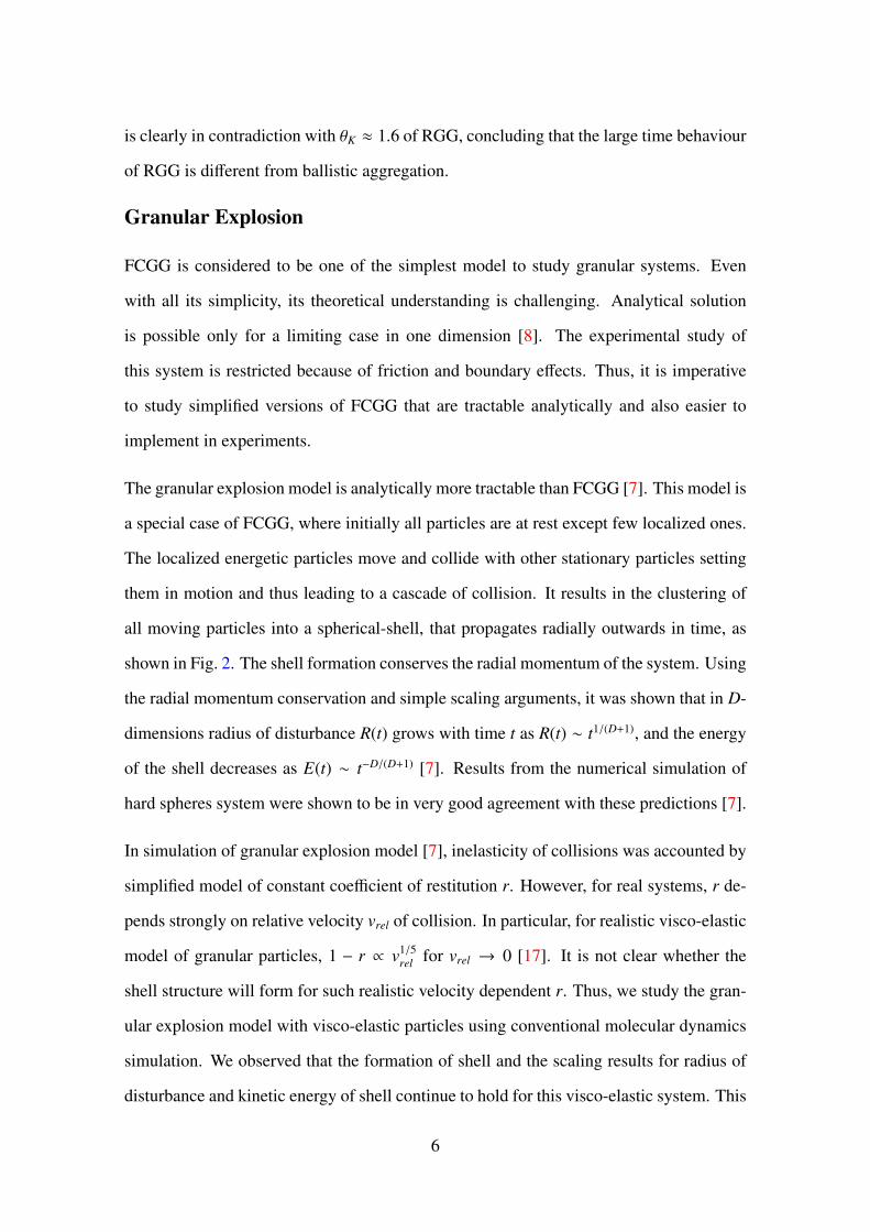
Granular Explosion

FCGG is considered to be one of the simplest model to study granular systems. Even

with all its simplicity, its theoretical understanding is challenging. Analytical solution

is possible only for a limiting case in one dimension [8]. The experimental study of

this system is restricted because of friction and boundary effects. Thus, it is imperative

to study simplified versions of FCGG that are tractable analytically and also easier to

implement in experiments.

The granular explosion model is analytically more tractable than FCGG [7]. This model is

a special case of FCGG, where initially all particles are at rest except few localized ones.

The localized energetic particles move and collide with other stationary particles setting

them in motion and thus leading to a cascade of collision. It results in the clustering of

all moving particles into a spherical-shell, that propagates radially outwards in time, as

shown in Fig. 2. The shell formation conserves the radial momentum of the system. Using

the radial momentum conservation and simple scaling arguments, it was shown that in D-

dimensions radius of disturbance R(t) grows with time t as R(t) ∼ t1/(D+1), and the energy

of the shell decreases as E(t) ∼ t−D/(D+1) [7]. Results from the numerical simulation of

hard spheres system were shown to be in very good agreement with these predictions [7].

In simulation of granular explosion model [7], inelasticity of collisions was accounted by

simplified model of constant coefficient of restitution r. However, for real systems, r de-

pends strongly on relative velocity vrel of collision. In particular, for realistic visco-elastic

model of granular particles, 1 − r ∝ v1/5rel

for vrel → 0 [17]. It is not clear whether the

shell structure will form for such realistic velocity dependent r. Thus, we study the gran-

ular explosion model with visco-elastic particles using conventional molecular dynamics

simulation. We observed that the formation of shell and the scaling results for radius of

disturbance and kinetic energy of shell continue to hold for this visco-elastic system. This

6

0

200

400

600

800

1000

0 200 400 600 800 1000

(a)

0

200

400

600

800

1000

0 200 400 600 800 1000

(b)

0

200

400

600

800

1000

0 200 400 600 800 1000

(c)

0

200

400

600

800

1000

0 200 400 600 800 1000

(d)

Figure 2: Moving (red) and stationary (green) particles for two dimensional granular ex-

plosion following an initial impulse at (500, 500). Panels (a)–(d) correspond to increasing

time. The moving particles cluster together to form a shell.

shows that the formation of shell by clustering is independent of details of the dissipation,

as long as some dissipation exists.

We apply the above results to a recent experiment on flowing granular material [6]. In

this experiment, a dilute monolayer of glass beads flowing down on an inclined plane

was perturbed by dropping a steel ball. The impact leads to clustering of particles into a

shell, leaving the region inside devoid of glass beads. This shell grows with time and its

radius was measured in the experiment using high speed cameras. A theoretical model

was proposed and analysed to derive an equation obeyed by the radius. The experimental

data was shown to be described very well by the numerical solution of the equation [6].

We note that the granular explosion model discussed above closely resembles the experi-

mental system when one transforms to the center of mass coordinates, and in the limit of

large impact energy, when the fluctuations of the particle velocities about the mean flow

may be ignored. We show that the earlier theory [6] for the experiment predicts that the

radius of disturbance grows logarithmically with time at large times. By a general argu-

7

ment for hard spheres, we show that the radius can not grow slower than t1/3, showing

that the theory cannot be right. We then show that the result for radius of disturbance pre-

dicted by the radial momentum conservation, R(t) ∼ t1/3 (in D = 2), fits very well to the

experimental data except at large times. At long times, the experimental data deviate from

the t1/3 behaviour, and grows with a different power law ∼ t0.18. This deviation could be

because of two approximations made when equating the granular explosion model with

the experiment.

First, we ignored the fluctuations of the velocities of the particles about the mean flow.

At earlier times, this approximation is reasonable, as the impact is intense and the typical

speeds of displaced particles are much faster than typical velocity fluctuations. How-

ever, the fluctuations become relevant at larger times. We modify the granular explosion

model to account for these velocity fluctuations. To incorporate these velocity fluctua-

tions, we modify the explosion model by assigning non-zero velocities to the particles

that were otherwise at rest in the explosion model. However, the typical velocities of

these particles is much smaller than the localised energetic particles. The simulation of

this modified model shows that when the velocity of the shell becomes of the order of

velocity fluctuations, the sharp shell starts becoming more diffuse and the enclosed empty

region disappears. This feature is very similar to as observed in the experiment. With the

destabilization of the shell, R(t) deviates from the t1/3 power law growth. However, this

deviation does not capture the long time behaviour of the radius, R(t) ∼ t0.18 as observed

in the experiment.

Second, we ignored the experimentally observed three dimensional nature of the shell

at later times. The shell presumably becomes three dimensional because a fast particle

when hemmed in by many surrounding particles may jump out of the plane due to a

collision with the floor and friction. This possibility results in radial momentum not

being conserved and hence a deviation from t1/3 behavior. To incorporate this effect, we

modified the granular explosion model in the following way. The two dimensional space

8

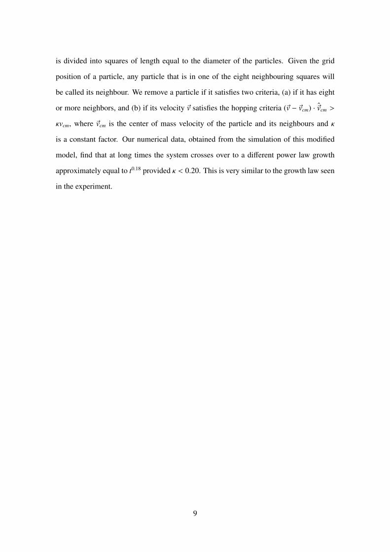
is divided into squares of length equal to the diameter of the particles. Given the grid

position of a particle, any particle that is in one of the eight neighbouring squares will

be called its neighbour. We remove a particle if it satisfies two criteria, (a) if it has eight

or more neighbors, and (b) if its velocity ~v satisfies the hopping criteria (~v − ~vcm) · ~vcm >

κvcm, where ~vcm is the center of mass velocity of the particle and its neighbours and κ

is a constant factor. Our numerical data, obtained from the simulation of this modified

model, find that at long times the system crosses over to a different power law growth

approximately equal to t0.18 provided κ < 0.20. This is very similar to the growth law seen

in the experiment.

9

List of Figures

1 The data for kinetic energy T (t) for different system sizes L collapse onto

a single curve when T (t) and t are scaled according to Eq. (1) with θT =

θm f

T= 6/5 and z = z

m f

BA= 5/2. The power law fits are shown by straight

lines. . . . . . . . . . . . . . . . . . . . . . . . . . . . . . . . . . . . . . 4

2 Moving (red) and stationary (green) particles for two dimensional gran-

ular explosion following an initial impulse at (500, 500). Panels (a)–(d)

correspond to increasing time. The moving particles cluster together to

form a shell. . . . . . . . . . . . . . . . . . . . . . . . . . . . . . . . . . 7

2.1 The temporal evolution of kinetic energy T (t) for two dimensional freely

cooling granular gas. The shown results are with n = 0.01 and r = 0.98.

The solid line is a power law t−2. . . . . . . . . . . . . . . . . . . . . . . 34

2.2 Sonine coefficient a2 vs the coefficient of normal restitution r in two (D =

2) and three (D = 3) dimensions. . . . . . . . . . . . . . . . . . . . . . . 41

2.3 Sonine coefficient a2 vs the coefficient of normal restitution r in D = 3.

The points show the result of DSMC simulation (data taken from [18])).

The line is a plot of theoretical result, Eq. (2.46). . . . . . . . . . . . . . . 41

2.4 Snapshots of freely cooling granular gas in two dimensions, starting from

uniform density and evolving to inhomogeneous regime. The coefficient

of restitution r = 0.10 . . . . . . . . . . . . . . . . . . . . . . . . . . . . 42

2.5 Translational kinetic energy T ′ as a function of scaled time τ for various

β (written in brackets). . . . . . . . . . . . . . . . . . . . . . . . . . . . 46

11

2.6 Rotational kinetic energy K′ as a function of scaled time τ for various β

(written in brackets). . . . . . . . . . . . . . . . . . . . . . . . . . . . . 47

2.7 Equipartition ratio Req = T ′/K′ as a function of scaled time τ for β =

0.5,−0.5 (written in brackets). . . . . . . . . . . . . . . . . . . . . . . . 47

2.8 Initial data curve (s-curve) and the parabola S. . . . . . . . . . . . . . . . 56

2.9 A parabola in double contact with the s-curve. . . . . . . . . . . . . . . . 57

2.10 A sequence of parabolas in double contact with the s-curve and the corre-

sponding velocity field. . . . . . . . . . . . . . . . . . . . . . . . . . . . 57

2.11 The temporal decay of kinetic energy T (t) for one dimensional FCGG, for

various r. Data for r = 0 (BA) case is also shown. Reprinted figure with

permission from E. Ben-Naim, S. Y. Chen, G. D. Doolen, and S. Redner,

Physical Review Letters, 83, 4069 (1999) [13]. Copyright (1999) by the

American Physical Society. . . . . . . . . . . . . . . . . . . . . . . . . . 61

2.12 Shock profile of one dimensional FCGG. Density and velocity in the in-

homogeneous regime are plotted. A line with slope t−1 is plotted for refer-

ence. Reprinted figure with permission from E. Ben-Naim, S. Y. Chen, G.

D. Doolen, and S. Redner, Physical Review Letters, 83, 4069 (1999) [13].

Copyright (1999) by the American Physical Society. . . . . . . . . . . . . 62

2.13 The ratio of the thermal energy Eth to the kinetic energy Ek as a function

of time. A line of slope −1/2 is plotted for reference. Reprinted figure

with permission from Xiaobo Nie, Eli Ben-Naim, and Shiyi Chen, Phys-

ical Review Letters, 89, 204301 (2002) [14]. Copyright (2002) by the

American Physical Society. . . . . . . . . . . . . . . . . . . . . . . . . . 64

4.1 The data for kinetic energy T (t) vs time t for different system sizes L. The

data are for φ = 0.208, r0 = 0.1, and δ = 10−4. . . . . . . . . . . . . . . . 81

12

4.2 The data for kinetic energy T (t) for different system sizes L collapse onto a

single curve when t and T (t) are scaled as in Eq. (4.2) with θT = θm f

T= 6/5

and z = zm f

BA= 5/2. The power law fits are shown by straight lines. The

data are for φ = 0.208, r0 = 0.1, and δ = 10−4. . . . . . . . . . . . . . . . 82

4.3 The dependence of kinetic energy T (t) on volume fraction φ. The solid

line is a power law t−6/5. The data is for r0 = 0.10, δ = 10−4. . . . . . . . . 83

4.4 The dependence of kinetic energy T (t) on coefficient of restitution r0. The

solid line is a power law t−6/5. The data is for φ = 0.208, δ = 10−4. . . . . 83

4.5 The dependence of kinetic energy T (t) on cutoff velocity δ. The solid line

is a power law t−6/5. The data is for φ = 0.208, r0 = 0.10. . . . . . . . . . 84

4.6 The variation of kinetic energy T (t) with time t for a velocity dependent

coefficient of restitution [see Eq. (4.1)] for different σ. The data are for

r0 = 0.1, δ = 10−4 and φ = 0.208. The straight line is a power law t−6/5. . . 84

4.7 Temporal evolution of kinetic energy T (t) for BA, with varying volume

fraction φ. The bold/dotted lines are power-laws with exponents 1.283/1.202. 85

4.8 Snapshots of FCGG (upper left) and BA (upper right) in the inhomoge-

neous regime. The lower panel shows the scaled mass distribution for the

FCGG (left) and BA (right). Mavg is the mean cluster size. The solid line

is a power law m−2.7. The data are for φ = 0.208, r0 = 0.10. . . . . . . . . 87

4.9 The largest mass Mmax as a function of time t. For the FCGG, r0 = 0.10,

δ = 10−4. Straight lines are power laws t0.94, t0.99, t1.03 (bottom to top). . . 88

4.10 The scaled velocity distribution function Φ(y) for the FCGG at times

t = 5, 10 (upper collapsed data) and t = 2000, 4000, 6000, 8000 (lower

collapsed data). The solid curve is a Gaussian. The data are for φ = 0.208,

r0 = 0.10. . . . . . . . . . . . . . . . . . . . . . . . . . . . . . . . . . . 90

4.11 The kurtosis κ as a function of time t. The data are for φ = 0.208, r0 = 0.10. 90

13

4.12 − lnΦ(y) as a function of y for the FCGG (lower data) and BA (upper

data). For FCGG, the times are t = 2000, 4000, 6000, 8000 and φ = 0.208,

r0 = 0.10. For BA, the times are t = 400, 800, 1600 and φ = 0.208. . . . . 91

5.1 Time evolution of translational kinetic energy T (t) for RGG when β > 0

for fixed r = 0.10. . . . . . . . . . . . . . . . . . . . . . . . . . . . . . . 98

5.2 Time evolution of translational kinetic energy T (t) for RGG when β < 0

for fixed r = 0.10. . . . . . . . . . . . . . . . . . . . . . . . . . . . . . . 99

5.3 Time evolution of rotational energy K(t) of RGG for β > 0 and fixed

r = 0.10. . . . . . . . . . . . . . . . . . . . . . . . . . . . . . . . . . . . 99

5.4 Time evolution of rotational energy K(t) of RGG for β < 0 and fixed

r = 0.10. . . . . . . . . . . . . . . . . . . . . . . . . . . . . . . . . . . . 100

5.5 Time evolution of rotational energy K(t) of RGG for different r and fixed

β = 0.60. . . . . . . . . . . . . . . . . . . . . . . . . . . . . . . . . . . . 101

5.6 Time evolution of the rotational energy K(t) of BA for different volume

fractions φ. . . . . . . . . . . . . . . . . . . . . . . . . . . . . . . . . . 102

6.1 Moving (red) and stationary (green) particles at times t = (a) 1000, (b)

2000, (c) 4000 and (d) 8000, following an isotropic impulse at (500, 500)

at t = 0. The moving particles are in a circular region. The data are for

elastic system, r = 1. . . . . . . . . . . . . . . . . . . . . . . . . . . . . 110

6.2 Radius of disturbance R(t) vs time t for elastic system in two dimensions.

The simulation data fits well with the power law t1/2. . . . . . . . . . . . 111

6.3 Moving (red) and stationary (green) particles at times t = (a) 103, (b) 104,

(c) 105 and (d) 106, following an isotropic impulse at (500, 500) at t = 0.

The moving particles cluster together at the disturbance front. The data

are for r = 0.10. . . . . . . . . . . . . . . . . . . . . . . . . . . . . . . . 112

14

6.4 The radial momentum as a function of time t. For elastic collisions, it

increases as√

t (the solid straight line is a power law√

t). For inelastic

collisions with r = 0.10, the radial momentum appears to increase very

slowly with time to a constant, when δ → 0. The data for the elastic

system have been scaled down by factor 1/2. . . . . . . . . . . . . . . . 114

6.5 Two curves from Fig. 6.4 are plotted to show clearly the slow increase of

the radial momentum. . . . . . . . . . . . . . . . . . . . . . . . . . . . . 114

6.6 Average scattering angle on collision vs time t. . . . . . . . . . . . . . . . 115

6.7 Radius of disturbance R(t) vs time t for inelastic system (r = 0.10) in two

dimensions. The simulation data fits well with the power law t1/3. . . . . . 115

6.8 (a) An image of the flow. The experiment was carried out in the shown

rectangular region where the flow is roughly homogeneous. (b) Images

of expanding hole at different times after the impact of a 16 mm diam-

eter steel sphere. Particles that were originally in a circular region have

clustered into a dense rim(white rim) surrounding the hole (black circu-

lar region).(c) Impact of a 2 mm diameter sphere. Reprinted figure with

permission from J. F. Boudet, J. Cassagne, and H. Kellay, Physical Re-

view Letters, 103, 224501 (2009) [6]. Copyright (2009) by the American

Physical Society. . . . . . . . . . . . . . . . . . . . . . . . . . . . . . . 117

6.9 Data for radius R(t) from simulations in two dimensions are compared

with BCK result [Eq. (6.9)] and t1/3. R0 and t0 in Eq. (6.9) are obtained by

fitting the initial time simulation data to Eq. (6.9) and are R0 = 10.30±0.21

and t0 = 35.79 ± 2.35. The data are for r = 0.10. . . . . . . . . . . . . . 121

6.10 Temporal variation of N(t), the number of collisions per particle per unit

distance for various r. For r < 1, N(t) is not constant as assumed by BCK. 122

6.11 Rate of collision N(t) as shown in Fig. 6.10 is multiplied by R, where R is

the radius of disturbance. NR is a constant at large times for r < 1. . . . . 123

15

6.12 Experimental data from Ref. [6] for radius R as a function of time t fol-

lowing an impact by steel balls of diameter 4 mm, 8 mm and 16 mm. The

solid/dashed lines have slope 1/3 and 0.18 respectively. Rs is the diameter

of a glass bead and ts is the mean time taken by a glass bead to traverse a

distance equal to its diameter. The data have been obtained from Ref. [6]. 124

6.13 Snapshots of inelastic I particles (red) and elastic E particles (green), when

Λ = 1/800, following an isotropic impulse at (500, 500) at t = 0. The time

increases from (a) to (d) and correspond to the times shown by labels a–

d in Fig. 6.14. Initially, the disturbance grows as in Fig. 6.3, but at late

times due to velocity fluctuations, the rim gets destabilized. The data are

for r = 0.10. . . . . . . . . . . . . . . . . . . . . . . . . . . . . . . . . . 125

6.14 The radius of disturbance R(t) as a function of time t for different values

of Λ. The effect of velocity fluctuations are felt later for smaller Λ. At

large times, the finite external pressure is able to compress the bubble,

with R(t) reaching a minimum when the density of the bubble approaches

the close packing density. A solid line of slope 1/3 is drawn for reference.

The data are for r = 0.10. . . . . . . . . . . . . . . . . . . . . . . . . . . 126

6.15 The R(t) vs t data of Fig. 6.14 when scaled according to Eq. (6.13). A

good collapse is obtained. . . . . . . . . . . . . . . . . . . . . . . . . . 127

6.16 Temporal variation of radius R(t) for κ = 0.20 with various initial velocity

v0. The solid line is a power law t0.18 while the dashed line is a power

law t1/3. The data with no hopping correspond to v0 = 1. All data are for

r = 0.10. . . . . . . . . . . . . . . . . . . . . . . . . . . . . . . . . . . . 127

7.1 Moving (red) and stationary (green) particles at times t = (a) 102, (b) 103,

(c) 104 and (d) 5 × 104, following an isotropic impulse at (0, 0) at t = 0.

The moving particles cluster together to form a shell. . . . . . . . . . . . 133

7.2 Temporal behaviour of radius of disturbance R(t) and number of active

particles N(t). . . . . . . . . . . . . . . . . . . . . . . . . . . . . . . . . 134

16

7.3 Temporal behaviour of kinetic energy E(t). . . . . . . . . . . . . . . . . . 135

17

List of Tables

2.1 Table showing the dependence of decay exponent θBAT on volume fraction

φ for two dimensional BA. Data are taken from [19]. . . . . . . . . . . . 53

4.1 Table showing the dependence of decay exponent θBAT on volume fraction φ. 85

5.1 Dependence of exponents θBAT and θBA

K on volume fraction φ in the BA

model. . . . . . . . . . . . . . . . . . . . . . . . . . . . . . . . . . . . . 101

18

Chapter 1

Introduction

In this chapter, we briefly introduce granular systems and in particular freely cooling

granular gas, that is the subject matter of this thesis. The organization of the chapters of

the thesis is also presented.

1.1 Nonequilibrium Systems

Equilibrium thermodynamics provided much of the conceptual underpinnings for the in-

dustrial revolution which had a great impact on the mankind progress during the 19th

century. Further conceptual progresses were made with the advent of equilibrium statis-

tical mechanics. However, many systems are inherently not in thermal equilibrium. This

class of out-of-equilibrium systems is very large and very diverse, and their study is there-

fore of great importance. The tools developed to study equilibrium phenomena have been

extended to the study of systems that are near to equilibrium.

Natural systems like granular and turbulent flows, living organisms, nanomaterials, and

biomolecules are very far from equilibrium. These systems can not be simply studied

with our current understanding of equilibrium and near-equilibrium phenomena. Intense

19

research in past two decades have enabled us with a substantial understanding of far from

equilibrium systems. Prototypical models encoding the general features of far from equi-

librium have been studied in detail. Examples include active matter, molecular motors and

ratchets, turbulence and wave turbulence, random heterogeneous media and granular sys-

tems, which is the subject of study of this thesis. Such models have enriched the theoret-

ical understanding of far from equilibrium phenomena with concepts such as fluctuation

theorems, non-equilibrium phase transitions, dynamic heterogeneity, fluctuation-induced

phenomena, and energy cascades, among others. But, as yet, a comprehensive theory of

non-equilibrium statistical mechanics is lacking. This is partly because of sheer diversity

of the phenomena involved.

1.2 Granular Systems

Granular systems are omnipresent in nature and are examples of systems far from equilib-

rium. In our daily lives we come across these systems in the form of food grains, mustard

seeds, coffee beans, steel balls, and sand. At larger length scale, we see them in the form

of rocks, boulders etc. These systems are present at the astrophysical level with examples

such as planetary rings and cosmic dust.

The study of granular physics has practical applications in chemical, pharmaceutical and

food industries. These industries deal with transportation and storage of granular ma-

terials. There are estimates that we waste 40% of the capacity of our industrial plants

because of problems related to transportation of these materials. Improved understanding

of granular materials could have significant impact on industry. In addition to practical

use, these systems find application in clarifying theoretical concepts of non-equilibrium

statistical mechanics.

There are two important aspects that contribute to the unique properties of granular ma-

terials. First, granular particles are macroscopic with sizes large enough that Brownian

20

motion is irrelevant. In other words, fluctuations induced by temperature are irrelevant.

At room temperature, the energy scale kBT of temperature is insignificant compared to the

typical kinetic and potential energies of a granular particle. As temperature is irrelevant,

system can not explore the whole phase space and exhibits multiple metastable steady

states which are far from equilibrium. Each metastable configuration will last indefinitely

unless perturbed by external disturbances.

Second is the dissipative nature of interaction between particles. Granular particles typ-

ically do not interact through long-range forces, but only when in mechanical contact.

Each collision results in a loss of kinetic energy. To explain where the dissipated energy

goes, the bulk of particle material is considered as a regular lattice composed of mass

points linked by elastic springs. Any collision of a particle leads to deformation of few

springs near the surface of particle. These deformed springs takes the dissipated energy

and distribute it to all springs. Thus, the energy lost in collision is converted into the inter-

nal energy stored in the springs [10]. These aspects make granular systems behave quite

differently from conventional solids, liquids and gases [1], and have tempted researchers

to consider it as an additional state of matter in it own right.

Traditionally for more than two centuries, scientific studies of granular systems have been

the domain of applied engineering research with contributions from notable names such

as Coulomb [20], Faraday [21], and Reynolds [22]. For the past two decades, a vast

amount of experimental, numerical and theoretical research is devoted within physics to

understand the complex static and dynamic behaviour of granular systems [1, 2, 3, 4,

23, 24, 25, 26]. Notable works include, slow relaxation in vibrated sand piles [27, 28,

29, 30], fluid like behaviour similar to those of conventional liquids [31, 32, 33, 34, 35],

heterogeneous force chains in granular pile [36, 37, 38], kinetic theory models for granular

flows [11, 39, 40, 41], vibration induced convection and heaping [21, 42, 43, 44, 45],

vibration induced size separation [46, 47, 48, 49], clustering in granular gases [12, 50, 51,

52].

21

1.3 Granular Gas

A dilute assembly of granular particles is referred as granular gas. This is a simple model

to study the effects of inelastic collisions. In this model, particles move ballistically until

they undergo momentum conserving inelastic collisions. Although most of the granular

gases in laboratories are man made, there are naturally occurring granular gases such as

interstellar dust and planetary rings in outer space.

In the absence of energy input from external sources, these particles dissipate kinetic

energy and come to rest. External driving is required to keep the system active. If the

loss of energy due to collisions is balanced by external driving, then the system reaches

different types of non-equilibrium steady states depending on the details of the problem. A

vast amount of research is devoted to the study of such externally driven granular gases [1,

2, 3]. Various driving mechanisms such as gravity [53, 54], vertical [55, 56] and horizontal

vibration [57, 58], rotating drums [59, 60], flows of interstitial fluids such as water and

air [61, 62], electric and magnetic fields [63, 64] have been implemented [3].

In the absence of external driving, the system evolves deterministically in time, and at

large times loses all its energy to come to rest. However, the approach to the steady state

can be quite non-trivial. This freely evolving granular gas may be further divided into two

sub-classes based on the initial energies of the particles:

• Freely cooling granular gas (FCGG): In the first, the particles are homogeneously

distributed in space and each particle has an energy drawn from some fixed distribu-

tion. We refer to this problem as the freely cooling granular gas (FCGG). FCGG is

a well studied model of granular physics. In addition to being a model that isolates

the effects of dissipation, it has applications in varied physical phenomena including

modelling of dynamics of granular systems [1, 3, 10, 65, 66], geophysical flows [4],

large-scale structure formation in the universe [5], and shock propagation [6, 7, 67].

It also belongs to the general class of non-equilibrium systems with limiting cases

22

being amenable to exact analysis [8, 68], and is an example of an ordering system

showing non-trivial coarsening behaviour [9, 69, 70, 71]. The dynamics of this

system has close connection with the shock dynamics of the well studied Burgers

equation [8, 72, 73, 74, 75].

• Granular explosion: In the second, the particles are homogeneously distributed as

in FCGG. However, almost all particles are at rest, and a few particles in a local-

ized volume possess non-zero initial kinetic energy. We refer to this model as the

granular explosion model. Granular explosion model is a special case of FCGG and

its study is motivated from the fact that it has certain advantages over FCGG. The

experimental study of FCGG is restricted because of friction and boundary effects.

These restrictions can be eliminated in experiments of granular explosion [6]. Also,

it is analytically more tractable than FCGG [7].

In this thesis, we study these two problems of freely evolving granular gas using large

scale molecular dynamics simulations and scaling analysis. Our particular focus is on the

large time behaviour of these systems.

1.4 Organization of the Chapters

The rest of the thesis is organized as follows.

In Chapter 2, we review earlier results on FCGG in detail.

In Chapter 3, the simulation methods used in this thesis are discussed. We have used two

fundamentally different approaches to molecular dynamics simulations. One is conven-

tional force based molecular dynamics for soft-particles, where the Newton’s equations of

motion for all particles are numerically integrated. In this method, the knowledge of the

interaction force is essential. The other is event-driven molecular dynamics for hard-core

particles which move freely and interact only on collision. At any stage of evolution, the

23

next collision occurring in the system is determined, and the position and velocity of two

particles involved in the binary collision is updated. This simulation method proceeds

through the event of one collision to the next collision, and is much efficient as compared

to conventional force based molecular dynamics.

The remaining chapters contain the original work of the thesis.

In Chapter 4, we study FCGG in three dimensions. The kinetic energy of FCGG de-

creases as a power law t−θT at large times t. Two theoretical conjectures exist for the

exponent θT . One based on mean-field analysis of ballistic aggregation of compact spher-

ical aggregates predicts θm f

T= 2D/(D + 2) in D dimensions. The other based on Burgers

equation describing anisotropic, extended clusters predicts θBET = D/2 when 2 ≤ D ≤ 4.

We do extensive simulations in three dimensions to find that while θT is as predicted by

ballistic aggregation, the cluster statistics and velocity distribution differ from it. Thus,

the FCGG fits to neither the ballistic aggregation or a Burgers equation description.

In Chapter 5, we study large time behaviour of the FCGG of rough particles in two

dimensions using large-scale event driven simulations and scaling arguments. During

collisions, rough particles dissipate energy in both the normal and tangential directions

of collision. At large times, when the system is spatially inhomogeneous, translational

kinetic energy and the rotational energy decay with time t as power-laws t−θT and t−θK .

We numerically determine θT ≈ 1 and θK ≈ 1.6, independent of the coefficients of resti-

tution. The inhomogeneous regime of the granular gas has been argued to be describable

by the ballistic aggregation model, where particles coalesce on contact. Using scaling

arguments, we predict θT = 1 and θK = 1 for ballistic aggregation. Simulations of bal-

listic aggregation with rotational degrees of freedom are consistent with these exponents.

While θT for rough granular gas matches with the corresponding exponent of ballistic ag-

gregation, the exponent θK is different. It concludes that the large time behaviour of rough

granular gas is different from ballistic aggregation.

In Chapter 6, we apply the results of granular explosion to a recent experiment [6] on

24

flowing granular material. The granular explosion model was studied in [7]. The distur-

bance created by the initially localized energetic particles leads to formation of spherical-

shell of moving particles, whose radius grows with time as R(t) ∼ t1/(D+1). In the ex-

periment [6], a dilute monolayer of glass beads flowing down on an inclined plane was

perturbed by dropping a steel ball. The impact leads to clustering of particles into a shell,

leaving the region inside devoid of glass beads. Noting the resemblance between the ex-

periment and granular explosion, we show that growth of radius predicted in granular

explosion R(t) ∼ t1/3 for D = 2 fits very well to the experimental data except at large

times. At long times, the experimental data exhibit a crossover to a different power law

behaviour, growing as ∼ t0.18. We attribute this crossover to the problem becoming effec-

tively three dimensional due to accumulation of particles at the shell front. We modify

the granular explosion model to incorporate this effect. The simulations of this modified

model captures the crossover seen in the experiment.

In Chapter 7, we study the granular explosion model with visco-elastic particles using

conventional molecular dynamics simulation. In simulations of granular explosion stud-

ied in [7], a simplified constant coefficient of restitution r is used to describe collisions.

However, for realistic visco-elastic model of granular particles, r is not a constant but

depends strongly on relative velocity of collision. We observed that the formation of

shell and the scaling result for radius of disturbance continue to hold for the visco-elastic

system.

Finally, in Chapter 8, we present the principal conclusions that emerge from the work in

this thesis, as well as some potential extensions.

25

Chapter 2

Freely Cooling Granular Gas: A Review

2.1 Introduction

In this chapter we review earlier results for the freely cooling granular gas. In Sec. 2.2,

we define the model precisely. During the initial stage of evolution, the system remains

homogeneous. This homogeneity allows the development of a Boltzmann type equation

for the granular gas, similar to molecular gases. The Boltzmann equation derivation and

its solution to obtain the velocity distribution function and dependence of energy on time

is reviewed in Sec. 2.3. Due to dissipation, the homogeneous regime is unstable and the

system evolves to inhomogeneous regime marked by presence of clusters. This regime

is mostly studied in simulations, which we have summarized in Sec. 2.4. In Sec. 2.5, we

review a detail study of the homogeneous cooling regime of freely cooling granular gas of

rough particles, where dissipation due to frictional interaction is taken into account. The

experimental studies of freely cooling granular gas are reviewed in Sec. 2.6. In Sec. 2.7,

we review the ballistic aggregation model (BA). This model is analytically tractable and

is argued to be a description for granular gas in the inhomogeneous regime. The inho-

mogeneous regime is also argued to be describable by Burgers like equation which we

discuss in Sec. 2.8.

27

2.2 Model

We consider a simple model for a granular particle, a sphere. Consider a collection of N

identical particles of mass m and diameter d, distributed homogeneously in D dimensional

space with linear length L. The velocities of the particles are initially chosen from a

fixed distribution, usually Gaussian or uniform. The system evolves freely, i.e., there

is no external driving. The particles move ballistically until they undergo momentum

conserving, inelastic collision with other particles. Since collisions are dissipative, the

kinetic energy of the system decreases. This freely evolving system is known as the freely

cooling granular gas (FCGG). In this thesis, we have considered FCGG of three kinds of

constituent particles as described below:

2.2.1 Rough Granular Gas (RGG)

The constituents of RGG are particles that dissipate energy in both normal and tangential

direction of collision. Consider the collision between two particles i and j. The quantities

~ri, ~vi, ~ωi denote the position of the centre, velocity and angular velocity of particle i. The

relative velocity of the point of contact, ~g is

~g = (~vi − ~ωi ×d

2~e) − (~v j + ~ω j ×

d

2~e), (2.1)

where ~e is unit vector in normal direction of collision, pointing from the centre of particle

j to the centre of particle i,

~e =~ri − ~r j

|~ri − ~r j|. (2.2)

We denote the normal and tangential components of ~g by ~g n and ~g t respectively. The

dissipation in normal and tangential directions are quantified by a coefficient of normal

restitution r and a coefficient of tangential restitution β, defined through the constitutive

28

equations [76]:

(~g n)′ = −r~g n (0 ≤ r ≤ 1), (2.3)

(~g t)′ = −β~g t (−1 ≤ β ≤ 1), (2.4)

where the primed quantities are the values post-collision. The post-collision velocities

may be obtained from linear and angular momentum conservation, combined with the

constitutive equations for dissipation, Eqs. (2.3) and (2.4):

~v ′i = ~vi −1 + r

2~g n − q(1 + β)

2q + 2~g t,

~v ′j = ~v j +1 + r

2~g n +

q(1 + β)

2q + 2~g t,

~ω′i = ~ωi +1 + β

d(q + 1)[~e × ~g t],

~ω′j = ~ω j +1 + β

d(q + 1)[~e × ~g t],

(2.5)

where q is the reduced moment of inertia, q = I/(md2/4) with I being the moment of

inertia. For homogeneous disk q = 1/2, and for homogeneous sphere q = 2/5. This set

of equations [Eq. (2.5)], is commonly known as collision law. For simplicity, most of the

studies do not consider the velocity dependence of r and β, and treat them as constants.

2.2.2 Smooth Granular Gas (SGG)

The constituents of SGG are particles that dissipate energy only in the normal direction of

collision while tangential component of relative velocity remains unchanged. For smooth

particles β = −1, and the above collision law [Eq. (2.5)] reduces to

~v ′i = ~vi −1 + r

2[(~vi − ~v j) · ~e ]~e ,

~v ′j = ~v j +1 + r

2[(~vi − ~v j) · ~e ]~e .

(2.6)

29

We have omitted the angular velocity terms as they do not change on collision. This is

one of the most widely studied model in the context of freely cooling granular gases.

2.2.3 Visco-Elastic Granular Gas

The interaction between granular particles need not be hard-core (as discussed above)

and is more generally modelled by soft-repulsive potential [50, 76]. Here, we discuss

viscoelastic interaction model [77]. This particular model quite successfully explained the

results of an experiment with ice balls [78], which are of importance for the investigation

of the dynamics of planetary rings [79].

The interaction force for elastic spheres was derived by Heinrich Hertz [80],

Fel =2Y

√

deff/2

3(1 − ν2)ξ3/2 ≡ ρξ3/2, (2.7)

where ξ is the compression between colliding spheres. Y and ν are Young modulus and

Poisson ratio of the particle material respectively, and ρ is introduced as a short-hand

notation for the elastic constant of material. The effective diameter of identical colliding

spheres deff = d/2. This interaction law was later extended to the collision of viscoelastic

particles [77],

F = ρξ3/2 +3

2Aρ

√

ξξ, (2.8)

where ξ is the compression velocity and the dissipative parameter A is

A =1

3

(3η2 − η1)2

(3η2 + 2η1)

(1 − ν2)(1 − 2ν)

Yν2. (2.9)

The viscous constants η1, η2 relate the dissipative stress tensor to the deformation rate

tensor. Equation (2.8) is derived with a quasistatic approximation which is valid when

the characteristic relative velocity of collision is much less than the speed of sound in

the material. This criteria is satisfied for many experimental situations. We mention

30

that Eq. (2.8) holds if viscoelasticity is the only dissipative process during the particle

collision.

The solution of collision process described by

d2ξ

dt2=

F

meff, (2.10)

where meff is effective mass and t is time, with initial conditions (assuming that the contact

of colliding particles starts at time t = 0)

ξ(t = 0) = 0 and ξ(t = 0) = gn, (2.11)

gives the coefficient of normal restitution,

r = ξ(tcont)/ξ(0), (2.12)

where tcont is the contact duration of colliding particles. These calculations were per-

formed in [81], to obtain r as a series in powers of (gn)1/5,

r = 1 −C1

(

3

2A

)

(

ρ

meff

)2/5

(gn)1/5 +C2

(

3

2A

)2 (

ρ

meff

)4/5

(gn)2/5 ± . . . , (2.13)

where coefficients C1 = 1.15344 and C2 = 0.79826 were obtained analytically and also

confirmed by simulations. A general framework has been provided in [81] to evaluate all

coefficients of the expansion, but the calculations are quite extensive. A solution similar

to Eq. (2.13) has been obtained using dimensional analysis method [17].

System being dissipative, the energy of the system decreases with time. The main quan-

tities of interest are translational kinetic energy T (t) and rotational kinetic energy K(t)

defined as

T (t) =2

D

1

N

S (t)∑

i=1

1

2mi~v

2i

, (2.14)

31

K(t) =2

2D − 3

1

N

S (t)∑

i=1

1

2Ii~ω

2i

, (2.15)

where mi and Ii are mass and moment of inertia of particle i. Throughout the thesis, we

consider FCGG of identical particles for which mi = m and Ii = I. S (t) is the total number

of particles in the system at time t, which for FCGG is S (t) = N at all times. In this thesis,

we have also studied ballistic aggregation model (see Sec. 2.7), where particles merge

completely on collision to form bigger aggregates. For this system, mi and Ii are changing

with time and total number of particles S (t) decreases with time.

Our discussion of RGG is limited to Sec. 2.5 and Chapter 5. The discussion of visco-

elastic granular gas is limited to Chapter 7. Unless otherwise mentioned, everywhere

else in the thesis, FCGG refers to hard-sphere SGG with collisions described by constant

coefficient of restitution r. For this system, K(t) does not change with time.

2.3 Kinetic Theory

The initial stage of evolution, where the spatial homogeneity of system is preserved is

called homogeneous cooling regime (HCR). In this regime, FCGG resembles an ordinary

molecular gas of elastic particles, except that T (t) decreases due to inelastic collisions.

This regime can be described by Boltzmann equation formalism. The velocity distribu-

tion function is given by an expansion around the Maxwell distribution, accounting the

deviations from Maxwell distribution by Sonine coefficients.

2.3.1 Haff’s Cooling Law

Before we discuss the Boltzmann equation formalism, we show that the temporal decay

behaviour of T (t) in HCR can be obtained by simple physical arguments. To this end, we

32

write a rate equation for T (t) as,

dT

dt= collision rate × average energy lost in one collision. (2.16)

Now, the typical relative energy lost in one collision is

1

2meff(v′ 212 − v 2

12) = −1

2meffv 2

12(1 − r2) ∝ −(1 − r2)T, (2.17)

where v12, v ′12 are the relative velocity before and after the collision and meff is the effective

mass of colliding particles. In writing Eq. (2.17), we have used the fact that the kinetic

energy of relative motion meffv 212/2 is on average of the same order as T .

To estimate the average number of collision in unit time, consider a particle moving with

average relative velocity v12, while all other particles are fixed scatterers. The volume

swept by this particle in unit time ∝ dD−1v12, giving

collision rate ∝ dD−1v12n ∝ ndD−1√

T , (2.18)

where n = N/LD is the number density. Using Eqs. (2.17) and (2.18), Eq. (2.16) becomes

dT

dt∝ −ndD−1(1 − r2)T 3/2. (2.19)

The solution of Eq. (2.19) for the case r = constant (independent of relative velocity)

yields

T (t) =T (0)

(1 + t/t0)2where t−1

0 ∝ ndD−1(1 − r2)√

T (0). (2.20)

This decay behavior given by Eq. (2.20) is known as Haff’s law. For times t ≫ t0,

T (t) ∼ t−2. This t−2 decay behaviour has been verified in numerical simulations [11, 82]

and experiments [83, 84, 85]. We reproduce this decay behaviour with simulations of two

dimensional FCGG and is shown in Fig. 2.1.

33

10-7

10-5

10-3

10-1

101

100 101 102 103 104 105 106

T(t

)/T

(0)

t

Haff’s Law

Figure 2.1: The temporal evolution of kinetic energy T (t) for two dimensional freely

cooling granular gas. The shown results are with n = 0.01 and r = 0.98. The solid line is

a power law t−2.

2.3.2 Boltzmann Equation

Boltzmann equation is the fundamental theoretical tool of the kinetic theory of gases.

This equation governs the time evolution of the velocity distribution function, where it

relates the velocity distribution function of the gas particles to the macroscopic proper-

ties of particle collisions. The velocity distribution function f (~r,~v, t) is defined such that

f (~r,~v, t) d~r d~v gives the number of particles in the infinitesimal phase-space volume d~r d~v

located at (~r,~v) at time t. Integrating this function over the full phase-space gives the total

number of particles N,∫

f (~r,~v, t) d~r d~v = N. (2.21)

For spatially homogeneous gas the distribution function is independent of ~r and has fol-

lowing properties

∫

f (~v, t) d~v = n, (2.22)

∫

~v f (~v, t) d~v = n 〈~v 〉 = 0, (2.23)

∫

1

2mv2 f (~v, t) d~v = n

⟨

1

2mv2

⟩

=D

2nT (t). (2.24)

34

The above equations relate the moments of f with the macroscopic properties of gas,

namely number density n, flow velocity (it is zero as we have assumed isotropic gas with

no macroscopic flow) and kinetic energy T (t).

We now outline the derivation of Boltzmann equation for inelastic gases. The number

of particles f (~v1, t) d~r1 d~v1 in a phase-space volume d~r1 d~v1 located at (~r1,~v1) changes

over time due to particle collisions. Particles belonging to this velocity interval, after

collision will in general move with velocities beyond this interval. Such collisions reduce

the number of particles in the considered volume and are called direct collisions. On the

contrary, inverse collisions are collisions in which particles not belonging to this velocity

interval (before collision) enter into this interval, increasing the number of particles in the

considered phase-space volume.

Consider a direct collision between particles of velocities ~v1 and ~v2. The post-collision

velocities are given by

~v ′1 = ~v1 −1 + r

2[(~v1 − ~v2) · ~e ]~e ,

~v ′2 = ~v2 +1 + r

2[(~v1 − ~v2) · ~e ]~e .

(2.25)

To estimate the number of direct collisions ν− occurring in time ∆t, we consider the scat-

tering of particles with velocities ~v1 at particles with velocities ~v2 that yields

ν−(~v1,~v2, ~e,∆t) = f (~v1, t) d~v1 d~r1 f (~v2, t) d~v2 dD−1|~v12 · ~e |∆t d~e. (2.26)

Now, we consider an inverse collision between particles of velocities ~v ′′1 and ~v ′′2 , where

the collision leads to post-collision velocities of particles as ~v1 and ~v2,

~v1 = ~v′′1 −

1 + r

2[(~v ′′1 − ~v ′′2 ) · ~e ]~e ,

~v2 = ~v′′2 +

1 + r

2[(~v ′′1 − ~v ′′2 ) · ~e ]~e .

(2.27)

35

Using (~v1 − ~v2) · ~e = −r(~v ′′1 − ~v ′′2 ) · ~e, Eqs. (2.27) can be written as

~v ′′1 = ~v1 −1 + r

2r[(~v1 − ~v2) · ~e ]~e ,

~v ′′2 = ~v2 +1 + r

2r[(~v1 − ~v2) · ~e ]~e .

(2.28)

Considering Eqs. (2.28) as a transformation, (~v ′′1 ,~v′′2 ) → (~v1,~v2), the Jacobian J of the

transformation for r = constant, reads J = 1/r. Similar to the number of direct collisions,

the number of inverse collisions in time ∆t is given by

ν+(~v ′′1 ,~v′′2 , ~e,∆t) = f (~v ′′1 , t) d~v ′′1 d~r1 f (~v ′′2 , t) d~v ′′2 dD−1|~v ′′12 · ~e |∆t d~e. (2.29)

Using d~v ′′1 d~v ′′2 = Jd~v1d~v2 in Eq. (2.29) gives

ν+(~v ′′1 ,~v′′2 , ~e,∆t) =

1

r2f (~v ′′1 , t) f (~v ′′2 , t)d

D−1|~v12 · ~e | d~v1 d~v2d~r1∆t d~e. (2.30)

With the knowledge of number of direct and inverse collisions for particular values of

~v1,~v2 and ~e, the total number of collisions which change the number of particles in the

considered phase space volume d~r1 d~v1 can be obtained by integrating over~v2 and~e. Thus,

the increase in the number of particles in the volume d~r1 d~v1 during the time interval ∆t is

given by

∆ [ f (~v1, t)] d~v1d~r1 =

∫

d~v2d~eΘ(−~v ′′12·~e)ν+(~v ′′1 ,~v′′2 , ~e,∆t)−

∫

d~v2d~eΘ(−~v12·~e)ν−(~v1,~v2, ~e,∆t),

(2.31)

where Θ(x) is the Heaviside step-function

Θ(x) =

1 for x ≥ 0,

0 for x < 0.(2.32)

Only such pairs for which ~v12 · ~e < 0 for direct collision and ~v ′′12 · ~e < 0 for inverse

collision lead to an impact. The Θ-function in Eq. (2.31) ensures this condition of col-

36

lision. To make the two step functions identical, we change the variable ~e → −~e in

the first integral of Eq. (2.31). This change of variable does not alter the transformation

(~v ′′1 ,~v′′2 )→ (~v1,~v2), while the Θ-function becomes

Θ(~v ′′12 · ~e) = Θ(−1

r~v12 · ~e) = Θ(−~v12 · ~e), (2.33)

where the property Θ(kx) = Θ(x) for any k > 0 is used. Now, we divide both sides of

Eq. (2.31) by d~v1 d~r1∆t and taking the limit ∆t → 0, we get the Boltzmann equation

∂

∂tf (~v1, t) = dD−1

∫

d~v2

∫

d~eΘ(−~v12·~e) |~v12·~e |[

1

r 2f (~v ′′1 , t) f (~v ′′2 , t) − f (~v1, t) f (~v2, t)

]

≡ I( f , f ),

(2.34)

where I( f , f ) is known as collision integral.

In this derivation of Boltzmann equation, we assumed an approximation known as hy-

pothesis of molecular chaos. While deriving the rates of direct and inverse collisions, we

counted independently the number of scatterers and scattered particles by taking the prod-

uct of two distributions functions, f (~v1, t) and f (~v2, t) for direct, and f (~v ′′1 , t) and f (~v ′′2 , t)

for inverse collisions. This holds true only when there are no correlations between parti-

cles, otherwise the two-particle distribution function f2(~v1,~v2,~r12, t) for the colliding pairs

should be considered. Correlations can be neglected for dilute systems. This approxima-

tion of using the product of two one-particle distribution functions is called the hypothesis

of molecular chaos.

Correlations occur in granular gas because of finite-volume effects, when possible col-

liders are screened by other particles. To obtain the rates of collisions, the two-particle

distribution function f2(~v1,~v2,~r12, t) at the contact distance between the particles r12 = d

must be known. Enskog suggested an approximation for accounting finite-volume effects:

f2(~v1,~v2, d, t) ≈ g2(d) f (~v1, t) f (~v2, t), (2.35)

37

where g2(d) is the contact value of the equilibrium pair correlation function g2(r12), which

is also known as Enskog factor. This function describes the probability that the distance

|~r1−~r2| between two particles is equal to r12. For a hard-sphere elastic fluid g2(d) reads [86]

g2(d) =

1−7φ/16

(1−φ)2 for D = 2,

2−φ2(1−φ)3 for D = 3,

(2.36)

where φ is the volume fraction. It is shown in simulations that Eq. (2.36) is also very accu-

rate for inelastic hard-spheres [87]. Physically, the factor g2(d) accounts for the increased

collision frequency in dense systems caused by excluded volume effects.

Thus, with this modification [Eq. (2.35)], the Boltzmann equation [Eq. 2.34] becomes

Boltzmann-Enskog equation

∂

∂tf (~v1, t) = g2(d)I( f , f ). (2.37)

2.3.3 Velocity Distribution and Kinetic Energy

For molecular gases in equilibrium, the velocity distribution is Maxwellian and indepen-

dent of time t. In granular gases, the energy of the system decreases due to dissipative col-

lisions leading to a time dependent velocity distribution. For near-elastic system (r . 1),

the kinetic energy decreases slowly and the system may be considered to be in an equi-

librium state at each time instant. With this adiabatic cooling assumption, it has been

shown that Eq. (2.37) admits an isotropic scaling solution, where the time dependence

of the velocity distribution function is argued to occur through a time dependent average

velocity [82, 88],

f (~v, t) =n

vDT

(t)f

(

v

vT (t)

)

=n

vDT

(t)f (c), (2.38)

38

with the scaled velocity c = v/vT (t). The thermal velocity vT (t) is defined by

T (t) =1

2mv2

T (t), (2.39)

where T (t) is given by second moment of f (~v, t) as defined in Eq. (2.24).

Substituting the scaled velocity ansatz [Eq. (2.38)] in the Boltzmann-Enskog equation

[Eq. (2.37)], and after doing some straightforward algebra [10], one obtains a time-

independent equation for the scaled velocity distribution

µ2

D

(

D + c1

∂

∂c1

)

f (c1) = I( f , f ), (2.40)

and a time-dependent equation for the evolution of kinetic energy

dT

dt= −2µ2

D

√

2

mg2(d)dD−1nT 3/2, (2.41)

where I( f , f ) is the dimensionless collision integral,

I( f , f ) =

∫

d~c2

∫

d~eΘ(−~c12 · ~e) |~c12 · ~e |[

1

r2f (c′′1 ) f (c′′2 ) − f (c1) f (c2)

]

. (2.42)

It is related to I( f , f ) as I( f , f ) = n2dD−1v1−DT I( f , f ). µp is the moment of dimensionless

collision integral given by

µp ≡ −∫

d~c1cp

1I( f , f ). (2.43)

These moments µp do not depend on time as I( f , f ) is time-independent.

Thus, the Boltzmann equation reduces to a set of two uncoupled equations, one describing

the scaled velocity distribution and the other the kinetic energy. The solution of Eq. (2.40)

is a complicated mathematical problem and analytical progress can be made only by mak-

ing approximations. The adiabatic cooling assumption suggests that the velocity distri-

bution is close to Maxwell distribution. Thus, we expand f (c) around the Maxwell dis-

39

tribution φ(c) [88, 89], in terms of Sonine polynomials S p(x) [see [10] for details about

Sonine polynomials],

f (c) = φ(c)

1 +

∞∑

p=1

apS p(c2)

, (2.44)

where

φ(c) ≡ π−D/2 exp(−c2). (2.45)

The Sonine polynomials expansion is applied to solve the Boltzmann equation [10], i.e., to

obtain the Sonine coefficients ap characterizing the velocity distribution. It can be shown

from the definitions of kinetic energy and thermal velocity that the first Sonine coefficient

a1 = 0. Neglecting higher Sonine coefficients (ap = 0 for p > 2) and characterizing the

velocity distribution by the next Sonine coefficient a2 only, the second coefficient a2 is

obtained to be

a2 =16 (1 − r) (1 − 2r2)

9 + 24D + 8rD − 41r + 30(1 − r) r2. (2.46)

This second Sonine coefficient a2 as a function of r for D = 2 and D = 3 is plotted

in Fig. 2.2. The small value of a2 has been used to justify the solution of Boltzmann

equation by an expansion around the Maxwell distribution. The small value of a2 also

justifies the exclusion of higher Sonine coefficients ap for p > 2. This result for a2

has been quantitatively confirmed by the Direct Simulation Monte Carlo (DSMC) of the

Boltzmann equation [18] as shown in Fig. 2.3 for D = 3.

The temporal behaviour of kinetic energy can be easily obtained by integrating Eq. (2.41)

yielding

T (t) =T (0)

(1 +Ct)2, with C =

µ2

D

√

2

mg2(d)dD−1n

√

T (0). (2.47)

This is same as what we obtained using simple physical arguments in Eq. (2.20).

40

-0.1

0

0.1

0.2

0.3

0.4

0 0.2 0.4 0.6 0.8 1

a 2

r

D = 2

D = 3

Figure 2.2: Sonine coefficient a2 vs the coefficient of normal restitution r in two (D = 2)

and three (D = 3) dimensions.

-0.016

-0.012

-0.008

-0.004

0

0.004

0.7 0.75 0.8 0.85 0.9 0.95 1

a 2

r

DSMCTheory

Figure 2.3: Sonine coefficient a2 vs the coefficient of normal restitution r in D = 3. The

points show the result of DSMC simulation (data taken from [18])). The line is a plot of

theoretical result, Eq. (2.46).

41

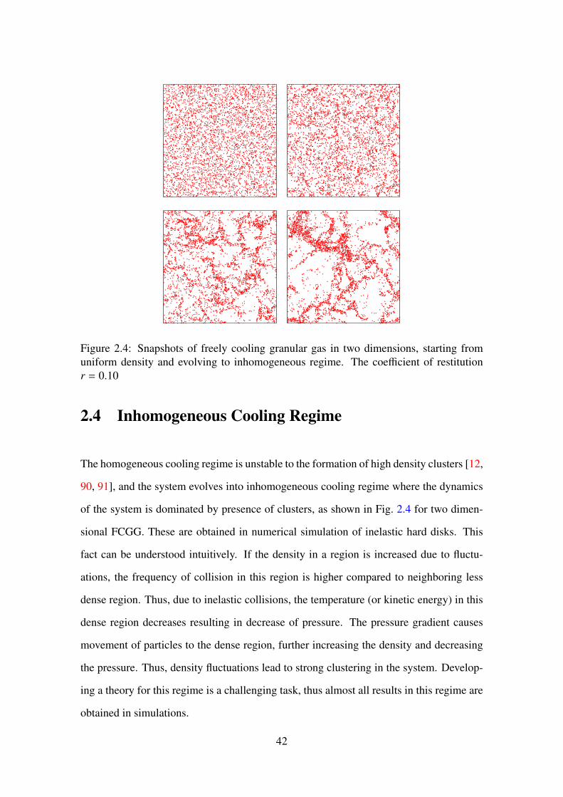
Figure 2.4: Snapshots of freely cooling granular gas in two dimensions, starting from

uniform density and evolving to inhomogeneous regime. The coefficient of restitution

r = 0.10

2.4 Inhomogeneous Cooling Regime

The homogeneous cooling regime is unstable to the formation of high density clusters [12,

90, 91], and the system evolves into inhomogeneous cooling regime where the dynamics

of the system is dominated by presence of clusters, as shown in Fig. 2.4 for two dimen-

sional FCGG. These are obtained in numerical simulation of inelastic hard disks. This

fact can be understood intuitively. If the density in a region is increased due to fluctu-

ations, the frequency of collision in this region is higher compared to neighboring less

dense region. Thus, due to inelastic collisions, the temperature (or kinetic energy) in this

dense region decreases resulting in decrease of pressure. The pressure gradient causes

movement of particles to the dense region, further increasing the density and decreasing

the pressure. Thus, density fluctuations lead to strong clustering in the system. Develop-

ing a theory for this regime is a challenging task, thus almost all results in this regime are

obtained in simulations.

42

Brito et al. [92] extended kinetic theory into the inhomogeneous cooling regime using

mode coupling methods, and found that in the inhomogeneous regime T (τ) ∼ τ−D/2,

where τ is the average number of collisions per particle and not the real time t. The

relation between τ and t is unclear [92]. This result agrees with simulations for near-

elastic (r ≈ 1) gases, but fails for large times and strongly inelastic (r ≪ 1) gases [92].

Ben-Naim et al. [13] studied FCGG in one dimension, where dissipation is modeled by

constant coefficient of restitution r. In the inhomogeneous regime, the kinetic energy T (t)

decays with time t as a power law T (t) ∼ t−θT , with θT = 2/3. The value of θT = 2/3 is

universal, independent of dissipation r.

Nie et al. simulated FCGG of hard disks in two dimensions [14]. They found that in the

inhomogeneous regime, energy decays as a power-law T (t) ∼ t−θT with θT = 1. Similar to

the one dimensional case, the decay exponent θT is independent of r, although its value is

different from the one dimensional case.

Chen et al. [93] simulated deformable spheres in two and three dimensions. In two dimen-

sions, θT was found to be 1, while for three dimensions it ranges from θT = 1.35 − 1.6,

depending on the parameters such as the volume fraction and coefficient of restitution.

Tube-like clusters were observed in three dimensions [93], which can be compared with

the string-like clusters in two dimensions [12]. The three dimensional results were how-

ever restricted due to small system sizes and insufficient temporal range.

Miller et al. [94] studied energy decay and clustering in two and three dimensions with

hard-sphere gas. The decay exponent θT was found to be 1 in two dimensions and 1.1 ±

.1 in three dimensions. It was found that one large cluster is formed which contains a

macroscopic fraction of particles.

Shinde et al. [9, 70, 71] studied FCGG in one dimension where velocity dependent coef-

43

ficient of restitution is considered. The coefficient of restitution is modeled as

r = (1 − r0) exp(−|vrel/δ|σ) + r0. (2.48)

For relative velocity vrel ≪ δ, r → 1, and for vrel ≫ δ, r → r0 < 1, mimicking the ob-

served behaviour of r in experiments [95, 96, 97]. The parameter σ controls the sharpness

of crossover from r0 to 1 around the crossover scale δ. It was found that the inhomoge-

neous regime is divided into two regimes by δ, an early regime when t ≪ δ−1 and late

regime when t ≫ δ−1. At early times, the system behaves as a completely inelastic gas

conforming to earlier studies [13, 15, 70, 71]. While at late times, the kinetic energy T (t)

continues to decay like t−2/3 as in early time regime, the spatial structural properties are

quite different. In a contrast to the early time regime, the Porod’s law for the density and

velocity structure function is violated in late time regime [9].

2.5 Homogeneous Cooling of Rough Granular Gas

The rough granular gas (RGG) is defined in Sec. 2.2. The homogeneous cooling regime

of RGG has been studied using kinetic theory and numerical simulations in [16], which

we briefly summarize in this section. Our summary is restricted to two dimensional RGG,

as the results in three dimensions are not qualitatively different from two dimensions [16].

The quantities of interest are the translational energy T (t) and rotational energy K(t) de-

fined in Eqs. (2.14) and (2.15). Assuming that the system is spatially homogeneous, the

kinetic theory calculation [16] yields the following coupled differential equations for T (t)

and K(t):

dT ′

dτ= −AT ′3/2 + BT ′1/2K′, (2.49)

dK′

dτ= 2BT ′3/2 − 2CT ′1/2K′, (2.50)

44

where dimensionless translational kinetic energy T ′(t) = T (t)/T (0) and dimensionless

rotational kinetic energy K′(t) = K(t)/T (0) is introduced, and time is also scaled as τ =

G T 1/2(0) t. A, B,C, and G are constants with their values given by

A =1 − r2

4+η

2(1 − η), (2.51)

B =η2

2q, (2.52)

C =η

2q

(

1 − ηq

)

, (2.53)

G = 4dN

L2

√

π

mg2(d), (2.54)

where η = q(1 + β)/(2q + 2), and g2(d) is the pair correlation function at contact.

To find the asymptotic value of the equipartition ratio Req = T ′/K′, we consider the

differential equation

dT ′

dK′=−AReq + B

2BReq − 2C. (2.55)

The solution of Eq. (2.55) yields

Req =(

2C − A +√

(2C − A)2 + 8B2)

/(4B), (2.56)

which is a constant. Thus, after some τ > τ0 when Req has reached the asymptotic constant

value as given by Eq. (2.56), both T ′ and K′ have the same decay behaviour. Substituting

K′ = T ′/Req in Eq. (2.49) gives

dT ′

dτ= −FT ′3/2, (2.57)

where F = A − B/Req. This equation is of the same functional form as for homogeneous

cooling of smooth spheres. Its solution is

T ′ =T ′(τ0)

[

1 + T ′(τ0)1/2(F/2)(τ − τ0)]2. (2.58)

Thus, asymptotically (τ → ∞) both energies decay as τ−2, which is the Haff’s law for

45

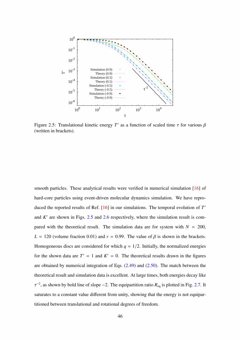
10-6

10-5

10-4

10-3

10-2

10-1

100

100 101 102 103 104

T’

τ

τ-2

Simulation (0.9)Theory (0.9)


Simulation (-0.5)Theory (-0.5)


Figure 2.5: Translational kinetic energy T ′ as a function of scaled time τ for various β

(written in brackets).

smooth particles. These analytical results were verified in numerical simulation [16] of

hard-core particles using event-driven molecular dynamics simulation. We have repro-

duced the reported results of Ref. [16] in our simulations. The temporal evolution of T ′

and K′ are shown in Figs. 2.5 and 2.6 respectively, where the simulation result is com-

pared with the theoretical result. The simulation data are for system with N = 200,

L = 120 (volume fraction 0.01) and r = 0.99. The value of β is shown in the brackets.

Homogeneous discs are considered for which q = 1/2. Initially, the normalized energies

for the shown data are T ′ = 1 and K′ = 0. The theoretical results drawn in the figures

are obtained by numerical integration of Eqs. (2.49) and (2.50). The match between the

theoretical result and simulation data is excellent. At large times, both energies decay like

τ−2, as shown by bold line of slope −2. The equipartition ratio Req is plotted in Fig. 2.7. It

saturates to a constant value different from unity, showing that the energy is not equipar-

titioned between translational and rotational degrees of freedom.

46

10-7

10-6

10-5

10-4

10-3

10-2

10-1

100

100 101 102 103 104

K’

τ

τ-2





Figure 2.6: Rotational kinetic energy K′ as a function of scaled time τ for various β


0

4

8

12

100 101 102 103 104

Req

τ



Figure 2.7: Equipartition ratio Req = T ′/K′ as a function of scaled time τ for β = 0.5,−0.5


47

2.6 Experiments of Freely Cooling Granular Gas

It is extremely hard to probe the dynamical behaviour of FCGG in experiments. In earth-

bound experiments, gravity as an external force is always present, due to which the system

can not evolve freely. Also, the system should be large enough so that the effects of

boundary conditions are negligible. Few experiments have overcome these difficulties.

We briefly summarize these experiments.

• Maaß et al. (2008) [83]: In this experiment, diamagnetic levitation was imple-

mented to compensate gravity. This method is more accessible compared to other

methods of compensating gravity such as parabolic flights or satellites. The ex-

perimental system was three dimensional. A helium cooled superconducting mag-

net coil able to generate field strengths upto 20T reduces the gravity to the order

of milligravity. The sample consisted of approximately 50-90 round and nearly

monodispersed bismuth shots. Bismuth was chosen because of its highly diamag-

netic nature. The metallic nature of the sample prevents electrostatic charges, so

there is no additional Coulomb interaction. However, bismuth has extremely low

coefficient of restitution, nearly 0.33-0.40, which makes the homogeneous cooling

regime quite shorter. Magnetic as well as mechanical excitations were used to im-

part initial energies to the particles. Snapshots of the freely evolving system were

recorded at a constant rate of 120 frames per second. The velocity of a particle is

then calculated using its position at two consecutive frames. As the cooling process

mainly involves the nonclustered particles (in the experiment, it was observed that

the velocity of a clustered particle is very low making it determination impossible),

the observed quantity in the study was the mean particle speed outside of a possible

cluster. Haff’s law is seen to describe the experimental data until clustering occurs

in the system.

• Grasselli et al. (2009) [84]: In this experiment, the freely cooling system consisted

48

of iron beads enclosed in a two dimensional cell. The wall of the cell was made of

glass in order to cancel electrostatic effects and to minimize the friction between the

beads and the walls. To remove the effect of gravity, this experiment was performed

in zero-gravity situations inside a special equipped airplane undergoing parabolic

flights. The temporal evolution of the system was recorded with a high-speed cam-

era at 470 frames per seconds. The coefficient of normal restitution was found to

be a constant at large relative velocities, and decreases when the relative velocity

decreases. This is in contrast with other experimental findings, where the coeffi-

cient of normal restitution increases when the relative velocity decreases. This is

because the velocity scale in this experiment is of the order of few centimeters per

second, while in previous experiments the typical relative velocity was larger than

1m/s. At such low velocities, adhesive forces are relevant resulting in smaller value

of coefficient of normal restitution. The measured kinetic energy decays faster than

that predicted by Haff’s law with constant coefficient of normal restitution. Bet-

ter fitting is obtained when rotational degree of freedom is taken into account. A

much better fitting is obtained if the Haff’s law is modified to take into account the

experimentally observed velocity dependent coefficient of restitution.

• Tatsumi et al. (2009) [85]: In this experiment, monodispersed zirconium beads

were confined in quasi two dimensional cell. The coefficient of restitution of zir-

conium beads is 0.76 approximately. The experiment was carried out in two types

of quasi two dimensional cells: a horizontal cell and a vertical cell. Around 2000

particles for the horizontal cell and 300 particles for the vertical cell were used in

experiment. This number is much higher as compared to above discussed Maaß et

al. experiment [83]. The cell was kept in vacuum condition to avoid hydrodynamic

interaction between particles. The initial velocities of the particles were generated

by vibrating the system electromagnetically. Microgravity condition was achieved

aboard a parabolic flight of a jet aircraft. Particle motion was captured by a high-

speed camera, at a frame rate of 1kHz. As long as clustering is absent in the system,

49

experimental data fits very well to the Haff’s law.

2.7 Ballistic Aggregation

In this section, we discuss the Ballistic Aggregation (BA) model (also called sticky gas)

[see Ref. [98] for a review]. In the following subsections, we first describe the model

in detail, followed by the mean-field scaling analysis of BA, and the simulation results

of this model. In the last subsection, we discuss connection between BA and Burgers

equation in one dimension.

2.7.1 Model

In the BA model, particles move ballistically and on collision merge to become a new

particle, whose shape is assumed to be spherical. To each particle i located at ~ri, we

associate a velocity ~vi, a mass mi and a radius ai. Consider the collision between particles

i and j. The mass m′ of the new particle is given by mass conservation

m′ = mi + m j, (2.59)

and its velocity ~v′ is given by linear momentum conservation

m′~v′ = mi~vi + m j~v j. (2.60)

The radius a′ of the new particle is obtained from volume conservation: a′D = aDi + aD

j .

The position ~r′ of the new particle is obtained from the conservation of center of mass:

m′~r′ = mi~ri + m j~r j. (2.61)

50

We can further consider particles having rotational degree of freedom and associate an

angular velocity ~ωi. The moment of inertia is given by Ii = qmia2i , where q is a number

which depends on dimensionality and the distribution of mass inside a particle. Its value

is 1/2 for a homogeneous disk, and 2/5 for a homogeneous sphere.

The new angular velocity ~ω′ is obtained from conservation of angular momentum. Let

I′ = qm′a′2 be the moment of inertia of the new particle. Then,

I′ ~ω′ = Ii~ωi + I j~ω j +mim j

mi + m j

(~ri − ~r j) × (~vi − ~v j). (2.62)

Equations (2.59)–(2.62) completely determine the mass, velocity, position and angular

velocity of the new particle. We note from Eqs. (2.59) and (2.60) that translational ve-

locities are independent of rotational motion. Except Chapter 5, everywhere else in this

thesis, we study BA without considering the rotational degrees of freedom.

2.7.2 Scaling Analysis of Ballistic Aggregation

Carnevale et. al. [15] carried out the mean-field scaling analysis of BA, and we recapitu-

late the analysis in this subsection. Consider a collection of spheres distributed randomly

in a D-dimensional space. Initially at time t = 0, the spheres are of average radius a0,

average mass m0, and with average separation l0. The velocities have root mean square

(rms) value of u0.

Initially at t = 0, the collision time τ0 is the ratio of the volume per particle to the rate at

which a sphere sweeps out the volume,

τ0 = lD0 /u0aD−1

0 , (2.63)

this expression being valid only at t = 0, when l0, a0 and u0 are the characteristic scales

of the system. We define N(t/τ0) as the expected number of initial spheres that have

51

aggregated into a single sphere at t. At t1 ≡ sτ0, we have a new initial condition with

scales

l1 = N1/D1

l0, (2.64)

m1 = N1m0, (2.65)

a1 = N1/D1

a0, (2.66)

u1 = u0/N1/21, (2.67)

τ1 = N(D+2)/2D

1τ0, (2.68)

where N1 ≡ N(s). The scaling for u1 in Eq. (2.67) is obtained using central limit theorem.

The momentum of an aggregate is the sum of N1 random vectors of typical length m0u0,

giving the expected size of the resultant random momentum as N1/21

m0u0. Dividing it by

m1 gives Eq. (2.67).

Now, consider t2 = sτ1 = sN1/θ

m f

T

1τ0, where θ

m f

T= 2D/(D + 2). At t2, the expected size

of an aggregate can be calculated using either t = 0 or t = t1 as the initial condition.

According to the first case, N(t2/τ0) = N(sN1/θ

m f

T

1) initial particles have aggregated into

a single sphere at t2. According to the second case, each aggregate at t2 is composed of

N(t2/τ1) = N1 particles from t1, and each particle at t1 is composed of N1 initial particles.

Therefore,

N(sN(s)1/θm f

T ) = N(s)2 or N(s) ∼ s θm f

T . (2.69)

Thus, the typical mass of an aggregate grows as Mt ∼ t θm f

T . The typical number of ag-

gregates then decreases as nt ∼ t−θm f

T , since total mass is conserved. With typical velocity

vt ∼ t−θm f

T/2, the kinetic energy of the system is given by

T (t) ∼ ntMtv2t ∼ t−θ

m f

T with θm f

T= 2D/(D + 2). (2.70)

52

Volume fraction φ Decay exponent θBAT

0.0008 1.12

0.0079 1.12

0.0393 1.10

0.3925 1.03

0.6280 1.00

Table 2.1: Table showing the dependence of decay exponent θBAT on volume fraction φ for

two dimensional BA. Data are taken from [19].

2.7.3 Simulation Results for Ballistic Aggregation

Numerical simulations of BA in one dimension [15] with point particles and a variety of

initial distribution of positions and velocities find θBAT = 2/3 validating the mean-field

prediction. Exact solution of BA in one dimension finds θBAT = 2/3 matching with the

mean-field and simulation result. However, simulations in two dimensions show signif-

icant deviations from the mean-field prediction [19, 99]. The BA model in D ≥ 2 is

different from D = 1. The size of particles, which can be scaled out in D = 1 becomes

a relevant variable in D ≥ 2. In D = 1, aggregation is a purely binary process, while

in higher dimensions owing to the spatial extension of newly formed aggregate, it may

overlap with other particles leading to a chain of multiple aggregation. The possibility of

multiparticle aggregation is higher for denser systems, thus making decay exponent θBAT

density dependent. Table 2.1 shows θBAT for varying volume fraction φ, for two dimen-

sional BA. For dilute systems, its value is very different from the mean-field value of one.

Its value increases with increase in density and saturates at the mean-field value.

The deviation from the mean-field value is because of the incorrect assumption that veloc-

ities of original particles contained within an aggregate are uncorrelated [19]. In general,

particles moving towards each other are more likely to collide compared to particles that

are moving away from each other, breaking the no-correlation assumption. It is shown

that mean-field no-correlation assumption is essentially the Maxwell model in context of

ballistic processes [19, 100]. The Maxwell model is obtained by replacing the relative

velocity in the Boltzmann equation by the root mean square velocity and this approxima-

53

tion allows for analytical progress of problem. The Maxwell model is an uncontrolled

approximation to the Boltzmann equation and the exponents found with this approach are

generally erroneous [19].

2.7.4 Burgers Equation and Ballistic Aggregation

In this subsection, we recapitulate the solution of Burgers equation in one dimension [74,

101] and its connection with ballistic aggregation as established in [74].

The one dimensional Burgers equation for the velocity field u(x, t) is

∂u

∂t+ u∂u

∂x=

1

R

∂2u

∂x2, (2.71)

where x is space coordinate, t is time. R = u0l0/ν is Reynolds number with the charac-

teristic velocity u0 and length l0 of the initial velocity field and ν is kinematic viscosity.

We are interested in the solution of Eq. (2.71) in high Reynolds numbers limit R ≫ 1

and large times t ≫ 1, under arbitrary continuous initial conditions u(x, 0), specified in an

infinite domain, −∞ < x < ∞. The Hopf–Cole transformation,

u = − 2

wR

∂w

∂x, (2.72)

transforms nonlinear Eq. (2.71) into a linear diffusion equation for w(x, t),

∂w

∂t=

1

R

∂2w

∂x2. (2.73)

Solving Eq. (2.73) for w and then using Eq. (2.72) gives

u(x, t) =

∫ ∞−∞

x−x′

texp

[

−R2Z(x, x′, t)

]

dx′

∫ ∞−∞ exp

[

−R2Z(x, x′, t)

]

dx′, (2.74)

54

where

Z(x, x′, t) =(x − x′)2

2t+

∫ x′

x0

u(x′′, 0)dx′′, (2.75)

where x0 is an arbitrary constant. Now, for a fix value of x and t > 0, and in the invis-

cid limit of R ≫ 1, the most important contribution to the integral will come from the

immediate neighborhood of point X, which is given by absolute minimum of Z(x, x′, t).

X = minx′

Z(x, x′, t). (2.76)

Thus, Eq. (2.74) reduces to

u(x, t) =x − X

t. (2.77)

We note that Eq. (2.77) does not generally represent a straight line since X is a function

of x and t. Now, to examine the dependence of X on x and t, we consider a geometric

interpretation of the minimum condition. As shown in Fig. 2.8, first we construct the

curve

s(x′) = −∫ x′

x0

u(x′′, 0)dx′′ + s(x0), (2.78)

which is completely determined by the initial velocity field of the problem. Second, we

construct a parabola

S (x′) =(x′ − x)2

2t+C, (2.79)

whose axis is the line x′ = x, and whose vertex becomes flatter with increasing t. Hence,

we have a different parabola for different x and t. We start with a large positive value of

constant C, so that the everywhere the S curve is well above the s curve. This is always

possible with the assumption that s(x′) < ∞ for all x′. Now, the minimum condition

dZ/dx′ = 0 gives

dS

dx′=

ds

dx′. (2.80)

In words, when the minimum condition is satisfied, the tangents to both curves, S (x′) and

s(x′) are parallel. The minima value X can thus be obtained by bringing the S curve down

55

y

x’

s-curve

First contact point

Axis of parabola S-curve (parabola)

x X

Figure 2.8: Initial data curve (s-curve) and the parabola S.

by decreasing the value of C, until it touches the s curve for the first time (see Fig. 2.8),

at which instant both curves have a common tangent at the point of contact. The point

X, where the contact occurs for the first time determines the absolute minimum of Z for

fixed x and t,

Z(x, x′, t)|X = (S (x, x′, t) − s(x, x′, t) −C)|X = −C. (2.81)

Now, to obtain u as a function of x for a fixed t, we must shift the axis of parabola S (x′).

The above described method for determining the absolute minimum through first contact

point can then be interpreted by requiring that the parabola S (x′) shall glide over the s

curve without ever cutting it. Thus, each position x of the axis will give the corresponding

X and u(x, t) can then be determined using Eq. (2.77).

It is possible that parabola S (x′) touches the s(x′) curve at two points simultaneously. This

possibility is higher for large t, when the parabola is rather flat. In such cases, Eq. (2.76)

has a double root. When t >> 1, all first contact points are closer to the tops of the s curve,

as the parabola is much flatter than the s curve (see Fig. 2.9). We denote the abscissa of

the ith top of such kind by ηi, where i = 0,±1,±2,....and η0 is the top closest to the origin.

For the chosen x, the abscissae of the two first contact points are denoted by Xi and Xi+1.

Since, Xi ≈ ηi and Xi+1 ≈ ηi+1, the function s(x′) can be expanded around ηi and ηi+1,

56

y

x’

x Xi+1ηi+1Xi

ηi

ηi,s(ηi)

ηi+1, s( ηi+1 )

Figure 2.9: A parabola in double contact with the s-curve.

x,

y

o

ox

u

ηi ηi+1

µi

ξi

ζi

Figure 2.10: A sequence of parabolas in double contact with the s-curve and the corre-

sponding velocity field.

57

and the integral [Eq. 2.74] is evaluated as the sum of contributions from these two parts

yielding,

u(x, t) =1

t

(

x − ηi + ηi+1

2

)

− 1

2t(ηi+1 − ηi) tanh

[

R

4t(ηi+1 − ηi)(x − ξi)

]

, (2.82)

where ξi is given by

ξi =ηi + ηi+1

2− s(ηi+1) − s(ηi)

ηi+1 − ηi

t +t

R(ηi+1 − ηi)ln

(

s′′(ηi+1)

s′′(ηi)

)

. (2.83)

This solution is valid in the region 12(ξi−1 + ξi) < x < 1

2(ξi + ξi+1) and for R ≫ 1, t ≫ 1.

For very large R such that R ≫ t ≫ 1, Eqs. (2.82) and (2.83) reduce to

u(x, t) =

x−ηi

tfor

ξi−1+ξi2< x < ξi,

x−ηi+1

tfor ξi < x <

ξi+ξi+1

2,

(2.84)

and

ξi =ηi+1 + ηi

2− s(ηi+1) − s(ηi)

ηi+1 − ηi

t. (2.85)

Equation (2.84) represents a discontinuity or a shock of strength µi/t located at ξi, where

µi = ηi+1 − ηi. (2.86)

It is easy to show that the shock moves with the velocity ζi/t, where

ζi = ξi −ηi+1 + ηi

2, (2.87)

which is equal to the velocity at the centre of the shock. It can be easily seen from

Eq. (2.85) that ξi coincides with the axis of the parabola passing through the two tops

(ηi, s(ηi)) and (ηi+1, s(ηi+1)) of s curve.

Thus, as shown in Fig. 2.10, the velocity profile is represented by a sequence of vertical

58

lines (shocks) connected by oblique lines of slope 1/t. The positions of shocks are given

by ξi, and ηi gives the positions where the oblique lines intersect x− axis. These shocks

move at different speeds determined by Eq. (2.87) and therefore collide with each other

from time to time. On collision, the shocks coalesce into one, with the strength of resultant

shock given by sum of the strengths of colliding shocks.

We consider the following two observations

1. The advance velocity ζi/t and the strength of shocks multiplied by t, µi are invariant

in time except at the instant of collision.

2. µi and µiζi/t are conserved at each collision. To see this, consider collision between

two shocks at ξi and ξi+1. The strength of resultant shock is given by

µ′ = ηi+2 − ηi = (ηi+2 − ηi+1) + (ηi+1 − ηi) = µi + µi+1. (2.88)

It is easy to show that µ′ζ′/t given by,

µ′ζ′

t=

1

t(ηi+2 − ηi)(ξ

′ − ηi+2 + ηi

2), (2.89)

with

ξ ′ =ηi+2 + ηi

2− s(ηi+2) − s(ηi)

ηi+2 − ηi

t, (2.90)

can be written as

µ′ζ′

t=µiζi

t+µi+1ζi+1

t. (2.91)

Thus, there is a one-to-one correspondence between the shock dynamics of Burgers equa-

tion and the dynamics of aggregating particles in ballistic aggregation (BA). A shock at

ξi with strength µi and velocity ζi/t can be thought of an aggregate in BA with mass µi,

moving with velocity ζi/t. These quantities are invariant in time except at the time of

collision. Equations (2.88) and (2.91) establish the mass and momentum conservation

respectively.

59

2.8 Freely Cooling Granular Gas and Burgers Equation

In this section, we discuss in detail two previous works on FCGG [13, 14], which we men-

tioned very briefly in Sec. 2.4. These works argue for a Burgers equation like description

for the large time behaviour of FCGG.

Ben-Naim et al. [13] studied FCGG in one dimension using event driven molecular dy-

namics simulation. The dissipation is accounted by constant coefficient of restitution r.

To circumvent inelastic collapse (whose detailed discussion we defer to Sec. 3.3.6), where

infinite collisions occur in finite time imposing practical difficulties in event-driven sim-

ulation of the system, a cutoff velocity δ was introduced. Collisions are elastic when

relative velocity is lower than δ, otherwise inelastic with constant r. The decay of kinetic

energy T (t) with time t is shown in Fig. 2.11. At initial times, the system remains homo-

geneous and it decays as T (t) ∼ t−2 (Haff’s law). After an r - dependent crossover (the

crossover time diverges in the elastic limit r → 1), the system evolves into inhomoge-

neous regime and it decay behaviour changes to a different power-law, T (t) ∼ t−θT , with

θT = 2/3. The value of θT = 2/3 is universal, independent of r. The curves for different

r are indistinguishable in the inhomogeneous regime, and are also indistinguishable from

the ballistic aggregation (r = 0) data. It was also noted that with δ = 0, the simulation

does not progress. We note that the mean-field scaling analysis [Eq. (2.70)] as well as the

exact solution of BA [8] predict the decay exponent to be 2/3 in one dimension.

With these observations, it was proposed that the FCGG is asymptotically in the univer-

sality class of a completely inelastic, sticky gas [13]. A simple physical picture was pro-

vided to understand this universality. Consider a collision between one moving particle

and cluster of N stationary particles in one dimension, where all particles are identical.

At any collision particle identities are considered to be exchanged, so that in an elastic

collision the particles merely pass through each other, while suffer a small deflection for

small inelasticity. The result of a collision between a particle with velocity v and another

60

100

101

102

103

104

105

106

t

10−5

10−4

10−3

10−2

10−1

100

T(t

)/T

(0)

r=0r=0.5,0.9,0.99 δ=10

−2

r=0.5,0.9,0.99 δ=0slope=−2/3

Figure 2.11: The temporal decay of kinetic energy T (t) for one dimensional FCGG, for

various r. Data for r = 0 (BA) case is also shown. Reprinted figure with permission

from E. Ben-Naim, S. Y. Chen, G. D. Doolen, and S. Redner, Physical Review Letters,

83, 4069 (1999) [13]. Copyright (1999) by the American Physical Society.

particle with velocity u is given by

v→ v − ǫ (v − u), (2.92)

where ǫ = (1 − r)/2. Thus, each collision between the incident particle and the next

stationary particle in the cluster reduces the incident particle velocity by roughly ǫ. The

incident velocity after N collisions is vN ≈ 1 − Nǫ. Now, for the particle to pass through

the cluster, N < ǫ−1. For this range of cluster sizes, the system remains spatially homo-

geneous and energy decay follows Haff’s law. If the cluster size is bigger than the critical

cluster size Nc(ǫ) ∼ ǫ−1, the incident particle is absorbed as if the coefficient of restitution

is r = 0. As clustering is more prominent in highly inelastic systems, lesser inelastic

system remains in homogeneous regime for longer times. Once the system crosses to the

inhomogeneous regime, system with any value of r < 1 behaves like r = 0.

Further confirmation of this universal behaviour is obtained by the measurement of ve-

61

0 5000 10000 15000 20000x

0

20

40

60

80

ρ(x)

0 5000 10000 15000 20000x

−0.04

−0.02

0

0.02

0.04

v(x)

Figure 2.12: Shock profile of one dimensional FCGG. Density and velocity in the inho-

mogeneous regime are plotted. A line with slope t−1 is plotted for reference. Reprinted

figure with permission from E. Ben-Naim, S. Y. Chen, G. D. Doolen, and S. Redner, Phys-

ical Review Letters, 83, 4069 (1999) [13]. Copyright (1999) by the American Physical

Society.

locity distribution [13]. It was found that in the inhomogeneous regime, the normalized

velocity distribution,

P(v, t) ∼ t1/3Φ(vt1/3), (2.93)

is described by an identical scaling function Φ(z) for all values of r < 1, including r = 0.

The scaling function Φ(z) was found to be Gaussian [13].

This universal behaviour, i.e., the convergence of all r < 1 curves to r = 0 shows that the

inhomogeneous regime of FCGG is described by sticky gas with r = 0 being the fixed

point. Since sticky gases are described by the inviscid limit of the Burgers equation as

discussed in Sec. 2.7.4, it was concluded that this continuum theory also describes the

asymptotics of the FCGG in the thermodynamic limit [13]. This conclusion was further

supported by comparing the velocity field profile. Shown in Fig. 2.12 is the velocity field

of one dimensional FCGG [13], which is similar to the velocity profile of the Burgers

equation solution (see Fig. 2.10). The 1/t slopes of the linear segments of the profile are

consistent with Burgers equation prediction (see Eq. 2.77).

62

It was speculated that r = 0 remains the fixed point even in higher dimensions D > 1 as

well [13]. It was shown in [5] that in higher dimensions, Burgers equation ~vt + ~v · ∇~v =

ν∇2~v approximately describes the sticky gas in the inviscid limit v → 0. Using this

correspondence, it was predicted that kinetic energy decreases as [5, 13].

T (t) ∼

t−D/2 for 2 ≤ D ≤ 4,

t−2 for D > 4.(2.94)

Nie et al. simulated FCGG of hard disks in two dimensions [14]. They found that in

the inhomogeneous regime, energy decays as a power-law T (t) ∼ A(r)t−θT with θT = 1.

Similar to the one dimensional case, the decay exponent θT is independent of r, but un-

like one dimensional case, T (t) has a dependence on r through the prefactor A(r). It

was observed that the dependence of A(r) on r becomes weaker for dilute systems, sug-

gesting completely universal behaviour in the dilute limit. The observed decay exponent

θT = 1 is predicted by both, the mean-field scaling analysis [Eq. (2.70)] and the corre-

spondence with Burgers equation [Eq. (2.94)]. In the inhomogeneous regime, the velocity

distribution function P(v, t) is described by universal scaling function Φ(z) independent

of coefficient of restitution r,

P(v, t) ∼ 1

v 2rms

Φ

(

v

vrms

)

. (2.95)

In simulations, the scaling function was found to be a Gaussian [14]. Thus r = 0 is indeed

the fixed point in two dimensions as speculated in [13].

To quantify collective motions and the corresponding velocity fluctuations in the inho-

mogeneous regime, the local kinetic energy Ek and the local thermal energy Eth was also

measured in simulations [14]. The local kinetic energy is defined as Ek =12〈ρu2〉 with the

density ρ and the velocity ~u = (ux, uy) obtained by averaging the corresponding quantities

over a small region. The local thermal energy Eth =12〈(vx−ux)

2+(vy−uy)2〉 is obtained by

subtracting the average local velocity ~u from the particle velocity ~v. The ratio of thermal

63

100

101

102

103

104

105

t

10−2

10−1

100

101

102

Eth/E

k

t−0.5

Figure 2.13: The ratio of the thermal energy Eth to the kinetic energy Ek as a function

of time. A line of slope −1/2 is plotted for reference. Reprinted figure with permission

from Xiaobo Nie, Eli Ben-Naim, and Shiyi Chen, Physical Review Letters, 89, 204301

(2002) [14]. Copyright (2002) by the American Physical Society.

to kinetic energy is shown in Fig. 2.13. Initially, the thermal energy is large compared to

the kinetic energy, indicating that particles move independently and there are no collective

motions in the system. However, at larger times in the inhomogeneous regime, thermal

energy becomes much smaller than the kinetic energy, showing the dominance of coher-

ent motion of particles in the system. Collective motion was earlier observed in numerical

simulations [12, 87, 90, 93] and as well as suggested by linear stability analysis of the hy-

drodynamic equations [12, 87]. At long times, the ratio was found to decay with time as

Eth/Ek ∼ t−0.5. The thermal energy Eth =12〈(∆v)2〉 quantifies local velocity fluctuations,

∆v. As Ek decays as t−1, ∆v ∼ t−3/4. The local velocity fluctuations ∆v ∼ t−3/4, are small

compared to the typical velocity v ∼ t−1/2, as ∆v/v ∼ t−1/4. The relatively small velocity

fluctuations imply presence of strong velocity correlations and a well-defined average lo-

cal velocity. Thus, a hydrodynamic description is plausible for the inhomogeneous regime

of FCGG.

Hydrodynamical equations of mass, momentum and energy balance [11, 12], can be used

to describe the collective motion of granular flow. As the thermal energy, i.e., the tem-

perature T , is negligible compared with the kinetic energy, the system can be expanded

64

around zero temperature. In particular, the pressure term in the momentum equation can

be ignored due to the fact that p ∼ T , while keeping the viscosity term since ν ∼ T 1/2.

Therefore, the governing equations are given as,

∂tρ + ∂α(ρuα) = 0, (2.96)

∂t(ρuα) + ∂β(ρuαuβ) = ∂βπαβ, (2.97)

παβ = ∂α(ρνuβ) + ∂β(ρνuα) − ∂γ(ρνuγ)δαβ, (2.98)

taken in the limit of vanishing viscosity, ν → 0. α, β, γ refer to spatial coordinates x,y,

and repeated indices are summed. The above equations are similar to the two dimensional

Burgers equation supplemented by the continuity equation [5, 101]. In two dimensions,

the formation of shocks corresponds to dense, thin, stringlike clusters as observed in

Ref. [12], where particles move parallel to the cluster orientation.

65

Chapter 3

Computational Methods

3.1 Introduction

Computer simulations are an important tool for studying granular materials. In the ab-

sence of a comprehensive theory of granular matter, computer simulations play an im-

portant role in developing phenomenology. Among the simulation methods for granular

systems, a widely used method is Molecular Dynamics. In conventional Molecular Dy-

namics (MD) simulation, Newton’s equations of motion of all particles in the system are

integrated numerically. This method is used for simulating systems with continuous in-

teraction potential. A major improvement in the conventional MD simulation is possible

when the particles in the simulation are considered hard. This efficient method is known

as Event Driven Molecular Dynamics (ED). In this chapter we describe these two simu-

lation methods in detail.

67

3.2 Molecular Dynamics Simulations

Granular systems are a collection of macroscopic particles, interacting only on mechani-

cal contact. Quantum effects being not important, the dynamics of this many-body system

is governed by Newton’s equation of motion. The motion of a particle i is determined by

the total force ~Fi exerted on i by all the other particles j, j , i, 1 ≤ j ≤ N:

md2~ri

dt2= ~Fi, 1 ≤ i ≤ N, (3.1)

where ~ri is the position of particle i at time t, and m is the mass of a particle. N is the total

number of particles in the system. In general, this system of coupled nonlinear differential

equations [Eq. (3.1)] can not be solved analytically. The approximate numerical solution

of these equations determines the evolution of the system, and is called Molecular Dy-

namics (MD). This MD is also known as conventional MD or force-based MD. Since

granular particles are rather rigid, their repulsive interaction force grows steeply with the

compression once the particles are in contact. This rigid nature demands very small in-

tegration time step for the computation of trajectories to obtain stable results. Thus, the

MD simulation of granular systems is computationally time consuming.

In this thesis, we have used MD to simulate visco-elastic particles. The interaction force

between these particles is discussed in detail in Sec. 2.2.3.

3.2.1 Integration Scheme

Once the interaction force is specified, what remains is to numerically integrate Eq. (3.1).

In this thesis, we have used Runge-Kutta scheme for numerical integration. Runge-Kutta

is a single-step method in the sense that information at only one previous step is required

to compute the solution at its present time. Higher order accuracy is achieved by con-

sidering intermediate times. Since a differential equation of order l can be reduced to

68

a system of l first-order equations, we below present Runge-Kutta scheme for solving a

first-order differential equation. Consider a first-order differential equation for y with t as

the independent variable:

dy

dt= f (t, y), (3.2)

where the function f (t, y) is known. In Runge-Kutta method, with the value of function

y known at t = tn, y(t = tn) ≡ yn, its value at next step tn+1 = tn + h is computed using a

formula of the form

yn+1 = yn + h

z∑

i=1

wiki, (3.3)

where h is the integration time step and wi’s are constants. The ki’s are given by

ki = f (tn + αih, yn +

i−1∑

j=1

βi jk j), (3.4)

where αi and βi j are constants with α1 = 0. To obtain all these constants, we expand

Eq. (3.3) using Taylor series about (tn, yn) and match terms up to the required order in h.

We here illustrate the procedure for second-order Runge-Kutta method for which z = 2.

Rearranging and expanding Eq. (3.3)

yn+1 − yn = h[w1 f (tn, yn) + w2 f (tn + α2h, yn + β21k1)],

hy′n +h2

2y′′n + . . . = h[w1 f (tn, yn) + w2 f (tn + α2h, yn + β21h f )],

h f +1

2h2( ft + f fy) + . . . = h(w1 f + w2 f ) + h2w2(α2 ft + β21 f fy) + . . . , (3.5)

where f = f (tn, yn), and ft, fy are the partial derivatives computed at the same point.

Comparing coefficients upto the second order expansion in h from Eq. (3.5) yields:

w1 + w2 = 1, w2α2 =1

2, w2β21 =

1

2. (3.6)

Thus, we have three nonlinear equations in four unknowns, which can be solved for w1, w2

and β21 in terms of α2. Three standard choices for α are 1/2, 2/3 and 1, yielding following

69

formulas:

yn+1 = yn + h f

(

tn +1

2h, yn +

1

2h fn

)

, (3.7)

yn+1 = yn +1

4h

[

f (tn, yn) + 3 f

(

tn +2

3h, yn +

2

3h fn

)]

, (3.8)

yn+1 = yn +1

2h[

f (tn, yn) + f (tn + h, yn + h fn)]

. (3.9)

These are the three standard second-order Runge-Kutta methods for solving differential

equation. However, the classical and the most widely used Runge-Kutta method is of

fourth order given by:

yn+1 = yn +h

6(k1 + 2k2 + 2k3 + k4),

k1 = f (tn, yn),

k2 = f (tn +1

2h, yn +

1

2k1), (3.10)

k3 = f (tn +1

2h, yn +

1

2k2),

k4 = f (tn + hn, yn + k3).

This formula can be derived by expanding Eq. (3.3) upto fourth order in h. The algebra is

however quite cumbersome. This fourth-order Runge-Kutta scheme (RK4) is fairly stable

for most of the physical problems. Apart from the above mentioned scheme, there are

many other fourth-order Runge-Kutta methods.

3.3 Event Driven Molecular Dynamics Simulations

The conventional MD is widely used for simulating systems where the interaction can be

expressed in terms of continuous potentials. In conventional MD, the equations of motion

are integrated numerically with a time step that is much smaller than the smallest time

scale in the problem. The restriction of small time step renders the simulations time con-

70

suming. In a system where there are no long-range interactions and particles interact only

on collision, a major improvement in the computational efficiency is possible if we take

the alternative route of step potentials. If the typical duration of a collision is much shorter

than the mean free time between successive collisions, collisions can be considered in-

stantaneous. This idealization of considering the collisions to be instantaneous assumes

that the particles are perfectly hard, and is sometimes called hard-sphere approximation.

In this hard-spheres system, particles follow linear trajectories until they encounter a col-

lision. Collision being an instantaneous process, all collisions in the system are binary. A

collision changes the velocities of the involved particles according to a collision law while

velocities of other particles remain unchanged. Thus, we have the information about the

position and velocity of every particle at every instant. With this information, the future

collision events can be easily calculated. This simulation method which proceeds with

the discrete events of collision is called Event Driven Molecular Dynamics (ED). This

method relying on the series of events is much more efficient than the conventional MD

involving time consuming numerical integrations. This method has found enormous suc-

cess in the study of granular gases as these systems satisfy very well both criteria required

by this method: (a) No long-range interaction, and (b) Granular particles are sufficiently

hard for the interactions to be instantaneous.

A sketch of event driven algorithm

1. Initialize the positions ~ri, velocities ~vi and angular velocities ~ωi of all particles 1 ≤

i ≤ N, at time t = 0.

2. Find the earliest occurring collision in the system. For this we must know the time

of occurrence of all possible future collisions.

3. Advance the system to the time of occurrence of this earliest collision.

• The new positions of all particles can be easily computed as particles are mov-

71

ing ballistically with their present velocities.

• The velocities of colliding particles can be computed from the collision law

which gives the post-collision velocities in terms of pre-collision velocities.

• The velocities of other particles remain unchanged.

4. Repeat step 2 − 3 for the desired number of times.

The details needed to execute these steps are explained in following subsections for a

system of identical hard-spheres with mass m and diameter d:

3.3.1 Initialization

The positions ~ri, velocities ~vi and angular velocities ~ωi of all particles are assigned at the

start of simulation. Care should be taken that there is no overlap between particles as ED

simulation deals with hard-particles.

3.3.2 Predicting Future Collisions

Since the ED simulation progresses with collisions events, we must have the information

about the next collision occurring in the system, the colliding partners and the time of

collision. Two particles i, j moving with velocities ~vi, ~v j and at positions ~ri, ~r j at present

time t will collide in future at time t∗i j if

|(~ri + (t∗i j − t)~vi) − (~r j + (t∗i j − t)~v j)| = d, (3.11)

has a solution t∗i j with t∗i j > t. Defining ~ri j = ~ri −~r j and ~vi j = ~vi −~v j, above equation can be

rewritten as

(t∗i j − t)2 + 2(t∗i j − t)~ri j · ~vi j

~v 2i j

+~r 2

i j − d2

~v 2i j

= 0. (3.12)

72

For a collision to occur, particles must approach each other, thus

~ri j · ~vi j < 0. (3.13)

Equation (3.12) has real solutions if

~ri j · ~vi j

~v 2i j

2

+d2 − ~r 2

i j

~v 2i j

> 0. (3.14)

The particles i, j will collide at t∗i j only when Eqs. (3.13) and (3.14) are satisfied. The time

t∗i j is given by the solution of Eq. (3.12) and is

t∗i j − t = −~ri j · ~vi j

~v 2i j

−

√

√

~ri j · ~vi j

~v 2i j

2

+d2 − ~r 2

i j

~v 2i j

. (3.15)

The numerical evaluation of Eq. (3.15) in a computer algorithm is not stable. This is

because, for very small distances on the particle surfaces (d ≈ |~ri j|), the difference of two

almost equally large numbers has to be computed which leads to large numerical errors.

A mathematically equivalent expression of Eq. (3.15) which is also numerically stable is:

t∗i j − t =~r 2

i j − d2

−~ri j · ~vi j +

√

(

~ri j · ~vi j

)2+ ~v 2

i j(d2 − ~r 2

i j)

. (3.16)

Thus, we determine the future collision time t∗i j of all pairs (i, j). The minimum of these

gives the earliest future collision time t∗.

3.3.3 Linear Motion

With the system at its present state at time t and the earliest future collision at time t∗, the

position of the particles at time t∗ is given by:

~ri(t∗) = ~ri(t) + (t∗ − t)~vi(t), 1 ≤ i ≤ N. (3.17)

73

3.3.4 Collision Law

Collision alters the velocities of the involved particles deterministically. The collision

law determines the post-collision velocities in terms of their pre-collision velocities and

coefficient of restitutions. The collision law for rough and smooth particles is discussed

in Sec. 2.2.1 and Sec. 2.2.2 respectively.

3.3.5 Cell Division

In order to determine the earliest occurring collision in the system, we must calculate the

collision time for all pairs of particles. There are N(N − 1)/2 pairs and this makes the

algorithm inefficient. The efficiency can be considerably improved by dividing the simu-

lation region into small cells whose edge length exceeds the particle diameter d. Particles

are associated to different cells according to there position coordinates. Particles occupy-

ing same cell or adjacent cells are called neighbours. With this construction, instead of

calculating the collision time of a particle with all other N − 1 particles, we calculate its

collision time with neighbouring particles only. It is quite likely for a particle to collide

with particles other than its neighbours. Such collisions are taken into account by intro-

ducing an additional event known as cell-crossing. Cell-crossing is the event of a particle

leaving its present cell and crossing to an adjacent cell. This can be easily computed. A

particle can collide with particles other than its neighbours only after cell-crossing. Thus,

in the event of cell-crossing of a particle, we calculate the future collision time of this

particle with its new neighbors. In this way the algorithm never misses any collision.

Incorporating cell-crossing events introduces additional work but overall this algorithm

makes the number of collision pairs for a particle local and independent of the system

size N, greatly improving the efficiency.

74

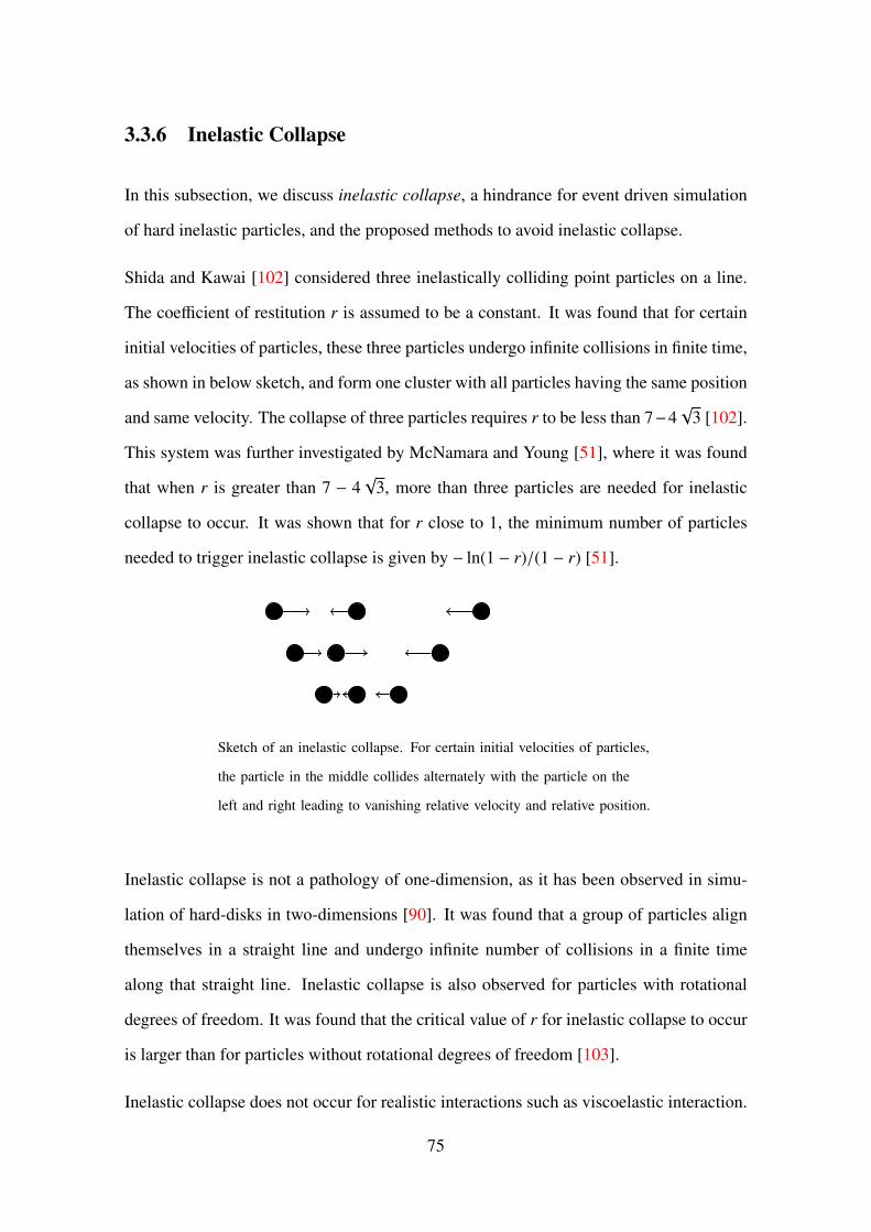
3.3.6 Inelastic Collapse

In this subsection, we discuss inelastic collapse, a hindrance for event driven simulation

of hard inelastic particles, and the proposed methods to avoid inelastic collapse.

Shida and Kawai [102] considered three inelastically colliding point particles on a line.

The coefficient of restitution r is assumed to be a constant. It was found that for certain

initial velocities of particles, these three particles undergo infinite collisions in finite time,

as shown in below sketch, and form one cluster with all particles having the same position

and same velocity. The collapse of three particles requires r to be less than 7−4√

3 [102].

This system was further investigated by McNamara and Young [51], where it was found

that when r is greater than 7 − 4√

3, more than three particles are needed for inelastic

collapse to occur. It was shown that for r close to 1, the minimum number of particles

needed to trigger inelastic collapse is given by − ln(1 − r)/(1 − r) [51].

Sketch of an inelastic collapse. For certain initial velocities of particles,

the particle in the middle collides alternately with the particle on the

left and right leading to vanishing relative velocity and relative position.

Inelastic collapse is not a pathology of one-dimension, as it has been observed in simu-

lation of hard-disks in two-dimensions [90]. It was found that a group of particles align

themselves in a straight line and undergo infinite number of collisions in a finite time

along that straight line. Inelastic collapse is also observed for particles with rotational

degrees of freedom. It was found that the critical value of r for inelastic collapse to occur

is larger than for particles without rotational degrees of freedom [103].

Inelastic collapse does not occur for realistic interactions such as viscoelastic interaction.

75

It is because of dependence of coefficient of restitution on relative velocity of collision.

For viscoelastic particles, r is not a constant but increases towards the elastic value of one

with decreasing relative velocity. As a result of which, the restriction on r for inelastic

collapse to occur is not satisfied for an infinite number of collisions. As soon as the

relative velocity is lower than a critical velocity, r becomes higher than the restricted

value and eventually the cluster dissolves [104].

Inelastic collapse is a major problem in event driven molecular dynamics simulation of

hard core inelastic particles. With a particle undergoing very large number of collisions

in a short time, the simulation practically can not proceed beyond that time. Several tricks

have been implemented to avoid inelastic collapse. Luding and McNamara introduced

the TC model [105], where each collision is assumed to last for a small finite time tc. If

a particle collides again within this time tc, the second collision is considered as elastic.

This model does not satisfy the condition of upper limit on r and interrupts the infinite

sequence of collisions. Deltour and Barrat [87] used the idea of rotating the velocities

after the collision by a small angle (less than 5) to avoid inelastic collapse.

A widely used method to circumvent inelastic collapse, suggested in Ref. [51] and first

implemented in Ref. [13] is the introduction of a cutoff velocity δ. Collisions are consid-

ered inelastic only when the normal relative velocity of collision is greater than this cutoff

velocity δ, otherwise elastic. This trick does not obey the restriction on r for the inelastic

collapse to occur. It also qualitatively captures the experimentally observed behaviour,

where r is seen to be a function of the relative velocity [95, 96]. The value of parameter

δ is generally chosen to be sufficiently small compared to the typical relative velocity of

collisions in the system. It then affects only those few particles involved in inelastic col-

lapse, and the dynamics of the system is mainly governed by inelastic collisions. We have

implemented this particular trick in all of our simulations.

76

Chapter 4

Energy Decay in Three-Dimensional

Freely Cooling Granular Gas

4.1 Introduction

In Chapter 2, we reviewed previous studies on freely cooling granular gas (FCGG) to

a good extent. We briefly summarize the important results to make this chapter self-

contained. In this chapter, our FCGG consists of hard-core smooth particles. For this

system, translational kinetic energy T (t) (defined in Eq. (2.14)) decreases with time t,

while rotational energy K(t) (Eq. (2.15)) is conserved. Our primary interest is clustering

of particles due to inelastic collisions and the temporal evolution of T (t) at large times t.

At initial times of the evolution of FCGG, particles remain homogeneously distributed

and kinetic theory predicts that T (t) decreases as (1 + t/t0)−2 (Haff’s law) where the time

scale t0 ∝ (1 − r2)−1 for constant coefficient of restitution r [11]. At later times, this

regime is destabilized by long wavelength fluctuations into an inhomogeneous cooling

regime dominated by clustering of particles [12, 90, 91]. In this latter regime, T (t) no

longer obeys Haff’s law but decreases as a power law t−θT , where θT depends only on

77

dimension D [13, 14]. Direct experiments on inelastic particles under levitation [83] or in

microgravity [84, 85] confirm Haff’s law. However, being limited by small number of par-

ticles and short times, they do not probe the inhomogeneous regime giving no information

about θT .

Two theoretical conjectures exist for the exponent θT . Extensive simulations in one [13]

and two [14] dimensions show that for any r < 1, the system is akin to a sticky gas

(r → 0), such that colliding particles stick and form aggregates. If it is assumed that the

aggregates are compact spherical objects, then the sticky limit corresponds to the well

studied ballistic aggregation model (BA). For BA in the dilute limit and the mean field

assumption of uncorrelated aggregate velocities, scaling arguments lead to θm f

T= 2D/(D+

2) and the presence of a growing length scaleLt ∼ t1/zm f

BA with zm f

BA= (D+2)/2 [15]. In one

dimension, BA is exactly solvable and θBAT = θ

m f

T[8, 72]. However, in two dimensions

and for dilute systems, it has been shown that θm f

Tis smaller than the numerically obtained

θBAT by 17% because of strong velocity correlations between colliding aggregates [19, 99].

The sticky limit has also been conjectured [13, 14] to be describable by Burgers-like

equation (BE) [101]. This mapping is exact in one dimension [74] and heuristic in two

and higher dimensions [14], and leads to θBET = 2/3 in D = 1, θBE

T = D/2 for 2 ≤ D ≤ 4,

and θBET = 2 for D > 4 [5, 106, 107].

The exponents θm f

Tand θBE

Tcoincide with each other in one and two dimensions and

also with numerical estimates of θT for the FCGG in these dimensions [13, 14]. In three

dimensions, they differ with θm f

T= 6/5 and θBE

T = 3/2. However, simulations that measure

θT in three dimensions have been inconclusive, being limited by small system sizes and

times, and the measured value of θT ranges from θT = 1.35− 1.6 [93] to θT ∼ 1 [94, 108].

Thus, it remains an open question as to which of the theories, if either, is correct.

To resolve this issue, in this chapter we study the FCGG in three dimensions using event-

driven molecular dynamics simulations. We conclude that θT ≈ θm f

T, conclusively ruling

out θBET as a possible solution. Comparing with the results of three dimensional BA,

78

we find that θm f

Tdescribes the energy decay in BA only when densities are high and

multiparticle collisions are dominant. We also find that the cluster size and the velocity

distributions of the particles in the FCGG and BA are strikingly different from each other.

The rest of the chapter is organized as follow. In Sec. 4.2, the details of the model and

simulation are provided. The simulation results for kinetic energy decay, cluster size

distribution and velocity distribution, for FCGG and BA are compared in Sec. 4.3. The

chapter is finally concluded in Sec. 4.4.

4.2 Simulation Details

Consider N identical hard-sphere particles distributed uniformly within a periodic three-

dimensional box of linear length L and with initial velocities chosen from a normal dis-

tribution. The mass and diameter of the particles are set equal to one. All lengths, masses

and times are measured in units of particle diameter, particle mass, and initial mean colli-

sion time. The system evolves in time without any external input of energy. All particles

move ballistically until they undergo momentum conserving, deterministic collisions with

other particles. Particles are considered smooth for which the collisions are described by

the collision law, Eq. (2.6).

As discussed in Sec. 3.3.6, to avoid inelastic collapse, the coefficient of restitution r is

generally chosen to be r0 (a constant less than unity) for vrel > δ and 1 (elastic) for vrel < δ,

where vrel is the normal component of the relative velocity of the colliding particles and δ

is a velocity scale. Thus, only in the limit δ → 0, all collisions are described by constant

coefficient of restitution.

However, the velocity scale δ is relevant experimentally and not just a computational tool.

Experimentally, r(vrel) approaches 1 when the vrel tends to zero, i.e., 1− r(vrel) = g(vrel/δ),

where g(x) ∼ xσ + O(x2σ), for x ≪ 1 and g(x) ∼ 1 − r0 for x → ∞ [95, 96]. It has also

been argued that a constant coefficient of restitution leads to an incomplete description

79

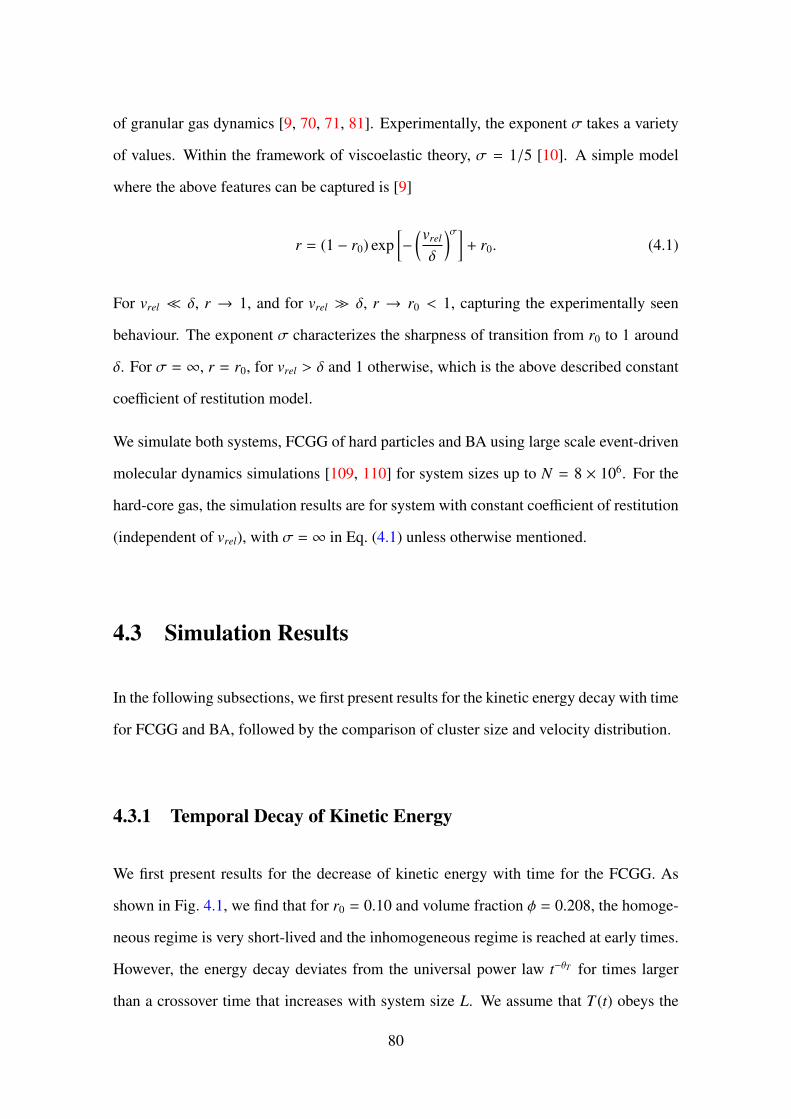
of granular gas dynamics [9, 70, 71, 81]. Experimentally, the exponent σ takes a variety

of values. Within the framework of viscoelastic theory, σ = 1/5 [10]. A simple model

where the above features can be captured is [9]

r = (1 − r0) exp[

−(

vrel

δ

)σ]

+ r0. (4.1)

For vrel ≪ δ, r → 1, and for vrel ≫ δ, r → r0 < 1, capturing the experimentally seen

behaviour. The exponent σ characterizes the sharpness of transition from r0 to 1 around

δ. For σ = ∞, r = r0, for vrel > δ and 1 otherwise, which is the above described constant

coefficient of restitution model.

We simulate both systems, FCGG of hard particles and BA using large scale event-driven

molecular dynamics simulations [109, 110] for system sizes up to N = 8 × 106. For the

hard-core gas, the simulation results are for system with constant coefficient of restitution

(independent of vrel), with σ = ∞ in Eq. (4.1) unless otherwise mentioned.

4.3 Simulation Results

In the following subsections, we first present results for the kinetic energy decay with time

for FCGG and BA, followed by the comparison of cluster size and velocity distribution.

4.3.1 Temporal Decay of Kinetic Energy

We first present results for the decrease of kinetic energy with time for the FCGG. As

shown in Fig. 4.1, we find that for r0 = 0.10 and volume fraction φ = 0.208, the homoge-

neous regime is very short-lived and the inhomogeneous regime is reached at early times.

However, the energy decay deviates from the universal power law t−θT for times larger

than a crossover time that increases with system size L. We assume that T (t) obeys the

80

10-9

10-7

10-5

10-3

10-1

100 101 102 103 104 105 106

T(t

)

t

t-θT

L = 62L = 98

L = 155L = 272

Figure 4.1: The data for kinetic energy T (t) vs time t for different system sizes L. The

data are for φ = 0.208, r0 = 0.1, and δ = 10−4.

finite size scaling form

T (t) ≃ L−zθT f

(

t

Lz

)

, t, L→ ∞, (4.2)

where z is the dynamical exponent, and the scaling function f (x) ∼ x−θT for x = tL−z ≪ 1.

The simulation data for different L collapse onto a single curve (see Fig. 4.2) when T (t)

and t are scaled as in Eq. (4.2) with θT = θm f

T= 6/5 and z = z

m f

BA= 5/2. The power law

x−6/5 extends over nearly five decades, confirming that the energy decay in the FCGG in

three dimensions has the exponents that are numerically indistinguishable from the mean-

field BA. The data conclusively rules out θBET = 3/2 as being the correct exponent. From

Fig. 4.2, we see that f (x) ∼ x−η for x ≫ 1 with η ≈ 1.83, such that at large times t ≫ Lz,

T (t) ∼ L1.58t−1.83.

We now show that θT measured from the data in Fig. 4.2 is independent of the volume

fraction φ, coefficient of restitution r0, and cutoff velocity δ. The systems with varying φ

are prepared by fixing L = 272 and varying N from 2 × 106(φ = 0.052) to 8 × 106(φ =

0.208). With increasing φ, we find that the crossover from homogeneous (T (t) ∼ t−2)

to inhomogeneous regime (T (t) ∼ t−6/5) occurs at earlier times [see Fig. 4.3]. In the

inhomogeneous regime, the curves are indistinguishable from each other. Thus, we see

81

10-4

10-2

100

102

104

106

108

10-6 10-5 10-4 10-3 10-2 10-1 100 101 102

f (x

)

x

x-6/5

x-1.83

L = 62L = 98

L = 155L = 272

Figure 4.2: The data for kinetic energy T (t) for different system sizes L collapse onto

a single curve when t and T (t) are scaled as in Eq. (4.2) with θT = θm f

T= 6/5 and

z = zm f

BA= 5/2. The power law fits are shown by straight lines. The data are for φ = 0.208,

r0 = 0.1, and δ = 10−4.

that the exponent θT = 6/5 holds even in the limit φ → 0. Similarly, with increasing

r0, though the inhomogeneous regime sets in at later times, it nevertheless exists with the

same power law t−θT [see Fig. 4.4]. Similar behaviour has been observed in one and two

dimensions [13, 14]. We also find no discernible dependence of the data on the parameter

δ [see Fig. 4.5]. However, we note that at much larger times (∼ δ−2/θT ), collisions become

mostly elastic and T (t) stops decreasing with time [13, 111]. A non-zero δ also results in

non-trivial coarsening [9].

Finally, we simulate the system using a more realistic velocity dependent coefficient of

restitution as in Eq. (4.1) with finite σ. Figure 4.6 shows the decay of T (t) with t for

varying σ, where it decays with exponent θT = 1.2 independent of σ. Thus, the decay

exponent for the velocity dependent coefficient of restitution is indistinguishable from the

constant coefficient of restitution value of θT = 1.2.

We note that θm f

Tneed not be equal to the actual BA exponent θBA

T [19, 99]. We study this

discrepancy in three dimensions by simulating BA directly. Two colliding particles are

replaced with a single particle whose volume is the sum of the volumes of the colliding

82

10-8

10-6

10-4

10-2

100

100 101 102 103 104 105 106

T(t

)

t

t-6/5

φ = 0.052φ = 0.079φ = 0.132φ = 0.208

Figure 4.3: The dependence of kinetic energy T (t) on volume fraction φ. The solid line is

a power law t−6/5. The data is for r0 = 0.10, δ = 10−4.

10-8

10-6

10-4

10-2

100

100 101 102 103 104 105 106

T(t

)

t

t-6/5

r0 = 0.10r0 = 0.50r0 = 0.80r0 = 0.99

Figure 4.4: The dependence of kinetic energy T (t) on coefficient of restitution r0. The

solid line is a power law t−6/5. The data is for φ = 0.208, δ = 10−4.

83

10-8

10-6

10-4

10-2

100

100 101 102 103 104 105 106

T(t

)

t

t-6/5

δ = 0.0005δ = 0.0001

δ = 0.00005

Figure 4.5: The dependence of kinetic energy T (t) on cutoff velocity δ. The solid line is a

power law t−6/5. The data is for φ = 0.208, r0 = 0.10.

10-6

10-4

10-2

100

100 101 102 103 104 105

T(t

)

t

t-6/5

σ = 3σ = 5σ = 8

Figure 4.6: The variation of kinetic energy T (t) with time t for a velocity dependent

coefficient of restitution [see Eq. (4.1)] for different σ. The data are for r0 = 0.1, δ = 10−4

and φ = 0.208. The straight line is a power law t−6/5.

84

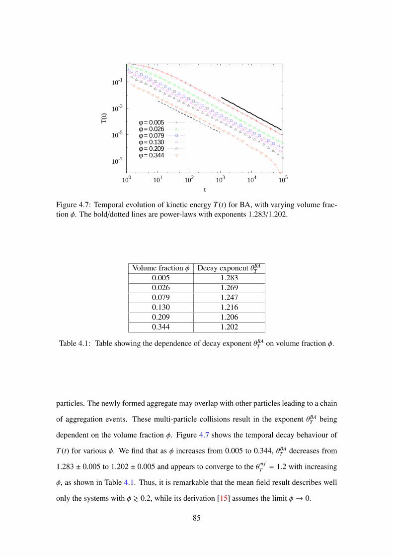
10-7

10-5

10-3

10-1

100 101 102 103 104 105

T(t

)

t

φ = 0.005φ = 0.026φ = 0.079φ = 0.130φ = 0.209φ = 0.344

Figure 4.7: Temporal evolution of kinetic energy T (t) for BA, with varying volume frac-

tion φ. The bold/dotted lines are power-laws with exponents 1.283/1.202.

Volume fraction φ Decay exponent θBAT

0.005 1.283

0.026 1.269

0.079 1.247

0.130 1.216

0.209 1.206

0.344 1.202

Table 4.1: Table showing the dependence of decay exponent θBAT on volume fraction φ.

particles. The newly formed aggregate may overlap with other particles leading to a chain

of aggregation events. These multi-particle collisions result in the exponent θBAT being

dependent on the volume fraction φ. Figure 4.7 shows the temporal decay behaviour of

T (t) for various φ. We find that as φ increases from 0.005 to 0.344, θBAT decreases from

1.283 ± 0.005 to 1.202 ± 0.005 and appears to converge to the θm f

T= 1.2 with increasing

φ, as shown in Table 4.1. Thus, it is remarkable that the mean field result describes well

only the systems with φ & 0.2, while its derivation [15] assumes the limit φ→ 0.

85

4.3.2 Cluster Size Distribution

The energy decay in FCGG and BA at higher densities being similar, how do other statisti-

cal properties compare? We first study clusters of particles in the inhomogeneous regime.

Snapshots of FCGG and BA (see Fig. 4.8) show that clusters in FCGG are extended as

opposed to compact spherical clusters (by construction) in BA. The spatial distribution of

particles is partially quantified by measuring the cluster size distribution N(m, t), where

m is the size of cluster. For the FCGG, the simulation box is divided into boxes of side

equal to the diameter of a particle. A box is said to be occupied if it contains the cen-

ter of a particle. Two occupied boxes belong to the same cluster if connected by nearest

neighbor occupied boxes. The cluster size distribution is then measured using the Hoshen-

Kopelman algorithm [112]. N(m, t) for the FCGG and BA, shown in the lower panel of

Fig. 4.8, are significantly different from one another. For the FCGG, N(m, t) consists of

two parts: a power law (∼ m−2.7) and a peak at large cluster sizes. The power law de-

scribes all clusters other than the largest cluster that accounts for the peak. The largest

cluster contains about 75% of the particles. For BA, N(m, t) is a power law for small

cluster sizes (∼ m−0.2) and exponential for cluster sizes larger than the mean cluster size.

Both of these distributions are different from the mean field result for N(m, t) obtained

from the Smoluchowski equation describing the temporal evolution of N(m, t):

N(m, t) =

m−1∑

m1=1

N(m1, t)N(m−m1, t)K(m1,m − m1)

− 2

∞∑

m1=1

N(m1, t)N(m, t)K(m1,m) m = 1, 2, . . . , (4.3)

where

K(m1,m2) ∝ (m−1/21+ m

−1/22

)(m1/31+ m

1/32

)2 (4.4)

is the collision kernel [98, 113]. For this kernel, it is known that that N(m, t) ∼ exp(−const×

m−1/2) for small m and N(m, t) ∼ exp(−const × m) for large m [98]. While the simulation

results for BA matches for large m, it is different (being a power law) for small m.

86

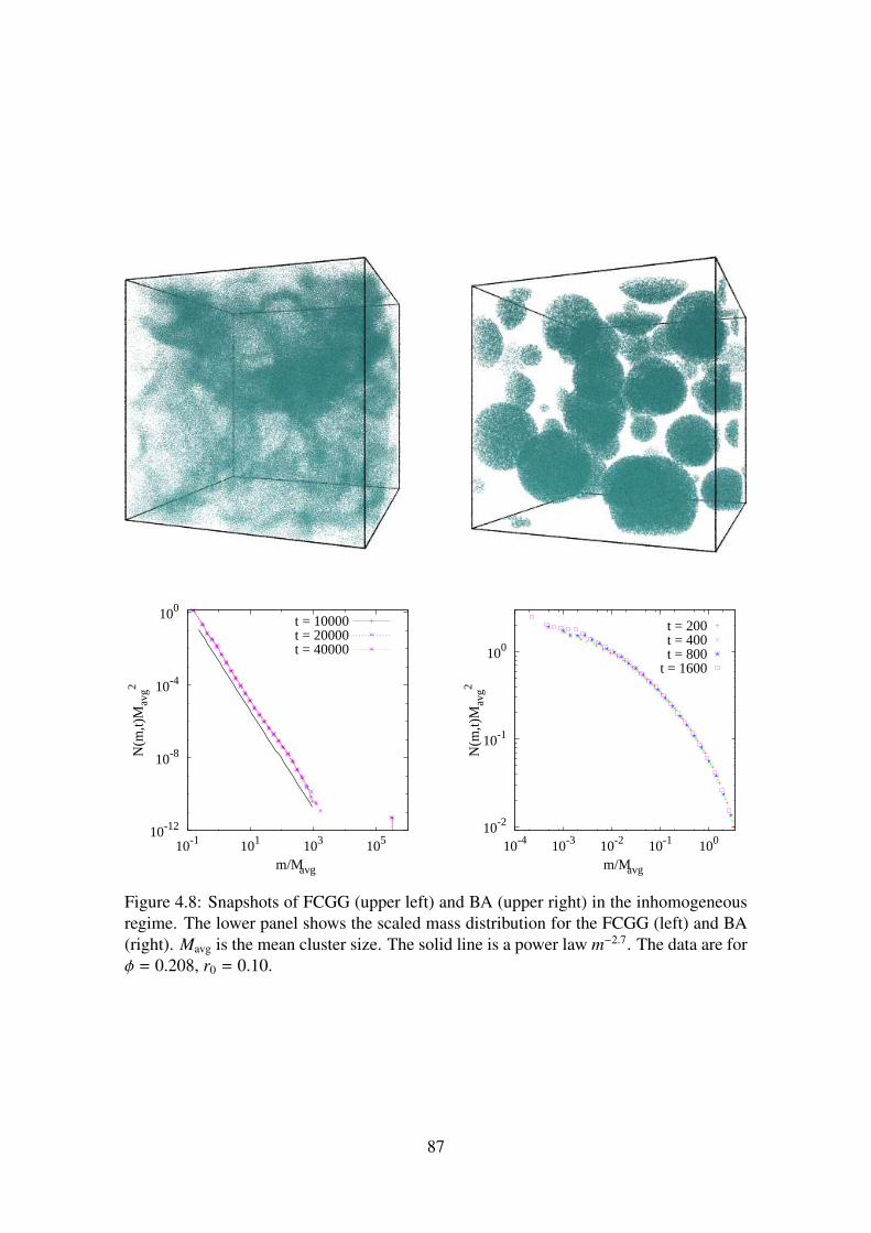
10-12

10-8

10-4

100

10-1 101 103 105

N(m

,t)M

avg2

m/Mavg

t = 10000t = 20000t = 40000

10-2

10-1

100

10-4 10-3 10-2 10-1 100

N(m

,t)M

avg2

m/Mavg

t = 200t = 400t = 800

t = 1600

Figure 4.8: Snapshots of FCGG (upper left) and BA (upper right) in the inhomogeneous

regime. The lower panel shows the scaled mass distribution for the FCGG (left) and BA

(right). Mavg is the mean cluster size. The solid line is a power law m−2.7. The data are for

φ = 0.208, r0 = 0.10.

87

10-5

10-4

10-3

10-2

10-1

100

100 101 102 103 104 105

Mm

ax/N

t

FCGG,φ = 0.208FCGG,φ = 0.132

BA, φ = 0.208BA, φ = 0.132BA, φ = 0.005

Figure 4.9: The largest mass Mmax as a function of time t. For the FCGG, r0 = 0.10,

δ = 10−4. Straight lines are power laws t0.94, t0.99, t1.03 (bottom to top).

Also, for the kernel in Eq. (4.4), it is expected that the largest cluster size Mmax increases

with time t as a power law t6/5 [98, 113], the mean field answer. We compare this predic-

tion with the simulations for the FCGG and BA. For the FCGG, rather than a power law

growth as in one and two dimensions and in mean field, there is a rapid increase in Mmax

(see upper two curves of Fig. 4.9) at a time that coincides with the onset of the inhomoge-

neous cooling regime. This rapid growth is similar to the gelation transition where a gel

containing a fraction of the total number of particles is formed in finite time. However

the kernel for BA is non-gelling with mass dimension 1/6, whereas the gelation transition

requires mass dimension to be larger than 1 [98, 113]. For BA, Mmax increases as a power

law (see bottom three curves of Fig. 4.9), with an exponent that increases with φ, and

possibly converges to the mean field value 6/5. Similar behavior is seen for the growth

of average cluster size of BA which grows as a power law with an exponent ranging from

1.06 for φ = 0.005 to 1.19 for φ = 0.313.

88

4.3.3 Velocity Distribution

We further compare the velocity distributions P(v, t), where v is any velocity component,

of the FCGG with that of BA. P(v, t) has the scaling form

P(v, t) =1

vrms

Φ

(

v

vrms

)

, (4.5)

where vrms is the time dependent root mean square velocity. The scaling function Φ(y)

is shown in Fig. 4.10 for different times. We note that in our simulations Φ(y) does not

depend on the coefficient of restitution or the initial velocity distribution, having checked

for Gaussian, uniform, and exponential distributions. For the FCGG, at short times when

the system is homogeneous (t = 5, 10 in Fig. 4.10), Φ(y) is an exponential e−αy as pre-

dicted by kinetic theory. We find α = 2.65, in good agreement with the kinetic theory

value 2.60 [89]. For larger times (t = 2000 – 8000 in Fig. 4.10), Φ(y) is clearly non-

Gaussian and has a tail that is overpopulated compared to the Gaussian (see comparison

with Gaussian in Fig. 4.10). A quantitative measure of the deviation from the Gaussian is

the kurtosis,

κ = 〈v4〉/〈v2〉2 − 5/3. (4.6)

Its value is zero for a Gaussian distribution. Figure 4.11 shows the time evolution of

kurtosis. The kurtosis after an initial increase, decreases and saturates to a non-zero value,

showing quantitatively that Φ(y) is non-Gaussian.

The large y behavior of Φ(y) is shown in Fig. 4.12. The large y behavior can be un-

derstood with a heuristic argument [13, 14]. The large velocity tails are dominated

by the fastest particles (v ≈ 1) present in the system initially, who have managed to

avoid any collision and are still moving with their initial velocity at time t. For such

a particle to avoid collision, an interval of length ∝ t ahead of the particle must be

empty. Now, for an initially random spatial distribution, the probability of obtaining

such an empty interval decays exponentially with length, giving the survival probabil-

89

10-9

10-7

10-5

10-3

10-1

0 1 2 3 4 5 6 7

Φ(y

)

y

(2π)-1/2exp(-y2/2)22 exp(-2.65 y)

Figure 4.10: The scaled velocity distribution function Φ(y) for the FCGG at times t =

5, 10 (upper collapsed data) and t = 2000, 4000, 6000, 8000 (lower collapsed data). The

solid curve is a Gaussian. The data are for φ = 0.208, r0 = 0.10.

0

0.1

0.2

100 101 102 103 104

κ

t

Figure 4.11: The kurtosis κ as a function of time t. The data are for φ = 0.208, r0 = 0.10.

90

100

101

102

10-2 10-1 100 101

-ln Φ

(y)

y

y5/3

y0.70

Figure 4.12: − lnΦ(y) as a function of y for the FCGG (lower data) and BA (upper data).

For FCGG, the times are t = 2000, 4000, 6000, 8000 and φ = 0.208, r0 = 0.10. For BA,

the times are t = 400, 800, 1600 and φ = 0.208.

ity S (v = 1, t) ∝ exp(−constant × t). Thus, the distribution for the fastest particles at

time t, P(1, t) = P(1, 0)S (1, t) ∝ exp(−constant × t). We assume a stretched exponential

large-velocity tail for the scaling function Φ(y) ∼ exp(−constant × |y|γ), for y → ∞, with

y = v/vrms ∼ vt θT /2. Comparison of P(1, t) from the survival probability argument with

the scaling behavior P(1, t) ∼ exp(−constant × tγθT /2) gives γ = 2/θT . For the FCGG (see

Fig. 4.12), we find that − ln[Φ(y)] ∼ y5/3, consistent with the heuristic argument, with

θT = 6/5. However, for BA we find − ln[Φ(y)] ∼ y0.70. The deviation of BA is surprising,

but may be rationalized. The argument for the exponential form of survival probability

implicitly assumes that the number of clusters reach a time independent distribution re-

sulting in a constant rate of collision. That this is true for the FCGG and not for BA can

be seen from the lower panels of Fig. 4.8, where Mmax and hence Mavg is nearly a constant

for the FCGG and time dependent for BA (see Fig. 4.9) at large times.

Thus, in spite of having the same form of energy decay, the local environment that a

particle in a FCGG sees around itself, is distinct from those in BA. In BA, two colliding

clusters rearrange their masses to form a new spherical cluster at every step. Due to

the lack of such dynamic cluster rearrangements, the FCGG remains locally structurally

91

anisotropic and disordered, as well as has a velocity distribution distinct from BA as

discussed above.

4.4 Conclusion

To summarize this chapter, we studied FCGG in three dimensions using large-scale event

driven molecular dynamics simulations. We found that the energy T (t) of this system

decreases as t−θT , with θT ≈ 6/5. This decay exponent is universal, i.e., independent

of the system parameters such as volume fraction, coefficient of restitution. The energy

continues to decay with the same exponent θT ≈ 6/5, when a more realistic, velocity

dependent coefficient of restitution model is considered.

This rules out Burgers like equations as a description of the FCGG at large times, which

predicted θT to be 1.5 in three dimensions. Our observed θT is indistinguishable from

the mean field result for dilute ballistic aggregation. The relation to ballistic aggregation

appears coincidental, as our direct numerical simulation of ballistic aggregation shows

that the energy of the dilute ballistic gas decaying with a different exponent. In addition,

the cluster size distribution as well as the velocity distribution of ballistic aggregation

are strikingly different from that of the FCGG. Thus, our study concludes that the freely

cooling FCGG fits to neither the ballistic aggregation or a Burgers equation description.

92

Chapter 5

Inhomogeneous Cooling of the Rough

Granular Gas in Two Dimensions

5.1 Introduction

In Chapter 4, we studied freely cooling granular gas of hard-core smooth particles, which

is also termed as smooth granular gas (SGG). In SGG, dissipation is considered only in

normal direction of collision which is accounted by the coefficient of normal restitution

r. However, realistic models of non-sliding collisions of hard spheres involve one more

parameter, the coefficient of tangential restitution β, quantifying the dissipation in tan-

gential direction of collisions [50, 114, 115, 116, 117]. This parameter β characterizing

tangential dissipation is ignored in most studies of the freely cooling granular gas.

In this chapter, we extend our study of freely cooling granular gas by including this param-

eter β. When the collisions include tangential dissipation β, the translational and rotational

modes are no longer independent of each other [16, 88, 118, 119, 120, 121, 122, 123, 124].

We call this model the rough granular gas (RGG). Of primary interest in this model is the

evolution of the translational kinetic energy T (t) and rotational energy K(t) with time t,

93

defined in Eqs. (2.14) and (2.15).

Studies of RGG have been limited to the homogeneous cooling regime. In this regime,

kinetic theory [16, 88, 118, 119, 120, 121] and simulations [16, 121] show that both trans-

lational energy T (t) and rotational energy K(t) decreases as t−2. However, the partitioning

of energy into the rotational and translational modes does not follow equilibrium equipar-

titioning, and depends on both r and β. In addition, the directions of the translational and

angular velocities of a particle were found to be strongly correlated [122, 125].

The inhomogeneous clustered regime of RGG is poorly studied. In this chapter, we study

the inhomogeneous regime of two dimensional RGG using large scale event driven molec-

ular dynamics simulations. Let T (t) ∼ t−θT and K(t) ∼ t−θK in this regime. We show that

θT is independent of β and is the same as that for SGG, i.e., θT ≈ 1. The exponent θK is

also shown to be independent of the choice of r and β, |β| < 1 and to be θK = 1.60 ± 0.04,

different from θK = 2 in the homogeneous regime. Thus, unlike the homogeneous regime,

the two exponents θT , θK differ from each other. These exponents are compared with the

corresponding exponents for BA with rotational degrees of freedom. The translational

energy of BA is independent of its rotational degrees of freedom and hence θBAT ≈ 1 for

large enough initial densities [99]. Numerically, we find that θBAK ≈ 1 for BA. We conclude

that the large time limit of RGG is different from that of BA, even though clustering is

present. Finally, we extend the scaling arguments of Ref. [15] to BA with rotational de-

gree of freedom. The scaling arguments predict θm f

K= 1 in two dimensions. This is clearly

in contradiction with the numerically obtained value of 1.6 ± 0.04. This further supports

the view [19, 99, 126], as concluded in previous chapter, that the energy decay in the SGG

being described accurately by θm f

T= 2D/(D + 2) in D dimensions is a coincidence.

The rest of the chapter is organized as follows. In Sec. 5.2, simulation details are provided.

The mean-field scaling theory of BA is recapitulated for SGG and extended to RGG in

Sec. 5.3. Section 5.4 contains simulation results for RGG and BA. Finally, we conclude

this chapter with a discussion in Sec. 5.5.

94

5.2 Simulation Details

Consider a system of N identical hard disks distributed uniformly in a two-dimensional

volume of linear length L with periodic boundary conditions in both directions. The mass

and diameter of the disks are taken to be unity. Initial translational and angular velocities

are drawn from a Gaussian distribution with mean zero and variance 1 and 8 respectively.

The variances are such that T (0) = 2K(0). Thus, energy is equipartitioned between all

three modes as one would expect in equilibrium. A particle moves ballistically till it

collides with another particle. Particles are considered rough for which the collisions are

described by the collision law, Eq. (2.5). We note that the translational kinetic energy and

rotational energy are both conserved only when r = 1(elastic) and β = −1. In this chapter,

we assume r and β to be constants, independent of the relative velocity of collision. BA

with rotational degree of freedom is discussed in detail in Sec. 2.7.1.

We simulate both RGG and BA in two dimensions using event driven molecular dynamics

simulations [110]. As discussed in last paragraph of Sec. 3.3.6, a cutoff velocity δ is

used to avoid inelastic collapse. This cutoff velocity introduces a timescale beyond which

collisions are mostly elastic, and the systems crosses over to a new regime where energy is

a constant. In our simulations, we choose δ = 10−5 for which we check that this crossover

timescale is much larger than the largest time in our simulations. Thus, the results in this

chapter are independent of δ. The results are for a system of N = 1562500 particles and

L = 2500 (volume fraction = 0.20).

5.3 Scaling Theory for Rotational Energy in Ballistic Ag-

gregation

The exponent θm f

Kfor BA may be determined using scaling arguments. In BA, particles

form spherical aggregates on collision. We first recapitulate the calculation of θm f

T=

95

2D/(D + 2) [15] as outlined in Refs. [19, 127]. Let n be the number density. It evolves in

time as

dn

dt= −n

τ, (5.1)

where τ is the mean collision time. In D dimensions,

1

τ∼ nvrmsR

D−1t , (5.2)

where vrms is the root mean squared velocity and Rt is the radius of a typical aggregate at

time t. Since total mass is conserved, Mtn ∼ 1 or equivalently Rt ∼ n−1/D. Substituting

for τ from Eq. (5.2) in Eq. (5.1),

dn

dt∼ −n1+1/Dvrms. (5.3)

The dependence of vrms on Mt is required. An aggregate of mass Mt is formed by aggre-

gation of Mt particles of mass 1. Conservation of linear momentum, combined with the

assumption of uncorrelated momenta, gives Mtvrms ∼ M1/2t , or vrms ∼ n1/2. Substituting

for vrms in Eq. (5.3), we obtain

n(t) ∼ t−2D/(D+2). (5.4)

The scaling of root mean square angular velocity ωrms with time t may be obtained from

conservation of angular momentum. If two particles i and j of masses mi, m j at ~ri, ~r j,

moving with velocities ~vi, ~v j, angular velocities ~ωi, ~ω j, and moment of inertia Ii and I j

collide to form a particle of mass m′ at ~r′ with velocity ~v′, and moment of inertia I′, then

its angular velocity ~ω′ is given by

I′ ~ω′ = Ii~ωi + I j~ω j +mim j

mi + m j

(~ri − ~r j) × (~vi − ~v j). (5.5)

Let ωrms be the root mean square angular velocity of the typical particle whose moment

of inertia is It ∼ MtR2t . In Eq. (5.5), there are three terms on the right hand side. We

96

first assume that the right hand side is dominated by the first two terms. Then the angular

momentum Itωrms is a sum of Mt random variables of mean zero and variance order 1,

giving

Itωrms ∼√

Mt. (5.6)

or equivalently ωrms ∼ M−(D+4)/(2D)t . But the rotational energy K(t) scales as K ∼ nItω

2rms.

Simplifying, we obtain K ∼ t−2, independent of dimension. We now assume that the right

hand side of Eq. (5.5) is dominated by the third term. Then, clearly Itωrms ∼ MtRtvrms.

Using Mtn ∼ 1, we obtain ωrms ∼ n(D+2)/(2D) ∼ t−1. The rotational energy Itω2rms now

scales as t−2D/(D+2). This has a slower decay in time than t−2 obtained from assuming

that Eq. (5.5) is dominated by the first two terms. The kinetic energy T ∼ nMtv2rms and

rotational energy K are thus given by

T ∼ t−2D/(D+2), (5.7)

K ∼ t−2D/(D+2), (5.8)

implying that θm f

T= θ

m f

K= 2D/(D+2). Thus, one expects that the ratio of the two energies

is a constant in the clustered inhomogeneous regime as it is in the homogeneous regime.


5.4.1 Rough Granular Gas (RGG)

We now present results for RGG obtained from numerical simulations. Figures 5.1 and 5.2

show the temporal evolution of translational kinetic energy T (t). Here, the coefficient of

normal restitution r = 0.1. For this value of r, the homogeneous regime is short lived.

The crossover time from the homogeneous to inhomogeneous regime depends on β, the

crossover time increasing with |β|. This is expected as increasing |β| corresponds to de-

97

10-5

10-4

10-3

10-2

10-1

100

100 101 102 103 104 105

T(t

)

t

t-1

β = 1.0β = 0.8β = 0.6β = 0.4β = 0.2

Figure 5.1: Time evolution of translational kinetic energy T (t) for RGG when β > 0 for

fixed r = 0.10.

creasing dissipation, and hence a longer homogeneous regime. For β < 0, the dependence

of the crossover time on β is very weak. For all values of β, the data is consistent with

θT = 1 (see Figs. 5.1 and 5.2), same as that obtained for SGG [14]. We check that the θT

remains the same for r = 0.5 and r = 1.0 (but |β| < 1). We conclude that θT for RGG is

independent of the values of both r and β. These extend the results obtained earlier for

SGG (β = −1), where θT was shown to be independent of r [13, 14, 126].

Figures 5.3 and 5.4 show the temporal evolution of rotational energy K(t) for β > 0 and

β < 0 respectively. The crossover to inhomogeneous regime occurs at a much later time

when compared with T (t). A signature of this difference in crossover times was observed

in Ref. [16], where T was found to deviate from the homogeneous cooling behaviour of

t−2 decay, while K still followed it. We also observe that the crossover times are much

larger for β < 0 as compared to that β > 0. When β = −1, K(t) is conserved. At large

times, the data for K(t) are completely independent of β (see Figs. 5.3 and 5.4). We

estimate θK = 1.60 ± 0.04.

We also confirm that θK is independent of r. In Fig. 5.5, we show the dependence of

K(t) on r by varying r and keeping β = 0.60 fixed. K(t), while decaying with a r-

98

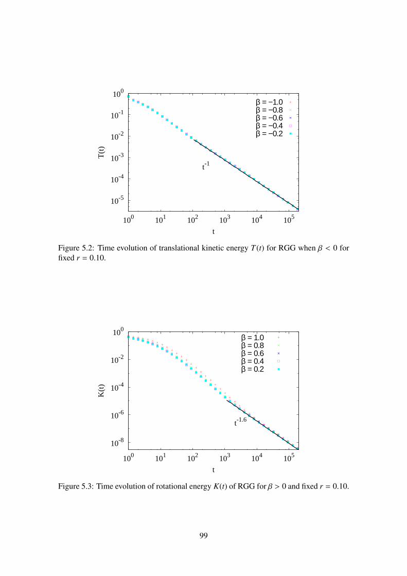
10-5

10-4

10-3

10-2

10-1

100

100 101 102 103 104 105

T(t

)

t

t-1

β = −1.0β = −0.8β = −0.6β = −0.4β = −0.2

Figure 5.2: Time evolution of translational kinetic energy T (t) for RGG when β < 0 for

fixed r = 0.10.

10-8

10-6

10-4

10-2

100

100 101 102 103 104 105

K(t

)

t

t-1.6

β = 1.0β = 0.8β = 0.6β = 0.4β = 0.2

Figure 5.3: Time evolution of rotational energy K(t) of RGG for β > 0 and fixed r = 0.10.

99

10-8

10-6

10-4

10-2

100

100 101 102 103 104 105

K(t

)

t

t-1.6

β = −1.0β = −0.8β = −0.6β = −0.4β = −0.2

Figure 5.4: Time evolution of rotational energy K(t) of RGG for β < 0 and fixed r = 0.10.

independent exponent, now has a r-dependent pre-factor. Thus, we conclude that at large

times, K(t) ≃ A(r)t−θK , where θK ≈ 1.60 is independent of r and β.

5.4.2 Ballistic Aggregation (BA)

We now present the results from numerical simulations of BA. In these simulations, when-

ever two particles collide we replace them with a single spherical particle conserving

mass, volume, linear and angular momenta as described in Eqs. (2.59)–(2.62). If the

new particle overlaps with another particle, then these two particles aggregate. Thus, a

collision between two particles may give rise to a chain of aggregation events.

For BA, it is easy to check from Eqs. (2.59) and (2.60) that including rotational degrees

of freedom does not affect the translational kinetic energy T (t). That being the case, we

expect that θBAT for the rough BA to be identical to that for the smooth BA. The numerical

values of θBAT for the rough BA for different initial volume fraction φ are tabulated in the

second column of Table 5.1. θBAT depends weakly on φ [19, 99, 126], and approaches 1

with increasing φ. θBAT = 1 for BA is consistent with the scaling arguments [see Eq. (5.7)],

and is equal to θT for RGG.

100

10-8

10-6

10-4

10-2

100

100 101 102 103 104 105

K(t

)

t

t-1.6

t-1.6

r = 0.1r = 0.8r = 0.9r = 1.0

Figure 5.5: Time evolution of rotational energy K(t) of RGG for different r and fixed

β = 0.60.

Table 5.1: Dependence of exponents θBAT and θBA

K on volume fraction φ in the BA model.

φ θBAT θBA

K

0.008 1.12-1.13 1.10-1.12

0.079 1.05-1.06 1.07-1.08

0.196 1.01-1.02 1.03-1.04

0.393 1.01-1.02 1.00-1.01

101

10-6

10-4

10-2

101 102 103 104 105

K(t

)

t

t-1.12

t-1.00

φ = 0.008φ = 0.079φ = 0.196φ = 0.393

Figure 5.6: Time evolution of the rotational energy K(t) of BA for different volume frac-

tions φ.

The variation of the rotational kinetic energy K(t) for BA with time t is shown in Fig. 5.6.

Similar to θBAT

, θBAK

also decreases with increasing volume fraction φ (see third column of

Table 5.1). With increasing φ, θBAK converges to a value very close to 1, different from that

obtained for RGG. Note that the scaling argument for BA predicts θm f

K= 1 (see Eq. 5.8).

5.5 Conclusion

To summarize, we investigated the large time behaviour of a freely cooling rough granular

gas in two dimensions using event-driven simulations. Each collision dissipates energy

in both the normal and tangential directions. We showed that in the clustered inhomo-

geneous regime, both the translational kinetic energy T (t) and the rotational energy K(t)

decay with time t as power-laws AT t−θT and AKt−θK where θT ≈ 1.0, and θK ≈ 1.6. These

exponents are universal and independent of r and β. Within numerical errors, AT is also

independent of r and β, while AK depends only on r. For ballistic aggregation with ro-

tational degree of freedom, wherein particles coalesce on contact, we find that θBAT ≈ 1.0

and θBAK ≈ 1.0 for large enough initial volume fraction φ. By extending an earlier scaling

102

theory for BA, we obtain θm f

K= 1, consistent with the numerically obtained value.

Kinetic theory for rough granular gases predicts that K(t)/T (t) tends to a non-zero con-

stant that depends on r and β [16, 118, 121]. In the inhomogeneous regime, since θT < θK

for the rough granular gas, the ratio K(t)/T (t) tends to zero at large times. Violation of

kinetic theory is not surprising given that it assumes that particles are homogeneously

distributed, which is not the case in the inhomogeneous regime.

The clustered regime of the freely cooling granular gas has been often thought to be de-

scribable by the large time behaviour of the ballistic aggregation model. This analogy

has been reinforced in particular by the fact that, within numerical error, energy decay in

both systems is the same in one, two and three dimensions [13, 14, 126]. However, it has

been shown that correlation functions that capture spatial distribution of particles and the

velocity distributions in the granular gas are different from that of BA [9, 126]. In partic-

ular, it has been argued that a coarse grained model with aggregation and fragmentation

is more suitable to study the clustered regime than one of pure aggregation as in the BA

model [71]. Here, the fact that the rotational energies in the two models decay with two

exponents is further evidence that the analogy should be used with care.

In the scaling arguments presented in this chapter and in Ref. [15], the correlations be-

tween velocities of colliding particles are ignored. Therefore, it has often been argued that

the efficacy of the scaling arguments is a coincidence [19, 99]. In this paper, we showed

that the extension of the scaling arguments to rotational energies correctly predict the nu-

merical results for BA, albeit for larger volume fractions φ. We conclude that the scaling

arguments are quite robust, rather the connection to granular gas is more suspect.

103

Chapter 6

Shock Propagation in Granular Flow

Subjected to an External Impact

6.1 Introduction

In this chapter, we study the granular explosion model. This model is a special case

of freely cooling granular gas, where all particles, except for a few localised particles,

are at rest. The name granular explosion stems from the similarity of this model to a

bomb/nuclear explosion [128, 129, 130], where a large amount of energy is deposited at

one place giving rise to a shock wave. Locally perturbed systems are the subject matter of

many recent experiments. Examples include crater formation by wind jets in the context

of lunar cratering [131], viscous fingering in grains confined in a Hele-Shaw cell when

displaced by gas or liquid [62, 132, 133], shock propagation in flowing glass beads fol-

lowing a sudden impact [6], signal propagation in dilute granular gas [134] as well as in

dense static granular material (see [135] and references within), and avalanches in sand

piles [136].

The granular explosion model is the inelastic version of the classic Taylor-von Neumann-

105

Sedov problem of shock propagation following a localized intense explosion [129]. In

the latter case, the exponents characterizing the power law growth of the radius of the

disturbance follows from energy conservation and simple dimensional analysis [128],

while the scaling functions can be calculated exactly following a more detailed analy-

sis [129, 130]. Theoretical, numerical and experimental studies of this problem are sum-

marized in Refs. [137, 138]. Simulations in a hard sphere model with elastic collisions

reproduce the results based on scaling arguments [139].

The granular explosion model was studied in Ref. [7] with hard inelastic particles using

event driven molecular dynamics simulations, and scaling arguments. By identifying ra-

dial momentum as a conserved quantity, and using scaling arguments, the radius of distur-

bance R(t) was predicted to increase with time t as a power law t1/(D+1) in D-dimensions.

This result was shown to be in very good agreement with data from numerical simulations

of the model.

In this chapter, we focus on an experiment [6] (henceforth referred to as BCK) on a

dilute monolayer of glass beads flowing on an inclined glass plane. In the experiment,

a steel ball, much larger in size than an individual glass bead, is dropped from a height

onto the flowing beads. The impact generates a circular region, devoid of glass beads,

whose radius increases with time. This radius was measured using high speed cameras.

A theoretical model was proposed, and analyzed to derive an equation obeyed by the

radius. The numerical solution of the equation was shown to match with the experimental

data [6].

The inelastic granular explosion model closely resembles the experimental system in

BCK, in the limit when the impact is very intense. In this chapter, we propose the power

law t1/3 (D = 2) as an alternate description of the radius of disturbance in the BCK ex-

periment. By re-examining the data in BCK, we show that, there are temporal regimes

in which the power law growth is a good description. At late times, the experimental

data deviate from the t1/3 behavior. This, we argue is due to the experimental system be-

106

coming effectively three dimensional due to accumulation of particles at the shock front,

and propose a simple model incorporating this effect. Our numerical data, obtained from

simulations of this model, show clearly the crossover and captures the long time behavior.

Since these results are in contradiction to those presented in BCK, we further analyze the

model proposed in BCK, and point out some shortcomings. In particular, we show nu-

merically that the main assumption of BCK is not correct. Though the experimental data

are not able to distinguish between the two theories because the time scales are not large

enough, the simulation data clearly bring out the deficiencies of the BCK theory at large

times.

A key feature of the freely cooling granular gas is the clustering due to inelastic col-

lisions. The freely cooling gas is well understood in one dimension and progressively

less understood as the dimension increases [13, 14, 15, 19, 93, 140]. Such systems are

challenging experimentally because inelasticity is overwhelmed by friction and boundary

effects. Friction can be eliminated in experiments on particles under levitation [83] or in

microgravity [84, 85], but are expensive to perform and are limited by small number of

particles and short times. In BCK, friction is balanced by gravity, and at high enough

impact energies, in the center of mass frame, mimics a stationary collection of inelastic

particles without friction. The boundary effects are eliminated as long as the shock does

not reach the edges of the container. Thus, it is an experiment where clustering due to

inelastic collisions can be studied easily.

The rest of the chapter is organized as follows. In Sec. 6.2, we define the hard core

granular explosion model. The temporal patterns arising in the system are discussed in

Sec. 6.3. The growth of radius of disturbance with time is obtained, using argument of

radial momentum conservation. In Sec. 6.4 we describe the experimental setup of BCK,

and the theoretical model reviewing the arguments that lead to the equation obeyed by

the radius of the disturbance. This equation is further analyzed to derive the asymptotic

long time behavior. The shortcomings of the BCK analysis are pointed out in Sec 6.5.

107

Our model reproduces the basic features of the experiment in BCK. The assumptions of

the analysis in BCK is tested within this model and counter evidence is presented. In

Sec. 6.6, we compare the experimental results in Ref. [6] with the power law growth rules

obtained in Ref. [7]. The data at intermediate times are well described by these power

laws. However, there is a crossover to a different behavior at large times. We examine

whether this large time behavior can be explained in terms of velocity fluctuations of the

particles or by making the rim three dimensional. We argue that it is plausible that the

three dimensional rim is responsible for deviation from power law growth and verify this

by simulation. This chapter is summarized in Sec. 6.7.

6.2 Model

The model is defined as follows. Consider a collection of identical hard sphere particles,

in two dimensions. The mass and diameter of the particles are set to unity. All the particles

are initially at rest and have a packing density 0.20, much smaller than the known random

closed packed density 0.84 in two dimensions [141, 142]. We model an isotropic impulse

by introducing four particles at the center with speed v0 in the directions 0, π/2, π, and

3π/2. Particles move ballistically until they undergo momentum conserving, deterministic

collisions with other particles. Particles are considered smooth for which the collisions

are described by the collision law, Eq. (2.6). The coefficient of restitution r = 1 for elastic

and 0 < r < 1 for inelastic collisions. As discussed in last paragraph of Sec. 3.3.6, to

avoid inelastic collapse in the inelastic system, a cutoff velocity δ is used, below which

collisions are considered elastic. The cutoff δ introduces a timescale in the problem at

large times, after which most of the collisions are elastic. For sufficiently small δ, the

elastic crossover timescale does not show up in our simulations.

We simulate the system in two dimensions using event driven molecular dynamics [110].

The data are typically averaged over 8 different initial realizations of the particle config-

108

urations. All lengths are measured in units of the particle diameter, and time in units of

initial mean collision time t0 = v−10 n−1/D, where v0 is the initial speed, n is the number

density. The value of δ is 10−4, unless specified otherwise. For these values of δ, all the

quantities that we measure except for the rate of collisions are independent of δ [7]. The

initial speed is v0 = 1 unless specified otherwise.

6.3 Analysis of the Model

In this section, we present the results obtained by the numerical simulation of the model.

The numerical results are explained by analysis based on radial momentum conservation.

6.3.1 Pattern Formation

First we consider the elastic system with r = 1. Figure 6.1 shows the time evolution of

the elastic system following an isotropic impulse. The four particles with non-zero initial

velocity set off a cascade of collisions leading to the formation of a circular region of

moving particles. This circular region grows outwards because of the collision of moving

particles near the boundary with the outside stationary particles.

The quantity of interest is the radius of disturbance R(t) which is defined as the average

distance of a moving particle from the center of mass of moving particles. Its tempo-

ral growth has been obtained by using simple dimensional analysis and energy conserva-

tion [128, 129, 130]. We reproduce it using simple scaling arguments. Assuming a power-

law growth for the radius of disturbance, R(t) ∼ tα, the typical velocity of a moving par-

ticle is V(t) = dR/dt ∼ t α−1, and the number of particles moving is Nm(t) ∼ R(t)D ∼ tαD.

The total energy of the system, E(t) ∼ Nm(t)V(t)2 ∼ tα(D+2)−2, is constant with time,

109

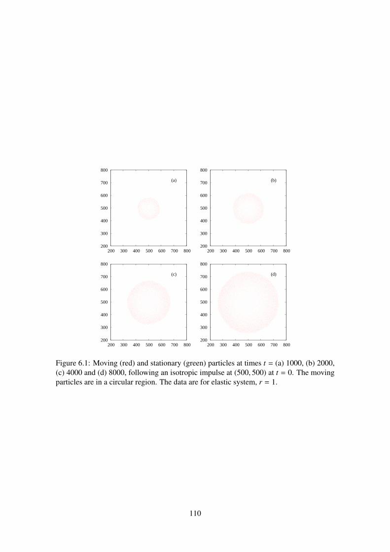
200

300

400

500

600

700

800

200 300 400 500 600 700 800

(a)

200

300

400

500

600

700

800

200 300 400 500 600 700 800

(b)

200

300

400

500

600

700

800

200 300 400 500 600 700 800

(c)

200

300

400

500

600

700

800

200 300 400 500 600 700 800

(d)

Figure 6.1: Moving (red) and stationary (green) particles at times t = (a) 1000, (b) 2000,

(c) 4000 and (d) 8000, following an isotropic impulse at (500, 500) at t = 0. The moving

particles are in a circular region. The data are for elastic system, r = 1.

110

101

102

103

101 102 103 104 105

R(t

)

t

t1/2

Elastic

Figure 6.2: Radius of disturbance R(t) vs time t for elastic system in two dimensions. The

simulation data fits well with the power law t1/2.

E(t) ∼ t0. Thus, the temporal growth of the radius of disturbance is given by

R(t) ∼ t2/(D+2). (6.1)

This power-law growth of radius [Eq. 6.1] was verified in numerical simulations [139] for

one and two dimensions. We reproduced it in our simulations and is shown in Fig. 6.2 for

two dimensions.

We now discuss our work where we consider the collisions to be inelastic. Throughout

this chapter we discuss this inelastic system unless otherwise mentioned. In Fig. 6.3, we

show the time evolution of the system following the isotropic impulse. As time increases,

all the particles that were originally in a roughly circular ring, cluster together at its rim.

The inside region is completely devoid of particles unlike the elastic case. We observe

clustering for all the values of r < 1 that we have simulated, with clustering setting in

at later times for larger coefficients of restitution. Temporal behavior of R(t) for this

system can be obtained by an argument based on radial momentum conservation, which

we discuss in next subsection.

111

0

200

400

600

800

1000

0 200 400 600 800 1000

(a)

0

200

400

600

800

1000

0 200 400 600 800 1000

(b)

0

200

400

600

800

1000

0 200 400 600 800 1000

(c)

0

200

400

600

800

1000

0 200 400 600 800 1000

(d)

Figure 6.3: Moving (red) and stationary (green) particles at times t = (a) 103, (b) 104,

(c) 105 and (d) 106, following an isotropic impulse at (500, 500) at t = 0. The moving

particles cluster together at the disturbance front. The data are for r = 0.10.

6.3.2 Radial Momentum Conservation

We first argue that the radial momentum in a fixed direction cannot decrease. It can

decrease only if the pressure outside the growing circular ring is larger than the pressure

inside. However, the outside pressure is zero since all the particles are stationary, and

the inside pressure is non-negative since it is a collection of hard-core repulsive particles.

Thus, the radial momentum of the system cannot decrease with time. The argument that

the radial momentum cannot decrease with time puts bounds on the growth exponent of

the radius of disturbance. Assuming that R(t) ∼ tα for t ≫ 1, the number of moving

particles Nm(t) ∼ tαD and the typical velocity of a particle in the ring V(t) = dR/dt ∼ tα−1.

Then, radial momentum that is NmV scales as tα(D+1)−1. We immediately obtain that the

radius cannot grow more slowly than R ∼ t1/(D+1), within the framework of the model.

We now argue that radial momentum is not just nondecreasing, but a constant of motion.

Every collision is momentum conserving. In addition, the clustering of all the displaced

particles at the rim of the ring prevents momentum being transferred in the negative radial

112

direction. If we further assume that once the dense rim is formed, the angular coordi-

nates of particles do not change much, then radial momentum is a constant of motion.

Therefore,

ΩDR(t)DV(t)∆θ = constant, (6.2)

where ΩD is the volume of a unit sphere in D-dimensions and ∆θ is the angular spread in

direction θ. The solution to Eq. (6.2) is

R(t) ∝ tα, t ≫ t′, (6.3)

where α = 1/(D + 1), and t′ is the initial mean collision time.

We present numerical evidence for radial momentum being a constant of motion, as ar-

gued above. In Fig. 6.4, the temporal variation of the radial momentum is shown for

different δ with fixed r = 0.10 and compared with the data for the elastic problem. When

all collisions are elastic, radial momentum increases as√

t. When collisions are inelas-

tic, radial momentum increases very slowly with time from an initial value of 4.0 to 8.6,

in nearly six decades of time (see Fig. 6.5). With the current data, it is not possible to

conclude with certainty that radial momentum will become a constant at large time when

δ → 0. However, one can rule out a power law growth. The radial momentum conser-

vation is strictly valid only when collisions are completely inelastic, r = 0 and δ = 0.

However, for other value of r and δ, even after formation of the circular band, colliding

particles may change their angular coordinates. Such changes in the angular coordinates

of the particles will result in increase of radial momentum. We checked that the average

change in angle following a collision decreases to zero with time, when δ is lowered as

shown in Fig. 6.6. The power-law growth of R(t) given by Eq. (6.3) which is based on

radial momentum conservation fits very well with the simulation data in two dimensions

as shown in Fig. 6.7.

113

101

102

103

101 102 103 104 105 106

Rad

ial m

omen

tum

t

Elastic δ = 10−2

δ = 10−3

δ = 10−4

δ = 10−5

Figure 6.4: The radial momentum as a function of time t. For elastic collisions, it in-

creases as√

t (the solid straight line is a power law√

t). For inelastic collisions with

r = 0.10, the radial momentum appears to increase very slowly with time to a constant,

when δ→ 0. The data for the elastic system have been scaled down by factor 1/2.

5

7

9

101 103 105

Rad

ial m

omen

tum

t

δ = 10−4

δ = 10−5

Figure 6.5: Two curves from Fig. 6.4 are plotted to show clearly the slow increase of the

radial momentum.

114

10-6

10-5

10-4

10-3

10-2

10-1

101 102 103 104 105 106

Ave

rage

Sca

tteri

ng A

ngle

t

δ =10−4

δ =10−5

δ =10−6

Figure 6.6: Average scattering angle on collision vs time t.

100

101

102

103

100 101 102 103 104 105 106

R(t

)

t

t1/3

Inelastic

Figure 6.7: Radius of disturbance R(t) vs time t for inelastic system (r = 0.10) in two

dimensions. The simulation data fits well with the power law t1/3.

115

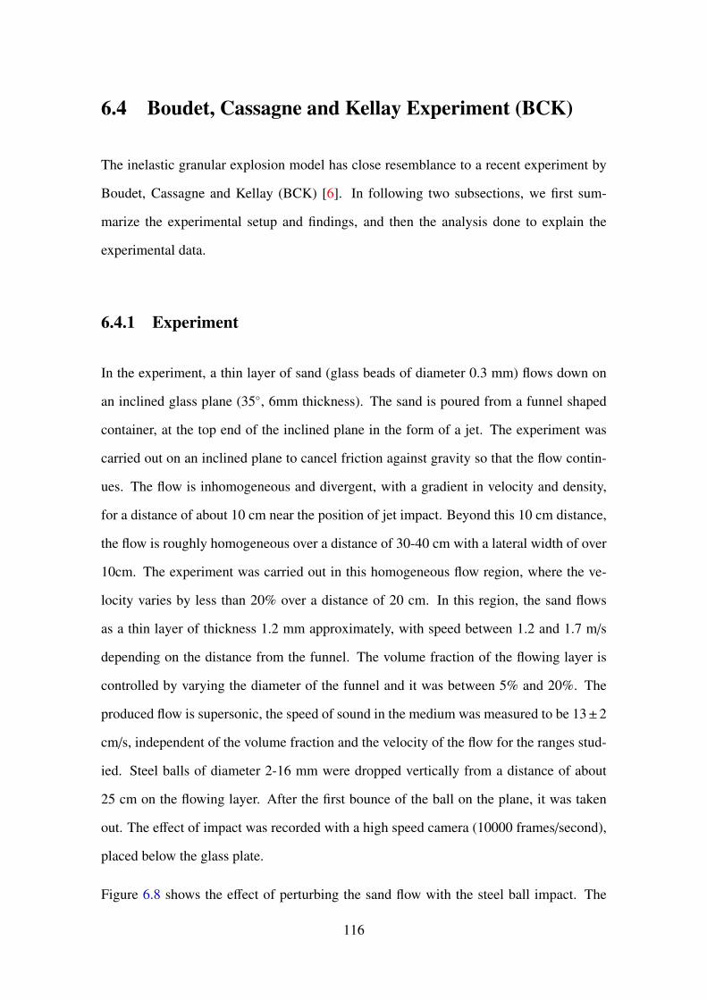
6.4 Boudet, Cassagne and Kellay Experiment (BCK)

The inelastic granular explosion model has close resemblance to a recent experiment by

Boudet, Cassagne and Kellay (BCK) [6]. In following two subsections, we first sum-

marize the experimental setup and findings, and then the analysis done to explain the

experimental data.

6.4.1 Experiment

In the experiment, a thin layer of sand (glass beads of diameter 0.3 mm) flows down on

an inclined glass plane (35, 6mm thickness). The sand is poured from a funnel shaped

container, at the top end of the inclined plane in the form of a jet. The experiment was

carried out on an inclined plane to cancel friction against gravity so that the flow contin-

ues. The flow is inhomogeneous and divergent, with a gradient in velocity and density,

for a distance of about 10 cm near the position of jet impact. Beyond this 10 cm distance,

the flow is roughly homogeneous over a distance of 30-40 cm with a lateral width of over

10cm. The experiment was carried out in this homogeneous flow region, where the ve-

locity varies by less than 20% over a distance of 20 cm. In this region, the sand flows

as a thin layer of thickness 1.2 mm approximately, with speed between 1.2 and 1.7 m/s

depending on the distance from the funnel. The volume fraction of the flowing layer is

controlled by varying the diameter of the funnel and it was between 5% and 20%. The

produced flow is supersonic, the speed of sound in the medium was measured to be 13±2

cm/s, independent of the volume fraction and the velocity of the flow for the ranges stud-

ied. Steel balls of diameter 2-16 mm were dropped vertically from a distance of about

25 cm on the flowing layer. After the first bounce of the ball on the plane, it was taken

out. The effect of impact was recorded with a high speed camera (10000 frames/second),

placed below the glass plate.

Figure 6.8 shows the effect of perturbing the sand flow with the steel ball impact. The

116

Figure 6.8: (a) An image of the flow. The experiment was carried out in the shown

rectangular region where the flow is roughly homogeneous. (b) Images of expanding hole

at different times after the impact of a 16 mm diameter steel sphere. Particles that were

originally in a circular region have clustered into a dense rim(white rim) surrounding the

hole (black circular region).(c) Impact of a 2 mm diameter sphere. Reprinted figure with

permission from J. F. Boudet, J. Cassagne, and H. Kellay, Physical Review Letters, 103,

224501 (2009) [6]. Copyright (2009) by the American Physical Society.

impact forces the sand grains to move radially outwards and form a dense rim, leaving

behind an empty circular region.

6.4.2 Analysis

We review the model studied in BCK to explain the experimental data, and then general-

ize it to D-dimensions and derive the asymptotic behaviour for small and large times. The

model is based on the experimental observation, that after the impact with the steel ball,

the displaced glass beads form a growing circular ring, devoid of beads. BCK considered

an idealized model where all the particles contained in a disk of radius R(t) at time t ac-

cumulate at the rim (boundary of ring). The remaining particles that are outside the disk

are assumed to be stationary. This mimics the experimental system when one transforms

to the center of mass coordinates, and in the limit of large impact energy, when the fluc-

tuations of the particle velocities about the mean flow may be ignored. Each particle at

the rim is assumed to move radially outwards with a speed V(t). As the ring moves out-

117

wards, more particles are absorbed into the ring. We reproduce the calculation in BCK,

but generalized to D-dimensions. The total kinetic energy E(t) is

E(t) =1

2ρ0ΩDR(t)DV(t)2, (6.4)

where ρ0 is the initial mass density, andΩD is the volume of a unit sphere in D-dimensions,

such that ρ0ΩDR(t)D is the total mass of displaced particles. The speed V(t) is

V(t) =dR(t)

dt. (6.5)

One more relation between E(t) and R(t) is required for the solution. If the particles

were elastic, then total energy is conserved, E(t) ∼ t0, and one obtains R(t) ∝ t2/(D+2); in

particular, R(t) ∝√

t in D = 2 [128]. However, when particles are inelastic, there is no

such conservation law, and energy decreases with time. BCK proceed by the following

argument. If r is the coefficient of restitution, then the loss of energy when a particle in

the rim collides with a stationary particle outside is 12(1 − r2)V(t)2. Thus, when the ring

moves out by a distance dR, then the change in energy dE is given by

dE = −1

2ΩDR(t)Dρ0V(t)2(1 − r2)N(t)dR, (6.6)

where N(t) is the number of collisions per particle per unit length, or equivalently, N(t)dR

is the number of collisions for each particle in the rim as it travels a distance dR. BCK

makes the strong assumption that N(t) is independent of the radius, and hence time t that

is,

N(t) = constant. (6.7)

Eliminating R(t) and V(t) in Eq. (6.6) using Eq. (6.4), one obtains

E(t) = E0 exp[

−N(1 − r2)R(t)]

, (6.8)

118

where E0 is the energy of impact at t = 0. It is now straightforward to obtain the equation

satisfied by the radius R(t):

t

t0

=

∫ R/R0

0

dx xD/2ex, (6.9)

where t−10 =

√

E0[N(1 − r2)]D+2/(ρ0ΩD2D+1) and R−10 = N(1 − r2)/2.

The experimental data in BCK was fitted to the numerical solution of Eq. (6.9) with D = 2.

Although the equation describes the data well (see Fig. 4 of Ref. [6]), we argue in next

section that the analysis has certain shortcomings, making the results questionable.

For later reference, it will be useful to derive the asymptotic solutions to Eq. (6.9). Let

α = ln(t/t0). Then for large times, it is straightforward to derive:

R

R0

= α

[

1 − D

2

lnα

α+

D

2

lnα

α2+ O

(

1

α2

)]

, α ≫ 1. (6.10)

The growth is logarithmic at large times in all dimensions. For short times, by writing the

exponential in Eq. (6.9) as a series, it is easy to obtain

R

R0

=

[

(D + 2)t

2t0

]2

D+2

1 + O

(

t

t0

)2

D+2

, t ≪ t0. (6.11)

For small times, the power law growth of radius is identical to the elastic case [128].

6.5 Critique of BCK Analysis

First, we show by a simple calculation that the solutions Eqs. (6.8) and (6.9) do not give

the correct results when D = 1. The solution Eqs. (6.8) and (6.9) are valid for all values

of r < 1, including r = 0. In one dimension, the special case r = 0, when particles stick

on collision, is easily solvable [7]. Let particles of mass m be initially placed equidistant

from each other with inter-particle spacing a. Pick a particle at random and give it a

velocity v0 to the right. When this particle collides with its neighbor, it coalesces with

119

it. After k collisions, the mass of the composite particle is (k + 1)m, its distance from the

impulse is R = ka, and its velocity, given by momentum conservation, is vk = v0/(k + 1)

towards the right. The time taken for k collisions is given by

tk =

k−1∑

i=0

a

vi

=ak(k + 1)

2v0

. (6.12)

Solving for k, we obtain k = (−1 +√

1 + 8tv0/a)/2. At large times t ≫ a/v0, the radius

and energy are R = ka ≈√

2v0at and E(t) = mv20a/(2R). The analysis in BCK for

energy [Eq. (6.8)] and radius [Eq. (6.10)] are not consistent with the exact solution in one

dimension.

Second, we show that the long time logarithmic growth of the radius of the disturbance, as

in Eq. (6.10), is not possible. Suppose we assume that Eq. (6.10) is right, i.e., R(t) ∼ ln t.

In two dimensions, the radial momentum is R(t)2V(t), where V(t) = dR/dt ∼ 1/t. Thus the

radial momentum scales as (ln t)2/t, implying that the radial momentum decreases with

time, which is impossible. Therefore, within the model, the logarithmic time dependence

of the radius is not possible.

Radial momentum conservation implies that R(t)D/2√

E(t) is a constant of motion. Equa-

tion (6.8) is clearly not consistent with this constraint, neither is Eq. (6.10) for growth of

radius consistent with Eq. (6.3).

We, therefore, conclude that the analysis of BCK is not completely satisfactory. Since

the solution of BCK [Eqs. (6.8) and (6.9)] was based on the assumption that N(t), the

rate of collisions per particle per unit distance, is a constant, we test the validity of this

assumption as well as the prediction of Eq. (6.9) in molecular dynamics simulations of a

hard sphere gas.

The formation of an empty region bounded by the moving particles (as in Fig. 6.3) is the

only requirement for the BCK theory to be applicable. Therefore, if the analysis in BCK

is correct, then the results for radius in Eq. (6.9) should describe the disturbance in the

120

100

101

102

103

100 101 102 103 104 105 106

R(t

)

t

t1/3

BCKSimulation

Figure 6.9: Data for radius R(t) from simulations in two dimensions are compared with

BCK result [Eq. (6.9)] and t1/3. R0 and t0 in Eq. (6.9) are obtained by fitting the initial

time simulation data to Eq. (6.9) and are R0 = 10.30 ± 0.21 and t0 = 35.79 ± 2.35. The

data are for r = 0.10.

hard sphere model too. In numerical simulations, data can be obtained for much longer

times than that in the experimental data in Ref. [6], and therefore be used to make a more

rigorous test of the assumptions and the conclusions of the BCK theory.

In Fig. 6.9, we compare the BCK result Eq. (6.9) for the radius with hard sphere simula-

tion data. The constants R0 and t0 in Eq. (6.9) are determined by fitting it to the numerical

data at early times. It is clear that Eq. (6.9) captures only the short time behavior. On the

other hand, the data at large times are consistent with the power law t1/3. We believe that

the discrepancies between the short and large time behavior are not brought out by the

experimental data as the time scales are not large enough.

We now make a direct test of the BCK assumption that N(t), the number of collisions per

particle per unit distance is a constant in time, as assumed in BCK. The data for N(t) are

shown in Fig. 6.10 for three different coefficients of restitution, one of them being r = 1.

While N(t) is a constant when collisions are elastic, it is clearly not so for r < 1, invali-

dating the BCK assumption. At large times, the rate of collisions become independent of

r as long as r < 1. This is consistent with the observations in the freely cooling granular

121

100

101

101 102 103 104 105

N(t

)

t

r = 0.10r = 0.50r = 1.00

Figure 6.10: Temporal variation of N(t), the number of collisions per particle per unit

distance for various r. For r < 1, N(t) is not constant as assumed by BCK.

gas [13, 14], where the long time behavior of E(t) and N(t) is independent of r, and hence

identical to r = 0, the sticky limit. Thus we could think of the rim as a solid annulus made

up of all the particles that have undergone at least one collision. Therefore, once the rim

forms, we expect that only the collisions of the particles that are at the outer edge of the

rim, with the stationary particles are relevant. Then, the collisions per particle on surface

per unit time, NR, should be constant. This is confirmed in the Fig. 6.11, where NR tends

to a constant independent of r, at large times. Since the relevant collisions are taking

place at the outer boundary of the rim, Eqs. (6.8) and (6.9) underestimate the radius, or

equivalently overestimate energy loss.

6.6 Comparison with Experimental Data

In this section, we compare the power law solution R(t) ∼ t1/3, obtained from the con-

servation of radial momentum, with the experimental data of Ref. [6]. We also consider

modifications in our above studied hard sphere model to account for the deviation of ex-

perimental data from the power-law t1/3 at large times.

122

100

101

102

100 101 102 103 104 105

NR

t

r = 0.10r = 0.50

Figure 6.11: Rate of collision N(t) as shown in Fig. 6.10 is multiplied by R, where R is

the radius of disturbance. NR is a constant at large times for r < 1.

6.6.1 Experimental Data and Power-Law t1/3

Figure 6.12 shows the experimental data (Fig. 4 of Ref. [6]) for the temporal variation of

the radius of disturbance R(t) following impacts with spheres of different diameter. The

black solid lines are power laws t1/3. There are temporal regimes where it matches well

with the experimental data. However, there are deviations from t1/3 at large times. There

is sufficient statistics for this late time regime only for the impact with the largest sphere.

For this data, we find that the data are best fitted by a power law t0.18 (see dashed line in

Fig. 6.12).

The experimental situation is more complicated than the simple hard sphere model for

which the power law growth is presumably the correct result. To equate the two, we had

to make approximations. First, we ignored the fluctuations of the velocities of the parti-

cles about the mean velocity. While this is reasonable for large impact velocities when

typical speeds of displaced particles are much larger than typical velocity fluctuations,

the fluctuations become relevant at late time. Second, we ignored the experimentally ob-

served three dimensional nature of the rim (see discussion in last but one paragraph of

Ref. [6]). Such a possibility will result in radial momentum not being conserved, thus

123

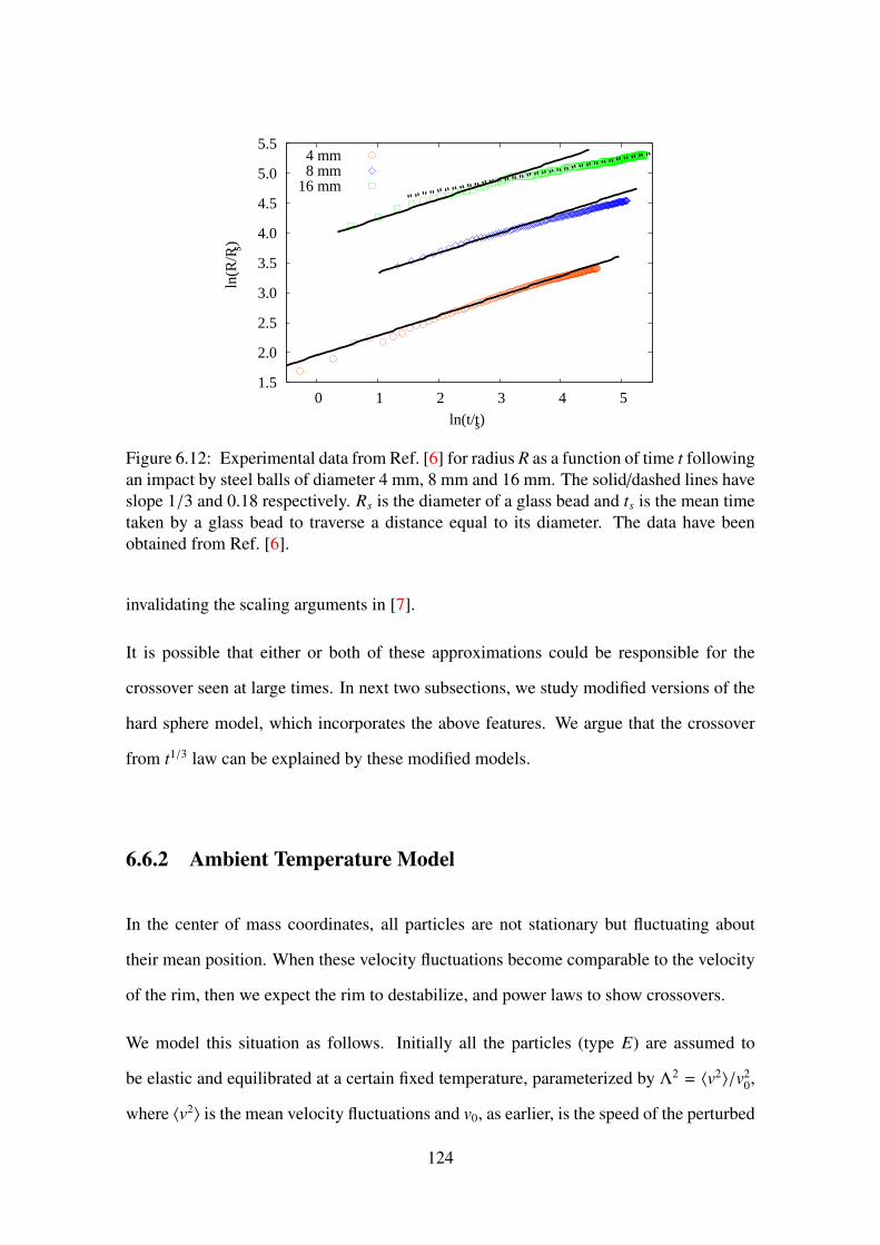
1.5

2.0

2.5

3.0

3.5

4.0

4.5

5.0

5.5

0 1 2 3 4 5

ln(R

/Rs)

ln(t/ts)

4 mm8 mm

16 mm

Figure 6.12: Experimental data from Ref. [6] for radius R as a function of time t following

an impact by steel balls of diameter 4 mm, 8 mm and 16 mm. The solid/dashed lines have

slope 1/3 and 0.18 respectively. Rs is the diameter of a glass bead and ts is the mean time

taken by a glass bead to traverse a distance equal to its diameter. The data have been

obtained from Ref. [6].

invalidating the scaling arguments in [7].

It is possible that either or both of these approximations could be responsible for the

crossover seen at large times. In next two subsections, we study modified versions of the

hard sphere model, which incorporates the above features. We argue that the crossover

from t1/3 law can be explained by these modified models.

6.6.2 Ambient Temperature Model

In the center of mass coordinates, all particles are not stationary but fluctuating about

their mean position. When these velocity fluctuations become comparable to the velocity

of the rim, then we expect the rim to destabilize, and power laws to show crossovers.

We model this situation as follows. Initially all the particles (type E) are assumed to

be elastic and equilibrated at a certain fixed temperature, parameterized by Λ2 = 〈v2〉/v20,

where 〈v2〉 is the mean velocity fluctuations and v0, as earlier, is the speed of the perturbed

124

300

400

500

600

700

300 400 500 600 700

(a)

300

400

500

600

700

300 400 500 600 700

(b)

300

400

500

600

700

300 400 500 600 700

(c)

300

400

500

600

700

300 400 500 600 700

(d)

Figure 6.13: Snapshots of inelastic I particles (red) and elastic E particles (green), when

Λ = 1/800, following an isotropic impulse at (500, 500) at t = 0. The time increases

from (a) to (d) and correspond to the times shown by labels a–d in Fig. 6.14. Initially, the

disturbance grows as in Fig. 6.3, but at late times due to velocity fluctuations, the rim gets

destabilized. The data are for r = 0.10.

particles. Λ = 0 corresponds to the case when all particles are initially stationary. An

isotropic impulse is imparted by introducing four particles (type I) at the center with

speed v0 in the directions 0, π/2, π, and 3π/2. Collisions between E particles are elastic.

Collisions involving at least one I particle are inelastic. If an E particle collides with an

I particle, then it becomes type I. This model captures shock propagation in a system

where all particles have some nonzero kinetic energy.

In Fig. 6.13, we show snapshots of the system at various times, when the Λ = 1/800. The

sharp rim starts becoming more diffuse as the velocity of the rim decreases, until the en-

closed empty region vanishes completely. These snapshots are qualitatively very similar

to that seen in the experiment for low speed impacts and at large times (see Fig. 6.8).

When the rim destabilizes, R(t) shows deviation from the t1/3 power law growth (see

Fig. 6.14). It is straight forward to estimate this crossover time tc. The instability sets

in when the speed of the rim is of the same magnitude as the velocity fluctuations, i.e.

125

101

102

101 102 103 104 105

R(t

)

t

a b

cd

Λ = 1/1600Λ = 1/800Λ = 1/400

Figure 6.14: The radius of disturbance R(t) as a function of time t for different values of

Λ. The effect of velocity fluctuations are felt later for smaller Λ. At large times, the finite

external pressure is able to compress the bubble, with R(t) reaching a minimum when the

density of the bubble approaches the close packing density. A solid line of slope 1/3 is

drawn for reference. The data are for r = 0.10.

vtc ∼ Λv0. Since vt ∼ dR/dt ∼ t−2/3, we immediately obtain tc ∼ Λ−3/2. Thus, R(t) should

have the scaling form

R(t) ∼ t1/3 f(

tΛ3/2)

, (6.13)

where f (x) is a scaling function with f (x) ∼ O(1), when x → 0. The curves for different

Λ collapse when scaled as in Eq. (6.13) [see Fig. 6.15].

6.6.3 Hopping Model

The introduction of a finite ambient temperature, while leading to the disintegration of

the rim, does not produce the large time behavior of the data for the radius. We now

ask whether the rim becoming three dimensional could be responsible for that. The rim

presumably becomes three dimensional because a fast particle when hemmed in by many

surrounding particles may jump out of the plane due to collision with floor and friction.

The net effect is a reduction in radial momentum, which could change the growth law.

126

1

3

5

10-3 10-1 101

R(t

) t-1

/3

t Λ3/2

Λ=1/1600Λ=1/800Λ=1/400

Figure 6.15: The R(t) vs t data of Fig. 6.14 when scaled according to Eq. (6.13). A good

collapse is obtained.

101

102

101 102 103 104 105 106 107

R(t

)

t

v0 = 1v0 = 2v0 = 4v0 = 8

no hopping

Figure 6.16: Temporal variation of radius R(t) for κ = 0.20 with various initial velocity

v0. The solid line is a power law t0.18 while the dashed line is a power law t1/3. The data

with no hopping correspond to v0 = 1. All data are for r = 0.10.

127

To mimic radial momentum leakage occurring at high densities, we consider the following

model. We divide the system into squares of length equal to diameter of the particles.

Given the grid position of a particle, any particle which is in one of the eight neighboring

squares will be called its neighbor. At any instant of time, if a particle has eight or more

neighbors, then we remove the particle if its velocity v satisfies the hopping criterion,

(v − vcm).vcm > κvcm, (6.14)

where vcm is the center of mass velocity of the particle and its neighbors. In words, the

longitudinal component of the velocity should be larger than vcm by a factor κ.

The hopping criterion is tested for all moving particles after every 100 collisions in the

system, and the results do not depend on this number provided it is not too large. The

results are shown in Fig. 6.16. The results obtained are insensitive to the value of κ

provided κ < 0.20. We find that at large times, the system crosses over to a different

power law growth ≈ t0.18, that is very similar to the growth law seen in the experiment.

While the aim of the model was to show that loss of radial momentum, at high densities,

can result in crossovers at large times, we obtain a quantitative match. As of now, we have

no explanation why the exponents have approximately the same numerical value, and it

could be just a coincidence.

6.7 Conclusion

In summary, we studied granular explosion model, where a stationary collection of hard

inelastic particles is perturbed by injecting energy to few localized particles. This initial

perturbation leads to clustering of all moving particles into a shell, that propagates radially

outwards in time [7]. We argued that the formation of the shell in the perturbed system

conserves radial momentum. This conservation law leads to a t1/(D+1) power law growth

for the radius of disturbance. Data from the numerical simulation of the model fits very

128

well to the predicted growth law of radius of disturbance.

We analyzed the recent experiment [6] of dropping spheres onto a flowing monolayer of

glass beads. Our inelastic granular explosion model closely resembles this experiment.

With this hard sphere system, we showed that the assumption of constant rate of collision

per particle per unit distance, made in the theory [6] to describe the experimental data is

correct only for elastic particles. For inelastic system, the relevant collisions are the colli-

sions of the particles at the outer edge of the rim with the stationary particles outside. The

t1/3 (D = 2) growth law describes the experimental data well except at large times when

the data show a crossover to a different power law growth. We attributed this crossover

to the rim becoming three dimensional because of high densities and collisions with the

floor. By constructing a simple model incorporating these effects, we were able to explain

the crossovers at large times.

The current experimental data can not distinguish between the theory in BCK and the

power law growth argued for in this chapter. If the experimental time scale is increased,

then such a distinction may be possible. It will be worthwhile to make the attempt.

Acknowledgment

We thank the authors of Ref. [6] for providing us with the experimental data.

129

Chapter 7

Shock Propagation in a Viscoelastic

Granular Gas

7.1 Introduction

In Chapter 6, we studied the granular explosion model, where a stationary collection of

inelastic particles is perturbed by a localized impulse, using scaling arguments and event

driven molecular dynamics simulations. By identifying radial momentum as a conserved

quantity, it was argued that, the radius of the disturbance R grows with time t as R(t) ∼ tα,

where α = 1/(D+1) in D dimensions. The arguments depended crucially on the formation

of a region devoid of particles, surrounded by a moving dense shell of particles.

In the numerical simulation of granular explosion studied in Chapter 6, particles were

considered hard and a simplified model of constant coefficient of restitution r was used

to account for the inelasticity of the collisions. Such a choice was motivated by compu-

tational efficiency. However, realistic coefficient of restitution depends strongly on the

relative velocity of collision vrel, r ≡ r(vrel) [17]. Experimentally, r(vrel) approaches 1

when the vrel tends to zero, i.e., 1 − r(vrel) = g(vrel/δ), where g(x) ∼ xσ + O(x2σ), for

131

x ≪ 1 and g(x) ∼ 1 − r0 for x → ∞ [95, 96], and δ is a velocity scale. The exponent

σ takes a range of values and is known to be 1/5 for visco-elastic particles [17] (see the

discussion in Sec. 2.2.3 for the visco-elastic particles). It is not clear whether the shell

structure will form for such velocity dependent r. In this chapter, we study the system

of visco-elastic particles in two dimensions using conventional molecular dynamics sim-

ulations. For this system, σ = 1/5 < 1, a case that cannot be studied by event driven

molecular dynamics simulations performed in Chapter 6, as inelastic collapse prevents

the simulation from proceeding forward [70].

The rest of the chapter is organized as follows. In Sec. 7.2, the simulation details of the

model are provided. The results obtained in molecular dynamics simulations are pre-

sented in Sec. 7.3. We conclude this chapter in Sec. 7.4.

7.2 Model and Simulation Details

The system that is simulated is defined as follows. We consider a collection of mono

dispersed discs distributed uniformly in two dimensions. The mass and radius of the

particles are taken to be unity. All particles are initially at rest. An isotropic impulse

is modeled by introducing four particles at the center with speed of unit magnitude, in

the directions 0, π/2, π, 3π/2. The particles move ballistically until they collide. The

interaction force during the collision is given by [77] (see Sec. 2.2.3 for details)

F = ρξ3/2 +3

2Aρ

√

ξξ, (7.1)

where ξ is the overlap between the colliding particles and ξ is the time derivative of

ξ. ρ and A are material parameters, characterizing the elastic and dissipative properties.

Collision conserve momentum, but not energy.

We simulate the system in two dimensions using conventional molecular dynamics simu-

132

-400

-200

0

200

400

-400 -200 0 200 400

(a)

-400

-200

0

200

400

-400 -200 0 200 400

(b)

-400

-200

0

200

400

-400 -200 0 200 400

(c)

-400

-200

0

200

400

-400 -200 0 200 400

(d)

Figure 7.1: Moving (red) and stationary (green) particles at times t = (a) 102, (b) 103, (c)

104 and (d) 5×104, following an isotropic impulse at (0, 0) at t = 0. The moving particles

cluster together to form a shell.

lations, where we have used fourth order Runge-Kutta (RK4) scheme for integrating the

equations of motion. The simulation data are for ρ = 104, A = 0.028 and volume fraction

φ = 0.20. The integration time step h in RK4 scheme is chosen to be h = 0.005, which is

sufficient to resolve the full collision process. The data are typically averaged over eight

different realizations of the particle configurations.


Figure 7.1 shows the time evolution of the system. The four non-stationary particles at

t = 0 move and collide with other stationary particles setting them in motion and leading

to a cascade of collisions. The active particles (particles that have collided at least once)

form a shell, enclosing a region devoid of particles. The shell moves out in time absorbing

the particles at the boundary. Thus, similar to the hard-core system with constant r, we

observe shell formation in this visco-elastic system.

133

101

102

103

104

101 102 103 104 105

R(t

), N

(t)

t

t1/3

t2/3

R(t)N(t)

Figure 7.2: Temporal behaviour of radius of disturbance R(t) and number of active parti-

cles N(t).

The radial momentum conservation argument predicts that the radius of disturbance grows

with t as R(t) ∼ t1/3, and the number of active particles grows as N(t) ∼ R2 ∼ t2/3

in D = 2. The simulation results for R(t) and N(t) as shown in Fig. 7.2 are in very

good agreement with these predictions. The kinetic energy E(t) of the shell is given by

E(t) ∼ N(t)V(t)2, where V(t) is the typical velocity of a particle in the shell and is given

by V(t) = dR/dt ∼ t−2/3. Thus, the energy decreases with time as E(t) ∼ t−2/3, and as

shown in Fig. 7.3 matches very well with the simulation data.

7.4 Conclusion

To summarize, we studied granular explosion model with visco-elastic particles using

molecular dynamics simulations. We reproduced the formation of a dense moving shell of

particles following a localized perturbation seen in hard-core granular explosion model [7]

and experiments [6]. The radius of shell increases with time as t1/3, and the energy de-

creases as t−2/3 in two dimensions. We find that the results of scaling arguments for hard

spheres system [7] continue to hold for visco-elastic particles, and thus is insensitive to

134

10-3

10-2

10-1

100

101 102 103 104 105

E(t

)

t

t-2/3

Figure 7.3: Temporal behaviour of kinetic energy E(t).

the form of the coefficient of restitution.

135

Chapter 8

Conclusion and Discussion

We now summarize the main results of this thesis, and discuss some possible future ex-

tensions. In this thesis, we studied freely cooling granular gas using large scale molecular

dynamics simulations and scaling analysis, with a particular attention on the large time

behaviour. At large times, the system behaviour is dominated by strong clustering.

In Chapter 4, we studied the long time behaviour of the freely cooling granular gas in

three dimensions using event driven molecular dynamics simulations. At large times, the

translational kinetic energy T (t) is found to decay with time t as a power law t−θT with

θT ≈ 6/5. This decay exponent is universal, independent of system parameters. This rules

out Burgers like equation as the continuum description of the long time behaviour of

granular gas, which predicted θT to be 3/2 in three dimensions. Our observed θT is indis-

tinguishable from the mean-field prediction for ballistic aggregation. However, our direct

numerical simulation of ballistic aggregation shows that the actual decay exponent de-

pends on density of system and differs from the mean-field prediction for dilute systems.

In addition, the cluster size distribution as well as the velocity distribution of ballistic ag-

gregation are strikingly different from that of the freely cooling granular gas. Thus, the

principal conclusion that emerges from our study is that, the freely cooling granular gas

fits to neither the ballistic aggregation or a Burgers equation description.

137

Our results clearly show the need for a new mathematical theory, beyond ballistic ag-

gregation and Burgers equation, to write the correct continuum equations for the freely

cooling granular gas, which is a very challenging task. The experimental investigation of

freely cooling granular gas is limited to homogeneous cooling regime, and it is desired to

design experiments to probe the inhomogeneous cooling regime.

In Chapter 5, we studied the large time behaviour of freely cooling granular gas of rough

particles in two dimensions using event driven molecular dynamics simulations. Rough

particles dissipate energy in both the normal and tangential direction of collision. We

showed that at large times when the system is in clustered inhomogeneous regime, the

temporal decay of translational kinetic energy T (t) and rotational energy K(t) is given by

power laws, T (t) ∼ t−θT and K(t) ∼ t−θK , with θT ≈ 1 and θK ≈ 1.6. These decay exponents

are independent of coefficients of restitution. We also studied the ballistic aggregation

with rotational degree of freedom. In our direct numerical simulation of this system, the

decay exponents are found to be θBAT ≈ 1 and θBA

K ≈ 1 for dense systems. Extension

of an earlier scaling theory for ballistic aggregation gives θm f

K= 1, consistent with the

numerically obtained value. In Chapter 4, we concluded that the ballistic aggregation

is not the correct description for the inhomogeneous cooling regime of freely cooling

granular gas. The fact that the rotational energies in the two models decay with different

exponents is a further support to our conclusion.

It has been earlier shown that in the homogeneous regime, the directions of the angular

velocity and translational velocity are correlated [122]. It would be interesting to see

whether this holds true in the inhomogeneous regime in three dimensions. Unfortunately,

simulations in three dimensions have strong finite size effects [126] and at the same time

the crossover time from the homogeneous regime to inhomogeneous regime for the ro-

tational energy is large. This makes it difficult to obtain a large enough temporal regime

where one may test for correlation. This is a promising area for future study.

Experiments have verified Haff’s law for the translational kinetic energy decay in the

138

homogeneous cooling regime [83, 84, 85]. It will be interesting to verify the rotational

energy decay behaviour of the homogeneous regime. It should not be very complicated,

especially in two dimensions where there is only one rotational mode. Also desired is the

investigation of the inhomogeneous cooling regime of this system.

In Chapter 6, we studied granular explosion model using event driven simulations and

scaling analysis. The cascade of collisions created by the initial perturbation leads to

clustering of all moving particles into a spherical shell. The region inside the spheri-

cal shell is devoid of particles. This formation of shell conserves radial momentum and

predicts a power law growth with time t for the radius of disturbance R(t) ∼ t1/(D+1), in

D dimensions. We applied the results of granular explosion to a recent experiment [6],

where a dilute monolayer of glass beads flowing down on an inclined plane was perturbed

by dropping a steel ball. We showed that the growth of radius predicted in granular ex-

plosion R(t) ∼ t1/3 for D = 2 describes the experimental data very well except at large

times. At long times, the experimental data shows a crossover to a different power law

growth ∼ t0.18. We attributed this crossover to the shell becoming effectively three dimen-

sional due to accumulation of particles at the shell front. The granular explosion model

is modified to incorporate this effect. Simulation of this modified model captured the

experimentally observed long time behaviour.

It will be quite interesting to see if any connection can be made between the granular

explosion in which most of the particles are initially stationary and the well studied freely

cooling granular gas, in which all particles initially have a nonzero kinetic energy. It may

be possible to think of the freely cooling gas as a collection of many explosions initiated

at different points in space, which interact when the shock fronts meet. Thus, it will be

useful to make a detailed study of the case of two interacting shocks.

The data for radius show a crossover from an initial elastic behavior t1/2 to an asymptotic

t1/3 growth law. It would be of interest to understand this crossover better. Exact solution

of the shock problem in one dimension with 0 < r < 1 would throw light on it. An

139

exact solution appears possible given that the freely cooling in one dimension is one of

the exactly solvable model in granular physics.

Finally, in Chapter 7, we studied granular explosion model with visco-elastic particles

using conventional molecular dynamics simulations. Visco-elastic model is a realistic

model for a granular particle for which the coefficient of restitution depends strongly on

relative velocity of collision. We observed that the formation of shell and scaling result

for the temporal growth of radius of disturbance, earlier obtained with simplified model

of constant coefficient of restitution, continue to hold for the visco-elastic system.

140

Bibliography

[1] H. M. Jaeger, S. R. Nagel, and R. P. Behringer, “Granular solids, liquids, and

gases,” Reviews of Modern Physics, vol. 68, pp. 1259–1273, 1996.

[2] L. P. Kadanoff, “Built upon sand: Theoretical ideas inspired by granular flows,”

Reviews of Modern Physics, vol. 71, pp. 435–444, 1999.

[3] I. S. Aranson and L. S. Tsimring, “Patterns and collective behavior in granular

media: Theoretical concepts,” Reviews of Modern Physics, vol. 78, pp. 641–692,

2006.

[4] C. S. Campbell, “Rapid granular flows,” Annual Review of Fluid Mechanics,

vol. 22, pp. 57–92, 1990.

[5] S. F. Shandarin and Y. B. Zeldovich, “The large-scale structure of the universe: Tur-

bulence, intermittency, structures in a self-gravitating medium,” Reviews of Modern

Physics, vol. 61, pp. 185–220, 1989.

[6] J. F. Boudet, J. Cassagne, and H. Kellay, “Blast shocks in quasi-two-dimensional

supersonic granular flows,” Physical Review Letters, vol. 103, p. 224501, 2009.

[7] Z. Jabeen, R. Rajesh, and P. Ray, “Universal scaling dynamics in a perturbed gran-

ular gas,” Europhysics Letters, vol. 89, p. 34001, 2010.

[8] L. Frachebourg, “Exact solution of the one-dimensional ballistic aggregation,”

Physical Review Letters, vol. 82, pp. 1502–1505, 1999.

141

[9] M. Shinde, D. Das, and R. Rajesh, “Violation of the porod law in a freely cooling

granular gas in one dimension,” Physical Review Letters, vol. 99, p. 234505, 2007.

[10] N. V. Brilliantov and T. Pöschel, Kinetic Theory of Granular Gases. Oxford: Ox-

ford University Press, 2004.

[11] P. K. Haff, “Grain flow as a fluid-mechanical phenomenon,” Journal of Fluid Me-

chanics, vol. 134, pp. 401–430, 1983.

[12] I. Goldhirsch and G. Zanetti, “Clustering instability in dissipative gases,” Physical

Review Letters, vol. 70, pp. 1619–1622, 1993.

[13] E. Ben-Naim, S. Y. Chen, G. D. Doolen, and S. Redner, “Shocklike dynamics of

inelastic gases,” Physical Review Letters, vol. 83, pp. 4069–4072, 1999.

[14] X. Nie, E. Ben-Naim, and S. Chen, “Dynamics of freely cooling granular gases,”

Physical Review Letters, vol. 89, p. 204301, 2002.

[15] G. F. Carnevale, Y. Pomeau, and W. R. Young, “Statistics of ballistic agglomera-

tion,” Physical Review Letters, vol. 64, pp. 2913–2916, 1990.

[16] S. Luding, M. Huthmann, S. McNamara, and A. Zippelius, “Homogeneous cool-

ing of rough, dissipative particles: Theory and simulations,” Physical Review E,

vol. 58, pp. 3416–3425, 1998.

[17] R. Ramirez, T. Poschel, N. V. Brilliantov, and T. Schwager, “Coefficient of restitu-

tion of colliding viscoelastic spheres,” Physical Review E, vol. 60, pp. 4465–4472,

1999.

[18] J. J. Brey, M. J. Ruiz-Montero, and D. Cubero, “Homogeneous cooling state of a

low-density granular flow,” Physical Review E, vol. 54, pp. 3664–3671, 1996.

[19] E. Trizac and P. L. Krapivsky, “Correlations in ballistic processes,” Physical Review

Letters, vol. 91, p. 218302, 2003.

142

[20] C. Coulomb, in Memoir de Mathematique et de Physique, vol. 7. Paris: Academie

des Sciences, L’Imprimerie Royale, 1773.

[21] M. Faraday, “On the forms and states of fluids on vibrating elastic surfaces,” Philo-

sophical Transactions of the Royal Society of London, vol. 52, pp. 319–340, 1831.

[22] O. Reynolds, “On the dilatancy of media composed of rigid particles in contact,

with experimental illustrations,” Philosophical Magazine, vol. 20, pp. 469–481,

1885.

[23] A. Kudrolli, “Size separation in vibrated granular materials,” Reports on Progress

in Physics, vol. 67, pp. 209–247, 2004.

[24] I. Goldhirsch, “Rapid granular flows,” Annual Review of Fluid Mechanics, vol. 35,

pp. 267–293, 2003.

[25] H. M. Jaeger and S. R. Nagel, “Physics of the granular state,” Science, vol. 255,

pp. 1523–1531, 1992.

[26] A. Mehta and G. C. Barker, “The dynamics of sand,” Reports on Progress in

Physics, vol. 57, pp. 383–416, 1994.

[27] H. M. Jaeger, C. H. Liu, and S. R. Nagel, “Relaxation at the angle of repose,”


[28] T. A. J. Duke, G. C. Barker, and A. Mehta, “A monte carlo study of granular relax-

ation,” Europhysics Letters, vol. 13, pp. 19–24, 1990.

[29] Y. Boguslavskii and S. Drabkin, “The kinetics of powder settlement caused by low

level vibration and elastic stresses,” Physica A, vol. 222, pp. 75–86, 1995.

[30] J. B. Knight, C. G. Fandrich, C. N. Lau, H. M. Jaeger, and S. R. Nagel, “Density

relaxation in a vibrated granular material,” Physical Review E, vol. 51, pp. 3957–

3963, 1995.

143

[31] S. Douady, S. Fauve, and C. Laroche, “Subharmonic instabilities and defects in a

granular layer under vertical vibrations,” Europhysics Letters, vol. 8, p. 621, 1989.

[32] O. Zik and J. Stavans, “Self-diffusion in granular flows,” Europhysics Letters,

vol. 16, p. 255, 1991.

[33] F. Melo, P. Umbanhowar, and H. L. Swinney, “Transition to parametric wave pat-

terns in a vertically oscillated granular layer,” Physical Review Letters, vol. 72,

pp. 172–175, 1994.

[34] H. K. Pak and R. P. Behringer, “Surface waves in vertically vibrated granular ma-

terials,” Physical Review Letters, vol. 71, pp. 1832–1835, 1993.

[35] H. K. Pak, E. Van Doorn, and R. P. Behringer, “Effects of ambient gases on granular

materials under vertical vibration,” Physical Review Letters, vol. 74, pp. 4643–

4646, 1995.

[36] T. Travers, M. Ammi, D. Bideau, A. Gervois, J. C. Messager, and J. P. Troadec,

“Uniaxial compression of 2d packings of cylinders. effects of weak disorder,” Eu-

rophysics Letters, vol. 4, p. 329, 1987.

[37] C. H. Liu, S. R. Nagel, D. A. Schecter, S. N. Coppersmith, S. Majumdar,

O. Narayan, and T. A. Witten, “Force fluctuations in bead packs,” Science, vol. 269,

pp. 513–515, 1995.

[38] S. N. Coppersmith, C. H. Liu, S. Majumdar, O. Narayan, and T. A. Witten, “Model

for force fluctuations in bead packs,” Physical Review E, vol. 53, pp. 4673–4685,

1996.

[39] J. T. Jenkins and S. B. Savage, “A theory for the rapid flow of identical, smooth,

nearly elastic, spherical particles,” Journal of Fluid Mechanics, vol. 130, pp. 187–

202, 1983.

144

[40] P. K. Haff, “A physical picture of kinetic granular fluids,” Journal of Rheology,

vol. 30, pp. 931–948, 1986.

[41] S. B. Savage and D. J. Jeffrey, “The stress tensor in a granular flow at high shear

rates,” Journal of Fluid Mechanics, vol. 110, pp. 255–272, 1981.

[42] P. Evesque and J. Rajchenbach, “Instability in a sand heap,” Physical Review Let-

ters, vol. 62, pp. 44–46, 1989.

[43] C. Laroche, S. Douady, and S. Fauve, “Convective flow of granular masses under

vertical vibrations,” Journal de Physique (France), vol. 50, pp. 699–706, 1989.

[44] J. B. Knight, H. M. Jaeger, and S. R. Nagel, “Vibration-induced size separation

in granular media: The convection connection,” Physical Review Letters, vol. 70,

pp. 3728–3731, 1993.

[45] E. E. Ehrichs, H. M. Jaeger, G. S. Karczmar, J. B. Knight, V. Y. Kuperman, and

S. R. Nagel, “Granular convection observed by magnetic resonance imaging,” Sci-

ence, vol. 267, pp. 1632–1634, 1995.

[46] J. C. Williams, “The segregation of particulate materials. A review,” Powder Tech-

nology, vol. 15, pp. 245–251, 1976.

[47] L. T. Fan, Y. M. Chen, and F. S. Lai, “Recent developments in solids mixing,”

Powder Technology, vol. 61, pp. 255–287, 1990.

[48] C. F. Harwood, “Powder segregation due to vibration,” Powder Technology, vol. 16,

pp. 51–57, 1977.

[49] W. Cooke, S. Warr, J. M. Huntley, and R. C. Ball, “Particle size segregation in a

two-dimensional bed undergoing vertical vibration,” Physical Review E, vol. 53,

pp. 2812–2822, 1996.

[50] O. R. Walton, in Particulate Two-Phase Flow. Boston: edited by M. C. Roco

(Butterworth-Heinemann), 1993.

145

[51] S. McNamara and W. R. Young, “Inelastic collapse and clumping in a one-

dimensional granular medium,” Physics of Fluids A, vol. 4, pp. 496–504, 1992.

[52] S. McNamara and W. R. Young, “Inelastic collapse in two dimensions,” Physical

Review E, vol. 50, pp. R28–R31, 1994.

[53] O. Pouliquen, J. Delour, and S. B. Savage, “Fingering in granular flows,” Nature,

vol. 386, pp. 816–817, 1997.

[54] Y. Forterre and O. Pouliquen, “Longitudinal vortices in granular flows,” Physical

Review Letters, vol. 86, pp. 5886–5889, 2001.

[55] J. S. Olafsen and J. S. Urbach, “Clustering, order, and collapse in a driven granular

monolayer,” Physical Review Letters, vol. 81, pp. 4369–4372, 1998.

[56] P. B. Umbanhowar, F. Melo, and H. L. Swinney, “Localized excitations in a verti-

cally vibrated granular layer,” Nature, vol. 382, pp. 793–796, 1996.

[57] K. Liffman, G. Metcalfe, and P. Cleary, “Granular convection and transport due to

horizontal shaking,” Physical Review Letters, vol. 79, pp. 4574–4576, 1997.

[58] G. H. Ristow, G. Straßburger, and I. Rehberg, “Phase diagram and scaling of

granular materials under horizontal vibrations,” Physical Review Letters, vol. 79,

pp. 833–836, 1997.

[59] J. Rajchenbach, “Flow in powders: From discrete avalanches to continuous

regime,” Physical Review Letters, vol. 65, pp. 2221–2224, 1990.

[60] P. Tegzes, T. Vicsek, and P. Schiffer, “Avalanche dynamics in wet granular materi-

als,” Physical Review Letters, vol. 89, p. 094301, 2002.

[61] O. Johnsen, R. Toussaint, K. J. Måløy, and E. G. Flekkøy, “Pattern formation during

air injection into granular materials confined in a circular hele-shaw cell,” Physical

Review E, vol. 74, p. 011301, 2006.

146

[62] B. Sandnes, H. A. Knudsen, K. J. Måløy, and E. G. Flekkøy, “Labyrinth patterns

in confined granular-fluid systems,” Physical Review Letters, vol. 99, p. 038001,

2007.

[63] I. S. Aranson, B. Meerson, P. V. Sasorov, and V. M. Vinokur, “Phase separation

and coarsening in electrostatically driven granular media,” Physical Review Letters,

vol. 88, p. 204301, 2002.

[64] A. Snezhko, I. S. Aranson, and W.-K. Kwok, “Structure formation in electromag-

netically driven granular media,” Physical Review Letters, vol. 94, p. 108002, 2005.

[65] T. Pöschel and S. Luding, eds., Granular Gases. Berlin: Springer, 2001.

[66] T. Pöschel and N. V. Brilliantov, eds., Granular Gas Dynamics. Berlin: Springer,

2003.

[67] S. N. Pathak, Z. Jabeen, P. Ray, and R. Rajesh, “Shock propagation in granular

flow subjected to an external impact,” Physical Review E, vol. 85, p. 061301, 2012.

[68] S. N. Majumdar, K. Mallick, and S. Sabhapandit, “Statistical properties of the fi-

nal state in one-dimensional ballistic aggregation,” Physical Review E, vol. 79,

p. 021109, 2009.

[69] S. K. Das and S. Puri, “Kinetics of inhomogeneous cooling in granular fluids,”

Physical Review E, vol. 68, p. 011302, 2003.

[70] M. Shinde, D. Das, and R. Rajesh, “Equivalence of the freely cooling granular gas

to the sticky gas,” Physical Review E, vol. 79, p. 021303, 2009.

[71] M. Shinde, D. Das, and R. Rajesh, “Coarse-grained dynamics of the freely cooling

granular gas in one dimension,” Physical Review E, vol. 84, p. 031310, 2011.

[72] L. Frachebourg, P. A. Martin, and J. Piasecki, “Ballistic aggregation: a solvable

model of irreversible many particle dynamics,” Physica A, vol. 279, pp. 69–99,

2000.

147

[73] R. Tribe and O. Zaboronski, “On the large time asymptotics of decaying burgers

turbulence,” Communications in Mathematical Physics, vol. 212, p. 415, 2000.

[74] S. Kida, “Asymptotic properties of Burgers turbulence,” Journal of Fluid Mechan-

ics, vol. 93, pp. 337–377, 1979.

[75] S. Dey, D. Das, and R. Rajesh, “Lattice models for ballistic aggregation in one

dimension,” Europhysics Letters, vol. 93, p. 44001, 2011.

[76] T. Pöschel and T. Schwager, Computational Granular Dynamics. Berlin: Springer,

2004.

[77] N. V. Brilliantov, F. Spahn, J.-M. Hertzsch, and T. Pöschel, “Model for collisions

in granular gases,” Physial Review E, vol. 53, pp. 5382–5392, 1996.

[78] F. G. Bridges, A. Hatzes, and D. N. C. Lin, “Structure, stability and evolution of

saturn’s rings,” Nature, vol. 309, pp. 333–335, 1984.

[79] R. Greenberg and A. Brahic, Planetary Rings. Tucson: University of Arizona

Press, 1984.

[80] H. Hertz, “Ueber die berührung fester elastischer körper,” Journal für die reine und

angewandte Mathematik, vol. 92, pp. 156–171, 1882.

[81] T. Schwager and T. Pöschel, “Coefficient of normal restitution of viscous particles

and cooling rate of granular gases,” Physical Review E, vol. 57, pp. 650–654, 1998.

[82] S. E. Esipov and T. Pöschel, “The granular phase diagram,” Journal of Statistical

Physics, vol. 86, pp. 1385–1395, 1997.

[83] C. C. Maaß, N. Isert, G. Maret, and C. M. Aegerter, “Experimental investigation

of the freely cooling granular gas,” Physical Review Letters, vol. 100, p. 248001,

2008.

148

[84] Y. Grasselli, G. Bossis, and G. Goutallier, “Velocity-dependent restitution coeffi-

cient and granular cooling in microgravity,” Europhysics Letters, vol. 86, p. 60007,

2009.

[85] S. Tatsumi, Y. Murayama, H. Hayakawa, and M. Sano, “Experimental study on

the kinetics of granular gases under microgravity,” Journal of Fluid Mechanics,

vol. 641, pp. 521–539, 2009.

[86] N. F. Carnahan and K. E. Starling, “Equation of state for nonattracting rigid

spheres,” The Journal of Chemical Physics, vol. 51, pp. 635–636, 1969.

[87] P. Deltour and J.-L. Barrat, “Quantitative study of a freely cooling granular

medium,” Journal de Physique I, vol. 7, p. 137, 1997.

[88] A. Goldshtein and M. Shapiro, “Mechanics of collisional motion of granular ma-

terials. Part 1. General hydrodynamic equations,” Journal of Fluid Mechanics,

vol. 282, pp. 75–114, 1995.

[89] T. P. C. van Noije and M. H. Ernst, “Velocity distributions in homogeneous granular

fluids: the free and the heated case,” Granular Matter, vol. 1, pp. 57–64, 1998.

[90] S. McNamara and W. R. Young, “Dynamics of a freely evolving, two-dimensional

granular medium,” Physical Review E, vol. 53, pp. 5089–5100, 1996.

[91] E. Efrati, E. Livne, and B. Meerson, “Hydrodynamic singularities and clustering in

a freely cooling inelastic gas,” Physical Review Letters, vol. 94, p. 088001, 2005.

[92] R. Brito and M. H. Ernst, “Extension of haff’s cooling law in granular flows,”

Europhysics Letters, vol. 43, p. 497, 1998.

[93] S. Chen, Y. Deng, X. Nie, and Y. Tu, “Clustering kinetics of granular media in

three dimensions,” Physics Letters A, vol. 269, pp. 218–223, 2000.

[94] S. Miller and S. Luding, “Cluster growth in two- and three-dimensional granular

gases,” Physical Review E, vol. 69, p. 031305, 2004.

149

[95] C. V. Raman, “The photographic study of impact at minimal velocities,” Physical

Review, vol. 12, pp. 442–447, 1918.

[96] E. Falcon, C. Laroche, S. Fauve, and C. Coste, “Behavior of one inelastic ball

bouncing repeatedly off the ground,” The European Physical Journal B, vol. 3,

pp. 45–57, 1998.

[97] L. Labous, A. D. Rosato, and R. N. Dave, “Measurements of collisional properties

of spheres using high-speed video analysis,” Physical Review E, vol. 56, pp. 5717–

5725, 1997.

[98] F. Leyvraz, “Scaling theory and exactly solved models in the kinetics of irreversible

aggregation,” Physics Reports, vol. 383, pp. 95–212, 2003.

[99] E. Trizac and J.-P. Hansen, “Dynamic scaling behavior of ballistic coalescence,”


[100] P. L. Krapivsky and E. Ben-Naim, “Aggregation with multiple conservation laws,”

Physical Review E, vol. 53, pp. 291–298, 1996.

[101] J. M. Burgers, The Non-Linear Diffusion Equation: Asymptotic Solutions and Sta-

tistical Problems. Boston: Reidel, 1974.

[102] K. Shida and T. Kawai, “Cluster formation by inelastically colliding particles in

one-dimensional space,” Physica A, vol. 162, pp. 145–160, 1989.

[103] N. Schörghofer and T. Zhou, “Inelastic collapse of rotating spheres,” Physical Re-

view E, vol. 54, pp. 5511–5515, 1996.

[104] D. Goldman, M. D. Shattuck, C. Bizon, W. D. McCormick, J. B. Swift, and H. L.

Swinney, “Absence of inelastic collapse in a realistic three ball model,” Physical

Review E, vol. 57, pp. 4831–4833, 1998.

[105] S. Luding and S. McNamara, “How to handle the inelastic collapse of a dissipative

hard-sphere gas with the TC model,” Granular Matter, vol. 1, pp. 113–128, 1998.

150

[106] S. E. Esipov and T. J. Newman, “Interface growth and Burgers turbulence: The

problem of random initial conditions,” Physical Review E, vol. 48, pp. 1046–1050,

1993.

[107] S. E. Esipov, “Energy decay in Burgers turbulence and interface growth: The prob-

lem of random initial conditions. II,” Physical Review E, vol. 49, pp. 2070–2081,

1994.

[108] S. Luding, “Structure and cluster formation in granular media,” Pramana, vol. 64,

pp. 893–902, 2005.

[109] D. C. Rapaport, “The event scheduling problem in molecular dynamic simulation,”

Journal of Computational Physics, vol. 34, pp. 184–201, 1980.

[110] D. C. Rapaport, The Art of Molecular Dynamics Simulations. Cambridge: Cam-

bridge University Press, 2004.

[111] T. Pöschel, N. V. Brilliantov, and T. Schwager, “Long-time behavior of granu-

lar gases with impact-velocity dependent coefficient of restitution,” Physica A,

vol. 325, pp. 274 – 283, 2003.

[112] J. Hoshen and R. Kopelman, “Percolation and cluster distribution. I. Cluster mul-

tiple labeling technique and critical concentration algorithm,” Physical Review B,

vol. 14, pp. 3438–3445, 1976.

[113] C. Connaughton, R. Rajesh, and O. Zaboronski, “Kinetics of cluster-cluster aggre-

gation,” in Handbook of Nanophysics: Clusters and Fullerenes (K. D. Sattler, ed.),

Taylor and Francis, 2010.

[114] A. Zippelius, “Granular gases,” Physica A, vol. 369, pp. 143–158, 2006.

[115] S. F. Foerster, M. Y. Louge, H. Chang, and K. Allia, “Measurements of the collision

properties of small spheres,” Physics of Fluids, vol. 6, pp. 1108–1115, 1994.

151

[116] O. Herbst, M. Huthmann, and A. Zippelius, “Dynamics of inelastically colliding

spheres with coulomb friction: Relaxation of translational and rotational energy,”

Granular Matter, vol. 2, pp. 211–219, 2000.

[117] I. Goldhirsch, S. H. Noskowicz, and O. Bar-Lev, “Nearly smooth granular gases,”

Physical Review Letters, vol. 95, p. 068002, 2005.

[118] M. Huthmann and A. Zippelius, “Dynamics of inelastically colliding rough

spheres:Relaxation of translational and rotational energy,” Physical Review E,

vol. 56, pp. R6275–R6278, 1997.

[119] J. T. Jenkins and M. W. Richman, “Kinetic theory for plane flows of a dense gas

of identical, rough, inelastic, circular disks,” Physics of Fluids, vol. 28, pp. 3485–

3494, 1985.

[120] C. K. K. Lun, “Kinetic theory for granular flow of dense, slightly inelastic, slightly

rough spheres,” Journal of Fluid Mechanics, vol. 233, pp. 539–559, 1991.

[121] S. McNamara and S. Luding, “Energy nonequipartition in systems of inelastic,

rough spheres,” Physical Review E, vol. 58, pp. 2247–2250, 1998.

[122] N. V. Brilliantov, T. Pöschel, W. T. Kranz, and A. Zippelius, “Translations and rota-

tions are correlated in granular gases,” Physical Review Letters, vol. 98, p. 128001,

2007.

[123] B. Gayen and M. Alam, “Orientational correlation and velocity distributions in

uniform shear flow of a dilute granular gas,” Physical Review Letters, vol. 100,

p. 068002, 2008.

[124] E. Ben-Naim and A. Zippelius, “Singular energy distributions in driven and un-

driven granular media,” Journal of Statistical Physics, vol. 129, pp. 677–697, 2007.

152

[125] R. Rongali and M. Alam, “Higher-order effects on orientational correlation and

relaxation dynamics in homogeneous cooling of a rough granular gas,” Physical

Review E, vol. 89, p. 062201, 2014.

[126] S. N. Pathak, Z. Jabeen, D. Das, and R. Rajesh, “Energy decay in three-dimensional

freely cooling granular gas,” Physical Review Letters, vol. 112, p. 038001, 2014.

[127] E. Ben-Naim, P. L. Krapivsky, F. Leyvraz, and S. Redner, “Kinetics of ballistically-

controlled reactions,” Journal of Physical Chemistry, vol. 98, pp. 7284–7288,

1994.

[128] G. Taylor, “The formation of a blast wave by a very intense explosion. I. Theoreti-

cal discussion,” Proceedings of the Royal Society of London A, vol. 201, pp. 159–

174, 1950.

[129] L. Sedov, Similarity and Dimensional Methods in Mechanics. Florida: CRC Press,

10 ed., 1993.

[130] J. von Neumann in Collected Works, p. 219, Oxford: Pergamon Press, 1963.

[131] P. T. Metzger, C. D. Immer, C. M. Donahue, B. M. Vu, R. C, L. III, and M. Deyo-

Svendsen, “Jet-induced cratering of a granular surface with application to lunar

spaceports,” Journal of Aerospace Engineering, vol. 21, p. 24, 2009.

[132] X. Cheng, L. Xu, A. Patterson, H. M. Jaeger, and S. R. Nagel, “Towards the

zero-surface-tension limit in granular fingering instability,” Nature Physics, vol. 4,

pp. 234–237, 2008.

[133] S. F. Pinto, M. S. Couto, A. P. F. Atman, S. G. Alves, A. T. Bernardes, H. F. V.

de Resende, and E. C. Souza, “Granular fingers on jammed systems: New fluid-

like patterns arising in grain-grain invasion experiments,” Physical Review Letters,

vol. 99, p. 068001, 2007.

153

[134] W. Losert, D. G. W. Cooper, and J. P. Gollub, “Propagating front in an excited

granular layer,” Physical Review E, vol. 59, pp. 5855–5861, 1999.

[135] S. Luding, “Granular media-information propagation,” Nature, vol. 435, pp. 159–

160, 2005.

[136] A. Daerr and S. Douady, “Two types of avalanche behaviour in granular media,”

Nature, vol. 399, p. 241, 1999.

[137] Y. B. Zel’dovich and Y. P. Raizer, Physics of Shock Waves and High Temperature

Hydrodynamic Phenomena. New York: Dover Publications, Inc., 2002.

[138] J. P. Ostriker and C. F. McKee, “Astrophysical blastwaves,” Reviews of Modern

Physics, vol. 60, pp. 1–68, 1988.

[139] T. Antal, P. L. Krapivsky, and S. Redner, “Exciting hard spheres,” Physical Review

E, vol. 78, p. 030301, 2008.

[140] E. Trizac and A. Barrat, “Free cooling and inelastic collapse of granular gases in

high dimensions,” The European Physical Journal E, vol. 3, pp. 291–294, 2000.

[141] D. E. G. Williams, “Packing fraction of a disk assembly randomly close packed on

a plane,” Physical Review E, vol. 57, pp. 7344–7345, 1998.

[142] D. Bideau and J. P. Troadec J. Phys. C, vol. 17, p. L371, 1984.

154

Large scale behaviour of the freely cooling granular gas - The ...

Documents

Transcript of Large scale behaviour of the freely cooling granular gas - The ...