Comparison of two 3D tracking paradigms for freely flying ...

Risse et al. EURASIP Journal on Image and Video Processing 2013, 2013:57http://jivp.eurasipjournals.com/content/2013/1/57

RESEARCH Open Access

Comparison of two 3D tracking paradigms forfreely flying insectsBenjamin Risse1,3*, Dimitri Berh1, Junli Tao2, Xiaoyi Jiang1, Reinhard Klette2 and Christian Klämbt3

Abstract

In this paper, we discuss and compare state-of-the-art 3D tracking paradigms for flying insects such as Drosophilamelanogaster. If two cameras are employed to estimate the trajectories of these identical appearing objects,calculating stereo and temporal correspondences leads to an NP -hard assignment problem. Currently, there are twodifferent types of approaches discussed in the literature: probabilistic approaches and global correspondenceselection approaches. Both have advantages and limitations in terms of accuracy and complexity. Here, we presentalgorithms for both paradigms. The probabilistic approach utilizes the Kalman filter for temporal tracking. Thecorrespondence selection approach calculates the trajectories based on an overall cost function. Limitations of bothapproaches are addressed by integrating a third camera to verify consistency of the stereo pairings and to reduce thecomplexity of the global selection. Furthermore, a novel greedy optimization scheme is introduced for thecorrespondence selection approach. We compare both paradigms based on synthetic data with ground truthavailability. Results show that the global selection is more accurate, while the previously proposedtracking-by-matching (probabilistic) approach is causal and feasible for longer tracking periods and very high targetdensities. We further demonstrate that our extended global selection scheme outperforms current correspondenceselection approaches in tracking accuracy and tracking time.

Keywords: Drosophila melanogaster; Fruit flies; 3D tracking; Unscented Kalman filter;Global correspondence selection; Gibbs sampling; Greedy optimization

1 IntroductionThe investigation of complex movement patterns of vari-ous organisms has become an integral subject of biologicalresearch. From a biological point of view, motion is thevisual response to any kind of perceivable stimulation.The nervous system is responsible for the perception, theintegration of the information, and the execution of thefinal response. One of the most popular model organismsto study how the nervous system controls locomotionis Drosophila melanogaster (i.e., fruit fly). Sophisticatedgenetic tools as well as advanced imaging techniques allowthe functional dissection of neural circuits [1-4].

Drosophila is a holomethabolous insect. In the lar-val stage, locomotion is confined to two dimensions,

*Correspondence: [email protected] of Mathematics and Computer Science, University of Münster,Einsteinstraße 62, Münster 48149, Germany3Department of Neuro and Behavioral Biology, University of Münster,Badestraße 9, 48149 Münster, GermanyFull list of author information is available at the end of the article

whereas the adult fly moves in two and three dimensions.Approaches dealing with crawling larvae are commonpraxis; thus, two-dimensional (2D) tracking is well estab-lished in behavioral experiments [3,5-8]. In addition, fliesconfined to 2D motion are often used in behavioral exper-iments [2,9-11]. Basically, there are two ways to preventthe flies from takeoff: cutting the wings [12] or using anarena with a flat ceiling [13]. Both manipulations couldlead to unnatural behavior [14]. Thus, three-dimensional(3D) tracking approaches are needed to address all kindsof behavioral phenotypes.

1.1 Related workWork on freely flying fruit flies is still in its infancy,because it requires dynamic 3D correspondence anal-ysis [15]. This analysis involves two challenging tasks:stereo matching (i.e., correspondence between cameraviews) and temporal tracking (i.e., correspondence over

© 2013 Risse et al.; licensee Springer. This is an Open Access article distributed under the terms of the Creative CommonsAttribution License (http://creativecommons.org/licenses/by/2.0), which permits unrestricted use, distribution, and reproductionin any medium, provided the original work is properly cited.

Risse et al. EURASIP Journal on Image and Video Processing 2013, 2013:57 of 13http://jivp.eurasipjournals.com/content/2013/1/57

time). Together they form the so-called general multi-index assignment problem [16]. This problem is non-deterministically polynomial-time hard (NP-hard) [16].If all correspondences are known, triangulation is used todetermine the 3D positions.

To avoid expensive multi-camera multi-target 3D track-ing, existing approaches typically either track in twodimensions (no stereo matching) [2,9-11] or track onlya single target (no ambiguities over time) [14,17]. Ifmulti-camera multi-target 3D tracking is required, stereomatching and temporal tracking can be solved separatelyby accepting a decrease of tracking accuracy [18-20].

Among others, there are two fundamentally differentparadigms used to capture 3D trajectories of multipleadult Drosophila. The first paradigm uses the extendedKalman filter and avoids complexity by separating stereoand temporal correspondence associations [21,22]. Due tothis separation, optimal results cannot be guaranteed, andfragmented tracks prevent the preservation of the fly iden-tities over time. The second paradigm performs a globalselection by combining both tasks to calculate the over-all best assignment [23]. As a result, identity preservationcan be achieved for many flies and frames. However, theamount of possible combinations increases exponentiallywith the number of animals and time steps; thus, currentsolutions are only able to track for a short period.

Another probabilistic approach addresses the trade-off between identity preservation and long-term exper-iments [24]. The authors use the Hungarian algorithmand Kalman filtering for stereo matching and temporalcorrespondence association. Focusing on applicability forbiologists, up to seven flies were evaluated in severalexperiments.

All the above-mentioned approaches focus on eithertracking a few hundreds of targets for a short period oftime or tracking less targets for more frames. High-densitytracking is used in different research areas like particletracking velocimetry [18,25] and tracking bats [26,27],bees [28] or fruit flies [20,23]. A quantitative comparisonof several three-dimensional Lagrangian particle trackingapproaches for high-density situations is given in [29].

Examples of long-term tracking approaches for fruitflies are given in [21,22,24,30,31]. In a recent publication,problems like noise and low frame rates are addressed tocalculate trajectories of wild mosquitoes [32]. The authorsused a probabilistic multi-target tracking for swarms of6 to 25 mosquitoes. If hundreds of flies are tracked fora comparatively long period, trajectories are fragmentedand the identity is not preserved. Furthermore, trackingseveral hundreds of flies simultaneously is not practicalfor most biological applications [24,30]. Only if swarm-ing behavior needs to be analyzed, ambiguous animals areneglected leading to a strongly varying number of targetsover time [33].

In a recent publication, multi-path branching was usedto handle occlusions by employing global optimizationwhen calculating the trajectories [34]. The algorithm wasexhaustively tested for both high-density and long-termsituations. Again, the tracking accuracy decreases if thenumber of targets and the number of frames increasessimultaneously.

1.2 Proposed algorithms and comparison schemeIn this paper, we compare identity preserving 3D trackingapproaches for long-term experiments considering bio-logical usability. First, we present algorithms for both theabove-mentioned paradigms (see Figure 1):

• The previously proposed tracking-by-matching(TbM) solution [35] integrates a third camera toconduct projection consistency check into theprobabilistic approach.

• In addition, we introduce a global correspondenceselection (GCS) algorithm (extension of [23]),calculating the global search space and minimizing acost function afterwards.

Limitations of the TbM and the GCS approach areaddressed by utilizing a third camera to verify the consis-tency of stereo pairings. The third camera is integrated bythe so-called projection consistency [35]. As a result, theamount of ambiguous temporal associations is reduced inthe TbM approach. The GCS approach benefits from theprojection consistency by means of a reduced overall com-plexity. Besides utilizing Gibbs sampling for optimization,as suggested by [23], we introduce an alternative greedyselection scheme (see Figure 1). It should be pointed outthat we use GCS in terms of optimizing a global searchspace, not determining the global optimum for our opti-mization task.

We compare both paradigms, the TbM and the GCSapproach, based on synthetic data; thus, the ground truthis available. Global correspondence selection was donevia Gibbs sampling [23] and greedy optimization utiliz-ing projection consistency. This leads to the comparisonscheme illustrated in Figure 1.

This paper is organized as follows: In Section 2, we pro-vide notes about notations and central equations. In par-ticular, the projection consistency is described in detail.Algorithms are presented in Section 2.2. Section 2.2.3describes the extensions of the GCS approach. Thesynthetic data and measures used for comparison aredescribed in Section 3. All results are listed in Section 4:We compare GCS approaches with the TbM approachin Sections 4.2, 4.3, and 4.4. In addition, we compareboth GCS approaches in more detail in Section 4.1.A concluding discussion of both paradigms is given inSection 5.


3D tracking approaches

Probabilistic tracking (TbM)

With Proj. Consistency

Global Corr. Selection (GCS)

Without Proj. Consist.

With Proj. Consistency

Gibbs Sampling optimization

Greedy optimization

comparison

not optimal

not optimal

optimal in theory

Figure 1 General comparison scheme of this paper. The new approach is highlighted in yellow.

2 MethodsBoth algorithms expect time-synchronized image streamsfrom up to three cameras. Let I i

t represent these imagesof cameras i = 1, 2, 3, and time t = 1, . . . , T . All cam-eras need to be calibrated; thus, the camera matrices Ki,rotation matrices (from camera i to camera j) Rij, andtranslation vectors tij are given. Then, the fundamentalmatrices can be calculated by

Fij = (Kjtij) × (

KjRij(Ki)−1) (1)

(for more details, see [36]). Consider a swarm of flyingtargets of similar appearance and small size. The centersof detected targets (i.e., blobs) in a single image I i

t aredenoted by Mi

t = {mini,t} = {(x, y)} for ni = 1, . . . , Ni

ttargets at time t, where (x, y) is the image coordinateof the objects’ centroid. The value Ni

t may differ due toocclusions or noise.

To calculate the 3D positions of the flies, stereo cor-respondences between detected blobs need to be estab-lished. Since we use three cameras, triplets of image points(m1

n1,t , m2n2,t , m3

n3,t) correspond to one target. In general,two 2D image coordinates are sufficient to calculate a sin-gle 3D position; thus, we define all possible pairs given byHij

t = Mit ×Mj

t between camera i and j. A pairing sijk,t ∈ Hij

tcould represent either a true or a false correspondence fortarget k.

2.1 Stereo matching and projection consistencyBoth paradigms perform stereo matching based on epipo-lar geometry and verify matches using the so-called pro-jection consistency constraint [35].

2.1.1 Stereo matchingStereo matching is used to identify possible pairingsbetween two respective views and thus result in possiblecorrespondences. For matching a point mi

ni,t in I it with

a point mjnj ,t in I j

t , both need to be located on the sameepipolar line. Given mi

ni,t , the corresponding epipolar linel jni in I j

t can be calculated by

l jni = Fijmi

ni,t . (2)

Detected points from Mjt lying on this epipolar line are

matched to mini,t and indicate possible pairings {sij

k,t} ⊂Hij

t .

2.1.2 Projection consistencySince we use three calibrated cameras, triplets of 2Dpoints (m1

n1,t , m2n2,t , m3

n3,t) located in images I1t ,I2

t , and I3t

correspond to the same target in the 3D space. Projectionconsistency is applied to those triplets to verify the overallmatch. This constraint is satisfied if the respective projec-tions from two 2D points (mi

ni,t , mjnj ,t) into the third view

Iht are sufficiently close to mh

nh,t . To project (mini,t , mj

nj ,t)

into Iht , we calculate the 3D coordinate ph

t by triangulat-ing (mi

ni,t , mjnj ,t) and use the camera matrices from Ih to

obtain the hypothetical 2D position m̃ht in Ih

t . Afterwards,we search for the closest point mh∗,t in Mh

t by

mh∗,t = minnh∈{1,...,Nh

t }

(dist(m̃h

t , mhnh,t) + (lh

ni)T mh

nh,t

), (3)

where the first summand is the Euclidean distancebetween the hypothetic position m̃h

t and the measuredpositions in Mh

t and the second summand is the distancebetween a measured point and the epipolar line lh

ni in viewIh corresponding to view I i. If

dist(m̃ht , mh∗,t) < τ , (4)

then blob m̃ht (and thus the underlying pairing

(mini,t , mj

nj ,t)) describes a correct stereo correspon-dence. τ is the threshold for the projection consistencyand depends on calibration accuracy. The triplet(mi

ni,t , mjnj ,t , mh

nh,t) satisfies the projection consistency ifmh

nh,t = mh∗,t , for all possible combinations i, j, h ∈ {1, 2, 3},(i �= j �= h).

2.2 Presented algorithmsTo compare current state-of-the-art tracking paradigms,we introduce the TbM algorithm and a GCS algorithm.


We try to overcome the limitations of probabilistic track-ing, namely the separation of stereo matching and tem-poral tracking, by integrating projection consistency intothe temporal tracking routine. Exponential complexity,arising in global correspondence selection algorithms,is avoided by reducing the global search space basedon the projection consistency. Correspondence selectioncan be done by Gibbs sampling [37] or in a greedymanner. Since we introduce a novel selection schemefor the GCS approach (yellow box in Figure 1), wedescribe it in more detail. The TbM is explicitly describedin [35].

2.2.1 Tracking-by-matching algorithmAs in all probabilistic tracking approaches, our trackingalgorithm models the position and motion informationof the targets independently from the stereo correspon-dences between the views. We use the unscented Kalmanfilter (UKF) as a Bayesian framework for 2D tracking[8,38]. Using the notation introduced above, every tar-get mi

ni,t in every view (i ∈ {1, 2, 3}) is represented byits own tracker Ti

k (i.e., a single UKF). Temporal track-ing is achieved by referring one of the measured ni-thtargets to a specific tracker k over time t (yellow box ‘tem-poral tracking’ in Figure 2). Thus, for each new frametriplet, every UKF predicts the next possible 2D posi-tion for its target. Then, detections close to the predic-tions are verified with projection consistency (green box‘Verify new triplet via proj. consist.’; for details, refer to[35]). In this way, the projection consistency constraintis used to integrate stereo matching into temporal track-ing. After updating all trackers Ti

k , this procedure isrepeated as long as there are further frames available(see Figure 2).

2.2.2 Global correspondence selectionBefore going into formal details, the following sectionintroduces the GCS algorithm in a top-down manner.

General workflow of the GCS approach. In distinctionfrom the TbM approach, temporal tracking and stereomatching is not done within the main loop (compare toFigure 2). In fact, a global search space named S is con-structed over all the accessible frames before the actualtracking (compare to box ‘Construction of S’). After-wards, the best possible assignments are calculated byminimizing an overall cost function operating on S.

To reduce the size of this search space, epipolar andtemporal assumptions are made before considering actualcorrespondences. As illustrated in Figure 2, possiblestereo correspondences between cameras 1 and 2 are cal-culated for every time step. Only blob pairings close totheir respective epipolar lines are considered as possible

stereo matches (box ‘Calculate stereo correspondences’).If projection consistency is used (dashed box in Figure 2),invalid matches are removed or replaced via Equation 4.Note that the third camera is only used to replace incor-rect matches from cameras 1 and 2. In other words,projection consistency is used to further reduce the setof possible pairings arising from I1 and I2. The resultingset of matches can be interpreted as a set of possible 3Dpositions. Given two sets of 3D positions for consecutivetime steps, possible temporal assignments can be calcu-lated (compared to box ‘Calculate temporal correspon-dences’). If a target has no successor within a 3D neigh-borhood (given by the maximal flight speed), it is removedfrom S.

This reduction is done for all available frames andtime steps T. After constructing the search space, sev-eral assignments are unique. Ambiguous pairings andambiguous temporal correspondences form natural clus-ters in S. Thus, only samples inside these clusters needto be optimized (see box ‘Get ambiguous clusters from S’in Figure 2). The subsequent optimization is done by acost function introduced below which incorporates stereoand temporal matching (Equation 6). We implementedtwo optimization strategies to find possible samples inthe respective clusters (see box ‘Greedy / Gibbs clusteroptimization’).

Formal definition of the search space. Let P(Hijt ) be the

power set of all pairings sijk,t ∈ Hij

t . To avoid additionalcomplexity, arising from pairwise pairings between threeviews, we use cameras 1 and 2 for stereo matching. Thus,the initial search space is constructed for H12

t . Blobs fromI3

t are only considered if projection consistency is used(see Section 2.2.3).

The subset containing Nt pairings from the power setP(H12

t ) is given by the set of Nt permutations PNt (H12t ) ⊂

P(H12t ) (i.e., PNt (H12

t ) contains all possible combina-tions of pairings with Nt elements). A single set S12

t =(s12

1,t , s122,t , . . . , s12

Nt ,t) ∈ PNt (H12t ) is called a configura-

tion and contains Nt stereo correspondences for timestep t. If camera indices are not necessary, we use(s1,t , s2,t , . . . , sNt ,t) = St = Sij

t and Ht = Hijt for i, j ∈ {1, 2, 3},

i �= j.Let S = (P(H1),P(H2), . . . ,P(HT )) be the set of all

configurations over all time steps, or SP = (PN1(H1),PN2(H2), . . . ,PNT (HT )) if the number of targets per timestep is known. A sequence of configurations between twotime steps t − 1 and t is denoted by St−1:t and containstemporal correspondences between consecutive frames.Thus, an overall solution, containing all tracks for all fliesand T time steps, is given by a sequence S1:T ∈ S. Theentire 3D trajectory of target k is then given by sk,1:T =(sk,1, sk,2, . . . , sk,T ).


Get next frame triplet

Construction of

Calculate stereo correspondences

Remove ambiguities via proj. consist.

Calculate temporal corresp.

Frames left?

Greedy / Gibbs cluster

optimization

Frames left?Stop

Stop

yes

no

yes

no

temporal tracking& stereo matching

Tracking by matching Global correspondence selection

Find start configuration

Initialize construction

Camera 1 and 2

Get ambiguous clusters from

stereo matching

Find triplets for first frames

Initialize UKF trackers

Triplet trackers left?

Predict detections with UKFs

Find new triplets & initialize new

trackers

Verify triplets via projection

consistency

Triplet valid?

Terminate trackers

Update UKFs

stereo matching

temporal tracking

no

yes

yes

no

stereo matching

Camera 1 and 2

Camera 1,2 and 3

Figure 2 Flow charts of the two 3D tracking paradigms. Temporal tracking is marked in yellow, stereo matching is marked in green, andprojection consistency is highlighted by dots.

Cost function. Stereo matching and temporal tracking isincorporated into a single optimization task, solving theoptimization problem

S∗1:T = arg min

S1:T ∈Sf (S1:T ). (5)

The cost function f (·) incorporates an epipolar con-straint fE(·) for stereo matching, kinetic coherence fK (·)for temporal tracking, and a so-called conservation-observation match fC(·) to punish multiple assignments.Thus, f (·) can be written as a sum of all the abovemen-tioned constraints

f (S1:T ) = α

T∑t=1

fE(St) + β

T∑t=1

fC(St , Ht)

+ γ

T∑t=1

fK (St−1, St) (6)

with weights α, β , and γ (compare to [23]).

Cost function summands. Epipolar costs are defined as

fE(St) =Nt∑

k=1ρe(sk,t),

where ρe(sk,t) sums the distances between the blobsmi

k,t , mjk,t from sk,t to its epipolar lines (compare

Section 2.1.1). To avoid improbable stereo matchings,values fE(·) larger than a threshold εE are set to ∞:

fE(St) =

⎧⎪⎪⎨⎪⎪⎩Nt∑

k=1ρe(sk,t) ∀k : ρe(sk,t) < εE

∞ otherwise.

(7)

The kinetic coherence

fK (St−1, St) =Nt∑

k=1ρk(sk,t−1, sk,t) =

Nt∑k=1

dist(pk,t−1, pk,t)


calculates the Euclidean distances dist(·) between 3Dpositions pk,t−1 and pk,t (defined by sk,t−1 and sk,t). ρk(·)expects two consecutive pairings for 3D coordinate cal-culation. Improbable temporal connections are set to ∞:

fK (St−1, St)=⎧⎨⎩

∑Nt

k=1ρk(sk,t−1, sk,t) ∀k :ρk(sk,t−1, sk,t)<εK

∞ otherwise.(8)

Finally, the conservation observation match is defined as

fC(St , Ht) = 1N1

t

N1t∑

k=1|nc(m1

k,t , St) − 1|

+ 1N2

t

N2t∑

k=1|nc(m2

k,t , St) − 1|,

where nc(mik,t , St) adds up the contributions of a blob mi

k,tin configuration St . If the number of correspondencesexceeds a threshold εC , configuration costs are set to ∞:

fC(St , Ht)={

ρc(St , M1t )+ρc(St , M2

t ) ∀k :nc(mk,t , St)<εC

∞ otherwise.(9)

where ρc(St , Mit) = 1

Nit

∑Nit

k=1 |nc(mik,t , St) − 1|.

Recursive decomposition. Equation 6 can be rewrittenin a recursive manner as follows:

f (S1:T ) = f (S1:t−1) + �f (St) (10)

with

�f (St) = αfE(St) + βfC(St , Ht) + γ fK (St−1, St). (11)

Thus, the whole optimization can be done by dynamicprogramming (for more details, see [23]).

Reduction of S. In [23], Gibbs sampling [37] is sug-gested to find the best possible sequence of configu-rations S∗

1:T ∈ S. Since S is a set of T power setsP(Ht), several steps are suggested to reduce the searchspace. First of all, sampling for solutions with Nt tar-gets for time t leads to a reduced set PNt (Ht). Thus,we redefine the overall search space for S∗

1:T by SP =(PN1(H1),PN2(H2), . . . ,PNT (HT )).

The set Ht is reduced by rejecting pairings which donot satisfy Equation 7. In the remaining subset Ht ⊂ Ht ,only blob pairings sk,t close to the respective epipolarlines are considered. Due to the recursive decomposi-tion given in Equation 10, the successor to St−1 can beselected from the Nt permutation PNt (Ht). Since kineticcosts are limited (see Equation 8), improbable temporalcorrespondences can be rejected from PNt (Ht). Figure 3

illustrates the reduction of the cardinality for an N1permutation.

After rejecting both impossible stereo matchings andtemporal correspondences, some sequences of configu-rations St−1:t ∈ (PNt−1(Ht−1),PNt (Ht)) are unique. Theremaining ambiguities form natural clusters C(t−δ:t),ν ⊂SP for δ + 1 frames and ν flies. Zou et al. [23] extendambiguous clusters by adjacent pairings. However, thesepairings can again be involved in an ambiguous cluster.Since we tried to keep the identity over time, we mergedthe clusters in these situations as long as there are noambiguous situations before and after each cluster any-more. In this way, the resultant clusters include overallambiguous situations, and the domain of Equation 5 isglobal.

Since the cluster size increases exponentially with thenumber of targets N and time steps T, Gibbs sampling alsorequires thousands of sampling steps to guarantee goodresults. Indeed, the authors of [23] were only able to trackfor less than 1 s of recording.

2.2.3 Introduced improvements for the GCS approachHere, we introduce two extensions to improve the perfor-mance of the GCS approach:

• Utilizing projection consistency to reject ambiguouspairings sk,t and thus reducing the sizes of the clusters

• Performing optimization in a greedy manner byselecting the best successor directly based onEquation 11

GCS with projection consistency. Similar to the aboveintroduced probabilistic tracking approach, ambiguitiesand wrong stereo matches increase the size of the searchspace H12

t . Thus, all pairings s12k,t ∈ H12

t are projected intothe view of the third camera I3. Only pairings satisfy-ing Equation 4 remain in H12

t ; inconsistent pairings arerejected.

An ambiguity is found if two pairings s12i,t , s12

j,t in theremaining H12

t share a single blob mk,t . The blob m3∗,t sat-isfying Equation 4 is then used to generate a new pairings∗i,t , containing m3∗,t from I3

t and the unambiguous blobfrom I1

t or I2t . Afterwards, ambiguous pairings in H12

t arereplaced by unique pairings s∗i,t .

Let H∗t be the reduced subset, containing the new

unique pairing s∗i,t (compare ‘H∗ with PC’ in Figure 4).The overall search space for Equation 5 is then given byS∗

P = (PN1(H∗1),PN2(H

∗2), . . . ,PNT (H∗

T )).The optimization of clusters based on Equation 5 via

Gibbs sampling is described in [23]. The greedy optimiza-tion strategy is described below.

Greedy optimization. Given a cluster with ambiguitiesC(t−δ:t),ν ⊂ S∗

P , a sequence of configurations St−δ:t ∈


Figure 3 Example for the cardinality reduction of S. For a given time t, only one target needs to be found; thus, P(Ht) reduces to PN1 (Ht). Theresultant search space is illustrated in column PN1 (Ht), containing only combinations of two blobs. The red blob detections do not satisfy theepipolar constraint (illustrated via red epipolar lines). In addition, the kinetic costs exceed the limit (indicated by the search sphere around the redblob). Thus, the cardinality of PN1 (Ht) further decreases to PN1 (Ht), containing a single unique pairing.

C(t−δ:t),ν must be determined. Let the sequence of con-figurations be St−δ:t = (S0, S1, . . . , Sδ), which must beoptimized for ν flies. For a given Si = (s1,i, s2,i, . . . , sν,i),a successor to every pairing sk,i is selected based onEquation 11, by choosing the pairing s∗,i+1 with minimalcosts (starting with i = 0 and k = 1). If, for example, s1,0

is already assigned to s1,1, a successor to s2,0 is selectedby s∗2,1 = arg min

s2,1∈S1α

∑N1i=1 fE(S1) + β

∑N1i=1 fC(S1, H1) + γ∑N1

i=1 fK (S0, S1). This is successively done for all pair-ings and all configurations until every pairing in everyconfiguration has a successor.

Figure 4 Example for pairings H with and without projection consistency (PC). One target is occluded in I2, and all possible combinations aregenerated between I1 and I2. Pairings that do not satisfy the PC constraint are removed, and ambiguous pairings are corrected using projectionconsistency.


2.2.4 Complexity of the algorithmsThe complexity of the GCS search space and thus thememory storage is O(kNT ) in theory (N is the number oftargets, T is the number of time steps, and k ≤ N denotesambiguities after cardinality reduction), since there are kN

possible configurations between two views and each ofthese configurations at t can be combined with all con-figurations at (t + 1). Optimization is only necessary forambiguous clusters C(t−δ:t),ν , therefore N = ν specifies thenumber of flies in this cluster and T = δ + 1 specifies thelength of the cluster. Thus, the global optimum must becalculated based on kNT possible cluster configurations.Given the recursive decomposition of Equation 10, thecomplexity of the cost calculations decreases to O(TkN ).The theoretical computational complexity is O(NTL) forGibbs sampling (where L is the number of sampling steps)and O(NT) for greedy optimization.

For TbM algorithm, no extra space for tracking isneeded. Thus, the memory storage complexity is O(NT).The time complexity is O((NT)2). For the first threeframes, exhausted search for triplets requires matching alldetections in two views.

3 Experiments3.1 Synthetic dataBoth tracking paradigms are evaluated using syntheticdata, generated by the swarm simulator introduced in[35]. The simulator generates all necessary data for track-ing (i.e., rendered images and camera matrices) and eval-uation (i.e., ground truth of the 2D and 3D trajectories).For our tests, three synchronized and calibrated camerasare placed around a 20×20×20 cm3 chamber. All moviesare recorded with 800 × 800 pixel resolution and 150 fps.Since the beam width of the field of view is 45°, all camerasare placed 80 cm away from the cube’s center. Rotationsaround the y-axes, for cameras 1, 2, and 3, are 0°, -120°,and 120°, respectively.

According to [39], the maximum flight speed is set to0.8 m/s. The crawling speed is reduced by the factor 0.1,and we use a Gaussian random walk for flight movementcalculation [35]. To achieve more realistic conditions andto increase the probability of occlusions and nearby tar-gets, we integrated negative geotaxis within our randomwalk model. Negative geotaxis describes the tendency ofDrosophila to orient themselves against the earth’s grav-ity [40]. We integrated negative geotaxis by manipulatingthe randomly generated velocity in the y direction vt =�vt−1 + nt (with Gaussian noise nt ∈ N (0, σ 2) andsmoothness � ∈ [0, 1]). With a probability of 0.002% the yentry of nt is forced to be zero or positive over time.

In this way, we generated several test movies with anincreasing number of targets. For most real-world loco-motion experiments, 50 flies per run are sufficient; thus,we generated movies with 10 to 50 targets and 1,000

frames (approximately 6 s; Sections 4.2 and 4.1). In addi-tion, we made a long-term movie with 50 flies over 3,000frames (Section 4.3) and high-density movies with a fewhundreds of flies and time steps (Section 4.4).

To guarantee identical raw data for both algorithms, the2D positions of all views are established by a separateblob detection routine. Resultant measurements containtime steps with several occluded flies in all views (lead-ing to changes in Ni

t ; compare to Table 1). We also addedGaussian noise (σ 2 = 0.001 in the intensity domain [0, 1])to the ground truth videos to simulate blob detectionsunder realistic conditions. Figure 5 shows an exampletriplet of noisy images of 200 flies.

3.2 Evaluation and comparison measureBoth paradigms are compared in terms of tracking accu-racy using the correspondence and association errors (Eca)[35]. The Eca is defined as follows:

Eca = Nc + NaT

, (12)

where Nc is the number of incorrect stereo matches, Nais the number of false temporal associations, and T is thenumber of frames. To calculate Na and Nc, all computed3D trajectories are assigned to their respective groundtruth paths. This assignment is used to calculate Euclideandistances between calculated positions and ground truthpositions. If the distance is not within a tolerance, Nc isincremented for each frame and time step. The temporalassociation value is incremented if the ID of the calculated3D paths changes between consecutive frames.

4 ResultsWe tested all combinations illustrated in Figure 1 asfollows:

• Tracking by matching method (named TbM)• GCS optimized via Gibbs sampling analogous to [23]

(named Gibbs)• GCS with projection consistency (PC) optimized via

Greedy (named Greedy PC)

General tracking results for 50 flies and over 1,000 timesteps are given in Figure 6.

Table 1 summarizes results for all approaches. Theresultant Eca value is additionally plotted in Figure 7a.

4.1 Gibbs sampling vs. greedy optimizationThe first observation is related to the number of occlu-sions and maximal cluster sizes. In general, the complexityof the global search space increases with the number oftargets and frames [16]. If there are only a few ambiguities(e.g., occlusions, nearby 3D paths), most of the corre-


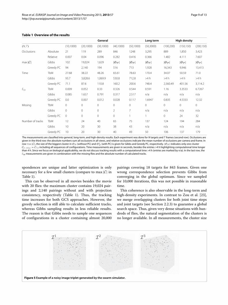
Table 1 Overview of the results

General Long term High density

(N, T) (10,1000) (20,1000) (30,1000) (40,1000) (50,1000) (50,3000) (100,200) (150,150) (200,150)

Occlusions Absolute 21 119 289 846 1248 3,295 889 1,850 3,423

Relative 0.007 0.04 0.096 0.282 0.416 0.366 1.482 4.111 7.607

max |C| Gibbs 102 19,024 1,629 |SP | |SP | |SP | |SP | |SP | |SP |Greedy PC 94 2,140 194 516 713 1,928 16,343 9,946 13,413

Time TbM 27.68 38.22 48.26 65.61 78.63 170.4 34.07 50.59 71.0

Gibbs 93.7 3,828.6 1,069.9 530.8 712.8 >4 h >4 h >4 h >4 h

Greedy PC 71.1 87.6 110.8 160.2 200.6 748.4 2,560.49 401.56 3,114.2

Eca TbM 0.009 0.052 0.33 0.326 0.544 0.591 1.16 3.3533 6.7267

Gibbs 0.085 1.657 0.791 0.317 2.517 n/a n/a n/a n/a

Greedy PC 0.0 0.007 0.012 0.028 0.117 1.6947 0.835 4.5333 12.32

Missing TbM 0 0 0 0 0 0 0 0 0

Gibbs 0 0 0 2 7 n/a n/a n/a n/a

Greedy PC 0 0 0 0 1 1 0 24 32

Number of tracks TbM 12 24 40 65 75 137 124 194 284

Gibbs 10 20 30 38 43 n/a n/a n/a n/a

Greedy PC 10 20 30 40 49 50 106 137 179

The measurements are classified into general, long-term, and high-density results. Each experiment was done for N targets and T frames (second row). Occlusions aregiven in the third row: the absolute numbers sum all occlusions in all views, and relative occlusions indicate the mean number of occlusions per camera and frame. Inrow max |C|, the size of the biggest cluster in SP (without PC) and S∗

P (with PC) is given for Gibbs and Greedy PC, respectively. |SP | indicates only one clusterC(t−δ:t),ν = CT ,N including all sequences of configurations. Time measurements are given in seconds, besides the entries >4 h highlighting computational time longerthan 4 h. Since we focus on biological applicability, we do not discuss tracking results with a computational time >4 h (entries are marked by n/a). In the last row, theEca measurements are given in combination with the missing flies and the absolute number of calculated tracks.

spondences are unique and latter optimization is onlynecessary for a few small clusters (compare to max |C| inTable 1).

This can be observed in all movies besides the moviewith 20 flies: the maximum cluster contains 19,024 pair-ings and 2,140 pairings without and with projectionconsistency, respectively (Table 1). Thus, the trackingtime increases for both GCS approaches. However, thegreedy selection is still able to calculate sufficient tracks,whereas Gibbs sampling results in less reliable results.The reason is that Gibbs needs to sample one sequencesof configurations in a cluster containing almost 20,000

pairings covering 18 targets for 843 frames. Given onewrong correspondence selection prevents Gibbs fromconverging in the global optimum. Since we sampledfor 10,000 iterations, this was not possible in reasonabletime.

This coherence is also observable in the long-term andhigh-density experiments. In contrast to Zou et al. [23],we merge overlapping clusters for both joint time stepsand joint targets (see Section 2.2.3) to guarantee a globalsearch space. Thus, given very dense situations with hun-dreds of flies, the natural segmentation of the clusters isno longer available. In all measurements, the cluster size

Figure 5 Example of a noisy image triplet generated by the swarm simulator.


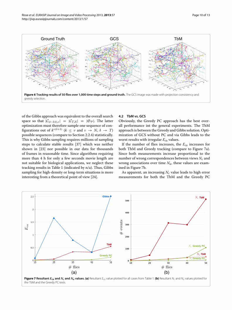
Ground Truth GCS TbM

Figure 6 Tracking results of 50 flies over 1,000 time steps and ground truth. The GCS image was made with projection consistency andgreedy selection.

of the Gibbs approach was equivalent to the overall searchspace so that |C(t−δ:t),ν | = |CT ,N | = |SP |. The latteroptimization must therefore sample one sequence of con-figurations out of kν(δ+1) (k ≤ ν and ν → N , δ → T)possible sequences (compare to Section 2.2.4) statistically.This is why Gibbs sampling requires millions of samplingsteps to calculate stable results [37] which was neithershown in [23] nor possible in our data for thousandsof frames in reasonable time. Since algorithms requiringmore than 4 h for only a few seconds movie length arenot suitable for biological applications, we neglect thesetracking results in Table 1 (indicated by n/a). Thus, Gibbssampling for high-density or long-term situations is moreinteresting from a theoretical point of view [24].

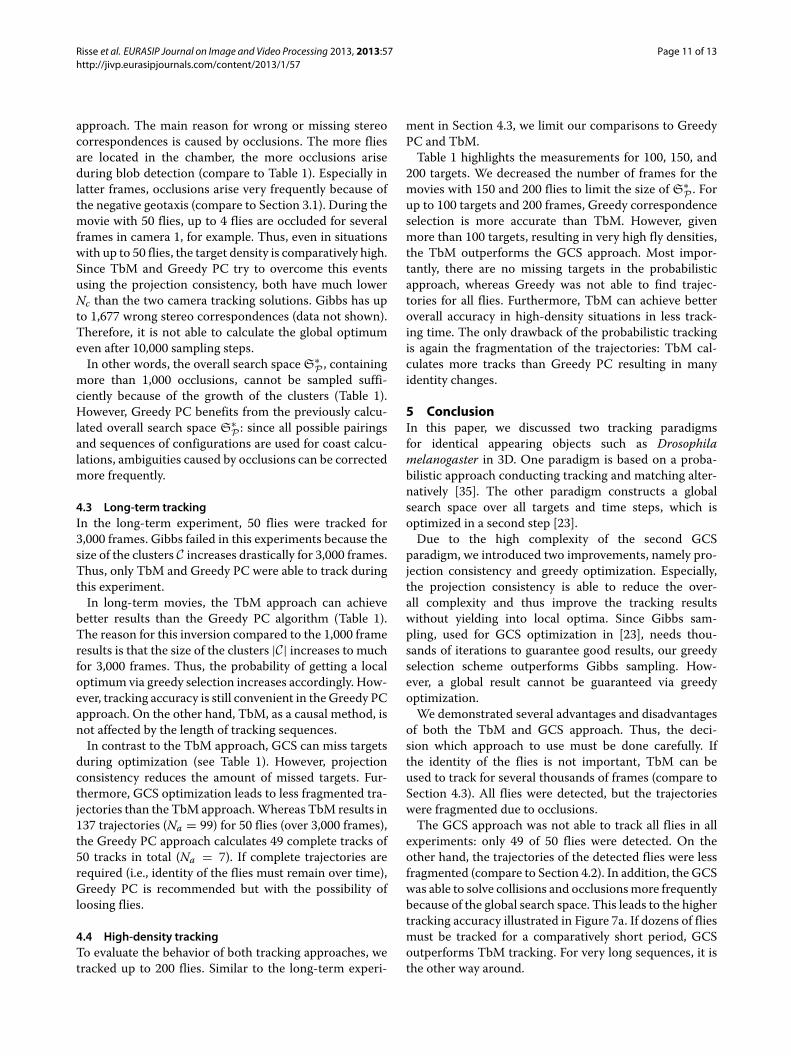
4.2 TbM vs. GCSObviously, the Greedy PC approach has the best over-all performance int the general experiments. The TbMapproach is between the Greedy and Gibbs solution. Opti-mization of GCS without PC and via Gibbs leads to theworst results with irregular Eca values.

If the number of flies increases, the Eca increases forboth TbM and Greedy tracking (compare to Figure 7a).Since both measurements increase proportional to thenumber of wrong correspondences between views Nc andwrong associations over time Na, these values are exam-ined in Figure 7b.

As apparent, an increasing Nc value leads to high errormeasurements for both the TbM and the Greedy PC

Figure 7 Resultant Eca and Nc and Na values. (a) Resultant Eca value plotted for all cases from Table 1. (b) Resultant Nc and Na values plotted forthe TbM and the Greedy PC tests.


approach. The main reason for wrong or missing stereocorrespondences is caused by occlusions. The more fliesare located in the chamber, the more occlusions ariseduring blob detection (compare to Table 1). Especially inlatter frames, occlusions arise very frequently because ofthe negative geotaxis (compare to Section 3.1). During themovie with 50 flies, up to 4 flies are occluded for severalframes in camera 1, for example. Thus, even in situationswith up to 50 flies, the target density is comparatively high.Since TbM and Greedy PC try to overcome this eventsusing the projection consistency, both have much lowerNc than the two camera tracking solutions. Gibbs has upto 1,677 wrong stereo correspondences (data not shown).Therefore, it is not able to calculate the global optimumeven after 10,000 sampling steps.

In other words, the overall search space S∗P , containing

more than 1,000 occlusions, cannot be sampled suffi-ciently because of the growth of the clusters (Table 1).However, Greedy PC benefits from the previously calcu-lated overall search space S∗

P : since all possible pairingsand sequences of configurations are used for coast calcu-lations, ambiguities caused by occlusions can be correctedmore frequently.

4.3 Long-term trackingIn the long-term experiment, 50 flies were tracked for3,000 frames. Gibbs failed in this experiments because thesize of the clusters C increases drastically for 3,000 frames.Thus, only TbM and Greedy PC were able to track duringthis experiment.

In long-term movies, the TbM approach can achievebetter results than the Greedy PC algorithm (Table 1).The reason for this inversion compared to the 1,000 frameresults is that the size of the clusters |C| increases to muchfor 3,000 frames. Thus, the probability of getting a localoptimum via greedy selection increases accordingly. How-ever, tracking accuracy is still convenient in the Greedy PCapproach. On the other hand, TbM, as a causal method, isnot affected by the length of tracking sequences.

In contrast to the TbM approach, GCS can miss targetsduring optimization (see Table 1). However, projectionconsistency reduces the amount of missed targets. Fur-thermore, GCS optimization leads to less fragmented tra-jectories than the TbM approach. Whereas TbM results in137 trajectories (Na = 99) for 50 flies (over 3,000 frames),the Greedy PC approach calculates 49 complete tracks of50 tracks in total (Na = 7). If complete trajectories arerequired (i.e., identity of the flies must remain over time),Greedy PC is recommended but with the possibility ofloosing flies.

4.4 High-density trackingTo evaluate the behavior of both tracking approaches, wetracked up to 200 flies. Similar to the long-term experi-

ment in Section 4.3, we limit our comparisons to GreedyPC and TbM.

Table 1 highlights the measurements for 100, 150, and200 targets. We decreased the number of frames for themovies with 150 and 200 flies to limit the size of S∗

P . Forup to 100 targets and 200 frames, Greedy correspondenceselection is more accurate than TbM. However, givenmore than 100 targets, resulting in very high fly densities,the TbM outperforms the GCS approach. Most impor-tantly, there are no missing targets in the probabilisticapproach, whereas Greedy was not able to find trajec-tories for all flies. Furthermore, TbM can achieve betteroverall accuracy in high-density situations in less track-ing time. The only drawback of the probabilistic trackingis again the fragmentation of the trajectories: TbM cal-culates more tracks than Greedy PC resulting in manyidentity changes.

5 ConclusionIn this paper, we discussed two tracking paradigmsfor identical appearing objects such as Drosophilamelanogaster in 3D. One paradigm is based on a proba-bilistic approach conducting tracking and matching alter-natively [35]. The other paradigm constructs a globalsearch space over all targets and time steps, which isoptimized in a second step [23].

Due to the high complexity of the second GCSparadigm, we introduced two improvements, namely pro-jection consistency and greedy optimization. Especially,the projection consistency is able to reduce the over-all complexity and thus improve the tracking resultswithout yielding into local optima. Since Gibbs sam-pling, used for GCS optimization in [23], needs thou-sands of iterations to guarantee good results, our greedyselection scheme outperforms Gibbs sampling. How-ever, a global result cannot be guaranteed via greedyoptimization.

We demonstrated several advantages and disadvantagesof both the TbM and GCS approach. Thus, the deci-sion which approach to use must be done carefully. Ifthe identity of the flies is not important, TbM can beused to track for several thousands of frames (compare toSection 4.3). All flies were detected, but the trajectorieswere fragmented due to occlusions.

The GCS approach was not able to track all flies in allexperiments: only 49 of 50 flies were detected. On theother hand, the trajectories of the detected flies were lessfragmented (compare to Section 4.2). In addition, the GCSwas able to solve collisions and occlusions more frequentlybecause of the global search space. This leads to the highertracking accuracy illustrated in Figure 7a. If dozens of fliesmust be tracked for a comparatively short period, GCSoutperforms TbM tracking. For very long sequences, it isthe other way around.


If high fly densities are needed for a comparatively longperiod, the size of the global search space prevents Gibbsoptimization, because it requires too many sampling iter-ations. In addition, greedy tracking quality decreases dras-tically compared to TbM (see Section 4.4). Thus, withoutfurther reductions of the global search space, probabilis-tic tracking is the preferable paradigm in high-densityexperiments.

TbM could be optimized in terms of tracking accuracy,whereas GCS could be optimized for longer tracking dura-tions and higher target densities. Possible improvementsfor the TbM approach are discussed in [35]. Here, we wantto focus on improvements of the GCS approach.

Currently, we use the third camera only to correctmismatches between cameras 1 and 2. The optimiza-tion scheme is still executed on pairings. Since pairwisecomparison in a triplet would further reduce the searchspace, all optimization steps could be done on three imagepoints.

The kinetic model given by Equation 8 is also a currentdrawback of the GCS approach. Only motion form (t − 1)

is considered for time step t. Thus, a more appropriatemotion model would further improve the accuracy of GCStracking.

Currently, we are developing a three-camera real-worldsetup to capture movies of adult Drosophila flies. Thus, weare going to test both algorithms on real video sequences,comparable to the synthetic data introduced above.

Competing interestsThe authors declare that they have no competing interests.

AcknowledgementsThe authors thank S. Strothoff for the discussion and help throughout theproject. Furthermore, we would like to thank the anonymous reviewers for thehelpful annotations and suggestions for improvements. We acknowledge thesupport by the Deutsche Forschungsgemeinschaft and Open AccessPublication Fund of University of Münster.

Author details1Department of Mathematics and Computer Science, University of Münster,Einsteinstraße 62, Münster 48149, Germany. 2Department of ComputerScience, University of Auckland, Tamaki Innovation Campus, Glen Innes, MorrinRoad, Auckland 1142, New Zealand. 3Department of Neuro and BehavioralBiology, University of Münster, Badestraße 9, 48149 Münster, Germany.

Received: 31 January 2013 Accepted: 19 September 2013Published: 31 October 2013

References

1. DM Gohl, MA Silies, XJ Gao, S Bhalerao, FJ Luongo, CC Lin, CJ Potter, TRClandinin, A versatile in vivo system for directed dissection of geneexpression patterns. Nat. Methods. 8(3), 231–237 (2011)

2. A Katsov, Motion processing streams in Drosophila are behaviorallyspecialized. Neuron. 59(2), 322–335 (2008)

3. B Risse, S Thomas, N Otto, T Löpmeier, D Valkov, X Jiang, C Klämbt, FIM anovel FTIR-based imaging method for high throughput locomotionanalysis. PloS one. 8(1), e53963 (2013)

4. MB Sokolowski, Drosophila: genetics meets behaviour. Nat. Rev. Genet.2(11), 879–890 (2001)

5. A Gomez-Marin, N Partoune, GJ Stephens, M Louis, Automated trackingof animal posture and movement during exploration and sensoryorientation behaviors. PloS one. 7(8), e41642 (2012)

6. D Grover, J Yang, D Ford, S Tavaré, J Tower, Simultaneous tracking ofmovement and gene expression in multiple Drosophila melanogaster fliesusing GFP and DsRED fluorescent reporter transgenes. BMC Res. Notes.2(1), 58 (2009)

7. S Lahiri, K Shen, M Klein, A Tang, E Kane, M Gershow, P Garrity, ADTSamuel, Two alternating motor programs drive navigation in Drosophilalarva. PloS one. e23(8), 180 (2011)

8. J Tao, R Klette, Tracking of 2D or 3D irregular movement by a family ofunscented Kalman filters. J. Inf. Convergence Commun. Eng. 10(3),307–314 (2012)

9. H Dankert, L Wang, ED Hoopfer, DJ Anderson, P Perona, Automatedmonitoring and analysis of social behavior in Drosophila. Nat. Methods.6(4), 297–303 (2009)

10. J Martin, A portrait of locomotor behaviour in Drosophila determined bya video-tracking paradigm. Behav. Process. 67(2), 207–219 (2004)

11. TA Ofstad, CS Zuker, MB Reiser, Visual place learning in Drosophilamelanogaster. Nature. 474(7350), 204–207 (2011)

12. J Colomb, L Reiter, J Blaszkiewicz, J Wessnitzer, Open source tracking andanalysis of adult Drosophila locomotion in Buridan’s paradigm with andwithout visual targets. PloS one. 7(11), e42247 (2012)

13. D Valente, I Golani, PP Mitra, Analysis of the trajectory of Drosophilamelanogaster in a circular open field arena. PloS one. 2(10),e1083 (2007)

14. SN Fry, M Bichsel, P Müller, D Robert, Tracking of flying insects usingpan-tilt cameras. J. Neurosci. Methods. 101(1), 59–67 (2000)

15. A Poore, Multidimensional assignment formulation of data associationproblems arising from multitarget and multisensor tracking. Comput.Optimization Appl. 3, 27–57 (1994)

16. RE Burkard, M Dell’Amico, S Martello, Assignment Problems, 1st edn(Society for Industrial Mathematics, Philadelphia, 2009)

17. LF Tammero, MH Dickinson, The influence of visual landscape on the freeflight behavior of the fruit fly Drosophila melanogaster. J. Exp. Biol.205(Pt 3), 327–343 (2002)

18. H Du, D Zou, YQ Chen, Relative epipolar motion of tracked features forcorrespondence in binocular stereo, in ICCV Conference Proceedings, Riode Janeiro, October 2007 (IEEE, Piscataway, 2007), pp. 1–8

19. D Engelmann, C Garbe, M Stohr, P Geißler, F Hering, B Jahne, Stereoparticle tracking, in 8th International Symposium on Flow Visualisation,Sorrento, 1–4 September (1998), pp. 1–10

20. HS Wu, Q Zhao, D Zou, YQ Chen, Acquiring 3D motion trajectories oflarge numbers of swarming animals, in IEEE 12th International Conferenceon Computer Vision Workshops, Kyoto, September to October 2009 (IEEE,Piscataway, 2009), pp. 593–600

21. D Grover, J Tower, S Tavaré, O fly, where art thou. J. R. Soc. Interface. 5(27),1181–1191 (2008)

22. AD Straw, K Branson, TR Neumann, MH Dickinson, Multi-camera real-timethree-dimensional tracking of multiple flying animals. J. R. Soc. Interface.8(56), 395–409 (2011)

23. D Zou, Q Zhao, HS Wu, YQ Chen, Reconstructing 3D motion trajectoriesof particle swarms by global correspondence selection, in IEEE 12thInternational Conference on Computer Vision, Kyoto, September to October2009 (IEEE, Piscataway, 2009), pp. 1578–1585

24. R Ardekani, A Biyani, JE Dalton, JB Saltz, MN Arbeitman, J Tower, SNuzhdin, S Tavaré, Three-dimensional tracking and behaviourmonitoring of multiple fruit flies. J. R. Soc. Interface. 10(78), 20120–547(2013)

25. F Pereira, H Stüer, EC Graff, M Gharib, Two-frame 3D particle tracking.Meas. Sci. Technol. 17(7), 1680–1692 (2006)

26. D Theriault, Z Wu, N Hristov, S Swartz, K Breuer, T Kunz, M Betke,Reconstruction and analysis of 3D trajectories of Brazilian free-tailed batsin flight (2010)

27. Z Wu, NI Hristov, TL Hedrick, TH Kunz, M Betke, Tracking a large number ofobjects from multiple views, in 2009 IEEE 12th International Conference onComputer Vision, Kyoto, September to October 2009 (IEEE, Piscataway,2009), pp. 1546–1553

28. A Veeraraghavan, M Srinivasan, R Chellappa, E Baird, R Lamont, Motionbased correspondence for 3D tracking of multiple Dim objects. IEEE Int.Conf. Acoustics Speech Signal Process (ICASSP). 2, pp. II (2006)


29. NT Ouellette, H Xu, E Bodenschatz, A quantitative study ofthree-dimensional Lagrangian particle tracking algorithms. Exp. Fluids40(2), 301–313 (2005)

30. KJ Kohlhoff, TR Jahn, DA Lomas, CM Dobson, DC Crowther, MVendruscolo, The iFly tracking system for an automated locomotor andbehavioural analysis of Drosophila melanogaster. Integr. Biol. (Camb). 3(7),755–760 (2011)

31. S Zou, P Liedo, L Altamirano-Robles, J Cruz-Enriquez, A Morice, DK Ingram,K Kaub, N Papadopoulos, JR Carey, Recording lifetime behavior andmovement in an invertebrate model. PloS one. 6(4), e18151 (2011)

32. S Butail, N Manoukis, M Diallo, JM Ribeiro, T Lehmann, DA Paley,Reconstructing the flight kinematics of swarming and mating in wildmosquitoes. J. R. Soc. Interface. 9(75), 2624–2638 (2012)

33. DH Kelley, NT Ouellette, Emergent dynamics of laboratory insect swarms.Sci. Rep. 3 (2013)

34. A Attanasi, A Cavagna, L Del Castello, I Giardina, A Jelic, S Melillo, L Parisi, EShen, E Silvestri, M Viale, Tracking in three dimensions via multi-pathbranching. CoRR abs/1305.1495 (2013)

35. J Tao, B Risse, X Jiang, R Klette, 3D Trajectory estimation of simulated fruitflies, in Proc 27th IVCNZ, (Dunedin, 26–28 November 2012)

36. R Hartley, A Zisserman, Multiple View Geometry in Computer Vision(Cambridge University Press, Cambridge, 2004)

37. S Geman, D Geman, Stochastic relaxation, Gibbs distributions and theBayesian restoration of images. IEEE Trans. Pattern Anal. Mach. Intell. 6(6),721–741 (1984)

38. EA Wan, R van der Menve, The unscented Kalman filter for nonlinearestimation, in Adaptive Systems for Signal Processing, Communications, andControl Symposium 2000, Lake Louise, Alta, October 2000 (IEEE,Piscataway, 2000), pp. 153–158

39. JH Marden, MR Wolf, KE Weber, Aerial performance of Drosophilamelanogaster from populations selected for upwind flight ability. J. Exp.Biol. 200(Pt 21), 2747–2755 (1997)

40. JW Gargano, I Martin, P Bhandari, MS Grotewiel, Rapid iterative negativegeotaxis (RING): a new method for assessing age-related locomotordecline in Drosophila. Exp. Gerontol. 40(5), 386–395 (2005)

doi:10.1186/1687-5281-2013-57Cite this article as: Risse et al.: Comparison of two 3D tracking paradigmsfor freely flying insects. EURASIP Journal on Image and Video Processing 20132013:57.

Submit your manuscript to a journal and benefi t from:

7 Convenient online submission

7 Rigorous peer review

7 Immediate publication on acceptance

7 Open access: articles freely available online

7 High visibility within the fi eld

7 Retaining the copyright to your article

Submit your next manuscript at 7 springeropen.com

Comparison of two 3D tracking paradigms for freely flying ...

Documents

Transcript of Comparison of two 3D tracking paradigms for freely flying ...