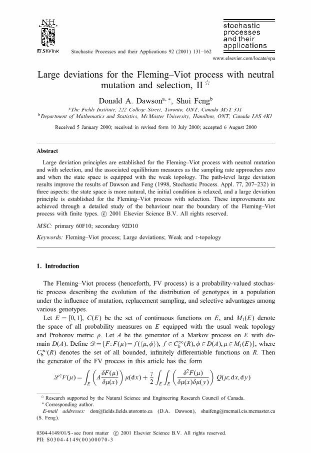
Stochastic Processes and their Applications 92 (2001) 131–162www.elsevier.com/locate/spa

Large deviations for the Fleming–Viot process with neutralmutation and selection, II(

Donald A. Dawsona ; ∗, Shui FengbaThe Fields Institute, 222 College Street, Toronto, ONT, Canada M5T 3J1

bDepartment of Mathematics and Statistics, McMaster University, Hamilton, ONT, Canada L8S 4K1

Received 5 January 2000; received in revised form 10 July 2000; accepted 6 August 2000

Abstract

Large deviation principles are established for the Fleming–Viot process with neutral mutationand with selection, and the associated equilibrium measures as the sampling rate approaches zeroand when the state space is equipped with the weak topology. The path-level large deviationresults improve the results of Dawson and Feng (1998, Stochastic Process. Appl. 77, 207–232) inthree aspects: the state space is more natural, the initial condition is relaxed, and a large deviationprinciple is established for the Fleming–Viot process with selection. These improvements areachieved through a detailed study of the behaviour near the boundary of the Fleming–Viotprocess with �nite types. c© 2001 Elsevier Science B.V. All rights reserved.

MSC: primary 60F10; secondary 92D10

Keywords: Fleming–Viot process; Large deviations; Weak and �-topology

1. Introduction

The Fleming–Viot process (henceforth, FV process) is a probability-valued stochas-tic process describing the evolution of the distribution of genotypes in a populationunder the in uence of mutation, replacement sampling, and selective advantages amongvarious genotypes.Let E = [0; 1], C(E) be the set of continuous functions on E, and M1(E) denote

the space of all probability measures on E equipped with the usual weak topologyand Prohorov metric �. Let A be the generator of a Markov process on E with do-main D(A). De�ne D={F :F(�)=f(〈�; �〉); f∈C∞

b (R); �∈D(A); �∈M1(E)}, whereC∞b (R) denotes the set of all bounded, in�nitely di�erentiable functions on R. Thenthe generator of the FV process in this article has the form

L F(�) =∫E

(A�F(�)��(x)

)�(dx) +

2

∫E

∫E

(�2F(�)

��(x)��(y)

)Q(�; dx; dy)

( Research supported by the Natural Science and Engineering Research Council of Canada.∗ Corresponding author.E-mail addresses: don@�elds.�elds.utoronto.ca (D.A. Dawson), shuifeng@mcmail.cis.mcmaster.ca

(S. Feng).

0304-4149/01/$ - see front matter c© 2001 Elsevier Science B.V. All rights reserved.PII: S0304 -4149(00)00070 -3

132 D.A. Dawson, S. Feng / Stochastic Processes and their Applications 92 (2001) 131–162

=f′(〈�; �〉)〈�; A�〉+ 2

∫ ∫f′′(〈�; �〉)�(x)�(y)Q(�; dx; dy); (1)

where

�F(�)=��(x) = lim�→0+

�−1{F((1− �)� + ��x)− F(�)};

�2F(�)=��(x)��(y)= lim�1→0+; �2→0+

(�1�2)−1{F((1− �1−�2)�+�1�x+�2�y)−F(�)};

Q(�; dx; dy) = �(dx)�x(dy)− �(dx)�(dy);

and �x stands for the Dirac measure at x∈E. The domain of L is D. E is called thetype space or the space of alleles, A is known as the mutation operator, and the lastterm describes the continuous sampling with sampling rate . If the mutation operatorhas the form

Af(x) =�2

∫(f(y)− f(x))�0 (dy)

with �0 ∈M1(E), we call the process a FV process with neutral mutation.For any symmetric bounded measurable function V (z; y) on E⊗2, let

V (�) =∫E

∫EV (z; y)� (dz)� (dy)

and ⟨�V (�)��

;�F��

⟩=∫E

∫E

∫E

�F��(z)[V (z; y)− V (y; w)]�(dz)�(dy)�(dw):

Then the generator of a FV process with neutral mutation and selection takes theform

L V F(�) =L F(�) +

⟨�V (�)��

;�F��

⟩; (1.2)

where V is called the �tness function which is assumed to be continuous in the sequel.A nice survey on FV process and their properties can be found in Ethier and Kurtz(1993). In particular, it is shown in Ethier and Kurtz (1993) that the martingale problemassociated with generators L and LV are well-posed.Let T ¿ 0 be �xed, and C([0; T ]; M1(E)) denote the space of all M1(E)-valued,

continuous functions on [0; T ]. For any � in M1(E), let P�; ;�0� and P�; ;V;�0

� be the lawsof the FV process with neutral mutation and FV process with neutral mutation andselection, respectively. ��; ;�0 and ��; ;�0 ;V will represent the corresponding equilibriummeasures.Let X(E) be the space of all �nitely additive, non-negative, mass one measures

on E, equipped with the smallest topology such that for all Borel subset B of E,�(B) is continuous in �. The �-algebra B of space X(E) is the smallest �-algebrasuch that for all Borel subset B of E, �(B) is a measurable function of �. It is clearthat M1(E) is a strict subset of X(E). In Dawson and Feng (1998), large deviationprinciple (henceforth, LDP) is established for equilibrium measures on space X(E) andpartial results are obtained for the path-level LPDs on a strange space under strongertopologies. In the present article we will �rst establish the LDPs for the equilibrium

D.A. Dawson, S. Feng / Stochastic Processes and their Applications 92 (2001) 131–162 133

measures on space M1(E), and compare these with results obtained in Dawson and Feng(1998). Secondly, we establish the LDPs for the FV process with neutral mutation andwith selection as → 0 on space C([0; T ]; M1(E)). These improve the correspondingresults in Dawson and Feng (1998) in three aspects: the space is more natural, theinitial condition is relaxed, and a full large deviation principle is established for theFV process with selection. This type of LDPs can be viewed as the in�nite-dimensionalgeneralization of the Freidlin–Wentzell theory. We prove the results through a detailedanalysis of the boundary behaviour of the FV process with �nite types.In Section 2, we list some preliminary results to make the paper self-contained.

LDPs for the equilibrium measures are the content of Section 3. The detailed study ofthe Fleming–Viot process with �nite type space is carried out in Section 4. Finally,in Section 5, we prove the LDPs for the FV process with neutral mutation and withselection.

2. Preliminary

In this section, we give some de�nitions and results in the theory of large deviations.A more complete introduction to the theory is found in Dembo and Zeitouni (1993).Properties of �nite additive measures will also be discussed.Let X be a Hausdor� space with �-algebra F. Here F could be smaller than the

Borel �-algebra on X . {P : ¿ 0} is a family of probability measures on (X;F).

De�nition 2.1. The family {P : ¿ 0} is said to satisfy a LDP with a good rate func-tion I if

1. for all x∈X; I(x)¿0;2. for any c¿0, the level set �(c) = {x∈X : I(x)6} is compact in X ;3. for any F-measurable closed subset F of X ,

lim sup →0

logP (F)6− infx∈ F

I(x);

4. for any F-measurable open subset G of X ,

lim inf → logP (G)¿− inf

x∈GI(x):

Functions satisfying the �rst two conditions are called good rate functions.

De�nition 2.2. The family {P : ¿ 0} is said to be exponentially tight if for any �¿ 0there exists a compact subset K� of X such that

lim sup →0

logP (Kc�)6− �;

where Kc� is the complement of K� in X .

The following result of Pukhalskii will be used repeatedly in the sequel.

134 D.A. Dawson, S. Feng / Stochastic Processes and their Applications 92 (2001) 131–162

Theorem 2.1 (Pukhalskii). Assume that the space X is a Polish space with metricd and F is the Borel �-algebra. Then the family {P : ¿ 0} satis�es a LDP withgood rate function I if and only if the family {P : ¿ 0} is exponentially tight; andfor any x∈X

− I(x) = lim�→0

lim sup →0

logP {y∈X : d(y; x)6�}

= lim�→0

lim inf →0

logP {y∈X : d(y; x)¡�}: (2.3)

If the family {P : ¿ 0} is exponentially tight; then for any sequence ( n) con-verging to zero from above as n goes to in�nity; there is a subsequence ( nk ) of ( n)such that {P nk

} satis�es a LDP with certain good rate function that depends on thesubsequence.

Proof. Part one and part two are Corollary 3:4 and Theorem (P) of Pukhalskii (1991)respectively.

Let X be a Polish space, M1(X ) denote the space of all probability measures on Xequipped with the weak topology. Let Cb(X ) and Bb(X ) denote the set of boundedcontinuous functions on X , and the set of bounded measurable functions on X , respec-tively. For any �; � in M1(X ), the relative entropy of � with respect to � is de�nedand denoted by

H (�|�) =∫X� log� d� if �.�;

∞ otherwise;(2.4)

where � is the Radon–Nikodym derivative of � with respect to �. It is known (cf.Donsker and Varadhan, 1975) that

H (�|�) = supg∈Cb(X )

{∫Xg d� − log

∫Xegd�

}

= supg∈ Bb(X )

{∫Xg d� − log

∫Xeg d�

}: (2.5)

The relative entropy is closely related to the rate functions discussed in Section 3.Finally, we present some results on �nitely additive measures in Yosida and Hewitt

(1952). Assume that the space X is a Polish space and F is the Borel �-algebra. LetN(X ) denote the set of all nonnegative, �nitely additive measures on (X; F). For any�; � in N(X ), we write �6� if for any B in F we have �(B)6�(B).

De�nition 2.3. Let � be any element in N(X ). If 0 is the only countably additivemeasure � satisfying 06�6�; then � is called a pure �nitely additive measure.

Here is an example of a pure �nitely additive measure. Let X = [0; 1]; F be theBorel �-algebra. De�ne measure � such that it only assumes the values of 0 and 1,�(A) = 1 if A contains [0; a) for some a¿ 0, �(A) = 0 if A has Lebesgue measurezero. The existence of such a �nitely additive measure is guaranteed by Theorem 4:1

D.A. Dawson, S. Feng / Stochastic Processes and their Applications 92 (2001) 131–162 135

in Yosida and Hewitt (1952). Since limn→∞ �([0; 1=n)) = 1 6= 0 = �({0}); � is notcountably additive. To see that it is pure �nitely additive, let � be any countablyadditive measure satisfying 06�6�. Then

�([0; 1]) = �({0}) + limn→∞ (1− �((0; 1=n])) = 0

which implies that � ≡ 0.

Theorem 2.2 (Yosida and Hewitt, 1952, Theorem 1:19). Let � be any non-negativepure �nitely additive measure; and � be any non-negative countably additive mea-sure on space (X;F). Then for any �¿ 0; there exists A in F such that �(Ac) =0; �(A)¡�; where Ac is the complement of A.

Theorem 2.3. Any non-negative measure � on space (X;F) can be uniquely writtenas the sum of a non-negative; countably additive measure �c and a non-negative; pure�nitely additive measure �p.

Proof. This is a combination of Theorems 1:23 and 1:24 in Yosida and Hewitt (1952).

3. Equilibrium LDPs

Let X(E) be the space of all �nitely additive, non-negative, mass one measures on Eequipped with the projective limit topology, i.e., the weakest topology such that for allBorel subset B of E, �(B) is continuous in �. Under this topology, X(E) is Hausdor�.The �-algebra B of space X(E) is the smallest �-algebra such that for all Borel subsetB of E; �(B) is a measurable function of �.It was incorrectly stated in Dawson and Feng (1998) that X(E) can be identi�ed with

M1(E) equipped with the �-topology for large deviation purposes. In this section we will�rst clarify the issues associated with equilibrium LDPs on the space X(E), and thenestablish the LDPs for equilibrium measures on M1(E) under the weak topology. Recallthat the �-topology on M1(E) is the smallest topology such that 〈�; f〉=

∫E f(x)�(dx) is

continuous in � for any bounded measurable function f on E. This topology is clearlystronger than the weak topology, and is the same as the subspace topology inheritedfrom X(E). We use M�

1 (E) to denote space M1(E) equipped with the �-topology.

Theorem 3.1. Every element � in X(E) has the following unique decomposition:

� = �ac + �s + �p; (3.1)

where �p is a pure �nitely additive measure; �ac and �s are both countably additivewith �ac.�0; �s⊥�0.

Proof. The result follows from Theorem 2.3 and the Lebesgue decomposition theorem.

Remark. An element � in X(E) is a probability measure if and only if �p(E) = 0.

136 D.A. Dawson, S. Feng / Stochastic Processes and their Applications 92 (2001) 131–162

For any � in X(E) satisfying �ac(E)¿ 0, let �ac(·|E)=�ac(·)=�ac(E). Then it is clearthat �ac(·|E) is in M1(E). � is said to be absolutely continuous with respect to �0, stilldenoted by �.�0, if �0(B) = 0 implies �(B) = 0. For any two probability measures�; �; H (�|�) denotes the relative entropy of � with respect to �. De�ne

I(�) =

�[H (�0|�ac(·|E))− log�ac(E)] if �.�0; �ac(E)¿ 0; � 6∈ M1(E);

�H (�0|�) if �.�0; �∈M1(E);

∞ else:

(3.2)

Remark. �.�0 implies that �s = 0.

Theorem 3.2. The family {��; ;�0} satis�es a LDP on X(E) with good rate function I .

Proof. Let

P= {{B1; : : : ; Br}: r¿1; B1; : : : ; Br is a partition of [0; 1]

by Borel measurable sets}: (3.3)

Elements of P are denoted by �; —; and so on. We say — � � i� — is �ner than �. ThenP partially ordered by � is a partially ordered right-�ltering set.For every — = (B1; : : : ; Br)∈P, let

X— =

{x = (xB1 ; : : : ; xBr ): xBi¿0; i = 1; : : : ; r;

r∑i=1

xBi = 1

}:

For any �= (C1; : : : ; Cl); — = (B1; : : : ; Br)∈P; — � �, de�ne

��—:X— → X�; (xB1 ; : : : ; xBr )→( ∑

Bk ⊂C1

xBk ; : : : ;∑

Bk ⊂Cl

xBk

):

Then {X—; ��—; �; —∈ J; �} becomes a projective system, and the projective limit ofthis system can be identi�ed as X(E).For any �nite partition �= (B1; : : : ; Br) of E, and any � in X(E), let

I�(�) =

∑r

k=1�0(Bk)log

�0(Bk)�(Bk)

if�.�0;

∞ else;

where we treat c=0 as in�nity for c¿ 0.Let

I(�) = � sup�

I�(�); (3.4)

where the supremum is taken over all �nite partitions of E.By the standard monotone class argument indicator function over an interval can

be approximated by bounded continuous functions pointwise. Hence, the restriction ofthe �-algebra B on M1(E) coincides with the Borel �-algebra generated by the weaktopology, and ��; ;�0 is well-de�ned on space (X(E); B).By using Theorem 3:3 of Dawson and G�artner (1987), one gets that ��; ;�0 satisti�es

a LDP with good rate function I . Hence to prove the theorem it su�ces to verify that

D.A. Dawson, S. Feng / Stochastic Processes and their Applications 92 (2001) 131–162 137

I(�) = I(�). This is true if � is not absolutely continuous with respect to �0 sinceboth are in�nity. The case of � in M1(E) follows from Lemma 2:3 in Dawson andFeng (1998). Now assume �.�0 and � 6∈ M1(E). Then we have �ac(E)¡ 1; �p 6= 0.If �ac(E) = 0, then by applying Theorem 2.2, both I and I are in�nity. Next weassume that � = �ac(E) is in (0; 1). By de�nition we have I(�)¿I�(�) for any �nitepartition � of E. Thus I¿I . On the other hand, for any n¿1 choose a set An suchthat �0(An)¡ 1=n2; �p(Acn) = 0. This is possible because Theorem 2.2 and �p is pure�nitely additive. It is clear that �0(

⋂ni=1 Ai)¡ 1=n2; �p((

⋂ni=1 Ai)c)=0. Hence by taking

intersection, the sequence {An} can be chosen to be decreasing. For any �nite partition� = (B1; : : : ; Br) we introduce a new �nite partition — = (B1 ∩ An; B1 ∩ Acn; : : : ; Br ∩ An;Br ∩ Acn). Note that for any pi; xi¿0; i = 1; 2 we have the inequality

(p1 + p2) logp1 + p2x1 + x2

6p1 logp1x1+ p2 log

p2x2

:

This implies

I�(�)6I—(�)

and

I—(�) =r∑

k=1

�0(Bk ∩ Acn) log�0(Bk ∩ Acn)�(Bk ∩ Acn)

+r∑

k=1

�0(Bk ∩ An) log�0(Bk ∩ An)�(Bk ∩ An)

¿r∑

k=1

�0(Bk ∩ Acn) log�0(Bk ∩ Acn)�(Bk ∩ Acn)

+ �0(An) log�0(An)�(An)

=r∑

k=1

�0(Bk ∩ Acn) log�0(Bk ∩ Acn)�(Bk ∩ Acn)

+ �0(An) log�0(An)

�(An) ∨ �:

Letting n go to in�nity, we get

I—(�)¿ limn→∞

r∑k=1

�0(Bk ∩ Acn) log�0(Bk ∩ Acn)�(Bk ∩ Acn)

=r∑

k=1

limn→∞ �0(Bk ∩ Acn) log

�0(Bk ∩ Acn)�(Bk ∩ Acn)

¿r∑

k=1

�0(Bk ∩ F) log�0(Bk ∩ F)�ac(Bk)

;

where F =⋃

n Acn. Since �0(Fc) = 0, we have

I(�)¿�I—(�)¿�r∑

k=1

�0(Bk)log�0(Bk)�ac(Bk)

;

which implies that

I(�)¿� sup�

{r∑

k=1

�0(Bk) log�0(Bk)�ac(Bk)

}= I(�):

138 D.A. Dawson, S. Feng / Stochastic Processes and their Applications 92 (2001) 131–162

Lemma 3.3. Assume that there is a sequence of decreasing intervals An such thatthe length of An converges to zero as n goes to in�nity; �0(An)¿ 0 for all n; and⋂

n An = {x0} with �0(x0) = 0. Then I(�) de�ned above is not a good rate functionon M�

1 (E).

Remark. Clearly a large class of probability measures including Lebesgue measuresatisfy the condition in Lemma 3.3. But pure atomic measures with �nite atoms do notsatisfy the condition.

Proof. We will construct a counter example. Assume that I(�) is a good rate function.Then for any �¿ 0, the level set �(�) = {�∈M1(E): I(�)6�} is a �-compact set.For any �∈ (0; 1); n¿1, choose �n(dx) = fn(x)�0(dx) with

fn(x) =�

�0(An)�An(x) +

1− �1− �0(An)

�Acn(x);

where �A is the indicator function of set A, and Ac denotes the complement of A. Byde�nition, we have

I(�n) = �H (�0|�n) = �∫Elog(1fn

)�0(dx)

= �∫An

log(�0(An)

�

)�0(dx) + �

∫Acn

log(�0(Acn)1− �

)�0(dx)

6 log1

�(1− �);

which implies that �n ∈�(�) with �=log1=�(1−�). Since � compactness implies the �sequential compactness (see G�anssler, 1971, Theorem 2:6), the sequence �n convergesin � topology to a measure � in �(�) and thus in weak topology to the same measure.For any continuous function g on E, one has

limn→∞ 〈�n; g〉= lim

n→∞

[∫An

�g(x)�0(An)

�0(dx) +∫Acn

(1− �)g(x)�0(Acn)

�0(dx)

]

= �g(x0) +∫{x0}c

(1− �)g(x)�0(dx);

which implies that �n converges weakly to � = ��{x0}(dx) + (1− �)�0(dx). This leadto the contradiction

H (�0|�) =∞6�:

Lemma 3.4. Assume �0 satis�es the condition in Lemma 3:3. Then it is impossible toestablish a LDP for the Poisson–Dirichlet distribution with respect to �0 on M�

1 (E)with a good rate function.

Proof. Being the projective limit of a system of Hausdor� space, the space X(E) isalso Hausdor�. By Tychono� theorem, the product space ��∈P X� is compact. sinceX(E) is a closed subset of ��∈P X�, it is also compact. Thus X(E) is a regular

D.A. Dawson, S. Feng / Stochastic Processes and their Applications 92 (2001) 131–162 139

topological space. Assume that a LDP is true on M�1 (E) with a good rate function

J (�). By Lemma 3.3, J must di�er from I . But the following arguments will lead tothe equality of the two which is an obvious contradiction.Fix an �0 in M1(E). The LDP on M�

1 (E) with good J implies the correspondingLDP on M1(E) with good J . Since M1(E) is regular, we get that for any �¿ 0 thereis an open neighborhood Gw of �0 such that

inf�∈Gw

J (�)¿(J (�0)− �) ∧ 1�;

where Gw is the closure in space M1(E).Let GX(E) be an open set in X(E) such that GX(E) ∩M1(E) = Gw. This is possible

because the subspace topology on M1(E) inherited from X(E) is stronger than theweak topology. Now from the two LDPs, we get

− infGw

I(�)6− infGX

I(�)6 lim inf →0

log��; ;�0 (GX(E)) = lim inf

→0 log��; ;�0 (G

w)

6 lim sup →0

log��; ;�0 (Gw)6− infGw

J (�);

which implies that

I(�0)¿ infGw

I(�)¿ infGw

J (�)¿(J (�0)− �) ∧ 1�:

Letting � approach zero we end up with I(�0)¿J (�0): On the other hand, since X(E)is also regular, we get that for any �¿ 0, there exists open set GX(E) containing �0such that

inf�∈GX(E)

I(�)¿(I(�0)− �) ∧ 1�

and GX(E) is the closure in X(E).Let G = GX(E) ∩M1(E). Then as before we get

− infG

J (�)6 lim inf →0

log��; ;�0 (G) = lim inf →0 log��; ;�0 (G

X(E))

6 lim sup →0

log��; ;�0 (GX(E))6− infGX(E)

I(�);

which implies that

J (�0)¿ infG

J (�)¿ infGX(E)

I(�)¿(I(�0)− �) ∧ 1�

and J (�0)¿I(�0).

From Theorem 3.1 and Lemma 3.4 we can see that in order to get an equilibriumLDP in the � topology, one has to expand M1(E) to a bigger space. Next we are goingto show that under a weaker topology, the weak topology, the equilibrium LDP holdson M1(E).First note that the space M1(E) is a compact, Polish space with Prohorov metric �.

Hence the sequence ��; ;�0 is exponentially tight. By Theorem 2.1, to obtain a LDP

140 D.A. Dawson, S. Feng / Stochastic Processes and their Applications 92 (2001) 131–162

for ��; ;�0 with a good rate function it su�ces to verify that there exists a function Jsuch that for every �∈M1(E),

lim�→0

lim inf →0

log��; ;�0{�(�; �)¡�}

= lim�→0

lim sup →0

log��; ;�0{�(�; �)6�}=−J (�): (3.5)

By Theorem 2.1, the function J is the good rate function.Let supp(�) denote the support of a probability measure �, and M1; �0 (E) = {�∈

M1(E): supp(�)⊂ supp(�0)}. Let {�n} be an arbitrary sequence in M1; �0 (E) that con-verges to a � in M1(E). Since supp(�0) is a closed set, we get

1 = lim supn→∞

�n{supp(�0)}6�{supp(�0)};

which implies that �∈M1; �0 (E). Hence M1; �0 (E) is a closed subset of M1(E).Next we prove (3.5) for

J (�) =

{�H (�0|�) if �∈M1; �0 (E);

∞ else;

We will treat 0 log 00 as zero.For any �∈M1(E), de�ne E�={t ∈ (0; 1): �({t})=0}. For any t1¡t2¡ · · ·¡tk ∈E�,

set �t1 ; :::; tk = (�([0; t1)); : : : ; �([tk ; 1])) which can be viewed as a probability measure onspace {0; 1; : : : ; k} with a probability �([ti; ti+1)) at i 6= k and �([tk ; 1]) at k. Set t0 = 0.

Lemma 3.5. For any �; �∈M1(E);

H (�|�) = supt1¡t2¡···¡tk ∈ E�;k¿1

H (�t1 ; :::; tk |�t1 ; :::; tk ): (3.6)

Proof. By Lemma 2:3 in Dawson and Feng (1998), we have

H (�|�)¿ supt1¡t2¡···¡tk ∈ E�;k¿1

H (�t1 ; :::; tk |�t1 ; :::; tk ): (3.7)

On the other hand, by (2.5) for any �¿ 0, there is a continuous function g on Esuch that

H (�|�)6∫

g d� − log(∫

eg d�)+ �:

Now choose tn1 ¡tn2 · · ·¡tnkn in E� such that

limn→∞ max

i=0;:::; kn−1

[|tni+1 − tni |+ max

t; s∈ [tni ; tni+1]|g(t)− g(s)|

]= 0:

This is possible because E� is a dense subset of E. Choose n large enough and lettn0 = 0, we get

H (�|�)6kn∑i=0

g(tni )�([tni ; t

ni+1)) + g(tnkn)�([t

nkn ; 1])

D.A. Dawson, S. Feng / Stochastic Processes and their Applications 92 (2001) 131–162 141

−log[kn−1∑i=0

eg(tni )�([tni ; t

ni+1)) + e

g(tnkn )�([tnkn ; 1])

]+ �+ �n(g)

6 sup�i ; i=0;:::; kn

{kn∑i=0

�i�([tni ; tni+1)) + �kn�([t

nkn ; 1])

−log[

kn−1∑i=0

e�i �([tni ; tni+1)) + e

�kn �([tnkn ; 1])

]}+ �+ �n(g)

= H (�tn1 ;:::;tkn |�tn1 ;:::;tkn ) + �+ �n(g);

where �n(g) converges to zero as n goes to in�nity. Letting n go to in�nity, then � goto zero, we get

H (�|�)6 supt1¡t2¡···¡tk ∈ E�;k¿1

H (�t1 ; :::; tk |�t1 ; :::; tk ):

This combined with (3.7) implies the result.

For any �¿ 0; �∈M1(E), let

B(�; �) = {�∈M1(E): �(�; �)¡�}; �B(�; �) = {�∈M1(E): �(�; �)6�}:Since the weak topology on M1(E) is generated by the family

{�∈M1(E): f∈Cb(E); x∈R; �¿ 0; |〈�; f〉 − x|¡�};there exist f1; : : : ; fm in Cb(E) and �¿ 0 such that

{�∈M1(E): |〈�; fj〉 − 〈�; fj〉|¡�: j = 1; : : : ; m}⊂B(�; �):

Let

C = sup{|fj(x)|: x∈E; j = 1; : : : ; m};and choose t1; : : : ; tk ∈E� such that

sup{|fj(x)− fj(y)|: x; y∈ [ti; ti+1]; i = 0; 1; : : : ; k; tk+1 = 1; j = 1; : : : ; m}¡�=4:

Choosing 0¡�1¡�=2(k + 1)C, de�ne

Vt1 ;:::;tk (�; �1) = {�∈M1(E): |�([tk ; 1])− �([tk ; 1])|¡�1;

|�([ti; ti+1))− �([ti; ti+1))|¡�1; i = 0; : : : ; k − 1}:Then for any � in Vt1 ;:::; tk (�; �1) and any fj, we have

|〈�; fj〉 − 〈�; fj〉| =∣∣∣∣∫[tk ;1]

fj(x)(�(dx)− �(dx))

+k−1∑i=0

∫[ti ; ti+1)

fj(x)(�(dx)− �(dx))

∣∣∣∣∣¡

�2+

k∑i=0

|fj(ti)|�1¡�;

142 D.A. Dawson, S. Feng / Stochastic Processes and their Applications 92 (2001) 131–162

which implies that

Vt1 ;:::; tk (�; �1)⊂{�∈M1(E): |〈�; fj〉 − 〈�; fj〉|¡�: j = 1; : : : ; m}⊂B(�; �):

Let

F(�) = (�([0; t1)); : : : ; �([tk ; 1])):

Then ��; ;�0 ◦ F−1 is a Dirichlet distribution with parameters (�= )(�([0; t1)); : : : ;�([tk ; 1])). By applying Theorem 2.2 in Dawson and Feng (1998) we get that for� in M1; �0 (E),

− J (�)6−�H (�t1 ; :::; tk0 |�t1 ; :::; tk )

6 lim inf →0

log��; ;�0{Vt1 ;:::; tk (�; �1)}

6 lim inf →0

log��; ;�0{B(�; �)}: (3.8)

Letting � go to zero, we end up with

− J (�)6 lim�→0

lim inf →0

log��; ;�0{B(�; �)}: (3.9)

For other �, (3.9) is trivially true.On the other hand, for any t1; : : : ; tk in E�, we claim that the vector function F is

continuous at �. This is because all boundary points have �-measure zero. Hence forany �2¿ 0, there exists �¿ 0 such that

�B(�; �)⊂Vt1 ;:::; tk (�; �2):

Let

�V t1 ;:::; tk (�; �2) = {�∈M1(E): |�([tk ; 1])− �([tk ; 1])|6�1;

|�([ti; ti+1))− �([ti; ti+1))|6�1; i = 0; : : : ; k − 1}:Then we have

lim�→0

lim sup →0

log��; ;�0{ �B(�; �)}6 lim�→0

lim sup →0

log��; ;�0{ �V t1 ;:::;tk (�; �2)}: (3.10)

By letting �2 go to zero and applying Theorem 2.2 in Dawson and Feng (1998) to��; ;�0 ◦ F−1 again, one gets

lim�→0

lim sup →0

log��; ;�0{ �B(�; �)}6− J ��t1 ; :::; tk0

(�t1 ; :::; tk ); (3.11)

where

J ��t1 ; :::; tk0

(�t1 ; :::; tk ) =

{�H (�t1 ; :::; tk0 |�t1 ; :::; tk ) if �t1 ; :::; tk.�t1 ; :::; tk0 ;

∞ else:

Finally, taking supremum over the set E� and applying Lemma 3.5, one gets

lim�→0

lim sup →0

log��; ;�0{ �B(�; �)}6− J (�); (3.12)

which, combined with (3.9), implies the following theorem.

D.A. Dawson, S. Feng / Stochastic Processes and their Applications 92 (2001) 131–162 143

Theorem 3.6. The family {��; ;�0} satis�es a LDP on M1(E) with good ratefunction J (�).

Remark. 1. By (3.2), for any � in M1(E), we have that I(�)=∞ if � is not absolutelycontinuous with respect to �0. On the other hand, if we choose �= 1

2�0 +12�0, then �

is not absolutely continuous with respect to �0 but J (�)¡∞. Hence the restriction ofI(�) on M1(E) is not equal to J (�).2. Let (�1; �2; : : :) be a probability-valued random variable that has the Poisson–

Dirichlet distribution with parameter �= (cf. Kingman, 1975), and �1; �2; : : : ; be i.i.d.with common distribution �0. Then ��; ;�0 is the distribution of

∑∞i=1 �i��i (cf. Ethier

and Kurtz, 1994, Lemma 4:2), and the LDP we obtained describes the large deviationsin the following law of large numbers:

∞∑i=1

�i��i ⇒ �0:

The new features are clearly seen by comparing this with the Sanov theorem thatdescribes the large deviations in the law of large numbers:

n∑i=1

1n��i ⇒ �0:

Corollary 3.1. The family {��; ;�0 ;V} satis�es a LDP on space M1([0; 1]) with goodrate function JV (�) = sup�{V (�)− J (�)} − (V (�)− J (�)).

Proof. By Lemma 4.2 of Ethier and Kurtz (1994), one has

��; ;�0 ;V (d�) = Z−1exp[V (�)

]��; ;�0 (d�); (3.13)

where Z is the normalizing constant.Since V (x) is continuous, we get that V (�)∈C(M1([0; 1])). By using Varadhan’s

Lemma, we have

lim →0

log Z = lim →0

log∫eV (�)= ��; ;�0 (d�) = sup

�{V (�)− J (�)}: (3.14)

By direct calculation, we get that for any �∈M1(E)

lim�→0

lim inf →0

log∫B(�;�)

eV (�)= ��; ;�0 (d�)

=V (�) + lim�→0

lim inf →0

log��; ;�0{B(�; �)}

=V (�) + lim�→0

lim sup →0

log��; ;�0{ �B(�; �)}

= lim�→0

lim inf →0

log∫�B(�;�)

eV (�)= ��; ;�0 (d�)

=V (�)− J (�);

144 D.A. Dawson, S. Feng / Stochastic Processes and their Applications 92 (2001) 131–162

which combined with (3.14) implies

lim�→0

lim inf →0

log��; ;�0 ;V{�(�; �)¡�}

= lim�→0

lim sup →0

log��; ;�0 ;V{�(�; �)6�}=−JV (�): (3.15)

Since the family {��; ;�0 ;V} is also exponentially tight, using Theorem 2.1 again,we get the result.

4. LDP for FV process with �nite types

We now turn to the study of LDP at the path-level. In this section, we focus on FVprocess with �nite types.Let En = {1; 2; : : : ; n}, and de�ne

Sn =

{x = (x1; : : : ; xn−1): xi¿0; i = 1; : : : ; n− 1;

n−1∑i=1

xi61

};

with S◦n denoting its interior. Then the FV process with n types is a FV process

with neutral mutation and type space En. It is a �nite-dimensional di�usion processstatisfying the following system of stochastic di�erential equations:

dx k(t) = bk(x (t))dt +√

n−1∑l=1

�kl(x (t))dBl(t); 16k6n− 1; (4.1)

where x (t)= (x 1(t); : : : ; x n−1(t)), bk(x (t))= �=2(pk − x k(t)), and �(x (t))=

(�kl(x (t)))16k; l6n−1 is given by

�(x (t))�′(x (t)) = D(x (t)) = (x k(t)(�kl − x l (t)))16k; l6n−1;

where pk = �0(k), and Bl(t); 16l6n− 1 are independent Brownian motions.Let P

x denote the law of x (·) starting at x. The LDP for P x on space C([0; T ];Sn)

as goes to zero has been studied in Dawson and Feng (1998) under the assumptionsthat pk is strictly positive for all k and x is in the interior of Sn. In this section we willconsider the LDP for P

x when these assumptions are not satis�ed, i.e., some of pk arezero or x is on the boundary. This creates serious di�culties because of the degeneracyand the non-Lipschitz behaviour of the square root of the di�usion coe�cient on theboundary. Let pn=1−

∑n−1i=1 pi, xn=1−

∑n−1i=1 xi, and bn(x)=(�=2)(pn− xn). If for a

particular k, pk = xk ∈{0; 1}, then xk(t) will be zero (or one) for all positive t. Thus,without the loss of generality, we assume that pk + xk is not zero or two for all k. Forany given p= (p1; : : : ; pn−1), de�ne

Zp = {x = (x1; : : : ; xn−1)∈Sn: 0¡xk + pk ¡ 2; k = 1; : : : ; n}:For any x in Zp, let H�;�

x is the set of all absolutely continuous element inC([�; �];Sn) starting at x, i.e.,

H�;�x =

{’∈C([�; �];Sn): ’(t) = x +

∫ t

�’(s) ds

}:

D.A. Dawson, S. Feng / Stochastic Processes and their Applications 92 (2001) 131–162 145

De�ne

I �;�x (’) =

12

∫ �

�

n∑i=1

(’i(t)−bi(’(t)))2

’i(t)dt; ’∈H�;�

x ;

∞; ’ 6∈ H�;�x ;

(4.2)

where ’n(t)=1−∑n−1

i=1 ’i(t), 0=0=0, c=0=∞ for c¿ 0, and the integrations are theLebesgue integrals. We denote I 0;Tx (H 0;T

x ) by Ix (resp. Hx ).

Lemma 4.1. For n= 2 and any ’(·) in C([0; T ];S2); we have

lim sup�→0

lim sup →0

logP x

{sup

t ∈ [0;T ]|x(t)− ’(t)|6�

}6− Ix(’): (4.3)

Proof. Since n=2, we have x= x1; p=p1. The result has been proved in the case of0¡x¡ 1; 0¡p¡ 1 in Theorem 3:3 of Dawson and Feng (1998). Next we considerthe remaining cases: (A) x=0; 0¡p¡ 1; (B) 06x¡ 1; p=1; (C) x=1; 0¡p¡ 1;(D) 0¡x61; p = 0. By dealing with 1 − x and 1 − p, we can derive (C) and (D)from (A) and (B), respectively.For any �¿ 0; N¿1, and 06a6b6T , set

B(’; �; a; b) ={ ∈C([0; T ];Sn): sup

a6t6b| (t)− ’(t)|6�

};

B◦(’; �; a; b) =

{ ∈C([0; T ];Sn): sup

a6t6b| (t)− ’(t)|¡�

}:

If ’ is not in Hx, either ’(0) 6= x or ’ is not absolutely continuous. Clearly theresult holds in the case of ’(0) 6= x. If ’ is not absolutely continuous, then there existc¿ 0 and disjoint subintervals [am

1 ; bm1 ]; : : : ; [a

mkm ; b

mkm ] such that

∑kml=1(b

ml − am

l ) → 0;

while∑km

l=1 |’(bml ) − ’(am

l )|¿c: By Chebyshev’s inequality and martingale property,we get

lim sup�→0

lim sup →0

logP x{B(’; �; 0; T )}

6 lim sup�→0

lim sup →0

log

(EP

x

{exp

(km∑l=1

1

[�l(x(bm

l )− x(aml ))

−∫ bml

aml

(�lb(x(s))− �2l

2x(s)(1− x(s)) ds

)])}

× inf ∈ B(’;�;0;T )

exp

(−

km∑l=1

1

[�l( (bm

l )− (aml ))−

∫ bml

aml

(�lb( (s))

−�2l2 (s)(1− (s)) ds

)]))

146 D.A. Dawson, S. Feng / Stochastic Processes and their Applications 92 (2001) 131–162

=−km∑l=1

[�l(’(bm

l )− ’(aml ))−

∫ bml

aml

(�lb(’(s))− �2l2’(s)(1− ’(s)) ds

]

6− c� + C(�)km∑l=1

(bml − am

l );

where �l = � sign(’(bml ) − ’(am

l )); l = 0; : : : ; km − 1, and C(�) is a positive constantdepending on �. Here

sign(c) =

1; c¿ 0;

−1; c¡ 0;

0; c = 0:

Now let m go to in�nity, and then let � go to in�nity, one ends up with

lim sup�→0

lim sup →0

logP x{B(’; �; 0; T )}6−∞=−Ix(’): (4.4)

Next we assume that ’∈Hx.(A) x=0; 0¡p¡ 1. Four cases need to be treated separately based on the behaviour

of ’.Case I: There is a t0¿ 0 such that ’(t) = 0 for all t in [0; t0].In this case Ix(’) =∞. On the other hand, choose � small enough such that

�¡min{p2;�pt08

}:

Then for any x(·) in C([0; T ];Sn) satisfying supt ∈ [0; t0] x(t)6�, we have

supt ∈ [0; t0]

[∫ t

0b(x(s)) ds− x(t)

]¿

�pt08

:

Next by choosing c = �p=8 �, we get

supt ∈ [0; t0]

[(−c)(x(t)−

∫ t

0b(x(s)) ds)− c2

2

∫ t

0x(s)(1− x(s)) ds

]¿

� 2p2t0128 �

;

which combined with Doob’s inequality implies

P x

{sup

06t6T|x(t)− ’(t)|6�

}6P

x

{sup

06t6t0x(t)6�

}

6P x

{sup

06t6t0

[(−�)

(x(t)−

∫ t

0b(x(s)) d s

)

−�2 2

∫ t

0x(s)(1− x(s)) ds

]¿

� 2p2t0128 �

}

6exp[−(� 2p2t0128 �

)]:

Letting go to zero, then � go to zero, we get (4.3).Case II: For all t in (0; T ], ’(t) stays away from 0 and 1.

D.A. Dawson, S. Feng / Stochastic Processes and their Applications 92 (2001) 131–162 147

For any N¿1, choose � small enough such that no functions in the setB(’; 2�; 1=N; T ) hit zero or one in the time interval [1=N; T ]. Let � be the law ofx 1=N under P

x . Then one gets

logP x{B(’; �; 0; T )}6 logP

x{B(’; �; 1=N; T )}

= log∫ 1

0P y{B(’; �; 1=N; T )}�(dy)

6 log sup|y−’(1=N )|6�

P y{B(’; �; 1=N; T )}

= logP y {B(’; �; 1=N; T )} for some |y − ’(1=N )|6�;

where in the last equality we used the property that the supremum of an upper semi-continuous function over a closed set can be reached at certain point inside the set.Noting that P

y coincides with a non-degenerate di�usion over the interval [1=N; T ]on any set that does not hit the boundary of [0; 1]. By the uniform large deviationprinciple for non-degenerate di�usions (cf. Dembo and Zeitouni, 1993), we get

lim sup →0

logP x{B(’; �; 0; T )}6− inf

|y−’(1=N )|6�inf

∈ B(’;�;1=N;T )I 1=N;Ty ( ): (4.5)

Assume that inf |y−’(1=N )|6� inf ∈ B(’;�;1=N;T ) I1=N;Ty ( ) is �nite for small �. Otherwise

Ix(’)¿I 1=N;T’(1=N )(’) = ∞, and the upper bound is trivially true. For any y satisfying

|y−’(1=N )|6�, in B(’; �; 1=N; T ) satisfying (1=N )=y, I 1=N;Ty ( )¡∞, we de�ne

for t in [1=N; T ]

� (t) = (t) + (’(1=N )− y):

Then it is clear that � is in B(’; 2�; 1=N; T ) and thus does not hit zero or one. Bydirect calculation, we get that

I 1=N;T’(1=N )( � )6I 1=N;T

y ( ) + �N ;

where �N goes to zero as � goes to zero for any �xed N . This combined with (4.5)implies that

lim sup�→0

lim sup →0

logP x

{sup

06t6T|x(t)− ’(t)|6�

}

6− lim�→0

inf ∈ B(’;2�;1=N;T )

I 1=N;T’(1=N )( ) =−I 1=N;T

’(1=N )(’); (4.6)

where the equality follows from the lower semicontinuity of I 1=N;T’(1=N )(·) at non-degenerate

paths. Finally by letting N go to in�nity we end up with (4.3).More generally, if ’(t) is in (0; 1) over [�; �]⊂ [0; 1], then the above argument

leads to

lim sup�→0

lim sup →0

logP x

{sup

06t6T|x(t)− ’(t)|6�

}6− I �;�’(�)(’): (4.7)

Case III: ’(t) is in (0; 1] for all t in (0; T ], i.e., ’ may hit boundary point 1.

148 D.A. Dawson, S. Feng / Stochastic Processes and their Applications 92 (2001) 131–162

Let

�1 = inf{t ∈ [0; T ]: ’(t) = 1}; �= inf{t ∈ [0; T ]: I 0; tx (’) =∞}:If �¡�1, (4.3) is proved by applying the arguments in Case II to the time interval[0; (�+ �1)=2]. Now assume that �¿�1.Since p¡ 1, one can �nd 0¡t3¡t2¡�1 satisfying inf s∈ [t3 ;�1]’(s)¿p. By using

result in Case II, we have

lim sup →0

logP x

{sup

t ∈ [0;T ]|x(t)− ’(t)|6�

}6− I 0; t2x (’):

Since I 0; t2x (’) is �nite for all t2, we get

Ix(’)¿ I 0; t2x (’) =12

∫ t2

0

(’(t)− (�=2)(p− ’(t)))2

’(t)(1− ’(t))dt

¿�2

∫ t2

t3(’(t)− p)

’(t)1− ’(t)

dt → ∞ as t2 ↗ �1; (4.8)

which implies (4.3).Case IV: A second visit to zero by ’(t) occurs at a strictly positive time.Let

�0 = inf{t ¿ 0: ’(t) = 0}¿ 0:

Choosing 0¡t1¡t2¡�0 such that inf t ∈ [t1 ;�0](p− ’(t))¿ 0. Then we have

Ix(’)¿ limt2↗�0

12

∫ t2

t1

(’(t)− (�=2)(p− ’(t)))2

’(t)dt

¿− limt2↗�0

�2

∫ t2

t1(p− ’(t))

’(t)’(t)

dt =∞:

This combined with (4.7) implies the result.(B) 06x¡ 1; p=1. First assume that Ix(’) is �nite (i.e. �=∞). For small �, de�ne

��(’) = {t ∈ [0; T ]: ’(t)¡ 1− �}=∞⋃i=1

(ai; bi):

Since the set {t ∈ [0; T ]:(’(t) − (�=2)(1 − ’(t)))2=’(t)(1 − ’(t)) = 0} has no con-tribution to the value of Ix(’) and the �niteness of Ix(’) implies that the set N ={t ∈ [0; T ]: (’(t)− (�=2)(1−’(t)))2=’(t)(1−’(t)) =∞} has zero Lebesgue measure,we may rede�ne the value of (’(t)−(�=2)(1−’(t)))2=’(t)(1−’(t)) to be zero on N

without changing the value of the rate function. After this modi�cation we can applythe monotone convergence theorem and get that I��

x (’) converges to Ix(’) as � goesto zero.By the Markov property and an argument similar to that used in deriving (4.5) and

(4.6), we have for any m¿1 and �¿ 0,

lim sup�→0

lim sup →0

logP x

{sup

t ∈ [0;T ]|x(t)− ’(t)|6�

}

D.A. Dawson, S. Feng / Stochastic Processes and their Applications 92 (2001) 131–162 149

6m∑i=1

lim sup�→0

lim sup →0

sup|y−’(ai)|6�

logP x

{sup

t ∈ [ai ;bi]|x(t)− ’(t)|6�

}

6−m∑i=1

lim inf�→0

inf|y−’(ai)|6�

inf ∈ B(’;�;ai ;bi)

I ai ;biy ( )

=−m∑i=1

I ai ;bi’(ai)(’): (4.9)

By letting m go to in�nity, and then � go to zero, we get (4.3).Next we assume the rate function is in�nity. By an argument similar to that used

in Case IV, we get the result for all paths that hit zero at a positive time. We nowassume that ’ does not hit zero at any positive time. If �¡�1 the result is true byusing the argument in Case III. Let us now assume that �16�6T .If ’(t) = 1 over [�; �+ �] for some �¿ 0, then we have limt↗� I 0; tx (’) =∞ and the

result follows by approaching � from below.If ’(�) is in (0; 1), then the result is obtained by using (4.7) in a small two-sided

neighborhood of � since the rate function over the neighborhood is in�nity.The only possibility left is that ’(�) = 1, and 0¡’(t)¡ 1 over (�; �] for some

�¡�6T . By applying (4.7) over [�; �] with �∈ (�; �) and letting � approach � fromabove, we get the result.

Lemma 4.2. For any n¿2 and any ’(·) in C([0; T ];Sn); we have that

for any x∈Zp; lim sup�→0

lim sup →0

logP x

{sup

t ∈ [0;T ]|x(t)− ’(t)|6�

}

6− Ix(’); (4.10)

for any x∈S◦n ∩Zp; lim inf

�→0lim inf

→0 logP

x

{sup

t ∈ [0;T ]|x(t)− ’(t)|¡�

}

¿− Ix(’): (4.11)

Proof. If ’(t)∈C([0; T ];Sn) and Ixi(’i) = ∞ for some i = 1; : : : ; n, where Ixi(’i)represents the rate function for the two-type process (xi(·);

∑j 6=i xj(·)), then we have

lim sup�→0

lim sup →0

logP x

{sup

t ∈ [0;T ]|x(t)− ’(t)|6�

}

6 lim sup�→0

lim sup →0

logP x

{sup

t ∈ [0;T ]|xi(t)− ’i(t)|6�

}

6− Ixi(’i) =−∞: (4.12)

Since for any k; l

(’k(t) + ’l(t)− bk(’(t))− bl(’(t)))2

’k(t) + ’l(t)

150 D.A. Dawson, S. Feng / Stochastic Processes and their Applications 92 (2001) 131–162

6(’k(t)− bk(’(t)))2

’k(t)+(’l(t)− bl(’(t)))2

’l(t);

we conclude that Ix(’) =∞ implies that Ixk (’k) =∞ for some 16k6n. Without theloss of generality, let us assume that k = 1. Thus by (4.12) and by applying Lemma4.1 to the two-type process (x1(·);

∑nj=2 xj(·)) we get both (4.10) and (4.11) when

Ix(’) =∞.Assume that Ix(’)¡∞ in the sequel, and thus ’ is in Hx.For any �¿ 0, let

T�(’) ={t ∈ [0; T ]: inf

16i6n{’i(t); 1− ’i(t)}¿�

}=

∞⋃j=1

(�j; �j):

By an argument similar to that used in the proof of (B) of Lemma 4.1, one canapply the monotone convergence theorem and get

Ix(’) = lim�→0

12

∫t ∈T�(’)

n∑i=1

(’(t)− bi(’(t)))2

’i(t)dt;

and so (4.10) follows.Next assume that x is in S

◦n ∩Zp. For convenience we assume that p1¿ 0. Since

Ix(’) is �nite, by applying the results in the proof of Lemma 4.1, ’1(t) will not hitzero at a later time. Thus d= inf 06t6T ’1(t)¿ 0. For any �¿ 0, choose � small suchthat (n − 1)�¡min{�=2; d=2; xi; i = 1; : : : ; xn}. For any 06t6T and i = 2; : : : ; n, seth�i (t) = 0 for ’i(t)¿�; h�

i (t) = �− ’i(t) for ’i(t)6�. Let

h�1(t) =

n∑i=2

h�i (t); ’�(t) = ’(t) + (−h�

1(t); h�2(t); : : : ; h

�n−1(t)):

Then it is clear that ’�(0)=’(0)=x, and ’�(t)∈S◦n for t in [0; T ]. It is also not hard

to see that ’�i (t)= � if ’(t)6�. Note that for any i=2; : : : ; n, if pi ¿ 0, then h�

i (t) ≡ 0for small enough �. Let Kp = {i∈{2; : : : ; n}: pi = 0}.By direct calculation, one gets

lim inf →0

logP x{B◦

(’; �; 0; T )}¿ lim inf →0

logP x{B◦

(’�; �=2; 0; T )}

¿ lim�→0

lim inf →0

logP x{B◦

(’�; �=2; 0; T )}¿− Ix(’�): (4.13)

Observe that

Ix(’�) =12

n∑i=1

∫ T

0

(’�i (t)− bi(’�(t)))2

’�i (t)

dt

=12

∑

i 6∈Kp∪{1}

∫ T

0

(’�i (t)− bi(’�(t)))2

’�i (t)

dt +∫ T

0

(’�1(t)− b1(’�(t)))2

’�1(t)

dt

+∑i∈Kp

∫ T

0

(’�i (t)− bi(’�(t)))2

’�i (t)

dt

D.A. Dawson, S. Feng / Stochastic Processes and their Applications 92 (2001) 131–162 151

612

∑

i 6=1; i 6∈Kp

∫ T

0

(’�i (t)− bi(’�(t)))2

’�i (t)

dt +∫ T

0

(’�1(t)− b1(’�(t)))2

’�1(t)

dt

+∑i∈Kp

∫ T

0

(’i(t)− bi(’(t)))2

’i(t)dt +

nT� 2

4�

; (4.14)

where in the last inequality we used the fact that ’�i (t) = � if ’(t)6�. For any i 6∈ Kp

and any t, we have ’�i (t) = ’(t) for small enough �. Hence by letting � go to zero,

we have∑i 6=1; i 6∈Kp

∫ T

0

(’�i (t)− bi(’�(t)))2

’�i (t)

dt →∑

i 6=1; i 6∈Kp

∫ T

0

(’i(t)− bi(’(t)))2

’i(t)dt: (4.15)

Let Np = {t ∈ [0; T ] :’i(t) = 0 for some i∈Kp}. Noting that(’�1(t))

26n∑

i∈Kp ∪{1}’i(t)

2: (4.16)

The �niteness of Ix(’(·)) implies that INpx (’(·)) = 0. By the dominated convergence

theorem, we get that

lim�→0

∫ T

0

(’�1(t)− b1(’�(t)))2

’�1(t)

dt = lim�→0

(∫Nc

p

+∫Np

)(’�1(t)− b1(’�(t)))2

’�1(t)

dt

=∫ T

0

(’1(t)− b1(’(t)))2

’1(t)dt: (4.17)

This, combined with (4.14) and (4.15), implies

lim sup�→0

Ix(’�)6Ix(’): (4.18)

Finally, by letting � go to zero, then � go to zero in (4.13), we get (4.11).

Remark. More detailed information about the way that a path leaves or approachesthe boundary can be obtained by an argument similar to that used in Feng (2000),where the one-dimensional continuous branching processes are studied.

Let Yp = {x∈Sn: xi ¿ 0 whenever pi ¿ 0}: Then we get the following:

Theorem 4.3. For any x∈Yn; the family {P x} ¿0 satis�es a LDP on space

C([0; T ];Sn) with speed and good rate function Ix;p(·) given by

Ix;p(’) =

12

∫ T

0

n∑i=1

(’i(t)− bi(’(t)))2

’i(t)dt; ’∈Hx;p;

∞; ’ 6∈ Hx;p;

(4.19)

where

Hx;p ={’∈C([0; T ];Sn): ’(t) = x +

∫ t

�’(s) ds; t ∈ [0; T ]

and ’i(t) ≡ 0 if xi = pi = 0}:

152 D.A. Dawson, S. Feng / Stochastic Processes and their Applications 92 (2001) 131–162

Proof. If xi = pi = 0 for some i = 1; : : : ; n− 1, then xi(t) ≡ 0 for all t in [0; T ]. Thisexplains the de�nition of the set Hx;p. By projection to lower dimension, the resultis reduced to the case where xi + pi ¿ 0 for all i. Then by applying Lemma 4.2 andTheorem 2.1, we get the result.

Remark. This result has been proved in Theorem 3:3 in Dawson and Feng (1998)under the assumption that xi ¿ 0; pi ¿ 0 for all i = 1; : : : ; n. Here we removed allrestrictions on x and p in the upper bound, and extend the lower bound to caseswhere pi can be zero for some i = 1; : : : ; n.

5. LDP for FV processes

Path level LDPs are established in this section for FV processes with neutral muta-tion, and with selection.

5.1. LDP for FV processes with neutral mutation

Let C1;0([0; T ] × E) denote the set of all continuous functions on [0; T ] × E withcontinuous �rst order derivative in time t. For any �∈M1(E), �(·)∈C([0; T ]; M1(E)),de�ne

Y�0 = {�∈M1(E): supp(�0)⊂ supp(�)} (5.1)

and

S�(�(·))

= supg∈C1;0([0;T ])×E)

{〈�(T ); g(T )〉 − 〈�(0); g(0)〉 −

∫ T

0〈�(s);

(@@s+ A

)g(s)〉 ds

−12

∫ T

0

∫ ∫g(s; x) g(s; y)Q(�(s); dx; dy) ds

}: (5.2)

Recall that for any � in M1(E), we have Q(�; dx; dy) = �(dx)�x(dy)− �(dx)�(dy).Let B1;0b ([0; T ]× E) be the set all bounded measurable functions on [0; T ]× E with

continuous �rst-order derivative in time t, and stepwise constant in x. For every functionf in C1;0([0; T ]×E) and any n, let fn(t; x)=f(t; i=n) for x in [i=n; (i+1)=n), fn(t; 1)=fn(t; (n − 1=n)). Then it is clear that fn is in B1;0b ([0; T ] × E) and fn converges to funiformly as n goes to in�nity. On the other hand, by interpolation, every element inB1b([0; T ] × E) can be approximated almost surely by a sequence in C1;0([0; T ] × E).Hence, we get

S�(�(·)) = supg∈ B1;0([0;T ])×E)

{〈�(T ); g(T )〉 − 〈�(0); g(0)〉

−∫ T

0〈�(s);

(@@s+ A

)g(s)〉 ds

−12

∫ T

0

∫ ∫g(s; x) g(s; y)Q(�(s); dx; dy) ds

}: (5.3)

D.A. Dawson, S. Feng / Stochastic Processes and their Applications 92 (2001) 131–162 153

De�nition 5.1. Let C∞(E) denote the set of all continuous functions on E possessingcontinuous derivatives of all order. An element �(·) in C([0; T ]; M1(E)) is said to beabsolutely continuous as a distribution-valued function if there exist M ¿ 0 and anabsolutely continuous function hM : [0; T ]→ R such that for all t; s∈ [0; T ]

supsupx ∈ E |f(x)|¡M

|〈�(t); f〉 − 〈�(s); f〉|6|hM (t)− hM (s)|:

Let H� be the collection of all absolutely continuous paths in C([0; T ]; M1(E))starting at �, and de�ne

K�(�(·)) =∫ T

0‖�(s)− A∗(�(s))‖2�(s) ds if �(·)∈H�;

∞ elsewhere;

where A∗ is the formal adjoint of A de�ned through the equality 〈A∗(�); f〉= 〈�; Af〉,and for any linear functional # on space C∞(E)

‖#‖2� = supf∈C∞(E)

[〈#; f〉 − 1

2

∫E

∫Ef(x)f(y)Q(�; dx; dy)

]:

Then we have the following.

Theorem 5.1. Assume �∈Y�0 . Then for any �(·) in C([0; T ]; M1(E)); we have

S�(�(·)) = K�(�(·)): (5.4)

Proof. By de�nition, we have

S�(�(·))6K�(�(·)):To get equality, we only need to consider the case when S�(�(·)) is �nite. For any[s; t]⊂ [0; T ]; and any f in C1;0([s; t]× E), let

ls; t(f) = 〈�(t); f(t)〉 − 〈�(s); f(s)〉 −∫ t

s〈�(u);

(@@u+ A

)f〉 du:

By introducing an appropriate Hilbert space structure and applying the Riesz Repre-sentation Theorem, one can �nd a square integrable function h such that

ls; t(f) =∫ t

s

∫E

∫Ef(u; x)h(u; y)Q(�(u); dx; dy) du; (5.5)

�(f) =∫ t

s

∫E

∫E

inff∈C1;0([s; t]×E)

(h(u; x)− f(u; x))(h(u; y)

−f(u; y))Q(�(u); dx; dy) du

6 inff∈C1;0([s; t]×E)

∫ t

s

∫E

∫E(h(u; x)− f(u; x))(h(u; y)

−f(u; y))Q(�(u); dx; dy) du

= 0 (5.6)

154 D.A. Dawson, S. Feng / Stochastic Processes and their Applications 92 (2001) 131–162

and

S�(�(·)) = 12∫ T

0

∫E

∫Eh(u; x)h(u; y)Q(�(u); dx; dy) du: (5.7)

From (5.5), we can see that �(·) is absolutely continuous as a distribution-valuedfunction. Applying (5.6),(5.7), and the fact that �(f)¿0, we get∫ T

0‖�(u)− A∗(�(u))‖�(u) du=

∫ T

0sup

g∈C∞(E){〈�(u)− A∗(�(u)); g〉

−12

∫E

∫Eg(x)g(y)Q(�(u); dx; dy)}du

=∫ T

0sup

f∈C1;0([0;T ]×E){〈�(u); f(u)〉−〈�(u); f+Af〉

−12

∫E

∫Ef(u; x)f(u; y)Q(�(u); dx; dy)}du

= S�(�(·))− 12 �(f) = S�(�(·)):

For further details, please refer to the appendix in Dawson and Feng (1998).

Remark. If E = {1; : : : ; n} for some n¿2, then we have C∞(E) = C(E), and theabsolute continuity of �(·) as a distribution-valued function is the same as the usualabsolute continuity as a real-valued function.For � in Y�0 ; �(·) in H� and i = 1; : : : ; n; let

’(s) = (’1(s); : : : ; ’n(s)); ’i(s) = �(s; i); bi(’(s)) = �=2(�0(i)− ’i(s));

xi = ’i(0):

Then we have

‖�(s)− A∗(�(s))‖2�(s) = supf∈C(E)

n∑

i=1

f(i)(’i(s)− bi(’(s)))

−12

n∑i; j=1

f(i)f(j)’i(s)(�ij − ’j(s))

:

If ’k(s) = ’k(s)− bk(’(s)) = 0, then we have

‖�(s)− A∗(�(s))‖2�(s) = supf∈C(E)

∑

i 6=k

f(i)(’i(s)− bi(’(s)))

− 12

n∑i; j 6=k

f(i)f(j)’i(s)(�ij − ’j(s))

:

This means that ’k(s) makes no contribution to ‖�(s)− A∗(�(s))‖2�(s).

D.A. Dawson, S. Feng / Stochastic Processes and their Applications 92 (2001) 131–162 155

If ’k(s) = 0; ’k(s) − bk(’(s)) 6= 0, then by choosing f(i) = 0 for i 6= k, f(k) =n sign(’k(s)−bk(’(s))), and let n go to in�nity, we get that ‖�(s)−A∗(�(s))‖2�(s)=∞.Assume that ’i(s)¿ 0 for all 16i6n. Noting that

∑ni=1 bi(’(s))=0, and

∑ni=1 ’i(s)

= 1, we get

‖�(s)− A∗(�(s))‖2�(s) = supf∈C(E)

n−1∑

i=1

(f(i)− f(n))(’i(s)− bi(’(s)))

− 12

n−1∑i; j=1

(f(i)−f(n))(f(j)−f(n))’i(s)(�ij−’j(s))

:

Since the matrix (’i(s)(�ij − ’j(s)))16i; j6n−1 is invertible and its inverse is given byEq. (3.4) in Dawson and Feng (1998), we get that

‖�(s)− A∗(�(s))‖2�(s) =n∑

i=1

(’i(s)− bi(’(s)))2

’i(s):

Since we treat 0=0 as zero, c=0 as in�nity for c¿ 0 in (4.2), we get that for �nitetype model,

Ix;p(’) = S�(�(·)); (5.8)

where p=(�0(1); : : : ; �0(n)). We thus derive a variational formula for the rate functionobtained in Theorem 4.3.For any �∈M1(E), let P

�; ;�0� be the law of the FV process with neutral mutation

on space C([0; T ]; M1(E)) starting at �.

Lemma 5.2. The family {P�; ;�0� } ¿0 is exponentially tight; i.e.; for any a¿ 1; there

exists a compact subset Ka of C([0; T ]; M1(E)) such that

lim sup →0

logP�; ;�0� {Kc

a}6− a; (5.9)

where Kca is the complement of Ka.

Proof. Let A be the neutral mutation operator. For any f in C(E), let

Mt(f) = 〈�(t); f〉 − 〈�(0); f〉 −∫ t

0〈�(s); Af〉 ds:

Then Mt(f) is a martingale with increasing process

〈〈M (f)〉〉t = ∫ t

0

∫ ∫f(x)f(y)Q(�(s); dx; dy)ds:

More generally, let M (dt; dx) denote the martingale measure obtained from Mt(f).In other words, M (dt; dx) is a martingale measure such that for any f in C(E),∫ t

0

∫Ef(x)M (dt; dx) =Mt(f):

For any t in [0; T ], let 0 = t0¡t1¡ · · ·¡tm = t be any partition of [0; t]. For anyfunction g in C1;0([0; T ]× E) and any u; v in [0; T ], let

Mu;v(g) = 〈�(v); g(v)〉 − 〈�(u); g(u)〉 −∫ v

u

⟨�(s);

(@@s+ A

)g⟩ds:

156 D.A. Dawson, S. Feng / Stochastic Processes and their Applications 92 (2001) 131–162

Then we have

M 0; t(g) =m∑

k=1

Mtk−1 ; tk (g)

=m∑

k=1

[〈�(tk); g(tk)− g(tk−1)〉+ 〈�(tk)− �(tk−1); g(tk−1)〉

−∫ tk

tk−1

⟨�(s);

(@@s+ A

)g⟩ds

]

=m∑

k=1

[〈�(tk); g(tk)− g(tk−1)〉 −

∫ tk

tk−1

⟨�(s);

@@s

g⟩ds

+ 〈�(tk)−�(tk−1); g(tk−1)〉−∫ tk

tk−1

〈�(s);A[g(tk−1)+(g−g(tk−1))]〉ds]

=m∑

k=1

[〈�(tk); g(tk)− g(tk−1)〉 −

∫ tk

tk−1

⟨�(s);

@@s

g⟩ds

]

+m∑

k=1

∫ tk

tk−1

g(tk−1))M (ds; dx)−m∑

k=1

∫ tk

tk−1

〈�(s); A(g− g(tk−1))〉ds:

Letting max16k6m {|tk − tk−1|} go to zero, we get∫ t

0

∫Eg(s; x)M (ds; dx) = 〈�(t); g(t)〉 − 〈�(0); g(0)〉

−∫ t

0

⟨�(s);

(@@s+ A

)g⟩ds; (5.10)

which is a P�; ;�0� -martingale with increasing process

∫ t

0

∫ ∫g(s; x)g(s; y)Q(�(s); dx; dy)ds:

Hence by the exponential formula, for any real number �, the following

Z t (g; �)=exp

(�∫ t

0

∫g(s; x)M (ds; dx)− �2

2

∫ t

0

∫ ∫g(s; x)g(s; y)Q(�(s); dx; dy)

)

is a P�; ;�0� -martingale.

For any �¿ 0; �∈ [0; T=2); we have

sup�∈M1(E)

P�; ;�0�

{sup

06s¡t6T; t−s¡�|〈�(t); f〉 − 〈�(s); f〉|¿�

}(5.11)

D.A. Dawson, S. Feng / Stochastic Processes and their Applications 92 (2001) 131–162 157

6[T=�]−1∑k=0

P�; ;�0�

{sup

k�6s¡t6(k+2)�∧T|〈�(t); f〉 − 〈�(k�); f〉|¿ �

2

}(5.12)

6T�

sup�∈M1(E)

P�; ;�0�

{sup

t ∈ [0;2�)|〈�(t); f〉 − 〈�(0); f〉|¿ �

2

};

where the Markov property is used in the last inequality. For any �xed f in C(E),the constant

c(f) = sup�∈M1(E)

[|〈�; f〉|+ 1

2

∫ ∫f(x)f(y)Q(�; dx; dy)

]

is �nite. Let c(T; f) = c(f) ∨ 2=T . For any � we have

�(〈�(t); f〉 − 〈�(0); f〉)− �Mt(f) +�2

2〈〈M (f)〉〉t

= �∫ t

0〈�(s); Af〉 ds+ �2

2

∫ t

0

∫ ∫f(x)f(y)Q(�(s); dx; dy)ds

6(1 + �)�c(T; f)t;

which implies

�(〈�(t); f〉 − 〈�(0); f〉)6(1 + �)�c(T; f)t + �Mt(f)− �2

2〈〈M (f)〉〉t : (5.13)

By Chebyshev’s inequality and the martingale property, we get

P�; ;�0�

{sup

t ∈ [0;2�)(〈�(t); f〉 − 〈�(0); f〉)¿ �

2

}

=P�; ;�0�

{sup

t ∈ [0;2�)Z t (f; �)¿�

( �2− 2(1 + �)c(T; f)�

)}

6exp(−�( �2− 2(1 + �)c(T; f)�

)): (5.14)

Choosing � = �= and minimizing with respect to �¿0 in (5.14), and by symmetry,one gets for �¿ 4c(T; f)�

P�; ;�0�

{sup

t ∈ [0;2�)|〈�(t); f〉 − 〈�(0); f〉|¿ �

2

}

62 exp(− (�− 4c(T; f)�)

2

32c(T; f)�

): (5.15)

For any b¿ 1, let

�n =T2n2

; �n(b) = 9Tc(T; f)√

b=n

and

Kf;b =⋂n

{sup

s¡t ∈ [0;T ]; t−s¡�n|〈�(t); f〉 − 〈�(s); f〉|6�n(b)

}:

158 D.A. Dawson, S. Feng / Stochastic Processes and their Applications 92 (2001) 131–162

Then we have

2(4c(T; f)�n) =4Tc(T; f)

n2¡

�n(b)2

(5.16)

and(�n(b)− 4c(T; f)�n)2

32c(T; f)�n¿81b(Tc(T; f))2n32Tc(T; f)

¿ 4bn: (5.17)

By (5.15)–(5.17), we have

sup�∈M1(E)

P�; ;�0� {Kc

f;b}

6∞∑n=1

T�n

sup�∈M1(E)

P�; ;�0�

{sup

t ∈ [0;2�n)|〈�(t); f〉 − 〈�(0); f〉|¿ �n(b)

2

}

6∞∑n=1

4n2exp(−4bn

)62

∞∑n=1

exp(−2bn

)62e−b= : (5.18)

Finally, choosing

Ka =⋂m

Kfm;ma;

and applying (5.18), we get (5.9).

Lemma 5.3. For any ��(·) in C([0; T ]; M1(E)); we have

lim sup�→0

lim sup →0

logP�; ;�0� {d(�(·); ��(·))6�}6− S�( ��(·)); (5.19)

where

d(�(·); ��(·)) = supt ∈ [0;T ]

�(�(t); ��(t)):

Proof. By de�nition, we have

S�(�(·)) = supg∈C1;0([0;T ])×E)

log Z1T (g; 1)(�(·)):

Applying Chebyshev’s inequality, we get that for any g∈C1;0([0; T ]× E)

P�; ;�0� {d(�(·); ��(·))6�}

6∫ Z

T (1 g; 1)(�(·))

inf {d(�(·); ��(·))6�}Z T ((1= )g; 1)(�(·))

dP�; ;�0�

6[

inf{d(�(·); ��(·))6�}

Z T

(1 g; 1)(�(·))

]−1;

which, combined with the relation Z T (1 g; 1) = (Z

1T (g; 1))

1= , implies

lim sup�→0

lim sup →0

logP�; ;�0� {d(�(·); ��(·))6�}

6− log Z1T (g; 1)( ��(·)): (5.20)

The lemma follows by taking supremum with respect to g in (5.20).

D.A. Dawson, S. Feng / Stochastic Processes and their Applications 92 (2001) 131–162 159

Lemma 5.4. For any ��(·) in C([0; T ]; M1(E)) and � in Y�0 ; we have

lim inf�→0

lim inf →0

logP�; ;�0� {d(�(·); ��(·))¡�}¿− S�( ��(·)): (5.21)

Proof. If S�( ��(·)) =∞, the result is clear. Next we assume that S�( ��(·))¡∞. ByTheorem 5.1, ��(·) is absolutely continuous in t as a distribution-valued function whichimplies the absolute continuity of �(t; [a; b)) and �(t; [a; b]) in t for a; b∈E.Let {fn ∈C(E): n¿1} be a countable dense subset of C(E). De�ne another metric

d on C([0; T ]; M1(E)) as follows:

d(�(·); �(·)) = supt ∈ [0;T ]

∞∑n=1

12n(|〈�(t); fn〉 − 〈�(t); fn〉| ∧ 1): (5.22)

Then d and d generate the same topology on C([0; T ]; M1(E)). Hence it su�ces toverify (5.21) with d in place of d. Clearly for any �¿ 0; ��∈C([0; T ]; M1(E)), thereexists a k¿1 such that

{�(·)∈C([0; T ]; M1(E)):|〈�(t); fn〉 − 〈 ��(t); fn〉|6�=2; n= 1; : : : ; k}⊂{d(�(·); ��(·))¡�}:

Next choose x0 = 0¡x1¡x2¡ · · ·¡xm ¡ 1 = xm+1 such that

max06i6m; x; y∈ [xi ; xi+1]

{|fn(y)− fn(x)|: 16n6k}6�6:

Let

Ux1 ;:::; xm

(��(·); �

6�

)={�(·)∈C([0; T ]; M1(E)):

supt ∈ [0;T ];06n6m−1

{|�(t)([xn; xn+1))− ��(t)([xn; xn+1))|;

|�(t)([xm; 1])− ��(t)([xm; 1])|}6 �6�

};

where � = supx;16n6k |fn(x)|. Then we have

Ux1 ;:::; xm

(��(·); �

6�

)⊂{d(�(·); ��(·))¡�}: (5.23)

Set

�(�(·)) = (�(·)([0; x1)); : : : ; �(·)([xm; 1])):The partition property (cf. Ethier and Kurtz, 1994) of the FV process implies thatP�; ;�0mu ◦ �−1 is the law of a FV process with �nite type space. This combined withTheorem 4.3, implies

lim inf�→0

lim inf →0

logP�; ;�0mu {d(�(·); ��(·))¡�}

¿ lim inf�→0

lim inf →0

logP�; ;�0� {Ux1 ;:::; xm( ��(·);

�6�)}

¿− IF(�);F(�0)(�( ��))¿− S�( ��(·)); (5.24)

where the last inequality follows from Theorem 4.3, (5.8), and (5.3).

160 D.A. Dawson, S. Feng / Stochastic Processes and their Applications 92 (2001) 131–162

Lemmas 5.2–5.4, combined with Theorem 2.1, imply the following.

Theorem 5.5. For any � in Y�0 ; the family P�; ;�0� satis�es a full LDP on C([0; T ];

M1(E)) with a good rate function S�(�(·)).

Remark. In Dawson and Feng (1998), the initial condition on � is supp(�)=supp(�0).The current condition allows supp(�0)⊂ supp(�).

5.2. LDP for FV processes with selection

For any �∈M1(E), let P�; ;V;�0� be the law of the FV process on C([0; T ]; M1(E)) with

�tness function V and initial point �. By the Cameron–Martin–Girsanov transformation(see Dawson, 1978) we have that,

dP�; ;V;�0�

dP�; ;�0�

= ZV (T ) = exp[1 GV (�(·))

]¿ 0; (5.25)

where

GV (�(·)) =∫ T

0

∫E

[∫EV (y; z)�(s; dz)

]M (ds; dy)

−12

∫ T

0

∫E

∫E

[∫EV (x; z)�(s; dz)

]

×[∫

EV (y; z)�(s; dz)

]Q(�(s); dx; dy)ds; (5.26)

and M (ds; dy) is the same martingale measure as in (5.10). De�ne

R(�; dx) =∫E

[∫EV (y; z)�(dz)

]Q(�; dx; dy):

Then we have the following theorem.

Theorem 5.6. For any � ∈ Y�0 ; the family {P�; ;V;�0� } satis�es a LDP on C([0; T ];

M1(E)) as goes to zero with a good rate function S�;V (�(·)) given by

S�;V (�(·)) = S�(�(· · ·))− �V (�(·))

=

∫ T

0‖�(s)− R(�(s))− A∗(�(s))‖2�(s) ds if �(·)∈H�;

∞ elsewhere;(5.27)

where

�V (�(·)) = 〈�(T ); V (�(T ))〉 − 〈�(0); V (�(0))〉

−∫ T

0〈�(s); ( @

@s+ A)V (�(s))〉 ds

D.A. Dawson, S. Feng / Stochastic Processes and their Applications 92 (2001) 131–162 161

−12

∫ T

0

∫E

∫E

[∫EV (x; z)�(s; dz)

] [∫EV (y; z)�(s; dz)

]

Q(�(s); dx; dy)ds: (5.28)

Proof. The identi�cation of the two expressions of S�;V (�(·)) has been proved in Eq.(3:43) in Dawson and Feng (1998). Since V (x) is continuous, we have that �V (�(·))is bounded continuous on space C([0; T ]; M1(E)). This, combined with the fact thatS�(�(·)) is a good rate function, implies that S�;V (�(·)) is a good rate function. Let

m= sup�(·)∈C([0;T ];M1(E))

∣∣∣∣∫ T

0

∫E

∫E

[∫EV (x; z)�(s; dz)

]

×[∫

EV (y; z)�(s; dz)

]Q(�(s); dx; dy)ds¡∞

∣∣∣∣ : (5.29)

For any measurable subset C of space C([0; T ]; M1(E)), by using (5.25), H�older’sinequality, and martingle property, we get for any �¿ 0; �¿ 0; 1=�+ 1=� = 1,

P�; ;V;�0� {C}

=∫CZV (T ) dP�; ;�0

�

6em=2 (∫

exp[�

∫ T

0

∫E

(∫EV (y; z)�(s; dz)

)M (ds; dy)

]dP�; ;�0

�

)1=�P�; ; �0� {C}1=�

6e(m=2 )(1+�)P�; ;�0� {C}1=�(

∫Z�V (T )dP�; ;�0

� )1=�

=e(m=2 )(1+�)P�; ;�0� {C}1=�; (5.30)

which combined with the exponential tightness of the family {P�; ;�0� } ¿0 implies that

the family {P�; ;V;�0� } ¿0 is also exponentially tight.

By choosing C = {�:d(�(·); �(·))6�} in (5.30), we get

lim�→0

lim sup →0

logP�; ;V;�0� {d(�(·); �(·))6�}6m(1 + �)

2− 1

�I�(�(·)) (5.31)

which implies that for any �(·) in the complement of H� one has

lim�→0

lim inf →0

logP�; ;V;�0� {d(�(·); �(·))6�}

= lim�→0

lim sup →0

logP�; ;V;�0� {d(�(·); �(·))6�}=−S�;V (�(·)): (5.32)

Next we assume that S�;V (�(·))¡∞.By an argument similar to that used in the derivation of (3:38) and (3:40) in Dawson

and Feng (1998), we get that for any �¿ 0, there exists �¿ 0 such that for any�¿ 0; �¿ 0; 1=�+ 1=� = 1,

lim sup →0

logP�; ;V;�0� {d(�(·); �(·))6�}6�V (�(·)) + 3 + �

2�

162 D.A. Dawson, S. Feng / Stochastic Processes and their Applications 92 (2001) 131–162

+1�lim sup

→0 logP�; ;�0

� {d(�(·); �(·))6�}; (5.33)

lim inf →0

logP�; ;V;�0� {d(�(·); �(·))¡�}¿�V (�(·))−

(2 +

�2�

)�

+� lim inf →0

logP�; ;�0� {d(�(·); �(·))¡�}: (5.34)

Letting � go to zero, then � go to zero and �nally � go to 1, we get that (5.32) isalso true for �(·) satisfying S�;V (�(·))¡∞. Applying Theorem 2.1 again, we get theresult.

Acknowledgements

We thank the referee for helpful comments and suggestions, and W. Stannat forsuggesting the type of example used in the proof of Lemma 3.3.

References

Dawson, D.A., 1978. Geostochastic calculus. Canad. J. Statist. 6, 143–168.Dawson, D.A., Feng, S., 1998. Large deviations for the Fleming–Viot process with neutral mutation andselection. Stochastic Process. Appl. 77, 207–232.

Dawson, D.A., G�artner, J., 1987. Large deviations from the McKean–Vlasov limit for weakly interactingdi�usions. Stochastics 20, 247–308.

Dembo, A., Zeitouni, O., 1993. Large Deviations and Applications. Jones and Bartlett Publishers, Boston.Donsker, M.D., Varadhan, S.R.S., 1975. Asymptotic evaluation of certain Markov process expectations forlarge time, I. Comm. Pure Appl. Math. 28, 1–47.

Ethier, S.N., Kurtz, T.G., 1993. Fleming–Viot processes in population genetics. SIAM J. Control Optim. 31(2), 345–386.

Ethier, S.N., Kurtz, T.G., 1994. Convergence to Fleming–Viot processes in the weak atomic topology.Stochastic Process. Appl. 54, 1–27.

Feng, S., 2000. The behaviour near the boundary of some degenerate di�usions under random perturbation.In: Gorostiza, L.G., Gail Ivano�, B., (eds.), Stochastic Models. CMS Conference Proceedings, Vol. 26,pp. 115–123.

G�anssler, P., 1971. Compactness and sequential compactness in spaces of measures. Z.Wahrsch, Verw. Geb.17, 124–146.

Kingman, J.F.C., 1975. Random discrete distributions. J. Roy. Statist. Soc. Ser. 37, 1–20.Pukhalskii, A.A., 1991. On functional principle of large deviations. In: Sazonov, V., Shervashidze, T. (Eds.),New Trends in Probability and Statistics, VSP Moks’las, Moskva.

Yosida, K., Hewitt, E., 1952. Finitely additive measures. Trans. Amer. Math. Soc. 72, 46–66.