Large Deformation Diffeomorphic Metric Curve Mapping

Large Deformation Diffeomorphic Metric Curve Mapping

Joan Glaunès,MAP5, CNRS UMR 8145, Université Paris Descartes, 75006 Paris, France

Anqi Qiu,Division of Bioengineering, National University of Singapore, 7 Engineering Drive 1, Block E3A04-15, Singapore 117574, Singapore [email protected]

Michael I. Miller, andCenter for Imaging Science, Johns Hopkins University, Baltimore, MD 21218, USA

Laurent YounesDepartment of Applied Mathematics and Statistics, Johns Hopkins University, Baltimore, MD 21218,USA

AbstractWe present a matching criterion for curves and integrate it into the large deformation diffeomorphicmetric mapping (LDDMM) scheme for computing an optimal transformation between two curvesembedded in Euclidean space ℝd. Curves are first represented as vector-valued measures, whichincorporate both location and the first order geometric structure of the curves. Then, a Hilbert spacestructure is imposed on the measures to build the norm for quantifying the closeness between twocurves. We describe a discretized version of this, in which discrete sequences of points along thecurve are represented by vector-valued functionals. This gives a convenient and practical way todefine a matching functional for curves. We derive and implement the curve matching in the largedeformation framework and demonstrate mapping results of curves in ℝ2 and ℝ3. Behaviors of thecurve mapping are discussed using 2D curves. The applications to shape classification is shown andexperiments with 3D curves extracted from brain cortical surfaces are presented.

KeywordsLarge deformation; Diffeomorphisms; Vector-valued measure; Curve matching

1 IntroductionMatching curves embedded in ℝ2 and ℝ3 is important in the fields of medical imaging andcomputer vision (Zhang 1994; Besl and McKay 1992; Feldmar and Ayache 1996). In medicalimaging, the most striking gross morphological features of the cerebral cortex are the sulcalfissures on the cortical surface (Welker 1990). They are selected as the basis for structuralanalysis on the internal surface anatomy of the brain because they separate functionally distinctregions and provide a natural topographic partition of the anatomy. Even though major sulciconsistently appear in all anatomies, they exhibit variability in size and configurations (Welker1990). A quantitative study of sulcal anatomical structures requires developing mathematicalmodels for characterizing shape and geometry of curves, and for accommodating the variability

© Springer Science+Business Media, LLC 2008Correspondence to: Anqi Qiu.J. Glaunès and A. Qiu contributed equally to this work.

NIH Public AccessAuthor ManuscriptInt J Comput Vis. Author manuscript; available in PMC 2010 April 22.

Published in final edited form as:Int J Comput Vis. 2008 December 1; 80(3): 317–336. doi:10.1007/s11263-008-0141-9.

NIH

-PA Author Manuscript

NIH


NIH


present across populations (Durrleman et al. 2007; Fillard et al. 2007; Thompson et al. 1996;Rettmann et al. 2002). Moreover, image boundary, contours, and skeletons are often used torepresent shapes of objects in many applications of computer vision, such as tracking humanbody motion in motion tracking, finding correspondence between maps and terrain images,object recognition and classification. All of these formulate two problems: representation ofcurves and mathematical models of transformations.

In non-rigid registration problems, desired transformations are often constrained to bediffeomorphic—one to one (invertible) and smooth with smooth inverse so that connected setsremain connected, disjoint sets remain disjoint, smoothness of features such as curves ispreserved, and coordinates are transformed consistently. Consequently, many researchers havepaid great attention to such diffeomorphic transformations particularly in the field ofComputational Anatomy for studying the geometric variation of human anatomy (e.g.Grenander and Miller 1998; Gee and Bajcsy 1999; Miller et al. 2002; Twining et al. 2002; Beget al. 2005; Joshi et al. 2004; Avants and Gee 2004; Thompson and Toga 1996; Thompson etal. 2004).

Over the past several years we have been using large deformation diffeomorphic metricmapping (LDDMM) (Joshi and Miller 2000; Camion and Younes 2001; Beg et al. 2005) tomap 3D volume coordinates in the brain as well as in the heart (Helm et al. 2006). This methodnot only provides a diffeomorphic correspondence φ between shapes C and S, but defines ametric distance in a shape space as well. The basic diffeomorphic metric mapping approachtaken for understanding structures of object shapes is to place the set of objects into a metricspace. The idea is to model the mapping of one from the other via a dynamic flow ofdiffeomorphisms (time dependent deformation) t ∈ [0, 1] of the ambient space ℝd. Instead ofworking directly in the space of diffeomorphisms, we work with time dependent vector fields,υt : ℝd → ℝd for t ∈ [0, 1], which model the infinitesimal efforts of the flow. The flow isthen defined via the differential equation

(1)

with , and the resulting diffeomorphism is given by the flow at time t = 1, . In orderto ensure that the resulting solution to this equation is a diffeomorphism, υt must belong to aspace, V, of regular vector fields (see Trouvé 1995; Dupuis et al. 1998 for specific

requirements), for t ∈ [0, 1] with . V is a Hilbert space with an associated kernelfunction kV, and norm ‖·‖V. This norm models the infinitesimal cost of the flow.

Assume that for any pair objects of C and S, there exists some vector fields υt such that thediffeomorphism transforms shape C to shape S, which we write . Then one can lookat the optimal vector fields υ̂t satisfying and minimizing the integral of theinfinitesimal costs. The metric distance between shapes, ρ(C, S), is defined as the length of thegeodesic path for t ∈ [0, 1] generated from C to S in the shape space. Such a metricbetween C and S has the form

(2)

Glaunès et al.

Int J Comput Vis. Author manuscript; available in PMC 2010 April 22.

NIH


NIH


NIH


In practice, we often define an inexact matching problem: find a diffeomorphism φ ̂t betweentwo objects C and S as a minimizer of

Equivalently, we have , where the vector fields υ̂t minimize the energy

(3)

and γ is a trade-off parameter. The first term in (3) is a regularization term to guarantee thesmoothness of deformation fields and the second term is a matching functional to quantify themismatching between the objects .

In this LDDMM framework, two matching techniques are commonly used that result indifferent models for . The first one is volume image matching, which works directlywith the raw 3D volume images, multi-valued vectors, as well as tensor matrices arising fromDTI studies (Beg 2003;Beg et al. 2005;Cao et al. 2005a,2005b), but is computationallyintensive. The second one is landmark matching which requires a manual or semi-automatedselection of landmarks on the images (Joshi and Miller 2000). In the case of brain images,however, landmarks are usually not just isolated points, but lie along sulcal or gyral curvesextracted from cortical surfaces which are themselves segmented from the 3D images. In sucha situation, the landmark matching tool is commonly used (Joshi et al. 2007;Bakircioglu et al.1999). It is imperfect, however, because it first requires to select the same number of pointson both source and target curves, and second it specifies arbitrary correspondences betweenspecific points on these curves, giving artificial constraints to the registration process. Toovercome this issue, some new methods were proposed, e.g. using level-sets representationsof the curves (Leow et al. 2004). In Glaunès et al. (2004), an extension of the LDDMM approachin which shapes are considered as unlabelled sets of landmarks has been proposed. However,as geometric objects, curves or surfaces should not be treated as a sequences of points becausethe higher order information (tangent vectors or curvature) is discarded when reducing 1D or2D manifolds into 0-dimensional point sets. In the case of surfaces, a representation viacurrents, or vector-valued measures, has recently been developed (Vaillant and Glaunès2005). It allows to put into the metric both location and tangential information of the surfaces.Tools presented in Glaunès et al. (2004) and Vaillant and Glaunès (2005) actually derive fromthe same general framework that defines computable metrics on any m-dimensionalsubmanifolds of ℝd with m ≤ d. The case of curves (m = 1) has been introduced shortly inGlaunès et al. (2006),Qiu et al. (2007). It is the purpose of this paper to present a fullmathematical explanation and derivation of this representation of curves in the LDDMMframework.

This model for curve matching is a special case of a general framework for submanifolds,which could be called measure or current matching, and uses ideas from geometric measuretheory and reproducing kernels while setting up into Grenander’s theory of deformabletemplates (Grenander and Miller 1998). Other examples had already been presented: surfacesin Vaillant and Glaunès (2005) and unlabelled point sets (which correspond to the 0-dimensional case) in Glaunès et al. (2004). In particular, the study and use of the metric distancedefined in the shape space for shape analysis has received great attention in computer visionand medical imaging as partly shown here in Sect. 5. The common approach consists in defininga Riemannian metric on the tangent space to a curve, i.e. the space of infinitesimaltransformations of a curve, and extending it to the whole space. Sharon and Mumford (2006)

Glaunès et al.


NIH


NIH


NIH


proposed a very elegant mathematical model for closed planar curves, which can not begeneralized. Younes (1998) proposed to use an elastic metric that measures the cost ofdeformation of the ambient space, which corresponds to the LDDMM setting describedpreviously and considered in the present paper. Recent works (Klassen et al. 2003; Mio andSrivastava 2004; Schmidt et al. 2006) have emphasized the efficiency of the shape space modelor developed its mathematical theory (Michor and Mumford 2007). However theseconstructions require that a smooth transformation actually exists between any two curves inthe space, which usually restricts the study to the subclass of closed, non crossing curves. Ourapproach is different in the sense that we do not claim to find exact correspondences betweencurves, but rather find a diffeomorphic transformation that match two curves up to anacceptable error. What we propose here is a way to compute this error, i.e. a model forevaluating the differences between shapes that remain after matching. It allows to comparecurves that may present noisy parts, or be composed of different numbers of connectedcomponents, or to match a closed curve to an open curve, etc. Such situations are common inpractical applications, which indicates that the curve mapping presented in this paper will bemore suitable to applications in computer vision and medical imaging analysis.

This paper is organized as follows. We start with the geometric representation of curves thatincorporates the geometry of the curves due to the sensitivity to both location and their tangentvectors (the first order local geometric structure) in Sect. 2.1. In Sect. 2.2, we describe thatsuch a representation of curves as mathematical objects provide elements in a vector spaceequipped with a computable normed distance. In Sect. 3, “closeness” between two curves isthen quantified by the norm-square distance between their associated representations, whichserves as matching criterion for finding an optimal transformation from one curve to the other.In Sect. 3.2, we integrate this matching functional with a variational optimization problem ofthe LDDMM and compute its gradient with respect to a linear transformation of the velocity,momentum. Appendix B, demonstrates the other use of the matching functional in thederivation of the similarity transformation (rotation, translation, and isotropic scaling). In Sect.5, we finally demonstrate the application of this method to curves in ℝ2 and ℝ3 and comparematched results and deformation fields between this method and the landmark matchingmethod (Joshi and Miller 2000) in the LDDMM framework.

2 Curves as Vector-Valued MeasuresWe define a norm that quantifies the similarity between two curves by first introducing ageometric representation of the curve and then inducing its norm in a Hilbert space via adifferential operator.

2.1 Geometric Curve RepresentationWe follow the approach presented (Vaillant and Glaunès 2005) for surfaces. However, we willnot use the term “currents” in this paper, nor use any notion of exterior calculus. Let C ⊂ ℝd

be an open or closed curve. We assume that C is both piecewise C0 and piecewise C1, whichmeans that it may be composed of several disconnected components, and may present a finitenumber of angular points. Let γC : [0, 1] → ℝd, s ↦ γC(s) = [x1(s), …, xd (s)] be aparametrization of this curve. At almost any point on the curve, the tangent vector is given by

. The existence of these tangent vectors along the curve gives us a naturalaction of the curve on vector fields w : ℝd → ℝd by the rule:

(4)

Glaunès et al.


NIH


NIH


NIH


where · denotes the dot product in ℝd. Intuitively, ⟨µC|w⟩ is large when the direction of the

vector field w(x) is close to the tangent vectors along the curve. It is close to zero whenw(x) is almost perpendicular to the curve, or when w(x) take small values (in norm) along thecurve. Figure 1 demonstrates the evaluation of ⟨µC|w⟩ in several cases when w(x) is parallelto the tangents of C (first panel), perpendicular to C (middle panel), and the norm of w(x) isclose to zero along the curve (last panel).

Hence both location and tangential information of the curve is integrated in this expression.Another important point here is that it is invariant under re-parametrization of the curve, sothat if we have a new parameter t = ψ(s), with ψ increasing, it is simple to show that ⟨µC|w⟩ isunaffected. However using t = ψ(s) with ψ decreasing will give an opposite value for ⟨µC|w⟩,which means that the representation is orientation dependent.

Equation (4) associates to every oriented curve C a unique representant µC which is a linearfunctional acting on vector fields of ℝd. Equivalently, µC can be understood as a vector-valuedBorel measure. Linear combinations of measures are defined with the rule ⟨αµC + βµS|w⟩ = α⟨µC|w⟩ + β ⟨µS|w⟩ for any α, β ∈ ℝ and curves C, S. In general, these combinations are notassociated to any curve, unless |α| = |β| = 1: for example, µC − µS corresponds to theconcatenation of curve C and curve S with opposite orientation.

The advantage here is to embed the curves in a vector space (of vector-valued measures) onwhich it is possible to use functional analysis tools to define norms and compare curves viathese norms. This will be developed in Sect. 2.2.

2.2 Norm on Vector-Valued MeasureWe would like to define a norm that computes a geometrical distance between two curves. Forinstance, Fig. 2 shows two parallel segments C and S with length 1 in ℝ2, separated by a smalldistance ε. We want the norm of the difference µC − µS of the corresponding vector-valuedmeasures to be small since the segments are close to each other.

This can be achieved if one puts constraints on the variations of the test vector fields w so thatthe evaluation of the curve representors µC and µS on w gives close results. To do so, we definea norm on vector fields in the form of

(5)

where L is a linear differential operator of sufficient order such that the following property onthe norm is guaranteed

(6)

for some fixed constant cW > 0. In this setting, test vector fields w will belong to the Hilbertspace W associated with the norm ‖·‖W.

Proposition 1—If property in (6) is satisfied, then the linear functional µC defined in (4) isa continuous linear functional on W.

Proof For any w ∈ W,

Glaunès et al.


NIH


NIH


NIH


where lC is the length of C.

We can therefor compare vector-valued measures via the dual norm, defined by:

Going back to example of Fig. 2, the evaluation of the difference µC − µS is

With γS(s) = (s, 0), γC(s) = (s, ε), , we get

where w1(s, 0) denotes the first coordinate of vector w(s, 0). The integrand w1(s, 0) − w1(s, ε)is bounded by ε ‖w‖1,∞, which in turn is bounded by εcW ‖w‖W from property (6). Hence thedual norm ‖µS − µC‖W* is bounded by εcW. When ε decreases, the norm ‖µC − µS‖W* goes tozero, as expected.

2.3 Explicit Expression of the Dual Norm with KernelsThe explicit expression of the dual norm involves the Green’s function kW(x, y) of the operatorL*L, where L* is the adjoint of L. kW(x, y) is also the reproducing kernel of the space W. It isdefined by the property

(7)

where ⟨·, · ⟩W represents the inner product of two vector fields in Hilbert space W. Note thatsince we are dealing with vector fields, kW(x, y) is a matrix operator, we need to apply it to avector ξ ∈ ℝd to get a proper definition.

To fix ideas at this point, one may choose L such that L*L = (Id − α2∇2)k for some constantsα > 0 (scale parameter) and integer k, which gives the Sobolev Hk Hilbert space. Thecorresponding kernel operator has explicit expression in terms of modified Bessel functionsof the second kind (McLachlan and Marsland 2007).

Lemma 1—The norm of the vector-valued measure µC in the dual space W* is equal to

Glaunès et al.


NIH


NIH


NIH


(8)

Proof

By Cauchy-Schwartz inequality, this achieves the maximum for ‖w‖W = 1 if

Therefore, we have

where (a) follows from the reproducing property of the kernel kW stated in (7).

The expression of the dual norm indicates that the central object in computations is the kernelkW. Mathematically it is possible to build the Hilbert space W and its dual starting from a givenpositive kernel (without any knowledge of operator L), with enough regularity to satisfy theproperty in (6). Links between properties of the kernel and properties of the space in this settingcan be found in Glaunès (2005). In short, kW should be twice differentiable and vanish at infinityup to order 1. If one additionally requires invariance with respect to rigid motions, one canprove that kW is defined by two scalar functions h, h⊥ : ℝ+ → ℝ such that for every x, y ∈ℝd, kW(x, y)α = h(|x − y|2)α if α is colinear to x − y, and kW(x, y)α = h⊥(|x − y|2)α if α · (x − y)= 0. For our applications we only consider “scalar” kernels kW(x, y) = h(|x − y|2)Id i.e. such that

h = h⊥, and in practice we tried Gaussian and Cauchy kernels.However it would be interesting to study the effect of using non scalar kernels.

3 Curve Matching via Deformation Maps3.1 A General Variational Formulation

In the previous section, we introduced representations of curves by vector-valued measuresand defined a computable norm in the space of measures to compare them. These tools giveus a practical way to define a matching functional between two curves C and S in ℝd. Let φ:

Glaunès et al.


NIH


NIH


NIH


ℝd → ℝd be a deformation map which is supposed to give an approximate correspondencebetween C and S. The accuracy of this matching can be measured by:

(9)

which can be rewritten in terms of kernel kW, according to (8),

The first and last terms are intrinsic energies of the two curves. Roughly, the more curved theyare, the higher energy they possess, since flat shaped parts of the curves tend to vanish in thespace of vector-valued measures. The middle term penalizes to mismatching between tangentvectors of S and those of φ (C).

Optimal matching between curves will be defined via minimization of a functional composedof the matching term E and optionally a regularization term to guarantee smoothness of thetransformations. We model deformation maps φ in the LDDMM framework. Certainly anyother model of transformations could be directly applied at this point. For instance, thesimilarity transformation (rotation, translation, and uniform scale) is derived in Appendix B.

3.2 Large Deformation Diffeomorphic Metric Curve MappingIn the LDDMM setting, we define the optimal matching, φ̂ between two curves C and S as

, υ ̂t being the minimizer of the energy

(10)

and is defined in (1).

The first term is the regularization term which controls the smoothness of the diffeomorphism,and the second term is the data attachment to quantify mismatching between deformed C andS. A general result (Trouvé 1995; Dupuis et al. 1998) guarantees existence of the solution tothis minimization problem.

In Glaunès et al. (2006), such variational problems for 2D curve matching in the largedeformation framework were studied, and precise forms of the optimal solutions were given.In this paper we will focus on the discrete formulation, leading to a practical matchingalgorithm.

Glaunès et al.


NIH


NIH


NIH


4 The Discrete Model4.1 Representation with Vector-Valued Dirac Functionals

First suppose that the curve C is continuous and discretized in a sequence of points x = (x1,…,xn) such that each xi belongs to the curve: for any parametrization γC we have xi = xsi for si ∈[0, 1]. We do not make any assumption on the way points xi are distributed along the curve. IfC is a closed curve then we assume xn = x1. We can associate to this sequence of points aspecific measure given by vector-valued Diracs:

where is the center between points of xi and xi+1, and τx,i = xi+1 − xi gives anapproximate tangent vector. This vector-valued measure is also defined by its pairing withsmooth vector fields w:

The important point here is that both the curves and their discrete representants (possibly withdifferent sampling rates) are embedded into the same space of vector-valued measures. Henceit will be possible to compare them via the dual norm introduced earlier.

If C is piecewise continuous, we build a discrete representation by summing the discretemeasures µx corresponding to each connected component.

4.2 Expression of the Dual NormThe dual norm of the discrete representant µx expresses conveniently in terms of the kernelkW:

(11)

Note that this is not an approximation of the dual norm, but an exact expression of the dualnorm of the discrete approximation of the curve. The following theorem shows that this discreterepresentant is a good approximation of the curve in space W.

Theorem 1—If the length of the piece of curve connecting two consecutive points

is bounded by δ, then ‖µx − µC‖W* ≤ cWδlC.

Proof For any w ∈ W,

Glaunès et al.


NIH


NIH


NIH


We have , so we can write:

Now , so we get

4.3 Matching Functional, Discrete Case

When curves C and S are discretized by point sequences , the sequenceof transformed points gives a discretization of the deformed curve φ(C). Here wewill derive algorithms based on the following matching functional:

(12)

which is explicitly

Note that curves C and S are not necessarily discretized into the same number of points fromthe above equation. This expression was also given in Qiu et al. (2007). We show the derivationof gradient of E(z, y) with respect to φ in Appendix A.

Glaunès et al.


NIH


NIH


NIH


4.4 LDDMM Variational Formulation in the Discrete Setting

Let be discrete samples of curves C and S respectively, and define thetrajectories xi(t) ≐ φt (xi) for i = 1, …, n. The optimal matching between samples x and y willbe defined as a minimizer of

(13)

where . The second term of J depends only on the positions of the finitenumber of points . In such a situation, like all point-based matching problems in thelarge deformation setting (Joshi and Miller 2000; Camion and Younes 2001), the followingreasoning apply: starting from any arbitrary state υ ̂t of the time-dependent vector fields, let usfind the optimal vector fields υt that keep trajectories unchanged and minimizethe functional. Since trajectories are fixed, in particular the end-points (xi (1)) are also fixed;hence the second term of J is constant for this sub-problem and we are left to find vector fieldswhich minimize the V-norm and satisfy for each time t and each 1 ≤ i ≤ n the constraint υt (xi(t))= ẋi (t) where xi (t) are the fixed trajectories. This is a classical interpolation problem in aHilbert space setting, for which the solution is expressed as a linear combination of splinevector fields involving the kernel operator kV:

(14)

where αk(t) are referred to as momentum vectors. These vectors can be computed fromtrajectories xi(t) by solving the system of linear equations

(15)

Now coming back to the main variational problem, we can restrict the domain of minimizationto the subspace of vector fields of the form given by expression in (14), and choose eithertrajectories xi(t) or momentum αi(t) as minimization variables. The choice of αi(t) avoids theinversion of linear systems, since in this case (15) is seen as an ODE system in the unknownxi(t).

The regularization term can be rewritten as a function of variables αi (t) and xi (t). From (14)and the reproducing property of kernel kV, we get

(16)

Glaunès et al.


NIH


NIH


NIH


(17)

Hence the explicit expression of functional in (13) is the following:

(18)

The derivation of the gradient of J with respect to αi(t) is given in Appendix D.

4.5 AlgorithmWe used a conjugate gradient routine to perform the minimization of functional J in (18) withrespect to variables αi (t). Of course any other optimization scheme could be considered at thispoint. The different steps required to compute the functional and its gradient for each iterationare the following:

1. from momentum vectors αi (t), compute trajectories xi (t) by integrating the systemof ordinary differential equations (ODE) using (15)

2. evaluate J from (18)

3. compute vectors ηi (t) by integrating the system of ODE in (28) in Appendix D

4. compute gradient (∇J)i (t) = 2γαi (t)+ ηi (t).

All time-dependent variables were evaluated on a uniform grid t1 = 0, …, tT = 1 and a predictor/corrector centered Euler scheme was used to solve the systems of ODE in (15) and (28). Thecomplexity of each iteration is of order dTN2, where N = max(n, m). To speed up computationswhen N is large, all convolutions by kernels kV and kW are accelerated with a multipole method(Yang et al. 2003), which reduces the complexity to dTN log(N).

5 ResultsIn our experiments, we first used the similarity transformation to transform curves into thesame orientation and scale, as described in Appendix B. Then, we applied the curve matchingunder the LDDMM setting to deform one curve to the other. Kernels of kV (x, y) and kW(x, y)

were radial with the form , where Id is the d × d identity matrix. σV and σW representthe kernel sizes of kV and kW, respectively. They were experimentally adjusted.

Glaunès et al.


NIH


NIH


NIH


5.1 2D Curve MatchingExamples—Shown in Fig. 3 are two-dimensional examples where the shape of curvesrepresent bones (the first row), or birds (the second row), or hands (the third row). In thisexperiment, we chose σV = 0.25 and σW = 0.1 and deformed source shapes to target shapes.The first column shows the target shape, while the rest columns show source shapes. In eachpanel of the second and third rows, the blue curve represents the source shape before the curvematching and the green curve represents the deformed source shape after the curve matching.The background grid shows the deformation field. Figure 4 shows the time sequence ofdeformation of the source configuration. The first panel shows the source hand in green andthe target hand in red. The last panel illustrates how close the deformed source curve (green)are to the target curve (red) after the curve matching. The middle panels demonstrate the smoothdeformation as the source hand moves to the target hand along the time.

Robustness Against Noise—One application of studying transformations is to classifyobjects into different shape groups. In our LDDMM framework, the velocity vectors transformone object to the other object and give the shortest geodesic path connecting these two objects.The length of the geodesic path defines a metric distance given in (2) and feature inclassification. As the purpose of classification, the metric distance should be robust againstnoise to achieve accurate classification. In this section, we claim that the curve matchingprovides a more accurate metric distance measurement and overcomes noise effect on matchingresults compared with the landmark matching (Joshi and Miller 2000;Allassonnière et al.2005) when outliers are chosen as landmark points.

Example A in Fig. 5 shows boats without and with a mast as the source and target curves inpanels (a, b), respectively. The curve and landmark matchings are applied to transforming thesource boat to the target boat and results are shown in panels (c, d). The matching term in (18)for the template is near to zero in the region of the mast so that there is no force to drive thesource boat to match the mast. The peak point of the mast is chosen as landmark in the landmarkmatching procedure so the source boat is deformed to the target boat at the mast. However, themetric distance (1.63) in the landmark matching is significantly larger than the one (0.13) inthe curve matching. If a threshold is selected to classify these boats, the landmark matchingprobably considers them in different shape categories while the curve matching recognizesthem as boats. When classifying shapes this problem typically arises as the result of imperfectextraction. The curve matching has less noise effect on the metric distance compared with thelandmark matching. A similar example is given in Fig. 5(B), one curve without a gap (sourceshape) and the other with a small gap (target shape). The metric distance (1.37) in the landmarkmatching is larger than the one (0.72) in the curve matching.

Box Bump Experiment—To study the behaviour of our curve matching algorithm, wecomputed matchings between two shapes (cyan and red curves in Fig. 6) composed of a boxwith a semi-circle. Each row in Fig. 6 shows one example representing the time evolution ofthe optimal diffeomorphism by green curve in each panel. The desired behaviour, in which thebump slides along the edge, occurs only when the bumps locations on the two shapes are close(see the top row of Fig. 6). Otherwise the deformation that flattens one bump and reforms theother one is prefered, because the deformation cost is lower (see the bottom row of Fig. 6).Note again that our algorithm matches shapes up to a small error, measured by the metric W*.Avoiding such solutions would require to put higher-order (typically curvature) informationinto the metric W*, while our metric only relies on tangential information.

Computing all pairwise matchings between 17 shapes composed of a box with a semi-circlewhen the locations of the bump on each curve subsequently moves further away, we mappedthe resulting distance matrix into a 2-dimensional coordinate system using classical

Glaunès et al.


NIH


NIH


NIH


multidimensional scaling (MDS) (Cox and Cox 2001). Figure 7 shows the locations of eachshape in the first two scaling dimensions. This confirms the previous analysis: while shapesare correctly ordered into a sequence, they seem to follow a highly curved path, because the“flatten and reform” solutions bound the metric distances between shapes.

Classification—We demonstrate pattern classification of metric distances among curvesshown in Fig. 8. The shapes in Fig. 8 were chosen from hand (10), dude (10), turtle (7), andfish (5). Special cases (hands and dudes with noise effect) are shown in the last two columnsof rows (a, b), which are similar cases as in Fig. 5. The reason for choosing fish and turtles isthat some of fish are outliers which are similar to turtles.

Our classification approach has three steps: map any two curves to each other and computemetric distances between them using (2), map metric distances into Euclidean space via MDS(Cox and Cox 2001), classify shapes via K-means clustering. Figure 9 shows the scatter plotof the curves in the features spaces generated from MDS. The numbers (1, 2, 3, 4) give theclassification results and respectively denote the categories of hand, turtle, fish, and dude. Onlytwo curves were wrongly classified as turtles. One is the hand shown in the second columnfrom the right in row (a), the other is the fish shown in the last column of row (d). As wementioned in the previous section, the small noise (e.g. the hand and dude in the last columnof rows (a, b)) does not inference the classification using the curve matching approach. Thesuccessful performance rate of our classification approach is 93.75%.

5.2 3D Curve MatchingIn this section, we illustrate matching results of 3D curves. All curves were extracted frombrain cortical surfaces and matched to the template curve. For the purpose of visualization, weshow deformed brain surfaces where the deformation fields obtained from the curve matchingwere interpolated.

Examples—One major application of the curve matching in medical imaging is to transformone anatomical structure to the other using anatomical curve information. For instance, curvesin the brain anatomy can be sulci or gyri that are conventional boundaries of cortical regions.In this experiment, we demonstrate how to warp one cortical surface to the other using thecurve matching method. Cortical surfaces shown in the following were generated from MRIimage volumes. A 3D subvolume encompassing the region of interest (ROI) was definedmanually in each volume. A Bayesian segmentation using the expectation-maximizationalgorithm to fit the compartmental statistics was used to label voxels in the subvolume as graymatter (GM), white matter (WM), or cerebrospinal fluid (CSF) (Joshi et al. 1999; Miller et al.2000). Surfaces were then generated at the GM/WM interface using a topology-correctionmethod and a connectivity-consistent isosurface algorithm (Han et al. 2001, 2002).

Figure 10(a) shows the target of planum temporale (PT) surface located on the superiortemporal gyrus (STG) posterior to the Heschl’s sulcus (HS) and extending to Sylvian fissure(SF). The structure of PT can be determined by three principal curves (STG, HS, SF) trackedby dynamic programming (Ratnanather et al. 2003). In this experiment, we fixed one surfaceas the target PT surface shown in Fig. 10(a). We extracted the three curves from twenty PTsurfaces as curve objects and registered them with the curves on the target curves using ourcurve matching algorithm. Finally, the deformation field was interpolated to the interior regionof PTs. The columns from left to right on rows (a)–(d) in Fig. 11 respectively illustrate thesource PT surface, deformed source PT, source PT superimposed with the target PT, anddeformed source PT with the target PT. As shown in Fig. 11, the performance for this datasetwas quite good. Panel (a) in Fig. 13 shows cumulative distance distributions before and afterthe matching process. The cumulative distance distribution plots the percentage of vertices

Glaunès et al.


NIH


NIH


NIH


whose distance to the target surface is less than d as a function of distance d. Gray curvescorrespond to the source surfaces, while black curves are for the deformed source surfaces afterthe matching. Red curves are the mean surface distance graphs before and after the matchingprocess from the bottom to the top, respectively. It is obvious that more vertices move closeto the target surface after the matching.

We applied the same strategy to match ten cingulate gyri (CG) to the target CG shown in panel(d) of Fig. 12. CG is a part of the limbic cortex and has functions related to symptoms ofSchizophrenia and Alzheimer’s disease. Panel (b) in Fig. 10 shows the six curves defined onthe target CG. Each curve is color coded with the index in the same color scheme. Panels (a)–(c) in Fig. 12 give examples of the source CG surfaces and their deformed versions. To validatethe matched results, we also computed the cumulative distance distributions shown in panel(b) of Fig. 13. This set of the CG curve mapping results have been used to detect the groupdifferences in the CG thickness between healthy comparison controls and patients withschizophrenia, which illustrated a successful application of the curve mapping in neuroimagingstudies (Qiu et al. 2007).

Comparison with Landmark Matching—The first purpose of this section is to comparethe matched results of PT surfaces via the curve matching algorithm with those from thelandmark matching algorithm. Twenty PTs were used in this experiment. As for the PTstructure, three corner points and three boundary curves of the PT are defined as point andcurve objects across the population. In the landmark matching process, five points equallyspaced on each boundary and the three corner points were chosen as point landmarks on eachPT surface. Then, the landmark matching algorithm (Allassonnière et al. 2005; Joshi and Miller2000) was applied to PTs to obtain the deformation field that was used to deform PT surfacesto the template. Since the PT structure is relatively flat and simple compared with otherstructures of the brain, the cumulative distance distribution between deformed source and targetsurfaces, as described in the previous section, can be used as quantitative validationmeasurement. Figure 14 shows the averages for the original source surfaces (solid line),deformed ones via the landmark matching (dashdot line), and deformed ones via the curvematching (dash line). This figure suggests that the cumulative distance distribution from thecurve matching algorithm is above that from the landmark matching algorithm, which impliesthat the curve matching algorithm introduced here significantly improves matching results interms of the surface distance measurement compared to those from the landmark matchingmethod.

The second aim of this section is to compare deformation fields of CG surfaces from thelandmark and curve matching algorithms. Landmark matching methods have been used to mapcurves and surfaces by extracting a pair labeled point sets from the curves as landmarks.However, manually labeling landmarks is labor-intensive as well as highly variable, andlandmark matching methods are sensitive to the labeling. Consequently, it may result in givingincorrect mapping. In this experiment, we give such an example to show matching results anddeformation fields via both landmark (Joshi and Miller 2000; Allassonnière et al. 2005) andcurve matching methods under the LDDMM framework. In the landmark matching process,seventy two landmarks were selected from the six curves shown in panel (b) of Fig. 10, twelvelandmarks per curve (Bakircioglu et al. 1998). After the landmark matching, the deformationfield was interpolated for the other vertices on the CG. Figure 15 and Figure 16 give exampleswhat the deformation fields are from the landmark and curve matchings. Panels (a)–(d) in bothfigures respectively show the target, source, deformed source CG surface after the landmarkmatching, and deformed source CG surface after the curve matching. Two red points aremarked on the target surface in Figs. 15(a) and 16(a). Compared to the positions of these twopoints on the source surface, the relative positions are changed after the landmark matchingprocess, which can be observed in panel (f) on both figures (zoom in version of the column in

Glaunès et al.


NIH


NIH


NIH


the triangulated mesh format). However, we do not observe such a change in the curve matchingshown in panels (g) of Figs. 15 and 16. Thus, we conclude that the curve matching gives moreproper deformation field due to incorporating the geometry information of the curves.

6 ConclusionIn this work we have proposed a mathematical framework in which both curves and theirdiscrete samples are represented as vector-valued measures and embedded in a Hilbert spacestructure. Coupled with a model of deformations of the ambient space, we designed variationalproblems for curve matching takes convenient explicit formulations due to the use of the kernelof the Hilbert norm. We derived the case of the large deformations, given by integration oftime-dependent vector fields. We also derived the case of the similitude transformation inAppendix B. We presented experiments for 2D and 3D curve mappings, and validated theaccuracy of matching as well as demonstrated the behaviors of the curve mapping. Resultsindicate that the curve matching gives good matching and proper deformation fields comparedto the landmark matching algorithm (Joshi and Miller 2000). We also proposed to apply thistechnique for shape classification using the metric distances provided by the large deformationframework.

AcknowledgmentsThe work reported here was supported by grants: NIH P41 RR15241, NSF DMS 0456253, and National Universityof Singapore start-up grant R-397-000-058-133.

Appendix A: Gradient of EAs the first step, we compute the derivative of the dissimilarity measure between two sequencesof points with respect to z, given in (19):

Let 1 ≤ q ≤ n and zq + εz̃q be a small perturbation of point zq ∈ ℝd, with other points fixed.

Since and τz,i = zi+1 − zi, we have

Glaunès et al.


NIH


NIH


NIH


We consider kernels of the form kW(x, y) = h(|x − y|2) and we note hx,y,i,j = h(|cx,i − cy,j|2) ∈ ℝ

and for any sequences of points x, yand indices i, j. We get

Hence the gradient of E with respect to zq is given by

(19)

Appendix B: Similarity Transformation

B.1 Quaternion Representation of Similitude TransformationHere we set d = 3 and look at transformations of the form φ(x) = Rx + b, where R is a similitudematrix defined by the direct product of uniform scale with orthogonal spatial rotation and b isa translation vector. The algebra of quaternions is a useful mathematical tool for formulatingthe composition of arbitrary spatial rotations, and establishing the correctness of algorithmsfounded upon such compositions. Here, we use the quaternion q = [a, s] to represent a similitudetransformation, where a is a vector with three entries a1, a2, a3 to describe spatial rotation ands is a scalar. We do not restrict the length of q to 1 so that the scaling factor is also considered.

Glaunès et al.


NIH


NIH


NIH


The group (Q, ◦) is defined as the set of quaternions Q with the law of composition ◦: Q × Q→ Q, given by

(20)

The inverse of q is , where q* is the conjugate of q defined as q* = [−a, s].According to the law of composition in (20), the similitude operation R on x ∈ ℝ3 is describedas [Rx, 0] = q ◦ [x, 0] ◦ q*, where

(21)

B.2 Similarity Alignment of CurvesIn the continuous setting, the alignment of two curves C and S is performed throughminimization of the following functional:

where φ(x) = Rx + b, with R parametrized by variables s and a via formula (21). When curvesC and S are discretized via sequences , we consider the functional

where zi = Rxi+ b. The derivative of this functional is computed in Appendix C.

Appendix C: Gradient of a Matching Functional with Respect to Parametersof Similarity Transformations

We need to compute the gradient of a dissimilarity functional

where and φ(x) = Rx+ b, R computed from parameters s and a via formula(21): Rx = 2sa × x + 2(a · x)a + (s2 − |a|2)x. Let first compute the gradient of J with respect toparameter s. We have

(22)

The gradient of J with respect to parameters a can be computed as follows. Let aε = a + εã andtake derivatives at ε = 0. We have

Glaunès et al.


NIH


NIH


NIH


Since (ã × xi) · ∇φ(xi)E = (xi × ∇φ(xi)E) · ã, we obtain

The first and third terms form a double wedge product: −(xi · ∇φ(xi)E)a + (a · ∇φ(xi)E)xi = (a ×xi) × ∇φ(xi)E so finally the gradient is

(23)

We can compute the derivative of the gradient of J with respect to translation b in the sameway as for s and get

(24)

The gradients with respect to s, a, and b in (22, 23, 24) all involve the term ∇φ(xi)E given in(19) (with zi = φ(xi)).

Appendix D: Gradient of a Point-based Matching Functional in the LargeDeformation Setting

We rewrite J into a matrix form

(25)

where αt and xt are vectors of momentum and coordinates of vertices at time t. E denotes thematching functional.

Lemma 2The gradient of J with respect to momentum αt with metric given by matrix kV (xt, xt) at time

t is of the form (∇J)t = 2γ αt + ηt, where vector and ∇x1E is given in (19).

Glaunès et al.


NIH


NIH


NIH


Proof Our first goal is to compute variation of velocity fields υt and trajectories xt given avariation αϵ = α + ϵα̃.

We have

(26)

and

(27)

For a variation αϵ = α + ϵα̃, computing the derivative with respect to ϵ in (26) yields thecorresponding variation of velocity field υ̃ = ∂ϵυϵ as the form

where ∂i is the derivative with respect to the ith variable in kV. Similarly, the correspondingvariation of trajectory from (15) is of the form

To obtain x̃t a manipulation is needed. The above equation can be rewritten as

which is a linear differential equation in variable x̃t. By the variation of constants method, weare able to write the solution of x̃t as

where operator Rst gives the solution of the homogeneous equation

It remains to express the variation of the energy ∂ϵJ in the form

Substituting υ̃t (x) and x̃t in ∂ϵJ, we have the second term as

Glaunès et al.


NIH


NIH


NIH


The third term can be rewritten as

We finally obtain

The gradient ∇J ∈ L2([0, 1], (ℝd)n) at time t is given

Vector and it can be written in the backward integralequation

(28)

The choice of the metric over momentum αt in the space of L2 is arbitrary. A reasonable choiceof metric is given by kV (xt, xt) with two-fold advantages of being closer to the metric inducingthe space of velocity field υ and simplifying the formula for the gradient. Therefore, the gradient(∇J)t can be simplified as

ReferencesAllassonnière S, Trouvé A, Younes L. Geodesic shooting and diffeomorphic matching via textured

meshes. EMMCVPR 2005:365–381.Avants B, Gee JC. Geodesic estimation for large deformation anatomical shape and intensity averaging.

NeuroImage 2004;23:139–150.Bakircioglu M, Grenander U, Khaneja N, Miller MI. Curve matching on brain surfaces using frenet

distances. Human Brain Mapping 1998;6(5–6):329–333. [PubMed: 9788068]Bakircioglu, M.; Joshi, S.; Miller, M. Image processing: Vol. 3661. Proc. SPIE medical imaging 1999.

Bellingham: SPIE; 1999. Landmark matching on brain surfaces via large deformationdiffeomorphisms on the sphere; p. 710-715.

Beg, MF. Variational and computational methods for flows of diffeomorphisms in image matching andgrowth in computational anatomy. Ph.D. dissertation. Johns Hopkins University; 2003.

Beg MF, Miller MI, Trouvé A, Younes L. Computing large deformation metric mappings via geodesicflows of diffeomorphisms. International Journal of Computer Vision 2005;61(2):139–157.

Besl P, McKay N. A method for registration of 3-d shapes. IEEE Transactions on Pattern Analysis andMachine Intelligence 1992;14(2):239–256.

Glaunès et al.


NIH


NIH


NIH


Camion, V.; Younes, L. Geodesic interpolating splines. In: Figueiredo, M.; Zerubia, J.; Jain, K., editors.Lecture notes in computer sciences: Vol. 2134. EMMCVPR 2001. Berlin: Springer; 2001.

Cao Y, Miller M, Winslow R, Younes L. Large deformation diffeomorphic metric mapping of vectorfields. IEEE Transactions on Medical Imaging 2005a;24:1216–1230. [PubMed: 16156359]

Cao, Y.; Miller, MI.; Winslow, RL.; Younes, L. ICCV. Los Alamitos: IEEE Comput. Soc.; 2005b. Largedeformation diffeomorphic metric mapping of fiber orientations; p. 1379-1386.

Cox, MF.; Cox, MAA. Multidimensional scaling. Boca Raton: Chapman and Hall; 2001.Dupuis P, Grenander U, Miller MI. Variational problems on flows of diffeomorphisms for image

matching. Quaterly of Applied Mathematics 1998;56:587–600.Durrleman S, Pennec X, Trouve A, Ayache N. Measuring brain variability via sulcal lines registration:

a diffeomorphic approach. Int. conf. med. image comput. comput. assist. interv 2007:675–682.Feldmar J, Ayache N. Rigid, affine and locally affine registration of free-form surfaces. International

Journal of Computer Vision 1996;18(2):99–119.Fillard P, Arsigny V, Pennec X, Hayashi K, Thompson P, Ayache N. Measuring brain variability by

extrapolating sparse tensor fields measured on sulcal lines. Neuroimage 2007;34:639–650. [PubMed:17113311]

Gee, JC.; Bajcsy, RK. Elastic matching: Continuum mechanical and probabilistic analysis. In: Toga,AW., editor. Brain warping. San Diego: Academic Press; 1999. p. 183-196.

Glaunès, J. Transport par difféomorphismes de points, de mesures et de courants pour la comparaison deformes etl l’anatomie numérique. Ph.D. dissertation. Université Paris 13; 2005.

Glaunès, J.; Trouvé, A.; Younes, L. CVPR. Los Alamitos: IEEE Comput. Soc.; 2004. Diffeomorphicmatching of distributions: A new approach for unlabelled point-sets and sub-manifolds matching; p.712-718.

Glaunès, J.; Trouvé, A.; Younes, L. Modeling planar shape variation via hamiltonian flows of curves. In:Krim, H.; Yezzi, A., editors. Statistics and analysis of shapes. Boston: Birkhauser; 2006.

Grenander U, Miller MI. Computational anatomy: An emerging discipline. Quarterly of AppliedMathematics 1998;56(4):617–694.

Han, X.; Xu, C.; Prince, JL. CVPR’2001 (Kauai, HI). Vol. Vol. 2. Los Alamitos: IEEE Comput. Soc.;2001. A topology preserving deformable model using level set; p. 765-770.

Han X, Xu C, Braga-Neto U, Prince J. Topology correction in brain cortex segmentation using amultiscale, graph-based algorithm. IEEE Transactions on Medical Imaging 2002;21:109–121.[PubMed: 11929099]

Helm PA, Younes L, Beg MF, Ennis DB, Leclercq C, Faris OP, McVeigh E, Kass D, Miller MI, WinslowRL. Evidence of structural remodeling in the dyssynchronous failing heart. Circulation Research2006;98:125–132. [PubMed: 16339482]

Joshi SC, Miller MI. Landmark matching via large deformation diffeomorphisms. IEEE Transactions onImage Processing 2000;9(8):1357–1370. [PubMed: 18262973]

Joshi M, Cui J, Doolittle K, Joshi S, Van Essen D, Wang L, Miller MI. Brain segmentation and thegeneration of cortical surfaces. NeuroImage 1999;9:461–476. [PubMed: 10329286]

Joshi SC, Davis B, Jomier M, Gerig G. Unbiased diffeomorphic atlas construction for computationalanatomy. NeuroImage 2004;23:151–160.

Joshi, AA.; Shattuck, DW.; Thompson, PM.; Leahy, RM. Registration of cortical surfaces using sulcallandmarks for group analysis of meg data. International congress series: Vol. 1300. New frontiers inbiomagnetism; Proceedings of the 15th international conference on biomagnetism; 21–25 August2006; Vancouver, BC, Canada. 2007. p. 229-232.

Klassen E, Srivastava A, Mio W, Joshi SH. Analysis of planar shapes using geodesic paths on shapespaces. IEEE Transactions on Pattern Analysis and Machine Intelligence 2003;26(3):372–383.[PubMed: 15376883]

Leow, A.; Thompson, PM.; Protas, H.; Huang, S-C. ISBI. Los Alamitos: IEEE Comput. Soc.; 2004. Brainwarping with implicit representations; p. 603-606.

McLachlan RI, Marsland S. N-particle dynamics of the Euler equations for planar diffeomorphisms.Dynamical Systems 2007;22(3):269–290.

Glaunès et al.


NIH


NIH


NIH


Michor PW, Mumford D. An overview of the Riemannian metrics on spaces of curves using theHamiltonian approach. Applied Computational Harmonic Analysis 2007;23(1):74–113.

Miller MI, Massie AB, Ratnanather JT, Botteron KN, Csernansky JG. Bayesian construction ofgeometrically based cortical thickness metrics. NeuroImage 2000;12:676–687. [PubMed: 11112399]

Miller MI, Trouvé A, Younes L. On the metrics and Euler-Lagrange equations of computational anatomy.Annual Review of Biomedical Engineering 2002;4:375–405.

Mio W, Srivastava A. Elastic-string models for representation and analysis of planar shapes. CVPR 2004;(2):10–15.

Qiu A, Younes L, Wang L, Ratnanather JT, Gillepsie SK, Kaplan G, Csernansky JG, Miller MI.Combining anatomical manifold information via diffeomorphic metric mappings for studyingcortical thinning of the cingulate gyrus in schizophrenia. NeuroImage 2007;37:821–833. [PubMed:17613251]

Ratnanather JT, Barta PE, Honeycutt NA, Lee N, Morris NG, Dziorny AC, Hurdal MK, Pearlson GD,Miller MI. Dynamic programming generation of boundaries of local coordinatized submanifolds inthe neocortex: application to the planum temporale. NeuroImage 2003;20(1):359–377. [PubMed:14527596]

Rettmann ME, Han X, Xu C, Prince JL. Automated sulcal segmentation using watersheds on the corticalsurface. NeuroImage 2002;15(2):329–344. [PubMed: 11798269]

Schmidt, FR.; Clausen, M.; Cremers, D. Shape matching by variational computation of geodesics on amanifold. In: Franke, K.; Müller, K-R.; Nickolay, B., editors. Lecture notes in computer science:Vol. 4174. DAGM-symposium. Berlin: Springer; 2006. p. 142-151.

Sharon E, Mumford D. 2d-shape analysis using conformal mapping. International Journal of ComputerVision 2006;70(1):55–75.

Thompson P, Toga A. A surface-based technique for warping three-dimensional image of the brain. IEEETransactions on Medical Imaging 1996;15(4):402–417. [PubMed: 18215923]

Thompson PM, Schwartz C, Lin RT, Khan AA, Toga AW. Three–dimensional statistical analysis ofsulcal variability in the human brain. Journal of Neuroscience 1996;16(13):4261–4274. [PubMed:8753887]

Thompson PM, Hayashi KM, Sowell ER, Gogtay N, Giedd JN, Rapoport JL, de Zubicaray GI, JankeAL, Rose SE, Semple J, Doddrell DM, Wang Y, van Erp TG, Cannon TD, Toga AW. Mappingcortical change in alzheimer’s disease, brain development, and schizophrenia. NeuroImage2004;23:S2–S18. [PubMed: 15501091]

Trouvé, A. An infinite dimensional group approach for physics based models. 1995. (Technical report).Electronically available at http://www.cis.jhu.edu

Twining, C.; Marsland, S.; Taylor, C. Measuring geodesic distances on the space of boundeddiffeomorphisms; Proceedings of the British machine vision conference (BMVC); September 2002;Cardiff. 2002. p. 847-856.

Vaillant, M.; Glaunès, J. Inform. proc. in med. imaging: Vol. 3565. Lecture notes in comput. sci. Berlin:Springer; 2005. Surface matching via currents; p. 381-392.

Welker W. Why does cerebral cortex fissure and fold? Cerebral Cortex 1990;83:3–136.Yang, C.; Duraiswami, R.; Gumerov, N.; Davis, L. Improved fast gauss transform and efficient kernel

density estimation. IEEE international conference on computer vision; 2003. p. 464-471.Younes L. Computable elastic distances between shapes. SIAM Journal on Applied Mathematics

1998;58:565–586.Zhang Z. Iterative point matching for registration of free-form curves and surfaces. International Journal

of Computer Vision 1994;13(2):119–152.

Glaunès et al.


NIH


NIH


NIH


http://www.cis.jhu.edu

Fig. 1.Evaluation of a vector field (blue arrows), w(x), along a curve (in red), C. Left: Directions ofvectors match those of the tangents to the curve. Middle: Directions are perpendicular to thecurve. Right: Directions match, but norm of vectors are close to zero along the curve

Glaunès et al.


NIH


NIH


NIH


Fig. 2.Two parallel segments C and S, separated by a small distance ε

Glaunès et al.


NIH


NIH


NIH


Fig. 3.Examples for plane curve matching. Bone, bird, and hand examples are respectively shown inrows. The first column shows target shapes. The second and third columns show source shapes.Blue curves are source shapes, while green curves are deformed source shapes

Glaunès et al.


NIH


NIH


NIH


Fig. 4.Panels from the left to the right depict the sequence of geodesic mappings connecting the sourcehand to the target hand at time t = 0, 0.2, 0.4, 0.6, 0.8, 1. The source shape and target shape arerespectively represented in green and red

Glaunès et al.


NIH


NIH


NIH


Fig. 5.Comparison between the landmark and curve matchings. In each example (A) or (B), panels(a, b) show the source and target curves. Panels (c, d) show results from the curve and landmarkmatchings, respectively. The target and the deformed source shapes are respectively shown inred and blue

Glaunès et al.


NIH


NIH


NIH


Fig. 6.Box bump experiments. Each row shows one mapping from a template (cyan curve) to a target(red curve) with evolution of at different times t ∈ [0, 1] denoted by green curves. Toprow: first experiment when two bumps on the template and target curves are close to each other.Bottom row: second experiment when two bumps on the template and target curves are furtherfrom each other

Glaunès et al.


NIH


NIH


NIH


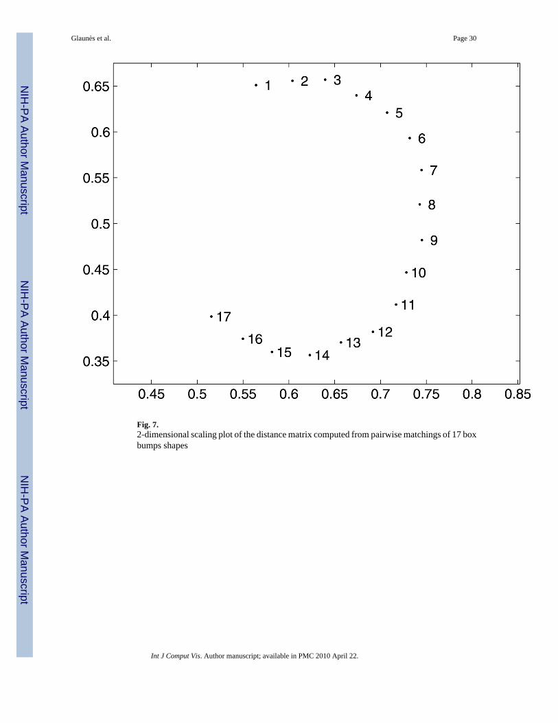
Fig. 7.2-dimensional scaling plot of the distance matrix computed from pairwise matchings of 17 boxbumps shapes

Glaunès et al.


NIH


NIH


NIH


Fig. 8.Rows (a–d) respectively show hand, dude, turtle, and fish

Glaunès et al.


NIH


NIH


NIH


Fig. 9.A scatter plot of feature dimensions from multidimensional scaling. 1: hand, 2: turtle, 3: fish,4: dude

Glaunès et al.


NIH


NIH


NIH


Fig. 10.Panel (a) shows the curve defined as boundary curve for planum temporale cortical surface.Panel (b) depicts six curves describing the main shape of cingulate gyrus. Each curve is coloreddifferently with indices in the same color scheme. The surfaces are colored by the curvatureinformation

Glaunès et al.


NIH


NIH


NIH


Fig. 11.Three-dimensional deformation of planum temporale cortical surface. Panels (a)–(d) depictthe deformation applied to planum temporale cortical surfaces. From the left to the right, panelsrespectively show the source and deformed source surfaces as well as the source and deformedsource surfaces overlaying with the target surface in red. Panel (e) shows the target of planumtemporale surface

Glaunès et al.


NIH


NIH


NIH


Fig. 12.Three-dimensional deformation of cingulate cortical surface. Panels (a)–(c) depict thedeformation applied to cingulate cortical surfaces. In each panel, the top row respectivelyshows the source and deformed source surfaces from the left to the right; the bottom shows thesource and deformed source surfaces overlaying with the target surface in red, which is shownon panel (d)

Glaunès et al.


NIH


NIH


NIH


Fig. 13.Panels (a) and (b) depict the cumulative distance distributions for planum temporale andcingulate surfaces. The cumulative distance distributions for the source surfaces are in gray,while the distributions for the deformed source surface are in black. Red curves are the meandistributions for the source and deformed source surfaces

Glaunès et al.


NIH


NIH


NIH


Fig. 14.Comparison of the cumulative distance distributions between the landmark and curvematchings. Solid, dashdot, and dash lines represent average cumulative distance distributionsover the original source, deformed source surfaces via the landmark and curve matchings,respectively

Glaunès et al.


NIH


NIH


NIH


Fig. 15.Comparison of deformation fields between the landmark and curve matchings. Panels (a–d)show the target, source, deformed source surface after the landmark matching, deformed sourcesurface after the curve matching. Red dots represents paired landmarks on the target and sourcesurfaces. Panels (e–g) show triangulated meshes respectively corresponding to the surfaces inpanels (b–d)

Glaunès et al.


NIH


NIH


NIH


Fig. 16.Comparison of deformation fields between the landmark and curve matchings. Panels (a–d)show the target, source, deformed source surface after the landmark matching, deformed sourcesurface after the curve matching. Red dots represents paired landmarks on the target and sourcesurfaces. Panels (e–g) show triangulated meshes respectively corresponding to the surfaces inpanels (b–d)

Glaunès et al.


NIH


NIH


NIH


Large Deformation Diffeomorphic Metric Curve Mapping

Documents

Transcript of Large Deformation Diffeomorphic Metric Curve Mapping