Language Modelling for Handwriting Recognition
178
HAL Id: tel-01781268 https://tel.archives-ouvertes.fr/tel-01781268 Submitted on 30 Apr 2018 HAL is a multi-disciplinary open access archive for the deposit and dissemination of sci- entific research documents, whether they are pub- lished or not. The documents may come from teaching and research institutions in France or abroad, or from public or private research centers. L’archive ouverte pluridisciplinaire HAL, est destinée au dépôt et à la diffusion de documents scientifiques de niveau recherche, publiés ou non, émanant des établissements d’enseignement et de recherche français ou étrangers, des laboratoires publics ou privés. Language Modelling for Handwriting Recognition Wassim Swaileh To cite this version: Wassim Swaileh. Language Modelling for Handwriting Recognition. Modeling and Simulation. Nor- mandie Université, 2017. English. NNT : 2017NORMR024. tel-01781268
-
Upload
khangminh22 -
Category
Documents
-
view
3 -
download
0
Transcript of Language Modelling for Handwriting Recognition

HAL Id: tel-01781268https://tel.archives-ouvertes.fr/tel-01781268
Submitted on 30 Apr 2018
HAL is a multi-disciplinary open accessarchive for the deposit and dissemination of sci-entific research documents, whether they are pub-lished or not. The documents may come fromteaching and research institutions in France orabroad, or from public or private research centers.
L’archive ouverte pluridisciplinaire HAL, estdestinée au dépôt et à la diffusion de documentsscientifiques de niveau recherche, publiés ou non,émanant des établissements d’enseignement et derecherche français ou étrangers, des laboratoirespublics ou privés.
Language Modelling for Handwriting RecognitionWassim Swaileh
To cite this version:Wassim Swaileh. Language Modelling for Handwriting Recognition. Modeling and Simulation. Nor-mandie Université, 2017. English. NNT : 2017NORMR024. tel-01781268

THÈSE
Pour obtenir le diplôme de doctorat
Spécialité Informatique
Préparée au sein de Laboratoire LITIS EA 4108Université de Rouen
Titre de la thèse
Présentée et soutenue parWassim SWAILEH
Language Modeling for
Handwriting Recognition
Thèse soutenue publiquement le 4 octobre 2017 devant le jury composé de
Mme. Laurence LIKFORMAN-SULEM Professeur à Telecom ParisTech Rapporteur
Mme. Véronique EGLIN Professeur à l'INSA de Lyon Examinateur
M. Antoine DOUCET professeur à l’Université de La Rochelle Examinateur
M. Christian VIARD-GAUDIN professeur à l’Université de Nantes Rapporteur
M. Thierry PAQUET professeur à l’Université Normandie – Université de Rouen Directeur

i
“Je tiens tout d’abord à remercier le directeur de cette thèse, M. Theirry Paquet, pourm’avoir fait confiance malgré les connaissances plutôt légères que j’avais en novem-bre 2013 sur la dynamique des systèmes de la reconnaissance de l’écriture, puis pourm’avoir guidé, encouragé, conseillé, fait beaucoup voyager pendant presque quatreans tout en me laissant une grande liberté et en me faisant l’honneur de me déléguerplusieurs responsabilités dont j’espère avoir été à la hauteur.
Je remercie tous ceux sans qui cette thèse ne serait pas ce qu’elle est : aussi bienpar les discussions que j’ai eu la chance d’avoir avec eux, leurs suggestions ou con-tributions. Je pense ici en particulier à M.Clement Chatelain, M.Pierrick Tranouez,M.Yann Soulard, M.Julien lerouge et M.Kamel Ait Mhand ”
Wassim Swaileh


iii
Contents
1 General Introduction to Handwriting Recognition 11.1 Introduction . . . . . . . . . . . . . . . . . . . . . . . . . . . . . . 1
1.1.1 definition . . . . . . . . . . . . . . . . . . . . . . . . . . . 11.1.2 History . . . . . . . . . . . . . . . . . . . . . . . . . . . . . 21.1.3 Challenges . . . . . . . . . . . . . . . . . . . . . . . . . . . 3
1.2 handwriting processing chain . . . . . . . . . . . . . . . . . . . . . 41.3 Problem formulation . . . . . . . . . . . . . . . . . . . . . . . . . 6
1.3.1 Optical models . . . . . . . . . . . . . . . . . . . . . . . . 61.3.2 language models . . . . . . . . . . . . . . . . . . . . . . . 81.3.3 System vocabulary . . . . . . . . . . . . . . . . . . . . . . 8
1.4 Handwriting recognition systems . . . . . . . . . . . . . . . . . . 91.4.1 Closed vocabulary systems . . . . . . . . . . . . . . . . . . 91.4.2 Dynamic vocabulary systems . . . . . . . . . . . . . . . . 101.4.3 Open vocabulary systems . . . . . . . . . . . . . . . . . . 10
1.5 Metrics . . . . . . . . . . . . . . . . . . . . . . . . . . . . . . . . . 101.6 conclusion . . . . . . . . . . . . . . . . . . . . . . . . . . . . . . . 11
2 Theoretical bases of handwriting optical models 132.1 Introduction . . . . . . . . . . . . . . . . . . . . . . . . . . . . . . 132.2 Hidden Markov Models (HMM) . . . . . . . . . . . . . . . . . . . 14
2.2.1 Introduction . . . . . . . . . . . . . . . . . . . . . . . . . . 142.2.2 Discrete Hidden Markov models . . . . . . . . . . . . . . . 142.2.3 Hidden Markov model structures . . . . . . . . . . . . . . 162.2.4 HMM design problems . . . . . . . . . . . . . . . . . . . . 19
First problem: Probability Evaluation . . . . . . . . . . . 19Forward algorithm . . . . . . . . . . . . . . . . . . . . . . 20Backward algorithm . . . . . . . . . . . . . . . . . . . . . 20Second problem:computing the optimal state sequence (De-
coding) . . . . . . . . . . . . . . . . . . . . . . . 21Viterbi algorithm . . . . . . . . . . . . . . . . . . . . . . . 21
2.2.5 Third problem: Parameter Estimation (model training) . . 22Viterbi training Algorithm . . . . . . . . . . . . . . . . . . 23Baum-Welch training Algorithm . . . . . . . . . . . . . . . 24
2.2.6 Continuous Hidden Markov model architecture . . . . . . . 252.3 Recurrent neural network (RNN) . . . . . . . . . . . . . . . . . . 27
2.3.1 introduction . . . . . . . . . . . . . . . . . . . . . . . . . . 272.3.2 Perceptron as a building block . . . . . . . . . . . . . . . . 27
Perceptron Learning rule . . . . . . . . . . . . . . . . . . . 29Learning by Error Minimisation . . . . . . . . . . . . . . . 30
2.3.3 Neural Networks Topologies . . . . . . . . . . . . . . . . . 31
iv
Multi-layer perceptron (MLP) . . . . . . . . . . . . . . . . 31Learning single layer perceptron . . . . . . . . . . . . . . . 33Learning MLP network by Back-propagation . . . . . . . . 34Recurrent Neural Network (RNN) . . . . . . . . . . . . . . 35Learning RNNs using back-propagation through time algo-
rithm BPTT . . . . . . . . . . . . . . . . . . . . 37Vanishing Gradient issue . . . . . . . . . . . . . . . . . . . 37CTC learning criterion . . . . . . . . . . . . . . . . . . . . 38Long Short-Term Memory Units (LSTM) . . . . . . . . . . 39Convolutional Neural Networks CNN . . . . . . . . . . . . 41
2.3.4 Handwriting recognition platforms and toolkits . . . . . . 422.4 conclusion . . . . . . . . . . . . . . . . . . . . . . . . . . . . . . . 44
3 State of the art of language modelling 453.1 Introduction . . . . . . . . . . . . . . . . . . . . . . . . . . . . . . 453.2 Language building units . . . . . . . . . . . . . . . . . . . . . . . 46
3.2.1 Primary units . . . . . . . . . . . . . . . . . . . . . . . . . 463.2.2 Lexical units . . . . . . . . . . . . . . . . . . . . . . . . . . 473.2.3 Sub-lexical units . . . . . . . . . . . . . . . . . . . . . . . 47
Spoken language dependent word decomposition into sub-lexical units . . . . . . . . . . . . . . . . . . . . . 48
Spoken language independent word decomposition into sub-lexical units . . . . . . . . . . . . . . . . . . . . . 52
3.2.4 Definitions . . . . . . . . . . . . . . . . . . . . . . . . . . . 553.3 Why statistical language models for handwriting recognition? . . 583.4 Statistical language modelling . . . . . . . . . . . . . . . . . . . . 59
3.4.1 General principles . . . . . . . . . . . . . . . . . . . . . . . 593.4.2 Language model quality evaluation . . . . . . . . . . . . . 603.4.3 N-gram language models . . . . . . . . . . . . . . . . . . . 623.4.4 Lack of data problem . . . . . . . . . . . . . . . . . . . . . 63
Discounting probabilities . . . . . . . . . . . . . . . . . . . 63Probability re-distribution . . . . . . . . . . . . . . . . . . 64smoothing techniques . . . . . . . . . . . . . . . . . . . . . 65Katz back-off . . . . . . . . . . . . . . . . . . . . . . . . . 65Absolute Discounting back-off . . . . . . . . . . . . . . . . 66Modified Kneser-Ney interpolation . . . . . . . . . . . . . 66
3.4.5 Hybrid language models vs. language model combination . 673.4.6 Variable length dependencies language models . . . . . . . 683.4.7 Multigrams language models . . . . . . . . . . . . . . . . . 693.4.8 Conctionest neural network language models . . . . . . . . 70
Feedforward Neural Network Based Language Model . . . 70Recurrent Neural Network Based Language Model . . . . . 71
3.4.9 caching language models . . . . . . . . . . . . . . . . . . . 733.4.10 Maximum entropy language models . . . . . . . . . . . . . 743.4.11 Probabilistic Context free Grammar . . . . . . . . . . . . . 74
3.5 Language models application domains . . . . . . . . . . . . . . . . 753.6 conclusion . . . . . . . . . . . . . . . . . . . . . . . . . . . . . . . 76

v
4 Design and evaluation of a Handwritting recognition system 774.1 Introduction . . . . . . . . . . . . . . . . . . . . . . . . . . . . . . 774.2 Datasets and experimental protocols . . . . . . . . . . . . . . . . 79
4.2.1 Training and evaluation databases . . . . . . . . . . . . . . 79RIMES dataset . . . . . . . . . . . . . . . . . . . . . . . . 79IAM dataset . . . . . . . . . . . . . . . . . . . . . . . . . . 79
4.2.2 Language model training corpora . . . . . . . . . . . . . . 80French extended Wikipedia corpus . . . . . . . . . . . . . 81French Wikipedia corpus . . . . . . . . . . . . . . . . . . . 81English LOB corpora . . . . . . . . . . . . . . . . . . . . . 81English Brown corpus . . . . . . . . . . . . . . . . . . . . 81English Wellington corpus . . . . . . . . . . . . . . . . . . 81English extended Wikipedia corpus . . . . . . . . . . . . . 82English Wikipedia corpus . . . . . . . . . . . . . . . . . . 82Softwares and tools . . . . . . . . . . . . . . . . . . . . . . 82
4.3 Pre-processing . . . . . . . . . . . . . . . . . . . . . . . . . . . . . 834.3.1 Related works . . . . . . . . . . . . . . . . . . . . . . . . . 834.3.2 Proposed method . . . . . . . . . . . . . . . . . . . . . . . 83
Test and validation protocols . . . . . . . . . . . . . . . . 884.4 Optical models implementations . . . . . . . . . . . . . . . . . . . 90
4.4.1 Feature descriptors . . . . . . . . . . . . . . . . . . . . . . 91A- Simple pixel based features . . . . . . . . . . . . . . . . 91B- HoG based features . . . . . . . . . . . . . . . . . . . . 91
4.4.2 Design and training optical models . . . . . . . . . . . . . 91A- HMM model optimization . . . . . . . . . . . . . . . . 92B- BLSTM architecture design . . . . . . . . . . . . . . . . 94
4.5 Language models and lexicons . . . . . . . . . . . . . . . . . . . . 954.5.1 Lexicon properties . . . . . . . . . . . . . . . . . . . . . . 96
A- Tokenisation . . . . . . . . . . . . . . . . . . . . . . . . 97B- Lexicon statistics . . . . . . . . . . . . . . . . . . . . . 98
4.5.2 Language model training . . . . . . . . . . . . . . . . . . . 101A- N-gram language models . . . . . . . . . . . . . . . . . 101B- Recurrent neural network language models (RNNLM) . 102
4.5.3 Decoding . . . . . . . . . . . . . . . . . . . . . . . . . . . 103A- Parameter optimization algorithm . . . . . . . . . . . . 104B- Decoding configurations / implementations . . . . . . . 106
4.5.4 Primary recognition results . . . . . . . . . . . . . . . . . 1084.6 Conclusion . . . . . . . . . . . . . . . . . . . . . . . . . . . . . . . 111
5 Handwriting recognition using sub-lexical units 1135.1 Introduction . . . . . . . . . . . . . . . . . . . . . . . . . . . . . . 1135.2 A supervised word decomposition methods into syllables . . . . . 1145.3 An unsupervised word decomposition into multigrams . . . . . . . 117
5.3.1 Hidden Semi-Markov Model General definition . . . . . . . 1185.3.2 Generating multigrams with HSMM . . . . . . . . . . . . . 1205.3.3 Learning multigrams from data . . . . . . . . . . . . . . . 121
5.4 Recognition systems evaluation . . . . . . . . . . . . . . . . . . . 124

vi
5.4.1 Experimental protocol . . . . . . . . . . . . . . . . . . . . 124A- Handwritten datasets . . . . . . . . . . . . . . . . . . . 125
5.4.2 B- Language models datasets and training . . . . . . . . . 1255.4.3 Recognition performance . . . . . . . . . . . . . . . . . . . 127
A- Using the RIMES and IAM resources only . . . . . . . 127B- Using additional linguistic resources . . . . . . . . . . . 127
5.5 Conclusion . . . . . . . . . . . . . . . . . . . . . . . . . . . . . . . 130
6 A Multi-lingual system based on sub-lexical units 1316.1 Introduction . . . . . . . . . . . . . . . . . . . . . . . . . . . . . . 1316.2 Brief literature overview . . . . . . . . . . . . . . . . . . . . . . . 132
6.2.1 Selective approach . . . . . . . . . . . . . . . . . . . . . . 1326.2.2 Unified approach . . . . . . . . . . . . . . . . . . . . . . . 1326.2.3 Multilingual with neural networks . . . . . . . . . . . . . . 133
6.3 Multilingual unified recognition systems . . . . . . . . . . . . . . 1336.3.1 Character set unification . . . . . . . . . . . . . . . . . . . 1346.3.2 Optical models unification . . . . . . . . . . . . . . . . . . 1356.3.3 Lexicons unification . . . . . . . . . . . . . . . . . . . . . . 1356.3.4 Unified language models . . . . . . . . . . . . . . . . . . . 138
6.4 Evaluation protocol and experimental results . . . . . . . . . . . . 1406.4.1 Results on RIMES test dataset . . . . . . . . . . . . . . . 1426.4.2 Results on IAM test dataset . . . . . . . . . . . . . . . . . 143
6.5 Conclusion . . . . . . . . . . . . . . . . . . . . . . . . . . . . . . . 145
Bibliography 151

vii
List of Figures
1.1 Examples of handwritten document taken from Arabic OpenHaRT13,Germanic READ & French Rimes data sets . . . . . . . . . . . . 2
1.2 Character ”r” writing style diversity according to its position inthe word, text example taken from the IAM database . . . . . . . 4
2.1 HMM Illustration . . . . . . . . . . . . . . . . . . . . . . . . . . . 162.2 Linear HMM example with 3 discrete observation symbols . . . . 172.3 Bakis model example with 3 discrete observation symbols . . . . . 172.4 Left to right HMM example with 3 discrete observation symbols . 172.5 Parallel Lift To Right HMM example with 3 discrete observation
symbols . . . . . . . . . . . . . . . . . . . . . . . . . . . . . . . . 182.6 Ergodic HMM example with 3 discrete observation symbols . . . . 182.7 Representation of the observation by Gaussian density functions
i.e Gaussian clusters . . . . . . . . . . . . . . . . . . . . . . . . . 252.8 Biological (upper figure) versus artificial neuron (lower figure) . . 272.9 Sigmoid Activation function . . . . . . . . . . . . . . . . . . . . . 292.10 Multi-layer perceptron (MLP) illustration . . . . . . . . . . . . . 322.11 Multi-layer perceptron (MLP) illustration . . . . . . . . . . . . . 332.12 Recurrent neural network (RNN) illustration Graves et al., 2006 . 352.13 Unrolled recurrent neural network (RNN) illustration . . . . . . . 352.14 Recurrent neural network (bidirectional-rnn) illustration . . . . . 362.15 LSTM functional illustration . . . . . . . . . . . . . . . . . . . . . 392.16 BLSTM functional illustration . . . . . . . . . . . . . . . . . . . . 402.17 ConvNets illustration example . . . . . . . . . . . . . . . . . . . . 41
3.1 Syllable phonetic components . . . . . . . . . . . . . . . . . . . . 503.2 Illustration of a sequence of graphones (Mousa and Ney, 2014) . . 523.3 Multigram structure and an example of word decomposition into
multigrams . . . . . . . . . . . . . . . . . . . . . . . . . . . . . . 553.4 Illustration of the Effective Coverage Rate (ECR) versus the Out-
Of-Vocabulary . . . . . . . . . . . . . . . . . . . . . . . . . . . . . 573.5 Illustration of the closed and open vocabularies . . . . . . . . . . 573.6 The architecture of a NN LM after training, where the first layer
is substituted by a look-up table with the distributed encoding foreach word ω ∈ Ω(Zamora-Martinez et al., 2014) . . . . . . . . . . 71
3.7 Recurrent neural network unfolded as a deep feedforward network,here for 3 time steps back in time(Mikolov, 2012) . . . . . . . . . 73
4.1 General architecture of the reading systems studied . . . . . . . . 784.2 The proposed generalized smearing approach for line detection. . . 84

viii
4.3 Steerable filters output for different values of the filter height (large,medium, low) from left to right. . . . . . . . . . . . . . . . . . . . 85
4.4 Potential line masks obtained for the corresponding steerable filtersof figure 4.3 above . . . . . . . . . . . . . . . . . . . . . . . . . . 86
4.5 Results of the validation process of text line masks of figure 4.4above . . . . . . . . . . . . . . . . . . . . . . . . . . . . . . . . . . 86
4.6 Text line mask, distance transform, line delimiters detected (leftto right) . . . . . . . . . . . . . . . . . . . . . . . . . . . . . . . . 87
4.7 Connected components splitting according to the boarders image . 874.8 Connected components assign to their corresponding text lines . . 874.9 MADDCAT line delimiter ground truth e) derived from word de-
limiters ground truth b) c) . . . . . . . . . . . . . . . . . . . . . . 884.10 Illustration of a touching characters split error. (a) Two touching
characters shown in green colour. (b) LITIS splitting decision levelaccording to the lines delimiter found by the method. (c) Reddotted line represents the correct splitting position. . . . . . . . . 90
4.11 Illustration of smearing method resulting text line segmentationsapplied for two images taken from READ 2017 handwriting com-petition training set . . . . . . . . . . . . . . . . . . . . . . . . . . 91
4.12 overview of the various optical models implemented in this thesis 924.13 Number of states per HMM models of RIMES character set . . . 934.14 Number of states per HMM models of IAM character set . . . . . 934.15 Illustration of the linguistic knowledge system components . . . . 964.16 Example of a word lattice produced by the N-best time synchronous
Viterbi beam search algorithm. Each word occupies an explicittime interval. . . . . . . . . . . . . . . . . . . . . . . . . . . . . . 104
4.17 An example of the token WFST which depicts the phoneme ”A”.We allow the occurrences of the blank label ”¡blank¿” and therepetitions of the non-blank label ”IH” . . . . . . . . . . . . . . . 107
4.18 The WFST for the lexicon entry ”is i s”. The ”¡eps¿” symbolmeans no inputs are consumed or no outputs are emitted. . . . . . 107
4.19 A trivial example of the grammar (language model) WFST. Thearc weights are the probability of emitting the next word whengiven the previous word. The node 0 is the start node, and thedouble-circled node is the end node (Miao, Gowayyed, and Metze,2015) . . . . . . . . . . . . . . . . . . . . . . . . . . . . . . . . . . 108
4.20 Line by line versus paragraph by paragraph decoding effect on therecognition performance in WER . . . . . . . . . . . . . . . . . . 108
4.21 Primary recognition results with HMM optical models and lan-guage models of words; a. RIMES and French wikipedia 6-gramLMs and lexicons tested on RIMES test dataset, b. IAM andEnglish Wikipedia 6-grams LMs and lexicons tested on IAM testdatasets . . . . . . . . . . . . . . . . . . . . . . . . . . . . . . . . 109
4.22 Primary recognition results with BLSTM optical models and lan-guage models of words; a. RIMES 9-gram LMs and lexicons whoseECR rates are decreasing from 100% to 80%, b. IAM 9-gram LMsand lexicons whose ECR rates are decreasing from 100% to 80% . 110

ix
5.1 ECR (%) of Lexique3 on RIMES (blue) and EHD on IAM (red),for words (left) and syllables (right) decomposition. . . . . . . . . 115
5.2 WER (%) as a function of T on the RIMES dataset (blue) and theIAM dataset (red), for an HMM based recognition system withHoG features . . . . . . . . . . . . . . . . . . . . . . . . . . . . . 117
5.3 Number of words of the RIMES vocabulary decomposed into nsyllables as a function of T. . . . . . . . . . . . . . . . . . . . . . 118
5.4 Number of words of the IAM vocabulary decomposed into n sylla-bles as a function of T. . . . . . . . . . . . . . . . . . . . . . . . . 119
5.5 General structure of a Hidden semi-Markov model. . . . . . . . . 1205.6 Performance obtained on RIMES as a function of the LM order
and for various LM using Hidden Markov Models . . . . . . . . . 126
6.1 The three unification stages in the design process of a unified rec-ognizer. . . . . . . . . . . . . . . . . . . . . . . . . . . . . . . . . 133
6.2 Statistics of the shared characters between the French RIMES andthe English IAM database . . . . . . . . . . . . . . . . . . . . . . 134
6.3 Evolution of the CER during the training epochs. . . . . . . . . . 1356.4 Size of the various lexicons on the RIMES, IAM, and the unified
datasets (from left to right). . . . . . . . . . . . . . . . . . . . . . 1366.5 ECR of the RIMES test dataset by the words, syllables and multi-
grams of the three corpora(from left to right : RIMES, IAM,RIMES+IAM. . . . . . . . . . . . . . . . . . . . . . . . . . . . . . 136
6.6 ECR of the IAM test datasets by the words, syllables and multi-grams of the three corpora (from left to right : IAM, RIMES,RIMES+IAM). . . . . . . . . . . . . . . . . . . . . . . . . . . . . 137
6.7 Size of the various lexicons on the FR, EN, and the unified datasets(from left to right). . . . . . . . . . . . . . . . . . . . . . . . . . . 137
6.8 The four experimental setups for analyzing the respective contri-butions of the unified optical models and the language models. . . 141
6.9 WER (%) on the RIMES dataset using the four experimental se-tups : blue = SS, Orange = SU, Red = US, Green = UU. . . . . 142
6.10 WER (%) on the RIMES dataset using the four experimental se-tups : blue = SS, Orange = SU, Red = US, Green = UU usingvery large FR+EN language models . . . . . . . . . . . . . . . . . 143
6.11 WER (%) on the IAM dataset using the four experimental setups: blue = SS, Orange = SU, Red = US, Green = UU. . . . . . . . 144
6.12 WER (%) on the IAM dataset using the four experimental setups: blue = SS, Orange = SU, Red = US, Green = UU using verylarge FR+EN language models . . . . . . . . . . . . . . . . . . . 145

xi
List of Tables
3.1 spoken & written language components . . . . . . . . . . . . . . . 463.2 n-grams versus multigrams examples . . . . . . . . . . . . . . . . 543.3 n-gram examples . . . . . . . . . . . . . . . . . . . . . . . . . . . 61
4.1 IAM dataset setups . . . . . . . . . . . . . . . . . . . . . . . . . . 804.2 RIMES and IAM database divisions used for training, validation
and test the HMM based and BLSTM-RNN based handwritingrecognition systems . . . . . . . . . . . . . . . . . . . . . . . . . . 80
4.3 Resume of the toolkits used for each systems realization task . . . 824.4 Method evaluation results . . . . . . . . . . . . . . . . . . . . . . 904.5 Optical models alignment optimization for training on RIMES and
IAM databases . . . . . . . . . . . . . . . . . . . . . . . . . . . . 944.6 Optical model performance measured by character error rate CER
during the training process on the training and validation datasetsfor the two configurations (I & II) . . . . . . . . . . . . . . . . . . 95
4.7 RIMES dataset lexicon properties. . . . . . . . . . . . . . . . . . . 984.8 IAM dataset lexicon properties. . . . . . . . . . . . . . . . . . . . 984.9 External resources lexicon properties on the RIMES test dataset. 994.10 External resources lexicon properties on the IAM test dataset. . . 1004.11 Influence of word language model order on the RIMES dataset,
using a closed lexicon of RIMES train and Wikipedia + RIMEStrain tokens, and for two optical model (WER%). . . . . . . . . . 101
4.12 performance of a second pass character RNNLM on the RIMESdataset compared to a traditional n-gram LM. . . . . . . . . . . . 103
5.1 Some examples of the Lexique3 and the English Hyphenation Dic-tionary. . . . . . . . . . . . . . . . . . . . . . . . . . . . . . . . . 115
5.2 Syllabification example on the query word \bonjour” . . . . . . . 1165.3 Syllabification results for French and English words using the su-
pervised syllabification method and the multigram generation method1245.4 Statistics of the various sub-lexical decompositions of the RIMES
and IMA vocabularies. . . . . . . . . . . . . . . . . . . . . . . . . 1245.5 RIMES dataset partitions . . . . . . . . . . . . . . . . . . . . . . 1255.6 IAM dataset partitions (following Bluche, 2015) . . . . . . . . . . 1255.7 BLSTM optical models performance only on the RIMES and on
the IAM dataset. . . . . . . . . . . . . . . . . . . . . . . . . . . . 1275.8 Recognition performance of the various open and closed vocabulary
systems trained on the RIMES resources only, (MG : multigram) . 1275.9 Recognition performance of the various open and closed vocabulary
systems trained on the IAM resources only, (MG : mulitgram) . . 128

xii
5.10 RIMES recognition performance of the various open and closedvocabulary systems trained on the French extended linguistic re-sources made of RIME train and wikipedia, (MG : mulitgram) . . 128
5.11 IAM recognition performance of the various open and closed vocab-ulary systems trained on the English extended linguistic resourcesmade of IAM train and LOB + Brown + Wellington corpora, (MG: mulitgram) . . . . . . . . . . . . . . . . . . . . . . . . . . . . . . 129
5.12 Performance comparison of the proposed system with results re-ported by other studies on the RIMES & IAM test datasets. . . . 130
6.1 Comparing the ECR of RIMES and IAM achieved by the special-ized corpora alone, and by the unified corpus. . . . . . . . . . . . 138
6.2 Comparing the ECR of RIMES and IAM achieved by the FR andEN corpora individually, and by the unified FR+EN corpus. . . . 138
6.3 Unified language models perplexities and OOV rates, for the spe-cialized and unified corpus. . . . . . . . . . . . . . . . . . . . . . . 139
6.4 Specialized language models perplexities and OOV rates, for thespecialized corpora. . . . . . . . . . . . . . . . . . . . . . . . . . . 139
6.5 Unified FR+EN language models perplexities and OOV rates, forthe specialized (FR and EN) and unified (FR+EN) corpus. . . . . 139
6.6 Specialized language models perplexities and OOV rates, for thespecialized corpora. . . . . . . . . . . . . . . . . . . . . . . . . . . 140
6.7 Specialized and unified optical model raw performance (withoutlanguage model). . . . . . . . . . . . . . . . . . . . . . . . . . . . 141

1
Chapter 1
General Introduction toHandwriting Recognition
1.1 Introduction
1.1.1 definition
With speech, cursive handwriting is still today the most natural way for hu-man’s communication and information exchanging. However, the digital ageis asking for digital assistants capable to automatically translate or transcribetexts in different languages, spoken or written on different media such as pa-per or electronic ink. Automatic Handwriting recognition comes as a responseto such a need.
Handwriting recognition is the task of transforming images of handwrittentexts, into their ASCII or Unicode transcriptions, generally for further treat-ments such as text processing, translation, classification, indexing or archiving.Handwritten texts can be obtained from a real time capturing device while theuser is writing (on-line), or from an off-line capturing process, once the in-formation has been written on paper. In the on-line (dynamic) handwritingrecognition case, one can use specific devices such as a digital pen which pro-vides dynamically the recognition system with several informations such aspen position over writing time, pen displacement velocity, inclination, pres-sure and so on. Regarding off-line handwriting recognition, one can only ex-ploit the handwriting in the form of a scanned document image. Thus, relevanthandwritten text description features have to be extracted using specific imageprocessing algorithms. Generally, the transcription process exploits the pixelvalues only, which makes the off-line handwriting recognition systems less ac-curate than the on-line ones. Printed or typewritten text recognition fall intothe off-line recognition problem and are known as Optical Character Recog-nition (OCR). But the regularity of typewritten texts make their recognitioneasier than for cursive handwriting.
The main task of an off-line continuous handwriting recognition system isto obtain the transcriptions of characters and words in forms of human lan-guage sentences from an acquired document image. This implies a process-ing chain that starts by an appropriate text localization process when com-plex two-dimensional spatial layouts are present. Once text regions have beenlocalized, text line images can be extracted using text localization algorithm.Then text line image pass thought a feature descriptor such as HoG (Histogram

2 Chapter 1. General Introduction to Handwriting Recognition
of Oriented Gradient) descriptor in order to represent the text line image viaa suitable numerical description vectors (feature vectors). These feature vec-tors represent the raw materials of the recognition engine. Given a text linedescription vectors, the recognition engine proposes the most likely transcrip-tion for the given text line descriptions with the guidance of a lexicon and alanguage model. Figure 1.1, shows three examples of document images writ-ten in French, German and Arabic languages which are taken from the FrenchRimes, German READ and Arabic OpenHaRT2013 data sets.
a. b.
c.
FIGURE 1.1: Examples of handwritten document taken from Ara-bic OpenHaRT13, Germanic READ & French Rimes data sets
1.1.2 History
The history of OCR systems started at the dawn of computer technology andevolved gradually in three ages during the past and current century. First ageextended from 1915 to 1980, it is characterized by the advent of character recog-nition methodologies such as template matching that was used for recognizingmachine-printed texts or well-separated handwritten symbols, for examplesZIP codes ( Arica and Yarman-Vural, 2001; Bluche, 2015). In 1915, EmmanuelGoldberg filed a patent for his machine controller which controlled in real timea machine via on-line recognition of digits written by the human operator. Forthis, an electrical sensor pen was used to trace the written digits on a tabletsurface (the patent of the sensor pen dated to 1888). The current principle ofOCR systems was first proposed by Gustav Tauschek in 1929. Basically, theidea was to find the best matching between the character shape and a set of
1.1. Introduction 3
metallic templates. By setting a photo-sensor behind the metallic templateswhich represented the set of the alphabetic characters, the printed characterwhich totally obscures the light from the photo-sensor is identified to be theassociated metallic template character class (Tang, Lee, and Suen, 1996). Afterthe birth of the first computers in 1940, some modern versions of handwrit-ing recognition systems appeared (Bledsoe and Browning, 1959; Mantas, 1986;Govindan and Shivaprasad, 1990). The basic idea was standing on some low-level image processing techniques applied on binary image in order to extracta set of feature vectors which represent the inputs of the recognition engine.At this age, recognition engines based on statistical classifiers were introduced(Suen, Berthod, and Mori, 1980; Mori, Yamamoto, and Yasuda, 1984; El-Sheikhand Guindi, 1988)
The second age represents the period between 1980 and 1990. It is charac-terized by the rapid and wide development of handwriting recognition method-ologies thanks to the advent of more powerful computer hardware and datacapturing devices. In addition to statistical classification methods, structuralmethods (see section 1.4.3.3) are introduced in many character recognition ap-plications. The applications were limited to two fields; the recognition of ad-dresses for automatic mail sorting and delivery (Kimura, Shridhar, and Chen,1993; Srihari, 2000; El-Yacoubi, Gilloux, and Bertille, 2002; Bluche, 2015), andthe bank cheque reading systems (Le Cun, Bottou, and Bengio, 1997; Guillevicand Suen, 1998; Gorski et al., 1999; Paquet and Lecourtier, 1993).
The third and current age extends from 1990 till nowadays. This age is theage of the big achievements in handwriting recognition research field. Newmethods and technologies were proposed by efficiently combining pattern recog-nition techniques with artificial intelligence methodologies such as neural net-works (NNs), hidden Markov models (HMM), fuzzy set reasoning, and natu-ral language processing (Arica and Yarman-Vural, 2001).
Nowadays applications of handwriting recognition tend to process lessconstrained documents layouts with very large vocabularies, for example, thetranscription of handwritten mail (Grosicki et al., 2009), information extrac-tion (Chatelain, Heutte, and Paquet, 2006), ancient document text recognition(Romero, Andreu, and Vidal, 2011; Sánchez et al., 2013)
1.1.3 Challenges
Handwriting recognition methods evolved gradually over years in order totackle different types of recognition problems with divers degrees of complex-ity. The simplest task is to recognize in isolation, a character or an alphanu-meric symbol regardless of its role in the word or the sentence it belongs to. Inthis case, the segmentation problem is supposed to be solved prior to the recog-nition step. Nowadays, handwriting recognition targets the recognition of cur-sive and unrestricted continuous handwriting where words or sub-word’s por-tions are written in a single stroke by connecting adjacent characters. In thiscase, the handwriting recognition uses implicit or explicit character segmen-tation methods. Handwriting recognition represents a challenging problembecause of the writing styles (the calligraphy) diversity and the variability of

4 Chapter 1. General Introduction to Handwriting Recognition
FIGURE 1.2: Character "r" writing style diversity according to itsposition in the word, text example taken from the IAM database
the image capturing conditions such as illumination, contrast and resolution.One can write same character with different shapes according to its position inthe words (begin, middle & end). Furthermore, a writer can write two differentcharacters using one single stroke with no care about the separation betweenthe two characters (Bluche, 2015).
Figure 1.2, illustrate the different shapes of the Latin character "r" accordingto its position in the word. In fact, it is difficult to recognize the character "r" intotal isolation without looking to its neighboring characters and its semanticcontext.
Before delving into the handwriting recognition processing techniques, thetext in the document image should be localized in rectangular zones, and mustbe distinguished from other residual graphical components within the samedocument, see (Mao, Rosenfeld, and Kanungo, 2003) for a survey and more de-tails about document analyses. Then text lines should be extracted from the lo-calized text region. Regarding to Ghosh et al. (Ghosh, Dube, and Shivaprasad,2010) the organized contests for text line extraction, this task is assumed asa challenging task. The major problem behind this task is the localization ofthe inflected (curvature) or maybe broken and overlapped text lines where theinter-space between the text lines are not tractable along the text zone width.For more details about the state of art of text line extraction techniques seechapter 4.
In fact, humans recognize a text trough a top level global view of the wholetext document, which makes them able to recognize characters and words intheir context. Similarly, computer vision try to mimic this ability by using ahierarchical structure in order to take account of contextual information abovehandwriting optical models during handwriting recognition.
The challenge behind a handwriting recognition system is the ability of thesystem to recognize the entire texts block regardless to the handwriting style,writing conditions and the text block image capturing condition.
1.2 handwriting processing chain
The handwriting processing chain consists of three main stages:
1. pre-processing stage: includes all the necessary faults correcting pro-cesses such as text localisation, line detection, image denoising, imageinclination and slant correction.

1.2. handwriting processing chain 5
2. Recognition stage: consists of matching text line extracted features to aset of character labels by using the couple of mathematical representa-tions called optical models and language model.
3. Post-recognition stage: aims to enhance the recognition rate by correctingthe sequence of characters produced in the recognition stage by usingmore sophisticated language models.
It is necessary to apply a set of processes to enhance the document image bycorrecting the introduced defects during the capturing process. Such defectsinclude:-
a. Poor image resolution.b. Noisy image.c. Illumination variations due to clarity faults.d. Image inclination and slant.e. Black boarders of image.
In between the pre-processing stage and the recognition stage of the hand-writing there is an intermediate process called feature extraction process. Fea-ture extraction process is the operation by which the segmented part of text(line, word or character) can be described by certain significant measures calleddescriptors. Every descriptor represents one dimension of the feature space,the extracted features represent the input of the classification operation. Selec-tion of a relevant feature extraction method is probably the single most impor-tant factor in achieving high recognition performance with much better accu-racy in handwriting recognition systems (Sahu and Kubde, 2013).
In the recent years, we have seen the emergence of deep neural networks.The strength of these new architectures of networks lies in its ability to learnrepresentation of features from the raw input data (pixels) directly, thus allow-ing to proceed without the need to define a feature space.
The recognition stage gives as an output a sequence of characters (classlabels) which are most likely the handwritten text on the document image.The recognition process consists of a search procedure which maps the op-tical models (which can be either characters, sub-words or words) with theobserved sequences of features. The idea is to decode the character hypothe-ses space in order to find the best mapping path represented by the maximumlikelihood between the optical models and the observed features, taking intoaccount some lexicon and language constraints.
There are two types of recognition errors: non-word errors and real worderrors. A non-word error is a word that is recognized by the recognition en-gine; however, it does not correspond to any entry in the language vocabularyfor example, when "how is your day" is recognized by the recognition engineas "Huw is your day" it is said to be a non-word error because "Huw" is notdefined in the English language. In contrast, a real-word error is a word that isrecognized by the recognition system and does correspond to an entry in thelanguage vocabulary, but it is grammatically incorrect with respect to the sen-tence in which it has occurred, for example, "How is your day" is recognized bythe OCR system "How is you day" the "you is considered as a real-word error(Bassil and Alwani, 2012). At the post-recognition stage, the recognition errors

6 Chapter 1. General Introduction to Handwriting Recognition
can be corrected by using two linguistic information sources: dictionaries andlanguage models.
1.3 Problem formulation
In order to automatically retrieve the handwritten text from an image, severalmethodologies of patterns recognition have been introduced in the literaturestanding on certain artificial intelligence technologies. The core function ofsuch technologies is to represent the image properties by probabilistic modelsthat represent the optical models, constrained by natural language grammarrepresented by the language model. Through a learning process, the opticalmodels are optimized on a set of annotated examples in order to achieve thebest possible character or word sequence transcription. On the other hand thelanguage model has to be representative of the text in the document image tobe recognized in order to get better performance.
Handwriting recognition can be achieved using one or two pass decodingalgorithms which are based on Bay’s rule. By decoding, we seek to retrievethe optimal sequence of words W that maximizes the a posteriori probabilityP (W |S) among all possible sentences W (see equation 1.1. Two important pa-rameters guide the decoding algorithm: they are the language model scalingparameter γ and the word insertion penalty parameter β that controls the in-sertion of too frequent short words. These two parameters need to be opti-mized for optimum coupling of the optical models with the considered lan-guage model, because these two models are estimated independently fromeach other during training.
By introducing the coupling hyper-parameters within the Bay’s formula,we obtain the general formulation of the handwriting recognition problem asstated by equation 1.1.
W = argmaxwP (W |X) ≈ argmaxwP (X|W )P (W )γβlength(W ) (1.1)
In this formula, X represents the sequence of observations (features) extractedfrom the image and P (X|W ) represents the likelihood that the features X aregenerated by the sentence W , it is deduced from the optical model. P (W ) isthe prior probability of the sentenceW , it is deduced from the language model.
From this general formula, we note that language model contribution hasthe same effect as the optical model contribution during the recognition. Theeffect of language model contribution on the handwriting recognition processrepresent the core study of this thesis.
1.3.1 Optical models
An optical model can be an optical template such as the primitive models thatwere used during the early studies of OCR, or a statistical model such as a Hid-den Markov model (HMM) or a Recurrent Neural Networks (RNN) or struc-tural model that can model the variation of patterns after a specific learning

1.3. Problem formulation 7
process. The OCR recognition problem is presented as a supervised classifi-cation or categorization task, where the classes are pre-defined by the systemdesigner. According to the literature, Optical models can be classified intoword, sub-word (BenZeghiba, Louradour, and Kermorvant, 2015), characterand sub-character (Bluche, 2015) optical models.
The goal of using word optical models is to recognize a word directly asa whole, without relying on a segmentation or an explicit representation ofthe parts (Bluche, 2015). Simple representation of the word is extracted fromthe image and matched against a lexicon as presented in (Madhvanath andGovindaraju, 1996; Madhvanath and Krpasundar, 1997) and applied for thecheck amount recognition task. The disadvantage of the word optical modelis the limitation of the vocabulary size because the number of optical modelsgrows linearly with the number of words in the vocabulary. Despite, the lim-ited size of training vocabulary cannot guarantee to provide enough exampleper model, so that they can not properly generalise to unseen examples. There-fore word optical models are limited to small vocabulary applications such asbank chicks.
To our knowledge, there was no attempts of using sub-word units as op-tical models in the literature. However in speech recognition, may be usedas accoustic models in placeof the full word model. Usually sub-word modelslike demi-syllables, syllables, phonemes, or allophones are used instead of full-word models (Mousa and Ney, 2014). The advantage of using sub-word unitsis that they reduce the model complexity, which allows a reliable parameterestimation. Since the set of sub-words is shared among all words, the searchvocabulary does not need to be equal to the training vocabulary. The acousticmodel of any new words that is not present in the pronunciation dictionarycan be assembled from the corresponding sequence of sub-word units.
Usually, the modern Large Vocabulary Continuous Speech Recognition (LVCSR) systems use the so-called context-dependent phoneme models whichare models of phonemes with some left and right context. For example, a tri-phone is a phoneme joined with its predecessor and successor. In fact, char-acters in the written language meets phonemes in the spoken language. Thecontextual modelling of the language characters can be viewed as a sub-wordoptical model, that because each character optical model is considered to beconditionally related to its neighbouring characters. The authors of (Ahmadand Fink, 2016) proposed a class-based contextual modelling for handwritingArabic text recognition based on HMM optical modelling.
The character optical models are used by almost all Large vocabulary con-tinuous handwriting recognition systems. The advantage of using characteroptical models is their reduced number of classes compared to the sub-wordand word optical models. Thus a moderate number of training examples issufficient to efficiently train the character optical models. Using the embeddedtraining techniques, there is no need to segment the text image into charactersfor training the optical models. Conventionally, the optical models representthe characters set of the language of interest.
For the sub-character optical models, the image is divided into sub-regionscorresponding to at most one character (Bluche, 2015). The idea is to find all

8 Chapter 1. General Introduction to Handwriting Recognition
possible image segmentations which is often derived from the character cur-vatures heuristically. A survey of character segmentation techniques was pre-sented by (Casey and Lecolinet, 1996). We will discuss in more details thetheoretical bases of the HMM and NN optical models in chapter 2.
1.3.2 language models
Sometimes the recognition engine decide for the recognition of a sequence oftokens (words) which may be grammatically or semantically incorrect. Manytechniques from the natural language processing field have been developedfor checking the validity of a sentence of words. A set of grammar rules canbe applied on a dataset of tokenized text in order to constrain the search spaceon a grammatically valid paths. For example, (Zimmermann, Chappelier, andBunke, 2006) re-scored a list of sentence hypotheses by using a probabilisticcontext-free grammar.
Generally speaking, language modelling for handwriting recognition usu-ally consists in giving a score to different word sequence alternatives (Bluche,2015). The common language modelling approach used for handwriting recog-nition (e.g. Rosenfeld, 2000 & Marti and Bunke, 2001) is the statistical ap-proach. It consists of n-gram language models or connectionist language mod-els based on neural network. This type of approaches estimates the a prioriprobability of observing a word sequence W from a large amount of trainingtext samples (Bluche, 2015).
The perplexity measure is used to measure the capability of a languagemodel to predict a given corpus. It is derived from the entropy of the proba-bility model and can be expressed as the following:
PPL = 2−1Nw
∑Nwk=1 log2P (wk|wk−1,...) (1.2)
where Nw is the number of words in the text. Language models with smallerperplexities are generally better at predicting a word given the history. How-ever, better perplexity does not mean better recognition performance accord-ing to (Klakow and Peters, 2002). A state of the art of language modelling willbe presented in chapter 3.
1.3.3 System vocabulary
When the recognition system introduces words optical models as well as lan-guage models, a predefined lexicon is already embedded in the recognitionengine, and limited to the set of words modelled (Bluche, 2015). However forlarge vocabulary it is necessary to introduce optical character models. The rep-resentation of words by their character sequences in a dictionary reduces thesize of the search space and help to alleviate the recognition ambiguities.
Indeed, the recognizable words are limited only to the dictionary wordsand the chance to encounter out of vocabulary words (OOV) during the recog-nition increases when dictionary size is small. The OOV represents the ratio ofnon-covered words by the lexicon dictionary and thus the language model on

1.4. Handwriting recognition systems 9
an evaluation data set. On the other hand, as the dictionary size increases, thesearch space grows accordingly which leads to higher recognition complexity.Furthermore, the competition between words increases proportionally to thedictionary size. Consequently, the selection of the smallest possible vocabularyachieving the highest coverage rate on unknown dataset is a real challenge.
The dictionary can be organized in such ways to enhance the recognitionspeed. The simplest way consists in computing scores for each word in thedictionary independently and decide for the word with the highest score. Thissolution is not satisfactory because the complexity increases linearly with thevocabulary size while many words share the same characters at same posi-tions. Therefore, another way to organize a vocabulary is called prefix tree. Inthis way, the vocabulary is organised as a tree, and the root is considered tobe the beginning character of a word. Each branch indicates another characterof the word and the terminal nodes contains the word made of the charac-ters along the path. By this way the shared prefix characters will be examinedonly once. More interested readers about the large vocabulary reduction andorganization techniques can see (Koerich, Sabourin, and Suen, 2003).
Finite-state Transducer (FSTs) (Mohri, 1997) is another interesting and effi-cient way for representing vocabulary. It consists of a directed graph with aset of states, transitions, initial and final states. The transitions from one stateto another are labeled with an input symbol from an input alphabet, and anoutput symbol from an output alphabet. When a sequence of input symbolsis provided, the FST follows the successive transitions for each symbol, andemits the corresponding output symbol. A valid sequence allows to reach afinal state with such sequence of transitions.
Vocabulary representation using FST defines the input alphabet as the setof characters, and the output alphabet matches the vocabulary. The compactstructure of the vocabulary FST is similar to the prefix tree vocabulary rep-resentation. FST representation has the advantage of its ability to integratethe language model within the search graph. FST representations of languagemodels are popular in speech recognition (Mohri, Pereira, and Riley, 2002)and are applied to handwriting recognition (e.g. in Toselli et al., 2004) and inseveral recognition toolkits such as Kaldi (Povey et al., 2011) or RWTH-OCR(Dreuw et al., 2012).
1.4 Handwriting recognition systems
In the literature, various structures have been proposed to perform handwrit-ing recognition (Plötz and Fink, 2009). According to their lexical structure, therecognition systems can be classified into three main categories:-
1.4.1 Closed vocabulary systems
The first category includes the closed vocabulary systems that are optimizedfor the recognition of words in a limited and static vocabulary. This kind ofsystem is used for specific applications such as bank checks reading (Gorski

10 Chapter 1. General Introduction to Handwriting Recognition
et al., 1999). In this case the optical models may be word models. These ap-proaches are often mentioned as global or holistic recognition.
1.4.2 Dynamic vocabulary systems
The second category includes dynamic vocabulary systems that are able to rec-ognize words never seen by the system during training. In this category, theoptical models are character models, and the approach is often referred as an-alytical recognition approaches that are guided by the knowledge of a lexicon(lexicon driven) and constrained by a language model during the recognitionphase. With this capability, these systems are used for general purpose appli-cations, such as recognition of historical documents, for example (Pantke et al.,2013) but they can not deal with unknown words (OOV) which words that donot appear in the vocabulary of the system.
1.4.3 Open vocabulary systems
The third category of approaches includes systems without vocabulary (lexi-con free) that perform recognition in lines of text by recognizing sequences ofcharacters. To improve their performance, these systems may use character se-quences models in the form of n-gram statistical models (Plötz and Fink, 2009)by considering the space between words as a character (Brakensiek, Rottland,and Rigoll, 2002). The advantage of these systems is their ability to recognizeany sequence of characters, including out of vocabulary words (OOV) such asnamed entities. Hence, they have the disadvantage of being less efficient thanprevious models in the absence of the sentence level modelling. Kozielski &al. (Kozielski et al., 2014b) have explored the use of character language models(for English and Arabic) using 10-gram character models estimated using theWitten-Bell method. They compared this lexicon free approach with a lexiconbased approach associated with a 3-gram language model of words estimatedusing the modified Kneser-Ney estimation method. They have also combinedthe two models (characters and words) by using two approaches. The first oneby building a global interpolated model of the two models, the second one byusing a combination of back-off models. The results show the effectiveness ofthe combination of the two language models using interpolation.
1.5 Metrics
The error rates (ER) commonly used for the evaluation of continuous textrecognition are the word error rate (WER) and character error rate (CER). Bothare calculated based on the number of substitutions, insertions and deletionsof words, respectively characters, and the number of words or characters inthe reference text using the following equation:
ER =#substitutions+ #insertions+ #deletions
#enforcements(1.3)

1.6. conclusion 11
This ER can be deduced from the Levenstein edit distance (Levenshtein, 1966),which is the minimum edit distance between two strings (recognition hypothe-ses and ground-truth) and can be retrieved efficiently with a dynamic pro-gramming algorithm (Bluche, 2015).
Note that although it is generally expressed in percentage, it may goes be-yond 100% because of the potential insertions. In this thesis, the reportedWERs are computed with the SClite (Fiscus, 1998) and Kaldi (Povey et al.,2011) implementation. Similarly, we can consider an even finer measure ofthe quality of the output sequence in terms of characters, which penalizes lesswords with a few wrong characters and is less dependent on the distributionof word lengths: the Character Error Rate (CER). It is computed like the WER,with characters instead of words. The white space character should be takeninto account in this measure, since this symbol is important to separate words.
1.6 conclusion
In this chapter, we have introduced the general problem of off-line handwrit-ing recognition, including the related history, processing chain and systems.We introduced the general formula of handwriting recognition systems andrelated hyper-parameters which require an optimisation stage in order to getthe optimal coupling of the optical model with the language model.
The main goal of this thesis has been to develop improved language mod-elling approaches for performing efficient large vocabulary unconstrained andcontinuous handwriting recognition for French and English handwritten lan-guages.
The work of this thesis has been focused in two major directions: the firstis to investigate the use of language dependent (syllables) and language inde-pendent (multigrams) types of sub-lexical units during the creation of the lan-guage models (LMs), the second is to investigate the enhancement of the hand-writing recognition performance by unifying the recoginition system compo-nents: the optical and language models. The use of sub-lexical units has lead toa significant increase in the overall lexical coverage indicated by a considerablereduction in the out-of-vocabulary (OOV) rates measured on the test datasets.This has introduced one step towards the solution of data sparsity and the poorlexical coverage problems. As a result, significant improvements in the recog-nition performance have been achieved compared to the traditional full-wordbased language model. The unification of the recognition systems producea generalized recognition whose performance outperform the performance ofits parents for similar language such as the French and English languages. Ex-periments have been conducted on the French RIMES and the English IAMhandwriting datasets.
This thesis consists of two main parts; theoretical part and experimenta-tion part. on the one hand, theoretical part includes the first three chapterswhich covers the state of the arts and the bibliographical and literature re-views. The experimentation part include the last three chapters which discussthe architecture of the developed recognition systems and the contributions ofthe sub-lexical units based models to the handwriting recognition.

12 Chapter 1. General Introduction to Handwriting Recognition
In chapter two, we present a state of the art of the handwriting optical mod-els stating the theoretical architecture and the related training algorithms foreach of Hidden Markov Models and Neural Network based optical models.We conclude this chapter with a comparative overview of the available toolk-its used for training and decoding the optical models.
A state of the art on the language modelling approaches and techniquesare presented in chapter three including language grammars and statisticallanguage models. In addition to an overview of spoken and written languagebuilding blocks, we discuss different aspects related to n-gram and conection-nist language model training and smoothing techniques.
The developed recognition processing chain of two different recognitionsystems is described in chapter four. The processing chain illustrates the dif-ferent architectures of optical models (HMM or BLSTM-CTC) and the n-gramlanguage models of different lexicon types (words, syllables, multigrams andcharacters) in addition to the decoding process. Some primary results are pre-sented to justify some choices regarding the decoding and language modellingapproaches.
The contribution of the sub-lexical units of syllables and multigrams arepresented in chapter five. The utilised supervised and unsupervised word de-composition into syllables and multigrams approaches are introduced justifiedwith some statistical analyses of the generated lexicons coverage rates on thetest datasets lexicons. State of the art recognition performance are obtained bythe multigrams language models on the RIMES and IAM test datasets.
In chapter six, we studied the possible ways to unify the French recognitionsystem with the English one. We studied the benefit of unifying sub-lexicalunits of both languages as well as unifying the optical character models. Weobserved that combining multigram sub-lexical units of both languages doesnot degrade the recognition performance while at the same time maintainingmoderate complexity in the language model due the use of sub-lexical units.

13
Chapter 2
Theoretical bases of handwritingoptical models
2.1 Introduction
Traditional handwriting recognition systems (Schambach, Rottland, and Alary,2008) use discrete (Kaltenmeier et al., 1993) or continuous (Marti and Bunke,2001) Hidden Markov Models (HMM) for modelling each building unit of thelanguage of interest with respect to the writing time frame on the writing di-rection (Jonas, 2009). Conventionally, the HMM models represent the opticalmodels of the character set of the language of interest.
An HMM consists of a set of dependent states associated with one or moreGaussian mixture density functions. The number of states in a sequentialHMM model defines its length. The number of states depends on the topologyof the HMM and the resolution used during the feature extraction process.In the literature, the variable length models show an improved recognitionperformance over the fixed length one because of their ability to adapt to thevariable length graphical representation of the characters. The Maximum Like-lihood Estimation (MLE) algorithm is used to estimate the optimal number ofstates per HMM character model (Zimmermann and Bunke, 2002).
For several years ago, neural networks have emerged in the handwritingrecognition field as a fast and reliable classification tool. Neural networks arecharacterized by their simple processing units namely called neurons and theirintensive weighted interconnections. The weights of the interconnections be-tween neurons are learned from training data. The neurons are organised intohierarchically "stacked" layers which consist of initial or input layer, interme-diate or hidden layer (these can be one or more stacked layers) and a final oroutput layer.
The information processing flows from the input layer through intermedi-ate layers towards the output layer which predicts the recognized characters orwords. The network layers are mutually interconnected from the input layertowards to output layer to form multi-layer neural networks.
In the literature, neural network architectures are classified into two spe-cific categories: feed-forward and recurrent networks. Recurrent neural net-works have the advantage over feed-forward neural networks of their ability

14 Chapter 2. Theoretical bases of handwriting optical models
to deal with sequences over time. In spite of the different underlying princi-ples, it can be shown that most of the neural networks architectures are equiva-lent to statistical pattern recognition methods (Ripley, 1993; Arica and Yarman-Vural, 2001).
Several types of NNs are used for handwriting recognition such as hand-written digits recognition (LeCun et al., 1989) using Convolutional NeuralNetwork or handwritten sentence recognition using Bidirectional Long-shortterm memory recurrent neural networks (Graves et al., 2006) (BLSTM-RNN)or multi - dimensional long-short term memory recurrent neural networks(MDLSM - RNN) (Bluche, 2015).
In this chapter, we present an overview of the theory of optical modelsin two parts before concluding with a list of recent available platforms. TheHidden Markov Model is the topic of the first part and the neural networkmodels are the topic of the second part.
2.2 Hidden Markov Models (HMM)
2.2.1 Introduction
Since several decades, Hidden Markov models are considered one of the mostefficient statistical tools for solving sequential pattern recognition problems,such as spoken language processing, DNA sequence alignment, handwritingrecognition. The name of this model holds the family name of a Russian sci-entist called Andrei Markov (1856-1922). Before delving deeper in the HiddenMarkov Models (HMM), let us recall the foundation of these models. Thesemodels fall into the probability theory by addressing the description and mod-elisation of stochastic process (random process). Briefly, stochastic process aredescribed by a collection of random variables (states) subject to change overtime. The Markov property has been introduced as one simplifying assump-tion so as to describe the evolution over time by making the variables onlydepend on some other random variables at the precedent time frame. Anystochastic process that obeys the Markov property is often called a Markovprocess. Such an hypothesis neglects the long term dependencies.
2.2.2 Discrete Hidden Markov models
Hidden Markov Models are generative stochastic models representing the gen-eration of an observed sequence O = (o1, . . . , ot, . . . , oT ) from a hidden statesequence Q = (q1, . . . , qt, . . . , qT )
The observation emission probability represents the possibility of gener-ating a certain observation from a certain model state. This distribution ex-plains the relation between the hidden states of the model and the observations(model outputs).
In case of discrete observations (which are related to Discrete HMM), theobservation emission probabilities are represented by a N × M matrix (thenumber of model states N cross of the number of distinct observation sym-bols) known in the literature by B = (bj(vk) = P [ot = vk|qt = sj]) where sj

2.2. Hidden Markov Models (HMM) 15
represents the model state j and vk represents the distinct observation k. Sothe observation emission probability bj(ot = vk) represents the probability ofgenerating the observation element ot = vk when the model state at time t isqt = sj .
Briefly, a HMM can be characterized by the following parameters:
1. N , the number of states in the model.
2. M , the number of distinct observation symbols.
3. A set of observation symbols V = vk, k = 1 . . .M
4. A set of states S = sj, j = 1 . . . N
5. The state transition probability distribution A = aij having the follow-ing properties:-
aij = P(qt = sj|qt−1 = si
)1 ≤ i, j ≤ N (2.1)
aij ≥ 0∑Ni=1 aij = 1
6. The observation emission probability N × M matrix, in the literatureknown by B =
(bj(ot = vk)
)when the model state is sj ,
bj(ot = vk) = P(ot = vk|qt = sj
)1 ≤ j ≤ N1 ≤ k ≤M
(2.2)
So the observation emission probability bj(ot = vk) represents the prob-ability of generating the observation element ot equal to the observationsymbol vk when the model state is sj at time step t.
7. The initial state distribution π = πi, where
πi = P(q1 = si
)1 ≤ i ≤ N (2.3)
The stochastic model is decomposed in two parts. First, the model assumesMarkov dependency between hidden states, which writes:
P (Q) =∏t
P (qt|qt−1) (2.4)
Second, the model assumes conditional independences of the observationswith respect to the hidden states, which writes:
P (O|Q) =∏t
P (ot|qt) (2.5)

16 Chapter 2. Theoretical bases of handwriting optical models
FIGURE 2.1: HMM Illustration
These two hypotheses allow writing the joint probability of the observationand state sequence as follows:
P (O,Q) = P (O|Q)P (Q) (2.6)
=∏t
P (ot|qt)P (qt|qt−1) (2.7)
where P (q1|q0) = π(q1). The model can be represented through the temporalgraph shown in figure 2.1 where arrows indicates the conditional dependencyinduced by the model. Finally, a HMM model λ can be characterized by thethree parameters λ = (A,B, π) which have the following representation:
π =
π1...πN
A =
a11 . . . a1N... . . . ...
aN1 . . . aNN
B =
b1(v1) · · · b1(vM)... . . . ...
bN(v1) · · · bN(vM)
In the literature an observation are commonly represented by real values.
Practically, a quantization process can be introduced so as to assign a discretelabel to the continuous observation. Such assignment can be made by intro-ducing a clustering stage such as K-means. This fall into the semi-continuousMarkov models. In fact, there is a risk of introducing quantization error withsuch quantization process. Such risk can be eliminated by introducing the con-tinuous HMM (see 2.2.6. below).
2.2.3 Hidden Markov model structures
In the main application areas of HMM-based modelling, the input data to beprocessed exhibits a chronological or linear structure (Fink, 2014). Therefore,it does not make sense for such applications to allow arbitrary state transitionswithin a HMM. Based on this fact, we can distinguish five different topologiesof HMM which are most often used in the literature:

2.2. Hidden Markov Models (HMM) 17
1. linear HMM: stands on the idea that states are sequentially structuredone after another without feedback loop and one forward jump from amodel state to the next, in other word every state of the model can bereached only from its previous neighbour state as seen in figure 2.2.
FIGURE 2.2: Linear HMM example with 3 discrete observationsymbols
2. Bakis HMM: Allows the state to transit linearly similarly as in linearmodel but contains one additional forward jump from current state qtto qt+2 as seen in figure 2.3.
FIGURE 2.3: Bakis model example with 3 discrete observationsymbols
3. Left to right HMM: Every possible forward jumps are allowed (no back-ward transition) as seen in figure 2.4.
FIGURE 2.4: Left to right HMM example with 3 discrete observa-tion symbols

18 Chapter 2. Theoretical bases of handwriting optical models
4. parallel left to right HMM: represents a special case of left to right HMMwhere the middle states of the model has a side transition route to theparallel row of states which give more flexibility for this model. Figure2.5 illustrates this model.
FIGURE 2.5: Parallel Lift To Right HMM example with 3 discreteobservation symbols
5. Ergodic HMM: All state transition paths along the model states are al-lowed as seen in figure 2.6 .
FIGURE 2.6: Ergodic HMM example with 3 discrete observationsymbols

2.2. Hidden Markov Models (HMM) 19
2.2.4 HMM design problems
We are considering the probability of producing a certain observation sequenceby a HMM. This probability is called the production probability P (O|λ) (Fink,2014). It indicates the ability of a HMM to generate the given observationsequence, thus it can be used as a basis for a classification decision (Fink,2014). We are interested in determining which model can produce the ob-servation with the highest probability or which is the most probable modelto produce the observation. When multiple HMM models are competing, thewinner HMM λj will be the model for which the posterior probability P (λj|O)becomes the maximum (Fink, 2014):
P (λj|O) = maxi
P (O|λi)P (λi)
P (O)(2.8)
When evaluating this expression, the probability P (O) of the data itselfrepresents a quantity irrelevant for the classification — or the maximizationof P (λi|O) — because it is independent of λi and, therefore, constant. Thusfor determining the optimal class, it is sufficient to consider the numerator ofequation 2.8 only:
λj = argmaxλi
P (λi|O) = argmaxλi
P (O|λi)P (λi)
P (O)= argmax
λiP (O|λi)P (λi) (2.9)
In general, one considers equally likely models and P (λi) can be omitted inequation 2.9. Therefore, the classification decision depends only on the emis-sion probability P (O|λi). In order to fit a HMM model to a real world applica-tion we need to find solutions to three main problems, which are the following:
First problem: Probability Evaluation
For a sequence of observations given a specific HMM, how do we compute theprobability that the observed sequence was produced by that HMM model. Inother words, the question to be answered is: what is the probability P (O|λ) thata particular sequence of observations O is produced by a particular model λ? Whenmultiple models are competing together, the target is to associate the modelwith the highest probability to generate the observed data. Computing thelikelihood of the observation sequence allows to rank the models. Followingthe definition of a HMM, we can compute the emission probability P (O|λ) bysumming the contribution of every state sequence Q and write:
P (O|λ) =∑Q
P (O,Q|λ) (2.10)
but for an observation of length T and a model with N hidden states, thenumber of hidden state sequences Q is NT which makes this computation un-tractable.

20 Chapter 2. Theoretical bases of handwriting optical models
For evaluating the production probability P (O|λ), we use two algorithms:the forward algorithm or the backwards algorithm (do not confuse them withthe forward-backward algorithm) (Rabiner, 1989).
Forward algorithm
The Forward Algorithm is a recursive algorithm for calculating the emissionprobability for the observation sequence of increasing length t using the partialand accumulative probability forward variable αt(i) of observing the partialsequence (o1, . . . , ot) and ending with state qt = si. let us define:
αt(i) = P (o1, o2 . . . ot, qt = si|λ) (2.11)
We can observe that there are N different ways of arriving in state qt =sj from state qt−1. They correspond to the N possible previous states qt−1 =si ; i ∈ 1, . . . , N which leads to the recursion formula, taking account of theHMM independent emission.
αt+1(j) = [N∑i=1
αt(i)aij]bj(ot+1) 1 ≤ t ≤ T − 1 (2.12)
Then we can derive the emission probability of O by
P (O|λ) =N∑i=1
αT (i) (2.13)
Backward algorithm
We can define the Backward variable βt(i) which represents the partial emis-sion probability of the observation sequence from ot+1 to the last time step T ,given the state at a time t is qt = si and the model λ.
βt(i) = P (ot+1, ot+2 . . . oT |qt = si, λ) (2.14)
For the same reasons as for computing the forward variable we write thefollowing recursion formula
βt(i) =∑N
j=1 aijbj(ot+1)βt+1(j), t = T − 1, T − 2, . . . , 1
1 ≤ i ≤ N(2.15)
and finally, we can compute the emission probability by
P (O|λ) =N∑j=1
β1(j)bj(o1) (2.16)
Obviously both Forward and Backward algorithms must give the same re-sults for total probabilities P (O|λ) = P (o1, o2, . . . , oT |λ). The complexity of

2.2. Hidden Markov Models (HMM) 21
computing the emission probability has reduced to O(N2×T ) which is accept-able in practical applications.
Second problem:computing the optimal state sequence (Decoding)
We try here to recover the hidden part (hidden model states) of a HMM byfinding the most likely hidden state sequence. The task, unlike the previousone, asks about the joint probability of the entire sequence of hidden states thatgenerates a particular sequence of observations (Rabiner, 1989). This problemis called decoding problem (Fink, 2014).
Decoding is predicting the hidden part of the model (the state sequenceQ) given the model parameters λ = (A,B, π) by choosing the optimal statesequence Q which maximizes the emission probability P (O,Q|λ) for a givenobservation sequence O. The optimal emission probability P ∗(O|λ) for gener-ating the observation sequence O along an optimal state sequence Q∗ can bedetermined by maximization over all individual state sequence Q (Fink, 2014).
P (O,Q∗|λ) = maxQ
P (O,Q|λ) (2.17)
Similarly as for computing the emission probability, the number of individualstate sequencesQ is too large to allow a direct computation of each probability,and decide for the maximum one. Fortunately, the Viterbi algorithm can com-pute the optimum state sequence by using dynamic programming principlewith a complexity of T ×N2.
Viterbi algorithm
To find the best state sequence Q = (q1, q2, . . . , qT ) which can approximatelygenerate the given observation sequenceO = (o1, o2, . . . , oT ) knowing the modelλ = (A,B, π) , let us define the probability of the best path ending at time t instate qt = si.
δt(i) = maxq1,q2,...,qt−1
P (o1, o2, . . . , ot, q1, q2, . . . , qt−1, qt = si|λ) (2.18)
As the probability of a partial path is monotonically decreasing while t is in-creasing, the optimal path is composed of the optimal partial path. therefore,the dynamic programming optimisation policy can be applied, and we canwrite.
δt+1(j) = maxi
(δt(i)aijbj(ot+1)
)(2.19)
The Viterbi algorithm can be achieved by the following steps:-
1- Initialization:
δ1(i) = πibi(o1) 1 ≤ i ≤ N
ϕ1(i) = 0
(2.20)

22 Chapter 2. Theoretical bases of handwriting optical models
2- Recursion:
δt+1(j) = maxi[δt(i)aij]bj(ot+1)For1 ≤ t ≤ T 1 ≤ j ≤ N
ϕt+1(j) = argmaxi[δt(i)aij](2.21)
3- Termination:
P ∗(O|λ) = P (O,Q∗|λ) = max1≤i≤N
δT (i) (2.22)
Q∗T = arg max1≤i≤N
δT (i) (2.23)
4- Back-Tracking of the optimal state sequence path:
For all times t where t = T − 1, T − 2, . . . , 1
Q∗t = ϕt+1(Q∗t+1) (2.24)
The difference between the forward algorithm and the Viterbi algorithm isthat the forward algorithm takes the sum of all previous paths into the cur-rent cell calculation while the Viterbi algorithm takes the max of the previouspaths into the current cell calculation, but they are very similar in nature andcomplexity.
2.2.5 Third problem: Parameter Estimation (model training)
Here we want to optimize the model parameters so as to best describe a givenobservation sequence or a set of observation sequences. The observation se-quences used to adjust the model parameters are called training sequences.The training problem is the crucial one for most applications of HMM. It allowsto adapt model parameters to create best models of real phenomena (Rabiner,1989).
For most of applications of HMM, we seek to use the ideal model whichhas approximately the same statistical properties as those of the data. To thisaim, we have to adapt or estimate a certain pre-selected model by an iterativeprocedure that is called model training. Normally, the pre-selected model hasto be selected by an expert.
Given an observation sequence O or a set of such sequences, the modellearning task is to find the best set of model parameters (A,B, π) which cangenerate approximately the same given observation sequence. No tractable al-gorithm is known for solving this problem exactly, but a local maximum likeli-hood can be derived efficiently using the Baum–Welch algorithm or the Viterbialgorithm (Rabiner, 1989).
In Viterbi training algorithm, only the probability P (O,Q∗|λ) of the re-spective optimal state sequence is considered (Fink, 2014). Instead of that, inthe Baum-Welch training algorithm the emission probability calculated overall model states P (O|λ) is considered. In general, the parameter estimation

2.2. Hidden Markov Models (HMM) 23
method guarantee a monotonic increase of the modelling quality only (Fink,2014):
Pλ ≥ Pλ (2.25)
where λ is the modified model version of the current HMM model λ.
Viterbi training Algorithm
For Viterbi Training method, the target is to choose the best scoring path ofstate sequence Q∗ by which the observation sequence O can be generated.Based on that, some iterative transformations on the pre-selected model pa-rameters λ = (A,B, π) will optimize the model parameters to its optimal val-ues, then we can get a trained model λ which has approximately the samestatistical properties of the given observation sequence. The Viterbi trainingalgorithm can be summarized in the following few steps.
step 1: Initialization step.
Choose a suitable initial model λ = (π,A,B) (the pre-selected model by anexpert) with the initial estimates of πi for starting and aij for the transitionprobabilities as well as the emission probabilities bj(ok).
step 2: segmentation step
Calculate the optimal state sequenceQ∗ which can generate the given observa-tion sequence O given the model λ. We are looking to calculate the δt(i) whichmaximizes the state score in order to determine the optimal state sequence Q∗.Let Xt(i) be the state of the optimal state sequence which is obtained by theViterbi algorithm.
Xt(i) =
1 if Q∗t = i and Q∗t = argmaxQ P (Q,O|λ)0 otherwise (2.26)
step 3: Parameters estimation step.
Once the optimal state sequence has been determined in step 2, the computa-tion of updated estimates of λ = (π, A, B) is the following:
aij =
∑T−1t=1 Xt(i)Xt+1(j)∑T−1
t=1 Xt(i)(2.27)
bj(ok) =
∑t:ot=ok
Xt(j)∑Tt=1Xt(j)
(2.28)
πi =
∑NSNB=1X1(i)
Numberofsequences(2.29)
where NS is the number of sequences, this step is called optimization step(Fink, 2014)

24 Chapter 2. Theoretical bases of handwriting optical models
step 4: Termination step.
The termination criteria for this method is considered by determining a thresh-old of improvement of the estimated probability P ∗(O|λ) Also a maximumnumber of iterations can be fixed.
As a conclusion, Viterbi algorithm depends on the partial production prob-ability P ∗(O|λ) which is calculated by taking into account only the optimalstate sequence Q∗ by which the highest state score δt(i) can be obtained.
Baum-Welch training Algorithm
The Baum–Welch algorithm is a special case of the expectation maximizationalgorithm (EM). The methodology of this algorithm stands on the optimizationcriterion of the total production probability P (O|λ) for which
P (O|λ) ≥ P (O|λ) (2.30)
The mechanism of this algorithm is represented in the following steps.
step 1: Initialization step
Choose randomly or by an expert initial parameter values for a HMM modelλ = (π,A,B).
step 2: expectation step (E)
1. Forward inference procedure: compute αt(i)
2. Backward inference procedure:compute βt(i):-
3. Deduce the posterior probability γ to be in state i at time t given theobservation sequence O is computed using α and β as follows:
γt(i) = P (qt = i|O, λ) =αt(i)βt(i)
P (O|λ)=
αt(i)βt(i)∑Ni=i αt(i)βt(i)
(2.31)
4. Computing ξt(i, j) the probability of being in state i at time t, and state jat time t+ 1 which reflects the effect of the state transition probability.
ξt(i, j) = P (qt = i, qt+1 = j|O, λ) (2.32)
step 3: Maximisation step (M)
At this stage we compute the updated estimates of the model parameters λ(π, A, B)by using the γt(i) and ξt(i, j) calculated in step 1 as the following:-
πi = γ1(i) (2.33)

2.2. Hidden Markov Models (HMM) 25
aij =
∑T−1t=1 ξt(i, j)∑T−1t=1 γt(i)
(2.34)
bj(ok) =
∑T−1t=1;ot=vk
γt(i)∑Tt=1 γt(i)
(2.35)
step 4: Termination step.
the termination of this algorithm depends of a stoping criterion that measuresthe achieved enhancement in the total production probability P (O|λ) at ev-ery update of the model parameter. For example, we can choose a percentagevalue ε = 0.01 as a threshold and compare the measured enhanced productionprobability as a likelihood probability η, where η(λ) is the likelihood probabil-ity calculated by the old model parameter estimates and η(λ) is the likelihoodprobability for the updated model parameter estimates which can be expressedas the following:
η(λ)− η(λ)
η(λ)≤ ε (2.36)
The algorithm jumps to step 3 while the criterion is not satisfied. otherwiseterminate the procedure;
2.2.6 Continuous Hidden Markov model architecture
The continuous nature of the observation vector (symbol vk) introduced bythe nature of the raw observation (pixels values or more elaborate features ex-tracted from the pixels) requires to introduce an appropriate calculation of theobservation emission probability bj(ot). The estimation procedure for the con-tinuous HMM parameters π and A is the same as the discrete HMM ones, thedifference is in the estimation of the parameter B which describes the observa-tion emission probabilities bj(ot).
The choice of a Gaussian mixture density function to represent the obser-vation emission probability bj(ot) comes from its ability to approximate anyprobability distribution function (Huang et al., 2001). Figure 2.7 shows a rep-resentation of the observation via multivariate Gaussian density functions.
FIGURE 2.7: Representation of the observation by Gaussian den-sity functions i.e Gaussian clusters

26 Chapter 2. Theoretical bases of handwriting optical models
For M Gaussian density functions, the model writes:
bj(ot) =M∑k=1
CjkN(ot, µjk, Ujk) =M∑k=1
Cjkbjk(ot) 1 < j < N (2.37)
M∑k=1
Cjk = 1 1 < j < N
Cjk ≥ 0 1 ≤ j ≤ N , 1 ≤ k ≤M
where N(ot, µjk, Ujk) denotes a single Gaussian density function with meanvector µ and covariance matrix U for the state j, M denotes the number ofmixture-components andCjk the weight for the kth mixture-component (Huanget al., 2001).
The Gaussian density function with mean vector µj and covariance matrixUj is calculated as the following:
bjk(ot) = N(ot, µjk, Ujk) =1√
(2π)n|Ujk|e−1/2(ot − µjk)′U−1
jk (ot − µjk) (2.38)
Where n represents the dimension of the observation vector ot and the primein (ot − µjk)′ denotes vector transpose.
The estimation of those probabilities is based on the estimation of the pa-rameters of the mixture Gaussian density functions Cjk, µjk and Ujk. Whenthe observation elements are assumed independent, the covariance matrix Uis reduced to a diagonal covariance (Huang et al., 2001).
In order to take into consideration the weight of each Gaussian mixturecomponent the calculation of the posterior probability γt(j, k) of being in statej at time t with kth mixture component accounting for ot is as the following:
γt(j, k) =
[αt(j)βt(j)∑Ni=1 αt(j)βt(j)
][Cjkbjk(ot)∑M
m=1 Cjmbjm(ot)
](2.39)
The estimation formulas for the coefficient of the Gaussian mixture densityfunctions Cjk, µjk and Ujk can be summarized as the following:-
Cjk =
∑Tt=1 γt(j, k)∑T
t=1
∑Mk=1 γt(j, k)
(2.40)
µjk =
∑Tt=1 γt(j, k).ot∑Tt=1 γt(j, k)
(2.41)
Ujk =
∑Tt=1 γt(j, k).(ot − µjk)(ot − µjk)′∑T
t=1 γt(j, k)(2.42)

2.3. Recurrent neural network (RNN) 27
Where γt(j, k) is the probability of being in the state j at time twith kth mixturecomponent accounting for ot.
2.3 Recurrent neural network (RNN)
2.3.1 introduction
In general, neural networks (NNs) are commonly used for building patternrecognition system with very good performance. The scientific term "(Artifi-cial) Neural Network" comes from the similarity of these models with the biolog-ical neurons. One of the most useful and powerful features of neural networksis their ability to learn and generalize from a set of training data.
Neural networks were introduced for the first time by Mc Culloch an Pitts(McCulloch and Pitts, 1943). The Perceptron notion was introduced by Rosen-blatt (Rosenblatt, 1958) and after years the Multi-Layer Perceptrons (MLP,(Rumelhart, Hinton, and Williams, 1988) was introduced. Recurrent neuralnetworks are the most convenient neural network type for solving handwrit-ing recognition problem thanks to their ability to process sequences (Graveset al., 2006).
2.3.2 Perceptron as a building block
The basic building block of an artificial neural network is the artificial neuronwhich is know by Perceptron. The artificial neuron consists of a processing unitwith weighted inputs and outputs. In fact, biological neurons receive signals
FIGURE 2.8: Biological (upper figure) versus artificial neuron(lower figure)

28 Chapter 2. Theoretical bases of handwriting optical models
to be processed in their cell body via a set of dendrites and send processedsignals out to other neurons via an axon. Similarly, the artificial neuron hasa number of inputs and a processing unit, and one output that can be fed tomultiple other neighbouring neurons at the next processing stage (next layer)as illustrated in figure 2.8.
The jth neuron with j ∈ 1, 2, . . . , n of an artificial neural network of nneurons consists of an activation function f(x) (also called transfer function)which receives vector of inputs ini with i ∈ 1, 2, . . . ,m (where m is the num-ber of inputs) and outputs outj which represent the jth binary decision outputwhere outj ∈ out1, out2, . . . , n. By definition, the neuron which classifiesits input into two output categories is called Perception (Freund and Schapire,1999). It can be formulated as the following
outj = f(n∑i=1
iniwij − θj) = step(w1jin1 + w2jin2 + . . .+ wnjinn − θj) (2.43)
where, wij ∈ w1j, w2j, . . . , wnj are the input vector weights and θj is the de-cision threshold associated to the neuron j, where step(x) = 1 if ini > θ and 0otherwise.
Training a single perceptron refers to determining the appropriate weightsand threshold that leads to produce the expected output once certain inputs aregiven to the perceptron. It is useful to simplify the mathematics by treating theneuron threshold as if it were just another input connection weight by eitherassuming that −θ = w0 is the weight of the input in0 = 1 for the neuron j(Bullinaria, 2004) or by representing the neuron j threshold by what is calledthe bias bj . Thus we can rewrite equation 2.43 as the following:
outj = step
(n∑i=1
wijini + bj
)= step
(n∑i=0
wijini
)(2.44)
For practical reasons, a continuous and differentiable function is preferredsuch as the hyperbolic tangent function (tanh), rectified linear unit (ReLU)and sigmoid function. The common choice is the sigmoid function because of itsnon-linearity and derivative nature.
σ(x) =1
1 + e−x
dσ(x)
dx= σ(x)× (1− σ(x))
The sigmoid function can never return a 0 or a 1 due to its asymptopic nature.

2.3. Recurrent neural network (RNN) 29
FIGURE 2.9: Sigmoid Activation function
Although, a binary classification decision can be taken from the output ofthe sigmoid such as:
outj =
0, if σ
(∑ni=1wijini + bj
)< 0.5
1, otherwise (2.45)
The thresholding of the sigmoid function output defines the binary classifierdecision boundary as a hyperplane according to the following equation:
bj + w1jin1 + . . .+ wnjinn = 0 (2.46)
An optimal perceptron is the one which can separate linearly the classificationproblem space.
Practically, the bias b value shift the hyperplane left and right on the inputspace and the weights W rotate it. In graphical terms the threshold translatesthe hyperplane while the weights rotate it. This threshold also need to be up-dated during the learning process as well as the inputs’ weights.
Perceptron Learning rule
Perceptron decision boundaries are hyperplanes, and we can think of learningas the process of shifting around the hyperplanes until each training exampleis classified correctly. The learning process starts with random initial weightsand adjust them in small number of steps until the required outputs are pro-duced by using an iterative learning algorithm.
Let the network weights at time t be wij(t) , then the shifting process cor-responds to moving them by a small amount ∆wij(t) so that at time t + 1 wehave weights as following:
wij(t+ 1) = wij(t) + ∆wij(t) (2.47)
Suppose the target output of the perceptron unit j is targj and the actual outputis outj = step(
∑iniwij), where ini are the activations of the input. The shifting
amount ∆wij(t) can be calculated from the difference between the traget out-put targj and the actual output outj of the perceptron unit j as the followingequation:
∆wij = η(targj − outj).ini (2.48)
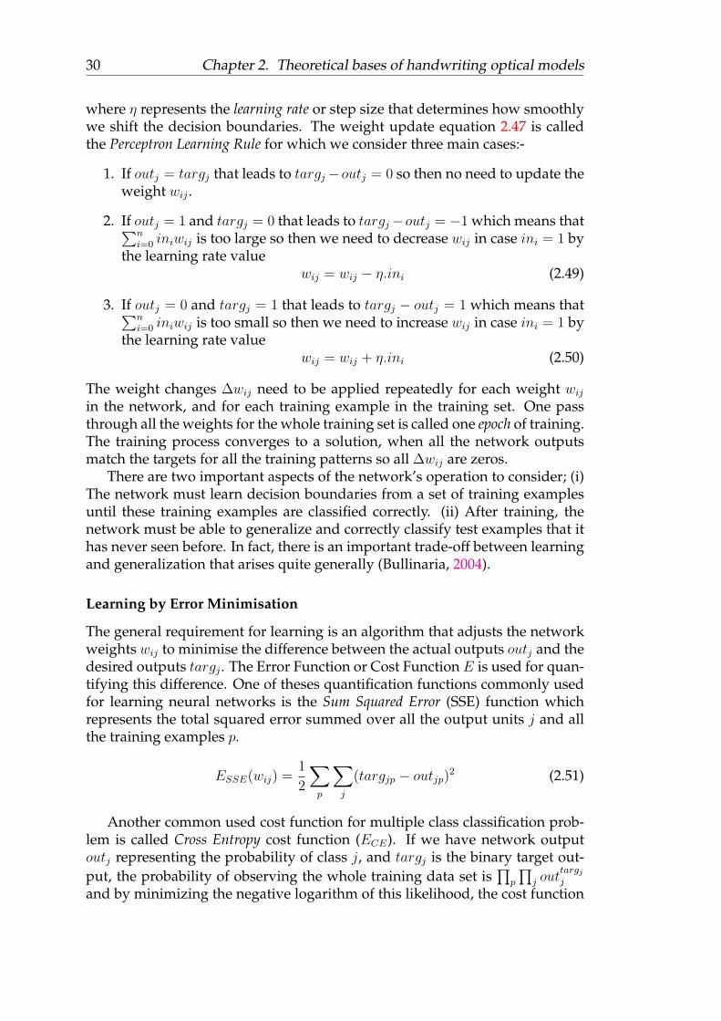
30 Chapter 2. Theoretical bases of handwriting optical models
where η represents the learning rate or step size that determines how smoothlywe shift the decision boundaries. The weight update equation 2.47 is calledthe Perceptron Learning Rule for which we consider three main cases:-
1. If outj = targj that leads to targj−outj = 0 so then no need to update theweight wij .
2. If outj = 1 and targj = 0 that leads to targj−outj = −1 which means that∑ni=0 iniwij is too large so then we need to decrease wij in case ini = 1 by
the learning rate valuewij = wij − η.ini (2.49)
3. If outj = 0 and targj = 1 that leads to targj − outj = 1 which means that∑ni=0 iniwij is too small so then we need to increase wij in case ini = 1 by
the learning rate valuewij = wij + η.ini (2.50)
The weight changes ∆wij need to be applied repeatedly for each weight wijin the network, and for each training example in the training set. One passthrough all the weights for the whole training set is called one epoch of training.The training process converges to a solution, when all the network outputsmatch the targets for all the training patterns so all ∆wij are zeros.
There are two important aspects of the network’s operation to consider; (i)The network must learn decision boundaries from a set of training examplesuntil these training examples are classified correctly. (ii) After training, thenetwork must be able to generalize and correctly classify test examples that ithas never seen before. In fact, there is an important trade-off between learningand generalization that arises quite generally (Bullinaria, 2004).
Learning by Error Minimisation
The general requirement for learning is an algorithm that adjusts the networkweights wij to minimise the difference between the actual outputs outj and thedesired outputs targj . The Error Function or Cost Function E is used for quan-tifying this difference. One of theses quantification functions commonly usedfor learning neural networks is the Sum Squared Error (SSE) function whichrepresents the total squared error summed over all the output units j and allthe training examples p.
ESSE(wij) =1
2
∑p
∑j
(targjp − outjp)2 (2.51)
Another common used cost function for multiple class classification prob-lem is called Cross Entropy cost function (ECE). If we have network outputoutj representing the probability of class j, and targj is the binary target out-put, the probability of observing the whole training data set is
∏p
∏j out
targjj
and by minimizing the negative logarithm of this likelihood, the cost function

2.3. Recurrent neural network (RNN) 31
becomesECE = −
∑p
∑j
targjp. log (outjp) (2.52)
By the training process we aim to minimize such error function. The networktraining by minimizing the Sum Squared Error means that the derivative ofthe error with respect to each network weight must be zero at the minimum
∂
∂wij
[1
2
∑p
∑j
(targjp − f(
∑i
inipwij)
)2 ]= 0 (2.53)
If we want to change given x value by ∆x to minimise a function f(x), what weneed to do depends on the gradient of f(x) at the current value of x accordingto
∆x = xnew − xold = −η∂f∂x
(2.54)
where η is a small positive constant specifying how much we change x, andthe derivative ∂f/∂x tells us which direction to go in. By iteration with equa-tion 2.54, the function f(x) will keep descending towards its minimum.Thisiterative procedure is known by gradient descent minimisation.
The idea is to apply a series of small updates to the weightswij ← wij+∆wijuntil the cost E(wij) is “small enough”. For this we need to determine thedirection that the weight vector need to change to best reduce the cost function.This can be achieved by knowing the effect of varying the weights wij on thegradient of the cost function E. By adjusting repeatedly the weights by smallsteps against the gradient, the cost function will move through a weight spaceand descends along the gradients towards the minimum value.
2.3.3 Neural Networks Topologies
Multi-layer perceptron (MLP)
The multi-layer notion of the perceptrons has been inspired from the biolog-ical neurons structures to form what is called multi-layer perceptron (MLP,(Rumelhart, Hinton, and Williams, 1988)). In this analogy, the inputs ini arereceived from other previous activated neurons outputs, that forms a neuralnetwork which consists of layers of mutually connected neurons with differentconnecting weights, starting form the input (first) layer through intermediatelayers towards the output (last) layer as illustrated in figure 2.10 .
Let W (l)ij denotes the weights of each neuron j of layer l applied on each
input i which is the output of the neuron i of layer l − 1. Thus the output(vector) of layer l namely out
(l)j can be computed by the multiplication of the
vector of inputs in(l) with the weight matrix W (l) considering the bias as oneof the input weights and the element-wise application of a non-linear function

32 Chapter 2. Theoretical bases of handwriting optical models
FIGURE 2.10: Multi-layer perceptron (MLP) illustration
fl.out
(l−1)i = ini
out(l)j = fl
(∑iW
(l)ij .out
(l−1)i
)out
(l+1)k = fl+1
(∑jW
(l+1)jk .out
(l)j
)...
(2.55)
The advantages of such organisation of layers is in the computation of thelayer output in a single feed-forward pass. The last layer neurons of the MLPare linear binary classifiers sharing the same input features (Bluche, 2015).Therefore, an MLP with several outputs is a multi-class classifier. (Bourlardand Wellekens, 1990) interpreted the network outputs as posterior probabil-ities. Posterior probabilities can be obtained by the application of a softmaxfunction instead of a sigmoid function at the output (last) layer. By denotingh =
∑iwijini as the activation of the neuron j (before the non-linear activation
function), and z its output, the softmax function can be defined for n neuronswith h1, . . . , hn activations as follows:
zi = softmax(hi) =ehi∑nk=1 e
hk(2.56)
where the output zi is satisfying two conditions, (i) zi ∈ [0, 1], (ii)∑n
i=1 zi = 1.By this, a probability distribution over all classes is defined which allows todecide for the class with the highest probability, i.e highest output.
With one single layer perceptron, it is not possible to deal with non-linearlyseparable problems. However, Multi-Layer Perceptrons (MLPs) are able tocope with non-linearly separable problems.

2.3. Recurrent neural network (RNN) 33
Learning single layer perceptron
Single layer perceptron means that the network consists of one layer of per-ceptrons for which we apply the learning process and one layer of inputs asshown in figure 2.11.
FIGURE 2.11: Multi-layer perceptron (MLP) illustration
We assume that we want to train a single layer network by adjusting itsweights wij to minimise the SSE (2.51) by making a series of gradient descentweight updates according to
∆wij = −η ∂E∂wij
(2.57)
If the transfer function for the output neurons is f(x), and the activations of theprevious layer k of neurons are ini , then the outputs are outj = f(
∑i iniwij) ,
and:
∆wij = −η ∂
∂wij
1
2
∑p
∑j
(targjp − f(
∑i
inipwij)
)2 (2.58)
where p ∈ p1, p2, . . . , pN are the training pattern. For training Single Layer Per-ceptrons, the delta rule of equation 2.58 and the perceptron learning rule haveexactly the same weight update equation obtained by two algorithms whichare theoretically different. The Perceptron Learning Rule was derived froma consideration of how we should shift around the decision hyper-planes forstep function outputs, while the Delta Rule emerged from a gradient descentminimisation of the Sum Squared Error for a linear output activation function(Bullinaria, 2004). The Perceptron Learning Rule will converge to zero error andno weight changes in a finite number of steps if the problem is linearly sepa-rable, but otherwise the weights will keep oscillating. On the other hand, theDelta Rule will (for sufficiently small η ) always converge to a set of weightsfor which the error is a minimum, though the convergence to the precise tar-get values will generally proceed at an ever decreasing rate proportional to theoutput discrepancies deltaj = targj − outj (Bullinaria, 2004). The output error

34 Chapter 2. Theoretical bases of handwriting optical models
deltaj at the unit j represents the difference between the target output targj atthe unit j and the unit output outj .
Learning MLP network by Back-propagation
Learning Multi-layer Perceptron network is motivated by the same principleas for single layer networks learning. The learning process aims to adjust thenetwork weights w(l)
ij of each layer l in order to minimize an output cost func-tion such as Cross Entropy Error function ECE Unfortunately, the error at eachintermediate layer in not known which prevent from using the gradient de-scent rule on each layer directly. This can be achieved by a series of gradientdescent weight updates.
∆w(l)ij = −η
∂E(w(l+1)ij )
∂w(l)ij
(2.59)
The linear final outputs can be written:
out(N)j =
∑i
out(N−1)i w
(N)ij =
∑i
f
(∑k
inkw(N−1)ki
)w
(N)ij (2.60)
It is only the outputs out(N)j of the final layer N (N ∈ 0, 1 . . . , n, . . . , N) that
appear in the output error function ECE . Meanwhile, the final layer outputswill depend on all predecessor layers of weights, and the learning algorithmwill adjust them all also, by backpropagation the error on each layer and up-dating the parameters simultaneously on each layer.
When implementing the Back-Propagation algorithm it is convenient to de-fine
delta(N)j = (targj − out(N)
j ) (2.61)
which is the output error. One the delta of the output layer N is computedaccording to equation 2.61, then the delta is back-propagated to earlier layersusing
delta(l)j =
(∑k
delta(l+1)k .w
(l+1)jk
).f ′(∑
i
out(l−1)i w
(l)ij
)(2.62)
Then each weight update equation can be written as:
∆w(l)hj = η
∑p
delta(l)pj .out
(l−1)ph (2.63)
∆w(l)hj = η
∑p
[(∑k
delta(l)pk .w
(l)jk
).out
(l−1)pj .
(1− out(l−1)
pj
)].inph (2.64)
So the weight w(l)hj between units h and j is changed in proportion to the
output of unit h and the delta of unit j. The weight changes at the earlier layer

2.3. Recurrent neural network (RNN) 35
(l− 1) now take on the same form as the layer (l), but the “error” delta at eachunit j is back-propagated from (l) each of the output units k via the weightsw
(l)jk .
Recurrent Neural Network (RNN)
The network contains at least one feed-back connection that makes its acti-vation flow round in a loop over time as shown in figure 2.12. Thanks to
FIGURE 2.12: Recurrent neural network (RNN) illustrationGraves et al., 2006
this property, the network is able to achieve temporal processing tasks suchas handwriting recognition and learn sequences like in language modellingtasks. Figure 2.13 shows a RNN being unrolled (or unfolded) into a full onehidden layer network. By unrolling we simply mean that we write out the net-work for the complete sequence. For example, if the sequence we care aboutis a sentence of 3 events, the network would be unrolled into a 3-layer neuralnetwork, one layer for each event.
FIGURE 2.13: Unrolled recurrent neural network (RNN) illustra-tion
Let xt and ot be the input and output vectors of events associated with twoconnection weights matrices U and V respectively. Furthermore, let denoteht as the hidden state (the memory unit) of the network which depends on

36 Chapter 2. Theoretical bases of handwriting optical models
the previous hidden state ht−1 and the input event at the current step xt con-sidering their associated weights W and U respectively. The hidden and out-put unit activation functions fh and fo are used for controlling the recurrentunit behaviour. Unlike a traditional deep neural network, which uses differentweights at each layer, the RNN network shares the same weights (U, V, W seenin figure 2.13) across all time steps. This reflects the fact that we are performingthe same task at each time step, just with different inputs. This greatly reducesthe total number of weights we need to learn.
The behaviour of the recurrent network can be described as a dynamicalsystem by a pair of non-linear matrix equations:
ht = fh (U.xt + W.ht−1) (2.65)
ot = fo(V.ht) (2.66)
The function f usually is a non-linearity such as tanh or ReLU. Theoretically,the state ht captures information about what happened in all the previous timesteps. The output at step ot is calculated solely based on the memory at time t.As briefly mentioned above, it’s a bit more complicated in practice because httypically can’t capture information from too many time steps ago.
Recurrent Neural Networks unit (RNNs) are popular models that haveshown great and promising results in many sequence related tasks such ashandwriting recognition and language modelling. The idea behind the lan-guage modelling using RNNs is to predict the next event on the line of eventswith keeping in mind the event which comes before it. However, for hand-writing recognition, the RNN is concerned by the identification of input eventswith regards to its history in some form of memory. Bidirectional RNNs (BRNNs,
FIGURE 2.14: Recurrent neural network (bidirectional-rnn) illus-tration
Schuster and Paliwal, 1997) are based on the idea that the output at time t may
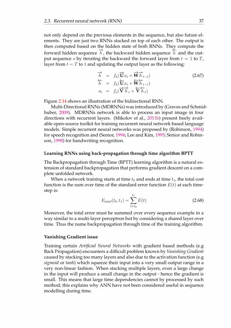
2.3. Recurrent neural network (RNN) 37
not only depend on the previous elements in the sequence, but also future el-ements. They are just two RNNs stacked on top of each other. The output isthen computed based on the hidden state of both RNNs. They compute theforward hidden sequence
−→h , the backward hidden sequence
←−h and the out-
put sequence o by iterating the backward the forward layer from t = 1 to T ,layer from t = T to 1 and updating the output layer as the following:
−→h = fh(
−→Uxt +
−→W−→h t−1) (2.67)
←−h = fh(
←−Uxt +
←−W←−h t−1)
ot = fo(−→V−→h t +
←−V←−h t)
Figure 2.14 shows an illustration of the bidirectional RNN.Multi-Directional RNNs (MDRNNs) was introduced by (Graves and Schmid-
huber, 2009). MDRNNs network is able to process an input image in fourdirections with recurrent layers. (Mikolov et al., 2011b) present freely avail-able open-source toolkit for training recurrent neural network based languagemodels. Simple recurrent neural networks was proposed by (Robinson, 1994)for speech recognition and (Senior, 1994; Lee and Kim, 1995; Senior and Robin-son, 1998) for handwriting recognition.
Learning RNNs using back-propagation through time algorithm BPTT
The Backpropagation through Time (BPTT) learning algorithm is a natural ex-tension of standard backpropagation that performs gradient descent on a com-plete unfolded network.
When a network training starts at time t0 and ends at time t1, the total costfunction is the sum over time of the standard error function E(t) at each time-step is:
Etotal(t0, t1) =
t1∑t=t0
E(t) (2.68)
Moreover, the total error must be summed over every sequence example in away similar to a multi-layer perceptron but by considering a shared layer overtime. Thus the name backpropagation through time of the training algorithm.
Vanishing Gradient issue
Training certain Artificial Neural Networks with gradient based methods (e.gBack Propagation) encounters a difficult problem known by Vanishing Gradientcaused by stacking too many layers and also due to the activation function (e.gsigmoid or tanh) which squeeze their input into a very small output range in avery non-linear fashion. When stacking multiple layers, even a large changein the input will produce a small change in the output - hence the gradient issmall. This means that large time dependencies cannot by processed by suchmethod; this explains why ANN have not been considered useful in sequencemodelling during time.

38 Chapter 2. Theoretical bases of handwriting optical models
CTC learning criterion
Graves et al., 2006 introduced the Connectionist Temporal Classification (CTC)criterion basically for mapping an input sequence x to an output sequence oflabels L (ex. characters) within RNN network by using N-to-N predictionswith no need for further post-processing. The problem is that the standardneural network objective functions are defined separately for each frame inthe training sequence; in other words, RNNs can only be trained to make aseries of independent label classifications. This means that the training datamust be pre-segmented, and that the network outputs must be post-processedto give the final label sequence. (Graves et al., 2006).
The proposed method defines the network outputs to be the set of possi-ble labels sequence introduced to get a better character representation, plus ablank output (∅). By this way, a sequence of predictions is mapped to the targetsequence of labels by removing repeated labels and the blanks for example:
aa ∅ bb ∅ a ⇒ aba
Training a RNN network using CTC criterion aims to maximize the prob-ability of the label sequence given the input sequence. Several prediction se-quences yield the same label sequence (e.g.aabb, aaab, a∅bb, ...). To simplify theanalogy with the methods presented previously, let Qn(L) be the set of all la-bels (prediction) mapping the groundtruth target sequence L.
p(L|x) =∑
q∈Q|x|(L)
|x|∏t=1
p(qt|L) (2.69)
This quantity can also be efficiently computed with a forward procedure ina way similar to the HMM. The mapping defines the allowed transitions be-tween labels: one can either continue to predict the same label, jump to the nextone if it is different, or jump to a blank. The forward and backward variablesare defined as follows, with L = l1, . . . , ln and L′ = l′1, . . . , l
′n = ∅l1∅, . . . , ∅ln∅
αt(l′s) = p(q1:t ∈ Qt(L1:s/2, qt = l′s|x) (2.70)
βt(l′s) = p(qt+1:T ∈ QT−t(Ls/2+1:|L|), qt = l′s|x) (2.71)
and the recurrences are:
αt(l′s) = p(qt = l′s|x)
k∑n=0
αt−1(ls−n) (2.72)
βt(l′s) =
k∑n=0
p(qt+1 = l′s+n|x)βt+1(l′s+n) (2.73)

2.3. Recurrent neural network (RNN) 39
where k = 1 when l′s = l′s−2 or l′s = l′s+2 for forward / backward variables,and k=2 otherwise. The α and β variables allow to compute
p(L|x) =∑
q∈Q|x|(L)
αt(q)βt(q) (2.74)
and the derivation of the cost− log p(L|x) leads to the following back-propagatederror:
∂E
∂atk= ytk −
∑s:µ(s)=k
αt(s)βt(s)∑r αt(r)βt(r)
(2.75)
were ytk is the output of the neural network at time t for label k, and atk arethe activations before the softmax.
Long Short-Term Memory Units (LSTM)
In RNNs, the vanishing gradient issue prevents the neural network to learn longtime dependencies (Bluche, 2015; Hochreiter, 1991; Bengio, Simard, and Fras-coni, 1994). The solution proposed by (Hochreiter and Schmidhuber, 1997) totackle this problem introduced a gating mechanism in form of a Long Short-Term Memory unit neural network (LSTM). Unlike the recurrent unit whichsimply computes a weighted sum of the input signal and applies a nonlin-ear activation function, each LSTM unit maintains a memory Ct at each timet. The temporal recurrent memory cell Ct is controlled by forget, input andoutput gates which serve to flush, change or retrieve data from the memorycell respectively. The gating mechanism is what allows LSTMs to explicitlymodel long-term dependencies. By learning the parameters for its gates, thenetwork learns how its memory cells should behave. The gate consists of anactivation function (like, sigmoid) and a point wise multiplication operation(Bluche, 2015). The gate outputs numbers between zero and one, decidingeither to let the whole information go when the output value is one or totalinformation blocking once the output value is zero.
FIGURE 2.15: LSTM functional illustration
Looking at figure 2.15, an LSTM unit is described by the following terms:-

40 Chapter 2. Theoretical bases of handwriting optical models
The Output Gate ot controls whether the LSTM unit emits its memory acti-vation output ht.
ot = σ(Wo.[xt, ht−1] + bo)ht = ot tanh(Ct)
(2.76)
The forget gate ft controls by interruption, the participation of the previousstate forward to the next one.
ft = σ(Wf .[xt, ht−1] + bf ) (2.77)
The Input Gate it decide whether the current cell input Ct has a contribu-tion to the memory cell state at the next time slot Ct+1.
it = σ(Wi.[xt, ht−1] + bi) (2.78)
The next cell state Ct can be obtained by.
Ct = tanh(Wc.[xt, ht − 1] + bc)
Ct = ft Ct−1 + it Ct(2.79)
Unlike the traditional recurrent unit which overwrites its content at eachtime-step, an LSTM unit is able to decide whether to keep the existing mem-ory state via the introduced gates. Intuitively, if the LSTM unit detects an im-portant feature from an input sequence at early stage, it easily carries this in-formation (the existence of the feature) over a long distance, hence, capturingpotential long-distance dependencies (Chung et al., 2014).
The LSTM unit is more powerful than the standard RNN’s one by the abil-ity of learning simple grammars (Hochreiter and Schmidhuber, 1997; Gersand Schmidhuber, 2001) and music composition (Eck and Schmidhuber, 2002).LSTM-RNN’s was successfully used for phonemes and speech recognition by(Graves and Schmidhuber, 2005; Graves, Mohamed, and Hinton, 2013).
FIGURE 2.16: BLSTM functional illustration
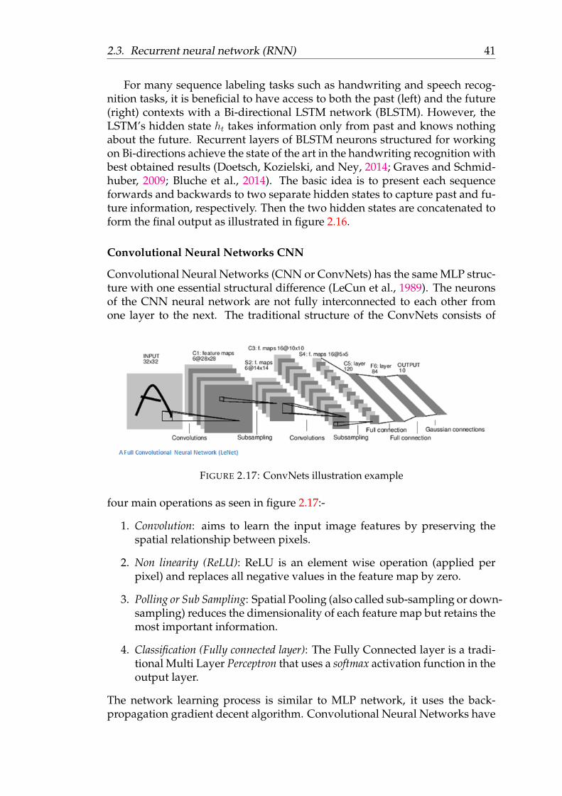
2.3. Recurrent neural network (RNN) 41
For many sequence labeling tasks such as handwriting and speech recog-nition tasks, it is beneficial to have access to both the past (left) and the future(right) contexts with a Bi-directional LSTM network (BLSTM). However, theLSTM’s hidden state ht takes information only from past and knows nothingabout the future. Recurrent layers of BLSTM neurons structured for workingon Bi-directions achieve the state of the art in the handwriting recognition withbest obtained results (Doetsch, Kozielski, and Ney, 2014; Graves and Schmid-huber, 2009; Bluche et al., 2014). The basic idea is to present each sequenceforwards and backwards to two separate hidden states to capture past and fu-ture information, respectively. Then the two hidden states are concatenated toform the final output as illustrated in figure 2.16.
Convolutional Neural Networks CNN
Convolutional Neural Networks (CNN or ConvNets) has the same MLP struc-ture with one essential structural difference (LeCun et al., 1989). The neuronsof the CNN neural network are not fully interconnected to each other fromone layer to the next. The traditional structure of the ConvNets consists of
FIGURE 2.17: ConvNets illustration example
four main operations as seen in figure 2.17:-
1. Convolution: aims to learn the input image features by preserving thespatial relationship between pixels.
2. Non linearity (ReLU): ReLU is an element wise operation (applied perpixel) and replaces all negative values in the feature map by zero.
3. Polling or Sub Sampling: Spatial Pooling (also called sub-sampling or down-sampling) reduces the dimensionality of each feature map but retains themost important information.
4. Classification (Fully connected layer): The Fully Connected layer is a tradi-tional Multi Layer Perceptron that uses a softmax activation function in theoutput layer.
The network learning process is similar to MLP network, it uses the back-propagation gradient decent algorithm. Convolutional Neural Networks have

42 Chapter 2. Theoretical bases of handwriting optical models
a good reputation in computer vision application field because of their excel-lent achievements with best performance results in various challenging taskssuch as object recognition (Szegedy et al., 2015), image segmentation (Fara-bet et al., 2013), speech recognition (Abdel-Hamid et al., 2012). They are alsoused for handwritten digits recognitions by (LeCun et al., 1989), then for wholehandwritten text (sentence) recognition by( LeCun et al., 1989; Bengio et al.,1995; Le Cun, Bottou, and Bengio, 1997; Bluche, Ney, and Kermorvant, 2013a;Bluche, Ney, and Kermorvant, 2013b).
2.3.4 Handwriting recognition platforms and toolkits
Several toolkits have been used for speech recognition or for handwriting recog-nition. Some of these toolkits support implementation of Hidden Markovmodel or neural network based HWR systems and provides sophisticated fa-cilities for speech analysis, HMM training, testing and results analysis.
We present a non-exhaustive list of HMM based platforms and toolkits thathelp to build HMM based HWR systems is the following:
1. HTK (Young and Young, 1993) consists of a set of library modules andtools available in C source form. The software supports HMMs usingboth continuous density mixture Gaussians and discrete distributionsand can be used to build complex HMM systems. initially, HTK is aHMM toolkit but recently, it has the ability to deal with deep neurl net-work architecture.
2. Juluis (Lee, Kawahara, and Shikano, 2001) is a high-performance, two-pass LVCSR decoder written in C and context-dependent HMM decod-ing (deal with HTK HMM formates).
3. Sphinx-4 (Walker et al., 2004) is a modular (written in Java) and plug-gable framework that incorporates design patterns from existing sys-tems, with sufficient flexibility to support emerging areas of research in-terest.
4. RWTH Aachen University speech recognition toolkit (Rybach et al., 2009)is written in C++ and consists of speaker adaptation, speaker adaptivetraining, unsupervised training, a finite state automata library, and anefficient tree search decoder components.
5. Kaldi (Povey et al., 2011) is an open-source toolkit for speech recognitionwritten in C++ and licensed under the Apache License v2.0. It providesthe tools to train HMM / NN optical models and intergrates Open-FSTlibrary (Allauzen et al., 2007) for decoding with Finite State Transducerstechniques.
Common NN based platforms and toolkits used for building HWR are pre-sented in the following list:-

2.3. Recurrent neural network (RNN) 43
1. RETURNN (Doetsch et al., 2016) is extensible and easily configurableneural network training software. It support training different recur-rent neural network topologies on multiple GPUs. RETURNN standson Theano as an top of layer for the Theano library which representsa bridge between research oriented software packages and applicationdriven machine learning software like Caffe (Jia et al., 2014). RETURNNextends RASR (Wiesler et al., 2014) to support various recurrent neuralnetworks architectures in ASR systems.
2. Theano (Bastien et al., 2012) is a Python based framework that supportthe automatic differentiation for symbolic mathematical tensor expres-sions. Expressions modelling represents a computational dependencygraph which can be augmented by an automatic optimization procedure.The abstract of each graph node can be defined for various types of hard-ware like CPUs or GPUs. By these properties, Theano is particularly use-ful for neural network training tasks.
3. Keras (Chollet, 2015) is a high-level data-driven machine learning frame-work based on Theano similar to RETURNN, Lasagne (Lasagne, 2017)and Blocks (Van Merriënboer et al., 2015). Recently, Keras starts to sup-port TensorFlow in addition to Theano as back-end with minimal restric-tions.
4. TensorFlow is the most recent open source machine learning package byGoogle (Abadi et al., 2016). It is actively developed and comes alreadywith many predefined solutions such as LSTMs, end-to-end systems andothers. TensorFlow is similar to Theano as it also works with symboliccomputation graphs and automatic differentiation.
5. Torch (Collobert, Bengio, and Mariéthoz, 2002) have its own program-ming language "Lua" and consists of many flexible and modular com-ponents that were developed by the community. In contrast to Theano,Torch does not use symbolic expressions and all calculations are doneexplicitly.
6. EEESEN (Miao, Gowayyed, and Metze, 2015) is a speech recognitiontoolkit which can be considered as an extension to Kaldi tool kit by addingrudimentary support for LSTMs networks. We used this toolkit for im-plementing our LSTM based handwriting recognition system.
There are some other notable NN-based frameworks which are written in C++such as Caffe (Jia et al., 2014), some others are Python-based such as Neon(Neon, 2017) and Brainstorm (Brainstorm, 2015). A comparison between Caffe,Neon, Theano, and Torch was presented by (Bahrampour et al., 2015).

44 Chapter 2. Theoretical bases of handwriting optical models
2.4 conclusion
In this chapter we aimed to present an overview of the theoretical bases of theoptical models as one of two essential components for any handwriting recog-nition system (the optical models and language models). An optical modelscan by introduced either by HMM models or neural network model. Discrete,continuous or semi-continuous HMM model can be used as an optical model,which represent generative model for sequence of observations.
Nowadays, MLP , RNN and their extension, represent the mile-stone ofa wide range of state of the art handwriting recognition systems thanks totheir discriminative nature in decision making. Such optical models fall inthe category of discriminative optical models, as opposed to HMM.
For the HMM based optical models, training the optical models can beachieved using the expectation maximization dynamic algorithms like Viterbiand forward-backward algorithms. Meanwhile, neural networks optical mod-els can be trained by using gradient descent algorithms such as back-propagation,back-propagation through time and CTC learning algorithm. The RNN basedrecognition system perform better than those base on HMM as mentioned bythe literature on the handwriting and speech recognition. tanh

45
Chapter 3
State of the art of languagemodelling
3.1 Introduction
Language modelling is the art of determining the probability of a sequenceof words (Joshua, 2001). Applications that deal with natural language data,(Written or spoken) require a representation of the characteristics of the treatedlanguage. For example, in case where the data are sentences, this representa-tion gives the possible associations of words. One of the important languagerepresentation is the language model which is able to capture language regu-larities.
Spoken language and written language differ by their low level structures(phonemes for spoken language and characters for written language) but theyfollow the same concatenation rules for higher level structures (ex. when con-structing sentences from "words").
Phonemes (ex. /@/) are the primary units of speech in a language. Conven-tionally, the term ”phone” designates the acoustic realization of a phoneme.Phonemes, are classified into two main categories: vowels and consonants.Vowels are linguistically characterized with respect to the pitching position inthe oral cavity [front - back], [high - low]. Consonants are characterized byconstriction or obstruction of important pitching in the oral cavity. In English40 phonemes are used to code the language, while 35 make up the French lan-guage, and only 25 phonemes are sufficient for coding the Italian language.One important thing to be considered here, is that vowels and consonantsphonemes in speech do not have corresponding written representation. There-fore, the low level representation of spoken and written languages do notmatch. Some language specific rules allow converting the spoken represen-tation to the written representation of that language.
In this chapter, we first give an overview of the spoken and written lan-guage building units which represent the bricks that must be defined beforebuilding any language model. Then we present a comparison between struc-tural modelling of the language (representation that stands on a set of rulesfor the composition of sentences) and statistical language modelling that isbased on the frequency computations of word occurrences in a sentence. Thesetwo approaches represent the two main approaches for natural language mod-elling. Then, we focus more in depth on the statistical modelling approach of

46 Chapter 3. State of the art of language modelling
language, since it is more adapted to our problem, and we compare in particu-lar different techniques of language modelling before finishing by introducingsome applications.
3.2 Language building units
According to the literature (Shaik et al., 2011; Xu et al., 1996), we can classifythe spoken / written language building units from the lexical point of viewinto three main categories (see Tables 3.1): lexical units, sub-lexical units andprimary units. In the following sections we try to illustrate and explain thistaxonomi of the human spoken and written language.
languageunits
lexicalunits
sub-lexicalunits
primaryunits
Speech Wordsmorphemes
phonemesphonoticsyllables
graphones
Writing Wordsmorphemes
Charactersgraphemicsyllables
htop Hyphens basedAlphanumeric characters
TABLE 3.1: spoken & written language components
3.2.1 Primary units
Both spoken and written languages are based on unambiguous primary unitswhich are either phonemes of spoken languages or characters and alphanu-meric symbols of written languages. Phonemes are represented ambiguouslyusing a phonetic alphabet (Alphabet Phonetique International (International-Phonetic-Association, 1999) but written languages do not use this alphabet,they use one of the many writing systems that have been introduced throughhistory.
The type of writing system used for a language is the most important fac-tor for determining the nature of the language primary units. Writing systemscan be logographic, where a large number (often thousands) of individual lo-gograms (symbols) represent words (Indurkhya and Damerau, 2010). A lo-gogram or logograph is a written symbol that represents a word or a phrase.Chinese characters and Japanese kanji alphabet are logograms; some Egyptianhieroglyphs and some graphemes in cuneiform scripts are also logograms. Incontrast, writing systems can be syllabic, in which individual symbols repre-sent syllables, or alphabetic, in which individual symbols (more or less) rep-resent sounds; unlike logographic systems, syllabic and alphabetic systemstypically have fewer than 100 symbols.

3.2. Language building units 47
Syllabic alphabets, are writing systems in which the main element is thesyllable. Syllables are built up of consonants, each of which has an inherentvowel. For example in Devangari writing system like "mAJ lVk dvnAgrFcþyog", diacritic symbols are used to change or mute the inherent vowel, andseparate vowel letters may be used when vowels occur at the beginning of asyllable or on their own. The majority of the written languages use an alpha-betic or syllabic system (Comrie, Matthews, and Polinsky, 1997). However,in practice, no modern writing system employs symbols of only one kind, sono natural language writing system can be classified as purely logographic,syllabic, or alphabetic (Indurkhya and Damerau, 2010).
In writing, the alphanumeric characters and symbols such as punctuationmarks sometimes attach the beginnings or/and the ends of the meaningfullanguage words like in the French sentence "C’est intéressant," or in the Englishsentence "I ’d like to jump!!". The punctuation characters (’), (,) and (!!) definesthe reading style of the handwriting. For example, the couple of characters(’d) represents an appreviation to the sentence "I would", while the punctu-ation character (’) does not make sense in a sentence if it was written alone.However, there are some other alphanumeric characters that are considered asa meaningful language word such as digits, mathematical symbols and ques-tion marks. Thus, meaningful alphanumeric characters and symbols can beconsidered as lexical, sub-lexical and primary building units the written lan-guage.
3.2.2 Lexical units
For the spoken and written language, the word is the lexical unit of a languagethat hold a significant meaning. Regarding to the writing systems, it is noteasy to determine what is meant by "word". Typically people initially thinkof items in a sentence separated by silence or white spaces or certain types ofpunctuation marks. In languages such as French, English, German or Arabicsuch concepts can be applied. In languages such as Bengali, chines, Japaneseor Thai, there are no separation mark between words, because a sequence ofadjacent characters can represent multiple words.
The notion of word is very important for most of the evaluation protocols,a word being defined as a sequence of characters sided by two white space forwriting or by silence for speech.
3.2.3 Sub-lexical units
Sub-lexical units are used in speech recognition as the acoustic model build-ing blocks rather than phonemes ( Choueiter, 2009). Sub-word units are alsoused for language modelling ( Shaik et al., 2011; Mousa et al., 2010; El-Desokyet al., 2009). For highly inflected languages such as German (Shaik et al., 2011)or Arabic (Märgner and El Abed, 2012), a large amount of words are derivedfrom the same root due to multiple factors such as inflection, derivation andcompounding. This morphological flexibility leads to high OOV rates andlarge language model perplexity. For such languages, sub-word units allow
48 Chapter 3. State of the art of language modelling
modelling OOV with lower perplexity language models. The perplexity is de-fined in information theory (Shannon, 1948) as a measurement of how wella probability distribution or probability model predicts a sample. It is usedfor comparing probability models such as language models. A low perplexityindicates the probability distribution is good at predicting the sample.
One important issue of language modelling with sub-lexical units is theproper choice of the sub-word units. According to Shaik (Shaik et al., 2011),sub-word units are classified into three main types:- morpheme based sub-word units, syllable based sub-word units and graphone based sub-wordsunits. While lexical units are defined with no ambiguity as the language words,sub-lexical units have at least five main definitions based on two main decom-position strategies:
Spoken language dependent word decomposition into sub-lexical units
The strategy of word decomposition into sub-lexical units relies on some spo-ken language aspects such as word morphology and word pronunciation thatgenerate the following three types of sub-lexical units:-
1. Morpheme sub-lexical units: the decomposition of a word accordingto its morphological structure produces sub-lexical semantic units calledmorphemes which represent the prefix, root and suffix parts of the word(ex. non-, perish, and -able as prefix, root and suffix respectively).
The morpheme is known as the smallest linguistic component of a wordthat has a semantic meaning. A word can be decomposed into a se-quence of morphemes by applying either supervised or unsupervisedapproaches. Supervised approaches (Adda-Decker and Adda, 2000) usea set of linguistic rules designed by an expert. Unsupervised approachesare almost statistical based data driven approaches (Adda-Decker, 2003).The proposed decompounding algorithm is corpus-based and languageindependent in the sense of no linguistic knowledge is required, except-ing a large text corpus. Word-specific decompounding rules are automat-ically extracted based on the branching factor of successor characters.
Morphemes have been used by Shaik (Shaik et al., 2011) for speech recog-nition and by Hamdani et al (Hamdani, Mousa, and Ney, 2013 for hand-writing recognition. Hamdani & al. proposed an Arabic handwritingrecognition system based on HMM models using a mixed language modelof words and sub-word units. The vocabulary contains words and sub-word units produced by a specific morphological decomposition methodof Arabic words which is based on the semantic decomposition of wordsinto roots, suffixes and prefixes (Creutz et al., 2007). The results showthe improvement provided by this system, notably to cope with OOV,compared to a lexicon driven recognition system.
2. Phonetic syllable sub-lexial units: Syllables are sub-lexical units that arebased on a phonetic decomposition. They are sometimes defined physi-ologically as a continuous unit of the spoken language which consists of

3.2. Language building units 49
a sound or a group of sounds uttered in one breath (Ryst, 2014; Brown,2006) for example the french word (bibliothécaire) has the phonologicalsyllable representation (bi - bli - O - te - kEK).
Syllables are generally centered around the vowels in English (Huang etal., 2001), French (Ryst, 2014) and German (Shaik et al., 2011). Acous-tic models of syllables and syllable-like units are implemented with suc-cess in (Choueiter, 2009; Ganapathiraju et al., 2001) and successful imple-mentation of syllabic language models are presented in (Xu et al., 1996)for Chinese, (Majewski, 2008) for Polish, (Schrumpf, Larson, and Eick-eler, 2005) for English and German language (Shaik et al., 2011). Syl-labic models based on hidden Markov model (HMM) are examined in(Jones, Downey, and Mason, 1997) and compared with mono-phonesHMM based acoustic models using a bigram language model. A Hy-brid syllable and phonetic based model was proposed by (Sethy, Ramab-hadran, and Narayanan, 2003) and the system shows better performancethan systems that use only one of these two models.
The syllable plays an important role in the organization of speech andlanguage (Kozielski, Doetsch, and Ney, 2013; Ryst, 2014). The syllableconsists of one or more written letters representing a unit of speech calledphoneme. The segmentation of speech into syllables can be achievedusing acoustic units or phonological units (Ridouane, Meynadier, andFougeron, 2011), and syllables produced by these two models are not al-ways compatible (Ryst, 2014). As illustrated in figure 3.1, most phoneti-cians agree that a syllable is composed basically of a rhyme that is pre-ceded by an onset (one or more consonants "C" optionally comes at thebeginning of the syllable). Inside a rhyme, the nucleus (usually a vowel"V") is the constitutive element of the syllable. This is followed by a coda(one or more consonants "C" at the end of the syllable) (Ryst, 2014). Thelanguages differ from each other with respect to topological parametersas optionality of the onset and admissibility of the codas. For example,the onsets are mandatory in German while the codas are prohibited inSpanish (Bartlett, Kondrak, and Cherry, 2009). In French and English,the nucleus is always considered as a vowel. Thus, counting the numberof syllables pronounced in a French or English, should be equivalent tocounting the number of pronounced vowels (Ryst, 2014). The phoneticstructure does not match the orthographic structure because of the sig-nificant difference between the vowel phoneme and the vowel charactersas illustrated in figure 3.1
Considering written languages, and according to (Flipo, Gaulle, and Van-cauwenberghe, 1994), in French the orthographic syllable differs from thephonetic syllable because it retains all "e" silent placed between two con-sonants or placed at the end of a word. Hyphenation rules separate thedouble consonants even if they are pronounced as a single consonant.For example, graphically there are three syllables in the French word pu-re-té even if we pronounce it as [ pyr-te ] (two phonetic syllables). The

50 Chapter 3. State of the art of language modelling
FIGURE 3.1: Syllable phonetic components
authors of (Roekhaut, Brognaux, and Beaufort, 2012) have classified thesyllables in three different categories:
• A phonetic syllable is composed of a combination of phonemes thatare pronounced in a single breath.
• A graphemic syllable represents a faithful transposition of phoneticsyllabification in the spelling of the word.
• An orthographic syllable applies hyphenation rules that must be-longs to writing.
It seems difficult to integrate these different views of specialists into arecognition system, but in any case, only graphemic or orthographic syl-lables provide a decomposition of writing that is likely to have an impacton a recognition system.
The Syllable based n-gram language model shows through our experi-ments good language modelling capacity with reduced language modelcomplexity as demonstrated in chapter 5, in addition to its ability to covera wide range of Out-Of-Vocabulary words. The syllable based n-grammodel suffer of losing word context with lower values of n-gram orders.Generally, it represents a good compromise between the word based lan-guage model and the character based language model for sufficientlyhight order n-gram language models.
3. Graphemic syllable sub-lexial units: derived from phonological sylla-bles, graphemic syllables have been introduced for written languages.The same example "bibliothécaire" has the following graphemic repre-sentation (bi - bli - o - thé - caire) . Thus, the graphemic syllable always
3.2. Language building units 51
respects the boundaries of the phonetic syllable. The graphemic syllableseems to occupy a prominent place in the learning process of the lan-guage. Several researchers believe that it is one of the basic units fromwhich to build gradually the recognition of the words of the language(Lecocq, 1991). A graphemic syllabic algorithm that relies on the strictlink between graphemes and phonemes of French was introduced by(Roekhaut, Brognaux, and Beaufort, 2012). In this context, we introduceda supervised syllabification algorithm (Swaileh and Paquet, 2016b) thatallow to decompose any French or English word into its syllable decom-positions. This approach will be developed in chapter 5.
4. Hyphen based sub-lexical units:
The hyphen (−) is a punctuation mark used to join words and to separatesyllables of a single word. The use of hyphens is called hyphenation. Inwriting, the hyphen is a single entity. In terms of character encoding anddisplay, this entity is represented by any of several characters and glyphs(including hard hyphens, soft or optional hyphens, and nonbreaking hy-phens), depending on the context of use. Hyphens are occasionally usedto denote syllabification, as in (syl-la-bi-fi-ca-tion).
There are a few hyphenation rules that will let one hyphenate almost allEnglish words properly as presented in (Beeton, 2010):
• Break words at morpheme boundaries (inter-face).
• Break words between doubled consonants (bat-tle).
• Never separate an English digraph (e.g., th, ch, sh, ph, gh, ng, qu)when pronounced as a single unit (au-thor but out-house).
• Never break a word before a string of consonants that cannot begina word in English (jinx-ing and not jin-xing).
• Never break a word after a short vowel in an accented syllable (rap-id but stu-pid).
The rules above leave more than one acceptable break between syllables,use the Maximal Onset Principle: If there is a string of consonants be-tween syllables, break this string as far to the left as you can (mon-strous).
Sometimes the rules conflict with each other. For example, ra-tio-nal getshyphenated after a short vowel in an accented syllable because ti acts asa digraph indicating that the ’t’ should be pronounced ’sh’.
Sometimes it’s not clear what constitutes a morpheme boundary: whyger-mi-nate and not germ-i-nate?
These rules are not mandatory and other rules can be used like the sim-plest rule of Mikolove (Mikolov et al., 2012) which split words at vowelsand limit the minimum size of the sub-lexical units to 2 characters.

52 Chapter 3. State of the art of language modelling
Spoken language independent word decomposition into sub-lexical units
Some heuristic and probabilistic approaches are used to produce sub-lexicalunits with no care about semantic or syntactic aspects of the language of inter-est. These kind of decomposition into sub-lexical units approaches have beenused with success by Shaik (Shaik et al., 2011) for speech recognition basedon a grapheme-to-phoneme (G2P) conversion model as described in (Bisaniand Ney, 2008), Benzeghiba (BenZeghiba, Louradour, and Kermorvant, 2015)for Arabic handwriting recognition using the definition of the Part-Of-Arabicword (PAW) and Feild (Feild, Learned-Miller, and Smith, 2013) for text scenerecognition using a probabilistic context free grammar (PCFG) model.
1. Graphone sub-lexical units: One of speech sub-lexical units is the gra-phone. The graphone units are derived from a grapheme-to-phoneme(G2P) conversion model (Bisani and Ney, 2008). It is a combination ofthe graphemic sub-word units with their context dependent pronuncia-tion forming one joint unit (Shaik et al., 2011), in other words, it is thejoint character-phoneme sub-lexical unit (Wang, 2009) as illustrated infigure 3.2.
FIGURE 3.2: Illustration of a sequence of graphones (Mousa andNey, 2014)
A model estimated over such units represents an implicit combinationof language model and pronunciation model in one joint probability dis-tribution (Shaik et al., 2011). Graphones are mainly used for modellingOOV. They can be derived directly from Grapheme-to-phoneme conver-sion as illustrated in (Bisani and Ney, 2008), or by using fixed-length sub-words units without any linguistic restrictions like in (Bisani and Ney,2005). A combination of the three types of sub-lexical units was studiedin (Shaik et al., 2011) for German and a hybrid speech recognition systemhas been implemented using a hybrid lexicon. In this system, the mostfrequent words of the language are used normally as full-words withoutdecomposition into sub-word units. Less frequent in-vocabulary wordsare decomposed into syllables. Finally, the OOV words are decomposedinto graphones.
2. Other spoken language independent decomposition into sub-lexicalunits: In the literature, there are few researchers who are using sub-lexical units in handwriting. Few of them used the Part-Of-Arabic word(PAW) sub-lexical units in order to tackle the problem of recognition con-fusion between inter-word and intra-words white space in Arabic hand-writing recognition system as illustrated by BenZeghiba (BenZeghiba,Louradour, and Kermorvant, 2015).

3.2. Language building units 53
BenZeghiba & al. (BenZeghiba, Louradour, and Kermorvant, 2015) pro-posed a hybrid model for the Arabic language, which is designed ac-cording to the observed frequency of words. The idea is to keep themost frequent words as is (without decomposition), and to decomposeonly the least frequent words into sub-word units or PAWs (Part of Ara-bic Words). By taking advantage of the specific property of the Arabiclanguage and script, a PAW is a sequence of characters that can be con-nected together. A character that cannot be connected with its followingneighbor defines the end of a PAW (AbdulKader, 2008). The advantageof a hybrid word - PAW model lies in the trade off between its modelingand generalization ability and its reduced size. The two models (hybridword / PAW) and PAW alone perform almost similarly on OOV wordsbut the hybrid system is less complex. Statistical models such as Proba-bilistic Context Free Grammar (PCFG) and multigrams model are usedfor decomposing words into sub-lexical units as illustrated by Feild & al.(Feild, Learned-Miller, and Smith, 2013).
Regarding English language, Jacqueline & al. (Feild, Learned-Miller, andSmith, 2013) proposed a probabilistic syllable model for scene text recog-nition such as advertisements panels. They used a probabilistic contextfree grammar (PCFG) that models each sub-lexical unit as a sequenceof characters generating a consonant or a vowel. The proposed modelshows good performance on OOV words such as proper nouns, underthe condition that these words should all be pronounceable in English.The PCFG model was built by learning a set of parsing rules of charac-ters using a syllabified dictionary. As a defect of this model, the methoddoes not use any information about successive syllables which leads to aloss of context modelization of syllables.
The multigram definition can be considered as an extension to the n-gram definition where the suffix "gram" can be defined as a languageunit of word, syllable, multigram or character. While the n-gram is de-fined as the sequence of language units of fixed and limited size n, themulitgram can be defined as a sequence of language units with variablelength. Table 3.2 shows some examples of the n-grams and multigramsof order n = (1, 2, 3, 4, 5) for the French word "Merci" and the englishword "Darling".
In the field of speech recognition and language processing, the choiceof sub-lexical units that structure the data stream affects massively theefficiency of the recognition algorithms. On the one hand, sub-lexicalunits may be determined by relying on some linguistic knowledge butwith the risk of being inadequate to the particular task at end, due to thespecificity of the data. On the other hand, it can be determined directlyfrom the data using machine-learning approaches.
Former works in speech recognition such as (Chou and Lookabaugh,1994; Sagisaka and Iwahashi, 1995; Bacchiani et al., 1996; Ries, Buo, andWang, 1995) show the impact of determining the sub-lexical units from

54 Chapter 3. State of the art of language modelling
Lexicontype
Frenchexamples
Englishexamples
n-gramsof
characters
uni-gram M e r c i D a r l i n gbi-gram Me, er, rc, ci Da, ar, rl, li, in, ngtri-gram Mer, erc, rci Dar, arl, rli, lin, ing4-gram Merc, erci Darl, arli, rlin, ling5-gram Merci Darli, arlin, rling
Multigramsdecompositions
m2gram Me, r, ci d, ar, li, ngm3gram Mer, ci dar, l, ingm4gram Merc, i dar, lingm5gram Merci dar, ling
TABLE 3.2: n-grams versus multigrams examples
the data directly, and yielded to the multigram model (Deligne and Bim-bot, 1997). The multigram model was first presented in (Bimbot et al.,1994) for language modelling by taking into account the variable lengthdependencies of words in a sentence. Theoretical formulation and evalu-ation of multigrams is presented in (Deligne and Bimbot, 1997; Deligne,Yvon, and Bimbot, 1996). It assumes the language produces a streamof words that flow off a memoryless source (Deligne and Bimbot, 1995).The language words are not independent, and their dependencies are ofvariable length. It can be opposed to the popular n-gram model (Jelinek,1990) which assumes that the statistical dependencies between words areof fixed length (n) along the whole flow of words (Deligne and Bimbot,1995), thus assuming an n-order Markov models of word streams. In then-multigram model (Bimbot et al., 1994), a sentence is considered as theconcatenation of independent (zero order Markov source) sequences ofwords of length k (with k ≤ n). Such concatenation of words (multi-gram) is commonly known as phrase in the natural language processingliterature. Then, the likelihood of the sentence is computed as the prod-uct of the individual phrases’s likelihood corresponding to each possiblesegment (multigram) (Deligne and Bimbot, 1995).
More formally, the multigram model is defined as a stochastic genera-tive model of variable length units (Deligne and Bimbot, 1997). Theseunits can be word phrases when considering language modelling, orthey can be character or phoneme sequences when considering hand-writing or speech recognition. Let us assume that a lexical source pro-duces a set of M sub-lexical units (multigrams) which are sequences oflength k characters (k ≤ n). While each data stream produced by thesource can be viewed as a sequence of T characters which are the pri-mary units of the observation sequence O = (c1, c2, . . . , ct, . . . , cT ), it canalso be viewed as a sequence S = (m1,m2, . . . ,ml, . . . ,mL) of multigramsof length L(L ≤ T ), each multi-gram ml being the concatenation of kcharacters ml = (ct, . . . , ct+k−1). As depicted on figure 3.3 below, themulti-gram decomposition corresponds to a particular segmentation ofthe input character string.

3.2. Language building units 55
FIGURE 3.3: Multigram structure and an example of word de-composition into multigrams
In the literature, this generative process of multigrams from the discreteobservation stream of characters has been modeled using variable lengthHidden Markov Models, assuming time independent multigrams (Deligneand Bimbot, 1997). Then, the likelihood of a particular multigram decom-position of the input string is computed as follows
P (O, S)∆= P (O|S)P (S) =
∏l
P (ctct+1 . . . ct+k−1|ml)P (ml) (3.1)
or more precisely
P (O, S) =∏l
P (ctct+1 . . . ct+k−1|dl = k)P (dl) (3.2)
where dl is the character duration of multigram ml. The main interest ofsuch modelling is to allow finding the optimal decomposition into multi-grams of a training corpus of text, thus providing an appealing approachfor the definition of sub-lexical units for any language without relying onlinguistic expertise for each dedicated language, the optimization pro-cess being unsupervised. In Deligne and Bimbot, 1997 the authors haveapplied the multigram model to derive sub-words phonetic units fromphonetic transcriptions of utterances using continuous observations se-quences. They also applied the model to derive the graphemic structureof text, considering discrete character observations. In their EM itera-tive optimization process, they introduced a heuristic by selecting themore frequent multigrams at each iteration, so as to optimize not onlythe data likelihood but also the complexity of the model so as to getbetter generalization capabilities of the model, following the MinimumDescription Length (MDL) principle. In Deligne and Sagisaka, 2000 thesame authors apply the multigram paradigm to language modelling (se-quences of words) and they report lower perplexity for the multigrammodel compared to the n-gram model.
3.2.4 Definitions
We present by the following, some essential definitions that help to identifyand evaluate the relationship between a training vocabulary / dataset and a

56 Chapter 3. State of the art of language modelling
test dataset.
• The word: standing on the standard handwriting recognition perfor-mance evaluation protocol of the Word Error Rate (WER), a word is de-fined as a sequence of characters sided by two white spaces. With defin-ing the character "|" as the word delimiter character, we consider inthe following coloured sentence six different words The French sentence
above contains an example of an entity name words, abbreviation wordand a date word. These words represent real problem while trainingthe language model, that because they may have rare occurrences in thelanguage model training corpora. For Building robust language model,the choice is to tokenize the training corpora and splitting the rare oc-currence words into sequences of alphanumeric words and then use thetoken building unit in place of the words for building the language mod-els.
• The token: it defines the language units used for building a languagemodel that can be a word or a smaller language units than a word, suchas sub-lexical, characters or orthographic symboles (e.g. ?,!,$,@,”,...etc).Looking at the sentence above, the token delimiter character "|" defines
twenty tokens that are derived from six words.
We need to deal with these two definition differently because we need toquantify the ability of the training corpus to cover the test corpus in terms ofwords and then we can study the relation between the training corpus cover-age with the handwriting recognition performance measured by the Word Er-ror Rate. We need also to quantify the ability of a language model of tokens tocover the tokenized test corpus in order to study the effect of language modelmissing words on the recognition performance, specially when the missingwords depend on the training corpus tokensiation strategy: lexical tokens, sub-lexical tokens and primary tokens. Based on the word and token definitions,we introduced two measures:
• The effective coverage rate (ECR): The proportion of words of the testdataset that belongs to the training dataset as illustrated in figure 3.4. Itmeasures the lexical proximity between two datasets of texts.
• The Out-Of-Vocabulary (OOV): The proportion of tokens of the test datasetthat do not belong to the language model lexicon (figure 3.4). It evaluatethe capacity of the language model to cover the test dataset.
The lexicon represents the essential linguistic source of information on whichthe language model training is based. Furthermore, the recognition systemscomplexities are determined standing on their lexicon sizes. The lexicon and
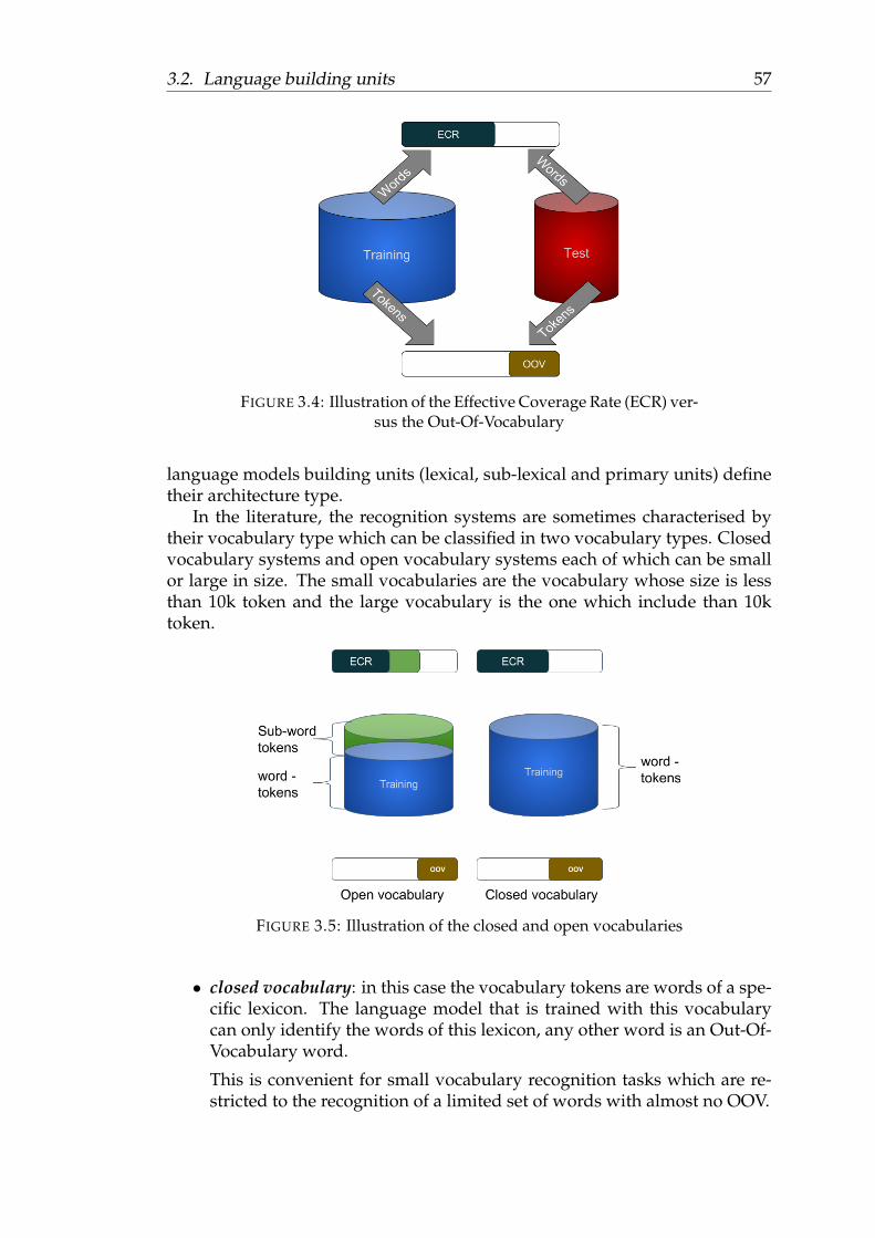
3.2. Language building units 57
FIGURE 3.4: Illustration of the Effective Coverage Rate (ECR) ver-sus the Out-Of-Vocabulary
language models building units (lexical, sub-lexical and primary units) definetheir architecture type.
In the literature, the recognition systems are sometimes characterised bytheir vocabulary type which can be classified in two vocabulary types. Closedvocabulary systems and open vocabulary systems each of which can be smallor large in size. The small vocabularies are the vocabulary whose size is lessthan 10k token and the large vocabulary is the one which include than 10ktoken.
FIGURE 3.5: Illustration of the closed and open vocabularies
• closed vocabulary: in this case the vocabulary tokens are words of a spe-cific lexicon. The language model that is trained with this vocabularycan only identify the words of this lexicon, any other word is an Out-Of-Vocabulary word.
This is convenient for small vocabulary recognition tasks which are re-stricted to the recognition of a limited set of words with almost no OOV.

58 Chapter 3. State of the art of language modelling
• open vocabulary: this vocabulary language models is composed of to-kens that are words and of some other tokens which represent a portionof the OOVs. By these tokens some words that do not belong to the lex-icon can be reconstructed, thus the effective coverage rate increases asa result of the OOVs reduction. In figure (figure 3.5) the ECR in bluecolour represents the effective coverage rate obtained by the word tokensof the language model and the green one represents the ratio of the recon-structed words thanks to the other sub-words tokens. These tokens canbe produced by replacing the words with rare occurrence in the trainingcorpus by the OOV token (<unk>) or by their set of characters (the greenpart of figure 3.5 represent the portion of the training lexicon which holdthe OOV tokens). In the literature, the recognition system that make useof the open vocabulary show slight performance degradation in compar-ison with the closed vocabulary based system performance.
In the following section, we give an overview on the natural language mod-elling approaches and some of their applications in real world applications.
3.3 Why statistical language models for handwrit-ing recognition?
Natural language modelling can be achieved with two main approaches: struc-tural and statistical approaches. In this section, we present these two ap-proaches and compare their advantages and disadvantages, to justify our choiceto work with the statistical approaches for the handwriting recognition.
In the structural approach, a language model is often defined as a set ofrules that build the language grammars. The set of such rules defines the pos-sibilities of word association, according to their lexical categories (noun, verb,adjective,.. etc), and makes it possible to model the structure of a given sen-tence (Chomsky, 2002). Therefore, these rules determine the validity of a sen-tence: if a sequence of rules can describe the sentence under examination thenthe sentence will be accepted, otherwise it will rejected by the model.
In the statistical approach, the language is represented by the occurrencefrequencies of each possible sequence of words. For this purpose, a represen-tative corpora (consists of blocks of texts about the domain of interest) are usedfor training the language model by the statistical inference algorithm (Man-ning and Schütze, 1999).
One of the advantages of statistical approaches is their independence fromthe language experts, as the language models are learned automatically fromcorpora. Modelling of the language following this approach is therefore de-pendent on the data used and can also attribute a non-zero probability to syn-tactically incorrect sentences which represent a drawback point for the statis-tical language modelling approaches. One of the advantages of models basedon structural approach is their ability to express the grammatical nature of thesentences. Nevertheless, one of the main difficulties of these methods remainsthe conception of the grammars, which means the definition of rules. Indeed,
3.4. Statistical language modelling 59
they must be robust enough to take into account all the syntactic hypothesesof a language.
It seems difficult for continuous handwriting recognition to develop a setof rules that describes the possible writing sentences specially when such sen-tences includes punctuation marks and written symbols associated with thelanguage meaningful words.
Due to the statistical nature of the language models constructed accordingto the statistical approach, their integration into a recognition system is moreeffective. Statistical language models have a great margin of flexibility in deci-sion making while they depend on the associated probability of the languagesentences. This probability evaluates whether or not the sentence is correct,in contrast to the structural approaches that associate a boolean decision ofaccepting or rejecting the sentence.
However, there are language models that combine both structural and sta-tistical approaches, such as Probabilistic-Context-Free-Grammars (PCFG) whichallow more flexible response by expressing the sentence validity in a proba-bilistic way. The use of PCFG models is more appropriate for tasks whosedomain is limited in vocabulary (because of the structural approach nature),such as address recognition (Srihari and Kuebert, 1997) or speech recognitionwith a specific and limited vocabulary (Jurafsky et al., 1995).
In the case of large vocabulary domains, these structural language modelscan be used in a second recognition pass to rearrange a list of sentences (Ha-cioglu and Ward, 2001) or in combination with a statistical language model(Zimmermann, Chappelier, and Bunke, 2006). In the latest cases, a statisticalmodel of the language is used jointly with the structural PCFG model.
Due to, the efficiency of integrating language models based on the statis-tical approaches into the handwriting recognition system and the simplicityof their learning procedures, we focused our work on the study of the statis-tical language modelling approaches, specially the back-off n-gram languagemodelling approach of the sub-lexical units.
3.4 Statistical language modelling
The goal of statistical language modelling is to predict the next word in textualdata given passed context; thus we are dealing with sequential data predic-tion problem when constructing language models (Mikolov et al., 2010). Wefirst present a general overview of the statistical language modelling principle.Then, we describe different measures to evaluate the language models quality.Finally, we focus on different language models and techniques for combininglanguage models.
3.4.1 General principles
Statistical modelling of language aims to capture the regularities of a languageby statistical inference on very large training corpora of text, composed of a setof topics in the language of interest (Manning and Schütze, 1999).

60 Chapter 3. State of the art of language modelling
A statistical language model makes it possible to evaluate the a priori prob-ability of a sequence ofN wordsW = w1 . . . wN . This probability is equal to theproduct of the probabilities of the words within its context as the following:
P (W ) =N∏i=1
P (wi|hi) (3.3)
Where P (wi|hi) is the occurrence probability of the word wi knowing that itcomes directly after the sequence of words hi = w1, . . . wi−1. These probabilitiesP (wi|hi) constitute the parameters of the language model. The sequence ofwords hi is called the history of the word wi. So for P (wi|hi) to be computedfor i = 1, a start-of-sentence marker < s > is added. We thus have h1 =< s >.Moreover, an end-of-sentence marker < /s > is added and included in theproduct of the probabilities of the words, then we can re-write equation 3.3 asfollow:
P (W ) =N+1∏i=1
P (wi|hi) (3.4)
where wN+1=</s>
3.4.2 Language model quality evaluation
The role of a language model is to estimate the a priori probability P (W ) of asequence of words W . Thus, as much as a word sequence W conform to thelanguage model, its probability will be higher. The simplest measure for eval-uating the quality of a language model is by measuring the affected probabilityupon a test data set T which is considered to be representative of the languageof interest and consists of a set of sentences (W1 . . .WN) whereN is the numberof sentences in T . From the probabilities P (wi|hi) given by the language modelLM , the probability of the sentences can be calculated using equation 3.4 andthe probability of the test dataset T is then given by:
P (T ) =N∏i=1
P (Wi) (3.5)
Thus, the language model assigning the highest probability to the test datasetT will be considered as the best model. This probability comes from the rela-tionship between prediction and compression, resulting from information the-ory (Shannon, 1948): given a language model LM which assigns a probabilityP (T ) to a test dataset T , a compression algorithm can be created to encode thetext to − log2(P (T )) bits. Thus, the cross entropy HLM of a language modelLM , on a test dataset T , is defined by:
HLM(T ) = − 1
|T |wlog2(P (T )) (3.6)
Where |T |w is the number of words in T The cross entropy evaluates howdifferent the language model is with the empirical distribution of the dataset.

3.4. Statistical language modelling 61
This value can be interpreted as the average number of bits needed to encodeeach of the |T |w words of the test dataset, using the compression algorithmassociated with the model LM . Therefore, the best language model will be theone which has the smallest cross entropy.
The Perplexity is a measure derived from cross entropy, which is in fact themost used measure to evaluate the performance of a language model. Theperplexity PPLM of a language model LM on a test dataset S corresponds tothe reciprocal of the mean probability given to each of the words of the testdataset T . It is related to the cross entropy by the equation:
PPLM = 2HLM (T ) (3.7)
This quantity accounts for the predictive power of the model LM . Thus,PPLM(T ) = k means that the language model LM hesitates on average be-tween k words. Thus, like cross entropy, the lower perplexity the best languagemodel.
In the context of handwriting recognition, it may also be advantageous tomeasure the recognition rates obtained on a test set, using different languagemodels in a recognition system. In fact, we will rather evaluate the error rateon words obtained on the test set, this indicator being well correlated withperplexity (Klakow and Peters, 2002): the lower the error rate, the better per-formance of the recognition system.
The main problem of equation 3.4 is the high number of different histori-cal data, which leads to a very large number of probabilities to be estimated.Moreover, most of these word histories appear so few times in the trainingcorpus which does not help in estimating their probability in a sufficiently re-liable way. One solution to solve this problem is to group word histories intoequivalence classes called n-grams:
P (wi|hi) ≈ P (wi|Φ(hi)) (3.8)
While Φ(hi) associates a class of equivalence to each word history hi. Ann-gram is a contiguous sequence of n items from a given sequence of text orspeech. The items can be phonemes, syllables, letters, words or base pairsaccording to the application. The n-grams typically are collected from a text orspeech corpus. When the items are words, n-grams may also be called shingles(Broder et al., 1997). An n-gram of size 1 is referred to as a "unigram"; size 2is a "bigram" (2-gram) (or, less commonly, a "digram"; size 3 is a "trigram" (3-gram). Larger sizes are sometimes referred to by the value of n-gram.
Unit Samplesequence
2-gramsequence
character . . . to_be_or_not_to_be. . .
. . . , to, o_, _b, be, e_, _o, or, r_,_n, no, ot, t_, _t, to, o_, _b, be, . . .
word . . . to be or not to be . . . . . . , to be, be or, or not, not to, to be, . . .
TABLE 3.3: n-gram examples

62 Chapter 3. State of the art of language modelling
3.4.3 N-gram language models
N-gram language models are the most widely used language models (Man-ning and Schütze, 1999). They are based on sequences of n words, the value nis called the order of the n-gram model: the word histories that end with thesame n − 1 words are considered to be equivalent. The name of the "n-grammodels" comes from the domain of the Markov models of which these modelsare instantiated. Thus, the n-gram language model can be seen as a Markovmodel of order n− 1. From Equation 3.8 we obtain:
P (wi|Φ(hi)) = P (wi|wi−1i−n+1) (3.9)
Where wi−1i−n+1 = wi−n+1 . . . wi−1 is the word history reduced to n− 1 words
that are the predecessor of the word wi. The probabilities P (wi|wi−1i−n+1) of the
equation 3.9 are generally estimated by the maximum likelihood estimation(MLE) on the training set:
P (wi|wi−1i−n+1) =
N(wi−1i−n+1wi)∑
wj∈V N(wi−1i−n+1wj)
(3.10)
Where N(.) is the number of occurrences of the word sequence of interest, inthe training corpus, and V the vocabulary.
Let’s take a practical application of a bigram language model on the follow-ing text corpus:
<s> JOHN READ MOBY DICK </s><s> OPEND READ BOOK LIBRARY </s><s> MARY READ A DIFFERENT BOOK </s><s> SHE READ A BOOK BY CHER </s>
The probability of the sentence "JOHN READ A BOOK" according to equation3.10 is the following, assuming n = 2.
p(<s> JOHN READ BOOK </s>)
= p(JOHN|<s>)p(READ|JOHN)p(BOOK|READ)p(</s>|BOOK)
=N(<s> JOHN)∑
wN(<s> w).N(JOHN READ)∑
wN(JOHN w).N(READ BOOK)∑
wN(READ w).N(BOOK </s>)∑wN(BOOK w)
=1
4
1
1
1
4
1
3≈ 0.021
While the probability of another sentence like "CHER READ BOOK" will bezero because the number of occurrence of the bigram CHER READ is equalto zero. In practice, the commonly used order n of a n-gram language modelof words (lexical units) is generally equal to 2 (bi-gram model) or 3 (trigram

3.4. Statistical language modelling 63
model) or even 4 or 5 but rarely beyond since the performances of the languagemodel slightly improve for higher order (Goodman, 2001) while the numberof parameters to be estimated increases exponentially with n. Indeed, for a tri-gram model with a vocabulary of 20000 words, the number of probabilities tobe estimated is 8.1012 = (20000)3. This limitation of the order n makes it diffi-cult to take into account long dependencies of the language sentences. Anotherlimitation of this approach is that admissible n-grams from a linguistic pointof view may have zero probability if they do not appear in the training corpus.
3.4.4 Lack of data problem
Despite the reduction in the number of probabilities to be estimated, by re-grouping the word histories in classes of equivalence (n-gram models), somepossible word sequences may not appear in the training corpus: their proba-bility of occurrence will be estimated as zero while it should not. To tackle thisproblem, one technical solution is to assign a non-zero probability to the se-quences that do not appear in the learning corpus, using a smoothing model.A general solution is based on the estimation of the conditional probabilityP (wi|wi−1
i−n+1) by combining two components: a discounting model and a re-distribution model which represent together the smoothing model. The oc-currence probabilities of the word sequences found in the training set are tobe discounted, then the discounted probability is redistributed among the n-grams (equivalence classes) of null occurrences.
Discounting probabilities
The discounting model is used to deduct a small amount of the probabilitiesallocated to the word sequences that are present in the training set. Two tech-niques make it possible to extract this mass of probabilities.
Linear discounting consists in taking fraction of the probability of a n-gram,according to its number of occurrences in the training set. The discountedprobability,PLeanDisc(wi|wi−1
i−n+1), of the n-gram wii−n+1 is expressed as the fol-lowing:
PLeanDisc(wi|wi−1i−n+1) =
N(wii−n+1)×rN(wi−1
i−n+1)if N(wii−n+1) > 0
0 otherwise(3.11)
Where r is the discounting factor relative to the number of occurrences ofthe n-gram (0 < r < 1). Then the mass of probabilities kept aside is given by:∑
N(wii−n+1)>0
PMLE(wi|wi−1i−n+1)−
∑N(wii−n+1)>0
PLeanDisc(wi|wi−1i−n+1) = 1− r (3.12)
where N(wii−n+1) is the number of occurrences of the n-gram N(wii−n+1) in thetraining set.
The Absolute Discounting consists in extracting a fixed value from the prob-ability of n-gram, independently from its number of occurrences. The reduced

64 Chapter 3. State of the art of language modelling
probability PDecAbs is defined by:
PAbsDisc(wi|wi−1i−n+1) =
N(wii−n+1)−DN(wi−1
i−n+1)if N(wii−n+1) > 0
0 otherwise(3.13)
Then the mass of probabilities kept aside is given by:
∑N(wii−n+1)>0
PMLE(wi|wi−1i−n+1)−
∑N(wii−n+1)>0
PAbsDisc(wi|wi−1i−n+1) = (3.14)
|wi−1i−n+1 : N(wii−n+1)) > 0| ×D
N(wi−1i−n+1)
where |wi−1i−n+1 : N(wii−n+1) > 0| is the number of distinct word histories
wi−1i−n+1 preceding the word wi and D the fixed discounting factor on the n-
grams.
Probability re-distribution
Once the mass probability has been extracted from the present n-grams, it mustbe then redistributed. This redistribution is usually done by affecting somevalues to unseen n-gram.
The back-off model redistribute the precedent extracted mass of probabili-ties over the absent n-grams only. The probability of the absent n-gram wii−n+1
defined by:
PBack−off (wi|wi−1i−n+1) =
PDisc..(wi|wi−1
i−n+1) if N(wii−n+1) > 0
λ(wi−1i−n+1)× PBack−off (wi|wi−1
i−n+2) otherwise(3.15)
where PDisc.. is one of the discounting models PAbsDisc or PLeanDisc, λ(wi−1i−n+1)
the back-off weights that depends of the words histories wi−1i−n+1 and wi−1
i−n+2 thelower order n-gram that corresponds to the n-gram wi−1
i−n+1. With the back-offprobability re-distribution approach, the probability of un-estimated tri-gramis the estimated based on the correspondent bi-gram or uni-gram probabilityif the bi-gram probability is absent.
Then the interpolation redistributes the extracted mass of probabilities PInt(wi|wi−1i−n+1)
over all the n-grams, whether or not they have been estimated. The probabilityof the n-gram wii−n+1
PInt(wi|wi−1i−n+1) =
PDisc..(wi|wi−1
i−n+1) + λ(wi−1i−n+1)× PInt(wi|wi−1
i−n+2) if N(wii−n+1) > 0
λ(wi−1i−n+1)× PInt(wi|wi−1
i−n+2) otherwise(3.16)
In the interpolation redistribution approach, and unlike the back-off approach,the probability of a trigram, for example, represents the combination of the

3.4. Statistical language modelling 65
corresponding bigram and unigrm probability estimations if the probability ofthe trigram is not estimated in the language model.
smoothing techniques
Whenever data sparsity is an issue, smoothing can improve performance, anddata sparsity is almost always an issue in statistical modelling. In the extremecase where there is so much training data that all parameters can be accuratelytrained without smoothing, one can almost always expand the model, by mov-ing to a higher n-gram model, to achieve improved performance. With moreparameters data sparsity becomes an issue again, but with proper smoothingthe models are usually more accurate than the original one. Thus, no matterhow much data one has, smoothing can almost always improve performance,and for a relatively small effort (Chen and Goodman, 1996).
We present a set of smoothing methods that consists of the combination ofthe discounting model and the redistribution model.
Katz back-off
This model (Katz backing-off) relies on the estimation of Good-Turing (lin-ear discounting model). The Good–Turing frequency estimation is a statisticaltechnique for estimating the probability of encountering an object of an unseenspecies, given a set of past observations of objects from different species (onecan refer to( Good, 1953) for more details). This is based on the fact that ann-gram appearing r times appears in fact r? times, where r? is defined by:
r? = (r + 1)nr + 1
nr(3.17)
where r is the number of the n-gram wii−n+1 occurrences and nr the numberof the n-grams appearing exactly r times in the training dataset. The usedredistribution model is of back-off type. The n-gram probability calculatedusing this method is given by
PKatz(wi|wi−1i−n+1) =
dr×r∑
wi∈VN(wi−1
i−n+1wi)if N(wii−n+1) > 0
γ(wi|wi−1i−n+1)× Pkatz(wi|wi−1
i−n+2) otherwise(3.18)
where dr represents the discounting ratio used for reducing the occurrencenumber of the n-grams found in the training dataset and γ(wi|wi−1
i−n+1) repre-sents the back-off weights calculated by:
γ(wi|wi−1i−n+1) =
1−∑
wi∈V :N(wi−1i−n+1wi)>0 Pkatz(wi|w
i−1i−n+1)∑
wi∈V :N(wi−1i−n+1wi)=0 Pkatz(wi|w
i−1i−n+2)
(3.19)
In fact, the n-gram that appear more than k times in the training data set areconsidered as reliable and their occurrence number not to be modified. Katzsuggests to set the value of k to 5. The discounting ratio dr can be calculated as

66 Chapter 3. State of the art of language modelling
follow:
dr =
r?r
if r ≤ 0
1 otherwise(3.20)
Absolute Discounting back-off
This model is characterised by an absolute discounting model with a back-off redistribution model. It calculates the n-gram probability by the followingequation:
PAbs(wi|wi−1i−n+1) =
maxN(wii−n+1)−D,0∑
wi∈VN(wii−n+1wi)
if N(wii−n+1) > 0
γ(wi|wi−1i−n+1)× PAbs(wi|wi−1
i−n+2) otherwise(3.21)
where the back-off weights is computed by
γ(wi|wi−1i−n+1) =
D∑wi∈V N(wii−n+1wi)
N1+(wii−n+1•)
and N1+(wii−n+1•) = |wi : N(wii−n+1) > 0| is the number of words that followthe word history wi−1
i−n+1 and occurred once or more, considering D a fixedcount whose value is estimated by:
D =n1
n1 + 2n2
(3.22)
where n1 and n2 are the total number of n-grams that occurred once and twicetime respectively in the training dataset.
Modified Kneser-Ney interpolation
This successful method was proposed by (Chen and Goodman, 1996). It con-sists of some modifications applied on the original Kneser-Ney smoothingmethod (Kneser and Ney, 1995) that combines the absolute discounting modeland interpolation redistribution models.
Let us take an example of a bi-gram in which the word Francisco is veryfrequent but it occurs after the word San in the training corpus most of thetime. The probability of the Francisco uni-gram is high and then the absolutediscount will assign a high probability to the word Francisco appearing afterany new word (different from San). Maybe, it is more reasonable not to giveit such high probability for each possible occurrence, whereas it systematicallyfollows the word San. In such case its probability is well modelled by the bi-gram model.
For Kneser and Ney, the uni-gram probability should not be calculated pro-portionally to the number of occurrences of a word but to the number of dif-ferent words following it; the number of accounts assigned to each of the uni-grams will be the number of words it follows simply. Therefore, the probability

3.4. Statistical language modelling 67
of a word is given by the following:
PKN(wi|wi−1i−n+1) = γ(wi−1
i−n+1)× PMLE(wi|wi−1i−n+1)
+(1− γ(wi−1i−n+1))×
N1+(•wii−n+2)∑wi∈V N1+(•wii−n+2wi)
where PMLE(wi−1i−n+1) is the initial probability ofwii−n+1 andN1+(•wii−n+2wi) rep-
resents the number of words wi−n+1 where wii−n+1 appeared once or more timein the training corpus. the back-off weight is calculated by
γ(wi−1i−n+1) =
D∑wi∈V N(wi−1
i−n+1wi)N1+(wi−1
i−n+1•) (3.23)
The introduced modification to this method consists of using three discountingparameters, D1, D2 and D3+, applied to the n-grams appearing one, two andthree times or more respectively. Thus, the parameter γ of equation 3.23 isrewritten as:
γ(wi−1i−n+1) =
D1 ×N1(wi−1i−n+1•) +D2 ×N2(wi−1
i−n+1•) +D3+ ×N3+(wi−1i−n+1•)∑
wi∈V N(wi−1i−n+1wi)
(3.24)where N1(wi−1
i−n+1•), N2(wi−1i−n+1•) and N3+(wi−1
i−n+1•) are defined by the sameway for the occurrence frequencies of once, twice, three times or more respec-tively. The optimum values of the parameters D1, D2 and D3+ are calculatedby the following equations:
D1 = 1− 2Y × n2
n1
D2 = 2− 3Y × n3
n2
D3+ = 3− 4Y × n4
n3
(3.25)
where Y = n1
n1+2n2and n1, n2, n3 and n4 are the total number of n-grams ap-
pearing once, twice, three or four times in the training corpus.
3.4.5 Hybrid language models vs. language model combina-tion
Language model combination has the interest of collecting the advantageousspecificities of each individual model and surpasses the best of them (Good-man, 2001). The simplest way to combine two or more homogeneous languagemodels (defined on the same language units e.g. words, syllables or characters)is known by the linear interpolation method. The produced language modelfrom the linear interpolation of K models is obtained by the weighted sum ofthe K models as the following:
PLinInterpol(wi|Φ(hi)) =K∑k=1
λkPk(wi|Φ(hi)) (3.26)

68 Chapter 3. State of the art of language modelling
where λk is the weight of the language model MLk and 0 ≤ λk ≤ 1. The valuesof these weights are a matter of optimization problem that leads to an optimalinterpolated language modelMLLinInterpol under the condition of
∑Kk=1 λk = 1.
The combination of language models that are built with different languageunits type (for example, words+characters or words+sub-lexical units) pro-duces a non-uniformed language model which is called hybrid language model.
3.4.6 Variable length dependencies language models
The order n of a n-gram model of words usually is less than 4 or 5, which doesnot allow for long dependencies in sentences to be modelled. When the orderof n-gram model increases, the probability of meeting exactly each existingword history decreases.
Based on this observation, skipping language model (Huang et al., 1993)stands on ignoring certain word histories (grams) that might be defined in thenormal n-gram language model. These models are used generally in combi-nation with n-gram language models in order to consider the short and thelong word context. One of the advantages of these language models is thatthey take into account similar word histories but not strictly identical and reg-ular context. However, the increment of the n-gram language model increasesthe amount of the model parameters which represent a draw-back for thesemodels.
Another extension of the n-gram models is based on the variation of thelength of the word history by keeping only the long word histories whose rela-tive information are present (Siu and Ostendorf, 2000). These models are calledpoly-gram models. The n-grams probabilities of poly-gram model (Kuhn, Nie-mann, and Schukat-Talamazzini, 1994) are estimated by interpolating the rel-ative frequencies of all k-grams, while k ≤ n. By this interpolation procedure,polygram model accounts for variable length dependencies of words, thus thismethod represents an alternative way to count for variable-length dependen-cies of language words sequences.
Their principle is thus to ensure a compromise between the relevance ofthe language model (keeping the most informative histories) and its numberof parameters. The advantage of the poly-gram models is the reduction of thenumber of their parameters, while maintaining similar performances.
There are other language models coping with variable length word his-tory such as Permugram language model (Schukat-Talamazzini et al., 1995)in which the considered word histories corresponds to a permutation of thewords of the current context. Another variable length word histories (variablelength dependencies) in which we are specifically interested is the multigramlanguage models (Deligne and Bimbot, 1995) in which the word histories areconsidered as a sequence of groups of words, more details about these modelsis presented in the next section.

3.4. Statistical language modelling 69
3.4.7 Multigrams language models
The multigram model provides a statistical tool to retrieve sequential variable-length regularities within streams of data (Deligne and Bimbot, 1997). Themultigram model was first presented by (Bimbot et al., 1994) for languagemodeling by taking into account variable-length dependencies of languagewords sequences. Theoretical formulation and evaluation of multigrams ispresented in (Deligne and Bimbot, 1997; Deligne, Yvon, and Bimbot, 1996). Itassumes the language as a stream that flow off a memoryless source of variablelength sequence of words (Deligne and Bimbot, 1995). The language words arenot independent, and their dependencies are of variable length. Conversely,the n-gram model (Jelinek, 1990) assumes that the statistical dependencies be-tween words are of fixed length n along the whole sentence (Deligne and Bim-bot, 1995).
In the m-multigram model (Bimbot et al., 1994), a sentence is consideredas the concatenation of independent variable-length sequences of words (upto length m) commonly known as phrases and the likelihood of the sentenceis computed as the sum of the individual likelihood corresponding to eachpossible segmentation (Deligne and Bimbot, 1995). The multigram model canbe characterized as a stochastic phrase-based model (Deligne and Sagisaka,2000).
Let W = (w1, . . . , wt, . . . , wT ) denotes a sequence of T words, and let Sdenote one possible segmentation of W into q sequences of words, formally,S = (m1,m2, . . . ,ml, . . . ,mq) and ml = (wt, . . . , wt+k−1) where ml is the se-quence of words of length k with k ≤ n and n is the maximum length of thesequence of words ml. The n-multigram model (n-mgr) computes the jointlikelihood Pmgr(W,S) of the corpus W associated to segmentation S as theproduct of the probabilities of the successive sequences of maximum lengthn:
P (W,S) =
l=q∏l=1
p(ml) (3.27)
Assuming that S represents the set of all possible segmentation of W intosequences of words, the likelihood of W is :
Pmgr(W ) =∑S∈S
P (W,S) (3.28)
The model parses the sequence of words W according to the most likely seg-mentation, thus yielding the approximation :
P ?mgr(W ) = max
S∈SP (W,L) (3.29)
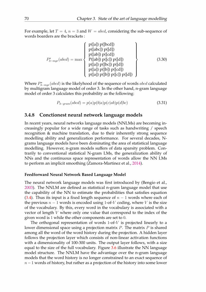
70 Chapter 3. State of the art of language modelling
For example, let T = 4, n = 3 and W = abcd, considering the sub-sequence ofwords boarders are the brackets :
P ?3−mgr(abcd) = max
p([a]) p([bcd])p([abc]) p([d])p([ab]) p([cd])P([ab]) p([c]) p([d])p([a]) p([bc]) p([d])p([a]) p([b]) p([cd])p([a]) p([b]) p([c]) p([d])
(3.30)
Where P ?3−mgr(abcd) is the likelyhood of the sequence of words abcd calculated
by multigram language model of order 3. In the other hand, n-gram languagemodel of order 3 calculates this probability as the following:
P3−gram(abcd) = p(a)p(b|a)p(c|ab)p(d|bc) (3.31)
3.4.8 Conctionest neural network language models
In recent years, neural networks language models (NNLMs) are becoming in-creasingly popular for a wide range of tasks such as handwriting / speechrecognition & machine translation, due to their inherently strong sequencemodelling ability and generalization performance. For several decades, N-grams language models have been dominating the area of statistical languagemodelling. However, n-gram models suffers of data sparsity problem. Con-trarily to conventional statistical N-gram LMs, the generalization ability ofNNs and the continuous space representation of words allow the NN LMsto perform an implicit smoothing (Zamora-Martinez et al., 2014).
Feedforward Neural Network Based Language Model
The neural network language models was first introduced by (Bengio et al.,2003). The NNLM are defined as statistical n-gram language model that usethe capability of the NN to estimate the probabilities that satisfies equation(3.4). Thus its input is a fixed length sequence of n − 1 words where each ofthe previous n − 1 words is encoded using 1-of-V coding, where V is the sizeof the vocabulary. By this, every word in the vocabulary is associated with avector of length V where only one value that correspond to the index of thegiven word is 1 while the other components are set to 0.
The orthogonal representation of words 1-of-V is projected linearly to alower dimensional space using a projection matrix P . The matrix P is sharedamong all the word of the word history during the projection. A hidden layerfollows the projection layer which consists of non-linear activation functionswith a dimensionality of 100-300 units. The output layer follows, with a sizeequal to the size of the full vocabulary. Figure 3.6 illustrate the NN languagemodel structure. The NNLM have the advantage over the n-gram languagemodels that the word history is no longer constrained to an exact sequence ofn− 1 words of history, but rather as a projection of the history into some lower

3.4. Statistical language modelling 71
FIGURE 3.6: The architecture of a NN LM after training, wherethe first layer is substituted by a look-up table with the dis-tributed encoding for each word ω ∈ Ω(Zamora-Martinez et al.,
2014)
dimensional space. As a result, the automatic clustering of the similar wordhistories, reduces the number of parameters. The weak point of these modelsis their very large computational complexity during training, which usuallyprohibits to train these models on full training set using the full vocabulary(Mikolov, 2012).
The applicability of neural network language models in unconstrained off-line handwriting recognition has been studied by (Zamora-Martinez et al.,2014). They also compared the performance of conventional n-gram languagemodels across of NNLMs on IAM handwriting database using two differentrecognition engines under different vocabulary sizes.
Recurrent Neural Network Based Language Model
The difference between the feed forward neural network language model NNLMand the recurrent neural network language model (RNNLM) architecture is inthe representation of the word history, in feed forward NNLM the word his-tory is still limited to the several previous words, meanwhile in RNNLM aneffective representation of word history is learned from the data during train-ing. The hidden layer of RNN represents all previous history and not just then − 1 previous words, thus the model can theoretically represent long contextpatterns (Mikolov, 2012). In addition, RNNLM have the advantage over feed-forward one of representing more advanced patterns in the sequential datasuch as the patterns that rely on words that could have occurred at variableposition in the history, the recurrent model can remember some specific wordsin the state of the hidden layer, while the feed-forward model would need
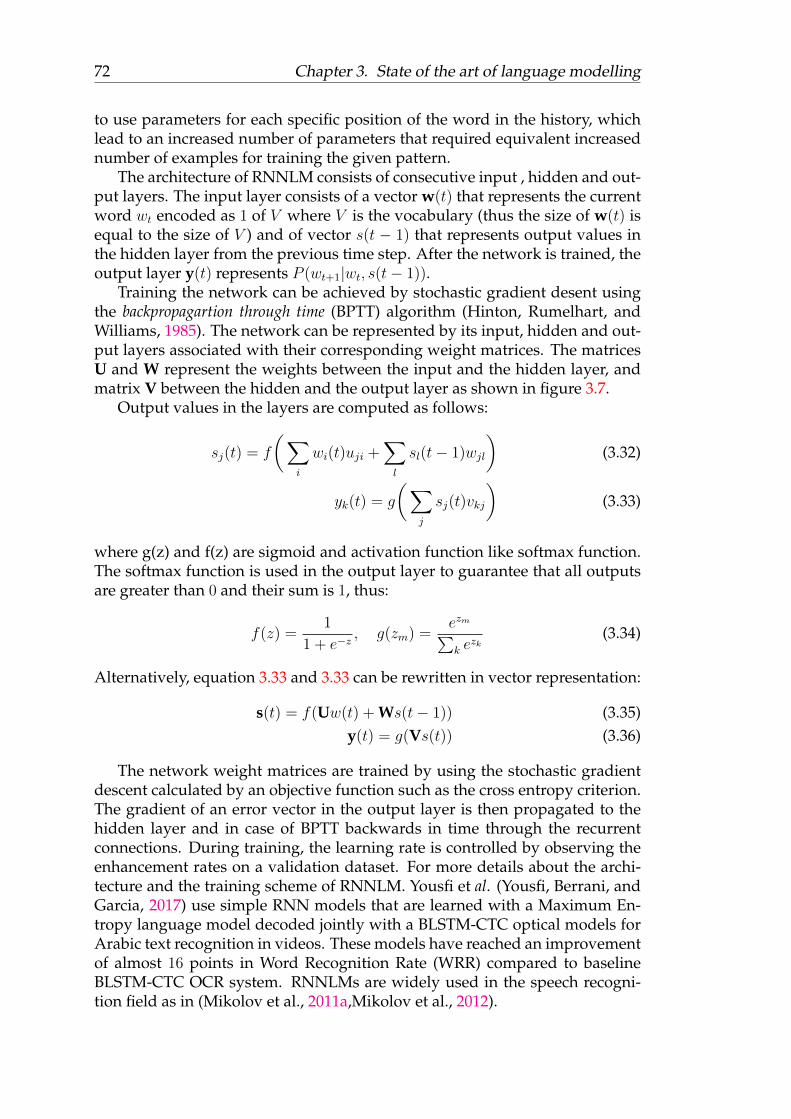
72 Chapter 3. State of the art of language modelling
to use parameters for each specific position of the word in the history, whichlead to an increased number of parameters that required equivalent increasednumber of examples for training the given pattern.
The architecture of RNNLM consists of consecutive input , hidden and out-put layers. The input layer consists of a vector w(t) that represents the currentword wt encoded as 1 of V where V is the vocabulary (thus the size of w(t) isequal to the size of V ) and of vector s(t − 1) that represents output values inthe hidden layer from the previous time step. After the network is trained, theoutput layer y(t) represents P (wt+1|wt, s(t− 1)).
Training the network can be achieved by stochastic gradient desent usingthe backpropagartion through time (BPTT) algorithm (Hinton, Rumelhart, andWilliams, 1985). The network can be represented by its input, hidden and out-put layers associated with their corresponding weight matrices. The matricesU and W represent the weights between the input and the hidden layer, andmatrix V between the hidden and the output layer as shown in figure 3.7.
Output values in the layers are computed as follows:
sj(t) = f
(∑i
wi(t)uji +∑l
sl(t− 1)wjl
)(3.32)
yk(t) = g
(∑j
sj(t)vkj
)(3.33)
where g(z) and f(z) are sigmoid and activation function like softmax function.The softmax function is used in the output layer to guarantee that all outputsare greater than 0 and their sum is 1, thus:
f(z) =1
1 + e−z, g(zm) =
ezm∑k e
zk(3.34)
Alternatively, equation 3.33 and 3.33 can be rewritten in vector representation:
s(t) = f(Uw(t) + Ws(t− 1)) (3.35)y(t) = g(Vs(t)) (3.36)
The network weight matrices are trained by using the stochastic gradientdescent calculated by an objective function such as the cross entropy criterion.The gradient of an error vector in the output layer is then propagated to thehidden layer and in case of BPTT backwards in time through the recurrentconnections. During training, the learning rate is controlled by observing theenhancement rates on a validation dataset. For more details about the archi-tecture and the training scheme of RNNLM. Yousfi et al. (Yousfi, Berrani, andGarcia, 2017) use simple RNN models that are learned with a Maximum En-tropy language model decoded jointly with a BLSTM-CTC optical models forArabic text recognition in videos. These models have reached an improvementof almost 16 points in Word Recognition Rate (WRR) compared to baselineBLSTM-CTC OCR system. RNNLMs are widely used in the speech recogni-tion field as in (Mikolov et al., 2011a,Mikolov et al., 2012).

3.4. Statistical language modelling 73
FIGURE 3.7: Recurrent neural network unfolded as a deep feed-forward network, here for 3 time steps back in time(Mikolov,
2012)
3.4.9 caching language models
One of the obvious disadvantage of n-gram language models is their limitedcapacity to represent long term patterns. It has been empirically observed thatmany words, especially the rare ones, have significantly higher chance of oc-curring again if they did occur in the recent history (Mikolov, 2012). Cashinglanguage model (Jelinek et al., 1991) consider a cash component for the wordoccurrences beside the training corpus for calculating its probabilities whichare estimated dynamically from the recent history (it usually represents fewhundreds of words) and interpolated with the main (static) n-gram model.
The advantage of the cache model is its highly reduced perplexity com-pared to the conventional n-gram models, that’s why this modelling approachis very popular in the language modelling related papers (Mikolov, 2012). Themain drawback of such model is in the correlation between the perplexity im-provements and word error rate reductions. Advanced versions of caching

74 Chapter 3. State of the art of language modelling
models like trigger models or LSA models have reported interesting WER re-duction. Recently, these models are not widely in practice (Mikolov, 2012).
3.4.10 Maximum entropy language models
The maximum entropy language models ME (Berger, Pietra, and Pietra, 1996)allow to incorporate many feature functions (for example, n-gram, n-class andskip-gram) using triggers and word features to obtain highly improved per-plexity, as well as significant word error rate reduction. The ME model is ex-pressed as an exponential model with a form
P (w|h) =e
(∑i λifi(w,h)
)Z(h)
(3.37)
wherew is a word in context h and Z(h) is used for normalizing the probabilitydistribution:
Z(h) =∑wi∈V
e
(∑j λjfi(wi,h)
)(3.38)
This model is reported to have a state-of-the-art performance on a broadcastnews speech recognition task, when applied to a very well tuned system thatis trained on large amounts of data and uses state of the art discriminativelytrained acoustic models. An alternative name of maximum entropy modelsused by the machine learning community is logistic regression (Mikolov, 2012)and Conditional Random Field (Sutton and McCallum, 2006).
3.4.11 Probabilistic Context free Grammar
A Probabilistic Context-Free Grammar (PCFG, Manning and Schütze, 1999) issimply a Context-Free Grammar with probabilities assigned to the rules suchthat the sum of all probabilities for all rules expanding the same non-terminalis equal to one. Context-free grammar (CFG) is a certain type of formal gram-mar: a set of production rules that describe all possible strings in a given for-mal language. Production rules are simple replacements just like replacing Aby α or β. In context-free grammars, all rules are one-to-one, one-to-many, orone-to-none. Rules can also be applied in reverse to check if a string is gram-matically correct according to the grammar. The PCFG grammar is definedby
• A set of terminals, related to the language words: wk where wk ∈ Vand V the language vocabulary.
• A set of non-terminals, related to grammatical objects: Ni.
• A starting symbol: N1.
• A set of derivation rules: Ni → ζj where ζj is a sequence of terminalsand non-terminals.

3.5. Language models application domains 75
• A set of probabilities evaluated automatically from a labelled corpus gov-erned by rules such as
∀i,∑j
P (Ni → ζj) = 1 (3.39)
Every derivation of a phrase is associated with a probabilistic score that repre-sents the product of the rules probability related to that derivation (phrase).
3.5 Language models application domains
Statistical Language Models estimate the distribution of various natural lan-guage phenomena for the purpose of speech and handwriting recognition andother language technologies. A First practical model was proposed in 1980(Della Pietra et al., 1992), since then many attempts have been made to im-prove the state of arts. Language models are commonly used in several do-mains beside speech and handwriting recognition such as:
1. Spelling correction: In the field of text processing application languagemodels are used to correct spellings (Kukich, 1992). Two types of errorscan be distinguished, the first is the non lexical word, where the error inwriting a word that does not belong to the language words (for examplethe word "bi y" in place of "bye"). These errors can be corrected by usinga lexicon and computing edit distance that can find the nearest word inthe lexicon. The second type of errors represents the miss-placed wordswhich are valid words but not coherent with the phrase structure (forexample, the French word "lange" in place of "langue". A language modelcan correct such type of errors by detecting the incorrect word in thesentence and correct it.
2. Language translation: The automatic translation of a sentence from asource language to a target language corresponds to interfering two typesof models (Brown et al., 1990). One model expresses the source languagesentence ideas using the words of the destination language, the secondmodel regulate the output of the first model to be structured correctlyfrom the grammar point of view of the destination language.
3. Corpora labelling: One of the most recent tasks is the corpora labellingtask which consists of labelling each corpus word with its grammaticalclass (Manning and Schütze, 1999). Almost, any word may belong tomultiple classes (for example the French word "souris" may be a nounand verb), so a language model is necessary to reduce the ambiguity inlabelling words by taking into account their context.
4. Information searching: With the growing mass of information in the in-ternet, searching of an information becomes an important field. In orderto respond effectively to the user query, the language model can be usedto incorporate the linguistic knowledge to the searching motors by usingsome sort of interpretations of the user natural lingual structured query.
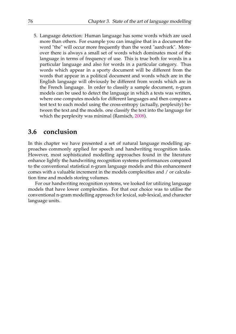
76 Chapter 3. State of the art of language modelling
5. Language detection: Human language has some words which are usedmore than others. For example you can imagine that in a document theword "the" will occur more frequently than the word "aardvark". More-over there is always a small set of words which dominates most of thelanguage in terms of frequency of use. This is true both for words in aparticular language and also for words in a particular category. Thuswords which appear in a sporty document will be different from thewords that appear in a political document and words which are in theEnglish language will obviously be different from words which are inthe French language. In order to classify a sample document, n-grammodels can be used to detect the language in which a texts was written,where one computes models for different languages and then compare atest text to each model using the cross-entropy (actually, perplexity) be-tween the text and the models. one classify the text into the language forwhich the perplexity was minimal (Ramisch, 2008).
3.6 conclusion
In this chapter we have presented a set of natural language modelling ap-proaches commonly applied for speech and handwriting recognition tasks.However, most sophisticated modelling approaches found in the literatureenhance lightly the handwriting recognition systems performances comparedto the conventional statistical n-gram language models and this enhancementcomes with a valuable increment in the models complexities and / or calcula-tion time and models storing volumes.
For our handwriting recognition systems, we looked for utilizing languagemodels that have lower complexities. For that our choice was to utilise theconventional n-gram modelling approach for lexical, sub-lexical, and characterlanguage units.

77
Chapter 4
Design and evaluation of aHandwritting recognition system
4.1 Introduction
In this chapter, we present the design of the different handwriting recognitionsystems that have been tested all along this thesis. The first experimentationshave been carried out using the standard HMM optical models. Of course thiswas a limitation regarding the state of the art performance obtained on the ref-erence datasets, even if our primary objective was to study the contribution oflanguage models to the performance of the whole system. This is the reasonwhy we decided to introduce LSTM Neural Networks in the system in place ofthe HMM stage. This chapter is intended to give a comprehensive, althoughlight, description of every stages required in the design of handwritten textrecognition systems. While chapter 2 and chapter 3 have been dedicated tothe fundamental aspects of optical and language models, here we concentrateon describing how to integrate these models together, in order to build an op-erational reading system that can take a full handwritten text image as inputand produce its transcription in electronic format at the output. Performanceevaluation as well as training of the various systems implemented have beencarried out using two popular datasets : the French RIMES dataset and theEnglish IAM dataset. They are described briefly in section 4.2 regarding theiroptical as well as linguistic content in terms of number of writers, lexicon sizeand coverage. The main components of a reading system are shown on figure4.1.
One of the primary components of the system is the preprocessing stagethat is design to determine the target text line images locations in the doc-ument image using some image processing or machine learning techniques.Once the text line images have been extracted, some image correction such asskew and slant correction algorithms can be applied for reducing the variabil-ity in the data and possibly enhance the recognition performance. Section 4.3is intended to describe this very important component of our whole readingsystem. The second important component of a text recognizer is the opticalmodel of characters. In section 4.4 we will describe our implementations andtraining of the two statistical optical models that have been tested during thisthesis: HMM and BLSTM-RNN optical models. Optical models provide like-lihood scores denoted P (S|W ) of observing the image, or a representation ofthe image denoted S, assuming a certain text transcription W . This section

78 Chapter 4. Design and evaluation of a Handwritting recognition system
FIGURE 4.1: General architecture of the reading systems studied
also includes a brief description of the features used as input of the opticalmodels. Section 4.5 is dedicated to the linguistic component of the system :the language model, that is design to estimate the probability of a certain tran-scription W , denoted by P (W ). All along this thesis we have studied the con-tribution of this component and we will briefly present the practical aspectsand problems related to combining lexicons and language models and havethem optimized on the appropriate training datasets. Most of the discussionwill rely on the linguistic properties of the two datasets used for the evaluation(RIMES and IMA datasets). Last but not least is the decoding component of the

4.2. Datasets and experimental protocols 79
recognition system. During recognition, the two system components (opticalmodel and language model) are combined together to build a hypotheses lat-tice called search space. The contribution of each model to the final recognitionresult is governed by equation 4.1. The two essential coupling parameters arethe language model scale parameter γ and word insertion penalty β. Thesetwo coupling parameters require careful optimization in order to obtain opti-mal recognition performance. We will discuss these questions in section 4.6.By the end of this presentation of each system component, we will give someprimary recognition results in section 4.7 and draw the main guidelines for ourcontributions in the next chapter (Chapter 5).
W = argmaxw
P (S|W )P (W )γβLength(W ) (4.1)
4.2 Datasets and experimental protocols
The experiments have been carried out on publicly available databases, in or-der to compare our work to other approaches and research groups (see Chap-ter 5). The scope of the experiments is limited to the French RIMES and theEnglish IAM databases. In addition, we make use of some large and diverscorpora for training the language models in same cases. In the next section,we describe the used datasets for training and evaluating the systems perfor-mances.
4.2.1 Training and evaluation databases
A conventional practice in handwriting recognition is to divide the databasesinto three different sets. The evaluation set (or test set) contains images neverseen during training, with which we evaluate our systems performances. Train-ing algorithms have some parameters themselves (the hyper-parameters), thatshould be set to train the systems. The development (or validation) set is an-other test set, on which we can check the best choice of values for these hyper-parameters.
RIMES dataset
The Rimes dataset (Grosicki and El-Abed, 2011) consists of images of hand-written letters from simulated French mail. We followed the setup of the IC-DAR 2011 competition. The available data are a training set of 1,500 para-graphs (11333 text lines), manually extracted from the images, and an eval-uation set of 100 paragraphs (748 text lines). We selected randomly 1333 ofthe training set text lines as a validation set, and trained the systems on theremaining 10000 text lines as illustrated in table 4.2.
IAM dataset
The IAM database (Marti and Bunke, 2002) consists of images of handwrit-ten pages. They correspond to English texts extracted from the LOB corpus
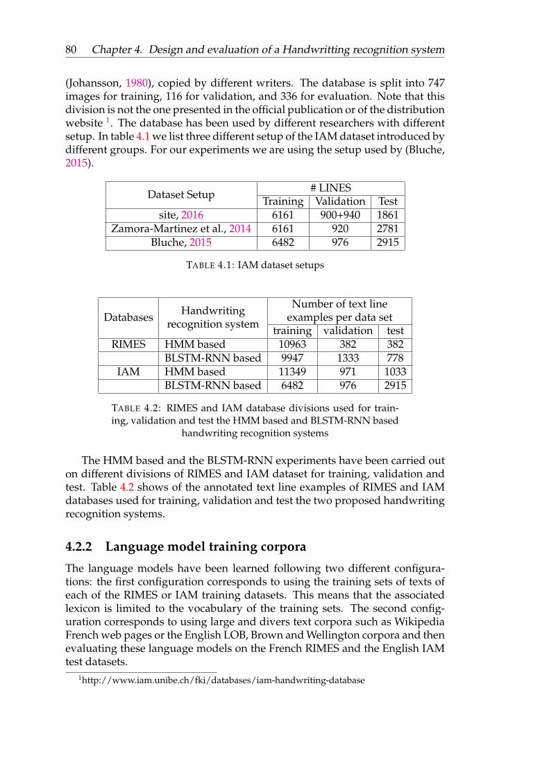
80 Chapter 4. Design and evaluation of a Handwritting recognition system
(Johansson, 1980), copied by different writers. The database is split into 747images for training, 116 for validation, and 336 for evaluation. Note that thisdivision is not the one presented in the official publication or of the distributionwebsite 1. The database has been used by different researchers with differentsetup. In table 4.1 we list three different setup of the IAM dataset introduced bydifferent groups. For our experiments we are using the setup used by (Bluche,2015).
Dataset Setup # LINESTraining Validation Test
site, 2016 6161 900+940 1861Zamora-Martinez et al., 2014 6161 920 2781
Bluche, 2015 6482 976 2915
TABLE 4.1: IAM dataset setups
Databases Handwritingrecognition system
Number of text lineexamples per data set
training validation testRIMES HMM based 10963 382 382
BLSTM-RNN based 9947 1333 778IAM HMM based 11349 971 1033
BLSTM-RNN based 6482 976 2915
TABLE 4.2: RIMES and IAM database divisions used for train-ing, validation and test the HMM based and BLSTM-RNN based
handwriting recognition systems
The HMM based and the BLSTM-RNN experiments have been carried outon different divisions of RIMES and IAM dataset for training, validation andtest. Table 4.2 shows of the annotated text line examples of RIMES and IAMdatabases used for training, validation and test the two proposed handwritingrecognition systems.
4.2.2 Language model training corpora
The language models have been learned following two different configura-tions: the first configuration corresponds to using the training sets of texts ofeach of the RIMES or IAM training datasets. This means that the associatedlexicon is limited to the vocabulary of the training sets. The second config-uration corresponds to using large and divers text corpora such as WikipediaFrench web pages or the English LOB, Brown and Wellington corpora and thenevaluating these language models on the French RIMES and the English IAMtest datasets.
1http://www.iam.unibe.ch/fki/databases/iam-handwriting-database

4.2. Datasets and experimental protocols 81
French extended Wikipedia corpus
This corpus was collected from the Wikipedia French version pages 2 that in-cludes diverse subjects. This corpus includes all the collected text data whichconsists of 529, 299 passage of text, 702, 097 word and 84, 236, 612 character,considering that a word is defined by a sequence of characters sided by twowhite spaces characters.
French Wikipedia corpus
The corpora represents a portion (10%) of the French extended Wikipedia pages,it consists of 52, 930 passage of text, 182, 735 words and 12, 921, 198 character.By analysing the effective coverage of the whole and partial Wikipedia cor-puses on the RIMES test dataset, we noticed that the difference in the effectivecoverage rate reported for the 50, 000 most frequent words of the extendedWikipedia corpus (83.28%) and for the 50, 000 most frequent words of the (par-tial) Wikipedia corpus (82.71%) on the RIMES test data set is around 0.57%which is not significant compared to the size of corpus lexicon size which in-creases from 182, 735 word to 702, 097 word for the partial and the whole cor-puses respectively. Therefore, we decided to carry out all our experiments withthis reduced size corpus.
English LOB corpora
The Lancaster-Oslo/Bergen Corpus (LOB Johansson, 1980) was compiled byresearchers at Lancaster, Oslo and Bergen universities. It consists of one mil-lion words of British English texts from 1961. The texts for the corpus weresampled from 15 different text categories. Each text is just over 2,000 wordslong (longer texts have been cut at the first sentence boundary after 2,000words) and the number of texts in each category varies.
English Brown corpus
The Brown Corpus (Francis and Kucera, 1979) was the first computer-readablegeneral corpus of texts prepared for linguistic research on modern English. Itwas compiled by W. Nelson Francis and Henry Kucera at Brown University inthe 1960s and contains over 1 million words (500 samples of 2000+ words each)of running text of edited English prose printed in the United States during thecalendar year 1961. There are six versions of the corpus available: the originalForm A, Form B from which punctuation codes have been omitted, the taggedForm C, Bergen Forms I & II and the Brown MARC Form.
English Wellington corpus
The Wellington Corpus (Bauer, 1993) of Written New Zealand English (WWC)consists of one million words of written New Zealand English collected from
2https://dumps.wikimedia.org

82 Chapter 4. Design and evaluation of a Handwritting recognition system
writings published in the years 1986 to 1990. The WWC has the same ba-sic categories as the Brown Corpus of written American English (1961) andthe Lancaster-Oslo-Bergen corpus (LOB) of written British English (1961). TheWWC consists of 2,000 word of different topics. Text categories include pressmaterial, religious texts, skills, trades and hobbies, popular lore, biography,scholarly writing and fiction.
English extended Wikipedia corpus
The Wikipedia English version pages was collected from the same source ofthe French one in order to build the English extended Wikipedia corpus. Thecorpus consists of 540, 385 passage of text, 994, 545 word and 128, 558, 999 char-acter.
English Wikipedia corpus
The corpora represents a portion (10%) of the English extended Wikipediapages, it consists of 53, 999 passage of text, 240, 659 words and 18, 193, 128character. Again, the difference in the effective coverage rate reported for the50, 000 most frequent words of the extended Wikipedia corpus (87.75%) and forthe 50, 000 most frequent words of the (partial) Wikipedia corpus (87.12%) onthe RIMES test data set is around 0.63% which is not significant compared tothe size of corpus lexicons size which increases from 240, 659 word to 994, 545word.
Softwares and tools
The introduced handwriting recognition systems in this theses are implementedand evaluated by using open source and free of charge toolkits so they are easyto be replicated with no cost. We can categories the utilized softwares and toolsaccording to the systems tasks into four main categories: Optical model train-ing toolkits, language model training toolkits, decoding tools and evaluationtools. Table 4.3 illustrates each toolkits used jointly with the system task thatrequired it for the two systems considered:
Tasks/toolkits
optical modeltraining tools
language modeltraining tools
decodingtools
evaluationtool
EESEN BLSTM-RNNHTK HMM HMM
MITLM BLSTM-RNNSRILM HMM & BLSTM-RNNKaldi
(open FST) BLSTM-RNN BLSTM-RNN
Sclite (NIST) HMM
TABLE 4.3: Resume of the toolkits used for each systems realiza-tion task
One can refer to (Miao, Gowayyed, and Metze, 2015) for more details aboutEESEN toolkit, (Young and Young, 1993) for HTK toolkit, (Povey et al., 2011)

4.3. Pre-processing 83
for Kaldi toolkit, (Stolcke, 2002) for SRILM toolkit and (Fiscus, 2015) for Sclitescoring toolkit from National Institute of Standards and Technology (NIST).
4.3 Pre-processing
In their full denomination, pre-processing includes image enhancement priorto image segmentation to get the image components localized, and allowingeach component to be passed to the recognition stage. During this thesis ourcontribution has been focused on the detection of text lines in images of textsblocks solely.
4.3.1 Related works
The difficulty of the line extraction task depends on the regularity of the hand-writing: length and height of text lines, straightness of baselines... The linesin handwritten documents are often irregular and have many defects whichmakes the detection of text lines delimiters difficult. The most problematicdefects being the overlapping lines (mainly due to the occurrence of the as-cenders and descenders), the touching characters across two consecutive lineswhich require special treatment (proper cutouts and assignment to the properline) and the skew variability between lines and within the same line. There-fore, line segmentation in unconstrained handwritten documents is a verychallenging task and is still an open research area. This is why, in the re-cent years, many papers have been published, and several contests have beenorganized during ICDAR2009 (Gatos, Stamatopoulos, and Louloudis, 2011),ICDAR2013 (Stamatopoulos et al., 2013), ICFHR 2010 (Gatos, Stamatopoulos,and Louloudis, 2010).
Three distinct approaches for line segmentation exist in the literature (Kat-souros and Papavassiliou, 2011): - bottom-up approaches try to merge the baseunits (mostly connected components) according to their spatial proximity toform horizontal lines - top-down approaches first locate the limits of the dif-ferent lines before assigning the base units to their respective lines – smearingmethods apply a blurring filter to the document image in order to reveal thestructure of the underlying lines through a "smearing" of the horizontal align-ments of black pixels. Proposed filters are either anisotropic Gaussian filters(Li et al., 2008; Bukhari, Shafait, and Breuel, 2009; Bukhari, Shafait, and Breuel,2009) or ellipsoid filters (Shi, Setlur, and Govindaraju, 2009). To be effective,the filters must be more elongated along the horizontal axis otherwise the blur-ring may merge close lines.
4.3.2 Proposed method
Because of the great variability between writer’s styles and the different scripts(latin, arabic, chinese, hindi...), existing methods do not generalize well to anytypes of documents (Katsouros and Papavassiliou, 2011). Therefore, it seemsthat the most robust methods will be those that do not use any a priori and

84 Chapter 4. Design and evaluation of a Handwritting recognition system
are able to adapt to the characteristics of each document (Papavassiliou et al.,2010). From the analysis of the results of international contests that have beenorganized few years ago, we came to the conclusion that smearing methodsmay have a great potential to generalize well to different scripts. Inspiredby (Shi, Setlur, and Govindaraju, 2009), we designed a generalized smearingmethod that does not require any prior setting. An iterative approach is usedas depicted on figure 4.2 below, in which the algorithm parameters (filter size)are adjusted at each iteration to detect new lines, with different size. Lines de-tected at each iteration are added to the final line detection result. As a mainadvantage, the method explores a wide range of potential line sizes and inte-grates a detection criterion allowing to validate or reject the line hypothesis,thus being robust with respect to the variability in size of the lines.
Input: text block image
Text lines masksgeneration
Text lines masksvalidation
update filtersheight value
iterationcondi-tion?
Text line localization
Assignement ofCCs to text lines
output: Textlines images
yes
no
FIGURE 4.2: The proposed generalized smearing approach forline detection.
The method is based on a generalized adaptive local connectivity map(ALCM) generated by a set of steerable filters (Shi, Setlur, and Govindaraju,2009) that process the image in different orientations. First the method locatesthe text lines through their masks that are the result of the ALCM. The adap-tive local connectivity map is defined as the result of the following filtering :
A(x, y) =
∫R2
f(x, y)GθoFH,FW (x− t, y − s)dtds (4.2)
where
Gθ0FH,FW (x, y) =
1 if(x, y) ∈ Eθo
FH,FW
0 otherwise(4.3)

4.3. Pre-processing 85
and
EθoFH,FW =
(x, y)|
x < FH cos(θ − θo)y < FW cos(θ − θo)
and 0 ≤ θ < 2π
(4.4)
Eθo is an ellipse with semi-minor axis FH,FW and rotated by the angle θo.For effective performance, 11 filters with different directions are used in therange [−20, 20] degrees, for each filter size. Filters elongation has been set toa constant ratio of 5 with the following equation : FW = 5FH . The iterativeprocess starts with a large filter height parameter (FH) set to a fraction of theestimated line height (ELH). At each iteration the filter height is decreased by15%. The iteration process stops once the current (FH) is lower than a fractionof ELH . Because the filtering process has no blurring significant effect on theimage below this value. On Figure 4.3 we can see the cumulated output ofthe steerable filters obtained for different filter sizes (from left to right). Thepotential line masks are obtained by binarizing these images as depicted infigure 4.4. This result highlight the capacity of the method to detect thin aswell as thick lines where necessary in the image.
FIGURE 4.3: Steerable filters output for different values of thefilter height (large, medium, low) from left to right.
At this stage, a text line mask may represent a group of lines, a part of aline or a single complete text line. Thus we need to check if the generatedmasks are valid before adding them to the validated text line masks image.Each connected component of the potential text line mask image is considereda valid line mask if its maximum vertical thickness is lower than twice its mostfrequent vertical thickness and lower than twice its average thickness. Theunderlying idea is that a line mask has almost a constant height so that itsmaximum, average and more frequent vertical thickness are relatively closeto each other. Once a CC is validated as a text line mask, we add it to thefinal validated text lines masks image. The result of the validation process isillustrated in Figure 4.5 below.
The validated text line masks image obtained should ideally content eachline of the document image by a single mask. However, when a text line of adocument image overlaps other text lines or has a sharp skew variation or avery wide inter-word spaces, it may be decomposed into several masks, eachcovering a portion of that text line. To improve the final masks image, we a

86 Chapter 4. Design and evaluation of a Handwritting recognition system
FIGURE 4.4: Potential line masks obtained for the correspondingsteerable filters of figure 4.3 above
FIGURE 4.5: Results of the validation process of text line masksof figure 4.4 above
post-processing stage is applied which merges masks that appear to be hori-zontally overlapping. Then, text lines boundaries are determined using linemasks positions. Finally the connected components are assigned to their re-spective lines. The text line masks obtained by this process are used to deter-mine the boundaries between the text lines of the document. For this purpose,we compute an anisotropic distance transform (the distance along the hori-zontal axis has half the weight of that of the vertical axis) of the mask image.The resulting distance map allows to assign each pixel to its nearest mask andto obtain the line delimiters and then the desired line images as depicted onfigure 4.6.
The line delimiters obtained are the default separators between lines of textbut there are some overlapping situations where a stroke may extend belowor above the delimiter, and we wish to affect the whole stroke to its properline rather than cutting the stroke in two parts and affect each part to twodifferent lines. Each connected component (CC) of the document image isassign to its proper text line using the following assignment rule. There aretwo possible situations: either a CC is totally included inside a line containeror it is localized in between two lines. In this later case, we have to determinewhether to assign CC to a single line or if CC must be splited. Let Hi be thepercentage of the height of CC that is included inside a line container Li. If Hi
is greater than a given threshold (which we empirically fix to 66%), then CCis affected to Li. Otherwise, we split CC at the Line delimiter and assign each
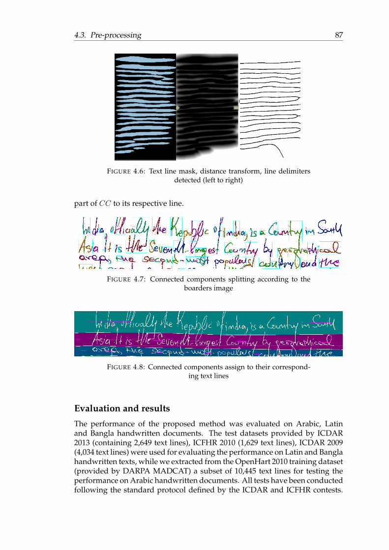
4.3. Pre-processing 87
FIGURE 4.6: Text line mask, distance transform, line delimitersdetected (left to right)
part of CC to its respective line.
FIGURE 4.7: Connected components splitting according to theboarders image
FIGURE 4.8: Connected components assign to their correspond-ing text lines
Evaluation and results
The performance of the proposed method was evaluated on Arabic, Latinand Bangla handwritten documents. The test datasets provided by ICDAR2013 (containing 2,649 text lines), ICFHR 2010 (1,629 text lines), ICDAR 2009(4,034 text lines) were used for evaluating the performance on Latin and Banglahandwritten texts, while we extracted from the OpenHart 2010 training dataset(provided by DARPA MADCAT) a subset of 10,445 text lines for testing theperformance on Arabic handwritten documents. All tests have been conductedfollowing the standard protocol defined by the ICDAR and ICFHR contests.

88 Chapter 4. Design and evaluation of a Handwritting recognition system
ICDAR and ICFHR data sets are originally oriented towards text line segmen-tation competitions, their documents do not include any non-text elementssuch as scratches, vertical/horizontal lines and random noise. In addition, theprovided pixel-wise ground truth represents exactly the text lines delimiterseven in the case of overlapping lines.
In contrast, the DARPA MADCAT training dataset was originally designfor handwriting text recognition competition. Therefore, it includes manykinds of non-text elements such as custom lines background, scratches, etc...For the tests we selected the document images that do not contain custom lines(such information is provided with the MADCAT dataset). However, the pro-vided ground truth gives only the bounding box position of words and textlines. This is insufficient for a precise segmentation of overlapping text lines.In order to get more precise line delimiters, we have used the word bound-ing boxes provided in the ground truth data so as to build a more precise linelocalization ground truth. Combining the word bounding boxes with the inter-words white spaces between bounding boxes allows to extract a more preciseline image, as depicted in figure 4.9 below.
FIGURE 4.9: MADDCAT line delimiter ground truth e) derivedfrom word delimiters ground truth b) c)
We can see that a small lower part of the line is still missing because it is notincluded in the bounding box of the text line. Following the ICDAR evaluationprotocol, this could cause the rejection of a correctly detected text lines. Theobtained ground truth is still too imprecise for an exact evaluation of text linesegmentation. We should remember this limitation when comparing the linesegmentation performance of the method on several datasets.
Test and validation protocols
We developed the test application as described in (Stamatopoulos et al., 2013,Gatos,Stamatopoulos, and Louloudis, 2010,Gatos, Stamatopoulos, and Louloudis,2011). AMatchRate(i, j) table is used to store the intersection values of the ONpixel sets of the result and the ground truth images. Let I denotes the set of allimage pixels, Gj denotes the set of all pixels inside the ground truth image,Ri
denotes the set of all pixels inside the result image and T (s) is a counting func-tion for the elements of the set s. The matching results between the jth ground

4.3. Pre-processing 89
truth image and the ith result image is represented by theMatchRate(i, j) tableas shown from equation 4.5.
MatchRate(i, j) =T (Gj ∩Ri ∩ I)
T ((Gj ∪Ri) ∩ I)(4.5)
We validate a one-to-one match between images j and i only if the matchingscore is equal to or above 95%.
The global performance of the method FM is evaluated as shown in equa-tion 4.7, by computing the detection rate DR that reflects the ability of themethod to detect the text lines and the detection accuracy rate RA that reflectsthe method detection accuracy. If N is the number of the ground truth ele-ments and M is the number of elements in the result, and O2O is the numberof validated one-to-one matches, then we calculateDR andRA using equation4.6.
DR =O2O
N, RA =
O2O
M(4.6)
FM =2 DR RA
DR +RA(4.7)
Results
The test results of our method (that we called "LITIS") are shown in table 4.4.Compared to methods that have the best performance on each contest data set,our method has similar but slightly lower performance. We noticed that veryfew errors are due to a bad detection of line borders. The majority of invalidlines are due to a wrong CC split. There are two cases of wrong splits: ei-ther the ascender or descender of a character across two overlapping text lineswas cut, or touching characters were segmented at the wrong position (Figure4.10). Therefore, the weak point that affects the performance of our methodlies precisely in the assignment of the connected component when they belongto more than one text line. As an advantage, the CUBS method is able to splitthe touching characters by using a specific algorithm that decides for the bestcutting position (Shi, Setlur, and Govindaraju, 2009). The results obtained onthe Arabic MADCAT dataset show a significant difference in the segmentationperformance compared with the Latin script. Most of this difference comesfrom the low quality ground truth, as discussed above. One can reasonablysuppose that the score obtained by our method on the MADCAT dataset is ac-tually much closer to the scores obtained on other datasets. Nevertheless, tothe best of our knowledge, these results are the first attempt to evaluate Arabictext line segmentation using the ICDAR competition protocol.
We searched for the optimal initial value of the filter’s height parameter foreach dataset by testing the various performance of the system for each value ofthe filter’s height ranging between 0.5×MDH up to 1.5×MDH as reported intable 4.4. Figure 4.11 shows two examples of the text line segmentation results(different colour for each localised text line) applied on document images takenfrom the READ handwriting recognition competition 2017.

90 Chapter 4. Design and evaluation of a Handwritting recognition system
a. b. c.
FIGURE 4.10: Illustration of a touching characters split error. (a)Two touching characters shown in green colour. (b) LITIS split-ting decision level according to the lines delimiter found by themethod. (c) Red dotted line represents the correct splitting posi-
tion.
ICDAR2013
ICFHR2010
ICDAR2009
MADCAT2010
Optimal filter’s Height 0.8×MDH MDH MDH 1.5×MDH
LITIS 97.18 % 96.75 % 98.86 % 92.21 %
CUBS 97.45 % 97.63 % 99.53 % ——
Best ONE INMC98.66% CUBS CUBS ——
TABLE 4.4: Method evaluation results
4.4 Optical models implementations
During this thesis we have implemented various configurations of characteroptical models that have been combined with various language models. Asdepicted in figure 4.12 two types of models have been developed. We startedour primary experiments with using the standard and popular generative Hid-den Markov Models. But the current state of the art has led us to introduceLSTM-RNN optical models. Both models take as input some predefine fea-tures that describe 1 dimensional (1D) streams of real valued feature vectors.The strength of recurrent neural networks lies in their capacity to learn theirown internal feature representation of the input data by the introduction ofhidden layers. As a consequence it is possible to introduce simple featuressuch as pixels values at the input of recurrent neural networks whereas hid-den Markov Models will benefit of having some more elaborated features tomodel the character classes. In the following subsections we first give a briefoverview of the used features descriptors, before giving some insights of thedesign and optimization (training) of the optical models.
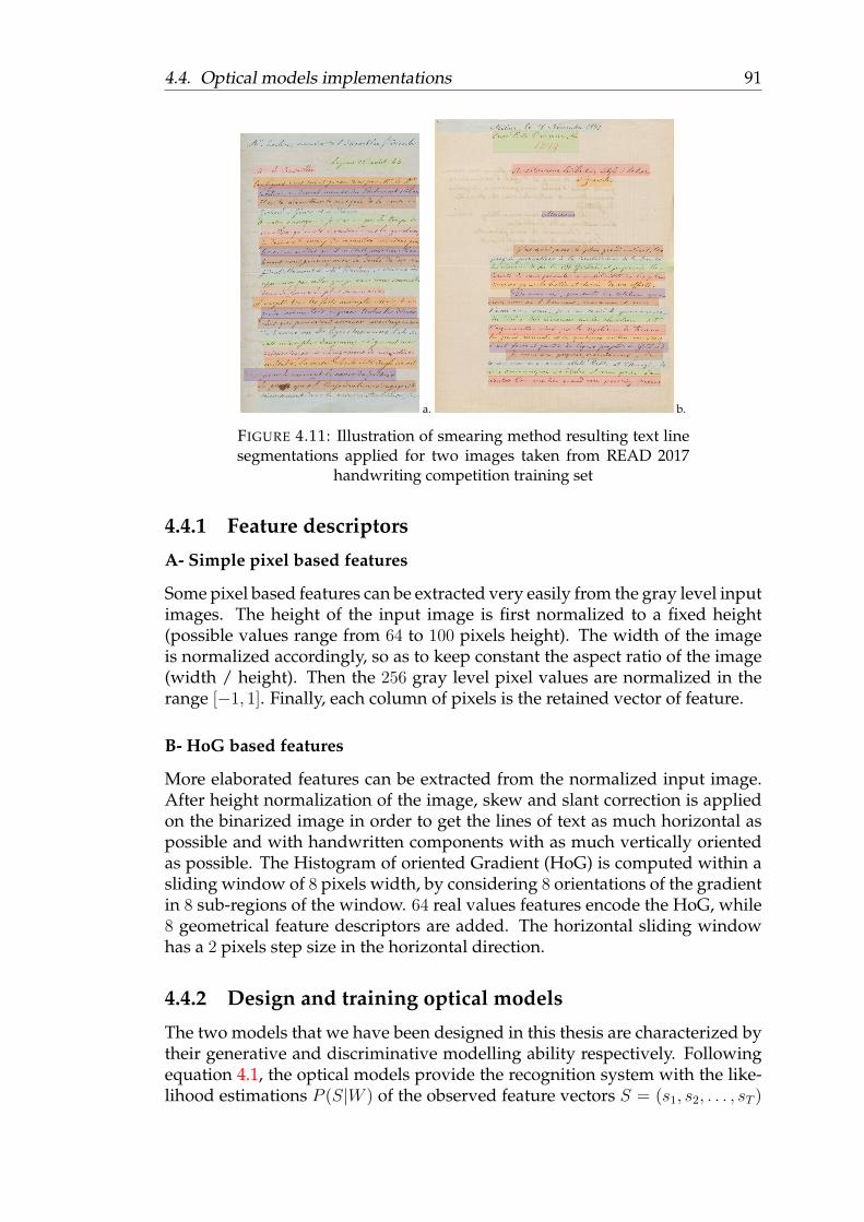
4.4. Optical models implementations 91
a. b.
FIGURE 4.11: Illustration of smearing method resulting text linesegmentations applied for two images taken from READ 2017
handwriting competition training set
4.4.1 Feature descriptors
A- Simple pixel based features
Some pixel based features can be extracted very easily from the gray level inputimages. The height of the input image is first normalized to a fixed height(possible values range from 64 to 100 pixels height). The width of the imageis normalized accordingly, so as to keep constant the aspect ratio of the image(width / height). Then the 256 gray level pixel values are normalized in therange [−1, 1]. Finally, each column of pixels is the retained vector of feature.
B- HoG based features
More elaborated features can be extracted from the normalized input image.After height normalization of the image, skew and slant correction is appliedon the binarized image in order to get the lines of text as much horizontal aspossible and with handwritten components with as much vertically orientedas possible. The Histogram of oriented Gradient (HoG) is computed within asliding window of 8 pixels width, by considering 8 orientations of the gradientin 8 sub-regions of the window. 64 real values features encode the HoG, while8 geometrical feature descriptors are added. The horizontal sliding windowhas a 2 pixels step size in the horizontal direction.
4.4.2 Design and training optical models
The two models that we have been designed in this thesis are characterized bytheir generative and discriminative modelling ability respectively. Followingequation 4.1, the optical models provide the recognition system with the like-lihood estimations P (S|W ) of the observed feature vectors S = (s1, s2, . . . , sT )

92 Chapter 4. Design and evaluation of a Handwritting recognition system
FIGURE 4.12: overview of the various optical models imple-mented in this thesis
towards a set of character classes. As presented in chapter 2, Hidden MarkovModels are generative models that are optimized using the expectation maxi-mization (EM) algorithm. This algorithm uses the likelihood criterion as train-ing criterion. The BLSTM-RNN optical models are trained using a discrim-inative approach that uses the posterior probability P (W |S) as training cri-terion and the Back-Propagation-Through-Time algorithm. In the followingparagraphs we give some more details about the optical models architecturesand their optimization procedure.
A- HMM model optimization
The internal structure of the HMM optical Models of characters is defined by avariable number of hidden states organized sequentially from left to right, andfor each of them, a fixed size Gaussian mixture is also determined. We choseto use mixtures with 20 Gaussians, which guarantee a description ability fairlyaccurate for each frame of feature descriptors. Determining the number ofhidden states is an optimization problem. An overestimated number of hid-den states leads to over-trained models. An underestimated number of statesleads to inadequate specialized models. This problem has been addressed in(Zimmermann and Bunke, 2002; Ait-Mohand, Paquet, and Ragot, 2014). Wehave been inspired by the proposed method in the first reference that is basedon the Bakis method in order to optimize the number of states of each charactermodel.
The principle of this method is as follows. Once a first training of one ini-tial set of character models has been carried out with a fixed number of states(5 states per model), we compute the average number of frames F per opticalmodel using a forced alignment decoding process of the corresponding models
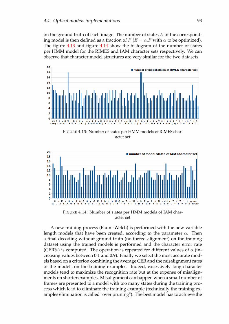
4.4. Optical models implementations 93
on the ground truth of each image. The number of states E of the correspond-ing model is then defined as a fraction of F (E = α.F with α to be optimized).The figure 4.13 and figure 4.14 show the histogram of the number of statesper HMM model for the RIMES and IAM character sets respectively. We canobserve that character model structures are very similar for the two datasets.
FIGURE 4.13: Number of states per HMM models of RIMES char-acter set
FIGURE 4.14: Number of states per HMM models of IAM char-acter set
A new training process (Baum-Welch) is performed with the new variablelength models that have been created, according to the parameter α. Thena final decoding without ground truth (no forced alignment) on the trainingdataset using the trained models is performed and the character error rate(CER%) is computed. The operation is repeated for different values of α (in-creasing values between 0.1 and 0.9). Finally we select the most accurate mod-els based on a criterion combining the average CER and the misalignment ratesof the models on the training examples. Indeed, excessively long charactermodels tend to maximize the recognition rate but at the expense of misalign-ments on shorter examples. Misalignment can happen when a small number offrames are presented to a model with too many states during the training pro-cess which lead to eliminate the training example (technically the training ex-amples elimination is called "over pruning"). The best model has to achieve the

94 Chapter 4. Design and evaluation of a Handwritting recognition system
minimum CER and the minimum misalignment rate (MAR%). This criterionis tested at each iteration of the Baum-Welch training procedure. Training isstopped after 30 iterations, with more iterations, we noticed that the best CERis reported within the 30 iteration. We then obtain optimized optical models.For the values of α listed in table 4.5, the selected the models which meet theselection criterion that minimize the CER% with minimum MAR% where themodels that are trained with 0.75 and 0.65 values of α on RIMES and IAM testdatabases respectively that realise 38.12% CER with 3.60% MAR on the RIMEStest dataset, however, 45.57% CER with 0.77% MAR on IAM test dataset.
α values [0,1]Databases Measures 0.55 0.65 0.75 0.85 0.95CER % 49,64 39,05 38,12 39,1 40,37RIMES MAR% 0.34 1.17 3.60 8.40 17.43CER % 53,47 45,57 49,9 50,87 47,76IAM MAR% 0.27 0.77 2.85 7.75 16.99
TABLE 4.5: Optical models alignment optimization for trainingon RIMES and IAM databases
B- BLSTM architecture design
The internal structure of the BLSTM-RNN optical model of characters is de-fined by a fixed number of neurons distributed and interconnected with eachother along a certain number of stacked BLSTM layers ending at the top layerof the stack by a fully connected CTC layer. For the BLSTM-RNN based hand-writing recognition system, we have design two optical model configurationsas illustrated in figure 4.12. Configuration (I) : consists of HoG features ex-tracted from the binarized input images that are used for training a BLSTM-RNN network composed of three layers, within each layer, there are 200 LSTMunits. Configuration (II) : consists of columns of pixels feature descriptors ex-tracted from the Gray level colour of the input image. The BLSTM-RNN net-work is characterized by four layers, each of which with 200 LSTM units.
During the training process the examples have been sorted according totheir number of frames in order to apply the principle of the curriculum learn-ing algorithm (Bengio et al., 2009), by starting the optical models training withfirst learning the short sequences and step by step go towards longer ones. Forthe two system configurations, the training by backpropagation through timeof the neural network starts with a learning rate of 10−5 and continues withno change for 100 epochs. Then the learning rate starts decaying by a ratio of0.5 and checking the enhancements of the network performance on the valida-tion set. The training process stops, if the performance enhancement betweentwo successive epochs is less than 0.0001. At every training epoch, the recogni-tion performance of the optical models are reported and the best trained mod-els are selected according to the character error rate (CER) on the validationdatasets. The recognition performance on RIMES dataset for the two opticalmodel configurations are illustrated in table 4.6, as well as for the English IAM

4.5. Language models and lexicons 95
dataset. Configuration (II) performs much better than configuration (I) with aCER lower by 2.95% on the IAM dataset, and lower by 10.7% on the RIMESdataset. As a conclusion of this section we can highlight the performance of
Datasets Optical modelsconfigurations
Trainingepoch # Learning
ratesCER% on validation
dataset
RIMESconfiguration
(I) 200 5.72643e−07 11,97
configuration(II) 137 6.04662e−08 9,03
IAMconfiguration
(I) 153 2.1937e−10 22
configuration(II) 120 2.16e−06 11,3
TABLE 4.6: Optical model performance measured by charactererror rate CER during the training process on the training and
validation datasets for the two configurations (I & II)
recurrent neural networks compared to those of HMM. BLSTM RNN achievea 9.03% CER on the RIMES validation dataset and 11.3% on the IAM validationdataset, whereas the HMM models obtain a 38.12% CER on RIMES and 45.57%on the IAM dataset. Moreover, the BLSTM-CTC optical model with the pixelvalues shows a significant improvement of 2% CER on the RIMES validationdataset and 10.7% CER on the IAM validation dataset.
4.5 Language models and lexicons
The language model contribution to the final recognition likelihood score isthe a priori probability P (W ) of the sentence as given in equation 4.1. Thisprobability helps the recognition process to favour sequences of words thatare linguistically valid and the most probable. In between the optical modelhypotheses which provides sequence of characters’ hypotheses with their like-lihood score, and the language model input which are sequences of lexicontokens, the recognition process has to integrate character concatenation rulesgiven by the recognition lexicon.
As shown on figure 4.15, the language component of the system must inte-grate both the recognition lexicon and the language model. Following chapter3, and as can be shown on this figure 4.15, closed vocabulary systems are de-fined by a working lexicon of words which prevent them to recognize out ofvocabulary words (OOV), thus the systems will lack generalization capabili-ties. One way to increase the lexicon generalization capabilities is to increasethe size of the working lexicon. However, large lexicons lead up to higher com-plexity (and perplexity) language models with which the recognition task hasmore difficulty due to the increased number of competing hypothesis whichmay content the target to be recognized. Reversely, small lexicons with high

96 Chapter 4. Design and evaluation of a Handwritting recognition system
FIGURE 4.15: Illustration of the linguistic knowledge systemcomponents
OOV rates make the language models unable to guide effectively the recog-nition process. Therefore, it is necessary to find a compromise between thelexicon size and the Out-Of-Vocabulary rate when determining the languagemodel lexicon. One alternative is to introduce sub-lexical units in place of lex-ical units. From the lexicon of word tokens, sub-lexical units can be derived indifferent ways to provide syllables or multi-grams, and this will be the topic ofchapter 5.
Simple models using characters only have also emerged as one possibleway to deal with OOV words. The open vocabulary systems can reach a nearly100% coverage rates of words of the test datasets and consequently we can ex-pect them to have lower Word Error Rates than closed vocabulary systems.This will however depend on the language model design and most impor-tantly on the properties of the training corpus compared to those of the testcorpus. Whatever the strategy adopted (closed or open vocabulary) the archi-tecture of the system is the same as shown on figure 4.15. First a token lexiconof words, sub-words units, or characters is defined, then a statistical languagemodel is trained on some training data in the form of a n-gram or a recurrentneural network language model based on the tokens that have been defined.
4.5.1 Lexicon properties
All along this thesis, the experimentations have been conducted on the tworeference datasets available: the French RIMES dataset, and the English IAMdataset. It is worth mentioning here their respective properties in terms oflexicon sizes, coverage rates, and introduce some additional external linguisticresources that have demonstrated to be necessary to achieve state of the artperformance, as they allow reaching much higher lexicon coverage rate, andimprove the linguistic context generalization capability of the language model.
4.5. Language models and lexicons 97
A- Tokenisation
Beside meaningful language words (a word is a sequence of characters sidedby a white space character), plain text corpus may contain sequences of al-phanumeric characters and symbols like bank account numbers, date or timeformats (such as 02/08/2000 or 10:30’PM’) which are counted as words accord-ing to the definition of a word, and the Word Error Rate metric, contrary to thespoken languages. Moreover, written languages include many punctuationmarks that have to be identified as they count as a word in the WER metric formost of the competitions. At last we have to pay much attention on modellingthe inter word white space. Indeed, most of the written languages include ablank separator between words that serve as an important visual word delim-iter, whatever the word is a word of the working lexicon or an alphanumericexpression, whereas the ASCII space character can serve as a natural worddelimiter when encoding texts in electronic format (and therefore space char-acter is not introduced in most language models devoted to Natural LanguageProcessing (NLP) Technics, here it is highly necessary that our optical modelincludes one class for the blank space (word delimiter). During decoding (seesection below) as the system combines the optical model with the languagemodel, it is necessary to integrate this optical model similarly to the integra-tion of other special characters. As a consequence of integrating punctuationmarks and blank character classes we must notice that the order of n-gram lan-guage models will be at least twice as the order of standard language modelsused by NLP technics.
The tokenization process is introduced as a necessary pre-processing stepfor preparing the training data according to the targeted type of languagemodel. During the experimentations, we have applied the following tokeniza-tion process on the training text corpora, before training the language model.The training text corpora are cleaned from any character not found in theRIMES or the IAM datasets. Recall that the RIMES dataset contains 100 al-phanumeric symbol classes and IAM dataset contains 80 alphanumeric sym-bol only. Then, token separators are explicitly introduced in the training cor-pus so as to allow training the language model with the desired lexicon entriesand the specific alphanumeric characters, including punctuation marks andthe white space character (word delimiters). By default our tokenizer includesvocabulary word tokens, punctuation marks token, numeric characters andsymbols (excluding simple characters). When testing the sub-lexical languagemodels introduced in Chapter 5, the tokenization process will be modified soas to decompose words into their sub-lexical units as well.
Some additional pre-processing steps have demonstrated to be effectiveduring the experimentations. Indeed, the text datasets are generally providedwith line breaks. By removing line breaks in the training corpus we aimed toimprove the performance of the language models by giving them the abilityof modelling long sequence dependencies of tokens (words, syllables, multi-grams and characters). Experiments have demonstrated a decrease between1% and 2% of the WER by removing line breaks from the training corpuswhen using the Wikipedia+RIMES corpora. Finally, we should not forget that

98 Chapter 4. Design and evaluation of a Handwritting recognition system
whereas we try to build the best suited language model to get the best open-vocabulary recognition system by introducing a specific tokenization processthat allow training the desired model, the evaluation process is conductedwithout no consideration about the internal representation of the languagemodel of the system. For the evaluation process, only the Word Error Rate iscomputed, which evaluates the capacity of the system to recognize any word(in lexicon or OOV) delimited between two white spaces, and by countingpunctuation marks.
B- Lexicon statistics
A first group of lexicons is derived from the vocabularies of the RIMES andIAM datasets only. In table 4.7 we see that the lexicon of RIMES training andvalidation datasets achieves a 93.7% effective coverage rate (ECR) on the testdataset with a small lexicon size of 5867 word tokens. This demonstrates thehomogeneity of the RIMES datasets in terms of lexicon coverage. In table 4.8
Lexicontype
ECR%on
the test dataset
Lexiconsize (words)
Vocabularysize (tokens)
RIMEStrain 93.29 8107 5484
RIMESvalid 84.42 2354 1810
RIMEStrain + valid 93.72 8760 5867
TABLE 4.7: RIMES dataset lexicon properties.
below, we see that the training and validation IAM datasets do not allow reach-ing sufficiently high lexicon coverage rates on the IAM test dataset to allowgetting interesting recognition performance. This raises the important ques-tion of choosing some external resources that could compensate for the lack ofavailable data in the training corpus. This is one of the most important differ-ence between the two RIMES and IAM datasets.
Lexicontype
ECR%on
the test dataset
Lexiconsize (words)
Vocabularysize (tokens)
IAMtrain 75.45 9956 7414
IAMvalid 67.17 2992 2219
IAMtrain + valid 78.92 11615 8291
TABLE 4.8: IAM dataset lexicon properties.
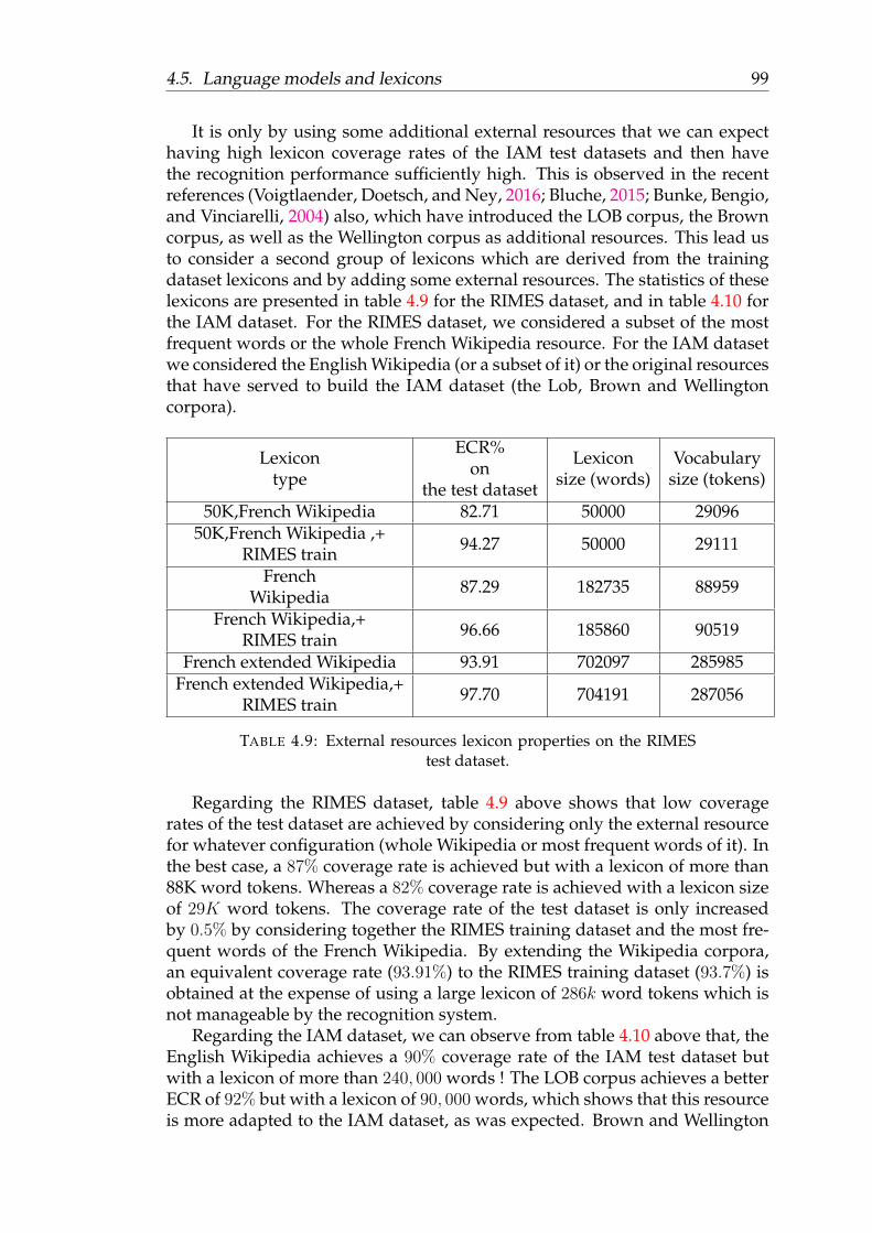
4.5. Language models and lexicons 99
It is only by using some additional external resources that we can expecthaving high lexicon coverage rates of the IAM test datasets and then havethe recognition performance sufficiently high. This is observed in the recentreferences (Voigtlaender, Doetsch, and Ney, 2016; Bluche, 2015; Bunke, Bengio,and Vinciarelli, 2004) also, which have introduced the LOB corpus, the Browncorpus, as well as the Wellington corpus as additional resources. This lead usto consider a second group of lexicons which are derived from the trainingdataset lexicons and by adding some external resources. The statistics of theselexicons are presented in table 4.9 for the RIMES dataset, and in table 4.10 forthe IAM dataset. For the RIMES dataset, we considered a subset of the mostfrequent words or the whole French Wikipedia resource. For the IAM datasetwe considered the English Wikipedia (or a subset of it) or the original resourcesthat have served to build the IAM dataset (the Lob, Brown and Wellingtoncorpora).
Lexicontype
ECR%on
the test dataset
Lexiconsize (words)
Vocabularysize (tokens)
50K,French Wikipedia 82.71 50000 2909650K,French Wikipedia ,+
RIMES train 94.27 50000 29111
FrenchWikipedia 87.29 182735 88959
French Wikipedia,+RIMES train 96.66 185860 90519
French extended Wikipedia 93.91 702097 285985French extended Wikipedia,+
RIMES train 97.70 704191 287056
TABLE 4.9: External resources lexicon properties on the RIMEStest dataset.
Regarding the RIMES dataset, table 4.9 above shows that low coveragerates of the test dataset are achieved by considering only the external resourcefor whatever configuration (whole Wikipedia or most frequent words of it). Inthe best case, a 87% coverage rate is achieved but with a lexicon of more than88K word tokens. Whereas a 82% coverage rate is achieved with a lexicon sizeof 29K word tokens. The coverage rate of the test dataset is only increasedby 0.5% by considering together the RIMES training dataset and the most fre-quent words of the French Wikipedia. By extending the Wikipedia corpora,an equivalent coverage rate (93.91%) to the RIMES training dataset (93.7%) isobtained at the expense of using a large lexicon of 286k word tokens which isnot manageable by the recognition system.
Regarding the IAM dataset, we can observe from table 4.10 above that, theEnglish Wikipedia achieves a 90% coverage rate of the IAM test dataset butwith a lexicon of more than 240, 000 words ! The LOB corpus achieves a betterECR of 92% but with a lexicon of 90, 000 words, which shows that this resourceis more adapted to the IAM dataset, as was expected. Brown and Wellington

100 Chapter 4. Design and evaluation of a Handwritting recognition system
Lexicontype
ECR%on
the test dataset
Lexiconsize (words)
Vocabularysize (tokens)
50K,English Wikipedia 84.6 50000 2947350K,English Wikipedia,+
IAM train 84.84 50000 31308
EnglishWikipedia 91.85 240659 103943
EnglishWikipedia,+
IAM train92.19 242928 104871
English extended Wikipedia 95.76 994545 311712LOB
corpus 99.33 98716 87777
LOB corpus includingIAM train only 92.7 95526 87501
Brown corpus,+IAM train 90.1 102775 51196
Browncorpus 89.35 100236 51165
Wellington corpus,+IAM train 91.47 98254 49234
Wellingtoncorpus 91.08 95781 48122
50K,LOB+Brown+Wellington 91.12 50000 29697LOB+Brown+Wellington 95.13 199521 87501
TABLE 4.10: External resources lexicon properties on the IAMtest dataset.
corpora achieve very similar ECR. Finally, by considering the most frequent50, 000 words of both LOB, Brown, and Wellington corpora, a 91.12% ECR isachieved but with a lexicon of 29, 697 word tokens only; whereas a ECR of95% is obtained when considering the whole three corpora of 199, 521 words.An equivalent hight coverage rate is obtained by using the English extendedWikipedia corpora (95.76%) with a lexicon of 994, 545 words which is not man-ageable by the recognition system. From these lexicon statistics, we see thatthe two popular datasets exhibit different properties in terms of lexicon cover-age of their test dataset by their training datasets. As the lexicon coverage rateachieved by the language model is the upper bound of the WER of the recogni-tion system, improving the coverage rate of the language model is one neces-sity for improving the WER, whatever the performance of the optical model,this is particularly necessary for the experimentations that will be conductedon the IAM dataset. A first strategy is to increase the lexicon size, but this is atthe expense of having a large language model of relatively high order. A sec-ond strategy is to introduce sub-lexicon units in the language model. Chapter5 will address this issue.

4.5. Language models and lexicons 101
4.5.2 Language model training
All along this thesis we have conducted most of our experimentations by in-tegrating n-gram statistical language models. However, some primary exper-iments have been conducted by using Recurrent Neural Networks LanguageModels. In this section, we give some details about training these two modelsand their first evaluation.
A- N-gram language models
During this thesis, we implemented various n-gram language models withdifferent toolkits. We started our primary experiments by combining HMMoptical models with n-gram LM models. At this time the language modelswere estimated by the constant discounting smoothing method with usingthe SRILM toolkit (Stolcke, 2002). Later on, when introducing the BLSTM-RNN optical model, we used modified Kneyser-Ney smoothing provided bythe MIT language modelling toolkit (Hsu, 2009) for training n-gram languagemodels. Modified Kneyser-Ney smoothing achieved similar or better perfor-mance compared to other estimation methods. We favoured the use of MITLMtoolkit because it offers the ability to tune the model (Kneyser-Ney) parame-ters using the Limited-memory BFGS (Broyden-Fletcher-Goldfarb-Shanno) op-timization algorithm using the validation datasets which consequently mini-mizes the language model perplexity.
As mentioned in the previous section, due to the presence of white spacesand punctuation marks, high order n-gram language models are required tocapture long distance dependencies. Remember that a n-gram of order n willin fact account for modelling word dependencies of order n/2. For example,n = 10 (which at first sight may appear a rather long history in the sentence) ac-counts for the last 4 words back in the past only. A value which is not that largein the field of statistical NLP. For validating the necessity of having high ordern-gram language models for handwriting recognition, we evaluated the contri-bution of various n-gram language models of increasing order to the recogni-tion performance of the system. This was repeated for various optical models(HMM and RNN) and using word n-gram language models. Language mod-els have been estimated from the RIMES train and Wikipedia + RIMES traintraining corpus. Table 4.11 below report the performance of two systems.
Trainingdatasets n-gram 2 3 4 5 6 7 8 9
RIMEStrain
HMM 22.7 17 17 16.8 16.9 16.9 17 17BLSTM 21.7 17.01 17.27 16.99 16.81 16.42 16.47 16.36
Wikipedia+RIMES train
HMM 36 29.8 29.6 29.5 29.3 — — —BLSTM 22.88 16.74 16.68 15.72 16.06 15.49 15.45 15.76
TABLE 4.11: Influence of word language model order on theRIMES dataset, using a closed lexicon of RIMES train andWikipedia + RIMES train tokens, and for two optical model
(WER%).

102 Chapter 4. Design and evaluation of a Handwritting recognition system
Best recognition performance of the HMM based recognition system are re-ported when using 6-gram language models. Whereas the BLSTM-RNN recog-nition system achieved its best performance with 9-gram language models ofwords. These results show that high order n-gram language models (in therange 6 to 10) are to be preferred to low orders. Of course, there are some wellknown drawback of using high order models, the most important one beingthe complexity of the model and number of parameters. What we can noticehere looking at these results is that parameter estimations using smoothingtechniques such as modified Kneyser-Ney are robust to the data sparsity prob-lems that can be encountered on too small training datasets.
Nevertheless, there are several problems with using n-gram language mod-els, the most important one being probably the problem of context (or topic)coverage. In fact, like the notion of lexicon coverage (Effective Coverage Rate),we can never guarantee that a n-gram language model trained on a certaincorpus will generalize well on a specific test corpus. As we will see in the nextchapters, the linguistic context coverage is not limited to the lexicon coverage,we expect that using a language models trained on a certain resource will helprecognizing words of another resource. Having generalizable language mod-els require the models to be trained on sufficiently general and large resources.Another limitation of statistical n-gram LM is that they don’t introduce somemore elaborated syntactical or grammatical knowledge. For example, n-gramdon’t use any notion of word classes or categories. Finally, a compromise be-tween the n-gram order, the recognition performance, and the computing ca-pacity of the machine in terms of time and memory space is to be determinedfor real applications. Such considerations have been mostly out of the scopeof this study as our systems have been implemented on machines with hugememory capacity (256 GB).
B- Recurrent neural network language models (RNNLM)
The advantage of the connectionist language models such as RNNLM overthe n-gram language models is their capacity to model the language variablelength dependencies of words. The primary experiments that we conductedwas using RNNLM during a second decoding pass (see next section “decod-ing” below) dedicated to rescoring the sentence recognition hypotheses. Dueto lack of time, the primary experiments were only conducted using charac-ter language models. 5-gram and 10-gram character language models wereused in the first decoding pass to generate the possible recognition hypothe-ses and their associated weights represented by a token-lattice. The RNNLMeffective parameter is the number of units in the hidden layer of the neural net-work. Three RNNLM language models have been trained on the Wikipedia +RIMES training datasets with 50,100 and 1000 units in the hidden layer re-spectively. The system with RNNLM at the second decoding pass overcomesthe n-gram models, as can be seen in table 4.12. It must be noticed howeverthat these experimentations have been carried out using a three layers BLSTMwith HOG features, which later on demonstrated to perform lower than otherarchitectures. Therefore these results are only provided to attest the capacity

4.5. Language models and lexicons 103
of RNNLM on language modeling task. However, as reported in the literature,we also observed that training RNNLM language models is time consuming,and requires multiple trials for choosing the proper number of hidden units inthe network (Yousfi, Berrani, and Garcia, 2017). This is also the reason why wedid not continue our experimentations in this direction further.
1st passdecoding
CharacterRNNLM Character
n-gram LM50units
100units
1000units
5-gram 28.64 25.27 22.28 25.9610-gram 22.06 18.67 18.31 18.92
TABLE 4.12: performance of a second pass character RNNLM onthe RIMES dataset compared to a traditional n-gram LM.
4.5.3 Decoding
Decoding is the process of combining the optical model character hypothe-ses together in order to build admissible character sequences (i.e. words /tokens) that belongs to the working lexicon and that are the most likely withrespect to the language model. Through the decoding step, we aim to deter-mine the most probable word sequence W given the observed optical featuresequence O using the information produced by the optical model and the lan-guage model. Decoding is the optimization process depicted by equation 4.1introduced at the early beginning of this chapter. It can be solved using Dy-namic Programming. The time synchronous beam search Viterbi algorithm isthe traditional decoding algorithm used for achieving speech and handwrit-ing recognition tasks. Ideally, a search algorithm should consider all possi-ble hypotheses based on a unified probabilistic framework that integrates allknowledge sources (optical and linguistic knowledge) (Xu et al., 1996).
When the explored search space becomes unmanageable, due to the in-creasing size of the vocabulary or the language models (high order), the searchmight be infeasible to implement or too long run. Then the solution is to re-strict the search space to a sub-set of hypotheses using what is called a beam.During Viterbi decoding at every time step, search paths that are unlikely tosucceed (less probable than the best path by a factor δ) are removed from thelist of hypotheses; thus the name Time Synchronous Beam Search ( beam searchparameter used for limiting the search space and beamlattice parameter whichinfluences speed of the lattice extraction). But this pruning strategy alone can-not cope with the complexity involved by managing high order language mod-els. In practice, time Synchronous Beam Search is generally implemented us-ing a limited history of two words at most (a 3-gram language model). Thisconstitutes a first decoding pass during which optical models, lexicon entriesand a low order language model are combined following equation 4.1. Out-puts of the first pass decoding is a word lattice (token lattice in general) thatcontains the N-best hypotheses as depicted on figure 4.16. A word-lattice (or

104 Chapter 4. Design and evaluation of a Handwritting recognition system
token-lattice) consists of the possible interconnected recognition hypothesesweighted by the optical models and language model’s weights. A second de-coding pass analyses the hypotheses network (word-lattice) using a n-gramlanguage model of higher order, which allows re-weighting the hypotheses.Alternatively, some RNN LM can be used during the second decoding pass.
FIGURE 4.16: Example of a word lattice produced by the N-besttime synchronous Viterbi beam search algorithm. Each word oc-
cupies an explicit time interval.
Two important parameters guide this first decoding pass: they are the lan-guage model scaling parameter γ and the word insertion penalty parameterβ that controls the insertion of too frequent short words. These two param-eters need to be optimized for optimum coupling of the optical model withthe language model, because these two models are estimated independentlyfrom each other during training. Both the HMM based and the BLSTM-CTCbased recognition systems have been implemented using a two pass decodingalgorithm. In practice, multipass search strategy using progressive knowledgesources can generate better results than a search algorithm forced to use lesspowerful models due to computation and memory constraints (Xu et al., 1996).We now give some details about optimizing the coupling parameters of thefirst decoding pass, before giving some more information on the algorithmicimplementations.
A- Parameter optimization algorithm
The language model and optical model coupling parameters have a direct ef-fect on the recognition performance. With the HMM optical models, HTK’sdecoding toolkit was used. The HTK decoding toolkit uses the token passingparadigm to find the best path and / or multiple alternative paths. In the lattercase, it generates a lattice containing the multiple hypotheses which can if re-quired be converted to an N-best list. For the token passing algorithm, a tokenrepresents a partial path through the recognition network extending from thetime 0 through to the time t of decoding.
The word insertion penalty is a fixed value added to each token when ittransits from the end of one word to the start of the next. The language modelscale parameter is the amount by which the language model probability is

4.5. Language models and lexicons 105
scaled before being added to each token as it transits from the end of one wordto the start of the next (Young and Young, 1993). During the first pass de-coding, the HTK decoding toolkit make use of the optical model and languagemodel coupling parameter in addition to the beam search parameter and builda token-lattice according to the equation 4.1. Then, during the second pass de-coding, the produced token-lattice is rescored by tuning the language modelscale parameter using the same language model used in the first decoding passor with using higher order n-gram language model.
The simplified way proposed in the Kaldi toolkit for optimizing the cou-pling of the two models is to introduce one single coupling parameter definedby equation 4.8 below, in which the optical-scale parameter α stands for the in-verse of the language model scale parameter γ; thus we can writer α = 1/γ.By comparing equation 4.1 and 4.8. we can see that optimizing the inser-tion penalty parameter is not possible in the standard first pass decoding withKaldi.
W = argmaxw
P (S|W )αP (W ) (4.8)
Thus, we developed our own optimization algorithm 1 within the Kaldiframework aiming to optimize the language model parameter and the wordinsertion penalty parameter during the second decoding pass as was possiblewith the HTK toolkit (during the first decoding pass). The parameter optimiza-
Input: validation set examples, n-gram language models FSTsOutput: best language model order, best language model scale, best word insertion penaltyγ ← the best language model scale parameter;β ← the best word insertion penalty parameter;n− gram← the best n-gram language model initγ ← initial language model scale used for token-lattice
generation = 0.1 ;beam← the beam search parameter used for limiting the search space = 16.0;beamlattice← the beam used for reducing the token-lattice size = 10 ;WIP ← a set of word insertion penalty values [-2,2] with a step value of 0.5 ;/* token-lattice generation through 1st pass decoding */forall n-gram models do
forall WIP doforall validation set examples do
* Building a world lattice by decoding the validation set examples using the initial parametersand the n-gram language model;
* Add insertion penalty value WIP to the generated token-lattice;* Store penalized token-lattice at each value of WIP
endend
end/* token-lattice rescoring during 2nd pass decoding */LMS ← a set of language model scales [0.1, 0.6] with a step value of 0.01 forall Penalized token-lattices do
forall LMS do* Rescoring the token-lattice with the language model scale LMS. * Decoding the tokenl-attice
returning the best bath as the recognized text line. * Computing the word error rate WER over allthe validation set and getting the WER scores as a results.
endend/* Best parameter setting of n-gram language model, language model scale and
word insertion penalty */γ, β, n− gram←min(of all WER scores) ; /* retrieving the best WER score which indicatesto the best parameters */
return γ, β, n− gram;
Algorithm 1: Coupling parameters optimization algorithm introduced in theKaldi toolkit.
tion algorithm is applied on the validation set and once the optimum values

106 Chapter 4. Design and evaluation of a Handwritting recognition system
of the coupling parameter have been determined, we carry out the decodingalgorithm on the test dataset with using the optimum values of the couplingparameters.
B- Decoding configurations / implementations
For the HMM based recognition system and during the first pass, we used abigram language model to produce a token-lattice using the initial optical andlanguage models parameters in addition to an important beam search parame-ter to limit the space of search within a reasonable limits of decoding time withregards to the recognition accuracy. In the second decoding pass, we re-scoredthe generated word-lattice using a 6-gram language model of words, syllablesor characters according to the decoding scenario. HTK HVite decoding toolwas used for the first decoding pass and the word-lattice scoring was achievedusing lattice-score tool from SRILM during the second decoding pass.
First the character hypotheses are arranged in a lexical tree where the firstcharacter of a word corresponds to the root of the lexical tree and the last onecorresponds to the leaf, this representation has the advantage to be compactby sharing the common prefixes of the whole lexicon on a single branch of thetree. One other advantage is that lexicon trees can be efficiently encoded usinga Finite State Transducer (FST).
We designed the BLSTM-RNN based recognition system, through the useof Weighted Finite State Transducers (WFST) automaton of Kaldi toolkit. Thesemethods are recently applied in continuous handwriting recognition (Bluche,Ney, and Kermorvant, 2014). By definition, a finite state transducer is a finiteautomaton whose transiting states are labelled with a couple of input and out-put symbols. A weighted finite state transducer adds a weight to each transi-tion i.e. to each pair of input and output symbols. Weights represent probabili-ties, penalties or any other quantitative values that accumulates over the trans-ducer paths in order to compute the overall weight (cost) of mapping the inputsymbol string to the output symbol string. Thus, a path through the transducerencodes the matching between an input symbol sequence or string and an out-put symbol sequence or string. The reader can refer to (Mohri, Pereira, andRiley, 2008) for more details about the weighted finite state transducer theoryand algorithms.
By using the general framework of WFST it is possible to design a spe-cific transducer for each component of the system : an optical model trans-ducer, a lexicon transducer and finally a language model transducer. Thenit becomes easy to combine these three components into a single WFST thatwill guide the first pass decoding. EESEN speech recognition implementation(Miao, Gowayyed, and Metze, 2015) uses Kaldi’s toolkit (Povey et al., 2011)and highly-optimized FST libraries such as OpenFST (Allauzen et al., 2007).The WFST decoding stage considers the CTC labels, lexicons and languagemodels as separate weighted finite state transducers denoted by T , L and Grespectively. After compiling the three WFST individually, they are composedgradually into a global compact search graph S by using two special WFSToperations known by Weighted determinization and minimization algorithms

4.5. Language models and lexicons 107
that optimize their time and space requirements. For more details about the de-terminization and minimization algorithms one can return to (Mohri, Pereira,and Riley, 2002). The overall order of the search graph generation FST opera-tions is given by:
S = T min(det(L G)) (4.9)
where , det and min denote composition, determinization and minimizationrespectively.
Optical model transducer T : The first WFST component maps a sequenceof frame labels to a single character unit. The character WFST is designed tosubsume all the possible label sequences at the frame level that correspond to acharacter. Therefore, this WFST allows occurrences of the blank label φ, as wellas any repetition of one specific character non-blank labels. For example, afterprocessing 5 frames, the RNN model may generate 3 possible label sequences“AAAAA”, “φ φ A A φ”. The token WFST maps all these 3 sequences into asingleton character unit “A”. We denote the token WFST by T .
FIGURE 4.17: An example of the token WFST which depictsthe phoneme "A". We allow the occurrences of the blank label
"<blank>" and the repetitions of the non-blank label "IH"
Lexicon transducerL: A lexicon WFST encodes the mapping from sequencesof character units to lexicon units. The input string is composed of characters,while the output is a lexicon token with the necessary epsilon (nul output to-ken). The lexicon WFST is denoted as L. Figure. 4.18 illustrates the structure.
FIGURE 4.18: The WFST for the lexicon entry "is i s". The "<eps>"symbol means no inputs are consumed or no outputs are emitted.
Language model transducer G: A language model WFST encodes the per-missible word sequences in a language/domain. The WFST shown in Figure.4.19 represents a trivial language model which accepts two sentences "how areyou" and "how is it". The WFST input symbols are the word tokens, and theoutputs are the words with the arc weights are the language model probabil-ities. With this WFST representation, CTC decoding in principle can leverageany language models that can be converted into WFSTs.
During the decoding process higher order language models are used formaintaining long distance dependency. For that, one need to take into accountthe token dependency between the first token of a text line and its history of to-ken defined by the last few tokens located in the previous text line. Therefore,

108 Chapter 4. Design and evaluation of a Handwritting recognition system
FIGURE 4.19: A trivial example of the grammar (language model)WFST. The arc weights are the probability of emitting the nextword when given the previous word. The node 0 is the start node,and the double-circled node is the end node (Miao, Gowayyed,
and Metze, 2015)
FIGURE 4.20: Line by line versus paragraph by paragraph decod-ing effect on the recognition performance in WER
we decided to adapt our decoding algorithms of the two system to decodeparagraph by paragraph rather than the traditional way of line by line de-coding. Figure 4.20 shows that we gain around 2% of recognition performanceenhancement when using the paragraph by paragraph decoding strategy com-pared with the recognition performance obtained by the line by line decodingstrategy. The primary recognition results illustrated in figure 4.20 was obtainedon RIMES test dataset by using the BLSTM-RNN based system with HoG fea-tures and language models of words of order 2-gram upto 7-gram trained onWikepedia + RIMES training dataset.
4.5.4 Primary recognition results
The conventional language models of words are evaluated and primary resultsis obtained by the handwriting recognition system making use of the HoG fea-tures. With the HMM models we built a handwriting recognition system pro-totype and studied the relation between the lexicons size and the OOV rate andthe consequence of the OOV rate on the recognition performance measured bythe Word Error Rate (WER%).
Figure 4.21 shows the performance achieved on the RIMES and IAM datasetby HMM optical model, and using different lexicons. Notice that a 100% cover-age rate is achieved with the RIMES/IAM dataset as the language model was

4.5. Language models and lexicons 109
(a.)
(b.)
FIGURE 4.21: Primary recognition results with HMM opticalmodels and language models of words; a. RIMES and Frenchwikipedia 6-gram LMs and lexicons tested on RIMES test dataset,b. IAM and English Wikipedia 6-grams LMs and lexicons tested
on IAM test datasets
trained using both training and test datasets. The other experiments have beenconducted with the French Wikipedia corpora for training a set of languagemodels of words for which a set of lexicons (wiki 60k down to wiki 3k word)was selected. The OOV rates reported on the RIMES test dataset increase pro-portional to the the lexicon size and the same phenomena is observed on theWER. This highlight the correlation between the lexicon size and the WER forthe closed vocabulary systems.
The same phenomena was observed on the IAM and English Wikepedialanguage models of word tokens which are illustrated in the right side of fig-ure 4.21. With the BLSTM-RNN based recognition system, we wanted to figureout the relationship between the effective coverage rate, OOV rate, lexicon sizeand the recognition performance in WER. The idea is to evaluate the recogni-tion performance with language models of word tokens that are trained on thewhole RIMES/IAM corpora (training, validation and test) with lexicons whichcover effectively the test data set by 100%, 95%, 90%, 85%, 80% (ECR). The lexi-con was arbitrary selected from the whole RIMES/IAM corpora to attend the
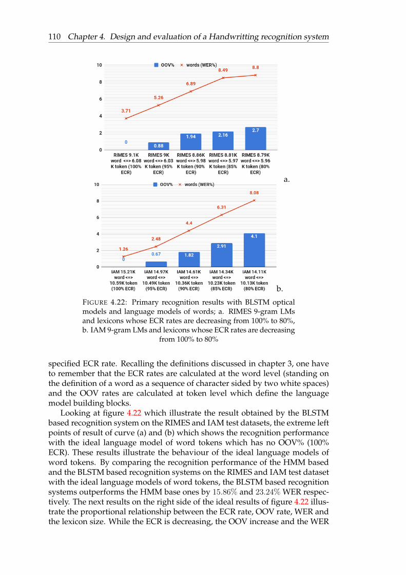
110 Chapter 4. Design and evaluation of a Handwritting recognition system
a.
b.
FIGURE 4.22: Primary recognition results with BLSTM opticalmodels and language models of words; a. RIMES 9-gram LMsand lexicons whose ECR rates are decreasing from 100% to 80%,b. IAM 9-gram LMs and lexicons whose ECR rates are decreasing
from 100% to 80%
specified ECR rate. Recalling the definitions discussed in chapter 3, one haveto remember that the ECR rates are calculated at the word level (standing onthe definition of a word as a sequence of character sided by two white spaces)and the OOV rates are calculated at token level which define the languagemodel building blocks.
Looking at figure 4.22 which illustrate the result obtained by the BLSTMbased recognition system on the RIMES and IAM test datasets, the extreme leftpoints of result of curve (a) and (b) which shows the recognition performancewith the ideal language model of word tokens which has no OOV% (100%ECR). These results illustrate the behaviour of the ideal language models ofword tokens. By comparing the recognition performance of the HMM basedand the BLSTM based recognition systems on the RIMES and IAM test datasetwith the ideal language models of word tokens, the BLSTM based recognitionsystems outperforms the HMM base ones by 15.86% and 23.24% WER respec-tively. The next results on the right side of the ideal results of figure 4.22 illus-trate the proportional relationship between the ECR rate, OOV rate, WER andthe lexicon size. While the ECR is decreasing, the OOV increase and the WER

4.6. Conclusion 111
increase proportionally.From these primary results, one can conclude that the recognition perfor-
mance (in WER) with the conventional language model of word tokens is af-fected proportionally with the OOV rates. The OOV rates decrease by increas-ing the lexicon size. However, this increases the recognition system complex-ity and some times becomes unmanageable. Therefore, it is required to finda compromise between the language model vocabulary size and the coveragerate on the target dataset by that vocabulary. Our main contribution in this the-ses is to introduce the use of the language models of sub-lexical units in placeof the conventional language model of words. The sub-lexical units representthe intermediate modelling units used for language modelling by which onecan realize the intended compromise.
4.6 Conclusion
We introduced in this chapter the description of the main processing chain ofour recognition systems which are based on HMM and BLSTM-RNN models.The main processing chain consists of the text line extraction, feature selectionand extraction, optical models, language models and decoding process. Thetwo systems differ from each other by their optical models types (HMM orBLSTM-RNN).
The two recognition systems (optical and language models) were trainedand evaluated on the French RIMES and the English IAM datasets. Differentlarge and external databases was used for training French and English lan-guage models with different lexicons size.
For the text line extraction process, we presented an iterative steerable fil-ters based method. For the optical models training, we observed the recogn-tion performance enhancement due to using the BLSTM-RNN optical modelsin comparison to weak performance of the HMM optical models. The linguis-tic knowledge representation was persented in form of lexicons and languagemodels of tokens (words, syllables, multigrams and characters). We definesthe effective coverage rate and the out-of-vocabulary rates measures to evalu-ate the lexicons and language models capacity to cover the test datasets.
By experiments, it was evident that the recognition performance increasedby 1% approximately when using the language model that trained on the cor-pus of text which include in addition to its text lines, one long text line thatrepresents the concatenation of whole corpus text lines. This can be explainedby the ability of the language model to capture long distance token dependen-cies through the long concatenation text line. In the same context, the para-graph by paragraph decoding strategy improves the recognition performanceby 2% approximately in comparison with the line by line decoding strategy.Two language modelling methods are examined, n-gram modelling approachfor general use in all our experiments and RNN language modelling approachin a special case of character based recognition system.


113
Chapter 5
Handwriting recognition usingsub-lexical units
5.1 Introduction
The significant progress observed these last years in the speech and handwrit-ing recognition field came from the advancement of deep learning techniquesand recurrent neural networks. But some open issues still remain which aremore oriented towards a better modelling of lexicons and languages. Whereasthe role of language models has been intensively studied in speech process-ing, very few studies have been devoted to Handwriting recognition. More-over, whereas speech and handwriting share the same properties in terms oflexicons and languages, they exhibit very different low level properties whenlooking at the phonetic structure of speech on the one hand, and the graphemicstructure of text on the other hand. Indeed, there is a discrepancy between theway of coding a text and the way of coding its oral pronunciation dependingon the nature of the language. In chapter 3, we have shown the very differencesbetween oral languages and written languages regarding their primary units(characters versus phonemes) and sub-lexical units (phonetic syllables versusgraphemic syllables). The speech recognition literature includes many studieswhere sub-lexical units have been successfully introduced as a mean to copewith Out Of Vocabulary (OOV) words. In comparison, to our knowledge, sucha strategy has not been studied in the field of handwriting recognition. We canhighlight the very few studies devoted to handwritten Arabic text recognitionusing PAW sub-lexical units (BenZeghiba, Louradour, and Kermorvant, 2015)or handwritten German text recognition, because German language allows thecomposition of words with some smaller words in a way similar to agglutina-tive languages (although German does not belong to agglutinative languages).Thus, German lexicons should be of very large size in order to get high Effec-tive Coverage Rates (ECR). Similar properties are observed for Italian languageas well.
Introducing sub-lexical units in a handwriting recognition system appearsan interesting, even necessary, strategy to overcome the problem of OOV. Inthis chapter we investigate the use of sub-lexical units such as syllables andmultigrams for handwriting recognition. The experiments are conducted onthe French RIMES dataset, and on the English IAM dataset. A first necessarystep towards this goal is the design of some automatic lexicon decomposition

114 Chapter 5. Handwriting recognition using sub-lexical units
algorithms able to provide the desired sub-lexical units. We propose two de-composition algorithms. The first one is a supervised syllabification methodthat exploits a linguistic datasets of word decomposition into syllables madeby experts to propose a decomposition into syllables for any given word usinga similarity measures. This method has the drawback of being dependent oflinguistic expertise which is available for very few languages and which doesnot cover all language vocabularies. The idea of the second decompositionmethod consists of using a Hidden Semi-Markovian Model (HSMM) whichlearns the regularities of character sequences called multigrams from a lexiconof words. N-multigram sub-lexical units (character sequences of at most Ncharacters) are finally using the Viterbi algorithm which provides the optimalsegmentation of the words of the training lexicon. The first approach has beenpresented in (Swaileh and Paquet, 2016c, Swaileh, Lerouge, and Paquet, 2016)while the second one will be presented in (Swaileh et al., 2017). This chapteris organized as follows. Section 5.2 presents a supervised sub-lexical decom-position approache into syllable, and section 5.3 is dedicated to unsuperviseddecomposition into multigrams. In section 5.4 we present the experimentalresults obtained using sub-lexical units for the recognition of French and En-glish Handwritten texts. These models compare favorably against the stan-dard word lexicon based approaches and the lexicon free approaches made ofcharacter n-gram language models.
5.2 A supervised word decomposition methods intosyllables
The word decomposition into sub-lexical units (syllables or multigrams) is ex-pressed in the literature by the syllabification process. Usually, the phoneticsyllables generation relies on linguistic and phonetic rules which form the ba-sis of the orthographic syllables. The orthographic syllables can be obtainedfrom a database of syllables designed by language experts such as the FrenchLexique3 database (New et al., 2004) and The Free English language Hyphen-ation dictionary (EHD) (Hindson, 2016). The Lexique3 database provides theorthographic syllabic decomposition of a lexicon of almost 142, 695 Frenchwords into 9, 522 syllables only. It therefore constitutes a linguistic knowledgebase from which our French syllabic model is developed. The free Englishlanguage Hyphenation Dictionary contains 166, 280 words decomposed into21, 991 syllables. Some examples of these two resources are provided on table5.1.
However, despite their relatively large size, it quickly becomes out thatthese linguistic resources by far do not cover the French or English vocabular-ies. For example, Lexique3 covers only 69.83% of RIMES vocabulary. SimilarlyEDH covers only 54.42% of the IAM vocabulary (see left side of figure 6.2).Right side of figure 6.2 shows the effective coverage rate (ECR) of Lexique3and of EHD on RIMES and IAM datasets respectively, when using the syllabicdecomposition. Although insufficient, we can see the increased coverage whenusing a syllabic decomposition of the RIMES or IAM data set. Therefore, we

5.2. A supervised word decomposition methods into syllables 115
Words Syllables
Lexique3examples
connaître con naî treadhésion ad hé sion
norvégiennes nor vé gien nesEnglish
HyphenationDectionary
abandonment a ban don mentabiotrophy ab i ot ro phy
zymosthenic zy mos then ic
TABLE 5.1: Some examples of the Lexique3 and the English Hy-phenation Dictionary.
have to find a general way for generating a syllabic decomposition of any cor-pus and learning a syllable based language models on it. For this purpose, wedeveloped an automatic syllabification method (Swaileh and Paquet, 2016b)and its source code is open source1.
FIGURE 5.1: ECR (%) of Lexique3 on RIMES (blue) and EHD onIAM (red), for words (left) and syllables (right) decomposition.
The syllabification method exploits the lexical and phonetic similarities be-tween the target word (to be decomposed into syllables) and the syllabifiedwords that belong to the dictionary. The method that we propose is based onmatching similar lexical and phonetic structures in order to provide a syllabicdecomposition of any unknown word. Let us assume a word lexicon L, thenth word entry being represented by its sequence of characters mn associatedwith its syllabic decomposition denoted sn, namely its sequence of syllables.Formally we can write L = (m1, s1), (m2, s2), . . . , (mn, sn), . . . , (ml, sl). Forany unknown word (not in L) represented by its character string m, we wishto determine its syllable representation s. The first idea is to search for the clos-est word mn in the dictionary. But two very similar words may have differentsyllabic decomposition, especially if they differ by a vowel, which often marksthe presence of a syllable. To take this information into account, we introducean syllabic structure that represents the word by its consonants and vowelsstring. For example, the word ”Bonjour” is encoded by its syllabic structure
1http://swaileh.github.io/Syllabifier

116 Chapter 5. Handwriting recognition using sub-lexical units
ss = ”CV CCV V C”. Then we can define a similarity measure by combiningboth representations according to equation 5.1, where Slex and Ssyl are respec-tively two similarity measures on the lexical and the syllabic representations:
SG((m, ss), (mi, ssi)
)=Slex(m,mi) + Ssyl(ss, ssi)
2(5.1)
Table 5.2 shows an illustration for the similarity measures obtained on oneexample. The similarity score between sequences of characters counts the av-erage number of identical character pairs at the same positions between thetwo sequences. When sequences have different size, the shorter one is com-pleted by space characters, so the two sequences have an identical size. By thisway, we make the segmentation into syllables based on the prefix of the dic-tionary word, possible errors may occur at word’s suffix that may be differentdue to of the completion of the words by spaces. When the lexicon entry that ismost similar to the unknown word gets a similarity score exceeding a thresh-old T , its syllabic representation serves as a model to decompose the unknownword. The segmentation into syllables of the unknown word is made at thesame positions as in the model.
Lexical similarity Slex = 5/8Query word b o n j o u r -Nearest lexicon entry t o u j o u r s
- o - j o u r -Syllabic similarity Ssyl = 6/8
Query word C V C C V V C -Nearest lexicon entry C V V C V V C C
C V - C V V C -Syllable decomposition
Query word b o n j o u rNearest lexicon entry t o u j o u r s
TABLE 5.2: Syllabification example on the query word ıbonjour
When the similarity score is below the threshold T , the decomposition intocharacters is chosen as the syllabic decomposition by default. Reasonable val-ues of T can be chosen between [0.5, 1]. Between these two extreme values,the choice of an optimal value is crucial because when T = 1 the algorithmsystematically will divide the unknown word into characters, which is not thegoal. Conversely, when T = 0.5, the algorithm will systematically propose asyllabification even if the word query has a structure different from the closestword belonging to the lexicon. In this case there is a big chance to producean erroneous syllabification. Such an example is the entity names which doesnot belong to the French or English spoken language. This margin of syllab-ification by mistake must be quantified by an linguist expert. It is thereforenecessary to optimize the value of T to find the one that minimizes both thenumber of words decomposed into characters and the number of erroneoussyllabification. A first possibility would be to optimize T by cross-validationA second approach consists in optimizing T with respect to the performance

5.3. An unsupervised word decomposition into multigrams 117
of the recognition system. Figure 5.2 shows the evolution of the Word ErrorRate of the recognition system on the two RIMES and IAM datasets. We no-tice a rather similar behaviour of the two systems with a turning point at cer-tain value of T beyond which the recognition system loses its lexicon coveragepower and simultaneously achieves lower recognition performance.
FIGURE 5.2: WER (%) as a function of T on the RIMES dataset(blue) and the IAM dataset (red), for an HMM based recognition
system with HoG features
We chose T = 0.6 for the RIMES dataset, and T = 0.7 for the IAM dataset.In this situation only 0.25% of the words in the RIMES dataset are not syllabi-fied. A close look at these errors shows that they correspond to out of Frenchvocabulary words, as for example the sequence ”SXNHBOO”. The same phe-nomenon is observed on the IAM dataset, for example the word ”Lollobrigida”is broken down into characters. by setting T = 0.7, only 0.37% of the words inthe IAM dataset are not syllabified, and decomposed into characters by error.A complementary analysis of the supervised syllabification method is illus-trated in figure 5.3 and figure 5.4. They represent the histograms of the num-ber of words decomposed into n syllables for the RIMES and IAM lexicons, asa function of the threshold T . It can be noted that the majority of words aredecomposed into 5 syllables at most on the RIMES dataset when T = 0.6. Itis also noted that, beyond 0.6, the number of words abnormally decomposedinto a large number of syllables increases, because the method favors the de-composition of words into characters beyond this threshold value. The sameobservations can be made on the IAM dataset from T = 0.7 (figure 5.5).
5.3 An unsupervised word decomposition into multi-grams
During chapter 3 we have seen that multigrams are variable length sequencesof elementary units that compose an observation stream, as opposed to fixedlength n-gram (Deligne and Bimbot, 1995). They have been introduced first for

118 Chapter 5. Handwriting recognition using sub-lexical units
FIGURE 5.3: Number of words of the RIMES vocabulary decom-posed into n syllables as a function of T.
language modelling of phrases, but later the same authors have studied theirpossible introduction as sub-lexical units for language modelling and speechrecognition (Deligne and Bimbot, 1997). If one consider the character to bethe primary units of a written language, then multigrams allow representingwords as the concatenation of variable length sequences of characters. To ourknowledge this study is the first application of multigram models to handwrit-ing recognition. In the original paper the authors have proposed an unsuper-vised training approach based on variable length Hidden Markov Models. Inthe next paragraphs, based on Hidden semi Markov Models, we introduce theformal definitions underlying the multigram paradigm.
5.3.1 Hidden Semi-Markov Model General definition
Formally, Hidden Semi-Markov Models (HSMM) are considered as one exten-sion of the traditional Hidden Markov Models (HMM) where the duration ofeach state is explicitly defined. Thus each state in the HSMM model can gener-ate an observation sequence of duration d. Assuming a discrete-time Markovmodel with a set of M Hidden states S = s1, s2, . . . , sM, a state sequenceof length T is denoted Q1:T = Q1 Q2 . . . Qt . . . QT , in which Qt is the state attime t. Q[t1, t2] = sm accounts for state sm starting at time t1 and ending attime t2 with a duration d = t2 − t1 + 1. Let O1:T = O1 O2 . . . Ot . . . OT de-notes the observation sequence of length T in which Ot is the observation attime t. The underlying unobservable (Hidden) state sequence that can gener-ate the observation sequence O1:T can be any state segmentation path writingQ[1:d1]Q[d1+1:d1+d2] . . . Q[d1+...+dn+1:T ] with
∑l dl = T .
One generally assumes that hidden state sequences with their respectiveduration are generated by a first order Markov source (Yu, 2010). Then the

5.3. An unsupervised word decomposition into multigrams 119
FIGURE 5.4: Number of words of the IAM vocabulary decom-posed into n syllables as a function of T.
transition probability from one state to another writes:
a(i,d)(j,d′) = P (Q[t−d′+1,t] = j|Q[t−d′−d+1,t−d′] = i) (5.2)
with the following two properties :∑j 6=i
∑d′
a(i,d)(j,d′) = 1 (5.3)
a(i,d)(i,d′) = 0 (5.4)
From this definition, we can see that state and duration are dependent onthe previous state and duration. Then, beeing in state i with duration d, themodel generates the observation sequence O[t−d+1,t] with the following emis-sion probability, assuming time independence of the observations:
b(i,d) = P (O[t−d+1,t]|Q[t−d+1,t] = i) (5.5)
The definition of the initial state distribution which represents the proba-bility of the initial state and its duration writes:
π(j,d) = P (Q[1:d] = j) (5.6)
Hidden semi Markov Models are sometimes named segmental models, as

120 Chapter 5. Handwriting recognition using sub-lexical units
the model explicitly accounts for state duration, thus it accounts for the seg-mentation of the observation stream into consecutive segments of variable du-ration (or variable length). Figure 5.5 illustrates the general structure of the un-derlying segmentation of the observation sequence by a HSMM. Looking for
FIGURE 5.5: General structure of a Hidden semi-Markov model.
the best segmentation of the observation stream is achieved through a Viterbidecoding process that search for the state sequence Q∗ that produces the high-est data likelihood.
5.3.2 Generating multigrams with HSMM
In the literature (Deligne and Bimbot, 1995), multigrams have been first in-troduced using a generative memoryless source emitting variable length se-quences of symbols or words. The memoryless source hypothesis is equivalentto assuming a zero order Markov source, while variable length observationstypically fall into the Hidden Semi Markov paradigm. With these hypotheses,the data likelihood with respect to the model can be expressed by the followingequation:
P (O,Q) =n∏l=1
P (O[t−dl+1,t]|Q[t−dl+1,t])P (Q[t−dl+1,t])
where dl is the duration of multigram l in the sequence, and Ql stands for thestate of the hidden underlying segmentation process.
A multigram being a specific sequence of characters of length d, modellingthe segmentation of a character string into multigrams can be accomplished byintroducing hidden states, each one accounting for the emission of sub unitsof length d. In other words, each state of the model sm is responsible for gen-erating every multigram of length m. Such segmental model induces a 0/1

5.3. An unsupervised word decomposition into multigrams 121
duration probability of the hidden states i.e. P (Q[t−dl+1,t] = sm) = δ(m, dl). Asa consequence the model also simplifies since the equality s(m) = d holds forevery value of d, which lead to the following equations:
P (O,Q) =∏l
P (O[t−dl+1,t]|Q[t−dl+1,t])δ(length(sl), dl)
which finally writes:
P (O,Q) =∏l
P (O[t−dl+1,t]|dl) (5.7)
We see that variable length sequences of characters (multigram) can be rep-resented by a zero order Hidden Discrete Semi Markov Source, with as muchhidden states as the maximum duration of a multigram considered. Training aHSMM from textual data will allow to optimize a generative model to producethe observed sequences of character according to their underlying multigramstructure, thus allowing to get an optimal multigram sublexical representationof words, as we will see in the next paragraph.
5.3.3 Learning multigrams from data
The estimation of the HSMM parameters would normally require knowingthe segmentation of the observed character strings into their multigram de-composition. Unfortunately this is exactly what we expect to determine fromthe observation of the raw textual data. Therefore learning multigrams fromdata has to be performed considering segmentation is missing. This problemhas received much attention in the literature and has been solved in an ele-gant manner by the Expectation Maximization (EM) algorithm (Deligne andBimbot, 1997). This algorithm iterates the expectation step (E) during whichstatistics about the missing data are gathered, followed by the Maximizationstep (M) that estimates the parameters of the model according to the likeli-hood maximization principle. In a way which is very similar to the estimationof HMM parameters, the following Forward and Backward variables are firstcomputed using the current model parameters λ following the above defini-tion:
αt(j, d) = αt(d)∆= P (Q[t−d+1:t] = d,O[1:t]|λ)
βt(j, d) = βt(d)∆= P (O[t+1:T ]|Q[t−d+1:t] = d, λ)
Assuming the zero order hypothesis the state transition probabilities can beignored, and the following recurrences hold and allow efficient computation

122 Chapter 5. Handwriting recognition using sub-lexical units
of the two variables.
αt(d) =∑d′
αt−d(d′)bd(O[t−d+1:t]) (5.8)
βt(d) =∑d′
bd′(O[t+1:t+d′])βt+d′(d′) (5.9)
Once the Forward and Backward variables are determined, the followingstatistics are computed as follows:
ηt(d)∆= P (Q[t−d+1:t] = d,O[1:T ]|λ) = αt(d)βt(d) (5.10)
ξt(d′, d)
∆= P (Qt = d′, Qt+1 = d,O1:T |λ)
ξt(d′, d) = αt(d
′)bd(O[t+1:t+d])βt+d(d) (5.11)
γt(d)∆= P (Qt = d,O1:T |λ) =
∑t
ητ (d)
P (O1:T ) =∑d
ηt(d) =∑d
αT (d) (5.12)
From these statistics, a new multigram HSMM model λ can be estimatedduring the maximization step using the following formulas which are the spe-cial multigram case of the general form of HSMM reestimation formulas Yu,2010:
The initial transition probabilities estimation is:
πd =ηd(d)∑j ηj(j)
d = 1 . . . dmax (5.13)
The observation probabilities estimation is:
bd(vd,j) =
∑t ηt(d)δ(O[t:t+d−1], vd,j)∑t,i ηt(d)δ(O[t:t+d−1], vd,i)
(5.14)
where vd,j is the jth multigram of length d.Finally, the global EM training algorithm of the model is depicted as follows
considering one single observation sequence:
• Start with an initial model λ = λ0
• E step : Compute the auxiliary variables αt(d), βt(d), ηt(j, d) and ξt(i, j)
• M step : Estimate the new model λ = πd, bd(vd,j)
• goto step E while P (O1:T ) increases
Training a HSMM with the EM algorithm does not require any segmenta-tion information of the input stream into multigrams as the algorithm takes

5.3. An unsupervised word decomposition into multigrams 123
account every segmentation path in the Forward Backward variables. The al-gorithm produces the optimal model λ considering any possible sequence ofcharacter (multigram) up to the length dmax. However, a certain amount ofthese multigrams have very low probability, while some others do not occurin the training data. The final step in training multigrams is to select the set ofthe most important ones. This is done by introducing a segmentation criteriaso as to select the multigrams that take part in a segmentation path when seg-menting the training data. We look for the most probable segmentation pathQ∗ for each training sample defined by:
Q∗ = argmaxQ
P (O1:T , Q1:T ) (5.15)
This problem is solved with the well known Viterbi algorithm by introducingthe partial optimal path up to time twith the probability δt(d) = P (O[1:t], Q[1:t]).Since this quantity is monotonously decreasing, the following recursion holds:
δt(d) = maxd′
δt−d(d′)b(O[t−d+1:t]) (5.16)
The best path is stored using the auxiliary variable ϕt(d) according to the fol-lowing equation:
ϕt(d) = argmaxd′
δt−d(d′)b(O[t−d+1:t]) (5.17)
By repeating this optimal segmentation procedure for each training sam-ple we can detect the most frequent and necessary multigrams that serve inthe optimal decomposition of the training corpus. However, doing so, eachmultigram contributes with a weight proportional to its likelihood b(O[t˘d+1:t)to the score of the path, which tends to favour short multigrams and penalizelonger ones that have relatively lower likelihood, as the number of potentialmultigrams increases exponentially with their length d. To remedy this phe-nomenon we introduce a penalizing factor so as to favor multigram paths withMinimum Description Length (MDL) over longer descriptions. This penaliz-ing factor was chosen to be the inverse multigram length exponent, so as tobalance the exponential decay of multigram likelihood. Finally the optimaldecoding of multigrams obey the following equation:
δt(d) = maxd′
δt−d(d′)b(O[t−d+1:t])
1/d (5.18)
Table 5.3 shows different examples of word decompositions for French andEnglish words using the supervised syllabification method which produce thesyllables in comparison with the multigram generation method which pro-duce multigrams of two to five different orders. The order of the multigrameindicates the maximum number of the characters in a multigram denoted by2-multigram for the second order multigram and so on for 3-mulitgram, 4-multigram and 5-multigram.
Table 5.4 shows the size of the lexicons for each type of sub-lexical unit, andallows comparison with the word lexicon size.

124 Chapter 5. Handwriting recognition using sub-lexical units
words syllables 2-multigram 3-multigram 4-multigram 5-multigram
FRMerci Mer ci Me r ci Mer ci Merci Merci
indiqué in di qué in di qu é ind iqu é ind iqué ind iquéGambetta Gam bet ta Ga mb et ta Ga mb ett a Gamb etta Gam betta
ENdarling dar ling d ar li ng dar l ing dar ling dar ling
Incredible in cre di ble in cr ed ib le in cre di ble in cred ible in credi bleGeoffrey Geof frey Ge of fr ey Ge off rey Geof frey Geo ffrey
TABLE 5.3: Syllabification results for French and English wordsusing the supervised syllabification method and the multigram
generation method
words syllables 2-multigram 3-multigram 4-multigram 5-multigramRIMEStraining 5.5k 2.9k 1.1k 3k 4.4k 5.2k
IAMtraining 7.4k 4.6k 0.8k 2.9k 5.6k 6.9k
TABLE 5.4: Statistics of the various sub-lexical decompositions ofthe RIMES and IMA vocabularies.
As a conclusion, in this section we have proposed two approach dedicatedto decompose a given lexicon into sub-lexical units. The supervised approachrelies on the linguistic expertise to decompose words into their syllabic rep-resentation, it requires having such expertise beforehand for each language.Multigram sub-lexical units have the advantage that they are determined with-out the need for external expertise, by using a data driven optimization train-ing algorithm only. The impact of these two approaches on a recognition sys-tem will be examined in the next section.
5.4 Recognition systems evaluation
In this section, experimental results are presented with the BLSTM-RNN op-tical model. This choice was made by considering the significant differencebetween the HMM based optical model and the BLSTM-RNN. From these ob-servations is was clear that only the experimentations made using the RNNoptical model can be compared to the state of the art reported in the litera-ture. In the following sections, we report on the performance of the systemobtained using sub-lexical units, and compare them with closed vocabularysystems made of word language models. Additionally, we also had a look atthe performance of character language model.
5.4.1 Experimental protocol
The BLSTM-CTC system was evaluated on the French RIMES and the En-glish IAM datasets with small and large vocabulary language models of multi-grams, and with using closed and open vocabulary configurations. We com-pare multigrams models with language models of words or characters. All

5.4. Recognition systems evaluation 125
recognition tasks were achieved on paragraph level to include more context inthe language model as demonstrated in chapter figure 4.20.
A- Handwritten datasets
From the RIMES dataset, we randomly selected 1, 333 text lines from 882 para-graphs of the training set for the system validation. the RIMES dataset training,validation and test partitions are illustrated in table 5.5.
Database Set #Pages #Lines #of vocabularywords
RIMESTrain 1350 9947 8.11kValid 150 1333 2.35kTest 100 778 5.6k
TABLE 5.5: RIMES dataset partitions
The IAM dataset (Marti and Bunke, 2002) has been used by different re-searchers with different setup. For our experiments we used the same subsetsas in (Bluche, 2015) and table 5.6 which is composed of a training set of 6, 482lines, a validation set of 976 line, and a test set of 2, 915 lines.
Database Set #Pages #Lines #of vocabularywords
IAMTrain 747 6,482 9.95kValid 116 976 2.99kTest 336 2,915 6.2k
TABLE 5.6: IAM dataset partitions (following Bluche, 2015)
5.4.2 B- Language models datasets and training
Regarding the French language resources, the tokenized RIMES training cor-pus vocabulary which contains 5.4k word tokens was used for training a closedvocabulary system with small lexicon. From the tokenized French Wikipediacorpus, we selected the 50k most frequent words before tokenization, whichgenerated a large lexicon of 29k word tokens achieving an effective coveragerate 82.71%. We used this lexicon (29k word token) for training two groups oflarge vocabulary language models : a closed vocabulary model by using theword tokens and open vocabulary model by using multigrams, syllables andcharacters.
Regarding the English language resources the IAM training dataset anno-tations are used for training a small vocabulary language model of words witha vocabulary of 7.3k word tokens. For training the large vocabulary languagemodels, we selected the vocabularies of the combination of LOB (excludingthe sentences that contain lines of the IAM test and validation sets), Brown andWellington corpora which makes vocabulary of 86.5k words after tokenization.

126 Chapter 5. Handwriting recognition using sub-lexical units
During all the experimentations, the multigram segmentation algorithmdefined above was used to generate the training corpus of multigrams fromthe tokenized corpus of text. Multigrams vocabularies are derived from theircorresponding small and large vocabularies of words that are used to train re-spectively small and large vocabularies language models (LM) of words. Themodified Kneser-Ney discounting method was used. We denote a multigramlanguage models bym−K-multigram whereK ∈ 2, 3, 4, 5 represents the maxi-mum number of characters per multigram, and wherem is the language modelorder.
As illustrated on figure 5.6, best recognition performance are achieved with9-gram language models (higher n-gram order) of words and multigrams andby 10-gram language model of characters. As expected, the figure also showsthat low order language models perform better with words and long multi-grams (5-multigram), whereas 2-multigram are the worst model in this case.We see that as the language model order increases, the performance of the vari-ous models come closer to each other. The models perform almost similarly fororders 7 and higher. For all other experimentations, we chose to use 9-gramlanguage models however, as the Kneser-Ney discounting method preventsfrom over-training the models. These results have been obtained on the RIMESdataset with the language model trained on the RIMES training dataset only(lexicon = 5, 4K word tokens). The optical model was a BLSTM model withHoG features for this experiment.
FIGURE 5.6: Performance obtained on RIMES as a function of theLM order and for various LM using Hidden Markov Models
As a prior experiment, we evaluated the contribution of the optical modelonly to the recognition task. Table 5.7 below shows the Character Error Rate(CER %) and the Word Error Rate (WER %) achieved by the optical model onthe two datasets.

5.4. Recognition systems evaluation 127
Test datasetsRIMES optical
modelIAM optical
modelCER WER CER WER
RIMES 12.32 38.88 – –IAM – – 18.91 52.13
TABLE 5.7: BLSTM optical models performance only on theRIMES and on the IAM dataset.
5.4.3 Recognition performance
A- Using the RIMES and IAM resources only
A first series of experiment was conducted using the resources provided by theRIMES or IAM dataset only. These resources are used for training the opticalmodels and the language models as well. Table 5.8 provides the performanceof the various models, closed vocabulary word models and open vocabularysub-lexical unit based models. We can see that all these models perform almostequally well with a small improvement with using sub-lexical units languagemodels. Even a simple character language model is better that a word model.The syllable model seems to perform similarly to a multigram (MG) model.
Trainingdata sets Measure French language models
words 5-MG 4-MG 3-MG 2-MG characters syllabes
RIMES trainingdataset
WER% 12.01 11.50 11.12 11.44 11.44 11.51 11.38CER% 6.43 6.43 5.79 5.90 5.87 5.63 5.82OOV% 3.10 1.61 1.16 0.53 0.16 0 0.63ECR% 93.29 97.43 98.01 98.84 98.98 100 98.6
Lex 5.5k 5.2k 4.4k 3k 1.1k 100 2.9k
TABLE 5.8: Recognition performance of the various open andclosed vocabulary systems trained on the RIMES resources only,
(MG : multigram)
The same experiment was conducted on the IAM dataset. In table 5.9 belowwe can see that there is a small increase by using sub-lexical units comparedword models. Sub-lexical units are to be preferred to the simple character mod-els. Compared to the performance obtained on the RIMES dataset we see alarge difference on WER and CER which can be explained by the low ECR ofthe training corpus on the test corpus. In other words, the linguistic trainingresource provided by the IAM training dataset in not sufficient to match thetargeted test corpus. Some additional more general resources are needed. Thiswas the motivation for conducting the experiments that we present in the nextsub-section D below.
B- Using additional linguistic resources
This series of experiments was conducted to assess the capacity of sub-lexicalunits based language models when trained or more general resources. No-tice that this was a necessity for the IAM dataset, as the training IAM dataset

128 Chapter 5. Handwriting recognition using sub-lexical units
Trainingdata sets Measure English language models
words 5-MG 4-MG 3-MG 2-MG characters syllabes
IAM trainingdataset
WER% 31.88 29.13 28.8 28.59 28.18 30.6 28.63CER% 15.21 13.09 12.86 12.71 12.54 19.49 12.60OOV% 14.1 10.95 7.3 2.2 0.22 0 5.01ECR% 75.45 84.18 88.59 92.97 99.42 100 91.1
Lex 7.4k 6.9k 5.6k 2.9k 0.8k 79 4.6
TABLE 5.9: Recognition performance of the various open andclosed vocabulary systems trained on the IAM resources only,
(MG : mulitgram)
achieves a moderate ECR on the test set of only 75.45%. On the contrary, by us-ing one large external resource for training a French language model, we willanalyse the generalization capability of this resource, and reversely we willhave an estimation of the specificity of the RIMEs dataset in terms of languagecoverage.
Trainingdata sets Measure French language models
words 5-MG 4-MG 3-MG 2-MG charactersWikipedia+
RIMES trainingdataset
(a)
WER% 18.68 13.88 12.29 12.37 10.78 13.47CER% 9.49 6.82 6.33 6.17 5.90 7.07OOV% 8.3 4.1 2.3 1.4 0.22 0ECR% 82.71 93.73 96.37 97.32 99.48 0
Lex 29k 19.3k 13.8k 6.3k 1.4k 100Wikipedia
dataset(b)
WER% 20.45 16.22 15.94 15.15 15.11 20.82CER% 10.62 8.30 9.10 8.33 9.25 10.10OOV% 8.3 4.1 2.3 1.4 0.22 0ECR% 82.71 93.73 96.37 97.32 99.48 0
Lex 29k 19.3k 13.8k 6.3k 1.4k 100
TABLE 5.10: RIMES recognition performance of the various openand closed vocabulary systems trained on the French extendedlinguistic resources made of RIME train and wikipedia, (MG :
mulitgram)
Table 5.10 shows that by augmenting the RIMES training corpus by theFrench Wikipedia allows a small decrease of the WER (1%) compared to train-ing the language models on the RIMES corpus alone. The 2-multigram modelperforms a little much better than other sub-lexical units based language mod-els. But when the language model are trained on the French Wikipedia only,although the models achieve similar ECR than the previous models, the recog-nition performance decrease by 5% at least for the best model, which again isa 2-multigram. This highlights the fact that 2-multigram is a good sub-lexicallanguage model, but that ECR is only one indicator for having good languagemodels, as two training resources may share the same lexicon, but have dif-ferent language models, as the words or sub-lexical units do not appear in thesame context. How to get better training corpus which should not only havehigh ECR but also provides similar contexts as the test corpus? This appears
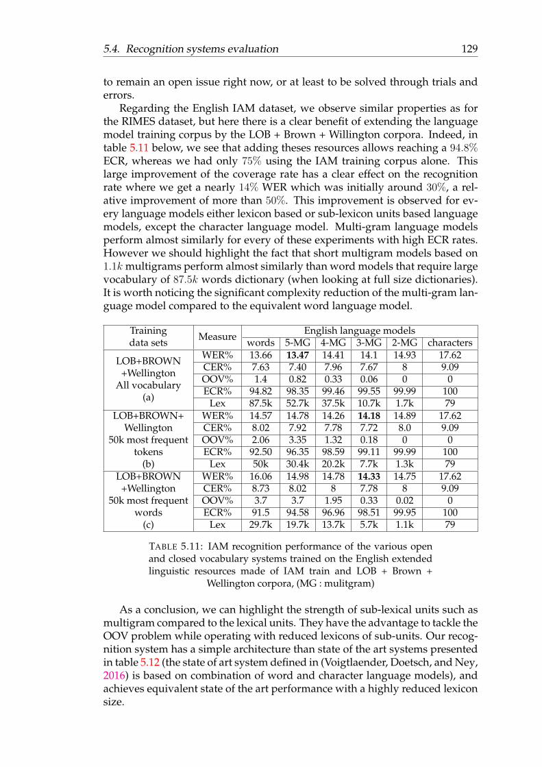
5.4. Recognition systems evaluation 129
to remain an open issue right now, or at least to be solved through trials anderrors.
Regarding the English IAM dataset, we observe similar properties as forthe RIMES dataset, but here there is a clear benefit of extending the languagemodel training corpus by the LOB + Brown + Willington corpora. Indeed, intable 5.11 below, we see that adding theses resources allows reaching a 94.8%ECR, whereas we had only 75% using the IAM training corpus alone. Thislarge improvement of the coverage rate has a clear effect on the recognitionrate where we get a nearly 14% WER which was initially around 30%, a rel-ative improvement of more than 50%. This improvement is observed for ev-ery language models either lexicon based or sub-lexicon units based languagemodels, except the character language model. Multi-gram language modelsperform almost similarly for every of these experiments with high ECR rates.However we should highlight the fact that short multigram models based on1.1k multigrams perform almost similarly than word models that require largevocabulary of 87.5k words dictionary (when looking at full size dictionaries).It is worth noticing the significant complexity reduction of the multi-gram lan-guage model compared to the equivalent word language model.
Trainingdata sets Measure English language models
words 5-MG 4-MG 3-MG 2-MG characters
LOB+BROWN+Wellington
All vocabulary(a)
WER% 13.66 13.47 14.41 14.1 14.93 17.62CER% 7.63 7.40 7.96 7.67 8 9.09OOV% 1.4 0.82 0.33 0.06 0 0ECR% 94.82 98.35 99.46 99.55 99.99 100
Lex 87.5k 52.7k 37.5k 10.7k 1.7k 79LOB+BROWN+
Wellington50k most frequent
tokens(b)
WER% 14.57 14.78 14.26 14.18 14.89 17.62CER% 8.02 7.92 7.78 7.72 8.0 9.09OOV% 2.06 3.35 1.32 0.18 0 0ECR% 92.50 96.35 98.59 99.11 99.99 100
Lex 50k 30.4k 20.2k 7.7k 1.3k 79LOB+BROWN
+Wellington50k most frequent
words(c)
WER% 16.06 14.98 14.78 14.33 14.75 17.62CER% 8.73 8.02 8 7.78 8 9.09OOV% 3.7 3.7 1.95 0.33 0.02 0ECR% 91.5 94.58 96.96 98.51 99.95 100
Lex 29.7k 19.7k 13.7k 5.7k 1.1k 79
TABLE 5.11: IAM recognition performance of the various openand closed vocabulary systems trained on the English extendedlinguistic resources made of IAM train and LOB + Brown +
Wellington corpora, (MG : mulitgram)
As a conclusion, we can highlight the strength of sub-lexical units such asmultigram compared to the lexical units. They have the advantage to tackle theOOV problem while operating with reduced lexicons of sub-units. Our recog-nition system has a simple architecture than state of the art systems presentedin table 5.12 (the state of art system defined in (Voigtlaender, Doetsch, and Ney,2016) is based on combination of word and character language models), andachieves equivalent state of the art performance with a highly reduced lexiconsize.

130 Chapter 5. Handwriting recognition using sub-lexical units
System RIMES-WER% IAM-WER%Our system 10.78 (by m2gram) 13.47 (by m5gram)Voigtlaender, Doetsch, and Ney, 2016 9.6 9.3Bluche et al.Bluche, 2015 11.8 11.9Doetsch et alDoetsch, Kozielski, and Ney, 2014 12.9 12.9Pham et al.Pham et al., 2014 12.3 13.6Zamora-Martínez et al. — 16.1
TABLE 5.12: Performance comparison of the proposed systemwith results reported by other studies on the RIMES & IAM test
datasets.
5.5 Conclusion
In this chapter, a set of sub-lexical units based language models recognitionapproaches have been investigated in order to deal with the challenges relatedto unconstrained continuous handwriting recognition. Experiments have beenconducted on the French RIMES and the English IAM handwriting datasets.Different types of lexicons and language models have been investigated likewords, syllables, multigrams and characters language models. A novel ap-proach was proposed for word decomposition into sub-lexical units such intosyllables and multigrams. To generate the syllabic model we stand on the Lex-ique3 dataset that provides an orthographic syllable modelling for the Frenchlanguage, and on the free English Hyphenation Dictionary (EDH), which pro-poses the orthographic modelling of English words by syllables decomposi-tion. By training a Hidden semi-Markovian Model (HSMM) on a large lexi-con of words of the language of interest (French or English), we were able totrain a model that captures variable length dependencies between charactersin an unsupervised way. For decomposing any word into a sequence of multi-grams, it is sufficient to decode the the words’ character sequence with theHSMM using Viterbi decoding algorithm. The sub-lexical (syllable and multi-grams) based language models offer many advantages over character modelsand word models. The advantages of these models are twofold. On the onehand, it is of limited complexity, since it works with a reduced lexicon of syl-lables. It follows an n-gram model of syllables which is itself more compact,so better parametrized, and therefore easier to optimize. On the other handit offers superior performance than a lexical model when working with outof vocabulary words, while achieving similar performance when trained oncorpus with high ECR on the test corpus.

131
Chapter 6
A Multi-lingual system based onsub-lexical units
6.1 Introduction
For a few decades, most handwriting recognition systems were designed ofrecognizing each language individually, even if they share the same set char-acters such as French and English, or Arabic and Persian. Indeed, Languagesof the same origins often share their character sets and/or glyph shapes. Forexample the Latin-root languages share at least 21 characters (Diringer, 1951),and Arabic, Persian and 12 other languages share at least 28 characters (Märgnerand El Abed, 2012). Inspired from this fact, almost all multilingual or multi-script recognition systems are designed to work with a unified character set(Kessentini, Paquet, and Benhamadou, 2008,Moysset et al., 2014,Kozielski etal., 2014b,Lee and Kim, 1997).
In this chapter we introduce sub-lexical unified models for French and En-glish handwriting recognition as demonstrated in chapter 5. For one singlelanguage a sub-lexical model exhibit a limited complexity in comparison to aword model, while recognition performance decrease very slightly. This prop-erty allows combining multiple languages in a unified sub-lexical model whilemaintaining an acceptable complexity in terms of lexicon size and statistical n-gram language models, maintaining equivalent recognition performance andeven enhanced performance in some cases. We also show that unification ofsimilar scripts in a single recognition system leads to better trained opticalcharacter models, due to the benefit of sharing training datasets between thelanguages, thus providing better performance of the unified system. This is ob-served for any kind of model used (characters, syllables, multigrams, words)on the experiments carried on the RIMES and IAM datasets.
This chapter has the following organisation: section 6.2 presents a litera-ture review about the different approaches used for developing multilingualrecognition systems and related previous work. Section 6.3 describes the char-acter sets, the optical models, the lexicons and the language models unifica-tion methodologies that we have applied for realizing the unified French andEnglish system. Section 6.4 discusses the evaluation protocols and the experi-mental results obtained by the unified recognition system using the specialisedand unified optical models with the association of language models of words,syllables, multigrams and characters. Section 6.5 draws the perspectives of theunified sub-lexical models within the conclusion.
132 Chapter 6. A Multi-lingual system based on sub-lexical units
6.2 Brief literature overview
In the literature there are different possible approaches for developing multi-lingual recognition systems that can be classified into two categories: selectiveapproaches and unified approaches.
6.2.1 Selective approach
The selective approach category includes two approaches. The first approachapplies different individual recognition systems, in a competitive way, for thesame samples and selects the one which provides the best confidence score.The second approach first detects the language of the samples before selectingan appropriate recognizer for the target language script detected (Lee and Kim,1997). The comparison of the scores obtained by several recognizers, whichhave different error ranges, and the pre-detection of the language, which is acomplex task, represent the major problems of these approaches. By exploitingthe multilingual MAURDOR dataset, (Moysset et al., 2014) proposed an En-glish, French and Arabic multilingual recognition system and (Kozielski et al.,2014a) proposed and English, French multilingual recognition system, whichbelong to this category.
6.2.2 Unified approach
The unified approach category uses a single system for recognizing any lan-guage, possibly using multiple scripts. Several multilingual or multiscriptrecognition systems are proposed in the literature. In (Kessentini, Paquet,and Benhamadou, 2008) the authors propose a multilingual system for Arabicand Latin handwriting recognition. In (Malaviya, Leja, and Peters, 1996) theauthors propose a handwriting recognition system for intermixed languagescripts such as Latin, Devanagari, and Kanji. A unified network-based hand-writing recognition system for Hangul and English language was proposedby (Lee and Kim, 1997). These approaches have the advantage of having asingle system for all recognition tasks, avoiding the problems envisaged inthe selective approaches. The disadvantage of the unified approaches is theproportional increase of the system’s complexity regarding to the number oflanguages due to their direct effect on lexicon size, which affects the overallsystem performance.
Almost all the proposed unified approaches are such that the unified multi-lingual system have lower performance in comparison to the specialised mono-lingual systems. This may be explained by the effect of the lexicon and the fastexpansion of the language model, due to the absence of alphabetical and/orlexical shared units between the considered languages and scripts.

6.3. Multilingual unified recognition systems 133
6.2.3 Multilingual with neural networks
Ghoshal et al. (Ghoshal, Swietojanski, and Renals, 2013) have been inves-tigated multilingual modelling using a hybrid system of Deep Neural Net-work (DNN) and Hidden Markov Model (HMM) for achieving speech recog-nition task. They carried out the experiment on the GlobalPhone corpus usingseven languages from three different language families: Germanic, Romance,and Slavic. This work focused on the multilingual acoustic modeling, andmade use of the pronunciation dictionary and language model of GlobalPhone(ready for use). This work concluded that the deep neural networks performa cascade of feature extraction, from lower-level to higher-level features, pro-vides an explanation for the promised enhancement that comes from the train-ing the hidden layers using data from multiple languages.
6.3 Multilingual unified recognition systems
The previous literature review has given us the motivation for designing a uni-fied system, which has the great advantage to be easy to implement because,only one single system must be designed and optimized. By combining thestrength of BLSTM used for the optical model, and the low complexity of sub-lexical units, we expect to get a lightly and powerful recognizer. To this end,this section describes the unified design approach that we conducted on theFrench and English systems components. The unification process includes theunification of the optical models, the lexicons and finally the language models,as illustrated in figure 6.1.
FIGURE 6.1: The three unification stages in the design process ofa unified recognizer.
The benefit of using the sub-lexical units (syllables and multigrams) forbuilding multilingual handwriting recognition systems has been studied through

134 Chapter 6. A Multi-lingual system based on sub-lexical units
two successive experiments. The first experiment aimed to examine the recog-nition performance of a unified handwriting recognition system with HMMoptical models operated with language models of words, syllables and char-acters. The system configuration was prepared to simulate an ideal case studyfor which we considered language models with a null OOV rate (all languagemodels fully covered the test dataset).
The objective of this experiment was to highlight the competitive perfor-mance of the syllable based model in comparison with the word and charactermodels. We will not spend much lines to discuss this first experiment. Theinterested reader can refer to (Swaileh and Paquet, 2016a) to get more infor-mation, but the most important conclusion to us was the fact that we observedsimilar performance when running the unified system, to those of each special-ized system. By the second experiment, we aimed to study the contribution ofthe unified optical and language models to the recognition performance of theunified handwriting recognition system which was based on state of the artBLSTM-RNN. Moreover, the experimental setup was design by consideringdifferent OOV rates of the unified lexicons and language models. In the fol-lowing paragraphs we describe the properties of each unified model.
6.3.1 Character set unification
The RIMES dataset is composed of 100 character classes while the IAM datasetcontains only 79 character classes. 77 character (including the white spacecharacter) classes are shared between the two datasets while in total the twodatasets contain 102 character classes. The whole character set of the EnglishIAM training dataset is included in the French RIMES training dataset excepttwo characters:"#" and "&". Of course, most of the additional character classesin the RIMES dataset are accented character. By looking at the distribution
FIGURE 6.2: Statistics of the shared characters between theFrench RIMES and the English IAM database
of characters over the two datasets, we can see in figure 6.2. that lower casecharacters are more frequent in the RIMES training dataset that because it con-tains 9947 sentence, 8107 word and 470, 317 character. On the other hand, IAMtraining dataset consists of 6482 sentence, 9956 word and 287, 727 character.The total number of characters in IAM training dataset represents 61.18% ofthe RIMES training dataset total number of characters. We believe that this

6.3. Multilingual unified recognition systems 135
difference in character frequencies may improve the unified optical model byhaving more training data for every classes.
6.3.2 Optical models unification
The unified French and English character set of the RIMES and IAM dataset aremodelled by a BLSTM-RNN. Training the unified BLSTM-CTC optical modelhas been carried out by combining the RIMES and IAM training datasets. Asalready presented in chapter 5, a curriculum learning like algorithm was intro-duced by sorting the training examples according to their image width. Fur-thermore, the French and English RIMES and IAM validation datasets havebeen combined for controlling the training process. The training process startswith a learning rate of 10−5 and ends with a value of 2.79e−07 after 108 train-ing epochs. Figure 6.3 shows the evolution of the network performance (CER)during the training epoch.
FIGURE 6.3: Evolution of the CER during the training epochs.
The unified optical model achieves a 8, 33% CER on the unified RIMES+IAMvalidation dataset which should be compared to CER obtained when trainingseparately the network on the RIMES and on the IAM dataset. In this casethe CER was 8, 95% on the RIMES dataset and 10, 41% on the IAM validationdatasets. This phenomenon can be explained by the effect of having moretraining data as illustrated in figure 6.2.
6.3.3 Lexicons unification
The third step in building the multilingual handwriting recognition systemis the unification of the French and English vocabularies (lexicons) and lan-guage models which are used by the system during the recognition process.Figure 6.4 shows the evolution of the various lexicons on the three datasets.It highlights the small increase of the 2-multigram lexicon and of the syllablelexicon when considering the unified corpus, while the word lexicon is the

136 Chapter 6. A Multi-lingual system based on sub-lexical units
FIGURE 6.4: Size of the various lexicons on the RIMES, IAM, andthe unified datasets (from left to right).
most affected in size. Similarly, We see that higher order multigrams lexiconsare more affected in size when considering the unified corpus. This is a directcombinatorial affect when looking at higher order multigrams.
FIGURE 6.5: ECR of the RIMES test dataset by the words, syl-lables and multigrams of the three corpora(from left to right :
RIMES, IAM, RIMES+IAM.
For a better understanding of the effect of unifying the two datasets, theeffective coverage rates (ECR) of the words, syllables, and multigrams lexicons(5-multigram, 4-multigram, 3-multigram, 2-multigram) on the RIMES datasetsis plotted on figure 6.5. We see that the unified lexicon has a very small effecton the ECR of the RIMES dataset. Figure 6.6 gives the ECR of the IAM datasetby the three corpora. We see that the unified lexicon improves the ECR forthe higher order multigrams and the word lexicons, whereas for low ordermultigram the best ECR is obtained with a very small lexicon.

6.3. Multilingual unified recognition systems 137
FIGURE 6.6: ECR of the IAM test datasets by the words, syllablesand multigrams of the three corpora (from left to right : IAM,
RIMES, RIMES+IAM).
To explore the impact of unifying external French and English linguistic re-sources on the same recognition task on RIMES and IAM test dataset, we uni-fied the English LOB, Brown and Wellington corpora lexicons with the FrenchWikipedia + RIMES training dataset lexicons. Let EN denotes the English lex-icons and language models that make use of the LOB, Brown and Wellingtoncorpus and let FR denotes the French lexicons and language models that makeuse of Wikipedia + RIMES corpora. We have to recall here that the EN lexiconmake use of all the corpus vocabulary while the FR lexicon make use only the50k most frequent words (29k token) of the Wikipedia corpora. The lexiconevolution on the FR, EN and the unified dataset is illustrated by figure 6.7.
FIGURE 6.7: Size of the various lexicons on the FR, EN, and theunified datasets (from left to right).
In table 6.1 we report the ECR of the RIMES and IAM test dataset for thevarious lexicons derived from the three corpora (RIMES, IAM, IAM+RIMES).And we compare them to the ECR obtained with the specialized lexicons. Weobserve that the unified lexicons have higher ECR of the RIMES and the IAM

138 Chapter 6. A Multi-lingual system based on sub-lexical units
test datasets, for example the lexicon of word of IAM training dataset coversthe IAM test dataset by 75.45% with 7.4k word tokens, while the same unifiedFrench and English lexicon of word covers the same test dataset by 80% with12k word token.
Lexicon type ECR of RIMESby RIMES
ECR of RIMESby IAM+RIMES
ECR of IAMby IAM
ECR of IAMby IAM+RIMES
Lexicon sizeof IAM+RIMES
words 93.29 96.23 75.45 80 12.5k5-multigram 97.43 97.76 84.18 85.81 10.9k4-multigram 98.01 98.53 88.59 89.9 8.5k3-multigram 98.98 99.14 92.97 96.22 4.6k
syllables 98.84 99.14 91.1 94.5 6.7k2-multigram 99.53 99.71 99.42 99.46 1.3k
TABLE 6.1: Comparing the ECR of RIMES and IAM achieved bythe specialized corpora alone, and by the unified corpus.
Similarly, in table 6.2 we report the ECR of the RIMES and IAM test datasetfor the lexicons derived from the FR, EN and FR+EN corpora. The same phe-nomena is repeating with these lexicons, the FR lexicon covers the RIMES testdataset by 82.27% with 29k word token while the unified FR+EN lexicon ofwords covers the same test dataset by 89.97% with 116k word token.
Lexicon type ECR of RIMESby FR
ECR of RIMESby FR+EN
ECR of IAMby EN
ECR of IAMby FR+EN
Lexicon sizeof FR+EN
words 82.27 89.97 95.13 98.6 116k5-multigram 93.73 95.22 98.34 98.58 71.6k4-multigram 96.37 98.2 99.46 99.68 50.5k3-multigram 97.32 98.48 99.48 99.8 16.9k2-multigram 99.48 99.82 100 100 3.1k
TABLE 6.2: Comparing the ECR of RIMES and IAM achieved bythe FR and EN corpora individually, and by the unified FR+EN
corpus.
6.3.4 Unified language models
The unified French and English vocabulary of the RIMES / IAM training cor-pora of words, syllables, multigrams (2-multigram, 3-multigram, 4-multigramand 5-multigram) and characters are used to train their corresponding (openor closed) language model. The n-gram language models were trained withthe modified Kneser-Ney smoothing method supported by the MIT languagemodelling toolkit. To consider the long distance dependencies while trainingthe language models, we trained 9-gram language models of words and multi-grams (5-multigram, 4-multigram, 3-multigram and 2-multigram) in additionto 10-gram language model of characters. Table 6.3 reports the perplexity val-ues and OOV rates of these models and compares theme to the values obtainedwith the specialized corpora.
We observed for the tables 6.3 and 6.4 that the OOV % rate reported forthe unified IAM+RIMES models on the RIMES and IAM test datasets are less

6.3. Multilingual unified recognition systems 139
Languagemodels
Unified IAM+RIMES modelsperplexiyon RIMES
perplexityon IAM
perplexty onIAM+RIMES
OOV %on RIMES
OOV %on IAM
OOV % onIAM+RIMES
words 17.26 33.98 29.28 2.9 13.9 11.535-multigram 15.62 45.92 35.92 1.37 9.96 7.994-multigram 14.61 45.65 35.34 0.85 6.3 5.023-multigram 13.52 43.78 33.80 0.44 1.61 1.35
syllables 13.29 42.16 29.18 0.45 4.5 2.82-multigram 12.11 22.66 19.76 0.11 0.10 0.1
characters 11.96 13.55 13.17 0 0 0
TABLE 6.3: Unified language models perplexities and OOV rates,for the specialized and unified corpus.
Languagemodels
SpecializedRIMES models
SpecializedIAM models
perplexity OOV % perplexity OOV %words 13.52 3.10 27.6 14.1
5-multigram 11.84 1.61 35.52 10.954-multigram 11.16 1.16 37.29 7.33-multigram 10.18 0.53 35.90 2.2
syllables 10.86 0.63 33.94 5.012-multigram 9.21 0.16 20.03 0.22
characters 9.6 0 12.1 0
TABLE 6.4: Specialized language models perplexities and OOVrates, for the specialized corpora.
than the ones reported for the specialized models on the same test datasets,for example the unified language model of word OOV% rate is less than thespecialized one by 0.2% on the RIMES and IAM test datasets. On the otherhands, the perplexity of the unified models are greater than the specializedones, for example; the perplexity of the unified language model of words onthe RIMES test data set is 17.26 where the specialized model of words have aperplexity of 13.52 on the same test dataset.
Language models Unified FR+EN modelsperplexityon RIMES
perplexityon IAM
perplexity onIAM+RIMES
OOV%on RIMES
OOV%on IAM
OOV% onIAM+RIMES
words 32.15 43.78 41.12 7.9 1.15 2.55-multigram 33.04 41.54 39.53 3.14 0.75 1.34-multigram 30.36 35.42 34.25 0.93 0.29 0.43-multigram 26.47 28.09 27.73 0.68 0.03 0.182-multigram 22.62 21.94 22.09 0.06 0 0.01Characters 18.82 19.04 18.98 0 0 0
TABLE 6.5: Unified FR+EN language models perplexities andOOV rates, for the specialized (FR and EN) and unified (FR+EN)
corpus.
With the FR and EN unified lexicons we trained the large vocabulary lan-guage models of words, muligrams and characters and their perplexities and
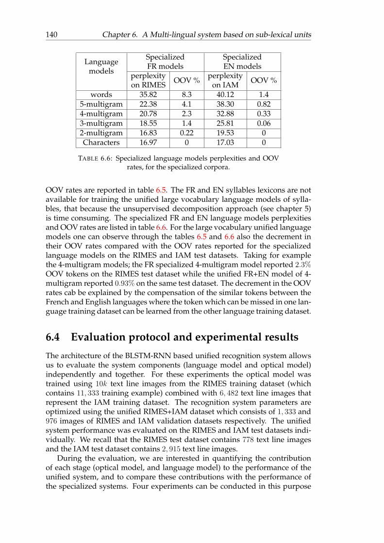
140 Chapter 6. A Multi-lingual system based on sub-lexical units
Languagemodels
SpecializedFR models
SpecializedEN models
perplexityon RIMES OOV % perplexity
on IAM OOV %
words 35.82 8.3 40.12 1.45-multigram 22.38 4.1 38.30 0.824-multigram 20.78 2.3 32.88 0.333-multigram 18.55 1.4 25.81 0.062-multigram 16.83 0.22 19.53 0Characters 16.97 0 17.03 0
TABLE 6.6: Specialized language models perplexities and OOVrates, for the specialized corpora.
OOV rates are reported in table 6.5. The FR and EN syllables lexicons are notavailable for training the unified large vocabulary language models of sylla-bles, that because the unsupervised decomposition approach (see chapter 5)is time consuming. The specialized FR and EN language models perplexitiesand OOV rates are listed in table 6.6. For the large vocabulary unified languagemodels one can observe through the tables 6.5 and 6.6 also the decrement intheir OOV rates compared with the OOV rates reported for the specializedlanguage models on the RIMES and IAM test datasets. Taking for examplethe 4-multigram models; the FR specialized 4-multigram model reported 2.3%OOV tokens on the RIMES test dataset while the unified FR+EN model of 4-multigram reported 0.93% on the same test dataset. The decrement in the OOVrates cab be explained by the compensation of the similar tokens between theFrench and English languages where the token which can be missed in one lan-guage training dataset can be learned from the other language training dataset.
6.4 Evaluation protocol and experimental results
The architecture of the BLSTM-RNN based unified recognition system allowsus to evaluate the system components (language model and optical model)independently and together. For these experiments the optical model wastrained using 10k text line images from the RIMES training dataset (whichcontains 11, 333 training example) combined with 6, 482 text line images thatrepresent the IAM training dataset. The recognition system parameters areoptimized using the unified RIMES+IAM dataset which consists of 1, 333 and976 images of RIMES and IAM validation datasets respectively. The unifiedsystem performance was evaluated on the RIMES and IAM test datasets indi-vidually. We recall that the RIMES test dataset contains 778 text line imagesand the IAM test dataset contains 2, 915 text line images.
During the evaluation, we are interested in quantifying the contributionof each stage (optical model, and language model) to the performance of theunified system, and to compare these contributions with the performance ofthe specialized systems. Four experiments can be conducted in this purpose

6.4. Evaluation protocol and experimental results 141
as depicted on figure 6.8 below. The first setup (1=UU, in green) consists incombining the unified optical model with the unified language models. Thesecond setup (2=US, in red) consists in combining the unified optical modelwith the specialized language model. The third setup (3=SU, in orange) com-bines the specialized optical model with the unified language model. Finally,the fourth setup (4=SS, in blue) combines the specialized optical model withthe specialized language model. The four setups will be evaluated on the IAMdataset and the RIMES dataset.
FIGURE 6.8: The four experimental setups for analyzing the re-spective contributions of the unified optical models and the lan-
guage models.
For the specialized and unified optical models, we evaluated two differ-ent groups of language models on the RIMES and IAM test datasets; the firstgroup contains the small vocabulary language models that are trained on theRIMES, IAM and the unified IAM+RIMES training datasets. The second groupcontains the large vocabulary language models which are trained with the FR,EN and FR+EN lexicons on their corresponding FR (Wikipedia + RIMES), EN(LOB, Brown and Wellington) corpora and the unified FR+EN training cor-pora.
A preliminary result is provided by analyzing the raw performance of theunified optical model alone. As reported in table 6.7 below, a slight improve-ment of the performance around 2% WER and CER on the RIMES datasets isobserved, compared to the performance of the specialized optical model. A3% improvement is observed on the IAM datasets, for both the WER and CER.This is a direct effect of having more data for training the optical model whichshare a lot of character classes, such improvement would not be possible forlanguages that do not share so many character classes, for examples languageswritten using different scripts.
Test datasetsRIMES optical
modelIAM optical
modelUnified optical
modelCER WER CER WER CER WER
RIMES 12.32 38.88 – – 10.02 36.3IAM – – 18.91 52.13 15.26 44.41
TABLE 6.7: Specialized and unified optical model raw perfor-mance (without language model).

142 Chapter 6. A Multi-lingual system based on sub-lexical units
We now provide the detailed analysis of the performance of the two unifiedstages using the four setups depicted above and for the two test datasets.
6.4.1 Results on RIMES test dataset
FIGURE 6.9: WER (%) on the RIMES dataset using the four ex-perimental setups : blue = SS, Orange = SU, Red = US, Green =
UU.
Figure 6.9 shows the performance obtained with the four configurations ofthe system, as a function of the lexical units considered (words, multigrams,and characters). A performance enhancement of around 1% of the WER isreported for every system that integrates the unified optical model (Red andGreen curves). Improvement is observed for every language models, whichperform nearly equally and better than the word language model, and thecharacter language model. The contribution of the unified language modelappears rather moderate compared to the improvement brought by the opticalmodel. But most importantly, we can highlight the fact that unifying two lan-guages in one single model does not affect the recognition performance. Thisis observed for both optical models, either specialized or unified. These in-teresting results must be analysed also by considering the lexicon size of thesub-lexical units based language models which is rather small when consider-ing character and 2-multigrams.
Similar to the experiments with small vocabulary language models, we car-ried the experiments with the FR large vocabulary language models whichgave the results illustrated in figure 6.10. These experiments results presentdifferent observations. Looking at the blue (SS) and orange (SU) curves we ob-serve that unifying large vocabulary language models (FR+EN) does not affectbrutally the recognition performance even if their unified FR and EN lexicons
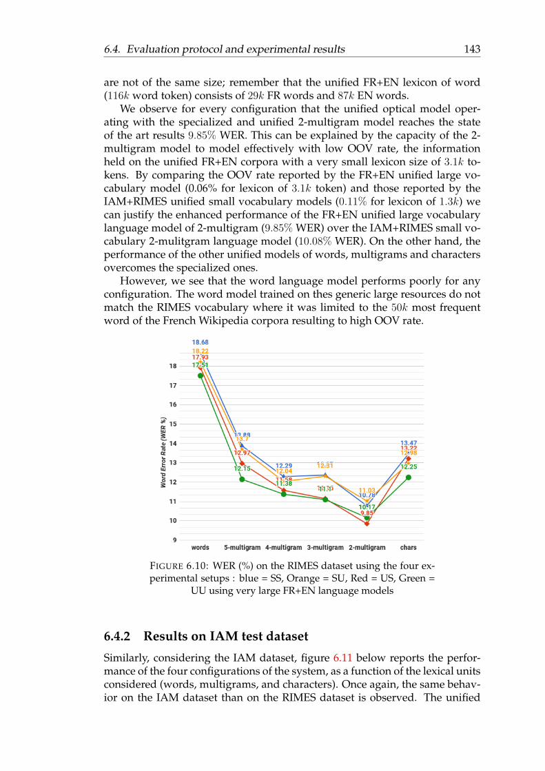
6.4. Evaluation protocol and experimental results 143
are not of the same size; remember that the unified FR+EN lexicon of word(116k word token) consists of 29k FR words and 87k EN words.
We observe for every configuration that the unified optical model oper-ating with the specialized and unified 2-multigram model reaches the stateof the art results 9.85% WER. This can be explained by the capacity of the 2-multigram model to model effectively with low OOV rate, the informationheld on the unified FR+EN corpora with a very small lexicon size of 3.1k to-kens. By comparing the OOV rate reported by the FR+EN unified large vo-cabulary model (0.06% for lexicon of 3.1k token) and those reported by theIAM+RIMES unified small vocabulary models (0.11% for lexicon of 1.3k) wecan justify the enhanced performance of the FR+EN unified large vocabularylanguage model of 2-multigram (9.85% WER) over the IAM+RIMES small vo-cabulary 2-mulitgram language model (10.08% WER). On the other hand, theperformance of the other unified models of words, multigrams and charactersovercomes the specialized ones.
However, we see that the word language model performs poorly for anyconfiguration. The word model trained on thes generic large resources do notmatch the RIMES vocabulary where it was limited to the 50k most frequentword of the French Wikipedia corpora resulting to high OOV rate.
FIGURE 6.10: WER (%) on the RIMES dataset using the four ex-perimental setups : blue = SS, Orange = SU, Red = US, Green =
UU using very large FR+EN language models
6.4.2 Results on IAM test dataset
Similarly, considering the IAM dataset, figure 6.11 below reports the perfor-mance of the four configurations of the system, as a function of the lexical unitsconsidered (words, multigrams, and characters). Once again, the same behav-ior on the IAM dataset than on the RIMES dataset is observed. The unified

144 Chapter 6. A Multi-lingual system based on sub-lexical units
optical model increases the WER by 4% and the CER by 2% CER, compared tothe performance of the systems that integrate a specialized optical model. Thisis observed for any of the small vocabulary language models with the best im-provement observed for the sub-lexical units based systems and especially forthe 2-multigram language model. Once again the contribution of the languagemodel appear rather limited to the recognition performance, but consideringthe two French and English languages there is no reason to believe that someperformance improvement should be gain by combining the two language.In fact, we could expect that the language modelling task should become morecomplex. These results clearly show that the unification of both language mod-els in one single language model has nearly no effect on the performance. Thiswas also observed on the RIMES dataset. As a conclusion we can highlightthat combining the two models allows improving the performance of the opti-cal model by the benefit of having more training samples per character classes,while at the same time combining the sub-lexical units based language mod-els does not degrade the performance while getting a very compact bi-linguallanguage model, with a small lexicon size.
FIGURE 6.11: WER (%) on the IAM dataset using the four exper-imental setups : blue = SS, Orange = SU, Red = US, Green = UU.
The large vocabulary FR, EN and the unified FR+EN language model wasevaluated for the four evaluation setups and the obtained results are illustratedin figure 6.12. The results shows the best recognition performances are ob-tained with the unified optical models with all language models. The special-ized optical model that works with the unified FR+EN language models showa slight performance degradation (as shown by the orange curve) comparedto the EN language models (blue curve) for all language models except the4-multigram and the characters language models.
By recalling the lexicon size and the OOV rates reported for the large vocab-ulary FR+EN unified languages model and the small vocabulary IAM+RIMESlanguage models listed in the tables 6.3, 6.4, 6.5 and 6.6, we observed thatthe unified large vocabulary language models reports small OOV rates whichjustify their state of the art recognition performance. For example: the uni-fied FR+EN large vocabulary language model of word reported 1.15% OOVwords while the specialized EN language model of word reported 1.4% OOV

6.5. Conclusion 145
words For this reason even the unified language model of words shows simi-lar performance as the multigram ones with the advantage of the small unifiedFR+EN lexicon size of multigram.
FIGURE 6.12: WER (%) on the IAM dataset using the four exper-imental setups : blue = SS, Orange = SU, Red = US, Green = UU
using very large FR+EN language models
6.5 Conclusion
In this chapter we studied the unified French/English models of words, sylla-bles, multigrams and characters for handwriting recognition. The sub-lexicalunits based systems offer many advantages over the character model whichmodels badly the words, and over the word model which models only a lim-ited number of words that are found in the vocabulary of the training corpus.The evaluation of the unified (optical and language) models in different op-erating setup with the specialized (optical and language) models offered usa clear vision about the behavior of the unified models. The enhancement ofthe unified optical model has the major contribution in enhancing the overallrecognition system performances as shown by the results above. The unifiedlanguage models have a slight enhancing contribution when they are operat-ing with the unified optical models. Indeed, they show equivalent behaviorto the pure specialized (optical and language) models behavior when operat-ing with the specialized optical models. But the more important contributionof these results regarding the language models is to show that one single bi-lingual language model composed of sub-lexical units does not degrade theperformance, thus allowing the design of lightly language models composedof sub-lexical units of both languages that can be introduced in one singlerecognition engine. As a general conclusion, these results show that sub-lexicalunits are good units for both French and English languages and that they sup-port to be mixed into one single recognition system.


147
Conclusions and Perspectives
The main goal of this thesis was to develop improved language modellingapproaches for performing efficient large vocabulary unconstrained and con-tinuous handwriting recognition of French and English handwritten docu-ments. In the literature, large vocabulary handwriting recognition systemsare described based on two main components: an optical model and a lan-guage model. The optical model matches the handwriting script observed inan image as a numerical sequence of observations features (denoted by S) toa sequence of characters which may represent a sequence of words (denotedby W) by the computation of a likelihood function denoted by P(S|W). Thelanguage model constrains the recognition hypotheses to be some admissi-ble sequences of words by the language, by the computation of the a prioriprobability P(W) of each hypothesis. In between the sequence of charactersproduced by the optical model and the sequence of words examined by thelanguage model, the system’s vocabulary allows to constrain the character hy-potheses to be some admissible words only. In practice, there is no vocabularywhich can cover all language words, including named entities and alphanu-meric strings such as reference numbers or bank identification numbers. As aconsequence, the words which are not introduced in the system’s vocabulary(Out-Of-Vocabulary words, OOV) can not be recognized by the system. This iswhat is called a closed vocabulary recognition system. To improve the recogni-tion performance one may try to increase the size of the system’s vocabulary,so as to reduce the OOV rate. But this is only possible with the expense ofincreasing the system’s complexity which leads to the degradation of the sys-tem’s performance. Therefore, it is required to find a compromise betweenthe vocabulary size, the time complexity of the system, and the recognitionperformance.
In the literature, there is two types of language model: closed vocabularylanguage models and open vocabulary language models. The closed vocabu-lary language models are trained on a fixed size vocabulary and any sequenceof words (W) that contains one or more OOVs are discarded from the estima-tion of the language model. On the contrary, the open vocabulary languagemodels account for the OOV words by affecting them a certain amount of thetotal probability thanks to the unknown class (<unk>), which introduces theOOV words within the language model vocabulary and training corpus. Fur-thermore, the OOVs can be represented in the language model vocabulary andtraining corpus by their sequence of characters. Thus, the language model willrepresent a hybrid language model of words and characters. But such mod-elling approach is not convenient, because words and character classes arecompeting each other, which increases the language model confusion. A freelexicon recognition system can be used to tackle the OOV problem. This sys-tem makes use of character classes only, with a high order language model to

148 Chapter 6. A Multi-lingual system based on sub-lexical units
introduce sufficient context in the model. Doing this way, almost every possi-ble character string is admissible, and there is almost no OOV. However, evenhigh order character language models perform poorly when working alonebecause of their poor capacity to model the context of the language sentence.Another effective way to tackle the OOV problem is to train separately twolanguage models: a word language model accounting for the most frequentwords in the training corpus, and a character language model. During the de-coding procedure the two models are synchronously working where the lan-guage model of character is introduced where the word language model hasdecoded an OOV word.
Alternatively, in this thesis we introduced sub-lexical units made of sylla-bles or multigrams in order to tackle the OOV problem. A complete process-ing chain of handwriting processing and recognition was implemented fromline detection in the document image to line recognition using the proposedopen-vocabulary sub-lexical units based language model. An automatic iter-ative text line segmentation smearing method was proposed with which weenhanced the extraction of the text line images on different datasets, withoutthe need to tune any parameter. Two types of optical models have been imple-mented. The first implementation consists of a classical HMM optical modelworking with Histogram of Gradient (HoG) features. The second implemen-tation consists of a state of the art BLSTM-RNN optical model which dealswith the pixel values directly. These systems have been trained and evalu-ated on the French RIMES and the English IAM datasets. The efficiency of theBLSTM-RNN optical model over the HMM one was noticeable by looking atthe Character Error Rate (CER) rates for the optical models alone. The systemvocabulary and language models were trained on the RIMES and IAM datasetsas well as on some additional external resources such as the French and En-glish Wikipedia pages and the English LOB, Brown and Wellington datasets.The results obtained with the BLSTM-RNN based recognition system are closeto the state of the art performance with the advantage of the system’s simplearchitecture with a reduced complexity thanks to the use of sub lexical units.
Sub-lexical based language models have been investigated using multi-grams and syllables. Two approaches have been used to provide word de-composition into sub-lexical units: a supervised and an unsupervised worddecomposition approach. Small and large vocabularies have been employedin the recognition systems in order to assess the actual potential of sub-lexicalbased models compared to full-word models. This approach has led to a sig-nificant increase in the overall lexical coverage, indicated by a considerablereduction of the out-of-vocabulary (OOV) rates measured on the test datasets.This has introduced a promising step towards the solution of dealing withlexicon with low coverage rates. As a result, significant improvements of therecognition performance have been achieved compared to the traditional full-word based language models.
Motivated by the interesting recognition performance obtained with sub-lexical units, we studied the possibilities of building a unified handwritingrecognition system for the French and English languages. The unification ofthe individual (specialised) French and English recognition systems has been

6.5. Conclusion 149
examined considering both the unification of the optical model and the uni-fication of the language model. By the introduction of sub-lexical units, theunified recognition system outperforms each individual specialized system.
As perspectives to the use of sub-lexical units in a handwriting recogni-tion system we can mention the use of connectionist language models. Suchmodels can account for variable length dependencies of language units in thelanguage model. This would remove the constraint of using the fix lengthdependency modelling introduced by the n-gram modelling approach. Also,by introducing connectionist language models we may explore new systemarchitectures composed solely of RNN for both the optical stage and the lan-guage stage. In this respect, we may take inspiration from the recent attentionmodels that have been proposed to achieve caption generation from images,or translation tasks. Another perspective is to introduce sub-lexical units inthe optical model, which would allow to introduce some multigrams opticalmodel accounting for the most frequent co-occuring characters. This could bedone at the expense of increasing the number of classes in the optical model.Finally, we may extend the unified modelling approache to include more lan-guages, possibly with different scripts such as Hindi, or Arabic languages toexplore more in depth the advantages of using sub-lexical units for unifyinghandwriting recognition systems.


151
Bibliography
Abadi, Martín et al. (2016). “Tensorflow: Large-scale machine learning on het-erogeneous distributed systems”. In: arXiv preprint arXiv:1603.04467.
Abdel-Hamid, Ossama et al. (2012). “Applying convolutional neural networksconcepts to hybrid NN-HMM model for speech recognition”. In: Acoustics,Speech and Signal Processing (ICASSP), 2012 IEEE International Conference on.IEEE, pp. 4277–4280.
AbdulKader, Ahmad (2008). “A two-tier Arabic offline handwriting recogni-tion based on conditional joining rules”. In: Arabic and Chinese HandwritingRecognition. Springer, pp. 70–81.
Adda-Decker, Martine (2003). “A corpus-based decompounding algorithm forGerman lexical modeling in LVCSR.” In: INTERSPEECH.
Adda-Decker, Martine and Gilles Adda (2000). “Morphological decompositionfor ASR in German”. In: Workshop on Phonetics and Phonology in ASR, Saar-brücken, Germany, pp. 129–143.
Ahmad, Irfan and Gernot A Fink (2016). “Class-Based Contextual Modeling forHandwritten Arabic Text Recognition”. In: Frontiers in Handwriting Recogni-tion, 2016. Proceedings. fifteenth International conference ICHFR. IEEE, pp. 369–374.
Ait-Mohand, Kamel, Thierry Paquet, and Nicolas Ragot (2014). “Combiningstructure and parameter adaptation of HMMs for printed text recognition”.In: Pattern Analysis and Machine Intelligence, IEEE Transactions on 36.9, pp. 1716–1732.
Allauzen, Cyril et al. (2007). “OpenFst: A general and efficient weighted finite-state transducer library”. In: International Conference on Implementation andApplication of Automata. Springer, pp. 11–23.
Arica, Nafiz and Fatos T Yarman-Vural (2001). “An overview of character recog-nition focused on off-line handwriting”. In: IEEE Transactions on Systems,Man, and Cybernetics, Part C (Applications and Reviews) 31.2, pp. 216–233.
Bacchiani, Michiel et al. (1996). “Design of a speech recognition system basedon acoustically derived segmental units”. In: Acoustics, Speech, and SignalProcessing, 1996. ICASSP-96. Conference Proceedings., 1996 IEEE InternationalConference on. Vol. 1. IEEE, pp. 443–446.
Bahrampour, Soheil et al. (2015). “Comparative study of caffe, neon, theano,and torch for deep learning”. In: arXiv preprint arXiv:1511.06435.
Bartlett, Susan, Grzegorz Kondrak, and Colin Cherry (2009). “On the syllabi-fication of phonemes”. In: Proceedings of Human Language Technologies: The2009 Annual Conference of the North American Chapter of the Association forComputational Linguistics. Association for Computational Linguistics, pp. 308–316.

152 BIBLIOGRAPHY
Bassil, Youssef and Mohammad Alwani (2012). “Ocr post-processing error cor-rection algorithm using google online spelling suggestion”. In: arXiv preprintarXiv:1204.0191.
Bastien, Frédéric et al. (2012). “Theano: new features and speed improvements”.In: arXiv preprint arXiv:1211.5590.
Bauer, Laurie (1993). Manual of information to accompany the Wellington corpus ofwritten New Zealand English. Department of Linguistics, Victoria Universityof Wellington Wellington.
Beeton, Barbara (2010). “Hyphenation exception log”. In: TUGboat-TeX UsersGroup 31.3, p. 160.
Bengio, Yoshua, Patrice Simard, and Paolo Frasconi (1994). “Learning long-term dependencies with gradient descent is difficult”. In: IEEE transactionson neural networks 5.2, pp. 157–166.
Bengio, Yoshua et al. (1995). “LeRec: A NN/HMM hybrid for on-line hand-writing recognition”. In: Neural Computation 7.6, pp. 1289–1303.
Bengio, Yoshua et al. (2003). “A neural probabilistic language model”. In: Jour-nal of machine learning research 3.Feb, pp. 1137–1155.
Bengio, Yoshua et al. (2009). “Curriculum learning”. In: Proceedings of the 26thannual international conference on machine learning. ACM, pp. 41–48.
BenZeghiba, Mohamed Faouzi, Jerome Louradour, and Christopher Kermor-vant (2015). “Hybrid word/Part-of-Arabic-Word Language Models for ara-bic text document recognition”. In: Document Analysis and Recognition (IC-DAR), 2015 13th International Conference on. IEEE, pp. 671–675.
Berger, Adam L, Vincent J Della Pietra, and Stephen A Della Pietra (1996). “Amaximum entropy approach to natural language processing”. In: Computa-tional linguistics 22.1, pp. 39–71.
Bimbot, Frederic et al. (1994). “Modeles de séquencesa horizon variable: Multi-grams”. In: Proc. XX-emes Journées d’Etude sur la Parole, pp. 467–472.
Bisani, Maximilian and Hermann Ney (2005). “Open vocabulary speech recog-nition with flat hybrid models.” In: INTERSPEECH, pp. 725–728.
— (2008). “Joint-sequence models for grapheme-to-phoneme conversion”. In:Speech Communication 50.5, pp. 434–451.
Bledsoe, Woodrow Wilson and Iben Browning (1959). Pattern recognition andreading by machine. PGEC.
Bluche, Théodore (2015). “Deep Neural Networks for Large Vocabulary Hand-written Text Recognition”. PhD thesis. Université Paris Sud-Paris XI.
Bluche, Théodore, Hermann Ney, and Christopher Kermorvant (2013a). “Fea-ture extraction with convolutional neural networks for handwritten wordrecognition”. In: 2013 12th International Conference on Document Analysis andRecognition. IEEE, pp. 285–289.
Bluche, Theodore, Hermann Ney, and Christopher Kermorvant (2013b). “Tan-dem HMM with convolutional neural network for handwritten word recog-nition”. In: Acoustics, Speech and Signal Processing (ICASSP), 2013 IEEE Inter-national Conference on. IEEE, pp. 2390–2394.
Bluche, Théodore, Hermann Ney, and Christopher Kermorvant (2014). “A Com-parison of Sequence-Trained Deep Neural Networks and Recurrent NeuralNetworks Optical Modeling for Handwriting Recognition”. In: International

BIBLIOGRAPHY 153
Conference on Statistical Language and Speech Processing. Springer, pp. 199–210.
Bluche, Théodore et al. (2014). “The a2ia arabic handwritten text recognitionsystem at the open hart2013 evaluation”. In: Document Analysis Systems(DAS), 2014 11th IAPR International Workshop on. IEEE, pp. 161–165.
Bourlard, Hervé and Christian J Wellekens (1990). “Links between Markovmodels and multilayer perceptrons”. In: IEEE Transactions on Pattern Anal-ysis and Machine Intelligence 12.12, pp. 1167–1178.
Brainstorm (2015). Brainstorm Kernel Description. URL: https://github.com/IDSIA/brainstorm (visited on 02/25/2017).
Brakensiek, Anja, Jörg Rottland, and Gerhard Rigoll (2002). “Handwritten ad-dress recognition with open vocabulary using character n-grams”. In: Fron-tiers in Handwriting Recognition, 2002. Proceedings. Eighth International Work-shop on. IEEE, pp. 357–362.
Broder, Andrei Z et al. (1997). “Syntactic clustering of the web”. In: ComputerNetworks and ISDN Systems 29.8-13, pp. 1157–1166.
Brown, Keith (2006). “Encyclopedia of language and linguistics”. In:Brown, Peter F et al. (1990). “A statistical approach to machine translation”. In:
Computational linguistics 16.2, pp. 79–85.Bukhari, Syed Saqib, Faisal Shafait, and Thomas M Breuel (2009). “Script-independent
handwritten textlines segmentation using active contours”. In: 2009 10th In-ternational Conference on Document Analysis and Recognition. IEEE, pp. 446–450.
Bullinaria, John A (2004). “Introduction to neural networks”. In: Lecture notes.Bunke, Horst, Samy Bengio, and Alessandro Vinciarelli (2004). “Offline recog-
nition of unconstrained handwritten texts using HMMs and statistical lan-guage models”. In: IEEE transactions on Pattern analysis and Machine intelli-gence 26.6, pp. 709–720.
Casey, Richard G and Eric Lecolinet (1996). “A survey of methods and strate-gies in character segmentation”. In: IEEE transactions on pattern analysis andmachine intelligence 18.7, pp. 690–706.
Chatelain, Clément, Laurent Heutte, and Thierry Paquet (2006). “Segmentation-driven recognition applied to numerical field extraction from handwrittenincoming mail documents”. In: International Workshop on Document AnalysisSystems. Springer, pp. 564–575.
Chen, Stanley F and Joshua Goodman (1996). “An empirical study of smooth-ing techniques for language modeling”. In: Proceedings of the 34th annualmeeting on Association for Computational Linguistics. Association for Compu-tational Linguistics, pp. 310–318.
Chollet, François et al. (2015). “Keras: Deep learning library for theano andtensorflow”. In: URL: https://keras. io/k.
Chomsky, Noam (2002). Syntactic structures. Walter de Gruyter.Chou, Philip A and Tom Lookabaugh (1994). “Variable dimension vector quan-
tization of linear predictive coefficients of speech”. In: Acoustics, Speech, andSignal Processing, 1994. ICASSP-94., 1994 IEEE International Conference on.Vol. 1. IEEE, pp. I–505.

154 BIBLIOGRAPHY
Choueiter, Ghinwa F (2009). “Linguistically-motivated sub-word modeling withapplications to speech recognition”. PhD thesis. Massachusetts Institute ofTechnology.
Chung, Junyoung et al. (2014). “Empirical evaluation of gated recurrent neuralnetworks on sequence modeling”. In: arXiv preprint arXiv:1412.3555.
Collobert, Ronan, Samy Bengio, and Johnny Mariéthoz (2002). Torch: a modularmachine learning software library. Tech. rep. Idiap.
Comrie, Bernard, Stephen Matthews, and Maria Polinsky (1997). The atlas oflanguages: The origin and development of languages throughout the world. Blooms-bury.
Creutz, Mathias et al. (2007). “Morph-based speech recognition and model-ing of out-of-vocabulary words across languages”. In: ACM Transactions onSpeech and Language Processing (TSLP) 5.1, p. 3.
Deligne, Sabine and Frederic Bimbot (1995). “Language modeling by variablelength sequences: Theoretical formulation and evaluation of multigrams”.In: Acoustics, Speech, and Signal Processing, 1995. ICASSP-95., 1995 Interna-tional Conference on. Vol. 1. IEEE, pp. 169–172.
Deligne, Sabine and Frédéric Bimbot (1997). “Inference of variable-length lin-guistic and acoustic units by multigrams”. In: Speech Communication 23.3,pp. 223–241.
Deligne, Sabine and Yoshinori Sagisaka (2000). “Statistical language model-ing with a class-basedn-multigram model”. In: Computer Speech & Language14.3, pp. 261–279.
Deligne, Sabine, François Yvon, and Frédéric Bimbot (1996). “Introducing sta-tistical dependencies and structural constraints in variable-length sequencemodels”. In: International Colloquium on Grammatical Inference. Springer, pp. 156–167.
Della Pietra, Stephen et al. (1992). “Adaptive language modeling using mini-mum discriminant estimation”. In: Proceedings of the workshop on Speech andNatural Language. Association for Computational Linguistics, pp. 103–106.
Diringer, David (1951). The alphabet: a key to the history of mankind.Doetsch, Patrick, Michal Kozielski, and Hermann Ney (2014). “Fast and robust
training of recurrent neural networks for offline handwriting recognition”.In: Frontiers in Handwriting Recognition (ICFHR), 2014 14th International Con-ference on. IEEE, pp. 279–284.
Doetsch, Patrick et al. (2016). “RETURNN: The RWTH extensible training frame-work for universal recurrent neural networks”. In: arXiv preprint arXiv:1608.00895.
Dreuw, Philippe et al. (2012). “RWTH OCR: A large vocabulary optical charac-ter recognition system for Arabic scripts”. In: Guide to OCR for Arabic Scripts.Springer, pp. 215–254.
Eck, Douglas and Juergen Schmidhuber (2002). “A first look at music composi-tion using lstm recurrent neural networks”. In: Istituto Dalle Molle Di StudiSull Intelligenza Artificiale 103.
El-Desoky, Amr et al. (2009). “Investigating the use of morphological decom-position and diacritization for improving Arabic LVCSR.” In: INTERSPEECH,pp. 2679–2682.

BIBLIOGRAPHY 155
El-Sheikh, Talaat S and Ramez M Guindi (1988). “Computer recognition ofArabic cursive scripts”. In: Pattern Recognition 21.4, pp. 293–302.
El-Yacoubi, Mounim A, Michel Gilloux, and J-M Bertille (2002). “A statisticalapproach for phrase location and recognition within a text line: an appli-cation to street name recognition”. In: IEEE Transactions on Pattern Analysisand Machine Intelligence 24.2, pp. 172–188.
Farabet, Clement et al. (2013). “Learning hierarchical features for scene label-ing”. In: IEEE transactions on pattern analysis and machine intelligence 35.8,pp. 1915–1929.
Feild, Jacqueline L, Erik G Learned-Miller, and David A Smith (2013). “Usinga probabilistic syllable model to improve scene text recognition”. In: Docu-ment Analysis and Recognition (ICDAR), 2013 12th International Conference on.IEEE, pp. 897–901.
Fink, Gernot A (2014). Markov models for pattern recognition: from theory to appli-cations. Springer Science & Business Media.
Fiscus, J (2015). Sclite scoring package, version 1.5. US National Institute of Stan-dard Technology (NIST).
Fiscus, Jon (1998). “Sclite scoring package version 1.5”. In: US National Instituteof Standard Technology (NIST), URL http://www. itl. nist. gov/iaui/894.01/tools.
Flipo, Daniel, Bernard Gaulle, and Karine Vancauwenberghe (1994). “Motifsfrançis de césure typographique”. In: Cahiers gutenberg n.
Francis, Winthrop Nelson and Henry Kucera (1979). Manual of information toaccompany a standard corpus of present-day edited American English, for use withdigital computers. Brown University, Department of Lingustics.
Freund, Yoav and Robert E Schapire (1999). “Large margin classification usingthe perceptron algorithm”. In: Machine learning 37.3, pp. 277–296.
Ganapathiraju, Aravind et al. (2001). “Syllable-based large vocabulary contin-uous speech recognition”. In: IEEE Transactions on speech and audio processing9.4, pp. 358–366.
Gatos, Basilios, Nikolaos Stamatopoulos, and Georgios Louloudis (2011). “IC-DAR2009 handwriting segmentation contest”. In: International Journal onDocument Analysis and Recognition (IJDAR) 14.1, pp. 25–33.
Gatos, Basilis, Nikolaos Stamatopoulos, and Georgios Louloudis (2010). “Icfhr2010 handwriting segmentation contest”. In: Frontiers in handwriting recog-nition (icfhr), 2010 international conference on. IEEE, pp. 737–742.
Gers, Felix A and E Schmidhuber (2001). “LSTM recurrent networks learn sim-ple context-free and context-sensitive languages”. In: IEEE Transactions onNeural Networks 12.6, pp. 1333–1340.
Ghosh, Debashis, Tulika Dube, and Adamane Shivaprasad (2010). “Script recog-nition—a review”. In: IEEE Transactions on pattern analysis and machine intel-ligence 32.12, pp. 2142–2161.
Ghoshal, Arnab, Pawel Swietojanski, and Steve Renals (2013). “Multilingualtraining of deep neural networks”. In: Acoustics, Speech and Signal Processing(ICASSP), 2013 IEEE International Conference on. IEEE, pp. 7319–7323.
Good, Irving J (1953). “The population frequencies of species and the estima-tion of population parameters”. In: Biometrika, pp. 237–264.

156 BIBLIOGRAPHY
Goodman, Joshua T (2001). “A bit of progress in language modeling”. In: Com-puter Speech & Language 15.4, pp. 403–434.
Gorski, Nikolai et al. (1999). “A2ia check reader: A family of bank check recog-nition systems”. In: Document Analysis and Recognition, 1999. ICDAR’99. Pro-ceedings of the Fifth International Conference on. IEEE, pp. 523–526.
Govindan, VK and AP Shivaprasad (1990). “Character recognition—a review”.In: Pattern recognition 23.7, pp. 671–683.
Graves, Alex, Abdel-rahman Mohamed, and Geoffrey Hinton (2013). “Speechrecognition with deep recurrent neural networks”. In: Acoustics, speech andsignal processing (icassp), 2013 ieee international conference on. IEEE, pp. 6645–6649.
Graves, Alex and Jürgen Schmidhuber (2005). “Framewise phoneme classifica-tion with bidirectional LSTM and other neural network architectures”. In:Neural Networks 18.5, pp. 602–610.
— (2009). “Offline handwriting recognition with multidimensional recurrentneural networks”. In: Advances in neural information processing systems, pp. 545–552.
Graves, Alex et al. (2006). “Connectionist temporal classification: labelling un-segmented sequence data with recurrent neural networks”. In: Proceedingsof the 23rd international conference on Machine learning. ACM, pp. 369–376.
Grosicki, Emmanuele and Haikal El-Abed (2011). “Icdar 2011-french hand-writing recognition competition”. In: Document Analysis and Recognition (IC-DAR), 2011 International Conference on. IEEE, pp. 1459–1463.
Grosicki, Emmanuèle et al. (2009). “Results of the rimes evaluation campaignfor handwritten mail processing”. In: 2009 10th International Conference onDocument Analysis and Recognition. IEEE, pp. 941–945.
Guillevic, Didier and Ching Y Suen (1998). “Recognition of legal amounts onbank cheques”. In: Pattern Analysis and Applications 1.1, pp. 28–41.
Hacioglu, Kadri and Wayne Ward (2001). “Dialog-context dependent languagemodeling combining n-grams and stochastic context-free grammars”. In:Acoustics, Speech, and Signal Processing, 2001. Proceedings.(ICASSP’01). 2001IEEE International Conference on. Vol. 1. IEEE, pp. 537–540.
Hamdani, Mahdi, Amr El-Desoky Mousa, and Hermann Ney (2013). “Openvocabulary Arabic handwriting recognition using morphological decom-position”. In: Document Analysis and Recognition (ICDAR), 2013 12th Interna-tional Conference on. IEEE, pp. 280–284.
Hindson, Matthew (2016). Free English language hyphenation dictionary. http:/ / hindson . com . au / info / free / free - english - language -hyphenation-dictionary/. [Online; accessed 21-Dec-2015].
Hinton, GE, DE Rumelhart, and RJ Williams (1985). “Learning internal repre-sentations by back-propagating errors”. In: Parallel Distributed Processing:Explorations in the Microstructure of Cognition 1.
Hochreiter, Sepp (1991). “Untersuchungen zu dynamischen neuronalen Net-zen”. PhD thesis. diploma thesis, institut für informatik, lehrstuhl prof.brauer, technische universität münchen.
Hochreiter, Sepp and Jürgen Schmidhuber (1997). “Long short-term memory”.In: Neural computation 9.8, pp. 1735–1780.

BIBLIOGRAPHY 157
Hsu, Bo-June Paul (2009). “Language modeling for limited-data domains”.PhD thesis. Massachusetts Institute of Technology.
Huang, Xuedong et al. (1993). “The SPHINX-II speech recognition system: anoverview”. In: Computer Speech & Language 7.2, pp. 137–148.
Huang, Xuedong et al. (2001). Spoken language processing: A guide to theory, algo-rithm, and system development. Prentice hall PTR.
Indurkhya, Nitin and Fred J Damerau (2010). Handbook of natural language pro-cessing. Vol. 2. CRC Press.
International-Phonetic-Association (1999). Handbook of the International PhoneticAssociation: A guide to the use of the International Phonetic Alphabet. Cam-bridge University Press.
Jelinek, Fred (1990). “Self-organized language modeling for speech recogni-tion”. In: Readings in speech recognition, pp. 450–506.
Jelinek, Frederick et al. (1991). “A Dynamic Language Model for Speech Recog-nition.” In: HLT. Vol. 91, pp. 293–295.
Jia, Yangqing et al. (2014). “Caffe: Convolutional architecture for fast featureembedding”. In: Proceedings of the 22nd ACM international conference on Mul-timedia. ACM, pp. 675–678.
Johansson, Stig (1980). “The LOB corpus of British English texts: presentationand comments”. In: ALLC journal 1.1, pp. 25–36.
Jonas, S (2009). “Improved modeling in handwriting recognition”. In: Mas-ter’s thesis, Human Language Technology and Pattern Recognition Group, RWTHAachen University, Aachen, Germany.
Jones, Rhys James, Simon Downey, and John SD Mason (1997). “Continuousspeech recognition using syllables.” In: Eurospeech.
Joshua T, Goodman JT (2001). “A bit of progress in language modeling ex-tended version”. In: Machine Learning and Applied Statistics Group MicrosoftResearch. Technical Report, MSR-TR-2001-72.
Jurafsky, Daniel et al. (1995). “Using a stochastic context-free grammar as alanguage model for speech recognition”. In: Acoustics, Speech, and SignalProcessing, 1995. ICASSP-95., 1995 International Conference on. Vol. 1. IEEE,pp. 189–192.
Kaltenmeier, Alfred et al. (1993). “Sophisticated topology of hidden Markovmodels for cursive script recognition”. In: Document Analysis and Recogni-tion, 1993., Proceedings of the Second International Conference on. IEEE, pp. 139–142.
Katsouros, Vassilis and Vassilis Papavassiliou (2011). Segmentation of handwrit-ten document images into text lines. Citeseer.
Kessentini, Yousri, Thierry Paquet, and Abdelmajid Benhamadou (2008). “Amulti-stream HMM-based approach for off-line multi-script handwrittenword recognition”. In: a a 1, p. 1.
Kimura, Fumitaka, Malayappan Shridhar, and Z Chen (1993). “Improvementsof a lexicon directed algorithm for recognition of unconstrained handwrit-ten words”. In: Document Analysis and Recognition, 1993., Proceedings of theSecond International Conference on. IEEE, pp. 18–22.
Klakow, Dietrich and Jochen Peters (2002). “Testing the correlation of worderror rate and perplexity”. In: Speech Communication 38.1, pp. 19–28.

158 BIBLIOGRAPHY
Kneser, Reinhard and Hermann Ney (1995). “Improved backing-off for m-gram language modeling”. In: Acoustics, Speech, and Signal Processing, 1995.ICASSP-95., 1995 International Conference on. Vol. 1. IEEE, pp. 181–184.
Koerich, Alessandro L, Robert Sabourin, and Ching Y Suen (2003). “Large vo-cabulary off-line handwriting recognition: A survey”. In: Pattern Analysis &Applications 6.2, pp. 97–121.
Kozielski, Michal, Patrick Doetsch, and Hermann Ney (2013). “Improvementsin rwth’s system for off-line handwriting recognition”. In: Document Anal-ysis and Recognition (ICDAR), 2013 12th International Conference on. IEEE,pp. 935–939.
Kozielski, Michal et al. (2014a). “Multilingual Off-line Handwriting Recogni-tion in Real-world Images”. In: Document Analysis Systems (DAS), 2014 11thIAPR International Workshop on. IEEE, pp. 121–125.
Kozielski, Michal et al. (2014b). “Open-lexicon Language Modeling Combin-ing Word and Character Levels”. In: Frontiers in Handwriting Recognition(ICFHR), 2014 14th International Conference on. IEEE, pp. 343–348.
Kuhn, Thomas, Heinrich Niemann, and Ernst Günter Schukat-Talamazzini (1994).“Ergodic hidden Markov models and polygrams for language modeling”.In: Acoustics, Speech, and Signal Processing, 1994. ICASSP-94., 1994 IEEE In-ternational Conference on. Vol. 1. IEEE, pp. I–357.
Kukich, Karen (1992). “Techniques for automatically correcting words in text”.In: ACM Computing Surveys (CSUR) 24.4, pp. 377–439.
Lasagne (2017). Lasagne, lightweight library to build and train neural networks inTheano, Kernel Description. URL: http://lasagne.readthedocs.org/(visited on 02/25/2017).
Le Cun, Yann, Leon Bottou, and Yoshua Bengio (1997). “Reading checks withmultilayer graph transformer networks”. In: Acoustics, Speech, and SignalProcessing, 1997. ICASSP-97., 1997 IEEE International Conference on. Vol. 1.IEEE, pp. 151–154.
Lecocq, Pierre (1991). Apprentissage de la lecture et dyslexie. Vol. 190. EditionsMardaga.
LeCun, Yann et al. (1989). “Backpropagation applied to handwritten zip coderecognition”. In: Neural computation 1.4, pp. 541–551.
Lee, Akinobu, Tatsuya Kawahara, and Kiyohiro Shikano (2001). “Julius—anopen source real-time large vocabulary recognition engine”. In:
Lee, Jay J and Jin H Kim (1997). “A unified network-based approach for onlinerecognition of multi-lingual cursive handwritings”. In: IWFHR.
Lee, Seong-Whan and Young-Joon Kim (1995). “A new type of recurrent neuralnetwork for handwritten character recognition”. In: Document Analysis andRecognition, 1995., Proceedings of the Third International Conference on. Vol. 1.IEEE, pp. 38–41.
Levenshtein, Vladimir I (1966). “Binary codes capable of correcting deletions,insertions and reversals”. In: Soviet physics doklady. Vol. 10, p. 707.
Li, Yi et al. (2008). “Script-independent text line segmentation in freestyle hand-written documents”. In: IEEE Transactions on Pattern Analysis and MachineIntelligence 30.8, pp. 1313–1329.
BIBLIOGRAPHY 159
Madhvanath, Sriganesh and Venu Govindaraju (1996). “Holistic lexicon reduc-tion for handwritten word recognition”. In: Electronic Imaging: Science &Technology. International Society for Optics and Photonics, pp. 224–234.
Madhvanath, Sriganesh and Venu Krpasundar (1997). “Pruning large lexiconsusing generalized word shape descriptors”. In: Document Analysis and Recog-nition, 1997., Proceedings of the Fourth International Conference on. Vol. 2. IEEE,pp. 552–555.
Majewski, Piotr (2008). “Syllable based language model for large vocabularycontinuous speech recognition of polish”. In: International Conference on Text,Speech and Dialogue. Springer, pp. 397–401.
Malaviya, Ashutosh, Christoph Leja, and Liliane Peters (1996). “Multi-scripthandwriting recognition with FOHDEL”. In: Fuzzy Information ProcessingSociety, 1996. NAFIPS., 1996 Biennial Conference of the North American. IEEE,pp. 147–151.
Manning, Christopher D, Hinrich Schütze, et al. (1999). Foundations of statisticalnatural language processing. Vol. 999. MIT Press.
Mantas, J (1986). “An overview of character recognition methodologies”. In:Pattern recognition 19.6, pp. 425–430.
Mao, Song, Azriel Rosenfeld, and Tapas Kanungo (2003). “Document structureanalysis algorithms: a literature survey”. In: Electronic Imaging 2003. Inter-national Society for Optics and Photonics, pp. 197–207.
Märgner, Volker and Haikal El Abed (2012). Guide to OCR for Arabic scripts.Springer.
Marti, U-V and Horst Bunke (2001). “Using a statistical language model to im-prove the performance of an HMM-based cursive handwriting recognitionsystem”. In: International journal of Pattern Recognition and Artificial intelli-gence 15.01, pp. 65–90.
— (2002). “The IAM-database: an English sentence database for offline hand-writing recognition”. In: International Journal on Document Analysis and Recog-nition 5.1, pp. 39–46.
McCulloch, Warren S and Walter Pitts (1943). “A logical calculus of the ideasimmanent in nervous activity”. In: The bulletin of mathematical biophysics 5.4,pp. 115–133.
Miao, Yajie, Mohammad Gowayyed, and Florian Metze (2015). “EESEN: End-to-end speech recognition using deep RNN models and WFST-based de-coding”. In: 2015 IEEE Workshop on Automatic Speech Recognition and Under-standing (ASRU). IEEE, pp. 167–174.
Mikolov, Tomáš (2012). “Statistical language models based on neural networks”.In: Presentation at Google, Mountain View, 2nd April.
Mikolov, Tomas et al. (2010). “Recurrent neural network based language model.”In: Interspeech. Vol. 2, p. 3.
Mikolov, Tomáš et al. (2011a). “Extensions of recurrent neural network lan-guage model”. In: Acoustics, Speech and Signal Processing (ICASSP), 2011IEEE International Conference on. IEEE, pp. 5528–5531.
Mikolov, Tomas et al. (2011b). “Rnnlm-recurrent neural network language mod-eling toolkit”. In: Proc. of the 2011 ASRU Workshop, pp. 196–201.

160 BIBLIOGRAPHY
Mikolov, Tomáš et al. (2012). “Subword language modeling with neural net-works”. In: preprint (http://www. fit. vutbr. cz/imikolov/rnnlm/char. pdf).
Mohri, Mehryar (1997). “Finite-state transducers in language and speech pro-cessing”. In: Computational linguistics 23.2, pp. 269–311.
Mohri, Mehryar, Fernando Pereira, and Michael Riley (2002). “Weighted finite-state transducers in speech recognition”. In: Computer Speech & Language16.1, pp. 69–88.
— (2008). “Speech recognition with weighted finite-state transducers”. In: SpringerHandbook of Speech Processing. Springer, pp. 559–584.
Mori, Shunji, Kazuhiko Yamamoto, and Michio Yasuda (1984). “Research onmachine recognition of handprinted characters”. In: IEEE Transactions onPattern Analysis and Machine Intelligence 4, pp. 386–405.
Mousa, Amr El-Desoky et al. (2010). “Sub-lexical language models for GermanLVCSR”. In: Spoken Language Technology Workshop (SLT), 2010 IEEE. IEEE,pp. 171–176.
Mousa, Amr Ibrahim El-Desoky and Hermann Ney (2014). Sub-word based lan-guage modeling of morphologically rich languages for LVCSR. Tech. rep. Fach-gruppe Informatik.
Moysset, Bastien et al. (2014). “The A2iA multi-lingual text recognition systemat the second Maurdor evaluation”. In: Frontiers in Handwriting Recognition(ICFHR), 2014 14th International Conference on. IEEE, pp. 297–302.
Neon (2017). Neon: Fast, scalable, easy-to-use Python based deep learning frameworkby Nervana Kernel Description. URL: https://github.com/nervanasystems/neon (visited on 02/25/2017).
New, Boris et al. (2004). “Lexique 3: A new French lexical database”. In: Behav-ior Research Methods, Instruments, & Computers 36.3, pp. 516–524.
Pantke, Werner et al. (2013). “HADARA–A software system for semi-automaticprocessing of historical handwritten Arabic documents”. In: Archiving Con-ference. Vol. 2013. 1. Society for Imaging Science and Technology, pp. 161–166.
Papavassiliou, Vassilis et al. (2010). “Handwritten document image segmenta-tion into text lines and words”. In: Pattern Recognition 43.1, pp. 369–377.
Paquet, Thierry and Yves Lecourtier (1993). “Automatic reading of the literalamount of bank checks”. In: Machine Vision and Applications 6.2-3, pp. 151–162.
Pham, Vu et al. (2014). “Dropout improves recurrent neural networks for hand-writing recognition”. In: Frontiers in Handwriting Recognition (ICFHR), 201414th International Conference on. IEEE, pp. 285–290.
Plötz, Thomas and Gernot A Fink (2009). “Markov models for offline hand-writing recognition: a survey”. In: International Journal on Document Analysisand Recognition (IJDAR) 12.4, pp. 269–298.
Povey, Daniel et al. (2011). “The Kaldi speech recognition toolkit”. In: IEEE2011 workshop on automatic speech recognition and understanding. EPFL-CONF-192584. IEEE Signal Processing Society.
Rabiner, Lawrence R (1989). “A tutorial on hidden Markov models and se-lected applications in speech recognition”. In: Proceedings of the IEEE 77.2,pp. 257–286.

BIBLIOGRAPHY 161
Ramisch, Carlos (2008). N-gram models for language detection.Ridouane, Rachid, Yohann Meynadier, and Cécile Fougeron (2011). “La syl-
labe: objet théorique et réalité physique”. In: Faits de langue 37, pp. 225–246.Ries, Klaus, Finn Dag Buo, and Ye-Yi Wang (1995). “Improved language mod-
elling by unsupervised acquisition of structure”. In: Acoustics, Speech, andSignal Processing, 1995. ICASSP-95., 1995 International Conference on. Vol. 1.IEEE, pp. 193–196.
Ripley, Brian D (1993). “Statistical aspects of neural networks”. In: Networksand chaos—statistical and probabilistic aspects 50, pp. 40–123.
Robinson, Anthony J (1994). “An application of recurrent nets to phone proba-bility estimation”. In: IEEE transactions on Neural Networks 5.2, pp. 298–305.
Roekhaut, Sophie, Sandrine Brognaux, and Richard Beaufort (2012). “Syllaba-tion graphémique automatique à l’aide d’un dictionnaire phonétique aligné”.In:
Romero, Verónica, Joan Andreu, Enrique Vidal, et al. (2011). “Handwritten textrecognition for marriage register books”. In: 2011 International Conference onDocument Analysis and Recognition. IEEE, pp. 533–537.
Rosenblatt, Frank (1958). “The perceptron: a probabilistic model for informa-tion storage and organization in the brain.” In: Psychological review 65.6,p. 386.
Rosenfeld, Roni (2000). “Two decades of statistical language modeling: Wheredo we go from here?” In:
Rumelhart, David E, Geoffrey E Hinton, and Ronald J Williams (1988). “Learn-ing representations by back-propagating errors”. In: Cognitive modeling 5.3,p. 1.
Rybach, David et al. (2009). “The RWTH aachen university open source speechrecognition system.” In: Interspeech, pp. 2111–2114.
Ryst, Elise (2014). “Syllabation en anglais et en français: considérations formelleset expérimentales”. PhD thesis. Paris 8.
Sagisaka, Yoshinori and Naoto Iwahashi (1995). “Objective optimization in al-gorithms for text-to-speech synthesis”. In: Speech Coding and Synthesis. Else-vier Science BV, pp. 686–706.
Sahu, Vijay Laxmi and Babita Kubde (2013). “Offline Handwritten Charac-ter Recognition Techniques using Neural Network: A Review”. In: Inter-national Journal of Science and Research (IJSR), India Online ISSN, pp. 2319–7064.
Sánchez, Joan Andreu et al. (2013). “tranScriptorium: a european project onhandwritten text recognition”. In: Proceedings of the 2013 ACM symposiumon Document engineering. ACM, pp. 227–228.
Schambach, Marc-Peter, Jörg Rottland, and Théophile Alary (2008). “How toconvert a Latin handwriting recognition system to Arabic”. In: Proceedingsof the international conference on frontiers in handwriting recognition, Montréal,Canada.
Schrumpf, Christian, Martha Larson, and Stefan Eickeler (2005). “Syllable-basedlanguage models in speech recognition for English spoken document re-trieval”. In: Proc. of the 7th International Workshop of the EU Network of Excel-lence DELOS on AVIVDiLib, Cortona, Italy, pp. 196–205.

162 BIBLIOGRAPHY
Schukat-Talamazzini, Ernst Günter et al. (1995). “Permugram language mod-els.” In: EUROSPEECH.
Schuster, Mike and Kuldip K Paliwal (1997). “Bidirectional recurrent neuralnetworks”. In: IEEE Transactions on Signal Processing 45.11, pp. 2673–2681.
Senior, Andrew W and Anthony J Robinson (1998). “An off-line cursive hand-writing recognition system”. In: IEEE transactions on pattern analysis and ma-chine intelligence 20.3, pp. 309–321.
Senior, Andrew William (1994). “Off-line cursive handwriting recognition us-ing recurrent neural networks”. In:
Sethy, Abhinav, Bhuvana Ramabhadran, and Shrikanth Narayanan (2003). “Im-provements in English ASR for the MALACH project using syllable-centricmodels”. In: Automatic Speech Recognition and Understanding, 2003. ASRU’03.2003 IEEE Workshop on. IEEE, pp. 129–134.
Shaik, M Ali Basha et al. (2011). “Hybrid Language Models Using Mixed Typesof Sub-Lexical Units for Open Vocabulary German LVCSR.” In: INTER-SPEECH, pp. 1441–1444.
Shannon, Claude Elwood (1948). “A mathematical theory of communication”.In: The Bell System Technical Journa 5.1, pp. 3–55.
Shi, Zhixin, Srirangaraj Setlur, and Venu Govindaraju (2009). “A steerable di-rectional local profile technique for extraction of handwritten arabic textlines”. In: 2009 10th International Conference on Document Analysis and Recog-nition. IEEE, pp. 176–180.
site, IAM official (2016). IAM Handwriting Database. URL: http://www.fki.inf.unibe.ch/databases/iam-handwriting-database/iam-handwriting-database#icdar02 (visited on 03/06/2017).
Siu, Manhung and Mari Ostendorf (2000). “Variable n-grams and extensionsfor conversational speech language modeling”. In: IEEE Transactions on Speechand Audio Processing 8.1, pp. 63–75.
Srihari, Sargur N (2000). “Handwritten address interpretation: a task of manypattern recognition problems”. In: International journal of pattern recognitionand artificial intelligence 14.05, pp. 663–674.
Srihari, Sargur N and Edward J Kuebert (1997). “Integration of hand-writtenaddress interpretation technology into the united states postal service re-mote computer reader system”. In: Document Analysis and Recognition, 1997.,Proceedings of the Fourth International Conference on. Vol. 2. IEEE, pp. 892–896.
Stamatopoulos, Nikolaos et al. (2013). “Icdar 2013 handwriting segmentationcontest”. In: 2013 12th International Conference on Document Analysis and Recog-nition. IEEE, pp. 1402–1406.
Stolcke, Andreas et al. (2002). “SRILM-an extensible language modeling toolkit.”In: Interspeech. Vol. 2002, p. 2002.
Suen, Ching Y, Marc Berthod, and Shunji Mori (1980). “Automatic recognitionof handprinted characters—the state of the art”. In: Proceedings of the IEEE68.4, pp. 469–487.
Sutton, Charles and Andrew McCallum (2006). “An introduction to condi-tional random fields for relational learning”. In: Introduction to statisticalrelational learning, pp. 93–128.

BIBLIOGRAPHY 163
Swaileh Wassim, Julien lerouge and Thierry Paquet (2016a). “Unified French /English syllabic model for handwriting recognition”. In: Handwriting Recog-nition (ICFHR), 2016 15th International Conference on Frontiers in HandwritingRecognition. under submission.
Swaileh, Wassim, Julien Lerouge, and Thierry Paquet (2016). “A Unified French/Englishsyllabic model for handwriting recognition”. In: Frontiers in HandwritingRecognition (ICFHR), 2016 15th International Conference on. IEEE, pp. 536–541.
Swaileh, Wassim and Thierry Paquet (2016b). “A syllable based model forhandwriting recognition”. In: Pattern Recognition (ICPR), 2016 23rd Inter-national Conference on Pattern Recognition. under submission.
— (2016c). “Un modèle syllabique du français et de l’anglais pour la recon-naissance de l’écriture”. In: Document numérique 19.2, pp. 117–134.
Swaileh, Wassim et al. (2017). “handwriting recognition with multigrams”. In:International conference in document analyses and Handwriting Recognition (IC-DAR), 2017 14th International Conference on.
Szegedy, Christian et al. (2015). “Going deeper with convolutions”. In: Proceed-ings of the IEEE Conference on Computer Vision and Pattern Recognition, pp. 1–9.
Tang, Yuan Y, Seong-Whan Lee, and Ching Y Suen (1996). “Automatic docu-ment processing: a survey”. In: Pattern recognition 29.12, pp. 1931–1952.
Toselli, Alejandro Hector et al. (2004). “Integrated handwriting recognition andinterpretation using finite-state models”. In: International Journal of PatternRecognition and Artificial Intelligence 18.04, pp. 519–539.
Van Merriënboer, Bart et al. (2015). “Blocks and fuel: Frameworks for deeplearning”. In: arXiv preprint arXiv:1506.00619.
Voigtlaender, Paul, Patrick Doetsch, and Hermann Ney (2016). “Handwrit-ing recognition with large multidimensional long short-term memory re-current neural networks”. In: Frontiers in Handwriting Recognition (ICFHR),2016 15th International Conference on. IEEE, pp. 228–233.
Walker, Willie et al. (2004). “Sphinx-4: A flexible open source framework forspeech recognition”. In:
Wang, Stanley Xinlei (2009). “Using graphone models in automatic speechrecognition”. PhD thesis. Citeseer.
Wiesler, Simon et al. (2014). “RASR/NN: The RWTH neural network toolkitfor speech recognition”. In: Acoustics, Speech and Signal Processing (ICASSP),2014 IEEE International Conference on. IEEE, pp. 3281–3285.
Xu, Bo et al. (1996). “Speaker-independent dictation of Chinese speech with32K vocabulary”. In: Spoken Language, 1996. ICSLP 96. Proceedings., FourthInternational Conference on. Vol. 4. IEEE, pp. 2320–2323.
Young, Steve J and Sj Young (1993). The HTK hidden Markov model toolkit: Designand philosophy. University of Cambridge, Department of Engineering.
Yousfi, Sonia, Sid-Ahmed Berrani, and Christophe Garcia (2017). “Contribu-tion of recurrent connectionist language models in improving LSTM-basedArabic text recognition in videos”. In: Pattern Recognition 64, pp. 245–254.
Yu, Shun-Zheng (2010). “Hidden semi-Markov models”. In: Artificial Intelli-gence 174.2, pp. 215–243.

164 BIBLIOGRAPHY
Zamora-Martinez, Francisco et al. (2014). “Neural network language modelsfor off-line handwriting recognition”. In: Pattern Recognition 47.4, pp. 1642–1652.
Zimmermann, Matthias and Horst Bunke (2002). “Hidden Markov model lengthoptimization for handwriting recognition systems”. In: Frontiers in Hand-writing Recognition, 2002. Proceedings. Eighth International Workshop on. IEEE,pp. 369–374.
Zimmermann, Matthias, J Chappelier, and Horst Bunke (2006). “Offline grammar-based recognition of handwritten sentences”. In: IEEE transactions on patternanalysis and machine intelligence 28.5, pp. 818–821.