Land Inequality and the Origin of Divergence and Overtaking in the Growth Process: Theory and...
43
Land Inequality and the Origin of Divergence and Overtaking in the Growth Process: Theory and Evidence ∗ Oded Galor, Omer Moav and Dietrich Vollrath † February 29, 2004 Abstract This research develops a unified growth theory that captures the transition from the domination of geographical factors in the determination of productivity in early stages of development to the domination of institutional factors in mature stages of development. It identifies a novel channel through which favorable geographical conditions that were inher- ently associated with inequality adversely affected the emergence of institutions that promote human capital accumulation. The research suggests that the distribution of land ownership within and across countries affected the nature of the transition from an agrarian to an in- dustrial economy generating diverging growth patterns across countries. Furthermore, the qualitative change in the role of land in the process of industrialization brought about changes in the ranking of countries in the world income distribution. The basic premise of this re- search, regarding the negative effect of land inequality on public expenditure on education is established empirically based on cross-state data from the High School Movement in the first half of the 20th century in the US. Keywords: Land Inequality, Institutions, Geography, Human capital accumulation, Growth JEL classification Numbers: O10, O40. ∗ We thank Daron Acemoglu, Josh Angrist, Andrew Foster, Eric Gould, Vernon Henderson, Saul Lach, Victor Lavy, Daniele Paserman, Kenneth Sokolof, and David Weil for helpful discussions, seminar participants at Brown University and Tel-Aviv University, and conference participants at the NBER Summer Institute, the Economics of Water and Agriculture, and From Stagnation to Growth, for helpful comments. Galor’s research is supported by NSF Grant SES-0004304. † Galor: Hebrew University and Brown University; Moav: Hebrew University; Vollrath: Brown University. 1
Transcript of Land Inequality and the Origin of Divergence and Overtaking in the Growth Process: Theory and...
Land Inequality and the Origin of Divergence and Overtaking in
the Growth Process: Theory and Evidence∗
Oded Galor, Omer Moav and Dietrich Vollrath†
February 29, 2004
Abstract
This research develops a unified growth theory that captures the transition from thedomination of geographical factors in the determination of productivity in early stages ofdevelopment to the domination of institutional factors in mature stages of development. Itidentifies a novel channel through which favorable geographical conditions that were inher-ently associated with inequality adversely affected the emergence of institutions that promotehuman capital accumulation. The research suggests that the distribution of land ownershipwithin and across countries affected the nature of the transition from an agrarian to an in-dustrial economy generating diverging growth patterns across countries. Furthermore, thequalitative change in the role of land in the process of industrialization brought about changesin the ranking of countries in the world income distribution. The basic premise of this re-search, regarding the negative effect of land inequality on public expenditure on educationis established empirically based on cross-state data from the High School Movement in thefirst half of the 20th century in the US.
Keywords: Land Inequality, Institutions, Geography, Human capital accumulation, Growth
JEL classification Numbers: O10, O40.
∗We thank Daron Acemoglu, Josh Angrist, Andrew Foster, Eric Gould, Vernon Henderson, Saul Lach, VictorLavy, Daniele Paserman, Kenneth Sokolof, and David Weil for helpful discussions, seminar participants at BrownUniversity and Tel-Aviv University, and conference participants at the NBER Summer Institute, the Economicsof Water and Agriculture, and From Stagnation to Growth, for helpful comments. Galor’s research is supportedby NSF Grant SES-0004304.
†Galor: Hebrew University and Brown University; Moav: Hebrew University; Vollrath: Brown University.
1
1 Introduction
The last two centuries have been characterized by a great divergence of income per capita across
the globe. The ratio of GDP per capita between the richest and the poorest regions has widened
considerably from a modest 3 to 1 ratio in 1820 to an 18 to 1 ratio in 2001 (Maddison (2001)).1
The origin of the Great Divergence has been a source of controversy. The relative role of geo-
graphical and institutions factors, ethnic, linguistic, and religious fractionalization, colonialism
and globalization has been in the center of a debate about the origins of this remarkable change
in the world income distribution in the past two centuries.
The role of institutional and cultural factors has been the focus of influential hypotheses
regarding the origin of the great divergence. North (1981), Landes (1998), Mokyr (1990, 2002),
and Parente and Prescott (2000) have argued that institutions that facilitated the protection
of property rights and enhanced technological research and the diffusion of knowledge, have
been the prime factors that enabled the earlier European take-off and the great technological
divergence across the globe.
The effect of geographical factors on economic growth and the great divergence have been
emphasized by Jones (1981), Diamond (1997) and Sacks and Werner (1995).2 The geographical
hypothesis suggests that more favorable geographical conditions made Europe less vulnerable
to the risk associated with climate and diseases, leading to the early European take-off, whereas
adverse geographical conditions in disadvantageous regions, generated permanent hurdles for
the process of development, contributing to the great divergence.3
Recent research by Engerman and Sokolof (2000) and Acemoglu, Johnson and Robinson
(2002) propose that initial geographical conditions had a persistent effect on the quality of insti-
tutions, leading to divergence and overtaking in economic performance. Engerman and Sokolof
(2000) provide descriptive evidence that geographical conditions that led to income inequality,
brought about oppressive institutions designed to preserve the existing inequality, whereas ge-
ographical characteristics that generated an equal distribution of income led to the emergence
of growth promoting institutions. Acemoglu, Johnson and Robinson (2002) provide evidence
that reversals in economic performance across countries have a colonial origin, reflecting institu-
1Some researchers (e.g., Jones (1997) and Pritchett (1997)) have demonstrated this diverging pattern persistedin the last decades as well. Interestingly, however, as established by Sala-i-Martin (2002), the phenomena has notbeen maintained across people in the world (i.e., when national boundaries are removed).
2See Hall and Jones (1999), Masters and McMillan (2001) and Hibbs and Olson (2004) as well.3Bloom, Canning and Sevilla (2003) cross section analysis rejects the geographical determinism, but maintain
nevertheless that favorable geographical conditions have mattered for economic growth since they increase thelikelihood of an economy to escape a poverty trap.
2
tional reversals that were introduced by European colonialism across the globe.4 “Reversals of
fortune” reflect the imposition of extractive institutions by the European colonialists in regions
in which favorable geographical conditions led to prosperity, and the implementation of growth
enhancing institutions in poorer regions.
Furthermore, the role of ethnic, linguistic, and religious fractionalization in the emergence
of divergence and “growth tragedies” has been linked to their effect on the quality of institu-
tions. Easterly and Levine (1997) and Alesina et al. (2003) demonstrate that geo-political
factors brought about a high degree of fractionalization in some regions of the world, leading to
the implementation of institutions that are not conducive for economic growth and thereby to
diverging growth paths across regions.
Empirical research suggests that indeed initial geographical conditions affected the cur-
rent economic performance primarily via their effect on institutions. Acemoglu, Johnson and
Robinson (2002), Easterly and Levine (2003), and Rodrik, Subramanian and Trebbi (2004)
provide evidence that variations in the contemporary growth processes across countries can be
attributed to institutional factors whereas geographical factors are secondary, operating primar-
ily via variations in institutions.
This paper develops a dynamic general equilibrium theory that unifies the geographical
and the institutional paradigms, capturing the transition from the domination of the geographi-
cal factors in the determination of productivity in early stages of development to the domination
of the institutional factors in mature stages of development. It identifies and establishes the em-
pirical validity of a novel channel through which favorable geographical conditions that were
inherently associated with inequality affected the emergence of human capital promoting insti-
tutions (e.g., public schooling, child labor regulations, abolishment of slavery, etc.),5 and thus
the pace of the transition from an agricultural to an industrial society.6
The research suggests that the distribution of land ownership within and across countries
and its effect on human capital formation, brought about diverging growth patterns across
countries. Land abundance,7 which was beneficial in early stages of development, generated a
4Additional aspects of the role of colonialism in comparative development are analyzed by Bertocchi andCanova (2002).
5The proposed mechanism focuses on the emergence of public education. Alternatively, one could have focusedon child labor regulation, linking it to human capital formation as in Doepke and Zilibotti (2003), or on theendogenous abolishment of slavery (e.g., Lagerlof (2003)) and the incentives it creates for investment in humancapital.
6As established by Chanda and Dalgaard (2003), variations in the structural composition of economies and inparticular the allocation of scarce inputs between the agriculture and the non-agriculture sectors are importantdeterminants of international differences in TFP, accounting for between 30 and 50 percents of these variations.
7Land abundance is defined in this paper as a high level of effective land per capita, determined by the size of
3
hurdle for human capital accumulation and economic growth among countries that were marked
by an unequal distribution of land ownership. The qualitative change in the role of land in
the process of industrialization created changes in the ranking of countries in the world income
distribution. Some land abundant countries which were associated with the club of the rich
economies in the pre-industrial revolution era and were characterized by an unequal distribution
of land, were overtaken in the process of industrialization by land scarce countries and were
dominated by other land abundant economies in which land distribution was rather equal.8
The accumulation of physical capital has raised the importance of human capital in the
process of industrialization, reflecting the complementarity between capital and skills. Invest-
ment in human capital, however, has been sub-optimal due to markets imperfections, and public
investment in education has been growth enhancing.9 Nevertheless, human capital accumulation
has not benefited all sectors of the economy. Due to a low degree of complementarity between
human capital and land,10 universal public education has increased the cost of labor beyond
the increase in the average labor productivity in the agricultural sector, reducing the return
to land. Landowners, therefore, had no economic incentives to support these growth enhanc-
ing educational policies as long as their stake in the productivity of the industrial sector was
insufficient.11
The theory suggests that the adverse effect of the implementation of universal public
education on landowners’ income from agricultural production is magnified by the degree of
concentration of land ownership. Hence, as long as landowners have affected the political pro-
cess and thereby the implementation of education reforms, inequality in the distribution of land
ownership has been a hurdle for human capital accumulation slowing the process of industri-
alization and the transition to modern growth.12 In these economies an inefficient education
the land, its quality and climatic conditions.8Thus reversal of fortune may occur due to internal economic forces, as well as the external forces proposed
by Acemoglu et al. (2002).9See Galor and Zeira (1993), Fernandez and Rogerson (1996), and Benabou (2000).10Although, rapid technological change in the agricultural sector may increase the return to human capital (e.g.,
Foster and Rosenzweig (1996)), the return to education is typically lower in the agricultural sector, as evident bythe distribution of employment in the agricultural sector. For instance, as reported by the U.S. department ofAgriculture (1998), 56.9% of agricultural employment consists of high school dropouts, in contrast to an averageof 13.7% in the economy as a whole. Furthermore, 16.6% of agricultural employment consists of workers with 13or more years of schooling, in contrast to an average of 54.5% in the economy as a whole.11Landowners, as well as other owners of factors of production, are assumed to influence the level of public
schooling but are limited in their power to levy taxes for their own benefit. Otherwise, following the CoasianTheorem, landed elite would prefer an optimal level of education, taxing the resulting increase in aggregateincome. Nevertheless, landowners may benefit from the economic development of other segments of the economydue to capital ownership, household’s labor supply to the industrial sector, the provision of public goods, anddemand spillover from economic development of the urban sector.12Consistently with the proposed theory, Deininger and Squire (1998) document that the level of education and
4
policy persisted and the growth path was retarded.13 In contrast, in societies in which agri-
cultural land was scarce or land ownership was distributed rather equally, growth enhancing
education policies were implemented.14 The process of industrialization fueled by the accu-
mulation of physical capital, has raised the interest of landowners in the productivity of the
industrial sector and might have brought about a qualitative change in landowners’ attitudes
towards education reforms. In particular, among land abundant economies, those in which land
is equally distributed adopted growth-enhancing public education earlier, generating diverging
growth patterns across countries.15
The proposed theory suggests that among economies marked by an unequal distribution
of land ownership, land abundance that was a source of richness in early stages of development,
is in fact the factor that led in later stages to under-investment in human capital and slower
economic growth.16 A complementary approach suggests that interest groups (e.g., landed
aristocracy and monopolies) block the introduction of new technologies and superior institutions
in order to protect their political power and thus maintain their rent extraction. Olson (1982),
Mokyr (1990), Parente and Prescott (2000), and Acemoglu and Robinson (2002) argue that this
type of conflict, in the context of technology adoption, has played an important role throughout
the evolution of industrial societies.17 Interestingly, the political economy interpretation of our
theory suggests, in contrast, that the industrial elite would relinquish power to the masses in
economic growth over the period 1960-1992 are inversely related to land inequality (across landowners) and therelationship is more pronounced in developing countries.13In contrast to the political economy mechanism proposed by Persson and Tabellini (2000), where land con-
centration induces landowners to divert resources in their favor via distortionary taxation, in the proposed theoryland concentration induces lower taxation so as to assure lower public expenditure on education, resulting ina lower economic growth. The proposed theory is therefore consistent with empirical findings that taxation ispositively related to economic growth (e.g., Benabou (1996) and Perotti (1996)).14The potentially adverse relationship between natural resources and growth is evident even in smaller time
frames. Sachs and Warner (1995) and Gylfason (2001) document a significant inverse relationship between naturalresources and growth in the post World-War II era. Gylfason finds that a 10% increase in the amount of naturalcapital is associated with a fall of about 1% in the growth rate. Furthermore, Gylfason (2001) argues that naturalresources crowd out human capital. In a cross section study, he reports significant negative relationships betweenthe share of natural capital in national wealth and public spending on education, expected years of schooling, andsecondary-school enrollments.15According to the theory, therefore, land reform would bring about an increase in the investment in human
capital. The differential increase in the productivity of workers in the industrial and the agricultural sectors wouldgenerate migration from the agricultural to the industrial sector accompanied by an increase in agricultural wagesand a decline in agricultural employment. Consistent with the proposed theory, Besley and Burgess (2000) findthat over the period 1958-1992 in India, land reforms have raised agricultural wages, despite an adverse effect onagricultural output.16Lane and Tornel (1996) suggest that the reversal of fortune of some natural resource abundant countries may
be attributed to the rigidity of rent seeking activities in periods of decline in their terms of trade.17Barriers to technological adoption that may lead to divergence are explored by Caselli and Coleman (2002),
Howitt and Mayer-Foulkes (2002) and Acemoglu, Aghion and Zilibotti (2003) as well.
5
order to overcome the desire of the landed elite to block economic development.18
The predictions of the theory regarding the adverse effect of the concentration of land
ownership on the implementation of education reforms is examined empirically based on cross-
state data from the High School Movement in the first half of the 20th century in the US.
Variations in public spending on education across states in the US during the high school
movement are utilized in order to examine the thesis that land inequality was a hurdle for
public investment in human capital. Historical evidence from the US on education expenditures
and land ownership in the period 1880-1920 suggests that land inequality had a significant
adverse effect on the timing of educational reforms during the high school movement in the
United States.
In addition, anecdotal evidence suggests that indeed the distribution of land within and
across countries affected the nature of the transition from an agrarian to an industrial economy
and has been significant in the emergence of sustained differences in human capital, income
levels, and growth patterns across countries.19 The link between land reforms and the increase
in governmental investment in education that is apparent in the process of development of several
countries lends credence to the proposed theory.
The process of development in Korea was marked by a major land reform followed by a
massive increase in governmental expenditure on education. During the Japanese occupation
in the period 1905-1945, land distribution in Korea became increasingly skewed and in 1945
nearly 70% of Korean farming households were simply tenants [Eckert, 1990]. In 1949, the
Republic of Korea instituted the Agricultural Land Reform Amendment Act that drastically
affected landholdings. Owner cultivated farm households increased from 349,000 in 1949 to
1,812,000 in 1950, and tenant farm households declined from 1,133,000 in 1949 to nearly zero in
1950 [Yoong, 2000]. Consistent with the proposed theory, following the decline in the inequal-
ity in the distribution of land, expenditure on education soared. In 1948, Korea allocated 8%
of government expenditures to education. Following a slight decline due to the Korean war,
educational expenditure has increased to 9.2% in 1957 and 14.9% in 1960, remaining at about
15% thereafter. Land reforms and the subsequent increase in governmental investment in edu-
cation were followed by a stunning growth performance that permitted Korea to nearly triple
its income relative to the United States in about twenty years, from 9% in 1965 to 25% in 1985.
Hence, consistently with the proposed theory, prior to its land reforms Korea’s income level
18See Lizzeri (2004) as well.19See Gerber (1991), Colleman and Caselli (2001) and Bertocchi (2002) as well.
6
was well below that of land-abundant countries in North and South America. However, in the
aftermath of the Korean’s land reform and its apparent effect on human capital accumulation,
Korea overtook some land abundant countries in South America that were characterized by an
unequal distribution of land.
North and South America provide anecdotal evidence for differences in the process of
development, and possibly overtaking, due to the effects of the distribution of land ownership
on education reforms within land-abundant economies. As argued by Engerman and Sokoloff
(2000) the original colonies in North and South America had vast amounts of land per person
and income levels comparable to the European ones. North and Latin America differed in
the distribution of land and resources. The United States and Canada were deviant cases
in their relatively egalitarian distribution of land. For the rest of the new world, land and
resources were concentrated in the hand of a very few, and this concentration persisted over a
very long period.20 Consistent with the proposed theory, these differences in land distribution
between North and Latin America, were associated with significant differences in investment
in human capital. As argued by Coatsworth (1993 pp 26-7) in the US there was a widespread
property ownership, early public commitment to educational spending, and a lesser degree of
concentration of wealth and income whereas in Latin America public investment in human
capital remained well below the levels achieved at comparable levels of national income in more
developed countries.21 Furthermore, Engerman and Sokoloff (2000) maintain that although all
of the economies in the western hemisphere were rich enough in the early 19th century to have
established primary schools, only the United States and Canada made the investments necessary
to educate the general population.
The proposed theory further suggests that the divergence in the growth performance of
North and Latin America in the second half of the twentieth century, (e.g., Argentina, Brazil,
Chile and Mexico vs. the US and Canada), may be attributed in part to the more equal
distribution of land in the North, whereas the overtaking (e.g., Mexico and Columbia overtaken
by Korea and Taiwan) may be attributed to the positive effect of land abundance in early stages
of development and the adverse effect of its unequal distribution in later stages of development.
Moreover, Nugent and Robinson (2002) show that in Costa Rica and Colombia where coffee is
typically grown in small farms (reflecting lower inequality in the distribution of land) income
20For instance, in Mexico in 1910, 0.2% of the active rural population owned 87% of the land [Estevo, 1983].21As argued by Engerman and Sokolof (2000), even among Latin American countries variations in the degree
of inequality in the distribution of land ownership were reflected in variation in investment in human capital. Inparticular, Argentina, Chile and Uruguay in which land inequality was less pronounces invested significantly morein education.
7
and human capital are significantly higher than that of Guatemala and El Salvador where coffee
plantations are rather large.22
2 The Basic Structure of the Model
Consider an overlapping-generations economy in a process of development. In every period the
economy produces a single homogeneous good that can be used for consumption and investment.
The good is produced in an agricultural sector and in a manufacturing sector using land, physical
and human capital as well as raw labor. The stock of physical capital in every period is the output
produced in the preceding period net of consumption and human capital investment, whereas
the stock of human capital in every period is determined by the aggregate public investment in
education in the preceding period. The supply of land is fixed over time and output grows due
to the accumulation of physical and human capital.
2.1 Production of Final Output
The output in the economy in period t, yt, is given by the aggregate output in the agricultural
sector, yAt , and in the manufacturing sector, yMt ;
yt = yAt + y
Mt . (1)
2.1.1 The Agricultural Sector
Production in the agricultural sector occurs within a period according to a neoclassical, constant-
returns-to-scale production technology, using labor and land as inputs. The output produced at
time t, yAt , is
yAt = F (Xt, Lt), (2)
where Xt and Lt are land and the number of workers, respectively, employed by the agricultural
sector in period t. Hence, workers’ productivity in the agricultural sector is independent of
their level of human capital. The production function is strictly increasing and concave, the
two factors are complements in the production process, FXL > 0, and the function satisfies
22In contrast to the proposed theory, Nugent and Robinson (2002) suggest that a holdup problem generated bythe monopsony power in large plantations prevents commitment to reward investment in human capital, whereassmall holders can capture the reward to human capital and have therefore the incentive to invest. Moreover,unlike our theory, their mechanism does not generate the economic forces that permit the economy to escape thisinstitutional trap.
8

the neoclassical boundary conditions that assure the existence of an interior solution to the
producers’ profit-maximization problem.23
Producers in the agricultural sector operate in a perfectly competitive environment. Given
the wage rate per worker, wAt , and the rate of return to land, ρt, producers in period t choose the
level of employment of labor, Lt, and land, Xt, so as to maximize profits. That is, {Xt, Lt} =argmax [F (Xt, Lt)− wtLt − ρtXt]. The producers’ inverse demand for factors of production is
therefore,wAt = FL(Xt, Lt);
ρt = FX(Xt, Lt).(3)
2.1.2 Manufacturing Sector
Production in the manufacturing sector occurs within a period according to a neoclassical,
constant-returns-to-scale, Cobb-Douglas production technology using physical and human cap-
ital as inputs. The output produced at time t, yMt , is
yMt = Kαt H
1−αt = Htk
αt ; kt ≡ Kt/Ht; α ∈ (0, 1), (4)
where Kt and Ht are the quantities of physical capital and human capital (measured in
efficiency units) employed in production at time t. Both factors depreciate fully after one
period. In contrast to the agricultural sector, human capital has a positive effect on workers’
productivity in the manufacturing sector, increasing workers’ efficiency units of labor.
Producers in the manufacturing sector operate in a perfectly competitive environment.
Given the wage rate per efficiency unit of human capital, wMt , and the rate of return to cap-
ital, Rt, producers in period t choose the level of employment of capital, Kt, and the num-
ber of efficiency units of human capital, Ht, so as to maximize profits. That is, {Kt,Ht} =argmax [Kα
t H1−αt − wMt Ht −RtKt]. The producers’ inverse demand for factors of production
is thereforeRt = αkα−1t ≡ R(kt);
wMt = (1− α)kαt ≡ wM(kt).(5)
2.2 Individuals
In every period a generation which consists of a continuum of individuals of measure 1 is born.
Individuals live for two periods. Each individual has a single parent and a single child. Individ-23The abstraction from technological change is merely a simplifying assumption. The introduction of endogenous
technological change would allow output in the agricultural sector to increase over time despite the decline in thenumber of workers in this sector.
9
uals, within as well as across generations, are identical in their preferences and innate abilities
but they may differ in their wealth.
Preferences of individual i who is born in period t (a member i of generation t) are
defined over second period consumption,24 cit+1, and a transfer to the offspring, bit+1.
25 They
are represented by a log-linear utility function
uit = (1− β) log cit+1 + β log bit+1, (6)
where β ∈ (0, 1).In the first period of their lives individuals devote their entire time for the acquisition of
human capital. In the second period of their lives individuals join the labor force, allocating the
resulting wage income, along with their return to capital and land, between consumption and
income transfer to their children. In addition, individuals transfer their entire stock of land to
their offspring.
An individual i born in period t receives a transfer, bit, in the first period of life. A fraction
τ t ≥ 0 of this capital transfer is collected by the government in order to finance public education,whereas a fraction 1− τ t is saved for future income. Individuals devote their first period for the
acquisition of human capital. Education is provided publicly free of charge. The acquired level
of human capital increases with the real resources invested in public education. The number
of efficiency units of human capital of each member of generation t in period t + 1, ht+1, is a
strictly increasing, strictly concave function of the government real expenditure on education
per member of generation t, et.26
ht+1 = h(et), (7)
where h(0) = 1, limet→0+ h0(et) = ∞, and limet→∞ h0(et) = 0. Hence, even in the absence of
real expenditure on public education individuals posses one efficiency unit of human capital -
basic skills.
In the second period life, members of generation t join the labor force earning the com-
petitive market wage wt+1. In addition, individual i derives income from capital ownership,
bit(1− τ t)Rt+1, and from the return on land ownership, xiρt+1, where xi is the quantity of land
24For simplicity we abstract from first period consumption. It may be viewed as part of the consumption ofthe parent.25This form of altruistic bequest motive (i.e., the “joy of giving”) is the common form in the recent literature
on income distribution and growth. It is supported empirically by Altonji, Hayashi and Kotlikoff (1997).26A more realistic formulation would link the cost of education to (teacher’s) wages, which may vary in the
process of development. As can be derived from section 2.4, under both formulations the optimal expenditureon education, et, is an increasing function of the capital-labor ratio in the economy, and the qualitative resultsremain therefore intact.
10

owned by individual i. The individual’s second period income, Iit+1, is therefore
Iit+1 = wt+1 + bit(1− τ t)Rt+1 + x
iρt+1. (8)
A member i of generation t allocates second period income between consumption, cit+1,
and transfers to the offspring, bit+1, so as to maximize utility subject to the second period budget
constraint
cit+1 + bit+1 ≤ Iit+1. (9)
Hence the optimal transfer of a member i of generation t is,27
bit+1 = βIit+1. (10)
The indirect utility function of a member i of generation t, vit is therefore
vit = log Iit+1 + ξ ≡ v(Iit+1), (11)
where ξ ≡ (1− β) log(1− β) + β log β. The indirect utility function is monotonically increasing
in Iit+1.
2.3 Physical Capital, Human Capital, and Output
Let Bt denote the aggregate level of intergenerational transfers in period t. It follows from (8)
and (10) that,
Bt = βyt. (12)
A fraction τ t of this capital transfer is collected by the government in order to finance public
education, whereas a fraction 1−τ t is saved for future consumption. The capital stock in periodt+ 1, Kt+1, is therefore
Kt+1 = (1− τ t)βyt, (13)
whereas the government tax revenues are τ tβyt.
Since population is normalized to 1, the education expenditure per young individual in
period t, et, is,
et = τ tβyt, (14)
and the stock of human capital, employed in the manufacturing sector in period t+1, Ht+1, is
therefore,
Ht+1 = θt+1h (τ tβyt) , (15)27Note that individual’s preferences defined over the transfer to the offspring, bit, or over net transfer, (1−τ t)b
it,
are represented in an indistinguishable manner by the log linear utility function. Under both definitions ofpreferences the bequest function is given by bit+1 = βIit+1.
11
where, θt+1 is the fraction (and the number) of workers employed in the manufacturing sector.
Hence, output in the manufacturing sector in period t+ 1 is,
yMt+1 = [(1− τ t)βyt]α[θt+1h (τ tβyt)]
1−α ≡ yM(yt, τ t, θt+1) (16)
and the physical-human capital ratio kt+1 ≡ Kt+1/Ht+1 is,
kt+1 =(1− τ t)βytθt+1h(τ tβyt)
≡ k(yt, τ t, θt+1), (17)
where kt+1 is strictly decreasing in τ t and in θt+1, and strictly increasing in yt. As follows from
(5), the capital share in the manufacturing sector is
(1− τ t)βytRt+1 = αyMt+1, (18)
and the labor share in the manufacturing sector is given by
θt+1h(τ tβyt)wMt+1 = (1− α)yMt+1. (19)
The supply of labor to agriculture, Lt+1, is equal to 1 − θt+1. Output in the agriculture
sector in period t+ 1 is therefore
yAt+1 = F (X, 1− θt+1) ≡ yA(θt+1;X) (20)
As follows from the properties of the production functions as long as, X > 0, and τ t < 1,
noting that yt > 0 for all t, both sectors are active in t+ 1. Hence, since individuals can either
supply one unit of labor to the agriculture sector and receive the wage wAt+1 or supply ht+1 units
of human capital to the manufacturing sector and receive the wage income ht+1wMt+1 it follows
that
wAt+1 = ht+1wMt+1 ≡ wt+1, (21)
and the division of labor between the two sectors, θt+1, noting (3), (5) and (17) is determined
accordingly.
Since the number of individuals in each generation is normalized to 1, aggregate wage
income in the economy, which equals to the sum of labor shares in the two sectors, equals wt+1.
Namely, as follows from (3), (19) and (20),
wt+1 = (1− θt+1)FL(X, 1− θt+1) + (1− α)yMt+1. (22)
12
Lemma 1 The fraction of workers employed by the manufacturing sector in period t+1, θt+1 :
(a) is uniquely determined:
θt+1 = θ(yt, τ t;X),
where θX(yt, τ t;X) < 0, θy(yt, τ t;X) > 0, and limy→∞ θ(yt, τ t;X) = 1.
(b) maximizes the aggregate wage income, wt+1, and output yt+1 in period t+ 1 :
θt+1 = argmaxwt+1 = argmax yt+1.
Proof.
(a) Substitution (3), (5), and (17) into (21) it follows that
FL(X, 1− θt+1) = h(τ tβyt)(1− α)
µ(1− τ t)βytθt+1h(τ tβyt)
¶α
, (23)
and therefore the Lemma follows from the properties of the agriculture production technology,
F (X,Lt), and the concavity of h(et).
(b) Since θt+1 equalizes the marginal return to labor in the two sectors, and since the marginal
product of factors is decreasing in both sectors, part (b) follows. ¤
Corollary 1 Given land size, X, prices in period t + 1 are uniquely determined by yt and τ t.
That iswt+1 = w(yt, τ t);Rt+1 = R(yt, τ t);ρt+1 = ρ(yt, τ t).
Proof. Follows from (3), (5), (17), (20) and Lemma 1. ¤
2.4 Efficient Expenditure on Public Education
This section demonstrates that the level of expenditure on public schooling (and hence the level
of taxation) that maximizes aggregate output is optimal from the viewpoint of all individuals
except for landowners who own a large fraction of the land in the economy.
Lemma 2 Let τ∗t be the tax rate in period t, that maximizes aggregate output in period t+ 1,
τ∗t ≡ argmax yt+1
(a) τ∗t equates the marginal return to physical capital and human capital:
θt+1wM(kt+1)h
0(τ∗tβyt) = R(kt+1).
13
(b) τ∗t = τ∗(yt) ∈ (0, 1) and τ∗(yt)yt, is strictly increasing in yt.
(c) τ∗t = argmaxwt+1 and dwt+1/dτ t > 0 for τ t ∈ (0, τ∗t ).(d) τ∗t = argmin ρt+1 and dρt+1/dτ t < 0 for τ t ∈ (0, τ∗t ).(e) τ∗t = argmax θ(yt, τ t;X) and dθ(yt, τ t;X)/dτ t > 0 for τ t ∈ (0, τ∗t ).(f) τ∗t = argmax yMt+1 and dyMt+1/dτ t > 0 for τ t ∈ (0, τ∗t ).(g) τ∗t = argmax(1− τ t)Rt+1 and d(1− τ t)Rt+1/dτ t > 0 for τ t ∈ (0, τ∗t ).
Proof.
(a) As follows from (16) and (20) aggregate output in period t+ 1, yt+1 is
yt+1 = yM(yt, τ t, θt+1) + y
A(θt+1;X). (24)
Hence, since τ∗t = argmax yt+1 and since, as established in Lemma 1, θt+1 = argmax yt+1, it
follows form the envelop theorem that the value of τ∗t satisfies the condition in part (a).
(b) It follows from part (a), (5) and (17) that
(1− τ∗t )βyth(τ∗tβyt)
=α
(1− α)h0(τ∗tβyt).
Hence, τ∗t = τ∗(yt) < 1 and τ∗t > 0 for all yt > 0 (since limet→0+ h0(et) = ∞) and τ∗(yt)yt is
strictly increasing in yt.
(c) Follows from the differentiation of wt+1 in (22) with respect to τ t using the envelop theorem
since, as established in Lemma 1, θt+1 = argmaxwt+1.
(d) Follows from part (c) noting that along the factor price frontier ρt decreases in wAt and
therefore in wt.
(e) Follows from part (c) noting that, as follows from the properties of the production function
(2), Lt+1 and wAt+1 are inversely related and hence θt+1 = 1−Lt+1 is positively related to wAt+1
and therefore to wt+1.
(f) Follows from differentiating yMt+1 in (16) with respect to τ t noting that yMt+1 is strictly in-
creasing in θt+1 and as follows from part (e) dθ(X, yt, τ t)/dτ t > 0 for τ t ∈ (0, τ∗).(g) Follows from part (f) noting that, as follows from (18), (1− τ t)Rt+1 = αyMt+1/(βyt). ¤
The size of the land, X, has two opposing effects on τ∗t . Since a larger land size implies
that employment in the manufacturing sector is lower, the fraction of the labor force whose
productivity is improved due to taxation that is designed to finance universal public education is
lower. In contrast, the return to each unit of human capital employed in the manufacturing sector
is higher while the return to physical capital is lower, since human capital in the manufacturing
sector is scarce. Due to the Cobb-Douglass production function in the manufacturing sector the
14
two effects cancel one another and as established in Lemma 2 the value of τ∗t is independent of
the size of land.
Furthermore, since the tax rate is linear and the elasticity of substitution between human
and physical capital in the manufacturing sector is unitary, as established in Lemma 2, the tax
rate that maximizes aggregate output in period t+1 also maximizes the wage per worker, wt+1,
and the net return to capital, (1 − τ∗t )Rt+1. If the elasticity of substitution would be larger
than unity but finite, then the tax rate that maximizes the wage per worker would have been
larger than the optimal tax rate and the tax rate that maximizes the return to capital would
have been lower, yet strictly positive. If the elasticity of substitution is smaller than unity, the
opposite holds.
Corollary 2 The optimal level of taxation from the viewpoint of individual i, is τ∗t for a suffi-
ciently low xi.
Proof. Since the indirect utility function, (11), is a strictly increasing function of the individual’s
second period wealth, and since as established in Lemma 2, wt+1, and (1−τ t)Rt+1 are maximizedby τ∗t , it follows from (8) that, for a sufficiently low xi, τ∗t = argmax v(Iit+1). ¤
Hence, the optimal level of taxation for individuals whose land ownership is sufficiently
low equals the level of taxation (and hence the level of expenditure on public schooling) that
maximizes aggregate output.
2.5 Political Mechanism
Suppose that changes in the existing educational policy require the consent of all segments of
society. In the absence of consensus the existing educational policy remains intact.
Suppose that consistently with the historical experience, societies initially do not finance
education (i.e., τ0 = 0). It follows that unless all segments of society would find it beneficial to
alter the existing educational policy the tax rate will remain zero. Once all segments of society
find it beneficial to implement educational policy that maximizes aggregate output, this policy
would remain in effect unless all segment of society would support an alternative policy.
2.6 Landlords’ Desirable Schooling Policy
Suppose that in period 0 a fraction λ ∈ (0, 1) of all young individuals in society are Landlordswhile a fraction 1−λ are landless. Each landlord owns an equal fraction, 1/λ, of the entire stockof land, X, and is endowed with bL0 units of output. Since landlord are homogeneous in period
15
0 and since land is bequeathed from parent to child and each individual has a single child and
a single parent, it follows that the distribution of land ownership in society and the division of
capital within the class of landlord is constant over time, where each landlord owns X/λ units
of land and bLt units of output in period t.
The income of each landlord in the second period of life, ILt+1, as follows from (8) and
Corollary 1 is therefore
ILt+1 = w(yt, τ t) + (1− τ t)R(yt, τ t)bLt + ρ(yt, τ t)X/λ, (25)
and bLt+1, as follows from (10) is therefore
bLt+1 = β[w(yt, τ t) + (1− τ t)R(yt, τ t)bLt + ρ(yt, τ t)X/λ] ≡ bL(yt, bLt , τ t;X/λ) (26)
Proposition 1 For any given level of capital and land ownership of each landlord (bLt ,λ;X)
there exists a sufficiently high level of output byt = by(bLt ,λ;X) above which the optimal taxationfrom a Landlord’s viewpoint, τLt , maximizes aggregate output, i.e.,
τLt ≡ argmax ILt+1 = τ∗t for yt ≥ bytwhere by(bLt , 1;X) = 0; limλ→0 by(bLt ,λ;X) =∞;byλ(bLt ,λ;X) < 0; byX(bLt ,λ;X) > 0.Proof. Follows from the properties of the agriculture production function (2), Lemma 1 and 2,
noting that, since 1− θt+1 = argmax ρt+1, for bLt = 0, dI
Lt+1/dwt+1 > 0 if λ > 1− θt+1. ¤
Corollary 3 For any given level of capital and land ownership of each landlord (bLt ,λ;X) there
exists a sufficiently high level of output byt = by(bLt ,λ;X) above which the level of taxation, τ∗t ,that maximizes aggregate output, is optimal from the viewpoint of every member of society.
Lemma 3 (a) The equilibrium tax rate in period t, τ t, is equal to either 0 or τ∗t , i.e.,
τ t ∈ {0, τ∗t};
(b) If t is the first period in which τ t = τ∗t then
τ t = τ∗t ∀t ≥ t.
Proof. follows from the political structure, Corollary 2 and the assumption that τ0 = 0. ¤
16
Lemma 4 Landlords desirable tax rate in period t, τLt ,
τLt =
τ∗t if bLt ≥ bt;
0 if bLt < bt,
where
bt =w(yt, 0)− w(yt, τ∗t ) + [ρ(yt, 0)− ρ(yt, τ
∗t )]X/λ
(1− τ∗t )R(yt, τ∗t )−R(yt, 0)≡ b(yt;X/λ),
and there exists a sufficiently large λ such that, b(yt,X/λ) = 0 for any yt.
Proof. Follows from (25) and Lemma 3. ¤
Corollary 4 The switch to the efficient tax rate τ∗t occurs when bLt ≥ bt, i.e.,
bLt ≥ bt if and only if t ≥ t.
3 The Process of Development
This section analyzes the evolution of an economy from an agricultural to an industrial-based
economy. It demonstrates that the gradual decline in the importance of the agricultural sector
along with an increase in the capital holdings in landlords’ portfolio may alter the attitude of
landlords towards educational reforms. In societies in which land is scarce or its ownership is
distributed rather equally, the process of development allows the implementation of an optimal
education policy, and the economy experiences a significant investment in human capital and a
rapid process of development. In contrast, in societies where land is abundant and its distribution
is unequal, an inefficient education policy will persist and the economy will experience a lower
growth path as well as lower level of output in the long-run.
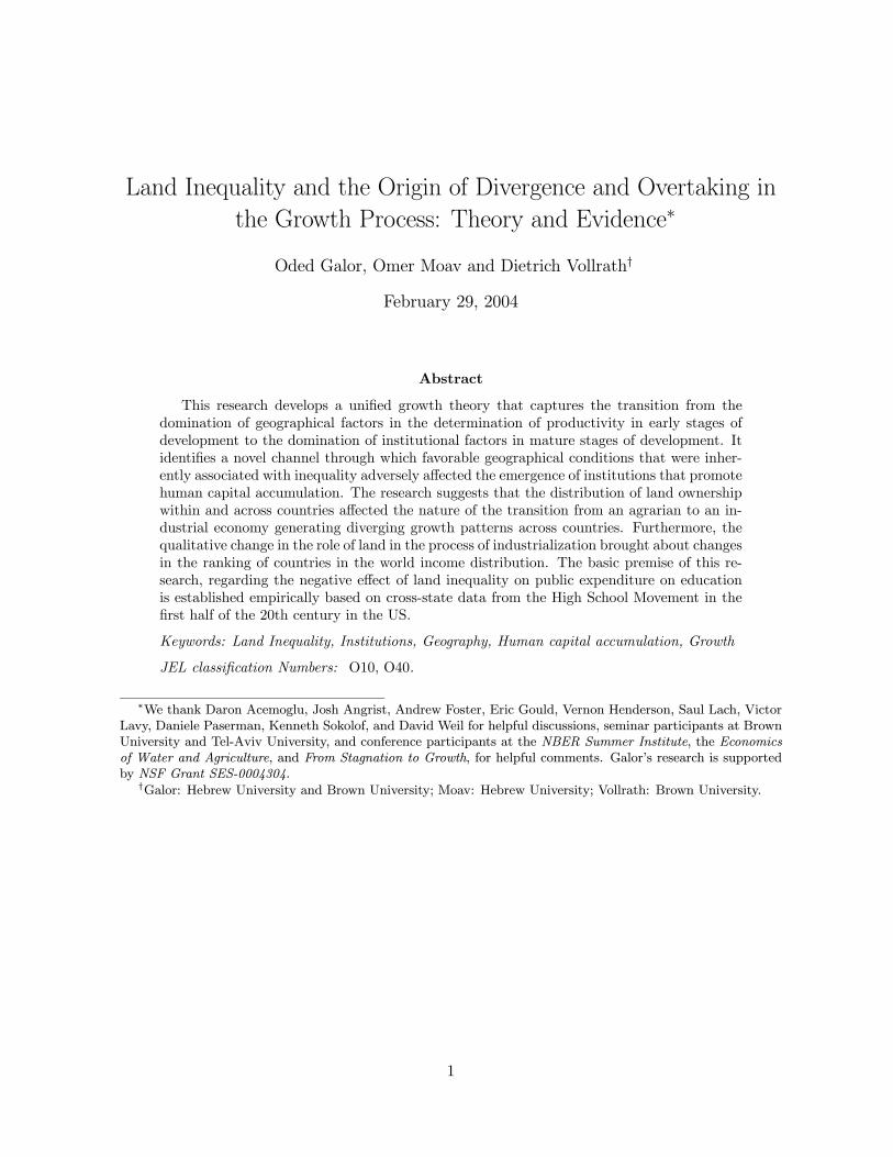
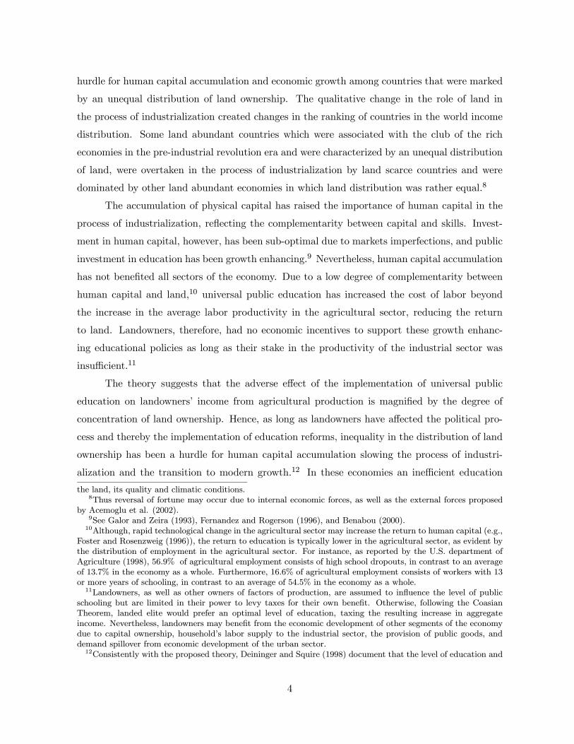
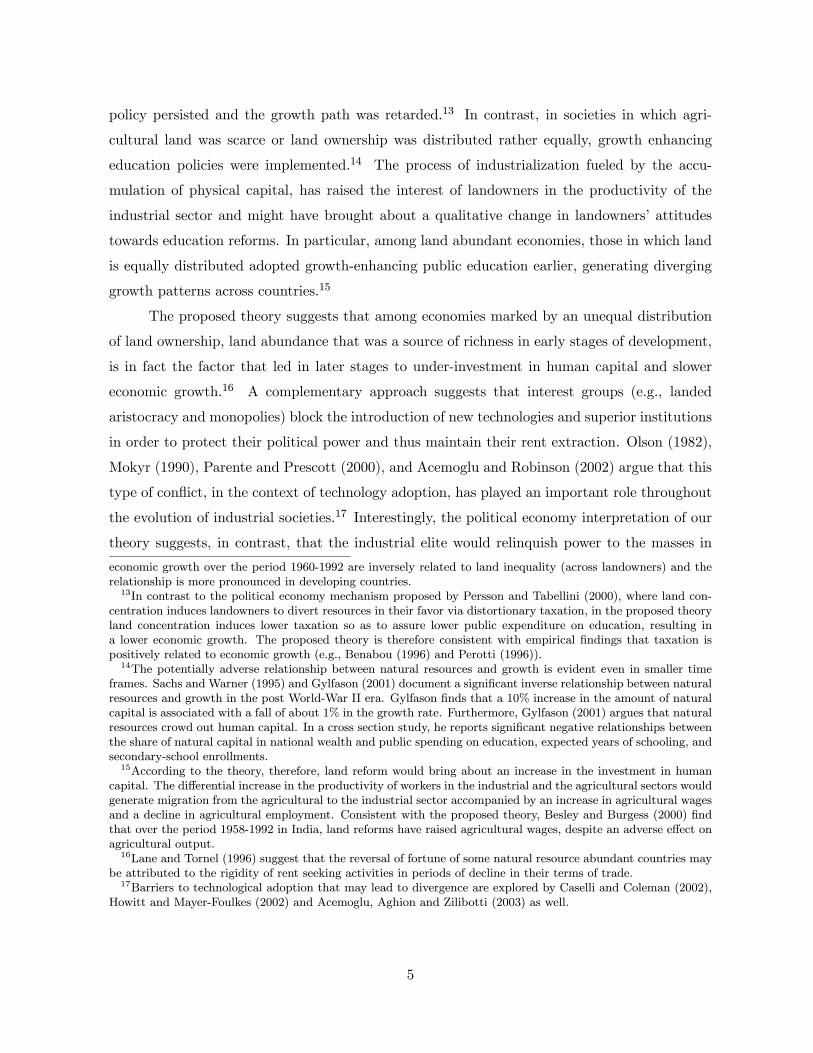
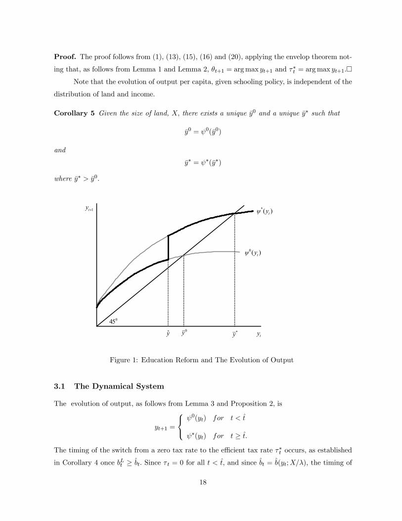
Proposition 2 The conditional evolution of output per capita, as depicted in Figure 1, is given
by
yt+1 =
ψ0(yt) ≡ (βyt)αθt+11−α + F (X, 1− θt+1) for τ = 0;
ψ∗(yt) ≡ [(1− τ∗t )βyt]α[θt+1h(τ∗tβyt)]1−α + F (X, 1− θt+1) for τ = τ∗,
where,
ψ∗(yt) > ψ0(yt) for yt > 0.
dψj(yt)/dyt > 0, d2ψj(yt)/dy
2t < 0, ψ
j(0) = F (X, 1) > 0, dψj(yt)/dX > 0, and
limyt→∞ dψj(yt)/dyt = 0, j = 0, ∗.
17
Proof. The proof follows from (1), (13), (15), (16) and (20), applying the envelop theorem not-
ing that, as follows from Lemma 1 and Lemma 2, θt+1 = argmax yt+1 and τ∗t = argmax yt+1.¤Note that the evolution of output per capita, given schooling policy, is independent of the
distribution of land and income.
Corollary 5 Given the size of land, X, there exists a unique y0 and a unique y∗ such that
y0 = ψ0(y0)
and
y∗ = ψ∗(y∗)
where y∗ > y0.
1+ty
ty*y0yy
045
)(* tyψ
)(0 tyψ
Figure 1: Education Reform and The Evolution of Output
3.1 The Dynamical System
The evolution of output, as follows from Lemma 3 and Proposition 2, is
yt+1 =
ψ0(yt) for t < t
ψ∗(yt) for t ≥ t.The timing of the switch from a zero tax rate to the efficient tax rate τ∗t occurs, as established
in Corollary 4 once bLt ≥ bt. Since τ t = 0 for all t < t, and since bt = b(yt;X/λ), the timing of
18
the switch, t, is determined by the co evolution of {yt, bLt } for τ t = 0
yt+1 = ψ0(yt)
bLt+1 = b0(yt, b
Lt )
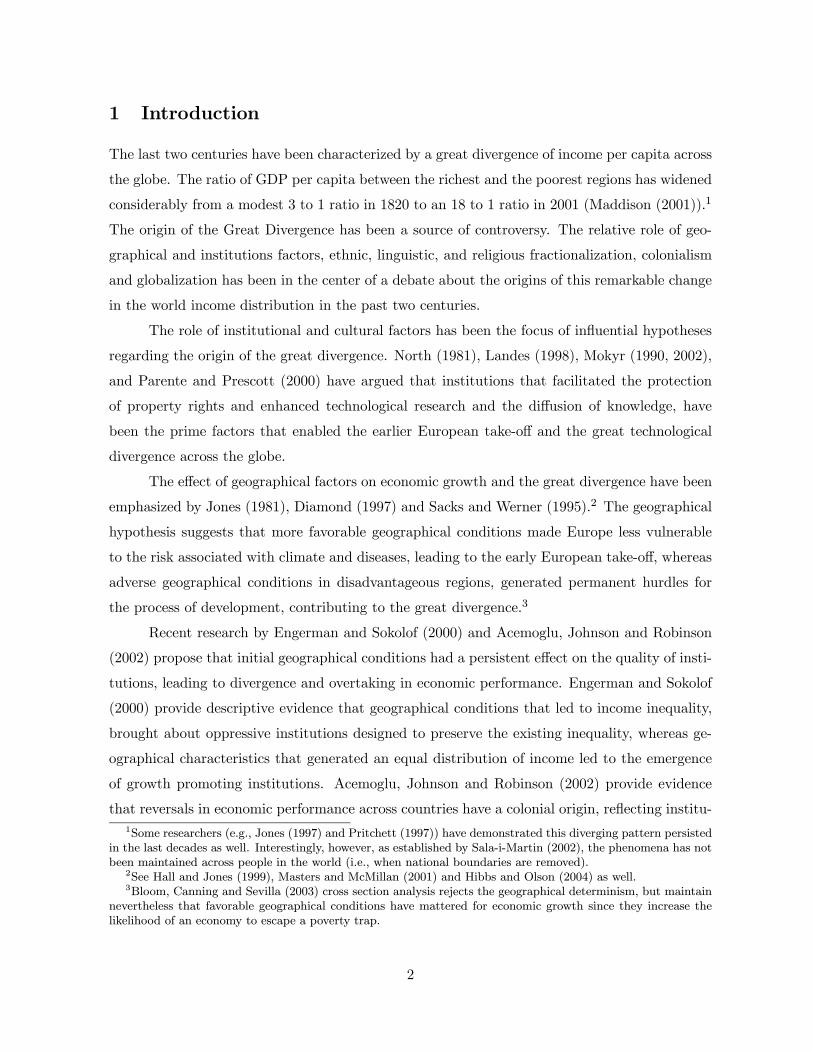
Let the bb locus (depicted in Figure 3) be the set of all pairs (bLt , yt) such that, for τ t = 0,
bLt is in a steady state. i.e., bLt+1 = b
Lt .
In order to simplify the exposition of the dynamical system it is assumed that the value
of β is sufficiently small,
β < 1/R(yt, 0) ∀yt (A1)
where as follows from (3), (5) and Lemma 1, R(yt, 0) < ∞ for all yt and therefore there exists
a sufficiently small β such that A1 holds.
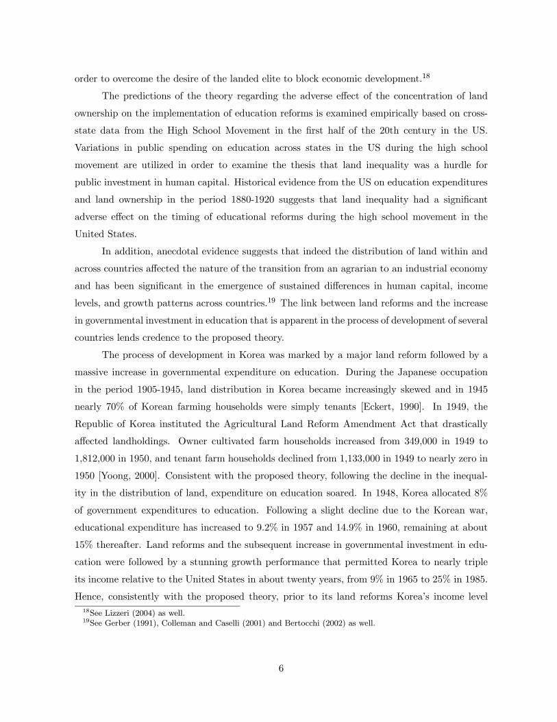
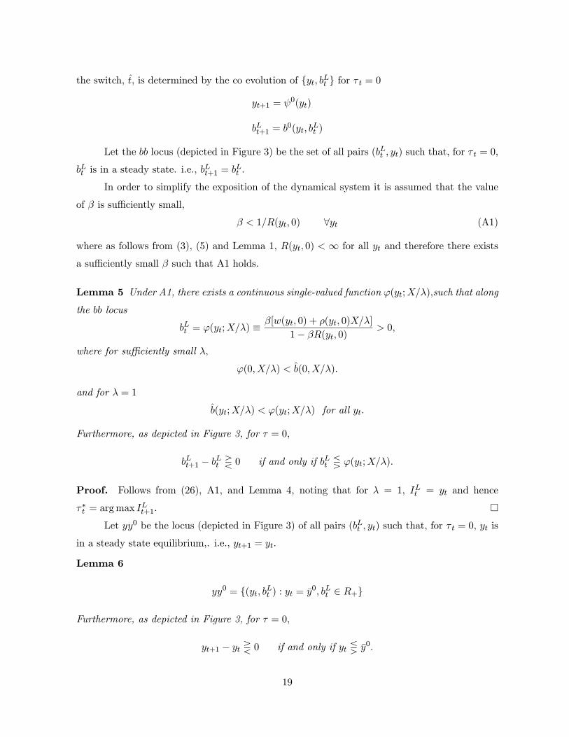
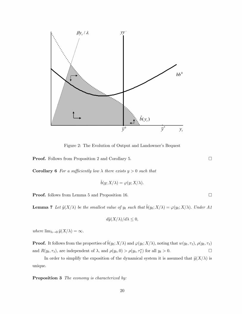
Lemma 5 Under A1, there exists a continuous single-valued function ϕ(yt;X/λ),such that along
the bb locus
bLt = ϕ(yt;X/λ) ≡ β[w(yt, 0) + ρ(yt, 0)X/λ]
1− βR(yt, 0)> 0,
where for sufficiently small λ,
ϕ(0,X/λ) < b(0,X/λ).
and for λ = 1
b(yt;X/λ) < ϕ(yt;X/λ) for all yt.
Furthermore, as depicted in Figure 3, for τ = 0,
bLt+1 − bLt R 0 if and only if bLt Q ϕ(yt;X/λ).
Proof. Follows from (26), A1, and Lemma 4, noting that for λ = 1, ILt = yt and hence
τ∗t = argmax ILt+1. ¤Let yy0 be the locus (depicted in Figure 3) of all pairs (bLt , yt) such that, for τ t = 0, yt is
in a steady state equilibrium,. i.e., yt+1 = yt.
Lemma 6
yy0 = {(yt, bLt ) : yt = y0, bLt ∈ R+}
Furthermore, as depicted in Figure 3, for τ = 0,
yt+1 − yt R 0 if and only if yt Q y0.
19
ty
λβ /ty
)(ˆ tyb0y
0bb
0yy
*y
Figure 2: The Evolution of Output and Landowner’s Bequest
Proof. Follows from Proposition 2 and Corollary 5. ¤
Corollary 6 For a sufficiently low λ there exists y > 0 such that
b(y;X/λ) = ϕ(y;X/λ).
Proof. follows from Lemma 5 and Proposition 16. ¤
Lemma 7 Let y(X/λ) be the smallest value of yt such that b(yt;X/λ) = ϕ(yt;X/λ). Under A1
dy(X/λ)/dλ ≤ 0,
where limλ→0 y(X/λ) =∞.
Proof. It follows from the properties of b(yt;X/λ) and ϕ(yt;X/λ), noting that w(yt, τ t), ρ(yt, τ t)
and R(yt, τ t), are independent of λ, and ρ(yt, 0) > ρ(yt, τ∗t ) for all yt > 0. ¤
In order to simplify the exposition of the dynamical system it is assumed that y(X/λ) is
unique.
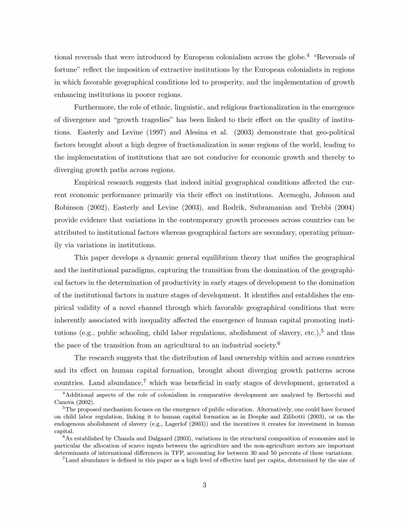
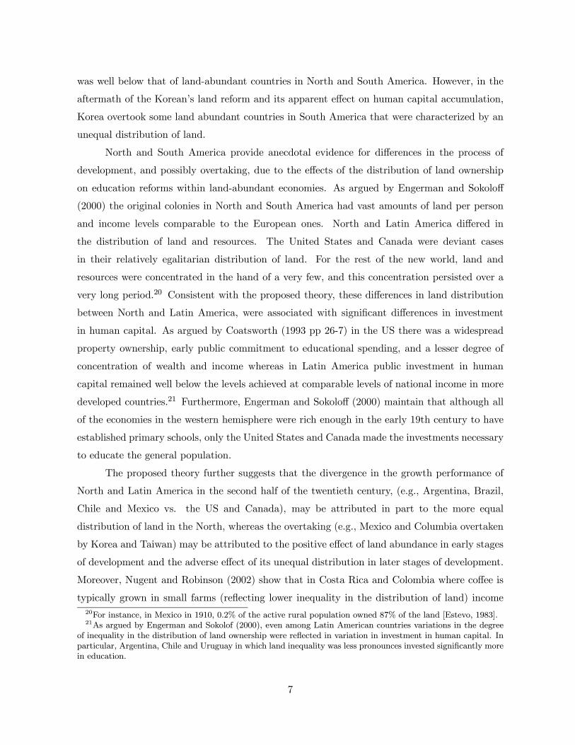
Proposition 3 The economy is characterized by:
20
ty
λβ /ty
)(ˆ tyb0y
0bb
0yy
*y
Figure 3: The Evolution of Output and Landowner’s Bequest
(a) A unique globally stable steady state equilibrium, y∗, if y(X/λ) < y0, that is if λ is sufficiently
large.
(b) Two locally stable steady states, y∗ and y0, if y(X/λ) > y0, that is if λ is sufficiently small.
Proof. Follows from the political mechanism, the definition of y and Lemma 5 and 7. ¤
Theorem 1 Consider countries that are identical in all respects except for their initial land
distribution.
(a) Countries that have a less equal land distribution, i.e., countries with a low level of λ,
will experience a delay in the implementation of efficient education policy and will therefore
experience a lower growth path.
(b) Countries characterize by a sufficiently unequal distribution of land and sufficiently low
capital ownership by the landlord will permanently conduct an inefficient education policy and
will therefore experience a lower growth path as well as a lower level of output in the long-run.
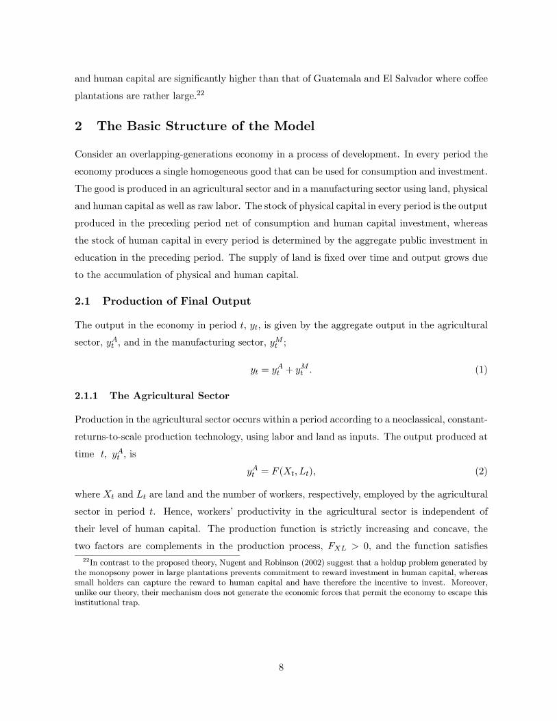
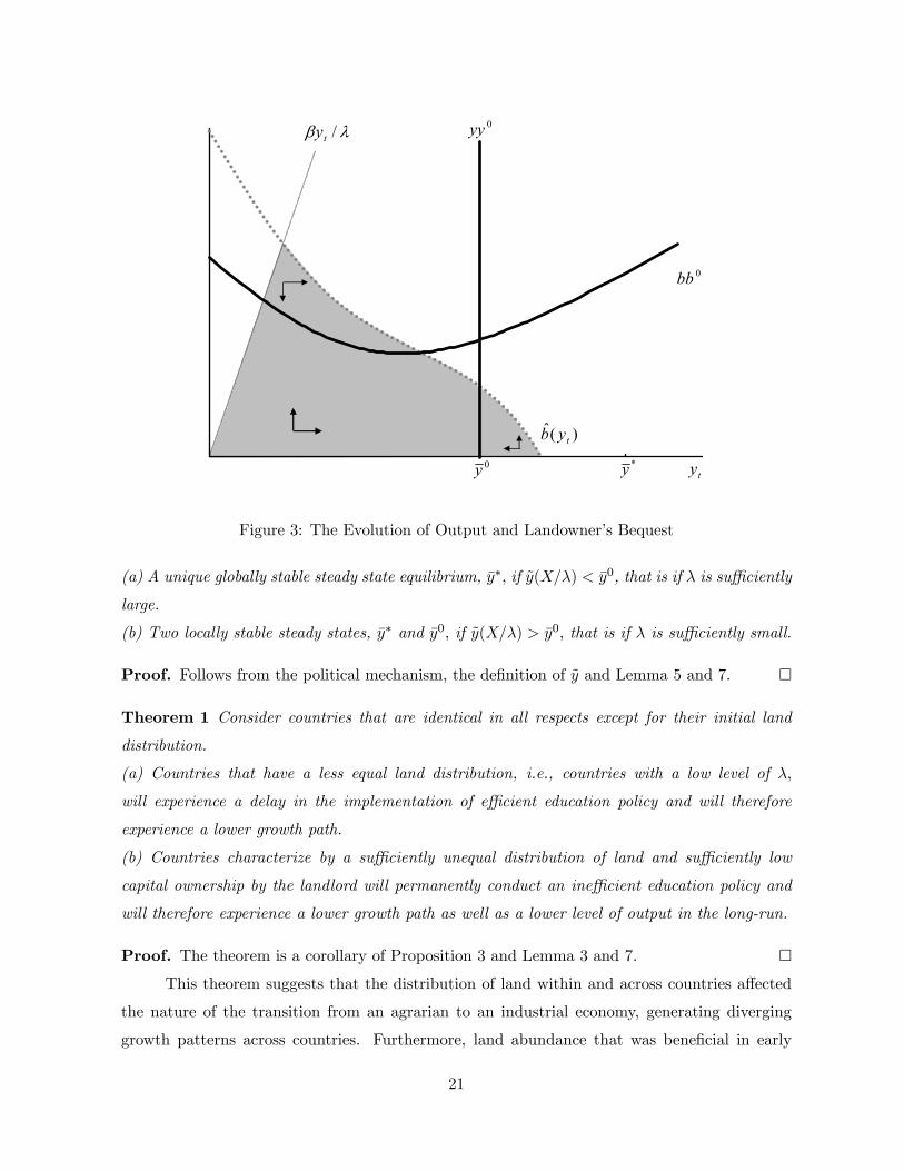
Proof. The theorem is a corollary of Proposition 3 and Lemma 3 and 7. ¤This theorem suggests that the distribution of land within and across countries affected
the nature of the transition from an agrarian to an industrial economy, generating diverging
growth patterns across countries. Furthermore, land abundance that was beneficial in early
21
stages of development, brought about a hurdle for human capital accumulation and economic
growth among countries that were marked by an unequal distribution of land ownership. As
depicted in Figure 4, some land abundant countries which were associated with the club of
the rich economies in the pre-industrial revolution era and were characterized by an unequal
distribution of land, were overtaken in the process of industrialization by land scarce countries.
The qualitative change in the role of land in the process of industrialization has brought about
changes in the ranking of countries in the world income distribution.
1+ty
tyBy ][ *Ay ][ 0By
045
Btyψ )]([ *
Btyψ )]([ 0
Ay
Atyψ )]([ 0
By0Ay0
Figure 4: Overtaking — country A is relatively richer in land, however, due to land inequality itfails to implement efficient schooling and is overtaken by country B. Alternatively, for a lowerdegree of inequality, country A will eventually implement education reforms and ultimatelytakeover country B (not captured in the figure).
4 Evidence from the US High School Movement
The central hypothesis of this research, that land inequality adversely affected the timing of
education reform, is examined empirically using variations in public spending on education
across states in the US during the high school movement. Historical evidence from the US on
education expenditures and land ownership in the period 1880-1920 suggests that land inequality
had a significant adverse effect on the timing of educational reforms during this period.
22
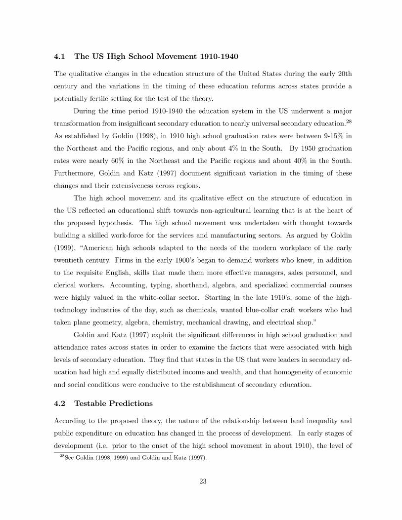
4.1 The US High School Movement 1910-1940
The qualitative changes in the education structure of the United States during the early 20th
century and the variations in the timing of these education reforms across states provide a
potentially fertile setting for the test of the theory.
During the time period 1910-1940 the education system in the US underwent a major
transformation from insignificant secondary education to nearly universal secondary education.28
As established by Goldin (1998), in 1910 high school graduation rates were between 9-15% in
the Northeast and the Pacific regions, and only about 4% in the South. By 1950 graduation
rates were nearly 60% in the Northeast and the Pacific regions and about 40% in the South.
Furthermore, Goldin and Katz (1997) document significant variation in the timing of these
changes and their extensiveness across regions.
The high school movement and its qualitative effect on the structure of education in
the US reflected an educational shift towards non-agricultural learning that is at the heart of
the proposed hypothesis. The high school movement was undertaken with thought towards
building a skilled work-force for the services and manufacturing sectors. As argued by Goldin
(1999), “American high schools adapted to the needs of the modern workplace of the early
twentieth century. Firms in the early 1900’s began to demand workers who knew, in addition
to the requisite English, skills that made them more effective managers, sales personnel, and
clerical workers. Accounting, typing, shorthand, algebra, and specialized commercial courses
were highly valued in the white-collar sector. Starting in the late 1910’s, some of the high-
technology industries of the day, such as chemicals, wanted blue-collar craft workers who had
taken plane geometry, algebra, chemistry, mechanical drawing, and electrical shop.”
Goldin and Katz (1997) exploit the significant differences in high school graduation and
attendance rates across states in order to examine the factors that were associated with high
levels of secondary education. They find that states in the US that were leaders in secondary ed-
ucation had high and equally distributed income and wealth, and that homogeneity of economic
and social conditions were conducive to the establishment of secondary education.
4.2 Testable Predictions
According to the proposed theory, the nature of the relationship between land inequality and
public expenditure on education has changed in the process of development. In early stages of
development (i.e. prior to the onset of the high school movement in about 1910), the level of
28See Goldin (1998, 1999) and Goldin and Katz (1997).
23
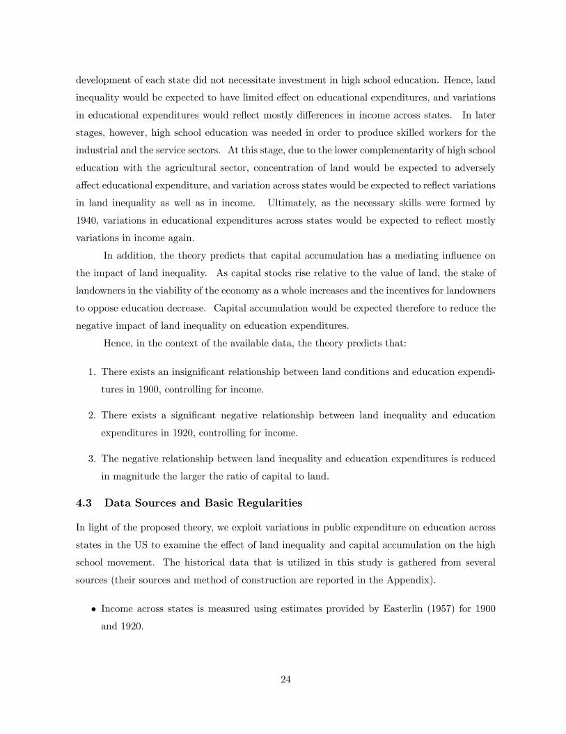
development of each state did not necessitate investment in high school education. Hence, land
inequality would be expected to have limited effect on educational expenditures, and variations
in educational expenditures would reflect mostly differences in income across states. In later
stages, however, high school education was needed in order to produce skilled workers for the
industrial and the service sectors. At this stage, due to the lower complementarity of high school
education with the agricultural sector, concentration of land would be expected to adversely
affect educational expenditure, and variation across states would be expected to reflect variations
in land inequality as well as in income. Ultimately, as the necessary skills were formed by
1940, variations in educational expenditures across states would be expected to reflect mostly
variations in income again.
In addition, the theory predicts that capital accumulation has a mediating influence on
the impact of land inequality. As capital stocks rise relative to the value of land, the stake of
landowners in the viability of the economy as a whole increases and the incentives for landowners
to oppose education decrease. Capital accumulation would be expected therefore to reduce the
negative impact of land inequality on education expenditures.
Hence, in the context of the available data, the theory predicts that:
1. There exists an insignificant relationship between land conditions and education expendi-
tures in 1900, controlling for income.
2. There exists a significant negative relationship between land inequality and education
expenditures in 1920, controlling for income.
3. The negative relationship between land inequality and education expenditures is reduced
in magnitude the larger the ratio of capital to land.
4.3 Data Sources and Basic Regularities
In light of the proposed theory, we exploit variations in public expenditure on education across
states in the US to examine the effect of land inequality and capital accumulation on the high
school movement. The historical data that is utilized in this study is gathered from several
sources (their sources and method of construction are reported in the Appendix).
• Income across states is measured using estimates provided by Easterlin (1957) for 1900and 1920.
24
• The characterization of the timing of the high school movement is based on the classifica-tion of Goldin (1998). As reflected in that study, in 1900 the high school movement had
only just begun and by 1920 it was well underway in nearly every state. By 1950 most
of the changes in secondary education had been completed. Limitations of data will only
permit us to examine the years 1900 and 1920.
• Land inequality is measured by the Gini coefficients on land distribution within each statethat we constructed using US Census data. The Gini coefficients are created for 1880,
1900 and 1920. The 1880 coefficients are used in some cases as direct controls for land
inequality, and in others as instruments for the 1900 and 1920 measures.29
• The relative importance of capital is measured by the ratio of total capital stock (Easterlin(1957)) to the total value of agricultural land obtained from the US Census. The ratio is
measured for the years 1880, 1900 and 1920.
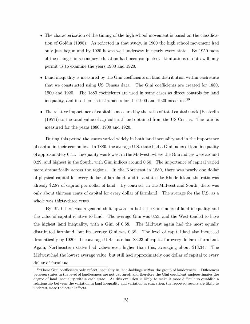
During this period the states varied widely in both land inequality and in the importance
of capital in their economies. In 1880, the average U.S. state had a Gini index of land inequality
of approximately 0.41. Inequality was lowest in the Midwest, where the Gini indices were around
0.29, and highest in the South, with Gini indices around 0.50. The importance of capital varied
more dramatically across the regions. In the Northeast in 1880, there was nearly one dollar
of physical capital for every dollar of farmland, and in a state like Rhode Island the ratio was
already $2.87 of capital per dollar of land. By contrast, in the Midwest and South, there was
only about thirteen cents of capital for every dollar of farmland. The average for the U.S. as a
whole was thirty-three cents.
By 1920 there was a general shift upward in both the Gini index of land inequality and
the value of capital relative to land. The average Gini was 0.53, and the West tended to have
the highest land inequality, with a Gini of 0.68. The Midwest again had the most equally
distributed farmland, but its average Gini was 0.38. The level of capital had also increased
dramatically by 1920. The average U.S. state had $3.23 of capital for every dollar of farmland.
Again, Northeastern states had values even higher than this, averaging about $13.34. The
Midwest had the lowest average value, but still had approximately one dollar of capital to every
dollar of farmland.29These Gini coefficients only reflect inequality in land-holdings within the group of landowners. Differences
between states in the level of landlessness are not captured, and therefore the Gini coefficient underestimates thedegree of land inequality within each state. As this exclusion is likely to make it more difficult to establish arelationship between the variation in land inequality and variation in education, the reported results are likely tounderestimate the actual effects.
25
These values indicate the changing nature of the U.S. economy over this period. As
agriculture became less significant there seems to have been a general upward shift in land
inequality, perhaps not unexpected, as some landowners consolidated holdings as others moved
on to invest in the new manufacturing sectors. The assets of the nation became increasingly
skewed towards physical capital, concurrent with the onset of the high school movement.
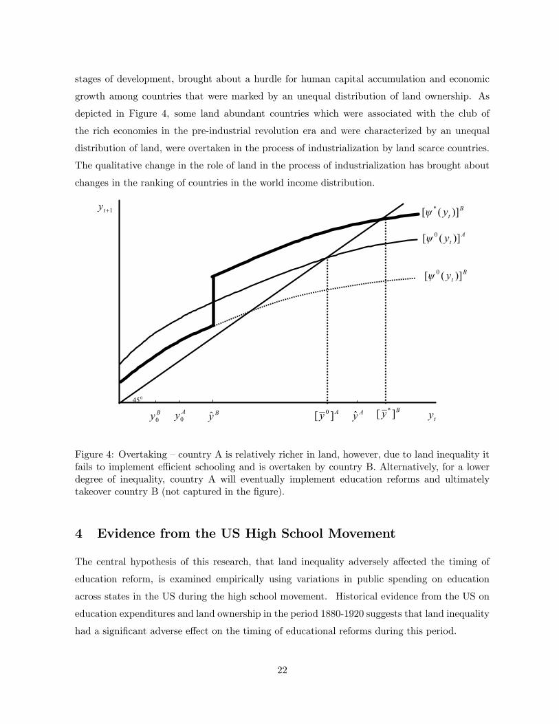
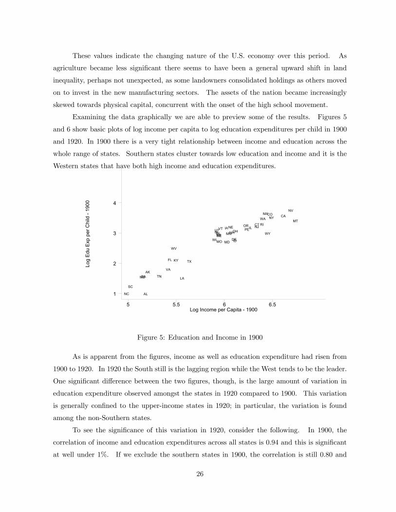
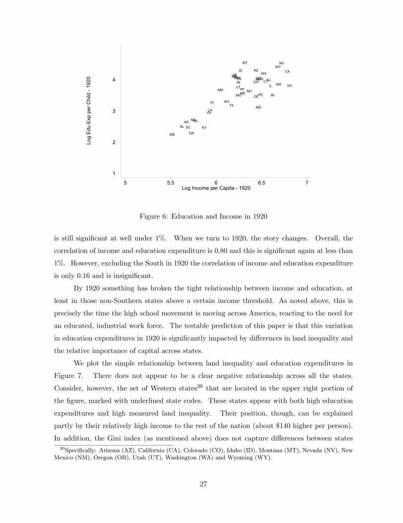
Examining the data graphically we are able to preview some of the results. Figures 5
and 6 show basic plots of log income per capita to log education expenditures per child in 1900
and 1920. In 1900 there is a very tight relationship between income and education across the
whole range of states. Southern states cluster towards low education and income and it is the
Western states that have both high income and education expenditures.
Log
Edu
Exp
per
Chi
ld -
1900
Log Income per Capita - 19005 5.5 6 6.5
1
2
3
4
AL
AK
CACO
CT
DE
FL
GA
ID
ILIN
IA
KS
KY
LA
ME
MD
MA
MI MN
MS
MO
MT
NE
NV
NH
NJ
NY
NC
OHORPE
RI
SC
TN
TX
UTVT
VA
WA
WV
WI
WY
Figure 5: Education and Income in 1900
As is apparent from the figures, income as well as education expenditure had risen from
1900 to 1920. In 1920 the South still is the lagging region while the West tends to be the leader.
One significant difference between the two figures, though, is the large amount of variation in
education expenditure observed amongst the states in 1920 compared to 1900. This variation
is generally confined to the upper-income states in 1920; in particular, the variation is found
among the non-Southern states.
To see the significance of this variation in 1920, consider the following. In 1900, the
correlation of income and education expenditures across all states is 0.94 and this is significant
at well under 1%. If we exclude the southern states in 1900, the correlation is still 0.80 and
26
Log
Edu
Exp
per
Chi
ld -
1920
Log Income per Capita - 19205 5.5 6 6.5 7
1
2
3
4
AL
AZ
AK
CA
COCT
DE
FL
GA
ID
ILIN
IAKS
KY
LA
ME
MD
MAMIMN
MS
MO
MT
NE
NV
NH
NJ
NMNY
NC
OHOR
PE RI
SC
TN
TX
UT
VT
VA
WA
WV
WI
WY
Figure 6: Education and Income in 1920
is still significant at well under 1%. When we turn to 1920, the story changes. Overall, the
correlation of income and education expenditure is 0.80 and this is significant again at less than
1%. However, excluding the South in 1920 the correlation of income and education expenditure
is only 0.16 and is insignificant.
By 1920 something has broken the tight relationship between income and education, at
least in those non-Southern states above a certain income threshold. As noted above, this is
precisely the time the high school movement is moving across America, reacting to the need for
an educated, industrial work force. The testable prediction of this paper is that this variation
in education expenditures in 1920 is significantly impacted by differences in land inequality and
the relative importance of capital across states.
We plot the simple relationship between land inequality and education expenditures in
Figure 7. There does not appear to be a clear negative relationship across all the states.
Consider, however, the set of Western states30 that are located in the upper right portion of
the figure, marked with underlined state codes. These states appear with both high education
expenditures and high measured land inequality. Their position, though, can be explained
partly by their relatively high income to the rest of the nation (about $140 higher per person).
In addition, the Gini index (as mentioned above) does not capture differences between states
30Specifically: Arizona (AZ), California (CA), Colorado (CO), Idaho (ID), Montana (MT), Nevada (NV), NewMexico (NM), Oregon (OR), Utah (UT), Washington (WA) and Wyoming (WY).
27
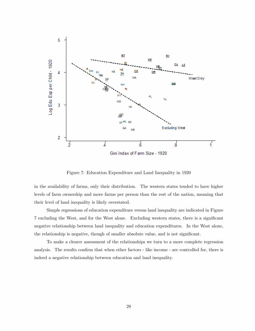
Figure 7: Education Expenditure and Land Inequality in 1920
in the availability of farms, only their distribution. The western states tended to have higher
levels of farm ownership and more farms per person than the rest of the nation, meaning that
their level of land inequality is likely overstated.
Simple regressions of education expenditure versus land inequality are indicated in Figure
7 excluding the West, and for the West alone. Excluding western states, there is a significant
negative relationship between land inequality and education expenditures. In the West alone,
the relationship is negative, though of smaller absolute value, and is not significant.
To make a clearer assessment of the relationships we turn to a more complete regression
analysis. The results confirm that when other factors - like income - are controlled for, there is
indeed a negative relationship between education and land inequality.
28
4.4 Empirical Specification and Results
The empirical analysis is based on simple cross-sectional regressions of states in both 1900 and
1920.31 Expenditure on education per child is the dependent variable in each case. Income
per capita in the years 1900 and 1920, respectively, a Gini coefficient for farm size distribution,
and the capital/land ratio are included as explanatory variables. In addition, the interaction
of the Gini and the capital/land ratio is included to capture test for the effects noted in predic-
tion 3 above. We use two-stage least square methods, with the 1880 values for the Gini and
capital/land ratio as instruments for the contemporaneous values, to avoid the endogeneity of
land distribution and capital/land ratios with education.
We check robustness by including the following controls: the percentage of population
that is black, the percentage of population that is urban, and the year the state was admitted
to the union. The percentage of population that is black is designed to capture the differential
effects of racial policies on educational expenditures. The percentage of population that resides
in urban areas is included to control for several possible influences: (a) economies of scale in
education that are more pronounced in urban areas, (b) variations in teacher salaries and thus
educational expenditures vary between rural-intensive and urban-intensive states, and (c) the
increased demand for education in urban-intensive states. The year of statehood is included to
control for several influences. As mentioned above, newer states tended to be more homogenous
in terms of population and to have farms more widely available. This measure also controls
for geographic variations between states in their distance to major markets, which may have an
additional influence on the need to develop industry and secondary education.
For the regressions, we include results from excluding the southern states. As seen above,
the South lagged far behind in income per capita and this lag may cause relationships to appear
which simply reflect some fundamental difference between the South and the rest of the nation.
At this point the South is only beginning to come out of the Reconstruction period following the
Civil War and there seems to be no question this was an important feature of its development.
In addition, we saw previously that the South’s income was distinctly lower than the rest of
the country, and this may have prevented them from reaching the stage at which high school
mattered to the economy. In this case, the predicted relationships of land
inequality and capital/land ratios may be irrelevant for the South.
31It should be noted that another avenue of empirical investigation would be to examine the differences in landconditions within states over time and their impacts on education expenditures. This research avenue, however,would generate severe problems of endogeneity. Furthermore, variations in land inequality over time within statesare smaller than that across states at any given time and are too subtle to offer much explanatory power.
29
4.4.1 2SLS Specifications
Tables 1 and 2 report the outcome of cross-sectional 2SLS regressions for the years 1900 and
1920, respectively. Column (1) in both tables shows the simple regression of expenditure per
child on income per capita.32 In 1900, the R-squared of the regression is roughly 89%. In
contrast, in 1920 the R-squared of the same regression is 64%. In 1920 - in the midst of the
high school movement - there are larger differences in education between states unexplained by
income than in 1900 - just prior to the beginning of the movement. As will become apparent,
land conditions are one of the significant determinants of the variation in education expenditure
in 1920.
The effect of land, in both distribution and importance to the economy is shown in columns
(2) thru (5) of both tables. We see that in 1900, there is a significant negative effect of the
Gini coefficient for land distribution but that this significance nearly disappears once we add
controls for race, urbanization and statehood. When the South is excluded, the relationship of
land inequality to education disappears completely in 1900. There is no evidence at any point
that the relative importance of capital to land has any impact on education expenditures in
1900. While this does not prove that land inequality was unimportant in generating differences
in education in 1900 it does, along with results that follow, offer evidence that the power of land
inequality was increasing over time as the high school movement progressed.
Table 2 shows the full impact of the land conditions in 1920. Consistent with the testable
predictions column (3) shows that with the addition of the interaction of the Gini index with the
capital/land ratio, the significance of the Gini index increases as well as the magnitude of the
estimated coefficient. This result, it should be noted, holds despite the presence of the outlying
western states seen in figure 7.
Column (4) includes the additional controls for urbanization, percentage black, and the
year of statehood. The effect of the percentage of black in the population on expenditures per
child is negative but not significant, perhaps indicating that some of the negative association of
race and education worked through poor land distributions for the black population (See Margo
[1990] for further discussion of the relationship between race and education in the South). The
percentage urban has no significant impact. The year of statehood shows up significantly and
with a positive coefficient. We cannot identify precisely what this represents, but we speculate
it is capturing the factors mentioned above in regard to the western states: homogeneity of
32For reasons explained in the Appendix, the 1900 regression includes only 41 states while the 1920 regressionincluded 45 states. Restricting the 1920 regression to the same 41 states as in 1900 has no effect on the results.
30
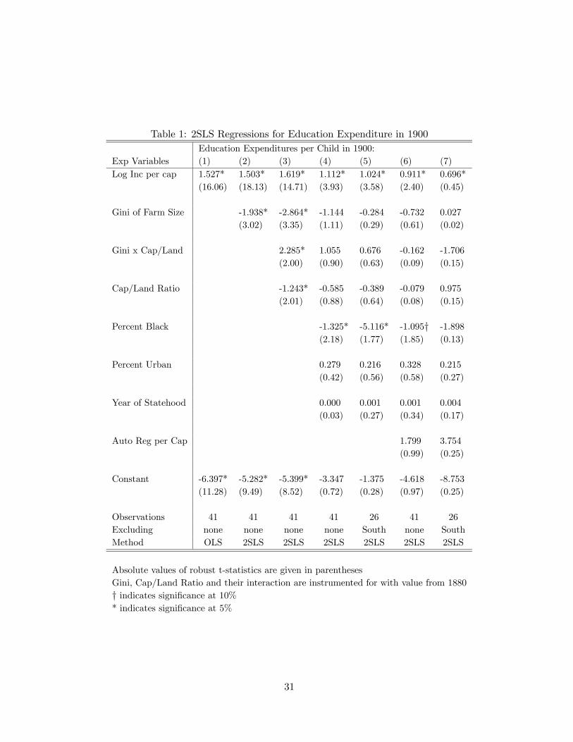
Table 1: 2SLS Regressions for Education Expenditure in 1900
Education Expenditures per Child in 1900:
Exp Variables (1) (2) (3) (4) (5) (6) (7)
Log Inc per cap 1.527* 1.503* 1.619* 1.112* 1.024* 0.911* 0.696*
(16.06) (18.13) (14.71) (3.93) (3.58) (2.40) (0.45)
Gini of Farm Size -1.938* -2.864* -1.144 -0.284 -0.732 0.027
(3.02) (3.35) (1.11) (0.29) (0.61) (0.02)
Gini x Cap/Land 2.285* 1.055 0.676 -0.162 -1.706
(2.00) (0.90) (0.63) (0.09) (0.15)
Cap/Land Ratio -1.243* -0.585 -0.389 -0.079 0.975
(2.01) (0.88) (0.64) (0.08) (0.15)
Percent Black -1.325* -5.116* -1.095† -1.898
(2.18) (1.77) (1.85) (0.13)
Percent Urban 0.279 0.216 0.328 0.215
(0.42) (0.56) (0.58) (0.27)
Year of Statehood 0.000 0.001 0.001 0.004
(0.03) (0.27) (0.34) (0.17)
Auto Reg per Cap 1.799 3.754
(0.99) (0.25)
Constant -6.397* -5.282* -5.399* -3.347 -1.375 -4.618 -8.753
(11.28) (9.49) (8.52) (0.72) (0.28) (0.97) (0.25)
Observations 41 41 41 41 26 41 26
Excluding none none none none South none South
Method OLS 2SLS 2SLS 2SLS 2SLS 2SLS 2SLS
Absolute values of robust t-statistics are given in parentheses
Gini, Cap/Land Ratio and their interaction are instrumented for with value from 1880
† indicates significance at 10%* indicates significance at 5%
31

Table 2: 2SLS Regressions for Education Expenditure in 1920
Education Expenditures per Child in 1920:
Exp Variables (1) (2) (3) (4) (5) (6) (7)
Log Inc per cap 1.519* 1.562* 1.895* 1.478* 1.162* 1.113* 1.187*
(10.42) (8.24) (10.30) (4.80) (4.37) (4.19) (3.57)
Gini of Farm Size -1.603† -1.721* -1.293* -0.932* -0.807† -0.968*
(1.86) (2.14) (3.05) (2.20) (1.86) (2.11)
Gini x Cap/Land 0.403 0.349† 0.549* 0.167 0.593
(1.22) (1.95) (2.31) (0.98) (1.12)
Cap/Land Ratio -0.242 -0.189† -0.301* -0.086 -0.324
(1.39) (1.93) (2.32) (0.90) (1.11)
Percent Black -0.582 -0.945 -0.456 -0.919
(0.85) (0.20) (0.77) (0.19)
Percent Urban -0.275 -0.408 -0.222 -0.414
(0.65) (1.14) (0.61) (1.19)
Year of Statehood 0.007* 0.004 0.006* 0.004
(3.18) (1.64) (2.87) (1.40)
Auto Reg per Cap 2.677* -0.269
(2.29) (0.12)
Constant -5.961* -5.389* -7.270* -17.014* -9.321* -13.819* -9.270†(6.62) (4.55) (7.43) (3.56) (1.99) (3.25) (1.87)
Observations 45 45 45 45 30 45 30
Excluding none none none none South none South
Method OLS 2SLS 2SLS 2SLS 2SLS 2SLS 2SLS
Absolute values of robust t-statistics are given in parentheses
Gini, Cap/Land Ratio and their interaction are instrumented for with value from 1880
† indicates significance at 10%* indicates significance at 5%
32
population and availability of farms to the population. The exclusion of the South, in column
(5), does not change the results significantly.
Given these results in columns (4) and (5), the net marginal effect of land inequality on
education expenditures becomes less negative as capital/land ratios increase, as predicted by
the theory. For the large majority of states the capital/land ratios are sufficiently low (the
median value is 0.17) that increasing land inequality would have a large negative impact on
education expenditures. On the upper end of the spectrum, states such as Massachusetts and
Rhode Island - both early industrializers in the U.S. - have high enough capital/land ratios that
increasing land inequality no longer has a net negative impact.
To get a sense of how important land inequality can be to education in 1920, consider
a simple example using the estimates from specification (4). Both Virginia and Indiana have
about $0.58 of capital for every dollar of land (a value very close to the median for 1920). At this
capital/land ratio, the marginal effect of the Gini index of education is −1.293+ 0.349× 0.58 =−1.091. The difference in Gini index between Indiana (0.38) and Virginia (0.55) is 0.17, and isroughly equivalent to moving from the 25th to the 75th percentile in the distribution of Gini’s
across states. The estimates imply that education expenditures were 18% lower in Virginia due
solely to this difference in land inequality. A difference this large would certainly have serious
consequences for education outcomes. Our estimates show not just a statistically significant
impact of land inequality on education, but a significant practical impact as well.
4.4.2 Land versus Income Inequality
The theory proposed in this paper is concerned with the distribution and relative importance
of land in the determination of education expenditures. A potential concern with the empirical
results to this point may be that the measure of land inequality, the farm size Gini index,
is simply a proxy for income inequality. Goldin and Katz (1997), in fact, find that income
inequality is associated with poor education outcomes across states during the US high school
movement. They reach this conclusion using in their regressions a proxy for the distribution of
income in a state: the number of automobile registrations per person.
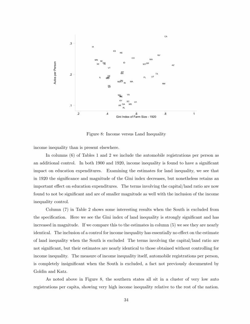
The measure of income inequality bears no discernible relationship to that of land in-
equality. Figure 8 plots the two series against each other. The overall level of correlation is
only 0.07, and is distinctly insignificant. One feature to note in this figure is the cluster of
southern states in the bottom center. These states have unexceptional land inequality but fall
well below the rest of the country in their levels of automobile registrations, indicating far larger
33
Aut
os p
er P
erso
n
Gini Index of Farm Size - 1920.2 .4 .6 .8 1
.1
.2
.3
NM
IA
NEKS
TX
ID
MT
NV
AK
MN
MS
KY
CO
MO
WYOR
CA
TN
GASC
VA
IN
IL UT
AZ
WA
NC
WI
FL
AL
WV
LA
VT
OH
MD
MI
ME
NH
NYPE
CT
DE
NJ MARI
Figure 8: Income versus Land Inequality
income inequality than is present elsewhere.
In columns (6) of Tables 1 and 2 we include the automobile registrations per person as
an additional control. In both 1900 and 1920, income inequality is found to have a significant
impact on education expenditures. Examining the estimates for land inequality, we see that
in 1920 the significance and magnitude of the Gini index decreases, but nonetheless retains an
important effect on education expenditures. The terms involving the capital/land ratio are now
found to not be significant and are of smaller magnitude as well with the inclusion of the income
inequality control.
Column (7) in Table 2 shows some interesting results when the South is excluded from
the specification. Here we see the Gini index of land inequality is strongly significant and has
increased in magnitude. If we compare this to the estimates in column (5) we see they are nearly
identical. The inclusion of a control for income inequality has essentially no effect on the estimate
of land inequality when the South is excluded The terms involving the capital/land ratio are
not significant, but their estimates are nearly identical to those obtained without controlling for
income inequality. The measure of income inequality itself, automobile registrations per person,
is completely insignificant when the South is excluded, a fact not previously documented by
Goldin and Katz.
As noted above in Figure 8, the southern states all sit in a cluster of very low auto
registrations per capita, showing very high income inequality relative to the rest of the nation.
34
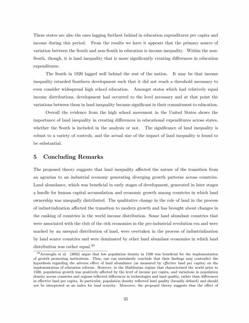
These states are also the ones lagging furthest behind in education expenditures per capita and
income during this period. From the results we have it appears that the primary source of
variation between the South and non-South in education is income inequality. Within the non-
South, though, it is land inequality that is more significantly creating differences in education
expenditures.
The South in 1920 lagged well behind the rest of the nation. It may be that income
inequality retarded Southern development such that it did not reach a threshold necessary to
even consider widespread high school education. Amongst states which had relatively equal
income distributions, development had occurred to the level necessary and at that point the
variations between them in land inequality became significant in their commitment to education.
Overall the evidence from the high school movement in the United States shows the
importance of land inequality in creating differences in educational expenditures across states,
whether the South is included in the analysis or not. The significance of land inequality is
robust to a variety of controls, and the actual size of the impact of land inequality is found to
be substantial.
5 Concluding Remarks
The proposed theory suggests that land inequality affected the nature of the transition from
an agrarian to an industrial economy generating diverging growth patterns across countries.
Land abundance, which was beneficial in early stages of development, generated in later stages
a hurdle for human capital accumulation and economic growth among countries in which land
ownership was unequally distributed. The qualitative change in the role of land in the process
of industrialization affected the transition to modern growth and has brought about changes in
the ranking of countries in the world income distribution. Some land abundant countries that
were associated with the club of the rich economies in the pre-industrial revolution era and were
marked by an unequal distribution of land, were overtaken in the process of industrialization
by land scarce countries and were dominated by other land abundant economies in which land
distribution was rather equal.33
33Acemoglu et al. (2002) argue that low population density in 1500 was beneficial for the implementationof growth promoting institutions. Thus, one can mistakenly conclude that their findings may contradict thehypothesis regarding the adverse effect of land abundance (as measured by effective land per capita) on theimplementation of education reforms. However, in the Malthusian regime that characterized the world prior to1500, population growth was positively affected by the level of income per capita, and variations in populationdensity across countries and regions reflected differences in technologies and land quality, rather than differencesin effective land per capita. In particular, population density reflected land quality (broadly defined) and shouldnot be interpreted as an index for land scarcity. Moreover, the proposed theory suggests that the effect of
35
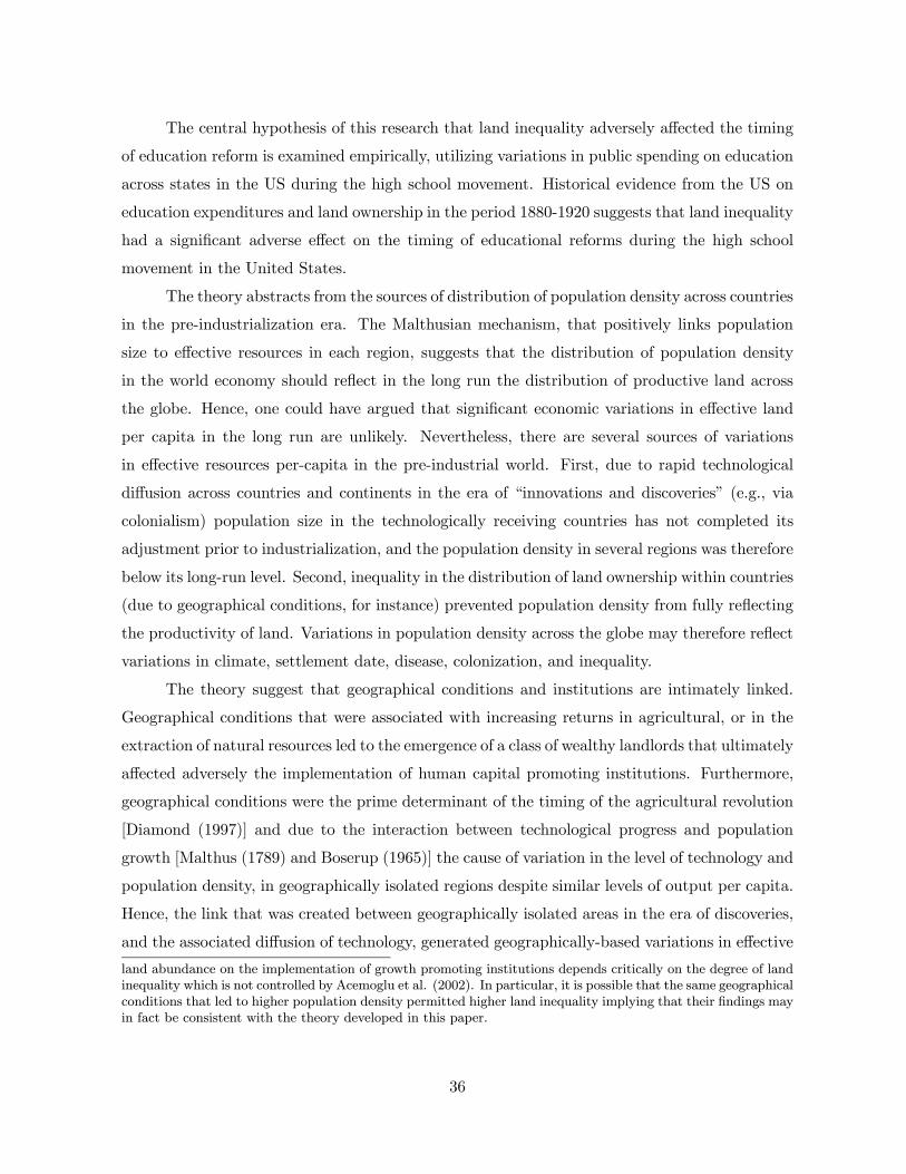
The central hypothesis of this research that land inequality adversely affected the timing
of education reform is examined empirically, utilizing variations in public spending on education
across states in the US during the high school movement. Historical evidence from the US on
education expenditures and land ownership in the period 1880-1920 suggests that land inequality
had a significant adverse effect on the timing of educational reforms during the high school
movement in the United States.
The theory abstracts from the sources of distribution of population density across countries
in the pre-industrialization era. The Malthusian mechanism, that positively links population
size to effective resources in each region, suggests that the distribution of population density
in the world economy should reflect in the long run the distribution of productive land across
the globe. Hence, one could have argued that significant economic variations in effective land
per capita in the long run are unlikely. Nevertheless, there are several sources of variations
in effective resources per-capita in the pre-industrial world. First, due to rapid technological
diffusion across countries and continents in the era of “innovations and discoveries” (e.g., via
colonialism) population size in the technologically receiving countries has not completed its
adjustment prior to industrialization, and the population density in several regions was therefore
below its long-run level. Second, inequality in the distribution of land ownership within countries
(due to geographical conditions, for instance) prevented population density from fully reflecting
the productivity of land. Variations in population density across the globe may therefore reflect
variations in climate, settlement date, disease, colonization, and inequality.
The theory suggest that geographical conditions and institutions are intimately linked.
Geographical conditions that were associated with increasing returns in agricultural, or in the
extraction of natural resources led to the emergence of a class of wealthy landlords that ultimately
affected adversely the implementation of human capital promoting institutions. Furthermore,
geographical conditions were the prime determinant of the timing of the agricultural revolution
[Diamond (1997)] and due to the interaction between technological progress and population
growth [Malthus (1789) and Boserup (1965)] the cause of variation in the level of technology and
population density, in geographically isolated regions despite similar levels of output per capita.
Hence, the link that was created between geographically isolated areas in the era of discoveries,
and the associated diffusion of technology, generated geographically-based variations in effective
land abundance on the implementation of growth promoting institutions depends critically on the degree of landinequality which is not controlled by Acemoglu et al. (2002). In particular, it is possible that the same geographicalconditions that led to higher population density permitted higher land inequality implying that their findings mayin fact be consistent with the theory developed in this paper.
36
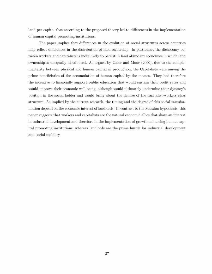
land per capita, that according to the proposed theory led to differences in the implementation
of human capital promoting institutions.
The paper implies that differences in the evolution of social structures across countries
may reflect differences in the distribution of land ownership. In particular, the dichotomy be-
tween workers and capitalists is more likely to persist in land abundant economies in which land
ownership is unequally distributed. As argued by Galor and Moav (2000), due to the comple-
mentarity between physical and human capital in production, the Capitalists were among the
prime beneficiaries of the accumulation of human capital by the masses. They had therefore
the incentive to financially support public education that would sustain their profit rates and
would improve their economic well being, although would ultimately undermine their dynasty’s
position in the social ladder and would bring about the demise of the capitalist-workers class
structure. As implied by the current research, the timing and the degree of this social transfor-
mation depend on the economic interest of landlords. In contrast to the Marxian hypothesis, this
paper suggests that workers and capitalists are the natural economic allies that share an interest
in industrial development and therefore in the implementation of growth enhancing human cap-
ital promoting institutions, whereas landlords are the prime hurdle for industrial development
and social mobility.
37
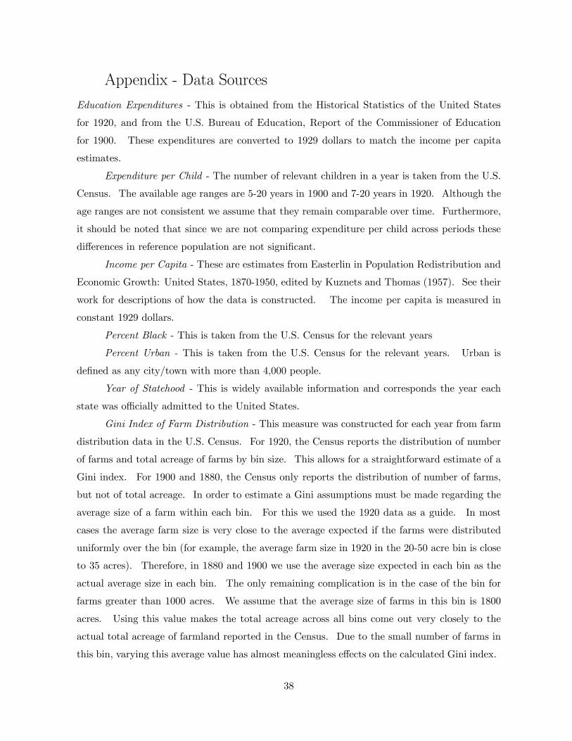
Appendix - Data Sources
Education Expenditures - This is obtained from the Historical Statistics of the United States
for 1920, and from the U.S. Bureau of Education, Report of the Commissioner of Education
for 1900. These expenditures are converted to 1929 dollars to match the income per capita
estimates.
Expenditure per Child - The number of relevant children in a year is taken from the U.S.
Census. The available age ranges are 5-20 years in 1900 and 7-20 years in 1920. Although the
age ranges are not consistent we assume that they remain comparable over time. Furthermore,
it should be noted that since we are not comparing expenditure per child across periods these
differences in reference population are not significant.
Income per Capita - These are estimates from Easterlin in Population Redistribution and
Economic Growth: United States, 1870-1950, edited by Kuznets and Thomas (1957). See their
work for descriptions of how the data is constructed. The income per capita is measured in
constant 1929 dollars.
Percent Black - This is taken from the U.S. Census for the relevant years
Percent Urban - This is taken from the U.S. Census for the relevant years. Urban is
defined as any city/town with more than 4,000 people.
Year of Statehood - This is widely available information and corresponds the year each
state was officially admitted to the United States.
Gini Index of Farm Distribution - This measure was constructed for each year from farm
distribution data in the U.S. Census. For 1920, the Census reports the distribution of number
of farms and total acreage of farms by bin size. This allows for a straightforward estimate of a
Gini index. For 1900 and 1880, the Census only reports the distribution of number of farms,
but not of total acreage. In order to estimate a Gini assumptions must be made regarding the
average size of a farm within each bin. For this we used the 1920 data as a guide. In most
cases the average farm size is very close to the average expected if the farms were distributed
uniformly over the bin (for example, the average farm size in 1920 in the 20-50 acre bin is close
to 35 acres). Therefore, in 1880 and 1900 we use the average size expected in each bin as the
actual average size in each bin. The only remaining complication is in the case of the bin for
farms greater than 1000 acres. We assume that the average size of farms in this bin is 1800
acres. Using this value makes the total acreage across all bins come out very closely to the
actual total acreage of farmland reported in the Census. Due to the small number of farms in
this bin, varying this average value has almost meaningless effects on the calculated Gini index.
38

Capital Levels - These are estimates from Easterlin in Population Redistribution and
Economic Growth: United States, 1870-1950, edited by Kuznets and Thomas (1957). See their
work for descriptions of how the data is constructed. The capital levels are measured in constant
1929 dollars.
Value of Farm Land - This is taken from the U.S. Census for the relevant years. The
reported value of farmland is converted to 1929 dollars.
Excluded States - across the periods studied in this paper not all current U.S. states were
actually members of the union. Because of this they are lacking data in one or many of the
sources we use. Excluded for these reasons from the 1900 regressions are: Alaska, Arizona,
Hawaii, New Mexico, North Dakota, Oklahoma, and South Dakota. Excluded from the 1920
regressions are: Alaska, Hawaii, North Dakota, Oklahoma, and South Dakota.
39
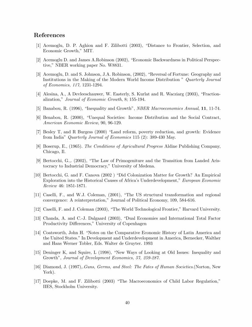
References
[1] Acemoglu, D. P. Aghion and F. Zilibotti (2003), “Distance to Frontier, Selection, andEconomic Growth,” MIT.
[2] Acemoglu D. and James A.Robinson (2002), “Economic Backwardness in Political Perspec-tive,” NBER working paper No. W8831.
[3] Acemoglu, D. and S. Johnson, J.A. Robinson, (2002), “Reversal of Fortune: Geography andInstitutions in the Making of the Modern World Income Distribution ” Quarterly Journalof Economics, 117, 1231-1294.
[4] Alesina, A., A Devleeschauwer, W. Easterly, S. Kurlat and R. Wacziarg (2003), “Fraction-alization,” Journal of Economic Growth, 8; 155-194.
[5] Banabou, R. (1996), “Inequality and Growth”, NBER Macroeconomics Annual, 11, 11-74.
[6] Benabou, R. (2000), “Unequal Societies: Income Distribution and the Social Contract,American Economic Review, 90, 96-129.
[7] Besley T, and R Burgess (2000) “Land reform, poverty reduction, and growth: Evidencefrom India” Quarterly Journal of Economics 115 (2): 389-430 May.
[8] Boserup, E., (1965). The Conditions of Agricultural Progress Aldine Publishing Company,Chicago, Il.
[9] Bertocchi, G.,. (2002), “The Law of Primogeniture and the Transition from Landed Aris-tocracy to Industrial Democracy,” University of Medena.
[10] Bertocchi, G. and F. Canova (2002 ) “Did Colonization Matter for Growth? An EmpiricalExploration into the Historical Causes of Africa’s Underdevelopment,” European EconomicReview 46: 1851-1871.
[11] Caselli, F., and W.J. Coleman, (2001), “The US structural transformation and regionalconvergence: A reinterpretation,” Journal of Political Economy, 109, 584-616.
[12] Caselli, F. and J. Coleman (2003), “The World Technological Frontier,” Harvard University.
[13] Chanda, A. and C.-J. Dalgaard (2003), “Dual Economies and International Total FactorProductivity Differences,” University of Copenhagen
[14] Coatsworth, John H. “Notes on the Comparative Economic History of Latin America andthe United States.” In Development and Underdevelopment in America, Bernecker, Waltherand Hans Werner Tobler, Eds. Walter de Gruyter. 1993
[15] Deninger K, and Squire, L (1998), “New Ways of Looking at Old Issues: Inequality andGrowth”, Journal of Development Economics, 57, 259-287.
[16] Diamond, J. (1997),.Guns, Germs, and Steel: The Fates of Human Societies.(Norton, NewYork).
[17] Doepke, M. and F. Zilibotti (2003) “The Macroeconomics of Child Labor Regulation,”IIES, Stockholm University.
40
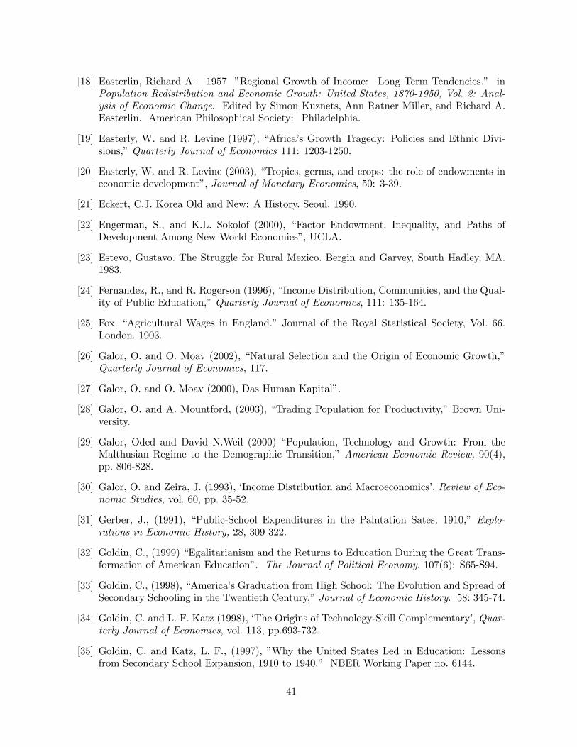
[18] Easterlin, Richard A.. 1957 ”Regional Growth of Income: Long Term Tendencies.” inPopulation Redistribution and Economic Growth: United States, 1870-1950, Vol. 2: Anal-ysis of Economic Change. Edited by Simon Kuznets, Ann Ratner Miller, and Richard A.Easterlin. American Philosophical Society: Philadelphia.
[19] Easterly, W. and R. Levine (1997), “Africa’s Growth Tragedy: Policies and Ethnic Divi-sions,” Quarterly Journal of Economics 111: 1203-1250.
[20] Easterly, W. and R. Levine (2003), “Tropics, germs, and crops: the role of endowments ineconomic development”, Journal of Monetary Economics, 50: 3-39.
[21] Eckert, C.J. Korea Old and New: A History. Seoul. 1990.
[22] Engerman, S., and K.L. Sokolof (2000), “Factor Endowment, Inequality, and Paths ofDevelopment Among New World Economies”, UCLA.
[23] Estevo, Gustavo. The Struggle for Rural Mexico. Bergin and Garvey, South Hadley, MA.1983.
[24] Fernandez, R., and R. Rogerson (1996), “Income Distribution, Communities, and the Qual-ity of Public Education,” Quarterly Journal of Economics, 111: 135-164.
[25] Fox. “Agricultural Wages in England.” Journal of the Royal Statistical Society, Vol. 66.London. 1903.
[26] Galor, O. and O. Moav (2002), “Natural Selection and the Origin of Economic Growth,”Quarterly Journal of Economics, 117.
[27] Galor, O. and O. Moav (2000), Das Human Kapital”.
[28] Galor, O. and A. Mountford, (2003), “Trading Population for Productivity,” Brown Uni-versity.
[29] Galor, Oded and David N.Weil (2000) “Population, Technology and Growth: From theMalthusian Regime to the Demographic Transition,” American Economic Review, 90(4),pp. 806-828.
[30] Galor, O. and Zeira, J. (1993), ‘Income Distribution and Macroeconomics’, Review of Eco-nomic Studies, vol. 60, pp. 35-52.
[31] Gerber, J., (1991), “Public-School Expenditures in the Palntation Sates, 1910,” Explo-rations in Economic History, 28, 309-322.
[32] Goldin, C., (1999) “Egalitarianism and the Returns to Education During the Great Trans-formation of American Education”. The Journal of Political Economy, 107(6): S65-S94.
[33] Goldin, C., (1998), “America’s Graduation from High School: The Evolution and Spread ofSecondary Schooling in the Twentieth Century,” Journal of Economic History. 58: 345-74.
[34] Goldin, C. and L. F. Katz (1998), ‘The Origins of Technology-Skill Complementary’, Quar-terly Journal of Economics, vol. 113, pp.693-732.
[35] Goldin, C. and Katz, L. F., (1997), ”Why the United States Led in Education: Lessonsfrom Secondary School Expansion, 1910 to 1940.” NBER Working Paper no. 6144.
41
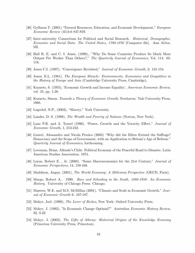
[36] Gylfason T. (2001).“Natural Resources, Education, and Economic Development,” EuropeanEconomic Review (45)4-6 847-859.
[37] Inter-university Consortium for Political and Social Research. Historical, Demographic,Economic and Social Data: The United States, 1790-1970 [Computer file]. Ann Arbor,MI.
[38] Hall R. E. and C. I. Jones, (1999),. ”Why Do Some Countries Produce So Much MoreOutput Per Worker Than Others?,” The Quarterly Journal of Economics, Vol. 114: 83-116.
[39] Jones C.I. (1997), “Convergence Revisited,” Journal of Economic Growth, 2: 131-154.
[40] Jones, E.L. (1981), The European Miracle: Environments, Economies and Geopolitics inthe History of Europe and Asia (Cambridge University Press, Cambridge).
[41] Kuznets, S. (1955), ‘Economic Growth and Income Equality’, American Economic Review,vol. 45, pp. 1-28.
[42] Kuznets, Simon. Towards a Theory of Economic Growth, Newhaven: Yale University Press,1968.
[43] Lagerlof, N-P., (2003), “Slavery,” York University.
[44] Landes, D. S. (1998), The Wealth and Poverty of Nations (Norton, New York).
[45] Lane P.R. and A. Tornel (1996). “Power, Growth and the Voracity Effect,” Journal ofEconomic Growth, 1, 213-242.
[46] Lizzeri, Alessandro and Nicola Persico (2003) “Why did the Elites Extend the Suffrage?Democracy and the Scope of Government, with an Application to Britain’s Age of Reform.”Quarterly Journal of Economics, forthcoming
[47] Loveman, Brian. Allende’s Chile: Political Economy of the Peaceful Road to Disaster. LatinAmerican Studies Association. 1974.
[48] Lucas, Robert E. , Jr. (2000). “Some Macroeconomics for the 21st Century,” Journal ofEconomic Perspectives, 14, 159-168.
[49] Maddison, Angus. (2001), The World Economy: A Millennia Perspective (OECD, Paris).
[50] Margo, Robert A.. 1990. Race and Schooling in the South, 1880-1950: An EconomicHistory. University of Chicago Press: Chicago.
[51] Masters, W.E. and M.S. McMillan (2001), “Climate and Scale in Economic Growth,” Jour-nal of Economic Growth 6: 167-187.
[52] Mokyr, Joel. (1990), The Lever of Riches, New York: Oxford University Press.
[53] Mokyr, J. (1992), ”Is Economic Change Optimal?” Australian Economic History Review,32, 3-23.
[54] Mokyr, J. (2002), The Gifts of Athena: Historical Origins of the Knowledge Economy(Princeton University Press, Princeton).
42
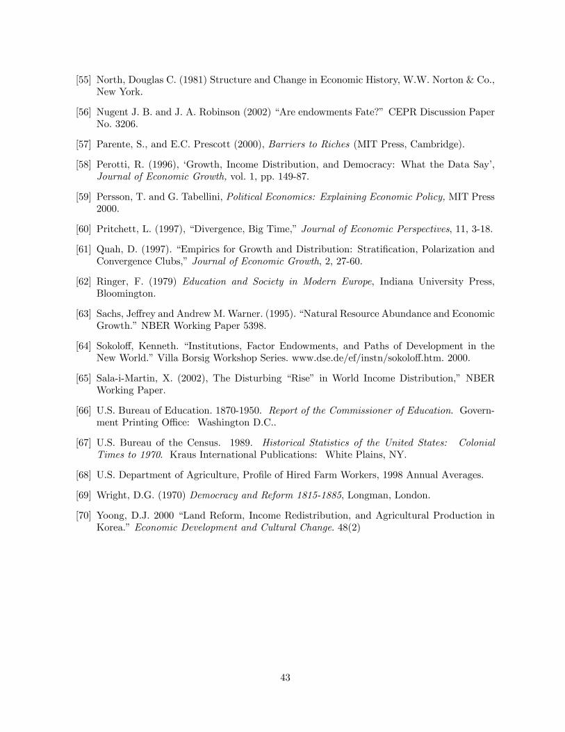
[55] North, Douglas C. (1981) Structure and Change in Economic History, W.W. Norton & Co.,New York.
[56] Nugent J. B. and J. A. Robinson (2002) “Are endowments Fate?” CEPR Discussion PaperNo. 3206.
[57] Parente, S., and E.C. Prescott (2000), Barriers to Riches (MIT Press, Cambridge).
[58] Perotti, R. (1996), ‘Growth, Income Distribution, and Democracy: What the Data Say’,Journal of Economic Growth, vol. 1, pp. 149-87.
[59] Persson, T. and G. Tabellini, Political Economics: Explaining Economic Policy, MIT Press2000.
[60] Pritchett, L. (1997), “Divergence, Big Time,” Journal of Economic Perspectives, 11, 3-18.
[61] Quah, D. (1997). “Empirics for Growth and Distribution: Stratification, Polarization andConvergence Clubs,” Journal of Economic Growth, 2, 27-60.
[62] Ringer, F. (1979) Education and Society in Modern Europe, Indiana University Press,Bloomington.
[63] Sachs, Jeffrey and Andrew M.Warner. (1995). “Natural Resource Abundance and EconomicGrowth.” NBER Working Paper 5398.
[64] Sokoloff, Kenneth. “Institutions, Factor Endowments, and Paths of Development in theNew World.” Villa Borsig Workshop Series. www.dse.de/ef/instn/sokoloff.htm. 2000.
[65] Sala-i-Martin, X. (2002), The Disturbing “Rise” in World Income Distribution,” NBERWorking Paper.
[66] U.S. Bureau of Education. 1870-1950. Report of the Commissioner of Education. Govern-ment Printing Office: Washington D.C..
[67] U.S. Bureau of the Census. 1989. Historical Statistics of the United States: ColonialTimes to 1970. Kraus International Publications: White Plains, NY.
[68] U.S. Department of Agriculture, Profile of Hired Farm Workers, 1998 Annual Averages.
[69] Wright, D.G. (1970) Democracy and Reform 1815-1885, Longman, London.
[70] Yoong, D.J. 2000 “Land Reform, Income Redistribution, and Agricultural Production inKorea.” Economic Development and Cultural Change. 48(2)
43