
Laboratory 1 Scientific Calculations and Basic Lab Techniques
Upload
khangminh22Category
view
2download
0
John MiltonStefan van der WaltCaleb MilesFernando PerezEmily NordhoffArthur H. LeeToru Ohira
Lab manual: Mathematics as alaboratory tool
Vol. 1 (Fall semester)
November 13, 2014
Springer


v
Dedication
On behalf of the contributors I dedicate these laboratory experiences to thelate John D. Hunter (1968–2012). Although all of us knew John either as a col-league and/or a teacher, few realized that many of the underlying pedagogical con-cepts for these laboratories arose from 20 years of conversations between John andme starting when he was my graduate student. I can still remember the day thatJohn, a second year PhD student, walked into my office and demanded that we nolonger use commercial software packages in our research, but instead use open-source resources, in particular Python. My apprehensions were soon dispelled whenI checked out the costs of maintaining software licenses for my students after grad-uation. Thus the decision to use Python as our programming language was born.John did not have the patience to do boring, repetitive bench top experiments byhand. Thus it was not surprising that a year later John had figured out how to geta computer to run his all of his recording and stimulation protocols for his neuro-physiological experiments on the motoneuron of the sea slug, Aplysia. Indeed, theexperiments described in his 2001 Journal of Neuroscience article were done whilewe sat together talking, occasionally sipping a glass of wine, while the computer didthe work while flashing the information on computer screens. Thus the decision toincorporate engineering concepts such as filtering and signaling and ultimately theuse of an Arduino board was made. John got tired about my insistence to preparefigures for publication by hand since I was not satisfied with figures prepared usingcommercial software packages. Beginning during his post-doctoral years in my labJohn developed his famous graphical software package, matplotlib. In 2004 Imoved to the Claremont Colleges and soon after John and I began taking about howscientific computing could be taught to undergraduate science students in a liberalarts environment. He invited me to a Scientific Python conference at Caltech, wherewith Andrew Straw, we began to formulate the idea of a scientific computing work-shop for undergraduate students. The first SciPy workshop was held in fall, 2007.With the addition of Fernando Perez, the fall semester SciPy workshops continuedyearly until 2012. Many of the exercises that our students enjoyed, e.g. the Moiredot program in Lab 4, the bird song spectrogram in Lab 9 and the filtering moonphotograph exercise in Lab 9, are exercises that were initially developed for theseworkshops. John emailed me from his hospital bed to tell me that he might not beable to do the 2012 SciPy workshop later that fall. The greatest reward that a teachercan receive is to be taught by their students. In knowing John D. Hunter I believethat I have been well blessed.
John G. Milton


Preface
The weekly laboratory experiences represent the way we teach the material pre-sented in Mathematics as a laboratory tool. We believe that a weekly 4-hour labo-ratory experience is an essential component of a course that teaches mathematicaltools to researchers who work in the laboratory. These laboratory sessions provide aunique opportunity for the lecturer to ensure that concepts are well understood andcan be implemented by every student. In our experience the “lights go on” when thestudent sees the result predicted by their paper and pencil calculations evolve on thecomputer that they control.
The laboratory exercises for the fall semester (Chapters 1-10) are given in Vol-ume 1 and those for the spring semester are given in Volume 2. The primary pur-pose of the first three laboratories is to introduce students into three programminglanguages that are used throughout: LaTeX, Python, and XPPAUT. Many of the lab-oratories are designed to introduce resources available in Python that are not alwayswell–documented, for example, resources related to the handling of jpg images andanimation. At the beginning of the course students log on to a Linux box that con-tains these program and learn to use these as well as elementary commands neces-sary to work in a Linux environment. As they become familiar with the use of theseprogramming languages they are required to install these programs on their personallaptop or desktop computer. Most students accomplish this by the 6-th Lab and cer-tainly before the 12-th Lab where this is a compulsory requirement. Installing thesoftware packages on each student’s laptop (which they do themselves) is essentialin order for them to translate the skills earned into their scientific activities after theycomplete the course.
vii


Acknowledgments
The laboratory exercises were developed over many years and could not have beendeveloped without the volunteer efforts of many people. In particular we acknowl-edge the efforts of Walter Cook (Harvey Mudd College) for the construction ofelectronic circuits, Boyle Ke (Keck Science Center for IT support, Emily Nordhofffor the development of thr Ardiuno lab and Caleb Mills (Class of ‘11, ClaremontMcKenna College) for lab instruction and the development of basic Python pro-grams.
ix


Contents
1 Communicating science(Lab 1) . . . . . . . . . . . . . . . . . . . . . . . . . . . . . . . . . . 1
2 Introducing XPPAUT (Lab 2) . . . . . . . . . . . . . . . . . . . . . . . . . . . . . . . . . . . 92.1 Background . . . . . . . . . . . . . . . . . . . . . . . . . . . . . . . . . . . . . . . . . . . . . . . 92.2 Exercise 1: First XPPAUT program . . . . . . . . . . . . . . . . . . . . . . . . . . . 102.3 Exercise 2: Second-order DDEs . . . . . . . . . . . . . . . . . . . . . . . . . . . . . . 132.4 Exercise 3: Phase plane representations . . . . . . . . . . . . . . . . . . . . . . . . 14
3 Introducing Python: Working with data (Lab 3) . . . . . . . . . . . . . . . . . . . 173.1 Background . . . . . . . . . . . . . . . . . . . . . . . . . . . . . . . . . . . . . . . . . . . . . . . 173.2 Exercise 1: Making figures using Matplotlib . . . . . . . . . . . . . . . . . . . . 203.3 Exercise 2: Adding a figure to a LaTeX document . . . . . . . . . . . . . . . 25
4 Working with arrays and eigenvalues (Lab 4) . . . . . . . . . . . . . . . . . . . . . 274.1 Background . . . . . . . . . . . . . . . . . . . . . . . . . . . . . . . . . . . . . . . . . . . . . . . 274.2 Exercise 1: Stability using XPPAUT . . . . . . . . . . . . . . . . . . . . . . . . . . . 314.3 Exercise 2: Stability using Python . . . . . . . . . . . . . . . . . . . . . . . . . . . . . 334.4 Exercise 3: Moire-Glass dot patterns . . . . . . . . . . . . . . . . . . . . . . . . . . 354.5 Exercise 4: Working with digital images . . . . . . . . . . . . . . . . . . . . . . . 37
5 The ’cubic’ nonlinearity: Excitable systems (Lab 5) . . . . . . . . . . . . . . . . 415.1 Background . . . . . . . . . . . . . . . . . . . . . . . . . . . . . . . . . . . . . . . . . . . . . . . 415.2 Exercise 1: The van der Pol oscillator . . . . . . . . . . . . . . . . . . . . . . . . . . 425.3 Exercise 2: Analog implementation of the van der Pol oscillator . . . . 435.4 Exercise 3: The Fitzhugh-Nagumo (FHN) neuron . . . . . . . . . . . . . . . . 455.5 Exercise 4: Reduced neuron models . . . . . . . . . . . . . . . . . . . . . . . . . . . 48
6 Bifurcation diagram: stopping spiking neurons with a single pulse(Lab 6) . . . . . . . . . . . . . . . . . . . . . . . . . . . . . . . . . . . . . . . . . . . . . . . . . . . . . . . . 536.1 Background . . . . . . . . . . . . . . . . . . . . . . . . . . . . . . . . . . . . . . . . . . . . . . . 536.2 Exercise 1: Making one-parameter bifurcation diagrams . . . . . . . . . . 556.3 Exercise 2: Bifurcation diagram: Hodgkin-Huxley neuron . . . . . . . . . 58
xi

xii Contents
6.4 Exercise 3: Stopping spiking neurons with a single pulse . . . . . . . . . . 61
7 Lab 7: Filters and convolution . . . . . . . . . . . . . . . . . . . . . . . . . . . . . . . . . . . 637.1 Background . . . . . . . . . . . . . . . . . . . . . . . . . . . . . . . . . . . . . . . . . . . . . . . 63
8 Lab 8: Fourier series: Gibbs phenomenon and filtering (Chapter 8) . . 738.1 Background . . . . . . . . . . . . . . . . . . . . . . . . . . . . . . . . . . . . . . . . . . . . . . . 738.2 Exercise 1: Gibbs phenomenon . . . . . . . . . . . . . . . . . . . . . . . . . . . . . . . 758.3 Exercise 3: Convolution: Graphical interpretation . . . . . . . . . . . . . . . . 758.4 Exercise 4: Making a sine wave from a square wave . . . . . . . . . . . . . . 76
9 Lab 9: FTT and power spectra . . . . . . . . . . . . . . . . . . . . . . . . . . . . . . . . . . 799.1 Background . . . . . . . . . . . . . . . . . . . . . . . . . . . . . . . . . . . . . . . . . . . . . . . 809.2 Exercise 1: Computing the power spectral density using mlab.psd() . 83
9.2.1 Power Spectral Density Recipe . . . . . . . . . . . . . . . . . . . . . . . . . 839.2.2 Example using mlab.psd() . . . . . . . . . . . . . . . . . . . . . . . . . . . . . 85
9.3 Exercise 2: Low-frequency signals . . . . . . . . . . . . . . . . . . . . . . . . . . . . 879.4 Exercise 3: FFT Applications . . . . . . . . . . . . . . . . . . . . . . . . . . . . . . . . . 88
9.4.1 Convolution: . . . . . . . . . . . . . . . . . . . . . . . . . . . . . . . . . . . . . . . . 889.4.2 Filtering images . . . . . . . . . . . . . . . . . . . . . . . . . . . . . . . . . . . . . 89
9.5 Spectrograms . . . . . . . . . . . . . . . . . . . . . . . . . . . . . . . . . . . . . . . . . . . . . . 90
10 Phase resetting oscillators (Lab 10) . . . . . . . . . . . . . . . . . . . . . . . . . . . . . . . 9310.1 Background . . . . . . . . . . . . . . . . . . . . . . . . . . . . . . . . . . . . . . . . . . . . . . . 9310.2 Exercise 1: Phase resetting curves . . . . . . . . . . . . . . . . . . . . . . . . . . . . . 9610.3 Exercise 2: Arnold tongue diagrams . . . . . . . . . . . . . . . . . . . . . . . . . . . 9810.4 Exercise 3: Phase locking modes for standard circle map . . . . . . . . . . 10010.5 Exercise 4: Phase locking modes for the periodically spiking HH
neuron . . . . . . . . . . . . . . . . . . . . . . . . . . . . . . . . . . . . . . . . . . . . . . . . . . . . 10110.6 Supplementary material: Phase resetting curves using XPPAUT . . . . 102
11 Blood cell dynamics: Oscillations, delays and chaos (Lab 11) . . . . . . . . 10711.1 Background . . . . . . . . . . . . . . . . . . . . . . . . . . . . . . . . . . . . . . . . . . . . . . . 108
11.1.1 Integrating DDEs using XPPAUT. . . . . . . . . . . . . . . . . . . . . . . 10811.1.2 Integrating DDEs using PyDelay . . . . . . . . . . . . . . . . . . . . . . . 110
11.2 Exercise 1: Periodic anemias . . . . . . . . . . . . . . . . . . . . . . . . . . . . . . . . . 11011.3 Exercise 2: Chaotic hematology . . . . . . . . . . . . . . . . . . . . . . . . . . . . . . 112
12 Arduino boards: Using your laptop in the laboratory(Lab 12) . . . . . . . 11512.1 Exercise 1: Blinking LEDs . . . . . . . . . . . . . . . . . . . . . . . . . . . . . . . . . . . 116
12.1.1 Background . . . . . . . . . . . . . . . . . . . . . . . . . . . . . . . . . . . . . . . . . 11612.1.2 The Code . . . . . . . . . . . . . . . . . . . . . . . . . . . . . . . . . . . . . . . . . . . 11712.1.3 The Potentiometer . . . . . . . . . . . . . . . . . . . . . . . . . . . . . . . . . . . 11912.1.4 A few more things to know . . . . . . . . . . . . . . . . . . . . . . . . . . . . 11912.1.5 The Code . . . . . . . . . . . . . . . . . . . . . . . . . . . . . . . . . . . . . . . . . . . 119
12.2 Exercise 2: Measuring Tremor . . . . . . . . . . . . . . . . . . . . . . . . . . . . . . . . 121

Contents xiii
12.2.1 What is an accelerometer? . . . . . . . . . . . . . . . . . . . . . . . . . . . . . 12212.2.2 The Code - Writing the Sketch . . . . . . . . . . . . . . . . . . . . . . . . . 12312.2.3 Calibration . . . . . . . . . . . . . . . . . . . . . . . . . . . . . . . . . . . . . . . . . . 12512.2.4 Data from fingertip movements . . . . . . . . . . . . . . . . . . . . . . . . 127
A Appendix A: Finding data for analysis . . . . . . . . . . . . . . . . . . . . . . . . . . . . 129
B Appendix B: Latex survival guide . . . . . . . . . . . . . . . . . . . . . . . . . . . . . . . . 133B.1 LaTeX manuals . . . . . . . . . . . . . . . . . . . . . . . . . . . . . . . . . . . . . . . . . . . . 134B.2 LaTeX . . . . . . . . . . . . . . . . . . . . . . . . . . . . . . . . . . . . . . . . . . . . . . . . . . . . 134
B.2.1 Text Editor . . . . . . . . . . . . . . . . . . . . . . . . . . . . . . . . . . . . . . . . . . 134B.2.2 Latex versus pdflatex . . . . . . . . . . . . . . . . . . . . . . . . . . . . . . . . . 135B.2.3 Viewing the LaTeX file . . . . . . . . . . . . . . . . . . . . . . . . . . . . . . . 135
B.3 Learning LaTeX . . . . . . . . . . . . . . . . . . . . . . . . . . . . . . . . . . . . . . . . . . . 135
C Appendix C: Introduction of Python by A. H. Lee . . . . . . . . . . . . . . . . . . 145C.1 Key references . . . . . . . . . . . . . . . . . . . . . . . . . . . . . . . . . . . . . . . . . . . . . 145C.2 How to run a Python interpreter . . . . . . . . . . . . . . . . . . . . . . . . . . . . . . . 145
C.2.1 Interactive mode . . . . . . . . . . . . . . . . . . . . . . . . . . . . . . . . . . . . . 145C.2.2 Script mode . . . . . . . . . . . . . . . . . . . . . . . . . . . . . . . . . . . . . . . . . 146
C.3 Basic data types and their values . . . . . . . . . . . . . . . . . . . . . . . . . . . . . . 148C.4 Comments . . . . . . . . . . . . . . . . . . . . . . . . . . . . . . . . . . . . . . . . . . . . . . . . 149C.5 Use of the print command in a script file . . . . . . . . . . . . . . . . . . . . . 149C.6 Variables . . . . . . . . . . . . . . . . . . . . . . . . . . . . . . . . . . . . . . . . . . . . . . . . . . 150C.7 Operating on values: operators and operands . . . . . . . . . . . . . . . . . . . . 151C.8 Order of precedence among operators . . . . . . . . . . . . . . . . . . . . . . . . . . 152C.9 Input from keyboard . . . . . . . . . . . . . . . . . . . . . . . . . . . . . . . . . . . . . . . . 152C.10 Functions and packages (libraries) . . . . . . . . . . . . . . . . . . . . . . . . . . . . 152C.11 Conditionals: doing it conditionally . . . . . . . . . . . . . . . . . . . . . . . . . . . 155C.12 Loops: doing it repeatedly . . . . . . . . . . . . . . . . . . . . . . . . . . . . . . . . . . . 157C.13 Compound data types: strings, lists, tuples . . . . . . . . . . . . . . . . . . . . . . 159C.14 Strings . . . . . . . . . . . . . . . . . . . . . . . . . . . . . . . . . . . . . . . . . . . . . . . . . . . 159
C.14.1 The for loop . . . . . . . . . . . . . . . . . . . . . . . . . . . . . . . . . . . . . . . . 161C.15 Lists . . . . . . . . . . . . . . . . . . . . . . . . . . . . . . . . . . . . . . . . . . . . . . . . . . . . . 163C.16 Modules . . . . . . . . . . . . . . . . . . . . . . . . . . . . . . . . . . . . . . . . . . . . . . . . . . 166C.17 Tuples . . . . . . . . . . . . . . . . . . . . . . . . . . . . . . . . . . . . . . . . . . . . . . . . . . . . 170C.18 Dictionaries . . . . . . . . . . . . . . . . . . . . . . . . . . . . . . . . . . . . . . . . . . . . . . . 172C.19 Files . . . . . . . . . . . . . . . . . . . . . . . . . . . . . . . . . . . . . . . . . . . . . . . . . . . . . 176
C.19.1 Text files . . . . . . . . . . . . . . . . . . . . . . . . . . . . . . . . . . . . . . . . . . . 178C.19.2 Exception handling . . . . . . . . . . . . . . . . . . . . . . . . . . . . . . . . . . . 179
C.20 More Python . . . . . . . . . . . . . . . . . . . . . . . . . . . . . . . . . . . . . . . . . . . . . . 180C.21 NumPy, SciPy, etc. . . . . . . . . . . . . . . . . . . . . . . . . . . . . . . . . . . . . . . . . . 180

xiv Contents
D Appendix D: The Scientific Python Ecosystem by F. Perez . . . . . . . . . . 181D.0.1 Scientific Python: a collaboration of projects built by
scientists . . . . . . . . . . . . . . . . . . . . . . . . . . . . . . . . . . . . . . . . . . . 181D.0.2 A note about the examples below . . . . . . . . . . . . . . . . . . . . . . . 183
D.1 Motivation: the trapezoidal rule . . . . . . . . . . . . . . . . . . . . . . . . . . . . . . . 184D.2 NumPy arrays: the right data structure for scientific computing . . . . 185
D.2.1 Basics of Numpy arrays . . . . . . . . . . . . . . . . . . . . . . . . . . . . . . . 185D.2.2 Indexing with other arrays . . . . . . . . . . . . . . . . . . . . . . . . . . . . . 188D.2.3 Arrays with more than one dimension . . . . . . . . . . . . . . . . . . . 189D.2.4 Operating with arrays . . . . . . . . . . . . . . . . . . . . . . . . . . . . . . . . . 192D.2.5 Linear algebra in numpy . . . . . . . . . . . . . . . . . . . . . . . . . . . . . . 195D.2.6 Reading and writing arrays to disk . . . . . . . . . . . . . . . . . . . . . . 196
D.3 High quality data visualization with Matplotlib . . . . . . . . . . . . . . . . . . 198D.3.1 Image display . . . . . . . . . . . . . . . . . . . . . . . . . . . . . . . . . . . . . . . 202D.3.2 Simple 3d plotting with matplotlib . . . . . . . . . . . . . . . . . . . . . . 203
D.4 IPython: a powerful interactive environment . . . . . . . . . . . . . . . . . . . . 203D.4.1 The IPython terminal . . . . . . . . . . . . . . . . . . . . . . . . . . . . . . . . . 205D.4.2 The graphical Qt console . . . . . . . . . . . . . . . . . . . . . . . . . . . . . . 211D.4.3 The IPython Notebook . . . . . . . . . . . . . . . . . . . . . . . . . . . . . . . . 212
References . . . . . . . . . . . . . . . . . . . . . . . . . . . . . . . . . . . . . . . . . . . . . . . . . . . . . . . . . 215

Chapter 1Communicating science(Lab 1)
We would all like to be good citizens of the scientific community. An importantpart of being a good citizen is being able to communicate results, papers, and ideas.Since many of our colleagues live in different parts of the world and hence havedifferent resources available to them we cannot always assume that they have thesame commercial software package (including upgrades) for preparing manuscriptsthat we do. Moreover, how can equations be exchanged easily by e-mail?
A modern day solution is to make use of the open source computing networkavailable on the Internet. In other words, we only require that our colleagues haveaccess to the Internet. There are all sorts of computer software packages availableon the Internet; many of them are exactly the same softwares that are presently usedat the cutting edges of scientific research (for example, check out the SciPy web-site). A big advantage is that once we become familiar with these products we haveaccess to them anywhere in the world. Study abroad students from The ClaremontColleges have already been able to use their experience with the open source com-puting network to help students, workers and scientists in the countries they havevisited.
Computer setup: This lab manual has been written with the assumption thatyour instructors have placed LaTeX, XPPAUT and Python onto a central Linuxcomputer that can be accessed either using computer terminal in a computer lab-oratory or, perhaps, by logging into using your laptop. However, it is now relativelyeasy to install all of these packages onto your own laptop for free. This is the pre-ferred way to do these labs because you retain the use of these tools for your ownpurposes after you complete the course1.
• LaTeX: See for example latex-project.org/ftp.html. Most studentsusing PC’s first installed MikTek (miktek.org) followed by Winshell (e.g.
1 Beginning fall, 2014 we require all students in this course to install these computer packagesonto their personal laptops. We do this in three stages: Week 1 (LaTeX); Week 2 (XPPAUT) andWeek 3 (Python). Our experience is that installing these packages is easier for students with PC’sthan those possessing Mac’s. Nonetheless all students with perseverance and the help of IT canaccomplish these tasks.
1

2 1 Communicating science(Lab 1)
www.winshell.de). Latex if often provided on the disks that come with thepurchase of a new Mac.
• XPP/XPPAUT: See www.math.pitt.edu/˜bard/xpp.html.• Python: We very strongly recommend that students install Enthought’s Canopy
Express (https://store.enthought.com). A huge advantage is thatpackages required to work with images and animation can readily be installedand managed through Canopy Express.
Today’s lab:In this lab we address how to prepare manuscripts containing equations and fig-
ures. The software package we will use is called LaTeX. This is the same softwarepackage that is used by the publishers of most journals and books that you readwhich contain equations. LaTeX is a completely different concept than, for exam-ple, a word processor such as WORD. Packages such as WORD are actually pro-grams that produce the document the way that the programmers who designed thispackage wanted it to be produced. In contrast, when we use LaTeX we write theprogram ourselves that will be used to generate the document. In fact, for many ofyou preparing a LaTeX document will be the first computer program that you havewritten! Since we are writing the program ourselves we can get an article that looksexactly like we want it to look. More importantly, the program is written using a texteditor2 and hence has the form of an ASCII file. This means that we can easily sendit to our colleagues by email and they can then run it locally on their own computerto generate the document.
It is really not very hard to learn to use LaTeX. We focus on the skill set necessaryto make the most basic LaTeX file (Appendix B). Of course there are many advancedfeatures available in LaTeX that are available which you can learn about as yousearch the Internet and/or discuss LaTeX with your colleagues. However, our goalis to be able to collaborate with others. We cannot assume that our colleagues knowthese advanced features or are even interested in learning how to use them. Thus, inour experience, collaboration is most successful when lines of communication arekept as simple as possible.
Most people learn LaTeX by doing it, i.e. their first experience is usually the re-sult of having to prepare their own paper because the journal publisher has asked forit. This is in fact how you will learn to use LaTeX. Your first assignment will be toreproduce two pages from a bio-mathematics book (see section labeled deliverableat end of the laboratory description). Of course it is necessary to know the basicstructure of the LaTeX file: the various commands that you need come from lookingthem up as you need them. This is why the Internet is so useful. Indeed we had tolook up a number of commands that we had never used before in order to make upthese notes! In this way we know them now!
2 A text editor is an editor which does not add any hidden format commands to the document. Inother words, what you see is what you get. In Microsoft environments, the text editors are Notepadand Wordpad; in LINUX two commonly used text editors are vi and emacs.

1 Communicating science(Lab 1) 3
Background: The main components of a LaTeX file are: 1) Preamble (Top mat-ter), 2) Main body, 3) Math modes, 4) Figures and Tables, and 5) Bibliography. Anintroduction to math modes is desribed in Appendix B which is available on thewebsite. The use of the basic commands are illustrated in today’s lab. We will dis-cuss how figures are introduced into a document in Lab 3. We do not need to knowhow to construct Tables or a bibliography for our purposes; however, these issuesare well documented on the Internet. Here we discuss the basic format of a LaTeXfile.
Preamble: The first line in the LaTeX program has the form
\documentclass[12pt]article
The term ’12pt’ means twelve points and sets the size of the print (This documenthas been printed using 12pt.). Points are the units that type-setters use to define thesize of characters on the printed page of, for example, a newspaper page. If youwant smaller print you could use, for example, 10pt, or bigger, 14pt, and so on. Theterm ‘article’ refers to the style that the paper will be prepared. Another style whichis often used is ’book’. Other styles are possible.
The preamble, or top matter, is everything from this line to the line
\begindocument
A typical preamble for passing in assignments to this course is
\usepackagegraphicx,times\titleBIO-133: Assignment number xxx\authorYour Name\\Your College
The preamble tells the program what fonts and style to use, the title and author ofthe article, and whether additional packages of commands need to be accessed inorder to produce the article. The preamble can be quite long since it is possible todefine new latex commands and environments. Additional packages are entered by\usepackage. Here we added the package graphicx and times: graphicxis the package that allow you to incorporate either *.eps or *.png into your document(discussed in Lab 3) and times means that the font will be New York Times style.Often journals, such as Nature, have there own packages and require you to declarethem in the usepackage statement. These *.sty files, and others, can readily belocated and downloaded from the Internet. In fact you could make up your own*.sty file and include it here (minus the extension); however, most people don’tdo this.
Main Body: The main body of LaTeX file is everything that lies between the com-mand
\begindocument
and the command

4 1 Communicating science(Lab 1)
\enddocument
The basic structure of the main body is
\begindocument\maketitle
text here\sectionyour section heading here
text here\subsectionyour sub-section heading here
text here\section*your section heading here
text here\subsection*your section heading here
text here..............................\enddocument
The commands \begindocument and \enddocument are manda-tory. The line \maketitle is included only if you made use of the lines \titleand/or \author in the preamble (which you will need to do for your assign-ments). The lines \section and \subsection generate, respectively, theappropriate section and sub–section numbers, whereas the lines \section*and \subsection* generate the same headings without the numbers.
Browser use: Anything that you would ever want to know about LaTeX can read-ily be tracked down on the Internet. Thus you will find it useful to have a browseropen in a second window of your computer as you prepare your first LaTeX docu-ment. Appendix B includes all of the math mode information that you will need forthis course.
Housekeeping: Perhaps the biggest issue when working with open source tools,such as LaTeX, is dealing with the directory system of the computer. Most presentday computer users don’t have to worry about directories and paths: just point,click, and drag! However, for computer programmers issues related to directoriesand paths are very important. We need to make directories to organize our work ina way that makes it easy for us to find things and we need paths so that a computerprogram can find items that it needs to complete its calculations such as figure files,data files, and where the outputs of the program should be written.
Paths always start from the root directory. On a PC the root directory is, bydefault, the hard disk specified by C, D, E, and so on. When we are in root theprompt on the command window will look like, for example, C:\. If you are auser in a Linux environment, the root directory is your home directory (the system’sadministrator has access to the root directory).
Referring to Figure 1.1, the root directory can be thought of as the root of a treefrom which many branches arise which themselves have branches, and so on. Let us

1 Communicating science(Lab 1) 5
Fig. 1.1 Example of path structure on a root directory. See text for discussion.
suppose that the root directory contains three sub–directories named apple, orangeand pear. If we are in root (i.e. on the screen we see C:\>), then we can type diror ls to obtain
<DIR> apple<DIR> orange<DIR> pear
The <DIR> do not appear when using Linux.Within the directory apple we have two directories, Ant and Bee, in the direc-
tory Orange we have the directories Walk and Run, and so on. What is the pathfor the directory Ant? The answer is
C:\Apple\Ant
Useful commands: These commands assume that either you are using the Com-mand Prompt window on a PC or are working on a Linux terminal (including MacOSX).
cd This means change directory. If we are in the root directory and want to be in thedirectory Orange we type
cd Orange
If we are in the directory
C:\Pear\Grass
and want to go to the directory
C:\Apple\Ant
we type

6 1 Communicating science(Lab 1)
cd C:\Apple\Ant
If you want to move up one directory you can use the command cd ... Finally ifyou want to move back to root you can use cd˜ in Linux and cd C:\ on a PC (inthe Command Prompt window).
pwd This command means pathway to directory. Another way to think of this com-mand is that it answers the question, “Where am I?” Thus when you are in anydirectory, you can obtain the path to that directory by typing pwd at the prompt.
mkdir You can create a directory with the command
mkdir name
rmdir You can remove a directory with the command
rmdir name
cp (copy) or mv (move) It is possible to move or copy files using the com-mands mv and cp (on PCs, respectively, move and copy. The move commandscan be used to rename a file, e.g.
mv test.dat test_new.dat
What is the command to move a file named test.dat located in the directory Grassto the directory Bee. The command depends on whether you are currently in Grassor somewhere else. If in Grass the command is
mv test.dat C:\Apple\Bee\.
or, in Linux,
mv test.dat ˜\Apple\Bee\.
The ’.’ means that the moved file is to have the same name in the new directory. Ofcourse you could move and changed the file name with one command, namely,
mv test.dat ˜\Apple\Bee\new_name.dat
If we are not in the directory Grass we can still move the file by using thecommand
mv ˜\Grass\test.dat ˜\Apple\Bee\.
It is important to organize our computer directories carefully so that you caneasily find things in the future. In your home directory make a directory called mtexwhich will contain your LaTeX documents (see below). It is useful to make sub–directories, each of which corresponds to one of the labs. For example, the documentprepared for today’s lab would be called Lab1 and so on. The path to this sub–directory from the home directory is ˜/mtex/Lab1.
Questions to answer: You will be provided with 1.5-2 pages from a mathematicalbiology textbook to reproduce. The LaTeXed article must be more than 1 page long

1 Communicating science(Lab 1) 7
in order to complete the exercise described in Lab 3. So let us know if it isn’t. Eachof you will have a different 1-2 pages to use to prepare your document.
Deliverable: Your LaTeX document must be completed before we do Lab 3. Youwill use your *.tex file to complete the exercise described in Lab 3 and then submita *.pdf at that time.


Chapter 2Introducing XPPAUT (Lab 2)
In biological applications it is quite rare that the solutions of the appropriate differ-ential equations can be obtained using paper and pencil. Thus we typically need touse computer programs to integrate these equations and to use as tools for analyzingtheir behaviors. In this course we use to types of computer programs: Python, a pro-gramming language, and XPPAUT a programming package that is very well suitedfor the analysis of many of the problems that arise in biology. Note that it is nowpossible to run XPPAUT within the Python ecosystem (Appendix D); however, wewill not do this in the lab.
XPPAUT is a ‘quick and easy’ to use programming package for investigatingthe differential equations [5]. An advantage of XPPAUT is that it can be used tointegrate discrete time systems, ordinary and delay differential equations, stochas-tic differential equations and partial differential equations. In addition, XPPAUT isparticularly well suited for the investigation of the dynamics of excitable systemscomposed of neurons and cardiac cells. Indeed, it is not uncommon that XPPAUTprograms can be located on the Internet for in the Supplemental materials for pub-lished papers on journal websites1. For example, the program we will use in Lab 6to study the Hodgkin-Huxley equation, hh.ode, can readily be found on the Inter-net. Can you locate this file? Hint: the program was developed by Micheal Guevaraat McGill University. Is it the same program that we have on our website!
2.1 Background
The lecture introduces the use of XPPAUT for the analysis of linear differentialequations. It is very easy to extend the use of XPPAUT to the study of nonlineardifferential equations. On the XPPAUT website check
Online Documentation
then check out1 Typically it is necessary to access these materials through the journal website.
9

10 2 Introducing XPPAUT (Lab 2)
Writing ODE filesReserved words & functionsCommon commands
Browser use: All of the information needed to program in XPPAUT can be ob-tained from the XPPAUT website. It is often possible to obtain additional help re-garding the use of specific XPPAUT commands by typing, for example, in Googlexppaut heav. Finally, it is often possible to locate programs on the Internet thatcan be used.
Housekeeping: Since XPPAUT file names have the form my_name.ode it isuseful to make a directory in the home directory called mode (in other words, myode files). Then we can make subdirectories in mode which contain XPPAUT pro-grams used for specific purposes, for example, for Lab 2. This will be useful whenwe require these programs for other purposes. An advantage of putting all of the datafiles and other materials necessary to run a program in the same subdirectory, thenwe don’t need to specify the directory paths in the program since, by default, thecomputer program always searches for files in the directory in which it is running.
Make sure that you are in your home directory (type pwd), then we perform thefollowing steps
mkdir modecd modemkdir Lab2cd Lab2
2.2 Exercise 1: First XPPAUT program
We illustrate the use of XPPAUT by using it to integrate the first–order ordinarydifferential equation
dxdt
=−kx (2.1)
Use a text editor, for example emacs, to create the file first_ode.ode. We re-mind the reader that it is useful to create this file in the directory Lab2. All XPPAUTfiles have the form
# Enter the equation (no spaces)dx/dt=k*x# Enter the initial conditionsinit x=1# Enter the parameter valuespar k=-0.1# Change default settings@ TOTAL=20,dt=0.05,xlo=0,xhi=100,ylo=0,yhi=1.5,maxstor=100000done

2.2 Exercise 1: First XPPAUT program 11
It should be noted that lines that begin with # are comments and are not actedupon by XPPAUT. The purpose of these lines is to make the code more readable fora user. However, you could simply write the program as
dx/dt=k*xinit x=1par k=-0.1@ TOTAL=20,dt=0.05,xlo=0,xhi=100,ylo=0,yhi=1.5,maxstor=100000done
Useful hints:1. TOTAL refers to the total time for the integration and dt is the step size
for the numerical integration. Thus if TOTAL=20 and dt=0.05, there will be20×20 = 400 time steps. The parameters xlo,xhi,ylo,yhi refer, respec-tively, to the dimensions of the x–axis and y–axis of the figure displayed byXPPAUT and not to the variables that appear in the differential equation. Theparameter maxstor sets the total number of time steps that will be kept inmemory (default value is 5000).
2. Likely the most common mistake made using XPPAUT is to add spaces to theentered equation to “make it look better”. Unfortunately the computer is notimpressed! Thus do not add spaces when you type in the equation. A good ruleof thumb is that when in doubt, no spaces!
3. The values of the initial conditions and parameters can readily be changed us-ing the on–screen menus provided by XPPAUT. In other words, it really doesnot matter which values you type into the *.ode program since you can easilychange them later.
4. The default integrator for an ordinary differential equation is a 4th–order Runge–Kutta algorithm. This is a common integrator used to study the differentialequations that arise in mathematical biology. There are two ways that the inte-grator can be changed: 1) on the XPPAUT start–up menu, click Numerics, thenMethod; and 2) in the change default settings part of the ode program type, forexample, meth=euler. One of the very useful features of XPPAUT is the easeby which it is possible to compare the effects of different numerical integratorsand their parameters on the simulation without writing new programs.
Running an XPPAUT program: The XPPAUT program is activated by typ-ing the command
xppaut first_ode.ode &
In a Linux environment the & is added since we do not want the whole CPU tobe involved in doing this calculation. In other words, by adding the & we make itpossible to do other computations at the same time.
Now press ENTER. The computer screen will look like that shown in Figure 2.1.

12 2 Introducing XPPAUT (Lab 2)
Fig. 2.1 Starting XPPAUT opens this window on the computer screen. The tabs for opening theadditional windows ICs, BCs, Delay, Parem, Eqns and Data are displayed in a row on the left sideof the top of the opened window.
Six additional windows can be opened (ICs, BCs, Delay, Param, Eqns, Data) byclicking on the appropriate icons. Since our goal is to integrate an ordinary differ-ential equation we need to open the menus ICs and Parem. Click on these icons anduse your mouse to arrange the computer screen so that it looks like that shown inFigure 2.2.
Fig. 2.2 This screen view was obtained by clicking on the Tabs ICs and Parem and then using thecomputer mouse to re–arrange the panels.
To run the program click ‘OK’ in the ‘Initial Data’ window and ‘Parameters’window and then ‘Go’ in the ‘Parameters’ window. The solution appears in themain window as it is computed (see Figure 2.3).

2.3 Exercise 2: Second-order DDEs 13
Fig. 2.3 The X versus T plot was produced by first clicking on ‘OK’ on the ICs panel and then‘Go’ on the Parem panel.
If you want to erase the solution, click on ‘Erase’. To quit the program, click on‘File’ and then ’Quit’.
Questions to be answered:1. In class we showed that the solution of (2.1) decreases exponentially when k < 0
and increases exponentially when k > 0. Do your simulations agree with thisexpectation?
2. The mathematical solution of (2.1) is x(0)exp(kt), where x(0) denotes the initialvalue (i.e., the number that appears in the IC window). Explain how can youverify that the numerically estimated solution has this form (Hint: what is the1/e time?)?
2.3 Exercise 2: Second-order DDEs
In order to use XPPAUT to integrate a second (and higher) order differential equa-tion it is necessary to rewrite the differential equation as a system of two (2) first-order differential equations, i.e.
dxdt
= f (x,y)
dydt
= g(x,y)
where f and g are functions of x and y.
Questions to be answered:
1. Write the second–order differential equation

14 2 Introducing XPPAUT (Lab 2)
Fig. 2.4 This window was obtained using a XPPAUT program that was written to integrate asecond–order linear differential equation. In preparation for re-plotting the data as a phase plane,we have clicked on ‘Viewaxes’ and then ‘2D’ to open the new panel shown on the lower left. Thevalues in the panel were typed in.
d2xdt2 +b
dxdt
+ cx = 0 (2.2)
as a system of two first–order differential equations.2. Write an XPPAUT to integrate this second–order differential equation. Call this
program second_ode.ode and put this file into the directory \mode\Lab2.A screen shot of the program we wrote is shown in Figure 2.4.
3. What is the characteristic equation and what are its roots?4. Determine values of the parameters b,c so that both roots are negative real num-
bers, complex numbers with negative real parts, and a pair of purely imaginarynumbers. In each case use your XPPAUT program to compute the solutions.Are the solutions qualitatively the same or do they differ? If they differ, thenwhat are the differences?
2.4 Exercise 3: Phase plane representations
Up to now we have plotted x or y versus time. In these plots, time appears explicitly(namely, it is the x–axis). However, there is another way to plot the data, namely xversus y. This type of plot is referred to as a phase plane plot and is characterizedby the fact that time does not appear explicitly.

2.4 Exercise 3: Phase plane representations 15
Fig. 2.5 The phase plane solution in the right panel was produced by clicking on the ‘OK’ Tab onthe ‘2D View’ shown in Figure 2.4.
After running XPPAUT, click on Viewaxes, then 2D (see Figure 2.4). The tablethat opens identifies the x–axis of the plot as time and the y–axis as the value of x.The ranges are those we entered in the last line of the program second_ode.ode.To obtain the phase plane representation, change the values so that y is plotted onthe y–axis and x is plotted on the x–axis. You will also need to adjust the ranges inthe two axis so that they span both positive and negative numbers, e.g.
xlo=-5,xhi=5,ylo=-5,yhi=5
Press ‘OK’ to obtain the phase plane representation (Figure 2.5).
1. For the values of b,c determined above, determine the phase plane for a pairof negative real numbers, a pair of complex numbers with negative real partand a pair of purely imaginary numbers. In our lectures we will describe theshape of the phase plane representations as a spiral, a focus and a center. Canyou guess which pair of eigenvalues corresponds to which type of phase planerepresentation?
Problem:In lecture we discussed the conditions for steady state for the consecutive reaction
Ak1−→ B
k2−→C , (2.3)
1. Write down the differential equations that describe this consecutive reaction asa system of three first–order differential equations.
2. Write a XPPAUT program to integrate these equations. Do the time courses ofA, B, and C resemble those we discussed in Chapter 3 on Mathematics as aLaboratory Tool?

16 2 Introducing XPPAUT (Lab 2)
3. Show that as the ratio k2/k1 becomes larger, the steady state condition for Bbecomes more reasonable.
4. Keep track of the values of k1,k2 you used in your simulations. In Lab 3 we willshow you how to write a Python program with matplotlib to make a figure.At that time we will ask you to produce a figure that shows these results. Notethat you can save yourself some time by clicking on Data, then Write to savethe data file after you run each simulation.
Deliverable:Use Lab2_template.tex to prepare the lab assignment.
Assignment hints:• A useful LaTeX environment for writing up your lab assignment is the verba-
tim environment, namely \beginverbatim .... \endverbatim.Whatever is placed within this environment appears in the LaTeX document aswritten.
• You can save a figure in XPPAUT by clicking on Graphic stuff, thenPostscript. This makes a *.ps figure which is likely not going to be muchuse to you since we can’t use such a figure in LaTeX and we don’t have apostscript printer. A very powerful software package for dealing with figures iscalled ghostscript. It is freely available and can be easily downloaded andinstalled from the Internet on your own computer. Using this software package itis possible to convert a *.ps figure to a *.pdf figure, by typing the command
ps2pdf name.ps

Chapter 3Introducing Python: Working with data (Lab 3)
Software packages such as XPPAUT are well suited for analyzing the propertiesof differential equations. However, in the laboratory we are also often interested inanalyzing the data collected experimentally. Typically this data is collected usingan instrument that is capable of exporting the data in the form of, for example, anASCII file. Thus an essential skill for laboratory researchers is the ability to writeour own programs to analyze collected data in whatever way we can imagine. In thislab we introduce the use of Python for this purpose1.
The important point concerning the use of Python for scientific programming isthe availability of packages that increase Python’s computational speed and useful-ness (see Appendices C and D). A very useful Internet website is SciPy
http://docs.scipy.org/doc/
It is worthwhile to become familiar with the content on this website. It should benoted that the term SciPy refers both to a package that can be imported as well as toScientific Python which means Python supplemented by packages. Many packagesare available (see the SciPy website) and more are being created. In this lab wefocus on two Python packages which are used in every Python program we willwrite, namely, numpy, the numerics packages, and matplotlib, the graphicspackage.
Question: What resources are available on the SciPy website for users interestedin neuroscience?, molecular biology?
3.1 Background
The lecture introduces Python programming skills that make it possible to importdata either generated by another computer program or collected by an experimentaldevice and then plot the observations using the matplotlib package. Appendices
1 Other possibilities are available such as MATLAB,OCTAVE, C++ and FORTRAN.
17

18 3 Introducing Python: Working with data (Lab 3)
C and D provide an introduction to, respectively, programming in Python and thePython ecosystem, including an introduction to matplotlib. It is useful to glanceover these documents; however, only a small portion of this material is covered intoday’s lab. In the coming weeks we will cover most of this information.
Browser use: All of the information needed to write Python programs and usethe matplotlib package (and more) are available on the Internet. Most of thePython commands we will use in this and the following laboratories are describedin Appendices C and D. By this point in the course the reader should realize howuseful it is to have access to the Internet while working with a computer (“everythingcan be located on the Internet”). For example, information concerning how to useany command in numpy, the numerical package for Python, plus an example ofthe command’s use can readily be obtained on Google. For example, if we want tounderstand how to use arange(), then type on Google
numpy arange
Not only will you get the information you wanted you will also be advised to use thecommand linspace() instead! Other hits on Google will explain why it is betterto use linspace(). The SciPy website (type SciPy) in Google provides muchmore information concerning on-line resources that are available (once on this web-site look under Additional Documentation). It should be noted that SciPyis an open source resource and thus it is not always well documented. Nonethelessby talking to colleagues and exploring the Internet it is usually possible to find outwhere things are located.
The most useful website for the matplotlib package is
http://matplotlib.org/
This is the website created by the late John D. Hunter, the creator of matplotlib.Particularly useful are the list of plotting commands, the gallery andthe tutorial by Nicolas Rougier. The gallery shows a number of different stylesfor making figures: see one that you like, click on it, and you obtain the Python codeused to produce the figure!
A great deal of confusion exists concerning whether the graphics package shouldbe imported into a Python program as matplotlib or pylab or some ver-sion thereof. The package matplotlib is the whole graphics package; how-ever, for many graphical applications the whole package is not needed. Thus it isbetter to import small parts, or modules, of matplotlib, namely pylab andmatplotlib.pyplot. The module pylab is most convenient for use withipython where the emphasis is on interactive calculation and plotting. We willintroduce ipython in the spring laboratory sessions. matplotlib.pyplot ismost useful in a non-interactive programming setting in which the investigator isexploring the data and obtaining clues to develop a program. By non-interactivecomputing we mean that the investigator works with a program script (a programsaved in a file myname.py). This type of programming is used when the same tasksare done over and over again (such as what the above program is done), i.e. there is

3.1 Background 19
no need for data exploration. Of course, in a course such as this, we require the useof program scripts so that we can evaluate your progress.
Housekeeping: The names of Python programs have the form myname.py. Aswe did in Lab 2 it is useful to organize our home directory. Make a directory calledpyfigs and inside this directory a sub-directory called Lab3.
As an illustration we export data generated by XPPAUT and use this data to makea figure that we can place inside the LaTeX document we began making in Lab 1.Run the program second_ode.ode using the values of the parameters, b and c,that produced a spiral wave in the phase plane. Once the program has been run, clickon Data, then Write. Call the data file spiral.dat.
Where is the file spiral.dat located? It will likely be saved in the directorythat contains second_ode.ode. Move this file to /pyprogs/Lab3 by typing
mv spiral.dat /pyprogs/Lab3/.
Note that the ‘.’ means that we want to use the same file name. If you prefer torename the moved file you could type
mv spiral.dat /pyprogs/Lab3/new_name.dat
Now open the file spiral.dat with the text editor by typing
emacs spiral.dat &
Why did we add the ‘&’?You should see three columns of numbers: the first column is time, the second
column is ‘x’, and the third column is ‘y’. Note that along each row the numbersare separately by spaces. This observation means that the data file is a .tsv file,i.e. a file of tab separated variables. Thus a better name for the data file would bespiral.tsv. We can rename spiral.dat as spiral.tsv by typing
mv spiral.dat spiral.tsv
It is also possible that numbers in a data file are separated by commas, namely a.csv file, where csv stands for comma separated variables. We could name suchfiles with the suffix .csv, i.e. myname.csv. As we will soon see, it is important toknow whether we have a .csv or a .tsv file when we write the computer programto analyze the data.
A second question concerns how the columns are numbered. In Python the firstcolumn is ‘0’, the second column is ‘1’, and so on. In some languages, such asMATLAB, the first column is labeled as ‘1’; however, for most computer languagesthe first column is labeled as ‘0’.
The data file spiral.tsv is an example of an array. In this case the array hasthree columns and N rows where N=time/dt and dt is the integration time step.

20 3 Introducing Python: Working with data (Lab 3)
3.2 Exercise 1: Making figures using Matplotlib
Python is a programming language such as C or Fortran. By itself Python is notwell suited for scientific research in the laboratory. However, it is possible to “putPython on steroids” by importing packages which provide specific tools that areuseful for scientific applications. Two commonly used packages are numpy whichprovides numerical tools based on arrays similar to those found in MATLAB andmatplotlib which provides graphical tools used, for example, to plot data in theform of figures and tables. Other packages are available: a list can be found at
http://www.scipy.org/SciPy_packages
Our first goal is to develop a Python program that imports a data file (array) gen-erated by some other program or a laboratory instrument, plot the data in the form ofa figure, and then save the figure in a form that is suitable for inclusion in a LaTeXdocument. Researchers do this over and over again and thus it is important to havesuch a program. This sounds like a tall task given that we are just beginning to learnto write Python programs. A good way to start to program in Python is to consideran illustrative example. Let’s examine the Python program data_plot.py
# Import the required packagesimport numpy as npimport matplotlib.pyplot as plt
# Import the data fileX=np.loadtxt(’spiral.tsv’)
# Extract the data from the arrayx0=X[:,0]x1=X[:,1]x2=X[:,2]
# Plot the data in the form of a figureplt.plot(x1,x2,’k-’,linewidth=2)plt.xlabel(’X’,fontsize=16)plt.ylabel(’Y’,fontsize=16)
# Save the figure in an appropriate formatplt.savefig(’spiral.png’,dpi=600)plt.savefig(’spiral.eps’,dpi=600)
# Show the figure on the compter screenplt.show()
Comments:1. Python gets it scientific usefulness by importing packages which contain func-
tions that are useful. These functions make it possible to integrate differentialequations, to perform statistical and time series analyses, to import photographsand bird songs, to animate simulations, and so on. The basic numerical package

3.2 Exercise 1: Making figures using Matplotlib 21
is numpy and the graphics package is called matplotlib (or pylab). Thefirst lines of a Python program imports these packages, for example, using thecommands2
import numpy as npimport matplotlib.pyplot as plt
It should be noted that other packages are available (see the SciPy website).These would be imported if they are required for the program you are writing.
2. When beginning to program in Python it is useful to specify the package fromwhich function was obtained. Thus, for example if we want to use the functionplot() in matplotlib.pyplot we write
plt.plot()
and so on.
3. The numpy function which makes it possible to import a data file is
X=np.loadtxt(’myname.tsv’)
Note that this command associates the label ‘X’ with the whole data array. Ifthe data file to be imported is a *.cvs file, then this command becomes
X=np.loadtxt(’myname.csv’,delimiter=’,’)
It should be noted that there are only two other ways that an array in Pythoncan be constructed. We will discuss these as our Python programming skillsincrease.
4. The next step is to extract from X the columns of data that correspond to time,x, and y. The command that extracts a single column of data, say the 0-th col-umn, from an array is x0=X[:,0]. This command associates x0 with the firstcolumn in X .This command is so useful that you should memorize it.Note that we have labeled the extracted column with the small letter, in thiscase x, which corresponds to the capital letter X used to specify the array. Thisis not necessary, but is useful for helping a reader of your program (includingyourself at a later date) to better see how the program is organized, especiallywhen more than one data set is imported into the program.
5. The command plt.plot() is a very powerful plotting command with lotsof actions. Go to the Matplotlib website and look up how to use plot(). Thecommand used in the above program is the most basic form of the command andplots the data using a black solid line (’k-’) of width 2. The PyLab websitealso gives all of the commands we can use to make our figure look pretty.
2 There are other ways to import these packages; however, for learning it is best to start in this way(see discussion).

22 3 Introducing Python: Working with data (Lab 3)
6. It is useful to get into the habit of saving figures in two forms: myname.epsfor use in LaTeX documents and myname.png for use in pdflatex files. Theresolution is given by specifying the dpi. The default resolution for most sci-entific journals is dpi=600.
Helpful hint: It should be noted that the above program can be used to importany 3-column data array and plot the data as a figure. You will likely use such aprogram many times over your scientific career. The good news is that we onlyneed to write (type) the whole program once in our lives! This is because we canuse a text editor, such as emacs, to modify the couple of lines of the program thatare needed for a specific use. Thus you might think about creating a subdirectoryin your home directory called template and then place a copy of the programin this directory. It might be reasonable to give the file a generic name such asplot_3column_data.py. Suppose you are working on your data in a subdi-rectory called Mydata and decided that you wanted to plot the data. Of course youcould write a new program to do this. However, we are suggesting that you do thefollowing
mv ˜/template/plot_3column_data.py ˜/Mydata/myname.py
You could then open myname.py using a text editor such as emacs, make the neces-sary corrections (change the name of the data file, change the variables to be plotted,etc), and then run the program. Our guess is that this procedure will take much lesstime than typing, and then debugging, a new program from scratch.
Differential equations using Python: The reader will no doubt wonderwhy we used one programming language to integrate the differential equation andanother to prepare the figure. Is it possible to do both steps within the same program?Fortunately the answer is YES. The following program entitled second_ode.pyshows how Python can be used to integrate a second order ordinary differentialequation and produce as output a figure suitable for publication.
import pylab as pltimport numpy as npimport scipy.integrate as integratea=1.0b=2.0t=np.linspace(0, 1, 100, endpoint=True)## Define deriv() for second-order differential equationdef derivs(state,t):
x,y = statedeltax = ydeltay = a*x + b*yreturn deltax,deltay
x0=1.0y0=0.0

3.2 Exercise 1: Making figures using Matplotlib 23
z0=[x0, y0]z=integrate.odeint(derivs, z0, t)## Output is the array z[] containing two columns# First column is ’0’ and contains x# Second column is ‘1’ and contains y#x=z[:,0]y=z[:,1]## plot x versus time# plt.plot(t,x,’k-’)## plot y versus time# plt.plot(t,y,’k-’)## plot phase plane#plt.plot(x,y,’k-’)#plt.show()
Comments:1. Functions that integrate ordinary differential equations are imported using the
statement
import scipy.integrate as integrate
2. The integrator odeint was developed by Lawrence Livermore National Lab-oratories. It does an adaptive time-step to achieve a desired level of solutionaccuracy. This software is designed to automatically switch between stiff andnon-stiff integration routines depending on the characteristics of the solution.A list of full options can be obtained in I-python by importing the packagescipy.integrate and then typing odeint?.
3. The integration duration and time step is set using
np.linspace(start,stop,N,endpoint=True).
This function generates N points equally spaced on the closed interval [start,stop].Note that the beginning and end points are included provided that we includeendpoint=True.It is also possible to set the integration duration and time using
np.arange(start,stop,step).
This function is not currently favored since when using a non-integer step, theresults will often not be consistent.

24 3 Introducing Python: Working with data (Lab 3)
4. The output of integrate.odeint() is the array z[]. The number ofcolumns in this array is equal to the dimension of the ordinary differential equa-tion. Since we are integrating a first-order ordinary differential equation there isonly one column of numbers. The first column in a numpy array is 0, hence thex are z[:,0].
5. Extension to higher order ODEs is straightforward; however, it is importantto remember to include all of the initial conditions that are required.
Questions to be answered:1. The Lotka-Volterra predator-prey equations are
dxdt
= k1x− k2xy
dydt
= k3xy− k4y
Write a Python program to integrate this equation and prepare a *.png figurethat shows the phase plane portrait. It is useful to call this program lotka.pyand store it in the directory pyprogs.
2. The equations for the van der Pol oscillator are
dxdt
=1ε
[y− x3
3+ x]
dydt
= −εx
where ε > 0 is a constant. Write a Python program to integrate this equationand prepare a *.png figure that shows the phase plane portrait. It is useful to callthis program vdp.py and store it in the directory pyprogs.
3. The equations for the Fitzhugh-Nagumo model (FHN) spiking neuron are [9,30] equation
dvdt
= f (v)−w+ Iext
dwdt
= bv− γw
where v plays the role of membrane potential, w is a recovery variable, Iext is anexternal applied current, f (v) is a cubic nonlinearity,
f (v) = v(a− v)(v−1)
and the parameters are 0 < a < 1, b > 0 and γ > 0. Write a Python programto integrate this equation and prepare a *.png figure that shows the phase planeportrait. It is useful to call this program fhn.py and store it in the directorypyprogs.

3.3 Exercise 2: Adding a figure to a LaTeX document 25
3.3 Exercise 2: Adding a figure to a LaTeX document
In order to introduce figures into our article we need to pay attention to the followingpoints:
1. We must include the user package graphicx in the preamble of the LaTeXfile.
2. The figure must be in the form of either a *.eps file, a *.png file, a *.jpg file ora *.pdf file.
3. Both types of files can be produced by matplotlib.4. When you use *.png or *.pdf or *.jpg (not *.jpeg), then you must use the
command pdflatex.5. For publication the pictures must be *.eps and hence you must use latex. An
advantage of latex documents is that they are often smaller than documentsprepared using pdflatex. The disadvantage is that the document is producedas a myname.dvi file. However, once again ghostscript comes to therescue: we use the command dvipdf to convert the file into a myname.pdffile.
The figure environment in LaTeX has the form
\beginfigure\centering\includegraphics[width=.5\textwidth]filename.eps\captionyour text here\labelyour label here\endfigure
You will find that it is quite tedious to place figures into a LaTeX document.The default mode for LaTeX is to put the figure at the end of the document. Thishappens because either the figure is to big to put it where you hoped that it would goor your placement conflicts in some way with items that are in the same region ofthe document where you want the figure. A good first step is to latex the documentbefore a new figure is added and pick the place where you want the added figure toappear: best choices are the top of the page or between paragraphs. Pick a reasonablefigure size, say 0.5, and add the figure environment statement to the appropriateplaced in your *.tex file. Now latex the file and see if the figure actually appearedwhere you hoped. Then add the second figure and repeat the process. The point isthat you need to place the figure in the document sequential in the order first throughlast. With a little practice you will get the hang of it!
Deliverable: Use Lab3_template.tex to prepare the lab assignment.


Chapter 4Working with arrays and eigenvalues (Lab 4)
The purpose of this lab is to get familiar with manipulating data arrays in numpy.
Browser use: This lab introduces the use of a number of Python packages thatare particularly useful for working with images such as *.jpg pictures taken witha cell phone. These packages include skimage and PIL (Python Imaging Li-brary). We strongly recommend installing Canopy Express on your computer:these packages can be readily installed using Package Manager to installscikits-image. Unfortunately many of these packages are not well documentedand hence the only way to learn about using them is to use these packages and con-sult the Internet: Chances are if you are having a problem, then someone else hasposted a question on the Internet about it and hopefully someone else has answeredit! In addition, Appendices C and D will be useful as references.
Housekeeping: In your home directory make two directories pyprogs andpyimages. It is convenient to put the programs we write in this lab into the di-rectory pyporgs since we will use them in future labs. The directory pyimageswill be used to store the programs that we will develop to manipulate images suchas *.jpg pictures.
4.1 Background
You can activate python in command mode, by typing the word python at thecommand prompt, then hit ENTER. In Canopy Express the command mode windowis opened when you type Editor (it’s the lower of the two windows that open). It isuseful to do this to follow the discussion. Now type
import numpy as np
then ENTER, so that you have access to the numpy library of commands.Here are two very important concepts in scientific computing that are often
under-emphasized:
27

28 4 Working with arrays and eigenvalues (Lab 4)
1. Not all numbers are the same: There are three basic number types: integers,floating point number and complex numbers. An integer is a number such as 1,2, 3, etc. Note that integers do not have a decimal point. A floating point numberis a number that has a decimal point, i.e 1.0, 2.2348016, and so on. A complexnumber has the form floating point number ± j floating point number.
In Python we can specify the data type by using the command dtype. Thus itwe want our number to be short integers we could specify
dtype=np.int8
if a floating point number
dtype=np.float32
and so on.
For imaging we most often use dtype=unit8. This notation stands for 8-byte, unsigned integers. Why are images limited to 8-bytes? There are two rea-sons: 1). Most computer monitors can only display 8 bytes, and 2) The humaneye is only able to render about 8 bytes of visual information. For a useful listof the possible dtypes seehttp://docs.scipy.org/doc/numpy/user/basics.types.html.
If we keep in mind that computers store objects as 0′s and 1′s it is not hardto imagine that we can specify dtypes that are not numbers. For example,dtype=str means a string of letters like a word and dtype=bool refers toeither True or False. We can even use the command dtype=object torefer to something that is none of the above.
2. An important data structure in numpy is the array. For an extensive dis-cussion of arrays in Python see Appendix C and using arrays in numpy seeAppendix D. Here we briefly touch on some of the important points.
An array is a table of objects (usually numbers for scientists) having n rowsand m columns. For scientists it is convenient to think of an array as a table ofdata. For example let us consider that the position of the hand during throwinga baseball has been recorded by motion capture cameras. The output of thecamera system is typically a table of data in which the first column is time, thesecond column is the position of the hand in the x=direction at time t, the thirdcolumn is the position in the y-direction at time t and the fourth column is the zposition of the hand at time t. Thus data array has n rows, where n is the nukberof time samples, and 4 columns. The shape of this data array is (n,4).
Suppose for simplicity that we have the array stored in the file test.dat
1 23 45 6
The shape of this array is 3 rows and 2 columns. We can load this data set intoour program using the command

4.1 Background 29
X = np.loadtxt(’test.dat’)
The command np.shape(X) tells us the shape of X and returns (3,2). Wecan also use the command reshape() to change the shape of X. Thus
Y=np.reshape(X,(6,1)))
returns
123456
3. Creating arrays: In the laboratory setting, the most common way to createan array in a Python program is to read in data using the np.loadtxt()command. In this case data file itself determines the way that the numbers arerepresented, the number of rows and the number of columns. The question ishow to create an array of a given shape inside a computer program. In otherwords for a situation in which we do not read in a data file as discussed above.The answer to this question is important because we often use a computer simu-lation of a model to predict what the behavior of the experimental observations.Since at some point we will need to compare prediction to observation we needto be able to make an array that contains the predictions of the model.
There are three ways to create an array and these are very similar in philosophyThe philosophy is the same: we create an array of the desired shape filled witheither 0’s, 1’s or random numbers and then replace these numbers by the numbergenerated by our computer simulations.
a. np.zeros(): In this case we create an arrays of 0′s of a required shape.For example, the command
X=np.zeros((2,2),dtype=np.float32)
creates the array
0. 0.0. 0.
b. The command np.ones() works in a similar way, except that instead of1′s we get 0′s.
c. The command np.random.rand() creates an array of a given shape ofrandom floating point numbers, e.g.
np.random.rand(2,2)
produces

30 4 Working with arrays and eigenvalues (Lab 4)
0.4823714 0.73987870.0082137 0.9087786
It should be noted that for np.zeros() and np.ones() we can specify thedtype, but for np.random.rand() the dtype is always a floating pointnumber.
4. Extracting data from arrays: Each element in an array occupies position (i, j)where i specifies the row and j specifies the column. Thus if we wanted to knowwhat is the value located in the second row, third position of array X we wouldtype X[2,3]. Note that an array position is enclosed by square brackets (incontrast in MATLAB we would use round brackets, i.e. X(2,3)). Keep inmind that the first element in the first row is X [0,0].
In many languages including Python, the colon : is very special. By itself itdenotes all of the corresponding row or column. Thus if we wanted to extractthe first column from array X we would type
x0=X[:,0]
and if we wanted to first row we would type
x0=X[0,:]
A colon : separating two numbers a : b means rows (columns) a to b. Thus
[1:5] means from 1 to 5
Here are some other useful array manipulations:
[1:] means 1 to end[len(a):1] means from length a to end[::n] means each n-th item in entire sequence
Of course we can also combine these notations, for example, if X was an arraywith shape (10,10), then
X[1:5,7:10]
would mean the first five rows and the last four columns.
5. Saving computer generated arrays as data files:Numpy lets you write arrays into files in two ways. In order to use these toolswell, it is critical to understand the difference between a text and a binary filecontaining numerical data. In a text file, the number π (referred to as pi innumpy) could be written as “3.141592653589793”, for example: a string ofdigits that a human can read, with in this case 15 decimal digits. In contrast,that same number written to a binary file would be encoded as 8 characters(bytes) that are not readable by a human but which contain the exact same datathat the variable pi had in the computer’s memory.
The tradeoffs between the two modes are thus:

4.2 Exercise 1: Stability using XPPAUT 31
• Text mode: occupies more space, precision can be lost (if not all digits arewritten to disk), but is readable and editable by hand with a text editor. Canonly be used for one- and two-dimensional arrays.
• Binary mode: compact and exact representation of the data in memory, can’tbe read or edited by hand. Arrays of any size and dimensionality can be savedand read without loss of information.
Here we discuss how to read and write arrays in text mode. Appendix D dis-cusses how to read and write arrays in binary mode.
The np.savetxt function saves an array to a text file, with options to controlthe precision, separators and even adding a header. Suppose we have an arrayX containing 10 numbers from 0 to 9 with shape (2,5) and we want to write itto a file called test.out. The command is
np.savetxt(’test.out’, X, fmt=’%1.3f’, header="My dataset")
and X is
# My dataset0.00 1.00 2.00 3.00 4.005.00 6.00 7.00 8.00 9.00
This is because we used the format option, fmt=’%1.2f’ to specify a floatingpoint number (hence the ‘f’), where the .2 indicates two decimal points. If wewanted the numbers to be in exponential format (like in MATLAB), we wouldchoose fmt=’%.2e’ to obtain
# My dataset0.00e+00 1.00e+00 2.00e+00 3.00e+00 4.00e+005.00e+00 6.00e+00 7.00e+00 8.00e+00 9.00e+00
We can read the data using np.loadtxt, namely
X=np.loadtxt(’test.out’)
If we write the command print X, we obtain
0. 1. 2. 3. 4.5. 6. 7. 8. 9.
Why does the file look this way? There are two reasons. First, the default datatype for np.loadtxt() is float. Second, comment lines started with # areignored. If we want to change these defaults, we can look up the options fornp.loadtxt() on the Internet.
4.2 Exercise 1: Stability using XPPAUT
In lecture we emphasized three concepts for determining the qualitative behavior ofthe differential equations we use to model biological phenomena: 1) fixed points,

32 4 Working with arrays and eigenvalues (Lab 4)
2) the characteristic equation, and 3) local stability. Briefly, the fixed points are thevalues of the variables for which all derivatives are equal to zero and ‘local stability’refers to the response of the dynamical system to a small perturbation away fromthe fixed point. Mathematically, the stability of the fixed point is obtained by firstlinearizing the differential equations using Taylor’s theorem and then using the usualAnsatz that x(t)∼ eλ t , to obtain a characteristic equation in terms of the eigenvalue,λ . The roots of the characteristic equation corresponds to the eigenvalues that we useto evaluate stability: the fixed point is stable if Re(λ ) < 0 and unstable if Re(λ ) > 0.
Performing all of these steps becomes increasingly difficult as the number ofvariables included in the model increases. Since realistic biological models oftencontain many variables, it quickly happens that we are not able to evaluate stabilityanalytically. Thus recourse to computer programming tools becomes necessary.
One possibility is to use a program such as XPPAUT. XPPAUT automaticallydetermines the eigenvalues from the phase plane representation. To see how this isdone consider the equation for a damped harmonic oscillator we studied in Lab 2.Construct the phase plane representation and then click on ‘Sing pts’ (Figure 4.1). Anew window opens which shows the fixed point (bottom), gives the stability (upperright) and classifies the eigenvalues.
Fig. 4.1 We obtained the classification of the fixed point and the eigenvalues by clicking on thetab ’Sing pts’ after we had changed the axes to make a phase plane portrait.. Note that that theclassification of the eigenvalues and the location of the fixed point are shown in the window thatopens, but the actual values of the eigenvalues are printed out in the Terminal window.
The XPPAUT convention for classifying the eigenvalues (shown in panel at upperleft in figure) is

4.3 Exercise 2: Stability using Python 33
c− : number of complex eigenvalues with negative real partc+ : number of complex eigenvalues with positive real partr− : number of real negative eigenvaluesr− : number of real positive eigenvaluesIm : number of pure imaginary eigenvalues
The values of the eigenvalues are printed in the window that you used to start XP-PAUT. Compare these values to the ones that you determined mathematically.
Exercise to do:Use XPPAUT to run one of the *.ode programs you wrote last lab. Once you
have a solution, click on Sing pts. Are the fixed points and the eigenvalues valuesthe same as you calculated using paper and pencil?
4.3 Exercise 2: Stability using Python
When we integrate a differential equation using numpy it is necessary to re-write itas a system of first-order differential equations, for example,
dxdt
= ax+by , (4.1)
dydt
= cx+dy ,
where the a,b,c,d are constants. In class we determined the eigenvalues by firstreconstructing the differential equation from (4.1)
d2xdt2 − (a+d)
dxdt
+(ad−bc)x = 0 ,
and then obtaining the λ ’s (eignevalues) from the characteristic equation
λ2− (a+d)λ +(ad−bc) = 0 . (4.2)
We adopted this procedure because a course in linear algebra is not a pre-requisitefor this course. However, this procedure rapidly becomes tedious as the number, n,of first-order differential equations increases, i.e.

34 4 Working with arrays and eigenvalues (Lab 4)
dx1
dt= c11x1 + c12x2 + c13x3 + · · ·+ c1,n ,
dx2
dt= c21x1 + c22x2 + c23x3 + · · ·+ c2,n , (4.3)
. = · · · ,dxn
dt= cn1x1 + cn2x2 + cn3x3 + · · ·+ cn,n .
In fact we know that when n > 4 it is unlikely we will be able to determine the λ ’sanalytically. Thus we must resort to numerical procedures.
The package np.linalg makes it easy to determine the eigenvalues for a sys-tem of linear differential equations of arbitrary size. In order to understand this weneed to learn a little bit of linear algebra. First we re-write (4.3) as
dx1/dtdx2/dt
. . .dxn/dt
=
c11 c12 . . . c1nc21 c22 . . . c2n. . . . . . . . . . . . .cn1 cn2 . . . cnn
x1x2. . .xn
. (4.4)
Equation (4.4) contains two n×1 arrays, one in which the elements are dxi/dt andone in which the elements are xi, and one n× n array containing the coefficients.The n×1 arrays corresponds to vectors and the n×n array containing n rows and ncolumns corresponds to a matrix. Using this notation we can re-write (4.1) as(
dx/dtdy/dt
)=(
a bc d
)(xy
). (4.5)
When we multiply a vector by a matrix we multiply a row of the matrix by thevector element by element. Thus we multiple the first element of the first row of thematrix by the first element of the vector, then the second element of the first row ofthe matrix by the second element of the vector, and so on. In this way way you cansee that (4.5) is an alternate way of writing (4.1).
We can also write (4.4) asdxdt≡ y = Ax , (4.6)
where the bold-face type is used to indicate matrices (capital letter) and vectors(small letters). Equation (4.6) describes a linear transformation that maps a givenarray x into a new array y. This statement will become much clearer when we dothe Glass-Moire dot exercise (below). The important point for our discussion is thatthe λ ’s (eigenvalues) can be determined from the matrix.Important point: Although it is useful to think of vectors and matrices as kindsof arrays (this in fact is what the programming language MATLAB does), in Pythonvectors and arrays are not simply kinds of arrays, especially when it comes to mul-tiplication. In other words in Python an array is not the same as a matrix.
The package numpy itself contains the package numpy.linalg which makesavailable a number of useful functions for working with vectors and matrices. Our

4.4 Exercise 3: Moire-Glass dot patterns 35
interest in this package stems from the fact that there is a function, eig(), whichoutputs the eigenvalues (also the eigenvectors). The important point is that eig()is not restricted to 2× 2-matrices, but can be used to determine the eigenvaluesfor n× n matrices where n ≥ 2. In order to use these functions it is necessary toremember two things: 1) the subscripts of the coefficients, ci j indicate, respectively,the row number (i) and column ( j) number, and 2) a matrix is constructed row byrow as
np.matrix([[x11, x12, .., xn], .., [xn1, xn2, .., xnn]])
Our discussion up to this point concerns only linear differential equations. Fornonlinear differential equations it will be necessary to linearize the equations abouta fixed point before we can use numpy.linalg.eig() to determine the eigen-values. It is posssible to write a computer program that does all of these steps (infact XPPAUT incorporates this). However, this is an advanced topic. Note that in ourtypical applications, the number of rows equals the number of columns. The outputof numpy.linalg.eig() is two nd.array’s: vals gives the λ ’s and vectsgives the eigenvectors. Here our interest here is on the eigenvalues.
Example: Write a computer program to determine the eigenvalues, λ ’s, for
dxdt
= y
dydt
= 3x−2y
Answer: A Python program that determines the eigenvalues for a system of linear differen-tial equations is
import numpy as npimport numpy.linalg as linalgX = np.matrix([[0.,1.],[3.,-2.]])vals, vects = linalg.eig(X)print vals
The result is λ = 1,−3. Question: Does this result agree with what you obtained usingpaper and pencil?
4.4 Exercise 3: Moire-Glass dot patterns
In the two-dimensional xy-plane, the values of x and y specify the coordinates of apoint. A common problem concerns the determination of the coordinates of a pointwhen the xy-plane is rotated by an angle θ . From introductory physics we know thatthe answer to this problem is solved using a rotation matrix, R, [27](
xy
)new
= R(
xy
)old
, (4.7)

36 4 Working with arrays and eigenvalues (Lab 4)
Fig. 4.2 A Moire-Glass Pattern that resembles the flow patterns near a saddle point. The two colorsdistinguish the position of the random rots before and after the 2D-plane was rotated by θ .
where
R =(
cos(θ) −sin(θ)sin(θ) cos(θ)
)is the rotation matrix.
It has been observed that when a random dot pattern is scaled, rotated, andsuperimposed over the original data, interesting visual patterns, known as Moire-Glass Patterns, emerge [1, 14]. Moire-Glass dot patterns are actively studied in psy-chophysics to understand how the nervous system perceives visual (sensory) stim-uli. A 2-D random dot pattern can be generated using np.rand() which gener-ates random numbers drawn a uniform probability distribution. Thus we can applytransformations to the random dot field, X1, using a scale, S, and rotation, R, namelyX2 = SRX1. If the scale and rotation factors are small, the transformation is analo-gous to a single step in the numerical solution of a second order ordinary differentialequation, namely, the discrete equation(
x(t +1)y(t +1
)= SR
(x(t)y(t)
), (4.8)
where we have written out X1 and X2 in terms of their (x,y) components. The plotof both X1 and X2 will reveal the structure of the vector field flow around the fixedpoint. The fixed point corresponds to the invariant point under the transformation.The eigenvalues of the transformation matrix M = SR determine the nature of thefixed point.
The program moire_glass.py generates a Moire-Glass dot pattern that re-sembles the vector flows in the vicinity of a saddle point (Figure 4.2). Although wehave not discussed how to multiple two matrices, we can see what M is by adding a

4.5 Exercise 4: Working with digital images 37
print M command line to the program to obtain the result. Once you have M youshould be able to determine the eigenvalues by determining the roots of the equation
λ2− (a+d)λ +ad−bc = 0
An important point is that in contrast to continuous differential equations, thestability for discrete time dynamical systems is determined by the modulus of theeigenvalue, namely
|λ |=√
Re(λ )2 + Im(λ )2 < 1
for stability and
|λ |=√
Re(λ )2 + Im(λ )2 > 1
for instability. For the choices of the parameters in the program moire_glass.pythe eignevalues are 0.95,1.05 and hence
|1.05|= 1.05 > 1
and|0.95|= 0.95 < 1
This means we have one unstable eigenvalue and one stable eigenvalue. In otherwords we have a saddle point. Determine sx and sy to see the Moire dot pattern fora node. However, in order to obtain a center and a spiral point it will be necessaryto add rotation (not too much!).
Questions to be answered:1. Rewrite (4.8) as a system of two equations.2. Using this information, determine values of sx,sy,θ in the program to obtain
the vector field flow for a center and a spiral point. Save these figures as a *.pngfile.
3. What happens as you increase θ? (for example, does the pattern become cleareror less clear?)
4.5 Exercise 4: Working with digital images
The images produced by a digital camera are most often in *.jpg format. The datain a *.jpg file are presented in the form of an array and thus we can apply the sametricks that we applied to the Moire dot patterns to digital photographs. Indeed, aninfamous felon recently altered his own picture in this way to brag about a crime hehad performed, and displayed the picture on YouTube. This felon did not realize thatan image which has been changed by coordinate transformations, can be changedback to the original. Thus the crook had unwittingly published his confession to thecrime for all to see!

38 4 Working with arrays and eigenvalues (Lab 4)
Fig. 4.3 A *.jpg picture on the Mona Lisa (left) that is swirled (middle) and then reverse swirled(right).
Skimage (a.k.a. scikit-image) is a collection of algorithms useful for im-age processing and computer vision. Here we use some of the tools in Skimage tocreate a swirled image similar to that that the felon used. Image swirling is a non-linear image deformation that creates a whirlpool effect (Figure 4.3). This imagewas produced using the program swirl_prog.py. This Python program repre-sents a jump in programming skills from the programs we have considered up tonow and thus we do not expect you to be able to digest all of the issues at this pointin time. Here we discuss the basic concepts involved in swirling an image.
When applying a geometric transformation on an image, we typically make useof a reverse mapping, i.e., for each pixel in the output image, we compute its cor-responding position in the input. The reason is that, if we were to do it the otherway around (map each input pixel to its new output position), some pixels in theoutput may be left empty. On the other hand, each output coordinate has exactly onecorresponding location in (or outside) the input image, and even if that position isnon-integer, we may use interpolation to compute the corresponding image value.
To perform a reverse mapping, namely a geometric warp, in skimage, you needto provide the reverse mapping to the skimage.transform.warp function. Forexample, consider the case where we would like to shift an image 50 pixels to theleft. The reverse mapping for such a shift would be
def shift_left(xy):xy[:, 0] += 50return xy
The corresponding call to warp is:
from skimage.transform import warp

4.5 Exercise 4: Working with digital images 39
warp(image, shift_left)
In order to understand the swirl transformation, consider the coordinate (x,y) inthe output image. The reverse mapping for the swirl transformation first computes,relative to a center, (x0,y0) using polar coordinates
θ = arctan(y/x)
ρ =√
(x− x0)2 +(y− y0)2
and then transforms them according to
r = ln(2)radius/5φ = rotation
s = strength
θ′ = φ + se−ρ/r+θ
where “strength” is a parameter for the amount of swirl, “radius“ indicates the swirlextent in pixels, and “rotation” adds a rotation angle. The transformation of “radius”into r is to ensure that the transformation decays to ≈ 1/1000th within the specifiedradius.
The program swirl_prog.py, takes a *.jpg picture, mona_lisa.jpg andapplies the swirl algorithm.
Questions to be answered:1. Take a picture with your cell phone and see if you can swirl part of the image
using swirl_prog.py. In its present form swirl_prog.py swirls a re-gion centered on the center of the picture. See if you can change this programso that it swirls some other region of the image. Save these as a *.png file.
Deliverable: Use Lab4_template.tex to prepare the lab assignment.


Chapter 5The ’cubic’ nonlinearity: Excitable systems (Lab5)
Arguably one of the most important milestones in the evolution of cellular behaviorswas the development of excitability [28]. In terms of our black box analogy, an ex-citable system is one which generates one type of output when the input is below athreshold, and a qualitatively different input when the input exceeds the threshold1.Many scientists will think of a spiking neuron as THE excitable cell. When thespiking neuron’s membrane potential is less than the spiking threshold the neurondoes not generate an action potential: action potentials are produced only when themembrane potential exceeds the threshold. However, excitability is also a propertyof all muscle cells (cardiac, skeletal, smooth), certain endocrine cells, such as thepancreatic β -cell, the excitable green algae including Nitella, and even sea sponges.From a mathematical point of view, excitability in excitable cells is most often asso-ciated with the presence of a cubic nonlinearity in the relevant system of differentialequations.
5.1 Background
The simplest dynamical system which possesses a cubic nonlinearity is
dxdt
= x− x3 . (5.1)
In class we showed that
1. There are 3 fixed-points: x = 0, x =±1.2. There is a double well dynamic potential, φ(x), described by
φ(x) =−x2
2+
x4
4.
1 A more precise definition is developed in this laboratory exercise.
41

42 5 The ’cubic’ nonlinearity: Excitable systems (Lab 5)
The XPPAUT program, cubic.ode integrates (5.1). What happens when wechoose the initial value of x, x(0) < 0? x(0) > 0? These simulations show that bista-bility is possible in a dynamical system which contains a cubic nonlinearity? Thislaboratory and the one which follows demonstrate that many other behaviors arealso possible in differential equations that possess a cubic nonlinearity.
Browser use: XPPAUT is widely regarded as the outstanding computer program-ming package for the investigation of excitable systems. This program is well docu-mented on the XPPAUT website. In addition it is often possible to obtain XPPAUTprograms for various excitable system from the Internet, including the XPPAUTwebsite. Many will be tempted to use XPPAUT to complete this laboratory; how-ever, some of the problems are actually easier to do using a Python program. Thisobservation emphasizes that before trying to solve a problem that one should con-sider which computer programming tool is best suited for the program at hand. Thedesign and dynamical properties of the electronic circuit implementation of the vander Pol oscillator is described by Ned J. Corron and a *.pdf can be obtained from
www.ccreweb.org/documents/physics/chaos/vdp2006.html
There is an error in Corron’s circuit diagram and this is corrected in Figure 5.1(see ∗).
Housekeeping: Depending on whether you use Python or XPPAUT to do thefollowing exercises, make appropriate sub-directories in, respectively, pyprogs ormode to put the programs and figures.
5.2 Exercise 1: The van der Pol oscillator
One of the very first examples to demonstrate that a stable periodic solution couldarise in a homogeneous system of ordinary differential equations (i.e. equations inwhich ‘t’ does not appear explicitly) was the van der Pol oscillator [36, 37]. Herethe term ‘stable’ means that there is a ‘steady state’ oscillation that is independentof the choice of initial conditions. This independence of the amplitude and period ofthe oscillation on the choice of initial conditions is in sharp contrast to the neutrallystable oscillations (centers) that we examined in the context of population cycles(Lotka-Volterra equations). The van der Pol equation was first derived to describean electronic circuit containing a triode resistor whose resistance depends on theapplied current. However, it quickly became apparent that this equation would de-scribe the dynamics of many other phenomena, including the heartbeat.
The van der Pol equations are
x =1k
[y− x3
3+ x]
, (5.2)
y = −kx .
Questions to be answered:

5.3 Exercise 2: Analog implementation of the van der Pol oscillator 43
1. What are the critical points for (5.2)?2. Classify the critical points with respect to type and local stability?3. What is the behavior when x or y become very large?4. Use the program vdp.py that you prepared in Lab 4 to answer the following
questions2.
• Examine the plot of x versus time for different values of k, say k = 0.1,k = 0.5 and k = 1.0. What seems to be happening to the waveforms as kgets larger? The solutions when k is small are suggestiuve of a relaxationoscillator. What aspect of the solutions justifies this terminology?
• Plot the phase plane (Lissajous diagram) for the van der Pol equation for theabove three values of k (do one value of k at a time). This diagram is con-structed by plotting y versus x. Once you have the phase plane representationsuperimpose the nullclines. The nullclines are the curves along which x = 0and y = 0. Does the relationship between the phase plane trajectory and thenullclines change as k changes?
• In what parts of the phase plane does the trajectory seem to be moving thefastest, along the nullclines or as it jumps between them. Hint: You can es-timate the speed at which the trajectory is moving by plotting data as pointsrather than as a line (in other words in plt.plot() use the print option’ko’ rather than ’k-’ ): the larger the gap between the data points thegreater the speed. You can increase dt, say from 0.05 to 0.1, to make it eas-ier to identify the regions of faster and slower speeds. Keep in mind that ifyou increase dt too much it is possible that the numerical algorithm used tointegrate (5.2) itself becomes unstable.
• What does the intersection between two nullclines correspond to?• See question in Deliverables.
5.3 Exercise 2: Analog implementation of the van der Poloscillator
It is easy to get accustomed to the idea that solving differential equations is some-thing that only can be done by a computer. However, before computers became read-ily available, differential equations were sometimes solved using an appropriatelyconstructed electronic circuit to obtain an analog (continuous time) solution. Oneadvantage of this approach is that potential errors due to digitization are eliminated.Another use of an analog circuit implementation is to establish the convergence of adigital algorithm to the true solution in a novel situation, such as a dynamical systemunder the influence of piecewise continuous feedback and noise (see, for example,[11]). Finally, it can be easier to study the effects of various inputs and perturbationson a dynamical system using an electrical circuit.
2 Alternatively you could write a program in XPPAUT, vdp.ode, to do these exercises; however,you will not be able to do all of them with the XPPAUT program.

44 5 The ’cubic’ nonlinearity: Excitable systems (Lab 5)
Fig. 5.1 The van der Pol electronic circuit.
A variety of electronic circuits that implement the van der Pol oscillator can befound using the Internet. The circuit diagram shown in Figure 5.1 was constructedby Walter J. Cook, Harvey Mudd College. It is modified by the addition of theconnection labeled ∗ from a circuit designed by Ned J. Corron. The presence of thisconnection is necessary for the circuit to produce an oscillation.
The circuit in Figure 5.1 integrates the modified van der Pol equation
dxdt
= y , (5.3)
dydt
= ε(α− x2)y− x ,
where α is an adjustable parameter. The components in this circuit have been chosenso that ε = 0.1.
Questions to be answered:1. Vary a from∼ 0 to 13.2. Use the oscilloscope to make a Lissajous plot, namely,
a plot of Va (proportional to x) versus Vb (proportional to y). Does the shape ofthe Lissajous plot change as a changes? Are their corresponding changes in theshape of the waveform of the oscillations as seen in plot of V versus time?
2. Write a computer program to integrate (5.3). Do changes similar to those ob-served for the electronic circuit occur as the parameter α is varied?

5.4 Exercise 3: The Fitzhugh-Nagumo (FHN) neuron 45
(a) (b)
(c) (d)
Fig. 5.2 Analog simulator of van der Pol equation. a) A bipolar 15V power is required. b) Thevalue of α can be adjusted by turning the nob. c) The value of Va can be measured and α calculatedas 10Va. d). The outputs, VxOUT and VyOUT , can be used to construct the Lissajous diagram(phase plane) using an oscilloscope. Remember to put the oscilloscope into ‘XY’ mode.
5.4 Exercise 3: The Fitzhugh-Nagumo (FHN) neuron
The Fitzhugh-Nagumo equation plays an important role in the analysis of excitablesystems. However, what do we mean by the term “excitable system”? What are theimportant properties of this equation? The Fitzhugh-Nagumo equation is
dvdt
= f (v)−w+ Iext , (5.4)
dwdt
= bv− cw ,
where 0 < a < 1, b > 0, and c > 0 and
f (v) = v(a− v)(v−1) .
In the mathematical biology literature the Lissajous diagram is called the phaseplane. It is possible to use the phase plane to obtain a qualitative understanding ofthe behavior of a dynamical system. Phase plane analysis is a very convenient toolfor the study of dynamical systems described by 2-D ODE. As for the van der Poloscillator, a key point in phase plane analysis is the construction of the nullclines.
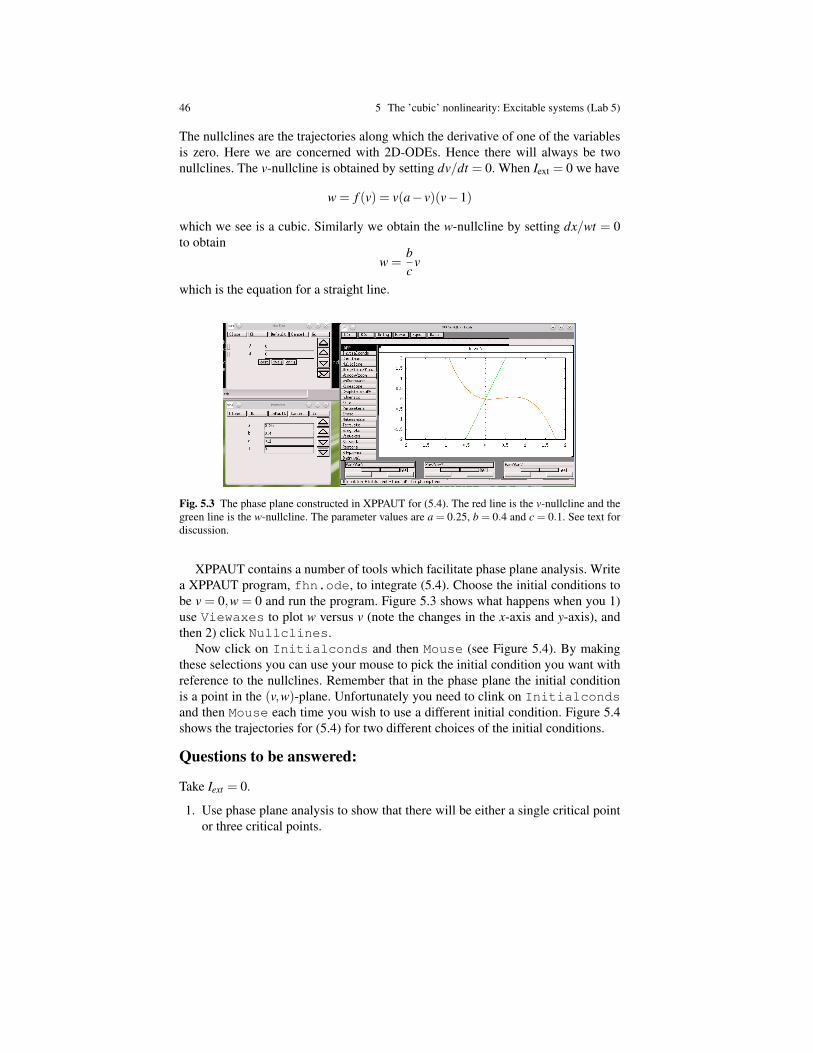
46 5 The ’cubic’ nonlinearity: Excitable systems (Lab 5)
The nullclines are the trajectories along which the derivative of one of the variablesis zero. Here we are concerned with 2D-ODEs. Hence there will always be twonullclines. The v-nullcline is obtained by setting dv/dt = 0. When Iext = 0 we have
w = f (v) = v(a− v)(v−1)
which we see is a cubic. Similarly we obtain the w-nullcline by setting dx/wt = 0to obtain
w =bc
v
which is the equation for a straight line.
Fig. 5.3 The phase plane constructed in XPPAUT for (5.4). The red line is the v-nullcline and thegreen line is the w-nullcline. The parameter values are a = 0.25, b = 0.4 and c = 0.1. See text fordiscussion.
XPPAUT contains a number of tools which facilitate phase plane analysis. Writea XPPAUT program, fhn.ode, to integrate (5.4). Choose the initial conditions tobe v = 0,w = 0 and run the program. Figure 5.3 shows what happens when you 1)use Viewaxes to plot w versus v (note the changes in the x-axis and y-axis), andthen 2) click Nullclines.
Now click on Initialconds and then Mouse (see Figure 5.4). By makingthese selections you can use your mouse to pick the initial condition you want withreference to the nullclines. Remember that in the phase plane the initial conditionis a point in the (v,w)-plane. Unfortunately you need to clink on Initialcondsand then Mouse each time you wish to use a different initial condition. Figure 5.4shows the trajectories for (5.4) for two different choices of the initial conditions.
Questions to be answered:
Take Iext = 0.
1. Use phase plane analysis to show that there will be either a single critical pointor three critical points.

5.4 Exercise 3: The Fitzhugh-Nagumo (FHN) neuron 47
Fig. 5.4 Once we have the phase plane displayed in XPPAUT we can pick the initial conditions byusing the mouse as described in the Discussion. These trajectories associated with the two initialconditions illustrate that the FHN neuron is in its excitable regime. Explain.
2. Take a = 0.25 and Ia = 0. Determine b and γ so that there is one stable criticalpoint. Verify your prediction and show two solutions that verify your prediction.
3. Pick an initial condition for which w < 0 but greater than the v-nullcline. Usephase plane analysis to guess what will happen and verify this with a simulation.Now pick an initial condition for which w > 0 but is less than the v-nullcline.Now what will happen. The difference between these two behaviors is whatdefines an excitable system.
4. The two nullclines divide the phase plane into four regions each characterizedby the sign of dv/dt and dw/dt. Identify these four regions in the phase plane.Using these results explain why the two choices in initial conditions in Fig-ure 5.4 lead to two different behaviors in the trajectories. This is one way toexplain the phenomena of excitability.
5. Take a = 0.25 and Ia = 0. Determine b and γ so that there are three critical pointsof which two are stable and one is unstable. Use the nullclines to identify whichcritical points are stable and which are not. Remember that the 1/e time for v ismuch shorter than that for w. Hence local stability is determined primarily bythe slope of the v-nullcline evaluated at the fixed-point. Verify your predictionsand show solutions that verify your predictions.
Take Iext > 0.
1. Use phase plane analysis to show that there will be either a single critical pointthat is excitable (there are two possibilities), a limit cycle, or bistability.
2. Verify these predictions using numerical simulations.3. See question in Deliverables.

48 5 The ’cubic’ nonlinearity: Excitable systems (Lab 5)
5.5 Exercise 4: Reduced neuron models
Neurons can generate a wide variety of spiking patterns (Figure 5.5). In fact, neu-roscientists often use the spiking pattern to identify the type of neuron that theyare working with. Eugene M. Izhikevich, a mathematical neuroscientist, realizedthat the different firing patterns exhibited by neurons depended very much on theproperties of the v and w nullclines [23]. As we saw for the FHN neuron, the v-nullcline (fast variable) has a cubic, or N-shape, and the w-nullcline, in general, asigmoid shape (the FHN neuron is the special case for which the w-nullcline is astraight line.). From this perspective the different spiking patterns of neurons arisesfrom details related to where the intersection occurs between the nullclines and theirshape [21, 22]. A similar idea was developed independently by Hugh Wilson [38].
Fig. 5.5 Examples of the different spiking behaviors observed for cortical neurons. Figure wasbeen reproduced from izhikevich.org with permission.
The Izhikevich equations take the form

5.5 Exercise 4: Reduced neuron models 49
dvdt
= 0.04v2 +5v+140−w+ Iext , (5.5)
dwdt
= a(bv−w) ,
with the auxiliary after-spike reset condition3
if v≥ 30mV, then
v ← c ,w ← w+d .
The reset condition means that when v ≥ 30mV, immediately set v to c and w tow+d.
Fig. 5.6 Four neuronal firing types generated by the reduced neuronal model: regular spiking (RS),fast spiking (FS), intrinsic bursting (IB), and chattering (CH). A single voltage trace for eachneuron type with a constant current input is shown in the lower four panels; the choices of the fourparameters, a,b,c,d for each spiking type are shown in the insets.
The Izhikevich model has the general form of an integrate and fire neuron model:when the membrane potential exceeds a threshold it generates an action potential.The occurrence of a spike immediately changes the spiking threshold (e.g. the neu-ron become transiently refractory) and the membrane potential (it hyper-polarizes,namely the membrane potential becomes slightly more negative than the neuron’s
3 The notation a← b was introduced by Izhikevich to indicate that a is immediately replaced by b.

50 5 The ’cubic’ nonlinearity: Excitable systems (Lab 5)
resting potential). Within the integrate-and-fire neuron framework, these changesare described by the after-spiking reset conditions.
Background: The program four_neuron.py, written by the late John D. Hunter,shows how the reset conditions are handled in a Python program. An example ofthe output of this program showing four different spiking patterns is shown in Fig-ure 5.6. For a very interesting application of the Izhikevich model neuron see
http://www.sciencebytes.org/2011/05/03/blueprint-for-the-brain/
We suspect that your programming skills in Python have not yet reached the stagethat you can comfortably understand the details of four_neuron.py. Don’t beconcerned! XPPAUT has a function, global, that makes handling the after spikereset condition for (5.5) very easy. This function has the format
global sign condition name1=form1;...
The function global defines a global flag allowing XPPAUT to implement deltafunctions. If sign=1, then the condition changes from negative to positive. Ifsign=-1, the condition changes from positive to negative. If sign=0, the con-dition vanishes identically. When the global flag is activated, each of the variablesin the ... is changed according to the values of the formulas. For example thestatement
global 1 x-1 x=0;y=y+a*sin(y)
means that when the sign of x− 1 changes from negative to positive, immediatelythen set x← 0 and y← y+a∗ sin(y).
Example: The simplest integrate-and-fire model takes the form
dvdt
= k ∗ v+vrest+ I (5.6)
with the auxiliary after-spike resetting
if v≥ vthres, then v← 0 .
The XPPAUT program, IF.ode, integrates an integrate-and-fire neuron.
Questions to be answered:1. Write a XPPAUT program to integrate the Izhikevich neuron. Note that by con-
vention the parameters are labeled a,b,c,d with the meaning as given above.Since investigators who use this model, for example in large scale neuron net-work simulations, refer to these parameters in this way it is important to use thesame parameter definitions in your model.
2. Try the following parameter choices
regular_spiking = 0.02, 0.2, -65, 8chattering = 0.02, 0.2, -50, 2

5.5 Exercise 4: Reduced neuron models 51
fast_spiking = 0.1, 0.2, -65, 2intrinsically_bursting = 0.02, 0.2, -55, 4thalamocortical = 0.02, 0.25, -65, 0.05
Do these parameter choices reproduce some of the spiking patterns shown inFigures 5.5 and 5.6?
Deliverable: Use Lab5_template.tex to prepare the lab assignment.


Chapter 6Bifurcation diagram: stopping spiking neuronswith a single pulse (Lab 6)
The qualitative behaviors of a dynamical system can change when parameters arechanged. For example, a stable fixed-point can become unstable, or vice versa.Moreover, for some dynamical systems it is possible that other types of dynami-cal behaviors can arise when a fixed-point become unstable, such as a limit cycleoscillation. If the mathematical equations are known then in principle it is possibleto summarize the parameter dependence of the dynamics in the form of a bifurca-tion diagram. A bifurcation diagram provides a road map that can be used in thelaboratory to directly link the predictions of a mathematical model to experimentalobservation. Are the predicted dynamics observed experimentally for the predictedparameter values? Do the dynamics change appropriately as experimentally accessi-ble parameters are changed? Even if a mathematical model has not been developed,a demonstrated qualitative change in dynamics as a parameter is changed can sparkthe interest of bio-mathematicians to work on the problem.
6.1 Background
In practice it is a challenging task to produce a bifurcation diagram both in mathe-matical models and in the laboratory. A fundamental problem is that the number ofparameters in biological systems can be very large. At present it is not known howto systematically explore the dynamics of a mathematical model using numericalmethods when the number of parameters is large. A very important computationalpackage for generating bifurcation diagrams in mathematical models in which thenumber of parameters is small is called AUTO
http://indy.cs.concordia.ca/auto/
One of the reasons why bio-mathematicians use XPPAUT is that it affords an easyaccess to AUTO [5]. AUTO uses a mathematical technique referred to as continua-tion to follow a particular solution (e.g. a fixed-point or a limit cycle) as a parameterchanges. For each choice of the parameters the stability of a particular solution
53

54 6 Bifurcation diagram: stopping spiking neurons with a single pulse (Lab 6)
branch is determined using a linear stability analysis. As we will see, AUTO pro-vides a number of tools to characterize the bifurcation of fixed-points and limitcycles. AUTO can be tricky to use and can fail in a dramatic fashion for certainproblems. However, even though AUTO is over 25 years old it still remains a majortool in the arsenal of an applied mathematician.
The experimental determination of a bifurcation diagram can be even more prob-lematic since for a biological system the identify of all of the parameters is notgenerally known and it may only be possible to alter some parameters, and eventhen, the range of possible variation may be small. However, as we have seen inlectures, sweeping a parameter, an experimentally attractive idea, can mis-identifythe location of the point where changes in stability occur. Moreover, as the edges ofstability are approached, the identification of the nature of the dynamics becomesdifficult due to slowing down phenomena. Nonetheless a number of experimentalparadigms have been developed in which it has been possible to at least partiallycharacterize the bifurcation diagram.
In this laboratory we illustrate the use of AUTO to characterize the onset of peri-odic spiking in a neuron. This type of bifurcation is characterized by the replacementof a stable fixed-point with a stable limit cycle and is referred to as a Hopf bifur-cation. A surprising prediction of the mathematical analysis is that it is possible toannihilate periodic spiking in a neuron by the application of a single, carefully-timedpulse. We demonstrate this phenomenon using a numerical experiment. This phe-nomenon was first demonstrated experimentally by R. Guttman and her colleaguesusing the squid giant axon [17].
Browser use: A user’s guide for running AUTO under XPPAUT can readily belocated on the Internet
http://www.math.pitt.edu/˜bard/xpp/help/xppauto.html
In this laboratory we illustrate AUTO using only very simple examples. Readerswho wish to extend the use of AUTO to their own research are recommended to readthe chapter in Ermentrout’s guide to XPPAUT [5]. XPPAUT can be run in Python(https://github.com/jsnowacki/xppy); however, we recommend firstlearning to run AUTO in XPPAUT before taking it on in Python. The ode ver-sion of the Hodgkin-Huxley (HH) equation, hh.ode, is the one written by MichaelGuevara (McGill University). You can either download this program from our web-site or from the Internet by typing hh.ode Guevara McGill in a web browser.The exercises involving the HH equation described here are modified from the com-puter exercises developed by Michael Guevara to explore the dynamical propertiesof the HH and Fitzhugh-Nagumo equations [16]. Students interested in the dynam-ical behaviors of neurons and excitable systems are recommended to work throughthe complete set of these exercises.
Housekeeping: It is useful to place all of the files related to the HH equation andits analysis in a directory called, for example, HHeqn.

6.2 Exercise 1: Making one-parameter bifurcation diagrams 55
6.2 Exercise 1: Making one-parameter bifurcation diagrams
We illustrate the procedure for obtaining a bifurcation diagram for the saddle nodebifurcation discussed in class. The generic equation for this bifurcation is
dxdt
= µ + x2 , (6.1)
where µ is the bifurcation parameter.The steps to determine the bifurcation diagram for (6.1) are as follows:
1. Write an .ode program to integrate (6.1).
2. It is very important to ensure that the solution has settled onto either a fixed-point or a limit cycle before using AUTO to continue the solution as a param-eter changes. In the case of (6.1) we know that a fixed-point solution (x∗ < 0)exists for µ < 0. Pick the initial condition x =−1 and run XPPAUT. The mostcommon cause of failure using AUTO is to use this program when the solu-tion is not already on a branch. With this in mind we extend the integrationby clicking on Initialconds Last. This XPPAUT command extends theintegration by an amount defined by TOTAL, from the step at which the pre-vious integration finished. Depending on the differential equation, the choiceof initial condition, and the parameter values it may be necessary to click onInitialconds Last several times.
Fig. 6.1 Clicking on File and then AUTO opens up the AUTO window.
3. The AUTO window (Figure 6.1) is activated by clicking on Auto whichis located under File. The most important functions for our purposes areParameter, Axes, Numerics, Run and Grab. A complete description ofall of the commands in AUTO is provided in the user’s guide cited above. The

56 6 Bifurcation diagram: stopping spiking neurons with a single pulse (Lab 6)
circle in the lower left of Figure 6.1 summarizes the number of stable and unsta-ble eigenvalues for a given choice of the bifurcation parameter(s): the numberof crosses inside the circle corresponds to the number of stable eigenvalues (i.e.eigenvalues with negative real part) and the number outside the circle corre-sponds to the number of unstable eigenvalues (the number of eigenvalues withpositive real part). How many crosses do you see for (6.1) and are they stableor unstable? How many crosses did you expect to see and why?
4. Click on Parameters. It is possible to declare up to 5 bifurcation parametersin this box. By default, XPPAUT chooses the first five parameters in the *.odeprogram. In our case there should be just one bifurcation parameter declared. Isthis correct?
5. Click on Axes and choose HiLo. Most of this box is already be filled outcorrectly. We see that the variable X will be plotted on the Y-axis and weare able to choose the range to vary the bifurcation parameter. Note thatXmin,Xmax,Ymin,Ymax refer to the dimensions of the bifurcation diagram andnot the variables and thus Xmin,Xmax refers to the range over which µ is varied.We suggest that you choose Xmin =−3 and Xmax = 1. The values Ymin,Ymax re-fer to the maximum and minimum values of a periodic orbit. Since (6.1) doesnot possess a periodic orbit these values are irrelevant for our purposes (seeExercise 2). Once you have completed the menu press OK.
6. Click on Numerics. For our purposes we can accept all of the default valuesexcept those for Par Min and Par Max. Choose these values so that µ isvaried from Par Min = -3 to Par Max =1, then push OK.
Fig. 6.2 A partial bifurcation diagram computed for (6.1). We have clicked on Grab and thus wesee three special points indicated by crosses. Note that there are actually four crosses but one is notshown. See text for discussion.

6.2 Exercise 1: Making one-parameter bifurcation diagrams 57
7. Click on Run Steady state. A thick black line will appear that extendsover the range that we varied µ (Figure 6.2. The fact that the line is thick meansthat the fixed-point is stable (a thin black line indicates an unstable fixed-point).If you do not see a line then the most likely causes is that you were not suf-ficiently close to the stable fixed-point solution when you started. Go back toStep 2.
8. Click on Grab. You will see a cross appear on the thick black line. You canuse the right and left arrow keys to move back and forth along this line. As youmove along this line in this way what happens to the eigenvalues (see circle inlower left hand corner). Also if you look in the window below the bifurcationdiagram you can see more information pertaining to the current location of themovable cross in the diagram, such as the value of µ and, in the case of a limitcircle, its period. Note that there are also crosses with numbers attached whichdo not move as you use the arrow keys. The points are special points since it ispossible to continue the solution from them. Using the Tab key you can movebetween the special points. When you are on one of these special points, thebottom window provides information the point type. In our case you will seeEP which means end point. If you see MX then this means you screwed up andit is back to step 2 that you go.
Fig. 6.3 The complete bifurcation diagram for (6.1) determined using AUTO.
9. In order to complete the bifurcation diagram it is necessary to continue to thesolution from one of the numbered special points. Use the Tab to position thecross on the special point labeled 1. Press Enter. Click on Numerics andchange the sign of Ds. Note that when we change the sign of Ds we reversethe starting direction for AUTO. Now click on Run and you should see thebifurcation diagram that we calculated in class (Figure 6.3).

58 6 Bifurcation diagram: stopping spiking neurons with a single pulse (Lab 6)
Questions to be answered:
1. Use XPPAUT to determine the bifurcation diagram for the transcritical bifurca-tion whose generic equation is
dxdt
= µx− x2 .
2. Use XPPAUT to determine the bifurcation diagram for the supercritical bifur-cation whose generic equation is
dxdt
= µx− x3 .
3. Use XPPAUT to determine the bifurcation diagram for the subcritical bifurca-tion whose generic equation is
dxdt
= µx+ x3 .
6.3 Exercise 2: Bifurcation diagram: Hodgkin-Huxley neuron
The determination of the bifurcation diagram for the HH equation by bio-mathematiciansmade it possible for neuroscientists to test the prediction of this equation in the lab-oratory using the squid giant axon (for a review see [16]). In this exercise we willAUTO to characterize the onset of regular spiking of the squid giant axon whena sufficient current is injected. The main difference in the use of AUTO for thisexercise is that we need to account for the appearance of a limit cycle.
Here are the steps we used to make this bifurcation diagram.
1. Download the program hh.ode from the class website. Note that this equationhas more parameters that can fit in the shown parameter box shown in XPPAUT.You can maneuver up and down the parameter list by using the ∨,∨∨,∧,∧∧buttons located on the parameter box.
2. Run XPPAUT to integrate this equation when the parameter curbias=0. Usethe Initialconds Last button several times to ensure that the HH equa-tion has settled onto the initial conditions of v, m, h, n (we obtained, respectively,−59.9996379,0.052955,0.5959941,0.317732).
3. After starting AUTO set the following parameters:
• In the Parameter window set the first parameter to be curbias (themenu will show blockna which is the first parameter declared in hh.ode.
• In the Axes window click on Hi-Lo. The y-axis should be V and the x-axis(called MainParm) should be curbias. Set Xmin = 0 and Xmax = 200 so

6.3 Exercise 2: Bifurcation diagram: Hodgkin-Huxley neuron 59
that curbias ranges from 0 to 200. Set Ymin =−80 and Ymax = 20 so thatthe amplitude of the limit cycle oscillation ranges from −80 to 20.
• In the Numerics menu set Par min = 0 and Par max = 200 (thissets the range over which the bifurcation parameter curbiaswill be varied.Set Nmax=500 to limit the number of points that will be computed along agiven branch of the bifurcation diagram to 500. In addition set Npr=500and Norm Max =150.
• Click on Run and then Steady state. You will see a thick line with 4special points.
• Click on Grab and use the Tab to move between them. From the bottomscreen we see that special points 1 and 4 are end points (EP) and specialpoints 2 and 3 are labeled as Hopf bifurcation points (HB). Note that the linebetween special points 2 and 3 is thin meaning that the fixed-point that existsfor this range of curbias values is unstable. Confirm this by looking at thecircle diagrams in the lower left hand corner of the AUTO screen.
• We can complete the bifurcation diagram by either starting at special point2 and increasing curbias, or by starting at special point 3 and decreas-ing curbias. Let’s start at special point 2. Use the Tab key to place thecross at this point and then press Enter. Note that the Run menu changes.Click on Periodic and the bifurcation diagram unfolds before your eyes(Figure 6.4)!
• XPPAUT (and mathematicians) typically use lines to indicate the stability offixed-points (remember that thick lines correspond to stable fixed-points andthin lines to unstable ones). Limit cycles are indicate by circles placed whichare positioned to indicate the maximum and minimum values of the oscil-lation: filled circles correspond to stable limit cycle oscillations and opencircles to unstable limit cycle oscillations.
Questions to be answered:
A bifurcation in which a stable fixed-point is replaced by a stable limit cycle iscalled a Hopf bifurcation. Specifically the bifurcation that occurs at special point 2 isa subcritical Hopf bifurcation and that which occurs at special point 3 is called a su-percritical Hopf bifurcation (more specifically if we consider curbias increasingwe have a reverse supercritical Hopf bifurcation). We will discuss these bifurca-tions in more detail later in the lectures. However, we can interpret the bifurcationdiagram to anticipate the properties of these bifurcations.
1. First consider the subcritical Hopf bifurcation that occurs at special point 2.
• What happens to the stability of the fixed-point at the bifurcation point? Isthe fixed-point destroyed at this Hopf bifurcation?

60 6 Bifurcation diagram: stopping spiking neurons with a single pulse (Lab 6)
Fig. 6.4 Bifurcation diagram for an HH-neuron determined using AUTO. See text for discussion.
• Use Zoom to examine the bifurcation diagram close to special point 2. Wesee that it is possible for a stable fixed-point and a stable cycle to co-exist.This bistability is a characteristic of a subcritical Hopf bifurcation? Whatdoes this mean (see also Exercise 3)?
• Suppose we start with a value of curbias much lower that special point2 and slowly increase it. How do you expect the amplitude of the oscilla-tion to grow: suddenly or gradually? The abrupt onset of a “high” amplitudeoscillation is a characteristic of a subcritical Hopf bifurcation.
• Now choose a value of curbias on the limit cycle and slowly decrease it.At some point the oscillation will disappear and we will be left with a stablefixed-point. Is the decreasing value of curbias at which the limit cycledisappears the same value of increasing curbias which caused the limitcycle? This observation illustrates the phenomenon of hysteresis.
2. Now consider the supercritical Hopf bifurcation associated with special point 3.
• What happens to the stability of the fixed-point at the bifurcation point? Isthe fixed-point destroyed at this Hopf bifurcation?
• How does the amplitude of the oscillation grow as the value of curbias isdecreased from special point 3: gradually or abruptly?
• Is this bifurcation associated with bistability?• Is this bifurcation associated with hysteresis?

6.4 Exercise 3: Stopping spiking neurons with a single pulse 61
Fig. 6.5 Changes in membrane potential for a periodically spiking HH-neuron.
6.4 Exercise 3: Stopping spiking neurons with a single pulse
The special point 3 occurs when curbias equals ∼ 150µA/cm2. This is a veryhigh current input for a neuron and likely is not biologically relevant. Thus biolog-ical interest centers on the behaviors associated by the subcritical Hopf bifurcation(special point 2).
Fig. 6.6 Stopping a periodically spiking HH-neuron with a single pulse. What stimulation param-eters do you think we used? Can you accomplish the same thing with a smaller, briefer and bettertime pulse? See text for discusison.
The practical implication of the presence of a subcritical Hopf bifurcation is be-cause of its association with bistability. In particular, a non-spiking state of the neu-ron co-exists with a periodically spiking state. Suppose we choose curbias close,

62 6 Bifurcation diagram: stopping spiking neurons with a single pulse (Lab 6)
but smaller, than special point 2. It should be possible to switch between the two sta-ble points by changing the initial conditions. How do we change initial conditions?A simple way is to use a carefully timed electrical pulse.
The program hh.ode contains parameters that make it possible to introducean electrical pulse of width (duration) and height (amplitude) at a specifiedtime (tstart). Figure 6.5 shows the changes in membrane potential for a period-ically spiking neuron. Guess at which point in the spike-to-spike interval where ahyper-polarizing pulse will stop the neuron from periodically spiking (Figure 6.6).At which point would a depolarizing pulse do the trick? Once the neuron is quies-cent what kind of pulse is needed to start it spiking again.
To test your predictions set curbias = 13. Set the pulse height to be 9 andthe width to be 1.5. Determine a time at which a hyper-polarizing pulse stops thespiking (Figure 6.6). Can you accomplish this task using an even briefer and andsmaller perturbation: sometimes an important goal is to determine the timing forwhich the smallest and briefest pulse accomplishes the above task. Now try thesame exercise using a depolarizing pulse accomplishes the same tasks.
DELIVERABLES:Use Lab6_template.tex to prepare the lab assignment.

Chapter 7Lab 7: Filters and convolution
One of the most remarkable properties of a linear dynamical system is its responseto sinusoidal inputs. As we learned in lecture, a sinusoidal input to a linear dynam-ical system produces a sinusoidal output having the same frequency as the input.However, the output sinusoid can differ in two ways from the input sinusoid: 1)its amplitude, and 2) its phase. Measurements of the phase and amplitude of theoutput to a sinusoidal input can be used to identify the differential equation whichbest captures the input-output relationships of the dynamical system. The graphicaltechnique for estimating the transfer function from these experimental observationsis the Bode plot. Once the transfer function has been determined the response of thedynamical system to any realizable input can be predicted. The purpose of this lab-oratory is to use computer experiments to verify these observations and to introducethe concepts of a filter and convolution.
7.1 Background
The lecture briefly reviews the concept of an impulse function, filtering and convo-lution. A practical, but important, detail concerns the representation of a sine wavewave in a computer program. We can write a simple program that plots a 10 secondinterval of a sine wave for a given frequency, f , and a given time step.
import numpy as npimport matplotlib.pyplot as plt
f=0.1t=np.linspace(start,stop,N,endpoint=True)x=np.sin(2*np.pi*f*t)plt.plot(t,x,’k-’)plt.show()
The period, T , is 1f , so when f = 0.1, we have T = 10. If we choose start
and stop to be, respectively, 0 and 10, then this would draw one cycle of a 0.1Hz
63

64 7 Lab 7: Filters and convolution
provided that N is chosen appropriately. The positive integer, N, is the number ofequally spaced time samples between, in this case, 0 and 10. It is important toremember that by choosing the endpoint=True option for np.linspace()both the starting and the end point are included, N points altogether. The time step,dt is
dt =stop-start
NWhat is a good choice of the number of time steps, N? If we choose N = 10, the
dt = 1 and we would obtain 10 identical xalues of x since we are sampled once perperiod. This is not a good choice of N since we cannot uniquely represent a func-tion using a single value. Next we could try N = 20. In principle we can uniquelyrepresent a sine wave if we sample at twice the frequency (this is the concept of theNyquist frequency that we will discuss in the next lab). However, x would not looklike a nice sine wave. So we must pick N larger: the larger N, the smaller st, andhence the more frequently the sine wave is sampled. However, it is also true thatthe larger N the more computer memory it takes to store in this case x and t, andthe greater the number of calculations that the computer must make. Thus there isa practical trade–off between the accuracy by which functions are to be representedand the time it takes the computer to complete its calculations. The bottom line isthat as we change f we need to adjust ts. A reasonable choice might be to samplethe sine wave 10−100 times per period. Ideally we would like to keep the numberof sample points per period the same as we change f .
Browser use: Have available the document intro_python.pdf on yourbrowser for review, in particular, the sections that deal with how to declare a func-tion. As always, information concerning the use of Python and matplotlib func-tions can be obtained from the Internet using a browser.
Housekeeping: Labs 8 and 9 use some of the programs and results that wedevelop in this lab. Thus it is useful to put today’s material in a sub-directory of˜\pyprogs called, for example, convol, namely ˜\pyprogs\convol. Thiswill make it easier for you to find these results when we need them.
Exercise 1: Bode plots: low–pass filter
1. Write a computer program to integrate
dxdt
= k1x+ sin2π f t , (7.1)
where k1 is a constant.2. Take k1 =−1.3. Vary frequency over a large range (say f = 0.01 to f = 100) and measure the
amplitude. Plot the amplitude versus frequency.4. Vary the frequency and measure the shift between the sine wave and the solution
of the equation. For example, we can plot the input and output sine wave n thesame figure. Plot the phase shift versus the frequency.

7.1 Background 65
5. Now change a to, let’s say, k1 = 10 and then k1 = 0.1. What happens?6. Construct the Bode plot by choosing a suitable range of f . For each choice of f
enter the amplitude and phase shift of the steady–state solution and write thesevalues in a *.tsv file. Use this *.tsv file to construct the phase part of theBode plot.
7. You have just constructed your first low pass filter. Answer the following:
• The frequency on the input sine wave and the output sine wave is the same.True of false?
• The output amplitude changes as a function of frequency. True or false?• The output sine wave is phase shifted compared to the input sine wave. True
or false?• Why is this type of filter called a low pass filter?
8. What is the transfer function for (7.1)?9. Show that the impulse function, I(t, t ′), is
I(t, t ′) = k1 exp(k1t) .
(Remember that the impulse function corresponds to the case when the inputis a delta function.) Is this the same as the answer we derived in class (Section7.3)?
10. The transfer function, C(s), for the thermometer is of the form
C(s) =1
1+αs.
Sketch the Bode plot. What is the corner frequency?
11. Consider the transfer function
C(s) =10
s(1+0.5s)(1+0.1s).
Sketch the Bode plot for the amplitude showing the contribution of each term.
Exercise 2: The convolution integral:The concept of convolution is one of the most important concepts in science:
every time one uses a device to make a measurement, one essentially performsa convolution. All physical observations are limited by the resolving power of in-struments, and for this reason alone convolution is ubiquitous. This principle doesnot only apply to laboratory instruments: our senses, e.g. vision, touch, smell, au-dition, proprioception, are also convoluted by the sensory receptors which translatephysical stimuli into neural spikes trains. This convolution is mathematically as theoperation
y(t) =∫
∞
−∞
x(t)h(t−u)du , (7.2)
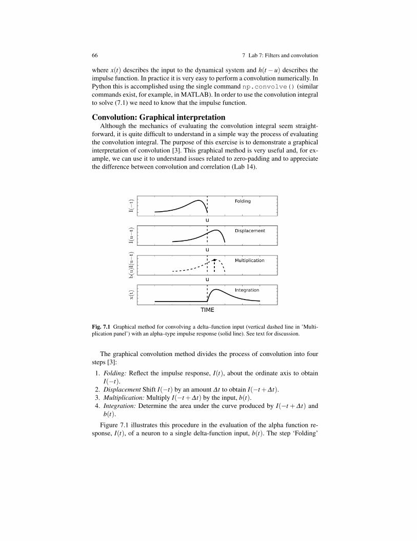
66 7 Lab 7: Filters and convolution
where x(t) describes the input to the dynamical system and h(t− u) describes theimpulse function. In practice it is very easy to perform a convolution numerically. InPython this is accomplished using the single command np.convolve() (similarcommands exist, for example, in MATLAB). In order to use the convolution integralto solve (7.1) we need to know that the impulse function.
Convolution: Graphical interpretationAlthough the mechanics of evaluating the convolution integral seem straight-
forward, it is quite difficult to understand in a simple way the process of evaluatingthe convolution integral. The purpose of this exercise is to demonstrate a graphicalinterpretation of convolution [3]. This graphical method is very useful and, for ex-ample, we can use it to understand issues related to zero-padding and to appreciatethe difference between convolution and correlation (Lab 14).
Fig. 7.1 Graphical method for convolving a delta–function input (vertical dashed line in ’Multi-plication panel’) with an alpha–type impulse response (solid line). See text for discussion.
The graphical convolution method divides the process of convolution into foursteps [3]:
1. Folding: Reflect the impulse response, I(t), about the ordinate axis to obtainI(−t).
2. Displacement Shift I(−t) by an amount ∆ t to obtain I(−t +∆ t).3. Multiplication: Multiply I(−t +∆ t) by the input, b(t).4. Integration: Determine the area under the curve produced by I(−t + ∆ t) and
b(t).
Figure 7.1 illustrates this procedure in the evaluation of the alpha function re-sponse, I(t), of a neuron to a single delta-function input, b(t). The step ‘Folding’

7.1 Background 67
means that we reflect the impulse response about the y-axis. The step ‘Displace-ment’ means that we slowly shift the reflected impulse in the positive direction alongthe x-axis. The step ‘Multiplication’ means that we multiple the reflected impulsewith the input. It is easiest to understand this step iteratively: for each time step dothe multiplication (and then Step 4), then displace the reflected impulse response an-other time step to the right and repeat the process. In general this corresponds to theshaded region under the two curves for which both functions are non-zero. Finallythe step ‘Integration’ calculates the area under the the two curves. In this examplethe area is easy to determine since by the shifting property of the delta-function(Section 6.3), the area is just the value of the alpha function at that point. The resultof convolution is the area computed in Step 4 as a function of time, namely as thereflected impulse response is shifted iteratively to the right.
Questions to be answered:
1. Use the graphical technique discussed in Section 8.3 to compute the convolutionfor the following choices of b(t) and I(t)
• b(t) = constant and I(t) = e−t
• b(t) is a single square wave pulse and I(t) = e−t (This is animated on theWikipedia site for Convolution.)
• Both b(t) and I(t) are square wave pulses (This is animated on the Wikipediasite for Convolution.)
Exercise 3: Computing the convolutionNumpy has a function called np.convolve(). Although it is tempting to think
that it would be easy to calculate the convolution of any function; there are somesubtleties.
The function np.convolve(r,s,mode=’full’) calculates the convolu-tion integral, denoted (r ∗ s), as
(r ∗ s) j =N/2
∑k=−N/2+1
s j−krk
where s is the discretely sampled signal and r is the discretely sampled impulsefunction [32]. Unfortunately this approximation assumes that the length of r is thesame as that of s and that s is periodic. Thus we need to figure out how to get aroundthese constraints. The solution involves padding the data and impulse response withzeros. This procedure is called zero padding.
The first constraint is easily dealt with since it is typically the case that the lengthof impuse response, M, is much shorter than the length of the signal, N. Thus weneed to pad the impulse function with zero is make M = N. The second problemis more subtle. Not only must the signal be considered to be periodic, but also theimpulse function. Therefore it happens that a portion at each end of the originalsignal is erroneously wrapped around by the convolution with the response function.

68 7 Lab 7: Filters and convolution
In other words, the first output channel (s∗r)0 is contaminated wuth some wrapped-around data from the far end of the data stream sN−1,sn−2, · · · . This we need to setup a buffer zone of zero-padded values at the end of s in order to make the effectsof this contamination equal to zero. How many zeros do we need top add? We needto pad the signal function on one end with the number of zeros equal to the lengthof the response function.
The numpy function, np.pad(), is very useful for handling issues related tozero padding
np.pad(array,pad_width,mode=None).
A useful feature of np,pad() is that we can pad to the left and/or to the right ofthe array. For example, if
x=[1,2,3]
then the command
X=np.pad(x,(0,3),’constant’)
yields
X=[1,2,3,0,0,0]
and the command
X=np.pad(x,(3,0),’constant’)
yields the array
X=[0,0,0,1,2,3]
However, we are still not done. In terms of our fold-displacement-multiplication-integration analogy for convolution, convolve() does not include the integrationstep. Thus we need to multiple the output of np.convolve() by the time step.
Questions to be answered:1. Write a computer program that uses np.convolve() to construct the Bode
plot for (7.1). Again for each choice of F , measure the amplitude and phaseshift using the steady state solution.
Exercise 4: Neural inputs: The program convolve_neural_spikes_alpha.pyuses the convolution integral to estimate the sub-threshold membrane potential whenthe impulse function is given by the alpha function
Iα(t, t ′) =±k2
m(t− t ′)e−km(t−t ′) if t ≥ t ′ ,0 t < t ′ .
(7.3)
The input spike train is modeled as a sequence of delta functions. Figure 7.2 showshow the membrane potential changes for a given periodic excitatory input.
Hints:

7.1 Background 69
Fig. 7.2 The membrane potential of a neuron (bottom panel) in response to a pulsatile, excitatoryinput whose timing corresponds to the timing of spikes in the spike train shown in the top panel.The changes in the neuron’s membrane potential following the arrival of each EPSP is describedby (7.3) with km = 0.5.
1. A common use of def is to define and introduce functions that are used for cal-culations in the program. The command r=impulse_response(t) evalu-ates the function for all of the values of t. Note that the commands in the defare indented by usually 4 spaces
2. Useful array manipulations:
[1:5] means from 1 to 5[1:] means 1 to end[len(a):1] means from length of a to end[::n] means each n-th item in entire sequence
3. The function plt.subplot() has the form
\verb+plt.subplot(row,column,panel number)
Which panel would be drawn using the command plt.subplot(223)?4. The package matplotlib.ticker includes a number of useful functions
that make it possible to, for example, change the spacing of the number on theaxis, etc. Labeling the subplots ax, bx, .. is necessary in order to use thefunctions within matplotlib.ticker. In the case of a figure that has onlyone panel, we can use the command plt.subplot(111).
Question to be answered:An impulse function can be used to model the changes in blood concentration of
a drug ingested orally. For example, if we take (7.3) as a simple impulse function

70 7 Lab 7: Filters and convolution
for drug ingestion, then the sharp rising portion indicates the time course of the druggoing from the stomach to the blood (more typically minutes), and the falling phasedescribes the clearance of drug from the body by the actions of the liver and kidneys(typically hours to days). Consider that a doctor prescribes a drug for which the e−1
time is ∼ 6 hours and asks that the patient take the medication 4 times a day. Mostpatients do not take the medication every 6 hours, but more often at 8am–noon–5pm–midnight. Write a computer program to look at the effects of different dosingschedules on blood levels to answer the following questions.
• Would it be better for the patient to take the medication three times a day, i.e.every 8 hours?
• If the e−1 time is∼ 4 hours, what would be the difference between the two dosingschedules?
• If the e−1 time is ∼ 12 hours, what would be the difference between the twodosing schedules?
Low-pass filters with two-polesHere we discuss the transfer function for a second-order linear ordinary differen-
tial equation. As we discussed in lecture it is traditional and convenient to write thedifferential equation in the form
1ω2
n
d2xdt2 +
2ε
ωn
dxdt
+ x = b(t) , (7.4)
where ωn = 2π fn is the natural frequency of the associated harmonic oscillator(Note that ωn = 2π fn). The damping ratio is ε:
ε > 1 : Overdamped ,
ε = 1 : Critically damped ,
1 > ε > 0 : Underdamped ,
ε = 0 : Undamped .
For the homogeneous ordinary differential equation
d2xdt2 +2εωn
dxdt
+ω2n x = 0 , (7.5)
the two eigenvalues are
λ1,2 =2εωn±
√(2εωn)2−4ω2
n
2,
= −εω2±ωn
√ε2−1 .
When we determine the impulse function we need to remember that the λ1,2are either be real negative numbers (the over-damped case) or a pair of complexnumbers with negative real parts (the under-damped case). This is because we can

7.1 Background 71
only define the impulse function for a dynamical system which in the absence of aninput has a stable fixed–point. For the over–damped case we have
I(t, t ′) =ωn
2√
ε2−1
[eλ1t − eλ2t
]. (7.6)
For the under-damped case we have
I(t, t ′) =σ2 +ω2
ωe−σt sin(ωt) , (7.7)
where σ is the absolute value of the real part of the complex eigenvalue and ω is theimaginary part.
Questions to be answered:Consider the second–order linear differential equation
d2xdt2 + k1
dxdt
+ k2x = sin2π f t , (7.8)
where k1,k2 are constants to be determined.
1. Choose the values of k1,k2 such that both eigenvalues are real and negative.In particular, pick the parameters so that one eigenvalues, λ1, is equal to −1.Construct the Bode plot when λ2 is smaller than λ1 and another when λ2 islarger. Compare these Bode plots to the one we obtained for (7.1). You should beable to sketch these Bode plots without using computer simulations (Of courseyou are welcome to use a computer program to confirm the validity of yoursketches.) What are the differences?
2. Pick values of k1,k2 such that the fixed–point of the homogeneous equation (i.e.,the right–hand side is 0) is a stable spiral point.
• For these choice of parameters, what is the natural frequency?• Write a computer program to show that as k1 approaches zero, (7.8) exhibits
resonance as f is closed to the natural frequency, fn. Your figure should showthe amplified solution (x versus t).
• Sketch the Bode plot for this case.
Deliverables:Assignment should be submitted as a *.pdf prepared using LaTeX. Answer the
questions. In those cases in which the figures are sketched, attach the sketches to theLaTeX document.


Chapter 8Lab 8: Fourier series: Gibbs phenomenon andfiltering (Chapter 8)
8.1 Background
In class we used the Fourier theorem to construct a Fourier series representation ofa periodic square wave. If the periodic square wave is written as an odd function,then the Fourier series is
g(t) =12
+2π
sin t +2
3πsin3t +
25π
sin5t + · · · .
Since odd numbers can be written as 2n−1, where n is an integer, we can re-writethis series as
g(t) =12
+∞
∑n=1
2(2n−1)π
sin(2n−1)t . (8.1)
There are two important properties of periodic square waves for bench top re-searchers. The first is Gibb’s phenomenon. Figure 8.1 shows the Gibbs phenomenonthat arises when we increase the number of terms in (8.1). Sharp transitions, suchas the edge of the square wave, generate high frequency components in the Fourierseries. Gibbs’s phenomena produces artifacts in jpg images (see Section 8.4) andalso produces aliasing (see Lab 9) that makes the determination of power spectraldescriptions of neural spike trains [12] and the EKG of the heart beat difficult.
The second important property concerns the relationship between square and sinewaves. At first sight this does not seem to be that important. However, in electronics,communication signals are often transmitted as square wave pulses and on arrivalto their destination are converted to sine waves. Moreover in an electronic circuitit is often easier to create a train of periodic square waves rather than to generatea sine wave. An example in biology arose in the measurement of the Bode plot forthe hyperosmolar response of yeast cells (Sections 7.4.2 and 7.6.2). From (8.1) wesee that a square wave can be thought of as a sine wave to which terms with higherfrequencies have been added. Thus an attractive idea to generate a sine wave is tolow-pass filter the train of periodic square waves to remove the higher frequencyterms, leaving the pure sine wave component behind.
73

74 8 Lab 8: Fourier series: Gibbs phenomenon and filtering (Chapter 8)
Fig. 8.1 Comparison of a square wave to the (8.1) using 50 terms. The little spikes at the cornersof the square wave (↓) represent the Gibbs phenomenon.
The purpose of this lab is to demonstrate Gibb’s phenomenon and then to use theconvolution integral to filter the square wave to make a sine wave. It is important tokeep in kind that this problem corresponds to the mathematical problem
output(t) =∫
∞
−∞
impulse response(u) input(t−u) du ,
where the input is the periodic square wave and the impulse response is that for aRC circuit, namely,
I(t, t ′) = ke−kt .
It is observed that at least a two-pole low pass filter is required.In Lab 9 we will show that we can also accomplish these goals using the fast
fourier transform (FFT). In this case we have
B( f ) = I( f ) f ilter( f ) .
Browser use: We use the function scipy.signal.square() to generate aperiodic train of square waves. The article written by R. Mark Stitt,
www.ti.com/lit/sbfapp3/sbfa003.pdf
provides background into the importance of converting square waves into sine wavesin industry. A number of animations which illustrate the act of convolution are avail-able on the Internet. In particular, we recommend the Wikipedia-Convolution entrysince it includes animations of the two convolutions studied in this Lab. Informa-tion concerning defining a function in Python and constructing a while loop caneither be obtained on the Internet or by consulting intro_python.pdf on ourwebsite.

8.3 Exercise 3: Convolution: Graphical interpretation 75
House keeping: It is useful to place the programs related to convolution into adirectory labeled, for example, convol. This is because we will use these programsin later labs and hence it is advantageous to be able to locate them quickly.
8.2 Exercise 1: Gibbs phenomenon
It is often necessary to evaluate a sum in a computer program, such as occurs in (??).In Python sums can be evaluated using a while loop. For example to determiney where
y =10
∑i=1
i2
we can write
sum=0n=1while n <11:
sum=sum+nˆ2n=n+1
print sum
It is possible to use a for loop in Python; however, a while loop construct istypically much faster.Questions to be answered:
1. Write a Python program using a while loop to compare g(t) to a periodicsquare wave as a function of the number of terms n. Compare the solution to aperiodic 2π-periodic square wave.
2. Rewrite your program by constructing a function that evaluates g(t) for an in-putted number of terms.
3. Modify this program by defining a function so that you can easily plot g(t)for different numbers of n on the same graph. This plot is useful to see theemergence of the square waves as the number of terms in the sum increases.
4. What happens to the Gibbs phenomenon when n becomes large?
8.3 Exercise 3: Convolution: Graphical interpretation
Note: This section has been moved to Lab 7.

76 8 Lab 8: Fourier series: Gibbs phenomenon and filtering (Chapter 8)
8.4 Exercise 4: Making a sine wave from a square wave
A sine wave can be created by low-pass filtering a square wave. It is necessary to useat least a two pole low-pass filter to make wave that looks sinusoidal. A RC circuitcorresponds to a one pole low-pass filter. Thus it should not be surprising that oneway a sine wave is created from a square wave is to pass the square wave signalthrough two consecutive RC-type circuits. Let’s use the convolution programs wedeveloped in Lab 7 to see how well this works.
We give you two useful hints:
1. A useful way to use scipy.signal.square() to generate a periodic trainof square waves is to write
t = np.linspace(0, 1, 100, endpoint=False)plt.plot(t, signal.square(2 * np.pi * 3 * t))
To illustrate, these lines of code have been written to generate a 3 Hz periodictrain of square waves sampled at 100 Hz for 1 s.
2. The cut-off frequency for a RC circuit whose impulse response is kekt is 1/k.
Fig. 8.2 a) An input signal consisting of a 5 Hz periodic train of square waves. b) the output signalafter passing through a one pole low-pass filter, and c) the output signal after passing throughtwo consecutive one pole low-pass filters. Note that the signals shown correspond to steady statesolutions, i.e., a large number of transient have been allowed to die out. It should be noted thatusing a one pole low-pass filter that it is possible to get other output waveforms. We have usedparameters that generate the “most sinusoidal shaped one”.
Questions to be answered

8.4 Exercise 4: Making a sine wave from a square wave 77
1. Write a computer program that uses the convolution program in Lab 7 to gen-erate a sine wave from a square wave. remember to include the modification tothe convolution program that we discovered in Exercise 3. The basic idea is toconvolve the periodic square wave train with a RC filter and then convolve theoutput with a second RC circuit. Figure 8.2 shows our attempt at this strategy.Clearly it is clearly better to use two RC circuits, namely a two-pole low-passfilter, in order to get an output that resembles a sine wave. In our case we choosek for each RC circuit to be the same. Can you do better by choosing differentk’s for each low-pass filter?
2. According to the principle of linear superposition one would expect that theresult of passing a signal through a two-pole filter would be the same as passinga signal through two consecutive one-pole filters having the same poles. To testthis hypothesis consider the impulse function for a second-order over dampeddifferential equation (Equation 6 in Lab 7). Pick two poles, λ1 and λ2 and writea computer program to convolve the square wave used in the previous questionwith this impulse response. Compare this result to that obtained by passing thesquare wave signal through two consecutive RC circuits, the first with pole λ1and the second with pole λ2. Are they the same?
Deliverables: Use Lab8_template.tex to prepare the lab assignment.


Chapter 9Lab 9: FTT and power spectra
The Fast Fourier Transform (FFT) is a fast and efficient numerical algorithm thatcomputes the Fourier transform. The power spectrum is a plot of the power, orvariance, of a time series as a function of the frequency1. If G( f ) is the Fouriertransform, then the power spectrum, W ( f ), can be computed as
W ( f ) = |G( f )|= G( f )G∗( f )
where G∗( f ) is the complex conjugate of G( f ). We refer to the power spectrumcalculated in this way as the periodogram.
Currently, many investigators prefer to estimate the power spectral density usingmatplotlib.mlab.psd(). This method is based on Welch’s averaged peri-odogram method. Welch’s method reduces noise in the estimated spectrum at theexpense of reducing the frequency resolution (see below). For many of the experi-mental uses of power spectra, the advantages of reducing the effects of noise out-weigh the dis-advantages of reduced frequency resolution. As we showed in lecturethere is little practiacl difference between determining the periodogram versus thepower spectral density. However, the flexibility of mlab.psd() provides esuffi-cient motivation to learn how to use this package.
Often overlooked is that the fact that W ( f ) is the power spectrum obtained for aninfinitely long time series measured with infinitely fine precision. In contrast, in thelaboratory we work with time series of finite length that are subjected to uncorre-lated, random inputs (noise) and effects introduced by the process of measuring thesignal.
The purpose of this laboratory is to illustrate the use of mlab.psd() and ex-plore a number of applications of the FFT and power spectra.
Browser: Essentially everything that you would ever want to know about the usesof the FFT can be located on the Internet by asking the right questions. In Python,
1 For simplicity we have assumed that the independent variable is time; however, it could alsobe a spatial dimension. We use the term power spectra as a collective term to include both theperiodogram and the power spectral density.
79

80 9 Lab 9: FTT and power spectra
the functions necessary to calculate the FFT are located in the numpy library calledfft. If we want to use the function fft(), we must add the following commandto the top matter of our program:
import numpy.fft as fft
Thus, the command for determining the FFT of a signal x(t) becomes fft.fft(x).Of course, you could import the fft-package from numpy under a different name;however, this might make the program less readable by others. Other functions re-lated to the use of the FFT are located in scipy such as the library signal, i.e.
import scipy.signal as signal
The description of each command and how to use it can easily be obtained by usingyour web browser and typing the name of the library together with the function thatyou want to know about.
House keeping: Today we will illustrate the applications of the FFT and thepower spectra by working with real data. The deliverables take the form of figuresprepared using Matplotlib. We suggest that you create a directory for each figurewhich contains both the data and the program(s) used to generate the required figure.This is actually a good habit to acquire. One advantage is that you don’t need toworry about specifying the required paths since, by default, a Python program looksfirst in the directory they are running for required input files. A second advantageoccurs if, my goodness, you actually need to modify your figure at a later datefollowing comments made by a grader or a reviewer of your article (senior thesis,publications, book).
9.1 Background
We illustrate the difference between W ( f ) and w( f ) by calculating the power spec-trum of x(t) = sin(2π f0t), where f0 is a particular frequency. By definition, theFourier transform of sin(2π f t) is
G(sin2π f0t)( f ) =∫
∞
−∞
e−2π j f t sin2π f0tdt (9.1)
where we have distinguished a particular value of the frequency, f , as f0. UsingEuler’s relation, we can write
sin2π f0t =e2π j f0t − e−2π j f0t
2 j
Substituting into (9.1), we obtain

9.1 Background 81
G(sin2π f0t)( f ) =∫
∞
−∞
e−2π j f t[
e2π j f0t − e−2π j f0t
2 j
]dt
=12 j
∫∞
−∞
[e−2π j( f− f0)t − e−2π j( f + f0)t
]dt
=12 j
[δ ( f − f0)−δ ( f + f0)]
=j2
[δ ( f + f0)−δ ( f − f0)]
Here we see that both the Fourier transform and the power spectrum, W ( f ), ofsin(2π f t) are predicted to be composed of two delta-functions, one centered at + f0and the other at − f0.
Fig. 9.1 Computer screen shot obtained after typing python at the Command prompt. The three>>> means that we are operating in script mode.
Now let’s use Python to compute the FFT and the power spectrum, w( f ). Pythoncan be run directly from the command line, namely in an interactive mode2 (amuch more powerful and popular version of interactive Python programming isiPython). To enable the interactive mode type python in your command win-dow (Figure 9.1). Type the lines of Python code shown in Figure 9.2 to obtain theFFT of a 1 Hz sine wave.
What does the output on the screen mean? First we note that there are 8 numbers(the sin(2π f0t) was digitized to give 8 data points per second), all of the numbersare written in the form of a complex number, and Python uses the convention thatj =√−1. By convention the FFT is outputted using reverse-wrap-around ordering.
For this example, the ordering of the frequencies is
[0,1,2,3,4,−3,−2,−1]
Note that the 8 discrete data points yield 8 Fourier coefficients and that the highestfrequency that will be resolved is the Nyquist frequency, N/2. The first half of thelist of numbers corresponds to the positive frequencies and the second half to the
2 Up to now we have run Python in its script mode, namely, we write computer program, name.pyand then run the program by typing python name.py (Did you remember to add the & ?). Thereare two advantages: 1) we can use the same program over and over again, and 2) the program givesus a permanent record of what we did. However, the interactive mode is useful when the goal issimply to explore data.

82 9 Lab 9: FTT and power spectra
Fig. 9.2 Obtaining the fft of a 1s 4Hz sine wave by running Python in script mode. Note that mostof the numbers for the fft are very small: there are two exceptions. See text for discussion.
negative frequencies. We suspect that most of you expected to see on the computerscreen
0.0000-0.0000 -4.0000j0.0000 0.0000j0.0000 0.0000j0.00000.0000 0.0000j0.0000 0.0000j-0.0000 +4.0000j
However, notice that many of the numbers are very, very small, for example of theorder 10−17. These numbers simply represent numerical noise in the computer. Ifwe set mentally all numbers < 10−3 equal to 0, then we obtain the expected result.
It should be noted that recent releases of numpy.fft include the commandsrfft() and irfft(). The advantage of using rfft() over fft() becomes ofpractical importance when we consider a problem that can arise when we computethe inverse FFT using ifft(). Since we typically have a real signal, we expectthat the inverse should also be real. However, it can happen, due to rounding errors,that ifft() contains complex numbers. The use of rfft() avoids this problem.
Thanks to the development of computer software packages, such as MATLAB,Mathematica, Octave and Python, this task has become much easier. A particularlyuseful function is Python’s matplotlob.mlab.psd() developed by the lateJohn D. Hunter3
matplotlib.mlab.psd(x, NFFT, Fs, detrend, window,noverlap=0, pad_to, sides=, scale_by_freq)
3 We strongly recommend that readers do not use pylab’s version of psd(). The mat-plolib.mlab.psd() produces the same power spectrum as obtained using the corresponding programsin MATLAB.

9.2 Exercise 1: Computing the power spectral density using mlab.psd() 83
It is important to keep in mind that psd() does not calculate the periodogram,but calculates the power spectral density using a mathematical method known asWelch’s method. The advantages of using mlab.psd() are that it is very versatileand for everyday use we can accept the default choices for most of the options.
Fig. 9.3 a) One-sided periodogram computed for 1s of a 4Hz sine wave using (9.1). b) One-sidedpower spectral density computed using mlab.psd() for the same signal used in a).
9.2 Exercise 1: Computing the power spectral density usingmlab.psd()
9.2.1 Power Spectral Density Recipe
In the not too distant past, obtaining proper power spectra was a task that was beyondthe capacity of most biologists4. However, thanks to the development of computersoftware packages such as MATLAB, Mathematica, Octave, and Python, this taskhas become much easier. Although it is relatively easy to write a computer programthat computes the periodogram, it is not so easy to write the program in a manner thatis convenient for many of the scenarios encountered by an experimentalist. For thisreason we strongly recommend the use of Python’s matplotlob.mlab.psd(),
4 For convenience we reproduce Section 8.4.5 here.

84 9 Lab 9: FTT and power spectra
developed by the late John D. Hunter using the method described by Bendat andPiersol [2].5 This function has the form
power, freqs = matplotlib.mlab.psd(x, NFFT, Fs,detrend, window, noverlap=0, pad_to, sides=,scale_by_freq)
The output is two one-dimensional arrays, one of which gives the values of thepower in db Hz−1, the other the corresponding values of the frequency.
The advantage of matplotlib.mlab.psd() is its versatility. Assuming thatan investigator has available a properly low-pass-filtered time signal, the steps forobtaining the power density density are as follows:
1. Enter the filtered and discretely sampled time signal x(t).2. The number of points per data block is NFFT. NFFT must be an even number.
The computation is most efficient if NFFT = 2n, where n a positive integer;however, with modern laptops, the calculations when NFFT 6= 2n are performedquickly.
3. Enter Fs. This parameter scales the frequency axis on the interval [0,Fs/2],where Fs/2 is the Nyquist frequency.
4. Enter the detrend option. Recall that it this a standard procedure to remove themean from the time series before computing the power spectrum.
5. Enter the windowing option. Keep in mind that using a windowing functionis better than not using one, and from a practical point of view, there is littledifference among the various windowing functions. The default is the Hanningwindowing function.
6. Typically accept the overlap default choice of 0 (see below for more details).7. Choose pad to (see below). The default is 0.8. Choose the number of sides. The default for real data is a one-sided power
spectrum.9. Choose scale by freq. Typically, you will choose the default, since that
makes the power spectrum compatible with that obtained using MATLAB.
The versatility of mlab.psd() resides in the interplay between the optionsNFFT, noverlap and pad to. The following scenarios illustrate the salientpoints for signals for which the mean has been removed.
1. Frequencies greater than 1 Hz: The options available depend on the length of x,L(x). If L(x) = NFFT, then the time is 1 sec and we can accept the defaults andthe command to produce the power spectrum. For example, when the digitiza-tion rate is 256 points per second the command would be
mlab.psd(x,256,256)
We can increase the resolution by using the pad to option. For example for asample initially digitzied at 256 Hz, we can calculate the power spectrum for a512 Hz digitization rate by using the command
5 Do not use PyLab’s version of psd(). The function matplolib.mlab.psd() produces thesame power spectrum as that obtained using the corresponding programs in MATLAB.

9.2 Exercise 1: Computing the power spectral density using mlab.psd() 85
mlab.psd(x,256,512,pad_to=512)
Finally we can average the time series by taking x to be an integer mutiple ofNFFT, Xn. This prodedure is useful when data is noisy and when we want to usethe noverlap option in addition to windowing to minimize power leakage.Thus the command takes the form
mlab.psd(X_n,256,256,noverlap=128)
It should be noted that the optimal choice for noverlap is one-half of NFFT,namely the length of the time series, including zero padding.
2. Frequencies less than 1 Hz: It is necessary to first determine the minimal lengthof time series that is required. Suppose we wanted to look for periodic compo-nents of the order of 0.1Hz. A 0.1Hz sinusoidal rhythm will have 1 cycle every10 seconds. Thus the length of time series must be at least 10 seconds long.However, we will clearly get a much better looking power spectrum the longerthe time series so maybe we should use 10 times longer, e.g. 100s. Thus thecommand becomes
mlab.psd(x,6400,64)
It is important to note that the characterization of the frequency content of bi-ological time series in the less than 1 Hz freqnecy range is made problematicbecause of the effects of non-stationarity. Thus the length of the time series andoften the particular segment of the time series to be analyzed must be chosenwith great care. In fact, it is in the analysis of such time series that many of theoptions available in mlab.psd() are most useful.
9.2.2 Example using mlab.psd()
Figure 9.3 shows the power spectrum determined for 1s of a 4 Hz sine wave sampledat 64 Hz. Note that we have plotted the results using a linear scale for both axis.What is the Nyquist frequency? It is 64/2 = 32 Hz. The periodogram is shownin Figure 9.3a. We obtained the periodogram by squaring (term-by-term) the fftshown in Figure 9.2. Since values except those at ±4Hz are zero we get two delta-functions, each with with height 16. We have plotted the one-sided power spectrum.
The power spectral density is shown in Figure 9.3b. The power spectral densitylooks different than the periodogram. Although both are centered at the expected4Hz, the power spectral density is broader than the periodogram. A rough estimateof the frequency resolution of a pure frequency in the power spectrum is the width ofthe peak at one-half height: the bigger the half width the lower the frequency resolu-tion. Thus the increased width of the 4Hz peak in Figure 9.3b reflects the decrease infrequency resolution obtained when on uses Welch’s method to estimate the powerspectral density. Keep in mind that the advantage of Welch’s method occurs whenwe have imperfect data of finite length subjected to random perturbations.

86 9 Lab 9: FTT and power spectra
Fig. 9.4 Loglog plot of power spectral density determined using mlab.psd() for 1s of a 4Hz sinewave. Note that we used the endpoint=False option in np.linspace(). What happens to the powerspectral density function when we choose the Default option, i.e. endpoint=True? Why?
Figure 9.4 shows the loglog plots of the power spectra shown in Figure 9.3. Wesuspect that most of you are surprised by the appearance of loglog plot of the powerspectral density. Why does it look this way? To answer this question it is importantto remember that the power spectrum is actually being computed for the signal thathas been filtered using the rectangular sampling function. Thus the power spectrumof a discrete frequency will resemble sinc(f). The reason that the ripples of thesinc function are not apparent is because of the averaging (smoothing) that is partof Welch’s method to determine the power spectral density.
Questions to be answered:1. Frequency resolution: The frequency resolution of the power spectral density
can be increased by increasing the length of the time series. In mlab.psd()we can increase the sample length by increasing the number of points in thedata block, i.e. by changing NFFT, but by keeping Fs the same. For example,if we had 10s of a 4Hz sine wave sampled at 64Hz, then NFFT = 640 andFs = 64. An alternate strategy is to pad with zeros. Modify sine_plot.pyto test these two methods, in each case observing what happens to the width ofthe peak at half-height.
2. Aliasing: What happens if we add to xt a second sine term having a frequencygreater than 32Hz? Write a program in which you determine the power spectrumfor the signal

9.3 Exercise 2: Low-frequency signals 87
xt(t) = sin(2π f1t)+ sin(2π f2t)
sampled at 64 Hz. Take, for example, f1 = 4 and f2 = 50. You will see two peaksin the power spectrum; one at 4Hz and the other at second frequency less thanthe Nyquist frequency, fnq. The appearance of a frequency component higherthan fnq as a frequency lower than fnq is referred to as aliasing. In other words,when frequencies higher than the Nyquist frequency, f0, are present, then thesehigher frequencies will be falsely reproduced as lower frequencies. It is thiseffect that is called aliasing. You can predict the aliased position of the highfrequency higher than the Nyquist frequency by using the relationship
sin(2π[2 fNyq− f ]tn +φ) =−sin(2π f ′tn−φ) ,
where φ is the phase and t ′ = 2 fNyq f . Thus for example, for a compact disk, theNyquist frequency is fnq = 22050. Hence a signal at a frequency of 34,100 Hzwill look exactly like a signal at a frequency of 44,100−34,100 = 10,000Hz.Use this equation to predict where the aliased sine wave peak will appear inyour power spectrum?
3. The data file, sway.csv, is a two minute recording of the fluctuations in thecenter of pressure (COP) for a healthy adult standing quietly on a force platformwith eye closed. The data is sampled at 200 Hz. The first column in the datafile is the x-coordinate (medio-lateral) of the COP and the second column isthe y-coordinate (anterior-posterior). Write a Python program to calculate X =√
x2 + y2 and then determine the power spectral density using psd(). Do youthink that there is a significant periodic component present?
The data file, fish_1s_10000.tsv, is 1 second of the electrical signalsgenerated by a Keck Science Department electric fish sampled at 10000 Hz.It is two columns of data: the first column is the time and the second columnis the voltage. The species of electric fish can often be determined from thepower spectrum [13]. A copy of the paper by Fugere and Kruhe on electric fishpower spectra will be supplied to you in the lab. Using the results of this paperdetermine which type of electric fish corresponds to the one you calculated thepower spectrum for.
9.3 Exercise 2: Low-frequency signals
In biology, we are often interested in detecting frequencies that are less than 1Hz. Examples include the resting adult respiratory rhythm (0.13− 0.33Hz), circa-dian rhythms (≈ 10−5Hz), a 10-year population cycle (≈ 10−9). How do we usemlab.psd() to calculate the power spectral density of such signals?
The important question to ask is what is the minimal length of time series that isrequired. Suppose we wanted to look for periodic components of 0.1Hz. A 0.1Hzrhythm will have 1 cycle every 10 seconds. Thus the length of time series must be

88 9 Lab 9: FTT and power spectra
at least 10 seconds long. However, we will clearly get a much better looking powerspectrum the longer the time series so maybe we should use 10 times longer, e.g.100s. In mlab.psd() we use the same trick as described above to increase theresolution, namely, we set for example NFFT=6400 and Fs=64. We will returnto this problem in Laboratory 11. However, you should verify that this procedureworks for calculating the power spectral density of a 0.1 Hz sine wave.
There are a number of important issues related to the characterization of theproperties of low frequency signals. The most important are related to the fact thatas the frequency we wish to resolve become slower, the length of the time seriesneeded to resolve the signal rapidly becomes very long. As the length of the re-quired signal becomes longer, issues related to the stationarity of the signal becomeimportant. For example, there can be slow DC-baseline drifts in the outputs of mea-surement devices, artifacts related to movement and sweating and as in the case ofthe EEG, biological systems tend to naturally be continuously varying. Thus it ispossible that a low frequency signal of interest can be lost in the non-stationarity ofthe process. Another problem arises because of the prevalence of noise in biologi-cal system which typically contributes power to the spectrum proportional to 1/ f .Consequently low-frequency signals can be lost in the noise.
9.4 Exercise 3: FFT Applications
9.4.1 Convolution:
Consider our black box analogy of a dynamical system. If the dynamical system islinear then the output for any input can be determined using the convolution integralas
output (t) =∫
∞
−∞
impulse (t) input (t−u)du .
If we use the Fourier transform then
Output ( f ) = Impulse ( f ) Input ( f ) , (9.2)
where the capital letters have been used to indicate the Fourier transform. Sincethe required Fourier transforms can be performed numerically using the FFT, (9.2)provides another method for solving the convolution integral.
However, there are practical problems using the FFT to solve the convolution in-tegral. The mathematical description of the integral transforms involves time seriesthat are infinitely long. On the other hand, experimentally attained time series arealways finite. Thus the will be effects, collectively referred to as end effects, thateffect the evaluation of the integral transform and consequently the evaluation ofthe convolution integral. The practical solution is to pad the time series with zeros[32]!

9.4 Exercise 3: FFT Applications 89
Performing the convolution integral assumes that 1) the length of the impulseresponse function is the same as the length of the input time series, and 2) the inputtime series is periodic. The solution to the first problem is straight-forward: we padthe impulse response function by extending it with 0’s so that its total length equalsthat of the input time series. In order to understand how the second problem canbe dealt with it is useful to refer to the graphical interpretation of the convolutionintegral that we introduced in Laboratory 8. As a consequence of folding, displace-ment and multiplication, a portion of each end of the input time series is erroneouslywrapped around by convolution with the impulse response function. Thus we needto pad one end of the input time series with zeros to ensure that the convolutionintegral is not contaminated from the effects of this wrap around effect. If the lengthof the time series is N and of the impulse function is M, then the input time series ispadded at one end with N +M zeros [32].
The program used in Laboratory 7 used np.convolve() to solve the con-volution integral can be modified to use np.fft.fft() to do the same exer-cise. The program is called convolve_fft.py. We have modified this pro-gram with the lines that pad with zeros deleted. You are asked to supply the miss-ing lines (if you can’t figure this out you can check the lines in the programsconvolve_fft_neuron.py or convolve_fft_sine.py on the website).
9.4.2 Filtering images
Convolution of an input with a linear filter in the temporal domain is equivalent tomultiplication of the Fourier transforms for the input and the filter in the frequencydomain. This provides a conceptually simple way to think about filtering: transformyour signal into the frequency domain, dampen the frequencies that you are notinterested in by multiplying the frequency spectrum by the desired weights, andthen do an inverse transform to get the filtered signal.
To illustrate consider the picture shown in the top left corner of Figure 9.5 wastaken by a camera attached to a robot on the surface of the moon (moonlanding.png).The picture is contaminated with high frequency noise related to the generation andtransmission of the image back to earth. How can we filter away the noise so thatwe can see the sharper image shown in the lower left hand corner of Figure 9.5?
The power spectrum of a natural scene has the form
power (f)≈ 1f α
where α ≈ 2 [7, 8, 35, 33, 34]. This observation means that the frequency con-tent is predominantly in the low frequency range. By convention the 2-D Fouriertransform of an image is plotted such that the center of the image corresponds tolow frequencies and the high frequencies are located at the corners of the image.Unfortunately, the np.fft.fft2() function in both MATLAB and Python plotsthe data in exactly the opposite manner, namely high frequency components located

90 9 Lab 9: FTT and power spectra
Fig. 9.5 High frequency noise filtering of a 2-D image in the Fourier domain. The upper two panelsshow the original image (left) and its spectral power (right). The lower two panels show the samedata with the high frequency power set to zero.
in the center and low frequency components at the corners. Fortunately the func-tion np.fft.fftshift() re-orders the frequencies correctly. The 2-D Fouriertransform of the image shown in the top left corner of Figure 9.5 is shown in the topright corner.
A simple way to remove the noise is to use a brick wall filter. This is accom-plished by setting the amplitudes of all of the frequency components greater that acut-off frequency to zero. The lower right-hand corner of Figure 9.5 shows the 2-DFourier transform of the brick all filtered image. This is not always the best way todo this filtering: sharp edges in one domain usually introduce artifacts in another.However, it is easy to do as a first pass and sometimes provides satisfactory results(see lower left hand corner of Figure 9.5).
The program moon.py filters the images shown in Figure 9.5. As in the pre-vious example, we ask you to supply the missing lines which perform the brickwall filtering (if you can’t figure this out you can check the lines in the programconvolve_fft.py on the website.
9.5 Spectrograms
A spectrogram is a plot of the power spectrum as a function of time. For each time(indicated on the x-axis) the variance of the power spectrum as a function of fre-quency is plotted along the y-axis. A color or gray scale is used to indicate themagnitude of the variance. In this way a 3-D plot is plotted in 2-D.

9.5 Spectrograms 91
Spectrograms are used to plot the power spectra describing the evolution of atime-varying process. Perhaps the most common uses of a spectrogram are to ana-lyze spoken words and the calls of animals, such as bird songs. Other applicationsincludes the analysis of music, sonar, radar and seismology.
Here we illustrate the use of a spectrogram by looking at a bird song. Most oftenbird songs are stored in a *.wav file. A *.wav file is the standard Microsoft audio fileformat. There are several Internet sites from which *.wav files can be downloadedfor analysis, for example,
http://www.ilovewavs.com/Effects/Birds/Birds.htm
Bird songs are also recorded in mp3 format. In this case the mp3 files can be con-verted to *.wav files.
Fig. 9.6 Spectrogram for a goldfinch.
There are two practical problems. First, in our experience, *.wav file downloadedfrom the Internet are often corrupted. Fortunately such files can often be restored byusing a software package called Audacity which can be freely downloaded. More-over, a useful U-tube video explains how to use Audacity to recover a corrupted*.wav file
http://www.youtube.com/watch?v=zaVr_WLikqs
The second problem is that Python currently has no audio playback software. There-fore in order to hear the birdsong you will need to use a Quick time player or someother software package to hear the bird song (Windows Media Player (PCs) or QuickTime (PCs and Mac’s).
Figure 9.6 shows the birdsong of a goldfinch downloaded from the above birdsong website. The bird calls out twice. By looking at the spectrogram alone, can

92 9 Lab 9: FTT and power spectra
you guess what the call sounds like? The Python program that generates this spec-trogram is called spectro_bird.py. Modify this program so that the generatedspectrogram uses a color scale instead of a gray scale.
Deliverables: Use Lab9_template.tex to prepare the lab assignment.

Chapter 10Phase resetting oscillators (Lab 10)
The response of a dynamical system to brief perturbations underlines the conceptof the local stability of a fixed-point and consequently that of the bifurcation dia-gram. It is natural to wonder about the responses of limit cycle oscillations to smallperturbations.
Fig. 10.1 Schematic representation of the effect of a single perturbation on a periodically spikingoscillator. See text for discussion.
10.1 Background
Figure 10.1 summarizes the key observations for the response of an oscillator to abrief stimulus. The dark vertical lines represent a marker event of the oscillation.Examples of a marker event include the generation of an action potential, or neuralspike (this lab), heel contact with the ground during walking, the onset of mitosis inperiodically dividing cells, and so on.
Prior to the introduction of the stimulus, the oscillator produces one neural spikeper period, T . The perturbed inter-spike interval is T ′. We consider the situationthat the rhythm is re-established “quickly” after the perturbation. This assumptionis equivalent to the observation that the effects of the perturbation disappear rapidlyon a time scale short compared to the period of the oscillator. The important point isthat the re-established rhythm has the same amplitude and inter-spike interval as itdid before it was perturbed. The lone exception occurs when the single pulses abol-
93

94 10 Phase resetting oscillators (Lab 10)
ishes the rhythm (as we saw in Laboratory 6). Although the rhythm is re-establishedfollowing the perturbation, subsequent spikes produced by the oscillator occur atdifferent times from what would have been observed in the absence of the perturba-tion (compare solid and dashed lines in Figure 10.2. In other words the effect of thebrief perturbation is to simply phase shift the oscillator.
Fig. 10.2 Effect of a single 15nA, 5ms hyper-polarizing square wave pulse on a repetitively spikingmotoneuron of the sea slug, Aplysia. A 3nA depolarizing current was injected into the motoneuronto cause it to spike periodically. The dashed lines show the unperturbed oscillator. Figure repro-duced from [10] with permission.
A single stimulus may lengthen or shorten the inter-spike interval. In Figure 10.1we show an example in which the perturbation lengthens the cycle, namely T ′ > T .The effects of the perturbation depend on the magnitude of the stimulus and the timeat which it is applied. It is convenient to describe the timing of the perturbation interms of the phase during the cycle that it arrived, i.e.
φ =tT
. (10.1)
It should be noted that φ is always a number between 0 and 1 and it is calculated us-ing the unperturbed inter-spike interval, T . Thus a more correct way to write (10.1)is to introduce the concept of the modulus, namely
φ =tT
mod 1 .
Modulo 1 means the we consider only the remainder when we divide t/T by 1.Hence 1.6 mod 1 = 0.6.
A plot of the phase shift of the oscillator as a function of the phase at whichthe perturbation was introduced is called the phase resetting curve. Phase resettingcurves are further sub-divided depending on how the phase shift is measured into 1)the phase response curve (PRC) and 2) the phase transition curve (PTC).
• The phase response curve (PRC) a plot of the change is phase, ∆φ , as a functionof the phase, φ , at which the perturbation was delivered. As we showed in lecture
∆φ = 1− T ′
T(10.2)

10.1 Background 95
• The phase transition curve (PTC) is a plot of the new phase, φ ′ versus the oldphase, φ . As we showed in lecture
φ′ =
[1+φ − T ′
T
]mod 1 , (10.3)
=[
φ − T ′
T
]mod 1 .
Fig. 10.3 Schematic representation of an Arnold tongue diagram. The horizontal dashed line isrelated to the Devil’s staircase (see text for discussion).
A remarkable observation is that the effects of periodic stimulation of an oscil-lator can be summarized in the form of an Arnold tongue diagram, such as shownin Figure 10.3. In this diagram stable modes of N : M phase locking occur whereN is the number of cycles of the stimulus and M is the number of cycles of thespontaneous rhythm and where N,M are positive integers. In practice the low-orderratios are most often seen, e.g. 1 : 1, 1 : 2, 3 : 2, 2 : 3 and so on. For each N : M,the phase locking patterns are arranged in tongues. As the stimulus amplitude (alsoreferred to as the coupling) becomes lower, the region in which a given N : M phaselocking mode is observed decreases. Thus for very low stimulus amplitudes it canbe difficult to maintain stable phase locking because of, for example, the effects ofnoise.
The purpose of this lab is to demonstrate how the PRC and PTC are measuredand the uses of these curves for interpreting the responses of biological oscillatorsto periodic stimulation in the form of an Arnold tongue diagram.
Browser use: The Scholarpedia page by Carmen Canavier on phase resetting
http://www.scholarpedia.org/article/Phase_response_curve
is excellent.
Housekeeping: Some of the laboratory exercises make use of some of the resultswe obtained with the HH-equation in Laboratory 6. Thus it might be useful fororganizational purposes to work in the HHeqns directory. Alternately you mightchoose to combine all of the exercises into a new directory called phase. If you

96 10 Phase resetting oscillators (Lab 10)
choose this option then move into HHeqns and copy hh.ode to phase using thecommand1
cp hh.ode ˜/phase/.
What does the . mean? What does the˜mean?
10.2 Exercise 1: Phase resetting curves
XPPAUT’s Poincare Max/Min option in XPPAUT can be used to determinethe phase resetting curves when the equation for the oscillator is known (see Supple-mentary Material at end of this lab). However, it is more relevant for those interestedin laboratory applications to construct the phase resetting curves point by point. Itis important to note that only three parameters can be measured: φ , T , and T ′.
First we suggest that you do some house keeping. Move to directory HHeqn andmake a second copy of hh.ode by typing the command
cp hh.ode hh_prc.ode
Run hh_prc.ode by picking a value of curbias so that the periodic spikingsolution does not co-exist with a stable fixed-point (use the bifurcation diagramfor the HH neuron that you prepared in Lab 6 to determine a suitable value ofcurbias). Click on Initialconds then Last several times to ensure thatyou are on the limit cycle. Using your text editor, e.g. emacs, replace the initialvalues of V,n,h,m with the values that appear in the initial values window. Savehh_prc.ode, exit XPPAUT, and then re-start XPPAUT using the newly editedversion of hh_prc.ode. The advantage of using hh_prc.ode in this way is thatby clicking on Default in the initial conditions menu we ensure that each time werun the program we start at the same place on the limit cycle.
It is easier to use XPPAUT to determine the phase resetting curves by choosingan inter-spike interval and then varying the timing of the perturbation on this interval(see below). For example we took curbias=25 and used the interval between thespike that occurs at 15.92 and 19.84, so that T ≈ 3.92. Pick an amplitude for theperturbation that is large enough to produce a phase shift. Note that we measuredthese times by left clicking on the mouse and reading the (x,y)-coordinates of thecursor below the graph. Use the cursor to check our estimate of T . An even simplerway is to measure the distance between consecutive spikes off the screen using aruler. For the purposes of this exercise it does not matter.
Note that T and the magnitude of the perturbation are constant. The timing ofthe perturbation is set in the parameter window. Thus by setting up the program asdescribed above, the only number we need to measure using the mouse cursor isthe time of the neural spike that occurs after the perturbation is delivered. In otherwords we have reduced our work load.
1 The purpose of this strategy is to keep an unaltered version of the program so that we can use itat another time.

10.2 Exercise 1: Phase resetting curves 97
Pick, for example,≈ 20 values of the time to introduce the perturbation that spanthe interval [15.92,19.84]: this means that we increase the time of the perturbationin 0.2s jumps. Use your text editor to create a data file (*.tsv) containing twocolumns of data: the first column is the time that the perturbation was delivered andthe second column is the length of the perturbed inter-spike interval.
Questions to answer:1. Write a Python program that uses the data you collected with the HH neuron to
calculate the PRC and the PTC.
2. What is the difference between the PRC and the PTC?
Comment: Although the PRC is widely used in the bio-mathematics literature, itsuse in the laboratory can be problematic. For example it is possible that eventswhich occur after the perturbation is delivered are obscured by the perturbationsitself (namely, there can be a stimulus artifact). In these cases it is necessary to mea-sure the phase difference asymptotically after several periods of the autonomouscycle have elapsed. However, an ambiguity arises because phase differences of−0.05,0.95,1.95 are asymptotically the same (remember that phase is defined mod-ulo the period so that it is a number between 0 and 1). As we will see in this labora-tory an advantage of the PTC is that it can be directly used in a circle map to predictthe responses to periodic stimulation (note that the PTC can be calculated form thePRC) (see below). Thus it has been suggested that the PTC curve should be used inroutine laboratory work [10, 15].
Questions to answer:1. Neurons exhibit two types of phase resetting responses referred to, respectively,
as Type 1 and Type 22. Type 1 phase resetting means that phase is only advancedby using brief depolarizing pulses. Type 2 phase resetting means that phase canbe either advanced or delayed depending on the timing of brief depolarizingpulses. What type of phase resetting does a Hodgkin-Huxley neuron exhibit?
2. What is a simple mathematical function that approximates the PTC curve youobtained for the HH neuron?
Comment: The differences in the phase resetting curves for neurons arises becauseof the different mechanisms involved in spike initiation [4, 19]. Type 1 neuronsare capable of summing inputs over a broad range of frequencies and hence arereferred to as integrators. On the other hand, Type 2 neurons tend to resonate to apreferred frequency and hence are referred to as resonators. Type 1 and 2 neuronsalso display differences in their ability to synchronize with other neurons in a neuralnetwork. Type 1 neurons cannot synchronize to purely excitatory synaptic inputs,but can synchronize if the inputs are purely inhibitory. In contrast, Type 2 neuronscan synchronize to both excitatory and inhibitory neurons.
2 Be careful not to confuse Type 1 and Type 2 neurons with Type I and Type II excitability.

98 10 Phase resetting oscillators (Lab 10)
Questions to answer:1. Is a HH neuron a resonator or an integrator?2. Can a HH neuron synchronize in a neural network with purely excitatory inputs
(YES or NO)?3. Can a HH neuron synchronize in a neural network with purely inhibitory inputs
(YES or NO)?
10.3 Exercise 2: Arnold tongue diagrams
In the laboratory it is easy to stimulate a neuron periodically. Thus at first sight itwould seem to be straightforward to construct the Arnold tongue diagram. However,this approach is not the most reliable way to determine the Arnold tongue diagram.First, a stable phase locking pattern does not mean that all of the solutions withinthe Arnold tongue look the same (see below). For example, for 1 : 1 phase lock-ing solutions can quantitatively differ by the phase in the cycle that the stimulus isdelivered. In other words the Arnold tongue groups solutions that are qualitativelythe same: 1 : 1 phase locked solutions all have the property that there is 1 stimu-lus delivered per 1 cycle of the oscillator. Second, the phase locking properties ofoscillators to periodic stimuli is very much a work in progress. In fact, it is oftenthe case that stable phase locking patterns can be observed experimentally for stim-ulus amplitudes that are larger than those for which a mathematical theory exists.Moreover, the phenomena that occur between the low-order Arnold tongues is verycomplex and only partially explained and explored. For example, it is known thatchaotic solutions can exist in these regions.
A reliable way to determine the Arnold tongue diagram for sufficiently smallstimulation amplitudes is to use the PTC. There are three steps in this procedure.
1. Construct circle map: The effect of a stimulus is to generate a new phase;however, its value remains a number between 0 and 1. Thus the dynamics canbe described by the circle map
φn+1 = f (φn) mod 1 ,
where f is a function to be determined3. Specifically the circle map takes theform
φn+1 = g(φ ,a)+tsT
mod 1 , (10.4)
3 We have defined the phase as a value between 0 and 1. Over the last century an elegant mathemat-ical theory was developed by Poincare and Arnold to analyze circle maps for situations in whichthe amplitude is not too large, and then extended to applications by the work of Winfree, Canavier,Glass, Ermentrout, and Strogatz. The mathematical definition of “not too large” is that there mustbe a 1 : 1 correspondence between φ and φ ′. Is this true for the phase resetting curves we havestudied in the lab today? Maps, f (φn, which exhibit this 1 : 1 property are said to be invertible.Note that if the goal is to compare prediction to observation then an experimental challenge is toensure that the amplitude and duration of the stimulus is in an appropriate range.

10.3 Exercise 2: Arnold tongue diagrams 99
where, and this is the IMPORTANT POINT, g(φ ,a) is the PTC curve, a isthe amplitude of the stimulus used to measure the PTC, and ts is the phase atwhich the stimulus is delivered. Thus by measuring the PTC we may be able todetermine the responses of the oscillator over a range of appropriately chosenstimulus amplitudes.
2. Calculate the rotation, or winding, number If we have an invertible map thenfor all N : M, where N,M are relatively prime, positive integers (i.e. no commondivisor except 1) the solutions of the circle map are periodic. Moreover, for eachchoice of the initial conditions the solution of the circle map asymptoticallyapproach a stable N : M phase locking pattern. The N : M values correspond tothe rotation, or winding number, ρ , and can be calculated as
ρ = limt→∞
∑nn=1 φn
n. (10.5)
In other words, all observed solutions within a given Arnold tongue are similarbecause they have the same ρ . An important practical point is that (10.5) refersto the cumulated phase and hence we do not take the modulus in evaluating thisexpression.
Fig. 10.4 Cobweb diagram approach for graphically iterating the quadratic map (thick line) forr = 3.25. The thin line shows xn = xn+1. The alternating vertical (green) and horizontal (red) linesillustrate the iterative process which is described in the text.
3. Identify the N : M pattern using a cobweb diagram If ρ is known then how dowe figure out the phase locking mode? The answer is make a cobweb diagramusing the program cobweb.py located on the website. A cobweb diagram is

100 10 Phase resetting oscillators (Lab 10)
way to graphically integrate an equation of the form
xn+1 = f (xn) . (10.6)
For illustration consider the quadratic map,
xn+1 = rxn(1− xn) ,
where r is a constant. Choose r = 3.25 which corresponds to a period-2 cycle.Figure 10.4 illustrates the cobwebbing procedure. Pick an initial value of x0 onthe xn axis. The value of x2 is found by drawing a vertical (green) line from x0on the xn-axis to the thick line (i.e. 3.25x0(1− x0), then a horizontal (red) lineto x0 = x1, and then a vertical (green) line (up or down as the case may be) tothe line xn = xn+1 , which yields x2, then a horizontal (red) to intersect withxn = xn+1 to obtain x3, and so on.
10.4 Exercise 3: Phase locking modes for standard circle map
We illustrate this procedure by considering the standard circle map
φn+1 = [φn +b+asin(2πφn)] mod 1 , (10.7)
where b is N/M. This map is invertible provided that a < 0.16. Comparing (10.7)with (10.4) we have b = ts/T and g(φ ,a) = φ +asin(2πφn).
Fig. 10.5 The devil’s staircase, namely a plot of the rotation number, ρ , as a function of the pa-rameter b.
Questions to be answered:
1. Use the program devils.py to determine the values of ρ as a function of b.Setting a = 0.15 results in the Devil’s staircase shown in Figure 10.5.
2. What is the relationship between Figure 10.5 and the Arnold tongue diagramshown in Figure 10.3? The Devil’s staircase is the Arnold’s tongue diagramviewed along one horizontal plane (dashed line) which corresponds to experi-ments done for one value of the stimulus amplitude. The “flat steps” correspondto the cross-section of the low-order Arnold tongues for the given amplitude. Byinspecting the figure we see that the most prominent steps occur for ρ equal to0.25,0.33,0.5,0.67,1.0. If you progressively decrease a you can, in principle,generate the Arnold tongue diagram one slice at a time. Counter-intuitively thisis the most reliable way for generating an Arnold tongue diagram since tryingto accomplish this directly from the time series is difficult and often can lead

10.5 Exercise 4: Phase locking modes for the periodically spiking HH neuron 101
to measurement errors related to determining whether or not the solution hassettled onto its asymptotic solution. Run this program for different values of aand use these observations to sketch the Arnold tongue diagram.
Fig. 10.6 Cobweb diagram for (10.7) for a choice of b corresponds to ρ = 23 with K = 0.15. This
solution correspond to a 2 : 3 solution: there are two contacts with the left branch of the circle mapfor every three contacts of both branches to compete the cycle.
3. Modify the cobweb.py to identify the phase locking pattern that correspondto the most prominent steps in the Devil’s staircase (Figure 10.5). For example,for ρ = 2/3, we obtain the 2 : 3 phase locking pattern shown in Figure 10.6.Why is this a 2 : 3 pattern. The value of m is equal to the number of steps togo around the closed orbit in Figure 10.6 for one complete cycle. This is thenumber of vertical dashed lines and hence we see that m = 3. The value of n isthe number of times per complete cycle that the closed orbit hits the branch ofthe map on the right. We see that n = 2 and hence we have a 2 : 3 phase lockingpattern. Practice identifying phased locked patterns by trying different valuesof the parameters. Note that within a given Arnold tongue the solutions can bequite complex; however, they are all qualitatively described by the same n : m.
4. Notice that in Figure 10.6 we choose a very small value of a. What happens tothe cobweb diagram as a is increased (remember that a≤ 0.16)? What happensto the N : M phase locking pattern?)
10.5 Exercise 4: Phase locking modes for the periodically spikingHH neuron
In Exercise 1 we measured the PTC for a periodically spiking neuron. Fit the ob-served PTC with a continuous mathematical expression, such as a polynomial. Forexample we choose PTC as

102 10 Phase resetting oscillators (Lab 10)
g(φ) = [1+φ + k ∗ sin(2πφ +π)] mod 1 .
In other words we approximated the PTC of the HH neuron as a standard circle mapphase shifted by π . What happens to the Devil’s staircase? Of course our choice offunction to fit PTC is not very accurate. Can you do better?
Questions to be answered:
1. Modify devils.py and cobweb.py using your expression that describesthe PTC (remember to first make a copy of this program, give it a new name,and work with the newly created program). The Devil’s staircase can be ob-tained by varying ts over the range [0,T ]. For a value of ts that yields valueof ρ corresponding to a low-order mode locking solution, use your modifiedcobweb.py to identify N : M.
Deliverables: Use Lab10_template.tex to prepare the lab assignment.
10.6 Supplementary material: Phase resetting curves usingXPPAUT
XPPAUT contains a very useful function in nUmerics called Poincare Max/Min.This function is based on the concept of a Poincare section that we discussed in lec-ture. Here we use this function to determine the period of an oscillator and then itsphase resetting properties. The basic idea is that we choose the Poincare section tocorrespond when the variable crosses a threshold value, say 0, in the positive direc-tion. In other words, in the absence of noise, the time between successive crossingsof the threshold corresponds to the period.
This procedure works best for oscillations characterized by one maxima per pe-riod. Here we illustrate the method by calculating the phase resetting responses ofthe van der Pol oscillator
dxdt
= y ,
dydt
= −x+ y∗ (1− x2) .
The program that you will need from the website is vdpphase.ode. Downloadthis program and open it up with your text editor (e.g. emacs).
The first task is to figure out how to make a pulse using XPPAUT. This can bedone by making use of the Heaviside function, heav(arg). This function is equalto 0 if arg1 < 0 and is equal to 1 otherwise. Draw the shape of the pulse that wouldbe drawn using the command
pulse(t)=heav(t)*heav(pw-t)
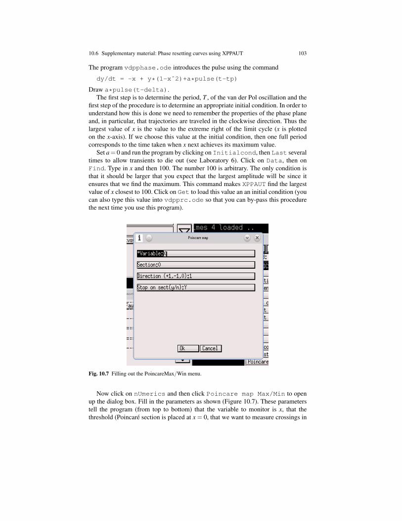
10.6 Supplementary material: Phase resetting curves using XPPAUT 103
The program vdpphase.ode introduces the pulse using the command
dy/dt = -x + y*(1-xˆ2)+a*pulse(t-tp)
Draw a*pulse(t-delta).The first step is to determine the period, T , of the van der Pol oscillation and the
first step of the procedure is to determine an appropriate initial condition. In order tounderstand how this is done we need to remember the properties of the phase planeand, in particular, that trajectories are traveled in the clockwise direction. Thus thelargest value of x is the value to the extreme right of the limit cycle (x is plottedon the x-axis). If we choose this value at the initial condition, then one full periodcorresponds to the time taken when x next achieves its maximum value.
Set a = 0 and run the program by clicking on Initialcond, then Last severaltimes to allow transients to die out (see Laboratory 6). Click on Data, then onFind. Type in x and then 100. The number 100 is arbitrary. The only condition isthat it should be larger that you expect that the largest amplitude will be since itensures that we find the maximum. This command makes XPPAUT find the largestvalue of x closest to 100. Click on Get to load this value an an initial condition (youcan also type this value into vdpprc.ode so that you can by-pass this procedurethe next time you use this program).
Fig. 10.7 Filling out the PoincareMax/Win menu.
Now click on nUmerics and then click Poincare map Max/Min to openup the dialog box. Fill in the parameters as shown (Figure 10.7). These parameterstell the program (from top to bottom) that the variable to monitor is x, that thethreshold (Poincare section is placed at x = 0, that we want to measure crossings in

104 10 Phase resetting oscillators (Lab 10)
the upward (1) direction (the downward direction would be −1, and finally we stoponce a crossing has been detected. Click OK.
Now click on Transient and choose 4: this allows the integration to proceedfor awhile without looking at and storing values and hence makes the programfaster to run. The choice of 4 is arbitrary; however, it must be a positive numbersmaller than the period. Exit the nUmerics window by pressing Esc. Now clickon Initialconds and then Go. When the program has finished click on Data,then on Home. You will see that Time has a value of 6.6647 and this value is thatof the period. As above, you can type this value into vdpphase.ode so that youcan by-pass this procedure the next time you use this program.
We are finally ready to calculate phase resetting curves. Note that vdpphase.odeuses an auxiliary function to calculate the phase response curve (PRC). You shouldalso define an auxiliary function to calculate the phase transition curve (PTC). Aproblem with XPPAUT is that it does not have a command to calculate the modulus.What strategies can you use to overcome this problem? Change the amplitude of theperturbation to a = 3. Click on Initialconds, then Range to open up the dialogbox shown in Figure 10.8. Fill it out as shown and then click OK. Use Viewaxesto put phase on the x-axis and prc on the y-axis.
Fig. 10.8 Filling out the Range menu.
Often we wish to compare the PRC’s obtained with different choices of a andpw. Since the memory resources of the computer are limited it is not a good ideato simply plot trajectories without pressing Erase. A better way is to “freeze” theimage by clicking on Graphic stuff and then Freeze On Freeze. In this

10.6 Supplementary material: Phase resetting curves using XPPAUT 105
way, the phase resetting curve is frozen onto the graph on the computer screen, butthe data is no longer stored in memory. Thus we free up computer resources for thenext calculation.


Chapter 11Blood cell dynamics: Oscillations, delays andchaos (Lab 11)
Time delays are intrinsic properties of all real, spatially extended biological systems.These time delays arise because it takes time for information to travel from point Ato point B. For example, in the nervous system time delays arise because axonalconduction velocities are finite. In the endocrine system, time delays arise becauseblood circulation times are finite. Another reason time delays arise is because ofprocessing times. For example, it takes time for an organism to mature before it isborn and attains reproductive age, for a protein to be synthesized, and so on. Animportant point is that if there is a time delay in the biological system, there shouldbe a time delay present in the relevant mathematical model.
Time delay differential equations (DDE) take the form, for example,
dxdt
+ k1x = f (x(t− τ))
where τ is the time delay, k1 is a constant, and x(t),x(t − τ) are, respectively, thevalues of the variable at time t and t− τ . In order to solve a delay differential equa-tion it is necessary to specify an initial function, Φ(s) where s ∈ [t0− τ, t0]. If wedefine the dimension of a dynamical system as the number of initial conditions thatmust be specified to uniquely determine a solution, we see that a DDE is an infi-nite dimensional differential equation. More importantly, for a DDE the dynamicsin the present depend on the dynamics in the past. This is completely different fromdynamical systems described by ordinary differential equations (ODE) in which dy-namical behaviors are completely determined by the present.
Just a few years ago there were no software packages available to integrate DDEs.At that time most investigators wrote there own computer code; most often usingan Euler integration scheme. One of the very first successful packages to integrateDDE was XPPAUT. Since that time many software packages have become avail-able, perhaps the most well developed are MATLAB’s dde23 and DDE-biftool.Pydelay is an implementation of dde23 into Python1.
1 Note that there is another package called PyDDE; however, we do not recommend using thispackage.
107

108 11 Blood cell dynamics: Oscillations, delays and chaos (Lab 11)
11.1 Background
The lecture introduces XPPAUT and Pydelay for the integration of DDEs. XP-PAUT is described in [5] and on the XPPAUT website and PyDelay is describedon the PyDelay website. Documentation concerning dde23 are the excellent pa-pers by L. F. Shampine and S. Thompson (easy to download from Internet). Thediscussion presented in these sources very much follows the presentation of the labmaterial given below.
Browser: Overall, the use of software packages to integrate DDEs is not as welldocumented on-line as the programs that integrate ordinary differential equations.On the Internet an example of how to use XPPAUT to integrate a DDE can be foundby either typing
XPP examples
or by visiting the website
www.math.pitt.edu/xpp/help/xppexample.html
Documentation for Pydelay can be found at
http://pydelay.sourceforge.net/
or by simply typing Pydelay in a web browser.
Housekeeping: No new file extensions are needed for programs that integrateDDEs. In other words they will have the file names myname.ode or myname.py.However, you may find it useful to put your DDE programs into a sub-directory ofyour home directory called delay.
11.1.1 Integrating DDEs using XPPAUT
We illustrate the use of XPPAUT for integrating DDEs with the Wright equation,namely, the first-order DDE
dxdt
= k1x(t− τ) . (11.1)
In XPPAUT, the term x(t−τ) is represented as delay(x,tau). With this in mindthe program delay_first_order.ode becomes
dx/dt=k1*delay(x,tau)par k1=-1,tau=0init x=1aux v=delay(x,tau)@ TOTAL=500,delay=10,xlo=0,xhi=500,ylo=-5,yhi=5,maxstor=100000done

11.1 Background 109
As for ordinary differential equations, the DDE is integrated by typing the com-mand
xppaut delay_first_order.ode &
The computer screen will look like that shown in Figure 11.1.
Fig. 11.1 When XPPAUT is used to integrate a DDE it is necessary to open three of the tabs,namely, ICs, Delay, and Param. We strongly recommend that the windows be arranged as shownin this figure. In order to successfully integrate a DE it is necessary to click ‘OK’ in ALL threewindows (e.g. from top to bottom) and then click ‘Go’ in the bottom window. This tedious processis necessary to ensure that the initial function is loaded correctly.
There are a number of points to keep in kind when using XPPAUT to integrateDDEs.
1. The parameter tau refers to the value of the time delay used in the simulation.The value of delay refers to the largest value of the delay that you might use.Thus the value of delay must be greater than or equal to the tau value. Itshould be noted that the value of delay reserves in memory the amount ofspace that will be required to store the initial function. This observation shouldbe kept in mind in choosing the largest delay that you will use.
2. XPPAUT constructs the initial function Φ(s) in two parts: the value of X(s) att(0) and a second part that is a function defined on the interval [−τ,0).
3. The functional part of the initial function can be introduced in two ways. Firstwe can use the Delay tab in the XPPAUT window (Figure 11.1). This is mostuseful when Φ(s) is either a constant or is described by a reserved functionsuch as exp(). Second, Φ(s) can be constructed in the form of tables whichare read into the program (see below).

110 11 Blood cell dynamics: Oscillations, delays and chaos (Lab 11)
4. The most important point to remember is that each time a simulation is done itis necessary to click ‘OK’ in both the ICs and Delay windows. We recommendthe procedure outlined in the legend to Figure 11.1.
5. It is often useful to define an auxiliary variable by adding the line
aux v=delay(x,tau)
to the program. This line defines the auxiliary variable, v, as the delayed valueof the value of the variable, x. This auxiliary variable can be use to construct aphase plane representation of the dynamics by using Viewaxes. For example,we can replace T by v in the Viewaxes window.
Questions:1. What is the fixed-point for (11.1)?2. The fixed-point for (11.1) becomes unstable when τ > | π
2k1|. For convenience
take k1 = −1.0. Pick different values of τ below this value. What happens tothe dynamics as τ → | π
2k1?
3. How do the behaviors of (11.1) differ between the case when τ = 0 (an ordinarydifferential equation) and the cases when τ 6= 0?
11.1.2 Integrating DDEs using PyDelay
We can also integrate DDEs using PyDelay. In our experience it is much easier touse XPPAUT; however, using PyDelay has advantages. The program first_delay.pyintegrates (11.1). Here we make a few comments.
1. The initial function, Φ(s), is created on [−τ,0] using histdic. It is incorpo-rated into the program through the command hist_from_arrays(histdic.There are other ways to do this, but the way we have done this is the most gen-erally applicable. Note that in this example we have introduced Φ(s) = constantby creating an array of 1’s and then multiplying by the constant.
2. The integrating time step is entered through the initial function, i.e. the inte-grator uses the same dt as the increment in the array. For more complicatedDDEs, PyDelay varies the integration step. This results in a much more ef-ficient and faster integration. This is done by adding the simulation parameterdtmax which sets the maximum value of the integration time step.
11.2 Exercise 1: Periodic anemias
Background: It is generally accepted that in mammals there exists a pluripotentialstem cell (PPSC) population capable of providing differentiated cells for the ery-throid series. Once a cell from the PPSC is committed to the erythroid series, it

11.2 Exercise 1: Periodic anemias 111
undergoes a series of nuclear divisions and enters a maturational phase for a periodof time before release into the blood as a mature erythrocyte. A fall in erythrocytenumbers leads to a decrease in hemoglobin levels and thus in arterial oxygen ten-sion. This decrease in arterial oxygen tension triggers the production of a substance,renal erythropoietin (REP). Increased levels of REP, in turn, increase the cellularproduction rate within the early committed erythroid series cells and, ultimately,circulating erythrocyte numbers.
In an intriguing series of experiments [31] showed that the induction of auto–immune hemolytic anemia (AIH) in rabbits is sometimes marked by a steadydepression of hemoglobin levels, and at other times by sustained oscillations inhemoglobin concentration and reticulocyte levels with a period of 16–17 days. In1979, Michael Mackey developed the model we will study in lab today to explainthese experimental observations [25].
Model:
E(t) = α(E(t− τ))−βE(t) (11.2)
whereα(E(t− τ)) =
αθ n
θ n +En(t− τ)
The important parameters for this model can be obtained from the literature and areequal to:
τ = 5.7daysα = 7.62×10¹⁰cells/kg/dayβ = 2.31×10⁻² day−1
θ = 2.47×10¹¹cells/kgE∗norm = 3.3× 10¹¹, where E∗norm is the normal circulating numbers of erthyro-
cytesn = 7.6
Questions to be answered:1. Write a computer program in XPPAUT to integrate equation (11.2).
2. You will find that the program becomes unstable whenever you run it. This isbecause the numbers are pretty big. Re-write (11.2) using
E =E
E∗norm
What is the equation in terms of this new variable using the values of the pa-rameters given above?
3. Write an XPPAUT program to integrate this new version of (11.2). What hap-pens when you run the program?
4. In auto-immune hemolytic anemia the peripheral destruction rate, β , is in-creased. What happens as β is increased from 0.02 in steps up to, let us say,

112 11 Blood cell dynamics: Oscillations, delays and chaos (Lab 11)
0.5? For each value of β estimate steady state values of E. If there is an oscil-lation estimate the minimum and maximum value of the oscillation. Plot thesevalues on the left axis as a function of β along the y-axis to generate a figurethat resembles the top panel in the left side of Figure 11.2. The graph shows aHopf bifurcation followed by a reverse Hopf bifurcation as β increases. Verifythat the middle and bottom panels of the left side of Figure 11.2 also describethe behavior of (11.2).
5. It is easy of difficult to pinpoint the exact value of β at which the limit cycleappears using numerical calculations. Describe the problem?
6. The right-hand side of Figure 11.2 shows blood cell populations of two strainsof rats following injection the same dose of 89Sr [29]. In terms of the top panelon the left–hand side of Figure 11.2 what initial and post-89Sr values of β woulddescribe the responses of RBC synthesis in these two strains of rats?
7. Write a PyDelay program to integrate the differential equation for E. Do youget the same results as you obtained for the XPPAUT program?
11.3 Exercise 2: Chaotic hematology
Background: The Mackey-Glass equation describes the growth of white blood cell(WBC) populations [26]. This equation takes the form
dxdt
+ k1x(t) = k2x(t− τ)Kµ
Kµ + x(t− τ)µ:= f (x(t− τ)) , (11.3)
where k1,k2,K are constants and µ is the bifurcation parameter. The right-hand sidedescribes the dependence of f (x(t−τ)) on x(t−τ). When x(t) is low, f (x(t−τ))≈k2x(t− τ). Since k2 > 0, we have positive feedback. This is because low x leads tothe production of a hormone, granulopoietin, that stimulates production. However,when x becomes high enough, f (x(t− τ)) ≈ 1
x(t−τ)µ . Thus we have negative feed-back. The type feedback described by f (x(t− τ)) is referred to as mixed feedbacksince it combines both negative and positive feedback.
Figure 11.3 plots the dynamics of x predicted by (11.3) as the gain in the feedbackproportional to µ , increases. As µ increases, we first see a variety of periodic oscil-lations (these arise by a series of bifurcations). When µ ≥ 9.70, we obtain a chaoticsolution. The Mackey-Glass equation was the first demonstration that chaotic dy-namics could be generated by a plausible physiological control mechanism. In otherwords, irregularly varying fluctuations in circulating blood cell numbers, such as ob-served in patients with CML, may not simply represent lab error but can representthe dynamics of a disease process. It should also be noted that when µ is increasedbeyond the chaotic region, the fluctuations in x again become more periodic, indi-cating that a reverse bifurcation can occur.

11.3 Exercise 2: Chaotic hematology 113
Fig. 11.2 a) A schematic representation of the control of PPSC regeneration. b) The qualitativebehavior of the model in (a) as β is increased. In the top panel, the dashed portion of the curve in-dicates the range of β over which cell numbers oscillate with a period that increases as β increases(middle panel). The solid lines bounding the dashed line indicate the maximum and minimum val-ues of the oscillating cell numbers, from which the variation in the amplitude of the oscillationwith β can be determined (bottom panel). (c) Variations in hematocrit for two congenitally anemicstrains of mice after injection of a single dose of 0.5µCi/g body weight 89Sr.
Subsequent work has shown that the Mackey-Glass equation does not providea valid description of WBC production. The main present–day use of the Mackey-Glass equation is to provide a convenient way to produce chaotic signals to use asbench marks for testing various time series analysis methods. The useful propertyis that in the chaotic regime, the dimension of the chaotic attractor increases as τ
increases [6].
Questions to be answered:

114 11 Blood cell dynamics: Oscillations, delays and chaos (Lab 11)
Fig. 11.3 Effect of changing the bifurcation parameter, µ , on the behavior of (11.3). Parameters:k = 1, β = 2, K = 1, and τ = 2. The initial function is x(0) = 0.5 and x(s) = 0.5,s ∈ [−τ,0).
1. Write a program using PyDelay to integrate (11.3). Note that this exercise ismuch, much easier to do using PyDelay than using XPPAUT. Check to seethat you can reproduce the dynamics shown in Figure 11.3).
2. Use mlab.psd() to calculate the power spectrum for the four values of µ
used in Figure 11.3. Keep in mind that the time step of the integration mustbe chosen to be short enough so that the numerical solution is valid, but thelength of the time series needs to be long enough to take into account that thefluctuations of WBC certainly occur on time scales much longer than 1s (seeLaboratory 9).
3. What are the differences in the power spectrum between the periodic regime of(11.3) (e.g. µ = 7) and the chaotic regime (e.g. µ = 9.69715).
Deliverables: Use Lab11_template.tex to prepare the lab assignment.

Chapter 12Arduino boards: Using your laptop in thelaboratory(Lab 12)
Up to now we have used our computer to prepare documents, collect informationfrom the Internet, analyze data and to study the dynamics of mathematical models ofbiological processes. However, a computer can also be used to translate mathemat-ical ideas into experimental paradigms. One way this becomes possible is throughthe use of an A/D board. For example, analog data from a measuring device pro-portional to the amplitude of a time-varying signal can be inputted to the computer(A/D conversion). The computer can then perform some necessary calculations andoutput a signal in the form of a voltage (D/A conversion) as an inputted stimulus tothe experimental preparation under study. In this way the computer can function as afeedback controller or to make it possible to measure a phase resetting curve (PRC)(Laboratory 10). Another possibility is that the computer can use inputted informa-tion to turn on and off various measuring devices and stimulators to make possiblethe design of automated recording and stimulation protocols [20]. This is becausedevices can be turned off and on using TTL (transistor–transistor logic) pulses (theinputs typically enter the measuring through connections located on the back of themachine). These TTL pulses can be generated by the computer and outputted usingD/A conversion. In fact, the availability of inexpensive, credit–card size StrawberryPi computers (originally developed by Raspberry Pi to introduce computer program-ming to elementary school children) has made it possible to build computers that arededicated to the performance of particular types of experiments or tasks.
Another strategy is to use the computer to program standalone electronic circuitto perform tasks while the main computer does something else. A common exam-ple arises in the collection of data from sensors. Today’s laboratory introduces theArduino board, an open–source electronics prototyping platform based on flexible,easy-to-use hardware and software. The uses of this board are only limited by theimagination of the user. Indeed one of our past students used an Arduino–type boardto program the amplifiers for their Alice Cooper–style band. The advantage of theArduino board stems from its open-source platform: many application programs canbe downloaded from the Arduino website (www.arduno.cc) and the Internet andcan often be readily implemented using inexpensive electronic components. For ex-
115

116 12 Arduino boards: Using your laptop in the laboratory(Lab 12)
ample, the light emitting diode (LED) we use for today’s lab cost $ 0.15 each (US)and the accelerometer cost $ 11.95 each.
Browser use: All of the built-in functions for Arduino can be found on the Ar-duino website: www.arduino.cc in the Reference section. Check it out! Datasheets for various electronic components can readily be obtained on the Internet, of-ten by entering the part number. For example, in the laboratory we use an accelerom-eter (MMA7361). Type the name of the accelerometer, i.e., MMA7361, into a searchengine and click on links until you find it. You should download the data sheet forMMA3761. In addition, websites that sell various are generally pretty good at sup-plying the data sheet as well. We bought the components used in this laboratoryfrom SparkFun.
Housekeeping: Today’s lab is run entirely using your own laptop. You shouldalready have installed Python (version 2.5 or higher but not versions 3+) and Mat-plotlib (version 1.1 or higher) on your personal laptop. In order to prepare for to-day’s lab you will need to install the Arduino software on your laptop: go to the Ar-duino website www.arduino.cc or type Arduino in your web browser), clickon Download tab at the top of the Home Page and follow the instructions appro-priate for your computer. Ideally you should have this software installed on yourlaptop before coming to today’s lab.
12.1 Exercise 1: Blinking LEDs
12.1.1 Background
We need to refresh our memories concerning electronic components and circuits.
• LED: stands for light-emitting diode. It can be turned on or off depending thedigital signal it receives. Each has two legs, one longer than the other. The longeris the positive leg and is called the anode. The shorter is the negative leg andcalled the cathode (labeled with a black stripe).
• Resistor: Each carries an electrical resistance. This resistance is delineated by thecolored stripes. It does not matter which direction they are connected. Each LEDrequires a resistor to limit the electrical current it receives.
• Digital pins: For dealing with digital signals. For us, this means either a “HIGH”or “LOW” signal. Pins 0 through 13 on the top row of the Arduino (see Fig-ure 12.1).
• Ground: Circuits need to be connected to a ground. Not literally the ground, butto a grounding pin. There are three ground pins on this Arduino and they arelabeled GND.

12.1 Exercise 1: Blinking LEDs 117
Fig. 12.1 An Arduino board connected to a LED using a breadboard and jumper wires. See textfor discussion.
12.1.2 The Code
The Arduino program is called a sketch. An Arduino computer program is verysimilar to C++ code. Loops are enclosed in and a ; is used to end every line. A// comments out everything after it and can be handy for making notes to yourself.
There are three basic, but required components to every Arduino sketch.
• Variable initialization: Establish the type, name, and initial value of the variablesthat will be used in the sketch. The int indicates this variable is an integer.We have named it led because it will be used for the LED experiment describedbelow. It is set to = 10 because we elected to use digital pin #10 on the Arduino(Figure 12.1.
int led = 10;
• The setup: This program only runs once when you first upload the sketch to theArduino. pinMode is a built-in function that sets the pin you are using and howyou want to use it. In this sketch, we are using the led pin that we establishedas digital pin #10 in the variable initializing section.
void setup()

118 12 Arduino boards: Using your laptop in the laboratory(Lab 12)
pinMode(led, OUTPUT);
• The loop: This loop will run forever as long as the Arduino has power (connectedto your computer through the USB). digitalWrite is another built in func-tion that, in this case, writes either a HIGH or LOW signal to the led pin. Writinga HIGH signal passes current to the led pin and through the resistor and LED,lighting it up. This particular loop turns the LED on, waits 1000ms (1 second),turns off and waits 1000ms. Then the loop starts over again and the LED blinksat 1 Hz
void loop()
digitalWrite(led, HIGH); // turn the LED ondelay(1000); // wait for a seconddigitalWrite(led, LOW); // turn the LED offdelay(1000); // wait for a second
Figure 12.1 shows the Arduino board set that we will use to make the LED blink:
Time to make it happen:
• open the Arduino program and a new sketch (don’t forget to “save as” and nameit something)
• write the sketch (initializing variables, setup and loop)• wire the circuit• plug in the Arduino and upload the sketch• watch the LED blink!
Fig. 12.2 Schematic diagram of a potentiometer. It does not matter which of the two connections(A, B) is ground and which is power.

12.1 Exercise 1: Blinking LEDs 119
12.1.3 The Potentiometer
We can change the blinking rate by including a potentiometer (Figure 12.2) into thecircuit (Figure 12.3). A potentiometer is essentially a variable resistor. Each poten-tiometer has three leads for ground, power and the wiper. Since the potentiometeris basically a resistor it does not matter whether which connection, A or B, is thepower and which is the ground. By turning the dial of the potentiometer, you changethe amount of resistance on either side of the wiper which is connected to the centerpin of the potentiometer. This changes the voltage at the center pin (wiper). Thisvoltage is the analog voltage that we read as an input.
12.1.4 A few more things to know
• Analog pin: An analog pin receives data from a sensor. We will use the analogReadfunction in the Arduino language. Arduinos have an analog-to-digital converterwhich reads the voltage and converts it into a value in the range of 0-1023. Thereare 210 values and hence we have a 10–byte A/D converter.
• 5V pin: This pin on the Arduino constantly delivers 5 volts of power to whateveris connected to it. This is not enough to hurt a person, generally, but it is enoughto hurt a sensor. So... do not connect the wiper (middle lead) of a potentiometerto 5V.
• Serial Port: Used for communication between the Arduino board and a computer.We can use the Arduino’s built-in serial monitor to communicate with an Arduinoboard. Click the serial monitor button in the tool bar and select the same baudrate (communication speed) used in the call to begin(). The default is 9600and this is what we will use.
12.1.5 The Code
The code used to read a potentiometer is as simple as the code we used to make theLED blink:
• Initializing variables: For this sketch, two variables need to be initialized. Onefor the pin that we’re going to use, and one for the reading from the potentiometer,
int pot = A0;int sensorVal = 0;
• The setup: Just like with the LED sketch, pinMode sets the pot pin as anINPUT. Serial.begin starts the connection with the Serial port so that wecan see the readings from the potentiometer. As mentioned earlier, the Arduino

120 12 Arduino boards: Using your laptop in the laboratory(Lab 12)
communicates with the serial port at a certain speed. The default is 9600 and thisis what we will use.
void setup()
pinMode(pot, INPUT);Serial.begin(9600);
• The loop: The signal from the potentiometer are read through the serial portusing the built-in analogRead function. Then, the readings are printed in theserial monitor.
void loop()
sensorVal = analogRead(pot);Serial.println(sensorVal);
Fig. 12.3 The Arduino board shown in Figure 12.1 now includes a potentiometer.
So, let’s hook it up and get this LED blinking! Notice how the negative, cathode,end of the LED is connected to the GND and the longer, positive anode is in serieswith a resistor in digital pin #10. To make this circuit, use the breadboards andjumper wires to connect the Arduino to the bread board, as seen in the schematic.

12.2 Exercise 2: Measuring Tremor 121
Just remember, the bread board makes connections across the rows horizontally.Because this potentiometer is basically a resistor, it does not matter which of thetwo outer leads goes to either power or ground. The convention is that the red wireis for power and the black wire is for grounding. Notice a potentiometer is connectedto an analog pin, not a digital pin. Remember the middle wiper lead CANNOT beconnected to 5V.
To obtain some readings using the potentiometer:
• write the sketch• wire the circuit• plug in the Arduino and upload the sketch• open the serial monitor (upper right corner)• turn the knob of the potentiometer• watch the readings in the serial monitor
Questions to be answered:
• How would you incorporate the potentiometer into the timing of the LED blinks?To ask it in a different way: How could you use the potentiometer to control thefrequency of the blinking LED?
• How could you use the potentiometer to make a dinner and control the brightnessof the LED?
Implement your ideas and see if they works. It may not work perfectly the firsttime so keep trying! Accomplishing this task will make a complete feedback loopand help show you how these little Arduinos are actually quite powerful micro–controllers.
12.2 Exercise 2: Measuring Tremor
Relax your hand and hold it in front of you with fingers outstretched. Have your labpartner look at your fingertip and they will notice that your fingertips are movingvery, very slightly. Don’t worry, these movements are normal and are called tremor.There are many contributions to your trembling fingertips. Physiological tremorrefers to frequency components in the 8− 12Hz frequency range and is thought tobe related to the dynamics of the stretch reflex [24]. Evidence in support of thishypothesis in the absence of these frequencies in some healthy individuals and inpatients with certain peripheral neuropathies and the magnitude of the latency for thestretch reflex ([24] and this lab). However, there are many other contributions to thefingertip tremor including those related to the beating of your heart (the so–called

122 12 Arduino boards: Using your laptop in the laboratory(Lab 12)
ballisto–cardiogram). What would be expected frequency range of contributions tothe tremor related to your heart beat?
Other types of tremors arise in patients with diseases of the nervous system.Examples include the pill-rolling tremor (∼ 4− 6Hz) observed in patients withParkinson’s disease when their hand is resting and essential tremor, a familial dis-order characterized by a tremor that worsens with movement. Thus neurologistsand neuro–scientists have directed considerable attention to the movements of thefingertip.
How can we measure fingertip tremor? One solution is to spend a lot of moneyand purchase an instrument designed especially to measure tremor. A more practi-cal solution is to use an Arduino board to collect data from a triaxial accelerometer,an electronic component that measures acceleration in 3D. Accelerometers are in-expensive and it is likely that you can purchase the same accelerometer as in thelaboratory instrument for less than $ 50 (the accelerometer we use in this lab costs$ 11.95). An additional advantage of measuring tremor in this way is that we maybe able to readily incorporate measurements of acceleration into novel experimentalparadigms. For example, a colleague developed a micro–accelerometer capable ofmeasuring limb movements in the developing chicken embryo F. Valero–Cuevas,personal communication).
Now that we are motivated, let’s measure fingertip tremor!
Fig. 12.4 The MMA7361 triaxial accelerometer purchased from SparkFun. See text for pin iden-tification.
12.2.1 What is an accelerometer?
Just like it sounds, an accelerometer measures acceleration. The acceleration that itmeasures includes gravity and when the sensor is accelerated through a motion. Theaccelerometer we are using is the triple axis accelerometer MMA7361. Triple axismeans that it can measure accelerations in all three planes: x, y, and z. On the frontof the accelerometer you can see the directions that each of the axes are pointing; xand y are in the plane of the breakout board and the z direction is straight out of theboard. The accelerometer is attached to a breakout board which makes it possible to

12.2 Exercise 2: Measuring Tremor 123
make connections to the Arduino board so that the accelerometer can receive powerand measurements can be recorded. The specification sheet for MMA7361 can bereadily found on the Internet. Using this information we can identify the pins on theThe different pins on the breakout board are:
• Vcc: Every sensor requires power to run. This sensor operates on relatively lowpower: only 3.3V. Be careful since the MMA7361 can not handle more voltagethan that. Remember with the potentiometer we used for the LED we could notplug the wiper into the 5V pin on the Arduino. The same thing goes in this labbut there are more pins to be careful about. Vcc can ONLY be connected to 3.3Von the Arduino. It might be helpful to cover the 5V pin with tape or put a littlewire in it to remember. If you do accidentally connect Vcc to 5V, the sensor willget warm and then hot and soon not work at all.
• GND: Just like we saw last time, everything that needs power also must begrounded. This connects to the GND pin on the Arduino.
• Zout: This is where the measurement in the z plane comes out of the breakoutboard. This connects to an analog pin.
• Yout: This is where the measurement in the y plane comes out of the breakoutboard. This connects to an analog pin.
• Xout: This is where the measurement in the x plane comes out of the breakoutboard. This connects to an analog pin.
• SLP: This is the sleep pin. It only understands a high or low signal so it will beconnected to a digital pin. Low is sleep and high is active. Its default position isLOW so it must be given a HIGH signal to be able to get out any measurements.
• 0GD: This is a zero-g detection pin that is also a binary pin. It can detect whenthe accelerometer is falling with the acceleration of gravity and can turn off therest of the sensor so it doesn’t get damaged when it eventually hits the floor. Weare not going to use this today.
• GSel: This pin allows you to indicate how sensitive you want the accelerometerto be. It’s default is ±1.5g when given a LOW signal and ±6g when HIGH. Wemay want to play around with this today.
• ST: This pin is a self-test pin used to check if the accelerometer is working cor-rectly. Hopefully we won’t need this today at all.
12.2.2 The Code - Writing the Sketch
12.2.2.1 Variable Initialization
Just as we did for controlling the blinking of a LED, we need to write a sketch.The first step is to write the variable initiation section. We advise that the sketch iswritten to initialize the pins related to all of the variables that will be measured. Thisorganization is useful when it is necessary to change a pin since it is only necessaryto change one number at the top of the sketch instead of referring to the changed pinthroughout the rest of the code. Note that it does not matter what number pin you
124 12 Arduino boards: Using your laptop in the laboratory(Lab 12)
assign to your pin variables, just that you get the correct type: digital or analog. Doyou remember the difference?
int zAxis = A0; // analogint yAxis = A1; // analogint xAxis = A2; // analogint slp = 4; // digital
These three variables are going to be what we name the measurement comingfrom the analog pin.
int z;int y;int x;
In addition we need to initialize two variables that will be sued for the timer (seebelow). They are initialized as long variables is that they could potentially get verylarge. For example we may decide to sample at 512 Hz for 10 minutes.
long currentTime = 0;long lastTime = 0;
12.2.2.2 The Setup
In the setup, we use pinMode to set up those pins that we will actually use (don’tforget about the Sleep pin! Go back up to where we were talking about what thispin does to figure out how to set it up.). The other thing that you need to do inthe setup is to begin the communication with the serial port. This is done usingSerial.begin. Just remember that the setup only runs once so anything thatyou only need to do once goes in the setup (hint: sleep pin).
12.2.2.3 The Loop
In the case of the blinking LED we used delay to make the loop. However, in thiscase we’re going to use a timer. There are a number of advantages for using a timer:1) using a timer prevents the loop from slowly down each time it is used; 2) it allowsgreater flexibility and speed options when printing data; and 3) it is possible to keeptrack of time efficiently. All of these advantages are important given that our ultimategoal is to calculate a power spectrum in order to determine the frequency contentof tremor. The biggest thing to understand is the function millis(). Calling thisfunction sets that variable to how long the program has been running, but not inseconds, in milliseconds. With that knowledge, take a look at this and see if it makessense. This is not going to be your whole loop and you don’t have to type this, justlook at it to understand · · · we just want to give you an idea of what a timer is:

12.2 Exercise 2: Measuring Tremor 125
void loop()
currentTime = millis();if ((currentTime-lastTime) > 100)
lastTime = currentTime;x = analogRead(xAxis);Serial.println(x);
What happens if you change the 100 to a 10?
Now that we know what a timer is, we can build the rest of the loop. Try this exampleout. You can tweak it as you want:
void loop()
currentTime = millis();if ((currentTime-lastTime) > 10)
lastTime = currentTime;z = analogRead(A0);y = analogRead(A1);x = analogRead(A2);
Serial.print("x: ");Serial.print(x);Serial.print("\ty: ");Serial.print(y);Serial.print("\tz: ");Serial.print(z);Serial.print("\n");
Once you’ve made the correct connections from the accelerometer to to the Ar-duino, upload the sketch and move the sensor around while looking at the serialmonitor. Do you see the values changing? What do they mean?
12.2.3 Calibration
The first thing we need to do with these accelerometers to understand their datais to calibrate them. The data from the potentiometer in the LED experiment took

126 12 Arduino boards: Using your laptop in the laboratory(Lab 12)
the form of numbers that were being printed on the serial monitor that were in therange of 0 to 1023. This is not specific to potentiometers but rather to the functionanalogRead. Every time you read from an analog pin, the numbers produced willbe in this range. However, to make sense of these numbers we need to know whatthe smallest number corresponds to? ±5V, ±1g, etc. Once we know the range wecan scale the remaining numbers as fraction of the whole range. The procedure ofdetermining the operating range of an accelerometer (or, in general, a sensor) iscalled calibration.
Calibrating the sensor to gravity is the easiest. We will do this by holding the sen-sor in different positions (i.e. the y axis pointed directly up) and taking the averageof the data and scaling it to gravity. Here is a suggestion of how we would do it:
• To make it simple, just print out one variable into the serial monitor at a time. So,maybe you do just use the first loop we wrote out above.
• To begin with the easiest, hold the sensor with the y axis pointed up. Keep it inthis position until you have gathered the data necessary.
• Upload the sketch onto the Arduino and open the serial monitor. Make sure theserial monitor is in auto-scroll mode.
• After a few seconds, uncheck the auto-scroll in the serial monitor and highlightall the data from where you stopped to near the top and copy it. The reason to dothis is to get the average reading for the sensor in this position and then you canscale it to gravity.
• It is convenient to past this list of data into an Excel file and then use Excel’s=average function to find the average of the data set.
• Do this for all 6 (two for each axis) positions. Remember to print out the correctaxis.
• Then set up your excel file to resemble that shown in Figure 12.5.
Fig. 12.5 Example of an Excel file setup that is useful for calibrating the accelerometer.
• The big-sized numbers in the third row are the averages of the whole columnbelow each. Notice how the larger numbers in the 400’s and 500’s are when theaxis on the sensor is pointed up. The 1 and -1 in the cells above that are indicatinghow we are going to scale the numbers. Essentially, we’re going to say that whenan axis is pointing up, that reading is equivalent to 1g or 9.8 m/s2
• Then we can use the Excel functions =slope and =intercept to find theproper scaling. The x-values should be the analogRead values and the y-values should be the 1 and −1. We’re using the simple mx + b equation to scalethe Arduino readings to gravity.

12.2 Exercise 2: Measuring Tremor 127
• Use these values (the slope and the intercept) to do some calculations in yourArduino sketch. Every sensor is going to be a little bit different but you can usethe one we developed in this lab as a starting point.
z = analogRead(A0);y = analogRead(A1);x = analogRead(A2);
float xx = x*.00623-2.099;float yy = y*.00600-2.170;float zz = z*.00596-1.836;
• Notice how we used the values of m and b determined using Excel for the calcu-lations in the Arduino loop (with a little bit of rounding).
• Once you’ve calibrated the sensor, now you can get meaningful data out of it!
Fig. 12.6 Triaxial accelerometer taped to index finger.
12.2.4 Data from fingertip movements
Once the accelerometer has been calibrated, rewrite the loop section in the sketchso that it will print out x,y and z data (and maybe even the time, if you want) oneach line. Then when you highlight and copy from the serial monitor, the data willbe organized nicely in columns. Create data showing different things. Attach theaccelerometer to your index finger being careful to also secure the cables so thatthey don’t move around (see Figure 12.6). Try just moving your hand back andforth at first to see how you accelerate and decelerate to change directions. Do thisin one plane first and then make your movement more complicated. Finally collectdata when your hand is relaxed and fingers are outstretched. This is the data we willanalyze below.
An important question is to decide how you want to plot the data and also howyou will determine the power spectrum. Of course we are going to use a Pythonprogram to accomplish these tasks. This means that we need to save the data ina format that can be used in our Python program. PC users can paste it the data

128 12 Arduino boards: Using your laptop in the laboratory(Lab 12)
into a plain text file (for example using Notepad) and then name it name.dat.Mac users can paste their data into TextEdit. In TextEdit, under the format tab,you can change the format to be plain text. Make a new folder and put the datasomewhere you’ll remember, like the desktop or in My Documents. This way, itwill be easier to find when you want to open it up using python.
Deliverables:
Use Lab12_template.tex to prepare the lab assignment.

Appendix AAppendix A: Finding data for analysis
Interesting data sets can be readily generated by integrating a differential equation.However, many students are much more interested in working on real data sets. It issurprisingly easy to obtain data for analysis.
Using an A/D board: By far the most exciting experience for science undergrad-uates is to analyze data that they collected themselves. Present day undergraduateteaching laboratories in biology, physiology and neuroscience have the ability tocollect and digitize biological signals (e.g. Backyard Brain, Phoenix, AD Instru-ments). Using these devices it is relatively straightforward to obtain ASCII data filesfor heartbeats, breathing, electromyographic (EMG), and electro-encephalographic(EEG) data for analysis. A popular laboratory experience was to record the signalsgenerated by an electric fish (see Subsection ??).
In addition a number of useful, open source Python packages have been devel-oped by Andrew Straw (Institute of Molecular Patholopgy, Vienna) that enable re-searchers to use their personal computer to run experiments control an A/D boardand hence collect data from multiple instruments. These software packages can bedownloaded from
http://strawlab.org/
These include:
1. The PyUniversal Library which enables data to be collected through an A/Dboard
https://code.astraw.com/projects/PyUniversalLibrary/
2. Vison Egg, a package for generating visual stimuli for psycho-physical experi-ments
http://visionegg.org/
3. Motmot, a package for real–time collection and analysis of uncompressed digi-tal images from a variety of courses
129

130 A Appendix A: Finding data for analysis
http://code.astraw.com/projects/motmot/
Electronic circuits: Many of the classic limit cycle oscillators of mathematical bi-ology can be implemented as an electronic circuit. For example, Project 2 (Chap-ter ??) shows how a circuit can be constructed to integrate the van der Pol oscillator.Data generated by this circuit can be collected using an A/D board and the resultscompared to those obtained usng numerical integration.
Internet data sets for analysis: A variety of databases exist on the Internet thatenable data sets to be freely downloadable. A very useful resource for obtainingdata from the Internet is Haddock and Dunn’s Practical Computing for Biologists[18]. These include
1. PhysioNet provides access to large collections of recorded physiological datasets
http://www.physionet.org/
2. Time Series Data Library, created by Rob Hyndman and now hosted by DataMarket.com,provides about 800 time series from different sources
http://robjhyndman.com/TSDL/
3. Google’s Trends provide data concerning google hits foe search words as afunction of time
http://www.google.com/trends/
4. National Center for Biotechnology Information website provides sequences forall known genes and, in some cases, the complete genome of an organism
www.ncbi.nlm.nih.gov
5. United States Census Bureau provides data sets for economic trends and demo-graphics
http://www.census.gov/
6. A variety of EEG data sets are available, including
http://kdd.ics.uci.edu/databases/eeg/eeg.data.htmlhttp://eeg.pl/epihttp://epilepsy.uni-freiburg.de/database
7. Birdsongs in the form of *.wav files can be downloaded and analyzed in thefrequency domain (see Chapter ??).
http://www.ilovewavs.com/Effects/Birds/Birds.htm
8. Stock history files can be downloaded from Yahoo! finance using the Pythonprogram snip_stock.

A Appendix A: Finding data for analysis 131
Using a camera: Most students has access to a digital camera. The digital imagesare in the format of a *.jpg file. These files can be readily handled in Python asshown in Labs 4 and 9.
Using a scanner: A scanner provides another route to obtain data. In particular,a figure can be scanned, converted to a *.png image, and the digitized using thefreely downloadable software package, Engauge
http://digitizer.sourceforge.net/


Appendix BAppendix B: Latex survival guide
The philosophy in this course is that we would like to be good citizens of the scien-tific community. An important part of being a good citizen is being able to commu-nicate results, papers, and ideas. Since many of our colleagues live in different partsof the world and hence have different resources available to them we cannot alwaysassume that our friends have the same software for preparing manuscripts that wedo. Moreover, since we use mathematics as our laboratory tool, how can equationsbe exchanged easily by e-mail.
The solution we are choosing in this course is to make use of the open sourcecomputing network. In other words, the only requirement that we require is thatour colleagues have access to the Internet. There are all sorts of computer softwarepackages available on the Internet; many of them are exactly the same softwaresthat are presently used at the cutting edges of scientific research. A big advantage isthat once we become familiar with these products we have access to them anywherein the world. Study abroad students from The Claremont Colleges have alreadybeen able to use their experience with the open source computing network to helpstudents, workers and scientists in the countries they have visited.
In this lab we address the problem as to how to manuscripts and figures to eachother. The software package we will use is called LaTeX. This is the same soft-ware package that is used by the publishers of most of the scientific articles that youread. LaTeX has a completely different concept than, for example, WORD. Pack-ages such as WORD are actually programs that produce the document the way thatthe programmers who designed this package wanted it to be produced. In contrast,when we use LaTex we write the program ourselves that will be used to generatethe document. Since we are writing the program ourselves we can get an article thatlooks exactly like we want it to look like. More importantly, the program is writtenusing a text editor (the same editor we will also use to write computer programsthat integrate equations) and has the form of an ASCII file. This means that we caneasily send it to our friends by email and they can then use it locally on their owncomputer to generate the document.
133

134 B Appendix B: Latex survival guide
B.1 LaTeX manuals
There are several manuals for LaTeX that are available for free on the Internet.Moreover you can also buy a variety of manuals at a bookstore. These notes givea minimum background and set of commands that will be useful for this course.However, as you get more and more experienced using LaTeX I suspect that youwill learn more commands.
B.2 LaTeX
There are three components to a LaTeX environment
1. An editor to edit and prepare tex files (named xxxxx.tex)2. The TeX program itself (latex xxxxx.tex or pdflatex xxxxx.tex)3. A way to view the result
There are many different combinations of the above components. In the past weheavily used MiTeK which is a Latex package designed to work with Windows. Inthis package all of these components are assembled into a single operating environ-ment. This year we are switching to LINUX so that both PC and Mac users willessentially be working in the same environment. In LINUX there are a number ofoptions available. However, they all work about the same; you will likely have yourfavorite. Here are some guidelines.
B.2.1 Text Editor
A LaTeX file can be thought of as the instructions that the LaTeX computer programuses to produce your article the way you told it to be produced. Like all computerprogram files the code is produced using a Text Editor. Note that the important pointof a text editor is that the editor adds no editing commands itself. In other words youare completely in control of exactly the way the article will appear in print. You nolonger have to worry about the WORD program doing lists the way you do not want.This is why LaTeX is the program used by publishing companies, etc.
This year we are switching to a LINUX environment. At the beginning of thecourse we will work in an openSUSE LINUX environment. Here, the text editor iscalled emacs. When we switch to a Ubuntu LINUX environment, the text editor iscalled gedit. It should be noted that in both environments you can install whatevertext editor you want (anything is likely better than Notepad/Wordpad); so you mightas well learn one and stick to it.
All LaTeX files have the form myfile name.tex, where the extension .tex is theimportant part. Using the text editors on LINUX we can created a new file with the

B.3 Learning LaTeX 135
command emacs xxx.tex or gedit xxx.tex or whatever. If the file alreadyexists we can open it the same way.
A nice thing about LINUX is that you can easily find out which text editor yoursystem has by knowing some of the names of existing text editors and using ’Help’or ’man’. It has become extremely easy to download these editors from the Internetand install them on your system.
B.2.2 Latex versus pdflatex
When you use the command latex xxx.tex you generate a file with the ex-tension xxx.dvi. When you use the command pdflatex xxx.tex you willproduce a xxx.pdf file.
The important difference between these files occurs when we try to incorporate afigure into the document. When we use the command latex xxx.tex all of thefigures in the document must be xxx.eps type files. When we use the commandpdflatex xxx.tex all of the figures in the document must be xxx.png typefiles.
Why are there two different ways to generate a LaTeX file? The advantage ofxxx.pdf files is that they do not require a postscript type printer in order to print.All we need is Adobe Reader which can be freely downloaded from the Internet.A second advantage of the use of pdflatex is that *.png, *.jpg, and *.pdffigures can be incorporated into the document using the \includegraphics.
Why worry about xxx.eps files at all? Journals require that final figures be inthe xxx.eps format. Thus when most people prepare figures for their documentsthey will prepare both a xxx.eps and a xxx.png version of the figure (as we willsee this is really easy to do).
B.2.3 Viewing the LaTeX file
In openSUSE the tool that is used to view a xxx.dvi file is xdvi xxx.dvi. Thetool that is used to view a xxx.pdf file is acroread xxx.pdf.
In Ubuntu the tool that is used to view a xxx.dvi file and a xxx.pdf isevince xxxx.x.
B.3 Learning LaTeX
Most people learn LaTeX by doing it, i.e. their first experience is usually the resultof having to prepare their own paper because the journal publisher has asked for it.This is in fact how you will learn to use LaTeX. It’s really not very hard. You do

136 B Appendix B: Latex survival guide
need to know the basic structure of the LaTeX file: the various commands that youneed come from looking them up as you need them. This is where the Internet is souseful (that’s where I found the links listed on your web page). Indeed I had to lookup a number of commands that I had never used before in order to make up thesenotes.
Here we focus on preparing the LaTeX file you will use to submit your assign-ments. In the next few weeks I will show you how to include a bibliography intoyour document and to cite references within the text. You should regard this as yourfirst step into the scientific world!
Structure of a LaTeX file
There are three main parts of a LaTeX file:
1. Preamble2. Body3. Math modes4. Bibliography
Preamble
The preamble is everything from the beginning of your file to the line \begindocument.It tells the program what fonts and style to use, the title and author of the article, andwhether additional packages of commands need to be accessed in order to producethe article. The basic structure of the preamble is
\documentclass[12pt]article\usepackagegraphicx,times\titleBIO--133: Assignment number xxx\authorYour Name\\Your College
The term ’12pt’ means twelve points. Points are the units that type–setters use.This article has been printed using 12pt. If you want smaller print you could use, forexample, 10pt, or bigger 14pt and so on.
The term ‘article’ just refers to the style that the paper will be prepared. The otherstyle often used is ’book’. Many other styles are possible.
Under \usepackage you get to include user packages that are not in thebasic LaTeX package. A common one is graphicx which allows you to includefigures (either *.eps or *.png)into your document(see below). The user packagestimes means that the font will be New York Times style. Often journals, such as

B.3 Learning LaTeX 137
Nature, have there own package and require you to include it at this line. In fact youcould make up your own *.sty file and include it here (minus the extension).
Main Body
The basic structure of the main body is
\begindocument\maketitle
text here
\sectionyour section heading here
text here
\subsectionyour sub-section heading here
text here
\enddocument
The commands \begindocument and \enddocument are manda-tory. The line \maketitle is included only if you made use of the lines \titleand/or \author in the preamble (which you will need to do for your assign-ments).
The lines \section and \subsection generate, respectively, the ap-propriate section and sub–section numbers, whereas the lines \section* and\subsection* generate the same headings without the numbers.
Math modes
Of course the whole point of LaTeX is to easily write text that includes equationsand mathematical symbols. The fact that we use only a text file and the softwarecan be downloaded from the Internet by anyone who has a connection is where thepopularity and power of this program comes from. Indeed scientists and mathemati-cians are so familiar with the commands that many use them in their e-mails to eachother.
The commands are actually pretty simple and once you get the hang of it you canguess what the command without having to look it up. However, until your brain

138 B Appendix B: Latex survival guide
accumulates the commands that you most frequently use it is a bit of a nuisancegoing back and forth between manual and your document.
Inserting mathematical expressions into a text line
You use $..$ to insert equations and mathematical symbols into text. For example,we have $math expression$, where $symbol$ is.
What about equations? The first question to ask is whether you want the equationnumbered or not. If you do not want the equation numbered, then
\[your equation, e.g. a=b\]
If you want the equation numbered, but don’t what to refer to it in your text, then
\beginequationyour equation here, e.g. a=b\endequation
Finally, if you want the equation numbered and want to be able to refer to thatequation in the text, then
\beginequationyour equation here, e.g. a=b\labelyour label here\endequation
The big difference between the last two options is the inclusion of the line\label in the latter. You can label anything this way, e.g. a figure, table, sectionheading, chapter, and so on. A useful hint is to use a label that you can rememberand which in some way describes what it is that you have labeled. Here’s how yourefer to it in the text
(\reflabel) yields (label)Chapter˜\reflabel yields Chapter label
Symbols
LaTeX is fun because you get to use all sorts of interesting symbols. Here are somesymbols that are frequently used in latex documents

B.3 Learning LaTeX 139
α \alpha β \beta τ \tau ϑ \varthetaπ \pi γ \vartheta φ \phi δ \deltaκ \kappa ρ \rho ϕ \varphi ε \epsilonλ \lambda µ \mu σ \sigma ψ \psiω \omage η \eta ξ \xi Γ \GammaΛ \Lambda Ψ \Psi ∆ \Delta Ω \OmegaΘ \Theta Π \Pi Φ \Phi
∑ \sum∫
\int∮
\oint ∏ \prod
cos \cos sin \sin tan \tan log \log
± \pm ≤ \le \ll ≥ \ge \gg • \bullet \circ \diamond≈ \approx ∼ \sim ' \simeq ∝ \propto≡ \equiv ∈ \in ← \leftarrow → \rightarrow
For a comprehensive list of all of the Latex symbols that are available see
http://www.tex.ac.uk/tex-archive/info/symbols/comprehensive/symbols-a4.pdf
Super and sub-scripts
Subscripts and superscripts are made, respectively, with the commands _ and ˆ.Sums and integrals (under symbols on previous page) have upper and lower lim-
its. We can use the symbols _ and ˆ to introduce these limits.The command \sum_i=1ˆn produces
n
∑i=1
and the command \int_aˆb produces∫ b
a
Two special considerations must be kept in mind when type setting integrals.
1. There should be a little extra space between the differential operators, e.g. dxand the integrands preceding it. Thus
\intˆb_a f(x) dx should be \intˆb_a \ dx
2. According to the International Standards Organization the ’d’ in dx should beupright. This means that if we want to be compliment with the world we needto type

140 B Appendix B: Latex survival guide
\intˆb_a f(x) \ \mathrmdx
Useful mathematical stuff
Roots: The command for the n-th root of an expression is
\sqrt[n]expression
For example \sqrt[3]2 produces
3√2
In the case of a square root you do not need the [2].
Fractions: The command for a fraction is
\fracexpression_aexpression_b
For example, \fracaˆ2+bˆ2y+x yields
a2 +b2
y+ x
Automatic sizing of brackets: Mathematics often contains bracketing symbols,usually in pairs that enclose part of the formula. Obviously when we print the textwe want these brackets to be scaled appropriately with respect to the mathematicalexpression(s) they surround. This is accomplished by typing
\left lbrack expression \right rbrack
where lbrack indicates [,\,( and rbrack indicates ],\,) and we notethat the brackets , require a \.
The math environments:
The math environments have the basic structure
\beginenvironmentcommands here\endenvironment
The math environments that we will use are called array, eqnarray, andfigure. As you will see the first two environments allow you to include systemsof equations, matrices, etc into your text and the last one introduces figures. There
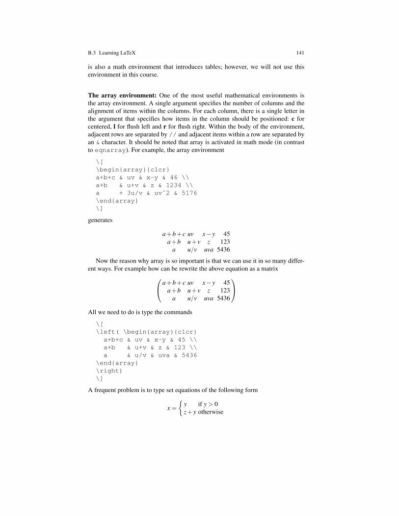
B.3 Learning LaTeX 141
is also a math environment that introduces tables; however, we will not use thisenvironment in this course.
The array environment: One of the most useful mathematical environments isthe array environment. A single argument specifies the number of columns and thealignment of items within the columns. For each column, there is a single letter inthe argument that specifies how items in the column should be positioned: c forcentered, l for flush left and r for flush right. Within the body of the environment,adjacent rows are separated by // and adjacent items within a row are separated byan & character. It should be noted that array is activated in math mode (in contrastto eqnarray). For example, the array environment
\[\beginarrayclcra+b+c & uv & x-y & 46 \\a+b & u+v & z & 1234 \\a + 3u/v & uvˆ2 & 5176\endarray\]
generates
a+b+ c uv x− y 45a+b u+ v z 123
a u/v uva 5436
Now the reason why array is so important is that we can use it in so many differ-ent ways. For example how can be rewrite the above equation as a matrix a+b+ c uv x− y 45
a+b u+ v z 123a u/v uva 5436
All we need to do is type the commands
\[\left( \beginarrayclcr
a+b+c & uv & x-y & 45 \\a+b & u+v & z & 123 \\a & u/v & uva & 5436
\endarray\right)\]
A frequent problem is to type set equations of the following form
x =
y if y > 0z+ y otherwise

142 B Appendix B: Latex survival guide
The becomes in LaTeX
\[x= \left\ \beginarraylly & \mboxif $y>0$ \\
z+y & \mboxotherwise\endarray
\right.\]
where we see how to type words inside of math mode (use \mbox) and what todo if you include only one member of a bracket pair (type a . where the missinglbrack or rbrack should be).
The eqnarray environment: The eqnarray environment is especially useful fortyping multi–line equations. In many ways the eqnarray environment works thesame way that the array environment works.
Here are some useful examples (note adding the ‘*’ deletes the equation number).
\begineqnarrayx & = & 17y \\y & > & a + 189 + \nonumber \\
& & b + 78\endeqnarray
generates
x = 17y (B.1)y > a+189+
b+78 (B.2)
where we see that the addition of \nonumber removes the equation number fromthe line it is typed on. On the other hand if we replaced eqnarray by eqnarray*no equations numbers would appear.
If the formula is too long to put into a single line, then we must tell LaTeX that the‘-‘ or ‘+’ is a binary operator. This is done by starting the formula with an invisiblefirst term, produced by \mbox with a null argument. Thus the commands
\begineqnarray*y & = & a + b + c + d + e + f + g \\
& & \mbox + h + j + k + l\endeqnarray*
generates
y = a+b+ c+d + e+ f +g
+h+ j + k + l

B.3 Learning LaTeX 143
Another way to divide an equation across multiple lines is to split it as follows
\begineqnarray*\lefteqna+b+c+d = \\& & e+f+g+h+ \\& & j + k + l + m + n\endeqnarray*
where we obtain
a+b+ c+d =e+ f +g+h+j + k + l +m+n
The figure environment In order to introduce figures into our article we need topay attention to the following points:
1. We must include the user package graphicx in the preamble of your LaTeXfile.
2. The figure must be in the form of either a *.eps file or a *.png file.3. Both types of files can be produced by MATPLOTLIB (Pylab).4. When you use *.png, then you must use the command pdflatex. This ap-
proach is good since you can use Adobe Acrobat Reader (can be downloadedfor free from the Internet) to print out your article on your own printer.
5. If you have access to a postscript printer (most of us do not), then you can use*.eps figures and the LaTeX command to process your article.
The environment has the form
\beginfigure\includegraphics[width=.9\textwidth]filename.eps\captionyour text here\labelyour label here\endfigure


Appendix CAppendix C: Introduction of Python by A. H.Lee
This tutorial assumes that the reader has no previous programming experience buthas access to an installation of Python. It is operating system independent (goodfor both Widows or OS X) and intended to be read in the given order. A table ofcontents is given at the end.
C.1 Key references
There is an excellent book available free online that will teach you the basics ofPython and some important concepts in computer science at the same time. Itis: Think Python: How to Think Like a Computer Scientist by Allen B. Downey(http://www.greenteapress .com/thinkpython/thinkpython.html),which I will refer to as [Downey] in the remainder of this tutorial.
C.2 How to run a Python interpreter
Two different ways of running a Python program are described. Use script mode ifyou have a long list of Python commands to run (or execute) in order; otherwiseinteractive mode may be more convenient.
C.2.1 Interactive mode
First, start a Python session. Here, I am using prompt> to mean whatever promptyou happen to be on when you start a command session with Windows or OS X.
Below are two sample sessions using python and ipython in that order on a MacOS X in an interactive mode.
145

146 C Appendix C: Introduction of Python by A. H. Lee
prompt> pythonEnthought Python Distribution -- www.enthought.comVersion: 7.1-2 (64-bit)
Python 2.7.2 |EPD 7.1-2 (64-bit)| (default, Jul 27 2011, 14:50:45)[GCC 4.0.1 (Apple Inc. build 5493)] on darwinType "packages", "demo" or "enthought" for more information.>>> 3 + 47>>> exit()
prompt> ipython[TerminalIPythonApp] Staging bundled ipython_config.py from defaultinto u’/Users/alee/.ipython/profile_default’Enthought Python Distribution -- www.enthought.com
Python 2.7.2 |EPD 7.1-2 (64-bit)| (default, Jul 27 2011, 14:50:45)Type "copyright", "credits" or "license" for more information.
IPython 0.11 -- An enhanced Interactive Python.? -> Introduction and overview of IPython’s features.%quickref -> Quick reference.help -> Python’s own help system.object? -> Details about ’object’, use ’object??’ for extra details.
In [1]: 3 + 4Out[1]: 7
In [2]: exit()
C.2.2 Script mode
You would prepare a Python script file containing a Python program and execute theprogram.
First, using a text editor of your choice create a file named hello.py containingthe following as its content:
print "\nHello world!"print "Welcome to the world of Python!"print "We will have some fun!!!"
This script file contains only three lines of print commands. To run this script, dothe following:

C.2 How to run a Python interpreter 147
1. Open a command (terminal) window. Here again I am assuming that you getprompt> as the prompt when you start your command window.
2. Go to the folder where hello.py is located. The cd command will be usefulas you move around the folders in your file system along with the ls commandfor Mac and dir command for Windows.
3. Try the python command with the script file (hello.py in this case) as fol-lows. The result of executing the program will be displayed.
prompt> python hello.py
Hello world!Welcome to the world of Python!We will have some fun!!!prompt>
The program files that I included in this tutorial are all valid Python script files.Try the following and see what happens:
prompt> ipython hello.py
You can run a script from ipython in addition to the usual interaction with theinterpreter. Here is a log of one such interaction:
prompt> ipythonEnthought Python Distribution -- www.enthought.com
Python 2.7.2 |EPD 7.1-2 (64-bit)| (default, Jul 27 2011, 14:50:45)Type "copyright", "credits" or "license" for more information.
IPython 0.11 -- An enhanced Interactive Python.? -> Introduction and overview of IPython’s features.%quickref -> Quick reference.help -> Python’s own help system.object? -> Details about ’object’, use ’object??’ for extra details.
In [1]: pwd # To see where I am in the file systemOut[1]: u’/Users/alee’
In [2]: cd python_2013 # To move to the folder python_2013/Users/alee/python_2013
In [3]: pwdOut[3]: u’/Users/alee/python_2013’
In [4]: execfile("hello.py") # Finally to run the script

148 C Appendix C: Introduction of Python by A. H. Lee
Hello world!Welcome to the world of Python!We will have some fun!!!
In [5]: exit()
Some of these interactions, e.g., the execfile command, are also available ina regular interactive python session. However, pwd and cd (the usual unix com-mands) are not available in regular python although they are available in ipython.
Whether you are using an interactive mode or a script mode, you can import othermodules into your python program. See the ”Modules” section later for detail.
C.3 Basic data types and their values
These are basic type values Python supports and some examples are given belowwithout much explanation. If you are not familiar with them, [Downey] is a goodsource for more information.
• Integers: 34, 2, -300, etc.• Real numbers (floating point numbers): 3.4, 2.0, -300.0, 3.14159, etc.• Booleans (logical values): True and False.• Strings: ’A’, ’a’, ”A”, ”a”, ”This is a string of letters”, ”Hello world!”, etc.
Strings are defined by enclosing a string of text in a pair of single or doublequotes. Python as in most languages recognizes them as a single entity (value)that can be manipulated much like a number (integer or a floating point number)can be, of course using some operators that make sense with strings.
Try the following with Python. The function type given an argument, say 3,returns the type of the value, e.g., integer for 3. The integer type is representedas <type ’int’> in Python.
>>> type (3)<type ’int’>
Now, real numbers (also known as floating point numbers) without listing output(try it yourself to see what output you get):
>>> type (3.14)
And, two boolean values:
>>> type (True)>>> type (False)
And, strings this time:
>>> type ("3")>>> type ("It is a nice day outside.")

C.5 Use of the print command in a script file 149
As you may have recognized it by now, any value the language Python, or any pro-gramming language in general, deals with has a type associated with the value. Byusing the type information a language processor (interpreter in the case of Python)understands what it is dealing with and distinguishes one type of value from another.That way, it would not try to do things that would not make sense, for example, try-ing to add a number to a string. It also uses the type information to decide how muchmemory to use to represent a value in memory. An integer is typically representedusing a smaller amount of memory (say 32 bits) than the amount of memory usedto represent a real number (say 64 bits). So, type information for any value we usein a program is important for the language processor as well as for the programmerswho write application programs.
In this tutorial we will deal with only a small number of types which will still besufficient for the kinds of programs that we will write.
Types such as int, float, boolean are called primitive data types. Later wewill see some compound data types such as string, list, tuples, etc.
C.4 Comments
Any line starting with a pound sign (#) in your Python program is considered acomment and will be ignored by the Python interpreter. I often add my explanationas a comment in a program file.
C.5 Use of the print command in a script file
Create a Python script file named print.py containing the following two lines:
3 + 4 + 2 # Line 1print 4 + 8 # Line 2
Now run that script in script mode, i.e., run it like this:
prompt> python print.py
then you will see output for only one of the two lines.The python interpreter in script mode will evaluate each line of your program
(script) and do exactly what you asked it to do. Line 1 above tells the interpreterto evaluate the expression (3 + 4 + 2) and do nothing else. So, it will evaluateit and produce 9 and that is all it does. Line 2 tells the interpreter to evaluatethe expression (4 + 8) and print it to the standard output device, which is yourcomputer screen. Prepare your script files with a print command sprinkled here andthere if it would make the program easier to understand when you run it.
You might wonder what is going on in an interactive mode as in ipython. WhenPython runs in an interactive mode, the interpreter works a little differently in that

150 C Appendix C: Introduction of Python by A. H. Lee
it interprets a line and furthermore prints the result to the screen which makes sensesince you are expecting to see the result on the screen. When you are in script mode,most likely you will write a series of lines of code and many of those lines will befor some intermediate steps of your program. You wouldn’t want to see the value ofeach line of your entire program printed on the screen. That would be too confusing.
C.6 Variables
In most programming we store a value with a name so we can refer to the valuerepeatedly by the name, often updating the value if necessary. Once a name is givena value, we can even update the value of the variable by assigning a new value, usingan assignment operator (=), as many times as we want if the logic of the programthat we write demands it. Let us see some examples next.
Establishing a variable name with a value associated with the name (again omit-ting output values – please try them as you read):
>>> message = "What’s up?">>> message
Updating the value of the variable with a new value:
>>> message = "What’s down?">>> message
Establishing a name with a value initially and then updating the value as you com-pute in your program is a pattern we use a lot, specially in Python. So, rememberthis pattern.
The variable message here happens to have a string value at this point, but youcan even assign an integer as its value at this point in the program like this:
>>> message = 234>>> message
But, it is usually not a good idea (not a good programming style) to mix differenttypes of values for a given variable unless it is logically necessary to do so in yourprogram. Programs are much easier to understand if you keep the variables withvalues of the same type throughout the lifetime of the variables. In other languagessuch as Java changing the type of a variable like this in mid-stream is not evenallowed. Here are some more variables with some values assigned.
>>> n = 22>>> n>>> n = 23>>> n>>> pi = 3.14159>>> pi

C.7 Operating on values: operators and operands 151
We already know how to get the types. Let us try them again here.
>>> type (message)>>> message = "back to string again">>> type (message)>>> type (n)>>> type (pi)
We can try some boolean variables, i.e., the variables with boolean values (aka log-ical values, namely, True or False). For example,
>>> larger = (45 > 10)>>> larger>>> larger = (45 < 10)>>> larger>>> same = (34 == 34)>>> same>>> type(same)
You will find variables useful as you write more complex programs.
C.7 Operating on values: operators and operands
Combining simple data values you can construct an arbitrarily complex expressionusing operators available in Python. I will try to give you a flavor of them here. Youcan find other operators and form more complex expressions.
>>> 22 + 33 - 10
Create some variables with a value assigned to each and try some expressions:
>>> hour = 5>>> minute = 30>>> hour - 2>>> hour*60 + minute>>> (3+4)*(40/10)+100>>> this = "Ham">>> that = " and cheese">>> more = " for breakfast!"
The + operator has a different meaning depending on what type of operands it op-erates on. If it is dealing with numbers, it will just add as usual. If the operands areof string type, it will concatenate the operands.
>>> this+that+more>>> this + that + more

152 C Appendix C: Introduction of Python by A. H. Lee
’==’ is the operator that tests if its two operands are equal or not. The result willbe True or False. Be careful not to use ’=’ when you actually mean ’==’. ’=’ is anassignment operator, whereas ’==’ is an equality testing operator. What would bethe type of issame after the line below is executed?
>>> issame = this == that
If you are not sure of operator precedence between two operators, use a pair ofparentheses to indicate your intention like this. ’not’ is the negation operator.
>>> isequal = (not (this == that))>>> issame>>> type(issame)>>> isequal>>> type(isequal)
C.8 Order of precedence among operators
The rules on operator precedence in Python is the same as what you would expectfor common operators, e.g., 4 + 3 * 2 evaluates to 10, not 14. If you are notsure, use parentheses to indicate your intention. We have also seen some operationson strings in the previous section.
C.9 Input from keyboard
There are two built-in functions for getting keyboard input, and they are: raw inputand input. Let us try these. When you run the program below, try ’4 + 5’ (with-out the quotes) as your input both times and see what the differences are betweenraw input and input. What you type in as input will not be evaluated if you useraw input:
>>> n = raw_input("Enter a numerical expression, e.g., 3 + 4: ")>>> n
This one will evaluate the input and print the evaluated result:
>>> n = input("Enter a numerical expression, e.g., 3 + 4: ")>>> n
C.10 Functions and packages (libraries)
Let us start with something that we are all familiar with. In Math, we first define andnext apply a function in 2 steps in that order like this:

C.10 Functions and packages (libraries) 153
(1) Definition: f(x) = 3xˆ2 + 2x + 1(2) Application: f(2) = 12 + 4 + 1 = 17
f(3) = 27 + 6 + 1 = 34
Once you define a function, you can call (apply/invoke/use) that function as manytimes as you wish.
In Python, the idea is the same. We only happen to be using a different language:different syntax, same semantics (at least for now):
(1) Definition:def f (x):
return 3*x**2 + 2*x + 1(2) Application:
f(2)which would compute 17 as its value.
Let’s look at it in more detail. In Python, a function must be defined using the fol-lowing syntax:
def <name>(<list_of_parameters>):<statements>
You can make up any name you want for the function that you create, except that youcan’t use a name that is a Python keyword. For example, def is a keyword reservedin the language Python, and you must avoid using it as a name that you create. Thelist of parameters specifies what information, if any, you have to provide in orderto use the function. There can be one or more of statements inside the function,but they must be indented from the def. In my examples, I will use the standardindentation of four blank spaces.
Function definitions are the first of several compound statements we will see, allof which have the same pattern:
1. A header, which begins with a keyword and ends with a colon (:). In case youhave not noticed it, the right parenthesis, the left parenthesis, and the colon areall required. Seemingly insignificant letters like these are part of the languagesyntax and Python like any other programming language is very picky about theexact syntax.
2. A body consisting of one or more Python statements, each indented the sameamount from the header. In a function definition, the keyword in the header isdef, which is followed by the name of the function and a list of parametersenclosed in parentheses. The parameter list may be empty, or it may containany number of parameters. In either case, the parentheses are required as is thecolon (:).
Here are a few examples:
>>> def f(x):return 3*x**2 + 2*x + 1

154 C Appendix C: Introduction of Python by A. H. Lee
>>> f(1)
>>> def g(x, y, z):return x * y + z
>>> g(2, 3, 4)
Try the above fragments of Python code in the given order.pow for power and abs for absolute are two of the many functions that are
already defined in the language that we can use. Those language provided functionsare called built-in functions as opposed to the ones that we programmers create,which are called user-defined functions. For example, f and g above are examplesof user-defined functions.
>>> f(pow(abs(-2), 3))
There are some libraries (packages) that need to be imported into the current modulebefore we can use any function that is defined in the library. math is one such librarythat contains many math related functions. We import a library by the importcommand like below:
>>> import math
Let us define a function named distance that computes the distance between twopoints: p1(x1, y1) and p2(x2, y2):
>>> def distance(x1, y1, x2, y2):dx = x2 - x1dy = y2 - y1dsquared = dx**2 + dy**2result = math.sqrt(dsquared)return result
>>> distance(0, 0, 3, 4)
Note that when we want to call a function defined in a library (aka package) otherthan the default package, we must specify the name of the package followed by adot (.) followed by the function that we want to use in the package. Note that wedid not have to use any package qualifier when we used the ones like print anddef because they are included in the base Python language package, i.e., defaultpackage. A few more example functions follow: isEven tells if a given number iseven or odd. % computes modulo and == tests to see if two values are equal or notproducing a boolean value, i.e., True or False.
>>> def isEven(x):return ((x % 2) == 0)
>>> isEven(3)

C.11 Conditionals: doing it conditionally 155
>>> def isDivisible(x,y):return (x % y) == 0
>>> isDivisible(30, 3)
Exercise 1. Define a function that converts a Celsius temperature value to aFahrenheit temperature and call it with some values such as 100, 0, -40, etc. I willprovide my answer to this exercise at the end of this file, but try it yourself beforeyou see mine.
Exercise 2. This time let us combine functions and input. Define a function thatreads a number from the user through keyboard input, calls the function that con-verts the number as Celsius temperature into Fahrenheit temperature, and returns thecomputed Fahrenheit temperature. After that you can run this program three times:once each with 100, 0, and -40 as input values.
Exercise 3. Define a function with three string parameters and returns a stringthat is the result of concatenating the three with a space as a separating characterbetween strings. Now, call the function with three strings as its actual arguments.
Exercise 4. See Section 3.15 of [Downey] if you want to see more exercise prob-lems.
Sample solutions to Exercises 1 and 2.
def c2f(c):return c * (9.0/5.0) + 32
def c2ftest():n = input("Enter a number: ")n = c2f(n)return n
c2ftest() # use 100, 0, or -40
# Note that c2ftest may be rewritten more succinctly this way:def c2ftest2():
return c2f(input("Enter a number: "))
c2ftest2() # use 100, 0, or -40
C.11 Conditionals: doing it conditionally
You need to understand boolean expressions to understand conditionals. If you arenot familiar with them, consult [Downey].
absolute taking one argument returns the absolute value of the given number.To compute the absolute value, it uses a conditional expression, i.e., if...else...Both syntax and semantics of a conditional expression is intuitive.
>>> def absolute(x):

156 C Appendix C: Introduction of Python by A. H. Lee
if x < 0:return -x
else:return x
>>> absolute(-34)
A conditional expression can be of the cascaded if...elif... ...else...form if you need to have multiple cases to handle, again intuitive (see examples be-low).
Note that if you define functions with the same name multiple times, the last oneoverwrites all the previous ones even if their signatures are different.
>>> def absolute(x):if x < 0:
return -xelif x > 0:
return xelse:
return 0>>> absolute(-34)>>> absolute(34)>>> absolute(0)
Exercise 1. Write a boolean function that determines if a given speed value iswithin the legal freeway speed on I-10 outside of the city limits. Once you definethe function, write a piece of code that calls the defined function and prints thecomputed result (True or False).
Exercise 2. Given a score out of 100, return a letter grade for the score. Let’sassign the letter grade using the grading scale given by the following table:
above 89: Aabove 79 and below 90: Babove 69 and below 80: Cabove 59 and below 70: Dbelow 60: F
and call the function at least five times, each time producing a different letter grade.It is okay to produce the final grade as a string value, e.g., ”A” for an A.
A side note: In Python a function name cannot be overloaded (unlike how it isin Java. Java supports function name overloading, but not in Python.). That is, youcannot define a function with different parameter lists to mean different functions.For example, if you redefine absolute with two parameters in the same sessionwhere absolute was defined earlier with one parameter, the earlier one is lost.So, you can call absolute with one argument okay here:
>>> absolute(-23)

C.12 Loops: doing it repeatedly 157
>>> def absolute(x, y):return x + y
But, you cannot call absolute with one parameter here any longer, thus I com-mented it out here.
# >>> absolute(-23)## Of course, this one below would certainly be okay.#>>> absolute(2, 3)
C.12 Loops: doing it repeatedly
Let us see what ’while’ does in the program below. ’while’ is used to cre-ate a while loop. That is, the body of the while loop, the two lines indented insidethe ’while’ loop in the example below, will be executed repeatedly as long as theboolean expression (n > 0) evaluates to True. So, for this style of loop to termi-nate eventually the value of n (called a loop control variable) must change inside theloop body in such a way that the boolean expression is moving toward evaluating toTrue.
If you call countdown with a negative number initially, what would happen?Well, it will get into an infinite loop... sort of... it will run until the computer getsinto a corrupted state or it runs out of memory depending on how the underlyinginterpreter behaves. At least you see a possible problem! If you do not update thevalue of the loop control variable inside the while loop, we will end up with a similarresult. Create a file named loops.py with the following as its content and run.
# We know what import does, right?import math
# precondition: n > 0 [the condition that must satisfy at the time the# function is called, i.e., before it is executed.]def countdown(n):
while n > 0:print nn = n - 1
print "Blastoff!"
countdown(5)
# Let us write a function that prints when called a log table.# The character sequence ’\t’ generates a tab character.#def print_table():

158 C Appendix C: Introduction of Python by A. H. Lee
x = 1.0while x < 10.0:
print x, ’\t’, math.log(x)x = x + 1.0
# An annotation as part of output (human readability is important!)print "print_table()"
# Finally, generate the table itself by calling the function.print_table()
# Let us improve the earlier definition of print_table by making it more# general. We will parameterize the function by allowing the ’from’ value# and the ’to’ value to be user definable as the function is called. This# is one of the very important techniques in programming - generalization!# abstraction! That is, we abstract with functions and generalize them# when it makes sense to do so.def print_table2(fr, to):
while fr < to:print fr, ’\t’, math.log(fr)fr = fr + 1.0
print "print_table2(10.0, 20.0)"
# As before generate a table, but using two values as actual arguments for# the two parameters that we introduced in the definition.#print_table2(10.0, 20.0)
# What would happen if you called it this way?#print "print_table2(30.0, 20.0)"print_table2(30.0, 20.0)
See how I used the print statements liberally in the code above to make it morereadable when we execute the program.
Exercise 1. Write a function that prints a table of a number, its square, and itssquare root in a range defined by two numbers. For example, numbers between 10and 20 and their squares and square roots in a table. Once the function is defined,call it and be sure that your program generates the table correctly.
Exercise 2. Write a function that reads two numbers from keyboard and usethose two numbers as lower and upper limits of the range that you would need forthe function that you wrote in Exercise 1 above. If the input values that your functionreads in are invalid, e.g., first number is larger than the second, your program mustread a pair of numbers repeatedly until you have two valid numbers. Once you havea good pair of numbers, then you can call the function defined in Exercise 1 above.

C.14 Strings 159
To make it a little more interesting, define a separate function that determines iftwo given numbers are valid or not, and use it as part of your reader function. Yes,you could easily do all that in a single function, but this will give you a chance topractise with multiple functions that make up a program. In fact, as you will learnlater if you continue to write more complex programs, this is a good way to dealwith complexity in your program design.
Exercise 3. See Section 7.9 of [Downey] if you want to see more exercise prob-lems.
C.13 Compound data types: strings, lists, tuples
So far we have mainly dealt with primitive data type values (and a little bit aboutstrings). That is, we have seen the following four data types: int (for integers),float (for real numbers), bool (for booleans), and str (for strings).
Strings are compound data whereas the other three are atomic. That is, a stringis made up of smaller pieces, namely characters. To be more precise, a string is asequence of characters.
Our main focus so far has been learning the basic language constructs and pro-gramming elements such as operators, conditionals, loops, functions, input, etc. us-ing simple data types.
Using the basic language constructs that we have already learned, we can enrichthe data types. We do so by learning compound data types. The compound data typeswe will learn include strings (in more detail), lists, and tuples. To write interestingprograms, we will need to know these compound data types as well. Let us do it.
C.14 Strings
A string is an ordered sequence of characters.String is a data structure and just like integer is a data structure. Integer is a very
simple data structure whereas string is a more complex data structure. Every timeyou encounter a new data structure in any language that you learn, figure out fourthings:
1. How to create an instance of that data structure and give a name to it. Here is anexample of how to create a string variable with a value:
sports = "basketball"
2. How to view the value of the data structure? This is what we call read access.Here are a few examples:
letter = sports[0] # to access the first character

160 C Appendix C: Introduction of Python by A. H. Lee
sports[1] # to access the second character
3. How to change the value of the data structure, if possible? For example, if wewant to modify the contents of sports so that it holds "Baseball" insteadof "baseball", we would have to assign a new character in that location ofthe sports string by using an assignment operator like this:
sports[0] = ’B’
but modifying an element in place in string is not allowed in Python. So, we callstring an immutable data structure in Python. The best you can do is to create anew string with a ’B’ in the first location and reassign the whole string to bethe new value of the variable sports. When we study lists later, we will beable to modify an element in a list in place. Stay tuned. Changing the value of avariable is called write access, and there are two forms of write access we canthink of when we deal with a string.
a. Changing a character in the string, e.g., by doing something like:
sports[0] = ’B’
but that is not allowed with a string because string is immutable in Python.b. Setting a new string to be the value of the variable, e.g.,
sports = Baseball
which is allowed in Python.
4. How to destroy the data structure when we are done using it. In a language suchas C or C++ you would have to worry about that, but not in Python.So, there are only three things to worry about when you encounter a new datastructure in Python. Sometimes, only two as with strings. I will tell you whichones to worry about each time a new data structure is introduced below.
Let us see some strings and related functions that we can use to manipulatestrings. Define a variable with the string value ’banana" as its initial value:
>>> fruit = "banana"
String is a compound value and we can access individual pieces in it. Here we areaccessing the second character in fruit.
>>> letter = fruit[1]>>> letter
Indices in Python are 0-based as in most other programming languages. So, fruit[1]is accessing the second character in the string.
>>> fruit[0]

C.14 Strings 161
Length of a string is available too.
>>> len(fruit)
More looping using strings would be instructive. Let us print fruit using a whileloop:
>>> i = 0>>> while i < len(fruit):
print fruit[i]i = i + 1
Exercise: Create a function that takes one string argument and prints the lettersbackward.
C.14.1 The for loop
We have learned one kind of a loop in Python so far: the while loop. Well,there is another looping construct in Python: the for loop. As you can see be-low, it has a very simple intuitive form. This loop is often referred to as thefor-each loop because that is what it really means. So, the example below canbe read as: ’for each letter referred to as c in the stringfruit, print the character c’, thus printing each letter in the stringto the standard output device, i.e., the computer screen. Remember that the body ofa for loop as with a body of a while loop or a function needs to be indented.
>>> for c in fruit:print c
Here is a simple yet fun thing to do. I think you can figure out what this does:
>>> prefixes = "JKLMNOPQ">>> suffix = "ack">>> for letter in prefixes:
print letter + suffix
Slicing a string: by using the ’:’ operator we can specify a range within the string.
>>> s = "Peter, Paul, and Mary">>> s[0:5] # 0 to 5, but 0 inclusive, 5 exclusive>>> s[7:11]>>> s[17:21]>>> s[:3] # 0 to 3, but 0 inclusive, 3 exclusive>>> s[17:] # 17 to the end, with 17 inclusive
Comparing strings: we can use the usual comparison operators that we use for num-bers to compare two strings.

162 C Appendix C: Introduction of Python by A. H. Lee
word = "apple"if word == "banana":
print "Yes, we have a banana!"else:
print "No, we don’t have a banana!"
if word < "banana":print "Your word, " + word + ", comes before banana."
elif word > "banana":print "Your word, " + word + ", comes after banana."
else:print "Yes, we have a banana!"
Finding a letter in a string: we can define a function that does that like this:
def find(str, ch):index = 0while index < len(str):
if str[index] == ch:return index
index = index + 1return -1
find("apple", ’l’)find("apple", ’p’)
Counting: count the occurrences of a letter in a string:
def count(str, ch):count = 0for char in str:
if char == ch:count = count + 1
return count
count("apple", ’p’)
There is a built-in string module that we can import:
import string
To see what things are included in the module:
dir(string)
Two of those are digits and find:
string.digitsstring.find

C.15 Lists 163
If you want to find the documentation on find, try this. Similarly you can finddocumentation on other functions as well.
string.find.__doc__
Based on the information obtained from the documentation, we can now call find:
string.find("banana", "nan")
C.15 Lists
Remember that a string is an ordered sequence of characters? Well, a list is an or-dered sequence of values of any type. Both strings and lists and other things thatbehave like an ordered sequence are called sequences.
Since a list is a data structure, think about four things about a new data structure:(1) How do you create one? (2) How do you access an element in it? (3) How doyou modify an element in it in place if possible? (4) How do you destroy it when wedon’t need it any more? (don’t worry about destroying one in Python)
Let us see some lists and related functions that we can use to manipulate lists.Also think about where lists would be useful as you write your programs.
Let us create a list on the fly and print it to the standard output device:
>>> [10, 20, 30, 40, 50]
Once more with different type of elements:
>>> ["Let", "us", "stop", "spams!"]
Once more with an element itself as a list:
>>> ["hello", 2.0, 5, ["nested", 2, True]]
Here is another way of creating a list:
>>> range(1, 7) # 1 inclusive, 7 exclusive
From 0 to 9 inclusive this time:
>>> range(10)
How about 1 to 10 in 2 or 3 increments?:
>>> range(1, 10, 2)>>> range(1, 10, 3)
Let us see how we access elements in a list. First create a list and make sure it isindeed created:
>>> numbers = [10, 20, 30, 40, 50]>>> numbers

164 C Appendix C: Introduction of Python by A. H. Lee
Remember that strings are immutable? Well, lists are mutable, which means thatwe can modify an element in a list in place. Let us try it and see if indeed themodification was done correctly in place.
>>> numbers[2] = 3>>> numbers
Use a for loop as we did with a string:
>>> for n in numbers:print n
Concatenating two lists together:
>>> a = [1, 2, 3]>>> b = [3, 4, 5]>>> a + b # note that neither a nor b has been changed.>>> c = a + b>>> c # note that neither a nor b has been changed. c is new.
What would you expect this to do? Well, verify your answer by running it.
>>> [0] * 4
How about this one? Again run it to see what it does.
>>> [1, 2, 3] * 3
Slicing lists, much like we did with strings:
>>> alist = [’a’, ’b’, ’c’, ’d’, ’e’, ’f’]>>> alist[1:3] # 1 inclusive, 3 exclusive>>> alist[:4] # 0 to 3 inclusive>>> alist[3:] # 3 and the rest>>> alist[:] # everything
Deleting elements of a list in place:
>>> del alist[2] # This is a destructive operation>>> alist>>> del alist[2:4] # 2 to 3 inclusive>>> alist
Inserting elements into a list: this is useful enough that we create a function for it:
def insert(u, v, i):u[i:i] = v
numbersinsert(numbers, [111], 1)numbers
insert(numbers, [22, 33, 44], 2)

C.15 Lists 165
numbers
insert(numbers, [[222, 333, 444]], 2)numbers
insert(numbers, range(1000, 2000, 500), 2)numbers
def sum(u):sum = 0for e in u:
sum = sum + ereturn sum
def ave(u):return sum(u) / len(u)
def makeList(u):return [u, ave(u)]
insert(numbers, [makeList(range(1, 5))], 2)numbers
Converting strings to lists: sometimes it is useful to convert a string into a list andmanipulate it as a list:
s1 = "Stop that!"list(s1)
Some basic functions dealing with lists:
def del_head(u):del u[0]
aa = [11, 22, 33, 44, 55]del_head(aa)aa
def tail(u):return u[1:]
tail(aa)aa
x = range(1, 11)x

166 C Appendix C: Introduction of Python by A. H. Lee
What does this do? For each element in x double it and includethem all in a list - neat, huh?
y = [j * 2 for j in x]y
Matrices can be represented as lists in Python. For example,
# | 1 2 3 |# | 4 5 6 |# | 7 8 9 |
m = [[1, 2, 3], [4, 5, 6], [7, 8, 9]]
mm[1]m[1] = [40, 50, 60]m
m[1][2]m[1][2] = 300m[1][2]
We can print the 3 rows in order like this:
for r in m:print r
We can print the 9 elements in order like this:
for r in m:for e in r:
print e
This is a rather inefficient way to deal with matrices in Python. To deal with matricesmore efficiently, learn how to use Numpy arrays.
C.16 Modules
Tuples and dictionaries are also compound data types and we will study them, butlet us study modules first before we continue with them.
Namespace is a concept used in programming languages. As we create functions,thus function names, we may want to create the same function name to mean differ-ent things in different contexts. For example, count may mean counting studentsor beans depending on which program you are dealing with. Rather than namingthem studentCount and beanCount we may want to name them both count,but in different contexts. We create a namespace in which names are contained. So

C.16 Modules 167
if we have a namespace that contains all the names that deal with students and an-other containing all the names that deal with beans, then we can use the same name,e.g., count, as long as we distinguish one from the other by using the name of thenamespace it belongs to. Namespace is used to manage names in a programminglanguage. After all, a program consists of a bunch of names such as variable names,function names, etc. When there are many names, it is easier to deal with them ifwe partition them into different spaces. Python like many other languages supportsthis mechanism and it is implemented by modules.
A module is a file containing Python definitions that are intended to be used inother Python programs. There are many Python modules that come with the lan-guage Python as part of the standard library. We have seen two of those already: thestring module and the math module.
Let us learn how to create a module of our own now. All we need to create amodule is a Python program file with a .py extension in the filename. For example,functions.py that I created earlier is one such module. Let us create one asfollows: we will create a file named seqtools.py that contains two definitionsnamed remove at and insert at. The file would contain the following:
# seqtools.py
def remove_at(seq, pos):return seq[:pos] + seq[pos+1:]
def insert_at(seq, pos, item):return seq[:pos] + item + seq[pos:]
Now, that we created a module seqtools.py, let us learn how to use it. Starta Python session in an interactive mode, and try the following.
>>> from seqtools import remove_at>>> s = "This is fun!">>> remove_at(s, 3)
’Thi is fun!’
As you can see, we are using the ’from . . . import’ command to import aspecific name (remove at) from a module (seqtools). We have imported onlyone definition out of two in seqtools.py.
In this particular situation we imported the name (remove at) into the currentmodule, which is the top-level, interactive module. Once you import it, you can usethe imported name as if the name was created in the current module that you are in.
One bad thing about the way it was just done is the following: if you already hadthe same name in the current module, the old one will be lost. To avoid this situa-tion, there is another way of importing. Here again I am showing you an interactivesession using an interactive mode to illustrate how it is done, like this:
>>> import seqtools>>> s = "This is fun!">>> seqtools.remove_at(s, 3)

168 C Appendix C: Introduction of Python by A. H. Lee
’Thi is fun!’
As you can see here we are importing everything from the module seqtools. Notethat we don’t say ’import seqtools.py’, but rather ’import seqtools’without the file extension (.py). Since there are two definitions in seqtools, bothare imported. If we import it this way, we must specify the module name along withthe name in the module if we want to use a name in the imported module.
We use the dot (’.’) operator to separate the module name and a name in themodule, e.g., seqtools.insert at. Suppose there was already a definitionnamed insert at in the current module. Then, insert at alone would referto the one in the current module, and seqtools.insert at would refer to theone from seqtools module.
Note that this works because we have the file seqtools.py located in thesame folder where the current python session was started at. If the module to beimported is located in a different folder, we would have to do a little more work. Iwill explain that a little later. Some programming languages use packages to meanmodules. I may use that term inadvertently in the future, and you will know what Imean if I do.
The ’from . . . import’ version also has a wildcard option: We can use’from modulename import *’ to mean import everything from the namedmodule, e.g.,
>>> from seqtools import *
This would import all the names from seqtools into the current module thusoverwriting any existing names if there are names that are the same in the currentmodule as the ones being imported from seqtools.
The dir(. . .) function is useful. Once you import a module, you can use thedir function to see all the functions defined in the module. For example, try thefollowing:
>>> import math>>> dir(math)
Getting back to the case where the module that you want to import is locatedelsewhere, what would we have to do if the module to be imported is located ina different folder than the folder where the current python session was started at?Well, if the module file is located in one of the folders that is included in the current’path’ for the python session, then you don’t need to do anything. If not, we willhave do some more work. So, how do we find out if the folder where the module tobe imported is located is in the path or not? Try this in your current Python session:
>>> import sys>>> sys.path
The value of sys.path is returned and it will show all the folders that are includedin the path. If the folder where the module is located is in the the path, you are done.If not, we have to include that folder in the path. Assuming that the module to be

C.16 Modules 169
imported is located in the folder: /Users/alee/python, this is what we woulddo:
>>> import os>>> os.path.join ## Just to see if join is available>>> <function join at 0x00A12F70>>>> sys.path ## Tried on a Mac machine (Unix)
## see init.py for Windows version[’’,’/Library/Frameworks/Python.framework/Versions/5.1.1/bin’,’/Library/Frameworks/Python.framework/Versions/5.1.1/lib/python25.zip’,(some omitted)u’/Users/alee/.ipython’]
>>> sys.path.append(os.path.join("/Users", "alee", "python"))>>> sys.path[’’,’/Library/Frameworks/Python.framework/Versions/5.1.1/bin’,’/Library/Frameworks/Python.framework/Versions/5.1.1/lib/python25.zip’,(some omitted)u’/Users/alee/.ipython’,’/Users/alee/python’]
Now, you can see that /Users/alee/python is included in the path, and youshould be able to import a module located in that folder, as you can see below:
>>> import seqtools>>> s = "Thisisfun...">>> seqtools.remove_at(s, 3)’Thiisfun...’
Note that remove at(s, 3) without seqtools. would not work. However,if you imported it using ’from seqtools import *’ then remove at(s,3) alone would work.
We can encapsulate all this stuff that I just did into a file named init.py so thatwe can use it to add something into the path. You may then use it every time youwant to do something like this. If you are using Windows, create init.py with thefollowing as its contents. Of course, you will have to use the appropriate names thatare meaningful for your situation. (The one I used above works for Mac OS X.):
import sysimport ossys.path.append(os.path.join("C:\\", "alee", "python"))
With init.py available, just do the following right after you start a new Pythonsession:
>>> execfile("init.py")
and then continue with whatever you wanted to do in your current Python session.

170 C Appendix C: Introduction of Python by A. H. Lee
C.17 Tuples
Remember that a string is an ordered sequence of characters? Also remember that alist is an ordered sequence of values of any type? We said both strings and lists andother things that behave like ordered sequences are called sequences. Also remem-ber that strings are immutable and lists are mutable?
A tuple, like a list, is a sequence of items of any type. Unlike lists, however, tuplesare immutable. The values of a tuple are indexed by integers as with the values in alist or string. As you will see below, sequences (strings, lists, and tuples) share somecommon operators.
Since a tuple is a data structure, think about four things you want to know abouta new data structure: (1) How do you create one? (2) How do you access an elementin it? (3) How do you modify an element in it in place if possible? Note that tuplesare immutable! (4) How do you destroy it when we don’t need it any more? (don’tworry about destroying one).
Let us see some tuples and related functions that we can use to manipulate tuples.Also think about where tuples would be useful in programming. Syntactically, atuple is a comma-separated sequence of values.
a = 2, 3, 4, 6, 7, 10a # (2, 3, 4, 6, 7, 10)
Although it is not necessary, it is conventional to enclose tuples in parentheses:
b = (20, 30, 40, 60, 70, 100)b # (20, 30, 40, 60, 70, 100)
To create a tuple with a single element, we have to include the final comma. Withoutthe comma, Python treats (5) as an integer in parentheses.
tup = (22,)type(tup) # <type ’tuple>
Another way to create a tuple is the built-in function tuple. With no argument, itcreates an empty tuple:
t = tuple()t # ()
If the argument is a sequence (string, list, or tuple), the result is a tuple with theelements of the sequence:
t = tuple(’apple’)t # (’a’, ’p’, ’p’, ’l’, ’e’)
Most list operators work on tuples. The bracket operator indexes an element:
tup = (’a’, ’b’, ’c’, ’d’, ’e’)tup[0] # ’a’
And, the slice operator selects a range of elements:

C.17 Tuples 171
tup[1:3] # (’b’, ’c’)
As expected you can’t modify an element in place–immutable!
# tup[2] = ’K’ # this would produce an error. What kind of error? Try it!
Although we can’t replace an element in place, we can rebind the variable with anew tuple:
tup = (’a’, ’b’, ’K’, ’d’, ’e’)
Tuple assignments: It is often useful to swap the values of two variables. Tupleassignment is convenient. To swap the values of a and b we can do the following:
aba, b = b, aab
The left side is a tuple of variables; the right side is a tuple of expressions. Eachvalue is assigned to its corresponding variable. All the expressions on the right sideare evaluated before any of the assignments. The number of variables on the left andthe number of values on the right have to be the same. More generally, the right sidecan be any kind of sequence (string, list, or tuple). For example, to split an emailaddress into a user name and a domain, you could write:
addr = ’[email protected]’uname, domain = addr.split(’@’)
Tuple as return values: Functions can return tuples as return values. For exam-ple, we could write a function that swap two parameters like this:
def swap(x, y):return y, x
Then, do the following to swap:
a, b = swap(a, b)
What would this definition of swap (called swapbad) do?
def swapbad(x, y):x, y = y, x
If we call this function like this:
swapbad(a, b)
then changing x inside swapbad makes x refer to a different value, but it has noeffect on a in the main frame. Similarly, changing y has no effect on b.
This would do the right thing, but a function like this would be redundant. I amusing this example to illustrate local variables and their relationship with variablesoutside a function, i.e., global variables.

172 C Appendix C: Introduction of Python by A. H. Lee
def swapgood(x, y):x, y = y, xreturn x, y
a, b = swapgood(a, b)
Lists and tuples: zip is a built-in function that takes two or more sequencesand zips them into a list of tuples where each tuple contains one element from eachsequence. This example zips a string and a list:
s = ’abc’t = [0, 1, 2]zip(s,t) # [(’a’, 0), (’b’, 1), (’c’, 2)]
You can use tuple assignment in a for loop to traverse a list of tuples:
t = [(’a’, 0), (’b’, 1), (’c’, 2)]for letter, number in t:
print number, letter
Each time through the loop, Python selects the next tuple in the list and assigns theelements to letter and number. Try it to see what output you get if it is not obvious.
If you combine zip, for, and tuple assignment, you get a useful idiom fortraversing two (or more) sequences at the same time. For example, has matchtakes two sequences, t1 and t2, and returns True if there is an index i such thatt1[i] == t2[i]:
def has_match(t1, t2):for x, y in zip(t1, t2):
if x == y:return True
return False
If you need to traverse the elements of a sequence and their indices, you can use thebuilt-in function enumerate. Try the following:
for index, element in enumerate(’abc’):print index, element
C.18 Dictionaries
All of the compound data types that we have studied so far–strings, lists, and tuples–are sequence types, which use integers as indices to access the values that are con-tained in them. If you try to use any other type as an index, you get an error.
A dictionary is also a compound data type. It is Python’s built-in mapping type.It maps keys, which can be any immutable type, to values, which can be any type,just like the values of a list or tuple.

C.18 Dictionaries 173
Abstractly and conceptually, a dictionary is a sequence of key-value pairs. Forexample, a phone book is a dictionary: name-number pairs, i.e., mapping of namesto phone numbers.
Remember we should know how to (1) create a new instance of this type, (2)do write access, (3) do read access, and (4) destroy it when you are done using it?Well, we will do (1), (2), and (3) by writing an example that maps English words toSpanish equivalents. For this dictionary, the indices are strings. As usual we won’tworry about destroying one since it will be done automatically by the Python sys-tem when you stop using the data structure that you created. It is called garbagecollection. We are talking about destroying the entire dictionary instance itself, notan entry in the dictionary. For individual entries, we will be able to remove a valuefrom a dictionary which will then be destroyed by the language system if it is notshared by any other data structure.
One way to create a dictionary is to start with an empty dictionary and startadding elements, i.e., pairs. Here is how you do it. I am creating a dictionary named’e2s’ (English to Spanish) initialized with an empty dictionary.
e2s =
This is how you put a key-value pair, i.e., ’one’ as the key and ’uno’ as the valueof the pair:
e2s[’one’] = ’uno’
One more with the two-dos pair:
e2s[’two’] = ’dos’
This is how you retrieve the value associated with a key:
e2s[’one’] # Just to do a read accesse2s[’one’] # If you want it to be printed on the screen
This will display the contents of the entire dictionary so far:
e2s
The elements of a dictionary appear in a comma-separated list as you can see in theprinted result above–you are using an interpreter to execute these lines, aren’t you?
Each entry (pair) contains an index and a value separated by a colon. In a dictio-nary, the indices are called keys, so the elements are called key-value pairs. Dictio-naries are also called association lists, the original term used in the Lisp program-ming language for the same concept.
You can create one dictionary with some initial pairs explicitly like this:
e2s = ’one’: ’uno’, ’two’: ’dos’, ’three’: ’tres’
Order of the pairs in a dictionary is not important. You can use a list of tuples toinitialize a new dictionary:
t = [(’a’, 0), (’b’, 1), (’c’, 2)]d = dict(t)d # ’a’: 0, ’b’: 1, ’c’: 1

174 C Appendix C: Introduction of Python by A. H. Lee
Combining dict and zip yields a concise way to create a dictionary:
d = dict(zip(’abc’, range(3)))d # ’a’: 0, ’c’: 2, ’b’: 1
Here is another dictionary:
inventory = ’apples’: 430, ’bananas’: 312, ’oranges’: 525, ’pears’: 217inventory
Deleting an entry (pair) from a dictionary:
del inventory[’pears’]inventory
Updating the value of a pair:
inventory[’apples’] = inventory[’apples’] + 10inventory
Updating the value of a pair once more:
inventory[’oranges’] = 0inventory
Note: index (key) must be unique in a dictionary, i.e., no two keys can be identicalalthough values do not need to be unique. This is like a function in math! Length ofa dictionary:
len(inventory)
Retrieve all the keys in a dictionary into a list:
e2s.keys()
Retrieve all the values in a dictionary into a list:
e2s.values()
Retrieve all the pairs in a dictionary into a list:
e2s.items()
Check if a key is contained in a dictionary
e2s.has_key(’one’)e2s.has_key(’deux’)
If you want to iterate through the pairs and add 10 to each:
for key in inventory.keys():inventory[key] = inventory[key] + 10
inventory.values()
If you want to iterate through the pairs and add 10 to each this way this time forkey in e2s.keys():

C.18 Dictionaries 175
e2s[key] = e2s[key] + str(10)e2s.values()
Combining items, tuple assignment, and for, you get the idiom for traversing thekeys and values of a dictionary. Try the following:
for key, val in e2s.items():print val, key
It is common to use tuples as keys in dictionaries (primarily because you can’t uselists). For example, pbook (a phone book dictionary) might map from last-name,first-name pairs to phone numbers.
first = ’john’last = ’doe’number = 9096070410pbook = pbook[last,first] = numberpbook[’jones’,’amy’] = 2133223333
The expression in the brackets is a tuple. We could use tuple assignment to traversethis pbook.
for last, first in pbook:print first, last, pbook[last,first]
This loop traverses the keys in pbook, which are tuples. It assigns the elements ofeach tuple to last and first, then prints the name and the corresponding phonenumber.
Using an alias vs. a copy: Let us create another map first:
opposites = ’up’: ’down’, ’right’: ’wrong’, ’true’: ’false’
This assignment creates an alias where both names reference the same identicaldictionary object.
alias = opposites
The ’copy’ command below creates a distinct copy of the original. There are twocopies now with different names: one called opposites and another called cp.
cp = opposites.copy()
Exercise 1. We can write a function that counts the number of occurrences ofa letter in a string. Or, a more general version of this problem would be to form ahistogram of the letters in the string, that is, how many times each letter appears.Such a histogram might be useful for compressing a text file. Because differentletters appear with different frequencies, we can compress a file by using shortercodes for common letters and longer codes for letters that appear less frequently.
Dictionaries provide an elegant way to generate a histogram. Here is a simpleprogram that would do that:

176 C Appendix C: Introduction of Python by A. H. Lee
>>> letter_counts = >>> for letter in "Mississippi":... letter_counts[letter] = letter_counts.get(letter, 0) + 1...>>> letter_counts’M’: 1, ’s’: 4, ’p’: 2, ’i’: 4
We start with an empty dictionary. For each letter in the string, we find the currentcount (possibly zero) and increment it. At the end, the dictionary contains pairs ofletters and their frequencies. It might be more appealing to display the histogram inalphabetical order. We can do that with the items and sort methods:
>>> letter_items = letter_counts.items()>>> letter_items.sort()>>> letter_items[(’M’, 1), (’i’, 4), (’p’, 2), (’s’, 4)]
You have seen the items method before, but sort is one of the first methods youhave encountered that applies to lists. There are several other list methods, includingappend, extend, and reverse. Consult the Python documentation for detailson these methods and some additional ones.
C.19 Files
We have now seen enough basic data structures that you will need in Python to writesome interesting programs. We will now study how to deal with data in a file.
While a program is running, its data is in memory. When the program ends, orthe computer shuts down, data in memory disappears. One of the easiest ways ofstoring the data permanently is to save it in a file. Files are usually stored on a harddrive, USB drive, CD, etc.
When there are a large number of files, they are often organized into directories(also called folders) in the file system of your computer. Each file is identified by aunique name, or a combination of a file name and a directory name.
Working with files is a lot like working with notebooks. To use a notebook, youhave to open it. When you are done, you have to close it. While the notebook isopen, you can either write in it or read from it. In either case, you know where youare in the notebook. Most of the time, you read the whole notebook in its naturalorder, but you can also skip around.
All of this applies to files as well. To open a file, you specify its name and indi-cate whether you want to read or write. Opening a file creates a file object. In thisexample, the variable f refers to the new file object.
f = open("test.dat", "w")f# <open file ’test.dat’, mode ’w’ at 0x2aaaaab80cd8>

C.19 Files 177
The open function takes two arguments: the first is the name of the file, and thesecond is the mode. Mode "w" means that we are opening the file for writing. Ifthere is no file named test.dat, it will be created when you are accessing it withthe ’w’ mode. If there already is one, it will be replaced by the file we are writing.
When we print the file object, we see the name of the file, the mode, and thelocation of the object. To put data in the file we invoke the write method on thefile object:
f.write("Now is the time")f.write("to close the file")
Closing the file tells the system that we are done writing and makes the file availablefor reading:
f.close()
Now, we can open the file again, this time for reading, and read the contents into astring. This time, the mode argument is "r" for reading:
f = open("test.dat", "r")
If we try to open a file with the read mode that does not exist, we get an error:
#f = open("test.cat","r")# IOError: [Errno 2] No such file or directory: ’test.cat’
f = open("test.dat","r")
Not surprisingly, the read method reads data from the file. With no arguments, itreads the entire contents of the file:
text = f.read()textNow is the timeto close the file
read can also take an argument that indicates how many characters to read:
f = open("test.dat","r")f.read(5)Now i
If not enough characters are left in the file, read returns the remaining characters.When we get to the end of the file, read returns the empty string:
f.read(1000006)s the timeto close the file
f.read()<Nothing this time>
Writing a function that copies a file: It reads and writes up to fifty characters at atime. The first argument is the name of the original file; the second is the name ofthe new file:

178 C Appendix C: Introduction of Python by A. H. Lee
def copyFile(oldFile, newFile):f1 = open(oldFile, "r")f2 = open(newFile, "w")while True: # infinite loop
text = f1.read(50)if text == "":
break # break out of the current loopf2.write(text)
f1.close()f2.close()return
The break statement is new. Executing it breaks out of the current loop; the flowof execution moves to the first statement after the loop. In this example, the whileloop is infinite because the value True is always true. The only way to get out ofthe loop is to execute break, which happens when text is the empty string, whichhappens when we get to the end of the file.
C.19.1 Text files
A text file is a file that contains printable characters and whitespace, organized intolines separated by newline characters. Since Python is specifically designed to pro-cess text files, it provides methods that make the job easy.
To demonstrate, we will create a text file with three lines of text separated bynewlines:
f = open("test1.dat", "w")f.write("line one\nline two\nline three\n")f.close()
The readline() method reads all the characters up to and including the nextnewline character (’\n’):
f = open("test1.dat", "r")f.readline()
readlines() returns all of the remaining lines as a list of strings:
f.readlines()
In this case, the output is in a list format, which means that the strings appear withquotation marks and the newline character appears as the escape sequence \n.
At the end of the file, readline returns the empty string and readlinesreturns the empty list:
>>> f.readline()

C.19 Files 179
>>> f.readlines()[]
Exercise 1: The following is an example of a line-processing program. filterFilemakes a copy of oldFile, omitting any lines that begin with a #:
def filterFile(oldFile, newFile):f1 = open(oldFile, "r")f2 = open(newFile, "w")while True:
text = f1.readline()if text == "":
breakif text[0] == ’#’:
continuef2.write(text)
f1.close()f2.close()return
The continue statement ends the current iteration of the loop, but continues loop-ing. The flow of execution moves to the top of the loop, checks the condition, andproceeds accordingly. Thus, if text is the empty string, the loop exits. If the firstcharacter of text is a hash mark, the flow of execution goes to the top of the loop.Only if both conditions fail do we copy text into the new file.
C.19.2 Exception handling
Whenever a runtime error occurs, it creates an exception. Usually, the program stopsand Python prints an error message. For example, dividing by zero creates an ex-ception:
>>> 55/0ZeroDivisionError: integer division or modulo
So does accessing a nonexistent list item:
>>> a = []>>> a[5]IndexError: list index out of range
Or, accessing a key that isn’t in the dictionary:
>>> b = >>> b[’what’]KeyError: what

180 C Appendix C: Introduction of Python by A. H. Lee
In each case, the error message has two parts: (1) the type of error before the colon,and (2) specifics about the error after the colon. Normally, Python also prints atraceback of where the program was at the time of error, but we have omitted thatfrom the examples.
Sometimes, we want to execute an operation that could cause an exception, butwe don’t want the program to stop. We can handle the exception using the try andexcept statements. For example, we might prompt the user for the name of a fileand then try to open it. If the file doesn’t exist, we don’t want the program to crash;we want to handle the exception. Here is one way to handle the situation:
filename = raw_input(’Enter a file name: ’)try:
f = open (filename, "r")except:
print ’There is no file named’, filename
The try statement executes the statements in the first block. If no exceptions occur,it ignores the except statement. If any exception occurs, it executes the statementsin the except branch and then continues.
We can encapsulate this capability in a function: exists takes a filename andreturns True if the file exists, False if it doesn’t:
def exists(filename):try:
f = open(filename)f.close()return True
except:return False
C.20 More Python
The online tutorial that I wrote can be found at http://www.cmc.edu/pages/faculty/alee/python/. This tutorial is a subset of the online version which covers some addi-tional topics: classes, objects, and arrays.
C.21 NumPy, SciPy, etc.
The online tutorial at http://www.cmc.edu/pages/faculty/alee/python/also discusses these topics briefly, which are useful for scientific computing.
You can find additional information on these topics at http://fperez.org/py4science/starter kit.html.

Appendix DAppendix D: The Scientific Python Ecosystem byF. Perez
While the Python language is an excellent tool for general-purpose programming,with a highly readable syntax, rich and powerful data types (strings, lists, sets, dic-tionaries, arbitrary length integers, etc) and a very comprehensive standard library,it was not designed specifically for mathematical and scientific computing. Neitherthe language nor its standard library have facilities for the efficient representationof multidimensional datasets, tools for linear algebra and general matrix manipula-tions (an essential building block of virtually all technical computing), nor any datavisualization facilities.
In particular, Python lists are very flexible containers that can be nested arbitrarilydeep and which can hold any Python object in them, but they are poorly suited torepresent efficiently common mathematical constructs like vectors and matrices. Incontrast, much of our modern heritage of scientific computing has been built on topof libraries written in the Fortran language, which has native support for vectors andmatrices as well as a library of mathematical functions that can efficiently operateon entire arrays at once.
D.0.1 Scientific Python: a collaboration of projects built byscientists
The scientific community has developed a set of related Python libraries that providepowerful array facilities, linear algebra, numerical algorithms, data visualization andmore. In this appendix, we will briefly outline the tools most frequently used forthis purpose, that make “Scientific Python” something far more powerful than thePython language alone.
For reasons of space, we can only describe in some detail the central Numpylibrary, but below we provide links to the websites of each project where you canread their documentation in more detail.
First, let’s look at an overview of the basic tools that most scientists use in dailyresearch with Python. The core of this ecosystem is composed of:
181

182 D Appendix D: The Scientific Python Ecosystem by F. Perez
• Numpy: the basic library that most others depend on, it provides a powerful ar-ray type that can represent multidmensional datasets of many different kinds andthat supports arithmetic operations. Numpy also provides a library of commonmathematical functions, basic linear algebra, random number generation andFast Fourier Transforms. Numpy can be found at http://numpy.scipy.orgnumpy.scipy.org
• Scipy: a large collection of numerical algorithms that operate on numpy arraysand provide facilities for many common tasks in scientific computing, includingdense and sparse linear algebra support, optimization, special functions, statis-tics, n-dimensional image processing, signal processing and more. Scipy can befound at http://scipy.orgscipy.org.
• Matplotlib: a data visualization library with a strong focus on producinghigh-quality output, it supports a variety of common scientific plot types intwo and three dimensions, with precise control over the final output and for-mat for publication-quality results. Matplotlib can also be controlled interac-tively allowing graphical manipulation of your data (zooming, panning, etc)and can be used with most modern user interface toolkits. It can be found athttp://matplotlib.sf.netmatplotlib.sf.net.
• IPython: while not strictly scientific in nature, IPython is the interactive envi-ronment in which many scientists spend their time. IPython provides a powerfulPython shell that integrates tightly with Matplotlib and with easy access to thefiles and operating system, and which can execute in a terminal or in a graphicalQt console. IPython also has a web-based notebook interface that can combinecode with text, mathematical expressions, figures and multimedia. It can be foundat http://ipython.orgipython.org.
While each of these tools can be installed separately, in our opinion the most con-venient way today of accessing them (especially on Windows and Mac computers)is to install the
http://www.enthought.com/products/epd\_free.php
Free Edition of the Enthought Python Distribution which contain all the above.Other free alternatives on Windows (but not on Macs) are
http://code.google.com/p/pythonxyPython(x,y)
and the
http://www.lfd.uci.edu/\ensuremath˜gohlke/pythonlibs
packages developed by Christoph Gohlke.These four ‘core’ libraries are in practice complemented by a number of other
tools for more specialized work. We will briefly list here the ones that we think arethe most commonly needed:
• Sympy: a symbolic manipulation tool that turns a Python session into a com-puter algebra system. It integrates with the IPython notebook, rendering resultsin properly typeset mathematical notation. http://sympy.orgsympy.org.

D Appendix D: The Scientific Python Ecosystem by F. Perez 183
• Mayavi: sophisticated 3d data visualization; http://code.enthought.com/projects/mayavicode.enthought.com/projects/mayavi.
• Cython: a bridge language between Python and C, useful both to optimizeperformance bottlenecks in Python and to access C libraries directly; http://cython.orgcython.org.
• Pandas: high-performance data structures and data analysis tools, with power-ful data alignment and structural manipulation capabilities; http://pandas.pydata.orgpandas.pydata.org.
• Statsmodels: statistical data exploration and model estimation; http://statsmodels.sourceforge.netstatsmodels.sourceforge.net.
• Scikit-learn: general purpose machine learning algorithms with a commoninterface; http://scikit-learn.orgscikit-learn.org.
• Scikits-image: image processing toolbox; http://scikits-image.orgscikits-image.org.
• NetworkX: analysis of complex networks (in the graph theoretical sense);http://networkx.lanl.govnetworkx.lanl.gov.
• PyTables: management of hierarchical datasets using the industry-standard HDF5format; http://www.pytables.orgwww.pytables.org.
Beyond these, for any specific problem you should look on the internet first, beforestarting to write code from scratch. There’s a good chance that someone, some-where, has written an open source library that you can use for part or all of yourproblem.
D.0.2 A note about the examples below
In all subsequent examples, you will see blocks of input code, followed by the re-sults of the code if the code generated output. This output may include text, graphicsand other result objects. These blocks of input can be pasted into your interactiveIPython session or notebook for you to execute. In the print version of this docu-ment, a thin vertical bar on the left of the blocks of input and output shows whichblocks go together.
If you are reading this text as an actual IPython notebook, you can pressShift-Enter or use the ‘play’ button on the toolbar (right-pointing triangle) toexecute each block of code, known as a ‘cell’ in IPython:
# This is a block of code, below you’ll see its outputprint "Welcome to the world of scientific computing with Python!"
Welcome to the world of scientific computing with Python!

184 D Appendix D: The Scientific Python Ecosystem by F. Perez
D.1 Motivation: the trapezoidal rule
In subsequent sections we’ll provide a basic introduction to the nuts and bolts ofthe basic scientific python tools; but we’ll first motivate it with a brief example thatillustrates what you can do in a few lines with these tools. For this, we will use thesimple problem of approximating a definite integral with the trapezoid rule:
∫ b
af (x)dx≈ 1
2
N
∑k=1
(xk− xk−1)( f (xk)+ f (xk−1)) .
Our task will be to compute this formula for a function such as:
f (x) = (x−3)(x−5)(x−7)+85
integrated between a = 1 and b = 9.First, we define the function and sample it evenly between 0 and 10 at 200 points:
def f(x):return (x-3)*(x-5)*(x-7)+85
import numpy as npx = np.linspace(0, 10, 200)y = f(x)
We select a and b, our integration limits, and we take only a few points in thatregion to illustrate the error behavior of the trapezoid approximation:
a, b = 1, 9xint = x[logical_and(x>=a, x<=b)][::30]yint = y[logical_and(x>=a, x<=b)][::30]
Let’s plot both the function and the area below it in the trapezoid approximation:
import matplotlib.pyplot as pltplt.plot(x, y, lw=2)plt.axis([0, 10, 0, 140])plt.fill_between(xint, 0, yint, facecolor=’gray’, alpha=0.4)plt.text(0.5 * (a + b), 30,r"$\int_aˆb f(x)dx$", horizontalalignment=’center’, fontsize=20);

D.2 NumPy arrays: the right data structure for scientific computing 185
Compute the integral both at high accuracy and with the trapezoid approximation
from scipy.integrate import quad, trapzintegral, error = quad(f, 1, 9)trap_integral = trapz(yint, xint)print "The integral is: %g +/- %.1e" % (integral, error)print "The trapezoid approximation with", len(xint), "points is:", trap_integralprint "The absolute error is:", abs(integral - trap_integral)
The integral is: 680 +/- 7.5e-12The trapezoid approximation with 6 points is: 621.286411141The absolute error is: 58.7135888589
This simple example showed us how, combining the numpy, scipy and matplotliblibraries we can provide an illustration of a standard method in elementary calculuswith just a few lines of code. We will now discuss with more detail the basic usageof these tools.
D.2 NumPy arrays: the right data structure for scientificcomputing
D.2.1 Basics of Numpy arrays
We now turn our attention to the Numpy library, which forms the base layer for theentire ‘scipy ecosystem’. Once you have installed numpy, you can import it as
import numpy
though in this book we will use the common shorthand

186 D Appendix D: The Scientific Python Ecosystem by F. Perez
import numpy as np
As mentioned above, the main object provided by numpy is a powerful array.We’ll start by exploring how the numpy array differs from Python lists. We start bycreating a simple list and an array with the same contents of the list:
lst = [10, 20, 30, 40]arr = np.array([10, 20, 30, 40])
Elements of a one-dimensional array are accessed with the same syntax as a list:
lst[0]
10
arr[0]
10
arr[-1]
40
arr[2:]
array([30, 40])
The first difference to note between lists and arrays is that arrays are homoge-neous; i.e. all elements of an array must be of the same type. In contrast, lists cancontain elements of arbitrary type. For example, we can change the last element inour list above to be a string:
lst[-1] = ’a string inside a list’lst
[10, 20, 30, ’a string inside a list’]
but the same can not be done with an array, as we get an error message:
arr[-1] = ’a string inside an array’
---------------------------------------------------------------------------ValueError Traceback (most recent call last)/home/fperez/teach/book-math-labtool/<ipython-input-13-29c0bfa5fa8a> in <module>()----> 1 arr[-1] = ’a string inside an array’
ValueError: invalid literal for long() with base 10: ’a string inside an array’

D.2 NumPy arrays: the right data structure for scientific computing 187
The information about the type of an array is contained in its dtype attribute:
arr.dtype
dtype(’int32’)
Once an array has been created, its dtype is fixed and it can only store elementsof the same type. For this example where the dtype is integer, if we store a floatingpoint number it will be automatically converted into an integer:
arr[-1] = 1.234arr
array([10, 20, 30, 1])
Above we created an array from an existing list; now let us now see other ways inwhich we can create arrays, which we’ll illustrate next. A common need is to havean array initialized with a constant value, and very often this value is 0 or 1 (suitableas starting value for additive and multiplicative loops respectively); zeros createsarrays of all zeros, with any desired dtype:
np.zeros(5, float)
array([ 0., 0., 0., 0., 0.])
np.zeros(3, int)
array([0, 0, 0])
np.zeros(3, complex)
array([ 0.+0.j, 0.+0.j, 0.+0.j])
and similarly for ones:
print ’5 ones:’, np.ones(5)
5 ones: [ 1. 1. 1. 1. 1.]
If we want an array initialized with an arbitrary value, we can create an emptyarray and then use the fill method to put the value we want into the array:
a = empty(4)a.fill(5.5)a
array([ 5.5, 5.5, 5.5, 5.5])

188 D Appendix D: The Scientific Python Ecosystem by F. Perez
Numpy also offers the arange function, which works like the builtin rangebut returns an array instead of a list:
np.arange(5)
array([0, 1, 2, 3, 4])
and the linspace and logspace functions to create linearly and logarithmically-spaced grids respectively, with a fixed number of points and including both ends ofthe specified interval:
print "A linear grid between 0 and 1:", np.linspace(0, 1, 5)print "A logarithmic grid between 10**1 and 10**4: ", np.logspace(1, 4, 4)
A linear grid between 0 and 1: [ 0. 0.25 0.5 0.75 1. ]A logarithmic grid between 10**1 and 10**4: [ 10. 100. 1000. 10000.]
Finally, it is often useful to create arrays with random numbers that follow a spe-cific distribution. The np.random module contains a number of functions that canbe used to this effect, for example this will produce an array of 5 random samplestaken from a standard normal distribution (0 mean and variance 1):
np.random.randn(5)
array([-0.08633343, -0.67375434, 1.00589536, 0.87081651, 1.65597822])
whereas this will also give 5 samples, but from a normal distribution with a meanof 10 and a variance of 3:
norm10 = np.random.normal(10, 3, 5)norm10
array([ 8.94879575, 5.53038269, 8.24847281, 12.14944165, 11.56209294])
D.2.2 Indexing with other arrays
Above we saw how to index arrays with single numbers and slices, just like Pythonlists. But arrays allow for a more sophisticated kind of indexing which is very pow-erful: you can index an array with another array, and in particular with an array ofboolean values. This is particluarly useful to extract information from an array thatmatches a certain condition.
Consider for example that in the array norm10 we want to replace all valuesabove 9 with the value 0. We can do so by first finding the mask that indicates wherethis condition is true or false:

D.2 NumPy arrays: the right data structure for scientific computing 189
mask = norm10 > 9mask
array([False, False, False, True, True], dtype=bool)
Now that we have this mask, we can use it to either read those values or to resetthem to 0:
print ’Values above 9:’, norm10[mask]
Values above 9: [ 12.14944165 11.56209294]
print ’Resetting all values above 9 to 0...’norm10[mask] = 0print norm10
Resetting all values above 9 to 0...[ 8.94879575 5.53038269 8.24847281 0. 0. ]
D.2.3 Arrays with more than one dimension
Up until now all our examples have used one-dimensional arrays. But Numpy cancreate arrays of aribtrary dimensions, and all the methods illustrated in the previoussection work with more than one dimension. For example, a list of lists can be usedto initialize a two dimensional array:
lst2 = [[1, 2], [3, 4]]arr2 = np.array([[1, 2], [3, 4]])arr2
array([[1, 2],[3, 4]])
With two-dimensional arrays we start seeing the power of numpy: while a nestedlist can be indexed using repeatedly the [ ] operator, multidimensional arrays sup-port a much more natural indexing syntax with a single [ ] and a set of indicesseparated by commas:
print lst2[0][1]print arr2[0,1]
22
Most of the array creation functions listed above can be used with more than onedimension, for example:

190 D Appendix D: The Scientific Python Ecosystem by F. Perez
np.zeros((2,3))
array([[ 0., 0., 0.],[ 0., 0., 0.]])
np.random.normal(10, 3, (2, 4))
array([[ 11.26788826, 4.29619866, 11.09346496, 9.73861307],[ 10.54025996, 9.5146268 , 10.80367214, 13.62204505]])
In fact, the shape of an array can be changed at any time, as long as the totalnumber of elements is unchanged. For example, if we want a 2x4 array with numbersincreasing from 0, the easiest way to create it is:
arr = np.arange(8).reshape(2,4)print arr
[[0 1 2 3][4 5 6 7]]
With multidimensional arrays, you can also use slices, and you can mix andmatch slices and single indices in the different dimensions (using the same arrayas above):
print ’Slicing in the second row:’, arr[1, 2:4]print ’All rows, third column :’, arr[:, 2]
Slicing in the second row: [6 7]All rows, third column : [2 6]
If you only provide one index, then you will get an array with one less dimensioncontaining that row:
print ’First row: ’, arr[0]print ’Second row: ’, arr[1]
First row: [0 1 2 3]Second row: [4 5 6 7]
Now that we have seen how to create arrays with more than one dimension, it’sa good idea to look at some of the most useful properties and methods that arrayshave. The following provide basic information about the size, shape and data in thearray:
print ’Data type :’, arr.dtypeprint ’Total number of elements :’, arr.sizeprint ’Number of dimensions :’, arr.ndimprint ’Shape (dimensionality) :’, arr.shapeprint ’Memory used (in bytes) :’, arr.nbytes

D.2 NumPy arrays: the right data structure for scientific computing 191
Data type : int32Total number of elements : 8Number of dimensions : 2Shape (dimensionality) : (2, 4)Memory used (in bytes) : 32
Arrays also have many useful methods, some especially useful ones are:
print ’Minimum and maximum :’, arr.min(), arr.max()print ’Sum and product of all elements :’, arr.sum(), arr.prod()print ’Mean and standard deviation :’, arr.mean(), arr.std()
Minimum and maximum : 0 7Sum and product of all elements : 28 0Mean and standard deviation : 3.5 2.29128784748
For these methods, the above operations area all computed on all the elements ofthe array. But for a multidimensional array, it’s possible to do the computation alonga single dimension, by passing the axis parameter; for example:
print ’For the following array:\n’, arrprint ’The sum of elements along the rows is :’, arr.sum(axis=1)print ’The sum of elements along the columns is :’, arr.sum(axis=0)
For the following array:[[0 1 2 3][4 5 6 7]]
The sum of elements along the rows is : [ 6 22]The sum of elements along the columns is : [ 4 6 8 10]
As you can see in this example, the value of the axis parameter is the dimensionwhich will be consumed once the operation has been carried out. This is why to sumalong the rows we use axis=0.
This can be easily illustrated with an example that has more dimensions; wecreate an array with 4 dimensions and shape (3,4,5,6) and sum along the axisnumber 2 (i.e. the third axis, since in Python all counts are 0-based). That con-sumes the dimension whose length was 5, leaving us with a new array that hasshape (3,4,6):
np.zeros((3,4,5,6)).sum(2).shape
(3, 4, 6)
Another widely used property of arrays is the .T attribute, which allows you toaccess the transpose of the array:
print ’Array:\n’, arrprint ’Transpose:\n’, arr.T

192 D Appendix D: The Scientific Python Ecosystem by F. Perez
Array:[[0 1 2 3][4 5 6 7]]
Transpose:[[0 4][1 5][2 6][3 7]]
We don’t have time here to look at all the methods and properties of arrays, here’sa complete list. Simply try exploring some of these IPython to learn more, or readtheir description in the full Numpy documentation:arr.T arr.copy arr.getfield arr.putarr.squeeze arr.all arr.ctypes arr.imagarr.ravel arr.std arr.any arr.cumprodarr.item arr.real arr.strides arr.argmaxarr.cumsum arr.itemset arr.repeat arr.sumarr.argmin arr.data arr.itemsize arr.reshapearr.swapaxes arr.argsort arr.diagonal arr.maxarr.resize arr.take arr.astype arr.dotarr.mean arr.round arr.tofile arr.basearr.dtype arr.min arr.searchsorted arr.tolistarr.byteswap arr.dump arr.nbytes arr.setasflatarr.tostring arr.choose arr.dumps arr.ndimarr.setfield arr.trace arr.clip arr.fillarr.newbyteorder arr.setflags arr.transpose arr.compressarr.flags arr.nonzero arr.shape arr.vararr.conj arr.flat arr.prod arr.sizearr.view arr.conjugate arr.flatten arr.ptparr.sort
D.2.4 Operating with arrays
Arrays support all regular arithmetic operators, and the numpy library also con-tains a complete collection of basic mathematical functions that operate on arrays.It is important to remember that in general, all operations with arrays are appliedelement-wise, i.e., are applied to all the elements of the array at the same time. Con-sider for example:
arr1 = np.arange(4)arr2 = np.arange(10, 14)print arr1, ’+’, arr2, ’=’, arr1+arr2
[0 1 2 3] + [10 11 12 13] = [10 12 14 16]
Importantly, you must remember that even the multiplication operator is by de-fault applied element-wise, it is not the matrix multiplication from linear algebra (asis the case in Matlab, for example):

D.2 NumPy arrays: the right data structure for scientific computing 193
print arr1, ’*’, arr2, ’=’, arr1*arr2
[0 1 2 3] * [10 11 12 13] = [ 0 11 24 39]
While this means that in principle arrays must always match in their dimension-ality in order for an operation to be valid, numpy will broadcast dimensions whenpossible. For example, suppose that you want to add the number 1.5 to arr1; thefollowing would be a valid way to do it:
arr1 + 1.5*np.ones(4)
array([ 1.5, 2.5, 3.5, 4.5])
But thanks to numpy’s broadcasting rules, the following is equally valid:
arr1 + 1.5
array([ 1.5, 2.5, 3.5, 4.5])
In this case, numpy looked at both operands and saw that the first (arr1) was aone-dimensional array of length 4 and the second was a scalar, considered a zero-dimensional object. The broadcasting rules allow numpy to:
• create new dimensions of length 1 (since this doesn’t change the size of the array)• ‘stretch’ a dimension of length 1 that needs to be matched to a dimension of a
different size.
So in the above example, the scalar 1.5 is effectively:
• first ‘promoted’ to a 1-dimensional array of length 1• then, this array is ‘stretched’ to length 4 to match the dimension of arr1.
After these two operations are complete, the addition can proceed as now bothoperands are one-dimensional arrays of length 4.
This broadcasting behavior is in practice enormously powerful, especially be-cause when numpy broadcasts to create new dimensions or to ‘stretch’ existingones, it doesn’t actually replicate the data. In the example above the operation iscarried as if the 1.5 was a 1-d array with 1.5 in all of its entries, but no actual arraywas ever created. This can save lots of memory in cases when the arrays in questionare large and can have significant performance implications.
The general rule is: when operating on two arrays, NumPy compares their shapeselement-wise. It starts with the trailing dimensions, and works its way forward, cre-ating dimensions of length 1 as needed. Two dimensions are considered compatiblewhen
• they are equal to begin with, or• one of them is 1; in this case numpy will do the ‘stretching’ to make them equal.

194 D Appendix D: The Scientific Python Ecosystem by F. Perez
If these conditions are not met, a ValueError: frames are not alignedexception is thrown, indicating that the arrays have incompatible shapes. The sizeof the resulting array is the maximum size along each dimension of the input arrays.
This shows how the broadcasting rules work in several dimensions:
b = np.array([2, 3, 4, 5])print arr, ’\n\n+’, b , ’\n----------------\n’, arr + b
[[0 1 2 3][4 5 6 7]]
+ [2 3 4 5]----------------[[ 2 4 6 8][ 6 8 10 12]]
Now, how could you use broadcasting to say add [4, 6] along the rows to arrabove? Simply performing the direct addition will produce the error we previouslymentioned:
c = np.array([4, 6])arr + c
---------------------------------------------------------------------------ValueError Traceback (most recent call last)/home/fperez/teach/book-math-labtool/<ipython-input-45-62aa20ac1980> in <module>()
1 c = np.array([4, 6])----> 2 arr + c
ValueError: operands could not be broadcast together with shapes (2,4) (2)
According to the rules above, the array cwould need to have a trailing dimensionof 1 for the broadcasting to work. It turns out that numpy allows you to ‘inject’ newdimensions anywhere into an array on the fly, by indexing it with the special objectnp.newaxis:
(c[:, np.newaxis]).shape
(2, 1)
This is exactly what we need, and indeed it works:
arr + c[:, np.newaxis]
array([[ 4, 5, 6, 7],[10, 11, 12, 13]])
For the full broadcasting rules, please see the official Numpy docs, which de-scribe them in detail and with more complex examples.

D.2 NumPy arrays: the right data structure for scientific computing 195
As we mentioned before, Numpy ships with a full complement of mathematicalfunctions that work on entire arrays, including logarithms, exponentials, trigono-metric and hyperbolic trigonometric functions, etc. Furthermore, scipy ships a richspecial function library in the scipy.specialmodule that includes Bessel, Airy,Fresnel, Laguerre and other classical special functions. For example, sampling thesine function at 100 points between 0 and 2π is as simple as:
x = np.linspace(0, 2*np.pi, 100)y = np.sin(x)
D.2.5 Linear algebra in numpy
Numpy ships with a basic linear algebra library, and all arrays have a dot methodwhose behavior is that of the scalar dot product when its arguments are vectors (one-dimensional arrays) and the traditional matrix multiplication when one or both ofits arguments are two-dimensional arrays:
v1 = np.array([2, 3, 4])v2 = np.array([1, 0, 1])print v1, ’.’, v2, ’=’, v1.dot(v2)
[2 3 4] . [1 0 1] = 6
Here is a regular matrix-vector multiplication, note that the array v1 should beviewed as a column vector in traditional linear algebra notation; numpy makes nodistinction between row and column vectors and simply verifies that the dimensionsmatch the required rules of matrix multiplication, in this case we have a 2×3 matrixmultiplied by a 3-vector, which produces a 2-vector:
A = np.arange(6).reshape(2, 3)print A, ’x’, v1, ’=’, A.dot(v1)
[[0 1 2][3 4 5]] x [2 3 4] = [11 38]
For matrix-matrix multiplication, the same dimension-matching rules must besatisfied, e.g. consider the difference between A×AT :
print A.dot(A.T)
[[ 5 14][14 50]]
and AT ×A:

196 D Appendix D: The Scientific Python Ecosystem by F. Perez
print A.T.dot(A)
[[ 9 12 15][12 17 22][15 22 29]]
Furthermore, the numpy.linalg module includes additional functionalitysuch as determinants, matrix norms, Cholesky, eigenvalue and singular value de-compositions, etc. For even more linear algebra tools, scipy.linalg containsthe majority of the tools in the classic LAPACK libraries as well as functions tooperate on sparse matrices. We refer the reader to the Numpy and Scipy documen-tations for additional details on these.
D.2.6 Reading and writing arrays to disk
Numpy lets you read and write arrays into files in a number of ways. In order touse these tools well, it is critical to understand the difference between a text and abinary file containing numerical data. In a text file, the number π could be written as“3.141592653589793”, for example: a string of digits that a human can read, within this case 15 decimal digits. In contrast, that same number written to a binary filewould be encoded as 8 characters (bytes) that are not readable by a human but whichcontain the exact same data that the variable pi had in the computer’s memory.
The tradeoffs between the two modes are thus:
• Text mode: occupies more space, precision can be lost (if not all digits are writtento disk), but is readable and editable by hand with a text editor. Can only be usedfor one- and two-dimensional arrays.
• Binary mode: compact and exact representation of the data in memory, can’t beread or edited by hand. Arrays of any size and dimensionality can be saved andread without loss of information.
First, let’s see how to read and write arrays in text mode. The np.savetxt func-tion saves an array to a text file, with options to control the precision, separators andeven adding a header:
arr = np.arange(10).reshape(2, 5)np.savetxt(’test.out’, arr, fmt=’%.2e’, header="My dataset")!cat test.out
# My dataset0.00e+00 1.00e+00 2.00e+00 3.00e+00 4.00e+005.00e+00 6.00e+00 7.00e+00 8.00e+00 9.00e+00
And this same type of file can then be read with the matching np.loadtxtfunction:

D.2 NumPy arrays: the right data structure for scientific computing 197
arr2 = np.loadtxt(’test.out’)print arr2
[[ 0. 1. 2. 3. 4.][ 5. 6. 7. 8. 9.]]
For binary data, Numpy provides the np.save and np.savez routines. Thefirst saves a single array to a file with .npy extension, while the latter can be usedto save a group of arrays into a single file with .npz extension. The files createdwith these routines can then be read with the np.load function.
Let us first see how to use the simpler np.save function to save a single array:
np.save(’test.npy’, arr2)# Now we read this backarr2n = np.load(’test.npy’)# Let’s see if any element is non-zero in the difference.# A value of True would be a problem.print ’Any differences?’, np.any(arr2-arr2n)
Any differences? False
Now let us see how the np.savez function works. You give it a filename andeither a sequence of arrays or a set of keywords. In the first mode, the function willauotmatically name the saved arrays in the archive as arr 0, arr 1, etc:
np.savez(’test.npz’, arr, arr2)arrays = np.load(’test.npz’)arrays.files
[’arr_1’, ’arr_0’]
Alternatively, we can explicitly choose how to name the arrays we save:
np.savez(’test.npz’, array1=arr, array2=arr2)arrays = np.load(’test.npz’)arrays.files
[’array2’, ’array1’]
The object returned by np.load from an .npz file works like a dictionary,though you can also access its constituent files by attribute using its special .ffield; this is best illustrated with an example with the arrays object from above:
print ’First row of first array:’, arrays[’array1’][0]# This is an equivalent way to get the same fieldprint ’First row of first array:’, arrays.f.array1[0]
First row of first array: [0 1 2 3 4]First row of first array: [0 1 2 3 4]

198 D Appendix D: The Scientific Python Ecosystem by F. Perez
This .npz format is a very convenient way to package compactly and withoutloss of information, into a single file, a group of related arrays that pertain to aspecific problem. At some point, however, the complexity of your dataset may besuch that the optimal approach is to use one of the standard formats in scientific dataprocessing that have been designed to handle complex datasets, such as NetCDF orHDF5.
Fortunately, there are tools for manipulating these formats in Python, and forstoring data in other ways such as databases. A complete discussion of the possibil-ities is beyond the scope of this discussion, but of particular interest for scientificusers we at least mention the following:
• The scipy.iomodule contains routines to read and write Matlab files in .matformat and files in the NetCDF format that is widely used in certain scientificdisciplines.
• For manipulating files in the HDF5 format, there are two excellent options inPython: The PyTables project offers a high-level, object oriented approach tomanipulating HDF5 datasets, while the h5py project offers a more direct map-ping to the standard HDF5 library interface. Both are excellent tools; if you needto work with HDF5 datasets you should read some of their documentation andexamples and decide which approach is a better match for your needs.
D.3 High quality data visualization with Matplotlib
The http://matplotlib.sf.netmatplotlib library is a powerful tool capa-ble of producing complex publication-quality figures with fine layout control in twoand three dimensions; here we will only provide a minimal self-contained introduc-tion to its usage that covers the functionality needed for the rest of the book. Weencourage the reader to read the tutorials included with the matplotlib documenta-tion as well as to browse its extensive gallery of examples that include source code.
Just as we typically use the shorthand np for Numpy, we will use plt for thematplotlib.pyplot module where the easy-to-use plotting functions reside(the library contains a rich object-oriented architecture that we don’t have the spaceto discuss here):
import matplotlib.pyplot as plt
The most frequently used function is simply called plot, here is how you canmake a simple plot of sin(x) for x ∈ [0,2π] with labels and a grid (we use the semi-colon in the last line to suppress the display of some information that is unnecessaryright now):

D.3 High quality data visualization with Matplotlib 199
x = np.linspace(0, 2*np.pi)y = np.sin(x)plt.plot(x,y, label=’sin(x)’)plt.legend()plt.grid()plt.title(’Harmonic’)plt.xlabel(’x’)plt.ylabel(’y’);
You can control the style, color and other properties of the markers, for example:
plt.plot(x, y, linewidth=2);
plt.plot(x, y, ’o’, markersize=5, color=’r’);

200 D Appendix D: The Scientific Python Ecosystem by F. Perez
We will now see how to create a few other common plot types, such as a simpleerror plot:
# example datax = np.arange(0.1, 4, 0.5)y = np.exp(-x)
# example variable error bar valuesyerr = 0.1 + 0.2*np.sqrt(x)xerr = 0.1 + yerr
# First illustrate basic pyplot interface, using defaults where possible.plt.figure()plt.errorbar(x, y, xerr=0.2, yerr=0.4)plt.title("Simplest errorbars, 0.2 in x, 0.4 in y");
A simple log plot

D.3 High quality data visualization with Matplotlib 201
x = np.linspace(-5, 5)y = np.exp(-x**2)plt.semilogy(x, y);
A histogram annotated with text inside the plot, using the text function:
mu, sigma = 100, 15x = mu + sigma * np.random.randn(10000)
# the histogram of the datan, bins, patches = plt.hist(x, 50, normed=1, facecolor=’g’, alpha=0.75)
plt.xlabel(’Smarts’)plt.ylabel(’Probability’)plt.title(’Histogram of IQ’)# This will put a text fragment at the position given:plt.text(55, .027, r’$\mu=100,\ \sigma=15$’, fontsize=14)plt.axis([40, 160, 0, 0.03])plt.grid(True)

202 D Appendix D: The Scientific Python Ecosystem by F. Perez
D.3.1 Image display
The imshow command can display single or multi-channel images. A simple arrayof random numbers, plotted in grayscale:
from matplotlib import cmplt.imshow(np.random.rand(5, 10), cmap=cm.gray, interpolation=’nearest’);
A real photograph is a multichannel image, imshow interprets it correctly:
img = plt.imread(’stinkbug.png’)print ’Dimensions of the array img:’, img.shapeplt.imshow(img);
Dimensions of the array img: (375, 500, 3)

D.4 IPython: a powerful interactive environment 203
D.3.2 Simple 3d plotting with matplotlib
Note that you must execute at least once in your session:
from mpl_toolkits.mplot3d import Axes3D
One this has been done, you can create 3d axes with the projection=’3d’keyword to add subplot:fig = plt.figure()fig.add_subplot(<other arguments here>, projection=’3d’)
A simple surface plot:
from mpl_toolkits.mplot3d.axes3d import Axes3Dfrom matplotlib import cm
fig = plt.figure()ax = fig.add_subplot(1, 1, 1, projection=’3d’)X = np.arange(-5, 5, 0.25)Y = np.arange(-5, 5, 0.25)X, Y = np.meshgrid(X, Y)R = np.sqrt(X**2 + Y**2)Z = np.sin(R)surf = ax.plot_surface(X, Y, Z, rstride=1, cstride=1, cmap=cm.jet,
linewidth=0, antialiased=False)ax.set_zlim3d(-1.01, 1.01);
D.4 IPython: a powerful interactive environment
A key component of the everyday workflow of most scientific computing environ-ments is a good interactive environment, that is, a system in which you can executesmall amounts of code and view the results immediately, combining both printing

204 D Appendix D: The Scientific Python Ecosystem by F. Perez
out data and opening graphical visualizations. All modern systems for scientificcomputing, commercial and open source, include such functionality.
Out of the box, Python also offers a simple interactive shell with very limitedcapabilities. But just like the scientific community built Numpy to provide arrayssuited for scientific work (since Pytyhon’s lists aren’t optimal for this task), it hasalso developed an interactive environment much more sophisticated than the built-in one. The http://ipython.orgIPython project offers a set of tools to makeproductive use of the Python language, all the while working interactively and withimmedate feedback on your results. The basic tools that IPython provides are:
1. A powerful terminal shell, with many features designed to increase the fluidityand productivity of everyday scientific workflows, including:
• rich introspection of all objects and variables including easy access to thesource code of any function
• powerful and extensible tab completion of variables and filenames,• tight integration with matplotlib, supporting interactive figures that don’t
block the terminal,• direct access to the filesystem and underlying operating system,• an extensible system for shell-like commands called ‘magics’ that reduce the
work needed to perform many common tasks,• tools for easily running, timing, profiling and debugging your codes,• syntax highlighted error messages with much more detail than the default
Python ones,• logging and access to all previous history of inputs, including across sessions
2. A Qt console that provides the look and feel of a terminal, but adds supportfor inline figures, graphical calltips, a persistent session that can survive crashes(even segfaults) of the kernel process, and more.
3. A web-based notebook that can execute code and also contain rich text and fig-ures, mathematical equations and arbitrary HTML. This notebook presents adocument-like view with cells where code is executed but that can be editedin-place, reordered, mixed with explanatory text and figures, etc.
4. A high-performance, low-latency system for parallel computing that supports thecontrol of a cluster of IPython engines communicating over a network, with opti-mizations that minimize unnecessary copying of large objects (especially numpyarrays).
We will now discuss the highlights of the tools 1–3 above so that you can make theman effective part of your workflow. The topic of parallel computing is beyond thescope of this document, but we encourage you to read the extensive documentationat
http://ipython.org/ipython-doc/rel-0.12.1/parallel/index.html\endvarbatimand\beginverbatim

D.4 IPython: a powerful interactive environment 205
http://minrk.github.com/scipy-tutorial-2011/tutorials
on this available on the IPython website.
D.4.1 The IPython terminal
You can start IPython at the terminal simply by typing: $ ipython which willprovide you some basic information about how to get started and will then opena prompt labeled In [1]: for you to start typing. Here we type 264 and Pythoncomputes the result for us in exact arithmetic, returning it as Out[1]:Python 2.7.2+ (default, Oct 4 2011, 20:03:08)Type "copyright", "credits" or "license" for more information.
IPython 0.13.dev -- An enhanced Interactive Python.? -> Introduction and overview of IPython’s features.%quickref -> Quick reference.help -> Python’s own help system.object? -> Details about ’object’, use ’object??’ for extra details.
In [1]: 2**64Out[1]: 18446744073709551616L
The first thing you should know about IPython is that all your inputs and outputsare saved. There are two variables named In and Out which are filled as you workwith your results. Furthermore, all outputs are also saved to auto-created variablesof the form NN where NN is the prompt number, and inputs to iNN. This allowsyou to recover quickly the result of a prior computation by referring to its numbereven if you forgot to store it as a variable. For example, later on in the above sessionyou can do:In [6]: print _118446744073709551616
We strongly recommend that you take a few minutes to read at least the basicintroduction provided by the ? command, and keep in mind that the %quickrefcommand at all times can be used as a quick reference “cheat sheet” of the mostfrequently used features of IPython.
At the IPython prompt, any valid Python code that you type will be executedsimilarly to the default Python shell (though often with more informative feedback).But since IPython is a superset of the default Python shell; let’s have a brief look atsome of its additional functionality.
Object introspectionA simple ? command provides a general introduction to IPython, but as indicated
in the banner above, you can use the ? syntax to ask for details about any object. Forexample, if we type 1?, IPython will print the following details about this variable:In [14]: _1?Type: longBase Class: <type ’long’>String Form:18446744073709551616

206 D Appendix D: The Scientific Python Ecosystem by F. Perez
Namespace: InteractiveDocstring:long(x[, base]) -> integer
Convert a string or number to a long integer, if possible. A floating
[etc... snipped for brevity]
If you add a second ? and for any oobject x type x??, IPython will try to providean even more detailed analsysi of the object, including its syntax-highlighted sourcecode when it can be found. It’s possible that x?? returns the same information asx?, but in many cases x?? will indeed provide additional details.
Finally, the ? syntax is also useful to search namespaces with wildcards. Sup-pose you are wondering if there is any function in Numpy that may do text-relatedthings; with np.*txt*?, IPython will print all the names in the np namespace(our Numpy shorthand) that have ‘txt’ anywhere in their name:In [17]: np.*txt*?np.genfromtxtnp.loadtxtnp.mafromtxtnp.ndfromtxtnp.recfromtxtnp.savetxt
Tab completionIPython makes the tab key work extra hard for you as a way to rapidly inspect
objects and libraries. Whenever you have typed something at the prompt, by hittingthe <tab> key IPython will try to complete the rest of the line. For this, IPythonwill analyze the text you had so far and try to search for Python data or files thatmay match the context you have already provided.
For example, if you type np.load and hit the key, you’ll see:In [21]: np.load<TAB HERE>np.load np.loads np.loadtxt
so you can quickly find all the load-related functionality in numpy. Tab completionworks even for function arguments, for example consider this function definition:In [20]: def f(x, frobinate=False):
....: if frobinate:
....: return x**2
....:
If you now use the <tab> key after having typed ‘fro’ you’ll get all valid Pythoncompletions, but those marked with = at the end are known to be keywords of yourfunction:In [21]: f(2, fro<TAB HERE>frobinate= frombuffer fromfunction frompyfunc fromstringfrom fromfile fromiter fromregex frozenset
at this point you can add the b letter and hit <tab> once more, and IPython willfinish the line for you:In [21]: f(2, frobinate=

D.4 IPython: a powerful interactive environment 207
As a beginner, simply get into the habit of using <tab> after most objects; it shouldquickly become second nature as you will see how helps keep a fluid workflowand discover useful information. Later on you can also customize this behavior bywriting your own completion code, if you so desire.
Matplotlib integrationOne of the most useful features of IPython for scientists is its tight integration
with matplotlib: at the terminal IPython lets you open matplotlib figures withoutblocking your typing (which is what happens if you try to do the same thing at thedefault Python shell), and in the Qt console and notebook you can even view yourfigures embedded in your workspace next to the code that created them.
The matplotlib support can be either activated when you start IPython by passingthe --pylab flag, or at any point later in your session by using the %pylab com-mand. If you start IPython with --pylab, you’ll see something like this (note theextra message about pylab):ipython --pylabPython 2.7.2+ (default, Oct 4 2011, 20:03:08)Type "copyright", "credits" or "license" for more information.
IPython 0.13.dev -- An enhanced Interactive Python.? -> Introduction and overview of IPython’s features.%quickref -> Quick reference.help -> Python’s own help system.object? -> Details about ’object’, use ’object??’ for extra details.
Welcome to pylab, a matplotlib-based Python environment [backend: Qt4Agg].For more information, type ’help(pylab)’.
In [1]:
Furthermore, IPython will import numpywith the np shorthand, matplotlib.pyplotas plt, and it will also load all of the numpy and pyplot top-level names so that youcan directly type something like:In [1]: x = linspace(0, 2*pi, 200)
In [2]: plot(x, sin(x))Out[2]: [<matplotlib.lines.Line2D at 0x9e7c16c>]
instead of having to prefix each call with its full signature (as we have been doingin the examples thus far):In [3]: x = np.linspace(0, 2*np.pi, 200)
In [4]: plt.plot(x, np.sin(x))Out[4]: [<matplotlib.lines.Line2D at 0x9e900ac>]
This shorthand notation can be a huge time-saver when working interactively (it’s afew characters but you are likely to type them hundreds of times in a session). But weshould note that as you develop persistent scripts and notebooks meant for reuse, it’sbest to get in the habit of using the longer notation (known as fully qualified namesas it’s clearer where things come from and it makes for more robust, readable andmaintainable code in the long run).
Access to the operating system and files

208 D Appendix D: The Scientific Python Ecosystem by F. Perez
In IPython, you can type ls to see your files or cd to change directories, justlike you would at a regular system prompt:In [2]: cd tests/home/fperez/ipython/nbconvert/tests
In [3]: ls test.*test.aux test.html test.ipynb test.log test.out test.pdf test.rst test.tex
Furthermore, if you use the ! at the beginning of a line, any commands you passafterwards go directly to the operating system:In [4]: !echo "Hello IPython"Hello IPython
IPython offers a useful twist in this feature: it will substitute in the command thevalue of any Python variable you may have if you prepend it with a $ sign:In [5]: message = ’IPython interpolates from Python to the shell’
In [6]: !echo $messageIPython interpolates from Python to the shell
This feature can be extremely useful, as it lets you combine the power and clar-ity of Python for complex logic with the immediacy and familiarity of many shellcommands. Additionally, if you start the line with two $$ signs, the output of thecommand will be automatically captured as a list of lines, e.g.:In [10]: !!ls test.*Out[10]:[’test.aux’,’test.html’,’test.ipynb’,’test.log’,’test.out’,’test.pdf’,’test.rst’,’test.tex’]
As explained above, you can now use this as the variable 10. If you directly wantto capture the output of a system command to a Python variable, you can use thesyntax =!:In [11]: testfiles =! ls test.*
In [12]: print testfiles[’test.aux’, ’test.html’, ’test.ipynb’, ’test.log’, ’test.out’, ’test.pdf’, ’test.rst’, ’test.tex’]
Finally, the special %alias command lets you define names that are shorthands forsystem commands, so that you can type them without having to prefix them via !explicitly (for example, ls is an alias that has been predefined for you at startup).
Magic commandsIPython has a system for special commands, called ‘magics’, that let you control
IPython itself and perform many common tasks with a more shell-like syntax: it usesspaces for delimiting arguments, flags can be set with dashes and all arguments aretreated as strings, so no additional quoting is required. This kind of syntax is invalidin the Python language but very convenient for interactive typing (less parentheses,

D.4 IPython: a powerful interactive environment 209
commands and quoting everywhere); IPython distinguishes the two by detectinglines that start with the % character.
You can learn more about the magic system by simply typing %magic at theprompt, which will give you a short description plus the documentation on allavailable magics. If you want to see only a listing of existing magics, you can use%lsmagic:In [4]: lsmagicAvailable magic functions:%alias %autocall %autoindent %automagic %bookmark %c%cd %colors %config %cpaste %debug %dhist %dirs%doctest_mode %ds %ed %edit %env %gui %hist %history%install_default_config %install_ext %install_profiles%load_ext %loadpy %logoff %logon %logstart %logstate %logstop%lsmagic %macro %magic %notebook %page %paste %pastebin%pd %pdb %pdef %pdoc %pfile %pinfo %pinfo2 %pop %popd%pprint %precision %profile %prun %psearch %psource %pushd %pwd%pycat %pylab %quickref %recall %rehashx%reload_ext %rep %rerun %reset %reset_selective %run %save %sc%stop %store %sx %tb %time %timeit %unalias %unload_ext %who%who_ls %whos %xdel %xmode
Automagic is ON, % prefix NOT needed for magic functions.
Note how the example above omitted the eplicit %marker and simply uses lsmagic.As long as the ‘automagic’ feature is on (which it is by default), you can omit the %marker as long as there is no ambiguity with a Python variable of the same name.
Running your codeWhile it’s easy to type a few lines of code in IPython, for any long-lived work
you should keep your codes in Python scripts (or in IPython notebooks, see below).Consider that you have a script, in this case trivially simple for the sake of brevity,named simple.py:In [12]: !cat simple.pyimport numpy as np
x = np.random.normal(size=100)
print ’First elment of x:’, x[0]
The typical workflow with IPython is to use the %run magic to execute your script(you can omit the .py extension if you want). When you run it, the script will ex-ecute just as if it had been run at the system prompt with python simple.py(though since modules don’t get re-executed on new imports by Python, all sys-tem initialization is essentially free, which can have a significant run time impact insome cases):In [13]: run simpleFirst elment of x: -1.55872256289
Once it completes, all variables defined in it become available for you to use inter-actively:In [14]: x.shapeOut[14]: (100,)

210 D Appendix D: The Scientific Python Ecosystem by F. Perez
This allows you to plot data, try out ideas, etc, in a %run/interact/edit cycle thatcan be very productive. As you start understanding your problem better you canrefine your script further, incrementally improving it based on the work you do atthe IPython prompt. At any point you can use the %hist magic to print out yourhistory without prompts, so that you can copy useful fragments back into the script.
By default, %run executes scripts in a completely empty namespace, to bettermimic how they would execute at the system prompt with plain Python. But if youuse the -i flag, the script will also see your interactively defined variables. This letsyou edit in a script larger amounts of code that still behave as if you had typed themat the IPython prompt.
You can also get a summary of the time taken by your script with the -t flag;consider a different script randsvd.py that takes a bit longer to run:In [21]: run -t randsvd.py
IPython CPU timings (estimated):User : 0.38 s.System : 0.04 s.
Wall time: 0.34 s.
User is the time spent by the computer executing your code, while System is thetime the operating system had to work on your behalf, doing things like memoryallocation that are needed by your code but that you didn’t explicitly program andthat happen inside the kernel. The Wall time is the time on a ‘clock on the wall’between the start and end of your program.
If Wall > User+System, your code is most likely waiting idle for certainperiods. That could be waiting for data to arrive from a remote source or perhapsbecause the operating system has to swap large amounts of virtual memory. If youknow that your code doesn’t explicitly wait for remote data to arrive, you shouldinvestigate further to identify possible ways of improving the performance profile.
If you only want to time how long a single statement takes, you don’t need to putit into a script as you can use the %timeit magic, which uses Python’s timeitmodule to very carefully measure timig data; timeit can measure even short state-ments that execute extremely fast:In [27]: %timeit a=110000000 loops, best of 3: 23 ns per loop
and for code that runs longer, it automatically adjusts so the overall measurementdoesn’t take too long:In [28]: %timeit np.linalg.svd(x)1 loops, best of 3: 310 ms per loop
The %runmagic still has more options for debugging and profiling data; you shouldread its documentation for many useful details (as always, just type %run?).

D.4 IPython: a powerful interactive environment 211
D.4.2 The graphical Qt console
If you type at the system prompt (see the IPython website for installation details, asthis requires some additional libraries):$ ipython qtconsole
instead of opening in a terminal as before, IPython will start a graphical console thatat first sight appears just like a terminal, but which is in fact much more capable thana text-only terminal. This is a specialized terminal designed for interactive scientificwork, and it supports full multi-line editing with color highlighting and graphicalcalltips for functions, it can keep multiple IPython sessions open simultaneously intabs, and when scripts run it can display the figures inline directly in the work area.
Fig. D.1 The IPython Qt console: a lightweight terminal for scientific exploration, with code,results and graphics in a soingle environment.
The Qt console accepts the same --pylab startup flags as the terminal, but youcan additionally supply the value --pylab inline, which enables the supportfor inline graphics shown in the figure. This is ideal for keeping all the code and

212 D Appendix D: The Scientific Python Ecosystem by F. Perez
figures in the same session, given that the console can save the output of your entiresession to HTML or PDF.
Since the Qt console makes it far more convenient than the terminal to editblocks of code with multiple lines, in this environment it’s worth knowing aboutthe %loadpy magic function. %loadpy takes a path to a local file or remote URL,fetches its contents, and puts it in the work area for you to further edit and execute. Itcan be an extremely fast and convenient way of loading code from local disk or re-mote examples from sites such as the http://matplotlib.sourceforge.net/gallery.htmlMatplotlib gallery.
Other than its enhanced capabilities for code and graphics, all of the features ofIPython we’ve explained before remain functional in this graphical console.
D.4.3 The IPython Notebook
The third way to interact with IPython, in addition to the terminal and graphical Qtconsole, is a powerful web interface called the “IPython Notebook”. If you run at thesystem console (you can omit the pylab flags if you don’t need plotting support):$ ipython notebook --pylab inline
IPython will start a process that runs a web server in your local machine and towhich a web browser can connect. The Notebook is a workspace that lets you exe-cute code in blocks called ‘cells’ and displays any results and figures, but which canalso contain arbitrary text (including LaTeX-formatted mathematical expressions)and any rich media that a modern web browser is capable of displaying.
In fact, this document was written as a Notebook, and only exported to LaTeX forprinting. Inside of each cell, all the features of IPython that we have discussed beforeremain functional, since ultimately this web client is communicating with the sameIPython code that runs in the terminal. But this interface is a much more rich andpowerful environment for maintaining long-term “live and executable” scientificdocuments.
Notebook environments have existed in commercial systems like Mathemat-ica(TM) and Maple(TM) for a long time; in the open source world the http://sagemath.orgSage project blazed this particular trail starting in 2006, andnow we bring all the features that have made IPython such a widely used tool to aNotebook model.
Since the Notebook runs as a web application, it is possible to configure it forremote access, letting you run your computations on a persistent server close to yourdata, which you can then access remotely from any browser-equipped computer. Weencourage you to read the extensive documentation provided by the IPython projectfor details on how to do this and many more features of the notebook.
Finally, as we said earlier, IPython also has a high-level and easy to use set oflibraries for parallel computing, that let you control (interactively if desired) notjust one IPython but an entire cluster of ‘IPython engines’. Unfortunately a detaileddiscussion of these tools is beyond the scope of this text, but should you need to

D.4 IPython: a powerful interactive environment 213
Fig. D.2 The IPython Notebook: text, equations, code, results, graphics and other multimedia inan open format for scientific exploration and collaboration
parallelize your analysis codes, a quick read of the tutorials and examples providedat the IPython site may prove fruitful.


References
1. I. Amidror. Glass patterns as Moire effects: new surprising results. Optics Lett., 28:7–9, 2003.2. J. S. Bendat and A. G. Piersol. Random Data: Analysis and Measurement Procedures, Second
Edition. John Wiley & Sons, New York, 1986.3. E. O. Brigham. The fast Fourier transform and its applications. Prentice Hall, Englewood, N.
J., 1988.4. B. Ermentrout. Type I membranes, phase resetting curves and synchrony. Neural Comp.,
8:979–1001, 1996.5. B. Ermentrout. Simulating, analyzing, and animating dynamical systems: A guide for XPPAUT
for researchers and students. SIAM, Philadelphia, 2002.6. J. D. Farmer. Chaotic attractors of an infinite–dimensional dynamical system. Physica D,
4:366–393, 1982.7. D. J. Field. Rotation between the statistics of natural images and the response properties of
cortical cells. J. Opt. Soc. Amer. A, 4:2379–2394, 1987.8. D. J. Field and N. Brady. Visual sensitivity, blur and the sources of variability in the amplitude
spectra of natural scenes. Vision Res., 37:3367–3382, 1997.9. R. Fitzhugh. Impulses and physiological states in theoretical models of nerve membranes.
Biophys. J., 1:445–466, 1961.10. J. Foss and J. Milton. Multistability in recurrent neural loops arising from delay. J. Neuro-
physiol., 84:975–985, 2000.11. J. Foss, F. Moss, and J. Milton. Noise, multistability, and delayed recurrent loops. Phys. Rev.
E, 55:4536–4543, 1997.12. A. S. French and A. V. Holden. Alias–free sampling of neuronal spike trains. Kybernetik,
5:165–171, 1971.13. V. Fugere and R. Krahe. Electric signals and species recognition in the wave–type gymnoti-
form fish apteronotus leptorhynchus. J. Exp. Biol., 213:225–236, 2010.14. L. Glass. Moire effect from random dots. Nature, 223:578–580, 1969.15. L. Glass and M. C. Mackey. From Clocks to Chaos: The rhythms of life. Princeton University
Press, Princeton, New Jersey, 1988.16. M. R. Guevara. Dynamics of excitable cells. In A. Beuter, L. Glass, M. C. Mackey, and M. S.
Titcombe, editors, Nonlinear dynamics in physiology and medicine, pages 87–121, New York,2003. Springer.
17. R. Guttman, S. Lewis, and J. Rinzel. Control of repetitive firing in squid axon membrane as amodel for a neuron oscillator. J. Physiol. (London), 305:377–395, 1980.
18. S. H. D. Haddock and C. W. Dunn. Practical Computing for Biologists. Sunderland, Mas-sachusetts, USA, 2011.
19. A. L. Hodgkin. The local electric changes associated wirh repetetive action in a non–modulated axon. J. Physiol., 107:165–181, 1948.
215

216 References
20. J. D. Hunter and J. G. Milton. Synaptic heterogeneity and stimulus–induced modulation ofdespression in cnetral synapses. J. Neuroscience, 21:5781–5793, 2001.
21. E. M. Izhikevich. Simple model of spiking neurons. IEEE Trans. Neural Net., 14:1569–1572,2003.
22. E. M. Izhikevich. Which model to use for cortical spiking neurons? IEEE Trans. Neural Net.,15:1063–1070, 2004.
23. E. M. Izhikevich. Dynamical systems in neuroscience: The geometry of excitability and burst-ing. MIT Press, MIT, 2007.
24. O. C. J. Lippold. Oscillation in the stretch reflex arc and the origin of the rhythmical 8–12 c/scomponent of physiological tremor. J. Physiol., 206:359–382, 1970.
25. M. C. Mackey. Periodic auto-immune hemolytic anemia: An induced dynamical disease. Bull.Math. Biol., 41:829–834, 1979.
26. M. C. Mackey and L. Glass. Oscillation and chaos in physiological control systems. Science,pages 287–289, 1977.
27. J. B. Marion. Classical dynamics of particles and systems, 2nd edition. Academic Press, NewYork, 1970.
28. R. W. Meech and G. O. Mackie. Evolution of excitability in lower metazoans. In InvertebrateNeurobiology, pages 581–616, New York, 2007. Cold Spring Harbour Laboratory Press.
29. J. G. Milton and M. C. Mackey MC. Periodic haematological diseases: Mystical entities ordynamical disorders? J. Royal College of Physicians of London, 23:236–241, 1989.
30. J. S. Nagumo, S. Arimoto, and S. Yoshizawa. An active pulse transmission line simulating anerve axon. Proc. IRE, 50:2061–2070, 1962.
31. J. S. Orr, J. Kirk, K. G. Gary, and J. R. Anderson. A study of the interdependence of red celland bone marrow stem cell populations. Brit. J. Haematol., 15:23–34, 1968.
32. W. H. Press, S. A. Teukolsky, W. T. Vetterling, and B. P. Flannery. Numerical recipes: The artof scientific computing, third edition. Cambridge University Press, New York, 2007.
33. D. L. Ruderman. Origins of scaling in natural images. Vision Res., 37:3385–3398, 1977.34. D. L. Ruderman and W. Bialek. Statistics of natural images: scaling in the woods. Phys. Rev.
Lett., 73:814–817, 1994.35. D. J. Tolhurst, Y. Tudmor, and T. Chao. Amplitude spectra of natural images. Ophthalm.
Physiol. Optics, 12:229–232, 1992.36. B. van der Pol. Forced oscillations in a circuit with nonlinear resistance (receptance with
reactive triod). Phil. Mag. (London, Edinburgh, and Dublin), 3:65–80, 1927.37. B. van der Pol and J. van der Mark. The heart beat considered as a relaxation oscillator, and
an electrical model of the heart. Phil. Mag. (7th ser.), 6:763–775, 1928.38. H. R. Wilson. Spikes, decisions and actions: dynamical foundations of neurosciences. Oxford
University Press, New York, 1999.
Copyright © 2022 FDOKUMEN