
L< OU 166588 >m
648
-
Upload
khangminh22 -
Category
Documents
-
view
0 -
download
0
Transcript of L< OU 166588 >m


TIGHT BINGINGBOOK

aL< OU 166588 >m> Q^ 73 7)
^ CD :< co


Preface to the First Edition
This book is an account of physical chemistry designed for stude.its in
the sciences and in engineering. It should also prove useful to chemists in
industry who desire a review of the subject.
The treatment is somewhat more precise than is customary in elementarybooks, and most of the important relationships have been given at least a
heuristic derivation from fundamental principles. A prerequisite knowledgeof calculus, college physics, and two years of college chemistry is assumed.
The difficulty in elementary physical chemistry lies not in the mathematics
itself, but in the application of simple mathematics to complex physicalsituations. This statement is apt to be small comfort to the beginner, who finds
in physical chemistry his 'ftrst experience with such applied mathematics.
The familiar x's and /s of the calculus course are replaced by a bewildering
array of electrons, energy levels, and probability functions. By the time these
ingredients are mixed well with a few integration signs, it is not difficult to
become convinced that one is dealing with an extremely abstruse subject.
Yet the alternative is to avoid the integration signs and to present a series of
final equations with little indication of their origins, and such a procedure is
likely to make physical chemistry not only abstruse but also permanently
mysterious. The derivations are important because the essence of the subject
is not in the answers we have today, but in the procedure that must be
followed to obtain these and tomorrow's answers. The student should try not
only to remember facts but also to learn methods.
There is more material included in this book than can profitably be dis-
cussed in the usual two-semester course. There has been a growing tendencyto extend the course in basic physical chemistry to three semesters. In our
own course we do not attempt to cover the material on atomic and nuclear
physics in formal lectures. These subjects are included in the text because
many students in chemistry, and most in chemical engineering, do not acquire
sufficient familiarity with them in their physics courses. Since the treatment
in these sections is fairly descriptive, they may conveniently be used for
independent reading.
In writing a book on as broad a subject as this, the author incurs an
indebtedness to so many previous workers in the field that proper acknow-
ledgement becomes impossible. Great assistance was obtained from manyexcellent standard reference works and monographs.
To my colleagues Hugh M. Hulburt, Keith J. Laidler, and Francis O.
Rice, I am indebted for many helpful suggestions and comments. The
skillful work of Lorraine Lawrence, R.S.C.J., in reading both galley and
page proofs, was an invaluable assistance. I wish to thank the staff of
Prentice-Hall, Inc. for their understanding cooperation in bringing thfc

vi PREFACE
book to press. Last, but by no means least, are the thanks due to mywife, Patricia Moore, who undertook many difficult tasks in the preparationof the manuscript.
PREFACE TO THE SECOND EDITION
In preparing the second edition of this book, numerous corrections of
details and improvements in presentation have been made in every chapter,but the general plan of the book has not been altered. My fellow physicalchemists have contributed generously of their time and experience, suggesting
many desirable changes. Special thanks in this regard are due to R. M. Noyes,R. E. Powell, A. V. Tobolsky, A. A. Frost, and C. O'Briain. A new chapteron photochemistry has been added, and recent advances in nuclear, atomic,
and molecular structure have been described.
W. J. MOOREBtoomington, Indiana

Contents
1. The Description of Physicochemical Systems . . 1
1. The description of our universe, /. 2. Physical chemistry, /. 3.
Mechanics: force, 2. 4. Work and energy, .?. 5. Equilibrium, 5. 6.
The thermal properties of matter, 6. 1. Definition of temperature, 8.
8. The equation of state, 8. 9. Gas thermometry: the ideal gas, JO.
10. Relationships of pressure, volume, and temperature, 12. 11. Lawof corresponding states, 14. 12. Equations of state for gases, 75, 13.
The critical region, 16. 14. The van der Waals equation and lique-faction of gases, 18. 15. Other equations of state,' 19. 16. Heat, 19.
17. Work in thermodynamic systems, 21. 18. Reversible processes,22. 19. Mciximum work, 23. 20. Thermodynamics and thermostatics,23.
2. The First Law of Thermodynamics 27
*1. The history of the First Law, 27. 2. Formulation of the First Law,28. 3?The nature of internal energy, 28. 4. Properties of exact differ-
entials, 29. 5? Adiabatic and isothermal processes, 30. 6? The heat
content or enthalpy, 30. 1? Heat capacities, 31. 8. The Joule experi-ment, 32. 9. The Joule-Thomson experiment, 33. 10. Application of
the First Law to ideal gases, 34. 1 1 . Examples of ideal-gas calcula-
tions, 36. 12. Thermochemistry heats of reaction, 38. 13. Heats of
formation, 39. 14. Experimental measurements of reaction heats, 40.
15. Heats of solution, 41. 16. Temperature dependence of reaction
heats, 43. 17. Chemical affinity, 45.
3. The Second Law of Thermodynamics .... 48
1. The efficiency of heat engines, 48. 2. The Carnot cycle, 48. 3. TheSecond Law of Thermodynamics, 51. 4. The thermodynamic temper-ature scale, 51. 5. Application to ideal gases, 53. 6. Entropy, 53. 1.
The inequality of Clausius, 55. 8. Entropy changes in an ideal gas, 55.
9. Entropy changes in isolated systems, 56- 10. Change of entropy in
changes of state of aggregation, 58. 1 r? Entropy and equilibrium, 58.
12. The free energy and work functions, 59. 13. Free energy and
equilibrium, 61. 14. Pressure dependence of the free energy, 61. 15.
Temperature dependence of free energy, 62. 1 6. Variation of entropywith temperature and pressure, 63. 17. The entropy of mixing, 64.
18. The calculation of thermodynamic relations, 64.
4. Thermodynamics and Chemical Equilibrium . . 69
1. Chemical affinity, 69. 2. Free energy and chemical affinity, 71. 3.
Free-energy and cell reactions, 72. 4. Standard free energies, 74. 5.
Free energy and equilibrium constant of ideal gas reactions, 75. 6.
The measurement of homogeneous gas equilibria, 7? 7. The principle

viii CONTENTS
of Le Chatelier, 79. 8. Pressure dependence of equilibrium constant,
80. 9. Effect of an inert gas on equilibrium, 81. 10. Temperaturedependence of the equilibrium constant, 83. 11. Equilibrium constants
from thermal data, 85. 12. The approach to absolute zero, 85. 13.
The Third Law of Thermodynamics, 87. 14. Third-law entropies, 89.
15. General theory of chemical equilibrium: the chemical potential,91. 16. The fugacity, 93. 17. Use of fugacity in equilibrium calcula-
tions, 95.
5. Changes of State 99
1. Phase equilibria, 99. 2. Components, 99. 3. Degrees of freedom,100. 4. Conditions for equilibrium between phases, 101. 5. The phaserule, 702. 6. Systems of one component water, 104. 1. The Clapey-ron-Clausius equation, 105. 8. Vapor pressure and external pressure,107. 9. Experimental measurement of vapor pressure, 108. 10. Solid-
solid transformations the sulfur system, 109. 11. Enantiotropismand monotropism, 111. 12. Second-order transitions, 112. 13. High-
pressure studies, 112.
6. Solutions and Phase Equilibria 116
I. The description of solutions, 116. 2. Partial molar quantities:
partial molar volume, 116. 3. The determination of partial molar
quantities, 118. 4. The ideal solution Raoult's Law, 120. 5. Equil-ibria in ideal solutions, 722. 6. Henry's Law, 722. 7. Two-componentsystems, 123. 8. Pressure-composition diagrams, 723. 9. Temper-ature-composition diagrams, 725. 10. Fractional distillation, 725.
II. Boiling-point elevation, 126. 12. Solid and liquid phases in equil-
ibrium, 128. 13. The Distribution Law, 130. 14. Osmotic pressure,757. 1 5. Measurement of osmotic pressure, 133. 16. Osmotic pressureand vapor pressure, 134\+ 17. Deviations from Raoult's Law, 135. 18.
Boiling-point diagrams, 736. 19. Partial miscibility, 737. 20. Con-
densed-liquid systems, 739. 21. Thermodynamics of nonideal solu-
tions: the activity, 747. 22. Chemical equilibria in nonideal solutions,
143. 23. Gas-solid equilibria, 144. 24. Equilibrium constant in solid-
gas reactions, 145. 25. Solid-liquid equilibria: simple eutectic dia-
grams, 145, 26. Cooling curves, 147. 27. Compound formation, 148.
28. Solid compounds with incongruent melting points, 149. 29. Solid
solutions, 750. 30. Limited solid-solid solubility, 757. 31. The iron-
carbon diagram, 752. 32. Three-component systems, 753. 33. Systemwith ternary eutectic, 154.
1. The Kinetic Theory 160
1 . The beginning of the atom, 160. 2. The renascence of the atom,767. 3, Atoms and molecules, 762. 4. The kinetic theory of heat, 763.
5. The pressure of a gas, 764. 6. Kinetic energy and temperature, 765.
7. Molecular speeds, 766. 8. Molecular effusion, 766. 9. Imperfect
gases van \der Waal's equation, 769. 10. Collisions between mole-
cules, 777. IK Mean free paths, 772. 12. The viscosity of a gas, 773.
13. Kinetic thec4*y of gas viscosity, 775. 14. Thermal conductivity

CONTENTS ix
and diffusion, 777, 15. Avogadro's Number and molecular dimen-
sions, 178. 16. The softening of the atom, 180. 17. The distribution of
molecular velocities, 181. 18. The barometric formula, 182. 19. Thedistribution of kinetic energies, 183. 20. Consequences of the distribu-
tion law, 183. 21. Distribution law in three dimensions, 186. 22. The
average speed, 187. 23. The equipartition of energy, J88. 24. Rota-
tion and vibration of diatomic molecules, 189. 26. The equipartjtion
principle and the heat capacity of gases, 792. 27. Brownian motion,193. 28. Thermodynamics and Brownian motion, 194. 29. Entropyand probability, 795.
8. The Structure of the Atom 200
1. Electricity, 200. 2. Faraday's Laws and electrochemical equiva-lents, 201. 3. The development of valence theory, 202. 4. ThePeriodic Law, 204. 5. The discharge of electricity through gases, 205.
6. The electron, 205. 7. The ratio of charge to mass of the cathode
particles, 206. 8. The charge of the electron, 209. 9 Radioactivity,277. 10. The nuclear atom, 272. 1 1. X-rays and atomic number, 213.
12. The radioactive disintegration series, 273. 13. Isotopes, 216. 14.
Positive-ray analysis, 216. 15. Mass spectra the Dempster method,218. 16. Mass spectra Aston's mass spectrograph, 279. 17. Atomic
weights and isotopes, 227. 18. Separation of isotopes, 223. 19.
Heavy hydrogen, 225.
9. Nuclear Chemistry and Physics 228
1. Mass and energy, 228. 2. Artificial disintegration of atomic nuclei,
229. 3. Methods for obtaining nuclear projectiles, 237. 4. The
photon, 232. 5. The neutron, 234. 6. Positron, meson, neutrino, 2J5.
7. The structure of the nucleus, 236. 8. Neutrons and nuclei, 238. 9.
Nuclear reactions, 240. 10. Nuclear fission, 241. 11. The trans-
uranimTLj^meB4^^2<O. 12, Nuclear chain reactions., 243. I IJEnergyproduction by the stars, 244. 14. Tracers, 245. 15. Nuclear spin, 247.
10. Particles and Waves 251
1. The dual nature of light, 257. 2. Periodic and wave motion, 257.
3. Stationary waves, 253. 4. Interference and diffraction, 255. 5.
Black-body radiation, 257. 6. Plank's distribution law, 259. 7. Atomic
spectra, 261. 8. The Bohr theory, 252. 9. Spectra of the alkali metals,
265. 10. Space quantization, 267. 11. Dissociation as series limit,
268. 12. The origin of X-ray spectra, 268. 13. Particles and waves,269. 14. Electron diffraction, 277. 15. The uncertainty principle,272. 16. Waves and the uncertainty principle, 274. 17. Zero-point
energy, 275. 18. Wave mechanics the Schrodinger equation, 275.
19. Interpretation of the y) functions, 276. 20. Solution of wave
equation the particle in a box, 277. 21. The tunnel effect, 279. 22.
The hydrogen atom, 280. 23. The radial wave functions, 282.
24. The spinning electron, 284. 25. The PauJi Exclusion Principle,285. 26, Structure of the periodic table, 285. 27. Atomic energylevels, 287.

x CONTENTS
11. The Structure of Molecules ....... 295
1. The development of valence theory, 295. 2. The ionic bond, 295.
3. The covalent bond, 297. 4. Calculation of the energy in H-H mole-
cule, 301. 5. Molecular orbitals, 303. 6. Homonuclear diatomic mole-
cules, 303. 1. Heteronuclear diatomic molecules, 307. 8. Comparisonof M.O. and V.B. methods, 307. 9. Directed valence, 308. 10. Non-localized molecular orbitals, 310. 11. Resonance between valence-
bond structures, 311. 12. The hydrogen bond, 313. 13. Pipole_momejj*s7 314. 14. Polarization of dielectrics, 314. 15. The induced
-^polarization, 316. 16. Determination of the dipole moment, 316. 17.
Dipole moments and molecular structure, 319. 18. Polarization and
refractivity, 320. 19. Dipole moments by combining dielectric con-
stant and refractive index measurements, 321. 20. Magnetism andmolecular structure, 322. 21. Nuclear paramagnetism, 324. 23.
Application of Wierl equation to experimental data, 329. 24. Mole-
cular spectra, 331. 25. Rotational levels far-infrared spectra, 333.
26. Internuclear distances from rotation spectra, 334. 21. Vibrational
energy levels, 334. 28. Microwave spectroscopy, 336. 29. Electronic
band spectra, 337. 30. Color and resonance, 339. 31. Raman
spectra, 340. 32. Molecular data from spectroscopy, 341. 33. Bond
energies, 342.
12. Chemical Statistics v......... 347
1. The statistical method, 347. 2. Probability of a distribution, 348.
3. The Boltzmann distribution, 349. 4. Internal energy and heat
capacity, 552. 5. Entropy and the Third Law, 352. 6. Free energy and
pressure, 354. 1. Evaluation of molar partition functions, 354. 8.
Monatomic gases translational partition function, 356. 9. Diatomicmolecules rotational partition function, 358. 10. Polyatomic mole-
cules rotational partition 'function, 359. 1 1 . Vibrational partition
function, 359. 12. Equilibrium constant for ideal gas reactions, 361.
\ 3. The heat capacity of gases, 361. 14. The electronic partition func-
tion, 363. 1 5. Internal rotation, 363. 1 6. The hydrogen molecules, 363.
17. Quantum statistics, 365.
13. Crystals <2 .......... 369
1 . The growth and form of crystals, 369. 2. The crystal systems, 370.
3. Lattices and crystal structures, 371. 4. Symmetry properties, 372. 5.
Space groups, 374. 6. X-ray crystallography, 375. 7. The Braggtreatment, 376. 8. The structures of NaCl and KC1, 377. 9. The
powder method, 382. 10. Rotating-crystal method, 383. 11. Crystal-structure determinations: the structure factor, 384. 12. Fourier
syntheses, 387. 13. Neutron diffraction, 389. 14. Closest packing of
spheres, 390. 15. Binding in crystals, 392. 16. The bond model, 392.
17. The band model, 395. 18. Semiconductors, 398. 19. Brillouin
zones, 399. 20. Alloy systems electron compounds, 399. 21. Ionic
crystals, 401. 22. Coordination polyhedra and Pauling's Rule, 403.
23. Crystal energy the Born-Haber cycle, 405. 24. Statistical thermo-
dynamics of crystals: the Einstein model, 406. 25. The Debye model,408.

CONTENTS xi
14. Liquids 413
1. The liquid state, 413. 2. Approaches to a theory for liquids, 415.
3. X-ray diffraction of liquids, 4/5. 4. Results of liquid-structure
investigations, 417. 5. Liquid crystals, 418. 6. Rubbers, 420. 7.
Glasses, 422. 8. Melting, 422. 9. Cohesion of liquids the internal
pressure, 422. 10. Intermolecular forces, 424. 11. Equation of state
and intermolecular forces, 426. 12. The free volume and holes in
liquids, 428. 13. The flow of liquids, 430. 14. Theory of viscosity, 431.
15. Electrochemistry 435
1. Electrochemistry: coulometers, 435. 2. Conductivity measure-
ments, 435. 3. Equivalent conductivities, 437. 4. The Arrhenius
ionization theory, 439. 5. Transport numbers and mobilities, 442.
6. Measurement of transport numbers Hittorf method, 442. 7.
Transport numbers moving boundary method, 444. 8. Results of
transference experiments, 445. 9. Mobilities of hydrogen and
hydroxyl ions, 447. 10. Diffusion and ionic mobility, 447. 1 1 . A solu-
tion of the diffusion equation, 448. 12. Failures of the Arrhenius
theory, 450. 1 3. Activities and standard states, 451. 14. Ion activities,
454. 15. Activity coefficients from freezing points, 455. 16. Activitycoefficients from solubilities, 456. 17. Results of activity-coefficient
measurements, 457.IS^^rfie Debye-Htickel theory, 458. 1 9. Poisson's
equation, 458. 20. Tne Poisson-Boltzmann equation, 460. 21. The
Debye-Hiickel limiting law, 462. 22. Advances beyond the Debye-Hiickel theory, 465. 23. Theory of conductivity, 466. 21. Acids and
bases, 469. 25. Dissociation constants of acids and bases, 471. 26.
Electrode processes: reversible cells, 473. 21. Types of half cells, 474.
28. Electrochemical cells, 475. 29. The standard emf of cells, 476. 30.
Standard electrode potentials, 478. 31. Standard free energies and
entropies of aqueous ions, 481. 32. Measurement of solubility pro-ducts, 482. 33. Electrolyte-concentration cells, 482. 34. Electrode-
concentration cells, 483.
16. Surface Chemistry 498
1. Surfaces and colloids, 498. 2. Pressure difference across curved
surfaces, 500. 4. Maximum bubble pressure, 502. 5. The Du Notiytensiometer, 502. 6. Surface-tension data, 502. 1. The Kelvin equa-tion, 504. 8. Thermodynamics of surfaces, 506. 9. The Gibbs adsorp-tion isotherm, 507. 10. Insoluble surface films the surface balance,508. 11. Equations of state of monolayers, 577. 12. Surface films of
soluble substances, 572. 13. Adsorption of gases on solids, 572. 14.
The Langmuir adsorption isotherm, 575. 15. Thermodynamics of the
adsorption isotherm, 576. 16. Adsorption from solution, 577. 17.
Ion exchange, 518. 18. Electrical phenomena at interfaces, 579. 19.
Electrokinetic phenomena, 520. 20. The stability of sols, 522.
17. Chemical Kinetics 528
1 . The rate of chemical change, 525. 2. Experimental methods ii|
kinetics, 529. 3. Order of a reaction, 530. 4. Molecularity of a rcac-

xii CONTENTS
tion, 531. 5. The reaction-rate constant, 532. 6. First-order rate
equations, 533. 1. Second-order rate equations, 534. 8. Third-order
rate equation, 536. 9. Opposing reactions, 537. 10. Consecutive
reactions, 559. II. Parallel reactions, 541. 12. Determination of the
reaction order, 541. 13. Reactions in flow systems, 543. 14. Effect of
temperature on reaction rate, 546. \ 5. Collision theory of gas reac-
tions, 547. 16. Collision theory and activation energy, 551. 17. First-
order reactions and collision theory, 557. 18. Activation in manydegrees of freedom, 554. 19. Chain reactions: formation of hydrogenbromide, 555. 20. Free-radical chains, 557. 21. Branching chains
explosive reactions, 559. 22. Trimolecular reactions, 562. 23. The
path of a reaction, and the activated complex, 563. 24. The transition-
state theory, 566. 25. Collision theory and transition-state theory,568. 26. The entropy of activation, 569. 27. Theory of unimolecular
reactions, 570. 28. Reactions in solution, 577. 29. Ionic reactions
salt effects, 572. 30. Ionic reaction mechanisms, 574. 31. Catalysis,575. 32. Homogeneous catalysis, 576. 33. Acid-base catalysis, 577.
34. General acid-base catalysis, 579. 35. Heterogeneous reactions,
580. 36. Gas reactions at solid surfaces, 582. 37. Inhibition by pro-ducts, 583. 38. Two reactants on a surface, 583. 39. Effect of temper-ature on surface reactions, 585. 40. Activated adsorption, 586. 41.
Poisoning of catalysts, 587. 42. The nature of the catalytic surface,
588. 43. Enzyme reactions, 589.
18. Photochemistry and Radiation Chemistry ... 595
1. Radiation and chemical reactions, 595. 2. Light absorption and
quantum yield, 595. 3. Primary processes in photochemistry, 597.
4. Secondary processes in photochemistry: fluorescence, 598. 5.
Luminescence in solids, 601. 6. Thermoluminescence, 603. 7.
Secondary photochemical processes: initiation of chain reactions,
604. 8. Flash photolysis, 606. 9. Effects of intermittent light, 607.
10. Photosynthesis in green plants, 609. 11. The photographic pro-
cess, 6/7. 12. Primary processes with high-energy radiation, 672. 13.
Secondary processes in radiation chemistry, 614. 14. Chemical
effects of nuclear recoil, 6/5.
Physical Constants and Conversion Factors . . . 618
Name Index 619
Subject Index 623

CHAPTER 1
The Description of Physicochemical Systems
J/ThcThe description of our universe. Since man is a rational being, he has
always tried to increase his understanding of the world in which he lives.
This endeavor has taken many forms. The fundamental questions of the end
and purpose of man's life have been illumined by philosophy and religion.
The form and structure of life have found expression in art. The nature of
the physical world as perceived through man's senses has been investigated
by science.
The essential components of the scientific method are experiment and
theory. Experiments are planned observations of the physical world. A theoryseeks to correlate observables with ideals. These ideals have often taken the
form of simplified models, based again on everyday experience. We have, for
example, the little billiard balls of the kinetic theory of gases, the miniature
hooks and springs of chemical bonds, and the microcosmic solar systems of
atomic theory.As man's investigation of the universe progressed to the almost infinitely
large distances of interstellar space or to the almost infinitesimal magnitudesof atomic structures, it began to be realized that these other worlds could not
be adequately described in terms of the bricks and mortar and plumbing of
terrestrial architecture. Thus a straight line might be the shortest distance
between two points on a blackboard, but not between Sirius and Aldebaran.
We can ask whether John Doe is in Chicago, but we cannot ask whether
electron A is at point B.
Intensive research into the ultimate nature of our universe is thus gradu-
ally changing the meaning we attach to such words as "explanation" or
"understanding." Originally they signified a representation of the strange in
terms of the commonplace; nowadays, scientific explanation tends more to
be a description of the relatively familiar in terms of the unfamiliar, light in
terms of photons, matter in terms of waves. Yet, in our search for under-
standing, we still consider it important to "get a physical picture" of the
process behind the mathematical treatment of a theory. It is because physicalscience is at a transitional stage in its development that there is an inevitable
question- as to what sorts of concepts provide the clearest picture.
v^J/Thysical chemistry. There are therefore probably two equally logical
approaches to the study of a branch of scientific knowledge such as physical
chemistry. We may adopt a synthetic approach and, beginning with the
structure and behavior of matter in its finest known states of subdivision,
gradually progress from electrons to atoms to molecules to states of
i
2 PHYSICOCHEMICAL SYSTEMS [Chap. 1
aggregation and chemical reactions. Alternatively, we may adopt an analyti-
cal treatment and, starting with matter or chemicals as we find them in the
laboratory, gradually work our way back to finer states of subdivision as we
require them to explain our experimental results. This latter method follows
more closely the historical development, although a strict adherence to his-
tory is impossible in a broad subject whose different branches have progressedat very different rates.
Two main problems have occupied most of the efforts of physical chem-
ists: the question of the position of chemical equilibrium, which is the
principal problem of chemical thermodynamics; and the question of the
rate of chemical reactions, which is the field of chemical kinetics. Since these
problems are ultimately concerned with the interaction of molecules, their
final solution should be implicit in the mechanics of molecules and molecular
aggregates. Therefore molecular structure is an important part of physical
chemistry. The discipline that allows us to bring our knowledge of molecular
structure to bear on the problems of equilibrium and kinetics is found in the
study of statistical mechanics.
We shall begin our introduction to physical chemistry with thermo-
dynamics, which is based on concepts common to the everyday world of
sticks and stones. Instead of trying to achieve a completely logical presenta-
tion, we shall follow quite closely the historical development of the subject,
since more knowledge can be gained by watching the construction of some-
thing than by inspecting the polished final product.
j Mechanics: force. The first thing that may be said of thermodynamicsis that the word itself is evidently derived from "dynamics,'* which is a
branch of mechanics dealing with matter in motion.
Mechanics is still founded on the work of Sir Isaac Newton (1642-1727),
and usually begins with a statement of the well-known equation
WIth
/= ma
dv
The equation states the proportionality between a vector quantity f,
called the force applied to a particle of matter, and the acceleration a of the
particle, a vector in the same direction, with a proportionality factor w,called the mass. A vector is a quantity that has a definite direction as well
as a definite magnitude. Equation (1.1) may also be written
f.
where the product of mass and velocity is called the momentum.
With the mass in grams, time in seconds, and displacement r in centi-
meters (COS system), the unit force is the dyne. With mass in kilograms, time
Sec. 4] PHYSICOCHEMICAL SYSTEMS 3
in seconds, and displacement in meters (MKS system), the unit force is the
newton.
Mass might also be introduced by Newton's "Law of Universal Gravi-
tation,"
f-'~rfwhich states that there is an attractive force between two masses propor-tional to their product and inversely proportional to the square of their
separation. If this gravitational mass is to be the same as the inertia! mass of
eq. (1.1), the proportionality constant ft 6.66 x 10~8 cm3sec""
2g"
1.
The weight of a body, W, is the force with which it is attracted towards
the earth, and naturally may vary slightly at various points on the earth's
surface, owing to the slight variation of r12 with latitude and elevation, and
of the effective mass of the earth with subterranean density. Thus
At New York City, g = 980.267 cm per sec2;
at Spitzbergen, g = 982.899;
at Panama, g = 978.243.
In practice, the mass of a body is measured by comparing its weight by
meanspf a balance with that of known standards (mjm2= W^W^).
Jltwo and energy. The differential element of work dw done by a force
/ that moves a particle a distance dr in the direction of the force is defined
as the product of force and displacement,
dw-^fdr (1.3)
For a finite displacement from rQ to rt , and a force that depends only on the
position r,
*' =P/(r)dr (1.4)Jr
The integral over distance can be transformed to an integral over time:
f l drM*Jt/ att
Introducing Newton's Law of Force, eq. (1.1), we obtain
f'i d*rdr,w = I m~~~-dt
Jt dt 2 dt
Since (d/dt)(dr/dt)*= 2(dr/dt)d*r/dt
2, the integral becomes
w = \rnvf-
\rnvf (1.5)
The kinetic energy is defined byEK = JlMP
2

4 PHYSICOCHEMICAL SYSTEMS [Chap, l
It is evident from eq. (1.5), therefore, that the work expended equals the
difference in kinetic energy between the initial and the final states,
\r)dr = EKl -EKQ (1.6)
An example of a force that depends only on position r is the force of
gravity acting on a body falling in a vacuum; as the body falls from a higher
to a lower level it gains kinetic energy according to eq. (1.6). Since the force
is a function only of r, the integral in eq. (1.6) defines another function of r,
which we may write
J/(r) dr -= -U(r)
Or /(/)- -dU/dr (1.7)
This new function U(r) is called the potential energy. It may be noted that,
whereas the kinetic energy EK is zero for a body at rest, there is no naturally
defined zero of potential energy; only differences in potential energy can be
measured. Sometimes, however, a zero of potential energy is chosen by
convention', an example is the choice U(r) for the gravitational potential
energy when two bodies are infinitely far apart.
Equation (1.6) can now be written
\ dr - Ufa)-
Ufa) - EKl -- EKQ
The sum of the potential and the kinetic energies, U + EK , is the total
mechanical energy of the body, and this sum evidently remains constant
during the motion. Equation (1.8) has the typical form of an equation ofconservation. It is a statement of the mechanical principle of the conservation
of energy. For example, the gain in kinetic energy of a body falling in a
vacuum is exactly balanced by an equal loss in potential energy. A force that
can be represented by eq. (1.7) is called a conservative force.
If a force depends on velocity as well as position, the situation is more
complex. This would be the case if a body is falling, not in a vacuum, but
in a viscous fluid like air or water. The higher the velocity, the greater is the
frictional or viscous resistance opposed to the gravitational force. We can no
longer write /(r)= dU/dr, and we can no longer obtain an equation such
as (1.8). The mechanical energy is no longer conserved.
From the dawn of history it has been known that the frictional dissipation
of energy is attended by the evolution of something called heat. We shall see
later how the quantitative study of such processes finally led to the inclusion
of heat as a form of energy, and hence to a new and broader principle of the
conservation of energy.The unit of work and of energy in the COS system is the erg, which is
the work done by a force of one dyne acting through a distance of one
centimeter. Since the erg is a very small unit for large-scale processes, it is

Sec. 5] PHYSICOCHEMICAL SYSTEMS
often convenient to use a larger unit, the joule, which is the unit of work in
the MKS system. Thus,
1 joule= 1 newton meter 107
ergs
The joule is related to the absolute practical electrical units since
1 joule= 1 volt coulomb
The unit of power is the watt.
1 watt = 1 joule per sec = 1 volt coulomb per sec = 1 volt ampere
<-& Equilibrium. The ordinary subjects for chemical experimentation are
not individual particles of any sort but more complex systems, which maycontain solids, liquids, and gases. A system is a part of the world isolated
from the rest of the world by definite boundaries. The experiments that we
perform on a system are said to measure its properties, these being the attri-
butes that enable us to describe it with all requisite completeness. This
complete description is said to define the state of the system.
A B c
Fig. l.la. Illustration of equilibrium.
The idea of predictability enters here; having once measured the prop-erties of a system, we expect to be able to predict the behavior of a second
system with the same set of properties from our knowledge of the behavior
of the original. This is, in general, possible only when the system has attained
a state called equilibrium. A system is said to have attained a state of equi-
librium when it shows no further tendency to change its properties with time.
A simple mechanical illustration will clarify the concept of equilibrium.
Fig. l.la shows three different equilibrium positions of a box resting on a
table. In both positions A and C the center of gravity of the box is lower
than in any slightly displaced position, and if the box is tilted slightly it will
tend to return spontaneously to its original equilibrium position. The gravi-
tational potential energy of the box in positions A or C is at a minimum, and
both positions represent stable equilibrium states. Yet it is apparent that
position C is more stable than position A, and a certain large tilt of A will
suffice to push it over into C. The position A is therefore said to be in meta-
stable equilibrium.
Position B is also an equilibrium position, but it is a state of unstable
equilibrium, as anyone who has tried to balance a chair on two legs will

PHYSICOCHEMICAL SYSTEMS [Chap. 1
agree. The center of gravity of the box in B is higher than in any slightly dis-
placed position, and the tiniest tilt will send the box into either position Aor C. The potential energy at a position of unstable equilibrium is a maximum,and such a position could be realized only in the absence of any disturbingforces.
These relations may be presented in more mathematical form by plottingin Fig. l.lb the potential energy of the system as a function of height r of
the center of gravity. Positions of
stable equilibrium are seen to be
minima in the curve, and the posi-
tion of unstable equilibrium is
represented by a maximum. Posi-
tions of stable and unstable equi-
librium thus alternate in any system.
For an equilibrium position, the
slope of the U vs. r curve, dU/dr,
equals zero and one may write the
equilibrium condition as
at constant r (= r ), dU
ABCPOSITION OF CENTER OF GRAVITY
Fig. l.lb. Potential energy diagram.
Although these considerations have been presented in terms of a simplemechanical model, the same kind of principles will be found to apply in the
more complex physicochemical systems that we shall study. In addition to
purely mechanical changes, such systems may undergo temperature changes,
changes of state of aggregation, and chemical reactions. The problem of
thermodynamics is to discover or invent new functions that will play the role
in these more general systems that the potential energy plays in mechanics.
^f. The thermal properties of matter. What variables are necessary in order
to describe the state of a pure substance ? For simplicity, let us assume that
the substance is at rest in the absence of gravitational and electromagneticforces. These forces are indeed always present, but their effect is most often
negligible in systems of purely chemical interest. Furthermore let us assume
that we are dealing with a fluid or an isotropic solid, and that shear forces
are absent.
To make the problem more concrete, let us suppose our substance is a
flask of water. Now to specify the state of this water we have to describe it
in unequivocal terms so that, for example, we could write to a fellow scientist
in Pasadena or Cambridge and say, "I have some water with the following
properties. . . . You can repeat my experiments exactly ifyou bring a sampleof water to these same conditions." First of all we might specify how muchwater we have by naming the mass m of our substance; alternatively wecould measure the volume K, and the density p.
Another useful property, the pressure, is defined as the force normal to
unit area of the boundary of a body (e.g., dynes per square centimeter). In

Sec. 6] PHYSICOCHEMICAL SYSTEMS 7
a state of equilibrium the pressure exerted by a body is equal to the pressureexerted upon the body by its surroundings. If this external pressure is denoted
by Pex and the pressure of the substance by P, at equilibrium P = Pex .
We have now enumerated the following properties: mass, volume, den-
sity, and pressure (m, K, p, P). These properties are all mechanical in nature;
they do not take us beyond the realm of ordinary dynamics. How many of
these properties are really necessary for a complete description? We ob-
viously must state how much water we are dealing with, so let us choose the
mass m as our first property. Then if we choose the volume F, we do not
need the density p, since p ml V. We are left with m, V, and P. Then wefind experimentally that, as far as mechanics is concerned, if any two of
these properties are fixed in value, the value of the third is always fixed. For
a given mass of water at a given pressure, the volume is always the same; or
if the volume and mass are fixed, we can no longer arbitrarily choose the
pressure. Only two of the three variables of state are independent variables.
In what follows we shall assume that a definite mass has been taken
say one kilogram. Then the pressure and the volume are not independentlyvariable in mechanics. The value of the volume is determined by the value
of the pressure, or vice versa. This dependence can be expressed by sayingthat V is a function of P, which is written
V=-f(P) or F(P9 K) = (1.9)
According to this equation, if the pressure is held constant, the volume of
our kilogram of water should also remain constant.
Our specification of the properties of the water has so far been restricted
to mechanical variables. When we try to verify eq. (1.9), we shall find that
on some days it appears to hold, but on other days it fails badly. The equation
fails, for example, when somebody opens a window and lets in a blast of
cold air, or when somebody lights a hot flame near our equipment. A new
variable, a thermal variable, has been added to the mechanical ones. If the
pressure is held constant, the volume of our kilogram of water is greater on
the hot days than on the cold days.The earliest devices for measuring "degrees of hotness" were based on
exactly this sort of observation of the changes in volume of a liquid.1 In
1631, the French physician Jean Rey used a glass bulb and stem partly filled
with water to follow the progress of fevers in his patients. In 1641, Ferdi-
nand II, Grand Duke of Tuscany, invented an alcohol-in-glass "thermo-
scope." Scales were added by marking equal divisions between the volumes
at "coldest winter cold" and "hottest summer heat." A calibration based on
two fixed points was introduced in 1688 by Dalence, who chose the melting
point of snow as 10, and the melting point of butter as +10. In 1694
1 A detailed historical account is given by D. Roller in No. 3 of the Harvard CaseHistories in Experimental Science, The Early Development of the Concepts of Temperatureand Heat (Cambridge, Mass.: Harvard Univ. Press, 1950).

8 PHYSICOCHEMICAL SYSTEMS [Chap. 1
Rinaldi took the boiling point of water as the upper fixed point. If one adds
the requirement that both the melting point of ice and the boiling point of
water are to be taken at a constant pressure of one atmosphere, the fixed
points^are precisely defined.
^Definition of temperature. We have seen how our sensory perception
of relative "degrees of hotness" came to be roughly correlated with volume
readings on constant-pressure thermometers. We have not yet demonstrated,
however, that these readings in fact measure one of the variables that define
the state of a thermodynamic system.
Let us consider, for example, two blocks of lead with known masses.
At equilibrium the state of block I can be specified by the independentvariables Pl and Fx . Similarly P2 and K2 specify the state of block II. If we
bring the two blocks together and wait until equilibrium is again attained,
i.e., until P19Vl9 P& and K2 have reached constant values, we shall discover
as an experimental fact that Pl9V
19P2 ,
and K2 are no longer all independent.
They are now connected by a relation, the equilibrium condition, which maybe written
Furthermore, it is found experimentally that two bodies separately in
equilibrium with the same third are also in equilibrium with each other.
That is, if
and F(P29 V29 P39 Ka) =
it necessarily follows that
It is apparent that these equations can be satisfied if the function F has the
special form
K2)- o (i. 10)
Thus F is the difference of two functions each containing properties pertain-
ing to one body only. The function /(P, V) defined in this way is called the
empirical temperature t. This definition of / is sometimes called the Zeroth
Law of Thermodynamics. From eq. (1.10) the condition for thermal equi-librium between two systems is therefore
It may be noted that, strictly speaking, the temperature is defined onlyfor a state of equilibrium. The state of our one kilogram of water, or lead,
is now specified in terms of three thermodynamic variables, P9 V, and /, of
which only two are independent.8. The equation of state. The properties of a system may be classified as
extensive or Intensive. Extensive properties are additive; their value for the
whole system is equal- to the sum of their values for the individual parts.

Sec. 8] PHYSICOCHEMICAL SYSTEMS
Sometimes they are called capacity factors. Examples are the volume and
the mass. Intensive properties, or intensityfactors, are not additive. Examplesare temperature and pressure. The temperature of any small part of a systemin equilibrium is the same as the temperature of the whole.
If P and V are chosen as independent variables, the temperature is somefunction of P and V. Thus
) (1.12)
For any fixed value of t, this equation defines an isotherm of the body under
consideration. The state of a body in thermal equilibrium can be fixed by
specifying any two of the three variables, pressure, volume, and temperature.
2 4 6 8 10 12 14 16 16 20V-LITERS
400 800 1200
07
06
05
0.4
0302
01
00
ISOCHORES
200 400 600
Fig. 1.2. Isotherms, isobars, and isochores for one gram of hydrogen.
The third variable can then be found by solving the equation. Thus, by
analogy with eq. (1.12) we may have:
V=f(t,P) (1.13)
P=--f(t,V) (1.14)
Equations such as (1.12), (1.13), (1.14) are called equations of state.
Geometrically considered, the state of a body in equilibrium can be
represented by a point in the PV plane, and its isotherm by a curve in the
PV plane connecting points at constant temperature. Alternatively, the state
can be represented by a point in the Vt plane or the Pt plane, the curves
connecting equilibrium points in these planes being called the isobars (con-
stant pressure) and isochores or isometrics (constant volume) respectively.
Examples of these curves for one gram of hydrogen gas are shown in
Fig. 1.2.
We have already seen how eq. (1.12) can be the basis for a quantitative
measure of temperature. For a liquid-in-glass thermometer, P is constant,
and the change in volume measures the change in temperature. The Celsius
(centigrade) calibration calls the melting point of ice at 1 atm pressure 0C,

10 PHYSICOCHEMICAL SYSTEMS [Chap. 1
and the boiling point of water at I atm pressure 100C. The reading at other
temperatures depends on the coefficient of thermal expansion a of the thermo-
metric fluid,
1 /9K\(1.15)
where K is the volume at 0C and at the pressure of the measurements. If a
is a constant over the temperature range in question, the volume increases
linearly with temperature:K
t
= K + a/K (1.16)
This is approximately true for mercury, but may be quite far from true for
other substances. Thus, although many substances could theoretically be
used as thermometers, the readings of these various thermometers would in
general agree only at the two fixed points chosen by convention.
9. Gas thermometry: the ideal gas. Gases such as hydrogen, nitrogen,
oxygen, and helium, which are rather difficult to condense to liquids, have
been found to obey approximately certain simple laws which make them
especially useful as thermometric fluids.
In his book, On the Spring of the Air, Robert Boyle2reported in 1660
experiments confirming Torricelli's idea that the barometer was supported
by the pressure of the air. An alternative theory proposed that the mercurycolumn was held up by an invisible rigid thread in its interior. In answering
this, Boyle placed air in the closed arm of a U-tube, compressed it by adding
mercury to the other arm, and observed that the volume of gas varied in-
versely as the pressure. He worked under conditions of practically constant
temperature.
Thus, at any constant temperature, he found
PV = constant (1.17)
If the gas at constant pressure is used as a thermometer, the volume of the
gas will be a function of the temperature alone.
By measuring the volume at 0C and at 100C a mean value of a can be
calculated from eq. (1.16),
^100- W + 1005) or a =
The measurements on gases published by Joseph Gay-Lussac in 1802,
extending earlier work by Charles (1787), showed that this value of a was a
constant for "permanent" gases. Gay-Lussac found (1808) the value to
be4^. By a much better experimental procedure, Regnault (1847) obtained
2^3.For every one-degree rise in temperature the fractional increase in the
gas volume is3of the volume at 0C.
2 Robert Boyle's Experiments in Pneumatics, Harvard Case Histories in ExperimentalScience No. 1 (Cambridge, Mass.: Harvard Univ. Press, 1950) is a delightful account ofthis work.

Sec. 9] PHYSICOCHEMICAL SYSTEMS 11
Later and more refined experiments revealed that the closeness with
which the laws of Boyle and Gay-Lussac are obeyed varies from gas to gas.Helium obeys most closely, whereas carbon dioxide, for example, is rela-
tively disobedient. It has been found that the laws are more nearly obeyedthe lower the pressure of the gas.
It is very useful to introduce the concept of an ideal gas, one that follows
the laws perfectly. The properties of such a gas usually can be obtained byextrapolation of values measured with real gases to zero pressure. Examples
36.75i
36.70
36.65
36.60
200 1200400 600 800 1000
PRESSURE - mm of Hg
Fig. 1.3. Extrapolation of thermal expansion coefficients to zero
pressure.
are found in some modern redetermi nations of the coefficient a shown
plotted in Fig. 1.3. The extrapolated value at zero pressure is
oc()
- 36.608 x 10~4,
or l/a --- 273.16
We may use such carefully measured values to define an ideal gas tem-
perature scale, by introducing a new temperature,
=t + = t + (273.16 0.01)"o
(1.18)
The new temperature T is called the absolute temperature (K); the zero onthis scale represents the limit of the thermal contraction of an ideal gas.
From eq. (1.16),
V T V TF- ('-I')
273.16
where V is now the volume of gas at 0C and standard atmospheric pressurePQ9 and VTj>o
is the volume at PQ and any other temperature T. The tempera-ture of the ice point on the absolute scale is written as T (273.16).
Boyle's Law eq. (1.17) states that for a gas at temperature T

12 PHYSICOCHEMICAL SYSTEMS [Chap. 1
Combining with eq. (1.19), we obtain
PV^ f^T=C-T (1.20)M)
The value of the constant C depends on the amount of gas taken, but for a
given volume of gas, it is the same for ail ideal gases. Thus for 1 cc of gasat 1 atm pressure, PV = 7)273.
For chemical purposes, the most significant volume is that of a mole of
gas, a molecular weight in grams. In conformity with the hypothesis of
Avogadro, this volume is the same for all ideal gases, being 22,414 cc at 0Cand 1 atm. Per mole, therefore,
PV=RT (1.21)
where R = 22,414/273.16 - 82.057 cc atm per C.
For n moles,
PY=nRT^^-RT (1.22)Mwhere m is the mass of gas of molecular weight M. In all future discussions
the volume V will be taken as the molar volume unless otherwise specified.
It is often useful to have the gas constant in other units. A pressure of
1 atm corresponds to 76.00 cm of mercury. A pressure of 1 atm in units of
dynes cm~2is 76.00 /3Hgo where
/>Hg is the density of mercury at 0C and
1 atm, and gQ is the standard gravitational acceleration. Thus 1 atm =76.00 x 13.595 x 980.665 =1.0130 X 10⁶ dyne cm-2
. The gas constant
R - 82.057 x 1.0130 x 106 - 8.3144 x 10⁷ergs deg~
l mole-1 == 8.3144
joules deg"1 mole*1
.
10. Relationships of pressure, volume, and temperature. The pressure,
volume, temperature (PVT) relationships for gases, liquids, and solids would
preferably all be succinctly summarized in the form of equations of state of
the general form of eqs. (1.12), (1.13), and (1.14). Only in the case of gaseshas there been much progress in the development of these state equations.
They are obtained not only by correlation of empirical PVT data, but also
from theoretical considerations based on atomic and molecular structure.
These theories are farthest advanced for gases, but more recent developmentsin the theory of liquids and solids give promise that suitable state equations
may eventually be available in these fields also.
The ideal gas equation PV = RT describes the PVT behavior of real
gases only to a first approximation. A convenient way of showing the devia-
tions from ideality is to write for the real gas :
PV=zRT (1.23)
The factor z is called the compressibility factor. It is equal to PV/RT. For an
ideal gas z = 1, and departure from ideality will be measured by the deviation
of the compressibility factor from unity. The extent of deviations from

Sec. 10] PHYSICOCHEMICAL SYSTEMS 13
ideality depends on the temperature and pressure, so z is a function of Tand P. Some compressibility factor curves are shown in Fig. 1.4; these are
determined from experimental measurements of the volumes of the gases at
different pressures.
Useful PVT data for many substances are contained in the tabulated
values at different pressures and temperatures of thermal expansion co-
efficients a [eq. (1.15)] and compressibilities /?.3 The compressibility* is
defined by1 IAV\
(1.24)
The minus sign is introduced because (3V/dP)T is itself negative, the volume
decreasing with increasing pressure.
Z2{C2H4/-N2
^>CH4
200 400 600 800 1000PRESSURE -ATM
Fig. 1.4. Compressibility factors at 0C.
1200
Since V /(P, T), a differential change in volume can be written 5:
For a condition of constant volume, V = constant, dV =- 0, and
-,,,6,
, v (3K/aP)r-
3See, for example, International Critical Tables (New York: McGraw-Hill, 1933); also
J. H. Perry, ed., Chemical Engineers9 Handbook (New York: McGraw-Hill, 1950), pp. 200,
205.4 Be careful not to confuse compressibility with compressibility factor. They are two
distinctly different quantities.6
Granville, Smith, Longley, Calculus (Boston: Ginn, 1934), p. 412.

14 PHYSICOCHEMICAL SYSTEMS [Chap. 1
Or, from eqs. (1.15) and (1.24), (3Pl3T)r =---a/0. The variation of P with T
can therefore readily be calculated if we know a and ft.
An interesting example is suggested by a common laboratory accident,
the breaking of a mercury-in-glass thermometer by overheating. If a thermo-
meter is exactly filled with mercury at 50C, what pressure will be developedwithin the thermometer if it is heated to 52C? For mercury, a 1.8 X10~4
deg-1
, p- 3.9 x 10- 6 atm-1
. Therefore (2P/dT)v --<x/ft
=-- 46 atm per
deg. For AT 2, A/> =-- 92 atm. It is apparent why even a little overheatingwill break the usual thermometer.
11. Law of corresponding states. If a gas is cooled to a low enough tem-
perature and then compressed, it can be liquefied. For each gas there is a
characteristic temperature above which it cannot be liquefied, no matter how
great the applied pressure. This temperature is called the critical temperatureTfy and the pressure that just suffices to liquefy the gas at Tc is called the
critical pressure Pc . The volume occupied at Tc and P
cis the critical volume
Vc
. A gas below the critical temperature is often called a vapor. The critical
constants for various gases are collected in Table 1.1.
TABLE 1.1
CRITICAL POINT DATA AND VAN DER WAALS CONSTANTS
The ratios of P, K, and T to the critical values Pc ,K
c , and Tc are called
the reduced pressure, volume, and temperature. These reduced variables maybe written
P V Tp r V T (\ ">7\rn ~ p ' '
it~
is 9 1 R ~T \ 1 '^')* c Y c 2 c
To a fairly good approximation, especially at moderate pressures, all
gases obey the same equation of state when described in terms of the reduced
variables, Pn ,Vw TR , instead of P, K, T. If two different gases have identical
values for two reduced variables, they therefore have approximately identical
values for the third: They are then said to be in corresponding states, and

Sec. 12] PHYSICOCHEMICAL SYSTEMS 15
LEGENDNITROGEN a N-BUTANEMETHANE a ISOPENTANEETHANEETHYLENE
N-HEPTANEA CARBON DIOXIDEWATER
23456REDUCED PRESSURE, PR
Fig. 1.5. Compressibility factor as function of reduced state variables.
[From Gouq-Jen Su, Ind. Eng. Chem., 38, 803 (1946).]
this approximation is called the Law of Corresponding States. This is equiva-
lent to Sciying that the compressibility facror z is the same function of the
reduced variables for all gases. This rule is illustrated in Fig. 1.5 for a number
of different gases, where z PV/RT is plotted at various reduced tempera-
tures, against the reduced pressure.
12. Equations of state for gases. If the equation of state is written in terms
of reduced variables as F(P& VE}^= TR ,
it is evident that it contains at least
two independent constants, characteristic of the gas in question, for examplePc and K
r. Many equations of state, proposed on semi-empirical grounds,
serve to represent the PVT data more accurately than does the ideal gas
equation. Several of the best known of these also contain two added con-
stants. For example:

16 PHYSICOCHEMICAL SYSTEMS [Chap. 1
Equation of van der Waals:
Equation of Berthelot:
(P
Equation of Dieterici:
P(V - b')ea
'IRTV = RT (1.30)
Van der Waals' equation provides a reasonably good representation of
the PVT data of gases in the range of moderate deviations from ideality.
For example, consider the following values in liter atm of the PV productfor carbon dioxide at 40C, as observed experimentally and as calculated
from the van der Waals equation:
P, atm 1 10 50 100 200 500 1100
PF, obs. 25.57 24.49 19.00 6.93 10.50 22.00 40.00
PK,calc. 25.60 24.71 19.75 8.89 14.10 29.70 54.20
The constants a and b are evaluated by fitting the equation to experimentalPVT measurements, or more usually from the critical constants of the gas.Some values for van der Waals' a and b are included in Table 1.1. Berthelot's
equation is somewhat better than van der Waals' at pressures not muchabove one atmosphere, and is preferred for general use in this range.
Equations (1.28), (1.29), and (1.30) are all written for one mole of gas.For n moles they become:
f )(V-nb) = nRT
n*A'
P(V-nb')ena 'IRTV ^ nRT
The way in which the constants in these equations are evaluated fromcritical data will now be described, using the van der Waals equation as an
example.13. The critical region. The behavior of a gas in the neighborhood of its
critical region was first studied by Thomas Andrews in 1869, in a classic
series of measurements on carbon dioxide. Results of recent determinationsof these PV isotherms around the critical temperature of 31.01C are shownin Fig. 1.6.
Consider the isotherm at 30.4, which is below Tc . As the vapor is com-
pressed the PV curve first follows AB, which is approximately a Boyle's lawisotherm. When the point B is reached, liquid is observed to form by the
appearance of a meniscus between vapor and liquid. Further compression

Sec. 13]
75
74
<73
COUJ
72
71
PHYSICOCHEMICAL SYSTEMS 17
31.523'
31.013'
VAN OER WAALS
B
\
\
30.409
32 36 40 44 48 52 56 60VOLUME
Fig. 1.6. Isotherms of carbon dioxide near the critical point.
64
then occurs at constant pressure until the point C is reached, at which all
the vapor has been converted into liquid. The curve CD is the isotherm of
liquid carbon dioxide, its steepness indicating the low compressibility of the
liquid.
As isotherms are taken at successively higher temperatures the points of
discontinuity B and C are observed to approach each other gradually, until
at 31.0lC they coalesce, and no gradual formation of a liquid is observable.
This isotherm corresponds to the critical temperature of carbon dioxide.
Isotherms above this temperature exhibit no formation of a liquid no matter
how great the applied pressure.Above the critical temperature there is no reason to draw any distinction

18 PHYSICOCHEMICAL SYSTEMS [Chap. 1
between liquid and vapor, since there is a complete continuity of states. This
may be demonstrated by following the path EFGH. The vapor at point E,
at a temperature below Tc , is warmed at constant volume to point /% above
Tc
. It is then compressed along the isotherm FG, and finally cooled at constant
volume along GH. At the point //, below Tc , the carbon dioxide exists as a
liquid, but at no point along this path are two phases, liquid and vapor,
simultaneously present. One must conclude that the transformation from
vapor to liquid occurs smoothly and continuously.14. The van der Waals equation and liquefaction of gases. The van der
Waals equation provides a reasonably accurate representation of the PVTdata of gases under conditions that deviate only moderately from ideality.
When an attempt is made to apply the equation to gases in states departing
greatly from ideality, it is found that, although a quantitative representationof the data is not obtained, an interesting qualitative picture is still provided.
Typical of such applications is the example shown in Fig. 1.6, where the
van der Waals isotherms, drawn as dashed lines, are compared with the
experimental isotherms for carbon dioxide in the neighborhood of the critical
point. The van der Waals equation provides an adequate representation of
the isotherms for the homogeneous vapor and even for the homogeneous
liquid.
As might be expected, the equation cannot represent the discontinuities
arising during liquefaction. Instead of the experimental straight line, it
exhibits a maximum and a minimum within the two-phase region. We note
that as the temperature gradually approaches the critical temperature, the
maximum and the minimum gradually approach each other. At the critical
point itself they have merged to become a point of inflection in the PKcurve.
The analytical condition for a maximum is that (OP/OK) and (d2P/dV
2)
< 0; for a minimum, (ZPfiV) = and (D2/>/3K
2) > 0. At the point of in-
flection, both the first and the second derivatives vanish, (DP/3K)
According to van der Waals' equation, therefore, the following three
equations must be satisfied simultaneously at the critical point (T = Tc ,
V= Vn P=-.Pt):
RTr
*r'V,
- b V*
RTf laPP\w) - =--
(vt -bp y*
When these equations are solved for the critical constants we find
(L31)

Sec. 15] PHYSICOCHEMICAL SYSTEMS 19
The values for the van der Waals constants are usually calculated from these
equations.
In terms of the reduced variables of state, PJf ,VR , and T
]{ , one obtains
from eq. (1.31):
The van der Waals equation then reduces to
As was pointed out previously, it is evident that a reduced equation of
state similar to (1.32) can be obtained from any equation of state containingno more than two arbitrary constants, such as a and b. The Berthelot equa-tion is usually used in the following form, applicable at pressures of the order
of one atmosphere:
+15 (-)]
15. Other equations of state. In order to represent the behavior of gaseswith greater accuracy, especially at high pressures or near their condensation
temperatures, it is necessary to use expressions having more than two adjust-
able parameters. Typical of such expressions is the very general virial equationof Kammerlingh-Onnes:
4 I ft^ 2
i
3-t- . .
The factors B(T) 9 C(T) 9 D(T), etc., are functions of the temperature, called
the second, third, fourth, etc., virial coefficients. An equation like this,
though difficult to use, can be extended to as many terms as are needed to
reproduce the experimental PKTdata with any desired accuracy.One of the best of the empirical equations is that proposed by Beattie
and Bridgeman in 1928. 6 This equation contains five constants in addition
to R, and fits the PKTdata over a wide range of pressures and temperatures,even near the critical point, to within 0.5 per cent.
16. Heat. The experimental observations that led to the concept of tem-
perature led also to the concept of heat. Temperature, we recall, has been
defined only in terms of the equilibrium condition that is reached when two
bodies are placed in contact. A typical experiment might be the introduction
of a piece of metal at temperature T2 into a vessel of water at temperature 7\.
To simplify the problem, let us assume that: (1) the system is isolated com-
pletely from its surroundings; (2) the change in temperature of the container
itself may be neglected; (3) there is no change in the state of aggregation of
either body, i.e., no melting, vaporization, or the like. The end result is that
'J. A. Beattie and O. C. Bridgeman, Proc. Am. Acad. Arts Sci., 63, 229-308 (1928).
J. A. Beattie, Chem. Rev., 44, 141-192 (1949).

20 PHYSICOCHEMICAL SYSTEMS [Chap. 1
the entire system finally reaches a new temperature T, somewhere between
7^ and T2 . This final temperature depends on certain properties of the water
and of the metal. It is found experimentally that the temperatures can alwaysbe related by an equation having the form
C2(T2~ 7')=C1(r-r1) (1.34)
Here C\ and C2 are functions of the mass and constitution of the metal and
of the water respectively. Thus, a gram of lead would cause a smaller tem-
perature change than a gram of copper; 10 grams of lead would produce10 times the temperature change caused by one gram.
Equation (1.34) has the form of an equation of conservation, such as
eq. (1.8). Very early in the development of the subject it was postulated that
when two bodies at different temperatures are placed in contact, somethingflows from the hotter to the colder. This was originally supposed to be a
weightless material substance, called caloric. Lavoisier, for example, in his
Traite elementaire de Chimle (1789), included both caloric and light amongthe chemical elements.
We now speak of a flow of heat q, given by
q- C2(T2 - r) - CAT -
T,) (1.35)
The coefficients C are called the heat capacities of the bodies. If the heat
capacity is reckoned for one gram of material, it is called the specific heat;
for one mole of material, the molar heat capacity.
The unit of heat was originally defined in terms of just such an experimentin calorimetry as has been described. The gram calorie was the heat that must
be absorbed by one gram of water to raise its temperature 1C. It followed
that the specific heat of water was 1 cal per C.
More careful experiments showed that the specific heat was itself a func-
tion of the temperature. It therefore became necessary to redefine the calorie
by specifying the range over which it was measured. The standard was taken
to be the 75 calorie, probably because of the lack of central heating in
European laboratories. This is the heat required to raise the temperature of
a gram of water from 14.5 to 15.5C. Finally another change in the definition
of the calorie was found to be desirable. Electrical measurements are capableof greater precision than calorimetric measurements. The Ninth International
Conference on Weights and Measures (1948) therefore recommended that
the joule (volt coulomb) be used as the unit of heat. The calorie, however, is
still popular among chemists, and the National Bureau of Standards uses a
defined calorie equal to exactly 4.1840 joules.
The specific heat, being a function of temperature, should be defined
precisely only in terms of a differential heat flow dq and temperature changedT. Thus, in the limit, eq. (1.35) becomes
or C = (1.36)

Sec. 17] PHYSICOCHEMICAL SYSTEMS 21
The heat added to a body in raising its temperature from 7\ to T2 is
therefore
(1.37)*=\ T\CdT
Since C depends on the exact process by which the heat is transferred, this
integral can be evaluated only when the process is specified.
If our calorimeter had contained ice at 0C instead of water, the heat
added to it would not have raised its temperature until all the ice had melted.
Such heat absorption or evolution accompanying a change in state of aggre-
gation was first studied quantitatively by Joseph Black (1761), who called it
latent heat. It may be thought of as somewhat analogous to potential energy.Thus we have latent heat of fusion, latent heat of vaporization, or latent
heat accompanying a change of one crystalline form to another, for examplerhombic to monoclinic sulfur.
17. Work in thermodynamic systems. In our discussion of the transfer of
heat we have so far carefully restricted our attention to the simple case in
which the system is completely isolated and
is not allowed to interact mechanically with
its surroundings. If this restriction does not
apply, the system may either do work on
its surroundings or have work done on itself.
Thus, in certain cases, only a part of the
heat added to a substance causes its tem-
perature to rise, the remainder being used
in the work of expanding the substance. The
amount of heat that must be added to
produce a certain temperature change depends on the exact process bywhich the change is effected.
A differential element of work may be defined by reference to eq. (1.3)
as dw /'dr, the product of a displacement and the component of force in
the same direction. In the case of a simple thermodynamic system, a fluid
confined in a cylinder with a movable piston (assumed frictionless), the work
done by the fluid against the external force on the piston (see Fig. 1.7) in a
differential expansion dV would be
Fig. 1.7. Work in expansion.
dw - J- A dr - />ex dV
Note that the work is done against the external pressure Pex .
If the pressure is kept constant during a finite expansion from
w dV = AK
(1.38)
to V*
(1.39)
If a finite expansion is carried out in such a way that each successive state
is an equilibrium state, it can be represented by a curve on the PV diagram,

22 PHYSICOCHEMICAL SYSTEMS [Chap. 1
since then we always have Pex= P. This is shown in (a), Fig. 1.8. In this
case,
dw = P dV (1.40)
On integration,
\v^j*PdY (1.41)
The value of the integral is given by the area under the PV curve. Only when
equilibrium is always maintained can the work be evaluated from functions
of the state of the substance itself, P and Y9 for only in this case does P -=- Pex .
It is evident that the work done in going from point I to point 2 in the
PV diagram, or from one state to another, depends upon the particular paththat is traversed. Consider, for example, two alternate paths from A to B in
(b), Fig. 1.8. More work will be done in going by the path ADB than by the
path ACB, as'is evident from the greater area under curve ADB. If we proceed
(a)
Fig. 1.8. Indicator diagrams for work.
from state A to state B by path ADB and return to A along BCA, we shall
have completed a cyclic process. The net work done by the system during this
cycle is seen to be equal to the difference between the areas under the two
paths, which is the shaded area in (b), Fig. 1.8.
It is evident, therefore, that in going from one state to another both the
work done by a system and the heat added to a system depend on the par-
ticular path that is followed. The reason why alternate paths are possible in
(b), Fig. 1.8 is that for any given volume, the fluid may exert different pres-
sures depending on the temperature that is chosen.
18. Reversible processes. The paths followed in the PV diagrams of
Fig. 1.8 belong to a special class, of great importance in thermodynamic
arguments. They are called reversible paths. A reversible path is one connect-
ing intermediate states all of which are equilibrium states. A process carried
out along such an equilibrium path will be called a reversible process.
In order, for example, to expand a gas reversibly, the pressure on the
piston must be released so slowly, in the limit infinitely slowly, that at everyinstant the pressure everywhere within the gas volume is exactly the same
and is just equal to the opposing pressure on the piston. Only in this case
can the state of the gas- be represented by the variables of state, P and V

Sec. 19] PHYSICOCHEMICAL SYSTEMS 23
Geometrically speaking the state is represented by a point in the PV plane.
The line joining such points is a line joining points of equilibrium.Consider the situation if the piston were drawn back suddenly. Gas would
rush in to fill the space, pressure differences would be set up throughout the
gas volume, and even a condition of turbulence might ensue. The state of the
gas under such conditions could no longer be represented by the two variables,
P and V. Indeed a tremendous number of variables would be required, corre-
sponding to the many different pressures at different points throughout the
gas volume. Such a rapid expansion is a typical irreversible process; the inter-
mediate states are no longer equilibrium states.
It will be recognized immediately that reversible processes are never
realizable in actuality since they must be carried out infinitely slowly. All
naturally occurring processes are therefore irreversible. The reversible pathis the limiting path that is reached as we carry out an irreversible processunder conditions that approach more and more closely to equilibrium con-
ditions. We can define a reversible path exactly and calculate the work done
in moving along it, even though we can never carry out an actual change
reversibly. It will be seen later that the conditions for reversibility can be
closely approximated in certain experiments.19. Maximum work. In (b), Fig. 1.8, the change from A to B can be
carried out along different reversible paths, of which two (ACB and ADB)are drawn. These different paths are possible because the volume Kis a func-
tion of the temperature 7, as well as of the pressure P. If one particular tem-
perature is chosen and held constant throughout the process, only one rever-
sible path is possible. Under such an isothermal condition the work obtained
in going from A to B via a path that is reversible is the maximum work possible
for the particular temperature in question. This is true because in the rever-
sible case the expansion takes place against the maximum possible opposingforce, which is one exactly in equilibrium with the driving force. If the
opposing force, e.g., pressure on a piston, were any greater, the processwould occur in the reverse direction ; instead of expanding and doing work
the gas in the cylinder would have work done upon it and would be com-
pressed.
20. Thermodynamics and thermostatics. From the way in which the
variables of state have been defined, it would appear that thermodynamics
might justly be called the study of equilibrium conditions. The very nature
of the concepts and operations that have been outlined requires this restric-
tion. Nowhere does time enter as a variable, and therefore the question of
the rate of physicochemical processes is completely outside the scope of this
kind of thermodynamic discussion. It would seem to be an unfortunate
accident of language that this equilibrium study is called thermodynamics',a better term would be thermostatics. This would leave the term thermo-
dynamics to cover the problems in which time occurs as a variable, e.g.,
thermalconductivity, chemical reaction rates, and the like. The analogy with

24 PHYSICOCHEMICAL SYSTEMS [Chap. 1
dynamics and statics as the two subdivisions of mechanics would then be
preserved.
Although the thermodynamics we shall employ will be really a thermo-
statics, i.e., a thermodynamics of reversible (equilibrium) processes, it should
be possible to develop a much broader study that would include irreversible
processes as well. Some progress along these lines has been made and the
field should be a fruitful one for future investigation.7
PROBLEMS
1. The coefficient of thermal expansion of ethanol is given by a 1.0414
x 10~3 t- 1.5672 x 10~6/ + 5.148 x 10~8
/2
, where t is the centigrade tem-
perature. If and 50 are taken as fixed points on a centigrade scale, what
will be the reading of the alcohol thermometer when an ideal gas thermo-
meter reads 30C?2. In a series of measurements by J. A. Beattie, the following values were
found for a of nitrogen :
P (cm) . . . 99.828 74.966 59.959 44.942 33.311
axlOVK- 1. . 3.6740 3.6707 3.6686 3.6667 3.6652
Calculate from these data the melting point of ice on the absolute ideal gasscale.
3. An evacuated glass bulb weighs 37.9365 g. Filled with dry air at 1 atm
pressure and 25C, it weighs 38.0739 g. Filled with a mixture of methane and
ethane it weighs 38.0347 g. Calculate the percentage of methane in the gasmixture.
4. An oil bath maintained at 50C loses heat to its surroundings at the
rate of 1000 calories per minute. Its temperature is maintained by an electri-
cally heated coil with a resistance of 50 ohms operated on a 110-volt line,
A thermoregulator switches the current on and off. What percentage of the
time will the current be turned on?
5. Calculate the work done in accelerating a 2000 kg car from rest to a
speed of 50 km per hr, neglecting friction.
6. A lead bullet is fired at a wooden plank. At what speed must it be
traveling to melt on impact, if its initial temperature is 25 and heating of
the plank is neglected? The melting point of lead is 327 and its specific heat
is 0.030 cal deg~'lg-
1.
7. What is the average power production in watts of a man who burns
2500 kcal of food in a day?
8. Show that
7See, for example, P. W. Bridgman, The Nature of Thermodynamics (New Haven:
Yale Univ. Press, 1941); K. G. Denbigh, The Thermodynamics ofthe Steady State (London:Methuen, 1951).
Chap. 1] PHYSICOCHEMICAL SYSTEMS 25
9. Calculate the pressure exerted by 10 g of nitrogen in a closed 1-liter
vessel at 25C using (a) the ideal gas equation, (b) van der Waals' equation.
10. Use Berthelot's equation to calculate the pressure exerted by 0.1 g of
ammonia, NH3 , in a volume of 1 liter at 20C11. Evaluate the constants a and b' in Dieterici's equation in terms of
the critical constants Pc , Vc , Tc of a gas.
12. Derive an expression for the coefficient of thermal expansion a for
a gas that follows (a) the ideal gas law, (b) the van der Waals equation.
13. The gas densities (g per liter) at 0C and 1 atm of (a) CO2 and (b)
SO2 are (a) 1.9769 and (b) 2.9269. Calculate the molar volumes of the gasesand compare with the values given by Berthelot's equation.
14. The density of solid aluminum at 20C is 2.70 g per cc; of the liquid
at 660C, 2.38 g per cc. Calculate the work done on the surroundings when10 kg of Al are heated under atmospheric pressure from 20 to 660C.
15. One mole of an ideal gas at 25C is held in a cylinder by a piston at
a pressure of 100 atm. The piston pressure is released in three stages: first to
50 atm, then to 20 atm, and finally to 10 atm. Calculate the work done bythe gas during these irreversible isothermal expansions and compare it with
that done in an isothermal reversible expansion from 100 to 10 atm at 25C.
16. Two identical calorimeters are prepared, containing equal volumes
of water at 20.0. A 5.00-g piece of Al is dropped into calorimeter A, and a
5.00-g piece of alloy into calorimeter B. The equilibrium temperature in Ais 22.0, that in B is 21.5. Take the specific heat of water to be independentof temperature and equal to 4.18 joule deg~
l. If the specific heat of Al is
0.887 joule deg"1, estimate the specific heat of the alloy.
17. According to Hooke's Law the restoring force/ on a stretched springis proportional to the displacement r (/-=- /cr). How much work must be
expended to stretch a 10.0-cm-long spring by 10 per cent, if its force constant
AC 105 dynes cm"1 ?
18. A kilogram of ammonia is compressed from 1000 liters to 100 liters
at 50. Calculate the minimum work that must be expended assuming (a)
ideal gas, (b) van der Waals' equation.
REFERENCES
BOOKS
1. Berry, A. J., Modern Chemistry (Historical Development) (London:
Cambridge, 1948).
2. Epstein, P. S., Textbook of Thermodynamics (New York: Wiley, 1937).
3. Guggenheim, E, A., Modern Thermodynamics by the Methods of Willard
Gibbs (London: Methuen, 1933).
4. Keenan, J. G., Thermodynamics (New York: Wiley, 1941).

26 PHYSICOCHEMICAL SYSTEMS [Chap. 1
5. Klotz, I. M., Chemical Thermodynamics (New York: Prentice-Hall,
1950).
6. Lewis, G. N., and M. Randall, Thermodynamics and the Free Energy ofChemical Substances (New York: McGraw-Hill, 1923).
7. MacDougall, F. H., Thermodynamics and Chemistry (New York: Wiley,
1939).
8. Planck, M., Treatise on Thermodynamics (New York: Dover, 1945).
9. Roberts, J. K., Heat and Thermodynamics (London: Blackie, 1951).
10. Rossini, F. D., Chemical Thermodynamics (New York: Wiley, 1950).
11. Sears, F. W., An Introduction to Thermodynamics, The Kinetic Theory ofGases, and Statistical Mechanics (Boston: Addison-Wesley, 1950).
12. Zemansky, M. W., Heat and Thermodynamics (New York: McGraw-
Hill, 1951).
ARTICLES
1. Birkhoff, G. D., Science in Progress, vol. IV, 120-149 (New Haven:
Yale Univ. Press, 1945), "The Mathematical Nature of Physical Theories."
2. Brescia, F.,/. Chem. Ed., 24, 123-128 (1947), 'The Critical Temperature."3. Reilly, D., /. Chem. Ed., 28, 178-183 (1951), "Robert Boyle and His
Background."4. Roseman, R., and S. KatzofT, J. Chem. Ed., 11, 350-354 (1934), "The
Equation of State of a Perfect Gas."
5. Woolsey, G., J. Chem. Ed., 16, 60-66 (1939), "Equations of State."

CHAPTER 2
The First Law of Thermodynamics
1. The history of the First Law. The First Law of Thermodynamics is an
extension of the principle of the conservation of mechanical energy. This
extension became natural when it was realized that work could be converted
into heat, the expenditure of a fixed amount of work always giving rise to
the production of the same amount of heat. To give the law an analytical
formulation, it was only necessary to define a new energy function that
included the heat.
The first quantitative experiments on this subject were carried out by
Benjamin Thompson, a native of Woburn, Massachusetts, who became
Count Rumford of The Holy Roman Empire. Commissioned by the Kingof Bavaria to supervise the boring of cannon at the Munich Arsenal, he
became impressed by the tremendous generation of heat during this opera-tion. He suggested (1798) that the heat arose from the mechanical energy
expended, and was able to estimate the amount of heat produced by a horse
working for an hour; in modern units his value would be 0.183 calorie per
joule. The reaction at the time to these experiments was that the heat was
produced owing to a lower specific heat of the metal in the form of fine
turnings. Thus when bulk metal was reduced to turnings it had to release
heat. Rumford then substituted a blunt borer, producing just as much heat
with very few turnings. The adherents of the caloric hypothesis thereuponshifted their ground and claimed that the heat arose from the action of air
on the metallic surfaces. Then, in 1799, Sir Humphry Davy provided further
support for Rumford's theory by rubbing together two pieces of ice by clock-
work in a vacuum and noting their rapid melting, showing that, even in the
absence of air, this latent heat could be provided by mechanical work.
Nevertheless, the time did not become scientifically ripe for a mechanical
theory of heat until the work of Dalton and others provided an atomic
theory of matter, and gradually an understanding of heat in terms of
molecular motion. This development will be considered in some detail in
Chapter 7.
James Joule, at the age of twenty, began his studies in 1840 in a labora-
tory provided by his father in a Manchester brewery. In 1843, he publishedhis results on the heating effect of the electric current. In 1849, he carefully
determined the mechanical equivalent of heat by measuring the work inputand the temperature rise in a vessel of water vigorously stirred with paddlewheels. His value, converted into our units, was 0.241 calorie per joule; the
accepted modern figure is 0.239. Joule converted electric energy and mechanical

28 THE FIRST LAW OF THERMODYNAMICS [Chap. 2
energy into heat in a variety of ways: electric heating, mechanical stirring,
compression of gases. By every method he found very nearly the same value
for the conversion factor, thus clearly demonstrating that a given amount of
work always produced the same amount of heat, to within the experimentalerror of his measurements.
2. Formulation of the First Law. The interconversion of heat and work
having been demonstrated, it is possible to define a new function called the
internal energy E. In any process the change in internal energy A, in passingfrom one state A to another 5, is equal to the sum of the heat added to the
system q and the work done on the system w. (Note that by convention
work done by the system is called positive, 4 H>.) Thus, A - q vv. Nowthe first law of thermodynamics states that this difference in energy A
depends only on the final state B and the initial state A 9and not on the path
between A and B.
&E=EB -EA = q-w (2.1)
Both q and w depend upon the path, but their difference^ w is independentof the path. Equation (2.1) therefore defines a new state function E. Robert
Mayer (1842) was probably the first to generalize the energy in this way.For a differential change eq. (2.1) becomes
dE = dq- dw (2.2)
The energy function is undetermined to the extent of an arbitrary addi-
tive constant; it has been defined only in terms of the difference in energybetween one state and another. Sometimes, as a matter of convenience, we
may adopt a conventional standard state for a system, and set its energy in
this state equal to zero. For example, we might choose the state of the systemat 0K and 1 atm pressure as our standard. Then the energy E in any other
state would be the change in energy in going from the standard state to the
state in question.
The First Law has often been stated in terms of the universal human
experience that it is impossible to construct a perpetual motion machine,
that is, a machine that will continuously produce useful work or energy from
nothing. To see how this experience is embodied in the First Law, consider
a cyclic process from state A to B and back to A again. If perpetual motion
were ever possible, it would sometimes be possible to obtain a net increase
in energy A > by such a cycle. That this is impossible can be ascertained
from eq. (2.1), which indicates that for any such cycle &E = (En EA)
+ (EA EB)= 0. A more general way of expressing this fact is to say that
for any cyclic process the integral of dE vanishes:
dE=Q (2.3)
3. The nature of internal energy. On page 6 we restricted the systemsunder consideration to those in a state of rest in the absence of gravitational
or electromagnetic fields. With these restrictions, changes in the internal

Sec. 4] THE FIRST LAW OF THERMODYNAMICS 29
energy E include changes in the potential energy of the system, and energyassociated with the addition or subtraction of heat. The potential energy
changes may be considered in a broad sense to include also the energy
changes caused by the rearrangements of molecular configurations that take
place during changes in state of aggregation, or in chemical reactions.
If the system were moving, the kinetic energy would have to be added to
E. If the restriction on electromagnetic fields were removed, the definition of
E would have to be expanded to include the electromagnetic energy. Simi-
larly, if gravitational effects were of interest, as in centrifugal operations, the
energy of the gravitational field would have to be included in or added to Ebefore applying the First Law.
In view of these facts, it has been remarked that even if somebody did
invent a perpetual motion machine, we should simply invent a new variety
of energy to explain it, and so preserve the validity of the First Law. Fromthis point of view, the First Law is essentially a definition of a function called
the energy. What gives the Law real meaning and usefulness is the practical
fact that a very small number of different kinds of energy suffice to describe
the physical world.
In anticipation of future discussions, it may be mentioned that experi-
mental proof of the interconversion of mass and energy has been provided
by the nuclear physicists. The First Law should therefore become a law of
the conservation of mass-energy, and the extension of thermodynamics alongthese lines is beginning to be studied. The changes in mass theoretically
associated with the energy changes in chemical reactions are so small that
they lie just outside the range of our present methods of measurement. Thus
they need not be considered in ordinary chemical thermodynamics.4. Properties of exact differentials. We have seen in Section 1-17 that the
work done by a system in going from one state to another is a function of
the path between the states, and that dw is not in general equal to zero.
The reason was readily apparent when the reversible process was considered.
Then, dw\P dV. The differential expression P dV cannot be inte-
J A J A
grated when only the initial and final states are known, since P is a function
not only of the volume Kbut also of the temperature 7, and this temperatureCB
may also change along the path of integration. On the other hand, I dE
can always be carried out, giving En EA , since is a function of the state
of the system alone, and is not dependent on the path by which that state is
reached or on the previous history of the system.
Mathematically, therefore, we distinguish two classes of differential ex-
pressions. Those such as dE are called exact differentials since they are
obtained by differentiation of some state function such as E. Those such as
dq or dw are inexact differentials, since they cannot be obtained by differen-
tiation of a function of the state of the system alone. Conversely, dq or dwcannot be integrated to yield a q or w. The First Law states that although

30 THE FIRST LAW OF THERMODYNAMICS [Chap. 2
dq and dw are not exact differentials, their difference dE = dq dw is an
exact differential.
The following statements are mathematically completely equivalent :
(1) The function E is a function of the state of a system.
(2) The differential dE is an exact differential.
(3) The integral of dE about a closed path dE is equal to zero.
As an important corollary of the fact that it is an exact differential, dE
may be written1
dE -( )
dx +( } dy (2.4)
\dx/ v \cy' x
where x and y are any other variables of state of the system, for instance
any two of P9 T, V. Thus, for example,
/XF\IT (2.5)
A further useful property of exact differential expressions is the Euler
reciprocity relation. If an exact differential is written dE = M dV + TV dT,
then
ar/ r \*VJ T(2 '6)
This can be seen immediately from the typical case of eq. (2.5), whence
eq. (2.6) becomes (32/8FOr) -- (d
2E/dTdV) since the order of differentiation
is immaterial.
5. Adiabatic and isothermal processes. Two kinds of processes occur fre-
quently both in laboratory experiments and in thermodynamic arguments.An isothermal process is one that occurs at constant temperature, Tconstant, dT 0. To approach isothermal conditions, reactions are often
carried out in thermostats. In an adiabatic process, heat is neither added to
nor taken from the system; i.e., q= 0. For a differential adiabatic process,
dq 0, and therefore from eq. (2.2) dE dw. For an adiabatic reversible
change in volume, dE ==- P dV. Adiabatic conditions can be approached
by careful thermal insulation of the system. High vacuum is the best insulator
against heat conduction. Highly polished walls minimize radiation. These
principles are combined in Dewar vessels of various types.
6. The heat content or enthalpy. No mechanical work is done during a
process carried out at constant volume, since V = constant, dV 0, w 0.
It follows that the increase in energy % equals the heat absorbed at constant
volume.
A-?r (2.7)
If pressure is held constant, as for example in experiments carried out
under atmospheric pressure, A = E2 El= q w q P(V2 Kx) or
1See, e.g., Granviller, Smith, Longley, Calculus (Boston: Ginn, 1934), p. 412.

Sec. 7] THE FIRST LAW OF THERMODYNAMICS 31
( 2 + PV*) (Ei + PV\) = <!P> where qp is the heat absorbed at constant
pressure. We now define a new function, called the enthalpy or heat content2
byH - E -\ PV (2.8)
Then A// = H2- H -
qp (2.9)
The increase in enthalpy equals the heat absorbed at constant pressure.
It will be noted that the enthalpy H9 like the energy *, is a function of the
state of the system alone, and is independent of the path by which that state
is reached. This fact follows immediately from the definition in eq. (2.8),
since", P, and V are all state functions.
7. Heat capacities. Heat capacities may be measured either at constant
volume or at constant pressure. From the definitions in eqs. (1.36), (2.7), and
(2.9):
heat capacity at constant volume: Cv-= ~ - I I (2.10)aT \oTfy
heat capacity at constant pressure: CP = -~\ ) (2.11)aT \dT/p
The capital letters Cv and CP are used to represent the heat capacities
per mole. Unless otherwise specified, all thermodynamic quantities that are
extensive in character will be referred to the molar basis.
The heat capacity at constant pressure CP is always larger than that at
constant volume CF ,because at constant pressure part of the heat added to
a substance is used in the work of expanding it, whereas at constant volume
aH of the added heat produces a rise in temperature. An important equationfor the difference CP Cv can be obtained as follows:
C" - C* =(I'),- (D K
=(fH'
+ P ()- (D F(2 ' 12)
Since, dE --
/3\ /3\ /3K\ p\
Substituting this value in eq. (2.12), we find
v l/dy\(2.13)
The term P(dV/dT)P may be seen to represent the contribution to the
specific heat CP caused by the expansion of the system against the external
2 Note carefully that heat content H and heat capacity dqjdT are two entirely different
functions. The similarity in nomenclature is unfortunate, and the term enthalpy is therefore
to be preferred to heat content.

32 THE FIRST LAW OF THERMODYNAMICS [Chap. 2
pressure P. The other term (dE/dV)T(dy/3T)j> is the contribution from the
work done in expansion against the internal cohesive or repulsive forces of
the substance, represented by a change of the energy with volume at constant
temperature. The term (dE/3V)T is called the internal pressure? In the case
of liquids and solids, which have strong cohesive forces, this term is large.In the case of gases, on the other hand, the term (dE/dV)T is usually small
compared with P.
In fact, the first attempts to measure (d/dY)T for gases failed to detect
it at all. These experiments were carried out by Joule in 1843.
8. The Joule experiment. Joule's drawing of his apparatus is reproducedin Fig. 2.1, and he described the experiment as follows. 4
I provided another copper receiver () which had a capacity of 134 cubicinches. ... I had a piece D attached, in the center of which there was a bore J of
an inch diameter, which could be closed per-
fectly by means of a proper stopcock. . . .
Having filled the receiver R with about 22
atmospheres of dry air and having exhausted the
receiver E by means of an air pump, I screwedthem together and put them into a tin can con-
taining 161 Ib. of water. The water was first
thoroughly stirred, and its temperature taken bythe same delicate thermometer which was madeuse of in the former experiments on mechanical
equivalent of heat. The stopcock was then
opened by means of a proper key, and the air
allowed to pass from the full into the empty re-
ceiver until equilibrium was established betweenthe two. Lastly, the water was again stirred and
Fig. 2.1. The Joule experiment. its temperature carefully noted.
Joule then presented a table of experimental data, showing that there was
no measurable temperature change, and arrived at the conclusion that "no
change of temperature occurs when air is allowed to expand in such a manneras not to develop mechanical power" (i.e., so as to do no external work).
The expansion in Joule's experiment, with the air rushing from R into
the evacuated vessel , is a typical irreversible process. Inequalities of tem-
perature and pressure arise throughout the system, but eventually an equi-librium state is reached. There has been no change in the internal energy of
the gas since no work was done by or on it, and it has exchanged no heat
with the surrounding water (otherwise the temperature of the water would
have changed). Therefore AE 0. Experimentally it is found that Ar 0.
It may therefore be concluded that the internal energy must depend only on
the temperature and not on the volume. More mathematically expressed:
3 Note that just as d/<V, the derivative of the energy with respect to a displacement, is a
force, the derivative with respect to volume, 5E/DK, is a force per unit area or a pressure.4
Phil. A%., 1843, p.- 263.
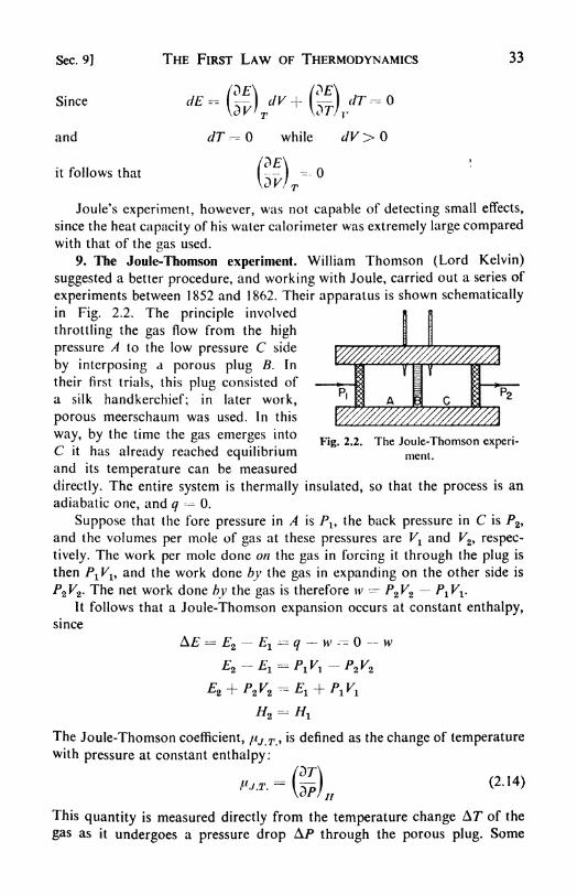
Sec. 9] THE FIRST LAW OF THERMODYNAMICS 33
while </K>0
Since
and
it follows that
Joule's experiment, however, was not capable of detecting small effects,
since the heat capacity of his water calorimeter was extremely large comparedwith that of the gas used.
9. The Joule-Thomson experiment. William Thomson (Lord Kelvin)
suggested a better procedure, and working with Joule, carried out a series of
experiments between 1852 and 1862. Their apparatus is shown schematically
in Fig. 2.2. The principle involved
throttling the gas flow from the high
pressure A to the low pressure C side
by interposing a porous plug B. In
their first trials, this plug consisted of
a silk handkerchief; in later work,
porous meerschaum was used. In this
way, by the time the gas emerges into
C it has already reached equilibriumand its temperature can be measured
directly. The entire system is thermally insulated, so that the process is an
adiabatic one, and q 0.
Suppose that the fore pressure in A is /\, the back pressure in C is P2 >
and the volumes per mole of gas at these pressures are V and K2 , respec-
tively. The work per mole done on the gas in forcing it through the plug is
then P^, and the work done by the gas in expanding on the other side is
P2V2 . The net work done by the gas is therefore w P2V2 P^V^It follows that a Joule-Thomson expansion occurs at constant enthalpy,
since
A E2 El q w --= w
E2 EI PI V\ ^2 ^2
E2 + P2V2 ^E,+ P.V,
Fig. 2.2. The Joule-Thomson experi-
ment.
The Joule-Thomson coefficient, /iJmTf9 is defined as the change of temperaturewith pressure at constant enthalpy:
/^r\
(2.14)
This quantity is measured directly from the temperature change A7 of the
gas as it undergoes a pressure drop A/> through the porous plug. Some

34 THE FIRST LAW OF THERMODYNAMICS [Chap. 2
experimental values of the J.-T. coefficients, which are functions of tem-
perature and pressure, are collected in Table 2.1.
TABLE 2.1
JOULE-THOMSON COEFFICIENTS FOR CARBON DIOXIDE*
/* (C per atm)
* From John H. Perry, Chemical Engineers' Handbook (New York: McGraw-Hill,
1941). Rearranged from Int. Crit. Tables, vol. 5, where further data may be found.
A positive //< corresponds to cooling on expansion, a negative \i to warm-
ing. Most gases at room temperatures are cooled by a J.-T. expansion.
Hydrogen, however, is warmed if its initial temperature is above -80C,but if it is first cooled below 80C it can then be cooled further by a J.-T.
effect. The temperature 80C at which jn^ is called the Joule-Thomson
inversion temperature for hydrogen. Inversion temperatures for other gases,
except helium, lie considerably higher.
10. Application of the First Law to ideal gases. An analysis of the theoryof the Joule-Thomson experiment must be postponed until the Second Lawof Thermodynamics has been studied in the next chapter. It may be said,
however, that the porous-plug experiments showed that Joule's original con-
clusion that (9/OK)T ^ for all gases was too broad. Real gases may have
a considerable internal pressure and work must be done against the cohesive
forces when they expand.An ideal gas may now be defined in thermodynamic terms as follows:
(1) The internal pressure (9/3K)T = 0.
(2) The gas obeys Boyle's Law, PV = constant at constant T.
It follows from eq. (2.5) that the energy of an ideal gas is a function of
its temperature alone. Thus dE -~- (3E/dT)y dT = Cv dT and Cv = dE/dT.
The heat capacity of an ideal gas also depends only on its temperature.These conclusions greatly simplify the thermodynamics of ideal gases, so
that many thermodynamic discussions are carried on in terms of the ideal
gas model. Some examples follow:

Sec. 10] THE FIRST LAW OF THERMODYNAMICS 35
Difference in heat capacities. When eq. (2.13) is applied to an ideal gas,
it becomes
Then, since PV = RT
/9F\ _R
and Cp Cv = R (2.15)
Heat capacities are usually given in units of calories per degree per mole,
and, in these units,
R - 8.3144/4.1840
= 1.9872 caldeg-1 mole-1
Temperature changes. Since dE Cv dT
Likewise for an ideal gas:
dH = CP dT
and A// = H2- H
=j*'Cv dT (2.17)
Isothermal volume or pressure change. For an isothermal change in an
ideal gas, the internal energy remains constant. Since dT - and
-0,
and dq = dw = P dV
Since p =
f 2 P\ dq = \
Ji Ji
dvRT-i V
or = w- *nn-^ = RTln (2.18)
Since the volume change is carried out reversibly, P always having its equi-
librium value RT/V, the work in eq. (2.18) is the maximum work done in an
expansion, or the minimum work needed to effect a compression. The equa-tion tells us that the work required to compress a gas from 10 atm to 100 atmis just the same as that required to compress it from 1 atm to 10 atm.

36 THE FIRST LAW OF THERMODYNAMICS [Chap. 2
Reversible adiabatic expansion. In this case, dq= 0, and dE = dw ~
~PdV.
From eq. (2.16) dw = Cv dT
For a finite change w \CV dTJ i
We may write eq. (2.19) as Cv dT + P dV -
_ dT dVWhence
(2.19)
(2.20)
(2.21)
Integrating between 7\ and 7^, and ^ and K2 ,the initial and final tempera-
tures and volumes, we have
Cv In J + R In =-- (2.22)' 1 ^1
This integration assumes that Cv is a constant, not a function of T.
We may substitute for R from eq. (2.15), and using the conventional
symbol y for the heat capacity ratio C^/Cy we find
ISOTHERMAL^v
ADIABATIC
(y-
7\
nTherefore,
Since, for an ideal gas,
(2.23)
Fig. 2.3. Isothermal and
adiabatic expansions.(2.24)
It has been shown, therefore, that for a reversible adiabatic expansion of an
ideal gas
PVY ^ constant (2.25)
We recall that for an isothermal expansion PV constant.
These equations are plotted in Fig. 2.3. A given pressure fall produces a
lesser volume increase in the adiabatic case, owing to the attendant fall in
temperature during the adiabatic expansion.11. Examples of ideal-gas calculations. Let us take 10 liters of gas at
and 10 atm. We therefore have 100/22.414 4.457 moles. We shall calculate
the final volume and the work done in three different expansions to a final
pressure of 1 atm. The heat capacity is assumed to be Cv = $R, independentof temperature.
Isothermal reversible expansion. In this case the final volume
V2= P^Pi -
(10)(10)/(1)- 100 liters

Sec. 11] THE FIRST LAW OF THERMODYNAMICS 37
The work done by the gas in expanding equals the heat absorbed by the gas
from its environment. From eq. (2.18), for n moles,
yq^ w nRTln -
V\
- (4.457)(8.314)(273.2)(2.303) log (10)
-23,3 10 joules
Adiabatlc reversible expansion. The final volume is calculated from
eq. (2.24), with
CP ($R f R) 5
Thus ^2H ~I K! (10)
3/5 - 10 - 39.8 liters
\ * 2
The final temperature is obtained from P2V2 nRT2 :
P,V, (1)(39.8)Tz ~
n'R (4.457X0.08205)m* K
For an adiabatic process, q=- 0, and A q u ^- - iv. Also, since Cr is
constant, eq. (2.16) gives
A - rtCjAr n%R(T2 7\) 9125 joules
The work done by the gas on expansion is therefore 9125 joules.
Irreversible adiabatic expansion. Suppose the pressure is suddenly released
to 1 atm and the gas expands adiabatically against this constant pressure.
Since this is not a reversible expansion, eq. (2.24) cannot be applied. Since
q = 0, A ~w. The value of A depends only on initial and final states:
A- - w =-/iCr(7*2-
7\)
Also, for a constant pressure expansion, we have from eq. (1.39),
Equating the two expressions for vv, we obtain
The only unknown is T2 :
-^(r-2732)=l^2
2 f \ 1 10>
Tz- 174.8K
Then A = vv =- fRn(\14.S 273.2)
=- 5470 joules

38 THE FIRST LAW OF THERMODYNAMICS [Chap. 2
Note that there is considerably less cooling of the gas and less work done
in the irreversible adiabatic expansion than in the reversible expansion.
12. Thermochemistry heats of reaction. Thermochemistry is the study of
the heat effects accompanying chemical reactions, the formation of solutions,
and changes in state of aggregation such as melting or vaporization. Physico-
chemical changes can be classified as endothermic, accompanied by the
absorption of heat, or exothermic, accompanied by the evolution of heat.
A typical example of an exothermic reaction is the burning of hydrogen:
H 2 f- i- O2- H2O (gas) f 57,780 cal at 18C
A typical endothermic reaction would be the reverse of this, the decom-
position of water vapor:
H2O - H2 -f I O2-
57,780 cal at 18C
Heats of reaction may be measured at constant pressure or at constant
volume. An example of the first type of experiment is the determination of
the heat evolved when the reaction takes place at atmospheric pressure in an
open vessel. If the reaction is carried out in a closed autoclave or bomb, the
constant-volume condition holds.
By convention, reaction heats are considered positive when heat is ab-
sorbed by the system. Thus an exothermic reaction has a negative "heat of
reaction." From eq. (2.7) the heat of reaction at constant volume,
Qv - A F (2.26)
From eq. (2.9) the heat of reaction at constant pressure,
QP - A//,>- A + P AK (2.27)
The heat of reaction at constant volume is greater than that at constant
pressure by an amount equal to the external work done by the system in
the latter case. In reactions involving only liquids or solids AFis so small
that usually P AK is negligible and Qv & QP . For gas reactions, however,
the P A V terms may be appreciable.The heat change in a chemical reaction can best be represented by
writing the chemical equation for the reaction, specifying the states of all
the reactants and products, and then appending the heat change, noting the
temperature at which it is measured. Since most reactions are carried out
under essentially constant pressure conditions, A// is usually chosen to
represent the heat of reaction. Some examples follow:
(1) SO2 (1 atm) + | O2 (1 atm) - SO3 (1 atm)A//298 - -10,300 cal
(2) CO2 (1 atm) + H2 (1 atm) - CO (I atm) + H2O (1 atm)A//298 - 9860 cal
(3) AgBr (cryst>+ \ C12 (1 atm) - AgCl (cryst) + \ Br2 (liq)
A//008- -6490 cal

Sec. 13] THE FIRST LAW OF THERMODYNAMICS 39
As an immediate consequence of the First Law, A or A// for anychemical reaction is independent of the path; that is, independent of anyintermediate reactions that may occur. This principle was first established
experimentally by G. H. Hess (1840), and is called The Law of Constant Heat
Summation. It is often possible, therefore, to calculate the heat of a reaction
from measurements on quite different reactions. For example: :
(1) COC12 -! H2S =-- 2 HCl + COS A//298 - -42,950 cai
(2) COS + H2S - H2O (g) + CS2 (1) A//298 - +3980 cai
(3) COC12 | 2 H2S - 2 HCl + H2O (g) + CS2 (1)
A #298 = "38,970 cai
13. Heats of formation. A convenient standard state for a substance maybe taken to be the state in which it is stable at 25C and 1 atm pressure; thus,
oxygen as O2 (g), sulfur as S (rhombic crystal), mercury as Hg (1), and so on.
By convention, the enthalpies of the chemical elements in this standard state
are set equal to zero. The standard enthalpy of any compound is then the
heat of the reaction by which it is formed from its elements, reactants and
products all being in the standard state of 25C and 1 atm.
For example:
(1) S + O2- SO2 A// 298
- -70,960 cai
(2) 2 Al + | O2- A12O23 A// 298
- -380,000 cai
The superscript zero indicates we are writing a standard heat of formation
with reactants and products at 1 atm; the absolute temperature is written as
a subscript. Thermochemical data are conveniently tabulated as heats of
formation. A few examples, selected from a recent compilation of the
National Bureau of Standards,5 are given in Table 2.2. The standard heat of
any reaction at 25C is then readily found as 'the difference between the
standard heats of formation of the products and of the reactants.
TABLE 2.2
STANDARD HEATS OF FORMATION AT 25C
Thermodynamic Properties'*).

40 THE FIRST LAW OF THERMODYNAMICS [Chap. 2
Many of our thermochemical data have been obtained from measure-
ments of heats of combustion. If the heats of formation of all its combustion
products are known, the heat of formation of a compound can be calculated
from its heat of combustion. For example
(1) C2H6 j I O2- 2 CO2 ~| 3 H2O (1) A// 298
- -373.8 kcal
(2) C (graphite) f O2-- CO2 A// 298
= -94.5 kcai
(3) H2 + I O2- H 2O (1) A// 298
- -68.3 kcai
(4) 2 C f 3 H 2-- C2H6 A// 298
--= -20.1 kcal
The data in Table 2.3 were obtained from combustion heats by F. D.
Rossini and his co-workers at the National Bureau of Standards. The
standard state of carbon has been taken to be graphite.
When changes in state of aggregation occur, the appropriate latent heat
must be added. For example:
S (rh) { O2 SO2 A// 298 -70.96 kcal
S (rh) S (mono) A// 298^ -0.08 kcal
S (mono) + O2- SO2 A// 298
. 70.88 kcal
14. Experimental measurements of reaction heats.6 The measurement of
the heat of a reaction consists essentially of a careful determination of the
amount of the chemical reaction that produces a definite measured changein the calorimeter, and then the measurement of the amount of electrical
energy required to effect exactly the same change. The change in question is
usually a temperature change. A notable exception is in the ice calorimeter,
in which one measures the volume change produced by the melting of ice,
and thereby calculates the heat evolution from the known latent heat of
fusion of ice.
The A// values in Table 2.3 were obtained by means of a combustion-
bomb calorimeter. It is estimated that the limit of accuracy with the present
apparatus and technique is 2 parts in 10,000. Measurements with a bombcalorimeter naturally yield A values, which are converted to A//'s via
eq. (2.27).
A thermochemical problem of great interest in recent years has been the
difference in the energies of various organic compounds, especially the hydro-carbons. It is evident that extremely precise work will be necessary to evaluate
such differences from combustion data. For example, the heat contents of
the five isomers of hexane differ by 1 to 5 kcal per mole, while the heats of
combustion of the hexanes are around 1000 kcal per mole; even a 0.1 per cent
uncertainty in the combustion heats would lead to about a 50 per cent un-
certainty in the energy differences. Important information about such small
a Clear detailed descriptions of the experimental equipment and procedures can befound in the publications of F. D. Rossini and his group at the National Bureau of Stan-
dards, J. Res. ofN.B.S., rf,.1 (1930); 13, 469 (1934); 27, 289 (1941).

Sec. 15] THE FIRST LAW OF THERMODYNAMICS 41
TABLE 2.3
HEATS OF FORMATION OF GASEOUS HYDROCARBONS
Substance
Paraffins :
MethaneEthane
Propanert-Butane
Isobutane
w-Pentane
2-Methylbutane
Tetramethylmethane
Monolefines:
Ethylene
Propylene1-Butene
cis-2-Butene
trans-2-Butene
2-Methylpropene1-Pentene
Diolefines:
Allene
1,3-Butadiene
1,3-Pentadiene
1,4-Pentadiene
Acetylenes :
Acetylene
Methylacetylene
Dimethylacetylene
Formula
CH 4
C 2H
C4H 10
C4H,C,H 12
QH!!
C2H 4
C,H.C4H 8
C 4H
fl
C,H 8
j (cal/mole)
17,8651 74-20,191 L 108
24,750 f 124
29,715 153
31,350 I 132
34,7394, 213
36,671 I 153
39,410 L 227
12,556 1 67
4956 t 110
383 JL 180
-1388 J 180- 2338 180- 3205 J. 165
-4644 .{ 300
46,046 260
26,865 -> 240
18,885 -f- 300
25,565 j : 300
54,228 J. 235
44,309 }- 240
35,221 -{- 355
energy differences can be obtained for unsaturated hydrocarbons by measure-
ment of their heats of hydrogenation. This method has been developed to a
high precision by G. B. Kistiakowsky and his co-workers at Harvard. 7
It is evident that in calorimetric experiments for example, in a deter-
mination of a heat of combustion the chemical reaction studied mayactually occur at a very elevated temperature. One measures, however, the
net temperature rise after equilibrium has been reached, and this usually
amounts to only a few degrees, owing to the high heat capacity of the calori-
meter. Since AE or A// depends only on the initial and final states, one
actually measures the A or A//, therefore, at around 25C, even though
temperatures of over 2000C may have been attained during the actual
combustion process.
15. Heats of solution. In many chemical reactions, one or more of the
reactants are in solution, and the investigation of heats of solution is an
important branch of thermochemistry. It is necessary to distinguish the
integral heat of solution and the differential heat of solution. The distinction
7
Kistiakowsky, et al., /. Am. Cfiem. Soc., 57, 876 (1935).

42 THE FIRST LAW OF THERMODYNAMICS [Chap. 2
between these two terms can best be understood by means of a practical
example.If one mole of alcohol (C2H5OH) is dissolved in nine moles of water, the
final solution contains 10 moles per cent of alcohol. The heat absorbed is the
integral heat of solution per mole of alcohol to form a solution of this final
composition. If the mole of alcohol is dissolved in four moles of water, the
integral heat of solution has a different value, corresponding to the formation
3000
m 2000
o2
I"? 1000
V10 20 30 40 50 60 70 80MOLES WATER/MOLES ALCOHOL
Fig. 2.4. Heat of solution of ethyl alcohol in water at 0C.
of a 20 mole per cent solution. The difference between any two integral heats
of solution yields a value for the integral heat of dilution. The example can
be written in the form of thermochemical equations as follows:
(1) C2H 5OH + 9 H2O - C2H5OH (10 mole % solution)
A// 273= -2300
(2) C2H 5OH -f- 4 H 2O - C2H 5OH (20% solution)
(3) C2H 5OH (20% solution) + 5 H 2O -= C2H5OH (10% solution;
A// 273- -1500
A// 273= -800
The heat of dilution from 20 to 10 per cent amounts to 800 cal per mole.
It is evident that the heat evolved ( A//) when a mole of alcohol is
dissolved in water depends upon the final concentration of the solution. If
one plots the measured integral heat of solution against the ratio moles
water per mole alcohol (njna\ the curve in Fig. 2.4 is obtained. As the
solution becomes more and more dilute, njna approaches infinity. The
asymptotic value of the heat of solution is called the heat of solution at
infinite dilution, A//^, For alcohol in water at 0C, this amounts to 3350

Sec. 16] THE FIRST LAW OF THERMODYNAMICS 43
calories. The values of A//80lution generally become quite constant with in-
creasing dilution, so that measured values in dilute solutions are usually
close to A//^. Often one finds literature values for which the dilution is not
specified.These are written, for aqueous solution, simply as in the following
example:NaCl + x H2O - NaCl (aq) h 1260 cal
:
In the absence of more detailed information, such values may be taken to
give approximately the A// at infinite dilution.
The integral solution heats provide an average A// over a range of con-
centrations. For example, if alcohol is added to water to make a 50 mole
per cent solution, the first alcohol added gives a heat essentially that for the
solute dissolving in pure water, whereas the last alcohol is added to a solution
of about 50 per cent concentration. For theoretical purposes, it is often
necessary to know what the A// would be for the solution of solute in a
solution of definite fixed concentration. Let us imagine a tremendous volume
of solution of definite composition and add one more mole of solute to it.
We can then suppose that this addition causes no detectable change in the
concentration. The heat absorbed in this kind of solution process is the
differential heat of solution. The same quantity can be defined in terms of a
very small addition of dn moles of solute to a solution, the heat absorbed
per mole being dq/dn and the composition of the solution remaining un-
changed. Methods of evaluating the differential heat will be considered in
Chapter 6.
16. Temperature dependence of reaction heats. Reaction heats depend on
the temperature and pressure at which they are measured. We may write the
energy change in a chemical reaction as
~^reactants
3pr0(1
From eq. (2.10),- = Crprod
- CFreact= ACr (2.28)
Similarly, f ,
= C'i* 'Q'react
- AQ, (2.29)
Integrating, at a constant pressure of 1 atm, so that A// is the standard A//,we obtain
A// T>- A//
Ti- ACp dT (2.30)
JT,
These equations were first ^et forth by G. R. Kirchhoff in 1858. Theystate that the difference between the heats of reaction at 7\ and at T2 is equalto the difference in the amounts of heat that must be added to reactants and

44 THE FIRST LAW OF THERMODYNAMICS [Chap. 2
products at constant pressure to raise them from 7\ to T2 . This conclusion
is an immediate consequence of the First Law of Thermodynamics.In order to apply eq. (2.30), expressions are required for the heat capaci-
ties of reactants and products over the temperature range of interest. Over
a short range, these may often be taken as practically constant, and we
obtain:
A// r A//TI
---= ACV(72 Tj)
More generally, the experimental heat-capacity data will be represented bya power series:
CV -a + bT-\- cT2f . . . (2.31)
Examples of such heat-capacity equations are given in Table 2.4. These
three-term equations fit the experimental data to within about 0.5 per cent
TABLE 2.4
HEAT CAPACITY OF GASES (273-1 500K)*
CP = a 4- bT i cT2(C/. in calories per deg per mole)
* H. M. Spencer, /. Am. Chem. Soc., 67, 1858 (1945). Spencer and Justice, ibid., 56,2311 (1934).
over a temperature range from 0C to 1250C. When the series expressionfor AC/> is substituted8
in eq. (2.30), the integration can be carried out
analytically. Thus at constant pressure, for the standard enthalpy change,
rf(A//) - AQ, dT - (A + BT + CT2 + . . .)dT
A// - A// -f-AT + i BT* + J Cr3 + . . . (2.32)
Here A// is the constant of integration.9Any one measurement of A// at
8 For a typical reaction, N8 -f-;
J H 2- NH 3 ; ACP = C
PNHi- i C^ t
-J PH .
9 If the heat-capacity equations are valid to 0K, we may note that at T = 0, A/f= A//
, so that the integration constant can be interpreted as the enthalpy change in the
reaction at 0K.

Sec. 16] THE FIRST LAW OF THERMODYNAMICS 45
a known temperature T makes it possible to evaluate the constant A// in
eq. (2.32). Then the A// at any other temperature can be calculated from
the equation. If the heat capacities are given in the form of a CP vs. T curve,
a graphical integration is often convenient.
Recently rather extensive enthalpy tables have become available, which
give H as a function of T over a wide range of temperatures. The use of
these tables makes direct reference to the heat capacities unnecessary.16. Chemical affinity. Much of the earlier work on reaction heats was
done by Julius Thomsen and Marcellin Berthelot, in the latter part of the
nineteenth century. They were inspired to carry out a vast program of
thermochemical measurements by the conviction that the heat of reaction
was the quantitative measure of the chemical affinity of the reactants. In the
words of Berthelot, in his Essai de Mecanique chimique (1878):
Every chemical change accomplished without the intervention of an external
energy tends toward the production of the body or the system of bodies that sets
free the most heat.
This principle is incorrect. It would imply that no endothermic reaction
could occur spontaneously, and it fails to consider the reversibility of chemi-
cal reactions. In order to understand the true nature of chemical affinity and
of .he driving force in chemical reactions, it is necessary to go beyond the
Firs. Law of Thermodynamics, and to investigate the consequences of the
second fundamental law that governs the interrelations of work and heat.
PROBLEMS
1. Calculate A and A// when 100 liters of helium at STP are heated to
100C in a closed container. Assume gas is ideal with Cv ^R.
2. One mole of ideal gas at 25C is expanded adiabatically and reversiblyfrom 20 atm to 1 atm. What is the final temperature of the gas, assuming
Cy = \R13. 100 g of nitrogen at 25C arc held by a piston under 30 atm pressure.
The pressure is suddenly released to 10 atm and the gas adiabatically
expands. If Cv for nitrogen- 4.95 cal per deg, calculate the final tempera-
ture of the gas. What are A and A// for the change? Assume gas is
ideal.
4. At its boiling point (100C) the density of liquid water is 0.9584 g per
cc; of water vapor, 0.5977 g per liter. Calculate the maximum work donewhen a mole of water is vaporized at the boiling point. How does this comparewith the latent heat of vaporization of water?
5. If the Joule-Thomson coefficient is /<t/ T^ 1.084 deg per atm and the
heat capacity CP = 8.75 cal per mole deg, calculate the change in enthalpyA// when 50 g of CO2 at 25C and 1 atm pressure are isothermally com-
pressed to 10 atm pressure. What would the value be for an ideal gas?

46 THE FIRST LAW OF THERMODYNAMICS [Chap. 2
6. Using the heat-capacity equation in Table 2.4, calculate the heat
required to raise the temperature of one mole of HBr from to 500C.
7. In a laboratory experiment in calorimetry 100 cc of 0.500 TV acetic acid
are mixed with 100 cc of 0.500 N sodium hydroxide in a calorimeter. The
temperature rises from 25.00 to 27.55C. The effective heat capacity of the
calorimeter is 36 cal per deg. The specific heat of 0.250 N sodium acetate
solution is 0.963 cal deg-1
g-1 and its density, 1.034g per cc. Calculate the
heat of neutralization of acetic acid per mole.
8. Assuming ideal gas behavior, calculate the values of &E 29Q for SO3
(g), H2O (g), and HCl (g) from the A// 298 values in Table 2 2.
9. From the heats of formation in Table 2.3, calculate A// 298 for the
following cracking reactions:
C2H6 + H2- 2 CH4
/i-C4H 10 | 3 H 2-- 4 CH4
iso-C4H 10 + 3 H2- 4 CH4
10. The heat of sublimation of graphite to carbon atoms has been esti-
mated as 170 kcal per mole. The dissociation of molecular hydrogen into
atoms, H2- 2 H, has A// - 103.2 kcal per mole. From these data and the
value for the heat of formation of methane, calculate the A// for C (g) +4 H (g) CH4 (g). One fourth of this value is a measure of the "energy of
the C H bond" in methane.
11. Assuming that the energy of the C H bond in ethane, C2H6 ,is the
same as in methane (Problem 10) estimate the energy of the C C bond in
ethane from the heat of formation in Table 2.3.
12. When w-hexane is passed over a chromia catalyst at 500C, benzene
is formed: C6H 14 (g)- C6H 6 (g) f 4 H2 , A// 298
^ 59.78 kcal per mole.
Calculate A// for the reaction at 500C (Table 2.4).
13. Derive a general expression for A// of the water gas reaction
(H 2 + CO2-= H 2O f CO) as a function of temperature. Use it to calculate
A// at 500K and 1000K.
14. From the curve in Fig. 2.4, estimate the heat evolved when 1 kg of
a 10 per cent (by weight) solution of ethanol in water is blended with 1 kg of
a 75 per cent solution of ethanol in water.
15. If a compound is burned under adiabatic conditions so that all the
heat evolved is utilized in heating the product gases, the maximum tempera-ture attained is called the adiabatic flame temperature. Calculate this tem-
perature for the burning of ethane with twice the amount of air (80 per cent
N2 ,20 per cent O2 ) needed for complete combustion to CO2 and H2O. Use
heat capacities in Table 2.4, but neglect the terms cT2.
16. Show that for a van der Waals gas, (3E/3K)r a/Y2.
17. Show that (dEpP)v - 0Cr/a.

Chap. 2] THE FIRST LAW OF THERMODYNAMICS 47
REFERENCES
BOOKS
See Chapter 1, p. 25.
ARTICLES
1. Parks, G. S., J. Chem. Ed., 26, 262-66 (1949), "Remarks on the Historyof Thermochemistry."
2. Menger, K., Am. J. Phys. 18, 89 (1950), "The Mathematics of Elementary
Thermodynamics."3. Sturtevant, J. M., Article on "Calorimetry" in Physical Methods of
Organic Chemistry, vol. 1, 311-435, edited by A. Weissberger (New York:
Interscience, 1945).

CHAPTER 3
The Second Law of Thermodynamics
1. The efficiency of heat engines. The experiments of Joule helped to
disprove the theory of "caloric" by demonstrating that heat was not a
"substance" conserved in physical processes, since it could be generated bymechanical work. The reverse transformation, the conversion of heat into
useful work, had been of greater interest to the practical engineer ever since
the development of the steam engine by James Watt in 1769. Such an engine
operates essentially as follows: A source of heat (e.g., a coal or wood fire)
is used to heat a "working substance" (e.g., steam), causing it to expand
through an appropriate valve into a cylinder fitted with a piston. The ex-
pansion drives the piston forward, and by suitable coupling mechanical
work can be obtained from the engine. The working substance is cooled bythe expansion, and this cooled working substance is withdrawn from the
cylinder through a valve. A flywheel arrangement returns the piston to its
original position, in readiness for another expansion stroke. In simplest
terms, therefore, any such heat engine withdraws heat from a heat source,
or hot reservoir, converts some of this heat into work, and discards the
remainder to a heat sink or cold reservoir. In practice there are necessarily
frictional losses of work in the various moving components of the engine.
The first theoretical discussions of these engines were expressed in terms
of the caloric hypothesis. The principal problem was to understand the
factors governing the efficiency e of the engine, which was measured by the
ratio of useful work output w to the heat input q2 .
we = -
(3.1)?2
A remarkable advance towards the solution of this problem was made in
1824 by a young French engineer, Sadi Carnot, in a monograph, Reflexions
sur la Puissance motrice du Feu.
2. The Carnot cycle. The Carnot cycle represents the operation of an
idealized engine in which heat is transferred from a hot reservoir at tem-
perature /2 is Partly converted into work, and partly discarded to a cold
reservoir at temperature tv (Fig. 3. la.) The working substance throughwhich these operations are carried out is returned at the end to the samestate that it initially occupied, so that the entire process constitutes a com-
plete cycle. We have written the temperatures as tl and t2 to indicate that
they are empirical temperatures, measured on any convenient scale what-
soever. The various steps in the cycle are carried out reversibly.
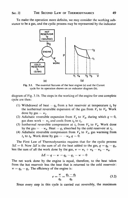
Sec. 2] THE SECOND LAW OF THERMODYNAMICS 49
To make the operation more definite, we may consider the working sub-
stance to be a gas, and the cyclic process may be represented by the indicator
WORK
12
V, V4
(0) (b)
Fig. 3.1. The essential features of the heat engine (a) and the Carnot
cycle for its operation shown on an indicator diagram (b).
diagram of Fig. 3.1b. The steps in the working of the engine for one complete
cycle are then :
(1) Withdrawal of heat --^-
q2 from a hot reservoir at temperature t2 bythe isothermal reversible expansion of the gas from Vv to V2 . Workdone by gas H^.
(2) Adiabatic reversible expansion from V2 to K3 , during which q= 0,
gas does work w2 and cools from /2 to tr
(3) Isothermal reversible compression at tl from K3 to F4 . Work done
by the gas w3 . Heat ql absorbed by the cold reservoir at tv(4) Adiabatic reversible compression from K4 to V
19 gas warming from
tl to t2 . Work done by gas^ n>4 , q = 0.
The First Law of Thermodynamics requires that for the cyclic processA = 0. Now A is the sum of all the heat added to the gas, q
= q2 qly
less the sum of all the work done by the gas, w = \vl + w2 vv3~ vv4 .
A* ^ q w ^ q2~
qlw ^=
The net work done by the engine is equal, therefore, to the heat taken
from the hot reservoir less the heat that is returned to the cold reservoir:
w = #2~~
9i- The efficiency of the engine is:
-
<tl 92
Since every step in this cycle is carried out reversibly, the maximum

50 THE SECOND LAW OF THERMODYNAMICS [Chap. 3
possible work is obtained for the particular working substance and tem-
peratures considered. 1
Consider now another engine operating, for example, with a different
working substance. Let us assume that this second engine, working between
the same two empirical temperatures /2 and tl9 is more efficient than engine 1;
that is, it can deliver a greater amount of work, w' > w, from the same
amount of heat q2 taken from the hot reservoir. (See Fig. 3. la.) It
could accomplish this only by discarding less heat, q < ql9 to the cold
reservoir.
Let us now imagine that, after the completion of a cycle by this sup-
posedly more efficient engine, the original engine is run in reverse. It therefore
acts as a heat pump. Since the original Carnot cycle is reversible, all the heat
and work terms are changed in sign but not in magnitude. The heat pumptakes in ql
of heat from the cold reservoir, and by the expenditure of work- w delivers q2 of heat to the hot reservoir.
For the first process (engine 2) w' q2 q^
For the second process (engine 1)- w -
q2 + ql
Therefore, the net result is: w' w = ql q^
Since w' > w, and ql > <//, the net result of the combined operation of these
two engines is that an amount of heat, q ql <?/, has been abstracted
from a heat reservoir at constant temperature tland an amount of work
w" = w' H' has been obtained from it, without any other change what-
soever taking place.
In this result there is nothing contrary to the First Law of Thermo-
dynamics, for energy has been neither created nor destroyed. The work done
would be equivalent to the heat extracted from the reservoir. Nevertheless,
in all of human history, nobody has ever observed the isothermal conversion
of heat into work without any concomitant change in the system. Think
what it would imply. It would not be necessary for a ship to carry fuel: this
wonderful device would enable it to use a small fraction of the immense
thermal energy of the ocean to turn its propellers and run its dynamos. Such
a continuous extraction of useful work from the heat of our environment has
been called "perpetual motion of the second kind," whereas the productionof work from nothing at all was called "perpetual motion of the first
kind." The impossibility of the latter is postulated by the First Law of
Thermodynamics; the impossibility of the former is postulated by the
Second Law.
If the supposedly more efficient Carnot engine delivered the same amountof work w as the original engine, it would need to withdraw less heat q2 < q2
1 In the isothermal steps, the maximum work is obtained on expansion and the mini-mum work done in compression of the gas (cf. p. 23). In the adiabatic steps A" = w, andthe work terms are constant once the initial and final states are fixed.
Sec. 3] THE SECOND LAW OF THERMODYNAMICS 51
from the hot reservoir. Then the result of running engine 2 forward and
engine 1 in reverse, as a heat pump, would be
(2) w^ fc'-fc'(1)
_ W = -ft+ft
?2-
?2=
ft~
ft^
<7
This amounts to the transfer of heat</from the cold reservoir at t
l to the
hot reservoir at t2 without any other change in the system.
There is nothing in this conclusion contrary to the First Law, but it is
even more obviously contrary to human experience than is perpetual motion
of the second kind. We know that heat always flows from the hotter to the
colder region. If we place a hot body and a cold body together, the hot one
never grows hotter while the cold one becomes colder. We know in fact that
considerable work must be expended to refrigerate something, to pump heat
out of it. Heat never flows uphill, i.e., against a temperature gradient, of its
own accord.
3. Th^Second Law of Thermodynamics- This Second Law may be ex-
pressed precisely in various equivalent forms. For example:The principle of Thomson. It is impossible by a cyclic process to take heat
from a reservoir and convert it into work without, in the same operation.
transferring heat from a hot to a cold reservoir.
The principle of Clausius. It is impossible to transfer heat from a cold to
a warm reservoir without, in the same process, converting a certain amountof work into heat.
Returning to Carnot's cycle, we have seen that the supposition that one
reversible cycle may exist that is more efficient than another has led to results
contradicting human experience as embodied in the Second Law of Thermo-
dynamics. We therefore conclude that all reversible Carnot cycles operating
between the same initial andfinal temperatures must have the same efficiency.
Since the cycles are reversible, this efficiency is the maximum possible. It is
completely independent of the working substance and is a function only of
the working temperatures :
*--f(ti,*J
4. The thermodynamic temperature scale. The principle of Clausius maybe rephrased as "heat never flows spontaneously, i.e., without the expenditureof work, from a colder to a hotter body." This statement contains essentially
a definition of temperature, and we may recall that the temperature conceptwas first introduced as a result of the observation that all bodies graduallyreach a state of thermal equilibrium.
Lord Kelvin was the first to use the Second Law to define a thermo-
dynamic temperature scale, which is completely independent of any thermo-
metric substance. The Carnot theorem on the efficiency of a reversible cycle

52 THE SECOND LAW OF THERMODYNAMICS [Chap. 3
may be written: Efficiency (independent of working substance) = (q2 qi)/q2
=/'('i. '2). or 1
-ft/ft =/'(^i, >2)- Therefore
-=/('i, /a) (3-3)ft
We have written /'('i, /2) and/('i> '2) 1 ~-/'('i '2) to indicate unspecified
functions of /tand /2 -
Consider two Carnot cycles such that: qjq2 =/(^i ^)J ft/?3 "/(^ '3)-
They must be equivalent to a third cycle, operating between /t and /3, with
^ A'i '3)- Therefore
^^^Wa) ^ * 2
But, if this condition is satisfied, we can write: J(tl9 t3)=
F(t^)IF(t^\f(t^ t3)
= F(t2)/F(t3). That is, the efficiency function, f(tl9/2), is the quotient of a
function of tl alone and a function of t2 alone. It follows that
* =(3.4)
Lord Kelvin decided to use eq. (3.4) as the basis of a thermodynamic
temperature scale. He took the functions F(t^) and F(/2) to have the simplest
possible form, namely, 7\ and To. Thus a temperature ratio on the Kelvin
scale was defined as equal to the ratio of the heat absorbed to the heat
rejected in the working of a reversible Carnot cycle.
** = P (3-5)<7i 7*i
The efficiency of the cycle, eq. (3.2), then becomes
The zero point of the thermodynamic scale is physically fixed as the
temperature of the cold reservoir at which the efficiency becomes equal to
unity, i.e., the heat engine is perfectly efficient. From eq. (3.6), in the limit
as 7\->0, <?-> 1.
The efficiency calculated from eq. (3.6) is the maximum thermal efficiency
that can be approached by a heat engine. Since it is calculated for a reversible
Carnot cycle, it represents an ideal that actual irreversible cycles can never
achieve. Thus with a heat source at 120C and a sink at 20C, the maximumthermal efficiency is 100/393 =- 25.4 per cent. If the heat source is at 220
and the sink still at 20, the efficiency is raised to 200/493 = 40.6 per cent.
It is easy to see why the trend in power plant design has been to higher tem-
peratures for the heat source. In practice, the efficiency of steam enginesseldom exceeds 80 per cent of the theoretical value. Steam turbines generally

Sec. 5] THE SECOND LAW OF THERMODYNAMICS 53
can operate somewhat closer to their maximum thermal efficiencies, since
they have fewer moving parts and consequently lower frictional losses.
5. Application to ideal gases. Temperature on the Kelvin, or thermo-
dynamic, scale has been denoted by the symbol T, which is the same symbolused previously for the absolute ideal gas scale. It can be shown that these
scales are indeed numerically the same by running a Carnot cycle with an
ideal gas as the working substance.
Applying eqs. (2.18) and (2.20) to the four steps:
(1) Isothermal expansion: \\\~
q2 RT2 In K2/Kt
C T(2) Adiabatic expansion: w2
~-*
Cv dT; qJ TI
(3) Isothermal compression: u 3 qiRT In VJV%
CT(4) Adiabatic compression: \v4
=*
Cv dT; q--
j TI
By summation of these terms, the net work obtained is w --=l + w2
RT2 ln V2/yi + RT\\nSince, from eq. (2.22), K,/^
- K3/K4 ,
w - R(T2 - T,) In ^- T,
92 7 2
Comparison with eq. (3.6) completes the proof of the identity of the ideal
gas and thermodynamic temperature scales.
6. Entropy. Equation (3.6) for a reversible Carnot cycle operating be-
tween T2 and 7\ irrespective of the working substance may be rewritten
?2 7\
Now it can be shown that any cyclic process can be broken down into a
number of Carnot cycles. Consider the perfectly general ABA of Fig. 3.2.
The area of the figure has been divided
into a number of Carnot cycles by the
crosshatched system of isothermals
and adiabatics. The outside bound-
aries of these little cycles form the
heavy zigzag curve which follows quite
closely the path of the general cycle
ABA. The inside portions of the little
Carnot cycles cancel out, since each
section is traversed once in the for-
ward direction and once in the reverse
direction. For example, consider theFig. 3.2. General cycle broken down
isothermal xy which belongs to an into Carnot cycles.
ISOTHERMALS
ADIABATICS

54 THE SECOND LAW OF THERMODYNAMICS [Chap. 3
expansion in the small cycle /?, and to a compression in the small cycle a,
all the work and heat terms arising from it thereby being canceled.
If eq. (3.7) is now applied to all these little Carnot cycles, we have for
the zigzag segments V q\T = 0. As the Carnot cycles are made smaller and
smaller, the boundary curve approaches more and more closely to that for
the general cyclic process ABA. In the limit, for differential Carnot cycles,
the area enclosed by the crooked boundary becomes identical with the area
of the cycle ABA. We can then replace the summation of finite terms by the
integration of differentials and obtain 2
(3.8)r-This equation holds true for any reversible cyclic process whatsoever.
Fig. 3-3. Carnot cycle on a TS diagram.
It may be recalled (p. 30) that the vanishing of the cyclic integral means
that the integrand is a perfect differential of some function of the state of
the system. This new function is defined by
*3.
T (for a reversible process) (3.9)
Thus,
. , c c_i_c c o-*-J/? A ~> 'i I'i
The function 5 was first introduced by Clausius in 1850, and is called the
entropy. Equation (3.9) indicates that when the inexact differential expression
dq is multiplied by 1/r, it becomes an exact differential; the factor \JT is
CBcalled an integrating multiplier. The integral dqKV is dependent on the
f ft* A.
path, whereas I dqrev/T is independent of the path. This, in itself, is an
alternative statement of the Second Law of Thermodynamics.It is interesting to consider the TS diagram in Fig. 3.3, which is analogous
to the PV diagram of Fig. 1.8. In the PV case, the area under the curve is a
2 See P. S. Epstein, Textbook of Thermodynamics (New York: Wiley, 1938), p. 57.

Sec. 7] THE SECOND LAW OF THERMODYNAMICS 55
measure of the work done in traversing the indicated path. In the TS diagram,the area under the curve is a measure of the heat added to the system. Tem-
perature and pressure are intensity factors ; entropy and volume are capacityfactors. The products P dV and T dS both have the dimensions of energy.
7. The inequality of Clausius. Equation (3.8) was obtained for a reversible
cycle. Clausius showed that for a cycle into which irreversibility enters at
any stage, the integral of dq\T is always less than zero.
?<0 (3.10)
The proof is evident from the fact that the efficiency of an irreversible
Carnot cycle is always less than that of a reversible cycle operating between
the same two temperatures. For the irreversible case, we therefore conclude
from eq. (3.6) that
</2
"T
<2
Then, instead of eq. (3.7), we find that
*_*<(>T, 7',
This relation is extended to the general cycle, by following the argumentbased on Fig. (3.2). Instead of eq. (3.8), which applies to the reversible case,
we obtain the inequality of Clausius, given by eq. (3.10).
8. Entropy changes in an ideal gas. The calculation of entropy changes in
an ideal gas is particularly simple because in this case (3/<)K)T 0, and
heat or work terms due to cohesive forces need not be considered at any
point. For a reversible process in an ideal gas, the First Law requires that
RTdVdq - dE + PdV~ Cy dT -\ y-
Therefore, ^ =^ + ^ (3.,,)
On integration, AS1 = S2- Sl
=-J
2
Cv d\n T fJ2
RdlnV
If Cr is independent of temperature,
AS- CF lnp+ Rln^ (3.12)7\ Vl
For the special case of a temperature change at constant volume, the
increase in entropy with increase in temperature is therefore
AS- CF ln^ (3.13)
If the temperature of one mole of ideal gas with Cy^ 3 is^ doubled, the
56 THE SECOND LAW OF THERMODYNAMICS [Chap. 3
entropy is increased by 3 In 2 --- 2.08 calories per degree, or 2.08 entropy
units (eu).
For the case of an isothermal expansion, the entropy increase becomes
AS- /?ln~- R\n Pl(3.14)
YI PZ
If one mole of ideal gas is expanded to twice its original volume, its entropyis increased by R In 2 1.38 eu.
9. Entropy changes in isolated systems. The change in entropy in goingfrom a state A to a state B is always the same, irrespective of the path between
A and B, since the entropy is a function of the state of the system alone. It
makes no difference whether the path is reversible or irreversible. Only in
case the path is reversible, however, is the entropy change given by
AS Stt-SA
--j ^(3.15)
In order to evaluate the entropy change for an irreversible process, it is
necessary to devise a reversible method for going from the same initial to
the same final state, and then to apply eq. (3.15).
In any completely isolated system we are restricted to adiabatic processes,
since no heat can either enter or leave such a system.3 For a reversible process
in an isolated system, therefore, dq and dS dq/T 0, or S --- constant.
If one part of the system increases in entropy, the remaining part must
decrease by an exactly equal amount.
A fundamental example of an irreversible process is the transfer of heat
from a hot to a colder body. We can make use of an ideal gas to carry out
the transfer reversibly, and thereby calculate the entropy change. The gas is
placed in thermal contact with the hot body at T2 and expanded reversibly
and isothermally until it takes up heat equal to q. To simplify the argument,it is assumed that the bodies have heat capacities so large that changes in
their temperatures on adding or withdrawing heat q are negligible. The gasis then removed from contact with the hot reservoir and allowed to expand
reversibly and adiabatically until its temperature falls to Tv Next it is placedin contact with the colder body at 7\ and compressed isothermally until it
gives up heat equal to q.
The hot reservoir has now lost entropy = q/T2 , whereas the cold reservoir
has gained entropy^ q/Tr The net entropy change of the reservoirs has
therefore been AS -<//7\
-q/T2 . Since T2 > 7\, AS > 0, and the entropy
has increased. The entropy of the ideal gas, however, has decreased by an
exactly equal amount, so that for the entire isolated system of ideal gas plus
heat reservoirs, AS for the reversible process. If the heat transfer had
3 The completely isolated system is, of course, a figment of imagination. Perhaps ourwhole universe might be considered as an isolated system, but no small section of it can be
rigorously isolated. As usual, -the precision and sensitivity of our experiments must beallowed to determine how the system is to be defined.

Sec. 9] THE SECOND LAW OF THERMODYNAMICS 57
been carried out irreversibly, for example by placing the two bodies in direct
thermal contact and allowing heatcj
to flow along the finite temperature
gradient thus established, there would have been no compensating entropydecrease. The entropy of the isolated system would have increased duringthe irreversible process, by the amount AS <//7\ qlT2 .
We shall now prove that the entropv ofan isolated system always increases
during an irreversible process. The proof of
this theorem is based on the inequality of
Clausius. Consider in Fig. (3.4) a perfectly
general irreversible process in an isolated
system, leading from state A to state B. It is
represented by the dashed line. Next consider
that the system is returned to its initial state
A by a reversible path represented by the
solid line from B to A. During this reversible Fig- 3.4. A cyclic process.
process, the system need not be isolated, and
can exchange heat and work with its environment. Since the entire cycle is
in part irreversible, cq. (3.10) applies, and
Writing the cycle in terms of its two sections, we obtain
^<0 (3.16)
The first integral is equal to zero, since during the process A >- B the systemis by hypothesis isolated and therefore no transfer of heat is possible. The
second integral, from eq. (3.15), is equal to St
SH . Therefore eq. (3.16)
becomes
SA -- SH < 0, or SH SA >
We have therefore proved that the entropy of the final state B is always
greater than that of the initial state A, if A passes to B by an irreversible
process in an isolated system.Since all naturally occurring processes are irreversible, any change that
actually occurs spontaneously in nature is accompanied by a net increase in
entropy. This conclusion led Clausius to his famous concise statement of the
laws of thermodynamics. "The energy of the universe is a constant; the
entropy of the universe tends always towards a maximum."This increasing tendency of the entropy has also been expressed as a
principle of the degradation of energy, by which it becomes less available
for useful work. Thus temperature differences tend to become leveled out,
mountains tend to become plains, fuel supplies become exhausted, and workis frittered away into heat by frictional losses. Interesting philosophical
58 THE SECOND LAW OF THERMODYNAMICS [Chap. 3
discussions have arisen from the entropy concept, notably the suggestion of
Sir Arthur Eddington that, because of its continuously increasing character,
"entropy is time's arrow"; that is, the constantly increasing entropy of the
universe is the physical basis of our concept of time. The "meaning" of
entropy will be displayed in another aspect when we discuss its statistical
interpretation.
10. Change of entropy in changes of state of aggregation. As an exampleof a change in state of aggregation we may take the melting of a solid. At a
fixed pressure, the melting point is a definite temperature Tm at which solid
and liquid are in equilibrium. In order to change some of the solid to liquid,
heat must be added to the system. As long as both solid and liquid are
present, this added heat does not change the temperature of the system, but
is absorbed by the system as the latent heat offusion Xf of the solid. Since
the change occurs at constant pressure, the latent heat, by eq. (2.9), equalsthe difference in enthalpy between liquid and solid. Per mole of substance,
A,-- A//7 --
//i, (|U jd //solid
At the melting point, liquid and solid exist together in equilibrium. The
addition of a little heat would melt some of the solid, the removal of a little
heat would solidify some of the liquid, but the equilibrium between solid
and liquid would be maintained. The Litent heat is necessarily a reversible
heat, because the process of melting follows a path consisting of successive
equilibrium states. We can therefore evaluate the entropy of fusion AS/ bya direct application of the relation A5 -
</rev/^ which applies to any rever-
sible isothermal process.
A//,
Tf
^liquid Ssolid~ AS, - ^ (3.17)
For example,4A//, for ice is 1430 cal per mole, so that AS, = 1430/273.2
= 5.25 cal deg"1 mole"1
.
By an exactly similar argument the entropy of vaporization ASy , the
latent heat of vaporization A//v , and the boiling point Tb are related by
-A _ A//*^vapor
~~^liquid
~" ASV ,= (3.18)
A similar equation holds for a change from one form of a polymorphicsolid to another, if the change occurs at a T and P at which the two forms
are in equilibrium, and if there is a latent heat A associated with the trans-
formation. For example, grey tin and white tin are in equilibrium at 13Cand 1 atm, and A = 500 cal. Then AS, = 500/286 = 1.75 cal deg-
1 mole-1.
11. Entropy and equilibrium. Now that the entropy function has been
defined and a method outlined for the evaluation of entropy changes, wehave gained a powerful tool for our attack on the fundamental problem of
4 Further typical data are'shown in Table 14.1 in sec. 14.8.

Sec. 12] THE SECOND LAW OF THERMODYNAMICS 59
physicochemical equilibrium. In our introductory chapter, the position of
equilibrium in purely mechanical systems was shown to be the position of
minimum potential energy. What is the criterion for equilibrium in a thermo-
dynamic system?
Any spontaneously occurring change in an isolated system is accom-
panied by an increase in entropy. From the First Law of Thermodynamicswe know that energy can be neither created nor destroyed, so that the
internal energy of an isolated system must be constant. The only way such
a system could gain or lose energy would be by some interaction with its
surroundings, but the absence of any such interaction is just what we meanwhen we say that the system is "isolated" no work is done on it; no heat
flows across its boundaries. If we restrict work to PV work (expansion or
compression), and exclude linear or surface effects, it follows also that
the volume of an isolated system must remain constant. An isolated
system may be defined, therefore, as a system of constant energy and constant
volume. The first sentence of this paragraph can thus be rephrased: In a
system at constant E and K, any spontaneous change is accompanied by an
increase in entropy.Now a system is said to be at equilibrium when it has no further tendency
to change its properties. The entropy of an isolated system will increase until
no further spontaneous changes can occur. When the entropy reaches its
maximum, the system no longer changes: the equilibrium has been attained.
A criterion for thermodynamic equilibrium is therefore the following: In a
system at constant energy and volume, the entropy is a maximum. At constant
E and K, the S is a maximum.
If instead of a system at constant E and K, a system at constant 5 and
V is considered, the equilibrium criterion takes the following form: At
constant S and V, the E is a minimum. This is just the condition applicable in
ordinary mechanics, in which thermal effects are excluded.
The drive, or perhaps better the drift, of physicochemical systems toward
equilibrium is therefore compounded of two factors. One is the tendencytoward minimum energy, the bottom of the potential energy curve. The
other is the tendency toward maximum entropy. Only if E is held con-
stant can S achieve its maximum; only if S is held constant can Eachieve its minimum. What happens when E and 5 are forced to strike a
compromise?12. The free energy and work functions. Chemical reactions are rarely
studied under constant entropy or constant energy conditions. Usually the
physical chemist places his systems in thermostats and investigates them
under conditions of approximately constant temperature and pressure.
Sometimes changes at constant volume and temperature are followed, for
example, in bomb calorimeters. It is most desirable, therefore, to obtain
criteria for thermodynamic equilibrium that will be applicable under these
practical conditions.

60 THE SECOND LAW OF THERMODYNAMICS [Chap. 3
To this end, two new functions have been invented, defined by the
following equations:A - E - TS (3.19)
F-- H TS (3.20)
A is called the work function', F is called the free energy.^ Both A and F, bytheir definitions in terms of state functions, are themselves functions of the
state of the system alone.
For a change at constant temperature,
A/I - A 7AS (3.21)
If this change is carried out reversibly, T AS q, and A/J A -q or
- A/* - uWx (3.22)
The work is the maximum obtainable since the process is reversible. Whenthe system isothermally performs maximum work u'mttx , its work function
decreases by A/f. In any naturally occurring process, which is more or less
irreversible, the work obtained is always less than the decrease in A.
From cqs. (3.19) and (3.20), since H E \ PV,
F---- A \ PV (3.23)
For a change at constant pressure,
AF - &A \ P AF (3.24)
From eqs. (3.22) and (3.24), at constant temperature and pressure,
-AF ,,'max P&Y (3.25)
The decrease in free energy equals the maximum work less the work done
by the expansion of the system at constant pressure. This work of expansionis always equal to P(V^ VJ P AK no matter how the change occurs,
reversibly or irreversibly, provided the external pressure is kept constant.
The net work over and above this is given by-AF/or a reversible process.
For an irreversible process the net work is always less than A/7. It may be
zero as, for example, in a chemical reaction carried out in such a way that
it yields no net work. Thus the combustion of gasoline in an automobile
engine yields net work, but burning the same gasoline in a calorimeter yields
none. The value of AFfor the change is the same in either case, provided the
initial and final states are the same.
A helpful interpretation of the entropy can be obtained in terms of the
new functions A and F. From eqs. (3.19) and (3.20), we can write for a changeat constant temperature,
A/4- A-TAS (3.21)
AF ----- A// - T AS (3.26)
5 Sometimes A is called the Helmholtz free energy, and F the Gibbs free energy or
thermodynamic potential.
Sec. 13] THE SECOND LAW OF THERMODYNAMICS 61
The change in the work function in an isothermal process equals the changein the energy minus a quantity TAS that may be called the unavailable
energy. Similarly, the change in free energy equals the total change in en-
thalpy minus the unavailable energy.
13. Free energy and equilibrium. The free energy function F may be used
to define a condition for equilibrium in a form that is more directly applicable
to experimental situations than the criteria in terms of the entropy. We have
seen that for a reversible process occurring at constant temperature and
pressure the net work done by the system is equal to the decrease in free
energy. For a differential change, therefore, under these reversible (i.e.,
equilibrium) conditions at constant temperature and pressure,
dF^ -</wnet (3.27)
Now most chemical laboratory experiments are carried out under such
conditions that no work is obtained from the system or added to the system
except the ordinary PV work,6 so that dwnet
^ 0. In these cases the equili-
brium criterion becomes simply:
At constant T and P, dF (3.28)
This may be stated as follows: Any change in a system at equilibrium at
constant temperature andpressure is such that thefree energy remains constant.
Thus we have obtained an answer to the question of how the drive to-
ward maximum entropy and the drive toward minimum energy reach a
compromise as a system tends toward equilibrium. From eq. (3.26) it is
evident that an increase in S and a decrease in H both tend to lower the
free energy. Therefore the third criterion for equilibrium can be written: at
constant T and P, the F is a minimum. A similar discussion of eq. (3.19)
provides the equilibrium condition at constant temperature and volume:
at constant T and K, the A is a minimum. These are the equilibrium conditions
that are of greatest use in most chemical applications.14. Pressure dependence of the free energy. From eq. (3.20), F = H TS
= E + PV TS. Differentiating, we obtain
dF = dE+PdY + VdP - TdS - S dT
Since dE = TdS - P dV
cJF = VdP - SdT (3.29)
Therefore, I I - V (3.30)
For an isothermal change from state (1) to state (2):
F2-
F, = bF^dF^l VdP (3.31)
6 Notable exceptions are experiments with electrochemical cells, in which electric work
may be exchanged with the system. A detailed discussion is given in Chapter 15.

62 THE SECOND LAW OF THERMODYNAMICS [Chap. 3
In order to integrate this equation, the variation of V with P must be
known for the substance being studied. Then if the free energy is known at
one pressure, it can be calculated for any other pressure. If a suitable equa-tion of state is available, it can be solved for V as a function of P, and
eq. (3.31) can be integrated after substituting this f(P) for V. In the simplecase of the ideal gas, V - RT/P, and
F2 Ft
- AFRT\n^ (3.32)
This gives the increase in free energy on compression, or decrease on ex-
pansion. For example, if one mole of an ideal gas is compressed isother-
mally at 300K to twice its original pressure, its free energy is increased by1.98 x 300 In 2 - 413 calories.
15. Temperature dependence of free energy. From eq. (3.29), at constant
pressure,
377" S (3 ' 33)
To integrate this equation, we must know S as a function of temperature.This question is considered in the next section. An alternative expressioncan be obtained by combining eq. (3.33) with eq. (3.20):
/DF\ F HW7 7> ~T~ (3.34)
For isothermal changes in a system, the variation of AF with temperature7
is then
/DAF\,
AF A//
(IT\r~AS =- -
T-
< 3 -35 >
This is called the Gibbs-Helmholtz equation. It permits us to calculate the
change in enthalpy A// from a knowledge of AF and the temperature co-
efficient of AF. Since
</(AF) AFd /AF\ d(
dT \T )
"T"dT T2
the Gibbs-Helmholtz equation can be written in the alternative forms:
A//
T' '
Or, = A//L 3(1 IT) \,,
7 For example the free energy change AF of a chemical reaction might be studied at a
series of different constant temperatures, always under the same constant pressure. The
equation predicts how the observed AF depends on the temperature at which the reaction is
studied.

Sec. 16] THE. SECOND LAW OF THERMODYNAMICS 63
Thus the slope of the plot of &F/Tvs. 1/7 is A//, the change in enthalpy.
Important applications of these equations to chemical reactions will be con-
sidered in the next chapter. They are especially important because manychemical processes are carried out in thermostats under practically constant
atmospheric pressure.
16. Variation of entropy with temperature and pressure. Besides its useful-
ness in the formulation of equilibrium conditions, the free-energy function
can be used to derive important relations between the other thermodynamicvariables. Consider, for example, the
mathematical identity
\3Tjp D:
By virtue of eqs. (3.30) and (3.33), this
identity yields an expression for the Cp
pressure coefficient of the entropy:8 T"
(<>>
Thus at constant temperature, dS
IP, so that
fJvaK\ f 1 '-
AS- L_ <//>-= - a*J/>, \dTj r Jl\
dP
(3.38)
Fig. 3.5, Graphical evaluation of the
entropy change with temperature.
To evaluate this integral, the equation of state or other PVT data must be
available. For an ideal gas, (3Fpr)7 > R/P. In this case eq. (3.37) becomes
dS RdlnP, or AS =- RlnPJP^^ Rln VJV19 as already shown in
Section 3.8.
The temperature variation of the entropy can be calculated as follows:
At constant pressure,
_ dq __dH CP dT~
T7"
T~
f~At constant volume,
Cv dT//c _ ^ - _ .^ ~
T~
T~
Thus at constant pressure,
S=\CP dlnT+ const
~dT+ const; AS
8Alternatively, apply Euler's rule to eq. (3.29).
(3.39)
(3.40)
= r "
Jr, fdT (3.41)

64 THE SECOND LAW OF THERMODYNAMICS [Chap. 3
When C/* is known as a function of 7", the entropy change is evaluated bythe integration in eq. (3.41). This integration is often conveniently carried
out graphically, as in Fig. 3.5: if CV\T is plotted against 7, the area under
the curve is a measure of the entropy change. The entropy change is also the
area under the curve of CP vs. In T.
17. The entropy of mixing. Consider two gases at a pressure P. If these
gases are brought together at constant temperature and pressure, they will
become mixed spontaneously by interdiffusion. The spontaneous process will
be associated with an increase in entropy. This entropy of mixing is of interest
in a number of applications, and it can be calculated as follows.
In the final mixture of gases the partial pressure of gas (1) is P1= A^P,
of gas (2), P2 X2P, where Xl and X2 are the mole fractions. 9 The AS of
mixing is equal to the AS required to expand each gas from its initial pressureP to its partial pressure in the gas mixture. On the basis of one mole of ideal
gas mixture,
AS XT.R In -
P-
f X2R In ~
- X^ In1X2R In
AS - -R(XlIn Xl + X2 In X2 )
This result can be extended to any number of gases in a mixture, yielding
AS- -R2XtlnX
t (3.42)
The equation is only approximately valid for liquid and solid solutions.
Let us calculate the entropy of mixing of the elements in air, taking the
composition to be 79 per cent N2 ,20 per cent O2 , and 1 per cent argon.
AS - -/?(0.79 In 0.79 + 0.20 In 0.20 + 0.01 In 0.01)
1.10 cal per deg per mole of mixture
18. The calculation of thermodynamic relations. One great utility of
thermodynamics is that it enables us by means of a few simple paper-and-
pencil operations to avoid many tedious and difficult laboratory experiments.The general aim is to reduce the body of thermodynamic data to relations
in terms of readily measurable functions. Thus the coefficients (3K/3r)P,
(3P/37V, and (3K/3P)r can usually be measured by straightforward experi-
ments. The results are often expressed implicitly in the equation of state for
the substance, of the general formf(P, V, T) = 0.
The heat capacity at constant pressure CP is usually measured directly
and Cv can then be calculated from it and the equation of state. Thermo-
dynamics itself does not provide any theoretical interpretation of heat
9 See Chapter 6, Section 1..

Sec. 18] THE SECOND LAW OF THERMODYNAMICS 65
capacities, the magnitudes of which depend on the structures and con-
stitutions of the substances considered.
The basic thermodynamic relations may be reduced to a few fundamental
equations:
(1) H -^ E + PV(2) A -- E TS
(3) F=E+-Py-TS(4) dE^TdS PdV(5) dH = TdS+ VdP
(6) dA - -SdT- PdV(7) dF- SdT f- VdP
Since dA and dF are perfect differentials, they obey the Euler condition
eq. (2.6), and therefore from (6) and (7)
(8) (*S
(9) QS/aP)T - -
By the definition of the heat capacities,
(10) Ct, -
(11) ? ~
These eleven equations are the starting point for the evaluation of all others. 10
The relation dE TdS P dV may be considered as a convenient ex-
pression of the combined First and Second Laws of Thermodynamics. By
differentiating it with respect to volume at constant temperature, ($EfiV)T- T(3S/dV)T
- P. Then, since (3S/dV)T -- (dPpT)r ,
This equation has often been called a thermodynamic equation of state, since
it provides a relationship among P, T, K, and the energy E that is valid for
all substances. To be sure, all thermodynamic equations are in a sense
equations of state, since they are relations between state variables, but
equations like eq. (3.43) are particularly useful because they are closely
related to the ordinary PVT data.
It is now possible by means of eq. (3.43) to prove the statement in the
previous chapter that a gas that obeys the equation PV ~ RT has a zero
internal pressure, (dE/3V)T . For such a gas T(3P/dT)y =-- RTJV --=-- P, so that
An equation similar to eq. (3.43) can be obtained in terms of the enthalpyinstead of the energy:
(3.44)
10 A. Tobolsky, /. Chem. Phys., 10, 644 (1942), gives a useful general method.

66 THE SECOND LAW OF THERMODYNAMICS [Chap. 3
An important application of this equation is the theoretical discussion of
the Joule-Thomson experiment. Since
it follows from eq. (3.44) that
TQVfiT),.- V
(3.45)
It is apparent that the Joule-Thomson effect can be either a warming or
a cooling of the substance, depending on the relative magnitudes of the two
terms in the numerator of eq. (3.45). In general, a gas will have one or more
inversion points at which the sign of the coefficient changes as it passes
through zero. The condition for an inversion point is that
=- Vp
A coefficient of thermal expansion is defined by
1
so that the Joule-Thomson coefficient vanishes when K -- <xKo r. For an
ideal gas this is always true (Law of Gay-Lussac) so that //./.T.is always zero
in this case. For other equations of state, it is possible to derive /iJmTm from
eq. (3.45) without direct measurement, if CP data are available.
These considerations are very important in the design of equipment for
the liquefaction of gases. Usually, the gas is cooled by doing external work
in an adiabatic expansion until it is below its inversion point, after which
further cooling is accomplished by a Joule-Thomson expansion. A further
discussion of the methods used for attaining very low temperatures will be
postponed till the next chapter. We shall then see that these low-temperaturestudies have an important bearing on the problem of chemical equilibrium.
PROBLEMS
1. A steam engine operates between 120 and 30C. What is the minimumamount of heat that must be withdrawn from the hot reservoir to obtain
1000 joules of work?
2. Compare the maximum thermal efficiencies of heat engines operatingwith (a) steam between 130C and 40C, (b) mercury vapor between 380Cand 50C.
3. A cooling system is designed to maintain a refrigerator at 20C in
a room at ambient temperature of 25C. The heat transfer into the refrigera-
tor is estimated as 104 joules per min. If the refrigerating unit is assumed to

Chap. 3] THE SECOND LAW OF THERMODYNAMICS 67
operate at 50 per cent of its maximum thermal efficiency, estimate the power(in watts) required to operate the unit.
4. Prove that it is impossible for two reversible adiabatics on a P-V
diagram to intersect.
5. One mole of an ideal gas is heated at constant pressure from 25 to
300C. Calculate the entropy change AS if Cv-= $R.
6. Find the increase in , //, 5, A, and Fin expanding 1.0 liter of an ideal
gas at 25C to 100 liter at the same temperature.
7. Ten grams of carbon monoxide at 0C are adiabatically and reversibly
compressed from 1 atm to 20 atm. Calculate A, A//, AS for the change in
the gas. Assume Cv = 4.95 cal per deg mole and ideal gas behavior. Wouldit be possible to calculate AF from the data provided?
8. At 5C the vapor pressure of ice is 3.012 mm and that of supercooled
liquid water is 3.163 mm. Calculate the AFper mole for the transition water
-> ice at -5C.
9. One mole of an ideal gas, initially at 100C and 10 atm, is adiabatically
expanded against a constant pressure of 5 atm until equilibrium is reattained.
If cr -= 4.50 -f 0.0057 calculate A, A//, AS for the change in the gas.
10. Calculate AS when 10 g of ice at 0C are added to 50 g of water at
40C in an isolated system. The latent heat of fusion of ice is 79.7 cal per g;
the specific heat of water, 1 .00 cal per g deg.
11. The following data are available for water: latent heat of vaporization9630 cal per mole; latent heat of fusion 1435 cal per mole. Molar heat
capacities: solid, CP =-0.50 + 0.030 T\ liquid, CP = 18.0; vapor, CP =7.256 + 2.30 x 10~3r+ 2.83 x 10~7r2
. Calculate AS when one mole of
water at 100K is heated at constant pressure of 1 atm to 500K.
12. Derive an expression for the Joule-Thomson coefficient of a van der
Waals gas.
13. Calculate the AS per liter of solution when pure N2 ,H2 , and NH 3
gases are mixed to form a solution having the final composition 20 per cent
N2 , 50 per cent H2 , and 30 per cent NH 3 (at S.T.P.).
14. Prove that a gas that obeys Boyle's Law and has zero internal pressurefollows the equation of state, PV = RT.
15. For each of the following processes, state which of the quantities A,A//, AS, AF, A/* are equal to zero.
(a) An ideal gas is taken around a Carnotcycle.
(b) H2 and O2 react to form H2O in a thermally isolated bomb.
(c) A nonideal gas is expanded through a throttling valve.
(d) Liquid water is vaporized at 100C and 1 atm pressure.
16. Derive the expression (3///3P)r = T(dSfiP)T + V.
11. Derive: (2CP/dP)T = -T(yv/dT*)M>.

68 THE SECOND LAW OF THERMODYNAMICS [Chap. 3
18. Evaluate the following coefficients for (a) an ideal gas; (b) a van der
Waals gas: (yppT*)y ; (3/aP)T ; (<>PfiV)8 \ (92K/arV
19. Derive expressions for: (a) (dA/dP)T in terms of P and V\ (b)
(dF/dT)^ in terms of A and T.
20. Bridgman obtained the following volumes for methanol under high
pressure, relative to a volume 1.0000 at 0C and I kg per cm2
:
P, kg/cm2
1 500 1000 2000 3000 4000 5000Vol. at 20 1.0238 0.9823 0.9530 0.9087 0.8792 0.8551 0.8354
Vol. at 50 1.0610 1.0096 0.9763 0.9271 0.8947 0.8687 0.8476
Use these data to estimate the AS when 1 mole of methanol at 35C and 1 kg
per cm2pressure is compressed isothermally to 5000 kg per cm
2.
REFERENCES
BOOKS
See Chapter 1, p. 25.
ARTICLES
1. Buchdahl, H. A., Am. J. Phys., 17, 41-46 (1949), "Principle of Cara-
theodory."2. Crawford, F. H., Am. J. Phys., 17, 1-5 (1949), "Jacobian Methods in
Thermodynamics."3. Darrow, K. K., Am. J. Phys., 12, 183-96 (1944), "Concept Of Entropy."4. Dyson, F. J., Scientific American, 191, 58-63 (1954), "What is Heat?"
5. LaMer, V. K., O. Foss, and H. Reiss, Ann. N. Y. Acad. Sci., 51, 605-26
(1949), "Thermodynamic Theory of J. N. Br0nsted."
CHAPTER 4
Thermodynamics and Chemical Equilibrium
1. Chemical affinity. The problem of chemical affinity may be sum-
marized in the question, "What are the factors that determine the positionof equilibrium in chemical reactions?"
The earliest reflections on this subject were those of the ancient al-
chemists, who endowed their chemicals with almost human natures, and
answered simply that reactions occurred when the reactants loved each other.
Robert Boyle, in The Sceptical Chymyst (1661), commented upon these
theories without enthusiasm: "I look upon amity and enmity as affections
of intelligent beings, and I have not yet found it explained by any, how those
appetites can be placed in bodies inanimate and devoid of knowledge or of
so much as sense."
Isaac Newton's interest in gravitational attractions led him to consider
also the problem of chemical interaction, which he thought might springfrom the same causes. Thus in 1701, he surveyed some of the existing
experimental knowledge, as follows:
When oil of vitriol is mix'd with a little water . . . in the form of spirit of vitriol,
and this spirit being poured upon iron, copper, or salt of tartar, unites with the
body and lets go the water, doth not this show that the acid spirit is attracted by the
water, and more attracted by the fix'd body than by the water, and therefore lets
go the water to close with the fix'd body? And is it not also from a natural attrac-
tion that the spirits of soot and sea-salt unite and compose the particles of sal-
ammoniac . . . and that the particles of mercury uniting with the acid particles of
spirit of salt compose mercury sublimate, and with particles of sulphur, composecinnaber . . . and that in subliming cinnaber from salt of tartar, or from quicklime, the sulphur by a stronger attraction of the salt or lime lets go the mercury, and
stays with the fix'd body ?
Such considerations achieved a more systematic form in the early
"Tables of Affinity," such as that of Etienne Geoffroy in 1718, which re-
corded the order in which acids would expel weaker acids from combination
with bases.
Claude Louis de Berthollet, in 1801, pointed out in his famous book,
Essai de statique chimique, that these tables were wrong in principle, since the
quantity of reagent present plays a most important role, and a reaction can
be reversed by adding a sufficient excess of one of the products. While servingas scientific adviser to Napoleon with the expedition to Egypt in 1799, he
noted the deposition of sodium carbonate along the shores of the salt lakes
there. The reaction Na2CO3 + CaCl2= CaCO3 + 2 NaCl as carried out in
the laboratory was known to proceed to completion as the CaCO3 was
69

70 THERMODYNAMICS AND CHEMICAL EQUILIBRIUM [Chap. 4
precipitated. Berthollet recognized that, under the peculiar conditions of large
excess of sodium chloride that occurred in the evaporating brines, the
reaction could be reversed, converting the limestone into sodium carbonate.
Berthollet, unfortunately, pushed his theorizing too far, and finally main-
tained that the actual composition of chemical compounds could be changed
by varying the proportions of the reaction mixture. In the ensuing contro-
versy with Louis Proust the Law of Definite Proportions was well established,
but Berthollet's ideas on chemical equilibrium, the good with the bad, were
discredited, and consequently neglected for some fifty years.1
It is curious that the correct form of what we now know as the Law ofChemical Equilibrium was arrived at as the result of a series of studies of
chemical reaction rates, and not of equilibria at all. In 1850, Ludwig Wilhelmy
investigated the hydrolysis of sugar with acids and found that the rate was
proportional to the concentration of sugar remaining undecomposed. In
1862, Marcellin Berthelot and Pean de St. Gilles reported similar results in
their famous paper2 on the hydrolysis of esters, data from which are shown
in Table 4.1. The effect on the products of varying the concentrations of the
reactants is readily apparent.
TABLE 4.1
DATA OF BERTHELOT AND ST. GILLES ON THE REACTION C2H 5OH -}- CH3COOH ^CH 3COOC2H 5 ! H 2
(One mole of acetic acid is mixed with varying amounts of alcohol, and the amount of ester
present at equilibrium is found)
In 1863, the Norwegian chemists C. M. Guldberg and P. Waage expressedthese relations in a very general form and applied the results to the problemof chemical equilibrium. They recognized that chemical equilibrium is a
dynamic and not a static condition. It is characterized not by the cessation
of all reaction but by the fact that the rates of the forward and reverse
reactions have become the same.
Consider the general reaction, A + B ^ C + D. According to the "law
of mass action," the rate of the forward reaction is proportional to the
1 We now recognize many examples of definite departures from stoichiometric com-
position in various inorganic compounds such as metallic oxides and sulfides, which are
appropriately called "berthollide compounds."2 Ann. chim. phys., [3] 65, 385 (1862).

Sec. 2] THERMODYNAMICS AND CHEMICAL EQUILIBRIUM 71
concentrations of A and of B. If these are written as (A) and (/?), Kforward =k\ (A)(B). Similarly, Kbackward = k*> (Q(D). At equilibrium, therefore,
^forward~
^backward so tnat
Thus(C}(D}
ThUS>
More generally, if the reaction is aA + bB cC + dD, at equilibrium
<
Equation (4.1) is a statement of Guldberg and Waage's Law of Chemical
Equilibrium. The constant K is called the equilibrium constant of the reaction.
It provides a quantitative expression for the dependence of chemical affinity
on the concentrations of reactants and products. By convention, the con-
centration terms for the reaction products are always placed in the numerator
of the expression for the equilibrium constant.
Actually, this work of Guldberg and Waage does not constitute a general
proof of the equilibrium law, since it is based on a very special type of rate
equation, which is certainly not always obeyed, as we shall see when we take
up the study of chemical kinetics. Their recognition that chemical affinity is
influenced by two factors, the "concentration effect" and what might be
called the "specific affinity," depending on the chemical nature of the reacting
species, their temperature, and pressure, was nevertheless very important.The equilibrium law will subsequently be derived from thermodynamic
principles.
2. Free energy and chemical affinity. The free-energy function described
in Chapter 3 provides the true measure of chemical affinity under conditions
of constant temperature and pressure. The free-energy change in a chemical
reaction can be defined as AF ^ Fprodut
.t8 ^reactants- When the free-energy
change is zero, there is no net work obtainable by any change or reaction
at constant temperature and pressure. The system is in a state of equilibrium.When the free-energy change is positive for a proposed reaction, net work
must be put into the system to effect the reaction, otherwise it cannot take
place. When the free-energy change is negative, the reaction can proceed
spontaneously with the accomplishment of useful net work. The larger the
amount of this work that can be accomplished, the farther removed is the
reaction from equilibrium. For this reason, AF has often been called the
driving force of the reaction. From the statement of the equilibrium law, it
is evident that this driving force depends on the concentrations of the re-
actants and products. It also depends on their specific chemical constitution,
and on the temperature and pressure, which determine the molar free-energyvalues of reactants and products.
If we consider a reaction at constant temperature, e.g., one conducted in

72 THERMODYNAMICS AND CHEMICAL EQUILIBRIUM [Chap. 4
a thermostat, AF = A// -f T AS. The driving force is seen to be made
up of two parts, a A// term and a 7 AS term. The A// term is the
reaction heat at constant pressure, and the T AS term is the heat changewhen the process is carried out reversibly. The difference is the amount of
reaction heat that can be converted into useful net work, i.e., total heat minus
unavailable heat.
If a reaction at constant volume and temperature is considered, the
decrease in the work function, A/l = AF + T AS, should be used as
the proper measure of the affinity of the reactants, or the driving force of
the reaction. The constant volume condition is much less usual in laboratory
practice.
It is now apparent why the principle of Berthelot and Thomsen (p. 45)
was wrong. They considered only one of the two factors that make up the
driving force of a chemical reaction, namely, the heat of reaction. They
neglected the T AS term. The reason for the apparent validity of their prin-
ciple was that for many reactions the A// term far outweighs the T AS term.
This is especially so at low temperatures; at higher temperatures the TASterm naturally increases.
The fact that the driving force for a reaction is large (AF is a large nega-tive quantity) does not mean that the reaction will necessarily occur under
any given conditions. An example is a bulb of hydrogen and oxygen on the
laboratory shelf. For the reaction, H2 + \ O2== H2O (g), AF298 = 54,638
cal. Despite the large negative AF, the reaction mixture can be kept for yearswithout any detectable formation of water vapor. If, after ten years on the
shelf, a pinch of platinum-sponge catalyst is added, the reaction takes place
with explosive violence. The necessary affinity was certainly there, but the
rate of attainment of equilibrium depended on entirely different factors.
Another example is the resistance to oxidation of such extremely active
metals as aluminum and magnesium. 2 Mg + O2(l atm) = 2 MgO (c);
AF298 136,370 cal. In this case, after the metal is exposed to air it
becomes covered with a very thin layer of oxide and further reaction occurs
at an immeasurably slow rate since the reactants must diffuse through the
oxide film. Thus the equilibrium condition is never attained. The incendiarybomb and the thermit reaction, on the other hand, remind us that the
large AF for this reaction is a valid measure of the great affinity of the
reactants.
3. Free-energy and cell reactions. Reactions occurring in electrochemical
cells with the production of electric energy are of especial interest in the
discussion of free-energy changes, since they can be carried out under con-
ditions that are almost ideally reversible. This practical reversibility is
achieved by balancing the electromotive force of the cell by an opposingemf which is imperceptibly less than that of the cell. Such a procedure can
be accomplished with the laboratory potentiometer, in which an external
source of emf, such as a battery, is balanced against the standard cell. The

Sec. 3] THERMODYNAMICS AND CHEMICAL EQUILIBRIUM 73
arrangement for this "compensation method" is shown in Fig. 4.1. Whenthe opposing emf's are balanced by adjustment of the slide wire 5, there is
no detectable deflection of the galvanometer G.
An electrochemical cell converts chemical free energy into electric free
energy. The electric energy is given by the product of the emf of the cell
times the amount of electricity flowing through it. Michael Faraday showed,in 1834, that a given amount of electricity was always produced by or would
produce the same amount of chemical reaction. For one chemical equivalentof reaction the associated amount of
electricity is called the Faraday, ^", CELLAR
and is equal to 96,519 coulombs.
Thus the electric energy available per
mole of reaction equals zS^", where
z is the number of equivalents per
mole and S is the emf of the cell. A GALVANOMETER(convenient energy unit is therefore
the volt-coulomb or joule.
When the reaction is carried out UNKNOWNemt
reversibly, this energy is the maxi- _. . . _ .,,
. r/., , , p-
7
,. Fig. 4.1. Compensation method for
mum available, or the net woi k w . measuring the emf of a cell without drawingIf the reaction is carried out at a current from it. When there is no deflection
finite rate, some of the energy is of galvanometer ffx- (SXISS')tft .
expended in overcoming the electric
resistance of the cell, appearing as heat. This Joule heat, 7 2/?, is the electrical
analogue of the frictional heat produced in irreversible mechanical pro-
cesses. We may now write, if ^ is the reversible emf,
(4.2)
This equation provides a direct method for evaluating the free-energy changein the cell reaction. If we know the temperature coefficient of the emf of the
cell, we can also calculate A// and AS for the reaction by means of eq. (3.35),
which on combination with eq. (4.2) yields the relations
A T-f >r<3r \ JP T \ AC T^ (A. "\\l\rt = 2^ \6 1-TIL],
IAO Z^ (4..J)\ #77 dT
In a later chapter, devoted to electrochemistry, we shall see that it is possible
to carry out many changes by means of reversible cells, and thereby to
evaluate AF and A// for the changes from measurements of the emf and its
temperature coefficient.
A cell that is occasionally used as a laboratory standard of emf is the
Clark cell shown in Fig. 4.2. The reaction in this cell is Zn -f Hg2SO4
ZnSO4 -f 2 Hg, or more simply, Zn -f 2 Hg+ = Zn++ + 2 Hg. The emf of
the cell is 1 .4324 volts at 1 5C and the temperature coefficient dSjdT =0.00119 volt per degree. It can therefore be calculated that for the cell

74 THERMODYNAMICS AND CHEMICAL EQUILIBRIUM [Chap. 4
ZINCSULFATESOLUTION
ZINCAMALGAM
SOLIDHg2S04
MERCURY
Fig. 4.2. A typical electrochemical
cell: the Clark cell.
reaction AF = (-1.4324 x 2 x 96,519 - -276,510 joule. From eq. (4.3),
AS- (-0.00119 x 2 x 96,519) - -229.7 joule deg-1 mole"1
. Whence,A// - AF f T AS = -276,510 - 66,200 - -342,710 joule. The value of
A// obtained from thermochemical data is 339,500, in good agreementwith the electrochemical value.
Since the temperature coefficient is negative, heat is given up to the
surroundings during the working of this cell, and the net work obtainable,
A/% is less than the heat of the reaction. There are other cells for which
the temperature coefficient is positive.
These cells absorb heat from the environ-
ment, and their work output, under re-
versible conditions, is greater than the
heat of the reaction.
These relationships, discovered theo-
retically by Willard Gibbs in 1876, were
first applied to experimental cases byHelmholtz in 1882. Before that time it was
thought, reasoning from the First Law,that the maximum work output that could
be achieved was the conversion of all of the
heat of reaction into work. The Gibbs-
Helmholtz treatment shows clearly that
the work output is governed by the value
of AFfor the cell reaction, not by that of A// The working cell can either
reversibly absorb heat from or furnish heat to its environment. This reversible
heat change then appears as the T AS term in the free-energy expression.
4. Standard free energies. In Chapter 2 (p. 39) the definition of standard
states was introduced in order to simplify calculations with energies and
enthalpies. Similar conventions are very helpful for use with free-energy data.
Various choices of the standard state have been made, one that is frequently
used being the state of the substance under one atmosphere pressure. This is
a useful definition for gas reactions ; for reactions in solution, other choices
of standard state may be more convenient and will be introduced as needed.
A superscript zero will be used to indicate a standard state of 1 atm pressure.
The absolute temperature will be written as a subscript.
The most stable form of an element in the standard state (1 atm pressure)
and at a temperature of 25C will by convention be assigned a free energyof zero.
The standard free energy of formation of a compound is the free energyof the reaction by which it is formed from its elements, when all the reactants
and products are in the standard state. For example:
H 2 (I atm) + i O2 (1 atm) - H2O (g; 1 atm) AF 298= -54,638
S (rhombic crystal) + 3 F2 (1 atm) - SF6 (g; 1 atm) AF 298= -235,000

Sec. 5] THERMODYNAMICS AND CHEMICAL EQUILIBRIUM 75
In this way it is possible to make tabulations of standard free energies
such as that given by Latimer,3examples from which are collected in
Table 4.2. Some of these free-energy values are determined directly from
reversible cell emf's but most are obtained by other methods to be described
later.
TABLE 4.2
STANDARD FREE ENERGIES OF FORMATION OF CHEMICAL COMPOUNDS AT 25C
Free-energy equations can be added and subtracted just as thermo-
chemical equations are, so that the free energy of any reaction can be cal-
culated from the sum of the free energies of the products minus the sum of
the free energies of the reactants.
\FC V F V F^-*r ~~Z, r products Z, r reactants
If we adopt the convention that moles of products are positive and moles of
reactants negative in the summation, this equation can be written concisely as
AF - 2 ", F> (4.4)
For example:Cu2 (c) T- NO (g)
^ 2 CuO (c) + i N2 (g)
From Table 4.2,
AF = 2 (-30.4) + i (0)- 20.66 - (-35.15) - -46.31 kcal
5. Free energy and equilibrium constant of ideal gas reactions. Many im-
portant applications of equilibrium theory are in the field of homogeneous
gas reactions, that is, reactions taking place entirely between gaseous pro-
ducts and reactants. To a good approximation in many such cases, the gases
may be considered to obey the ideal gas laws.
The variation at constant temperature of the free energy of an ideal gas
8 W. M. Latimer, The Oxidation States of the Elements, 2nd ed. (New York: Prentice-
Hall, 1952).

76 THERMODYNAMICS AND CHEMICAL EQUILIBRIUM [Chap. 4
is given from eq. (3.29) as dF = V dP = RTdln P. Integrating from F and
P, the free energy and pressure in the chosen standard state, to F and P,
the values in any other state, F - F = RTln (P/P). Since P = 1 atm, this
becomes
F-F = RT\nP (4.5)
Equation (4.5) gives the free energy of one mole of an ideal gas at pressure
P and temperature 7, minus its free energy in a standard state at P = I atm
and temperature T.
If an ideal mixture of ideal gases is considered, Dalton's Law of Partial
Pressures must be obeyed, and the total pressure is the sum of the pressures
that the gases would exert if each one occupied the entire volume by itself.
These pressures are called the partial pressures of the gases in the mixture,
Pj, 7*2 ... Pn . Thus if /?t
is the number of moles of gas / in the mixture,
RTP-lP, =
-fI", (4.6)
For each individual gas / in the mixture eq. (4.5) can be written
Fl-F? = RTlnP, (4.7)
For nt moles, n
t(Fl F) = RTntIn P
t. For a chemical reaction, therefore,
from eq. (4.4),
AF - AF = RT 2 ntIn P
t (4.8)
If we now consider the pressures Ptto be the equilibrium pressures in
the gas mixture, AF must equal zero for the reaction at equilibrium. Thuwe obtain the important relation
- AF = RT 2 ntIn P** (4.9)
AFor 2 ,
^ P** - -
Since AF is a function of the temperature alone, the left side of this ex-
pression is equal to a constant at constant temperature. For a typical reaction,
aA + bB --= cC 4- dD, the summation can be written out as
This expression is simply the logarithm of the equilibrium constant in terms
of partial pressures, Kp . Equation (4.9) therefore becomes
-AF- RTlnK, (4.10)
The analysis in this section has now established two important results.
The constancy of the expression

Sec. 6] THERMODYNAMICS AND CHEMICAL EQUILIBRIUM 77
at equilibrium has been proved by thermodynamic arguments. This con-
stitutes a thermodynamic proof of the Law of Chemical Equilibrium. Second,
an explicit expression has been derived, eq. (4.10), which relates the equili-
brium constant to the standard free-energy change in the chemical reaction.
We are now able, from thermodynamic data, to calculate the equilibrium
constant, and thus the concentration of products from any given concentra-
tion of reactants. This was one of the fundamental problems that chemical
thermodynamics aimed to answer.
Sometimes the equilibrium constant is expressed explicitly in terms of
concentrations ct
. For an ideal gas PI n^RT/V) c{RT. Substituting in
eq. (4.11), we find
CA^B
Kp= Kc(RT)*
n(4.12)
Here Kcis the equilibrium constant in terms of concentrations (e.g., moles
per liter) and A is the number of moles of products less that of reactants in
the stoichiometric equation for the reaction.
Another way of expressing the concentrations of the reacting species is
in terms of mole fractions. The mole fraction of component / in a mixture
is defined by
*, - Yn(4 - 13>
It is the number of moles of a component / in the mixture divided by the
total number of moles of all the components. It follows that Pt=
Therefore the equilibrium constant in terms of the mole fractions is
Since K9 for ideal gases is independent of pressure, it is evident that Kx is
a function of pressure except when A/2 = 0. It is thus a "constant" only with
respect to variations of the A"s at constant T and P.
6, The measurement of homogeneous gas equilibria. The experimentalmethods for measuring gaseous equilibria can be classified as either static or
dynamic.In the static method, known amounts of the reactants are introduced
into suitable reaction vessels, which are closed and kept in a thermostat
until equilibrium has been attained. The contents of the vessels are then
analyzed in order to determine the equilibrium concentrations. If the reaction
proceeds very slowly at temperatures below those chosen for the experiment,it is sometimes possible to "freeze the equilibrium" by chilling the reaction
vessel rapidly. The vessel may then be opened and the contents analyzed
chemically.

78 THERMODYNAMICS AND CHEMICAL EQUILIBRIUM [Chap. 4
This was the procedure used by Max Bodenstein4 in his classic investiga-
tion of the hydrogen-iodine equilibrium: H2 + I2= 2 HI. The reaction pro-
ducts were treated with an excess of standard alkali; iodide and iodine were
determined by titration, and the hydrogen gas was collected and its volume
measured. For the formation of hydrogen iodide, A/? = 0; there is no changein the number of moles during the reaction. Therefore Kv
= Kc Kx .
If the initial numbers of moles of H2 and I2 are a and b, respectively,
they will be reduced to a x and b x with the formation of 2x moles of
HI. The total number of moles at equilibrium is therefore a -f b + c, where
c is the initial number of moles of HI.
Accordingly the equilibrium constant can be written
- 2*)
The (a + b + c) terms required to convert "number of moles" into "mole
fraction" have been canceled out between numerator and denominator. In
a run at 448C, Bodenstein mixed 22.13 cc at STP of H2 with 16.18 of I2 ,
and found 25.72 cc of HI at equilibrium. Hence
K~ - _25/72i- - -215(22.13
-12.86)(16.18
-12.86)
In the dynamic method for studying equilibria, the reactant gases are
passed through a thermostated hot tube at a rate slow enough to allow
complete attainment of equilibrium. This condition can be tested by makingruns at successively lower flow rates, until there is no longer any change in
the observed extent of reaction. The effluent gases are rapidly chilled and
then analyzed. Sometimes a catalyst is included in the hot zone to speed the
attainment of equilibrium. This is a safer method if a suitable catalyst is
available, since it minimizes the possibility of any back reaction occurringafter the gases leave the reaction chamber. The catalyst changes the rate of
a reaction, not the position of final equilibrium.
These flow methods were extensively used by W. Nernst and F. Haber
(around 1900) in their pioneer work on technically important gas reactions.
An example is the "water-gas equilibrium," which has been studied both
with and without an iron catalyst.5 The reaction is
H2 + C02- H2 + CO, and K9
= ^HiQfCQ
If we consider an original mixture containing a moles of H2 , b moles of
CO2, c moles of H2O, and d moles of CO, the analysis of the data is as
follows.
4Z.physik. Chem., 22, \ (1897); 29, 295 (1899).
5 Z. anorg. Chem., 38. 5 (1904).
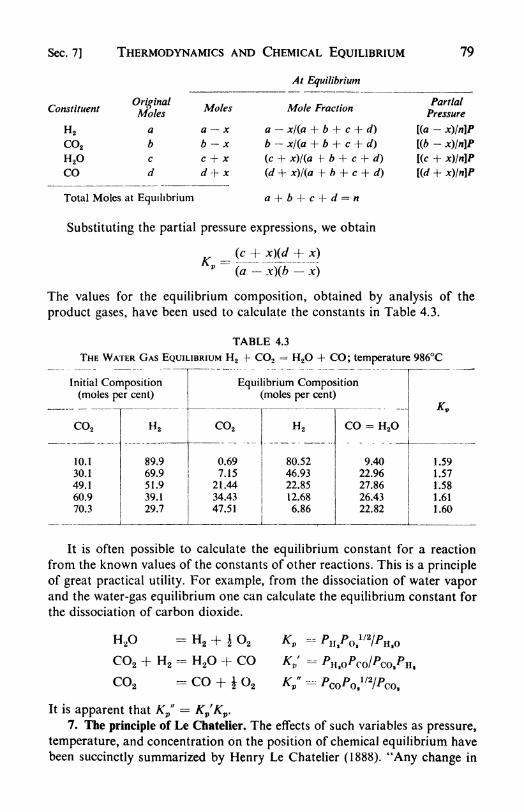
Sec. 7] THERMODYNAMICS AND CHEMICAL EQUILIBRIUM 79
Total Moles at Equilibrium a + b jrc + d = n
Substituting the partial pressure expressions, we obtain
^
The values for the equilibrium composition, obtained by analysis of the
product gases, have been used to calculate the constants in Table 4.3.
TABLE 4.3
THE WATER GAS EQUILIBRIUM H2 -f CO2= H2O -f CO; temperature 986C
It is often possible to calculate the equilibrium constant for a reaction
from the known values of the constants of other reactions. This is a principle
of great practical utility. For example, from the dissociation of water vaporand the water-gas equilibrium one can calculate the equilibrium constant for
the dissociation of carbon dioxide.
HaO
CO2
CO2
= HH2- H2O
2
CO
CO + O2
It is apparent that AT/-= KV'KV .
7. The principle of Le Chatelier. The effects of such variables as pressure,
temperature, and concentration on the position of chemical equilibrium have
been succinctly summarized by Henry Le Chatelier (1888). "Any change in
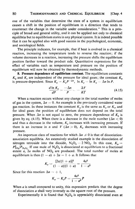
80 THERMODYNAMICS AND CHEMICAL EQUILIBRIUM [Chap. 4
one of the variables that determine the state of a system in equilibriumcauses a shift in the position of equilibrium in a direction that tends to
counteract the change in the variable under consideration." This is a prin-
ciple of broad and general utility, and it can be applied not only to chemical
equilibria but to equilibrium states in any physical system. It is indeed possible
that it can be applied also with good success in the psychological, economic,
and sociological fields.
The principle indicates, for example, that if heat is evolved in a chemical
reaction, increasing the temperature tends to reverse the reaction; if the
volume decreases in a reaction, increasing the pressure shifts the equilibrium
position farther toward the product side. Quantitative expressions for the
effect of variables such as temperature and pressure on the position of
equilibrium will now be obtained by thermodynamic methods.
8. Pressure dependence of equilibrium constant. The equilibrium constants
Kp and Kcare independent of the pressure for ideal gases; the constant Kx
is pressure-dependent. Since Kx= KPP
An, In Kx
-= In Kv- A In P.
dP"
P RT'
When a reaction occurs without any change in the total number of moles
of gas in the system, A/? = 0. An example is the previously considered water
gas reaction. In these instances the constant Kpis the same as Kx or K
c , and
for ideal gases the position of equilibrium does not depend on the total
pressure. When AH is not equal to zero, the pressure dependence of Kx is
given by eq. (4.15). When there is a decrease in the mole number (A/z < 0)
and thus a decrease in the volume, Kx increases with increasing pressure. If
there is an increase in n and V (A/7 > 0), Kx decreases with increasing
pressure.
An important class of reactions for which A -- is that of dissociation-
association equilibria. An extensively studied example is the dissociation of
nitrogen tetroxide into the dioxide, N2O4 2 NO2 . In this case, Kp=
PxoJP$ to t' Jf one m le f N2O4 is dissociated at equilibrium to a fractional
extent a, 2a moles of NO2 are produced. The total number of moles at
equilibrium is then (1 a) ~\- 2a = 1 + a. It follows that
(\-a)/(\+a) 1-02
Since for this reaction AA? -^~f 1,
p~
*
When a is small compared to unity, this expression predicts that the degreeof dissociation a shall vary inversely as the square root of the pressure.
Experimentally it is found that N2O4 is appreciably dissociated even at

Sec. 9] THERMODYNAMICS AND CHEMICAL EQUILIBRIUM 81
room temperatures. As a result, the observed pressure is greater than that
predicted by the ideal gas law for a mole of N2^4 s *nce ea h m le yields
1 -\- a moles of gas after dissociation. Thus P (ideal) RTfV, whereas
P (observed) - (1 + a)RT/V. Hence a - (K/*r)(/>ob8- />ldcal).
This behavior provides a very simple means for measuring a. For example,in an experiment at 318K and 1 atm pressure, a is found to be 0.38. There-
fore Kx= 4(0.38)
2/(1
- 0.38 2)- 0.67. At 10 atm pressure, Kx
- 0.067 and
a is 0.128.
Among the most interesting dissociation reactions are those of the
elementary gases. The equilibrium constants for a few of these are collected
in Table 4.4.
TABLE 4.4
EQUILIBRIUM CONSTANTS OF DISSOCIATION REACTIONS
9. Effect of an inert gas on equilibrium. In reactions in which there is no
change in the total number of moles, AH = 0, and the addition of an inert
gas cannot affect the composition of the equilibrium mixture. If, however,
A ^ 0, the inert gas must be included in calculating the mole fractions and
the total pressure P. Let us consider as an example the technically important
gas reaction, SO2 + \ O2= SO3 . In this case A =
|, and Kp= KXP~
1/2.
Let the initial reactant mixture contain a moles of SO2 ,b moles of O2, and
c moles of inert gas, for example N2 . If y moles of SO3 are formed at equi-
librium, the equilibrium mole fractions are
b - (y/2) y
Here n is the total number of moles at equilibrium: n a + b + c (y/2).
The equilibrium constant,
K = K P1/2 =*
y/n yn1/2
[(a [a-

82 THERMODYNAMICS AND CHEMICAL EQUILIBRIUM [Chap. 4
It follows that = /a y
/?S 3 __
"so,
where ws()i , w80a , w0i , /? are the equilibrium mole numbers.
Let us now consider three cases. (1) If the pressure is increased by com-
pressing the system without addition of gas from outside, n is constant, and
as P increases, n$ Jn$0t a lso increases. (2) If an inert gas is added at constant
volume, both n and P increase in the same ratio, so that the equilibrium
conversion of SO2 to SO3 ,wSO|//7SOi remains unchanged. (3) If an inert gas
is added at constant pressure, n is increased while P remains constant, and
this dilution of the mixture with the inert gas decreases the extent of con-
version /fso>s<vThis reaction is exothermic, and therefore increasing the temperature
decreases the formation of products. The practical problem is to run the
reaction at a temperature high enough to secure a sufficiently rapid velocity,
without reaching so high a temperature that the equilibrium lies too far to
the left. In practice, a temperature around 500C is chosen, with a platinumor vanadium-pentoxide catalyst to accelerate the reaction. The equilibrium
constant from 700 to 1200K is represented quite well by the equationIn Kp
= (22,6QO/RT) - (21.36/7?). At 800K, therefore, Kv- 33.4.
Let us now consider two different gas mixtures, the first containing20 per cent SO2 and 80 per cent O2 at 1 atm pressure, and a second containingin addition a considerable admixture of nitrogen, e.g., 2 per cent SO2 ,
8 percent O2 , 90 per cent N2 ,
at 1 atm pressure. Letting y moles SO3 at equi-
librium, we obtain:
I II
Ks-
ffpP1
/2 = 33.4 Kx
- KpPll2 = 33.4
y y1 ~ (y/2) 1
-(y/2)
0.2 -y roSj- O/2)]1
/1 0.02 - y ["0.08 -(y/2)]
1/2
1-
(y/2) I 1-
'(y/2)J 1
-(y/2)
I 1 - (^T J
/ -2.000/ -I- 0.681^
- 0.0641 =0 / -0.1985/ + 6.81 X 10~3
j
y = 0.190 64.06 X 10~6 =
y - 0.0180
95% conversion of SO2 to SO3 90% conversion of SO2 to SO3
The cubic equations that arise in problems like these are probably best
solved by successive approximations. Beginning with a reasonable value
guessed for the percentage conversion, a sufficiently accurate solution can
usually be obtained after three or four trials.

Sec. 10] THERMODYNAMICS AND CHEMICAL EQUILIBRIUM 83
10. Temperature dependence of the equilibrium constant. An expression
for the variation of KP with temperature is derived by combining eqs. (4.10)
and (3.36). Since
v (4.10)
and
therefore
A//c
r 2
dT
(3.36)
(4.16)
It is apparent that if the reaction is endothermic (A// positive) the
equilibrium constant increases with temperature; if the reaction is exothermic
(A// negative) the equilibrium con-
stant decreases as the temperature is
raised.
Equation (4.16) can also be written:
iH(4.17)
d(\IT) R
Thus if In Kp is plotted against \/T9
the slope of the curve at any point is
equal to A// //?. As an example of
this treatment, the data for the varia-
tion with temperature of the 2 HI --=
H2 + I2 equilibrium are plotted in
Fig. 4.3. The curve is almost a straight
line, indicating that A// is approxi-
mately constant for the reaction over
the experimental temperature range.
The value calculated from the slope at
400C is A// = 7080 cal.
It is also possible to measure the
equilibrium constant at one tempera-ture and with a value of A// obtained
from thermochemical data to calculate the constant at other temperatures.
Equation (4.16) can be integrated, giving
In
VL25 150 1.75
Fig. 4.3. The variation with temper-ature of Kf
= PH2Pi.JPm". (Data of
Bodenstein.)
Since, over a short temperature range, A/f may often be taken as approxi-
mately constant, one obtains
InKJTj -A//
R (4.18)

84 THERMODYNAMICS AND CHEMICAL EQUILIBRIUM [Chap. 4
If the variations of the heat capacities of the reactants and products are
known as functions of temperature, an explicit expression for the tempera-ture dependence of A// can be derived from Kirchhoff's equation (2.29).
This expression for A// as a function of temperature can then be substituted
into eq. (4.16), whereupon integration yields an explicit equation for K9 as
a function of temperature. This has the form
In K, - - A// //?r + A In T + BT + CT* . . . + I (4.19)
In this case, as usual, the value of the integration constant / can be deter-
mined if the value of Kp is known at any one temperature, either experiment-
ally or by calculation from AF. It will be recalled that one value of A// is
needed to determine A// , the integration constant of the Kirchhoff
equation.
To summarize, from a knowledge of the heat capacities of the reactants
and products, and of one value each for A// and A^,it is possible to calculate
the equilibrium constant at any temperature.As an example, consider the calculation of the constant for the water-
gas reaction as a function of the temperature.
CO + H2 (g)- H2 + C02 ;
Kv-^co>
-CO rH,0
From Table 4.2, the standard free-energy change at 25C is:
A/r 298= -94,240 - (-54,640 - 32,790) - -6810
6810
298^
From the enthalpies of formation on page 39,
A# 298- -94,050 - (-57,800 - 26,420) = -9830
The heat capacity table on page 44 yields for this reaction
Thus In KV298= - = 1 1.48, or Kv298
= 9.55 X 10*
= -0.515 + 6.23 x 10~3r- 29.9 x 10~7r2
From eq. (2.32),
A// = A// - 0.5157+ 3.12 x 10~3r2 - 10.0 x 1Q-T3
Substituting A// = -9830, T = 298K, and solving for A//, we get
A// = 9921. Then the temperature dependence of the equilibrium
constant, eq. (4.19), becomes
By inserting the value ofln Kv at 298K, the integration constant can be

Sec. 11] THERMODYNAMICS AND CHEMICAL EQUILIBRIUM 85
evaluated as / = 3.97. The final expression for Kv as a function of tem-
perature is, therefore,
In K - -3.97 +9- - 0.259 In T + 1.56 x I0~3r - 2.53 x 10~7r2
For example, at 800K, In K9= 1.63, Kv
- 5.10.
11. Equilibrium constants from thermal data. We have now seen how a
knowledge of the heat of reaction and of the temperature variation of the
heat capacities of reactants and products allows us to calculate the equi-librium constant at any temperature, provided there is a single experimentalmeasurement of either K9 or AF at some one temperature. If an independentmethod is available for finding the integration constant /in eq. (4.19), it will
be possible to calculate K9 without any recourse to experimental measure-
ments of the equilibrium or of the free-energy change. This calculation would
be equivalent to the evaluation of the entropy change, AS , from thermal
data alone, i.e., heats of reaction and heat capacities. If we know AS and
A//, Kp can be found from AF - A// - TA5.From eq. (3.41), the entropy per mole of a substance at temperature T
is given by
5 = frCP rflnr+S
where 5 is the entropy at 0K. 6 If any changes of state occur between the
temperature limits, the associated entropy changes should be added. For a
gas at temperature Tthe general expression for the entropy therefore becomes
o'Q,cryst
din T + ^^ +J^CP^dlnT
A// r T
+ -=rSE + Cp^dlnT+S, (4.20)* b JT
/'Jo
All these terms can be measured except the constant S . The evaluation
of this constant becomes possible by virtue of the third fundamental law of
thermodynamics.12. The approach to absolute zero. The laws of thermodynamics are in-
ductive in character. They are broad generalizations having an experimentalbasis in certain human frustrations. Our failure to invent a perpetual-motionmachine has led us to postulate the First Law of Thermodynamics. Our
failure ever to observe a spontaneous flow of heat from a cold to a hotter
body or to obtain perpetual motion of the second kind has led to the state-
ment of the Second Law. The Third Law of Thermodynamics can be based
on our failure to attain the absolute zero of temperature. A detailed studyof refrigeration principles indicates that the absolute zero can never be
reached.
8 Be careful not to confuse 5, the entropy in the standard state of 1 atm pressure, andS" , the entropy at 0K.
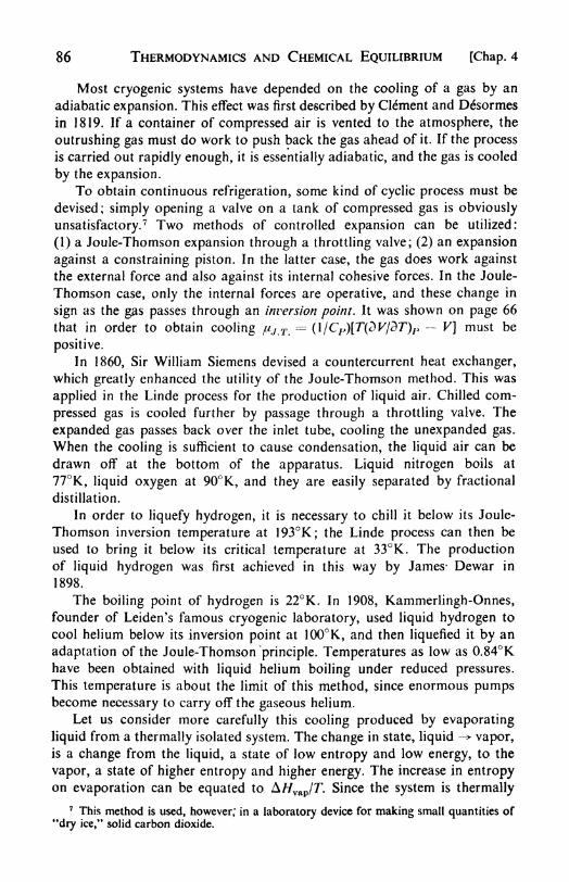
86 THERMODYNAMICS AND CHEMICAL EQUILIBRIUM [Chap. 4
Most cryogenic systems have depended on the cooling of a gas by an
adiabatic expansion. This effect was first described by Clement and Desormes
in 1819. If a container of compressed air is vented to the atmosphere, the
outrushing gas must do work to push back the gas ahead of it. If the process
is carried out rapidly enough, it is essentially adiabatic, and the gas is cooled
by the expansion.To obtain continuous refrigeration, some kind of cyclic process must be
devised; simply opening a valve on a tank of compressed gas is obviously
unsatisfactory.7 Two methods of controlled expansion can be utilized:
(1) a Joule-Thomson expansion through a throttling valve; (2) an expansion
against a constraining piston. In the latter case, the gas does work against
the external force and also against its internal cohesive forces. In the Joule-
Thomson case, only the internal forces are operative, and these change in
sign as the gas passes through an inversion point. It was shown on page 66
that in order to obtain cooling //t/ T = (\/CP)[T(dV/dT)P V] must be
positive.
In 1860, Sir William Siemens devised a countercurrent heat exchanger,
which greatly enhanced the utility of the Joule-Thomson method. This was
applied in the Linde process for the production of liquid air. Chilled com-
pressed gas is cooled further by passage through a throttling valve. The
expanded gas passes back over the inlet tube, cooling the unexpanded gas.
When the cooling is sufficient to cause condensation, the liquid air can be
drawn off at the bottom of the apparatus. Liquid nitrogen boils at
77K, liquid oxygen at 90K, and they are easily separated by fractional
distillation.
In order to liquefy hydrogen, it is necessary to chill it below its Joule-
Thomson inversion temperature at 193K; the Linde process can then be
used to bring it below its critical temperature at 33K. The productionof liquid hydrogen was first achieved in this way by James- Dewar in
1898.
The boiling point of hydrogen is 22K. In 1908, Kammerlingh-Onnes,founder of Leiden's famous cryogenic laboratory, used liquid hydrogen to
cool helium below its inversion point at 100K, and then liquefied it by an
adaptation of the Joule-Thomson principle. Temperatures as low as 0.84Khave been obtained with liquid helium boiling under reduced pressures.
This temperature is about the limit of this method, since enormous pumpsbecome necessary to carry off the gaseous helium.
Let us consider more carefully this cooling produced by evaporating
liquid from a thermally isolated system. The change in state, liquid -> vapor,is a change from the liquid, a state of low entropy and low energy, to the
vapor, a state of higher entropy and higher energy. The increase in entropyon evaporation can be equated to A//vap/r. Since the system is thermally
7 This method is used, however; in a laboratory device for making small quantities of
"dry ice,** solid carbon dioxide.
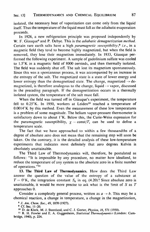
Sec. 13] THERMODYNAMICS AND CHEMICAL EQUILIBRIUM 87
isolated, the necessary heat of vaporization can come only from the liquid
itself. Thus the temperature of the liquid must fall as the adiabatic evaporation
proceeds.In 1926, a new refrigeration principle was proposed independently by
W. F. Giauque8 and P. Debye. This is the adiabatic demagnetization method.
Certain rare earth salts have a high paramagnetic susceptibility? i.e., in a
magnetic field they tend to become highly magnetized, but when the field is
removed, they lose their magnetism immediately. In 1933, Giauque per-
formed the following experiment. A sample of gadolinium sulfate was cooled
to 1.5K in a magnetic field of 8000 oersteds, and then thermally isolated.
The field was suddenly shut off. The salt lost its magnetism spontaneously.Since this was a spontaneous process, it was accompanied by an increase in
the entropy of the salt. The magnetized state is a state of lower energy and
lower entropy than the demagnetized state. The change, magnetized -> de-
magnetized, is therefore analogous to the change, liquid-> vapor, discussed
in the preceding paragraph. If the demagnetization occurs in a thermally
isolated system, the temperature of the salt must fall.
When the field was turned off in Giauque's experiment, the temperaturefell to 0.25K. In 1950, workers at Leiden10 reached a temperature of
0.0014K by this method. Even the measurement of these low temperaturesis a problem of some magnitude. The helium vapor-pressure thermometer is
satisfactory down to about 1K. Below this, the Curie-Weiss expression for
the paramagnetic susceptibility, # ^= const/r, can be used to define a
temperature scale.
The fact that we have approached to within a few thousandths of a
degree of absolute zero does not mean that the remaining step will soon be
taken. On the contrary, it is the detailed analysis of these low-temperature
experiments that indicates most definitely that zero degrees Kelvin is
absolutely unattainable.
The Third Law of Thermodynamics will, therefore, be postulated as
follows: "It is impossible by any procedure, no matter how idealized, to
reduce the temperature of any system to the absolute zero in a finite number
of operations."11
13. The Third Law of Thermodynamics. How does the Third Lawanswer the question of the value of the entropy of a substance at
T = 0K, the integration constant SQ in eq. (4.20)? Since absolute zero is
unattainable, it would be more precise to ask what is the limit of S as T
approaches 0.
Consider a completely general process, written as a -> b. This may be a
chemical reaction, a change in temperature, a change in the magnetization,8
/. Am. Chem. Soc., 49, 1870 (1927).9 Cf. Sec. 1 1-20.10 D. de Klerk, M. J. Steenland, and C. J. Gorter, Physica, 16, 571 (1950).11 R. H. Fowler and E. A. Guggenheim, Statistical Thermodynamics (London: Cam-
bridge, 1940), p. 224.

88 THERMODYNAMICS AND CHEMICAL EQUILIBRIUM [Chap. 4
or the like. The entropies of the system in the two different states a and b
can be written as :
(4.21)
SaQ and SbQ are the limiting entropy values as T approaches zero.
Let us start with the system a at a temperature Tf
and allow the processa -> b to take place adiabatically and reversibly, the final temperature beingT" . The entropy must remain constant, so that Sa
= Sb , or
+J7 Q d In T = 5&0 +/J'Cb dlnT
In order for the temperature T" in the final state to equal zero, it would be
necessary to have
SbQ -Sa0^*' Ca d\nT (4.22)
As T -> 0, Cn-> 0. Now if 550 > 5a0 it is possible to choose an initial T'
that satisfies this equation, since the integral is a positive quantity. In this
way the process a -> b could be used to reach the absolute zero starting from
this T 1
. This conclusion, however, would be a direct contradiction of the
Third Law, the principle of the unattainability of absolute zero. The only
escape is to declare that Sb0 cannot be greater than 5a0 . Then there can be
no 7" that satisfies the condition (4.22). The same reasoning, based uponthe reverse process b -> a, can be used to show that 5*a0 cannot be greater
than SbQ .
Since SaQ can be neither greater than nor less than S60 ,it must be equal
to SbQ . In order to conform with the principle of the unattainability of
absolute zero, therefore, it is necessary to have
5rt0-560 or AS =
(4.23)
This equation indicates that for any change in a thermodynamic systemthe limiting value of AS as one approaches absolute zero is equal to zero.
The change in question may be a chemical reaction, a change in physical
state such as magnetized ^ demagnetized, or in general any change that can
in principle be carried out reversibly. This requirement of a possible reversible
process is necessary, since otherwise there would be no way of evaluatingthe AS for the change being considered.12 The statement in eq. (4.23) is the
12 This restriction may be a little too severe. In one-component systems, changes of one
polymorphic crystal to another may also have A5 = 0. Examples are white tin -> grey tin,
diamond -> graphite, monochnic sulfur -> rhombic sulfur, zinc blende -> wurtzite. The heat
capacity of the metastable form can be measured at low temperatures, and by extrapolationto 0K and assuming 5 0, it is possible to obtain a "Third-Law entropy,*' as defined in
the next section.

Sec. 14] THERMODYNAMICS AND CHEMICAL EQUILIBRIUM 89
famous heat theorem first proposed by Walther Nernst in 1906. It has served
as a useful statement of the Third Law of Thermodynamics.Certain types of systems therefore do not fall within the scope of eq. (4.23).
For example, any reaction that changed the identity of the chemical elements,
i.e., nuclear transmutation, would not be included, since there is no thermo-
dynamic method of calculating AS for such a change. This restriction, of
course, does not affect chemical thermodynamics in any way, since the nuclei
of the elements retain their identities in any chemical change.Another class of changes that must be excluded from eq. (4.23) comprises
those in which the system passes from a metastable to a more stable state.
Such changes are essentially irreversible and can proceed in one direction
only, namely, toward the more stable states. Certain systems can become
"frozen" in nonequilibrium states at low temperatures. Examples are glasses,
which can be regarded as supercooled liquids, and solid solutions and alloys,
in which there is a residual entropy of mixing. At sufficiently low tempera-
tures, the glass is metastable with respect to the crystalline silicates of which
it is composed, and the solid solutions are less stable than a mixture of
pure crystalline metals. Yet the rate of attainment of equilibrium becomes
so slow in the very cold solids that transformations to the more stable
states do not occur. Such systems have an extra entropy, which can be
considered as an entropy of mixing, and this may persist at the lowest tem-
peratures attainable experimentally. This fact does not contradict eq. (4.23)
because a change such as "metastable glass ~> crystalline silicates" cannot
be carried out by a reversible isothermal path. Hence these metastable states
are said to be "nonaccessible," and the changes do not lie within the scopeof eq. (4.23). These cases will be discussed later from a statistical point of
view in Chapter 12.
14. Third-law entropies. Only changes or differences in entropy have any
physical meaning in thermodynamics. When we speak of the entropy of a
substance at a certain temperature, we really mean the difference between its
entropy at that temperature and its entropy at some other temperature,
usually 0K. Since the chemical elements are unchanged in any physico-chemical process, we can assign any arbitrary values to their entropies at
0K without affecting in any way the values of AS for any chemical change.It is most convenient, therefore, to take the value of 5 for all the chemical
elements as equal to zero. This is a convention first proposed by Max Planck
in 1912.
It then follows, from eq. (4.23), that the entropies of all pure chemical
compounds in their stable states at 0K are also zero, because for their
formation from the elements, AS = 0. This formulation is equivalent to
setting the constant 5 in eq. (4.20) equal to zero.
It is now possible to use heat-capacity data extrapolated to 0K to deter-
mine so-called third-law entropies, which can be used in equilibrium calcula-
tions. As an example, the determination of the standard entropy, SQ
29B, for
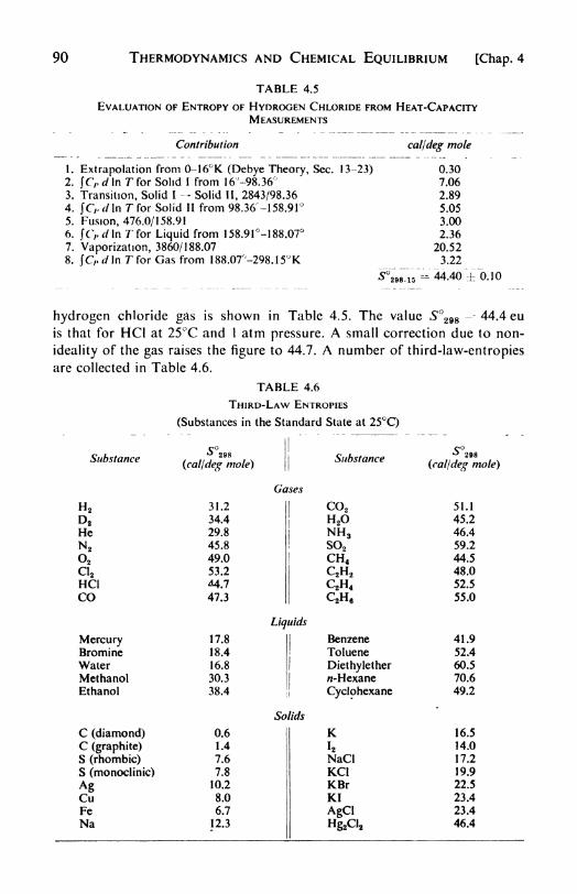
90 THERMODYNAMICS AND CHEMICAL EQUILIBRIUM [Chap. 4
TABLE 4.5
EVALUATION OF ENTROPY OF HYDROGEN CHLORIDE FROM HEAT-CAPACITYMEASUREMENTS
Contribution
1. Extrapolation from 0-16K (Debye Theory, Sec. 13-23)2. lC,,d\r\ Tfor Solid I from 16
J
~98.36
3. Transition, Solid I Solid II, 2843/98.364. JO</ln 7 for Solid II from 98.36
r
-l 58.91
5. Fusion, 476.0/158.916. JCV/ln Tfor Liquid from 158.91-! 88.07
7. Vaporization, 3860/188.078. JCW In Tfor Gas from 188.07-298.15K
caljdeg mole
0.30
7.06
2.89
5.05
3.00
2.36
20.52
3.22
S~~~
5 -44.40 0. 10
hydrogen chloride gas is shown in Table 4.5. The value S 298 44.4 eu
is that for HC1 at 25C and 1 atm pressure. A small correction due to non-
ideality of the gas raises the figure to 44.7. A number of third-law-entropies
are collected in Table 4.6.
TABLE 4.6
THIRD-LAW ENTROPIES
(Substances in the Standard State at 25C)
Substance
H 2
D2
HeN2
2
C12
HC1CO
MercuryBromineWaterMethanolEthanol
C (diamond)C (graphite)S (rhombic)S (monoclinic)
AgCuFeNa
(calldeg mole)
31.2
34.4
29.8
45.8
49.0
53.2
44.7
47.3
17.8
18.4
16.8
30.3
38.4
0.6
1.4
7.6
7.8
10.2
8.0
6.7
12.3
Gases
Liquids
Solids
Substance
C02
H2
NH 3
S02
CH4
C2H2
C2H4
C2H,
Benzene
Toluene
Diethyletherrt-Hexane
Cyclphexane
KI2
NaClKClKBrKI
AgClHg2Cl2
298
(calldeg mole)
51.1
45.2
46.4
59.2
44.5
48.0
52.5
55.0
41.9
52.4
60.5
70.6
49.2
16.5
14.0
17.2
19.9
22.5
23.4
23.4
46.4

Sec. i5] THERMODYNAMICS AND CHEMICAL EQUILIBRIUM 91
The standard entropy change AS in a chemical reaction can be calculated
immediately, if the standard entropies of products and reactants are known.
AS - 2 ", S?
One of the most satisfactory experimental checks of the Third Law is pro-vided by the comparison of AS values obtained in this way from low-
temperature heat capacity measurements, with AS values derived either
from measured equilibrium constants and reaction heats or from the tem-
perature coefficients of celt emf's eq. (4.3). Examples of such comparisonsare shown in Table 4.7. The Third Law is now considered to be on a firm
experimental basis. Its full meaning will become clearer when its statistical
interpretation is considered in a later chapter.
The great utility of Third Law measurements in the calculation of
chemical equilibria has led to an intensive development of low-temperature
heat-capacity techniques, using liquid hydrogen as a refrigerant. The ex-
perimental procedure consists essentially in a careful measurement of the
temperature rise that is caused in an insulated sample by a carefully measured
energy input.
We have now seen how thermodynamics has been able to answer the
old question of chemical affinity by providing a quantitative method for
calculating (from thermal data alone) the position of equilibrium in chemical
reactions.
TABLE 4.7
CHECKS OF THE THIRD LAW OF THERMODYNAMICS
Reaction
Ag (c) f i Br2 (1)- AgBr (c)
Ag (c) + * C12 (g)- AgCl (c)
Zn (c) + J 2 (g)= ZnO (c)
C M 2 (g)= CO (g)
CaC03 (c)- CaO (c) + CO2 (g)
15. General theory of chemical equilibrium: the chemical potential. Wehave so far confined our attention to equilibria involving ideal gases. Therelations discovered are of great utility, and are accurate enough for the
discussion of most homogeneous gas equilibria. Some gas reactions, how-
ever, are carried out under such conditions that the ideal gas laws are no
longer a good approximation. Examples include the high-pressure synthesesof ammonia and methanol. In addition, there are the great number of
chemical reactions that occur in condensed phases such as liquid or even
solid solutions. In order to treat these reactions especially, a more general
equilibrium theory will be needed.

92 THERMODYNAMICS AND CHEMICAL EQUILIBRIUM [Chap. 4
The composition of a system in which a chemical reaction is taking placeis continually changing, and the state of the system is not defined by specifying
merely the pressure, volume, and temperature. In order to discuss the changesof composition it is necessary to introduce, in addition to P9 V, and T, newvariables that are a measure of the amount of each chemical constituent of
the system. As usual, the mole will be chosen as the chemical measure, with
the symbols nl9 w2 n3 . . . nl representing the number of moles of constituent
1, 2, 3, or i.
It then follows that each thermodynamic function depends on these /i/s
as well as on P, V, and T. Thus, E - E(P, V, T, nt); F = F(P, V, T, n,\ etc.
Consequently, a perfect differential, for example of the free energy, becomes
By eq. (3.29) dF ~ ~S dT + V dP for any system of constant composition,
i.e., when all dn%
0. Therefore
= -SdT + VdP + -
dn, (4.25)T,P,n,
The coefficient (dF/dn t)T P n> , first introduced by Gibbs, has been given a
special name because of its great importance in chemical thermodynamics.It is called the chemical potential, and is written as
(4 '26)
It is the change of the free energy with change in number of molestof
component /, the temperature, the pressure, and the number of moles of all
other components in the system being kept constant. Using the new symbol,
eq. (4.25) becomes
dF - -5 dT + VdP + 2 Hi dn, (4.27)i
At constant temperature and pressure,
</F=2^<**. (4-28)
The condition for equilibrium, dF 0, then becomes
I to **< = <> (4.29)i
For an ideal gas, the chemical potential is simply the free energy per mole
at pressure Pt. Therefore from eq. (4.7),
(4.30)
The value of //, for the ideal gas is the same whether the ideal gas is pure
gas at a pressure Ptor is in an ideal gas mixture13 at partial pressure Pt
. If,
13 This statement is a definition of an ideal gas mixture. To be precise, one must distin-
guish an ideal gas mixture from a mixture of ideal gases. There might be specific interactions
between two ideal gases that would cause their mixture to deviate from ideality.
Sec. 16] THERMODYNAMICS AND CHEMICAL EQUILIBRIUM 93
however, the gas mixture is not ideal, this identity no longer holds true.
Various interaction forces come into operation, and the evaluation of ^ {
becomes a separate experimental problem in each case.
16. The fugacity. Because relations such as eq. (4.30) lead to equationsof such simple form in the development of the theory of chemical equilibrium,
it is convenient to introduce a new function, called the fugacity of the sub-
stance, that preserves the form of eq. (4.30) even for nonideal systems.Therefore we write
dfi= VdP = RTdlnf, and /i,
- -RTlnJ i
where/- is the fugacity of the substance, and/? is its fugacity in the standard
state. It now becomes desirable to change the definition of the standard state
so that instead of the state of unit pressure, it becomes the state of unit
fugacity,/?= 1. Then
Vi-tf-RTlnfi (4.31)
Now the treatment of equilibrium in Section 4-5 can be carried throughin terms of the fugacity and chemical potential. This leads to an expressionfor the equilibrium constant which is true in general, not only for real
(nonideal) gases but also for substances in any state of aggregation what-
soever:
f cf d
f~~
f af b
JA JB
-A// - RT \nKf (4.32)
The fugacity of a pure gas or of a gas in a mixture can be evaluated if
sufficiently detailed PVT data, are available. This discussion will be limited
to an illustration of the method for determining the fugacity of a pure gas.
In this case,
dF=dp=VdP (4.33)
If the gas is ideal, V = RT/P. For a nonideal gas, this is no longer true. Wemay write a - Fideal
- Kreal- (RT/P)
-K, whence V = (RT/P) ~ a. Sub-
stituting this expression into eq. (4.33), we find
RTdlnf- dF=dfA = RTctlnP - adP
The equation is integrated from P = to P.
RT\f
dlnf=RTfP
d\nP-(PadP
J/,p=oJ JP-O Jo
As its pressure approaches zero, a gas approaches ideality, and for an ideal
gas the fugacity equals the pressure, /= P [cf. eqs. (4.30 and (4.31)]. The
lower limits of the first two integrals must therefore be equal, so that we
obtain
RT\nf= RT In P -JP
<2 dP (4.34)

94 THERMODYNAMICS AND CHEMICAL EQUILIBRIUM [Chap. 4
This equation enables us to evaluate the fugacity at any pressure and
temperature, provided PVT data for the gas are available. If the deviation
from ideality of the gas volume is plotted against P, the integral in eq. (4.34)
can be evaluated graphically. Alternatively, an equation of state can be used
to calculate an expression for a as a function of P, making it possible to
evaluate the integral by analytical methods.
The fugacity may be thought of as a sort of idealized pressure, which
measures the true escaping tendency of a gas. In Chapter 1, it was pointed
V2 6 8 10 12 14 16 18 20 22 24
REDUCED PRESSURF-Ffe
Fig. 4.4. Variation of activity coefficient with reduced pressure at
various reduced temperatures.
out that the deviations of gases from ideality are approximately determined
by their closeness to the critical point. This behavior is confirmed by the
fact that at the same reduced pressures all gases have approximately the
same ratio of fugacity to pressure. The ratio of fugacity to pressure is called
the activity coefficient, y =f/P. Figure 4.4 shows a family of curves14relating
the activity coefficient of a gas to its reduced pressure PK at various values
of the reduced temperature Tlf. To the approximation that the law of corre-
sponding states is valid, all gases have the same value of y when they are in
corresponding states, i.e., at equal PR and TI{
. This is a very useful principle,
14Newton, Ind. Eng. Chem., 27, 302 (1935). Graphs for other ranges of PR and TR are
included in this paper.

Sec. 17] THERMODYNAMICS AND CHEMICAL EQUILIBRIUM 95
for it allows us to estimate the fugacity of a gas solely from a knowledge of
its critical constants.
17. Use of fugacity in equilibrium calculations. Among the industrially
important gas reactions that are carried out under high pressures is the
synthesis of ammonia: | N2 + $ H2= NH3 . This reaction has been carefully
investigated up to 1000 atm by Larson and Dodge.15 The per cent of NH3
in equilibrium with a three-to-one H2-N2 mixture at 450C and various total
pressures is shown in Table 4.8. In the third column of the table are the
values of Kp= PyuJPy^Pa?'
2 calculated from these data.
Since Kp for ideal gases should be independent of the pressure, these
results indicate considerable deviations from ideality at the higher pressures.
Let us therefore calculate the equilibrium constant Kf using Newton's graphsto obtain the fugacities. We are therefore adopting the approximation that
the fugacity of a gas in a mixture is determined only by the temperature and
by the total pressure of the gas mixture.
Consider the calculation of the activity coefficients at 450C (723K) and
600 atm.
PC TC PR TR r
N2 '33.5 126 17.9 5.74 1.35
H2 . 12.8 33.3 46.8 21.7 1.19
NH3 . . . 111.5 405.6 5.38 1.78 0.85
The activity coefficients y are read from the graphs, at the proper values of
reduced pressure PH and reduced temperature TR . (Only the NH3 values are
found in Fig. 4.4; the complete graphs must be consulted for the other gases.)
TABLE 4.8
EQUILIBRIUM IN THE AMMONIA SYNTHESIS AT 450C WITH 3 : 1 RATIO OF H2 TO N2
Since the fugacity/^ yP, we can write in general Kf= KYK^ where
in this case Kv= ^H^N^H,372
- The values of Kv and Kf are shown in
Table 4.8. There is a marked improvement in the constancy of Kf as com-
pared with Kv . Only at 1000 atm does the approximate treatment of the
fugacities appear to fail. To carry out an exact thermodynamic treatment, it
15 /. Am. Chem. Soc., 45, 2918 (1923); 46, 367 (1924).
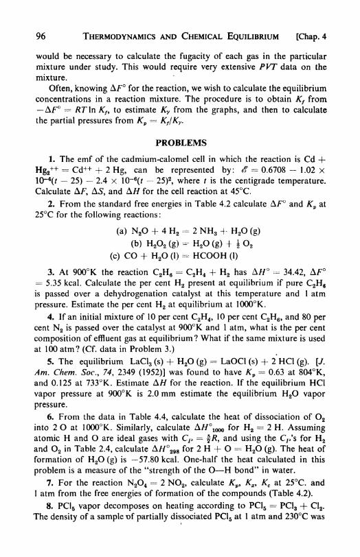
96 THERMODYNAMICS AND CHEMICAL EQUILIBRIUM [Chap. 4
would be necessary to calculate the fugacity of each gas in the particular
mixture under study. This would require very extensive PVT data on the
mixture.
Often, knowing AF for the reaction, we wish to calculate the equilibriumconcentrations in a reaction mixture. The procedure is to obtain Kf from
AF = RTln Kf, to estimate Ky from the graphs, and then to calculate
the partial pressures from Kp Kf/Ky .
PROBLEMS
1. The emf of the cadmium-calomel cell in which the reaction is Cd +Hg2
++ = Cd++ + 2 Hg, can be represented by: ? = 0.6708 - 1.02 x
10~4(/ 25) 2.4 x 10~6(r-
25)2
, where t is the centigrade temperature.Calculate AF, AS, and A// for the cell reaction at 45C.
2. From the standard free energies in Table 4.2 calculate A/70 and Kv at
25C for the following reactions :
(a) N2O + 4 H2- 2 NH3 + H2O (g)
(b) H2 2 (g)-H20(g) + |02
(c) CO + H2O (1)= HCOOH (1)
3. At 900K the reaction C2H6= C2H4 + H2 has A// - 34.42, AF
= 5.35 kcal. Calculate the per cent H2 present at equilibrium if pure C2H6
is passed over a dehydrogenation catalyst at this temperature and 1 atm
pressure. Estimate the per cent H2 at equilibrium at 1000K.
4. If an initial mixture of 10 per cent C2H4 , 10 per cent C2H6 , and 80 percent N2 is passed over the catalyst at 900K and 1 atm, what is the per cent
composition of effluent gas at equilibrium? What if the same mixture is used
at 100 atm? (Cf. data in Problem 3.)
5. The equilibrium LaCl3 (s) + H2O (g)- LaOCl (s) + 2 HCl (g). [/.
Am. Chem. Soc. 9 74, 2349 (1952)] was found to have Kp- 0.63 at 804K,
and 0.125 at 733K. Estimate A// for the reaction. If the equilibrium HCI
vapor pressure at 900K is 2.0mm estimate the equilibrium H2O vapor
pressure.
6. From the data in Table 4.4, calculate the heat of dissociation of O2
into 2 O at 1000K. Similarly, calculate A// 1000 for H2= 2 H. Assuming
atomic H and O are ideal gases with CP = f/*, and using the Q>'s for H2
and O2 in Table 2.4, calculate A// 298 for 2 H + O = H2O (g). The heat of
formation of H2O(g) is 57.80 kcal. One-half the heat calculated in this
problem is a measure of the "strength of the O H bond" in water.
7. For the reaction N2O4 2 NO2 , calculate KP ,Kx, Kc at 25C. and
1 atm from the free energies of formation of the compounds (Table 4.2).
8. PC1 5 vapor decomposes on heating according to PC15= PC13 + C12 .
The density of a sample t>f partially dissociated PC15 at 1 atm and 230C was

Chap. 4] THERMODYNAMICS AND CHEMICAL EQUILIBRIUM 97
found to be 4.80 g per liter. Calculate the degree of dissociation a and AFfor the dissociation at 230C.
9. The following results were obtained for the degree of dissociation of
CO2 (CO2= CO + i O2) at 1 atm:
K . . . 1000 1400 2000a . . . 2.0 x 10~7 1.27 x 10~ 4 1.55 x 10~2
What is AS for the reaction at 1400K?
10. The free energy of formation of H2S is given by AF = 19,200
+ 0.94rin T - 0.001 65T2 - 0.00000037r3 + 1-657. H2 + J S2 (g)- H2S
(g). If H2S at 1 atm is passed through a tube heated to 1200K, what is per
cent H2 in the gas at equilibrium?
11. Jones and Giauque obtained the following values for CP of nitro-
methane. 16
KCPKCP
The melting point is 244.7K, heat of fusion 2319cal per mole. The
vapor pressure of the liquid at 298.1K is 3.666 cm. The heat of vaporizationat 298.1K is 9147 cat per mole. Calculate the Third-Law entropy of CH3NO2
gas at 298.1K and 1 atm pressure (assuming ideal gas behavior).
12. Using the Third-Law entropies in Table 4.6 and the standard heats
of formation calculate the equilibrium constants at 25C of the following
reactions :
H2 + C12- 2 HC1
CH4 + 2 2= C02 + 2 H2 (g)
2Ag(s) + Cl2 -2AgCi(s)
13. For the reaction CO + 2 H2- CH3OH (g), AF - -3220 cal at
700K. Calculate the per cent CH3OH at equilibrium with a 2 : 1 mixture of
H2 + CO at a pressure of 600 atm using (a) ideal gas law, (b) Newton's
fugacity charts.
14. At high temperature and pressure, a quite good equation of state for
gases is P(V b) = RT. Calculate the fugacity of N2 at 1000 atm and
1000C according to this equation, if b = 39.1 cc per mole.
15. Show that
T,F,n, \s,P fn,W t ' S,V,n,
16. Amagat measured the molar volume of CO2 at 60C.
Pressure, atm . . 13.01 35.42 53.65 74.68 85.35
Volume, cc . . 2000.0 666.7 400.0 250.0 200.0
16 /. Am. Chem. Soc., 69, 983 (1947).
98 THERMODYNAMICS AND CHEMICAL EQUILIBRIUM [Chap. 4
Calculate the activity coefficient y = f/P for CO2 at 60C and pressures of
10, 20, 40, and 80 atm.
17. When rt-pentane is passed over an isomerization catalyst at 600 K,
the following reactions occur :
(A) CH3CH2CH2CH2CH3- CH3CH(CH3)CH2CH3 (B)
- C(CH3)4 (C)
The free energies of formation at 600K are: (A) 33.79, (B) 32.66, (C) 35.08
kcal per mole. Calculate the composition of the mixture when complete
equilibrium is attained.
18. For the reaction 3 CuCl (g)- Cu3C)3 (g), Brewer and Lofgren [J.
Am. Chem. Soc., 72, 3038 (1950)] found AF - -126,400 - 12.5iriog T+ 104.7 T. What are the A// and AS of reaction at 2000K? What is the
equilibrium mole fraction of trimer in the gas at 1 atm and 2000K?
REFERENCES
BOOKS
1. Kubaschewski, O., and E. L. Evans, Metallurgical Thermochemistry
(London: Butterworth, 1951).
2. Putnam, P. C., Energy in the Future (New York: Van Nostrand, 1953).
3. Squire, C. F., Low Temperature Physics (New York: McGraw-Hill, 1953).
4. Wenner, R. R., Thermochemical Calculations (New York: McGraw-Hill,
1941).
Also see Chapter 1, p. 25.
ARTICLES
1. Chem. Revs., 39, 357-481 (1946), "Symposium on Low TemperatureResearch."
2. Daniels, F., Scientific American, 191, 58-63 (1954), "High Temperature
Chemistry,"3. Huffman, H. M.,' Chem. Revs., 40, 1-14 (1947), "Low Temperature
Calorimetry."4. Lemay, P., and R. Oesper, /. Chem. Ed., 23, 158-65, 230-36 (1946),
"Claude Berthollet"
5. Oesper, R., /. Chem. Ed., 21, 263-64 (1944), "H. Kammerlingh-Onnes."6. Urey, H. C., /. Chem. Soc., 562-81 (1947), "Thermodynamic Properties
of Isotopic Substances."
7. Walden, P., /. Chem. Ed., 31, 27-33 (1954), "Beginnings of the Doctrine
of Chemical Affinity."
8. Watson, R. G., Research, 7, 34-40 (1954), "Electrochemical Generation
of Electricity."

CHAPTER 5
Changes of State
1. Phase equilibria. Among the applications of thermodynamics is the
study of the equilibrium conditions for changes such as the melting of ice,
the solution of sugar, the vaporization of benzene, or the transformation of
monoclinic to rhombic sulfur. Certain fundamental principles are applicable
to all such phenomena, which are examples of "changes in state of aggrega-tion" or "phase changes."
The word phase is derived from the Greek (pa.ai<t, meaning "appearance."If a system is "uniform throughout, not only in chemical composition, but
also in physical state,"1
it is said to be homogeneous, or to consist of onlyone phase. Examples are a volume of air, a noggin of rum, or a cake of ice.
Mere difference in shape or in degree of subdivision is not enough to deter-
mine a new phase. Thus a mass of cracked ice is still only one phase.2
A system consisting of more than one phase is called heterogeneous.
Each physically or chemically different, homogeneous, and mechanically
separable part of a system constitutes a distinct phase. Thus a glassful of
water with cracked ice in it is a two-phase system. The contents of a flask
of liquid benzene in contact with benzene vapor and air is a two-phase
system; if we add a spoonful of sugar (practically insoluble in benzene) we
obtain a three-phase system: a solid, a liquid, and a vapor phase.
In systems consisting entirely of gases, only one phase can exist at equi-
librium, since all gases are miscible in all proportions (unless, of course, a
chemical reaction intervenes, e.g., NH3 + HC1). With liquids, depending on
their mutual miscibility, one, two, or more phases can arise. Many different
solid phases can coexist.
2. Components. The composition of a system may be completely de-
scribed in terms of the "components" that are present in it. The ordinary
meaning of the word "component" is somewhat restricted in this technical
usage. We wish to impose a requirement of economy on our description of
the system. This is done by using the minimum number of chemically distinct
constituents necessary to describe the composition of each phase in the
system. The constituents so chosen are the components. If the concentrations
of the components are stated for each phase, then the concentrations in each
phase of any and all substances present in the system are uniquely fixed.
This definition may be expressed more elegantly by saying that the com-
1J. Willard Gibbs.
2 This is because we are assuming, at this stage in our analysis, that a variable surface
area has no appreciable effect on the properties of a substance.
QO

100 CHANGES OF STATE [Chap. 5
ponents are those constituents whose concentrations may be independently
varied in the various phases.
Consider, for example, a system consisting of liquid water in contact
with its vapor. We know that water is composed of hydrogen and oxygen,but these elements are always present in fixed and definite proportions. The
system therefore contains one component only.
Another example is the system consisting of calcium carbonate, calcium
oxide, and carbon dioxide. A chemical reaction between these compounds is
possible, CaCO3 CaO + CO2 . In this case, three phases are present,
gaseous CO2 , solid CaCO3 and CaO. Two components are required in order"
to describe the composition of all of these phases, the most suitable choice
being CaO and CO2 .
A less obvious example is the system formed by water and two salts
without a common ion, e.g., H2O, NaCl, KBr. As a result of interaction
between ions in solution four different salts, or their hydrates, may occur in
solid phases, namely NaCl, KBr, NaBr, KC1. In order to specify the com-
position of all possible phases, four components are necessary, consisting of
water and three of the possible salts. This fixes the concentrations of three
of the four ions in any phase, and the fourth is fixed by the requirement of
over-all electrical neutrality.
Careful examination of each individual system is necessary in order to
decide the best choice of components. It is generally wise to choose as com-
ponents those constituents that cannot be converted into one another byreactions occurring within the system. Thus CaCO3 and CaO would be a
possible choice for the CaCO3 CaO + CO2 system, but a poor choice
because the concentrations of CO2 would have to be expressed by negative
quantities. While the identity of the components is subject to some degree
of choice, the number of components is always definitely fixed for any
given case.
Even the last statement should perhaps be modified, because the actual
choice of the number of components depends on how precisely one wishes
to describe a system. In the water system, there is always some dissociation
of water vapor into hydrogen and oxygen. At moderate temperatures, this
dissociation is of no consequence in any experimental measurements, and to
consider it in deciding the number of components would be unduly scrupu-lous.3 The precision with which experimental data on the system can be
obtained should be allowed to decide borderline cases.
3. Degrees of freedom. For the complete description of a system, the
numerical values of certain variables' must be reported. These variables are
3It is worth noting that the mere dissociation of water into hydrogen and oxygen does
not create new components, because the proportion of H2 to O2 is always fixed at 2:1,
since we exclude the possibility that additional H 2 or O2 can be added to the system.The reason why an extra component, either H2 or O2 , might conceivably be required is
that H 2 and O2 dissolve to different extents in the water, so that their ratio is no longerfixed at 2:1 in each phase.

Sec. 4] CHANGES OF STATE 101
chosen from among the "state functions" of the system, such as pressure,
temperature, volume, energy, entropy, and the concentrations of the various
components in the different phases. Values for all of the possible variables
need not be explicitly stated, for a knowledge of some of them definitely
determines the values of the others. For any complete description, however,
at least one capacity factor is required, since otherwise the mass of the systemis undetermined, and one is not able, for example, to distinguish between a
system containing a ton of water and one containing a few drops.An important feature of equilibria between phases is that they are in-
dependent of the actual amounts of the phases that may be present.4 Thus
the vapor pressure of water above liquid water in no way depends on the
volume of the vessel or on whether a few milliliters or many gallons of water
are in equilibrium with the vapor phase. Similarly, the concentration of a
saturated solution of salt in water is a fixed and definite quantity, regardless
of whether a large or a small excess of undissolved salt is present.
In discussing phase equilibria, we therefore need not consider the capacity
factors, which express the absolute bulk of any phase. We consider only the
intensity factors, such as temperature, pressure, and concentrations. Of these
variables a certain number may be independently varied, but the rest are
fixed by the values chosen for the independent variables and by the thermo-
dynamic requirements for equilibrium. The number of the intensive state
variables that can be independently varied without changing the number of
phases is called the number of degrees offreedom of the system, or sometimes
the variance.
For example, the state of a certain amount of a pure gas may be specified
completely by any two of the variables, pressure, temperature, and density.
If any two of these are known, the third can be calculated. This is therefore
a system with iwo degrees of freedom, or a bivariant system.In the system "water water vapor," only one variable need be specified
to determine the state. At any given temperature, the pressure of vapor in
equilibrium with liquid water is fixed in value. This system has one degreeof freedom, or is said to be univariant.
4. Conditions for equilibrium between phases. In a system containing
several phases, certain thermodynamic requirements for the existence of
equilibrium may be derived.
For thermal equilibrium it is necessary that the temperatures of all the
phases be the same. Otherwise, heat would flow from one phase to another.
This intuitively recognized condition may be proved by considering two
phases a and /? at temperatures ra,Tft
. The condition for equilibrium at
constant volume and composition is given on p. 59 as dS 0. Let 5a and
Sft be the entropies of the two phases, and suppose there were a transfer of
heat dq from a to /? at equilibrium.
4 This statement is proved in the next Section. It is true as long as surface area variations
are left out of consideration. (See Chapter 16.)

102 CHANGES OF STATE [Chap. 5
Then dS = dS* + dSft = or --| + -|
-
whence 7a - 7* (5.1)
For mechanical equilibrium it is necessary that the pressures of all the
phases be the same. Otherwise, one phase would increase in volume at the
expense of another. This condition may be derived from the equilibrium
condition at constant over-all volume and temperature, dA 0. Supposeone phase expanded into another by 6V. Then
or P - Pft (5.2)
In addition to the conditions given by eqs. (5.1) and (5.2), a condition is
needed that expresses the requirements of chemical equilibrium. Let us con-
sider the system with phases a and ft maintained at constant temperatureand pressure, and denote by n*, /?/*, the numbers of moles of some particular
component / in the two phases. From eq. (3.28) the equilibrium condition
becomes dF 0, or
dF |
- tf*-=0 (5.3)
Suppose that a process occurred by which dntmoles of component / were
taken from phase a and added to phase ft. (This process might be a chemical
reaction or a change in aggregation-state.) Then, by virtue of eq. (4.28),
eq. (5.3) becomes-^
/i f to, + /*//!,=
or ^ - p* (5.4)
This is the general condition for equilibrium with respect to transport of
matter between phases, including chemical equilibrium between phases. For
any component / in the system, the value of the chemical potential /^ must
be the same in every phase.An important symmetry between the various equilibrium conditions is
apparent in the following summary:
Capacity Intensity Equilibrium
factor factor condition
S T T* = TP
V P P = Pft
5. The phase rule. Between 1875 and 1878, Josiah Willard Gibbs, Pro-
fessor of Mathematical Physics at Yale University, published in the Trans-
actions of the Connecticut Academy of Sciences a series of papers entitled
"On the Equilibrium of Heterogeneous Substances." In these papers Gibbs
disclosed the entire science, of heterogeneous equilibrium with a beauty and
preciseness never before and seldom since seen in thermodynamic studies.

Sec. 5] CHANGES OF STATE 103
Subsequent investigators have had little to do save to provide experimentalillustrations for Gibbs's equations.
The Gibbs phase rule provides a general relationship among the degreesof freedom of a system/, the number of phases /?,
and the number of com-
ponents c. This relationship always is
f^c-p + 2 (5.5)
The derivation proceeds as follows:
The number of degrees of freedom is equal to the number of intensive
variables required to describe a system, minus the number that cannot be
independently varied. The state of a system containing p phases and c com-
ponents is specified at equilibrium if we specify the temperature, the pressure,
and the amounts of each component in each phase. The total variables
required in order to do this are therefore pc -\- 2.
Let n* denote the number of moles of a component / in a phase a. Since
the size of the system, or the actual amount of material in any phase, does
not affect the equilibrium, we are really incerested in the relative amounts of
the components in the different phases and not in their absolute amounts.
Therefore, instead of the mole numbers n* 9 the mole fractions X? should be
used. These are given by
For each phase, the sum of the mole fractions equals unity.
Xf + X,' + AV [-... -+ X? = 1
or 2 X>" =- 1 (5-6)I
If all but one mole fraction are specified, that one can be calculated from
eq. (5.6). If there are/? phases, there are/? equations similar to eq. (5.6), and
therefore p mole fractions that need not be specified since they can be cal-
culated. The total number of independent variables to be specified is thus
pc + 2 p or p(c 1) + 2.
At equilibrium, the eqs. (5.4) impose a set of further restraints on the
system by requiring that the chemical potentials of each component be the
same in every phase. These conditions are expressed by a set of equationssuch as :
V* = fit = /*!"= ...
^ -^ = ^ --
'
- (5.7)
Each equality sign in this set of equations signifies a condition imposed onthe system, decreasing its variance by one. Inspection shows that there are
therefore c(p 1) of these conditions.

104 CHANGES OF STATE [Chap. 5
The degrees of freedom equal the total required variables minus the
restraining conditions. Therefore
f-=p(c- l) + 2-c(/>- 1)
f=c-p + 2 (5.8)
6. Systems of one component water. In the remainder of this chapter,
systems of one component will be considered. These systems comprise the
study of the conditions of equilibrium in changes in the state of aggregationof pure substances.
From the phase rule, when c* !,/= 3/?,
and three different cases
are possible:
p ^l,/
r - 2 bivariant system
p --= 2,f^= 1 univariant system
p _z_- 3,/ invariant system
These situations may be illustrated by the water system, with its three
familiar phases, ice, water, and steam. Since the maximum number of degrees
of freedom is two, any one-component system can be represented by a two-
dimensional diagram. The most convenient variables are the pressure and
the temperature. The water system is shown in Fig. 5.1.
.0075 100TEMPERATURE - *C
374
Fig. 5.1. The water system schematic. (Not drawn to scale.)
The diagram is divided into three areas, the fields of existence of ice,
water, and steam. Within these single-phase areas, the system is bivariant,
and pressure and temperature may be independently varied.

Sec. 7] CHANGES OF STATE 105
Separating the areas are lines connecting the points at which two phases
may coexist at equilibrium. Thus the curve AC dividing the liquid from the
vapor region is the familiar vapor-pressure curve of liquid water. At any
given temperature there is one and only one pressure at which water vaporis in equilibrium with liquid water. The system is univariant, having one
degree of freedom. The curve AC has a natural upper limit at the point C,
which is the critical point, beyond which the liquid phase is no longer
distinguishable from the vapor phase.
Similarly, the curve AB is the sublimation-pressure curve of ice, giving
the pressure of water vapor in equilibrium with solid ice, and dividing the
ice region from the vapor region.
The curve AD divides the solid-ice region from the liquid-water region.
It shows how the melting temperature of ice or the freezing temperature of
water varies with the pressure. It is still an open question whether such
curves, at sufficiently high pressures, ever have a natural upper limit beyondwhich solid and liquid are indistinguishable.
These three curves intersect at a point A, at which solid, liquid, and vaporare simultaneously at equilibrium. This point, which occurs at 0.0075C and
4.579 mm pressure, is called a triple point. Since three phases coexist, the
system is invariant. There are no degrees of freedom and neither pressure
nor temperature can be altered even slightly without causing the disappear-ance of one of the phases.
It should be noted that this triple point is not the same as the ordinary
melting point of ice, which by definition is the temperature at which ice and
water are in equilibrium under an applied pressure of 1 atm or 760 mm.This temperature is, by definition, 0C.
Liquid water may be cooled below its freezing point without solidifying.
In AE we have drawn the vapor-pressure curve of this supercooled water,
which is a continuous extension of curve AC. It is shown as a dotted line
on the diagram since it represents a metastable system. Note that the meta-
stable vapor pressure of supercooled water is higher than the vapor pressureof ice.
The slope of the curve A D, the melting-point curve, is worth remarking.It shows that the melting point of ice is decreased by increasing pressure.
This is a rather unusual behavior; only bismuth and antimony amongcommon substances behave similarly. These substances expand on freezing.
Therefore the Le Chatelier principle demands that increasing the pressureshould lower the melting point. The popularity of ice skating and the flow
of glaciers are among the consequences of the peculiar slope of the melting
point curve for ice. For most substances, the density of the solid is greater
than that of the liquid, and by Le Chatelier's principle, increase in pressure
raises the melting point.
7. The Clapeyron-CIausius equation. There are two fundamental theoreti-
cal equations that govern much of the field of phase equilibrium. The first

106 CHANGES OF STATE [Chap. 5
is the Gibbs phase rule, which determines the general pattern of the phase
diagram. The second is the Clapeyron-Clausius equation, which determines
the slopes of the lines in the diagram. It is a quantitative expression for the
Le Chatelier principle as it applies to heterogeneous systems. First proposed
by the French engineer Clapeyron in 1834, it was placed on a firm thermo-
dynamic foundation by Clausius, some thirty years later.
From eq. (5.4) the condition for equilibrium of a component / between
two phases, a and /7, is ju^-=
///. For a system of one component, the
chemical potentials // are identical with the free energies per mole F, so that
F* Fft at equilibrium. Consider two different equilibrium states, at slightly
separated temperatures and pressures :
(1) T,P, F* - Fft.
(2) T + dT, P + dP, F* + dF* - Fft\- dF?.
It follows that dF* - dFfl
. The change in F with T and P is given by
eq. (3.29), dF = V dP - S dT. Therefore, V dP - 5a dT - V& dP - S? dT9 or
dP_S'-S^ASdT VP - Ka AK ^ ' '
If the heat of the phase transformation is /I, AS is simply A/T where Tis the temperature at which the phase change is occurring. The Clapeyron-Clausius equation is now obtained as
^ - -A (5 10)dT (5 ' 10)
This equation is applicable to any change of state: fusion, vaporization,
sublimation, and changes between crystalline forms, provided the appro-
priate latent heat is employed.In order to integrate the equation exactly, it would be necessary to know
both X and AK as functions of temperature and pressure.5 The latter corre-
sponds to a knowledge of the densities of the two phases over the desired
temperature range. In most calculations over short temperature ranges,
however, both X and AKmay be taken as constants.
In the case of the change "liquid ^ vapor," several approximations are
possible, leading to a simpler equation than eq. (5.10),
dT
Neglecting the volume of the liquid compared with that of the vapor, and
assuming ideal gas behavior for the latter, one obtains
d In P _ Avap
~W =Kf* (5 ' 12)
6 A good discussion of the temperature variation of A is given by Guggenheim, Modern
Thermodynamicsy p. 57. The variation with pressure of A and A Kis much less than that with
temperature.

Sec. 8] CHANGES OF STATE 107
A similar equation would be a good approximation for the sublimation
curve.
Just as was shown for eq. (3.36), this may also be written
wTn=~R (5 - 13)
If the logarithm of the vapor pressure is plotted against 1/r, the slope of
the curve at any point multiplied by R yields a value for the heat of vapori-
zation. In many cases, since X is effectively constant over short temperature
ranges, a straight-line plot is obtained. This fact is useful to remember in
extrapolating vapor pressure data.
When A is taken as constant, the integrated form of eq. (5.12) is
ln
-h -*(?-) (5 - 14)
An approximate value for Avap
can often be obtained from Troutorfs
Rule (1884):
^ & 22 cal deg"1 mole" 1
The rule is followed fairly well by many nonpolar liquids (Sec. 14-8). It is
equivalent to the statement that the entropy of vaporization is approximatelythe same for all such liquids.
8. Vapor pressure and external pressure. It is of interest to consider the
effect of an increased hydrostatic pressure on the vapor pressure of a liquid.
Let us suppose that an external hydrostatic pressure Pp is imposed on a
liquid of molar volume Vv Let the vapor pressure be P, and the molar
volume of the vapor Vg
. Then at equilibrium at constant temperature:
</Fvap
= rfFllq
or Vg dP - V, dPe
or ~ Vl(5.15)
dl f Vfl
This is sometimes called the Gibbs equation. If the vapor is an ideal gas, this
equation becomes
"(-.SrHSince the molar volume of the liquid does not vary greatly with pressure,
this equation may be integrated approximately, assuming constant Vt
:
n \r f n n '\
In theory, one can measure the vapor pressure of a liquid under an
applied hydrostatic pressure in only two ways: (1) with an atmosphere of
"inert" gas; (2) with an ideal membrane semipermeable to the vapor. In
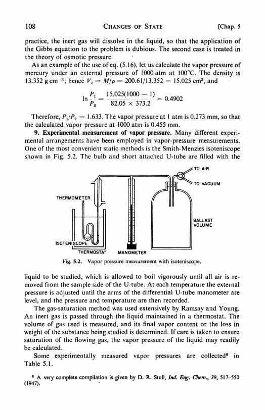
108 CHANGES OF STATE [Chap. 5
practice, the inert gas will dissolve in the liquid, so that the application of
the Gibbs equation to the problem is dubious. The second case is treated in
the theory of osmotic pressure.
As an example of the use of eq. (5.16), let us calculate the vapor pressure of
mercury under an external pressure of 1000 atm at 100C. The density is
13.352 gem-3; hence V,
= M/p = 200.61/13.352 - 15.025 cm3, and
Pl 15.025(1000-1)In
>l
=lilQrx 373.2
Therefore, Pi/P2= 1.633. The vapor pressure at 1 atm is 0.273 mm, so that
the calculated vapor pressure at 1000 atm is 0.455 mm.9. Experimental measurement of vapor pressure. Many different experi-
mental arrangements have been employed in vapor-pressure measurements.
One of the most convenient static methods is the Smith-Menzies isoteniscope
shown in Fig. 5.2. The bulb and short attached U-tube are filled with the
TO AIR
THERMOMETER
ISOTENISCOPE
TO VACUUM
BALLASTVOLUME
THERMOSTAT MANOMETER
Fig. 5.2. Vapor pressure measurement with isoteniscope.
liquid to be studied, which is allowed to boil vigorously until all air is re-
moved from the sample side of the U-tube. At each temperature the external
pressure is adjusted until the arms of the differential U-tube manometer are
level, and the pressure and temperature are then recorded.
The gas-saturation method was used extensively by Ramsay and Young.An inert gas is passed through the liquid maintained in a thermostat. The
volume of gas used is measured, and its final vapor content or the loss in
weight of the substance being studied is determined. If care is taken to ensure
saturation of the flowing gas, the vapor pressure of the liquid may readily
be calculated.
Some experimentally measured vapor pressures are collected6 in
Table 5.1.
6 A very complete compilation is given by D. R. Stull, Ind. Eng. Chem., 39, 517-550
(1947).

Sec. 10] CHANGES OF STATE
TABLE 5.1
TYPICAL VAPOR PRESSURE DATA
109
10. Solid-solid transformations the sulfur system. Sulfur provides the
classical example of a one-component system displaying a solid-solid trans-
formation. The phenomenon of polymorphism, discovered by Mitscherlich
in 1821, is the occurrence of the same chemical substance in two or
more different crystalline forms. In the case of elements, it is called
aIlotropy.
Sulfur occurs in a low-temperature rhombic form and a high-temperaturemonoclinic form. The phase diagram for the system is shown in Fig. 5.3.
The pressure scale in this diagram has been made logarithmic in order to
bring the interesting low-pressure regions into prominence.The curve AB is the vapor-pressure curve of solid rhombic sulfur. At
point B it intersects the vapor-pressure curve of monoclinic sulfur BE, and
also the transformation curve for rhombic-monoclinic sulfur, BD. This inter-
section determines the triple point B, at which rhombic and monoclinic sulfur
and sulfur vapor coexist. Since there are three phases and one component,
f= c p-^-2 3 3 0, and point B is an invariant point. It occurs at
0.01 mm pressure and 95.5C.
The density of monoclinic sulfur is less than that of rhombic sulfur, and
therefore the transition temperature (Sr ^ Sm) increases with increasing
pressure.
Monoclinic sulfur melts under its own vapor pressure of 0.025 mm at
120C, the point E on the diagram. From E to the critical point F there
extends the vapor-pressure curve of liquid sulfur EF. Also from , there
extends the curve ED, the melting-point curve of monoclinic sulfur. The
density of liquid sulfur is less than that of the monoclinic solid, the usual
situation in a solid-liquid transformation, and hence ED slopes to the right
as shown. The point E is a triple point, Sm-Sliq-S
vap .
The slope of BD is greater than that of ED, so that these curves intersect
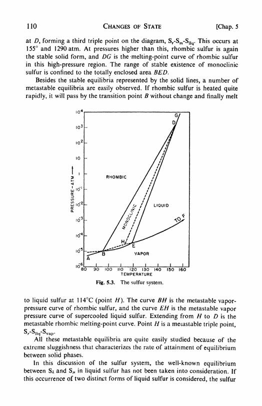
110 CHANGES OF STATE [Chap. 5
at Z), forming a third triple point on the diagram, Sf-Sm-Sllq. This occurs at
155 and 1290atm. At pressures higher than this, rhombic sulfur is againthe stable solid form, and DG is the melting-point curve of rhombic sulfur
in this high-pressure region. The range of stable existence of monoclinic
sulfur is confined to the totally enclosed area BED.Besides the stable equilibria represented by the solid lines, a number of
metastable equilibria are easily observed. If rhombic sulfur is heated quite
rapidly, it will pass by the transition point B without change and finally melt
10'
IO
10
10*
RHOMBIC
80 90 100 110 120 130 140 150 160TEMPERATURE
Fig. 5.3. The sulfur system.
to liquid sulfur at 1 14C (point //). The curve BH is the metastable vapor-
pressure curve of rhombic sulfur, and the curve EH is the metastable vapor
pressure curve of supercooled liquid sulfur. Extending from H to D is the
metastable rhombic melting-point curve. Point H is a metastable triple point,S r-Sliq
-Svap .
All these metastable equilibria are quite easily studied because of the
extreme sluggishness that characterizes the rate of attainment of equilibriumbetween solid phases.
In this discussion of the sulfur system, the well-known equilibriumbetween SA and S
/4in liquid sulfur has not been taken into consideration. If
this occurrence of two distinct forms of liquid sulfur is considered, the sulfur

Sec. 11] CHANGES OF STATE 111
system can no longer be treated as a simple one-component system, but
becomes a "pseudobinary" system.7
11. Enantiotropism and monotropism. The transformation of monoclinic
to rhombic sulfur under equilibrium conditions of temperature and pressure
is perfectly reversible. This fact is, of course, familiar, since the transforma-
tion curve represents a set of stable equilibrium conditions. Such a changebetween two solid forms, occurring in a region of the phase diagram where
both are stable, is called an enantiotropic change.
On the other hand, there are cases in which the transformation of one
solid form to another is irreversible. The classical example occurs in the
VAPOR
ENANTIOTROPISM
VAPOR
MONOTROPISM
T
Fig. 5.4. Enantiotropic and monotropic changes.
phosphorus system, in the relations between white (cubic) phosphorus and
violet (hexagonal) phosphorus. When white phosphorus is heated, trans-
formation into violet phosphorus occurs at an appreciable rate at tem-
peratures above 260; but solid violet phosphorus is never observed to
change into solid white phosphorus under any conditions. In order to obtain
white phosphorus, it is necessary to vaporize the violet variety, whereuponthe vapor condenses to white phosphorus.
Such an irreversible solid-state transformation is called a monotropic
change. It may be characterized by saying that one form is metastable with
respect to the other at all temperatures up to its melting point. The situa-
tion is shown schematically in Fig. 5.4. The transition point (metastable)
between the two solid forms in this case lies above the melting point of
either form.
7 If SA and S^ came to equilibrium quickly when the T or P of the liquid was changed,the sulfur system would still have only one component (unary system) as explained in foot-
note 3. If SA and S^ were present in fixed proportions, which did not change with rand P,
because the time of transformation was very long compared with the time of the experiment,the sulfur system would have two components (binary system). In fact it appears that the
time of transformation is roughly comparable with the time of most experiments, so that
the observed behavior is partly unary and partly binary, being called "pseudobinary."

112 CHANGES OF STATE [Chap. 5
Actually, the phosphorus case is complicated by the occurrence of several
molecular species, P2 ,P4 ,
P% , and so on, so that considerations based on a
one-component system must be applied with caution.
12. Second-order transitions. The usual change of state (solid to liquid,
liquid to vapor, etc.) is called & first-order transition. At the transition tem-
perature Ttat constant pressure, the free energies of the two forms are equal,
but there is a discontinuous change in the slope of the F vs. T curve for the
substance at Tt
. Since (3F/3T) S, there is therefore a break in the
S vs. T curve, the value of AS at Tt being related to the observed latent heat
for the transition by AS = XjTt. There is also a discontinuous change in
volume AF, since the densities of the two forms are not the same.
A number of transitions have been studied in which no latent heat or
density change can be detected. Examples are the transformation of certain
metals from ferromagnetic to paramagnetic solids at their Curie points, the
transition of some metals at low temperatures to a condition of electric
superconductivity, and the transition observed in helium from one liquid
form to another. 8 In these cases, there is a change in slope, but no dis-
continuity, in the S vs. T curve at Tt
. As a result, there is a break ACP in
the heat capacity curve, since Cp= T(dS/dT)r . Such a change is called a
second-order transition.
13. High-pressure studies. It is only a truism that our attitude toward
the physical world is conditioned by the scale of magnitudes provided in
our terrestrial environment. We tend, for example, to classify pressures or
temperatures as high or low by comparing them with the fifteen pounds per
square inch and 70F of a spring day in the laboratory, despite the fact that
almost all the matter in the universe exists under conditions very different
from these. Thus, even at the center of the earth, by no means a large astro-
nomical body, the pressure is around 1,200,000 atm, and substances at this
pressure would have properties quite unlike those to which we are accus-
tomed. At the center of a comparatively small star, like our sun, the pressure
would be around ten billion atmospheres.The pioneer work of Gustav Tammann on high-pressure measurements
has been greatly extended over the past twenty years by P. W. Bridgmanand his associates at Harvard. Pressures up to 400,000 atm have been
achieved and methods have been developed for measuring the properties of
substances at 100,000 atm. 9
The attainment of such pressures has been made possible by the con-
struction of pressure vessels of alloys such as Carboloy, and by the use of a
multiple-chamber technique. The container for the substance to be studied
is enclosed in another vessel, and pressure is applied both inside and outside
the inner container, usually by means of hydraulic presses. Thus although
8 W. H. Keesom, Helium (Amsterdam: Elsevier, 1942).* For details see P. W. Bridgman, The Physics of High Pressures (London: Bell & Co.,
1949), and his review article, Rev. Mod. Phys., 18, 1 (1946).
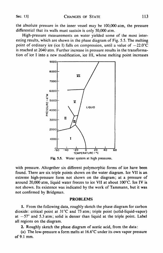
Sec. 13] CHANGES OF STATE 113
the absolute pressure in the inner vessel may be 100,000 atm, the pressuredifferential that its walls must sustain is only 50,000 atm.
High-pressure measurements on water yielded some of the most inter-
esting results, which are shown in the phase diagram of Fig. 5.5. The melting
point of ordinary ice (ice I) falls on compression, until a value of 22.0Cis reached at 2040 atm. Further increase in pressure results in the transforma-
tion of ice I into a new modification, ice III, whose melting point increases
9000
8000-
7000 -
6000 -
5000 -
1 4000 -
3000-
2000 -
1000 -
-20 20TEMPERATURE -*C
Fig. 5.5. Water system at high pressures.
with pressure. Altogether six different polymorphic forms of ice have been
found. There are six triple points shown on the water diagram. Ice VII is an
extreme high-pressure form not shown on the diagram; at a pressure of
around 20,000 atm, liquid water freezes to ice VII at about 100C. Ice IV is
not shown. Its existence was indicated by the work of Tammann, but it was
not confirmed by Bridgman.
PROBLEMS
1. From the following data, roughly sketch the phase diagram for carbon
dioxide: critical point at 31C and 73 atm; triple point (solid-liquid-vapor)
at 57 and 5.3 atm; solid is denser than liquid at the triple point. Label
all regions on the diagram.
2. Roughly sketch the phase diagram of acetic acid, from the data:
(a) The low-pressure a form melts at 16.6C under its own vapor pressure
of 9. 1 mm.

114 CHANGES OF STATE [Chap. 5
(b) There is a high-pressure /? form that is denser than the a, but both
a and /? are denser than the liquid.
(c) The normal boiling point of liquid is 1 18C.
(d) Phases a, /?, liquid are in equilibrium at 55C and 2000 atm.
3. Sketch the liquid-solid regions of the phase diagram of urethane.
There are three solid forms, a, /?, y. The triple points and the volume changes
AF in cc per kg at the triple points are as follows:
(a) liq, a, /? P - 2270 atm / - 66C AK (I-
a) = 25.3
(I-
ft - 35.5
(a _ ft ^ 10.2
(b) liq, ft y P - 4090 atm / - 77C A V: (I-
ft)= 18.4
(1-
y) - 64.0
0?-
y)- 45.6
(c) a, /?, y - P = 3290 atm / - 25.5C A K: (a-
ft - 9.2
(/?-
y)- 48.2
(a-
y) - 57.4
4. The density />of ice at 1 atm and 0C is 0.917 g per cc. Water under
the same conditions has p -=--
l.OOOg per cc. Estimate the melting point of
ice under a pressure of 400 atm assuming that p for both ice and water is
practically constant over the temperature and pressure range.
5. Bridgman found the following melting points / (C) and volume
changes on melting AK(cc per g) for Na:
P, kg/cm2
. 1 2000 4000 6000
/ . 97.6 114.2 129.8 142.5
AK . . 0.0279 0.0236 0.0207 0.0187
Estimate the heat of fusion of sodium at 3000 atm.
6. Estimate the vapor pressure of mercury at 25C assuming that the
liquid obeys Trouton's rule. The normal boiling point is 356.9C.
7. The vapor pressure of solid iodine is 0.25 mm and its density 4.93 at
20C. Assuming the Gibbs equation to hold, calculate the vapor pressure of
iodine under a 1000-atm argon pressure.
8. In a determination of the vapor pressure of ethyl acetate by the gas
saturation method 100 liters of nitrogen (STP) were passed through a
saturator containing ethyl acetate at 0C, which lost a weight of 12.8g.
Calculate vapor pressure at 0C.
9. The vapor pressures of liquid gallium are as follows:
/, C . 1029 1154 1350
P, mm . . 0.01 0.1 1.0
Calculate A//, AF, and AS for the vaporization of gallium at 1154C.
10. At 25C, the heat of combustion of diamond is 94.484 kcal per mole
and that of graphite is 94.030. The molar entropies are 0.5829 and 1.3609 cal
per deg mole, respectively. Find the AFfor the transition graphite -> diamond
at 25C and 1 atm. The densities are 3.513 g per cc for diamond and 2.260
Chap. 5] CHANGES OF STATE 115
for graphite. Estimate the pressure at which the two forms would be in
equilibrium at 25C. You may assume the densities to be independent of
pressure.
11. Sketch graphs of F, S, V, Q> against T at constant P, and P at
constant T, for typical first- and second-order phase transitions.
12. From the data in Table 5.1, plot log P vs. T~ l for water and calculate
the latent heats of vaporization of water at 20 and at 80C.
REFERENCES
BOOKS
1. Bridgman, P. W., The Physics of High Pressures (London: Bell, 1949).
2. Findlay, A., The Phase Rule (New York: Dover, 1945).
3. Marsh, J. S., Principles of Phase Diagrams (New York: McGraw-Hill,
1935).
4. Ricci, J. E., The Phase Rule and Heterogeneous Equilibrium (New York:
Van Nostrand, 1951).
5. Tammann, G., The States of Aggregation (New York: Van Nostrand,
1925).
6. Wheeler, L. P.,Josiah WillardGibbs(New Haven: Yale Univ. Press, 1953).
ARTICLES
1. Bridgman, P. W., Science in Progress, vol. Ill, 108-46 (New Haven: Yale
Univ. Press, 1942), "Recent Work in the Field of High Pressures."
2. Garner, W. E.,/. Chem. Soc., 1961-1973 (1952), "The Tammann Memor-
ial Lecture."
3. Staveley, L. A. K., Quart. Rev., 3, 65-81 (1949), "Transitions in Solids
and Liquids."4. Swietoslawski, W., J. Chem. Ed., 23, 183-85 (1946), "Phase Rule and the
Action of Gravity."5. Ubbelohde, A. R., Quart. Rev., 4, 356-81 (1950), "Melting and Crystal
Structure."

CHAPTER 6
Solutions and Phase Equilibria
1. The description of solutions. As soon as systems of two or more com-
ponents are studied, the properties of solutions must be considered, for a
solution is by definition any phase containing more than one component.This phase may be gaseous, liquid, or solid. Gases are in general miscible
in all proportions, so that all mixtures of gases, at equilibrium, are solutions.
Liquids often dissolve a wide variety of gases, solids, or other liquids, and
the composition of these liquid solutions can be varied over a wide or narrow
range depending on the particular solubility relationships in the individual
system. Solid solutions are formed when a gas, a liquid, or another solid
dissolves in a solid. They are often characterized by very limited concentra-
tion ranges, although pairs of solids are known, for example copper and
nickel, that are mutually soluble in all proportions.It is often convenient in discussing solutions to call some components
the solvents and others the solutes. It should be recognized, however, that
the only distinction between solute and solvent is a verbal one, although the
solvent is usually taken to be the constituent present in excess.
The concentration relations in solutions are expressed in a variety of
units. The more important of these are summarized in Table 6.1.
TABLE 6.1
CONCENTRATION OF SOLUTIONS
2. Partial molar quantities: partial molar volume. The equilibrium prop-erties of solutions are described in terms of the thermodynamic state func-
tions, such as P, T, K, ", 5, F, //. One of the most important problems in
the theory of solutions is how these properties depend on the concentrations
of the various components. In discussing this question, it will be assumed
that the solution is kept at constant over-all pressure and temperature.Consider a solution containing nA moles of A and nB moles of B. Let the
volume of the solution be K, and assume that this volume is so large that

Sec. 2] SOLUTIONS AND PHASE EQUILIBRIA 117
the addition of one extra mole of A or of B does not change the concentration
of the solution to an appreciable extent. The change in volume caused by
adding one mole of A to this large amount of solution is then called the
partial molar volume of A in the solution at the specified pressure, tempera-
ture, and concentration, and is denoted by the symbol VA . It is the changeof volume K, with moles of A, nA ,
at constant temperature, pressure; and
moles of B, and is therefore written as
One reason for introducing such a function is that the volume of a
solution is not, in general, simply the sum of the volumes of the individual
components. For example, if 100ml of alcohol are mixed at 25C with
100 ml of water, the volume of the solution is not 200 ml, but about 190 ml.
The volume change on mixing depends on the relative amount of each
component in the solution.
\fdnA moles of A and dnB moles of B are added to a solution, the increase
in volume at constant temperature and pressure is given by the complete
differential,
-(")*, + () *.A'*M WB'*A
or dV --= VA dnA + Pyy dntt (6.2)
This expression can be integrated, which corresponds physically to increasing
the volume of the solution without changing its composition, VA and Vnhence being held constant. 1 The result is
V = VAnA + VBnB (6.3)
This equation tells us that the volume of the solution equals the number of
moles of A times the partial molar volume of A, plus the number of moles
of B times the partial molar volume of B.
On differentiation, eq. (6.3) yields
<*V= VA dnA + nA d?A + VB dnB + nB dVB
By comparison with eq. (6.2), it follows that
or dVA - - dVB (6.4)nA
Equation (6.4) is one example of the Gibbs-Duhem equation. This par-
ticular application is in terms of the partial molar volumes, but any other
1
Mathematically, the integration is equivalent to the application of Euler's theorem to
the homogeneous differential expression. See D. V. Widder, Advanced Calculus (New York:
Prentice-Hall, 1947), p. 15.

118 SOLUTIONS AND PHASE EQUILIBRIA [Chap. 6
partial molar quantity may be substituted for the volume. These partial
molar quantities can be defined for any extensive state function. For example:
Sl . a.
WA'T,I',H.' ' n
The partial molar quantities are themselves intensity factors, since theyare capacity factors per mole. The partial molar free energy is the chemical
potential /i.
All the thermodynamic relations derived in earlier chapters can be
applied to the partial molar quantities. For example:
/v' (6 ' 5)
The general thermodynamic theory of solutions is expressed in terms of
these partial molar functions and their derivatives just as the theory for
pure substances is based on the ordinary thermodynamic functions.
3. The determination of partial molar quantities. The evaluation of the
partial quantities will now be described, using the partial molar volume as
an example. The methods for ffA , SA , FA9 and so on, are exactly similar.
The partial molar volume VA , defined by eq. (6.1), is equal to the slope
of the curve obtained when the volume of the solution is plotted against the
molal concentration of A. This follows since the molal concentration mA is
the number of moles of A in a constant quantity, namely 1000 grams, of
solvent B.
The determination of partial molar volumes by this slope method is
rather inaccurate; the method of intercepts is therefore usually preferred. To
employ this method, a quantity is defined, called the molar volume of the
solution v, which is the volume of the solution divided by the total number
of moles of the various constituents. For a two-component solution:
"A + "B
Then, Y = v (nA + nB)
and PA =
Now the derivative with respect to mole number of A, nA , is transformed
into a derivative with respect to mole fraction of B, XB .
dv
since XK = ^> 1^1 =- JL("A + '

Sec. 3] SOLUTIONS AND PHASE EQUILIBRIA 119
Thus eq. (6.6) becomes : VA = v
V
nB dv
nA + ns dXB
xdv
AB Ti7~ (6.7)
The application of this equation is illustrated in Fig. 6.1, where v for a
solution is plotted against the mole fraction. The slope S^ is drawn tangentto the curve at point P, corresponding to a definite mole fraction XB
'
. The
line ^iA 2 is drawn through P parallel to O^O2 . Therefore the distance
Si
2
XB i
MOLE FRACTION OF B-XB
Fig. 6.1. Determination of partial molar volumes intercept method.
OlA l v, the molar volume corresponding to XB . The distance SlA l is
equal to the slope at XB multiplied by XB , i.e., to the term in eq. (6.7),
Xn (dv/dXB). It follows that O^ = OlA l SlA
l equals VA , the partial
molar volume of A in the solution. It can readily be shown that the intercepton the other axis, O252 , is the partial molar volume of B, PB . This con-
venient intercept method is the one usually used to determine partial molar
quantities. It is not restricted to volumes, but can be applied to any extensive
state function, 5, H, E, F9 and so on, given the necessary data. It can also
be applied to heats of solution, and the partial molar heats of solution so
obtained are the same as the differential heats described in Chapter 2.
If the variation with concentration of a partial molar quantity is knownfor one component in a binary solution, the Gibbs-Duhem equation (6.4)
permits the calculation of the variation for the other component. This cal-
culation can be accomplished by graphical integration of eq. (6.4). For
example:

120 SOLUTIONS AND PHASE EQUILIBRIA [Chap. 6
where X is the mole fraction. If XB\XA is plotted against Vn , the area under
the curve gives the change in VA between the upper and lower limits of
integration. The VA of pure A is simply the molar volume of pure A, and
this can be used as the starting point for the evaluation of VA at any other
concentration.
4. The ideal solution Raoult's Law. The concept of the "ideal gas" has
played a most important role in discussions of the thermodynamics of gases
and vapors. Many cases of practical interest are treated adequately by means
of the ideal gas approximations, and even systems deviating largely from
ideality are conveniently referred to the norm of behavior set by the ideal
case. It would be most helpful to find some similar concept to act as a guidein the theory of solutions, and fortunately this is indeed possible. Because
they are very much more condensed than gases, liquid or solid solutions
cannot be expected to behave ideally in the sense of obeying an equation of
state such as the ideal gas law. Ideality in a gas implies a complete absence
of cohesive forces; the internal pressure, (3E/c>V)T 0. Ideality in a solution
is defined by complete uniformity of cohesive forces. If there are two com-
ponents A and B, the forces between A and A, B and /?, and A and B are
all the same.
A property of great importance in the discussion of solutions is the vapor
pressure of a component above the solution. This partial vapor pressure
may be taken as a good measure of the escaping tendency of the given species
from the solution. The exact measure of this escaping tendency is the fugacity,
which becomes equal to the partial pressure when the vapor behaves as an
ideal gas. The tendency of a component to escape from solution into the
vapor phase is a very direct reflection of the physical state of affairs within
the solution,2 so that by studying the escaping tendencies, or partial vapor
pressures, as functions of temperature, pressure, and concentration, we
obtain a description of the properties of the solution.
This method is a direct consequence of the relation between chemical
potential and fugacity. If we have a solution, say of A and J9, the chemical
potential of A in the solution must be equal to the chemical potential of Ain the vapor phase. This is related to the fugacity by eq. (4.31), since
If we know the pressure, the temperature, and the chemical potentials of
the various components, we then have a complete thermodynamic descrip-
tion of a system, except for the absolute amounts of the various phases. The
partial vapor pressures are important because they are an approximateindication of the chemical potentials.
A solution is said to be ideal if the escaping tendency of each component
2 One may think of an analogy in which a nation represents a solution and its citizens
the molecules. If life in the nation is a good one, the tendency to emigrate will be low. This
presupposes, of course, the absence of artificial barriers.

Sec. 4] SOLUTIONS AND PHASE EQUILIBRIA 121
is proportional to the mole fraction of that component in the solution. It is
helpful to look at this concept from a molecular point of view. Consider an
ideal solution of A and B. The definition of ideality then implies that a
molecule of A in the solution will have the same tendency to escape into the
vapor whether it is surrounded entirely by other A molecules, entirely byB molecules, or partly by A and partly by B molecules. This means that the
intermolecular forces between A and A, A and B, and B and B, are all
essentially the same. It is immaterial to the behavior of a molecule what
sort of neighbors it has. The escaping tendency of component A from such
200
180
160
0140E6120
a: 60
<40
20
TOTALVAPOR
*--^PRESSURE
.
AC2H4Br2
.2 3 .4 .5 .6 .7 .8 .9 1.0
MOLE FRACTION OF C3H6Br2 BC3H6 Br2
Fig. 6.2. Pressures of vapors above solutions of ethylene bromide and
propylene bromide at 85C. The solutions follow Raoult's Law.
an ideal solution, as measured by its partial vapor pressure, is accordinglythe same as that from pure liquid A, except that it is proportionately reduced
on account of the lowered fraction of A molecules in the solution.
This law of behavior for the ideal solution was first given by Francois
Marie Raoult in 1886, being based on experimental vapor-pressure data. It
can be expressed as
PA = *A PA (6-9)
Here PA is the partial vapor pressure of A above a solution in which its
mole fraction is XA , and PA is the vapor pressure of pure liquid A at the
same temperature.If the component B added to pure A lowers the vapor pressure, eq. (6.9)
can be written in terms of a relative vapor pressure lowering,
(6.10)
1 22 SOLUTIONS AND PHASE EQUILIBRIA [Chap. 6
This form of the equation is especially useful for solutions of a relatively
involatile solute in a volatile solvent.
The vapor pressures of the system ethylene bromide propylene bromide
are plotted in Fig. 6.2. The experimental results almost coincide with the
theoretical curves predicted by eq. (6.9). The agreement with Raoult's Lawin this instance is very close.
Only in exceptional cases are solutions found that follow Raoult's Law
closely over an extended range of concentrations. This is because ideality
in solutions implies a complete similarity of interaction between the com-
ponents, which can rarely be achieved.
This equality of interaction leads to two thermodynamic conditions:
(1) there can be no heat of solution; (2) there can be no volume change on
mixing. Hence, AF80lution- and A//80hltion - 0.
5. Equilibria in ideal solutions. If we wish to avoid the assumption that
the saturated vapor above a solution behaves as an ideal gas, Raoult's Law
may be written
fA~XA ft (6.11)
where/4 and/jj' are the fugacities of A in the solution, and in pure A. It is
evident from eq. (6.8) that
dp -- RTd\nfA RTd\nXA (6.12)
Then, following the sort of development given in Section 4-5, one obtains
for the equilibrium constant in an ideal solution
-AF --= RT\r\Kx
with K<'-'r* (6 ' 13)AA AB
for the typical case.
6. Henry's Law. Consider a solution of component B, which may be
called the solute, in A 9 the solvent. If the solution is sufficiently diluted, a
condition ultimately is attained in which each molecule of B is effectively
completely surrounded by component A. The solute B is then in a uniform
environment irrespective of the fact that A and B may form solutions that
are far from ideal at higher concentrations.
In such a very dilute solution, the escaping tendency of B from its uniform
environment is proportional to its mole fraction, but the proportionality
constant k no longer is P#. We may write
PB - kXB (6.14)
This equation was established and extensively tested by William Henryin 1803 in a series of measurements of the pressure dependence of the solu-
bility of gases in liquids. Some results of this type are collected in Table 6.2.
The fc's are almost constajit, so that Henry's Law is nearly but not exactly
obeyed.

Sec. 7] SOLUTIONS AND PHASE EQUILIBRIA 123
TABLE 6.2
THE SOLUBILITY OF GASES IN WATER (ILLUSTRATING HENRY'S LAW PB = kXB, THE GASPRESSURE BEING IN ATM AND XB BEING THE MOLE FRACTION)
As an example, let us calculate the volume of oxygen (at STP) dissolved
in 1 liter of water in equilibrium with air at 23. From eq. (6.14) the mole
fraction of O2 is Xn = P#/k. Since PB = 0.20, and from the table k =4.58 x 10⁴ ,
Xn - 4.36 x 10~6 . In 1 liter of H2O there are 1000/18 =55.6 moles. Thus XR nnl(nu + 55.6), or nB = 2A3 x 10~4
. This number
of moles of oxygen equals 5.45 cc at STP.
Henry's Law is not restricted to gas-liquid systems, but is followed by a
wide variety of fairly dilute solutions and by all solutions in the limit of
extreme dilution.
7. Two-component systems. For systems of two components the phase
rule, /= c p + 2, becomes/= 4 p. The following cases are possible:
p ^= [, / ^ 3 trivariant system
p 2, / 2 bivariant system
p 3, f= 1 univariant system
p = 4, f~ invariant system
The maximum number of degrees of freedom is three. A complete
graphical representation of a two-component system therefore requires a
three-dimensional diagram, with coordinates corresponding to pressure,
temperature, and composition. Since a three-dimensional representation is
usually inconvenient, one variable is held constant while the behavior of
the other two is plotted. In this way, plane graphs are obtained showing
pressure vs. composition at constant temperature, temperature vs. com-
position at constant pressure, or pressure vs. temperature at constant
composition.8. Pressure-composition diagrams. The example of a (P-X) diagram in
Fig. 6.3a shows the system ethylene bromide-propylene bromide, which obeysRaoiilt's Law quite closely over the entire range of compositions. The
straight upper line represents the dependence of the total vapor pressure

124 SOLUTIONS AND PHASE EQUILIBRIA [Chap. 6
above the solution on the mole fraction in the liquid. The curved lower line
represents the dependence of the pressure on the composition of the vapor.Consider a liquid of composition X2 at a pressure P2 (point C on the
diagram). This point lies in a one-phase region, so there are three degrees of
freedom. One of these degrees is used by the requirement of constant tem-
perature for the diagram. Thus for any arbitrary composition X2 , the liquid
solution at constant T can exist over a range of different pressures.
As the pressure is decreased along the dotted line of constant com-
position, nothing happens until the liquidus curve is reached at B. At this
point liquid begins to vaporize. The vapor that is formed is richer than the
140
138
P. 136
134
132
VAPOR
.1 .2 3 .4 .5 .6 .7 .8 .9 1.0
A *B~" BC2 H4 Br2
Fig. 6.3a. Pressure-composition (mole
01 2345.6 789 10
Fig. 6.3b. Temperature-compositionfraction) diagram for system obeying diagram for system obeying Raoult's
Raoult's Law. Law.
liquid in the more volatile component, ethylene bromide. The compositionof the first vapor to appear is given by the point A on the vapor curve.
As the pressure is further reduced below B, a two-phase region on the
diagram is entered. This represents the region of stable coexistence of liquid
and vapor. The dotted line passing horizontally through a typical point Din the two-phase region is called a tie line', it connects the liquid and vapor
compositions that are in equilibrium.
The over-all composition of the system is X2 . This is made up of liquid
having a composition X{and vapor having a composition X3 . The relative
amounts of the liquid and vapor phases required to yield the over-all
composition are given by the lever rule: if (/) is the fraction of liquid
and (v) the fraction3 of vapor, (/)/(r)-
(Jjf3- XZ)/(X2
-A\). This rule
3 Since a mole fraction diagram is being used, (v) is the fraction of the total number of
moles that is vapor. On a weight fraction diagram, (v} would be the weight fraction that is
vapor.

Sec. 9] SOLUTIONS AND PHASE EQUILIBRIA 125
is readily proved: It is evident that X2-= (l)Xl I [1
~(I)]X& or (7)^
(X2- *s)/(*i- *s)- Similarly (v)
- 1-
(/) (X,- X2)/(Xl-
JIT,). Hence
(/)/() =(*3 - *,)/(*a-
A\), the lever rule.
As the pressure is still further decreased along BF more and more liquid
is vaporized till finally, at F, no liquid remains. Further decrease in pressure
then proceeds in the one-phase, all-vapor region.
In the two-phase region, the system is bivariant. One of the degrees of
freedom is used by the requirement of constant temperature; only one
remains. When the pressure is fixed in this region, therefore, the compositionsof both the liquid and the vapor phases are also definitely fixed. They are
given, as has been seen, by the end points of the tie line.
9. Temperature-composition diagrams. The temperature-composition dia-
gram of the liquid-vapor equilibrium is the boiling-point diagram of the
solutions at the constant pressure chosen. If the pressure is one atmosphere,the boiling points are the normal ones.
The boiling-point diagram for a solution in which the solvent obeysRaoult's Law can be calculated if the vapor pressures of the pure com-
ponents are known as functions of temperature (Fig. 6.3b). The two end
points of the boiling-point diagram shown in Fig. 6.3b are the temperaturesat which the pure components have a vapor pressure of 760 mm, viz.,
131.5C and 141.6C. The composition of the solution that boils anywherebetween these two temperatures, say at 135C, is found as follows:
According to Raoult's Law, letting XA be the mole fraction of C2H 4Br2 ,
760 -= PAXA + PK(\ - XA ). At 135, the vapor pressure of C2H4Br2 is
835mm, of C3H 6Br2 , 652mm. Thus, 760 - 835 XA -f 652(1 - XA \ or
XA 0.590, Xn ^ 0.410. This gives one intermediate point on the liquidus
curve; the others are calculated in the same way.The composition of the vapor is given by Dalton's Law:
The vapor-composition curve is therefore readily constructed from the
liquidus curve.
10. Fractional distillation. The application of the boiling-point diagramto a simplified representation of distillation is shown in Fig. 6.3b* Thesolution of composition X begins to boil at temperature Tv The first vaporthat is formed has a composition Y, richer in the more volatile component.If this is condensed and reboiled, vapor of composition Z is obtained. This
process is repeated until the distillate is composed of pure component A. In
practical cases, the successive fractions will each cover a range of com-
positions, but the vertical lines in Fig. 6.3b, may be considered to represent
average compositions within these ranges.

126 SOLUTIONS AND PHASE EQUILIBRIA [Chap. 6
_
CONDENSER
LIQUIDFEED
A fractionating column is a device that carries out automatically the
successive condensations and vaporizations required for fractional distilla-
tion. An especially clear example of this is the "bubble-cap" type of column
in Fig. 6.4. As the vapor ascends from the boiler, it bubbles through a film
of liquid on the first plate. This liquid is
somewhat cooler than that in the boiler, so
that a partial condensation takes place. The
vapor that leaves the first plate is therefore
richer than the vapor from the boiler in the
more volatile component. A similar enrich-
ment takes place on each succeeding plate.
Each attainment of equilibrium between
liquid and vapor corresponds to one of the
steps in Fig. 6.3b.
The efficiency of a distilling column is
measured by the number of such equilibrium
stages that it achieves. Each such stage is
called a theoretical plate. In a well designed
bubble-cap column, each unit acts very nearly
as one theoretical plate. The performance of
various types of packed columns is also
described in terms of theoretical plates. The
separation of liquids whose boiling points lie
close together requires a column with a con-
siderable number of theoretical plates. The number actually required de-
pends on the cut that is taken from the head of the column, the ratio of
distillate taken off to that returned to the column.4
11. Boiling-point elevation. If a small amount of a nonvolatile solute is
dissolved in a volatile solvent, the solution being sufficiently dilute to behave
ideally, the lowering of the vapor pressure can be calculated from eq. (6.10).
As a consequence of the lowered vapor pressure, the boiling point of the
solution is higher than that of the pure solvent. This fact is evident on
inspection of the vapor pressure curves in Fig. 6.5.
The condition for equilibrium of a component A, the volatile solvent,
between the liquid and vapor phases is simply ju,Av =
[iAl
. From eq. (6.12),
t*Al
PA + RTln XA , where fiA is the chemical potential of pure liquid
A, i.e., fJLA when XA 1. At the boiling point the pressure is 1 atm, so that
/// = iff* the chemical potential of pure A vapor at 1 atm. Therefore
(l*A9 = PA
I
) becomes JUA = p% + RT\n XA . For the pure component A 9 the
chemical potentials // are identical with the molar free energies F. Hence,
BOILER
Fig. 6.4. Schematic draw-
ing of bubble-cap column.
4 For details of methods for determining the number of theoretical plates in a column,see C. S. Robinson and E. R. Gilliland, Fractional Distillation (New York: McGraw-Hill,

Sec. 11] SOLUTIONS AND PHASE EQUILIBRIA 127
From eq. (3.36), 5(F/T)/3T = ~H/T\ so that differentiating the above
yields
H? - H? = -
Since H^ H% is the molar heat of vaporization,
RT2
I ATM
SOLUTION -
PURE SOLIDPURE LIQUID -PURE SOLIDrwrt <JWL.II/
irwr\u s>v*>i_iu
EQUILIBRIUM^/ fEQUILIBRIUM
/
Lf_+_____/___/^
,^/,^<?/'</:*^-
^:<y
|m wo
FR DER B.P EL.
Fig. 6.5. Diagram showing the elevation of the boiling point caused byaddition of a nonvolatile solute to a pure liquid.
Taking A as constant over the temperature range, this equation is integrated
between the limits set by the pure solvent (XA = 1, T = 7^) and the solution
R r TTQ
When the boiling-point elevation is not large, TTQ can be replaced by T2
.
If XB is the mole fraction of solute, the term on the left can be written
In (I XB\ and then expanded in a power series. Writing A7^ for the
boiling-point elevation, T jT,we obtain
RTJi X

128 SOLUTIONS AND PHASE EQUILIBRIA [Chap. 6
When the solution is dilute, XB is a small fraction whose higher powers maybe neglected. Then,
RT 2
AT^y-*-** (6.15)^vap
In the dilute solutions for which eq. (6.15) is valid, it is also a goodapproximation to replace XB by (WBMA)/(WAMS); WB, MB> and WAy MAbeing the masses and molecular weights of solute and solvent. Then,
- _B*vap WAMB
'
/vap
WAMB
where /vap is the latent heat of vaporization per gram. Finally WB\WAMB
is set equal to w/1000, m being the weight molal concentration, moles of
solute per 1000 grams of solvent. Thus,
and KB is called the molal boiling-point elevation constant.
For example, for water TQ= 373.2, /
vap 538 cal per g. Hence
(1.986)(373.2)*KB =
1538X1000T=
'5 4
For benzene, KB -2.67; for acetone, 1.67, etc.
The expression (6.16) is used frequently for molecular-weight determination
from the boiling-point elevation. From KB and the measured TB , we calculate
m, and then the molecular weight from MB 1000 WBjmWA . For manycombinations of solute and solvent, perfectly normal molecular weights are
obtained. In certain instances, however, there is apparently an association or
dissociation of the solute molecules in the solution. For example, the molec-
ular weight of benzoic acid in acetone solution is found to be equal to the
formula weight of 122.1. In 1 per cent solution in benzene, benzoic acid has
an apparent molecular weight of 242. This indicates that the acid is to a
considerable extent dimerized into double molecules. The extent of associa-
tion is greater in more concentrated solutions, as is required by the Le Chatelier
principle. From molecular-weight determinations at different concentra-
tions, it is possible to calculate the equilibrium constant of the reaction
(C6H5COOH)2= 2 C6H5COOH.
12. Solid and liquid phases in equilibrium. The properties of solutions
related to the vapor pressure are called colligatwe from the Latin, colligatus,
collected together. They are properties which depend on the collection of
particles present, that is, on the number of particles, rather than on the kind.
A colligative property amenable to the same sort of treatment as the boiling-
point elevation is the depression of the freezing point. That this also has its
origin in the lowering of the vapor pressure in solutions can be seen by

Sec. 12] SOLUTIONS AND PHASE EQUILIBRIA 129
inspection of Fig. 6.5. The freezing point of pure solvent, Tmo is lowered to
Tm in the solution.
It should be understood that "freezing-point depression curve" and
"solubility curve" are merely two different names for the same thing that
is, a temperature vs. composition curve for a solid-liquid equilibrium at
some constant pressure, usually chosen as one atmosphere. Such a diagramis shown in Fig. 6.13 (p. 147) for the system benzene-chloroform. The curve
CE may be considered to illustrate either (1) the depression of the freezing
point of benzene by the addition of chloroform, or (2) the solubility of solid
benzene in the solution. Both interpretations are fundamentally equivalent:in one case, we consider Tas a function of c; in the other, c as a function of
T. The lowest point E on the solid-liquid diagram is called the eutectic point
(evT'^KTO?, "easily melted").
In this diagram, the solid phases that separate out are shown as purebenzene (A) on one side and pure chloroform (B) on the other. It becomes
evident in the next section that this is not exactly correct, since there is
usually at least a slight solid solution of the second component B in the solid
component A. Nevertheless the absence of any solid solution is in manycases a good enough approximation.
The equation for the freezing-point depression, or the solubility equationfor ideal solutions, is derived by essentially the same method used for the
boiling-point elevation. In order for a pure solid A to be in equilibrium with
a solution containing A, it is necessary that the chemical potentials of A be
the same in the two phases, JUA* =
fiAl
. From eq. (6.12) the chemical potential
of component A in an ideal solution is JUAI =
fiA -f RT\t\ XA , where p,Ais the chemical potential of pure liquid A. Thus the equilibrium condition
can be written HA* =
fiA f RTln XA . NowjtiA
8 andfj,A are simply the
molar free energies of pure solid and pure liquid, hence
Z^/--=l*XA (6.17)
Since we have d(F/T)/3T = H/T* from eq. (3.36), differentiation of
eq. (6.17) with respect to T yields
1 2 ^/l V(6.18)
RT* RT* dT
Integrating this expression from TQ9 the freezing point of pure A, mole
fraction unity, to T, the temperature at which pure solid A is in equilibriumwith solution of mole fraction XA ,
we obtain5
^fus
5 It is a good approximation to take Afu8 independent of T over moderate ranges of
temperature.

130 SOLUTIONS AND PHASE EQUILIBRIA [Chap. 6
This is the equation for the temperature variation of the solubility XA of a
pure solid in an ideal solution.
As an example, let us calculate the solubility of naphthalene in an ideal
solution at 25C. Naphthalene melts at 80C, and its heat of fusion at the
melting point is 4610 cal per mole. Thus, from eq. (6.19),
4610(353.2-
1 - 298.2-1)- 2.303 log XA
1.986
XA - 0.298
This is the mole fraction of naphthalene in any ideal solution, whatever the
solvent may be. Actually, the solution will approach ideality only if the
solvent is rather similar in chemical and physical properties to the solute.
Typical experimental values for the solubility XA of naphthalene in various
solvents at 25C are as follows: chlorobenzene, 0.317; benzene, 0.296;
toluene, 0.286; acetone, 0.224; hexane, 0.125.
The simplification of eq. (6.19) for dilute solutions follows from the same
approximations used in the boiling-point elevation case. The final expressionfor the depression of the freezing point &TF -^ T T is
RTK -
For example: water, KF = 1.855; benzene, 5.12; camphor, 40.0, and so on.
Because of its exceptionally large KF , camphor is used in a micro method for
molecular-weight determination by freezing-point depression.13. The Distribution Law. The equilibrium condition for a component A
distributed between two phases a and ft is pA*
/^/, From eq. (6.8),
fA = //. If the solutions are ideal, Raoult's Law is followed, and fA =XA/A* where fA is the fugacity of pure A (equal, if the vapor is an ideal
gas/ to the vapor pressure PA . Thus XA*fA = JT//J, or XA* - Xj, and
as long as the solutions are ideal, the solute A must be distributed equally
between them.
If the solutions do not follow Raoult's Law, but are sufficiently dilute to
follow Henry's Law,/^ kAXA , and it follows that
y a k a
JT,=F?
- * <6 -21 )AA KA
The ratio of the Henry's Law constants, KD , is called the distribution constant
(or distribution coefficient). Thus KD is a function of temperature and pressure.
Equation (6.21) is one form of the Nernst Distribution Law*In a dilute solution, XA = nAj(nA + nB) ^ nAjnu & cAMB/\QQQpIi ,
where CA is the ordinary molar concentration and MB and pB are the mole-
cular weight and density of the solvent. With this approximation, the ratio
W. Nernst, Z. physik. Chem., 8, 110 (1891).

Sec. 14] SOLUTIONS AND PHASE EQUILIBRIA 131
of mole fractions is proportional to the ratio of molar concentrations, and
eq. (6.21) becomes
^4 = KD (6-22)CA
P
A test of the Law in this form, for the distribution of iodine between water
and carbon bisulfide may be seen in Table 6.3.
TABLE 6.3
DISTRIBUTION OF I2 BETWEEN CS2 AND H2O AT 1 8
If association, dissociation, or chemical reaction of the distributed com-
ponent takes place in either phase, modification of the Distribution Law is
required. For example, if a solute S is partly dimerized to S2 molecules in
both phases, there will be two distribution equations, one for monomer and
one for dimer, but the two distribution constants will not be independent,
being related through the dissociation constants of the dimers.
Solvent extraction is an important method for the isolation of pure
organic compounds. Apparatus has been developed by L. C. Craig7 at the
Rockefeller Institute to carry out continuously hundreds of successive stages
of extraction by the so-called "countercurrent distribution method."
14. Osmotic pressure. The classical trio of colligative properties, of which
boiling-point elevation and freezing-point depression are the first two
members, is completed by the phenomenon of osmotic pressure.
In 1748, the Abbe Nollet described an experiment in which a solution of
"spirits of wine" was placed in a cylinder, the mouth of which was closed
with an animal bladder and immersed in pure water. The bladder was
observed to swell greatly and sometimes even to burst. The animal membraneis semipermeable; water can pass through it, but alcohol cannot. The in-
creased pressure in the tube, caused by diffusion of water into the solution,
was called the osmotic pressure (from the Greek, coer/jos "impulse").The first detailed quantitative study of osmotic pressure is found in a
series of researches by W. Pfeffer, published in 1877. Ten years earlier,
Moritz Traube had observed that colloidal films of cupric ferrocyanide acted
as semipermeable membranes. PfefTer deposited this colloidal precipitate
within the pores of earthenware pots, by soaking them first in copper sulfate
and then in potassium ferrocyanide solution. Some typical results of measure-
ments using such artificial membranes are summarized in Table 6.4.
7 L. C. Craig and D. Craig, "Extraction and Distribution," in Techniques of Organic
Chemistry, ed. by A. Weissberger (New York: Interscience, 1950).
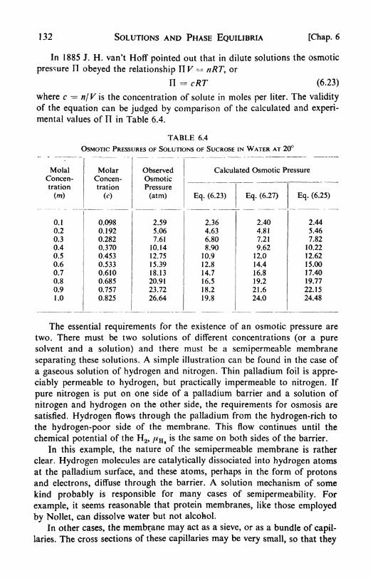
132 SOLUTIONS AND PHASE EQUILIBRIA [Chap. 6
In 1885 J. H. van't Hoff pointed out that in dilute solutions the osmotic
pressure FI obeyed the relationship II V = nRT, or
II = cRT (6.23)
where c = w/Kis the concentration of solute in moles per liter. The validity
of the equation can be judged by comparison of the calculated and experi-
mental values of II in Table 6.4.
TABLE 6.4
OSMOTIC PRESSURES OF SOLUTIONS OF SUCROSE IN WATER AT 20
The essential requirements for the existence of an osmotic pressure are
two. There must be two solutions of different concentrations (or a puresolvent and a solution) and there must be a semipermeable membrane
separating these solutions. A simple illustration can be found in the case of
a gaseous solution of hydrogen and nitrogen. Thin palladium foil is appre-
ciably permeable to hydrogen, but practically impermeable to nitrogen. If
pure nitrogen is put on one side of a palladium barrier and a solution of
nitrogen and hydrogen on the other side, the requirements for osmosis are
satisfied. Hydrogen flows through the palladium from the hydrogen-rich to
the hydrogen-poor side of the membrane. This flow continues until the
chemical potential of the H2 , /%, *s ^e same on both sides of the barrier.
In this example, the nature of the semipermeable membrane is rather
clear. Hydrogen molecules are catalytically dissociated into hydrogen atoms
at the palladium surface, and these atoms, perhaps in the form of protonsand electrons, diffuse through the barrier. A solution mechanism of some
kind probably is responsible for many cases of semipermeability. For
example, it seems reasonable that protein membranes, like those employed
by Nollet, can dissolve water but not alcohol.
In other cases, the membrane may act as a sieve, or as a bundle of capil-
laries. The cross sections of these capillaries may be very small, so that they

Sec. 15] SOLUTIONS AND PHASE EQUILIBRIA 133
can be permeated by small molecules like water, but not by large molecules
like carbohydrates or proteins.
Irrespective of the mechanism by which the semipermeable membrane
operates, the final result is the same. Osmotic flow continues until the
chemical potential of the diffusing component is the same on both sides, of
the barrier. If the flow takes place into a closed volume, the pressure therein
necessarily increases. The final equilibrium osmotic pressure can be cal-
culated by thermodynamic methods. It is the pressure that must be applied
to the solution in order to prevent flow of solvent across the semipermeablemembrane from the pure solvent into the solution. The same effect can be
produced by applying a negative pressure or tension to the pure solvent.
15. Measurement of osmotic pressure. We are principally indebted to two
groups of workers for precise measurements of osmotic pressure: H. N.
Morse, J. C. W. Frazer, and their colleagues at Johns Hopkins, and the
Earl of Berkeley and E. G. J. Hartley at Oxford. 8
CAPILLARYMANOMETERFOR PRESSUREMEASUREMENT
SOLUTION =-_.- -
POROUS CELL-IMPREGNATED
WITHCu2 Fe(CN)6
(o)
APPLIEDPRESSURE
CAPILLARY FORMEASURING FLOWTHROUGH CELL*
PRESSUREGAUGE
SOLUTION' LWATER ^IMPREGNATEDCELL
(b)
Fig. 6.6. Osmotic pressure measurements: (a) method of Frazer;
(b) method of Berkeley and Hartley.
The method used by the Hopkins group is shown in (a), Fig. 6.6. The
porous cell impregnated with copper ferrocyanide is filled with water and
immersed in a vessel containing the aqueous solution. The pressure is
measured by means of an attached manometer. The system is allowed to
stand until there is no further increase in pressure. Then the osmotic pres-
sure is just balanced by the hydrostatic pressure in the column of solution.
The pressures studied extended up to several hundred atmospheres, and a
8 An excellent detailed discussion of this work is to be found in J. C. W. Frazer's
article, 'The Laws of Dilute Solutions'1
in A Treatise on Physical Chemistry, 2nd ed.,
edited by H. S. Taylor (New York: Van Nostrand, 1931), pp. 353-414.

134 SOLUTIONS AND PHASE EQUILIBRIA [Chap. 6
number of ingenious methods of measurement were developed. These
included the calculation of the pressure from the change in the refractive
index of water on compression, and the application of piezoelectric gauges.
The English workers used the apparatus shown schematically in (b),
Fig. 6.6. Instead of waiting for equilibrium to be established and then
reading the pressure, they applied an external pressure to the solution just
sufficient to balance the osmotic pressure. This balance could be made very
precisely by observing the level of liquid in the capillary tube, which would
fall rapidly if there was any flow of solvent into the solution.
16. Osmotic pressure and vapor pressure. Consider a pure solvent A that
is separated from a solution of B in A by a membrane permeable to A alone.
At equilibrium an osmotic pressure FI has developed. The condition for
equilibrium is that the chemical potential of A is the same on both sides of
the membrane, /if // /. Thus the }tA in the solution must equal that of
the pure A. There are two factors tending to make the value of pA in the
solution different from that in pure A. These factors must therefore have
exactly equal and opposite effects on fiA . The first is the change in pA pro-
duced by dilution of A in the solution. This change causes a lowering of pA
equal to A/*=- RT\nP 4/PA [eq. (6.8) with /=/>]. Exactly counteracting
this is the increase in pA in the solution due to the imposed pressure II.
From eq. (6.5) dp PdP, so that A/ J
nVA dP.
At equilibrium, therefore, in order that pA in solution should equal pA
in the pure liquid, J*
1
VA dP -= -RT\n(PA/PA ). If it is assumed that the
partial molar volume VA is independent of pressure, i.e., the solution is
practically incompressible,
PJT =firing (6.24)
The significance of this equation can be stated as follows: the osmotic
pressure is the external pressure that must be applied to the solution to
raise the vapor pressure of solvent A to that of pure A.
In most cases, also, the partial molar volume of solvent in solution VAcan be well approximated by the molar volume of the pure liquid VA . In the
special case of an ideal solution, eq. (6.24) becomes
HVA - -RT\nXA (6.25)
By replacing XA by (1 XB) and expanding as in Section 6-11, the dilute
solution formula is obtained:
HVA = RTXB (6.26)
Since the solution is dilute,
RT nII w -S *< RTm' (6.27)
This is the equation used by Frazer and Morse as a better approximation

Sec. 17] SOLUTIONS AND PHASE EQUILIBRIA 135
than the van't HofT equation (6.23). As the solution becomes very dilute, m'
the volume molal concentration approaches c the molar concentration, and
we find as the end product of the series of approximations
Ft = RTc (6.23)
The adequacy with which eqs. (6.23), (6.25), and (6.27) represent the
experimental data can be judged from the comparisons in Table 6.4.9
17. Deviations from Raoult's Law. Only a very few of the many liquid
solutions that have been investigated follow Raoult's Law over the complete
600
500
EE
u-400(
IDCO
C/>
(T
a 200
100
400
320
240
160
80
f).0 .2 .4 .6 .8
CH2(OCH3)2 MOLE FRACTION CSa
(a)
1.0 ^0 .2 A .6 .8
CS 2 (CH 3 )2CO MOLE FRACTION CHC13 CH Cl*
(b)
Fig. 6.7. (a) Positive deviation from Raoult's Law the PX diagram of carbon
bisulfide-methylal system, (b) Negative deviation from Raould's Law the PXdiagram of chloroform-acetone system.
range of concentrations. It is for this reason that the greatest practical
application of the ideal equations is made in the treatment of dilute solutions,
in which the solvent obeys Raoult's Law and the solute obeys Henry's Law.
Nevertheless, one of the most instructive ways of qualitatively discussing
the properties of nonideal solutions is in terms of their deviations from
ideality. The first extensive series of vapor-pressure measurements, per-
mitting such comparisons, were those made by Jan von Zawidski, around
1900.
Two general types of deviation were distinguished. An example exhibiting
a positive deviation from Raoult's Law is the system carbon bisulfide-
methylal, whose vapor-pressure-composition diagram is shown in (a),
Fig. 6.7. An ideal solution would follow the dashed lines. The positive9 The osmotic pressures of solutions of high polymers and proteins provide some of the
best data on their thermodynamic properties. A typical investigation is that of Shick, Doty,and Zimm, /. Am. Chetn. Soc., 72, 530 (1950).
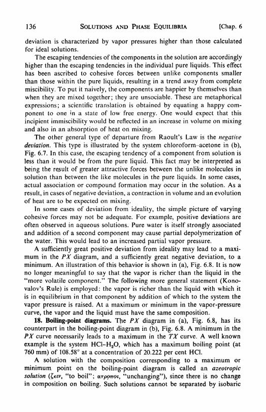
136 SOLUTIONS AND PHASE EQUILIBRIA [Chap. 6
deviation is characterized by vapor pressures higher than those calculated
for ideal solutions.
The escaping tendencies of the components in the solution are accordingly
higher than the escaping tendencies in the individual pure liquids. This effect
has been ascribed to cohesive forces between unlike components smaller
than those within the pure liquids, resulting in a trend away from complete
miscibility. To put it naively, the components are happier by themselves than
when they are mixed together; they are unsociable. These are metaphorical
expressions; a scientific translation is obtained by equating a happy com-
ponent to one in a state of low free energy. One would expect that this
incipient immiscibility would be reflected in an increase in volume on mixingand also in an absorption of heat on mixing.
The other general type of departure from Raoult's Law is the negative
deviation. This type is illustrated by the system chloroform-acetone in (b),
Fig. 6.7. In this case, the escaping tendency of a component from solution is
less than it would be from the pure liquid. This fact may be interpreted as
being the result of greater attractive forces between the unlike molecules in
solution than between the like molecules in the pure liquids. In some cases,
actual association or compound formation may occur in the solution. As a
result, in cases of negative deviation, a contraction in volume and an evolution
of heat are to be expected on mixing.In some cases of deviation from ideality, the simple picture of varying
cohesive forces may not be adequate. For example, positive deviations are
often observed in aqueous solutions. Pure water is itself strongly associated
and addition of a second component may cause partial depolymerization of
the water. This would lead to an increased partial vapor pressure.
A sufficiently great positive deviation from ideality may lead to a maxi-
mum in the PX diagram, and a sufficiently great negative deviation, to a
minimum. An illustration of this behavior is shown in (a), Fig. 6.8. It is nowno longer meaningful to say that the vapor is richer than the liquid in the
"more volatile component." The following more general statement (Kono-valov's Rule) is employed: the vapor is richer than the liquid with which it
is in equilibrium in that component by addition of which to the system the
vapor pressure is raised. At a maximum or minimum in the vapor-pressure
curve, the vapor and the liquid must have the same composition.18. Boiling-point diagrams. The PX diagram in (a), Fig. 6.8, has its
counterpart in the boiling-point diagram in (b), Fig. 6.8. A minimum in the
PX curve necessarily leads to a maximum in the TX curve. A well known
example is the system HC1-H2O, which has a maximum boiling point (at
760 mm) of 108.58 at a concentration of 20.222 per cent HC1.
A solution with the composition corresponding to a maximum or
minimum point on the boiling-point diagram is called an azeotropicsolution (c>, "to boil"; arppTros, "unchanging"), since there is no changein composition on boiling. Such solutions cannot be separated by isobaric

Sec. 19] SOLUTIONS AND PHASE EQUILIBRIA 137
distillation. It was, in fact, thought at one time that they were real chemical
compounds, but changing the pressure changes the composition of the
azeotropic solution.
The distillation of a system with a maximum boiling point can be dis-
cussed by reference to (b), Fig. 6.8. If the temperature of a solution havingthe composition / is raised, it begins to boil at the temperature tv The first
vapor that distills has the composition y, richer in component A than is the
original liquid. The residual solution therefore becomes richer in B; and if
the vapor is continuously removed the boiling point of the residue rises, as
LIQUID
VAPOR
VAPOR
LIQUID
X
(a)
A v IX
(b)
I' B
Fig. 6.8. Large negative deviation from Raoult's Law. The PXcurve has a minimum; the TX curve has a maximum.
its composition moves along the liquidus curve from / toward m. If a frac-
tional distillation is carried out, a final separation into pure A and the
azeotropic solution is achieved. Similarly a solution of original composition/' can be separated into pure B and azeotrope.
19. Partial miscibility. If the positive deviations from Raoult's Lawbecome sufficiently large, the components may no longer form a continuous
series of solutions. As successive portions of one component are added to
the other, a limiting solubility is finally reached, beyond which two distinct
liquid phases are formed. Usually, but not always, increasing temperaturetends to promote solubility, as the thermal kinetic energy conquers the
reluctance of the components to mix freely. In otjier words, the T AS term
in AF = A// T AS* becomes more important. A solution that displays a
large positive deviation from ideality at elevated temperatures therefore
frequently splits into two phases when it is cooled.
A PC diagram for a partially miscible liquid system, such as aniline and
water, is shown in (a), Fig. 6.9. The point x lies in the two-phase region and
corresponds to a system of two liquid solutions, one a dilute solution of
aniline in water having the composition y, and the other a dilute solution of
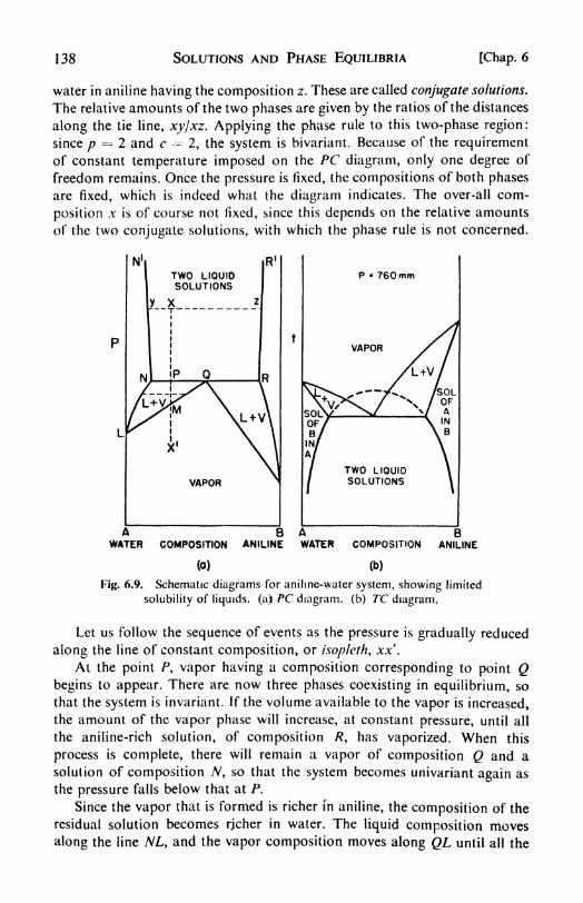
138 SOLUTIONS AND PHASE EQUILIBRIA [Chap. 6
water in aniline having the composition z. These are called conjugate solutions.
The relative amounts of the two phases are given by the ratios of the distances
along the tie line, xy/xz. Applying the phase rule to this two-phase region:
since p 2 and c -- 2, the system is bivariant. Because of the requirement
of constant temperature imposed on the PC diagram, only one degree of
freedom remains. Once the pressure is fixed, the compositions of both phases
are fixed, which is indeed what the diagram indicates. The over-all com-
position x is of course not fixed, since this depends on the relative amounts
of the two conjugate solutions, with which the phase rule is not concerned.
P 760mm
VAPOR
VAPOR
A B AWATER COMPOSITION ANILINE WATER
BCOMPOSITION ANILINE
(a) (b)
Fig. 6.9. Schematic diagrams for aniline-water system, showing limited
solubility of liquids, (a) PC diagram, (b) TC diagram.
Let us follow the sequence of events as the pressure is gradually reduced
along the line of constant composition, or isopleth, xx',
At the point P, vapor having a composition corresponding to point Qbegins to appear. There are now three phases coexisting in equilibrium, so
that the system is invariant. If the volume available to the vapor is increased,
the amount of the vapor phase will increase, at constant pressure, until all
the aniline-rich solution, of composition /?, has vaporized. When this
process is complete, there will remain a vapor of composition Q and a
solution of composition N9so that the system becomes univariant again as
the pressure falls below that at P.
Since the vapor that is formed is richer in aniline, the composition of the
residual solution becomes rjcher in water. The liquid composition moves
along the line NL, and the vapor composition moves along QL until all the

Sec. 20] SOLUTIONS AND PHASE EQUILIBRIA 139
liquid has been transformed into vapor, at the point M. After this, further
decrease in pressure proceeds at constant vapor composition along MX' .
It may be noted that the two conjugate solutions N and R have the same
total vapor pressure and the same vapor composition. It follows that the
partial" vapor pressure of component A above a dilute solution of A in B is
the same as the vapor pressure of A above the dilute solution of B in A. For
example, if benzene and water are mixed at 25C, two immiscible layers are
formed, one containing 0.09 per cent C6H 6 and 99.91 per cent H2O, the other
99.81 per cent C6H6 and 0.19 per cent H2O. The partial pressure of benzene
above either of these solutions is the
same, namely 85 mm.In (a), Fig. 6.9, the lines NN' and
RR' are almost vertical, since the
solubility limits are only slightly de-
pendent on pressure. Change in tem-
perature, on the other hand, maygreatly affect the mutual solubility of
two liquids. In (b), Fig. 6.9, the TC
diagram for the water-aniline system is
drawn for the constant pressure of
one atmosphere (normal-boiling-point
diagram). Increasing the temperaturetends to close the solubilitv gap, the
difference between the concentrations
of the two conjugate solutions.
The interpretation of the solubility gap can be given in terms of the free
energy of the system. At some constant temperature, let us plot the molar
free energy of the system, defined as F =-- F/(nA -f- nB ), against the mole
fraction of B, XB , for both the a and ft phases. In Fig. 6.9b, for example,these phases would be the two immiscible liquid solutions. The diagramobtained, Fig. 6.10, is an exact analog of Fig. 6.1, which was used for the
determination of partial molar volumes. In this case, the intercept of the
common tangent to the two F vs. X curves gives the value of the partial
molar free energies, or chemical potentials, of the two components. At this
composition, therefore, /// = /^/, and// yy
a/y f/, i.e., the condition for
equilibrium of components A and B between the two phases is fulfilled. The
corresponding mole fractions represent the phase-boundary compositions;at any composition between X'B and X"B ,
the system will split into two
distinct phases, since in this way it can reach its minimum free energy. For
XB < X'B , however, pure phase a gives the lowest free energy, and for
XB > X"B , pure phase ft.
20. Condensed-liquid systems. In (b), Fig. 6.9, the variation of solubility
with temperature is shown for only one pressure. At high enough tempera-tures boiling occurs, and it is therefore not possible to trace the ultimate
Fig. 6.10. Partial miscibility deter-
mined by free energy.

140 SOLUTIONS AND PHASE EQUILIBRIA [Chap. 6
course of the solubility curves. One might expect that the solubility gapwould close completely if a high enough temperature could be reached
before the onset of boiling. This expectation is represented by the dashed line
in (b), Fig. 6.9.
A number of condensed systems have been studied, which illustrate com-
plete liquid-liquid solubility curves. A classical example is the phenol-water
system of Fig. 6.11 (a). At the temperature and composition indicated bythe point x, two phases coexist, the conjugate solutions represented by y and
Fig. 6.11. Partial miscibility of two liquids, (a) phenol-water system,
(b) tnethylamine-water system, (c) nicotine-water system.
z. The relative amounts of the two phases are proportional, as usual, to the
segments of the tie line.
As the temperature is increased along the isopleth XX \ the amountof the phenol-rich phase decreases and the amount of water-rich phaseincreases.
Finally at Y the compositions of the two phases become identical,
the phenol-rich phase disappears completely, and at temperatures above Ythere is only one solution.
This gradual disappearance of one solution is characteristic of systems
having all compositions except one. The exception is the composition corre-
sponding to the maximum in the TC curve. This composition is called the
critical composition and the temperature at the maximum is the critical
solution temperature or upper consolute temperature. If a two-phase system
having the critical composition is gradually heated [line CC in (a), Fig. 6.11]
there is no gradual disappearance of one phase. Even in the immediate
neighborhood of the maximum d, the ratio of the segments of the tie line
remains practically constant. The compositions of the two conjugate solu-
tions gradually approach each other, until, at the point d, the boundary line
between the two phases suddenly disappears and a single-phase systemremains.

Sec. 21] SOLUTIONS AND PHASE EQUILIBRIA 141
As the critical temperature is slowly approached from above, a most
curious phenomenon is observed. Just before the single homogeneous phase
passes over into two distinct phases, the solution is diffused by a pearly
opalescence. This critical opalescence is believed to be caused by the scatter-
ing of light from small regions of slightly differing density, which are formed
in the liquid in the incipient separation of the two phases.
Strangely enough, some systems exhibit a lower consolute temperature.At high temperatures, two partially miscible solutions are present, which
become completely intersoluble when sufficiently cooled. An example is the
triethylamine-water system in (b), Fig. 6.11, with a lower consolute tem-
perature of 18.5 at 1 atm pressure. It is almost impossible to locate the
critical composition exactly, since lowering the temperature a fraction of a
degree greatly increases the solubility. This somewhat weird behavior suggests
that large negative deviations from Raoult's Law (e.g., compound formation)
become sufficient at the lower temperatures to counteract the positive
deviations responsible for the immiscibility.
Finally, systems have been found with both upper and lower consolute
temperatures. These are most common at elevated pressures, and indeed
one would expect all systems with a lower consolute temperature to displayan upper one at sufficiently high temperature and pressure. An atmospheric-
pressure example is the nicotine-water system of Fig. 6.11 (c). Havingcome to solutions of this type, we have run the gamut of deviations from
ideality.
21. Thermodynamics of nonideal solutions: the activity. A complete
thermodynamic description of a solution, except for its amount, can be
expressed in terms of the temperature, the pressure, and the chemical poten-tials of the various components. All the other thermodynamic functions can
be derived from these.
For a single pure ideal gas, the change in chemical potential is given from
eq. (4.33) as dp RTdln P. By integration we obtain ^ = // + RT In P,
where ju is the chemical potential of the gas at one atmosphere pressure.
For a pure gas, this equation is identical with F F + RTlnP, where Fis the free energy per mole.
If the gas is not ideal, the fugacity is defined by the equation ft=
JLL +RTlnf. Such an equation holds also for any component in a mixture of gases
(gaseous solution). The constant p is a function of temperature alone. It is
the chemical potential of the gas in its standard state of unit fugacity, or the
standard free energy of the gas.
The same equation is valid for a component in a liquid or solid solution,
since at equilibrium the chemical potential must be the same in the con-
densed phase as in the vapor. For a component A,
(6.8)
If the vapor above the solution can be considered to behave as an ideal

142 SOLUTIONS AND PHASE EQUILIBRIA [Chap. 6
gas, fA PA ,and
/LIA /tA + RTinPA . For an ideal solution, PA =XA/A = XAPA> and therefore
(6.28)nXA
The two constant terms can be combined, giving
P.i= 1% + *T\n XA (6.29)
This is the expression for the chemical potential in an ideal solution, pA
being the chemical potential of A when XA - \; i.e., of pure liquid A. It
should be clearly understood that p,A is a function of both temperatureand pressure, in contrast with JUA in eq. (6.8). This is because the vapor
pressure of the pure liquid, PA in eq. (6.28), is a function of both temperatureand over-all pressure (p. 107).
In the discussion of nonideal solutions we can always use the chemical
potential, obtained from eq. (6.8) in terms of the partial vapor pressure or
fugacity. Sometimes, however, it is convenient to introduce a new function,
the activity a, which was invented by G. N. Lewis. It is defined as follows
so as to preserve the form of eq. (6.29),
pA-
fiA 4 RTlnaA (6.30)
or P^ I-
where y a/X is called the activity coefficient.
One advantage of the activity coefficient is that it indicates at a glancethe magnitude of the deviation from ideality in the solution. In terms of the
activity, Raoult's Law becomes simply a = X, or y = 1 .
Comparing eq. (6.30) with eqs. (6.28) and (6.8), we find that
*A -4 (6.31)J A
The activity is accordingly the ratio of the fugacity to the fugacity in the
standard state. We have implicitly taken this standard state to be pure A,
but other definitions might have been used. For a gas/J = 1 and therefore
aA ~fA , the activity equals the fugacity.
Equation (6.31) provides the most direct method of determining the
activity of a component in a solution. It is usually sufficiently accurate to
ignore gas imperfections and set the fugacity ratio equal to the vapor pressure
ratio, so that aA = PA/PA .
Some activities calculated in this way from vapor-pressure data are
collected in Table 6.5. Once the activity of one component has been obtained
as a function of concentration, the activity of the other component in
a binary solution can be calpulated from the Gibbs-Duhem equation.

Sec. 22] SOLUTIONS AND PHASE EQUILIBRIA 143
TABLE 6.5
ACTIVITIES OF WATER AND SUCROSE IN THEIR SOLUTIONS AT 50C OBTAINED FROMVAPOR PRESSURE LOWERING AND THE GIBBS-DUHEM EQUATION
Corresponding with eq. (6.4) for the partial molar volumes, we have for the
partial molar free energies or chemical potentials,
d/lA ^ -
nA
From eq. (6.30), d\n aA --= d In a,,
If aB is known as a function of XJ}9 aA can be obtained by a graphical
integration.
Activities can also be calculated from any of the colligative propertiesrelated to the vapor pressure. The details of these calculations are to be
found in various treatises on thermodynamics.10
22. Chemical equilibria in nonideal solutions. The activity function defined
in eq. (6.30) is useful in discussing the equilibrium constants of reactions in
solution. It is readily proved (cf. p. 76) that for the schematic reaction
aA + bB^cC + dD
aS a r(6.32)
and A/*- RTln Ka
In terms of activity coefficients and mole fractions,
"a A. a A. & y a y b -~r"x7A 7s AA A B
In an ideal solution, all the activity coefficients become equal to unity,
10 G. N. Lewis and M. Randall, Thermodynamics and Free Energy of Chemical Sub-stances (New York: McGraw-Hill, 1923), p. 278.

144 SOLUTIONS AND PHASE EQUILIBRIA [Chap. 6
and the equilibrium constant is simply Kx . Extensive data on the activity
coefficients of components in solutions of nonelectrolytes are not available,
and the most important applications of eq. (6.32) have been made in electro-
lytic solutions, which will be discussed in Chapter 15.
23. Gas-solid equilibria. The varieties of heterogeneous equilibrium that
have been considered so far have almost all been chosen from systems
involving liquid and vapor phases only. Some systems of the solid-vapor and
solid-liquid types will now be described. Most of the examples will be chosen
200
160
160
140
: 120
=JOO
60
60
40
20
SATURATEDSOLUTION *CuS04 -5H20t VAPOR
CuS04 '5l
CuS04-3H2 '
+ 2H2
100
90
80
70
60
>40
30
20
10
20 30 40 50 60 70 80 90 KX) 110 120
t,c
(0)
t -50*C
CuS04 3H2
GuS04 + H2- H212345
MOLES H20/MOLE CuS04IN SOLID
(b)
Fig. 6.12. The system CuSO4~H 2O.
from two-component systems, with only a brief introduction to three-
component phase diagrams.A two-component gas-solid system in which there is no appreciable
solid-solution formation is exemplified by: CaCO3 ^ CaO f CO2 . Since
c 2, the degrees of freedom are/^ 4 p. If the two solid phases are
present, together with the gaseous phase CO2 , the system is univariant,
/=4 3=1. At a given temperature, the pressure of CO2 has a fixed
value. For example, if CO2 is admitted to a sample of CaO at 700C, there
is no absorption of gas until a pressure of 25 mm is reached; then the CaOtakes up CO2 at constant pressure until it is completely converted into
CaCO3 , whereupon further addition of CO2 again results in an increase in
pressure.
The pressure-temperature diagram for such a system is therefore similar
to the vapor-pressure curve of a pure liquid or solid. The CO2 pressure has
been loosely called the "dissociation pressure of CaCO3." Since the pressurehas a definite value only when the vapor phase is in equilibrium with both
solid phases, it is really necessary to speak of the "dissociation pressure in
the system CaCO3-CaO-CO2."

Sec. 24] SOLUTIONS AND PHASE EQUILIBRIA 145
The necessity of specifying both the solid phases is to be emphasized in
systems formed by various salts, their hydrates, and water vapor. The case
of copper sulfate-water is shown in (a), Fig. 6.12, on a PT diagram, and in
(b), Fig. 6.12, on a PC diagram. As long as only the two phases are present,
a salt hydrate can exist in equilibrium with water vapor at any temperatureif the pressure of water vapor is (1) above the dissociation pressure to lower
hydrate or anhydrous salt and (2) below the dissociation pressure of the
next higher hydrate or the vapor pressure of the saturated solution. State-
ments in the older literature that a given hydrate "loses water at 1 10C" are
devoid of precise meaning.When the pressure of water vapor falls below the dissociation pressure
for the system, efflorescence occurs, as the hydrate loses water and its surface
becomes covered with a layer of lower hydrate or anhydrous salt. When the
vapor pressure exceeds that of the saturated aqueous solution, deliquescence
occurs, and the surface of hydrate becomes covered with a layer of saturated
solution.
24. Equilibrium constant in solid-gas reactions. The equilibrium constant
for a reaction involving solid phases can be discussed conveniently by con-
sidering a typical reaction of this kind, the reduction of zinc oxide by carbon
monoxide, ZnO (s) f CO -> Zn (g) + CO2 .
The equilibrium constant in terms of activities can be written as follows:
Ka= gzn*C(\ AF - -RTln Ka (6.33)
The activity is the ratio of the fugacity under the experimental conditions to
the fugacity in a standard state, fAlf^ The standard state of a pure solid
component is taken to be its state as a pure solid at one atmosphere pressure.
The fugacity of the solid varies so slightly with pressure that over a con-
siderable range of pressure, fAlf% for a solid is effectively a constant equalto unity. Making this very good approximation, the expression in eq. (6.33)
becomes
aco /co
If the gases are considered to be ideal the activity ratio equals the partial
pressure ratio, and K9= /WW^co-
This discussion leads to the following general rule: no terms involving
pure solid or liquid components need be included in equilibrium constants
for solid-gas or liquid-gas reactions, unless very high precision is required,in which case there may be a small pressure correction to Kv or Kf .
Equilibrium data for the reduction of zinc oxide are given in Table 6.6.
25. Solid-liquid equilibria: simple eutectic diagrams. For two-component
solid-liquid equilibria in which the liquids are completely intersoluble in all
proportions and there is no appreciable solids-solid solubility, the simple

146 SOLUTIONS AND PHASE EQUILIBRIA [Chap. 6
TABLE 6.6
THE EQUILIBRIUM ZnO -f CO ^ Zn h CO2 (TOTAL PRESSURE = 760 MM)
diagram of Fig. 6.13 is obtained. Examples of systems of this type are
collected in Table 6.7.
TABLE 6.7
SYSTEMS WITH SIMPLE EUTECTIC DIAGRAMS SUCH AS FIG. 6.13
Consider the behavior of a solution of composition X on cooling alongthe isopleth XX' . When point P is reached, pure solid A begins to separatefrom the solution. As a result, the residual solution becomes richer in the
other component B, its composition falling along the line PE. At any point
Q in the two-phase region, the relative amounts of pure A and residual
solution are given as usual by the ratio of the tie-line segments. When pointR is reached, the residual solution has the eutectic composition E. Further
cooling now results in the simultaneous precipitation of a mixture of A andB in relative amounts corresponding to E.
The eutectic point is an invariant point on a constant pressure diagram;since three phases are in equilibrium,/^ c p + 2 = 2 --/? + 2 --= 4
3=1, and the single degree of freedom is used by the choice of the constant-
pressure condition.

Sec. 26] SOLUTIONS AND PHASE EQUILIBRIA 147
Microscopic examination of alloys often reveals a structure indicatingthat they have been formed from a melt by a cooling process similar to that
considered along the isopleth XX' of
Fig. 6.13. Crystallites of pure metal
are found dispersed in a matrix of
finely divided eutectic mixture. An
example taken from the antimony-lead system is shown in the photo-
micrograph of Fig. 6.14.
26. Cooling curves. The methodof cooling curves is one of the most
useful for the experimental study of
solid-liquid systems. A two-compo-nent system is heated until a homo-
geneous melt is obtained. A thermo-
couple, or other convenient device
for temperature measurement, is
- PER CENT B -
Fig. 6.13. Simple eutectic diagram for
two components, A and B, completely inter-
soluble as liquids but with negligible solid-
solid solubility.
immersed in the liquid, which is keptin a fairly well insulated container.
As the system slowly cools, the
temperature is recorded at regular time intervals. Examples of such curves
for the system shown in Fig. 6.13 are drawn in Fig. 6.15.
The curve a for pure A exhibits a gradual decline until the melting point
of A is reached. It then remains perfectly flat as long as solid and liquid A
Fig. 6.14. Photomicrograph at 50X of 80 per cent Pb-20 per cent Sb,
showing crystals of Sb in a eutectic matrix. (Courtesy Professor Arthur
Phillips, Yale University.)
are both present, and resumes its decline only after all the liquid has solidified.
The curve for cooling along the isopleth XX' is shown in b. The decline as
the homogeneous melt is cooled becomes suddenly less steep when the tem-
perature is reached corresponding to point P, where the first solid begins to

148 SOLUTIONS AND PHASE EQUILIBRIA [Chap. 6
separate from the solution. This change of slope is a consequence of the
liberation of latent heat of fusion during the solidification of A. The more
gradual decline continues until the eutectic temperature is reached. Thenthe cooling curve becomes absolutely flat. This is because the eutectic pointin a two-component system, just as the melting point of one component, is
an invariant point at constant over-all pressure. If the composition of the
COMPOSITION
ALONG \EUTECTIC\COMPOSITION
(0)
TIME
Fig. 6.15. Cooling curves for various compositions on the simple eutectic
diagram of Fig. 6.13.
system chosen initially happened to be the same as that of the eutectic, the
cooling curve would be that drawn in c.
The duration of the constant-temperature period at the eutectic tempera-ture is called the eutectic halt. This halt is a maximum for a melt having the
eutectic composition.Each cooling curve determination yields one point on the TC diagram
(point of initial break in slope) in addition to a value for the eutectic tempera-ture. By these methods, the entire diagram can be constructed.
27. Compound formation. If aniline and phenol are melted together in
equimolar proportions, a definite compound crystallizes on cooling,C6H5OH-C6H5NH2 . Pure phenol melts at 40C, pure aniline at -6.1C,and the compound melts at 3lC. The complete TC diagram for this system,in Fig. 6.16, is typical of many instances in which stable compounds occur
as solid phases. The most convenient way of looking at such a diagramis to imagine it to be made up of two diagrams of the simple eutectic
type placed side by side. In this case, one such diagram would be the
phenol-compound diagram, and the other the aniline-compound diagram.The phases corresponding with the various regions of the diagram are
labeled.
A maximum such as the point C is said to indicate the formation of a

Sec. 28] SOLUTIONS AND PHASE EQUILIBRIA 149
compound with a congruent melting point, since if a solid having the com-
position C6H5OH-C6H5NH2 is heated to 31C, it melts to a liquid of identical
composition. Compounds with congruent melting points are readily detected-
o
UJ<
S 1liJ
40
30
20
Olr'0
-10
-20,
(b)
rSOLID PHENOL[
+ SOLUTION
SOLID COMPOUNDSOLUTIONJ
SOLID PHENOL+
SOLID COMPOUND
SOLUTION
SOLID ANILINE+
SOLID COMPOUND.1 .2 .3 4 .5 .6 .7 .8 .9 1.0
CgHsOH MOLE FRACTION ANILINE C6 H5NH2
(0)
Fig. 6.16. The system phenol-aniline.
by the cooling-curve method. A liquid having the composition of the com-
pound exhibits no eutectic halt, behaving in every respect like a single pure
component.28. Solid compounds with incongruent melting points. In some systems,
solid compounds are formed that do not melt to a liquid having the same
composition, but instead decompose before such a melting point is reached.
An example is the silica-alumina system (Fig. 6.17), which includes a com-
pound, 3Al2O3-SiO2 , called mul/ite.
If a melt containing 40 per cent A12O3 is prepared and cooled slowly,
solid mullite begins to separate at about 1780C. If some of this solid com-
pound is removed and reheated along the line XX', it decomposes at 1800Cinto solid corundum and a liquid solution (melt) having the composition P.
Thus: 3Al2O3-SiO2-* A12O3 + solution. Such a change is called incongruent
melting, since the composition of the liquid differs from that of the solid.
The point P is called the incongruent melting point or the peritectic point
(rrjKTo*, "melting"; TTC/M, "around"). The suitability of this name becomes
evident if one follows the course of events as a solution with composition3Al2O3-SiO2 is gradually cooled along XX' . When the point M is reached,

150 SOLUTIONS AND PHASE EQUILIBRIA [Chap. 6
solid corundum (A12O3) begins to separate from the melt, whose com-
position therefore becomes richer in SiO2 , falling along the line MP. When
the temperature falls below that of the peritectic at />, the following change
occurs: liquid + corundum --> mullite. The solid A12O3 that has separated
2100
60 3A1203 80 100Si02 A\203
w PER CENT A1203
Fig. 6.17. System displaying peritectic.
reacts with the surrounding melt to form the compound mullite. If a specimentaken at a point such as Q is examined, the solid material is found to consist
of two phases, a core of corundum surrounded by a coating of mullite. It
was from this characteristic appearance that the term "peritectic" originated.
29. Solid solutions. Solid solutions are in theory no different from other
kinds of solution: they are simply solid phases containing more than one
1500
1452
I00010 20 30 4p 50 60 70 80 90 100
Cu wt PER CENT NICKEL Ni
Fig. 6.18. The copper-nickel system a continuous series of solid
solutions.
component. The phase rule makes no distinction between the kind of phase
(gas, liquid, or solid) that occurs, being concerned only with how many

Sec. 33] SOLUTIONS AND PHASE EQUILIBRIA 155
pure tin melts at 232C and pure bismuth at 268C, their eutectic being at
133C and 42 per cent Sn. The Sn-Bi eutectic temperature is lowered by the
addition of lead to a minimum at 96C and a composition of 32 per cent Pb,
16 per cent Sn, 52 per cent Bi. This is the ternary eutectic point.
Pb Pb
Sn Bi Sn
SOLID Pb+ SOLUTION
SOLID Pb ^L+ SOLIDSn Pb /-SOLID Pb
+ SOLUTIONSOLUTION
325 a 315
(0) (b)
SOLID Pb +SOLID S
SOLUTION
182 133
(0 (d)
SOLID Pb 4- SOLUTION
SOLID Pb + SOLID Bi
SOLUTION
Bi
Fig. 6.22. The system Pb-Sn-Bi : three-dimensional diagram and iso-
thermal sections.
Without using a solid model, the behavior of this system is best illustrated
by a series of isothermal sections, shown in Fig. 6.22. Above 325C (a), the
melting point of pure lead, there is a single liquid solution. At around 315C(b) the system consists of solid Pb and solution. The section at 182C (c)
indicates the binary eutectic of Sn and Pb. Below this temperature, solid Pband solid Sn both separate from the solution. At 133C the binary eutectic
between Sn and Bi is reached (d). Finally, in (e) at 100C there is shown a
section slightly above the ternary eutectic.
The subject of ternary diagrams is an extended and very important one,
and only a few of the introductory aspects have been mentioned. For further
details some of the special treatises that are available should be consulted. 11
11J. S. Marsh, Principles ofPhase Diagrams (New York: McGraw-Hill, 1935); G. Mas-
sing, Introduction to the Theory of Three Component-Systems (New York: Reinhold, 1944).

156 SOLUTIONS AND PHASE EQUILIBRIA [Chap. 6
PROBLEMS
1. Solutions are prepared at 25C containing 1000 g of water and n moles
of NaCl. The volume is found to vary with n as V =- 1001.38 + 16.6253 +1.7738 3/2 + 0.1194fl2
. Draw a graph showing the partial molar volumes
of H2O and NaCl in the solution as a function of the molality from to 2
molal.
2. In the International Critical Tables (vol. Ill, p. 58) there is an extensive
table of densities of HNO3 H2O solutions. Use these data to calculate, bythe graphical method of Fig. 6.1, the partial molar volumes of H2O and
HNO3 in 10, 20, 30, and 40 per cent solutions at 25.
3. When 2 g of nonvolatile hydrocarbon containing 94.4 per cent C is
dissolved in 100 g benzene, the vapor pressure of benzene at 20C is lowered
from 74.66 mm to 74.01 mm. Calculate the empirical formula of the hydro-carbon.
4. Pure water is saturated with a 2 : 1 mixture of hydrogen and oxygenat a total pressure of 5 atm. The water is then boiled to remove all the gases.
Calculate the per cent composition of the gases driven off (after drying). Use
data from Table 6.2.
5. Water and nitrobenzene can be considered to be immiscible liquids.
Their vapor pressures are: H 2O, 92.5mm at 50C; 760mm at 100C;C6H5NO2 ,
22.4 mm at 10QC; 148 mm at 150C. Estimate the boiling pointof a mixture of water and nitrobenzene at 1 atm pressure. In a steam dis-
tillation at 1 atm how many grams of steam would be condensed to obtain
one gram of nitrobenzene in the distillate?
6. The following data were obtained for the boiling points at 1 atm of
solutions of CC14 in C2C1 4 :
Mole fraction
CCI4 inliq. . 0.000 0.100 0.200 0.400 0.600 0.800 1.000
Mole fraction
CCI 4 invap. . 0.000 0.469 0.670 0.861 0.918 0.958 1.000
Boiling pointC . . 120.8 108.5 100.8 89.3 83.5 79.9 76.9
If half of a solution 30 mole per cent in CC14 is distilled, what is the com-
position of the distillate? If a solution 50 mole per cent in CC14
is distilled
until the residue is 20 mole per cent CC14 , what is approximate compositionof the distillate?
7. A compound insoluble in water is steam distilled at 97.0C, the dis-
tillate containing 68 wt. per cent H2O. The vapor pressure of water is 682 mmat 97. What is the molecular weight of the compound?
8. When hexaphenylethane is dissolved in benzene, the f.pt. depressionof a 2 per cent solution is 0.219C; the b.pt. elevation is 0.135. Calculate
the heat of dissociation of hexaphenylethane into triphenylmethyl radicals.
Chap. 6] SOLUTIONS AND PHASE EQUILIBRIA 1 57
9. Calculate the weight of (a) methanol, (b) ethylene glycol which, when
dissolved in 4.0 liters of water, would just prevent the formation of ice at
-10C.
10. The solubility of picric acid in benzene is:
/, C . . 5 10 15 20 25 3t
g/100gC6H6 . 3.70 5.37 7.29 9.56 12.66 21.38
The melting points of benzene and picric acid are 5.5 and 121.8C. Calculate
the heat of fusion of picric acid.
11. The osmotic pressure at 25C of a solution of /Mactoglobulin con-
taining 1.346 g protein per 100 cc solution was found to be 9.91 cm of water.
Estimate the molecular weight of the protein.
12. For the ideal solutions of ethylene bromide and propylenc bromide
(p. 124), draw a curve showing how the mole fraction of C2H4Br2 in the
vapor varies with that in the liquid. Use this curve to estimate the number
of theoretical plates required in a column in order to yield a distillate with
mole fraction of C2H 4 Br2 0.9 from a solution of mole fraction 0. 1 . Assumetotal reflux.
13. Calculate the distribution coefficient K for piperidine between water
and benzene at 20C, given :
g solute/ 1 00 cc water layer . . 0.635 1.023 1.635 2.694
g solute/100 cc benzene layer . . 0.550 0.898 1.450 2.325
14. A solution of 3.795 g sulfur in 100 g carbon bisulfide (b.pt. CS2
46.30C; A//vap= 6400 cal per mole) boils at 46.66C. What is the formula
of the sulfur molecule in the solution?
15. The melting points and heats of fusion of 0, /?,m dinitrobenzenes are:
116.9, 173.5, 89.8, and 3905, 3345, 4280 cal per mole [Johnston, J. Phys.
Chem., 29, 882, 1041 (1925)]. Assuming the ideal solubility law, calculate the
ternary eutectic temperature and composition for mixtures of o, m, p com-
pounds.
16. The following boiling points are obtained for solutions of oxygen and
nitrogen at 1 atm:
b.pt., K . . 77.3 78.0 79.0 80.0 82.0 84.0 86.0 88.0 90.1
Mole % O inliq.
. 8.1 21.6 33.4 52.2 66.2 77.8 88.5 100
Mole%Oinvap. 2.2 6.8 12.0 23.6 36.9 52.2 69.6 100
Draw the TX diagram. If 90 per cent of a mixture containing 20 per cent O2
and 80 per cent N2 is distilled, what will be the composition of the residual
liquid and its b.pt. ? Plot an activity a vs. mole fraction X diagram from the
data.
17. For a two-component system (A, B) show that:

158 SOLUTIONS AND PHASE EQUILIBRIA [Chap. 6
18. Redder and Barratt [/. Chem. Soc., 537 (1933)] measured the vapor
pressures of potassium amalgams at 387.5C, at which temperature the vapor
pressure of K is 3.25 mm, of Hg 1280 mm.
Mole % K inliq.
. 41.1 46.8 50.0 56.1 63.0 72.0
PofHg, mm . 31.87 17.30 13.00 9.11 6.53 3.70
PofK, mm . 0.348 0.68 1.07 1.69 2.26 2.95
Calculate the activity coefficients of K and Hg in the amalgams and plot
them vs. the composition in the range studied.
19. The equilibrium pressures for the system CaSO4-2 H2O = CaSO4 +2 H2O, and the vapor pressures of pure water, at various temperatures are:
/, C 50 55 60 65
CaSO4 system, mm . .80 109 149 204
H 2O, mm .... 92 118 149 188
The solubility of CaSO4 in water is so low that the vapor pressure of the
saturated solution can be taken to equal that of pure water.
(a) State what happens on heating the dihydrate in a previously evacu-
ated sealed tube from 50 to 65C. (b) What solid phase separates when a
solution of CaSO4 is evaporated at 65, at 55C? (c) What solid phase
separates on evaporating at 55 if, when the solution becomes saturated,
enough CaCl2 is added to reduce its v.p. by 10 per cent?
20. Data for the Au-Te system:
wt. % Te 10 20 30 40 42 50 56.4 60 70 82.5 90 100
f.pt., C 1063 940 855 710 480 447 458 464 460 448 416 425 453
Sketch the phase diagram. Label all regions carefully. Describe what happenswhen a melt containing 50 per cent Te is cooled slowly.
21. The dissociation pressure of galactose monohydrate is given by
Iog10 />(mrn)- 7.04 - 1780/7. Calculate AF, A//, AS , at 25C for the
dissociation.
22. The solubility of glycine in liquid ammonia was found to be:
Moles per liter . . . 0.20 0.65 2.52
/, C -77 -63 -45
Estimate the heat of solution per mole.
23. For the free energies of formation of Cu2O and CuO the following
equations are cited :
Cu20: AF = -40,720 + 1.1771n T - 1.545 x lQr*T* -f 85.771/2-f 6.977
CuO: AF = -37,680 + 1.757 In T - 2.73 X 10-872 + 85.77' /2 + 9.497
What product is formed when O2 at 10 mm pressure is passed over copperat900C?
REFERENCES
BOOKS
1. Brick, R. M., and A. Phillips, Structure and Properties of Alloys (NewYork: McGraw-Hill, 1949).

Chap. 6] SOLUTIONS AND PHASE EQUILIBRIA 159
2. Carney, T. P., Laboratory Fractional Distillation (New York: Macmillan,
1949).
3. Guggenheim, E. A., Mixtures (New York: Oxford, 1952).
4. Hildebrand, J. H., and R. L. Scott, Solubility of Nonelectrolytes (NewYork: Reinhold, 1950).
5. Hume-Rothery, W., J. W. Christian, and W. B. Pearson, Metallurgical
Equilibrium Diagrams (London: Inst. of Physics, 1952).
6. Shand, S. J., Rocksfor Chemists (London: Murby, 1952).
7. Wagner, C, Thermodynamics of Alloys (Cambridge, Mass: Addison-
Wesley, 1952).
8. Weissberger, A. (editor), Physical Methods of Organic Chemistry , vol. I
(New York: Interscience, 1950). Articles on determination of melting
point, boiling point, solubility, osmotic pressure.
ARTICLES
1. Chem. Rev., 44, 1-233 (1949), "Symposium on Thermodynamics of
Solutions."
2. Fleer, K. B., /. Chem. Ed., 22, 588-92 (1945), "Azeotropism."3. Hildebrand, J. H., J. Chem. Ed., 25, 74-77 (1948), "Ammonia as a
Solvent."
4. Teller, A. J., Chem. Eng., 61, 168-88 (1954), "Binary Distillation."

CHAPTER 7
The Kinetic Theory
1. The beginning of the atom. Thermodynamics is a science that takes
things more or less as it finds them. It deals with pressures, volumes, tem-
peratures, and energies, and the relations between them, without seeking to
elucidate further the nature of these entities. For thermodynamics, matter is
a Continuous substance, and energy behaves in many ways like an incom-
pressible, weightless fluid. The analysis of nature provided by thermo-
dynamics is very effective in a rather limited field. Almost from the beginningof human thought, however, man has tried to achieve an insight into the
structure of things, and to find an indestructible reality beneath the ever-
changing appearances of natural phenomena.The best example of this endeavor has been the development of the
atomic theory. The word atom is derived from the Greek aro/io?, meaning"indivisible" ;
the atoms were believed to be the ultimate and eternal particles
of which all material things were made. Our knowledge of Greek atomism
comes mainly from the long poem of the Roman, Lucretius, De Rerwn
Natura "Concerning the Nature of Things," written in the first century
before Christ. Lucretius expounded the theories of Epicurus and of
Democritus :
The same letters, variously selected and combined
Signify heaven, earth, sea, rivers, sun,
Most having some letters in common.But the different subjects are distinguished
By the arrangement of letters to form the words.
So likewise in the things themselves,
When the intervals, passages, connections, weights,
Impulses, collisions, movements, order,
And position of the atoms interchange,So also must the things formed from them change.
The properties of substances were determined by the form of their atoms.
Atoms of iron were hard and strong with spines that locked them together
into a solid; atoms of water were smooth and slippery like poppy seeds;
atoms of salt were sharp and pointed and pricked the tongue; whirling atoms
of air pervaded all matter.
Later philosophers were inclined to discredit the atomic theory. Theyfound it hard to explain the many qualities of materials, color, form, taste,
and odor, in terms of naked, colorless, tasteless, odorless atoms. Manyfollowed the lead of Heraclitus and Aristotle, considering matter to be
formed from the four "elements," earth, air, fire, and water, in varying
160

Sec. 2] THE KINETIC THEORY 161
proportions. Among the alchemists there came into favor the tria prima of
Paracelsus (1493-1541), who wrote:
Know, then, that all the seven metals are born from a threefold matter, namely,
Mercury, Sulphur, and Salt, but with distinct and peculiar colorings.
Atoms were almost forgotten till the seventeenth century, as the al-
chemists sought the philosopher's stone by which the "principles" could be
blended to make gold.2. The renascence of the atom. The writings of Descartes (1596-1650)
helped to restore the idea of a corpuscular structure of matter. Gassendi
(1592-1655) introduced many of the concepts of the present atomic theory;his atoms were rigid, moved at random in a void, and collided with one
another. These ideas were extended by Hooke, who first proposed (1678)
that the "elasticity" of a gas was the result of collisions of its atoms with
the retaining walls.
The necessary philosophic background for the rapid development of
atomism was now provided by John Locke. In his Essay on Human Under-
standing (1690), he took up the old problem of how the atoms could account
for all the qualities perceived by the senses in material things. The qualities
of things were divided into two classes. The primary qualities were those of
shape, size, motion, and situation. These were the properties inherent in the
corpuscles or atoms that make up matter. Secondary qualities, such as color,
odor, and taste, existed only in the mind of the observer. They arose when
certain arrangements of the atoms of matter interacted with other arrange-
ments of atoms in the sense organs of the observer.
Thus a "hot object" might produce a change in the size, motion, or
situation of the corpuscles of the skin, which then produces in the mind the
sensations of warmth or of pain. The consequences of Locke's empiricismhave been admirably summarized by J. C. Gregory.
1
The doctrine of qualities was a curiously dichotomized version of perception.A snowflake, as perceived, was half in the mind and half out of it, for its shape was
seen but its whiteness was only in the mind. . . . This had quick consequencesfor philosophy. . . . The division between science and philosophy began about the
time of Locke, as the one turned, with its experimental appliances, to the study of
the corpuscular mechanism, and the other explored the mind and its ideas. Theseverance had begun between science and philosophy and, although it only gradually
progressed into the nineteenth century cleft between them, when the seventeenth
century closed, physical science was taking the physical world for her domain, and
philosophy was taking the mental world for hers.
In the early part of the eighteenth century, the idea of the atom became
widely accepted. Newton wrote in 1718:
It seems probable to me that God in the beginning formed matter in solid,
massy, hard, impenetrable, movable particles, of such sizes and figures, and with
such other properties, and in such proportion, as most conduced to the end for
which He formed them.
1 A Short History of Atomism (London: A. & C. Black, Ltd., 1931).

162 THE KINETIC THEORY [Chap. 7
Newton suggested, incorrectly, that the pressure of a gas was due to repulsiveforces between its constituent atoms. In 1738, Daniel Bernoulli correctlyderived Boyle's Law by considering the collisions of atoms with the container
wall.
3. Atoms and molecules. Boyle had discarded the alchemical notion of
elements and defined them as substances that had not been decomposed in
the laboratory. Until the work of Antoine Lavoisier from 1772 to 1783,
however, chemical thought was completely dominated by the phlogiston
theory of Georg Stahl, which was actually a survival of alchemical concep-tions. With Lavoisier's work the elements took on their modern meaning,and chemistry became a quantitative science. The Law of Definite Propor-tions and The Law of Multiple Proportions had become fairly well established
by 1808, when John Dalton published his New System ofChemical Philosophy .
Dalton proposed that the atoms of each element had a characteristic
atomic weight, and that these atoms were the combining units in chemical
reactions. This hypothesis provided a clear explanation for the Laws ofDefinite and Multiple Proportions. Dalton had no unequivocal way of
assigning atomic weights, and he made the unfounded assumption that in
the most common compound between two elements, one atom of each wascombined. According to this system, water would be HO, and ammonia NH.If the atomic weight of hydrogen was set equal to unity, the analytical data
would then give O = 8, N - 4.5, in Dalton's system.At about this time, Gay-Lussac was studying the chemical combinations
of gases, and he found that the ratios of the volumes of the reacting gaseswere small whole numbers. This discovery provided a more logical methodfor assigning atomic weights. Gay-Lussac, Berzelius, and others felt that the
volume occupied by the atoms of a gas must be very small compared withthe total gas volume, so that equal volumes of gas should contain equalnumbers of atoms. The weights of such equal volumes would therefore be
proportional to the atomic weights. This idea was received coldly by Daltonand many of his contemporaries, who pointed to reactions such as that
which they wrote as N + O NO. Experimentally the nitric oxide wasfound to occupy the same volume as the nitrogen and oxygen from whichit was formed, although it evidently contained only half as many "atoms."2
Not till 1860 was the solution to this problem understood by most
chemists, although half a century earlier it had been given by AmadeoAvogadro. In 1811, he published in the Journal de physique an article that
clearly drew the distinction between the molecule and the atom. The "atoms"of hydrogen, oxygen, and nitrogen are in reality "molecules" containing twoatoms each. Equal volumes of gases should contain the same number ofmolecules (Avogadro's Principle).
Since a molecular weight in grams-(mole) of any substance contains the
same number of molecules, 'according to Avogadro's Principle the molar2 The elementary corpuscles of compounds were then called "atoms" of the compound.

Sec. 4] THE KINETIC THEORY 163
volumes of all gases should be the same. The extent to which real gases
conform to this rule may be seen from the molar volumes in Table 7.1 cal-
culated from the measured gas densities. For an ideal gas at 0C and 1 atm,
the molar volume would be 22,414 cc. The number of molecules in one mole
is now called Avogadro's Number N.
TABLE 7.1
MOLAR VOLUMES OF GASES IN cc AT 0C AND 1 ATM PRESSURE
Hydrogen . . 22,432Helium . . . 22,396Methane . . . 22,377
Nitrogen . . . 22,403
Oxygen . . . 22,392Ammonia . . 22,094
Argon . . . 22,390Chlorine . . . 22,063Carbon dioxide . . 22,263Ethane . . . 22,172
Ethylene . . . 22,246
Acetylene . . . 22,085
The work of Avogadro was almost completely neglected until it was
forcefully presented by Cannizzaro at the Karlsruhe Conference in 1860.
The reason for this neglect was probably the deeply rooted feeling that
chemical combination occurred by virtue of an affinity between unlike ele-
ments. After the electrical discoveries of Galvani and Volta, this affinity
was generally ascribed to the attraction between unlike charges. The idea
that two identical atoms of hydrogen might combine into the compoundmolecule H2 was abhorrent to the chemical philosophy of the early nineteenth
century.
4. The kinetic theory of heat. Even among the most primitive peoplesthe connection between heat and motion was known through frictional
phenomena. As the kinetic theory became accepted during the seventeenth
century, the identification of heat with the mechanical motion of the atoms
or corpuscles became quite common.Francis Bacon (1561-1626) wrote:
When I say of motion that it is the genus of which heat is a species I would be
understood to mean, not that heat generates motion or that motion generates heat
(though both are true in certain cases) but that heat itself, its essence and quiddity,is motion and nothing else. . . . Heat is a motion of expansion, not uniformly of
the whole body together, but in the smaller parts of it ... the body acquires a
motion alternative, perpetually quivering, striving, and struggling, and initiated by
repercussion, whence springs the fury of fire and heat.
Although such ideas were widely discussed during the intervening years,
the caloric theory, considering heat as a weightless fluid, was the working
hypothesis of most natural philosophers until the quantitative work of Rum-ford and Joule brought about the general adoption of the mechanical theory.
This theory was rapidly developed by Boltzmann, Maxwell, Clausius, and
others, from 1860 to 1890.
According to the tenets of the kinetic theory, both temperature and
pressure are thus manifestations of molecular motion. Temperature is a
measure of the average translational kinetic energy of the molecules, and

164 THE KINETIC THEORY [Chap. 7
pressure arises from the average force resulting from repeated impacts of
molecules with the containing walls.
5. The pressure of a gas. The simplest kinetic-theory model of a gas
assumes that the volume occupied by the molecules may be neglected com-
pletely compared to the total volume. It is further assumed that the molecules
behave like rigid spheres, with no forces of attraction or repulsion between
them except during actual collisions.
In order to calculate the pressure in terms of molecular quantities, let us
consider a volume of gas contained in a cubical box of side /. The velocity
c of any molecule may be resolved into components u, v, and w, parallel to
the three mutually perpendicular axes X, Y, and Z, so that its magnitude is
given byC2^_ U2 +V2 + W2
(7.1)
Collisions between a molecule and the walls are assumed to be perfectly
elastic; the angle of incidence equals the angle of reflexion, and the velocity
changes in direction but not in magnitude. At each collision with a wall
that is perpendicular to X, the velocity component u changes sign from
} u to -w, or vice versa; the momentum component of the molecule accord-
ingly changes from imw to ^mu, where m is the mass of the molecule. The
magnitude of the change in momentum is therefore 2 mu.
The number of collisions in unit time with the two walls perpendicular
to X is equal to w//, and thus the change in the X component of momentumin unit time is 2mu -
(u/l)-- 2mu2
/l.
If there are N molecules in the box, the change in momentum in unit
time becomes 2(/Ww(2)//), where (w
2) is the average value of the square of
velocity component3u. This rate of change of momentum is simply the force
exerted by the molecules colliding against the two container walls normal to
X, whose area is 2/2 . Since pressure is defined as the force normal to unit area,
_ 2Nm(u2) Nm(rf)
P ^21* -I
" ~V~
Now there is nothing to distinguish the magnitude of one particular
component from another in eq. (7.1) so that on the average (u2)=
(v2)=
(w2). Thus 3(w
2) (c
2) and the expression for the pressure becomes
(7.2)V '3K
The quantity (c2) is called the mean square speed of the molecules, and
may be given the special symbol C2. Then C = (c
2)172
is called the root mean
3 Not to be confused with the square of the average value of the velocity component,which would be written (w)
2. In this derivation we are averaging w2
, not //.
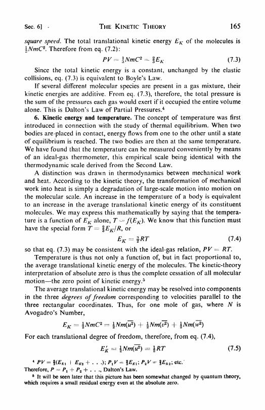
Sec. 6] - THE KINETIC THEORY 165
square speed. The total translational kinetic energy EK of the molecules is
iNmC*. Therefore from eq. (7.2):
PV = \NrnC* ^%EK (7.3)
Since the total kinetic energy is a constant, unchanged by the elastic
collisions, eq. (7.3) is equivalent to Boyle's Law.
If several different molecular species are present in a gas mixture, their
kinetic energies are additive. From eq. (7.3), therefore, the total pressure is
the sum of the pressures each gas would exert if it occupied the entire volume
alone. This is Dalton's Law of Partial Pressures.4
6. Kinetic energy and temperature. The concept of temperature was first
introduced in connection with the study of thermal equilibrium. When two
bodies are-placed in contact, energy flows from one to the other until a state
of equilibrium is reached. The two bodies are then at the same temperature.
We have found that the temperature can be measured conveniently by means
of an ideal-gas thermometer, this empirical scale being identical with the
thermodynamic scale derived from the Second Law.
A distinction was drawn in thermodynamics between mechanical work
and heat. According to the kinetic theory, the transformation of mechanical
work into heat is simply a degradation of large-scale motion into motion on
the molecular scale. An increase in the temperature of a body is equivalentto an increase in the average translational kinetic energy of its constituent
molecules. We may express this mathematically by saying that the tempera-ture is a function of EK alone, T -^ f(EK). We know that this function must
have the special form T %EK/R, or
EK - $RT (7.4)
so that eq. (7.3) may be consistent with the ideal-gas relation, PV RT.
Temperature is thus not only a function of, but in fact proportional to,
the average translational kinetic energy of the molecules. The kinetic-theory
interpretation of absolute zero is thus the complete cessation of all molecular
motion the zero point of kinetic energy.5
The average translational kinetic energy may be resolved into componentsin the three degrees offreedom corresponding to velocities parallel to the
three rectangular coordinates. Thus, for one mole of gas, where TV is
Avogadro's Number,
EK =
For each translational degree of freedom, therefore, from eq. (7.4),
E'K - \Nm^f) - \RT (7.5)
* PV = l(EKl \ EK2 + ...); P,V - \EKl \P2 y =- E
Therefore, P = /\ + P2 + . . ., Dalton's Law.5
It will be seen later that this picture has been somewhat changed by quantum theory,which requires a small residual energy even at the absolute zero.

166 THE KINETIC THEORY [Chap. 7
This is a special case of a more general theorem known as the Principle of
the Equipartition of Energy.7. Molecular speeds. Equation (7.3) may be written
C2 =--=
3/>(7.6)
P
where/>
-= NmjV is the density of the gas. From eqs. (7.3) and (7.4) we
obtain for the root mean square speed C, if M is the molecular weight,
23RT 3RT^ ~ ~ ~
The average speed c, as we shall see later, differs only slightly from the root
mean square speed :
From eq. (7.6), (7.7), or (7.8), we can readily calculate average or root
mean square speeds of the molecules of any gas at any temperature. Some
results are shown in Table 7.2. The average molecular speed of hydrogen at
25C is 1768 m per sec or 3955 mi per hr, about the speed of a rifle bullet.
The average speed of a mercury vapor atom would be only about 400 mi
per *hr.
TABLE 7.2
AVERAGE SPEEDS OF GAS MOLECULES AT 0CMeters/sec
. 1692.0
. 1196.0
. 170.0
. 600.6
. 454.2
. 425.1
. 566.5
We note that, in accordance with the principle of equipartition of energy,at any constant temperature the lighter molecules have the higher average
speeds. This principle extends even to the phenomena of Brownian motion,
where the dancing particles are some thousand times heavier than the
molecules colliding with them, but nevertheless have the same averagekinetic energy.
8. Molecular effusion. A direct experimental illustration of the different
average speeds of molecules of different gases can be obtained from the
phenomenon called molecular effusion. Consider the arrangement shown in
(a), Fig. 7.1. Molecules from a vessel of gas under pressure are permitted to
escape through a tiny orifice, so small that the distribution of the velocities

Sec. 8] THE KINETIC THEORY 167
of the gas molecules remaining in the vessel is not affected in any way; that
is, no appreciable mass flow in the direction of the orifice is set up. The
number of molecules escaping in unit time is then equal to the number that,
in their random motion, happen to hit the orifice, and this number is pro-
portional to the average molecular speed.
In (b), Fig. 7.1 is shown an enlarged view of the orifice, having an area
ds. If all the molecules were moving directly perpendicular to the openingwith their mean speed r, in one second all those molecules would hit the
opening that were contained in an element of volume of base ds and height c,
or volume c ds, for a molecule at a distance c will just reach the orifice at
(b)
Fig. 7.1. Effusion of gases.
the end of one second. If there are n molecules per cc, the number striking
would be nc ds. To a first approximation only one-sixth of all the molecules
are moving toward the opening, since there are six different possible direc-
tions of translation corresponding to the three rectangular axes. The number
of molecules streaming through the orifice would therefore be \nc ds, or perunit area \nc.
Actually, the problem is considerably more complicated, since half the
molecules have a component of motion toward the area, and one must
average over all the different possible directions of motion. This gives the
result: number of molecules striking unit area per second = number of
molecules effusing through unit area per second = \nc.
It is instructive to consider how this result is obtained, since the averagingmethod is typical of many kinetic-theory calculations. This derivation will be
the only one in the chapter that makes any pretense of exactitude, and maytherefore serve also to inculcate a proper suspicion of the cursory methods
used to obtain subsequent equations.If the direction of the molecules is no longer normal to the wall, instead
of the situation of Fig. 7. 1 , we have that of Fig. 7.2(a). For^any given direction
the number of molecules hitting ds in unit time will be those contained in a
cylinder of base ds and slant height c. The volume of this cylinder is c cos ds,
and the number of molecules in it is nc cos 6 ds.
The next step is to discover how many molecules out of the total have

168 THE KINETIC THEORY [Chap. 7
NORMAL
velocities in the specified direction. The velocities of the molecules will be
referred to a system of polar coordinates [Fig. 7.2.(b)] with its origin at the
wall of the vessel. We call such a representation a plot of the molecular
velocities in "velocity space." The
distance from the origin c defines
the magnitude of the velocity, and
the angles and<f> represent its
direction. Any particular direction
from the origin is specified by the
differential solid angle doj. The
fraction of the total number of
molecules having their velocities
within this particular spread of
directions is */a>/477 since 4?r is the
total solid angle subtended by the
surface of a sphere. In polar co-
(c)
(a)
(b)
Fig. 7.2. Calculation of gaseous effusion.
Element of solid angle is shown in (c).
ordinates this solid angle is given6
by sin 6 dOd<f>.
The number of molecules hit-
ting the surface ds in unit time
from the given direction (6, (/>)be-
comes ( 1 /47r)nc cos sin 6 dOdc/>
ds.
Or, for unit surface, it is (l/47r)rtccos sin 6 dOd<j>.
In order to find the
total number striking from all directions, dn'/dt, this expression must be
integrated :
dn fw/2
f2"
1
-y = --nccosO sind<f>
dOat Jo Jo 4-7T
The limits of integration of<f>
are from to 2?r, corresponding to ail the
directions around the circle at any given 0. Then is integrated from to
7T/2. The final result for the number of molecules striking unit area in unit
time is then
^ -i nc (7.9)
The steps of the derivation may be reviewed by referring to Fig. 7.2.
If p is the gas density, the weight of gas that effuses in unit time is
From eq. (7.8)
dW^ _~dt
"
dW _ /
~dt
~~ nvl/2
P \bM)
(7.10)
(7.11)
6 G. P. Harriwell, Principles of Electricity and Electromagnetism (New York: McGraw-Hill, 1949), p. 649.

Sec. 9] THE KINETIC THEORY 169
For the volume rate of flow, e.g., cc per sec per cm2,
1/2
dt
- (--V\l-nMJ(7.12)
It follows that at constant temperature the rate of effusion varies in-
versely as the square root of the molecular weight. Thomas Graham (1848)
was the first to obtain experimental evidence for this law, which is nownamed in his honor. Some of his data are shown in Table 7.3.
TABLE 7.3
THE EFFUSION OF GASES*
Gas
Air .
Nitrogen ,
OxygenHydrogenCarbon dioxide .
* Source: Graham, "On the Motion of Gases," Phil. Trans. Roy. Soc. (London), 136,
573 (1846).
It appears from Graham's work, and also from that of later experi-
menters, that eq. (7.12) is not perfectly obeyed. It fails rapidly when one
goes to higher pressures and larger orifices. Under these conditions the
molecules can collide many times with one another in passing through the
orifice, and a hydrodynamic flow towards the orifice is set up throughoutthe container, leading to the formation of a jet of escaping gas.
7
It is evident from eq. (7.12) that the effusive-flow process provides a
good method for separating gases of different molecular weights. By using
permeable barriers with very fine pores, important applications have been
made in the separation of isotopes. Because the lengths of the pores are
considerably greater than their diameters, the flow of gases through such
barriers does not follow the simple orifice-effusion equation. The dependenceon molecular weight is the same, since each molecule passes through the
barrier independently of any others.
9. Imperfect gases van der Waals' equation, The calculated properties
of the perfect gas of the kinetic theory are the same as the experimental
properties of the ideal gas of thermodynamics. It might be expected then
that extension and modification of the simplified model of the perfect gas
should provide an explanation for observed deviations from ideal-gas
behavior.
7 For a discussion of jet flow, see H. W. Liepmann and A. E. Puckett, Introduction to
Aerodynamics ofa Compressible Fluid (New York: Wiley, 1947), pp. 32 et seq.
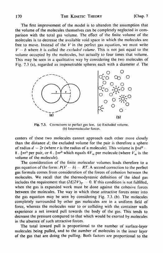
170 THE KINETIC THEORY [Chap. 7
The first improvement of the model is to abandon the assumption that
the volume of the molecules themselves can be completely neglected in com-
parison with the total gas volume. The effect of the finite volume of the
molecules is to decrease the available void space in which the molecules are
free to move. Instead of the V in the perfect gas equation, we must write
V b where b is called the excluded volume. This is not just equal to the
volume occupied by the molecules, but actually to four times that volume.
This may be seen in a qualitative way by considering the two molecules of
Fig. 7.3 (a), regarded as impenetrable spheres each with a diameter d. The
QD oo. o
o
(o)
oo
o(b)
Fig. 7.3. Corrections to perfect gas law. (a) Excluded volume,
(b) Intermolecular forces.
centers of these two molecules cannot approach each other more closely
than the distance d\ the excluded volume for the pair is therefore a sphereof radius d 2r (where r is the radius of a molecule). This volume is JTrrf
3 --
8 . |77r3per pair, or 4 . ^vrr
3 which equals 4Vm per molecule (where Vm is the
volume of the molecule).
The consideration of the finite molecular volumes leads therefore to a
gas equation of the form: P(V b) ---- RT. A second correction to the perfect
gas formula comes from consideration of the forces of cohesion between the
molecules. We recall that the thermodynamic definition of the ideal gasincludes the requirement that (dE/dV)T 0. If this condition is not fulfilled,
when the gas is expanded work must be done against the cohesive forces
between the molecules. The way in which these attractive forces enter into
the gas equation may be seen by considering Fig. 7.3. (b). The molecules
completely surrounded by other gas molecules are in a uniform field of
force, whereas the molecules near to or colliding with the container walls
experience a net inward pull towards the body of the gas. This tends to
decrease the pressure compared to that which would be exerted by molecules
in the absence of such attractive forces.
The total inward pull is proportional to the number of surface-layermolecules being pulled, and to the number of molecules in the inner layer
of the gas that are doing the pulling. Both factors are proportional to the
Sec. 10] THE KINETIC THEORY 171
density of the gas, giving a pull proportional to p2
, or equal to c/>2
, where
c is a constant. Since the density is inversely proportional to the volume
at any given pressure and temperature, the pull may also be written a/V2 .
This amount must therefore be added to the pressure to make up for the
effect of the attractive forces. Then,
(Y- b)^RT (7.13)
This is the famous equation of state first given by van der Waals in 1873.
It provides a good representation of the behavior of gases at moderate
densities, but deviations become very appreciable at higher densities. The
values of the constants a and b are obtained from the experimental PVTdata at moderate densities, or more usually from the critical constants of
the gas. Some of these values were collected in Table 1.1 on p. 14.
Equation (7.13) may also be written in the form
PV-^RT+bP -^+^2 (7.14)
The way in which this equation serves to interpret PV vs. P data may be
seen from an examination of the compressibility factor curves at different
temperatures, shown in Fig. 1.5 (p. 15). At sufficiently high temperaturesthe intermolecular potential energy, which is not temperature dependent,becomes negligible compared to the kinetic energy of the molecules, which
increases with temperature. Then the equation reduces to PV -= RT + bP.
At lower temperatures, the effect of intermolecular forces becomes more
appreciable. Then, at moderate pressures the ~a\ V term becomes important,and there are corresponding declines in the PV vs. P curves. At still higher
pressures, however, the term +ab/V2predominates, and the curves eventually
rise again.
10. Collisions between molecules. Now that the oversimplification that
the molecules of a gas occupy no volume themselves has been abandoned,
it is possible to consider further the phenomena that depend on collisions
between the molecules. Let us suppose that all the molecules have a diameter
d, and consider as in Fig. 7.4 the approach of a molecule A toward another
molecule B.
A "collision" occurs whenever the distance between their centers becomes
as small as d. Let us imagine the center of A to be surrounded by a sphere of
radius d. A collision occurs whenever the center 'of another molecule comes
within this sphere. If A is traveling with the average speed c, its "sphereof influence" sweeps out in unit time a volume nd^c. Since this volume
contains n molecules per cc, there are -nnd^c collisions experienced by A persecond.
A more exact calculation takes into consideration that only the speed of

172 THE KINETIC THEORY [Chap. 7
a molecule relative to other moving molecules determines the number of
collisions Zx that it experiences. This fact leads to the expression
Zj -^ V27wd2c (7.15)
The origin of the A/2 factor may be seen by considering, in Fig. 7.5, the
relative velocities of two molecules just before or just after a collision. The
2d
Fig. 7.4. Molecular collisions.
limiting cases are the head-on collision and the grazing collision. The averagecase appears to be the 90 collision, after which the magnitude of the relative
velocity is V2c.
If we now examine the similar motions of all the molecules, the total
(b) (C)
Fig. 7.5. Relative speeds, (a) Head-on collision.
(b) Grazing collision, (c) Right-angle collision.
number of collisions per second of all the n molecules contained in one cc
of gas is found, from eq. (7.15), to be
Zn - (7.16)
The factor J is introduced so that each collision is not counted twice (onceas A hits B, and once as B hits A).
11. Mean free paths. An important quantity in kinetic theory is the
average distance a molecule travels between collisions. This is called the
mean free path. The average number of collisions experienced by one mole-
cule in one second is, from eq. (7.15)^ -=- \^2irnd 2c. In this time the

Sec. 12] THE KINETIC THEORY 173
molecule has traveled a distance c. The mean free path A is therefore c/Zlt or
(7.17)
In order to calculate the mean free path, we must know the molecular
diameter d. This might be obtained, for example, from the van der Waalsb ( 4Vm) if the value of Avogadro's Number N were known. So far, our
development of kinetic theory has provided no method for obtaining this
number. The theory of gas viscosity as developed by James Clerk Maxwell
presents a key to this problem, besides affording one of the most strikingdemonstrations of the powers of the kinetic theory of gases.
12. The viscosity of a gas. The concept of viscosity is first met in problemsof fluid flow, treated by hydrodynamics and aerodynamics, as a measure of
-AREA
Fig. 7.6. Viscosity of fluids.
the frictional resistance that a fluid in motion offers to an applied shearingforce. The nature of this resistance may be seen from Fig. 7.6 (a). If a fluid
is flowing past a stationary plane surface, the layer of fluid adjacent to the
plane boundary is stagnant; successive layers have increasingly highervelocities. The frictional force /, resisting the relative motion of any two
adjacent layers, is proportional to S, the area of the interface between them,and to dvjdr, the velocity gradient between them. This is Newton's Law of
Viscous Flow,
dvf^viS-j- (7.18)
dr
The proportionality constant r\is called the coefficient of viscosity. It is
evident that the dimensions of rjare ml~l
t~~l
. In the COS system, the unit is
g per cm sec, called the poise.
174 THE KINETIC THEORY [Chap. 7
The kind of flow governed by this relationship is called laminar or
streamline flow. It is evidently quite different in character from the effusive
(or diffusive) flow previously discussed, since it is a massive flow of fluid, in
which there is superimposed on all the random molecular velocities a com-
ponent of velocity in the direction of flow.
An especially important case of viscous flow is the flow through pipes or
tubes when the diameter of the tube is large compared with the mean free
path in the fluid. The study of flow through tubes has been the basis for
many of the experimental determinations cf the viscosity coefficient. The
theory of the process was first worked out by J. L. Poiseuille, in 1844.
Consider an incompressible fluid flowing through a tube of circular cross
section with radius R and length L. The fluid at the walls of the tube is
assumed to be stagnant, and the rate of flow increases to a maximum at the
center of the tube [see Fig. 7.6 (b)]. Let v be the linear velocity at any distance
r from the axis of the tube. A cylinder of fluid of rad'"<; r experiences a
viscous drag given by eq. (7.18) as
V dvi r
Jr --1J/ *L
For steady flow, this force must be exactly balanced by the force drivingthe fluid in this cylinder through the tube. Since pressure is the force per unit
area, the driving force is _
/,= wVi -
J*a)
where Pl is the fore pressure and P% the back pressure.
Thus, for steady flow, fr fr
fp _ p \
On integration, v =--- -----\ r-- r2 + const&
According to our hypothesis, v = when /-=/?; this boundary condition
enables us to determine the integration constant, so that we obtain finally
The total volume of fluid flowing through the tube per second is calculated
by integrating over each element of cross-sectional area, given by 2-nr dr [see
Fig. 7.6 (c)]. Thus
dv f\ J ^Pi ~^2)*4
~dt^k2 dr ^ """
*>^ (7 - 19>ZLrj

Sec. 13] THE KINETIC THEORY 175
This is Poiseuille's equation. It was derived for an incompressible fluid
and therefore may be satisfactorily applied to liquids but not to gases. For
gases, the volume is a strong function of the pressure. The average pressure
along the tube is (Pl + ^2)/2- If ^o is tne pressure at which the volume is
measured, the equation becomes
dV
dt(7.20)
By measuring the volume rate of flow through a tube of known dimen-
sions, the viscosity i]of the gas can be determined. Some results of such
measurements are collected in Table 7.4.
TABLE 7.4
TRANSPORT PHENOMENA IN GASES
(At 0C and 1 aim)
13. Kinetic theory of gas viscosity. The kinetic picture of gas viscosity
has been represented by the following analogy: Two railroad trains are
moving in the same direction, but at different speeds, on parallel tracks. The
passengers on these trains amuse themselves by jumping back and forth
from one to the other. When a passenger jumps from the more rapidly
moving train to the slower one he transports momentum of amount mv,
where m is his mass and v the velocity of his train. He tends to speed up the
more slowly moving train when he lands upon it. A passenger who jumpsfrom the slower to the faster train, on the other hand, tends to slow it down.
The net result of the jumping game is thus a tendency to equalize the velocities
of the two trains. An observer from afar who could not see the jumpers
might simply note this result as a frictional drag between the trains.
The mechanism by which one layer of flowing gas exerts a viscous drag

176 THE KINETIC THEORY [Chap. 7
on an adjacent layer is exactly similar, the gas molecules taking the role of
the playful passengers. Consider in Fig. 7.7 a gas in a state of laminar flow
parallel to the Y axis. Its velocity increases from zero at the plane x to
larger and larger values of v with increasing x. If a molecule at P crosses to
g, in one of its free paths between collisions, it will bring to Q, on the
average, an amount of momentum which is less than that common to the
position Q by virtue of its distance along the A' axis. Conversely, if a molecule
travels from Q to P it will transport to the lower, more slowly moving layer,
an amount of momentum in excess of that belonging to that layer. The net
result of the random thermal motions of the molecules is to decrease the
average velocities of the molecules in
the layer at Q and to increase those
in the layer at P. This transport of
momentum tends to counteract the
velocity gradient set up by the shear
forces acting on the gas.
The length of the mean free pathX may be taken as the average dis-
tance over which momentum is trans-
ferred. 8 If the velocity gradient is
du/dx, the difference in velocity be-
tween the two ends of the free pathis X du/dx. A molecule of mass m,
passing from the upper to the lower
layer, thus transports momentum
equal to wA du/dx. On the average,
one-third of the molecules are moving up and down; if n is the number
of molecules per cc and c their average speed, the number traveling up and
down per second per square cm is-J-
nc. The momentum transport persecond is then \nc mX(du/dx)*
This momentum change with time is equivalent to the frictional force of
eq. (7.18) which was/^~ r)(du/dx) per unit area. Hence
Fig. 7.7. Kinetic theory of gas
viscosity.
du~Tdx
du- -
dx
(7.21)
The measurement of the viscosity thus allows us to calculate the value of
the mean free path A. Some values obtained in this way are included in
Table 7.4, in Angstrom units (1 A = 10~8cm).
8 This is not strictly true, and proper averaging indicates f A should be used.9 The factor J obtained here results from the cancellation of two errors in the derivation.
From eq. (7.9) one should take nc as the molecules moving across unit area but properaveraging gives the distance between planes as JA instead of A.
Sec. 14] THE KINETIC THEORY 177
By eliminating A between eqs. (7.17) and (7.21), one obtains
n - -^- (7.22)3\/2W2
This equation indicates that the viscosity of a gas is independent of its
density. This seemingly improbable result was predicted by Maxwell on
purely theoretical grounds, and its subsequent experimental verification was
one of the great triumphs of the kinetic theory. The physical reason for the
result is clear from the preceding derivation: At lower densities, fewer
molecules jump from layer to layer in the flowing gas, but, because of the
longer free paths, each jump carries proportionately greater momentum.For imperfect gases, the equation fails and the viscosity increases with
density.
The second important conclusion from eq. (7.22) is that the viscosity of
a gas increases with increasing temperatuie, linearly with the \/T. This con-
clusion has been well confirmed by the experimental results, although the
viscosity increases somewhat more rapidly than predicted by the \/T law.
14. Thermal conductivity and diffusion. Gas viscosity depends on the
transport of momentum across a momentum (velocity) gradient. It is a
typical transport phenomenon. An exactly similar theoretical treatment is
applicable to thermal conductivity and to diffusion. The thermal conductivityof gases is a consequence of the transport of kinetic energy across a tem-
perature (i.e., kinetic energy) gradient. Diffusion of gases is the transport of
mass across a concentration gradient.
The thermal conductivity coefficient K is defined as the heat flow per unit
time q, per unit temperature gradient across unit cross-sectional area, i.e., by
cdT
q =. K- S-ax
By comparison with eq. (7.21),
dT 1,de
K nc/.ax 3 ax
where de/dx is the gradient of e, the average kinetic energy per molecule.
Nowde dT de
where m is the molecular mass and c v is the specific heat (heat capacity per
gram). It follows that
K -^ lnmcvch \pcvcX ^ r\cv (7.23)
Some thermal conductivity coefficients are included in Table 7.4. It
should be emphasized that, even for an ideal gas, the simple theory is approxi-
mate, since it assumes that all the molecules are moving with the same speed,
c, and that energy is exchanged completely at each collision.

178 THE KINETIC THEORY [Chap. 7
The treatment of diffusion is again similar. Generally one deals with the
diffusion in a mixture of two different gases. The diffusion coefficient D is
the number of molecules per second crossing unit area under unit con-
centration gradient. It is found to be10
D --JVi*2 +- iVa*i
where Xl and X2 are the mole fractions of the two gases in the mixture. If
the two kinds of molecules are essentially the same, for example radioactive
chlorine in normal chlorine, the self-diffusion coefficient is obtained as
D &c (7.24)
The results of the simple mean-free-path treatments of the transport
processes may be summarized as follows:
Now van der Waals' b is given by
b - - 47V
15. Avogadro's number and molecular dimensions. Equation (7.22) may be
written, from eq. (7.8),
Me 2V1RTM71^
(7.25)
(7.26)
Let us substitute the appropriate values for the hydrogen molecule, H2 ,
all in CGS units.
M= 2.016 6-26.6
?7-0.93 x 10~4 r= 298KR = 8.314 x 10⁷
Solving for d, we find d -=-- 2.2 x 10~8 cm.
6 3
Multiplying these two equations, and solving for d,
10 For example, see E. H. Kennard, Kinetic Theory of Gases (New York: McGraw-HilJ,1938), p. 188.
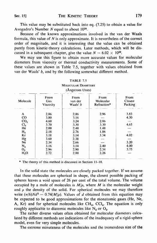
Sec. 15] THE KINETIC THEORY 179
This value may be substituted back into eq. (7.25) to obtain a value for
Avogadro's Number TV equal to about 1024 .
Because of the known approximations involved in the van der Waals
formula, this value of TV is only approximate. It is nevertheless of the correct
order of magnitude, and it is interesting that the value can be obtained
purely from kinetic-theory calculations. Later methods, which will be dis-
cussed in a subsequent chapter, give the value TV 6.02 x 10²³ .
We may use this figure to obtain more accurate values for molecular
diameters from viscosity or thermal conductivity measurements. Some of
these values are shown in Table 7.5, together with values obtained from
van der Waals' b, and by the following somewhat different method.
TABLE 7.5
MOLECULAR DIAMETERS
(Angstrom Units)
* The theory of this method is discussed in Section 1 1-18.
In the solid state the molecules are closely packed together. If we assume
that these molecules are spherical in shape, the closest possible packing of
spheres leaves a void space of 26 per cent of the total volume. The volume
occupied by a mole of molecules is M/p, where M is the molecular weightand p the density of the solid. For spherical molecules we may therefore
write (7r/6)Nd* = Q.14(M/p). Values of d obtained from this equation maybe expected to be good approximations for the nionatomic gases (He, Ne,
A, Kr) and for spherical molecules like CH4 , CC1 4 . The equation is only
roughly applicable to diatomic molecules like N2 or O2 .
The rather diverse values often obtained for molecular diameters calcu-
lated by different methods are indications of the inadequacy of a rigid-sphere
model, even for very simple molecules.
The extreme minuteness of the molecules and the tremendous size of the

180 THE KINETIC THEORY [Chap. 7
Avogadro Number N are strikingly shown by two popular illustrations given
by Sir James Jeans. If the molecules in a glass of water were turned into
grains of sand, there would be enough sand produced to cover the whole
United States to a depth of about 100 feet. A man breathes out about 400 cc
at each breath, or about 1022 molecules. The earth's atmosphere contains
about 1044 molecules. Thus, one molecule is the same fraction of a breath
of air as the breath is of the entire atmosphere. If the last breath of Julius
Caesar has become scattered throughout the entire atmosphere, the chances
are that we inhale one molecule from it in each breath we take.
16. The softening of the atom. We noted before that the viscosity of a gas
increases more rapidly with temperature than is predicted by the \/T law.
This is because the molecules are not actually hard spheres, but must be
regarded as being somewhat soft, or surrounded by fields of force. This
is true even for the atom-molecules of the inert gases. The higher the tem-
perature, the faster the molecules are moving, and hence the further one
molecule can penetrate into the field of force of another, before it is repelled
or bounced away. The molecular diameter thus appears to be smaller at
higher temperatures. This correction has been embodied in a formula due to
Sutherland (1893)
d*--<Il\\\-) (7.27)
Here d^ and C are constants, d^ being interpreted as the value of d as T
approaches infinity.
More recent work has sought to express the temperature coefficient of
the viscosity in terms of the laws of force between the molecules. Thus here,
just as in the discussion of the equation of state, the qualitative picture of
rigid molecules must be modified to consider the fields of force between
molecules.
We recall from Chapter 1 that forces may be represented as derivatives
of a potential-energy function,/^ (<3(7/cV), and a representation of this
function serves to illustrate the nature of the forces. In Fig. 7.8 we have
drawn the mutual potential energy of pairs of molecules of several different
gases. We may imagine the motion of one molecule as it approaches rapidlytoward another to be represented by that of a billiard ball rolled with con-
siderable force along a track having the shape of the potential curve. As the
molecule approaches another it is accelerated at first, but then slowed downas it reaches the steep ascending portion of the curve. Finally it is broughtto a halt when its kinetic energy is completely used up, and it rolls back downand out the curve again. Since the kinetic energy is almost always greaterthan the depth of the potential-energy trough, there is little chance of a
molecule's becoming trapped therein. (If it did, another collision would soon
knock it out again.)
This softening of the original kinetic-theory picture of the atom as a

Sec. 17] THE KINETIC THEORY 181
hard rigid sphere was of the greatest significance. It immediately suggestedthat the atoms could not be the ultimate building units in the construction
of matter, and that man must seek still further for an indestructible reality
to explain the behavior of material things.
So far in this chapter we have dealt with average properties of largecollections of molecules : average velocities, mean free paths, viscosity, and
DISTANCE BETWEENMOLECULES
-15
Fig. 7.8. Mutual potential energy of pairs of molecules.
so on. In what follows, the contributions of the individual molecules to these
averages will be considered in some detail.
17. The distribution of molecular velocities. The molecules of a gas in
their constant motion collide many times with one another, and -these
collisions provide the mechanism through which the velocities of individual
molecules are continually changing. As a result, there exists a distribution
of velocities among the molecules; most have velocities with magnitudesclose to the average, and relatively few have velocities much above or muchbelow the average.
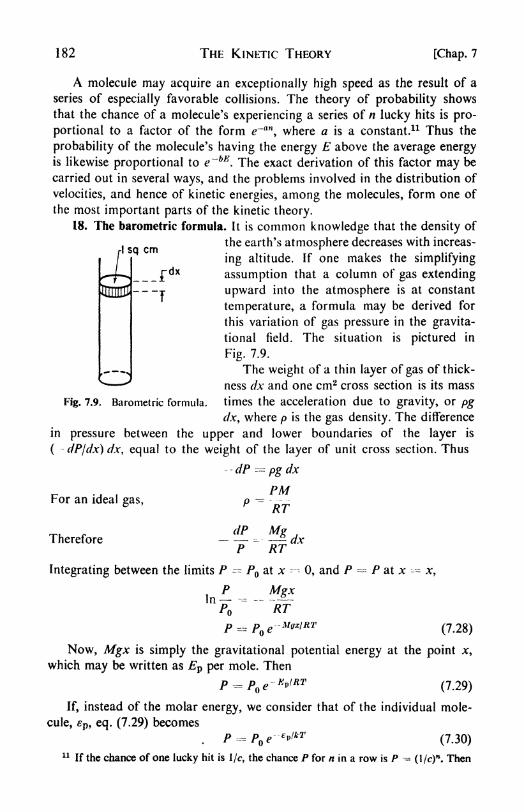
182 THE KINETIC THEORY [Chap. 7
I sq cm
.__fd *
A molecule may acquire an exceptionally high speed as the result of a
series of especially favorable collisions. The theory of probability shows
that the chance of a molecule's experiencing a series of n lucky hits is pro-
portional to a factor of the form e~an,where a is a constant.11 Thus the
probability of the molecule's having the energy E above the average energyis likewise proportional to e~bE . The exact derivation of this factor may be
carried out in several ways, and the problems involved in the distribution of
velocities, and hence of kinetic energies, among the molecules, form one of
the most important parts of the kinetic theory.
18. The barometric formula. It is common knowledge that the density of
the earth's atmosphere decreases with increas-
ing altitude. If one makes the simplifying
assumption that a column of gas extending
upward into the atmosphere is at constant
temperature, a formula may be derived for
this variation of gas pressure in the gravita-
tional field. The situation is pictured in
Fig. 7.9.
The weight of a thin layer of gas of thick-
ness dx and one cm2 cross section is its mass
Fig. 7.9. Barometric formula, times the acceleration due to gravity, or pg
dx, where/>
is the gas density. The difference
in pressure between the upper and lower boundaries of the layer is
( -dP/dx)dx, equal to the weight of the layer of unit cross section. Thus
dP = pgdx
A ^
PMror an ideal gas, p -=
D_Kl
ThereforeRT
dx
Integrating between the limits P PQ at x 0, and P P at x --= x,
P MgxIn
RTn r> _ -MgxIRT ("l *)Q\r r e \i .LO)
Now, Mgx is simply the gravitational potential energy at the point x,
which may be written as E^ per mole. Then
P^PQ e~E IHT
(7.29)
If, instead of the molar energy, we consider that of the individual mole-
cule, ep , eq. (7.29) becomes
. P = P e" e *lltr(7.30)
11 If the chance of one lucky hit is 1/c, the chance P for n in a row is P - (I/c)w
. Then

Sec. 19] THE KINETIC THEORY 183
The constant k is called the Bohzmann constant. Ft is the gas constant permolecule.
Equation (7.30) is but one special case of a very general expressionderived by L. Boltzmann in 1886. This states that if A?O is the number of
molecules in any given state, the number n in a state whose potential energyis e above that of the given state is
n = n^e-hlkT
(7.31)
19. The distribution of kinetic energies.12 To analyze more closely the
kinetic picture underlying the barometric formula, let us consider the in-
dividual gas molecules moving with their diverse velocities in the earth's
gravitational field. The velocity components parallel to the earth's surface
(in the y and z directions along which no field exists) are not now of interest
and only the vertical or x component u need be considered.
The motion of a molecule with an upward velocity u is just like that of
a ball thrown vertically into the air. If its initial velocity is w , it will rise
with continuously decreasing speed, as its kinetic energy is transformed into
potential energy according to the equation
mgx i/w/ 2 iww2
At the height, x =- uQ2/2g, it will stop, and then fall back to earth.
The gravitational field acts as a device that breaks up the mixture of
various molecular velocities into a "spectrum" of velocities. The slowest
molecules can rise only a short distance; the faster ones can rise propor-
tionately higher. By determining the number of molecules that can reach
any given height, we can likewise determine how many had a given initial
velocity component.As is to be expected from the physical picture of the process, the dis-
tribution of kinetic energies k among the molecules must follow an ex-
ponential law just as the potential energy distribution does. Representingthe fraction of molecules having a velocity between u and u f du by dnfn^this law may be written from eq. (7.31) as
- Ae~^lkT du (7.32)"o
Here A is a constant whose value is yet to be determined.
20. Consequences of the distribution law. This distribution law is com-
pletely unaffected by collisions between molecules, since a collision results
only in an interchange of velocity components between two molecules.
Expressions exactly similar to eq. (7.32) must also hold for the velocity
12 The method suggested here is given in detail by K. F. Herzfeld in H. S. Taylor'sTreatise on Physical Chemistry, 2nd ed. (New York: Van Nostrand, 1931), p. 93.

184 THE KINETIC THEORY [Chap. 7
distributions in the y and z directions, since it is necessary only to imaginesome sort of potential field in these directions in order to analyze the
velocities into their spectrum.
I50 r
OJ
ca
I ~
(TUJ
50
1C
200 400 600 800 1000 2000
u, METERS /SECOND
Fig. 7.10. One-dimensional velocity distribution (nitrogen at 0C).
The constant A 9 in eq. (7.32), may be evaluated from the fact that the
sum of all the fractions of molecules in all the velocity ranges must be unity.
Thus, integrating over all possible velocities from oo to + oo, we have
r+oo _WM /2JITA e du -~1
J - oo
mu2
2
2kT^ X
+oo
A' ^ ' ^
Letting
2^7^\i/2 /*+
V/ J-c
Since
Therefore, eq. (7.32) becomes
1/2
(7.33)
This function is shown plotted in Fig. 7.10. It will be noted that the
fraction of the molecules with a velocity component in a given range declines

Sec. 20] THE KINETIC THEORY 185
at first slowly and then rapidly as the velocity is increased. From the curve
and from a consideration of eq. (7.33), it is evident that as long as Jmw2 < kT
the fraction of molecules having a velocity u falls off slowly with increasing u.
When %mu2 = \QkT, the fraction has decreased to e~10 , or 5 x 10~5 times its
value at \rn\f1 = kT. Thus only a very small proportion of any lot of mole-
cules can have kinetic energies much greater than kT per degree of freedom.
If, instead of a one-dimensional gas (one degree of freedom of trans-
lation), a two-dimensional gas is considered, it can be proved13 that the
probability of a molecule having a given x velocity component u in no way
depends on the value of its y component v. The fraction of the molecules
having simultaneously velocity components between u and u + du, and v
and v -f- dv, is then simply the product of the two individual probabilities.
dn I m \
^=
\27Tkf)(7.34)
This sort of distribution may be graphically represented as in Fig. 7.11,
where a coordinate system with u and v axes has been drawn. Any point in
the (w, v) plane represents a simul-
taneous value of u and v\ the planeis a two-dimensional velocity spacesimilar to that used on p. 168. The
dots have been drawn so as to
represent schematically the density
of points in this space, i.e., the
relative frequency of occurrence of
sets of simultaneous values of u
and v.
The graph bears a striking re-
semblance to a target that has been
peppered with shots by a marks-
man aiming at the bull's-eye. In
the molecular case, each individualFig. 1Mm Distribution of points in two-
molecular-velocity component, u or dimensional velocity space: vx = u; vv- v.
v, aims at .the value zero. The
resulting distribution represents the statistical summary of the results. The
more skilful the marksman, the more closely will his results cluster around
the center of the target. For the molecules, the skill of the marksman has its
analogue in the temperature of the gas. The lower the temperature, the better
the chance a molecular-velocity component has of coming close to zero.
If, instead of the individual components u and v, the resultant speed c
is considered, where c2 = u2 + v29 it is evident that its most probable value
is not zero. This is because the number of ways in which c can be made up18 For a discussion of this theorem see, for example, J. Jeans, Introduction to the
Kinetic Theory of Gases (London: Cambridge, 1940), p. 1Q5.
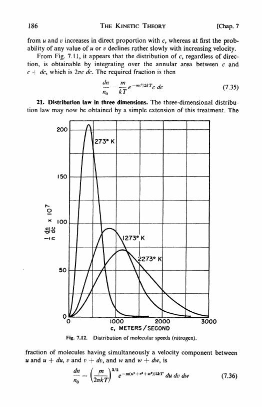
186 THE KINETIC THEORY [Chap. 7
from u and v increases in direct proportion with c, whereas at first the prob-
ability of any value of u or v declines rather slowly with increasing velocity.
From Fig. 7.11, it appears that the distribution of c, regardless of direc-
tion, is obtainable by integrating over the annular area between c andc | dc, which is 2nc dc. The required fraction is then
dn m .,.., .
__ e (7.35)
21. Distribution law in three dimensions. The three-dimensional distribu-
tion law may now be obtained by a simple extension of this treatment. The
200
1000 2000C, METERS /SECOND
Fig. 7.12. Distribution of molecular speeds (nitrogen).
3000
fraction of molecules having simultaneously a velocity component between
u and u + du, v and v + dv, and w and w + dw, is
dn_ 1""
m\2irkTj
(7.36)
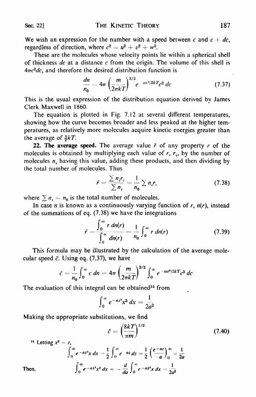
Sec. 22] THE KINETIC THEORY 187
We wish an expression for the number with a speed between c and c + dc,
regardless of direction, where c2 = u2 + v2 + w2.
These are the molecules whose velocity points lie within a spherical shell
of thickness dc at a distance c from the origin. The volume of this shell is
477-cVc, and therefore the desired distribution function is
*
This is the usual expression of the distribution equation derived by James
Clerk Maxwell in 1860.
The equation is plotted in Fig. 7.12 at several different temperatures,
showing how the curve becomes broader and less peaked at the higher tem-
peratures, as relatively more molecules acquire kinetic energies greater than
the average of fkT.
22. The average speed. The average value f of any property r of the
molecules is obtained by multiplying each value of r, r,, by the number of
molecules nl having this value, adding these products, and then dividing by
the total number of molecules. Thus
where 2 ni
=~ no *s the total number of molecules.
In case n is known as a continuously varying function of r, n(r), instead
of the summations of eq. (7.38) we have the integrations
Jordn\r) 1 Too
-r - = --L rdnw (7 -39>'
dn(r) "oj
This formula may be illustrated by the calculation of the average mole-
cular speed c. Using eq. (7.37), we have
c - - f c dn - 47r (^r\m
I" e -""V^V jcnQ
J o xlirkT] J o
The evaluation of this integral can be obtained14 from
1>~~ (
2a*
Making the appropriate substitutions, we find
c'=O1/2
<>14
Letting x2 =
z,
Too if 00 l/C~ a2:\
001
Joe'aXxdx ^2J^ e aZdz =
2 I'^/o=
2a
Too
I puxJ Q
ed

188 THE KINETIC THEORY [Chap. 7
Similarly, the average kinetic energy can readily be evaluated as
\& dn
2/7 Jo
This yields- \kT (7.41)
23. The equipartition of energy. Equation (7.41) gives the average trans-
lational kinetic energy of a molecule in a gas. It will be noted that the average
energy is independent of the mass of the molecule. Per mole of gas,
/C(t,a,,)- INkT- $RT (7.42)
For a monatomic gas, like helium, argon, or mercury vapor, this translational
kinetic energy is the total kinetic energy of the gas. For diatomic gases, like
N 2 or C1 2 ,and polyatomic gases, like CH 4 or N 2O, there may also be energy
associated with rotational and vibrational motions.
A useful model for a molecule is obtained by supposing that the masses
of the constituent atoms are concentrated at points. As will be seen in
Chapter 9, almost all the atomic mass is in fact concentrated in a tiny
nucleus, the radius of which is about 10 13 cm. Since the over-all dimensions
of molecules are of the order of 10~8cm, a model based on point masses is
physically most reasonable. Consider a molecule composed of n atoms. In
order to represent the instantaneous locations in space of A? mass points, weshould require 3/7 coordinates. The number of coordinates required to locate
all the mass points (atoms) in a molecule is called the number of its degrees
offreedom. Thus a molecule of n atoms has 3/7 degrees of freedom.
The atoms within each molecule move through space as a connected
entity, and we can represent the translational motion of the molecule as a
whole by the motion of the center of mass of its constituent atoms. Three
coordinates (degrees of freedom) are required to represent the instantaneous
position of the center of mass. The remaining (3/7 3) coordinates representthe so-called internal degrees offreedom.
The internal degrees of freedom may be further subdivided into rotations
and vibrations. Since the molecule has moments of inertia / about suitably
chosen axes, it can be set into rotation about these axes. If its angular velocityabout an axis is (, the rotational kinetic energy is i/o>
2. The vibratory
motion, in which one atom in a molecule oscillates about an equilibrium
separation from another, is associated with both kinetic and potential
energies, being in this respect exactly like the vibration of an ordinary spring.
The vibrational kinetic energy is also represented by a quadratic expression,
*,mv2
. The vibrational potential energy can in some cases be represented also
by a quadratic expression, but in the coordinates q rather than in the
velocities, for example, i/o/2
. Each vibrational degree of freedom would then
contribute two quadratic rterms to the total energy of the molecule.
By an extension of the derivation leading to eq. (7.41), it can be shown

Sec. 24] THE KINETIC THEORY 189
that each of these quadratic terms that comprise the total energy of the
molecule has an average value of \kT. This conclusion, a direct consequenceof the Maxwell-Boltzmann distribution law, is the most general expressionof the Principle of Equipartition of Energy.
24. Rotation and vibration of diatomic molecules. The rotation of a di-
atomic molecule may be visualized by reference to the so-called dumbbell
model in Fig. 7.13, which might represent a molecule such as H2 , N 2 , HCI,
(b)
Fig. 7.13. Dumbbell rotator.
or CO. The masses of the atoms, mr and w2 , are concentrated at points,
distant rx and r2 , respectively, from the center of mass. The molecule there-
fore has moments of inertia about the X and Z axes, but not about the Yaxis on which the mass points lie.
The energy of rotation of a rigid body is given by
rot- Uco* (7.43)
where o> is the angular velocity of rotation, and / is the moment of inertia.
For the dumbbell model, / = w^2 + w2r22
.
The distances rx and r2 from the center of mass are
m2 mi
Thus (7.44)
The quantity (7.45)
is called the reduced mass of the molecule. The rotational motion is equivalent
to that of a mass p at a distance r from the intersection of the axes.
Only two coordinates are required to describe such a rotation com-
pletely; for example, two angles 6 and<f>
suffice to fix the orientation of the
rotator in space. There are thus two degrees of freedom for the rotation of
a dumbbell-like structure. According to the principle of the equipartition of

190 THE KINETIC THEORY [Chap. 7
energy, the average rotational energy should therefore be rot=
- RT.
The simplest model for a vibrating diatomic molecule (Fig. 7.14) is the
harmonic oscillator. From mechanics we know that simple harmonic motion
occurs when a particle is acted on by a restor-
ing force directly proportional to its distance
, t*99$w$9999f{pt ,ft from the equilibrium position. Thus
Fig. 7.14. Harmonic oscil-
lator. The constant K is called the force constant.
The motion of a particle under the influ-
ence of such a restoring force may be represented by a potential energyfunction U(r).
f Pu\f= -\Sr-)^-
lcr
U(r) -Jicr
2(7.47)
This is the equation of a parabola and the potential-energy curve is
drawn in Fig. 7.15. The motion of the partide, as has been pointed out in
previous cases, is analogous to that of a ball moving on such a surface.
Starting from rest at any position r, it has
only potential energy, U = i/cr2
. As it rolls
down the surface, it gains kinetic energy upto a maximum at position r 0, the equi-
librium interatomic distance. The kinetic
energy is then reconverted to potential
energy as the ball rolls up the other side of
the incline. The total energy at any time is
always a constant,
U(r)
Evih
-r +r ^
Fig. 7.15. Potential curve of
harmonic oscillator.It is apparent, therefore, that vibrating
molecules when heated can take up energy as both potential and kinetic
energy of vibration. The equipartition principle states that the average
energy for each vibrational degree of freedom is therefore kT, \kT for the
kinetic energy plus \kT for the potential energy.
For a diatomic molecule the total average energy per mole therefore
becomes~
^tnms + rot + ^vib=- $RT + RT + RT -
25. Motions of polyatomic molecules. The motions of polyatomic mole-
cules can also be represented by the simple mechanical models of the rigidrotator and the harmonic oscillator. If the molecule contains n atoms, there

Sec. 25] THE KINETIC THEORY 191
are (3n 3) internal degrees of freedom. In the case of the diatomic molecule,
3n 3 -- 3. Two of the three internal coordinates are required to represent
the rotation, leaving one vibrational coordinate.
In the case of a triatomic molecule, 3/7 3 6. In order to divide these
six internal degrees of freedom into rotations and vibrations, we must first
consider whether the molecule is linear or bent. If it is linear, all the atomic
mass points lie on one axis, and there is therefore no moment of inertia about
this axis. A linear molecule behaves like a diatomic molecule in regard to
rotation, and there are only two rotational degrees of freedom. For a linear
triatomic molecule, there are thus 3n 3 2 4 vibrational degrees of
freedom. The average energy of the molecules according to the Equipartition
Principle would therefore be
E ~~~^trans I ^rot ^ ^vih
=- 3(\RT) + 2(\RT) ^ 4(RT] 6 1
2 RT per mole
A nonlinear (bent) triatomic molecule has three principal moments of
inertia, and therefore three rotational degrees of freedom. Any nonlinear
polatomic molecule has 3/76 vibrational degrees of freedom. For the
triatomic case, there are therefore three vibrational degrees of freedom. The
average energy according to the Equipartition Principle would be
E 3(1 RT) ~\ 3(1 RT) f 3(RT)
6RT per mole
Examples of linear triatomic molecules are HCN, CO2 , and CS2 . Bent
triatomic molecules include H2O and SO2 .
The vibratory motion of a collection of mass points bound together bylinear restoring forces [i.e., a polyatomic molecule in which the individual
atomic displacements obey eq. (7.46)] may be quite complicated. It is always
possible, however, to represent the complex vibratory motion by means of
a number of simple motions, the so-called normal modes of vibration. In a
normal mode of vibration, each atom in the molecule is oscillating with the
same frequency. Examples of the normal modes for linear and bent triatomic
molecules are shown in Fig. 7.16. The bent molecule has three distinct
normal modes, each with a characteristic frequency. The frequencies of
course have different numerical values in different compounds. In the case
of the linear molecule, there are four normal modes; two correspond to
stretching of the molecule (vl9 v3) and two correspond to bending (v2a ,v2b).
The two bending vibrations differ only in that one is in the plane of the
paper and one normal to the plane (denoted by + and ). These vibrations
have the same frequency, and are called degenerate vibrations.
When we described the translational motions of molecules and their
consequences for the kinetic theory of gases, it was desirable at first to employa very simplified model. The same procedure has been followed in this dis-
cussion of the internal molecular motions. Thus diatomic molecules do not

192 THE KINETIC THEORY [Chap. 7
really behave as rigid rotators, since, at rapid rotation speeds, centrifugal
force tends to separate the atoms by stretching the bond between them.
9 6 '2a
I/I V2 1/3
Fig. 7.16. Normal modes of vibration of triatomic molecules.
Likewise, a more detailed theory shows that the vibrations of the atoms are
not strictly harmonic.
26. The equipartition principle and the heat capacity of gases. Accordingto the equipartition principle, a gas on warming should take up energy in
all its degrees of freedom, \RT per mole for each translational or rotational
coordinate, and RT per mole for each vibration. The heat capacity at con-
stant volume, Cv --= (3E/DTV, could then be readily calculated from the
average energy.From eq. (7.42) the translational contribution to Cv is (f)/?. Since
R *= 1 .986 cal per degree C, the molar heat capacity is 2.98 cal per degree C.
When this figure is compared with the experimental values in Table 7.6, it
is found to be confirmed for the monatomic gases, He, Ne, A, Hg, which
TABLE 7.6
MOLAR HEAT CAPACITY C v OF GASES
Gas
He, Ne, A, HgH2 .
N2 . .
Oa . .
CI2 . .
H 2OC0a . .
Temperature (C)
-100
2.98
4.18
4.95
4.98

Sec. 27] THE KINETIC THEORY 193
have no internal degrees of freedom. The observed heat capacities of the
diatomic and polyatomic gases are always higher, and increase with tem-
perature, so that it may be surmised that rotational and vibrational contri-
butions are occurring.For a diatomic gas, the equipartition principle predicts an average energy
of (%)RT, or Cv ()R -= 6.93. This value seems to be approached at high
'temperatures for H2 , N2 , O2 , and C12 , but at lower temperatures the experi-
mental Cv values fall much below the theoretical ones. For polyatomic gases,
the discrepancy with the simple theory is even more marked. The equi-
partition principle cannot explain why the observed Cr is less than predicted,
why Cv increases with temperature, nor why the Cr values differ for the
different diatomic gases. The theory is t)ius satisfactory for translational
motion, but most unsatisfactory when applied to rotation and vibration.
Since the equipartition principle is a direct consequence of the kinetic
theory, and in particular of the Maxwell-Boltzmann distribution law, it is
evident that an entirely new basic theory will be required to cope with the
heat capacity problem. Such a development is found in the quantum theoryintroduced in Chapter 10.
27. Brownian motion. In 1827, shortly after the invention of the achro-
matic lens, the botanist Robert Brown15 studied pollen grains under his
microscope and watched a curious behavior.
While examining the form of these particles immersed in water, I observed manyof them very evidently in motion; their motion consisting not only of a change of
place in the fluid, manifested by alterations of their relative positions, but also not
infrequently of a change in form of the particle itself; a contraction or curvature
taking place repeatedly about the middle of one side, accompanied by a correspond-
ing swelling or convexity on the opposite side of the particle. In a few instances the
particle was seen to turn on its longer axis. These motions were such as to satisfy
me, after frequently repeated observations, that they arose neither from currents in
the fluid, nor from its gradual evaporation, but belonged to the particle itself.
In 1888, G. Gouy proposed that the particles were propelled by collisions
with the rapidly moving molecules of the suspension liquid. Jean Perrin
recognized that the microscopic particles provide a visible illustration of
many aspects of the kinetic theory. The dancing granules should be governed
by the same laws as the molecules in a gas.
One striking confirmation of this hypothesis was discovered in Perrin's
work on the distribution of colloidal particles in a gravitational field, the
sedimentation equilibrium. By careful fractional centrifuging, he was able
to prepare suspensions of gamboge16
particles that were spherical in shapeand very uniform in size. It was possible to measure the radius of the particles
either microscopically or by weighing a counted number. If these granules
15 Brown, Phil. Mag., 4, 161 (1828); 6, 161 (1829); 8, 41 (1830).18
Gamboge is a gummy material from the desiccation of the latex secreted by garciniamore/la (Indo-China). It is used as a bright yellow water color.

194 THE KINETIC THEORY [Chap. 7
behave in a gravitational field like gas molecules, their equilibrium distribu-
tion throughout a suspension should obey the Boltzmann equation
(7.48)
Instead of m we may write $7rr3(p p t ) where r is the radius of the particle,
and p and p tare the densities of the gamboge and of the suspending liquid.
Then eq. (7.48) becomes-
Pi)
RTN (7.49)
Fig. 7.17. Sedimentation
equilibrium.
By determining the difference in the numbers of particles at heights separated
by h, it is possible to calculate a value for
Avogadro's Number N.
A drawing of the results of Perrin's micro-
scopic examination of the equilibrium distri-
bution with granules of gamboge 0.6/* in
diameter17is shown in Fig. 7.17. The relative
change in density observed in 10/j of this
suspension is equivalent to that occurring in
6 km of air, a magnification of six hundred
million.
The calculation from eq. (7.49) resulted
in a value of N 6.5 x 10²³ . This value is
in good agreement with other determinations, and is evidence that the visible
microscopic particles are behaving as giant molecules in accordance with
the kinetic theory. These studies were welcomed at the time as a proof of
molecular reality.
28. Thermodynamics and Brownian motion. A striking feature of the
Brownian motion of microscopic particles is that it never stops, but goes on
continuously without any diminution of its activity. This perpetual motion
is not in contradiction with the First Law, for the source of the energy that
moves the particles is the kinetic energy of the molecules of the suspending
liquid. We may assume that in any region where the colloid particles gainkinetic energy, there is a corresponding loss in kinetic energy by the molecules
of the fluid, which undergoes a localized cooling. This amounts to perpetualmotion of the second kind, for the transformation of heat into mechanical
energy is prohibited by the Second Law, unless there is an accompanyingtransfer of heat from a hot to a cold reservoir.
The study of Brownian motion thus reveals an important limitation of
the scope of the Second Law, which also allows us to appreciate its true
nature. The increase in potential energy in small regions of a colloidal sus-
pension is equivalent to a spontaneous decrease in the entropy of the region.
On the average, of course, over long periods of time the entropy of the entire
171 micron (/<)
- 10~3 mm = I0~6 m.

Sec. 29] THE KINETIC THEORY 195
system does not change. In any microscopic region, however, the entropy
fluctuates, sometimes increasing and sometimes decreasing.
On the macroscopic scale such fluctuations are never observed, and the
Second Law is completely valid. No one observing a book lying on a desk
would expect to see it spontaneously fly up to the ceiling as it experienced a
sudden chill. Yet it is not impossible to imagine a situation in which all the
molecules in the book moved spontaneously in a given direction. Such a
situation is only extremely improbable, since there are so many molecules in
any macroscopic portion of matter.
29. Entropy and probability. The law of the increase of entropy is thus
a probability law. When the number of molecules in a system becomes
sufficiently small, the probability of observing a spontaneous decrease in
entropy becomes appreciable.
The relation between entropy and probability may be clarified by con-
sidering (Fig. 7.18) two different gases, A and /?, in separate containers.
oo oo00 00 O
00 ~ _ *T.
B A+BFig. 7.18. Increase in randomness and entropy on mixing.
Mien the partition is removed the gases diffuse into each other, the process
Continuing until they are perfectly mixed. If they were originally mixed, weshould never expect them to become spontaneously unmixed by diffusion,
since this condition would require the simultaneous adjustment of some 1024
different velocity components per mole of gas.
The mixed condition is the condition of greater randomness, of greater
disorder; it is the condition of greater entropy since it arises spontaneouslyfrom unmixed conditions. [The entropy of mixing was given in eq. (3.42).]
Hence entropy is sometimes considered a measure of the degree of disorder
or of randomness in a system. The system of greatest randomness is also
the system of highest statistical probability, for there are many arrange-ments of molecules that can comprise a disordered system, and much fewer
for an ordered system. When one considers how seldom thirteen spadesare dealt in a bridge hand,
18 one can realize how much more probable is the
mixed condition in a system containing 1024 molecules.
Mathematically, the probabilities of independent individual events are
multiplied together to obtain the probability of the combined event. The
18 Once in 653,013,559,600 deals, if the decks are well-shuffled and the dealers virtuous.

196 THE KINETIC THEORY [Chap. 7
probability of drawing a spade from a pack of cards is 1/4; the probability
of drawing two spades in a row is (1/4)(12/51); the probability of drawingthe ace of spades is (1/4)0/13) - 1/52. Thus W12
= WJV<^ Entropy, on the
other hand, is an additive function, S12= Sl + S2 . This difference enables us
to state that the relation between entropy S and probability W must be a
logarithmic one. Thus,
S - a In W f- b (7.50)
The value of the constant a may be derived by analyzing from the view-
point of probability a simple change for which the AS is known from
thermodynamics. Consider the expansion of one mole of an ideal gas,
originally at pressure Pl in a container of volume Vl9
into an evacuated
container of volume K2 . The final pressure is P2 and the final volume, K,
IV2 . For this change,
-*
(7.5,,
When the containers are connected, the probability wlof finding one
given molecule in the first container is simply the ratio of the volume Vl to
the total volume Vl -(- K2 or vv
t--=
V^\(V^ !K2). Since probabilities are
multiplicative, the chance of finding all TV molecules in the first container,
I.e., the probability Wl of the original state of the system, is
Since in the final state all the molecules must be in one or the other of
the containers, the probability W2~
\N
1.
Therefore from eq. (7.50),
Comparison with eq. (7.51) shows that a is equal to k, the Boltzmann
constant. Thus
S - k In W + b
WAS - S2
- Sl-.-- k In y/
2
(7.52)Wv
This relation was first given by Boltzmann in 1896.
For physicochemical applications, we are concerned always with entropy
changes, and may conveniently set the constant b equal to zero. 19
The application of eq. (7.52) cannot successfully be made until we have
more detailed information about the energy states of atoms and molecules.
19 A further discussion of this point is to be found in Chapter 12.

Sec. 29] THE KINETIC THEORY 197
This information will allow us to calculate W and hence the entropy and
other thermodynamic functions.
The relative probability of observing a decrease in entropy of AS below
the equilibrium value may be obtained by inverting eq. (7.52):
~ -=- *-**'* (7.53)rreq
For one mole of helium, S/k at 273 -^ 4 x 1025 . The chance of observingan entropy decrease one-millionth of this amount is about e~w". It is evi-
dent, therefore, that anyone observing a book flying spontaneously into the
air is dealing with a poltergeist and not an entropy fluctuation (probably!).
Only when the system is very small is there an appreciable chance of ob-
serving a large relative decrease in entropy.
A further analysis may be made of the driving force of a chemical re-
action or other change, AF =^ - A// -f T&S. It is made up of two terms,
the heat of the reaction and the increase in randomness times the tempera-ture. The higher the temperature, the greater is the driving force due to the
increase in disorder. This may be physically clearer in the converse state-
ment: The lower the temperature, the more likely it is that ordered states
can persist. The drive toward equilibrium is a drive toward minimum
potential energy and toward maximum randomness. In general, both can-
not be achieved in the same system under any given set of conditions. The
free-energy minimum represents (at constant T and P) the most satisfactory
compromise that can be attained.
PROBLEMS
1. At what speeds would molecules of hydrogen and oxygen have to
leave the surface of (a) the earth, (b) the moon, in order to escape into
space? At what temperatures would the average speeds of these molecules
equal these "speeds of escape"? The mass of the moon can be taken as
-fa that of the earth.
2. Calculate the number of (a) ergs per molecule, (b) kcal per mole
corresponding to one electron volt per molecule. The electron volt is the
energy acquired by an electron in falling through a potential difference of
one volt. What is the mean kinetic energy of a molecule at 25C in ev?
What is A: in ev per C?
3. The density of nitrogen at 0C and 3000 atm is 0.835 g per cc. Cal-
culate the average distance apart of the centers of the molecules. How does
this compare with the molecular diameter calculated from van der Waals'
b = 39.1 cc per mole?
4. In the method of Knudsen [Ann. Physik, 29, 179 (1909)], the vapor

198 THE KINETIC THEORY [Chap. 7
pressure is determined by the rate at which the substance, under its equi-
librium pressure, diffuses through an orifice. In one experiment, beryllium
powder was placed inside a molybdenum bucket having an effusion hole
0.318 cm in diameter. At 1537K, it was found that 0.00888 g of Be effused
in 15.2 min. Calculate the vapor pressure of Be at 1537K.
5. Two concentric cylinders are 10cm long, and 2.00 and 2.20cm in
diameter. The space between them is filled with nitrogen at 10~2 mm pressure.
Estimate the heat flow by conduction between the two cylinders when they
differ in temperature by 10C.
6. At 25 C what fraction of the molecules in hydrogen gas have a kinetic
energy within kT 10 per cent? What fraction at 500C? What fraction of
molecules in mercury vapor?
7. Derive an expression for the fraction of molecules in a gas that have
an energy greater than a given value E in two degrees of freedom.
8. Show that the most probable speed of a molecule in a gas equals
V2kT/m.
9. Derive the expression (\mc2) %kT from the Maxwell distribution
law.
10. In a cc of oxygen at 1 atm and 300K, how many molecules have
translational kinetic energies greater than 2 electron volts? At 1000K?
11. What is the mean free path of argon at 25C and a pressure of I atm?
Of 10-5 atm?
12. A pinhole 0.2 micron in diameter is punctured in a liter vessel con-
taining chlorine gas at 300 K and 1 mm pressure. If the gas effuses into a
vacuum, how long will it take for the pressure to fall to 0.5 mm?13. Perrin studied the distribution of uniform spherical (0.212^ radius)
grains of gamboge (p= 1.206) suspended in water at 15C by taking counts
on four equidistant horizontal planes across a cell 100/< deep. The relative
concentrations of grains at the four levels were
level: 5/< 35 // 65 /< 95 ju
concentration: 100 47 22.6 12
Estimate Avogadro's Number from these data.
14. Show that the number of collisions per second between unlike mole-
cules, A and 8, in one cc of gas is
where the reduced mass, JLI (tnAmIi)/(mA + mB). In an equimolar mixture
of H2 and I2 at 500K and 1 atm calculate the number of collisions per sec
per cc between H 2 and H 2 , H 2 and I2 , I2 and I2 . For H 2 take d =r 2. 18A, for
U, d -- 3.76 A.

Chap. 7] THE KINETIC THEORY 199
15. The f )rce constant of O2 is 1 1.8 x 10⁵ dynes per cm and r(>
1.21 A.
Estimate the potential energy per mole at r = 0.8r .
16. Calculate the moments of inertia of the following molecules: (a)
NaCl, r -= 2.51 A; (b) H2O, 'OH = -957 A, L HOH - 105 3'.
17. In Fig. 7.18, assume that there are 10 white balls and 10 black balls
distributed at random between the two containers of equal volume. What is
the AS between the random configuration and one in which there are 8 white
balls and 2 black balls in the left-hand container, and 2 whites and 8 blacks
in the right. Calculate the answer by eq. (7.52) and also by eq. (3.42). What
is the explanation of the different answers?
18. In a carefully designed high vacuum system it is possible to reach a
pressure as low as 10~10 mm. Calculate the mean free path of helium at this
pressure and 25C.
19. The permeability constant at 20C of pyrex glass to helium is given
as 6.4 x 10~12 cc sec" 1per cm
2 area per mm thickness per cm of Hg pressure
difference. The helium content of the atmosphere at sea level is about
5 x 10~4 mole per cent. Suppose a 100 cc round pyrex flask with walls
2 mm thick was evacuated to 10~10 mm and sealed. What would be the
pressure at the end of one year due to inward diffusion of helium?
REFERENCES
BOOKS
1. Herzfeld, K. F. and H. M. Smallwood, "Kinetic Theory of Ideal Gases,"
in Treatise on Physical Chemistry, vol. II, edited by H. S. Taylor and
S. Glasstone (New York: Van Nostrand, 1951).
2. Jeans, J. H., Introduction to the Kinetic Theory of Gases (London: Cam-
bridge, 1940).
3. Kennard, E. H., Kinetic Theory ofGases (New York: McGraw-Hill, 1938).
4. Knudsen, M., The Kinetic Theory of Gases (London: Methuen, 1950).
5. Loeb, L. B., Kinetic Theory of Gases (New York: McGraw-Hill, 1927).
ARTICLES
1. Furry, W. H., Am. J. Phys., 16, 63-78 (1948), "Diffusion Phenomena in
Gases."
2. Pease, R. N., J. Chem. Ed., 16, 242-47, 366-73 (1939), "The Kinetic
Theory of Gases."
3. Rabi, I. L, Science in Progress, vol. IV (New Haven: Yale Univ. Press,
1945), 195-204, "Streams of Atoms."
4. Rodebush, W. H., /. Chem. Ed., 27, 39-43 (1950), "The Dynamics of
Gas Flow."
5. Wheeler, T. S., Endeavour, 11, 47-52 (1952), "William Higgins, Chemist."
CHAPTER 8
The Structure of the Atom
1. Electricity. The word "electric" was coined in 1600 by Queen Eliza-
beth's physician, William Gilbert, from the Greek, r/Aocrpov, "amber."
It was applied to bodies that when rubbed with fur acquired the propertyof attracting to themselves small bits of paper or pith. Gilbert was un-
willing to admit the possibiliy of "action at a distance," and in his treatise
De Magnete he advanced an ingenious theory for the electrical attraction.
An effluvium is exhaled by the amber and is sent forth by friction. Pearls
carnelian, agate, jasper, chalcedony, coral, metals, and the like, when rubbed are
inactive; but is there nought emitted from them also by heat and friction? There
is indeed, but what is emitted from the dense bodies is thick and vaporous [and thus
not mobile enough to cause attractions].
A breath, then . . . reaches the body that is to be attracted and as soon as it is
reached it is united to the attracting electric. For as no action can be performed bymatter save by contact, these electric bodies do not appear to touch, but of necessity
something is given out from the one to the other to come into close contact therewith,
and to be a cause of incitation to it.
Further investigation revealed that materials such as glass, after rubbingwith silk, exerted forces opposed to those observed with amber. Two varieties
of electricity were thus distinguished, the vitreous and the resinous. Twovarieties of effluvia, emanating from the pores of the electrics, were invoked
in explanation. Electricity was supposed to be an imponderable fluid similar
in many ways to "caloric." Frictional machines for generating high electro-
static potentials were devised, and used to charge condensers in the form of
Leiden jars.
Benjamin Franklin (1747) considerably simplified matters by proposinga one-fluid theory. According to this theory, when bodies are rubbed together
they acquire a surplus or deficit of the electric fluid, depending on their
relative attraction for it. The resultant difference in charge is responsible for
the observed forces. Franklin established the convention that the vitreous
type of electricity is positive (fluid in excess), and the resinous type is negative
(fluid in defect).
In 1791, Luigi Galvani accidentally brought the bare nerve of a partially
dissected frog's leg into contact with a discharging electrical machine. The
sharp convulsion of the leg muscles led to the discovery of galvanic elec-
tricity, for it was soon found that the electric machine was unnecessary and
that the twitching could be produced simply by bringing the nerve endingand the end of the leg into contact through a metal strip. The action was
Sec. 2] THE STRUCTURE OF THE ATOM 201
enhanced when two dissimilar metals completed the circuit. Galvani, a
physician, named the new phenomenon "animal electricity" and believed
that it was characteristic only of living tissues.
Alessandro Volta, a physicist, Professor of Natural Philosophy at Pavia,
soon discovered that the electricity was of inanimate origin; and usingdissimilar metals in contact with moist paper, he was able to charge an
electroscope. In 1800 he constructed his famous "pile," consisting of manyconsecutive plates of silver, zinc, and cloth soaked in salt solution. From the
terminals of the pile the thitherto static-electrical manifestations of shock
and sparks were obtained.
The news of Volta's pile was received with an enthusiasm and amazement
akin to that occasioned by the uranium pile in 1945. In May of 1800,
Nicholson and Carlyle decomposed water into hydrogen and oxygen bymeans of the electric current, the oxygen appearing at one pole of the pile
and the hydrogen at the other. Solutions of various salts were soon decom-
posed, and in 1806-1807, Humphry Davy used a pile to isolate sodium and
potassium from their hydroxides. The theory that the atoms in a compoundwere held together by the attraction between unlike charges immediately
gained a wide acceptance.
2. Faraday's Laws and electrochemical equivalents. In 1813 Michael
Faraday, then 22 years old and a bookbinder's apprentice, went to the
Royal Institution as Davy's laboratory assistant. In the following years,
he carried out the series of researches that were the foundations of electro-
chemistry and electromagnetism.
Faraday studied intensively the decomposition of solutions of salts, acids,
and bases by the electric current. With the assistance of the Rev. William
Whewell, he devised the nomenclature universally used in these studies:
electrode, electrolysis, electrolyte, ion, anion, cation. The positive electrode
is called the anode (oo>, "path"); the negative ion (IOP, "going"), which
moves toward the anode, is called the anion. The positive ion, or cation, moves
toward the negative electrode, or cathode.
Faraday proceeded to study quantitatively the relation between the
amount of electrolysis, or chemical action produced by the current, and the
quantity of electricity. The unit of electric quantity is now the coulomb or
ampere second. The results were summarized as follows: 1
The chemical power of a current of electricity is in direct proportion to the
absolute quantity of electricity which passes. . . . The substances into which these
[electrolytes] divide, under the influence of the electric current, form an exceedingly
important general class. They are combining bodies, are directly associated with the
fundamental parts of the doctrine of chemical affinity; and have each a definite
proportion, in which they are always evolved during electrolytic action. I have
proposed to call . . . the numbers representing the proportions in which they are
evolved electrochemical equivalents. Thus hydrogen, oxygen, chlorine, iodine, lead,
1 Phil. Trans. Roy. Soc., 124, 77 (1834).

202 THE STRUCTURE OF THE ATOM [Chap. 8
tin, are ions\ the three former are anions, the two metals are cations, and 1, 8, 36,
125, 104, 58 are their electrochemical equivalents nearly.Electrochemical equivalents coincide, and are the same, with ordinary chemical
equivalents. I think I cannot deceive myself in considering the doctrine of definite
electrochemical action as of the utmost importance. It touches by its facts more
directly and closely than any former fact, or set of facts, have done, upon the
beautiful idea that ordinary chemical affinity is a mere consequence of the electrical
attractions of different kinds of matter. . . .
A very valuable use of electrochemical equivalents will be to decide, in cases of
doubt, what is the true chemical equivalent, or definite proportional, or atomic
number [weight] of a body. ... I can have no doubt that, assuming hydrogen as
1, and dismissing small fractions for the simplicity of expression, the equivalentnumber or atomic weight of oxygen is 8, of chlorine 36, of bromine 78.4, of lead
103.5, of tin 59, etc , notwithstanding that a very high authority doubles several of
these numbers.
The "high authority" cited was undoubtedly Jons Jakob Berzelius, whowas then using atomic weights based on combining volumes and gas-density
measurements. Faraday believed that when a substance was decomposed, it
always yielded one positive and one negative ion. Since the current liberates
from water eight grams of oxygen for each gram of hydrogen, he concluded
that the formula was HO and that the atomic weight of oxygen was equalto 8. It will be recalled that the work of Avogadro, which held the key to
this problem, was lying forgotten during these years.
3. The development of valence theory. Much new knowledge about the
combinations of atoms was being gained by the organic chemists. Especially
noteworthy was the work of Alexander Williamson. In 1850 he treated
potassium alcoholate with ethyl iodide and obtained ordinary ethyl ether.
At that time, most chemists, using O 8, C 6, were writing alcohol
as C4H 5OOH, and ether C4H 5O. If O 1 6, C 1 2 were used, the formulas
would be
Williamson realized that his reaction could be readily explained on this
basis as
r\ i p if i _ i/ii
-25 r\
K f W ~ K1 * C2HJ
The older system could still be maintained, however, if a two-step reaction
was postulated :
C 4H5O-OK KO I C4H 5OC
4H 5 l 4 KO - KI + C4H5O
Williamson settled the question by treating potassium ethylate with methyliodide. If the reaction proceeded in two steps, he should obtain equalamounts of diethyl and dimethyl ethers:
C 4H 5O pK ------ KO + C 4H5O
'
C2H 3 l + 'KO - KI + C2H 3O

Sec. 3] THE STRUCTURE OF THE ATOM 203
On the other hand, if the oxygen atom held two radicals, a new compound,
methyl ethyl ether, should be the product :
4-3 - KI + 25
K t-j j-
iu+ CH
The new compound was indeed obtained. This was the first unequivocalchemical demonstration that the formulas based on C 12, O --
16, must
be correct. The concept of valence was gradually developed as a result of
such organic-chemical researches.
It should be mentioned that as early as 1819 two other important criteria
for establishing atomic weights were proposed. Pierre Dulong and Alexis
Petit pointed out that, for most solid elements, especially the metals, the
product of the specific heat and the atomic weight appeared to be a constant,
with a value of around 6 calories per C. If this relation is accepted as a
general principle, it provides a guide by which the proper atomic weight can
be selected from a number of multiples.
In the same year, Eilhard Mitscherlich published his work on isomor-
phism of crystals, based on an examination of such series as the alums and
the vitriols. He found that one element could often be substituted for an
analogous one in such a series without changing the crystalline form, and
concluded that the substitute elements must enter into the compound in the
same atomic proportions. Thus if alum is written KA1(SO4)2-12 H2O,
ferric alum must be KFe(SO4 )2-12 H2O, and chrome alum must be
KCr(SO4 )2-12 H2O. The analyst is thus enabled to deduce a consistent set
of atomic weights for the analogous elements in the crystals.
Avogadro's Hypothesis, when resurrected at the 1860 conference, re-
solved all remaining doubts, and the old problem of how to determine the
atomic weights was finally solved.
We now recognize that ions in solution may bear more than one elemen-
tary charge, and that the electrochemical equivalent weight is the atomic
weight M divided by the number of charges on the ion z. The amount of
electricity required to set free one equivalent is called the faraday, and is
equal to 96,519 coulombs.
The fact that a definite quantity of electric charge, or a small integral
multiple thereof, was always associated with each charged atom in solu-
tion strongly suggested that electricity was itself atomic in nature. Hence,
in 1874, G. Johnstone Stoney addressed the British Association as
follows:
Nature presents us with a single definite quantity of electricity which is inde-
pendent of the particular bodies acted on. To make this clear, I shall express
Faraday's Law in the following terms. . . . For each chemical bond which is
ruptured within an electrolyte a certain quantity of electricity traverses the electrolyte
which is the same in all cases.
In 1891, Stoney proposed that this natural unit of electricity should be

204 THE STRUCTURE OF THE ATOM [Chap. 8
given a special name, the electron. Its magnitude could be calculated by
dividing the faraday by Avogadro's Number.
4. The Periodic Law. The idea that matter was constituted of some ninety
different kinds of fundamental building blocks was not one that could appealfor long to the mind of man. We have seen how during the nineteenth
century evidence was being accumulated from various sources, especially
the kinetic theory of gases, that the atom was not merely a minute billiard
ball, a more detailed structure being required to explain the interactions
between atoms.
In 1815, William Prout proposed that all atoms were composed of atoms
of hydrogen. In evidence for this hypothesis, he noted that all the atomic
weights then known were nearly whole numbers. Prout's hypothesis won
many converts, but their enthusiasm was lessened by the careful atomic
weight determinations of Jean Stas, who found, for example, that chlorine
had a weight of 35.46.
Attempts to correlate the chemical properties of the elements with their
atomic weights continued, but without striking success till after 1860, when
unequivocal weights became available. In 1865, John Newlands tabulated
the elements in the order of their atomic weights, and noted that every
eighth element formed part of a set with very similar chemical properties.
This regularity he unfortunately called "The Law of Octaves." The suggested
similarity to a musical scale aroused a good deal of scientific sarcasm, and
the importance of Newland's observations was drowned in the general
merriment.
From 1868 to 1870, a series of important papers by Julius Lothar Meyerand Dmitri Mendeleev clearly established the fundamental principles of the
Periodic Law. Meyer emphasized the periodic nature of the physical pro-
perties of the elements. This periodicity is illustrated by the well-known
graph of atomic volume vs. atomic weight. Mendeleev arranged the elements
in his famous Periodic Table. This Table immediately systematized inorganic
chemistry, made it possible to predict the properties of undiscovered elements,
and pointed strongly to the existence of an underlying regularity in atomic
architecture.
Closer examination revealed certain defects in the arrangement of ele-
ments according to their atomic weights. Thus the most careful determina-
tions showed that tellurium had a higher atomic weight than iodine, despite
the positions in the Table obviously required by their properties. After
Sir William Ramsay's discovery of the rare gases (1894-1897), it was found
that argon had an atomic weight of 39. 88, which was greater than that of
potassium, 39.10. Such exceptipns to the arrangement by weights suggestedthat the whole truth behind the Periodic Law was not yet realized.

Sec. 5] THE STRUCTURE OF THE ATOM 205
5. The discharge of electricity through gases. The answer to this and
many other questions about atomic structure was to be found in a quite
unexpected quarter the study of the discharge of electricity through gases.
William Watson,2 who proposed a one-fluid theory of electricity at the
same time as Franklin, was the first to describe the continuous discharge of
an electric machine through a rarefied gas (1748).
It was a most delightful spectacle, when the room was darkened, to see the
electricity in its passage: to be able to observe not, as in the open air, its brushes or
pencils of rays an inch or two in length, but here the corruscations were of the whole
length of the tube between the plates, that is to say, thirty-two inches.
Progress in the study of the discharge was retarded by the lack of suitable
air pumps. In 1855, Geissler invented a mercury pump that permitted the
attainment of higher degrees of vacuum. In 1858, Julius Pliicker observed
the deflection of the negative glow in a magnetic field and in 1869 his student,
Hittorf, found that a shadow was cast by an opaque body placed between
the cathode and the fluorescent walls of the tube, suggesting that rays from
the cathode were causing the fluorescence. In 1876, Eugen Goldstein called
these rays cathode rays and confirmed the observation that they traveled
in straight lines and cast shadows. Sir William Crookes (1879) regarded the
rays as a torrent of negatively ionized gas molecules repelled from the
cathode. The charged particle theory was contested by many who believed
the rays were electromagnetic in origin, and thus similar to light waves. This
group was led by Heinrich Hertz, who showed that the cathode radiation
could pass through thin metal foils, which would be impossible if it were
composed of massive particles.
Hermann von Helmholtz, however, strongly championed the particle
theory; in a lecture before the Chemical Society of London in 1881 he
declared :
If we accept the hypothesis that the elementary substances are composed of
atoms, we cannot avoid concluding that electricity also, positive as well as negative,is divided into definite elementary portions which behave like atoms of electricity.
6. The electron. In 1895, Wilhelm Roentgen discovered that a very pene-
trating radiation was emitted from solid bodies placed in the path of cathode
rays. An experimental arrangement for the production of these "X rays" is
shown in Fig. 8.1.
J. J. Thomson in his Recollections and Reflections* has described his first
work in this field:
It was a most fortunate coincidence that the advent of research students at the
Cavendish Laboratory came at the same time as the announcement by Roentgen of
his discovery of the X rays. I had a copy of his apparatus made and set up at the
Laboratory, and the first thing I did with it was t6 see what effect the passage of
2 Phil. Trans. Roy. Soc., 40, 93 (1748); 44, 362 (1752).3 G. Bell and Sons, London, 1933.

206 THE STRUCTURE OF THE ATOM [Chap. 8
these rays through a gas would produce on its electrical properties. To my great
delight I found that this made it a conductor of electricity, even though the electric
force applied to the gas was exceedingly small, whereas the gas when it was not
exposed to the rays did not conduct electricity unless the electric force were in-
creased many thousandfold. . . The X rays seemed to turn the gas into a gaseous
electrolyte.I started at once, in the late autumn of 1895, on working at the electric properties
of gases exposed to Roentgen rays, and soon found some interesting and suggestive
HIGH VOLTAGESOURCE
\kANODE(TARGET)
CATHODE
////>.,^X-RAYS
Fig. 8.1. Production of X-rays.
results. . . . There is an interval when the gas conducts though the rays have
ceased to go through it. We studied the properties of the gas in this state, and found
that the conductivity was destroyed when the gas passed through a filter of glasswool.
A still more interesting discovery was that the conductivity could be filtered out
without using any mechanical filter by exposing the conducting gas to electric forces.
The first experiments show that the conductivity is due to particles present in the
gas, and the second shows that these particles are charged with electricity. The
conductivity due to the Roentgen rays is caused by these rays producing in the gasa number of charged particles.
7. The ratio of charge to mass of the cathode particles. J. J. Thomsonnext turned his attention to the behavior of cathode rays in electric and
magnetic fields,4using the apparatus shown in Fig. 8.2.
Fig. 8.2. Thomson's apparatus for determining e\m of cathode
particles.
The rays from the cathode C pass through a slit in the anode A, which is a metal
plug fitting tightly into the tube and connected with the earth; after passing througha second slit in another earth-connected metal plug B, they travel between two
parallel aluminium plates about 5 cm apart; they then fall on the end of the tube
4Phil. Mag., 44, 293 (1897).

Sec. 7] THE STRUCTURE OF THE ATOM 207
and produce a narrow well-defined phosphorescent patch. A scale pasted on the
outside of the tube serves to measure the deflection of this patch.At high exhaustions the rays were deflected when the two aluminium plates
were connected with the terminal of a battery of small storage cells; the rays were
depressed when the upper plate was connected with the negative pole of the battery,the lower with the positive, and raised when the upper plate was connected with
the positive, the lower with the negative pole.
In an electric field of strength , a particle with charge e will be subjectto a force of magnitude Ee. The trajectory of an electron in an electric field
of strength E perpendicular to its direction of motion may be illustrated by
Fig. 8.3. Deflection of electron in an electric field.
the diagram in Fig. 8.3. If m is the mass of the electron, the equations of
motion may be written :
rin ~~ --- Eedt*
(8.2)
With /- as the instant the particle enters the electric field, its velocity
in the y direction is zero at / -= 0. This velocity increases while the electron
is in the field, while its initial velocity in the x direction, r() ,remains constant.
Integrating eqs. (8.2) we obtain
eE ,
x =- V =2m
(8.3)
Equations (8.3) define a parabolic path, as is evident when t is eliminated
from the equations, giving
*8(8.4)
After the electron leaves the field, it travels along a straight line tangent
to this parabolic path. In many experimental arrangements, its total path is

208 THE STRUCTURE OF THE ATOM [Chap. 8
considerably longer than the length of the electric field, so that the deflection
in the^ direction experienced while in the field is comparatively small com-
pared to the total observed deflection. To a good approximation, therefore,
the parabolic path can be considered as a circular arc of radius RE , with the
force exerted by the field equal to the centrifugal force on the electron in this
circular path,
eE- ^ (8.5)KK
The time required to traverse the field of length / is simply l/v so that
the deflection in eq. (8.3) becomes
eE /2
2m r 2
Thus 1 ?*(8.6)m rE
The ratio of charge to mass may be calculated from the deflection in the
electric field, provided the velocity of the particles is known. This may be
obtained by balancing the deflection in the electric field by an oppositedeflection in a magnetic field. This magnetic field is applied by the pole
pieces of a magnet M mounted outside the apparatus in Fig. 8.2, so that the
field is at right angles to both the electric field and to the direction of motion
of the cathode rays.
A moving charged particle is equivalent to a current of electricity, the
strength of the current being the product of the charge on the particle and
its velocity. From Ampere's Law, therefore, the magnitude of the force on
the moving charge is given by
/-= evBunO (8.7)
where is the angle between the velocity vector v and the magnetic induction
vector B. When the magnetic field is perpendicular to the direction of
motion, this equation becomes
/- evB (8.8)
Figure 8.4 illustrates the directional factors involved.
The force on the electron due to the magnetic field is always perpendicularto its direction of motion, and thus a magnetic field can never change the
speed of a moving charge, but simply changes its direction. As in eq. (8.5),
the force may be equated to the centrifugal force on the electron, which in
this case moves in a truly circular path. Thus
mv2
Bev -
(8.9)KH
If now the force due to the, magnetic field exactly balances that due to
the electric field, the phosphorescent patch in Thomson's apparatus will be

Sec. 8] THE STRUCTURE OF THE ATOM 209
brought back to its initial position. When this occurs, evB- Ee and v
-
EjB.When this value is substituted in eq, (8.6) one obtains
m2yE
(8.10)
The units in this equation may be taken to be those of the absolute
practical (MKS) system. The charge e is in coulombs; the electric field E in
volts per meter; the magnetic induction B in webers per square meter
(1 weber per meter2 ~ 104 gausses); and lengths and masses are in meters
and kilograms, respectively.
MAGNETICFIELDB
Fig. 8.4. Deflection of moving electron in magnetic field.
Thomson found the experimental ratio of charge to mass to be of the
order of 1011 coulombs per kilogram. The most recent value of e/m for the
electron is e/m 1.7589 x 10¹¹ coulomb per kilogram 5.273 x 10¹⁷ esu
per gram.The value found for the hydrogen ion, H+, in electrolysis was 1836 times
less than this. The most reasonable explanation seemed to be that the mass
of the cathode particle was only j-8~cthat of the hydrogen ion ; this presumption
was soon confirmed by measurements of e, the charge borne by the particle.
8. The charge of the electron. In 1898, Thomson succeeded in measuringthe charge of the cathode particles. Two years before, C. T. R. Wilson had
shown that gases rendered ionizing by X rays caused the condensation of
clouds of water droplets from an atmosphere supersaturated with water
vapor. The ions formed acted as nuclei for the condensation of the water
droplets. This principle was later used in the Wilson Cloud Chamber to
render visible the trajectories of individual charged corpuscles, and thus
made possible much of the experimental development of modern nuclear
physics.
Thomson and Townsend observed the rate of fall of a cloud in air and

210 THE STRUCTURE OF THE ATOM [Chap. 8
from this calculated an average size for the water droplets. The number of
droplets in the cloud could then be estimated from the weight of water
precipitated. The total charge of the cloud was measured by collecting the
charged droplets on an electrometer. The conditions of cloud formation
were such that condensations occurred only on negatively charged particles.
Making the assumption that each droplet bore only one charge, it was now
possible to estimate that the value of the elementary negative charge was
e ~ 6.5 x 10~10 esu. This was of the same order of magnitude as the chargeon the hydrogen ion, and thus further evidence was provided that the cathode
particles themselves were "atoms" of negative electricity, with a mass ~^that of the hydrogen atom.
The exact proof of this hypothesis of the atomic nature of electricity and
a careful measurement of the elementary electronic charge were obtained in
1909 by Robert A. Millikan in his beautiful oil-drop experiments. Millikan
was able to isolate individual droplets of oil bearing an electric charge, and
to observe their rate of fall under the combined influences of gravity and
an electric field.
A body falls in a viscous medium with an increasing velocity until the
gravitational force is just balanced by the frictional resistance, after which
it falls at a constant "terminal velocity," v. The frictional resistance to a
spherical body is given by Stoke's equation of hydrodynamics as
f-=-(mYirv (8.11)
whererj
is the coefficient of viscosity of the medium and r the radius of the
sphere. The gravitational force (weight) is equal to this at terminal velocity,
so that, if p is the density of the body, and/>
that of the fluid medium,
far*g(p-
Po)^ 67T
*lrv (8 - 12)
If a charged oil droplet falls in an electric field, it can be brought to rest
when the upward electric force is adjusted to equal the downward gravita-
tional force,
eE = fri*g(P-
ft) (8.13)
Since r may be calculated from the terminal velocity in eq. (8.12), only the
charge e remains unknown in eq. (8.13). Actually, somewhat better results
were obtained in experiments in which the droplet was observed falling
freely and then moving in an electric field. In all cases, the charge on the
oil droplets was found to be an exact multiple of a fundamental unit charge.This is the charge on the electron, whose presently accepted value is
5
e = (4.8022 0.0001) x 10~10 esu
= (1.6018 0.00004) x 10-19 coulomb
5 Millikan's result of 4.774 x 10~10 esu was low, owing to his use of an erroneous value
for the viscosity of air. J. D. Stranathan, The Particles of Modern Physics (Philadelphia:BJakiston, 1954), Chap. 2, gives a most interesting account of the measurements of e.

Sec. 9] THE STRUCTURE OF THE ATOM 21 1
9. Radioactivity. The penetrating nature of the X rays emitted whencathode rays impinged upon solid substances was a matter of great wonder
and interest for the early workers in the field, and many ingenious theories
were advanced to explain the genesis of the radiation. It was thought at one
time that it might be connected with the fluorescence observed from the
irradiated walls of the tubes. Henri Becquerel therefore began to investigate
a variety of fluorescent substances to find out whether they emitted pene-
trating rays. All trials with various minerals, metal sulfides, and other com-
pounds known to fluoresce or phosphoresce on exposure to visible light
gave negative results, until he recalled the striking fluorescence of a sampleof potassium uranyl sulfate that he had prepared 15 years previously. After
exposure to an intense light, the uranium salt was placed in the dark-room
under a photographic plate wrapped in "two sheets of thick black paper."The plate was darkened after several hours' exposure.
Becquerel soon found that this amazing behavior had nothing to do with
the fluorescence of the uranyl salt, since an equally intense darkening could
be obtained from a sample of salt that had been kept for days in absolute
darkness, or from other salts of uranium that were not fluorescent. The
penetrating radiation had its source in the uranium itself, and Becquerel
proposed to call this new phenomenon radioactivity*
It was discovered that radioactive materials, like X rays, could render
gases conducting so that charged bodies would be discharged, and the dis-
charge rate of electroscopes could therefore be used as a measure of the
intensity of the radiation. Marie Curie examined a number of uranium com-
pounds and ores in this way, and found that the activity of crude pitchblendewas considerably greater than would be expected from its uranium content.
In 1898, Pierre and Marie Curie announced the separation from pitchblendeof two extremely active new elements, polonium and radium.
Three different types of rays have been recognized and described in the
radiation from radioactive materials. The ft rays are high-velocity electrons,
as evidenced by their deviation in electric and magnetic fields, and ratio of
charge to mass. Their velocities range from 0.3 to 0.99 that of light. The
a rays are made up of particles of mass 4 (O = 16 scale) bearing a positive
charge of 2 (e 1 scale). They are much less penetrating than ft rays, by a
factor of about 100. Their velocity is around 0.05 that of light. The y rays
are an extremely penetrating (about 100 times ft rays) electromagnetic radia-
tion, undeflected by either magnetic or electric fields. They are similar to
X rays, but have a much shorter wave length.
Owing to their large mass, the a particles travel through gases in essen-
tially straight lines, producing a large amount of ionization along their paths.
The paths of ft particles are longer than those of a's, but are much more
irregular on account of the easy deflection of the lighter ft particle.
The phenomena of radioactivity as well as the observations on the
6Compt. rend., 127, 501, March 2 f 1896.

212 THE STRUCTURE OF THE ATOM [Chap. 8
electrical discharge in gases provided evidence that electrons and positive
ions were component parts of the structure of atoms.
10. The nuclear atom. The problem of the number of electrons contained
in an atom attracted the attention of Thomson and of C. G. Barkla. From
measurements of the scattering of light, X rays, and beams of electrons, it
was possible to estimate that this number was of the same order as the
atomic weight. To preserve the electrical neutrality of the atom, an equal
number of positive charges would then be necessary. Thomson proposed an
atom model that consisted of discrete electrons embedded in a uniform
sphere of positive charge.
Lord Rutherford7 has told the story of the next great development in the
problem, at the University of Manchester in 1910.
In the early days I had observed the scattering of a particles, and Dr. Geiger in
my laboratory had examined it in detail. He found in thin pieces of heavy metal
that the scattering was usually small, of the order of one degree. One day Geigercame to me and said, "Don't you think that young Marsden, whom I am trainingin radioactive methods, ought to begin a small research?" Now 1 had thought that
too, so I said, "Why not let him see if any a particles can be scattered through a
large angle?" I may tell you in confidence that 1 did not believe they would be,
since we knew that the a particle was a very fast massive particle, with a great deal
of energy, and you could show that if the scattering was due to the accumulated
effect of a number of small scatterings, the chance of an a particle's being scattered
backwards was very small. Then I remember two or three days later Geiger comingto me in great excitement and saying, "We have been able to get some of the a
particles coming backwards. . . ." It was quite the most incredible event that has
ever happened to me in my life. It was almost as incredible as if you fired a 15-inch
shell at a piece of tissue paper and it came back and hit you.On consideration I realized that this scattering backwards must be the result of
a single collision and when I made calculations I saw it was impossible to get any-
thing of that order of magnitude unless you took a system in which the greater partof the mass of the atom was concentrated in a minute nucleus. . . .
~
In the experimental arrangement used by Marsden and Geiger, a pencil
of a particles was passed through a thin metal foil and its deflection observed
on a zinc sulfide screen, which scintillated whenever struck by a particle.
Rutherford enunciated the nuclear model of the atom in a paper pub-lished8 in 1911. The positive charge is concentrated in the massive center of
the atom, with the electrons revolving in orbits around it, like planets around
the sun. Further scattering experiments indicated that the number of elemen-
tary positive charges in the nucleus of an atom is equal within the experi-mental uncertainty to one-half its atomic weight. Thus carbon, nitrogen, and
oxygen would have 6, 7, and 8 electrons, respectively, revolving around a
like positive charge. It follows that the charge on the nucleus or the numberof orbital electrons may be set equal to the atomic number of the element,
the ordinal number of the position that it occupies in the periodic table.
7 Ernest Rutherford, Lecture at Cambridge, 1936, in Background to Modern Science,ed. by J. Needham and W. Pagel (London: Cambridge, 1938).
8Phil. Mag., 21, 669 (1911).

Sec. ll] THE STRUCTURE OF THE ATOM 213
According to the nuclear hypothesis, the a particle is therefore the nucleus
of the helium atom. It was, in fact, known that a particles became helium
gas when they lost their energy.
11. X rays and atomic number. The significance of atomic number was
strikingly confirmed by the work of H. G. J. Moseley.9 Barkla had discovered
that in addition to the general or white X radiation emitted by all the ele-
ments, there were several series of characteristic X-ray lines peculiar to each
element. Moseley found that the frequency v of a given line in the character-
istic X radiation of an element depended on its atomic number Z in such a
way that
Vv-=fl(Z-6) (8.14)
where, for each series, a and b are constant for all the elements. The method
by which the wave length of X rays is measured by using the regular inter-
atomic spacings in a crystal as a diffraction grating will be discussed in
Chapter 13.
When the Moseley relationship was plotted for the K* X-ray lines of the
elements, discontinuities in the plot appeared corresponding te missingelements in the periodic table. These vacant spaces have since been filled.
This work provided further convincing evidence that the atomic number
and not the atomic weight governs the periodicity of the properties of the
chemical elements.
12. The radioactive disintegration series. Rutherford in 1898, soon after
the discovery of radioactivity, observed that the activity from thorium would
diffuse through paper but not through a thin sheet of mica. The radioactivity
could also be drawn into an ionization chamber by means of a current of
air. It was therefore evident that radioactive thorium was continuously pro-
ducing an "emanation" that was itself radioactive. Furthermore, this emana-
tion left a deposit on the walls of containers, which was likewise active.
Each of these activities could be quantitatively distinguished from the others
by its time of decay. As a result of a large amount of careful research byRutherford, Soddy, and others, it was gradually established that a whole
series of different elements was formed by consecutive processes of radio-
active change.The number of radioactive atoms that decomposes per second is directly
proportional to the number of atoms present. Thus
Jf=e~"
(8 - 15)
if NQ is the number of radioactive atoms present at t - 0. The constant A is
9 Phil. Mag., 26, 1024 (1913); 27, 703 (1914).

214 THE STRUCTURE OF THE ATOM [Chap. 8
called the radioactive-decay constant', the larger the value of A, the more
rapid the decay of the radioactivity.
The exponential decay law of eq. (8.15) is plotted in curve A, Fig. 8.5,
the experimental points being those obtained from uranium Xl9 the first
product in the uranium series. A sample of uranium or of any of its salts is
found to emit both a and ft particles. If an iron salt is added to a solution
100
60 80 100
TIME, DAYS
Fig. 8.5. Radioactive decay and regeneration of UX t .
of a uranium salt, and the iron then precipitated as the hydroxide, it is found
that the ft activity is removed from the uranium and coprecipitated with the
ferric hydroxide. This ft activity then gradually decays according to the
exponential curve A of Fig. 8.5. The original uranium sample gradually
regains ft activity, according to curve B. It is apparent that the sum of the
activities given by curves A and B is always a constant. The amount of UX1
(the ft emitter) decomposing per second is just equal to the amount beingformed from the parent uranium.

Sec. 12] THE STRUCTURE OF THE ATOM 215
element is the half-life period r, the time required for the activity to be
reduced to one-half its initial value. From eq. (8.15), therefore,
In 2
r0.693
(8.16)
The half life of uranium is 4.4 x 10⁹ years, whereas that of UX^ is 24.5
days. Because of the long life of uranium compared to UX t ,the number of
uranium atoms present in a sample is effectively constant over measurable
experimental periods, and the recovery curve of Fig. 8.5 reaches effectively
the same initial activity after repeated separations of daughter UX tfrom the
parent uranium.
Many careful researches of this sort by Rutherford, Soddy, A. S. Russell,
K. Fajans, R. Hahn, and others, are summarized in the complete radioactive
series, such as that for the uranium family shown in Table 8.1. Examination
TABLE 8.1
RADIOACTIVE SERIES URANIUM FAMILY
of the properties of the elements in this table established two important
general principles. When an atom emits an a particle, its position is shifted
two places to the left in the periodic table; i.e., its atomic number is decreased
by two. The emission of a ft particle shifts the position one place to the
right, increasing the atomic number by one. It is evident, therefore, that the
source of the ft particles is in the nucleus of the atom, and not in the orbital
electrons. No marked change in atomic weight is associated with the ft
emission, whereas a emission decreases the atomic weight by four units.

216 THE STRUCTURE OF THE ATOM [Chap. 8
13. Isotopes. An important consequence of the study of the radioactive
series was the demonstration of the existence of elements having the same
atomic number but different atomic weights. These elements were called
isotopes by Soddy, from the Greek taos TOKOS, "the same place" (i.e., in
the periodic table).
It was soon found that the existence of isotopes was not confined to the
radioactive elements. The end product of the uranium series is lead, which,
from the number of intermediate a particle emissions, should have an
atomic weight of 206, compared to 207.21 for ordinary lead. Lead from the
mineral curite (containing 21.3 per cent lead oxide and 74.2 per cent uranium
trioxide), which occurs at Katanga, Belgian Congo, was shown to have an
atomic weight of 206.03. This fact provided confirmation of the existence of
nonradioactive isotopes and indicated that substantially all the lead in curite
had arisen from the radioactive decay of uranium. The time at which the
uranium was originally deposited can therefore be calculated from the
amount of lead that has been formed. The geologic age of the earth obtained
in this way is of the order of 5 X 10⁹years. This is the time elapsed since the
minerals crystallized from the magma.The existence of isotopes provided the solution to the discrepancies in
the periodic table and to the problem of nonintegral atomic weights. The
measured atomic weights are weighted averages of those of a number of
isotopes, each having a weight that is nearly a whole number. The generality
of this solution was soon shown by the work of Thomson on positive rays.
14. Positive-ray analysis. In 1886, Eugen Goldstein, using a dischargetube with a perforated cathode, discovered a new type of radiation streaming
Fig. 8.6. Thomson's apparatus for positive-
ray analysis.
into the space behind the cathode, to which he gave the name Kanahtrahlen.
Eleven years later the nature of these rays was elucidated by W. Wien, whoshowed that they were composed of positively charged particles with ratios
e/m of the same magnitude as those occurring in electrolysis. It was reason-
able to conclude that they were free positive ions.
In 1912, Thomson took up,the problem of the behavior of positive raysin electric and magnetic fields, using the apparatus shown in Fig. 8.6. The

Sec. 14] THE STRUCTURE OF THE ATOM 217
positive rays, generated by ionization of the gas in a discharge tube A, were
drawn out as a thin pencil through the elongated hole in the cathode B.
They were then subjected in the region EE' simultaneously to a magneticand to an electric field.
This was accomplished by inserting strips of mica insulation (D, D') in
the soft iron pole pieces of the magnet. Then by connecting E and"
to a
bank of batteries, it was possible to supply an electric field that would act
parallel to the magnetic field of the magnet.The trace of the deflected positive rays was
recorded on the photographic plate P.
The effect of the superimposed fields maybe seen from Fig. 8.7. Consider a positive ion
with charge e to be moving perpendicular to
the plane of the paper so that, if undeflected,
it would strike the origin O. If it is subjected
somewhere along its path to the action of an
electric field directed along the positive Xdirection, it will be deflected from O to P,
the deflection being inversely proportional to
the radius of curvature of the approximatelycircular path traveled in the electric field
between the plates at EE' in Thomson's apparatus. The actual magnitudeof the deflection depends on the dimensions of the apparatus. From
eq. (8.5) and Fig. 8.3, the deflection may therefore be written, taking /q as a
proportionality constant,
x = ^ =^jr (8.17)
If instead of the electric field a magnetic field in the same direction acts
on the moving ion, it will be deflected upwards from O to Q 9 the deflection
being given from eq. (8.9) by
Fig. 8.7. Thomson's parabolamethod.
mv (8-18)^ '
The constants kl are the same in eqs. (8.17) and (8.18) if the electric and
magnetic fields act over the same length of the ion's path, as is the case in
Thomson's apparatus.If the electric and magnetic fields act simultaneously, the ion will be
deflected to a point R dependent on its velocity v, and its ratio of charge to
mass. In general, the individual positive ions in a beam are traveling with
different velocities, and the pattern they form on a viewing screen may.becalculated by eliminating v between eqs. (8.17) and (8.18). Thus
if C
*1 ~TT' XEm (8.19)

218 THE STRUCTURE OF THE ATOM [Chap. 8
This is the equation of a parabola. The important conclusion is thereby
established that all ions of given ratio of charge to mass will strike the screen
along a certain parabolic curve. Since the charge e' must be an integral
multiple of the fundamental electronic charge e, the position of the parabolawill effectively be determined only by the mass of the positive ion.
The first evidence that isotopes existed among the stable elements was
found in Thomson's investigation of neon in 1912. He observed a weak
parabola accompanying that of Neon 20, which could be ascribed only to a
Neon 22.
As a result of the work of A. J. Dempster, F. W. Aston, and others,
positive-ray analysis has been developed into one of the most precise
methods for measuring atomic masses. The existence of isotopes has been
shown to be the rule rather than the exception among the chemical elements.
Apparatus for measuring the masses of positive ions are known as mass
spectrographs when a photographic record is obtained, and otherwise as
mass spectrometers.
15. Mass spectra The Dempster method. The disadvantage of the para-bola method is that the ions of any given e/m are spread out along a curve
so that the density of the pictures ob-
tained is low at reasonable times of
exposure. It was most desirable to makeuse of some method that would bring all
I 1
~II y ions of the same e/m to a sharp focus.
-L fi*tA ^ S\\ ^ne way ^ doing tn *s devised by
A. J. Dempster in 1918, is shown in
Fig. 8.8. The positive ions are obtained
by vaporizing atoms from a heated fila-
ment A, and then ionizing them by means
of a beam of electrons from an "electron
gun"10 at B. Alternatively, ions can be
Fig. 8.8. Dempster's mass spectrom-eter (direction focusing).
formed by passing the electron beam
through samples of gas. A potential
difference V between A and the slit Caccelerates the ions uniformly, so that they issue from the slit with approxi-
mately the same kinetic energies,
V - e (8.20)
The region D is a channel between two semicircular pieces of iron, throughwhich is passed the field from a powerful electromagnet. The field direction
is perpendicular to the plane of the paper. The ions emerge from the slit Cin various directions, but since they all have about the same velocity, they
10 An electron gun is an arrangement by which electrons emitted from a filament are
accelerated by an electric field and focused into a beam with an appropriate slit system.

Sec. 16] THE STRUCTURE OF THE ATOM 219
are bent into circular paths of about the same radius, given by eq. (8.9) as
R = mv/Be . Therefore, from eq. (8.20),
m7' 2V (8.21)
It is apparent that for any fixed value of the magnetic field B, the accelera-
ting potential can be adjusted to bring the ions of the same m/e' to a focus
80
60
Icr
UJ>
20X 124 AND
SCALE MAGNIFIED4O X
124 126 128 130 132 134ATOMIC MASS
Fig. 8.9. Isotopes of xenon.
136 138
at the second slit F, through which they pass to the electrometer G. The
electrometer measures the charge collected or the current carried throughthe tube by the ions. This was the method used by Dempster in operatingthe apparatus; it is called "direction focusing." A typical curve of ion current
vs. the mass number calculated from eq. (8.21) is shown in Fig. 8.9, the
heights of the peaks corresponding to the relative abundances of the isotopes.
16. Mass spectra Aston's mass spectrograph. A different method of
focusing was devised by F. W. Aston in 1919, and used by him in the first
extensive investigations of the occurrence of stable isotopes. The principle
of this method may be seen from Fig. 8.10.
Positive ions are generated in a gas discharge tube (not shown) and drawn
off through the very narrow parallel slits Sl and S2 . Thus, in contrast with

220 THE STRUCTURE OF THE ATOM [Chap. 8
Dempster's system, a thin ribbon of rays of closely defined direction is taken
for analysis ; the velocities of the individual ions may vary considerably, since
they have been accelerated through different potentials in the discharge tube.
The thin beam of positive rays first passes through the electric field
between parallel plates Pl and P2 . The slower ions experience a greater
deflection, since they take longer to traverse the field ; the beam is accordingly
spread out, as well as being deflected as shown.
A group of these rays, selected by the diaphragm D, next passes between
the parallel pole pieces of the magnet M. The slower ions again experience
the greater deflection. If the magnetic deflection $ is more than twice the
S,S2
Fig. 8.10. Aston's mass spectrograph (velocity focusing).
electric deflection 0, all the ions, regardless of velocity, will be brought to a
sharp focus at some point on the photographic plate P. Aston's method is
therefore called "velocity focusing."
More recent developments in mass spectrometry have combined velocity
and direction focusing in a single instrument. The design has been refined to
such an extent that it is possible to determine atomic masses to an accuracyof one part in 100,000. The precise determination of atomic weights with
the mass spectrometer is accomplished by carefully comparing sets of closely
spaced peaks. Thus one may resolve doublets such as H2+ and He++,
16O+and CH 4+, C lf and D3+.
nBy working with such doublets, instrumental
errors are minimized.
Mass spectrometers are finding increasing application in the routine
analysis of complex mixtures of compounds, especially of hydrocarbons.For example, a few tenths of a milliliter of a liquid mixture of isomeric
hexanes and pentanes can be quantitatively analyzed with a modern mass
spectrometer, a task of insuperable difficulty by any other method. Hydro-carbon isomers do not differ in mass, but each isomer ionizes and decom-
poses in a different way as a result of electron impact. Therefore each isomer
yields a characteristic pattern of mass peaks in the spectrometer. Most com-mercial mass spectrometers follow the Dempster-type design.
11 The symbol D stands for deuterium or heavy hydrogen, H2, which will be discussed
infollowing sections.

Sec. 17] THE STRUCTURE OF THE ATOM 221
It may be noted that mass-spectrometer chemistry often seems to have
little respect for our preconceived notions of allowable ionic species. Thus
Ha4" and D3+ are observed, and benzene vapor yields some C6+, a benzene
ring completely stripped of its hydrogens. Such ions have, of course, a less
than ephemeral lifetime, since they take only about a microsecond (10~6sec)
to traverse the spectrometer tube.
17. Atomic weights and isotopes. A partial list of naturally occurringstable isotopes and their relative abundance is given in Table 8.2. Not all of
these isotopes were first discovered by positive-ray analysis, one notable
exception being heavy hydrogen or deuterium, whose existence was originally
demonstrated from the optical spectrum of hydrogen.The isotopic weights in Table 8.2 are not exactly integral. Thus the old
TABLE 8.2

222 THE STRUCTURE OF THE ATOM [Chap. 8
hypothesis of Prout is nearly but not exactly confirmed. The nearest whole
number to the atomic weight is called the mass number of an atomic species.
A particular isotope is conventionally designated by writing the mass number
80
70
60
50
40
30
20
10
-10
CURVE FOR LIGHT ELEMENTS
4He
02468 10 12 14 16 18 20 22 24MASS NUMBER
(0)
zO
<r -4u_
o -6z
5" 8
2 -10
-12
- CURVE FOR HEAVY ELEMENTS
l
20 40 60 80 100 120 140 160 180 200 220 240MASS NUMBER
(b)
Fig. 8.11. Packing fraction curves, (a) Curve for light elements,
(b) Curve for heavy elements.
as a left- or right-hand superscript to the symbol of the element; e.g.,2H,
U235, and so on.
The packing fraction of an isotope is defined by
atomic weight mass numberpacking fraction =
mass number
The curves in Fig. 8.11 show how the packing fraction varies with mass
number, according to the latest atomic-weight data. The further discussion
of these curves, whose explanation requires an enquiry into the structure of
the atomic nucleus, will be postponed till the following chapter.

Sec. 18] THE STRUCTURE OF THE ATOM 223
It will be noted that oxygen, the basic reference element for the calcula-
tion of atomic weights, is itself composed of three isotopes, 16, 17, and 18.
Chemists have been unable to abandon the convention by which the mixture
of isotopes constituting ordinary oxygen is assigned the atomic weightO ~
16. Weights calculated on this basis are called chemical atomic weights.
The physicists prefer to call O1616, whence ordinary oxygen becomes
O -^ 16.0043. This leads to a set of physical atomic weights.
18. Separation of isotopes. For a detailed discussion of separation
methods, reference may be made to standard sources. 12 Several of the more
important procedures will be briefly discussed.
1. Gaseous diffusion. This was the method used to separate235UF6 from
238UF6 in the plant at Oak Ridge, Tennessee. The fundamental principle
involved has been discussed in connection with Section 7-8 on the effusion
of gases.
The separation factor f of a process of isotope separation is defined as
the ratio of the relative concentration of a given species after processing to
its relative concentration before processing. Thus/ (fli7AI2
/
)/( /7i/AI2) where
(nl9 A?/) and (>*2> "2') are tne concentrations of species 1 and 2 before and
after processing. Uranium 235 occurs in natural uranium to the extent of
one part in 140 (njn^ -=1/140). If it is desired to separate 90 per cent
pure U 235 from U238, therefore, the over-all separation factor must be
/- (9/l)/(l/140)- 1260.
For a single stage of diffusion the separation factor cannot exceed the
ideal value a, given from Graham's Law, as a VM2/Mly where M2 and
M1are the molecular weights of the heavy and light components, respec-
tively. For the uranium hexafluorides, a = A/352/349 1.0043.
Actually, the value of/for a single stage will be less than this, owing to
diffusion in the reverse direction, nonideal mixing at the barrier surface, and
partially nondiffusive flow through the barrier. It is therefore necessary to
use several thousand stages in a cascade arrangement to effect a considerable
concentration of 235UF6 . The theory of a cascade is very similar to that of
a fractionating column with a large number of theoretical plates. The
light fraction that passes through the barrier becomes the feed for the next
stage, while the heavier fraction is sent back to an earlier stage.
It may be noted that UF6 has at least one advantage for use in a process for
separating uranium isotopes, in that there are no isotopes of fluorine except19F.
2. Thermal diffusion. This method was first successfully employed byH. Clusius and G. Dickcl,
13 and the experimental arrangement is often
12 H. S. Taylor and S. Glasstone, Treatise on Physical Chemistry, 3rd ed. (New York:
Van Nostrand, 1941); H. D. Smyth, Atomic Energyfor Military Purposes (Princeton Univ.
Press, 1945); F. W. Aston, Mass Spectra and Isotopes, 4th ed. (New York: Longmans, 1942).13
Naturmssenschaften, 26, 546 (1938). For the theory of the thermal diffusion separa-tion see K. Schafer, Angew. Chem., 59, 83 (1947). The separation depends not only on mass
but also on difference in intermodular forces. With isotopic molecules the mass effect
predominates and the lighter molecules accumulate in the warmer regions.

224 THE STRUCTURE OF THE ATOM [Chap. 8
called a Clusius column. It consists of a long vertical cylindrical pipe with
an electrically heated wire running down its axis. When a temperature
gradient is maintained between the hot inner wire and the cold outer walls,
the lighter isotope diffuses preferentially from the cold to the warmer regions.
The separation is tremendously enhanced by the convection currents in the
tube, which carry the molecules arriving near the warm inner wire upwardsto the top of the column. The molecules at the cold outer wall are carried
downwards by convection.
With columns about 30 meters high and a temperature difference of
about 600C, Clusius was able to effect a virtually complete separation of
the isotopes of chlorine, Cl35 and Cl37 .
The cascade principle can also be applied to batteries of thermal diffusion
columns, but for mass production of isotopes this operation is in general
less economical than pressure-diffusion methods.
3. Electromagnetic separators. This method employs large mass spectro-
meters with split collectors, so that heavy and light ions are collected separ-
ately. Its usefulness is greatest in applications in which the throughput of
material is comparatively small.
4. Separation by exchange reactions. Different isotopic species of the
same element differ significantly in chemical reactivity. These differences are
evident in the equilibrium constants of the so-called isotopic exchangereactions. If isotopes did not differ in reactivity, the equilibrium constants
of these reactions would all be equal to unity. Some actual examples follow:
J S162 + H2
18 -=i S18
2 + H216 K =-- 1.028 at 25C
i3CO + i2CQ2= 12CO + 13CO2 K = 1.086 at 25C
15NH3(g) + 14NH4+(aq.)= 14NH3(g) + 15NH4+(aq.) K - 1.023 at 25C
Such differences in affinity are most marked for the lighter elements, for
which the relative differences in isotopic masses are greater.
Exchange reactions can be applied to the separation of isotopes. The
possible separation factors in a single-stage process are necessarily very
small, but the cascade principle is again applicable. H. C. Urey and H. G.
Thode concentrated 15N through the exchange between ammonium nitrate
and ammonia. Gaseous ammonia was caused to flow countercurrently to a
solution of NH44
ions, which trickled down columns packed with glasshelices or saddles. After equilibrium was attained in the exchange columns,8.8 grams of 70.67 per cent 15N could be removed from the system, as nitrate,
every twelve hours.
As a result of exchange reactions, the isotopic compositions of naturally
occurring elements show small but significant variations depending on their
sources . If we know the equilibrium constant of an exchange reaction over
a range of temperatures, it should be possible to calculate the temperatureat which a product was formed, from a measurement of the isotopic ratio
in the product. Urey has applied this method, based on O18: O16
ratios, to

Sec. 19] THE STRUCTURE OF THE ATOM 225
the determination of the temperature of formation of calcium carbonate
deposits. The exchange equilibrium is that between the oxygen in water and
in bicarbonate ions. The temperature of the seas in remote geologic eras can
be estimated to within 1C from the O18: O16 ratio in deposits of the shells
of prehistoric molluscs.
19. Heavy hydrogen. The discovery of the hydrogen isotope of mass 2,"
which is called deuterium, and the investigation of its properties compriseone of the most interesting chapters in physical chemistry.
In 1931, Urey, Brickwedde, and Murphy proved the existence of the
hydrogen isotope of mass 2 by a careful examination of the spectrum of a
sample of hydrogen obtained as the residue from the evaporation of several
hundred liters of liquid hydrogen. Deuterium is contained in hydrogen to the
extent of one part in 4500.
In 1932, Washburn and Urey discovered that an extraordinary concen-
tration of heavy water, D2O, occurred in the residue from electrolysis of
water. 14 The production of 99 per cent pure D2O in quantities of tons per
day is now a feasible operation. Some of the properties of pure D2O as
compared with ordinary H2O are collected in Table 8.3.
TABLE 8.3
PROPERTIES OF HEAVY WATER AND ORDINARY WATER
Property
Density at 25C ....Temperature of maximum density .
Melting point ....Boiling point ....Heat of fusion ....Heat of vaporization at 25 .
Dielectric constant
Refractive index at 20 (Na D line)
Surface tension (20C) .
Viscosity (10C) .
PROBLEMS
1. An Na4"
ion is moving through an evacuated vessel in the positive
x direction at a speed of 107 cm per sec. At x 0, y =~ 0, it enters an
electric field of 500 volts per cm in the positive y direction. Calculate its
position (;c, y) after 10~6 sec.
2. Make calculations as in Problem 1 except that the field is a magneticfield of 1000 gauss in the positive z direction.
14 The mechanism of the separation of H 1 from H2during electrolysis is still obscure.
For discussions see Eyring, et aL, J. Chem. Phys., 7, 1053 (1939); Urey and Teal, Rev. Mod.
Phys., 7, 34(1935).

226 THE STRUCTURE OF THE ATOM [Chap. 8
3. Calculate the final position of the Na+ ion in the above problems if
the electric and magnetic fields act simultaneously.
4. Consider a Dempster mass spectrometer, as shown in Fig. 8.8, with a
magnetic field of 3000 gauss and a path radius of 5.00 cm. At what accelera-
ting voltage will (a) H+ ions, (b) Na^ ions be brought to focus at the ion
collector ?
5. Radium-226 decays by a particle emission with a half life of 1590
years, the product being radon-222. Calculate the volume of radon evolved
from 1 g of radium over a period of 50 years.
6. The half life of radon is 3.825 days. How long would it take for 90 per
cent of a sample of radon to disintegrate? How many disintegrations per
second are produced in a microgram ( 1 0~6g) of radium ?
7. Derive an expression for the average life of a radioactive atom in
terms of the half life r.
8. The half life of thorium-C is 60.5 minutes. How many disintegrations
would occur in 15 minutes from a sample containing initially 1 mg of Th-C
(at wt. 212)?
9. Radioactivity is frequently measured in terms of the curie (c) defined
as the quantity of radioactive material producing 3.7 X 10¹⁰ disintegrations
per sec. The millicurie is 10~3 c, the microcurie, 10~ 6c. How many grams of
(a) radium, (b) radon are there in one curie?
10. It is found that in 10 days 1.07 x 10~3 cc of helium is formed from
the a particles emitted by one gram of radium. Calculate a value for the
half life of radium from this result.
11. The half life of U-238 is 4.56 x 10⁹ years. The final decay product is
Pb-206, the intermediate steps being fast compared with the uranium dis-
integration. In Lower Pre-Cambrian minerals, lead and uranium are found
associated in the ratio of approximately 1 g Pb to 3.5 g U. Assuming that all
the Pb has come from the U, estimate the age of the mineral deposit.
12. A ft particle moving through a cloud chamber under a magnetic field
of 10 oersteds traverses a circular path of 18 cm radius. What is the energyof the particle in ev?
REFERENCES
BOOKS
1. Born, M., Atomic Physics (London: Blackie, 1951).
2. Feather, N., Lord Rutherford (London: Blackie, 1940).
3. Finkelnburg, W., Atomic Physics (New York: McGraw-Hill, 1950).4. Rayleigh, Lord, Life ofJ. J. Thomson (Cambridge University Press, 1942).5. Richtmeyer, F. K., and E. A. Kennard, Introduction to Modern Physics
(New York: McGraw-Hill, ,1947).
6. Semat, H., Introduction to Atomic Physics (New York: Rinehart, 1946).

Chap. 8] THE STRUCTURE OF THE ATOM 227
7. Stranathan, J. D., The Particles of Modern Physics (Philadelphia: Blaki-
ston, 1954).
8. Tolansky, S., Introduction to Atomic Physics (London: Longmans, 1949).
9. Van Name, F., Modern Physics (New York: Prentice-Hall, 1952).
ARTICLES
1. Birge, R. T., Am. J. Phys., 13, 63-73 (1945), "Values of Atomic Con-
stants."
2. Glasstone, S., /. Chem. Ed., 24, 478-81 (1947), "William Prout."
3. Hooykaas, R., Chymia, 2, 65-80 (1949), "Atomic and Molecular Theorybefore Boyle."
4. Jauncey, G. E., Am. J. Phys., 14, 226-41 (1946), "The Early Years of
Radioactivity."
5. Lemay, P., and R. E. Oesper, Chymia, 1, 171-190 (1948), "Pierre Louis
Dulong."6. Mayne, K. I., Rep. Prog. Phys., 15, 24-48 (1952), "Mass Spectrometry."7. Rayleigh, Lord, /. Chem. Soc., 467-75 (1942), "Sir Joseph J. Thomson."
8. Urey, H. C, Science in Progress, vol. I (New Haven: Yale University
Press, 1939), 35-77, "Separation of Isotopes."
9. Winderlich, R., J. Chem. Ed., 26, 358-62 (1949), "Eilard Mitscherlich."

CHAPTER 9
Nuclear Chemistry and Physics
1. Mass and energy. During the nineteenth century, two important prin-
ciples became firmly established in physics : the conservation of mass and
the conservation of energy. Mass was the measure of matter, the substance
out of which the physical world was constructed. Energy seemed to be an
independent entity that moved matter from place to place and changed it
from one form to another.
In a sense, matter contained energy, for heat was simply the kinetic
energy of the smallest particles of matter, and potential energy was associated
with the relative positions of material bodies. Yet there seemed to be one
instance, at Jeast, in which energy existed independently of matter, namelyin the form of radiation. The electromagnetic theory of Clerk Maxwell
required an energy in the electromagnetic field and the field traversed empty
space. Yet no experiments can be performed in empty space, so that actually
this radiant energy was detected only when it impinged on matter. Now a
very curious fact was observed when this immaterial entity, light energy,struck a material body.
The observation was first made in 1628 by Johannes Kepler, who noted
that the tails of comets always curved away from the sun. He correctly-
assigned the cause of this curvature to a pressure exerted by the sun's rays.
In 1901 this radiation pressure was experimentally demonstrated in the
laboratory, by means of delicate torsion balances. Thus the supposedlyimmaterial light exerts a pressure. The pressure implies a momentum asso-
ciated with the light ray, and a momentum implies a mass. If we return to
Newton's picture of a light ray as made up of tiny particles, simple calcula-
tions show that the energy of the particles E is related to their 'mass by the
equationE - c2m (9.1)
where c is the speed of light.
As a result of Albert Einstein's special theory of relativity (1905) it
appeared that the relation E c*m was applicable to masses and energiesof any origin. He showed first of ail that no particle could have a speed
greater than that of light. Thus the inertial resistance that a body offers to
acceleration by an applied force must increase with the speed of the body.As the speed approaches that of light, the mass must approach infinity. The
relation between mass and speed v is found to be
(9.2)
228

Sec. 2] NUCLEAR CHEMISTRY AND PHYSICS 229
When v = the body has a rest mass, mQ . Only at speeds comparable with
that of light does the variation of mass with speed become detectable.
Equation (9.2) has been confirmed experimentally by measurements of e/mfor electrons accelerated through large potential differences.
If a rapidly moving particle has a larger mass than the same particle
would have at rest, it follows that the larger the kinetic energy, the larger
the mass, and once again it turns out that the increase in mass Am and the
increase in kinetic energy AE are related by A" - c2 AAW. As we shall see
in the next section, the Einstein equation E = c2m has been conclusively
checked by experiments on nuclear reactions.
The situation today is therefore that mass and energy are not two distinct
entities. They are simply two different names for the same thing, which for
want of a better term is called mass-energy. We can measure mass-energy in
mass units or in energy units. In the COS system, the relation between the
two is: 1 gram ^ c2ergs
= 9 x 10²⁰ ergs. One gram of energy is sufficient to
convert 30,000 tons of water into steam.
2. Artificial disintegration of atomic nuclei. In 1919, Rutherford found
that when a particles from Radium C were passed through nitrogen, protonswere ejected from the nitrogen nuclei. This was the first example of the dis-
integration of a normally stable nucleus. It was soon followed by the demon-
stration of proton emission from other light elements bombarded with
a particles.
In 1923, P. M. S. Blackett obtained cloud-chamber photographs showingthat these reactions occurred by capture of the a particle, a proton and a new
nucleus then being formed. For example,
7N14 + 2He4 > (9P) -> iH
1 + 817
This type of reaction does not occur with heavy elements because of the
large electrostatic repulsion between the doubly charged alpha and the high
positive charges of the heavier nuclei.
It was realized that the singly charged proton, 1H 1,would be a much
more effective nuclear projectile, but it was not available in the form of
high-velocity particles from radioactive materials. J. D. Cockroft and
E. T. S. Walton1 therefore devised an electrostatic accelerator. This appara-tus was the forerunner of many and ever more elaborate machines for pro-
ducing high-velocity particles. The protons produced by ionization of
hydrogen in an electric discharge were admitted through slits to the accel-
erating tube, accelerated across a high potential difference, and finally
allowed to impinge on the target.
The energy unit usually used in atomic and nuclear physics, the electron
volt, is the energy acquired by an electron in falling through a potential
difference of one volt. Thus 1 ev = eV ~ 1.602 x 10~19 volt coulomb
1 Proc. Roy. Soc., A 729, 477 (1930); 136, 619 (1932).

230 NUCLEAR CHEMISTRY AND PHYSICS [Chap. 9
(joule)= 1.602 x 10~12 erg. The usual chemical unit is the kiiocalorie per
mole.
1.602 x 10~19 x 6.02 x 1023,
.
,
! ev ____ ^ 23.05 kcal per mole
One of the first reactions to be studied by Cockroft and Walton was
iH1
-f 3Li7 -> 2 2He
4
The bombarding protons had energies of 0.3 million electron volt (mev.)
From the range of the emergent a particles in the cloud chamber, 8.3 cm,
their energy was calculated to be 8.6 mev each, or more than 17 mev for the
pair. It is evident that the bombarding proton is merely the trigger that sets
off a tremendously exothermic nuclear explosion.
The energies involved in these nuclear reactions are several million times
those in the most exothermic chemical changes. Thus an opportunity is pro-
vided for the quantitative experimental testing of the E = c2m relation. The
mass-spectrographic values for the rest masses of the reacting nuclei are
found to be
H + Li = 2 He
1.00812 + 7.01822 2 x 4.00391
Thus the reaction occurs with a decrease in rest mass Aw of 0.01852 g per
mole. This is equivalent to an energy of
0.01852 x 9 x 1020 - 1.664 x 10¹⁹ erg per mole
I 664 x 1019
or -' - 2.763 x 10~5erg per lithium nucleus
O.v/^c X L\J
or 2.763 x 10~5 x 6.242 x 1011 - 17.25 x 10⁶ - 17.25 mev
This figure is in excellent agreement with the energy observed from the
cloud-chamber experiments. Nor is this an isolated example, for hundreds
of these nuclear reactions have been studied and completely convincingevidence for the validity of the equation E = c2m has been obtained.
It has become rather common to say that a nuclear reaction like this
illustrates the conversion of mass to energy, or even the annihilation of
matter. This cannot be true in view of the fact that mass and energy are the
same. It is better to explain what happens as follows: Rest mass is a par-
ticularly concentrated variety of energy; Jeans once called it bottled energy.When the reaction 1H1 + 3Li
7 -> 2 2He4 takes place, a small amount of this
bottled energy is released ; it appears as kinetic energy of the particles re-
acting, which is gradually degraded into the random kinetic energy or heat
of the environment. As the molecules of the environment gain kinetic energy,
they gain mass. The hotter a substance, the greater is its mass. Thus, in the
nuclear explosion, the concentrated rest mass (energy) is degraded into the
heat mass (energy) of the environment. There has been no over-all changein mass and no over-all change in energy; mass-energy is conserved.

Sec. 3] NUCLEAR CHEMISTRY AND PHYSICS 231
The measurement of the large amounts of energy released in nuclear
reactions now provides the most accurate known means of determining small
mass differences. The reverse process of calculating atomic masses from the
observed energies of nuclear reactions is therefore widely applied in the
determination of precise atomic weights. A few of the values so obtained
are collected in Table 9.1 and compared with mass-spectrometer data. The
TABLE 9.1
ATOMIC WEIGHTS (O16 - 16.0000)
agreement between the two methods is exact, within the probable error of the
experiments. It would be hard to imagine a more convincing proof of the
equivalence of mass and energy. The starred isotopes are radioactive, and
the only available mass values are those from the E = c2m relation.
3. Methods for obtaining nuclear projectiles. It was at about this point in
its development that nuclear physics began to outgrow the limitations of
small-scale laboratory equipment. The construction of machines for the pro-
duction of enormously accelerated ions, capable of overcoming the repulsive
forces of nuclei with large atomic numbers, demanded all the resources of
large-scale engineering.One of the most generally useful of these atom-smashing machines has
been the cyclotron, shown in the schematic drawing of Fig. 9.1, which was
invented by E. O. Lawrence of the University of California. The charged
particle is fed into the center of the "dees" where it is accelerated by a strongelectric field. The magnetic field, however, constrains it to move in a circular
path. The time required to traverse a semicircle is t ^R^v = (TT/B) (m/e)
from eq. (8.9); this is a constant for all particles having the same ratio e/m.
The electric field is an alternating one, chosen so that its polarity changeswith a frequency twice that of the circular motion of the charged particle.
On each passage across the dees, therefore, the particle receives a new for-
ward impulse, and describes a trajectory of ever increasing radius until it is
drawn from the accelerating chamber of the cyclotron. The 184-in. machine
at Berkeley, California, will produce a beam of 100 mev deuterons (nuclei of
deuterium atoms) having a range in air of 140 fe'et.

232 NUCLEAR CHEMISTRY AND PHYSICS [Chap. 9
A limit to the energy of ions accelerated in the original type of cyclotron
is the relativistic increase of mass with velocity; this eventually destroys the
synchronization in phase between the revolving ions and the accelerating
field across the dees. This problem has been overcome in the synchro-
cyclotron, in which frequency modulation, applied to the alternating accel-
erating potential, compensates for the relativistic defocusing. This modifica-
tion of the original design of the Berkeley instrument has more than doubled
the maximum ion energies obtained.
Iniulotor Feed lines
Oee
Internal beam
Electric
deflector
Vacuum can
Lower pole
Magnetpole piece
Fig. 9.1. Schematic diagram of the cyclotron. (From Lapp and Andrews,
Nuclear Radiation Physics, 2nd Ed. Prentice-Hall, 1954.)
The synchrotron employs modulation of both the electric accelerating
field and the magnetic focusing field. With this principle, it is possible to
achieve the billion-volt range for protons. The cosmotron, a synchrotron
completed in 1952 at Brookhaven National Laboratory, accelerates protonsin a toroidal vacuum chamber with orbits 60 ft in diameter. The C-shaped
magnets are placed around the vacuum chamber. Pulses of about 1011 protonsat 3.6 mev are fired into the chamber. After about 3 x 10⁶ revolutions, the
pulse of protons has reached 3 bev (3000 mev), and is brought to the target.
A similar machine at Berkeley is designed to produce 10 bev protons. These
particles are thus well within the energy range of cosmic rays.
4. The photon. The essential duality in the nature of radiation has alreadybeen remarked: sometimes it is appropriate to treat it as an electromagnetic
wave, while at other times a corpuscular behavior is displayed. The particle
of radiation is called the photon.A more detailed discussion of the relation between waves and particles
will be given in the next chapter. One important result may be stated here.
A homogeneous radiation of wave length A or frequency v = cjX may be
considered to be composed of photons whose energy is given by the relation,
= hv (9.3)

Sec. 4] NUCLEAR CHEMISTRY AND PHYSICS 233
Here h is a universal constant, called Planck's constant, with the value
6.624 x 10~27erg sec. A photon has no rest mass, but since e me2
, its
mass is m hv/c2
.
The corpuscular nature of light was first clearly indicated by the photo-electric effect, discovered by Hertz in 1887, and theoretically elucidated byEinstein in 1905. Many substances, but notably the metals, emit elections
when illuminated with light of appropriate wave lengths. A simple linear
relation is observed between the maximum kinetic energy of the photo-electrons emitted and the frequency of the incident radiation. The slope of
the straight line is found to be Planck's constant h. Thus,
\mv2 = hv ~ < (9.4)
Such an equation can be interpreted only in terms of light quanta, or
photons, which in some way transmit their energy hv to electrons in the
metal, driving them beyond the field of attraction of the metal ions. The
term<f> represents the energy necessary
to overcome the attractive force tendingto hold the electron within the metal.
If a photon (e.g., from X or y rays)
strikes an electron, an interchange of
energy may take place during the collision.
The scattered photon will have a higher
frequency if it gains energy, a lower fre-
quency if it loses energy. This is called the
Compton effect.
Consider in Fig. 9.2 a photon, with Fig. 9.2. The Compton effect,
initial energy hv, hitting an electron at
rest at O. Let hv' be the energy of the scattered photon and let the scattered
electron acquire a speed v. Then ifm is the mass of the electron, its momentumwill be mv and its kinetic energy \mv
2. The scattering angles are a and ft.
The laws of conservation of energy and of momentum both apply to the
collision. From the first,
hv = hv' + \mv2
From the second, for the jc and y components of the momentum,
hv hv'r^ cos a + mv cos p
c c
hv' .= sin a mv sin pc
Eliminating ft from the momentum equations by setting sin2 ft + cos2ft
=1, and assuming that v' v <^ v, we find for the momentum imparted to
the electron,
2hv . a-*(9 '5)

234 NUCLEAR CHEMISTRY AND PHYSICS [Chap. 9
Then from the energy equation, by eliminating v, the change in frequency of
the photon is
hv*&v -- v _ v
' ~( 1_ cos a )
me2
The predicted angular dependence of the change in frequency has been
confirmed experimentally in studies of the Compton scattering of X rays byelectrons in crystals. The Compton effect has also been observed in cloud-
chamber photographs.5. The neutron. In 1930, W. Bothe and H. Becker discovered that a very
penetrating secondary radiation was produced when a particles from polo-
nium impinged on light elements such as beryllium, boron, or lithium. Theybelieved this radiation to consist of 7 rays of very short wavelength, since no
track was made in a cloud chamber, and therefore charged particles were
not being formed.
In 1932, Frederic and Irene Curie-Joliot found that this new radiation
had much greater ionizing power after it had passed through paraffin, or
some other substance having a high hydrogen content, and during its passage
protons were emitted from these hydrogen-rich materials.
James Chadwick2 solved the problem of the new "radiation." He realized
that it was made up of particles of a new kind, having a mass comparablewith that of the proton, but bearing no electric charge. These particles were
called neutrons. Because of its electrical neutrality, forces between the neutron
and other particles become appreciable only at very close distances of
approach. The neutron, therefore, loses energy only slowly as it passes
through matter; in other words, it has a great penetrating power. The
hydrogen nucleus is most effective in slowing a neutron, since it is of com-
parable mass, and energy exchange is a maximum between particles of like
mass, during actual collisions or close approaches.The reaction producing the neutron can now be written
2He4
4- 4Be* - 6C12 + ^Neutrons can be produced by similar reactions of other light elements with
high energy a particles, protons, deuterons, or even y rays, for example :
1H 2 + /n>-> 1H l + /2
1
Hl + 3Li7 ~>
4Be7 + o/?
1
Beams of neutrons can be formed by means of long pinholes or slits in
thick blocks of paraffin, and methods are available for producing beams of
uniform energy.3
Because it can approach close to an atomic nucleus without being electro-
statically repelled, the neutron is an extraordinarily potent reactant in nuclear
processes.2 Proc. Roy. Soc., A 136, 692 (1932).3 E. Fermi, J. Marshall, and L. Marshall, Phys. Rev., 72, 193 (1947); W. Zinn, ibid., 71,
757 (1947).

Sec. 6] NUCLEAR CHEMISTRY AND PHYSICS 235
6. Positron, meson, neutrino. The year 1932 was a successful one for
nuclear physics, because two new fundamental particles were discovered,
the neutron and the positron. The latter was detected by Carl D. Anderson
in certain cloud-chamber tracks from cosmic rays. The positron is the
positive electron e+. It had previously been predicted by the theoretical work
of Dirac. In 1933 Frederic and Irene Curie-Joliot found that a shower of
positrons was emitted when a rays from polonium impinged on a beryllium
target. When targets of boron, magnesium, or aluminum were used, the
emission of p6sitrons was observed to continue for some time after the
particle bombardment was stopped. This was the first demonstration of
artificial radioactivity.4 A typical reaction sequence is the following:
5B10 + 2He
4 ->On
l + 7N 1:i
; 7N 13 ->6C13 + e+
More than a thousand artificially radioactive isotopes are now known,
produced in a variety of nuclear reactions. 5
The positron escaped detection for so long because it can exist onlyuntil it happens to meet an electron. Then a reaction occurs that annihilates
both of them, producing a y-ray photon:
e -\
f e~~ -> hv
The energy equivalent to the rest mass of an electron is:
f - me2 - 9.11 x 10-28 x (3.00 x 1010)2 --- 8.20 x 10 7
erg
If this is converted into a single y-ray photon, the wavelength would be
A -
n,c~
9.U X-IO
The y radiation obtained in 'the annihilation of electron-positron pairs has
either this wavelength or one-half of it. The latter case corresponds to the
conversion of the masses of both e+ and e~~ into a single y-ray photon. The
reverse process, the production of an electron-positron pair from an energetic
photon, has also been observed.
In 1935, H. Yukawa proposed for the structure of the nucleus a theorythat postulated the existence of a hitherto unknown kind of particle, which
would be unstable and have a mass of about 150 (electron~
1). From 1936
to 1938 Anderson's work at Pasadena revealed the existence of particles,
produced by cosmic rays, which seemed to have many of the properties
predicted by Yukawa. These particles are the ^-mesons, which may be
charged plus or minus, have a mass of 209 2, and a half life of 2.2 x 10~6
sec. The particles required by the theory, however, resemble more closely
the 7r-mesons, discovered in 1947 by the Bristol cosmic-ray group headed byC. F. Powell. These have a mass of 275, and decay to /^-mesons, with a
half life of 2.0 x 10~8sec. Several other particles, with masses of 800 to
4 C. R. Acad. Set. Paris, 198, 254, 559 (1934).5 G. Seaborg and I. Perlman, Rev. Mod. Phys., 20, 585 (1948).

236 NUCLEAR CHEMISTRY AND PHYSICS [Chap. 9
1300, have also been discovered. The theoretical interpretation of the variety
of particles now known will require some new great advance in fundamental
theory.
In order to satisfy the law of conservation of mass-energy in radioactive
decays, decay of mesons, and similar processes, it is necessary to postulate
the existence of neutral particles with rest masses smaller than that of the
electron. These neutrinos have not yet been detected by physical methods,
since their effects are necessarily small.
7. The structure of the nucleus. The discovery of the neutron led to an
important revision in the previously accepted picture of nuclear structure.
Instead of protons and electrons, it is now evident that protons and neutrons
are the true building units. These are therefore called nucleons.
Each nucleus contains a number of protons equal to its atomic number
Z, plus a number of neutrons /?, sufficient to make up the observed mass
number A. Thus, A n + Z.
The binding energy E of the nucleus is the sum of the masses of the
nucleons minus the actual nuclear mass M. Thus,
E -=- Zmn + (A- Z)m n M (9.6)
The proton mass m ir= 1.00815, the neutron mass m n 1.00893 in atomic
mass units. To convert this energy from grams per mole to mev per nuclcon, it
must be multiplied byC2
._ 934
W x 10 x 1.602 x 10~12
One of the convincing arguments against the existence of electrons as
separate entities in the nucleus is based on the magnitude of the observed
binding energies. For example, if the deuteron 1H 2 were supposed to be
made up of two protons and an electron, the binding energy would be
0.001 53 gram per mole. Yet the electron's mass is only 0.00055 gram per
mole. For the electron to preserve its identity in the nucleus while creatinga binding energy about three times its own mass would seem to be physically
most unreasonable.
We do not yet know the nature of the forces between nucleons. The
nuclear diameter is given approximately by d 1.4 x 10~13 Am cm, A beingthe mass number. The forces therefore must be extremely short-range, unlike
electrostatic or gravitational forces. The density of nuclear material is around
1014 g per cc. A drop big enough to see would weigh 107 tons. There is an
electrostatic repulsion between two protons, but this longer-range (inverse
square) force is outweighed by the short-range attraction, so that at separa-tions around 10~13 cm the attraction between two protons is about the same
as that between two neutrons or a neutron and a proton. According to
Yukawa's theory, the attractive forces between nucleons are due to a new
type of radiation field, in which the mesons play a role like that of the
photons in an ordinary electromagnetic field.
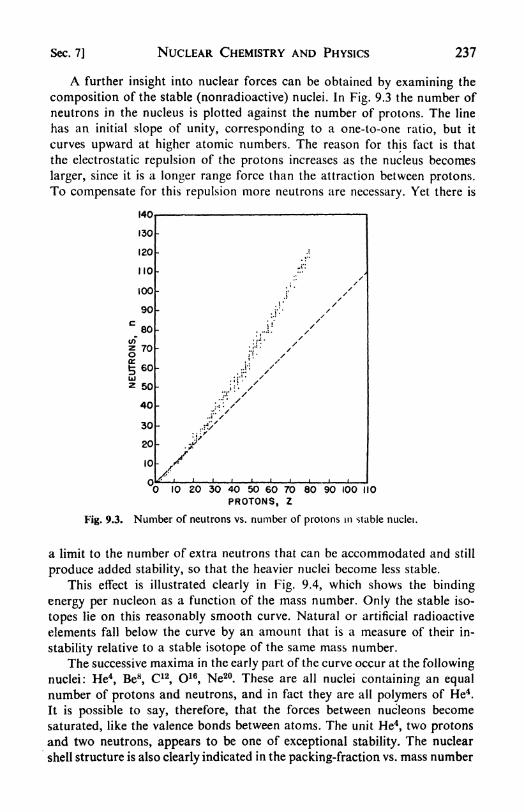
Sec. 7] NUCLEAR CHEMISTRY AND PHYSICS 237
A further insight into nuclear forces can be obtained by examining the
composition of the stable (nonradioactive) nuclei. In Fig. 9.3 the number of
neutrons in the nucleus is plotted against the number of protons. The line
has an initial slope of unity, corresponding to a one-to-one ratio, but it
curves upward at higher atomic numbers. The reason for this fact is that
the electrostatic repulsion of the protons increases as the nucleus becomes
larger, since it is a longer range force than the attraction between protons.To compensate for this repulsion more neutrons are necessary. Yet there is
140
130
120
MO
100
90
c/>
i 70
t;60
UJ2 50
40
30
20
10
10 20 30 40 50 60 70 80 90 100 110
PROTONS, Z
Fig. 9.3. Number of neutrons vs. number of protons in stable nuclei.
a limit to the number of extra neutrons that can be accommodated and still
produce added stability, so that the heavier nuclei become less stable.
This effect is illustrated clearly in Fig. 9.4, which shows the binding
energy per nucleon as a function of the mass number. Only the stable iso-
topes lie on this reasonably smooth curve. Natural or artificial radioactive
elements fall below the curve by an amount that is a measure of their in-
stability relative to a stable isotope of the same mass number.
The successive maxima in the early part of the curve occur at the following
nuclei: He4, Be8
, C12,O16
,Ne20
. These are all nuclei containing an equal
number of protons and neutrons, and in fact they are all polymers of He4.
It is possible to say, therefore, that the forces between nucleons become
saturated, like the valence bonds between atoms. The unit He4, two protons
and two neutrons, appears to be one of exceptional stability. The nuclear
shell structure is also clearly indicated in the packing-fraction vs. mass number
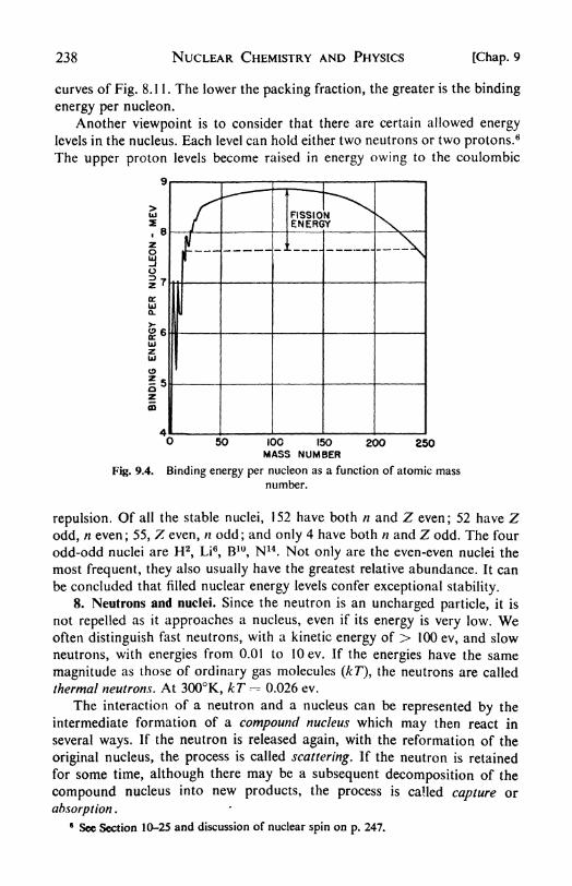
238 NUCLEAR CHEMISTRY AND PHYSICS [Chap. 9
curves of Fig. 8.1 1 . The lower the packing fraction, the greater is the binding
energy per nucleon.
Another viewpoint is to consider that there are certain allowed energylevels in the nucleus. Each level can hold either two neutrons or two protons.
6
The upper proton levels become raised in energy owing to the coulombic
50 200 250100 150
MASS NUMBER
Fig. 9.4. Binding energy per nucleon as a function of atomic mass
number.
repulsion. Of all the stable nuclei, 152 have both n and Z even; 52 have Zodd, n even; 55, Z even, n odd; and only 4 have both n and Z odd. The four
odd-odd nuclei are H2,Li6
, B10,N14
. Not only are the even-even nuclei the
most frequent, they also usually have the greatest relative abundance. It can
be concluded that filled nuclear energy levels confer exceptional stability.
8. Neutrons and nuclei. Since the neutron is an uncharged particle, it is
not repelled as it approaches a nucleus, even if its energy is very low. Weoften distinguish fast neutrons, with a kinetic energy of > 100 ev, and slow
neutrons, with energies from 0.01 to 10 ev. If the energies have the same
magnitude as those of ordinary gas molecules (kT), the neutrons are called
thermal neutrons. At 300K, kT --= 0.026 ev.
The interaction of a neutron and a nucleus can be represented by the
intermediate formation of a compound nucleus which may then react in
several ways. If the neutron is released again, with the reformation of the
original nucleus, the process is called scattering. If the neutron is retained
for some time, although there may be a subsequent decomposition of the
compound nucleus into new products, the process is called capture or
absorption .
* See Section 10-25 and discussion of nuclear spin on p. 247.

Sec. 8] NUCLEAR CHEMISTRY AND PHYSICS 239
A quantitative description of the interaction between a nucleus and a
neutron is given in terms of the effective nuclear cross section, a. Consider
a beam of neutrons in which the neutron flux is n per cnv2
per sec. If the
beam passes through matter in which there are c nuclei of a given kind per
cc, the number of neutrons intercepted per sec in a thickness fix is given by
- dn nac dx (9.7)
An initial flux of n is therefore reduced after a distance .v to nx n ccax
.
The scattering cross section as is distinguished from the absorption cross
section crrt ,and a as \
a(l
. Nuclear cross sections are generally of the order
10~24 cm2, and the whimsical physicists have called this unit the barn.
500
CD
J 100
oUJ
oo:oj<i-o
50
10
I 500
Fig. 9.5.
5 10 5O 100
NEUTRON ENERGY-6V
Nuclear cross section of silver. [From Rainwater, Havens, Wu,and Dunning, Phys. Rev. 71, 65 (1947),]
The cross sections depend on the kinetic energy of the neutrons and maybe quite different in the low- and high-velocity ranges. The dependence of a
on energy yields important information about energy levels in the nucleus,
for when the neutron energy is very close to a nuclear energy level, a
"resonance" occurs that greatly facilitates capture of the neutron, and
hence greatly increases the value of au . For example, for thermal neutrons,
a^H1)= 0.31 barn, a^H2
)- 0.00065 barn. Both ^H
1 andXH 2 have high
scattering cross sections, and are therefore effective in slowing fast neutrons,
but many of the thermal neutrons produced would be lost by capture to
jH1 dH 1 + Q/2
1 ->1H2
). It is for this reason that heavy water is a much moreefficient neutron moderator than light water. In H2O a thermal neutron
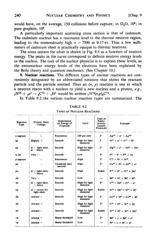
240 NUCLEAR CHEMISTRY AND PHYSICS [Chap. 9
would have, on the average, 150 collisions before capture; in D2O, 104;in
pure graphite, 103 .
A particularly important scattering cross section is that of cadmium.
The cadmium nucleus has a resonance level in the thermal neutron region,
leading to the tremendously high a = 7500 at 0.17ev. Thus a few milli-
meters of cadmium sheet is practically opaque to thermal neutrons.
The cross section for silver is shown in Fig. 9.5 as a function of neutron
energy. The peaks in the curve correspond to definite neutron energy levels
in the nucleus. The task of the nuclear physicist is to explain these levels, as
the extranuclear energy levels of the electrons have been explained bythe Bohr theory and quantum mechanics. (See Chapter 10.)
9. Nuclear reactions. The different types of nuclear reactions are con-
veniently designated by an abbreviated notation that shows the reactant
particle and the particle emitted. Thus an (n, p) reaction is one in which
a neutron reacts with a nucleus to yield a new nucleus and a proton, e.g.,
7N14 + X -*6C14 + iH
1 would be written 7N14(/i,/7)6C14
.
In Table 9.2 the various nuclear reaction types are summarized. The
TABLE 9.2
TYPES OF NUCLEAR REACTIONS
Reaction
Type
n capture
np
no.
n,2n
p capture
pn
pen
Normal MassChange
Slightly +
si 4 light clem,si heavy
Very -
si 4- light elem.
heavy

Sec. 10] NUCLEAR CHEMISTRY AND PHYSICS 241
second column gives the normal rest-mass change for the reaction. A positivemass change is equivalent to an endothermic reaction, a negative mass
change to an exothermic reaction. The next column indicates how the yield
depends on the energy of the bombarding particle. In most cases there is a
smooth increase in yield with increasing energy, but for capture processesthere is a marked resonance effect.
10. Nuclear fission. Perusal of the binding energy curve in Fig. 9.4 reveals
that a large number of highly exothermic nuclear reactions are possible,
since the heavy nuclei toward the end of the periodic table are all unstable
relative to the nuclei lying around the maximum of the curve.
In the January 1939 number of Naturwissenschaften, Otto Hahn and
S. Strassman reported that when the uranium nucleus is bombarded with
neutrons it may split into fragments, one of which they identified as an
isotope of barium. About 200 mev of energy is released at each fission.
It was immediately realized that secondary neutrons would very possibly
be emitted as a result of uranium fission, making a chain reaction possible.
The likelihood of this may be seen as follows: Consider the fission of a
92U235 nucleus to yield, typically, a 56Ba139 as one of the observed disintegra-
tion products. If balance is to be achieved between the numbers of protonsand neutrons before and after fission, the other product would have to be
36Kr98
. This product would be far heavier than any previously known krypton
isotope, the heaviest of which was 36Kr87
, a ft" emitter of 4 hours half-life.
Now the hypothetical 36Kr96 can get back to the proton-neutron curve of
Fig. 9.3 by a series of ft" emissions, and in fact a large number of new ft"
emitters have been identified among the fission products. The same result
can be achieved, however, if a number of neutrons are set free in the fission
process. Actually, both processes occur.
The fission process usually consists, therefore, of a disintegration of
uranium into two lighter nuclei, one of mass number from 82 to 100, and
the other from 128 to 150, plus a number, perhaps about three, of rapidly
moving neutrons. In only about one case in a thousand does symmetricalfission into two nuclei of approximately equal mass occur.
To determine which isotope of uranium is principally responsible for
fission, A. O. Nier and his coworkers separated small samples of U235
(0.7 per cent abundance) and U238(99.3 per cent) with a mass spectrometer.
It was found that U 235undergoes fission even when it captures a slow
thermal neutron, but U238is split only by fast neutrons with energies greater
than 1 mev. As usual, the capture cross section for slow neutrons is much
greater than that for fast neutrons, so that U235 fission is a much more likely
process than that of U238. The process of fission can be visualized by con-
sidering the nucleus as a drop of liquid. When a neutron hits it, oscillations
are set up. The positive charges of the protons acquire an unsymmetrical
distribution, and the resulting repulsion can lead to splitting of the nuclear
drop. Since U 235 contains an odd number of neutrons, when it gains a

242 NUCLEAR CHEMISTRY AND PHYSICS [Chap. 9
neutron considerable energy is set free. This kinetic energy starts the dis-
turbance within the nucleus that leads to fission. The isotope U238already
contains an even number of neutrons, and the capture process is not so
markedly exothermic. Therefore the neutron must be a fast one, bringing
considerable kinetic energy into the nucleus, in order to initiate fission.
Fission of other heavy elements, such as lead, has been produced by bom-
bardment with 200 mev deuterons produced by the Berkeley cyclotron.
Fission can also be induced by y rays with energies greater than about 5 mev
(photofissiori).
In Fig. 9.6 are shown the mass distributions of the fission products in
three different cases that have been carefully studied. When fission is produced
uj 6
u. (/)
O <
50 IOO
MASS NUMBER
ISO
Fig. 9.6. Mass distribution of products in three different fission reactions. The
energies of the particles initiating the fission are: n, thermal; a, 38 mev; rf, 200 mev.
Note how the distribution becomes more symmetrical as the energy of the incident
particle increases. (From P. Morrison, "A Survey of Nuclear Reactions" in Experi-mental Nuclear Physics, ed. E. Segre, Wiley, 1953.)
by highly energetic particles, the distribution of masses is quite symmetrical,and the most probable split is one that yields two nuclei of equal mass. This
is the result that would be expected from the liquid-drop model. The un-
symmetrical splitting that follows capture of slower particles has not yet
received a satisfactory theoretical explanation, but it is undoubtedly related
to the detailed shell structure inside the nucleus.
A nuclear reaction of great interest is spontaneous fission, discovered in
1940 by Flerov and Petrzhak in the U.S.S.R. It cannot be attributed to cosmic
radiation or to any other known external cause, and it must be considered to

Sec. 11] NUCLEAR CHEMISTRY AND PHYSICS 243
be a new type of natural radioactivity. For example, when about 6 g of Th232
were observed for 1000 hr, 178 spontaneous fissions were detected. Sponta-neous fission is usually a very rare reaction, but it becomes much more
frequent in some of the transuranium elements.
11. The transuranium elements. In 1940, E. McMillan and P. H. Abelson7
found that when U 238is irradiated with neutrons, a resonance capture can
occur that leads eventually to the formation of two new transuranium
elements.
U238 f"1 -92
92U 239 23inin->
93Np239-f
The 94Pu239
is a weakly radioactive a emitter (r 2.4 x 10⁴ years). Its
most important property is that, like U235,
it undergoes fission by slow
neutrons.
It was shown by G. T. Seaborg8 and his coworkers that bombardment
of U 238 with a particles leads by an (a, n) reaction to Pu241. This is a ft emitter
and decays to give 95Am 241, an isotope of americium which is a-radioactive
with 500 years half-life. By 1954, the last of the transuranium elements to have
been prepared were curium (96), berkelium (97), californium (98), and
elements (99) and (100). Curium can be made by an (a, ri) reaction on Pu239:
94Pu239 f 2He
4 ^ ^ + 96Cm242
The preparation of new examples of the transuranium elements has been
facilitated by the technique of using heavy ions accelerated in the cyclotron.
Thus high energy beams of carbon ions, (6C12)6 !
, can increase the atomic
number of a target nucleus by six units in one step. For example, isotopes of
californium have been synthesized as follows: 9
92U238 + 6C12 -> 98Cf244 + 6/1
Element (99) was prepared by:
92U 238 + 7N 14 -> 99X247 + 5/i
12. Nuclear chain reactions. Since absorption of one neutron can initiate
fission, and more than one neutron is produced at each fission, a branchingchain can occur in a mass of fissionable material. The rate of escape of
neutrons from a mass of U 235,for example, depends on the area of the
mass, whereas the rate of production of neutrons depends on the volume.
As the volume of the mass is increased, therefore, a critical point is finally
reached at which neutrons are being produced more rapidly than they are
being lost.
7Phys. Rev., 57, 1185 (1940).
8Science, 104, 379 (1946); Chem. Eng. News, 25, 358 (1947).
9 A. Ghiorso, S. G. Thompson, K. Street, and G. T. Seaborg, Phys. Rev. 81, 1954 (1951).
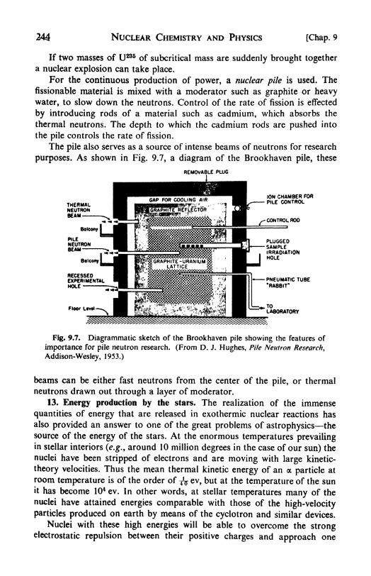
244 NUCLEAR CHEMISTRY AND PHYSICS [Chap. 9
If two masses of U235 of subcritical mass are suddenly brought togethera nuclear explosion can take place.
For the continuous production of power, a nuclear pile is used. The
fissionable material is mixed with a moderator such as graphite or heavy
water, to slow down the neutrons. Control of the rate of fission is effected
by introducing rods of a material such as cadmium, which absorbs the
thermal neutrons. The depth to which the cadmium rods are pushed into
the pile controls the rate of fission.
The pile also serves as a source of intense beams of neutrons for research
purposes. As shown in Fig. 9.7, a diagram of the Brookhaven pile, these
REMOVABLE PLUG
ION CHAMBER FORPILE CONTROL
PNEUMATIC TUBERABBIT"
Fig. 9.7. Diagrammatic sketch of the Brookhaven pile showing the features of
importance for pile neutron research. (From D. J. Hughes, Pile Neutron Research,
Addison-Wesley, 1953.)
beams can be either fast neutrons from the center of the pile, or thermal
neutrons drawn out through a layer of moderator.
13. Energy production by the stars. The realization of the immense
quantities of energy that are released in exothermic nuclear reactions has
also provided an answer to one of the great problems of astrophysics the
source of the energy of the stars. At the enormous temperatures prevailingin stellar interiors (e.g., around 10 million degrees in the case of our sun) the
nuclei have been stripped of electrons and are moving with large kinetic-
theory velocities. Thus the mean thermal kinetic energy of an a particle at
room temperature is of the order of^ ev, but at the temperature of the sunit has become 104 ev. In other words, at stellar temperatures many of the
nuclei have attained energies comparable with those of the high-velocity
particles produced on earth by means of the cyclotron and similar devices.
Nuclei with these high energies will be able to overcome the strongelectrostatic repulsion between their positive charges and approach one

Sec. 14] NUCLEAR CHEMISTRY AND PHYSICS 245
another sufficiently closely to initiate various nuclear reactions. It is these
so-called thermonuclear reactions that account for the energy production of
the stars.
In 1938, Carl von Weizsacker and Hans Bethe independently proposeda most ingenious mechanism for stellar-energy production. This is a cycle
proceeding as follows:
C 12 + H 1 ->N 13-\- hv
N 13 -C 13I- <?-
C 13 f H 1 -^ N 14|- hv
N uI H 1 ^O irM hv
O15 ^N 154-e'-
N 15-h H 1 >C12
-|- He4
The net result is the conversion of four H nuclei into one He nucleus throughthe mediation of C 12 and N 14 as "catalysts" for the nuclear reaction; 30mevare liberated in each cycle. This carbon cycle appears to be the principal
source of energy in very hot stars (T> 5 x 10sK).
The energy of somewhat cooler stars, like our sun (T ~ 10" K), appearsto be generated by the proton-proton cycle :
iH1 + t
H l -- jH- | H |0.42 mev
^ + XH 2 --2He
34- y f 5.5 mev
2He3 + 2He
3 -2He
4 f 21H 1
f 12.8 mev
The net result is the conversion of 4 protons to one helium nucleus, with the
liberation of 24.6 mev plus the annihilation energy of the positron.
Gamow has estimated10 that reactions between hydrogen nuclei ^H 1-|
tH2 ->2He3
4- y; 2 jH2 ->
2He4
-1 y) would have an appreciable rate at
temperatures below 106 degrees; reactions of protons with lithium nuclei
( XH 1-f 3Li
6 -^2He
4-f 2He
3; XH 1
f 3Li7 -> 2 2He
4) require about 6 x 10⁶
degrees; reactions such as jH1 + 5B
10 -->6CX1
h y require about 107degrees.
The temperatures attainable by means of uranium or plutonium fission
are high enough to initiate thermonuclear reactions of the lighter elements.
The fission reaction acts as a "match" to start the fusion reactions. Easiest
of all to "ignite" should be mixtures containing tritium, the hydrogen isotope
of mass 3.
XH3 + jH2 --
2He44 On
l f 17.6 mev (y)
!H3 f 1H1 -
2He4 + 19.6 mev (y)
The tritium can be prepared by pile reactions such as 3 Li(J
f A?1 ^
2He4 f 1
H3.
The isotope Li6 has an abundance of 7.52 atom per cent.
14. Tracers. The variety of radioactive isotopes now available has made
possible many applications in tracer experiments, in which a given type of
atom can often be followed through a sequence of chemical or physical
10George Gamow, The Birth and Death of the Sun (frew York: Penguin, 1945), p. 128.

246 NUCLEAR CHEMISTRY AND PHYSICS [Chap. 9
changes. Stable isotopes can also be used as tracers, but they are not so
easily followed and are available for relatively few elements. Radioactive
isotopes can be obtained from four principal sources: (1) natural radio-
activity; (2) irradiation of stable elements with beams of ions or electrons
obtained from accelerators such as cyclotrons, betatrons, etc.; (3) pile
irradiation with neutrons; (4) fission products. In Table 9.3 are listed a few
of the many available isotopes.
TABLE 9.3
ARTIFICIAL RADIOACTIVE ELEMENTS
Nucleus Activity HalfLife
One of the earliest studies with radioactive tracers used radioactive lead
to follow the diffusion of lead ions in solid metals and salts. For example,a thin coating of radiolead can be plated onto the surface of a sample of
metallic lead. After this is maintained at constant temperature for a definite
time, thin slices are cut off and their radioactivity measured with a Geigercounter. The self-diffusion constant of Pb in the metal can readily be cal-
culated from the observed distribution of activity. Many such diffusion
studies have now been made in metals and in solid compounds. The results
obtained are of fundamental importance in theories of the nature and prop-erties of the solid state. Diffusion in liquids, as well as the permeability of
.natural and synthetic membranes, can also be conveniently followed byradioactive tracer methods.
The solubility of water in pure hydrocarbons is so low that it is scarcely
measurable by ordinary methods. If water containing radioactive hydrogen,or tritium, ^^ a ft~~ emitter of 12 years half life, is used, even minute amounts
dissolved in the hydrocarbons are easily measured.11
A useful tracer method is isotopic dilution analysis. An example is the
determination of amino acids in the products of protein hydrolysis. The
conventional method would require the complete isolation of each amino
acid in pure form. Suppose, however, a known amount of an amino acid
11 C. Black, G. G. Joris, and H. S. Taylor, /. Chem. Phys., 16, 537 (1948).

Sec. 15] NUCLEAR CHEMISTRY AND PHYSICS 247
labeled with deuterium or carbon-14 is added to the hydrolysate. After
thorough mixing, a small amount of the given acid is isolated and its activity
measured. From the decrease in activity, the total concentration of the acid
in the hydrolysate can be calculated.
Tracers are used to elucidate reaction mechanisms. One interesting
problem was the mechanism of ester hydrolysis. Oxygen does not have a
radioactive isotope of long enough half life to be a useful tracer, but the
stable O18 can be used. By using water enriched with heavy oxygen (O*) the
reaction was $hown to proceed as follows:
O OR C/ + HO*H -, R-C< I
R'OHXOR' XO*H
The tagged oxygen appeared only in the acid, showing that the OR group is
substituted by O*H in the hydrolysis.12
Radioactive isotopes of C, Na, S, P, etc., are of great use in investigations
of metabolism. They supplement the stable isotopes of H, N, and O. For
^example it has been found that labeled phosphorus tends to accumulate
preferentially in rapidly metabolizing tissues. This has led to its trial in cancer
therapy. The results in this case have not been particularly encouraging, but
it may be possible to find metabolites or dyes that are specifically concen-
trated in tumor tissues, and then to render these compounds radioactive byinclusion of appropriate isotopic atoms. 13
15. Nuclear spin. In addition to its other properties, the nucleus mayhave an intrinsic angular momentum or spin. All elementary particles (i.e.,
neutrons, protons, and electrons) have a spin of one-half in units of h/27r.
The spin of the electron will be considered in some detail in the next chapter.
The spin of the elementary particles can be either plus or minus. If an axis is
imagined passing through the particle, the sign corresponds to a clockwise or
counterclockwise spin, although this picture is a very crude one. The spin of
a nucleus is the algebraic sum of the spins of the protons and neutrons that
it contains.
The hydrogen nucleus, or proton, has a spin of one-half. If two hydrogenatoms are brought together to form H2 , the nuclear spins can be either
parallel ( 1f ) or antiparallel ( 11, ). Thus there are two nuclear spin isomers of
H2 . The molecule with parallel spins is called "orthohydrogen," the one
with antiparallel spins is called "parahydrogen." Since spins almost never
change their orientation spontaneously, these two isomers are quite stable.
They have different heat capacities and different molecular spectra. Other
molecules composed of two identical nuclei having nonzero spin behave
similarly, but only in the cases of H2 and D2 are there marked differences in
physical properties.
12 M. Polanyi and A. L. Szabo, Trans. Farad. Soc., 30, 508 (1934).13 M. D. Kamen, Radioactive Tracers in Biology (New York: Academic, 1947).

248 NUCLEAR CHEMISTRY AND PHYSICS [Chap. 9
PROBLEMS
1. What is the Am in g per mole for the reaction H2 -f t O2 H2O for
which A// - - 57.8 kcal per mole?
2. From the atomic weights in Table 9.1, calculate the AE in kcal per
mole for the following reactions:
^ + o/;'- ^2, tH2
f- o*1 =^ 1H 1
f e - X, 2 tH2 -2He
4
3. Calculate the energies in (a) ev (b) kcal per mole of photons having
wavelengths of 2.0 A, 1000 A, 6000 A, 1 mm, 1 m.
4. To a hydrolysate from 10 g of protein is added 100 mg of pure
CD3CHNH2COOH (deuterium-substituted alanine). After thorough mixing,
100 mg of crystalline alanine is isolated which has a deuterium content of
1.03 per cent by weight. Calculate the per cent alanine in the protein.
5. A 10-g sample of iodobenzene is shaken with 100 ml of a 1 M KI solu-
tion containing 2500 counts per min radio-iodine. The activity of the iodo-
benzene layer at the end of 2 hours is 250 cpm. What per cent of the iodine
atoms in the iodobenzene have exchanged with the iodide ions in solution?
6. Calculate the mass of an electron accelerated through a potential of
2 x 10⁸ volts. What would the mass be if the relativity effect is ignored?
7. Naturally occurring oxygen consists of 99.76 per cent O16, 0.04 per
cent O17, and 0.20 per cent O18
. Calculate the ratio of atomic weights on the
physical scale to those on the chemical scale.
8. The work function of a cesium surface is 1.81 volts. What is the
longest wavelength of incident light that can eject a photoelectron from Cs?
9. The 77-meson has a mass about 285 times that of the electron; the
/t-meson has a mass about 215 times that of the electron. The 7r-meson
decays into a //-meson plus a neutrino. Estimate A for the reaction in ev.
10. Calculate the energy necessary to produce a pair of light mesons.
This pair production has been accomplished with the 200-in. California
cyclotron.
11. The scattering cross section, a, of lead is 5 barns for fast neutrons.
How great a thickness of lead is required to reduce the intensity of a neutron
beam to 5 per cent of its initial value? How great a thickness of magnesiumwith a = 2 barns?
12. According to W. F. Libby [Science, 109, 22V (1949)] it is probablethat radioactive carbon- 14 (r
= 5720 years) is produced in the upper atmo-
sphere by the action of cosmic-ray neutrons on N 14, being thereby main-
tained at an approximately constant concentration of 12.5 cpm per g of
carbon. A sample of wood from an ancient Egyptian tomb gave an activity
of 7.04 cpm per g C. Estimate the age of the wood.
13. A normal male subject weighing 70.8 kg was injected with 5.09 ml
of water containing tritium (9' x 109 cpm). Equilibrium with body water was

Chap. 9] NUCLEAR CHEMISTRY AND PHYSICS 249
reached after 3 hr when a 1-ml sample of plasma water from the subject had
an activity of 1.8 x 10⁵ cpm. Estimate the weight per cent of water in the
human body.
14. When 38Sr88
is bombarded with deuterons, 38Sr89
is formed. The cross
section for the reaction is 0.1 barn. A SrSO4 target 1.0 mm thick is exposedto a deuteron beam current of 100 microamperes. If scattering of deuterons
is neglected, compute the number of Sr atoms transmuted in 1.0 hr. TheSr88 is 82.6 per cent of Sr, and Sr89 is a Remitter of 53-day half life. Computethe curies of Sr89 produced.
15. When 79Au197
(capture cross section ac
=-- 10~22 cm2) is irradiated with
slow neutrons it is converted into 79Au198(r --= 2.8 days). Show that in general
the number of unstable nuclei present after irradiation for a time / is
o^(1_ e^
A
Here nQ is the number of target atoms and<f>
is the slow neutron flux. For the
case in question, calculate the activity in microcuries of a 100-mg gold sample
exposed to a neutron flux of 200/cm2 sec for 2 days.
16. The conventional unit of quantity of X radiation is the roentgen, r.
It is the quantity of radiation that produces 1 esu of ions in 1 cc of air at
STP (1 esu === 3.3 x 10~10 coulomb). If 32.5 ev are required to produce a
single ion pair in air, calculate the energy absorbed in 1 liter of air per
roentgen.
17. Potassium-40 constitutes 0.012 per cent of natural K, and K is 0.35
per cent of the weight of the body. K40 emits /? and y rays and has r
4.5 x 10⁸ yr. Estimate the number of disintegrations per day of the K40 in
each gram of body tissue.
18. The isotope 89Ac225 has r 10 days and emits an a with energy of
5.80 mev. Calculate the power generation in watts per 100 mg of the isotope.
REFERENCES
BOOKS
1. Baitsell, G. A. (editor), Science in Progress, vol. VI (New Haven: Yale
Univ. Press, 1949). Articles by H. D. Smyth on Fission; J. A. Wheeler on
Elementary Particles; E. O. Lawrence on High Energy Physics; G. T.
Seaborg on Transuranium Elements.
2. Bethe, H., Elementary Nuclear Theory (New York: Wiley, 1947).
3. Friedlander, G., and J. W. Kennedy, Introduction to Radiochemistry (NewYork: Wiley, 1949).
4. Gamow, G., and C. L. Critchfield, Theory ofAtomic Nucleus and Nuclear
Energy Sources (New York: Oxford, 1949).
5. Goodman, C. (editor), The Science and Engineering of Nuclear Power
(2 vols) (Boston: Addison-Wesley, 1947, 1949).

250 NUCLEAR CHEMISTRY AND PHYSICS [Chap. 9
6. Halliday, D., Introductory Nuclear Physics (New York: Wiley, 1950).
7. Hughes, D. J., Pile Neutron Research (Boston: Addison-Wesley, 1953).
8. Lapp, R. E., and H. L. Andrews, Nuclear Radiation Physics, 2nd ed.
(New York: Prentice-Hall, 1954).
9. Libby, W. F., Radiocarbon Dating (Chicago: Univ. of Chicago Press,
1952).
ARTICLES
1. Anderson, C. D., Science in Progress, 7, 236-249 (1951), 'The ElementaryParticles of Physics."
2. Curtan, S. C., Quart. Rev., 7, 1-18 (1953), "Geological Age by Means of
Radioactivity/'
3. Dunning, J. R., Science in Progress, 7, 291-355 (1951), "Atomic Structure
and Energy."4. Hevesy, G. C., J. Chem. Soc., 1618-1639 (1951), "Radioactive Indicators
in Biochemistry."5. Pryce, M. H. L., Rep. Prog. Phys., 17, 1-35 (1954), "Nuclear Shell
Structure."
6. Wilkinson, M. K., Am. J. Phys., 22, 263-76 ( 1 954), "Neutron Diffraction."

CHAPTER 10
Particles and Waves
1. The dual nature of light. It has already been noted that in the historyof light two different theories were alternately in fashion, one based on the
particle model and the other on the wave model. At the present time both
must be regarded with equal respect. In some experiments light displays
notably corpuscular properties: the photoelectric and Compton effects can
be explained only by means of light particles, or photons, having an energys hv. In other experiments, which appear to be just as convincing, the
wave nature of light is manifest: polarization and interference phenomenarequire an undulatory theory.
This unwillingness of light to fit neatly into a single picture frame has
been one of the most perplexing problems of natural philosophy. The situa-
tion recalls the impasse created by the "null result" of the Michelson-Morley
experiment. This result led Einstein to examine anew one of the most basic
of physical concepts, the idea of the simultaneity of events in space and time.
The consequence of his searching analysis was the scientific revolution
expressed in the relativity theories.
An equally fundamental enquiry has been necessitated by the develop-ments arising from the dual nature of light. These have finally required a
re-examination of the meaning and limitations of physical measurement
when applied to systems of atomic dimensions or smaller. The results of
this analysis are as revolutionary as the relativity theory; they are embodied
in what is called quantum theory or wave mechanics. Before discussing the
significant experiments that led inexorably to the new theories, we shall
review briefly the nature of vibratory and wave motions.
2. Periodic and wave motion. The vibration of a simple harmonic oscilla-
tor, discussed on page 190, is a good example of a motion that is periodic
in time. The equation of motion (/= ma) is md2x/dt
2--== KX. This is a
simple linear differential equation.1
It can be solved by first making the sub-
stitution p dx/dt. Then d*x/dt* =--dpjdt
-=(dp/dx)(dx/dt)
=p(dp/dx), and
the equation becomesp(dp\dx) + (K/W)X 0. Integrating,p2+(t</m)x
2 = const.
The integration constant can be evaluated from the fact that when the
oscillator is at the extreme limit of its vibration, x = A, the kinetic energyis zero, and hence p 0. Thus the constant = (K/m)A
2. Then
1See, for example, Granvi lie et al., Calculus, p. 383..
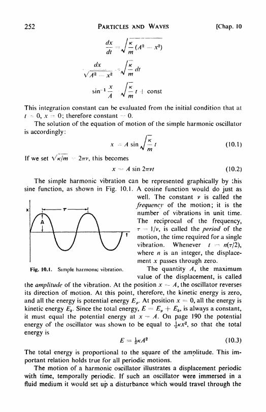
252 PARTICLES AND WAVES [Chap. 10
~~dfV/,4 2 - *2
. ,X IK
sin" 1 -
/ t -\ constA *< m
This integration constant can be evaluated from the initial condition that at
/ =-- 0, A- ---=-- 0; therefore constant 0.
The solution of the equation of motion of the simple harmonic oscillator
is accordingly:
x -= AsmJ-~t (10.1)
If we set VK//W ---2771-, this becomes
x ^ A sin 2irvt (10.2)
The simple harmonic vibration can be represented graphically by this
sine function, as shown in Fig. 10.1. A cosine function would do just as
well. The constant v is called the
frequency of the motion; it is the
number of vibrations in unit time.
The reciprocal of the frequency,r -=
]/v, is called the period of the
motion, the time required for a single
vibration. Whenever t--
n(r/2),
where n is an integer, the displace-
ment x passes through zero.
Fig. 10.1. Simple harmonic vibration. The quantity A, the maximumvalue of the displacement, is called
the amplitude of the vibration. At the position x =- A, the oscillator reverses
its direction of motion. At this point, therefore, the kinetic energy is zero,
and all the energy is potential energy Ep . At position x 0, all the energy is
kinetic energy Ek . Since the total energy, E = Ep + Ek , is always a constant,
it must equal the potential energy at x -= A. On page 190 the potential
energy of the oscillator was shown to be equal to }2KX2
, so that the total
energy is
E - \KA2
(10.3)
The total energy is proportional to the square of the amplitude. This im-
portant relation holds true for all periodic motions.
The motion of a harmonic oscillator illustrates a displacement periodic
with time, temporally periodic. If such an oscillator were immersed in a
fluid medium it would set up a disturbance which would travel through the

Sec. 3] PARTICLES AND WAVES 253
medium. Such a disturbance would be not only temporally periodic but also
spatially periodic. It would constitute what is called a wave. For example, a
tuning fork vibrating in air sets up sound waves. An oscillating electric dipolesets up electromagnetic waves in space.
Let us consider a simple harmonic wave moving in one dimension, x. If
one takes an instantaneous "snapshot" of the wave, it will have the form of
a sine or cosine function. This snapshot is the profile of the wave. If at a
point x = the magnitude of the disturbance<f> equals 0, then at some
further point x = A, the magnitude will again be zero, and so on at 2A,
3A . . . A. This quantity A is called the wavelength. It is the measure of the
wave's periodicity in space, just as the period T is the measure of its periodicityin time. The profile of the simple sine wave has the form:
<-,4sin27r~ (10.4)X.
Now consider the expression for the wave at some later time /. The idea
of the velocity of the wave must then be introduced. If the disturbance is
moving through the medium with a velocity c in the positive x direction, in
a time t it will have moved a distance ct. The wave profile will have exactlythe same form as before if the origin is shifted from ;c = to a new origin
at x = ct. Referred to this moving origin, the wave profile always maintains
the form of eq. (10.4). To refer the disturbance back to the stationary origin,
it is necessary only to subtract the distance moved in time t from the value
of x. Then the equation for the moving wave becomes
f\
<f>^-Asm~(x-ct) (10.5)
Note that the nature of the disturbance<f>
need not be specified: in the case
of a water wave it is the height of the undulation ; in the case of an electro-
magnetic wave it is the strength of an electric or magnetic field.
Now it is evident that c/A is simply the frequency: v = c/A. The numberof wavelengths in unit distance is called the wave number, k I/A, so that
eq. (10.5) can be written in the more convenient form:
<f>= A sin 27r(kx
-vt) (10.6)
3. Stationary waves. In Fig. 10.2, two waves, fa and fa, are shown that
have the same amplitude, wavelength, and frequency. They differ only in
that fa has been displaced along the X axis relative to fa by a distance d/2,7rk.
Thus they may be written
fa = A sin 2ir(kx vt)
fa = A sin [2ir(kx vt) + d]
The quantity d is called the phase of fa relative to fa.

254 PARTICLES AND WAVES [Chap. 10
When the displacement is exactly an integral number of wavelengths,the two waves are said to be in phase \ this occurs when d = 2?r, 4?r, or anyeven multiple of 77. When d --=
77, 3rr 9 or any odd multiple of n, the two waves
are exactly out of phase. Interference phenomena are readily explained in
terms of these phase relationships, for when two superimposed waves of
equal amplitude are out of phase, the resultant disturbance is reduced to zero.
Fig. 10.2. Waves differing in phase.
The expression (10.6) is one solution of the general partial differential
equation of wave motion, which governs all types of waves, from tidal waves
to radio waves. In one dimension this equation is
In three dimensions the equation becomes
v a;2
(10.7)
(10.8)
The operator V2(del squared) is called the Laplacian.
One important property of the wave equation is apparent upon inspec-
tion. The disturbance $ and all its partial derivatives appear only in terms
of the first degree and there are no other terms. This is therefore a linear
homogeneous differential equation.2
It can be verified by substitution that if
fa and <^2 are any two solutions of such an equation, then a new solution can
be written having the formi i
ii / 1 r\ r>\
<p-
fli9i ~r #2r2 (10.9)
where al and a2 are arbitrary constants. This is an illustration of the principle
of superposition. Any number of solutions can be added together in this wayto obtain new solutions. This is essentially what is done when a complicated
vibratory motion is broken down into its normal modes (page 191), or whena periodic function is represented by a Fourier series.
An important application of the superposition principle is found in the
addition of two waves of the form of eq. (10.6) that are exactly the same
8Granvilie, he. c//., pp. 372, 377.

Sec. 4] PARTICLES AND WAVES 255
except that they are going in opposite directions. Then the new solution
will be
</>-^ A sin 2rr(kx vt) + A sin 2v(kx } vt)
or ^ 2A sin 27r&jc cos 27rvt (10.10)
. x\ y xv
since sin x + sin j 2 sin cos
This new wave, which does not move either forward or backward, is a
stationary wave. The waves of the original type [eq. (10.6)] are called pro-
gressive waves. It will be noted that in the stationary wave represented by
eq. (10.10), the disturbance<f> always vanishes, irrespective of the value of /,
for points at which sin 2-nkx = or x 0, iAr, $A% S/v . . . (n/2)k. These
points are called nodes. The distance between successive nodes is Ik or A/2,
one-half a wavelength. Midway between the nodes are the positions of
maximum amplitude, or antinodes.
Solutions of the one-dimensional type, which have just been discussed,
will apply to the problem of a vibrating string in the idealized case in which
there is no damping of the vibrations. In a string of infinite length one can
picture the occurrence of progressive waves. Consider, however, as in Fig.
10.2, a string having a certain finite length L. This limitation imposes certain
boundary conditions on the permissible solutions of the wave equation. If the
ends of the string are held fixed: at x and at x L, the displacement
<f)must 0. Thus there must be an integral number of nodes between and
L, so that the allowed wavelengths are restricted to those that obey the
equation
nY L (10.11)
where n is an integer. This occurrence of whole numbers is very typical of
solutions of the wave equation under definite boundary conditions. In order
to prevent destruction of the wave by interference, there must be an integral
number of half wavelengths fitted within the boundary. This principle will
be seen to have important consequences in quantum theory.
4. Interference and diffraction. The interference of light waves can be
visualized with the aid of the familiar construction of Huygens. Consider,
for example, in (a) Fig. 10.3, an effectively plane wave front from a single
source, incident upon a set of slits. The latter is the prototype of the well
known diffraction grating. Each slit can now be regarded as a new light
source from which there spreads a semicircular wave (or hemispherical in
the three-dimensional case). If the wavelength of the radiation is A, a series
of concentric semicircles of radii A, 2A, 3A . . . may be drawn with these
sources as centers. Points on these circles represent the consecutive maxima
in amplitude of the new wavelets. Now, following Huygens, the new resultant
wave fronts are the curves or surfaces that are simultaneously tangent to the

256 PARTICLES AND WAVES [Chap. 10
a cos oi
secondary wavelets. These are called the "envelopes" of the wavelet curves
and are shown in the illustration.
The important result of this construction is that therfe are a number of
possible envelopes. The one that moves straight ahead in the same direction
as the original incident light is called the zero-order beam. On either side of
this are first-, second-, third-, etc., order diffracted beams. The angles bywhich the diffracted beams deviate from the original direction evidently
depend on the wavelength of the incident radiation. The longer the wave-
length, the greater is the diffraction. This is, of course, the basis for the use
of the diffraction grating in the measurement of the wavelength of radiation.
l*f ORDER
ORDER
2nd ORDER
(a) (b)
Fig. 10.3. Diffraction: (a) Huygens* construction; (b) path difference.
The condition for formation of a diffracted beam can be derived from a
consideration of (b) Fig. 10.3, where attention is focused on two adjacent slits.
If the two diffracted rays are to reinforce each other they must be in phase,otherwise the resultant amplitude will be cut down by interference. Thecondition for reinforcement is therefore that the difference in path for the two
rays must be an integral number of wavelengths. If a is the angle of diffraction
and a the separation of the slits, this path difference is a cos a and the
condition becomes
a cos a = /a (10.12)
where h is an integer.
This equation applies to a linear set of slits. For a two-dimensional plane
grating, there are two similar equations to be satisfied. For the case of light
incident normal to the grating,
a cos a = AA
b cos ft= A
It will be noted that the diffraction is appreciable only when the spacings

Sec. 5] PARTICLES AND WAVES 257
of the grating aj^rftt very much larger than the wavelength of the incident
light. In order /to obtain diffraction effects with X rays, for example, the
spacings should be of the order of a few Angstrom units.3
Max von Laue, in 1912, realized that the interatomic spacings in crystals
were probably of the order of magnitude of the wavelengths of X rays.
Crystal structures should therefore serve as three-dimensional diffraction
gratings for X rays. This prediction was immediately verified in the critical
experiment of Friedrich, Knipping, and Laue. A typical X-ray diffraction
picture is shown in Fig. 13.7 on page 375. The far-reaching consequences of
Laue's discovery will be considered in some detail in a later chapter. It is
mentioned here as a demonstration of the wave properties of X rays.
5. Black-body radiation. The first definite failure of the old wave theoryof light was not found in the photoelectric effect, a particularly clear-cut case,
but in the study of black-body radiation. All objects are continually absorbingand emitting radiation. Their properties as absorbers or emitters may be
extremely diverse. Thus a pane of window glass will not absorb much of
the radiation of visible light but will absorb most of the ultraviolet. A sheet
of metal will absorb both the visible and the ultraviolet but may be reasonably
transparent to X rays.
In order for a body to be in equilibrium with its environment, the radia-
tion it is emitting must be equivalent (in wavelength and amount) to the
radiation it is absorbing. It is possible to conceive of objects that "are perfect
absorbers of radiation, the so-called ideal black bodies. Actually, no sub-
stances approach very closely to this ideal over an extended range of wave-
lengths. The best laboratory approximation to an ideal black body is not a
substance at all, but a cavity.
This cavity, or hohlraum, is constructed with excellently insulating walls,
in one of which a small orifice is made. When the cavity is heated, the radia-
tion from the orifice will be a good sample of the equilibrium radiation within
the heated enclosure, which is practically ideal black-body radiation.
There is a definite analogy between the behavior of the radiation within
such a hohlraum and that of gas molecules in a box. Both the molecules and
the radiation are characterized by a density and both exert pressure on the
confining walls. One difference is that the gas density is a function of the
volume and the temperature, whereas the radiation density is a function of
temperature alone. Analogous to the various velocities distributed amongthe gas molecules are the various frequencies distributed among the oscilla-
tions that comprise the radiation.
At any given temperature there is a characteristic distribution of the gas
velocities given by Maxwell's equation. The corresponding problem of the
spectral distribution of black-body radiation, that is, the fraction of the
8It is also possible to use larger spacings and work with extremely small angles of
incidence. The complete equation, corresponding to eq. (10.12), for incidence at an angle
oto, is 0(cos a cos ao)= M.

258 PARTICLES AND WAVES [Chap. 10
total energy radiated that is within each range of wavelength, was first
explored experimentally (1877-1900) by O. Lummer and E. Pringsheim.Some of their results are shown in Fig. 10.4. These curves indeed have a
marked resemblance to those of the Maxwell distribution law. At high tem-
peratures the position of the maximum is shifted to shorter wavelengthsan iron rod glows first dull red, then orange, then white as its temperatureis raised and higher frequencies become appreciable in the radiation.
140
12345WAVE LENGTH, MICRONS
Fig. 10.4. Data of Lummer and Pringsheim on spectral distribution
of radiation from a black body at three different temperatures.
When these data of Lummer and Pringsheim appeared, attempts were
made to explain them theoretically by arguments based on the wave theoryof light and the principle of equipartition of energy. Without going into the
details of these efforts, which were uniformly unsuccessful, it is possible to
see why they were foredoomed to failure.
According to the principle of the equipartition of energy, an oscillator in
thermal equilibrium with its environment should have an average energy
equal to kT, \kT for its kinetic energy and \kT for its potential energy,where k is the Boltzmann constant. This classical theory states that the
average energy depends in no way on the frequency of the oscillator. In a
system containing 100 oscillators, 20 with a frequency vl of 1010 cycles per
sec and 80 with v2=-- 1014 cycles per sec, the equipartition principle predicts
that 20 per cent of the energy shall be in the low-frequency oscillators and80 per cent in the.high-frequency oscillators.
The radiation within a hohlraum can be considered to be made up of
Sec. 6] PARTICLES AND WAVES 259
standing waves of various frequencies. The problem of the energy distribu-
tion over the various frequencies (intensity / vs. v) apparently reduces to
the determination of the number of allowed vibrations in any range of
frequencies.
The possible high-frequency vibrations greatly outnumber the low-
frequency ones. The one-dimensional case of the vibrating string can be
used to illustrate this fact. We have seen in eq. (10.11) that in a string of
length L, standing waves can occur only for certain values of the wavelength
given by X = 2L/n. It follows that the number of allowed wavelengths from
any given value A to the maximum 2L is equal to n -= 2L/A. We wish to find
the additional number of allowed wavelengths that arise if the limiting wave-
length value is decreased from X to A dX. The result is obtained bydifferentiation4 as
dn = ^dl (10.13)A
This indicates that the number of allowed vibrations in a region from A to
A dk increases rapidly as the wavelength decreases (or the frequency
increases). There are many more high-frequency than low-frequency vibra-
tions. The calculation in three dimensions is more involved5 but it yields
essentially the same answer. For the distribution of standing waves in an
enclosure of volume V, the proper formula is dn (Sir F/A4)c/A, or
dn^%7T-v*dv (10.14)c3
Since there are many more permissible high frequencies than low fre-
quencies, and since by the equipartition principle all frequencies have the
same average energy, it follows that the intensity / of black-body radiation
should rise continuously with increasing frequency. This conclusion follows
inescapably from classical Newtonian mechanics, yet it is in complete dis-
agreement with the experimental data of Lummer and Pringsheim, which
show that the intensity of the radiation rises to a maximum and then falls
off sharply with increasing frequency. This abject failure of classical mechani-
cal principles when applied to radiation was viewed with unconcealed dismay
by the physicists of the time. They called it the "ultraviolet catastrophe."6. Planck's distribution law. The man who first dared to discard classical
mechanics and the equipartition of energy was Max Planck. Taking this
step in 1900, he was able to derive a new distribution law, which explainedthe experimental data on black-body radiation.
Newtonian mechanics (and relativity mechanics too) was founded uponthe ancient maxim that natura non facit saltum ("nature does not make a
jump"). Thus an oscillator could be presumed to take up energy continuously
4It is assumed that in a region of large L and small A, n is so large that it can be con-
sidered to be a continuous function of A.5 R. H. Fowler, Statistical Mechanics (London: Cambridge, 1936), p. 112.

260 PARTICLES AND WAVES [Chap. 10
in arbitrarily small increments. Although matter was believed to be atomic
in its constitution, energy was assumed to be strictly continuous.
Planck discarded this precept and suggested that an oscillator, for
example, could acquire energy only in discrete units, called quanta. The
quantum theory began therefore as an atomic theory of energy. The magni-tude of the quantum or atom of energy was not fixed, however, but dependedon the oscillator frequency according to
s - hv (10.15)
Planck's constant h has the dimensions of energy times time (e.g., 6.62 x10⁻²⁷ erg sec^ a quantity known as action.
According to this hypothesis it is easy to see qualitatively why the in-
tensity of black-body radiation always falls off at high frequencies. At fre-
quencies such that hv ^> kT, the size of the quantum becomes much larger
than the mean kinetic energy of the atoms comprising the radiator. The
larger the quantum, the smaller is the chance of an oscillator having the
necessary energy, since this chance depends on an e~ h'f*T Boltzmann factor.
Thus oscillators of high frequency have a mean energy considerably less
than the kT of the classical case.
Consider a collection of N oscillators having a fundamental vibration
frequency v. If these can take up energy only in increments of hv, the allowed
energies are 0, hv, 2hv, 3hv, etc. Now according to the Boltzmann formula,
eq. (7.31), if NQ is the number of systems in the lowest energy state, the
number N{ having an energy e
{above this ground state is given by
AT,= TV/**
1
(10.16)
In the collection of oscillators, for example,
NI = N e~ hvlkT
N* = Ne-~2hvlkT
N3= NQe~*
hvlkT
The total number of oscillators in all energy states is therefore
-tfo 2t-O
The total energy of all the oscillators equals the energy of each level times
the number in that level.
E = #

Sec. 7] PARTICLES AND WAVES 261
The average energy of an oscillator is therefore
. E _e ~~
~N~
According to this expression, the mean energy of an oscillator whosefundamental frequency is v approaches the classical value of kT when hv
becomes much less than kT. 1Using this equation in place of the classical
equipartition of energy, Planck derived an energy-distribution formula in
excellent agreement with the experimental data for black-body radiation.
The energy density E(v) dv is simply the number of oscillations per unit
volume between v and v + dv [eq. (10.14)] times the average energy of an
oscillation [eq. (10.17)]. Hence Planck's Law is
STT/Zr3 dvE(v) dv - -
hv/kT--
(10.18)
7. Atomic spectra. Planck's quantum theory of energy appeared in 1901.
Strong confirmation was provided by the theory of the photoelectric effect
proposed by Einstein in 1905. Another most important application of the
theory was soon made, in the study of atomic spectra.
An incandescent gas emits a spectrum composed of lines at definite wave-
lengths. Similarly if white light is transmitted through a gas, certain wave-
lengths are absorbed, causing a pattern of dark lines on a bright backgroundwhen the emergent light is analyzed with a spectrograph. These emission
and absorption spectra must be characteristic of certain preferred frequencies
in the gaseous atoms and molecules. A sharply defined line spectrum is
typical of atoms. Molecules give rise to spectra made up of bands, which
can often be analyzed further into closely packed lines. For example, the
spectra of atomic hydrogen (H) and of molecular nitrogen (N2) are shown
in Fig. 10.5a and b.
In 1885, J. J. Balmer discovered a regular relationship between the fre-
quencies of the atomic hydrogen lines in the visible region of the spectrum.The wave numbers v' are given by
with Wj=
3, 4, 5 . . . etc. The constant ^ is called the Rydberg constant,
and has the value 109,677.581 cm"1. It is one of the most accurately known
physical constants.
6 In eq. (10.17) let e~x = y, then the denominator S/ = 1 + y 4- y* -f-
. . .=
1/(1~y\ (y< 1). The numerator, Zi>'
=y(\ + 2v + 3/ +...)= yl(\
-y)
2, (y < 1)
so that eq. (10.17) becomes hvy/(l-
y) = Ar/fr*"/**1 -
1).7 When hv < kT, e^/**
1
1 -f (hv/kT).

262 PARTICLES AND WAVES [Chap. 10
Other hydrogen series were discovered later, which obeyed the more
general formula,
JL.-JL)!/
(10.19)
Lyman found the series with 2= 1 in the far ultraviolet, and others were
found in the infrared by Paschen (/ 2=
3), Bracket! (na 4), and Pfund
H, A.
Fig. 10.5a. Spectra of atomic hydrogen. (From Herzberg, Atomic Spectra and
Atomic Structure, Dover, 1944.)
fcjJK-ftfVl^MIBffP 8''' vCTPFig. 10.5b. Spectra of molecular nitrogen. (From Harrison, Lord, and
Loofbourow, Practical Spectroscopy, Prentice-Hall, 1948.)
(/?2=
5). A great number of similar series have been observed in the atomic
spectra of other elements.
8. The Bohr theory. These characteristic atomic line spectra could not be
explained on the basis of the Rutherford atom. According to this model,
electrons are revolving around a positively charged nucleus, the coulombic
attraction balancing the force due to the centripetal acceleration. The classical
theory of electromagnetic radiation demands that an accelerated electric
charge must continuously emit radiation. If this continuous emission of
energy actually occurred, the electrons would rapidly execute a descending
spiral and fall into the nucleus. The Rutherford atom is therefore inherently
unstable according to classical mechanics, but the predicted continuous
radiation does not in fact occur. The fact that the electrons in atoms do not
follow classical mechanics is also clearly shown by the heat-capacity values
of gases. The Cv for monatomic gases equals fR, which is simply the amount
expected for the translation of the atom as a whole. It is evident that the
electrons in the atoms do not take up energy as the gas is heated.
Niels Bohr, in 1913, suggested that the electrons can revolve around the
nucleus only in certain definite orbits, corresponding to certain allowed

Sec. 8] PARTICLES AND WAVES 263
energy states. Radiation is emitted in discrete quanta whenever an electron
falls from an orbit of high to one of lower energy, and is absorbed whenever
an electron is raised from a low to a higher energy orbit. If Eniand E
ntare
the energies of two allowed states of the electron, the frequency of the spectral
line arising from a transition is
A 1
v = = -(Eni-E
nt) (10.20)
A separate and arbitrary hypothesis is needed to specify which orbits are
allowed. The simplest orbits of one electron moving in the field of force of
a positively charged nucleus are the circular ones. For these orbits, Bohr
postulated the following frequency condition: 8only those orbits occur for
which the angular momentum mvr is an integral multiple of h\2-n.
mvr = n~> n - 1, 2, 3 . . . (10.21)ITT
The integer n is called a quantum number.
The mechanics of motion of the electron in its circular orbit of radius r
can be analyzed starting with Newton's equation,/ ma. The force is the
coulombic attraction between nucleus, with charge Ze, and electron, i.e.,
Ze2/r
2. The acceleration is the centripetal acceleration, v2/r. Therefore
Ze2/r
2 mv2/r, and
(10.22)mv*
h2
Then, from eq. (10.21) r - n2 -(10.23)
In the case of a hydrogen atom Z ==-1, and the smallest orbit, n 1,
would have a radius,
"o= TT~2 - '529 A (10 '24)
4n2me2
This radius is of the same order of magnitude as that obtained from the
kinetic theory of gases.
It may be noted that the radii of the circular Bohr orbits depend on the
square of the quantum number. It can now be demonstrated that the Balmer
series arises from transitions between the orbit with n = 2 and outer orbits;
in the Lyman series, the lower term is the orbit with n = 1 ; the other series
are explained similarly. These results are obtained by calculating the energies
corresponding to the different orbits and applying eq. (10.20). The energylevel diagram for the hydrogen atom is shown in Fig. 10.6.
8 It will be seen a little later that this condition is simply another form of Planck's
hypothesis that h is the quantum of action.

264 PARTICLES AND WAVES [Chap. 10
Fig. 10.6. Energy levels of the H atom. (After G. Herzberg,Atomic Spectra, Dover, 1944.)
The total energy E of any state is the sum of the kinetic and potential
energies:
^^
* pr
Ze* Ze2
From eq. (10.22), E =
/
Therefore from eq. (10.23), E ==
The frequency of a spectral line is then
2r
Z2
l2"""^2 (10.25)
(10.26)

Sec. 9] PARTICLES AND WAVES 265
Comparison with the experimental eq. (10.19) yields a theoretical value of
the Rydberg constant for atomic hydrogen of
.^-~ 109,737 cm-ch3
This is in excellent agreement with the experimental value.
This pleasing state of affairs represented a great triumph for the Bohr
theory and lent some solid support to the admittedly ad hoc hypothesis on
which it is based.
Several improvements in the original Bohr theory were made by Arnold
Sommerfeld. He considered the possible elliptical orbits of an electron
around the nucleus as one focus. Such orbits are known to be stable con-
figurations in dynamical systems such as the planets revolving around the
sun.
For a circular orbit, the radius r is constant so that only angular momen-
tum, associated with the variable 6, need be considered. For elliptical orbits
two quantum numbers are needed, for the two variables r and 0. The
azimutha! quantum number k was introduced to give the angular momentumin units of h\1-n. The principal quantum number n was defined9 so that the
ratio of the major axis to the minor axis of the elliptical orbit was n\k.
Then k can take any value from 1 to /?, the case n k corresponding to
a circular orbit.
9. Spectra of the alkali metals. An electron moving about a positively
charged nucleus is moving in a spherically symmetrical coulombic field of
force. Besides the hydrogen atom, a series of hydrogenlike ions satisfy this
condition. These ions include He^, Li++, and Be l++, each of which has a
single electron. Their spectra are observable when electric sparks discharge
through the vapour of the element (spark spectra). They are very similar in
structure to the hydrogen spectrum, but the different series are displaced to
shorter wavelengths, as a consequence of the dependence of frequency on
the square of the nuclear charge, given by eq. (10.26).
If an electron is moving in a spherically symmetrical field, the energylevel is the same for all elliptical orbits of major axis a as it is for the circular
orbit of radius a. In other words, the energy is a function only of the principal
quantum number n. All energy levels with the same n are the same, irrespec-
tive of the value of k, the azimuthal quantum number. For example, if
n = 3, there are three superimposed levels or terms of identical energy,
having k = 1, 2, or 3. Such an energy level is said to have a threefold de-
generacy. Actually, even in hydrogen, a very slight splitting of these degener-
ate levels is found in the fine structure of the spectra, revealed by spectro-
graphs of high resolving power.
9 Derivations and detailed discussions of these aspects of the old quantum theory maybe found in S. Dushman's article in Taylor's Treatise on Physical Chemistry, 2nd ed., p. 1 170.

266 PARTICLES AND WAVES [Chap. 10
EV5.37
5
UL
For most of the atoms and ions that may give rise to spectra the electrons
concerned in the transitions are not moving in spherically symmetric fields.
Consider, for example, the case of the lithium atom, which is typical of the
alkali metals. The electron whose transitions are responsible for the observed
spectrum is the outer, valence, or optical electron. This electron does notmove in a spherical field, since its position at any instant is influenced bythe positions of the two inner electrons. If the outer electron is on one side
of the nucleus, it is less likely that the other two will be there also, becauseof the electrostatic repulsions. Thus the field is no longer spherical, and the
elliptical orbits can no longer have the same energy as a circular orbit of the
same n value. The elliptical orbits will havedifferent energy levels depending on their
ellipticity, which is governed by the allowedvalues of the azimuthal quantum number k.
For each n, there will be n different energylevels characterized by different k's.
The lowest ojr ground state is that for
which n = 1 and k ^ 1. States with k ~ 1
are called s states. This is therefore a Is
state. When n = 2, k can be either 1 or 2.
States with k = 2 are called p states. Wetherefore have a 2s state and a 2p state.
Similarly, when n = 3, we have 3s, 3p, and3d (k = 3) states; when n = 4, we have
4s, 4/?, 4J, and 4f(k = 4) states.
In this discussion there has been a tacit
assumption that the energy levels of the
atom are determined solely by the quan-tum states of the valence electrons. This
is actually not true, and all the electrons and even the nucleus should beconsidered in discussing the allowed energy states. Then, instead of the
quantum number k, which gives the angular momentum of the singleelectron, a new quantum number L must be used that gives the resultant
angular momentum of all the electrons. According as L ~ 0, 1, 2, 3 .
etc., we refer to the atomic states as S, P, A F . . . etc. In the case of atomslike the alkali metals, which have only one valence electron, it turns outthat the resultant angular momenta of the inner electrons add vectorially to
zero. Therefore in this case only ttie single electron need be considered after
all.10 Nevertheless we shall use the more proper notation, 5, />, D, F, to
refer to the energy levels.
The energy-level diagram for lithium is shown in Fig. 10.7. The observed
10 The situation becomes more complicated when there are two or more optical electrons.An excellent discussion is given by G. H. Herzberg, Atomic Spectra and Atomic Structure(New York: Dover Publications, 1944).
Fig. 10.7. Energy levels and spec-tral transitions in the lithium atom.

Sec. 10] PARTICLES AND WAVES 267
spectral series arise from the combinations of these terms, as shown in the
diagram. It will be noted that only certain transitions are allowed; others are
forbidden. Certain selection rules must be obeyed, as for example in this case
the rule that AL must be + 1 or 1 .
Experimentally four distinct series have been observed in the atomic
spectra of the alkalis. The principal series is the only one found in absorption
spectra and arises from transitions between the ground state 1*9 andfc
the
various P states. It may be written symbolically :
v^ 15 - mP
Absorption spectra almost always arise from transitions from the groundstate only, since at ordinary temperatures the proportion of atoms in excited
states is usually vanishingly small, being governed by the exponential Boltz-
mann factor e~^ElkT
. At the much higher temperatures required to excite
emission spectra, some of the higher states are sufficiently populated byatoms to give rise to a greater variety of lines.
Thus in the emission spectra of the alkali metals, in addition to the prin-
cipal series, three other series appear. These may be written symbolically as
v 2P - mS the sharp series
v 2P - mD the diffuse series
v --= 3D mF the fundamental series
The names are not notably descriptive, although the lines in the sharp series
are indeed somewhat narrower than the others.
10. Space quantization. So far in the discussion of allowed Bohr orbits,
we have not considered the question of how the orbits can be oriented in
space. This is because in the absence of an external electric or magneticfield there is no way of distinguishing between different orientations, since
there is no physically established axis of reference. If an atom is placed in a
magnetic field, however, one can ask how the orbits will be oriented relative
to the field direction.
The answer given by the Bohr theory is that only certain orientations
are allowed. These are determined by the condition that the component of
angular momentum in the direction of the magnetic field, e.g., in the Zdirection, must be an integral multiple of h/27r. Thus
P.- % (10.27)
where m is the magnetic quantum number. This behavior is called space
quantization.
The allowed values of m are 1, 2, 3, etc., up to &, k being the
azimuthal quantum number, which gives the magnitude of the total angular

268 PARTICLES AND WAVES [Chap. 10
k3Fig. 10.8. Spatial quantiza-
tion of angular momentum in a
magnetic field H.
momentum in units of h/2ir. An example of space quantization for the case
k = 3 is illustrated in Fig. 10.8.
For any value of k, there are 2k allowed orientations corresponding to
the different values of m. In the absence of an external field, the correspond-
ing energy level will be 2/r-fold degenerate.
In the presence of an electric or magneticfield this energy level will be split into its
individual components. This splitting gives
rise to a splitting of the corresponding spec-
tral lines. In a magnetic field this is called
the Zeeman effect', in an electric field, the
Stark effect. This observed splitting of the
spectral lines is the experimental basis for the
introduction into the Bohr theory of space
quantization and the quantum number m.
11. Dissociation as series limit. It will be
noted in the term diagram for lithium that the
energy levels become more closely packed as
the height above the ground state increases.
They finally converge to a common limit
whose height above the ground level corresponds to the energy necessary to
remove the electron completely from the field of the nucleus. In the observed
spectrum, the lines become more and more densely packed and finally
merge into a continuum at the onset of dissociation. The reason for the
continuous absorption or emission is that the free electron no longer has
quantized energy states but can take up kinetic energy of translation
continuously.
The energy difference between the series limit and the ground level
represents the ionization potential I of the atom or ion. Thus thefast ionization
potential of Li is the energy of the reaction Li+ 4- e -> Li. The second
ionization potential is the energy of Li+ f + e -> Li+.
Examples of ionization potentials are given in Table 10.1. The way in
which the values of / vary with position in the periodic table should be
noted. This periodicity is very closely related to the periodic character of the
chemical properties of the elements, for it is the outer electrons of an atom
that enter into its chemical reactions. Thus the alkali metals have low
ionization potentials; the inert gases, high ionization potentials.
12. The origin of X-ray spectra. The origin of the characteristic X-rayline series studied by Moseley (see Chapter 8) is readily understood in terms
of the Bohr theory. The optical spectra are caused by transitions of outer or
valence electrons, but the X-ray spectra are caused by transitions of the
inner electrons. X rays are generated when high-velocity particles such as
electrons impinge upon a suitable target. As the result of such a collision,
an electron may be driven completely from its orbit, leaving a "hole" in the

Sec. 13] PARTICLES AND WAVES 269
TABLE 10.1
IONIZATION POTENTIALS OF CHEMICAL ELEMENTS (IN ELECTRON VOLTS)
target atom. When electrons in outer shells, having larger values of the
principal quantum number n, drop into this hole, a quantum of X radiation
is emitted.
13. Particles and waves. One might go on from here to describe the
further application of the Bohr theory to more complex problems in atomic
structure and spectra. Many other quite successful results were obtained,
but there were also a number of troublesome failures. Attempts to treat
cases in which more than one outer electron is excited, as in the helium
spectrum, were in general rather discouraging.
The Bohr method is essentially nothing more than the application of a
diminutive celestial mechanics, with coulombic rather than gravitational
forces, to tiny solar-system models of the atom. Certain quantum conditions
have been arbitrarily superimposed on this classical foundation. The rather
capricious way in which the quantum numbers were introduced and adjusted
always detracted seriously from the completeness of the theory.
Now there is one branch of physics in which, as we have seen, integral
numbers occur very naturally, namely in the stationary-state solutions of
the equation for wave motion. This fact suggested the next great advance in
physical theory: the idea that electrons, and in fact all material particles,
must possess wavelike properties. It was already known that radiation
exhibited both corpuscular and undulatory aspects. Now it was to be shown,
first theoretically and soon afterwards experimentally, that the same must
be true of matter.
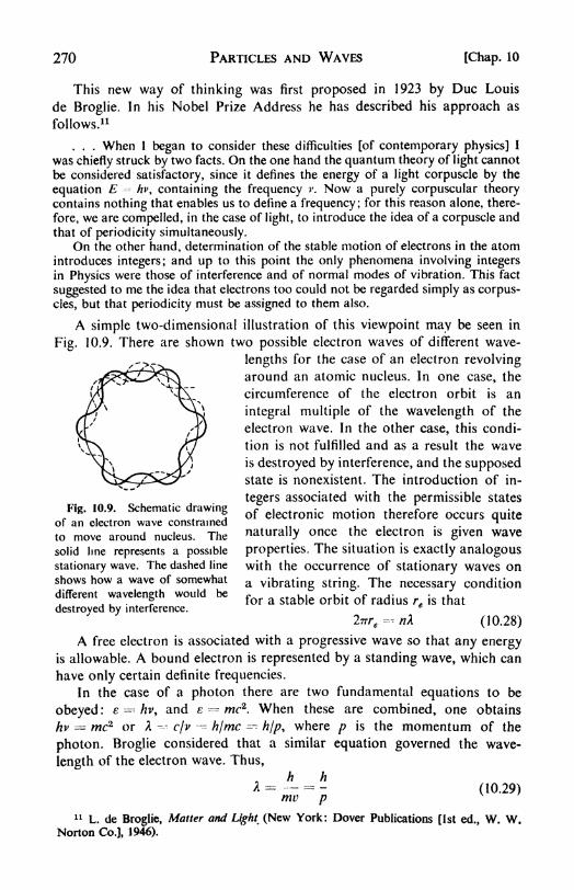
270 PARTICLES AND WAVES [Chap. 10
This new way of thinking was first proposed in 1923 by Due Louis
de Broglie. In his Nobel Prize Address he has described his approach as
follows. 11
. . . When 1 began to consider these difficulties [of contemporary physics] I
was chiefly struck by two facts. On the one hand the quantum theory of light cannot
be considered satisfactory, since it defines the energy of a light corpuscle by the
equation E ---= hv, containing the frequency v. Now a purely corpuscular theorycontains nothing that enables us to define a frequency; for this reason alone, there-
fore, we are compelled, in the case of light, to introduce the idea of a corpuscle and
that of periodicity simultaneously.On the other hand, determination of the stable motion of electrons in the atom
introduces integers; and up to this point the only phenomena involving integersin Physics were those of interference and of normal modes of vibration. This fact
suggested to me the idea that electrons too could not be regarded simply as corpus-
cles, but that periodicity must be assigned to them also.
A simple two-dimensional illustration of this viewpoint may be seen in
Fig. 10.9. There are shown two possible electron waves of different wave-
lengths for the case of an electron revolvingaround an atomic nucleus. In one case, the
circumference of the electron orbit is an
integral multiple of the wavelength of the
electron wave. In the other case, this condi-
tion is not fulfilled and as a result the wave
is destroyed by interference, and the supposedstate is nonexistent. The introduction of in-
tegers associated with the permissible statesFig. 10.9. Schematic drawing Qf e|ectronic motjon therefore occurs quiteof an electron wave constrained
~
to move around nucleus. The naturally once the electron is given wave
solid line represents a possible properties. The situation is exactly analogous
stationary wave. The dashed line with the occurrence of stationary waves onshows how a wave of somewhat a vibrating string. The necessary conditiondifferent wavelength would be
for a staWc^ Qf radius.
fc
destroyed by interference.e
27rre
=-. nX (10.28)
A free electron is associated with a progressive wave so that any energyis allowable. A bound electron is represented by a standing wave, which can
have only certain definite frequencies.
In the case of a photon there are two fundamental equations to be
obeyed : e ~ hv, and e = me2. When these are combined, one obtains
hv = me2 or X ----c/v
-= h/mc hip, where p is the momentum of the
photon. Broglie considered that a similar equation governed the wave-
length of the electron wave. Thus,
* *A = = -
(10.29)mv p11 L. de Broglie, Matter and Light^ (New York: Dover Publications [1st ed., W. W.
Norton Co.], 1946).

Sec. 14] PARTICLES AND WAVES 271
The original Bohr condition for a stable orbit was given by eq. (10.21)
as 27Ttnvre= nh. By combination with eq. (10.28), one again obtains eq.
(10.29) so that the Broglie formulation gives the Bohr condition directly.
The Broglie relation, eq. (10.29), is the fundamental one between the
momentum of the electron considered as a particle and the wavelength of its
associated wave. Consider, for example, an electron that has been accelerated
through a potential difference V of 10 kilovolts. Then Ve ~ -i/w2, and its
velocity would be 5.9 x 109 cm per sec, about one-fifth that of light. The
wavelength of such an electron would be
h 6.62 x 10~27
~mv
~(9AI x \Q
r)(53~
0.12 A
This is about the same wavelength as that of rather hard X rays.
H2
a F22-
Golf ball
Baseball
TABLE 10.2
WAVELENGTHS OF VARIOUS PARTICLES
Table 10.2 lists the theoretical wavelengths associated with various
particles.12 The wavelengths of macroscopic bodies are exceedingly short,
so that any wave properties will escape our observation. Only in the atomic
world does the wave nature of matter become manifest.
14. Electron diffraction. If any physical reality is to be attached to the
idea that electrons have wave properties, a 1 .0 A electron wave should be
diffracted by a crystal lattice in very much the same way as an X-ray wave.
Experiments along this line were first carried out by two groups of workers,
who shared a Nobel prize for their efforts. C. Davisson and L. H. Germer
worked at the Bell Telephone Laboratories in New York, and G. P. Thom-
son, the son of J. J. Thomson, and A. Reid were at the University of Aber-
deen. Diffraction diagrams obtained by Thomson by passing beams of
12 After J. D. Stranathan, The Particles of Modern physics (Philadelphia: Blakiston,
1942), p. 540.

272 PARTICLES AND WAVES [Chap. 10
electrons through thin gold foils are shown in Fig. 10.10. The wave nature
of the electron was unequivocally demonstrated by these researches. More
recently, excellent diffraction patterns have been obtained from crystals
placed in beams of neutrons.
Electron beams, owing to their negative charge, have one advantage not
possessed by X rays as a means of investigating the fine structure of matter.
Appropriate arrangements of electric and magnetic fields can be designed to
act as "lenses" for electrons. These arrangements have been applied in the
[The photograph below
was one of the first ob-
tained. The one at the
right is a recent example.]
Fig. 10.10. Diffraction diagrams obtained by passing beams of electrons
through thin gold foils. (Courtesy Professor Sir George Thomson.)
development of electron microscopes capable of resolving images as small as
20 A in diameter. We could wish for no clearer illustrations of the wave
properties of electrons than the beautiful electron micrographs of viruses,
fibers, and colloidal particles that have been obtained with these instruments.
15. The uncertainty principle. In the development of atomic physics wehave noted the repeated tendency toward the construction of models of the
atom and its constituents from building blocks that possess all the normal
properties of the sticks and stones of everyday life. One fundamental axiom
of the classical mechanics developed for commonplace occurrences was the
possibility of simultaneously measuring different events at different places.
Such measurement appears at first to be perfectly possible because to a first
approximation the speed of light is infinitely large, and it takes practically
no time to signal from place to place. More refined measurements must
consider the fact that this speed is really not infinite, but only 3 x 1010 cm
per sec. This speed is indeed large compared with that of a rocket, but not
compared with that of an accelerated electron. As a result, attempts to applythe old mechanics to moving electrons were a failure, and the new relativisitic
mechanics of Einstein was needed to correct the situation.
Sec. 15] PARTICLES AND WAVES 273
In a similar way, in our ordinary macroscopic world, the value of the
Planck constant h may be considered to be effectively zero. The Broglie
wavelengths of ordinary objects are vanishingly small, and a batter need
not consider diffraction phenomena when he swings at an inside curve. If
we enter into the subatomic world, h is no longer so small as to be negligible.
The Broglie wavelengths of electrons are of such a magnitude that diffraction
effects occur in crystal structures.
One of the fundamental tenets of classical mechanics is that it is possible
to specify simultaneously the position and momentum of any body. The
strict determinism of mechanics rested upon this basic assumption. Knowingthe position and velocity of a particle at any instant, Victorian mechanics
would venture to predict its position and velocity at any other time, past or
future. Systems were completely reversible in time, past configurations beingobtained simply by substituting / for t in the dynamical equations. But, is
it really possible to measure simultaneously the position and momentum of
any particle? The possible methods of measurement must be analyzed in
detail before an answer can be given.
To measure with precision the position of a very small object, a micro-
scope of high resolving power is required. With visible light one cannot
expect to locate objects much smaller than a tenth of a micron. The size of
the smallest body that can be observed is limited by diffraction effects, which
begin to create a fuzziness in the image when the object is of the same order
of magnitude as the wavelength of the incident light. The limit of resolution
is given according to the well known formula of Abbe as R A/2/4, and
the maximum value of the numerical aperture A is unity.
In order to determine the position of an electron to within a few per cent
uncertainty, radiation of wavelength around 10~10 cm or 10~2 A would have
to be used. We shall conveniently evade the technical problems involved in
the design and manufacture of a microscope using these y rays. With such
very short rays, there will be a very large Compton effect, and the y ray will
impart considerable momentum to the electron under observation. This
momentum is given by eq. (9.5) as mv = 2(hv/c) sin a/2. Since the range in
scattering angle is from to 7T-/2, corresponding to the aperture of the micro-
scope (A = 1), the momentum is determined only to within an uncertainty
of A/?= mv & A/A. On account of diffraction, the error A^ in the determina-
tion of position is of the order of the wavelength A.
The product of the uncertainty in momentum times the uncertainty in
position is therefore of the order of h,
&p-&q~h (10.30)
This is the famous uncertainty principle of Werner Heisenberg (1926). It is
impossible to specify simultaneously the exact position and momentum of a
particle because our measuring instruments necessarily disturb the object
being measured. This disturbance is negligible with man-sized objects, but

274 PARTICLES AND WAVES [Chap. 10
the disturbance of atom-sized particles cannot be neglected. Herein is the
essential meaning of the failure of classical mechanics and the success of
wave mechanics. 13
16. Waves and the uncertainty principle. Some kind of uncertainty prin-
ciple is always associated with a wave motion. This fact can be seen very
clearly in the case of sound waves. Consider the case of an organ pipe, set
into vibration by depressing a key, whose vibration is stopped as soon as the
key is released. The vibrating pipe sets up a train of sound waves in the air,
which we hear as a note of definite frequency. Now suppose the time between
the depression and the release of the key is gradually shortened. As a result,
the length of the train of waves is shortened also. Finally the time will come
when the period during which the key is depressed is actually less than the
period r of the sound wave, the time required for one complete vibration.
Once this happens, the frequency of the wave is no longer precisely deter-
mined, for at least one complete vibration must take place to define the
frequency. It appears, therefore, that the time and the frequency cannot both
be fixed at any arbitrary value. If a very small time is chosen, the frequencybecomes indeterminate.
When waves are associated with particles, a similar uncertainty principle
is a necessary consequence. If the wavelength or frequency of an electron
wave, for example, is to be a definitely fixed quantity, the wave must be
infinite in extent. Any attempt to confine a wave within boundaries requires
destructive interference at these boundaries in order to reduce the resultant
amplitudes there to zero. This interference can be secured only by super-
imposing waves of different frequencies. It follows that an electron wave of
perfectly definite frequency, or momentum, must be infinitely extended and
therefore must have a completely indeterminate position. In order to fix
the position, superimposed waves of different frequency are required, and
as the position becomes more closely defined the momentum becomes
fuzzier.
The uncertainty relation eq. (10.30) can be expressed not only in terms
of position and momentum but also for energy and time. Thus,
A/? A? - AF A/ ?v h (10.31)
This equation is used to estimate the sharpness of spectral lines. In general,
lines arising from transitions from the ground state of an atom are sharp.This is because the optical electron spends a long time in the ground state
and thus A", the uncertainty in the energy level, is very small. On the other
hand, the lifetime of excited states may sometimes be very short, and trans-
itions between such excited energy levels may give rise to diffuse or broad-
ened lines as a result of the uncertainty A in the energy levels, which is
18Many natural philosophers would, not agree with this statement. See H. Margenau,
Physics Today, 7, 6 (1954).

Sec. 17] PARTICLES AND WAVES 275
reflected in an uncertainty, Av -= A//z, in the frequency of the observed
line.14
17. Zero-point energy. According to the old quantum theory, the energylevels of a harmonic oscillator were given by En nhv. If this were true the
lowest energy level would be that with n 0, and would therefore have zero
energy. This would be a state of complete rest, represented by the minimumin the potential energy curve in Fig. 7.15.
The uncertainty principle does not allow such a state of completelydefined position and completely defined (in this case, zero) momentum. As
a result, the wave treatment shows that the energy levels of the oscillators
are given by
*=
( + I)'"' 0- 32)
Now, even when n 0, the ground state, there is a residual zero-point energy
amounting to
=-, \hv (10.33)
This must be added to the Planck expression for the mean energy of an
oscillator, which was derived in eq. (10.17).
18. Wave mechanics the Schrodinger equation. In 1926, Erwin Schr5-
dinger and W. Heisenberg independently laid the foundations for a distinctly
new sort of mechanics which was expressive of the wave-particle duality of
matter. This is called wave or quantum mechanics.
The starting point for most quantum mechanical discussions is the
Schrodinger wave equation. We may recall that the general differential
equation of wave motion in one dimension is given by eq. (10.7) as
_
dx*~
&'
a/ 2
where<f>
is the displacement and v the velocity. In order to separate the
variables, let<f>
=---y(x) sin 2-nvt. On substitution in the original equation,
this yields
d*W 47T2V2
T? + ^T-V = (10-34)dx* v2
This is the wave equation with the time dependence removed. In order
to apply this equation to a "matter wave," the Broglie relation is introduced,
as follows: The total energy E is the sum of the potential energy U and the
kinetic energy p2j2m. E = p*/2m + U. Thus, p = [2m(E - (7)]
1/2, or
X = hip= h[2m(E U)]~
m. Substituting this in eq. (10.34), one obtains:
(,0.35)
14 This is not the only cause of broadening of spectral lines. There is in addition a
pressure broadening due to interaction with the electric fields of neighboring atoms or
molecules, and a Doppler broadening, due to motion of the radiating atom or molecule
with respect to the observer.

276 PARTICLES AND WAVES [Chap. 10
This is the famous Schrftdinger equation in one dimension. For three
dimensions it takes the formo2.*|W + -r^-(E- U)y>
= (10.36)rr
Although the equation has been obtained in this way from the ordinarywave equation and Broglie's relation, it is actually so fundamental that it is
now more usual simply to postulate the equation as the starting point of
quantum mechanics, just as Newton's/^ ma is postulated as the starting
point of ordinary mechanics.
As is usual with differential equations, the solutions of eq. (10.36) for
any particular set of physical conditions are determined by the particular
boundary conditions imposed upon the system. Just as the simple wave
equation for a vibrating string yields a discrete set of stationary-state solutions
when the ends of the string are held fixed, so in general solutions are obtained
for the SchrOdinger equation only for certain energy values E. In many cases
the allowed energy values are discrete and separated, but in certain other
cases they form a continuous spectrum of values. The allowed energy values
are called the characteristic, proper, or eigen- values for the system. The
corresponding wave functions y am called the characteristic functions or
eigenfunctions.
19. Interpretation of the y functions. The eigenfunction ip is by nature a
sort of amplitude function. In the case of a light wave, the intensity of the
light or energy of the electromagnetic field at any point is proportional to
the square of the amplitude of the wave at that point. From the point of
view of the photon picture, the more intense the light at any place, the more
photons are falling on that place. This fact can be expressed in another way
by saying that the greater the value of y>, the amplitude of a light wave in
any region, the greater is improbability of a photon being within that region.
It is this interpretation that is most useful when applied to the eigen-
functions of Schrftdinger's equation. They are therefore sometimes called
probability amplitudefunctions. If y(x) is a solution of the wave equation for
an electron, then the probability of finding the electron within the rangefrom x to x + dx is given
16by y>
2(x)dx.
The physical interpretation of the eigenfunction as a probability ampli-tude function is reflected in certain mathematical conditions that it must
obey. It is required that y>(x) be singleTvalued, finite, and continuous for all
physically possible values of x. It must be single-valued, since the probability
of finding the electron at any point x must have one and only one value. It
cannot be infinite at any point, for then the electron would be fixed at exactly
that point, which would be inconsistent with the wave properties. The require-
ment of continuity is helpful in the selection of physically reasonable solutions
for the wave equation.15 Since the function y may be a complex quantity, the probability is written more
generally as ^v>, where $ is the complex conjugate of y>. Thus, e.g., if y>= e~ ix
t y>= *'*

Sec. 20] PARTICLES AND WAVES 277
20. Solution of wave equation the particle in a box. The problem of
finding the solution of the wave equation in any particular case may be an
extremely difficult one. Sometimes a solution can be devised in principle that
in practice would involve several decades of calculations. The recent develop-ment of high-speed calculating machines has greatly extended the range of
problems for which numerical solutions can be obtained.
The simplest case to which the wave equation can be applied is that of a
free particle; i.e., one moving in the absence of any potential field. In this
case we may set U = and the one-dimensional equation becomes
87T2/M-- EV =
A solution of this equation is readily found16 to be
y A sin (-^V2mE x \
(10.37)
(10.38)
where A is an arbitrary constant. This is a perfectly allowable solution as
long as E is positive, since the sine of a real quantity is everywhere single-
valued, finite, and continuous. Thus all positive values of E are allowable
w(a) (b) (0
Fig. 10.11. Electron in a one-dimensional box. (a) the potential function,
(b) allowed electron waves, (c) tunnel effect.
and the free particle has a continuous spectrum of energy states. This con-
clusion is in accord with the picture previously given of the onset of the
continuum in atomic spectra as the result of dissociation of an electron from
the atom.
What is the effect of imposing a constraint upon the free particle by
requiring that its motion be confined within fixed boundaries? In three
16See, for example, Granville et-aL, op. ciY., p. 390. The solution can be verified by
substitution into the equation.

278 PARTICLES AND WAVES [Chap. 10
dimensions this is the problem of a particle enclosed in a box. The one-
dimensional problem is that of a particle required to move between set
points on a straight line. The potential function that corresponds to such a
condition is shown in (a), Fig. 10.11. For values of x between and a the
particle is completely free, and U =- 0. At the boundaries, however, the
particle is constrained by an infinite potential wall over which there is no
escape; thus U --= oo when x ^ 0, x - a.
The situation now is similar to thcit of the vibrating string considered at
the beginning of the chapter. Restricting the electron wave within fixed
boundaries corresponds to seizing hold of the ends of the string. In order
to obtain stable standing waves, it is again necessary to restrict the allowed
wavelengths so that there is an integral number of half wavelengths between
and a; i.e., n(A/2) a. Some of the allowed electron waves are shown in
(b), Fig. 10.11, superimposed upon the potential-energy diagram.The permissible values of the kinetic energy En of the electron in a box
can be obtained from the Broglie relation X -
hjmv.
2
i= \m
(10.39)
From this equation, two important consequences can be deduced which
will hold true for the energy of electrons, not only in this special case, but
quite generally. First of all, it is apparent that as the value of a increases,
the energy decreases. Other factors being the same, the more room the
electron has to move about in, the lower will be its energy. The more localized
is its motion, the higher will be its energy. Remember that the lower the
energy, the greater the stability of a system.
Secondly, the integer n is a typical quantum number, which now appears
quite naturally and without any ad hoc hypotheses. It determines the number
of nodes in the electron wave. When n 1 there are no nodes. When n 2
there is a node in the center of the box; when n -- 3 there are two nodes, and
so on. The value of the energy depends directly on 2, and therefore rises
rapidly as the number of nodes increases.
The extension of the one-dimensional result to a three-dimensional box
of sides a, b, and c is very simple. The allowed energy levels for the three-
dimensional case depend on a set of three integers (n l9 2 , %): since there are
three dimensions, there are three quantum numbers.
h* In* TV* 32\
=o-(-V + 7J + -r) 00.40)8/w \ a2 b* c* /
This result shows that according to wave mechanics even the trans-
lational motion of a particle in a box is quantized. Because of the extremely

Sec. 21] PARTICLES AND WAVES 279
small value of h2 these levels lie very closely packed together except in cases
where the dimensions of the box are vanishingly small.
If electron waves in one dimension are comparable with vibrations of a
violin string, those in two dimensions are like the pulsations of a drumhead,whereas those in three dimensions are like the vibrations of a block of steel.
The waves can then have nodes along three directions, and the three quantumnumbers determine the number of nodes.
21. The tunnel effect. Let us take a baseball, place it in a well constructed
box, and nail the lid down tightly. Now any proper Newtonian will assure
us that the ball is in the box and is going to stay there until someone takes
it out. There is no probability that the ball will be found on Monday inside
the box and on Tuesday rolling along outside it. Yet if we transfer our
attention from a baseball in a box to an electron in a box, quantum mechanics
predicts exactly this unlikely behavior.
To be more precise, consider in (c), Fig. 10.11, a particle moving in a
"one-dimensional box" with a kinetic energy Ek . It is confined by a potential-
energy wall of thickness d and height UQ . Classical mechanics indicates that
the particle can simply move back and forth in its potential energy well;
since the potential-energy barrier is higher than the available kinetic energy,
the possibility of escape is absolutely nil.
Quantum mechanics tells a different story. The wave equation (10.35) for
the region of constant potential energy UQ is
*) 4 (87T2w/7*
2) (E - U )y>
-
This equation has the general solution
W -- ^ e^^!/i)^2m(E'-Un )x
In the region within the box E ^ U(}and this solution is simply the familiar
sine or cosine wave of eq. (10.38) written in the complex exponential form. 17
In the region within the potential-energy barrier, however, UQ > ",so that
the expression under the square root sign is, negative. One can therefore
multiply out a V 1 term, obtaining the following result:
y>-= Ae-V*1^***^'*
(10.41)
This exponential function describes the behavior of the wave function
within the barrier. It is evident that according to wave mechanics the prob-
ability of finding an electron in the region of negative energy is not zero,
but is a certain finite number that falls off exponentially with the distance
of penetration within the barrier . The behavior of the wave function is shown
in (c), Fig. 10.11. So long as the barrier is not infinitely high nor infinitely
wide there is always a certain probability that electrons (or particles in
general) will leak through. This is called the tunnel effect.
17See, for example, Courant and Robbins, What Is Mathematics (New York: Oxford,
1941), p. 92, for a description of this notation: eio =- cos -f / sin 0.

280 PARTICLES AND WAVES [Chap. 10
The phenomenon is not observed with baseballs in boxes or with cars in
garages,18
being rendered extremely improbable by the various parametersin the exponential. In the world of atoms, however, the effect is a commonone. One of the best examples is the emission of an a particle in a radio-
active disintegration. The random nature of this emission is a reflection of
the fact that the position of the particle is subject to probability laws.
22. The hydrogen atom. If the translational motion of the atom as a
whole and the motion of the atomic nucleus are neglected, the problem of
the hydrogen atom can be reduced to that of a single electron in a coulombic
field. This is in a sense a modification of the problem of a particle in a three-
dimensional box, except that now the box is spherical. Also, instead of steep
walls and zero potential energy within, there is now a gradual rise in potential
with distance from the nucleus: at r = oo, U 0; at r = 0, U = oo.
The potential energy of the electron in the field of the nucleus is given byU -= e2/r. The Schrddinger equation therefore becomes
In view of the spherical symmetry of the potential field, it is convenient to
transform this expression into spherical coordinates,
i a / a^A i a2^ i a / a^A
r* Or V Or /+
r2 sin2 6
*
M>*+^sinO
'
00 \Sm
OO/+
The polar coordinates r, 0, and<f>
have their usual significance (Fig. 7.2,
page 168). The coordinate r measures the radial distance from the origin;
is a "latitude"; and<f>
a "longitude." Since the electron is moving in three
dimensions, three coordinates obviously suffice to describe its position at
any time.
In this equation, the variables can be separated, since the potential is a
function of r alone. Let us substitute
That is, the wave function is a product of three functions, one of which
depends only on r, one only on 6, and the last only on<f>.We shall skip the
intervening steps in the solution and the application of the boundary con-
ditions that permit only certain allowed eigenfunctions to be physically
meaningful.19 From our previous experience, however, we shall not be sur-
prised to find that the final solutions represent a set of discrete stationary
18 This extreme example is described by G. Gamow in Mr. Tompkins in Wonderland(New York: Macmillan, 1940), which is recommended as an introduction to this chapter in
Physical Chemistry.19 For the steps in the solution see, for example, L. Pauling and E. B. Wilson, Introduc-
tion to Quantum Mechanics (New York: McGraw-Hill, 1935), Chap. V.
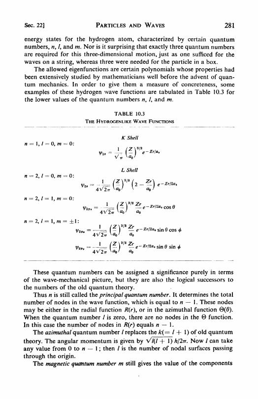
Sec. 22] PARTICLES AND WAVES 281
energy states for the hydrogen atom, characterized by certain quantumnumbers, n, /, and m. Nor is it surprising that exactly three quantum numbersare required for this three-dimensional motion, just as one sufficed for the
waves on a string, whereas three were needed for the particle in a box.
The allowed eigenfunctions are certain polynomials whose properties had
been extensively studied by mathematicians well before the advent of quan-tum mechanics. In order to give them a measure of concreteness, some
examples of these hydrogen wave functions are tabulated in Table 10.3 for
the lower values of the quantum numbers n, /, and m.
TABLE 10.3
THE HYDROGENLIKE WAVE FUNCTIONS
K Shell
n = i, / = o, m = 0:
/2T\ 3/2
1 /2T\ 3
--^ ~V-rr \<V
L Shell
n = 2, / = 0, m = 0:
-!=(?)''' (2 -*)*-*4X/27TW V <*J
Y>2P .- -44V 2-
=2, /= 1,/n = 1:
v = L^ (? )
3/25: e -Zr/2 sin cos
4V/27T ^o 7flb
_
4V27
These quantum numbers can be assigned a significance purely in terms
of the wave-mechanical picture, but they are also the logical successors to
the numbers of the old quantum theory.
Thus n is still called the principal quantum number. It determines the total
number of nodes in the wave function, which is equal to n 1 . These nodes
may be either in the radial function R(r), or in the azimuthal function 0(0).
When the quantum number / is zero, there are no nodes in the function.
In this case the number of nodes in R(r) equals n 1 .
The azimuthal quantum number /replaces the k(= I + 1) of old quantum
theory. The angular momentum is given by Vl(l + 1) H/2iT. Now / can take
any value from to n 1 ; then / is the number of nodal surfaces passing
through the origin.
The magnetic quantum number m still gives the value of the components

282 PARTICLES AND WAVES [Chap. 10
of angular momentum along the r axis, since p0tZ mh/27T9 exactly as in
eq. (10.27). The allowed values of m now run from / to {-/, including zero.
The great advantage of the new theory is that these numbers all arise
quite naturally from Schrodinger's equation.
n = 3
(a)
mo 6
Fig. 10.12. (a) Radial part of wave functions for hydrogen atom, (b) Radial
distribution functions giving probability of finding electrons at a given distance
from nucleus. (After G. Herzberg, Atomic Spectra, Dover, 1944.)
23. The radial wave functions. In (a), Fig. 10.12, the radial wave functions
have been plotted for various choices of n and /. In case / 0, all the nodes
appear in the radial function.
The value of ^2(r) is proportional to the probability of finding the electron
at any particular distance r in some definite direction from the nucleus. More
important physically is the radial distribution function, 47rr2^2(r), which gives
the probability of finding the electron within a spherical shell of thickness dr

Sec. 23] PARTICLES AND WAVES 283
at a distance r from the nucleus, irrespective of direction. (Compare the
problem of gas-velocity distribution on page 187.) The radial distribution
functions are shown in (b), Fig. 10.12. In place of the sharply defined electron
orbits of the Bohr theory, there is a more diffuse distribution of electric
charge. The maxima in these distribution curves, however, correspond closely
with the radii of the old Bohr orbits. Yet there is always a definite probability
n -2/ -o
> 2, m - 1 3, m -
n = 3, m 2 n =3, m = db 1 n =
3, w = n = 4, m
Fig. 10.13. Electron clouds of the H atom. (From Herzberg, Atomic Spectra and
Atomic Structure, Dover, 1944.)
of finding the electrons much closer to or much farther from the nucleus.
The strict determinism of position in the classical description has been
replaced by the probability language of wave mechanics.
A particularly clear illustration of the wave mechanical representation of
the hydrogen atom can be obtained from the illustrations in Fig. 10.13.
Here the intensity of the shading is proportional to the value of y>2, the
probability distribution function. There is a greater probability of an electron
being in a light-colored region. It should be clearly understood that quantummechanics does not say that the electron itself is smeared out into a cloud.

284 PARTICLES AND WAVES [Chap. 10
It is still to be regarded as a point charge. Its position and momentum cannot
be simultaneously fixed, and all that the theory can predict that has physical
meaning is the probability that the electron is in any given region.
A wave function for an electron is sometimes called an orbital. When/ = we have an 5 orbital, which is always spherically symmetrical. When/ = 1 we have a p orbital. The p orbitals can have various orientations in
space corresponding to the allowed values of w, which may be 1, 0, or +LIn Fig. 10.14, the angular parts of the wave functions are represented for s
z
Fig. 10.14. Polar representation of absolute values of angular part of wave
function for the H atom. The j-type function (/== 0) is spherically symmetrical.
There are three possible />-type functions, directed along mutually perpendicularaxes (x, y. z).
and p orbitals, and the directional1
character of the p orbitals is very evident.
It will be shown later that the directional character of certain chemical
bonds is closely related to the directed orientations of these orbitals.
24. The spinning electron. There is one aspect of atomic spectra that
cannot be explained on the basis of either the old quantum theory or the
newer wave mechanics. This is the multiplicity or multiple! structure of
spectral lines. Typical of this multiplicity are the doublets occurring in the
spectra of the alkali metals: for example, in the principal series each line is
in reality a closely spaced double line. This splitting is revealed immediatelywith a spectroscope of good resolving power. The occurrence of double lines
indicates that each term or energy level for the optical electron must also be
split into two.

Sec. 25] PARTICLES AND WAVES 285
A satisfactory explanation for the occurrence of multiple energy levels
was first proposed in 1925 by G. E. Uhlenbeck and S. Goudsmit. Theypostulated that an electron itself may be considered to be spinning on its
axis.20 As a result of spin the electron has an inherent angular momentum.
Along any prescribed axis in space, for example, the direction of a magneticfield, the components of the spin angular momentum are restricted to values
given by sh/2-rr, where s can have only a value of + J or -J.
In effect, the electron spin adds a new quantum number s to those re-
quired to describe completely the state of an electron. We now have, therefore,
the following quantum numbers:
n the principal quantum number; allowed values 1, 2, 3, . . .
/ the azimuthal quantum number, which gives the orbital angularmomentum of the electron; allowed values 0, 1, 2, . . ., n I.
m the magnetic quantum number, which gives the allowed orientation
of the "orbits" in an external field; allowed values /, / + 1
-/ + 2, . . ., + /.
s the spin quantum number; allowed values \-\ or J.
25. The Pauli Exclusion Principle. An exact solution of the wave equationfor an atom has been obtained only in the case of hydrogen; i.e., for the
motion of a single electron in a spherically symmetric coulombic field.
Nevertheless, in more complex atoms the energy levels can still be specified
in terms of the four quantum numbers n, /, m, s 9 although in many cases the
physical picture of the significance of the numbers will be lost. This is
especially true of electrons in inner shells, for which a spherically symmetricfield would be a very poor approximation. On the other hand, the behavior
of an outer or valence electron is sometimes strikingly similar to that of the
electron in the hydrogen atom. In any case, the important fact is that the
four quantum numbers still suffice to specify completely the state of an
electron even in a complex atom.
There is a most important principle that determines the allowable quan-tum numbers for an electron in an atom and consequently has the most
profound consequences for chemistry. It is the Exclusion Principle, first
enunciated by Wolfgang Pauli. In a single atom no two electrons can have
the same set offour quantum numbers, n, /, m, s. At present this principle
cannot be derived from fundamental concepts, but it may have its ultimate
origin in relativity theory. It is suggestive that relativity theory introduces a
"fourth dimension," so that a fourth quantum number becomes necessary.
26. Structure of the periodic table. The general structure of the periodic
table is immediately clarified by the Exclusion Principle. We recall that even
in a complex atom the energy levels of the electrons can be specified by
80 No attempt will be made to reconcile this statement with the idea that an electron is
x>int charge. It is merely
properties of electrons, ab.a point charge. It is merely a convenient pictorial way of speaking of one of the fundamental
about which the complete story is not yet written.

286 PARTICLES AND WAVES [Chap. 10
means of four quantum numbers : , /, m, s. The Exclusion Principle requires
that no two electrons in an atom can have the same values for all four quan-tum numbers. The most stable state, or ground state, of an atom will be that
in which the electrons are in the lowest possible energy levels that are con-
sistent with the Exclusion Principle. The structure of the periodic table is a
direct consequence of this requirement.
The lowest atomic energy state is that for which the principal quantumnumber n is 1, and the azimuthal quantum number / is 0. This is a Is state.
The hydrogen atom has one electron and this goes therefore into the \s level.
The helium atom has two electrons, which may both be accommodated in
the \s state if they have opposing spins. With two electrons in the \s state,
there is an inert gas configuration since the shell n 1 or K shell is com-
pleted. The completed shell cannot add electrons and a large energy would
be needed to remove an electron.
Continuing to feed electrons into the lowest lying energy levels, we come
to lithium with 3 electrons. The first two go into the Is levels, and the third
electron must occupy a 2s level. The 2s electron is much less tightly bound
than the Is electrons. The first ionization potential of Li is 5.39 ev, the second
75.62 ev. This is true because the 2s electron is usually much farther from
the nucleus than the Is, and besides it is partially shielded from the +3nuclear charge by the two Is electrons. A Is electron, on the other hand, is
held by the almost unshielded +3 nuclear charge.
The L shell, with n --=2, can hold 8 electrons two 2s and six 2p electrons,
the quantum numbers being as follows :
n I
2
m
-1
+ 1
s
4
4
4
4
When the L shell is filled, the next electron must enter the higher-lying
M shell of principal quantum number n = 3.
A qualitative picture of the stability of the complete octet is obtained by
considering the elements on either side of neon.
The attraction of an electron by the positively charged nucleus is governed
by Coulomb's Law, but for electrons outside the innermost shell the shielding
effect of the other electrons must be taken into consideration. For a given

Sec. 27] PARTICLES AND WAVES 287
electron, the shielding effect of other electrons is pronounced only if theylie in a shell between the given electron and the nucleus. Electrons in the
same shell as the given electron have little shielding effect.
Thus in fluorine, the nuclear charge is -f 9; each of the five 2p electrons
is attracted by this +9 charge minus the shielding of the Is and 2s electrons,
four in all, resulting in an effective nuclear charge of about 4 5. The 2pelectrons in fluorine are therefore tightly held, the first ionization potential
being about 18 volts. If an extra electron is added to the 2p level in fluorine,
forming the fluoride ion F~, the added electron is also tightly held by the
effective +5 nuclear charge. The electron affinity of F is 4.12ev; that is,
F + e->F- + 4.12ev.
Now suppose one attempted to add another electron to F~ to form F 53.
This electron would have to go into the 3s state. In this case, all ten of the
inner electrons would be effective in shielding the -f 9 nucleus, and indeed
the hypothetical eleventh electron would be repelled rather than attracted.
Thus the fluoride ion is by far the most stable configuration and the -1
valence of fluorine is explained. If the tendency of one atom to add an
electron (electron affinity) is of the same magnitude as the tendency of
another atom to lose an electron (ionization potential) a stable electrovalent
bond is possible.
Considering now the sodium atom, we can see that its eleventh electron,
3s1,
is held loosely (/~ 5.11 ev). It is shielded from the +11 nucleus by
10 inner electrons.
If we continue to feed electrons into the allowed levels, we find that the
3/? level is complete at argon (Is22s2
2/?63s23/?
6), which has the stable s2
/?6 octet
associated with inert gas properties.
27. Atomic energy levels. In Table 10.4 the assignment of electrons to
levels is shown for all the elements, in accordance with our best present
knowledge as derived from chemical and spectroscopic data.
In the element following argon, potassium with Z = 19, the last electron
enters the 4s orbital. This is required by its properties as an alkali metal, and
the fact that its spectral ground state is *S as in Li and Na. We may well
ask, however, why the 4s orbitals are lower than the 3d orbitals, which pro-
vide 10 vacant places. The answer to this question should help to clarify the
structure of the remainder of the periodic table and the properties of the
elements in the transition series. It may be noted that in this section we are
speaking of orbitals, or quantum mechanical wave functions y> for the elec-
trons. The Bohr picture was useful in dealing with the lighter elements (up to
A) but it gives an inadequate picture of the remainder of the periodic table.
The reason why the 4s orbital for potassium has a lower energy than a
3d orbital arises from the fundamental difference in form of s, p, and d
orbitals. The electron distributions in. the 3s, 3/?, and 3d orbitals for the
hydrogen atom were shown in (b), Fig. 10.12. The ordinates of the curves
are proportional to the radial distribution functions, and therefore to the

TABLE 10.4
ELECTRON CONFIGURATIONS OF THE ELEMENTS

TABLE 10.4 (Cont.)

290 PARTICLES AND WAVES [Chap. 10
probability of finding an electron within a given region. Now, of course,
these hydrogen wave functions are not a completely accurate picture of the
orbitals in a more complex atom with many electrons. The approximationis satisfactory, however, for valence electrons, which move in the hydrogen-like field of a nucleus shielded by inner electrons.
The 4s and 3p orbitals predict a considerable concentration of the charge
cloud closely around the nucleus,21 whereas the 3d orbital predicts an ex-
tremely low probability of finding the electron close to the nucleus. As a
result of this penetration of the 4s orbital inward towards the nucleus, a
4s electron will be more tightly bound by the positive nuclear charge, and
will therefore be in a lower energy state than a 3d electron, whose orbital
does not penetrate, and which is therefore more shielded from the nucleus
by the inner shells. It is true that the most probable position for a 4s electron
is farther from the nucleus than that for a 3d electron; the penetration effect
more than makes up for this, since the coulombic attraction decreases as
the square of r, the distance of the electron from the nucleus. Since 4s lies
lower than 3d, the nineteenth electron in potassium enters the 4s rather than
the 3d level, and potassium is a typical alkali metal.
In Fig. 10.15 the relative energies of the orbitals are plotted as functions
of the atomic number (nuclear charge). This graph is not quantitatively
exact, but is designed to show roughly how the relative energy levels of the
various orbitals change with increasing nuclear charge. The energies are
obtained from atomic spectra.
Although the effect is not shown in the figure, it should be noted that the
energy levels of the s and p orbitals fall steadily with increasing atomic
number, since the increasing nuclear charge draws the penetrating s and porbitals closer and closer to the nucleus. At low atomic numbers, up to
Z ^ 20 (Ca), the 3d levels are not lowered, since there are not yet sufficient
electrons present for the d's to penetrate the electron cloud that surrounds
and shields the nucleus. As more electrons are added, however, the 3d
orbitals eventually penetrate the shielding electrons and begin to fall with
increasing Z. This phenomenon is repeated later with the 4rfand 4f orbitals.
At high Z, therefore, orbitals with the same principal quantum number tend
to lie together; at low Z they may be widely separated because of different
penetration effects.
Following calcium, the 3d orbitals begin to be filled rather than the 4p.
One obtains the first transition series of metals, Sc, Ti, V, Cr, Mn, Fe, Co, Ni.
These are characterized by variable valence and strongly colored compounds.Both these properties are associated with the closeness of the 4s and 3d levels,
21 The distinct difference between this quantum-mechanical picture and the classical
Bohr orbits should be carefully noted. There are four successive maxima in the y function
for the 4s orbital, at different distances from the nucleus. The quantum mechanical pictureof an atom is a nucleus surrounded by a cloud of negative charge. There are differences in
density of the cloud at different distances from the nucleus. The cloud is the superpositionof the v> functions for all the orbitals occupied by electrons.

Sec. 27] PARTICLES AND WAVES 291
which provide a variable number of electrons for bond formation, and
possible excited levels at separations corresponding with the energy available
in visible light (~ 2 ev).
The filling of the 3d shell is completed with copper, which has the con-
figuration \s*2s*2p*3s*3p*3dl 4sl
. Copper is not an alkali metal despite the
outer 4s electron, since the 3d level is only slightly below the 4s and Cu++
ions are readily formed.
2s
Fig. 10.15. Dependence of energies of orbitals on the nuclear charge Z.
The next electrons gradually fill the 4s and 4p levels, the process being
completed with krypton. The next element, rubidium, is a typical alkali with
one 5s electron outside the 4s24pB octet. Strontium, with two 5s electrons, is
a typical alkaline earth of the Mg, Ca, Sr, Ba series.
Now, however, the 4d levels become lowered sufficiently to be filled
before the 5p. This causes the second transition series, which is completedwith palladium. Silver follows with the copper type structure, and the filling
of the 5,y and 5p levels is completed with xenon. A typical alkali (Cs) and
alkaline earth (Ba) follow with one and two 6s electrons.
The next electron, in lanthanum, enters the 5d level, and one might
suspect that a new transition series is underway. Meanwhile, however, with

292 PARTICLES AND WAVES [Chap. 10
increasing nuclear charge, the 4forbitals have been drastically lowered. The
4/ levels can hold exactly 14 electrons.22 As these levels are filled, we obtain
the 14 rare earths with their remarkably similar chemical properties, deter-
mined by the common 5s25p6 outer configuration of their ions. This process
is complete with lutecium.
The next element is hafnium, with 5d26s2 . Its properties are very similar
to those of zirconium with 4d25s2 . This similarity in electronic structures was
predicted before the discovery of hafnium, and led Coster and Hevesy to look
for the missing element in zirconium minerals, where they found it in 1923.
Following Hf the 5d shell is filled, and then the filling of the 6p levels is
completed, the next s2p* octet being attained with radon. The long missing
halogen (85) and alkali (87) below and above radon have been found as
artificial products from nuclear reactions. 23They are called "astatine" and
"francium."
Radium is a typical alkaline earth metal with two Is electrons. In the
next element, actinium, the extra electron enters the 6d level, so that the
outer configuration is 6d lls2; this is to be compared with lanthanum with
5d*6s2. It was formerly thought that the filling of the 6d levels continued in
the elements following actinium. As i result of studies of the properties of
the new transuranium elements it now appears more likely that actinium
marks the beginning of a new rare-earth group, successive electrons enteringthe 5f shell. Thus the trivalent state becomes more stable compared to the
quadrivalent state as one proceeds through Ac, Th, Pa, U, Np, Pu, Am, Cm,just as it does in the series La, Ce, Pr, Nd, Pm, Sm, Eu, etc. This is true because
successive electrons added to the/shell are more tightly bound as the nuclear
charge increases. The actinide "rare earths" therefore resemble the lanthanide
rare earths rather than the elements immediately above themselves in the
periodic table.
PROBLEMS
1. What is the average energy, , of a harmonic oscillator of frequency1013 sec-1 at 0, 200, 1000C? What is the ratio ejkT at each temperature?
2. The K* X-ray line of iron has a wavelength of 1 .932 A. A photon of
this wavelength is emitted when an electron falls from the L shell into a
vacancy in the K shell. Write down the electronic configuration of the ions
before and after emission of this line. What is the energy difference in kcal
per mole between these two configurations?
" As follows:
n 4
/ 3
m 3, -2, -1, 0, 4-1, +2, -fl
* i, i, i, i, t, t, *
23 For an excellent account, see Glenn T. Seaborg, "The Eight New Synthetic Elements,"American Scientist, 36, 361 (1948).

Chap. 10] PARTICLES AND WAVES 293
3. The fundamental vibration frequency of N 2 corresponds to a wavenumber of 2360 cm"1
. What fraction of N2 molecules possess no vibrational
energy (except their zero-point energy) at 25C ?
4. The first line in the Lyman series lies at 1216 A, in the Balmer series,
at 6563 A. In the absorption spectra of a certain star, the Balmer line appearsto have one-fourth the intensity of the Lyman line. Estimate the temperatureof the star.
5. Calculate the ionization potential of hydrogen as the energy requiredto remove the electron from r r - 0.53A to infinity against the coulombic
attraction of the proton.
6. An excited energy level has a lifetime of 10~10 sec. What is the mini-
mum width of the spectral line arising in a transition from the ground state
to this level ?
7. Calculate the wavelength of a proton accelerated through a potential
difference of 1 mev.
8. For a particle of mass 9 x 10~28g confined to a one-dimensional box
100 A long, calculate the number of energy levels lying between 9 and 10 ev.
9. Consider an electron moving in a circular path around the lines of
force in a magnetic field. Apply the Bohr quantum condition eq. (10.21) to
this rotation. What is the radius of the orbit of quantum number n 1 in
a magnetic field of 105 gauss?
10. The Kal X-ray line is emitted when an electron falls from an L level
to a hole in the K level. Assume that the Rydberg formula holds for the
energy levels in a complex atom, with an effective nuclear charge 7! equalto the atomic number minus the number of electrons in shells between the
given electron and the nucleus. On this basis, estimate the wavelength of
the Afal X-ray line in chromium. The experimental value is 2.285 A.
11. The wave function for the electron in the ground state of the hydrogenatom is yls
=(7ra
3)~
1/2e~r/a,where a is the radius of the Bohr orbit.
Calculate the probability that an electron will be found somewhere between
0.9 and 1.1 a . What is the probability that the electron will be beyond 2 a ?
12. Write an account of the probable inorganic chemistry of Np, Pu,
Am, Cm, in view of their probable electron configurations. Compare the
chemistry of astatine and iodine, francium and cesium.
REFERENCES
BOOKS
1. de Broglie, L., Matter and Light (New York: Dover, 1946).
2. Heitler, W., Elementary Wave Mechanics (New York: Oxford, 1945).
3. Herzberg, G., Atomic Spectra and Atomic Structure (New York: Dover
Publications, 1944).

294 PARTICLES AND WAVES [Chap. 10
4. Mott, N. F., Elements of Wave Mechanics (Cambridge: Cambridge Univ.
Press, 1952).
5. Pauling, L., and E. B. Wilson, Introduction to Quantum Mechanics (NewYork: McGraw-Hill, 1935).
6. Pitzer, K. S., Quantum Chemistry (New York: Prentice-Hall, 1953).
7. Slater, J. C, Quantum Theory of Matter (New York: McGraw-Hill, 1951).
8. Whittaker, E. T., From Euclid to Eddington, A Study of Conceptions
of the External World (London: Cambridge, 1949).
ARTICLES
1. Compton, A. H., Am. J. Phys. 9 14, 80-84 (1946), "Scattering of X-RayPhotons."
2. de Vault, D., /. Chem. Ed., 21, 526-34, 575-81 (1944), "The Electronic
Structure of the Atom."
3. Glockler, G.,J. Chem. Ed., 18, 418-23 (1941), "Teaching the Introduction
to Wave Mechanics."
4. Margenau, H., Am. J. Phys., 13, 73-95 (1945); 12, 119-30, 247-68 (1944),
"Atomic and Molecular Theory Since Bohr."
5. Meggers, W. F., /. Opt. Soc. Am., 41, 143-8 (1951), "Fundamental
Research in Atomic Spectra."6. Zworykin, V. K., Science in Progress, vol. Ill (New Haven: Yale Univ.
Press, 1942), pp. 69-107, "Image Formation by Electrons."

CHAPTER 11
The Structure of Molecules
1. The development of valence theory. The electrical discoveries at the
beginning of the nineteenth century strongly influenced the concept of the
chemical bond. Indeed, Berzelius proposed in 1812 that all chemical com-
bination was caused by electrostatic attraction. As it turned out 115 years
later, this theory happened to be true, though not in the sense supposed byits originator. It did much to postpone the acceptance of diatomic structures
for the common gaseous elements, such as H^ N2 , and O2 . It was admitted
that most organic compounds fitted very poorly into the electrostatic scheme,
but until 1828 it was widely believed that these compounds were held together
by "vital forces," arising by virtue of their formation from living things. In
that year, Wohler's synthesis of urea from ammonium cyanate destroyed this
distinction between organic and inorganic compounds, and the vital forces
gradually retreated to their present refuge in living cells.
Two general classes of compounds came to be distinguished, with an
assortment of uncomfortably intermediate specimens. The polar compounds,of which NaCl was a prime example, could be adequately explained as being
composed of positive and negative ions held together by coulombic attrac-
tion. The nature of the chemical bond in the nonpolar compounds, such as
CH 4 , was completely obscure. Nevertheless, the relations of valence with
the periodic table, which were demonstrated by Mendeleev, emphasized the
remarkable fact that the valence of an element in a definitely polar compoundwas usually the same as that in a definitely nonpolar compound, e.g., O in
K 2O and (C2H5)2O.
In 1904 Abegg pointed out the rule of eight: To many elements in the
periodic table there could be assigned a negative valence and a positive valence
the sum of which was eight, for example, Cl in LiCl and C12O7 , N in NH3
and N2O5 . Drude suggested that the positive valence was the number of
loosely bound electrons that an atom could give away, and the negativevalence was the number of electrons that an atom could accept.
Once the concept of atomic number was clearly established by Moseley
(1913), further progress was possible, for then the number of electrons in an
atom became known. The special stability of a complete outer octet of
electrons was soon noticed. For example: He, 2 electrons; Ne, 2 + 8 elec-
trons; A, 2 4- 8 + 8 electrons. In 1916, W. Kossel made an important con-
tribution to the theory of the electrovalent bond, and in the same yearG. N. Lewis proposed a theory for the nonpolar bond.
Kossel explained the formation of stable ions by a tendency of the atoms
295

296 THE STRUCTURE OF MOLECULES [Chap. 11
to gain or lose electrons until they achieve an inert-gas configuration. Thus
argon has a completed octet of electrons. Potassium has 2 + 8 + 8 + 1, and
it tends to lose the outer electron, becoming the positively charged K+ ion
having the argon configuration. Chlorine has 2 + 8 + 7 electrons and tends
to gain an electron, becoming Cl with the argon configuration. If an atom
of Cl approaches one of K, the K donates an electron to Cl, and the resulting
ions combine as K fCl:, the atoms displaying their valences of one. The
extension to other ionic compounds is familiar.
G. N. Lewis proposed that the links in nonpolar compounds resulted
from the sharing of pairs of electrons between atoms in such a way as to
form stable octets to the greatest possible extent. Thus carbon has an atomic
number of 6; />., 6 outer electrons, or 4 less than the stable neon configura-tion. It can share electrons with hydrogen as follows:
Hxo
XOH
Each pair of shared electrons constitutes a single covalent bond. The Lewis
theory explained why the covalence and electrovalence of an atom are usually
identical, for an atom usually accepts one electron for each covalent bond
that it forms.
The development of the Bohr theory led to the idea that the electrons
were contained in shells or energy levels at various distances from the nucleus.
These shells were specified by the quantum numbers. By about 1925, a
systematic picture of electron shells was available that represented very well
the structure of the periodic table and the valence properties of the elements.
The reason why the electrons are arranged in this way was unknown. The
reason why a shared electron pair constitutes a stable chemical bond was
also unknown.
An answer to both these fundamental chemical problems was provided
by the Pauli Exclusion Principle. Its application to the problem of the
periodic table was shown in the previous chapter. Its success in explainingthe nature of the chemical bond has been equally remarkable.
2. The ionic bond. The simplest type of molecular structure to understand
is that formed from two atoms, one of which is strongly electropositive (lowionization potential) and the other, strongly electronegative (high electron
affinity). Such, for example, would be sodium and chlorine. In crystalline
sodium chloride, one cannot speak of an NaCl molecule since the stable
arrangement is a three-dimensional crystal structure of Na+ and Cl~ ions.
In the vapor, however, a true NaCl molecule exists, in which the binding is
almost entirely ionic.
The attractive force between two ions with charges q and q2 can be
represented at moderate distances of separation r by the coulombic force

Sec. 3] THE STRUCTURE OF MOLECULES 297
or ty a potential V ~q\q^r. If the ions are brought so close to-
gether that their electron clouds begin to overlap, a mutual repulsion between
the positively charged nuclei becomes evident. Born and Mayer have sug-
gested a repulsive potential having the form U be~r/a,where a and b are
constants.
The net potential for two ions is therefore
+ be r/a(11-1)
This potential-energy function is plotted in Fig. 11.1 for NaCl, the minimum
in the curve representing the stable internuclear separation for a Na+Cl~
5 10 15 20
INTERNUCLEAR SEPARATION, r, A
Fig. 11.1. Potential energy of Na+}- Cl . (The internuclear distance in the stable
molecule is 2.51 A. Note the long range of the coulombic attraction.)
molecule. Spectra of this molecule are observed in the vapor of sodium
chloride.
3. The covalent bond. One of the most important of all the applications
of quantum mechanics to chemistry has been the explanation of the nature
of the covalent bond. The simplest example of such a bond is found in the
H2 molecule. Although Lewis, in 1918, declared that this bond consists of a
shared pair of electrons, it was in 1927 that a real understanding of the
nature of the binding was provided by the work of W. Heitler and F. London.
If two H atoms are brought together there results a moderately com-
plicated system consisting of two 4- 1 charged nuclei and two electrons. If
the atoms are very far apart their mutual interaction is effectively nil. In

298 THE STRUCTURE OF MOLECULES [Chap. 1 1
other words, the potential energy of interaction V ~ when the internuclear
distance r oo. At the other extreme, if the two atoms are forced very
closely together, there is a large repulsive force between the two positively
charged nuclei, so that as r -> 0, U > oo. Experimentally we know that two
hydrogen atoms can unite to form a stable hydrogen molecule, whose dis-
sociation energy is 4.48 ev, or 103.2 kcal per mole. The internuclear separationin the molecule is 0.74 A.
-5 -
0.5 2.5I 1.5 2
ANGSTROMSFig. 11.2. Potential energy curve for hydrogen molecule. (Note the shorter
range of the valence forces in H2 , as compared with the ionic molecule NaClshown in Fig. 11.1.)
These facts about the interaction of two H atoms are summarized in the
potential-energy curve of Fig. 11.2. The problem before us is to explain the
minimum in the curve. This is simply another way of asking why a stable
molecule is formed, or what is the essential nature of the covalent bond in H2 .
The quantum-mechanical problem is to solve the Schrodinger equationfor the system of two electrons and two protons. Consider the situation in
Fig. 11.3, where the outer electron orbits overlap somewhat. According to
quantum mechanics, of course, these orbits are not sharp. There are eigen-functions ^(1) for electron (1) and y(2) for electron (2), which determine
the probability of finding the electrons at any point in space. As long as the
atoms are far apart, the eigenfunction for electron (1) on nucleus (a) will be
simply that found on page 281 for the ground state of a hydrogen atom
namely, yls(\)-
(7ra *)-l/2e~r/a:

Sec. 3] THE STRUCTURE OF MOLECULES 299
For the two electrons, a wave function is required that expresses the
probability of simultaneously finding electron (1) on nucleus (a) and electron
(2) on nucleus (b). Since the combined probability is the product of the two
individual probabilities, such a function would be a(\)b(2). Here a(\) and
b(2) represent eigenfunctions for electron (1) on nucleus (a) and electron (2)
on nucleus (b).
A very important principle must now be considered. There are no physical
differences and no way of distinguishing between a system with (1) on (a)
and (2) on (b) and a system with (2) on
(a) and (1) on (b). The electrons cannot
be labeled. The proper wave function
for the system must contain in itself an
expression of this fundamental truth.
To help solve this problem we need
only recall from page 254 that if ^i
and y>2 are two solutions of the wave
equation, then any linear combinationFig< u 3 , nteract,on of two h>drogen
of these solutions is also a solution, e.g., atoms.
ciVi + C21/V There are two particular
linear combinations that inherently express the principle that the electrons
are indistinguishable. These are
Vf = fl(l)A(2) + a(2)b(\)
V_ -a(\)b(2) -a(
If the electrons are interchanged in these functions, y>+ is not changed at all;
it is called a symmetricfunction. y_ is changed to y>_, but this in itself does
not change the electron distribution since it is y>* which gives the probability
of finding an electron in a given region, and ( 1/>)
2 =y>2
. The function ^_is called antisymmetric.
So far the spin properties of the electrons have not been included, and
this must be done in order to obtain a correct wave function. The electron-
spin quantum number s, with allowed values of either + 1 or I, determines
the magnitude and orientation of the spin. We introduce two spin functions
a and ft corresponding to s - +A and s = \. For the two-electron systemthere are then four possible complete spin functions:
Spin Function Electron 1 Electron 2
a(l)a(2) -ft +i0)0(2) +J -100M2) -J -fj
00)0(2) -t -*
When the spins have the same direction they are said to be parallel', when
they have opposite directions, antiparallel.
Once again, however, the fact that the electrons are indistinguishable

300 THE STRUCTURE OF MOLECULES [Chap. 11
forces us to choose linear combinations for the two-electron system which
are either symmetric or antisymmetric. There are three possible symmetric
spin functions:
a(l)a(2) \
sym
There is one antisymmetric spin function :
<x(l)/3(2) oc(2)/?(l) antisym
The possible complete wave functions for the H-H system are obtained
by combining these four possible spin functions with the two possible orbital
wave functions. This leads to eight functions in all.
At this point in the argument the Pauli Principle enters in an important
way. The Principle is stated in a more general form than was used before:
"Every allowable eigenfunction for a system of two or more electrons must
be antisymmetric for the interchange of the coordinates of any pair of
electrons." It will be shown a little later that the prohibition against four
identical quantum numbers is a special case of this statement.
As a consequence of the exclusion principle, the only allowable eigen-
functions are those made up either of symmetric orbitals and antisymmetric
spins or of antisymmetric orbitals and symmetric spins. There are four such
combinations for the H-H system:
'
The term symbol S expresses the fact that the molecular state has a
total angular momentum of zero, since it is made up of two atomic S terms.
The multipliu.y of the term, or number of eigenfunctions correspondingwith it, is added as a left-hand superscript. This multiplicity is always2f? + 1 where & is the total spin.
The way in which the general statement of the exclusion principle reduces
to that in terms of quantum numbers can readily be seen in a typical example.
Multiplying out the *X function gives y>= aa(l)6(2) aa(2)6(l). If the
quantum numbers n, /, m are the same for both electrons, their orbital func-
tions are identical, a = b, so that y = a<x.(\)afi(2) aa(2)00(l). If the fourth
quantum number s is also the same for both, either or,the spin
functions must be either both a or both /?. Then y = 0, that is, the proba-
bility of such a system is zero, In other words, eigenfunctions that assign
Sec. 4] THE STRUCTURE OF MOLECULES 301
identical values of n, /, m, and s to two electrons are outlawed. This result
was shown in a special case, but it is in fact a completely general consequenceof the requirement of antisymmetry.
4. Calculation of the energy in H-H molecule. The next step is to calculate
the energy for the interaction of two hydrogen atoms using the allowed
wave functions. The different electrostatic interactions are shown in Fig. 1 1 .3:
i. electron (1) with electron (2), potential, (7,2/ri2
ii. electron (1) with nucleus (/>), /2 e2/rlb
iii. electron (2) with nucleus (a\ t/3^ ez/r2a
iv. nucleus (a) with nucleus (/?), (74^ e2/ratt
Note that the interactions of electron (1) with its own nucleus (a) and of
electron (2) with nucleus (b) are already taken into account by the fact that
we are starting with two hydrogen atoms.
The potential for the interaction of two electrons a distance r12 apart is
/! -e2/rl2 . In order to find the energy of interaction, we must multiplythis by the probability of finding an electron in a given element of volume
dv, and then integrate over all of space. Since the required probability is
ifdv, this gives E ---
J U^dv. Since the total potential is U U -f t/2 +U3 + t/4 ,
the total energy of interaction of the two hydrogen atoms becomes
--=J t/yVr (11.2)
This energy must now be calculated for both the symmetric and the anti-
symmetric orbital wave functions. Squaring these functions, one obtains
y2 -02
(l)/>*(2) f <P(2)b\ I) 2a( 1)6(2X2)6(1)
The f sign is for the XS function, the sign for the 32 function.
The integral in eq. (1 1.2) can therefore be written
E^2C2A (11.3)
where C = J Ua\\}b*(2)dv
A -J Ua(\)b(\)a(2)b(2)dv
( ' '
C is called the coulombic energy , and A is called the exchange energy.
The coulombic energy is the result of the ordinary electrostatic interaction
between the charges of the electrons and the nuclei. The behavior of this
coulombic energy as the two hydrogen atoms approach each other can be
estimated qualitatively as follows, although the actual integration is not too
difficult if we use the simple Is orbitals for a and b. At large intern uclear
distances, C is zero. At very small distances C approaches infinity owing to
the strong repulsions between the nuclei. At intermediate distances where
the electron clouds overlap there is a net attractive potential since portions
of the diffuse electron clouds are close to the nuclei and the resulting attrac-
tion more than compensates for the repulsions between different parts of tL
diffuse clouds and between the still relatively distant nuclei. The resulting

302 THE STRUCTURE OF MOLECULES [Chap. 1 1
dependence of the coulombic energy on the internuclear distance r is shownas curve C in Fig. 1 1 .4.
The depth of the minimum in the coulombic potential energy curve is
only about 0.6 ev compared to the observed 4.75 ev for the H-H bond. Theclassical electrostatic interaction between two hydrogen atoms is thus com-
pletely inadequate to explain the strong covalent bond. The solution to the
problem must be in the specifically quantum mechanical phenomenon of the
exchange energy A.
The exchange energy arises from the fact that the electrons are indis-
tinguishable, and besides considering the interaction of electron 1 on nucleus
a, we have to consider interactions
occurring as if electron 1 were on
nucleus b. Since quantum mechanics
is expressed in the language of y>
functions, we even have to consider
interactions arising between chargedensities that represent electron 1 on
both a and b simultaneously. Even
to try to express the phenomenon in
terms of artificially labeled electrons
involves us in difficulties, but it is
clear qualitatively that "exchange"
may increase the density of electronic
charge around the positive nuclei
and so increase the binding energy.Like the coulombic energy, the
exchange energy is zero when there
is no overlap. At a position of large
overlap it may lead to a large attrac-
tive force and large negative potential
energy. The exact demonstration of this fact would require the evaluation
of the integral. When this is done we obtain a curve for the variation of
A with r.
The total energy of interaction 2C 2A can now be plotted. It is clear
that 2C I 2A leads to a deep minimum in the potential energy curve. This
is the solution for the symmetric orbital wave function; i.e., the anti-
symmetric spin function. It is the case, therefore, in which the electron spinsare antiparallel. The spin of one electron is -| i, and that of the other is i.
The other curve, 2C-2/4, corresponds to the antisymmetric orbital wave
function, which requires symmetric spin functions, or parallel spins. Thetwo curves are drawn as *S and 3X in Fig. 11.4. The deep minimum in the1S curve indicates that the Heitler-London theory has successfully explainedthe covalent chemical bond in the hydrogen molecule. The binding energyis about 10 per cent coulombic, and 90 per cent exchange energy.
o -IUl_iu -2
-3
-4/EXPERIMENTAL
"
CURVE
05 10 15 20
A
25 30 35
Fig. 11.4. Heitler-London treatment of
the H 2 molecule.

Sec. 5] THE STRUCTURE OF MOLECULES 303
Since the covalent bond is formed between atoms that share a pair of
electrons with opposite spins, covalence is often called spin valence. Onlywhen the spins are opposed is there an attractive interaction due to the
exchange phenomenon. If the spins are parallel, there is a net repulsionbetween two approaching hydrogen atoms. It is interesting to note that if
two H atoms are brought together, there is only one chance in four that
they will attract each other, since the stable state is a singlet and the repulsive
state is a triplet.
The Heitler-London theory is an example of the valence-bond (V.B.)
approach to molecular structure.
5. Molecular orbitals. An alternative to the Heitler-London method of
applying quantum mechanics to molecular problems is the method of mole-
cular orbitals, developed by Hund, Mulliken, and Lennard-Jones. Instead of
starting with definite atoms, it assumes the nuclei in a molecule to be held
fixed at their equilibrium separations, and considers the effect of gradually
feeding the electrons into the resulting field of force. Just as the electrons in
an atom have definite orbitals characterized by quantum numbers, n, /, m,and occupy the lowest levels consistent with the Pauli Principle, so the elec-
trons in a molecule have definite molecular orbitals and quantum numbers,and only two electrons having opposite spins can occupy any particular
molecular orbital. In our description of the molecular orbital (M.O.) method
we shall follow an excellent review by C. A. Coulson. 1
For diatomic molecules, the molecular quantum numbers include a prin-
cipal quantum number n, and a quantum number A, which gives the com-
ponents of angular momentum in the direction of the internuclear axis.
This A takes the place of the atomic quantum number /. We may have states
designated <r, TT, <5 . . . as A 0, 1,2 . . . .
6. Homonuclear diatomic molecules. Homonuclear diatomic molecules
are those that are formed from two identical atoms, like H2 , N2 , and O2 .
Such molecules provide the simplest cases for application of the M.O.
method.
If a hydrogen molecule, H2 ,is pulled apart, it gradually separates into
two hydrogen atoms, Ha and H6 , each with a single \s atomic orbital. If the
process is reversed and the hydrogen atoms are squeezed together, these
atomic orbitals coalesce into the molecular orbital occupied by the electrons
in H 2 . We therefore adopt the principle that the molecular orbital can be
constructed from a linear combination of atomic orbitals (L.C.A.O.). Thus
y y(A : Is) -}- yy(B : Is)
Since the molecules are completely symmetrical, y must be 1. Then
there are two possible molecular orbitals :
v,- y(A : Is) + y(B : Is)
^M= y(A : Is)
~ y(B : Is)
1
Quarterly Reviews, 1, 144 (1947).

304 THE STRUCTURE OF MOLECULES [Chap. 11
These molecular orbitals are given a pictorial representation in (a), Fig.
11.5. The Is A.O.'s are spherically symmetrical (see page 283). If two of
these are brought together until they overlap, the M.O. resulting can be
represented as shown. The additive one, vv leads to a building up of charge
(o)
J V"(A U)t^(B'U)
B A^(A2Py 2Py
2P)
F'ig. 11.5. Formation of molecular orbitals by linear combinations of
atomic orbitals.
density between the nuclei. The subtractive one, yu ,has an empty space free
of charge between the nuclei. Both these M.O.'s are completely symmetricalabout the internuclear axis; the angular momentum about the axis is zero,
and they are called a orbitals. The first one is designated as a a\s orbital.
It is called a bonding orbital, for the piling up of charge between the nuclei
tends to bind them together. The second one is written as a* Is, and is an
antibonding orbital, corresponding to a net repulsion, since there is no

Sec. 6] THE STRUCTURE OF MOLECULES 305
shielding between the positively charged nuclei. Antibonding orbitals will
be designated with a star.
A further insight into the nature of these orbitals is obtained if we
imagine the H nuclei squeezed so tightly together that they coalesce into
the united nucleus of helium. Then the bonding orbital a\s merges into the
Is atomic orbital of helium. The antibonding o*\s must merge into the next
lowest A.O. in helium, the 2s. This 2s level is 19.7 ev above the Lv, and this
energy difference is further evidence of the antibonding nature of the a* Is.
The electron configurations of the molecules are built up just as in the
atomic case, by feeding electrons one by one into the available orbitals. In
accordance with the Pauli Principle, each M.O. can hold two electrons with
opposite spins.
In the case of H2 , the two electrons enter the o\s orbital. The configura-
tion is (als)2 and corresponds to a single electron pair bond between the
H atoms.
The next possible molecule would be one with three electrons, He2+.
This has the configuration (orl,s)2(cr*l,s)
1. There are two bonding electrons
and one antibonding electron, so that a net bonding is to be expected. The
molecule has, in fact, been observed spectroscopically and has a dissociation
energy of 3.0 ev.
If two helium atoms are brought together, the result is (crls)2(tf* Is)
2.
Since there are two bonding and two antibonding electrons, there is no ten-
dency to form a stable He2 molecule. We have now used up all of our avail-
able M.O.'s and must make some more in order to continue the discussion.
The next possible A.O.'s are the 2s, and these behave just like the Is
providing a2s and a*2s M.O.'s with accommodations for four more elec-
trons. If we bring together two lithium atoms with three electrons each, the
molecule Li2 is formed. Thus
Li[]s*2sl] 4 Li[\s*2s
l] ->Li2[(a\s)*(o*\s)*(a2s)*]
Actually, only the outer-shell or valence electrons need be considered, and
the M.O.'s of inner #-shell electrons need not be explicitly designated.
The Li2 configuration is therefore written as [KK(a2s)'2] . The molecule
has a dissociation energy of 1.14ev. The hypothetical molecule Be2 , with
eight electrons, does not occur, since the configuration would have to be
[KK(a2s)2(a*2s)*\.
The next atomic orbitals are the 2/?'s shown in Fig. 10.14. There are
three of these, pX9 pv , pZ9 mutually perpendicular and with a characteristic
wasp-waisted appearance. The most stable M.O. that can be formed from
the atomic p orbitals is one with the maximum overlap along the inter-
nuclear axis. This M.O. is shown in (b), Fig. 1 1.5, and with the corresponding
antibonding orbital can be written
y>=
ip(A : 2px) + y(B : 2Px) <*lp
: 2px)- y(B : 2px) o*2p

306 THE STRUCTURE OF MOLECULES [Chap. II
These orbitals have the same symmetry around the internuclear axis as the
a orbitals formed from atomic s orbitals. They also have a zero angularmomentum around the axis.
The M.O.'s formed from the p vand p z A.O.'s have a distinctly different
form, as shown in (c), Fig. 1 1.5. As the nuclei are brought together, the sides
of the py or p z orbitals coalesce, and finally form two streamers of charge
density, one above and one below the internuclear axis. These are called
TT orbitals; they have an angular momentum of one unit.
We can summarize the available M.O.'s as follows, in order of increasing
energy:
crhy < cr*l s < o2s < o*2s < o2p < 7Ty2p 7r
z2p < Try*2p rrz*2p < o*2p
With the good supply of M.O.'s now available, the configurations of
other homonuclear molecules can be determined, by feeding pairs of electrons
with opposite spins into the orbitals.
The formation of N2 proceeds as follows :
There are six net bonding electrons, so that it can be said that there is a
triple bond between the two N's. One of these bonds is a a bond; the other
two are TT bonds at right angles to each other.
Molecular oxygen is an interesting case:
O[\s22s*2p*] f- O(\s
22s22p
4]-> O2[KK(a2s)
2(o*2s)
2(o2p)
2(7r2p)*(TT*2p)
2]
There are four net bonding electrons, or a double bond consisting of a a and
a TT bond. Note that a single bond is usually a a bond, but a double bond is
not just two equivalent single bonds, but a a plus a TT. In O2 ,the (n*2p)
orbital, which can hold 4 electrons, is only half filled. Because of electrostatic
repulsion between the electrons, the most stable state will be that in which
the electrons occupy separate orbitals and have parallel spins. Thus these
two electrons are assigned as (TTy*2p)l(7r.*2p)
1. The total spin of O2 is then
if = 1, and its multiplicity, 2^ + 1~
3. The ground state of oxygen is32.
TABLE 11.1
PROPERTIES OF HOMONUCLEAR DIATOMIC MOLECULES
Molecule

Sec. 7] THE STRUCTURE OF MOLECULES 307
In the M.O. method, all the electrons outside closed shells make a con-
tribution to the binding energy between the atoms. The shared electron pair
bond is not particularly emphasized. The way in which the excess of bondingover antibonding orbitals determines the tightness of binding may be seen byreference to the simple diatomic molecules in Table 11.1.
7. Heteronuclear diatomic molecules. If the two nuclei in a diatomic
molecule are different, it is still possible to build up molecular orbitals byan L.C.A.O., but now the symmetry of the homonuclear case is lost. Con-
sider, for example, the molecule HC1. The bond between the atoms is un-
doubtedly caused mainly by electrons in an M.O. formed from the \s A.O.
of H and a 3/7 A.O. of Cl.
The M.O. can be written as
:\s) + yy(Q\ :
3/7)
Now y is no longer 1, but there are still a bonding orbital for f-y and an
antibonding orbital for y. Actually, the chlorine has a greater tendencythan the hydrogen to hold electrons, and thus the resulting M.O. partakesmore of the chlorine A.O. than of the hydrogen A.O.
The larger y, the more unsymmetrical is the orbital, or the more polar
the bond. Thus in the series HI, HBr, HC1, HF, the value of y increases as
the halogen becomes more electronegative.
8. Comparison of M.O. and V.B. methods. Since the M.O. and the V.B.
methods are the two basic approaches to the quantum theory of molecules,
it is worth while to summarize the distinctions between them.
The V.B. treatment starts with individual atoms and considers the inter-
action between them. Consider two atoms a and b with two electrons (I)
and (2). A possible wave function is ^, a(\)b(2). Equally possible is
i/>2^
b(\)a(2), since the electrons are indistinguishable. Then the valence
bond (Heitler-London) wave function is
The M.O. treatment of the molecule starts with the two nuclei. If a(\) is
a wave function for electron (I) on nucleus (a), and b(\) is that for electron (I)
on nucleus (b\ the wave function for the single electron moving in the field
of the two nuclei is y>i= cva(\) + c2b(\) (L.C.A.O.). Similarly for the second
electron, y2= ^0(2) + c2b(2). The combined wave function is the product
of these two, or
VMO ViVa --= c^a(\)a(2) + c* b(\)b(2) + Clc2[a(\)b(2) f- a(2)b(\)}
Comparing the yVB with the ^MO> we see that VMO gives a Iarge weight
to configurations that place both electrons on one nucleus. In a molecule
AB, these are the ionic structures A+Br and A~B+ . The ^vn neglects these
ionic terms. Actually, for most molecules, M.O. considerably overestimates
the ionic terms, whereas V.B. considerably underestimates them. The true

308 THE STRUCTURE OF MOLECULES [Chap. 1 1
structure is usually some compromise between these two extremes, but the
mathematical treatment of such a compromise is much more difficult.
9. Directed valence. In the case of polyatomic molecules, a rigorous M.O.
treatment would simply set up the nuclei in their equilibrium positions and
pour in the electrons. It is, however, more desirable to preserve the idea of
definite chemical bonds, and to do this we utilize bond orbitals, or localized
molecular orbitals.
For example, in the water molecule, the A.O.'s that take part in bond
formation are the \s orbitals of hydrogen, and the 2px and 2py of oxygen.
The stable structure will be that in which there is maximum overlap of these
orbitals. Since px and pv are at right angles to each other, the situation in
Fig. 11.6 is obtained. The observed valence angle in H2O is not exactly 90
y
Fig. 11.6. Formation of a molecular orbital for H2O.
but actually 105. The difference can be ascribed in part2 to the polar nature
of the bond; the electrons are drawn toward the oxygen, and the residual
positive charge on the hydrogens causes their mutual repulsion. In H2S the
bond is less polar and the angle is 92. The important point is the straight-
forward fashion in which the directed valence is explained in terms of the
shapes of the atomic orbitals.
The most striking example of directed valence is the tetrahedral orienta-
tion of the bonds formed by carbon in aliphatic compounds. To explain
these bonds, it is necessary to introduce a new principle, the formation of
hybrid orbitals. The ground state of the carbon atom is \s22s22p*. There are
two uncoupled electrons 2px , 2pu , and one would therefore expect the carbon
to be bivalent. In order to display a valence of four, the carbon atom must
have four electrons with uncoupled spins. The simplest way to attain this
condition is to excite or promote o,ne of the 2s electrons into the/? state, and
to have all the resulting p electrons with uncoupled spins. Then the outer
configuration would be 2s2/?3
, with 2,?f 2/?J.J2/? 1/f2/^j.This excitation requires
the investment of about 65 kcal per mole of energy, but the extra binding
energy of the four bonds that are formed more than compensates for the
promotion energy, and carbon is normally quadrivalent rather than bivalent.
If these four 2s2p* orbitals of carbon were coupled with the Is orbitals
2 A more detailed theory shows that the 2s electrons of the oxygen also take part in the
bonding, forming hybrid orbitals like those discussed below for carbon.

Sec. 9] THE STRUCTURE OF MOLECULES 309
of hydrogen to yield the methane molecule, it might at first be thought that
three of the bonds would be different from the remaining one. Actually, of
course, the symmetry of the molecule is such that all the bonds must be
exactly the same.
Pauling3 showed that in a case like this it is possible to form four
identical hybrid orbitals that are a linear combination of the s and p orbitals.
These are called tetrahedral orbitals, tl9 /2 > 'a *4 since they are spatially
directed to the corners of a regular tetrahedron. One of them is shown in
(a), Fig. 11.7. In terms of the 2s and 2p orbitals it has the form: y^) =
\\p(2s) + (V3/2)y(2px). The hybrid / orbitals then combine with the Is
orbitals of hydrogen to form a set of localized molecular orbitals for methane.
(0)
Fig. 11.7. Hybrid atomic orbitals for carbon: (a) a single tetrahedral
orbital; (b) three trigonal orbitals.
The tetrahedral orbitals are exceptionally stable since they allow the electron
pairs to avoid one another to the greatest possible extent.
In addition to the tetrahedral hybrids, the four sp3 orbitals of carbon
can be hybridized in other ways. The so-called trigonal hybrids mix the 2s,
2px ,and 2py to form three orbitals at angle of 120. These hybrids are shown
in (b), Fig. 11.7. For example, y - Viy<2s) -f V|y<2/7x). The fourth A.O.,
2/? z , is perpendicular to the plane of the others. This kind of hybridization
is that used in the aromatic carbon compounds like benzene, and also in
ethylene, which are treated separately in the next section.
Hybrid orbitals are not restricted to carbon compounds. An interesting
instance of their occurrence is in the compounds of the transition elements.
It will be recalled that these elements have a d level that is only slightly
lower than the outer s level. Cobalt, for example, has an outer configuration
of 3d 74s2 . The cobaltic ion, Co+++, having lost three electrons, has 3*/8
. It is
noted for its ability to form complexes, such as the hexamminocobaltic ion,
H.N^ /NH3 1
H3N Co NH3
\NHa
8 L. Pauling, Nature of the Chemical Bond (Ithaca, N.Y.: Cornell Univ. Press, 1940),
p. 85.
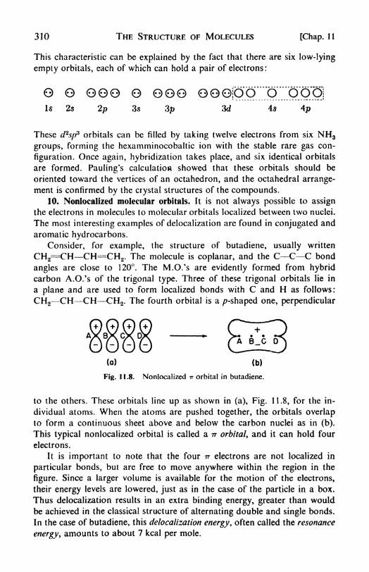
310 THE STRUCTURE OF MOLECULES [Chap. 11
This characteristic can be explained by the fact that there are six low-lying
empty orbitals, each of which can hold a pair of electrons:
O OOOiIs 2s 2p 3s 3p 3d 4s 4p
These cPspP orbitals can be filled by taking twelve electrons from six NH3
groups, forming the hexamminocobaltic ion with the stable rare gas con-
figuration. Once again, hybridization takes place, and six identical orbitals
are formed. Pauling's calculation showed that these orbitals should be
oriented toward the vertices of an octahedron, and the octahedral arrange-
ment is confirmed by the crystal structures of the compounds.10. Nonlocalized molecular orbitals. It is not always possible to assign
the electrons in molecules to molecular orbitals localized between two nuclei.
The most interesting examples of delocalization are found in conjugated and
aromatic hydrocarbons.
Consider, for example, the structure of butadiene, usually written
CH2=CH~-CH=CH2 . The molecule is coplanar, and the C C C bond
angles are close to 120. The M.O.'s are evidently formed from hybridcarbon A.O.'s of the trigonal type. Three of these trigonal orbitals lie in
a plane and are used to form localized bonds with C and H as follows:
CH2 CH CH CH2 . The fourth orbital is a /?-shaped one, perpendicular
(a) (b)
Fig. 11.8. Nonlocalized IT orbital in butadiene.
to the others. These orbitals line up as shown in (a), Fig. 11.8, for the in-
dividual atoms. When the atoms are pushed together, the orbitals overlapto form a continuous sheet above and below the carbon nuclei as in (b).
This typical nonlocalized orbital is called a n orbital, and it can hold four
electrons.
It is important to note that the four TT electrons are not localized in
particular bonds, but are free to move anywhere within the region in the
figure. Since a larger volume is available for the motion of the electrons,
their energy levels are lowered, just as in the case of the particle in a box.
Thus delocalization results in an extra binding energy, greater than would
be achieved in the classical structure of alternating double and single bonds.
In the case of butadiene, this delocalization energy, often called the resonance
energy, amounts to about 7 kcal per mole.
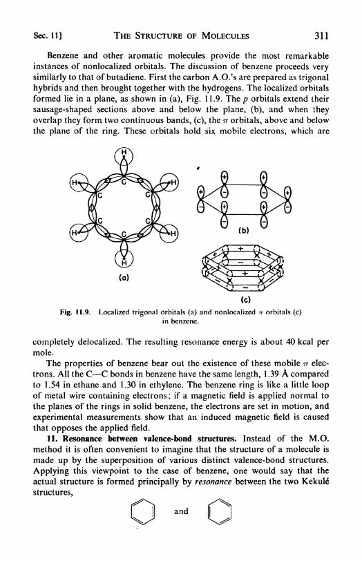
Sec. 11] THE STRUCTURE OF MOLECULES 311
Benzene and other aromatic molecules provide the most remarkable
instances of nonlocalized orbitals. The discussion of benzene proceeds very
similarly to that of butadiene. First the carbon A.O.'s are prepared as trigonal
hybrids and then brought together with the hydrogens. The localized orbitals
formed lie in a plane, as shown in (a), Fig. 1 1.9. The p orbitals extend their
sausage-shaped sections above and below the plane, (b), and when they
overlap they form two continuous bands, (c), the TT orbitals, above and below
the plane of the ring. These orbitals hold six mobile electrons, which are
Fig. 11.9. Localized trigonal orbitals (a) and nonlocalized -n orbitals (c)
in benzene.
completely delocalized. The resulting resonance energy is about 40 kcal permole.
The properties of benzene bear out the existence of these mobile -n elec-
trons. All the C C bonds in benzene have the same length, 1.39 A comparedto 1.54 in ethane and 1.30 in ethylene. The benzene ring is like a little loopof metal wire containing electrons; if a magnetic field is applied normal to
the planes of the rings in solid benzene, the electrons are set in motion, and
experimental measurements show that an induced magnetic field is caused
that opposes the applied field.
11. Resonance between valence-bond structures. Instead of the M.O.
method it is often convenient to imagine that the structure of a molecule is
made up by the superposition of various distinct valence-bond structures.
Applying this viewpoint to the case of benzene, one would say that the
actual structure is formed principally by resonance between the two Kekule"
structures,
and

312 THE STRUCTURE OF MOLECULES
with smaller contributions from the three Dewar structures,
[Chap. 11
According to the resonance theory, the eigenfunction ^ describing the
actual molecular structure is a linear combination of the functions for
possible valence bond structures,
This is an application of the general superposition principle for wave func-
tions. Each eigenfunction y corresponds to some definite value E for the
energy of the system. The problem is to determine the values of al9
a2 , #3 ,
etc., in such a way as to make E a minimum. The relative magnitude of these
coefficients when E is a minimum is then a measure of the contribution to
the over-all structure of the different special structures represented by
Vi ^2 Y>3 1* must be clearly understood that the resonance description
does not mean that some molecules have one structure and some another.
The structure of each molecule can only be described as a sort of weighted
average of the resonance structures.
Two rules must be obeyed by possible resonating structures: (1) The
structures can differ only in the position of electrons. Substances that differ
in the arrangement of the atoms are ordinary isomers and are chemicallyand physically distinguishable as
dis^jjact* compounds. (2) The resonating
structures must have the same number of paired and unpaired electrons,
otherwise they would have different total spins and be physically distinguish-
able by their magnetic properties.
In substituted benzene compounds, the contributions of various ionic
structures must be included. For example, aniline has the following resonance
structures :
H H H
N
H H H H
covalent ionic
The ionic structures give aniline an additional resonance energy of 7 kcal,
compared with benzene. The increased negative charge at the ortho and para
positions in aniline accounts for the fact that the NH2 group in aniline directs
positively charged approaching substituents (NOa+, Br+) to these positions.
The way in which the V.B. method would treat the hydrogen halides is

Sec. 12] THE STRUCTURE OF MOLECULES 313
instructive. Two important structures are postulated, one purely covalent
and one purely ionic :
H+ :C1:~ and H:C1:
The actual structure is visualized as a resonance hybrid somewhere between
these two extremes. Its wave function is
V ~~^covalent +
The value of a is adjusted until the minimum energy is obtained. Then
(a2/! + a2
) 100 is called the per cent ionic character of the bond. For the
various halides the following results are found :
The bond in HI is predominantly covalent; in HF, it is largely ionic. The
distinction between these different bond types is thus seldom clearcut, and
most bonds are of an intermediate nature.
The tendency of a pair of atoms to form an ionic bond is measured bythe difference in their power to attract an electron, or in their electronegativity.
Fluorine is the most, and the alkali metals are the least, electronegative of
the elements. The fractional ionic character of a bond then depends uponthe difference in electronegativity of its constituent atoms.
12. The hydrogen bond. It has been found that in many instances a
hydrogen atom can act as if it formed a bond to two other atoms instead of
to only one. A typical example is the dimer of formic acid, which has the
structure
O H O/ \
H C C H\ /O H O
This hydrogen bond is not very strong, usually having a dissociation energyof about 5 kcal, but it is extremely important in many structures, such as the
proteins. It occurs in general between hydrogen and the electronegative
elements N, O, F, of small atomic volumes.
We know that hydrogen can form only one covalent bond, since it has
only the single Is orbital available for bond formation. Therefore the hydro-
gen bond is essentially an ionic bond. Since the proton is extremely small,
its electrostatic field is very intense. A typical hydrogen-bonded structure is
the ion (HF2)~, which occurs in hydrofluoric acid and in crystals such as
KHF2 . It can be represented as a resonance hybrid of three structures,
:F: H F- F~ H :F: F- H+ F-

314 THE STRUCTURE OF MOLECULES [Chap. 11
The ionic F H fF~ structure is the most important. It is noteworthy that
electroneg^Hve elements with large ionic radii, e.g., Cl, have little or no
tendenc^o form hydrogen bonds, presumably owing to their less concen-
trates electrostatic fields.
13. Dipole moments. If a bond is formed between two atoms that differ
in electronegativity, there is an accumulation of negative charge on the
more electronegative atom, leaving a positive charge on the more electro-
positive atom. The bond then constitutes an electric dipole, which is bydefinition an equal positive and negative charge, _q, separated by a distance
r. A dipole, as in (a), Fig. 11.10, is
characterized by its dipole moment, a
vector having the magnitude qr and
the direction of the line joining the
positive to the negative charge. Thedimensions of a dipole moment are
charge times length. Two charges with
the magnitude of e(4.80 x 10~10esu)
separated by a distance of I A would
have a dipole moment of 4.80 x 10~~18
csu cm. The unit 10~18 esu cm is
called the debye, (d).
If a polyatomic molecule contains
two or more dipoles in different bonds, the net dipole moment of the mole-
cule is the resultant of the vector addition of the individual bond moments.
An example of this is shown in (b), Fig. 11.10.
The measurement of tha dipole moments of molecules provides an insight
into their geometric structure and also into the character of their valence
bonds. Before we can discuss the determination of dipole moments, however,
it is necessary to review some aspects of the theory of dielectrics.
14. Polarization of dielectrics. Consider a parallel-plate capacitor with
the region between the plates evacuated, and let the charge on one plate be
-for and on the other a per square centimeter. The electric field within the
capacitor is then directed perpendicular to the plates and has the magnitude4
EQ-- 47TCT. The capacitance is
q aA A
Fig. 11.10. (a) Definition of dipole
moment; (b) vector addition of dipole
moments in orthodichlorobenzene.
where A is the area of the plates, rfthe distance, and (/the potential difference
between them.
Now consider the space between the plates to be filled with some material
substance. In general, this substance falls rather definitely into one of two
classes, the conductors or the insulators. Under the influence of small fields,
electrons move quite freely through conductors, whereas in insulators or
4See, for example, G. P. Harnwell, Electricity and Magnetism (New York: McGraw-
Hill, 1949), p. 26.

Sec. 14] THE STRUCTURE OF MOLECULES 315
dielectrics these fields displace the electrons only slightly from their equi-librium positions.
An electric field acting on a dielectric thus causes a separation of positive
and negative charges. The field is said to polarize the dielectric. This polarizo-tion is shown pictorially in (a), Fig. 11.11. The polarization can occur in twa
ways: the induction effect and the orientation effect. An electric field alwaysinduces dipoles in molecules on which it is acting, whether or not they contain
dipoles to begin with. If the dielectric does contain molecules that are per-
manent dipoles, the field tends to align these dipoles along its own direction.
The random thermal motions of the molecules oppose this orienting action.
I CM
(a) (b)
Fig. 11.11. (a) Polarization of a dielectric; (b) definition of the
polarization vector, P.
Our main interest is in the permanent dipoles, but before these can be studied,
effects due to the induced dipoles must be clearly distinguished.
It is found experimentally that when a dielectric is introduced between
the plates of a capacitor the capacitance is increased by a factor e, called the
dielectric constant. Thus if C is the capacitance with a vacuum, the capaci-
tance with a dielectric is C eC . Since the charges on the capacitor plates
are unchanged, this must mean that the field between the plates is reduced
by the factor e, so that E = EQ/e.
The reason why the field is reduced is clear from the picture of the
polarized dielectric, for all the induced dipoles are aligned so as to producean over-all dipole moment that cuts down the field strength. Consider in
(b), Fig. 11.11, a unit cube of dielectric between the capacitor plates, and
define a vector quantity P called the polarization, which is the dipole moment
per unit volume. Then the effect of the polarization is equivalent to that
which would be produced by a charge of -fP on one face and ~P on the
other face (1 cm2) of the cube. The field in the dielectric is now determined
by the net charge on the plates, so that
J-47r(er-P) (11.5)
A new vector has been defined, called the displacement D, which depends
only on the charge or, according to D = 47ror. It follows that
D-J5+4rrP, and DIE = e (11.6)
It is apparent that in a vacuum, where e = 1, D = E.

316 THE STRUCTURE OF MOLECULES [Chap. 11
15. The induced polarization. Let us consider the induced or distortion
polarization, PI} , produced by an electric field acting on a dielectric that does
not contain permanent dipoles.
The first problem to be solved is the magnitude of the dipole moment minduced in a molecule by the field acting on it. It may be assumed that this
induced moment is proportional to the intensity of the field5 F, so that
m-aoF (11.7)
The proportionality constant OQ is called the distortion polarizability of the
molecule. It is the induced moment per unit field strength, and has the
dimensions of a volume, since q r/(q/r2) r
3v.
At first it might seem that the field acting on a molecule should be simplythe field E of eq. (1 1.5). This would be incorrect, however, for the field that
polarizes a molecule is the local field immediately surrounding it, and this is
different from the average field E throughout the dielectric. For an isotropic
substance this local field can be calculated6 to be
F-B + *?-*(I I J)
In the absence of permanent dipoles, the polarization or dipole moment
per unit volume is the number of molecules per cc, , times the averagemoment induced in a molecule, m. Thus, from eqs. (11.7) and (11.8),
- /7<x (E +
Since, from eq. (11.6), E(e 1)^-- 4*rPD ,
477/700
3(H.9)
This is the Clausius-Mossotti equation.
Multiplying both sides by the ratio of molecular weight to density M/p,
4
B + 2 p 3p 3
The quantity PM is called the molar polarization. So far it includes only the
contribution from induced dipoles, and in order to obtain the completemolar polarization, a term due to permanent dipoles must be added. ->
16. Determination of the dipole moment. Having examined the effect of
induced dipoles on the dielectric constant, we are in a position to consider
5 This is true only for isotropic substances; otherwise, for example in nonisotropic
crystals, the direction of the moment may not coincide with the field direction. This dis-
cussion therefore applies only to gases, liquids, and cubic crystals.6 A good derivation is given by Slater and Frank, Introduction to Theoretical Physics
(New York: McGraw-Hill, 1933), p. 278; also, Syrkin and Dyatkina, The Structure ofMolecules (New York: Interscience, 1950), p. 471.

Sec. 16] THE STRUCTURE OF MOLECULES 317
the influence of permanent dipoles. If the bonds in a molecule are ionic or
partially ionic, the molecule has a net dipole moment, unless the individual
bond moments add vectorially to zero.
It is now possible to distinguish an orientation polarization of a dielectric,
which is that caused by permanent dipoles, from the distortion polarization,
caused by induced dipoles.
There will always be an induced moment. It is evoked almost instanta-
neously in the direction of the electric field. It is independent of the tempera-
ture, since if the molecule's position is disturbed by thermal collisions, the
dipole is at once induced again in the field direction. The contribution to the
polarization caused by permanent dipoles, however, is less at higher tem-
peratures, since the random thermal collisions of the molecules oppose the
tendency of their dipoles to line up in the electric field.
It is necessary to calculate the average component of a permanent dipolein the field direction as a function of the temperature. Consider a dipole with
random orientation. If there is no field, all orientations are equally probable.This fact can be expressed by saying that the number of dipole momentsdirected within a solid angle da) is simply Adw, where A is a constant depend-
ing on the number of molecules under observation.
If a dipole moment //is oriented at angle to a field of strength F its
potential energy7
is U - //Fcos 0. According to the Boltzmann equation,the number of molecules oriented within the solid angle da} is then
Ae-' ulkT dco = A
The average value of the dipole moment in the direction of the field, by
analogy with eq. (7.39), can be written
A* cos (>lkT1 cos Oda>
To evaluate this expression, let [iFjkT x, cos =y; then dw -- 2-n- sin 9 dO
- 277 dy.
Thus*
i (ex e~x)
Since e**dy~- ----------
_ s
m ex -- = coth x -- = L(x)p ex e~
x x x
Here L(x) is called the "Langevin function," in honor of the inventor of this
treatment.
7Harnwell, op. cit., p. 64.
M

318 THE STRUCTURE OF MOLECULES [Chap. 11
In most cases x =[iF/kTis a very small number8 so that on expanding L(x)
in a power series, only the first term need be retained, leavingL(x) = x/3, or
/|2
The total polarizability of a dielectric is found by adding this contribution
due to permanent dipoles to the distortion polarizability, and may be written
a = ao 4- CM2/3*r). Instead of eq. (1 1.10), the total polarization is therefore
This equation was first derived by P. Debye.
40
i 30O
NJ
5 20.joa.
3 .0
1.0 5.02.0 3.0 4.0
1/TXlO3
Fig. 11.12. Application of the Debye equation to the polarizations of
the hydrogen ha 1ides.
When the Clausius-Mossotti treatment is valid,9
e -1 M /
PU - - - - ^e + 2 P
For gases, e is not much greater than 1, so that
E -1 M 4n=
"=- ^ ao (11.13)
8 Values of n range around 10"18(esu) (cm). If a capacitor with 1 cm between plates is
(3
x 10^\
airiov" 10
"17erg comPared witn kT = 10
~14 er
at room temperature.9 This is the case only for gases or for dilute solutions of dipolar molecules in non-polar
solvents. If there is a high concentration of dipolar molecules, as in aqueous solutions, there
are localized polarization fields that cannot be treated by the Clausius-Mossotti method. In
other words, the permanent dipoles tend to influence the induced polarization.
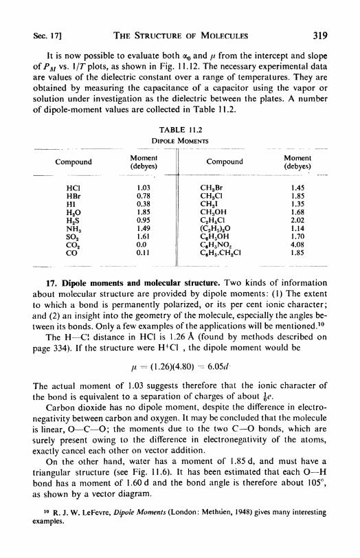
Sec. 17] THE STRUCTURE OF MOLECULES 319
It is now possible to evaluate both OQ and // from the intercept and slope
ofPM vs. l/T^plots, as shown in Fig. 11.12. The necessary experimental data
are values of the dielectric constant over a range of temperatures. They are
obtained by measuring the capacitance of a capacitor using the vapor or
solution under investigation as the dielectric between the plates. A number
of dipole-moment values are collected in Table 11.2.
17. Dipole moments and molecular structure. Two kinds of information
about molecular structure are provided by dipole moments: (1) The extent
to which a bond is permanently polarized, or its per cent ionic character;
and (2) an insight into the geometry of the molecule, especially the angles be-
tween its bonds. Only a few examples of the applications will be mentioned. 10
The H Cl distance in HC1 is 1.26 A (found by methods described on
page 334). If the structure were H+C1,the dipole moment would be
H - (1.26)(4.80)- 6.05d
The actual moment of 1.03 suggests therefore that the ionic character of
the bond is equivalent to a separation of charges of about \e.
Carbon dioxide has no dipole moment, despite the difference in electro-
negativity between carbon and oxygen. It may be concluded that the molecule
is linear, O C O; the moments due to the two C O bonds, which are
surely present owing to the difference in electronegativity of the atoms,
exactly cancel each other on vector addition.
On the other hand, water has a moment of 1.85d, and must have a
triangular structure (see Fig. 1 1 .6). It has been estimated that each O Hbond has a moment of 1.60d and the bond angle is therefore about 105,
as shown by a vector diagram.
10 R. J. W. LeFevre, Dipole Moments (London: Methiien, 1948) gives many interesting
examples.

320 THE STRUCTURE OF MOLECULES [Chap. 11
A final simple example is found in the substituted benzene derivatives:
OH OH
- 1.55 1.70
The zero moments of /?-dichloro- and sym-trichlorobenzene indicate that
benzene is planar and that the C -Cl bond moments are directed in the
plane of the ring, thereby adding to zero. The moment of />di-OH benzene,
on the other hand, shows that the O H bonds are not in the plane of the
ring, but directed at an angle to it, thus providing a net moment.
18. Polarization and refractivity. It may be recalled that one of the most
interesting results of Clerk Maxwell's electromagnetic theory of light11 was
the relationship f /r^2
,where nR is the index of refraction. Thus the
refractive index is related through eq. (11.10) to the molar polarization.
The physical reason for this relationship can be understood without
going into the details of the electromagnetic theory. The refractive index of
a medium is the ratio of the speed of light in a vacuum to its speed in the
medium, nR - c/cm . Light always travels more slowly through a material
substance than it does through a vacuum. A light wave is a rapidly alternating
electric and magnetic field. This field, as any other, acts to polarize the
dielectric through which it passes, pulling the electrons back and forth in
rapid alternation. The greater the polarizability of the molecules, the greater
is the field induced in opposition to the applied field, and the greater therefore
is the "resistance" to the transmission of the light wave. Thus high polariz
ability means low cm and high refractive index. We have already seen that
increasing the polarization increases the dielectric constant. The detailed
theory leads to the Maxwell relation, e -= nn2
.
This relation is experimentally confirmed only under certain conditions:
(1) The substance contains no permanent dipoles.
(2) The measurement is made with radiation of very long wavelength, in
the infrared region.
(3) The refractive index is not measured in the neighborhood of a wave-
length where the radiation is absorbed.
The first restriction arises from the fact that dielectric constants are
measured at low frequencies (500 to 5000 kc), whereas refractive indices are
measured with radiation of frequency about 1012 kc. A permanent dipole
cannot line up quickly enough to follow an electric field alternating this
rapidly. Permanent dipoles therefore contribute to the dielectric constant
but not to the refractive index.
The second restriction is a result of the effect of high frequencies on the
11 G. P. Harnwell, opt cit., p. 579.

Sec. 19] THE STRUCTURE OF MOLECULES 321
induced polarization. With high-frequency radiation (in the visible) only the
electrons in molecules can adjust themselves to the rapidly alternating electric
fields; the more sluggish nuclei stay practically in their equilibrium positions.
With the lower-frequency infrared radiation the nuclei are also displaced.
It is customary, therefore, to distinguish, in the absence of permanent
dipoles, an electronic polarization PK and an atomic polarization PA . The
total polarization, PA \ PK , is obtained from dielectric-constant measure-
ments or infrared determinations of the refractive index. The latter are hard
to make, but sometimes results with visible light can be successfully extra-
polated. The electronic polarization PK can be calculated from refractive
index measurements with visible light. Usually PA is only about 10 per cent
of PE ,and may often be neglected.
When the Maxwell relation is satisfied, we obtain from eq. (11.10) the
Lorenz-Lorentz equation:n 2 t AY
vri'7=
/>A/ (1L14)
The quantity at the left of eq. (11.14) is often called the molar refraction
RM . When the Maxwell relation holds, RM - PM .
It will be noted that the molar refraction RM has the dimensions of
volume. It can indeed be shown from simple electrostatic theory12 that a
sphere of conducting material of radius r, in an electric field F, has an induced
electric moment of m = r3/7. According to this simple picture, the molar
refraction should be equal to the true volume of the molecules contained in
one mole. A comparison of some values of molecular volume obtained in
this way from refractive index measurements with those obtained from
van der Waal's b was shown in Table 7.5.
19. Dipole moments by combining dielectric constant and refractive index
measurements. The Lorenz-Lorentz equation also provides an alternative
method of separating the orientation and the distortion polarizations, and
thereby determining the dipole moment. A solution of the dipolar compoundin a nonpolar solvent e.g., nitrobenzene in benzene-- is prepared at various
concentrations. The dielectric constant is measured and the apparent molar
polarization calculated from eq. (1J.10). This quantity is made up of the
distortion polarizations of both solute and solvent plus the orientation
polarization of the polar solute. The molar polarizations due to distortion
can be set equal to the molar refractions RM , calculated from the refractive
indices of the pure liquids. When these RM are subtracted from the total
apparent PM ,the remainder is the apparent molar orientation polarisation
for the solute alone. This polarization is plotted against the concentration in
the solution and extrapolated to zero concentration. 13 A value is obtained in
12 Slater and Frank, op. r/7., p. 275.13 E. A. Guggenheim, Trans. Faraday Soc., 47, 573 (1951), gives an improved method
for extrapolation.

322 THE STRUCTURE OF MOLECULES [Chap. 1 i
this way from which the effect of dipole interaction has been eliminated.
From eq. (11.13), therefore, it is equal to (4n/3)N([i*/3kT) and the dipole
moment of the polar solute can be calculated.
20. Magnetism and molecular structure. The theory for the magnetic
properties of molecules resembles in many ways that for the electric polariza-
tion. Thus a molecule can have a permanent magnetic moment and also a
moment induced by a magnetic field.
Corresponding to eq. (11.6), we have
B H + 4nI (11.15)
where B is the magnetic induction, H is the field strength, and / is the in-
tensity of magnetization or magnetic moment per unit volume. These
quantities are the magnetic counterparts of the electrical D, /?, and P. In a
vacuum B H, but otherwise B -= e'H, where t', the permeability, is the
magnetic counterpart of the dielectric constant F. Usually, however, mag-netic properties are discussed in terms of
~X (H.16)
where % is called the magnetic susceptibility per unit volume of the medium.
(Electric susceptibility would be P/E.)The susceptibility per mole is %M - (M/p)x- The magnetig^fffialogue of
eq. (11. 13) is
(1U7)
where a is the induced moment and JUM is the permanent magnetic dipole
moment. Just as before, the two effects can be experimentally separated by
temperature-dependence measurements.
An important difference from the electrical case now appears, in that
> or XM> can be either positive or negative. If %M is negative, the mediumis called diamagnetic; if %M is positive, it is called paramagnetic. For iron,
nickel, and certain alloys, %M is positive and much larger than usual, by a
factor of about a million. Such substances are called ferromagnetic. From
eq. (11.15) it can be seen that the magnetic field in diamagnetic substances
is weaker than in a vacuum, whereas in paramagnetic substances it is
stronger.
An experimental measurement of susceptibility can be made with the
magnetic balance. The specimen is suspended so that it is partly inside and
partly outside a strong magnetic field. When the magnet is turned on, a
paramagnetic substance tends to be drawn into the field region, a dia-
magnetic tends to be pushed out of the field. From the weight required to
restore the original balance point, the susceptibility is calculated.
Sec. 20] THE STRUCTURE OF MOLECULES 323
The phenomenon of diamagnetism is the counterpart of the distortion
polarization in the electrical case. The effect is exhibited by all substances
and is independent of the temperature. A simple interpretation is obtained
if one imagines the electrons to be revolving around the nucleus. If a mag-netic field is applied, the velocity of the moving electrons is changed, pro-
ducing a magnetic field that, in accordance with Lenz's Law, is opposed in
direction to the applied field. The diamagnetic susceptibility is therefore
always negative.
When paramagnetism occurs, the diamagnetic effect is usually quite over-
shadowed, amounting to only about 10 per cent of the total susceptibility.
Paramagnetism is associated with the orbital angular momentum and the
spin of uncoupled electrons, i.e., those that are not paired with others having
equal but opposite angular momentum and spin.
An electron revolving in an orbit about the nucleus is like an electric
current in a loop of wire, or a turn in a solenoid. The resultant magneticmoment is a vector normal to the plane of the orbit, and proportional to
the angular momentum p of the revolving electron. In the MKS system of
units (charge in coulombs) the magnetic moment is (e/2m)p (weber meters).14
Since p can have only quantized values, m^l-n, where mlis an integer, the
allowed values of the magnetic moment are m^eh^nm). It is evident, there-
fore, that there is a natural unit of magnetic moment, eh/47rm. It is called the
Bohr magneton.The ratio of magnetic moment to angular momentum is called the gyro-
magnetic ratio, R . For the orbital motion of an electron, Rg e/2m. The
spinning electron also acts as a little magnet. For electron spin, however,
Rg= e/m. Since the intrinsic angular momentum of an electron can have
only quantized values %(h/2ir), the magnetic moment of an unpairedelectron is eh/fam, or one Bohr magneton.
In the case of molecules, only the contributions due to spin are very
important. This is true because there is a strong internal field within a mole-
cule. In a diatomic molecule, for example, this field is directed along the
internuclear axis. This internal field holds the orbital angular momenta of
the electrons in a fixed orientation. They cannot line up with an external
magnetic field, and thus the contribution they would normally make to the
susceptibility is ineffective. It is said to be quenched. There remains only the
effect due to the electron spin, which is not affected by the internal field.
Thus a measurement of the permanent magnetic moment of a molecule tells
us how many unpaired spins there are in its structure.
There have been many applications of this useful method,15 of which
only one can be mentioned here. Let us consider two complexes of cobalt,
14 A derivation is given by C. A. Coulson, Electricity (New York: Interscience, 1951),
p. 91. In electrostatic units the magnetic moment is (e/2mc)p twhere c is the speed of light
i/i vacuo.16 P. W. Selwood, Magnetochemistry (New York: Interscience, 1943).

324 THE STRUCTURE OF MOLECULES [Chap. 11
{Co(NH3)6} C13 and K 3{CoF6}. Two possible structures may be suggested for
such complexes, one covalent and one ionic, as follows:
3d 4s 4p Unpaired Spins
Covalent . 11 11 11 11 ft 11 ft ft ft
Ionic . . 11 t t t t .. 4
The hexammino complex is obviously covalent, but the structure of the
hexafluoro complex is open to question. It is found that the hexammino
complex has zero magnetic moment, whereas the {CoF6}r
complex has a
moment of 5.3 magnetons. The structures can thus be assigned as follows:
NR,H3N
Co
NFi,
NFL
C1= and
21. Nuclear paramagnetism. In addition to the magnetism due to the
electrons in an atom there is also magnetism due to the nuclei. We mayconsider a nucleus to be composed of protons and neutrons, and both these
nucleons have intrinsic angular momenta or spins, and hence act as ele-
mentary magnets. In most nuclei these spins add to give a nonzero resultant
nuclear spin. It was first predicted that the magnetic moment of the protonwould be 1 nuclear magneton, ehl^-nM, where M is the proton mass. Actually,
however, the proton has a magnetic moment of 2.79245 nuclear magnetons,and the neutron moment is -1.9135. The minus sign indicates that the
moment behaves like that of a negatively charged particle. Since M is almost
2000 times the electronic mass m, nuclear magnetic moments are less than
electronic magnetic moments by a factor of about 1000.
The existence of nuclear magnetism was first revealed in the hyperfine
structure of spectral lines. As an example consider the hydrogen atom, a
proton with one orbital electron. The nucleus can have a spin / i4, and
the electron can have a spin S = i. The nuclear and the electron spins can
be either parallel or antiparallel to each other, and these two different align-
ments will differ slightly in energy, the parallel state being higher. Thus the
ground state of the hydrogen atom will in fact be a closely spaced doublet,
and this splitting is observed in the atomic spectra of hydrogen, if a spectro-
graph of high resolving power is employed. The spacing between the two
levels, A -- hv, corresponds to a frequency v of 1420 megacycles. After the
prediction of the astrophysicist van der Hulst, an intense emission of radia-
tion at this frequency was observed from clouds of interstellar dust. The
study of this phenomenon is an important part of the rapidly developing
subject of radioastronomy, which is providing much information about
hitherto uncharted regions of our universe.

Sec. 21] THE STRUCTURE OF MOLECULES 325
If a nucleus with a certain magnetic moment is placed in a magnetic
field, we can observe the phenomenon of space quantization (see page 267).
The component of the moment in the direction of the field is quantized, and
for each allowed direction there will be a slightly different energy level. For
readily accessible magnetic fields, the* frequencies v A//i for transitions
between two such levels also lie in the microwave range of radio frequencies.
TEST TUBEWITH SAMPLE
TRANSMITTERCOIL
Fig. 11.13. Simplified apparatus for basic nuclear magnetic resonance
experiment. (Drawing courtesy R. H. Varian.)
For example, at a field of 7050 gauss, the frequency for protons is 30 mega-
cycles. The earlier attempts to detect these transitions were unsuccessful,
but in 1946 E. M. Purcell and Felix Bloch independently developed the
method of nuclear magnetic resonance.
The principle of this method is shown in Fig. 11.13. The field H of the
magnet is variable from to 10,000 gauss. This field produces an equi-
distant splitting of the nuclear energy levels which arise as a result of space
quantization. The low-power radio-frequency transmitter operates at, for
example, 30 megacycles. It causes a small oscillating magnetic field to be
applied to the sample. This field induces transitions between the energy
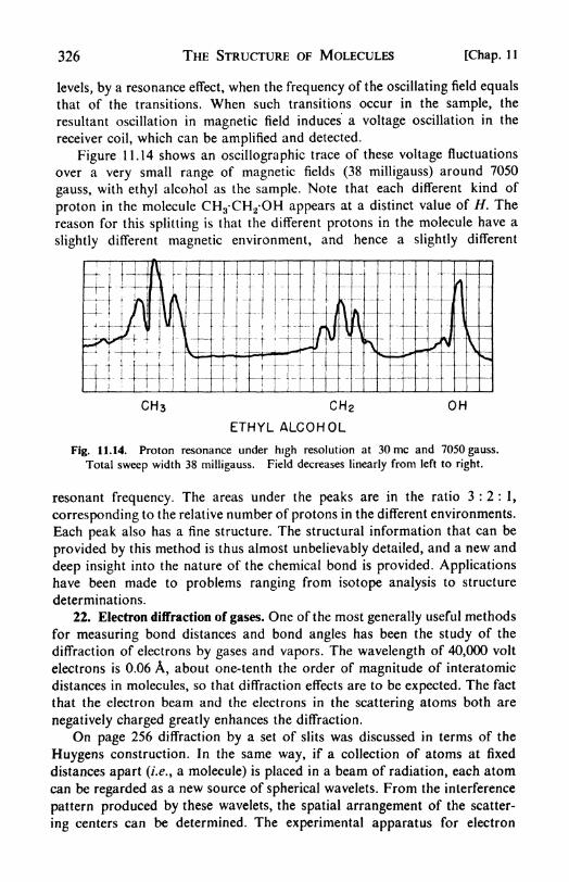
326 THE STRUCTURE OF MOLECULES [Chap. 1 1
levels, by a resonance effect, when the frequency of the oscillating field equals
that of the transitions. When such transitions occur in the sample, the
resultant oscillation in magnetic field induces a voltage oscillation in the
receiver coil, which can be amplified and detected.
Figure 11.14 shows an oscillographic trace of these voltage fluctuations
over a very small range of magnetic fields (38 milligauss) around 7050
gauss, with ethyl alcohol as the sample. Note that each different kind of
proton in the molecule CH 3-CH2-OH appears at a distinct value of H. The
reason for this splitting is that the different protons in the molecule have a
slightly different magnetic environment, and hence a slightly different
CH 2
ETHYL ALCOHOL
OH
Fig. 11.14. Proton resonance under high resolution at 30 me and 7050 gauss.
Total sweep width 38 milligauss. Field decreases linearly from left to right.
resonant frequency. The areas under the peaks are in the ratio 3:2: 1,
corresponding to the relative number of protons in the different environments.
Each peak also has a fine structure. The structural information that can be
provided by this method is thus almost unbelievably detailed, and a new and
deep insight into the nature of the chemical bond is provided. Applications
have been made to problems ranging from isotope analysis to structure
determinations.
22. Electron diffraction of gases. One of the most generally useful methods
for measuring bond distances and bond angles has been the study of the
diffraction of electrons by gases and vapors. The wavelength of 40,000 volt
electrons is 0.06 A, about one-tenth the order of magnitude of interatomic
distances in molecules, so that diffraction effects are to be expected. The fact
that the electron beam and the electrons in the scattering atoms both are
negatively charged greatly enhances the diffraction.
On page 256 diffraction by a set of slits was discussed in terms of the
Huygens construction. In the same way, if a collection of atoms at fixed
distances apart (i.e., a molecule) is placed in a beam of radiation, each atom
can be regarded as a new source of spherical wavelets. From the interference
pattern produced by these wavelets, the spatial arrangement of the scatter-
ing centers can be determined. The experimental apparatus for electron

Sec. 22] THE STRUCTURE OF MOLECULES 327
diffraction is illustrated in Fig. 11.15. The type of pattern found is a series
of rings similar to those in Fig. 10.10 but somewhat more diffuse.
The electron beam traverses a collection of many gas molecules, oriented
at random to its direction. It is most interesting that maxima and minima
Fig. 11.15. Schematic diagram of electron diffraction apparatus.
are observed in the diffraction pattern despite the random orientation of the
molecules. This is because the scattering centers occur as groups of atoms
with the same definite fixed arrangement within every molecule. A collection
of individual atoms, e.g., argon gas, would give no diffraction rings. Diffrac-
tion by gases was treated theoretically (for X rays) by Debye in 1915, but
electron-diffraction experiments were not carried out till the work of Wierl
in 1930.
We can show the essential features of the diffraction theory by considering
the simplest case, that of a diatomic molecule. 16 The molecule is representedin Fig. 11.16 with one atom A, at the origin, and the other B, a distance r
away. The electron beam enters along Y'A
and the diffracted beam, scattered throughan angle 0, is picked up at P on a photo-
graphic film, a distance R from the origin.
The angles a and<f> give the orientation of
AB to the primary beam.
The interference between the waves
scattered from A and B depends on the
difference between the lengths of the pathswhich they traverse. This path difference
is 6 - AP CB - BP. The difference inFig . n 16 Scattering of electrons
phase between the two scattered waves is by a diatomic molecule.
In order to add waves that differ in phase and amplitude, it is convenient
to represent them in the complex plane and to add vectorially.17 In our case
we shall assume for simplicity that the atoms A and B are identical. Then the
resultant amplitude at P is A --= A -f /V"'2^. A^ called the atomic scatter-
ing factor, depends on the number of electrons in the atom. The intensity of
18 The treatment follows that given by M. H. Pirenne, The Diffraction of X rays and
Electrons by Free Molecules (London: Cambridge, 1946), p. 7.
17 See Courant and Robbins, What Is Mathematics ?
(New York: Oxford, 1941), p. 94.

328 THE STRUCTURE OF MOLECULES [Chap. 11
radiation is proportional to the square of the amplitude, or in this case to
AA, the amplitude times its complex conjugate. Thus
A 2 /O I ZirioJ* i ,.27n<5/A\^o v^ ~r c -re ;
- 2/* 2( 1 + cos
-^- j- 4^ 2 cos2
It is now necessary to express 6 in terms of r, /, 0, a, and(/>.
This can
be done by referring to Fig. 11.16. We see first of all that CB -~ r sin a
sin<f>.
Then BP VR2 + r2 2rR sin a sin (6 + </).Since r is a few
Angstroms while R is several cm, r <; /?, so that r2 is negligible and the
square root can be expanded18 to yield BP R r sin <x sin (0 -f- <).
Then we have 6 = AP CB #P r sin a [sin (0 + </>)sin $ - 2r sin
0/2 sin a cos[< + (0/2)].
In order to obtain the required formula for the intensity of scattering of
a randomly oriented group of molecules, it is necessary to average the
expression for the intensity at one particular orientation (a, <f>)over all
possible orientations. The differential element of solid angle is sin a dend<f>,
and the total solid angle of the sphere around AB is 4-rr. Hence the required
average intensity becomes
,4^o
2 r r jo r L^ 2\] , M
lav~ cos 2
2-rr - sin - sin a cos + -I sin a da. dd>
4n Jo Jo L A 2 \ 07 J
On integration,19 fav
- 2 A 2 i\ +
A n
"' '
( 1L18)47T .
where x = sin -
18 From the binomial theorem, (1 f x)1
/2 = 1 + x Jx
2 + . . . .
19 Let
/<,= L L cos2 (A cos ft) dp sin a da.
IT > >
where
A = ~.- sin - sin a and p $ -f 0/2
Then since cos2 p = (1 f cos 2/?)/2, we obtain
7- = VJo Jo (y + cos (2
where / is the Bessel function of order zero (see Woods, Advanced Calculus, p. 282). This
can now be integrated by introducing the series expansion of
2 ("
I

Sec. 23] THE STRUCTURE OF MOLECULES 329
In Fig. 11.17, }\A is plotted against x, and the maxima and minima in
the intensity are clearly evident.
In a more complex molecule with atoms j, k (having scattering factors
Aj, A k) a distance r)k apart, the resultant intensity would be
(11.19)
This is called the "Wierl equation." The summation must be carried out
over all pairs of atoms in the molecule.
5
4
C\j O "5
\~ 2
I
27T 67T 87T I07T
Fig. 11.17. Scattering curve for diatomic molecule plot of eq. (11.18).
In the case of the homonuclear diatomic molecule already considered,
eq. (1 1.19) becomes
sin AT22- A A A A Asi i/i j-
-|- /i i/l 2A A^ 4- A A
' ^12Sm
Since ru =-- r22=- 0, and (sin x)/x -> 1 as x > 0, and rl2
=- r21=^
r, this
reduces to eq. (1 1.18).
23. Application of Wierl equation to experimental data. The scattering
angles of maximum intensity are calculated from the positions of the dark
rings on the picture and the geometry of the apparatus and camera. This
gives an experimental scattering curve, whose general form resembles that of
the theoretical curve shown in Fig. 11.17, although the positions of the
maxima depend, of course, on the molecule being studied. Then a particular
molecular structure is assumed and the theoretical scattering curve corre-
sponding to it is calculated from eq. (11.19). For example, in the benzene
structure there are three different carbon-carbon distances, six between ortho
positions, six between meta positions, and three between para positions.
Therefore the r}k terms consist of 6rcc , 6(V3 rcc), and 3(2 rcc). The positions
where in our case x ~ 2B sin a, with B = (2wr/A) sin 6/2. The required integral is given in
Pierce's tables (No. 483) as
C* - r/i f:
The series that results is that for (sin x)/x. (Pierce No. 772.)
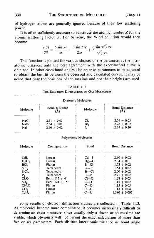
330 THE STRUCTURE OF MOLECULES [Chap. 11
of hydrogen atoms are generally ignored because of their low scattering
power.It is often sufficiently accurate to substitute the atomic number Z for the
atomic scattering factor A. For benzene, the Wierl equation would then
become
7(61) 6 sin xr 3 sin 2xr 6 sin A/3 xr
Z*=~~x7~
~f
~~^x7~+
^~Vlxr~~
This function is plotted for various choices of the parameter r, the inter-
atomic distance, until the best agreement with the experimental curve is
obtained. In other cases bond angles also enter as parameters to be adjusted
to obtain the best fit between the observed and calculated curves. It may be
noted that only the positions of the maxima and not their heights are used.
TABLE 11.3
THE ELECTRON DIFFRACTION OF GAS MOLECULES
Molecule
NaClNaBrNal
Bond Distance
(A)
Diatomic Molecules
Molecule
2.51 - 0.03
2.64 i_ 0.01
2.90 0.02
C1 2
Br2
Bond Distance
(A)
2.01 -b 0.03
2.28 0.02
2.65 0.10
Polyatomic Molecules
Molecule Configuration Bond Bond Distance
Some results of electron diffraction studies are collected in Table 11.3.
As molecules become more complieated, it becomes increasingly difficult to
determine an exact structure, since usually only a dozen or so maxima are
visible, which obviously will not permit the exact calculation of more than
five or six parameters. Each distinct interatomic distance or bond angle

Sec. 24] THE STRUCTURE OF MOLECULES 331
constitutes a parameter. It is possible, however, from measurements on
simple compounds, to obtain quite reliable values of bond distances and
angles, which may be used to estimate the structures of more complexmolecules.
Some interesting effects of resonance on bond distances have been
observed. For example, the C Cl distance in CH3C1 is 1.76 A but in
CH2=CHCi it is only 1.69 A. The shortening of the bond is ascribed to
resonance between the following structures:
Cl: Cl^
/' .. /H2O=C and H2C C
\ \H H
The C Cl bond in ethylene chloride is said to have about 18 per cent double
bond character.
24. Molecular spectra. Perhaps the most widely useful of all methods
for investigating molecular architecture is the study of molecular spectra. It
affords information about not only the dimensions of molecules but also the
possible molecular energy levels. Thus, other methods pertain to the groundstate of the molecule alone, but the analysis of spectra also elucidates the
nature of excited states.
It has been mentioned that the spectra of atoms consist of sharp lines,
and those of molecules appear to be made up of bands in which a densely
packed line structure is sometimes revealed under high resolving power.
Spectra arise from the emission or absorption of definite quanta of radia-
tion when transitions occur between certain energy levels. In an atom the
energy levels represent different allowed states for the orbital electrons. Amolecule too can absorb or emit energy in transitions between different
electronic energy levels. Such levels would be associated, for example, with
the different 'molecular orbitals discussed on pages 303-311. In addition
there are two other possible ways in which a molecule can change its energy
level, which do not occur in atoms. These are by changes in the vibrations
of the atoms within the molecule and by changes in the rotational energy of
the molecule. These energies, like the electronic, are quantized, so that onlycertain distinct levels of vibrational and rotational energy are permissible.
In the theory of molecular spectra it is customary, as a good first approxi-
mation, to consider that the energy of a molecule can be expressed simplyas the sum of electronic, vibrational, and rotational contributions. Thus,
E - Zfelee -} vib + rot (11.20)
This complete separation of the energy into three distinct categories is not
strictly correct. For example, the atoms in a rapidly rotating molecule
are separated by centrifugal forces, which thus affect the character of the

332 THE STRUCTURE OF MOLECULES [Chap. 11
vibrations. Nevertheless, the approximation of eq. (11.20) suffices to
explain many of the observed characteristics of molecular spectra.
It will be seen in the following discussions that the separations between
electronic energy levels are usually much larger than those between vibra-
tional energy levels, which in turn are much larger than those between
rotational levels. The type of energy-level diagram that results is shown in
Fig. 1 1.18. Associated with each electronic level there is a series of vibrattonal
J'
J'
J'-
Fig. 11.18. Energy-level diagram for a molecule. Two electronic levels
A and B, with their vibrational levels (v) and rotational levels (J)
levels, each of which is in turn associated with a series of rotational levels.
The close packing of the rotational levels is responsible for the banded
structure of molecular spectra.
Transitions between different electronic levels give rise to spectra in the
visible or ultraviolet region; these are called electronic spectra. Transitions
between vibrational levels within the same electronic state are responsible
for spectra in the near infrared (< 20/^), called vibration-rotation spectra.
Finally, spectra are observed in the far infrared (> 20^) arising from transi-
tions between rotational levels belonging to the same vibrational level; these
are called pure rotation spectra.
Sec. 25] THE STRUCTURE OF MOLECULES 333
25. Rotational levels far-infrared spectra. The model of the rigid rotator,
described on page 189, may be used for the interpretation of pure rotation
spectra. The calculation of the allowed energy levels for such a system is a
straightforward problem in quantum mechanics. The SchrCdinger equationin this case is very similar to that for the motion of the electron about the
nucleus in the hydrogen atom, except that for a diatomic molecule it is a
question of the rotation of two nuclei about their center of mass. We recall
that the rotation of a dumbbell model is equivalent to the rotation of the
reduced mass // at a distance r from the rotation axis. For a rigid rotator the
potential energy U is zero, so that the wave equation becomes
V ^0 (11.21)
Without too great difficulty this equation can be solved exactly.20
It is
then found that the eigenfunction y is single valued, continuous, and finite,
as is required for physical meaning, only for certain values of the energy Ey
the allowed eigenvalues. These are
WA./10 _/(/+!)trai
'
fcrV* ~~"M*r ( }
Here / is the moment of inertia of the molecule and the rotational quantumnumber J can have only integral values, 0, 1,2, 3, etc.
The value of J gives the allowed values of the rotational angular momen-
tum/?,
in units of h/2n: p =-- (h/27r)Vj(J + 1) ^ (h/2n) J. This is exactly
similar to the way in which the quantum number / in the hydrogen-atom
system, and the corresponding A in molecules, determine the orbital angularmomenta of electrons.
The selection rule for rotational levels is found to be A/ = or 1.
Thus an expression for AE for the rigid-rotator model is readily derived
from eq. (11.22). Writing B =--h/Kir'*!, we obtain for two levels with
quantum numbers J and J': A ^ hv hB[J(J f 1) -J \J' + I)]. Since
v -= (A//0, and7 -J' = 1,
v = 2fl/ (11.23)
The spacing between energy levels increases linearly with 7, as shown in
Fig. 11.18. The absorption spectra due to pure rotation arise from transitions
from each of these levels to the next higher one. By means of a spectrograph
of good resolving power, the absorption band will be seen to consist of a
series of lines spaced an equal distance apart. From eq. (11.23) this spacing
is AT --- v v ----- 2B.
Pure rotation spectra occur only when the m9lecule possesses a permanent
20 K. S. Pitzer, Quantum Chemistry (New York: Prentice-Hall, 1953), p. 53. An
approximate formula is obtained directly from the Bohr hypothesis that the angularmomentum is quantized in units of h/2ir. Thus /co = Jh/2*, and the kinetic energy
rV.
334 THE STRUCTURE OF MOLECULES [Chap. 1 1
dipole moment. This behavior has been elucidated by quantum mechanical
arguments, but it can be understood also in. terms of the classical picture
that radiation is produced when a rotating dipole sends out into space a
train of electromagnetic waves. If a molecule has no dipole, its rotation
cannot produce an alternating electric field.
We have discussed only the problem of the diatomic rotator. The rota-
tional energy levels of polyatomic molecules are considerably more complex,but do not differ much from the diatomic case in the principles involved.
26. Internuclear distances from rotation spectra. The analysis of rotation
spectra can give accurate values of the moments of inertia, and hence inter-
nuclear distances and shapes of molecules. Let us consider the example of
HC1.
Absorption by HC1 has been observed in the far infrared, around
A = 50 microns or v --= 200cm"1. The spacing between successive lines is
A/ 20.1 to 20.7 cm"1. Analysis shows that the transition from / = to
J 1 corresponds to a wave number of v' I/A= 20.6 cm"1
. The frequencyis therefore
v - ~ - (3.00 x 10¹⁰)(20.6) - 6.20 x 10¹¹ sec'1
A
The first rotational level, / = 1, lies at an energy of
hv - (6.20 x 10U)(6.62 x 10~27) - 4.10 x 10~15erg
Fromeq. (11.22),
=1^=4.10X10-
so that /= 2.72 x 10-40 gcm2
Since / ---jur
2,where // is the reduced mass, we can now determine the inter-
nuclear distance r. For HC1,
72 x i()-40 \ 1/2
(2l
27. Vibrational energy levels. Investigations in the far infrared are difficult
to make, and a much greater amount of useful information has been obtained
from the near-infrared spectra, arising from transitions between different
vibrational energy levels.
The simplest model for a vibrating molecule is that of the harmonic
oscillator, whose potential energy is given by U -=J/cjt
2,the equation of a
parabola. The Schrftdinger equation is therefore:
=(11.24)

Sec. 27] THE STRUCTURE OF MOLECULES 335
The solution to this equation can be obtained exactly by quite simplemethods. 21 The result has already been mentioned as a consequence of
uncertainty-principle arguments (page 275), being
vib=
( + i)** (11.25)
The energy levels are equally spaced, and the existence of a zero point energy,
EQ ~=\hv$ when v = 0, will be noted. The selection rule for transitions
between vibrationai energy levels is found to be Ai? i I .
Actually, the harmonic oscillator is not a very good model for molecular
vibrations except at low energy levels, near the bottom of the potential-
energy curve. It fails, for example, to represent the fact that a molecule maydissociate if the amplitude of vibration becomes sufficiently large. The sort
of potential-energy curve that should be used is one like that pictured for
the hydrpgen molecule in Fig. 1 1.2 on page 298.
Two heats of dissociation may be defined by reference to this curve. The
xpectroscopic heat of dissociation, De ,is the height from the asymptote to the
minimum. The chemical heat ofdissociation, Z), is measured from the ground
state of the molecule, at v = 0, to the onset of dissociation. Therefore,
De= + !Av (11-26)
In harmonic vibration the restoring force is directly proportional to the
displacement r. The potential-energy curve is parabolic and dissociation can
never take place. Actual potential-energy curves, like that in Fig. 1 1.2, corre-
spond to anharmonic vibrations. The restoring force is no longer directly
proportional to the displacement. The force is given by dU/dr, the slope
of the potential curve, and this decreases to zero at large values of r, so that
dissociation can occur as the result of vibrations of large amplitude.The energy levels corresponding to an anharmonic potential-energy curve
can be expressed as a power series in (v f- i),
vib= hv[(v \ 1)
- xe(v + i)2 + yf(v + I)
3 -. . .] (1 1.27)
Considering only the first anharmonic term, with anharmonicitv constant, xe :
vib MM |) -/iwt,(r f i)2
(11.28)
The energy levels are not evenly spaced, but lie more closely together as the
quantum number increases. This fact is illustrated in the levels superimposedon the curve in Fig. 1 1 .2. Since a set of closely packed rotational levels is
associated with each of these vibrationai levels, it is sometimes possible to
determine with great precision the energy level just before the onset of the
continuum, and so to calculate the heat of dissociation from the vibration-
rotation spectra.
As an example of near-infrared spectra, let us consider some observations
with hydrogen chloride. There is an intense absorption band at 2886cm"1.
21Pauling and Wilson, he. cit., p. 68. A student might well study this as a typical
quantum mechanical problem, since it is about the simplest one available.

336 THE STRUCTURE OF MOLECULES [Chap, n
This arises from transitions from the state with v = to that with v = 1, or
Ay = +1. In addition, there are very much weaker bands at higher fre-
quencies, corresponding to Ai? =-= +2, +3, . . . etc., which are not com-
pletely ruled out for an anharmonic oscillator.
For the v = 1 band in HCl, we have, therefore,
v = (2886) x 3 x 1010 - 8.65 x 10¹³ sec"1
as the fundamental vibration frequency. This is about one hundred times the
rotation frequency found from the far-infrared spectra.
The force constant of a harmonic oscillator with this frequency, from
eq. (10.2), would be K --=-- 4n*v2p = 4.81 x 10⁵ dynes per cm. If the chemical
bond is thought of as a spring, the force constant is a measure of its tightness.
Potential-energy curves of the type shown in Fig. 11.2 are so generally
useful in chemical discussions that it is most convenient to have an analytical
expression for them. An empirical function that fits very well is that suggested
by P. M. Morse:
I/- D,(l *-'-'>)* (11.29)
Here /?is a constant that can be evaluated in terms of molecular parameters
as ft- v V2n*[i/De .
28. Microwave spectroscopy. Microwaves are those with a wavelength in
or around the range from 1 mm to 1 cm. Their applications were rapidly
advanced as a result of wartime radar research. In recent years, radar tech-
niques have been applied to spectroscopy, greatly extending the accuracywith which we can measure small energy jumps within molecules.
In ordinary absorption spectroscopy, the source of radiation is usually a
hot filament or high-pressure gaseous-discharge tube, giving in either case a
wide distribution of wavelengths. This radiation is passed through the
absorber and the intensity of the transmitted portion at diffeient wavelengthsis measured after analysis by means of a grating or prism. In microwave
spectroscopy, the source is monochromatic, at a well defined single wave-
length which can, however, be rapidly varied (fiequency modulation). It is
provided by an electronically controlled oscillator employing the recently
developed klystron or magnetron tubes. After passage through the cell con-
taining the substance under investigation, the microwave beam is picked up
by a receiver, often of the crystal type, and after suitable amplification is fed
to a cathode-ray oscillograph acting as detector or recorder. The resolving
power of this arrangement is 100,000 times that of the best infrared grating
spectrometer, so that wavelength measurements can be made to seven
significant figures.
One of the most thoroughly investigated of microwave spectra has been
that of the "umbrella" inversion of the ammonia molecule, the vibration in
which the nitrogen atom passes back and forth through the plane of the
three hydrogen atoms. The rotational fine structure of this transition has
been beautifully resolved, over 40 lines having been catalogued for 14NH3

Sec. 29] THE STRUCTURE OF MOLECULES 337
and about 20 for 15NH3 . Such measurements provide an almost embarrassingwealth of experimental data, permitting the construction of extremely detailed
theories for the molecular energy levels.
Pure rotational transitions in heavier molecules are inaccessible to ordi-
nary infrared spectroscopy because, in accord with eq. (11.22), the largemoments of inertia would correspond to energy levels at excessively long,
wavelengths. Microwave techniques have made this region readily accessible.
From the moments of inertia so obtained, it is possible to calculate inter-
nuclear distances to better than _t0.002 A. A few examples are shown in
Table 11.4.
TABLE 11.4
INTERNUCIEAR DISTANCES FROM MICROWAVE SPECTRA
By observing the spectra under the influence of an electric field (Stark
effect) the dipole moments of gas molecules can be accurately determined.
Microwave measurements also afford one of the best methods for finding
nuclear spins.
29. Electronic band spectra. The energy differences A between electronic
states in a molecule are in general much larger than those between successive
vibrational levels. Thus the corresponding electronic band spectra are
observed in the visible or ultraviolet region. The A's between molecular
electronic levels ape usually of the same order of magnitude as those between
atomic energy levels, ranging therefore from 1 to 10 ev.
In Fig. 11.19 are shown the ground state of a molecule (Curve A), and
two distinctly different possibilities for an excited state. In one (Curve B),
there is a minimum in the potential energy curve, so that the state is a stable
configuration for the molecule. In the other (Curve C), there is no minimum,and the state is unstable for all internuclear separations.
A transition from ground state to unstable state would be followed
immediately by dissociation of the molecule. Such transitions give rise to
a continuous absorption band in the observed spectra. Transitions between
different vibrational levels of two stable electronic states also lead to a band
in ihe spectra, but in this case the band can be analyzed into closely packedlines corresponding to the different upper and lower vibrational and rota-
tional levels. The task of the spectroscopist is to measure the wavelengths of
the various lines and interpret them in terms of the energy levels from which

338 THE STRUCTURE OF MOLECULES [Chap. 1 1
they arise. There is obviously a wealth of experimental data here, which
should make possible a profound knowledge of the structure of molecules.
There is a general rule, known as the Franck-Condon principle, which is
helpful in understanding electronic transitions. An electron jump takes place
very quickly, much more quickly than the period of vibration of the atomic
nuclei (~ 10~13sec), which are heavy and sluggish compared with electrons.
It can therefore be assumed that the positions and velocities of the nuclei are
virtually unchanged during transitions,22 which can thus be represented by
vertical lines drawn on the potential energy curves, Fig. 11.19.
Fig. 11.19. Transitions between electronic levels in molecules.
By applying the Franck-Condon principle it is possible to visualize howtransitions between stable electronic states may sometimes give rise to dis-
sociation. For example, in Curve A of Fig. 11.19, the transition XX' leads
to a vibrational level in the upper state that lies above the asymptote to the
potential energy curve. Such a transition will lead to dissociation of the
molecule.
If a molecule dissociates from an excited electronic state, the fragments
formed, atoms in the diatomic case, are not always in their ground states.
In order to obtain the heat of dissociation into atoms in their ground states,
it is therefore necessary to subtract the excitation energy of the atoms. For
22It may be noted that the vertical line for an electronic transition is drawn from a
point on the lower curve corresponding with the midpoint in the internuclear vibration.
This is done because according to quantum mechanics the maximum in \p in the groundstate lies at the mid-point of the vibration. This is not true in higher vibrational states,
for which the maximum probability lies closer to the extremes of the vibration. Classical
theory predicts a maximum probability at the extremes of the vibration.

Sec. 30] THE STRUCTURE OF MOLECULES 339
example, in the ultraviolet absorption spectrum of oxygen there is a series
of bands corresponding to transitions from the ground state to an excited
state. These bands converge to the onset of a continuum at 1759 A, equiva-lent to 7.05 ev. The two atoms formed by the dissociation are found to be
a normal atom (3P state) and an excited atom (1 D state). The atomic spec-
trum of oxygen reveals that this 1 D state lies 1 .97 ev above the ground state.
Thus the heat of dissociation of molecular oxygen into two normal atoms
(O2- 2 O (3P) ) is 7.05 - 1 .97 - 5.08 ev or 1 17 kcal per mole.
30, Color and resonance. The range of wavelengths from the red end of
the visible spectrum at 8000 A to the near ultraviolet at 2600 A correspondswith a range of energy jumps from 34 to 1 14 kcal per mole/ A compoundwith an absorption band in the visible or near ultraviolet must therefore
possess at least one electronic energy level from 34 to 114 kcal above the
ground level. This is not a large energy jump compared with the energy of
binding of electrons in an electron pair bond. It is therefore not surprising
that most stable chemical compounds are actually colorless. In fact, the
appearance of color indicates that one of the electrons in the structure is
loosely held and can readily be raised from the ground molecular orbital to
an excited orbital.
For example, molecules containing an unpaired electron (odd molecules
and free radicals) are usually colored (NO2 ,CIO2 , triphenylmethyl, etc.).
Groups such as NO2 , C==O, or N N often confer color on a mole-
cule since they contain electrons, in 7r-type orbitais, that are readily raised
to excited orbitais.
In other cases, resonance gives rise to a series of low-lying excited levels.
The ground state in the benzene molecule can be assigned an orbital written
as yA + yRy where A and B denote the two Kekule structures shown on
page 311. The first excited state is then y>A yB . This state lies 115 kcal
above the ground level, and the excitation of an electron into this state is
responsible for the near-ultraviolet absorption band of benzene around
2600 A.
In a series of similar molecules such as benzene, naphthalene, anthracene,
etc., the absorption shifts toward longer wavelength as the molecule becomes
longer. The same effect is observed in the conjugated polyenes; butadiene
is colorless but by the time the chain contains about twelve carbon atoms,
the compounds are deeply colored. This behavior can be explained in terms
of the increasing delocalization of the ^-electrons as the length of the mole-
cule increases. Let us recall the simple expression for the energy levels of an
electron in a box, eq. (10.39), En= /zV/8m/
2, where /is the length of the box.
In a transition from n^ to n2 the energy jump is (/i2/8m/
2) (nf w2
2). Thus
not only the value of the energy but also the size of the energy jump falls
markedly with increasing /. Now the molecular orbitals in organic molecules
are of course not simple potential boxes, but the situation is physically very
similar. Anything that increases the space in which the 7r-electron is free to

340 THE STRUCTURE OF MOLECULES [Chap. 11
move tends to decrease the energy gap between the ground state and excited
states, and shifts the absorption toward the red.
Most dyes have structures that consist of two resonating forms. For
instance, the phenylene blue ion is
/ vw v +NH NH2
In this and similar cases, the transition responsible for the color can be
ascribed to an electron jump between a yA + y>B anc* ay>A yB orbital.
31. Raman spectra. If a beam of light is passed through a medium, a
certain amount is absorbed, a certain amount transmitted, and a certain
N
Fig. 11.20. Raman spectrum of O2 excited by Hg 2537-A line. (From Herzberg,Molecular Spectra and Molecular Structure, Van Nostrand, 1950.)
amount scattered. The scattered light can be studied by observations per-
pendicular to the direction of the incident beam. Most of the light is scattered
without change in wavelength (Rayleigh scattering); but there is in addition
a small amount of scattered light whose wavelength has been altered. If the
incident light is monochromatic, e.g., the Na D line, the scattered spectrumwill exhibit a number of faint lines displaced from the original wavelength.An example is shown in Fig. 11.20.
This effect was first observed by C. V. Raman and K. S. Krishnan in
1928. It is found that the Raman displacements, Av, are multiples of vibra-
tional and rotational quanta characteristic of the scattering substance. There
are therefore rotational and vibration-rotational Raman spectra, which are
the counterparts of the ordinary absorption spectra observed in the far and
near infrared. Since the Raman spectra are studied with light sources in the
visible or ultraviolet, they provide a convenient means of obtaining the same
sort of information about molecular structure as is given by the infrared
spectra. In many cases, the two methods supplement each other, since vibra-
tions and rotations that are not observable in the infrared (e.g., from mole-
cules without permanent dipoles) may be active in the Raman.
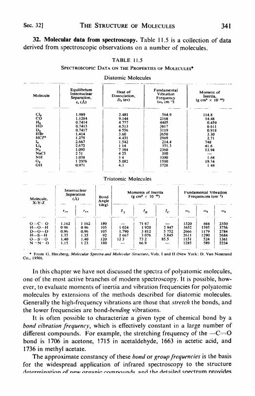
Sec. 32] THE STRUCTURE OF MOLECULES 341
32. Molecular data from spectroscopy. Table 1 1.5 is a collection of data
derived from spectroscopic observations on a number of molecules.
TABLE 11.5
SPECTROSCOPIC DATA ON THE PROPERTIES OF MOLECULES*
Diatomic Molecules
Triatomic Molecules
* From G. Herzberg, Molecular Spectra and Molecular Structure, Vols. I and II (New York: D. Van NostrandCo., 1950).
In this chapter we have not discussed the spectra of polyatomic molecules,
one of the most active branches of modern spectroscopy. It is possible, how-
ever, to evaluate moments of inertia and vibration frequencies for polyatomicmolecules by extensions of the methods described for diatomic molecules.
Generally the high-frequency vibrations are those that stretch the bonds, and
the lower frequencies are bond-bending vibrations.
It is often possible to characterize a given type of chemical bond by a
bond vibration frequency, which is effectively constant in a large number of
different compounds. For example, the stretching frequency of the O-Obond is 1706 in acetone, 1715 in acetaldehyde, 1663 in actetic acid, and
1736 in methyl acetate.
The approximate constancy of these bond or groupfrequencies is the basis
for the widespread application of infrared spectroscopy to the structure
H^termination r\f* n<\i/ /"\ranir rrmnnnHc anrl th* HftnilpH cnPftrilTTI nrOV1flP.<5
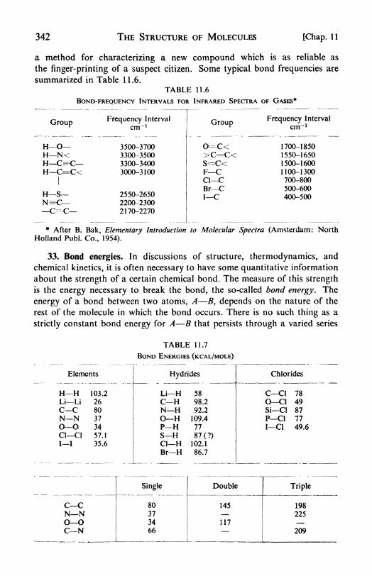
342 THE STRUCTURE OF MOLECULES [Chap. 11
a method for characterizing a new compound which is as reliable as
the finger-printing of a suspect citizen. Some typical bond frequencies are
summarized in Table 1 1 .6.
TABLE 11.6
BOND-FREQUENCY INTERVALS FOR INFRARED SPECTRA OF GASES*
Group
H--<
H N<
H C=C<I
H SN^Cc-c
Frequency Interval
3500-3700
3300-35003300-3400
3000-3100
2550-26502200-23002170-2270
* After B. Bak, Elementary Introduction to Molecular Spectra (Amsterdam: NorthHolland Publ. Co., 1954).
33. Bond energies. In discussions of structure, thermodynamics, and
chemical kinetics, it is often necessary to have some quantitative information
about the strength of a certain chemical bond. The measure of this strength
is the energy necessary to break the bond, the so-called bond energy. The
energy of a bond between two atoms, A B, depends on the nature of the
rest of the molecule in which the bond occurs. There is no such thing as a
strictly constant bond energy for A B that persists through a varied series
TABLE 11.7
BOND ENERGIES (KCAL/MOLE)

Sec. 33] THE STRUCTURE OF MOLECULES 343
of compounds. Nevertheless, it is possible to strike an average from which
actual A B bonds do not deviate too widely.
Pauling has reduced a large amount of experimental data to a list of
normal covalent single-bond energies.23 If the actual bond is markedly
polarized (partial ionic character), or if through resonance it acquires some
double-bond character, its energy may be considerably higher than the norm.
Values from a recent compilation24 are given in Table 1 1 .7. These values
are obtained by a combination of various methods: (1) spectroscopy, (2)
thermochemistry, and (3) electron impact. The electron impact method
employs a mass spectrometer and gradually increases the energy of the
electrons from the ion gun until the molecule is broken into fragments.An instance of the application of thermochemical data is the following
determination of the O H bond strength :
H2~ 2 H AH = 103.4 kcal (spectroscopic)
O2= 2 O AH 1 18.2 (spectroscopic)
H2 f- * O2-= H2 AH - - 57.8 (calorimetric)
2 H + O = H2O AH - 220.3
This is A// for the formation of 2 O H bonds, so that the bond strength is
taken as 220.3/2 - 110 kcal.
PROBLEMS
1. Write down possible resonance forms contributing to the structures of
the following: CO2 ,CH3COO-, CH2.CH-CH:CH 2 , CH3NO2 , C6H5C1,
C6H5NH2 , naphthalene.
2. On the basis of molecular orbital theory, how would you explain the
following? The binding energy of N24 is 6.35 and that of N2 7.38 ev, whereas
the binding energy of O2+
is 6.48 and that of O2 , 5.08 ev.
3. The following results are found for the dielectric constant e of gaseoussulfur dioxide at 1 atm as a function of temperature:
K 267.6 297.2 336.9 443.8
e . 1.009918 1.008120 1.005477 1.003911
Estimate the dipole moment of SO2 , assuming ideal gas behavior.
4. M. T. Rogers25 found the following values for the dielectric constant e
and density p of isopropyl cyanide at various mole fractions X in benzene
solution at 25C:
X . . . 0.00301 0.00523 0.00956 0.01301 0.01834 0.02517
e . . . 2.326 2.366 2.442 2.502 2.598 2.718
P . . . 0.87326 0.87301 0.87260 0.87226 0.87121 0.87108
For pure C3H 7NC, p = 0.7'6572, refractive index nD = 1.3712; for pure
23 For a full discussion: L. Pauling, op. cit., p. 53.24 K. S. Pitzer, J. Am. Chem. Soc., 70, 2140 (1948).26 J. Am. Chem. Soc.> 69, 457 (1947).

344 THE STRUCTURE OF MOLECULES [Chap. 11
benzene, p 0.87345, nD -=- 1.5016. Calculate the dipole moment /i of
isopropyl cyanide.
5. Chlorobenzene has /t-- 1.55 d, nitrobenzene //
= 3.80 d. Estimate the
dipole moments of: metadinitrobenzene, orthodichlorobenzene, metachloro-
nitrobenzene. The observed moments are 3.90, 2.25, 3.40 d. How would you
explain any discrepancies?
6. The angular velocity of rotation o> 27rvrot where vroi is the rotation
frequency of a diatomic rotor. The angular momentum is (h/27r)Vj(J | 1).
Calculate the rotation frequency of the HC1 molecule for the state with
/ --=--- 9. Calculate the frequency of the spectral line corresponding to the
transition J ^ 9 to / - 8.
7. In the far infrared spectrum of HBr is a series of lines having a separa-
tion of 16.94cm *. Calculate the moment of inertia and the internuclear
separation in HBr from this datum.
8. In the near infrared spectrum of carbon monoxide there is an intense
band at 2144cm" 1. Calculate (a) the fundamental vibration frequency of
CO; (b) the period of the vibration; (c) the force constant; (d) the zero-point
energy of CO in cal per mole.
9. Sketch the potential-energy curve for the molecule Li2 according to
the Morse function, given D - 1.14 ev, v ~- 351.35 cm"1, rf 2.672 A.
10. The Schumann-Runge bands in the ultraviolet spectrum of oxygen
converge to a well defined limit at 1759 A. The products of the dissociation
are an oxygen atom in the ground state and an excited atom. There are two
low-lying excited states of oxygen,1 D and 1S at 1.967 and 4.190 volts above
the ground state. By referring to the dissociation data in Table 4.4, page 81,
decide which excited state is formed, and then calculate the spectroscopic
dissociation energy of O2 into two O atoms in the ground state.
11. In a diffraction investigation of the structure of CS2 with 40-kv
electrons, Cross and Brockway26 found four sharp maxima ( f+) each
followed by a weak maximum ( 4 ) and a deep minimum ( ), at the followingvalues of 4-77/A (sin 0/2)
4.713 6.312 7.623 8.698 10.63 11.63 12.65 14.58 15.54 16.81
I f- -I -I \ \- -f- -}-+ 4- + +
CS2 is a linear molecule. Calculate the C S distance from these data,
using the approximation that the scattering factor is equal to the atomic
number Z.
12. With data from Table 11.5, draw to scale the first five rotational
levels in the molecule NaCl. At what frequency would the transition J = 4
to75 be observed? In NaCl vapor at 1000C what would be the relative
numbers of molecules in the states with J = 0, J = 1, and J = 2.
*J. Chem. Phys., 3, 821 (1935).

Chap. 11] THE STRUCTURE OF MOLECULES 345
13. In ions of the first transition series, the paramagnetism is due almost
entirely to the unpaired spins, being approximately equal to/* 2v
/
S(S -f- 1 )
magnetons where S is the total spin. On this basis, estimate // for K13, Mn f 2
,
Co+ 2, and Cu+.
REFERENCES
BOOKS
1. Bates, L. F., Modern Magnetism (London: Cambridge, 1951).
2. Bottcher, C. J. F.., Theory of Electric Polarisation (Amsterdam: Elsevier,
1952).
3. Burk, R. E., and O. Grummitt (editors), Chemical Architecture (NewYork: Interscience, 1948).
4. Coulson, C. A., Valence (New York: Oxford, 1952).
5. Debye, P., Polar Molecules (New York: Dover, 1945).
6. Gaydon, A. G., Dissociation Energies (London: Chapman and Hall,
1952).
7. Gordy, W., W. V. Smith, and R. F. Trambarulo, Microwave Spectra-
scopy (New York: Wiley, 1953).
8. Herzberg, G., Infrared and Raman Spectra (New York: Van Nostrand,
1945).
9. Herzberg, G., Molecular Spectra and Molecular Structure (New York:
Van Nostrand, 1950).
10. Ketelaar, J. A. A., Chemical Constitution (Amsterdam: Elsevier, 1953).
11. Palmer, W. G., Valency, Classical and Modern (Cambridge, 1944).
12. Pauling, L., The Nature of the Chemical Bond (Ithaca: Cornell Press,
1940).
13. Pitzer, K. S., Quantum Chemistry (New York: Prentice-Hall, 1953).
14. Rice, F. O., and E. Teller, The Structure of Matter (New York: Wiley,
1949).
ARTICLES
1. Condon, E. U., Am. J. Phys., 75, 365-74 (1947), "The Franck-Condon
Principle and Related Topics."2. Klotz, I. M., /. Chem. Ed., 22, 328-36 (1945), "Ultraviolet Absorption
Spectroscopy."3. Mills, W. H., J. Chem. Soc., 1942, 457-66 (1942), "The Basis of Stereo-
chemistry."4. Pake, G. E., Am. J. Phys., 18, 438-73 (1950), "Nuclear Magnetic
Resonance."
5. Pauling, L., /. Chem. Soc., 1461-67 (1948), "The Modern Theory of
Valency."6. Purcell, E. M., Science, 118, 431-36 (1953), "Nuclear Magnetic
Resonance."

346 THE STRUCTURE OF MOLECULES [Chap. 11
7. Selwood, P. W., /. Chem. Ed., 79, 181-88 (1942), "Magnetism and
Molecular Structure."
8. Spurr, R., and L. Pauling, J. Chem. Ed., 18, 458-65 (1941), "Electron
Diffraction of Gases."
9. Sugden, S., J. Chem. Soc., 328-33 (1943), "Magnetochemistry."10. Thompson, H. W., J. Chem. Soc.
9183-92 (1944), "Infrared Measure-
ments in Chemistry."11. Wilson, E. B., Ann. Rev. Phys. Chem., 2, 151-76 (1951), "Microwave
Spectroscopy of Gases".

CHAPTER 12
Chemical Statistics
1. The statistical method. If you take a deck of cards, shuffle it well, and
draw a single card at random, it is not possible to predict what the card will
be, unless you happen to be a magician. Nevertheless, a -number of significant
statements can be made about the result of the drawing. For example: the
probability of drawing an ace is one in thirteen;the probability of drawing
a spade is one in four; the probability of drawing the ace of spades is one in
fifty-two. Similarly, if you were to ask an insurance company whether a
certain one of its policyholders was going to be alive 10 years from now, the
answer might be: "We cannot predict the individual fate of John Jones, but
our actuarial tables indicate that the chances are nine out of ten that he will
survive."
We are familiar with many statements of this kind and call them "statisti-
cal predictions." In many instances it is impossible to foretell the outcome
of an individual event, but if a large number of similar events are considered,
a statement based on probability laws becomes possible. An example from
physics is found in the disintegration of radioactive elements. No one can
determine a priori whether an isolated radium atom will disintegrate within
the next 10 minutes, the next 10 days, or the next 10 centuries. If a milligramof radium is studied, however, we know that very close to 2.23 x 10¹⁰ atoms
will explode in any 10-minute period.
Some applications of statistical principles to chemical systems were dis-
cussed in Chapter 7. It was pointed out that since the atoms and molecules
of which matter is composed are extremely small, any large-scale body con-
tains an enormous number of elementary particles. It is impossible to keeptrack of so many individual particles. Any theory that attempts to interpret
the behavior of macroscopic systems in terms of atoms and molecules must
therefore rely heavily on statistical considerations. But just because a systemdoes contain so very many particles, its actual behavior will be practically
indistinguishable from.that predicted by statistics. If a man tossed 10 coins,
the result might deviate widely from 50 per cent heads; if he tossed a thous-
and, the percentage deviation would be fairly small; but if some tireless
player were to toss 1023 coins, the result would be to all intents and purposes
exactly 50 per cent heads.
We have seen already that from the molecular-kinetic point of view the
Second Law of Thermodynamics is a statistical law. It expresses the drive
toward randomness or disorder in a system containing a large number of
particles. Applied to an individual molecule it has no meaning, for in this
347

348 CHEMICAL STATISTICS [Chap. 12
case any distinction between heat (disordered energy) and work (ordered
energy) disappears. Even for intermediate cases, such as colloidal particles
in Brownian motion, the Second Law is inapplicable, since the particles
contain only about 106 to 109 atoms.
Now that the structures and energy levels of atoms and molecules have
been considered, in Chapters 8 through 11, it is possible to see how the
behavior of macroscopic systems is determined by these atomic and mole-
cular parameters. We shall confine our attention to systems in equilibrium,
which are usually treated by thermodynamics. This is not, however, a necessary
restriction for the statistical method, which is competent to handle also
situations in which the system is changing with time. These are some-
times called "rate processes," and include transport phenomena, such as
diffusion and thermal conductivity, as well as the kinetics of chemical
reactions.
Statistical thermodynamics is still a very young science, and many funda-
mental problems remain to be solved. Thus the only systems that have been
treated at all accurately are ideal gases and perfect crystals. Imperfect gases
and liquids present unsurmounted difficulties.
2. Probability of a distribution. The discussion of statistical thermo-
dynamics upon which we are embarking will not be distinguished for its
mathematical precision, nor will any attempt be made to delve into the
logical foundations of the subject.1
The general question to be answered is this: given a macroscopic physical
system, composed of molecules (and/or atoms), and knowing from quantummechanics the allowed energy states for these molecules, how will we dis-
tribute the large number of molecules among the allowed energy levels? The
problem has already been discussed for certain special cases, the answers
being expressed in the form of "distribution laws," for example, the Maxwell
distribution law for the kinetic energies of molecules, the Planck distribution
law for the energies of harmonic oscillators. We wish now to obtain a more
general formulation.
The statistical treatment is based on an important principle: the most
probable distribution in a system can be taken to be the equilibrium dis-
tribution. In a system containing a very large number of particles, deviations
from the most probable distribution need not be considered in defining the
equilibrium condition. 2
We first require an expression for the probability P of a distribution.
Then the expression for the maximum probability is obtained by setting the
variation of P equal to zero, subject to certain restraining conditions imposedon the system.
1 For such treatments, see R. H. Fowler and E. A. Guggenheim, Statistical Thermo-
dynamics (London: Cambridge, 1939); and R. C. Tolman, Statistical Mechanics (NewYork: Oxford, 1938).
a See J. E. Mayer and M. Mayer, Statistical Mechanics (New York: Wiley, 1940), for
a good discussion of this point.
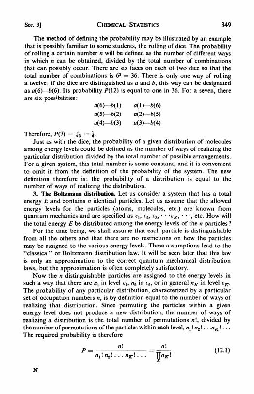
Sec. 3] CHEMICAL STATISTICS 349
The method of defining the probability may be illustrated by an examplethat is possibly familiar to some students, the rolling of dice. The probabilityof rolling a certain number n will be defined as the number of different waysin which n can be obtained, divided by the total number of combinations
that can possibly occur. There are six faces on each of two dice so that the
total number of combinations is 62 36. There is only one way of rolling
a twelve; if the dice are distinguished as a and b y this way can be designatedas a(6) b(6). Its probability P(\2) is equal to one in 36. For a seven, there
are six possibilities:
a(6)-b(\) a(l)-b(6)
a(5)-b(2) a(2)~b(5)
a(4)-b(3)
Therefore, P(7) = H\ =-J.
Just as with the dice, the probability of a given distribution of molecules
among energy levels could be defined as the number of ways of realizing the
particular distribution divided by the total number of possible arrangements.For a given system, this total number is some constant, and it is convenient
to omit it from the definition of the probability of the system. The new
definition therefore is: the probability of a distribution is equal to the
number of ways of realizing the distribution.
3. The Boltzmann distribution. Let us consider a system that has a total
energy E and contains n identical particles. Let us assume that the allowed
energy levels for the particles (atoms, molecules, etc.) are known from
quantum mechanics and are specified as el9 2 , % " " '
K>' ' ' etc - How will
the total energy E be distributed among the energy levels of the n particles?
For the time being, we shall assume that each particle is distinguishable
from all the others and that there are no restrictions on how the particles
may be assigned to the various energy levels. These assumptions lead to the
"classical" or Boltzmann distribution law. It will be seen later that this law
is only an approximation to the correct quantum mechanical distribution
laws, but the approximation is often completely satisfactory.
Now the n distinguishable particles are assigned to the energy levels in
such a way that there are nt in level el9n2 in 2 ,
or in general nK in level eK .
The probability of any particular distribution, characterized by a particular
set of occupation numbers , is by definition equal to the number of ways of
realizing that distribution. Since permuting the particles within a given
energy level does not produce a new distribution, the number of ways of
realizing a distribution is the total number of permutations !, divided bythe number of permutations of the particles within each level, ^ ! n2 \ . . .nK ! . . .
The required probability is therefore
(.2..). nK \
N

350 CHEMICAL STATISTICS [Chap. 12
As an example of this formula, consider four particles a, b, c, d distributed
so that two are in el9 none in 2 and one ea h in a and 4- The possible
arrangements are as follows :
There are twelve arrangements as given by the formula [0!=
1]:
,22!0! 1! 1! 2- 1 1 1
Note that interchanges of the two particles within level sl are not significant.
Returning to eq. (12.1), the equilibrium distribution is the one for which
this probability is a maximum. The maximum is subject to two conditions,
the constancy of the number of particles and the constancy of the total
energy. These conditions can be written
= n
Y FI, nKeK - E2 '2)
By taking the logarithm of both sides of eq. (12.1), the continued productis reduced to a summation.
In In n\ nK l
The condition for a maximum in P is that the variation of P, and hence of
In P, be zero. Since In A?! is a constant,
Stirling's formula3 for the factorials of large numbers is
In n\ = n In n n
(12.3)
(12.4)
3 For derivation see D. Widder, Advanced Calculus (New York: Prentice-Hall, 1947),
f>.317.

Sec. 3] CHEMICAL STATISTICS 351
Therefore eq. (12.3) becomes
^ 2 nK ^n nK ~ ^ ^ w^ =
or 2 In 77^^ -(12.5)
The two restraints in eq. (12.2), since n and E are constants, can be
written
(5/2^2 (5 i,- =AIT v ji n < 12 -6)oE ^= Z, GK onK
These two equations are multiplied by two arbitrary constants,4 a and /?,
and added to eq. (12.5), yielding
S a a/i^ + S /?eA, a/ijr + Z\nnK SnK - (12.7)
The variations 6nK may now be considered to be perfectly arbitrary (the
restraining conditions having been removed) so that for eq. (12.7) to hold,
each term in the summation must vanish. As a result,
In nK + a f fteK ~
or nK -=e~*e-*** (12.8)
This equation has the same form as the Boltzmann distribution law
previously obtained and suggests that the constant ft equals \jkT. It could
have been calculated anew. Thus
nK ^ e -*e~*KlkT (12.9)
It is convenient at this point to make one extension of this distribution
law. It is possible that there may be more than one state corresponding with
the energy level eK . If this is so, the level is said to be degenerate and should
be assigned a statistical weight gK , equal to the number of superimposedlevels. The distribution law in this more general form is accordingly
e-**tkT
(12.10)
The constant a is evaluated from the condition
ZnK = n
whence S e~ *gKe~ **lkT = n
Therefore eq. (12.10) becomes
-eKlkT"
* This is an application of Lagrange*s method of undetermined multipliers, the stan-
dard treatment of constrained maxima problems. See, for example, D. Widder, Advanced
Calculus, p. 113

352 CHEMICAL STATISTICS [Chap. 12
This is the Boltzmann distribution law in its most general form. The
expression 2 gKe~'*lkT
*n ^e denominator of eq. (12. 1 1) is very important in
statistical mechanics. It is called the partition function, and will be denoted
by the symbol-*** (12-12)
The average energy e of a particle is given by (see eq. 7.38)
=
or g = kT* (12.13)oT
4. Internal energy and heat capacity. It is now possible to make use of
the distribution law to calculate the various functions of thermodynamics.
Thermodynamics deals not with individual particles, but with large-scale
systems containing very many particles. The usual thermodynamic measure
is the mole, 6.02 x 10²³ molecules.
Instead of considering a large number of individual particles, let us
consider a large number of systems, each containing a mole of the substance
being studied. The average energy of these systems will be the ordinaryinternal energy E. We again use eq. (12.13), except that now a whole systemtakes the place of each particle. If the allowed energies of the whole systemare El9 2, . . . EK , the average energy will be
Writing Z-S&t*-**'*71
(12.14)
then, E = kT*--- (12.15)oT
We may call Z the molar partitionfunction to distinguish it from the molecular
partition function/. It is also called the sum-over-states
From eq. (12.15) the heat capacity at constant volume is
5T
5. Entropy and the Third Law. Equation (12.16) can be employed to
calculate the entropy in terms of the molar partition function Z. Thus :

Sec. 5] CHEMICAL STATISTICS 353
Integrating by parts, we find
5 = :
) +*r/ v *>o
T /a In ZdT
ET
(12.17)
In this equation, only 5 and \k lnZ| T=0 are temperature-independentterms. The constant term, 5 , the entropy at the absolute zero, is therefore
5 = *lnZ| T. = *In ft (12.18)
Here gQ is the statistical weight of the Jowest possible energy state of the
system. Equation (12.18) is the statistical-mechanical formulation of the
Third Law of Thermodynamics.If we consider, for example, a perfect crystal at the absolute zero, there
will usually be one and only one equilibrium arrangement of its constituent
atoms, ions, or molecules. In other words, the statistical weight of the lowest
energy state is unity: the entropy at 0K becomes zero. This formulation
ignores the possible multiplicity of the ground state due to nuclear spin. If
the nuclei have different nuclear-spin orientations, there will be a residual
entropy at 0K. In chemical problems such effects are of no importance,since in any chemical reaction the nuclear-spin entropy would be the same
on both sides of the reaction equation. It is thus conventional to set 5 -=
for the crystalline elements and hence for all crystalline solids.
Many statistical calculations on this basis have been quantitatively
checked by experimental Third-Law values based on heat-capacity data.
Examples are given in Table 12.1.
TABLE 12.1
COMPARISON OF STATISTICAL (SPECTROSCOPIC) AND THIRD-LAW (HEAT-CAPACITY)ENTROPIES

$54 CHEMICAL STATISTICS [Chap. 12
In certain cases, however, it appears that even at absolute zero the
particles in a crystal may persist in more than one geometrical arrangement.An example is crystalline nitrous oxide. Two adjacent molecules of N2O can
be oriented either as (ONN NNO) or as (NNO NNO). The energy difference
A between these alternative configurations is so slight that their relative
probability e*EIRT
is practically unity even at low temperatures. By the time
the crystal has been cooled to the extremely low temperature at which even
a minute A might produce a reorientation, the rate of rotation of the
molecules within the crystal has become vanishingly slow. Thus the random
orientations are effectively "frozen." As a result, heat-capacity measure-
ments will not include a residual entropy SQ equal to the entropy of mixingof the two arrangements. From eq. (3.42) this would amount to
5 - -R S X, In X, - R(\ In J + In i)- R In 2 - 1.38 eu
It is found that the entropy calculated from statistics is actually larger by1.14eu than the Third-Law value, which is within the experimental uncer-
tainty of iO.25 eu in SQ . A number of examples of this type have been
carefully studied. 5
If the substance at temperatures close to 0K is not crystalline, but a
glass, there is also a residual entropy owing to the randomness characteristic
of vitreous structures.
Another instance of a residual entropy of mixing at 0K arises from the
isotopic constitution of the elements. This effect can usually be ignored since
in most chemical reactions the isotopic ratios change very slightly.
As a result of this discussion, we shall set SQ~- in eq. (12.18), obtaining
S ~+*lnZ (12.19)
6. Free energy and pressure. From the relation A = E TS and eqs.
(12.15) and (12.19), the work function becomes
A = -kT\nZ (12.20)
The pressure, @A/dV)T , is then
P = kT*^ (12.2.)
The Gibbs free energy is simply F = A -\- PV, and from AF the equi-
librium constants for a reaction can be calculated.
Expressions have now been obtained that enable us to calculate all
thermodynamic properties of interest, once we know how to evaluate the
molar partition function Z.
7. Evaluation of molar partition functions. The evaluation of the molar
partition function Z has not yet been accomplished for all types of systems,which is of course hardly surprising, for the function Z contains in itself the
5 For the interesting case of ice, see L. Pauling, /. Am. Chem. Soc., 57, 2680 (1935).

Sec. 7] CHEMICAL STATISTICS 355
answer to all the equilibrium properties of matter. If we could calculate Zfrom the properties of individual particles, we could then readily calculate
all the energies, entropies, free energies, specific heats, and so forth, that
might be desired.
In many cases, it is a good approximation to consider that EK , an energyof the system, can be represented simply as the sum of energies EK of non-
interacting individual particles. This would be the case, for example, of a
crystal composed of independent oscillators, or of an almost perfect gas in
which the intermolecular forces were negligible. In such instances we can
write
EK ^ i(0 + 2(2) -I- *3(3) f . . . eN(N) (12.22)
This expression indicates that particle (1) occupies an energy level el9 particle
(2) an energy level F2 , etc. Each different way of assigning the particles to
the energy levels determines <* distinct state of the system EK .
The molar partition function, or sum over the states EK , then becomes
(The statistical weights gK are omitted for convenience in writing the ex-
pressions.) The second summation must be taken over all the different waysof assigning the particles to the energy levels EK . It can be rewritten as
e
Since each particle has the same set of allowed energy levels, this sum is
equal6 to
(2 e- 8*lkT
)N
KThus we find that Z =--/*
The relation Z /'vapplies to the case in which rearranging the particles
among the energy levels in eq. (12.22) actually gives rise to different states
that must be included in the summation for Z. This is the situation in a
perfect crystal, the different particles (oscillators) occupying distinct localized
positions in the crystal structure.
In the case of a gas, on the other hand, each particle is free to move
throughout the whole available volume. States in the gas that differ merely
*It may be rather hard to see this equality at first. Consider therefore a simple case in
which there are only two particles (1) and (2) and two energy levels ft and e
2 . The ways of
assigning the particles to the levels are:
i=
i (0 Ma (2), 2=
*i (2) + 2 (1), E* = i (1) t- FI (2),
The sum over states is:
Z = e-W* -f e-E*l*T 4- e~
which is equal to
*lkT -f e~*
Now it is evident that this is identical with
fn = (S*-**/**
1
)1 = (e~*il
kT -f e-

356 CHEMICAL STATISTICS [Chap. 12
by the interchange of two particles are not distinguishable and should be
counted only once. If each level in eq. (12.22) contains only one particle,7
the number of permutations of the particles among the levels is AH We there-
fore divide the expression for Z by this factor, obtaining for the ideal gas
case, Z -(!/#!)/*.Thus the relations between /and Z in the two extreme cases are
Ideal crystals Z -/*1 (12.23)
Ideal gases Z =N J
N
Intermediate kinds of systems, such as imperfect gases and liquids, are muchmore difficult to evaluate.
In proceeding to calculate the partition functions for an ideal gas, it is
convenient to make use of a simplifying assumption. The energy of a mole-
cule will be expressed as the sum of translational, rotational, vibrational, and
electronic terms. Thus= ?trans + *rot +" fvlb + *elec (12.24)
It follows that the partition function is the product of corresponding terms,
/" ftr&nsfiotf\lbfelec (12.25)
The simplest case to be considered is that of the monatomic gas, in which
there are no rotational or vibrational degrees of freedom; except at very high
temperatures the electronic excitation is usually negligible.
8. Monatomic gases translational partition function. In Section 10-20 it
was shown that the translational energy levels for a particle in a one-
dimensional box are given by
The statistical weight of each level is unity, gn = 1. Therefore the molecular
partition function becomes
~*!*ml
*}
The energy levels are so closely packed together that they can be considered
to be continuous, and the summation can be replaced by an integration,
7 When the volume is large and the temperature not very low, there will be many more
energy levels than there are particles. This will be evident on examination of eq. (10.39) for
the levels of a particle in a box. Since there is no housing shortage, there is no reason for the
particles to "double-up" and hence the assumption of single occupancy is a good one. Fora further discussion, see Tolman, he. cit., pp. 569-572.
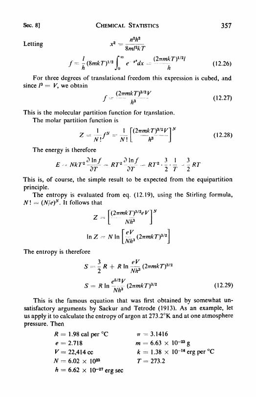
Sec. 8] CHEMICAL STATISTICS 357
(12.26)
For three degrees of translational freedom this expression is cubed, and
since /3
K, we obtain
(,2.27)
This is the molecular partition function for translation.
The molar partition function is
(12 28)\
( }
The energy is therefore
This is, of course, the simple result to be expected from the equipartition
principle.
The entropy is evaluated from eq. (12.19), using the Stirling formula,
AM = (N/e)N
. It follows that
Nlf
The entropy is therefore
(12.29)ATT
This is the famous equation that was first obtained by somewhat un-
satisfactory arguments by Sackur and Tetrode (1913). As an example, let
us apply it to calculate the entropy of argon at 273.2K and at one atmosphere
pressure. Then
R = 1.98 cal per C 77 = 3.1416
* = 2.718 m-6.63 X 10"23 g
V = 22,414 cc k - 1.38 x 10~18 erg per C# = 6.02 x 10²³ 7- 273.2
h = 6.62 x 10~27 ergsec
358 CHEMICAL STATISTICS [Chap. 12
On substituting these quantities into eq. (12.29), the entropy is found to
be 36.2 cal per deg mole.
9. Diatomic molecules rotational partition function. The energy levels
for diatomic molecules, according to the rigid-rotator model, were given by
eq. (11. 22) as
J(J_+ l)/r
fr<)t^ "
~87T2/
If the moment of inertia / is sufficiently high, these energy levels become so
closely spaced as to be practically continuous. This condition is, in fact,
realized for all diatomic molecules except H2 , HD, and D2 . Thus for F2 ,
/ - 25.3 x 10~40 gcm2; for N2 ,
13.8 x lO^40;but for H2 , / - 0.47 x 1Q-40 .
These values are calculated from the interatomic distances and the masses
of the molecules, since / = //r2
.
Now the multiplicity of the rotational levels requires some consideration.
The number of ways of distributing J quanta of rotational energy between
two axes of rotation equals 2J -f 1, for in every case except J there are
two possible alternatives for each added quantum. The statistical weight of
a rotational level J is therefore 2J + 1 .
The rotational partition function now becomes
/rot -= E (27 4 \)e/<>+ !>*//"'
(12.30)
Replacing the summation by an* integration, since the levels are closely
spaced, we obtain
One further complication remains. In homonuclear diatomic molecules
(N14N 14, C135C1
35, etc.) only all odd or all even /'s are allowed, depending on
the symmetry properties of the molecular eigenfunctions. If the nuclei are
different (N14N 15, HC1, NO, etc.) there are no restrictions on the allowed
7's. A symmetry number a is therefore introduced, which is either a = 1
(heteronuclear) or a = 2 (homonuclear). Then
^ot ~ -
ah2(12.32)
As an example of the application of this equation, consider the calcula-
tion of the entropy of F2 at 298.2K, assuming translational and rotational
contributions only. From eq. (12.29), the translational entropy is found to
be 36.88 eu. Then the rotational part is

Sec. 10] CHEMICAL STATISTICS 359
Note that the rotational energy is simply RT in accordance with the equi-
partition principle. Substituting / 25.3 x lO'40, Srot 8.74 eu. Adding
the translational term, we have
S =-- Smt f 5tran8- 8.74 h 36.88 - 45.62 eu
This compares with a total entropy of 5I
298- 48.48 eu. The vibrational
contribution at 25C is therefore small.
10. Polyatomic molecules rotational partition function. The partition
function in eq. (12.32) holds also for linear polyatomic molecules, with a - 2
if the molecule has a plane of symmetry (such as O C O), and a -1 if
it has not (such as N-^N-- O).
For a nonlinear molecule, the classical rotational partition function has
been found to be
/rrot
In this equation A, /?, C are the three principal moments of inertia of the
molecule. The symmetry number a is equal to the number of equivalent
ways of orienting the molecule in space. For example: H 2O, a 2; NH3 ,
a-3;CH4 ,o- 12;C6H 6 ,
a == 12.
11. Vibrational partition function. In evaluating a partition function for
the vibrational degrees of freedom of a molecule, it is often sufficient to use
the energy levels of the harmonic oscillator, which from eq. (11.25) are
fvib-~ 0' f i)** (12.34)
At low temperatures vibrational contributions are usually small and this
approximation is adequate. For reasonably exact calculations at higher tem-
peratures the anharmonicity of the vibrations must be considered. Some-
times the summation for f can be made by using energy levels obtained
directly from molecular spectra.
The partition function corresponding to eq. (12.34) would be, for each
vibrational degree of freedom,
f = J e -( p +W' vikT -__- e
-i' vW' y e -rWkT
V V
/vil) -f-""m
'(l -<,-*'/)-! (12.35)
The total vibrational partition function is the product of terms such as eq.
(12.35), one for each of the normal modes of vibration of the molecule,
Aib-'TFAvib < 12 -36>
i
For the purposes of tabulation and facility in calculations, the vibrational
contributions can be put into more convenient forms.
The vibrational energy, from eqs. (12.15), (12.23), and (12.35), is
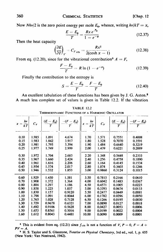
360 CHEMICAL STATISTICS [Chap. 12
Now Nhv/2 is the zero point energy per mole , whence, writing hvjkT = x,
^-^4 (12-37)
(12.38)
Then the heat capacity
JRx*2(cosh x 1)
From eq. (12.20), since for the vibrational contribution8 A F,
( I --.;C,, v
Finally the contribution to the entropy is
* ^0 * ''0o
(12.39)
(12.40)T T
An excellent tabulation of these functions has been given by J. G. Aston. 9
A much less complete set of values is given in Table 12.2. If the vibration
TABLE 12.2
THERMODYNAMIC FUNCTIONS OF A HARMONIC OSCILLATOR
8 This is evident from eq. (12.21) since /vib is not a function of K, P =--0, F = A +
py=A.9 H. S. Taylor and S. Glasstone, Treatise on Physical Chemistry, 3rd ed., vol. 1
, p. 655
(New York: Van Nostrand, 1942).

Sec. 12] CHEMICAL STATISTICS 361
frequency is obtainable from spectroscopic observations, these tables can be
used to calculate the vibrational contributions to the energy, entropy, free
energy, and heat capacity.
12. Equilibrium constant for ideal gas reactions. From the relation
AF RTln Kv , the equilibrium constant can be calculated in terms of
the partition functions. From eqs. (12.20) and (12.23), A = ~Ar7'lirZ =kTln(f
y/N\). From the Stirling formula, N! - (N/e)
N, and since for an
ideal gas,F - A+PY= A f RT, we find that F = - RT In (f/N). Let us write
J yint~
,3 -J Y
where /int denotes the internal partition functions, /rot /vib /elcc ,and /' is
the partition function per unit volume; i.e., f/V. Then, the free energy'
The standard free energy F is the F at unit pressure of one atmosphere.The volume of a mole of ideal gas under standard conditions of 1 atm
pressure is V RT/l. The standard free energy is accordingly10
F - RT \nfkTFor a typical reaction aA + bB ^-- cC \ dD,
J AJ
Therefore, K, -v fi o i*f b
J AJ B
Fromeq. (4.12),** rrr: /Cc(/v/ )
If the concentration terms in Kcare expressed in units of molecules per cc
rather than the more usual moles per cc, we obtain the more concise
expression,ft
c f d
/'A/'B
This equation can easily be given a simple physical interpretation. Con-
sider a reaction A -> B, then Kc
' ^/B'//A'- The partition function is the sum
of the 'probabilities e~ efkT of all the different possible states of the molecules
(/= e" elkT). The equilibrium constant is therefore the ratio of the total
probability of the occurrence of the final state to the total probability of the
occurrence of the initial state.
13. The heat capacity of gases. The statistical theory that has now been
outlined provides a very satisfactory interpretation of the temperature
dependence of the heat capacity of gases.The translational energy is effectively nonquantized. It makes a constant
contribution Cv = $/?, for all types of molecules.
10 Note that k is in units of cc atm/C.
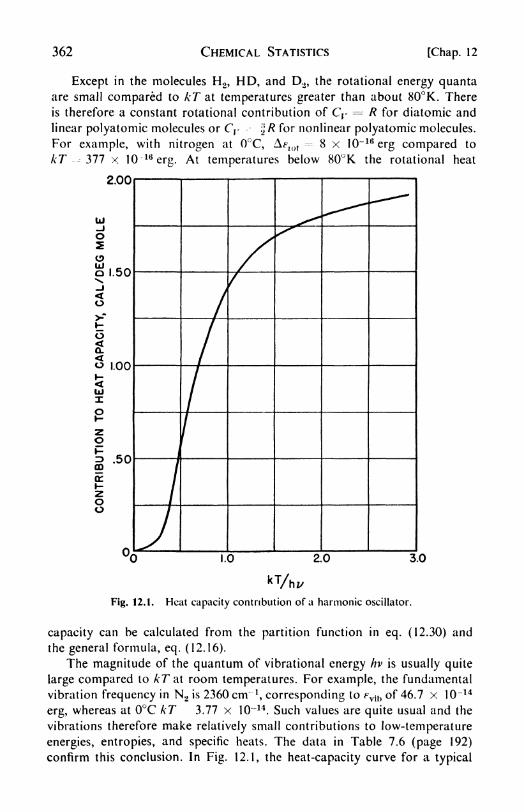
362 CHEMICAL STATISTICS [Chap. 12
Except in the molecules H 2 , HD, and D2 ,
the rotational energy quantaare small compared to kT at temperatures greater than about 80K. There
is therefore a constant rotational contribution of Cv = R for diatomic and
linear polyatomic molecules or Cr $R for nonlinear polyatomic molecules.
For example, with nitrogen at 0C, Aflot
=-- 8 x 10~ 16erg compared to
AT - 377 x 10 16erg. At temperatures below 80K the rotational heat
2.00
LJ
O
o 1.50>*_i<o>?
o
o i.OO
io
o
2OO
V1.0 2.0 3.0
"/hi,
Fig. 12.1. Heat capacity contribution of a harmonic oscillator.
capacity can be calculated from the partition function in eq. (12.30) and
the general formula, eq. (12.16).
The magnitude of the quantum of vibrational energy hv is usually quite
large compared to kT at room temperatures. For example, the fundamental
vibration frequency in N 2 is 2360 cm" 1, corresponding to fvib of 46.7 x 10~ 14
erg, whereas at 0C kT 3.77 x 10~14. Such values are quite usual and the
vibrations therefore make relatively small contributions to low-temperature
energies, entropies, and specific heats. The data in Table 7.6 (page 192)
confirm this conclusion. In Fig. 12.1, the heat-capacity curve for a typical

Sec. 14] CHEMICAL STATISTICS 363
harmonic oscillator is shown as a function of 7/0,,, where Ov---- hvfk is
called the characteristic temperature of the vibration. As the temperature is
raised, vibrational excitation becomes more and more appreciable. If weknow the fundamental vibration frequencies of a molecule, we can determine
from Fig. 12.1 or Table 12.2 the corresponding contribution to Cr at any
temperature. The sum of these contributions is the total vibrational heat
capacity.
14. The electronic partition function. The electronic term in the partition
function is calculated directly from eq. (12.12) and the observed spectro-
scopic data for the energy levels. Often the smallest quantum of electronic
energy is so large compared to kT that at moderate temperatures the elec-
tronic energy acquired by the gas is negligible. In other cases, the groundstate may be a multiplet, but have energy differences so slight that it may be
considered simply as a degenerate single level.
There are, however, certain intermediate cases in which the multiplet
splitting is of the order of kT at moderate temperatures. A notable exampleis NO, with a doublet splitting of around 120 crn^ 1 or 2.38 x 10~14
erg. Anelectronic contribution to the heat capacity is well marked in NO. Complica-tions arise in these cases, however, owing to an interaction between the
rotational angular momentum of the nuclei (quantum number J) and the
electronic angular momentum (quantum number A). The detailed analysis is
therefore more involved than a simple separation of the internal energy into
vibrational, rotational, and electronic contributions would indicate. 11
15. Internal rotation. When certain polyatomic molecules are studied, it
is found that the strict separation of the internal degrees of freedom into
vibration and rotation is not valid. Let us compare, for example, ethyfene
and ethane, CH2 CH 2 and CH3 CH3 .
The orientation of the two methylene groups in C2H4 is fixed by the
double bond, so that there is a torsional or twisting vibration about the
bond but no complete rotation. In ethane, however, there is an internal
rotation of the methyl groups about the single bond. Thus one of the vibra-
tional degrees of freedom is lost, becoming an internal rotation. This
rotation would not be difficult to treat if it were completely free and un-
restricted, but such is not the case. There are potential-energy barriers,
amounting to about 3000 calories per mole, which must be overcome before
rotation occurs. The maxima in energy occur at positions where the hydrogenatoms on the two methyl groups are directly opposite to one another, the
minima at positions where the hydrogens are "staggered."
The theoretical treatment of the problems of restricted internal rotation
is still incomplete, but good progress is being made. 12
16. The hydrogen molecules. Since the moment of inertia of the hydrogen
molecule, H2 , is only 0.47 x 10~ 40 gcm2, the quantum of rotational energy
11 Fowler and Guggenheim, op. cif. t p. 102.12
J. G. Aston, loc. cit., p. 590.

364 CHEMICAL STATISTICS [Chap. 12
is too large for a classical treatment. To evaluate the partition function, the
complete summation must her carried out. When this was first done, using
eq. (12.30), modified with a symmetry number a = 2, the calculated specific
heats were in poor agreement with the experimental values. It was later
realized that the discrepancy must be a result of the existence of the two
nuclear-spin isomers for H2 .
The proton (nucleus of the H atom) has a nuclear spin / -= % in units of
/J/27T. The spins of the two protons in the H2 molecule may either parallel or
oppose each other. These two spin orientations give rise to the two spinisomers:
ortho H2 spins parallel resultant spin-= 1
para H 2 spins antiparallel resultant spin
Spontaneous transitions between the ortho and para states are strictly
prohibited. The ortho states are associated with only odd rotational levels
(J I, 3, 5 . . .), and para states have only even rotational levels (J =0, 2, 4 . . .). The nuclear-spin weights are gNS
- 3 for ortho, correspondingto allowed directions 4-1,0, -1, andgNS 1 for para, whose resultant spin
13
is 0. At quite high temperatures (~ 0C), therefore, an equilibrium mixture
of hydrogen consists of three parts ortho and one part para. At quite low
temperatures (around 80K, liquid-air temperature) the equilibrium con-
dition is almost pure para hydrogen, with the molecules in the lowest rota-
tional state, J = 0.
The equilibrium is attained very slowly in the absence of a suitable
catalyst, such as oxygen adsorbed on charcoal, or other paramagnetic sub-
stance. It is thus possible to prepare almost pure/?-H2 by adsorbing hydrogenon oxygenated charcoal at liquid-air temperatures, and then warming the
gas in the absence of catalyst.
The calculated heat capacities of pure />-H2 , pure o-H2 and of the 1:3
normal H2 , are plotted in Fig. 12.2. Mixtures of o- and/?-H2 are conveniently
analyzed by measuring their thermal conductivities, since these are pro-
portional to their heat capacities.
A similar situation arises with deuterium, D2 . The nuclear spin of the
D atom is 1. The possible resultant values for D2 are therefore 0, 1, and 2.
Of these, / = and 2 belong to the ortho modification and / ~ 1 is the para.
The weights (2/ } 1) are 1 + 5 = 6, and 3, respectively. The high-tempera-ture equilibrium mixture therefore contains two parts ortho to one part para.
In the molecule HD, which is not homonuclear, there are no restrictions
on the allowed rotational energy levels. The partition function of eq. (12.30)
is directly applicable.
Other diatomic molecules composed of like nuclei with nonzero nuclear
spins may also be expected to exist in both para and ortho modifications.
13Compare the spatial quantization of the orbital angular momentum of an electron,
page 268.

Sec. 17] CHEMICAL STATISTICS 365
Any thermodynamic evidence for such isomers would be confined to ex-
tremely low temperatures, because their rotational energy quanta are small.
The energy levels are so close together that in calculating heat capacities it
is unimportant whether all odds or all evens are taken. It is necessary only
< 3.00
Fig. 12.2.
100 200 300DEGREES KELVIN
Heat capacities of pure para-hydrogen, pure ortho-hydrogen,and 3-o to \~p normal hydrogen.
to divide the total number of levels by a =- 2. Spectroscopic observations,
however, will often reveal an alternating intensity in rotational lines caused
by the different nuclear-spin statistical weights.
17. Quantum statistics. In deriving the Boltzmann statistics, we assumed
that the individual particles were distinguishable and that any number of
particles could be assigned to one energy level. We know from quantummechanics that the first of these assumptions is invalid. The second assump-tion is also incorrect if one is dealing with elementary particles or particles
composed of an odd number of elementary particles. In such cases, the
Pauli Exclusion Principle requires that no more than one particle can gointo each energy level. If the particles considered are composed of an even
number of elementary particles, any number can be accommodated in a
single energy level.
Two different quantum statistics therefore arise, which are characterized
as follows:
Name
(1) Fermi-Dirac
(2) Bose-Einstein
Obeyed by
Odd number of elementary
particles (e.g., electrons,
protons)
Even number of elementary
particles (e.g., deuterons,
photons)
Restrictions on nK
Only one particle perstate, nK < gK
Any number of particles
per state
It is interesting to note that photons follow the Bose-Einstein statistics,
indicating that they are complex particles and recalling the formation of
electron-positron pairs from X-ray photons.

366 CHEMICAL STATISTICS [Chap. 12
A schematic illustration of the two types of distribution would be
O00O O O OF.D. B.E.
Distribution laws are calculated for these two cases by exactly the same
sort of procedure as was used for the Boltzmann statistics.14 The results are
found to be very similar,
< 12 -42 >
F.D. case +B.E. case
Now in almost every case the exponential term is very large compared to
unity, and the Boltzmann statistics are a perfectly good approximation for
almost all practical systems. This can be seen by using the value of e* =f/nfrom eq. (12.10). The condition for the Boltzmann approximation is then
e/kT f----^
1, orn
Using the translational partition function /in eq. (12.27), we have
etl1fT(27rmkTj^V^ ->' (12 -43)
This condition is obviously realized for a gas at room temperature. It is
interesting to note, however, the circumstances under which it would fail.
If n/V, proportional to the density, became very high, the classical statistics
would eventually become inapplicable. This is the situation in the interior of
the stars, and forms the basis of R. H. Fowler's brilliant contribution to
astrophysics. A more mundane case also arises, namely in the electron gasin metals. We shall consider this in the next chapter, with only a brief
mention here. A metallic crystal, to a first approximation, may be considered
as a regular array of positive ions, permeated by a gas ofMobile electrons.
In this case the density term in eq. (12.43) is exceptionally high and in
addition the mass term m is lower by about 2 x 10³ than in any molecular
case. Thus the electron gas will not obey Boltzmann statistics; it must indeed
follow the Fermi-Dirac statistics since electrons obey the Pauli Principle.
PROBLEMS
1. In the far infrared spectrum of HC1, there is a series of lines with a
spacing of 20.7 cm"1. In the near infrared spectrum, there is an intense band
at 3.46 microns. Use these data to calculate the entropy of HC1 as an ideal
gas at 1 atm and 298 K.
14 For these calculations, see, for example, Tolman, op. cit,, p. 388.
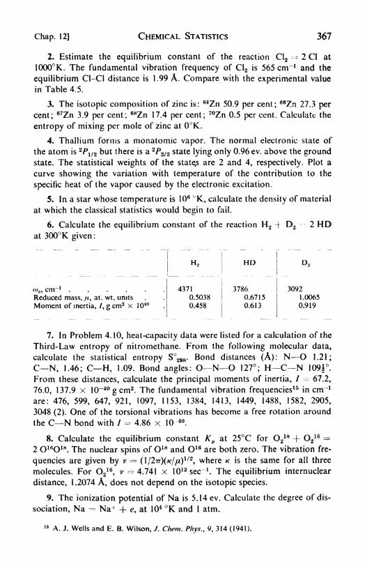
Chap. 12] CHEMICAL STATISTICS 367
2. Estimate the equilibrium constant of the reaction C12--- 2 Cl at
1000K. The fundamental vibration frequency of C12 is 565 cm" 1 and the
equilibrium C1-C1 distance is 1.99 A. Compare with the experimental value
in Table 4.5.
3. The isotopic composition of zinc is:64Zn 50.9 per cent;
68Zn 27.3 per
cent;67Zn 3.9 per cent;
68Zn 17.4 per cent;70Zn 0.5 per cent. Calculate the
entropy of mixing per mole of zinc at 0K.
4. Thallium forms a monatomic vapor. The normal electronic state of
the atom is2P1/2 but there is a 2
P^/2 state lying only 0.96 ev. above the groundstate. The statistical weights of the state.s are 2 and 4, respectively. Plot a
curve showing the variation with temperature of the contribution to the
specific heat of the vapor caused by the electronic excitation.
5. In a star whose temperature is 106 K, calculate the density of material
at which the classical statistics would begin to fail.
6. Calculate the equilibrium constant of the reaction H 2 f D2 2 HDat 300K given:
)e , cm" 1 .....Reduced mass, /i, at. wt. units
Moment of inertia, /, g cm2 x 1040
7. In Problem 4.10, heat-capacity data were listed for a calculation of the
Third-Law entropy of nitromethane. From the following molecular data,
calculate the statistical entropy S 298 . Bond distances (A): N O 1.21;
CN, 1.46; C H, 1.09. Bond angles: O N O 127; H C N 109J.From these distances, calculate the principal moments of inertia, / = 67.2,
76.0, 137.9 x 10~40 gcm2
. The fundamental vibration frequencies15 in cm"1
are: 476, 599, 647, 921, 1097, 1153, 1384, 1413, 1449, 1488, 1582, 2905,
3048 (2). One of the torsional vibrations has become a free rotation around
the CN bond with / = 4.86 x 10 40.
8. Calculate the equilibrium constant Kp at 25C for O21H + O2
16 -2 O 16O1H
. The nuclear spins of O18 and O16 are both zero. The vibration fre-
quencies are given by v = (l/27r)(/c/1/2
,where K is the same for all three
molecules. For O210
, v 4.741 x 10¹³ sec" 1. The equilibrium internuclear
distance, 1.2074 A, does not depend on the isotopic species.
9. The ionization potential of Na is 5.14 ev. Calculate the degree of dis-
sociation, Na -= Na+ + e, at 104 K and 1 atm.
15 A. J. Wells and E. B. Wilson, /. Chem. Phys., 9, 314 (1941).

368 CHEMICAL STATISTICS [Chap. 12
REFERENCES
BOOKS
1. Born, M., Natural Philosophy of Cause and Chance (New York: Oxford,
1949).
2. Dole, M., Introduction to Statistical Thermodynamics (New York:
Prentice-Hall, 1954).
3. Gurney, R. W., Introduction to Statistical Mechanics (New York:
McGraw-Hill, 1949).
4. Khinchin, A. I., Statistical Mechanics (New York: Dover, 1949).
5. Lindsay, R. B., Physical Statistics (New York: Wiley, 1941).
6. Rushbrooke, G. S., Introduction to Statistical Mechanics (New York:
Oxford, 1949).
7. Schrddinger, E., Statistical Thermodynamics (Cambridge, 1946).
8. Ter Haar, D., Elements of Statistical Mechanics (New York: Rinehart,
1954).
ARTICLES
1. Bacon, R. H., Am. J. Phys., 14, 84-98 (1946), "Practical Statistics for
Practical Physicists/'
2. Eyring, H., and J. Walter, /. Chem. Ed., 18, 73-78 (1941), "ElementaryFormulation of Statistical Mechanics."

CHAPTER 13
Crystals
1. The growth and form of crystals. The symmetry of crystalline forms,
striking a responsive chord in our aesthetic nature, has fascinated manymen, from the lapidary polishing gems for a royal crown to the natural
philosopher studying the structure of matter. Someone once said that the
beauty of crystals lies in the planeness of their faces. It was also the measure-
ment and explanation of these plane faces that first demanded scientific
attention.
In 1669, Niels Stensen (Steno), Professor of Anatomy at Copenhagenand Vicar Apostolic of the North, compared the interfacial angles in various
specimens of quartz rock crystals. An interfacial angle may be defined as the
angle between lines drawn perpendicular to two faces. Steno found that the
corresponding angles (in different crystals) were always equal. After the
invention of the contact goniometer in 1780, this conclusion was checked and
extended to other substances, and the constancy of interfacial angles has
been called the "first law of crystallography."It was a most important principle, for out of a great number of crystalline
properties it isolated one that was constant and unchanging. Different crystals
of the same substance may differ greatly in appearance, since correspondingfaces may have developed to diverse extents as the crystals were growing.The interfacial angles, nevertheless, remain the same.
We can consider that a crystal grows from solution or melt by the de-
position onto its faces of molecules or ions from the liquid. If molecules are
deposited preferentially on a certain face, this face will not extend rapidly in
area, compared with faces at angles to it on which deposition is less frequent.
The faces with the largest area are therefore those on which added molecules
are deposited most slowly.
Sometimes an altered rate of deposition can completely change the form,
or habit, of a crystal. A well known case is sodium chloride, which growsfrom pure water solution as cubes, but from 15 per cent aqueous urea
solution as octahedra. It is believed that urea is preferentially adsorbed on
the octahedral faces, preventing deposition of sodium and chloride ions, and
therefore causing these faces to develop rapidly in area.
The real foundations of crystallography may be said to date from the
work of the Abbe Rene Just Haiiy, Professor of the Humanities at the
University of Paris. In 1784, he proposed that the regular external form of
crystals was a reflection of an inner regularity in the arrangement of their
constituent building units. These units were believed to be little cubes or
369

370 CRYSTALS [Chap. 13
polyhedra, which he called the molecules integrates of the substance This
picture also helped to explain the cleavage of crystals along uniform planes.The Haiiy model was essentially confirmed, 128 years later, by the work of
Max von Laue with X-ray diffraction, the only difference being in a moreadvanced knowledge of the elementary building blocks.
2. The crystal systems. The faces of
crystals, and also planes within crystals, can
be characterized by means of a set of three
noncoplanar axes. Consider in Fig. 13.1 three
axes having lengths a, b, and c, which are cut
by the plane ABC, making intercepts OA, OB,and OC. If a, b, c, are chosen as unit lengths,
the lengths of the intercepts may be expressedas OAja, OBjh, OC/c. The reciprocals of these
Fig. 13.1. Crystal axes.lengths will then be a/OA, b/OB, c/OC. Now it
has been established that it is always possibleto find a set of axes on which the reciprocal intercepts of crystal faces are
small whole numbers. Thus, if //, k, /are small integers:
OA ocThis is equivalent to the law of rational intercepts, first enunciated by Haiiy.The use of the reciprocal intercepts (hkl) as indices defining the crystal faces
was first proposed by W. H. Miller in 1839. If a face is parallel to an axis,
(001)
(III) (211)
Fig. 13.2. Miller indices.
the intercept is at oo, and the Miller index becomes l/oo or 0. The notation
is also applicable to planes drawn within the crystal. As an illustration
of the Miller indices, some of the planes in a cubic crystal are shown in
Fig. 13.2.

Sec. 3] CRYSTALS 371
According to the set of axes used to represent their faces, crystals maybe divided into seven systems. These are summarized in Table 13.1. They
range from the completely general set of three unequal axes (a, b, c) at three
unequal angles (a, /?, y) of the triclinic system, to the highly symmetrical set
of three equal axes at right angles of the cubic system.
TABLE 13.1
THE SEVEN CRYSTAL SYSTEMS
3. Lattices and crystal structures. Instead of considering, as Haiiy did,
that a crystal is made of elementary material units, it is helpful to introduce
a geometrical idealization, consisting only of a regular array of points in
space, called a lattice. An example in two dimensions is shown in Fig. 13.3.
o1
Fig. 13.3. Two-dimensional lattice with unit cells.
The lattice points can be connected by a regular network of lines in
various ways. Thus the lattice is broken up into a number of unit cells. Some
examples are shown in the figure. Each cell requires two vectors, a and b,
for its description. A three-dimensional space lattice can be similarly divided
into unit cells that require three vectors for their description.
If each point in a space lattice is replaced by an identical atom or groupof atoms there is obtained a crystal structure. The lattice is an array of points;
in the crystal structure each point is replaced by a material unit.
In 1848, A. Bravais showed that all possible space lattices could be

372 CRYSTALS [Chap. 13
assigned to one of only 14 classes. 1 The 14 Bravais lattices are shown in
Fig. 13.4. They give the allowed different translational relations between
points in an infinitely extended regular three-dimensional array. The choice
of the 14 lattices is somewhat arbitrary, since in certain cases alternative
descriptions are possible.
TRICLINIC
A
2 SIMPLE 3 SIDE-CENTEREDMONOCLINIC MONOCLINIC
\4. SIMPLE 5 END-CENTEREDORTHORHOMBIC ORTHORHOMBIC
6. FACE-CENTERED 7 BODY-ORTHORHOMBIC CENTERED
ORTHORHOMBIC
9 RHOMBOHEDRAL 10 SIMPLE II BODY-CENTERED8. HEXAGONAL TETRAGONAL TETRAGONAL
Fig. 13.4. The fourteen Bravais lattices.
4. Symmetry properties. The word "symmetry" has been used in referringto the arrangement of crystal faces. It is now desirable to consider the nature
of this symmetry in more detail. If an actual crystal of a substance is studied,
some of the faces may be so poorly developed that it is difficult or impossibleto see its full symmetry just by looking at it. It is necessary therefore to
1 A lattice that contains body-, face-, or end-centered points can always be reduced to
one that does not (primitive lattice). Thus the face-centered cubic can be reduced to a
primitive rhombohedral. The centered lattices are chosen when possible because of their
higher symmetry.

Sec. 4] CRYSTALS 373
consider an ideal crystal in which all the faces of the same kind are developedto the same extent. It is not only in face development that the symmetry of
the crystal is evident but also in all of its physical properties, e.g., electric
and thermal conductivity, piezoelectric effect, and refractive index.
Symmetry is described in terms of certain symmetry operations, which
are those that transform the crystal into an image of itself. The symmetry
operations are imagined to be the result of certain symmetry elements: axes
of rotation, mirror planes, and centers of inversion. The possible symmetryelements of finite figures, i.e., actual crystals, are shown in Fig. 13.5 with
schematic illustrations.
(a) T (b)
MM/ v-
i'
Fig. 13.5. Examples of symmetry elements: (a) mirror plane m; (b) rotation
axes; (c) symmetry center 1 ; (d) twofold rotary inversion axis 2.
The possible combinations of these symmetry elements that can occur in
crystals have been shown to number exactly 32. These define the 32 crystallo-
graphic point groups* which determine the 32 crystal classes.
The symbols devised by Hermann and Mauguin are used to represent the
symmetry elements. An axis of symmetry is denoted by a number equal to
its multiplicity. The combination of a rotation about an axis with reflection
through a center of symmetry is called an "axis of rotary inversion"; it is
denoted by placing a bar above the symbol for the axis, e.g., 2, 3. The center
of symmetry alone is then T. A mirror plane is given the symbol m.
All crystals necessarily fall into one of the seven systems* but there are
several classes in each system. Only one of these, called the holohedral class,
possesses the complete symmetry of the system. For example, consider two
crystals belonging to the cubic system, rock salt (NaCl) and iron pyrites
(FeS2). Crystalline rock salt, Fig. 13.6, possesses the full symmetry of the
cube: three 4-fold axes, four 3-fold axes, six 2-fold axes, three mirror planes
perpendicular to the 4-fold axes, six mirror planes perpendicular to the 2-fold
axes, and a center of inversion. The cubic crystals of pyrites might at first
seem to possess all these symmetry elements too. Closer examination reveals,
2 A set of symmetry operations forms a. group when the consecutive application of anytwo operations in the set is equivalent to an operation belonging to the set (law of multi-
plication). It is understood that the identity operation, leaving the crystal unchanged, is
included in each set; that the operations are reversible; and that the associative law holds,
A(BC) = (AB)C.
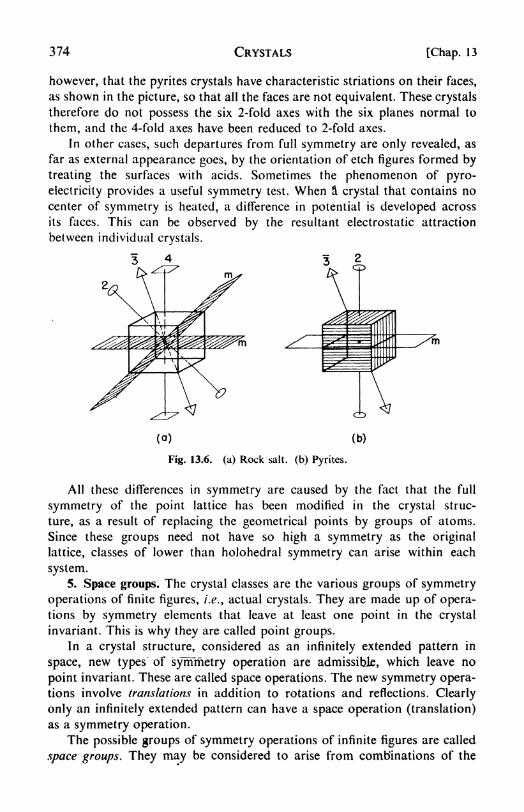
374 CRYSTALS [Chap. 13
however, that the pyrites crystals have characteristic striations on their faces,
as shown in the picture, so that all the faces are not equivalent. These crystals
therefore do not possess the six 2-fold axes with the six planes normal to
them, and the 4-fold axes have been reduced to 2-fold axes.
In other cases, such departures from full symmetry are only revealed, as
far as external appearance goes, by the orientation of etch figures formed by
treating the surfaces with acids. Sometimes the phenomenon of pyro-
electricity provides a useful symmetry test. When & crystal that contains no
center of symmetry is heated, a difference in potential is developed across
its faces. This can be observed by the resultant electrostatic attraction
between individual crystals.
CD
(a) (b)
Fig. 13.6. (a) Rock salt, (b) Pyrites.
All these differences in symmetry are caused by the fact that the full
symmetry of the point lattice has been modified in the crystal struc-
ture, as a result of replacing the geometrical points by groups of atoms.
Since these groups need not have so high a symmetry as the original
lattice, classes of lower than holohedral symmetry can arise within each
system.5. Space groups. The crystal classes are the various groups of symmetry
operations of finite figures, i.e., actual crystals. They are made up of opera-tions by symmetry elements that leave at least one point in the crystal
invariant. This is why they are called point groups.In a crystal structure, considered as an infinitely extended pattern in
space, new types of symmetry operation are admissible, which leave no
point invariant. These are called space operations. The new symmetry opera-tions involve translations in addition to rotations and reflections. Clearly
only an infinitely extended pattern can have a space operation (translation)
as a symmetry operation.
The possible groups of symmetry operations of infinite figures are called
space groups. They may be considered to arise from combinations of the
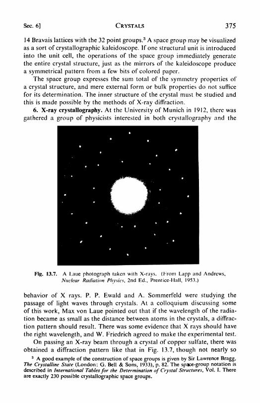
Sec. 6] CRYSTALS 375
14 Bravais lattices with the 32 point groups.3 A space group may be visualized
as a sort of crystallographic kaleidoscope. If one structural unit is introduced
into the unit cell, the operations of the space group immediately generatethe entire crystal structure, just as the mirrors of the kaleidoscope producea symmetrical pattern from a few bits of colored paper.
The space group expresses the sum total of the symmetry properties of
a crystal structure, and mere external form or bulk properties do not suffice
for its determination. The inner structure of the crystal must be studied and
this is made possible by the methods of X-ray diffraction.
6. X-ray crystallography. At the University of Munich in 1912, there was
gathered a group of physicists interested in both crystallography and the
Fig. 13.7. A Laue photograph taken with X-rays. (From Lapp and Andrews,
Nuclear Radiation Physics, 2nd Ed., Prentice-Hall, 1953.)
behavior of X rays. P. P. Ewaid and A. Sommerfeld were studying the
passage of light waves through crystals. At a colloquium discussing some
of this work, Max von Laue pointed out that if the wavelength of the radia-
tion became as small as the distance between atoms in the crystals, a diffrac-
tion pattern should result. There was some evidence that X rays should have
the right wavelength, and W. Friedrich agreed to make the experimental test.
On passing an X-ray beam through a crystal of copper sulfate, there was
obtained a diffraction pattern like that in Fig. 13.7, though not nearly so
3 A good example of the construction of space groups is given by Sir Lawrence Bragg,The Crystalline State (London: G. Bell & Sons, 1933), p. 82. The spjice-group notation is
described in International Tables for the Determination of Crystal Structures, Vol. I. There
are exactly 230 possible crystallographic space groups.

376 CRYSTALS [Chap. 13
distinct in these first trials. The wave properties of X rays were thus definitely
established and the new science of X-ray crystallography began.
Some of the consequences of Laue's great discovery have already been
mentioned, and on page 257 the conditions for diffraction maxima from a
regular three-dimensional array of scattering centers were found to be
cos (a 00) hh
cos08-/? )-*A (13.1)
cos (y- y )
- tt
If monochromatic X rays are used, there is only a slim chance that the
orientation of the crystal is fixed in such a way as to yield diffraction maxima.
The Laue method, however, uses a continuous spectrum of X radiation with
a wide range of wavelengths. This is the so-called white radiation, conveniently
obtained from a tungsten target at high voltages. In this case, at least some
of the radiation is at the proper wavelength to experience interference effects,
no matter what the orientation of crystal to beam.
7. The Bragg treatment. When the news of the Munich work reached
England, it was immediately taken up by W. H. Bragg and his son W. L.
Fig. 13.8. Bragg scattering condition.
Bragg who had been working on a corpuscular theory ofX rays. W. L. Bragg,
using Laue-type photographs, analyzed the structures of NaCl, KC1, and
ZnS (1912, 1913). In the meantime (1913), the elder Bragg devised a spectrom-eter that measured the intensity of an X-ray beam by the amount of ioniza-
tion it produced, and he found that the characteristic X-ray line spectrumcould be isolated and used for crystallographic work. Thus the Bragg method
uses a monochromatic (single wavelength) beam of X rays.
The Braggs developed a treatment of X-ray scattering by a crystal that
was much easier to apply than Laue's theory, although the two are essentially
equivalent. It was shown that the scattering of X rays could be representedas a "reflection" by successive planes of atoms in the crystal. Consider, in
Fig. 13.8, a set of parallel planes in the crystal structure and a beam of
X rays incident at an angle 0. Some of the rays will be "reflected" from the
upper layer of atoms, the angle of reflection being equal to the angle of inci-
dence. Some of the rays will be absorbed, and some will be "reflected" from
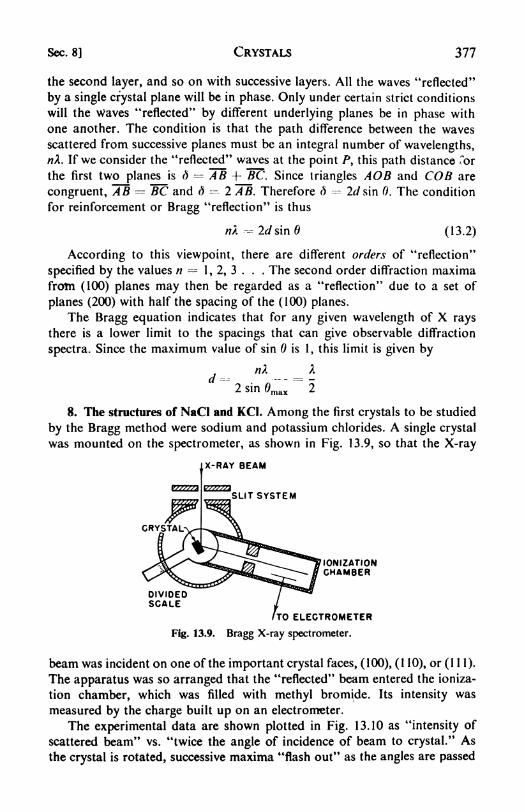
Sec. 8] CRYSTALS 377
the second layer, and so on with successive layers. All the waves "reflected"
by a single crystal plane will be in phase. Only under certain strict conditions
will the Waves "reflected" by different underlying planes be in phase with
one another. The condition is that the path difference between the waves
scattered from successive planes must be an integral number of wavelengths,nk. If we consider the "reflected" waves at the point P, this path distance Tor
the first two planes is 6 = "AB + ~BC. Since triangles AOB and COB are
congruent, AB BC and d 2 AB. Therefore d 2d sin 0. The condition
for reinforcement or Bragg "reflection" is thus
/7A-2</sin0 (13.2)
According to this viewpoint, there are different orders of "reflection"
specified by the values n = 1, 2, 3 . . . The second order diffraction maxima
from (100) planes may then be regarded as a "reflection" due to a set of
planes (200) with half the spacing of the (100) planes.
The Bragg equation indicates that for any given wavelength of X rays
there is a lower limit to the spacings that can give observable diffraction
spectra. Since the maximum value of sin is 1, this limit is given by
"A --~2 sin max
"2
8. The structures of NaCl and KC1. Among the first crystals to be studied
by the Bragg method were sodium and potassium chlorides. A single crystal
was mounted on the spectrometer, as shown in Fig. 13.9, so that the X-ray
IX-RAY BEAM
L-V/V//J
SLIT SYSTEM
IONIZATIONCHAMBER
**" ^^J^^DIVIDEDSCALE
/TO ELECTROMETER
Fig. 13.9. Bragg X-ray spectrometer.
beam was incident on one of the important crystal faces, (100), (1 10), or (1 1 1).
The apparatus was so arranged that the "reflected" beam entered the ioniza-
tion chamber, which was filled with methyl bromide. Its intensity was
measured by the charge built up on an electrometer.
The experimental data are shown plotted in Fig. 13.10 as "intensity of
scattered beam" vs. "twice the angle of incidence of beam to crystal." As
the crystal is rotated, successive maxima "flash out" as the angles are passed
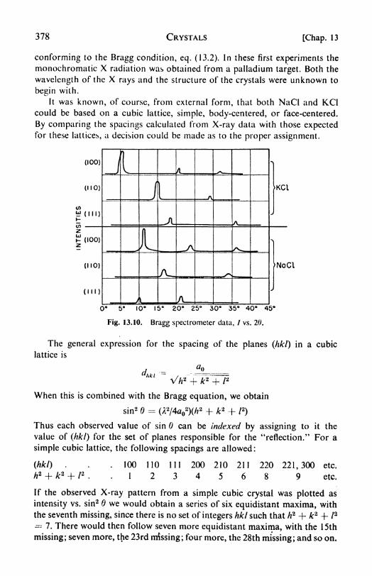
378 CRYSTALS [Chap. 13
conforming to the Bragg condition, eq. (13.2). In these first experiments the
monochromatic X radiation was obtained from a palladium target. Both the
wavelength of the X rays and the structure of the crystals were unknown to
begin with.
It was known, of course, from external form, that both NaCl and KC1could be based on a cubic lattice, simple, body-centered, or face-centered.
By comparing the spacings calculated from X-ray data with those expectedfor these lattices, a decision could be made as to the proper assignment.
0* 5 10 15 20 25 30 35 40 45
Fig. 13.10. Bragg spectrometer data, / vs. 20.
The general expression for the spacing of the planes (hkl) in a cubic
lattice is
-"Vh*-+k*ni
When this is combined with the Bragg equation, we obtain
sin2 6 = (A2/4a
2)(//
2 + k2 + I2)
Thus each observed value of sin can be indexed by assigning to it the
value of (hkl) for the set of planes responsible for the "reflection." For a
simple cubic lattice, the following spacings are allowed:
(hkl) . . . 100 110 111 200 210 211 220 221,300 etc.
h2 + k2 + 12
. .1 2 3 4 5 6 8 9 etc.
If the observed X-ray pattern from a simple cubic crystal was plotted as
intensity vs. sin2 we would obtain a series of six equidistant maxima, with
the seventh missing, since there is no set of integers hkl such that h2 + k2 + I2
7. There would then follow seven more equidistant maxima, with the 15th
missing; seven more, the 23rd missing; four more, the 28th missing; and so on.
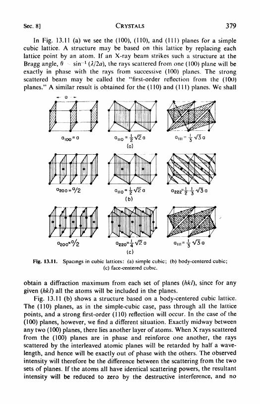
Sec. 8] CRYSTALS 379
In Fig. 13.11 (a) we see the (100), (110), and (111) planes for a simplecubic lattice. A structure may be based on this lattice by replacing each
lattice point by an atom. If an X-ray beam strikes such a structure at the
Bragg angle, sin" 1(A/20), the rays scattered from one (100) plane will be
exactly in phase with the rays from successive (100) planes. The strongscattered beam may be called the "first-order reflection from the (100)
planes." A similar result is obtained for the (1 10) and (111) planes. We shall
-*- a ^
Fig. 13.11. Spacings in cubic lattices: (a) simple cubic; (b) body-centered cubic;
(c) face-centered cubic.
obtain a diffraction maximum from each set of planes (hkl), since for any
given (hkl) all the atoms will be included in the planes.
Fig. 13.11 (b) shows a structure based on a body-centered cubic lattice.
The (110) planes, as in the simple-cubic case, pass through all the lattice
points, and a strong first-order (1 10) reflection will occur. In the case of the
(100) planes, however, we find a different situation. Exactly midway between
any two (100) planes, there lies another layer of atoms. When X rays scattered
from the (100) planes are in phase and reinforce one another, the rays
scattered by the interleaved atomic planes will be retarded by half a wave-
length, and hence will be exactly out of phase with the others. The observed
intensity will therefore be the difference between the scattering from the two
sets of planes. If the atoms all have identical scattering powers, the resultant
intensity will be reduced to zero by the destructive interference, and no
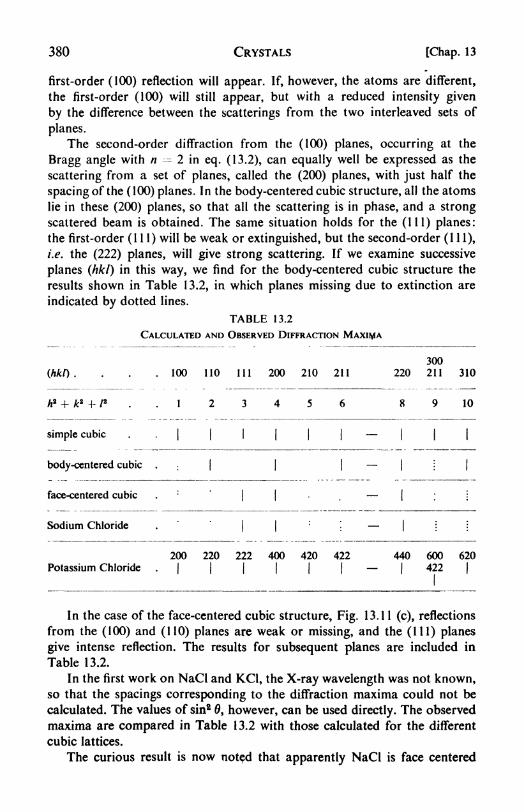
380 CRYSTALS [Chap. 13
first-order (100) reflection will appear. If, however, the atoms are different,
the first-order (100) will still appear, but with a reduced intensity given
by the difference between the scatterings from the two interleaved sets of
planes.
The second-order diffraction from the (100) planes, occurring at the
Bragg angle with n ^ 2 in eq. (13.2), can equally well be expressed as the
scattering from a set of planes, called the (200) planes, with just half the
spacing of the (100) planes. In the body-centered cubic structure, all the atoms
lie in these (200) planes, so that all the scattering is in phase, and a strong
scattered beam is obtained. The same situation holds for the (111) planes:
the first-order (111) will be weak or extinguished, but the second-order (111),
i.e. the (222) planes, will give strong scattering. If we examine successive
planes (hkl) in this way, we find for the body-centered cubic structure the
results shown in Table 13.2, in which planes missing due to extinction are
indicated by dotted lines.
TABLE 13.2
CALCULATED AND OBSERVED DIFFRACTION MAXIMA
300
(hkl) . ... 100 110 111 200 210 211 220 211 310
/,2 + p 4. 72 ! 2 3 4 5 6 8 9 10
simple cubic .
| ||
| | | | | |
body-centered cubic: | | | III
face-centered cubic
Sodium Chloride
200 220 222 400 420 422 440 600 620
Potassium Chloride .1 I I I I I I 422 I
In the case of the face-centered cubic structure, Fig. 13.1 1 (c), reflections
from the (100) and (110) planes are weak or missing, and the (111) planes
give intense reflection. The results for subsequent planes are included in
Table 13.2.
In the first work on NaCl and KC1, the X-ray wavelength was not known,so that the spacings corresponding to the diffraction maxima could not be
calculated. The values of sin2 0, however, can be used directly. The observed
maxima are compared in Table 13.2 with those calculated for the different
cubic lattices.
The curious result is now not^d that apparently NaCl is face centered

Sec. 8] CRYSTALS 381
Fig. 13.12. Sodium chloride
structure.
while KC1 is simple cubic. The reason why the KC1 structure behaves toward
X rays like a simple cubic array is that the scattering powers of K+ and Cl~
ions are indistinguishable since they both have an argon configuration with
18 electrons. In the NaCl structure the difference in scattering power of the
Na+ and Cl~ ions is responsible for the deviation from the simple cubic
pattern.
The observed maxima from the (111) face of NaCl include a weak peakat an angle of about 10, in addition to the stronger peak at about 20,
corresponding to that observed with KC1. These results are all explained bythe NaCl structure shown in Fig. 13.12, which consists of a face-centered
cubic array of Na+ ions and an interpenetrating face-centered cubic array of
Cl~ ions. Each Na+ ion is surrounded by six
equidistant Cl~ ions and each Cl~ ion bysix equidistant Na+ ions. The (100) and (1 10)
planes contain an equal number of both
kinds of ions, but the (111) planes consist of
either all Na f or all Cl~ ions. Now if X rays
are scattered from the (111) planes in NaCl,whenever scattered rays from successive Na+
planes are exactly in phase, the rays scattered
from the interleaved Cl~ planes are retarded
by half a wavelength and are therefore exactlyout of phase. The first-order (111) reflection is therefore weak in NaCl since
it represents the difference between these two scatterings. In the case of KC1,where the scattering powers are the same, the first-order reflections are
altogether extinguished by interference. Thus the postulated structure is in
complete agreement with the experimental X-ray evidence.
Once the NaCl structure was well established, it was possible to calculate
the wavelength of the X rays used. From the density of crystalline NaCl,
p = 2.163 g per cm3, the molar volume is M/p =--- 58.45/2.163 = 27.02 cc per
mole. Then the volume occupied by each NaCl unit is 27.02 : (6.02 x 10²³)= 44.88 x 10~24 cc. In the unit cell of NaCl, there are eight Na+ ions at the
corners of the cube, each shared between eight cubes, and six Na+ ions at
the face centers, each shared between two cells. Thus, per unit cell, there are
8/8 + 6/2 = 4 Na+ ions. There is an equal number of Cl~ ions, and there-
fore four NaCl units per unit cell. The volume of the unit cell is there-
fore 4 x 44.88 x 10"24 = 179.52 (A)3
. The interplanar spacing for the
(200) planes is \a =- J179.52173 =r 2.82 A. Substituting this value and the
observed diffraction angle into the Bragg equation, A = 2(2.82) sin 5 58';
A - 0.586 A.
Once the wavelength has been measured in this way, it can be used to
determine the interplanar spacings in other crystal structures. Conversely,
crystals with known spacings can be used to measure the wavelengths of
other X-ray lines. The most generally useful target material is copper, with

382 CRYSTALS [Chap. 13
A -- 1.537 A (A^), a convenient length relative to interatomic distances.
When short spacings are of interest, molybdenum (0.708) is useful, and
chromium (2.285) is often employed for study of longer spacings.
The Bragg spectrometer method is generally applicable but is quite time
consuming. Most crystal structure investigations have used photographicmethods to record the diffraction patterns. Improved spectrometers have
been developed recently in which a Geiger-counter tube replaces the electrom-
eter and ionization chamber.
9. The powder method. The simplest technique for obtaining X-ray diffrac-
tion data is the powder method, first used by P. Debye and P. Scherrer.
Instead of a single crystal with a definite orientation to the X-ray beam, a
CYLINDRICAL"CAMERA
POWDERSPECIMEN
X-RAYBEAM
FILM
Fig. 13.13. The powder method. Powder picture of sodium chloride, Cu-Karadiation, (c). (Courtesy Dr. Arthur Lessor, Indiana University.)
mass of finely divided crystals with random orientations is used. The experi-
mental arrangement is illustrated in (a), Fig. 13.13. The powder is contained
in a thin-walled glass capillary, or deposited on a fiber. Polycrystalline metals
are studied in the form of fine wires. The sample is rotated in the beam to
average as well as possible the orientations of the crystallites.
Out of the many random orientations of the little crystals, there will be
some at the proper angle for X-ray reflection from each set of planes.
The direction of the reflected beam is limited only by the requirement that
the angle of reflection equal the angle of incidence. Thus if the incident angleis 0, the reflected beam makes an angle 20 with the direction of the incident
beam, (b), Fig. 13.13. This angle 26 may itself be oriented in various directions
around the central beam direction, corresponding to the various orientations
of the individual crystallites. For each set of planes, therefore, the reflected
beams outline a cone of scattered radiation. This cone, intersecting a

Sec. 10] CRYSTALS 383
cylindrical film surrounding the specimen, gives rise to the observed dark
lines. On a flat plate film, the observed pattern consists of a series of con-
centric circles. A typical X-ray powder picture is shown in (c), Fig. 13.13.
It may be compared with the electron-diffraction picture obtained byG. P. Thomson from a polycrystalline gold foil (page 272).
After obtaining a powder diagram, the next step is to index the lines,
assigning each to the responsible set of planes. The distance x of each line
from the central spot is measured carefully, usually by halving the distance
between the two reflections on either side of the center. If the film radius is
r, the circumference 2nr corresponds to a scattering angle of 360. Then,
x/2irr= 2(9/360. Thus is calculated and, from eq. (13.2), the interplanar
spacing.
The spacing data are often used, without further calculation, to identify
solids or analyze solid mixtures. Extensive tables are available4 that facilitate
the rapid identification of unknowns.
To index the reflections, one must know the crystal system to which the
specimen belongs. This system can sometimes be determined by microscopicexamination. Powder diagrams of monoclinic, orthorhombic, and triclinic
crystals may be almost impossible to index. For the other systems straight-
forward methods are available. Once the unit-cell size is found, by calculation
from a few large spacings (100, 110, 111, etc.), all the interplanar spacingscan be calculated and compared with those observed, thus completing the
indexing. Then more precise unit-cell dimensions can be calculated from
high-index spacings. The general formulae giving the interplanar spacingsare straightforward derivations from analytical geometry.
5
10. Rotating-crystal method. The rotating-single-crystal method, with
photographic recording of the diffraction pattern, was developed by E.
Schiebold around 1919. It has been, in one form or another, the most widelyused technique for precise structure investigations.
The crystal, which is preferably small and well formed, perhaps a needle
a millimeter long and a half-millimeter wide, is mounted with a well defined
axis perpendicular to the beam which bathes the crystal in X radiation. The
film may be held in a cylindrical camera, and the crystal is rotated slowly
during the course of the exposure. In this way, successive planes pass throughthe orientation necessary for Bragg reflection, each producing a dark spot
on the film. Sometimes only part of the data is recorded on a single film, by
oscillating through some smaller angle rather than rotating through 360.
An especially useful method employs a camera that moves the film back and
forth with a period synchronized with the rotation of the crystal. Thus the
position of a spot on the film immediately indicates the orientation of the
crystal at which the spot was formed (Weissenberg method).
We cannot give here a detailed interpretation of these several varieties
4J. D. Hanawalt, Ind. Eng. Chem. Anal., 10, 457 (1938).
6 C. W. Bunn, Chemical Crystallography (New York: Oxford, 1946), p. 376.

384 CRYSTALS [Chap. 13
,
Fig. 13.14. Rotation picture of zinc oxine dihydrate Weisscnberg method.
(Courtesy Prof. L. L. Merritt, Indiana University.)
of rotation pictures.6 A typical example is shown in Fig. 13.14. Methods
have been developed for indexing the various spots and also for measuringtheir intensities. These data are the raw material for crystal-structure
determinations.
11. Crystal-structure determinations: the structure factor. The problem of
reconstructing a crystal structure from the intensities of the various X-raydiffraction maxima is analogous in some ways to the problem of the forma-
tion of an image by a microscope. According to Abbe's theory of the micro-
scope, the objective gathers various orders of light rays diffracted by the
specimen and resynthesizes them into an image. This synthesis is possible
because two conditions are fulfilled in the optical case: the phase relation-
ships between the various orders of diffracted light waves are preserved at
all times, and optical glass is available to focus and form an image with
radiation having the wavelength of visible light. We have no such lenses for
forming X-ray images (compare, however, the electron microscope), and the
way in which the diffraction data are necessarily obtained (one by one)
means that all the phase relationships are lost. The essential problem in
determining a crystal structure is to regain this lost information in some wayor other, and to resynthesize the structure from the amplitudes and phasesof the diffracted waves.
We shall return to this problem in a little while, but first let us see howthe intensities of the various spots on an X-ray picture are governed by the
crystal structure. 7 The Bragg relation fixes the angle of scattering in terms of' See Bragg, he. cit., p. 30. Also Bunn, he. c//., p. 137.7 This treatment follows that given by M. J. Buerger in X-Ray Crystallography (New
York: Wiley, 1942), which.should be consulted for more details.
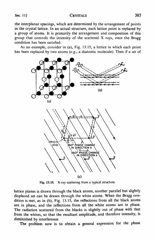
Sec. 11] CRYSTALS 385
the interplanar spacings, which are determined by the arrangement of pointsin the crystal lattice. In an actual structure, each lattice point is replaced bya group of atoms. It is primarily the arrangement and composition of this
group that controls the intensity of the scattered X rays, once the Braggcondition has been satisfied.
As an example, consider in (a), Fig. 13.15, a lattice in which each pointhas been replaced by two atoms (e.g., a diatomic molecule). Then if a set of
Fig. 13.15. X-ray scattering from a typical structure.
lattice planes is drawn through the black atoms, another parallel but slightly
displaced set can be drawn through the white atoms. When the Bragg con-
dition is met, as in (b), Fig. 13.15, the reflections from all the black atoms
are in phase, and the reflections from all the white atoms are in phase.
The radiation scattered from the blacks is slightly out of phase with that
from the whites, so that the resultant amplitude, and therefore intensity, is
diminished by interference.
The problem now is to obtain a general expression for the phase

386 CRYSTALS [Chap. 13
difference. An enlarged view of the structure (two-dimensional) is shown in
(c), Fig. 13.15, with the black atoms at the corners of a unit cell with sides
a and /?, and the whites at displaced positions. The coordinates of a black
atom may be taken as (0, 0) and those of a white as (x, y). A set of planes
(hk) is shown, for which it is assumed the Bragg condition is being fulfilled;
these are actually the (32) planes in the figure. Now the spacings a/h alonga and b/k along b correspond to positions from which scattering differs in
phase by exactly 360 or 2rr radians, i.e., scattering from these positions is
exactly in phase. The phase difference between these planes and those going
through the white atoms is proportional to the displacement of the white
atoms. The phase difference Px for displacement v in the a direction is given
by x/(a/h) --= PJ2ir, or Px 2irh(x/a). The total phase difference for dis-
placement in both a and b directions becomes
/>, -f Py- 2*
By extension to three dimensions, the total phase change that an atom at
(xyz) in the unit cell contributes to the plane (hkl) is
We may recall (page 327) that the superposition of waves of different
amplitude and phase can be accomplished by vectorial addition. If /j and
/2 are the amplitudes of the waves scattered by atoms (1) and (2), and Pl
and P2 are the phases, the resultant amplitude is F f\?lPl
4-/2^/J
". For
any number of atoms,^' (13-4)
When this is combined with eq. (13.3), there is obtained an expression for
the resultant amplitude of the waves scattered from the (hkl) planes by all
the atoms in a unit cell:
F(hkl) = ZJK <?****!*+w* * '*/')(13.5)
The expression F(hkl) is called the structure factor of the crystal. Its
value is determined by the exponential terms, which depend on the positions
of the atoms, and by the atomic scattering factorsfK ,which depend on the
number and distribution of the electrons in the atom, and on the scattering
angle 0.
The intensity of scattered radiation is proportional to the absolute value
of the amplitude squared, \F(hkl)\2
. The crystal structure problem nowbecomes that of obtaining agreement between the observed intensities and
those calculated from a postulated structure. Structure-factor expressionshave been tabulated for all the space groups.
8
8 International Tables for the Determination of Crystal Structures (1952). It is usually
possible to narrow the choice of space groups to two or three by means of study of missingreflections (hkl) and comparison with the tables.

Sec. 12] CRYSTALS 387
As an example of the use of the structure factor let us calculate F(hkl)
for the 100 planes in a face-centered cubic structure, eg., metallic gold. In
this structure there are four atoms in the unit cell (Z 4), which may be
assigned coordinates (xja, v/b, z/c) as follows: (000), (J i 0), (i J), and
(0 i i). Therefore, from eq."(13.5)
-- fAu(2 h 2^)
since e"1
cos TT + / sin TT --- 1
Thus the structure factor vanishes and there is therefore zero intensity of
scattering from the (100) set of planes. This is almost a trivial case, since
inspection of the face-centered cubic structure immediately reveals that there
is an equivalent set of planes interleaved midway between the 100 planes, so
that the resultant amplitude of the scattered X rays must be reduced to zero
by interference. In more complicated instances, however, it is essential to
use the structure factor to obtain a quantitative estimation of the scattering
intensity expected from any set of planes (hkl) in any postulated crystal
structure.
12. Fourier syntheses. An extremely useful way of looking at a crystal
structure was proposed by Sir William Bragg when he pointed out that it
may be regarded as a periodic three-dimensional distribution of electron
density, since it is the electrons that scatter the X rays. Any such density
function may be expressed as a Fourier series, a summation of sine and
cosine terms. 9It is more concisely written in the complex exponential form.
Thus the electron density in a crystal may be represented as
p(xyz)- \ \ A pQr
e **P*!* ^ '////ft i /r)( { 3 6)
p _ oo q uj r or
It is not hard to show10 that the Fourier coefficients A wr are equal to
the structure factors divided by the volume of the unit cell. Thus
p(xyz)1 SSX F(hkl)e"^^rla ^ vlb^ lf}
(13.7)
This equation expresses the fact that the only Fourier term that contributes
to the X-ray scattering by the set of planes (hkl) is the one with the coefficient
F(hkl), which appears intuitively to be the correct formulation.
Equation (13.7) summarizes the whole problem involved in structure
determinations, since in a very real sense the crystal structure is simply
p(xyz). Positions of individual atoms are peaks in the electron density
function/>,
and interatomic regions are valleys in the plot of p. Thus if we
knew the F(hkiy$ we could immediately plot the crystal structure. All we
know, however, are the intensities, which are proportional to \F(hkl)\2
. As
9See, for example, Widder, Advanced Calculus, p. 324.
10Bragg, op. cit., p. 221.

388 CRYSTALS [Chap. 13
stated earlier, we know the amplitudes but we have necessarily lost the
phases in taking the X-ray pattern.
A trial structure is now assumed and the intensities are calculated. If the
assumed arrangement is even approximately correct, the most intense
observed reflections should have large calculated intensities. The observed
F's for these reflections may be put into the Fourier series with the calculated
signs.11 The graph of the Fourier summation will give new positions for the
VAAX \ \ \
Fig. 13.16. Fourier map of electron density in glycylglycine projectedon base of unit cell: (a) 40 terms; (b) 100 terms; (c) 200 terms.
atoms, from which new f's can be calculated, which may allow more of the
signs to be determined. Gradually the structure is refined as more and moreterms are included in the synthesis. In Fig. 13.16 are shown three Fourier
summations for the structure of glycylglycine. As additional terms are in-
cluded in the summation, the resolution of the structure improves, just as
the resolution of a microscope increases with objectives that catch more andmore orders of diffracted light.
Sometimes a heavy atom can be introduced into the structure, whose
position is known from symmetry arguments. The large contribution of the
heavy atom makes it possible to determine the phases of many of the F's.
11 The complete Fourier series is rarely used; instead, various two-dimensional pro-jections are preferred.

Sec. 13] CRYSTALS 389
This was the method used with striking success by J. M. Robertson in his
work on the phthalocyanine structures,12 and in the determination of the
structure of penicillin. This last was one of the great triumphs of X-ray
crystallography, since it was achieved before the organic chemists knew the
structural formula.
13. Neutron diffraction. Not only X-ray and electron beams, but also
beams of heavier particles may exhibit diffraction patterns when scattered
from the regular array of atoms in a crystal. Neutron beams have proved to
be especially useful for such studies. The wavelength is related to the mass
and velocity by the Broglie equation, X -- hjmv. Thus a neutron with a
speed of 3.9 x 105 cm sec"1(kinetic energy 0.08 ev) would have a wave-
length of 1 .0 A. The diffraction of electron rays or X rays is caused by their
interaction with the orbital electrons of the atoms in the material throughwhich they pass; the atomic nuclei contribute practically nothing to the
scattering. The diffraction of neutrons, on the other hand, is primarilycaused by two other effects: (a) nuclear scattering due to interaction of the
neutrons with the atomic nuclei, (b) magnetic scattering due to interaction of
the magnetic moments of the neutrons with permanent magnetic moments
of atoms or ions.
In the absence of an external magnetic field, the magnetic moments of
atoms in a paramagnetic crystal are arranged at random, so that the magnetic
scattering of neutrons by such a crystal is also random. It contributes onlya diffuse background to the sharp maxima occurring when the Bragg con-
dition is satisfied for the nuclear
scattering. In ferromagnetic materials,
however, the magnetic moments are
regularly aligned so that the resultant
spins of adjacent atoms are parallel,
even in the absence of an external
field. In antiferromagnetic materials,
the magnetic moments are also regu-
larly aligned, but in such a way that
adjacent spins are always opposed.The neutron diffraction patterns dis-
tinguish experimentally between these
different magnetic structures, and indi-
cate the direction of alignment of spins
within the crystal.
For example, manganous oxide,
MnO, has the rock-salt structure (Fig. 13.12), and is antiferromagnetic. The
detailed magnetic structure as revealed by neutron diffraction is shown in
Fig. 13.17. The manganous ion, Mn+2, has the electronic structure 3s23p
B3d*.
12J. Chem. Soc. (London), 1940, 36. For an account of the work on penicillin, see
Research, 2, 202 (1949).
CHEMICALUNITCELL
Fig. 13.17. Magnetic structure of MnOas found by neutron diffraction. Note
that the "magnetic unit cell" has twice the
length of the "chemical unit cell." [FromC. G. Shull, E. O. Wollan, and W. A.
Strauser, Phys. Rev., 81, 483 (1951).]

390 CRYSTALS [Chap. 13
The five 3c/ electrons are all unpaired, and the resultant magnetic moment
is 2V%(jf I 1)= 5.91 Bohr magnetons. If we consider Mn+2 ions in
successive (111) planes in the crystal, the resultant spins are oriented so
that they are alternately positively and negatively directed along the [100]
direction.
Another useful application of neutron diffraction has been the location
of hydrogen atoms in crystal structures. It is usually impossible to locate
hydrogen atoms by means of X-ray or electron diffraction, because the small
scattering power of the hydrogen is completely overshadowed by that of
heavier atoms. The hydrogen nucleus, however, is a strong scatterer of
neutrons. Thus it has been possible to work out the structures of such com-
pounds as UH3 and KHF2 neutron-diffraction analysis.13
14. Closest packing of spheres. Quite a while before the first X-ray struc-
ture analyses, some shrewd theories about the arrangement of atoms and
(a) (b)
/ /
(c;
(c) (d)
Fig. 13.18. (a) Hexagonal closest packing; (b) cubic closest packing (edge cut
away to show closest packing normal to cube diagonals); (c) plan of hexagonalclosest packing; (d) plan of cubic closest packing.
molecules in crystals were developed from purely geometrical considerations.
From 1883 to 1897, W. Barlow proposed a number of structures based onthe packing of spheres.
There are two different ways in which spheres of the same size can be
packed together so as to leave a minimum of unoccupied volume, in each
case 26 per cent voids. They are the hexagonal-closest-packed (hep) and the
13S. W. Peterson and H. A. Levy, /. Chem. Phys., 20, 704 (1952).

Sec. 14] CRYSTALS 391
cubic-closest-packed (ccp) arrangements depicted in Fig. 13.18. In ccp the
layers repeat as ABC ABC ABC . . ., and in hep the order is AB AB AB... It will be noted that the ccp structure may be referred to a face-centered-
cubic unit cell, the (ill) planes being the layers of closest packing.The ccp structure is found in the solid state of the inert gases, in crystal-
line methane, etc. symmetrical atoms or molecules held together by van
der Waals forces. The high-temperature forms of solid H2 ,N 2 , and O2 occur
in hep structures.
The great majority of the typical metals crystallize in the ccp, the hep,or a body-centered-cubic structure. Some examples are collected in Table
13.3. Other structures include the following:14 the diamond-type cubic of
TABLE 13.3
STRUCTURES OF THE METALS
grey tin and germanium; the face-centered tetragonal, a distorted fee, of
y-manganese and indium; the rhombohedral layered structures of bismuth,
arsenic, and antimony; and the body-centered tetragonal of white tin. It
will be noted that many of the metals are polymorphic (allotropic), with two
or more structures depending on conditions of temperature and pressure.
The nature of the binding in metal crystals will be discussed later. For
the present, we may think of them as a network of positive metal ions
packed primarily according to geometrical requirements, and permeated bymobile electrons. This so-called electron gas is responsible for the high
conductivity and for the cohesion of the metal.
The ccp metals, such as Cu, Ag, Au, Ni, are all very ductile and malle-
able. The other metals, such as V, Cr, Mo, W, are harder and more brittle.
This distinction in physical properties reflects a difference between the struc-
ture types. When a metal is hammered, rolled, or drawn, it deforms by the
gliding of planes of atoms past one another. These slip planes are those that
contain the most densely packed layers of atoms. In the ccp structure, the
slip planes are therefore usually the (111), which occur in sheets normal to
14 For descriptions see R. W. G. Wyckoff, Crystal Structures (New York: Interscience,
1948).

392 CRYSTALS [Chap. 13
all four of the cube diagonals. In the hep and other structures there is onlyone set of slip planes, e.g., those perpendicular to the hexagonal axis. Thus
the ccp metals are characteristically more ductile than the others, since theyhave many more glide ways.
15. Binding in crystals. The geometrical factors, seen in their simplest
form in the closest packed structures of identical spheres, are always very
important in determining the crystal structure of a substance. Once theyare satisfied, other types of interaction must also be considered. Thus,
for example, when directed binding appears, closest packing cannot be
achieved.
Two different theoretical approaches to the nature of the chemical bond
in molecules have been described in Chapter 11. In the method of atomic
orbitals, the point of departure is the individual atom. Atoms are brought
together, each with the electrons that "belong to it," and one considers the
effect of an electron in one atomic orbital upon that in another. In the second
approach, the electrons in a molecule are no longer assigned possessively to
the individual atoms. A set of nuclei is arranged at the proper final distances
and the electrons are gradually fed into the available molecular orbitals.
For studying the nature of binding in crystals, these two different treat-
ments are again available. In one case, the crystal structure is pictured as an
array of regularly spaced atoms, each possessing electrons used to form
bonds with neighboring atoms. These bonds may be ionic, covalent, or
intermediate in type. Extending throughout three dimensions, they hold the
crystal together. The alternative approach is once again to consider the nuclei
at fixed positions in space and then gradually to pour the electron cement
into the periodic array of nuclear bricks.
Both these methods yield useful and distinctive results, displaying com-
plementary aspects of the nature of the crystalline state. We shall call the
first treatment, growing out of the atomic-orbital theory, the bond model of
the solid state. The second treatment, an extension of the method of mole-
cular orbitals, we shall call, for reasons to appear later, the band model of
the solid state.
16. The bond model. If we consider that a solid is held together bychemical bonds, it is useful to classify the bond types. Even though the
available classifications are as usual somewhat frayed at the edges, the
following categories may be distinguished:
(1) The van der Waals bonds. These bonds are the result of forces between
inert atoms or essentially saturated molecules. These forces are the same as
those responsible for the a term in the van der Waals equation. Crystals held
together in this way are sometimes called molecular crystals. Examplesare nitrogen, carbon tetrachloride, benzene. The molecules tend to pack
together as closely as their geometry allows. The binding between the mole-
cules in van der Waals structures represents a combination of factors such
as dipole-dipole and dipole-polarization interactions, and the quantum

Sec. 16] CRYSTALS 393
mechanical dispersion forces, first elucidated by F. London, which are often
the principal component.15
(2) The ionic bonds. These bonds are familiar from the case of the NaClmolecule in the vapor state (page 297). In a crystal, the coulombic interaction
between oppositely charged ions leads to a regular three-dimensional struc-
ture. In rock salt, each positively charged Na f ion is surrounded by six
negatively charged Cl ions, and each Cl is surrounded by six Na j
. There
are no sodium-chloride molecules unless one wishes to regard the. entire
crystal as a giant molecule.
The ionic bond is spherically symmetrical and undirected; an ion will be
surrounded by as many oppositely charged ions as can be accommodated
ID
(o) (b)
Fig. 13.19. (a) Diamond structure; (b) graphite structure.
geometrically, provided that the requirement of over-all electrical neutrality
is satisfied.
(3) The covalent bonds. These bonds, we recall, are the result of spin
valence (page 303), the sharing between atoms of two electrons with anti-
parallel spins. When extended through three dimensions, they may lead to
a variety of crystal structures, depending on the valence of the constituent
atoms, or the number of electrons available for bond formation.
A good example is the diamond structure in (a), Fig. 13.19. The structure
can be based on two interpenetrating face-centered cubic lattices. Each point
in one lattice is surrounded tetrahedrally by four equidistant points in the
other lattice. This arrangement constitutes a three-dimensional polymer of
carbon atoms joined together by tetrahedrally oriented sp3 bonds. Thus the
configuration of the carbon bonds in diamond is similar to that in the
aliphatic compounds such as ethane. The C C bond distance is 1.54 A in
both diamond and ethane. Germanium, silicon, and grey tin also crystallize
in the diamond structure.
The same structure is assumed by compounds such as ZnS (zinc blende),
Agl, A1P, and SiC. In all these structures, each atom is surrounded by four
unlike atoms oriented at the corners of a regular tetrahedron. In every case
the binding is primarily covalent. It is interesting to note that it is not neces-
sary that each atom provide the same number of valence electrons; the
15 See Chapter 14, Sect. 10.

394 CRYSTALS [Chap. 13
Fig. 13.20. Structure of
selenium
structure can occur whenever the total number of outer-shell electrons is just
four times the total number of atoms.
There is also a form of carbon, actually the more stable allotrope, in
which the carbon bonds resemble those in the aromatic series of compounds.This is graphite, whose structure is shown in
(b), Fig. 13.19. Strong bonds operate within
each layer of carbon atoms, whereas muchweaker binding joins the layers; hence the
slippery and flaky nature of graphite. The
C C distance within the layers of graphiteis 1.34 A, identical with that in anthracene.
Just as in the discussion of the nature
of binding in aromatic hydrocarbons (page
311), we can distinguish two types of electrons within the graphite struc-
ture. The a electrons are paired to form localized-pair (sp2) bonds, and
the 77 electrons are free to move throughout the planes of the C6 rings.
Atoms with a spin valence of only 2 cannot form regular three-dimen-
sional structures. Thus we have the interesting structures of selenium (Fig.
13.20), and tellurium, which consist
of endless chains of atoms extending
through the crystal, the individual
chains being held together by much
weaker forces. Another way of solving
the problem is illustrated by the struc-
ture of rhombic sulfur, Fig. 13.21.
Here there are well defined, puckered,
eight-membered rings of sulfur atoms.
The bivalence of sulfur is maintained
and the S8 "molecules" are held
together by van der Waals attractions.
Elements like arsenic and antimonythat in their compounds display a
covalence of 3 tend to crystallize in
structures that contain well defined
layers of atoms.
(4) 77?^ intermediate-type bonds.
Just as in individual molecules, these
bonds arise from resonance between
covalent and ionic contributions.
Alternatively, one may consider the
polarization of one ion by an oppositely charged ion. An ion is said to be
polarized when its electron "cloud" is distorted by the presence of the
oppositely charged ion. The larger an ion the more readily is it polarized,and the smaller an ion the rhore intense is its electric field and the greater
Fig. 13.21. Structure of rhombic
sulfur.

Sec. 17] CRYSTALS 395
Hg. 13.22, Structure of ice.
its polarizing power. Thus in general the larger anions are polarized by the
smaller cations. Even apart from the size effect, cations are less polarizable
than anions because their net positive charge tends to hold their electrons
in place. The structure of the ion is also important: rare-gas cations such
as K+ have less polarizing power than transition cations such as Ag+,since their positive nuclei are more effectively shielded.
The effect of polarization may be seen in the structures of the silver
halides. AgF, AgCl, and AgBr have the-rock-salt structure, but as the anion
becomes larger it becomes more strongly polarized by the small Ag+ ion.
Finally, in Agl the binding has very little ionic character and the crystal has
the zinc-blende structure. It has been
confirmed spectroscopically that crystal-
line silver iodide is composed of atoms
and not ions.
(5) The hydrogen bond. The hydrogen
bond, discussed on page 313, plays an
important role in many crystal struc-
tures, e.g., inorganic and organic acids,
salt hydrates, ice. The structure of ice is
shown in Fig. 13.22. The coordination
is similar to that in wurtzite, the hexago-nal form of zinc sulfide. Each oxygen is
surrounded tetrahedrally by four nearest neighbors at a distance of 2.76 A.
The hydrogen bonds hold the oxygens together, leading to a very openstructure. By way of contrast, hydrogen sulfide, H 2S, has a ccp structure,
each molecule having twelve nearest neighbors.
(6) 77?? metallic bond. The bond model has also been extended to metals.
According to this picture, the metallic bond is closely related to the ordinarycovalent electron-pair bond. Each atom in a metal forms covalent bonds by
sharing electrons with its nearest neighbors. It is found that there are more
orbitals available for bond formation than there are electrons to fill them.
As a result the covalent bonds resonate among the available interatomic
positions. In the case of a crystal this resonance extends throughout the
entire structure, thereby producing great stability. The empty orbitals permit
a ready flow of electrons under the influence of an applied electric field,
leading to metallic conductivity.
Structures such as those of selenium and tellurium, and of arsenic and
antimony, represent transitional forms in which the electrons are much
more localized because the available orbitals are more completely filled.
In a covalent crystal like diamond the four.s/;
3 tetrahedral orbitals are
completely filled.
17. The band model. It was in an attempt to devise an adequate theory
for metals that the band model had its origin. The high thermal and electrical
conductivities of metals focused attention on the electrons as the important
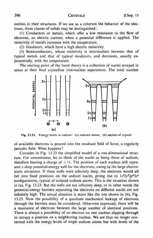
396 CRYSTALS [Chap. 13
entities in their structures. If we use as a criterion the behavior of the elec-
trons, three classes of solids may be distinguished:
(1) Conductors or metals, which offer a low resistance to the flow of
electrons, an electric current, when a potential difference is applied. The
resistivity of metals increases with the temperature.
(2) Insulators, which have a high electric resistivity.
(3) Semiconductors, whose resistivity is intermediate between that of
typical metals and that of typical insulators, and decreases, usually ex-
ponentially, with the temperature.The starting point of the band theory is a collection of nuclei arrayed in
space at their final crystalline internuclear separations. The total number
3s
2p
2
I
-a -
(a)
(b)
Fig. 13.23. Energy levels in sodium: (a) isolated atoms; (b) section of crystal.
of available electrons is poured into the resultant field of force, a regularly
periodic field. What happens?Consider in Fig. 13.23 the simplified model of a one-dimensional struc-
ture. For concreteness, let us think of the nuclei as being those of sodium,
therefore bearing a charge of + 1 1 . The position of each nucleus will repre-
sent a deep potential-energy well for the electrons, owing tp the large electro-
static attraction. If these wells were infinitely deep, the electrons would all
fall into fixed positions on the sodium nuclei, giving rise to l^Zs^/^S-s1
configurations, typical of isolated sodium atoms. This is the situation shown
in (a), Fig. 13.23. But the wells are not infinitely deep, or in other words the
potential-energy barriers separating the electrons on different nuclei are not
infinitely high. The actual situation is more like the one shown in (b), Fig.
13.23. Now the possibility of a quantum mechanical leakage of electrons
through the barriers must be considered. Otherwise expressed, there will be
a resonance of electrons between the large number of identical positions.
There is always a possibility of an electron on one nucleus slipping throughto occupy a position on a neighboring nucleus. We are thus no longer con-
cerned with the energy levels of single sodium atoms but with levels of the

Sec. 17] CRYSTALS 397
crystal as a whole. Then the Pauli Principle comes into play, and tells us
that no more than two electrons can occupy exactly the same energy level.
Once the possibility of electrons moving through the structure is admitted,we can no longer consider the energy levels to be sharply defined. The sharpIs energy level in an individual sodium atom is broadened in crystalline
sodium into a band of closely packed energy levels. A similar situation arists
for the other energy levels, each becoming a band of levels as shown in (b),
Fig. 13.23.
Each atomic orbital contributes one level to a band. In the lower bands
(Is, 2s, 2p) there are therefore just enough levels to accommodate the number
of available electrons, so that the bands are completely filled. If an external
electric field is applied, the electrons in the filled bands cannot move under
its influence, for to be accelerated by the field they would have to move into
somewhat higher energy levels. This is impossible for electrons in the interior
of a filled band, since all the levels above them are already occupied, and the
Pauli Principle forbids their accepting additional tenants. Nor can the elec-
trons at the very top of a filled band acquire extra energy, since there are no
higher levels for them to move into. Very occasionally, it is true, an electron
may acquire a relatively terrific jolt of energy and be knocked completelyout of its band into a higher unoccupied band.
So much for the electrons in the lower bands. The situation is verydifferent in the uppermost band, the 3s, which is only half filled. An electron
in the interior of the 3s band still cannot be accelerated because the levels
directly above are already filled. Electrons toward the top of the band, how-
ever, can readily move up into unfilled levels within the band. This is what
happens when an electric field is applied and a current flows. It will be
noticed from the diagram that the topmost band has actually broadened
sufficiently to overlap the tops of the potential-energy barriers, so that these
electrons can move quite freely through the crystal structure.
According to this idealized model in which the nuclei are always arrangedat the points of a perfectly periodic lattice, there would indeed be no resist-
ance at all offered to the flow of an electric current. The resistance arises from
deviations from perfect periodicity. An important loss of periodicity is caused
by the thermal vibrations of the lattice nuclei. These vibrations destroy the
perfect resonance between the electronic energy levels and cause a resistance
to the free flow of electrons. As would be expected, the resistance therefore
increases with the temperature. Another illustration of the same principle is
found in the increased resistance that results when an alloying constituent is
added to a pure metal, and the regular periodicity of the structure is dimin-
ished by the foreign atoms.
At this point the reader may well be thinking that this is a pretty picture
for a univalent metal such as sodium, but what of magnesium with its two
3s electrons and therefore completely filled 3s bands ? Why isn't it an insulator
instead of a metal? The answer is that in this, and similar cases, detailed

398 CRYSTALS [Chap. 13
calculations show that the 3p band is low enough to overlap the top of the
35 band, providing a large number of available empty levels.
Thus conductors are characterized either by partially filled bands or by
overlapping of the topmost bands. Insulators have completely filled lower
bands with a wide energy gap between the topmost filled band and
the lowest empty band. These models are represented schematically in
Fig. 13.24.
The energy bands in solids can be studied experimentally by the methods
of X-ray emission spectroscopy.16 For example, if an electron is driven out of
the \s level in sodium metal (Fig. 13.23b) the Ka X-ray emission occurs when
an electron from the 3^ band falls into the hole in the Is level. Since the 3s
FILLED IMPURITYLEVELS
EMPTY IMPURITYLEVELS
(a)
Fig. 13.24. Band models of solid types: (a) insulator; (b) metal;
(c) semiconductor.
electron can come from anywhere within the band of energy levels, the X rays
emitted will have a spread of energies (and hence frequencies) exactly corre-
sponding with the spread of allowed energies in the 3s band. The following
widths (in ev) were found for the conduction bands in a few of the solids
investigated :
Li Na Be Mg Al
4.1 3.4 14.8 7.6 13.2
18. Semiconductors. Band models for semiconductors are also included
in Fig. 13.24. These models possess, in addition to the normal bands, narrow
impurity bands, either unfilled levels closely above a filled band or filled levels
closely below an empty band. The extra levels are the result of either foreign
atoms dissolved in the structure or a departure from the ideal stoichiometric
composition. Thus zinc oxide normally contains an excess of zinc, whereas
cuprous oxide normally contains an excess of oxygen. Both these compoundsbehave as typical semiconductors. Their conductivities increase approxi-
mately exponentially with the temperature, because the number of conduc-
tion electrons depends on excitation of electrons into or out of the impurity
levels, and excitation is governed by an e~*E/HT Boltzmann factor.
16 A review by N. F. Mott gives further references. Prog. Metal Phys. 3, 76-1 14 (1952),"Recent Advances in the Electron Theory of Metals."

Sec. 19] CRYSTALS 399
If the energy gap between the filled valence band and the empty con-
duction band is narrow enough, a crystal may be a semiconductor even
in the absence of effects due to impurities. Germanium with an energy gapof 0.72 ev and grey tin with O.lOev are examples of such intrinsic semi-
conductors.
19. Brillouin zones. The band theory of the crystalline state leads to a
system of allowed energy levels separated by regions of forbidden energy.
In other words, electron waves having a forbidden energy cannot pass throughthe crystal. Those familiar with radio circuits would say that the periodic
crystal structure acts as a band-pass filter for electron waves.
In this simple picture we have not considered the variety of periodic
patterns that may be encountered by an electron wave, depending on the
direction of its path through the crystal. When this is done, it is found that
special geometrical requirements are imposed on the band structure, so that
it is not necessarily the same for all directions in space. Now we can see
qualitatively an important principle. If an electron wave with an energy in
a forbidden region were to strike a crystal, it could not be transmitted, but
would instead be strongly scattered or "reflected" in the Bragg sense. The
Bragg relation therefore defines the geometric structure of the allowed
energy bands. This principle was first enunciated by Leon Brillouin, and the
energy bands constructed in this way are called the Brillouin zones of
the crystal.
The quantitative application of the zone theory is still in its early stages.
Qualitatively it is clear that the properties of crystals are determined by the
nature of the zones and the extent to which they are filled with electrons.
This interpretation is especially useful in elucidating the structures of metal
alloys.
20. Alloy systems electron compounds. If two pure metals crystallize in
the same structure, have the same valence and atoms of about the same size,
they may form a continuous series of solid solutions without undergoing
any changes in structure. Examples are the systems Cu-Au and Ag-Au.When these conditions are not fulfilled, a more complicated phase diagram
will result. An example is that for the brass system, copper and zinc. Pure
copper crystallizes in a face-centered-cubic structure and dissolves up to about
38 per cent zinc in this a phase. Then the body-centered-cubic ft phase super-
venes. At about 58 per cent zinc, a complex cubic structure begins to form,
called "y brass," which is hard and brittle. At about 67 per cent Zn, the hexa-
gonal closest packed e phase arises, and finally there is obtained ther\ phase
having the structure of pure zinc, a distorted hep arrangement.It is most interesting that a sequence of structure changes very similar to
these is observed in a wide variety of alloy systems. Although the com-
positions of the phases may differ greatly, the /?, y, and e structures are quite
typical. W. Hume-Rothery was the first to show that this regular behavior
was related to a constant ratio of valence electrons to atoms for each phase.

400 CRYSTALS [Chap. 13
Examples of these ratios are shown in Table 13.4. The transition metals Fe,
Co, Ni follow the rule if the number of their valence electrons is taken as
zero.17 In all these cases, the zone structure determines the crystal structure,
and the composition corresponding to each structure is fixed by the number
of electrons required to fill the zone. Such alloys are therefore sometimes
called electron compounds.
TABLE 13.4
ELECTRON COMPOUNDS ILLUSTRATING HUME-ROTHERY RULE
Alloy*
ft Phases (Ratio 3/2
3:23:23:23:26:49:63:33:2
y Phases (Ratio 21/13)
Cu6Zn8
Fe5Zn21
Cu9Ga4
Cu9Al4Cu31Sn8
e Phases (Ratio 7/4)
The body-centered /? brass structure illustrates another interesting
property of some alloy systems, the order-disorder transition. At low
temperatures, the structure is ordered; the copper atoms occupy only the
17Pauling has pointed out that it seems to be unreasonable to say that iron, which is
famous for its great strength, contributes nothing to the bonding in iron alloys. From
magnetic moments and other data he concludes that iron actually contributes between5 and 6 bonding electrons per atom [/. Am. Chem. Soc., 69, 542 (1947)].
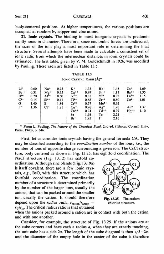
Sec. 21] CRYSTALS 401
body-centered positions. At higher temperatures, the various positions are
occupied at random by copper and zinc atoms.
21. Ionic crystals. The binding in most inorganic crystals is predomi-
nantly ionic in character. Therefore, since coulombic forces are undirected,
the sizes of the ions play a most important role in determining the final
structure. Several attempts have been made to calculate a consistent set of
ionic radii, from which the internuclear distances in ionic crystals could be
estimated. The first table, given by V. M. Goldschmidt in 1926, was modified
by Pauling. These radii are listed in Table 13.5.
TABLE 13.5
IONIC CRYSTAL RADII (A)*
o
0.60
0.31
0.20
0.15
1.40
1.36
Me
* From L. Pauling, The Nature of the Chemical Bond, 2nd ed. (Ithaca: Cornell Univ.
Press, 1940), p. 346.
First, let us consider ionic crystals having the general formula CA. They
may be classified according to the coordination number of the ions; i.e., the
number of ions of opposite charge surrounding a given ion. The CsCl struc-
ture, body centered as shown in Fig. 13.25, has eightfold coordination. The
NaCi structure (Fig. 13.12) has sixfold co-
ordination. Although zinc blende (Fig. 13.19a)
is itself covalent, there are a few ionic crys-
tals, e.g., BeO, with this structure which has
fourfold coordination. The coordination
number of a structure is determined primarily
by the number of the larger ions, usually the
anions, that can be packed around the smaller
ion, usually the cation. It should therefore
depend upon the radius ratio, /*Cation/ranion
rc/rA . The critical radius ratio is that obtained
when the anions packed around a cation are in contact with both the cation
and with one another.
Consider, for example, the structure of Fig. 13.25. If the anions are at
the cube corners and have each a radius a, when they are exactly touching,
the unit cube has a side 2a. The length of the cube diagonal is then \/3 2a,
and the diameter of the empty hole in the center of the cube is therefore
Fig. 13.25. The cesium
chloride structure.

402 CRYSTALS [Chap. 13
V/3 2a 2a --= 2a(\/3 1). The radius of the cation exactly filling this
hole is thus a(\/3 1), and the critical radius ratio becomes rc/rA =a(\/3 ])/a ----- 0.732. By this simple theory, whenever the ratio falls below
0.732, the structure can no longer have eightfold coordination, and indeed
should go over to the sixfold coordination of NaCl.
In the sixfold coordination, a given ion at the center of a regular octa-
hedron is surrounded by six neighbors at the corners. The critical radius
ratio for this structure may readily be shown to be \/2-
1 0.414. The
next lower coordination would be threefold, at the corners of an equilateral
triangle, with a critical ratio of 0.225.
The structures and ionic-radius ratios of a number of CA compoundsare summarized in Table 13.6. The radius-ratio rule, while not infallible,
provides the principal key to the occurrence of the different structure types.
TABLE 13.6
STRUCTURES AND RADIUS RATIOS OF CA IONIC CRYSTALS
CesiumChloride
Structure -
Sodium Chloride Structure
Zinc Blende
or Wurtzite
Structure
Theoretical Range
CsClCsBrCsl
The structures of CA2 ionic crystals are found to be governed by the
same coordination principles. Four common structures are shown in Fig.
13.26. In fluorite each Ca++ is surrounded by eight F~ ions at the corners of
a cube, and each F~ is surrounded by four Ca+4~
at the corners of a tetra-
hedron. This is an example of 8 : 4 coordination. The structure of rutile
illustrates a 6 : 3 coordination, and that of cristobalite a 4 : 2 type. Once
again the coordination is determined primarily by the radius ratio.
The cadmium-iodide structure illustrates the result of a departure from
typically ionic binding. The iodide ion is easily polarized, and one can
distinguish definite CdI2 groups forming a layerlike arrangement.

Sec. 22] CRYSTALS 403
(d)
Fig. 13.26. CA 2 structures: (a) fluonte; (b) rutile; (c) ft cnstobalite;
(d) cadmium iodide.
22. Coordination polyhedra and Pauling's Rule. Many inorganic crystals
contain oxygen ions; their size is often so much larger than that of the cations
that the structure is largely determined by the way in which they pack to-
gether. The oxygens are arranged in coordination polyhedra around the
cations, some common examples being the following:
Around B: 3 O\s at corners of equilateral triangle
Si, Al, Be, B, Zn : 4 O's at corners of tetrahedron
Al, Ti, Li, Cr: 6 O's at corners of octahedron
For complex structures, Pauling has given a general rule that determines
how these polyhedra can pack together. Divide the valence of the positive
ion by the number of surrounding negative ions; this gives the fraction of
the valence of a negative ion satisfied by this positive ion. For each negative
ion, the sum of the contributions from neighboring positive ions should
equal its valence. This rule simply expresses the requirement that electro-
static lines of force, starting from a positive ion, must end on a negative ion
in the immediate vicinity, and not be forced to wander throughout the
structure seeking a distant terminus.
As an example of the application of the rule, consider the silicate group,
(SiO4). The valence of the positive ion, Si+4 , is +4. Therefore each O ion
has one valence satisfied by the Si+4 ion, i.e., one-half of its total valence of
two. It is therefore possible to join each corner of a silicate tetrahedron to
another silicate tetrahedron. It is also possible for the silicates to share edgesand faces, although these arrangements are less favorable energetically, since
they bring the central Si+4 ions too close together.
In the (A1O6) octahedron, only a valence of \ for each O is satisfied
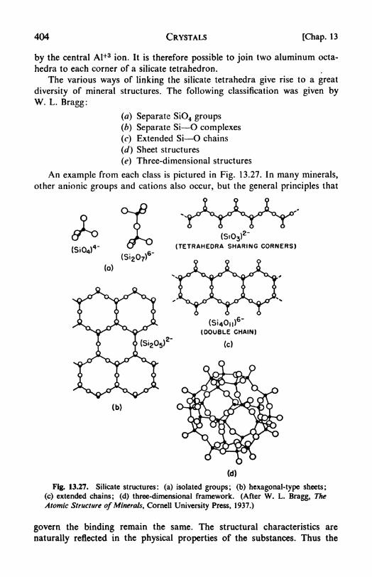
404 CRYSTALS [Chap. 13
by the central Al+3 ion. It is therefore possible to join two aluminum octa-
hedra to each corner of a silicate tetrahedron.
The various ways of linking the silicate tetrahedra give rise to a great
diversity of mineral structures. The following classification was given byW. L. Bragg:
(a) Separate SiO4 groups
(b) Separate Si O complexes
(c) Extended Si O chains
(d) Sheet structures
(e) Three-dimensional structures
An example from each class is pictured in Fig. 13.27. In many minerals,
other anionic groups and cations also occur, but the general principles that
(S.04)4 "
(S.03)<
(TETRAHEDRA SHARING CORNERS)
(Si 2o7r(0)
(Si2 5)
z
(Si40,,)6"
(DOUBLE CHAIN)
(C)
Fig. 13.27. Silicate structures: (a) isolated groups; (b) hexagonal-type sheets;
(c) extended chains; (d) three-dimensional framework. (After W. L. Bragg, The
Atomic Structure of Minerals, Cornell University Press, 1937.)
govern the binding remain the same. The structural characteristics are
naturally reflected in the physical properties of the substances. Thus the

Sec. 23] CRYSTALS 405
chainlike architecture is found in the asbestos minerals, the sheet arrange-ment in micas and talcs, and the feldspars and zeolites are typical three-
dimensional polymers.23. Crystal energy the Born-Haber cycle. The binding energy in a purely
ionic crystal can be calculated via ordinary electrostatic theory. The potential
energy of interaction of two oppositely charged ions may be written
-z&e2 be2U=-Y~ +
7n(13.8)
where r is the internuclear separation and ze the ionic charge.In calculating the electrostatic energy of a crystal, we must take into
account not only the attraction between an ion and the oppositely chargedions coordinated around it, but also the repulsions between ions of like signat somewhat larger separations, then attractions between the unlike ions
once removed, and so on. Therefore, for each ion the electrostatic interaction
will be a sum of terms, alternately attractive and repulsive, and diminishingin magnitude owing to the inverse-square law. For any given structure this
summation amounts to little more than relating all the different internuclear
distances to the smallest distance r. Thus, corresponding with eq. (13.8) for
an ionic molecule, there is obtained for the potential energy of an ionic
crystal per mole
u, -<"?" + (,>
The constant A, which depends on the type of crystal structure, is called the
Madelung constant. 1* If e is in esu and if is in kcal per mole, one has the
following typical A values: NaCl structure, A ----- 1.74756; CsCl, 1.76267;
rutile, 4.816.
At the equilibrium internuclear distance r, the energy is a minimum, so
that (dU/dr)ft0. Hence for the case zl
----- z2 ,
ANe2z2 nBe2
ANz*t
I AM(13.10)
n
The value of the exponent n in the repulsive term can be estimated from
the compressibility of the crystal, since work is done against the repulsive
forces in compressing the crystal. Typical values of n range from 6 to 12,
indicative of the rapid rise in repulsion as the internuclear separation is
narrowed.
18J. Sherman, Chem. Rev., 77, 93 (1932).

406 CRYSTALS [Chap. 13
The so-called crystal energy is obtained from eqs. (13.9) and (13.10) as
This is the heat of reaction of gaseous ions to yield the solid crystal. For
example, for rock salt:
Na-(g)-| Cl-(g)- NaCl(c) f c
Calculated values of Ec can be compared with other thermochemical
quantities by means of the Born-Haber cycle. For the typical case of NaCl,this has the form:
NaCl (c)------
E-c- -> Na *(g) + Cl" (g)
.
Na (c) + C1 2 (g)- -- - -> Na (g) 4 Cl (g)
The energetic quantities entering into the cycle are defined as follows, all
per mole:
EC the crystal energy
Q the standard heat of formation of crystalline NaCl
S = heat of sublimation of metallic Na
/ the ionization potential of Na
A - the electron affinity of Cl
D = the heat of dissociation of C1 2 (g) into atoms
For the cyclic process, by the First Law of Thermodynamics:
c- S f / f iD -A - Q (13.12)
All the quantities on the right side of this equation can be evaluated, at
least for alkali-halide crystals, and the value obtained for the crystal energycan be compared with that calculated from eq. (13.11). The ionization
potentials / are obtained from atomic spectra, and the dissociation energies
D can be accurately determined from molecular spectra. Most difficult to
measure are the electron affinities A. 19
A summary of the figures obtained for various crystals is given in Table
13.7. When the calculated crystal energy deviates widely from that obtained
through the Born-Haber cycle, one may suspect nonionic contributions to
the crystal binding.
24. Statistical thermodynamics of crystals: the Einstein model. If one
could obtain an accurate partition function for a crystal, it would then be
possible to calculate immediately all its thermodynamic properties by makinguse of the general formulas of Chapter 12.
For one mole of a crystalline substance, containing N atoms, there are
19See, for example, P. P. Sutton and J. E. Mayer, J. Chem. Phys., 2, 146 (1934); 3, 20
(1935).

Sec. 24] CRYSTALS 407
TABLE 13.7
THE BORN-HABER CYCLE
(Energy Terms in Kilocalories per Mole)
*Calculated, Eq. (13.11).
3W degrees of freedom. Except when there is rotation of the atoms within
the solid, we can consider that there are 3jV vibrational degrees of freedom,
since 3W 6 is to all intents and purposes still 3N. The precise determina-
tion of 3N normal modes of vibration for such a system would be an im-
possible task, and it is fortunate that some quite simple approximations give
sufficiently good answers.
First of all, let us suppose that the 3N vibrations arise from independent
oscillators, and then that these are harmonic oscillators, which is a good
enough approximation at low temperatures, when the amplitudes are small.
The model proposed by Einstein in 1906 assigned the same frequency v to
all the oscillators.
The crystalline partition function according to the Einstein model is,
from eqs. ( 12.35) and (12.23),
(13.14)
(13.15)
(13.16)
(13.17)
z = *
It follows immediately that,
E - E - 3Nhv(ehv/kT ~
I)"1
S=3m[f*lkT--~\n(l e
Cy ^=
3yVA:rin(l
/2V hv
Particularly interesting is the predicted temperature variation of Cv . Werecall that Dulong and Petit, in 1819, noted that the molar heat capacities
of the solid elements, especially the metals, were usually around 3R = 6
calories per degree. Later measurements showed that this figure was merely

408 CRYSTALS [Chap. 13
a high-temperature limiting value, approached by different elements at
different temperatures.If we expand the expression in eq. (13.17) and simplify somewhat,
20 weobtain
______ (13 ig\^ ' }
When r is large, this expression reduces to Cv 37*. For smaller T's, a
curve like the dotted line in Fig. 13.28 is obtained, the heat capacity beinga universal function of (v/T). The frequency v can be determined from one
experimental point at low temperatures and then the entire heat-capacity
curve can be drawn for the substance. The agreement with the experimentaldata is good except at the lowest temperatures. It is clear that the higherthe fundamental vibration frequency v, the larger is the quantum of vibra-
tional energy, and the higher the temperature at which Cv attains the
classical value of 3R. For example, the frequency for diamond is 2.78 x10¹³ sec-1
, but for lead it is only 0.19 x 10¹³ sec"1, so that Cv for diamond
is only about 1.3 at room temperature, but Cv for lead is 6.0. The elements
that follow Dulong and Petit's rule are those with relatively low vibration
frequencies.
25. The Debye model. If, instead of a single fundamental frequency, a
spectrum of vibration frequencies is taken for the crystal, the statistical
problem becomes somewhat more complicated. One possibility is to assume
that the frequencies are distributed according to the same law as that givenon page 261 for the distribution of frequencies in black-body radiation.
This problem was solved by P. Debye.Instead of using eq. (13.14), the energy must be obtained by averaging
over all the possible vibration frequencies vtof the solid, from to VM the
maximum frequency. This gives
M hv~ ~~~'
3N o ***- 1
=i?o 7^-\ (13- 19)
Since the frequencies form a virtual continuum the summation is replaced
by an integration, by using the distribution function for the frequenciesfound in eq. (10.14) (multiplied by $ since we have one longitudinal and two
transverse vibrations, instead of the two transverse of radiation). Thus
dn ^f(v)dv = 1277- ^ r2 dv (13.20)c^
where c is now the velocity of elastic waves in the crystal. Then eq. (13.19)
becomes
E ~ E "* "-^ dv (13 -21)
Recalling that cosech x = 2y(e"- -), and e* = 1 + x + (x/2!) + (*/3!) + . . . .

Sec. 25] CRYSTALS 409
Before substituting eq. (13.20) in (13.21) we eliminate c by using eq.
(10.14), since when n = 3N9 v = vM9 for each direction of vibration,
4n3 a _ 47T
39N
2
Then eq. (13.21) becomes
Jo
By differentiation with respect to Ty
Cv =TV vV'
Jo (e*""
lkT dv~r kT*v~*
Let us set x = Hv/kT, whereupon eq. (13.23) becomes
(13.22)
(13.23)
krv r
vM7 Jo v - o*(13 '24)
The Debye theory predicts that the heat capacity of a solid as a function
of temperature should depend only on the characteristic frequency VM . If
Fig. 13.28. The molar heat capacity of solids. (After F. Seitz, The Modern
Theory of Solids, McGraw-Hill, 1940.)
the heat capacities of different solids are plotted against kTjhvM , they should
fall on a single curve. Such a plot is shown in Fig. 13.28, and the confirma-
tion of the theory appears to be very good. Debye has defined a characteristic
temperature, &D hvM/k, and some of these characteristic temperatures are
listed in Table 13.8 for various solids. The theory of Debye is really adequate
for isotropic solids only, and further theoretical work will be necessary

410 CRYSTALS [Chap. 13
before we have a comprehensive theory applicable to crystals with more
complicated structures.
TABLE 13.8
DEBYE CHARACTERISTIC TEMPERATURES
The application of eq. (13.24) to the limiting cases of high and very low
temperatures is of considerable interest. When the temperature becomes
large, ehvlkT becomes small, and the equation may readily be shown to reduce
to simply Cv ~- 3/?, the Dulong and Petit expression. When the temperaturebecomes low, the integral may be expanded in a power series to show that
Cv- aT* (13.25)
This r3 law holds below about 30 K and is of great use in extrapolating
heat-capacity data to absolute zero in connection with studies based on the
Third Law of Thermodynamics (cf. page 90).
PROBLEMS
1. Show that a face-centered-cubic lattice can also be represented as a
rhombohedral lattice. Calculate the rhombohedral angle a.
2. To the points in a simple orthorhombic lattice add points at \ \ 0,
\ \\ I.e., at the centers of a pair of opposite faces in each unit cell. Prove
that the resulting arrangement of points in space is not a lattice.
3. Prove that the spacing between successive planes (hkl) in a cubic
lattice is a/Vh* f k2-f~ 7
2 where a is the side of the unit cell.
4. The structure of fluorite, CaF2 , is cubic with Z --- 4, aQ 5.45 A. The
Ca++ ions are at the corners and face centers of the cube. The F~ ions are at
(Hi, Hi, HI, Hi, *ft, if*. Hi. Hi)- Calculate the nearest
distance of approach of Ca Ca, F F, Ca F. Sketch the arrangement of
ions in the planes 100, 110, 111.
5. MgO has the NaCl structure and a density of 3.65 g per cc. Calculate
the values of (sin 0)/A at which scattering occurs from the planes 100, 110,
111,210.

Chap. 13] CRYSTALS 411
6. Nickel crystallizes in the fee structure with aQ 3.52 A. Calculate the
distance apart of nickel atoms lying in the 100, 1 10, and 1 1 1 planes.
7. A Debye-Scherrer powder picture of a cubic crystal with radiation of
X -~ 1.539 A displayed lines at the following scattering angles:
Note: w weak; s strong; m medium; v very.
Index these lines. Calculate a(}for the crystal. Identify the crystal. Explain
the intensity relation between lines 5 and 4 in terms of the structure factor.
8. Calculate the atomic volume for spheres of radius 1 A in ccp and hepstructures. Give the unit cell dimensions, aQ for cubic, aQ and r for hexagonal.
9. Show that the void volume for spheres in both ccp and hep is 25.9 percent. What would be the per cent void in a bcc structure with corner atoms
in contact with the central atom?
10. White tin is tetragonal with a(}
bQ 5.819 A, and c()
3.175 A.
Tin atoms are at 000, i J , i j, i |. Calculate the density of the crystal.
Grey tin has the diamond structure with a{}
-- 6.46 A. Describe how the tin
atoms must move in the transformation from grey to white tin.
11. In a powder picture of lead with Cu Ka radiation (X 1.539 A) the
line from the 531 planes appeared at sin 0.9210. Calculate a and the
density of lead.
12. The Debye characteristic temperature of copper is (H) =-- 315UK. Cal-
culate the entropy of copper at 0C and 1 atm assuming that a 4.95 x10~5
deg"1
, Po 7.5 x 10 7 atm l, independent of the temperature.
13. Calculate the proton affinity of NH3 from the following data (i.e., the
A for reaction NH3 + H f NH4f). NH 4F crystallizes in the ZnO type
structure whose Madelung constant is 1.64. The Born repulsion exponentfor NH4F is 8, the interionic distance is 2.63 A. The electron affinity of
fluorine is 95.0 kcal. The ionization potential of hydrogen is 31 1.9 kcal. The
heats of formation from the atoms are: NH 3 279.6; N2--= 225; H2
-
104.1 ;F2- 63.5 kcal. The heat of reaction \ N2 (g) | 2 H2 (g) -f J F2(g)
-NH4+F~(c)is 11 1.9 kcal.
REFERENCES
BOOKS
1. Barrett, C. S., Structure of Metals (New York: McGraw-Hill, 1952).
2. Bragg, W. H., and W. L. Bragg, The Crystalline State, vol. I (London:
Bell, 1934).
3. Buerger, M. J., X-Ray Crystallography (New York: Wiley, 1942).

412 CRYSTALS [Chap. 13
4. Bunn, C. W., Chemical Crystallography (New York: Oxford, 1945).
5. Evans, R. C., Crystal Chemistry (London: Cambridge, 1939).
6. Hume-Rothery, W., Atomic Theoryfor Students of Metallurgy (London:Institute of Metals, 1947).
7. Kittel, C., Introduction to Solid-State Physics (New York: Wiley, 1953).
8. Lonsdale, K., Crystals and X-Rays (New York: Van Nostrand, 1949).
9. Phillips, F. C., An Introduction to Crystallography (New York: Long-
mans, 1946).
10. Wells, A. F., Structural Inorganic Chemistry (New York: Oxford, 1950).
11. Wilson, A. H., Semiconductors and Metals (London: Cambridge, 1939).
12. Wooster, W. A., Crystal Physics (London: Cambridge, 1938).
ARTICLES
1. Bernal, J. D., /. Chem. Soc., 643-66 (1946), "The Past and Future of
X-Ray Crystallography."2. DuBridge, L. A., Am. J. Phys., 16, 191-98 (1948), "Electron Emission
from Metal Surfaces."
3. Frank, F. C., Adv. Phys., /, 91-109 (1952), "Crystal Growth and Disloca-
tions."
4. Fuoss, R. M., J. Chem. Ed., 19, 190-93, 231-35 (1942), "Electrical Pro-
perties of Solids."
5. Lonsdale, K., Endeavour, 6, 139-46 (1947), "X-Rays and the Carbon
Atom."
6. Robertson, J. M., /. Chem. Soc., 249-57 (1945), "Diffraction Methods in
Modern Structural Chemistry."7. Sidhu, S. S., Am. J. Phys. 9 16, 199-205 (1948), "Structure of Cubic
Crystals."
8. Smoluchowski, R., and J. S. Koehler, Ann. Rev. Phys. Chem., 2, 187-216
(1951), "Band Theory and Crystal Structure."
9. Weisskopf, V. F., Am. J. Phys., 11, 111-12 (1943), "Theory of the Elec-
trical Resistance of Metals."

CHAPTER 14
Liquids
1. The liquid state. The crystalline and the gaseous states of matter have
already been surveyed in some detail. The liquid state remains to be con-
sidered. Not that every substance falls neatly into one of these three classifi-
cations there is a variety of intermediate forms well calculated to perplexthe morphologist : rubbers and resins, glasses and liquid crystals, fibers and
protoplasm.
Gases, at least in the ideal approximation approached at high tempera-tures and low densities, are characterized by complete randomness on the
molecular scale. The ideal crystal, on the other hand, is one of nature's most
orderly arrangements. Because the extremes of perfect chaos and perfect
harmony are both relatively simple to treat mathematically, the theory of
gases and crystals is at a respectably advanced stage. Liquids, however,
representing a peculiar compromise between order and disorder, have so far
defied a comprehensive theoretical treatment.
Thus in an ideal gas, the molecules move independently of one another
and interactions between them are neglected. The energy of the perfect gasis simply the sum of the energies of the individual molecules, their internal
energies plus their translational kinetic energies; there is no intermolecular
potential energy. It is therefore possible to write down a partition function
such as that in eq. (12.23), from which all the equilibrium properties of the
gas are readily derived.
In a crystalline solid, translational kinetic energy is usually negligible.
The molecules, atoms, or ions vibrate about equilibrium positions to which
they are held by strong intermolecular, interatomic, or interionic forces. In
this case too, an adequate partition function, such as that in eq. (13.13), can
be obtained.
In a liquid, on the other hand, the situation is much harder to define.
The cohesive forces are sufficiently strong to lead to a condensed state, but
not strong enough to prevent a considerable translational energy of the in-
dividual molecules. The thermal motions introduce a disorder into the liquid
without completely destroying the regularity of its structure. It has therefore
not yet been possible to devise an acceptable partition function for liquids.
It should be mentioned that in certain circles it is now considered in-
delicate to speak of individual molecules in condensed systems, such as
liquids or solids. As James Kendall once put it, we may choose to imaginethat "the whole ocean consists of one loose molecule and the removal of a
fish from it is a dissociation process."
413p
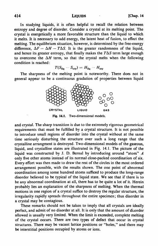
414 LIQUIDS [Chap. 14
In studying liquids, it is often helpful to recall the relation between
entropy and degree of disorder. Consider a crystal at its melting point. The
crystal is energetically a more favorable structure than the liquid to which
it melts. It is necessary to add energy, the latent heat of fusion, to effect the
melting. The equilibrium situation, however, is determined by the free-energy
difference, AF = A// JAS. It is the greater randomness of the liquid,
and hence its greater entropy, that finally makes the T&S term large enoughto overcome the A// term, so that the crystal melts when the followingcondition is reached :
The sharpness of the melting point is noteworthy. There does not in
general appear to be a continuous gradation of properties between liquid
CRYSTAL LIQUID GAS
Fig. 14.1. Two-dimensional models.
and crystal. The sharp transition is due to the extremely rigorous geometrical
requirements that must be fulfilled by a crystal structure. It is not possible
to introduce small regions of disorder into the crystal without at the same
time seriously disturbing the structure over such a long range that the
crystalline arrangment is destroyed. Two-dimensional models of the gaseous,
liquid, and crystalline states are illustrated in Fig. 14.1. The picture of the
liquid was constructed by J. D. Bernal by introducing around "atom" A
only five other atoms instead of its normal close-packed coordination of six.
Every effort was then made to draw the rest of the circles in the most ordered
arrangement possible, with the results shown. The one point of abnormal
coordination among some hundred atoms sufficed to produce the long-rangedisorder believed to be typical of the liquid state. We see that if there is to
be any abnormal coordination at all, there has to be quite a lot of it. Herein
probably lies an explanation of the sharpness of melting. When the thermal
motions in one region of a crystal suffice to destroy the regular structure, the
irregularity rapidly spreads throughout the entire specimen; thus disorder in
a crystal may be contagious.
These remarks should not be taken to imply that all crystals are ideally
perfect, and admit of no disorder at all. It is only that the amount of disorder
allowed is usually very limited. When the limit is exceeded, complete meltingof the crystal occurs. There are two types of defect that occur in crystal
structures. There may be vacant lattice positions or "holes," and there maybe interstitial positions occupied by atoms or ions.

Sec. 2] LIQUIDS 415
It is sometimes convenient to classify liquids, like crystals, from a rather
chemical standpoint, according to the kind of cohesive forces that hold them
together. Thus there are the ionic liquids such as molten salts, the liquid
metals consisting of metal ions and fairly mobile electrons, liquids such as
water held together mainly by hydrogen bonds, and finally molecular liquids
in which the cohesion is due to the van der Waals forces between essentially
saturated molecules. Many liquids fall into this last group, and even when
other forces are present, the van der Waals contribution may be large. The
nature of these forces will be considered later in this chapter.
2. Approaches to a theory for liquids. From these introductory remarks
it may be evident that there are three possible ways of essaying a theory of
the liquid state, two cautious ways and one direct way.The cautious approaches are by way of the theory of gases and the
theory of solids. The liquid may be studied as an extremely imperfect gas.
This is a reasonable viewpoint, since above the critical point there is no
distinction at all between liquid and gas, and the so-called "fluid state" of
matter exists. On the other hand, the liquid may be considered as similar to
a crystal, except that the well-ordered arrangement of units extends over
a short range only, five or six molecular diameters, instead of over the whole
specimen. This is sometimes called "short-range order and long-range dis-
order." This is a reasonable viewpoint, since close to the melting point the
density of crystal and liquid are very similar; the solid usually expands about
10 per cent in volume, or only about 3 per cent in intermodular spacing,
when it melts. It should be realized too that whatever order exists in a liquid
structure is continuously changing because of thermal motions of the in-
dividual molecules; it is the time average of a large number of different
arrangements that is reflected in the liquid properties.
The imperfect-gas theory of liquids would be suitable close to the critical
point; the disordered-crystal theory would be best near the melting point.
At points between, they might both fail badly. A more direct approach to
liquids would abandon these flanking attacks and try to develop the theory
directly from the fundamentals of intermolecular forces and statistical
mechanics. This is a very difficult undertaking, but a beginning has been
made by Max Born, J. G. Kirkwood, and others.
We shall consider first some of the resemblances between liquid and
crystal structures, as revealed by the methods of X-ray diffraction.
3. X-ray diffraction of liquids. The study of the X-ray diffraction of
liquids followed the development of the method of Debye and Scherrer for
powdered crystals. As the particle size of the powder decreases, the width
of the lines in the X-ray pattern gradually increases. From particles around
100 A in diameter, the lines have become diffuse halos, and with still further
decrease in particle size the diffraction maxima become blurred out altogether.
If a liquid were completely amorphous, i.e., without any regularity of
structure, it should also give a continuous scattering of X rays without

416 LIQUIDS [Chap. 14
maxima or minima. This was actually not found to be the case. A typical
pattern, that obtained from liquid mercury, is shown in (a), Fig. 14.2, as a
microphotometer tracing of the photograph. This reveals the maxima and
minima better than the unaided eye. One or two or sometimes more intensity
maxima appear, whose positions often correspond closely to some of the
larger interplanar spacings that occur in the crystalline structures. In the
case of the metals, these are the close-packed structures. It is interesting that
a crystal like bismuth, which has a peculiar and rather loose solid structure,
3i
t 2
V5 10 15 20 25 3.0
(d) DISTANCE FROM CENTRAL SPOT ON FILM-Cm
5 10 II T2
Fig. 14.2.
4 5 6 7 8 9
(b) f- ANGSTROM UNITS
(a) Photometric tracing of liquid-mercury picture; (b) radial
distribution function for liquid mercury.
is transformed on melting into a close-packed structure. We recall that
bismuth is one of the few substances that contract in volume when melted.
The fact that only a few maxima are observed in the diffraction patternsfrom liquids is in accord with the picture of short-range order and increasingdisorder at longer range. In order to obtain the maxima corresponding to
smaller interplanar spacings or higher orders of diffraction, the long-rangeorder of the crystal must be present.
The diffraction maxima observed with crystals or liquids should be dis-
tinguished from those obtained by the X-ray or electron diffraction of gases.The latter arise from the fixed positions of the atoms within the molecules.
The individual molecules are far apart and distributed at random. In derivingon page 327 the diffraction formula for gases, we considered only a singlemolecule and averaged over all possible orientations in space. With both
solids and liquids the diffraction maxima arise from the ordered arrangement

Sec. 4] LIQUIDS 417
of the units (molecules or atoms) in the condensed three-dimensional struc-
ture. Thus gaseous argon, a monatomic gas, would yield no maxima, but
liquid argon displays a pattern similar to that of liquid mercury.It is possible to analyze the X-ray diffraction data from liquids by using
the Bragg relation to calculate spacings. A more instructive approach, how-
ever, is to consider a liquid specimen as a single giant molecule, and then to
use the formulas, such as eq. (11.19), derived for diffraction by single
molecules. A simple theory is obtained only in the case of monatomic liquids,
such as the metals and group O elements.
The arrangement of atoms in such a liquid is described by introducingthe radial distribution function g(r). Taking the center of one atom as origin,
this g(r) gives the probability of finding the center of another atom at the
end of a vector of length r drawn from the origin. The chance of finding
another atom between a distance r and r \ dr, irrespective of angular
orientation, is therefore 47rr2g(r)dr (cf. page 187). It is now possible to
obtain, for the intensity of scattered X radiation, an expression similar to
that in eq. (11.19), except that instead of a summation over individual
scattering centers, there is an integration over a continuous distribution of
scattering matter, specified by g(r). Thus
1(0) f 4rrrWr) ^ dr (14.1)Jo fir
sin I-
I
\^/As before, /^
=* A
By an application of Fourier's integral theorem, this integral can be
inverted,1yielding
By use of this relationship it is possible to calculate a radial-distribution
curve, such as that plotted in (b), Fig. 14.2, from an experimental scattering
curve, such as that in (a), Fig. 14.2. The regular coordination in the close-
packed liquid-mercury structure is clearly evident, but the fact that maximain the curve are rapidly damped out at larger interatomic distances indicates
that the departure from the ordered arrangement becomes greater and
greater as one travels outward from any centrally chosen atom.
4. Results of liquid-structure investigations. X-ray diffraction data from
liquids are not sufficiently detailed to permit complete structure analyses like
those of crystals. This situation is probably inevitable because the diffraction
experiments reveal only an average or statistical structure, owing to the
continual destruction and reformation of ordered arrangements by the
thermal motions of the atoms or molecules in the liquid.
One view, however, proposed by G. W. Stewart (around 1930), is that
1See, for example, H. Bateman, Partial Differential Equations ofMathematical Physics
(New York: Dover Publications, 1944), p. 207.

418 LIQUIDS [Chap. 14
there are actually large regions in a liquid that are extremely well ordered.
These are called cybotactic groups, and are supposed to contain up to
several hundred molecules. These islands of order are dispersed in a sea of
almost completely disordered molecules, whose behavior is essentially that
of a very dense gas. There is a dynamic equilibrium between the cybotactic
groups and the unattached molecules. This picturesque model is probablyunsuitable for the majority of liquids and it is usually preferable to think of
the disorder as being fairly well averaged throughout the whole structure.
The results with liquid metals have already been mentioned. They appearto have approximately close-packed structures quite similar to those of the
solids, with the interatomic spacings expanded by about 5 per cent. The
number of nearest neighbors in a close-packed structure is twelve. In liquid
sodium, each atom is found to have on the average ten nearest neighbors.
One of the most interesting liquid structures is that of water. J. Morganand B. E. Warren2 have extended and clarified an earlier discussion byBernal and Fowler. They studied the X-ray diffraction of water over a rangeof temperatures, and obtained the radial distribution curves.
The maximum of the large first peak occurs at a distance varying from
about 2.88 A at 1.5C to slightly over 3.00 A at 83C. The closest spacingin ice is at 2.76 A. It might at first be thought that this result is in disagree-
ment with the fact that there is a contraction in volume of about 9 per cent
when ice melts. Further analysis shows, however, that the coordination in
liquid water is not exactly the same as the tetrahedral coordination of four
nearest neighbors in ice. The number of nearest neighbors can be estimated
from the area under the peaks in the radial-distribution curve, with the
following results:
Temperature, C:Number nearest neighbors:
1.5
4.4
13
4.4
30
4.6
62
4.9
83
4.9
Thus the tetrahedral arrangement in ice is partially broken down in water,
to an extent that increases with temperature. This breakdown permits closer
packing, although water is of course far from being a closest-packed struc-
ture. The combination of this effect with the usual increase of intermolecular
separation with temperature explains the occurrence of the maximum in the
density of water at 4C.
Among other structures that have been investigated, those of the long-chain hydrocarbons may be mentioned. These molecules tend to pack with
parallel orientations of the chains, sometimes suggesting an approach to
Stewart's cybotactic models.
5. Liquid crystals. In some substances the tendency toward an ordered
arrangement is so great that the crystalline form does not melt directly to a2
J. Chem. Phys., 6, 666 (1938). This paper is recommended as a clear and excellent
example of the X-ray method as applied to liquids.

Sec. 5] LIQUIDS 419
liquid phase at all, but first passes through an intermediate stage (the meso-
morphic or paracrystalline state), which at a higher temperature undergoesa transition to the liquid state. These intermediate states have been called
liquid crystals, since they display some of the properties of each of the
adjacent states. Thus some paracrystalline substances flow quite freely but
(a)
I I Hill 1 1111 II II III!
(b)
(c) (d)
Fig. 14.3. Degrees of order: (a) crystalline orientation and periodicity;
(b) smectic orientation and arrangement in equispaced planes, but no periodicity
within planes; (c) nematic orientation without periodicity; (d) isotropic fluid
neither orientation nor periodicity.
are not isotropic, exhibiting interference figures when examined with polar-
ized light ; other varieties flow in a gliding stepwise fashion and form "graded
droplets" having terracelike surfaces.
A compound frequently studied in its paracrystalline state is />-azoxy-
anisole,
O
OCHaCH
The solid form melts at 84 to the liquid crystal, which is stable to 150 at
which point it undergoes a transition to an isotropic liquid. The compoundethyl /7-anisalaminocinnamate,
:H=N/ \ CH=CP/ \_CH=N/ \_CH=CH COOC2H5

420 LIQUIDS [Chap. 14
passes through three distinct paracrystalline phases between 83 and 139.
Cholesteryl bromide behaves rather differently.3 The solid melts at 94 to
an isotropic liquid, but this liquid can be supercooled to 67 where it passes
over into a metastable liquid-crystalline form.
Liquid crystals tend to occur in compounds whose molecules are
markedly unsymmetrical in shape. For example, in the crystalline state
long-chain molecules may be lined up as shown in (a), Fig. 14.3. On raising
the temperature, the kinetic energy may become sufficient to disrupt the
binding between the ends of the molecules but insufficient to overcome the
strong lateral attractions between the long chains. Two types of anisotropic
melt might then be obtained, shown in (b) and (c), Fig. 14.3. In the smectic
(ojurjypQL, "soap") state the molecules are oriented in well-defined planes.
When a stress is applied, one plane glides over another. In the nematic
(*>/7//a, "thread") state the planar structure is lost, but the orientation is pre-
served. With some substances, notably the soaps, several different phases,
differentiated by optical and flow properties, can be distinguished between
typical crystal and typical liquid.
It has been suggested that many of the secrets of living substances maybe elucidated when we know more about the liquid-crystalline state. JosephNeedham4 has written :
Liquid crystals, it is to be noted, are not important for biology and embryologybecause they manifest certain properties which can be regarded as analogous to
those which living systems manifest (models), but because living systems actuallyare liquid crystals, or, it would be more correct to say, the paracrystalline state
undoubtedly exists in living cells. The doubly refracting portions of the striated
muscle fibre are, of course, the classical instance of this arrangement, but there are
many other equally striking instances, such as cephalopod spermatozoa, or the
axons of nerve cells, or cilia, or birefringent phases in molluscan eggs, or in nucleus
and cytoplasm of echinoderm eggs. . . .
The paracrystalline state seems the most suited to biological functions, as it
combines the fluidity and diffusibility of liquids while preserving the possibilities of
internal structure characteristic of crystalline solids.
6. Rubbers. Natural rubber is a polymerized isoprene,' with long hydro-carbon chains of the following structure:
( CH2 CH CH2 CH2 )n
I
CH3
The various synthetic rubbers are al$o long, linear polymers, with similar
structures. The elasticity of rubber is a consequence of the different degreesof ordering of these chains in the stretched and unstretched states. Anidealized model of the rubber chains when stretched and when contracted
3J. Fischer, Zeit. physik. Chern., 160A, 110 (1932).
4Joseph Needham, Biochemistryand Morphogenesis (London: Cambridge, 1942), p. 661.

Sec. 6] LIQUIDS 421
is shown in Fig. 14.4. Stretching forces the randomly oriented chains into a
much more ordered alignment. The unstretched, disordered configuration is
a state of greater entropy, and if the tension is released, the stretched rubber
spontaneously reverts to the unstretched condition.
Robert Boyle and his contemporaries talked about the "elasticity of a
gas," and although we hear this term infrequently today, it is interesting to
noie that the thermodynamic interpretations of the elasticity of a gas and of
the elasticity of a rubber band are in fact the same. If the pressure is released
on a piston that holds gas in a cylinder, the piston springs back as the gas
expands. The expanded gas is in a state of higher entropy than the com-
(o) (b)
Fig. 14.4. Idealized models of chains in rubber:
(a) stretched; (b) contracted.
pressed gas: it is in a more disordered state since each molecule has a larger
volume in which to move. Hence the compressed gas spontaneously expandsfor the same reason that the stretched rubber band spontaneously contracts.
From eq. (6) on page 65, the pressure is
(14.3)
For a gas, the (dE/3V)T term is small, so that effectively P = T(dS/dV)T ,
and the pressure varies directly with r, and is determined by the change in
entropy with the volume. The analog of eq. (14.3) for a rubber band of
length L in which the tension is K is
(14.4)
It was found experimentally that K varies directly with T, so that, just as in
the case of an ideal gas, the term involving the energy must be negligible.
It was this observation that first led to the interpretation of rubber elasticity
as an entropy effect.

422 LIQUIDS [Chap. 14
7. Glasses. The glassy or vitreous state of matter is another example of
a compromise between crystalline and liquid properties. The structure of a
glass is essentially similar to that of an associated liquid such as water, so
that there is a good deal of truth in the old description of glasses as super-
cooled liquids. The two-dimensional models in Fig. 14.5, given by W. H.
Zachariasen, illustrate the differences between a glass and a crystal.
The bonds are the same in both cases, e.g., in silica the strong electro-
static Si O bonds. Thus both quartz crystals and vitreous silica are hard
and mechanically strong. The bonds in the glass differ considerably in length
and therefore in strength. Thus a glass on heating softens gradually rather
(o) (b)
Fig. 14.5. Two-dimensional models for (a) crystal and (b) glass.
than melts sharply, since there is no one temperature at which all the bonds
become loosened simultaneously.The extremely low coefficient of thermal expansion of some glasses,
notably vitreous silica, is explicable in terms of a structure such as that in
Fig. 14.5. The structure is a very loose one, and just as in the previously
discussed case of liquid water, increasing the temperature may allow a closer
coordination. To a certain extent, therefore, the structure may "expand into
itself." This effect counteracts the normal expansion in interatomic distance
with temperature.8. Melting. In Table 14.1 are collected some data on the melting point,
latent heat of fusion, latent heat of vaporization, and entropies of fusion
and vaporization of a number of substances.
It will be noted that the heats of fusion are much less than the heats of
vaporization. It requires much less energy to convert a crystal to liquid than
to vaporize a liquid.
The entropies of fusion are also considerably lower than the entropies of
vaporization. The latter are quite constant, around 21.6 eu (Trouton's rule).
The constancy of the former is not so marked. For some classes of sub-
stances, however, notably the close-packed metals, the entropies of fusion
are seen to be remarkably constant.
9. Cohesion of liquids the internal pressure. We have so far been dis-
cussing the properties of liquids principally from the disordered-crystai
point of view. Whatever the model chosen for the liquid state, the cohesive

Sec. 9] LIQUIDS 423
TABLE 14.1
DATA ON MELTING AND VAPORIZATION
Metals
NaAlKFe
AgPt
Hg
Ionic Crystals
6.72
6.15
4.33
4.42
4.65
13.07
109
93
Molecular Crystals
H2
H2
ANH3
C2H5OH
0.028
1.43
0.280
1.84
1.10
2.35
0.22
11.3
1.88
7.14
10.4
8.3
forces are of primary importance. Ignoring, for the time being, the origin of
these forces, we can obtain an estimate of their magnitude from thermo-
dynamic considerations. This estimate is provided by the so-called internal
pressure.
We recall from eq. (3.43) that
v- = T -dT
p (14.5)
In the case of an ideal gas, the internal pressure term />,= (5Ej^V)T is
zero since intermolecular forces are absent. In the case of an imperfect gas,
the (dE/dV)T term becomes appreciable, and in the case of a liquid it maybecome much greater than the external pressure.
The internal pressure is the resultant of the forces of attraction and the
forces of repulsion between the molecules in a liquid. It therefore depends

424 LIQUIDS [Chap. 14
markedly on the volume K, and thus on the external pressure P. This effect
is shown in the following data for diethyl ether at 25C.
P(atm): 200
P<(atm): 2790800
28402000
2530
5300
2020
7260
40
9200
-159011,100-4380
For moderate increases in P, the Ptdecreases only slightly, but as P exceeds
5000 atm, the Pt begins to decrease rapidly, and goes to large negative values
as the liquid is further compressed. This behavior is a reflection, on a larger
scale, of the law of force between individual molecules that was illustrated
in Fig. 7.8. on page 181.
Internal pressures at 1 atm and 25C are summarized in Table 14.2,
taken from a compilation by J. H. Hildebrand. With normal aliphatic hydro-carbons there appears to be a gradual increase in P
twith the length of the
chain. Dipolar liquids tend to have somewhat larger values than nonpolar
liquids. The effect of dipole interaction is nevertheless not predominant. As
might be expected, water with its strong hydrogen bonds has an exceptionally
high internal pressure.
TABLE 14.2
INTERNAL PRESSURES OF LIQUIDS
(25C and 1 atm)
Compound Pi atm
2,370
2,510
2,970
3,240
3,310
3,640
3,660
3,670
13,200
20,000
Hildebrand was the first to point out the significance of the internal
pressures of liquids in determining solubility relationships. If two liquids
have about the same Pt , their solution has little tendency toward positive
deviations from Raoult's Law. The solution of two liquids differing con-
siderably in Pt
will usually exhibit considerable positive deviation from
ideality, i.e., a tendency toward lowered mutual solubility. Negative devia-
tions from ideality are still ascribed to incipient compound or complexformation,
10. Intel-molecular forces. It should be clearly understood from earlier
discussions (cf. Chapter 11) that all the forces between atoms and molecules
are electrostatic in origin. They are ultimately based on Coulomb's Law of
the attraction between unlike, and the repulsion between like charges. Oneoften speaks of long-range forces and short-range forces. Thus a force that

Sec. 10] LIQUIDS 425
depends on 1/r2 will be effective over a longer range than one dependent on
1/r7
. All these forces may be represented as the gradient of a potential func-
tion,/= 3//3r, and it is often convenient to describe the potential energies
rather than the forces themselves (See Fig. 7.8, page 181.) The followingvarieties of intermolecular and interionic potential energies may then be
distinguished:
(1) The coulombic energy of interaction between ions with net charges,
leading to a long-range attraction, with U ~ r^ 1.
(2) The energy of interaction between permanent dipoles, with U ~ r~6.
(3) The energy of interaction between an ion and a dipole induced by it
in another molecule, with U ~ r~4 .
(4) The energy of interaction between a permanent dipole and a dipole
induced by it in another molecule, with U ~ r~6.
(5) The forces between neutral atoms or molecules, such as the inert
gases, with U ~ r~B.
(6) The overlap energy arising from the interaction of the positive nuclei
and electron cloud of one molecule with those of another. The overlap leads
to repulsion at very close intermolecular separations, with an r~9 to r~12
potential.
The van der Waais attractions between molecules must arise from inter-
actions belonging to classes (2), (4), and (5).
The first attempt to explain them theoretically was that of W. H. Keesom
(1912), based on the interaction between permanent dipoles. Two dipoles in
rapid thermal motion may sometimes be oriented so as to attract each other,
sometimes so as to repel each other. On the average they are somewhat closer
together in attractive configurations, and there is a net attractive energy.
This energy was calculated5 to be
,--
where ^ is the dipole moment. The observed r~6dependence of the interaction
energy, or r~7dependence of the forces, is in agreement with deductions from
experiment. This theory is of course not an adequate general explanation of
van der Waals' forces, since there are considerable attractive forces between
molecules, such as the inert gases, with no vestige of a permanent dipole
moment.
Debye, in 1920, extended the dipole theory to take into account the
induction effect. A permanent dipole induces a dipole in another molecule
and a mutual attraction results. This interaction depends on the polariza-
bility a of the molecules, and leads to a formula,
UU = - (14.7)
5J. E. Lennard-Jones, Proc. Phys. Soc. (London), 43, 461 (1931).
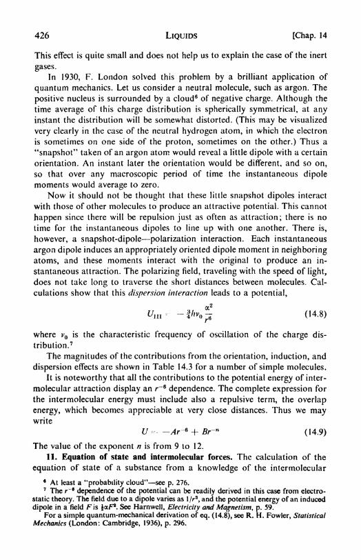
426 LIQUIDS [Chap. 14
This effect is quite small and does not help us to explain the case of the inert
gases.
In 1930, F. London solved this problem by a brilliant application of
quantum mechanics. Let us consider a neutral molecule, such as argon. The
positive nucleus is surrounded by a cloud 6 of negative charge. Although the
time average of this charge distribution is spherically symmetrical, at anyinstant the distribution will be somewhat distorted. (This may be visualized
very clearly in the case of the neutral hydrogen atom, in which the electron
is sometimes on one side of the proton, sometimes on the other.) Thus a
"snapshot" taken of an argon atom would reveal a little dipole with a certain
orientation. An instant later the orientation would be different, and so on,
so that over any macroscopic period of time the instantaneous dipole
moments would average to zero.
Now it should not be thought that these little snapshot dipoles interact
with those of other molecules to produce an attractive potential. This cannot
happen since there will be repulsion just as often as attraction; there is no
time for the instantaneous dipoles to line up with one another. There is,
however, a snapshot-dipole polarization interaction. Each instantaneous
argon dipole induces an appropriately oriented dipole moment in neighboring
atoms, and these moments interact with the original to produce an in-
stantaneous attraction. The polarizing field, traveling with the speed of light,
does not take long to traverse the short distances between molecules. Cal-
culations show that this dispersion interaction leads to a potential,
Um -- -IK^ (14.8)
where VQ is the characteristic frequency of oscillation of the charge dis-
tribution. 7
The magnitudes of the contributions from the orientation, induction, and
dispersion effects are shown in Table 14.3 for a number of simple molecules.
It is noteworthy that all the contributions to the potential energy of inter-
molecular attraction display an r~6dependence. The complete expression for
the intermolecular energy must include also a repulsive term, the overlap
energy, which becomes appreciable at very close distances. Thus we maywrite
U=- ~Ar - + Br~n (14.9)
The value of the exponent n is from 9 to 12.
11. Equation of state and intermolecular forces. The calculation of the
equation of state of a substance from a knowledge of the intermolecular
6 At least a "probability cloud" see p. 276.7 The r~* dependence of the
potentialcan be readily derived in this case from electro-
static theory. The field due to a dipole varies as 1/r3
,and the potential energy of an induced
dipole in a field F is fcaF2
. See Harnwell, Electricity and Magnetism, p. 59.
For a simple quantum-mechanical derivation of eq. (14.8), see R. H. Fowler, Statistical
Mechanics (London: Cambridge, 1936), p. 296.

Sec. ii] LIQUIDS
TABLE 14.3
RELATIVE MAGNITUDES OF INTERMOLECULAR INTERACTIONS*
427
*J. A. V. Butler, Ann. Rep. Chem. Soc. (London), 34, 75 (1937).
| Units of erg cm x 10 60.
forces is in general a problem of great complexity. The method of attack
may be outlined in principle, but so far the mathematical difficulties have
proved so formidable that in practice a solution has been obtained only for
a few drastically simplified cases.
We recall that the calculation of the equation of state reduces to cal-
culating the partition function Z for the system. From Z the Helmholtz free
energy A is immediately derivable, and hence the pressure, P --- ~(dA/dV)T .
To determine the partition function, Z = S e~E i
/kT^ ^Q energy levels
of the system must be known. In the cases of ideal gases and crystals it is
possible to use energy levels for individual constituents of the system, such
as molecules or oscillators, ignoring interactions between them. In the case
of liquids, this is not possible since it is precisely the interaction between
different molecules that is responsible for the characteristic properties of a
liquid. It would therefore be necessary to know the energy levels of the
system as a whole, for example, one mole of liquid. So far this problem has
not been solved.
An indication of the difficulties of a more general theory may be obtained
by a consideration of the theory of imperfect gases. In this case we consider
that the total energy of the system H can be divided into two terms, the
kinetic energy EK , and the intermolecular potential energy U: H = EK + U.
For a mole of gas, U is a function of the positions of all the molecules.
For the N molecules in a mole there are 37V positional coordinates, q, ft,
ft . . . ft^ Therefore, U = U(ql9 ft, ft ft,v)-
The partition function may now be written
Z = S e-(E*+ U)lkT = 2 e-s*lkT S e~ ulkT
(14.10)
It is not necessary to consider quantized energy levels, and Z may be

428 LIQUIDS [Chap. 14
written in terms of an integration, rather than a summation over discrete
levels.
Z=Xe-**l*TS. . .Se-
u >" '****dql9 dqt. . . dq^ (14.11)
The theoretical treatment of the imperfect gas reduces to the evaluation
of the so-called configuration integral,
f)(T)= /.../ <?-"<'
' '"dqlt dqz . . . dqw (14.12)
Since this is a repeated integral over 3N coordinates, </it will be easily
appreciated that its general evaluation is a matter of unconscionable diffi-
culty, so that the general theory has ended in a mathematical cul-de-sac.
Physically, however, it is evident that the potential energy of interaction,
even in a moderately dense gas, does not extend much beyond the nearest
neighbors of any given molecule. This simplification still leaves a problem of
great difficulty, which is at present the subject of active research.
The only simple approach is to consider interactions between pairs of
molecules only. This would be a suitable approximation for a slightly im-
perfect gas. One lets <f>(rl9)be the potential energy of interaction between two
molecules / and j separated by a distance /, and assumes that the total
potential energy is the sum of such terms.
over pairs
When this potential is substituted in eq. (14.12), the configuration integral
can be evaluated. The details of this very interesting, but rather long,
calculation will not be given here. 8
Efforts have been made to solve the configuration integral for more
exact assumptions than the interaction between pairs. These importantadvances toward a comprehensive theory for dense fluids are to be found
in the works of J. E. Lennard-Jones, J. E. Mayer, J. G. Kirkwood, and
Max Born.
12. The free volume and holes in liquids. There have been many attemptsto devise a workable theory for liquids that would avoid entanglement with
the terrible intricacies of the configuration integral. One of the most success-
ful efforts has been that of Henry Eyring, based on the concept of a freevolume. The liquid is supposed to be in many respects similar to a gas. In a
gas, the molecules are free to move throughout virtually the whole container,
the excluded volume (four times van der Waals' b) being almost negligible
at low densities. In a liquid, however, most of the volume is excluded volume,and only a relatively small proportion is a void space or free volume in which
the centers of the molecules can manoeuvre.
Eyring then assumes that the partition function for a liquid differs from
that for a gas in two respects: (I) the free volume V1
is substituted for the
8 See J. C. Slater, Introduction to Chemical Physics (New York: McGraw-Hill, 1 939),
p. I9l.

Sec. 12] LIQUIDS 429
total volume F; (2) the zero point of energy is changed by the subtraction
of the latent heat of vaporization from the energy levels of the gas. Thus,instead of eq. (12.28), one obtains
( '__ /
11(1
~Nl[ If \
The idea of a free volume in liquids is supported experimentally by
Bridgman's studies of liquid compressibilities. These are high at low pressures,
07 08TAc
REDUCED TEMPERATURE
0.9 1.0
Fig. 14.6. Law of rectilinear diameters.
but after a compression in volume of about 3 per cent, the compressibility
coefficient decreases markedly. The initial high compressibility correspondsto "taking up the slack" in the liquid structure or using up the free volume.
A useful model is sometimes provided by considering that the free
volume is distributed throughout the liquid in the form of definite holes
in a more closely packed structure. We should not think of these holes as
being of molecular size, since there is probably a distribution of smaller
holes of various sizes. The vapor is mostly void space with a few molecules
moving at random. The liquid is a sort of inverse of this picture, being
mostly material substance with a few holes moving at random.
As the temperature of a liquid is raised, the concentration of molecules
in its vapor increases and the concentration of holes in the liquid alsp in-
creases. Thus as the vapor density increases the liquid density decreases,
until they become equal at the critical point. We might therefore expect the

430 LIQUIDS [Chap. 14
average density of liquid and vapor to be constant. Actually, there is a slight
linear decrease with temperature. This behavior was discovered by L.
Cailletet and E. Mathias (1886), and has been called the law of rectilinear
diameters. It may be expressed as pav = p aT, where pav is the arith-
metical mean of the densities of the liquid and the vapor in equilibrium with
it, and p and a are characteristic constants for each substance. The relation-
ship is illustrated in Fig. 14.6 where the data for helium, argon, and ether
are plotted in terms of reduced variables to bring them onto the same scale.
13. The flow of liquids. Perhaps most typical of all the properties of
fluids is the fact that they begin to flow appreciably as soon as a shearingstress is applied. A solid, on the other hand, apparently supports a very con-
siderable shear stress, opposing to it an elastic restoring force proportionalto the strain, and given by Hooke's Law,/ KX.
Even a solid flows somewhat, but usually the stress must be maintained
for a long time before the flow is noticeable. This slow flow of solids is called
creep, and it can become a serious concern to designers of metal structural
parts. Under high stresses, creep passes over into the plastic deformation of
solids, for example, in the rolling, drawing, or forging of metals. These
operations proceed by a mechanism involving the gliding of slip planes
(page 391). Although creep is usually small, it must be admitted that the
flow properties of liquids and solids differ in degree and not in kind.
The fact that liquids flow immediately under even a very small shear
force does not necessarily mean that there are no elastic restoring forces
within the liquid structure. These forces may exist without having a chance
to be effective, owing to the rapidity of the flow process. The skipping of a
thin stone on the surface of a pond demonstrates the elasticity of a liquid
very well. An interesting substance, allied to the silicone rubbers, has been
widely exhibited under the name of "bouncing putty." This curious material
is truly a hybrid of solid and liquid in regard to its flow properties. Rolled
into a sphere and thrown at a wall, it bounces back as well as any rubber
ball. Set the ball on a table and it gradually collapses into a puddle of viscous
putty. Thus under long-continued stress it flows slowly like a liquid, but
under a sudden sharp blow it reacts like a rubber.
Some of the hydrodynamic theory of fluid flow was discussed in Chapter7 (page 173) in connection with the viscosity of gases. It was shown how the
viscosity coefficient could be measured from the rate of flow through cylin-drical tubes. This is one of the most convenient methods for use with liquidsas well as gases, the viscosity being calculated from the Poiseuille equation,
Note that the equation for an incompressible fluid is suitable for liquids,
whereas that for a compressible fluid is used for gases.
In the Ostwald type of viscometer, one measures the time required for

Sec. 14] LIQUIDS 431
a bulb of liquid to discharge through a capillary under the force of its own
weight. It is usual to make relative rather than absolute measurements with
these instruments, so that the dimensions of the capillary tube and volume
of the bulb need not be known. The time 7 required for a liquid of known
viscosity ?? , usually water, to flow out of the bulb is noted. The time t9 for
the unknown liquid is similarly measured. The viscosity of the unknown is
where p and px are the densities of water and unknown.
Another useful viscometer is the Happier type, based on Stokes' formula
[eq.(S.ll)]:
\^ JL. = (m
By measuring the rate of fall in the liquid (terminal velocity v) of metal
spheres of known radius r and mass w, the viscosity may be calculated,
since the force /is equal to (m mQ)g, where m is the mass of liquid dis-
placed by the ball.
14. Theory of viscosity. The hydrodynamic theories for the flow of liquids
and gases are very similar. The kinetic-molecular mechanisms differ widely,
as might be immediately suspected from the difference in the dependence of
gas and liquid viscosities on temperature and pressure. In a gas, the viscosity
increases with the temperature and is practically independent of the pressure.
In a liquid, the viscosity increases with the pressure and decreases exponen-
tially with increasing temperature.
The exponential dependence of liquid viscosity on temperature was first
pointed out by J. deGuzman Carrancio in 1913. Thus the viscosity coefficient
may be written
77=-- Ae*K^IRT(14.14)
The quantity A vl8 is a measure of the energy barrier that must be overcome
before the elementary flow process can occur. It is expressed per mole of
liquid. The term e~^E^RT can then be explained as a Boltzmann factor
giving the fraction of the molecules having the requisite energy to surmount
the barrier.
In Table 14.4 are collected the values A vig for a number of liquids,
together with values of AZ^p for purposes of comparison.9 The energy
required to create a hole of molecular size in a liquid is Avap
. The fact
that the ratio of AEvl8 to A isvap about \ to \ for many liquids suggests
that the viscous-flow process requires a free space about one-third to one-
fourth the volume of a molecule. A noteworthy exception to the constancy
of the A vig : Avftp
ratio is provided by the liquid metals, for which the
9 R. H. Ewell and Henry Eyring, J. Chem. Phys., 5, 726 (1937).
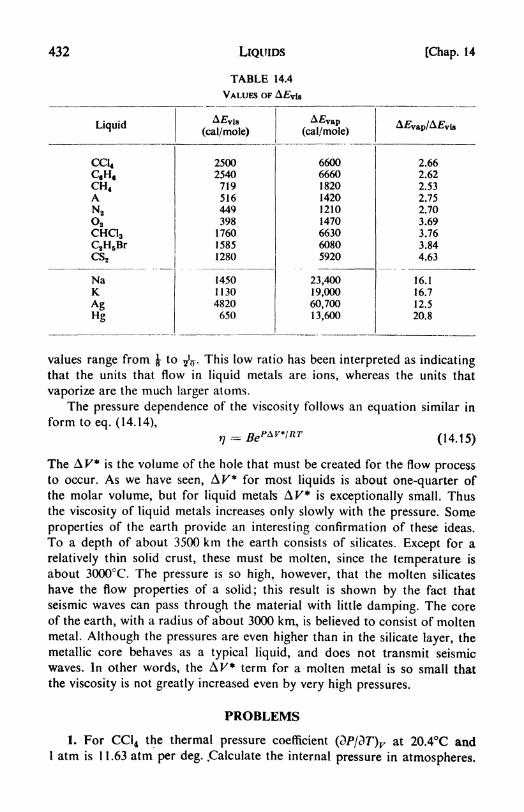
432 LIQUIDS [Chap. 14
TABLE 14.4
VALUES OF AVis
values range from & to 7V- This low ratio has been interpreted as indicatingthat the units that flow in liquid metals are ions, whereas the units that
vaporize are the much larger atoms.
The pressure dependence of the viscosity follows an equation similar in
form to eq. (14.14),
The AF* is the volume of the hole that must be created for the flow processto occur. As we have seen, AF* for most liquids is about one-quarter of
the molar volume, but for liquid metahs AF* is exceptionally small. Thusthe viscosity of liquid metals increases only slowly with the pressure. Some
properties of the earth provide an interesting confirmation of these ideas.
To a depth of about 3500 km the earth consists of silicates. Except for a
relatively thin solid crust, these must be molten, since the temperature is
about 3000C. The pressure is so high, however, that the molten silicates
have the flow properties of a solid; this result is shown by the fact that
seismic waves can pass through the material with little damping. The core
of the earth, with a radius of about 3000 km, is believed to consist of moltenmetal. Although the pressures are even higher than in the silicate layer, the
metallic core behaves as a typical liquid, and does not transmit seismic
waves. In other words, the AF* term for a molten metal is so small that
the viscosity is not greatly increased even by very high pressures.
PROBLEMS
1. For CC14 the thermal pressure coefficient @P/dT)y at 20.4C and1 atm is 11.63 atm per deg. .Calculate the internal pressure in atmospheres.

Chap. 14] LIQUIDS 433
2. The following values were found for the viscosity of liquid CC14 :
Plot these data and calculate AEvis .
3. The liquid and vapor densities of ethanol in equilibrium at various
temperatures are:
The critical temperature is 243C. What is the critical volume?
4. Suppose that the holes in liquid benzene are of the same order of size
as the molecules. Estimate the number of holes per cc at 20C where the
vapor pressure is 77 mm. Hence estimate the free volume in liquid benzene
in cc per mole. Van der Waals' b for benzene is 1 1 5 cc per mole. If b is four
times the volume of the molecules and molecules are closely packed in liquid
benzene, estimate the free volume on this basis. The density of benzene at
20C is 0.879 g per cc.
5. The equation of state of a rubber band is K = CT(L/LQ L 2/L
2),
where K is the tension and L is the length at zero tension. In a case with
L = 20cm and C = 1.33 x 10³ dynes deg-1
, a band is stretched at 25Cto 40cm. What is the decrease in entropy of the rubber band?
6. A certain glass at 800C has a viscosity of 106 poise and a density of
3.5 g crrr3 . How long would a 5 mm diameter platinum ball require to fall
1 .0 cm through the hot glass ?
REFERENCES
BOOKS
1. Frenkel, J., The Kinetic Theory of Liquids (New York: Oxford, 1946).
2. Green, H. S., The Molecular Theory of Fluids (New York: Interscience,
1952).
3. Kimball, G. E., 'The Liquid State," in Treatise on Physical Chemistry,
vol. II, ed. by H. S. Taylor and S. Glasstone (New York: Van Nostrand,
1951).
ARTICLES
1. Condon, E. U., Am. J. Phys., 22, 310-17 (1954), 'The Glassy State."
2. Hildebrand, J. H., Proc. Phys. Soc. (London), 56, 221-39 (1944), 'The
Liquid State."

434 LIQUIDS [Chap. 14
3. Hirschfelder, J. O., J. Chem. Ed., 16, 540-44 (1939), 'The Structure of
Liquids."4. Kirkwood, J. G., Science in Progress, vol. Ill (New Haven: Yale Uni-
versity Press, 1942), 208-221, 'The Structure of Liquids."5. Rowlinson, J. S., Quart. Rev., 8, 168-91 (1954), "Tntermolecular Forces
and Properties of Matter."
6. Ubbelohde, A. R., Quart. Rev., 4, 356-81 (1950), "Melting and Crystal
Structure."

CHAPTER 15
Electrochemistry
1. Electrochemistry: coulometers. The subject of electrochemistry, the
interrelations of electrical and chemical phenomena, is an exceedingly broad
one since, as we have seen, all chemical interactions are fundamentallyelectrical in nature. In a more restricted sense, however, electrochemistryhas come to mean the study of solutions of electrolytes and the phenomenaoccurring at electrodes immersed in such solutions. The electrochemistry of
solutions may claim a special interest from physical chemists since it was in
this field that physical chemistry first emerged as a distinct and characteristic
science. Its first journal, Die Zeitschriftfur physikalische Chemie, was founded
in 1887 by Wilhelm Ostwald, and the early volumes are devoted mainly to
the researches in electrochemistry of Ostwald, van't Hoff, Kohlrausch,
Arrhenius, and others of their "school."
The early history of electrical science has already been discussed as an
introduction to Chapter 8. Its culmination was Faraday's discovery of the
quantitative laws of electrolysis.
These laws became the basis for the construction of coulometers for
measuring quantity of electricity. A standard instrument is the silver coulo-
meter, based on the mass of silver deposited at a platinum cathode by the
passage of the electric current through an aqueous silver nitrate solution.
One coulomb of electricity is equivalent to 0.001 11 800 g of silver. The
iodine coulometer depends on the volumetric estimation of the iodine
liberated by electrolysis of a potassium iodide solution. The experimental
precautions needed for precise coulometry have been extensively studied. 1
2. Conductivity measurements. From the very beginning one of the
fundamental theoretical problems in electrochemistry was how the solutions
of electrolytes conducted an electric current.
Metallic conductors were known to obey Ohm's Law,
,- ,
where / is the current (amperes), ff is the electromotive force, emf (volts),
and the proportionality constant R is called the resistance (ohms). The
resistance depends on the dimensions of the conductor:
R = pl (15.2)A
1See, for example, H. S. Taylor, Treatise on Physical Chemistry, 2nd ed., pp. 591-598.
435

436 ELECTROCHEMISTRY [Chap. 15
Here / is the length and A the cross-sectional area, and the specific resistance
p (ohm cm) is called the resistivity. The reciprocal of the resistance is called
the conductance (chirr1) and the reciprocal of the resistivity, the specific
conductance or conductivity K (ohm"1 cm"1
).
The earliest studies of the conductivity of solutions were made with
rather large direct currents. The resulting electrochemical action was so great
that erratic results were obtained, and it appeared that Ohm's Law was not
obeyed; i.e., the conductivity seemed to depend on the emf. This result was
largely due to polarization at the electrodes of the conductivity cell, i.e., a
departure from equilibrium conditions in the surrounding electrolyte.
AC-1000 CYCLES
(a)
LABORATORYCELL
^| DIPPING
PJCELL
(b)
Fig. 15.1. Conductivity measurement.
These difficulties were overcome by the use of an alternating-current
bridge, such as that shown in (a), Fig. 15.1. With a-c frequencies in the audio
range (1000-4000 cycles per sec) the direction of the current changes so
rapidly that polarization effects are eliminated. One difficulty with the a-c
bridge is that the cell acts as a capacitance in parallel with a resistance, so
that even when the resistance arms are balanced there is a residual unbalance
due to the capacitances. This effect can be partially overcome by inserting
a variable capacitance in the other arm of the bridge, but for very precise
work further refinements are necessary.2Microphones formerly were used
to indicate the balance point of the bridge, but the preferred indicator is
now the cathode-ray oscilloscope. The voltage from the bridge mid-point is
filtered, amplified, and fed to the vertical plates of the oscilloscope. A small
portion of the bridge input signal is fed to the horizontal plates of the scope
through a suitable phase-shifting network. When the two signals are properly
phased, the balance of capacitance is indicated by the closing of the loopon the oscilloscope screen, and the balance of resistance is indicated bythe tilt of the loop from horizontal.
Typical conductivity cells are also shown in Fig. 15.1. Instead of measur-
ing their dimensions, we now usually calibrate these cells before use with a
solution of known conductivity, such as normal potassium chloride. Thecell must be well thermostated since the conductivity increases with the
temperature.
1 T. Shedlovsky, /. Am. Chenr. Soc., 54, 141 1 (1932); W. F. Luder, ibid.. 62, 89 (1940).
Sec. 3] ELECTROCHEMISTRY 437
As soon as reliable conductivity data were available it became apparentthat solutions of electrolytes followed Ohm's Law. The resistance was in-
dependent of the emf, and the smallest applied voltage sufficed to producea current of electricity. Any conductivity theory would have to explain this
fact: the electrolyte is always ready to conduct electricity and this capability
is not something produced or influenced by the applied emf.
On this score, the ingenious theory proposed in 1805 by Baron C. J.
von Grotthuss must be adjudged inadequate. According to his theory, the
molecules of electrolyte were supposed to be very polar, with positive and
negative ends. An applied field lined them up in a chain. Then the field
caused the molecules at the end of the chain to dissociate, the free ions thus
formed being discharged at the electrodes. Thereupon, there was an exchangeof partners along the chain. Before further conduction could occur, each
molecule had to rotate under the influence of the field to reform the original
oriented chain.
Despite its shortcomings, the Grotthuss theory was valuable in empha-
sizing the necessity of having free ions in the solution to explain the observed
conductivity. We shall see later that there are some cases in which a mechan-
ism similar to that of Grotthuss may actually be followed.
In 1857, Clausius proposed that especially energetic collisions between
undissociated molecules in electrolytes maintained at equilibrium a small
number of charged particles. These particles were believed to be responsible
for the observed conductivity.
3. Equivalent conductivities. From 1869 to 1880, Friedrich Kohlrausch
and his coworkers published a long series of careful conductivity investiga-
tions. The measurements were made over a range of temperatures, pressures,
and concentrations.
Typical of the painstaking work of Kohlrausch was his extensive purifica-
tion of the water used as a solvent. After 42 successive distillations in vacuo,
he obtained a conductivity water having a K of 0.043 x 10~6 ohm"1 cm"1 at
18C. Ordinary distilled water in equilibrium with the carbon dioxide of the
air has a conductivity of about 0.7 x 10~6.
To reduce his results to a common concentration basis, Kohlrausch
defined a function called the equivalent conductivity,
A =4 (15.3)c*
The concentration c* is in units of equivalents per cc; the reciprocal (f>-- \/c*
is called the dilution, in cc per equivalent. The equivalent conductivity would
be the conductance of a cube of solution having one square centimeter cross
section and containing one equivalent of dissolved electrolyte.
Some values for A are plotted in Fig. 15.2. On the basis of their con-
ductivity behavior two classes of electrolytes can be distinguished. Strong
electrolytes, such as most salts and acids like hydrochloric, nitric, and

438 ELECTROCHEMISTRY [Chap. 15
sulfuric, have high equivalent conductivities which increase only moderatelywith increasing dilution. Weak electrolytes, such as acetic and other organicacids and aqueous ammonia, have much lower equivalent conductivities at
high concentrations, but the values increase greatly with increasing dilution.
The value of A extrapolated to zero concentration is called the equivalent
conductivity at infinite dilution, A . The extrapolation is made readily for
strong electrolytes but is impossible to make accurately for weak electrolytes
175
4 6 .8 1.0
Vc"- C IN EQUIVALENTS/LITER
Fig. 15.2. Equivalent conductivities vs. square roots of concentration.
because of their tremendous increase in A at high dilutions, where the
experimental measurements become very uncertain. It was found that the
data were fairly well represented by the empirical equation
A = AO - kec1'2
(15.4)
where kc is an experimental constant.
Kohlrausch observed certain interesting relations between the values of
AD for different electrolytes : the difference in A for pairs of salts having a
common ion was always nearly constant. For example (at 18C):
NaCl 108.99 NaNO3 105.33 NaBr 111.10
KC1 130.10 KNO3 126.50 KBr 132.30
21.11 21.17 21.20
Sec. 4] ELECTROCHEMISTRY 439
Thus no matter what the anion might be, there was a constant difference
between the conductivities of potassium and sodium salts. This behavior
could be readily explained if A is the sum of two independent terms, one
characteristic of the anion and one of the cation. Thus
A - V + V (15.5)
where A + and A~
are the equivalent ionic conductivities at infinite dilution.
This is Kohlrausch's law of the independent migration of ions.
This rule made it possible to calculate the A for weak electrolytes like
organic acids from values for their salts, which are strong electrolytes. For
example (at 18C):
A (HAc) - A (NaAc) + A (HC1) - A (NaCl)
- 87.4 + 379.4 109.0 =-- 357.8
4. The Arrhenius ionization theory. From 1882 to 1886, Julius Thomsen
published data on the heats of neutralization of acids and bases. He found
that the heat of neutralization of a strong acid by a strong base in dilute
solution was always very nearly constant, being about 13,800 calories per
equivalent at 25C. The neutralization heats of weak acids and bases were
lower, and indeed the "strength" of an acid appeared to be proportional to
its heat of neutralization by a strong base such as NaOH.These results and the available conductivity data' led Svante Arrhenius
in 1887 to propose a new theory for the behavior of electrolytic solutions.
He suggested that an equilibrium exists in the solution between undissociated
solute molecules and ions which arise from these by electrolytic dissociation.
Strong acids and bases being almost completely dissociated, their interaction
was in every case simply H+ ~f OH H2O, thus explaining the constant
heat of neutralization.
While Arrhenius was working on this theory, the osmotic-pressure studies
of van't Hoff appeared, which provided a striking confirmation of the new
ideas. It will be recalled (page 132) that van't Hoff found that the osmotic
pressures of dilute solutions of nonelectrolytes often followed the equationII = cRT. The osmotic pressures of electrolytes were always higher than
predicted from this equation, often by a factor of two, three, or more, so
that a modified equation was written as
II - icRT (15.6)
Now it was noted that the van't Hoff u/ factor" for strong electrolytes was
very closely equal to the number of ions that would be formed if a solute
molecule dissociated according to the Arrhenius theory. Thus for NaCl,
KC1, and other uniunivalent electrolytes, i = 2; for BaCl2 ,K2SO4 , and other
unibivalent species, i = 3 ; for LaCl3, / = 4.
On April 13, 1887, Arrhenius wrote to van't Hoff as follows:
It is true that Clausius had assumed that only a minute quantity of dissolved
electrolyte is dissociated, and that all other physicists and chemists had followed

440 ELECTROCHEMISTRY [Chap. 15
him; but the only reason for this assumption, as far as I can understand, is a strong
feeling of aversion to a dissociation at so low a temperature, without any actual
facts against it being brought forward. ... At extreme dilution all salt molecules
are completely dissociated. The degree of dissociation can be simply found on this
assumption by taking the ratio of the equivalent conductivity of the solution in
question to the equivalent conductivity at the most extreme dilution.
Thus Arrhenius would write the degree of dissociation a as
a = A (15.7)Ao
The van't Hoff / factor can also be related to a. If one molecule of solute
capable of dissociating into n ions per molecule is dissolved, the total number
of particles present will be i = 1 a + nan. Therefore
a = i^-i (15.8)n 1
Values of a for weak electrolytes calculated from eqs. (15.7) and (15.8) were
found to be in good agreement.
Applying the mass-action principle to ionization, Ostwald obtained a
dilution law, governing the variation of equivalent conductivity A with con-
centration. For a binary electrolyte AB with degree of dissociation a, whose
concentration is c moles per liter:
AB ^ A+ + B~c(l a) etc <xc
(1 -a)From eq. (15.7), therefore,
-
AO(AO- A)
This equation was closely obeyed by weak electrolytes in dilute solutions.
An example is shown in Table 15.1. In this case, the "law" is obeyed at
concentrations below about 0. 1 molar, but discrepancies begin to appear at
higher concentrations.
The accumulated evidence gradually won general acceptance for the
Arrhenius theory, although to the chemists at the time it still seemed most
unnatural that a stable molecule when placed in water should spontaneouslydissociate into ions. This criticism was in fact justified and it soon became
evident that the solvent must play more than a purely passive role in the
formation of an ionic solution.
We now know that the crystalline salts are themselves formed of ions in
regular array, so that there is no question of "ionic dissociation" when theyare dissolved. The process of solution simply allows the ions to be separatedfrom one another. The separation is particularly easy in aqueous solutions
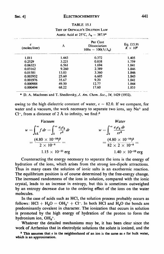
Sec. 4] ELECTROCHEMISTRY 441
TABLE 15.1
TEST OF OSTWALD'S DILUTION LAW
Acetic Acid at 25C, A = 387.9*
w
* D. A. Maclnnes and T. Shedlovsky, J. Am. Chem. Soc., 54, 1429 (1932).
owing to the high dielectric constant of water, e =r 82.0. If we compare, for
water and a vacuum, the work necessary to separate two ions, say Na+ and
Cl~, from a distance of 2 A to infinity, we find:3
Vacuum Water
f00
,, f^2 , [fdr = \
r dr w -J2A h r2 J2
_ (4.80 X IP"10)2
_ __ (4.80 X 1Q-10)2
_2 x 10-
~~
""82 x "2 X 10⁻⁸~~
1.15 x 10-n erg 1.40 x 10~13 erg
Counteracting the energy necessary to separate the ions is the energy of
hydration of the ions, which arises from the strong ion-dipole attractions.
Thus in many cases the solution of ionic salts is an exothermic reaction.
The equilibrium position is of course determined by the free-energy change.The increased randomness of the ions in solution, compared with the ionic
crystal, leads to an increase in entropy, but this is sometimes outweighed
by an entropy decrease due to the ordering effect of the ions on the water
molecules.
In the case of acids such as HC1, the solution process probably occurs as
follows: HC1 + H2O - OH3+ + Cl~. In both HC1 and H2O the bonds are
predominantly covalent in character. The ionization that occurs in solution
is promoted by the high energy of hydration of the proton to form the
hydronium ion, OH3+
.
Whatever the detailed mechanisms may be, it has been clear since the
work of Arrhenius that in electrolytic solutions the solute is ionized, and the
8 This assumes that e in the neighborhood of an ion is the same as c for bulk water,which is an approximation.

442 ELECTROCHEMISTRY [Chap. 15
transport of the ions in an electric field is responsible for the conductivity of
the solutions.
5. Transport numbers and mobilities. The fraction of the current carried
by a giverriomc speci&~l7Tsolution is called the transport number or trans-
ference number of that ion.
From Kohlrausch's law, eq. (15.5), the transference numbers /+ and /
~
of cation and anion at infinite dilution may be written
V - V = (15.10)A o yxo
The mobility I of an ion is defined as its velocity in an electric field of
unit strength. The usual units are cm sec *
per volt cm"1(cm
2 sec" 1 volt"1).
Consider a one-square-centimeter cross section taken normal to the
direction of the current in an electrolyte. The total current / passing throughthis area is the sum of that carried by the positive and that carried by the
negative ions. Thus / ^n\v\z+e + n_v z^e, where n+ and /?_ are the con-
centrations in ions per cc, z+ and z_ are the number of charges on positive
and negative ions, v{and v_ are the velocities of the ions, and e is the elec-
tronic charge. The requirement for over-all electrical neutrality is n+z+ =/i._z_, so that
/ n+z+e(v, \ v_) (15.11)
For a unit cube of electrolyte, from eqs. (15.2) and (15.3): / = &\p ---- K$(2fAc*. Since n\z^e is the charge in one cc and J*", the faraday, is the chargein one equivalent,
From eqs. (15.1 1) and (15.12),
"^ "= "+z+*(+
Now v+/ and vj are the mobilities, l+ and /_. Therefore
JiJP = /+ + /_, and
It follows also from eq. (15.10) that
/ = i__,
6. Measurement of transport numbers Hittorf method. The method of
Hittorf is based on concentration changes in the neighborhood of the elec-
trodes caused by the passage of current through the electrolyte. The principle

Sec. 6] ELECTROCHEMISTRY 443
of the method may be illustrated by reference to Fig. 15.3. Imagine a cell
divided into three compartments as shown. The situation of the ions before
the passage of any current is represented schematically as (a), each -| or
sign indicating one equivalent of the corresponding ion.
Now let us assume that the mobility of the positive ion is three times
that of the negative ion, / f 3/_. Let 4 faradays of electricity be passed
through the cell. At the anode, therefore, four equivalents of negative ions
are discharged, and at the cathode, four equivalents of positive ions. Four
faradays must pass across any boundary
plane drawn through the electrolyte par-
allel to the electrodes. Since the posi-
tive ions travel three times faster than
the negative ions, 3 faradays are carried
across the plane from left to right by the +3=lrj
positive ions while one faraday is beingcarried from right to left by the negative
ions. This transfer is depicted in panel (b)
of the picture. The final situation is
shown in (c). The change in number of
equivalents around the anode, A*a= 6
p.
g 15 3 T rt numbers- 3 = 3; around the cathode, A*c=.-
(Hittorf method).6 5 -- 1. The ratio of these concentra-
tion changes is necessarily identical with the ratio of the ionic mobilities:
A*a/A c= IJL - 3.
Suppose the amount of electricity passed through the cell has been
measured by a coulometer in series, and found to be q faradays. Provided
the electrodes are inert, q equivalents of cations have therefore been dis-
charged at the cathode, and q equivalents of anions at the anode. The net
loss of solute from the cathode compartment is
A/?c- q
-t+ q - q(\
-/+)=
qt_
Thus /_ = * /+= (15.15)
where A/IO is the net loss of solute from the anode compartment. Since
/+ + *- = 1, both transport numbers can be determined from measurements
on either compartment, but it is useful to have both analyses as a check.
In the experiment just described, it is assumed that the electrodes are
inert. In other cases ions may pass into the solution from the electrodes.
Consider, for example, a silver anode in a silver nitrate solution. When
electricity passes through the cell, there will be a net increase in the amountof electrolyte in the anode compartment, equal to the number of equivalentsof silver entering the solution at the anode minus the number of equivalentsof silver crossing the boundary of the anode compartment.

444 ELECTROCHEMISTRY [Chap. 15
Fig. 15.4. Hittorf transport
apparatus.
An experimental apparatus for carrying out these determinations is shownin Fig. 15.4. The apparatus is filled with a standardized electrolyte solution
and a current, kept low to minimize thermal effects, is passed through the
solution for some time. The total amount of
electricity is measured with a coulometer.
The solutions are drawn separately from
the three sections of the cell and analyzed.
Analysis gives the mass of solute and the
mass of solvent in the solutions from the
electrode compartments. Since the mass of
solute originally associated with this mass
of solvent is known, A a and Ac can be
found by difference. Ideally there should be
no change in concentration in the middle
compartment, but small changes arising from diffusion may detract from
the accuracy of the determination.
7. Transport numbers moving boundary method. This method is based
on the early work of Sir Oliver Lodge (1886) who used an indicator to follow
the migration of ions in a conducting gel. For example, a solution of barium
chloride may be placed around platinum electrodes serving as anode and
cathode. The two sides of the cell are then connected by means of a tube
filled with gelatin acidified with acetic acid to make it conducting and con-
taining a small amount of dissolved silver sulfate as indicator. As the current
is passed, the Ba++ and Cl~ ions migrate into
the gel from opposite ends, forming pre-
cipitates of BaSO4 and AgCl, respectively.
From the rate of progression of the white
precipitate boundaries, the relative velocities
of the ions may be estimated.
The more recent applications of this
method discard the gel and indicator and use
an apparatus such as that in Fig. 15.5, to
follow the moving boundary between two
liquid solutions. For example, the electrolyte
to be studied, CA, is introduced into the
apparatus in a layer above a solution of a
salt with a common anion, C'A, and a cation
whose mobility is considerably less than that
dfr
CA
C'A
Fig. 153. Moving-boundary cell.
of the ion C+. When a current is passed through the cell, A~ ions movedownwards toward the anode, while C+ and C"+ ions move upwards toward
the cathode. A sharp boundary is preserved between the two solutions since
the more slowly moving C"+ ions never overtake the C+ ions; nor do the
following ions, C"+, fall far behind, because if they began to lag, the solution
behind the boundary would become more dilute, and its higher resistance

Sec. 8] ELECTROCHEMISTRY 445
and therefore steeper potential drop would increase the ionic velocity. Even
with colorless solutions, the sharp boundary is visible owing to the different
refractive indices of the two solutions.
Suppose the boundary moves a distance x for the passage of q coulombs.
The number of equivalents transported is then qj^, of which t+ql^ are
carried by the positive ion. Recalling that c* is the concentration in equi-
valents per cc, the volume of solution swept out by the boundary during the
passage of q coulombs is t+qf&c*. If a is the cross-sectional area of the tube,
xa = t+q/^c*, or
(.5.16)
8. Results of transference experiments. Some of the measured transport
numbers are summarized in Table 15.2. With these values it is possible to
TABLE 15.2
TRANSPORT NUMBERS OF CATIONS IN WATER SOLUTIONS AT 25C*
* L. G. Longsworth, J. Am. Chem. Soc. t 57, 1185 (1935); 60, 3070 (1938).
calculate from eq. (15.10) the equivalent ionic conductivities A, some of
which are given in Table 15.3. By the use of Kohlrausch's rule, they may
TABLE 15.3
EQUIVALENT IONIC CONDUCTIVITIES AT INFINITE DILUTION, ^, AT 25C*
D. Maclnnes, Principles ofElectrochemistry (New York: Reinhold, 1939).
Q

446 ELECTROCHEMISTRY [Chap. 15
be combined to yield values for the equivalent conductivities A of a wide
variety of electrolytes.
It has been mentioned that ions in solution are undoubtedly hydrated,
so that the observed transport numbers are actually not those of the "bare
ions" but of solvated ions. It was pointed out by Nernst that if a nonionized
substance, such as urea or a sugar, is added to the solution in a Hittorf
transference apparatus, its concentration in the end compartments should
change as a result of the transport of water by the hydrated ions. This
expectation was experimentally realized. From the equivalent ionic conduc-
tivities it is possible to calculate the mobilities of the ions by use of eq.
(15.13). Some results are given in Table 15.4. The effect of hydration is
shown in the set of values for Li+, Na+, K+. Although Li+ is undoubtedlythe smallest ion, it has the lowest mobility; i.e., the resistance to its motion
through the solution is highest. This resistance must be partly due to a
tightly held sheath of water molecules, bound by the intense electric field of
the small ion.
TABLE 15.4
MOBILITIES OF IONS IN WATER SOLUTIONS AT 25C
(cm2 sec" 1 volt" 1
)
Cations
H+K+Ba4
Na+
The passage of an ion through a liquid under the influence of an applied
electric field E might be treated approximately as a hydrodynamic problemsimilar to the fall of a spherical body through a viscous medium under the
influence of a gravitational field (cf. the oil drop experiment, page 210, and
the H5ppler viscometer, page 431). Then for steady flow the viscous resist-
ance, given by the Stokes formula, would be balanced by the electric force:
farjrv zeE. Or, since v El, fy ze/67rr. From this follows the relation,
i?A -- constant, known as "Walden's rule." It has a rather wide range of
experimental validity when tested by measuring the A of electrolytes in
solutions of different viscosities. Its derivation from Stokes's Law is prob-
ably a specious one, for it seems unreasonable to apply the hydrodynamic
equation, meant for a continuous fluid, to the motion of ions whose radii are
about the same as those of the solvent molecules. Walden's rule may there-
fore simply imply that ionic conductance and viscous flow proceed by similar
mechanisms. In water, for example, both have a temperature coefficient
corresponding to an e~^KIRT term with A around 3500 calories per mole.

Sec. 9] ELECTROCHEMISTRY 447
9. Mobilities of hydrogen and hydroxyl ions. An examination of Table 15.4
reveals that, with two exceptions, the ionic mobilities in aqueous solutions
do not differ as to order of magnitude, being all around 6 x 10~4 cm2 sec"1
volt" 1. The exceptions are the hydrogen and hydroxyl ions with the abnor-
mally high mobilities of 36.2 x 10~4 and 20.5 x 10~4.
The high mobility of the hydrogen ion is observed only in hydroxylic
solvents such as water and the alcohols, in which it is strongly solvated, for
example, in water to the hydronium ion, OH3+. It is believed to be an exampleof a Grotthuss type of conductivity, superimposed on the normal transport
process. Thus the OH3+ ion is able to transfer a proton to a neighboring
water molecule,
H H H HI I I I
H O H H- O H - H O -f H O H-f 4-
This process may be followed by the rotation of the donor molecule so that
it is again in a position to accept a proton:
H HI
^I
H O OHThe high mobility of the hydroxyi ion in water is also believed to be
caused by a proton transfer, between hydroxyl ions and water molecules,
H H H HIII I
O + H O -> OH I O
10. Diffusion and ionic mobility. The speed v of an ion of charge q in an
electric field E is related to its mobility / by v = qEL The driving force in
such ionic migration is the negative gradient of the electric potential U:
E ~-3U/dx. Even in the absence of an external electric field, however,
ions can migrate if there is a difference in chemical potential /i between
different parts of the system. The migration of a substance under the action
of a difference in chemical potential is called diffusion. Just as the electric
force (per unit charge) on each particle equals the negative gradient of electric
potential, so the diffusive force equals the negative gradient of chemical poten-
tial. In one dimension, therefore, the force on a particle of the /th kind is
, = _1Jl N'
Since /refers to one mole of particles, it has been divided by Avogadro's
Number N. The velocity under the action of unit force is the generalized
mobility v,, so that v ~ ( vJN)(d[i t/dx). The net flow of material through
unit cross section in unit time is therefore

448 ELECTROCHEMISTRY [Chap. 15
where ni
is the number of particles in unit volume. For a sufficiently dilute
solution, fr= RTln c
i + //?, and dpjdx = (RT/c^dcJdx). Hence,
In 1855 Pick stated in his empirical "First Law of Diffusion" that the flow
six is proportional to the gradient of concentration:
Jtt =-/><^ (15.17)
The proportionality factor /), is called the diffusion coefficient. Thus Di=
kTVf. Since the electric mobility /, vtq, we have
kTA = A (15.18)
This equation was derived by Nernst4 in 1888. It indicates that diffusion
experiments can yield much the same kind of information about ionic
mobilities as that obtained from conductivity data. Equation (15.18) ob-
viously applies to the diffusion of a single ionic species only. An experimental
example would be the diffusion of a small amount of HC1 dissolved in a
solution of KC1. The Cl~ concentrations would be constant throughout the
system, and the experiment would measure diffusion of the H+ ions alone.
In other cases, such as diffusion of salts from concentrated to dilute solution,
it is necessary to use a suitable average value of the diffusion coefficients of
the ions to represent the over-all D. For instance, Nernst showed that for
electrolytes of type CA, the proper average is
11. A solution of the diffusion equation. Equation (15.17) gives only the
steady-state condition for diffusion, but the way in which the concentration
may change with time in any region of the solution can be found as follows.
Consider a region of unit cross-section and of length dx, extending from
x to x + dx. The increase in concentration within this region in unit time
is the excess of material diffusing into the region over that diffusing out,
divided by the volume dx:
dc
dc /a2c\Therefore ^
- D^ j
(15.20)
4Z.physik. Chem. t 2, 613 (1888).

Sec. 11] ELECTROCHEMISTRY 449
This equation is Pick's "Second Law of Diffusion." It has the same form as
the equation for heat conduction, dT/dx = K(d2Tpx2
) y where A' is the thermal
conductivity divided by the heat capacity per unit volume. Thus all the solu-
tions of heat conduction problems, which have been obtained for a great
variety of boundary conditions, can be directly applied to problems of diffu-
sion.
We shall consider one solution only, which illustrates very well the
phenomena of interest. Suppose an extremely thin, effectively planar layer of
the diffusing substance is introduced at the surface of the diffusion medium,
Fig. 15.6. Distribution of concentration of diffusing substance at various times.
Plot of eq. (15.21) for both -f and- jt-direction. For diffusion from an interface
between two regions, the c in eq. (15.21) must be divided by 2.
x = 0. Thus at t = 0; x = 0, c = c ; but at / 0, for all x > 0, c 0. It
can readily be shown5 that the solution of eq. (15.20) for these initial condi-
tions is
- = (irDty-1 '* e-*l4Di
(15.21)*o
The sort of concentration vs. distance curves that result for various times are
shown in Fig. 15.6. The originally sharply defined source of diffusing material
broadens with time; the resulting curves are in fact Gaussian error curves.
The diffusion data can be evaluated from eq. (15.21) by plotting, for a given
time, In c vs. x2; the slope of the straight line equals (4Dt)~
l.
The probability p(x)dx that a given particle has diffused from x = to a
region between x and x + dx is simply proportional to the concentration in
this region. The average distance traversed by the diffusing particles is given
by the mean square displacement6
:
\irDt)-e** f*Dl dx
Hence, A^ = 2Dt (15.22)
This useful expression can be applied directly to measure the diffusion
coefficient of visible particles, e.g., colloidal particles in Brownian motion.
5 H. S. Carslaw and J. C. Jaeger, Conduction of Heat in Solids (New York: Oxford,
1947), p. 33.8 One averages the square of the distance since in some cases diffusion in both the
positive and the negative x directions can occur.

450 ELECTROCHEMISTRY [Chap. 15
The displacements of a large number of individual particles after a time / are
squared and averaged to give A*2. Equation (15.22) is also often used to give
a rapid estimate of the mean distance of diffusion in various solid and liquid
systems.12. Failures of the Arrhenius theory. After the controversies over the
theory of ionic dissociation had somewhat abated, it began to be realized
that the Arrhenius theory was unsatisfactory on a number of points, none
of which was among those urged against it by its fierce original opponents.The behavior of strong electrolytes presented many anomalies. The
Ostwald dilution law was not closely followed by moderately strong electro-
lytes like dichloroacetic acid, although it agreed well with the data for weak
acids like acetic. Also values for the degree of dissociation a of strong
electrolytes obtained from conductance ratios were not in agreement with
those from van't Ho'rT / factors, and the "dissociation constants" calculated
by the mass-action law were far from constant.
Another discrepancy was in the neutralization heats of strong acids and
bases. Although one of the first supports for the ionization theory was the
constancy of these A// values for different acid-base pairs, more critical
examination indicated that the A// values were actually too concordant to
satisfy the theory. According to Arrhenius, there should have been small
differences in the extents of ionization of acids such as HC1, H2SO4 ,HNO3 ,
etc., at any given concentration, and these differences should have been
reflected in corresponding differences in the A// values, but such distinctions
were not in fact observed.
Another flaw was the variation of transport numbers with concentration
c. At low concentrations, these numbers were found to follow an equationof the form t --= t
(}A \/c, where / is the value at infinite dilution and A is
a constant. The Arrhenius theory would predict that the numbers of both
positive and negative current carriers should increase equally with increasing
dilution. It provided no explanation of why their relative mobilities should
vary.A very striking argument against the partial dissociation of strong elec-
trolytes was provided by the ionic structure of crystalline salts.
Finally, studies of the absorption spectra of solutions of strong electro-
lytes failed to reveal any evidence for undissociated molecules.
As early as 1902, a possible explanation of many of the above deficiencies
of the dissociation theory was suggested by van Laar, who called attention
to the strong electrostatic forces that must be present in an ionic solution
and their influence on the behavior of the dissolved ions. In 1912, a detailed
but highly mathematical discussion of this problem was given by S. R. Milner.
In 1923 the problem was taken up by P. Debye and E. Hiickel, whose
theory provided the basis for the modern treatment of strong electrolytes.
It starts with the assumption that in strong electrolytes the solute is com-
pletely dissociated into ions. The observed deviations from ideal behavior,

Sec. 13] ELECTROCHEMISTRY 451
e.g., apparent degrees of dissociation of less than 100 per cent, are to be
ascribed entirely to the electrical interactions of the ions in solution. These
deviations are therefore greater with more highly charged ions and in more
concentrated solutions.
The electrical interaction theory can be applied to equilibrium problems,and also to the important transport problems in the theory of electrical con-
ductivity. Before describing these applications we shall discuss the nomen-
clature and conventions employed for the thermodynamic properties of
electrolytic solutions.
13. Activities and standard states. The thermodynamic description of non-
ideal solutions was discussed in Section 6-21. The activity atand activity
coefficient yA of a component A in solution were defined by means of the
equation:
/'A /*A IRT \n TA XA !<A f- RT]n <*A
It should be emphasized that the activity is a dimensionless quantity, beingthe ratio of the fugacity of the substance in a given system to its fugacity in
some standard state (aA = fA lfA )- The choice of the standard state is not
dictated by any physical principles; it is subject only to the convenience of
the person who is using the thermodynamic theory. Thus, in Section 6-21,
we defined the standard state as the state of the pure solvent A at the tem-
perature and pressure at which we investigate the variation in concentration
of the solution. As the composition of the solution approaches closer and
closer to pure A, deviations from ideality (Raoult's Law) become less and
less. Our choice of standard state is convenient for this situation, since it
requires that in the limit as XA -> \,fA -->fA , and hence aA /i//^ --> 1.
The chemical potential //^' is therefore the free energy of pure A at the
specified temperature and pressure, i.e., FA . We also note that as XA > 1,
yA -> 1. The deviation from unity of the activity coefficient defined in this
way is a measure of the deviation of component A from the ideal behavior
expressed in Raoult's Law.
An inconvenient feature of this definition is also evident, however, in
that it makes IIA , the chemical potential in the standard state, and hence
fA , functions of pressure as well as of temperature. A somewhat different
definition is therefore usually employed, which takes as the standard state
the pure substance at unit pressure. Thus the chemical potential in the stan-
dard statefiA is the same as FA ,
the standard free energy as ordinarilydefined. Also, fA is a function only of temperature, which is more con-
venient. Every silver lining has its cloud, however, and we must note that
with this new definition, it is only in the special case of unit pressure that
aA v XA as XA ~ > 1-
For work with dilute solutions it is often convenient to define a standard
state different from that just described. As a solution is progressively diluted,
the component designated as solvent A tends to obey Raoult's Law, but

452 ELECTROCHEMISTRY [Chap. 15
only for an ideal solution does the solute B also follow Raoult's Law. At
sufficiently low concentrations, however, the solute always tends to follow
Henry's Law. An alternative convention for activity coefficients is based on
this fact. The activity coefficient yn is defined so that, at unit pressure, it
approaches unity as the mole fraction of solute XR approaches zero. Thus
as Xn -> 0, yfi-> 1, and aB -> XB . The departure of yn from unity (at unit
pressure) is a measure of the departure of the solute behavior from that in
an extremely dilute solution.
Instead of eq. (6.32) we have
P* = Pif + *T In 7B*H = /'*' + RT In aa (15.23)
Now fix* is no longer the chemical potential of pure solute B; it is the
chemical potential of B in a standard state consistent with our new definition
fs--kT *
Mole fraction XB '
Fig. 15.7. Definition of standard state for a solute B, based on Henry's Lawin dilute solution.
of activity coefficients. The activity is, of course, given by aB = fB/fB '9
wherefu*
is the fugacity in the new standard state.
The determination of this standard state will be made clear by a reference
to Fig. 15.7, which shows a plot of the fugacity of the solute B,fB , against
its mole fraction XB . In dilute solution (as the fugacity follows
Henry's Law,/# kjjXj^ where kH is the Henry's Law constant. (We mayrecall that/)? differs from the partial vapor pressure PB only by the correction
for nonideality of the vapor.) As the solution becomes more concentrated,
the experimental fn deviates from the straight line graph of Henry's Law.
Therefore the actual value of Ju at XB = 1 (denoted by fB*) may differ
widely from the extrapolated value fB\ obtained by assuming that Henry'sLaw holds all the way to XB = 1 . The extrapolation, shown as a dashed
line in the figure, leads to the value fB* kn . We should note that this

Sec. 13] ELECTROCHEMISTRY 453
standard state is not an actual physical state of the solution. It is the hypo-thetical state that the solute would have if its mole fraction were unity,while at the same time it existed in an environment typical of a solution so
very dilute that each solute molecule was free from any interaction with neigh-
boring solute molecules. That this definition of standard state does indeed
lead to Henry's Law at low concentrations can easily be seen as follows:
"* ='7T fit -'kit* and <*!*= yn*BJB
therefore, fB kHynXB , and as yn - > 1, fB -> kHXn . These activity co-
efficients based on Henry's Law and mole fractions are sometimes called
rational activity coefficients.
In dealing with dilute solutions of electrolytes it is more usual to expressconcentrations in terms of molalities m or molarities r, instead of mole
fractions X. If MA and M7i are the molecular weights of solvent and solute,
and p is the density of the solution, these quantities are related by
- - - (152411000 f mMA lOOOp cMH + cMA
v ' '
In dilute solutions, mMA ,cMn , cMA become negligible compared to 1000,
andp approaches pA9 the density of pure solvent. Then, eq. (15.24) reduces to
x - -^ - MA'*~
1000"~
lOOOpA
For use with m and r as concentration units, two new activity coefficients
and activities have been defined as follows:
[i= p f RTln y
mm -fi
m+ RTln arn
(15.25)
p = /i8C + RTln fc =r=. p" + RT\n ac
(I5.25a)
In dilute aqueous solutions, the molar and molal concentrations are nearly
equal, so that ym & y
c. In solutions more dilute than about 0.01 A/, even
yx
(the rational activity coefficient) does not differ appreciably from the
other two. At unit pressure, all the activity coefficients approach unity as
the solution approaches infinite dilution, and their departures from unity are
a convenient measure of the departures from Henry's Law. 7 The standard
states corresponding to //*m and p,*
cin eqs. (15.25) and (15.25a) are determined
in each case by a graph similar to Fig. 15.7. The fugacities at low concen-
trations are plotted against m (or c) and extrapolated to m - 1 (or c ~ 1)
with the aid of the appropriate form of Henry's Law, fB = kH'm (or
fB ~ kH "c). One further important practical point remains to be noted. In
a dilute solution of an electrolyte, the solute will be dissociated to yield two
or more ions from each solute molecule. The correct form of Henry's Law7 Because m and c are not proportional to X at higher concentrations, y
m and y6 are
not unity for an ideal solution unless it is dilute. The molal concentration m is frequentlyused because m does not vary with temperature, whereas c is temperature dependent because
it varies with the density of the solution.

454 ELECTROCHEMISTRY [Chap. 15
must take into account this dissociation. For a uniunivalent electrolyte like
HC1, for example, Henry's Law in molal concentration units will be/HC1 =kfj'm
2. Therefore, in order to find kn
'
=f'm
, /*Hci must ^e plotted against
/n2, instead of m.
14. Ion activities. In dealing with electrolytic solutions it would appar-
ently be most convenient to use the activities of the different ionic species
present in the solution. There are serious difficulties in the way of such a
procedure. The requirement of over-all electrical neutrality in the solution
prevents any increase in the charge due to positive ions without an equalincrease in the charge due to negative ions. For example, we can change the
concentration of a solution of sodium chloride by adding an equal number
of sodium ions and of chloride ions. If we were to add sodium ions alone or
chloride ions alone, the solution would acquire a net electric charge. The
properties of ions in such a charged solution would differ considerably from
their properties in the normal uncharged solution. There is in fact no con-
ceivable way of measuring the individual ion activities, for there is no wayof separating effects due to positive ions from those due to the accompanying
negative ions in an uncharged solution.
It is nevertheless convenient to have an expression for the activity of an
electrolyte in terms of the ions into which it dissociates. Consider the strong
electrolyte CA 9 dissociated in solution according to CA = C f + A~. Its
activity a may be arbitrarily written as a ~ a+ a^ a 2. Now a defined in
this way is called the mean activity of the ions, and a+ and a_ are the con-
ventional individual ion activities.
For the general case, C,v A v-
v^ C } + v _A~. The ion activities are then
written
a==a+v+aj- = a v
(15.26)
with v+ + v_ = v
Mean ionic activity coefficients and mean ionic concentrations can be
similarly defined. Note that the mean values are geometric means of the
individual ion values. 8
In terms of the molal concentrations m, a+ =~ y^m . Now m v
m^m_v. Since the ionic concentrations are related to m by m+ -- v+m and
m .-- v_m, we can write
For the special case of a uniunivalent electrolyte, m =-- m.8 Sometimes estimates of single ion activities are made by various approximate methods.
For example, the potassium ion and the chloride ion in KC1 both have the argon configura-tion and are therefore nearly the same size. In a KC1 solution it should be a good approxi-mation to set tfK ,
= ac iso that K
2 -= acl2 a 2
. Having obtained values for two ion
activities in this way, we could construct a consistent set of values for others.
In a following section we shall see that it is possible to calculate single ion activities fromelectrostatic and statistical theory (method of Debye and Hiickel). So far such theories are
valid only in extremely dilute solutions. Comparison with experiment is always made in
terms of the mean activities.

Sec. 15] ELECTROCHEMISTRY 455
The activities can be determined by several different methods. Amongthe most important are measurements of the colligative properties of solu-
tions, like freezing point depression and osmotic pressure, measurements
of the solubilities of sparingly soluble salts, and methods based on the emfof electrochemical cells. We shall describe the first two methods now, post-
poning consideration of the emf method until cell reactions have been
considered in more detail.
15. Activity coefficients from freezing points. For a two-component solu-
tion with solute (1) and solvent (0), the Gibbs-Duhem equation may be
written
A/, <///! + A/O rf//-
Combination with eq. (15.25) yields
/?!d In a
1 i- n(}d In tf -=
Equation (6.18) applies to an ideal solution. For a dilute, nonideal solution,
we have instead
d \nciQ A
~~df~"RT2
The freezing point depression AT - T T9 and since T2 ^ ro2
,
Therefore * ,,, = -(l)
<, ,n , =(^) (-A )
If Af is the molecular weight of solvent, we have in 1000 g of solvent:
1000 A?O 1000-
Here K is the molal freezing point depression constant (page 130), and the
number of moles of (1) in 1000 g solvent is/?j
mv
Fromeq. (15.26)
^ = aj^ 7v mv
(v^v^)
so that Jin a, dlny+m = d\ny, |d\nm ^ ----
(15.27)11 * - vmK
Let/ = I (&T/vmK), whereupon
dmy 2vmK \vKnr
, /tdm
or --1= -dj+V ~J) --J J m

456 ELECTROCHEMISTRY [Chap. 15
By comparing this with eq. (15.27):
dlny H- dlnm -- ~dj + (1 ])~mor dlny --= -dj -jdlnm (15.28)
As m approaches 0, the solution approaches ideality, and y ~+ 1 while
j ->0. (Since for an ideal solution t^TjvmK = 1.) Therefore, on integration
of eq. (15.28), we obtain
The integration in this expression can be carried out graphically from a series
of measurements of the freezing point depression in solutions of low knownconcentrations. We plot j/m vs. m, extrapolate to zero concentration, and
measure the area under the curve.
A treatment exactly similar to the above is applicable to osmotic-pressuredata. The activity coefficient determined from eq. (15.29) is that in terms of
molal concentrations, y^m
.
16. Activity coefficients from solubilities. This method, applicable to
sparingly soluble salts, may be illustrated by the typical example of silver
chloride, AgCl. For the solution of AgCl in water we may write: AgCl ^Ag f
-I- Cl~. The equilibrium constant becomes K' ~ a+ajas but since as is
invariable owing to the presence of the solid phase, we usually write the so-
called solubility product constant as
K**-
*Ag*ci"" *+*- = Y+y-C+C- (15.30)
where c is the molar concentration. The solubility SQ of AgCl is simplysQ= c+ c__. The solubility product constant may therefore be written
KSp" 7
2V whenceK 1/2
Y = ^- (15.31)so
Note that this is the activity coefficient in terms of molar concentrations, yc
.
If we can find the constant K8P , we can at once obtain activity coefficients
from the measured solubilities s .
At infinite dilution, or zero concentration, the activity coefficient y
approaches 1, and thus as the concentration approaches 0, s approachesK
SJ1
l/2. The procedure adopted is therefore to measure the solubility, of AgCl
for example, in a series of solutions containing decreasing concentrations of
an added electrolyte, such as KNO3 . The solubilities may then be plotted
against the salt concentration, and an extrapolation to zero concentration
gives K9P .
Extrapolations like this are most accurate if the functions plotted can be
chosen so as to give a linear graph. In this case a linear graph can be obtained

Sec. 17] ELECTROCHEMISTRY 457
if we plot the log of the solubility against the square root of a quantity s,
called the ionic strength of the solution. This is defined by-
s - l^mrf (15.32)
The summation is carried out over all the ionic species in the solution, with
molalities miand charges z,.
TABLE 15.5
MOLAL ACTIVITY COEFFICIENTS OF ELECTROLYTES
17. Results of activity-coefficient measurements. Activity coefficients ob-
tained by various methods9 are summarized in Table 15.5 and plotted in
1.4
8 12 16 2.0 24 2.8
CONCENTRATION-MOLES/ LITER
Fig. 15.8. Activity coefficients of electrolytes.
Fig. 15.8. It will be noted that quite typically the coefficients decline markedlywith increasing concentration in dilute solution, but then pass through
9 A very complete tabulation is given by W. M. Latimer, Oxidation Potentials (NewYork: Prentice-Hall, 2nd ed., 1952).
458 ELECTROCHEMISTRY [Chap. 15
minima and rise again in more concentrated solutions. The interpretation of
this behavior constitutes one of the principal problems in the theory of strong
electrolytes, to which we shall now turn our attention.
18. The Debye-Hiickel theory. The theory of Debye and Hiickel is based
on the assumption that strong electrolytes are completely dissociated into
ions. Observed deviations from ideal behavior are then ascribed to electrical
interactions between the ions. To obtain theoretically the equilibrium prop-erties of the solutions, it is necessary to calculate the efotra'free energy
arising from these electrostatic interactions.
If the ions were distributed completely at random, the chances of finding
a positive or a negative ion in the neighborhood of a given ion would be
identical. In such a random distribution there would be no electrostatic
energy, ^ince on the average attractive configurations would be exactly
balanced by repulsive configurations. It isf evident that this cannot be the
physical situation, since inthd^ immedjiate neighborhood of a positive ion,
a negative ion is more likely to be fouhd than another positive ion. Indeed,
were it not for the fact that the ions are continually being batted about bymolecular collisions, an ionic solutioh might acquire a well ordered structure
similar to that of an ionic crystal. The thermal motions effectively prevent
any complete ordering, but the finAl situation is a dynamic compromisebetween the electrostatic interactions tending to produce ordered con-
figurations and the kinetic collisions tending to destroy them.
The electrolyte is assumed^ to be completely dissociated and all deviations
from ideal behavior are ascribed to the electrical interactions. Our problemis tq calculate the average electric potential U of a given ion in the solution
due to all the other ions. Knowing U we can calculate the work that must be
expended to charge the i(/ns reversibly to this potential, and this work will
be the free energy due to electrostatic interactions. The extra electric free
energy is simply related to the ionic activity coefficient, since both are a
measure of the deviation from ideality.
19. Poisson's equation. The starting point in the calculation of the poten-tial U is an expression for the average distribution of the ions, which weshall obtain in the next section. Let us call the average density of electric
charge in any region of the solution p, e.g., in units of esu per cc. Those
conversant with electrical theory will recall that the potential U is related to
p by Poisson's differential equation:
V 2*/ - - ~ (15.33)
where t- is the dielectric constant. We can, however, obtain quite simply the
form of this equation that we need, by an application of Gauss's theorem of
electrostatics. 10
10 For a further discussion see, for example, Harnwell, Electricity and Magnetism, p. 16.
If the charge is in MKS units (coulombs), a factor f appears in Coulomb's Law and all
expressions derived from it, e.g. yf =

Sec. 19] ELECTROCHEMISTRY 459
In (a), Fig. 15.9, is shown an electric point charge </,surrounded by a
surface S. The electric field intensity at any point is by definition the force
exerted on a unit charge placed at that point, so that in this case it is byCoulomb's Law:
E*=l
i*'
It is a component of a vector in the direction of the line joining the two
charges.
Consider a small element dS of the surface S. The component of the
field strength normal to dS is
En- Er cos (, r)
-^cos (n, r)
where cos (it, r) is the cosine of the angle between the normal n to dS and
the radius r giving the direction of the spherically symmetric field.
(a) (b)
Fig. 15.9. The Poisson equation.
The component of the area dS in the direction r is
dS' -
.Now the area dS' is related to r and the solid angle do by dS' r2dco.
Thereforer*d<o
cfS ------ -
cos (n,r)
It follows that En dS qdco/e. Integrating this over the entire solid angle
subtended by a sphere of radius r, which is 4?r, we obtain
f w rfS-?f4W
Ao ^(15.34)
Js ne Jo f
This is Gauss's theorem: the integral of the normal component of the electric
field intensity over a closed surface equals 4-rT/e times the charge enclosed
within the surface.
Let us now apply this theorem to the special situation of two concentric
spheres, Fig. 15.9(b). The problem is to find the field due to the charges

460 ELECTROCHEMISTRY*
[Chap. 15
contained in an annular shell of thickness dr between the two spheres. For
the two spherical surfaces Sland 52 :
f En dSl + f En dS2= x (total charge within shell) (15.35)
'Si JS*
The total charge within the shell, for the case of interest, may be expressedas a charge density p times the volume of the shell 4iTr2 dr; i.e., 4?rr2p dr.
Then eq. (15.35) becomes
Er+dr 47r(r } dr)2 - 4rrr2p dr
dENow, Er^ dr
= Er + ~
Ignoring terms containing the product of two differentials, we find
d(r*Er) r*dEr + 2rEr dr = r2p dr
8
.-(r> r)-_ (15.36)
The field strength may be represented as the negative gradient of the
potential, Er~ -
dU/dr, so that eq. (15.36) becomes
This expression is the special form of Poisson's equation (15.33) for a
spherically symmetrical problem; i.e., when p is a function only of r.
This is the situation of interest since on the average a given ion will be
surrounded by a spherically symmetrical distribution of oppositely charged
ions, forming the so-called ionic atmosphere. We wish to calculate the averageelectrostatic potential due to a central ion and its surrounding atmosphere.The solutions of eq. (15.37) give the potential in any region as a function of
the charge density p. The next step is therefore to calculate p for the arrayof ions.
20. The Poisson-Boltzmann equation. The Boltzmann theorem (page 183)
informs us that if ntis the average number of ions of kind / in unit volume
in the solution, the number A?/ in any particular region of the solution whose
potential energy is Ev above the average is
n! = /f,e-*'/*r
If an ion of charge q lis brought to a region of potential Uy its potential
energy is q tU. For such ions the Boltzmann equation is therefore
/ = nte-*u'*T
(15.38)

Sec, 20] ELECTROCHEMISTRY 461
The charge density in a region whose potential is U is simply the summation
of this expression over the different kinds of ion that may be present in the
solution, each multiplied by its appropriate charge qr
~ V vt 'si V M ft a~Q\U\kT /\C 1Q\p~
2j nl (j t
~ Zj ntcf t
*(ij.jy)
The Debye-Hiickel treatment now considers a solution so dilute th^ ions
will rarely be very close together. This condition implies that the interionic
potential energy is small, and indeed much less than the average thermal
energy, so that q tU <^ kT. Then the exponential factor in eq. (15.39) may be
expanded as follows :
kT 2\\kT)
Terms higher than the second being negligible, eq. (15.39) becomes
y __ E. v 2
The first term vanishes by virtue of the requirement of over-all electrical
neutrality, and with q t= z
te,
e2UP ^ -
L/i,z f
8(15.40)
It should be noted that S ntz
t
2is closely related to the ionic strength,
which was defined as s = I 2 mtz
t
2.
By substituting eq. (15.40) into eq. (15.37), there is obtained the Poisson-
Boltzmann equation.dU\
~r-^U (15.41)
47T>2
where b2 = -^ntz
t
z(15.42)
The quantity l/b has the dimensions of a length, and is called the Debye
length. It may be thought of as an approximate measure of the thickness
of the ionic atmosphere^ i.e., the distance over which the electrostatic field
of an ion extends with appreciable strength. For example, in a one-molar
aqueous solution of uniunivalent electrolyte at 25C, l/b 3.1 A.
The Poisson-Boltzmann equation (15.41) can be readily solved by makingthe substitution u = rU, whence d*u/dr* = b2u, so that
u = Ae~br + Bebr(15.43)
or i/ s= :4e-*r +-e r
462 ELECTROCHEMISTRY [Chap. 15
A and B are the constants of integration, to be determined from the boundaryconditions. In the first place, U must vanish as r goes to infinity, so that
Ac-* Be*0- -
-}
00 00
This can be true only if B 0, since the limit of e r/r as r goes to infinity is
not zero. We then have left
UAe<"
r
The constant A can be determined by the fact that when b 0, the con-
centration is zero, and therefore the potential is simply that of a single ion
in the absence of any other charges, namely U ~ze/er. Thus ze/er
- A/r
and A ze/t. Therefore the final solution becomes
UZe~Q'br
(15.44)er
Once again, for the case of the very dilute solution (since b is a function
of the concentration) the exponential may be expanded, giving
-rp paU---, e-*
r
<*--(! -br)tr tr
U *?--*-* (15.45)er f
Here it is evident that the first term ze/rr is simply the potential at a
distance r due to an ion of charge ze in a medium of dielectric constant e.
The term zeh/f is then the potential due to the other ions, those formingthe ionic atmosphere of the given ion. It is this extra potential that is related
to the extra free energy of the ionic solution.
21. The Debye-Hiickel limiting law. For a single given ion the extra free
energy is equal to the work that must be expended to charge the ion re-
versibly to the required potential U zeb/r.
=I
ze dU' =\ ( "^ )
Jo Jo \ b /dU'
__
--rV> (15.46)
Now, on the assumption that deviations of the dilute ionic solution from
ideality are caused entirely by the electrical interactions, it can be shownthat this extra electric free energy per ion is simply ATln y, where y is the
conventional ion activity coefficient. Let us write for the chemical potential
of an ionic species /',
/*,= RTlnat + /i?
jn i=
fii (ideal) + //, (electrical)
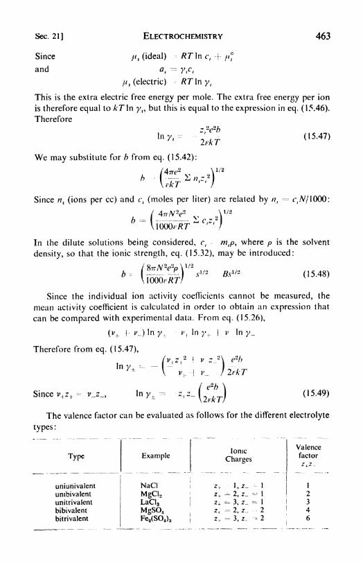
Sec. 21]
Since
and
ELECTROCHEMISTRY
/, (ideal)^ RTlnc, -\- tf
/^(dectric) RTln y t
463
This is the extra electric free energy per mole. The extra free energy per ion
is therefore equal to 7 In y,, but this is equal to the expression in eq. (15.46).
Therefore
(15.47)
We may substitute for b from eq. (15.42):
Since nt (ions per cc) and c\ (moles per liter) are related by //,
=f,AY 1000:
In the dilute solutions being considered, c, mtp 9 where p is the solvent
density, so that the ionic strength, cq. (15.32), may be introduced:
(15.48)
Since the individual ion activity coefficients cannot be measured, the
mean activity coefficient is calculated in order to obtain an expression that
can be compared with experimental data. From eq. (15.26),
(v+ I O In y t.
-i'
t
In y+ Iv In y_
Therefore from eq. (15.47),
Since i>+z f.
-v_z_,
v z_
(15.49)
The valence factor can be evaluated as follows for the different electrolyte
types :

464 ELECTROCHEMISTRY [Chap. 15
Let us now transform eq. (15.49) into base-10 logarithms and introduce
the values of the universal constants. If e is taken as 4.80 x 10~10esu, R
must be 8.31 X 10⁷erg per C. mole. The result is the Debye-Huckel limiting
law for the activity coefficient,
(s\ 1/2-~I= -Az+z_sw (15.50)
For water at 25C, e 78.54, p = 0.997, and the equation becomes
log y = - 0.509 z+z_Vs (15.51)
In the derivation of the limiting law it was consistently assumed that the
analysis applied only to dilute solutions. It is not to be expected therefore
80r
40 60 80
vr x io 3
100 120
Fig. 15.10. Activity coefficients of sparingly soluble salts in salt solutions
[After Bronsted and LaMer, /. Am. Chem. Soc., 46, 555 (1924).]
that the equation should hold for concentrated solutions, nor does it. As
solutions become more and more dilute, however, the equation should
represent the experimental data more and more closely. This expectationhas been fulfilled by numerous measurements, so that the Debye-HUckel
theory for very dilute solutions may be considered to be well substantiated.
For example, in Fig. 15.10 some experimental activity coefficients are
plotted against the square roots of the ionic strengths. These data were
obtained by applying the solubility method to sparingly soluble complex

Sec. 22] ELECTROCHEMISTRY 465
salts in the presence of added salts such as NaCl, BaCl2 , KNO3 . The straight
lines indicate the theoretical curves predicted by the limiting law, and it is
evident that these limiting slopes are followed at low ionic strengths.
Another successful experimental test has been the measurement of
activity coefficients for the same electrolyte in solvents with various dielectric
constants. 11
22. Advances beyond the Debye-Hiickel theory. It would of course be
desirable to have a theory that could be applied to solutions more concen-
trated than those for which the D-H treatment is valid, solutions usuallyso dilute that they have been uncharitably called slightly contaminated
distilled water. Like the general theory of liquids, this is one of the majorunsolved problems in physical chemistry, for when the simplifying assump-tion of extreme dilution is abandoned, the mathematical treatment becomes
discouragingly messy.In 1928, Gronwall, LaMer, and Sandved carried the Debye-Hiickel
theory one step further. Instead of assuming in eq. (15.39) that Uq is muchless than kT, they retained the exponential factor and solved the resulting
Poisson-Boltzmann equation in terms of a series expansion. Their results,
though cumbersome, appeared to be valid at higher concentrations than
those of the original D-H theory.
A clearer physical picture of what may be happening in more concen-
trated solutions has been provided by the ionic association theory, developed
independently by N. Bjerrum, and by R. M. Fuoss and C. Kraus. As solutions
become more concentrated it is likely that definite though transient ion pairs
are formed, held together by electrostatic attraction. This tendency to pair
formation will be greater the lower the dielectric constant of the solvent and
the smaller the ionic radii, both of these factors tending to increase the
electrostatic attractions.
We may be inclined to suspect that with this theory an historical circle
has been completed, returning us to the original Arrhenius concept. There
is, however, a real distinction, albeit a somewhat subtle one. Arrhenius
presumed that in strong electrolytes there were neutral molecules, which
ionized to an extent increasing with the dilution. According to the new
theory, the solution contains nothing but ions, which are electrostatically
associated to an extent that increases with the concentration.
The degree of association may become very appreciable even in a solvent
of high dielectric constant e, such as water. Bjerrum has calculated that in
one-normal aqueous solution uniunivalent ions having a diameter of 2.82 Aare 13.8 per cent associated; of 1.76 A, 28.6 per cent associated. For solvents
of lower e the association would be still greater. Such association into ion
pairs would lower the values of the ionic activity coefficients.
There are two other factors, not considered in the D-H treatment, that
tend to become important in concentrated solutions. One is the effect of
11 H. S. Harned et al., J. Am. Chem. Soc. t 61, 49 (1939).

466 ELECTROCHEMISTRY [Chap. 15
repulsive forces between ions at close distances of approach, called the ionic
size effect. It is analogous to the b factor in van der Waals' equation, and
tends to cut down the electrostatic interactions by preventing very close
approaches between charges. In the derivation of the limiting law, eq. (15.50),
it was assumed that the ions were point charges. Debye and Huckel made
an improved theory which took into account the finite sizes of the ions. The
resulting expression for the mean activity coefficient is
logy,
~ Az^ Vs(15 .52)
1
where A and B have the same significance as in eqs. (15.48) and (15.50), and
(I is the average effective diameter of the ions. The product clB is usually close
to unity.
Probably of greater importance is the effect of the ions on the solvent
molecules. It is known from transference experiments that ions in solution
are solvated, especially in polar solvents like water. This is confirmed bythe well known salting-out effect, by which added electrolytes decrease the
solubility of nonelectrolytes. Some of the solvent molecules appear to be
held so tightly by the ions that they are not able to participate in the solution
of neutral solutes. For example, the solubility (25C) of diethyl ether in purewater is 0.91 mole per liter, but in 15 per cent sodium chloride solution it is
reduced to 0.13 mole per liter.
The solvent molecules surrounding an ion are highly oriented and
polarized. It is likely, therefore, that the dielectric constant of the solvent
is considerably enhanced. As a result interionic attractions decrease; con-
sequently the ionic activity coefficients increase. In Fig. 15.8 it was noted
that the observed y's finally rise at higher concentrations. Both the ionic
size effect and the polarization effect contribute to this rise.
23. Theory of conductivity. The interionic attraction theory was also
applied by Debye and Huckel to the electric conductivity of solutions. An
improved theory was given by Lars Onsager (1926-1928). The calculation of
the conductivity is a difficult problem, and we shall content ourselves with
a qualitative discussion. 12
Under the influence of an electric field an ion moves through a solution
not in a straight line, but in a series of zigzag steps similar to those of
Brownian motion. The persistent effect of the potential difference ensures
an average drift of the ions in the field direction.
Opposing the electric force on the ion is first of all the frictional drag of
the solvent. Although the solvent is not a continuous medium, Stokes's Lawis frequently used to estimate this effect (cf. page 446 and Walden's rule).
Since the molecules of solvent and the ions are about the same size, it is
12 See H. S. Harned and B. B. Owen, The Physical Chemistry of Electrolytic Solutions
(New York: Reinhold, 1943).

Sec. 23] ELECTROCHEMISTRY 467
more likely that the ion moves by jumping from one "hole" to another in
the liquid.
In addition to the viscous effect, two important electrical effects must be
considered. As shown in (a), Fig. 15.11, an ion in any static position is
surrounded by an ionic atmosphere of opposite charge. If the ion jumps to
a new position, it will tend to drag with it this oppositely charged aura. The
ionic atmosphere, however, has a certain inertia, and cannot instantaneously
readjust itself to the new position of its central ion. Thus around a movingion the atmosphere becomes asymmetric, as in (b), Fig. 15.11. Behind the
(o) (b)
Fig. 15.11. (a) Ionic atmosphere surrounding ion at rest; (b) asymmetriccloud around moving ion.
ion there is a net accumulation of opposite charge, which exerts an electro-
static drag, decreasing the ionic velocity in the field direction. This retarda-
tion is called the asymmetry effect. It will obviously be greater at higher ionic
concentrations.
A second electrical action that lowers the mobility of the ions is called
the electrophoretic effect. The ions comprising the atmosphere around a
given central ion are themselves moving, on the average in the opposite
direction, under the influence of the applied field. Since they are solvated,
they tend to carry along with them their associated solvent molecules, so
that there is a net flow of solvent in a direction opposite to the motion of
any given (solvated) central ion, which is thus forced to swim "upstream"
against this current.
The steady state of motion of an ion can be found by equating the
electric driving force to the sum of the frictional, asymmetric, and electro-
phoretic retardations. Onsager calculated each of the terms in this relation-
ship, and thereby obtained a theoretical equation for the equivalent con-
ductivity of a uniunivalent electrolyte in the limiting case of dilute solutions:
f 82.4 8.20 x 10⁵. ] /- /1CC^A = A o
~ Lni/21
-,:7
r)3/2
AoJVc (15.53)
Here c is the concentration of ionized electrolyte in moles per liter, which
if dissociation is not complete must be calculated from the degree of dis-
sociation oc. Similar equations were derived for electrolytes of other valence
types.13
13 See S. Glasstone, Introduction to Electrochemistry (New York: Van Nostrand, 1942),
p. 89.

468 ELECTROCHEMISTRY [Chap. 15
The Onsager equations provide good agreement with the experimental
conductivity data at low concentrations. Their range of validity is greater
for uniunivalent electrolytes than for those whose ions bear higher charges,
but as limiting laws they hold at extreme dilutions for all valence types.
Further confirmation of the essential correctness of the Debye-HUckel-
Onsager picture is obtained from two interesting effects occurring in con-
ductivity measurements.
The Debye-Falkenhagen effect is observed when conductivities are studied
at high a-c frequencies, of the order of 3 x 10⁶ cycles per sec. As the fre-
quency of the electric field is increased, a point is eventually reached at
XX) .01 .02 03
V?
Fig. 15.12. Conductance of tetraisoamyl-ammonium nitrate in dioxane-water.
[Fuoss and Kraus, /. Am. Chem. Sor. 55, 2387 (1933).]
which the ionic atmosphere no longer can follow the rapidly changing field
at all. Then the ions move practically independently of one another as the
influence of their atmospheres becomes unimportant. Thus at high enough
frequencies an increase in the conductivity of a solution is expected, and
has been actually observed.
A second support for the ionic atmosphere model is found in the Wien
effect. At sufficiently high field strengths, of the order of 105 volts per cm,the conductivity is also observed to increase. The explanation is that the
velocities of the ions become so high, with these large fields, that the ionic
atmospheres are left behind entirely, and the ions move independently.In more concentrated solutions marked deviations from the Onsager
equation are found, so that one may even obtain equivalent conductivityvs. concentration curves like that in Fig. 15.12. An interesting interpretation
of the minima in such curves has been based on the ion-association theory.14
The ion pairs (H--
) are electrically neutral and do not contribute to the
equivalent conductivity, which therefore falls as more pairs are formed. As
14 R. Fuoss and C. Kraus, /. Am. Chem. Soc., 55, 21 (1933).

Sec. 24] ELECTROCHEMISTRY 469
the solution becomes still more concentrated, triple ions, either (H----
(-)
or (--
1
--), begin to be formed from some of the pairs, and since these
triplets bear a net charge, they contribute to the conductivity, which therefore
increases from its minimum value.
24. Acids and bases.15 The concepts "acid" and "base" have had a long
and interesting share in the history of chemistry. The distinctive behavior of
these substances has always presented a challenge to theoretical inter-
pretation.
Arrhenius's solution of the problem was to define an acid as a compoundthat dissociated in solution to yield a hydrogen ion, and a base as a com-
pound yielding a hydroxyl ion. Then the process of neutralization was
simply H+ + OH~ = H2O. These definitions relied exclusively on the phe-
nomena observed in aqueous solutions, and it was evident that they would
have to be broadened in some way.In 1922-1923, J. N. Br0nsted and M. Lowry advanced a new set of
criteria. They proposed to define an acid as any compound that can lose a
proton, and a base as any compound that can accept a proton. Thus
A =- H+ + Bacid proton base
The compound B was called the conjugate base of the acid A. Some exampleswould be
HAc = H+ + Ac
= H+ f NH3
Bases and acids might be either neutral molecules or ions.
It was soon realized that the free proton probably never occurs in solu-
tion, the solvent itself acting as a proton acceptor in other words, as a base.
Theiefore, the typical reactions should be written in the symmetrical form:
Acid (I) + Base (II)= Acid (II) + Base (I)
HAc + H2O - H3O + Ac-
NH4+ + H2O = H30* + NH3
H2 + CN- - HCN + OH-
Note that, depending on its partner, a compound, such as water in these
examples, can act either as an acid or as a base. The complete similarity
between the ammonium ion, NH4+, and the hydronium ion, H3O+, is
apparent.An interesting application of the Br0nsted concept is found in the study
of a series of strong acids: HC1O4 , H2SO4 , HNO3 , HBr, HC1, etc. In aqueoussolution these acids are all about equally strong. That is to say, the equi-
librium, HX -|- H2O = H3O+ + X~, lies in every case extremely far to the
16 For a comprehensive treatment of this important subject, see W. F. Luder and
S. Zuffanti, The Electronic Theory of Acids and Bases (New York: Wiley, 1946).

470 ELECTROCHEMISTRY [Chap. 15
right, mainly owing to the large hydration energy of the proton. When the
acids are dissolved in glacial acetic acid, very distinct differences in their
strengths become apparent. Then the equilibria are: HX + CH 3COOH =CH3COOH 2
+ f X . The acetic-acid molecule is not very anxious to accepta proton, and only when the other acid is a particularly insistent donor does
the equilibrium lie sufficiently toward the right to produce a considerable
number of ions. In a 0.005 molar solution in glacial acetic acid the equivalent
conductivity of HC1O4 is more than fifty times that of HNO3 . It is therefore
evident that HC1O4 is a much stronger acid than HNO3 , once the leveling
effect of a solvent such as water is eliminated. 16
The Br0nsted picture still does not represent the full generality of acid-
base phenomena. Further investigations in nonaqueous solutions, notably
by C. A. Kraus and E. C. Franklin, revealed that familiar acid-base prop-erties could be displayed by solutions that contained no protons at all.
For example, the following typical neutralization reaction can be followed
in chlorobenzene solution with crystal violet as an indicator:
BC13 I (C2H5 )3N (C2H5 )3N:BC13
acid base
The indicator is yellow in the presence of excess acid, and violet in basic
solutions.
In 1923 G. N. Lewis advanced a new concept of acids and bases derived
from the electronic theory of valence. This generalized theory is indeed so
broad that it removes the problem from the confines of the chemistry of
ions into the domain of the formation of covalent bonds. Lewis defined an
acid as a substance that can accept a pair of electrons from a donor sub-
stance, the base. The process called "neutralization" is therefore the forma-
tion of a covalent bond in which both electrons of the shared pair are pro-
vided by the base. It may be recalled that this is the type of bond that used
to be called the "dative bond" or the "coordinate link." For example:
H+ + :6:H~ = H:6:H
Cl H Cl HC1:B + :N:H = C1:B:N:H
Cl H Cl Hacid + base = covalent compound
The close relationship between acid-base and oxidation-reduction re-
actions is now apparent. Both acids and oxidizing agents tend to acceptelectrons. They are said to be electrophilic or electron-loving reagents. Anacid accepts a share in a pair of electrons held by a base, forming a co-
ordinate covalent bond. An oxidizing agent accepts electrons provided bya reducing agent, but keeps them all to, itself instead of sharing them with
16I. M. Kolthoff and A. Willman, /. Am. Chem. Soc., 56, 1007 (1934).

Sec. 25] ELECTROCHEMISTRY 471
the donor. Bases and reducing agents are called electrodotic or electron-
giving reagents.
The same reactant can display either acid-base or oxidation-reduction
properties depending upon its reaction partner. Thus the sulfide ion behaves
as a base toward water:
H
:S:|2H-.6.H - H.S.H
!2:6:~
On the other hand, it behaves as a rcductant toward an oxidizing agent like
ferric ion :
:S:- -f 2Fe'^ :S: \~ 2 Fe< '
25. Dissociation constants of acids and bases. A typical acid HA reacts
as follows when dissolved in water: HA {-- H 2O H:iO f
}A . The equi-
librium constant may be written:
If the solution is dilute, the activity of the water alla0 may be taken to be
the same as its concentration r, which will effectively be a constant equalto the number of moles of water in one liter. This constant may be divided
out of the equilibrium constant K& to give the simpler expression:
For a base B, the reaction is BfH2O -- BH+
}OH . The equilibrium
constant becomes
These constants, ATa and K\), are sometimes called the dissociation con-
stants for the acid and base, and they provide a measure of their "strengths."
The constants can be obtained from conductance measurements or bymeasurements of hydrogen-ion concentrations combined with appropriate
activity coefficients. The hydrogen-ion concentration can be measured
colorimetrically with indicators, but more precise values are obtained by
potentiometric methods that will be described later.
Let us write, using the notation H f instead of H 3O+
^H^A 7n 7A-Aa'
In dilute solution the molecule HA, being uncharged and therefore not
subject to electrical interactions, may be assigned an activity coefficient of
unity. Then
>WA-

472 ELECTROCHEMISTRY [Chap. 15
From the Ostwald dilution law,17
eq. (15.9), this would become
a2ca ~
(1-
a)YR+YA~
with a = - A/A . Thus the constant ATa can be evaluated by combining con-
ductivity measurements in dilute solution with suitable activity-coefficient
values, obtained experimentally or from the Debye-Huckel theory.
Some measured constants for acids and bases are summarized in Table
15.6, in the form ofpK& or pK\) values; by analogy with the definition of /?H,
pK -- -log K.
TABLE 15.6*
DISSOCIATION OF ACIDS AND BASES IN WATER SOLUTION AT 25C
* H. S. Harned and B. B. Owen, Chem. Rev., 25, 31 (1939); J. F. J. Dippy, ibid., 151.
For an acid and its conjugate base we have the relationship
K. (15.54)
where K8
is the dissociation constant of the solvent. For example, consider
acetic acid HAc, and its conjugate base Ac~:
HAc + H2O - H3O+ + Ac-
Ac- + H2O = OH- + HAcThen,
Kw is the dissociation constant "of the solvent water.
17 More exact methods are based on the Onsager conductivity theory. See Glasstone,
op. cit., pp. 163-169.

Sec. 26] ELECTROCHEMISTRY 473
The value of Kw can be calculated from the measurements of Kohlrausch
and Heydweiller18 on the conductivity of extremely pure water. These data
are given in Table 15.7 at various temperatures. The degree of dissociation
TABLE 15.7
CONDUCTIVITY ANiJPlCiM PRODUCT OF WATER
a is calculated from the relation a A/A ,A being the sum of the equi-
valent ionic conductivities of H+ and OH~ at infinite dilution. From Table
15.3 this sum at 25 is 349.8 -}- 198 - 547.8. From eq. (15.3), A - */r*,
where c* is the number of moles of water in one cc, 0.0553. Thus A =0.062 x 10~6
/0.0553 = 1.05 x 10~6. Since the ionic concentrations are very
low, the activity coefficients may be taken as unity, so that Kw CH+COH _ =a2cw
2, where cw is the number of moles of liquid water in one liter. The cal-
culated ion products are included in Table 15.7. At 25, Kw & 10~14 , so that
the hydrogen ion concentration CH + ^ 10~ 7 moles per liter, or the pH & 7.
When an acid and base are mixed, neutralization occurs, but except in
the case of strong acids and bases, i.e., those for which dissociation is essen-
tially complete, the compound formed may react with the solvent. This
process is called solvolysis, or in the special case of water, hydrolysis. For a
compound BA in water:
BA + H2O = HA + BOH
The hydrolysis constant is
or Kh= (15.55)
It can easily be shown that the hydrolysis constants are related to the
dissociation constants as follows:
Salt of weak acid and strong base : Kh= KJK*
Salt of weak base and strong acid : Kh= KJKb
Salt of weak acid and weak base: Kh= KJKAK\>
(15.56)
26. Electrode processes: reversible cells. So far we have been considering
only those aspects of electrochemistry that deal with the state of affairs
within solutions of electrolytes. The second important branch of the subject
is concerned with what happens when electrodes are immersed in these
solutions and connected via an external metallic conductor.
An electrode dipping into a solution is said to constitute a half cell \ the
18Z.physik. Chem., 14, 317 (1894).

474 ELECTROCHEMISTRY [Chap. 15
combination of two half cells is a typical electrochemical cell. An example is
the Clark cell of Fig. 4.2.
We shall be interested primarily in the class of cells called reversible cells.
These may be recognized by the following criterion : The cell is connected
-with a potentiometer arrangement for emf measurement by the compensationmethod (page 73). The emf of the cell is measured: (a) with a minute current
flowing through the cell in one direction; (b) then with an imperceptible flow
of current; (c) and finally with a minute flow in the opposite direction. If a
cell is reversible its emf may change only slightly during this sequence, and
there should be no discontinuity in the emf value at the point of balance (b).
Reversibility implies that any chemical reaction occurring in the cell can
proceed in either direction, depending on the flow of current, and at the null
point the driving force of the reaction is just balanced by the compensatingemf of the potentiometer. If a cell is reversible, it follows that the half cells
comprising it are both reversible.
27. Types of half cells. A great many chemical reactions can be carried
out in cells so as to yield electric energy, and there is a corresponding variety
in the types of available half cells.
One of the simplest consists of a metal electrode in contact with a solution
containing ions of the metal, e.g., silver in silver-nitrate solution. Such a half
cell is represented as Ag|Agf(c
>
), where c is the silver-ion concentration, and
the vertical bar denotes the phase boundary. The reaction occurring at this
electrode is the solution or deposition of the metal, according to Ag ^
Ag+ I-- e.
It is sometimes convenient to form a metal electrode by using an amalgaminstead of the pure metal. A liquid amalgam has the advantage of eliminating
nonreproducible effects due to strains in the solid metals or traces of im-
purities at the electrode surface. In some instances a dilute amalgam electrode
can be successfully employed while the pure metal would react violently with
the solution, for example in the sodium amalgam half cell, NaHg(r1)|Na+( 2).
If the amalgam is saturated with the solute metal, the electrode is equivalentto a pure metal electrode, since the chemical potential of a component in its
saturated solution equals the chemical potential of pure solute. If the amalgamis not saturated, methods are available for calculating the emf of a pure metal
electrode from a series of measurements at different amalgam concentrations.
Gas electrodes can be constructed by placing a strip of nonreactive metal,
usually platinum or gold, in contact with both the solution and a gas stream.
The hydrogen electrode consists of a platinum strip exposed to a current of
hydrogen, and partially immersed in an acid solution. The hydrogen is
probably dissociated into atoms at the catalytic surface of the platinum, the
electrode reactions being\ H 2
=-- HH =-- H^ f e
over-all: \ H2 =~H+> e

Sec. 28] ELECTROCHEMISTRY 475
The chlorine electrode operates similarly, negative chloride ions beingformed in the solution : e \ I C12
^ Cl .
An oxidation-reduction electrode is formed by an inert metal dipping into
a solution containing ions in two different oxidation states, e.g., ferric and
ferrous ions in the half cell Pt|Fe'f
, Fe 4 *+. When electrons are supplied to
the electrode, the reaction is Fe ff !
~ + e - Fe H . Since it is the function of
electrodes either to accept electrons from, or to donate electrons to ions in
the solution, they are all in a sense oxidation-reduction electrodes. The
difference between the silver electrode and the ferric-ferrous electrode is that
in the former the concentration of the lower oxidation state, metallic silver,
cannot be varied.
All the electrodes so far considered are examples of what are sometimes
called "electrodes of the first kind." Electrodes of the "second kind" consist
of a metal in contact with one of its slightly soluble salts; in the half cell, this
salt is in turn in contact with a solution containing a common anion. An
example is the silver-silver chloride half cell: Ag|AgCl|Cl (t\). The electrode
reaction can be considered to proceed in two steps:
AgCl(s) Ag^ f Cl
_ Ag 1 + e Ag(s)or over-all: AgCl (s) 1 e - Ag (s) f Cl
:
It is interesting to note that such an electrode is thermodynamically
equivalent to a chlorine electrode (C1 2 |CI ) in which the gas is at a pressure
corresponding to the dissociation pressure of AgCl according to AgCl
Ag 1 2 C12 - This is an especially useful fact in view of the experimentaldifficulties involved in the use of reactive gas electrodes.
28. Electrochemical cells. When two suitable half cells are connected one
obtains an electrochemical cell. The connection is made by bringing the
solutions of the half cells into contact, so that ions can pass between them.
If the two solutions are the same, no problems arise, but if they are different
they must be kept from mixing appreciably by interdiffusion. At the inter-
face between the two solutions there is a liquid junction. We shall postponeconsideration of cells of this kind, and consider first of all some cells without
liquid junctions.
It is necessary to adopt some standard notation for writing down a cell,
the chemical reaction occurring in it, and the sign of its emf. Two sign con-
ventions are in common use in the scientific literature, one used by American
chemists and the other used by the rest of the world, including American
electroplaters. With some misgivings, we shall follow the former.
We therefore decide that a positive emf represents a tendency for positive
ions to pass spontaneously from left to right through the cell as written, or of
negative ions to pass from right to left. If the electrodes are connected
through a metallic conductor, electrons flow through the external circuit
from left to right.

476 ELECTROCHEMISTRY [Chap. 15
From eq. (4.2) the relation between the reversible emf and the maximum
work, AF, for the cell reaction is AF = z&&'
. Thus a positive emf cor-
responds with a negative AF and therefore a positive driving force for the
reaction.
Consider, for example, the Weston cell, which is universally used as a
standard cell It has a voltage of & = 1.01810 volts at 25C and a very small
temperature coefficient. The cell may be written
Cd (12.5% amalgam)|CdS04* H2O (s)|CdSO4 (sat)|Hg2SO4 (s)|Hg
Now for positive emf the positive ions proceed from left to right throughthe cell; the electrons proceed from left to right through the external circuit.
Thus the reaction at the left-hand electrode must be an oxidation, the
loss of electrons according to Cd = Cd++ + 2e. These electrons flow throughthe metallic conductor to the right-hand electrode, where they are given upto the mercurous ion, reducing it to mercury: Hg2
f+ + 2e 2 Hg. The net
cell reaction is the sum of the two electrode processes, or Cd + Hg2++ =
Cd++ + 2 Hg. In terms of the salts present, this reaction might be written
Cd + Hg2SO4= CdSO4 + 2 Hg. The cell reaction is a displacement.
An example in which the reaction is a combination is found in the cell,
Pt|H2 (1 atm)|HCl (0.1 m)|C!2 (1 atm)|Pt
The emf of the cell is 1.485 volts, so that the direction of the current flow is
the same as before. The electrode processes are
i H2- H+ + e
t C12 + e = Cl-
Over-all reaction: \ H2 +'\ C12= HCl (0.1 m)
29. The standard emf of cells. Let us consider the generalized cell reaction:
aA + bB = cCdD. By comparison with eq. (4.8) the free-energy changein terms of the activities a of the reacting species is
Since AF ztffF, division by -rz^" gives
A
When the activities of all the products and reactants are unity, the value
of the emf is <? - -AF/z^. This ? is called the standard emf of the cell.
It is related to the equilibrium constant of the cell reaction, since
AF RTA- (15 '58)
The determination of the standard emf's of cells is therefore one of the most
important procedure^ in electrochemistry. We shall illustrate a useful method
by means of a typical example.

Sec. 29] ELECTROCHEMISTRY 477
Consider the cell shown in Fig. 15.13, consisting of a hydrogen electrode
and a silver-silver chloride electrode immersed in a solution of hydrochloricacid:
Pt(H2)|HCl(m)|AgCl|Ag
The electrode reactions are
H2- FT
AgCl -f e - Ag + Cl-
The over-all reaction is accordingly
AgCl + 1 H2- H+ + Cl- + Ag
COPPER WIRE LEADSTO POTENTIOMETER
H-HClSOLUTION
-Ag FOILCOVEREDWITH AgCl
Fig. 15.13. Hydrogen electrode and silver-silver chloride electrode in
arrangement for standard emf determination.
From eq. (15.57) the emf of the cell is
Setting the activities of the solid phases equal to unity, and choosing the
hydrogen pressure so that #HI= 1 (for ideal gas P 1 atm), we obtain the
equation
o = & - In #H+^CI~
Introducing the mean activity of the ions defined by eq. (15.26), we have
g = <? In a = -- In y m (15.59)
On rearrangement,

478 ELECTROCHEMISTRY [Chap. 15
According to the Debye-Huckel theory, in dilute solutions In y~ AVm,
where A is a constant. Hence the equation becomes
- 2RT. _ 12RTA}
If the quantity on the left is plotted against Vm, and extrapolated back to
m = 0, the intercept at m =gives the value of & .
19 For this cell one
obtains <T = 0.2225 volt at 25C.Once the standard emf has been determined in this way, eq. (15.59) can
be used to calculate mean activity coefficients for HC1 from the measured
emf's $ in solutions of different molalities m.
30. Standard electrode potentials. Rather than tabulate data for all the
numerous cells that have been measured, it would be much more convenient
to make a list of "single-electrode potentials" of the various half cells. Cell
emf's could then be obtained simply by taking differences between these
electrode potentials. The status of single-electrode potentials is similar to
that of single-ion activities. In 1899 Gibbs20pointed out that it is not possible
to devise any experimental procedure that will measure a difference in
electric potential between two points in media of different chemical com-
position for instance, a metal electrode and the surrounding electrolyte.
What we always in fact measure is a difference in potential between two
points at the same chemical composition, such as two brass terminals of a
potentiometer.Consider an ion of copper, (a) in metallic copper, (b) in a solution of
copper sulfate. Its state is determined by its chemical environment, usually
expressed by its chemical potential //, and by its electrical environment,
expressed by its electric potential U. But there is no way of experimentally
separating these two factors, as indeed is apparent from the facts that there
is no way of separating electricity from matter, and that the phenomena we
call "chemical" are all "electrical" in origin. Thus we can measure only the
electrochemical potential of an ion, //-
^ -f U. It may sometimes be con-
venient to make an arbitrary separation of this quantity into two parts;
such conventional separations seem to be helpful in some theoretical
discussions.
Although absolute single-electrode potentials are not measurable, the
problem of reducing the cell emf's to a common basis may be solved by
expressing all the values relative to the same reference electrode. The choice
of a conventional reference state does not affect the values of differences
between the electrode potentials, i.e., the cell emf's. The reference electrode
is taken to be the standard hydrogen electrode, which is assigned by conven-
19 A. S. Brown and D. A. Maclnnes, /. Am. Chem. Soc., 57, 1356 (1935). In practice anextended form of the Debye-Hiickel theory is often used to give a somewhat better extra-
polation function.20 Collected Works, vol. 1, p. 429. See also E. A. Guggenheim, /. Phys. Chem., 33, 842
(1929).

Sec. 30] ELECTROCHEMISTRY 479
tion the value <? --= 0. It is the hydrogen electrode in which (a) the pressure
of hydrogen is 1 atm (strictly, unit fugacity, but the gas may be taken to be
ideal), (b) the solution is a hydrogen acid in which the mean ionic activity is
a = 1. Thus: Pt|H2 (1 atm)|(H* (a -1).
The emf of the cell formed by combining any electrode with the standard
hydrogen electrode gives the electrode potential on the hydrogen scale, <^H .
If the emf is the standard emf <f, it gives the standard electrode potential on
the hvdrogen scale <*u-
To maintain the usual sign convention, always write down the completecell with the electrode to be measured at the left and the hydrogen electrode
at the right. For example, in the previous section, the cell Pt(H2)| HC1| AgCl|Agwas found to have a standard potential ff - 0.2225 v. The cell Ag|AgCl|-
HCl|(H2)Pt would have ff - - 0.2225 v. The standard potential of the
Ag| AgCl electrode would thus be <? H - -0.2225 - 0.0 - 0.2225 v.
Instead of measuring an electrode directly against the standard hydrogen
electrode, it can be measured against any other electrode whose rf, r has
been determined. The normal calomel electrode is frequently used in this wayas a subsidiary reference standard: Hg|Hg2Cl 2|KCl (1 normal), <f H-0.2802 v (25C). We must subtract 0.2802 v from emfs measured against
the normal calomel electrode to bring them onto the standard hydrogenscale.
21
A summary of standard electrode potentials is given in Table 15.8. These
may be called oxidation potentials, because the magnitude of the positive
potential represents the tendency of oxidation, i.e., loss of electrons, to occur
at the electrode. A positive value for rf H indicates that the reduced form of
the half cell is a better reducing agent than hydrogen. For example:
Cd - = Cd+< -4 2e, <T It- 0.402
Therefore the reaction Cd + 2 H 4 -> Cd 4 f} H2 will proceed with a poten-
tial of ff ~= <?H --= 0.402 v. The positive potential corresponds to a
negative AF and therefore a spontaneous reaction. The cell would be
written:
Cd|Cd*+, H+(0. -1)|H2 (1 atm)
Two half-cell reactions and potentials may be subtracted to obtain the
<? for a complete chemical reaction. For example:
Cd = Cd+ 4} 2e <* 0.403
2 Ag - 2 Ag+ + 2e ff =- 0.799
CdT ~2 Agr ='Cd^-l7 2~Ag
"
"rf' -1 .202
Sometimes it is necessary to add or subtract two half reactions to obtain
the $ of a third half reaction. Then one must be careful to add or subtract
21 The symbol <^ H is often written simply <f. Unless otherwise stated it will be under-
stood that the potential is given on the hydrogen scale.

480 ELECTROCHEMISTRY [Chap. 15
TABLE 15.8
STANDARD OXIDATION POTENTIALS*
* W. M. Latimer, Oxidation Potentials (New York: Prentice-Hall, 2nd ed., 1952).

Sec. 31] ELECTROCHEMISTRY 481
the actual free energies in volt equivalents so that the different numbers of
electrons are properly accounted for. For example :
Volt
S Equivalents
4 H2O + Mn++ --= MnO4
- + 8 H+ + 5<r 1 .52 -7.60
2 H2Ojf Mjv- MnO2 + 4 H+ + 2e~ -1.28 2.56~~
2 H 2C+ nO2^"MnOr + 4~Hr+~3e~ 1.68 -5.04
31. Standard free energies and entropies of aqueous ions. Closely* related
to the standard electrode potential on the hydrogen scale is the standardfree
energy ofan ion. Once again, all values are referred to a conventional reference
standard, the hydrogen ion at a =1, which is taken to have a standard free
energy of zero. Consider again the reaction
Cd + 2 H+ ~> Cd++ + H2rf H - 0.403 (25C)
If all the reactants are in their standard states:22
-z& - AF --= /V+ + /">.- /"W- 2F lv
Now FUt and /* Cd are zero because the free energies of the elements are
taken as zero in their standard states at 25C, and F lv is zero by our con-
vention. It follows that
/V* -= Af - -z*T - 2_x_-403 _x *.-, _ ,8.59 kcal per mole
4.184
In addition to the standard ionic free energies, it is useful to obtain also
the standard ionic entropies, S. These are the partial molar entropies of the
ions in solution relative to the conventionally chosen standard that sets the
entropy of the hydrogen ion at unit activity equal to zero, S u <
--0. These
ionic entropies provide a measure of the ordering effect produced by an ion
on the surrounding water molecules. Small ions like Li f and F have lower
entropies than larger ions like Na4 and Cl~. This difference is in accord with
the data from transference experiments discussed on page 446. Ions bearing
a multiple charge are found to have especially low entropies in aqueous
solution, as a result of their strong electrostatic attraction for the water
dipoles and correspondingly large ordering effect on the solvent.
One method for calculating the ionic entropies may be illustrated in
terms of our example, the Cd f + ion. Consider again the reaction: Cd +2 H+ - Cd4 + + H2 . The standard entropy change is AS S (vl ,, } 5 Hi
2 S H <- S CA . Now S cd and S Ut have been evaluated from Third-Law
measurements and statistical calculations, being 31.23 and 12.3 cal per degat 25C. By our convention, Hf is zero. Therefore 5 Cl,i, A5 18.93.
The value of AS can be obtained from AS -= (A// &FC)/T. If cadmium
is dissolved in a large excess of very dilute acid, the heat of solution per mole
of cadmium is the standard enthalpy change A//, since in the extremely22 The free energies are written F because for species in solution they are the partial
molar free energies or chemical poten tials.

482 ELECTROCHEMISTRY [Chap. 15
dilute solution all the activity coefficients approach unity. This experiment
yields the value A// = 16,700 cal. The AF from the cell emf was found to
be -18,580 cal. Therefore AS - (-16,700 f 18,580)/298.2 - 6.22 cal per
deg. It follows that S Cd ,. - 12.7 cal per deg.
The methods described for determining the thermodynamic properties of
ions in solution represent only a few examples of many possible ways of
combining thermodynamic data. Latimer's book, The Oxidation States ofthe Elements and Their Potentials in Aqueous Solutions, should be consulted
for a thorough survey of this important field and extensive tables of the
thermodynamic quantities.
32. Measurement of solubility products. Standard electrode potentials can
be combined to yield the ff and thus the AF and equilibrium constant for
the solution of salts. It is thus possible to calculate solubilities for salts even
in cases where an extremely low solubility would make direct measurements
very difficult. As an example, consider silver iodide, which dissolves accordingto: Agl Ag+ + I~. The solubility product constant is /Qp OAR'^I-
A cell whose net reaction corresponds to the solution of solid silver iodide
can be formed by combining a silver electrode with a silver-silver iodide
electrode, Ag|Ag+,l |AgI (s)|Ag. The electrode reactions are
Ag - Ag>- + e <T - -0.7995
e 4- Agl (s)_=_Ag + \2_ ^ - -0.1510
Over-all: Agl(s) = Ag j + r <f -, -0.9505
Then, from AF - -z& = ~RT\n AT8p ,
(0.951 x 96,520)lOtZ-in *ur\ "
~ * iO.V/D
Assuming unit activity coefficients in the very dilute solution of Agl, this
AT8p corresponds to a solubility of 2.47 x 10~6
g per liter.
33. Electrolyte-concentration cells. The cells so far described have all
been chemical cells, producing electrical energy from chemical changes.
There is also an important class of cells in which no net chemical changeoccurs. These are called concentration cells, because they owe their emf to
concentration changes either in the electrolyte or in the electrodes (e.g., in
amalgams).For the cell, Pt|H 2jHCl (r)|AgCl|Ag, the cell reaction is \ H2 + AgCl
- Ag { HC1 (c). Measurements with two different hydrochloric acid con-
centrations c yielded the following results:
c # F( joules)
0.0010 0.6095 58,8200.0483 0.3870 37,340
If two such cells are set up so as to oppose each other, the combination
constitutes a cell that can be written as follows:
Ag|AgCl|HCl(r2)|H2|HCl(

Sec. 34] ELECTROCHEMISTRY 483
The over-all change in this cell is simply the difference between the changesin the two separate cells: for the passage of each faraday the transfer of
one mole of HCi from concentration c2 to cl9 HCI (c2) > HCI (ct). Note,
however, that there can be no direct transport of electrolyte from one side
to the other. The HCI is removed from the left side by the reaction, HCI f- Ag= AgCl -f H2 . It is added to the right side by the reverse of this reaction.
Fiom the data above, if c\= 0.00 1 and c2
- 0.0483, the free energy of
dilution is AF- 21,480, and - 21,480/96,520 0.2225.
34. Electrode-concentration cells. An example of an electrode-concentra-
tion cell would be one consisting of two hydrogen electrodes operating at
different pressures and dipping into a hydrochloric-acid solution:
Pt|H2 (PO|HCl(a)|H2 (P2)|Pt
At the left electrode: \ H2 (P^ = H+ (am ) (- e
At the right: H^ (0H .) h e - i H2 (P2)
The over-all change is accordingly H2 (Pj) \ H2 (P2), the transfer of one
equivalent of hydrogen from pressure Plto P2 . The emf of the cell is
g :^ P
P\
An interesting type of electrode concentration cell is one in which two
amalgam electrodes of different concentrations dip into a solution containingthe solute metal ions. For example:
Cd.Hg(fl1)|CdS04|Cd-Hg(fl2)
The emf of this cell arises from the net work obtained in transferringcadmium from an amalgam where its activity is av to one with activity 2 .
The emf is therefore :
If the amalgams are considered to be ideal solutions, one may replace the
activities by mole fractions. In Table 15.9 are some experimental data for
TABLE 15.9
CADMIUM AMALGAM ELECTRODE-CONCENTRATION CELLS*
* G. Hulett, J. Am. Chem. Soc., 30, 1805 (1908).

484 ELECTROCHEMISTRY [Chap. 15
these cells, together with the calculated emf's based on ideal solutions. The
approach to the theoretical values with increasing dilution may be noted.
Electrode-concentration cells are especially useful in studying the thermo-
dynamics of alloys.25
35. Cells with liquid junctions. If the two electrodes of a cell are immersed
in two different solutions, these solutions must be brought into contact
in order to complete the electrical circuit. The contact can be madeeither directly or through a salt bridge, a connecting tube filled with salt
solution.
The liquid-to-liquid junctions are designed so as to minimize mixing of
the solutions by interdiffusion. Sometimes a flowing junction is used for
greater reproducibility.
As was pointed out in Section 30, it is not possible to measure a difference
in electrical potential between two chemically different media. Therefore
liquid-junction potentials cannot be directly measured.
Attempts have been made to calculate liquid-junction potentials by
solving diffusion equations for the ions in solution. Consider, for example,a junction between a solution of HC1 and a solution of KCl. If the con-
centrations are about the same, one would expect the HC1 solution to lose
H+ ions by diffusion more rapidly than the KCl solution loses K+ ions,
because the H^ ion has a much higher mobility. Thus the HC1 side of
the contact would become negatively charged relative to the KCl side.
Semi-quantitative estimates based on this picture have led to junction
potentials of from 5 to 30 millivolts, not large compared with the usual
cell emf's.
Attempts have been made to eliminate the liquid-junction potential by
using a salt bridge. Concentrated solutions of KCl or NH4NO3 are often
used in the bridge. The ions in these solutions have nearly the same transport
numbers, and one may hope that the two cell-solution-bridge-solution
potentials will be nearly equal numerically but opposite in sign.
The most encouraging thing about cells with liquid junctions is that
standard emf's obtained from them, when careful procedures are followed,
often agree very closely with the results from cells without liquid junctions.
We thus can feel considerable confidence in the necessary approximations.Cells without liquid junctions are used wherever possible, but in some
applications, such as the measurements of /?H, or of oxidation-reduc-
tion potentials of organic compounds, it is necessary to employ liquid
junctions.
36. Oxidation-reduction reactions. Cells with liquid junctions are fre-
quently used to study the equilibrium in oxidation-reduction reactions.
Special interest has been focused on the oxidations of organic substances
occurring in living cells, in view of the importance of such processes in
cellular metabolism and respiration. Although the particular example is not
'-''J. Chipman, Discussions of the Faraday Soc.> 4, 23 (1948).

Sec. 36] ELECTROCHEMISTRY 485
a biological reaction, the principles involved can be illustrated by the
oxidation of hydroquinone to quinone. The reaction is2(i
OH O
+ 2 H+ + 2e
OHQH2
OQ
If an inert metal electrode (Au or Pt) is placed in a solution containinga mixture of hydroquinone and quinone, the reaction can be made to pro-ceed in either direction by supplying or removing electrons at the electrode.
LEADS TOPOTENTIOMETER
CURRENT OFPURE NITROGEN
-KClSOLUTION
SOLUTION OFHYDROQUINONE,QUINONE ANDBUFFER
Fig. 15.14. Experimental arrangement for measuring emf of an oxidation-
reduction reaction, or for a potentiometric titration.
A complete cell can be formed by coupling this hydroquinone electrode with
a calomel electrode or other reference half cell. A typical experimental
arrangement is shown in Fig. 15.14. The cell may be written
Au|QH2, Q (buffer: H+)|KC1, Hg2CI2|Hg2Cl2 (s)|Hg
The cell reaction is
At the left:
At the right:
Over-all:
QH2= Q + 2 H+ + 2e
_ l2f^ 2_Hg + 2Cl^_
QH2 + Hg2Cl2= Q + 2Hg"+ 2" + 2 C>
26Hydroquinone is a weak acid but in moderately acid solutions its dissociation is
negligible. Under certain conditions the reaction proceeds in two steps, removal of one
electron forming a highly colored semiquinone. See L. Michaelis, C.hem. Revs., 22, 437 (1938).

486 ELECTROCHEMISTRY [Chap. 15
The emf can be written
(15.60)
TITRATEDSYSTEM
TITRANTSYSTEM
Since Q and QH2 are uncharged species, it is a good approximation to
replace their activity ratio by a concentration ratio. Then from measured
values of 6 at known acid strength, it is possible to calculate <^ and hence
the equilibrium constant of the oxidation-reduction reaction. Note that the
of the cell and therefore the driving force of the reaction depend on the
acid concentration.
By adding an oxidizing agent from the burette, it is possible to titrate the
reduced form. As the concentration of QH2 approaches zero, it is evident
from eq. (15.60) that approaches minus
infinity. Consequently, when the amount of
QH 2 remaining unoxidized becomes very
small, the change in the measured cell emf
becomes very steep. Of course does not
actually go to oo, because as the end point
of the titration is approached the concentra-
tion of unreacted oxidizing agent (titrant)
becomes appreciable, so that a new oxida-
tion-reduction equilibrium is set up with an
emf characteristic of the titrant system. The
course of a typical potentiometric titration is
shown in Fig. 15.15. If the standard poten-
tials of the titrated system and the titrant system are sufficiently far apart,
a good end point can be readily determined.
37. Measurement of pH. We often need to know the concentration of
hydrogen ions in aqueous solution. In 1909 S. P. S0rensen invented the
symbol pH as a convenient expression for this quantity, defined by pHIog10 CH +, where cll+ is the molar concentration.
In 1909 strong electrolytes like HC1 were believed to be only partially
dissociated even in dilute solutions. The degree of dissociation was believed
to be given by a = A/A . Values of cll+ were accordingly calculated from
the equivalent conductivities, and S0rensen set up his pH scale on this basis.
It now appears that strong electrolytes are completely dissociated in dilute
solutions, so that the S0rensen pH scale is unsatisfactory.
For most practical purposes the pH is a number determined by potentio-
metric measurement of a cell emf. Since cell emf's depend on activities and
not on concentrations it is probably wise to abandon the definition of pHby a concentration scale, except as a first approximation. It might seem
Fig. 15.15. Course of emf in a
potentiometric titration.
Sec. 38] ELECTROCHEMISTRY 487
logical to define /;H as loglo air ,but this definition has the considerable
drawback that H , is not itself an experimentally measurable quantity.The best procedure seems to be to define a /;H scale by reference to the
measured emf of a cell consisting of a hydrogen electrode combined with
some reference electrode. Such a cell might be
(Pt)H 2 , 1 atm|H+r iKCl (saturated);1
Hg2Cl2 , KCl|Hg2Cl2|Hg
This cell contains two liquid junctions at the KCl salt bridge, so that we
cannot separate the hydrogen electrode potential from the measured emf.
If such a separation were possible we could write the emf as
RTX -6\K(
- ~\na
We now arbitrarily define the /?H by writing
RT<? = rcf -{ 2.303 ~p\\ (15.61)
We choose a value for <frcf that will give a /?H value in accord with other
thermodynamic data, such as the dissociation constants of weak acids. For
the 0.1 normal KCl-caiomel electrode this value at 25C is ^ rol- 0.3358 v.
Therefore eq. (15.61), defining the /;H, can be written (at 25C)
<? - 0.3358 ^^0.3358P
2.303 RT};? 1X0592
The hydrogen electrode is not well suited for routine /;H measurements
because it requires a source of gaseous hydrogen and it is sensitive to various
"poisons" that inhibit the catalytic activity of the platinized platinumsurface. The most convenient method of measuring p\\ is undoubtedly bymeans of the glass electrode. The operation of this interesting device depends
upon the difference in potential across a glass membrane separating solutions
of different /?H.27
38. Concentration cells with transference. In electrolyte-concentration
cells without liquid junctions, the type previously described, there is no direct
flow of electrolyte from one solution to the other. An example of a con-
centration cell that does have direct contact between the solutions is
H2 (1 atm)|HCl (aj j HCl (*2)|H2 (1 atm)
t_C\~
The r's are the ionic transport numbers. For the passage of each faraday.of
charge, the following changes occur in the cell:
A. At the electrodes. (1) One equivalent of H+ is formed at the left, bythe reaction i H2
> H+(aj). (2) One equivalent of H+ is removed at the
27 M. Dole, The Glass Electrode (New York: Wiley, 1941).

488 ELECTROCHEMISTRY [Chap. 15
right, by the reaction H+(a2)-> i H2 . The net result of the electrode processes
is H+(a2 ) -> H+(fll ).
B. At the liquidjunction. (1) / equivalents of Cl~ ions pass from right to
left, from the solution of activity a2 to that of activity av (2) t+ 1 t_
equivalents of H 1 ions pass from left to right, from activity al to a2 .
The net result of these changes at the electrodes and at the junction is
UHC1) at 2-> /_(HC1) at at
Since the electrodes are reversible with respect to the cation H+, the transport
number / of the anion occurs in the expression for the net change.
Such a cell is called a concentration cell with transference. Note that it
requires electrodes reversible with respect to only one of the ions. Concen-
tration cells without transference require one electrode reversible with respect
to the anion and one with respect to the cation.
The free-energy change of the cell reaction is AF = t_2RT In (a^a^. The
emf of the cell is accordingly
The same process, dilution of HCl from a2 to al9 can be carried out in the
cell without transference whose emf is
<r=24Tln*
It follows that >- = -F (15.62)
From the ratio of the emf of concentration cells with and without trans-
ference, transport numbers can be obtained that are in good agreement with
those measured in other ways. The result in eq. (15.62) is, however, an
approximation based on the assumption that the transport numbers do not
depend on the concentration.
39. Electrolysis and polarization: decomposition voltages. So far we have
been considering electrode processes that are essentially reversible. These
processes provide values for the equilibrium emf's of cells, which are related
to the thermodynamic functions. The condition of reversibility is practically
attained by balancing the cell emf against an external emf until only an
imperceptible current flows through the cell, so that the cell reactions proceed
extremely slowly. For many of the applications of electrochemistry, it is
obviously necessary to consider more rapid reaction rates. Then there is
necessarily a departure from the equilibrium situation. Either the cell re-
actions proceed spontaneously to generate electric energy, or an external
source of electric energy is used to effect chemical reactions (electrolyses).
Let us consider, for example, the electrolysis of a dilute solution of
hydrochloric acid. Platinum electrodes are introduced into the solution and

Sec. 39] ELECTROCHEMISTRY 489
connected, through a device for varying the voltage, to an external source of
emf, such as a storage battery. The arrangement in (a), Fig. 15.16, mayconveniently be used. If the applied voltage is gradually increased and the
current flowing through the cell is measured as a function of the potential
difference across the electrodes, the typical result shown in (b), Fig. 15.16,
is obtained. The current is extremely small until a certain definite voltage is
reached; thereafter the current-voltage curve rises steeply. The voltage at
which the current begins to flow freely corresponds to that at which bubbles
BATTERY
VOLTAGEDIVIDER
AMMETER
CELL
TOPOTENTIOMETER
DECOMPOSITIONVOLTAGE
Fig. 15.16. (a) Measurement of decomposition voltage; (b) current-voltage curve.
of gas are first discharged from the electrodes. It is called the decomposition
voltage of the solution.
The reason for the occurrence of a definite decomposition voltage in this
instance is quite evident. As soon as the potential difference is set up between
the electrodes, hydrogen ions migrate to the cathode and chloride ions to
the anode. The ions are discharged, forming layers of adsorbed gas on the
inert metal surfaces. Instead of having two platinum electrodes we now have
a hydrogen electrode and a chlorine electrode. The result is a typical chemical
cell:
Pt|H 2|H+-Cl-(0)|CI2|Pt
The cell produces a back emf, which counterbalances the external emf. Its
reversible emf at 25 is given by
= * + 0.059 log10 (flH **ci-)
From Table 15.8 the standard electrode potential^-- 1.3583. If the solution
is taken to be one normal, the activity coefficient of HC1 is 0.82, so that the
reversible emf would be - 1.3583 - 0.0051 = 1.3532.
The observed decomposition voltage is close to this value, being 1.31 v
at 25C in the 1 N solution. It is evident that, in this case decomposition
begins when the applied voltage reaches the reversible emf of the cell set up
by the electrolysis of the solution. In other cases, however, the decomposition
voltage actually required may be considerably above the calculated reversible
decomposition voltage.
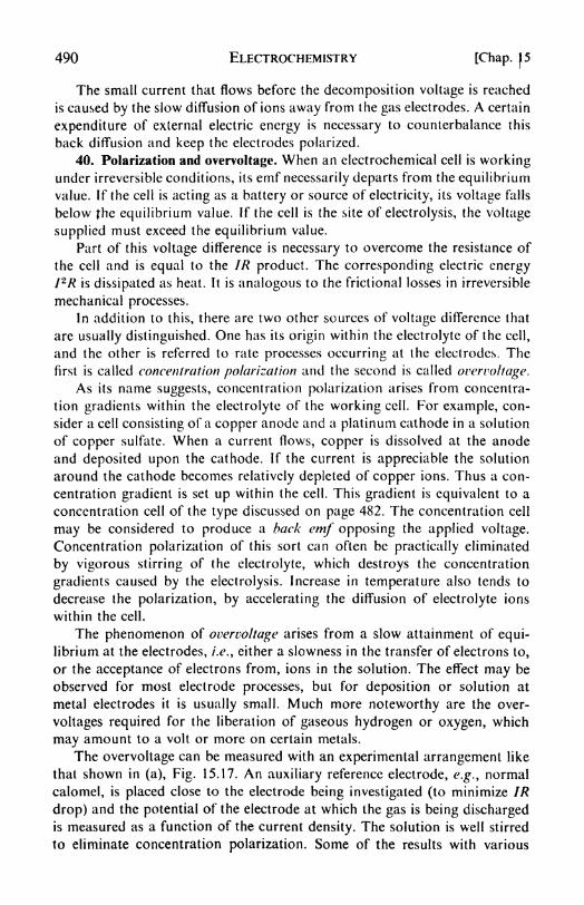
490 ELECTROCHEMISTRY [Chap. f5
The small current that flows before the decomposition voltage is reached
is caused by the slow diffusion of ions away from the gas electrodes. A certain
expenditure of external electric energy is necessary to counterbalance this
back diffusion and keep the electrodes polarized.
40. Polarization and overvoltage. When an electrochemical cell is workingunder irreversible conditions, its emf necessarily departs from the equilibrium
value. If the cell is acting as a battery or source of electricity, its voltage falls
below the equilibrium value. If the cell is the site of electrolysis, the voltage
supplied must exceed the equilibrium value.
Part of this voltage difference is necessary to overcome the resistance of
the cell and is equal to the IR product. The corresponding electric energyI 2R is dissipated as heat. It is analogous to the frictional losses in irreversible
mechanical processes.
In addition to this, there are two other sources of voltage difference that
are usually distinguished. One has its origin within the electrolyte of the cell,
and the other is referred to rate processes occurring at the electrodes. The
first is called concentration polarization and the second is called overvoltage,
As its name suggests, concentration polarization arises from concentra-
tion gradients within the electrolyte of the working cell. For example, con-
sider a cell consisting of a copper anode and a platinum cathode in a solution
of copper sulfate. When a current flows, copper is dissolved at the anode
and deposited upon the cathode. If the current is appreciable the solution
around the cathode becomes relatively depleted of copper ions. Thus a con-
centration gradient is set up within the cell. This gradient is equivalent to a
concentration cell of the type discussed on page 482. The concentration cell
may be considered to produce a back emf opposing the applied voltage.
Concentration polarization of this sort can often be practically eliminated
by vigorous stirring of the electrolyte, which destroys the concentration
gradients caused by the electrolysis. Increase in temperature also tends to
decrease the polarization, by accelerating the diffusion of electrolyte ions
within the cell.
The phenomenon of overvoltage arises from a slow attainment of equi-
librium at the electrodes, i.e., either a slowness in the transfer of electrons to,
or the acceptance of electrons from, ions in the solution. The effect may be
observed for most electrode processes, but for deposition or solution at
metal electrodes it is usually small. Much more noteworthy are the over-
voltages required for the liberation of gaseous hydrogen or oxygen, which
may amount to a volt or more on certain metals.
The overvoltage can be measured with an experimental arrangement like
that shown in (a), Fig. 15.17. An auxiliary reference electrode, e.g., normal
calomel, is placed close to the electrode being investigated (to minimize IR
drop) and the potential of the electrode at which the gas is being dischargedis measured as a function of the current density. The solution is well stirred
to eliminate concentration polarization. Some of the results with various
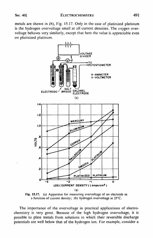
Sec. 40] ELECTROCHEMISTRY 491
metals are shown in (b), Fig. 15.17. Only in the case of platinized platinumis the hydrogen overvoltage small at all current densities. The oxygen over-
voltage behaves very similarly, except that here the value is appreciable even
on platinized platinum.
A-AMMETERV-VOLTMETER
-3 -2 -I
LOG ( CURRENT DENSITY ) ( amps/cm 2)
(b)
Fig. 15.17. (a) Apparatus for measuring overvoltage of an electrode as
a function of current density; (b) hydrogen overvoltage at 25C.
The importance of the overvoltage in practical applications of electro-
chemistry is very great. Because of the high hydrogen overvoltage, it is
possible to plate metals from solutions in which their reversible discharge
potentials are well below that of the hydrogen ion. For example, consider a

492 ELECTROCHEMISTRY [Chap. 15
cell consisting of platinum electrodes in a solution of zinc ions and hydrogenions at unit activity. The reversible potentials of the half cells are
of the zinc: i Zn \ Zn++ + e - 0.762
of the hydrogen : $H2=- H+ + e <T -
If hydrogen were discharged at its reversible potential, it should be liberated
at the cathode at a much lower voltage than that required to plate out zinc.
The overvoltage of hydrogen on zinc, however, amounts to about 1.0 v, so
that in an actual electrolysis, zinc will first be deposited on the cathode. The
hydrogen ion will not be discharged until the zinc concentration has fallen
to such a point that the emf of the zinc half cell lies above the hydrogen
overvoltage.
Many theories have been proposed to account for the overvoltage.28
They agree in postulating a slow step in the electrode reaction, which requires
the surmounting of a considerable potential energy barrier. For a charged
particle (ion) the applied emf serves to lower the energy barrier.
PROBLEMS
1. After passage of an electric current for 45 minutes, 7.19 mg of silver
are found to be deposited in a silver coulometer. Calculate the averagecurrent.
2. A conductivity cell filled with a 0.1 molar solution of potassiumchloride at 25C has a measured resistance of 24.96 ohms. Calculate the cell
constant if the conductivity K for 0.1 molar KC1 is 0.01 1639 ohm" l cm" 1 and
conductivity water with K =~ 7.5 x 10 8 ohm" 1 cirr 1is used to make up the
solutions. Filled with a 0.0 1 molar solution of acetic acid the cell resistance
is 1,982 ohms. Calculate the equivalent conductivity of acetic acid at this
concentration.
3. The following are the conductivities of chloroacetic acid in aqueoussolution at 25C:
1/r (liter/mole) . .16 32 64 128 256 512 1,024
equiv. cond., A . . 53.1 72.4 96.8 127.7 164 205.8 249.2
If A 362, are these values in accord with the Ostwald Dilution Law?
4. If the purest water has a conductivity of 6.2 x 10~8 ohm"1 cm"1 at
25C, calculate the K of a saturated solution of CO2 in water at 25C if the
CO2 pressure is maintained at 20 mm and the equilibrium constant for the
reaction, H2O(l) + CO2 (aq)=- HCO3
" + H+, is 4.16 x 10~ 7. The solu-
bility of CO2 in water follows Henry's Law with a constant k' --- 0.0290 mole
lir1 atm-1[cf. Maclnnes and Belek, J. Am. Chem. Soc., 55, 2630 (1933)].
5. The conductivity of a saturated solution of silver chloride in pure
28J. Bockris, Chem. Rev., 43, 525 (1948).

Chap. 15] ELECTROCHEMISTRY 493
water at 20C is 1.26 x 10~6 ohm"1 cm"1
higher than that for the water used.
Calculate the solubility of AgCl in water.
6. Draw a calculated curve showing how the conductivity of the solution
varies as 10 ml of 0.1 N NaOH is titrated with 1 1 ml of 0.1 N HC1.
7. An 0.01 N silver nitrate solution is used with silver electrodes in a
determination of the transference number of the Ag+ ion by the Hittorf
method; 32.10 mg of silver are deposited in a silver coulometer in series with
the Hittorf cell. At the end of the run the 20.09 g of solution in the anode
compartment are found to contain 39.66 mg of Ag; the 27.12 g of solution
in the cathode compartment contain 11.14mg of Ag. Calculate the Ag+transference number.
8. E. W. Washburn [J. Am. Chem. Soc., 31, 322 (1909)] measured the
transference of the ions in a KCI solution to which was added an inert
compound, raffinose, in order to detect the transport of water by the hydratedions. The original concentration of the KCI was 1.24molal, of raffinose
0.1 molal (formula: C 18H 32O16). Ag-AgCl electrodes were used. In a run with
5.3685 g silver deposited in the coulometer the following data were obtained:
Anode compartment, 103.21 g solution containing 6.510 per cent KCI,
4.516 per cent raffinose. Cathode compartment, 85.280 g, 10.030 per cent
KCI, 4.290 per cent raffinose. If tnw is number of moles of water transported
from anode to cathode for passage of one faraday of electricity, nsand nw
are number of moles of salt and of water in original solution, show that
/ _ JH (ng/nw)&nw . Here tu is the apparent (Hittorf) transference number
and / is the true transference number corrected for the transport of water.
Calculate /H and / in this experiment. If all the water of hydration is assumed
to be held by the K+ ion and none by the Cl~ ion, calculate the mean number
of molecules of water held by each K+ ion.
9. In a transport experiment in 0.02 molar NaCl solution at 25C by the
moving boundary method, Longsworth [J. Am. Chem. Soc., 54, 2741 (1932)]
found the boundary between NaCl and CdCl2 solutions to move 6.0 cm in
2,070 seconds with a current of 0.00160 amp. (Tube cross section 0.12 cm2.)
Calculate /4
.
10. From data in Table 15.4, calculate the transport number of the K4
ion in K 2SO4 .
11. From the following freezing-point depressions for aqueous solutions
of sodium chloride, calculate the activity coefficient ym of NaCl in 0.05 molal
solution [G. N. Lewis and M. Randall J. Am. Chem. Soc., 43, 1112
(1921)].
molality, m . . . 0.01 0.02 0.05 0.10 0.20 0.50
f. pt. dep. C . . 0.0361 0.0714 0.1758 0.3470 0.6850 1.677
12. From the molal activity coefficients in Table 15.5, calculate the mean
ionic activity in 0.1 molal solution of AgNO3, CuSO4 ,CaCl2 .

494 ELECTROCHEMISTRY [Chap. 15
13. The solubility of AgIO3 in KNO3 solutions has been measured byKolthoff and Lingane [J. Phys. Chem., 42, 133 (1938)] at 25C:
KNO3 , m/1 ... 0.001301 0.003252 0.006503 0.01410
AglO3 , m/1 x 104. . 1.761 1.813 1.863 1.908 1.991
Compare these results with the Debye-Huckel limiting law for solubilities
and calculate the activity coefficients of AgIO3 in the solutions.
14. Calculate the ionic strengths of one-molal solutions of KNO3 ,
K 2S04 ,K 4Fe(CN)6 .
15. Calculate the "thickness of the ionic atmosphere" according to the
Debye-Hiickel theory in 0.1 and 0.01 molar solutions of a uniunivalent
electrolyte in (a) water at 25C with dielectric constant 8 ^ 78; (b) 70 per
cent ethanol in water at 25C with F 38.5.
16. The solubility of barium sulfate in water at 25C is 0.957 x 10~5 mper liter. Using the Debye-HUckel theory, calculate AF for the change:BaSO4 (s)
=-- Ba++ f SO4
-(aq).
17. The solubility-product constant of AgCl at 25C is tf8p
--- (Ag)(Cl-)----- 1.20 x 10~ l
. Calculate from the Debye-Huckel theory (limiting law) the
solubility of AgCl in water and in a 0.01 M solution of (a) NaCl, (b) NaNO3 .
18. For an incompletely dissociated electrolyte the Onsager equation is:
A a[A (A { A )\/ac]. If we let A' [A (A + ^A )Vac] be
the equivalent conductivity at the actual ionic concentration (ac) in the
solution, it is evident that a A/A'. For dichloroacetic acid in 0.03 molar
solution at 25, A =-- 273 ohrrr 1 cm- 1. A is 388.5, Calculate the degree of
dissociation a from the Onsager expression. (Hint: use a procedure of
successive approximations to find A', starting with a A/A .)
19. Use the value of a calculated in problem 18 to obtain the thermo-
dynamic equilibrium constant for the dissociation of dichloroacetic acid.
The solution is so dilute that the activity of the undissociated acid can be set
equal to its concentration and the mean ionic activity can be calculated from
the Debye-Huckel limiting law.
20. A 0.1 molar H3PO4 solution is titrated with NaOH using methyl
orange as an indicator to an endpoint at /?H 4.3. The dissociation constants
of H 3PO4 are 7.5 x 10~ 3, 6 x 10~ 8
,and 3.6 x 10~13
. Calculate the fractions
of acid converted to H2PO4
~and HPO4 ~\
21. Calculate the /;H of a 0.1 M solution of ammonium lactate at 25C.Lactic acid, /?Ka 3.86; ammonia, /?K& 4.76.
22. In water solution, amino acids exist mainly as zwitterions, e.g.,
glycine as <NH3CH2COO . For ^NH3CH2COOH - +NH3CH2COO +H+, PK* 2.35 ; for +NH3CH2COO- - NH 2CH2COQ- + H+, PK*
~9.78.
Calculate the /?H of a 0.1 M glycine solution.
23. The /;H at which an amphoteric electrolyte yields an equal concen-
tration of positive and negative ions is called the isoelectric point. Show that
Chap. 15] ELECTROCHEMISTRY 495
if the activity coefficients of all the ions are taken as unity, this /?H-=
|(/>Ka + />Kb). Hence estimate the isoelectric point of glycine from the data
in the previous problem.
24. Devise cells in which the cell reactions are the following:
(a) 2 AgBr |H 2
- 2 Ag -} 2 HBr
(b) H 2 + I 2- 2 HI
(c) S2 8 \2 I~ I 2 + 2 S04
(d) 2 Fe+3 + CH3CHO |H2O - 2 Fe42 f CH 3COOH I 2 H^
(e) Ni f 2 H 2O - Ni(OH)2 + H2
Write down the cells with proper regard for the sign convention. Calculate
the <f for these cells from the standard electrode potentials. Assume any
liquid-junction potentials are eliminated. The solubility of AgBr is 2.10 x
10~G mole per liter.
25. Mercuric nitrate and ferrous nitrate, each in 0.01 molar solution, are
mixed in equal volumes at 25C. From the standard potentials in Table 15.8,
find the equilibrium concentration of ferric ion in the solution. Activity
coefficients may be estimated from the Debye-Huckel Limiting Law.
26. Calculate the values of the oxidation potential ff of the electrode
Pt/Fe+4
, Fe'++ as a function of the per cent oxidized form. Use concentra-
tions in place of activities. Plot the results.
27. A solution 0.1 molar in lactic acid is mixed with an equal volume of
a 0.1 molar methylene blue solution. Calculate the equilibrium concentration
of lactic acid given the following oxidation potentials at 25 C:
methylene white --methylene blue 4- 2 H +
I 2e' V 0.53 v
lactic acid -=pyruvic acid I 2 H f
f- 2e~ f> =-- 0.20 v
28. The emf 's of the cell H2/HCl (/w)/AgCl/Ag at 25C are as follows
[cf. Harned and Ehlers, J. Am. Chem. Soc., 54, 1350 (1932)]:
<f
0.38568
0.35393
0.35316
0.31774
Calculate <f for the cell by the following method of graphical extrapolation.
We can write - ^ A log aHCl where A = 2.303 RT/&. This becomes
S -| 2A log AW ^ S>' - 2A log y+ . From Debye-Huckel theory, logy f
~BVm. Thus: S + 2A log w -= + 2ABVm. Plot the left side of this
expression vs. Vm and extrapolate to m 0, the intercept giving 6n
\ (See
Harned's paper for a more precise method of extrapolation.)
29. From the value of obtained above and the measured emf 's, cal-
culate the mean activity coefficients y of HCI at the various concentrations.
496 ELECTROCHEMISTRY [Chap. 15
30. The cell, Sn(liq)/SnCl2 in molten KC1 + LiCl/Sn-Sb liquid solution,
was measured at 905K at various mole fractions of tin in the solution with
antimony:
XBn . .0.1 0.2 0.3 0.4 0.5 0.6 0.7 0.8 0.9
*<v). . 0.11984 0.08379 0.05905 0.04545 003705 0.02845 0.01725 0.00992 0.00523
If pure liquid tin is chosen as the standard state, AF = FA F% =--
= RTln aA , where aA is the activity of tin in the electrode solution. Plot ySnand ysb as functions of TSn .
31. The emf of the cell H2(/>)/0.1 m HCl/HgCl/Hg was studied as a
function of the hydrogen pressure at 25:
P(atm) . . 1.0 37.9 51.6 110.2 286.6 731.8 1035.2
. . 399.0 445.6 449.6 459.6 473.4 489.3 497.5
Calculate the activity coefficients of hydrogen gas (y -=f/P) and plot them
as a function of the pressure over the given range.
32. For the cell H2/HCl/AgCl/Ag, <T --= 0.222 v. If the measured emf is
0.385 v what is the pli of the HCl solution?
33. Copper is being plated onto a platinum electrode from a 0.5 molar
copper sulfate solution, 0.01 molar in H2SO4 . If the hydrogen overvoltageon copper is 0.23 v, what will be the residual Cu++ concentration in the
solution when H2 evolution begins at cathode?
34. It is desired to separate Cd f+ and Zn H by electrolytic deposition of
the Cd n . The ff for the cadmium electrode is 0.402 v, for the zinc 0.762 v.
The overvoltages are Cd ^ 0.48 v; Zn = 0.70 v. Discuss the feasibility of
the separation in a solution originally 0.1 molar in Zn f+ and Cd4"1".
REFERENCES
BOOKS
1. Butler, J. A. V., Electrical Phenomena at Interfaces (London: Methuen,
1951).
2. Glasstone, S., Introduction to Electrochemistry (New York: Van Nos-
trand, 1942).
3. Gurney, R. W., Ionic Processes in Solution (New York: McGraw-Hill,
1953).
4. Harned, H. H., and B. B. Owen, Physical Chemistry of Electrolytic
Solutions (New York: Reinhold, 1943).
5. Kolthoff, I. M., and H. A. L fd\tenan 9 pH and Electrotitrations(New York:
Wiley, 1941).
6. Latimer, W. M., Oxidation Potentials (New York: Prentice-Hall, 1952).
7. Luder, W. F., and S. Zuffanti, The Electronic Theory of Acids and Bases
(New York: Wiley, 1946).
8. Maclnnes, D. A., The Principles of Electrochemistry (New York: Rein-
hoU, 1939).

Chap. 15] ELECTROCHEMISTRY 497
ARTICLES
1. Audrieth, L. F., and T. Moeller, /. Chem. Ed., 20, 219-222 (1943), "Acid-
Base Relationships at Higher Temperatures."2. Bockris, J. O., Chem. Rev., 43, 525-575 (1948), "The Hydrogen Over-
potential."
3. Denbigh, K. G., J. Chem. Ed., 18, 126-130 (1941), "Theory of the
Solubility Product."
4. Hamer, W. J., /. Electrochem. Soc., 99, 331c-343c (1952), "Fifty Years
of Electrochemical Theory."5. Harned, H. S., Chem. Rev., 40, 461-522 (1947), "Diffusion in Electrolyte
Solutions."
6. Luder, W. F., and A. A. Vernon, J. Chem. Ed., 22, 63-67 (1945),
"Electrochemical Conventions."
7. Maclnnes, D. A., Science in Progress, vol. II (New Haven: Yale Univ.
Press, 1940), 197-231, "Motion of Ions and Proteins in Electric Fields."
8. Merrill, R. C, J. Chem. Ed., 27, 312-328 (1950), "Colloidal Electrolytes."
9. Owen B. B., /. Chem. Ed., 21, 59-63 (1944), "Effect of Pressure on the
Properties of Electrolytic Solutions."
10. van Rysselberghe, P., and A. H. Gropp, J. Chem. Ed., 21, 96-99 (1944),
"Solubility Products of Metallic Sulfides."

CHAPTER 16
Surface Chemistry
1. Surfaces and colloids. When in Chapter 5 we defined the concept of
phase and discussed the thermodynarnic treatment of phase equilibria, we
were careful to impose a restriction on the validity of the results obtained,
owing to our neglect of any effects that might arise from variation of the
interfacial areas separating different phases. Furthermore, a phase was
defined as a part of a system that was "homogeneous throughout." Such a
definition implies that the matter deep in the interior of a phase is subject
to exactly the same conditions as the matter at the exterior which forms the
surface. This is clearly impossible in any case, since the molecules (or ions)
in the interior are surrounded on all sides by the uniform field of force of
neighbor molecules (or ions) of the same
substance. The molecules at the surface are
bounded on one side by neighbors of the
same kind but on the other side by an entirely
different sort of environment.
Consider, for example, the surface of a
liquid in contact with its vapor, shown in Fig.
16.1. A molecule in the interior of the liquid is
Fig. 16.1. Liquid-vapor*n a un^ rm field f force. A molecule at the
interface. surface is subject to a net attraction toward
the bulk of the liquid, which is not compen-sated by an equal attraction from the more highly dispersed vapor molecules.
Thus all liquid surfaces, in the absence of other forces, tend to contract to the
minimum area. For example, freely suspended volumes of liquid assume a
spherical shape, since the sphere has the minimum surface-to-volume ratio.
In order to extend the area of an interface like that in Fig. 16.1, i.e., to
bring molecules from the interior into the surface, work must be done
against the cohesive forces in the liquid. It follows that the surface portions
of the liquid have a higher free energy than the bulk liquid. This extra
surface free energy is more usually described by saying that there is a surface
tension, acting parallel to the surface, which opposes any attempt to extend
the interface. A tension is a negative 'pressure; pressure is a force per unit
area, so that surface pressure is a force per unit length. If the surface tension
is y, the work done by the surface in extending its area by an amount da is
dw =-- --y da dF, whence
dF=ydo (16.1)
where dF is the change in free energy.
498

Sec. 1] SURFACE CHEMISTRY 499
The units of surface tension are evidently dynes per cm in the COSsystem. The problems arising in the measurement and interpretation of the
surface tension will be taken up later in this chapter. The subject was intro-
duced here at the beginning to illustrate the new type of variable that enters
into the description of physicochemical systems as soon as surfaces are
explicitly considered. Since the surface of a liquid does not have the same
free energy as the bulk liquid, it cannot be said to be in the same thermo-
dynamic state or to be part of the same phase.When will it be necessary to consider these surface effects? First of all
it will obviously be necessary when we wish deliberately to focus our atten-
tion on interfacial phenomena rather than bulk properties. Secondly, there
will be instances when the interfacial phenomena must be taken into con-
sideration in order to study the system at all. This second case will arise
when any considerable fraction of the material in the system exists at or near
interfaces.
The degree of subdivision or particle size of a substance is usually the
decisive factor determining iis surface-to-volume ratio. Extremely porousmaterials are apparently exceptional cases, but these materials may often be
treated as loose aggregates of very small particles. For example, suppose wehave a gram of crystalline silica. If for simplicity the crystals, with density p,
are considered to be small cubes, all of side /, their total surface area will be
6/2 _ 6
pP~~pl
With p = 2.30, the following results are obtained for the surface area in cm2
per gram at various particle sizes:
/ (cm) A (cm2/g)
JO- 1 26.1
10~32,610
10 5261,000
10~82,610,000
10-726,100,000
It is evident that the area increases enormously as the particle size de-
creases. The lower end of the scale, with / below about 10 7 cm or 10 A,
corresponds to the dimensions expected for ordinary molecules. Fromaround 10~ 7 to 10 4 cm there extends the domain of colloids. For particles
of colloidal dimensions surface phenomena play a preeminent role, and
indeed much of colloidal chemistry is essentially surface chemistry. This
entire field is one of extraordinary interest because of its intimate connection
with biochemical and physiological processes. The building blocks of living
matter, protein molecules, are so large that their dimensions fall within the
colloidal realm. From the viewpoint of physical chemistry the living cell is a
complex colloidal system.The great variety of possible colloidal systems may be recalled by

500 SURFACE CHEMISTRY [Chap. 16
reference to Table 16. 1 where they are classified according to the kinds of dis-
persed phase and dispersion medium. We shall be able to discuss only a few
of these systems; a fairly comprehensive treatment would require another
book at least as large as this one.
TABLE 16.1
CLASSIFICATION OF COLLOIDS
DispersionMedium
GasGas
Liquid
Liquid
LiquidSolid
Solid
DispersedPhase
LiquidSolid
Gas
LiquidSolid
GasSolid
Examples
Aerosols: fogs, mists
Aerosols : smokesGas emulsions: foamsEmulsions
Suspensions : sols and gelsSolid foams
(e.g., pumice)Solid sols (e.g., colloidal gold in glass)
2. Pressure difference across curved surfaces. Interfaces between two
liquids and between a liquid and a vapor are most conveniently studied,
because the molecules in fluids are not
rigidly fixed in position. They therefore
tend to adjust themselves to changes at
the interface in such a way as to record
automatically the surface tension. This
possibility does not arise with liquid-solid
or solid-gas interfaces, and measurement
of the interfacial tensions in these cases
is made by indirect methods.
As a direct consequence of the exist-
ence of a surface tension, it can be shown
that across any curved liquid surface there
must exist a difference in pressure, the
pressure being greater on the concave side
than on the convex side.
If a curved surface is displaced parallel
to itself to a new position, its area must
change if its curvature is to remain the
same. Work must be done against the surface tension to effect this changein area.
In Fig. 16.2 is shown a spherical bubble of gas of radius R at the end of
a fine capillary tube fitted with a piston. Let the equilibrium pressure inside
the bubble be AP. It will be assumed that this pressure is entirely due to the
surface tension, i.e., the effect of the weight of the liquid will be neglected.
Suppose the piston is advanced so as to expand the bubble radius by dR,
thereby increasing its surface area 4irR2 by STT/? dR9 and its volume faR
9by
Fig. 16.2. The pressure difference
across a curved interface.

Sec. 3] SURFACE CHEMISTRY 501
The work done against the surface tension y dA is equal to the
work done in the expansion at constant pressure (P dV) 9 so that
dR)
and (16.2)
This result applies to liquid-liquid as well as to gas-liquid interfaces. For a
more general curved surface with radii of curvature Rl and R2 it becomes1
A/> = y\-^ (16.3)
3. Capillary rise. The rise or fall of liquids in capillary tubes and its
application to the measurement of surface tension may now be treated as a
direct consequence of the fundamental eq. (16.2). Whether a liquid rises in
*'-*
cos9
Fig. 16.3. Capillary rise.
a glass capillary, like water, or is depressed, like mercury, depends on the
relative magnitude of the forces of cohesion between the liquid molecules
themselves, and the forces of adhesion between the liquid and the walls of
the tube. These forces determine the contact angle 0, which the liquid makes
with the tube walls (Fig. 16.3). If this angle is less than 90, the liquid is
said to wet the surface and a concave meniscus is formed. A contact angle
of 90 corresponds to a plane meniscus; a contact angle greater than 90, to
a convex meniscus.
The occurrence of a concave meniscus leads to a capillary rise. The
pressure under the meniscus is less than that at the plane surface of liquid
outside the tube. Liquid rises in the tube until the weight of the liquid column
balances the pressure difference. The liquid column acts as a manometer to
register the pressure difference across the concave meniscus.
Consider, Fig. 16.3, a cylindrical tube whose radius r is sufficiently small
that the surface of the meniscus can be taken as a section of a sphere with
radius R. Then, since cos = r/R, from eq. (16.2) AP = (ly cos 0)/r. If
the capillary rise is h, and if p and/3
are the densities of the liquid and
the surrounding fluid, the weight of the cylindrical liquid column is
1 N. K. Adam, Physics and Chemistry of Surfaces (New York: Oxford, 1944, p. 8).

502 SURFACE CHEMISTRY [Chap. 16
rrr2gh(p
-PQ), or the force per unit area balancing the pressure difference
is gh(p PQ). Therefore
2ycos<9 1 1-A,), 7 -
**(P-
Po) r
In many cases the contact angle is practically zero, and if the surround-
ing fluid is a vapor, its density p is negligible compared to p. These approxi-
mations lead to the frequently used formula:
y ^Ipghr (16.4)
4. Maximum bubble pressure. Blowing bubbles provides a second con-
venient way of measuring surface tensions. Consider a bubble being formed
at the end of a small tube immersed in liquid. As one begins to apply pressure,
the radius of the bubble is comparatively large. As the bubble grows, the
radius at first decreases until it reaches a minimum when the bubble is a
hemisphere with a radius equal to that of the small tube. Any further increase
in pressure will lead to the loss of the bubble, which will expand and free
itself from the tube.
It is clear from eq. (16.2) that the maximum pressure that the bubble can
sustain will be that at the position of minimum radius. The applied pressure
is balanced by the pressure difference across the curved surface plus a hydro-static pressure depending on the depth h of the tube outlet under the liquid.
Therefore the surface tension is determined from
Anax ^ 7 4 gh(p ~Po) (16.5)
5. The Du Noiiy tensiometer. Frequently used for measurements of surface
or interfacial tension is the tensiometer designed by Lecomte Du Noiiy. Aplatinum ring of radius r is attached to a torsion balance, and the force
required to remove the ring from the surface or interface is measured directly.
The surface tension acts over the circumference of the ring and there are
two sides to the new surface that is formed, so that the applied force/--=
4?rry.
A number of correction factors are necessary for precise work. 2
6. Surface-tension data. Some values for the surface tensions of pure
liquids are collected in Table 16.2. Liquids with exceptionally high surface
tensions, such as water, are those in which the cohesive forces between the
molecules are large, the surface tension being a measure of the work that
must be done to bring a molecule from the interior to the surface. We might
expect liquids with high surface tension to have high internal pressures, and
this relationship is in general confirmed by a comparison of Table 16.2 with
Table 14.2.
The surface tensions of solutions may be given a simple qualitative inter-
pretation. Consider, for example, aqueous solutions. Substances that
2 P. Lecomte Du Nouy, /. Gen. Physiol., 7, 521 (1918); 7, 403 (1925).

Sec. 6J SURFACE CHEMISTRY 503
TABLE 16.2
SURFACE TENSION DATA
A. Surface Tensions of Pure Substances at 20C Dynes per Cm
IsopentaneNickel carbonylDiethyl ether .
/i-Hexane
Ethyl mercaptanEthyl bromide
13.72
14.6
17.10
18.43
21.82
24.16
Ethyl iodide .
BenzeneCarbon tetrachloride
Methylene iodide .
Carbon bisulfide
Water .
29.9
28.86
26.66
50.76
32.33
72.75
B. Surface Tensions of Liquid Metals and Molten Salts
markedly lower the surface tension of water are those that, like the fatty
acids, contain both a polar hydrophilic group and a nonpolar hydrophobic
group. The hydrophilic group, e.g., COOH in the fatty acids, makes the
molecule reasonably soluble if the nonpolar residue is not too predominant.One may expect the hydrocarbon residues in the fatty acids to be extremelyuncomfortable3
in the interior of an aqueous solution, and little work is
required to persuade them to come from the interior to the surface. This
qualitative picture leads to the conclusion that solutes lowering the surface
tension of a liquid tend to accumulate preferentially at the surface. They are
said to be positively adsorbed at the interface.
On the other hand, solutes such as ionic salts usually increase the surface
tension of aqueous solutions above the value for pure water, although these
increases are much smaller than the decreases produced by fatty acids and
similar compounds. The reason for the observed increases is that the dis-
solved ions, by virtue of ion-dipole attractions, tend to pull the water mole-
cules into the interior of the solution. Additional work must be done againstthe electrostatic forces in order to create new surface. It follows that in such
solutions the surface layers are poorer in solute than is the bulk solution. The
solute is said to be negatively adsorbed at the interface.
After the thermodynamic treatment of surfaces has been discussed, it
will be possible to give these qualitative conclusions a more quantitative
formulation.
3 A way of saying the free energy of the state is high.
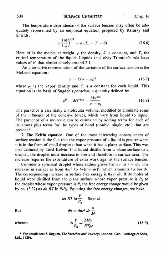
504 SURFACE CHEMISTRY [Chap. 16
The temperature dependence of the surface tension may often be ade-
quately represented by an empirical equation proposed by Ramsay and
Shields:
y^-j =*'(re -r-6) (16.6)
Here A/ is the molecular weight, p the density, k' a constant, and Tc the
critical temperature of the liquid. Liquids that obey Trouton's rule have
values of k' that cluster closely around 2.1.
An alternative representation of the variation of the surface tension is the
McLeod equation:
y ^ C(p A,)4
(16.7)
where pQ is the vapor density and C is a constant for each liquid. This
equation is the basis of Sugden's parachor, a quantity defined by
My174
^ - A/C1/4 - (16.8)P-
PQ
The parachor is essentially a molecular volume, modified to eliminate some
of the influence of the cohesive forces, which vary from liquid to liquid.
The parachor of a molecule can be estimated by adding terms for each of
its atoms plus terms for the types of bond (double, single, etc.) that are
present.4
7. The Kelvin equation. One of the most interesting consequences of
surface tension is the fact that the vapor pressure of a liquid is greater whenit is in the form of small droplets than when it has a plane surface. This was
first deduced by Lord Kelvin. If a liquid distills from a plane surface to a
droplet, the droplet must increase in size and therefore in surface area. The
increase requires the expenditure of extra work against the surface tension.
Consider a spherical droplet whose radius grows from r to r + dr. The
increase in surface is from 4-rrr2 to 4n(r -\- dr)
2, which amounts to STTT dr.
The corresponding increase in surface free energy is fayr dr. If dn moles of
liquid were distilled from the plane surface whose vapor pressure is P to
the droplet whose vapor pressure is P, the free energy change would be given
by eq. (3.32) as dn RT\nP/PQ . Equating the free energy changes, we have
PdnRTln- = Snyr dr
M)
But dn = 4rrr2 dr fM
whence \n ~- = ~~(16.9)
4 For details see: S. Sugden, The Parachor and Valency (London: Geo. Rutledge & Sons,
Ltd., 1929).
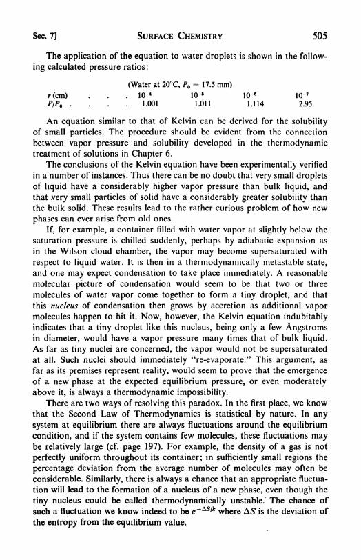
Sec. 7] SURFACE CHEMISTRY 505
The application of the equation to water droplets is shown in the follow-
ing calculated pressure ratios :
(Water at 20C, /> = 17.5 mm)
r(cm) . . . 10-* 10-6 10-6 1Q-7
P/Po .1.001 1.011 1.114 2.95
An equation similar to that of Kelvin can be derived for the solubility
of small particles. The procedure should be evident from the connection
between vapor pressure and solubility developed in the thermodynamictreatment of solutions in Chapter 6.
The conclusions of the Kelvin equation have been experimentally verified
in a number of instances. Thus there can be no doubt that very small dropletsof liquid have a considerably higher vapor pressure than bulk liquid, and
that .very small particles of solid have a considerably greater solubility than
the bulk solid. These results lead to the rather curious problem of how new
phases can ever arise from old ones.
If, for example, a container filled with water vapor at slightly below the
saturation pressure is chilled suddenly, perhaps by adiabaiic expansion as
in the Wilson cloud chamber, the vapor may become supersaturated with
respect to liquid water. It is then in a thermodynamically metastable state,
and one may expect condensation to take place immediately. A reasonable
molecular picture of condensation would seem to be that two or three
molecules of water vapor come together to form a tiny droplet, and that
this nucleus of condensation then grows by accretion as additional vapormolecules happen to hit it. Now, however, the Kelvin equation indubitably
indicates that a tiny droplet like this nucleus, being only a few Angstromsin diameter, would have a vapor pressure many times that of bulk liquid.
As far as tiny nuclei are concerned, the vapor would not be supersaturated
at all. Such nuclei should immediately "re-evaporate." This argument, as
far as its premises represent reality, would seem to prove that the emergenceof a new phase at the expected equilibrium pressure, or even moderatelyabove it, is always a thermodynamic impossibility.
There are two ways of resolving this paradox. In the first place, we knowthat the Second Law of Thermodynamics is statistical by nature. In any
system at equilibrium there are always fluctuations around the equilibrium
condition, and if the system contains few molecules, these fluctuations maybe relatively large (cf. page 197). For example, the density of a gas is not
perfectly uniform throughout its container; in sufficiently small regions the
percentage deviation from the average number of molecules may often be
considerable. Similarly, there is always a chance that an appropriate fluctua-
tion will lead to the formation of a nucleus of a new phase, even though the
tiny nucleus could be called thermodynamically unstable.' The chance of
such a fluctuation we know indeed to be e~~^lk where AS is the deviation of
the entropy from the equilibrium value.

506 SURFACE CHEMISTRY [Chap. 16
It is unlikely, however, that new phases often arise by this fluctuation
mechanism and the resultant spontaneous nucleation. Calculations show that
the chance e~~*sik is usually much too small. It is more likely that tiny solid
particles, e.g., dust particles, act as nuclei for further condensation or for
crystallization in supersaturated vapors or solutions. Actually, super-saturated vapors seem to be much less finicky than supersaturated solutions
about the sort of nuclei that are required. This is because a liquid will con-
dense on almost any surface, but crystallization requires the presence of
crystal faces of the proper kind. We are perhaps all familiar with the legend-
ary organic chemist who prepared a compound for the first time, and wasunable to bring it to crystallization. A call to a friend brought some seed
crystals, and no sooner was the envelope opened than the solution at the
other end of the laboratory began to crystallize. Thereafter no difficulty wasever experienced in crystallizing that particular compound: the seeds were in
the air.
The phenomena in the change liquid ^- vapor are similar. We have all
been troubled with the bumping of liquids and have learned to use boiling
chips. It has been shown by E. N. Harvey that water carefully freed fromall dissolved gases can be heated to 200C before ebullition takes place, withalmost explosive violence. 5
8. Thermodynamics of surfaces. In Fig. 16.4 are represented two phases,a and
ft, separated by an interfacial region. The exact position of this region
depends on how we choose to draw the
A A1
boundary planes AA' and BB'. It seems
S <r S* reasonable to place these planes so that
B B' the following condition is satisfied: thereP is no appreciable inhomogeneity in the
Fig. 16.4. Definition of surface properties of the bulk phase a up to the
phase. surface AA', nor in those of phase /? upto the surface BB'. Within the interfacial
region the properties of the system vary continuously from purely a- at
AA' to purely /?- at BB'. Because of the short range of intermodular
forces, the interfacial region will usually be not more than a few molecular
diameters in thickness. 6
Any surface SS' drawn within the interfacial region parallel to the sur-
faces A A' and BB' is called a surface phase, and is designated by a symbol a.
A surface phase defined in this way has an area but no thickness. It is a
strictly two-dimensional phase. Its area will be denoted by Aa.
The composition of the surface phase will be described in terms of
quantities n. We define n as the number of moles of component / in the6 E. N. Harvey et a/., J. Am. Chem. Soc., 67, 156 (1945).6
It should be noted, however, that the attractive forces exerted by an extended surfacehave a much longer range than those from an isolated molecule. The latter depend on r~\and the former fall off as /-*. For an extensive survey of the depth of the surface zone seeJ. C. Henniker, Rev. Mod. Phys. 21, 322 (1949).

Sec. 9] SURFACE CHEMISTRY 507
surface film region, between AA' and BB', minus the number of moles of /
that would be within this region if the phases a and ft both extended all the
way to the surface SS' with unchanged bulk properties. It is evident accord-
ing to this definition that n? may be either positive or negative. Now the
surface concentration c, in moles per square centimeter, is defined by
<V = ^ (16.10)
Other thermodynamic functions, such as surface energya
, surface
entropy 5, surface free energy F 9 can be defined by exactly the same method
used for the n. They are the differences between the energy, entropy, or free
energy of the actual interfaciai region and the values calculated on the
assumption that the phases remain uniform up to the dividing surface.
It .is always possible to place the dividing surface SS' so that for one
particular component (O) the surface concentration, cQa
is zero; i.e., the
number of moles of component (O) in the interfaciai film between A A' and
BB' is exactly what it would be if the bulk phases a and ft both remained
homogeneous right up to the dividing surface SS'. When the position of the
interface is chosen in this way, the surface concentrations c of the other
components are said to be the concentrations adsorbed at the interface. This
adsorption can be either positive or negative. In the examples previously
considered, solutes dissolved in water, it was found that fatty acids were
positively adsorbed at the solution-vapor interface, whereas ionic salts
tended to be negatively adsorbed. Now that this concept of adsorption has
been given a precise definition, it is possible to derive a thermodynamicrelation between the extent of adsorption and the change in the surface
tension of the solution. This relation is the famous Gibbs adsorption isotherm.
Its derivation proceeds very similarly to that of the Gibbs-Duhem equationdiscussed on page 117.
9. The Gibbs adsorption isotherm. We shall consider a system that, for
simplicity, consists of two components distributed in two bulk phases with
a surface phase a. Then, in addition to the ordinary state variables describing
the bulk phases, new state variables must be introduced to define the state
of the surface phase. Our consideration will be restricted to a system at
constant temperature and pressure and constant composition of the bulk
phases. For the bulk phases alone the differential of the free energy function
would be, from eq. (4.27), dF =------- S* dT - S** dT + Fa dP f Vft dP +a t dnf + /^i dn-f + jn2 dn + A/2 dn2
ft. This entire expression vanishes at
constant temperature, pressure, and composition.When the surface phase is considered we must add the following terms:
dFa = ~Sa dT+y dA af- ^ dnf f /i2 dn
At constant temperature this differential of the surface free energy becomes
dFa - y dA + p l dn{ + fi2 dn2a
(16.1 1)

508 SURFACE CHEMISTRY [Chap. 16
Integrating this expression while holding the intensity factors constant
(or using Euler's theorem), we obtain
F = yA + wf + //2<The complete differential is therefore
dFa - y dA |- Aady ~\- ^ dnf + nf d^ + //2 dn2 + < dfa
Comparison with eq. (16.1 1) yields
A* dy = n d^ n2a du2
Division by Aagives
dy = -cf dfr-cf <//<a (16.12)
Let us now choose the dividing surface so that the excess of one com-
ponent (1), which may be called the solvent, vanishes. Then
dy ------ -Ta <//i 2 (16.13)
where F2 is the concentration of component (2) adsorbed at the interface.
Equation (16.13) may be written [from eq. (6.32)]
dy = -RTP2 dlna2 (16.14)
For an ideal solution, a2~= X2 , the mole fraction, so that
rfy=- -RTT2 d\n X2
For a dilute solution, X2 becomes proportional to c2 , the molar concentra-
tion, and
1 dv(16.16)
These equations are various forms of the Gibbs adsorption isotherm.
The isotherm has been experimentally verified by the ingenious experimentsof J. W. McBain at Stanford University. He employed an adaptation of a
swiftly moving microtome to slice off the top layer (around 0.05 mm) from
a solution and scoop it into a sample tube. The composition of this layer
could then be taken to determine F2, and this experimental F2 could be
compared with that calculated, via the Gibbs isotherm, from the variation
of the surface tension with the concentration of the bulk solution.
The isotherm may also be verified indirectly in a quite remarkable waywhich will be revealed in a following section, after another technique for
studying surface films has been described.
10. Insoluble surface films the surface balance. As a result of the pioneerwork of Fraulein Pockels (1891) and Lord Rayleigh (1899) it was discovered
that in some cases sparingly soluble substances would spread over the
surface of liquids to form a film exactly one molecule thick. These uni-
molecular films may be regarded as essentially two-dimensional states of
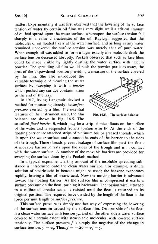
Sec. 10] SURFACE CHEMISTRY 509
matter. Experimentally it was first observed that the lowering of the surface
tension of water by certain oil films was very slight until a critical amount
of oil had spread upon the water surface, whereupon the surface tension fell
sharply to a value characteristic of the oil. Rayleigh suggested that the
molecules of oil floated freely at the water surface, and as long as any water
remained uncovered the surface tension was merely that of pure water.
When enough oil was added to form a layer exactly one molecule thick the
surface tension decreased abruptly. Pockels observed that such surface films
could be made visible by lightly dusting the water surface with talcum
powder. The spreading oil film would push the powder particles away, the
area of the unpowdered portion providing a measure of the surface covered
by the film. She also introduced the
valuable technique of cleaning the water
surface by sweeping it with a barrier
which pushed any surface contamination
to the end of the tray.
In 1917, Irving Langmuir devised a
method for measuring directly the surface
pressure exerted by a film. The essential
features of the instrument used, the film Fig. 16.5. The surface balance,
balance, are shown in Fig. 16.5. The
so-called fixed barrier B, which may be a strip of mica, floats on the surface
of the water and is suspended from a torsion wire W. At the ends of the
floating barrier are attached strips of platinum foil or greased threads, which
lie upon the water surface and connect the ends of the barrier to the sides
of the trough. These threads prevent leakage of surface film past the float.
A movable barrier A rests upon the sides of the trough and is in contact
with the water surface. A number of the movable barriers are provided for
sweeping the surface clean by the Pockels method.
In a typical experiment, a tiny amount of the insoluble spreading sub-
stance is introduced onto the clean water surface. For example, a dilute
solution of stearic acid in benzene might be used; the benzene evaporates
rapidly, leaving a film of stearic acid. Now the moving barrier is advanced
toward the floating barrier. As the surface film is compressed it exerts a
surface pressure on the float, pushing it backward. The torsion wire, attached
to a calibrated circular scale, is twisted until the float is returned to its
original position. The required force divided by the length of the float is the
force per unit length or surface pressure.
This surface pressure is simply another way of expressing the loweringof the surface tension caused by the surface film. On one side of the float
is a clean water surface with tension y , and on the other side a water surface
covered to a certain extent with stearic acid molecules, with lowered surface
tension y. The surface pressure / is simply the negative of the change in
surface tension, y y . Thus,/ Ay = yQ y.
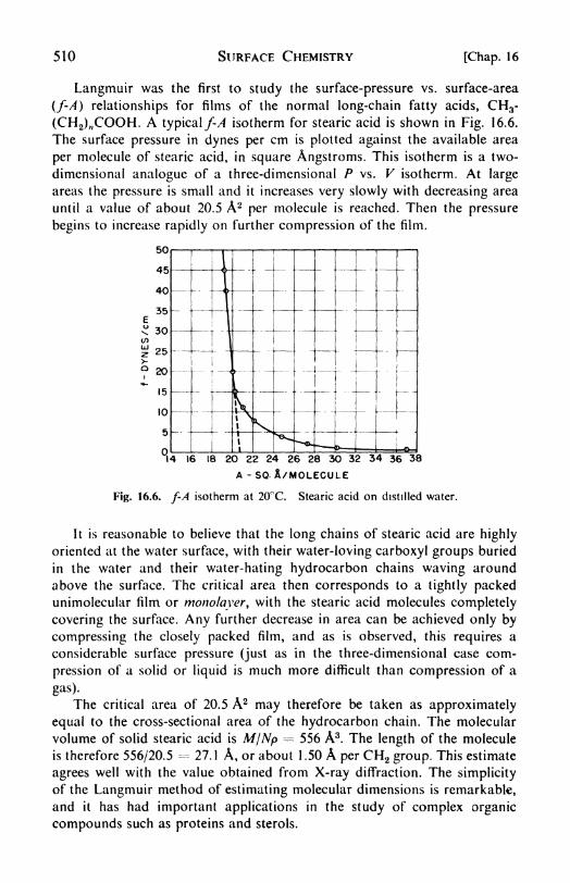
510 SURFACE CHEMISTRY [Chap. 16
Langmuir was the first to study the surface-pressure vs. surface-area
(f-A) relationships for films of the normal long-chain fatty acids, CH3-
(CH2 ),tCOOH. A typical/-/f isotherm for stearic acid is shown in Fig. 16.6.
The surface pressure in dynes per cm is plotted against the available area
per molecule of stearic acid, in square Angstroms. This isotherm is a two-
dimensional analogue of a three-dimensional P vs. V isotherm. At large
areas the pressure is small and it increases very slowly with decreasing area
until a value of about 20.5 A2per molecule is reached. Then the pressure
begins to increase rapidly on further compression of the film.
14 16 18 20 22 24 26 28 3O 32 34 36 38
A -SQ. A/MOLECULE
Fig. 16.6. f-A isotherm at 20C. Stearic acid on distilled water.
It is reasonable to believe that the long chains of stearic acid are highly
oriented at the water surface, with their water-loving carboxyl groups buried
in the water and their water-hating hydrocarbon chains waving around
above the surface. The critical area then corresponds to a tightly packedunimolecular film or monolayer, with the stearic acid molecules completely
covering the surface. Any further decrease in area can be achieved only by
compressing the closely packed film, and as is observed, this requires a
considerable surface pressure (just as in the three-dimensional case com-
pression of a solid or liquid is much more difficult than compression of a
gas).
The critical area of 20.5 A2may therefore be taken as approximately
equal to the cross-sectional area of the hydrocarbon chain. The molecular
volume of solid stearic acid is MjNp = 556 A3. The length of the molecule
is therefore 556/20.5 = 27. 1 A, or about 1.50 A per CH2 group. This estimate
agrees well with the value obtained from X-ray diffraction. The simplicity
of the Langmuir method of estimating molecular dimensions is remarkable,
and it has had important applications in the study of complex organic
compounds such as proteins and sterols.

Sec. 11] SURFACE CHEMISTRY 511
11. Equations of state of monolayers. The detailed study of various sub-
stances in unimolecular films has revealed a great variety in the observed
f-A isotherms. Sometimes the films appear to behave like two-dimensional
gases, sometimes like two-dimensional liquids or solids. In addition, there
are other types of monolayer that seem to have no exact analogues in the
three-dimensional world. They can be recognized, however, at definite
surface phases by the discontinuities in the f-A diagram which signal their
occurrence.
In Fig. 16.7 are a series off-A isotherms obtained for a number of the
fatty acids CnH2nflCOOH at 25C. These curves resemble the P-V isotherms
Fig. 16.7. f-A isotherms at low pressures.
for a gas in the neighborhood of the critical temperature. There is a section
at low pressures corresponding to the high compressibility of a gas. Then
there is an intermediate region where a very small increase in pressure pro-
duces a large decrease in volume (the isotherm here does not seem to be
absolutely flat and the analogy with the two-phase region in the P-V isotherm
is imperfect). Finally there is a rapid rise in the/-/4 curve corresponding to
the compression of a condensed phase. With decreasing molecular weightthe quasi-two-phase region becomes less evident, and finally the isotherm
appears to be gaseous throughout as in the dotted curve.
If a surface film behaves as an ideal two-dimensional gas, correspondingto the three-dimensional PV RT
9we should have 7
fA = kT (16.17)
The area A is usually expressed in A2per molecule, and/ in dynes per cm.
The units of A: are then (ergs x 10~16) per C. For example at 300K,/4 =
1.37 x 10-16 x 10+16 x 300 - 411.
Condensed films often follow an equation of State of the form
f=b-aA (16.18)
7 This can be proved by working through the derivation on p. 164 for a two-dimensional
case. We find fA = NmC* = EK and Ef = RT.

512 SURFACE CHEMISTRY [Chap. 16
where a and b are constants. This equation indicates that the area decreases
linearly with increasing surface pressure, i.e., the compressibility of the film
is a constant.
Films of the various "liquid" types obey other more complicated equa-tions of state. It is apparent that the ordinary three-dimensional states of
aggregation have many counterparts in the two-dimensional world of
monolayers.12. Surface films of soluble substances. As the chain length in the fatty-
acid series decreases, the acids become more soluble in water. Finally the
solubility becomes so considerable that there is a gradual transition from
the formation of practically insoluble surface films to the formation of
dilute solutions of the acids in water. The surface tension of pure water is
markedly lower by solution of these acids, and accordingly the solute acid
is strongly adsorbed at the surface of the solution. This is the situation
treated by the Gibbs adsorption isotherm.
As one travels down the homologous series of fatty acids, there is clearly
no change in the essential physical situation. There is in each case a loweringof the surface tension, y y, which may be equated to an equivalent
surface pressure/. If the surface film is soluble, however, it is not possible
to apply the film-balance technique, because the fatty-acid molecules can
then bypass the barrier by ducking under it through the solvent.
Experimental measurements by Traube showed that in sufficiently dilute
solutions the lowering of the surface tension becomes a linear function of
the solute concentration. Thus we may write, with B a constant,
From the Gibbs adsorption isotherm,
r = A dy2
~~
RT' dc,
It follows that T2
=--^ = J-Kl Kl
Since the area per molecule A is simply 1/AT2 , this expression becomes
fA - kT. This is exactly the same equation as that obtained with the surface
balance for an insoluble unimolecular film of the gaseous type. Surface films
formed by spreading insoluble substances and those formed by the positive
adsorption of solutes at the surface of a solution are basically alike.
13. Adsorption of gases on solids. We turn our attention next to what at
first seems like a distinctly different variety of surface phenomenon. This is
the adsorption onto the surface of a solid either of vapor or of componentsfrom a liquid solution. The experimental methods used for studying these
adsorptions are so different from those employed in surface-tension measure-
ments that the fundamental similarity of the phenomena was obscured for
a long time. The adsorption of vapors on solids will be considered first.

Sec. 13] SURFACE CHEMISTRY 513
Two experimental arrangements for measuring vapor adsorption are
illustrated in Fig. 16.8. One is an adsorption balance designed by McBainand Bakr. The adsorbent (substance on which the adsorption takes place) is
contained in a light platinum bucket suspended by a spiral of quartz fiber.
The adsorbate (substance that is adsorbed) is at the bottom of the glass tube
enclosing the spiral and bucket. The spiral has been calibrated by hanging
weights on it, so that any measured elongation, observed with a traveling
(a) (b)
Fig. 16.8. Experimental gas adsorption methods: (a) Gravimetric
McBain balance, (b) Volumetric.
microscope, corresponds to a known weight. The adsorbate is kept frozen
while the tube is evacuated and sealed off. Then it is warmed by a carefully
regulated oven surrounding the lower portion of the tube. The temperatureof this oven controls the vapor pressure of the adsorbate. The temperature of
the adsorbent is controlled by another oven encasing the upper part of the
tube. The amount of gas adsorbed is then measured directly by the gain in
weight of the adsorbent. The measurements are extended over a range of
adsorbent pressures to obtain the adsorption isotherm.
A second experimental arrangement is used in the volumetric method.
The adsorbate vapor is contained in a calibrated gas buret (B), and its
pressure is measured with the manometer (A/).. The adsorbent is contained
in a thermostated sample tube (T), separated from the adsorbate by a stop-
cock or cutoff. All the volumes in the apparatus- are calibrated. When vaporis admitted to the adsorbent sample, the amount adsorbed can be calculated
from the pressure reading after equilibrium is attained. A series of measure-
ments at different pressures determines the adsorption isotherm.

514 SURFACE CHEMISTRY [Chap. 16
Two typical isotherms are shown in Fig. 16.9. Instead of the pressure,
the relative pressure P/PQ is used as a coordinate, where P is the vapor
pressure of the liquid adsorbate at the temperature of the isotherm. These
isotherms illustrate the two distinct kinds of adsorption behavior that are
usually distinguished. The case of nitrogen on silica gel at 196C is an
example of physical adsorption. The case of oxygen on charcoal at 100C is
a typical chemisorption. There are, as usual, instances in which it is hard to
280-
.2 .4 .6 .8 1.0
RELATIVE PRESSURE - P/Po
Fig. 16.9. Adsorption isotherms.
assign the adsorption definitely to one of these types, but in most cases the
decision is not difficult.
Physical adsorption is due to the operation of forces between the solid
surface and the adsorbate molecules that are similar to the van der Waals
forces between molecules. These forces are undirected and relatively non-
specific. They ultimately lead to the condensation of a vapor into a liquid,
when P becomes equal to P . The energies of adsorption involved are of the
order of a few hundred to a few thousand calories per mole. There will
usually be little physical adsorption until the relative pressure P/P reaches
an appreciable value (around 0.05). The adsorption increases rapidly at high
P/PQ, finally leading to condensation on the surfaces. Even before condensa-
tion occurs, for example at relative pressures around 0.8, there may be
several superimposed layers of adsorbate on the surface. Physical adsorptionis generally quite readily reversible, i.e., on decreasing the pressure the
adsorbed gas is desorbed along the same isotherm curve. An exception to

Sec. 14] SURFACE CHEMISTRY 515
this rule is observed when the adsorbent contains many fine pores or
capillaries.8
In contrast with physical adsorption, chemisorption is the result of much
stronger binding forces, comparable with those leading to the formation of
chemical compounds. The adsorption may be regarded as the formation of
a sort of surface compound. The energies of adsorption range from about
104 to 105 calories per mole. Chemisorption is seldom reversible. Generallythe solid must be heated to a higher temperature and pumped at a high
vacuum to remove chemisorbed gas. Sometimes the gas that is desorbed is
not the same as that adsorbed; for example, after oxygen is adsorbed on
charcoal at 10CTC, heating and pumping will cause the desorption of carbon
monoxide. On the other hand, hydrogen chemisorbed on nickel, presumablywith the formation of surface Ni H bonds, can be recovered as H 2 . Chemi-
sorption is completed when a surface is covered by an adsorbed monolayer,but there is good evidence that physical adsorption may lead to adsorbed
layers several molecules thick. Sometimes a physically adsorbed layer mayform on top of an underlying chemisorbed layer.
There are cases known in which the same system exemplifies physi-
sorption at one temperature and chemisorption at some higher temperature.Thus nitrogen is physisorbed on iron at 190C and chemisorbed with
the formation of surface iron nitride at 500C. Chemisorption is of par-
ticular importance in contact catalysis, and this field will be discussed
in the next chapter as an important aspect of chemical kinetics. Most
of the following discussion will be applicable to both physical and chemical
adsorption.
14. The Langmuir adsorption isotherm. The first fundamental theory of
the adsorption of gases on solids was proposed by Langmuir in 1916. Heassumed that the adsorbed molecules could cover a surface until a completeunimolecular layer was formed, after which there was no further adsorption.The Langmuir isotherm may be most easily derived from a kinetic discussion
of the condensation and evaporation of gas molecules at the surface. Let
be the fraction of the surface area that is covered by adsorbed molecules at
any time. Then the rate of evaporation of molecules from the surface is pro-
portional to 0, or equal to kfl, where kv
is a constant at constant tempera-ture. This assumption implies that there are no lateral interactions between
adsorbed molecules, so that a molecule can evaporate from a well covered
surface just as readily as from an almost bare one. The rate of condensation
of molecules on the surface is proportional to the area that is not already
covered, 1 0; and to the rate at which molecules strike the surface, which
for a given temperature varies directly as the gas pressure. The condensation8 Just as the vapor pressure of liquids with convex surface (e.g., droplets) is greater than
that for plane surfaces, so the vapor pressure of liquids with concave surfaces is less. The
change is given by the Kelvin equation. Therefore condensation in capillaries is facilitated,
whereas evaporation from capillaries is retarded. When capillary condensation occurs, the
adsorption isotherm exhibits hysteresis on desorption.

516 SURFACE CHEMISTRY [Chap. 16
-= --
k, + k2P(16.19)
rate is therefore set equal to k2P(l 6). At equilibrium, the rate of con-
densation equals the rate of evaporation, so that k vQ == k2P(\ 0), or
JLT>
where a
The Langmuir isotherm is shown in the graph in Fig. 16.10. Among the
experimental isotherms that appear to be of this type are oxygen on tungstenand nitrogen on mica.
Two limiting cases of the Langmuir isotherm are often of special interest.
When the surface is practically bare, e.g., at low pressures, the term k2P is
I0small compared to kl9 and eq. (16.19)
reduces to
.8
.6
.2
Fig. 16.10.
is the flat region
practically unity,
~P (16.20)
This linear dependence of surface covered
on the pressure is evident in the low-
pressure region of the isotherm curve.
At high pressures, or with particularly
strong adsorption at lower pressures,
the surface is virtually saturated and
increasing the pressure has little effect
on the amount of gas adsorbed. This
of the isotherm. From eq. (16.19) when becomes
-PLangmuir isotherm.
.
The uncovered surface is inversely proportional to the pressure.
In many instances the experimental isotherms cannot be fitted to a
Langmuir-type expression. There is no leveling off in the amount of adsorp-tion at high pressures; instead the typical S-shaped isotherm of Fig. 16.9 is
obtained. Such curves are especially characteristic of physical adsorption.The Langmuir isotherm fits most cases of chemisorption.
15. Thermodynamics of the adsorption isotherm. A thermodynamic theoryof the adsorption isotherm has been developed by G. Jura and W. D.
Harkins. 9It is based on the recognition of the important fact that adsorbed
films on solid surfaces(e.g., solid-vapor interfaces) are not essentially
different from the films at liquid-vapor interfaces treated by the Gibbs
equation (16.14).
When we are dealing with the adsorption of a gas at a solid surface,
instead of the activity a of a component in the solution, we can substitute
the fugacity of the gas, or as a good approximation simply the pressure. If
9J. Am. Chem. Soc., 68, 1941 (1946).

Sec. 16] SURFACE CHEMISTRY 517
v is the volume of gas adsorbed per gram of solid, and s is the area of the
solid in cm2per g (specific area), then v/s is the volume of gas per cm
2 of
solid. If V is the molar volume of the gas, v/sV\s the number of moles of gasadsorbed per cm
2 of solid surface. But this is exactly T2 , so eq. (16.14) maybe written, since the differential of surface pressure df
=dy,
RTvdf ^ ^-dlnP (16.22)
Now if the two-dimensional equation of state (f-A isotherm) of the
adsorbed monolayer is known, it is possible to integrate eq. (16.22) to cal-
culate the ordinary v-P adsorption isotherm for the vapor. Conversely one
can use the observed isotherms to determine the two-dimensional equationsof state. This treatment brings the adsorption of vapors on solids and the
surface tension lowering by films on liquids together into a single com-
prehensive theory. We shall take as an example the case in which the ad-
sorbed film is of the condensed type, following eq. (16.18).
Since A (sVjNv), where N is the Avogadro Number, we have from
eq. (16.18)
df= -adA/vr~
Substituting this in eq. (16.22), we find
C-4- = d\i\P (16.23)lr
where the constant C = (aW/2NRT). Integration of eq. (16.23) yields
B -4- InP (16.24)r-
Here B is an integration constant.
If the adsorption data are plotted as 1/r2 vs In P, it is found that in many
cases linear graphs are obtained. These straight lines indicate that over a
considerable pressure range the adsorbed films are of the condensed type.10 In
other cases, different two-dimensional equations of state lead to correspond-
ingly different v-P isotherms. Sometimes phase changes are observed in the
adsorption isotherms, the occurrence of which leads to definite breaks and
discontinuities in the/-/4 curves.
16. Adsorption from solution. The adsorption of components from solu-
tion onto the surfaces of solid adsorbents, although it has not yet received
any satisfactory theoretical treatment, is a phenomenon of great practical
importance. Every organic chemist is acquainted with the use of activated
charcoal as a decolorizing agent; this material has an extremely high surface
area, ranging up to 200 meter2per gram. Adsorbents such as diatomaceous
10 The constant C, the negative of the slope of the linear plot, has been shown byHarkins to be simply related to the surface area of the adsorbent s. Thus s == kiVC where
&! is a constant for each adsorbate at constant temperature.

518 SURFACE CHEMISTRY [Chap. 16
earth and kieselguhr are used in refining vegetable oils. Chromatographic
adsorption analysis has become one of the most important methods of
separating natural products such as amino acids, peptides, and plant pig-
ments. 11Many of the biochemical reactions catalyzed by enzymes probably
occur by virtue of an adsorption from solution onto the enzyme surface.
Adsorption from solution dpes not in general appear to lead to layers
more than one molecule thick. For many cases the experimental data can
be fairly well represented by an empirical isotherm proposed by Freundlich
in 1909:
- - V1/n(16.25)m
i
*
Here x and m are the masses of substance adsorbed anjd (>f adsorbent respec-
lively; c is the concentration of the solution v/hen equilibrium is-Teached;
and n is an empirical constant usually greater than unity. This equation
implies that if log x/m is plotted against log c, a straight line will be obtained
with slope I///:
v 1
log-- log A! 4--logc (16.26)m n
The Freundlich isotherm is somewhat related to the Langmuir isotherm,
eq. (16.19). When the surface is almost covered, the Langmuir isotherm
reduces to x/m A^c =A^; when the\urface is/almost bare, to x/m = kvc
l.
In an intermediate region, it is reasonable to pxpect that the isotherm could
be approximated by raising the concentratio^ to some fractional power, i.e.,
byeq. (16.25).
17. Ion exchange.12
Adsorption of electrolytes from solution often occurs
as a specific reaction between ions in th^ solution and localized sites on the
adsorbent. The reaction involved is/ essentially a reversible double de-
composition, in which one of the reactants is free to move throughout the
solution and the oth6r is held fixed to the solid surface. For example,
Na+ + +H 5 = H+ + Na+ S
where 5 denotes the solid surface.
An early example of such a reaction was noted by Aristotle (c. 335 B.C.)
when he asked: "Why is it that waters near the sea are usually fresh and not
salty? Is it because water that has been allowed to filter through sand
becomes more drinkable?" Certain sands and zeolites have long been used
as water conditioners, exchanging, for example, calcium ions in the water
for sodium ions on their surfaces.
The present wide extension of ion-exchange processes is due to the
development of synthetic resins with a variety of useful special properties.A typical example may be described. Styrene, C6H5-CH=CH 2 , is polymerized
11 See Strain, Chromatographic Adsorption Analysis (New York: Interscience, 1942).12 G. E. Boyd, Ann. Rev. Phys. Chem., 2, 309 (1951).

Sec. 18] SURFACE CHEMISTRY 519
with about 10 per cent divinylbenzene to yield a polymer of cross-linked
linear chains. This polymer is sulfonated with sulfuric acid or chlorosulfonic
acid to introduce into the structure about one SO3H group per benzene
residue. The resulting resin behaves as a solid strong acid. This material is
a good cation exchanger. An anion exchanger can be made by introducingCH2NR :i
OH groups into the original polymer. In general, the cations
with the highest charge and smallest ionic size are most tightly held by the
resin. It is most likely that other common adsorbents, such as charcoal or
kieselguhr, also owe their effectiveness to an ion-exchange mechanism.
Ion-exchange resins have been applied in chromatographic analysis. Acolumn of adsorbent is percolated with the solution to be separated, and
then a suitable solvent is passed through the column. The adsorbed solutes
may then occur in distinct bands along the absorption column. One of the
most striking successes of this method has been the separation of rare earth
cations of both the lanthanide and actinide series.13
18. Electrical phenomena at interfaces. Across any interface separating
two phases there is in general a difference in electric potential, since the
electrical environment of a test charge changes as it is carried from one-
phase to the other. We have already had occasion to mention this fact in
the previous chapter, in the discussion of electrode and liquid-junction
potentials.14
The potential difference across an interface, since electricity is atomic in
nature, may conveniently be pictured as an electrical double layer. One phase
acquires a net negative charge (excess of electrons), and the other acquires
a net positive charge (deficiency of electrons). The first quantitative discussion
of this double layer was given in 1879 by Helmholtz, who considered the
case of a solid immersed in a solution. He suggested the picture shown in
(a), Fig. 16.11, a layer of ions at the solid surface and a rigidly held layer
of oppositely charged ions in the solution. The electric potential correspond-
ing to such a charge distribution is also shown. Such double layers are sup-
posed to exist not only at plane surfaces, but also surrounding solid particles
suspended in a liquid medium.
The Helmholtz double layer is equivalent to a simple parallel-plate
capacitor. If / is the distance separating the oppositely charged plates and
e the dielectric constant of the medium, the capacitance of such a capacitor
per square centimeter of interface is e/4rr/. If q is the surface charge density
(e.g., coulombs per cm2) the potential difference At/ across a double layer is
(16.27)e
13 F. H. Spedding, Disc. Faraday Soc., 7, 214 (1949); B. H. Ketelle and G. E. Boyd,J. Am. Chem. Soc., 72, 1862 (1951).
14Although the interfacial potential differences are not experimentally measurable, they
have been widely used in theoretical discussions, some examples of which are given in the
remainder of this chapter.

520 SURFACE CHEMISTRY [Chap. 16
The Helmholtz model of the double layer is clearly inadequate, since
the thermal motions of the liquid molecules could scarcely permit such a
rigid array of charges at the interface. 15 Much more reasonable, therefore,
is the diffuse double layer proposed by Stern in 1924. This is shown in (b),
Fig. 16.11. The charge on the solid is rigidly fixed. Adsorbed on top of this
there may be a practically immobile layer of oppositely charged molecules
of the liquid. Further in the solution there is a diffuse layer of charge, which
HELMHOLTZMODEL
STERNMODELS
FIXED
+f
f - +*
">:
++
++
FIXED MOBILE
*.*;
FIXED MOBILE
(0) (b)
Fig. 16.11. Models for electrical double layers and potential fall in layers.
may have a sign either the same as or opposite from that of the adsorbed
layer. Only this diffuse region is free to move, for example under the influence
of an applied potential difference. The potential drop in the diffuse layeris called the zeta potential.
19. Electrokinetic phenomena. Four interesting effects, all ascribable to
the existence of a diffuse mobile double layer at phase interfaces, are groupedunder the name of electrokinetic phenomena.
First, there is electroosmosis, the motion of liquid through a membraneunder the influence of an applied electric field. For simplicity a single
capillary tube may be considered; typical membranes may be thought of as
bundles of such capillaries connected in diverse ways. At the walls of the
tube there is a double layer, with zeta potential . If the strength of the
applied electric field is J?, the force acting on a charge q is Eq.16 See page 461 and the discussion of the Debye-Hiickel ionic atmosphere.

Sec. 19] SURFACE CHEMISTRY 521
The treatment of viscosity on page 173 may be consulted for the com-
parable case in which the force is a mechanical one, i.e., a pressure difference
between the ends of the tube. Just as in that case, the force tending to movethe liquid is opposed by a frictional resistance equal to yv/l where rj is the
viscosity and v/l the velocity gradient. For steady flow, from eq. (16.27),
r\v\l= Eq = Ee/47rl, and
(16.28)
This gives the linear velocity of flow in terms of the potential and
readily obtainable experimental quantities. The volume rate of flow is
obtained by multiplying by the cross-sectional area of the capillary tube. It
should be noted that for the potential the simple formula for the potential
drop in a Helmholtz double layer was used. This is actually a permissible
approximation, because if we used a diffuse double layer and integrated
over each differential section of its thickness, we should find the potential
proportional to / and the velocity gradient proportional to I//, so that the
thickness of the double layer would drop out of the calculation in anyevent. 16
The converse of electroosmosis is the streaming potential. This is the
potential difference that arises across a capillary tube or membrane when a
stream of liquid is forced through it. The diffuse double layer is swept along
by the fluid flow, so that opposite charges are built up at opposite ends of
the tube.
Electroosmosis and streaming potential are observed when we are dealingwith a fixed solid surface, like the wall of a tube. If the solid surface is that
of a colloidal particle, which is itself free to move through the solution, the
electrokinetic effects, though arising from the same cause, the existence of a
double layer at the interface, appear in a somewhat different guise.
Electrophoresis is the name given to the migration of charged particles in
an electric field. It is in fact not really different from the migration of ions,
and the particles may be regarded as colloidal electrolytes. Electrophoresis
has been of the greatest importance in the study of solutions of proteins.
The experimental techniques have been intensively developed by Arne
Tiselius and his coworkers at Uppsala, using an apparatus similar to the
transport-number cell shown on page 444. Many proteins, as obtained from
natural sources such as blood plasma or serum, are really mixtures of several
distinct chemical individuals. The behavior of such preparations during
electrophoresis provides one of the best ways of separating homogeneous
components that can be characterized as pure proteins. The separation de-
pends on the charge carried by the protein molecules, and not on their size.
The protein solution is introduced into one arm of the cell and in the
18 For cylindrical tubes it is not quite correct to use the formula for a parallel-plate
capacitor, and the constant 4n is therefore not quite correct.

522 SURFACE CHEMISTRY [Chap. 16
other arm is placed an appropriate buffer solution. As a current is passed,
the more highly charged proteins migrate faster than the less charged pro-
teins, so that finally the solution is separated into a sequence of well defined
bands. Since the solutions are transparent, the bands are recorded by an
interferometric technique, which gives an extremely sensitive indication of
changes in the refractive index..17
The fundamental equation governing electrophoresis may be taken to
be the same as eq. (16.28), r = V/47r//. Now v is the speed of migration of
the colloidal particles, at whose surface there is a double-layer potential .
In the case of protein molecules, it is likely that the double layer arises from
the ionization of side-chain amino-acid groups ( COOH, NH 2 , etc.). Thus
the picture is exactly like that used in the Debye-Hiickel theory of an ion
with its surrounding "atmosphere." The thickness of the double layer cor-
responds to the thickness of the ionic atmosphere. In other cases, the double
layer may be due to adsorption of ions from the solution onto the surface
of the colloidal particle. The origin of the charge, however, has little influence
on the final effect.
The quartet of electrokinetic phenomena is completed by the Dorn effect.
This bears the same relation to electrophoresis as streaming potential bears
to electroosmosis. It is the potential difference that is set up in a solution
when particles are allowed to fall through it.
All of these electrokinetic effects have been interpreted in terms of the
zeta potential in an electrical double layer. Unfortunately we have no means
of measuring the zeta potential apart from the equations describing the
electrokinetic phenomena. Thus the theory seems to lead us around a circle.
The circle is not an entirely vicious one, however, because the zeta potentials
calculated from measurements of different effects are often quite con-
cordant, and this fact tends to substantiate the underlying model. The
calculated potentials range from one or two to 40 to 50 millivolts.
20. The stability of sols. Suspensions in a liquid medium of particles in
the colloidal size range are called sols. Two kinds of sols are usually dis-
tinguished. Lyophobic, or solvent-hating, sols are those in which there is
little solvation of the colloidal particles. Typical examples are the sols pro-duced by arcing electrodes of platinum, gold, and other metals under water,
the ferric oxide sol produced by adding a base to a solution of ferric ions,
colloidal sulfur produced by reduction of thiosulfate. Lyophilic, or solvent-
loving, sols are characterized by strong solvation of the colloidal particles.
Examples are protein sols such as gelatin, starch sols and, in some instances,
colloidal silica. One of the most striking distinctions between the two typesof sol is observed in their viscosities; the viscosity of lyophobic sols is not
very different from that of the suspension medium, whereas lyophilic sols
have greatly enhanced viscosities, leading in many cases to the formation of
gels at higher concentrations.
17See, for example, L. G. Longsworth and D. A. Maclnnes, Chem. Rev., 24, 271 (1939).

Sec. 20] SURFACE CHEMISTRY 523
The solvation of colloidal particles helps to account for the stability of
the sols. It is clear that the tendency to attain a minimum surface free energyshould lead two colliding particles to coalesce into a larger particle with
lower surface area. This lower surface area, however, would allow less
solvation, and it seems that in the case of the hydrophilic sols this solvation
energy more than compensates for the greater surface energy of small
particles.
In the case of the lyophobic sols, the solvation energy plays a relatively
unimportant role. The reason why these sols do not coagulate is that the
particles bear electric charges of the same sign. In Fig. 16.12 is a representa-
'H+
7TH+
Fig. 16.12. Particles in arsenious-sulfide sol.
tion of an arsenious-sulfide sol. The negative charges lead to mutual repul-
sions, which prevent the particles from approaching each other closely
enough to coalesce.
The study of the coagulation of sols by added electrolytes reveals another
difference between the lyophilic and the lyophobic species. Lyophilic sols
are not sensitive to small concentrations of electrolytes, but large concentra-
tions may "salt them out" of solution. The effect seems to be due to a
competition for solvent between the electrolyte ions and the colloidal
particles. Owing to their superiority in numbers and in intensity of ion-
dipole interaction, the ions finally take possession of so much solvent
(usually water) that the colloids are forced to retire precipitately from the
solution.
By way of contrast, lyophobic sols are commonly coagulated by very
small concentrations of added electrolyte. The mechanism is undoubtedlythe adsorption of oppositely charged ions at the surface of the colloidal
particle. This adsorption neutralizes the electrical double layer and lowers

524 SURFACE CHEMISTRY [Chap. 16
the zeta potential. When has been lowered below a certain critical value,
of the order of 10-30 millivolts, coagulation occurs.
In Table 16.3 are summarized the coagulation values for two typical
hydrosols, one negatively charged (As2S3) and one positively charged
(Fe2O3). The ion in the electrolyte whose sign is opposite to that of the sol
has by far the most important effect on the coagulation. The higher the
charge of these ions, the greater is the coagulating power of the electrolyte.
Thus AI+++ is more effective than K ! in coagulating the negative As2S3 sol.
The ion with the same sign as the sol appears to exercise some protective
effect. Thus in precipitating the As2S3 sol, KC1 is more effective than K 2SO4 ,
presumably because the SO4
"ion is more protective than the Cl~ ion for a
negative sol.
TABLE 16.3
COAGULATION VALUES FOR SOLS*
* M. B. Weiser and E. B. Middleton, /. Phys. Chem., 24, 30 (1920); H. Freundlich,Z. phys. Chem., 73, 385 (1910).
PROBLEMS
1. How many sodium-ion sites are there per cm2 of crystal surface in
cubic crystallites of sodium chloride? If the crystallites are 1 /t long, how
many sites are there per gram?2. Estimate the height to which a column of water will rise in a glass
tube of (a) 1 // diameter, (b) 10// diameter. Assume zero contact angle.
3. What pressure in atmospheres would be necessary to blow capillarywater out of a sintered glass filter with a uniform pore width of 0.10 //?
4. 20 ml of a saturated solution of PbSO4 (0.0040 g per liter) containingradiolead (Th-B) as a tracer to the extent of 1600 counts per minute is shaken
with 1.000 g of precipitated PbSO4 . The final count in the solution is 450 cpm.If the PbSO4 "molecule" has an area of 18.4 A2
, calculate the surface area
of the PbSO4 in cm2per g.
5. From the Kelvin equation for the vapor pressure of small particles,
derive an equation for the solubility of small particles. If the bulk solubility

Chap. 16] SURFACE CHEMISTRY 525
of dinitrobenzene in water is 10~3 mole per liter, estimate the solubility of
crystallites 0.01 // in diameter.
6. Harkins and Wampler [J. Am. Chem. Soc., 53, 850 (1931)] obtained
the following data for solutions of /7-butanol in water at 20C:
Molality, m 0.00329 0.00658 001320 0.0264 0.0536 0.1050 0.2110 0.4330
Activity, a . . 0.00328 0.00654 0.01304 00258 0.0518 0.0989 0.1928 0.3796
Surf. ten. y . 72.80 72.26 70.82 6800 63.14 56.31 4808 38.87
By means of the Gibbs adsorption isotherm, plot anf-A isotherm from these
data. Note that in calculating the surface concentration the number of
molecules already present in the surface must be considered in addition to
those adsorbed at the interface.
7. An insoluble compound X spreads on water to give a gaseous-type
film, at low concentrations. When 10 7
g of X is added to a 200-cm2surface,
the surface tension at 25C is lowered by 0.20 dyne cm 1. Calculate the
molecular weight of X.
8. Cassel and Neugebauer [J. Phys. Chem., 40, 523 (1936)] measured the
lowering of the surface tension of mercury by adsorbed xenon at 0C.
P, mmXe . . . 69 93 146 227 278
y- ylf dyne cm" 1
. . 0.80 1.10 1.75 2.75 3.35
Calculate the number of Xe atoms adsorbed per cm2 at P = 278 mmand estimate the fraction of the mercury surface that is then covered
by xenon.
9. Calculate the surface pressure /at which the average intermolecular
distance in a two-dimensional ideal gas at 0C is equal to that in a three-
dimensional ideal gas at 1 atm and 0C.
10. How would you plot the Langmuir isotherm in order to obtain a
straight line? Apply the linear plot to the data for oxygen on silica at 0C.
[Markham and Benton, J. Am. Chem. Soc., 53, 497 (1931)]:
p, mm . . . . 83.0 142.4 224.3 329.6 405.1 544.1 667.5 760.0
Vol ads, cc at STP/g . 0.169 0.284 0.445 0.646 0.790 1.043 1.270 1.430
11. Derive the v~P adsorption isotherm for the cases in which the surface
film/-/* equations of state are (a)/4= kT, (b) (/ f aA~2
)A ~- kT (inclusion
of a van der Waals type molecular interaction term, a being a constant).
12. The "isosteric" heat of adsorption can be obtained by applying the
Clapeyron equation to the variation with temperature of the pressure at
which a constant amount of vapor is adsorbed (i.e., the vapor pressure of
the surface film at constant amount adsorbed). Calculate A//adB and hence
AFada and A5adg from the following results for N2 on charcoal :
194K,/>, atm . 1.5 4.6 12.5 66.4
273K,^,atm . 5.6 35.4 150 694
CcadsatSTP . 0.145 0.894 3.468 12.042

526 SURFACE CHEMISTRY [Chap. 16
13. The adsorption on charcoal of acetone in aqueous solution was
found to be
Acetone cone, mole per liter 0.00234 0.01465 0.04103 0.08862 0.17759 0.26897
Millimoles ads per gramcharcoal . . . 0.208 0.618 1.075 1.50 2.08 2.88
Fit these results to a Freundlich isotherm and find the best value for the
exponent I//?.
14. The motion of a quartz particle 1 /iin diameter in water suspension
was followed under a potential gradient of 10 volts per cm, the observed
velocity being 3.0 x 10 3 cm per sec. Calculate the zeta potential at the
quartz-water interface. Estimate the number of charges carried by the
particle.
15. The zeta potential of water against glass is about 0.050 v. Calculate
the rate of flow of water by electroosmosis at 25C through a glass capillary
1 cm long and 1 mm diameter if the potential difference between the ends is
40 v.
REFERENCES
BOOKS
1. Adam, N. K., The Phvsics and Chemistry of Surfaces (New York:
Oxford, 1941).
2. Alexander, A. E., and P. Johnson, Colloid Science (New York: Oxford,
1949).
3. Boer, J. H. de, 77?? Dynamical Character of Adsorption (New York:
Oxford, 1953).
4. Burdon, R. S., Surface Tension (London: Cambridge, 1948).
5. Freundlich, H., Capillary Chemistry (New York: Dutton, 1923).
6. Gregg, S. J., The Surface Chemistry of Solids (London: Chapman and
Hall, 1951).
7. Harkins, W. D., The Physical Chemistry of Surface Films (New York:
Reinhold, 1952).
8. Kruyt, H. R. (editor), Colloid Science (Amsterdam: Elsevier, 1952).
9. McBain, J. W., Colloid Science (Boston: Heath, 1950).
10. Roberts, J. K., Some Problems in Adsorption (London: Cambridge,1939).
ARTICLES
1. Alberty, R. A., /. Chem. Ed., 25, 426-33, 619-25 (1948), "Introduction
to Electrophoresis."
2. Beams, J. W., Science in Progress, vol. II (New Haven: Yale Univ.
Press, 1940), 232-64, 'The Ultracentrifuge."
3. Langmuir, I., J. Chem. Soc., 511-43 (1940), "Monolayers on Solids."
4. Martin, A. J. P., Endeavour, 6, 21-28 (1947), "The Principles of Chroma-
tography."

Chap. 16] SURFACE CHEMISTRY 527
5. Oster, G., Chem. Rev., 43, 319-65 (1948), "Applications of Light Scatter-
ing to Chemistry."6. Pauling, L., Endeavour, 7, 43-53 (1948),
"Antibodies and Specific Bio-
logical Forces."
7. Rideal, E. K., J. Chem. Soc., 423-27 (1945), "Reactions in Monolayers."8. Snell, C. T., /. Chem. Ed., 24, 505-1 1 (1947), "Synthetic Detergents and
Surface Activity."
9. Svedberg, T., Endeavour, 6, 89-95 (1947), "The Ultracentrifuge."
10. Tiselius, A., Endeavour, 11, 5-16 (1952), "Some Recent Advances in
Chromatography."

CHAPTER 17
Chemical Kinetics
**f. The rate of chemical change. The basic questions in physical chemistryare two: where are chemical reactions going, and how fast are they getting
there? The first is the problem of equilibrium, or chemical statics; the
second is the problem of the rate of attainment of equilibrium, or chemical
kinetics.
Chemical kinetics is usually subdivided into the study of homogeneousreactions, those occurring entirely within one phase, and of heterogeneous
reactions, those occurring at an interface between phases. Some reactions
consisting of a number of steps may begin at a surface, continue in a homo-
geneous phase, and sometimes terminate on a surface.
Qualitative observations of the velocity of chemical reactions were
recorded by early writers on metallurgy, brewing, and alchemy, but the first
significant quantitative investigation was that of L. Wilhelmy, in 1850. Hestudied the inversion of cane sugar (sucrose) in aqueous solutions of acids,
following the change with a polarimeter:
H.O;C 12H 2,On -*C6H 1S0. I-C,H 120.Sucrose GI14cose Fructose
Wilhelmy found that the rate of decrease in the concentration of sugar c
with time / was proportional to the concentration of sugar remaining un-
converted. This reaction velocity was written as dc/dt-
-k^c. The constant
A:t is called the rate constant or the specific rate of the reaction. 1Its value was
found to be proportional to the acid concentration. Since the acid does not
appear in the stoichiometric equation for the reaction, it is acting as a
catalyst, increasing the reaction rate without being consumed itself.
Wilhelmy integrated the differential equation for the rate, obtainingIn c = k-it + constant. At t 0, the concentration has its initial value c ,
so that the constant is In c . Therefore, In c kt + In c , or c ctie~ kit
. This
integrated equation was checked by Wilhelmy, and the exponential decrease
of concentration with time was closely followed by his data. On the basis of
this work, Wilhelmy deserves to be called the founder of chemical kinetics.
The important paper of Guldberg and Waage, which appeared in 1863,
has already been described (page 70). It emphasized the dynamic nature of
chemical equilibrium, by setting the equilibrium constant equal to the ratio
of rate constants, K kf/kb .
1 The words "rate," "speed," "velocity" are all synonymous in chemical kinetics,
though not so in physical mechanics.
528

Sec. 2] CHEMICAL KINETICS 529
In 1865-1867, A. V. Harcourt and W. Esson2 studied the reaction between
potassium permanganate and oxalic acid. They showed how to calculate
rate constants for a reaction in which the velocity is proportional to the
product of the concentrations of two reactants. They also discussed the
theory of consecutive reactions.
The science of chemical kinetics was now well under way, and to date
hundreds of reaction rates have been measured. Yet there is still a great
need for accurate experimental data.
2. Experimental methods in kinetics. An experimental determination of
reaction velocity requires a good thermostat to maintain the system at
constant temperature and a good clock to measure the passage of time.
These two requisites are not hard to obtain. It is the pursuit of the third
variable, the concentration of reactants or products, that is the source of
most difficulties.
A reaction cannot be turned on and off like a stopcock, although a
reaction occurring at an elevated temperature can often be virtually stopped
by cooling the system. If one takes a sample of the reaction mixture at 2:00
P.M., one would like to know the composition at 2:00 P.M., but few analytical
methods are that rapid. It may be 2 : 05 before the result is obtained, and thus,
especially in rapid reactions, it is difficult to determine the concentration c
at a definite time t by any sampling technique.
The best method of analysis is therefore one that is practically con-
tinuous, and does not require the removal of successive samples from the
reaction mixture. Physical properties can be used in this way in appropriate
cases. Wilhelmy's use of optical rotation is a case in point. Other physical
methods have included :
(1) Absorption spectra and colorimetric analysis;
(2) The measurement of dielectric constant3;
(3) The measurement of refractive index4;
(4) Dilatomeric methods, based on the change in volume due to reaction.
One of the most frequently used techniques, applicable to many gas
reactions, is to follow the change in pressure. This change can be read almost
instantaneously, or it can be recorded automatically. The method would be
an ideal one if gas reactions often ran smoothly according to a single stoichio-
metric equation. Unfortunately, however, many gas reactions are beset by
complications and side reactions so that a simple pressure change without
concurrent analysis of the reaction products has often led to deceptive
results. For example, the decomposition of ethane according to C2H6->
C2H4 + H2 is accompanied by a change in pressure, but actually some
methane, CH4 , is included among the products.
2 A. V. Harcourt and W. Esson, Proc. Roy. Soc., 14, 470 (1865). Phil. Trans., 156, 193
(1866); 757, 117(1867).3 T. G. Majury and H. W. Melville, Proc. Roy. Soc., A 205, 496 (1951).4 N. Grassie and H. W. Melville, ibid., A 207, 285 (1951).

530 CHEMICAL KINETICS [Chap. 17
There is unlimited scope for experimental ingenuity in the measurement
of extremely rapid reactions. A noteworthy example is the work of Johnston
and Yost3 on 2 NO2 -f O3-= N2O5 under conditions in which reaction is
complete within 0.1 sec. A stream of O2 -f NO2 was mixed with a stream of
3 -f O2 in a chamber with tangential jets. After mixing, which was completewithin 0.01 sec, a magnetically operated steel gate trapped a portion of the
gas mixture. The disappearance of the NO2twhich is brown, was followed
by the change of intensity of a beam of transmitted light. The beam was
chopped with a rotating sector wheel 300 times per second, and the pulses
were allowed to fall on a photomultiplier tube, the output of which was
connected to an oscillograph. The pulsations on the oscillograph screen were
photographed, the height of each peak giving the NO2 concentration at
intervals of T^ sec.
^jb. Order of a reaction. The experimental data of chemical kinetics are
records of concentrations of reactants and products at various times, the
temperature usually being held constant throughout any one run. On the
other hand, the theoretical expressions for reaction rates as functions of the
concentrations of reactants, and sometimes of products, are differential
equations of the general form, dcjdt~
f(c^ c2 . . . cn ). Here c^ is the par-
ticular product or reactant whose concentration is being followed. Before
comparing theory with experiment, it is necessary either to integrate the
theoretical rate law, or to differentiate the experimental concentration vs.
time curve. The first procedure is usually followed.
The rate laws are of practical importance since they provide concise
expressions for the course of the reaction and can be applied in calculating
reaction times, yields, and optimum economic conditions. Also, the laws
often afford an insight into the mechanism by which the reaction proceeds.On the molecular scale the course of a reaction may be complex, and some-
times the form of the empirical rate law will suggest the particular path via
which the reaction takes place.
In many instances the rate, which will be written as the decrease in con-
centration of reactant A 9 dcA /dt, is found to depend on the product of
concentration terms. For example,
~~"A _ lf'r a r t> r n* CA C
J?' ' CN
The order of the reaction is defined as the sum of the exponents of the
concentration terms in this rate law.
For example, the decomposition of nitrogen pentoxide, 2 N2O6->
4 NO2 -f O2 , is found to follow the law, dc$tOJdt= k^^. This is there-
fore a first-order reaction.
The decomposition of nitrogen dioxide, 2 NO2-> 2 NO + O2 , follows
the law, d(NO2)/dt=
2(NO2)2
. This is a second-order reaction. The
8 H. S. Johnston and D. M. Yost, /. Chem. Phys., 77, 386 (1949).
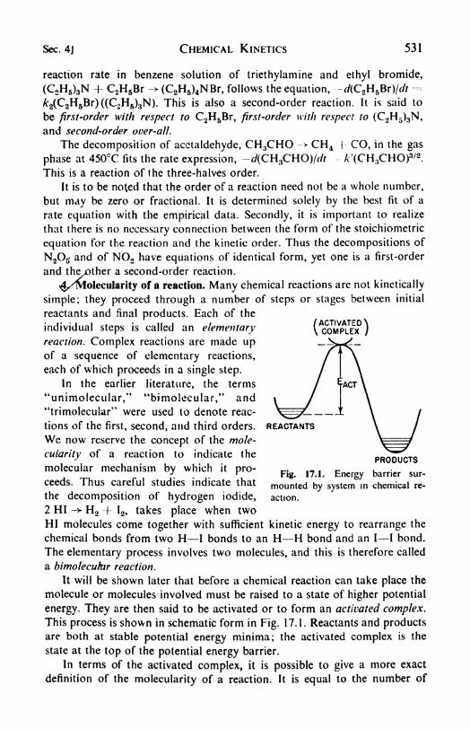
Sec. 4J CHEMICAL KINETICS 531
/ACTIVATED\\ COMPLEX )
reaction rate in benzene solution of triethylamine and ethyl bromide,
(C2H5)3N + C2H5Br -> (C2H5)4NBr, follows the equation, -rf(C2H 5 Br)/<//-
A-2(C2H5Br)((C2H5)3N). This is also a second-order reaction. It is said to
be first-order with respect to C2H5Br, first-order with respect to (C2H 5 )3N,
and second-order over-all.
The decomposition of acetaldehyde, CH 3CHO -> CH 4 | CO, in the gas
phase at 450C fits the rate expression, -rf(CH3CHO)/* A'(CH3CHO)3/2.
This is a reaction of the three-halves order.
It is to be noted that the order of a reaction need not be a whole number,
but may be zero or fractional. It is determined solely by the best fit of a
rate equation with the empirical data. Secondly, it is important to realize
that there is no necessary connection between the form of the stoichiometric
equation for the reaction and the kinetic order. Thus the decompositions of
N2O$ and of NO3 have equations of identical form, yet one is a first-order
and the Bother a second-order reaction.
^f/'Mtolecularity of a reaction. Many chemical reactions are not kinetically
simple; they proceed through a number of steps or stages between initial
reactants and final products. Each of the
individual steps is called an elementaryreaction. Complex reactions are made upof a sequence of elementary reactions,
each of which proceeds in a single step.
In the earlier literature, the terms
"unimolecular," "bimolecular," and"trimolecular" were used to denote reac-
tions of the first, second, and third orders.
We now reserve the concept of the mole-
cularity of a reaction to indicate the
molecular mechanism by which it pro-ceeds. Thus careful studies indicate that
the decomposition of hydrogen iodide,
2 HI -> H2 + I 2 , takes place when two
HI molecules come together with sufficient kinetic energy to rearrange the
chemical bonds from two H I bonds to an H H bond and an I I bond.
The elementary process involves two molecules, and this is therefore called
a bimolecufar reaction.
It will be shown later that before a chemical reaction can take place the
molecule or molecules involved must be raised to a state of higher potential
energy. They are then said to be activated or to form an activated complex.This process is shown in schematic form in Fig. 17.1. Reactants and productsare both at stable potential energy minima; the activated complex is the
state at the top of the potential energy barrier.
In terms of the activated complex, it is possible to give a more exact
definition of the molecularity of a reaction. It is equal to the number of
REACTANTS
PRODUCTS
Fig. 17.1. Energy barrier sur-
mounted by system in chemical re-
action.

532 CHEMICAL KINETICS [Chap. 17
molecules of reactants that are used to form the activated complex. In the
case of the hydrogen-iodide decomposition, the complex is formed from two
HI molecules, and the reaction is bimolecular. Clearly the molecularity of a
reaction must be a whole number, and in fact it is found to be one, two, or
rarely, three.
The experimental rate measurements show that the rate of decompositionof hydrogen iodide is - dcm /dt A'2rm 2
. This is therefore a second-order
reaction. All bimolecular reactions are second-order, but the converse is not
true; there are second-order reactions that are not bimolecular.
A good example of a unimolecular reaction is a radioactive decay, e.g.,
Ra -> Rn -f a. Only one atom is involved in each disintegration, and the
reaction is unimolecular. It also follows a first-order law, dn^Jdt --=-
A^/ffta, where /?Ra is the number of radium atoms present at any time.
The concept of molecularity should be applied only to individual elemen-
tary reactions. If a reaction proceeds through several stages, there is little
point in talking about its molecularity, since one step may involve two
molecules, another three, and so on.
At the risk of repetition: reaction order applies to the experimental rate
equation I molecularity applies to the theoretical mechanism.
^y The reaction-rate constant. The experimental data in a kinetic experi-
ment are values of concentrations at various times. Unless otherwise specified,
the concentration unit is moles per liter, and the time is measured in seconds.
It is purely a matter of convenience whether the reaction is followed by the
decrease in one of the reactants or by the increase in one of the products.
These quantities are related by the stoichiometric equation for the reaction.
Consider the decomposition of nitrogen pentoxide, 2 N2O6> 4 NO2 +
O2 . Velocity can be expressed in three ways: the rate of disappearance of
N2O5 , dcNn0Jdt; the rate of formation of NO2 , +dc^QJdt\ the rate of forma-
tion of O2 , +dc Jdt. Actually, the NO2 dimerizes to N2O4 , but the equili-
brium for this association is established very rapidly and can easily be taken
into acccount, since the equilibrium constant is well known. It is found that
the N2O5 decomposition follows a first-order law over a range of pressures
(10~3 to lOatm) and temperatures (0 to 200C). This law can be written in
three ways:
a _ ,
Ki
From the stoichiometry it is evident that k: i/r/= 2k^'. The lesson
to be learned is that it is always desirable to state clearly what rate law is
being used to express the experimental results. Then the rate constant will
have an unambiguous meaning. The choice is arbitrary but it should be
explicit.
The units of the rate constant depend on the order of the reaction. For
first order, dc/dt = k^, the units of kl are moles liter*1 sec"1 x liter

Sec. 6] CHEMICAL KINETICS 533
mole- 1 = sec"1. For second order, cfc/dt
= A:2c2
, the units of Ar2 are molesliter*1 sec"1 x (liter mole"1
)2 = liter mole 1 sec"1
. In general, for a reaction
of the Arth order, the dimensions of the constant kn are (time)""1(concen-
tration)1^.
OK First-order rate equations. The differential rate equatioa is almost
always integrated before it is applied to the experimental data, although
t-secxlO
Fig. 17.2. A first-order reaction. The thermal decomposition of
nitrogen pentoxide, plotted according to eq. (17.2).
occasionally slopes of concentration vs. time curves are taken to determine
dcjdt directly.
Consider a first-order reaction, A -> B + C. Let the initial concentration
of A be a moles per liter. If after a time /, x moles per liter of A have de-
composed, the remaining concentration of A is a x9 and x moles per liter
of B or C have been formed. The rate of formation of B or C is thus dxjdt,
and for a first-order reaction this is proportional to the instantaneous
concentration of A, so that
-.-Separating the variables and integrating, we obtain
In (a x) ^ kvt + const
(17.1)
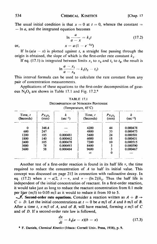
534 CHEMICAL KINETICS [Chap. 17
The usual initial condition is that x = at t = 0, whence the constant
In a, and the integrated equation becomes
aIn (17.2)
or, x = a({ -e"*)If In (a/a
-x) is plotted against /, a straight line passing through the
origin is obtained, the slope of which is the first-order rate constant A>
1.
If eq. (17.1) is integrated between limits xl to x2 and t
lto /2 , the result is
In - ~ -A-^/2
- ft)
a ^2
This interval formula can be used to calculate the rate constant from any
pair of concentration measurements.
Applications of these equations to the first-order decomposition of gase-
ous N2O5 are shown in Table 17.1 and Fig. 17.2. 6
TABLE 17.1
DECOMPOSITION OF NITROGEN PENTOXIDE
(Temperature, 45C)
Another test of a first-order reaction is found in its half life r, the time
required to reduce the concentration of A to half its initial value. This
concept was discussed on page 215 in connection with radioactive decay. In
eq. (17.2) when x - a/2, / = r, and T = (In 2)/kv Thus the half life is
independent of the initial concentration of reactant. In a first-order reaction,
it would take just as long to reduce the reactant concentration from 0.1 mole
per lijer (m/1) to 0.05 m/1 as it would to reduce it from 10 to 5.
^X Second-order rate equations. Consider a reaction written as A + B ->
C -f D- Let the initial concentrations,at / = be a m/1 of A and b m/1 of B.
After a time /, ;c m/1 of A, and of By will have reacted, forming x m/1 of Cand of D. If a second-order rate law is followed,
~ = k2(a-
x)(b-
x) (17.3)at
F. Daniels, Chemical Kinetics (Ithaca: Cornell Univ. Press, 1938), p. 9.

Sec. 7] CHEMICAL KINETICS 535
Separating the variables, we have
d^(a-sX*^) '
The expression on the left is integrated by breaking it into partial fractions.
The integration yields
nn_(^x) 7Jn(6-^] r; ngta b
When / --- 0, x 0, and constant = In (a/b)/(a b\ Therefore the inte-
grated second-order rate law is
A reaction found to be second-order is that between ethylene bromide
and potassium iodide in 99 per cent methanol, C2H 4Br2 + 3 KI C2H4 +2 KBr + KI3 . Sealed bulbs containing the reaction mixture were kept in a
thermostat. At intervals of two or three minutes a bulb was withdrawn, and
its contents were analyzed for iodine by means of the thiosulfate titra-
tion. The second-order rate law is d(\ 2)/dt--= dx/dt = /r2(C2H4Br2)(KI)
= k z(a x)(b 3x), and the integrated equation is
1 . b(a-x)I|-j
Is- -t
3a b a(b-
3jt)2
Figure 17.3 is a plot of the left side of this equation against time. The excellent
linearity confirms the second-order law. The slope of the line is the rate
constant, k2-- 0.299 liter mole"1 min.- 1
A special case of the general second-order equation (17.3) arises when
the initial concentrations of both reactants are the same, a -- b. This con-
dition can be purposely arranged in any case, but it will be necessarily true
whenever only one reactant is involved in a second-order reaction. An
example is the decomposition of gaseous hydrogen iodide, 2 HI ~> H2 4- I2
which follows the rate law, -d(Hl)/dt - /c2(HI)2
.
In these cases the integrated equation (17.4) cannot be applied, since
when a = b it reduces to k2 t =-0/0, which is indeterminate. It is best to
return to the differential equation, which becomes dx/dt ~ k2(a x)2
. Inte-
gration yields f/ v5 Jl/(0 x) = k2t + const
When r = 0, x = 0, so that const = I /a. The integrated rate law is therefore
,
* =k2t (17.5)a(a
- x)
The half life of a second-order decomposition is found from eq. (17.5)
by setting x = a/2 when / = r, so that r -^ \/k2a. The half life varies in-
versely as the initial concentration. For instance, the partial pressure of

536 CHEMICAL KINETICS [Chap. 17
decomposing HI would take twice as long to fall from 100 to 50 mm as it
would to fall from 200 to 100 mm.
t=59.7
04 8 12 16 20 24 28
TIME-MINUTES
Fig. 17.3. The second-order reaction,
C2H4Br2 + 3K1 -> C2H4 } 2KBr I KI3
[From R. T. Dillon, J. Am. Chem. Soc., 54, 952 (1932).]
tf Third-order rate equation. Third-order reactions arc quite rare, and all
that have been studied fall into the class:
2A + B -> products
a 2x b x x
The differential rate equation is. accordingly dx\dt = k%(a 2x)\b x).
This equation can be integrated by breaking it into partial fractions. The
result, after we apply the initial condition, x = at t 0, is
___1 \(2b
-d)2x b(a
-2x)l _
(2b - a)2
[ ~a(a~ 2x)+
a(b^x)\~
3'
Examples of gas reactions of the third order, following this rate law, are:
2 NO + O2-> 2 NO2
2 NO + Br2-^ 2 NOBr
2 NO + C12~> 2 NOC1
In every case, -</(NO)/<// = Ar3(NO)2(X2).

Sec. 9] CHEMICAL KINETICS 537
9. Opposing reactions. If a reaction is to proceed for some time at a
measurable rate, the initial conditions must evidently be fairly remote from
the final equilibrium. In many instances the position of equilibrium is so far
on the product side, at the temperature and pressure chosen for the experi-
ment, that for all practical purposes one can say that the reaction goes "to
completion." This is the case in the N2O5 decomposition and the oxidation
of iodide ion that have been described. There are other cases in which a con-
siderable concentration of reactants remains when equilibrium is reached.
A well known example is the hydrolysis of ethyl acetate in aqueous solution,
CH3COOC2H5 + H 2O ^ CH3COOH 4- C2H5OH. In such instances, as the
product concentrations are gradually increased, the velocity of the reverse
reaction becomes appreciable. The measured rate of change is thereby de-
creased, and in order to deduce a rate equation to fit the empirical data, the
opposing reaction must be taken into consideration.
The form of the over-all rate equation will be considered for three varie-
ties of such opposed reactions: opposing first orders, opposing second orders,
and first vs. second order.
Consider the first species in a reaction A ^ B. Let the first-order rate
constant in the forward direction be A' l5 in the reverse, k_.v Initially at /
the concentration of A is a and of B is b. If after a time r, x moles per liter
of A have been transformed into B, the concentration of A is a x, and
that of B is b + x. The differential rate equation is therefore
^ -k,(a
~x)
-k_,(b f x)
or-^- (k v f k_J(m - x)
where m --=- (k^ ~ k. ib)l(k lf- A'_ l ). Integration yields
In =(k, f _!>/ (17.6)m x
By Guldberg and Waage's principle, the equilibrium constant K =- kl/k_l .
Thus equilibrium measurements can be combined with rate data to separate
the forward and reverse constants in eq. (17.6).
Such reversible first-order reactions arc to be found in some of the intra-
molecular rearrangements and isomerizations studied by G. B. Kistiakowskyand his co-workers. 7 The cis-trans isomerization of styryl cyanide vapor was
followed by the change in the refractive index of the solution obtained on
condensation.C6H6-CH C6H5-CH
II^ II
NC CH CH CN
Equilibrium at 300C is at about 80 per cent trans-isomer.
7Kistiakowsky et */., J. Am. Chem. Soc., 54, 2208 (1932); 5(5, 638 (1934); 57, 269 (1935);
5, 2428(1936).

538 CHEMICAL KINETICS [Chap. 17
The case of opposing bimolecular reactions was first treated by MaxBodenstein in his classic study of the combination of hydrogen and iodine. 8
Between 250 and 500C the reaction H2 + I2> 2 HI can be conveniently
studied, but at higher temperatures the equilibrium lies too far on the re-
actant side. Even in the cited temperature range the reverse reaction must be
considered in order to obtain satisfactory rate constants. The concentrations
at time / will be denoted as follows:
H2 I2 2 HI
- *-
The net rate of formation of HI is
<'">
When the equilibrium constant K = k2fk 2 is introduced into eq. (17.7) and
the equation integrated, the result is
/a + b m
with m
7TK)
556
575
629
666700781
TABLE 17.2
RATE CONSTANTS FOR THE REACTION H2 -f I2 ^ 2 HI
1.19 x3.53 x6.76 x3.79 x1.72 X
10-*
10 4
10 3
io-2
10-1
3.58
2.11 x7.30 x1.81 x1.32 x6.95 X1.06 x
10~8
io-6
10-4
io~2
io-2
10-1
K -
5.64
4.85
3.73
2.87
2.43
1.51
Good constants obtained from this rather formidable expression are
shown in Table 17.2 for a number of temperatures, together with values of
K and A'__2 from separate experiments.The third type of opposing reaction, first vs. second order, may be
8Bodenstein, Z.physik. Chem., 13, 56 (1894); 22, 1 (1897); 29, 295 (1898).

Sec. 10] CHEMICAL KINETICS 539
written schematically for the case in which, at t = 0, (B) (C) = 0,
and (A) a.
A
a x
B+ C
xxThe differential equation is dxjdt -- k^a x) k2x
2. The integration
yields9
IV2l
2mt
with
* =
m ---
In
1/2
These equations would apply to the rate of dissociation of nitrogen
tetroxide, N2O4 ^ 2 NO2 ,but no adequate data are available for this re-
action owing to its extreme rapidity. It might have been expected that the
reversible dissociation of elementary gases, e.g., C12 ^ 2 Cl, would also
follow this law. It is found, however, that two atoms usually recombine onlyin the presence of a third particle or on the wall of the reaction vessel,
CliCl -h Af -> C1 2 f M. The third particle M is required to take up the
excess energy generated in the collision, thereby preventing the atoms from
flying apart again.
10. Consecutive reactions. It often happens that the product of one
reaction becomes itself the reactant of a following reaction. There may be a
series of consecutive steps. Only in the simplest cases has it been possible to
obtain solutions to the differential equations of theie reaction systems. Theyare especially important in polymerization and depolymerization processes,
and the investigator of chemical kinetics is often blocked here by inade-
quacies in the available mathematics.
A simple consecutive-reaction scheme that can be treated exactly is one
involving only irreversible first-order steps. The general case of n steps has
been solved,10 but only the example of two steps will be discussed. This can
be written
x y z
The simultaneous differential equations are
dx _ ,,Jy _ /, , ,
dz
9 E. A. Moelwyn-Hughes, Physical Chemistry (London: Cambridge, 1947), p. 636.10 H. Dostal, Monatshefte (Vienna), 70, 324 (1937). For second-order steps, see P. J.
Flory, J. Am. Chem. Soc., 62, 1057, 1561, 2255 (1940).

540 CHEMICAL KINETICS [Chap. 17
The first equation can be integrated directly, giving In x = k^t +const. When / = 0, let x = a, the initial concentration of A. Then const.
= In a, and x = ae~ kli. The concentration of A declines exponentially
with the time, as in any first-order reaction.
Substitution of the value found for x into the second equation gives
dy
dt= k^y + k^ae
-At*
This is a linear differential equation of the first order, whose solution 11is
When / = 0, y = 0, so- that const = k^al(k^ A^).
We now have expressions for x and y. In the reaction scheme followed
there is no change in the total number of molecules, since every time an A
disappears a B appears, and every time a B disappears a C appears. Thus
x + y + z a, and z is calculated to be
z +ki
(17.8)
In Fig. 17.4, the concentrations x, j, z are plotted as functions of the
time, assuming k 2kl
/
. The intermediate concentration y rises to a maxi-
100 120
Fig. 17.4. Concentration changes in consecutive first-order reactions.
mum and then falls asymptotically to zero, while the final product rises
gradually to a value of a.
11Granville, Calculus, p. 380.
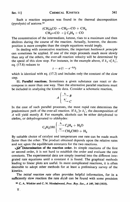
Sec. 11] CHEMICAL KINETICS 541
Such a reaction sequence was found in the thermal decomposition
(pyrolysis) of acetone.12
(CH3)2CO -> CH2=CO + CH4
CH2=CO -> i C2H4 + CO
The concentration of the intermediate, ketene, rises to a maximum and then
declines during the course of the reaction. Actually, however, the decom-
position is more complex than the simple equations would imply.
In dealing with consecutive reactions, the important bottleneck principle
can sometimes be applied. If one of the steps proceeds much more slowly
than any of the others, the over-all reaction velocity will be determined bythe speed of this slow step. For instance, in the example above, if k <^ /,
eq. (17.8) reduces to
z = a(l -<rw)
which is identical with eq. (17.2) and includes only the constant of the slow
step.
11. Parallel reactions. Sometimes a given substance can react or de-
compose in more than one way. Then the alternative parallel reactions must
be included in analyzing the kinetic data. Consider a schematic reaction,
-It:In the case of such parallel processes, the most rapid rate determines the
predominant path of the over-all reaction. If kl ;> /:/, the decomposition of
A will yield mostly B. For example, alcohols can be either dehydrated to
olefins, or dehydrogenated to aldehydes:
CH3CHO + H2
By suitable choice of catalyst and temperature one rate can be made muchfaster than the other. The product obtained depends upon the relative rates
and not upon the equilibrium constants for the two reactions.
vJ^Determination of the reaction order. In simple reactions of the first
or second order, it is not hard to establish the order and evaluate the rate
constants. The experimental data are simply inserted into the different inte-
grated rate equations until a constant k is found. The graphical methods
leading to linear plots are useful. In more complicated reactions, it is often
desirable to adopt other methods for at least a preliminary survey of the
kinetics.
The initial reaction rate often provides helpful information, for in a
sufficiently slow reaction the rate dxjdt can be found with some precision
C. A. Winklcr and C. N. Hinshelwood, Proc. Roy. Soc., A 149, 340 (1935).
T.

542 CHEMICAL KINETICS [Chap. 17
before there has been any extensive chemical change. It is then possible to
assume that all the reactant concentrations are still effectively constant at
their initial values. If A f B + C -> products, and the initial concentrations
are,0, b, <?, the rate can be written quite generally as
j-- k (a -. Jt)
n '
(b-
*)" (c-
x)nt
If x is very small, the initial rate will be
^kan * bn * cn>
dt
While we keep b and c constant, the initial concentration of a can be varied,
and the resultant change of the initial rate measured. In this way the value
of n lis estimated. Similarly, by keeping a and c constant while we vary b,
a value of /72 is found;and with a and b constant, variation of c yields n3 .
The initial-rate method is especially useful in those reactions that cannot
be trusted to progress to any appreciable extent without becoming involved
in labyrinthine complications. If the order of reaction found by using initial
rates differs from that found by using the integrated rate equation, it is
probable that the products are interacting with the initial reactants.
A frequently useful way of finding the reaction order is the isolation
method, devised by W. Ostwald. If all the reactants save one, say A, are
present initially in high concentrations, their concentrations during the re-
action will be relatively much less changed than that of A. In fact, they maybe taken to be effectively constant, and the rate equation will have the
approximate form :
^ - k (a-
*)Wl bn * c
n >. . .
= k' (a-
x)n *
dt
By comparing the data with integrated forms of this equation for various
choices of n^ it is possible to determine the order of the reaction with respect
to component A. The orders with respect to B, C, etc., are found in like
manner.
The isolation method is often practiced of necessity in reactions in
solution if the solvent is one reactant. For example, in the hydrolysis of
ethyl acetate, CH3COOC2H5 + H2O ^ CH3COOH + C2H5OH, the ester
concentration is much lower than that of the solvent, water. The reaction
follows a rate law that is first order with respect to the ester, the water
concentration being effectively constant:
f](f^\i C^OOC* H ^3
df
f- -
2(CH3COOC2H5)(H20) == ^(CH3COOC2H6)
Another way of holding the concentration of a reactant constant is to use
a saturated solution with an excess of pure solute phase always present.

Sec. 13] CHEMICAL KINETICS 543
An interesting general method of finding the over-all reaction order is
based on the half-life times. If all the reactants are taken to have stoichio-
metric initial concentrations a, the rate law takes the form dx\dt kn(a x)n
.
Integrating and setting x = at t = 0, we find
*/--M !---LI""'-n-ilfa-xr-* a-']
When the time / equals the half life T, x = a/2, so that
log r = (1-
n) log a + log (17.9)
3.0
2.9
2.8
2 '7
2.6
2.5
2.4
2.3
2.2
2.11.5 2.0 2.5
LOG Po
3.0
If log r is plotted against log a, a straight line should be obtained whose
slope is (1 n). In gas reactions
the initial pressure can be used
instead of the initial concentration.
The half lives determined byA. Farkas13 for the homogeneous
para-ortho hydrogen conversion at
923K are shown in the log-log plot
in Fig. 17.5. The slope of the line
is -0.52; thus (1-
n)-= -0.52,
and n = 1.52. The reaction is one
of the three-halves order. The
reason for this order is that the
change H2 (/?)-> H2 (o) proceeds
through atomic hydrogen formed
by the dissociation H2> 2 H. Then
H f H2 (p) -> H2 (o) + H. The
rate is proportional to (H)(/?-H2). From the dissociation equilibrium
(H) = #1/2(H2)1/2
, so that the rate is kK^p-HJ***.13. Reactions in flow systems. The rate equations that have been discussed
all apply to static systems, in which the reaction mixture is enclosed in a
vessel at constant volume and temperature. We must now consider flow
systems, in which reactants enter continuously at the inlet of a reaction
vessel, while the product mixture is withdrawn at the outlet. We shall
describe two examples of flow systems: (a) a reactor in which there is no
stirring; (b) a reactor in which complete mixing is effected at all times by
vigorous stirring.
Figure 17.6 shows a tubular reactor through which the reaction mixture
passes at a volume rate of flow u (e.g., in liters per sec). Let us consider an
18 A. Farkas, Z. physik. Chem., B 10, 419 (1930).
Fig. 17.5. Plot of log half-life vs. log initial
pressure for/?-<? H2 conversion.

544 CHEMICAL KINETICS [Chap. 17
element of volume dV sliced out of this tube, and focus attention on one
particular component k, which enters this volume element at a concentration
ck and leaves at ck dck
. If there is no longitudinal mixing, the net changewith time of the number of moles of k within dV (dnk\di) will be the sum of
two terms, one due to chemical reaction within dV, and the other equal to
the excess of k entering dV over that leaving. Thus,
(17.10)dt
The chemical reaction rate per unit volume is denoted by rk . The explicit
form of rk is determined by the rate law for the reaction : for a reaction first
order with respect to k, rk-= k^c^, for second order, rk
= k2ck2, etc.
dV
cK-dcK
Fig. 17.6. Element of volume in a flow reactor.
After reaction in the flow system has continued for some time, a steadystate is attained, in which the number of moles of each component in anyvolume element no longer changes with time, the net flow into the element
exactly balancing the reaction within it. Then dnkjdt-
0, and eq. (17.10)
becomes
rk dY-udck -Q (17.11)
After rk is introduced as a function of ck , the equation can be integrated.
For example, with rk k-^c^
dV _ dckK
lU Ck
The integration is carried out between the inlet and the outlet of the reactor.
-kl~ = \n (17.12)u c
ti
The total volume of the reactor is VQ9 and cktand c
kiare the concentrations
of k at the outlet and inlet, respectively.
It may be noted that eq. (17.12) reduces to the integrated rate law for a
first-order reaction in a static system if the time / is substituted for V /u.
The quantity K /w is called the contact time for the reaction; it is the averagetime that a molecule would take to pass through the reactor. Thus eq. (17.12)
allows us to evaluate the rate constant k1 from a knowledge of the contact

Sec. 13] CHEMICAL KINETICS 545
time, and of the concentrations of reactant fed to the tube and recovered at
the end of the tube. For other reaction orders also, the correct flow reactor
equation is obtained by substituting V /u for / in the equation for the static
system. Many reactions that are too swift for convenient study in a static
system can be followed readily in a flow system, in which the contact time
is reduced by use of a high flow rate and a small volume.
The derivation of eq. (17.11) tacitly assumed that there was no volume
change AK as a result of the reaction. Any AK would affect the flow rate
at constant pressure. In liquid-flow systems, the effects of AK lire generally
Fig. 17.7. A stirred flow reactor.
negligible, but for gaseous systems the form of the rate equations is con-
siderably modified. A convenient collection of integrated rate laws including
such cases is given by Hougen and Watson. 14
An example of a stirred flow reactor15 is shown in Fig. 17.7. The reactants
enter the vessel at A, and stirring at 3000 rpm effects mixing within about a
second. The product mixture is removed at B at a rate exactly balancing the
feed. After a steady state is attained, the composition of the mixture in the
reactor remains unchanged as long as the composition and rate of supply of
reactants is unchanged. Equation (17.1 1) still applies, but in this case dV =K , the total reactor volume, and dck -= c
ki- c
knwhere c
kiand c
ktare
the initial and final concentrations of reactant k. Thus
dt
With this method, there is no need to integrate the rate equation. One point
14 O. A. Hougen and K. M. Watson, Chemical Process Principles (Part 3) (New York:
Wiley, 1947), p. 834.
K. G. Denbigh, Trans. Faraday Soc., 40, 352 (1944) ; Disc. Faraday Soc., 2, 263 (1947).

546 CHEMICAL KINETICS [Chap. 17
on the rate curve is obtained from each steady-state measurement, and a
number of runs with different feed rates and initial concentrations is required
to determine the order of the reaction.
An important application of the stirred flow reactor is the study of
transient intermediate:, the concentration of which in a static system might
quickly reach a maximum value, and then fall to zero. An illustration was
shown in Fig. 17.4. For example, in the reaction between Fe f3 and Na2S2O3 ,
a violet color appears, which fades within one or two minutes. In a stirred
flow reactor, the conditions can be adjusted so that the color is maintained,
and the intermediate responsible, which appears to be FeS2O3+
,can be
studied spectroscopically.
The living cell is in some ways analogous to a continuous flow reaction
vessel, in which reactants and products are transferred by diffusion across
the cell membrane.
sWf Effect of temperature on reaction rate. So far we have been concerned
with the problem of finding how the chemical kinetics depends on the con-
centrations of the various components of the reaction system. This first step
is necessary in reducing the raw material of the experimental data to a refined
form suitable for theoretical interpretation. The next question is how the
constants of the rate equations depend on variables such as temperature and
total pressure. The temperature effect has been tremendously useful in
providing an insight into the theory of all rate processes.
In 1889, Arrhenius pointed out that since the van't Hoff equation for
the temperature coefficient of the equilibrium constant was din KJdT =AE//?r
2, whereas the mass-action law related the equilibrium constant to a
ratio of rate constants, Kc= kf/kb ,
a reasonable equation for the variation
of rate constant with temperature might be
The quantity Ea is called the activation energy of the reaction.
If Ea is not itself temperature dependent, eq. (17.10) yields on integration
In k = --- + In A (17.14)J\T
where In A is the constant of integration. Hence
A is called the frequency factor. This is the famous Arrhenius equation for
the rate constant.
From eq. (17.14) it follows that a plot of the logarithm of the rate con-
stant against the reciprocal of the absolute temperature should be a straight
line. The validity of the equation is excellently confirmed in this way for a
large number of experimental velocity constants. An example from the data

Sec. 15] CHEMICAL KINETICS 547
of Bodenstein on the H2 + I2= 2 HI reaction is shown in Fig. 17.8. We shall
see later that the Arrhenius equation is only an approximate representationof the temperature dependence of k y but the approximation is usually a very
good one.
According to Arrhenius, eq. (17.15) indicates that molecules must acquirea certain critical energy En before they can react, the Boltzmann factor
e-E /RT be ing the fraction of molecules that manages to obtain the necessary
energy. This interpretation is still held to be essentially correct.
35
25
15
oo
-05 N120 130 140 150 160 1.70 1.80
I/T XI03
Fig. 17.8. Temperature dependence of rate constant for formation of
hydrogen iodide, illustrating applicability of the Arrhenius equation.
By referring back to Fig. 17.1 on page 531, we can obtain a picture of the
activation energy as the potential-energy hill that must be climbed to reach
the activated state. It is evident also that the heat of reaction Qv is the differ-
ence between the activation energies of forward and backward reactions,
^2V- Et -Eb (17.16)
15. Collision theory of gas reactions. Reaction velocities have been studied
in gaseous, liquid, and solid solutions, and at the interfaces between phases.
Homogeneous reactions in liquid solutions have undoubtedly been investi-
gated most extensively, because they are of great practical importance and
usually require only relatively simple experimental techniques. From a
theoretical point of view, however, they suffer from the disadvantage that
our understanding of liquids and solutions is inadequate, especially on the
molecular scale that is important in chemical changes.
Homogeneous gas reactions, therefore, though harder to follow experi-
mentally, should be more amenable to theoretical elucidation. The statistical
theory of gases is well developed and provides an insight into the factors
governing the reaction rates.
The first theory of gas reactions postulated that in order for molecules
to interact, they must approach each other so closely that they can be said
to be in collision. Sometimes a rearrangement of chemical bonds occurs

548 CHEMICAL KINETICS [Chap. 17
during a collision, forming new molecules from the old ones. The speed of
the reaction is equal to the number of collisions per second times the fraction
of the collisions that are effective in producing chemical change.The formula for the number of collisions per second between like mole-
cules in one cc of gas is obtained from eq. (7.16).
Zn = 4\7r/i =- 2M* (17.17)V 7T/n v m
Here n is the number of molecules per cc, d is the molecular diameter, and
V%kT/7rm is the average speed of a molecule of mass m. In the case of unlike
molecules whose concentrations are ^ and /?2 ,the collision frequency
becomes
7$kTTTA(17.18)
TTfA
Now dl2~ (d} + d2)/2 is the mean molecular diameter and the reduced
mass /* mlm2/(fn l + w2 ). Note that the factor \ is not included in the
expression for unlike molecules since a collision of the type B ~> A is now
distinguishable from A -> B.
Let us calculate Zu for hydrogen-iodide molecules at 700K and 1 atm
pressure. From gas viscosity d = 4 x 10~ 8 cm. The mass m =127.9/6.02 X
1023 - 2.12 x 10~22 g; w = PVNIRT - 1 x 1 x 6.02 x 10*782.05 X 700- 1.05 x 10¹⁹ . Substituting in eq. (17.17), we find Zu = 1.33 x 1028 . At a
given temperature and pressure the Zn for different molecules hardly ever
varies by a factor of more than 50, and for molecules of low molecular
weight the variations are much less. (The variable factor is d2/mm and rfmay
run from 2 to 20 A.)
Now it is obvious that not every collision can lead to reaction; the
collision frequency is so extremely large that if such were the case all chemical
reactions would be essentially completed in a fraction of a second. The
hypothesis is therefore made that only those collisions lead to reaction in
which the sum of the energies of the colliding molecules exceeds a certain
critical value 16. The problem is therefore to calculate the chance that a pair
of molecules has an energy greater than E.
The first question that arises is what energy is to be taken into considera-
tion. A complex molecule can acquire energy in various degrees of freedom:
translational kinetic energy, rotational kinetic energy, vibrational kinetic
and potential energy. Can all of this energy be utilized in effecting the re-
arrangement of bonds that is called a "chemical reaction" ?
The simplest form of the collision theory says that only two degrees of
freedom are utilized. These degrees of freedom can best be visualized as the
16 This hypothesis, that if energy is less than E there is never reaction, but if greater thanthere is always reaction, is not very reasonable. A reaction probability that is some
function of the energy would be more logical.
Sec. 15] CHEMICAL KINETICS 549
components of the translation of each molecule along the line of centers at
the time of collision. In other words, only the velocity components in the
direction of a head-on collision are effective. The chance that two molecules
have a relative head-on velocity r, such that \mc2 --,has already been
calculated, under a slightly different guise, in Chapter 7. Since the choice of
direction is entirely arbitrary, it is simply the distribution law in two dimen-
sions, eq. (7.35):
dn ^ I m \
n^
""
\kTJ
We wish to transform this expression into the distribution function for the
kinetic energy per mole, E^ }>Nmc2. Since dE --- Nmc dc, and R = Nk,
the result is
^H - - _L e~ EIRTdE
n RTThis is the chance of a molecule's having an energy between E and E + dEin two degrees of freedom. The chance of its having an energy greater than
E is obtained by integrating from E to oo,
RT_ e -EIRT
E
The simple collision theory for a bimolecular reaction therefore gives
for the number of molecules reacting per second:
dn number of collisions per sec x chance of
dt collision having energy E or greater
= Z e~EIRT
The velocity is usually expressed in moles per liter reacting per second,
dc/dt= kfaCi. Since c =--- l&n/N, dc/dt
= (\&/N)dn/dt. The reaction rate
is, accordingly, .
dc _ \<Pdn 106
eft N dt N 2
N dn . L dn~~ withdt dt
Substituting the kinetic-theory expression for Z12 from eq. (17.18), we have
^or k, = ---r- with - Z122 12
k2= Ae-*'*T - e
-K'RT(17.19)
13 ^
TTfl
This theoretical expression can be compared with experiment in several
ways. It contains three quantities that are not known a priori, the rate constant
&2 , the collision diameter dl2t and the activation energy E. The following
comparisons are possible: (1) With a value of E from the Arrhenius equationfor the temperature coefficient, and a value of dl2 from kinetic theory (e.g.,
viscosity), k2 can be calculated and compared with experiment. (2) With the

550 CHEMICAL KINETICS [Chap. 17
experimental k2 at one temperature and the kinetic-theory c/12 , a calculated
value of E can be compared with the value from the temperature coefficient.
(3) With the experimental E and k2 , a dl2 can be calculated and comparedwith kinetic-theory or electron-diffraction diameters.
Let us apply method (1) to the HI decomposition. Using the previouslycited values for the constants and for dl2 , we obtain
k - 7 r-EiRT _._ -_2~
103*2 n " "
103(1.05 x 101')
2*
---7.26 x
The experimental is 43,700 cal. Thus at 700K the calculated rate
constant is 2.10 x 10~3liter mole"1 sec^1
. The experimental value obtained
by Bodenstein was 1.57 x 10~3. The success of the collision theory in this
case is quite remarkable.
Unfortunately, there are few simple second-order gas reactions that can
be similarly tested. Table 17.3 contains some of the available data. The cal-
culated frequency factors A are usually around 1011in units of liter mole"1
sec"1, so that observed differences in the reaction velocities are caused mainly
by activation-energy differences. The experimental A values sometimes
deviate considerably from the theoretical.
TABLE 17.3
SECOND-ORDER GAS REACTIONS
Reaction ..,_ ,
Rate Constant
(liter sec'1 mole~l)
(1) 2 HI -* H2 + I 2.05 x 10 r1/a *-4
(2) H2 + I2-> 2 HI 3.3 X 10⁹ T1/2 e-38,900/J?T
(3) 2 NO2-> 2 NO f O2 1.31 x 10⁸ T 1 '2 ^-2
(4) 2 NOC1 -> 2 NO + C12 4.3 x 10⁸ J1
(5) CH3I + HI - CH4 -f I2 5.22 x 10¹⁰
(6) C2H6I + HI -* C2H 6 + I2 1.34 x 10l T1/a ^-2
CH2
The collision theory gives a crude physical picture of how bimolecular
gas reactions occur which is roughly correct as far as it goes, but factors
other than an activation energy and a rigid-sphere collision frequency mayinfluence the rate of reaction. At one time it was popular to rewrite the
theoretical equation (17.16) as k2 =pAe~EIRT9 where/?, which was called

Sec. 16] CHEMICAL KINETICS 551
the stericfactor, was supposed to measure the geometrical requirements that
must be met if two colliding molecules are to interact. Since there was no
independent way to estimate p 9 it was always possible to assign whatever
value was necessary to obtain agreement with experiment. It became simplya measure of the discrepancy between simple collision theory and the
experimental results.
tx<5ollision theory and activation energy. The collision-theory expression
for the rate constant contains, in addition to the strongly temperature-
dependent e~EIRT term, a mild temperature dependence in the frequencyfactor. Equation (1 7. 19) can be written &2
= a T* /2e~EIRT
9 so that d In k2/dT -=
(E + %RT)/RT2
. Thus the Arrhenius energy of activation is Ea-~~- E + %RT.
It is worth while to make this correction in performing calculations with the
theory, but it hardly affects the linear plot of In k vs. 1/7*.
There is no reason to assume that the activation energy should be strictly
independent of temperature and in careful work a slight temperature depend-ence has often been noted. The dependence of the heat of reaction, AE or
A/f, on temperature is given by Kirchhoff's Equation (page 43) and Ea maybehave similarly.
17. First-order reactions and collision theory. The collision theory was
developed about the time of World War I by M. Trautz, W. C. McC. Lewis,
and others, and as we have seen, it gives a fairly satisfactory account of bi-
molecular reactions. At the same time a number of gas reactions were beingstudied that were kinetically of the first order and apparently simple uni-
molecular decompositions. These reactions seemed to present a paradox: the
necessary activation energy must evidently come from the kinetic energytransferred during collisions, yet the reaction velocity did not depend on the
collision frequency.In 1919, a flurry of excitement was caused in the small world of kineticists
by the suggestion that the activation of molecules in these unimolecular
decompositions was actually effected, not by collisions, but by the absorptionof radiation from their environment, especially infrared radiation from the
walls of the reaction vessel. This theory was very short-lived since no radia-
tion effects could be demonstrated experimentally, and a better solution of
the problem was proposed shortly thereafter. In 1922, F. A. Lindemann
(now Lord Cherwell) showed how the collisional mechanism for activation
could lead to first-order kinetics.
Consider a molecule A which decomposes according to A -> B + C,
with a first-order rate law, d(A)/dt = k^(A). In a vessel full of A, the
intermolecular collisions are continually producing molecules with higherthan average energy, and indeed sometimes molecules with an energy above
some critical value necessary for the activation that precedes decom-
position. Let us suppose that there is a certain time lag between activation
and decomposition; the activated molecule does not immediately fall to
pieces, but moves around for a while in its activated state. Sometimes it

552 CHEMICAL KINETICS [Chap. 17
may meet an energy-poor molecule, and in the ensuing collision it may be
robbed of enough energy to be deactivated.
The situation can be represented as follows:
k>
A -f A ^ A + A**- I *i
B+ C
Activated molecules are denoted by A*. The bimolecular rate constant for
activation is A'2 , for deactivation A'_2 . The decomposition of an activated
molecule is a true unimolecular reaction with rate constant AVThe process called activation consists essentially in transferring trans-
lational kinetic energy into energy stored in internal degrees of freedom,
especially vibrational degrees of freedom. 17 The mere fact that a molecule is
moving rapidly, i.e., has a high translational kinetic energy, does not make
it unstable. In order to cause reaction, the energy must get into the chemical
bonds, where high-amplitude vibrations will lead to ruptures, decompositions,
and rearrangements. The transfer of energy from translation to vibration can
occur only in collisions with other molecules or with the wall. The situation
is like that of two rapidly moving automobiles: their kinetic energies will not
wreck them unless they happen to collide and the kinetic energy of the whole
is transformed into internal energy of the parts.
The point of the Lindemann theory is that there is a lag between the
activation of the internal degrees of freedom and the subsequent decom-
position. The reason is that a polyatomic molecule can take up collisional
energy into a number of its 3n - 6 vibrational degrees of freedom, and then
some time may elapse before this energy flows into the one bond that breaks.
The Lindemann scheme cannot be treated exactly since the differential
equations to which it leads are not soluble in closed form. They are
dt
-d(A)
dt
An approximation is therefore made that is frequently used in chemical
kinetics when the mathematical going becomes too rough. This is the steady-
state approximation. It is assumed that after the reaction has been under wayfor a short time, the rate of formation of activated molecules equals their
rate of disappearance, so that the net rate of change in (A*) is zero, d(A*)/dt= 0. In justification of this assumption it can be said that there are not very
17 Sometimes it is necessary to change the electronic state of a molecule in order to
effect the reaction. Such reactions are exceptionally slow if they depend on thermal activa-
tion. They are called nonadiabatic reactions, an unfortunate name since it has nothing to
do with the term adiabatic as used in thermodynamics.

Sec. 17] CHEMICAL KINETICS 553
many activated molecules present in any event. The value of (A*) is neces-
sarily small, so that the value of its rate of change must be small, and can
usually be set equal to zero without serious error.
With d(A*)jdt = 0, the first equation above becomes k2(A)2
A'_2
(A*)(A) k^A*) = 0, and the steady-state concentration of A* is
(A*) -k.'_2(A)
The reaction velocity is the rate at which A* decomposes into B and C, or
(
k(A*)-) /
-- (17.20)dt k_2(A) + k
l
Two special cases now arise.
If the rate of decomposition of (A*) is much greater than its rate of
deactivation, k^ :> k_2(A) and the net rate reduces to
This expression is the ordinary second-order law.
On the other hand, if the rate of deactivation of A* is much greater than
its rate of decomposition, k_2(A)^ k\, 300and the over-all rate becomes
260
_x 220
180
140
IOOH
60{
d(B) A'^dt k . 2
Xl
It is evident that it is possible to obtain
first-order kinetics while preserving a
collisional mechanism for activation.
This will be the result whenever the
activated molecule has so long a life-
time that it is usually deactivated bycollision before it has a chance to break
into fragments.
Fortunately, there is a fairly critical
experimental test of the Lindemann
theory. As the pressure in the reacting
system is decreased, the rate of de-
activation, k_2(A*)(A), must likewise
decrease, and at low enough pressures
the condition for first-order kinetics
must always fail when k__2(A) is no longer much greater than kv The
observed first-order rate constant should therefore fall off at low pressures
to reach eventually a second-order constant.
In Fig. 17.9 are plotted the rate constants obtained by H. C. Ramsperger18
18 H. C. Ramsperger, /. Am. Chem. Soc., 49, 912 (1927).
20*100 200 300 400 500
INITIAL PRESSURE- mm
Fig. 17.9. Falling-off of rate constant
of azomethane decomposition at low
pressures:
(CH 3 )2N2
- C2H 6 i N,.

554 CHEMICAL KINETICS [Chap. 17
for the first-order thermal decomposition of azomethane at various initial
pressures. In most of the first-order reactions that have been investigated,
the rate constant decreases at low pressures (usually 10-100 mm). If the
falling rate constant is merely the result of a lowered probability of deactiva-
tion, it should be possible to restore the initial rate by adding a sufficient
pressure of a completely inert gas. This inert-gas effect has been noted in a
number of cases.
The Lindemann theory of unimolecular reactions is very plausible and
provides the best explanation for many experiments. Yet some reactions once
thought to be simple unimolecular decompositions have been shown to pro-
ceed via complex chain mechanisms, which often yield deceptively simple rate
laws. This aspect of gas kinetics will be considered a little later in the chapter.
18. Activation in many degrees of freedom. When the first-order rate
constant begins to fall at lower pressures, the rate of formation of activated
molecules is no longer much greater than their rate of decomposition, and in
fact the over-all rate is beginning to be determined by the rate of supply of
activated molecules. According to simple collision theory, therefore, the rate
at this point should be about Zue~ f:iRT. When this prediction was compared
with experiment in the typical case of the azomethane decomposition, it was,
found that the reaction was going about 108 times faster than was permissible
by simple collision theory.
This unfortunate contradiction was soon remedied by C. N. Hinshelwood
and G. N. Lewis (independently). The e EIRT term used to calculate the
fraction of activated molecules is based on the condition that the critical
energy is acquired in two translational degrees of freedom only. If energy in
various internal degrees of freedom also can be transferred in collisions, the
probability of a molecule's getting the necessary E is much enhanced. Instead
of a simple e~EIRT term, the chance is now19
Here s is the number of "square terms" in which the energy can be acquired:
translational or rotational energy has one square term per degree of freedom,
\mv2 or i/w2; vibrational energy has one for kinetic energy, i/wr
2, and one
for potential energy, i/or2
.
The rate of activation may now be increased by a large factor/,. For the
azomethane case, with E - 52,400, T = 563, the factor /,=-- 108 when
s ----- 16. The observed rate of activation can therefore be explained by calling
on 16 "square terms" or about 8 vibrational degrees of freedom. Since the
molecule contains 10 atoms, there are altogether 3/16 ~ 24 vibrations.
The Lewis-Hinshelwood theory would include a third of these in the activa-
tion process.
19 This is a good approximate formula when E> RT. A derivation is given by Moelwyn-Hughes, Physical Chemistry, p. 69.

Sec. 19] CHEMICAL KINETICS 555
It has so far proved possible in every case to find a value of s that explainsthe observed activation rate.
20 Since it may not be easy to transfer energyfrom translation to vibration and from one vibration to another, the Lewis-
Hinshelwood theory would seem to necessitate extremely sticky collisions.
Moreover, a clear-cut decision on the validity of the theory is prevented bythe possible occurrence of chain reactions in many first-order decompositions.It is now necessary to consider in some detail these chain reactions, which
add so many interesting complications to gas kinetics.
19. Chain reactions: formation of hydrogen bromide. After Bodenstein
had completed his study of the hydrogen-iodine reaction, he turned to
hydrogen-bromine, H2 -\- Br2~ 2 HBr, probably expecting to find another
example of bimolecular kinetics. The results21 were surprisingly different, for
the reaction velocity was found to fit the rather complicated expression,
</(HBr)
dt m + (HBr)/(Br2)
where m and k are constants. Thus the velocity is inhibited by the product,HBr. In the initial stages of the combination, (HBr)/(Br2) is a small fraction
so that d(HBr)/dt = '(H2)(Br2)1/2
,with an over-all order of 3/2.
There was no interpretation of this curious rate law for thirteen years.
Then the problem was solved independently and almost simultaneously byChristiansen, Herzfeld, and Polanyi. They proposed a chain of reactions
with the following steps:
A-,
Chain initiation (1) Br2 -^2Br
Chain propagation (2) Br f H2 '-^HBr (- H
(3) H + Br2 *'->HBr } Br
Chain inhibition (4) H + HBr --'- H2 -+ Br
*.
Chain breaking (5) 2 Br * Br2
The reaction is initiated by bromine atoms from the thermal dissociation
Br2= 2 Br. The chain propagating steps (2) and (3) form two molecules of
HBr and regenerate the bromine atom, ready for another cycle. Thus veryfew bromine atoms are needed to cause an extensive reaction. Step (4) is
introduced to account for the observed inhibition by (HBr); since this in-
hibition is proportional to the ratio (HBr)/(Br2^ it is evident that HBr and
Br2 compete, so that the atom being removed must be H rather than Br. .
In order to derive the kinetic law from the chain mechanism, the
20 R. A. Ogg, in J. Chem. Phys., 27, 2079 (1953), has proposed an interesting chain
mechanism for the N2O6 case, which previously appeared exceptional,21 M. Bodenstein and S. C. Lind, Z. physik. Chem., 57, 168 (1906).

556 CHEMICAL KINETICS [Chap. 17
stationary-state treatment is applied to the reactive atoms, which must be
present in low concentrations.
dt
A:2(Br)(H2) + *3(H)(Br2) + 4(H)(HBr) -
- - A:2(Br)(H2 )-
Ar3(H)(Br2 )-
A:4(H)(HBr)
These two simultaneous equations are solved for the steady-state concen-
trations of the atoms, giving
[k 1 1/2 (k I
(Br)- -!
(Br8 ) (H)-*g yf
The rate of formation of the product, HBr, is
^T^ " A'2(Br)(H2) f *3(HXBr2 ) Ar4(H)(HBr)
Introducing the values for (H) and (Br) and rearranging, we find
dYHBr) k AT, AT-1
Ar^2
A'~^2(H )(Br W2
~dT~~
k.3k~^1 HHB^Br^F1
This agrees exactly with the empirical expression, but now the constants
k and m are interpreted as composites of constants for step reactions in the
chain. Note that kjk^ = K is the equilibrium constant for the dissociation
Br2- 2Br.
The H2 -| C12 2 HCl reaction is more difficult to study. It is exceed-
ingly sensitive to light, which starts a chain reaction by photodissociation of
chlorine, C12 + hv -> 2 Cl. The subsequent reaction steps are similar to those
with Br2 . The thermal reaction proceeds similarly but it is complicated bywall effects and traces of moisture and oxygen.
Why is the reaction of iodine with hydrogen so different from that of
bromine or chlorine? In the iodine case the most rapid mechanism is a
TABLE 17.4
THE HYDROGEN-HALOGEN REACTIONSAPPROXIMATE ACTIVATION ENERGIES OF ELEMENTARY STEPS

Sec. 20] CHEMICAL KINETICS 557
homogeneous bimolecular combination, whereas with bromine the chain
mechanism provides a more rapid path. Whenever parallel processes are
possible, the most rapid one predominates. Approximate activation energies
for the different steps in the H2 -j X2 2 HX reactions are shown in
Table 17.4. The most significant differences are in the X + H 2 HX -f Hreaction. In the case of X = Br, this has an E ~ 24 kcal, and for X I,
E 34 kcal. The higher activation energy effectively prevents the chain-
propagation reaction with iodine atoms.
20. Free-radical chains. During the 1920's, a number of organic-molecule
decompositions were investigated that seemed to be straightforward uni-
molecular reactions displaying a marked Lindemann effect at low pressures.
It now appears that many of these reactions may actually have complicatedchain mechanisms. The clue to their character was found in the transient
existence of organic free radicals.
In 1900, Moses Gomberg discovered that hexaphenylethane dissociates in
solution into two triphenylmethyl radicals,
(C6H 5)3C-C(C6H 5 )3-> 2 (C6H5 )3C
Such compounds with trivalent carbon atoms were at first believed to be
chemical anomalies capable of occurring only in complex molecules.
One of the first suggestions that simple radicals might act as chain
carriers in chemical reactions was made in 1925 by Hugh S. Taylor.22 If a
mixture of hydrogen and mercury vapor is irradiated with ultraviolet light
of X =--- 2537 A, the mercury atoms are raised to a higher electronic state.
They then react with hydrogen molecules, producing hydrogen atoms:
Hg(lS ) 1- M2537 A) -> Hge^)
HgePO I- H2-> HgH ! H
If ethylene is added to the reaction mixture, there is a rapid reaction to form
ethane, butane, and some higher polymeric hydrocarbons. Taylor suggestedthat the hydrogen atom combined with ethylene, forming a free ethyl radical,
C2H5 , which then started a chain reaction,
H + C2H4 C2
H5
C2H5 + H2- C2H6 + H, etc.
In 1929, F. Paneth and W. Hofeditz obtained good evidence that aliphatic
free radicals occur in the decomposition of molecules of the metallic alkyls,
such as mercury dimethyl and lead tetraethyl. The experiment of Paneth23is
represented in Fig. 17.10. A current of pure nitrogen at 1-2 mm pressure was
saturated with lead tetramethyl vapor by passing over the liquid in A. The
vapors were next passed through a tube heated at B to about 450C. A lead
mirror was deposited on the tube at the heated section, owing to the de-
composition of the Pb(CH3)4 . The vapors from the decomposition, after
22 Trans. Faraday Soc., 21, 560 (1925).23 Berichtet 62t 1335(1929).

558 CHEMICAL KINETICS [Chap. 17
flowing down the tube a distance of 10 to 30cm, were passed over a pre-
viously deposited mirror of lead at 100C. It was observed that this mirror
was gradually removed. It appears therefore that the metal alkyl first breaks
into free methyl radicals, Pb(CH3)4-> Pb 4- 4 CH3 . These are carried along
in the stream of nitrogen for a considerable distance before they recombine
to stable hydrocarbons. They remove metallic mirrors by reacting with the
metal to form volatile alkyls. Thus if the mirror is zinc, Zn(CH3)2 can be
recovered; if antimony, Sb(CH3)3 is recovered as the mirror is removed.
N, MOVABLE
.TO PUMPS
Fig. 17.10. Paneth apparatus for detection of free radicals.
From 1932 to 1934, F. O. Rice and his collaborators24 showed that the
thermal decomposition by the Paneth technique of many organic compoundssuch as (CH3)2CO, C2H 6 and other hydrocarbons, gave products that would
remove metal mirrors. They therefore concluded that free radicals were
formed in the primary steps of the decomposition of all these molecules.
In 1935 an important theoretical advance was made by Rice and Herz-
feld.25They showed how free-radical chain mechanisms could be devised that
would lead to a simple over-all kinetics. The products from the decom-
positions were in good agreement with the proposed radical mechanisms. Atypical example is the following possible mechanism for the decompositionof acetaldehyde, CH3CHO -> CH 4 + CO.
(1) CH3CHO -'-+ CH3 + CHO
(2) CH3CHO + CH3-*1- CH 4 + CO + CH3
(3) 2CH3 ^C.HeOne primary split into methyl radicals can result in the decomposition of
many CH3CHO molecules, since the chain carrier, CH3 , is regenerated in
step (2). Applying the steady-state treatment to the CH 3 concentration,
so that
dt
(CH3)
= = - *3(CH3)2
(CH3CHO)1/2
24 F. O. Rice, J. Am. Chem. Sbc., 53, 1959 (1931); F. O. Rice, W. R. Johnston, andB. L. Evering, ibid., 54, 3529 (1932); F. O. Rice and A. L. Glasebrook, ibid., 56, 2381 (1934).
25/. Am. Chem. Soc., 56, 284 (1934).

Sec. 21] CHEMICAL KINETICS 559
The reaction rate based on methane formation is then
^-^ = A'2(CH3)(CH3CHO) --Ar2 t^Y* (CH3CHO)3/2
Ctt \^3'
The free-radical scheme predicts an order of 3/2. Actually the experi-mental data do not permit a clear decision between a 3/2-order reaction anda first-order reaction falling off gradually to second order in accordance wfth
the Lindemann theory.
According to the chain mechanism the empirical rate constant is actually
composite: /:3/2=
2(&!/ 3)1/2
. The empirical activation energy is therefore
related to the activation energies of the elementary reactions by Ea
The activation energy of the primary split Elcan be calculated from the
heat of reaction, since Q -= El /, where "/ is the E for the reverse
reaction. For a radical recombination E is almost zero, so that Q ~ Elt
Thus El can be set equal to the strength of the C C bond, about 84 kcal.
The energy E2 is about 8 kcal and E3 is close to 0. Therefore, the predictedEa= 8 + 1(84 )
r 50 teal. The experimental Ea is 46 kcal.
A primary split into free radicals usually requires a high activation energywhereas E for an elementary decomposition into the final products may be
considerably lower. Yet a rapid reaction is possible in spite of the high initial
E because of the long chain of steps of low activation energy following the
formation of the radicals. Sometimes the scales may be delicately balanced
between the two mechanisms, and in certain temperature ranges the radical
mechanism and the intramolecular-decomposition mechanism simultane-
ously occur to appreciable extents. There is good evidence that free-radical
chains play an important role in the pyrolyses of hydrocarbons, aldehydes,
ethers, ketones, metal alkyls, and many other organic compounds.The observed first-order rate constants often decline with pressure, but
the free-radical theory also has an explanation for this behavior. At low
pressures it is easier for radicals to diffuse to the walls of the reaction vessel
where they are destroyed by adsorption and recombination. Thus the radical
chains are shorter at lower pressures and the rate constant declines.
21. Branching chains explosive reactions. Most spectacular of chemical
reactions are the explosions, which proceed so swiftly that they are com-
pleted within a fraction of a second. Special techniques are required to studytheir kinetics. 26 The theory of chain reactions gives a good interpretation of
many of their peculiar features.
The formation of H2O from H2 and O2 when the mixture is heated or
reaction is otherwise initiated has been the subject of hundreds of papers,
and is still a problem for active research. This reaction displays the upperand lower pressure limits characteristic of many explosions, as shown in
28See, for example, Third Symposium on Combustion, Flame, and Explosion Phenomena
(Baltimore: Williams and Wilkins, 1949).

560 CHEMICAL KINETICS [Chap. 17
Fig. 17.11. If the pressure of a 2: 1 mixture of H2 and O2 is kept below the
lower line on the diagram, the thermal reaction proceeds slowly. At a tem-
perature of 500, this lower pressure limit is shown at 1.5 mm, but its value
depends on the size of the reaction vessel. If the pressure is raised above this
value, the mixture explodes. As the pressure is raised still further, there is a
rather unexpected phenomenon. Above a pressure of 50 mm at 500C there
is no longer an explosion, but once againa comparatively slow reaction. This upper
explosion limit is strongly temperature-
dependent, but it does not vary with size
of vessel.
There are two general reasons for an
explosive reaction. If an exothermic reaction
is carried out in a confined space, the heat
evolved often cannot be dissipated. The
temperature therefore increases, so that the
reaction is accelerated exponentially, andthere is a corresponding rise in the rate of
heat production. The reaction velocity in-
creases practically without bound and the
result is called a thermal explosion.
In other systems the thermal effects are
less decisive, and the explosion is due to a
different cause, namely, the occurrence of
branched chains in the reaction mechanism.
In the chain reactions discussed so far, each
propagating sequence leads to the forma-
tion of a molecule of product and the
regeneration of the chain carrier. If more than one carrier is produced from
the original one, we have a branched chain.
Let us see how the possibility of branching can influence the kinetics of
the following schematic chain reaction, in which R represents the reactive
chain carrier:
400 44O 460 520 560
TEMPERATURE,'C
Fig. 17.11. Explosion limits of
a stoichiometric hydrogen-oxygenmixture in a spherical KCl-coated
vessel of 7.4 cm diameter. (After
B. Lewis and G. V. Elbe, Combus-
tion, Flames, and Explosions of
Gases, Academic Press, 1953, p. 29.)
R
R Ak
'-P
R destruction
In this scheme P is the final product and a is the number of chain carriers
formed from one initial R in the chain propagating step. The destruction of
chain carriers can occur in two ways. They may diffuse to the walls of the
reaction vessel where they become adsorbed and combine in a surface
reaction, or they may be destroyed in the gas phase.
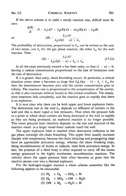
Sec. 21] CHEMICAL KINETICS 561
If the above scheme is to yield a steady reaction rate, d(R)/dt must be
zero.
-jf= = k^AY ~ k2(R)(A) i aA' 2(/?)(/0
- kR)
k (AY1
or (R)"
r
*,(/ixi r+ A-3
The probability of destruction, proportional to A:3 ,can be written as the sum
of two terms, one k(J
for the gas phase reaction, the other kw for the wall
reaction. Then
In all the cases previously treated a has been unity, so that (1 a) --= 0,
leaving a radical concentration proportional to the rate of formation over
the rate of destruction.
If a is greater than unity, chain branching occurs. In particular, a critical
situation arises when a becomes so large that A 2(/4)(a 1)= kg + kw ,
for
then the denominator becomes zero and the carrier concentration goes to
infinity. The reaction rate is proportional to the concentration of the carrier,
so that it also increases without bound at this critical condition. The steady-
state treatment fails completely, and the reaction goes so rapidly that there
is an explosion.It is now clear why there can be both upper and lower explosion limits.
The destruction rate at the wall kw depends on diffusion of carriers to the
wall and this is more rapid at low pressures. Thus when the pressure falls
to a point at which chain carriers are being destroyed at the wall as rapidly
as they are being produced, an explosive reaction is no longer possible.
This lower pressure limit therefore depends on the size and material of the
reaction vessel: in a larger vessel fewer radicals reach the wall.
The upper explosion limit is reached when destructive collisions in the
gas phase outweigh the chain branching. This upper limit usually increases
sharply with temperature, because the chain initiating and propagating steps
have an appreciable activation energy, whereas the chain breaking steps,
being recombinations of atoms or radicals, need little activation energy. In
fact, the presence of a third body is often required to carry off the excess
energy generated in the highly exothermic recombination reactions. The
velocity above the upper pressure limit often becomes so great that the
reaction passes over into a thermal explosion.For the hydrogen-oxygen reaction a chain scheme somewhat like the
following appears to be reasonable:
(1) H2 + O2 ->HO2 + H(2) H2 + HO2
-> OH + H2O
(3) OH + H2-* H2 + H

562 CHEMICAL KINETICS [Chap. 17
(4) O2 + H -> OH + O
(5) H2 + O ~> OH + H
(6) HO2 + wall -> removal
(7) H + wall -> removal
(8) OH + wall -> removal
The hydroxyl radical, OH, has been spectroscopically detected in the reaction
mixture. Chain branching occurs in steps (4) and (5) since OH, O, and H are
all active chain propagators.22. Trimolecular reactions. The necessity of a third body to carry off the
excess energy in atom recombinations is well established. Studies have shown
that such reactions as M + H + H > H2 + M and M + Cl -f Cl -> C12 +M are of the third order. The factors that determine the relative efficiencies
in promoting recombination of different third bodies M are of great interest
in connection with the problem of energy transfer between molecules. In a
study of the recombination of iodine and bromine atoms produced by thermal
decomposition of the molecules, Rabinowitsch27 measured the rate constants
for the reaction, X + X + M -- X2 + M: -d(X)ldt = k^(X)2(M). The
values of k3 in units of (molecules/cc)~2 sec" 1 x 1032 were:
It is difficult to calculate the number of "triple collisions" that occur in
a gas, but a fairly good estimate should be that the ratio of binary collisions
Z12 to triple collisions Z121 is equal to the ratio of the mean free path to the
molecular diameter A/rf. As d is of the order of 10~8 cm, and A at 1 atm
pressure is about 10~5 cm for most gases, the ratio is about 1000. Rabino-
witsch found that this ratio, Z12/Z121 , closely paralleled the rate constants of
the halogen atom-recombination reactions. In this case at least, the efficiency
of the third body seems to depend mainly on the number of triple collisions
it undergoes.Besides three-body recombinations, the only known gas reactions that
may be trimolecular are the third-order reactions of nitric oxide mentioned
on page 536. Trautz showed that these may actually consist of two bimole-
cular reactions; for example,
(1) 2 NO ^ N2O2
(2) N2 2 + 2-'-
27Rabinowitsch, Trans. Faraday Soc., 33, 283 (1937).

Sec. 23] CHEMICAL KINETICS 563
If equilibrium is set up in (1), K = (N2O2)/(NO)2
. Then, from (2),
ffi^ - *2(N2 2)(02) = M:(NO)2(02)
The observed third-order constant is k3 = k2K.
23. The path of a reaction, and the activated complex. With the develop-ment of quantum theory and statistical mechanics powerful tools became
available for a renewed theoretical attack on chemical kinetics. The simple
collision theory can give only qualitative results. It predicts that all bi-
molecular gas reactions have rate constants around \Qwe~EIRT liter sec"1
mole"1,and it is powerless to deal with deviations from this figure. Applied
to reactions in solution, the collision theory is even less adequate for there
is no unequivocal way of calculating a collision frequency in solution. The
newer theories of chemical kinetics dispense with the crude concept of a
collision and inquire how the potential energy of the system of nuclei and
electrons of the reacting molecules varies as the molecules are brought
together.
This is, of course, a problem for quantum mechanics, but it would be
hopeless to attempt an exact solution for complicated molecules. It may be
recalled that even in calculating stable equilibrium states for molecules, the
only success so far achieved has been in the case of H 2 , a two-electron
problem. On the experimental side, molecular spectra have provided muchinformation about the energy levels and potential-energy diagrams of mole-
cules, and some of these data help to elucidate molecular reactions.
The first successful application of quantum mechanics to a chemical
reaction was made in 1931 by Henry Eyring and M. Polanyi.28They chose
as their subject one of the simplest of all chemical processes, the reaction of
a hydrogen atom with a hydrogen molecule.
It is possible to follow this reaction because there are two nuclear-spin
isomers of H2 . Pure para-H2 can t>e made by cooling ordinary equilibriumH2 (3 ortho to 1 para) to 190C in contact with a charcoal catalyst. This
para-Hz is then stable unless it is heated to high temperatures or broughtinto contact with a catalyst after warming. In the presence of hydrogen
atoms, the reaction H + H2 (/?)-> H 2 (0) + H occurs. This reaction was
studied by A. Farkas between 600 and 900C, the source of H atoms beingthe thermal dissociation H2
= 2 H, whose equilibrium is well known. Geib
and Harteck29 followed the reaction between and 100C, using H atoms
produced by passing an electric discharge through H2 . The extent of con-
version could be followed by continuous measurement of the thermal con-
ductivity of the gas, which is different for/?- and o-H2 owing to the difference
in their specific heats. Both investigations agreed that the activation energyof tine reaction is about 7.0 kcal.
28Eyring and Polanyi, Z. physik. Chem., B 72, 279 (1931).
29 K. H. Geib and P. Harteck, Z. physik. Chem., Bodenstein Festband, 849 (1931).
564 CHEMICAL KINETICS [Chap. 17
The reaction between hydrogen atoms and hydrogen molecules can also
be followed by using deuterium. Then, D + H H->D H + H. The
activation energy is 8.5 kcal.
Quantum mechanics treats the reaction as the problem of calculating
the potential energy of a system of three hydrogen atoms for all possible
distances of separation between the nuclei. It would seem at first that at
least six coordinates have to be used: atom (1) could be taken as fixed, and
then we could use x2y2z2 for atom (2) and .V3j3z3 for atom (3). Fortunately,
preliminary calculations showed that such great detail is not necessary; it is
sufficient to calculate the potential energy of the system as one atom, say D,
approaches along the line of centers of the molecule H H. This path will
be the most favorable for a reaction to follow, for in this way the approach-
ing atom overlaps the electron cloud of only one of the two other atoms.
Only two coordinates are therefore needed : r2 , the distance between the two
hydrogen nuclei H 4 and H#, and rl9 the distance of D from H 4 .
The reaction then consists in moving the atom D along a straight line
through H H until it reaches an intermediate configuration D H H. As
the D atom nears the H H, the H atom on the opposite side graduallystretches away, and finally, if reaction occurs, it departs along the line of
centers, leaving as final product D H + H.
To plot the potential energy as a function of rtand r2 , a three-dimen-
sional diagram is needed, but this plot can be represented by contour lines
on a planar map. By appropriately skewing the rland r2 axes with respect
to each other, it is possible to represent the conversion of translational to
vibrational energy by the motion of a point (or ball) sliding on the potential-
energy surface.30
The completed diagram for the system D ~f H H is shown in (a),
Fig. 17.12. It will repay careful study until the three-dimensional form of the
potential energy landscape can be clearly visualized from the map. Even for
this simple system, the quantum-mechanical calculations are forced to rely
on some rather drastic approximations, but the result is essentially correct.
Consider a cut taken through the map at rt= 4.0 A, i.e., at a D H
separation sufficiently large to leave the H H molecule practically undis-
torted. The cross section, shown in (b), Fig. 17.12, is then simply the poten-tial energy curve for the H2 molecule that was described on page 298. Thelowest level is the zero point energy of H2 , 6.2 kcal per mole. Higher levels
represent vibrational excitation. The plateau at the northeast of the mapcorresponds to complete dissociation of both hydrogen molecules into H+ H + D. In accord with our previous data from the potential-energycurve of H2 ,
it is 109 kcal high, or 103 kcal above the zero-point energyin H2 .
If one travels along the valley floor, following the dashed line on the
30S. Glasstone, K. J. Laidler, and H. Eyring, The Theory ofRate Processes (New York:
McGraw-Hill, 1941), p. 100.

Sec. 23] CHEMICAL KINETICS 565
map, the view to right and left looks like the cross section in (b), Fig. 17.12.
The elevation, however, gradually rises as one traverses the mountain pass,
reaching a height of 14 kcal at the saddle point, whereupon there is a slight
40/1
10 15 20 25 30ANGSTROMS -*-r,
(a)
40
1*2
(b)
Fig. 17.12. The potential-energy surface for the reaction D -f Ha=
(After H. Eyring.)
HD + H.
dip into a shallow bowl or crater situated at the mid-point of the pass. This
depression, where the arrows make a turn on the map, occurs at a con-
figuration D H H, with T!= r2 0.95 A. This distance is considerably
greater than the normal internuclear separation in H2, which is 0.74 A.

566 CHEMICAL KINETICS [Chap. 17
The configuration at the midpoint of the mountain pass between the two
valleys is the activated complex for the reaction. When the system reaches
this configuration, it can either decompose into DH f H by moving downinto the other valley, or return along its original path into D (- H2 .
If the potential energy is drawn as a function of distance along the
reaction path (dashed line), Fig. 17.12 (c) is obtained. This diagram is almost
the same as Fig. 17.1 on page 531, and indeed the little depression at the
top of the path is not important to the argument. It is evident that the
minimum energy barrier that must be surmounted is 7.8 kcal, and this is
the calculated energy of activation for the reaction.
The potential-energy surface gives a picture of a chemical reaction from
beginning to end. In any reaction there is always a certain configuration at
the top of the barrier, the activated complex, which must be reached by the
reactants before transformation to products can occur. Only in very simple
examples can the potential-energy surface be calculated by quantum mech-
anics, and then only by means of drastic approximations. The importantfeature of the new theory, however, is the clear physical picture it gives.
The concept of a collision of hard spheres is replaced by that of a smooth
and continuous transition from reactants to products.24. The transition-state theory. The rate of any chemical reaction can be
formulated in terms of its activated complex.31 The rate of reaction is simply
the number of activated complexes passing per second over the top of the
potential-energy barrier. This rate is equal to the concentration of activated
complexes times the average velocity with which a complex moves across to
the product side. It makes no difference how these complexes happen to be
formed, or how many intermediate stages there may be between reactants
and activated complexes. This fact vitiates at one stroke a good deal of
popular speculation on mechanisms leading from reactants to complexes.The calculation of the concentration of activated complexes is greatly
simplified if it is assumed that they are in equilibrium with the reactants.
This equilibrium can then be treated by means of statistical mechanics. The
activated complex is not a state of stable equilibrium since it lies at a maxi-
mum and not a minimum of potential energy.32 Yet more detailed calcula-
tions have shown that there is probably little error in treating the equilibrium
by ordinary thermodynamic or statistical methods, except perhaps in the case
of extremely rapid reactions.
31 The quantitative formulation of reaction rates in terms of activated complexes wasfirst extensively used in the work of H.
Eyring [/. Chem. Phys., 3, 107 (1935); Chem. Rev., 17,
65 (1935)]. This theory has been applied to a wide variety of "rate processes*' besides
chemical reactions, such as the flow of liquids, diffusion, dielectric loss, internal friction in
high polymers. Other noteworthy contributions to the basic theory were made by M. G.Evans and M. Polanyi [Trans. Faraday Soc., 31, 875 (1935)], H. Pelzer and E. Wigner[Z.ohysik. Chem., B 15, 445 (1932)].
*aStrictly speaking the activated state should lie at the maximum in free energy. The
calculation of this would be even more difficult than the calculation of the potential energysurface.

Sec. 24] CHEMICAL KINETICS 567
For example, consider a simple bimolecular reaction :
A + B -+ (AB)* -> products
If the activated complex (AB)* is in equilibrium with reactants, the equili-
brium constant for the formation of complexes is K* = (AB*)/(A)(B). The
concentration of complexes is (AB)* K*(A)(B).
According to the transition-state theory, the rate of reaction is d(A)ldt
(AB)* x (rate of passage over barrier). The rate of passage over the
barrier is equal to the frequency with which the complex flies apart into the
products. The complex flies apart when one of its vibrations becomes a
translation, and what was formerly one of the bonds holding the complex
together becomes simply the line of centers between separating fragments.
The frequency v is equal to p/h where f is the average energy of the vibration
that leads to decomposition. Since this is by hypothesis a thoroughly excited
vibration at the temperature 7, it has its classical energy E = kT, and the
corresponding frequency becomes v - kT/h.
The reaction rate is therefore
The rate constant is
kTk, ---- -- K* (17.22)
This is the general expression given by the transition-state theory for the
rate constant of any elementary reaction. To be precise, this expression for k2
should be multiplied by a factor K, the transmission coefficient, which is the
probability that the complex will dissociate into products instead of back into
reactants. For most reactions K is between 0.5 and 1.0.
The activated complex is similar to a normal stable molecule in every
respect save one. The sole difference is that one, of its vibrational degrees of
freedom is missing, having been transformed into the translation along the
reaction coordinate that leads to disruption of the complex. Instead of
3n 6 vibrations, therefore, a nonlinear complex has 3n 7. A linear
complex has 3/76 instead of the 3n 5 for a linear normal molecule.
The statistical expression for the equilibrium constant K*9 from eq.
(12.41), is
Thus
k*= T-7T e
~*SJ*T(17 '23)
n JAJK
The /'s are the partition functions of activated complex and reactants, and
AE0 is the difference in the zero-point energies of reactants and complex,* - (EOA + EOB + . . .)

568 CHEMICAL KINETICS [Chap. 17
A thermodynamic formulation of eq. (17.22) can also be given by intro-
ducing the standard free energy change, A/^* == RTln K
c*. Note that
this is the difference between the free energy of the activated complex and
that of the reactants, when all are in their standard states. In this case the
standard state has been taken to be the state of unit concentration, because
rate constants are usually expressed in terms of concentrations. Since
AF* A//* - T AS *, eq. (17.22) becomes
The quantities A/70 *, A// *, and AS * are called the free energy of activa-
tion, the enthalpv or heat of activation, and the entropy of activation.
Now A//* is almost equivalent to the experimental energy of activation
Ea in the Arrhenius equation. Actually A//* =- AE* + P AK*. In liquid
and solid systems the P&V term is negligible at ordinary pressures, so that
fromeq. (17.24),
</ln*. E. W+ + RTt ^ ^ = A/r* +^
In Ideal gases, A//* - A* + />AF* - AE* + A/7* RT. In this case,
therefore,
2 a _ A//* -(A/7*
- l)RT
~dT" " "" ~ '
and Ea--= A//* - (A* - \)RT
The term Art* is the number of moles of complex, always equal to one,
minus the number of moles of reactants. In a unimolecular reaction, there-
fore, AA?* = 0; in a bimolecular reaction, A* 1, etc. The entropyof activation can therefore readily be calculated from the experimentalk and Ea .
25. Collision theory and transition-state theory. Since the activated-
complex theory is more comprehensive than the collision theory, the latter
should appear as one of its special cases. This can be demonstrated by con-
sidering a bimolecular reaction between two atoms, A and B:
A + B -> (AB)* -> products
The statistical theory expresses the rate constant as
k .
2~
h
The activated complex (A B)* has five degrees of freedom, three trans-
lational and two rotational (the missing vibration has disappeared into the
decomposition coordinate). The atoms A and B have translational degrees of

Sec. 26] CHEMICAL KINETICS 569
freedom only. Using the formulas of Chapter 12, the rate constant, with
concentration units of molecules per cc, can be written
k =.k_L .
2h
Note that the mass of the activated complex is m* = mt |
mn . If r,
is the internuclear separation, the moment of inertia of the complex is
Introducing this value of / into the expression for A'2 ,
JSJRT
This becomes identical with the collision-theory expression in cq. (17.19)
when expressed in the same units.
Thus the transition-state theory reduces to collision theory when the
reactants are two atoms, or more generally, whenever all terms due to
internal degrees of freedom, except two rotational terms, cancel out between
reactants and activated complex. The essential defect of the collision theoryis revealed to be its neglect of internal degrees of freedom. It treats the
reactant molecules as rigid spheres rather than as pulsating structures of
nuclei and electrons. The old steric or probability factor/;was a measure of
this deficiency. The transition-state theory gives a formally complete account
of the effect of internal degrees of freedom, yet we never have adequatedetails of the dimensions of the activated complex and its vibration fre-
quencies. The best that can be done is to assign approximate values to the
partition functions, based on our experience with normal molecules.
The probability of reactions between polyatomic molecules may be
lowered because rotational and translational freedoms are lost when the
reactants are tied together into the activated complex. This loss of freedom
or increase in order is measured also by the entropy of activation, which
simply expresses the statistical factors in thermodynamic language.26. The entropy of activation. The idea of an entropy of activation was
developed by Rodebush, La Mer, and others, before the advent of the
activated-complex theory, which gave it a precise formulation.
A positive activation entropy AS* means that the entropy of the complexis greater than the entropy of the reactants. A loosely bound complex has
a higher entropy than a tightly bound one. More often there is a decrease
in entropy in passing to the activated state.
In bimolecular reactions the complex is formed by association of two
individual molecules, and there is a loss of translational and rotational free-
dom, so that AS* is negative. In fact, sometimes AS* is not notably different

570 CHEMICAL KINETICS [Chap. 17
from AS for the complete reaction. This situation is often found in reactions
of the type A -f B -> AB, and indicates that the activated complex (AB)* is
similar in structure to the product molecule AB.
Formerly such reactions were considered to be very "abnormal" since
they had to be assigned very low steric factors. It is now clear that the slow
velocity is simply the result of the increase in order, and consequent decrease
in entropy, when the complex is formed.
27. Theory of unimolecular reactions. The essential theoretical problem in
unimolecular reactions is to extend and refine the Lindemann theory, so that
we can interpret the kinetic constants in terms of the molecular structures and
vibration frequencies of the reacting molecules. Once a molecule has obtained
more than a certain critical amount of internal energy, it is said to be activated.
The first part of the problem is to calculate the rate at which a molecule can
accumulate this energy. The next question is how long will it take, on the
average, for this energy to flow into the bond which is to be broken in the
decomposition process. Kassel33 and others, in 1932, modified the simple
equation (17.20) to take into consideration the fact that the lifetime of an
activated molecule must depend upon the amount of internal energy that it
has acquired in excess of the minimum critical amount required for dissocia-
tion. This theory has been greatly extended by N. B. Slater.34 For the limiting
high-pressure rate (first-order rate constant), Slater finds the expression
/, V--EOIRT /\ 7 *>c\kl^ ve (1/.Z3)
where v is a weighted root mean square of the frequencies of the normal
modes of vibration of the molecule.
Va>, 2\1/2
The constants at ,
called amplitude factors, can be calculated from the force
constants of the vibrations, and the masses of the atoms in the molecule.
Confirmation of the general form of eq. (17.25) is provided by the fact that
molecular vibration frequencies v are of the order of 1013 sec" 1,and the fre-
quency factors of most unimolecular reactions cluster closely about this
figure.
The more difficult part of the theory is to calculate the pressure dependenceof the rate in the region where the collisional activations are insufficient to
maintain a first-order kinetics. Slater has obtained a solution for this problemalso, based on a treatment of the vibrating molecule as a collection of classical
harmonic oscillators. The results of this theory are most encouraging, but
their mathematical form is not very succinct, and we must refer the reader to
the original papers for the detailed theoretical equations.
33L. S. Kassel, J. Chem. Phys., 21, 1093 (1953). This paper contains references to the
earlier work.34 N. B. Slater, Proc. Roy. Soc., A, 218, 224 (1953); PhiL Trans. A, 246, 57 (1953).

Sec. 28] CHEMICAL KINETICS 571
28. Reactions in solution. It has not been possible to make a completetheoretical analysis of the rates of reactions in liquid solutions, although
many special aspects of such reactions are quite well understood. It mightseem that collision theory should hardly be applicable at all, since there is
no unequivocal way of calculating collision frequencies. It turns out, how-
ever, that even the gas-kinetic expressions sometimes give reasonable values
for the frequency factors.
First-order reactions, such as the decomposition of N2O5 , C12O, or
CH2I2 , and the isomerization of pinene, proceed at about the same rate in
gas phase and in solution. It appears, therefore, that the rate is the same
whether a molecule becomes activated by collision with solvent molecules
or by gas-phase collisions with others of its own kind. It is more remarkable
that many second-order, presumably bimolecular, reactions have rates close
to those predicted from the gas-kinetic collision theory. Some examples are
shown in the last column of Table 1 7.5. The explanation of such an agreementseems to be the following. Any given reactant solute molecule will have to
diffuse for some distance through the solution before it meets another
reactant molecule. Thus the number of such encounters will be lower than in
the gas phase. Having once met, however, the two reactant molecules will
remain close to each other for a considerable time, being surrounded by a
"cage" of solvent molecules. Thus repeated collisions between the same pair
of reactant molecules may occur. The net result is that the effective collision
number is not much different from that in the gas phase.
TABLE 17.5
EXAMPLES OF REACTIONS IN SOLUTION
Reaction
C2H 5ONa + CH 3 I
C2H 5ONa I C6H5CH 2 I
NH4CNO -> (NH2)2COCH2C1COOH I OH-C2H 5Br + OH-(C2H 5 )3N f C2H5Br
CS(NH2)2 + CH3I
C l2H 22On + H 2-> 2 C6H 12 6
(sucrose)
There are other cases in which the calculated constant deviates by factors
ranging from 109 to 10~9. A high frequency factor corresponds to a large
positive AS1
*, and a low frequency factor to a negative AS*. The remarks
on the significance of AS* in gas reactions apply equally well here.
Association reactions may be expected to have low frequency factors

572 CHEMICAL KINETICS [Chap. 17
owing to the decrease in entropy when the activated complex is formed. An
example is the Menschutkin reaction, combination of an alkyl halide with a
tertiary amine: (C2H5)3N + C2H6Br -> (C2H5)4NBr. Such reactions have
values of AS* from 35 to 50 eu, usually nearly equal to the AS for the
complete reaction.
A striking example of another kind is found in the rates of denaturation
of proteins. Every time we boil an egg, we carry out, among other reactions,
the denaturation of egg albumin from a soluble globular protein to an in-
soluble fibrous protein. A remarkable property of the denaturation reaction
is its unusually high temperature coefficient. Atop Pikes Peak, where water
boils at 91C, it would take 12 hours to hardboil an egg (without a pressure
cooker). Since about 10 minutes are required at 100C the corresponding
energy of activation is 130 kcal. This is a surprisingly high figure when it is
remembered that the usual reaction proceeding at a measurable rate at 100Chas an activation energy of about 15 kcal. From an activation-energy stand-
point one might think that it should be impossible to hardboil an egg at all.
The reason why the reaction does proceed quite rapidly is that it has the
extraordinarily high positive entropy of activation of -j 315.7 eu.
The native protein is a highly organized structure; it is the very anti-
thesis of randomness or disorder. The denaturated protein, by contrast, is
disordered and random. In such a change there is a great entropy increase,
and apparently the activated complex partakes of a good deal of the dis-
orderliness of the final product. Bound water molecules or ions may be set
free on denaturation, also contributing to the increase in entropy. Hence the
high AS* and the possibility of the hardboiled egg.
29. Ionic reactions salt effects. Electrostatic interactions cause the equi-
librium properties of ionic solutions to deviate greatly from ideality. The
same causes are responsible for a number of unusual features in the kinetics
of reactions between ions. The first effective treatment of these reactions was
provided by J. N. Br0nsted and N. Bjerrum in their activity-rate theory.
Proposed in 1922, this is essentially an activated-complex theory applied to
charged particles.
Consider a reaction between two ions, A z* and BZB, ZA and ZB being the
ionic charges. It proceeds through an activated complex, (AB)1-^**.
A ZA-{- BZB -> (AB)
Z*+ Z* > products
Example: S2O8
~-\- \~ -> (S2O8 if - > 2SO4 + i! 2
The complex is considered to be in equilibrium with reactants, but since
we are dealing with ions, it is necessary to express the equilibrium constant
in activities rather than concentrations:

Sec. 29] CHEMICAL KINETICS 573
The tf's and y's are the activities and activity coefficients. The concentration
of activated complexes is c* =
0.60
.30
Fig. 17.13. Variations of rates of ionic reactions with the ionic strength. The circles
are experimental values: the lines are theoretical, from eq. (17.27).
(1) 2[Co(NH 3) 5Br]^ f Hg++ -\- 2H 2O - 2[Co(NH 3)6H 2O]+++ -f HgBr2
(2) S 2 8
=4- 21- = I 2 4 2S04
=
(3) [NO 2NCOOC 2H 5]- -4- OH- - N 2O 41 CO3= + C2H 5OH
(4) Inversion of cane sugar(5) H 2 2 -f 2H + f 2Br~ = 2H aO 4 Br a
(6) [Co(NH 3) 5Br]++ -f OH~ - [Co(NH3)5OH]^ ^ + Br~
The reaction rate is (dcA/dt)= k2cAcB = (kT/h)c*. The rate constant is
(17.26)n y
' n y
In dilute aqueous solution the activity coefficient terms can be estimated
from the Debye-Hiickel theory. From eq. (15.51), at 25C in an aqueous
U

574 CHEMICAL KINETICS [Chap. 17
solution, Iog10 y l
-= 0.509 zf^s. Taking the loglo of eq. (17.26) and sub-
stituting the Debye-Huckel expression, we get
kT v 4v /;>
logw *8 -=log10 -;-A:* + log10^n y~*~
B + [ 0.509 z/ - 0.509 z/?
2 + 0.509 (ZA + z/?)
2] vA
logw *2* + 1.018 z 4z7,v^ (17.27)
The constant Iog10 (kTjh)K* has been written as B.
The Br0nsted equation (17.27) predicts that the plot of Iog10 A'2 vs. the
square root of the ionic strength should be a straight line. For a water solution
at 25C the slope is nearly equal to ZAZB , the product of the ionic charges.Three special cases can occur:
(.1) If z,and z/y have the same sign, z^z7/ is positive, and the rate constant
increases with the ionic strength.
(2) If ZA and zn have different signs, zAzn is negative, and the rate con-
stant decreases with the ionic strength.
(3) If one of the reactants is uncharged, zAzH is zero and the rate constant
is independent of the ionic strength.
Those theoretical conclusions have been verified in a number of experi-
mental studies. A few examples are illustrated in Fig. 17.13. This change of
k2 with s is called the primary kinetic salt effect. It should be noted that the
ionic strength s is calculated from iwtz,
2,and the summation is extended
over all the ionic species present in solution, not merely the reactant ions.
Much of the earlier work on ionic reactions is comparatively useless
because the salt effect was not understood. It is now often the practice in
following the rate of an ionic reaction to add a considerable excess of an
inert salt, e.g., NaCl, to the solution, so that the ionic strength is effectively
constant throughout the reaction. If pure water is used, the change in ionic
strength as the reaction proceeds may lead to erratic velocity constants.
30. Ionic reaction mechanisms. Besides the salt effect discussed by
Br0nsted, specific interactions between the ions in solution may influence
the reaction rates. For reactions between ions of the same charge sign, the salt
effect often appears to be governed predominantly by the concentrations and
charges of those added ions with a sign opposite to that of the reactant ions.35
The mechanism of ionic reactions is often indirectly determined byelectrostatic factors, in particular the strong repulsion between ions of the
same sign. The reaction 2 Fe i3 + Sn F2 2 Fe f2 + Sn f4,for example, occurs
rapidly, but the mechanism is probably a series of steps involving the transfer
of single electrons between species of opposite charge sign :
36
SnCl2 |- 2 Cl~ ^ SnCl4
SnCl4 + Fe+3 -> Fe+2 + SnCl4
"
SnCl4- + Fe+3 -> Fe+2 + SnCl4
35 A. R. Olson and T. R. Simonson, /. Chem. Phys., 77, 1167 (1949).86
J. Weiss, J. Chem. Soc., 309 (1944).

Sec. 31] CHEMICAL KINETICS 575
Another instance is the over-all reaction,
5 HBr + HBrO3= 3 Br2 + 3 H 2O
The rate equation is </(Br2 )/<//= A'(H+)
2(Br-)(BKV). Note that the rate
equation bears no relation to the stoichiometric equation. Owing to electro-
static repulsion, it is unlikely that Br~ and BrO3
~ions react directly, and the
following rate controlling step is suggested by the rate equation:
HBr t HBrO3-* HBrO + HBrO2
Rapid secondary reactions yield the final products. Since (HBr) ~ (H K)(Br~),
and (HBrO3 )~ (H+)(BrO3~), the observed kinetics is obtained.
31. Catalysis. The word "catalysis" (Katalyse) was coined by Berzelius
in 1835: "Catalysts are substances which by their mere presence evoke
chemical reactions that would not otherwise take place." The Chinese Tsoo
Mel is more picturesque; it also means "the marriage broker," and so
implies a theory of catalytic action. The idea of catalysis extends far back
into chemical history. The quest of the alchemist for the philosopher's stone
seems like the search of the modern petroleum chemist for the magical
catalyst that will convert crude petroleum into high octane fuel. In a four-
teenth-century Arabian manuscript, Al Alfani described the "Xerion, aliksir,
noble stone, magisterium, that heals the sick, and turns base metals into
gold, without in itse/f undergoing the least change" The earliest consciouslyused catalysts were the ferments or enzymes. "In the seeding and growth of
plants, and in the diverse changes of the fluids of the animal body in sickness
and in health, a fermentative action takes place" (Marquers, 1778).
Noteworthy was the idea that a mere trace of catalyst suffices to produce
great changes, without itself being changed. Its action has been likened to
that of a coin inserted in a slot machine that yields valuable products and
also returns the coin. In a chemical reaction the catalyst enters at one stage
and leaves at another. The essence of catalysis is not the entering but the
falling out.
Wilhelm Ostwald was the first to emphasize that the catalyst influences
the rate of a chemical reaction but has no effect on the position of equi-
librium. His famous definition was: "A catalyst is a substance that changesthe velocity of a chemical reaction without itself appearing in the end
products." Ostwald showed that a catalyst cannot change the equilibrium
position, by a simple argument based on the First Law of Thermodynamics.Consider a gas reaction that proceeds with a change in volume. The gas is
confined in a cylinder fitted with a piston; the catalyst is in a small receptaclewithin the cylinder, and can be alternately exposed and covered. If the
equilibrium position were altered by exposing the catalyst, the volume
would change, the piston wouVJ move up and down, and a perpetual-motionmachine would be available.
Since a catalyst can change t^ rate but not the equilibrium, it follows

576 CHEMICAL KINETICS [Chap. 17
that a catalyst must accelerate the forward and reverse reactions in the same
proportion, since K = kfjk b . Thus catalysts that accelerate the hydrolysis of
esters must also accelerate the esterification of alcohols; dehydrogenation
catalysts like nickel and platinum are also good hydrogenation catalysts;
enzymes like pepsin and papain that catalyze the splitting of peptides must
also catalyze their synthesis from the amino acids.
A distinction is generally made between homogeneous catalysis, the
entire reaction occurring in a single phase, and heterogeneous catalysis at
phase interfaces. The latter is also called contact or surface catalysis.
32. Homogeneous catalysis. An example of homogeneous catalysis in the
gas phase is the effect of iodine vapor on the decomposition of aldehydes and
ethers. The addition of a few per cent of iodine often increases the rate of
pyrolysis several hundredfold. The reaction velocity follows the equation,
Dependence of the rate on catalyst concentration is characteristic of homo-
geneous catalysis. The catalyst acts by providing a path for the decomposi-tion that has a considerably lower activation energy than the uncatalyzed
path. In this instance the uncatalyzed pyrolysis has an Ea- 53 kcal, whereas
with added iodine the Ea drops to 34 kcal.
Most examples of homogeneous catalysis have been studied in liquid
solutions. In fact, catalysis in solution is the rule rather than the exception,and it can even be maintained that most reactions in liquid solutions would
not proceed at an appreciable rate if catalysts were rigorously excluded.
Since the catalysts are usually acids and bases, it is not easy to controvert
this hypothesis.The general formulation of catalysis in solution postulates the formation
of an intermediate complex between reactant and catalyst. Suppose the
change A -> B is catalyzed by a substance X, through formation of an
intermediate /. Then
A + X ^ /, I--+B+Xt-i
'
Making the steady-state assumption, d(I)/dt=
0, we find
i i 2
Two limiting cases of eq. (17.28) now arise. If k^^k2 , most of the
complexes /revert to the initial reactant A, and only a small fraction proceedto the final product B. Then eq. (17.28) becomes f^A/^-i) (A)(X\ and the
decomposition of the intermediate is the rate-determining step. In a case like
this, / is called an Arrhenius intermediate.
The other limiting case is 2> k_v Tten the slow step is the rate of
formation of intermediate /, and eq. (17.2*) reduces to k^A^X). This kind
Sec. 33] CHEMICAL KINETICS 577
of / is called a van't Hoff intermediate. In either case, the over-all rate is
proportional to the catalyst concentration (X).
The distinction between the two types of intermediate is in most cases
difficult or impossible to make experimentally.37 In any case, the catalysts
usually act by lowering the activation energy of the reaction.
The reaction, 2I~ ~f- S2O8
=-> I2 + 2SCV, is markedly catalyzed by
ferrous or ferric ions. Copper ions have a lesser effect. When Fe++ and
Cu-^ ions are both added, their effects are not simply additive; the rate
is still more enhanced. This phenomenon is called promoter action and is
often observed in catalysis. For example, /V/2,500,000 Cu++ has itself no
detectable effect on the velocity, but added to a reaction mixture that
already contains yV/32,000 Fe++ , it increases the rate by 15 per cent. Apossible explanation is that the promoter selectively catalyzes the decom-
position of the intermediate formed with the first catalyst, i.e., it increases
the constant k2 in eq. (17.28).
33. Acid-base catalysis. Among the most interesting cases of homo-
geneous catalysis are reactions catalyzed by acids and bases. This acid-base
catalysis is of the utmost importance, governing the rates of a great number
of organic reactions, and especially many of the processes of physiological
chemistry, for it is likely that many enzymes act as acid-base catalysts.
The earliest studies in this field were those by Kirchhoff in 1812 on the
conversion of starch to glucose by the action of dilute acids, and by Thenard
in 1818 on the decomposition of hydrogen peroxide in alkaline solutions.
The classic investigation of Wilhelmy in 1 850 dealt with the rate of inversion
of cane sugar by acid catalysts. The hydrolysis of esters, catalyzed by both
acids and bases, was extensively studied in the latter half of the nineteenth
century. The catalytic activity of an acid in these reactions became one of
the accepted measures of "acid strength," being very useful to Arrhenius
and Ostwald in the early days of the ionization theory.
In Table 17.6 are some of Ostwald's results on sucrose inversion and
methyl-acetate hydrolysis. If we write the acid as HA these reactions are
C12H22On -f H2 + HA -> C6H12 6 + C6H12O6 + HACH3COOCH3 + H2O + HA -> CH^COOH + CH3OH + HA
The reaction rate may be written dx\dt = ^CH3COOCH3)(H2O)(HA).
Since the water is present in large excess, its concentration is effectively
constant. The rate therefore reduces to: dxjdt = fc"(HA)(CH3COOCH3).
Now k*' is called the catalytic constant. The values in Table 17.6 are all
relative to HC1 = 100.
Ostwald and Arrhenius showed that the catalytic constant of an acid is
proportional to its equivalent conductivity. They concluded that the nature
of the anion was unimportant, and that the only active catalyst was the
hydrogen ion, H+.87 Cf. G. M. Schwab, H. S. Taylor, and R. Spence, Catalysis (New York: Van Nostrand,
1937), p. 68.

578 CHEMICAL KINETICS [Chap. 17
TABLE 17.6
OSTWALD'S DATA ON THE CATALYTIC CONSTANTS OF DIFFERENT ACIDS
In other reactions it was necessary to consider the effect of the OH~ ion
and also the rate of the uncatalyzed reaction. This led to a three-term equa-tion for the observed rate constant, k --- A' f A'H .(H
f) -)- A'OH_(OH-). Since
in aqueous solution Kw - (H+)(OH~),
* = * + *H .(H+) +^^ (17.29)
Since Kw is about lO"14,in 0.1 N acid (OH~) is 10~13
, and in 0.1 N base
(OH~) is 10-1. There is a 1012-fold change in (OH~) and (H+) in passing
oo
pH
Fig. 17.14. Acid-base catalysis: the influence ofpH on rate constants.
from dilute acid to dilute base. Therefore the (OH~) catalysis will be negli-
gible in dilute acid and the (H+) catalysis negligible in dilute base, except in
the unusual event that the catalytic constants for H4 and OH- differ by as
much as 1010 . By measurements in acid and basic solutions it is therefore
generally possible to evaluate kn + and &OH _ separately.

Sec. 34] CHEMICAL KINETICS 579
If kH+ = ii- a minimum in the over-all rate constant occurs at the
neutral point. If either kn+ or /:OH - is very low, there is no rise in k on the
corresponding side of the neutral point. These and other varieties of rate
constant vs. pH curve, arising from different relative values of & , /CH ,, and
^OH- are shown in Fig. 17.14.
Examples of each of the different types have been studied experimen-
tally.38They include the following:
(a) The mutarotation of glucose
(b) Hydrolysis of amides, y-lactones, esters; halogenation of acetone
(c) Hydrolysis of alkyl orthoacetates
(d) Hydrolysis of /Mactones, decomposition of nitramide, halogenationof nitroparaffins
(e) Inversion of sugars, hydrolysis of diazoacetic ester, acetals
(f) Depolymerization of diacetone alcohol; decomposition of nitroso-
acetonamine
34. General acid-base catalysis. Advances in our understanding of acid-
base catalysis have been closely linked with improvements in the theory of
electrolytic solutions. The early notion that the conductance ratio, A/A , of
a strong electrolyte measures its degree of dissociation has been superseded
by the Debye-Hiickel idea of complete ionization. In fact, one of the first
evidences for the latter viewpoint was the observation of Bjerrum that the
catalytic activity of strong acids is proportional to their total concentration
in solution rather than to the H+ concentration as calculated from the
Arrhenius theory.
The influence of added salts in the primary kinetic salt effect has alreadybeen noted. In addition to this direct dependence of reaction rate on ionic
strength, there is an indirect influence important in catalyzed reactions. In
solutions of weak acids and bases, added salts, even if they do not possess
a common ion, may change the H+ or OH~ ion concentration through their
effect on the activity coefficients. For an acid HA -> H+ + A~,
Any change in the ionic strength of the solution affects the y terms and
hence the concentration of H f. Consequently, if the reaction is catalyzed
by H 1 or OH" ions, the reaction rate is dependent on the ionic strength. This
is called the secondary kinetic salt effect. Unlike the primary effect it does not
alter the rate constant provided this is calculated from the true H+ or OH~concentration.
The broader picture of the nature of acids and bases given by the work
of Br0nsted and Lowry (page 469) implies that not only H+ and OH~ but
also the undissociated acids and bases should be effective catalysts. The
38 See A. Skrabal, Z. /. Elektrochem., 33, 322 (1927); R. P. Bell, Acid-Base Catalysis
(New York: Oxford, 1941).

580 CHEMICAL KINETICS [Chap. 17
essential feature of catalysis by an acid is the transfer of a proton from acid
to substrate,39 and catalysis by a base involves the acceptance of a proton
by the base. Thus in Br0nsted-Lowry nomenclature, the substrate acts as a
base in acid catalysis, or as an acid in basic catalysis. In the case of hydrogenion catalysis in aqueous solution, the acid is really the hydronium ion, OH3+.
For example, the hydrolysis of nitramide is susceptible to basic but not
to acid catalysis.
NH2N02 + OH- -> H2 + NHN02
~
NHNO2
~ -> N2O + OH-
Not only the OH~ ion but also other bases can act as catalysts, e.g., the
acetate ion :
NH2N02 + CH3COO- >CH3COOH + NHNO2
~
NHNO2~ -> N2O + OH-
OH- + CH3COOH -> H2O + CH3COO~
The reaction rate with different bases B is always v = kB(B) (NH2NO2).
Br0nsted found that there was a relation between the catalytic constant kBand the dissociation constant KB of the base, namely,
kB - CKJ (17.30)
or log kB = log C + $ log KBHere C and /? are constants for bases of a given charge type. Thus the
stronger the base, the higher the catalytic constant.40
The nitramide hydrolysis displays general basic catalysis. Other reactions
provide examples of general acid catalysis, with a relation like eq. (17.30)
between kA and KA . There are also reactions with both general acid and
general basic catalysis.
Since a solvent like water can act as either an acid or a base, it is often
itself a catalyst. What was formerly believed to be the uncatalyzed reaction,
represented by kQ in eq. (17.29), is in most cases undoubtedly a reaction
catalyzed by the solvent acting as acid or base.
35. Heterogeneous reactions. In our description of homogeneous reactions
a number of instances have been noted in which the surface of the reaction
vessel has a definite influence on the kinetics. Such an effect is very importantin establishing the lower pressure limit of an explosive chain reaction. There
are many reactions whose velocities are immeasurably slow in homogeneous
gaseous or liquid solutions, but which go quite swiftly if a suitable solid
surface is available. In fact, in some instances the solid surface can alter the
entire course of the reaction.
The earliest instance of this contact action or contact catalysis was the
dehydrogenation of alcohols by metals studied by van Marum in 1796. In
39 Substance whose reaction is being catalyzed.40 For polybasic bases, a correction must be made. See R. P. Bell, op. cit., p. 83.

Sec. 35] CHEMICAL KINETICS 581
1817, Davy and Dobereiner investigated the glowing of certain metals in a
mixture of air and combustible gases ; and in 1 825, Faraday worked on the
catalytic combination of hydrogen and oxygen. These studies laid the
experimental foundations of heterogeneous kinetics.
An interesting example was found41 in the bromination of ethylene:
C2H4 + Br2-- C2H4Br2 . This reaction goes quite readily in a glass vessel
at 200C, and it was at first thought to be an ordinary homogeneous com-
bination, but the rate seemed to be higher in smaller reaction vessels. Whenthe vessel was packed with lengths of glass tubing or with glass beads, the
rate was considerably enhanced. This method is frequently used for detecting
wall reactions. An increased rate in a packed vessel indicates that a con-
siderable share of the observed reaction is heterogeneous, on the packing and
wall, rather than homogeneous, in the gas phase only. A further test was
made by coating the inside of the reaction bulb with paraffin wax. This
coating inhibited the reaction almost completely.
The decomposition of formic acid illustrates the specificity often dis-
played by surface reactions. If the acid vapor is passed through a heated
glass tube, the reaction is practically one-half dehydration and one-half
dehydrogenation.
(1) HCOOH -> H 2O I CO(2) HCOOH -> H 2 + CO2
If the tube is packed with alumina, A1 2O3 , only reaction (1) occurs; but if
it is packed with zinc oxide, ZnO, (2) is the exclusive result. Thus different
surfaces can accelerate different parallel paths, and so in effect determine the
nature of the products.
It seems evident that the catalytic action of a surface depends on its
adsorption of the reactants. Many features of heterogeneous kinetics can be
explained by this hypothesis and the application of Langmuir's equation.A surface reaction can usually be broken into the following elementary
steps :
(1) Diffusion of reactants to surface
(2) Adsorption of reactants at surface
(3) Chemical reaction on the surface
(4) Desorption of products from surface
(5) Diffusion of products away from surface
These are consecutive steps and if any one is much slower than all the others,
it will become rate-determining.
Steps (1) and (5) are usually rapid. Only with extremely active catalysts
might they determine the over-all rate. Diffusion has a \/T and chemical
reaction has an e~ ElRT temperature dependence. Therefore, if a catalytic
reaction rate increases only slightly with temperature, it may be diffusion-
controlled.
41 R. G. W. Norrish, /. Chem. Soc., 3006 (1923).

582 CHEMICAL KINETICS [Chap. 17
Steps (2) and (4) are generally more rapid than step (3), but reactions are
known in which they may be the slow stages. Usually, however, the reaction
at the surface, step (3), is believed to be rate-determining.
36. Gas reactions at solid surfaces. The Langmuir isotherm (page 515)
is based on thre gradual coverage of a surface with adsorbed molecules,
saturation occurring when the adsorbed layer is uniformly one molecule
thick. The isotherm is especially applicable to cases of chemisorption, in
which the adsorbed molecules are held to the surface by bonds comparablewith those in chemical compounds. This is also the kind of adsorption that
can greatly accelerate reaction rates, the chemisorbed layer playing the role
of an intermediate compound in catalyzing the reaction. On the other hand,
physical or van der Waals adsorption can hardly have more than the slight
effect on reaction rates caused by an increased concentration in the adsorbed
layer.
The Langmuir isotherm was illustrated in Fig. 16.10 on page 516. It can
be roughly divided into three sections: (a) the range of small adsorption or
nearly bare surface, where the fractional surface coverage~-~ bP\ (b) an
intermediate region in which approximately= bPlfn
\ (c) the region of
almost complete coverage, where effectively-
1 over a considerable
pressure range. The particular adsorbate gas and adsorbent solid will deter-
mine the region of the isotherm useful in a given system. If a gas is strongly
adsorbed, the surface may be almost covered even at low pressures; but if
a gas is weakly adsorbed, the linear section =- bP may extend to quite high
pressures.
In a heterogeneous gas reaction, it can usually be assumed that only the
adsorbed gas undergoes reaction.42 If a single reactant is being decomposedat an active surface, three simple special cases can arise. The reaction rate
will be proportional to 0, the fraction of surface covered.
(1) Single reactant, weakly adsorbed, 6?-=bP. Rate: -dPjdt --=0= =
k bP = k'P. The reaction is first order. Examples of this kind include the
decomposition of arsine and phosphine on glass, AsH3-> As + $ H2 ;
hydrogen iodide on platinum, 2 HI ~> H 2 + I 2 .
(2) Single reactant, moderately adsorbed, = bPl/n. Rate: -dPjdt =
k bO = k bPlln -= k'Plln. An example is the decomposition of arsine on a
surface of metallic arsenic, following the equation dP/dt = kP-Q.
(3) Single reactant, strongly adsorbed, 0=1. Rate: dP/dt ~~= k =k P. In such a case the reaction velocity is independent of the pressure.
This is called a zero-order reaction, a variety of concentration dependence
having no parallel in purely homogeneous reactions. The integrated rate
equation is P =k$t + const or
/V-P-Av (17.31)
where P is the initial pressure. When P =.-- 4P ,t = r the half life, so that
42I. Langmuir, Trans. Faraday Soc., 77, 621 (1921).

Sec. 37] CHEMICAL KINETICS 583
r =-i(A)/^o)- Examples of zero-order reactions include the decomposition of
hydrogen iodide on gold and of ammonia on tungsten. Note that HI on Pt
is first order, but HI on Au is zero order. It can be concluded that HI is
strongly adsorbed on Au, but only weakly adsorbed on Pt.
Many of these reactions on metal surfaces can be conveniently studied
by means of wire filaments sealed into bulbs that can be filled with reactant.
The wire can be heated by passage of an electric current and its temperaturecalculated from the electric resistance. A manometer is attached to the bulb
to measure pressure changes.37. Inhibition by products. So far only adsorption of the reactants has
been considered. In other reactions the products are also adsorbed by the
solid catalyst, and the competition between reactant and product molecules
for the available surface is revealed in the rate equations.
If two adsorbates, A and /?, are rivals for the same surface, the kinetic
treatment of Langmuir can be applied to the condensation and evaporationof each of them. Corresponding with eq. (16.19), the following result is
obtained for A and Jh the fractions of area covered by A and B at partial
pressures PA and PB , with adsorption coefficients bA and bn .
A =^ -b4P-L__ f ()
bPRA
\ + bAPA + bHP1{
B1 -} bAPA I
bnPBThe kinetic equations that arise owing to adsorption of two gases can
usually be interpreted by these Langmuir isotherms. The following are
important special cases:
(1) Reactant A is weakly adsorbed and a product B is strongly adsorbed.
Then bAPA <^b^Pjf ^> 1. The reaction velocity is still proportional to A ,
the surface covered with reactant, which in this case, from eq. (17.32), is
A~
*>APAlbBPR . Thus, -dPJdt k'0A-= kPA /PB . An example of this
behavior is found in the decomposition of ammonia on a platinum filament,
2 NH3-> N 2 -f 3 H 2 , the rate law being dPmiJdt kPyHJPllt
. The
product, H2 ,is strongly adsorbed and inhibits the reaction.
(2) Both reactant and product are strongly adsorbed. Then bAPA ^>1 <^bBPB9 and = bAPA /(bAPA -f bBPB). In the dehydration of ethanol on
a copper catalyst,
C2H5OH >C2H4 |H2O
Traces of water are strongly adsorbed and severely inhibit the reaction.
38. Two reactants on a surface. From the examples already described, it
is simple to extend the Langmuir isotherm treatment to the interaction of
two gases. Usually only the results need be cited, since they are readilyderived from eq. (17.32).
With two reactants, both weakly adsorbed, the rate is -dPjdt =- kOA B= k2PAPjj. This yields a regular second-order kinetics so that such reactions

584 CHEMICAL KINETICS [Chap. 17
might sometimes be mistaken for homogeneous bimolecular processes. An
example is the previously mentioned bromination of ethylene on glass.
An interesting case is that of two reactants, A weakly and B moderatelyadsorbed. Then,
b AP A bnPnn A A r\ u _wU A ,\ . '. _> ^> VTt ,~ . , ~ v
bBPB) baPB )
dtA B
(1 + bBP^f (i + bBPB)*
If PB is held constant while PA is varied, the reaction appears to be first-
order with respect to A. On the other hand, if PA is held constant while PB
100 200 300 400CARBON DIOXIDE PRESSURE, mm
Fig. 17.15. Effect of CO2 pressure on the water-gas reaction at
a platinum surface.
is varied, the rate first rises with PB , then passes through a maximum anddeclines. The maximum occurs at PB = ljbB . In physical terms, when the
pressure of B becomes too high, B begins to usurp more than its fair share
of the surface and ultimately inhibits the rate.
Hinshelwood and Prichard43 found that the water-gas reaction (H2 +CO2 ->H2O + CO) on a platinum filament. at 1000C conformed to this
behavior. Normally this reaction would proceed in both directions, but a
* J. Chem. Soc., 806 (1925).

Sec. 39] CHEMICAL KINETICS 585
(
clever expedient rendered it essentially unidirectional. The bulb with the
heated filament was completely immersed in a freezing mixture of dry ice
and ether, so that as soon as any water vapor formed, it condensed imme-
diately on the walls. Under these conditions and a fixed hydrogen pressure
of 100 mm, the results shown in Fig. 17.15 were obtained for the dependenceof velocity on the carbon dioxide pressure.
The case of reactant A weakly and B strongly adsorbed obviously leads
to dP/dt = kPA\PB . Bodenstein found for the oxidation of carbon mon-
oxide on hot quartz, CO + 4 O2-> CO2 , dPco/dt - kPCQ/P0t . The
oxygen is strongly adsorbed.
The success of the simple Langmuir isotherms in explaining so manyfeatures of heterogeneous gas reactions is indeed one of the most encouraging
chapters in chemical kinetics. The phenomena are so diverse and remarkable
that they would certainly be completely mystifying without the underlying
pattern traced by the theoretical interpretation.
39. Effect of temperature on surface reactions. In all the surface reactions
so far discussed it would appear that the slowest step is the actual chemical
change occurring in the adsorbed molecules. Neither the rate of adsorptionnor the rate of desorption seems to be directly rate-determining, since a
satisfactory explanation of the kinetics is given by the Langmuir isotherm,
which assumes that the adsorption-desorption equilibrium is established.
The observed rate is then determined by the amount of surface covered by
reacting molecules and by the specific velocity of the surface reaction. The
influence of temperature on the rate therefore must include two factors, the
effect on the surface area covered, and the effect on the surface reaction itself.
The plot of log k vs. 1/7" is usually linear for a heterogeneous reaction,
just as it is in the homogeneous case. From the slope of the straight line an
activation energy Ea can be calculated by using the Arrhenius equation.
This Ea is called the apparent activation energy, since it is usually a composite
quantity, including not only the true activation energy of the surface reaction
Eiy
but also heats of adsorption of reactants and products. The relation
between Ea and Et depends on the particular kinetics followed.
A zero-order reaction is a particularly simple case, since here 0=1, and
as long as the reaction remains zero-order, the fraction of surface covered is
independent of temperature, and Ea always equals Et. The decomposition of
HI on gold is a zero-order reaction with Ea--- E
i
= 25 kcal. The homo-
geneous gas phase decomposition has an Ea 44 kcal. The lowering of the
activation energy by 19 kcal is a measure of the marked catalytic effect of
the metal surface. An even greater lowering is observed in the zero-order
decomposition of ammonia on tungsten with Ea= 39 kcal. The homo-
geneous reaction has an activation energy of over 90 kcal.
If the reactant is weakly adsorbed there are two superimposed tempera-ture effects on the velocity, since the fraction of surface covered is usually
strongly temperature-dependent.
586 CHEMICAL KINETICS [Chap. 17
The relation between true and apparent activation energies becomes
E(l
-= Et A, where A is the heat of adsorption. The true activation energy
of the surface reaction is lowered by an amount equal to the heat of
adsorption.44
If dPjdt kPAIPB (reactant A weakly adsorbed, product or second
reactant B strongly adsorbed) the relation is Ea- E
tAA + XR . For example,
Hinshelwood found E(l
- 140 kcal for the decomposition of ammonia on
platinum. Then En-- E
tANHt h A
II. The heat of adsorption of hydrogen
is around 1 10 kcal. Since the ammonia is weakly adsorbed, ^NHs is probably
only about 5 kcal. Thus 140 - Et
5 } 1 10, or Et
--- 35 kcal. On tungsten,
the ammonia decomposition is zero order, and Ea--= E
t-= 39 kcal.
40. Activated adsorption. Often the potential-energy barrier that must be
surmounted before adsorption can occur is small or negligible, and the
adsorption rate is governed by the rate of supply of gas to the bare surface.
Sometimes, however, a considerable activation energy, ad , may be requiredfor adsorption, and its rate, ae~ E**IRT , may become slow enough to deter-
mine the over-all speed of a surface reaction. Adsorption that requires an
appreciable activation energy has been called activated adsorption.
The chemisorption of gases on metals usually does not require any
appreciable activation energy. The work of J. K. Roberts45 showed that the
adsorption of hydrogen on carefully cleaned metal filaments proceeds
rapidly even at about 25K, to form a tightly held monolayer of adsorbed
hydrogen atoms. The heat of adsorption is close to that expected for the
formation of covalent metal-hydride bonds. These results were confirmed
and extended to other metal-gas systems in the work of O. Beeck with
evaporated metal films. 46
One important exception to this type of behavior has been found in the
adsorption of nitrogen on an iron catalyst at about 400C. 47 This adsorptionis a slow activated adsorption and it seems to be the rate determining stepin the synthesis of ammonia of these catalysts. If S is the catalyst surface,
the reaction can be represented as follows:
NH}5 -^ NH2}S -> NH3}S -> NH3
H)" -H?
Activated adsorption Surface reaction Desorption
The adsorption and activation of the hydrogen was ruled out as the slow
step because the exchange reaction H 2 -f D2 ^ 2 HD occurs on the catalyst44 The reader can easily outline the derivations. See Schwab, Taylor, and Spence, op. cit.,
p. 236.45
J. K. Roberts, Some Problems in Adsorption (London: Cambridge, 1939).46 O. Beeck, Discussions Faraday Soc., #, 1 18 (1950).47
P. H. Emmett and S. Brunauer, /. Am. Chem. Soc., 62, 1732 (1940).

Sec. 41] CHEMICAL KINETICS 587
even at liquid-air temperatures, presumably via the dissociation of H2 and
D2 into adsorbed atoms. Then it was found that the hydrogens in NH 3 are
readily exchanged with deuterium from D2 on the catalyst at room tempera-ture. This indicates that processes involving N H bonds are not likely to
be rate-determining. The only possible slow step seems to be the activated
adsorption of N2 itself, and this probably governs the speed of the synthetic
ammonia reaction. It should be noted that this mechanism is distinctly
different from the rate determining reaction on the surface, which is the basis
of the Langmuir treatment.
41. Poisoning of catalysts. A feature of catalytic action that was noted in
the earliest studies and has been ever since a source of sorrow to the chemical
manufacturer and of pleasure to the research chemist is the poisoning of
catalysts by small amounts of foreign substances. Faraday emphasized that
platinum used in catalyzing the combination of H2 and O2 must be clean and
free of grease, and that carbon monoxide must be absent. The highly effective
catalytic action of platinum on the oxidation of SO2 to SO3 was known early
in the nineteenth century, but the process could not be applied practically
because the catalyst soon lost all its activity. Not until the reactant gases
were obtained in a highly purified state, free of sulfur and arsenic compounds,was it possible to run the reaction for extended periods of time.
Yet, even in industrial catalysis, poisoning is not an unmitigated evil.
Sometimes a poison will prevent an undesired reaction. In the dehydrogena-tion of alcohol to acetaldehyde on nickel, C2H 5OH - CH3CHO -> CH4 +CO, the second stage is poisoned by water vapor. In the preparation of
acetaldehyde, ordinary 95 per cent alcohol gives a better yield than absolute
alcohol. A similar example is the preparation of formaldehyde from methanol
with a copper-ceria catalyst, CH:iOH -> HCHO > CO + H 2 . Traces of
chloroform or carbon bisulfide are added to poison the second step.
Sometimes poisoning is highly preferential. A platinum catalyst will
hydrogenate either an aromatic ring, like benzene, or an aliphatic ring, like
limonene. When poisoned with a little thiophene, the first reaction is elimi-
nated but the second remains.
It is not just a coincidence that catalyst poisons such as CO, H2S, arseni-
cals, and the like are also strong physiological poisons. The reason they
poison animals is that they inhibit vital biochemical reactions by poisoningthe enzymes that catalyze them.
Poison and reactants compete for the available catalyst surface. If the
poison wins, the catalyst cannot act. Thus poisons for metallic catalysts are
compounds that are strongly adsorbed by the metals. An important question
now arises: does the extent of inhibition of the catalyst correspond quantita-
tively with the fraction of its surface that is seized by the poison? In some
cases it does, but cases are also known in which a small amount of poison
produces more inhibition than can be explained by a surface-area effect alone.
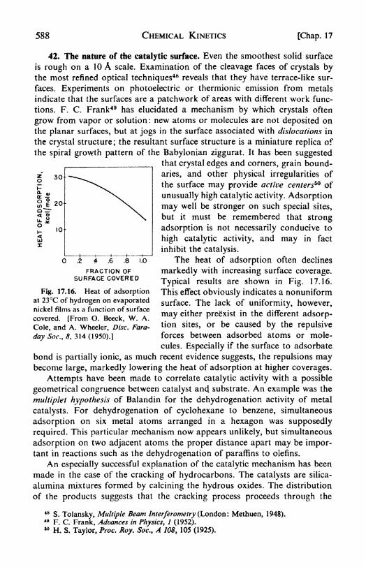
588 CHEMICAL KINETICS [Chap. 17
30
20
10
S
42. The nature of the catalytic surface. Even the smoothest solid surface
is rough on a 10 A scale. Examination of the cleavage faces of crystals bythe most refined optical techniques
48 reveals that they have terrace-like sur-
faces. Experiments on photoelectric or thermionic emission from metals
indicate that the surfaces are a patchwork of areas with different work func-
tions. F. C. Frank 49 has elucidated a mechanism by which crystals often
grow from vapor or solution : new atoms or molecules are not deposited onthe planar surfaces, but at jogs in the surface associated with dislocations in
the crystal structure; the resultant surface structure is a miniature replica of
the spiral growth pattern of the Babylonian ziggurat. It has been suggestedthat crystal edges and corners, grain bound-
aries, and other physical irregularities of
the surface may provide active centers of
unusually high catalytic activity. Adsorption
may well be stronger on such special sites,
but it must be remembered that strong
adsorption is not necessarily conducive to
high catalytic activity, and may in fact
inhibit the catalysis.
The heat of adsorption often declines
markedly with increasing surface coverage.
Typical results are shown in Fig. 17.16.
This effect obviously indicates a nonuniform
surface. The lack of uniformity, however,
may either preexist in the different adsorp-tion sites, or be caused by the repulsive
forces between adsorbed atoms or mole-
cules. Especially if the surface to adsorbate
bond is partially ionic, as much recent evidence suggests, the repulsions maybecome large, markedly lowering the heat of adsorption at higher coverages.
Attempts have been made to correlate catalytic activity with a possible
geometrical congruence between catalyst ami substrate. An example was the
muhiplet hypothesis of Balandin for the dehydrogenation activity of metal
catalysts. For dehydrogenation of cyclohexane to benzene, simultaneous
adsorption on six metal atoms arranged in a hexagon was supposedly
required. This particular mechanism now appears unlikely, but simultaneous
adsorption on two adjacent atoms the proper distance apart may be impor-tant in reactions such as the dehydrogenation of paraffins to olefins.
An especially successful explanation of the catalytic mechanism has been
made in the case of the cracking of hydrocarbons. The catalysts are silica-
alumina mixtures formed by calcining the hydrous oxides. The distribution
of the products suggests that the cracking process proceeds through the
48 S. Tolansky, Multiple Beam Interferometry (London : Methuen, 1948).49 F. C. Frank, Advances in Physics, 1 (1952).50 H. S. Taylor, Proc. Roy. Soc., A 108, 105 (1925).
.2 4 .6 .8 1.0
FRACTION OFSURFACE COVERED
Fig. 17.16. Heat of adsorptionat 23C of hydrogen on evaporatednickel films as a function of surface
covered. [From O. Beeck, W. A.
Cole, and A. Wheeler, Disc. Fara-
day Soc., 5,314(1950).]

Sec. 43] CHEMICAL KINETICS 589
intermediate formation of carbonium ions. 51 Let us first consider a simple
example of a carbonium-ion mechanism, that proposed for the Friedel-Crafts
reaction with an A1C13 catalyst :
(1)
(2)
(3)
CH3C1 + A1C18- CH3+(A1C14)-
CH3+ + C6H6
- C6H5-CH3 + H+
H+ f (A1C14)-= HC1 -f A1C13
The A1C13 acts as a Lewis acid, an acceptor of a pair of electrons. The reaction
is thus an example of a generalized acid catalysis in nonaqueous solution.
It has been shown 52 that the solid silica-alumina cracking catalysts also
have acidic properties : they react with carbonate solutions to evolve carbon
dioxide; they catalyze the inversion of sucrose; they react with and are
poisoned by volatile bases such as ammonia and quinoline. The acidic, active
centers appear to be sites in which an Al f3 ion is surrounded by O ions
tetrahedrally coordinated to Si+ 4 ions. Such a site may act as a strong Lewis
acid as follows :
RH +
OI I
Al O Si
I I
O
OI
H Al O Si-
I I
O
The subsequent cracking reaction is a cleavage of the carbonium ion R+ at
a position one carbon atom away from the C+ .
From the examples that have been given, it is evident that no single
theory can account for all the phenomena of contact catalysis. The field has
been of great interest to physical chemists because it combines the problemsof chemical kinetics with those of the fundamental theory of the solid state.
It is also not lacking in industrial applications.
43. Enzyme reactions. The catalysts devised by man have accomplished
many noteworthy results in their appointed role as accelerators of chemical
reaction rates. Yet their successes appear crude and insignificant when com-
pared with the catalytic activity of the enzymes elaborated by living cells to
promote physiological processes.
Consider one example among many, the formation of proteins. This is a
synthesis the most skillful organic chemist has been unable to achieve in the
laboratory, yet it is carried out rapidly and continuously by living cells. The
isotopic tracer experiments of R. Schoenheimer53 have shown that protein
51 B. S. Greensfelder, H. H. Voge, and G. M. Good, Ind. Eng. Chem., 41, 2573 (1949).52 T. H. Milliken, G. A. Mills, and A. G. Oblad, Disc. Faraday Soc., 8, 279 (1950).53 R. Schoenheimer, The Dynamic State of Body Constituents (Cambridge, Mass.:
Harvard Univ. Press, 1946).

590 CHEMICAL KINETICS [Chap. 17
molecules in the liver tissue of the rat have an average lifetime of only ten
days. In addition to this continuous self-replacement, the liver synthesizes
glycogen or animal starch from glucose; it manufactures urea which is
excreted as the end product of nitrogen metabolism; and it also undertakes
to detoxicate any number of unwanted substances, rendering them harmless
to the animal organism. This tremendous metabolic activity of the liver is
approached, but nowhere equaled, by the chemical activity of other kinds of
cells.
H. Buchner was the first to establish, in 1897, that the intact cell was not
necessary for many of these catalytic actions, since cell-free filtrates could be
prepared containing the enzymes in solution. Enzymes are specific, colloidal
catalysts. All known enzymes are proteins, so they are necessarily colloids,
falling in the range of particle diameter from 10 to 100 m/. Enzyme catalysis
is therefore midway between homogeneous and heterogeneous catalysis, and
is sometimes called microheterogeneous. A theoretical discussion can be based
either on intermediate compound formation between enzyme and substrate
molecules in solution, or on adsorption of substrate at the surface of the
enzyme.
Enzymes are extremely specific in their catalytic actions. Urease will
catalyze the hydrolysis of urea, (NH2)2CO, in dilutions as high as one part
of enzyme in ten million of solution, yet it has no detectable effect on the
hydrolysis rate of substituted ureas, e.g., methyl urea, (NH2)(CH3NH)CO.Pepsin will catalyze the hydrolysis of the peptide glycyl-L-glutamyl-L-tyrosine,
but it is completely ineffective if one of the amino acids has the opposite
optical configuration of the D-form, or if the peptide is slightly different,
e.g., L-glutamyl-L-tyrosine.
It must be confessed that little is known about the mechanism of enzymeaction. Almost all enzymes fall into one of two large classes, the hydrolytic
enzymes and the oxidation-reduction enzymes. The enzymes of the first class
appear to be complex acid-base catalysts, accelerating ionic reactions, prin-
cipally the transfer of hydrogen ions. The protein enzymes contain both
NH3+ and COO groups, and therefore act as both acids and bases, and
should be very effective in this type of catalysis provided geometrical con-
ditions are satisfied. The oxidation-reduction enzymes catalyze electron
transfers, perhaps through intermediate radical formation.
The kinetics of enzyme reactions can often be interpreted successfully
by some sort of intermediate complex theory; e.g., that of Michaelis and
Menten. 54 The work of Sumner, Northrop, and others in preparing pure
crystalline enzymes has now made it possible to measure the absolute rate
constants cf enzyme reactions. When these data are obtained and successfully
interpreted, we shall have made a considerable advance toward an under-
standing of the physical chemistry of living cells.
54 Biochem. Zeit., 49, 333 (1913); B. Chance, J. Biol. Chem., 151, 553 (1943).

Chap. 17] CHEMICAL KINETICS 591
PROBLEMS
1. The conversion of acetochloroacetanilide (A) into /;-chloroacetanilide
(B) was followed by adding KI solution and titrating the iodine liberated
with standardized thiosulfate solution. The KI reacts with A only.
Time, hr: I 2 3 468ml 0.iyVS2O3--: 49.3 35.6 25.75 18.5 14.0 7.3 4.6
Calculate the first-order rate constant in sec~ 1
.
2. The inversion of sucrose, C12H 22OU {H 2O - C6H 12O6 -f C6H 12O6 ,
proceeded as follows at 25C:
Time, min: 30 60 90 130 180
Sucrose inverted,
moles per liter: 0.1001 0.1946 0.2770 0.3726 0.4676
The initial concentration of sucrose was 1.0023 moles per liter. Calculate the
first-order rate constant and the half life of the reaction. Why does this
reaction follow a first-order law despite the fact that water enters into the
stoichiometric equation? How long would it take to invert 95 per cent of a
pound of sugar?
3. The hydrolysis of ethylnitrobenzoate by hydroxyl ions (NO2C6H4-
COOC2H 5 + OH- - NO2qsH 4COOH f C2H 5OH) proceeds as follows at
15C [J. Chem. Soc\, 1357 (1936)] when the initial concentrations of both
reactants are 0.05 mole per liter.
Time, sec: 120 180 240 330 530 600
%hydrolyzed: 32.95 41.75 48.8 58.05 69.0 70.35
Calculate the second-order rate constant.
4. The reaction 2 NO -f 2 H 2= N 2 + 2 H 2O was studied with equi-
molar quantities of NO and H 2 at various initial pressures:
Initial pressure, mm: 354 340.5 375 288 251 243 202
Half life, r min: 81 102 95 140 180 176 224
Calculate the over-all order of reaction.
5. The reaction SO2C12= SO2 -f C1 2 is a first-order gas reaction with
A'i- 2.2 x 10 5 sec- 1
at 320C. What per cent of SO2C1 2 is decomposedon heating at 320C for 90 min?
6. The racemization of an optically active halide in solution is first order
with respect to the reactant in each direction and the rate constants are equal.
R^jjRgCX (dextro) ^ RjR^CX (laevo). If the initial reactant is puredextro and the rate constant is 1.90 x 10~6 sec"1
, find (a) the time to 10 percent reaction, (b) the per cent reaction after 24 hours.
7. The reaction C2H6= C2H4 -f H2 follows approximately a 3/2-order
law in its initial stages. At 910K the rate constant is 1.13 sec" 1lit
172 mole"172.
Calculate the initial rate, d(C2H6 )/*//, for an ethane pressure of (a) 100 mm,(b) 300 mm.

592 CHEMICAL KINETICS [Chap. 17
8. Find the reaction order and rate constant for C6H5N2CI = C6H5C1 +N2 at 50C if the initial diazobenzenechloride concentration is 10 g per liter
and:
/,min: 6 9 12 14 18 22 24 26 30 oo
N2 evolved, cc: 19.3 26.0 32.6 36.0 41.3 45.0 46.5 48.4 50.4 58.3
9. Find the rate law of the reaction 3 HNO2- H2O + 2 NO + H+ +
NO3~
if the first two of the following steps rapidly attain equilibrium and the
third step is slow:
(1) 2 HN02- NO + N02 + H2
(2) 2 N02= N2 4
(3) N2 4 + H2- HN02 + H+ + NO3
~
10. Explain the following facts from the standpoint of the adsorption
properties of the reactant and product molecules :
(a) The decomposition of NH3 on W is zero order.
(b) The decomposition of N2O on Au is first order.
(c) The recombination of H atoms on Au is second order.
(d) The decomposition rate of NH3 on Pt is proportional to /^H./^H,-
(e) The decomposition rate ofNH3 on Mo is strongly retarded by N2 but
does not approach zero as the surface becomes saturated with N2 .
(f) The rate of 2 SO2 + O2- 2 SO3 on Pt is ^ (SO2)/(SO3)
1/2 when O2
is in excess.
11. In what proportion of bimolecular collisions does the energy of the
"head-on" collision exceed 60 kcal at 300K, at 600K, at 1000K?
12. The following mechanism has been proposed for the thermal de-
composition of acetone:
(1) CH3COCH3-
/q -> CH3 + CH3CO - 84 kcai
(2) CH3CO - k2~> CH3 + CO E = 10 kcal
(3) CH3 + CH3COCH3- *3
-> CH4 + CH2COCH3 E - 15 kcal
(4) CH2COCH3-
4-> CH3 + CH2CO E - 48 kcal
(5) CH3 + CH2COCH3- ks
-> C2H5COCH3 E = 5 kcal
Express the over-all rate in terms of the individual rate constants, taking
reaction (1) to be first order. Calculate (a) the over-all energy of activation;
(b) the chain length given by the ratio of the chain propagating reaction to
the cha,in stopping reaction. What is the order of the over-all reaction if
reaction (1) becomes second order?
13. Triethylamine and methyl iodide are mixed at initial concentrations
of 0.02 mole per liter.
Time, sec: 325 1295 1530 1975
% reacted: 31.4 64.9 68.8 73.7
Determine the second-order rate constant. Would you expect the rate to be

Chap. 17] CHEMICAL KINETICS 593
greater or less if (a) neutral salts were added; (b) the dielectric constant of
the solvent were increased? Give reasons.
14. Derive the rate laws for the following competitive reactions :
(1) Dipeptide -\- enzyme = complex(2) Complex = dipeptide + enzyme(3) Complex -= enzyme -f- amino acids
Discuss the design of an experiment to obtain the dissociation constant of
the complex from kinetic data.
15. In the polymerization reactions, A + A = A 2 \ A 2 + A A 3 \ A 3 +A = A . . ., etc., if all the rate constants are identical, the integrated rate
equation has the form
4 + *'
Here y is the amount of polymer (A 2 + A% + A + . . . An), a is the initial
amount of reactant A, k is the rate constant, and / is the time. Find the
equation for dy/dt, the polymerization rate. What will be the apparent order
of reaction during a single run? What will be the order based on the initial
rates if the concentration a is varied?
16. A certain reaction is 20 per cent complete in 15 min at 40C and in
3 min at 60C. Estimate its activation energy.
17. For the decomposition of N2O5 ,
Temperature, C: 25 35 45 55 65
10**! -sec-1: 1.72 6.65 24.95 75 240
Calculate A and E for the reaction, in the equation k = Ae~KjRT . Calculate
AF*, A//*, and AS*, for the reaction at 50C.
18. Consider a reaction subject to acid catalysis that follows the Br0nsted
relation kA = CAT". Suppose that the reaction is studied in an aqueoussolution 0. 1 molar in acetic acid and 0. 1 molar in sodium acetate. For three
hypothetical values 0.1, 0.5, and 1.0 of a, calculate the proportion of the
catalysis that would be due to each of the following: H3O+, H2O, CH3COOH.
19. The rate constant of 2 N2O = 2 N2 + O2 is 4.2 x 10⁹ exp
( 53,000/#r) sec-1 . A stream of N2O is passed through a tube 20 mm in
diameter and 20 cm long at a rate of 1 liter per min. At what temperatureshould the tube be heated in order to have 1 .0 per cent O2 in the exit gas ?
20. A sample of nickel foil weighing 5.328 g and having a surface area of
258 cm2per g was exposed to pure oxygen at 500C and 10 cm pressure.
Time, hr: 23456789 10
O2 uptake, cc at
10mm,20C: 52.4 70.2 85.1 97.9 106.6 118.0 127.7 137.0 146.3
The reaction is Ni + | O2= NiO. Fit the data to the parabolic rate law
dy/dt a/y where y is the film thickness, t is the time and a is the rate

594 CHEMICAL KINETICS [Chap. 17
constant. Calculate a. (NOTE: Integrate the rate equation assuming that at
/ = 0, y = y ,and cast the integrated equation into a linear form. Then plot
the results.)
REFERENCES
BOOKS
1. Amis, E. S., Kinetics of Chemical Change in Solution (New York: Mac-
millan, 1948).
2. Daniels, F., Chemical Kinetics (Ithaca: Cornell Univ. Press, 1938).
3. Frost, A. A., and R. G. Pearson, Kinetics and Mechanism (New York:
Wiley, 1953).
4. Glasstone, S., K. J. Laidler, and H. Eyring, The Theory of Rate Processes
(New York: McGraw-Hill, 1941).
5. Griffith, R. H., The Mechanism of Contact Catalysis (New York: Oxford,
1946).
6. Hinshelwood, C. N., The Kinetics of Chemical Change (New York:
Oxford, 1942).
7. Laidler, K. J., Chemical Kinetics (New York: McGraw-Hill, 1950).
8. Moelwyn-Hughes, E. A., The Kinetics of Reactions in Solution (NewYork: Oxford, 1947).
9. Steacie, E. W. R., Free Radical Mechanisms (New York: Reinhold,
1946).
ARTICLES
1. Bell, R. P., J. Chem. Soc., 629-34 (1943), "Theory of Reaction Kinetics
in Solution."
2. Dainton, F. S., /. Chem. Soc., 1533-1546 (1952), "Atoms and Radicals
in Aqueous Media."
3. Eyring, H., Science in Progress, vol. IV (New Haven: Yale Univ. Press,
1944), "The Drift toward Equilibrium."4. Garvin, D., and G. B. Kistiakowsky, J. Chem. Phys., 20, 105-113 (1952),
"The Kinetics of Coordinate Bond Formation."
5. Hinshelwood, C. N.,/. Chem. Soc., 694-701 (1947), "Some Observations
on Present Day Chemical Kinetics."
6. Laidler, K. J., and S. Glasstone,/. Chem. Ed., 25, 383-87 (1948), "Rate,
Order, and Molecularity in Chemical Kinetics."
7. Michaelis, L., Science in Progress, vol. V (New Haven: Yale Univ.
Press, 1947), 119-48, "Oxidation and Respiration."8. Moore, W. J., /. Electrochem. Soc., 100, 302-313 (1953), "Oxidation of
Metals at High Temperatures."9. Polanyi, M., Endeavour, 8, 3-10 (1949), "Mechanism of Chemical
Reactions."
10. Taylor, H. S., Science in Progress, vol. V (New Haven: Yale Univ. Press
1947), 91-118, "Contact Catalysis Between Two Wars."

CHAPTER 18
Photochemistry and Radiation Chemistry
1. Radiation and chemical reactions. Thus far our account of chemical
kinetics has considered only thermal reactions, those in which the energyneeded to climb the hill leading to the activated state comes from the random
energies of the reacting molecules and their neighbors. A different way of
providing the necessary energy is to bring the reactant molecule into
"collision" with quanta of electromagnetic energy (photons); with high-
velocity electrons (p rays); or with other corpuscular beams, such as neutrons,
protons, or a-particles, obtained either from nuclear reactions or from
electric accelerators. The study of reactions caused by any of these methods
is the field called radiation chemistry. The name arose from the historical
fact that the emissions from radioactive elements were called rays, a, /?,
and y.
The older field called photochemistry would logically appear to be a
subdivision of radiation chemistry. It is the science of the chemical effects
of light, where light includes the infrared and ultraviolet, as well as the
visible regions of the spectrum, i.e., the range of wavelength from about
1000 to 10,000 A. The energies of quanta in this range vary from about
1 to lOev, or 23 to 230 kcal per mole. These energies are comparable in
order of magnitude with the strengths of chemical bonds. Thus, if a molecule
absorbs a photon of visible light, definite chemical effects may be expected,
yet the collision is still a rather gentle one, and the effects usually follow
paths made familiar from spectroscopic studies. In particular, there is
almost never enough energy in a single quantum to activate more than one
molecule in the primary step.
On the other hand, if a 1,000,000 ev y-ray photon traverses a medium,thousands of molecules may become activated along its trajectory. As we
shall see, these activations often result in ionization of the molecules,
whereas in the photochemical region, ionization would be a rare occurrence.
Radiations like a, /?, y rays, neutrons, and cyclotron beams, are therefore
called ionizing radiations. Usually, when we speak of radiation chemistry
we mean the science of the chemical effects of such highly energetic, ionizing
rays. We tend, therefore, to divide the whole subject, on energetic grounds,into photochemistry and radiation chemistry.
2. Light absorption and quantum yield. Light incident upon a system can
be transmitted, refracted and scattered, or absorbed. Grotthuss and Draper,in 1818, first stated the principle that only the absorbed light can produce a
chemical change. The fraction of incident light absorbed by a medium is
595

596 PHOTOCHEMISTRY AND RADIATION CHEMISTRY [Chap. 18
proportional to the thickness of the medium that is traversed. This law was
originally stated, in 1729, in a memoir by P. Bouguer, and was later re-
discovered by Lambert. It can be expressed as
~^adx (18.1)
where / is the intensity of light at a distance x from its entry into the medium,and a is called the absorption coefficient or extinction coefficient. On integra-
tion with the boundary condition / = 7 at x 0, we obtain
I=I e~ a*(18.2)
In 1852, Beer showed, for many solutions of absorbing compounds in
practically transparent solvents, that the coefficient a was proportional to
the concentration of solute c. Thus Beer's law is
(18.3)
If c is the molar concentration, a' is called the molar extinction coefficient.
The light absorbed is
7a = / -/-/ (l -*-*<*)
These absorption laws are the bases for various spectrophotometric methods
of analysis.1They are obeyed strictly only for monochromatic light.
A device that measures the total amount of incident radiation is called
an actinometer. This measurement, actinometry, is a necessary part of any
quantitative study of photochemical reactions. Two types of actinometer are
commonly used.
One is a thermopile. It consists of a number of thermocouples connected
in series, with their hot junctions imbedded at a blackened surface which
absorbs almost all the incident light and converts it into heat. Calibrated
lamps of known energy output are available from the National Bureau of
Standards. The emf developed by the thermopile is measured first with the
standard lamp and then with the source of radiation of unknown intensity.
The reaction vessel is mounted between the thermopile and the light, and
the radiation absorbed by the reacting system is measured by the difference
between readings with the vessel filled and empty.Instead of a thermopile, it is possible to employ relative methods of
actinometry, which are based on the amount of chemical change producedin previously studied reactions. The quantum yield of a photochemicalreaction is the number of molecules of reactant consumed or product formed
per quantum of light absorbed. One of the most reproducible reactions is
the decomposition of oxalic acid photosensitized by uranyl salts. The uranylion UO2
++ absorbs radiation from 2500 to 4500 A, becoming an excited ion
1Sec, for example, the complete account given by M. G. Mellon, Analytical Absorption
Spectroscopy (New York: Wiley, 1950).

Sec. 3] PHOTOCHEMISTRY AND RADIATION CHEMISTRY 597
(UO2++)* which decomposes the oxalic acid. This reaction has a quantum
yield of 0.50.
UO2++ + hv-> (U<V+)*
(UO2++)* + (COOH)2-> UO2
++-f- CO2 + CO 4- H2O
The oxalic acid concentration is easily followed by titration with perman-
ganate. A quartz vessel filled with the uranyl oxalate mixture can be used
exactly like the thermopile, the light absorbed being calculated from the
oxalic acid decomposed and the known quantum yield. Another reaction
sometimes used as an actinometer is the photochemical hydrolysis of chloro-
acetic acid, CICH2COOH + H2O + hv -> CH2OHCOOH + HC1. This re-
action has a quantum yield of 0.31.
Shortly after the advent of the quantum theory, Einstein applied it to
photochemical reactions. He stated the rule that one quantum of absorbed
radiation activates one molecule of absorbent, but this activated molecule
does not necessarily undergo chemical reaction. The energy EK = Nhv,
where N is the Avogadro Number, is called one einstein. The value of the
einstein varies with the wavelength. For visible green light with X =- 6000 A,
it has a value in kilocalories of
6.02 x 10²³x_6.62 _x_l(^_
27 x 3.0 xJO10
~ ~ ": a
This is enough energy to break moderately strong bonds, but for C Cbonds and others with strengths higher than 72 kcal it is necessary to use
radiation in the ultraviolet region.
3. Primary processes in photochemistry. The results of the absorption of
a quantum of radiation were described in some detail in Chapters 10 and 11,
in the sections on atomic and molecular spectra.
Absorption by an atom in the line-spectrum region leads to an excited
atom; in the region of continuous absorption, to an ion plus an electron.
Absorption by molecules can lead to the different results shown in
Fig. 18.1. In (a) the transition is from a stable ground state to a stable
excited state. The corresponding spectrum consists of discontinuous bands
with a fine structure of closely packed lines. In (b) the transition is to an
unstable state that immediately undergoes dissociation. Absorption of a
quantum in case (b') also leads to dissociation, because the energy level
reached lies above the binding energy, of the excited state. Both (b) and (b')
correspond to continuous absorption spectra, without bands. A third and
less usual result is shown in (c). The initial transition is from one stable state
to another, but the upper state is "intersected" by the potential-energy
surface of an unstable state, and the excited molecule can switch over to this
after one or more vibrations. The resultant spectra are quite diffuse but not
completely continuous. This phenomenon was named predissociation byV. Henri.

598 PHOTOCHEMISTRY AND RADIATION CHEMISTRY [Chap. 18
It should be noted that all the transitions in Fig. 18.1 are depicted as
vertical jumps on the potential-energy diagrams. This picture is in accord
\
(0) (b)
(b') (c)
Fig. 18.1. Primary photochemical processes.
with the Franck-Condon principle that electronic transitions occur without
influencing the positions of the nuclei.
4. Secondary processes in photochemistry: fluorescence. If the light absorp-tion lies in the banded region of the spectrum, there are several careers opento the excited molecule formed in the primary step. (1) It may re-emit a
quantum of either the same or a different frequency. This emission is called
fluorescence or phosphorescence. (2) It may collide with other molecules and
pass on to them some or all of its excitation energy. This energy either can
cause reaction in the other molecule, or can be gradually degraded into heat.
(3) It may collide with another molecule and react with it. (4) It may spon-
taneously decompose if the excitation energy reaches a bond that can be
broken (predissociation).
Fluorescence is the emission of light which has been absorbed by the
molecule. It should not be confused with the scattering of light which has
not been absorbed, i.e., the Rayleigh scattering without change in wave-
length, and the Raman scattering with change in wavelength. The natural
life time of an excited state in a molecule undisturbed by collisions is about
10~8 sec. At a pressure of one atmosphere, a molecule experiences about
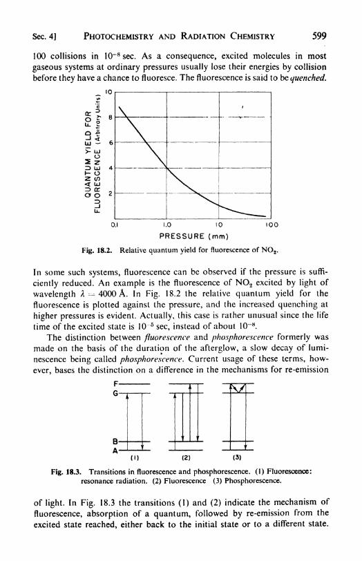
Sec. 4] PHOTOCHEMISTRY AND RADIATION CHEMISTRY 599
100 collisions in 10~ 8 sec. As a consequence, excited molecules in most
gaseous systems at ordinary pressures usually lose their energies by collision
before they have a chance to fluoresce. The fluorescence is said to be quenched.
10
!!S 6
15 UJh- OZ (O< LJr> <ro o
ID
O.I 1.0 10 100
PRESSURE (mm)
Fig. 18.2. Relative quantum yield for fluorescence of NO2 .
In some such systems, fluorescence can be observed if the pressure is suffi-
ciently reduced. An example is the fluorescence of NO2 excited by light of
wavelength A 4000 A. In Fig. 18.2 the relative quantum yield for the
fluorescence is plotted against the pressure, and the increased quenching at
higher pressures is evident. Actually, this case is rather unusual since the life
time of the excited state is 10 5sec, instead of about 10~8
.
The distinction between fluorescence and phosphorescence formerly was
made on the basis of the duration of the afterglow, a slow decay of lumi-
nescence being called phosphorescence. Current usage of these terms, how-
ever, bases the distinction on a difference in the mechanisms for re-emission
F-
G-
B-
A-(i) (2) (3)
Fig. 18.3. Transitions in fluorescence and phosphorescence. (1) Fluorescence:
resonance radiation. (2) Fluorescence (3) Phosphorescence.
of light. In Fig. 18.3 the transitions (1) and (2) indicate the mechanism of
fluorescence, absorption of a quantum, followed by re-emission from the
excited state reached, either back to the initial state or to a different state.
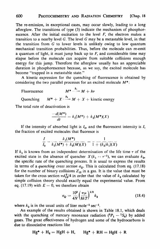
600 PHOTOCHEMISTRY AND RADIATION CHEMISTRY [Chap. 18
The re-emission, in exceptional cases, may occur slowly, leading to a long
afterglow. The transitions of type (3) indicate the mechanism of phosphor-escence. After the initial excitation to the level F, the electron makes a
transition to a nearby level G. The level G may be a metastable level, in that
the transition from G to lower levels is unlikely owing to low quantummechanical transition probabilities. Thus, before the molecule can re-emit
a quantum of light, it must jump back up to F, and considerable time mayelapse before the molecule can acquire from suitable collisions enough
energy for this jump. Therefore the afterglow usually has an appreciableduration in phosphorescence because, as we say, the excited molecule has
become "trapped in a metastable state."
A kinetic expression for the quenching of fluorescence is obtained by
considering the two parallel processes for an excited molecule M* :
Fluorescence M* --*M -f- hv
Quenching M* + X * M + X + kinetic energy
The total rate of deactivation is
- Arx(A/*) + k2(M*)(X)at
If the intensity of absorbed light is 7, and the fluorescent intensity is /,
the fraction of excited molecules that fluoresce is
1
Q
If k is known from an independent determination of the life time r of the
excited state in the absence of quencher X(k\ -- r" 1), we can evaluate k2t
the specific rate of the quenching process. It is usual to express the results
in terms of a quenching cross section aQ . This is calculated from eq. (17.18)
for the number of binary collisions Z12 in a gas. It is the value that must be
taken for the cross section rrd^/4 in order that the value of k2 calculated by
simple collision theory should exactly equal the experimental value. From
eq. (17.19) with E = 0, we therefore obtain
where k2 is in the usual units of liter mole'1 sec"1.
An example of the results obtained is shown in Table 18.1, which deals
with the quenching of mercury resonance radiation (3Pt
15 ) by added
gases. The great effectiveness of hydrogen and some of the hydrocarbons is
due to dissociative reactions like
Hg* + H2= HgH + H, Hg* + RH - HgH + R

Sec. 5] PHOTOCHEMISTRY AND RADIATION CHEMISTRY 601
TABLE 18.1
EFFECTIVE CROSS SECTIONS FOR QUENCHING MERCURY FLUORESCENCE
Gas
2
H2
CONH3
1018 <rQ~ cm2
2.48
26.2
0.06
24.0.
5. Luminescence in solids. The phenomena of excitation followed byre-emission or deactivation are basically the same in solid, liquid, and
gaseous systems. In solids, the processes of energy transfer do not, of course,
involve collisions, but the degradation of the electronic energy of excitation
into the thermal vibrational energy of the crystal provides an analogousmechanism of quenching.
Luminescent solids have been classified as (I) pure, (2) impurity activated.
Examples of type (1) are certain inorganic salts such as those of the uranyl
ion UO2+2
. Light absorption by these ions is followed by fluorescence both
in the crystalline state and in solution, and it is evident that quenching is not
efficient. The reason seems to be that electronic excitation occurs in inner
orbitals that are effectively shielded from interaction with vibrational levels
of neighboring ions or molecules. Another example of a pure luminescent
solid is anthracene, which displays a pale violet fluorescence in the purest
samples ever obtained. The reason why quenching is inefficient in anthracene
can be at least qualitatively understood from the nature of its structure. As
shown on page 311 for benzene, the carbon-carbon links in anthracene
consist of strong electron-pair a-bonds in the plane of the rings, and over-
lapping 7r-orbitals filled with electrons which are free to move around the
ring system. When anthracene absorbs a quantum at about 3700 A, a TT-
electron is excited from a filled energy band to an upper empty band. The
vibrations of the C C and C H bonds in anthracene are closely coupledwith the cr-bonds, but are not much influenced by the positions of the
7T-electrons. Therefore the excitation energy of the rr-electrons is not rapidly
degraded into thermal vibrational energy, and is instead re-emitted as the
violet fluorescence.
If an anthracene crystal contains as little as 0.01 per cent of naphthacene,the characteristic green fluorescence of naphthacene appears and the violet
anthracene fluorescence is almost entirely suppressed. When such a crystal
is heated, the green fluorescence disappears at the instant of melting, and the
violet anthracene fluorescence reappears. The explanation of these remark-
able events seems to be the following. When the anthracene crystal absorbs
a photon and one of its Tr-electrons is excited to an upper band, a hole is left
behind in the lower band. The hole, being a location of missing negative
charge, has an effective positive charge, and hence attracts the electron,
somewhat in the way that an H+ nucleus attracts its planetary electron. Such
an association between an excited electron and the hole it has reluctantly

602 PHOTOCHEMISTRY AND RADIATION CHEMISTRY [Chap. 18
TRAPS
left behind is called an exciton. Now the exciton hops about through the
crystal until it happens to hit a naphthacene molecule, which traps it long
enough for the fluorescent emission to take place. Thus, although the photonis almost always absorbed in an anthracene molecule, it is almost alwaysemitted from a naphthacene molecule. The example of naphthacene in
anthracene is midway between the pure luminescent crystal and the typicalcase of impurity activated crystals.
The example of zinc sulfide may be considered as typical of impurityactivation. Pure ZnS of stoichiometric composition displays practically no
luminescence. If this material is heated at 500-1000C it dissociates slightly
to form ZnS with excess Zn interstitially dissolved: ZnS(c) -> Zn, (in ZnS)+ 2 $2- The excess Zn atoms form impuritycenters of the type shown in Fig. 13.24 on
page 398. When illuminated with light of
about 3400 A, the heat-treated ZnS displaysa blue fluorescence and a short-lived phos-
phorescence. The spectra of the fluorescence
and of the phosphorescence are the same, as
would be expected from the trap mechanism
of phosphorescence shown in Fig. 18.3. TheZnS on illumination also becomes a better
conductor of electricity; this phenomenon is
called photoconductivity.
An oversimplified model to account for
these observations is shown in Fig. 18.4. Thelevels / and 7t represent a ground state and
an excited state for an impurity center, e.g., an interstitial zinc atom. If a
quantum of radiation of sufficient energy is absorbed by the crystal, an elec-
tron may be driven from the filled band to the empty conduction band,and a hole is left in the filled band. If the hole and the electron remained
associated, the result would be an exciton, similar to that found in
anthracene. In pure ZnS, the electron and the positive hole will recombine
without the emission of light, the energy being dissipated as heat. The im-
purity centers, such as excess Zn, provide a mechanism by which the excita-
tion energy can be re-emitted as light. The theoretical interpretation of how
they provide this luminescent pathway is still in an unsatisfactory state.
Both pure ZnS and impurity activated ZnS contain "traps" for electrons,
metastable levels from which transition to the ground state is forbidden.
These traps may be dislocations, grain boundaries, or other impurities in the
crystals. Only by thermal excitation back to the conduction band can anelectron escape from its trap and eventually emit the phosphorescent radia-
tion. For such a thermal excitation from T to C, the probability p per unit
time has the simple form of a first order rate constant,/?~ ae~ Eim\ where E
is the energy gap between T and C. If n is the number of electrons trapped
FILLED BAND
\\\\\\\\\\\Ss
Fig. 18.4. Band model for an
impurity-activated phosphor.

Sec. 6] PHOTOCHEMISTRY AND RADIATION CHEMISTRY 603
at any instant, the phosphorescent intensity is proportional to their rate of
escape,
dnI - - - pn - nae"EIRT (18.5)
For a fixed temperature, integration of this equation gives the decay of
phosphorescence with time. For the typical example of a thallium activated
KC1 phosphor, the constants are a 3 x 10 sec"1, and E = 15.5 kcal per
mole.
6. Tbermoluminescence. Some phosphors, illuminated while cold, store
energy which can later be released as light when they are heated. This phenom-enon is called thermolwninescence. In a typical experiment, a SrS phosphor
300 550350 400 450 500
TEMPERATURE, K
Fig. 18.5. Thermoluminescence of a strontium-sulfide phosphor.
was illuminated at room temperature, the light was turned off, and the
phosphor was heated at a steady rate of 2.5 per sec. The resulting light
emission is shown in Fig. 18.5. It is clear that two distinct trap levels occur,
which lead to the two peaks in the thermoluminescent curve.
The mathematical analysis of these curves is based on eq. (18.5), which
may be written
dt
For a constant heating rate, dT ==- c dt, and
Thus, /=--- = n ae"EIRT exp (-
f
T- e"E>RT dT\
dt \ J Q c I

604 PHOTOCHEMISTRY AND RADIATION CHEMISTRY [Chap. 18
If the reader cares to take the time to plot this expression for a suitable
choice of parameters, he will find that it reproduces an approximately bell-
shaped curve like one of those in Fig. 18.5. Thus experiments on thermo-
luminescence are often used to measure the trap depths E in phosphors.7. Secondary photochemical processes: initiation of chain reactions. If a
molecule is dissociated into fragments as a consequence of absorbing a
quantum of radiation, extensive secondary reactions may occur. These are
especially likely since the fragments are often atoms or radicals, which are
by nature highly reactive. Sometimes, also, the products of the primaryfission process are still in excited states, as so-called hot atoms or hot radicals.
For example, if a mixture of chlorine and hydrogen is exposed to light
in the continuous region of the absorption spectrum of chlorine (A < 4800 A)an extremely rapid reaction to hydrogen chloride ensues. The quantum yield
<I> is 104 to 106 . Bodenstein was the first to explain the high value of O in
terms of a long reaction chain. The first step is dissociation of the chlorine
molecule,
(1) C\2 + hv^2C\ (Va K,
This is followed by
(2) Cl + H2-> HC1 + H k2
(3) H + C12-> HCi + Cl 3
(4) Cl -> \ C12 (on wall) A:4
If we set up the steady-state expressions for (Cl) and (H) in the usual way(page 552), we obtain for the rate of HCI production,
- A:2(C1)(H2) +dt
Instead of reaction (4), the chain-ending step might be a gas-phase re-
combination of chlorine atoms, perhaps with cooperation of a third body Mto carry away excess energy.
(5) C1 + C1 (+Af)->Cl2 (+M) 5
In this case, the calculated rate expression would be
dt^ '
It might be thought that a few simple experiments would suffice to decide
whether the rate depends on the first power or on the square root of the
light absorbed, and hence to decide the most likely chain-ending mechanism.
In fact, however, after dozens of extensive investigations, some questionsstill remain unanswered. It is likely that reactions (4) and (5) both contribute
to the chain ending under most experimental conditions, since in most
Sec. 7] PHOTOCHEMISTRY AND RADIATION CHEMISTRY 605
experiments with pure H2 and C12 the rate depends on //, with n somewhere
between and 1. The reaction is very sensitive to traces of impurities,
especially oxygen, which acts as an inhibitor by removing H atoms: H +2 (+A/)->H02 (+M).In contrast with the high quantum yields of the H2 + C12 reaction are
yields in the photochemical decompositions (photolyses) of the alky! iodides.
These compounds have a region of continuous absorption in the near ultra-
violet, at 2300 to 2500 A, which leads to a break into free alky!' radicals and
iodine atoms,
CH3I -f Av -> CH3 f I
The quantum yield of the photolysis is only about 10~2. The reason for the
low O is that the most likely secondary reaction is a recombination, CH3 + I
-> CH3I. Only a few radicals react with more alkyl iodide, CH3 -j- CH3I
-> CH4 + CH2I. The final products are CH4 , CH2I2 , and I2 . If mercury vaporis added to the system, the quantum yield is much increased. It is evident
that the mercury acts by removing iodine atoms, preventing their recom-
bination with alkyl radicals.
A reaction that has received especially careful study is the photolysis of
acetone; more than fifty research papers have been devoted to it during the
past 25 years.
(CH3)2CO + hv -> C2H6 + CO
Small amounts of methane and biacetyl are also formed. Acetone absorbs
ultraviolet light, with a banded spectrum from 3300 to 2950 A merging into
a continuous absorption that extends to 2200 A. Electronic excitation in the
carbonyl group is responsible for this absorption, but the C=O bond is
strong and energy must flow into the weaker C C bonds before dissociation
can occur.
In an investigation by Farrington Daniels and G. H. Damon,2 acetone
vapor contained in a quartz vessel was irradiated with virtually mono-chromatic light obtained from a high-pressure mercury-vapor lamp with a
quartz monochromator. (This instrument is an adaptation of the spectro-
graph, designed to isolate and focus a concentrated beam of light having a
well defined wavelength.) In a typical experiment, radiation at A ~ 3130 Awas used. Measurement with a thermopile gave an absorption rate of
85,200 erg per sec over a period of 23,000 sec. The volume of the vessel was
60.3 cc, the thermostat temperature 56C, and the pressure increased from
760 to 790.4 mm or AP = 30.4 mm.
Apart from minor subsidiary reactions, two moles of product appear for
each mole of acetone decomposed. The number of molecules decomposedwas therefore
1 J. Am. Chem. Soc., 55, 2363 (1933).
X

606 PHOTOCHEMISTRY AND RADIATION CHEMISTRY [Chap. 18
The number of quanta absorbed was
_ 85,200 x 23,000 x 3.13 x I0~5
q '"6.62 x fo-~x 3.0 x
" 3 " 8 X I0
The quantum yield was therefore O n/q^ 0.17. It is evident that of the
quanta absorbed, less than one in five leads to reaction.
When acetone vapor is irradiated with ultraviolet light there is an intense
and beautiful green fluorescence, and it was thought at first that the light
that did not cause reaction was emitted in fluorescence. Daniels measured
the fluorescent intensity and found that it actually accounted for less than
3 per cent of the light absorbed. Thus about 80 per cent of the radiation
absorbed is degraded into heat. It was later shown that the fluorescence was
due to biacetyl.
^ The products from acetone photolysis in a flow system remove lead
mirrors, forming Pb(CH 3 )43
. This result, as well as other evidence, indicates
that methyl radicals are formed. The most likely mechanism for the photoly-sis appears to be4
(CH3 )2CO + hv > CH3 4- CH3COCH3 f CH3
. C2H6
CH3CO 4- CH 3CO - (CH3CO)2
CH3CO >CH3 -f COCH3 4- CH3CO ^ (CH3 )2CO
The recombination reaction accounts for the low quantum yield, and, as
would be expected, the yield therefore increases as the pressure is lowered.
8. Flash photolysis. The new technique called flash photolysis promisesto be especially useful in the study of atoms and radicals that have only a
short lifetime before reacting.5 A powerful flash of light, with an energy up
to 10* joules and a duration of about 10~4sec, is obtained by discharging a
bank of capacitors through an inert gas such as argon or krypton. Thereactants are in a vessel aligned parallel with the lamp, and at the instant of
the flash, an extensive photolysis of the absorbing gas occurs in the reaction
vessel. Thus the primary products of photolysis, usually radicals and atoms,are produced in much higher concentrations than in the usual experimentwith continuous, relatively low-level illumination. A good method for
following the subsequent reactions of the radicals is to make a continuous
photographic record of their absorption spectra.
An example of a flash-photolysis investigation is the study by Porter and
Wright of the reaction between chlorine and oxygen. A mixture of 10 mm3 T. G. Pearson, /. Chem Soc., 1934, 1718; T. G. Pearson and R. H. Purcell, ibid.,
1935, 1151.4 A complete discussion of the evidence for the mechanism and a solution of the steady-
state rate equation are given by W. Davis, Chem. Rev., 40, 201 (1947).5 R. G. W. Norrish and G. Porter, Nature, 164, 658 (1950); G. Porter, Proc. Roy. Soc.
A 200,284(1950).

Sec, 9] PHOTOCHEMISTRY AND RADIATION CHEMISTRY 607
C1 2 and 600 mm O2 was used in a typical experiment. The flash dissociates
almost all the C12 to Cl atoms. In the first second after the flash there is a
rapid reaction to form the previously unobserved radical CIO, which is
detected by its absorption spectrum.
C12 4 hv-+2 Cl
2 Cl + O2> 2 CIO
The kinetics of the subsequent disappearance of the CIO radicals is now
readily followed by a continuous measurement of the intensities of their
absorption spectra. The removal of CIO is found to be a second-order
reaction,-d(C\Q)jdt -- /:
2(C1O)2
,with k2
- 4.2 x 10⁷exp [(0 650)/RT]
liter mole"1 sec"1. The constant is uncertain because the molar extinc-
tion coefficient of the CIO radicals has not been accurately determined,
and the experimental measurements give spectral intensities and not tdft-
centrations.
9. Effects of intermittent light. In the flash-photolysis experiment, a high
initial concentration is formed of reactive intermediates, which gradually
disappear by various reactions during the dark period. In the usual photo-chemical experiments, a steady intensity of light is used, so that inter-
mediates build up to a steady-state concentration, which is maintained
during the course of the run. Let us consider now a situation in which there
is a regular sequence of light and dark periods. A convenient way to achieve
such an intermittent illumination is to place between the light source and
the reaction vessel a rotating circular disk from which sectors have been cut.
If four sectors, for example, have angles of 22i and are evenly spaced, the
light and dark periods in the vessel will be in the ratio 1 : 3, and the flashing
rate will be four times the rotation speed of the disk.
The use of the method can be illustrated in terms of a simple schematic
reaction mechanism:
(1) A 2 { hv - 2A
(2) A + B -> C + A
(3) 2A ~> stable product
The steady-state concentration of the radicals A is (A) (O/a/2/r3)1/2
. If the
sector wheel with one-quarter open area is rotated very rapidly (and by
"rapidly" we mean with a period much less than the half life for disappear-ance of radicals A in the dark), the net result is the same as if the intensity
of a steady illumination was reduced to one-quarter. Thus the steady-state
concentration of A, and hence the rate of reaction, is reduced by a factor of
(i)1/2 =
i- On the other hand, suppose that the period of rotation of the
sector is long compared to the half life of A. In this case, the concentration
of A during each dark period will fall far below the steady-state value. The
net result will be the same as if the time of reaction is reduced to one-quarter

608 PHOTOCHEMISTRY AND RADIATION CHEMISTRY [Chap. 18
with the light intensity unchanged. Thus the rate of reaction would be
reduced by a factor of . In Fig. 18.6, (a) shows how the concentration of
radicals varies during the two experiments, and (b) shows how the reaction
rate varies with sector speed.The transition region between reaction rates for slow rotation and those
for fast rotation will occur when the sector period is about equal to the half
life of the reactive intermediate. Thus the experiments with intermittent
(a)
TIME
(b)
SECTOR ROTATION SPEED
Fig. 18.6. The effect of intermittent light on (a) radical concentration
(b) reaction rate, for a case in which rate depends on /a1 /2.
illumination provide a method for measuring short half lives of inter-
mediates, which would be difficult to study by other methods. It must be
noted, however, that the method cannot be used if the over-all rate is pro-
portional to /a , the first power of the light intensity.
A typical sector study6 was that of the photochemical formation of
phosgene, which follows a mechanism proposed by Bodenstein:
Cl2 + Av
Cl + COCOCI
COCI + CI2
COCI + CI
Cl + Cl
COCI
Cl + COCOCI2 + Cl
CO + C12
6 W. G. Burns and F. S. Dainton, Trans. Faraday Soc., 48, 39 (1952).

Sec. 10] PHOTOCHEMISTRY AND RADIATION CHEMISTRY 609
The observed rate law is
From the Bodenstein mechanism, k' k^k^lkjc^11*. The application of
the sector technique made it possible to evaluate each of the rate constants.
For example, in liter mole"1 sec"1,
4- 2.5 x 10⁹ exp(-2960//?r)
A:5= 4.0 X 10¹¹ exp (-830/flr)
Reaction (5) goes at almost every collision, with a very small energy barrier.
In reaction (4) the activation energy is only 5 per cent of the energy of
the Cl Cl bond that is broken, whereas the frequency factor is only 1
per cent of the collision frequency. The low frequency factor indicates a
loss of freedom and decrease in entropy when the activated complex is
formed.
In addition to its use in studying intermediates of short life, there is
evidence that the principle of intermittent illumination is used by Nature in
the ingenious fashion that is typical of her chemical processes. The responseof plants to the relative length of day and night is called photoperiodism.This phenomenon was first clearly described in 1920, by Garner and Allard
of the U.S. Department of Agriculture. Flowering plants may be divided
into three classes :
(1) Long-day plants flower only when the daily period of illumination is
greater than some critical time, e.g., spinach flowers only when the length of
day exceeds 13 to 14hr.
(2) Short-day plants flower only when the length of day is less than a
critical value; for example, 14 to 14.5 hr for chrysanthemum.
(3) Day-neutral plants do not exhibit photoperiodism in their flowering.
Depending on the plant, from 2 to 30 cycles of light and dark are needed
to initiate flowering. Even a single flash of light during a dark period maysometimes prevent flowering. The photoperiodic process that controls
flowering occurs in the leaves of the plants; in some cases the plant will
flower if even one leaf receives the proper light cycle. Although the chemical
compounds responsible for initiation or inhibition of flowering are not yet
completely known, they appear to act as hormones which build up to a
critical concentration in dark periods, and are photochemically destroyedin light periods. Other photoperiodic effects are known in both plants and
animals, such as the shedding leaves by deciduous trees, and, possibly, the
hibernation of the groundhog.10. Photosynthesis in green plants. The ultimate source of most of the
energy on earth, except nuclear energy, is the radiation received from the
sun. This radiation is converted by photosynthesis in green plants into
chemical potential energy stored in coal, oil, and carbohydrates. Green

610 PHOTOCHEMISTRY AND RADIATION CHEMISTRY [Chap. 18
plants are reducing agents, converting carbon dioxide and water into fuels.
Animals are oxidizing agents, burning the fuels back into water and carbon
dioxide. The Second Law of Thermodynamics insists that this vital cycle
cannot continue without some outside energy source besides the heat of the
environment. The external energy that keeps the cycle spinning comes from
the sun's rays. The mechanism of photosynthesis is one of the greatest
problems in chemical kinetics.
It has been estimated that during the summer season an average of 1 to
2 cal per cm2per min of radiant energy is incident upon green plants in an
open field. Of this energy only 2 to 3 per cent is stored in the plant at the
end of the summer.
The photosynthetic reaction can be written schematically as
(1) n CO2 -f n H2O + light > (CH2O)n 4- n O2
The final products are carbohydrates, such as cellulose and starch. The
reaction occurs through the mediation of chlorophyll, a magnesium-por-
phyrin compound. This compound is green since it has two strong absorption
bands, one in the red around 6600 A, the other in the blue around 4250 A.
The maximum intensity of sunlight is in the green region of the spectrum,but most of this green light is not utilized by plants.
Reaction (1) above for n = 1, i.e., one monomer unit incorporated in a
carbohydrate, has a A// = 120 kcal. Photosynthesis can occur with light of
7000 A. Since quanta of this red light amount to 38 kcal per mole, at least
three or four quanta would be needed to fulfil the energetic requirement for
photosynthesis. Under favorable conditions and for short intervals of time,
the quantum efficiency of photosynthesis may approach this theoretical
limit, reaching perhaps 5 or 6 quanta per CH2O unit, or a quantum yield Oof 0.1 6 to 0.20.
Important information on the photosynthetic mechanism has been
obtained from tracer experiments. By means of O-18 it was shown that the
evolved oxygen comes entirely from the H2O, with none from the CO2 . In
other words, the H2O reduces the CO2 .
Good progress in elucidating the mechanism of photosynthesis has been
made by Melvin Calvin and his co-workers at Berkeley. Their technique has
been to supply radioactive (C-14) CO2 to an aqueous suspension of algae,
and to isolate the various radioactive carbon compounds formed after
exposure of the suspension to light. Even after 60 sec illumination, about a
dozen compounds incorporating C-14 could be detected by an autoradio-
graph of a paper chromatogram. If the temperature of the algae is lowered
to 4C and they are given only 10 sec illumination, only one product appearson the chromatogram, phosphoglyceric acid, H
2O3PO CH2 CHOHC*O2H. This is the earliest intermediate yet identified in the photosynthetic
process. Since most of the radioactivity occurs in the carboxyl carbon, the
step by which CO2 is incorporated appears to be a reaction between CO2

Sec. 11] PHOTOCHEMISTRY AND RADIATION CHEMISTRY 611
and some two-carbon compound, or some two-carbon group that readily
splits off from a larger molecule.
Calvin has also suggested a plausible mechanism for the elementary step
that utilizes the light quantum, the so-called quantum conversion in photo-
synthesis. The chloroplasts of the plant contain granules (grana) which each
contain thousands of molecules of chlorophyll stacked in an almost close
packed array. Each packet of molecules acts as a unit in light absorption,
so that a quantum absorbed by any one molecule produces an exciton which
can move freely throughout the entire granum. Associated with each 1000
chlorophyll molecules is a molecule of 6,8 thioctic acid,
CH2
/\CH2 CH ~(CH2 )4-CO2H
II
s s
Calvin suggested in 1952 that the conversion of the light quantum occurs
when the exciton finds itself next to an adsorbed disulfide,
+ (CHL.)*~> +(CHL.)
S S S S
The dithiyl free radical can then abstract hydrogen from suitable donors,
forming the disulfhydryl compound, which can reduce other reducing agents
in the cell, and thus lead to the reduction of CO2 .
11. The photographic process. The general features of photography are
familiar. A photographic plate is prepared by coating glass or plastic with
a film of gelatin in which are suspended small crystals of silver bromide.
The AgBr grains average 10~5 to 10~ 4 cm in diameter, and contain 1011 to
1012 ion pairs. When the film is exposed to light, a latent image is formed,
which is believed to consist of submicroscopic specks of silver in some of
the grains. The photochemical formation of this latent image is very sensitive
to traces of substances, such as silver or silver sulfide, which act as nuclei at
which growth of silver can begin in the grains. The latent image is developedto a negative image by exposure to a mild reducing agent; in this step the
grains which contain silver specks are largely reduced to silver. Finally, the
negative is fixed by dissolving the unreduced silver bromide in sodium
thiosulfate.
The problem of outstanding photochemical interest is how the absorbed
light forms the latent image. The quantum yield with light of low intensity
approaches <!> = 1, i.e., every quantum of light absorbed leads to the forma-
tion of one silver atom. The light quanta, however, are absorbed at random
over the surface of the AgBr grain, and yet the silver is deposited at relatively
few specks within each grain. How is this process accomplished?

612 PHOTOCHEMISTRY AND RADIATION CHEMISTRY [Chap. 18
The first satisfactory theory was proposed in 1938 by R. W. Gurney and
N. F. Mott. 7 There is good evidence that the primary absorption in the AgBrcrystal occurs in the Br~ ions as Br~ + hv -> Br -f e. Light absorption in the
ultraviolet region is required to excite an electron from a Br~ ion in an
ordinary lattice position. The absorption at longer wavelengths is probablydue to Br~ ions at dislocations or other disturbed positions in the structure.
The electron is raised to an empty band in which it can move freely;
hence the AgBr becomes photoconducting. The mobile electron moves
through the AgBr crystal until it becomes trapped in a pre-existing silver
nucleus or in a low-lying energy level of a sensitizer such as Ag2S. Thus a
center of negative charge is produced, attracting Ag+ ions, which can move
through the crystal via interstitial positions. When an Ag^ ion reaches the
negative center it is neutralized, Ag+ + e -> Ag, and the silver nucleus is
thus enlarged. Once a few specks of silver emerge as nuclei, they will catch
the photochemically produced electrons, and then grow further by attracting
Ag+ ions.
The Br atom eventually reaches the surface of the AgBr by a process of
electron transfer, Br~ + Br -> Br + Br~. It can then react with constituents
of the gelatin. The Br atom is a center of missing negative charge, and it is
called a positive hole. The Gurney-Mott theory in its original form requires
that these positive holes do not recombine with the electrons. As a result of
ingenious experiments with thin films of pure AgBr single crystals, J. M.
Hedges and J. W. Mitchell8 have been led to a modification of the theory.
They suggest that the function of the sensitizer is to trap the positive holes,
preventing their recombination with the electrons. The electrons are then
trapped at crystal imperfections, and the silver particles grow there to form
the latent image.It may not be too far-fetched to see a certain similarity between the
processes of photography and those of photosynthesis. In both cases a light
quantum absorbed in one place can produce a chemical effect some distance
away, and in both cases the absorbent is dispersed in small grains in a
protein material.
12. Primary processes with high-energy radiation. Table 18.2 summarizes
some information about the sources of high-energy radiations. All these
radiations produce ionization in the matter through which they pass. The
Einstein law of photochemical equivalence (page 597) has its counterpart in
the principle that the amount of chemical reaction is proportional to the
number of ion pairs produced in the reaction medium by an ionizing radia-
tion. The history of this principle goes back to a calculation made by W. H.
Bragg in 1907, which indicated that the number of molecules of water de-
composed by radon was equal to the number of ions that the same amountof radon would have produced in air. Bragg, however, was evidently not
7 Proc. Roy. Soc., A 164, 151 (1938).8 Phil. Mag. 44, 357 (1953).

Sec. 12] PHOTOCHEMISTRY AND RADIATION CHEMISTRY 613
TABLE 18.2
RADIATIONS EMPLOYED IN RADIATION CHEMISTRY
c Radiation Typical MaximumbourceParticle Energy, mev
X-ray tube Photon 0.6
Van de Graaf generator Electron 6
Proton 6
Cyclotron Proton 40Deuteron 20
Alpha 10
Neutron 40
Betatron Electron 20Photon
Nuclear reactor (pile) Photon Dependent on conditions
NeutronFission recoil
Natural or artificial Photon Dependent on isotoperadioactive isotope Electron
AlphaAtom recoil
impressed by this agreement, which he noted as "a curious parallelism in
numbers." In 1908, W. Duane demonstrated that the chemical effects of
a-particles were due to the ionization they caused, and in 1910 Marie Curie
clearly stated the law of equivalence for a-particles in water. From about
1911 onwards S. C. Lind made use of ion-pair yields in an extensive series
of experiments. He found that for some reactions the quantum yield with
light and the ion-pair yield with a-particles were nearly identical, but in
other cases they might differ by a factor of two or three.
The details of the ionization process depend somewhat on the particle
concerned. When an X ray or y ray interacts with a molecule, the most
frequent result is the ejection of an electron by the Compton effect (page
233); i.e., the process is a "collision" between a photon and an electron, in
which the electron is driven out of its molecule, and the photon is deflected
with altered energy and momentum. The formation of a photoelectron by a
process of absorption of the photon, which is the usual event with low-
energy quanta, is much less likely at high energies. For example, with 100 kv
X rays, only 3 per cent of the electrons are photoelectrons, and 97 per cent
are Compton electrons. At 1 mev, almost all the electrons ejected are Comp-tons, which have an average energy of 440 kv. As a 440 kv electron is slowed
to room temperature (~ 0.02 ev) it ionizes or excites many molecules as it
passes near them. One ion pair is produced for about each 30 ev, so that the

614 PHOTOCHEMISTRY AND RADIATION CHEMISTRY [Chap. 18
440 kv electron produces about 15,000 ion pairs, and two or three times
that many excited molecules. The effect of the single ion formed in the first
ionization will obviously be negligible compared with that of the numerous
secondary ions and excited molecules.
The principal difference between the effects of electrons and those of ions
is due to the slower speed of the latter. A proton travels one-fortieth as fast
as an electron of the same energy. Thus, for a given path distance, the slowly
moving ion produces many more ionizations than the swift electron. For
example, per micron of path in water, a 440-kv electron would cause about
two ionizations, but a proton of the same energy would cause about 2000
ionizations. The effectiveness in causing ionization simply depends on the
length of time that the moving particle remains in the immediate neighbor-hood of the molecule.
The primary effects of fast neutrons differ somewhat from those of the
charged particles, since a neutron can penetrate the electron cloud around
an atomic nucleus without electrostatic repulsion. A neutron can thus
literally knock the nucleus out of an atom, and usually the nucleus is knocked
out so vigorously that some of the electrons are left behind and ionization
results. The ejected nuclei may produce further secondary displacements and
ionizations. Energetic ions can also knock out nuclei in this way, but theyare much less effective than neutrons. For example,
9 in aluminum, a 2-mev
neutron will produce about 6000 primary displacements, but a 20-mev
proton will produce only about 80. Available sources of radiation are intense
enough to produce extensive displacements in solids. For example, in a
layer 1 mm deep exposed to a cyclotron beam of 20 mev protons, about
10 per cent of the nuclei would be displaced after an irradiation of 1 coulomb
per cm2
. A solid in which the atoms have been displaced in this way is said
to be discomposed. The phenomena of discomposition were first described byE. Wigner during the development of nuclear reactors (piles).
13. Secondary processes in radiation chemistry. As radiation passes
through a reaction medium, several excited molecules are formed for each
ion formed. The excited molecules are even more important than this fact
would indicate, however, since one of the most probable secondary reactions
of an ion is its neutralization to yield an excited molecule. 10 If we use a
broken arrow to indicate a reaction caused by high-energy radiation, a
schematic reaction sequence is as follows.
+ e
A*
> break into radicals
A* --> rearrangement to molecules
9 F. Scitz, Disc. Faraday Soc., 5, 271 (1949).10 H. Eyring, J. Hirschfelder, and H. S. Taylor, /. Chem. Phys., 4, 479, 570 (1936).

Sec. 14] PHOTOCHEMISTRY AND RADIATION CHEMISTRY 615
It should be noted that any one of these steps may involve reactions more
complicated than the simple ones written. For example, the ionization step
may occur with a rupture of bonds, as A -~~-> B+ 4 C f- e. The large
number of excited molecules formed in irradiated systems explains the
parallelism frequently observed between photochemical and radiochemical
reactions.
Examples of many typical reactions are provided by the results observe^on irradiation of water. Aqueous systems have been most intensively studied
because of their great importance in radiobiology. In pure water, the first
steps, regardless of the source of radiation, appear to be
H2O H 2O )e
H2CM f H2O > HgO* + OH
The fate of the OH radicals seems to depend on the type of radiation. With
slow moving particles (a's) many OH radicals may be produced close to-
gether, and a likely subsequent step is radical combination,
2 OH -> H2O2
With fast particles (/?, y) the OH radical concentration along the paths is
much lower, and removal of radicals by the following sequence appearsreasonable:
e + H 2O -> OH + HH -f H -> H 2
H + OH > H2O
The dependence of intermediate concentrations on the path of radiation
through the system, and the diffusion of intermediates away from the tracks
of the radiation particles are typical features of this field of chemical
kinetics.
14. Chemical effects of nuclear recoil. When a nucleus emits an a, /?, or y
particle, conservation of momentum requires that the product nucleus recoil
in a direction opposite to that of the emitted particle. An important effect
of such recoil was discovered by Szilard and Chalmers in 1934. Theyirradiated ethyl iodide (C2H5 I
127) with neutrons: I
127(, y)I
128. The I
128is a
/? emitter of 25 min half life. The ethyl iodide, after irradiation, was shaken
with a dilute aqueous solution of ordinary iodine, in which it is not appre-
ciably soluble; much of the radioactive I128 was then found in the aqueous
layer. Exchange between iodine in ethyl iodide and that in aqueous solution
is known to be very slow. It appears, therefore, that the recoil of the iodine
nucleus on emission of the y particle is sufficiently energetic to break the
C I bond in C2H5I, thereby converting the iodine into a water-soluble form.
The Szilard-Chalmers effect has since been' observed in many n, y re-
actions. Besides its intrinsic interest as a new kind of chemical reaction, the
effect has practical value in that it provides a method of preparing highlyconcentrated radioactive elements.

616 PHOTOCHEMISTRY AND RADIATION CHEMISTRY [Chap. 18
PROBLEMS
1. When propionaldehyde is irradiated at 200 mm and 30C with light
of wavelength 3020 A, the quantum yield for CO production is found to be
0.54. If the incident light intensity is 15,000 erg per sec, calculate the rate of
CO formation. What is the light intensity in einsteins per sec?
2. The photochemical chlorination of chloroform (CHC13 + C12=
HC1 + CC14) follows the rate equation d(CC\^)/dt= A:7a
1/2(Cl2)
1/2(CHCl3),
where /a is the intensity of light absorbed. Devise a reaction scheme to
explain this kinetics.
3. In a study of the quenching of sodium resonance radiation at 200C,it is found that 1.6 mm of N2 reduces the fluorescence intensity to 50 percent of the value in the absence of added gas. If the natural lifetime of the
excited Na atom is 10~7sec, calculate the quenching cross section for N2 .
4. Show that when a y ray of energy EY in ev, is ejected from a nucleus
of mass m atomic weight units, the recoil kinetic energy of the nucleus in
ev is Ea= 5.33 x \Q~wEY
2/m. Calculate the recoil energy of Zn-65 on
emission of a 1.1 mev y ray.
5. Consider a europium-activated SrSiO3 phosphor with a single trap
depth of 0.72 ev and a= 1.5 x 10⁹ seer1. Calculate the time for the
luminescent intensity to decay to one-half its initial value at 100K and
at 400K.
6. A photographic film is exposed for 10~3 sec to a 100-watt incandescent
light at a distance of 10 meters. If 5 per cent of the power is emitted as visible
light to which the film is sensitive, estimate the number of silver atoms that
will be produced in a AgBr grain 10 microns in diameter.
REFERENCES
BOOKS
1. Bowen, E. J., Chemical Aspects ofLight (New York: Oxford, 1946).
2. Garlick, G. F. J., Luminescent Materials (New York: Oxford, 1949).
3. James, T. H., and G. C. Higgins, Fundamentals of Photographic Theory
(New York: Wiley, 1948).
4. Lea, D. E., Action of Radiation on Living Cells (London: Cambridge,
1947).
5. Mott, N. F., and R. W. Gurney, Electronic Processes in Ionic Crystals
(New York: Oxford, 1940).
6. Noyes, W. A., and P. A. Leighton, The Photochemistry of Gases (NewYork: Reinhold, 1941).
7. Rollefson, G. K., and M. Burton, Photochemistry and the Mechanism ofChemical Reactions (New York: Prentice-Hall, 1939).

Chap. 18] PHOTOCHEMISTRY AND RADIATION CHEMISTRY 617
ARTICLES
1. Annual Reviews ofPhysical Chemistry. (Stanford, Cal.: Ann. Reviews, Inc.,
1950 to date.) These volumes contain expert reviews of recent progress in
photochemistry and radiation chemistry.
2. Allen, A. O., Disc. Faraday Soc., 12, 79-87 (1952), "Mechanism of
Decomposition of Water by Ionizing Radiations."
3. Bowen, E. J., Quart. Rev., 1, 1-15 (1947), "Fluorescence and Fluorescence
Quenching."4. Bowen, E. J., Quart. Rev., 4, 236-250 (1950), "Light Absorption and
Photochemistry."5. Burton, M., J. Chem. Ed., 28, 404-420 '(1951), "An Introduction to
Radiation Chemistry."6. Libby, W. F., /. Am. Chem. Soc., 69, 2523-34 (1947), "Chemistry of
Energetic Atoms Produced by Nuclear Reactions."
7. Massey, H. S. W., Disc. Faraday Soc., 12, 24-33 (1952), "Gaseous Ions
and Their Reactions."
8. Maddock, A. G., Research, 2, 556-63 (1949), "Chemical Effects of
Nuclear Recoil."

PHYSICAL CONSTANTS AND CONVERSION FACTORS
Electronic charge e
Planck constant /?
Velocity of light c
Electron rest mass m
Avogadro number TV
Gas constant per mole R
Boltzmann constant k
Faraday constant
Physical Constants
(4.8029 0.0002) x 10~10 esu
(6.6252 0.0005) x 10~27erg sec
(299,792.9 0.8) km sec'1
(9.1085 0.0006) x 10~ 28g
(6.0247 0.0004) x lO^mole-1
(8. 3 166 0.0004) x 107erg deg-
1 mole'1
(1.3804 0.0001) x 10-16 erg deg-1
(96,520 3) coulomb mole-1
Conversion Factors
1 bar - 1.000 x 10⁶ dyne cm2
1 atm - 1.01325 bar - 1.0332 x 10⁴ kg m 2
1 erg- 1 x 10~7
joule^ 2.3901 x 10" 8 defined calorie
1 defined calorie = 4.1840 joule
1 BTU - 1055 joule
1 electron volt - (1.60207 0.00007) x 10~12 erg=- 23.053 kcal mole"1
Wavelength corresponding to 1 ev - (12,397.8 0.5) x 10~8 cm
1 kw - 1.341 hp - 239 cal sec-1 - 2545 BTU hr'1
1 coulomb = 3 x 10⁹ esu
1 weber m~2 = 104 gauss= (3 x 10⁶)-
1 esu
618

Name Index
ABBE, 273, 384
Abegg, 295
Abelson, 243
Allard, 609
Anderson, 235
Andrews, 16
Aristotle, 160, 518
Arrhenius, 435, 439, 469, 546, 576, 577
Aston, F. W., 219
Aston, J. G., 360, 363
Avogadro, 12, 162
BACON, 163
Balmer, 261
Barkla, 212, 213
Barlow, 390
Beattie, 19
Becker, 234
Becquerel, 211
Beeck, 586, 588
Beer, 596
Berkeley, 133
Bernal, 414
Bernouilli, 162
Berthelot, 16,45, 70, 72
Berthollot 69
Berzehus, 162, 202, 295, 575
Bethe, 245
Bjerrum, 465, 572, 578
Black, 21
Blackett, 229
Bloch, 325
Bodenstein, 78, 83, 538, 555, 604, 608
Bohr, 262
Boltzmann, 163, 183, 196, 349
Bom, 295, 405, 415, 428
Bothe, 234
Bouguer, 596
Boyle, 10,69,421Bracken, 262
Bragg, 376, 387, 404
Bravais, 371
Brewer, 98
Brickwedde, 225
Bridgman, 24, 112,429Brillouin, 399
Broglie, 270
Bronsted, 464, 469, 572, 580
Brown, 193
Brunauer, 586
Buerger, 384
CAILLETET, 430
Calvin, 610
Cannizzaro, 163
Carlyle, 201
Carnot, 48
Celsius, 9
Chadwick, 234
Chalmers, 614
Charles, 10
Cherwell, 551, 570
Christiansen, 555
Clapeyron, 106
Clausius, 51, 55, 57, 106, 163, 316, 437
Clement, 86
Clusius, 223
Cockroft, 229
Compton, 233
Condon, 338
Coster, 292
Coulson, 303
Craig, 131
Crookes, 205
Curie, 211, 613
DAINTON, 608
Dalence, 7
Dalton, 27, 162, 165
Daniels, 534, 605
Davisson, 271
Davy, 27, 201, 581
Debye, 87, 318, 327, 382, 408, 425, 450,
458, 468
Democritus, 160
Dempster, 218
Denbigh, 24, 545
Descartes, 161
Desormes, 86
Dewar, 86, 312
Dickel, 223
Dieterici, 16
Dillon, 536
Dirac, 235, 365
Dobereiner, 589
Dodge, 95
Dorn, 522
Draper, 595
Drude, 295
Duane, 613
Duhem, 119
Dulong, 203, 407
DuNoiiy, 502
EDDINGTON, 58
Einstein, 228, 233, 251, 261, 365, 407, 597
619

620 NAME INDEX
Emmett, 586
Epicurus, 160
Epstein, 54
Esson, 529
Evans, 566
Ewald, 375
Eyring, 428, 563, 565, 614
FAJANS, 215
Falkenhagen, 468
Faraday, 73, 201,435, 581
Farkas, 543
Fermi, 234, 365
Fick, 448
Flerov, 242
Fowler, 87, 348, 366
Franck, 338
Frank, 588
Franklin, B., 200
Franklin, E. C., 470
Frazer, 133
Freundlich, 518
Friedrich, 257, 375
Fuoss, 465
GALVANI, 162, 200
Gamow, 245
Garner, 609
Gassendi, 161
Gay-Lussac, 10, 162
Geiger, 212
Geissler, 205
Geoffrey, 69
Germer, 271
Giauque, 87
Gibbs, 60, 62, 74, 99, 102, 107, 119, 478,507
Gilbert, 200
Goldschmidt, 401
Goldstein, 205, 216
Gomberg, 557
Goudsmit, 285
Gouy, 193
Graham, 169
Gregory, 161
Gronwall, 465
Grotthuss, 437, 595
Guggenheim, 87, 321, 348
Guldberg, 70, 528
Gurney, 612
Guzman, 431
HABER, 78, 405
Hahn, 215, 241
Harcourt, 529
Harkins, 516
Hartley, 133
Harvey, 506
Hauy, 369
Heisenberg, 273, 275
Heitler, 295
Helmholtz, 60, 62, 74, 205, 519
Henri, 597
Henry, 122
Heraclitus, 160
Hermann, 373
Hertz, 205, 233
Herzberg, 341
Herzfeld, 183, 555, 558
Hess, 39
Hevesy, 292
Hildebrand, 424
Hinshelwood, 554, 584
Hirschfelder, 614
Hittorf, 205, 443
Hofeditz, 557
Hooke, 25, 1<61
Hoppler, 431
Hougen, 545
Huckel, 450, 458
Hume-Rothery, 399
Hund, 303
Huygens, 255
JEANS, 180, 185,230Johnston, 530
Johot, 234, 235
Joule, 27, 32
Jura, 516
KAMMERLINGH-ONNES, 19, 86
Kassel, 570
Keesom, 425
Kelvin, 33, 51, 504
Kepler, 228
Kirchhoff, 43, 577
Kirkwood, 415, 428
Kistiakowsky, 41, 537
Klerk, 87
Knipping, 257
Knudsen, 197
Kohlrausch, 435, 437, 439, 450, 473
Kossel, 295
Kraus, 465, 470
Krishnan, 340
LAMBERT, 596
LaMer, 464, 465, 569
Langevin, 317
Langmuir, 509, 515, 582
Larson, 95
Latimer, 257, 370, 375
Lavoisier, 20, 162
Lawrence, 231
LeChatelier, 79
Lennard-Jones, 303, 428
Lewis, G. N., 142, 295, 471, 554
Lewis, W. C., 551

NAME INDEX 621
Libby, 248
Lind, 555, 613
Lindemann, 551, 570
Locke, 161
Lodge, 444
London, 295, 426
Longsworth, 448
Lorentz, 320
Lorenz, 320
Lowry, 469, 580
Lucretius, 160
Lummer, 258
MADELUNG, 405
Marquers, 575
Marsden, 212
Matthias, 430
Mauguin, 373
Maxwell, 163, 173, 177, 187, 228 320
Mayer, J. E., 295, 348, 428
Mayer, R., 28
McBain, 508, 513
McLeod, 504
McMillan, 243
Mendeleev, 204, 295
Menzies, 108
Meyer, 205
Michaelis, 485, 590
Miller, 370
Millikan, 210
Milner, 450
Mitchell, 612
Mitscherlich, 109, 203
Morgan, 417
Morrison, 242
Morse, H. N., 133
Morse, P. M., 336
Moseley, 213, 295
Mossotti, 316
Mott, 612
Mulliken, 303
Murphy, 225
NEEDHAM, 420
Nernst, 78, 89, 130,446,448Newlands, 204
Newton, 1., 2, 69, 161, 162, 173
Newton, R., 94
Nicholson, 201
Nier, 241
Nollet, 131
Norrish, 581, 606
Northrup, 590
OBLAD, 589
Ogg, 555
Onsager, 466
Ostwald, 430. 435, 440, 542, 575, 577
PANETH, 557
Paracelsus, 161
Paschen, 262
Pauli, 285, 297
Pauling, 309, 343, 400, 401, 403
Pelzer, 566
Perrin, 193
Petit, 203, 407
Petrzhak, 242
Pfeffer, 131
Pfund, 262
Pirenne, 327
Planck, 89, 259
Plucker, 205
Pockels, 508
Poiseuille, 174
Poisson, 458
Polanyi, 247, 555, 563, 566
Porter, 606
Powell, 235
Pringsheim, 258
Prout, 204
Purcell, 325
RABINOWITSCH, 562
Rainwater, 239
Raman, 340
Ramsay, 204, 504
Ramsperger, 553
Raoult, 121
Rayleigh, 508
Regnault, 10
Reid, 271
Rey, 7
Rice, 558
Rinaldi, 8
Roberts, 586
Robertson, 389
Rodebush, 569
Rontgen, 205
Roozeboom, 153
Rossini, 40
Rumford, 27
Russell, 215
Rutherford, 122, 213, 215, 229
SACKUR, 357
Sandved, 465
Scherrer, 382
Schiebold, 383
Schoenheimer, 589
Schrodinger, 275
Seaborg, 243
Siemens, 86
Slater, 570
Soddy, 213, 215,216Sommerfeld, 262, 375
Sorensen, 486St. Gilles, 70
622 NAME INDEX
Stahl, 162
Stas, 204Stensen, 369
Stern, 520Stewart, 417
Stoney, 203
Strassman, 241
Su, 15
Sugden, 504
Sumner, 590Sutherland, 180
Szilard, 614
TAMMANN, 112
Taylor, 557, 588, 614Tetrode, 357
Thode, 224
Thompson, B., 27
Thomsen, J., 45, 72, 435Thomson, G. P., 271
Thomson, J. J., 205, 206, 209, 212, 216Thomson, W., 33, 51, 504
Tobolsky, 65
Tolman, 348
Torncelli, 10
Townsend, 209
Traube, 131, 508
Trautz, 551, 562Trouton, 107
UHLENBECK, 285
Urey, 224, 225
VAN DER HULST, 324van der Waals, 16, 425van Laar, 450van Marum, 580van't Hoff, 132, 435, 439, 577Volta, 162, 201
WAAGE, 70, 528
Walden, 446Walton, 229
Warren, 417Washburn, 225
Watson, 205Watt, 48Weiss, 574
Weissenberg, 383
Weizsacker, 245
Whewell, 201
Wien, 216, 468Wierl, 327
Wigner, 566, 614
Wilhelmy, 70, 528, 557Williamson, 202
Wilson, 209Wohler, 295
YOST, 530
Yukawa, 235
ZACHARIASEN, 422Zawidski, 135
Subject Index
ABSOLUTF ZFRO, 85, 165
unattamability, 87
Absorption coefficient, 596
Accelerators, 229
Acids, 469
catalysts, 577-580dissociation constants 471
Lewis, 470
nonaqueous solution, 470
proton theory, 469
Actmides, 292
Actmometry, 596
Action, 260Activated complex, 531, 563, 566
Activation, 551, 554
Activation energy, 546
apparent, 585
calculation of, 563-566collision theory, 551
viscous flow, 432Active centers, 588
Activity, 141-144
coefficient, 94, 142, 453
electrolytes, 451-457
freezing point and, 455
ionic, 454
solubility and, 456
solutions, 451
vapor pressure and, 143
Activity-rate theory, 572
Adiabatic, 30
demagnetization, 87
ideal gas, 36
Adsorption, 503, 507
activated, 586
catalysis and, 581
chemical, 514
gases on solids, 512
heat of, 525, 586, 588
isotherm, 513, 516
Freundhch, 518
Gibbs, 507
Langmuir, 515
physical, 514
from solution, 517
Affinity, 45, 69
free energy and, 71
Age hardening, 152
Allotropy, 109, 391
Alloys, 399, 484
Alpha particle, 212, 213, 613
Alums, 203
Ammonia synthesis, 95
Amplitude, 252
factor, 570
Angular momentum, 267, 333
Anharmonicity, 335
Antiferromagnetism, 389
Arr'nemus:
equation, 545
intermediate, 576
lomzjtion theory, 439, 450
Asymmetry effect, 467
Atomic:
energy levels, 287
number, 212, 236, 295
recombination, 539
srattermg factor, 386
spectra, 261
structure, 200 227
theory, 160
weights, 162, 202, 221, 231
chemical, 223
physical, 223
Austenite, 153
Avogadro:number, 173, 178, 194, 226
principle, 12, 162, 202
Azeotropic solution, 136
BAND, ENFRGY, 395-399, 602
Barn, the, 239
Barometric formula, 182
Base, 469
Benzene, resonance, 31 1
Berthollides, 70
Beta rays, 211,
Bimolecular reaction, 531
Black-body radiation, 257
Boiling point, 125, 126-128, 136
Boltzmann constant, 183
Boltzmann equation, 183, 317, 349-352, 366
Bond:
angles, 341
covalent, 296, 393
crystalline, 392
energies, 342
frequencies, 341
ionic, 296, 393
metallic, 395
van der Waals, 392
Born-Haber cycle, 405
Bottleneck principle, 541
Boyle's Law, 10, 165
Bragg equation, 377
Bravais lattices. 372
623

624 SUBJECT INDEX
Brillouin zones, 399
Broglie equation, 270Brownian motion, 193-195
Bubbles, 502
CADMIUM, CROSS-SECTION, 240
Cage, solvent, 571
Caloric, 20, 27, 48, 200
Calorie, 20
Calorimetry, 20, 40Canal rays, 216
Capacity factors, 9, 101
Capillary condensation, 515
Capillary rise, 501
Carbon, atomic orbitals, 309Carbon-14 dating, 248Carbon dioxide:
isotherms, 17
Joule-Thomson coefficients, 34Carnot cycle, 48, 51, 53, 54
Catalysis, 575-590
acid-base, 577
contact, 580
homogeneous, 576
poisoning, 587
Catalytic constant, 577Cathode rays, 205Cavendish Laboratory, 205, 212
Cells, see Electrochemical cells
Cementite, 152
COS units, 2
Chain reaction, 243, 555, 557, 559, 604Chemical potential, 91, 118, 126, 129, 134
diffusion and, 447ideal gas, 92
ions, 478
solutes, 141
Chemisorption, 514, 586
Chlorophyll, 611
Chromatographic analysis, 519
Clapeyron-Clausius equation, 105
Clark cell, 73Closest packing, 179, 390Cloud chamber, 209
Colligative properties, 128Collision diameter, 549
Collisions, molecular, 171, 548
triple, 562Collision theory, 547-555, 568
in solution, 571
Colloids, 498-500Color, 339Column:
Clusius, 224
fractionating, 126
Combining volumes, 162
Compensation method, 73
Components, 99
Compounds, phase diagrams, 149
Compressibility, 13, 429
Compressibility factor, 12, 15
Compton effect, 233, 251, 273, 613
Conductivity, electrical, 435-447
equivalent, 437, 445
Grotthuss, 437, 447of water, 473, 437
theory, 466
Configuration integral, 428Conservation :
energy, 4, 27
mass-energy, 230Contact angle, 501
Contact time, 544
Continuity of states, 18
Cooling curve, 148Coordination number, 401
Coordination polyhedra, 403
Corresponding states, 14, 94Cosmic rays, 235
Cosmotron, 232
Coulometers, 435
Covalence, 296, 393
Cracking, catalytic, 588
Creep, 430Critical:
constants, 14
opalescence, 141
point, 14, 140
Cryogenics, 86
Crystals, 369-412bonds in, 392
classes, 373
cleavage, 370
defects, 414
energy, 405
growth, 369, 588
habit, 369mterfacial angles, 369
interplanar spacing, 378
ionic, 401
lattice, 371
structure factor, 384
systems, 370unit cells, 371
Crystallography, first law, 369
point groups, 373
space groups, 374
X-ray, 375-389
powder method, 382rotation method, 383
Crystal structures:
brass, 399Cdl 2 , 402
CsCl, 401
diamond, 393Fourier synthesis, 387
graphite, 393
ice, 395

SUBJECT INDEX 625
Crystal structures (cont.):
KC1, 377
metals, 391
MnO, 389
NaCl, 377
S, 394
Se, 394
silicates, 404
ZnS, 393, 401
Curie, the, 226
Curie-Weiss Law, 87
Cybotactic groups, 418
Cyclic process, 22, 53
Cyclotron, 231
DEBYE :
equation, 318
length, 461
unit, 314
Debye-Falkenhagen effect, 468
Debye-Hiickel theory, 458-465
Decomposition voltage, 488
Definite proportions, law of, 70, 162
Degeneracy, 265
Degree of freedom, 100, 165, 188, 191
Deliquescence, 145
Delocalization, 310, 339
Deuterium, 220, 225
Diamagnetism, 322
Diatomic molecule, 189
average energy, 190
electron diffraction, 327
spectroscopic data, 341
Dielectric constant, 315, 321
Differential, exact, 30
Diffraction, 255-257
electron, 271, 326
neutron, 389
x-ray, 257, 375, 415
Diffusion :
coefficient, 448
differential equation, 448
gas, 178, 223, 581
ionic solutions, 447
solids, 246
thermal, 223
Dilution law (Ostwald), 440, 472
Dipole moments, 314-322
interaction of, 425
Dislocations, 588
Dispersion forces, 426
Displacement, 315
Dissociation:
acids and bases, 471
atomic, 268
electrolytic, 439-441, 450
gases, 81
Distillation, 125
Distribution coefficient, 130
Distribution Law, Maxwell, 186
Planck, 259, 261, 348
Dorn effect, 522
Double-bond character, 331
Double-layer, electrical, 519
Driving force, 71, 197
Dyne, the, 2
EARTH, 216, 432
Efficiency, heat engines, 48-52
Efflorescence, 145
Effusion, 166-169
Eigenfunction, 276, 281
Einstein, the, 597
Electricity, 200
discharge in gases, 205
Electrochemical cells, 72, 473-^92
electrode concentration, 483
electrolyte concentration, 482
half, 474
liquid junction, 475, 484, 487
sign convention, 475
Electrochemical equivalents, 201
Electrochemical potential, 478
Electrochemistry, 435-497Electrode:
amalgam, 474
calomel, 479
gas, 474
hydrogen, 474, 478
metal, 474
oxidation-reduction, 475
second-kind, 475
standard potential, 478
Electrodotic reagent, 471
Electrokinetic phenomena, 520-522
Electrolysis, 201,488Electron, 204-210
affinity, 287-
charge, 209
compounds, 399
configuration in atoms, 288
diffraction, 271, 326
gas, 366, 381
gun, 218
indistinguishability, 299
mass, 206-209
microscope, 272
octet, 286
optical, 266
orbits, 263
pi, 310, 394
-positron pairs, 235
spin, 284
traps, 602
valence, 266
volt, 229
wavelength, 270
Electronegativity, 313

626 SUBJECT INDEX
Electro-osmosis, 520
Electrophi lie reagent, 470
Electrophoresis, 521
Electrophoretic effect, 467
Elements, electronic structure, 288
Emanation, 213
EMF, 73
hack, 489
standard, 476
Enantiotropy, 1 1 1
Energy, 29, 532
average, 352
bands, 395-399
bond, 46, 342
conservation, 4
coulombic, 301
crystal, 405
equipartition, 166, 189, 192, 258
exchange, 301
hydrogen molecule, 298
mterionic, 297
intermolecular, 180,426kinetic, 3, 29, 188
levels, molecular, 332
mass and, 228
melting, 423
potential, 4, 6
resonance, 310
stellar, 245
unavailable, 61
vibrational, 252, 261
zero-point, 275
Enthalpy, 30, 45, 83
Entropy, 53-63
activation, 568-569cell reactions, 73
equilibrium and, 58
heat capacity and, 85, 90
ideal gas, 55
ionic solutions, 441, 481
isolated system, 56
mixing, 64, 89
nuclear spin, 353
phase change and, 58
pressure dependence, 63
probability and, 195-197
Second Law and, 54, 57
spcctroscopic, 353
statistical formula, 357
temperature dependence, 63
Third Law and, 89, 352
time's arrow, 58
zero-point, 87-89
Enzymes, 589
Equation of state, 8
gases, 16
intermolecular forces and, 426
rubber band, 421
thermodynamic, 65
Equilibrium, 5, 91
chemical, 70, 77, 102
enthalpy and, 74
free energy and, 61, 77
ideal solution, 122
mechanical, 102
nomdeal solution, 143
phase, 101, 126, 128, 144, 145
thermal, 101
thermodynamics, and, 69-98
Equilibrium constants, 76, 77, 93, 143
inert gas effect, 81
isotopic, 224
pressure dependence, 80
rate constants and, 528
statistical formula, 361
temperature dependence, 83
Erg, the, 4
Escaping tendency, 94, 120
Etch figures, 374
Eutectic, 129, 146-148, 154
Eutectoid, 153
Exchange reaction, 224
Exciton, 602
Exclusion principle, 285, 296, 300, 305, 397
Expansion, work of, 21
Expansivity, 10
Explosions, 559
Extensive properties, 8
Extinction coefficient, 596
FARADAY, THE, 73, 203
Faraday's Laws, 201
Ferromagnetism, 322, 389
Films, suface, 508-512, 517
Fission, 242
Flow :
effusive, 169
jet, 169
laminar, 174
viscous, 173
Flow systems, 543
Fluctuation, 197, 505
Fluorescence, 211, 598-601
Force, 2
centrifugal, 192
conservative, 4
intermolecular, 171
nuclear, 236
surface, 506
vital, 295
Force constant, 190, 252, 334
Fourier synthesis, 387
Fractional distillation, 125
Franck-Condon Principle, 338, 598
Free energy, 59
activation, 568
affinity and, 71
SUBJECT INDEX 627
Free energy (cont.):
cell reactions, 73, 476concentration and, 92
equilibrium and, 61, 75
formation, 75
Gibbs, 60
Helmholtz, 60
ideal gas, 76
ionic, 481
pressure dependence, 61
solubility and, 139
standard, 74
statistical formula, 354
surface, 498, 507
temperature dependence, 62
Free path, mean, 172
Free radicals, 557, 604, 608
Free volume, 428
Freezing-point depression, 128-130
Frequency, 252, 306, 341-342
Frequency factor, 546, 570
Fugacity, 93, 120
charts, 95
equilibrium and, 95
solids, 145
solutions, 141
GAMMA RAYS, 211, 613
Gas:collision frequency in, 198
constant, 12
diffusion in, 177
elasticity, 161, 421
electron-diffraction, 326-331
free path, 172, 176
heat capacity, 44, 192, 361
ideal, 10, 34
imperfect, 169
liquefaction, 18
pressure, 10, 164
reactions, 547, 550
solubility, 123
thermal conductivity, 175, 177
thermometry, 10
viscosity, 173-177
volume, 163
Gauss theorem, 459
Gay-Lussac Law, 1 1
Gels, 522
Gibbs-Duhem equation, 117, 143
Gibbs-Helmholtz equation, 62, 73
Glass, 422
Gravitation, 3
Gyromagnetic ratio, 323
HALF-LIFE, 215, 543
Harmonic oscillator, 190, 251, 335, 360Heat, 4, 19
Joulean, 73
Heat (cont.):
kinetic theory, 163
latent, 21, 58,422of activation, 568
of adsorption, 525, 586of dilution, 42
of dissociation, 335, 341
of formation, 41
of hydrogenation, 41
of reaction, 38, 40, 43
of solution, 41, 481
pump, 50
summation, constant, 39
theorem, Nernst, 89
Heat capacity, 20, 31
crystals, 407 410
gases, 44, 361
hydrogen, 364
metals", 203, 408
statistical formula, 352
Heitler-London theory, 300-303
Helium, liquid, 86
Henry's Law, 122,452Hess's Law, 39
Hume-Rothery rule, 399
Hydrogen :
electrode, 474
liquid, 86
ortho-para, 247, 543, 563
reactions, 538, 556, 562, 565, 604
Hydrogen atom, 264, 280, 282
spectra, 261
wave functions, 280, 281
Hydrogen bond, 313, 395
Hydrogen ion, 447
Hydrogen molecule, 298, 300-303, 363
Hydrolysis, 473
Hydromum ion, 441, 447, 469
Hydroqumone, 485
ICF POLYMORPHISM, 113
Ideal gas, 10, 11, 34
calculations, 35, 37
Carnot cycle, 53
entropy, 55
equilibrium, 75
free energy, 62
heat capacity, 35
mixture, 92
Ideal solution, 120-122
deviations, 135
solubility in, 129
Indicator diagram, 22, 49
Induction, dipole, 315
Inequality of Clausius, 55
Integrating multiplier, 54
Intensity factors, 8, 101, 118
Intercept method, 118
Interfaces, phase, 498, 512

628 SUBJECT INDEX
Interfacial angles, 369
Interference, 255Intermediate complex, 576Intermolecular forces, 180, 425Internuclear distance, 334, 337, 341Intramolecular rearrangement, 537Inversion temperature, 34, 66, 86Ion exchange, 518Ionic atmosphere, 460, 467Ionic character, 313, 319Ionic radii, crystal, 401Ionic strength, 457, 573
lonization, 613
potential, 268
theory, 439, 450Ions :
activities, 454
hydration, 441, 446
interactions, 458, 465
migration, 439Iron-carbon system, 1 52
Isobar, 9
Isochore, 9
Isometric, 9
Isomorphism, 203
Isopleth, 138
Isoteniscope, 108
Isotherm, 9, 30, 510
Isotopes, 216-219, 221dilution analysis, 246
exchange, 224
separation, 223
JOULE, THE, 5, 20Joule experiment, 32Joule-Thomson experiment, 33, 66, 86
KELVIN EQUATION, 504Kinetic energy, 3, 165, 183, 188Kinetic salt effect, 574, 579
Kinetics, chemical, 528-594Kinetic theory of gases, 160-199Konovalov rule, 136
x
LANTHANIDES, 292
Laplacian, 254Latent heat, 21
Lattice, 371
Le Chatelier Principle, 79, 105, 128
Leveling effect, 470Lever rule, 124Lewis acid, 470
Light, 251
absorption, 595
intermittent, 607
scattering, 598Linde process, 86Linear differential equation, 254
Liquefaction of gases, 1 8, 66, 86
Liquid-crystals, 418
Liquid junction (cell), 475, 484
Liquids, 413-434cohesion, 422holes in, 428internal pressure, 422-424
partition function, 427, 429radial distribution function, 417surface tension, 503
theory, 415, 426-430
X-ray diffraction, 415
Liquidus curve, 124
Liver, turnover in, 590
Luminescence, solids, 601
MADELUNG CONSTANT, 405
Magnetic:balance, 322
moment, 322-323
quenching, 324
resonance, 325
susceptibility, 322
Magneton, Bohr, 323
nuclear, 324
Mass, 2,3
energy and, 228^
reduced, 180
rest, i9Mass action, 70
Mass-energy, 29, 22?, 230Mass number, 222
Mass-spectrometry, 216-221Maxwell distribution law, 187Mean free p^th, 172
Mechanical equivalent of heat, 27
Meltirk point, 105, 414, 422, 149
depression, 128-130
incongruent, 149
Mernbranev semipermeable, 131
Mesomorphic state, 419
Meson, ^35Metals, 395-399
liquid, 418Metastable system, 105, 110
Michelson-Morley experiment, 251
Micron, the, 194
Microwaves, 336Miller indices, 370MKS system, 3, 209
Mobility, ionic, 442, 446diffusion and, 447
Moderator, 239
Mole, 12
Molecularity, 531
Molecular orbitals, 303-308Molecular spectra, 331-342Molecular structure, 295-346Molecular weight, 128

SUBJECT INDEX 629
Molecules, 162
collisions in gas, 171
cross-section, 510
diameter, 170, 179
diatomic, 190, 306-307
effusion, 166-169
hitting unit area, 168
linear, 190
mean free path, 172
polyatomic, 190
speed, 187, 198, 164-166
structure, 295-346
velocity distribution, 181-187
Moment of inertia, 189, 333, 341
rotational levels and, 358
Momentum, 2, 273
Monolayer, 510
Monotropy, 1 1 1
Morse function, 336
Multiple proportions, law of, 162
NEUTRALIZATION, 470
Neutrino, 236
Neutron, 234
beams, 244
capture, 238
chemical effects, 614
diffraction, 389
magnetic moment, 324
nuclear structure and, 237-238
thermal, 238
Newton, the, 3
Normal modes, 191, 254, 570
Nuclear magnetic resonance, 325
Nuclear reactions, 240, 243, 244
Nucleation, 505
Nucleons, 236
Nucleus, atomic, 212
artificial disintegration, 229
binding energy, 236
cross section, 239
density, 236
spin, 247
OCTET, 286
Ohm's Law, 435
Oil-drop experiment, 210
Orbital, 284bond, 308
bonding, 304
energies, 291
hybrid, 308
linear combination, 303
molecular, 303-307
penetration, 290
pi, 310, 601
tetrahedral, 309
>rder of reaction, 530, 541
dentation, dipole, 315
Osmotic pressure, 108, 131-135
electrolytes, 439van't Hoff equation, 132, 439
Overvoltage, 490-492Oxidation potentials, 479
Oxidation-reduction, 485
PACKING FRACTION, 222, 238
Parachor, 504
Paracrystallme state, 419
Paramagnetism, 87, 322
nuclear, 324
Partial molar quantities, 116, 118
Partial pressure, 76, 165
Particle in a box, 277
Partition function, 352-354
crystals, 356
electronic, 363
equilibrium constant and, 361
ideal gas, 356
liquids, 427, 429
rotational, 358
translational, 356
vibrational, 359
Pauli principle, see Exclusion principlePearlite, 153
Penetration, 290
Period, 252
Periodic Law, 204
Periodic table, 285
Peritectic, 150
Permeability, magnetic, 322
Perpetual motion, 28
second kind, 50
/?H, 486
Phase, 99
equilibria, 116-159
rule, 102
surface, 506
wave, 253
Phlogiston, 162
Phosphorescence, 598
Photochemistry, 595-617
primary processes, 597
secondary processes, 598, 604
Photoconductivity, 602, 612
Photoelectric effect, 233, 251
Photography, 61 1
Photolysis, 605
flash, 606
Photon, 232
Photoperiodism, 609
Photosensitization, 596
Photosynthesis, 609-611
Pile, nuclear, 244
voltaic, 201
Planck constant, 233, 260, 263
Plasticity, 430
Plate, theoretical, 126
630 SUBJECT INDEX
Poise, the, 1 73
Poisemlle equation, 175, 430Poisson equation, 458
Polarizability, 316
Polarization:
concentration, 490
crystal structure and, 395
dielectric, 314-316
electrolytic, 488
Poltergeist, 197
Polymorphism, 109
Positive hole, 612
Positron, 235
Potential energy, 4-6
surface, 564
vibrational, 188
Potentiometer, 72
Potentiometnc titration, 485
Predissociation, 597
Pressure, 6
bubble, 502
center of earth, 1 12
curved surface, 500
dissociation, 145
gas, 10, 164
high, 112
internal, 32, 422-424
relative, 514
surface, 509
statistical formula, 354
units, 12
Probability, 348
entropy and, 195-197
Promoter, 577
Promotion, 308
Protein denaturation, 572
Proton resonance, 326
Prout's hypothesis, 204, 222
Pseudobinary system, 1 1 1
Pyroelectncity, 374
QUALITIES, 161
Quantum:action, 260
energy, 260
mechanics, 275-284, 297-303, 563
statistics, 365
yield, 595
Quantum number, 263, 278, 285
azimuthal, 265, 281
magnetic, 267,281
molecular, 303
principal, 265, 281
spin, 285
Quenching of fluorescence, 600
RADIAL DISTRIBUTION FUNCTION, 282, 417
Radiation:
black-body, 257
Radiation (cont.Y.
chemistry, 595, 612-617
density, 257
frequency distribution, 258
ionizing, 595
pressure, 228, 257
Radioactivity, 21 1-216
artificial, 235
decay law, 213
half life, 215
series, 213-215
tracers, 246
Radioastronomy, 324
Radium, 21 1
Radius ratio, 402
Raman spectra, 340
Randomness, 195, 354
Raoult's Law, 120-122, 135, 451
Rare earths, 292Rare gases, 204
Rate constant, 528, 532, 549
Rational intercepts, law of, 370
Rays, a, ft ;>, 211
positive, 216
Reactions:
chain, 555
consecutive, 539
elementary, 531, 581
first-order, 533, 551,570flow system, 543-546
heterogeneous, 580-589inhibition of, 583
ionic, 572-575
nonadiabatic, 552
opposing, 537
parallel, 541
quantum theory, 563
rate and temperature, 546, 551, 560, 572585
second-order, 534, 550
solution, 571
surface, 581-589
third-order, 536
trimolecular, 562
zero-order, 582
Reciprocity relation (Euler), 30, 65
Rectilinear diameters, law of, 429
Reduced variables, 14
Refraction, molar, 321
Refractive index, 320
Refractivity, 320
Refrigeration, 85-87
Relativity, 228, 251
Resistivity, 436
Resonance, 310, 312, 394color and, 339
nuclear, 239, 325
proton, 326Resonance radiation, 599

SUBJECT INDEX 631
Reversibility, 22
of cells, 473
Rontgen, the, 249
Rotation, 188
internal, 363
Rotator, rigid, 1 89
Rubber, 420
Rydberg constant, 261, 265
SALT BRIDGE, 484Salt hydrates, 145
Salting-out, 466
Scattering:
alpha particles, 212
cross sections, 240
neutron, 238
X-ray, 385
Schrbdmger equation, 276, 277, 280
Sector, photochemical, 608
Sedimentation, 193
Selection rules, 267
Semiconductors, 399
Separation factor, 223
Slip planes, 391
Solid-state, theory of, 392-399
Sols, 522
Solubility:
curve, 129
equation, ideal, 129
gap, 139, 151
product constant, 456, 482
solid-solid, 151
Solutions, 116-158
boiling point, 125
concentration units, 116
conjugate, 138
gases in water, 123
heats, 41
ideal, 120
nonideal, 141
partial vapor pressures, 121
pressure vs. composition, 124
solid, 150-151
surface tension, 503
temperature vs. composition, 124
Solvolysis, 473
Space groups, 374
Space quantization, 267
Specific heat, 20, see also Heat capacitySpecific rate, 528
Spectra:alkali metals, 265
atomic, 261-269
band, 261
Bohr theory, 262
electronic, 332fine structure, 265
hyperfine structure, 324
infra-red, 333
Spectra (cont.):
line, 261-262line widths, 274-275
microwave, 336
molecular, 331-342
*multiplets, 284
Raman, 340
rotation, 332
vibration, 332, 334
Speed, relative, 172, 549
Standard state:
activated complexes, 568
electrolytes, 451-454
elements, 74
energy, 28
free energy, 74
fugacity, 93
heat of formation, 39
solution, 142, 451
Stark effect, 268
Stars, energy of, 244
State, 5
nonaccessible, 89
steady, 552
variables of, 6, 30
Statistical thermodynamics, 347-368
crystals, 406-410Statistical weight, 351, 358
Statistics, quantum, 365
Steady-state, 552
Steam engine, 48
Steel, 153
Stenc factor, 551
Stirred-flow reactor, 545
Stokes equation, 210, 446, 466
Streaming potential, 521
Structure factor, 384
Sublimation, 107
Sulfur, 109, 394
Sum-over-states, 352
Superposition principle, 254
Surface:
balance, 508
chemistry, 498-527
concentration, 507
entropy, 507
films, 508-512, 517
phase, 506
pressure, 509
reactions, 580-589
tension, 498-504, 512
Susceptibility, magnetic, 87, 322
Symmetry:crystallographic, 373
number, 358
wave functions and, 299
Synchrotron, 232
System, 5
condensed-liquid, 140

632 SUBJECT INDEX
System (cont.):
one-component, 104
two-component, 123
three-component, 153
TEMPERATURE, 8, 19, 51, 163, 351 .y
absolute, 11
characteristic, 363, 409
consolute, 140
critical, 14, 140
Debye, 409
geologic (0-1 8), 225
ideal-gas scale, 1 1
reaction rate and, 546, 585
thermodynamic, 51
Tensiometer, 502
Thermal conductivity, 177
Thermal expansivity, 10
Thermal variables, 7
Thermochemistry, 38-45
Thermodynamic potential, 60
Thermodynamics, 23, 160
adsorption, 516
basic equations, 65
Brownian motion and, 194
chemical equilibrium and, 69-98First Law, 27-47, 49, 57, 65, 85, 575
harmonic-oscillator functions, 360
nonideal solutions, 141
Second Law, 48-68, 50, 58, 65, 85, 194,
610
statistical, 347-366
surface, 506Third Law, 85, 87-91, 352-354
Zeroth law, 8
Thermoluminescence, 603
Thermometer, 8
Thermonuclear reactions, 245
Thermopile, 596
Thermoscope, 7
Themostatics, 23
Three-body reaction, 562
Tie-line, 124, 154
Tracers, 245-247
Transference number, see Transport numberTransition :
first-order, 112
order-disorder, 400
second-order, 112
Transition series, 290
Transition-state theory, 566-569Transmission coefficient, 567
Transport number, 442-450cell-emf method, 487
Hi|torf method, 442
rowing-boundary method, 444
Transport phenomena, 175
Transuranium elements, 243
Triangular diagram, 153
Triple ions, 469
Triple point, 105, 109
Tritium, 245
Trouton's rule, 107, 422Tunnel effect, 277-279
ULTRAVIOLET CATASTROPHE, 259
Uncertainty principle, 272-275Unimolecular reactions, 532, 551, 570Unit cell, 371
Uranium, 211,215, 223
fission, 241
VALENCE, 202, 295-313bond method, 303, 307
directed, 308
spin, 303
van der Waals equation, 16, 18, 169-171,425
van't Hoff /-factor, 439, 450van't Hoff intermediate, 577
Vapor pressure, 106, 109
external pressure and, 107
fugacity and, 120, 142
measurement, 108
osmotic pressure and, 134
small droplets, 504
solutions, 121
Variance, 101
Velocity distribution, 184-187
Vibrations, 188-192
anharmonic, 335
degenerate, 191
energy levels, 332
harmonic, 254
normal modes, 191
of string, 255
Vinal equation, 19
Viscosity :
coefficient, 173
gas, 173-180ionic mobility and, 467
liquids, 430-433
sols, 522
Volume:
atomic, 204
critical, 14
excluded, 170
partial molar, 116-120, 134
WALDEN'S RULE, 446
Water, 104
conductivity, 473
heavy, 225
high pressure, 113
ionic dissociation in, 441
ion product, 473
molecular orbitals, 308
radiation chemistry of, 615

SUBJECT INDEX 633
Water (cont.):
structure, 418
Water-gas equilibrium, 78
Watt, the, 5
Wave function, 276, see Orbital
of H atom, 281
Wavelength, 253
of particles, 271
Wave mechanics, 275-284Wave number, 253
Waves, 251
frequency distribution, 259
one-dimensional, 255
stationary, 253
uncertainty principle and, 274
Weight, 3
Wierl equation, 329
\\ieneffect, 468
Work, 3
expansion, 21
maximum, 23
net, 60
Work function, 59-60statistical formula, 354
X-RAYS:
characteristic, 213
crystallography, 375-389
discovery, 205
diffraction, 257, 376,415emission spectra, 398
scattering, 385
spectra, 268
spectrometer, 376
unit of, 249
wavelength, 381
ZEEMAN EFFECT, 268
Zeitschnft f. physikalische Chemie, 435
Zeolites, 405, 518
Zero-order reaction, 582
Zero-point energy, 275, 360Zeroth law of thermodynamics, 8
Zeta potential, 520, 522, 524


![2]m](https://static.fdokumen.com/doc/165x107/63213e05e9691360fe02237c/2ou-166782-m.jpg)

