Applied Mathematics and Computation 187 (2007) 250–265

www.elsevier.com/locate/amc

Kronecker operational matrices for fractional calculusand some applications

Adem Kilicman *, Zeyad Abdel Aziz Al Zhour

Department of Mathematics, University Putra Malaysia (UPM), 43400 Serdang, Selangor, Malaysia

Institute for Mathematical Research, University Putra Malaysia (UPM), 43400 Serdang, Selangor, Malaysia

Institute of Advanced Technology, University Putra Malaysia (UPM), 43400 Serdang, Selangor, Malaysia

Dedicated to Professor H.M. Srivastava on the occasion of his 65th birthday

Abstract

The problems of systems identification, analysis and optimal control have been recently studied using orthogonal func-tions. The specific orthogonal functions used up to now are the Walsh, the block-pulse, the Laguerre, the Legendre, Haarand many other functions. In the present paper, several operational matrices for integration and differentiation are studied.we introduce the Kronecker convolution product and expanded to the Riemann–Liouville fractional integral of matrices.For some applications, it is often not necessary to compute exact solutions, approximate solutions are sufficient becausesometimes computational efforts rapidly increase with the size of matrix functions. Our method is extended to find theexact and approximate solutions of the general system matrix convolution differential equations, the way exists whichtransform the coupled matrix differential equations into forms for which solutions may be readily computed. Finally, sev-eral systems are solved by the new and other approaches and illustrative examples are also considered.� 2006 Elsevier Inc. All rights reserved.

Keywords: Kronecker product; Convolution product; Kronecker convolution product; Vector operator; Operational matrix; Laplacetransform

1. Introduction

One of the principle reasons is that matrices arise naturally in communication systems, economic planning,statistics, control theory and other fields of pure and applied mathematics [2,4,7]. Another is because an m · n

matrix can be valued as representing a linear map from an n-dimensional vector space to an m-dimensionalvector space, and conversely, all such maps can be represented as m · n matrices. The operational matricesfor integration and differentiation are studied by many authors [1,3,6,10]. For example, Mouroutsos and

0096-3003/$ - see front matter � 2006 Elsevier Inc. All rights reserved.

doi:10.1016/j.amc.2006.08.122

* Corresponding author. Address: Institute of Advanced Technology, University Putra Malaysia (UPM), 43400 Serdang, Selangor,Malaysia.

E-mail addresses: akilic@fsas.upm.edu.my (A. Kilicman), zeyad1968@yahoo.com (Z.A.A. Al Zhour).

A. Kilicman, Z.A.A. Al Zhour / Applied Mathematics and Computation 187 (2007) 250–265 251

Sparis [6] solved the control problem using Taylor series operational matrices for integration, Chen et al. [3]solved the distributed systems by using Walsh operational matrices and Wang [10] introduced the inversions ofrational and irrational transfer functions by using the generalized block pulse operational matrices for differ-entiation and integration. The Kronecker convolution product is an interesting area of current research and infact plays an important role in applications, for example, Sumita [9], established the matrix Laguerre trans-form to calculate matrix convolutions and evaluated a matrix renewal function.

In the present paper, several operational matrices for integration and differentiation are studied. we intro-duce the Kronecker convolution product and expanded to the Riemann–Liouville fractional integral of matri-ces. For some applications, it is often not necessary to compute exact solutions, approximate solutions aresufficient because sometimes computational efforts rapidly increase with the size of matrix functions. Ourmethod is extended to find the exact and numerical solutions of the general system matrix convolution differ-ential equations, the way exists which transform the coupled matrix differential equations into forms for whichsolutions may be readily computed. Finally, several systems are solved by the new and other approaches andillustrative examples are also considered.

As usual, the notations A{�1}(t) and detA(t) are the inverse and determinant of matrix function A(t),respectively, with respect to convolution. The notations AT(t) and Vec A(t) are transpose and vector-operatorof matrix function A(t), respectively. The term ‘‘Vec A(t)’’ will be used to transform a matrix A(t) into a vectorby stacking its column one underneath.The notations d(t) and Qn(t) = Ind(t) are the Dirac delta function andDirac identity matrix, respectively, where In is the identity scalar matrix of order n · n. Finally, the notationsA(t) ~ B(t) and A(t) * B(t) are the convolution and Kronecker convolution products, respectively. Finally,A � B stands for the Kronecker product ; A � B = [aijB]ij.

2. Operational matrices for integration and differentiation

2.1. Taylor series operational matrix for integration

A function f(t) that is analytic function at the neighborhood of the point t0 can be expanded in the followingformula:

f ðtÞ ¼X1n¼1

anunðtÞ; ð1Þ

where an ¼ 1n!

dnf ð0Þdtn

� �and un(t) = tn.

To obtain an approximate expression of the analytic function f(t) we may truncate the series (1) up to the(r + 1)th term:

f ðtÞ ’Xr

n¼1

anunðtÞ: ð2Þ

By defining the coefficient vector cT as:

cT ¼ ða0; . . . ; arÞ ð3Þ

and the power series basis vector uT(t) as:

uTðtÞ ¼ ðu0ðtÞ; . . . ;urðtÞÞ: ð4Þ

Eq. (2) can written in the following compact form:

f ðtÞ ’ cTuðtÞ: ð5Þ

The basis functions un(t) satisfy the following relation:

unðtÞ ¼ tun�1ðtÞ: ð6Þ

Now, one can easily show that Z t

0

unðxÞdx ¼ tnþ1

nþ 1� t

nþ 1unðtÞ ¼

1

nþ 1unþ1ðtÞ: ð7Þ

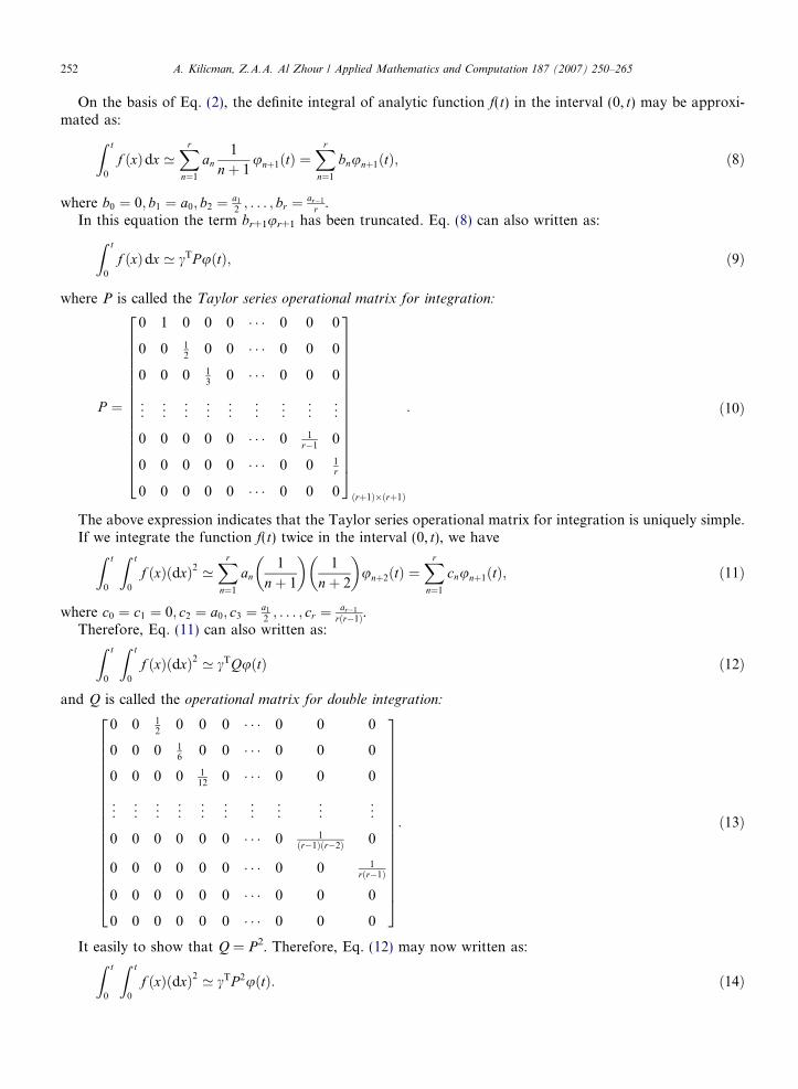
252 A. Kilicman, Z.A.A. Al Zhour / Applied Mathematics and Computation 187 (2007) 250–265

On the basis of Eq. (2), the definite integral of analytic function f(t) in the interval (0, t) may be approxi-mated as:

Z t

0

f ðxÞdx ’Xr

n¼1

an1

nþ 1unþ1ðtÞ ¼

Xr

n¼1

bnunþ1ðtÞ; ð8Þ

where b0 ¼ 0; b1 ¼ a0; b2 ¼ a1

2; . . . ; br ¼ ar�1

r .In this equation the term br+1ur+1 has been truncated. Eq. (8) can also written as:

Z t

0

f ðxÞdx ’ cTPuðtÞ; ð9Þ

where P is called the Taylor series operational matrix for integration:

P ¼

0 1 0 0 0 � � � 0 0 0

0 0 12

0 0 � � � 0 0 0

0 0 0 13

0 � � � 0 0 0

..

. ... ..

. ... ..

. ... ..

. ... ..

.

0 0 0 0 0 � � � 0 1r�1

0

0 0 0 0 0 � � � 0 0 1r

0 0 0 0 0 � � � 0 0 0

26666666666666664

37777777777777775ðrþ1Þ�ðrþ1Þ

: ð10Þ

The above expression indicates that the Taylor series operational matrix for integration is uniquely simple.If we integrate the function f(t) twice in the interval (0, t), we have

Z t

0

Z t

0

f ðxÞðdxÞ2 ’Xr

n¼1

an1

nþ 1

� �1

nþ 2

� �unþ2ðtÞ ¼

Xr

n¼1

cnunþ1ðtÞ; ð11Þ

where c0 ¼ c1 ¼ 0; c2 ¼ a0; c3 ¼ a1

2; . . . ; cr ¼ ar�1

rðr�1Þ.Therefore, Eq. (11) can also written as:

Z t

0

Z t

0

f ðxÞðdxÞ2 ’ cTQuðtÞ ð12Þ

and Q is called the operational matrix for double integration:

0 0 12

0 0 0 � � � 0 0 0

0 0 0 16

0 0 � � � 0 0 0

0 0 0 0 112

0 � � � 0 0 0

..

. ... ..

. ... ..

. ... ..

. ... ..

. ...

0 0 0 0 0 0 � � � 0 1ðr�1Þðr�2Þ 0

0 0 0 0 0 0 � � � 0 0 1rðr�1Þ

0 0 0 0 0 0 � � � 0 0 0

0 0 0 0 0 0 � � � 0 0 0

26666666666666666664

37777777777777777775

: ð13Þ

It easily to show that Q = P2. Therefore, Eq. (12) may now written as:

Z t

0

Z t

0

f ðxÞðdxÞ2 ’ cTP 2uðtÞ: ð14Þ

A. Kilicman, Z.A.A. Al Zhour / Applied Mathematics and Computation 187 (2007) 250–265 253

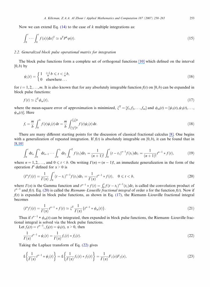
Now we can extend Eq. (14) to the case of k multiple integrations as:

Z t

0

� � �Z t

0

f ðxÞðdxÞk ’ aTP kuðtÞ: ð15Þ

2.2. Generalized block pulse operational matrix for integration

The block pulse functions form a complete set of orthogonal functions [10] which defined on the interval[0,b) by

wiðtÞ ¼1 i�1

m b 6 t < im b;

0 elsewhere . . .

�ð16Þ

for i = 1,2, . . . ,m. It is also known that for any absolutely integrable function f(t) on [0,b) can be expanded inblock pulse functions:

f ðtÞ ’ nT/mðtÞ; ð17Þ

where the mean-square error of approximation is minimized, nT = [f1, f2, . . . , fm] and /m(t) = [w1(t),w2(t), . . . ,wm(t)]. Here

fi ¼mb

Z b

0

f ðtÞwiðtÞdt ¼ mb

Z imð Þb

i�1mð Þb

f ðtÞwiðtÞdt: ð18Þ

There are many different starting points for the discussion of classical fractional calculus [8]. One beginswith a generalization of repeated integration. If f(t) is absolutely integrable on [0, b), it can be found that in[8,10]

Z t

0

dtn

Z tn

0

dtn�1 � � �Z t3

0

dt2

Z t2

0

f ðt1Þdt1 ¼1

ðnþ 1Þ!

Z t

0

ðt � t1Þn�1f ðt1Þdt1 ¼1

ðnþ 1Þ! tn�1 � f ðtÞ; ð19Þ

where n = 1,2, . . . , and 0 6 t < b. On writing C(n) = (n � 1)!, an immediate generalization in the form of theoperation Ia defined for a > 0 is

ðIaf ÞðtÞ ¼ 1

CðaÞ

Z t

0

ðt � t1Þa�1f ðt1Þdt1 ¼1

CðaÞ ta�1 � f ðtÞ; 0 6 t < b; ð20Þ

where C(a) is the Gamma function and ta�1 � f ðtÞ ¼R t

0 f ðt � t1Þa�1ðt1Þdt1 is called the convolution product ofta�1 and f(t). Eq. (20) is called the Riemann–Liouville fractional integral of order a for the function f(t). Now iff(t) is expanded in block pulse functions, as shown in Eq. (17), the Riemann–Liouville fractional integralbecomes

ðIaf ÞðtÞ ¼ 1

CðaÞ ta�1 � f ðtÞ ’ nT 1

CðaÞ fta�1 � /mðtÞg: ð21Þ

Thus if ta�1* /m(t) can be integrated, then expanded in block pulse functions, the Riemann–Liouville frac-

tional integral is solved via the block pulse functions.Let f1(t) = ta�1, f2(t) = wi(t), a > 0, then

1

CðaÞ ta�1 � wiðtÞ ¼

1

CðaÞ f1ðtÞ � f2ðtÞ: ð22Þ

Taking the Laplace transform of Eq. (22) gives

£1

ta�1 � wiðtÞ� �

¼ £1

f1ðtÞ � f2ðtÞ� �

¼ 1F 1ðsÞF 2ðsÞ; ð23Þ

CðaÞ CðaÞ CðaÞ

254 A. Kilicman, Z.A.A. Al Zhour / Applied Mathematics and Computation 187 (2007) 250–265

where

F 1ðsÞ ¼ £fta�1g ¼ CðaÞsa

;

F 2ðsÞ ¼ £fwiðtÞg ¼1

s£

d

dtwiðtÞ

� �� ,

1

se�

i�1m½ �bs � e�

im½ �bs

n o:

ð24Þ

Since C(a + 1) = aC(a), thus Eq. (23) can be written as:

£1

CðaÞ ta�1 � wiðtÞ

� �¼ 1

Cðaþ 1ÞCðaþ 1Þ

saþ1e�

i�1m½ �bs � e�

im½ �bs

n o: ð25Þ

Taking the inverse Laplace transform of Eq. (25) yields

1

CðaÞ

Z t

0

ðt � t1Þa�1wiðt1Þdt1 ¼1

Cðaþ 1Þ t � i� 1

mb

� �a

u t � i� 1

mb

� �� t � i

mb

� �a

u t � im

b� �

; ð26Þ

where u(t) is the unit step function. Further, it can be derived from Eq. (18) that

tauðtÞ ’ ½c1; c2; . . . ; cm�/mðtÞ ¼ CT/mðtÞ; ð27Þ

where

ci ¼bm

� �a iaþ1 � ði� 1Þaþ1

aþ 1: ð28Þ

Moreover, from the disjoint property of the block pulse functions [5]

wiðtÞwjðtÞ ¼wiðtÞ i ¼ j;

0 i 6¼ j:

�ð29Þ

It is obvious that

t � i� 1

mb

� �a

u t � i� 1

mb

� �’ ½0; 0; . . . ; 0; c1; c2; . . . ; cm�iþ1�/mðtÞ; ð30Þ

t � im

b� �a

u t � im

b� �

’ ½0; 0; . . . ; 0; c1; c2; . . . ; cm�1�/mðtÞ: ð31Þ

Thus Eq. (26) becomes

1

CðaÞ

Z t

0

ðt � t1Þa�1wiðt1Þdt1 ’1

Cðaþ 1Þ ½0; 0; . . . ; 0; c1; c2 � c1; . . . ; cm�iþ1 � cm�i�/mðtÞ ð32Þ

for i = 1,2, . . . ,m. Here,

cr � cr�1 ¼bm

� �a1

aþ 1½raþ1 � 2ðr � 1Þaþ1 þ ðr � 2Þaþ1� ð33Þ

for r = 2,3, . . . ,m � i + 1 and c1 ¼ bm

�a 1aþ1

.Now we can also write Eq. (32) as:

1

CðaÞ

Z t

0

ðt � t1Þa�1wiðt1Þdt1 ’bm

� �a1

Cðaþ 2Þ ½0; 0; . . . ; 0; n1; n2; . . . ; nm�iþ1�/mðtÞ; ð34Þ

where

n1 ¼ 1; np ¼ paþ1 � 2ðp � 1Þaþ1 þ ðp � 2Þaþ1 ðp ¼ 2; 3; . . . ;m� iþ 1Þ: ð35Þ

Finally, for i = 1,2, . . . ,m, Eq. (34) can be written as:

1

CðaÞ

Z t

0

ðt � t1Þa�1/mðt1Þdt1 ’ F a/mðtÞ; ð36Þ

A. Kilicman, Z.A.A. Al Zhour / Applied Mathematics and Computation 187 (2007) 250–265 255

where

F a ¼bm

� �a1

Cðaþ 2Þ

1 n2 n3 � � � nm

0 1 n2 � � � nm�1

0 0 1 � � � nm�2

0 0 0 . .. ..

.

0 0 0 0 1

266666664

377777775

ð37Þ

is called the generalized block pulse operational matrix for integration.For example, if a = b = 1, we then have n1 = 1, np = p2 � 2 (2 � 1)2 + (p � 2)2 = 2, for all p = 2,3, . . . ,m

and

Z t

0

/mðt1Þdt1 ’ F 1/mðtÞ ¼1

2m

1 2 2 � � � 2

0 1 2 � � � 2

0 0 1 � � � 2

0 0 0 . .. ..

.

0 0 0 0 1

26666664

37777775/mðtÞ:

The generalized block pulse operational matrices Da for differentiation can be derived simply by inverting theFa matrices. Let

Da ¼ F �1a ¼

mb

� �aCðaþ 2Þ

1 n2 n3 � � � nm

0 1 n2 � � � nm�1

0 0 1 � � � nm�2

0 0 0 . .. ..

.

0 0 0 0 1

266666664

377777775

�1

¼ mb

� �aCðaþ 2Þ

d1 d2 d1 � � � dm

0 d1 d2 � � � dm�1

0 0 d1 � � � dm�2

0 0 0 . .. ..

.

0 0 0 0 d1

266666664

377777775:

ð38Þ

Thus

1 n2 n3 � � � nm

0 1 n2 � � � nm�1

0 0 1 � � � nm�2

0 0 0 . .. ..

.

0 0 0 0 1

266666664

377777775:

d1 d2 d3 � � � dm

0 d1 d2 � � � dm�1

0 0 d1 � � � dm�2

0 0 0 . .. ..

.

0 0 0 0 d1

266666664

377777775¼ Im; ð39Þ

where Im is the identity matrix of order m · m. After equating both sides of Eq. (39), we get

d1 ¼ 1; d2 ¼ �n2d1; . . . ; dm ¼ �Xm

i¼2

nidm�iþ1: ð40Þ

Note that if a = 0, then F0 = D0 = Im which corresponds to s0 = 1 in the Laplace domain. It is obvious thatthe Fa and Da matrices perform as s�a and sa in the Laplace domain and as fractional (operational) integratorsand differentiators in the time domain.

For example, let a = 0.5, m = 4, b = 1, the operational matrices F0.5 and D0.5 which correspond to s�0.5 ands0.5 are computed below:

n1 = 1, n2 ¼ 2ffiffiffi2p� 2 ¼ 0:8284, n3 ¼ 3

ffiffiffi3p� 4

ffiffiffi2pþ 1 ¼ 0:5393, n4 ¼ 8� 6

ffiffiffi3pþ 2

ffiffiffi2p¼ 0:4631, d1 ¼ 1,

d2 = �0.8284, d3 = 0.1470, n4 = �0.1111, Cð2:5Þ ¼ 0:75Cð0:5Þ ¼ 0:75ffiffiffipp¼ 1:3293 and

256 A. Kilicman, Z.A.A. Al Zhour / Applied Mathematics and Computation 187 (2007) 250–265

F 0:5 ¼

0:3761 0:3116 0:2028 0:1640

0 0:3761 0:3116 0:2028

0 0 0:3761 0:3116

0 0 0 0:3761

266664

377775

D0:5 ¼

2:6857 �2:2025 0:2028 �0:2954

0 2:6857 �2:2025 0:3098

0 0 2:6857 �2:2025

0 0 0 2:6857

266664

377775:

3. Convolution product and Riemann–Liouville fractional integral of matrices

Definition 1. Let A(t) = [fij(t)] and B(t) = [gij(t)] be m · m absolutely integrable matrices on [0, b). Theconvolution and Kronecker convolution product s are matrix functions defined by

(i) Convolution product:

AðtÞ � BðtÞ ¼ ½hijðtÞ�; hijðtÞ ¼Xm

k¼1

Z t

0

fikðt � t1Þgkjðt1Þdt1 ¼Xm

k¼1

fikðtÞ � gkjðtÞ: ð41Þ

(ii) Kronecker convolution product

AðtÞ ~ BðtÞ ¼ ½fijðtÞ � BðtÞ�ij: ð42Þ

Here, fij(t) * B(t) is the ijth submatrix of order m · m and A(t) ~ B(t) is of order m2 · m2.

Definition 2. Let AðtÞ ¼ 1CðaijÞ t

aij�1h i

and B(t) = [gij(t)] be m · m absolutely integrable matrices on [0,b). TheRiemann–Liouville Fractional Integral of A(t) and B(t) is a matrix functions defined by

ðIaij BÞðtÞ ¼ AðtÞ � BðtÞ; aij > 0: ð43Þ

Definition 3. Let A(t) = [fij(t)] be m · m absolutely integrable matrices on [0, b). The determinant, inverse andk-power of A(t) respect to the convolution are defined by

(i) Determinant:

det AðtÞ ¼Xm

j¼1

ð�1Þjþ1f1jðtÞ � D1j; ð44Þ

where Dij the determinant of the (m � 1) · (m � 1) matrix function obtained from A(t) by deleting row i

and column j of A(t). We call Dij(t) the minor A(t) of corresponding to the entry of fij(t) of A(t).For exam-ple, if A(t) = [fij(t)] be 2 · 2 absolutely integrable matrices on [0, b), then

det AðtÞ ¼ f11ðtÞ � f22ðtÞ � f12ðtÞ � f21ðtÞ:

(ii) Inversion:

Af�1gðtÞ ¼ ½qijðtÞ�; qijðtÞ ¼ ðdet AðtÞÞf�1g � adjAðtÞ: ð45Þ

Here, (det A(t)){�1} exists, (detA(t)){�1}* detA(t) = d(t) and note that A{�1}(t) * A(t) = A(t) * A{�1}(t) =

Qm(t), where Qm(t) = Imd(t) is the Dirac identity matrix and d(t) is the Dirac identity function.

(iii) k- power convolution product:

AfkgðtÞ ¼ ½f fmgij ðtÞ�; f fmgij ðtÞ ¼Xm

r¼1

f fm�1gir ðtÞ � frjðtÞ: ð46Þ

A. Kilicman, Z.A.A. Al Zhour / Applied Mathematics and Computation 187 (2007) 250–265 257

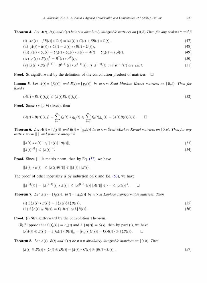
Theorem 4. Let A(t), B(t) and C(t) be n · n absolutely integrable matrices on [0,b).Then for any scalars a and b

ðiÞ ½aAðtÞ þ bBðtÞ� � CðtÞ ¼ aAðtÞ � CðtÞ þ bBðtÞ � CðtÞ; ð47ÞðiiÞ ðAðtÞ � BðtÞÞ � CðtÞ ¼ AðtÞ � ðBðtÞ � CðtÞÞ; ð48ÞðiiiÞ AðtÞ � QnðtÞ ¼ QnðtÞ � QnðtÞ � AðtÞ ¼ AðtÞ; QnðtÞ ¼ IndðtÞ; ð49ÞðivÞ ½AðtÞ � BðtÞ�T ¼ BTðtÞ � ATðtÞ; ð50ÞðvÞ ½AðtÞ � BðtÞ�f�1g ¼ Bf�1gðtÞ � Af�1gðtÞ; if Af�1gðtÞ and Bf�1gðtÞ are exist: ð51Þ

Proof. Straightforward by the definition of the convolution product of matrices. h

Lemma 5. Let A(t) = [fij(t)] and B(t) = [gij(t)] be m · m Semi-Markov Kernel matrices on [0,b). Then for

fixed t

ðAðtÞ � BðtÞÞði; jÞ 6 ðAðtÞBðtÞÞði; jÞ: ð52Þ

Proof. Since t 2 [0,b) (fixed), then

ðAðtÞ � BðtÞÞði; jÞ ¼Xm

k¼1

fikðtÞ � gkjðtÞ 6Xm

k¼1

fikðtÞgkjðtÞ ¼ ðAðtÞBðtÞÞði; jÞ: �

Theorem 6. Let A(t) = [fij(t)] and B(t) = [gij(t)] be m · m Semi-Markov Kernel matrices on [0,b). Then for any

matrix norm kÆk and positive integer k

kAðtÞ � BðtÞk 6 kAðtÞkkBðtÞk; ð53ÞkAðtÞfkgk 6 kAðtÞkk

: ð54Þ

Proof. Since kÆk is matrix norm, then by Eq. (52), we have

kAðtÞ � BðtÞk 6 kAðtÞBðtÞk 6 kAðtÞkkBðtÞk:

The proof of other inequality is by induction on k and Eq. (53), we have

kAfkgðtÞk ¼ kAfk�1gðtÞ � AðtÞk 6 kAfk�1gðtÞkkAðtÞk 6 � � � 6 kAðtÞkk: �

Theorem 7. Let A(t) = [fij(t)], B(t) = [gij(t)] be m · m Laplace transformable matrices. Then

ðiÞ £fAðtÞ � BðtÞg ¼ £fAðtÞg£fBðtÞg; ð55ÞðiiÞ £fAðtÞ ~ BðtÞg ¼ £fAðtÞg � £fBðtÞg: ð56Þ

Proof. (i) Straightforward by the convolution Theorem.

(ii) Suppose that £{fij(t)} = Fij(s) and £ {B(t)} = G(s), then by part (i), we have

£fAðtÞ ~ BðtÞg ¼ £½fijðtÞ � BðtÞ�ij ¼ ½F ijðsÞGðsÞ� ¼ £fAðtÞg � £fBðtÞg: �

Theorem 8. Let A(t), B(t) and C(t) be n · n absolutely integrable matrices on [0,b). Then

½AðtÞ ~ BðtÞ� � ½CðtÞ ~ DðtÞ� ¼ ½AðtÞ � CðtÞ� ~ ½BðtÞ � DðtÞ�: ð57Þ

258 A. Kilicman, Z.A.A. Al Zhour / Applied Mathematics and Computation 187 (2007) 250–265

Proof. The (i, j)th block of [A(t) ~ B(t)]*[C(t) ~ D(t)] is obtained by taking the convolution product of ith rowblock of A(t) ~ B(t) and the jth column block of C(t) ~ D(t),i.e.,

½fi1ðtÞ � BðtÞ � � � finðtÞ � BðtÞ� �

h1jðtÞ � DðtÞ

..

.

hnjðtÞ � DðtÞ

26664

37775 ¼

Xn

k¼1

ðfikðtÞ � hkjðtÞ � BðtÞ � DðtÞÞ

and the (i, j)th block of the right hand side [A(t) * C(t)] ~ [B(t) * D(t)] obtained by the definition of the Kro-necker convolution product xij(t)*(B(t) * D(t)) where xij is the (i, j)th element in A(t) * C(t). But the rule of con-volution product

xijðtÞ ¼Xn

k¼1

ðfikðtÞ � hkjðtÞÞ: �

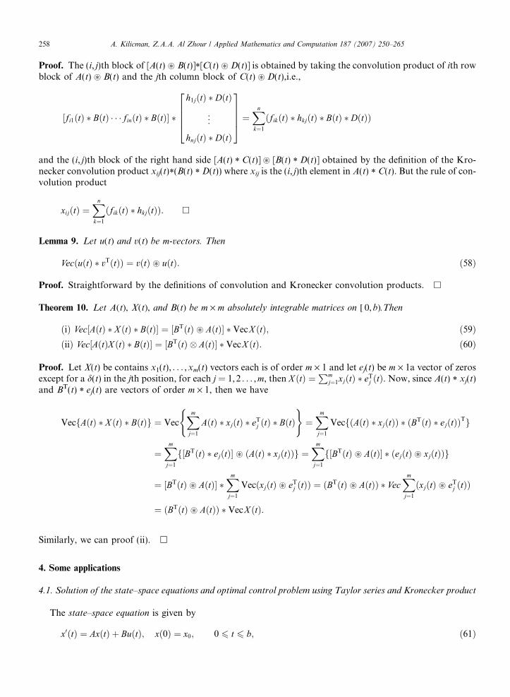
Lemma 9. Let u(t) and v(t) be m-vectors. Then

VecðuðtÞ � vTðtÞÞ ¼ vðtÞ ~ uðtÞ: ð58Þ

Proof. Straightforward by the definitions of convolution and Kronecker convolution products. h

Theorem 10. Let A(t), X(t), and B(t) be m · m absolutely integrable matrices on [0,b).Then

ðiÞ Vec½AðtÞ � X ðtÞ � BðtÞ� ¼ ½BTðtÞ ~ AðtÞ� � Vec X ðtÞ; ð59ÞðiiÞ Vec½AðtÞX ðtÞ � BðtÞ� ¼ ½BTðtÞ � AðtÞ� � Vec X ðtÞ: ð60Þ

Proof. Let X(t) be contains x1(t), . . . ,xm(t) vectors each is of order m · 1 and let ej(t) be m · 1a vector of zerosexcept for a d(t) in the jth position, for each j = 1,2 . . . ,m, then X ðtÞ ¼

Pmj¼1xjðtÞ � eT

j ðtÞ. Now, since A(t) * xj(t)and BT(t) * ej(t) are vectors of order m · 1, then we have

VecfAðtÞ � X ðtÞ � BðtÞg ¼ VecXm

j¼1

AðtÞ � xjðtÞ � eTj ðtÞ � BðtÞ

( )¼Xm

j¼1

VecfðAðtÞ � xjðtÞÞ � ðBTðtÞ � ejðtÞÞTg

¼Xm

j¼1

f½BTðtÞ � ejðtÞ� ~ ðAðtÞ � xjðtÞÞg ¼Xm

j¼1

f½BTðtÞ ~ AðtÞ� � ðejðtÞ ~ xjðtÞÞg

¼ ½BTðtÞ ~ AðtÞ� �Xm

j¼1

VecðxjðtÞ ~ eTj ðtÞÞ ¼ ðBTðtÞ ~ AðtÞÞ � Vec

Xm

j¼1

ðxjðtÞ ~ eTj ðtÞÞ

¼ ðBTðtÞ ~ AðtÞÞ � Vec X ðtÞ:

Similarly, we can proof (ii). h

4. Some applications

4.1. Solution of the state–space equations and optimal control problem using Taylor series and Kronecker product

The state–space equation is given by

x0ðtÞ ¼ AxðtÞ þ BuðtÞ; xð0Þ ¼ x0; 0 6 t 6 b; ð61Þ

A. Kilicman, Z.A.A. Al Zhour / Applied Mathematics and Computation 187 (2007) 250–265 259

where xðtÞ 2 Rn, uðtÞ 2 Rm analytic and A, B are known constant matrices. The input vector u(t) may be ex-panded in Taylor series as follows:

uðtÞ ¼

u1ðtÞu2ðtÞ

..

.

umðtÞ

2666664

3777775 ¼

h10 h11 h12 � � � h1;r�1

h20 h21 h22 � � � h2;r�1

..

. ... ..

. ... ..

.

hm0 hm1 hm2 � � � hm;r�1

2666664

3777775 �

u0ðtÞu1ðtÞ

..

.

ur�1ðtÞ

2666664

3777775 ¼ H � uðtÞ; ð62Þ

where H is a known constant matrix.Similarly, the state vector x(t) may also be expanded in Taylor series as follows:

xðtÞ ¼

x1ðtÞx2ðtÞ

..

.

xnðtÞ

2666664

3777775 ¼

f10 f11 f12 � � � f1;r�1

f20 f21 f22 � � � f2;r�1

..

. ... ..

. ... ..

.

fn0 fn1 fn2 � � � fn;r�1

2666664

3777775:

u0ðtÞu1ðtÞ

..

.

ur�1ðtÞ

2666664

3777775 ¼ ½f0; f1; f2; . . . ; fr�1�:uðtÞ ¼ F � uðtÞ; ð63Þ

where F contains the unknown coefficients of the Taylor expansion of the state vector x(t).Next by integrating the space–state equation in Eq. (61), we have

xðtÞ � xð0Þ ¼ AZ t

0

xðrÞdrþ BZ t

0

uðrÞdr: ð64Þ

Introducing Eqs. (62), (63) in (64) and using the integration property of the operational matrix P expressedby (15), we obtain

ðF � AFP ÞuðtÞ ¼ ðBHP þ EÞuðtÞ; ð65Þ

where E = [x0 0 0 . . . 0].

In Eq. (65), the matrix BHP + E is known; therefore, we have the following system for the unknown matrixF:

AFP � D; D ¼ �BHP � E: ð66Þ

This system may be written in a simpler form by using the Kronecker product, actually we have

Mf ¼ ðA� P T � InrÞf ¼ d; ð67Þ

where M = PT � A � Inr is a nr · nr matrix and

f ¼ Vec F ¼

f0

f1

..

.

fr�1

266664

377775; d ¼ Vec D ¼

d0

d1

..

.

dr�1

266664

377775;

i.e., fi and di are the ith columns of F and D, respectively. Here,

M ¼ P T � A� Inr ¼

pA pA � � � pA

pA pA � � � pA

..

. ... ..

. ...

pA pA � � � pA

266664

377775� Inr

is called the Kronecker operational matrix, where Inr is an identity matrix of order nr · nr.The solution of Eq. (67) is f = M�1d = (PT � A � Inr)

�1d.

260 A. Kilicman, Z.A.A. Al Zhour / Applied Mathematics and Computation 187 (2007) 250–265

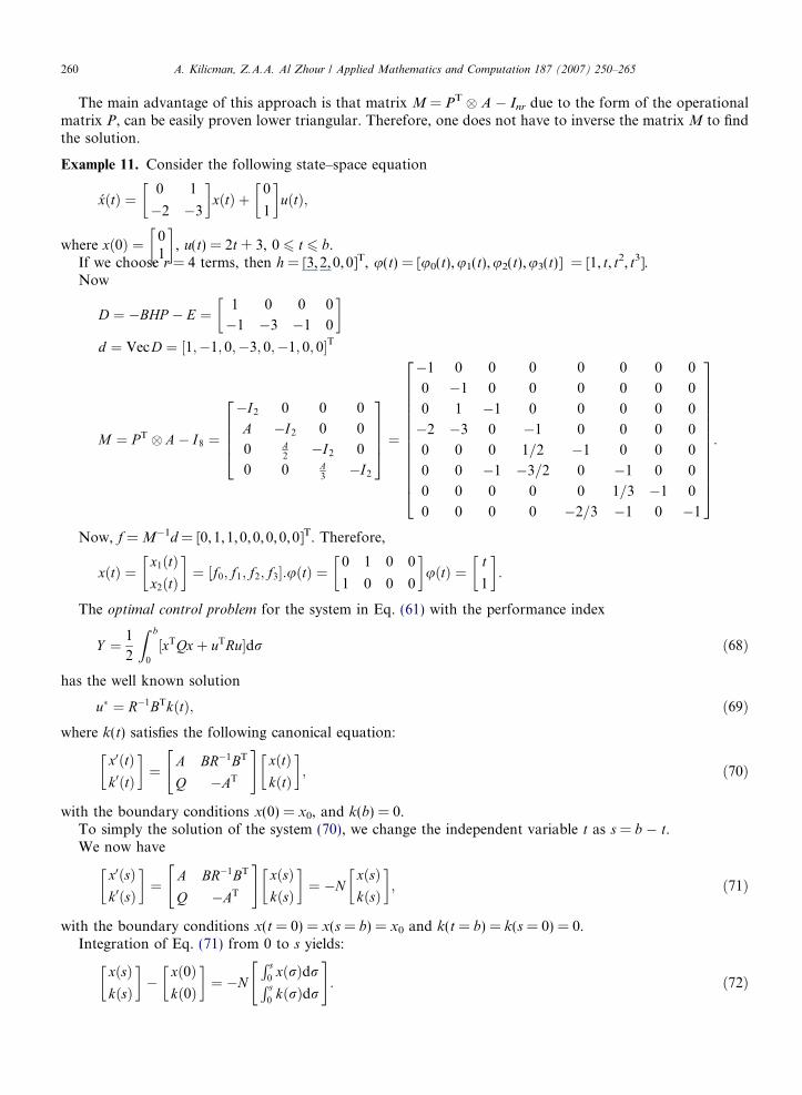
The main advantage of this approach is that matrix M = PT � A � Inr due to the form of the operationalmatrix P, can be easily proven lower triangular. Therefore, one does not have to inverse the matrix M to findthe solution.

Example 11. Consider the following state–space equation

�xðtÞ ¼0 1

�2 �3

� xðtÞ þ

0

1

� uðtÞ;

where xð0Þ ¼ 01

� , u(t) = 2t + 3, 0 6 t 6 b.

If we choose r = 4 terms, then h = [3,2,0,0]T, u(t) = [u0(t),u1(t),u2(t),u3(t)] = [1, t, t2, t3].Now

D ¼ �BHP � E ¼ 1 0 0 0

�1 �3 �1 0

� d ¼ Vec D ¼ ½1;�1; 0;�3; 0;�1; 0; 0�T

M ¼ P T � A� I8 ¼

�I2 0 0 0

A �I2 0 0

0 A2�I2 0

0 0 A3�I2

26664

37775 ¼

�1 0 0 0 0 0 0 0

0 �1 0 0 0 0 0 0

0 1 �1 0 0 0 0 0

�2 �3 0 �1 0 0 0 0

0 0 0 1=2 �1 0 0 0

0 0 �1 �3=2 0 �1 0 0

0 0 0 0 0 1=3 �1 0

0 0 0 0 �2=3 �1 0 �1

26666666666664

37777777777775:

Now, f = M�1d = [0, 1,1,0,0,0,0,0]T. Therefore,

xðtÞ ¼x1ðtÞx2ðtÞ

� ¼ ½f0; f1; f2; f3�:uðtÞ ¼

0 1 0 0

1 0 0 0

� uðtÞ ¼

t

1

� :

The optimal control problem for the system in Eq. (61) with the performance index

Y ¼ 1

2

Z b

0

½xTQxþ uTRu�dr ð68Þ

has the well known solution

u� ¼ R�1BTkðtÞ; ð69Þ

where k(t) satisfies the following canonical equation:

x0ðtÞk0ðtÞ

� ¼ A BR�1BT

Q �AT

" #xðtÞkðtÞ

� ; ð70Þ

with the boundary conditions x(0) = x0, and k(b) = 0.To simply the solution of the system (70), we change the independent variable t as s = b � t.We now have

x0ðsÞk0ðsÞ

� ¼ A BR�1BT

Q �AT

" #xðsÞkðsÞ

� ¼ �N

xðsÞkðsÞ

� ; ð71Þ

with the boundary conditions x(t = 0) = x(s = b) = x0 and k(t = b) = k(s = 0) = 0.Integration of Eq. (71) from 0 to s yields:

xðsÞkðsÞ

� �

xð0Þkð0Þ

� ¼ �N

R s0

xðrÞdrR s0

kðrÞdr

" #: ð72Þ

A. Kilicman, Z.A.A. Al Zhour / Applied Mathematics and Computation 187 (2007) 250–265 261

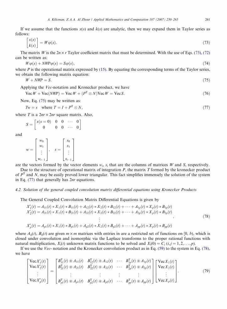
If we assume that the functions x(s) and k(s) are analytic, then we may expand them in Taylor series asfollows:

xðsÞkðsÞ

� ¼ W uðsÞ: ð73Þ

The matrix W is the 2n · r Taylor coefficient matrix that must be determined. With the use of Eqs. (73), (72)can be written as:

W uðsÞ þ NWPuðsÞ ¼ SuðsÞ; ð74Þ

where P is the operational matrix expressed by (15). By equating the corresponding terms of the Taylor series,we obtain the following matrix equation:

W þ NWP ¼ S: ð75Þ

Applying the Vec-notation and Kronecker product, we have

VecW þ VecðNWP Þ ¼ Vec W þ ðP T � NÞVec W ¼ Vec S: ð76Þ

Now, Eq. (75) may be written as:

Tw ¼ s where T ¼ I þ P T � N ; ð77Þ

where T is a 2nr · 2nr square matrix. Also,

S ¼ xðs ¼ 0Þ 0 0 � � � 0

0 0 0 � � � 0

�

and

w ¼

w0

w1

..

.

wr�1

26664

37775; s ¼

s0

s1

..

.

sr�1

26664

37775

are the vectors formed by the vector elements wi, si that are the columns of matrices W and S, respectively.Due to the structure of operational matrix of integration P, the matrix T formed by the kronecker product

of PT and N, may be easily proved lower triangular. This fact simplifies immensely the solution of the systemin Eq. (77) that generally has 2nr equations.

4.2. Solution of the general coupled convolution matrix differential equations using Kronecker Products

The General Coupled Convolution Matrix Differential Equations is given by

X 01ðtÞ ¼ A11ðtÞ � X 1ðtÞ � B11ðtÞ þ A12ðtÞ � X 2ðtÞ � B12ðtÞ þ � � � þ A1pðtÞ � X pðtÞ � B1pðtÞX 02ðtÞ ¼ A21ðtÞ � X 1ðtÞ � B21ðtÞ þ A22ðtÞ � X 2ðtÞ � B22ðtÞ þ � � � þ A2pðtÞ � X pðtÞ � B2pðtÞ

..

.

X 0pðtÞ ¼ Ap1ðtÞ � X 1ðtÞ � Bp1ðtÞ þ Ap2ðtÞ � X 2ðtÞ � Bp2ðtÞ þ � � � þ AppðtÞ � X pðtÞ � BppðtÞ

; ð78Þ

where Aij(t), Bij(t) are given m · m matrices with entries in are a restricted set of functions on [0, b), which isclosed under convolution and isomorphic via the Laplace transforms to the proper rational functions withnatural multiplication, Xi(t) unknown matrix functions to be solved and Xi(0) = Ci (i, j = 1,2, . . . ,p).

If we use the Vec- notation and the Kronecker convolution product as in Eq. (59) to the system in Eq. (78),we have

Vec X 01ðtÞVec X 02ðtÞ

..

.

Vec X 0pðtÞ

266664

377775 ¼

BT11ðtÞ ~ A11ðtÞ BT

12ðtÞ ~ A12ðtÞ � � � BT1pðtÞ ~ A1pðtÞ

BT21ðtÞ ~ A21ðtÞ BT

22ðtÞ ~ A22ðtÞ � � � BT2pðtÞ ~ A2pðtÞ

..

. ... ..

. ...

BTp1ðtÞ ~ Ap1ðtÞ BT

p2ðtÞ ~ Ap2ðtÞ � � � BTppðtÞ ~ AppðtÞ

266664

377775

Vec X 1ðtÞVec X 2ðtÞ

..

.

Vec X pðtÞ

26664

37775: ð79Þ

262 A. Kilicman, Z.A.A. Al Zhour / Applied Mathematics and Computation 187 (2007) 250–265

This system may be written in a simpler form by

x0ðtÞ ¼ HðtÞ � xðtÞ; xðtÞ ¼ c; ð80Þ

where

x0ðtÞ ¼

Vec X 01ðtÞ

Vec X 02ðtÞ

..

.

Vec X 0pðtÞ

26666664

37777775; xðtÞ ¼

Vec X 1ðtÞ

Vec X 2ðtÞ

..

.

VecX pðtÞ

26666664

37777775

ð81Þ

HðtÞ ¼

BT11ðtÞ ~ A11ðtÞ BT

12ðtÞ ~ A12ðtÞ � � � BT1pðtÞ ~ A1pðtÞ

BT21ðtÞ ~ A21ðtÞ BT

22ðtÞ ~ A22ðtÞ � � � BT2pðtÞ ~ A2pðtÞ

..

. ... ..

. ...

BTp1ðtÞ ~ Ap1ðtÞ BT

p2ðtÞ ~ Ap2ðtÞ � � � BTppðtÞ ~ AppðtÞ

266666664

377777775: ð82Þ

Now if we use Laplace transform to Eq. (80), we have

£fx0ðtÞg ¼ £fHðtÞ � xðtÞg: ð83Þ

Let Y(s) = £{x(t)}, G(s) = £{H(t)}, we have

Y ðsÞ ¼ fsI � GðsÞgf�1gc; sI > GðsÞ: ð84Þ

Taking the inverse Laplace transform of Eq. (84) yields

xðtÞ ¼ £�1 s I � GðsÞs

� �� �f�1g( )

c ¼ £�1 1

sI � GðsÞ

s

� �f�1g !( )

c ¼ I � ðI � I � HðtÞÞf�1gc; ð85Þ

where I is an identity scalar matrix.Suppose that Q(t) = I * H(t), then (I � I * H(t)){�1} = (I � Q(t)){�1} can be obtained by two ways, either by

truncated series development or by explicit inversion within the above described convolution algebra. In thefirst case, we have

ðI � QðtÞÞf�1g ¼ I þXn

k¼1

QfkgðtÞ þ RnðtÞ: ð86Þ

Here,

Qfnþ1gij ðtÞ ¼

Xk2N

Z t

0

QikðuÞQfngkj ðt � uÞdu ð87Þ

and Q{1}(t) = Q(t).The total error is given by

RnðtÞ ¼X1

k¼nþ1

QfkgðtÞ ¼ Qfnþ1gðtÞ � ðI þ QðtÞ þ Qf2gðtÞ þ � � �Þ ¼ Qfnþ1gðtÞ � ðI � QðtÞÞf�1g: ð88Þ

Now for any matrix norm satisfying:

kQfngðtÞk 6 kQðtÞkn; ð89Þ

then the total error due to the above truncation is also bounded by (89), if kQ(t)k < 1, then

kRnðtÞk 6kQðtÞknþ1

1� kQðtÞk : ð90Þ

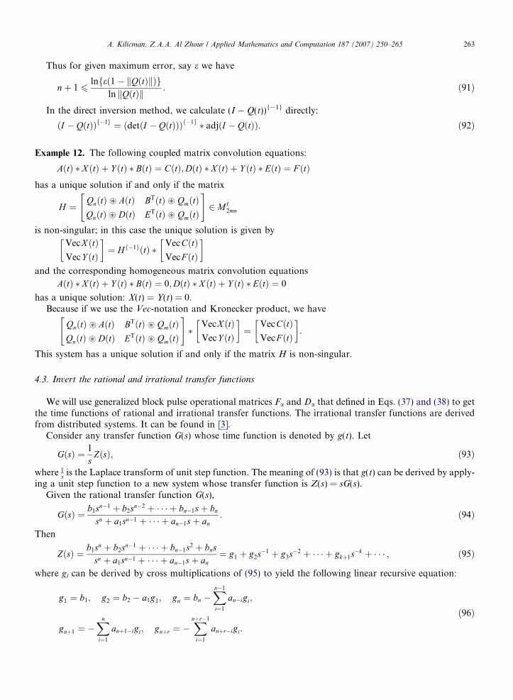
A. Kilicman, Z.A.A. Al Zhour / Applied Mathematics and Computation 187 (2007) 250–265 263

Thus for given maximum error, say e we have

nþ 1 6lnfeð1� kQðtÞkÞg

ln kQðtÞk : ð91Þ

In the direct inversion method, we calculate (I � Q(t)){�1} directly:

ðI � QðtÞÞf�1g ¼ ðdetðI � QðtÞÞÞf�1g � adjðI � QðtÞÞ: ð92Þ

Example 12. The following coupled matrix convolution equations:

AðtÞ � X ðtÞ þ Y ðtÞ � BðtÞ ¼ CðtÞ;DðtÞ � X ðtÞ þ Y ðtÞ � EðtÞ ¼ F ðtÞ

has a unique solution if and only if the matrix

H ¼ QnðtÞ ~ AðtÞ BTðtÞ ~ QmðtÞQnðtÞ ~ DðtÞ ETðtÞ ~ QmðtÞ

" #2 MI

2mn

is non-singular; in this case the unique solution is given by

Vec X ðtÞVec Y ðtÞ

� ¼ H f�1gðtÞ �

VecCðtÞVec F ðtÞ

�

and the corresponding homogeneous matrix convolution equations

AðtÞ � X ðtÞ þ Y ðtÞ � BðtÞ ¼ 0;DðtÞ � X ðtÞ þ Y ðtÞ � EðtÞ ¼ 0

has a unique solution: X(t) = Y(t) = 0.Because if we use the Vec-notation and Kronecker product, we have

QnðtÞ ~ AðtÞ BTðtÞ ~ QmðtÞQnðtÞ ~ DðtÞ ETðtÞ ~ QmðtÞ

" #�

VecX ðtÞVec Y ðtÞ

� ¼

Vec CðtÞVec F ðtÞ

� :

This system has a unique solution if and only if the matrix H is non-singular.

4.3. Invert the rational and irrational transfer functions

We will use generalized block pulse operational matrices Fa and Da that defined in Eqs. (37) and (38) to getthe time functions of rational and irrational transfer functions. The irrational transfer functions are derivedfrom distributed systems. It can be found in [3].

Consider any transfer function G(s) whose time function is denoted by g(t). Let

GðsÞ ¼ 1

sZðsÞ; ð93Þ

where 1s is the Laplace transform of unit step function. The meaning of (93) is that g(t) can be derived by apply-

ing a unit step function to a new system whose transfer function is Z(s) = sG(s).Given the rational transfer function G(s),

GðsÞ ¼ b1sn�1 þ b2sn�2 þ � � � þ bn�1sþ bn

sn þ a1sn�1 þ � � � þ an�1sþ an: ð94Þ

Then

ZðsÞ ¼ b1sn þ b2sn�1 þ � � � þ bn�1s2 þ bnssn þ a1sn�1 þ � � � þ an�1sþ an

¼ g1 þ g2s�1 þ g3s�2 þ � � � þ gkþ1s�k þ � � � ; ð95Þ

where gi can be derived by cross multiplications of (95) to yield the following linear recursive equation:

g1 ¼ b1; g2 ¼ b2 � a1g1; gn ¼ bn �Xn�1

i¼1

an�igi;

gnþ1 ¼ �Xn

i¼1

anþ1�igi; gnþr ¼ �Xnþr�1

i¼1

anþr�igi:

ð96Þ

264 A. Kilicman, Z.A.A. Al Zhour / Applied Mathematics and Computation 187 (2007) 250–265

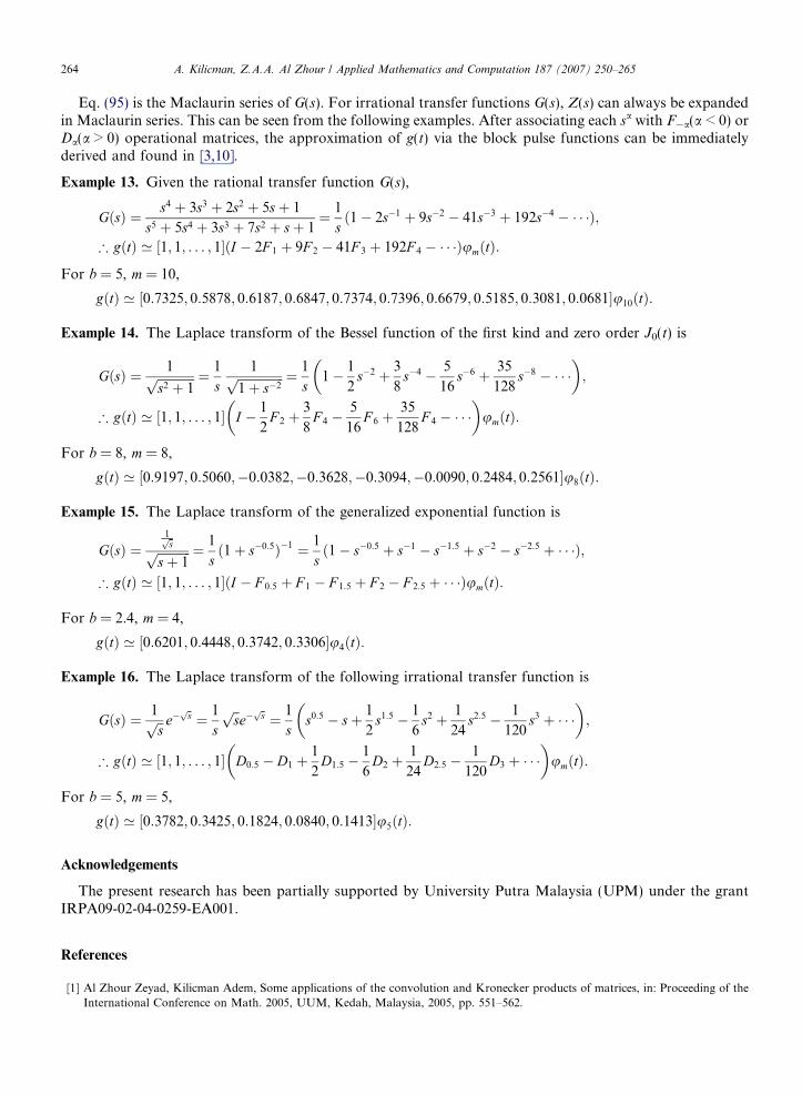
Eq. (95) is the Maclaurin series of G(s). For irrational transfer functions G(s), Z(s) can always be expandedin Maclaurin series. This can be seen from the following examples. After associating each sa with F�a(a < 0) orDa(a > 0) operational matrices, the approximation of g(t) via the block pulse functions can be immediatelyderived and found in [3,10].

Example 13. Given the rational transfer function G(s),

GðsÞ ¼ s4 þ 3s3 þ 2s2 þ 5sþ 1

s5 þ 5s4 þ 3s3 þ 7s2 þ sþ 1¼ 1

sð1� 2s�1 þ 9s�2 � 41s�3 þ 192s�4 � � � �Þ;

) gðtÞ ’ ½1; 1; . . . ; 1�ðI � 2F 1 þ 9F 2 � 41F 3 þ 192F 4 � � � �ÞumðtÞ:

For b = 5, m = 10,

gðtÞ ’ ½0:7325; 0:5878; 0:6187; 0:6847; 0:7374; 0:7396; 0:6679; 0:5185; 0:3081; 0:0681�u10ðtÞ:

Example 14. The Laplace transform of the Bessel function of the first kind and zero order J0(t) is

GðsÞ ¼ 1ffiffiffiffiffiffiffiffiffiffiffiffis2 þ 1p ¼ 1

s1ffiffiffiffiffiffiffiffiffiffiffiffiffiffiffi

1þ s�2p ¼ 1

s1� 1

2s�2 þ 3

8s�4 � 5

16s�6 þ 35

128s�8 � � � �

� �;

) gðtÞ ’ ½1; 1; . . . ; 1� I � 1

2F 2 þ

3

8F 4 �

5

16F 6 þ

35

128F 4 � � � �

� �umðtÞ:

For b = 8, m = 8,

gðtÞ ’ ½0:9197; 0:5060;�0:0382;�0:3628;�0:3094;�0:0090; 0:2484; 0:2561�u8ðtÞ:

Example 15. The Laplace transform of the generalized exponential function is

GðsÞ ¼1ffiffispffiffiffiffiffiffiffiffiffiffiffisþ 1p ¼ 1

sð1þ s�0:5Þ�1 ¼ 1

sð1� s�0:5 þ s�1 � s�1:5 þ s�2 � s�2:5 þ � � �Þ;

) gðtÞ ’ ½1; 1; . . . ; 1�ðI � F 0:5 þ F 1 � F 1:5 þ F 2 � F 2:5 þ � � �ÞumðtÞ:

For b = 2.4, m = 4,

gðtÞ ’ ½0:6201; 0:4448; 0:3742; 0:3306�u4ðtÞ:

Example 16. The Laplace transform of the following irrational transfer function is

GðsÞ ¼ 1ffiffisp e�

ffiffisp¼ 1

s

ffiffisp

e�ffiffisp¼ 1

ss0:5 � sþ 1

2s1:5 � 1

6s2 þ 1

24s2:5 � 1

120s3 þ � � �

� �;

) gðtÞ ’ ½1; 1; . . . ; 1� D0:5 � D1 þ1

2D1:5 �

1

6D2 þ

1

24D2:5 �

1

120D3 þ � � �

� �umðtÞ:

For b = 5, m = 5,

gðtÞ ’ ½0:3782; 0:3425; 0:1824; 0:0840; 0:1413�u5ðtÞ:

Acknowledgements

The present research has been partially supported by University Putra Malaysia (UPM) under the grantIRPA09-02-04-0259-EA001.

References

[1] Al Zhour Zeyad, Kilicman Adem, Some applications of the convolution and Kronecker products of matrices, in: Proceeding of theInternational Conference on Math. 2005, UUM, Kedah, Malaysia, 2005, pp. 551–562.

A. Kilicman, Z.A.A. Al Zhour / Applied Mathematics and Computation 187 (2007) 250–265 265

[2] T. Chen, B.A. Francis, Optimal Sampled-Data Control Systems, Springer, London, 1995.[3] C.F. Chen, Y.T. Tsay, T.T. Wu, Walsh operational matrices for fractional calculus and their applications to distributed systems, J.

Frankin Inst. 303 (3) (1977) 267–284.[4] A.E. Gilmour, Circulant Matrix Methods for the Numerical solutions of Partial Differential Equations by FFT Convolutions, New

Zealand, 1987.[5] K. Maleknejad, M. Shaherezaee, H. Khatami, Numerical solution of integral equations systems of second kind by Block Pulse

Functions, Appl. Math. Comput. 166 (2005) 15–24.[6] S.G. Mouroutsos, P.D. Sparis, Taylor Series approach to system identification, analysis and optimal control, J. Frankin Inst. 319 (3)

(1985) 359–371.[7] L. Nikolaos, Dependability analysis of Semi-Markov system, Reliab. Eng. Syst. Safety 55 (1997) 203–207.[8] B. Ross, Fractional Calculus and its Applications, Springer-Verlag, Berlin, 1975.[9] H. Sumita, The Matrix Laguerre Transform, Appl. Math. Comput. 15 (1984) 1–28.

[10] C.-H. Wang, On the generalization of Block Pulse Operational matrices for fractional and operational calculus, J. Frankin Inst. 315(2) (1983) 91–102.