Kinetics and Transport Phenomena in the Chemical Decomposition ...

Kinetics and Transport Phenomena in the Chemical Decomposition of

Copper Oxychloride in the Thermochemical Cu-Cl Cycle

By

Gabriel D. Marin

A Thesis Submitted in Partial Fulfillment

of the Requirements for the Degree of

Doctor of Philosophy in Mechanical Engineering

in

The Faulty of Engineering and Applied Sciences

University of Ontario Institute of Technology

April 2012

© Gabriel Marin, 2012

iii

Abstract _______________________________________________________________________________

The thermochemical copper-chlorine (Cu-Cl) cycle for hydrogen production

includes three chemical reactions of hydrolysis, decomposition and electrolysis. The

decomposition of copper oxychloride establishes the high-temperature limit of the cycle.

Between 430 and 530 oC, copper oxychloride (Cu2OCl2) decomposes to produce a molten

salt of copper (I) chloride (CuCl) and oxygen gas. The conditions that yield equilibrium at

high conversion rates are not well understood. Also, the impact of feed streams containing

by-products of incomplete reactions in an integrated thermochemical cycle of hydrogen

production are also not well understood. In an integrated cycle, the hydrolysis reaction

where CuCl2 reacts with steam to produce solid copper oxychloride precedes the

decomposition reaction. Undesirable chlorine may be released as a result of CuCl2

decomposition and mass imbalance of the overall cycle and additional energy

requirements to separate chlorine gas from the oxygen gas stream.

In this thesis, a new phase change predictive model is developed and compared to

the reaction rate kinetics in order to better understand the nature of resistances. A Stefan

boundary condition is used in a new particle model to track the position of the moving

solid-liquid interface as the solid particle decomposes under the influence of heat transfer

at the surface. Results of conversion of CuO*CuCl2 from both a thermogravimetric (TGA)

microbalance and a laboratory scale batch reactor experiments are analyzed and the rate of

endothermic reaction determined. A second particle model identifies parameters that

impact the transient chemical decomposition of solid particles embedded in the bulk fluid

iv

consisting of molten and gaseous phases at high temperature and low Reynolds number.

The mass, energy, momentum and chemical reaction equations are solved for a particle

suddenly immersed in a viscous continuum. Numerical solutions are developed and the

results are validated with experimental data of small samples of chemical decomposition

of copper oxychloride (CuO*CuCl2). This thesis provides new experimental and

theoretical reference for the scale-up of a CuO*CuCl2 decomposition reactor with

consideration of the impact on the yield of the thermochemical copper-chlorine cycle for

the generation of hydrogen.

v

To my wife

Mimi

and my beloved daughters

Isabella and Valentina,

for their unconditional patience and love

vi

Acknowledgments ________________________________________________________________________

I look back to these great years at UOIT and I can only be grateful for all the great

support and direction received. All these years have polished my spirit and made me a

more conscious and learning oriented professional.

First, I want to acknowledge the professional and unconditional support received

from my supervisors, Dr. Greg F. Naterer and Kamiel Gabriel. They have not only

provided continuous guidance throughout my research, but also a reference to exemplary

ethical values. This research could have not been possible without their continuous

support and enthusiasm.

I also want to thank Dr. Zhaolin Wang for providing a stimulating and creative

environment in addition to timely scientific insights in moments of difficult decisions. He

promoted a scientific approach and professional perspective where learning experiences

flourished.

This research also brought me close to great new friends from whom I am thankful

for their support. Especially Dr. Venkata Daggupati had the patience to explain things

clearly and repeat when necessary, helping me understand phenomena in the context of

mathematical analysis. Also, thanks to my dear friend Dr. Juan Carlos Ramirez at Purdue

University for being there whenever I needed direction. Their friendly support and

patience made a difference in moments of uncertainty.

vii

I also want to thank Ed Secnik for his commitment to a quiet and safe environment

and call to discipline, and for his diligence with the lab infrastructure. His approach is a

great reference for the future.

I am also very thankful with members of the committee, Dr. Ibrahim Dincer, and

Dr. Liliana Trevani for the time and patience while reviewing my thesis and providing

feedback when requested. Their input and direction brought additional meaning to this

research. Similarly, I would like to thank you Dr. Antonio Mazza for volunteering his

time as external reviewer of my thesis.

Thanks to Dr. Brad Easton for his kind support while facilitating his lab for a

critical part of my experimental work with TGA, and for the timely training facilitated by

Patrick Edge. Also, I could not have navigated successfully through the complexity of

XRD analysis without the unconditional help from George Kretschmann at the

Department of Geology of the University of Toronto. George made the learning

experience enjoyable and efficient at all times.

Finally, my sincere thanks go to the people and organizations that support research

at UOIT by providing critical financial resources. Support from the Natural Sciences and

Engineering Research Council of Canada, the Ontario Research Fund, Atomic Energy of

Canada Limited, and the Faculty of Engineering and Applied Science at UOIT are

gratefully acknowledged.

viii

Table of Contents Certificate of Approval ............................................................................................................. ii

Abstract…. .............................................................................................................................. iii

Acknowledgments ................................................................................................................... vi

List of Figures .......................................................................................................................... x

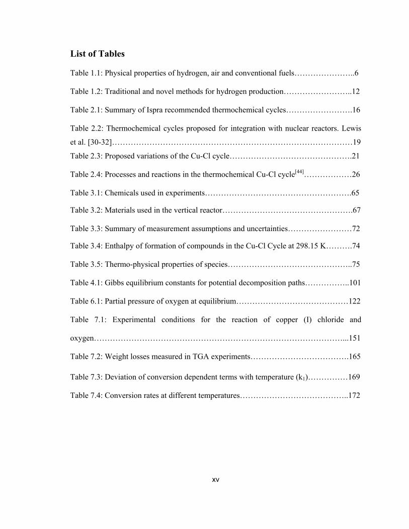
List of Tables .......................................................................................................................... xv

Nomenclature ........................................................................................................................ xvi

Chapter 1 – Introduction ........................................................................................................... 1

1.1 Background ............................................................................................................... 1

1.1.1 Hydrogen as an Energy Carrier ...................................................................... 5

1.1.2 Hydrogen from Thermochemical Cycles ..................................................... 11

1.2 Motivation and Objectives of Thesis ...................................................................... 14

Chapter 2 - Literature Review ................................................................................................ 16

2.1 Thermochemical Cycles .......................................................................................... 16

2.2 Thermochemical Cu-Cl Cycle ................................................................................. 20

2.3 Three Reactions Thermochemical Cu-Cl Cycle...................................................... 27

2.3.1 Electrolysis Reaction .................................................................................... 27

2.3.2 Hydrolysis Reaction ..................................................................................... 29

2.3.3 Decomposition Reaction .............................................................................. 33

2.4 Experimental and Theoretical Models .................................................................... 38

2.4.1 Moving Interface Models ............................................................................. 39

2.4.2 Chemical Reaction Models .......................................................................... 43

2.4.3 Experimental Data Fitting ............................................................................ 46

2.4.4 The Damkohler Number ............................................................................... 50

2.4.5 Momentum Analysis .................................................................................... 51

2.4.6 Dimensional Analysis ................................................................................... 57

2.5 Experimental Methods ............................................................................................ 58

2.6 Uncertainty and Error .............................................................................................. 60

Chapter 3 – Experiments on the Decomposition Reactor ...................................................... 62

3.1 Approaches to Experimental Work ......................................................................... 62

3.2 Experimental Apparatus and Set Up ....................................................................... 63

3.3 Chemicals and Materials ......................................................................................... 65

3.4 Forward Reaction .................................................................................................... 67

ix

3.5 Reverse Reaction ..................................................................................................... 70

3.6 Uncertainty and Error .............................................................................................. 71

Chapter 4 - Model of the Decomposition Kinetics ................................................................. 80

4.1 Hydrolysis Reaction for Production of Copper Oxychloride .................................. 81

4.2 Thermodynamic Analysis of the Reverse Reaction ................................................ 84

4.3 Copper Oxychloride Decomposition Reaction ....................................................... 93

4.3.1 Thermodynamic Equilibrium of the Decomposition Reaction ..................... 99

4.4 Experimental Rate of Reaction ............................................................................. 102

Chapter 5 - Model of Moving Boundary Heat Transfer ....................................................... 107

5.1 Energy Equation .................................................................................................... 109

5.2 Dimensional Analysis ........................................................................................... 112

5.3 Resistances ............................................................................................................ 114

Chapter 6 - Model of Thermochemical Decomposition ....................................................... 117

6.1 Physical Problem Description ............................................................................... 117

6.1.1 Continuity Equation ................................................................................... 117

6.1.2 Energy Equation ......................................................................................... 123

6.1.3 Momentum Equation .................................................................................. 123

6.1.4 Boundary and Initial Conditions ................................................................ 125

6.1.5 Dimensional Analysis and Scaling ............................................................. 126

Chapter 7 - Results and Discussions .................................................................................... 130

7.1 Pathways of Chemical Decomposition ................................................................. 130

7.2 Reversibility of Decomposition Reaction ............................................................. 150

7.3 Rate of Reaction .................................................................................................... 156

7.4 Phase Change Decomposition ............................................................................... 169

7.5 Reactor Dynamics ................................................................................................. 173

Chapter 8 - Conclusions and Recommendations for Future Research ................................. 182

8.1 Conclusions ........................................................................................................... 182

8.2 Recommendations for Future Research ................................................................ 187

References ............................................................................................................................ 189

x

List of Figures

Fig. 1.1: World energy consumption projected to 2030 ………………………………….3

Fig. 1.2: Weight and energy content of liquid fuels relative to liquid hydrogen…………..7

Fig. 1.3: Concentration range of flammability of hydrogen and conventional fuels in

standard air at 25 oC and 1Atm…………………………………………………………….8

Fig. 2.1: Flow diagram of the three reaction thermochemical Cu-Cl cycle………………25

Fig. 2.2: Typical path for thermodynamic calculations of reactions……………………..36

Fig. 3.1: Experimental apparatus with vertical split reactor for chemical

decomposition……………………………………………………………………….……65

Fig. 3.2: Experimental configuration for the reaction of molten CuCl and O2…………..69

Fig. 4.1: Paths for thermodynamic calculations of copper oxychloride………………….86

Fig. 4.2: Standard enthalpy ( HTr ) and entropy ( ST

r ) of the reverse reaction at

various temperatures……………………………………………………………………...89

Fig. 4.3: Standard Gibbs free energy ( GTr ) of the reverse reaction at various

temperatures…………………………………………………………………………...….90

Fig. 4.4: Gibbs free energy of CuCl + O2 reaction at various operating conditions……...91

Fig. 4.5: Vapour pressure of CuCl at various temperatures……………………………....92

Fig. 4.6: Gibbs energy of reactions of two pathways (path A in open markers) for

decomposition of copper oxychloride at atmospheric pressure………………………….96

Fig. 4.7: Effects of reactor pressure in the Gibbs energy of the copper oxychloride

decomposition reaction…………………………………………………………………...98

xi

Fig. 5.1: Particle interface, species and temperature profiles during thermal

decomposition…………………………………………………………………………..108

Fig. 7.1 Oxygen formation from decomposition of a 50 g. batch of CuO*CuCl2 at 570 oC

and 1.003 atm…………………………………………………………………………....131

Fig. 7.2: Oxygen formation from decomposition of a 100 g. batch of CuO* CuCl2 at

average temperature of 560 oC and 1.003 atm……………………………………….….132

Fig. 7.3: Oxygen formation from decomposition of a 100 g. batch of CuO*CuCl2 at

average temperature of 530 oC and 1.003 atm…………………………………….…….133

Fig. 7.4: Oxygen formation from decomposition of a 100 g batch of CuO*CuCl2 at

average temperature of 490 oC and 1.003 atm……………………………………….….134

Fig. 7.5: Oxygen yield and CuCl weight loss due to evaporation from samples of 100 g of

Cuo*CuCl2 at different temperatures……………………………………………………135

Fig. 7.6: Decomposition of CuO*CuCl2 in a semi-batch operation with a feed rate of

0.085 mol/min and average bath temperature of 490 oC………………………………..136


0.085 mol/min and average bath temperature of 510 oC………………………………..137


0.085 mol/min and average bath temperature of 530 oC…………………………..……138

Fig. 7.9: Concentration of unreacted solids in molten salt at 490 oC vs. formation of

molten CuCl…………………………………………………………………………..…139


molten CuCl……………………………………………………………………………..140

xii

Fig. 7.11: Concentration of unreacted solids in molten salt at 530 oC with formation of

molten CuCl………………………………………………………………………..……141

Fig. 7.12: Ratio of unreacted vs. fed CuO*CuCl2 at several average temperatures of

molten CuCl……………………………………………………………………………..142

Fig. 7.13: Partial pressure of chlorine at equilibrium with the decomposition of CuCl2.

(Dokiya-Kotera at 92 mm Hg vs. Present study at atmospheric conditions)……………143

Fig. 7.14: Sample of products of copper oxychloride decomposition……………………...……146

Fig. 7.15: XRD Reflections of products of decomposition of copper oxychloride at 550

oC………………………………………………………………………………………...147

Fig. 7.16: Equilibrium analysis of extent of reaction vs. experimental results for the

decomposition of copper oxychloride at temperatures from 450 oC to 560 oC, and

atmospheric pressure…………………………………………………………………….148

Fig. 7.17: Theoretical evolution of residual chlorine from excess CuCl2 using proposed

mechanistic analysis of reactions vs. experimental results in the range of 450 oC to 560

oC; 1 mol/L oxygen, and atmospheric pressure………………………………………....149

Fig. 7.18: XRD results of products of CuCl + O2 at 450 oC, 1-hour test (experiment set #1

in Table 7.1)……………………………………………………………………………..152

Fig. 7.19: XRD results of products of CuCl + O2 at 500 oC, 1 hour test (experiment set #2

in Table 7.1)……………………………………………………………………………..153

Fig. 7.20: XRD results of CuCl and O2 at 500 oC, 1-hour test (experiment set #3 in Table

7.1)………………………………………………………………………………………154

Fig. 7.21: Impurities in the CuCl reactant, molten at 500 oC (experiment set #4 in Table

7.1)………………………………………………………………………………………155

xiii

Fig. 7.22: X-Ray diffraction analysis of a standard sample of stoichiometric

CuO*CuCl2……………………………………………………………………………156

Fig. 7.23: Proportion of solids from Rietveld quantification of XRD analysis. Samples of

decomposition of CuO*CuCl2 at different temperatures……………………………….157

Fig. 7.24: Measured weight percent of thermogravimetric decomposition vs. change of

heat flow………………………………………………………………………………...159

Fig. 7.25: Stages of weight losses from TGA experiments during decomposition of

samples of CuO*CuCl2 at 430 oC……………………………………………………….160

Fig. 7.26: Total experimental heat of decomposition of CuO*CuCl2 and evaporation of

CuCl, and energy of reaction of CuO chlorination as reported by Serban et al. ……….161

Fig. 7.27: Comparison of thermogravimetric decomposition of CuO*CuCl2 at several

temperatures……………………………………………………………………………..162

Fig. 7.28: Rate of reaction of CuO and Cl2 vs. rate of release of Cl2 from CuO*CuCl2

(TGA experiments [44, 55])…………………………………………………………….163

Fig. 7.29: Reduced time plot of decomposition rates of CuO*CuCl2 at 530 oC (TGA and

batch reactor experiments)………………………………………………………………166

Fig. 7.30: Curve fitting of experimental data from conversion of CuO*CuCl2 vs.

time...................................................................................................................................167

Fig. 7.31: Curve fitting of conversion data at different temperatures…………………...168

Fig. 7.32: Solid-liquid interface tracking for several Stefan numbers…………………170

Fig. 7.33: Rates of reaction compared to experimental data…………………………….171

Fig. 7.34: Solid particle shrinking radius and temperature profile for several initial

diameters…………………………………………………………………………...……174

xiv

Fig. 7.35: Impact of liquid temperature on the dynamics of decomposition for 0.5 mm

particles………………………………………………………………………………….175

Fig. 7.36: Sensitivity to the differential of initial temperature of the solid particle and the

molten continuum………………………………………………………………………176

Fig. 7.37: Effects of the difference of temperature between the particle and the continuum

on the dynamics of decomposition…………………………………………………...…178

Fig. 7.38: Dynamics of reaction and concentration of solids for particles of 0.2 mm, at full

conversion and average =1…………………………………………………………….179

Fig. 7.39: Dimensionless residence time of decomposition of particles and experimental

results of the normalized time at 50% conversion, versus average temperature of the

molten medium………………………………………………………………………….180

Fig. 7.40: Evolution of the overall Nusselt number as a result of varying radius of a

particle of CuO*CuCl2 undergoing chemical decomposition…………………………181

xv

List of Tables

Table 1.1: Physical properties of hydrogen, air and conventional fuels…………………..6

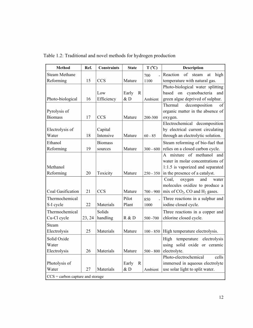
Table 1.2: Traditional and novel methods for hydrogen production……………………..12

Table 2.1: Summary of Ispra recommended thermochemical cycles…………………….16

Table 2.2: Thermochemical cycles proposed for integration with nuclear reactors. Lewis

et al. [30-32]………………………………………………………………………………19

Table 2.3: Proposed variations of the Cu-Cl cycle……………………………………….21

Table 2.4: Processes and reactions in the thermochemical Cu-Cl cycle[44]………………26

Table 3.1: Chemicals used in experiments……………………………………………….65

Table 3.2: Materials used in the vertical reactor………………………………………….67

Table 3.3: Summary of measurement assumptions and uncertainties……………………72

Table 3.4: Enthalpy of formation of compounds in the Cu-Cl Cycle at 298.15 K……….74

Table 3.5: Thermo-physical properties of species………………………………………..75

Table 4.1: Gibbs equilibrium constants for potential decomposition paths……………..101

Table 6.1: Partial pressure of oxygen at equilibrium……………………………………122

Table 7.1: Experimental conditions for the reaction of copper (I) chloride and

oxygen…………………………………………………………………………………...151

Table 7.2: Weight losses measured in TGA experiments……………………………….165

Table 7.3: Deviation of conversion dependent terms with temperature (k1)……………169

Table 7.4: Conversion rates at different temperatures…………………………………..172

xvi

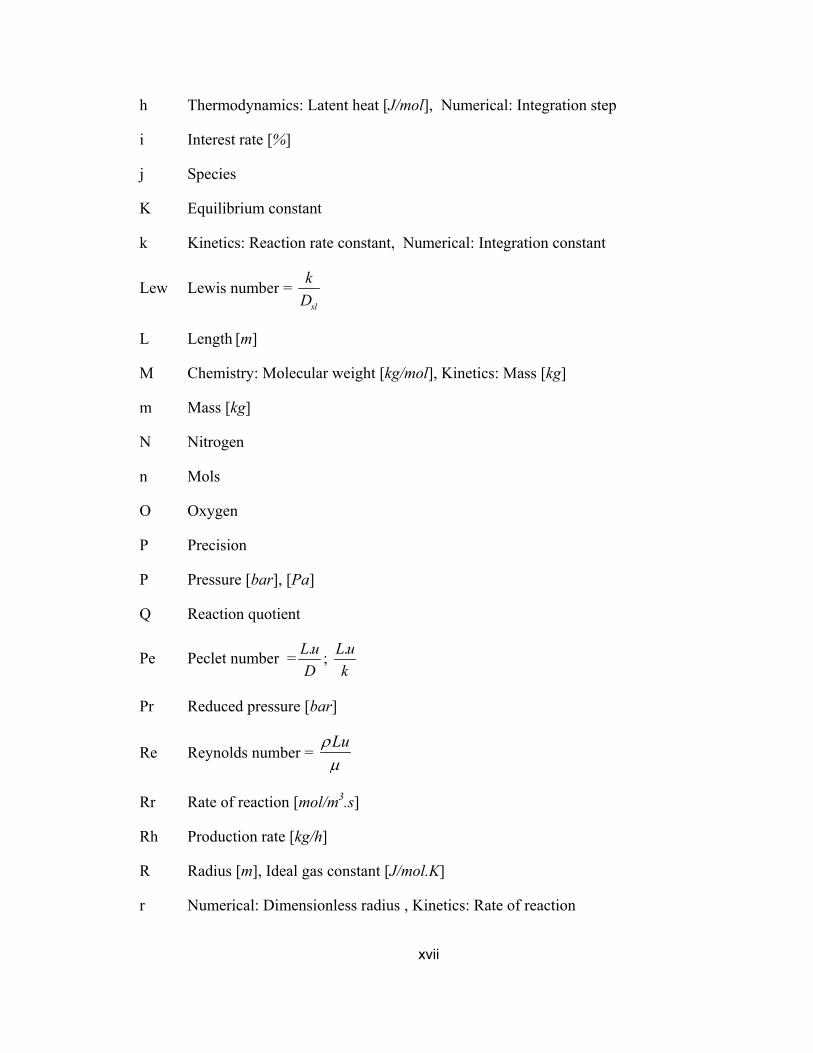
Nomenclature

a Kinetics: Diameter [m], Chemistry: Activity

A Analyzer percent reading

Ac Actual capacity [kg/h]

B Bias

b Constant

C Concentration [mol/m3]

c Constant

Cp Specific heat capacity [J/mol.K]

Ck Capital cost [$]

D Diffusivity [m2/s]

d Distance [m], diameter [m]

Da Damkohler number =.

o

Rr

C

;

122.

o sl

Rr a

C D

Dp Distance from plant [km]

Dy Days of operation [days/year]

E Activation Energy [J/mol.K]

F Force [kg.m/s2], Flow [l/s]

f Thermodynamics: Fugacity , Concentration: Volume fraction

G Gibbs free energy [J/mol]

g Gravity acceleration [m/s2]

H Enthalpy [J/mol]

Hc Capital cost factor [$/kg]

Ht Transportation cost factor [$/kg]

xvii

h Thermodynamics: Latent heat [J/mol], Numerical: Integration step

i Interest rate [%]

j Species

K Equilibrium constant

k Kinetics: Reaction rate constant, Numerical: Integration constant

Lew Lewis number = sl

k

D

L Length [m]

M Chemistry: Molecular weight [kg/mol], Kinetics: Mass [kg]

m Mass [kg]

N Nitrogen

n Mols

O Oxygen

P Precision

P Pressure [bar], [Pa]

Q Reaction quotient

Pe Peclet number =.L u

D;

.L u

k

Pr Reduced pressure [bar]

Re Reynolds number = Lu

Rr Rate of reaction [mol/m3.s]

Rh Production rate [kg/h]

R Radius [m], Ideal gas constant [J/mol.K]

r Numerical: Dimensionless radius , Kinetics: Rate of reaction

xviii

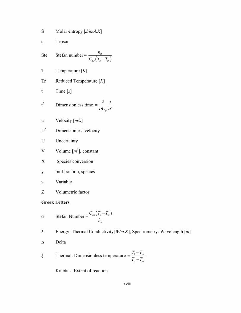
S Molar entropy [J/mol.K]

s Tensor

Ste Stefan number =

sl

ps o m

h

C T T

T Temperature [K]

Tr Reduced Temperature [K]

t Time [s]

t* Dimensionless time

2p

t

C a

u Velocity [m/s]

U* Dimensionless velocity

U Uncertainty

V Volume [m3], constant

X Species conversion

y mol fraction, species

z Variable

Z Volumetric factor

Greek Letters

α Stefan Number = ps o m

sl

C T T

h

λ Energy: Thermal Conductivity[W/m.K], Spectrometry: Wavelength [m]

∆ Delta

Thermal: Dimensionless temperature l m

o m

T T

T T

Kinetics: Extent of reaction

xix

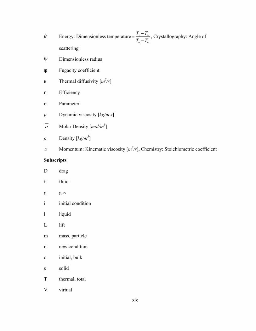
Energy: Dimensionless temperature s m

o m

T T

T T

, Crystallography: Angle of

scattering

Ψ Dimensionless radius

φ Fugacity coefficient

к Thermal diffusivity [m2/s]

η Efficiency

σ Parameter

Dynamic viscosity [kg/m.s]

Molar Density [mol/m3]

ρ Density [kg/m3]

Momentum: Kinematic viscosity [m2/s], Chemistry: Stoichiometric coefficient

Subscripts

D drag

f fluid

g gas

i initial condition

l liquid

L lift

m mass, particle

n new condition

o initial, bulk

s solid

T thermal, total

V virtual

xx

Abbreviations

ANL Argon National Laboratories USA

CFD Computational Fluid Dynamics

CANDU Canadian Deuterium Uranium

ICE Internal Combustion Engine

IEA International Energy Agency

NOx Nitrogen Oxide

NHI National Hydrogen Initiative USA

NIST National Institute of Standards and Technology USA

PEM Proton Exchange Membrane

RKF Runge-Kuttta-Fehlberg

SCWR Supercritical Water Reactor

XRD X-ray Diffraction

Chapter 1 – Introduction ________________________________________________________________________

This thesis provides new contributions to the state of the art of the thermochemical Cu-Cl

cycle for hydrogen production. The experiments and theoretical models complement

previous proof of concept experiments and add to the existing understanding of key

aspects of the cycle. The results will help move forward the effort to implement a scale-up

version of the Cu-Cl cycle for hydrogen production.

1.1 Background

The history of hydrogen analysis starts when it was first recognized as a distinct element

in 1766 by the British scientist Henry Cavendish (as cited in Nyserda [1]) by reacting zinc

metal with hydrogen chloride. Then in 1800, English scientist William Nicholson and Sir

Antony Carlisle discovered that applying electric current to water produced hydrogen and

oxygen gases through a process known as electrolysis. Opposite to the electrolytic cell, a

galvanic cell, known today as the fuel cell, combines hydrogen and oxygen gases to

produce water and electricity. The galvanic effect was first discovered in 1845 by Swiss

chemist Christian Friedrich Schoenbein. This discovery inspired Jules Verne in 1874 who

prophetically examined the potential use of hydrogen in his fiction book entitled “The

Mysterious Island” and pronounced: “I believe that water will one day be employed as

fuel, that hydrogen and oxygen which constitute it, used singly or together, will furnish an

inexhaustible source of heat and light, of an intensity of which coal is not capable”.

These meaningful events occur parallel to the need of humanity for energy sources

and carriers that contain less carbon at each stage of civilization. Wood, coal, oil, and

natural gas have preceded the growing quest for energy from cleaner sources, where

2

hydrogen can have an important role of carrying it to where it is needed and from

sustainable, clean sources. To be considered clean, hydrogen must be produced from non-

carbon primary energy sources such as nuclear, hydro, wind, solar, geothermal, wave and

tidal, and to some extent biomass. Thus, since hydrogen can be produced from clean

sources, the role of hydrogen has been widely accepted as important for a sustainable

energy future. Therefore, the strategies for implementation of a hydrogen based economy

that competes with the established fossil-fuel economy are tightly connected to the

development of renewable energy.

The role of renewable energy and its introduction into the fossil fuel based energy

system has been actively researched and debated in the political, scientific and economic

areas. Furthermore, there has been some action from governments to promote renewables

in response to scientific concerns of global warming, commercial interest for new

business opportunities justified by high prices of fossil fuels, and technological challenges

associated to the development of renewable energies. A more pragmatic approach

recognizes that the economic participation of clean energy technologies in the bulk of the

economic activity that derives from the energy business is still incipient, that fossil fuels

overwhelmingly dominate the market, and that this situation will prevail for the years to

come. Analysis of historical data published by BP Statistical Review in June 2011 [2] and

projections from BP Energy Outlook 2030 [3] and the International Energy Agency [4] on

world energy consumption indicated that the participation of renewables in 2010 was 1.3

% with hydro at 6.5 %, and that by 2030 the participation will grow to 4.8 and 7.0%

respectively.

3

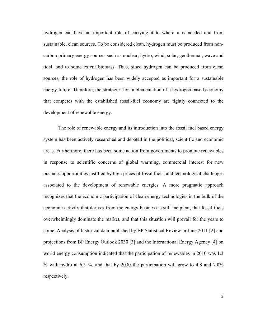
Figure 1.1 indicates the participation of all forms of energy in the global spectrum

of consumption to 2030. In the figure, the total energy consumption is normalized to the

levels of 2030. Even though the growth of renewable energy has been almost exponential

during the last 10 years, its participation in the global energy supply is still low, on the

order of 1%. The relatively increasing numbers are stimulated by high prices and the

implementation of efficiency measures that reduce the rate of consumption of fossil fuels

and coal, thus making the proportion of renewables more significant.

Fig. 1.1: World energy consumption projected to 2030 [3]

The growth in participation of renewable energy does not necessarily indicate that

the hydrogen economy is moving ahead. Renewable sources are being used directly for

the generation and utilization of electricity, or in the case of liquid fuels from renewable

sources such as biomass or some biofuels, directly injected in burners for industrial

application. This leads to an ease of transportation of energy. It is easier to transfer the

energy from the source as electricity or as liquid than it is in any form of hydrogen.

4

Furthermore, the immediate utilization of the forms of renewable energy makes it

unnecessary for the hydrogen transformation, a transition that contrasts with the versatility

of fossil fuels that can be easily stored and transported. To compete with this unique

characteristic, a replacement fuel must provide similar characteristics or be supported by

the appropriate infrastructure.

Electricity is relatively easy to transport but hard to store, thus it must be used

when it is produced. The ideal energy carrier is easy to transport and easy to store.

Hydrogen has been recognized as an energy carrier for over a century now, however, its

main utilization today is for the refinement and upgrading of fossil fuels as a fundamental

component of the liquid fuels where natural gas has been the main feedstock for its

production. More than 96% of the hydrogen produced in the world today results from

transformation of natural gas and light hydrocarbons as indicated by Ball and Wietschel

[5] and the Gas Encyclopaedia [6], a process that also produces significant amounts of

greenhouse gas.

Hydrogen was used in the 1860s and mixed with carbon monoxide, methanol and

other hydrocarbons to produce town-gas for street lighting as well as for cooking and

heating. Hydrogen offers a number of advantages in synergy with the need for sustainable

growth in balance with nature if it is produced from clean and renewable sources. The

utilization of hydrogen is also an emission free process that results in the production of

water at the point of use. Except for electricity, hydrogen is the only energy carrier that

can be produced from any local primary energy source. Produced in parallel with the

generation of electricity from renewable resources, hydrogen can be used to smooth out

5

the intermittent and unpredictable nature of those primary energy sources and store energy

for use when it is most needed. Unlike other electric energy storage systems, stored

hydrogen does not vanish and the storage systems do not lose retention capability with

time and/or temperature. Thus, hydrogen is a secondary energy carrier in the sense that it

needs to be produced from a primary energy source, like electricity. It offers the unique

possibility of being produced and consumed without polluting the environment, but the

challenges of producing, storing and transporting hydrogen are also unique due to its

differentiating physical properties.

1.1.1 Hydrogen as an Energy Carrier

Hydrogen is second only to uranium in gravimetric energy density and at least 2.5

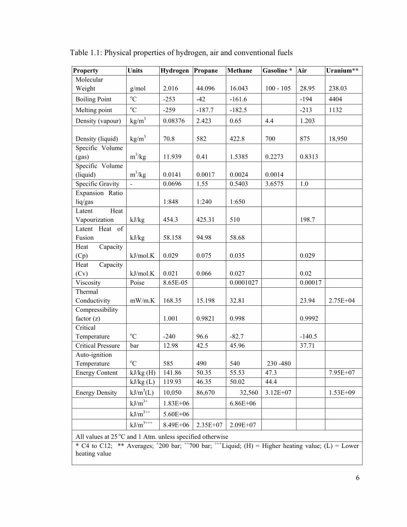
times larger than gasoline and about three times larger than methanol. Table 1.1 details

the physical characteristics of hydrogen and compares it with air and fuels of common

use. In addition to being produced from clean renewable energy, hydrogen is attractive for

its high energy content (Higher Heating Value).

Hydrogen contains the highest energy to weight ratio, thereby making it the

preferable fuel for space exploration where weight has critical importance. Unfortunately,

its volumetric energy density is the lowest at atmospheric conditions and must be

liquefied, reaching up to 8.5 x106 kJ/L while consuming about 30% of the energy

contained in the hydrogen. The low energy density of hydrogen at atmospheric conditions

implies that additional energy must be used to compress or liquefy the gas to increase its

volumetric energy density before it can be used in applications similar to those of

conventional fuels.

6

Table 1.1: Physical properties of hydrogen, air and conventional fuels

Property Units Hydrogen Propane Methane Gasoline * Air Uranium** Molecular Weight g/mol 2.016 44.096 16.043 100 - 105 28.95 238.03

Boiling Point oC -253 -42 -161.6 -194 4404

Melting point oC -259 -187.7 -182.5 -213 1132

Density (vapour) kg/m3 0.08376 2.423 0.65 4.4 1.203

Density (liquid) kg/m3 70.8 582 422.8 700 875 18,950

Specific Volume (gas) m3/kg 11.939 0.41 1.5385 0.2273 0.8313 Specific Volume (liquid) m3/kg 0.0141 0.0017 0.0024 0.0014 Specific Gravity - 0.0696 1.55 0.5403 3.6575 1.0 Expansion Ratio liq/gas 1:848 1:240 1:650 Latent Heat Vapourization kJ/kg 454.3 425.31 510 198.7 Latent Heat of Fusion kJ/kg 58.158 94.98 58.68 Heat Capacity (Cp) kJ/mol.K 0.029 0.075 0.035 0.029 Heat Capacity (Cv) kJ/mol.K 0.021 0.066 0.027 0.02 Viscosity Poise 8.65E-05 0.0001027 0.00017 Thermal Conductivity mW/m.K 168.35 15.198 32.81 23.94 2.75E+04 Compressibility factor (z) 1.001 0.9821 0.998 0.9992 Critical Temperature oC -240 96.6 -82.7 -140.5 Critical Pressure bar 12.98 42.5 45.96 37.71 Auto-ignition Temperature oC 585 490 540 230 -480 Energy Content kJ/kg (H) 141.86 50.35 55.53 47.3 7.95E+07 kJ/kg (L) 119.93 46.35 50.02 44.4

Energy Density kJ/m3(L) 10,050 86,670 32,560 3.12E+07 1.53E+09

kJ/m3+ 1.83E+06 6.86E+06

kJ/m3++ 5.60E+06

kJ/m3+++ 8.49E+06 2.35E+07 2.09E+07

All values at 25 oC and 1 Atm. unless specified otherwise * C4 to C12; ** Averages; +200 bar; ++700 bar; +++Liquid; (H) = Higher heating value; (L) = Lower heating value

7

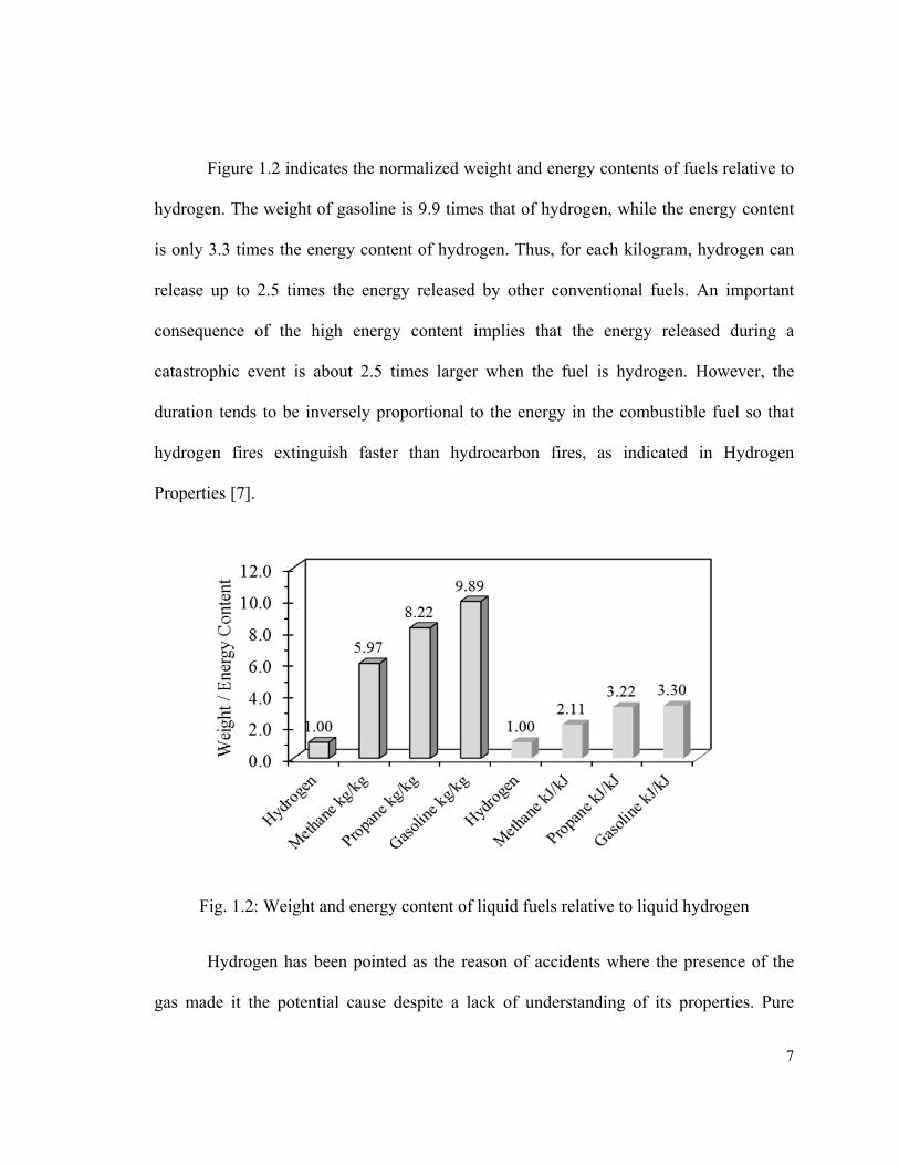
Figure 1.2 indicates the normalized weight and energy contents of fuels relative to

hydrogen. The weight of gasoline is 9.9 times that of hydrogen, while the energy content

is only 3.3 times the energy content of hydrogen. Thus, for each kilogram, hydrogen can

release up to 2.5 times the energy released by other conventional fuels. An important

consequence of the high energy content implies that the energy released during a

catastrophic event is about 2.5 times larger when the fuel is hydrogen. However, the

duration tends to be inversely proportional to the energy in the combustible fuel so that

hydrogen fires extinguish faster than hydrocarbon fires, as indicated in Hydrogen

Properties [7].

Fig. 1.2: Weight and energy content of liquid fuels relative to liquid hydrogen

Hydrogen has been pointed as the reason of accidents where the presence of the

gas made it the potential cause despite a lack of understanding of its properties. Pure

8

hydrogen is odourless, colorless and tasteless making it almost undetectable from leaks in

daylight. Like any other gas, hydrogen may produce asphyxiation by displacing oxygen to

concentration levels that possess risk for human breathing. Levels of oxygen below 19.5%

result in asphyxiation, and concentrations below 12% produce unconsciousness without

prior warning symptoms. However, hydrogen is approximately 14 times lighter than

atmospheric air, such that when leaks occur, hydrogen rises rapidly and it moves away

from the leaking zone.

Fig. 1.3: Concentration range of flammability of hydrogen and conventional fuels in

standard air at 25 oC and 1Atm.

Methane is approximately 2 times lighter than air, thus it does not move away as

fast, and gasoline and propane are several times heavier than air and will follow the shape

of the terrain and form pools upon leaking. Hydrogen remains flammable in air at

concentrations between the limits of 4% and 75%, and it is explosive in the range of 15 to

59%. Methane is flammable in the range of 5.3 to 15% and gasoline in the range of 1.0 to

7.6%. The relative ranges of flammability are indicated in Fig. 1.3. However, in the

9

absence of sparks or sources of ignition, hydrogen in the range of flammability

concentrations does not initiate self-sustained combustion before reaching a temperature

of 585 oC, while methane will self-ignite at 540 and gasoline at 240 oC when in the

flammability concentrations. Although hydrogen has a higher auto-ignition temperature, it

requires very low ignition energy of 0.02 mJ, about one order of magnitude lower than

methane or gasoline.

Because of the high energy content, hydrogen is very attractive to the

transportation industry especially with fuel cells. Fuel cells, namely the Proton Exchange

Membrane (PEM) fuel cell operate at efficiencies as high as 60% as indicated by Mert et

al. [8]. They have been proposed as a substitute for the internal combustion engine (ICE)

in automobiles. On the other hand, the automotive industry has been developing the ICE

for the last 100 years. The ICE operates on the principle of the Otto cycle, which

engineers have endeavoured to improve by challenging the thermodynamic limits. High

temperature limits of materials, concerns about formation and emission of nitrogen oxides

(NOx) and auto-ignition issues impose additional limits.

The overall efficiency of the Otto cycle is in the range of 25% to a maximum of

32% when using anhydrous alcohol fuels as indicated in Economy and Energy [9]. Thus it

indicates that a vehicle using a PEM fuel cell requires approximately half the weight of

fuel to perform the same amount of work when using hydrogen. However, the volume of

this mass of hydrogen is substantially larger than gasoline. The automotive fuel cells have

progressed significantly in recent years, but technical developments are still necessary to

achieve the performance and cost goals necessary to compete with the ICE. A study by

10

Hooks and Jackson [10] on analysis of the challenges for implementation of fuel cell

vehicles and fuelling stations in California indicated that the primary improvements

include simultaneously increasing the power density of the membrane-electrode

assemblies (MEAs) to reduce the overall size of the fuel cell stack, reducing the catalyst

loading and associated cost, increasing the operating life, and expanding the operational

temperature range of the cell.

Frenette and Forthoffer [11] reported the result of experiences with a fleet of fuel

cell vehicles by Ford Company over more than one million miles or 30,000 hours in

different environments. Several aspects of the experience and technology issues were

discussed. Among them, storage of hydrogen on-board remains an issue. The study

concluded that major technological improvements are needed for on-board hydrogen

storage to enable a travel range equivalent to conventional combustion engines.

With today’s state of the art technology, the required volume of a gaseous

hydrogen tank to contain the equivalent energy of a conventional gasoline tank varies

depending on storage pressure. For the same vehicle range, the volume of a hydrogen tank

at 10,000 psi (700 bar) would be nearly 5 times larger than a conventional gasoline tank;

while at 5,000 psi (350 bar) the volume would be approximately 7.5 times larger than a

conventional tank. No near-term solution for improved storage has been identified to

provide a competitive operating range without compromising existing vehicle platforms.

Thus, significant technology challenges exist for the deployment of fuel cell vehicles from

the perspective of the vehicle platform itself. Additional challenges exist for the

development of the appropriate infrastructure to support hydrogen fuelling of vehicles. In

11

general, a hydrogen infrastructure will arise naturally as long as the cost of hydrogen is

competitive in the fuels market.

A different scenario for the deployment of hydrogen is present when stationary

applications are considered. Hydrogen produced from renewable resources can be utilized

directly in many stationary applications where weight and space are not a significant

constraint. Hydrogen generation plants working in tandem with nuclear plants, solar

plants, geothermal or wind can be used to produce clean hydrogen and smooth the peaks

and valleys of power generation by storing energy in the form of hydrogen and generating

power when it is needed and price competitive. Several methods of clean hydrogen

production exist today, differentiated by the source of primary energy, level of maturity of

the technology, and overall efficiency.

About 96% of today’s hydrogen is produced from fossil fuels and the remaining

portion is produced via electrolysis or a sub-product of chloralkaly plants. Technologies

using fossil fuels have been proposed as a means of producing clean hydrogen based on

the assumption of integrated Carbon Capture and Storage (CCS), such that power plants

operate on hydrogen rich fuels following a CO2 separation process, as indicated in the

International Energy Agency Task 16 [12]. Thus, the concept of clean hydrogen is subject

to the premise of capturing and storing CO2, a concept frequently questioned because of

the probability of stored CO2 leaking back to the atmosphere.

1.1.2 Hydrogen from Thermochemical Cycles

Thermochemical cycles have been identified as a potential technology to compete

with the traditional and mature electrolysis technology for hydrogen generation.

12

Table 1.2: Traditional and novel methods for hydrogen production

Method Ref. Constraints State T (oC) Description

Steam Methane Reforming 15 CCS Mature

700 - 1100

Reaction of steam at high temperature with natural gas.

Photo-biological 16 Low Efficiency

Early R & D Ambient

Photo-biological water splitting based on cyanobacteria and green algae deprived of sulphur.

Pyrolysis of Biomass 17 CCS Mature 200-300

Thermal decomposition of organic matter in the absence of oxygen.

Electrolysis of Water 18

Capital Intensive Mature 60 - 85

Electrochemical decomposition by electrical current circulating through an electrolytic solution.

Ethanol Reforming 19

Biomass sources Mature 300 - 600

Steam reforming of bio-fuel that relies on a closed carbon cycle.

Methanol Reforming 20 Toxicity Mature 250 - 350

A mixture of methanol and water in molar concentrations of 1:1.5 is vaporized and separated in the presence of a catalyst.

Coal Gasification 21 CCS Mature 700 - 900

Coal, oxygen and water molecules oxidize to produce a mix of CO2, CO and H2 gases.

Thermochemical S-I cycle 22 Materials

Pilot Plant

850 - 1000

Three reactions in a sulphur and iodine closed cycle.

Thermochemical Cu-Cl cycle 23, 24

Solids handling R & D 500 -700

Three reactions in a copper and chlorine closed cycle.

Steam Electrolysis 25 Materials Mature 100 - 850 High temperature electrolysis.

Solid Oxide Water Electrolysis 26 Materials Mature 500 - 800

High temperature electrolysis using solid oxide or ceramic electrolyte.

Photolysis of Water 27 Materials

Early R & D Ambient

Photo-electrochemical cells immersed in aqueous electrolyte use solar light to split water.

CCS = carbon capture and storage

13

Several technologies for the generation of clean hydrogen have been proposed and

presented and are found at different stages of development as indicated in Table 1.2. The

Thermochemical Cu-Cl cycles have been proposed for integration with any of the

Generation IV nuclear reactors currently under consideration as discussed by M.A. Rosen

[13] and Elder and Allen [14].

The cycles are based on chemical reactions using familiar concepts of chemistry

and chemical engineering and supported, in most cases, by technologically mature

physical processes. Proof of concept experimental work and analysis has been

implemented in several cycles as indicated in Table 1.2 [15 – 27], from which the Sulfur-

Iodine (S-I) and Copper-Chlorine (Cu-Cl) cycles are at the most advanced phase of

development.

The possibility of integrating hydrogen production with nuclear power generation

has been discussed for a long time and thermochemical cycles are an attractive option

because of high thermodynamic efficiency, as discussed by Naterer et al. [23]. The Cu-Cl

cycle operates at a maximum temperature of 550 oC and separates water through three

reactions complemented by several physical steps that use mature, commercial technology

as discussed by Wang et al. [24].

The lower temperature and less corrosive species in the Cu-Cl cycle, when

compared to the Sulphur-Iodine cycle at 850 oC, facilitate the design of heat exchangers

and reactors with potentially fewer material corrosion challenges.

The Cu-Cl cycle is the subject of this thesis specifically with detailed experimental

work on the chemical decomposition reaction. This thesis provides new understanding

14

that allows the safe design of a reactor for integration with the hydrolysis and electrolysis

reactions in the Cu-Cl cycle.

1.2 Motivation and Objectives of Thesis

This thesis focuses on selected key questions that must be answered for the

effective design of a reactor used in the decomposition of CuO*CuCl2. In particular, the

main hypothesis to be tested is that the yield from samples of CuO*CuCl2 undergoing

thermal decomposition is impacted by the concentration of solids in the molten CuCl and

the difference of temperatures between the solid and the molten bath. For a given

temperature, the rate of solids fed to the reactor must be maintained below a critical

concentration. This hypothesis will be examined in detail in this thesis.

The main objective of this research is to develop and validate new predictive

models and experimental methods of transport phenomena of the physical processes of

decomposition in the copper oxychloride reactor, as follows.

1. Assemble relevant mass, momentum and energy equations and develop

mathematical models for the analysis of the convection and diffusion

phenomena for a solid particle submerged in molten salt, and with chemical

decomposition occurring in a transition layer at the particle surface.

2. Develop new semi-analytical solutions to the mathematical models and

implement numerical solutions via a computer simulation method for design

purposes.

3. Analyze and validate the predictions of theoretical models using experimental

results of the chemical decomposition.

15

4. Determine concentration vs. time correlations and develop a reaction rate

equation. Recommend implications on the scale-up of the thermochemical Cu-

Cl cycle.

16

Chapter 2 - Literature Review ________________________________________________________________________

2.1 Thermochemical Cycles

Thermochemical cycles have been proposed as an alternative and potentially

more efficient method to produce hydrogen from water. The International Round Table on

Direct Production of Hydrogen with Nuclear Heat held in Ispra, Italy in 1969 set the

criteria for evaluation of thermochemical cycles as discussed by Beghi [28].

Table 2.1: Summary of Ispra recommended thermochemical cycles

Mark Chemicals Temperature (oC) No. of reactions Mark 1 Hg, Ca, Br 780 4 Mark 1B Hg, Ca, Br 780 5 Mark 1C Cu, Ca, Br 770 4 Mark 1S Hg, Sr, Br 770 3 Mark 2 Mn, Na, (K) 770 3 Mark 2C Mn, Na, (K), C 750 4 Mark 3 V, Cl, O 800 4 Mark 4 Fe, Cl, S 800 4 Mark 5 Hg, Ca, Br, C 850 5 Mark 6 Cr, Cl, Fe, (V) 800 4 Mark 6C Cr, Cl, Fe, (V) Cu 800 5 Mark 7 Fe, Cl 800 5 Mark 7A Fe, Cl 800 5 Mark 7B Fe, Cl 850 5 Mark 8 Mn, Cl 850 3 Mark 9 Fe, Cl 650 3 Mark 10 I, S, N 850 6 Mark 11 S (hybrid) 850 2 Mark 12 I, S, N, Zn 850 4 Mark 13 Br, S (hybrid) 850 3 Mark 14 Fe,Cl 650 5 Mark 15 Fe, Cl 730 4 Mark 16 S, I 850 3 Mark 17 Sulfur-Iodine 850 3

17

A list of proposed cycles then emerged as indicated in Table 2.1 (Mark 1 to 17)

and a three stages process of evaluation was initiated. Thermochemical decomposition of

water for hydrogen production was transformed from theoretical concept to a promising

reality. Since then, over 350 potential cycles have been identified. At the end of the 1990s,

Brown et al. [29], a group of researchers working under the Nuclear Energy Research

Initiative (NERI) Program of the U.S. Department of Energy, applied screening criteria to

over 115 cycles. They scored the cycles based on the number of chemical reactions,

number of separation steps, maximum temperature and number of published references,

among others, to arrive at 40 cycles.

A second screening with consideration for environmental, safety and health

aspects reduced the number to 25 cycles. More recently the Nuclear Hydrogen Initiative

(NHI) of the U.S. Department of Energy, Office of Nuclear Energy Science and

Technology supported the re-evaluation of thermochemical cycles in the literature having

both promising efficiencies and proof-of-concept. The NHI program is connected to the

Next Generation Nuclear Plant (Gen IV) program to develop a reactor capable of

providing high-temperature process heat. Because high-temperature processes that use

high temperature heat achieve higher efficiency, R&D has been focused on

thermochemical cycles, hybrid thermochemical cycles, and high-temperature electrolysis.

The focus of the NHI initiative was to identify and develop nuclear technologies

that produce hydrogen from water feedstock at prices that are competitive with other fuels

and using domestic process materials by 2019. Lewis et al. [30-32], working under the

NHI program, and with focus on the first two categories of high-temperature processes,

18

applied new screening criteria to recently published literature on thermochemical cycles in

Table 2.2. The program had an objective to determine cycles that justify additional

research and complement the NHI portfolio of hydrogen technologies that can operate

with nuclear reactors. The maximum temperature of the cycle determines the type of heat

source required. This parameter was used as part of the criteria for selection, with the

baseline Sulfur-Iodine cycles setting the limit at 825-850 oC.

The Sulfur-Iodine cycle consists of three reactions. It has been developed

extensively with the design and construction of a lab scale cycle to investigate the

potential of using nuclear energy. Analysis and experiments performed at the Sandia

National Lab with participation of General Atomics between 2002 and 2008 and

discussed by Russ and Pickard [33] found many challenges associated with complex

multiphase reaction equilibrium, high temperatures, strong acids and materials

requirements. The experimental work has not yet conclusively answered questions on

preferable technologies, sources of energy and disposal of products of side reactions as

reported by Russ and Pickard [33].

The study by Lewis et al. [30-32] recommended the Cu-Cl cycle for additional

research and discarded the others based on criteria of low yield equilibrium due to

competing product formation, requirements to develop new technologies to improve

yields in reverse reactions, high maximum temperatures, difficult separation of gas, solid

or liquid phases, slow kinetics, proof of concept experimental work, and missing data,

among others.

19

Table 2.2: Thermochemical cycles proposed for integration with nuclear reactors. Lewis

et al. [30-32]

Cycle # Reactions T (oC)

Hybrid Chlorine 1

Cl2(g) + H2O(g) 2HCl(g) +0.5O2(g) 850

2HCl(g) H2(g) +Cl2(g) (electrolytic) 75

Magnesium-Iodine 2

6/5MgO(s) + 6/5I2(l)1/5Mg(IO3)2(s) +MgI2(a) 120

1/5Mg(IO3)2(s)1/5MgO(s) + 1/5I2(g) + 1/2O2(g) 600

MgI2.6H2O(s)5MgO(s) + 5H2O(g) + 2HI(g) 450

2HI(g)I2(g) + H2(g) 500

Copper-Sulphate 3

2H2O(l) + SO2(g)H2SO4(a) + H2(g) (electrolytic) 25

CuO(s) + H2SO4(a) + xH2OCuSO4 .(x-1)H2O(s,a) 25

CuSO4.(x -1)H2OCuSO4 + 4H2O 525

CuSO4(s)CuO(s)+SO2(g)+0.5O2(g) 825

Iron-Chlorine 4

3FeCl2(s) + 4H2O(g)Fe3O4(s) + 6HCl(g) + H2(g) 925

Fe3O4(s) + 8HCl(g) FeCl2 + 2FeCl3 +4H2O(g) 125

2FeCl3(s)2FeCl2(s) + Cl2(g) 425

Cl2 +H2O(g) 2HCl(g) + 0.5O2(g) 925

Vanadium-Chloride 5

2VCl2(s) + 2HCl(a)VCl3(s) + H2(g) 120

4VCl3(s) 2VCl4(g) + 2VCl2(s) 766

2VCl4(l)2VCl3 + Cl2 (g) 200

Cl2(g) +H2O(g) 2HCl(g) +0.5O2(g) 875

Cerium-Chlorine 6

2CeO2(s) + 8HCl(g) 2CeCl3(s) + Cl2(g) 110

2CeCl3(s) + 4H2O(g) 2CeO2(s) + 6HCl(g) 925

Cl2(g) + H2O(g) 2HCl(g) + 0.5O2(g) 850

Copper - Chlorine (Dokiya and Kotera) 7a

2CuCl2 + H2O(g) 2CuCl(l) + 0.5O2(g) + 2HCl(g) 700

2CuCl(a) +2HCl(g) H2(g) + 2 CuCl2(s) (electrolytic) 25

Copper - Chlorine (University of Illinois, Argon National Labs) 7b

4CuCl(a) 2CuCl2(a) + 2Cu(s) (electrolytic) 25

2Cu(s) + 2HCL(g) 2CuCl(l) + H2(g) 425

2CuCl2(s) + H2O(g) Cu2OCl2(s) + 2HCl(g) 425

Cu2OCl2 2CuCl(l) +0.5O2(g) 535

Copper – Chlorine (Argonne National Lab) 7c

2CuCl +2HCl(a) 2CuCl2 + H2(g) (electrolytic) 80

2CuCl2(s) + H2O(g) Cu2OCl2(s) + 2HCl(g) 425

Cu2OCl2 2CuCl(l) +0.5O2(g) 535

Hybrid Calcium-Bromide 8

CaBr2 +H2O(g) CaO + 2HBr(g) 770

2HBr(g) H2(g) +Br2(g) (Plasma) 50

CaO + Br2(g) CaBr2 + 0.5O2(g) 550

20

2.2 Thermochemical Cu-Cl Cycle

The Cu-Cl cycle is characterized by a lower maximum temperature, no catalyst required

for thermal reactions (e.g. low energy of reaction), all reactions already demonstrated at a

laboratory scale, and efficiency and hydrogen costs within DOE’s targets. Naterer et al.

[34] provided a cost comparison for hydrogen produced through electrolysis and the

thermochemical Cu-Cl cycle. The study assumed similar conditions for hydrogen

transportation and electrolysis operation outside peak hours. At 10 tons/day, electrolysis

yields a total hydrogen cost of 2.69 $/kg, while hydrogen produced through a

thermochemical Cu-Cl cycle results in a total cost of 2.71 $/kg. At a larger capacity of

200 ton/day, the thermochemical cycle results in a hydrogen cost of 2.00 $/kg. The

advantage occurs from the intensive capital requirement for electrolysis at higher

capacities. The cost of hydrogen from the thermochemical cycle is consistent with the

goals set by DOE at US 3.80 $/kg (delivered, untaxed) in its Hydrogen Posture Plan [35].

Lower temperatures and mildly aggressive chemicals result in lower technological

and economic challenges. The Cu-Cl cycle, with a thermodynamic limit at 530 oC, has

been proposed as a candidate for integration with a Supercritical Water Reactor (SCWR),

Canada’s generation IV nuclear reactor as discussed by Wang et al. [36].

Further integration with nuclear reactors including traditional water electrolysis

that uses off-peak electricity was discussed by Naterer et al. [37]. Hydrogen can provide

both benefits of carrying and storing energy. It was proposed that the base load of the

reactor can be used in the thermochemical Cu-Cl cycle and that remaining energy is used

to produce electricity for regular consumption. Thus, peaks and valleys of electric power

21

consumption can be smoothed out through the generation of electrolytic hydrogen. This

concept takes advantage of the fast response capability of electrolytic hydrogen plants.

Furthermore, the relatively low temperatures of operation of the Cu-Cl cycle open the

possibility to obtain heat from other sources such as surplus heat from industrial

processes, solar energy, geothermal or upgraded heat from other clean thermal sources.

Table 2.3: Proposed variations of the Cu-Cl cycle

Variations of the thermochemical Cu-Cl cycle as indicated in Table 2.3 have been

proposed and discussed in the literature. It is important to clarify that the past literature

No. Ref. Type T oC Reactants Products∆H

(kJ/mol)

1 Wang et al. C, x 450 2Cu (s) + 2HCl (g) 2CuCl (m) + H2 (g) N/A

[36] E 80 4CuCl (aq) + 2Cu (s) 2CuCl2 (aq) N/A

Dr, e 150 CuCl2 (aq) + 2H2O (l) CuCl2*H2(s) + H2O (g) 165.2*

H, e 375 2CuCl2*H2O (s) + H2O (g) CuO*CuC(s) + 2H2O (g) + 2HCl (g) N/A

D, e 530 CuO*CuCl2 (s) 2CuCl (m) + 0.5O2 (g) 129.3*

2 Wang et al. C, x 450 2Cu (s) + 2HCl (g) 2CuCl (m) + H2 (g) -1.7*

[36] E 80 4 CuCl (aq) 2Cu (s) + 2CuCl2 (aq) 96.2*

H, e 375 2CuCl2 (aq) + H2O (g) CuO*CuC(s) + H2O (g) + 2HCl (g) N/A

D, e 530 CuO*CuCl2 (s) 2CuCl (m) + 0.5O2 (g) 129.3*

3 Wang et al. C, x 450 2Cu (s) + 2HCl (g) 2CuCl (aq) + H2 (g) -1.7*

[36] E 80 4CuCl (aq) 2Cu (s) + 2CuCl2 (aq) 96.2*

D, e 600 CuCl2 (aq) + H2O (g) 2CuCl (m) + H2O (g) + 2HCl (g) + 0.5O2(g) N/A

4 Dokiya H, e 700 2CuCl2 (s) + H2O (g) 2CuCl (m) + 2HCl (g) + 0.5O2(g) 148**

[38] E 25 2CuCL (aq) 2CuCl2 (s) + 2HCl (g) + H2 (g) 75**

5 Carty et al. E 80 4CuCl (aq) 2Cu (s) + 2CuCl2 (aq) + 2HCl (g) 96.2*

[40] C, x 425 2Cu (s) + 2CuCl (m) H2 (g) -1.7*

UI/ANL H, e 425 2CuCl2 (s) + H2O (g) Cu2OCl2 (s) + 2HCl (g) N/A

D, e 535 Cu2OCl2 (s) + 2CuCl (m) + 0.5O2 (g) 129.3*

6 Lewis et al. E 80 2CuCl (aq) + 2HCL (aq) 2CuCl2 (aq) + H2 (g) 93.7*

[32] H, e 425 2CuCL2 (s) + H2O (g) Cu2OCl2 (s) + 2HCL (g) 116.7*

ANL/UOIT D,e 535 Cu2OCl2 (s) 2CuCl (m) + 0.5O2 (g) 129.3*

R = Reagent; P = Product; m = molten; aq = aqueous; l = liquid; s = solid; g = gasE = Electrolysis; H = Hydrolysis; C = Chlorination; D = Decomposition; Dr = Drying; e = endothermic; x = exothermic* Lewis et al. [32]

22

refers to steps and reactions in a mixed manner that does not differentiate physical from

chemical process.

The analysis presented here differentiates the physical (step) that affects the form

but not the chemical composition from the chemical (reaction) where the transformation

of species occurs. Table 2.3 presents a summary of six versions of the Cu-Cl cycle that

include cycles of five, four, three and two cyclic reactions and steps as presented by Wang

et al. [38]; Naterer et al. [39]; Dokiya and Kotera [40] and Lewis et al. [31].

The four reactions cycle, No. 1, discussed by Wang et al. [38] and Naterer et al.

[39] starts with solid copper reacted exothermically in a chlorination reaction with

hydrogen chloride at 450 oC to produce hydrogen gas and molten CuCl. The temperature

differential with the subsequent electrolysis reaction opens the possibility for significant

heat recovery within the cycle. Experimental work to recover heat from molten CuCl is

currently under investigation at UOIT. The second reaction of this proposed cycle uses the

electrolytic oxy-reduction (also known as dismutation) of CuCl that results in solid copper

and aqueous copper (II) chloride as products. Handling of the mixture of solids and

aqueous products from electrolysis is a major technological challenge. A third step uses a

drying process to produce partially hydrated copper (II) chloride particles and evaporated

water.

Preliminary experimental work reported by Naterer et al. [41] indicated that drying

of CuCl2 is an energy intensive process that impacts the efficiency and cost of the cycle.

The experimental work used a spray dryer to process CuCl2 with a water content of 8.2

and 2.0 mol-water/mol-CuCl2 and obtained particles in the range of 100 to 200 microns.

23

The drying process is challenging because of the large volume of atmospheric air and

energy required. The water splitting reaction occurs in a fluidized bed reactor at 375 oC

where the solid particles in contact with superheated steam produce a solid mixture of

CuO and CuCl2 and a gaseous stream of vapor and hydrogen chloride. Further separation

of the gas streams is required. The last reaction in the cycle results from the

decomposition of CuO*CuCl2 and results in molten CuCl and oxygen gas.

The four-one cycle (No. 2) was replaced with a four-step cycle that combines step

3 and reaction 4. Since reaction four implies hydrolysis of CuCl2, there is no need to

completely dry the products in step 3. Preliminary research and thermodynamic analysis

indicated that hydrolysis requires water in excess of the stoichiometric quantity. However,

this change results in a requirement of a larger quantity of high quality heat for the

combined process. The analysis reported by Wang et al. [38] indicated that the reactor for

the combined chemical reaction must process five times more heat than the reactor for the

chemical reaction of step 4 in the four-one cycle. Combination of step 3 into the chemical

reaction results in more heat requirements. The increased heat load leads to larger

engineering challenges for the reactor design and lower overall efficiency of the Cu–Cl

cycle. This option has not been pursued further beyond this publication.

A three-reaction cycle (No. 3) was also discussed by Wang et al [38]. Starting with

the chlorination of copper and following with the oxy-reduction of CuCl, the cycle closes

with the direct decomposition of CuCl2 at 600 oC. The decomposition reaction results in

the production of vapor, hydrogen chloride and oxygen. The three gases must follow a

separation process, which is energy intensive and results in further challenges and lower

24

overall efficiency of the cycle. The higher temperature requirement separated this option

from possible integration with Canada’s Gen IV Supercritical Water Reactor and hence it

has been set aside.

Dokiya and Kotera [40] proposed a two reaction cycle (No. 4). The first reaction is

the hydrolysis of CuCl2 at 700 oC. They performed proof of concept experiments, and

further development resulted in a division of the hydrolysis reaction into two separate

reactions to facilitate the separation of gases. The challenges of gas separation, reversible

reactions and higher temperature requirements resulted in no further research. The

elevated temperature results in the production of molten CuCl and a mixture of hydrogen

chloride and oxygen gases. The requirement for separation of gases at higher temperatures

resulted in additional engineering challenges and neglected the possibility of integration

with the SCWR as discussed before. Although it is attractive because of its simplicity, this

possibility has not been further investigated.

The University of Illinois at Chicago (UIC) and the Argonne National Lab (ANL)

performed studies intended to demonstrate the feasibility of a four reaction hybrid Cu-Cl

cycle (No. 5). Carty et al. [42] recommended this cycle as one of the most promising

cycles after analyzing thermochemical cycles for hydrogen production based on the

criteria of reactions whose free energy change lies within 10 kcal for a given temperature.

Following the proof of concept experiments and analysis from UIC and ANL, the

cycle was recommended for further R&D, while major challenges were identified for the

development of the copper electrolyzer. In the electrolysis reaction, an aqueous solution

of 10 to11 mol/L of CuCl and water results in the formation of solid copper and CuCl2 in

25

aqueous form. The chlorination of solid copper in contact with hydrogen chloride results

in the release of gaseous hydrogen and molten CuCl. HCl and copper oxychloride are

produced as a result of chemical hydrolysis of CuCl2. Oxygen is then released in the

decomposition reaction that results in the formation of molten CuCl. The proposed four-

step cycle did not provide new venues to the challenges of electrolysis with solid products

and hence it has not been pursued further. Nixon et al. [43] synthetized samples of

Cu2OCl2 by using CuCl or CuCl2 in contact with air between 325 and 400 oC. The

synthesis was followed by further thermogravimetric decomposition at temperatures up to

580 oC. The experiments indicated a two-step reaction mechanism followed by

vaporization of CuCl. Preliminary research and proof of concept experiments of a three

reaction cycle were carried out at the Argonne National Lab and reported by Lewis et al.

[32]. The new proposed cycle (No. 6) in Fig. 2.1 simplifies the process and reduces the

capital cost while operating at a lower efficiency.

Fig. 2.1: Flow diagram of the three reaction thermochemical Cu-Cl cycle [44]

26

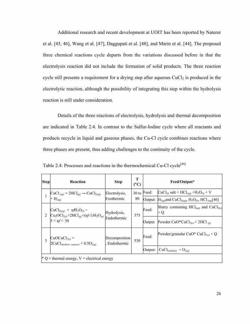
Additional research and recent development at UOIT has been reported by Naterer

et al. [45, 46], Wang et al. [47], Daggupati et al. [48], and Marin et al. [44]. The proposed

three chemical reactions cycle departs from the variations discussed before in that the

electrolysis reaction did not include the formation of solid products. The three reaction

cycle still presents a requirement for a drying step after aqueous CuCl2 is produced in the

electrolytic reaction, although the possibility of integrating this step within the hydrolysis

reaction is still under consideration.

Details of the three reactions of electrolysis, hydrolysis and thermal decomposition

are indicated in Table 2.4. In contrast to the Sulfur-Iodine cycle where all reactants and

products recycle in liquid and gaseous phases, the Cu-Cl cycle combines reactions where

three phases are present, thus adding challenges to the continuity of the cycle.

Table 2.4: Processes and reactions in the thermochemical Cu-Cl cycle[44]

Step Reaction Step T

(C)Feed/Output*

1 CuCl (aq) + 2HCl(g) → CuCl2(aq) + H2(g)

Electrolysis, Exothermic

30 to 80

Feed: CuCl(l) salt + HCl(aq) +H2O(l) + V

Output: H2(g)and CuCl2(aq), H2O(l), HCl (aq)[46]

2 CuCl2(aq) + nfH2O(l) = Cu2OCl2(s)+2HCl(g)+(nf-1)H2O(g)

5 < nf < 30

Hydrolysis, Endothermic

375 Feed:

Slurry containing HCl(aq) and CuCl2(s)

+ Q

Output Powder CuO*CuCl2(s) + 2HCl (g)

3 CuOCuCl2(s) = 2CuCl(molten+vapour) + 0.5O2(g)

Decomposition, Endothermic

530 Feed:

Powder/granular CuO* CuCl2(s) + Q

Output: CuCl(molten) + O2(g)

* Q = thermal energy, V = electrical energy

27

The hydrolysis reaction of the three reaction cycle uses an aqueous solution of

solid CuCl2 to react with steam at temperatures of 370 to 400 oC. This approach requires a

previous step where the aqueous solution is preheated or the water is removed so that it

does not inhibit contact with superheated steam in the hydrolysis reactor. The three

reaction cycle thus requires an additional step where CuCl2 is dried by using low quality

heat and then solid particles are fed into the hydrolysis reactor. Other physical steps may

be required to support the reactions in the cycle including heat recovery, gas separation,

water removal and separation of solids.

2.3 Three Reactions Thermochemical Cu-Cl Cycle

2.3.1 Electrolysis Reaction

The three reaction thermochemical cycle includes an electrolytic reaction at

approximately 80 oC where the products are a solution of aqueous CuCl2, H2O, HCl and

gaseous hydrogen. The design of the electrolyzer is expected to be simpler since a liquid

is split to produce a mixture of gas and liquid, which is a mature technology and the

capital cost is expected to be lower than electrolysis with solid products. Proof of concept

experiments have been completed successfully and the electrolyzer is subject to further

development at AECL (Stolberg et al. [49]) and UOIT where Naterer et al. [41] discussed

recent advances in the electrolysis process. Furthermore, Ranganathan and Easton [50]

performed electrochemical experiments to determine the suitability of materials for use in

the electrolysis step of the cycle. The study characterized Amionsilane-based electrodes

for use as anodes in the electrolyser and concluded that ceramic carbon electrodes (CCE)

are a promising alternative for anode materials with good thermal stability.

28

At the electrolyser, the copper (I) ion is oxidized in the presence of hydrogen

chloride to copper (II) at the anode, while the hydrogen ion is reduced at the cathode. The

majority of copper species is anionic and thus cannot permeate through the cationic

membrane. However, it has been reported that a considerable amount of neutral copper

species exists and permeates through the membrane creating metallic deposits at the

cathode, resulting in significant reduction of hydrogen production.

AECL has demonstrated the experimental operation of a CuCl / HCl electrolyzer

while operating at current density of 0.1 A/cm2 and cell voltages in the range 0.6 to 0.7 V.

Lewis et al. [51] reported results at the Pennsylvania State University of electrolyzer

experiments operating at 80 oC for 36 hours with 0.25 A/cm2 and 0.7 V. The results

indicated hydrogen production in agreement with Faraday’s Law. The goal was to

achieve stable long term performance of the electrolyzer.

DOE proposed a milestone date of 2012 to optimize the electrolyzer design and

reach a target of 0.6-0.7 V at 0.5 A/cm2 while operating a membrane electrode assembly

(MEA) for at least one week. The objectives also specify that copper permeation should

be reduced to 10% of that of Nafion® membranes at 80 oC. The reported experimental

results at AECL, UOIT and Penn State University have provided a lifetime expectation in

agreement with the above goals, with a report on two membranes identified with copper

diffusivity <10% of Nafion® and chemically and thermally stable at 80 oC for over 40

hours.

However, longer duration experiments are required since electrolyzers tend to

suffer slow degradation over time making lifetime projection experiments a critical aspect

29

in the determination of the best technology for this particular application. One particular

challenge for the development will be the determination of the level of impurities that can

be tolerated from the incoming stream of aqueous CuCl/HCl. A typical electrolyzer

operation requires high levels of purification of the species before they enter the MEA,

adding substantial cost and complexity to the operation.

2.3.2 Hydrolysis Reaction

Significant challenges have been identified for the hydrolysis reaction. The

stoichiometric reaction indicates that a half mole of water is required for each mole of

copper (II) chloride to produce one mole of copper oxychloride (Cu2OCl2) and two moles

of hydrogen chloride (HCl). In a detailed kinetics analysis of the hydrolysis reaction,

Daggupati et al. [48, 52] reported the occurrence of parallel competing reactions. In

addition to producing Cu2OCl2, the reaction of CuCl2 and H2O resulted in the production

of CuCl and the release of oxygen and chlorine gas. The theoretical analysis concluded

that high temperature favors higher equilibrium conversions, increased the decomposition

of solid CuCl2 and the formation of free chlorine, a non-desirable condition for efficient

operation of the cycle.

Experimental studies reported by Ferrandon et al. [53] confirmed the theoretical

analysis and the need for water vapor in excess of the reaction stoichiometry.

Experiments with molar ratios of steam to copper (H2O / Cu) above 20 resulted in

conversions up to 92%. Thermodynamic simulations using Aspen Plus® indicated yields

of 95% Cu2OCl2 required the steam to copper molar ratio to be maintained near 17 with

temperatures at 380-390 oC. At a steam to copper ratio of 5, the yield was only 30%. This

30

effect conflicts from an energy utilization perspective with a result that a higher ratio

steam / Cu, yields a larger energy required for vaporization. Thus, there is a compromise

between high yield and low energy consumption. The experiments were conducted with a

carrier gas to remove HCl gas from the reaction zone.

The presence of a carrier gas in the hydrolysis reaction contributes to the removal of

free chlorine and hence the incomplete conversion of CuCl2. In a real situation, there is no

carrier gas that will remove chlorine from the reaction zone and conversion rates should

be higher. However, as the steam to copper ratio was allowed to decrease, more CuCl2

was available for decomposition, resulting in the production of CuCl and release of

chlorine. In past experimental work by Ferrandon et al. [53] the phase composition of

products was determined by powder X-ray diffraction. A quantitative analysis was

performed and indicated the presence of CuCl and un-reacted CuCl2 in the solids. The

amount of Cu2OCl2 was determined based on the oxygen evolution from decomposition

of the solid products in a catalytic reactor. At atmospheric pressure and a molar ratio of

steam to CuCl2 of 10, the reaction yielded 60% Cu2OCl2 and 7% CuCl. Reducing the

reactor pressure to 0.4 bar resulted in a yield of 75% Cu2OCl2 and 4% CuCl, with the

balance of un-reacted CuCl2. The experimental and theoretical studies indicated that the

reaction can be achieved with high yields (of copper oxychloride and hydrochloric acid)

when the molar steam to copper ratio is increased to between 7 and 20.

Daggupati et al. [52, 54] performed a chemical equilibrium analysis of the

hydrolysis reaction to determine the impact of temperature, pressure and excess steam on

the extent of reaction, and confirmed that low pressures result in higher conversion of

31

CuCl2. The thermodynamic analysis indicated that the steam to copper ratio can be

reduced by decreasing the reaction pressure but this implies significant additional energy

to balance the benefit of a reduced steam to copper ratio. The studies also concluded that

the hydrogen chloride production step favours higher temperatures, excess steam and

lower pressures. The study also suggested that the best operating conditions for complete

consumption of chlorine during the hydrolysis reaction and minimization of excess steam

occurs at temperatures of about 400 ◦C. Also, the partial pressure differences between the

copper (II) chloride decomposition and the chlorine reverse reaction should be positive to

facilitate the consumption of free chlorine. Under all circumstances, the presence of free

chlorine needs be averted by a rapid reaction with CuO before it exits the reaction zone

mixed with oxygen product.

Further thermal analyses of mixtures of CuCl and CuCl2 by Biltz and Fisher (cited

by Levy and Goreaud [55]) indicated a melting point of 422ºC for CuCl and 630ºC for

CuCl2. According to the authors, the equilibrium of the reaction CuCl2 ↔ CuCl + ½ Cl2

would lead to saturated vapor at 500ºC of 133 Pa CuCl and 13 Pa CuCl2 in a closed vessel.

If the decomposition reaction is conducted in open atmosphere, a significant amount of

chlorine would be released when above 380 oC. Lewis et al. [56] reported results of

experimental hydrolysis in a fixed bed micro-reactor system. The focus of the

experimental work was to find the parameters that maximize the yield of CuO*CuCl2

while minimizing the formation of CuCl. The hydrolysis reaction reaches equilibrium at

conversion stages that vary depending upon the combination of temperature, steam ratio

and pressure. Despite these advances, it is still not well understood what are the ideal

conditions for hydrolysis to yield high conversion to Cu2OCl2 and minimize side reactions

32

or unreacted products. The past literature indicated that incomplete hydrolysis reactions

are expected at equilibrium with the presence of free chlorine, CuCl2 and CuCl in addition

to Cu2OCl2 in the products.

Removing chlorine gas from the HCl stream in hydrolysis and from oxygen in the

decomposition reactor requires cryogenic processes that are energy intensive. Other

technologies for removal of chlorine from a stream of gases have been reported in the

literature. Lindbråthen et al. [57] examined low cost Polydimethylsiloxane (PDMS)

membranes for the recovery of chlorine gas from gas streams in chloralkaly plants. The

theoretical modeling of three different membrane materials including PDMS, surface

modified glass and glass hollow fiber concluded that more research is required before

membranes can economically substitute cryogenic processes for separation of chlorine

from tail gas.

By-products of the hydrolysis reaction impact the operation further ahead within the

cycle. The presence of chlorine with HCl gases may impact the operation of the

electrolyzer. Free chlorine in the aqueous solution of CuCl may be a problem for the

electrolytic reaction, shortening the life of the membrane and electrodes, or resulting in

side reactions. The presence of CuCl does not impact the decomposition reaction further

ahead since CuCl is a product of the decomposition of Cu2OCl2 end therefore it is

naturally present in the products. However, the presence of unreacted CuCl2 with the

incoming Cu2OCl2 results in decomposition of CuCl2 and further release of chlorine.

Chlorine mixes with the oxygen product of decomposition and must be separated and

captured before oxygen can be used or released to the atmosphere. Also, the continuous

33

loss of chlorine results in mass imbalances of the entire cycle requiring the addition of

fresh HCl to the stream. Current research at UOIT is aimed at determining the equilibrium

conditions of the hydrolysis reaction as a function of steam / copper ratios. Preliminary

results suggest the possibility of obtaining high yields with ratios below 5, but this is still

to be confirmed.

2.3.3 Decomposition Reaction

The thermal decomposition of materials is usually called thermolysis in the literature

involving calorimetric studies of materials. Thermolysis is commonly used in

physicochemistry studies involving the relationship between intermolecular forces,

reaction kinetics, chemical and physical properties. Thermal decomposition of materials is

also associated with pyrolysis, the oxidation of materials at high temperature, and also

associated to thermal degradation.

The influence of heat and mass transfer effects and the impact of temperatures,

pressures, concentrations and mechanism of chemical decomposition are of major interest.

The phenomena associated with chemical decomposition of solid particles that results in

liquid and gaseous species with heat and mass transfer are complex. Few or no past

studies address it in a comprehensive manner. A common approach uses a two phase

analysis that oversimplifies the phenomena.

Naterer et al. [58] conducted a preliminary analysis of the integrated cycle with

emphasis on heat recovery and overall resistances. They described the decomposition of

copper oxychloride particles into molten salt and oxygen as a result of heat absorption

34

from the surrounding molten bath. The analysis considered solid particles descending in

molten CuCl while experiencing thermochemical decomposition and oxygen gas bubbles

ascending through the molten salt. Simultaneously, the liquid CuCl formed flows into the

bulk of molten salt. The model described a particle that vanishes as the decomposition

progresses. The analysis assumed that oxygen bubbles leave the molten salt immediately

suggesting that resistances due to increased void fraction of gas in the thermally

conductive molten salt may be negligible.

The decomposition of Cu2OCl2 can occur through different competing reactions.

Except for the two reaction variation discussed by Dokiya and Kotera [40] and the three

reaction cycle suggested by Wang et al. [38], the cycles include the thermal

decomposition of either CuO*CuCl2 or Cu2OCl2. In both cases, the thermodynamic

analysis indicated that maximum conversion and equilibrium is achieved around 530 or

535 oC. In all cases, the decomposition resulted in production of molten CuCl and

gaseous O2 according to stoichiometric proportions. The decomposition of Cu2OCl2 and

the possible competing reactions were first discussed by Levy and Goreaud [55] and two

possible reaction paths were identified. The analysis concluded that the thermal

decomposition occurs as a combination of these paths where copper oxychloride

undergoes an intermediate path with CuO and CuCl2 present. Experimental results

reported by Marin et al. [44] indicated that the decomposition reaction of CuO*CuCl2

occurs in at least two steps and that the temperature and pressure of the system impact the

presence of chlorine in the products. Preliminary experiments confirmed that when a

mixture of CuO*CuCl2 and CuCl2 product of hydrolysis is present in the oxygen reactor,

chlorine is also released.

35

More modeling and experimental work is required in order to understand the

parameters that determine the optimum yield of decomposition of CuO*CuCl2. Serban et

al. [59] performed proof of concept experiments of the decomposition in cycle No. 6 of

Table 2.3 by using CuO*CuCl2. Since this reagent can be synthetically obtained from

stoichiometric amounts of CuCl2 and CuO at temperatures between 370 and 470 oC, the

subsequent kinetic study was performed using mixtures of CuO and CuCl2. Further

thermogravimetric experiments assumed that the decomposition occurs as a two

competing reactions where CuCl2 releases chlorine and then reacts with copper oxide to

release oxygen. The decomposition occurred with intermediate release of CuCl and Cl2

first, followed by the production of CuCl and oxygen after the chlorination reaction of

CuO.

A comparison of thermogravimetric curves with experiments of decomposition of

Cu2OCl2 reported by Levy and Goreaud [55] indicated that the decomposition of

CuO*CuCl2 behaves in a similar manner to decomposition of Cu2OCl2, with a Gibbs

energy of reaction of 61.3 and 68.7 kJ/mol (25 oC) and equilibrium at 530 and 610 oC,

respectively. These results agree with the Hess law for the enthalpy change, where the

enthalpy of reaction for the production of either species results in the same enthalpy

change and it is independent of the path of reaction as indicated in Fig. 2.2. The thermo-

physical properties of Cu2OCl2 were calculated from the properties of compounds and

elements using regression constants and known data of the specific heat, enthalpy and

entropy at the ambient temperature from NIST [60]. These studies suggest that the results

of theoretical and experimental analysis of thermal decomposition of CuO*CuCl2 provide

36

the adequate frame of reference for further development of the cycle, although further

research is recommended.

Fig. 2.2: Typical path for thermodynamic calculations of reactions

The thermodynamic path in Fig 2.2 and used in this thesis is applied to the

endothermic decomposition of well-mixed, dehydrated, equi-molar samples of solid CuO

+ CuCl2. It was assumed that the mixture decomposes through a first order reaction that

resulted in gas and liquid release.

The experimental decomposition of CuO*CuCl2 resulted invariably in an

equilibrium mixture of products indicating some degree of reverse reaction. Depending on

the average temperature of the reaction, conversions of 60 to 95% were obtained. The

conversion rate was confirmed via XRD analysis and quantification of the products of

decomposition. There is no evidence in the past literature of experimental work on the

reverse reaction in isolation. The reverse reaction was reported by Lamberti et al. [61] as

one of three reactions in a process of oxychlorination for the recovery of HCl produced by

the cracking of 1,2-dichloroethane. Although no experimental evidence was provided, the

hypothesis of three reactions was supported through spectroscopy analysis of products to

determine the presence of CuO as a shifted phase in the spectrum. The reactions occurred

37

in the presence of CuCl2/Al2O3 catalyst along with the interaction with reagents. Although

no conclusive evidence can be taken from the analysis, it suggested that the reverse

reaction may occur in the presence of a catalyst. This situation however is not present in

the decomposition reaction in the thermochemical Cu-Cl cycle..

A detailed analysis of one possibility of the reverse reaction was discussed by

Marin et al. [62] and results were confirmed with XRD analysis of experimental samples

of bubbling oxygen in molten CuCl. Furthermore, other potential reactions are the result

of the presence of water from hydrolysis. A kinetics study of halides decomposition by

Ramumarthy and Secco [63] indicated that a compound in the form of Cu(OH)Cl will

decompose at temperatures between 230 and 280 oC to produce CuO, CuCl2 and H2O.

Marin et al. [44] discussed results of experiments and analysis to understand the possible

paths for the thermal decomposition of CuO*CuCl2 by following two proposed paths

discussed in the literature. First, a mechanistic approach to the decomposition of Cu2OCl2

was reported by Levy and Goreaud [55] with two competing reactions. Measurements

were conducted at temperatures between 375 and 550 oC. The XRD measurements

indicated the presence of a larger amount of CuCl2 compared to CuO.

A second possible path for the decomposition of a mixture of CuO and CuCl2 was

reported by Serban et al. [59]. The experiments used an equi-molar mixture of CuO and

CuCl2 in a vertical reactor at 500 oC. The XRD analysis of the solid products indicated

that the solid phase is pure CuCl. The analysis concluded that oxygen evolution is limited

by the decomposition of CuCl2. The reaction was assumed to occur in two stages, with

38

intermediate release of chlorine in the first step and displacement of oxygen in the second

step producing a mixture of chlorine, oxygen and copper (I) chloride.

Serban et al. [59] reported oxygen production above the amount indicated by

equilibrium at the temperature of the experiment. The reactant for the oxygen production

included CuCl2. Thus chlorine gas is expected to be present in the products. Parallel

experiments were conducted in a thermogravimetric analyzer to understand the thermal

decomposition of CuCl2. The decomposition temperature falls into the range of 390-450

oC. Similarly, experimental results indicated that the mix of CuO*CuCl2 starts to

decompose at temperatures above 430 oC. Results by Walter-Levy and Goreaud [55]

indicated that Cu2OCl2 is stable up to the temperature of 370 oC, with formation of Cl2

between 375 and 470 oC and products of decomposition including Cl2, O2 and CuCl2

beyond 475 oC. From the aspect of integration with its upstream hydrolysis reaction, this

means if the extent of reaction in hydrolysis is below completion and the hydrolysis

products contain un-reacted CuCl2, when these hydrolysis products are decomposed in the

downstream oxygen reactor, it will also result in the release of undesirable chlorine gas

together with oxygen. This becomes a safety and efficiency concern since additional steps

and energy are required to separate chlorine from the oxygen and recycle the gases back

into the cycle.

2.4 Experimental and Theoretical Models

Prior discussion explained the background for models to predict the conversion of

solid CuO*CuCl2 into copper (I) chloride and oxygen. To further understand the

phenomena and resistances that result in equilibrium conditions in the decomposition of

39

CuO*CuCl2 particles, it was also necessary to develop theoretical models that

complement the experimental work.

2.4.1 Moving Interface Models

Modeling of particles that change phase is often conducted by tracking a moving

interface. Thermodynamics of a reaction that involves a diffusing species by

implementing a moving boundary model was analysed by Chatterjee and Chaturvedi [64].

The model used a general formulation for a moving boundary problem in which heat is

generated at the boundary due to an exothermic reaction involving a species which

diffuses into a dispersed medium. They considered a reaction-diffusion moving boundary

problem involving both heat and mass transfer due to a species that diffuses into a

spherical porous solid reacting medium. Although this approach provided valuable

information to minimize hot spots in the reactor, it did not account for resistances that

impact the intrinsic reaction such as convective heat transfer away from the reacting

surface.

A different approach to a phase change boundary problem where one of the

boundary conditions induces solid-liquid phase change is known as a “Stefan problem”.

The Stefan problem was first described and analytical solutions were first presented by

Josef Stefan in 1889 with original work on the formation of ice in the polar seas. Several

studies following thereafter to include more details are given by Vuik [65]. Ozisik [66]

developed a coupled integral formulation to obtain an analytical expression for the

location of the moving interface. Exact solutions of moving boundary problems that

include melting or solidification are difficult because the location of the moving interface

itself is not known. It is determined as a result of the solution itself. In most cases, exact

40

solutions can only be obtained for large times and infinite or semi-infinite regions. Exact

solutions that represent melting of spherical particles do not exist and past studies have

generally used approximate and numerical solutions.

Several numerical methods have been developed for the solution of the Stefan

problem. Caldwell and Kwan [67] described and compared several methods for the

numerical solution of one-dimensional Stefan problems. Typical solutions apply to

melting in a half-plane, outward cylindrical solidification and outward spherical

solidification.

The enthalpy method uses an enthalpy form of the energy equation and it is one of

the most common methods. In the formulation, the enthalpy function is introduced such

that it is satisfied at the interface as a discontinuity of the enthalpy. The terms represent

the sum of sensible heat and latent heat, and the enthalpy follows the temperature function

except where phase change occurs in which case there is a jump that is proportional to the

Stefan number. Discretization of the heat equation then results in a set of non-linear

equations. The enthalpy method provides a relatively easier path for implementation. The

boundary immobilization method (BIM) uses a transformation of coordinates to transform

the problem into a fixed boundary problem.

Similarly, the perturbation method uses a transformation by considering that the

moving boundary is a monotonic function of time and it replaces the time variable with a

moving boundary variable. This method is more elaborate and only works for small

Stefan numbers. Other less common methods include the Heat Balance Integral Method

(HBIM) and the Nodal Integral Method (NIM) where the space domain is discretized into

41

space-time nodes. These methods have been shown to be efficient, but require

complicated formulations and often have convergence difficulties. A space-averaged

time-dependent temperature and a time-averaged space-dependent temperature are then

tracked at each node. Voller and Cross [68], developed a very accurate solution that starts

with the enthalpy method. It demonstrated the application to two dimensional problems.

Dewynne and Hill [69] developed integral formulations for Stefan problems

involving an infinite slab and inward solidification of cylinders and spheres. The proposed

solutions were applied to Stefan problems where the initial temperature is different from

the fusion temperature. The majority of applications assume that the solid phase is

initially at the fusion temperature and that the moving boundary must be tracked as a

function of latent heat. Dewyne and Hill [69] approximations included a pseudo steady-

state estimate, large Stefan number expansion, and approximations based on integral

iterations with a series solutions. The limitations of the solutions were discussed in view

of problems of diffusion with simultaneous chemical reactions, although no solutions

were provided. The authors used the Green function with mapping kernels to develop

complex integral solutions for two-phase moving boundary problems involving slabs,

cylinders and spheres.

Hsieh [70] presented numerical solution methods for Stefan problems with a

moving heat front traveling at a constant velocity in a fixed direction. The method

transformed the problem to moving coordinates and used a Laplace transform to develop

exact solutions in quasi-steady state over short periods of time. This method applies to

42

extrapolation of well-known phenomena, thus not recommended given the limited current

understanding of the decomposition reaction that may not result in adequate predictions.

Lenvenspiel [71] presented two methods to analyze a particle undergoing a non-

catalytic chemical reaction: the progressive conversion model and the shrinking un-

reacted core model. A detailed discussion of the shrinking core model indicated that the

model is not applicable to situations where a solid reacts as a result of heating only

without interacting with other species. The shrinking core model was used by Daggupati

et al. [48] in the hydrolysis reaction of CuCl2 and steam to predict the rate of formation of

HCl and CuO*CuCl2 in the Cu-Cl cycle. In the progressive conversion model, a reactant

gas diffuses into the particle and solid reactant is converted continuously and

progressively throughout the particle. A solid crust forms on the surface as the gas

diffuses through to reach the solid core. In the shrinking core model, the reaction occurs

first at the outer surface and the zone of reaction then moves into the solid, leaving behind

completely converted material. However, when a solid is converted under the influence of

heat transfer, there is an important exception to the shrinking core model.

Ishida and Wen [72-74] conducted comparisons of kinetic and diffusion models

for solid–gas reactions and reported that the shrinking core model is the best

representation for a majority of reacting gas-solid systems with two exceptions: (i) The

situation of a slow reaction of a gas with a very porous solid; and (ii) the situation of solid

conversion under the action of heat transfer only. The shrinking core model considers the

resistances of reactant gas entering the particle by diffusing through the reacted film. This

resistance exists in the opposite direction to the heat flow in the case of a particle of

43

copper oxychloride undergoing endothermic decomposition. Thus, the transport

phenomena of thermal decomposition will be analyzed through a combination of

experimental and theoretical models.

2.4.2 Chemical Reaction Models

A parallel approach to the solution of a moving interface by Brown and Churchill

[75] and Guffy [76] suggested methods for approximation of planar solutions applicable

to spherical coordinates in order to obtain the temperature profile within the melting

spherical particle through a Fourier series. The method applies to particles with low

thermal conductivity and a Biot number larger than 1. Mosally et al. [77] applied a heat

balance integral method to a single-phase Stefan problem. The rationale was based on the

use of appropriate exponential functions in place of polynomials in order to enhance the

solution accuracy of heat balance integrals. The method requires a sound understanding of

the governing functions that define the temperature profile and relies on the proper

identification of a realistic exponential function. Dewynne and Hill [69] considered the

melting of initially sub-cooled solids in planar, cylindrical and spherical geometries. The

integral-differential equations enabled the integration of the interface movement within

upper and lower bounds. The enthalpy method was also applied by using the numerical

temperature profiles to evaluate the integrals of the heat equation. The method did not

converge to solutions for small times of interface movement.

Scale-up of chemical reactors is usually implemented after detailed understanding

of the kinetics, thermodynamics and mass and heat transport resistances of the reactions

have been properly understood. It is unpractical to build reactors to try all possible

44

combinations of conditions for a reaction to occur. Engineers rely on proof of concept

results and small sample lab experiments to obtain preliminary conclusions on the

configuration of reactors. Furthermore, theoretical models supported by experimental data

with small samples are normally used. Average mass and heat transfer coefficients are

determined with theoretical-experimental models and applied to the design and scaling-up

of reactors.

Hoon and Tin [78] used an external mass transfer model for quiescent enzyme

systems. The model used theoretical mass transfer correlations of the Reynolds and

Schmidt numbers to predict the hydrolysis of palm olein immersed in immobilized lipase.

The proportionality and power constants of the mass transfer equation were determined by

experimental work. The model used the apparent reaction rate by tracking the inlet and

outlet concentrations of palm olein in the column and assuming that the column is

perfectly mixed. A mass balance was applied to the reservoir for determination of the

residence time. The rate model assumed a first-order reaction on the surface of a particle

to determine the rate constant by using the slope of the experimental curve of

concentration vs. time. The mass balance equation was then integrated to obtain an

apparent rate of reaction expression. The surface first-order reaction rate constant was

then combined with the rate of external mass transfer in order to identify the contributions

of mass transfer resistances at constant temperature. Thus, a microscopic-level

decomposition model of a solid particle describing the rate of movement of the interface

resembles the rate of reaction when modified by the overall resistances (Cussler [79]).

The mass transfer correlation model was presented in terms of dimensionless numbers

making it useful for design and simulation of the reactor performance.

45

In a similar approach, Leyva-Ramos et al. [80] modeled the adsorption of fluoride

on bone char by using diffusion and kinetic models of particles in conjunction with

experimental work of small samples. Bone char, also known as ivory black, is a granular

material produced by charring animal bones and used to remove fluoride from water. The

study used a diffusion model in three steps: external mass transport, intra-particle

diffusion and the adsorption rate. The experimental adsorption equilibrium data at

different temperatures and particle diameters were interpreted by using isotherms to

determine rate constants with a least-square method. The kinetic models fitted

satisfactorily the experimental concentration decay curves. However, the kinetics order

varied considerably with operating conditions and the model did not explain the reason of

the trend. This conclusion is typical in the process of finding the right model that predicts

behavior of chemical reactions, diffusion, and heat and mass transport phenomena.

Cheung et al. [81] developed four different kinetic models to predict the sorption

capacity of chitosan, a natural polymer used in water treatment, for copper ions. They

recognized that the effect of transport phenomena and chemical reactions are often

experimentally inseparable and that usually obey multiple order kinetics. Whether it is a

reaction controlled process, diffusion controlled process or a combination of the two; this

implied that the four models were used to find the best fitting equation which correlated

the theoretical predicted data with the experimental data.

The methodology used by Hoon and Tin [78], Leyva-Ramos et al. [80] and

Cheung et al. [81] discussed above used an experimental rate of reaction to complement

the theoretical analysis and produce a reliable model. Analysis of small samples in

46

specialized reactors and associated techniques of thermogravimetric analysis (TGA) are

often used to determine the kinetic parameters of a given chemical reaction. The

experimental data are then fitted to linear regressions to obtain rate constants for

concentration versus time, or temperature, or both depending on the nature of the reaction.

Wilburn and Sharp [82] conducted experiments under isothermal conditions and

monitored the time required to reach 50% of reacted species. They then calculated the

reduced time as t/t(50%) and generated graphs of conversion vs. reduced time. The

procedure allows for comparison with existing and well known reduced time plots for

different reaction mechanisms in order to determine the most probable type of mechanism

followed by the reaction. Wilburn and Sharp [82] published a study of numerical data for

nine commonly used solid state reaction equations and indicated that these reactions can

be expressed as a function of the reduced time and a constant term that depends on the

order of kinetics. They indicated that the procedure can be applied to reactions that are

diffusion controlled or obey first order kinetics.

2.4.3 Experimental Data Fitting

Singh et al. [83, 84] conducted experimental work on the decomposition of

hydrogen sulfate salts of diphenylamine through isothermal and non-isothermal TGA. The

reaction kinetics fitted an Arrhenius type equation, and spectrometric analysis

observations allowed them to conclude that the decomposition is controlled by proton

transfer with the formation of liquid and gaseous residuals. Further experimental work

with thermal decomposition of arylammonium sulfates were fitted to the Avrami-Erofeev

equation for kinetic orders 2 and 3 to obtain linear regressions of concentration vs. time.

47

The Avrami-Erofeev equation relates how solids transform from one phase to

another during a chemical reaction. Avrami [85, 86] developed theories of kinetics of

phase change supported by extensive experimental work. The analysis concluded that for

a given substance, there is a range of temperatures and concentrations throughout which

the kinetics of phase change in the characteristic time scale remains unchanged. This

observation indicated that results of isothermal reaction curves can be used to describe

phenomena under varying conditions of temperature and concentration. Similarly,

Levenspiel [71] presented a detailed discussion of chemical reaction mechanisms, kinetics

and reaction orders. A common procedure in the determination of kinetic order and

energy of reactions indicated that chemical reactions are represented by a concentration

dependent function and a temperature dependent function. The Arrhenius equation

represents accurately the majority of chemical reactions where equilibrium conditions are

dependent on temperature of reaction. The concentration function follows from the linear

regression of concentration vs. time where several curve fitting mechanisms are

suggested. The occurrence of several reactions competing in parallel suggests that the

order of reaction is above 1. The Avrami-Erofeev correlation to the concentration curve

applies to reactions that result in phase change and behave at orders between 2 and 3.

Researchers have used numerical methods in order to model the complexity of

phenomena associated with particles immersed in a continuum, with several numerical

strategies found in the past literature that are used to describe interfaces and their motion.

Pfeefer and Happel [87] presented a solution to the problem of predicting particle heat and

mass transfer rates in multi-particle, gas-solid phase systems. They used a free surface

model and assumed that the fluid properties remain constant with temperature. They

48

applied a boundary condition function of a product of the dimensionless radius and the

Damkohler number to model a diffusion phenomenon with a surface chemical reaction.

The free surface model requires the introduction of special methods to define the location

of the interface, its movement and its influence on a flow. The complexity of the method

makes it necessary to use numeric solutions.

The free-surface method is often applied in computational fluid dynamics (CFD) It

is used in cases where the density difference between the solid and gas is large. Sussman

et al. [88] applied a sharp interface method for the computation of incompressible,

immiscible two-phase flows. The method is suitable and robust even for large density and

viscosity ratios to the order of 1,000 to 1. CFD methods are used to simulate the

interaction of liquids and gases with surfaces defined by specific boundary conditions.

They provide valuable information in situations of transonic or turbulent flow. The initial

modelling of particles in a quiescent molten continuum can be modeled with computer

tools that do not require the computer time required by CFD applications.

Robustness of a CFD method is defined in terms of its capacity to handle wide

ranges of physical and geometrical parameters. The free surface method was successfully

applied to several phenomena and configurations including a droplet under the influence

of currents, bubble oscillation driven by surface tension, capillarity instability problems

and in general, the determination of 3-D bubble dynamics. The method uses an Eulerian-

Lagrangian framework in order to handle the immersed moving boundary. The

Lagrangian method uses a grid that is embedded and moves with the fluid, thus

immobilizing the interface, while the Eulerian frame allows for the continuous update

49

during calculations of the frame of reference. However, the past literature indicated the

existence of other methods that may apply closer to the phenomenon of a particle

undergoing decomposition.

Wang et al. [89] investigated the behaviour of a buoyancy-driven bubble rising in

an infinite and stationary liquid. The solution used the Volume of Fluid (VOF) method

and gave consideration to the deformation of the bubble with density ratios assumed as

0.001 and a viscosity ratio of gas to liquid at 0.01. The VOF method assumes a control

volume of the size of the grid cell values of temperature, pressure, velocity, etc. The

method is applicable to modeling of slurry reactors using computational fluid dynamics

(CFD) but it requires large computational power.

Every method offers particular advantages and disadvantages. The past literature

indicated that the methods discussed above were applied to phenomena occurring in two-

phase environments. Different assumptions and simplifications were used to approach the

solution of equations and results adjusted as required to simulate the phenomena. The

complexity of thermal decomposition reactions occurs because heat and mass is

transported simultaneously away from the solid particle with the gas phase, while heat

transport occurs towards the solid particle through the liquid phase. The phenomena

results from a thermochemical reaction, with the dynamics of each phase impacting the

rate of decomposition. Thus further considerations are necessary before a model can be

selected and developed.

50

2.4.4 The Damkohler Number

The Damkohler number is a dimensionless number that relates the chemical

reaction timescale to a parallel phenomenon occurring in the system such as the

convective mass transport rate. It also relates the characteristic fluid time to the

characteristic chemical reaction time. It provides a first approach to estimate the overall

resistances that result in a lower heat and mass transfer rate and impact the residence time

in the reactor.

Bazbauers [90] conducted experimental work to investigate reacting flows in

which mixing rates have the same order of magnitude as reaction rates under conditions of

interest. The experiments were conducted in a turbulent grid diffusion burner designed to

operate under a wide range of temperatures and high dilution in order to create flat

turbulent flames. The results of experiments were presented in terms of the Damkohler

number. The complexity of the reaction and the dynamics was described in terms of the

Damkohler ratio that indicated faster reaction rates than those obtained with mean values

in the chemical kinetic analysis. Typical Da numbers have been determined for different

types of reactions where the Da number can be used as a reference for preliminary design

of reactors.

Fogler [91] discussed the applicability of Da numbers to several situations of

chemical engineering. Da numbers below 0.1 indicate a slow dynamic and high

reversibility, while a trend to Da numbers higher than 1 indicates fast dynamics with low

reversibility. An equilibrium approach was used by Daggupati et al. [48] while analyzing

a reaction where decomposition of CuCl2 results in liquid CuCl and chlorine gas. They

assumed a steady-state process with equimolal counter-diffusion of species and also that

51

the concentration of gas in the bulk was lower than the interface based on equilibrium

conditions. Equilibrium considerations are useful in estimating the variable concentration

of species in the process of modeling the moving interface of a particle undergoing a

chemical reaction.

2.4.5 Momentum Analysis

A significant number of publications reported on analysis and modeling efforts to

determine the momentum of solid particles immersed in a continuum. Momentum

analysis provides important information on velocities for the analysis of mass and heat

transfer. Doichinova et al. [92] analyzed the dissolution of solid particles by considering a

primary and secondary flow velocity within a control volume in a quiescent fluid. The

former velocity is a result of the rate of change of radius of the particle, The second

velocity results from a concentration gradient.

Krishna [93] used the Maxwell-Stefan diffusion equations that describe diffusion

in multicomponent systems at steady-state under no velocity gradients. The model was

applied to non-ideal liquid mixtures and it used a matrix method of representation for the

numerical solution for a spherical particle immersed in a gaseous flowing stream. The

analysis is based on a film model for a single particle and it assumed a constant gas

composition at the surface of the sphere. Experimental evidence supports the applicability

of the Maxwell-Stefan equation for the description of multicomponent mass transfer with

binary diffusivities, where diffusivity is dominant over convective mass transport.

A rigorous calculation of the rates of mass transfer in mixtures with three or more

components is complicated by the coupling between individual concentration gradients as

52

discussed by Smith and Taylor [94]. Furthermore, this coupling may result in species

transfer in opposite directions to those expected due to reverse diffusion. They may not

diffuse at all or may diffuse in the absence of any driving force. Such limitations imply in

that exact analytical solutions for the general n-component case are only known for a film

model of steady state, one-dimensional mass transfer. The analysis suggested that unless

this is carefully addressed, diffusivity considerations can introduce significant errors in

the modeling.

Yang [95] used a boundary layer divided into two parts, one towards the outer

edge and the other adjacent to the surface, and a successive approximation method to

obtain the solution in both regions. The analysis specifies the temperature at the outer

edge and the interface with a profile in between. It recognizes an unsteady transport

phenomenon due to the fast occurrence of mass and heat transfer. In such situations,

assumptions of steady state are not representative of the phenomenon with a low Fourier

number where the transport of heat through the thin interface occurs faster than the rate of

thermal energy storage. Furthermore, the model assumed that the fluid motion relative to a

spherical particle can be dominated exclusively by shear forces when the density

difference between the particle and fluid is small. The shear forces provide a potential

approach in situations of one dimensional mass transfer, whereas the combination of fluid

stress from binary fluids at the solid surface is complex due to the independent

contribution of different phases as in the case of decomposition of CuO*CuCl2.

Numerical modeling of moving interface phenomena in isothermal and non-

isothermal processes applies to manufacturing processes that include mould filling, hot

53

rolling, hot metal forming, conversion and refinement of metals, among others. A

numerical solution in the context of finite elements was discussed by Cruchaga and

Celentano [96] and applied to thermally coupled flow problems with phase change effects.

The numerical analysis was subdivided into two time-varying subdomains occupied by

two different phases. They identified the main difficulties as a result of the convective

effects, updating of the moving interface and the description of the phenomena in the

presence of materials with large differences in physical properties, added to the release or

absorption of latent heat. The study presented a numerical solution to the problem of

incompressible thermally coupled flow, including interfaces and phase change effects.

Chemical reactions were not considered in the additional complexity that arises from

concentration driven diffusion and multiple phases as in the case of chemical

decomposition of CuO*CuCl2 in a molten salt with release of gas, liquid and simultaneous

phase change.

Hughmark [97] reported correlations for continuous phase transfer coefficients for

spherical solid particles and bubbles in turbulent fluid fields. The correlations were

presented as dimensionless transport coefficients based upon the shear velocity, Schmidt

and Prandtl numbers. The analysis assumed that the slip velocity was represented by the

vector-addition of the particle-fluid velocity and the terminal settling velocity of the

particle for a Reynolds number ranging from 0.1 to 1.

Gan et al. [98, 99] analysed the sedimentation of a dispersed phase in a continuum

accompanied by the interfacial activity such as chemical reactions and phase change. The

analysis considered a single particle with zero initial velocity and a solid to fluid density

54

ratio of 1.00232. It indicated that melting adds three elements of new physics to the

dynamics of a particle: changing inertia and weight of the particle, the flow of the newly

melted layer down the particle surface, and downward thermal convection induced in the

neighbourhood of the particle. It was observed that at small Stefan numbers (Ste << 1),

there is little melting and the particle settles steadily along the centerline of the control

volume. At the other extreme, with large Stefan numbers (Ste >>1), melting is so rapid

that the process do not have time to develop before the particle disappears. The velocity of

the particle is characterized by the Grashof number based on the ratio of buoyancy to

viscous forces. Modeling in the flow regime of 0 < Gr < 500 indicated that the particle

accelerates monotonically, reaching a maximum and then declining with a loss of mass

and eventually settling steadily. This effect that is more pronounced at higher Stefan

numbers.

Grevrin and Masbernat [100] analysed bioreactors and particle–fluid interactions

using continuity and momentum equations in both phases with an interfacial momentum

term accounting for the drag force only. They considered that inertia forces have little

effect and they obtained a form of terminal local velocity modified by the mole-fraction of

the solid. Thelen and Ramirez [101] used a similar approach for solid fluidization in the

Stokes flow regime by simplifying the momentum balance to an algebraic relation

between drag, buoyant and diffusive forces. Zastawny et al. [102] derived drag and lift

force expressions for non-spherical particles. They proposed correlations for the lift force,

drag force, and torque caused by the rotation of a particle. They concluded that the

behavior of non-spherical particles with a fluid flow is a complex subject even for axy-

symmetric particles and uniform flow.

55

Pfeffer and Happel [103] analyzed the dissolution of solid particles embedded in a

concentric spherical volume of a size slightly larger than the volume of the particle. The

spherical control volume was used for the initial calculation of concentrations by applying

a spherical geometry relationship to determine the concentration of solid as a function of

changing radius. The analysis used a velocity profile determined by tangential

components of stress at the surface of the particle, as a result of drag forces on a sphere

falling in a fluid field. The study assumed each particle in a cloud was limited to motion

within a concentric mass of fluid and the authors applied a numerical solution to the case

of a chemical reaction at the surface. They assumed a first order surface chemical

reaction and solved the problem for a dimensionless concentration ratio. The ratio was

calculated by integrating the local concentration over the surface of the particle. They

found that the Damkohler number is a monotonic function of the dimensionless

concentration of products, and concluded that the model can be applied to more complex

surface chemical reactions.

Happel [103] developed a mathematical treatment on the basis that two concentric

spheres can serve as a model for a random assemblage of particles moving relative to a

fluid. The inner sphere comprises the particle and the outer sphere has the fluid envelope.

The appropriate boundary conditions that result from these assumptions enabled a closed

solution that satisfied the Navier-Stokes equations while omitting inertia terms from the

assumed low density differences. A free surface model was adopted and a mathematical

model developed in relation to experimental results with accuracy of +/- 15%.

56

Due to the unique properties of a spherical geometry, development of the

appropriate continuity time-dependent differential equations provides a non-zero transfer

rate when solved for steady state conditions as discussed by Nelson and Galloway [104].

This leads to the well-known value of 2 for the Nusselt and Sherwood numbers at zero

Reynolds number. However, attempts to derive expressions for heat and mass transfer

based on theories for a single particle will fail if applied to a highly concentrated

dispersed phase. The consequence of the proximity of particles results in a boundary

condition where the radial gradient of concentration / temperature is zero since flow is

reduced and the Reynolds number approaches zero. The hindrance effect can also be seen

from the convective effect of other species in the gaseous or liquid phase surrounding the

particle. In the case of thermal decomposition of CuO*CuCl2, the net effect may result in

hindrance of heat transfer and thus a reduced rate of reaction.

Froment and Bischoff [105] presented a detailed analysis of the phenomena

occurring in a chemical reaction and developed a general set of equations that describe

mass, energy and momentum transport in all types of reactors. The entire set of equations

used to represent the general problem can be simplified depending upon the specific type

of reactor. The expressions provide a general frame of continuity for a species reacting in

a flowing fluid where the density, temperature and composition are varying as a function

of time and position. One form of the continuity equation is then required to represent the

phase in which one particular species is reacting. A boundary condition and generally a

term linking heat transfer between phases are used to link the equations. An extension of

Fick’s law is used to express the molar flux in cases where the flow can be assumed linear

or perfectly ordered. Also, appropriate multicomponent diffusion like the Stefan-Maxwell

57

equation can be used. Furthermore, when integral averages are considered over the spatial

directions, the equations of continuity reduce to those of ideal reactors and they can be

applied to a control volume element of the reactor. For many cases, the cross-sectional

average values of concentration and temperature can be used in the equations instead of

spatially distributed values.

Above treatments of the continuity equations provide a wide range of possibilities

to approach the problem of chemical decomposition. Experimental data, regressions and

theoretical models are necessary to develop a comprehensive understanding. No one

single approach provides the solution without neglecting some aspects of the phenomena.

Once the measurable physical quantities have been identified and the governing equations

are established, it is important to understand the proportion of magnitude between the

independent terms such that no effort is spent in solving terms that do not significantly

impact the phenomena.

2.4.6 Dimensional Analysis

Ruzicka [106] presented an extensive discussion of dimensional analysis and

scaling and the implications of using dimensionless equations in the analysis of the

phenomena. The dimensionless equations are independent of the system of units while the

dimensionless numbers are relevant to the problem in question. Furthermore, the

dimensionless equations provide a measure of proportion between terms and they apply to

similar systems in terms of geometry, kinematics, dynamics, etc., thus providing an

important tool for scale-up of systems.

58

Dimensional analysis does not necessarily follow a rigorous procedure; the choice

of physical quantities is highly subjective and it requires a solid understanding of the

problem. The analysis should take into account the system geometry, material properties,

kinematic and dynamic aspects and external conditions, among others. Even if the

equations cannot be solved, a dimensional analysis provides an indication of the relevant

quantities. For instance, the Peclet number indicates the coupling between the transport by

hydrodynamic convection and mass transfer due to molecular diffusion. It can also be

interpreted as the ratio of heat transport by convection vs. heat transport by conduction.

The Reynolds number indicates the relative importance of inertial to viscous forces. The

presence of these terms in a dimensionless governing equation indicates a measure of the

relative magnitude of driving forces and provides new information for understanding of

the phenomenon.

Astarita [107] discussed several examples of dimensional analysis and scaling and

demonstrated how it can provide significant insight into the solution of the problem. In

order to have the appropriate scaling, it is necessary to have prior knowledge of the

processes as a result of experiments, physical intuition or numerical analysis of similar

cases. The limited understanding of the experimental decomposition of CuO*CuCl2

indicated that it is a result of complex competing convective and diffusive heat and mass

transfer phenomena where dimensional analysis provides a tool for simplification of the

governing equations.

2.5 Experimental Methods

A combination of experimental work and modeling is necessary to verify the

hypothesis of this thesis. Several types of thermal experimental techniques exist as

59

discussed by Scott [108]. The basic techniques include thermogravimetric Analysis

(TGA), Differential Thermal Analysis (DTA), Differential Scanning Calorimetry (DSC),

Thermo Magnetometry (TM), and Dielectric Thermal Analysis (DTA). TGA, DTA and

DSC are complementary techniques which can be performed simultaneously. A review of

techniques suggested that TGA is an appropriate technique to monitor thermal

decomposition of materials, among others. The results of TGA are usually reported in the

form of curves relating mass lost from the sample against temperature or time.

Furthermore, past literature reported some data of decomposition of CuCl2 using TGA.

This data were found useful when comparing possible paths of decomposition.

Past literature indicated that TGA is the best technology that allows comparison

with other experimental setups where the majority of experiments were conducted,

namely a vertical split reactor and heating mantles. Each technology enabled the

observation of the phenomena from different perspectives. TGA also has the capability to

decompose small samples while supplying a predetermined constant heat rate and

monitoring weight losses. The sample is contained in a closed chamber and the

environment is continuously purged with a predetermined flow of inert gas. The

temperature of the sample is closely monitored through a thermocouple. Unless integrated

with a mass spectrometer, it does not provide for monitoring of the composition of gas or

vapor species. It provides valuable data for the analysis of ratios of decomposition.

A heating mantle is a less stringent environment where temperature control

provides feedback for the on-off operation of a resistive heater that transfers heat to the

vessel containing a sample mainly through convection and conduction. It provides for an

60

open environment where the sample can be observed directly as the phenomena occurs. It

was set following recommendations outlined by Moffat [109]. A heating mantle does not

have provision for weight or gas monitoring. Split reactors are commonly used for

research purposes and they provide a starting point for customization to fit the

requirements of the reaction under investigation. Reactors allow for the decomposition of

larger samples and can be arranged for continuous monitoring of gaseous species flowing

in and out of the reactor. Reactors are limited by the access to information on weight of

the sample only before and after the experiments.

2.6 Uncertainty and Error

With experimental data from different equipment and the possibility to compare

the information, it is critical to understand the magnitude of error in each set of

measurements. The inherent error of experiments and subsequent interpretations and

calculations can be determined by the Kline and McClintock method for experimental

uncertainty [110] and the discussion by Moffat [109]. The method describes a systematic

approach to determination of uncertainty with consideration for the true value and the

measured value. It is however rare that the true value is known unless it can be determined

from baseline experiments, conservation laws or the exact solution. The uncertainty

attributed to a measurement is an estimate of the possible residual error after all

corrections have been made.

Thus, the uncertainty is determined by the residual error after corrections, not the

original error. Therefore, as explained by Moffat [109], the list of effects that must be

counted as possible error sources depends on which criteria are applied to select as the

definition of a true value. For instance, in the case of a temperature measurement, the true

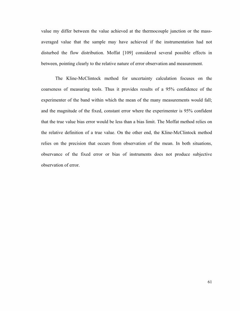
61

value my differ between the value achieved at the thermocouple junction or the mass-

averaged value that the sample may have achieved if the instrumentation had not

disturbed the flow distribution. Moffat [109] considered several possible effects in

between, pointing clearly to the relative nature of error observation and measurement.

The Kline-McClintock method for uncertainty calculation focuses on the

coarseness of measuring tools. Thus it provides results of a 95% confidence of the

experimenter of the band within which the mean of the many measurements would fall;

and the magnitude of the fixed, constant error where the experimenter is 95% confident

that the true value bias error would be less than a bias limit. The Moffat method relies on

the relative definition of a true value. On the other end, the Kline-McClintock method

relies on the precision that occurs from observation of the mean. In both situations,

observance of the fixed error or bias of instruments does not produce subjective

observation of error.

62

Chapter 3 – Experiments on the Decomposition Reactor ________________________________________________________________________

3.1 Approaches to Experimental Work

The experiments in this thesis were designed to satisfy the following criteria.

1. Obtain a direct measure of mass loss / gain whether gas or solid to simplify the

interpretation of data and facilitate a comparison of results from different

techniques.

2. Collect data of measurable variables and obtain the time averaged value in order to

scharacterize the analysis.

3. Use raw species that represent products from hydrolysis at equilibrium conditions.

A common direct method of mass loss tracking includes thermogravimetric analysis that

is performed at isothermal or variable temperature conditions. The analysis can also be

conducted under constant heat flux conditions. Thermogravimetric analysers are designed

specifically for these situations and the data is automatically collected. Other techniques

for thermal decomposition used a simple Erlenmeyer flask heated from the bottom in a

heating mantle. The initial mass is then compared to the final mass and the difference

corresponds with the mass of volatiles. A third technique used a split reactor connected to

a series of sensors in order to monitor the evolution of volatiles in a continuous manner.

Weight differences are then compared with the mass of volatiles measured and

decomposition rates calculated. The three techniques were used in the experimental

analysis of decomposition of a mixture of CuO*CuCl2. Each technique provided a

different set of information that was correlated with consideration to its limitations.

63

3.2 Experimental Apparatus and Set Up

A review of thermal experimental techniques indicated that TGA is an appropriate

technique to monitor the thermal decomposition of materials. The results of TGA are

usually reported in the form of curves relating the mass lost from the sample against

temperature or time. TGA also has the capability to decompose small samples while

supplying a predetermined constant heat rate and monitoring weight losses. The sample is

contained in a closed chamber and the environment is continuously purged with a

predetermined flow of inert gas. The temperature of the sample is closely monitored

through a thermocouple in direct contact. Unless integrated with a mass spectrometer,

TGA does not provide for monitoring of the composition of gas or vapor species. It

provides valuable data for the analysis of rates of weight loss that can then be correlated

to decomposition rates. Experiments were repeated under similar conditions of initial

mass and molar ratios, initial weight, and purge gas flow at atmospheric pressure.

Isothermal experiments were conducted in a thermogravimetric analyser. The

TGA experiments used the SDT Q600 equipment with a sample capacity up to 200 mg on

a microbalance, sensitivity of 0.1 µg and precision of +/- 2%. The instrument provides

measurements of heat flow and weight change. The temperature of the sample is

monitored and controlled via type R, platinum-rhodium thermocouples. Special care was

taken in the preparation of samples for the TGA experiments due to the small size of the

samples. A 10 g sample was placed and thin-spread in the oven at 150 oC for 24 hours and

then carefully packed in a sealed glass container. The samples were then placed in the

chamber and the following standard procedure was used: Continuous purge with 50

ml/min gas argon; Initial equilibrium and isothermal for 5 minutes at 30 oC; Temperature

64

ramp up at 20 oC/min to 110 oC; Isothermal to equilibrium for 10 minutes; Temperature

ramp up at 20 deg C/min to the desired temperature of decomposition (i.e., 450, 470, 490,

510 or 530 oC); Isothermal for up to 120 minutes incremental; Stop measurements and set

air cooling on. The samples consisted of 30 to 55 mg of CuO*CuCl2. The results were

analyzed using the accompanying Universal Analysis 2000 data analysis software.

A heating mantle is a less stringent environment where a gross temperature control

provides feedback for the on-off operation of a resistive heater that transfers heat to the

vessel containing the sample through convection and conduction. It does not have

provisions for weight monitoring. It provides for an open environment where the sample

can be observed directly as the phenomenon occurs. The thermocouples were protected

from the oxidizing environment by means of a thermo-well and set following

recommendations outlined by Moffat [109].

Split reactors are commonly used for research purposes and they provide a starting

place for customization to fit the requirements of the reaction under investigation.

Reactors allow for the decomposition of larger samples and they can be customized for

continuous monitoring of gaseous species flowing in and out of the reactor. Reactors are

limited by the access to information on weight of the sample only before and after the

experiments and data are obtained to be representative of average quantities. The vertical

split reactor was set as indicated in Fig. 3.1 and 3.2 for the forward and reverse reaction

respectively.

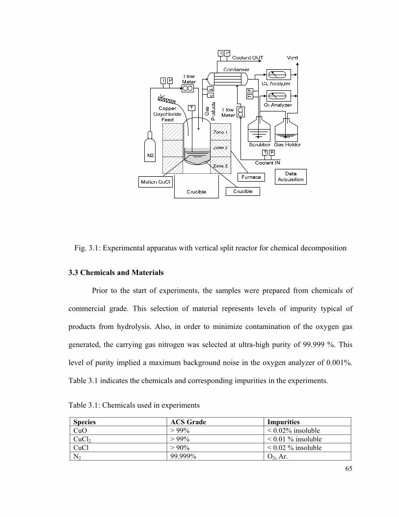
65

Fig. 3.1: Experimental apparatus with vertical split reactor for chemical decomposition

3.3 Chemicals and Materials

Prior to the start of experiments, the samples were prepared from chemicals of

commercial grade. This selection of material represents levels of impurity typical of

products from hydrolysis. Also, in order to minimize contamination of the oxygen gas

generated, the carrying gas nitrogen was selected at ultra-high purity of 99.999 %. This

level of purity implied a maximum background noise in the oxygen analyzer of 0.001%.

Table 3.1 indicates the chemicals and corresponding impurities in the experiments.

Table 3.1: Chemicals used in experiments

Species ACS Grade Impurities CuO > 99% < 0.02% insoluble CuCl2 > 99% < 0.01 % insoluble CuCl > 90% < 0.02 % insoluble N2 99.999% O2, Ar.

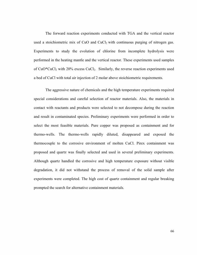
66

The forward reaction experiments conducted with TGA and the vertical reactor

used a stoichiometric mix of CuO and CuCl2 with continuous purging of nitrogen gas.

Experiments to study the evolution of chlorine from incomplete hydrolysis were

performed in the heating mantle and the vertical reactor. These experiments used samples

of CuO*CuCl2 with 20% excess CuCl2. Similarly, the reverse reaction experiments used

a bed of CuCl with total air injection of 2 molar above stoichiometric requirements.

The aggressive nature of chemicals and the high temperature experiments required

special considerations and careful selection of reactor materials. Also, the materials in

contact with reactants and products were selected to not decompose during the reaction

and result in contaminated species. Preliminary experiments were performed in order to

select the most feasible materials. Pure copper was proposed as containment and for

thermo-wells. The thermo-wells rapidly diluted, disappeared and exposed the

thermocouple to the corrosive environment of molten CuCl. Pirex containment was

proposed and quartz was finally selected and used in several preliminary experiments.

Although quartz handled the corrosive and high temperature exposure without visible

degradation, it did not withstand the process of removal of the solid sample after

experiments were completed. The high cost of quartz containment and regular breaking

prompted the search for alternative containment materials.

67

Table 3.2: Materials used in the vertical reactor

Material Location Maximum Temperature, oC

Fluid / Species

Stainless Steel 316 Secondary containment reactor

630 CuCl vapours, Cl2 gas, O2

gas Alumina Primary

containment 550 Molten CuCl, Cl2 gas, O2 gas

Hastelloy C Thermo-well 550 Molten CuCl, O2 gas, Cl2

gas. Stainless Steel 316 Discharge ports 350 O2 gas, N2, CuCl vapours PTFE tubing Feed/discharge ports 100 O2 gas, Cl2 gas, CuCl

vapours Stainless Steel 416 Feeding ports Ambient CuO*CuCl2, Air, N2, CuCl2

Test experiments were conducted and coupons of several materials were placed in a

crucible with a CuCl sample and brought to temperatures above 500 oC. The sample was

contained in crucibles of alumina, and the thermocouples used thermo-wells of Hastelloy

C. Materials tested and locations within the reactor are indicated in Table 3.2. Although

hastelloy C and SS 316 were selected for the most stringent applications, chemical attack

and corrosion were evident. The corrosion rate however was slow enough for practical

application during experimental testing.

3.4 Forward Reaction

For the forward reaction, heat is supplied to the reactor by a 100 cm vertical split-

type furnace with three heating zones, independently controlled via SCR power control

modules, and with a PID control interface. The furnace can operate within 1 deg C of the

targeted temperature and within the range of 50 to 1000 oC. The heating zones are

independently powered for further heat flux control, and independently controlled via one

68

type K thermocouple for each heating zone. This arrangement provides a uniform

temperature field to the reactor. The body of the reactor and pipes are made of stainless

steel 316 and hastelloy-C, and the crucible containing the sample is made of ceramic.

The reactor chamber provides secondary containment to the sample, channelling

the gases outside via a liquid seal that maintains back-pressure within the chamber slightly

above atmospheric pressure. A pressurized reactor prevents atmospheric gases from

entering and contaminating the products of the reaction. One stream of gas products is

directed to an ABB-AO202 chlorine gas analyzer that provides readings in a continuous

manner, with linearity of 1% of span and repeatability of 0.5% of span. Continuous time

correction is applied to readings to compensate for instrument response time and space

velocity of the sample. A second stream is directed to an on-line oxygen gas analyzer that

uses a zirconium oxide sensor with five sensing ranges and a sampling pump connected in

parallel. The oxygen analyzer is calibrated with analytical grade (99.999%) nitrogen for

zero reading and atmospheric air for span reading. The AMI-201RSP continuous oxygen

analyzer has five selectable ranges of operation, minimum detection of 0.01% and

repeatability of +/- 0.2% of range. The error of readings of gas composition, including the

calibration gas and response time of analyzer, was estimated at 1%.

The CuCl vapour tends to travel with the gases product of decomposition. In

order to overcome this problem, a condenser is installed on the discharge of the reactor.

Carrier gas nitrogen is injected in the reactor at constant pressure and continuous flow is

measured via an O-FMA1600MA differential pressure mass-flow-meter with +/- 0.8%

reading accuracy, +/- 0.2% repeatability, and pressure / temperature compensation.

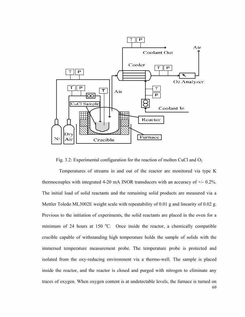
69

Fig. 3.2: Experimental configuration for the reaction of molten CuCl and O2

Temperatures of streams in and out of the reactor are monitored via type K

thermocouples with integrated 4-20 mA INOR transducers with an accuracy of +/- 0.2%.

The initial load of solid reactants and the remaining solid products are measured via a

Mettler Toledo ML3002E weight scale with repeatability of 0.01 g and linearity of 0.02 g.

Previous to the initiation of experiments, the solid reactants are placed in the oven for a

minimum of 24 hours at 150 oC. Once inside the reactor, a chemically compatible

crucible capable of withstanding high temperature holds the sample of solids with the

immersed temperature measurement probe. The temperature probe is protected and

isolated from the oxy-reducing environment via a thermo-well. The sample is placed

inside the reactor, and the reactor is closed and purged with nitrogen to eliminate any

traces of oxygen. When oxygen content is at undetectable levels, the furnace is turned on

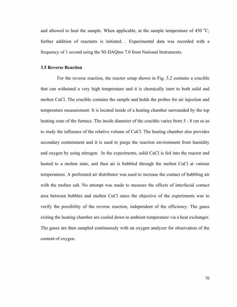
70

and allowed to heat the sample. When applicable, at the sample temperature of 450 oC,

further addition of reactants is initiated. . Experimental data was recorded with a

frequency of 1 second using the NI-DAQmx 7.0 from National Instruments.

3.5 Reverse Reaction

For the reverse reaction, the reactor setup shown in Fig. 3.2 contains a crucible

that can withstand a very high temperature and it is chemically inert to both solid and

molten CuCl. The crucible contains the sample and holds the probes for air injection and

temperature measurement. It is located inside of a heating chamber surrounded by the top

heating zone of the furnace. The inside diameter of the crucible varies from 5 - 8 cm so as

to study the influence of the relative volume of CuCl. The heating chamber also provides

secondary containment and it is used to purge the reaction environment from humidity

and oxygen by using nitrogen. In the experiments, solid CuCl is fed into the reactor and

heated to a molten state, and then air is bubbled through the molten CuCl at various

temperatures. A perforated air distributor was used to increase the contact of bubbling air

with the molten salt. No attempt was made to measure the effects of interfacial contact

area between bubbles and molten CuCl since the objective of the experiments was to

verify the possibility of the reverse reaction, independent of the efficiency. The gases

exiting the heating chamber are cooled down to ambient temperature via a heat exchanger.

The gases are then sampled continuously with an oxygen analyzer for observation of the

content of oxygen.

71

The total quantity of reacted oxygen can be determined from integration of the

concentration curve and the flow rates of air which are monitored in a real-time mode.

The oxygen quantity was calculated by assuming ideal behaviour as follows:

1 22 2 2

2 1

1

22.4O O N

PTm p F

P T

(3.1)

In this equation, P1, T1 and P2, T2 represent the pressure and temperature at the inlet and

outlet conditions, respectively. Also, pO2, FN2 and mO2 represent the partial pressure of

oxygen, flow of nitrogen and mass flow of oxygen, respectively.

The solid products of reaction were analyzed by x-ray diffraction (XRD) with a

PANalytical X’pert diffractometer where the diffraction angle 2-Tetha was allowed to

change between 5 and 60 degrees. Subsequent quantification used the X-pert PANalytical

quantification software.

3.6 Uncertainty and Error

The collected data was used for the generation of the rate of reaction. Each data set

collected through different techniques brings intrinsic errors that must be carefully

understood and analyzed. The inherent error of experiments and subsequent

interpretations and calculations were determined by following the method for

experimental uncertainty as outlined by Kline and McClintock [110] and the discussion

by Moffat [109]. The cumulative volume of gasses generated at standard conditions is

obtained by integrating the curve of the mass balance over the time period. The mass

balance of gases is calculated by using Raoult’s law for the mole fractions and partial

pressures in parallel with a mass balance as follows:

72

2 2 2out N O ClF F F F (3.2)

The volume of gas yielded results from the integration of the instantaneous curve of

gas produced vs. time:

2

2 2

1

O OV X Fdt

(3.3)

The mass loss from the mixture of CuO*CuCl2 reactant is measured as the

difference between the weights of the full and empty crucible, and before and after the

reaction:

0 1solidsM m m (3.4)

Table 3.3: Summary of measurement assumptions and uncertainties

Parameter / Procedure Range Bias Precision Error % R2 Nitrogen flow meter 0-2 SLPM 0.8 0.2 Percent oxygen 0-25% 0.01 0.2 Percent chlorine analyzer 0-10% 1.0 0.5 Reactor temperature 370-1000 oC 0.2 0.1 Reactor pressure 0-5 bar 0.6 0.06 Weight Scale 0-400 g 0.0002 0.0001 Reactor data acquisition 0-24 mA 0.12 0.1 Reactor conversion curve fitting 3.6 0.9835 Zero intercept reactor conversion curve fitting

20.0 0.9898

Reactor temperature fitting 0.9534 TGA weight measurement 0.2 TGA conversion curve fitting 1.5 0.9908 TGA temperature curve fitting 0.9030 NIST Cu, Cl2, O2 data 0.08 Uniform density solid and liquid 4.83 - 4.18 13.5 Average density at equilibrium 8.97 Average numerical error (local) % 0.01 Bias and Precision values are +/-

73

Uncertainty calculations were taken over a representative time period of the

experiments. Experiments were repeated under similar conditions of initial mass and

molar ratios, initial weight, reactor pressure and purge gas flow. A steady set of readings

from the data acquisition system was selected over a time period for uncertainty

calculations. The uncertainty of the total mol evolution was calculated as 1.28%, and

determined by following a combination of precision (random) contributions to the

uncertainty of , ,nn P and a bias contribution to the uncertainty of , nn B . The two

contributions were evaluated separately in terms of the sensitivity of coefficients

following the Kline and McClintock [110] equation for error propagation. Table 3.3

contains a tabulation of precision and bias limits for variables and parameters used in

uncertainty calculations.

The enthalpy and entropy changes for each component are calculated from the

integration of the heat capacity curve. The parameters of the Cp curve are obtained from

NIST [60] for the most common species. The equations apply to species where no phase

transition occurs:

T

PT dTCH

2525 (3.5)

T

PT

T

dTCS

2525 (3.6)

The Gibbs free energy of formation of products and reactants was calculated from

their enthalpy and entropy of formation:

74

STHG Tf

Tf

Tf (3.7)

where HTf and ST

f are the standard enthalpy and entropy of formation, respectively.

The accuracy of thermodynamic data in the theoretical modeling as well as the

interpretation of experimental results may impact the conclusions of the study. Parry [111]

presented calorimetric measurements of heat capacity for copper oxychloride in the range

of 20 to 410 oC, assumed a monotonically increasing function beyond that temperature

and used a Debye and Einstein extrapolation method to obtain thermodynamic data to 550

oC. Although the heat capacity changes rapidly in the low-temperature range and

uncertainty arose in this region, the slope of the curve decreases in the high temperature

range beyond 400 oC to less than 5 J/mol.K per 100 oC.

Table 3.4: Enthalpy of formation of compounds in the Cu-Cl Cycle at 298.15 K

Compound Enthalpy of Formation (kJ/mol)* Standard Deviation

CuCl2 -217.4 -217.4 -218.0 -205.9 -205.9 5.83%

CuO -162.0 -155.8 -156.1 -156.1 -156.1 0.13%

CuCl -137.0 -137.0 -136.8 -137.0 -138.1 0.57%

CuOCuCl2 -381.3 -381.0 -385.1 -381.3** 1.54%

HCl -92.31 -93.4 -93.3 0.48%

H2O -241.82 -285.8 -285.8 1.88%

Reference [108] [49] [50] [52] Present study***

* Standard temperature of 298.15 K ** T. Parry [111] *** NIST [60]

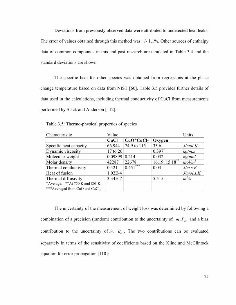
75

Deviations from previously observed data were attributed to undetected heat leaks.

The error of values obtained through this method was +/- 1.1%. Other sources of enthalpy

data of common compounds in this and past research are tabulated in Table 3.4 and the

standard deviations are shown.

The specific heat for other species was obtained from regressions at the phase

change temperature based on data from NIST [60]. Table 3.5 provides further details of

data used in the calculations, including thermal conductivity of CuCl from measurements

performed by Slack and Anderson [112].

Table 3.5: Thermo-physical properties of species

Characteristic Value Units CuCl CuO*CuCl2 Oxygen Specific heat capacity 66.944 74.9 to 115 33.6 J/mol.KDynamic viscosity 17 to 26 0.397* kg/m.sMolecular weight 0.09899 0.214 0.032 kg/mol Molar density 42287 22678 16.19, 15.18** mol/m3

Thermal conductivity 0.421 0.451*** 0.03 J/m.s.KHeat of fusion 1.02E-4 J/mol.s.K Thermal diffusivity 3.34E-7 5.515 m2/s*Average; **At 750 K and 803 K ***Averaged from CuO and CuCl2

The uncertainty of the measurement of weight loss was determined by following a

combination of a precision (random) contribution to the uncertainty of , ,mm P and a bias

contribution to the uncertainty of ,m mB . The two contributions can be evaluated

separately in terms of the sensitivity of coefficients based on the Kline and McClintock

equation for error propagation [110]:

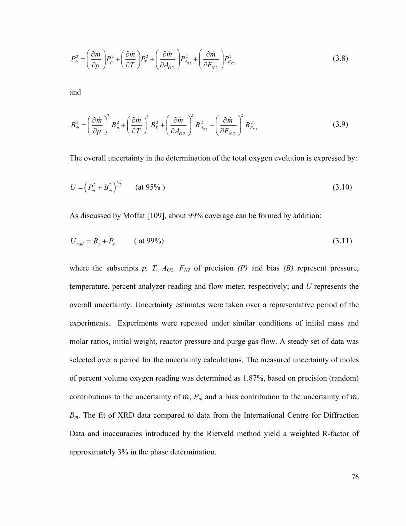
76

2 2

2 2 2 2 2

2 2O Nm p T A F

O N

m m m mP P P P P

p T A F

(3.8)

and

2 2

2 22 22 2 2 2 2

2 2O Nm p T A F

O N

m m m mB B B B B

p T A F

(3.9)

The overall uncertainty in the determination of the total oxygen evolution is expressed by:

1

2 2 2m mU P B

(at 95% ) (3.10)

As discussed by Moffat [109], about 99% coverage can be formed by addition:

add x xU B P ( at 99%) (3.11)

where the subscripts p, T, AO2, FN2 of precision (P) and bias (B) represent pressure,

temperature, percent analyzer reading and flow meter, respectively; and U represents the

overall uncertainty. Uncertainty estimates were taken over a representative period of the

experiments. Experiments were repeated under similar conditions of initial mass and

molar ratios, initial weight, reactor pressure and purge gas flow. A steady set of data was

selected over a period for the uncertainty calculations. The measured uncertainty of moles

of percent volume oxygen reading was determined as 1.87%, based on precision (random)

contributions to the uncertainty of , Pm and a bias contribution to the uncertainty of ,

Bm. The fit of XRD data compared to data from the International Centre for Diffraction

Data and inaccuracies introduced by the Rietveld method yield a weighted R-factor of

approximately 3% in the phase determination.

77

The composition of the reaction product is analyzed by an X-ray diffraction

(XRD) technique after solidification of CuCl. Bragg's Law of XRD diffraction is

represented as follows:

2 sinn d (3.12)

The equation describes how the cleavage face of crystals scatters X-ray beams at

certain angles of incidence. When the angle of incidence θ equals the angle of scattering,

and the path-length difference equals an integer number of wavelengths n, then peaks of

scattered intensity can be observed as described in “Introduction to X-ray Diffraction”

[113] and discussed by XRD quantification by Leroux et al. [114]. In the equation, d

represents the distance between atomic layers in the crystal. Lambda, λ, is the known

wavelength of incidence of the X-ray beams and n is an integer.

Bragg's Law conditions occur at a different d-spacing in materials with a

polycrystalline structure. A pattern can then be obtained by plotting the angular positions

and intensities of the resultant diffracted peaks of radiation. The diffracted peaks are a

characteristic that depend exclusively on the crystalline structure of the sample. If the

sample contains a mixture of different phases, the pattern shows the reflections of

individual phase characteristics at different angular positions. Powder diffraction XRD

was applied to a 1 mm thick sample in a 2 cm2 bed in order to characterize the

crystallographic structure. The measurements used a Philips PW 1830HT generator with a

PW1050 goniometer, PW3710 control, X-pert software (2007 version; International

Centre for Diffraction Data) and Rietveld refinement software. The Rietveld refinement

method optimizes the model function to minimize the weighted sum of squared

78

differences between the observed and computed intensity values. In the XRD analysis of

the CuCl samples, the angle 2-θ was allowed to vary within a range of 5 to 60 degrees.

The uncertainty from data collection and instrumentation is a function of the

measurement of temperature and conversion dependent variables as follows:

2 2 2, , , ,r s g sw f T f x f T T f N O Cl m (3.13)

In deriving the rate of reaction equation, the Avrami-Erofeev linear fitting was

used for the concentration vs. time curve, and a zero crossing approximation was then

adopted. The curve of concentration vs. temperature was fitted to the Arrhenius equation.

The overall measurement uncertainty of the rate expression obtained from this analysis is

a function of the uncertainty of all independent variables. The estimated uncertainty of the

experimental vs. calculated data yields an uncertainty of +/- 0.04 mol/m2.s. There is an

additional error that results from the numerical analysis in simulating the chemical

decomposition of a particle. The dynamics of the system are fast and the size of particles

small. Therefore, error propagation from numerical iterations has a significant impact on

results. The Runge–Kutta–Fehlberg method uses a Runge-Kutta-4 method together with a

higher order method that predicts the adaptive step-size. In order to monitor and control

local error the procedure of Vettering and Teukolsky [115] was used and it selected a

desired accuracy ∆o of O-6 (overall tolerance level). The error is estimated as:

6

*1 1 1

1

'n n i i ii

z z c c k

(3.14)

79

where z represents the variable calculated with RK-4 and z’ the same variable calculated

with the RKF method. The values of k and c are the RK-4 delta midpoint and the

improved Cash and Karp [116] constants, respectively. The average error of local

calculations in the desired accuracy is indicated in Table 3.1. The step size is adjusted

accordingly based on the desired accuracy and the new scale ∆1 by following the

correlation of Cash and Karp [116]:

0.2

11

ooh h

(3.15)

In the next chapter, a predictive model of transport phenomena will be presented.

80

Chapter 4 - Model of the Decomposition Kinetics _______________________________________________________________________________

The thermal decomposition of copper oxychloride is a complex phenomenon that

results in a three-phase system of heat and mass transfer, its understanding requires an

analysis from several fronts. First, a detailed analysis of the hydrolysis reaction in view of

the past literature provides the basic understanding of the nature of products that feed the

decomposition reactor. Because of the closed nature of the cycle, the decomposition

reactor is fed with products of reactions from the hydrolysis reactor that may carry

unreacted CuCl2 and other species. Thus, a mixture of CuO*CuCl2 was adopted for the

decomposition reaction experiments since the potential presence of free CuCl2 with the

products of hydrolysis is represented in the mixture. The preparation of the mixture also

adds some variability to the sample to an extent comparable to the variability of products

from hydrolysis. This process suggested a reproduction of the nature of the feedstock to

the reactor with the potential presence of free CuCl2. This decomposition of the mixture

reflects better the non-uniform nature of the feedstock. Second, the decomposition

reaction may follow either path as discussed by Levy and Goreaud [55] and Serban et al.

[59].

These paths need to be considered and understood for this kinetic analysis to be

complete. In their analysis, both researchers suggested the intermediate presence of a

mixture of CuO and CuCl2 as a path to the release of oxygen. Furthermore, Serban et

al.[59] proposed using a mix in experiments intended to understand the kinetics analysed

the decomposition of CuCl2 with release of chlorine. Third, the product of decomposition

at equilibrium is the result of the balance between the forward and reverse reaction, such

81

that aspects that promote the reverse reaction and the thermodynamic limits will also be

analyzed here. Fourth, the analysis of the thermodynamic aspects of the decomposition

reaction provided new light on the second law limits and implications on equilibrium

conditions of varying pressure and temperature.

These four aspects will be analyzed such that experiments of the forward reaction

can be understood with confidence before arriving at a rate of reaction expression and

attempting a theoretical model of the phenomena.

4.1 Hydrolysis Reaction for Production of Copper Oxychloride

A complete hydrolysis reaction produces Cu2OCl2 (copper oxyxhloride) and HCl

(hydrogen chloride) as a result of the reaction of CuCl2 and steam at 380 oC. Past research

indicated that the molar fraction of water must be in excess of the stoichiometric value in

order to obtain reasonable conversion to copper oxychloride and hydrogen chloride.

However, as the ratio of steam increases, more energy is required to heat steam and the

HCl produced is more diluted.

Analysis of experimental results reported by Lewis et al. [32] and Ferrandon et al.

[53] indicated that the maximum conversion to copper oxychloride is achieved at molar

ratios of steam to copper in the vicinity of 20. Experiments where the steam ratio was

higher than 20 increased the amount of un-reacted CuCl2 found in the solid products, in

addition to CuCl. The ratio of un-reacted CuCl2 in the products decreased when the

reactor operated under vacuum conditions. Dagupatti et al. [48, 52] presented a

thermodynamic analysis of the reaction based on the equilibrium conversion and extent of

82

reaction. The study considered a mechanistic analysis of the hydrolysis of CuCl2 with

three competing reactions as indicated in the following equations.

2CuCl2(s) + H2O(g) Cu2OCl2 + 2HCl (4.1)

2CuCl2(s) 2CuCl(s) + Cl2(g) (4.2)

Cl2(g) +H2O(g) 2HCl(g) + ½ O2(g) (4.3)

The study considered equilibrium conversion using the Gibbs free energy of

reaction and the extent of reaction analysis. Increasing the initial mole fraction of steam

and decreasing the total pressure of the system resulted in lower equilibrium constants and

higher equilibrium conversion. Overall, the analysis indicated that the hydrolysis reaction

favours high temperature, excess steam and lower than atmospheric pressures. The excess

steam in the reaction also consumes the released chlorine. At a temperature of 380 oC and

atmospheric pressure, the change in Gibbs energy of the hydrolysis reaction is negative

and the reaction is spontaneous. At 380 oC and atmospheric pressure, the analysis

predicted that the yield of Cu2OCl2 is approximately 5% for stoichiometric steam ratios.

The analysis also predicted a yield of 80% when pressure is decreased to 0.5 bar, and the

steam ratio is increased to 5 mol/L. In a separate study, Ferrandon et al. [53]

experimented with 40 mg of CuCl2 at 350 oC and reported XRD intensity peaks of 0.6 for

copper oxychloride in the products, in addition to CuCl, when using 2500 ppm of water

vapour.

Ferrandon et al. [53] used a vertical spray reactor at 400 oC with an ultrasonic

nozzle to promote the contact between a solution of CuCl2.H2O and steam. Upon

83

atomization of the solution, water evaporates rapidly from the droplets. The particles of

CuCl2 react with steam or thermally decompose before reaching the bottom of the spray

reactor. The phase composition of products was determined by powder X-ray diffraction.

A quantitative analysis was performed in the solids to determine the content of CuCl. The

amount of Cu2OCl2 was determined based on oxygen evolution from decomposition of

the solid products in a catalytic reactor. At atmospheric pressure and a molar ratio of

steam to CuCl2 of 10, the reaction yielded 60% Cu2OCl2 and 7% CuCl. Reducing the

reactor pressure to 0.4 bar resulted in a yield of 75% Cu2OCl2 and 4% CuCl, with the

balance of un-reacted CuCl2.

Past literature indicated that the reaction in Eq. (3.2) does not proceed to

completion, and that certain amounts of chlorine will result from the decomposition of

CuCl2. Some chlorine recombines with steam to produce hydrogen chloride as in Eq.

(3.4). Since the two species are gaseous, the probability of collisions occurring and

resulting in strong bonds that generate a new compound is low, resulting in free chlorine

mixed with products. Free chlorine in the gas products does not represent a problem for

the subsequent decomposition of copper oxychloride in the oxygen reactor, but it is a

polluting agent that must be separated from the oxygen stream. Free chlorine mixed with

hydrogen chloride may be a problem for the electrolytic reaction, shortening the life of the

membrane and electrodes, or resulting in side reactions. This aspect requires further

research. The presence of CuCl in the products of hydrolysis is acceptable since it is also a

product of the decomposition of copper oxychloride in the oxygen reactor. Finally,

depending on the molar fraction of steam and factors related to the geometry and

efficiency of the reactor, the presence of un-reacted CuCl2 in the products of hydrolysis is

84

highly probable. Free CuCl2 in the oxygen reactor results in the release of chlorine,

changes the balance of partial pressures in the reactor, and reduces the oxygen yield and

purity.

4.2 Thermodynamic Analysis of the Reverse Reaction

Copper oxychloride is not commercially available and it exists in nature in very

few locations as a mineral called melanothallite. Lewis et al. [56] reported micro-scale

attempts to reproduce the hydrolysis reaction with limited results. Dr. Greg Hope at Griffit

University, Australia (as cited by Parry [111]) prepared copper oxychloride in a laboratory

through a slow synthesis process that utilized an equi-molar mixture of copper oxide

(CuO) and cupric chloride (CuCl2 or copper II chloride) in a quartz tube vacuum heated

for several days at 400 oC. Krivovichec and Filatov [117] synthetized melanothallite in a

small reactor at temperatures between 370 and 470 oC. The temperature ranges and

duration of these experiments suggests that the reaction of CuCl2 and CuO may not occur

for practical reasons within the short time of duration and temperature ranges of the

experiments of this research. Furthermore, the experimental work reported in past

literature indicated that the most probable result of decomposition of CuO*CuCL2 and of

copper oxychloride are molten CuCl, oxygen gas and to a minor degree, chlorine gas.

With the predominant presence of free oxygen and molten CuCl, the probability of a

reverse reaction that involves these two species is higher than a reverse reaction involving

CuO and CuCl2. Based on the above discussion, this study proceeded to analyze the path

for a probable reverse reaction in the decomposition of copper oxychloride as follows:

2CuCl (l) + ½ O2 (g) = Cu2OCl2(s) (4.4)

85

The spontaneity of the reaction in Eq. (4.4) can be predicted from the change of

the Gibbs free energy of the reaction, GTr . Any deviation from standard conditions can

influence the behaviour of the reaction. The reaction Gibbs free energy GTr can be

calculated as follows:

ln( )T T or r rG G RT Q (4.5)

where T or G is the change of Gibbs free energy of the reaction at standard pressure and

temperature, and Qr is the reaction quotient defined by the stoichiometric ratio of the

product and reactant fugacity. Since CuCl and Cu2OCl2 exist in the form of a condensed

state, the reaction quotient can be simplified by:

2

1/2

1

( / )r oO

QP P

(4.6)

where Qr represents the reaction quotient, P is the standard pressure (100 kPa) and 2OP

is the partial pressure of O2 under actual reaction conditions. When the reaction reaches

equilibrium, the quotient is equal to the reaction equilibrium constant K as defined by:

lnT or G RT K (4.7)

and K is then determined by:

2

1/2

1

( / )oO

K QP P

(4.8)

86

where GTr can be calculated from the molar Gibbs free energy of formation of the

product and reactants:

2 2 2( ) ( ) ( )[2 1/ 2 ]T o T o T o T or f Cu OCl f CuCl f OG G G G (4.9)

where 2 2( )

T of Cu OClG and ( )

T of CuClG are the molar Gibbs free energy of formation for CuCl

and Cu2OCl2, respectively. The Gibbs free energy of formation of each reactant and

product can be calculated from their enthalpy and entropy of formation:

T o T o T of f fG H T S (4.10)

where T of H and T o

f S are the standard enthalpy and entropy of formation of the species

at temperature T.

Fig. 4.1: Paths for thermodynamic calculations of copper oxychloride

Limited data of T of H and T o

f S have been reported for CuCl and Cu2OCl2 in the

temperature range of 400 to 550 oC. CuCl exists in the solid phase up to the temperature

of 412 oC. At this temperature, it remains solid with a different microstructure and

87

thermo-physical properties. This phase is identifiable between the temperatures of 412 to

423 oC. Beyond this temperature, CuCl remains liquid in the range of temperatures of

interest with significant vaporization beyond the temperature of 550 oC. The thermo-

physical properties of Cu2OCl2 are calculated from the properties of compounds and

elements. The procedure utilizes known data of enthalpy and entropy at ambient

temperature. For the product Cu2OCl2 in Eq. (4.17), the schematic of a thermodynamic

method in Fig. 4.1 is used for the calculation of T of H :

The method also applies to the calculation of STf , then

252 2 25 25 2 25 2 25[ ( ) ] [ ( ) ( ) ( ) ]T o o o T o T o T o T

f fH H H Cu OCl H Cu H O H Cl (4.11)

252 2 25 25 2 25 2 25[ ( ) ] [ ( ) ( ) ( ) ]T o o o T o T o T o T

f fS S S Cu OCl S Cu S O S Cl (4.12)

where the enthalpy and entropy changes for each component are calculated based on the

following equations:

25 25

TT oPH C dT (4.13)

25 25

TT o PC dTS

T (4.14)

A similar methodology is adopted for the reactants CuCl and O2 in Eq. (4.4) for the

calculation of T of H and T o

f S shown in Fig 4.2. The correlations of CP and the values of

25 of H for Cu, O2, Cl2 and CuCl reported by NIST [60] are adopted in this thesis. The

reactant CuCl experiences a phase change from solid to liquid at the temperature of 430

88

oC (803.15 K). The entropy change ∆S at the melting point is calculated with the

following equation:

803.15

omeltingo

melting

HS

(4.15)

where ∆H represents the enthalpy of phase change. For Cu2OCl2, only the experimental

data of specific heat capacity at constant pressure CP in the temperature range of 25 - 410

oC was reported by Parry [111]. The following equation is proposed to correlate the data:

2 2( ) 99.23243 0.021622P Cu OClC T (4.16)

where CP and T have units of J/mol·K and K, respectively. The relative standard deviation

of Eq. (4.16) in the temperature range of 25 - 410 oC is within 3%, so it will be assumed to

be extended to the temperature of 550 oC. This theoretical projection in the range of

decomposition of copper oxychloride introduces additional uncertainty to the

thermodynamic calculations. This is due to the unknown degree of stability of copper

oxychloride beyond the temperature reported in past studies.

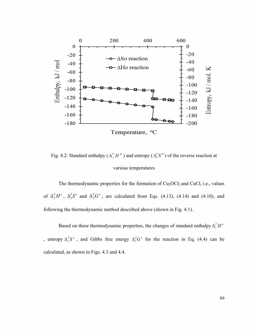
89

Fig. 4.2: Standard enthalpy ( HTr ) and entropy ( ST

r ) of the reverse reaction at

various temperatures

The thermodynamic properties for the formation of Cu2OCl2 and CuCl, i.e., values

of T of H , T o

f S and T ofG , are calculated from Eqs. (4.13), (4.14) and (4.10), and

following the thermodynamic method described above (shown in Fig. 4.1).

Based on these thermodynamic properties, the changes of standard enthalpy T or H

, entropy T or S , and Gibbs free energy T o

r G for the reaction in Eq. (4.4) can be

calculated, as shown in Figs. 4.3 and 4.4.

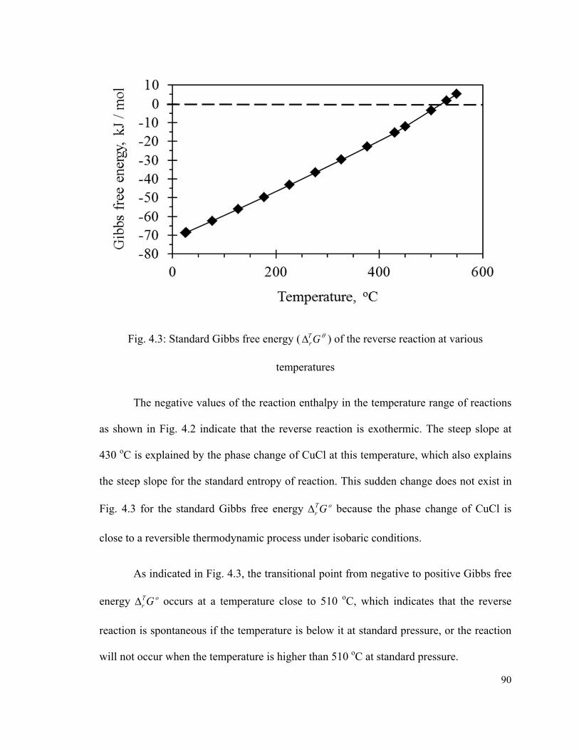
90

Fig. 4.3: Standard Gibbs free energy ( GTr ) of the reverse reaction at various

temperatures

The negative values of the reaction enthalpy in the temperature range of reactions

as shown in Fig. 4.2 indicate that the reverse reaction is exothermic. The steep slope at

430 oC is explained by the phase change of CuCl at this temperature, which also explains

the steep slope for the standard entropy of reaction. This sudden change does not exist in

Fig. 4.3 for the standard Gibbs free energy T or G because the phase change of CuCl is

close to a reversible thermodynamic process under isobaric conditions.

As indicated in Fig. 4.3, the transitional point from negative to positive Gibbs free

energy T or G occurs at a temperature close to 510 oC, which indicates that the reverse

reaction is spontaneous if the temperature is below it at standard pressure, or the reaction

will not occur when the temperature is higher than 510 oC at standard pressure.

91

Fig. 4.4: Gibbs free energy of CuCl + O2 reaction at various operating conditions

Figure 4.4 shows results for the operating pressure range of 1.0 ×10-10 to 100 bars

to represent the range of vacuum to highly pressurized reactors. An analysis of Fig. 4.4

indicates that the reverse reaction may be minimized by either decreasing the oxygen

pressure or increasing the reaction temperature. When the oxygen pressure is decreased to

below one bar, a vacuum will be created. Since the produced oxygen in the forward

reaction is often pressurized for further storage or utilization in other units that consume

oxygen, a vacuum oxygen reactor may increase the power consumption of the vacuum

and pressurization for industrial scale oxygen production. In addition, a vacuum is more

likely than pressurization to introduce other gases into the oxygen production reactor.

Furthermore, negative pressure may also increase the generation of CuCl vapour.

Therefore, a vacuum oxygen production reactor is not suggested for the Cu-Cl cycle.

92

A method of minimizing the reverse reaction is to increase the operating

temperature. However, if the temperature is higher than 530 oC, significant amounts of

CuCl vapour may be generated, as observed in the reactor and oxygen outlet in the

experiments.

Fig. 4.5: Vapour pressure of CuCl at various temperatures

Figure 4.5 shows the vapour pressure of CuCl based on experimental data reported

in previous studies by Brewer and Lofgren [118] and Mizuno et al. [119]. The

temperature must be below 530 oC in order to maintain the vapour pressure of CuCl below

1,000 Pa (0.01 bar). For CuCl vapour minimization and the simultaneous impact of

pressure and temperature on the Gibbs free energy, the optimum operating pressure is

suggested in the range of 1 - 2 bars and a temperature in the range of 525 - 550 oC.

93

Although it is desirable to decompose Cu2OCl2 at lower temperatures,

experimental results of the decomposition of copper oxychloride indicate that the

conversion rate is very low below 500 oC . This is due to the increased spontaneity of the

reverse reaction at lower temperatures. As shown in Fig. 4.3, the Gibbs free energy of the

reverse reaction is positive at temperatures above 510 oC.

Furthermore, Fig. 4.3 indicates that the reverse reaction is spontaneous (∆G < 0)

when the operating temperature is below 450 oC, and the oxygen pressure is higher than

0.01 bars. This implies the reverse reaction may occur in the process of reactant

preheating from a temperature significantly lower than 450 oC. This situation may occur

when species are transferred from the hydrolysis reaction to the downstream oxygen

production reaction as shown in Fig. 4.3.

Lower pressure in the reaction system moves the curve to the left, thus lowering

the temperature for equilibrium. Furthermore, the decomposition reaction occurs with

removal of oxygen from the reacting zone. Thus even if the conditions for the reverse

reaction are present, the produced CuCl is starved for oxygen to react. This effect is

confirmed by Le’Chatelier’s principle, thus promoting the forward reaction.

4.3 Copper Oxychloride Decomposition Reaction

It can be prepared in small quantities in the laboratory through a lengthy process that

used an equi-molar mixture of copper oxide (CuO) and copper II chloride (CuCl2). The

decomposition experiments with a mixture have been justified in the past literature on the

basis that the intermediate reactions occur through the decomposition of CuCl2 and the

reaction of CuO in competing dynamics. Also, the absence of easy access to the

94

compound has motivated the experiments of decomposition reported in the literature are a

result of either copper-oxychloride (Cu2OCl2) or from a mix of CuO and CuCl2 identified

as CuO*CuCl2. Since the decomposition of the mix represents a more stringent situation,

it was decided that the experimental work would be conducted on a stoichiometric

mixture of CuO andCuCl2.

Two potential paths for the decomposition of copper oxychloride have been

discussed in the literature. The treatment of the decomposition reaction suggested an

intermediate step where the compound is treated as a mixture of CuO and CuCl2 rather

than copper oxychloride. A mechanistic approach to copper oxychloride decomposition

was first proposed by Walter-Levy et al. [55]. The experiments indicated that copper

oxyxhloride is stable until the temperature of 370 oC is reached. Between 375 oC and 470

oC, Cl2 is released with the formation of CuCl and CuO plus small amounts of CuCl2.

From 475 oC to 550 oC, XRD reveals larger amounts of CuCl2 in the products while the

amount of CuO was reduced. The decomposition reaction is analyzed in view of two

consecutive reactions as follows:

Cu2OCl2 --> CuCl + CuO + ½ Cl2 (4.17)

CuO + Cl2 --> CuCl2 + ½ O2 (4.18)

The competing reaction occurs in parallel, and the experimental results indicated that the

secondary reaction was responsible for a partial decrease of CuO due to Cl2 from the

former reaction. In the analysis this set of reactions is called path A.

95

Another approach to the analysis of the decomposition of copper oxychloride was

recently proposed by Serban et al. [59]. The experiments used an equi-molar mixture of

CuO and CuCl2 in a vertical reactor at 500 oC. The XRD analysis of the solid products

indicated that the solid phase is pure CuCl. The analysis used a mechanistic approach

(path B) and concluded that the oxygen evolution is limited by the decomposition of

CuCl2. The reaction occurred in two consecutive stages as follows:

CuCl2(s) CuCl(s) + ½ Cl2(g) (4.19)

CuO(s) + ½ Cl2(g) CuCl(s) + ½ O2(g) (4.20)

The competing reaction in Eq. (4.19) is the heterogeneous, endothermic thermolysis

of cupric (II) chloride. The observations indicated that even though only 60%

decomposition of CuCl2 is achieved at 530 oC, the presence of CuO in the mixture

appeared to promote the release of Cl2. This effect was also observed by Serban et al. [59]

and resulted in decomposition of CuCl2 at lower temperatures. The study also concluded

that the Cl2 released is completely consumed in the reaction with CuO as in Eq. (4.20)

since no free Cl2 was detected in the gas products.

96

Fig. 4.6: Gibbs energy of reactions of two pathways (path A in open markers) for

decomposition of copper oxychloride at atmospheric pressure

The Gibbs energy of reaction provides an indication of the probability of either

mechanistic approach to occur. Figure 4.6 indicates the temperatures at which each of the

possible reactions becomes spontaneous. The Gibbs free energy of the reaction in Eq.

(4.19) indicates that the reaction reaches equilibrium at 500 oC, and it is spontaneous

beyond this temperature, with more chlorine available to react with CuO as the

temperature increases. Furthermore, experimental results also indicated that the

decomposition of CuCl2 is not completed until it reaches 600 oC.

The two mechanistic approaches coincide in the intermediate release of chlorine and

displacement of oxygen out of copper oxide to produce either copper (I) chloride or

copper (II) chloride. Experiments conducted by Marin et al. [44, 62] indicated that the

97

decomposition of CuO*CuCl2 results in a mixture of oxygen, chlorine and CuCl vapour.

The occurrence of CuCl vapour is anticipated because the melting point of CuCl is 430

oC, below the temperature of the experiments.

CuCl vapours condense as soon as gases exit the reactor, given the high differential

between the phase change temperatures and ambient such that the overall impact of CuCl

vapours in the evolution rate of gases is not obvious. The partial pressure of chlorine is

several orders of magnitude larger than CuCl vapour which rises rapidly beyond 430 oC. It

results in the potential presence of CuCl vapour in the oxygen stream. The

thermodynamic analysis of the decomposition of CuCl2 indicated that at a temperature of

470 oC, the Gibbs energy of the decomposition of CuCl2 becomes negative and therefore

the reaction becomes spontaneous. The Gibbs energy of reaction of copper oxide and

chlorine is also negative in this range of temperature, therefore, in the presence of copper

oxide, free chlorine can react to produce CuCl or CuCl2 as indicated by the curves in Fig.

4.6, to release oxygen. Furthermore, when CuCl2 is entrained with copper oxychloride in

the products of hydrolysis, it continues to decompose spontaneously beyond 470 oC and

beyond what can possibly react with CuO.

To study the effect of the operating pressure on the chemical streams among

integrated reactions, the Gibbs energy of the competing reactions is used at low and

standard pressures in Fig. 4.7. At 0.1 bar, the decomposition of CuCl2 reaches equilibrium

at 350 oC and becomes spontaneous above that temperature. By comparison, the

decomposition of Cu2OCl2 at the same temperature and pressure is not spontaneous.

Copper oxychloride is stable up to the temperature of 470 oC.

98

Fig. 4.7: Effects of reactor pressure in the Gibbs energy of the copper oxychloride

decomposition reaction

Between 375 oC and 470 oC, it decomposes with the formation of CuCl, CuCl2 and

chlorine as discussed by Marin et al. [44]. The Gibbs free energy of reaction in Fig. 4.7

indicates that the second reaction occurs as soon as chlorine is available in the system.

Also, the slope of the Gibbs curve indicates that more CuCl2 decomposes at low pressure

and within the same temperature range compared to atmospheric pressure. Operating at

pressures under atmospheric pressure does not change the mechanics of reactions. The

advantages of operating the reactor at lower pressures can also be seen from Fig 4.7 where

the difference of slopes between the curves at 1 bar and 0.1 bar indicated that the

advantages of lowering the temperature threshold of the oxygen production reactor may

be compromised with the additional mechanical energy requirement. This alternative has

considerable impact on the overall efficiency on the cycle and the final cost of hydrogen.

99

4.3.1 Thermodynamic Equilibrium of the Decomposition Reaction

The equilibrium of phases in any mixture of species is the result of thermal,

mechanical and chemical potential equilibrium. As the species in the mixture are

influenced by chemical reactions, the condition of chemical reaction equilibrium needs to

be considered in addition to those mentioned above. At the point of chemical equilibrium,

the forward and backward reaction rates balance so there is no change in the Gibbs energy

of reaction as expressed by Eq. (4.4):

With the forward and backward reaction rates balanced, the expression to the left in

Eq. (4.5) becomes zero, and the reaction quotient Qr at equilibrium is called the

equilibrium constant at the given temperature. Therefore, the change in Gibbs energy at a

specific temperature is defined by Eq. (4.7), with Qr = Keq, where ∆rGo is the standard

Gibbs energy of reaction. It results from the sum of the standard Gibbs energy of the

reaction products minus the sum of standard Gibbs energy of reactants; and standard

denotes ideal behaviour. At equilibrium, the change in Gibbs free energy of the reaction

equals zero, and the reaction quotient represents the equilibrium constant. A deviation

from standard conditions influences the temperature at which the reaction becomes

spontaneous. The deviation from the reference state (1 bar) can be described in terms of

fugacity. A method similar to that applied to the reverse reaction in Eq. (4.4) is used and

applied to the decomposition as described in Eqns. (4.17 – 4.18). In terms of the fugacity

coefficient φ and the mole fraction as discussed by Avrami [85] and represented in the

following equation:

RC CD D

A B A B

vv vv vC D C Dv v v voA B A B

y y PK T

y y P

(4.21)

100

where A, B, C, D represent the species in the reaction. At low differential pressures, the

fugacity of condensed phases becomes 1. Also, as gases approach ideal gas behaviour, the

fugacity coefficient approaches a value of unity. The reactions occur at atmospheric

pressure or very close to 1 bar. Therefore, assume ideal gas behaviour for this analysis.

The mole fraction of gaseous species can be expressed as a function of the extent of

reaction:

,1

jo

i i i j ji

n n v

(4.22)

where j represents the number of reactions, and there is one extent of reaction for each

reaction. For the copper oxychloride decomposition in Eq. (4.17), the equilibrium constant

in terms of partial pressures is represented by:

2 2 2

2 2

0.5 11 1

1

ˆ ˆ ˆˆ

1Cl CuCl Cu OCLCuO

CuCl CuO Cu OCl

f a aaK

bar a a a

(4.23)

The initial number of moles of chlorine is zero, therefore the number of moles of

chlorine as determined from Eq. (4.17) is 2

12Cln , and the total number of moles in the

gas phase at any time is calculated as 2

12Cln n . Also, the activity for condensed and

solid species is typically 1. From Eq. (4.18) and with consideration for activity of

condensed phases and ideal gas behaviour,

2

0.5

1Cl

o

y PK

P

(4.24)

101

Here 2

1/21 ClK P , (for the reaction in Eq. (4.17)); (4.25)

Applying similar procedure to reactions in Eqns. (4.18, 4.19) and (4.20) respectively, we

obtain:

1/222 2

2 1/22

0.5 0.5 1

1K

P

, (for reaction in Eq. (4.18)) (4.26)

23 ClK P , (for the reaction in Eq. (4.19)) (4.27)

24

21K

, (for the reaction in Eq. (4.20)) (4.28)

Numerical solutions are presented for a system with a mixture of copper oxide

and copper (II) chloride. Low values of equilibrium constants indicate high rates of

conversion at equilibrium. Serban et al. [59] reported equilibrium constant values between

6.013 and 7.767 at temperatures of 480 to 515oC, respectively, for the CuO and Cl2

reaction in Eq. (4.20).

Table 4.1: Gibbs equilibrium constants for potential decomposition paths

It can be inferred from Fig. 4.6 that products dominate the mixture at higher temperatures.

Thus, a high value of the equilibrium constant based on the Gibbs energy of reaction

Path Reaction Temperature oC 430 450 500 530 550

A Cu2OCl2 = CuCl + CuO + ½ Cl2 0.017 0.028 0.087 0.160 0.240 A CuO + Cl2 = CuCl2 + ½ O2 8.90 7.10 4.30 3.30 2.80 B CuCl2 = CuCl+ ½ Cl2 0.468 0.677 1.569 2.474 3.292 B CuO + ½ Cl2 = CuCl + ½ O2 4.156 4.822 6.794 8.200 9.235

102

indicates that a larger proportion of the mixture at equilibrium is due to products rather

than unreacted reactants (tabulated in Table 4.1).

Higher values of the equilibrium constant derived from path B suggest that this

path results in higher conversion. This information is useful if the path could be selected

and controlled. However, the decomposition will occur through either or both. The most

efficient path will dominate. The path is then determined by several factors that need to be

understood and their impact on the rate of reaction. Those factors, among others, include

the concentration of solids, heat flux, hindering effects such as partial pressure of oxygen,

and CuCl vapour formation which is function of the temperature of the molten salt.

4.4 Experimental Rate of Reaction

In the kinetics model in the following section, the rate expression for a species “i”

in general will be written as a product of a temperature dependent term and a composition

dependent term as follows:

1 2 1 2*ir f composition f temperature k k

(4.29)

where k1 is the concentration dependent term and k2 is the temperature dependent term.

For the conversion dependent term, Wilburn and Sharp [82] used a reduced time method

and applied it to three different conditions, each a function of the heat flux. In the

decomposition of copper oxychloride, two different conditions were considered: one

where heat transfer into the sample was high, representative of a TGA apparatus; and in

the other condition, heat transfer into the sample was low, representative of an apparatus

in which relatively large samples are used. Alternative, the latter case occurs if heat must

103

flow through a ceramic crucible (e.g. quartz) tube or where a gaseous space exists before

reaching the sample, a situation typical of a batch reactor.

The Avrami-Erofeev equation (as cited by Singh et al. [83] and Avrami [85])

relates how solids transform from one phase to another during a chemical reaction. It is

assumed that the decomposition occurs at the same rate in all directions of the particle,

and that the decomposition rate does not depend on the extent of reaction:

0.5

1 ln 1r X k X (4.30)

In the reactor experiments, the partial pressure of oxygen started to increase at 430

oC, suggesting that pure CuCl2 starts to decompose at or before this temperature thereby

making Cl2 available to displace O2 out of CuO. Although CuCl2 does not decompose

completely before reaching 630 oC, the presence of CuO seems to favour its

decomposition. The highest rates of decomposition of CuO*CuCl2 at 93% were observed

at temperatures of 530 oC. Marin et al. [44] presented experimental results that supported

two different pathways of decomposition of CuO*CuCl2. A first-order reaction does not

fit the decomposition. An empirical curve fitting procedure is used by following the

Avrami-Erofeev equation. The regression has been approximated to a line crossing the

origin, with a magnitude of error of the correlation as reported in Table 3.1.

Following the linear curve fitting of conversion vs. time using the Avrami-Erofeev

equation, the rate equation in terms of the conversion of CuO*CuCl2 can be represented

by the following expression:

104

0.5

0 1 ln 1X

n k Xt

(4.31)

Using separation of variables and introducing the following transformation:

0.5ln 1V X

(4.32)

2 ln 1 XVe e (4.33)

Substituting in Eq. (4-31),

2

0 10.5

2

ln 1

V

o

X Ven n dV k t

VX

(4.34)

Then integration yields:

2

12 Vo on e dV n erf V k t

(4.35)

Substituting from Eq. (4-32):

1ln 1on erf X k t

(4.36)

where k1 represents the conversion dependent term in the rate Eq. (4-29).

The temperature dependent term is obtained following the Arrhenius law. The conversion

of CuO*CuCl2 at several temperatures tabulated against 1/T (temperature in K) resulted in

a linear correlation. A pre-exponential factor is obtained from the linear regression of

concentration vs. temperature. The slope of the curve provides the value of the energy of

105

reaction. It can be observed that the energy of reaction is positive as a result of the

endothermic nature of the reaction.

The combined conversion and temperature rates result in the overall rate of

reaction equation:

/0 0

1 2

ln 1*

E RTn k e erf Xr k k

t

(4.37)

Serban et al. [59] analyzed the decomposition of CuO*CuCl2 via TGA

experiments. In the experiments, free chlorine is injected to a sample of CuO heated at

480 oC. The chlorination resulted in oxygen release and the apparent activation energy

was estimated at 45 kJ/mol. Although not directly comparable, the analysis of

experimental data in this research resulted in apparent activation energy of 22 kJ/mol at

530 oC. Based on the expressions for a conversion dependent term and a temperature

dependent term, and introducing a thermal resistance factor by comparison with the pure

phase change model, a final correlation for the rate of reaction expression is obtained as

follows:

/0 0

2

ln 1 1*

E RT

c

n k e erf XRr

t L

(4.38)

where the resulting rate of reaction units are given in mol/m2.s. The initial number of

moles of CuO*CuCl2 is indicated by n0. Also, Lc represents the characteristic length of the

system, impacted by the shape of the crucible as discussed previously. The results suggest

that the relation of instantaneous volume of sample versus some surface of the reactor

106

impact the rate of reaction in a manner that is inversely proportional to the magnitude of

the characteristic length. As the size of the sample decays in a batch process, the net heat

flow to the sample is reduced due to the reduced surface area. This effect results in decay

of the rate of decomposition as indicated by the experimental data.

107

Chapter 5 - Model of Moving Boundary Heat Transfer ________________________________________________________________________

In this chapter, a model is developed for heat transport across a stagnant liquid

film that surrounds the particle. A moving interface is assumed at the solid-liquid

interface and heat transport across the interface is the dominant rate limiting mechanism.

Other transport resistances are neglected in the model. The rate is then modelled by an

empirical factor that accounts for other thermal resistances. The phase change model

assumes symmetry and uniform properties in a spherical region surrounding a particle.

The model neglects convective effects or mass transfer resistances. The rate at which the

interface moves inwards represents the rate at which the concentration of solid changes.

There exists a relation between the change phase model and the rate of chemical

decomposition of a solid particle with the reaction occurring at the interface surface,

where the proportionality constant is a function of the magnitude of mass transport, heat

transport and chemical reaction resistances. The solution of the energy equation in a solid

particle subject to a moving boundary that arises from the phase change provides an

expression from which the position of the interface of solid and liquid can be tracked as

the decomposition occurs. A model of coupled processes is developed to gain new

understanding of the magnitude of resistances that affect the conversion rate of

CuO*CuCl2 in a reactor by a comparison with experimental data. The energy equation

will be written separately for the solid and liquid phases, and the temperature is coupled to

the dynamic interface movement through the interfacial energy balance.

The decomposition of spherical particles of CuO*CuCl2 in sizes ranging from 100

microns to 200 microns will be analyzed with a particular focus on the heat transfer

108

processes. The resistances to heat transfer will be analyzed and a decomposition model

will be developed and compared with experimental data. The resistances arise from gas

diffusion from the transition surface and through the liquid phase, thereby increasing the

resistance to heat conduction through molten CuCl and reducing the rate at which heat

reaches the solid core. A separate analysis of the mass diffusion resistance is beyond the

scope of this thesis and it is not included in the following analysis.

Fig. 5.1: Particle interface, species and temperature profiles during thermal decomposition

It is assumed that the latent heat for CuCl melting is absorbed at the transition of

solid CuO*CuCl2 and molten CuCl simultaneously with the energy required for

decomposition. A sharp interface exists at this transition. Heat is initially transferred to the

molten product, then to the surface of the particle and this causes the phase interface to

appear. The interface moves inwards and a liquid phase occurs at the outer surface of the

particle. The supplied heat must then be conducted through the liquid phase into the

moving interface. The solid reactant will decompose and the molten product appears as

109

soon as the high temperature is experienced at the phase interface. This yields a sharp

moving front at r = S(t) that separates the solid and liquid regions as indicated in Fig. 5.1.

5.1 Energy Equation

The energy equations are given by:

22

1l lPl l

T TC r

t r r r

(5.1)

22

1s sPs s

T TC r

t r r r

(5.2)

for the liquid and solid phases, respectively. The phase change model considers a particle

wherein the solid portion does not have an internal spatial temperature gradient. The

initial temperature of the solid equals the phase change temperature while the liquid phase

presents a temperature profile. Following these assumptions, this analysis focuses on the

solution of Eq. (5.1).

The total heat supplied to the particle must equal the heat required for chemical

decomposition. In the decomposition of CuO*CuCl2, the total heat per mol supplied must

provide the required heat to the endothermic reaction enthalpy, ΔHR, and the heat

required for the CuCl phase change, L.

Rq L H (5.3)

The reaction enthalpy is determined by the formation enthalpy of products (molten

CuCl and oxygen) and reactant (mixture of CuCl2 and CuO) in the temperature range of

interest as discussed by Marin et al. [62] and indicated in the following expression:

110

R prod reacH H H (5.4)

The phase change heat consists of two sources: one is the melting of CuCl

produced in the reaction, and the other is the partial evaporation of molten CuCl. Since the

CuCl evaporation is partial, the CuCl phase change enthalpy caused by the partial

evaporation of CuCl is determined by the evaporation latent heat and the production rate

of CuCl vapour. The maximum partial pressure of the CuCl vapour corresponds to its

thermodynamic equilibrium vapour pressure. Therefore, the upper thermodynamic limit of

the evaporated amount is determined by both the equilibrium vapour pressure and the

oxygen production rate if the oxygen bubbles are saturated with CuCl vapour immediately

after oxygen is produced. The CuCl vapour production rate is determined by the O2

production rate, i.e., decomposition rate of reactant, and the evaporation rate of molten

CuCl. Since the coupled processes are complex in this three-phase reacting system,

assumptions are adopted for purposes of modeling. The assumptions are reasonable for

the actual processes in a larger scale system because the gas bubbles would experience a

longer path while passing through a deeper molten CuCl bath. The oxygen production rate

is determined by the reaction decomposition rate, and based on the saturation partial

pressure as reported in past studies by Marin et al. [62].

In this first part of the model, the movement of the interface with time as a result

of the phase change is predicted. The system is characterized by Stokes flow where heat

conduction prevails over convection. Thermal radiation and other heat transfer

mechanisms are lumped into a single effective heat transfer term. Therefore, at the

interface, the heat balance is given by.

111

s ls l

r S t

dS tT TL

r r dt

(5.5)

Since the solid portion of the particle remains at constant temperature and there is no

temperature gradient, Eq. (5.5) reduces to:

ll

r S t

dS tTL

r dt

(5.6)

where

s s l l

t

n n

n

(5.7)

The average liquid-solid density is calculated with consideration of the number of

moles present in each phase at equilibrium. The error inherent in this consideration is

indicated in Table 3.1. Furthermore, it is assumed that there is a negligible temperature

gradient in the solid. With T(r,t) assumed continuous within the range S t r a , the

governing equations are then defined by Eq. (5.1) and the Dirichlet boundary and initial

conditions of the problem, as well as the interfacial Stefan condition given by Eq. (5.6)

and:

, oT a t T at r = a (5.8)

0, mT t T at r = 0 (5.9)

,0 mT r T

(5.10)

112

5.2 Dimensional Analysis

Define the following non-dimensional relations, which will be used to formulate

an integral solution of the Stefan problem for the spherical particles:

m

o m

T T

T T

(5.11)

r

a

(5.12)

2p

tt

C a

(5.13)

S tR t

a

(5.14)

Substituting these relations into the energy equation, Eq. (5.1) yields:

22

2 2

1 12

t

(5.15)

with the conditions:

, 1t at = 1 (5.16)

, 0t at = 0 (5.17)

,0 0 at t* = 0 (5.18)

113

dR t

dt

(5.19)

where the ratio of the latent heat of fusion to sensible heat of the liquid is called the Stefan

constant:

pl o m

L

C T T

(5.20)

The equations are solved by introducing the following transformation:

, * ,V t t

(5.21)

Applying the transformations to the system of equations results in the following

heat equation and Dirichlet boundary conditions:

2

2

V V

t

(5.22)

1, 1 1, 1ot V t

(5.23)

0, 0 0, 0t V t

(5.24)

,0 0 ,0 0V (5.25)

where represents the thermal diffusivity, pC , of the liquid phase. The above

relations represent a form of non-homogenous heat transfer problem. Apply separation of

variables and use the methods of Brown and Churchill [75] and Guffy [76] for

114

transformations to spherical coordinates, to obtain the following solution for the

temperature profile in the form of a Fourier series:

2

2 22

1

12, 1 1 sin

nn

n

e nn n

(5.26)

where

2/t a s (5.27)

The Fourier series in Eq. (5.26) provides the temperature profile within the

melting spherical particle. Higher order terms are neglected and then the temperature

profile is applied to the Stefan boundary condition in Eq. (5.19). Following integral and

differential numerical procedures as described by Mosally et al. [77], and applying a one-

step Simpson’s rule, the position of the transition surface is obtained as the solid particle

melts. Figure 5.1 indicates the variables and conditions in the phase change analysis.

Following the temperature profile, a step by step method was applied to obtain the

position of the interface via a Matlab algorithm. At small Stefan number (i.e., large ∆T),

the particle vanishes in almost linear proportion to the dimensionless time . The rate of

disappearance becomes asymptotic as the Stefan number becomes larger (i.e., small ∆T).

The model represents the melting rate of a particle of CuO*CuCl2.

5.3 Resistances

The moving interface of the physical problem of phase change of a particle of

CuO*CuCl2 can be related to the conversion rate as the solid reactant produces molten

115

product. The resulting differences between this model and the rate of reaction of

decomposition kinetics provide a measure of the resistances associated to the

decomposition of CuO*CuCl2. A simultaneous heat and mass transfer process occurs

while the particle decomposes. The time needed for the particle to decompose and melt

completely is assumed to approximately match the time needed for oxygen gas to evolve

out of the particle. Oxygen gas diffuses through the liquid layer of the particle, which is

the same layer through which heat is conducted from the surface of the particle to the

solid core.

At the particle surface, the overall resistance is a result of heat, chemical reaction

and mass diffusion resistances. These resistances are higher at lower temperatures as

indicated from experiments by lower conversions of CuO*CuCl2. Although the

decomposition of CuO*CuCl2 is assumed to be isothermal, the driving force for heat

transfer is a temperature differential, which competes for dominance with the driving

force for the movement of oxygen based on the gas concentration differential. Several

past studies have analyzed the phenomenon of diffusion from a particle and assumed the

bulk concentration to be zero, hence creating a driving force for gas evolution (Daggupati

et al. [52]). Hindering effects produce an overall resistance that is a function of heat

transport, mass transport and chemical reaction resistances as discussed in Cussler [79]:

1 2 3

1

1/ 1/ 1/A pe

r rK

(5.28)

where rA, rp are the adjusted rate and the phase change rate, respectively. The resistances

1, 2, 3 represent thermal, mass diffusivity and chemical reaction resistance,

116

respectively. The chemical reaction resistance is impacted by the equilibrium constant for

the chemical reaction, Ke, resulting from the equilibrium between the forward and reverse

reactions. Hence, assuming that all resistances of the chemical reaction, mass diffusion

and thermal diffusion contribute to the thermal resistance, this yields the following

general expression:

, , ,A p c pr r f L C

(5.29)

The adjusted rate equals the phase change rate adjusted by a function of bulk

density of the material , the characteristic length of the sample, Lc, the specific heat

capacity, Cp, and the thermal conductivity of the sample. The phase change model

assumes a uniform temperature through the solid portion of the sample. Therefore, the

spatial temperature variation is neglected and the overall thermal conductivity of the

sample is represented by the thermal conductivity of CuCl. These variables contribute to

the thermal diffusivity that may be interpreted in terms of a characteristic time τ required

to change the temperature of the particle. It is defined as:

2cL

(5.30)

where 2c p cL V A is the characteristic length of the system (Naterer [120]). The overall

resistance is impacted by the rate of heat transfer through the liquid phase into the sample.

117

Chapter 6 - Model of Thermochemical Decomposition ________________________________________________________________________

6.1 Physical Problem Description

The model in this chapter starts from the general equations for the analysis of

chemical transport phenomena (Froment and Bischoff [105]). A schematic of the physical

phenomena of a solid particle under chemical decomposition and the released species of

liquid and gaseous phases are shown in Fig. 5.1. It is assumed that the heat required for

the reaction and the phase change is gained by thermal conductivity through the molten

phase, then into the moving interface and the solid particle. Simultaneously, the gaseous

phase with bubbles moves as a result of either density differential or concentration

differential that promotes convective transport of gas and heat away from the reaction

zone. The chemical decomposition of the solid occurs over a range of temperatures

defined between Tm and To. For the thermal decomposition of CuO*CuCl2, these limits

are known to be 430 oC and 530 oC, and decomposition beyond 530 oC is not favoured

due to the exponential increase of the CuCl vapour pressure.

6.1.1 Continuity Equation

The mass continuity equation applied to chemical reactors was thoroughly

discussed by Froment and Bischoff [105]. The equation can be applied to a continuous,

plug or batch reactor by following the appropriate simplifications. The assumptions and

simplifications are discussed further down in this section.The general equation of mass

continuity with reacting species is given as follows:

*j jjj f jf j

f

C CC u D Rr

t

(6.1)

118

where the terms in the equation from left to right represent the transient accumulation or

depletion of species j; the transport of species j by convective flow; the diffusion of

species j in a binary system; and the total rate of change of species j due to a chemical

reaction, respectively. The rate of reaction term is negative for reactants and positive for

products.

Consider a particle initially at a temperature Tm suddenly immersed in a continuum

at temperature To > Tm. The fluid is assumed quiescent such that heat transfer by

convection is significantly smaller in comparison to the heat transfer by conduction,

indicating a relatively low Peclet number, and low Reynolds numbers within the control

volume due to radial diffusion of gas away from the solid particle. It is assumed that heat

conduction inside the solid occurs faster than heat convection at the surface, and that

spatial temperature gradients are negligible. Therefore, from Eq. (6.1):

s ss s f sl s

f

C CC u D Rr

t

(6.2)

ll l l

CC u Rr

t

(6.3)

gg g g

CC u Rr

t

(6.4)

where the subscripts s, l, g refer to solid, liquid and gas phases respectively. It is assumed

that there is convective and diffusive transport of solids in the liquid, and that diffusive

transport of gas in the binary system of gas and liquid can be neglected. Assuming that the

119

particle decomposition occurs as a first order surface reaction, the concentrations within

the control volume maintain the following relation:

12

2gs l

CC C

t t t

(6.5)

Adding Eqns. (6.2- 6.4) and substituting:

3.5 3.5s ss s l l g g f sl s

f

C CC u C u C u D Rr

t

(6.6)

where the total change of moles due to the rate of reaction of each species are related by

122s l gRr Rr Rr (6.7)

The transport phenomenon is directly correlated to the slip velocity at the surface

of the particle. Using the procedure of Pfeffer and Happel [87] drag forces on a sphere

falling in a fluid field produce a velocity field with vector components in the radial and

angular directions. In the following analysis, the velocity field is decomposed into the

undisturbed terminal velocity and the disturbed radial velocity due solely to the chemical

decomposition of the solid core. Assume the velocity field is equal to the terminal velocity

acting on the center of the particle and a radial velocity component that results from the

radial mass transport of gas and liquid products as follows:

g g

Ru y

t

(6.8)

l l

Ru y

t

(6.9)

Daggupati et al. [48] analyzed the decomposition of CuCl2 into CuCl and Cl2(g)

and assumed that the rate of decomposition is controlled by the rate of desorption of gas

120

from the interface. They assumed that the principle of equi-molar counter diffusion

applies and determine an equivalent binary diffusion term in order to calculate the gas

concentration. They also applied a spherical geometry relationship to determine the

concentration of solid as a function of the changing radius, r. In a similar approach,

Pfeffer and Happel [87] analysed the dissolution of solid particles embedded in a spherical

volume of larger size than the volume of the particle. The spherical control volume was

used for the initial calculation of concentrations. This section uses a similar procedure and

assumes that a perfect spherical shape of the solid is maintained during the chemical

decomposition. The concentration of solid within a spherical volume of initial radius “b”

can be calculated as:

3

ss s

o

n RC

V b (6.10)

The concentration is estimated with respect to the fraction of each phase in the fluid as

follows:

3 3

3fl l

b RC y

b

(6.11)

2

33l l f

RdC y dR

b (6.12)

3 3

3g g f

b RC y

b

(6.13)

2

33g g f

RdC y dR

b

(6.14)

It is also assumed that the density remains uniform between phases. The average

density of fluids in the decomposition phenomenon is estimated from the sum of densities

121

at equilibrium averaged over the total number of moles present. The overall density of the

fluid is a function of the number of moles present at any time in each phase,

i i

fTi

nn

(6.15)

where the total number of moles is given by:

T s l gn n n n (6.16)

Assume that the density of each phase remains constant through the transient phenomena.

Thus, following Eq. (6.6):

(1 ) ss sn x V ; 2 sl sn x V ; 1

2 sg sn x V (6.17)

Therefore, the fluid density can be approximated as:

12

12

2 1

2 (1 )g l s

f

x x x

x x x

(6.18)

It is assumed that the reaction at the interface reaches instantaneous equilibrium

during the transient process, such that the concentration of gas versus the average fluid

density Cg/ρf can be approximated by the mole fraction of the gas at equilibrium, “yg”.

Referring to the decomposition of CuO*CuCl2, it occurs according to the following

stoichiometric equation:

122( ) ( ) ( )* 2s molten sCuO CuCl CuCl O

(6.19)

The phenomenon under consideration occurs at a low pressure and therefore it is assumed

that the gas phase follows ideal gas behaviour. Therefore, the equilibrium constant in

terms of fugacity is based on the stoichiometric relation of the chemical decomposition as

follows:

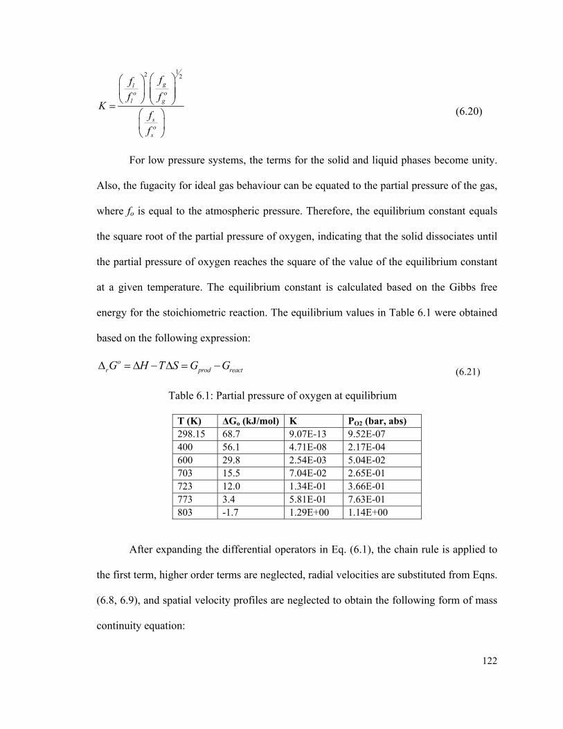
122

12 2gl

o ol g

so

s

ff

f fK

f

f

(6.20)

For low pressure systems, the terms for the solid and liquid phases become unity.

Also, the fugacity for ideal gas behaviour can be equated to the partial pressure of the gas,

where fo is equal to the atmospheric pressure. Therefore, the equilibrium constant equals

the square root of the partial pressure of oxygen, indicating that the solid dissociates until

the partial pressure of oxygen reaches the square of the value of the equilibrium constant

at a given temperature. The equilibrium constant is calculated based on the Gibbs free

energy for the stoichiometric reaction. The equilibrium values in Table 6.1 were obtained

based on the following expression:

or prod reactG H T S G G

(6.21)

Table 6.1: Partial pressure of oxygen at equilibrium

T (K) ΔGo (kJ/mol) K PO2 (bar, abs) 298.15 68.7 9.07E-13 9.52E-07 400 56.1 4.71E-08 2.17E-04 600 29.8 2.54E-03 5.04E-02 703 15.5 7.04E-02 2.65E-01 723 12.0 1.34E-01 3.66E-01 773 3.4 5.81E-01 7.63E-01 803 -1.7 1.29E+00 1.14E+00

After expanding the differential operators in Eq. (6.1), the chain rule is applied to

the first term, higher order terms are neglected, radial velocities are substituted from Eqns.

(6.8, 6.9), and spatial velocity profiles are neglected to obtain the following form of mass

continuity equation:

123

2 2 2 2

2 23 3 3 3 3 3 3 3 3 3

10.5 3 3 3 6

3.5

s ts s l f g f s sl

s

R R R R R R R Ru y y D

f a t f a f a t f a t f a

Rr

(6.22)

6.1.2 Energy Equation

The thermal energy change within a particle balances the energy gained through

the liquid phase by conduction, energy transported by the released gas phase and the

thermal energy of reaction. It is assumed that heat is transported by conduction through

the liquid phase and convection through the gas bubbles. Also, it is assumed that the net

exchange of thermal radiation between the liquid and solid bodies is relatively small and

that radiation heat exchange can be lumped together with an equivalent heat transfer

coefficient to arrive at the following expression:

ss ps l l g pg g g s

TC T C u T H Rr

t

(6.23)

Expanding the differential operators and disregarding higher order terms leads to the

following form of the energy equation:

2 gs l ls gp pg g s

TT TC C u H Rr

t R R R

(6.24)

6.1.3 Momentum Equation

Consider the phenomenon of solid particles falling in a quiescent fluid and

experiencing both phase change and chemical reaction in the range of mid Stefan numbers

(Ste ≈ 1). The dynamics of the solid particle has characteristics similar to those observed

by Gan et al. [98, 99]. The fluid surrounding the particle is assumed quiescent as the

124

particle shrinks. A variable velocity profile develops with time. In this analysis, assume

that the particle remains spherical through the period of decomposition and the velocity of

the particle is determined by the balance of drag and buoyancy forces due to the

differences of the density of solid-liquid phases as described by the following Navier-

Stokes equation:

f fs s su u u s Ft

(6.25)

For steady flow at low Reynolds numbers, the transient term /u dt , convective

acceleration and the second order tensor s (pressure gradient) are neglected, and the

balance of momentum of the particle yields:

0D s s l PG VM LF V g F F F (6.26)

where the forces acting on the particle are drag, buoyancy, pressure gradient, virtual mass

and lift.

The process of decomposition occurs fast enough for the force of hydrodynamic

pressure gradient, FPG, to be negligible. Since the particle is not accelerated at a high rate,

the virtual mass force FVM is neglected. Furthermore, since there is no component of fluid

velocity perpendicular to the main particle displacement, the lift force FL is neglected.

0D s s lF V g (6.27)

Using the solution to the Stokes equation in the flow regime of Re < 0.2, the drag

coefficient is calculated by equating the drag equation to the Stokes equation:

125

3 34 43 36 st s lu R R g R g (6.28)

leading to the following terminal velocity of the particle:

22

9st p l

Ru g

(6.29)

In order to complete the problem formulation, boundary and initial conditions are

required.

6.1.4 Boundary and Initial Conditions

The concentrations of products within the control volume are assumed zero at the

moment when the particle reaches the terminal velocity. Also, a zero radial temperature

gradient is assumed in the solid particle, and the Stefan condition applies to the liquid

phase exclusively. The following initial and boundary conditions are obtained:

Cl = 0 at t = 0 (6.30)

Cg = 0 at t =0 (6.31)

Rr = 0 at t = 0 (6.32)

T = Tm at R = 0 (6.33)

T = To at R = a (6.34)

ll sl l

dTRh

t dR

(at R(t) ) (6.35)

In the next section, these governing equations will be re-written in non-dimensional form.

126

6.1.5 Dimensional Analysis and Scaling

The dimensional analysis of transient decomposition of solid particles via

equilibrium follows the methodology explained by Ruzicka [106]. Dimensional analysis

of the governing equations provides the order of magnitude of individual terms. The mass

continuity equation is characterized by the parameters (D, ρ) and the dimensional

variables (t, m, R, u) that contain the fundamental physical units (m, u). There exist two

dimensionless quantities that define the phenomena. In fundamental units, the mass

continuity equation can be written as:

2 2 2

3 3 3 3

1L L L L L L DLV Rr

L t L L t L t L (6.36)

which simplifies to:

21

m

DaPe

(6.37)

where Da = ((Rr*t)/ρo)1/2. Hydrodynamic convection balances the rate of reaction and the

diffusive transport by having similar impact in the overall phenomenon.

Similarly, the energy equation is characterized by the parameters (∆H, Cp, ρ) and

the dimensional variables (T, t, m, R, u) that are constituted in the fundamental physical

units (T, m, u). This indicates that there exist two dimensionless quantities that define the

phenomena. In fundamental units, the energy equation can be written as:

2p p

T H Rr T TV

t C C L L

(6.38)

127

2

T RrT T TV

t L L

(6.39)

11 1

T

DaPe

(6.40)

Following the mass continuity analysis, the PeT term is also small and therefore

neglected in the solution of the energy equations.

In scaling of the state equations, the following dimensionless variables are

adopted:

2s psC a

t t

(6.41)

Rr

a (6.42)

122

s

so sl

Rr aDa

C D

(6.43)

st

sl

u aU

D (6.44)

s m

o m

T T

T T

(6.45)

l m

o m

T T

T T

(6.46)

The mass, energy and momentum equations become:

128

2 2 2 2(3 3 10.5) 3 6 3.5s sl g

ry y r Lew U r Da

t

(6.47)

1 2 gg

s s

r rrr y

t Ste t r t

(6.48)

32

s stuR e

g

(6.49)

where

fs

s

,

gg

s

, and

2s

o m

H Rr arr

T T

are dimensionless variables. These

equations are solved subject to the following non-dimensional initial and boundary

conditions:

= 0 at t* = 0 (Ts = Tm) (6.50)

x = 0 at t* = 0 (Rrs = 0) (6.51)

U* = ut at t* = 0 (Vs = Vt) (6.52)

= at r = 0 (Tl = Ts) (6.53)

= 1 at r= 1 (Tl = To) (6.54)

r

= 0 at r=1 (Tl = Ts) (6.55)

r dSte

t dr

(Stefan condition) (6.56)

129

Assume a quadratic profile for the liquid phase temperature with the following

conditions:

at r = 0 (6.57)

1 at r =1 (6.58)

0r

at r =1 (6.59)

Therefore, this leads to the following profile for the dimensionless liquid temperature:

21 2 1r r (6.60)

This completed the model of the transport phenomena. In the next chapter, a case study of

hydrogen utilization and application to trains will be presented.

130

Chapter 7 - Results and Discussions _______________________________________________________________________________

7.1 Pathways of Chemical Decomposition

Two mechanistic approaches to the decomposition of copper oxychloride in prior

chapter indicated that one of the paths may prevail depending on the temperature, pressure

and side products/reactants present in the sample that result from the presence of

unreacted products from hydrolysis. A potential mass imbalance occurs as undesirable

side reactions arise in the oxygen reactor with chlorine leaving the reactor in gaseous

form, and CuCl2 with the solids. In complete decomposition, the oxygen production

reaction results in a pure liquid phase of molten CuCl and oxygen. Instead, the conversion

rates obtained in experiments and measured from TGA conducted in this thesis indicated

values between 65 and 95%, indicating that the conversion follows the competing

reactions discussed (path A and path B) and results in a mix of CuCl, CuCl2, Cl2 and O2 in

the product streams. It was found in the experiments that a gas mixture with oxygen,

chlorine and CuCl vapour was produced.

The decomposition of CuO*CuCl2 appeared to start at different temperatures,

depending upon the temperature of the environment. In batch reactor experiments, the

sample released oxygen at an initially high rate, while semi-batch experiments indicated

an initially low rate of oxygen formation, followed by a trend to steady state. This trend

occurred at a later time in lower temperature experiments.

131

Fig. 7.1 Oxygen formation from decomposition of a 50 g. batch of CuO*CuCl2 at

570 oC and 1.003 atm

Figure 7.1 illustrates the oxygen evolution vs. time from the batch reaction

experiments. The readings corresponded to a decomposition experiment where a well-

mixed sample of CuO powder and dehydrated CuCl2 powder was heated to 570 oC.

Decomposition of the 50 g sample was monitored for one hour until the oxygen readings

were undetectable. With the reactor temperature set to reach 570 oC in the sample, the

decomposition appeared to start at 500 oC as indicated in Fig. 7.1. The decomposition of

CuO*CuCl2, as measured from oxygen formation, occurred consistently in all

experiments with three characteristic stages, 1) initial rush with high rate of oxygen

generation; 2) a brief plateau where oxygen generation seemed to stabilize; and 3) an

asymptotic decay of the rate of decomposition where oxygen generation slowly falls to

close to zero. The time distributions of these phenomena indicated that the initial increase,

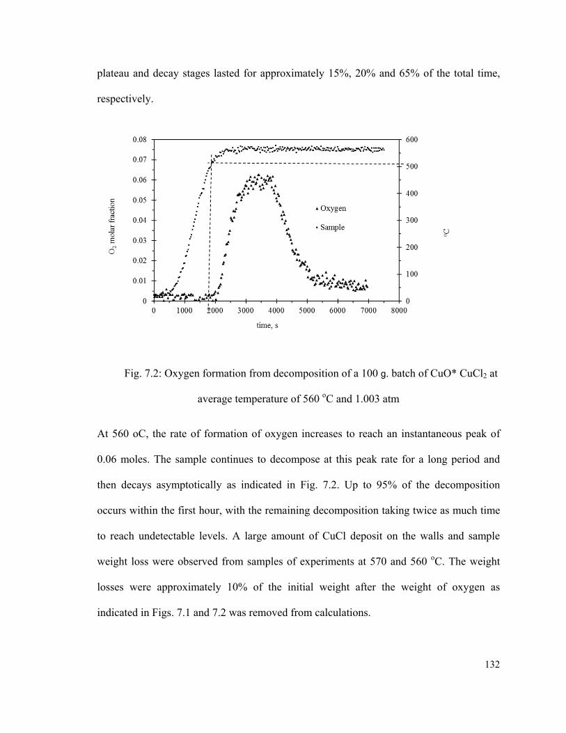
132

plateau and decay stages lasted for approximately 15%, 20% and 65% of the total time,

respectively.

Fig. 7.2: Oxygen formation from decomposition of a 100 g. batch of CuO* CuCl2 at

average temperature of 560 oC and 1.003 atm

At 560 oC, the rate of formation of oxygen increases to reach an instantaneous peak of

0.06 moles. The sample continues to decompose at this peak rate for a long period and

then decays asymptotically as indicated in Fig. 7.2. Up to 95% of the decomposition

occurs within the first hour, with the remaining decomposition taking twice as much time

to reach undetectable levels. A large amount of CuCl deposit on the walls and sample

weight loss were observed from samples of experiments at 570 and 560 oC. The weight

losses were approximately 10% of the initial weight after the weight of oxygen as

indicated in Figs. 7.1 and 7.2 was removed from calculations.

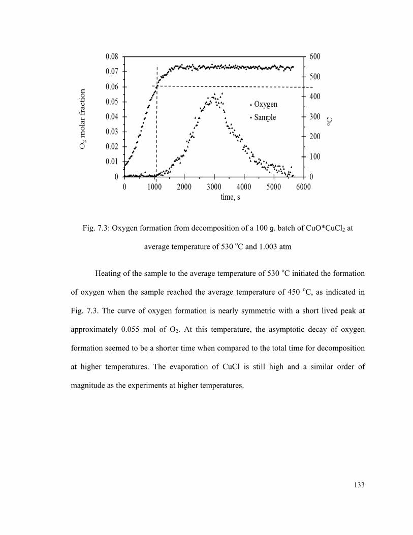
133

Fig. 7.3: Oxygen formation from decomposition of a 100 g. batch of CuO*CuCl2 at


Heating of the sample to the average temperature of 530 oC initiated the formation

of oxygen when the sample reached the average temperature of 450 oC, as indicated in

Fig. 7.3. The curve of oxygen formation is nearly symmetric with a short lived peak at

approximately 0.055 mol of O2. At this temperature, the asymptotic decay of oxygen

formation seemed to be a shorter time when compared to the total time for decomposition

at higher temperatures. The evaporation of CuCl is still high and a similar order of

magnitude as the experiments at higher temperatures.

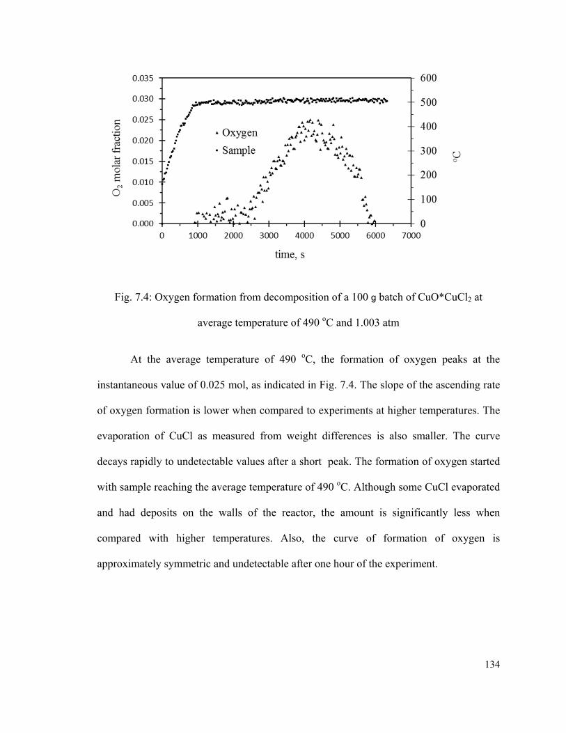
134

Fig. 7.4: Oxygen formation from decomposition of a 100 g batch of CuO*CuCl2 at


At the average temperature of 490 oC, the formation of oxygen peaks at the

instantaneous value of 0.025 mol, as indicated in Fig. 7.4. The slope of the ascending rate

of oxygen formation is lower when compared to experiments at higher temperatures. The

evaporation of CuCl as measured from weight differences is also smaller. The curve

decays rapidly to undetectable values after a short peak. The formation of oxygen started

with sample reaching the average temperature of 490 oC. Although some CuCl evaporated

and had deposits on the walls of the reactor, the amount is significantly less when

compared with higher temperatures. Also, the curve of formation of oxygen is

approximately symmetric and undetectable after one hour of the experiment.

135

Fig. 7.5: Oxygen yield and CuCl weight loss due to evaporation from samples of 100 g of

Cuo*CuCl2 at different temperatures

Higher oxygen yields from decomposition at higher average temperatures resulted in

in a trend of high CuCl evaporation as indicated in Fig. 7.5. The rate of evaporation does

not decay in proportion to the yield as seen from the curve in Fig. 7.6. A trend to increase

the net amount of CuCl evaporated at lower temperatures may be due to longer times

required for decomposition. Thus, it was inhered that CuCl vapour is carried away with

oxygen gas and also evaporated from the surface. Although less gas is produced at lower

temperatures, still the weight losses of CuCl vapour are comparable to losses at high

temperatures.

Figure 7.6 indicates the results of decomposition of a mix of CuO*CuCl2 in a semi-

batch reactor configuration. The sample was supplied into a molten bath containing 0.5

mol of CuCl at the average temperature of 490 oC. The data, averaged over periods of five

minutes and three experiments at each temperature, were collected for a total of five to six

hours. It provides an indication of the behaviour of the decomposition reactions with

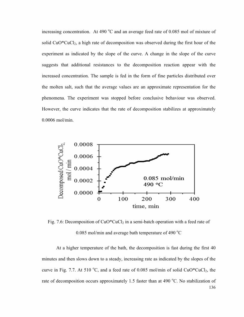
136

increasing concentration. At 490 oC and an average feed rate of 0.085 mol of mixture of

solid CuO*CuCl2, a high rate of decomposition was observed during the first hour of the

experiment as indicated by the slope of the curve. A change in the slope of the curve

suggests that additional resistances to the decomposition reaction appear with the

increased concentration. The sample is fed in the form of fine particles distributed over

the molten salt, such that the average values are an approximate representation for the

phenomena. The experiment was stopped before conclusive behaviour was observed.

However, the curve indicates that the rate of decomposition stabilizes at approximately

0.0006 mol/min.


0.085 mol/min and average bath temperature of 490 oC

At a higher temperature of the bath, the decomposition is fast during the first 40

minutes and then slows down to a steady, increasing rate as indicated by the slopes of the

curve in Fig. 7.7. At 510 oC, and a feed rate of 0.085 mol/min of solid CuO*CuCl2, the

rate of decomposition occurs approximately 1.5 faster than at 490 oC. No stabilization of

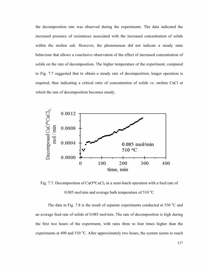
137

the decomposition rate was observed during the experiments. The data indicated the

increased presence of resistances associated with the increased concentration of solids

within the molten salt. However, the phenomenon did not indicate a steady state

behaviour that allows a conclusive observation of the effect of increased concentration of

solids on the rate of decomposition. The higher temperature of the experiment, compared

to Fig. 7.7 suggested that to obtain a steady rate of decomposition, longer operation is

required, thus indicating a critical ratio of concentration of solids vs. molten CuCl at

which the rate of decomposition becomes steady.



The data in Fig. 7.8 is the result of separate experiments conducted at 530 oC and

an average feed rate of solids of 0.085 mol/min. The rate of decomposition is high during

the first two hours of the experiment, with rates three to four times higher than the

experiments at 490 and 510 oC. After approximately two hours, the system seems to reach

138

steady state conditions where the rate of oxygen and molten CuCl generation balances the

rate of addition of solids at 0.085 mol/min. An approximation to a steady state condition

can be observed between the second and fifth hours of experimentation. This observation

indicates that the resistances to chemical decomposition reach a critical point due to the

concentration of solids versus the molten liquid and gas evolution rates. After

approximately the fourth hour, the slope of the curve started to change and became

negative with a progressive accentuation of the effect. The change of slope is presumably

due to the increased presence of solids fed into the molten salt that eventually inhibit the

rate at which heat reaches the particles. This effect contributed to the increased presence

of gas bubbles and led to reduced heat transfer within the system and longer time for heat

to reach the solid particles.



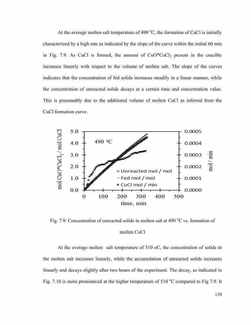
139

At the average molten salt temperature of 490 oC, the formation of CuCl is initially

characterized by a high rate as indicated by the slope of the curve within the initial 60 min

in Fig. 7.9. As CuCl is formed, the amount of CuO*CuCl2 present in the crucible

increases linearly with respect to the volume of molten salt. The slope of the curves

indicates that the concentration of fed solids increases steadily in a linear manner, while

the concentration of unreacted solids decays at a certain time and concentration value.

This is presumably due to the additional volume of molten CuCl as inferred from the

CuCl formation curve.


molten CuCl

At the average molten salt temperature of 510 oC, the concentration of solids in

the molten salt increases linearly, while the accumulation of unreacted solids increases

linearly and decays slightly after two hours of the experiment. The decay, as indicated in

Fig. 7.10 is more pronounced at the higher temperature of 510 oC compared to Fig 7.9. It

140

can be observed that CuO*CuCl2 decomposes slightly faster at this higher temperature as

indicated by a larger slope of the CuCl formation curve.


molten CuCl

The formation of CuCl reaches a steady state condition at approximately 0.0018

mol/min with an average molten CuCl temperature of 530 oC. The rate of formation

decays after some time with the addition of more CuO*CuCl2 as indicated in Fig. 7.11.

This is expected by the decomposition of solids indicated in Fig. 7.9. At this temperature,

the concentration of solids fed to the reactor vs. CuCl is no longer linear, The

accumulation of unreacted solids decays with the generation of CuCl. This decay is

however due to the increased volume of molten salt since a plot of absolute accumulation

of solids vs. time indicated that it remains linear. Thus, it can be inferred that the

decomposition rate decays not only as a consequence of the concentration of solids

increasing, and also, presumably as a result of the increased presence of gas bubbles in the

molten salt.

141

Fig. 7.11: Concentration of unreacted solids in molten salt at 530 oC with formation of

molten CuCl

The accumulation of unreacted solid is higher with lower molten salt temperatures

as indicated in Fig. 7.12. The ratio of unreacted to fed CuO*CuCl2 decays linearly with

time and seems to reach steady state, indicating that a large portion of solids remains

unreacted with average temperatures at 490 oC. At the higher temperature of 510 oC, the

ratio of unreacted to fed solids continued to decay, with no indication of stabilization

within the time of experiments. A large difference of the ratios of accumulation exists

with respect to experiments at the average temperature of 530 oC. The ratio of unreacted

solids decays rapidly and seemed to reach steady state after 350 min. There is also a trend

to increase in the concentration of unreacted CuO*CuCl2 at the end of the experiments.

This effect can be inferred from the decay in decomposition of solids and formation of

molten CuCl as indicated in Figs. 7.8 and 7.11.

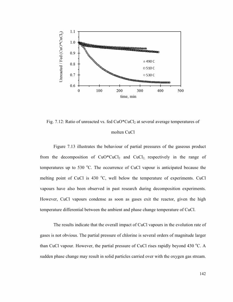
142

Fig. 7.12: Ratio of unreacted vs. fed CuO*CuCl2 at several average temperatures of

molten CuCl

Figure 7.13 illustrates the behaviour of partial pressures of the gaseous product

from the decomposition of CuO*CuCl2 and CuCl2, respectively in the range of

temperatures up to 530 oC. The occurrence of CuCl vapour is anticipated because the

melting point of CuCl is 430 oC, well below the temperature of experiments. CuCl

vapours have also been observed in past research during decomposition experiments.

However, CuCl vapours condense as soon as gases exit the reactor, given the high

temperature differential between the ambient and phase change temperature of CuCl.

The results indicate that the overall impact of CuCl vapours in the evolution rate of

gases is not obvious. The partial pressure of chlorine is several orders of magnitude larger

than CuCl vapour. However, the partial pressure of CuCl rises rapidly beyond 430 oC. A

sudden phase change may result in solid particles carried over with the oxygen gas stream.

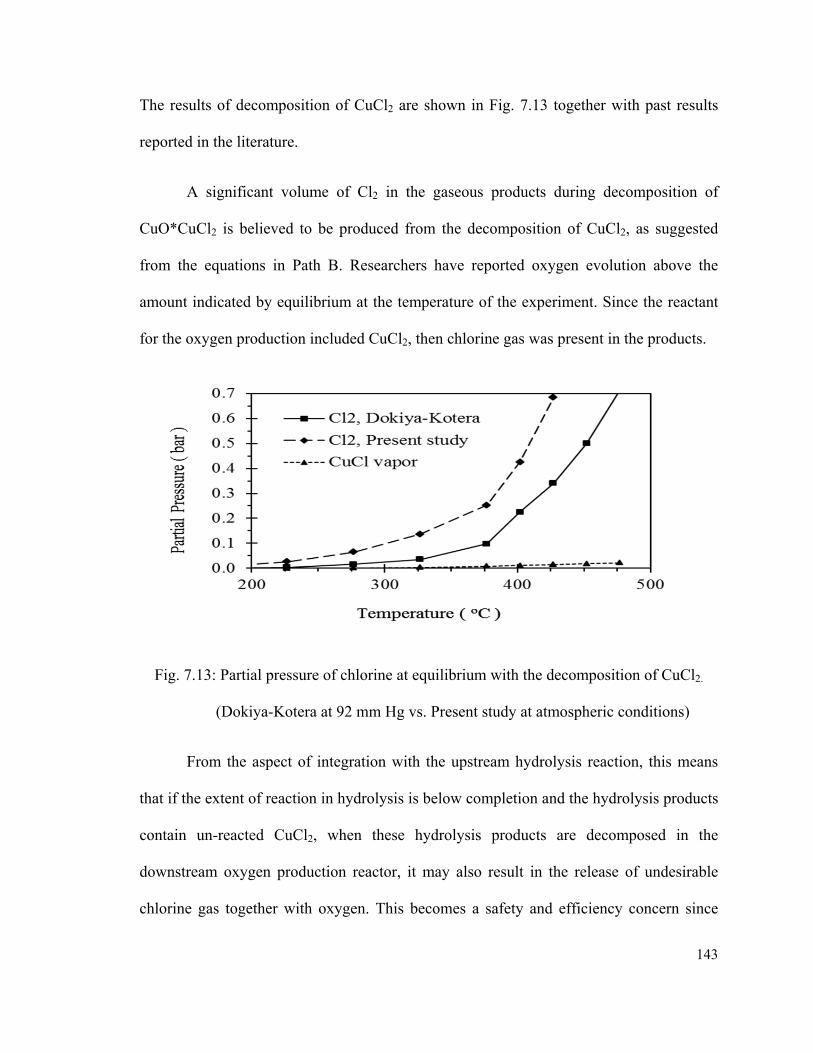
143

The results of decomposition of CuCl2 are shown in Fig. 7.13 together with past results

reported in the literature.

A significant volume of Cl2 in the gaseous products during decomposition of

CuO*CuCl2 is believed to be produced from the decomposition of CuCl2, as suggested

from the equations in Path B. Researchers have reported oxygen evolution above the

amount indicated by equilibrium at the temperature of the experiment. Since the reactant

for the oxygen production included CuCl2, then chlorine gas was present in the products.

Fig. 7.13: Partial pressure of chlorine at equilibrium with the decomposition of CuCl2.

(Dokiya-Kotera at 92 mm Hg vs. Present study at atmospheric conditions)

From the aspect of integration with the upstream hydrolysis reaction, this means

that if the extent of reaction in hydrolysis is below completion and the hydrolysis products

contain un-reacted CuCl2, when these hydrolysis products are decomposed in the

downstream oxygen production reactor, it may also result in the release of undesirable

chlorine gas together with oxygen. This becomes a safety and efficiency concern since

144

additional steps and energy are required to separate chlorine from the oxygen and recycle

the gases back through the cycle. The experimental results are consistent with proof-of-

principle tests performed by Serban et al. [59] in a thermogravimetric analysis of the

decomposition of CuCl2. The experiments used 50 mg of CuCl2 heated to temperatures of

600 oC and the authors reported weight losses of 8.6 mg, equivalent on a stoichiometric

basis to a 63% chlorine release.

Figure 4.5 shows the thermodynamic analysis of the decomposition of CuCl2. At

the temperature of 430 oC, the Gibbs energy of decomposition of CuCl2 becomes negative

and thereby the reaction becomes spontaneous. Within that same range of temperature, the

reaction of copper oxide with chlorine is also spontaneous as indicated by the Gibbs

energy in Fig. 4.5. To visualize the compositions in the output stream of oxygen

production, the thermodynamic results for the competing reactions in paths A and B are

also shown in Fig. 4.5. The Gibbs energy curves also provide a comparison with

variations 1 and 2 of the Cu-Cl cycle, specifically for the decomposition of copper

oxychloride. As CuO reacts with chlorine, some CuCl and CuCl2 form and oxygen is

released. The negative Gibbs energy of reaction between CuO and Cl2 favors the

formation of CuCl2 over CuCl as indicated in Fig. 4.6. When CuCl2 is entrained by the

copper oxychloride in the products of hydrolysis, it continues to decompose

spontaneously beyond 470 oC and beyond what can possibly react with the available CuO,

resulting in chlorine gas evolution together with oxygen.

To study the effect of operating pressure on the chemical streams among integrated

reactions, the Gibbs energy of the competing reactions is used at low and standard

145

pressures in Fig. 4.4. At 0.1 bar, the decomposition of CuCl2 reaches equilibrium at 370

oC and becomes spontaneous above that temperature. By comparison, the decomposition

of Cu2OCl2 at the same temperature and pressure is not spontaneous. Experimental results

indicated that copper oxychloride is stable up to the temperature of 430 oC. Between 435

oC and 470 oC, it decomposes with the formation of CuCl, CuCl2 and chlorine. The

mechanistic analysis suggested by path B indicates that the released Cl2 then reacts with

CuO to produce CuCl and O2. The Gibbs free energy of reaction in Fig. 4.6 indicates that

the second reaction occurs as soon as chlorine is available in the system. Also, the slope

of the Gibbs curve in Fig. 4.7 indicates that more CuCl2 decomposes at low pressure and

within the same temperature range compared to operating at atmospheric pressure.

Operating at pressures below atmospheric pressure does not change the mechanics of the

reactions. Figure 4.7 also shows (through the difference of slopes between the curves at 1

bar and 0.1 bar) that the advantages of lowering the temperature threshold of the oxygen

production reactor may be compromised with the additional mechanical energy

requirement and with the presence of more chlorine in the gas products.

The solid products of oxygen production from the mixture of CuO and CuCl2 appear

as a black hard sintered material, as shown in Fig. 7.14. The solid product of

decomposition of the CuO*CuCl2 mixture has identical physical appearance samples from

the decomposition of copper oxychloride. The solids are mildly hygroscopic, and they can

be pulverized with the utilization of mechanical effort.

The products of decomposition have a fragile solid appearance once at ambient

temperature. The solid is porous and breaks with medium effort, indicating that an

146

additional process must be introduced for the cycle integration before the downstream

electrolysis reaction.

Fig. 7.14: Sample of products of copper oxychloride decomposition

The cake of solid CuCl must be mechanically removed from the oxygen production

reactor and then pulverized. In this condition, the solids can be dissolved in water and HCl

for the preparation of aqueous solution needed by the electrolytic hydrogen production

cell. Since the CuCl must be first solidified, thermal energy recuperated from the phase

change of molten salts from the decomposition reactor can be used elsewhere in the Cu-Cl

cycle for thermal energy integration.

The analysis based on XRD powder techniques of the composition of the solid

product of the oxygen production resulted in patterns of Fig. 7.15. The spectrum revealed

a mixture of solids where copper oxide, copper (II) chloride and copper (I) chloride were

present. The major product component is CuCl with mixed quantities of CuCl2 and CuO.

The analysis of the relative amounts of XRD peaks with reference to standard samples

147

indicated an approximate composition of solids of 70% CuCl and 20% CuCl2. The results

of XRD analysis appear to confirm the pathways of the decomposition reaction as

discussed above with a combination of products of paths A and B.

From the aspect of the process integration, Fig. 7.16 shows that the un-reacted CuCl2

in the hydrolysis reactor may not be fully decomposed in its downstream oxygen

production reaction. Therefore, CuCl2 may be further carried by CuCl to the downstream

cell for the electrolytic hydrogen production. This same situation occurs with CuO present

in the stream output from the oxygen reactor. This situation significantly reduces the

possibility of adopting certain variations of integration of the Cu-Cl cycle.

Fig. 7.15: XRD Reflections of products of decomposition of copper oxychloride at 550

oC.

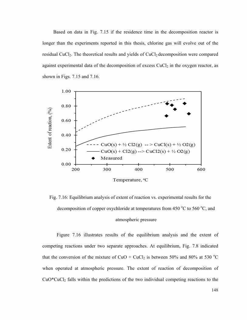
148

Based on data in Fig. 7.15 if the residence time in the decomposition reactor is

longer than the experiments reported in this thesis, chlorine gas will evolve out of the

residual CuCl2. The theoretical results and yields of CuCl2 decomposition were compared

against experimental data of the decomposition of excess CuCl2 in the oxygen reactor, as

shown in Figs. 7.15 and 7.16.

Fig. 7.16: Equilibrium analysis of extent of reaction vs. experimental results for the

decomposition of copper oxychloride at temperatures from 450 oC to 560 oC, and

atmospheric pressure

Figure 7.16 illustrates results of the equilibrium analysis and the extent of

competing reactions under two separate approaches. At equilibrium, Fig. 7.8 indicated

that the conversion of the mixture of CuO + CuCl2 is between 50% and 80% at 530 oC

when operated at atmospheric pressure. The extent of reaction of decomposition of

CuO*CuCl2 falls within the predictions of the two individual competing reactions to the

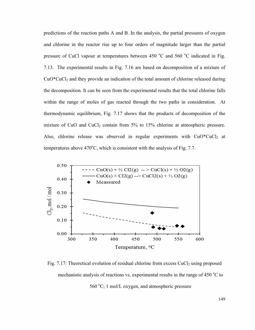
149

predictions of the reaction paths A and B. In the analysis, the partial pressures of oxygen

and chlorine in the reactor rise up to four orders of magnitude larger than the partial

pressure of CuCl vapour at temperatures between 450 oC and 560 oC indicated in Fig.

7.13. The experimental results in Fig. 7.16 are based on decomposition of a mixture of

CuO*CuCl2 and they provide an indication of the total amount of chlorine released during

the decomposition. It can be seen from the experimental results that the total chlorine falls

within the range of moles of gas reacted through the two paths in consideration. At

thermodynamic equilibrium, Fig. 7.17 shows that the products of decomposition of the

mixture of CuO and CuCl2 contain from 5% to 15% chlorine at atmospheric pressure.

Also, chlorine release was observed in regular experiments with CuO*CuCl2 at

temperatures above 470oC, which is consistent with the analysis of Fig. 7.7.

Fig. 7.17: Theoretical evolution of residual chlorine from excess CuCl2 using proposed

mechanistic analysis of reactions vs. experimental results in the range of 450 oC to

560 oC; 1 mol/L oxygen, and atmospheric pressure

150

The analysis indicates that at equilibrium, the decomposition reaction may result

in a complex mixture of CuO*CuCl2, CuO, CuCl, CuCl2, O2 and Cl2, and other species

that depend upon the contents of hydrolysis products. The results suggested that the

reverse reaction must also be considered. Experiments to reproduce a reverse reaction

with CuCl and oxygen did not result in production of copper oxychloride. However, the

presence of CuCl2 and CuO may result in the formation of copper oxychloride that will

decompose given the spontaneity of the decomposition reaction, according to the Gibbs

energy of reaction, at temperatures beyond 500 oC. The standard Gibbs free energy of the

reverse reaction in Fig. 4.3 suggests the spontaneity of the reaction in the temperature

range, presumably due to the fact that the Gibbs free energy is negative for this reaction at

the reaction conditions. This does not conflict with the experimental results because the

oxygen partial pressure in the experiments was below the standard value with a partial

pressure of O2 in the experiments below 1.0 bar, which may significantly lower the

possibility of a reverse reaction based on the Gibbs free energy. This observation also

suggests that the reverse reaction may be a function of the oxygen pressure in the reactor.

7.2 Reversibility of Decomposition Reaction

The experiments of the reverse reaction did not result in detectable observations

during preheating of CuCl and O2. Furthermore, the XRD reflections (see XRD results in

Figs. 7.18 – 7.21) did not show traces of Cu2OCl2 after experiments. Several conditions

can lead to these results. For example, the reverse reaction below 450 oC is too slow to be

measured. The sensitivity of the oxygen sensor and XRD may not be sufficient to detect

the composition change. Also, as suggested by the negative value of Gibbs free energy,

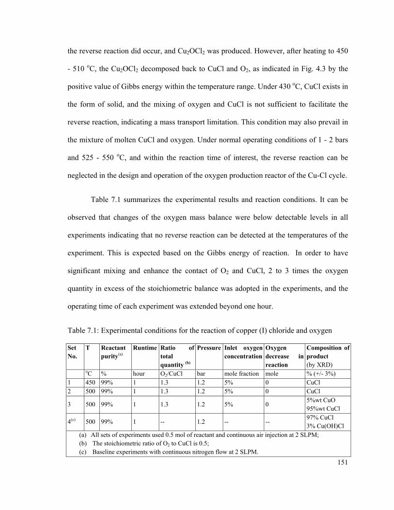
151

the reverse reaction did occur, and Cu2OCl2 was produced. However, after heating to 450

- 510 oC, the Cu2OCl2 decomposed back to CuCl and O2, as indicated in Fig. 4.3 by the

positive value of Gibbs energy within the temperature range. Under 430 oC, CuCl exists in

the form of solid, and the mixing of oxygen and CuCl is not sufficient to facilitate the

reverse reaction, indicating a mass transport limitation. This condition may also prevail in

the mixture of molten CuCl and oxygen. Under normal operating conditions of 1 - 2 bars

and 525 - 550 oC, and within the reaction time of interest, the reverse reaction can be

neglected in the design and operation of the oxygen production reactor of the Cu-Cl cycle.

Table 7.1 summarizes the experimental results and reaction conditions. It can be

observed that changes of the oxygen mass balance were below detectable levels in all

experiments indicating that no reverse reaction can be detected at the temperatures of the

experiment. This is expected based on the Gibbs energy of reaction. In order to have

significant mixing and enhance the contact of O2 and CuCl, 2 to 3 times the oxygen

quantity in excess of the stoichiometric balance was adopted in the experiments, and the

operating time of each experiment was extended beyond one hour.

Table 7.1: Experimental conditions for the reaction of copper (I) chloride and oxygen

Set No.

T Reactant purity(a)

Runtime Ratio of total quantity (b)

Pressure Inlet oxygen concentration

Oxygen decrease in reaction

Composition of product (by XRD)

oC % hour O2/CuCl bar mole fraction mole % (+/- 3%) 1 450 99% 1 1.3 1.2 5% 0 CuCl 2 500 99% 1 1.3 1.2 5% 0 CuCl

3 500 99% 1 1.3 1.2 5% 0 5%wt CuO 95%wt CuCl

4(c) 500 99% 1 -- 1.2 -- -- 97% CuCl 3% Cu(OH)Cl

(a) All sets of experiments used 0.5 mol of reactant and continuous air injection at 2 SLPM; (b) The stoichiometric ratio of O2 to CuCl is 0.5; (c) Baseline experiments with continuous nitrogen flow at 2 SLPM.

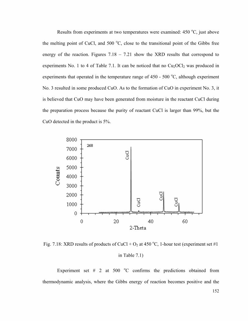
152

Results from experiments at two temperatures were examined: 450 oC, just above

the melting point of CuCl, and 500 oC, close to the transitional point of the Gibbs free

energy of the reaction. Figures 7.18 – 7.21 show the XRD results that correspond to

experiments No. 1 to 4 of Table 7.1. It can be noticed that no Cu2OCl2 was produced in

experiments that operated in the temperature range of 450 - 500 oC, although experiment

No. 3 resulted in some produced CuO. As to the formation of CuO in experiment No. 3, it

is believed that CuO may have been generated from moisture in the reactant CuCl during

the preparation process because the purity of reactant CuCl is larger than 99%, but the

CuO detected in the product is 5%.

Fig. 7.18: XRD results of products of CuCl + O2 at 450 oC, 1-hour test (experiment set #1

in Table 7.1)

Experiment set # 2 at 500 oC confirms the predictions obtained from

thermodynamic analysis, where the Gibbs energy of reaction becomes positive and the

153

reaction is not spontaneous. CuCl remained unchanged through the experiment as

indicated from the XRD analysis in Fig. 7.18. No further experiments were performed at

higher temperatures since the XRD and positive Gibbs energy of reaction from

thermodynamic analysis did not indicate the probability of this path occurring at higher

temperature.

Fig. 7.19: XRD results of products of CuCl + O2 at 500 oC, 1 hour test (experiment set #2

in Table 7.1)

The composition of the reactant CuCl for experiment No. 3 was analyzed to

determine the level of impurity. As shown in Fig. 7.14, the only impurity in CuCl was

found to be CuO-HCl, which may generate CuO through the following reaction discussed

by Ramamurthy and Secco [63]:

2CuOHCl = CuO + CuCl2 + H2O (7.1)

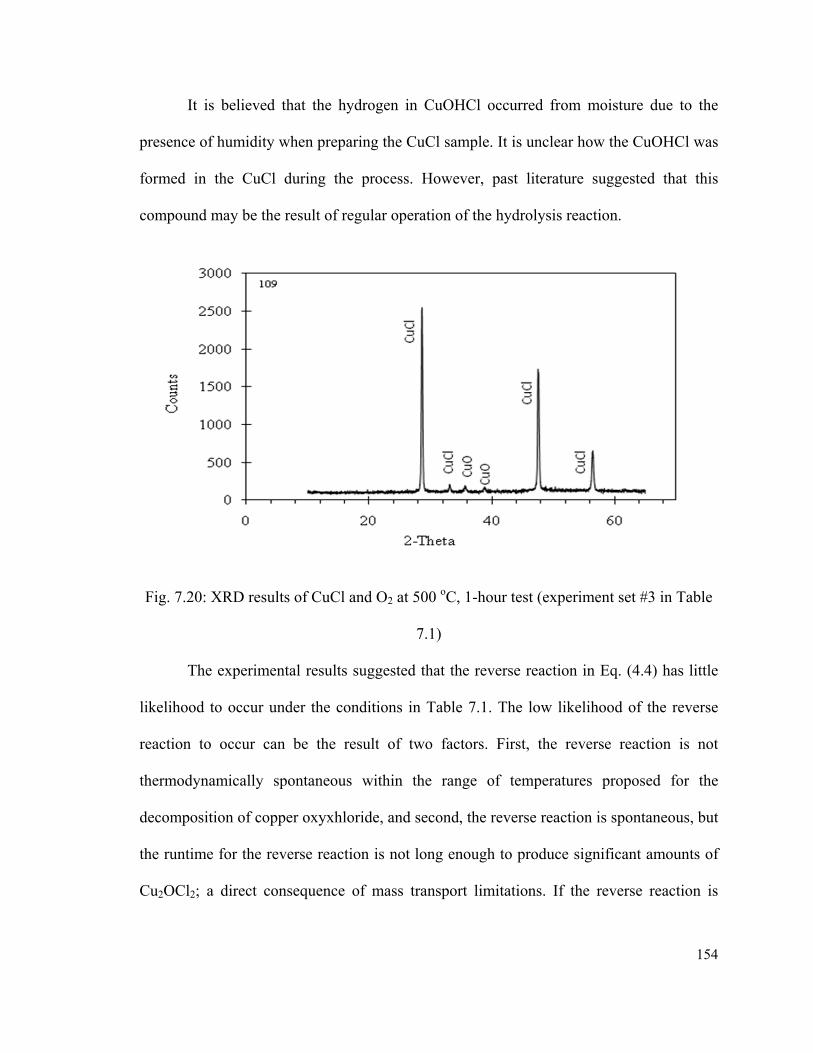
154

It is believed that the hydrogen in CuOHCl occurred from moisture due to the

presence of humidity when preparing the CuCl sample. It is unclear how the CuOHCl was

formed in the CuCl during the process. However, past literature suggested that this

compound may be the result of regular operation of the hydrolysis reaction.

Fig. 7.20: XRD results of CuCl and O2 at 500 oC, 1-hour test (experiment set #3 in Table

7.1)

The experimental results suggested that the reverse reaction in Eq. (4.4) has little

likelihood to occur under the conditions in Table 7.1. The low likelihood of the reverse

reaction to occur can be the result of two factors. First, the reverse reaction is not

thermodynamically spontaneous within the range of temperatures proposed for the

decomposition of copper oxyxhloride, and second, the reverse reaction is spontaneous, but

the runtime for the reverse reaction is not long enough to produce significant amounts of

Cu2OCl2; a direct consequence of mass transport limitations. If the reverse reaction is

155

spontaneous, then the run time must be very long, or the equipment size must be very

large for the reverse reaction to produce measurable amounts of Cu2OCl2.

Experiment set # 4 resulted in solids with the presence of CuCl-OH as indicated in Fig.

7.21. Since the samples are prepared from commercial grade species, it is believed that

some humidity contamination may be present and this presumably is an explanation for

the presence of OH.

Fig. 7.21: Impurities in the CuCl reactant, molten at 500 oC (experiment set #4 in Table

7.1)

The above results and analysis of reaction paths, equilibrium and reverse reaction

provide valuable information for the modeling of the multiphase reacting system. At the

microscopic level, the system corresponds to the decomposition of solid reactant particles

156

and phase transition of a molten product at a gas-liquid-solid interface with kinetics

determined through a reaction rate expression.

7.3 Rate of Reaction

The products of experimental decomposition of 100 g samples of CuO*CuCl2

were first examined using XRD and Rietveld quantification. The quantification procedure

yielded in errors of +/- 10%. Figure 7.22 shows the spectrum obtained from XRD analysis

of a sample of unreacted CuO*CuCl2. The sample was prepared from species of CuO and

CuCl2 and well mixed in stoichiometric proportions. The Rietveld analysis from the XRD

spectrum in Fig 7.22 resulted in 24.92% CuCl2 and 75.06% CuO. Applying this

proportion to the original sample indicated a net error of +/- 7.5%. This magnitude of

error confirms the potential deviations expected from the analysis using a combination of

XRD and Rietveld quantification.

Fig. 7.22: X-Ray diffraction analysis of a standard sample of stoichiometric CuO*CuCl2

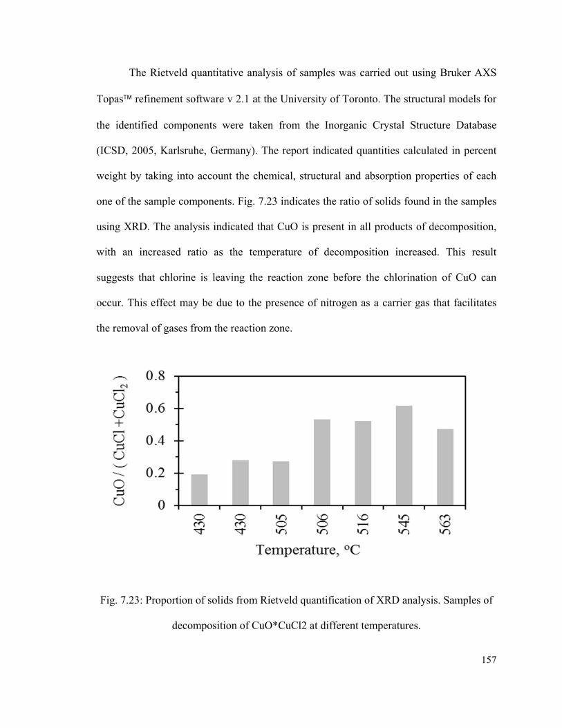
157

The Rietveld quantitative analysis of samples was carried out using Bruker AXS

Topas refinement software v 2.1 at the University of Toronto. The structural models for

the identified components were taken from the Inorganic Crystal Structure Database

(ICSD, 2005, Karlsruhe, Germany). The report indicated quantities calculated in percent

weight by taking into account the chemical, structural and absorption properties of each

one of the sample components. Fig. 7.23 indicates the ratio of solids found in the samples

using XRD. The analysis indicated that CuO is present in all products of decomposition,

with an increased ratio as the temperature of decomposition increased. This result

suggests that chlorine is leaving the reaction zone before the chlorination of CuO can

occur. This effect may be due to the presence of nitrogen as a carrier gas that facilitates

the removal of gases from the reaction zone.

Fig. 7.23: Proportion of solids from Rietveld quantification of XRD analysis. Samples of

decomposition of CuO*CuCl2 at different temperatures.

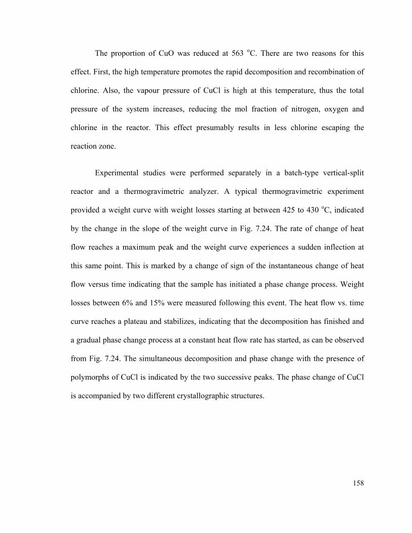
158

The proportion of CuO was reduced at 563 oC. There are two reasons for this

effect. First, the high temperature promotes the rapid decomposition and recombination of

chlorine. Also, the vapour pressure of CuCl is high at this temperature, thus the total

pressure of the system increases, reducing the mol fraction of nitrogen, oxygen and

chlorine in the reactor. This effect presumably results in less chlorine escaping the

reaction zone.

Experimental studies were performed separately in a batch-type vertical-split

reactor and a thermogravimetric analyzer. A typical thermogravimetric experiment

provided a weight curve with weight losses starting at between 425 to 430 oC, indicated

by the change in the slope of the weight curve in Fig. 7.24. The rate of change of heat

flow reaches a maximum peak and the weight curve experiences a sudden inflection at

this same point. This is marked by a change of sign of the instantaneous change of heat

flow versus time indicating that the sample has initiated a phase change process. Weight

losses between 6% and 15% were measured following this event. The heat flow vs. time

curve reaches a plateau and stabilizes, indicating that the decomposition has finished and

a gradual phase change process at a constant heat flow rate has started, as can be observed

from Fig. 7.24. The simultaneous decomposition and phase change with the presence of

polymorphs of CuCl is indicated by the two successive peaks. The phase change of CuCl

is accompanied by two different crystallographic structures.

159

Fig. 7.24: Measured weight percent of thermogravimetric decomposition vs. change of

heat flow.

The two structures appear at different levels of enthalpy of fusion and at

temperatures from 420 to 430 oC. The analysis of such structures is beyond the scope of

this thesis. This event is followed by a smooth curve of weight loss, indicative of CuCl

evaporation.

Additional detail of composition of gases and vapour that result from a

thermogravimetric decomposition can be obtained via a chromatographic analyser. The

analysis in this research is based only on weight loss curves and therefore a series of

stages are identified that represent characteristic phenomena of the decomposition. The

stages are characterized by humidity evaporation, decomposition, and CuCl evaporation.

160

Fig. 7.25: Stages of weight losses from TGA experiments during decomposition of

samples of CuO*CuCl2 at 430 oC

The TGA results were characterized by three stages as indicated in Fig 7.25. In

stage A, the losses corresponded with the approximated water content of the samples. The

samples of CuO*CuCl2 were stored in the oven for at least 24 hours prior to the

experiments. However, the highly hygroscopic properties of CuCl2 and the small size of

the sample used in TGA increase the possibility of water being adsorbed during

preparation of the sample before TGA experimentation. Stage B in Fig. 7.25 characterizes

the fast decomposition of CuO*CuCl2 with weight losses between 7 and 10% that closely

corresponds with oxygen content. Finally, stage C corresponds to the evaporation of

CuCl. Depending on the temperature of the experiment, when the remaining sample

weight reaches between 28% and 12%, the weight losses have stopped, indicating that

only non-volatile substances remain in the crucible.

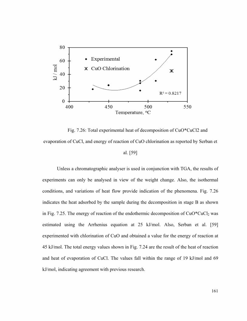
161

Fig. 7.26: Total experimental heat of decomposition of CuO*CuCl2 and

evaporation of CuCl, and energy of reaction of CuO chlorination as reported by Serban et

al. [59]

Unless a chromatographic analyser is used in conjunction with TGA, the results of

experiments can only be analysed in view of the weight change. Also, the isothermal

conditions, and variations of heat flow provide indication of the phenomena. Fig. 7.26

indicates the heat adsorbed by the sample during the decomposition in stage B as shown

in Fig. 7.25. The energy of reaction of the endothermic decomposition of CuO*CuCl2 was

estimated using the Arrhenius equation at 25 kJ/mol. Also, Serban et al. [59]

experimented with chlorination of CuO and obtained a value for the energy of reaction at

45 kJ/mol. The total energy values shown in Fig. 7.24 are the result of the heat of reaction

and heat of evaporation of CuCl. The values fall within the range of 19 kJ/mol and 69

kJ/mol, indicating agreement with previous research.

162

Fig. 7.27: Comparison of thermogravimetric decomposition of CuO*CuCl2 at

several temperatures

The thermogravimetric data corresponding to stage B in Fig. 7.25 is presented in

detail for decomposition at several temperatures in Fig. 7.27. At high temperatures, the

decomposition continues for a longer time to attain higher conversions. This is

presumably one reason for the overall lower rate of decomposition at high temperature.

Another possible reason is the increased presence of oxygen gas in the molten salt that

inhibits the transport of heat. Except for decomposition at 430 oC, the overall rate of

decomposition seems to be lower at higher temperatures, with a higher total conversion as

the temperature is increased.

The non-volatiles are presumed to be un-reacted CuO (copper oxide). This occurs

because solid CuO changes phase at 1326 oC and evaporates at 2000 oC. Experiments

163

conducted by Nixon et al. [43] indicated that O2 is consumed by the products of

decomposition to form CuO at higher temperatures and confirm the validity of this

assumption. This possibility is also explained based on the mechanistic analysis of two

parallel and competing reactions during decomposition as indicated in Eqns. (4.17) and

(4.18). Serban et al. [59] measured the kinetics of the reaction between Cl2 and CuO, and

estimated the rates of reaction at four different temperatures of 480, 490, 500 and 515°C.

The rate of reaction obtained for the reaction in Eq. (4.17) is a function of partial pressure

of Cl2 and O2, referring to the weight of CuO in the reactants.

122( ) ( ) 2( ) ( )* s molten g sCuO CuCl CuCl Cl CuO

(7.2)

1 12 2( ) 2( ) ( ) 2( )s g molten gCuO Cl CuCl O (7.3)

The rate of reaction equation was applied to the volumes of reactants in the TGA

experiments. Based on the results, given similar volumes of CuO, the decomposition of

CuO*CuCl2 is slower than the reaction of CuO and Cl2. This can be observed from Fig.

7.28 where the rates of reaction are plotted at different temperatures. This also implies

that the overall rate of reaction for CuO*CuCl2 decomposition is strongly impacted by the

decomposition of CuCl2, which becomes the controlling reaction. Further experimental

results by Marin et al. [44] confirmed the existence of at least two pathways for the

decomposition reaction, with remaining CuO a result of incomplete CuCl2 decomposition.

164

Fig. 7.28: Rate of reaction of CuO and Cl2 vs. rate of release of Cl2 from CuO*CuCl2

(TGA experiments [44, 55])

Readings from experiments at 450 oC, 490 oC, 510 oC and 530 oC resulted in the

remaining weights of CuO of 26%, 24%, 24% and 15.1% of the initial sample,

respectively. By performing a mass balance using the above mechanistic approach, the

mol ratio of un-reacted CuO resulting from thermogravimetric experiments can be

calculated based on the stoichiometric equation as follows:

122( ) ( ) 2( )* 2s molten gCuO CuCl CuCl O

(7.4)

With consideration of incomplete decomposition and residual reactants, the reaction is

described by the following expression:

122( ) ( ) 2( ) ( ) 2( )* 2 1 2s molten g s gCuO CuCl CuCl O CuO Cl

(7.5)

where the coefficient η < 0.5 is the molar percent of residual CuO within the temperature

range of experiments. The conversion rate of CuO*CuCl2 can then be calculated with

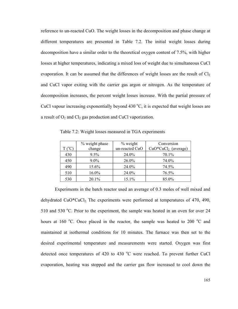
165

reference to un-reacted CuO. The weight losses in the decomposition and phase change at

different temperatures are presented in Table 7.2. The initial weight losses during

decomposition have a similar order to the theoretical oxygen content of 7.5%, with higher

losses at higher temperatures, indicating a mixed loss of weight due to simultaneous CuCl

evaporation. It can be assumed that the differences of weight losses are the result of Cl2

and CuCl vapor exiting with the carrier gas argon or nitrogen. As the temperature of

decomposition increases, the percent weight losses increase. With the partial pressure of

CuCl vapour increasing exponentially beyond 430 oC, it is expected that weight losses are

a result of O2 and Cl2 gas production and CuCl vaporization.

Table 7.2: Weight losses measured in TGA experiments

T (oC) % weight phase

change % weight

un-reacted CuO Conversion

CuO*CuCl2 (average)

430 9.5% 24.0% 70.1%

450 9.0% 26.0% 74.0%

490 15.6% 24.0% 74.5%

510 16.0% 24.0% 76.5%

530 20.1% 15.1% 85.0%

Experiments in the batch reactor used an average of 0.3 moles of well mixed and

dehydrated CuO*CuCl2. The experiments were performed at temperatures of 470, 490,

510 and 530 oC. Prior to the experiment, the sample was heated in an oven for over 24

hours at 160 oC. Once placed in the reactor, the sample was heated to 200 oC and

maintained at isothermal conditions for 10 minutes. The furnace was then set to the

desired experimental temperature and measurements were started. Oxygen was first

detected once temperatures of 420 to 430 oC were reached. To prevent further CuCl

evaporation, heating was stopped and the carrier gas flow increased to cool down the

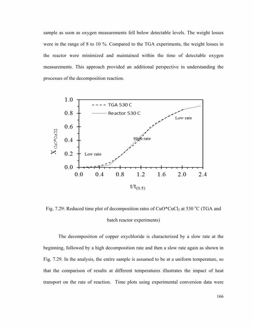
166

sample as soon as oxygen measurements fell below detectable levels. The weight losses

were in the range of 8 to 10 %. Compared to the TGA experiments, the weight losses in

the reactor were minimized and maintained within the time of detectable oxygen

measurements. This approach provided an additional perspective in understanding the

processes of the decomposition reaction.

Fig. 7.29: Reduced time plot of decomposition rates of CuO*CuCl2 at 530 oC (TGA and

batch reactor experiments)

The decomposition of copper oxychloride is characterized by a slow rate at the

beginning, followed by a high decomposition rate and then a slow rate again as shown in

Fig. 7.29. In the analysis, the entire sample is assumed to be at a uniform temperature, so

that the comparison of results at different temperatures illustrates the impact of heat

transport on the rate of reaction. Time plots using experimental conversion data were

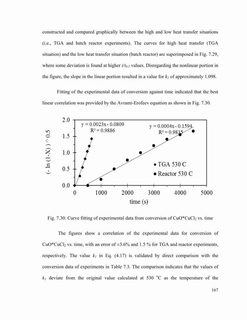
167

constructed and compared graphically between the high and low heat transfer situations

(i.e., TGA and batch reactor experiments). The curves for high heat transfer (TGA

situation) and the low heat transfer situation (batch reactor) are superimposed in Fig. 7.29,

where some deviation is found at higher t/t0.5 values. Disregarding the nonlinear portion in

the figure, the slope in the linear portion resulted in a value for k1 of approximately 1.098.

Fitting of the experimental data of conversion against time indicated that the best

linear correlation was provided by the Avrami-Erofeev equation as shown in Fig. 7.30.

Fig. 7.30: Curve fitting of experimental data from conversion of CuO*CuCl2 vs. time

The figures show a correlation of the experimental data for conversion of

CuO*CuCl2 vs. time, with an error of ±3.6% and 1.5 % for TGA and reactor experiments,

respectively. The value k1 in Eq. (4.17) is validated by direct comparison with the

conversion data of experiments in Table 7.3. The comparison indicates that the values of

k1 deviate from the original value calculated at 530 oC as the temperature of the

168

experiment decreases. The alternative to an Arrhenius relationship directly from data

fitting to a non-isothermal model is difficult for this system. This observation suggests the

need for a temperature dependent term as indicated in Eq. (4.17). The effect is more

evident in the case of experiments performed in the reactor where heat transfer resistances

are higher. The temperature dependence of decomposition of CuO*CuCl2 according to

Arrhenius’ law is illustrated in Fig. 7.31.

Fig. 7.31: Curve fitting of conversion data at different temperatures

The curves show the dependence of conversion versus temperature for

experiments performed in the reactor and the thermogravimetric microbalance analyzer.

Data from experiments at the same temperature was averaged in order to facilitate the

analysis.

169

Table 7.3: Deviation of conversion dependent terms with temperature (k1)

TGA Experiments Reactor Experiments

T (oC) t(s) X k1 Deviation T (oC) t(s) X k1 Deviation

530 596 0.85 0.0023 -0.6% 532 4426 0.93 0.00037 7.9%

510 535 0.77 0.0022 2.2% 523 5552 0.87 0.00026 35.7%

490 538 0.75 0.0022 5.5% 507 5204 0.84 0.00026 35.0%

450 572 0.74 0.0020 11.8% 502 3777 0.84 0.00036 10.4%

430 682 0.70 0.0016 30.0% 481 4723 0.76 0.00025 36.8%

469 6150 0.74 0.00019 52.8%

7.4 Phase Change Decomposition

A comparison between the decomposition rate that results from an analysis of

experiments and a theoretical phase change model provides an indication of the overall

resistances that impact the conversion. Based on the phase change model (Stefan problem)

and thermo-physical properties reported in Table 7.4, sample solutions of the phase

interface movement are plotted at various times in Fig. 7.32. The results indicate the

position of the interface for several Stefan numbers. Also, the position of the interface for

a Stefan number of 2.0 is depicted based on a solution of the Stefan problem for spherical

coordinates presented by Dewynne and Hill [69]. Reasonable agreement is achieved, to

provide useful validation of the predictive model. At higher temperatures, the Stefan

number is lower and the interface moves faster, resulting in an almost linear correlation of

radius vs. time. At lower temperatures and larger Stefan numbers, the movement of the

interface is slower and the radius reduces in an asymptotic manner.

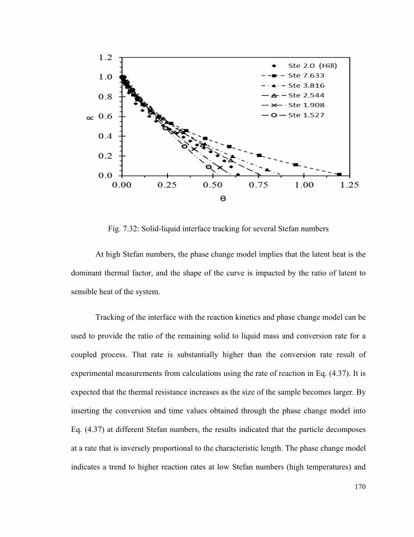
170

Fig. 7.32: Solid-liquid interface tracking for several Stefan numbers

At high Stefan numbers, the phase change model implies that the latent heat is the

dominant thermal factor, and the shape of the curve is impacted by the ratio of latent to

sensible heat of the system.

Tracking of the interface with the reaction kinetics and phase change model can be

used to provide the ratio of the remaining solid to liquid mass and conversion rate for a

coupled process. That rate is substantially higher than the conversion rate result of

experimental measurements from calculations using the rate of reaction in Eq. (4.37). It is

expected that the thermal resistance increases as the size of the sample becomes larger. By

inserting the conversion and time values obtained through the phase change model into

Eq. (4.37) at different Stefan numbers, the results indicated that the particle decomposes

at a rate that is inversely proportional to the characteristic length. The phase change model

indicates a trend to higher reaction rates at low Stefan numbers (high temperatures) and

171

higher thermal resistances at lower temperatures (high Stefan numbers). Similarly, the

experimental data indicated that the high heat flux experimental data from TGA analysis

yields higher decomposition rates. The analysis suggests a decomposition reaction limited

by conduction heating of the sample. Slow heat transfer to the sample surface occurs due

to the conduction resistance in the liquid and solid phases. The conduction heating is

further hindered by the formation of gaseous oxygen at the interface and gas diffusion in

the liquid phase. Using the values in Eq. (4.37) resulted in the curve of phase change in

Fig. 7.33, where the characteristic lengths have been calculated based on spherical shapes.

Fig. 7.33: Rates of reaction compared to experimental data

These results suggest a strong dependence of reaction kinetics on the dynamically

varying shape and exposed surface area of the sample as indicated by the characteristic

time, which indicates the importance of heat transfer area for both conduction and phase

change.

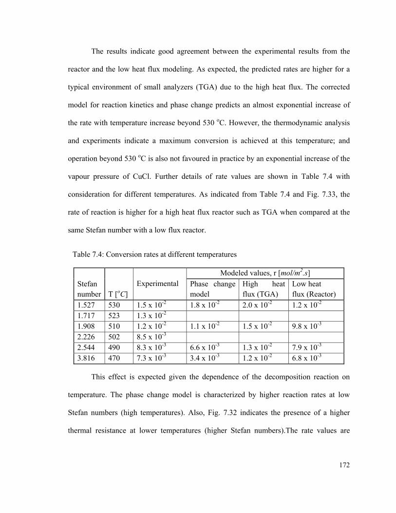
172

The results indicate good agreement between the experimental results from the

reactor and the low heat flux modeling. As expected, the predicted rates are higher for a

typical environment of small analyzers (TGA) due to the high heat flux. The corrected

model for reaction kinetics and phase change predicts an almost exponential increase of

the rate with temperature increase beyond 530 oC. However, the thermodynamic analysis

and experiments indicate a maximum conversion is achieved at this temperature; and

operation beyond 530 oC is also not favoured in practice by an exponential increase of the

vapour pressure of CuCl. Further details of rate values are shown in Table 7.4 with

consideration for different temperatures. As indicated from Table 7.4 and Fig. 7.33, the

rate of reaction is higher for a high heat flux reactor such as TGA when compared at the

same Stefan number with a low flux reactor.

Table 7.4: Conversion rates at different temperatures

Stefan number T [oC]

Experimental Modeled values, r [mol/m2.s]

Phase change model

High heat flux (TGA)

Low heat flux (Reactor)

1.527 530 1.5 x 10-2 1.8 x 10-2 2.0 x 10-2 1.2 x 10-2 1.717 523 1.3 x 10-2 1.908 510 1.2 x 10-2 1.1 x 10-2 1.5 x 10-2 9.8 x 10-3 2.226 502 8.5 x 10-3 2.544 490 8.3 x 10-3 6.6 x 10-3 1.3 x 10-2 7.9 x 10-3 3.816 470 7.3 x 10-3 3.4 x 10-3 1.2 x 10-2 6.8 x 10-3

This effect is expected given the dependence of the decomposition reaction on

temperature. The phase change model is characterized by higher reaction rates at low

Stefan numbers (high temperatures). Also, Fig. 7.32 indicates the presence of a higher

thermal resistance at lower temperatures (higher Stefan numbers).The rate values are

173

approximately one order of magnitude higher at 530 oC when compared to values at lower

temperatures. This observation was confirmed by the experimental data.

7.5 Reactor Dynamics

A dimensionless number that arises in the analysis of chemical reactions is the

Damkohler number. It has a physical interpretation in terms of diffusion, rate of reaction

and characteristic time of the system. It is also an indication of the residence time

involving the ratio of fluid motion versus characteristic reaction time, with large

Damkohler numbers associated more closely with irreversible reactions. The analysis is

applicable to solid particles under chemical decomposition that leads to gas and liquid

products. An additional complexity in the decomposition is that the sample may be

entering the reactor contaminated with products of an incomplete upstream hydrolysis

reaction such as CuCl, H2O and CuCl2. This thesis analyzes the decomposition of pure

CuO*CuCl2 particles based on theoretical and experimental results that did not account

for impurities. The analysis did not extend to the impact of impurities on the yield of

decomposition, therefore the results must be used with care in terms of the effect that the

presence of side products/reagents may have on the overall extent of reaction.

Numerical predictions of the rate of shrinkage and evolution of temperature with

time are shown in Fig. 7.34 for two different initial diameters of the particle. For a

maximum conversion of 90%, decomposition of the smaller particle essentially stops

before reaching a temperature of ≈ 0.02. With larger particles of 0.6 mm in diameter,

the decomposition rate approaches zero at approximately one tenth of r, while the solid

temperature reaches 0.21. A larger particle size impacts the overall decomposition rate

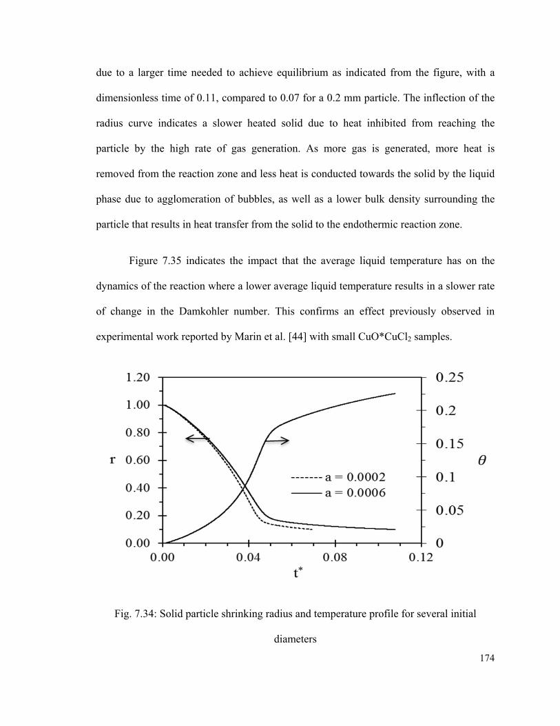
174

due to a larger time needed to achieve equilibrium as indicated from the figure, with a

dimensionless time of 0.11, compared to 0.07 for a 0.2 mm particle. The inflection of the

radius curve indicates a slower heated solid due to heat inhibited from reaching the

particle by the high rate of gas generation. As more gas is generated, more heat is

removed from the reaction zone and less heat is conducted towards the solid by the liquid

phase due to agglomeration of bubbles, as well as a lower bulk density surrounding the

particle that results in heat transfer from the solid to the endothermic reaction zone.

Figure 7.35 indicates the impact that the average liquid temperature has on the

dynamics of the reaction where a lower average liquid temperature results in a slower rate

of change in the Damkohler number. This confirms an effect previously observed in

experimental work reported by Marin et al. [44] with small CuO*CuCl2 samples.

Fig. 7.34: Solid particle shrinking radius and temperature profile for several initial

diameters

175

The decomposition is relatively fast when the low end of the temperature range is

reached and the rate continues to increase as the temperature rises. The relation between

the Damkohler number and the total time of reaction, however, indicated that high rates of

decomposition are maintained for a short time, with most of the decomposition occurring

in the range of Da ≈ 1. The inflection of the curve confirms the phenomena of a slower

heated solid which affects the dynamics of the reaction before reaching equilibrium.

The effect can be observed in experimental decomposition of CuO*CuCl2, where

the rate of oxygen generation diminishes in an asymptotic manner towards the end of the

decomposition in the reactor. This effect occurs from competing processes of heat and

mass transfer due to gas diffusion away from the reaction zone.

Fig. 7.35: Impact of liquid temperature on the dynamics of decomposition for 0.5 mm

particles

The typical behaviour of gas evolution from the decomposition of small samples

of CuO*CuCl2 in Fig. 7.1 indicated that the amount of released gas increases in an

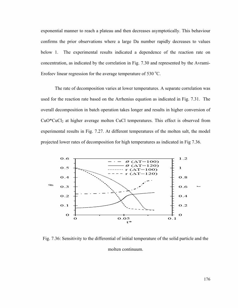
176

exponential manner to reach a plateau and then decreases asymptotically. This behaviour

confirms the prior observations where a large Da number rapidly decreases to values

below 1. The experimental results indicated a dependence of the reaction rate on

concentration, as indicated by the correlation in Fig. 7.30 and represented by the Avrami-

Erofeev linear regression for the average temperature of 530 oC.

The rate of decomposition varies at lower temperatures. A separate correlation was

used for the reaction rate based on the Arrhenius equation as indicated in Fig. 7.31. The

overall decomposition in batch operation takes longer and results in higher conversion of

CuO*CuCl2 at higher average molten CuCl temperatures. This effect is observed from

experimental results in Fig. 7.27. At different temperatures of the molten salt, the model

projected lower rates of decomposition for high temperatures as indicated in Fig 7.36.

Fig. 7.36: Sensitivity to the differential of initial temperature of the solid particle and the

molten continuum.

177

A larger temperature differential results in a higher heat flux into the particle, and

faster decomposition. However, the total conversion is still lower than a smaller

temperature differential. This sensitivity explains the behaviour discussed in relation to

experimental results as indicated in Fig. 7.27.

A lumped capacitance model was used. These considerations were applied to the

model of chemical decomposition and resulted in a rate of decomposition very sensitive to

the initial temperature of the particle. When the size of the particle is too small, the

dynamic of decomposition is impacted by the temperature differential between the particle

and continuum as indicated in Fig. 7.37. The Damkohler number is lower for a larger

temperature differential but the dynamics are equal at the extremes of the process of

decomposition. First, as the particle enters the molten bath, the increase in temperature of

the particle is relatively slow since the dynamics of the reaction decays asymptotically.

The resistance imposed by the oxygen bubbles impacts the heat transport from the

beginning. Towards the end of the decomposition, the dynamics are similar for both

temperature differentials, presumably because the temperature of the particles is closer to

the temperature of the molten continuum. Assuming the same conversion at the end of

decomposition, the phenomenon takes longer for the lower temperature differential.

178

Fig. 7.37: Effects of the difference of temperature between the particle and the continuum

on the dynamics of decomposition.

The decomposition in all cases started at Damkohler numbers close to 1 and

rapidly decayed as indicated in Fig. 7.38. This is an indication of rapid chemical

decomposition and a reaction driven process, impacted also by the slower rate of heat and

mass transfer at the interface. After the reaction occurs with the Damkohler number

falling below 1, the concentration of solids reduces rapidly with the Damkohler number

over a long period of time. A curve of Da vs. t* indicated that at least 95% of the

decomposition occurs at or below Da ≈ 1. At the inflection, the curve also indicates that

full decomposition requires a longer residence time because of the particle descent. These

observations suggest that equilibrium conversion can be achieved at lower temperatures.

Total conversion, however, requires long residence times.

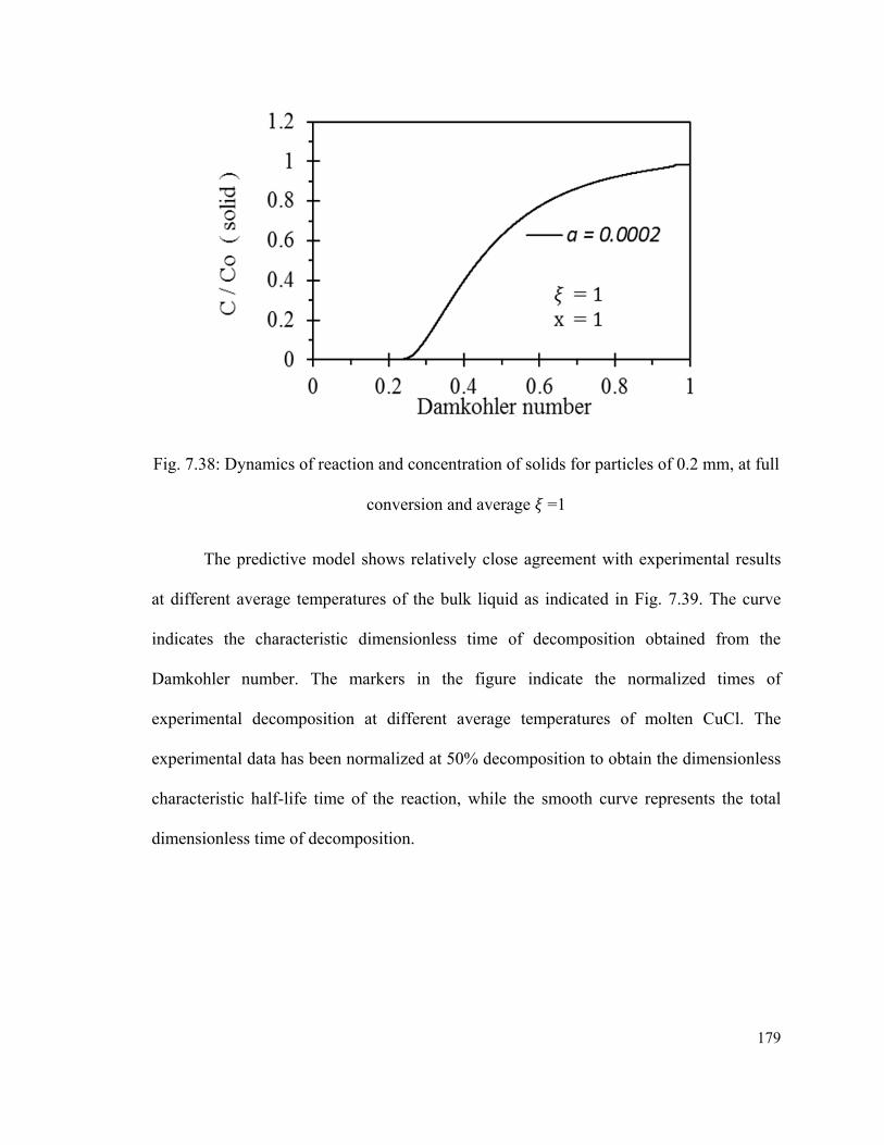
179

Fig. 7.38: Dynamics of reaction and concentration of solids for particles of 0.2 mm, at full

conversion and average =1

The predictive model shows relatively close agreement with experimental results

at different average temperatures of the bulk liquid as indicated in Fig. 7.39. The curve

indicates the characteristic dimensionless time of decomposition obtained from the

Damkohler number. The markers in the figure indicate the normalized times of

experimental decomposition at different average temperatures of molten CuCl. The

experimental data has been normalized at 50% decomposition to obtain the dimensionless

characteristic half-life time of the reaction, while the smooth curve represents the total

dimensionless time of decomposition.

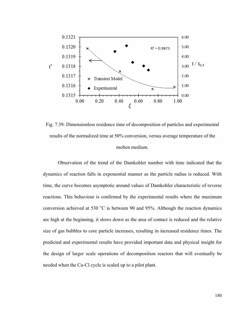
180

Fig. 7.39: Dimensionless residence time of decomposition of particles and experimental

results of the normalized time at 50% conversion, versus average temperature of the

molten medium.

Observation of the trend of the Damkohler number with time indicated that the

dynamics of reaction falls in exponential manner as the particle radius is reduced. With

time, the curve becomes asymptotic around values of Damkohler characteristic of reverse

reactions. This behaviour is confirmed by the experimental results where the maximum

conversion achieved at 530 oC is between 90 and 95%. Although the reaction dynamics

are high at the beginning, it slows down as the area of contact is reduced and the relative

size of gas bubbles to core particle increases, resulting in increased residence times. The

predicted and experimental results have provided important data and physical insight for

the design of larger scale operations of decomposition reactors that will eventually be

needed when the Cu-Cl cycle is scaled up to a pilot plant.

181

The decomposition occurs through a succession of stages in which the heat flux

towards the particle is impacted by the transport phenomenon itself. As more gas is

generated, more heat is removed from the reaction zone and less heat is conducted

towards the solid by the liquid phase due to agglomeration of bubbles. The bulk density of

liquid surrounding the particle is lower and the overall phenomenon results in heat

transfer from the solid to the endothermic reaction zone.

Fig. 7.40: Evolution of the overall Nusselt number as a result of varying radius of a

particle of CuO*CuCl2 undergoing chemical decomposition

The heat transfer occurs mainly as a result of conduction through the liquid phase.

As the gas phase molar fraction increases, the liquid becomes less dense and the heat

transport results from a combination of convection and conduction. This effect is

indicated in Fig. 7.40 by the higher Nusselt number as the particle radius decays.

182

Chapter 8 - Conclusions and Recommendations for Future Research

8.1 Conclusions ________________________________________________________________________

This research provided a significant improvement to the understanding of the

chemical decomposition of copper oxychloride in the Cu-Cl cycle. The decomposition

process is impacted by the number of particles per unit volume. The analysis indicated

that the residence time increases by 60% with an increase of particle size from 0.0002 to

0.0005 m. When accounting for losses, this increase of residence time will result in a

lower overall cycle efficiency. High concentration of solids promotes a higher rate of

reaction but the dynamics decays faster when the concentration is above approximately

40%. Therefore, it is desirable to maintain concentrations between 20 and 40% such that

the average dynamics of the reaction promotes a steady rate of decomposition. These

results are useful for providing operational parameters of future scaled-up reactors.

An analysis of the chemical streams of neighboring reactions and their interactions

within the Cu-Cl cycle indicated that if CuCl2 is not fully converted to Cu2OCl2 in the

hydrolysis reactor, it will release up to 0.15 moles of chlorine per mole of oxygen

produced in the downstream decomposition reactor. The residual CuCl2 in the oxygen

production reactor will enter the electrolytic reaction, causing a potential loss of efficiency

in the electrolysis process. In addition, the processes for separation of oxygen and chlorine

may require additional energy and reduce the efficiency of the Cu-Cl cycle.

The complexity of the chemical streams also influences the thermal energy

integration of the Cu-Cl cycle. The decomposition reactor operates at the highest

temperature of the cycle implying a potential for heat recovery. The low density of gases

183

at atmospheric pressure makes difficult the implementation of heat recovery strategies. As

more gases exit the reactor, further heat losses occur, increasing the need for thermal

energy input to the cycle, potentially reducing the overall efficiency. It was found that

reducing the pressure in the reactor does not result in significant reduction of the amount

of chlorine produced, although the high temperature threshold of the Cu-Cl cycle is

reduced when operating at lower pressures. The results indicated that the amount of CuCl

vapor in the gas stream of the oxygen production reaction is much less significant than

chlorine gas. This observation is confirmed by both experimental results and analysis of

molar fractions and partial pressures of chlorine and oxygen versus CuCl vapour.

Experimental results and thermodynamic analysis indicated that a reverse reaction

has little probability of occurring when the molten bath is maintained at temperatures

above 500 oC. Thus, the reactor should be designed in a way such that the preheating time

of the solid particles is minimized as to prevent the occurrence of decomposition and a

reverse reaction that may result in additional formation of CuCl2 during the preheating

period. This observation was confirmed by the theoretical models. Further research should

be conducted to understand the impact of the presence of humidity in the reagents in the

oxygen reactor. This aspect has critical importance since a portion of experimental results

had to be discarded because the XRD analysis indicated the presence of Cu-hydrates.

Also, the products of hydrolysis may contain some humidity that is fed to the

decomposition reactor.

Thermodynamic models were designed in order to utilize data available of

elementary species at standard conditions. Data was then projected to the desired

184

temperatures of operation by using regressions based on the specific heat of reagents and

products. The data included the standard entropy, enthalpy and Gibbs free energy of

formation at different temperatures. The lack of experimental calorimetric data at the high

range of temperature added uncertainty to the analysis. However, the experimental results

indicated the expected behavior to a reasonable extent. Analysis of the combined effects

of pressure and temperature on the Gibbs free energy of the reaction indicated that the

optimum operating conditions correspond to pressures in the range of 1 - 2 bars, and

temperatures within 525 - 550 oC. Furthermore, a three-phase thermochemical model

confirmed the experimental observation that the decomposition reaction is highly dynamic

in the range of temperatures below 530 oC. However, the thermodynamic analysis

indicates that the reverse reaction of CuCl and oxygen becomes spontaneous with a

negative Gibbs free energy below 500 oC. Therefore, the ideal range of operation for

decomposition falls between these two limits of temperature. Higher temperatures

promote the evaporation of CuCl and they are not desirable. Similarly, low pressures

below atmospheric disfavor the reverse reaction. Thus, at lower pressures the reactor can

reduce the temperature of the decomposition. However, the thermal balance does not

compensate the mechanical energy required to maintain vacuum in the reactor. Thus,

within the residence time of reactants in the decomposition reactor, at temperatures above

500 oC and atmospheric pressure, it is reasonable to expect conversions in the order of

65% and higher.

The decomposition of CuO*CuCl2 is an endothermic reaction coupled with phase

change, mass diffusion, and heat transport by convection and conduction. The rapid

dynamics of the reaction undergoes resistance by various mechanisms that include the

185

agglomeration of particles and the slow removal of oxygen gas from the reacting zone. A

rate of reaction expression indicated a complex logarithmic relation of time and

concentration of solids in the reactor in batch operation. Experiments conducted in a semi-

batch environment with continuous addition of solids and continuous removal of gases

indicated, as expected, that the rate of reaction is reduced as the rate of addition of solids

is increased. Thus the number of solid particles available at any time with the level of

energy of decomposition depends on the spatial concentration of solids, and the dispersion

rate that depends on contact area between solid particles and molten CuCl. Furthermore,

the contact area is reduced as oxygen evolves and creates void volumes between the liquid

and the solid particles. A phase change model based on the experimental rate of reaction

indicated that the overall thermal resistance is the result of a surface factor in addition to

other factors. The resistances occur as a result of coupled heat and mass transfer, and

chemical phenomena.

Small Reynolds and Peclet numbers imply that heat transfer in the direction of the

core particle is mainly due to conduction through the liquid phase that dominates over

convective phenomena. The rate of reaction is compromised with the evolution of the

temperature and concentration fields as indicated by a relatively low Damkohler number.

Simultaneously, the heat transfer phenomenon is hindered by the diffusion of gas away

from the decomposing solid particle. Thus, the net result is a shrinking solid particle with

a reduced heat flow due to the resistance imposed by a large number of gas bubbles

moving away from the core.

186

The results of this research suggest that solid concentration has a key role in the

dynamics of the reaction. It is expected that the presence of more solids results in larger

area of contact and therefore more heat transferred to the reaction zone. However, with

more solids present in the molten liquid, more gas is produced and more heat is removed

from the reaction zone. Also, as more gas is produced, the mole fraction of liquid is

reduced and a net hindering effect results in the conduction of heat through the molten

species. These two effects produce a reaction system that must balance the requirement of

heat for chemical decomposition and the losses of heat with the product, with a reduced

capacity to transfer heat towards the particle. Therefore, in addition to maintaining a given

concentration of solids according to the heat flux, it is critical to promote a well

distributed dispersion of particles within the molten continuum.

The dynamics of the reaction is indicated by Damkohler numbers in the order of

10 at the beginning of the decomposition of a particle. As heat conduction is obstructed

with the flow of oxygen generated, the dynamics of the reaction are reduced as indicated

by a falling Damkohler number. With the Damkohler number falling asymptotically to

values typical of reversibility, the residence time to achieve high conversions becomes too

large for practical applications. Thus, other means are necessary to reduce the residence

time while increasing conversion. It is unknown if mechanical aids such as agitation will

minimize the effect that appears when the core particle radius has been reduced beyond

conversion rates of 90 or 95%.

The observations provide insight for the effective design of an oxygen reactor in

the thermochemical cycle of Cu-Cl for hydrogen generation. Since hydrogen must

187

compete with existing technologies, an efficient reactor ultimately contributes to make

hydrogen more competitive.

8.2 Recommendations for Future Research

The experiments of this research were conducted in TGA, batch and semi-batch

experiments. It is believed that the most viable operation of the decomposition reactor for

an initial scale-up of the Cu-Cl cycle will be a batch reactor. However, the experimental

results indicated that the best operation resulted from a semi-batch operation with

continuous addition of solids and continuous removal of oxygen. The kinetics of reaction

should be researched under dynamic conditions. The experimental results in this thesis

were obtained from reactors were the molten salt remained quiescent. Mechanical

agitation and experiments in a continuously steered reactor may result in better dynamics

at higher Damkohler number. A reaction environment with higher Damkohler number

allows also for higher concentration rates. Furthermore, the experiments were conducted

with the injection of a carrying gas. The presence of a carrying gas results in lower

probability of a reverse reaction occurring as oxygen is rapidly evacuated from the

reaction zone. This effect confirms the predictions of Le’Chatelier phenomenon. Thus, a

higher Damkohler and a reduced Le’Chatelier phenomenon may counteract each other in

the desirable situation of not using a carrying gas. Experiments are recommended where

oxygen is allowed to exit the reaction zone without the utilization of a carrying gas. This

is a condition that is desirable for the scale-up of the cycle without the extra expense of a

carrying gas.

The experiments in this research were conducted with a stoichiometric mixture of

CuO-CuCl2 since the mixture is a more stringent situation for testing the decomposition

188

reaction. Furthermore, the decomposition mechanisms indicated that at some intermediate

step, the reaction is the result of competing reactions that include CuCl2 and CuO

separately. It is recommended that experiments be conducted with the utilization of

products of hydrolysis as they become available and that composition of products be

carefully monitored via gas analysers, and XRD. Non-isothermal TGA experiments

should be conducted and experiments with a variable heat flux are recommended. The

results should be compared to a theoretical model of heat and mass transfer. Experiments

need to be conducted to validate the observations of CuCl vapour with oxygen gas and

determine the mechanisms to return the condensed matter back to the reactor bed. Finally,

further measurements of chlorine gas from decomposition of hydrolysis products should

provide a better understanding of the phenomenon in an integrated environment.

The dynamics of reaction indicated that the conversion of solids falls

asymptotically around non-zero values, impacting the residence time in the reactor.

Mechanical means of reducing this time while increasing the conversion should also be

explored.

189

References ________________________________________________________________________

[1] New York State Energy Research and Development Authority (NYSERDA),

February 2012, Hydrogen Fact Sheet, retrieved March 1st from

http://www.fuelcelleducation.org/wpcontent/themes/sandbox/pdf/History%20of%

20Hydrogen.pdf

[2] BP Statistical review of world energy June 2011, retrieved Feb 2012 from

http://bp.com/statisticalreview

[3] BP Statistical review, Energy outlook 2030, January 2011, retrieved Feb 2012

from http://search.babylon.com/?q=BP+Statistical+review&s=web&as=0&rlz=

0&babsrc=SP_ss

[4] International Energy Agency, World Energy Outlook 2011, executive summary,

retrieved Feb 2012 from

http://www.iea.org/weo/docs/weo2011/executive_summary.pdf

[5] M. Ball and M. Wietschel, The future of hydrogen – opportunities and challenges,

International Journal of Hydrogen Energy, 34 (2009) 615-627

[6] Air Liquide, Gas Encyclopaedia, March 2011, retrieved Feb 2012 from

http://encyclopedia.airliquide.com/encyclopedia.asp

[7] Hydrogen Properties, College of the Desert, Hydrogen Fuel Cells and Related

Technologies, Rev 0, Dec 2001, retrieved March 2012 from

190

http://www1.eere.energy.gov/hydrogenandfuelcells/tech_validation/pdfs/fcm01r0.

pdf

[8] S.O. Mert, I. Dincer, Z. Ozcelik, Performance investigation of a transportation

PEM fuel cell system, International Journal of Hydrogen Energy, 37 (2012) 623-

633.

[9] Economy and Energy No 79, Oct/Dec 2010, Ministerio da Ciencia e Tecnologia,

retrieved Feb 2012 from http://www.ecen.com/eee79/eee79e/ecen_79e.htm,

http://www.ecen.com/content/eee7/motoref.htm

[10] M. Hooks, M. Jackson, Hydrogen and FCV implementation storyline, TIAX LLC,

May 24 2007

[11] G. Frenette, D. Forthoffer, Economic and commercial viability of hydrogen fuel

cell vehicles from an automotive manufacturer perspective, International Journal

of Hydrogen Energy, 34 (2009) 3578-3588

[12] International Energy Agency Task 16: Hydrogen from carbon-containing

materials, 2006, retrieved Feb 2012 from

http://ieahia.org/pdfs/finalreports/Task16FinalReport.pdf

[13] M.A. Rosen, Advances in hydrogen production by a thermochemical water

decomposition: A review, Energy Journal 35 (2010) 1068-1076

[14] R. Elder, R. Allen, Nuclear heat for hydrogen production: Coupling a very

high/high temperature reactor to a hydrogen production plant, Progress in Nuclear

Energy, 51 (2009) 500-525

191

[15] J.C. Molburg, R.D. Doctor, Hydrogen form steam methane reforming with CO2

capture, Argonne National Labs, 20th Annual International Pittsburgh Coal

Conference, Sept 2003, retrieved Dec 2011 from

http://www.netl.doe.gov/technologies/hydrogen_clean_fuels/refshelf/papers/pgh/h

ydrogen%20from%20steam%20methane%20reforming%20for%20carbon%20dio

xide%20cap.pdf

[16] P.C. Mannes, J. Yu, C. Eckert, M.L. Ghirardi, Photobiological hydrogen

production prospects and challenges, American society of microbiology, June

2009, retrieved Jan 2012 from

http://www.microbemagazine.org/index.php?option=com_content&view=article&

id=309:photobiological-hydrogen-productionprospects-and-

challenges&catid=132:featured&Itemid=196

[17] D. Mohan, C.U. Pittman, P.H. Steel, Pyrolysis of wood / biomass for bio – oil: A

critical review, Energy and Fuels Journal, 20 (2006) 848 – 889

[18] K. Zeng, D. Zhang, Recent progress in alkaline water electrolysis for hydrogen

production and applications, Progress in Energy and Combustion Science, 36

(2010) 307 – 326

[19] G.A. Dluga, J.R. Slage, L.D. Schnidt, X.E. Verykios, Renewable hydrogen from

ethanol by autothermal reforming, Science, 303 (2004) 993 – 996

[20] P.J. de Wild, M.J. Verhaak, Catalytic production of hydrogen from methanol,

Catalysis Today, 60 (2000) 3 -10

192

[21] H. Watanabe, M. Otaka, Numerical simulation of coal gasification in entrained

flow coal gasifier, Fuel, 85 (2006) 1935 – 1943

[22] Y.H Jung, Y.H Jeong, Development of the once-through hybrid sulphur process

for nuclear hydrogen production, International Journal of Hydrogen Production, 35

(2010) 12255 – 12267

[23] G. Naterer, G, Suppiah S, Lewis M, Gabriel K, Dincer I, Rosen MA, et al. Recent

Canadian advances in nuclear-based hydrogen production and the thermochemical

Cu–Cl cycle. Int J Hydrogen Energy, 34 (7) (2009) 2901–2917

[24] Z. Wang, V. N. Daggupati, G. Marin, K. Pope, Y. Xiong, E. Secnik, G. F. Naterer,

K. S. Gabriel, Towards System Integration of the Cu-Cl Thermochemical

Hydrogen Production Cycle, International Conference on Hydrogen Production,

Thessaloniki, Greece, June 19-22, 2011

[25] C.M. Stoots, J.E. O’Brien, K.G. Condie, J.J. Hartvigsen, High temperature

electrolysis for large-scale hydrogen production from nuclear energy –

Experimental investigations, International Journal of Hydrogen Energy, 35 (2010)

4861 – 4870

[26] S.D. Ebbesen, J. Hegh, K.A. Nielsen, J.U. Nielsen, M. Mogensen, Durable solid

oxide cell stack for production of Hydrogen and synthesis gas by high temperature

electrolysis, International Journal of Hydrogen Energy, 36 (2011) 7363 – 7373

[27] E. Broda, Utilization of solar radiation for water photolysis, International Journal

of Hydrogen Energy, 5 (1980) 453 – 454

193

[28] G.E. Beghi, A decade of research on thermochemical hydrogen at the joint

research centre, Ispra, International Journal of Hydrogen Energy, 11 (12) (1986)

761 -771

[29] L.C. Brown, G.E. Besenbruch, , R.D. Lentsch, K.R. Schultz, J.F. Funk, P.S.

Pickard. A.C. Marshall, S.K. Showalter, High efficiency generation of hydrogen

fuels using nuclear power, GA A23451, Final technical report prepared under the

Nuclear Energy Research Initiative (NERI), San Diego, CA, 2003. Retrieved Jan

2011 from http://www.energy.ca.gov/ab1007/documents/2007-05-

31_joint_workshop/2007-05-31_HYDROGEN_FUEL_CELL_SCENARIO.PDF

[30] M.A. Lewis, J.G. Masin, P.A. O’Hare, Evaluation of alternative thermochemical

cycles. Part I: The methodology, International Journal of Hydrogen Energy, 34 (9)

(2009) 4115 - 4124

[31] M.A. Lewis, J.G. Masin, P.A. O’Hare, Evaluation of alternative thermochemical

cycles. Part II: The down-selection process, International Journal of Hydrogen

Energy, 34 (2009) 4125-4135

[32] M.A. Lewis, J.G. Masin, R.B. Vilim, Development of the low temperature Cu-Cl

cycle. Proceedings of 2005 International congress on advances in nuclear power

plants, ICAPP ’05, May 15-19, 2005, Seoul, Korea, American Nuclear Society,

May 2005

[33] B. Russ, P. Pickard, S. Kung, Sulfur-Iodine thermochemical cycle, Project PD-12,

2009 DOE Hydrogen Program Review, Alburquerque, NM, USA

194

[34] G.F. Naterer, M. Fowler, J. Cotton, K. Gabriel, Synergistic Roles of Off-Peak

Electrolysis and Thermochemical Production of Hydrogen from Nuclear Energy in

Canada, International Journal of Hydrogen Energy, 33 (23), (2008) 6849-6857

[35] Hydrogen Posture Plan, an Integrated Research, Development and Demonstration

Plan, United States Department of Energy, United States Department of

Transportation, December 2006, from http://www.hydrogen.energy.gov/

pdfs/hydrogen_posture_plan_dec06.pdf

[36] Z. L. Wang, G. F. Naterer, K. S. Gabriel, S. Supphia, SCWR-hydrogen plant

thermal integration, paper presented at the 2nd Conference Canada-China Joint

Conference on Super-Critical Water-Cooled Reactors, Nuclear Engineering

International, Toronto, April 2010

[37] G. Naterer, S. Suppiah, M. Lewis, K. Gabriel, I. Dincer, M.A. Rosen, M. Fowler,

G. Rizvi, E.B. Easton, B.M. Ikeda, M.H. Kaye, L. Lu, I. Pioro, P. Spekkens, P.

Tremaine, J. Mostaghimi, J. Avsec, J. Jiang, Recent Canadian advances in nuclear

based hydrogen production and the thermochemical Cu-Cl cycle, international

Journal of Hydrogen Energy, 34 (2009) 2901-2917.

[38] Z. L. Wang, G. F. Naterer, K. S. Gabriel, R. Gravelsins, V. N. Daggupati,

Comparison of different copper–chlorine thermochemical cycles for hydrogen

production, International Journal of Hydrogen Energy, 34 (2009) 3267 – 3276

[39] G.F. Naterer, S. Suppiah, L. Stolberg, M. Lewis, Z. Wang, V. Daggupati, K.

Gabriel, I. Dincer, M.A. Rosen, P. Spekkens, S.N. Lvov, M. Fowler, P. Tremaine,

J. Mostaghimi, E.B. Easton, L. Trevani, G. Rizvi, B.M. Ikeda, M.H. Kaye, L. Lu,

I. Pioro, W.R. Smith, E. Secnik, J. Jiang, J. Avsec, Canada’s program on nuclear

195

hydrogen production and the thermochemical Cu-Cl cycle, International Journal of

Hydrogen energy, 35 (20) (2010) 10905-10926

[40] D. Dokiya, Y. Kotera, Hybrid cycle with electrolysis using a Cu-Cl system.

International Journal of Hydrogen Energy, 1(1976) 117-121

[41] G.F. Naterer, V.N. Daggupati, G. Marin, K.S. Gabriel, Z.L. Wang,

Thermochemical hydrogen production with a copper–chlorine cycle, II: Flashing

and drying of aqueous cupric chloride, International Journal of Hydrogen Energy,

33 (2008) 5451-5459

[42] Carty RH, Mazumder MM, Schreider JD, Pangborn JB. Thermochemical

hydrogen production, vols. 1–4. Chicago, IL: Gas Research Institute for Gas

Technology, GRI-80/0023, 1981.

[43] A. Nixon, M. Ferrandon, M. H. Kaye, L. Trevani, Thermochemical production of

hydrogen, Synthesis, characterization, and decomposition of copper oxychloride,

Journal of Thermal Analysis and Calorimetry, Nov 2011.

[44] G.D. Marin, Z. Wang, G.F. Naterer, K. Gabriel, By-products and reaction

pathways for integration of the Cu–Cl cycle of hydrogen production, International

Journal of Hydrogen Energy, 36 (2011) 13414-13424

[45] G.F. Naterer, S. Suppiah, L. Stolberg, M. Lewis, M. Ferrandon, Z. Wang, I.

Dincer, K. Gabriel, M.A. Rosen, E. Secnik, E.B. Easton, L. Trevani, I. Pioro, P.

Tremaine, S. Lvov, J. Jiang, G. rizvi, B.M. Ikeda, L. Lu, M. Kaye, W.R. Smith, J.

Mostaghimi, P. Spekkens, M. Fowler, J. Avsec, Clean hydrogen production with

the Cu-Cl cycle-Progress of International consortium. I: Experimental unit

196

operations, International Journal of Hydrogen Energy, 36 (24) (2011) 15486-

15501

[46] G.F. Naterer, S. Suppiah, L. Stolberg, M. Lewis, M. Ferrandon, Z. Wang, I.

Dincer, K. Gabriel, M.A. Rosen, E. Secnik, E.B. Easton, L. Trevani, I. Pioro, P.

Tremaine, S. Lvov, J. Jiang, G. rizvi, B.M. Ikeda, L. Lu, M. Kaye, W.R. Smith, J.

Mostaghimi, P. Spekkens, M. Fowler, J. Avsec, Clean hydrogen production with

the Cu-Cl cycle-Progress of international consortium. II: Simulations,

thermochemical data and materials, International Journal of Hydrogen Energy, 36

(24) (2011) 15486-15501

[47] Z. Wang, G.F. Naterer, K.S. Gabriel, E. Secnik, R. Gravelsins, V. Daggupati,

Thermal designs of a solar hydrogen plant with a copper-chlorine cycel and

molten salt energy storage, 36 (17) (2011) 11258-11272

[48] V.N. Daggupati, G.F. Naterer, K.S. Gabriel, R.J Gravelsins, Z.L. Wang, Efects of

atomization conditions and flow rates on spray drying of cupric chloride particle

formation, International Journal of Hydrogen Energy, 36 (17) (2011) 11353-11359

[49] L. Stolberg, H.A. Boniface, S. McMahon, Electrolysis of the CuCl/HCl system for

the production of nuclear hydrogen, presented at the Fourth International Topical

meeting on High temperature Reactor Technology, ASME, Sept 2008,

Washington, USA

[50] S. Ranganathan, E. B. Easton, Ceramic carbon electrode based anodes for use in

the copper chlorine thermochemical cycle, Proceedings of the International

197

Conference on Hydrogen Production, May 2009, Canada, from http://faculty.

uoit.ca/easton/17018.pdf

[51] M. Lewis, M. Ferrandon, S. Nigoyi, S. Ahmed, C. Fan, R. Sharna, M. Fedkin, M.

Hickner, S. Lvov, D. Tatterson. L. Nitsche, L. Wedgwood, Membrane /

Electrolyzer development in the Cu-Cl thermochemical cycle, presented at the

Hydrogen Program Annual Merit Review Meeting, Arlington VA, May 12, 2011

[52] V.N. Daggupati, G.F. Naterer, K.S. Gabriel, R.J. Gravelsins, Z.L. Wang, Solid

particle decomposition and hydrolysis reaction kinetics in Cu-Cl thermochemical

hydrogen production, International Journal of Hydrogen Energy, 35 (2010) 4877-

4882

[53] M.S. Ferrandon, M.A. Lewis, F. Alvarez, E. Shafirovich, Hydrolysis of CuCl2 in

the Cu–Cl thermochemical cycle for hydrogen production: Experimental studies

using a spray reactor with an ultrasonic atomizer, International Journal of

Hydrogen Energy, 35 (2010) 1895 – 1904

[54] V. N. Daggupati, G. F. Naterer, K. S. Gabriel, R. J. Gravelsins, Z. L. Wang,

Equilibrium conversion in Cu–Cl cycle multiphase processes of hydrogen

production, Thermochimica Acta, 496 (2009) 117 – 123

[55] M. L. Walter-Levy, M Goreaud, Sur la Formation des Chlorures Culvriques par

Vola Seche. II.- Thermolyse des Chlorures Neutras et Basiques, Laboratorie de

Chimie Minerale de la Faculte des Sciences de Caen, 1971, 22.7.70

[56] M. A. Lewis, M. S. Ferrandon, D. F. Tatterson, P. Mathias, Evaluation of

alternative thermochemical cycles – Part III, further development of the Cu–Cl

cycle, International Journal of Hydrogen Energy, 34 (2009) 4136 – 4145

198

[57] A. Lindbråthen, M.B. Hagg, Membrane separation of chlorine gas, Chemical

Engineering and Processing: Process Intensification, 48 (2009) 1-16

[58] G.F. Naterer, K. Gabriel, Z.L. Wang, V.N. Daggupati, R. Gravelsins,

Thermochemical hydrogen production with a copper–chlorine cycle. I: oxygen

release from copper oxychloride decomposition, International Journal of Hydrogen

Energy, 33 (2008) 5439-5450

[59] Serban, M. A. Lewis, J. K. Basco, Kinetic Study of the Hydrogen and Oxygen

Production Reactions in the Copper-Chloride Thermochemical Cycle, American

Institute of Chemical Engineering, Spring National Meeting, New Orleans, LA,

April 25-29, 2004

[60] National Institute of Standards and Technology. Chemistry WebBook. NIST,

February 1, 2010, retrieved Oct 2010 from http://webbook.nist.gov/chemistry/.

[61] C. Lamberti, C. Prestipino, L. Capello, S. Bordiga, A. Zec, G. Spotto, S. Diaz, A.

Marsella, B. Cremaschi, M. Garilli, S. Vidotto, G. Leofanti, The CuCl2/Al2O3

Catalyst Investigated in Interaction with Reagents, International Journal of

Molecular Science, 2 (2001) 230-245

[62] G.D. Marin, Z. Wang, G.F. Naterer, K. Gabriel, X-ray diffraction study of

multiphase reverse reaction with molten CuCl and oxygen, Thermochimica Acta,

524 (2011) 109-116

[63] P. Ramamurthy, E.A. Secco, Studies on metal hydroxyl compounds IX. Kinetics

of thermal decomposition of twelve copper halides derivatives, Canadian Journal

of Chemistry 47 (20) (1969) 3915 - 3918

199

[64] A. Chatterjee and S. Chaturvedi, Heat transfer in a reaction–diffusion system with

a moving heat source, International Journal of Heat and Mass Transfer, 54 (2011)

326-337

[65] C. Vuik, Some historical notes on the Stefan problem. Faculty of Electrical

Engineering, Mathematics and Computer Science, Delft University of Technology,

Nov. 13, 2003, Delft, The Netherlands

[66] M. N. Ozisik, Heat Conduction, second edition, Department of Mechanical and

Aerospace Engineering, North Caroline State University, Wiley, New York, 1993

[67] J. Caldwell, Y.Y. Kwan, Numerical methods for one-dimensional Stefan

problems, Communications in Numerical Methods Engineering, 20 (2004) 535-

545

[68] V. Voller, M. Cross, Accurate solutions of moving boundary problems using the

enthalpy method, International Journal of Heat and Mass Transfer, 24 (1981) 545-

556

[69] J.N Dewynne, J. Hill, On a Multiphase Stefan Problem, first edition, Department

of Mathematics, University of Wollongong, Wollongong, Australia, May 1985

[70] C.K. Hsieh, Exact solution of Stefan problems for a heat front moving at constant

velocity in a quasi-steady state, International Journal of Heat and Mass Transfer,

38 (1) (1995) 71-79

200

[71] O. Levenspiel (1999) Elements of Chemical Reaction Engineering, 3rd ed.,

Prentice Hall, New York

[72] M. Ishida, C.Y. Wen, Comparison of kinetic and diffusional models for solid-gas

reactions. American Institute of Chemical Engineering Journal, 14 (1968) 311-317

[73] M Ishida and Wen, C. Y. (1971). Comparison of zone-reaction model and

unreacted-core shrinking model in solid-gas reactions - Isothermal analysis.

Chemical Engineering Science, 26, 1031-1041

[74] M. Ishida, C.Y. Wen, T. Shirai, (1971). Comparison of zone reaction model and

unreacted-core shrinking model in solid-gas reactions - II Non-isothermal analysis.

Chemical Engineering Science, 26 (1971) 1043-1048

[75] J. W. Brown, R.V. Curchill, Fourier Series and Boundary Value Problems, sixth

edition, McGraw Hill, New York, 2008

[76] D.G. Guffy, Transform Methods for Solving Partial Differential Equations, second

edition, Chapman and Hall / CRC, London, 2004

[77] F. Mosally , A.S. Wood, A. Al-Fhaid, An exponential heat balance integral

method, Applied Mathematics and Computation, 130 (2002) 87-100

[78] C.Y. Hoon, L.C. Tin, External mass transfer model for a re-circulated packed-bed

batch reactor on the hydrolysis of palm olein using immobilized lipase,

Proceedings of the 1st International Conference on Natural Resources Engineering

& Technology 2006, Putrajaya, 24-25 July 2006, Malaysia, 500-509

201

[79] E.L. Cussler, Diffusion Mass Transfer in Fluid Systems, third edition, Cambridge

University Series, 2009

[80] R. Leyva-Ramos, J. Rivera-Utrilla, N.A. Medellin Castillo, M.Sanchez-Polo,

Kinetic modeling of fluoride adsorption from aqueous solution onto bone char,

Chemical Engineering Journal, 158 (2010) 458-467

[81] W.H. Cheung, J.C.Y. Ng, G. McKay, Kinetic analysis of the sorption of copper II

ions on chitosan, Journal of Chemical Technology and Biotechnology, 78 (2003)

562-571

[82] F.W. Wilburn, J.H. Sharp, The influence of heat transfer on reduced time plots,

Journal of Thermal Analysis, 41 (1994) 483-492

[83] G. Singh, P. Srivastava, J. Srivastave Kinetics of thermal decomposition of

dichloroanilinium bromide salts, Journal of Thermal Analysis and Calorimetry 89

(2007) 181 - 189

[84] G. Singh, I.P. Singh, K. Jain, M. Jain, Kinetics of thermal decomposition of

Arylammonium Sulfates, Part 2: m-Ditoluidinum Sulfate, Journal of the Chemical

Society Perkins Translations, 2 (1993) 1521 - 1524

[85] M. Avrami, Kinetics of phase change I, General Theory, Journal of Chemical

Physics, 7 (1939) 1103-1112

[86] M Avrami, Kinetics of phase change. II Transformation time relations for random

distribution of nuclei, Journal of Chemical Physics, 8 (1940) 212-224

202

[87] R. Pfeffer, J. Happel, Analytical study of heat and mass transfer in multi-particle

system at low Reynolds number, American Institute of Chemical Engineering, 10

(5) (1964) 605

[88] M. Sussman, K.M. Smith, M.Y. Hussaini, M. Ohta, R. Zhi-Wei, A sharp interface

method for incompressible two-phase flows, Journal of Computational Physics,

221 (2007) 469-505

[89] H. Wang, Z. Zhang, Y. Yang, Z. Hui-sheng, Viscosity effects on the behaviour of

a rising bubble, Journal of Hydrodynamics, 22 (1) (2010) 81-89

[90] G. Bazbauers, Experimental investigation of low Damkohler number in turbulent

reaction, (Master Thesis), Department of Mechanical Engineering, Massachusetts

Institute of Technology, Cambridge, Massachusetts, USA. (1995)

[91] H.S. Fogler (2011) Essentials of chemical reaction engineering, Prentice Hall

International Series in the Physical and Chemical Engineering Sciences, Upper

Saddle River, NJ

[92] M. Doichinova, O. Lavrenteva, Chr. Boyadjiev, Non-linear mass transfer from a

solid spherical particle dissolving in a viscous fluid, International Journal of Heat

and Mass Transfer, 54 (2011), 2998-3003

[93] R. Krishna, Mass transport from a spherical body into a multicomponent fluid

stream, Letters in Heat and Mass Transfer, Vol. 3 (1976) 257-266.

203

[94] L.W. Smith, Ross Taylor, Film models for multi-component mass transfer: A

statistical comparison. Industrial Engineering Chemistry Fundamentals, 22 (1983)

97-104

[95] W.J. Yang, Transient heat transfer in a thick thermal boundary layer with spherical

symmetry, Letters on Heat and Mass Transfer, University of Michigan, 4 (1977)

75-84,

[96] M. Cruchaga* and D. Celentano, Numerical analysis of thermally coupled flow

problems with interfaces and phase change effects, International Journal of

Computational Fluid Dynamics, 16 (4) (2002) 247-262

[97] G.A. Hughmark, Heat and mass transfer for spherical particles in a fluid field,

Industrial Engineering Chemical Foundations Journal, 19 (1980) 198-201

[98] H. Gan, J Feng, H.H. Hu, Simulation of the sedimentation of melting solid

particles, International Journal of Multiphase Flow, 29 (2003) 751-769

[99] H. Gan, J. Chang, J. Feng, H.H. Hu, Direct numerical simulation of solid particles

with thermal convection, Journal of Fluid Mechanics, 481 (2003) 385-411

[100] F. Grevrin, O. Masbernat, Numerical study of solid-liquid fluidization dynamics,

American Institute of Chemical Engineering Journal, 56 (11) (2010)

[101] T.V. Thelen, W.F. Ramirez, Modeling of solid-liquid fluidization in the stokes

flow regime using two phase flow theory, American Institute of Chemical

Engineering Journal, 45 (4) (1999) 708-723

204

[102] M. Zastawny, G. Mallouppas, F. Zhao, B. van Wachem, Derivation of drag and lift

force and torque coefficients for non-spherical particles in flows, International

Journal of Multiphase Flow, in press, (2011)

[103] J Happel, Viscous flow in multiparticle systems: Slow motion of fluids relative to

beds of spherical particles, American Institute of Chemical Engineering Journal, 4

(2) (1958) 197-201

[104] P.A. Nelson, T.R. Galloway Particle to fluid heat and mass transfer in dense

systems of fine particles, Chemical Engineering Science, 30 (1975) 1-6

[105] G. F. Froment, K. B Bischoff, J. De Wilde (2011) 3rd ed., Chemical reactor

analysis and design, John Wiley and Sons, New York

[106] M.C. Ruzicka, Review on dimensionless numbers, Chemical Engineering

Research and Design Journal, 86 (2008) 835–868

[107] G. Astarita, Dimensional analysis, scaling, and orders of magnitude, Chemical

Engineering Science, 52 (24 (1997) 4681 - 4698

[108] R.P.W. Scott, Physical Chemistry Resources, Book 5, Thermal Analysis, (on line)

retrieved Sept. 2011 from http://physicalchemistryresources.com/

Book5_Thermal_Analysis.pdf

[109] R.J. Moffat, Some experimental methods for heat transfer studies, Experimental

Thermal and Fluid Science, 3 (1990) 14 - 32

205

[110] Kline, S. J., and F. A. McClintock, “Describing Uncertainties in Single-Sample

Experiments,” Mechanical Engineering, 75 (1) (1953)

[111] T Parry, Thermodynamics and Magnetism of Cu2OCl2, Department of Chemistry

and Biochemistry, Brigham Young University, 2008, Provo, Utah, USA

[112] G.A. Slack, P. Anderson, Pressure and temperature effects on thermal conductivity

of CuCl, American Physics Society, Physical Review B, 26 (4) (1982)

[113] Introduction to X-ray Diffraction. PANalytical Speciris, 2010, Panalytical B.V.,

Almelo, The Netherlands

[114] J. Leroux, D.H. Lennox, K. Kay. Direct Quantitative X-Ray Analysis by

Diffraction-Absorption Techniques, Journal of Analytical Chemicstry, 25 (1953)

740-743.

[115] W.T. Vettering, S.A. Teukolsky, W.H. Press, B.P. Flannery, Numerical Recipes

in C: The art of scientific computing (1992) Cambridge University Press, 2nd ed.,

New York

[116] Cash, J.R., and Karp, A.H. 1990, ACM Transactions on Mathematical Software,

16 (2) (1990) 201–222

[117] S.V. Krivovichev, S.K. Filatov, The cuprite-like framework of OCu4 tetrahedra in

the crystal structure of synthetic melanothallite, Cu2OCl2 and its negative thermal

expansion, The Canadian Mineralogist, 40 (2002) 1185-1190

[118] L. Brewer, N. L. Lofgren, The Thermodynamics of Gaseous Cuprous Chloride,

Monomer and Trimer, Journal of the American Chemical Society, 72 (1950) 3038

206

[119] S. Mizuno, K. Nakayama, T. Kawachi, Y. Kojima, F. Watanabe, H. Matsuda, and

M. Takada, Enhancement of Chloride Volatilization of Zn, Pb and Cu from

Molten Fly Ash under Reduced Pressure, The Society of Chemical Engineers

Japan, 32 (2006) 99–102.

[120] G.F. Naterer, Heat Transfer in Single and Multiphase Systems, Mechanical

Engineering Series, CRC Press, 2003

[121] Y Haseli, G.F. Naterer, I. Dincer, Comparative assessment of greenhouse gas

mitigation of hydrogen passenger trains, International Journal of Hydrogen Energy

33 (7) (2008) 1788-1796

[122] GO Transit Lakeshore Corridor 2031, addendum to April 08, October 20, 2008,

Final Report, Toronto

[123] GO Transit Lakeshore Express Rail Benefits Case, June 2009, Metrolinx. 20 Bay

Street, Suite 901, Toronto, ON M5J 2N8

[124] Alistair I. Miller, Hydrail: An adaptable, Low Cost Alternative to Electrification,

Hydrogen and Fuel Cells Conference Vancouver, April 2007.

[125] J. Marcinkoski, J. P. Kopasz, T. G. Benjamin, Progress in the DOE fuel cell

subprogram efforts in polymer electrolyte fuel cells, International Journal of

Hydrogen Energy, 33 (14) (2008) 3894-3902

[126] Rail Safety Standards Board, T 531 Feasibility study into the use of hydrogen fuel

– Final Report, Rail Safety and Standards Board, AEA Technology Rail, 2005

207

[127] Locomotive Emissions Monitoring Program, Environment Canada, EPS 2/TS/20,

978-09734044-8-7, Catalogue Number EN 49-1/2-17, Railway Association of

Canada/Environment Canada 2006

[128] Air Quality Assessment Report for GO Transit Georgetown, Ortech

Environmental, , 804 Southdown Road, Mississauga, ON, L5J 2Y4, April 2009,

appendix C1

[129] M. Balat, Potential importance of Hydrogen as Future Solution to transportation

and Environmental Problems, International Journal of Hydrogen Energy 33 (15)

(2008) 4013- 4029

[130] M. Orham, M. Wietschel, The Future of Hydrogen Opportunities and Challenges,

International Journal of Hydrogen Energy, 34 (2), (2009) 615-627

[131] National Renewable Energy Laboratory, Costs of Storing and Transporting

Hydrogen, Report number NREL/TP-570-25106, 1998

[132] The European Hydrogen Train, feasibility study, main report, July 2005-August

2006

[133] Michael Ball, Martin Wietschel, The future of Hydrogen, opportunities and

Challenges, International Journal of Hydrogen Energy, 34 (2) (2009) 615-627

[134] H. Tsuchiya, O Kobayashi, Mass production cost of PEM fuel cell by learning

curve, International Journal of Hydrogen Energy, 29 (2004) 985-990,

[135] National Research Council, The hydrogen economy, opportunities, constraints,

barriers and R&D needs, Committee on Alternatives and Strategies for Future

Hydrogen Production, National Academies Press, 2004

208

[136] Jones L.E, Hayward G.W, Fuel Cell Alternative for Locomotive Propulsion,

International Journal of Hydrogen Energy, 10 (7-8), (1985) 505-516

[137] Roadmap on Manufacturing R&D for the Hydrogen Economy, Proceedings from

the Workshop on Manufacturing R&D for the Hydrogen Economy, Washington,

D.C., July 14-15, 2005

[138] S. Butterworth, AEA Technology Rail, Feasibility Study into the Use of Hydrogen

Fuel, Final Report, T531

[139] Go Transit fleet facts, http://www.gotransit.com/public/en/aboutgo/fleet.htm

[140] L.C Brown et al, High Efficiency Generation of Hydrogen Fuels Using Nuclear

Power, Nuclear Energy Research Initiative Program, DOI, DE-FG03-99SF21888,

June 2003

[141] Nuclear production of hydrogen, technologies and perspectives for global

deployment / International Nuclear Societies Council (INSC), LaGrange Park,

Illinois.

[142] Supply mix advice report, OPA, Dec 2005, 1339 part 1-2, Toronto

[143] Ontario News room, Move-Ontario 2020, June 15 2007 The cost of congestion,

Government of Ontario, Toronto.

[144] F. Aube, Guide for Computing CO2 Emissions Related to Energy Use. CANMET,

Energy Diversification Research Laboratory.

[145] W. A. Amos, Costs of Storing and Transporting Hydrogen, National Renewable

Energy Laboratory, Report number NREL/TP-570-25106, 1998, Golden, Colorado

209

[146] Y Haseli, G.F. Naterer, I. Dincer, Comparative assessment of greenhouse gas

mitigation of hydrogen passenger trains, International Journal of hydrogen Energy,

33 (7), (2008) 1788-1796

[147] IESO Weekly Market Report, IESO Customer Relations, Oct 7 - Oct 13, 2009,

Independent Electricity System Operator, Toronto

[148] P. L. Spath, M.K. Mann, Life Cycle Assessment of Hydrogen Production via

Natural Gas Steam Reforming, National Renewable Energy Laboratory, Report

number NREL/TP-570-27637, 2001, Golden, Colorado

Kinetics and Transport Phenomena in the Chemical Decomposition ...

Documents

Transcript of Kinetics and Transport Phenomena in the Chemical Decomposition ...