Kinematical and nonlocality effects on the nonmesonic weak hypernuclear decay
36
arXiv:nucl-th/0212017v3 7 Jul 2003 Kinematical and nonlocality effects on the nonmesonic weak hypernuclear decay C. Barbero 1 , C. De Conti ∗ 2 , A. P. Gale˜ao † 3 and F. Krmpoti´ c 4,1 1 Departamento de F´ ısica, Universidad Nacional de La Plata C.C. 67, 1900 La Plata, Argentina 2 Instituto Tecnol´ ogico de Aeron´ autica, Centro T´ ecnico Aeroespacial 12228-900 S˜ ao Jos´ e dos Campos-SP, Brazil 3 Instituto de F´ ısica Te´ orica, Universidade Estadual Paulista Rua Pamplona 145, 01405-900 S˜ ao Paulo-SP, Brazil 4 Instituto de F´ ısica, Universidade de S˜ ao Paulo C. P. 66318, 05315-970 S˜ ao Paulo-SP, Brazil. 23 June 2003 Abstract We make a careful study about the nonrelativistic reduction of one-meson-exchange models for the nonmesonic weak hypernuclear decay. Starting from a widely accepted effective coupling Hamiltonian involving the exchange of the complete pseudoscalar and vector meson octets (π, η, K, ρ, ω, K * ), the strangeness-changing weak ΛN → NN transition potential is derived, including two effects that have been systematically omitted in the literature, or, at best, only partly considered. These are the kinematical effects due to the difference between the lambda and nucleon masses, and the first-order nonlocality corrections, i.e., those involving up to first-order differential operators. Our analysis clearly shows that the main kinematical effect on the local contributions is the reduction of the effective pion mass. The kinematical effect on the nonlocal contributions is more complicated, since it activates several new terms that would otherwise remain dormant. Numerical results for 12 Λ C and 5 Λ He are presented and they show that the combined kinematical plus nonlocal corrections have an appreciable influence on the partial decay rates. However, this is somewhat diminished in the main decay observables: the total nonmesonic rate, Γ nm , the neutron-to-proton branching ratio, Γ n /Γ p , and the asymmetry parameter, a Λ . The latter two still cannot be reconciled with the available experimental data. The existing theoretical predictions for the sign of a Λ in 5 Λ He are confirmed. PACS: 21.80.+a; 21.10.Tg; 13.75.Ev; 21.60.-n Keywords: Hypernuclei; Nonmesonic decay; One-meson-exchange model ∗ Present address: Instituto de Ciˆ encias, Universidade Federal de Itajub´a, Avenida BPS 1303/Pinheirinho, 37500-903 Itajub´a-MG, Brazil. † Corresponding author: [email protected] 1
-
Upload
independent -
Category
Documents
-
view
0 -
download
0
Transcript of Kinematical and nonlocality effects on the nonmesonic weak hypernuclear decay

arX
iv:n
ucl-
th/0
2120
17v3
7 J
ul 2
003
Kinematical and nonlocality effects on the
nonmesonic weak hypernuclear decay
C. Barbero1, C. De Conti∗2, A. P. Galeao† 3 and F. Krmpotic4,1
1 Departamento de Fısica, Universidad Nacional de La Plata
C.C. 67, 1900 La Plata, Argentina2 Instituto Tecnologico de Aeronautica, Centro Tecnico Aeroespacial
12228-900 Sao Jose dos Campos-SP, Brazil3 Instituto de Fısica Teorica, Universidade Estadual Paulista
Rua Pamplona 145, 01405-900 Sao Paulo-SP, Brazil4 Instituto de Fısica, Universidade de Sao Paulo
C. P. 66318, 05315-970 Sao Paulo-SP, Brazil.
23 June 2003
Abstract
We make a careful study about the nonrelativistic reduction of one-meson-exchange modelsfor the nonmesonic weak hypernuclear decay. Starting from a widely accepted effectivecoupling Hamiltonian involving the exchange of the complete pseudoscalar and vector mesonoctets (π, η, K, ρ, ω, K∗), the strangeness-changing weak ΛN → NN transition potentialis derived, including two effects that have been systematically omitted in the literature,or, at best, only partly considered. These are the kinematical effects due to the differencebetween the lambda and nucleon masses, and the first-order nonlocality corrections, i.e.,those involving up to first-order differential operators. Our analysis clearly shows that themain kinematical effect on the local contributions is the reduction of the effective pion mass.The kinematical effect on the nonlocal contributions is more complicated, since it activatesseveral new terms that would otherwise remain dormant. Numerical results for 12
ΛC and 5
ΛHe
are presented and they show that the combined kinematical plus nonlocal corrections have anappreciable influence on the partial decay rates. However, this is somewhat diminished in themain decay observables: the total nonmesonic rate, Γnm, the neutron-to-proton branchingratio, Γn/Γp, and the asymmetry parameter, aΛ. The latter two still cannot be reconciledwith the available experimental data. The existing theoretical predictions for the sign of aΛ
in 5ΛHe are confirmed.
PACS: 21.80.+a; 21.10.Tg; 13.75.Ev; 21.60.-nKeywords: Hypernuclei; Nonmesonic decay; One-meson-exchange model
∗Present address: Instituto de Ciencias, Universidade Federal de Itajuba, Avenida BPS 1303/Pinheirinho,37500-903 Itajuba-MG, Brazil.
†Corresponding author: [email protected]
1

1 Introduction
The free decay of a Λ hyperon occurs almost exclusively through the mesonic mode, Λ → πN ,with the nucleon emerging with a momentum of about 100 MeV/c. Inside nuclear matter (pF ≈270 MeV/c) this mode is Pauli blocked, and, for all but the lightest Λ hypernuclei (A ≥ 5),the weak decay is dominated by the nonmesonic channel, ΛN → NN , which liberates enoughkinetic energy to put the two emitted nucleons above the Fermi surface. In the absence ofstable hyperon beams, these nonmesonic decays offer the only way available to investigate thestrangeness-changing weak interaction between hadrons. (For reviews on hypernuclear decay,see Refs. [1]–[3].)
The simplest model for this process is the exchange of a virtual pion [4], and in fact this canreproduce reasonably well the total (nonmesonic) decay rate, Γnm = Γn + Γp, but fails badlyfor other observables like the ratio of neutron-induced (Λn→ nn) to proton-induced (Λp → np)transitions, Γn/Γp, and the asymmetry parameter aΛ. The deficiency of this model is attributedto effects of short range physics, which should be quite important in view of the large momentumtransfers involved (∼ 400 MeV/c). Although there have been some attempts to account forthis fact by making use of quark models to compute the shortest range part of the transitionpotential [5]–[9], most of the theoretical work opted for the addition of other, heavier mesons inthe exchange process [10]–[23]. None of these models gives fully satisfactory results. Inclusionof correlated two-pion exchange has not been completely successful either [24, 25]. Nor have theaddition of uncorrelated two-pion exchange, two-nucleon induced transitions or medium effects,treated within the nonrelativistic [26]–[31] or relativistic [32] propagator approaches, been ofmuch help.
Here, we concentrate on the line of one-meson-exchange (OME) models [4]–[25]. We do notexplicitly discuss hybrid models, i.e., those involving quark degrees of freedom [5]–[9]. However,much of the theoretical developments we present could be generalized to include them. Alsotwo-pion exchange [24, 25] could be brought into our general framework. The main ingredientsof OME models are the effective baryon-baryon-meson weak and strong Hamiltonians. These areconstructed in the language of relativistic field theory, but in almost all calculations (exceptionsare Refs. [14]–[16]) one has proceeded to make a nonrelativistic reduction for the extractionof the transition potential. This often involves some further approximations, like neglectingthe nonlocality in this potential, and balancing by hand the distorted kinematics in the OMEFeynman amplitudes, resulting from the difference between initial and final baryon masses. Thisnot only alters the different terms in the transition potential, but also eliminates several of them.Our main purpose here is to assess the relative importance of these effects.
The paper is organized as follows. Most of the formalism is developed in Section 2. InSubsection 2.1, we explain the construction of the nonrelativistic transition potential, taking duecare of the kinematics and including nonlocal terms, and, in Subsection 2.2, we give a motivationfor not neglecting a priori the lambda-nucleon mass difference. In Subsections 2.3 and 2.4,the explicit expressions for the local and first-order nonlocal contributions to the transitionpotential due to the exchange of a π, ρ, K or K∗ meson are derived and commented. Theones corresponding to the η and ω exchanges can be easily obtained by analogy with those ofthe π and ρ, respectively, thus allowing the inclusion of the full pseudoscalar and vector mesonoctets, as deemed necessary by the present day consensus. In Subsection 2.5, we describe howto take the finite size effects into account by means of form factors. Our numerical resultsare reported in detail and discussed in Section 3. The phenomenological way to include shortrange correlations is presented in Subsection 3.1, together with the main expressions for thecalculation of the transition rates in the extreme particle-hole model of Ref. [21], and all this
2

is applied to the decay of 12ΛC. In Subsection 3.2, we do the same for 5
ΛHe and compute alsothe asymmetry parameter. Finally, Section 4 summarizes our main conclusions. Some usefulformulas are collected in Appendix A and a specific point relating to our phase conventions isdiscussed in Appendix B.
2 OME transition potential
2.1 General discussion
.
.
F = x1 x2p1; s1Np01; s01
Np2; s2Np02; s02a b
Figure 1: OME Feynman amplitude in coordinate space.
The transition rate for the nonmesonic weak decay of a hypernucleus in its ground state |I〉,having energy EI , to a residual nucleus in any of the allowed final states 〈F |, having energiesEF , and two outgoing nucleons is given by Fermi’s golden rule,
Γ = 2π∑
s′1s′2 F
∫ ∫
d3p′1
(2π)3d3p′
2
(2π)3δ(E′
1 + E′2 + EF − EI)
∣
∣
∣〈p′1s
′1 p′
2s′2 , F |V |I〉
∣
∣
∣
2. (1)
To construct the transition potential V in one-meson-exchange models, one starts from the freespace Feynman amplitude depicted in Fig. 1, where x = (t,x) denotes space-time coordinates,p, momentum, and s, spin and, eventually, other intrinsic quantum numbers (such as isospin).In the remainder of this subsection we will consider a general situation, i.e., without specifyingwhich baryons are propagating in each of the four legs, or which meson is being exchanged,
3

or yet the exact nature of the couplings at the two vertices. This will be particularized toΛ-hypernuclear decay in the subsections that follow.
Vertices a and b correspond to coupling Hamiltonians of the general form (c = a or b)
Hc(x) = gcψ(x) [Γc(∂)φ(x)]ψ(x), (2)
where ψ and φ stand for the baryon and meson fields, respectively, gc is a coupling constantand Γc may contain differential operators, in which case they are understood to be acting onthe boson field only. The Feynman rules give
F = (2π)4 δ(E′1 + E′
2 − E1 − E2) δ(p′1 + p′
2 − p1 − p2)F , (3)
where Ei =√
M2i + p2
i (i = 1, 2) for the incoming baryons, having masses Mi, and similarly
(primed quantities) for the outgoing ones, and F is the Feynman amplitude in momentum space.Choosing the CM frame,
− p1 = p2 = p, −p′1 = p′
2 = p′, (4)
this can be put in the form
iF (p′,p; s′1s′2s1s2) = χ†
s′1χ†
s′2V (p′,p) χs1 χs2 (5)
withV (p′,p) = u′1(−p′) u′2(p
′) V(q) u1(−p)u2(p), (6)
where ui(pi)χsi and χ†
s′iu′i(p
′i) (i = 1, 2) are the momentum eigenspinors and their conjugates
for the incoming and outgoing baryons, respectively, and, denoting the meson propagator by D,
− iV(q) = [−igaΓa(iq)] iD(q) [−igbΓ
b(−iq)]. (7)
We have introduced the 4-momentum transfer in the CM frame, q = (ω,q), with
ω =1
2(E1 − E′
1 + E′2 − E2), q = p′ − p. (8)
Notice that we have directed q from vertex a to vertex b.The nonrelativistic transition potential V is given by the identification
〈p′|V |p〉 = V (p′,p), (9)
where an expansion up to quadratic terms in momentum/mass is implied. To this end it isconvenient to change the momentum variables to q, defined in Eq. (8), and
Q =mp′ +m′p
m+m′, (10)
where m and m′ are the initial and final reduced masses,
1
m=
1
M1+
1
M2,
1
m′=
1
M ′1
+1
M ′2
. (11)
In this transformation, the following relations hold:
p′2
2m′+
p2
2m=
1
2
(
1
m′+
1
m
)
Q2 +q2
2(m+m′)(12)
4

and
p′ · r′ − p · r = Q · (r′ − r) + q ·(
m′r′ +mr
m+m′
)
, (13)
wherer = r2 − r1 and r′ = r′
2 − r′1 (14)
are, respectively, the initial and final relative coordinates.The contribution of any given meson, i, to Eq. (9) has the general form
Vi(p′,p) =
vi(p′,p)
q2 + µ2i − ω2
, (15)
where µi is the meson mass. The nonrelativistic expansion of the numerator in Eq. (15) posesno problem, but the denominator does not truly have such an expansion.1 Therefore, it needs aspecial treatment. Recall that, strictly speaking, the Feynman amplitude F in Eq. (5) is definedonly for energy-conserving transitions, i.e., for E1 + E2 = E′
1 +E′2, and in this case one has, in
the nonrelativistic approximation,
p2
2m− p′2
2m′∼= M ′
1 +M ′2 −M1 −M2. (16)
This relation together with Eq. (12) allow us to write, again in the nonrelativistic approximation,
ω ∼= M0 −q2
2Mq− Q2
2MQ, (17)
where we have introduced the kinematical masses M0, Mq and MQ, given by
M0 =1
2
[
1 +1
2
(
M1 −M2
M1 +M2+M ′
1 −M ′2
M ′1 +M ′
2
)]
(M1 −M ′1)
+1
2
[
1 − 1
2
(
M1 −M2
M1 +M2+M ′
1 −M ′2
M ′1 +M ′
2
)]
(M ′2 −M2),
1
Mq=
1
4
(
M1 −M2
M1 +M2− M ′
1 −M ′2
M ′1 +M ′
2
)
1
m+m′,
1
MQ=
1
4
(
M1 −M2
M1 +M2− M ′
1 −M ′2
M ′1 +M ′
2
)(
1
m+
1
m′
)
. (18)
It is clear that, whenever the absolute values of the differences of baryon masses are much smallerthan the corresponding sums, as is the case, e.g., for hypernuclear decay, one can take advantageof the inequalities |M0/Mq| ≪ 1 and |M0/MQ| ≪ 1 to write the following approximation
1
q2 + µ2i − ω2
∼= 1
1 + M0Mq
1
q2 + µ2i
−M0MQ
(
1 + M0Mq
)2
Q2
(q2 + µ2i )
2, (19)
where we have introduced the effective meson mass
µi =
√
√
√
√
µ2i −M2
0
1 + M0Mq
. (20)
1The nonrelativistic approximation is for the baryon dynamics.
5

The net result is that the nonrelativistic approximation, as defined here, will reduce V (p′,p)to a quadratic polynomial in Q,
V (p′,p) ∼= V (0)(q) + V (1)(q) · Q + Q · V(2)(q) · Q, (21)
whose coefficients V (0), V (1) and V(2) are themselves, excluding the denominators that come
from the meson propagators, polynomials of degree 2, 1 and 0, respectively, in q. This Q
dependence translates, in the coordinate representation, into an expansion in the nonlocality ofthe transition potential. To see this, we make use of Eq. (9) to write2
〈r′|V |r〉 =
∫
d3p′
(2π)3
∫
d3p
(2π)3〈 r′ |p′ 〉〈p′|V |p〉〈p | r 〉
≡∫
d3p′
(2π)3
∫
d3p
(2π)3eip
′·r′
e−ip·r V (p′,p). (22)
Changing the integration variables to (q,Q), making use of Eq. (13) and truncating, for sim-plicity, the quadratic polynomial in Eq. (21) at the linear term, this gives
〈r′|V |r〉 ∼=[
V (0)(r′) − iV (1)(
m′r′+mr
m+m′
)
· ∇′]
δ(r′ − r), (23)
where
V (0)(r) =
∫
d3q
(2π)3eiq·r V (0)(q) (24)
and
V (1)(r) =
∫
d3q
(2π)3eiq·r V (1)(q). (25)
This means that for any state of relative motion, Ψ,
〈r|V |Ψ〉 = V (r)Ψ(r), (26)
with the transition potential in coordinate space, V (r), given, as an operator in wave-functionspace, by
V (r) = V (0)(r) + V (1)(r) (27)
where V (0)(r) is the local potential, and the differential operator
V (1)(r) = −i m
m+m′
(
∇ · V (1)(r))
− iV (1)(r) · ∇, (28)
its first-order nonlocality correction3. For our purposes here it will be sufficient to stop at thisorder, and we will not consider the second-order corrections, that would come from the last termin Eq. (21).
Before closing this subsection, let us make a brief comment on our treatment of the ω2 termin the meson propagator in Eq. (15), more specifically, on the expression we use for the timecomponent, ω, of the 4-momentum transfer in Eq. (8). We are extracting the transition potentialfrom the Feynman diagram in Fig. 1, in which the baryons are on their mass shells. However, as
2To do this we have to assume that Eqs. (9) and (21) hold for p and p′ unrestricted, although V (p′, p) wasextracted from the Feynman amplitude F in Eqs. (3) and (5), which, being related to a T-matrix, is unambiguousonly for energy-conserving transitions.
3Notice that, despite its name, this has a local piece, namely, the first term in Eq. (28), where(
∇ · V (1)(r))
≡
divV (1)(r).
6

already alluded to in footnote 2, we need to extend these OME amplitudes to the off-shell region,for which there is no unique procedure. In the meson-exchange theory for the strong NN force,this is done by treating the two interacting particles through the Bethe-Salpeter equation [33],and this ambiguity appears in the choice of which one of its various tridimensional reductionsto use. This issue, which is related to meson retardation effects, has been much discussed inthe past [34]–[41], but remains unsettled. We have followed the general philosophy of Machleidtand collaborators [38]–[40], to the effect that, for the case of similar masses, the best choice is touse tridimensional reductions that treat the two particles symmetrically, like the Blankenbecler-Sugar [42] or the Thompson [43] equations. One, then, puts the two interacting particles equallyoff-shell in the CM frame, and fixes the time-components of the relative 4-momenta in theinitial and final two-particle propagators at the values p0 = 1
2(E2 − E1) and p′0 = 12 (E′
2 − E′1),
respectively. (See, for instance, Eq. (2.28) in Ref. [37], remembering our convention in Eq. (4).)This leads directly to our expression for ω in Eq. (8). Notice that, for strictly equal masses, thisgives ω = 0, being, therefore, equivalent, in this case, to the instantaneous approximation. Ourchoice for ω in Eq. (8) leads, in the nonrelativistic approximation, to Eq. (17) and, consequently,to the expansion of the meson propagators in Eq. (19). We are confident that this is appropriatefor processes not too far off the energy-shell. In other situations that might occur, for instance,in a fully microscopic treatment of short-range correlations, this point should be reexamined.
2.2 Kinematical effects
In computing the OME Feynman amplitudes contributing to the strong NN force it is standardpractice [39] to avoid the kinematical complications due to the difference between the neutronand proton masses by setting
Mn,Mp → M ≡ (Mn +Mp)/2, (29)
which can be justified by the small value of the ratio
Mn −Mp
M= 0.0014. (30)
The analogous practice is followed in the calculation of the transition potentials for the weakdecay of Λ-hypernuclei [18]. In this case, however, one equally sidesteps the lambda-nucleonmass difference, by setting, at the vetex where the Λ decays,
MΛ,M → M ≡ (MΛ +M)/2, (31)
despite the fact that the corresponding ratio,
MΛ −M
M= 0.17, (32)
is nowhere as small.Undoubtedly, this approximation considerably simplifies the calculations. However, in view
of the nonnegligible value of the ratio (32), it seems appropriate to investigate the effects ofthe latter approximation. To this end, we examine below, for each meson in the pseudoscalarand vector octets, the expression for the nonrelativistic OME transition potential obtained byaccepting the approximation in Eq.(29), but not that in Eq.(31). This gives for the kinematicalmasses (18)
M0 =1
4
(
MΛ −M
MΛ +M
)
(3MΛ +M) = 92.18 MeV ,
7

1
Mq=
1
2
(
MΛ −M
3MΛ +M
)
1
M= 2.196 × 10⁻⁵ MeV−1 ,
1
MQ=
1
4
(
MΛ −M
MΛ +M
)(
3MΛ +M
MΛM
)
= 8.800 × 10⁻⁵ MeV−1, (33)
where we have used [44] M = 938.92 MeV and MΛ = 1115.68 MeV . The approximation (31)would have set M0, 1/Mq and 1/MQ to zero.
2.3 Contributions of nonstrange mesons
For the nonstrange mesons, we have, acting respectively at the vertices a and b in Fig. 1, weak(W ) and strong (S) coupling Hamiltonians that we take to be the same as those in Ref. [18].For the pion they are
HWΛNπ = iGF µ
2π ψN (Aπ +Bπγ5)φ(π) · τ
(
0
1
)
ψΛ, (34)
HSNNπ = igNNπ ψNγ5 φ(π) · τ ψN , (35)
where GF µ2π = 2.21 × 10⁻⁷ is the Fermi weak coupling-constant, Aπ and Bπ are fitted to the
free Λ decay, and gNNπ is taken from OME models for the strong NN force. The isospurion(01
)
is used to enforce the ∆T = 12 rule for isospin violation, observed in the free Λ decay [18]. For
the rho meson, we have
HWΛNρ = GF µ
2π ψN
[(
Aργνγ5 +BV
ρ γν +BTρ
σµν∂µ
2M
)
φ(ρ)ν · τ
]
(
0
1
)
ψΛ, (36)
HSNNρ = ψN
[(
gVNNρ γ
ν + gTNNρ
σµν∂µ
2M
)
φ(ρ)ν · τ
]
ψN . (37)
The corresponding Hamiltonians for the η and ω are completely analogous to those of the π andρ, respectively, if one takes into consideration their isoscalar nature.
The weak couplings of the heavier mesons are theoretically inferred from those of the pionthrough unitary-symmetry arguments and other relationships. The strong ones are again takenfrom OME models for the nuclear force. We will follow the parametrization adopted in Ref. [18],where further details can be found on this matter. For definiteness, the numerical values arereproduced in Table 1.
2.3.1 One pion exchange
The local nonrelativistic one-pion-exchange transition potential is given in momentum space by
V (0)π (q) = −
(
1 +M0
Mq
)−1
GF µ2π
gNNπ
2Mτ 1 · τ 2
(
Aπ +Bπ
2Mσ1 · q
)
σ2 · qq2 + µ2
π
, (38)
where
M =M + 3MΛ
3M +MΛM. (39)
Comparing Eq.(38) with the result that would have been obtained under approximation (31),namely, [18, Eq.(24)]
V (0)π (q) = −GF µ
2π
gNNπ
2Mτ 1 · τ 2
(
Aπ +Bπ
2Mσ1 · q
)
σ2 · qq2 + µ2
π
, (40)
8

Table 1: Coupling constants, masses (µi) and cutoff parameters (Λi) for the nonstrange mesons.The weak couplings are in units of GF µ
2π. Adapted from Ref. [18].
Meson Coupling Constants µi Λi
i Weak Strong [MeV] [GeV]PV PC
π Aπ = 1.05 Bπ = −7.15 gNNπ = 13.3 140.0 1.30
η Aη = 1.80 Bη = −14.3 gNNη = 6.40 548.6 1.30
ρ Aρ = 1.09 BVρ = −3.50 gV
NNρ = 3.16 775.0 1.40
BTρ = −6.11 gT
NNρ = 13.3
ω Aω = −1.33 BVω = −3.69 gV
NNω = 10.5 783.4 1.50
BTω = −8.04 gT
NNω = 3.22
it is possible to estimate the relative size of the effects of the more accurate treatment of thekinematics, adopted here, from the following correction factors:
(1 +M0/Mq)−1 = 0.998, M/M = 0.996 (41)
andµπ/µπ = 0.752. (42)
If each of these values were equal to unity, there would be no effect at all. Apparently, thesituation is not much different from this, except in the last case, which will have a noticeableeffect since it increases by ∼ 35% the range of the corresponding contribution to the transitionpotential.
When changing to the coordinate representation through Eqs. (24) or (25), the shape func-tions
fC(r, µ) =
∫
d3q
(2π)3eiq·r
1
q2 + µ2=
e−µr
4πr,
fV (r, µ) = − ∂
∂rfC(r, µ) = µ
(
1 +1
µr
)
fC(r, µ) ,
fS(r, µ) =1
3
[
µ2 fC(r, µ) − δ(r)]
,
fT (r, µ) =1
3µ2[
1 +3
µr+
3
(µr)2
]
fC(r, µ) (43)
naturally arise, accordingly as the numerators in the Fourier transforms are, respectively, aconstant, a vector, a scalar or a tensor built, at most quadratically, from q. In terms of these,we get, for the potential (38) in coordinate space,
V (0)π (r) =
(
1 +M0
Mq
)−1
GF µ2π
gNNπ
2Mτ 1 · τ 2
[
− iAπ fV (r, µπ)σ2 · r
9

+Bπ
2MfS(r, µπ)σ1 · σ2 +
Bπ
2MfT (r, µπ)S12(r)
]
, (44)
where r = r/r and S12(r) = 3(σ1 · r)(σ2 · r) − σ1 · σ2. Under approximation (31), this wouldreduce to
V (0)π (r) = GF µ
2π
gNNπ
2Mτ 1 · τ 2
[
− iAπ fV (r, µπ)σ2 · r
+Bπ
2MfS(r, µπ)σ1 · σ2 +
Bπ
2MfT (r, µπ)S12(r)
]
. (45)
The first-order nonlocality coefficient in momentum space, appearing in Eq. (21), is given,for the pion, by
V (1)π (q) = −
(
1 +M0
Mq
)−1
GF µ2π
gNNπ
2Mτ 1 · τ 2
(
Bπ
2Mσ1
)
σ2 · qq2 + µ2
π
, (46)
where1
M=
1
M− 1
MΛ. (47)
Changing to the coordinate representation according to Eq. (25), we get
V (1)π (r) = −i
(
1 +M0
Mq
)−1
GF µ2π
gNNπ
2M
Bπ
2Mτ 1 · τ 2 fV (r, µπ) (σ2 · r) σ1 (48)
and introducing this into Eq. (28) yields for the first-order nonlocality correction
V (1)π (r) =
(
1 +M0
Mq
)−1
GF µ2π
gNNπ
2M
Bπ
2Mτ 1 · τ 2 ×
2MΛ
3MΛ +M[fS(r, µπ)σ1 · σ2 + fT (r, µπ) S12(r)]
− fV (r, µπ) (σ2 · r) (σ1 · ∇)
. (49)
The mass averaging approximation (31) would set 1/M to zero. Therefore, V(1)π (q) = 0 and
there would be no first-order nonlocality correction for the pion under this approximation, i.e.,
ˆV(1)
π (r) = 0 . (50)
2.3.2 One rho exchange
The one-rho-exchange contribution to the local nonrelativistic transition potential in momentumspace is
V (0)ρ (q) =
(
1 +M0
Mq
)−1
GF µ2π τ 1 · τ 2
[
K1ρ −K2
ρ q2
−K3ρ (σ1 × q) · (σ2 × q)
− iK4ρ (σ1 × σ2) · q +K5
ρ (σ1 · q)] 1
q2 + µ2ρ
, (51)
10

where, for notational convenience, we have introduced the coefficients
K1ρ = BV
ρ gVNNρ ,
K2ρ = BV
ρ gVNNρ
(
1
4M
)2
+
(
1
4M
)2
+1
2
(
1
Mq
)2
+
(
BVρ
2M
gTNNρ
2M+BT
ρ
2M
gVNNρ
2M
) (
1 +M0
Mq
)
+BT
ρ
2M
gTNNρ
2M
(
M20
4MM
)
,
K3ρ =
[
BVρ
2M+BT
ρ
2M
(
1 +M0
Mq
)][
gVNNρ
2M+gTNNρ
2M
(
1 +M0
Mq
)]
,
K4ρ = Aρ
[
gVNNρ
2M+gTNNρ
2M
(
1 +M0
Mq
)]
,
K5ρ = Aρ
gTNNρ
2M
(
M0
2M
)
. (52)
The corresponding potential under approximation (31), V(0)ρ (q), can be obtained from
Eq. (51) through the substitutions:4
V (0)ρ → V (0)
ρ , Kjρ → Kj
ρ (j = 1–5) , M0/Mq → 0 , µρ → µρ , (53)
with
K1ρ = BV
ρ gVNNρ ,
K2ρ = BV
ρ gVNNρ
[
(
1
4M
)2
+
(
1
4M
)2]
+BV
ρ
2M
gTNNρ
2M+BT
ρ
2M
gVNNρ
2M,
K3ρ =
(
BVρ +BT
ρ
2M
) (
gVNNρ + gT
NNρ
2M
)
,
K4ρ = Aρ
(
gVNNρ + gT
NNρ
2M
)
,
K5ρ = 0 . (54)
Let us now compare Eqs. (52) with the corresponding expressions under approximation (31),namely, Eqs. (54). Firstly, we notice that the two correction factors in Eq. (41) as well as
µρ/µρ = 0.992
are very close to unity. Secondly, we also notice that the relative values of the remainingcorrection terms can be estimated from
1
2
(
1
Mq
)2/[
(
1
4M
)2
+
(
1
4M
)2]
= 1.85 × 10⁻³,
4This agrees with Eq. (34) of Ref. [18], except for a wrong sign (Aρ → −Aρ) and an omitted term (∝ q2).
11

M20
4MM= 2.21 × 10⁻³,
M0
2M= 4.91 × 10⁻²
and are, therefore, considerably less than unity. We, thus, expect that, as far as the localcontributions are concerned, only very small corrections will result from the more accuratetreatment of the kinematics in the present case.
Making use of Eq. (24), we get, for the potential (51) in coordinate space,
V (0)ρ (r) =
(
1 +M0
Mq
)−1
GF µ2π τ 1 · τ 2
K1ρ fC(r, µρ) + 3K2
ρ fS(r, µρ)
+ 2K3ρ fS(r, µρ)σ1 · σ2 −K3
ρ fT (r, µρ)S12(r)
+ fV (r, µρ)[
K4ρ (σ1 × σ2) + iK5
ρ σ1
]
· r
. (55)
Once more, the corresponding potential under approximation (31) can be obtained from theabove equation by means of the substitutions (53).
For the rho meson, the coefficient of the linear term in Eq. (21) is given by
V (1)ρ (q) = −
(
1 +M0
Mq
)−1
GF µ2π τ 1 · τ 2 ×
[
K6ρ q − iK7
ρ σ1 × q − iK8ρ σ2 × q
−K9ρ (σ1 × q) × σ2 +K10
ρ (σ2 × q) × σ1
+K11ρ σ1 − iK12
ρ σ1 × σ2
] 1
q2 + µ2ρ
, (56)
where
K6ρ = BV
ρ gVNNρ
1
16M
(
3
M− 1
M
)
+BVρ
gTNNρ
2M
M0
4MM
+BT
ρ
2MgVNNρ
[
1
2M
(
1 +M0
Mq
)
− M0
2MM
]
+BT
ρ
2M
gTNNρ
2M
M20
4MM,
K7ρ = BV
ρ gVNNρ
[
1
8M
(
2
M+
1
M
)
+1
8MM
]
+BVρ
gTNNρ
2M
M0
4MM
+BT
ρ
2MgVNNρ
[
1
2
(
2
M+
1
M
)
(
1 +M0
Mq
)]
+BT
ρ
2M
gTNNρ
2M
M20
4MM,
K8ρ = BV
ρ gVNNρ
1
4M
(
1
M+
1
M
)
+BVρ
gTNNρ
2M
[
1
2
(
2
M+
1
M
)
(
1 +M0
Mq
)]
+BT
ρ
2MgVNNρ
M0
4MM+BT
ρ
2M
gTNNρ
2M
M0
2
[
1
M
(
1 +M0
Mq
)
+M0
MM
]
,
K9ρ = BV
ρ
gTNNρ
2M
M0
2MM+BT
ρ
2M
gTNNρ
2M
M0
M
(
1 +M0
Mq
)
,
K10ρ = BV
ρ gVNNρ
1
4MM+BV
ρ
gTNNρ
2M
1
2M
(
1 +M0
Mq
)
+BT
ρ
2MgVNNρ
M0
4MM+BT
ρ
2M
gTNNρ
2M
M0
2M
(
1 +M0
Mq
)
,
12

K11ρ = Aρ g
VNNρ
[
1
2
(
2
M+
1
M
)]
,
K12ρ = Aρ
gTNNρ
2M
M0
M, (57)
with1
M=
1
M+
1
MΛ. (58)
To get the first-order nonlocality correction V(1)ρ (r), we need first to change (56) to the coordi-
nate representation, according to Eq. (25). This gives
V (1)ρ (r) = −
(
1 +M0
Mq
)−1
GF µ2π τ 1 · τ 2 ×
fV (r, µρ)
r
[
iK6ρ r +K7
ρ σ1 × r +K8ρ σ2 × r
− iK9ρ (σ1 × r) × σ2 + iK10
ρ (σ2 × r) × σ1
]
+ fC(r, µρ)[
K11ρ σ1 − iK12
ρ σ1 × σ2
]
. (59)
Introducing (59) into Eq. (28) and noticing that −iσ × r ·∇ = σ · l, where l = −ir × ∇ is therelative orbital angular momentum, we obtain, finally,
V (1)ρ (r) =
(
1 +M0
Mq
)−1
GF µ2π τ 1 · τ 2 ×
2MΛ
3MΛ +M
[
fS(r, µρ)(
3K6ρ + 2(K10
ρ −K9ρ)σ1 · σ2
)
− (K10ρ −K9
ρ) fT (r, µρ)S12(r)
− fV (r, µρ)(
K12ρ σ1 × σ2 + iK11
ρ σ1
)
· r]
− fV (r, µρ)
r
[
K6ρ r · ∇ +K7
ρ σ1 · l +K8ρ σ2 · l
+ (K10ρ −K9
ρ)σ1 · σ2 r · ∇+K9
ρ σ2 · r σ1 · ∇ −K10ρ σ1 · r σ2 · ∇
]
+ fC(r, µρ)(
K12ρ σ1 × σ2 + iK11
ρ σ1
)
· ∇
. (60)
Under approximation (31), the only surviving coefficients for the nonlocal potential wouldbe
K7ρ = BV
ρ gVNNρ
1
4M
(
1
M+
2
M
)
+BT
ρ
2MgVNNρ
(
1
M+
1
M
)
,
K8ρ = BV
ρ gVNNρ
1
4M
(
1
M+
2
M
)
+ BVρ
gTNNρ
2M
(
1
M+
1
M
)
,
K11ρ = Aρ g
VNNρ
(
1
M+
1
M
)
, (61)
13

and Eq. (60) would reduce to
ˆV(1)
ρ (r) = −GF µ2π τ 1 · τ 2
[
fV (r, µρ)
r
(
K7ρ σ1 · l + K8
ρ σ2 · l)
− iK11ρ fC(r, µρ)σ1 · ∇ +
i
2K11
ρ fV (r, µρ)σ1 · r]
. (62)
2.3.3 Extension to η and ω exchanges
If one remembers to make the replacement τ 1 ·τ 2 → 1, the results obtained above for the π andρ mesons can be straightforwardly extended to the η and ω, respectively, and the correspondingexpressions need not be reproduced here. Let us just mention that the ratios µη/µη = 0.985 andµω/µω = 0.992 are very close to unity and, consequently, as happened for the ρ, the effects ofthe reduction of the effective mass are much less important for these mesons than they are forthe pion.
2.4 Contributions of strange mesons
For the strange mesons, the weak and strong vertices in Fig. 1 are interchanged with respect tothose for the nonstrange ones, i.e.,
a = W, b = S (nonstrange mesons),
a = S, b = W (strange mesons). (63)
For the kaon, the effective Hamiltonian for the strong coupling is [18, Eq.(28)]
HSΛNK = igΛNK ψNγ5 φ
(K) ψΛ, (64)
while, for the weak one, it is [18, Eq.(29)]
HWNNK = iGF µ
2π ψN
[
CPVK
(
0
1
)
(
φ(K))†
+DPVK
(
φ(K))†(
0
1
)]
+ γ5
[
CPCK
(
0
1
)
(
φ(K))†
+DPCK
(
φ(K))†(
0
1
)]
ψN . (65)
For the K∗, we have, for the strong coupling [18, Eq.(38)],
HSΛNK∗ = ψN
[(
gVΛNK∗ γν + gT
ΛNK∗
σµν∂µ
2M
)
φ(K∗)ν
]
ψΛ, (66)
and for the weak one [18, Eq.(39)],
HWNNK∗ = GF µ
2π ψN
γν
[
CPC,VK∗
(
0
1
)
(
φ(K∗)ν
)†+DPC,V
K∗
(
φ(K∗)ν
)†(
0
1
)]
+σµν∂µ
2M
[
CPC,TK∗
(
0
1
)
(
φ(K∗)ν
)†+DPC,T
K∗
(
φ(K∗)ν
)†(
0
1
)]
+ γνγ5
[
CPVK∗
(
0
1
)
(
φ(K∗)ν
)†+DPV
K∗
(
φ(K∗)ν
)†(
0
1
)]
ψN . (67)
We again follow the parametrization adopted in Ref. [18], and collect the numerical values inTable 2 for convenience.
14

Table 2: Coupling constants, masses (µi) and cutoff parameters (Λi) for the strange mesons.The weak couplings are in units of GF µ
2π. Adapted from Ref. [18].
Meson Coupling Constants µi Λi
i Weak Strong [MeV] [GeV]PV PC
K CPVK = 0.76 CPC
K = −18.9 gΛNK = −14.1 495.8 1.20
DPVK = 2.09 DPC
K = 6.63
K∗ CPVK∗ = −4.48 CPC,V
K∗ = −3.61 gVΛNK∗ = −5.47 892.4 2.20
CPC,TK∗ = −17.9 gT
ΛNK∗ = −11.9
DPVK∗ = 0.60 DPC,V
K∗ = −4.89
DPC,TK∗ = 9.30
These mesons are isodoublets, and in terms of their different charge states we can write
φ(K) ≡(
φ(K+)
φ(K0)
)
=[
φ(K+) τ+ + φ(K0)]
(
0
1
)
,
(
φ(K))†(
0
1
)
=(
φ(K0))†,
(
0
1
)
(
φ(K))†
=(
φ(K+))†
τ− +1
2
(
φ(K0))†
(1 − τ0) (68)
for the kaon, and similar equations for the K∗. As a result, when applying the Feynman rulesto compute the transition potential as explained in Subsection 2.1, the isospurion will permitthe introduction of isospin operators of the form
I =1
2C (1 + τ 1 · τ 2) +D (69)
for each of the different couplings in Eqs. (65) and (67). Explicitly, they are
IPVK =
1
2CPV
K (1 + τ 1 · τ 2) +DPVK ,
IPCK =
1
2CPC
K (1 + τ 1 · τ 2) +DPCK , (70)
for the kaon, and
IPC,VK∗ =
1
2CPC,V
K∗ (1 + τ 1 · τ 2) +DPC,VK∗ ,
IPC,TK∗ =
1
2CPC,T
K∗ (1 + τ 1 · τ 2) +DPC,TK∗ ,
IPVK∗ =
1
2CPV
K∗ (1 + τ 1 · τ 2) +DPVK∗ , (71)
15

for the K∗. It then becomes apparent that each such coupling will give a contribution propor-tional to 1
2 C+D to the isoscalar potential and a similar one proportional to 12 C to the isovector
potential.
2.4.1 One K exchange
The contribution to the local nonrelativistic transition potential in momentum space due to thismeson is
V(0)K (q) =
(
1 +M0
Mq
)−1
GF µ2π
gΛNK
2M
(
IPVK − IPC
K
2Mσ2 · q
)
σ1 · qq2 + µ2
K
. (72)
Comparing this with the result that would have been obtained under approximation (31),namely5,
V(0)K (q) = GF µ
2π
gΛNK
2M
(
IPVK − IPC
K
2Mσ2 · q
)
σ1 · qq2 + µ2
K
, (73)
and noticing that the two correction factors in Eq. (41) as well as
µK/µK = 0.982
are very close to unity, one can see that, for the kaon, only very small corrections will result inthe local contributions from the more accurate treatment of the kinematics. The expression forthe potential (72) in coordinate space is
V(0)K (r) =
(
1 +M0
Mq
)−1
GF µ2π
gΛNK
2M
[
iIPVK fV (r, µK)σ1 · r
+IPCK
2MfS(r, µK)σ1 · σ2 +
IPCK
2MfT (r, µK)S12(r)
]
, (74)
and, under approximation (31), this becomes
V(0)K (r) = GF µ
2π
gΛNK
2M
[
iIPVK fV (r, µK)σ1 · r
+IPCK
2MfS(r, µK)σ1 · σ2 +
IPCK
2MfT (r, µK)S12(r)
]
. (75)
Starting with the first-order nonlocality coefficient in momentum space in Eq. (21), we have,for the kaon,
V(1)K (q) =
(
1 +M0
Mq
)−1
GF µ2π
gΛNK
2M
(
IPVK − IPC
K
2Mσ2 · q
)
σ1
q2 + µ2K
, (76)
which, in the coordinate representation, becomes
V(1)K (r) =
(
1 +M0
Mq
)−1
GF µ2π
gΛNK
2M
[
IPVK fC(r, µK)σ1
− iIPCK
2MfV (r, µK) (σ2 · r)σ1
]
. (77)
5This differs from Eqs. (24) and (31) of Ref. [18] in the sign of IPVK and the interchange of σ1 and σ2.
16

Introducing this into Eq. (28) yields, for the first-order nonlocal potential,
V(1)K (r) =
(
1 +M0
Mq
)−1
GF µ2π
gΛNK
2M×
2MΛ
3MΛ +M
[
IPCK
2MfS(r, µK)σ1 · σ2 +
IPCK
2MfT (r, µK) S12(r)
+ iIPVK fV (r, µK) (σ1 · r)
]
− iIPVK fC(r, µK) (σ1 · ∇) − IPC
K
2MfV (r, µK) (σ2 · r)(σ1 · ∇)
. (78)
As already stated, the mass averaging approximation (31) would set 1/M , defined in Eq. (47),to zero. Therefore, there would be no first-order nonlocality correction for the kaon under thisapproximation, i.e.,
ˆV(1)
K (r) = 0 . (79)
2.4.2 One K∗ exchange
For one-K∗-exchange, the local nonrelativistic transition potential in momentum space is
V(0)K∗ (q) =
(
1 +M0
Mq
)−1
GF µ2π
[
K1K∗ − K2
K∗ q2
− K3K∗ (σ1 × q) · (σ2 × q)
− i K4K∗ (σ1 × σ2) · q + K5
K∗ (σ2 · q)] 1
q2 + µK∗
, (80)
where we have introduced the isospin operators
K1K∗ = gV
ΛNK∗ IPC,VK∗ ,
K2K∗ = gV
ΛNK∗ IPC,VK∗
(
1
4M
)2
+
(
1
4M
)2
+1
2
(
1
Mq
)2
+
(
gTΛNK∗
2M
IPC,VK∗
2M+gVΛNK∗
2M
IPC,TK∗
2M
) (
1 +M0
Mq
)
+gTΛNK∗
2M
IPC,TK∗
2M
(
M20
4MM
)
,
K3K∗ =
[
IPC,VK∗
2M+IPC,TK∗
2M
(
1 +M0
Mq
)][
gVΛNK∗
2M+gTΛNK∗
2M
(
1 +M0
Mq
)]
,
K4K∗ = IPV
K∗
[
gVΛNK∗
2M+gTΛNK∗
2M
(
1 +M0
Mq
)]
,
K5K∗ = IPV
K∗
gTΛNK∗
2M
(
M0
2M
)
. (81)
The corresponding potential under approximation (31), V(0)K∗ (q), can be obtained from
Eq. (80) through the substitutions:
V(0)K∗ → V
(0)K∗ , Kj
K∗ → ˆKj
K∗ (j = 1–5) , M0/Mq → 0 , µK∗ → µK∗ , (82)
17

with
ˆK1K∗ = gV
ΛNK∗ IPC,VK∗ ,
ˆK2K∗ = gV
ΛNK∗ IPC,VK∗
[
(
1
4M
)2
+
(
1
4M
)2]
+gTΛNK∗
2M
IPC,VK∗
2M+gVΛNK∗
2M
IPC,TK∗
2M,
ˆK3K∗ =
(
IPC,VK∗ + IPC,T
K∗
2M
) (
gVΛNK∗ + gT
ΛNK∗
2M
)
,
ˆK4K∗ = IPV
K∗
(
gVΛNK∗ + gT
ΛNK∗
2M
)
,
ˆK5K∗ = 0 . (83)
By an analysis very similar to the one performed for the ρ meson and noticing that
µK∗/µK∗ = 0.994
is also very close to unity, one concludes that, again in the present case, only very small correc-tions will result in the local contributions from the more accurate treatment of the kinematics.
For completeness, we give below the expression for the potential (80) in coordinate space:
V(0)K∗ (r) =
(
1 +M0
Mq
)−1
GF µ2π
K1K∗fC(r, µK∗) + 3K2
K∗fS(r, µK∗)
+ 2K3K∗ fS(r, µK∗)σ1 · σ2 − K3
K∗ fT (r, µK∗)S12(r)
+ fV (r, µK∗)[
K4K∗ (σ1 × σ2) + iK5
K∗ σ2
]
· r
. (84)
Once more, the corresponding potential under approximation (31) can be obtained from Eq. (84)by means of the substitutions (82).
The first-order nonlocality coefficient in momentum space, appearing in Eq. (21), for thismeson, is
V(1)K∗(q) = −
(
1 +M0
Mq
)−1
GF µ2π ×
[
K6K∗ q − iK7
K∗ σ1 × q − iK8K∗ σ2 × q
− K9K∗ (σ1 × q) × σ2 + K10
K∗ (σ2 × q) × σ1
− K11K∗ σ2 + iK12
K∗ σ1 × σ2
] 1
q2 + µ2K∗
, (85)
where
K6K∗ = gV
ΛNK∗ IPC,VK∗
1
16M
(
3
M− 1
M
)
+ gVΛNK∗
IPC,TK∗
2M
M0
4MM
+gTΛNK∗
2MIPC,VK∗
[
1
2M
(
1 +M0
Mq
)
− M0
2MM
]
+gTΛNK∗
2M
IPC,TK∗
2M
M20
4MM,
K7K∗ = gV
ΛNK∗ IPC,VK∗
[
1
8M
(
2
M+
1
M
)
+1
8MM
]
+ gVΛNK∗
IPC,TK∗
2M
M0
4MM
+gTΛNK∗
2MIPC,VK∗
1
2
(
2
M+
1
M
)
(
1 +M0
Mq
)
+gTΛNK∗
2M
IPC,TK∗
2M
M20
4MM,
18
K8K∗ = gV
ΛNK∗IPC,VK∗
1
4M
(
1
M+
1
M
)
+ gVΛNK∗
IPC,TK∗
2M
1
2
(
2
M+
1
M
)
(
1 +M0
Mq
)
+gTΛNK∗
2MIPC,VK∗
M0
4MM+gTΛNK∗
2M
IPC,TK∗
2M
M0
2
[
1
M
(
1 +M0
Mq
)
+M0
MM
]
,
K9K∗ = gV
ΛNK∗
IPC,TK∗
2M
M0
2MM+gTΛNK∗
2M
IPC,TK∗
2M
M0
M
(
1 +M0
Mq
)
,
K10K∗ = gV
ΛNK∗ IPC,VK∗
1
4MM+ gV
ΛNK∗
IPC,TK∗
2M
1
2M
(
1 +M0
Mq
)
+gTΛNK∗
2MIPC,VK∗
M0
4MM+gTΛNK∗
2M
IPC,TK∗
2M
M0
2M
(
1 +M0
Mq
)
,
K11K∗ = gV
ΛNK∗ IPVK∗
1
2
(
2
M+
1
M
)
+gTΛNK∗
2MIPVK∗
M0
2M,
K12K∗ = gV
ΛNK∗ IPVK∗
1
2M+gTΛNK∗
2MIPVK∗
M0
2M, (86)
with 1/M and 1/M as defined in Eqs. (47) and (58). To get the first-order nonlocality correction
V(1)K∗ (r), we need first to change (85) to the coordinate representation. This gives
V(1)K∗(r) = −
(
1 +M0
Mq
)−1
GF µ2π ×
fV (r, µK∗)
r
[
iK6K∗ r + K7
K∗ σ1 × r + K8K∗ σ2 × r
− iK9K∗ (σ1 × r) × σ2 + iK10
K∗ (σ2 × r) × σ1
]
− fC(r, µK∗)[
K11K∗ σ2 − iK12
K∗ σ1 × σ2
]
. (87)
Introducing (87) into Eq. (28), we obtain, finally,
V(1)K∗ (r) =
(
1 +M0
Mq
)−1
GF µ2π ×
2MΛ
3MΛ +M
[
fS(r, µK∗)(
3K6K∗ + 2(K10
K∗ − K9K∗)σ1 · σ2
)
− (K10K∗ − K9
K∗) fT (r, µK∗)S12(r)
+ fV (r, µK∗)(
K12K∗ σ1 × σ2 + iK11
K∗ σ2
)
· r]
− fV (r, µK∗)
r
[
K6K∗ r · ∇ + K7
K∗ σ1 · l + K8K∗ σ2 · l
+ (K10K∗ − K9
K∗)σ1 · σ2 r · ∇+ K9
K∗ σ2 · r σ1 · ∇ − K10K∗ σ1 · r σ2 · ∇
]
− fC(r, µK∗)(
K12K∗ σ1 × σ2 + iK11
K∗ σ2
)
· ∇
. (88)
If one assumed that the averaged-mass approximation (31) could be made, several terms in
19

the nonlocal potential would disappear. The only remaining coefficients would be
ˆK7K∗ = gV
ΛNK∗ IPC,VK∗
1
4M
(
1
M+
2
M
)
+gTΛNK∗
2MIPC,VK∗
(
1
M+
1
M
)
,
ˆK8K∗ = gV
ΛNK∗ IPC,VK∗
1
4M
(
1
M+
2
M
)
+ gVΛNK∗
IPC,TK∗
2M
(
1
M+
1
M
)
,
ˆK11K∗ = gV
ΛNK∗ IPVK∗
(
1
M+
1
M
)
, (89)
and the first order nonlocality correction would reduce to
ˆV(1)
K∗(r) = −GF µ2π
[
fV (r, µK∗)
r
(
ˆK7K∗ σ1 · l + ˆK8
K∗ σ2 · l)
+ i ˆK11K∗ fC(r, µK∗)σ2 · ∇ − i
2ˆK11
K∗ fV (r, µK∗)σ2 · r]
. (90)
It is interesting to point out that, whereas the first-order nolocal terms are systematicallyomitted in the literature on nonmesonic decay, they are routinely included in the closely relateddomain of strangeness-conserving, parity-violating nuclear forces. (See, for instance, Eq. (115)
in Ref. [45].) We note, however, that the terms proportional to K11 and ˆK11, for the vectormesons, have been recently discussed in the literature [21].
2.5 Finite size effects
Before closing this section, let us mention a refinement that should always be added to the strictOME description we have been developing up to now, especially when large momentum transfersare involved, as is the case for nonmesonic hypernuclear decays. This is the effect of the finitesize (FS) of the interacting baryons and mesons at each vertex.
Taking a clue from the OME models for the NN force [38, 39], the FS effects are phenomeno-logically implemented in momentum space by inserting, at each vertex in Fig. 1, a form factor,which we choose to be of the monopole type,
Λ2i − µ2
i
q2 + Λ2i
, (91)
where i refers to the meson involved and Λi are the cutoff parameters in Tables 1 and 2. Thiscorresponds in coordinate space to replacing, in the expressions for the transition potentialdiscussed in Subsections 2.3 and 2.4, each of the shape functions (43) as follows:
fN (r, µi) → fN(r, µi) − fN (r,Λi) +Λ2
i − µ2i
2Λi
∂
∂ΛifN (r,Λi), (92)
where N = C, V, S, T . When the kinematical effects are ignored, Eqs. (91) and (92) should bemodified by making µi → µi, thus leading to agreement with Ref. [18].
In what follows, it is to be understood that these FS effects are always included.
3 Numerical results and discussion
3.1 Decay rates
We present here the numerical results for the different contributions to the nonmesonic weakdecay rates of 12
ΛC. We consider, separately, the neutron-induced (n) and the proton-induced
20

(p) contributions, as well as those coming from the parity-conserving (PC) and parity-violating(PV ) transitions. All quantities are in units of the free Λ decay constant, Γ0 = 2.50× 10⁻⁶ eV.The main observables are the total nonmesonic decay constant Γnm = Γn + Γp and the ratioΓn/Γp, whose experimental estimates are in the ranges 0.89 – 1.14 and 0.52 – 1.87, respectively,with large error bars [46]–[50]. Most, if not all, calculations in the context of OME models givereasonable results for Γnm but fail completely for Γn/Γp. However, our main objective here isnot so much to try to reproduce the experimental values for these observables, but rather toassess the relative importance of the kinematical and nonlocality effects, usually ignored, in theirtheoretical prediction. For simplicity, we restrict the discussion of the nonlocality corrections tothose of first-order.
For the explicit evaluation of the transition rates, we follow the approach of Ref. [21]. The ini-tial and final nuclear states in Eq. (1) are described in the extreme particle-hole model (EPHM),taking as vacuum the simplest possible shell-model approximation for the ground state of 12C,namely, 1s1/2 and 1p3/2 orbitals completely filled with neutrons and protons.6 The Λ single-particle state has quantum numbers j1 = 1s1/2 and the nucleon inducing the transition occupiesa j2 = 1s1/2 or 1p3/2 orbital. Therefore, [21, Eqs.(4.2,3)]
|I〉 = |(j1Λ) (jn)−1;JI〉 , |F 〉 = |(jn)−1 (j2N)−1;JF 〉 , (93)
where JI = 1, j = 1p3/2, N = p or n for proton- or neutron- induced transitions, respec-tively, and JF takes all the values allowed by angular momentum coupling and (when relevant)antisymmetrization. Then, changing the momentum variables in Eq. (1) to relative (p′) andcenter-of-mass (P ′) momenta, making a multipole decomposition of the corresponding free wavesand performing the angular integrations, one gets, for N -induced transitions, [21, Eqs.(2.4,9)]
ΓN =16M3
π
∑
j2JF
∫ ∆j2N
0dǫ′√
ǫ′(∆j2N − ǫ′) ×
∑
l′L′λ′S′
J′T ′M′T
∣
∣
∣〈p′l′P ′L′λ′S′J ′T ′M ′T , (jn)−1 (j2N)−1;JF ;JI |V |(j1Λ) (jn)−1;JI〉
∣
∣
∣
2, (94)
where T ′ is the total isospin of the two emitted nucleons and the angular momentum couplingsl′ + L′ = λ′, λ′ + S′ = J ′ and J ′ + JF = JI are carried out. One also has P ′ = 2
√Mǫ′,
p′ =√
M(∆j2N − ǫ′) and ∆j2N = MΛ −M + εj1Λ + εj2N , where the single-particle energies are
taken from experiment, according to Table 3 of Ref. [15].After some standard manipulations, Eq. (94) takes the form [21, Eqs.(2.13),(4.4)]
ΓN =16M3
π
∑
j2
∫ ∆j2N
0dǫ′√
ǫ′(∆j2N − ǫ′) ×∑
J ′
F j2NJ ′
∑
l′L′λ′S′T ′
∣
∣M(p′l′P ′L′λ′S′J ′T ′ ; j1Λ j2N)∣
∣
2, (95)
which allows a nice separation between the nuclear structure aspects and those of the decaydynamics proper. The nuclear structure factor is, in second-quantized notation,
F j2NJ ′ =
1
2JI + 1
∑
JF
∣
∣
∣〈I||(
a†j2N a†j1Λ
)
J ′||F 〉
∣
∣
∣
2, (96)
6As shown in that reference, further sophistication of the nuclear structure description has little effect on thenonmesonic decay rates.
21

and its nonzero values, for the nuclear states in Eqs. (93), are: F1s1/2 n0 = F
1s1/2 p0 = 1/2,
F1s1/2 n1 = F
1s1/2 p1 = 3/2, F
1p3/2 n1 = 7/4, F
1p3/2 n2 = 5/4, F
1p3/2 p1 = 3/2 and F
1p3/2 p2 = 5/2. (See
Table I in Ref. [23].) On the other hand, the nuclear matrix element governing the decay is
M(p′l′P ′L′λ′S′J ′T ′ ; j1Λ j2N) =
1√2
[
1 − (−)l′+S′+T ′
]
(
p′l′P ′L′λ′S′J ′T ′MT
∣
∣ V∣
∣j1Λ j2N J ′)
, (97)
where (· · ·| V |· · ·) is a direct matrix element and the factor in front takes care of antisymmetriza-tion. To compute the isospin part of this matrix element, one writes the baryon content of the ketas |ΛN) = |12 mtΛ
12 mtN ), where mtN takes the values mtp = 1/2 for protons and mtn = −1/2
for neutrons, while, in accordance with the isospurion stratagem, one treats the Λ as if it corre-sponded to mtΛ = −1/2. On the bra side, one sets MT = mtΛ +mtN . To simplify the spatialintegration, one resorts to a Moshinsky transformation [51] of the initial ΛN system. To thisend, the shell-model radial wave functions are approximated by those of a harmonic oscillatorwith a length parameter of b = 1.75 fm, which is an average between the values appropriate for aΛ and for a nucleon [16]. Some useful expressions for the computation of these matrix elementsare given in Appendix A.
As done in Ref. [21] and already stated above, the FS effects are taken into account asindicated in Subsection 2.5. Another important effect to include due to the relatively largemomentum transfers involved in nonmesonic decays is that of short range correlations (SRC).The most satisfactory way to deal with the SRC between the Λ and the inducing nucleon in theinitial state would be through a finite-nucleus G-matrix calculation [52]. However, as mentionedin Ref. [18], this can be well simulated by means of the correlation function
gΛN (r) =(
1 − e−r2/α2)2
+ βr2 e−r2/γ2, (98)
with α = 0.5 fm, β = 0.25 fm−2 and γ = 1.28 fm. As for the SRC between the two emittednucleons, one might want to perform a T-matrix calculation including final state interactionsalong the lines of Ref. [53].7 A simpler, if less satisfactory, way is to again appeal to a correlationfunction, like [54]
gNN (r) = 1 − j0(qcr) , (99)
where j0 is a spherical Bessel function and qc = 3.93 fm−1. For our purposes here, it is sufficientto follow Ref. [21] and opt for these phenomenological correlation functions. Thus, in thecalculation of the nuclear matrix elements in Eq. (97) we simply make the replacements
|j1Λ j2N J) → gΛN (r) |j1Λ j2N J) ,(
p′l′P ′L′λ′S′J ′T ′M ′T
∣
∣ →(
p′l′P ′L′λ′S′J ′T ′M ′T
∣
∣ gNN (r) . (100)
Following the discussion in Subsections 2.3 and 2.4, we initially focus our attention on thereduction of the effective meson masses, µi in Eq. (20), especially that of the pion, µπ in Eq. (42),and show that indeed this is the main kinematical effect for the local potential, but not so forthe nonlocal one. To this end we give, in Tables 3 and 4, the corrections that should be added,according to several different calculations, to the standard OME results, i.e., those obtainedwhen both the kinematical and the nonlocality effects are completely ignored. In Table 3, are
7In fact, there are claims that this is very important for a good description of the nonmesonic decay observables[20].
22

Table 3: Corrections due to the kinematical effects on the nonmesonic decay rates of 12ΛC in
several OME models, when only the local potential is included in the calculation. See text fordetailed explanation.
Model/Kinematics ΓPCn ΓPV
n ΓPCp ΓPV
p Γnm Γn/Γp
π
averaged 0 0 0 0 0 0µπ → µπ 0.0019 0.0230 0.0974 0.0601 0.1823 0.0031
full 0.0019 0.0224 0.1000 0.0586 0.1829 0.0024
(π, η,K)
averaged 0 0 0 0 0 0µπ → µπ 0.0024 0.0292 0.0615 0.0653 0.1583 −0.0275µi → µi 0.0023 0.0359 0.0498 0.0707 0.1586 −0.0150
full 0.0023 0.0353 0.0508 0.0694 0.1577 −0.0156
π + ρ
averaged 0 0 0 0 0 0µπ → µπ 0.0008 0.0214 0.0712 0.0658 0.1593 0.0055µi → µi 0.0008 0.0209 0.0711 0.0685 0.1614 0.0047
full 0.0008 0.0206 0.0729 0.0652 0.1597 0.0046
(π, η,K) + (ρ, ω,K∗)
averaged 0 0 0 0 0 0µπ → µπ 0.0048 0.0245 0.0710 0.0803 0.1807 −0.0103µi → µi 0.0058 0.0323 0.0605 0.0953 0.1940 −0.0032
full 0.0058 0.0306 0.0619 0.0878 0.1862 −0.0033
the corrections corresponding to calculations that use only the local potential, and in Table 4,those corresponding to calculations that include also the first-order nonlocality terms. In eachtable, the first column indicates which mesons have been included in the exchange process andhow far the kinematical effects due to the lambda-nucleon mass difference have been taken intoconsideration. The entry “averaged” means that the mass-averaging approximation (31) hasbeen made and, consequently, no kinematical effects have been included, while µπ → µπ orµi → µi indicates that they partly have been, through these replacements made, respectively,
for the pion alone or for all the mesons, in the expressions for the mass-averaged potentials V(0)i
and ˆV(1)
i in Subsections 2.3 and 2.4. (Excluding, of course, the factor GF µ2π.) Finally, the entry
“full” means that the kinematical effects have been fully taken into account, by making use of
the complete expressions for V(0)i and V
(1)i when constructing the local transition potential and
(for Table 4) its first-order nonlocality correction.Examining the first block in Table 3, one notices immediately that, when only the local
potential is included in the calculation, the kinematical effects are well represented, for the pion,by the replacement µπ → µπ in the expression (45) for the local transition potential obtainedwhen they are completely negleted. Thus, the further modifications caused by these effects in thelocal potential, which lead to the “full” expression (44), are of less importance. Comparing the
23

Table 4: First-order nonlocality corrections for the nonmesonic decay rates of 12ΛC in several
OME models, and for different treatments of the kinematical effects. See text for detailedexplanation.
Model/Kinematics ΓPCn ΓPV
n ΓPCp ΓPV
p Γnm Γn/Γp
π
averaged 0 0 0 0 0 0µπ → µπ 0 0 0 0 0 0
full 0.0032 0 0.0729 0 0.0761 −0.0062
(π, η,K)
averaged 0 0 0 0 0 0µπ → µπ 0 0 0 0 0 0µi → µi 0 0 0 0 0 0
full 0.0037 −0.0332 0.0312 −0.0335 −0.0318 −0.0401
π + ρ
averaged 0.0001 0.0016 0.0004 −0.0102 −0.0080 0.0034µπ → µπ 0.0001 0.0017 0.0003 −0.0110 −0.0088 0.0032µi → µi 0.0001 0.0018 0.0003 −0.0114 −0.0091 0.0033
full 0.0023 0.0014 0.0386 −0.0088 0.0334 −0.0001
(π, η,K) + (ρ, ω,K∗)
averaged 0.0013 −0.0471 −0.0008 −0.0970 −0.1435 −0.0238µπ → µπ 0.0014 −0.0500 −0.0011 −0.1027 −0.1524 −0.0227µi → µi 0.0015 −0.0522 −0.0011 −0.1071 −0.1589 −0.0229
full 0.0133 −0.0901 0.0404 −0.1425 −0.1790 −0.0515
last two lines in the remaining blocks of this table, one concludes that the analogous statementholds also for the other mesons. Finally, knowing this and comparing the second and third linesin these same blocks, one can see that the main local kinematical correction is that affecting thepion exchange. All these conclusions are in agreement with the discussion in Subsections 2.3.1,2.3.2, 2.3.3, 2.4.1 and 2.4.2.
Going now to Table 4, one sees that the situation is quite different as regards the influence ofthe kinematical effects on the nonlocal potential. In fact, the first two blocks show that, in OMEmodels containing only pseudoscalar mesons, the first-order nonlocality corrections vanish unlessone takes the kinematical effects fully into account. This is just a restatement of Eqs. (50), (79)and the analogous result for the η meson. Similarly, examination of the last two blocks showsthat, in OME models containing vector mesons, if one does not take the kinematical effectsfully into account the first-order nonlocality corrections generally turn out very different fromtheir actual values. The mere replacement µi → µi does not work well in this case. This is sobecause, as can be seen in Subsections 2.3.2 and 2.4.2, several nonlocal terms appear as a directconsequence of the kinematical effects, rather than simply being modified by them. Therefore, tobe consistent, one should take the kinematical effects due to the lambda-nucleon mass differencefully into account when dealing with the nonlocality corrections.
24

Table 5: Analysis of the different contributions to the nonmesonic decay rates of 12ΛC in sev-
eral OME models. All corrections are computed with “full” kinematics. See text for detailedexplanation.
Model/Contributions ΓPCn ΓPV
n ΓPCp ΓPV
p Γnm Γn/Γp
π
Uncorrected value 0.0063 0.1162 0.6019 0.2887 1.0131 0.1375Local kinem. corr. 0.0019 0.0224 0.1000 0.0586 0.1829 0.0024
1st -order nonloc. corr. 0.0032 0 0.0729 0 0.0761 −0.0062Corrected value 0.0114 0.1386 0.7748 0.3473 1.2721 0.1337
(π, η,K)
Uncorrected value 0.0056 0.2345 0.2124 0.3813 0.8339 0.4045Local kinem. corr. 0.0023 0.0353 0.0508 0.0694 0.1577 −0.0156
1st -order nonloc. corr. 0.0037 −0.0332 0.0312 −0.0335 −0.0318 −0.0401Corrected value 0.0116 0.2366 0.2944 0.4172 0.9598 0.3488
π + ρ
Uncorrected value 0.0056 0.1004 0.5140 0.3608 0.9807 0.1212Local kinem. corr. 0.0008 0.0206 0.0729 0.0652 0.1597 0.0046
1st -order nonloc. corr. 0.0023 0.0014 0.0386 −0.0088 0.0334 −0.0001Corrected value 0.0087 0.1224 0.6255 0.4172 1.1738 0.1257
(π, η,K) + (ρ, ω,K∗)
Uncorrected value 0.0241 0.2218 0.2961 0.6238 1.1657 0.2672Local kinem. corr. 0.0058 0.0306 0.0619 0.0878 0.1862 −0.0033
1st -order nonloc. corr. 0.0133 −0.0901 0.0404 −0.1425 −0.1790 −0.0515Corrected value 0.0432 0.1623 0.3984 0.5691 1.1729 0.2124
To better visualize our findings, we exhibit in Table 5 an analysis of the different contribu-tions to the nonmesonic decay rates of 12
ΛC in the four OME models we have been considering.In the first line of each block, we give the values that would be obtained for the transitionrates in the standard OME approach, i.e., when neither the kinematical, nor the nonlocalitycorrections are included. On the second line, are the corrections to these values arising from thekinematical effects related to the lambda-nucleon mass difference, but still restricted to the localcontributions only. On the third line, we have the first-order nonlocality corrections, and on thelast one, the values of the decay rates including the two corrections. As required by consistency,according to our previous discussion, both corrections are computed with the kinematical effectsfully taken into account.
Examining this table, one notices that the kinematical and the nonlocality corrections aretypically of comparable sizes. Furthermore, for the partial and total decay rates, the formerones are always positive, while the latter are sometimes negative. Consequently, the two cor-rections should be included simultaneously, or not at all. Another point to remark is that themodifications in the uncorrected values of these decay rates when going from one OME model toanother are of the same general magnitude as these corrections within each model. Therefore,
25

it might be questionable to consider other mesons besides the pion without, at the same time,including the kinematical and nonlocality corrections.
The influence of the two effects together in the several partial decay rates varies around∼ 80% for ΓPC
n and ∼ 20% for the other ones, depending on the OME model. The net effect onthe main decay obervables is smaller: it is ∼ 15% for Γnm and ∼ 10% for the ratio Γn/Γp, againdepending on the OME model considered. As one can see, these corrections are of no help tosolve the discrepancy between the theoretical prediction and the experimental determinationsfor the latter quantity. They are too small for that, and usually go in the wrong direction.As a final observation, notice that the combined correction affects very differently the parity-conserving and the parity-violating transitions, especially when strange mesons are involved. Forinstance, in the model including the full pseudoscalar and vector meson octets (fourth block),the uncorrected value for ΓPC/ΓPV is 0.379, while the corrected one is 0.604.
One might wonder how important the corrections are for each meson-exchange taken inisolation. To answer this question, we show in Table 6 the different contributions to the partialand total decay rates, as well as to the n/p ratio, coming from each meson acting alone. Ofcourse, in actual fact the contributions of the several mesons interfere with each other, so thatthe numbers shown in this table do not have any direct physical meaning, but they serve as anindication of the importance of the two corrections for each meson.
The local kinematical corrections affect the pion more than any other meson, as expecteddue to its low mass. There, the effect on the decay rates is of the order of 20 – 30%, while forthe other mesons it does not exceed ∼ 10%. For the n/p ratio, the effect is always negligible.
The first-order nonlocality corrections vary a lot, both in sign, and in magnitude. Dependingon the meson and on the partial rate considered, the corrections can be as low as a few per cent,but in many cases reach the 50% level. The effect on the omega-exchange is exceptionally large,specially for the parity-violating transitions, where, in fact, more than half of the contributioncomes from the nonlocal terms. However, for this meson the parity-conserving transitions arefar more important and, besides this, the net nonlocal PC contribution is opposite to the PVone, such that the final effect of the nonlocal corrections on the total decay rate is of lessthan 5%. This is again an indication that the effects we are considering here are not exactlysmall, although, due to a series of compensations, they end up by not affecting the usual decayobservables too much.
3.2 Asymmetry parameter
The only remaining nonmesonic decay observable, beyond Γnm and Γn/Γp, that has been mea-sured to date is the asymmetry parameter, aΛ, which depends on the interference between theamplitudes for PC and PV proton-induced transitions to final states with different isospins. Thisparameter is a characteristic of the nonmesonic decay of a polarized Λ in the nuclear medium,having been defined so as to subdue the influence of the particular hypernucleus considered [15].It is experimentally extracted from measurements of the asymmetry, Ay, in the angular distribu-tion of the emitted protons in the nonmesonic decay of polarized hypernuclei [55, 56]. There arelarge discrepancies, both experimentally and theoretically, in the determination of aΛ [3, Sec.7 ],specially after the newest experimental results for the decay of 5
ΛHe [56], which give a positivevalue for this observable, differently from all previous measurements. In strong disagreementwith that, all calculations so far find a negative value for aΛ [3], which makes the investigationof the kinematical plus nonlocality corrections on this observable particularly relevant.
For the case of 5ΛHe, the following expression can be used to compute the asymmetry param-
26
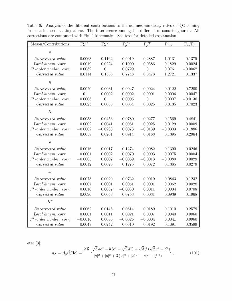
Table 6: Analysis of the different contributions to the nonmesonic decay rates of 12ΛC coming
from each meson acting alone. The interference among the different mesons is ignored. Allcorrections are computed with “full” kinematics. See text for detailed explanation.
Meson/Contributions ΓPCn ΓPV
n ΓPCp ΓPV
p Γnm Γn/Γp
π
Uncorrected value 0.0063 0.1162 0.6019 0.2887 1.0131 0.1375Local kinem. corr. 0.0019 0.0224 0.1000 0.0586 0.1829 0.0024
1st -order nonloc. corr. 0.0032 0 0.0729 0 0.0761 −0.0062Corrected value 0.0114 0.1386 0.7748 0.3473 1.2721 0.1337
η
Uncorrected value 0.0020 0.0031 0.0047 0.0024 0.0122 0.7200Local kinem. corr. 0 0.0002 0.0002 0.0001 0.0006 −0.0047
1st -order nonloc. corr. 0.0003 0 0.0005 0 0.0007 −0.0130Corrected value 0.0023 0.0033 0.0054 0.0025 0.0135 0.7023
K
Uncorrected value 0.0058 0.0453 0.0780 0.0277 0.1569 0.4841Local kinem. corr. 0.0002 0.0041 0.0061 0.0025 0.0129 0.0009
1st -order nonloc. corr. −0.0002 −0.0233 0.0073 −0.0139 −0.0303 −0.1886Corrected value 0.0058 0.0261 0.0914 0.0163 0.1395 0.2964
ρ
Uncorrected value 0.0016 0.0017 0.1274 0.0082 0.1390 0.0246Local kinem. corr. 0.0001 0.0002 0.0070 0.0003 0.0075 0.0004
1st -order nonloc. corr. −0.0005 0.0007 −0.0069 −0.0013 −0.0080 0.0029Corrected value 0.0012 0.0026 0.1275 0.0072 0.1385 0.0279
ω
Uncorrected value 0.0073 0.0020 0.0732 0.0019 0.0843 0.1232Local kinem. corr. 0.0007 0.0001 0.0051 0.0001 0.0062 0.0028
1st -order nonloc. corr. 0.0016 0.0037 −0.0030 0.0011 0.0034 0.0708Corrected value 0.0096 0.0058 0.0753 0.0031 0.0939 0.1968
K∗
Uncorrected value 0.0062 0.0145 0.0614 0.0189 0.1010 0.2579Local kinem. corr. 0.0001 0.0011 0.0021 0.0007 0.0040 0.0060
1st -order nonloc. corr. −0.0016 0.0086 −0.0025 −0.0004 0.0041 0.0960Corrected value 0.0047 0.0242 0.0610 0.0192 0.1091 0.3599
eter [3]:
aΛ = Ay(5ΛHe) =
2ℜ[√
3 ae∗ − b (c∗ −√
2 d∗) +√
3 f (√
2 c∗ + d∗)]
|a|2 + |b|2 + 3 (|c|2 + |d|2 + |e|2 + |f |2) , (101)
27

where
a = 〈np,1S0|V |Λp,1S0〉= M(pl=0 PL=0 λ=0 S=0 J=0 T =1 MT =0 ;Λp, (1s1/2)
2 J=0) ,
b = i〈np,3P0|V |Λp,1S0〉= iM(pl=1 PL=0 λ=1 S=1 J=0 T =1 MT =0 ;Λp, (1s1/2)
2 J=0) ,
c = 〈np,3S1|V |Λp,3S1〉= −M(pl=0 PL=0 λ=0 S=1 J=1 T =0 MT =0 ;Λp, (1s1/2)
2 J=1) ,
d = −〈np,3D1|V |Λp,3S1〉= M(pl=2 PL=0 λ=2 S=1 J=1 T =0 MT =0 ;Λp, (1s1/2)
2 J=1) ,
e = i〈np,1P1|V |Λp,3S1〉= −iM(pl=1 PL=0 λ=1 S=0 J=1 T =0 MT =0 ;Λp, (1s1/2)
2 J=1) ,
f = −i〈np,3P1|V |Λp,3S1〉= −iM(pl=1 PL=0 λ=1 S=1 J=1 T =1 MT =0 ;Λp, (1s1/2)
2 J=1) . (102)
The extra factors in the transition amplitudes are due to differences in phase conventions, asexplained in Appendix B, and we have rewritten them in terms of the nuclear matrix elementsdefined in Eq. (97).
It is important to realize that the formula (101) is not of general validity, and is, in fact,merely an approximation taken over from the result valid for a free space process [57] and adaptedsomehow to the hypernuclear decay situation. In particular, there is no definitive prescriptionon how to devide the energy liberated in the decay, ∆F , between the relative and CM motions ofthe emitted nucleons. It seems that, based on the expectation that the final result be insensitiveto this point, some authors merely take P = 0 in Eqs. (102), while others integrate over phasespace, both the numerator, and the denominator in Eq. (101). We have checked that the twoprescriptions indeed give similar results for 5
ΛHe, and opted to tabulate only those correspondingto the first one. A more rigorous calculation of aΛ is planned for the near future.
We give, in Table 7, the results we obtained for the decay rates and asymmetry parameter of5ΛHe. The calculation goes along similar lines to those explained in Subsection 3.1, except for theobvious changes. The (hyper)nuclear model-space is restricted to the 1s1/2 orbital; the relevant
nuclear structure factors, Eq. (96), are [23] F1s1/2 n0 = F
1s1/2 p0 = 1/2, F
1s1/2 n1 = F
1s1/2 p1 = 3/2;
we used 1.62 fm for the oscillator length parameter; and took ∆F = 153.83 MeV. It is clear fromthis table that the comments made above about the decay rates of 12
ΛC remain qualitatively validin the present case. As to the asymmetry parameter, the effect of the two corrections reaches∼ 18% in the π+ ρ model, but is of only ∼ 5% in the complete model. On the average, it variesaround ∼ 10%. It is interesting to observe that the two corrections always go in the direction ofmaking aΛ even more negative, thus confirming the sign of the existing theoretical predictionsfor this observable in contraposition to its most recent experimental determination.
4 Summary and conclusions
We have proposed an approach that naturally establishes a hierarchy for the different levels ofapproximation in the extraction of the nonrelativistic transition potential in OME models ingeneral. The central result is Eq. (21). The first term corresponds to the local approximation,
28

Table 7: Analysis of the different contributions to the nonmesonic decay rates and asymmetryparameter of 5
ΛHe in several OME models. All corrections are computed with “full” kinematics.See text for detailed explanation.
Model/Contributions ΓPCn ΓPV
n ΓPCp ΓPV
p ΓPC/ΓPV aΛ
π
Uncorrected value 0.0004 0.0739 0.3889 0.1479 1.7553 −0.4351Local kinem. corr. 0.0005 0.0130 0.0599 0.0258 −0.0295 −0.0084
1st -order nonloc. corr. 0.0011 0 0.0461 0 0.1810 −0.0021Corrected value 0.0020 0.0869 0.4949 0.1737 1.9068 −0.4456
(π, η,K)
Uncorrected value 0.0013 0.1734 0.1261 0.2077 0.3342 −0.5852Local kinem. corr. 0.0008 0.0234 0.0280 0.0327 0.0229 −0.0106
1st -order nonloc. corr. 0.0013 −0.0285 0.0176 −0.0215 0.0952 −0.0406Corrected value 0.0034 0.1683 0.1717 0.2189 0.4523 −0.6364
π + ρ
Uncorrected value 0.0001 0.0648 0.3135 0.1939 1.2118 −0.2665Local kinem. corr. 0.0001 0.0121 0.0433 0.0299 −0.0251 −0.0217
1st -order nonloc. corr. 0.0004 0.0016 0.0245 −0.0056 0.1003 −0.0273Corrected value 0.0006 0.0785 0.3813 0.2182 1.2870 −0.3155
(π, η,K) + (ρ, ω,K∗)
Uncorrected value 0.0112 0.1672 0.1778 0.3642 0.3558 −0.5131Local kinem. corr. 0.0026 0.0206 0.0344 0.0442 0.0233 −0.0090
1st -order nonloc. corr. 0.0054 −0.0715 0.0237 −0.0897 0.2073 −0.0167Corrected value 0.0192 0.1163 0.2359 0.3187 0.5864 −0.5388
usually adopted in the literature on nonmesonic decay. The second one, to the first-ordernonlocality correction, which we have included in our calculations here. And the last one, to thesecond-order nonlocality correction, which we have neglected. We have also given a detailed andgeneral account on how to deal accurately with the kinematical effects that result when one hasdifferent baryon masses on the four legs in the OME Feynman amplitude in Fig. 1. All this wasparticularized to Λ hypernuclear nonmesonic decay and detailed expressions for all contributionsto the transition potential coming from the exchange of the complete pseudoscalar and vectormeson octets were given.
Using this formalism, we have investigated the relative importance of two effects sistemati-cally ignored in OME models for the nonmesonic weak decay of Λ-hypernuclei. First, that of anaccurate treatment of the kinematics, i.e., of taking into account the difference in mass betweenthe hyperon and the nucleon, when determining the OME transition potential. Secondly, weconsidered the influence of the first-order nonlocality-correction terms. Surprisingly, in view ofthe nonnegligible value of the mass-asymmetry ratio in Eq. (32), we came to the conclusion thatthe kinematical effect on the local potential is small, except for the reduction of the effectivemass of the pion, Eq. (42), which implies an increase of ∼ 35% in the range of the correspond-
29

ing transition potential. However its indirect influence is important, since it activates severalnonlocal terms in the transition potential.
Our conclusion is that the influence of the two effects together on the partial decay rates issizeable, the full amount depending on which mesons are included. It can be very large for ΓPC
n ,often exceeding 100%, while it typically stays in the 20–30% range for the other partial rates.The effects are somewhat washed out in the main decay observables, averaging to ∼ 15% for thetotal nonmesonic decay rate, Γnm = Γn + Γp, and to ∼ 10% for, both the neutron- to proton-induced ratio, Γn/Γp, and the asymmetry parameter, aΛ. In particular, they do not in any wayaccount for the well known discrepancy between the standard OME predictions for the lattertwo observables and their measured values [3]. To summarize, although the kinematical andnonlocality effects can be very important for particular transitions, they end up by not affectingthe main decay observables too much. One can partly understand this from the following twofacts:
1. The most affected transitions are by far the neutron-induced, parity-conserving ones. How-ever those contribute very little to Γnm and to Γn/Γp, and not at all to aΛ, which is aproperty of proton-induced transitions only.
2. The largest relative effect of the nonlocality corrections is on the PV transitions comingfrom the one-omega-exchange process. However, for this meson, the PC transitions aremuch more important and they are affected in the opposite direction. As a result thetwo effects are largely neutralized in any of the main decay observables, which depend on,either the sum of the intensities, or the product of the amplitudes for these two types oftransitions.
We have also shown that the parameter ΓPC/ΓPV is strongly affected in OME models thatinclude strange mesons. The relative correction is of ∼ 30% in the (π + η + K) model and of∼ 60% in the complete model. However, none of the three nonmesonic decay observables thathave been measured up to now is sensitive to this ratio.
Let us finalize by saying that, although the effects we have studied here can be consideredsmall in view of the imprecision of the available measurements and the degree of uncertaintypresently existing in the parameters of OME models for nonmesonic decay (particularly couplingconstants), they are not altogether negligible. In fact, in many cases they appear to influencethe theoretical predictions by roughly as much as the inclusion of other mesons beyond the pionin the exchange process. It seems, therefore, that they have a part to play in OME modelsfor nonmesonic hypernuclear decays, specially if one takes into consideration that more detailedand accurate experimental data on this issue is forthcoming.
Acknowledgements
C. B. and F. K. are fellows of the CONICET (Argentina) and acknowledge the support ofCONICET under grant PIP 463, of ANPCyT (Argentina) under grant BID 1201/OC-AR (PICT03-04296) and of Fundacion Antorchas (Argentina). The work of C. D. C. was supported byFAPESP (Sao Paulo, Brazil). One of us (C. B.) would like to thank G. Garbarino, A. Parrenoand A. Ramos for helpful discussions about the asymmetry parameter.
30

Appendices
A Calculation of nuclear matrix elements
We collect in this appendix some useful expressions for the calculation of the several matrixelements contributing to Eq. (97). As mentioned below that equation, the first step is to factorout the baryon content of the initial state,
|j1Λ j2N J) = |j1 j2 J) |ΛN) ≡ |n1l1j1 n2l2j2 J) |ΛN) , (A1)
and perform a Moshinsky transformation [51] for its space-spin part,
|n1l1j1 n2l2j2 J) =√
(2j1 + 1)(2j2 + 1)∑
λS
√
(2λ+ 1)(2S + 1)
l112 j1
l212 j2
λ S J
×∑
nlNL
|nlNLλSJ) (nlNLλ| n1l1 n2l2 λ) . (A2)
A look at Subsections 2.3 and 2.4 shows that the operators involved are always of the generalform v(r)Ω(σ1,σ2, r,∇). All matrix elements are diagonal in the quantum numbers L and J ,and the needed results are listed below. Some of them have already been given in Ref. [21] butare repeated here for completeness.8
(
p′l′ P ′Lλ′S′J∣
∣ v(r) |nlNLλSJ) =
δl′lδλ′λδS′S
(
P ′L∣
∣ NL)(
p′l′∣
∣ v(r) |nl) , (A3)
(
p′l′ P ′Lλ′S′J∣
∣ v(r)σ1 · σ2 |nlNLλSJ) =
δl′lδλ′λδS′S [2S(S + 1) − 3](
P ′L∣
∣ NL)(
p′l′∣
∣ v(r) |nl) , (A4)
(
p′l′ P ′Lλ′S′J∣
∣ v(r)S12(r) |nlNLλSJ) =
(−)L+J+1 δS1δS′1
√
120(2l′ + 1)(2l + 1)(2λ′ + 1)(2λ + 1)
×(
l′ 2 l0 0 0
)
λ′ 2 λl L l′
1 2 1λ J λ′
(
P ′L∣
∣ NL)(
p′l′∣
∣ v(r) |nl) , (A5)
(−)S′+S (p′l′ P ′Lλ′S′J
∣
∣ v(r)σ1 · r |nlNLλSJ) =(
p′l′ P ′Lλ′S′J∣
∣ v(r)σ2 · r |nlNLλSJ) =
(−)L+J+1√
6(2l′ + 1)(2l + 1)(2λ′ + 1)(2λ + 1)(2S′ + 1)(2S + 1)
×(
l′ 1 l0 0 0
)
λ′ 1 λl L l′
S′ 1 S12
12
12
S′ 1 Sλ J λ′
×(
P ′L∣
∣ NL)(
p′l′∣
∣ v(r) |nl) , (A6)
8There are some misprints in the formulas for the matrix elements in the published version of Ref.[21]. Thesemisprints, however, do not occur in its preprint version, axXiv:nucl-th/0011092.
31

(
p′l′ P ′Lλ′S′J∣
∣ iv(r)(σ1 × σ2) · r |nlNLλSJ) =
(−)L+J+S (δS′0δS1 + δS′1δS0)√
12(2l′ + 1)(2l + 1)(2λ′ + 1)(2λ+ 1)
×(
l′ 1 l0 0 0
)
λ′ 1 λl L l′
S′ 1 Sλ J λ′
(
P ′L∣
∣ NL)(
p′l′∣
∣ v(r) |nl) , (A7)
(−)S′+S (p′l′ P ′Lλ′S′J
∣
∣ v(r)σ1 · ∇ |nlNLλSJ) =(
p′l′ P ′Lλ′S′J∣
∣ v(r)σ2 · ∇ |nlNLλSJ) =
(−)L+J+1√
6(2l′ + 1)(2l + 1)(2λ′ + 1)(2λ + 1)(2S′ + 1)(2S + 1)
×(
l′ 1 l0 0 0
)
λ′ 1 λl L l′
S′ 1 S12
12
12
S′ 1 Sλ J λ′
×(
P ′L∣
∣ NL)(
p′l′∣
∣ v(r)dV (l′, l; r) |nl) , (A8)
(
p′l′ P ′Lλ′S′J∣
∣ iv(r)(σ1 × σ2) · ∇ |nlNLλSJ) =
(−)L+J+S (δS′0δS1 + δS′1δS0)√
12(2l′ + 1)(2l + 1)(2λ′ + 1)(2λ + 1)
×(
l′ 1 l0 0 0
)
λ′ 1 λl L l′
S′ 1 Sλ J λ′
×(
P ′L∣
∣ NL)(
p′l′∣
∣ v(r)dV (l′, l; r) |nl) , (A9)
(−)S′+S (p′l′ P ′Lλ′S′J
∣
∣ v(r)σ1 · l |nlNLλSJ) =(
p′l′ P ′Lλ′S′J∣
∣ v(r)σ2 · l |nlNLλSJ) =
(−)l+L+J+1 δl′l
√
6l(l + 1)(2l + 1)(2λ′ + 1)(2λ + 1)(2S′ + 1)(2S + 1)
×
λ′ 1 λl L l′
S′ 1 S12
12
12
S′ 1 Sλ J λ′
×(
P ′L∣
∣ NL)(
p′l′∣
∣ v(r) |nl) , (A10)
(
p′l′ P ′Lλ′S′J∣
∣ iv(r)(σ1 × σ2) · l |nlNLλSJ) =
(−)l+L+J+S δl′l (δS′0δS1 + δS′1δS0)√
12l(l + 1)(2l + 1)(2λ′ + 1)(2λ + 1)
×
λ′ 1 λl L l′
S′ 1 Sλ J λ′
(
P ′L∣
∣ NL)(
p′l′∣
∣ v(r) |nl) , (A11)
(
p′l′ P ′Lλ′S′J∣
∣ v(r)r · ∇ |nlNLλSJ) =(
p′l′ P ′Lλ′S′J∣
∣ v(r)dS(r) |nlNLλSJ) =
δl′lδλ′λδS′S
(
P ′L∣
∣ NL)(
p′l′∣
∣ v(r)dS(r) |nl) , (A12)
(
p′l′ P ′Lλ′S′J∣
∣ v(r)σ1 · σ2 r · ∇ |nlNLλSJ) =(
p′l′ P ′Lλ′S′J∣
∣ v(r)σ1 · σ2 dS(r) |nlNLλSJ) , (A13)
32
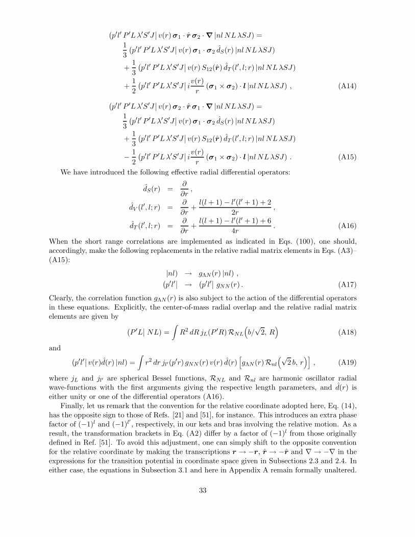
(
p′l′ P ′Lλ′S′J∣
∣ v(r)σ1 · r σ2 · ∇ |nlNLλSJ) =
1
3
(
p′l′ P ′Lλ′S′J∣
∣ v(r)σ1 · σ2 dS(r) |nlNLλSJ)
+1
3
(
p′l′ P ′Lλ′S′J∣
∣ v(r)S12(r) dT (l′, l; r) |nlNLλSJ)
+1
2
(
p′l′ P ′Lλ′S′J∣
∣ iv(r)
r(σ1 × σ2) · l |nlNLλSJ) , (A14)
(
p′l′ P ′Lλ′S′J∣
∣ v(r)σ2 · r σ1 · ∇ |nlNLλSJ) =
1
3
(
p′l′ P ′Lλ′S′J∣
∣ v(r)σ1 · σ2 dS(r) |nlNLλSJ)
+1
3
(
p′l′ P ′Lλ′S′J∣
∣ v(r)S12(r) dT (l′, l; r) |nlNLλSJ)
− 1
2
(
p′l′ P ′Lλ′S′J∣
∣ iv(r)
r(σ1 × σ2) · l |nlNLλSJ) . (A15)
We have introduced the following effective radial differential operators:
dS(r) =∂
∂r,
dV (l′, l; r) =∂
∂r+l(l + 1) − l′(l′ + 1) + 2
2r,
dT (l′, l; r) =∂
∂r+l(l + 1) − l′(l′ + 1) + 6
4r. (A16)
When the short range correlations are implemented as indicated in Eqs. (100), one should,accordingly, make the following replacements in the relative radial matrix elements in Eqs. (A3)–(A15):
|nl) → gΛN (r) |nl) ,(
p′l′∣
∣ →(
p′l′∣
∣ gNN (r) . (A17)
Clearly, the correlation function gΛN (r) is also subject to the action of the differential operatorsin these equations. Explicitly, the center-of-mass radial overlap and the relative radial matrixelements are given by
(
P ′L∣
∣ NL) =
∫
R2 dR jL(P ′R)RNL
(
b/√
2, R)
(A18)
and(
p′l′∣
∣ v(r)d(r) |nl) =
∫
r2 dr jl′(p′r) gNN (r) v(r) d(r)
[
gΛN (r)Rnl
(√2 b, r
)]
, (A19)
where jL and jl′ are spherical Bessel functions, RNL and Rnl are harmonic oscillator radialwave-functions with the first arguments giving the respective length parameters, and d(r) iseither unity or one of the differential operators (A16).
Finally, let us remark that the convention for the relative coordinate adopted here, Eq. (14),has the opposite sign to those of Refs. [21] and [51], for instance. This introduces an extra phasefactor of (−1)l and (−1)l
′, respectively, in our kets and bras involving the relative motion. As a
result, the transformation brackets in Eq. (A2) differ by a factor of (−1)l from those originallydefined in Ref. [51]. To avoid this adjustment, one can simply shift to the opposite conventionfor the relative coordinate by making the transcriptions r → −r, r → −r and ∇ → −∇ in theexpressions for the transition potential in coordinate space given in Subsections 2.3 and 2.4. Ineither case, the equations in Subsection 3.1 and here in Appendix A remain formally unaltered.
33

B Phase conventions for a, b, . . . f
With the phase conventions of Nabetani et al. (N.O.S.K.), in Ref. [57], from which Eq. (101) isobtained, the transition amplitudes are defined as follows:
a =(
〈pn,1S0|V |pΛ,1S0〉)
N.O.S.K.,
b =(
〈pn,3P0|V |pΛ,1S0〉)
N.O.S.K.,
c =(
〈pn,3S1|V |pΛ,3S1〉)
N.O.S.K.,
d =(
〈pn,3D1|V |pΛ,3S1〉)
N.O.S.K.,
e =(
〈pn,1P1|V |pΛ,3S1〉)
N.O.S.K.,
f =(
〈pn,3P1|V |pΛ,3S1〉)
N.O.S.K.. (B1)
The relationship with our phase conventions is
(
〈pn, 2S′+1l′J |V |pΛ, 2S+1lJ〉)
N.O.S.K.= (−)S
′+S i−l′ 〈np, 2S′+1l′J |V |Λp, 2S+1lJ 〉 , (B2)
where the first correction is due to the change in ordering in the Clebsch-Gordan couplingsfor the spins, and the second one, to the fact that we do not include the phase il
′in the final
partial-wave radial function (cf. Eq. (A19)). This explains the extra phase factors appearing inEq. (102).
Notice that there is no factor (−)l′+l in Eq. (B2) as might be expected due to the change
in ordering of the two particles in both the initial and final states, the reason being that this iscompensated by the fact that we use the opposite convention for the relative coordinates.
References
[1] J. Cohen, Prog. Part. Nucl. Phys. 25 (1990) 139.
[2] E. Oset and A. Ramos, Prog. Part. Nucl. Phys. 41 (1998) 191.
[3] W. M. Alberico and G. Garbarino, Phys. Rep. 369 (2002) 1.
[4] J. B. Adams, Phys. Rev. 156 (1967) 832. (Cf. correction pointed out in Ref. [10].)
[5] C.-Y. Cheung, D. P. Heddle and L. S. Kisslinger, Phys. Rev. C 27 (1983) 335.
[6] K. Maltman and M. Shmatikov, Phys. Lett. B 331 (1994) 1.
[7] T. Inoue, S. Takeuchi and M. Oka, Nucl. Phys. A 597 (1996) 563.
[8] T. Inoue, M. Oka, T. Motoba and K. Itonaga, Nucl. Phys. A 633 (1998) 312.
[9] K. Sasaki, T. Inoue and M. Oka, Nucl. Phys. A 669 (2000) 331.
[10] B. H. J. McKellar and B. F. Gibson, Phys. Rev. C 30 (1984) 322.
[11] K. Takeuchi, H. Takaki and H. Bando, Prog. Theor. Phys. 73 (1985) 841.
[12] G. Narduli, Phys. Rev. C 38 (1988) 832.
34

[13] A. Parreno, A. Ramos and C. Bennhold, Phys. Rev. C 52, R1768 (1995). Erratum: ibid.54 (1996) 1500.
[14] A. Ramos, C. Bennhold, E. van Meijgaard and B. K. Jennings, Phys. Lett. B 264 (1991)233. (See criticism in Ref. [16].)
[15] A. Ramos, E. van Meijgaard, C. Bennhold and B. K. Jennings, Nucl. Phys. A 544 (1992)703. (See criticism in Ref. [16].)
[16] A. Parreno, A. Ramos and E. Oset, Phys. Rev. C 51 (1995) 2477.
[17] J. F. Dubach, G. B. Feldman, B. R. Holstein and L. de la Torre, Ann. Phys. (N.Y.) 249
(1996) 146.
[18] A. Parreno, A. Ramos and C. Bennhold, Phys. Rev. C 56 (1997) 339.
[19] K. Hagino and A. Parreno, Phys. Rev. C 63 (2001) 044318.
[20] A. Parreno and A. Ramos, Phys. Rev. C 65 (2001) 015204.
[21] C. Barbero, D. Horvat, F. Krmpotic, T. T. S. Kuo, Z. Narancic and D. Tadic, Phys. Rev.C 66 (2002) 055209.
[22] E. Bauer and F. Krmpotic, Nucl. Phys. A 717 (2003) 217.
[23] F. Krmpotic and D. Tadic, arXiv:nucl-th/0212040. (To appear in Braz. J. Phys. 33
(2003).)
[24] M. Shmatikov, Nucl. Phys. A 580 (1994) 538.
[25] K. Itonaga, T. Ueda and T. Motoba, Phys. Rev. C 65 (2002) 034617.
[26] E. Oset and L. L. Salcedo, Nucl. Phys. A 443 (1985) 704.
[27] W. M. Alberico, A. De Pace, M. Ericson and A. Molinari, Phys. Lett. B 256 (1991) 134.(See criticism in Ref. [28].)
[28] A. Ramos, E. Oset and L. L. Salcedo, Phys. Rev. C 50 (1994) 2314.
[29] A. Ramos, M. J. Vicente-Vacas and E. Oset, Phys. Rev. C 55 (1997) 735. Erratum: ibid.66 (2002) 039903.
[30] W. M. Alberico, A. De Pace, G. Garbarino and A. Ramos, Phys. Rev. C 61 (2000) 044314.
[31] D. Jido, E. Oset and J. E. Palomar, Nucl. Phys. A 694 (2001) 525.
[32] L. Zhou and J. Piekarewicz, Phys. Rev. C 60 (1999) 024306.
[33] E. E. Salpeter and H. A. Bethe, Phys. Rev. 84 (1951) 1232.
[34] G. Schierholz, Nucl. Phys. B 40 (1972) 335.
[35] R. M. Woloshyn and A. D. Jackson, Nucl. Phys. B 64 (1973) 269.
[36] K. Erkelenz, Phys. Rep. 13 C (1974) 191.
[37] B. Silvestre-Brac, A. Bilal, C. Gignoux and P. Schuck, Phys. Rev. D 29 (1984) 2275.
35

[38] R. Machleidt, K. Holinde and Ch. Elster, Phys. Rep. 149 (1987) 1.
[39] R. Machleidt, Adv. Nucl. Phys. 19 (1989) 189.
[40] R. Brockmann and R. Machleidt, Phys. Rev. C 42 (1990) 1965.
[41] F. Gross, J. W. Van Orden and K. Holinde, Phys. Rev. C 45 (1992) 2095.
[42] R. Blankenbecler and R. Sugar, Phys. Rev. 142 (1966) 1051.
[43] R. H. Thompson, Phys. Rev. D 1 (1970) 110.
[44] R. M. Barnett et al. (Particle Data Group), Rev. Mod. Phys. 68 (1996) 611.
[45] B. Desplanques, J. F. Donoghue and B. R. Holstein, Ann. Phys. (N.Y.) 124 (1980) 449.
[46] A. Montwill et al., Nucl. Phys. A 234 (1974) 413.
[47] J. J. Szymanski et al., Phys. Rev. C 43 (1991) 849.
[48] H. Noumi et al., Phys. Rev. C 52 (1995) 2936.
[49] H. Bang et al., Phys. Rev. Lett. 81 (1998) 4321.
[50] O. Hashimoto et al., Phys. Rev. Lett. 88 (2002) 042503.
[51] M. Moshinsky, Nucl. Phys. 13 (1959) 104.
[52] D. Halderson, Phys. Rev. C 48 (1993) 581.
[53] M. I. Haftel and F. Tabakin, Nucl. Phys. A 158 (1970) 1.
[54] W. Weise, Nucl. Phys. A 278 (1977) 402.
[55] S. Ajimura et al., Phys. Lett. B 282 (1992) 293.
[56] S. Ajimura et al., Phys. Rev. Lett. 84 (2000) 4052.
[57] H. Nabetani, T. Ogaito, T. Sato and T. Kishimoto, Phys. Rev. C 60 (1999) 017001.
36