Kent Academic Repository

Kent Academic RepositoryFull text document (pdf)

Copyright & reuseContent in the Kent Academic Repository is made available for research purposes. Unless otherwise stated allcontent is protected by copyright and in the absence of an open licence (eg Creative Commons), permissions for further reuse of content should be sought from the publisher, author or other copyright holder.

Versions of researchThe version in the Kent Academic Repository may differ from the final published version. Users are advised to check http://kar.kent.ac.uk for the status of the paper. Users should always cite the published version of record.

EnquiriesFor any further enquiries regarding the licence status of this document, please contact: [email protected]

If you believe this document infringes copyright then please contact the KAR admin team with the take-down information provided at http://kar.kent.ac.uk/contact.html

Citation for published version

Zakaria, Nurulhuda Binti (2017) Long-term population ecology of the great crested newt in Kent. Doctor of Philosophy (PhD) thesis, University of Kent,.

DOI

Link to record in KAR

https://kar.kent.ac.uk/77422/

Document Version

UNSPECIFIED

Title: Long-term population ecology of the great crested newt in Kent

Abstract: Climate change has been recognized as one of the causes of global amphibian

population declines. Amphibians may be particularly susceptible to climatic changes, as a

result of their ectothermic life style and dependence on moisture. Climatic factors may

affect amphibian population dynamics deterministically or stochastically, and can act at

both local and regional levels. Using capture-mark- recapture (CMR) methods,

population dynamics of great crested newts over two decades were compared between

two separate populations in Canterbury, Kent in order to explore local and regional

drivers of population change. Accurate individual identification is a basic assumption of

capture-mark-recapture methods. A comparison of manual and computer-assisted photo

identification programs verified that the spot patterns of individual newts did not change

significantly through time, and were sufficiently varied to reliably identify individual

newts. At a metapopulation located within an agricultural landscape, capture-mark-

recapture modelling revealed variations in survival, detectability, and population size

between years. Low annual survival of adult newts was related to mild, wet winters which

impacted the metapopulation at the regional level. Therefore, survival varied between

years but not between subpopulations. Regardless of this regional effect, the four

subpopulations were generally asynchronous in their dynamics, but the persistence of the

metapopulation depended on a single source pond that was the smallest water body

within the system. At a further population two miles away, survival since 2001 was

constant and high every year despite mild, wet winters. Management practised through

draining and refilling the ponds did have an apparent effect on the number of newts

captured over the subsequent years. Population increase could be due to the decrease in

predatory invertebrates following pond desiccation and a subsequent increase in

recruitment levels. Body condition may be linked to the survival of amphibians.

However, there was no influence of climatic conditions on the body condition at either of

the populations studied. Nevertheless, body condition was related to survival at one of the

populations, and body condition was lower in ponds with high densities of newts.

Consequently, the persistence of the two populations relies on a combination of (1) local,

population-specific factors - such as population density and pond desiccation, and (2)

regional factors, such as climate that affect recruitment and survival from each pond.

However, conservation actions at the local scale may offset reduced larval recruitment

and adult survival at the regional scale.

Word count / number of pages: 55,273/ 208

Year of submission: 2019

Academic school /centre: School of Anthropology and Conservation

Long-Term Population Ecology

of the Great Crested Newt

in Kent

Nurulhuda Binti Zakaria

Thesis submitted for the degree of Doctor of Philosophy

July 2017

The Durrell Institute of Conservation and Ecology University of Kent,

Canterbury, CT2 7NR, England

i

ABSTRACT

Climate change has been recognized as one of the causes of global amphibian

population declines. Amphibians may be particularly susceptible to climatic changes,

as a result of their ectothermic life style and dependence on moisture. Climatic

factors may affect amphibian population dynamics deterministically or

stochastically, and can act at both local and regional levels. Using capture-mark-

recapture (CMR) methods, population dynamics of great crested newts over two

decades were compared between two separate populations in Canterbury, Kent in

order to explore local and regional drivers of population change. Accurate individual

identification is a basic assumption of capture-mark-recapture methods. A

comparison of manual and computer-assisted photo identification programs verified

that the spot patterns of individual newts did not change significantly through time,

and were sufficiently varied to reliably identify individual newts. At a

metapopulation located within an agricultural landscape, capture-mark-recapture

modelling revealed variations in survival, detectability, and population size between

years. Low annual survival of adult newts was related to mild, wet winters which

impacted the metapopulation at the regional level. Therefore, survival varied

between years but not between subpopulations. Regardless of this regional effect, the

four subpopulations were generally asynchronous in their dynamics, but the

persistence of the metapopulation depended on a single source pond that was the

smallest water body within the system. At a further population two miles away,

survival since 2001 was constant and high every year despite mild, wet winters.

Management practised through draining and refilling the ponds did have an apparent

effect on the number of newts captured over the subsequent years. Population

increase could be due to the decrease in predatory invertebrates following pond

desiccation and a subsequent increase in recruitment levels. Body condition may be

linked to the survival of amphibians. However, there was no influence of climatic

conditions on the body condition at either of the populations studied. Nevertheless,

body condition was related to survival at one of the populations, and body condition

was lower in ponds with high densities of newts. Consequently, the persistence of

the two populations relies on a combination of (1) local, population-specific factors -

such as population density and pond desiccation, and (2) regional factors, such as

climate that affect recruitment and survival from each pond. However, conservation

actions at the local scale may offset reduced larval recruitment and adult survival at

the regional scale.

ii

ACKNOWLEDGMENTS

I would firstly, like to express my sincere gratitude to my supervisor, Professor

Richard Griffiths for his invaluable time and ongoing support throughout this

project. He has been kind and always come with great suggestions and guidance

along the way. I would like to thank Dr. Joseph Tzanopolous, for his kind support

and encouragement, and in particular for taking the time to guide me through the

final thesis writing. Many thanks to Dr. Rachel McCrea for her useful advice in

relation to program MARK.

I would like to extend my gratitude to the Malaysia Ministry of Higher Education

and Universiti Malaysia Terengganu, that without whom this project and much of my

academic career over the past few years would not have been possible.

I would like to thank to the numerous field students and volunteers of which there

are too many to name, who have collected and collated the data from both the sites

surveyed over the last 20 years.

Exceptional gratitude to all my fellow DICE friends - Andy, Aydan, Aziz, Ben,

Debbie, Dimitrious, Gail, Helena, Izabela, Jim, Jinks, Lydia, Leonel, Moacir, Samia,

Tristan, and Rob. Thank you for your encouragement throughout my time at DICE.

Many thanks to Faeiqah, Hafizah, Ismatul, Munirah and Salahuddin for the moral

and emotional support that you have provided me during my time here.

Special thanks to my family at home whose continuous encouragement have made

me come this far. I would like to thank my very patient life partner, Azwan for being

my voice of reason, for his love and companionship and all round support throughout

my endeavours. Lastly and by no means least, to my life-coach, my late father

Zakaria Bin Ngah: because I owe it all to you. Many Thanks!

iii

TABLE OF CONTENTS

Page

Abstract ........................................................................................................................ i

Acknowledgments ....................................................................................................... ii

Table of Contents ....................................................................................................... iii

List of Tables .............................................................................................................. ix

List of Figures ............................................................................................................. xi

CHAPTER:

1.0 General Introduction ..................................................................................... 1

1.1 Threatened Amphibians ....................................................................... 1

1.2 Global Amphibian Declines ................................................................ 2

1.3 Climate Change and Amphibians ........................................................ 3

1.4 Great Crested Newt… ......................................................................... 6

1.4.1 Classification and Description ................................................. 6

1.4.2 Breeding Migration… ............................................................. 7

1.4.3 Distribution… .......................................................................... 9

1.4.4 Conservation Status ............................................................... 11

1.5 Metapopulations ................................................................................ 11

1.6 Population Regulation in Amphibians ............................................... 16

1.7 Research Objectives .......................................................................... 19

1.8 Thesis Structure ................................................................................. 20

2.0 Study

2.1

Site and Methods .............................................................................. 23

Study Sites .................................................................................... ….23

2.1.1 Well Court Farm, Blean………………………………...….26

2.1.2 Field Site, University of Kent……………………...........….30

iv

2.2 Data Collection .................................................................................. 33

2.3 Newt Identification ............................................................................ 34

2.4 Weather Records ............................................................................... 35

2.5 Mark Recapture Analysis .................................................................. 36

3.0 Accuracy of Photo Identification of Newts by Manual and

Computer Identification Methods ............................................................. 40

Abstract .......................................................................................................... 40

3.1 Introduction ....................................................................................... 41

3.1.1 Aims and Objectives .............................................................. 45

3.2 Materials and Methods ...................................................................... 46

3.2.1 Study Site and Photograph Collection ................................... 46

3.2.2 Manual Photo-Identification Evaluation ............................... 48

3.2.3 Computer-assisted Pattern Recognition

Program Evaluation ............................................................... 50

3.2.4 Statistical Analysis ................................................................ 55

3.3 Results ............................................................................................... 56

3.3.1 Manual Identification ............................................................ 56

3.3.2 Software Evaluation .............................................................. 57

3.4 Discussion .......................................................................................... 63

3.4.1 Manual Photo-identification .................................................. 63

3.4.2 Computer-assisted Photo-identification ................................ 66

4.0 Metapopulation Dynamics of the Great Crested Newt in

an Agricultural Landscape ......................................................................... 74

Abstract ......................................................................................................... 74

Introduction…………………...……………………………………………..75

4.1 Study Site and Methods ..................................................................... 78

4.1.1 Study Site ............................................................................... 78

v

4.1.2 Survey Methods ..................................................................... 78

4.1.3 Climatic Covariates ............................................................... 79

4.1.4 Data Analysis ......................................................................... 80

4.2 Results ............................................................................................... 80

4.2.1 Capture Rates ......................................................................... 80

4.2.2 Movement between Ponds ..................................................... 82

4.2.3 Model without Climatic Covariates Used in the

CJS Method in Program MARK ........................................... 84

4.2.4 Model with Climatic Covariates ............................................ 86

4.2.5 Population Estimate ............................................................... 90

4.3 Discussion .......................................................................................... 91

5.0 Colonisation and Population Dynamics of the Great Crested

Newt in Newly Created Ponds .................................................................... 99

Abstract .......................................................................................................... 99

5.1 Introduction ..................................................................................... 100

5.2 Study Site and Methods ................................................................... 102

5.2.1 Study Site ............................................................................. 102

5.2.2 Survey Methods ................................................................... 103

5.2.3 Newt Identification .............................................................. 105

5.2.4 Weather Records ................................................................. 105

5.2.5 Capture-mark-recapture Modelling ..................................... 105

5.3 Results ............................................................................................. 105

5.3.1 Adult Capture ...................................................................... 105

5.3.2 Variation in Survival and Detectability between

Sexes without Climatic Covariates ...................................... 107

5.3.3 Variation in Survival and Detectability with the

Climatic Covariates ............................................................. 110

5.3.4 Detectability and Population Estimates ............................... 114

vi

5.4 Discussion ........................................................................................ 115

6.0 Comparison of Body Condition Index and the Survivorship

of the Great Crested Newt in Two Populations ...................................... 123

Abstract ........................................................................................................ 123

6.1 Introduction ..................................................................................... 124

6.2 Study Site and Methods ................................................................... 126

6.2.1 Study Site ............................................................................. 126

6.2.2 Materials and Methods ........................................................ 127

6.3 Results ............................................................................................. 131

6.3.1 Well Court Metapopulation ................................................. 131

6.3.2 Field Site Population ........................................................... 138

6.3.3 Interaction Effects of Pond and Year .................................. 142

6.3.4 Interaction between Population and Body

Condition ............................................................................. 143

6.4 Discussion ........................................................................................ 146

7.0 General Discussion .................................................................................... 153

7.1 Population Growth and Regulation ................................................. 153

7.2 Conclusion: Conservation Implications .......................................... 156

8.0 References .................................................................................................. 160

9.0 Appendices ................................................................................................. 186

Appendix I Published Paper in Scientific Reports .................................. 187

ix

LIST OF TABLES

Page

Table 2.1 Lists of publications from two study sites

23

Table 4.1 Initial model deviance and c-hat by groups, plus

adjustments. The adjustment used for each group is

highlighted in bold

83

Table 4.2 Comparison of the two most parsimonious models in each

group size for the Well Court data; t = time, and g = ponds

86

Table 4.3 CJS model selection based upon ΔQAICc in program

MARK; Phi = survival, p = detectability, t = time, and g =

ponds. Climatic variable; SR = spring rainfall, and NAR =

non-aquatic rainfall. NP = number of parameters, and

QAICc = quasi Akaike information criteria from adjusted

data

86

Table 5.1 Initial model deviance and c-hat, plus adjustments. The

adjustment used is highlighted in bold

106

Table 5.2 The most parsimonious models for Triturus cristatus at the

Field Site. Model notation as described in the methods, Phi

= survival, and p = detection rates. NP = number of

parameters

107

Table 5.3 Likelihood ratio tests for the three most parsimonious

models with the ∆QAICc value below than 10.0

107

Table 5.4 Survival and detection rates from model Phi(.) p(g)

108

Table 5.5 Survival and detection rates from model Phi(g) p(g)

108

Table 5.6 CJS model selection based upon ∆QAICc in program

MARK; Phi = survival and p = detection rates. Climatic

variables; NAR = non- aquatic rainfall, WT = winter

temperature, SR = spring rainfall, and AF = air frost. NP =

number of parameters, and QAICc = quasi Akaike

information criteria from data adjusted using c-hat

110

Table 5.7 Likelihood ratio tests for the three most parsimonious

models with the ∆QAICc value below than 10.0

111

Table 6.1 Summary of results of analysis of variance using a two-way

ANOVA, showing how body condition index of male great

crested newts was affected by the factors of pond and year

of sampling

133

x

Table 6.2 Model selection based on ΔQAICc values with the c-hat

corrected as 1.52. Phi = survival, p = detection rate, t = time,

(.) = constant, and BCI = body condition index. Climatic

variable; NAR = non-aquatic rainfall, SR = spring rainfall,

and WT = winter temperature. NP = number of parameters,

and QAICc = quasi Akaike information criteria

136

Table 6.3 Model selection based on ΔQAICc values with the c-hat

corrected as 1.21. Phi = survival, p = detection rate, t =

time, (.) = constant, and BCI = body condition index.

Climatic variable; NAR = non-aquatic rainfall, SR = spring

rainfall, and WT = winter temperature. NP = number of

parameters, and QAICc = quasi Akaike information criteria

140

xi

LIST OF FIGURES

Page

Figure 1.1 Distribution of the great crested newt in Britain from JNCC

(2017), based on various data sources

10

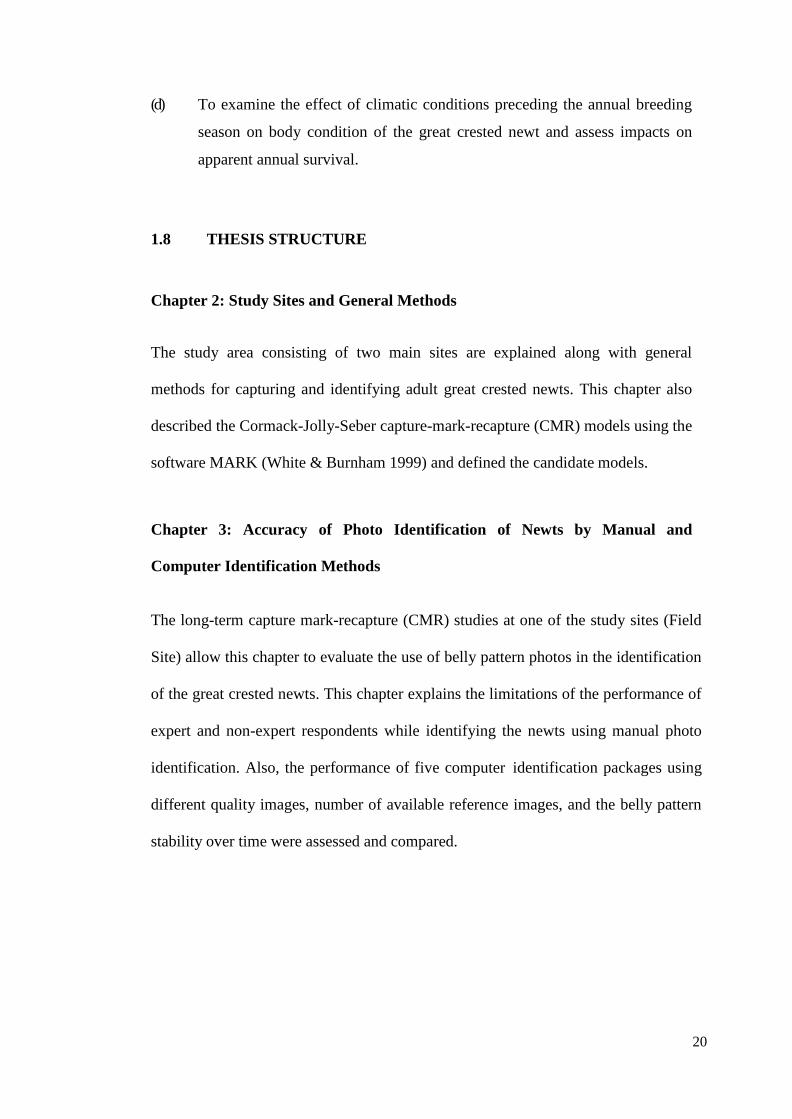
Figure 2.1 Ponds in the two main study areas, with Well Court pond

sites indicated by green dots and Field Site by red dot. Map

was adapted from Ordnance Survey

25

Figure 2.2 Ordnance Survey map showing the survey area of Well

Court farm. The position of each of the survey ponds is

shown with a red dot and initials of the pond

26

Figure 2.3 Four pond systems in Well Court Farm, Blean with (a)

Garden ponds, (b) Snake pond, (c) Swimming pool, and (d)

Pylon pond

27

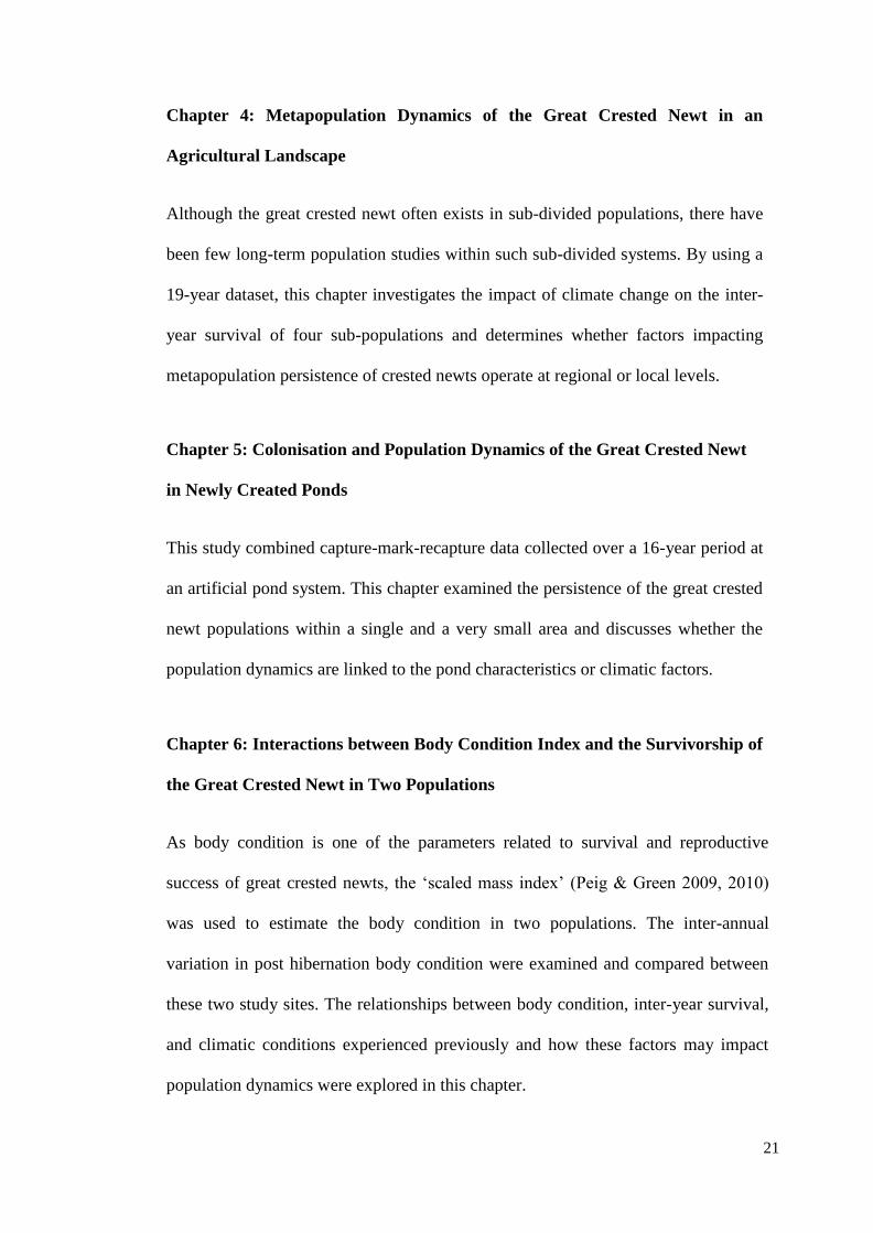
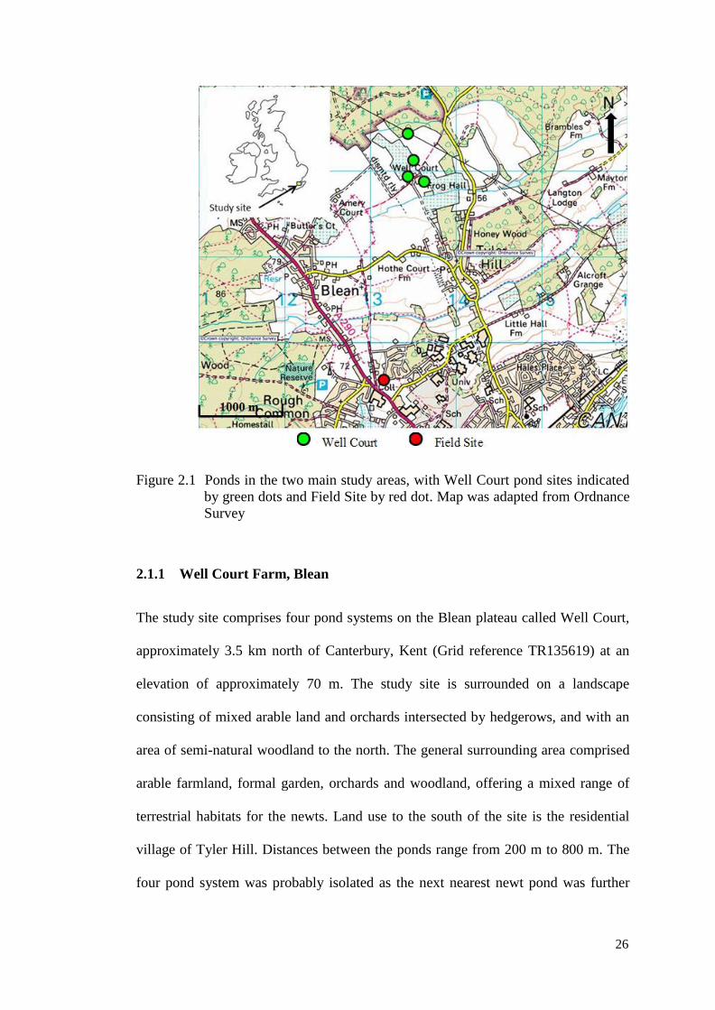
Figure 2.4 The red pin showing study site consisted with eight artificial

ponds within a fenced enclosure, map was adapted from

Earthstar Geoghraphics SIO

31

Figure 2.5 Plan of the layout at the Field Site Ponds, adapted from

Lewis (2012). The numbers within the ponds indicate bottle-

trap positions. Traps 1 and 2 are at the shallow end of each

pond, 5 and 6 at the deep end. Traps 7 and 8, when used are

laid below traps 5 and 6

31

Figure 2.6 A cross section of a Field Site pond showing its tapered

design and measurements, from Wright (2009). Also, trap

placement within each pond

32

Figure 2.7 Example of photo utilised for individual photo identification

34

Figure 3.1 Example of two good quality images (1a left and 1b left) and

two poor quality images (1a right and 1b right). Poor quality

image of 1(a) right had flash reflection, 1(b) right was out of

focus

48

Figure 3.2 (a) and (b) are examples of images from 4 different

individuals that have some similarity but unclear

distinctiveness of belly pattern

48

Figure 3.3 Example some of the belly pattern images that were used for

reference in newt identification

49

Figure 3.4 (A) The original, non-processed picture. (B) The pattern

with superimposed grid and the preview to pattern selection

in true and false colour. (C) The extracted pattern and the

53

xii

proposed matches (1–5) in order of likelihood supplemented

by the original pictures of the extracted pattern and the

selected one. Screenshot was taken from AMPHIDENT

software.

Figure 3.5 Time taken to identify newt individuals. On the left side of

red line were the recaptures and on the right were the newly

captured newts

56

Figure 3.6 Accuracy scores of each test category from two groups;

expert and non- expert. (a) Photo quality test, (b) pattern

distinctiveness test, and (c) consistency test.

57

Figure 3.7 Examples of belly pattern changes over > 6 yrs. Images (a)

and (b) were taken from different newts

58

Figure 3.8 Summary of results from paired sample of t-test analyses for

five different softwares packages that compare the accuracy

scores of good and low quality images. The degree of

freedom (d.f.) for each test was 49

59

Figure 3.9 Effect of multiple images on visual matching success of

computer-assisted image matching system. Accuracy scores

clearly increase when more reference images are available

60

Figure 3.10 The accuracy scores in relation to time (years) between

captures. The box shows a summary of results from two-

way ANOVA comparing the accuracy scores of different

packages. The degrees of freedom for each test was d.f.N =

8, d.f.D = 392

62

Figure 4.1 Garden Ponds trapping plan with the number shows the trap

position

78

Figure 4.2 Total capture and recapture of individual adults by year

80

Figure 4.3 Total adult captures comparing Garden Ponds with total

metapopulation

81

Figure 4.4 Distance and number of adult migrations between ponds

within the Well Court metapopulation

82

Figure 4.5 Time-dependent model parameter [Phi(t)], and covariate-

dependent [Phi(NAR+SR)] parameter estimates

87

Figure 4.6 Relationship between spring period rainfall (SR) and inter-

year survival (a), and non-aquatic period rainfall (NAR) and

inter-year survival (b). Survival estimates are based on

model Phi(NAR+SR)

88

xiii

Figure 4.7 Population estimates for the total metapopulation by year,

based on detection rate and individuals captured by pond

using model Phi(t) p(g+t). Vertical lines show 95%

confidence intervals.

90

Figure 5.1 A bottle trap, (a) with and (b) without the funnel in position.

Note the string used to attach the bottle to a stick on the bank

of the pond to maintain the air bubble at the top of the bottle

102

Figure 5.2 Bottle traps in position in one of the experimental ponds.

Note the air bubble left in each bottle to allow surfacing for

air, especially visible in the bottle on the top right corner.

Two traps are also set on the bottom of the deep end of the

pond until the third week of April

103

Figure 5.3 Total captures of individual adults by year and sex. A and C

= pond drainage and relining; B = creation of 4 new ponds

105

Figure 5.4 Inter-year survival rate showing variation over time and

variation by climate where phi = survival, and NAR =

normalized non-aquatic period rainfall

112

Figure 5.5 Relationship between non-aquatic period rainfall (NAR) and

inter-year survival (r2 = -0.484, p < 0.004, N = 15). Survival

estimates are based on model Phi(NAR)

112

Figure 5.6

Detection rate by year for the Field Site ponds. Error bars

denoted the standard error

113

Figure 5.7 Population estimates for the total population by year, based

on detection rate and individuals captured by year using

model Phi(NAR). Vertical lines show 95% confidence

intervals

114

Figure 6.1 Number of adult males captured at each pond in 2002-2013

130

Figure 6.2 Well Court annual March and April average of mass (g) and

snout vent length (SVL) for males. Error bars denote

standard error

131

Figure 6.3 The intraspecific allometric regression of ln body mass (m;

g) on ln snout-vent length (SVL; mm) in male newts at Well

Court

131

Figure 6.4 Mean of body condition index (BCI) of adult males in each

study year, 2002–2013 at the Well Court. Error bars denote

standard error

133

xiv


study pond at Well Court over the period 2002-2013. Error

bars denote standard error

134

Figure 6.6 Field Site annual March and April average of mass (g) and

snout vent length (SVL) for males. Error bars denote

standard error

137

Figure 6.7 The intraspecific allometric regression of ln body mass (m;

g) on ln snout-vent length (SVL; mm) in male newts at the

Field Site

138


study year, 2003–2015 at the Field Site. Error bars denote

standard error

139

Figure 6.9 Relationship between annual male survival, and body

condition index (BCI) in the previous year between 2003

and 2015 at the Field Site. The fitted line was derived from

a regression of survival male against BCI (F = 19.03, R2 =

0.634, N = 13, P < 0.001)

141

Figure 6.10 Comparison of male mean annual BCI scores at the Well

Court metapopulation, and Field Site population. Errors bars

denote the 95% confidence intervals

142

Figure 6.11 Population estimates for the Garden ponds population at

Well Court by year, based on detection rate using model

Phi(t) p(t)

143

Figure 6.12 Linear regression analysis of body condition index (BCI)

against male population size for Garden ponds at Well Court

(F = 8.36, R2 = 0.456, N = 12, P < 0.016)

144

Figure 6.13 Population estimates for the Field Site population by year,

based on detection rate using model Phi(BCI) p(t)

144

Figure 6.14 Linear regression analysis of body condition index (BCI)

against male population for Field Site ponds (F = 12.47, R2 =

0.305, N = 13, P < 0.046)

145

1

CHAPTER 1

GENERAL INTRODUCTION

1.1 THREATENED AMPHIBIANS

Amphibians comprise a threatened species group and are declining throughout their

distribution range (Fischer et al. 2009). The reasons for diminishing amphibian

populations have been investigated and disputed widely and appear to vary among

species in different parts of the world (D´Amen et al. 2011). Possible reasons for

these declines include changing climate, habitat modification, over-exploitation,

introduction of alien species, diseases and emissions of environmental hazards

(Kiesecker et al. 2001; Teixeira & Arntzen 2002; Collins & Storfer 2003; Lips et al.

2005; Cushman 2006; Hamer & McDonnell 2008). In Europe, 59% of amphibians

have decreasing populations, and nearly 25% of amphibian species are considered

threatened (Temple & Cox 2009). Here, the most evident causes for decreasing

numbers and loss of populations are habitat destruction and landscape fragmentation,

followed by pollution with climate change, invasive alien species and pathogens

(Griffiths et al. 1996; Oldham & Swan 1997; Wood et al. 2003; Cushman 2006;

Edgar & Bird, 2006; Temple & Cox 2009).

Previous studies have demonstrated that many populations and species have

vanished from even seemingly pristine natural habitats within recent decades (Ron et

al. 2003; Burrowes et al. 2004; Gallant et al. 2007). Although direct human activities

such as habitat destruction or fragmentation may drive amphibians to extinction

(Chanson et al. 2008), it was the strong decline or even extinction of

1

2

amphibian populations without any noticeable human influence that first raised

concern among amphibian ecologists and conservationists (Blaustein & Wake 1990).

Nevertheless, it may be challenging to differentiate population declines from short-

term ‘troughs’ because amphibian populations may display strong year-to-year

natural fluctuations (Pechmann et al. 1991). Long time-series of amphibian

populations are therefore much needed. The analysis of such long time-series would

give a better indication actual population trends. Equally, analysing long-term data

may reveal some of the factors that regulate the dynamics of amphibian populations,

and ultimately control population distribution and abundance. This study is one of

the longest population studies on amphibians in Europe.

1.2 GLOBAL AMPHIBIAN DECLINES

Global declines of amphibians refer to the occurrence of population declines and

even extinctions of amphibian species across the world (Whittaker et al. 2013).

Alford et al. (2001) suggested that the declines had been occurring at a global scale

since 1990 and this situation goes beyond the overall biodiversity crisis (Pechmann

& Wilbur 1994). Indeed, inspection of 935 amphibian populations across the world,

Houlahan et al. (2000) highlighted that amphibian declines were on a global scale.

Concern over amphibian population declines was raised at the First World Congress

of Herpetology, held in Canterbury, UK in 1989 (Wake 1991). This was followed in

1990 by a meeting in California, USA, in which herpetologists reported on apparent

declines in amphibians from many parts of the world (Wake 1991). The congress

caused a renewed interest in amphibian conservation as within a few years declines

were reported for more than 500 amphibian species out of an estimated total of just

over 4000 at the time (Beebee & Griffiths 2005).

2

3

According to the IUCN, almost a third of the world’s amphibians are believed to be

at risk of extinction and are now more threatened and declining more rapidly than

either birds or mammals (Stuart et al. 2004). Of 6000+ species, 165 are believed to

be extinct with a further 1,896 species threatened (Stuart et al. 2008). Common

amphibian species are also demonstrating population declines such as common toad

(Bufo bufo) in Europe (Johnson et al. 2011) and the northern leopard frog

(Lithobates pipiens) in several states of the USA (Bonardi et al. 2011). Among

amphibians, newts and salamanders (Caudata) are the most endangered, with 47 %

of threatened species occurring within this group (Stuart et al. 2008). Most species

are classified as Least Concern under the International Union for the Conservation

of Nature (IUCN) Red List (Stuart et al. 2008) but they have also shown declines

over parts of their range. This is particularly the case for the great crested newt

(Triturus cristatus), a flagship species at the European Union level, and one of the

amphibians to be specially protected under the Habitats Directive (Edgar & Bird

2005). The great crested newt declined remarkably during the latter part of the

twentieth century, primarily as a result of agricultural intensification (Langton et al.

2001). They are rather more demanding in their habitat requirements than other

widespread amphibian species in Europe, and as a result they have declined more

markedly.

1.3 CLIMATE CHANGE AND AMPHIBIANS

Global mean temperature has risen by 0.6°C throughout the past 100 years, which is

the hottest period of the preceding millennium (Jones et al. 2001). Over the last

three decades, precipitation and temperature abnormalities have been recorded to

negatively influence the population dynamics of various organisms and thus

4

associated to a decline in biodiversity (Cayuela et al. 2017). As an ectothermic

animal which is able to maintain body temperature by attaining outside heat itself,

all aspects of amphibian life history are strongly subjected to the external

environment, including climate (Morris 1992). Amphibians are appropriate

biological models for examining this issue as species inhabit various positions along

the fast–slow continuum (Cayuela et al. 2017). Amphibian maximum longevity

ranges from a few years to a century, and their yearly fecundity varies from a few

eggs to clutches of more than 25,000 (Wells 2010). Global climate change as a

cause of amphibian declines has been studied in relation to increasing temperatures.

However, research suggests that changing climatic conditions will impact

synergistically with other factors including UV-B radiation due to thinning of ozone

layer and diseases that impact on populations (D'Amen & Bombi 2009). For

example, the western toad (Bufo boreas) in North America seems to experience egg

survival of only up to 50% due to the synergistic effects of UV-B, pathogenic fungi

and lower water levels due to changes in climate (Kiesecker & Blaustein 1995).

Pounds et al. (2006) predict that amphibian populations, specifically in tropical

regions, will decline in warm years by changing disease dynamics. In Europe, Bosch

et al. (2007) examined 28 years of data on 10 amphibian species within central

Spain and concluded that an increase in temperature and moisture during the

breeding season stimulate the growth of Batrachochytrium dendrobatidis, the fungal

agent of the disease chytridiomycosis, resulting an increase in infected species.

Pounds et al. (1999) link the extinction of an entire species, the golden toad (Bufo

periglenes) in Costa Rica, to global warming effects on montane dry-season mist

frequencies. Animals that occupy tropical montane cloud forests may be particularly

susceptible to rapid climate change that may change pattern of cloud formation and

5

thereby the availability of water (Still et al. 1999). Within the UK, climate change is

predicted to bring hotter, drier summers and mild, wet winters (DEFRA 2009).

Increasing mean temperature, for example, could affect amphibians by increasing

mortality and lower fecundity in female survivors. In a population study, Reading

(2007) discovered a correlation between a decline in the body condition of female

common toads (Bufo bufo) and their annual survival. There was a relationship

between mild winters and body size, resulting in the production of fewer eggs. In a

study in Kent, male great crested newts (Triturus cristatus) exhibited a lower

estimated annual survival after increased air temperatures in winter (Griffiths et al.

2010).

The outcome of climate change is diverse, and effects can be beneficial as well as

negative to amphibian breeding phenology. Changes in temperature and

precipitation on pond hydrology and hydroperiod (the duration of a

temporary/ephemeral pond retain water) may produce severe effects on amphibians

(Corn 2005). As a consequence of early drying of temporary or ephemeral ponds,

amphibian larvae may experience a shorter time to complete their metamorphosis

(Rowe & Dunson 1995). Changes in pond hydrology and breeding phenology may

influence growth rates of amphibian larvae (Boone et al. 2002). The relationships

between amphibians and their predators may change because predation on

amphibian larvae is related to size. Earlier breeding could increase risk of exposure

to extreme temperatures from more variable early spring weather (Corn & Muths

2002). On the contrary, an alteration in breeding activity to earlier in the season may

extend time for development and growth of amphibian larvae. Large sized

individuals may have higher fitness/body condition and survive over winter better

than small sized individuals (Reading & Clarke 1999). In adult, skip breeding can

6

reduce annual variation in adult survival by decreasing the cost of reproduction on

survival when extreme environmental conditions occur (Cayuela et al. 2016).

Generally since 1960s, spring activities have occurred progressively (Walther et al.

2002). Global meta-analyses over 1,700 species predict spring events will be earlier

by an average of 2.3 days per decade (Parmesan & Yohe 2003). Several studies

have indicated a tendency towards breeding earlier by some amphibian species. One

of the longest data series for amphibians - 140 years of surveillance by volunteers

in Finland was documented by Terhivuo (1988), who conclude that common frogs

(Rana temporaria) bred 2 to 13 days earlier in the 1980s compare to 1840s, taking

account of variation due to latitude. The most noticeable changes in the

breeding time were recorded in England, where the three species of newt (Triturus

cristatus, T. vulgaris. T. helveticus) started breeding 5–7 weeks earlier in 1990–1994

compared to the first five years, 1978–1982, and two anuran species (Bufo calamita

and Rana kl. esculenta) produced eggs in the ponds 2–3 weeks earlier (Beebee

1995). These trends correlate with warmer spring temperature increasing since the

1970s associated with the North Atlantic Oscillation (Forchhammer et al. 1998).

1.4 GREAT CRESTED NEWT

1.4.1 Classification and Description

The great crested newt, Triturus cristatus (Laurenti 1768) is classified in the order

Caudata, the tailed amphibians, which contain 10 families containing about 550

species (AmphibiaWeb 2017). They are part of the family Salamandridae that is

distributed across Europe, Asia Minor and the Middle East (Griffiths 1996). The

crested newt, also called the northern crested newt or warty newt, is the largest newt

7

found in Britain. Females are larger than males and can measure up to 16 cm while

males measure 14 to 15 cm. The great crested newt’s back and flank is dark black-

brown in colour, with a warty skin surface dotted with tiny white spots. The belly is

either orange or yellow-coloured with large, black blotches, which have a distinctive

pattern in each individual. The great crested newt is sexually dimorphic, especially

during the breeding season. The males develop a silver-grey stripe on the middle of

the tail on each side. A black jagged crest running along their back, then a separate

smoother-edged crest runs to the tip of tail. These breeding embellishments develop

in the water (Griffiths & Mylotte 1988). These sexual characteristics are reduced

during the terrestrial phase (Baker 1992). Females lack a crest, tail flash and swollen

cloaca, but have a yellow-orange stripe along the lower edge of the tail.

1.4.2 Breeding Migration

The seasonal activity and migration of crested newts was recorded more than 100

years ago (Durigen 1897). The newts migrate to breed in water (Kupfer & Kenitz

2000), and the migration usually takes place between February and April (Langton

et al. 2001). The first migrations usually occur after dark when night air temperature

is above 4-5 ⁰C, with migratory activity peaking during and immediately after

consecutive humid nights (Jehle et al. 2011). Temperature threshold for crested

newts’ migration is higher than the smaller species (Griffiths & Raper 1994).

Langton et al. (2001) documented that the distance covered in one night can reach

120 m, or in exceptional cases up to 1000 m. The migration of all newts is not

synchronous and animals can be recorded migrating several months after first

reaching the pond (Langton et al. 2001). On average, male newts arrive at a pond a

few days earlier before females presumably enhancing their chances for mating

8

success (Jehle et al. 2011). Arntzen (2002) documented data from 27 years of field

work at more than 500 ponds in western France, and report that males also have a

tendency to leave the ponds before females, regardless of a slightly longer overall

aquatic phase. In a pond subject to large water level fluctuations and high newt

densities, the mean aquatic phase lasted only 60 days (Jahn 1995). On the other

hand, Griffiths and Mylotte (1987) report an average aquatic phase of seven months

(March-September) in an upland area which is longer than normally observed. By

August, most crested newts have emigrated back onto land and adults usually stay

within 250 m surrounding of the breeding pond during the winter terrestrial

phase (Langton et al. 2001). Metamorphosed larvae leave the ponds from early

August (English Nature 2001).

Apart from reproduction, crested newts also exploit their breeding ponds for feeding

and this plays an important role for resource acquisition (Jehle et al. 2011). Cooke

(1974) recorded that adult crested newts consume tadpoles that are maximally 45 –

50 mm long and weigh up to 1 g. Hagstrom (1971) documented two smooth newts

in the stomach of a female crested newt of 127 mm in length. Griffiths and Myotte

(1987) by using stomach flushing documented crested newts feeding on small prey

items such as waterfleas and seed shrimps and larger prey size such as leeches,

snails and common frog tadpoles. Jehle et al. (2011) suggest that energy budgets

during the aquatic phase are largely influenced by the high activity levels required

for reproduction. Sinsch et al. (2003) observed that females gained weight during

the aquatic phase, whereas males lost weight. Mullner (1991) and Stoefer (1997)

recorded a weight gain for both sexes, but with large underlying individual-specific

variation involving gains as well as losses.

Amphibians seem to orientate to the breeding ponds by a combination of methods

9

such as the sun, stars, moon, polarized light and landmarks, conspecifics

vocalizations, earth magnetic fields, or home pond odour (Griffiths 1996; Hayward

et al. 2000). Newts have been suggested to move in a non-random way towards the

ponds and can locate a breeding pond based on pond odour (Joly & Miaud 1993)

and travelling in straight lines away from the pond and orientate towards preferred

habitat in the area (Malmgren 2002). Their preferred habitats include deciduous

woodland, hedgerows, shrubs and trees (Jehle & Arntzen 2000). The movement

direction also remains similar over the years (Malmgren 2002). This

information later can be used to determine optimum habitat and used in

conservation purposes (Dodd & Cade 1998).

1.4.3 Distribution

The great crested newt has a broad range, covering the majority of central and

northern Europe including southern Scandinavia. Its range extends to the west into

central France, the Benelux countries and Great Britain (Beebee & Griffiths 2000).

In Great Britain, the great crested newt is widely distributed across much of lowland

England (Figure 1.1). The species is absent from the far southwest of England and

parts of Wales and Scotland (Jehle et al. 2011). Wilkinson et al. (2011) estimated

the number of breeding ponds in the Great Britain to be 61,000 across the country.

Large, well- established ponds that are that have plenty of weed cover but are

devoid of fish seem to be favoured. The crested newt will sometimes utilise

garden/ornamental ponds, but to a lesser extent than the smooth newt or common

frog.

Although the distribution of crested newts is well understood, a relatively small

proportion of populations have been formally recorded (Jehle et al. 2011). Survey

10

effort has varied substantially over time and across the Great Britain, corresponding

to recording projects and surveyor numbers (Gleed-Owen et al. 2005). The UK’s

largest crested newt populations tend to form in abandoned mineral extraction sites

such as chalk, clay and rock quarries. These sites usually contain large, unshaded,

fish-free ponds that offer ideal breeding conditions for newts which immigrate from

smaller ponds in nearby areas (Jehle et al. 2011). Some crested newt populations in

the Great Britain are very large. One at Hampton Nature Reserve, Peterborough is

said to be the biggest in the world with over 30,000 adults according to one survey

(Beebee & Griffiths 2000). Nevertheless, there is no doubt that the species has

declined dramatically over the past 50 years and may still be decreasing faster than

any other species of British amphibian or reptile (Beebee & Griffiths 2000).

Figure 1.1 Distribution of the great crested newt in Britain from JNCC (2017), based

on various data sources

11

1.4.4 Conservation Status

In view of the declining conservation status across Europe, great crested newts are

listed on Annexes II and IV of the EU Natural Habitats Directive and Appendix II of

the Bern Convention. In the UK the species is protected under Schedule 5 of the

Wildlife and Countryside Act 1981 and Schedule 2 of the Conservation of Habitats

and Species (Amendment) Regulations, 2012, (Regulation 40). These laws set out

activities that constitute offences. The newts are protected against killing, injuring,

taking, taking or damaging eggs, certain forms of disturbance (for instance at a

breeding pond or during hibernation), and possession and sale are prohibited. Due to

their legal protection, great crested newts often come into conflict with human

development. In such cases there is a legal obligation to carry out some form of

mitigation, involving population assessments, possibly translocations and the

construction of new habitats. The great crested newt is one of only four amphibians

that are protected by the UK Biodiversity Action Plan and, guidance on

development in relation to crested newts can be found in ‘Great Crested Newt

Mitigation Guidelines’ handbook (English Nature 2001) which should be followed

by developers.

1.5 METAPOPULATIONS

Modern metapopulation theory originates from a framework laid out by Levins

(1969). The underlying concepts were that area could be split into patches of habitat

enclosed by an incompatible environment, the matrix, which individuals can live

but not reproduce. Therefore, dispersing or migrating animals link subpopulations in

various habitat patches into a network, a metapopulation. To support viable

populations, many ponds depend on the immigration of individuals from

12

neighbouring ponds. Populations that produce a large number of offspring can

supply neighbouring populations with some of their young, overall increasing the

number of individuals inhabiting a given pond network. Such points are considered

in the metapopulation concept, which looks simultaneously at sets of populations (or

subpopulations) that are to some extent, connected with each other. However, it is

still debatable whether typical amphibian breeding ponds represent true

metapopulations or not. They are often either completely isolated from each other,

or linked to an extent that population size fluctuations become coupled (Jehle et al.

2005). Metapopulation concepts play an important role in explaining the local

occurrence of crested newts. Great crested newts have generally been considered as

existing in metapopulations (e.g. Miaud et al. 1993; Griffiths & Williams 2000;

Malmgren 2002). For example, Griffiths (2004) used a Population Viability

Analysis (PVA) to show that the crested newt persisted better in several connected

small ponds compared to a single and isolated large pond.

In reality, spatial variation in patch size and habitat quality results in variation in

demographic rates and local extinction probability among populations (Coulson et

al. 1999). Additional models have been developed which relax Levins’ assumption

that all populations are correspondingly susceptible to local extinction. Source-sink

models are based on the ‘rescue-effect’ which refers to the process by which

dispersal from large and/or more productive populations prevents the extinction of

smaller and/or less productive populations (Brown & Kodric-Brown 1977). Source-

sink metapopulation structure takes into account differences in the quality of

habitats (Gaggioti 1996). ‘Source’ populations occupy high quality habitats; as a

consequence they are self-sustaining and may provide surplus individuals that

disperse to less productive ‘sink’ populations. Sink populations occupy low quality

13

habitats, where within-population reproduction is inadequate to balance mortality.

The persistence of sink populations is governed by continued immigration from

source populations (Thomas & Kunin 1999). The number of sink populations is

reliant on the species dispersal rate and the excess productivity of source

populations. In species with high rates of dispersal, sink populations may be

predominant (Donovan et al. 1995).

In species where the probability of local extinction is high, existence as multiple

populations is expected to increase regional persistence, as the chance of

simultaneous extinction in all populations is low compared to the risk of extinction

in single population (Hanski 1997). If the dynamics of the subpopulations are

synchronized, then they will have a tendency to function as a single large

population, and there will be a possibility that all populations will decline - and even

go extinct - at the same time (Griffiths & Williams 2001). Environmental

stochasticity frequently performs on a regional scale and may cause populations to

fluctuate in synchrony (Harrison & Taylor 1997). The effects of this regional

correlation in environmental conditions can be reduced if stochastic variation in

local habitat quality results in local asynchrony (Sutcliffe et al. 1996). Synchrony

among populations may also result when dispersal among populations occurs at a

high rate (Sutcliffe et al. 1996). If dispersal among populations is so high that

individuals are equally likely to breed in a neighbouring patch as in the original

patch, then the dynamics of the populations will not be independent and the

population forms a patchily distributed, continuous population (Ruxton et al. 1997).

Therefore, asynchrony between subpopulations can ensure that sources of

colonizers will always compensate for extinctions elsewhere within the

metapopulation system (Griffiths & Williams 2001). A metapopulation consists of a

14

group of populations whose dynamics are predominantly independent, where an

individual has a much lower probability of mating with an individual from a

neighbouring population than with one from its original population (Stacey et al.

1997).

For an understanding of the dynamics of crested newt metapopulations, researchers

need to quantify the amount of migration between ponds. However, studies that

allow firm quantitative conclusions are very rare, because it is logically difficult and

very time consuming to follow the fate of hundreds to thousands of individuals

(adults and juveniles) at several breeding ponds over several years. Griffiths et al.

(2010) summarised a long-term study on four ponds separated from each other by

between 200 m and 800 m. Adult population size fluctuations were largely

asynchronous between populations, and only a small proportion of adults (< 1% of

captures) migrated between ponds. However, recruitment of offspring to the whole

metapopulation relied on a single source, and the three other ponds were

characterised by frequent reproductive failures. The study reveals that inter-pond

connectivity mediated through recruitment is a vital parameter in determining the

survival of population sat suboptimal sites.

An indirect approach to reconstructing migration rates between ponds is offered by

genetic inferences. Jehle et al. (2005) investigated 15 ponds that were separated

from each other by between 400 m and 6000 m, using DNA fingerprints to identify

those eggs that were the result of mating between a resident and an immigrant newt.

Recent dispersal occurred only between five population pairs, and mostly took

place from large to small populations without any migrant moving in the opposite

direction, supporting the idea of source-sink processes within the metapopulation

15

system. Pair-wise genetic distances between ponds were also correlated to some

extent with between-pond geographical distances. This shows that at a larger

temporal scale, closely co-located populations are more connected to each other

than more distant ponds. Baker and Halliday (1999) report that newly created ponds

did not become colonised by crested newts when they were more than 400 m away

from existing populations, suggesting that in their case regular movements were

only performed within shorter distances. In a large-scale mitigation project in

Hampshire, UK, 898 newt individuals were intercepted between 250 m and 500 m

from the breeding pond (Redgrave 2009).

Metapopulation considerations are important when assessing the ability of

populations to persist. By collecting ecological data in and around a large number of

ponds, Rannap et al. (2009) revealed that the distance to the nearest occupied pond

was the second-most important after the diversity of invertebrate fauna out of 27

variables that determine whether a given pond harboured crested newts or not.

Halley et al. (1996) used a mathematical model to show that crested newt

populations only have a high probability of surviving more than 20 generations

when they are large (consisting of at least 40 females), or when they lie at a distance

of less than 500 m from an adjacent site. Their model predicted that no small

population (< 10 individuals) would survive further away than 750 m from a source

pond, whereas large populations (> 100 individuals) only need to be within 1,500 m

of a source pond. Such estimations are in line with Griffiths & Williams (2000) and

Griffiths (2004), who used Population Viability Analysis (PVA) to predict that

when isolated, even large populations have a high probability of becoming extinct

over a 50-year period. Several smaller populations result in a slightly higher

probability for local crested newt persistence than a single large population, and

16

persistence vastly increases when smaller populations are not isolated from each

other. Griffiths et al. (2010) used twelve years of empirical demographic data to

project the fate of four connected subpopulations into the next ten years. Extinction

risks varied considerably between populations, depending most strongly on juvenile

dispersal and adult survival.

Taken together, these studies demonstrate that the occasional exchange of

individuals between populations is essential to enable the local long-term survival of

crested newts. However, merely protecting existing networks of ponds might not be

a sufficient management strategy to ensure population persistence. Karlson et al.

(2007) used a simulation model that also incorporated ecological pond parameters to

predict the fate of 18 crested newt populations. According to their results, active

management such as pond restoration and the construction of new ponds is required

for the survival of crested newts beyond the next 50 years, as existing ponds become

gradually more unsuitable through shading and natural succession.

1.6 POPULATION REGULATION IN AMPHIBIANS

In order to conserve amphibians in the future, researchers need to be able to

distinguish between natural population declines, which are a normal part of the life

history of these animals, and declines which are instead due to anthropogenic causes

(Bancila et al. 2010). To achieve this objective, one of the most important steps is to

fully understand the population dynamics of amphibians. Populations can be

regulated through density-dependent (intrinsic) and density-independent (extrinsic)

factors (Turchin 1999, Sibly et al. 2005, Knape & de Valpine 2011). Density-

dependent factors include predation, competition, waste accumulation, parasitism

17

and disease; their effect increases with population density. Density-independent

factors include climatic and environmental changes, the effect of which does not

depend on population density.

Bjørnstad and Grenfell (2001) Begon and Mortimer (1981) concluded that the

distinction between density-dependent (biotic) and density-independent (abiotic)

factors is appropriate, since these two factors can act together to influence

population density. For example, if climatic variation causes a restriction in the

habitat of a certain species, this will also cause an increase in density, and thus in

competition. The final effect on population abundance will be a consequence of both

the climatic variation and the increased competition (Turchin 1999). Amphibian

populations to certain extent may be prone to environmental stressors as long as

their mortality is compensatory rather than additive (Bancila et al. 2016). Low

survival induced by an environmental stressor may lead to reduce mortality in

another life cycle stage that there is low or no net effect of the stressor (Lebreton

2005). There may be no effect on the population viability although an environmental

stressor may affect individuals (Vonesh & De la Cruz 2002). Many studies reported

the importance of density dependence at various life stages of amphibians. In the

larval stage, food competition is typical and leads to reduced size at metamorphosis

or to decreased larval survival, which may influence juvenile and adult performance

(Schmidt et al. 2012). Indeed, similar actions may also initiate density dependence

in terrestrial phases since adult body size can vary with abundance in adult

amphibians (Green & Middleton 2013).

According to Odum (1971), density-independent factors, typical of low- diversity

habitats, tend to bring out variations in population size which are often drastic, and

18

cause a shifting of carrying-capacity levels. Density-independent factors also tend to

occur irregularly and on the contrary, density-dependent factors tend to be regular

and cyclic. Density-dependent effects are more important in high-diversity habitats

and tend to maintain population sizes in an equilibrium state. For example, Gill

(1979) studied the density-dependent regulation of natural breeding populations of

the red-spotted newt, and suggests that the original populations were at carrying

capacity, and that density dependence in annual survival was a mechanism by which

breeding population sizes of newts adjusted to fluctuations in density.

In stage-structured life cycles, density-independence survival is characterized by a

linear relationship between survival to the next life stage and density. However, most

studies have examined mechanistic stressor effects on specific stages with less

consideration for how stage-specific density dependent bottlenecks might confer

population-level resilience to perturbation. With density-independent survival, the

effect of stressors on one stage is directly translated to the next, and potentially to

emergent population dynamics.

Other factors also contribute to the regulation of animal populations (Begon &

Mortimer 1981). Genetic effects can be responsible for differences in reproductive

rate between generations in the same population, which can have regulatory effect.

Territoriality is another way in which animal populations partition resources, and

thus minimise intraspecific competition. Spatial dynamics, which involves

immigration or emigration in response to density variations, has the same function.

The complexity of the interactions between all the above-mentioned factors makes it

very hard to understand which mechanisms regulate the fluctuations of a particular

population. In amphibians, the situation is complicated by the fact that these animals

19

exhibit a complex life cycle (Wilbur 1980). Thus includes several life stages (egg,

larva, eft, immature and, adult) that inhabit very different ecological niches.

Therefore, regulation may occur at one or more stages, and its mechanisms will

probably be different at each stage. In the UK, compared to that other species of

amphibian, the ecology of crested newts has been relatively well studied in recent

years and researchers are starting to piece together the various factors that regulate

populations (Beebee & Griffiths 2000).

1.7 RESEARCH OBJECTIVES

Although various aspects of the great crested newt ecology have been studied, there

are still many areas that are poorly understood. Effective conservation of declining

crested newt populations requires a detailed understanding of their population

dynamics. This includes knowledge of metapopulation dynamics and the impacts of

climate change on the populations. The general aim of this study is to increase

knowledge and understanding of the impact of climatic changes on ecology of the

great crested newts within a natural and semi-natural area in the south-east Kent.

The following specific objectives will be investigated to meet the aim of this study:

(a) To evaluate the performance of manual identification and automatic

recognition software in the context of a long-series mark-recapture study of

the great crested newt, and understand the limitations and key issues

associated with the techniques;

(b) To explore the population structure and metapopulation dynamics of the

great crested newts within an agricultural area;

(c) To investigate the colonisation and population dynamics of great crested newt

in newly created ponds; and

20

(d) To examine the effect of climatic conditions preceding the annual breeding

season on body condition of the great crested newt and assess impacts on

apparent annual survival.

1.8 THESIS STRUCTURE

Chapter 2: Study Sites and General Methods

The study area consisting of two main sites are explained along with general

methods for capturing and identifying adult great crested newts. This chapter also

described the Cormack-Jolly-Seber capture-mark-recapture (CMR) models using the

software MARK (White & Burnham 1999) and defined the candidate models.

Chapter 3: Accuracy of Photo Identification of Newts by Manual and

Computer Identification Methods

The long-term capture mark-recapture (CMR) studies at one of the study sites (Field

Site) allow this chapter to evaluate the use of belly pattern photos in the identification

of the great crested newts. This chapter explains the limitations of the performance of

expert and non-expert respondents while identifying the newts using manual photo

identification. Also, the performance of five computer identification packages using

different quality images, number of available reference images, and the belly pattern

stability over time were assessed and compared.

21

Chapter 4: Metapopulation Dynamics of the Great Crested Newt in an

Agricultural Landscape

Although the great crested newt often exists in sub-divided populations, there have

been few long-term population studies within such sub-divided systems. By using a

19-year dataset, this chapter investigates the impact of climate change on the inter-

year survival of four sub-populations and determines whether factors impacting

metapopulation persistence of crested newts operate at regional or local levels.

Chapter 5: Colonisation and Population Dynamics of the Great Crested Newt

in Newly Created Ponds

This study combined capture-mark-recapture data collected over a 16-year period at

an artificial pond system. This chapter examined the persistence of the great crested

newt populations within a single and a very small area and discusses whether the

population dynamics are linked to the pond characteristics or climatic factors.

Chapter 6: Interactions between Body Condition Index and the Survivorship of

the Great Crested Newt in Two Populations

As body condition is one of the parameters related to survival and reproductive

success of great crested newts, the ‘scaled mass index’ (Peig & Green 2009, 2010)

was used to estimate the body condition in two populations. The inter-annual

variation in post hibernation body condition were examined and compared between

these two study sites. The relationships between body condition, inter-year survival,

and climatic conditions experienced previously and how these factors may impact

population dynamics were explored in this chapter.

22

Chapter 7: General Discussions

This chapter will discuss the factors that that govern the dynamics of the great

crested newt populations at both study sites. The analysis of such long time-series

would allow this chapter to conclude whether the dynamic of the population was

driven alone by intrinsic density dependence, extrinsic factors, or a combination of

factors. Implications for understanding of the ecology of this species and its

conservation will be discussed in light of results obtained from each area of study.

23

CHAPTER 2

STUDY SITE AND METHODS

2.1 STUDY SITES

The main study area constituted a 5 km x 5 km grid, originating at TR 1100590 in

the southwest corner and extending to TR 1600640 in the northeast and, situated to

the north of Canterbury in southeast England. This area was located within the Blean

plateau, an area characterised by cold, wet soils derived from the underlying London

clay and at elevations of 50 – 75 metres above mean sea level (Sewell 2006). Within

the area were mixed landscape of woodland fragments, and agricultural lands that

were used for grazing, fruit orchards and arable. Two pond systems were the subjects

of investigation, and these are described separately within this thesis in Chapters 4

and 5 (Figure 2.1).

Chapter 4 is based on information collected at four farmland ponds occupied by

great crested newts near Canterbury (TR135619), where a metapopulation of great

crested newts has been studied over 19 breeding seasons (from 1995 until 2013). It is

situated on the Blean plateau at Well Court farm, approximately 3.5 km north of

Canterbury at an elevation of approximately 70 m. The surrounding landscape

comprised mixed arable farmland and orchards that are intersected by hedgerows,

formal garden, and semi-natural woodland to the north, offering a mixed range of

terrestrial habitats for the newts. Land use to the south of the site is the residential

village of Tyler Hill. For most of the study period, the farm was used for market

gardening and orchards, with some land used for arable crops, principally wheat

24

(Sewell 2006).

Chapters 3 and 5 are based on information collected over 18 years at another site (the

Field Site) where weekly trapping was also conducted during the breeding season

from 1999 till 2016. This study site is located at the north-western part of the

University of Kent campus (TR 130597). The immediate surrounding habitat to this

site consists of rough grassland and surrounding this area was the University

grounds, mown on a regular basis, residential with houses and gardens, sports fields

and a paddock. The population of crested newts is small and in most years has not

been greater than sixty individuals. Following pond creation in 1999, male crested

newts were first recorded in 1999, and females from 2000. The origin of these

colonisers is unknown, but may have been from an occupied pond 220 m to the

north, or a formerly occupied pond 300 m to the southeast. The additional years of

data collected from these two study sites since these earlier studies have enabled

more detailed analysis of population trends. The lists of the previous publications and

theses which originated from Well Court farm and Field Site are summarized in

Table 2.1.

Table 2.1 Lists of publications from two study sites

Year Author Publications/Theses Study site

2017 Buxton et

al.

Is the detection of aquatic environmental

DNA influenced by substrate type? PLOS

ONE 12: p. e0183371

Field Site

2017 Buxton et

al.

Seasonal variation in environmental DNA in

relation to population size and environmental

factors. Scientific Reports 7: p. e46294

Field Site

2012 Lewis An evaluation of mitigation actions for great

crested newts at development sites. PhD

thesis, University of Kent

Field Site

25

2010 Griffiths et

al.

Dynamics of a declining amphibian

metapopulation: Survival, dispersal and the

impact of climate. Biological Conservation

143: 485-491

Well Court

2009 Wright Assessing the status of newts within ponds

using bottle traps: colonisation, behavioural

interactions and microhabitat preference.

MSc thesis, University of Kent

Field Site

2006 Sewell Great crested newts (Triturus cristatus) as

indicators of pond biodiversity. PhD thesis,

University of Kent

Well Court

2002 Walsh Population dynamics of the Great Crested

Newt (Triturus cristatus) in south-east

England: An eight year study. MSc thesis,

University of Glasgow

Well Court

2002 Young Population ecology and behavioural

interactions of smooth newts, Triturus

vulgaris, and common frogs, Rana

temporaria, in garden ponds. PhD thesis,

University of Kent

Field Site

2000 Griffiths &

Williams

Modelling population dynamics of great

crested newts (Triturus cristatus): A

population viability analysis. Herpetological

Journal 10: 157-163

Well Court

1996 Bonetti Geographical variation in growth, size and

body condition between amphibian

populations. MSc thesis, University of Kent

Well Court

1999 Williams Metapopulation dynamics of the crested

newt, Triturus cristatus. PhD thesis,

University of Kent

Well Court

26

Figure 2.1 Ponds in the two main study areas, with Well Court pond sites indicated

by green dots and Field Site by red dot. Map was adapted from Ordnance

Survey

2.1.1 Well Court Farm, Blean

The study site comprises four pond systems on the Blean plateau called Well Court,

approximately 3.5 km north of Canterbury, Kent (Grid reference TR135619) at an

elevation of approximately 70 m. The study site is surrounded on a landscape

consisting of mixed arable land and orchards intersected by hedgerows, and with an

area of semi-natural woodland to the north. The general surrounding area comprised

arable farmland, formal garden, orchards and woodland, offering a mixed range of

terrestrial habitats for the newts. Land use to the south of the site is the residential

village of Tyler Hill. Distances between the ponds range from 200 m to 800 m. The

four pond system was probably isolated as the next nearest newt pond was further

27

than the normal dispersal distance (i.e. > 1 km from any of the studied ponds) of

great crested newts (Griffiths et al. 2010).

Well Court is a privately owned farm and as a result, the ponds are protected from

any outside urban effect. However, pesticides and fertilizers were applied to adjacent

fields. The metapopulation was studied over four ponds or groups of ponds; the

Garden ponds, Pylon pond, Snake pond and Swimming pool (Figure 2.2). The ponds

studied differed in size and characteristics and were created for different reasons

(Figure 2.3). The linear distances from Garden ponds to the Snake pond and Snake

pond to the Pylon pond are 200 m and 375 m, respectively.

Figure 2.2 Ordnance Survey map showing the survey area of Well Court farm. The

position of each of the survey ponds is shown with a red dot and initials of

the pond

28

Figure 2.3 Four pond systems in Well Court Farm, Blean with (a) Garden ponds,

(b) Snake pond, (c) Swimming pool, and (d) Pylon pond

The Garden ponds

The Garden ponds at Well Court Farm were created in 1970 (Williams 1999). The

Garden ponds system comprised three artificial butyl-lined ponds situated in the

farmhouse garden and has a surface area between 4.5 and 32 m with a maximum

depth of 1 m. Garden pond 1, the biggest one, has a surface area of about 25 m2,

while Garden pond 2 is the smallest one (about 7 m2). Garden pond 1 is situated

within 2 m of two other garden ponds and divided by a narrow path. Garden ponds 2

and 3 have low numbers of newts and are also prone to drying out in mid-season.

Great crested newts move without restriction between them, based on the evidence of

weekly capture records. Hence, all newts captured at these ponds were grouped

together as describing a population covering a single site. There are flower-beds and

(c) (d)

3

(a) (b)

29

ornamental plants around these ponds and the grass is cut regularly. The aquatic

vegetation consisted of Nymphaea alba (white water lily), Ranunculus lingua

(greater spearwort) and Crassula helmsii (pigmyweed). Introductions of North

American fathead minnow (Pimpaphales promelas) were reported in 1997 (Williams

1999) and goldfish (Carrasius auratus) have also been recorded in various years, but

no fish occurred from 2007 onwards. The Garden ponds are located approximately

mid-way between the Snake pond and the Swimming pool, approximately 230 m.

The Snake pond

The pond is situated among fields and orchards and its shoreline is surrounded by

very thick hedges. This is a large semi-natural pond with a variable shape and surface

area of roughly between 160 m2 and 270 m

2, depending on water levels. However,

this pond fluctuates in depth between weeks and the maximum water depth is

roughly 2 m. Water levels decreased during most summers and in September 2005

the pond was nearly dry (Sewell 2007). The aquatic vegetation includes Sparganium

erectum (branched bur-reed), Nymphaea spp. (water lily), Berula erecta (water

parsnip), Eleocharis spp. (hairgrass), Elodea spp. and Lemna minor (tiny- leafed

duckweed). The nearest pond to the Snake Pond was the Garden pond system;

approximately 230 m away. Very little aquatic vegetation was noted in this pond

over the study period.

Swimming pool

This is an old, abandoned concrete Swimming pool, surrounded by a damp woodland

area. Its shape is rectangular and its size area is about 50 m2. The water surface is

covered by a thick layer of tiny-leafed duckweed (Lemna minor) and algae. Although

the pool is more than 2 m deep, the water level dropped considerably during the

30

season, leaving a gap of c. 50 cm between the water surface and the soil level. Newts

that try to leave the pond in such a situation may well be able to climb up the vertical

walls by clinging to the rough surface, or they may use the stalks of grass and plants

around the pond edges.

The Pylon pond

This is a rectangular semi-natural pond with a surface area of about 185 m

2 and has a

maximum depth of about 1.5 m. It is bordered by a narrow belt of hedgerow which

separates it from arable fields on three sides. The fourth side is bordered by

deciduous woodland. Through the peak season, most of the water body was covered

by submergent or emergent vegetation, but the water level fell during the summer

months. There is an array of macrophyte species present in this pond with

Ranunculus aquatilis (water crowfoot) as an abundant plant and also including the

invasive species, Crassula helmsii (pigmyweed), Rorippa nasturtium-aquaticum

(watercress) and Solanum dulcamara (woody nightshade). The nearest pond to the

Pylon pond was the Snake pond, located 350 m to the south.

2.1.2 Field Site, University Of Kent

The study site is situated on the north-western part of the of the University of Kent

campus at Canterbury (Grid reference TR129596) (Figure 2.4). The site consisted of

eight artificial ponds, each of 2 m x 1 m x 0.7 m deep size located within a fenced

enclosure (Figure 2.5). Four ponds were constructed in February 1998 using PVC

liner, filled with tap water and left to colonise naturally. In 2008, four new ponds

were created adjacent to the four old ponds. Each of the ponds had a wedge-shaped

profile, with the bottom sloping from a shoreline to a deeper end (about 0.7 m)

31

(Figure 2.6). The ponds were laid out parallel to each other in a row and separated by

4 m strips of grassland.

The water bodies were colonised by duckweed (Lemna) and filamentous algae, and

overhanging grass provided egg-laying sites. There were no other emergent or

submerged aquatic plants. The ponds were surrounded by bramble (Rubus fruticosus

agg.), common nettle (Urtica dioica), chamomile (Chamaemelum nobile), thistle

(Cirsium vulgare) and rough grassland. The surrounding area was mostly residential

with houses and gardens, sports fields and paddocks. There were several other ponds

within one kilometre, the nearest being 450 m away. All three native species of newt

(Lissotriton vulgaris, L. helveticus and Triturus cristatus) and one non-native

species, Ichthyosaura alpestris naturally colonised the ponds and used them as

breeding sites. In the early years, there was the occasional frog but no other species

of amphibian were found in these ponds in recent years. Aquatic invertebrates

comprised pond skaters (Aquarius remigis), backswimmers (Notonecta glauca),

beetles (Dytiscus marginalis), dragonflies (Aeshna cyanea) and damselflies

(Coenagrion pulchellum).

Male crested newts were first recorded in 1999, and females from 2000, since then

the population has been monitored and all individuals can be individually recognised

(Lewis 2012). The origin of these colonisers is unknown, but may have been from an

occupied pond 450 m to the north, or a formerly occupied pond 300 m to the

southeast (Sewell 2006).

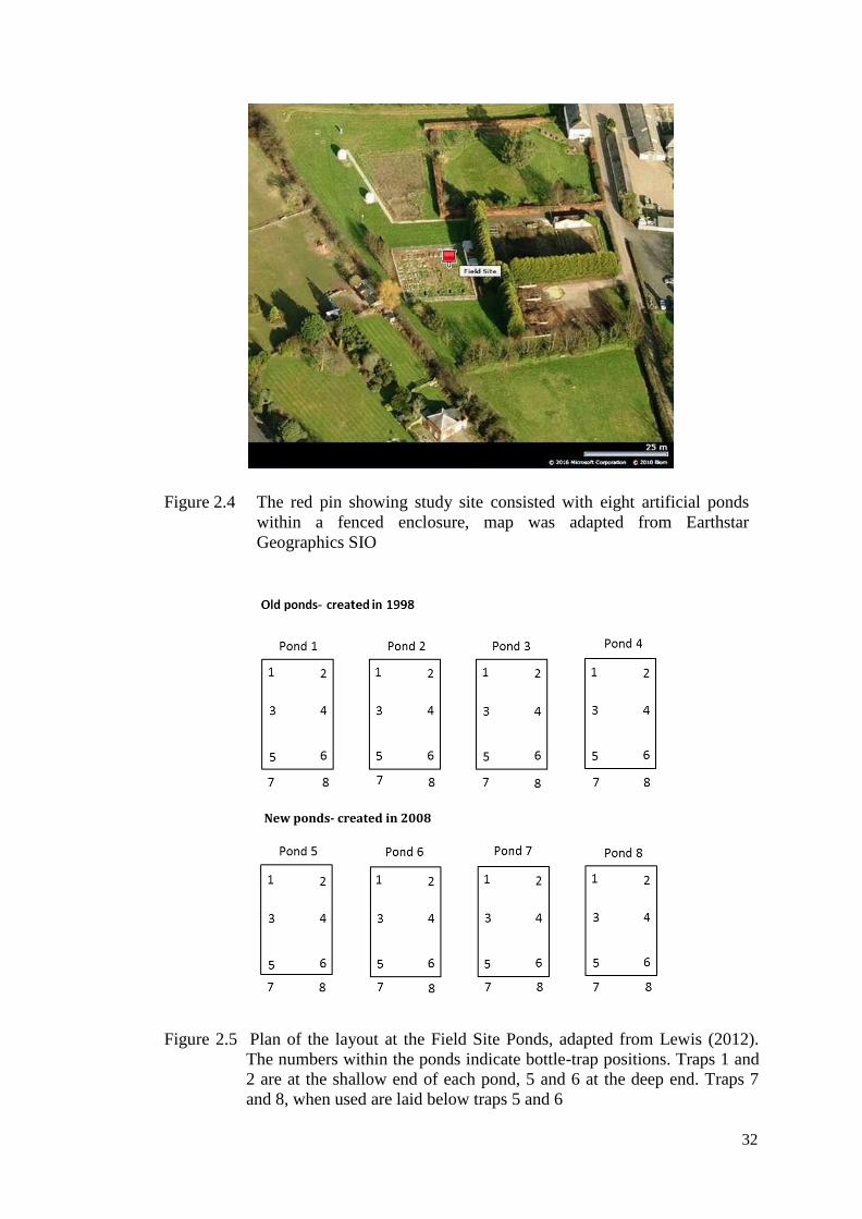
32

New ponds- created in 2008

Figure 2.4 The red pin showing study site consisted with eight artificial ponds

within a fenced enclosure, map was adapted from Earthstar

Geographics SIO

Figure 2.5 Plan of the layout at the Field Site Ponds, adapted from Lewis (2012).

The numbers within the ponds indicate bottle-trap positions. Traps 1 and

2 are at the shallow end of each pond, 5 and 6 at the deep end. Traps 7

and 8, when used are laid below traps 5 and 6

New ponds- created in 2008

33

Figure 2.6 A cross section of a Field Site pond showing its tapered design and

measurements, from Wright (2009). Also, trap placement within each

pond

2.2 DATA COLLECTION

The chosen method for this study was trapping during the aquatic breeding season.

Field surveys at Well Court were carried out annually from 1995 until 2013, and at

the Field Site from 1999 until 2016. My own data collection at Well Court was

conducted in 2013 only (permission for access was withdrawn after 2013) and, at the

Field Site between 2014 and 2016. However, analyses at both of the study sites

include the full data set. Trapping were commenced on the Thursday night/Friday

morning most closely matching the night of 28th

February/1st March in each year.

Trapping then continued at weekly intervals until the end of the aquatic period (i.e.

when no further newts were trapped), this usually occurred at the end of July

although there was variation from year to year.

Newts at the Well Court ponds were captured by using funnel traps as described by

Griffiths (1985), spaced at two metre intervals along the shoreline of the ponds.

Traps were numbered and the positions of each trap marked on a plan to allow for

34

continuity of data between years. The size of trap used was based on a 1 litre plastic

bottle, with the funnel inverted into the body and held in place by a cane inserted

through the trap and into the bottom of the pond. Where this was not possible for

artificial ponds where the pond had a plastic or similar liner, traps were secured to

nearby vegetation or stones by means of a piece of string.

Trapping was carried out in a similar manner at the Field Site ponds, except that the

interval between traps was one metre. The trap arrangement is described in detail in

Chapter 4 (Well Court) and Chapter 5 (Field Site). Traps were set between 2000 and

2200 hrs and were then checked and emptied between 0730 and 0900 hrs the next

morning depending on the season.

2.3 NEWT IDENTIFICATION

Newts trapped were recorded according to pond, trap number, species and sex, and

released back into the pond where they were caught. Smooth and palmate newts were

counted but not marked or measured in any way. The great crested newts were

placed in a rectangular transparent plastic tray and restrained by a foam rubber

sponge (Figure 2.7). They were then measured; this included the snout-vent length

(from the tip of the snout to the hind margin of the cloaca) and the tail length (from

the hind margin of the cloaca to the tip of the tail). This was achieved using a 30 cm

ruler, with measurements being taken to the nearest 1 mm. The great crested newts

were then dried of excess water using a paper towel and measured using a digital

balance to the nearest 0.1 g.

Each crested newt exhibits a belly pattern that is unique to that individual. Thus,

identification of each crested newt captured was enabled by photographing the belly

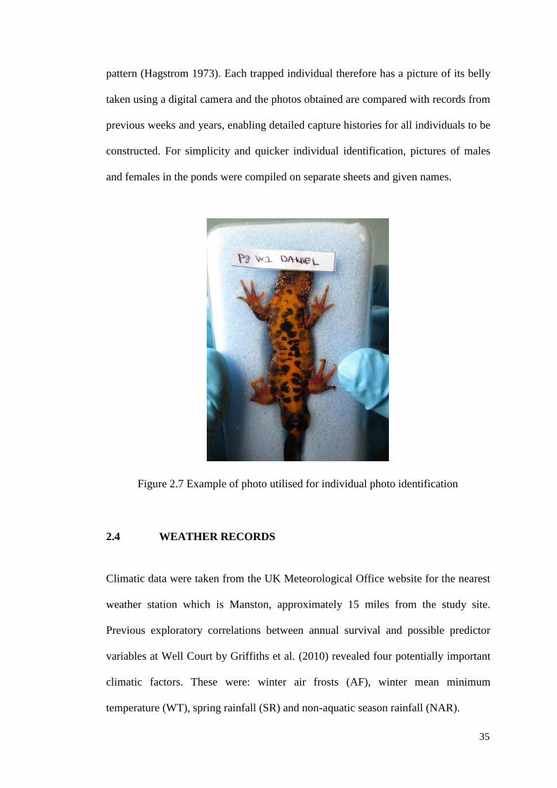
35

pattern (Hagstrom 1973). Each trapped individual therefore has a picture of its belly

taken using a digital camera and the photos obtained are compared with records from

previous weeks and years, enabling detailed capture histories for all individuals to be

constructed. For simplicity and quicker individual identification, pictures of males

and females in the ponds were compiled on separate sheets and given names.

Figure 2.7 Example of photo utilised for individual photo identification

2.4 WEATHER RECORDS

Climatic data were taken from the UK Meteorological Office website for the nearest

weather station which is Manston, approximately 15 miles from the study site.

Previous exploratory correlations between annual survival and possible predictor

variables at Well Court by Griffiths et al. (2010) revealed four potentially important

climatic factors. These were: winter air frosts (AF), winter mean minimum

temperature (WT), spring rainfall (SR) and non-aquatic season rainfall (NAR).

36

Winter air frost was defined as the total number of days of air frost in the months of

December, January and February combined. Winter mean minimum temperature was

defined as the mean daily minimum temperature (0C) over the period December-

February each winter. Spring rainfall was defined as the combined rainfall (mm) in

the months of March, April and May each year, whilst non-aquatic period rainfall

was defined as total rainfall (mm) over the remainder of the calendar year (January-

February plus June-December), the period in which most newts were expected to be

absent from ponds. Dividing the rainfall data into spring rainfall (SR) and non-

aquatic season rainfall (NAR) was regarded as applicable given the different impacts

of rainfall on aquatic and terrestrial stages of newts.

2.5 MARK RECAPTURE ANALYSIS

To estimate between-year survival and detection rates, individual capture histories

were used after annualising all the weekly capture data for each year (i.e. an

individual was scored as ‘1’ if captured in any week in a particular year and ‘0’ if not

captured at all in the year). As well as examining survival and detection probabilities,

the study also sought to test whether these probabilities varied between sexes.

Capture histories for all males and females were constructed over a nineteen- year

period for the Well Court and sixteen-year period for the Field Site. Juveniles were

excluded from this analysis because the belly pattern may change as the animal

grows, making identification unreliable. As survival rate calculation depends on

survival between years, nineteen years of data effectively give eighteen (i.e. n – 1)

estimates of annual survival.

37

The probabilities of survival and detectability were estimated using Program MARK

(White & Burnham 1999). MARK was used to estimate differences in the rate of

survival and detectability within the population, both over time and between the

sexes, using the Cormack-Jolly-Seber (CJS) model. The CJS model has four basic

assumptions, as follows:

1. Every animal present in the population at time (i) has the same probability

of recapture (pi);

2. Every marked animal in the population immediately after time (i) has the

same probability of surviving to time (i + 1);

3. Marks are not lost or missed; and

4. All samples are instantaneous relative to the interval between occasions (i)

and (i + 1) and each release is made immediately after the sample.

Pre-defined and customised models were used in MARK, allowing analyses that

were both time and group dependent. Model assumptions followed Williams et al.

(2002), whilst model notation followed Lebreton et al. (1992), as follows:

Phii survival probability from time i to i +1;

pi probability of detection (i.e. capture or recapture) at time

i;

(g) group (sex and/or pond) dependent survival or detection;

(t) time dependent survival or detection;

(g*t) both group dependent and time dependent survival or

detection; and

(.) constant survival or capture rate.

Up to sixteen candidate models could be run from each data set as follows:

Phi(.) p(.) Survival and detection rates constant

38

Phi(.) p(g) Survival rate constant, detection varies by group

Phi(.) p(t) Survival rate constant, detection varies over time

Phi(.) p(g*t) Survival rate constant, detection varies by both group and

time

Phi(g) p(.) Survival rate varies by group, detection rate constant

Phi(g) p(g) Survival and detection rates vary by group

Phi(g) p(t) Survival rate varies by group, detection varies over time

Phi(g) p(g*t) Survival rate varies by group, detection by both group and

time

Phi(t) p(.) Survival rate varies by time, detection rate constant

Phi(t) p(g) Survival rate varies by time, detection varies by group

Phi(t) p(t) Survival and detection rates vary over time

Phi(t) p(g*t) Survival rate varies over time, detection by both group

and time

Phi(g*t)p(.) Survival rate varies by group and time, detection rate

constant

Phi(g*t)p(g) Survival rate varies by group and time, detection varies

by group

Phi(g*t)p(t) Survival rate varies by group and time, detection varies

by time

Phi(g*t)p(g*t) Survival and detection rates both vary by group and time

The number of groups used also varied as follows:

Single group No variation between sex or pond

Two groups Variation between sexes

Four groups Variation between the four ponds tested

Eight groups Variation between both pond and sex

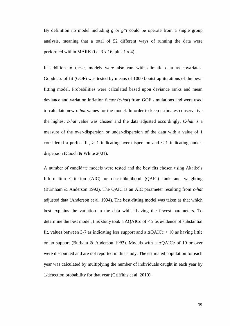
39

By definition no model including g or g*t could be operate from a single group

analysis, meaning that a total of 52 different ways of running the data were

performed within MARK (i.e. 3 x 16, plus 1 x 4).

In addition to these, models were also run with climatic data as covariates.

Goodness-of-fit (GOF) was tested by means of 1000 bootstrap iterations of the best-

fitting model. Probabilities were calculated based upon deviance ranks and mean

deviance and variation inflation factor (c-hat) from GOF simulations and were used

to calculate new c-hat values for the model. In order to keep estimates conservative

the highest c-hat value was chosen and the data adjusted accordingly. C-hat is a

measure of the over-dispersion or under-dispersion of the data with a value of 1

considered a perfect fit, > 1 indicating over-dispersion and < 1 indicating under-

dispersion (Cooch & White 2001).

A number of candidate models were tested and the best fits chosen using Akaike’s

Information Criterion (AIC) or quasi-likelihood (QAIC) rank and weighting

(Burnham & Anderson 1992). The QAIC is an AIC parameter resulting from c-hat

adjusted data (Anderson et al. 1994). The best-fitting model was taken as that which

best explains the variation in the data whilst having the fewest parameters. To

determine the best model, this study took a ΔQAICc of < 2 as evidence of substantial

fit, values between 3-7 as indicating less support and a ΔQAICc > 10 as having little

or no support (Burham & Anderson 1992). Models with a ΔQAICc of 10 or over

were discounted and are not reported in this study. The estimated population for each

year was calculated by multiplying the number of individuals caught in each year by

1/detection probability for that year (Griffiths et al. 2010).

40

CHAPTER 3

ACCURACY OF PHOTO IDENTIFICATION OF NEWTS BY MANUAL

AND COMPUTER IDENTIFICATION METHODS

ABSTRACT

Accurate individual identification is a basic assumption of capture-mark-recapture

methods. When overlooked, errors can bias demographic parameter estimates. The

study was conducted using 15 years of images captured at the Field Site population.

Expert newt researchers more consistently identified the same newt than non-experts

when the same images were repeated, and were more cautious identifying two

different individuals with similar patterns. However, both experts and non-experts

had difficulty identifying newts from poor quality images. Computer-assisted

methods using five software packages proved that the spot patterns of individual

newts did not change significantly through time, and were sufficiently varied to

allow their individual identification. The accuracy of each software package

gradually decreased using low quality images and increased with the increase

number of reference images. With a database comprising 136 individuals, manual

identification was more accurate and quicker than software packages. However, if

the number of images increases, manual identification will become unfeasible and

software packages can be successfully employed for the identification of individuals

in large populations of animals.

41

3.1 INTRODUCTION

Individual identification of animals is necessary in many types of ecological studies

(Nietfeld et al. 1994). One of the most basic mechanisms of animal population

biology is the capability to identify and track individual animals over time and space

(Bolger et al. 2012). Estimates of population size, survival and reproduction rates,

and migration rates typically involve identifying previously marked or sighted

individuals (Nichols 1992). Conventionally, animal identification involves capturing

and placing clear and distinctive marks on them (Williams et al. 2002). The most

common method for identifying individual amphibians is by applying artificial marks

such as PIT-tags, visible implanted elastomers, bands, or tattoos (Mettouris et al.

2016). However, ethical and methodological objections to such methods have been

raised and there is broad interest in developing alternative methods. Some of these

invasive techniques may lead to stress and influence the survival or behaviour of the

studied animal (Antwis et al. 2014). In addition, there have been concerns about

ethical and animal welfare issues that arise from their broad use (Perry et al. 2011).

One alternative is to use photo-identification methods (PIMs) to identify individuals

based on their natural markings. Photo-identification methods (PIMs), which use

photographs of unique natural markings to identify individuals (Bradfield 2004),

avoid most of the ethical issues associated with artificial marking methods, and it can

be quick, easy, and inexpensive to generate images in the field. Nowadays,

photography remains one of the quickest and affordable ways of "labelling"

substantial numbers of individuals in a population (Harting et al. 2004). In recent

years, camera trapping is widely used, especially to study medium-to-large terrestrial

mammals and birds, arboreal mammals, small mammals and herpetofauna. Camera

42

trapping is the use of remotely triggered cameras that automatically take images

and/or videos of animals or other subjects passing in front of them (Rovero et al.

2013).

Images captured are usually stored in a library to be visually examined later for

matches and to develop individual capture history files (Speed et al. 2007). Although

it is possible to manage small numbers of photographs manually, the task becomes

increasingly inefficient and error-prone when library sizes are large (Arntzen et al.

2004). Therefore, many studies involving photographic identification now apply one

or more of the following techniques to minimize the amount of manual matching: 1)

classification of unique characteristics into a searchable database (e.g. Petersen

1972); 2) semi-automated matching with pattern recognition algorithms (e.g. Gamble

et al. 2008); or 3) computer-assisted extraction of morphometric information (e.g.

Araabi et al. 2000).

Researchers entering this rapidly expanding field should consider several major

factors before deciding if, and what type of visual recognition method is appropriate

for their study context. A basic understanding of the history, limitations, and key

issues associated with photographic identification will serve to improve experimental

design and analysis, facilitate comparisons between studies, and efficiently advance

the methodology and technology associated with this field.

Volunteers – or ‘citizen scientists’ - have contributed for centuries to ecological

surveys (Cohn 2008), and have been increasingly engaged by scientists over the past

few decades to assist and support scientific research (Silvertown 2009). A central

aspect of volunteer involvement is the collection of data, which often contribute

significantly to research projects, especially when guided by experienced scientists

43

(Foster-Smith & Evans 2003). Clearly, the accuracy and consistency of data

collected by volunteers is a critical aspect of these projects, as data are often used to

support scientific publications and management planning decisions. Volunteers are

associated with the image of the well-meaning ‘amateur’, however volunteers can

often be dedicated individuals already working or studying in a relevant field area

and may either have or achieve high standards of expertise (Foster-Smith & Evans

2003). If sufficiently trained, volunteers can gather high quality data (Newman et al.

2003), but the reliability of data collected by novice volunteers has sometimes been

disputed (Cohn 2008).

In photo-identification studies, the probability of recognizing, and thus recapturing, a

marked individual is dependent on three major factors: 1) individual distinctiveness;

2) stability of the pattern; and 3) quality of the photograph (Hammond et al. 1990;

Friday et al. 2000). The first of these factors, distinctiveness, is based on another

primary assumption of CMR studies - that each individual in a population has a

distinct mark by which it can be identified. “Distinctiveness” has also been defined

as “recognisability” (Hammond et al. 1990), “unique information content” that each

individual contributes to distinguishing itself from others (Burghardt 2008) and “the

degree of visibility of permanent marks” allied to the “ease of individual

identification” (Forcada & Aguilar 2000). Across species, distinctiveness is

commonly age or sex dependent. Most amphibians, pinnipeds, and birds, for

instance, fail to develop a stable pattern until they reach sexual maturity because

juveniles often exhibit different pigmentation patterns to adults (e.g. Forcada &

Aguilar 2000). Similarly, with morphological marks, it is typically older manatees,

and female otters that have the highest degree of scarring available to photograph

(Langtimm et al. 2004; Finerty et al. 2007). Within a species there is natural variation

44

in morphology and/or pigmentation among individuals (Friday et al. 2000). The more

divergent the pattern or shape between two photos, the easier it is for an observer or a

computer to identify, code, or rank the individuals as different (Agler 1992). Lastly,

if not accounted for, gradations in distinctiveness can potentially cause both human

and computer processing errors or bias in matching (Harting et al. 2004).

Another source of processing error in identifying individuals relates to the quality of

the photographic image. In general, quality has been broadly defined with respect to

several secondary factors: 1) clarity, sharpness, or focus (Friday et al. 2000); 2)

contrast or the degree of difference between blacks and whites (Friday et al. 2000);

3) noise or the amount of unnecessary background information in the frame with the

individual of interest (Gamble et al. 2008); 4) resolution or the amount of available

pixel information (Markowitzet et al. 2003); 5) glare or specularity (Gamble et al.

2008); and 6) relative size of the animal of interest in the picture frame (Sears et al.

1990). Weather, water depth or turbidity, patterns in the background environment,

and ambient light are just a few natural environmental variables that affect

photographic quality (Markowitzet et al. 2003; Langtimm et al. 2004).

Photographing individuals in their natural environments typically precludes the

controlled lighting, uniform background, and limited movement that would otherwise

improve photographic quality. In fact, it is this unpredictability of photographic

quality and its complex relationship with distinctiveness that continues to prevent

widespread use of fully automated matching systems (Shirley et al. 2010).

On the other hand, automatic recognition software approaches based on pattern

recognition hold the promise to become useful for monitoring efforts and mark-

recapture studies for a wide range of animals that differ individually in body pattern

45

traits (Drechsler et al. 2015). For large populations, computer-assisted photo-

recognition programs may be needed as the time required for manual matching may

be excessive (Knox et al. 2013). Pattern recognition software may increase the speed

of correct identifications (relative to manual matching) regardless of the user’s

experience (Gamble et al. 2008). Pattern recognition programmes are useful for

monitoring efforts and mark-recapture studies for a wide range of animals that differ

individually in observable patterns (Drechsler et al. 2015). While numerous

computer-assisted programmes have been introduced, there have been few studies to

thoroughly test their performance across large datasets. Therefore, performance tests

in large datasets are crucial if automatic approaches aim to be competitive and

challenge the predominant manual approaches still used in many mark-recapture

studies (Drechsler et al. 2015). Nevertheless, computer-based methods vary in their

degree of accuracy and all require some additional visual confirmation that the

correct match has been identified by the program (Knox et al. 2013). This study

tested the performance of recognition software based on standardized images in the

context of a large mark-recapture study in the great crested newt.

3.1.1 Aims and Objectives

The general purpose of PART 1 was to assess how experience in using manual

photo-identification may affect the correct identifications of individual newts. The

specific objectives were:

1) to compare expert and non-expert ability to detect distinctiveness of the belly

pattern of the newts;

2) to test expert and non-expert accuracy in identifying good and low quality

46

images of newt belly pattern; and

3) to evaluate the performance consistency of experts and non-experts in

identifying the great crested newt using the belly pattern images.

The general aim of PART 2 was to evaluate the performance of the computer-

assisted photo-identification packages that are available for the public to access. The

primary objectives were:

1) to determine whether pattern recognition software can be used to distinguish

the same individual newts over several years;

2) to test whether good and low quality images of the ventral patterns of

individual newts can be used to reliably distinguish between individuals

accurately;

3) to assess how the number of reference images can improve the accuracy of

pattern recognition software; and

4) to describe the advantages and limitations of this approach.

3.2 MATERIALS AND METHODS

3.2.1 Study Site and Photograph Collection

The identities of newts captured were individually recorded using a simple

photographic recording system. This record is based on 3542 images from 156 adult

great crested newts captured and photographed in ponds at a Field Site on the

University of Kent campus at Canterbury (Grid reference TR132595) throughout

2000 and 2016 during the aquatic breeding season (March-July). Each individual was

47

placed into a small, transparent plastic dish and restrained by a cover of foam rubber

to prevent them from turning over. Great crested newts were held between the

forefingers and a photograph taken of the ventral surface.

Images of individual belly patterns were taken subsequently and catalogued using

digital camera 12.1 megapixels Canon Power Shot A1100 IS equipped with 6.2-24.8

mm lenses with ‘Macro’ setting. Images were taken by experts and trained

volunteers, and the photographic process lasted approximately 30 seconds for each

newt. Afterwards newts were released into the ponds to which they were captured.

The images are of varying resolution, in 24-bit colour. Newts were individually

identified by distinct belly pattern spot and several photographs of the same newt

were taken in each session.

Previous study by Gowans and Whitehead (2001) highlighted the importance of

obtaining high quality images, so animals were ‘clean’ (i.e., free of debris that could

obscure natural marks) and excess water was removed using paper towels. Apart

from that, animals were secured in a position that did not conceal ventral markings.

A minimum of 4-5 images per specimen were taken to ensure correct focus and

framing. However, poor quality images were also captured and have been used in

reliability tests of good and low quality images. The belly pattern of newts was

compared with the previous year’s record and the new individuals were sexed and

coded individually. A minimum of three high quality images were selected from each

capture event. Selected images were saved in a new directory for individual

identification.

48

3.2.2 Manual Photo-Identification Evaluation

This survey is designed to investigate the accuracy of photo-identification techniques

in identifying individual great crested newts. A total of 214 respondents took part in

the study: 83 experts and 131 non-experts. An expert was defined as a person who

has experience capturing and handling newts in the wild; non-experts had no such

experience. Participants ranged in age from 18 to 65; however the great majority

were from the 25-34 age group range. Data from this study have been divided into

three main sections to test the reliability score between the good and poor quality

images, the pattern distinctiveness of the belly pattern, and the consistency of experts

and non-experts in answering sequential test involving the same images of the same

individual that were presented twice.

The time taken to identify each newt was recorded in seconds. The low quality

images (Figure 3.1) were defined as images having either a flash reflection, out of

focus and out of frame, newts in a position that distorted ventral marking or newts

were unclean (contain debris that could obscure natural marks). In the pattern

distinctiveness section, each respondent was shown two different newts images that

had some pattern similarity and could potentially be confused (e.g. central

continuous line; scattered small spots - Figure 3.2). Every respondent was shown 20

pairs of images from each test section through an online questionnaire and asked to

decide whether they think the images came from the same individual or not. There

was no maximum or minimum time involved in answering this test but the duration

that each respondent spent to complete the test was recorded.

Additionally, a total of 30 newts captured in the 2015 sampling season were used to

determine how long it will take to identify individual using manual identification.

49

From this sample, 20 newts were recorded as recaptures and 10 newts were new. 136

belly pattern images from the previous sampling season (2008-2014) were used for

reference in the identification process. Figure 3.3 shows some of the belly pattern

images from the previous newts that were recorded at the Field Site.

(a) (b)

Figure 3.1 Example of two good quality images (1a left and 1b left) and two poor

quality images (1a right and 1b right). Poor quality image of 1(a) right

had flash reflection, 1(b) right was out of focus

(a) (b)

Figure 3.2 (a) and (b) are examples of images from 4 different individuals that have

some similarity but unclear distinctiveness of belly pattern

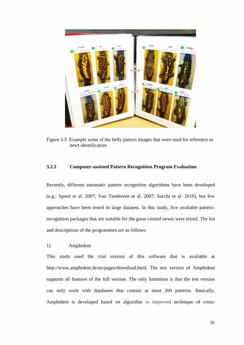
50

Figure 3.3 Example some of the belly pattern images that were used for reference in

newt identification

3.2.3 Computer-assisted Pattern Recognition Program Evaluation

Recently, different automatic pattern recognition algorithms have been developed

(e.g.: Speed et al. 2007; Van Tienhoven et al. 2007; Sacchi et al. 2010), but few

approaches have been tested in large datasets. In this study, five available pattern-

recognition packages that are suitable for the great crested newts were tested. The list

and descriptions of the programmes are as follows:

1) Amphident

This study used the trial version of this software that is available at

http://www.amphident.de/en/pages/download.html. The test version of Amphident

supports all features of the full version. The only limitation is that the test version

can only work with databases that contain at most 200 patterns. Basically,

Amphident is developed based on algorithm in improved technique of cross-

http://www.amphident.de/en/pages/download.html

51

correlation comparisons to find similar sign (e.g., a specific spot pattern) in a large

arrangement of related signals again. A thorough explanation and how the program

work is illustrated by Matthé et al. (2008). The program also came with the option to

crop certain angle of the belly pattern from the images, if some parts of the picture

are of low quality. Based on a similarity values for a particular pattern (i.e., for an

individual), the program suggests user maximum the best 30 ranked matching

patterns in a descending order from the database. The user then requires to compare

by eye and decided whether the pattern is already contained in the database, that is,

whether an individual has been recaptured or not.

2) APHIS

APHIS (Automatic Photo-Identification Suite) was specially designed by Moya et al.

(2015) to deal with sample sets of over a hundred images per field campaign and

image library libraries containing more than a thousand samples. APHIS uses two

approaches for photo-matching, the Spot Pattern Matching (SPM) and the Image

Template Matching (ITM). The former has been built on the already existing I3S

algorithm (Van Tienhoven et al. 2007) while the latter is a novel approach based on

pixel matching that minimizes the user’s pre-processing effort. ITM is a fast-running

alternative to study species with clear or easily recognizable spots or coloured parts

of the skin. The workflow and graphic interface of APHIS have been designed to

reduce the time invested by the researcher in analytical tasks and to enhance user

experience. An important feature in APHIS is the automatic creation of log files that

register the score lists obtained at each comparison. It also produces a registry of the

matches validated by the user, which will lead to an easy analysis of capture-

recapture data. APHIS v.1.0 (freely available at http://www.imedea.uib-

csic.es/bc/ecopob/) combines C++ and Java modules.

http://www.imedea.uib-csic.es/bc/ecopob/)

http://www.imedea.uib-csic.es/bc/ecopob/)

52

3) I3S

This pattern-matching program was developed by Van Tienhoven et al. (2007) using

Java 1.4.2 and C++, and requires the Java Run-time environment to run on personal

computers. The entire code for the pattern-matching system, known as I3S

(Interactive Individual Identification System) is available at

http://www.reijns.com/i3s. An image is opened in the application. Using a computer

mouse, the user manually selects the three reference points to define the common

reference area. The user then points out the most distinct pigment spots of each

animal. Between 12 and 40 spots are selected within the reference area. The centre of

each spot is marked and where spots overlap or join, the apparent centres of such

spots are marked. The size of the spots is currently not considered important,

whereas their relative position to one another is. The user can compare the image of

the unknown individual with up to 50 possible matches provided in the list.

4) Wild-ID

Wild-ID was introduced by Bolger et al. (2012) and is available at

http://envs.dartmouth.edu/people/douglas-thomas-bolger. Wild-ID processes the

images in each dataset sequentially and calculates a similarity score for each pair of

images. After all similarity scores are computed, Wild-ID presents the top-20 ranking

images for each image for visual confirmation through the user interface.

Consequently, the final decision for accepting or rejecting a match is left to the user.

5) Zoometrics

The prototype of this software was implemented in MATLAB 8.0 (The MathWorks,

USA) and was described by Hoque et al. (2011). In order to find the similarity

between two newts, the corresponding Region of Interests (ROIs) are compared. To

http://www.reijns.com/i3s

http://envs.dartmouth.edu/people/douglas-thomas-bolger

53

compensate the misalignment due to flexible segmentation mechanism, a subsection

of the ROI is isolated from one image that scans over the second image. A score is

generated for each overlapping region and the overall comparison score is the one

that shows maximum similarity.

To start with, images of the ventral side of individual newts were entered into the

computer-assisted photo-identification software. Figure 3.4 shows the example of

workflow of pattern extraction with Amphident software. Generally, the computer-

assisted photo-identification involved the following steps:

(i) New images were downloaded into an image library;

(ii) The belly pattern is then extracted by first marking the area of the belly pattern,

that is, defining the region of the belly pattern by the user;

(iii) The program then extracts this region from the original images into a black and

white picture;

(iv) It is then further modified by a median filter to remove noise of edges and

small spots;

(v) The obtained pattern is then compared with all existing patterns in the

database;

(vi) For each pairwise comparison, a similarity value is determined by the number

of matching pixels of both patterns;

(vii) The higher the number of matching pixels between shapes, that is, the more

similar the patterns are, the higher the similarity score.

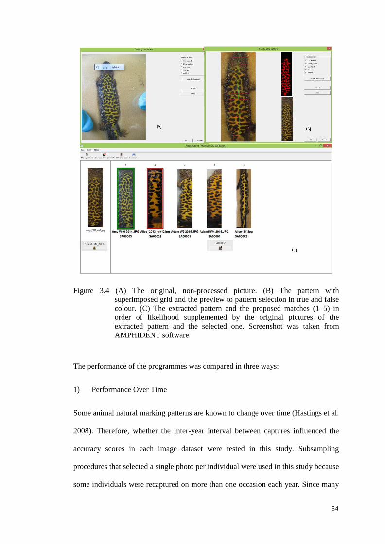
54

Figure 3.4 (A) The original, non-processed picture. (B) The pattern with

superimposed grid and the preview to pattern selection in true and false

colour. (C) The extracted pattern and the proposed matches (1–5) in

order of likelihood supplemented by the original pictures of the

extracted pattern and the selected one. Screenshot was taken from

AMPHIDENT software

The performance of the programmes was compared in three ways:

1) Performance Over Time

Some animal natural marking patterns are known to change over time (Hastings et al.

2008). Therefore, whether the inter-year interval between captures influenced the

accuracy scores in each image dataset were tested in this study. Subsampling

procedures that selected a single photo per individual were used in this study because

some individuals were recaptured on more than one occasion each year. Since many

55

recaptures occur within one breeding season, this study selected only 50 pair

matched-images (100 images) for each interval years in order to ensure longer

periods were included in subsamples. Accuracy score of the matched images at the

top 10 rankings were calculated to see if the scores were inversely related to the time

interval between captures.

2) Number of reference images

The performance of the programmes were tested by randomly selecting between one

and ten reference images per newt from the dataset and using all the remaining newts

images as a test set. A total of 50 newts were used in this experiment. The number of

times the correct newt was ranked in the Top 10 best matches was measured as a

percentage. To correct for random effects, the same experiments were repeated 100

times and the averages were calculated over all results.

3) Image quality

Image quality can affect matching success (Kelly 2001). Therefore, images for

matching were segregated into two groups based on their quality type: a ‘low quality’

group and a ‘good quality’ group images. The experiment was run on 50 different

newts. The number of times the correct newt was ranked in the Top 10 best matches

was measured as a percentage. To correct for random effects, the same experiments

were repeated 100 times and the averages were calculated over all results.

3.2.4 Statistical Analysis

Scores from expert and non-expert respondents were divided into three categories:

photo quality, pattern distinctiveness and consistency. To ascertain whether there

56

was a difference in the performance of expert and non-expert respondents in using

manual photo-identification methods, tests were run using Mann-Whitney U tests for

the photo quality and pattern distinctiveness categories. Non-parametric tests were

used for the photo quality and pattern distinctiveness statistical tests because the

accuracy scores mean from these data were not normally distributed. Additionally, as

the data were normally distributed, a parametric paired sample t-test was used to

compare the accuracy score mean from first and second responses in sequential tests

to evaluate the performance consistency in both respondent groups. To evaluate the

software performance in identifying poor and good quality images, the accuracy

scores for each of the packages was tested using a paired sample t-test. A two way

ANOVA was performed to see whether accuracy score was influenced by the belly

pattern stability across nine years of dataset. All statistical analysis was run through

Minitab 17.

3.3 RESULTS

3.3.1 Manual Identification

It took an average of 64.5±24.4 seconds for an expert to identify a recaptured newt

from the 136 photographs (Figure 3.5). It took a significantly longer time to

determine that a new newt was a new individual, 207 ± 33 seconds (t = 13.4, d.f. =

28, P < 0.0001)

57

Figure 3.5 Time taken to identify newt individuals manually from 136 photographs. On

the left side of red line were the recaptures and on the right were the newly

captured newts

Expert and non-expert performance in manual identification

The experts recorded higher accuracy (score) in all three main tests than the non-expert

group (Figure 3.6). The greatest accuracy from the expert group was achieved both by

pattern distinctiveness and consistency, with on average 99.0% of matches made

correctly. The lowest accuracy was recorded in terms of image quality (94%). The

patterns for non-experts were similar, but on average they were 2-5% less accurate in

their matchings than experts, but the differences between experts and non-experts were

not always significant. For example, when image quality was considered, there was no

difference between experts and non-experts in their accuracy (U = 97.0, P = 0.239).

However, in terms of pattern distinctiveness the score in the expert group was higher

than the non- expert group (U = 56.5, p < 0.006). Only the non-expert group recorded

significant difference in accuracy scores between two sequential tests involving the

same images of the same individual that were presented twice (t = 2.3, p < 0.039). This

result indicates that non-experts were more inconsistent when presented with the same

0

2

4

6

8

10

12

0-30 31-60 61-90 91-120 121-150 151-180 181-210 211-240

Nu

mb

er

of

ne

wts

Time (seconds)

Newly captured newts Recaptured newts

58

pair of images twice. On the contrary, the expert group displayed consistency over these

two sequential tests because there was no significant difference in accuracy scores

recorded between these two tests (t = 1.6, p = 0.134).

Figure 3.6 Accuracy scores of each test category from two groups; expert and non-

expert. Photo quality test, Pattern distinctiveness test, and Consistency test

3.3.2 Software Evaluation

A total of 3127 adult great crested newt were captured from 154 individuals during the

17-year period. The vast majority of these individuals (n = 120) were captured more

than twice and there were only 34 images for which individuals that were captured only

once. It was evident that a high proportion of previously recorded individuals were

recaptured every year. On average, almost 0.82% of animals were recaptured at least

once in earlier years. More detailed analysis of individually recognized newts indicated

that most animals probably return to the Field Site annually (see Chapter 5).

0.94

0.99 0.99

0.92

0.94

0.97

0.88

0.9

0.92

0.94

0.96

0.98

1

Photo quality Pattern distinctiveness Consistency

Acc

ura

cy s

core

s

Category

Expert

Non-expert

U = 97.0 p = 0.239

U = 56.5 p < 0.006

t = 1.6 p = 0.134

t = 2.3 p < 0.039

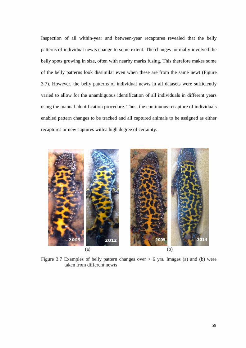
59

Inspection of all within-year and between-year recaptures revealed that the belly

patterns of individual newts change to some extent. The changes normally involved the

belly spots growing in size, often with nearby marks fusing. This therefore makes some

of the belly patterns look dissimilar even when these are from the same newt (Figure

3.7). However, the belly patterns of individual newts in all datasets were sufficiently

varied to allow for the unambiguous identification of all individuals in different years

using the manual identification procedure. Thus, the continuous recapture of individuals

enabled pattern changes to be tracked and all captured animals to be assigned as either

recaptures or new captures with a high degree of certainty.

(a) (b)

Figure 3.7 Examples of belly pattern changes over > 6 yrs. Images (a) and (b) were

taken from different newts

60

Image quality

The highest accuracy for the good quality images was achieved using Amphident

software, which correctly identified 85% of the images in the Top 10 rankings. Wild- ID

was second, with 79% accuracy, followed by I3S, with 78% accuracy, Zoometrics

(75%) and APHIS (66%). However, the accuracy scores for each software package

gradually decreased with the low quality images. Figure 3.8 clearly shows that the

accuracy scores of low quality images were nearly half that of the good quality images.

Wild-ID software recorded the highest accuracy scores for the low quality images

(56%) with Amphident yielding the lowest scores recorded (32%). From the paired t-

tests, there was a significant difference in accuracy scores between good and low quality

images for each of the software packages. Due to the direction of the t- value, this study

concluded that there was a significant improvement in accuracy scores following the use

of the good quality images.

Good quality images Low quality images

0.9

0.8

0.7

0.6

0.5

0.4

0.3

0.2

0.1

Amphident APHIS I3S Wild-ID Zoometrics Software

Figure 3.8 Summary of results from paired sample of t-test analyses for five different

softwares packages that compare the accuracy scores of good and low

quality images. The degree of freedom (d.f.) for each test was 49

t = 12.85 P < 0.024

t = 34.75 P < 0.001

t = 20.6 P < 0.02

t = 25.32 P < 0.001

t = 42.76 P < 0.001

Acc

ura

cy s

core

s

61

Number of reference images

Considering multiple images per animal, accuracy scores increased nonlinearly as the

number of total images available for matching increased (Figure 3.9). For example,

accuracy increased from 76% using a single image to 92% when three reference images

were available. Generally, an accuracy rate of ±75% required that at least three good

quality images were available for an individual animal for accurate matching.

Figure 3.9 Effect of multiple images on visual matching success of computer-

assisted image matching system. Accuracy scores clearly increase when

more reference images are available

With only one reference image to test against, 65-85% of the images in the test database

were correctly ranked as the correct choice (Top 10). Again, the greatest accuracy when

multiple images were tested was by Amphident. Even if only one reference image was

available for the comparison, it yielded an 84.7% chance of placing the image in the

top 10. This recognition ability increased to an almost 93% chance of it being in the top

10 ranking using three reference images. APHIS software recorded the lowest accuracy

0.5

0.55

0.6

0.65

0.7

0.75

0.8

0.85

0.9

0.95

1

1 2 3 4 5 6 7 8 9 10

Acc

ura

cy s

core

s

Number of images inspected

Amphident

APHIS

I3S

Wild-ID

Zoometrics

62

scores (66%) when using only one reference image. However, it can be seen clearly

from Figure 3.9 that these scores increased rapidly (84%) with the inclusion of four

reference images of the same newt.

Pattern stability

Considering the reliability of reference images from the same newts captured in

different years, the accuracy scores did not decrease as newts get older (Figure 3.10). A

subsample of 50 newts recaptured over nine years showed the consistency of

characteristics belly patterns that were recognized by the programs. It should be noted

here that only the ‘year of capture’ data were available. Therefore, newts captured in the

same calendar year are shown as having a 0 (zero) time interval. Overall, the variation

in the accuracy scores over time did not vary between years for each of the software

package. A two-way ANOVA analysis with the individual as a fixed factor and year as

random factor was run on a sample of 50 newts to determine if there were differences in

accuracy scores due to the time interval between captures. The results showed that the

programmes performed well even when newts get older and the patterns potentially

change (Figure 3.10).

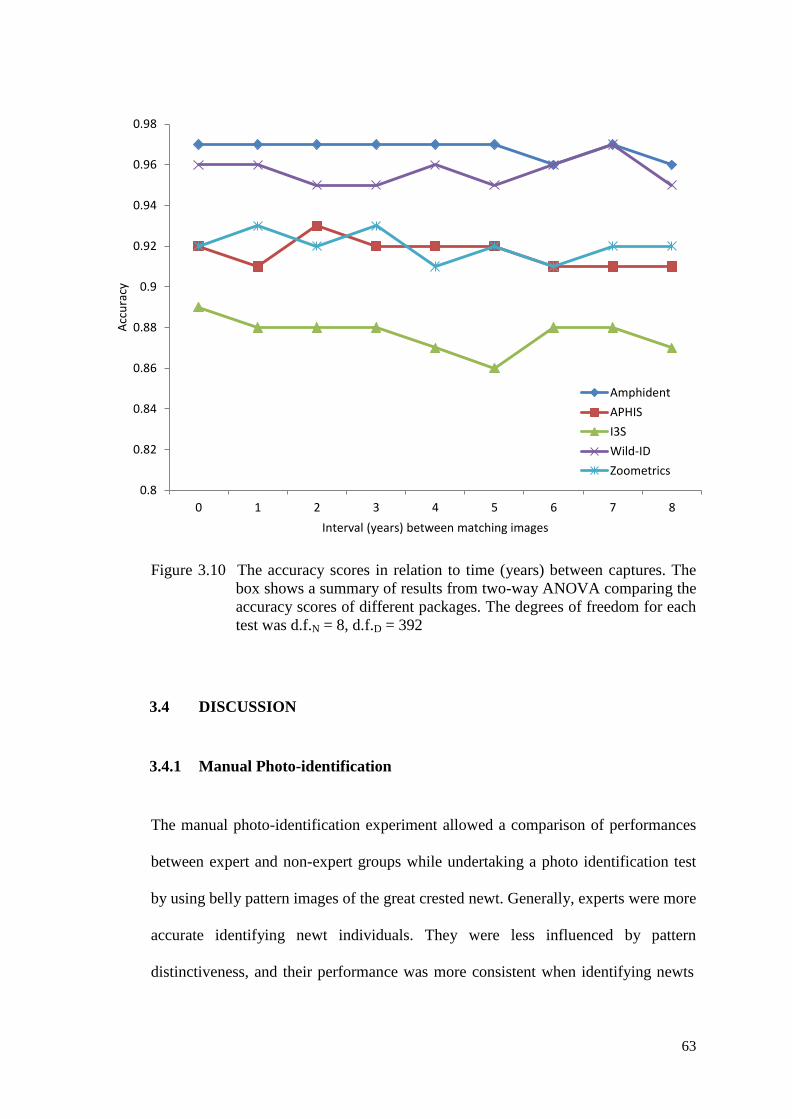
63

Figure 3.10 The accuracy scores in relation to time (years) between captures. The

box shows a summary of results from two-way ANOVA comparing the

accuracy scores of different packages. The degrees of freedom for each

test was d.f.N = 8, d.f.D = 392

3.4 DISCUSSION

3.4.1 Manual Photo-identification

The manual photo-identification experiment allowed a comparison of performances

between expert and non-expert groups while undertaking a photo identification test

by using belly pattern images of the great crested newt. Generally, experts were more

accurate identifying newt individuals. They were less influenced by pattern

distinctiveness, and their performance was more consistent when identifying newts

0.8

0.82

0.84

0.86

0.88

0.9

0.92

0.94

0.96

0.98

0 1 2 3 4 5 6 7 8

Acc

ura

cy

Interval (years) between matching images

Amphident

APHIS

I3S

Wild-ID

Zoometrics

64

in two sequential tests. However, both experts and non-experts had difficulty in

identifying individuals from poor quality images as the accuracy scores were the

lowest in this category compared to the belly pattern distinctiveness and performance

consistency categories. In spite of that, the ability to identify individuals from poor

quality images appeared to not vary greatly between experts and non-experts. When

accuracy scores from experts and non-experts were combined, low quality images

were most inaccurately identified by the respondents (93%), followed by images

with low pattern distinctiveness (97%) and consistency (98%). As the quality of the

image decreases, the information in the natural markings of newts becomes obscured,

and it becomes increasingly difficult to recognize the individual.

If mark-recapture studies do not take into account the potentially confounding effects

of image quality, probability of recapture and error type/rate can be affected. Gowans

and Whitehead (2001) found that the use of high-quality images for the identification

of individual whales reduced the number of errors in photographic matching. In

addition, digital photography has improved the image quality and increased the

efficiency of analyses in the identification of several species of dolphins (Markowitz

et al. 2003). In this study, high-quality images allowed respondents to better

discriminate between spots on the newt’s belly, and enabled them to distinguish spots

that were close together. The use of digital cameras increased the number of images

that could be obtained in the field, thereby increasing the probability of obtaining

good images. Digital images also increased the speed at which they could be loaded

into a computer for analysis while preserving their quality.

65

The results of the pattern distinctiveness tests indicate that skill level was a predictor

of performance in photo-identification methods. Pattern distinctiveness tests showed

that experts more reliably distinguished similar newts than non-experts. On the other

hand, the non-expert group had little difficulty differentiating two different newts

that had similar belly patterns. This finding supports the notion that untrained

volunteers are less accurate in their identifications (Alldredge et al. 2007). However,

the current study suggests that if sufficiently trained, non-experts can perform as

good as experts. Furthermore, the belly pattern technique is relatively easy to learn

(Chase et al. 2015). Several studies have focused on factors that could affect non-

experts’ performance in identifying animals. Previous knowledge, prior experience,

training, difficulty of task, commitment, physical fitness and familiarity with the

environment, have all been found to have an effect on non-experts’ ability to conduct

identifications based on natural markings (Schmitt & Sullivan 1996; Foster-Smith &

Evans 2003; Newman et al. 2004).

Before any identification system based on natural markings is developed, it is

important to know whether the use of natural markings will be reliable (Pennycuick

1978). The success of the system relies on spot patterns that are variable enough to

reliably identify individuals. The results from this test support the claim that newt

belly patterns are unique and vary sufficiently to be used reliably to identify

individuals. Indeed, 98.9% of matches by experts are correct when the patterns are

similar. The results from the consistency test indicated that skill level again was a

predictor in the respondents’ performance. The expert group demonstrated similar

accuracy scores in sequential tests where the same images of the same individual

were presented twice. This finding indicates experts more consistently correctly

identified newts compared to non-experts. Even though the performance of non-

66

experts was inconsistent, they recorded slightly higher scores when answering the

second sequential test. Non-experts improved their scores in the second set of

questions (99%) compared to the first (94%). Non-experts therefore improve in their

identifications as they gain experience in photo identification methods. Prior

experience and knowledge of the subject do influence the ability of a person to

identify great crested newts.

3.4.2 Computer-assisted Photo-identification

Computer-assisted photo-recognition produced high matching success particularly

using good quality images. Although the accuracy scores for each program are

generally good in all packages, AMPHIDENT recorded the highest scores. This

study clearly demonstrates that the AMPHIDENT program is able to reliably identify

individuals with a high accuracy for the high quality images and outperformed other

programmes, although it was less reliable than other programmes with low quality

images. AMPHIDENT has been developed specifically to identify individual great

crested newts and fire-bellied toads (genus Bombina). This program applies the basis

of a cross-correlation comparison technique to identify individuals based on unique

colouration (Drechsler et al. 2014). Drechsler et al. (2014) found that of the 206 total

recaptures identified, AMPHIDENT was able to correctly identify 78.86% and the

false rejection rate (FRR) was only 2% and no false acceptances (FAR) were

observed. They suggested that the high accuracy of AMPHIDENT program may be

due to unusual areas of a shape pattern that makes the individual unique and are

rarely form in other individuals which later can be marked as a distinctive character

for identification.

67

In comparison, using Wild-ID Bendik et al. (2013) indicate a FRR of 0.76% for a

large dataset of Jollyville Plateau salamanders (Eurycea tonkwae) using good quality

images and 15.9% when using poor quality images, respectively. Until now, most of

the computer-based individual pattern recognition approaches have been developed

for a single or a group of target species and may have limited use for accurate

identification of individuals of other species. However, WILD-ID is based on the

scale-invariant feature transform (SIFT) algorithm, a method that extracts distinctive

features independent of image scale and rotation (Lowe 2004): it has been developed

by Bolger et al. (2012) as pattern matching software that has the potential for

application to other species. AMPHIDENT presently has been introduced for shape

pattern feature for several amphibian species. Drechsler et al. (2014) advise that the

fundamental algorithm of AMPHIDENT offers an excellent recognition precision for

individuals and performs at least as accurately as the WILD-ID software in large

datasets.

The high matching accuracy attained with the WILD-ID software may be dissimilar

for other forms of animal patterns. Morrison et al. (2011) applied the programme to

patterns in wildebeest using search criteria that involved comparing the top 20

highest scoring candidate matches and achieved a False Rejection Rate (FRR) of

5.8%. However, Morrison et al. (2011) also demonstrate that these methods do not

need to be free from error to sufficiently estimate population parameters. With

ZOOMETRICS, this program is still being developed for the great crested newt and

with the sophisticated classification scheme (e.g. sexes, stages and locations) should

improve the error rates (Hoque et al. 2011). This technique could be applied to the

standardized images taken of each newt. With optimization, its performance could be

even further improved.

68

The accuracy of image matches decreases dramatically when using low quality

images. The errors tend to occur when images contain external sources of variation

(e.g. lighting, foreground objects, photographic perspective, mud or dust on fur etc.)

that alter the visible pattern in the photograph so that either the computer algorithm

or human observer cannot detect the true pattern (Morrison et al. 2011). The main

source of low quality images in this study were from out of focus images, reflective

camera flash, and debris cover. Bendik et al. (2013) using WILD-ID program

observed error rates of 15.9% by using low quality images compared to only 0.76%

when using high quality images. Hastings et al. (2008) using the same program noted

that inclusion of low quality images reduced ranking success by 20% and increased

additional visual matching error up to 20%. Thus, the advantage of computer-

assisted pattern recognition diminishes when photo quality is poor, requiring visual

inspection for more image pairs. Therefore, subjective grading of quality of images

was required to control or account for misidentification of individuals. Sacchi et al.

(2010) suggests that a strict standardization of the image collection process might

further reduce the possibility of misclassifications. This has been done in other

studies using image-matching of individuals (Friday et al. 2001; Kelly 2001).

This study indicates that pattern-matching accuracy improves if there are multiple

reference images against which comparisons could be made. Morrison et al. (2011)

recommended that researchers estimate the error rates prior to sampling so that they

can select an appropriate sampling intensity. If the error rate is high and cannot be

reduced by other measures, relatively high sampling intensity will be necessary to

ensure that estimates based on available data have sufficient accuracy. Fortunately,

photographic mark-recapture study for the great crested newt here is well suited for

increasing sampling intensity and sample sizes because of the relative ease with

69

which additional individuals can be photographed although generally recapture rates

are low in most field studies. Photographing individuals twice or more in quick

succession on the same day would be one possible way to do this as long as the two

images were as challenging to match as ones taken on different days or years

(Morrison et al. 2011). We recommend that the image repository should include at

least three good quality images of each individual for reliable identification. In many

historical studies of photo-identification, only the best quality images are retained as

the reference material because of limited storage capacity for images (Van

Tienhoven et al. 2007). The use of available pattern-recognition software may

require a larger repository of images to be maintained, but a typical modern

computer and large storage is now cost-effective to achieve.

One concern with using spot patterns as a mark-recapture technique is that an

individual’s spot pattern could change over time, rendering the spot pattern

unreliable if there gaps of several years between recaptures (Chase et al. 2015). The

stability in the belly pattern means that adults can be reliably identified for the rest of

their lives when recaptured over several years using either manual or computer

methods. Jonas et al. (2011) emphasize the importance of knowing whether or not

body markings are variable before relying on these markings to identify individuals

in a study. Qualitative observations suggest that belly patterns of the same great

crested newt did not change much once they became an adult (> 2 years). Inspection

of 450 captured newt images taken over nine years revealed that the spot patterns of

adult great crested newts did not change much over time and are sufficiently varied

to allow their individual identification using photo-recognition programs for the rest

of their lives. However, a qualifier here is that is the case only for adults. Belly

pattern may change between metamorphosis and adulthood, thus caution may be

70

needed if sub-adults are included in any study. Some other species of pond breeding

salamanders (e.g; Ambystoma spp.) can serve as model amphibians for long-term

mark-recapture studies using pattern recognition because of their individually

distinctive patterning, relatively low vagility, and predictable movement patterns

associated with reproduction (Petranka 1998; Smlitsch 2008). Up until recently, and

compared to other marking methods, pattern mapping was considered appropriate

only for short studies of small populations (Arntzen et al. 2004). This study clearly

shows that this is not the main concern anymore. Recent study by Mettouris et al.

(2016) using Wild-ID program revealed that the spot patterns of individual alpine

newts (Ichthyosaura alpestris) and smooth newts (Lissotriton vulgaris) did not

change through time, and were sufficiently varied to allow their individual

identification even in the larger datasets. Using ZOOMETRIC, Hoque et al (2011)

observed that the variation of scores for the great crested newt over six years of study

period was not significant. They suggested that a variable threshold may be used in

the classification process to accommodate this phenomenon.

The errors in computer-assisted photo-identification in other species are more likely

to occur due to pattern changes with age (Knox et al. 2013). Usually, spots grow in

size, often nearby marks join. This change therefore makes the patterns look

dissimilar even when these are from the same individual. Analysing Eurycea

salamanders using Wild-ID, Bendik et al. (2013) suggest that photo-identification

errors are mostly due to lost or evolving marks. Stebbins (1985) observed that tiger

salamanders of all subspecies may darken with age. He therefore, suggests that age,

not environment is a key factor in spot change. Reaser (1995) found that the spot

pattern of adult California tiger salamanders (Ambystoma californiense) kept in

captivity changed over time. Waye (2013) observed the spot patterns changing while

71

the salamanders were in captivity and not in their natural habitat. However, the

extent and especially the variety of changes in a relatively uniform and stable

environment make it difficult to identify any particular factor directing those changes

(Waye 2013). Therefore, the success and usefulness of photo-identification will

largely be determined by how stable and easily distinguishable each animal’s belly

pattern is, and how many animals are involved. If there are strong similarities among

individuals and high pattern complexity, the risk of misidentification increases. This

can result in lower accuracy in identification and as a consequence, faulty estimates

of population parameters. Bendik et al. (2013) suggests that species whose natural

marks change quickly over time, either seasonally or annually will require relatively

short intervals between capture periods or capture rates within periods to maintain

sufficiently low error rates.

When comparing between manual and computer-assisted photo identification, the

current study shows that experts can achieve nearly 100% accuracy when identifying

good quality images and they take just 1-2 minutes to identify a newt based on 136

images taken from study site. In contrast, none of the computer packages get near

this level of accuracy and it would take longer to identify one newt individual.

However, if the number of reference images increases, manual identification will

become impractical. According to Bolger et al. (2012), manual photo-identification

has been applied mainly in the studies of relatively small animal populations and is

less practicable for larger populations. Large images catalogues are bulky, offering

the possibility of visual pattern-matching errors increase as the number of images

increases (Gamble et al. 2008). Computer-assisted photo identification is vital for

labour savings by minimises the total number of ‘match’ or ‘no-match’ judgements

that have to be made by an observer (Bolger et al. 2012). In a catalogue of 2551

72

images of migratory wildebeest (Connochaetes taurinus), Morrison et al.

(2011) estimated that computer-assisted photo- identification generate to a one third

time savings comparative to a completely manual photo-identification. In a capture-

mark-recapture study, labour savings by using computer-assisted photo-identification

methods allows a larger number of images to be handled with a given level of work,

which can lead into higher recapture rates (Bolger et al. 2012). An increase in

recapture rates increases the power of population estimates and led to a bigger

number of parameters to be assessed, such as animal movement or transition

probabilities in multistate models (Williams et al. 2002). One potential constraint of

computer-assisted photo-identification methods is that they might create

misidentification errors that may bias mark-recapture population estimates

(Yoshizaki et al. 2009). False rejection rates, FRR (failing to match two images of

the same individual) can be high and may generate positive bias in population

estimates and negative bias in survival estimates (Bolger et al. 2012). To overcome

this problem, Hastings et al. (2008) suggest that misidentification error must be

estimated when assessing the efficiency of computer- assisted photo-identification

package.

In conclusion, no method of individual identification can be guaranteed to be

completely error-free. The overall performance of each method and the impacts of

different kinds and rates of error on inferences will depend on the organism, field

conditions, dataset sizes, and study questions. Computer-assisted pattern-recognition

methods appear to be less effective for low quality images. However, moderate

quality images, for example if slightly out of focus or blurred because of movement

could still be used as long as the arrangement of the spots, and their relative position

to one another could be discerned. This study also proves that the misidentification

73

errors are not likely to be happened in photo-identification of the great crested newt

because the marking pattern is stable over time. Vincent et al. (2001) suggest that if

marking patterns are adequately diversify between individuals, stable over time, and

observers obtain adequate training, the frequency of false acceptance should be

relatively rare. The important thing is the analytical approach need focuses on

minimizing the effects of misidentification errors.

74

CHAPTER 4

METAPOPULATION DYNAMICS OF THE GREAT CRESTED NEWT IN

AN AGRICULTURAL LANDSCAPE

ABSTRACT

Understanding the relationship between climate-driven habitat conditions and

survival is key to preserving amphibian in the challenge of rapid climate change.

This study describes how climatic factors influenced the dynamics of the great

crested newt (Triturus cristatus) metapopulation over 19 years through interactions

with adult survival. A capture-mark-recapture (CMR) study over nineteen years

(1995 – 2013) was conducted within an agricultural site of Well Court farm,

Canterbury. Model selection based on Akaike's Information Criterion indicated that

apparent annual survival varied with year but did not differ between ponds or sex,

and detection probabilities fluctuated widely between years and ponds. Estimates of

metapopulation size varied considerably between pond and year. Further analysis of

CMR with climatic covariates found that low annual survival of adult newts was

related to mild, wet winters which impacted the metapopulations at the regional

level. Therefore, survival varied between years but not between subpopulations. Only

1.4% inter-pond movements that were recorded indicate that metapopulation

persistence is determined by larval recruitment that acts as a local factor in the ponds.

This level of recruitment, adult survival and dispersal may not be enough to maintain

metapopulation persistence by the rescue effect from source ponds in the future.

Therefore management should aim to ensure aquatic habitat and terrestrial habitat are

maintained to limit any extinction of any populations.

75

4.1 INTRODUCTION

Amphibians are currently experiencing global declines, the causes of which include

habitat destruction and fragmentation, emerging diseases, the introduction of alien

species and climate change (Blaustein & Kiesecker 2002; Beebee & Griffiths 2005;

Cushman 2006). The most recent records from the International Union for

Conservation of Nature’s (IUCN) Red List of Threatened Species™ estimated that

nearly 40% of amphibian species are vulnerable to extinction, with the number of

Threatened amphibian species are nearly the same as the total of Threatened species

of birds and mammals combine together. Furthermore, although amphibians have

survived multiple previous global mass extinctions, in the last 20-40 years rapid

population declines have taken place on a scale not previously seen (Bishop et al.

2012).

Amphibians together with other taxa are likely to be enormously exposed to future

climatic changes (Lemckert & Penman 2012). Amphibians are particularly

susceptible to such environmental changes because of their ectothermic physiology

and dependence on moisture (Wells 2007). As ectotherms, amphibians and other taxa

in general are highly influenced by the physical environment, a number of these

declines could be directly or indirectly linked to climate change (Blaustein et al.

2010). Climate, especially rainfall and temperature, directly affects many amphibians

and other ectothermic animal through physiological limitations associated with

species tolerances and the seasonal timing of activities such as growth and

reproduction (Todd et al. 2010). Several studies have noticed earlier breeding in

many amphibian species in regions that have experienced recent climate warming

(Beebee 1995, 2002; Gibbs & Breisch 2001).

76

The global declines of many amphibian populations stress the need for long-term

information on their demography and population dynamics (Blaustein et al. 1994).

Issues relating to population assessment are therefore a key concern for those trying

to conserve these groups, with detection and survival rates amongst the key factors.

Amphibians are useful as a model system for studying the impacts of climate change

because amphibian reproduction is strongly tied to water availability, water quality,

and precipitation patterns. These three main factors are predicted to be extremely

affected by climate change. Climatic factors may lead to a serious impact on

amphibian populations and communities at various spatial and ecological scales

(Griffiths et al. 2010). At the local landscape level, shifts in pond hydroperiods

because of the climate influence can modify amphibian aquatic habitat (breeding

site) heterogeneity, a requirement for persistence of diverse communities (Werner et

al. 2009).

Many pond-breeding amphibian populations that exist as a metapopulation may rely

upon the degree to which their habitat is fragmented (Marsh & Trenham 2001). The

term ‘metapopulation’ was introduced by Levins (1969) to interpret a model

of population dynamics of insect pests in agricultural areas, but the concept has been

widely used to species that live in in artificially or naturally fragmented habitats. The

Levins concept and model has become the classical metapopulation. More recently,

Hanski and Gilpin (1991) interpreted a metapopulation as a “set of local populations

which interact via individuals moving among populations”. In addition, Hanski and

Simberloff (1997) defined a metapopulation “as a set of local populations within

some larger area, where typically migration from one local population to at least

some other patches is possible”.

77

Metapopulation ideas have frequently been applied to the conservation of

amphibians because many species breed in discrete, patchily distributed water bodies

(Griffiths et al. 2010). Amphibians are potentially attractive candidates for

metapopulation studies, as they have highly patchy distribution patterns based on

seasonal breeding aggregations at temporary ponds (Griffiths & Williams 2001). In

this study, the term ‘metapopulation’ refers to a subdivided population that has a

spatial structure and linked by dispersal. As the persistence of a metapopulation is

ultimately determined by birth rates and death rates, the impact of climate on

survival within different sub-populations is fundamental to understanding the

dynamics and conservation of the system (Griffiths et al. 2010). These studies are

valuable for conservation biology because they can provide an empirical basis for

discovering the effect of habitat fragmentation and connectivity on local and regional

population persistence (Marsh & Trenham 2001). They also provide a framework for

predicting the consequences of future habitat loss and fragmentation on populations

of interest (Marsh & Trenham 2001).

In this study, capture-mark-recapture data collected over 19 years (1995-2013) for a

metapopulation of the great crested newts (Triturus cristatus) is examined to explore

the impact of variation in survival on the metapopulation dynamics of the great

crested newt. The study site was within an agricultural landscape near Canterbury,

Kent, United Kingdom. In particular, the annual survival rates between

subpopulations, between sexes and between years were investigated and were related

to climatic factors. Additional information on the survival of great crested newts will

be highly informative in highlighting possible effects on population dynamics.

78

4.2 STUDY SITE AND METHODS

4.2.1 Study Site

Well Court Farm, Blean

Refer to Chapter 2

4.2.2 Survey Methods

The chosen method for this study was trapping during the aquatic breeding season.

Field surveys have been carried out annually from 1995 until 2013. My own data

collection was conducted in 2013 only (permission for access was withdrawn after

2013), but analyses include the full data set. Traps were constructed from 1 litre

plastic drink bottles, with the tapered end removed and inverted to create a funnel

effect, through which a cane was passed and secured in the bottom of the pond

(Griffiths 1985). Where ponds had synthetic liners (Garden Ponds), traps were

secured to nearby vegetation or stones by means of string. The traps were spaced at

approximately 2 metre intervals along the shoreline. Traps were numbered and their

positions marked on a plan to allow for continuity of data between years.

A total of 108 traps were set each week, 26 at the Garden ponds and 16 at the

Swimming pool and 33 each at the Snake and Pylon ponds (Figure 4.1). In most

years two of the Garden Ponds dried up in early summer, reducing the number of

traps set to 12. In some years the Pylon pond also dried up and if the pond

desiccated, the number of traps was reduced accordingly, with a spacing of 1-2 m

between traps had being maintained as far as possible.

79

Figure 4.1 Garden Ponds trapping plan with the number shows the trap position

Trapping started on the last Thursday in the month of February, and continued at

weekly intervals until the end of the aquatic period (i.e. when no further newts were

trapped), this usually occurred at the end of July. Traps were set between 2000 and

2200 hrs and were then checked and emptied between 0730 and 0900 hrs the next

morning depending on the season. Any great crested newts captured were given a

code that included details of the pond in which the capture occurred, the week of

capture and the sex of the individual. The belly pattern of each great crested newt

captured was photographed with the code visible.

4.2.3 Climatic Covariates

Refer to Chapter 2

1 2 3

4 5

6 7 8 9

10

11

12

G1

1

2 3

4

5 6

G2

1

2

4

5

6

7 8

G3

3

80

4.2.4 Data Analysis

Refer to Chapter 2

4.3 RESULTS

4.3.1 Capture Rates

Over the 19 years of the study to the end of the 2013 season, 1,991 individuals were

recorded from 3,522 captures. On average each individual was caught 1.77 times

over the 19 breeding seasons. There was, however, high variation from year to year

as well as between individuals. The actual number of newts captured in each year is

shown in Figure 4.2 below in terms of the total number of captures and recaptures in

each year for the whole metapopulation. Captures only are shown for 1995, the first

year of the study, and then the data are split each subsequent year between new

captures and recaptures of previously encountered individuals. The ratio of new

individuals to recaptured individuals shows variation from year to year.

In most years the majority of the population was in the Garden Ponds, and it is here

that the majority of successful breeding attempts occurred during the study period, as

evidenced by the number of well-grown larvae and metamorphs found in traps at the

end of each breeding season. Figure 4.3 demonstrates number of adult captures in

each year for the four ponds (Well Court) and in terms of the proportion found in the

main breeding site, Garden ponds. Larvae were only captured in the Snake Pond and

Pylon Pond in years 2 and 12 respectively, but no larvae were ever captured in the

Swimming Pool. If it occurred at all, recruitment from the Pylon, Snake and

Swimming Pool sited was therefore likely to have been intermittent.

81

Declines in captures at the Garden ponds were followed by declines in the number of

crested newts caught at all sites in subsequent years, with this pattern being

particularly apparent in the major decline over the period 2000-2003. The more

recent years of 2004-2013 showed counts fluctuating steadily but still lower than

those experienced at the start of the survey period. Count data therefore suggest a

population that is fluctuating from year to year.

Figure 4.2 Total capture and recapture of individual adults by year

0

50

100

150

200

250

300

Nu

mb

er o

f in

div

idu

als

Year

Recaptures Captures

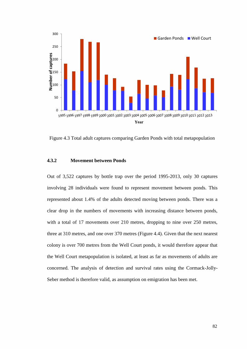
82

Figure 4.3 Total adult captures comparing Garden Ponds with total metapopulation

4.3.2 Movement between Ponds

Out of 3,522 captures by bottle trap over the period 1995-2013, only 30 captures

involving 28 individuals were found to represent movement between ponds. This

represented about 1.4% of the adults detected moving between ponds. There was a

clear drop in the numbers of movements with increasing distance between ponds,

with a total of 17 movements over 210 metres, dropping to nine over 250 metres,

three at 310 metres, and one over 370 metres (Figure 4.4). Given that the next nearest

colony is over 700 metres from the Well Court ponds, it would therefore appear that

the Well Court metapopulation is isolated, at least as far as movements of adults are

concerned. The analysis of detection and survival rates using the Cormack-Jolly-

Seber method is therefore valid, as assumption on emigration has been met.

0

50

100

150

200

250

300

Nu

mb

er o

f ca

ptu

res

Year

Garden Ponds Well Court

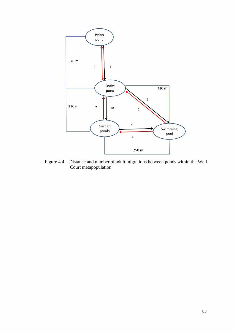
83

Figure 4.4 Distance and number of adult migrations between ponds within the Well

Court metapopulation

84

4.3.3 Model without Climatic Covariates Used in the CJS Method in

Program MARK

Data using the various group sizes were run and the most parsimonious model in

each group noted, along with its deviance and c-hat (Table 4.1). Means were then

taken for the 1000 bootstrap iterations run at each group size and c-hat adjustment

calculated by deriving model deviance by bootstrap mean deviance and model c-hat

by bootstrap mean c-hat. Cooch and White (2001) note that there is no clear view on

which of these is the better approach and recommend using the higher of the two

figures, on the basis that it is better to take a conservative view and consider the data

a poorer fit (i.e. further from 1) than a better fit. In the case of the Well Court data

this means that the c-hat adjustment has been based on deviance in all cases.

Anderson et al. (1994) state that with real data c-hat should always be expected to be

> 1, but should not generally exceed 4. As the observed c-hat derived here is <4,

and MARK allows for the simple alteration of the figure, it is well within acceptable

parameters for a non-theoretical study. The effect of adjusting c-hat to the new value

is to widen the confidence intervals for both detection and survival, but this should

be viewed as a correction of the over-dispersion and nothing more.

Table 4.1 Initial model deviance and c-hat by groups, plus adjustments. The

adjustment used for each group is highlighted in bold

No. of

groups

Model

deviance

Model

c-hat

Bootstrap

mean

deviance

Bootstrap

mean c-hat

Deviance

based

adjustment

C-hat

based

adjustment

8 703.69 4.75 478.67 3.49 1.47 1.36

4 608.99 4.55 448.74 5.68 1.36 0.80

2 703.69 4.75 549.86 3.96 1.28 1.12

1 517.99 5.29 374.05 3.86 1.38 1.37

85

Likelihood ratio tests (LRT) were carried out between first and second ranking

models for four, two and one group analyses, but were not possible for the eight-

group analysis, as the two models are not nested together. LRT test for single-group

(χ2 = 59.5, d.f. = 16, p < 0.0001) suggests that the most parsimonious model fits the

data radically better than even the second best, with the two-group (χ2 = 16.80, d.f. =

18, p = 0.5370) and four-group dataset (χ2 = 16.51, d.f. = 13, p = 0.2224) the

differences between first and second models are less clear.

Models were also compared by QAICc (Table 4.2), and these show very strong

support for the most parsimonious model in all four cases. In the case of the eight-

group analyses, time-dependent model, Phi(t) p(t) has a QAICc weight of 1, with all

other models having a weight of 0. The most parsimonious models in the other three

datasets are also very strong, the second most parsimonious in the four-group

analysis being the strongest amongst the second placed, but the comparison with the

most parsimonious model of 1/0.006 suggests that the most parsimonious model fits

the data 166.7 times better than the second. Models other than the most parsimonious

in each group size will therefore only be used with extreme caution. Where models

have a similar AIC (or QAIC) weighting it is possible to run model averaging

comparisons within MARK to determine the model that is the best fit, but given the

differences in QAICc weightings here model averaging would not impact on any of

the groups.

For the most parsimonious model, a survival rate varies between years in all four

cases. In summary, the survival rates from the single-group model are 0.565 ± 0.012,

two-group (0.5654 ± 0.014), four-group (0.574 ± 0.014) and eight-group (0.598 ±

0.0005). Detectability varied between years in all cases except for the four-group

86

case. In this case, all four pond systems have a different detectability each year. The

second most parsimonious model in each case showed a different result. Survival rate

and detectability is constant each year for the eight and single-group, respectively.

Meanwhile, for the four-group case, survival rate and detectability varies each year.

Survival rate varies between male and female newts and detectability varies between

years for the two-group case.

4.3.4 Model with Climatic Covariates

Two extra models which allow for an additive group and temporal effect (g*t) were

fitted and compared to the other basic model (Table 4.3). The time-dependant model

without covariates, Phi(t) p(g+t) emerged as the best model followed by Spring

rainfall and Non-aquatic rainfall covariate-dependent model [Phi(SR*NAR) p(g+t)]

as the second best model. Although the basic model had a smaller ΔQAICc value, the

increase in fit was not substantial enough to indicate that the basic model was more

parsimonious. Hence, those two best models are both important in this study. As the

remaining models had a ΔQAICc value larger than 10, there was insufficient

evidence to consider these models for further analysis.

Survival varied between 0.2 and 0.77 over the years from time dependent model,

Phi(t) and, between 0.38 and 0.75 from covariate-dependent model, Phi(SR*NAR).

However, survival did not vary between ponds for both models. These indicate that

only regional effects rather than local effects on all the ponds are affecting survival.

Both model Phi(t) and Phi(SR*NAR) in Figure 4.5 indicated that inter-year survival

remained high in the period 1995- 1998, before declining to a low in 2000-2001,

after which there was a recovery. The Phi(SR*NAR) model pointed out that Non-

aquatic rainfall (NAR) and Spring rainfall (SR) nicely explained the temporal

Table 4.2 Comparison of the two most parsimonious models in each group size for the Well Court data; t = time, and g = ponds

No. of groups

Most

parsimonious

QAICc weight

Model

likelihood

2nd most

parsimonious

QAICc weight

Model

likelihood

8 Phi(t) p(t) 1.000 1.000 Phi(.) p(t) 0.000 0.000

4 Phi(t) p(g) 1.000 1.000 Phi(t) p(t) 0.006 0.006

2 Phi(t) p(t) 1.000 1.000 Phi(g*t) p(t) 0.000 0.000

1 Phi(t) p(t) 1.000 1.000 Phi(.) p(t) 0.000 0.000

Table 4.3 CJS model selection based upon ΔQAICc in program MARK; Phi = survival, p = detectability, t = time, and g = ponds. Climatic

variable; SR = spring rainfall, and NAR = non-aquatic rainfall. NP = number of parameters, and QAICc = quasi Akaike information

criteria from adjusted data

Model QAICc ΔQAICc QAICc

Model

NP QDeviance

87

Weights Likelihood

Phi(t) p(g+t) 2646.02 0.000 0.661 1.000 38 560.38

Phi(SR*NAR) p(g+t) 2647.35 1.338 0.339 0.512 25 588.55

Phi(t) p(g) 2669.63 23.612 0.000 0.000 22 616.97

Phi(t) p(t) 2679.26 33.245 0.000 0.000 35 599.85

Phi(g) p(t) 2680.59 34.579 0.000 0.000 22 627.94

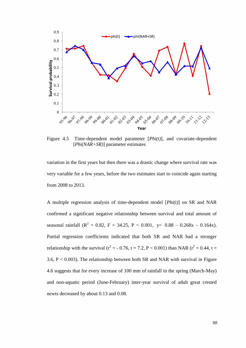
89

Figure 4.5 Time-dependent model parameter [Phi(t)], and covariate-dependent

[Phi(NAR+SR)] parameter estimates

variation in the first years but then there was a drastic change where survival rate was

very variable for a few years, before the two estimates start to coincide again starting

from 2008 to 2013.

A multiple regression analysis of time-dependent model [Phi(t)] on SR and NAR

confirmed a significant negative relationship between survival and total amount of

seasonal rainfall (R2 = 0.82, F = 34.25, P < 0.001, y= 0.88 – 0.268x – 0.164x).

Partial regression coefficients indicated that both SR and NAR had a stronger

relationship with the survival (r2 = - 0.76, t = 7.2, P < 0.001) than NAR (r

2 = 0.44, t =

3.6, P < 0.003). The relationship between both SR and NAR with survival in Figure

4.6 suggests that for every increase of 100 mm of rainfall in the spring (March-May)

and non-aquatic period (June-February) inter-year survival of adult great crested

newts decreased by about 0.13 and 0.08.

0

0.1

0.2

0.3

0.4

0.5

0.6

0.7

0.8

0.9

Surv

ival

pro

bab

ility

Year

phi(t) phi(NAR+SR)

88

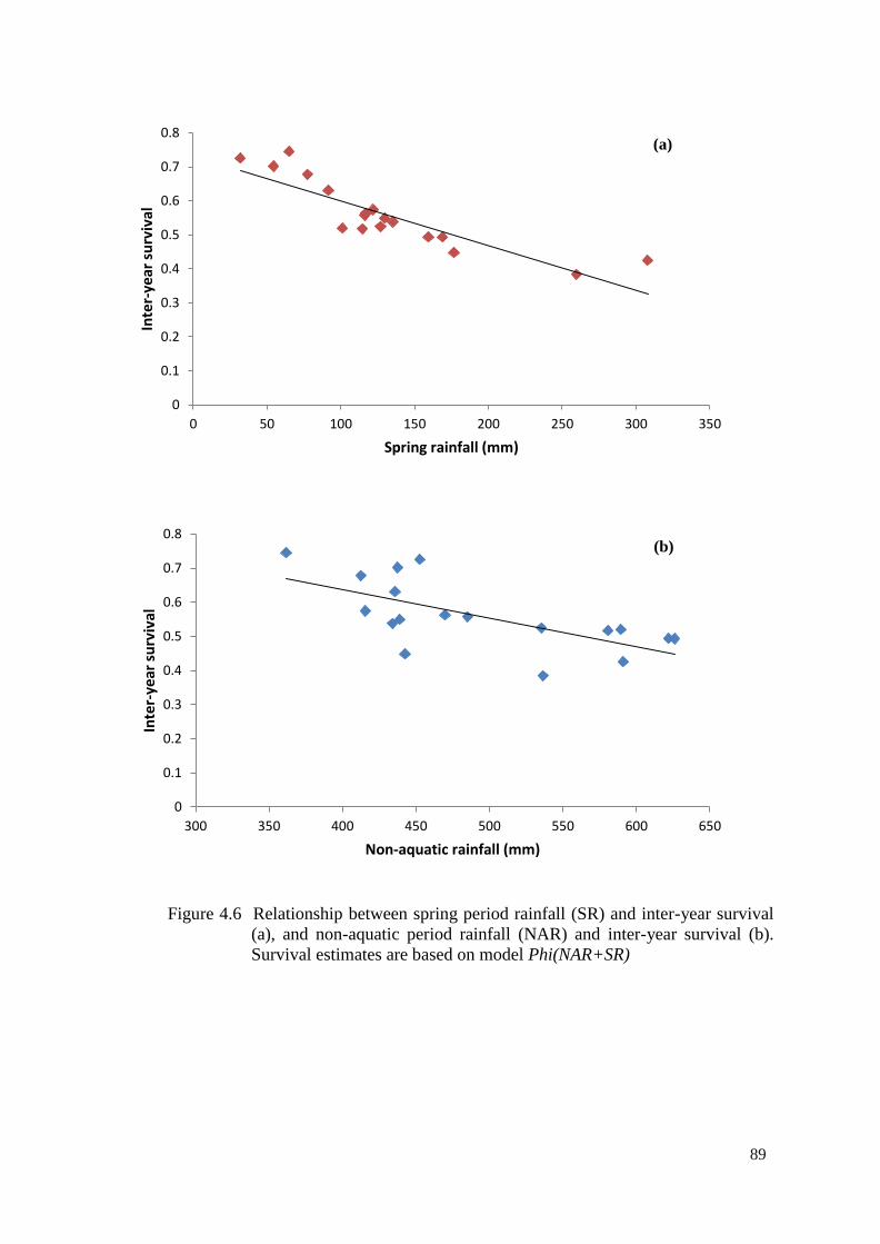
90

Figure 4.6 Relationship between spring period rainfall (SR) and inter-year survival

(a), and non-aquatic period rainfall (NAR) and inter-year survival (b).

Survival estimates are based on model Phi(NAR+SR)

0

0.1

0.2

0.3

0.4

0.5

0.6

0.7

0.8

0 50 100 150 200 250 300 350

Inte

r-ye

ar s

urv

ival

Spring rainfall (mm)

0

0.1

0.2

0.3

0.4

0.5

0.6

0.7

0.8

300 350 400 450 500 550 600 650

Inte

r-ye

ar s

urv

ival

Non-aquatic rainfall (mm)

(a)

(b)

89

91

4.3.5 Population Estimate

Detection rates at 0.66 (95% confidence interval 0.611 - 0.703) and 0.84 (0.737 –

0.911) were high in the Garden Ponds and Swimming pool respectively, but lower at

0.38 (0.313 – 0.441) in the Snake pond and also in the Pylon pond at 0.24 (0.115 –

0.423). The wide 95% confidence interval for the Pylon pond reflects the low and

inconsistent capture rate at that site. There was a significant correlation between the

inter-year survival rate in the Spring rainfall and Non-aquatic rainfall covariate-

dependant model [Phi(SR*NAR) p(g+t)] and time-dependent model [Phi(t) p(g+t)]

model (r = 0.63, d.f. = 18, P = 0.038). Thus, the population estimates for the Well

Court metapopulation were prepared using the known number of captures by year

multiplied by 1/detection rate for each pond from the time dependent model [Phi(t)

p(g+t)]. Annual captures by pond are shown in Figure 4.7. The largest number of

adult great crested newts was found in the Garden ponds (1826/4049), followed by

Snake pond (1579/4049), Pylon pond (354/4049), and Swimming pool (290/4049).

Population sizes were generally high in the period 1997-2001, and then declined

thereafter to almost half from the previous years until 2008. The contribution each

pond made to the overall metapopulation size varied between years, as the

detectability varied between ponds. There was a significant correlation between the

population trends in the Garden Ponds and Swimming Pool (r = 0.828, d.f. = 18, P <

0.001) although the Garden Ponds – which was the smallest water body within the

system - was the main source site of the metapopulation. Pairwise correlations

between the trends in the other subpopulations were all non-significant. Fluctuations

between different subpopulations therefore appear to be largely asynchronous.

90

92

Figure 4.7 Population estimates for the total metapopulation by year, based on

detection rate and individuals captured by pond using model Phi(t)

p(g+t). Vertical lines show 95% confidence intervals.

4.4 DISCUSSION

The study system comprised a subdivided population based on four breeding sites,

and displayed some of the characteristics predicted by metapopulation theory.

Regardless of how many groups were included in the dataset, with or without

climatic covariates, the most parsimonious model in all cases shows survival rates to

change over time rather than be affected by variation between ponds or between

sexes. This is also the case in the second ranked covariate-dependent model,

Phi(SR*NAR) p(g+t) which suggests that survival rates are closely linked to non-

aquatic, NAR (January- February and June-December in each calendar year) and

spring season rainfall, SR (Mac-May) rather than to conditions specific to an

individual pond or sex group. This study indicates that survival ranged between 0.2

0

200

400

600

800

1000

1200

Po

pu

lati

on

est

imat

e

Year

Pylon pond

Swimming pool

Snake pond

Garden ponds

91

93

and 0.77 over the years from the top ranking time-dependent model, Phi(t) and,

between 0.38 and 0.75 from second covariate-dependent model, Phi(SR*NAR).

However, survival is constant between ponds for both models. Previous population

studies on amphibians reveal considerable variation in annual survival (Cooke &

Arnold 2003, Gill 1978). Hagstrom (1979) estimated relatively high annual survival

(78%) in a great crested newt population. In three separate studies, Baker (1999)

found annual survival ranged from 31 to 100%, Arntzen & Teunis (1993) observed

survival of between 33 and 57% and Griffiths et al. (2010) estimated values at

between 25 and 80%.

Griffiths et al. (2010) also used the Well Court data set, albeit with fewer years (1995

– 2006), and found that variation in survival between years was inversely related to

winter temperatures and winter rainfall. They discovered that the low annual survival

of great crested newt was related to mild winters and heavy rainfall. This study has

gone further by using the whole 19 years dataset (1995-2013) and found that only

rainfall mainly affected newt survival in the additional years from 2006 – 2013. The

importance of rainfall both prior to and after each aquatic season on survival rates the

following year is intriguing. Like many other temperate amphibians, great crested

newts usually hibernate on land, and gaseous exchange occurs by pumping air into

the lungs as well as across the skin surface. In soil filled with water, newts may face

respiratory challenges pumping air into the lungs. This limitation may lead to

deficiency of oxygen reaching tissues, resulting in severe hypoxia (Shoemaker et al.

1992). This may be reflected in reduced survival.

Although the ponds differed in size and biological characteristics, the survival rate

was found to be the same in all ponds, although varying over time. This may have

implications for the management of populations as it suggests a relationship between

92

94

rainfall with inter-year survival. A note of caution about this relationship must,

however, be sounded. Other factors may cause poor survival, or apparent survival

rates at individual ponds. An example is provided by the results for the 2006 survey

in Figure 6. Here the evidence for the climatic variables suggests that survival from

the previous year should have been high, whilst capture evidence showed that it

declined. One possible explanation for the difference was that conditions in the

largest of the Garden ponds were particularly poor in the 2006. During the summer

of 2005 the Garden ponds were left unmanaged and contain submerged and

overhanging vegetation, and this was not cleared until the following year (Griffiths et

al. 2010). Poor aquatic habitat may therefore have affected survival in that year.

Although management was carried out it was not completed until after the trapping

season had ended. Captures were therefore very low during that year, but this is more

likely to represent poor conditions in the trapping environment leading to low

detection rather than a low survival rate. Use of climatic data to anticipate likely

survival of amphibians between years is therefore more appropriate at the landscape

level than for individual ponds.

The evidence presented here suggests that amphibians show short time delays in

their response to climatic variation. In this study, it has been shown that rainfall is an

important determinant of inter-year amphibian survival rate and short-term climatic

fluctuations may be useful for monitoring the inter-year survival of amphibians.

Projections for climate warming in the UK (Hulme 2002) suggest that by the 2080s

annual temperatures may rise between 2.0 and 3.5 0C, whilst summer precipitation

may decline by up to 50%. Conversely, heavy winter precipitation may increase with

the overall precipitation levels remaining reasonably constant. In the recent report of

IPCC (2013), climate change is projected to increase low-percentile winter

93

95

temperatures than the mean, thereby decreasing temperature variability. Projecting

data for individual years and locations into long-term climatic predictions is difficult,

and the data presented here have represented year-to-year fluctuations rather than

lasting trends. It does appear, however, that a succession of warm, wet winters could

have major impacts on the survival of isolated metapopulations.

Population estimates have been based on detection rates and the actual number of

individual crested newts caught in each year. The differences in overall population

confidence intervals from year to year reflect the varying contribution of each pond

within the metapopulation to the overall estimate for each year. The pond with the

widest confidence interval in detection is the Pylon pond. This pond was not

surveyed for the first two years of the study, and the absence of any data for these

years and the consequent absence of any influence in the population estimate for

those years have helped keep the confidence intervals for 1995 and 1996 narrow. In

contrast, during those years when the capture rate in this pond was high, such as

1999 and 2000, the influence of the pond on the overall capture rate is very high and

in extending the limits of the overall confidence intervals even higher. The Snake

pond also has a low detection rate, but here the confidence intervals are narrower.

Although there is fluctuation in catches from year to year, it is not as low as the

Pylon pond capture rates. The Swimming pool represents a site that has a different

pattern of captures to the Pylon pond. Detection rates were high at this site which

was investigated from the very first year of the survey. That it made no contribution

to the overall population estimate after 2002 is a function of the steady decline of the

population from a peak in 1995 to extinction by 2003. This pond would therefore

have contributed to narrow confidence intervals at the start of the study and would

have influenced their widening as it became less important in the overall population.

94

96

The study of the four populations at Well Court was an investigation of

metapopulation dynamics at a small spatial scale. The populations were assumed to

form an isolated metapopulation during the 19 years for which they were studies.

The dynamics of the Well Court populations were not influenced by dispersal from

population outside of the Well Court study area and the dispersal was infrequent

among the Well Court ponds (ca. 2.3% of individuals changing patch per season)

which were separated by 200-800 m. Given the apparently low rate of adult dispersal

between ponds in Well Court area, this observation supports the assumption that the

dynamics of the Well Court populations were not influenced by dispersal from

populations outside of the Well Court study area. The metapopulation described here

shows some source/sink characteristics (Pulliam1988), with only two known

breeding (= source) sites amongst the four sites monitored.

Pylon pond and Swimming pool may be termed sink ponds as adults have been

caught in most or all years but there has been no evidence of successful breeding

except in year 12 in Pylon pond. Newt larvae were never captured here, indicating

repeated reproductive failure. A possible cause for unsuccessful juvenile recruitment

at Pylon pond was the reduced water level in the summer months, and the consequent

failure of newt larvae to complete metamorphosis. The pond drying process is not

uncommon, leading to a loss of juvenile production in many amphibian species that

breed in ponds (Kupfer & Kneitz 2000). At the Swimming pool, possible causes of

recruitment failure may have been associated with high predation by numerous

diving beetles (Dytiscus marginalis) and dragonfly larvae (Aeshna cyanea) as it

never dries completely. Newt larvae are for the most part, solitary animals that live in

aquatic vegetation to avoid predators but are nevertheless devoured by a wide

95

97

range of aquatic invertebrates including dytiscid water beetles, backswimmer bugs

(e.g. Notonecta species) and odonate larvae, as well as vertebrate such as fish, water

birds, adult amphibian and amphibious reptiles (Beebee 1996). Even the larvae of

crested newts which have powerful skin toxins as adults, are highly vulnerable to fish

predation (Beebee 1996).

If those two ponds may be termed sinks, the Garden ponds are sources, for here

regular breeding and recruitment into the metapopulation occurred. The Garden

ponds were subject to immigration and emigration of both adults and juveniles. The

findings contradict Oldham et al. (2000), who considered smaller ponds to be

unsuitable for supporting viable breeding populations of great crested newts.

However, Oldham et al. (2000) did note that intermittent drying of ponds at a rate of

once per decade may have an overall beneficial effect, preventing the colonisation/

persistence of aquatic predators that rely on permanent water bodies more than

newts. The Snake pond probably fluctuates between source and sink. In most years

these ponds also represented the majority of the metapopulation in terms of captures

and individuals. If reducing survival rates leads to smaller populations in all ponds, it

appears likely that populations in the sink ponds will decline as surviving adults find

themselves increasingly able to find space in the breeding pond. This may already be

in progress, with populations at the Pylon pond and Swimming Pool declining to

extinction with no evidence of recolonization. This study therefore suggests that

increasingly poor survival rates as non-aquatic and spring season rainfall increases

will affect metapopulations by reducing the number of ponds in use, leaving breeding

ponds increasingly isolated and at high risk of extinction. There is already some

evidence of this process. The population estimate shows high estimates for the years

1997, 1998, 1999 and 2000 and was low in other years. Evidence presented of inter-

96

98

pond migrations shows that the majority of observed movements of adults (19 out

of a total of 30) occurred in these same four years. Therefore, as the overall

metapopulation decreases, so does gene flow between ponds.

The failure to move to other ponds may have been a function of the distance between

ponds in relation to landscape structure. The ponds were located within an

agricultural landscape at distances of not less than 250 m apart and the Garden

ponds, which held the largest local population of the great crested newt was

potentially isolated by a human settlement and frequently-used trail. Mullner (2001)

discovered that the great crested newt only emigrated up to 50 m from the breeding

ponds. Jehle and Arntzen (2000) pointed out low migration distances with an average

of less than 20 m for radio-tracked newts. Nevertheless, Kupfer (1998) indicated an

ability of the great crested newt to move up to several hundred meters to a breeding

site. It must be concluded that the realised movement activity of newts from the pond

depends on the habitat qualities of the surrounding environment (Mullner 2001). If

local refuges and food are abundant in habitat adjacent to the pond, the newts would

use them (Madison & Farrand 1998). The variation of known migration distances

probably indicates an adaptive flexibility in response to local habitat conditions.

However, this conclusion must be treated carefully as the main dispersal occurs in

juveniles. Once adults return to a pond, they remain fairly faithful to that pond.

Adults often show high breeding site fidelity and individuals frequently return to

their natal site (Griffiths 1996). This is possibly due to their constraining demands

for complex landscape structures with high connectivity (Marsh & Trenham 2001).

Populations are truly sub-divided when their dynamics are due mainly to within-

patch recruitment rather than immigration (Harrison & Taylor 1997). This was true

97

99

for all populations in the Well Court metapopulation. Productive populations

(Garden ponds) were thought to function in the rescue of unproductive populations

(Snake pond). Dispersal among populations, mainly juveniles was sufficiently

frequent to enable the colonization of a new pond and was expected to lead to the

‘rescue’ of a declining population. Fluctuations in the size of each population were

explained by fluctuations in within population rates of adult survival and recruitment,

not by fluctuations in the dynamics of the other populations. The persistence of all

populations therefore appeared to be governed mainly by within- population

processes.

98

100

CHAPTER 5

COLONISATION AND POPULATION DYNAMICS OF THE GREAT

CRESTED NEWT IN NEWLY CREATED PONDS

ABSTRACT

The declining amphibian problem can serve as a model for understanding the global

biodiversity crisis in general. However, before this can happen more research is

needed into amphibian population dynamics particularly their ability to colonise and

re-colonise areas. This study investigates eight small ponds on the University of Kent

campus that have contained a population of limited size since colonization in 2000.

Capture-mark-recapture (CMR) data collected over a 16 year period was combined

to explore the impact of variation in survival on the population dynamics of the great

crested newt (Triturus cristatus). A total of 126 individuals were recorded from 430

captures in the breeding seasons 2000 to 2016. Model selection based on quasi-

likelihood Akaike Information Criterion (QAICc) with climatic covariates indicated

that apparent annual survival was high and did not vary between years despite mild,

wet winter conditions. Splitting captures by gender suggested that males had a higher

detection rate than females. Estimates of population size ranged from 13 to 57

individuals between years. Management practised through draining and refilling the

ponds did have an apparent effect on the number of newts captured over subsequent

years. Population increase could be due to the decrease in predatory invertebrates

following pond desiccation and a subsequent increase in recruitment levels.

Ultimately, conservation actions need to embrace management to reduce survival and

enhance recruitment.

99

101

5.1 INTRODUCTION

Globally, 32% of amphibian species are threatened with extinction, more than in any

other vertebrate class (Hof et al. 2011). The mechanisms that underlie amphibian

declines are very complex and many causal factors are involved. Recent changes in

global climate might impact adversely on amphibian populations (Beebee & Griffiths

2005). Global mean temperature rose by about 0.6°C over the past 100 years, which

has had huge impacts on amphibians (Carey 2003). Various amphibian species at

different spatial scales are apparently being affected by climate change and climate

extremes (Shoo et al. 2011). The breeding phenology and distributions of various

amphibian species are being shifted across the world (Blaustein et al. 2010).

Parmesan (2007) confirmed that compared to any other functional/taxonomic group,

amphibians have significantly started earlier their breeding activity, similar with

changes in butterflies, birds, and trees. Mild winters have been linked with reduced

fecundity in females and earlier breeding due to a lower body condition (Benard

2015). Although amphibian populations experience significant natural fluctuations,

the impacts of unprecedented climate extremes and climate change are far less well

understood (Scheele et al. 2012).

Climate change - including extremes in rainfall - is forecasted to be one of the most

significant drivers of ecological change in the forthcoming century (Lawler et al.

2009). Although some researchers have related declines in amphibian populations to

changes in rainfall (e.g. Pounds et al. 1999; Pounds 2001; McMenamin et al. 2008),

the potential effects of variable patterns of seasonal rainfall have largely been

overlooked in studies with temperate amphibians. Instead, investigations with

amphibians have almost entirely focussed on the effects of increased temperature.

100

102

There is a need to test the hypothesis that seasonal rainfall events may become

increasingly more influential on amphibians, especially in relation to the timing of

reproduction. Examining how species react to shifts in climate may contribute an

important early step in understanding and forecasting the effects of long-term climate

change (Debinski et al. 2006).

Amphibians are effective as a model framework for investigating the impacts of a

changing climate because their reproduction is rely closely to water availability,

water quality, and patterns of rainfall, all of which are anticipated to be affected by

climate change (NAST 2000). Hydroperiod - the period during which a waterbody

holds water (Ryan & Winne 2001) - is an important pond feature that directly

influences survivorship of pond-breeding amphibians (Pechmann et al. 1989). Short-

term variations in rainfall can affect the hydroperiod of a temporary pond in an

erratic way, and this may influence the survival of amphibians in a stochastic way

(Griffiths et al. 2010). Moreover, recruitment seems to be extremely sensitive to

rainfall as reproduction in amphibians is highly influenced by hydroperiod (Blaustein

et al. 2010). Hydroperiods and pond features will probably be altered by climate

change as seasonal hydrology shifts (Brooks 2009). The climate change model by

Heisler-White et al. (2008) predict more variable patterns of rainfall, with extended

droughts and higher (but less) rainfall occurrences, tallying with increased

temperatures. Such disparity in the temporal distribution, rather than the total amount

of rainfall per se, may be associated with population fluctuations in amphibians

(Stewart 1995).

The great crested newt was chosen as a model species in this study because they may

be sensitive to climate change and depend on small waterbodies that are liable to

101

103

desiccation (Blaustein et al. 2010). Examining the impacts of climate change on a

sensitive species such as the great crested newt could consequently lead to a wider

understanding of the conservation needs of other amphibian species that are highly

vulnerable to climate change. This study combined capture-mark-recapture data

collected over a 16 year period to explore the impact of variation in survival on the

population dynamics of the great crested newt (Triturus cristatus). This study

examines eight small ponds on the north western boundary of the University of Kent

campus that have contained a population of limited size since colonization in 2000.

Unlike Well Court farm (Chapter 4), these ponds are located outside an agricultural

area and are being well protected and managed with regular pond draining and

relining. Thus, effects of disturbance and pond management on the dynamics of the

newt populations can further be investigated and compared. Additionally, since these

two study sites are located just three miles apart and feature same weather conditions

every year, impacts of local and regional factors on newts population persistence can

be analysed further. In particular, this study tests the hypotheses that: (1) annual

survival varies between years; (2) annual survival is related to climatic factors and

possibly climate change; and (3) males and females have an equal chance of survival

and being detected on the trapping occasion and, (4) pond management enhance

larval recruitment and survival of the great crested newt.


5.2.1 Study Site

Field Site

Refer to Chapter 2

102

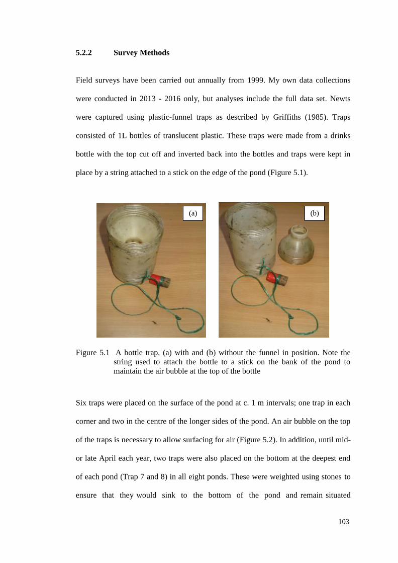
104

5.2.2 Survey Methods

Field surveys have been carried out annually from 1999. My own data collections

were conducted in 2013 - 2016 only, but analyses include the full data set. Newts

were captured using plastic-funnel traps as described by Griffiths (1985). Traps

consisted of 1L bottles of translucent plastic. These traps were made from a drinks

bottle with the top cut off and inverted back into the bottles and traps were kept in

place by a string attached to a stick on the edge of the pond (Figure 5.1).

Figure 5.1 A bottle trap, (a) with and (b) without the funnel in position. Note the

string used to attach the bottle to a stick on the bank of the pond to

maintain the air bubble at the top of the bottle

Six traps were placed on the surface of the pond at c. 1 m intervals; one trap in each

corner and two in the centre of the longer sides of the pond. An air bubble on the top

of the traps is necessary to allow surfacing for air (Figure 5.2). In addition, until mid-

or late April each year, two traps were also placed on the bottom at the deepest end

of each pond (Trap 7 and 8) in all eight ponds. These were weighted using stones to

ensure that they would sink to the bottom of the pond and remain situated

(a) (b)

103

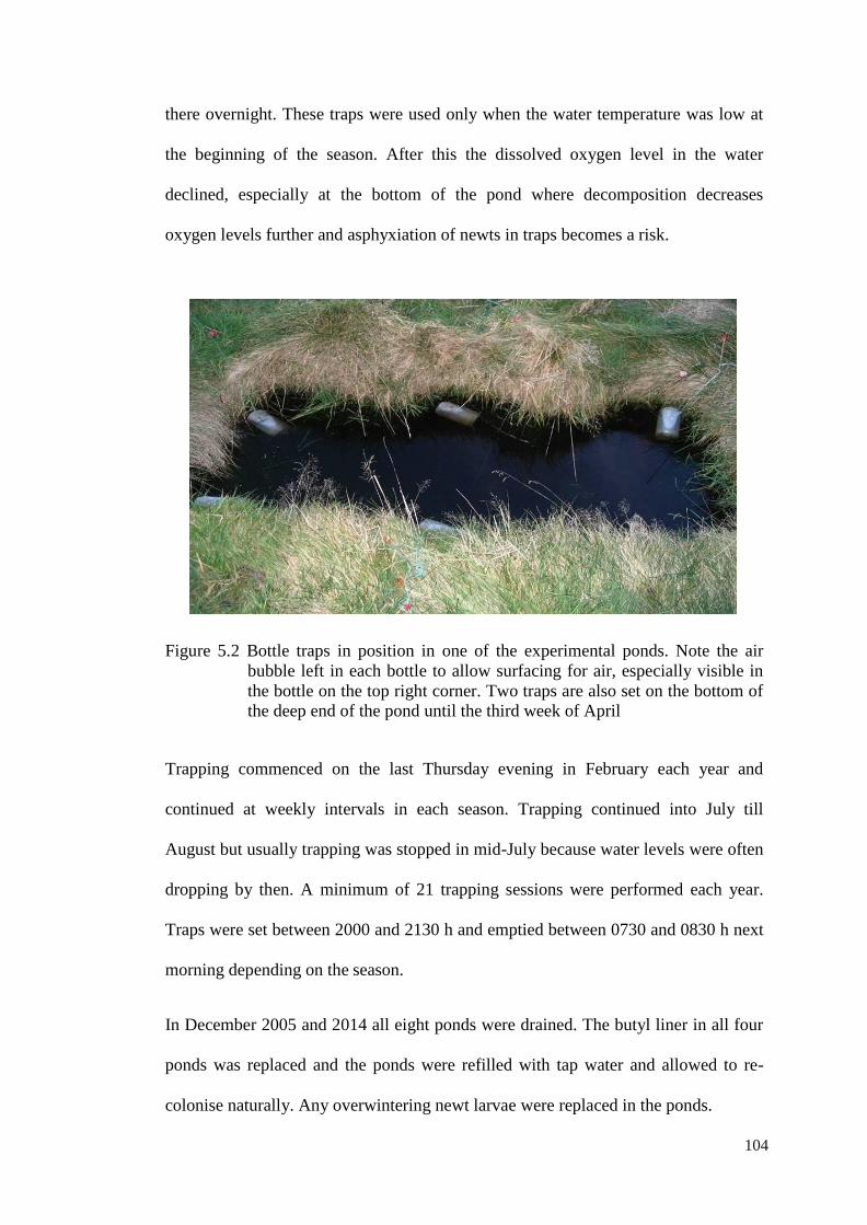
105

there overnight. These traps were used only when the water temperature was low at

the beginning of the season. After this the dissolved oxygen level in the water

declined, especially at the bottom of the pond where decomposition decreases

oxygen levels further and asphyxiation of newts in traps becomes a risk.

Figure 5.2 Bottle traps in position in one of the experimental ponds. Note the air

bubble left in each bottle to allow surfacing for air, especially visible in

the bottle on the top right corner. Two traps are also set on the bottom of

the deep end of the pond until the third week of April

Trapping commenced on the last Thursday evening in February each year and

continued at weekly intervals in each season. Trapping continued into July till

August but usually trapping was stopped in mid-July because water levels were often

dropping by then. A minimum of 21 trapping sessions were performed each year.

Traps were set between 2000 and 2130 h and emptied between 0730 and 0830 h next

morning depending on the season.

In December 2005 and 2014 all eight ponds were drained. The butyl liner in all four

ponds was replaced and the ponds were refilled with tap water and allowed to re-

colonise naturally. Any overwintering newt larvae were replaced in the ponds.

104

106

5.2.3 Newt Identification

Refer to Chapter 2

5.2.4 Weather Records

Refer to Chapter 2

5.2.5 Capture-mark-recapture Modelling

Because of the small size of the ponds, a weekly trapping programme captures most

individuals in the ponds during most weeks of the breeding season, enabling detailed

life histories to be built up. Refer to Chapter 2 for details of capture-mark-recapture

analysis.

5.3 RESULTS

5.3.1 Adult Capture

Over the 16 years of the study to the end of the 2015 season, 430 captures of 126

individual newts had been made. A total of 64 and 62 individual males and females

were captured respectively. The presence of larvae and metamorphs in the ponds in

all years of the study indicated annual recruitment from this site. Details of the yearly

males and females captured for the year 2000-2015 are shown in Figure 5.3. Great

crested newts were detected in both the old ponds, created in 1998 and new ponds,

created in 2009. The trends in the first eight years (2000-2007) were different from

those in the second eight years (2008-2015). A rapid increase in the number of newts

recorded was observed in 2008, two winters after draining and relining. The number

of individuals captured rose again to 40 individual newts during 2010 surveys, two

105

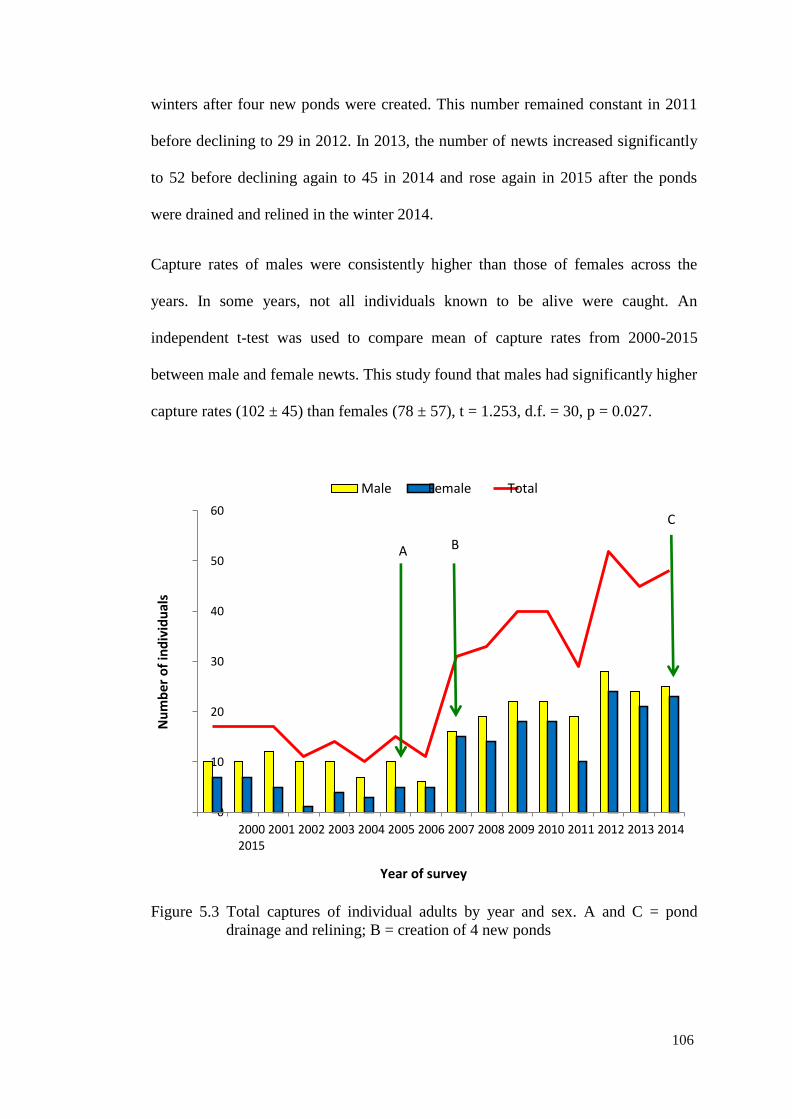
107

winters after four new ponds were created. This number remained constant in 2011

before declining to 29 in 2012. In 2013, the number of newts increased significantly

to 52 before declining again to 45 in 2014 and rose again in 2015 after the ponds

were drained and relined in the winter 2014.

Capture rates of males were consistently higher than those of females across the

years. In some years, not all individuals known to be alive were caught. An

independent t-test was used to compare mean of capture rates from 2000-2015

between male and female newts. This study found that males had significantly higher

capture rates (102 ± 45) than females (78 ± 57), t = 1.253, d.f. = 30, p = 0.027.

Male Female Total

60

50

40

30

20

10

0

2000 2001 2002 2003 2004 2005 2006 2007 2008 2009 2010 2011 2012 2013 2014 2015

Year of survey

Figure 5.3 Total captures of individual adults by year and sex. A and C = pond

drainage and relining; B = creation of 4 new ponds

C

A B

Nu

mb

er o

f in

div

idu

als

106

108

5.3.1 Variation in Survival and Detectability between Sexes without

Climatic Covariates

Models using males and females as a grouping factor (group = 2) were run and the

most parsimonious model noted, along with its deviance and c-hat (Table 5.1). Mean

deviance were then taken for the 1000 bootstrap iterations and c-hat adjustment

calculated by dividing model deviance by bootstrap mean deviance and model c-hat

by bootstrap mean c-hat. Cooch and White (2001) note that there is no clear view on

which of these is the better approach and recommend using the higher of the two

figures, on the basis that it is better to take a conservative view and consider the data

a poorer fit (i.e. further from 1) than a better fit. In the case of the Field Site data, this

means that the c-hat adjustment has been based on deviance in all cases. The results

from 1000 bootstrap iterations showed that the data were over-dispersed and c-hat

values were corrected to 1.03.

Table 5.1 Initial model deviance and c-hat, plus adjustments. The adjustment used is

highlighted in bold

No of Model Model Bootstrap Bootstrap Deviance C-hat

groups deviance c-hat mean

deviance

mean

c-hat

based

adjustment

based

adjustment

2 258.5043 4.63 245.31 5.97 1.03 0.78

A summary of the most parsimonious models after c-hat adjustment is shown in

Table 5.2, below. The model with constant survival but detection rates varying

between males and females [Phi(.) p(g)] is the one best supported by the data, with

an AICc weight of 0.574 that is only 1.545 times better than the next best supported

model with an AICc weight of 0.371. However, the best model is 11.6 times better

supported than the third best supported model. The fact that these models are the

107

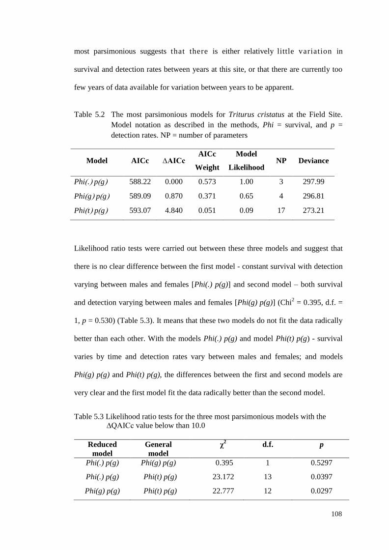
109

most parsimonious suggests that there is either relatively little variation in

survival and detection rates between years at this site, or that there are currently too

few years of data available for variation between years to be apparent.

Table 5.2 The most parsimonious models for Triturus cristatus at the Field Site.

Model notation as described in the methods, Phi = survival, and p =

detection rates. NP = number of parameters

Model AICc ∆AICc AICc

Weight

Model

Likelihood NP Deviance

Phi. pg 588.22 0.000 0.573 1.00 3 297.99

Phig pg 589.09 0.870 0.371 0.65 4 296.81

Phit pg 593.07 4.840 0.051 0.09 17 273.21

Likelihood ratio tests were carried out between these three models and suggest that

there is no clear difference between the first model - constant survival with detection

varying between males and females [Phi(.) p(g)] and second model – both survival

and detection varying between males and females [Phi(g) p(g)] (Chi2 = 0.395, d.f. =

1, p = 0.530) (Table 5.3). It means that these two models do not fit the data radically

better than each other. With the models Phi(.) p(g) and model Phi(t) p(g) - survival

varies by time and detection rates vary between males and females; and models

Phi(g) p(g) and Phi(t) p(g), the differences between the first and second models are

very clear and the first model fit the data radically better than the second model.

Table 5.3 Likelihood ratio tests for the three most parsimonious models with the

∆QAICc value below than 10.0

Reduced

model

General

model

χ2 d.f. p

Phi(.) p(g) Phi(g) p(g) 0.395 1 0.5297

Phi(.) p(g) Phi(t) p(g) 23.172 13 0.0397

Phi(g) p(g) Phi(t) p(g) 22.777 12 0.0297

108

110

Output for the most parsimonious model of all, model Phi(.) p(g), is shown below as

Table 5.4. This model provides a fixed survival rate both over time and between the

sexes, but separates out detection rates between male and female. This does not

imply that survival rates are the same for both sexes, merely that there is insufficient

data upon which to separate them.

Table 5.4 Survival and detection rates from model Phi(.) p(g)

Parameter Estimate Standard

error

95% confidence

interval

Survival (overall) 0.83 0.0195 0.7909-0.8675

Detection (male) 0.92 0.0226 0.8594-0.9503

Detection (female) 0.73 0.0443 0.6383-0.8109

In view of the close ranking of the models, model Phi(g) p(g) is also considered,

although it must be noted that this is only considered to fit the data 0.87 times as

well as the best fit model Phi(.) p(g), above. Details for this model are shown below

as Table 5.5. Both survival and detection rates are therefore higher for males than

they are for females. In the case of detection, this is confirmed by both models used,

in the case of survival it is confirmed by the second method only. Nevertheless, there

is very little difference between the two top models in terms of parameter estimates.

Table 5.5 Survival and detection rates from model Phi(g) p(g)

Parameter Estimate Standard

error

95% confidence

interval

Survival (male) 0.85 0.0241 0.7964-0.8913

Survival (female) 0.81 0.0323 0.7354-0.8624

Detection (male) 0.91 0.0229 0.8570-0.9495

Detection (female) 0.74 0.0441 0.6468-0.8189

109

111

5.3.2 Variation in Survival and Detectability with the Climatic Covariates

A model that included climatic covariates as additive factors was fitted and

compared to the other basic models (Table 5.6). The best model fit without

covariates remained Phi(.) p(sex), i.e. survival is constant between years, but

detection rates varied between male and female. With the ΔQAICc below 2 as an

evidence of substantial fit (Burnham & Anderson 2002), the first three models; Phi(.)

p(g), Phi(g) p(g) and, Phi(NAR) p(t) were regarded as important models in this study.

Likelihood ratio tests were carried out between seven models that had ΔQAICc less

than 10 and suggest that there are no clear differences between the first and six

following models except between model Phi(.) p(g) and model Phi(t) p(g) (χ2 =

24.775, d.f. = 14, p = 0.037) (Table 5.7). This means that the Phi(.) p(g) model fits

the data radically better than the Phi(t) p(g) model. Although the model fit without

covariates had a smaller QAICc value, the increase in fit was not substantial enough

to indicate that the model fit without covariates was more parsimonious.

Survival between years was plotted from model Phi(NAR) p(t) output as in Figure

5.4. Inter-year survival was the highest in the period 2004-2005 and 2011-2012 with

the value of 0.894 ± 0.03 and 0.896 ± 0.03, respectively. The lowest inter-year

survival rate was recorded in 2013-2014 (0.76 ± 0.04). Exploratory correlations

between annual survival and potential climatic predictors revealed a highly

significant negative relationship with non-aquatic season rainfall (NAR) (Figure

5.5). From Figure 5.5, it can be seen clearly that the survival rate is decreasing if the

NAR is increasing.

110

113

Table 5.6 CJS model selection based upon ∆QAICc in program MARK; Phi = survival and p = detection rates. Climatic variables; NAR = non-

aquatic rainfall, WT = winter temperature, SR = spring rainfall, and AF = air frost. NP = number of parameters, and QAICc = quasi

Akaike information criteria from data adjusted using c-hat

No Model QAICc ΔQAICc AICc Weights Model Likelihood NP QDeviance

1 Phi(.) p(g) 588.22 0.00 0.3871 1.0000 3 297.99

2 Phi(g) p(g) 589.09 0.87 0.2505 0.6472 4 296.81

3 Phi(NAR) p(t) 589.83 1.61 0.1731 0.4471 4 297.55

4 Phi(NAR + WT) p(t) 590.96 2.74 0.0983 0.2540 6 294.57

5 Phi(t) p(g) 593.06 4.80 0.0344 0.0888 17 273.21

6 Phi(NAR + SR) p(t) 593.29 5.07 0.0307 0.0792 6 296.90

7 Phi(NAR + WT + AF) p(t) 594.40 6.18 0.0177 0.0456 8 293.84

111

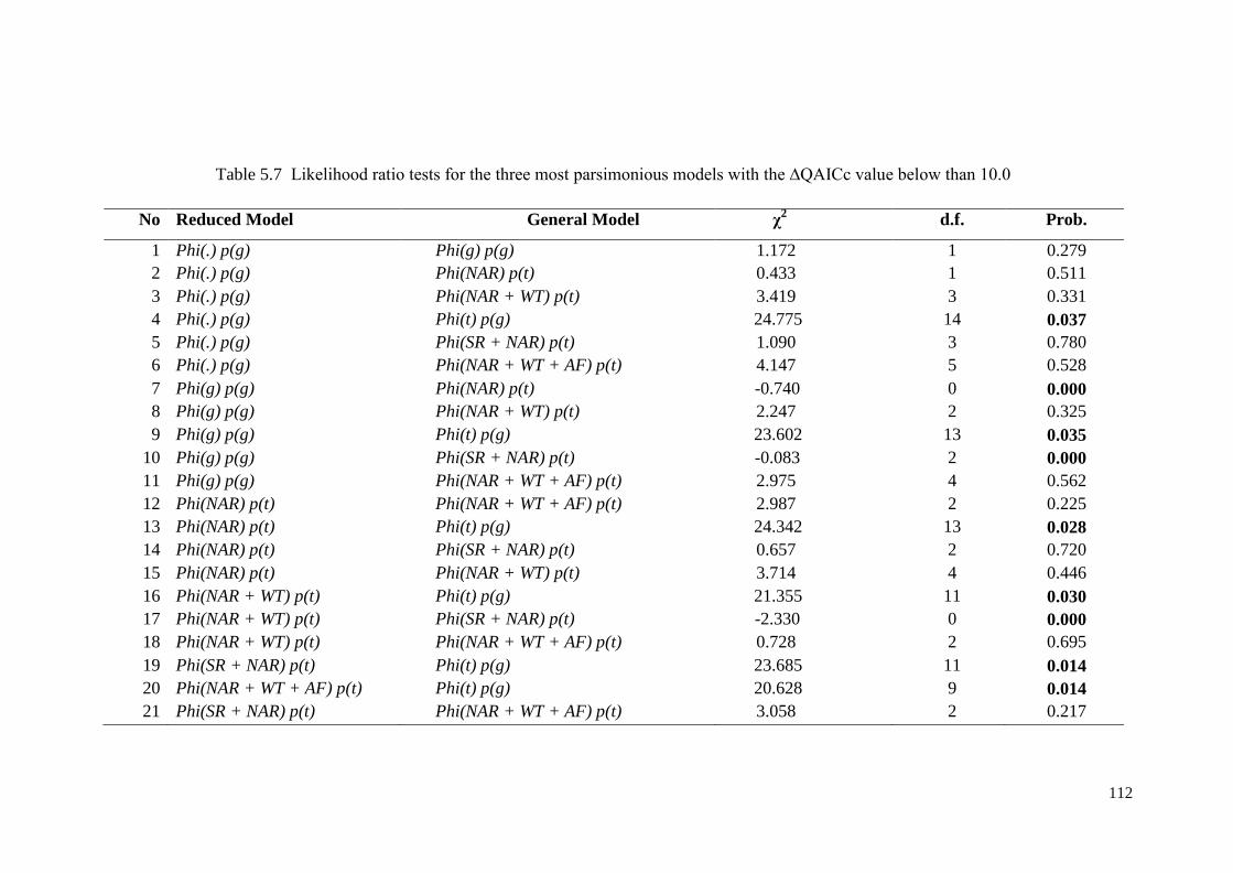
113

Table 5.7 Likelihood ratio tests for the three most parsimonious models with the ∆QAICc value below than 10.0

No Reduced Model General Model χ

2 d.f. Prob.

1 Phi(.) p(g) Phi(g) p(g) 1.172 1 0.279

2 Phi(.) p(g) Phi(NAR) p(t) 0.433 1 0.511

3 Phi(.) p(g) Phi(NAR + WT) p(t) 3.419 3 0.331

4 Phi(.) p(g) Phi(t) p(g) 24.775 14 0.037

5 Phi(.) p(g) Phi(SR + NAR) p(t) 1.090 3 0.780

6 Phi(.) p(g) Phi(NAR + WT + AF) p(t) 4.147 5 0.528

7 Phi(g) p(g) Phi(NAR) p(t) -0.740 0 0.000

8 Phi(g) p(g) Phi(NAR + WT) p(t) 2.247 2 0.325

9 Phi(g) p(g) Phi(t) p(g) 23.602 13 0.035

10 Phi(g) p(g) Phi(SR + NAR) p(t) -0.083 2 0.000

11 Phi(g) p(g) Phi(NAR + WT + AF) p(t) 2.975 4 0.562

12 Phi(NAR) p(t) Phi(NAR + WT + AF) p(t) 2.987 2 0.225

13 Phi(NAR) p(t) Phi(t) p(g) 24.342 13 0.028

14 Phi(NAR) p(t) Phi(SR + NAR) p(t) 0.657 2 0.720

15 Phi(NAR) p(t) Phi(NAR + WT) p(t) 3.714 4 0.446

16 Phi(NAR + WT) p(t) Phi(t) p(g) 21.355 11 0.030

17 Phi(NAR + WT) p(t) Phi(SR + NAR) p(t) -2.330 0 0.000

18 Phi(NAR + WT) p(t) Phi(NAR + WT + AF) p(t) 0.728 2 0.695

19 Phi(SR + NAR) p(t) Phi(t) p(g) 23.685 11 0.014

20 Phi(NAR + WT + AF) p(t) Phi(t) p(g) 20.628 9 0.014

21 Phi(SR + NAR) p(t) Phi(NAR + WT + AF) p(t) 3.058 2 0.217

112

115

Figure 5.4 Inter-year survival rate showing variation over time and variation by

climate where phi = survival, and NAR = normalized non-aquatic period

rainfall

Figure 5.5 Relationship between non-aquatic period rainfall (NAR) and inter-year

survival (r2 = -0.484, p < 0.004, N = 15). Survival estimates are based on

model Phi(NAR)

-0.3

-0.2

-0.1

0

0.1

0.2

0.3

0.4

0.5

0.55

0.6

0.65

0.7

0.75

0.8

0.85

0.9

0.95

No

rmal

ize

d N

AR

Inte

r-ye

ar s

urv

ival

rat

e

Year

phi NAR

0.6

0.65

0.7

0.75

0.8

0.85

0.9

0.95

350 400 450 500 550 600 650 700

Surv

ival

(P

hi)

Non-aquatic rainfall (mm)

113

116

5.3.3 Detectability and Population Estimates

The analysis of the 16-year population trend at the Field Site revealed that overall

detection rate was 0.84 ± 0.07 based on the third ranking model, Phi(.) p(g). Initially,

the detection rate was high in 2001, and then underwent a decline, before a gradual

recovery after 2005 (Figure 5.6). The detection rate fell to its lowest point in 2012

(0.69 ± 0.06). Splitting captures by gender suggested that males (0.915 ± 0.02) had

higher detection rate than females (0.833 ± 0.04). Population estimates were

prepared using the known number of captures by year multiplied by 1/detection rate

for year. Population sizes were generally low in the period 2001-2007, and then grew

thereafter (Figure 5.7).

Figure 5.6 Detection rate by year for the Field Site ponds. Error bars denoted the

standard error

0.5

0.55

0.6

0.65

0.7

0.75

0.8

0.85

0.9

0.95

1

00-01 01-02 02-03 03-04 04-05 05-06 06-07 07-08 08-09 09-10 10-11 11-12 12-13 13-14 14-15

De

tect

ion

rat

e

Year

114

117

Figure 5.7 Population estimates for the total population by year, based on detection

rate and individuals captured by year using model Phi(NAR). Vertical

lines show 95% confidence intervals

5.4 DISCUSSION

It has been shown in this study that there was evidence of variation in detectability

between the sexes. Males demonstrated a higher detection rates than females. This

finding met Assumptions 1 and 2 of the Cormack Jolly-Seber model that animals

have equal chances of both surviving to the next sampling occasion and, if they do,

of then being detected. Analysis of the 16-year population trends reported that the

adult survival was high with the males having higher survival rates than females.

One of the best fitting models suggested that survival was negatively affected by the

non-aquatic season rainfall.

The most likely explanation for lower female detection rates is that females may skip

a breeding season and spend multiple years in the terrestrial habitat between breeding

events. There have been several reported examples of females of closely related

0

10

20

30

40

50

60

70

2001 2002 2003 2004 2005 2006 2007 2008 2009 2010 2011 2012 2013 2014 2015

Esti

mat

ed

po

pu

lati

on

Year

115

118

species skipping a breeding season. Jehle et al. (2005) recorded the behaviour in the

Danube crested newt (Triturus dobrogicus), whilst Arntzen (2002) recorded it in

marbled newts (Triturus mamoratus). Church et al. (2007) found that in tiger

salamanders (Ambystoma tigrinum), <30% of females and <50% of males breed in a

given year. This may account for the detection rates between years, and in particular

the lower return rate in females who need to produce eggs and are thereby subjected

to higher energetic costs. Even in species that breed every year, salamanders may

skip a breeding season when environmental conditions are not favourable (Kinkead

& Otis 2007). The majority of skipped season records in this study occur in 2003

(Sewell 2006), and it is possible that in this year breeding conditions were unsuitable

for this species or conditions prior to the breeding season were unsuitable and

females were unable to mature egg clutches.

One of the other possible explanations for higher detection rates in males is they

have a higher probability of being captured in traps as they arrive early and spent a

longer time in ponds during the breeding season, likely enhancing their chances for

reproductive success (Jehle et al. 2011). In contrast, females in most years were first

caught in weeks 4-5 (mid to late March). Last capture dates were over a similar short

period in most years. Kupfer and Kneitz (2000) showed that males may visit the

pond area on mild nights from the beginning of January and some males do not leave

the breeding ponds until the autumn (Kupfer & Kneitz 2000). That males spent

longer in the breeding ponds than females is unsurprising, and entirely consistent

with other studies such as Hedlund & Robertson (1989), who attributed this

behaviour to the lekking mate selection system of the species. This male-biased sex

ratio operated through the breeding season. Males maximise their breeding chances

by remaining in the pond until there are no more females available, whereas once a

116

119

female has laid her eggs there is no breeding advantage to her in staying.

Population estimates have been based on detection rates and the actual number of

individual crested newts caught in each year. The pond management that occurred in

2006 obviously had positive effects on the newt population (Wright 2009). There

was a trend for numbers to increase after pond management. In 2008 and 2016, the

numbers of new great crested newts captured increased and these new individuals

were assumed to be first time breeders on the basis of their relatively small size.

Great crested newts return to water to breed at 2-3 years old and the influx of new

great crested juveniles in 2008 and 2016 was thought to be due to the high

recruitment levels of 2005 and 2014 when early life stages benefited from a

reduction in predatory species present in the ponds. When the ponds were drained

invertebrate predator species were removed and as a result, recruitment the following

year increased for the species. Therefore the new great crested newts arriving in 2008

were probably from the larval cohort of 2006 having returned to the ponds two years

later to breed. The influx of new great crested juveniles in 2008 was thought to be

due to the high recruitment levels of 2006 when early life stages benefited from a

reduction in predatory species present in the eight ponds.

The mark-recapture analysis of the 16-year population trends revealed that adult

survival at the Field Site was high, 0.83 ± 0.02 with the males having higher survival

rates than females. Cummins and Swan (2000) found a survival rate of 0.85 (not

broken down by sex), a similar rate to that given here, but surveyed in a larger and

deeper pond than those at the Field Site. Arntzen and Teunis (1993) found no

significant difference in survival rates between sexes, whilst other studies using

capture-mark-recapture have suggested annual rates of between 0.50 - 0.78

(Hagstrom 1979; Hedlund 1990; Griffiths et al. 2010). Variation in survival rates

116

117

120

between males and females is clear, since this emerged from the second best model

in the CJS analysis in Mark. From both analyses with and without climatic

covariates, males always have a higher survival rates than females. The difference in

detectability between males and females is also clearly evident from the raw data

which shows a higher capture rate of males when the individuals were 64 against 62.

Grayson et al. (2011) suggest that the majority of males are more likely to remain

near the pond compared to females, to exploit their competitive breeding advantage.

While males tend to remain near the breeding ponds, females generally engage in

searching for food or dispersing and resting in a considerable distance from the

breeding pool. When gravid females are ready to return to the breeding ponds again,

they likely have a reduction in their movement. The high resting metabolic rates and

reduced movement performance of gravid female salamanders compared to males

may have important implications for the reproductive ecology and life history

of salamanders (Finkler et al. 2003). Gravid females usually display a reduction in

movement (Shine 1980; Seigel et al. 1987). Such reductions in performance may be

based on physical hindrance of movements during locomotion (Sinervo et al. 1991),

or physiological changes associated with carrying eggs (Olsson et al. 2000).

This reduction in movement may form a substantial component of the overall cost of

reproduction. Gravid females with reduced movement may be more susceptible to

predation or parasitism (Miles et al. 2000), thus reducing chances of survival to the

next reproductive event. Additionally, gravid females may be less capable of

foraging (Cooper et al. 1990), thus reducing energetic intake that would contribute to

survivorship and future fecundity. These factors may in turn constitute selective

pressures for behavioural and morphological characteristics of females that directly

118

121

or indirectly reduce the cost of reproduction, such as changes in body size or in the

relative size of morphological structures that influence movement performance

(Shine et al. 1998) and alterations in habitat selection, feeding, and defensive

behaviours (Brodie 1989; Cooper et al. 1990; Charland & Gregory 1995).

The third best fitting model, Phi(NAR) suggested that survival was adversely affected

by non-aquatic season rainfall (January-February + June-December), and there was a

strong negative relationship between survival and rainfall. A study near the same site

in 1995-2006 by Griffiths et al. (2010) also demonstrated a variation in survival

between years that was inversely related to rainfall. However, their study also

identified that the low survival is related to the mild winters. In temperate

ectotherms, continuous mild winter may cause depleting energy reserves of

hibernating animals, while them being able to feed, resulting in poor breeding

conditions the following spring (Reading 2007). However, this study suggests that

high winter rainfall had a greater effect than mild winter temperature. In winter, great

crested newts enter a period of low activity which usually begins in late September to

mid-October and most animals are dormant by the end of November. While

hibernating on land, gaseous exchange occurs by pumping air into the lungs as well

as across the skin surface. In waterlogged soils, only gaseous exchange across the

skin may be possible and this may substantially reduce the ability to meet certain

respiratory challenges. Amphibians can suffer mass mortalities from anoxia when

hibernating under waterlogged soils for unusually long periods as explained earlier in

Chapter 4 (Shoemaker et al. 1992). This may be reflected in reduced survival.

Temperature and rainfall are two important climatic factors that are crucial to

amphibian physiology and behaviour because of their part in reproductive migrations

119

122

and gametogenesis (Beebee 1995; Todd & Winne 2006). Consequently mild winters

may also result in reduced survival across the metapopulation (Griffiths et al. 2010).

The present analyses suggest that high winter rainfall had a greater effect than mild

winter temperatures. Globally, according to the Intergovernmental Panel on Climate

Change (IPCC), the upcoming risk of both droughts and floods will increase in a

warmer climate (Kundzewiczet al. 2007). Model predictions for the 2090s imply that

globally, the proportion of the land surface in extreme drought events is projected to

increase by 10 to 30 fold (Burke et al. 2006). At the same time, the episodes of heavy

rainfall will possibly increase over many parts of the world in the 21st century

(Seneviratne et al. 2012). Many amphibians have evolved in hibernation in response

to cold temperatures and as a consequence, enabling survival under adverse

environmental conditions play an important part in their life-history strategy (Wells

2007). However, markedly high temperatures during hibernation may also cause

negative effects due to the increase in metabolic rate (Gilloly et al. 2001).

Consequently, this can result in poor adult body condition after hibernation (Reading

2007), declines in reproductive investment (Jorgensen 1986), and increase in

mortality (Corns & Muths 2002). Furthermore, Parmesan (2007) proposes that

climate warming also make the hibernation period shorter. Shortening in hibernation

period then might influence reproduction as since hibernation has been proposed to

be a required life stage for the maturation of germ cells in some amphibians species

(Brenner 1969). Climate change impacts on ecological aspects also comprise trophic

mismatches (Gao et al. 2015). Shifts in breeding phenology caused by climate

warming may cause temporal mismatches alter trophic relationships within food

webs and affect secondary productivity (Gouveia 2013). Temperature-induced

changes in phenology have driven birds to mislead peaks of food abundance and

120

123

breeding activity (Van Der Jeugd et al. 2009). This situation can directly influence

their individual body condition and population dynamics.

Furthermore, it has been suggested that the shift in rainfall patterns (Duellman &

Trueb 1985) can alter the breeding phenology of amphibian species that reproduce in

ponds. If ponds fill later in the season, then the shorter hydroperiod could lead to an

increase in competition, higher predation rate and, lower survival. Meanwhile

organisms are concentrated in the remaining ponds and they are more vulnerable to

disease transmission and outbreaks. Shifts in breeding phenology of amphibian could

therefore result in complex impacts on populations, altering the structure of

population, and then likely causing declines of susceptible populations (Donnelly &

Crump 1998).

Additionally, climatic changes can influence species distributions, normally through

species-specific physiological thresholds of temperature and rainfall tolerance

(Dervo et al. 2016). Amphibian migration between breeding and hibernation ranges

in spring and autumn is a demanding stage with decreased survival, and potentially

changes in this migration activity as a result of climate change could thus have

implications at a population level. Normally newts initiate their migration in spring at

the end of frost periods with increasing temperatures and when stimulated by rainfall

(Malmgren 2007). Dervo et al. (2016) noted interspecific variation in migration

pattern between the newts L. vulgaris and T. cristatus, as functions of temperature

and rainfall. Rainfall was important for the migration pattern of both species. For L.

vulgaris, numbers of migrators increased at lower temperatures but were dependent

on higher rainfall levels as compared to T. cristatus. This could indicate that L.

vulgaris are dependent on more stable temperatures compared to T. cristatus in order

to sustain high numbers of migrators.

121

124

The observed decline in amphibian populations may directly or indirectly be linked

to climate change as rainfall and temperature are key climate components acting

directly on processes important for the population dynamics for amphibians (Dervo

et al 2016). Predicted changes in survival rate and population size in relation to

global warming concur with other studies of amphibians (e.g., Reading 2007) as well

as species from other taxa such as birds (e.g., Both & Viser 2005). Very few studies,

however, focus on the combined effect of multiple climate components. Given the

strong support for interactive effects of both rainfall and temperature on the survival

of the amphibians here, this study urges that both components should be considered

in future studies of climate effects.

122

125

CHAPTER 6

COMPARISON OF BODY CONDITION INDEX AND THE SURVIVORSHIP

OF THE GREAT CRESTED NEWT IN TWO POPULATIONS

ABSTRACT

Body condition has been related to fitness, and consequently survival of amphibians.

It also may reflect variation in climatic conditions experienced previously. A ‘scaled

mass index’ was used to estimate the body condition index (BCI) of male great

crested newts in two separate populations in Canterbury, Kent. BCI were measured

between 2002 and 2015 for 204 individual from four ponds in Well Court and 63

individuals from the Field Site. Annual survival was estimated from Cormack-Jolly-

Seber capture-mark-recapture (CMR) models with climatic data and BCI as

covariates. Model fit was determined using the quasi-likelihood Akaike Information

Criterion (QAICc). Both study sites showed variation in body condition over the

years. The BCI of each study site for each year was then compared over the 11 year

period when they were monitored simultaneously. Higher body condition in Field

Site ponds may be linked to higher habitat quality compared to the Well Court ponds

that exist in agricultural areas. There was no effect of climatic conditions on the body

condition at either of the populations studied. However, body condition was related

to survival at one of the populations. Further analysis indicates that body condition

was lower in ponds with high densities of newts. Generally, this study suggests that

body condition is related to a local factor – population density, and habitat quality

rather than regional or climatic factors. Agricultural activity may adversely affect the

body condition of amphibians and pose a threat to their conservation.

123

126

6.1 INTRODUCTION

Body condition is defined as the relative size of energy stores (Jakob et al. 1996) and

is assumed to be influenced by health and fitness of animals. Body condition

provides information on the health of an individual and can affect a number of

survival related behaviours (Hoey & McCormick 2004). Body condition is also

important because it may be related to population and habitat quality parameters

(Bancila et al. 2010). The body condition index is proposed as a simple and non-

invasive way to measure an animal’s fitness. Generally, the body condition index

(BCI) is determined by the relationship between body mass and body size, and is

indicative of an animal's health or well-being (Sivan et al. 2014). The old method of

estimating body condition is based on the direct measurement amount of fat deposits,

but this technique is destructive for the studied animals (Blackwell 2002). Other

alternative methods suggested such as total body electrical conductivity operating for

estimating lipid and lean body mass in mammals and small birds have not proved

very reliable (Bancila et al. 2010).

Considering that many species are fully protected by law, and many amphibian

populations are declining (Stuart et al. 2004), non-destructive techniques are required

to estimate body condition. Body condition indices (BCI) based on allometric

relationships between length and body mass has been introduced as an alternative to

the direct measurement of destructive techniques. Most commonly used body

condition indices are several proportions between a linear measure of body size and

body mass indices (BSI), or the use of residuals from a linear regression of body

mass against BSI (Green 2001). Amphibians are very responsive to environmental

quality and its change because of their complex life cycle that involves aquatic and

124

127

terrestrial life stages (Bancila et al. 2010). Evaluating the body condition of

amphibian populations is one of the options to test their responses to environmental

stress. Body condition indices may indicate past foraging success, fighting ability,

and the capacity to cope with environmental pressures, which may impact on

reproductive success (Jakob & Marshall 1996).

Body condition and the climatic factors affecting it have gained much research

interest recently, especially in the context of changing climate and its impact on

amphibian populations (Reading 2007). According to Tomasevic et al. (2007), body

condition is a crucial parameter related to survival and reproductive success. In

temperate zone amphibians, body reserves are depleted during hibernation and

breeding, and replenished during the following active period (Reading & Clarke

1995). Thus, inter-annual differences in body condition may reflect variation in

climatic conditions experienced during the previous year, during hibernation, or

immediately after emerging from hibernation (Tomasevic et al. 2007). Reading and

Clarke (1995) found that change in body condition of female (Bufo bufo) was

significantly correlated with temperature variation over an 11-year period. In a still

longer-term study (23 years), Reading (2007) demonstrated clear relationships

between increase in mean temperature, body condition decline, and decrease in

fecundity. This may be because individuals use up more body fat reserves at higher

temperatures due to increased metabolism (Reading 2007). This may result in

increased susceptibility to disease, lower reproductive success, and subsequent

population decline (Jarvis 2015).

Although several great crested newt population studies have been conducted (e.g.

Baker 1999, Williams 1999, Jarvis 2010), few have examined factors affecting body

125

128

condition indices and how this may impact population size (but see Jarvis 2015).

Jarvis (2015) found that BCI varied significantly between years but there was no

significant relationship between BCI scores and mean winter minimum air

temperature. In the present study, the ‘scaled mass index’ (Peig & Green 2009, 2010)

was used to estimate the body condition in two populations of the great crested newt.

This study was based on a set of body length and body mass data collected from four

sub-populations at Well Court (see Chapter 4) and a population at the Field Site (see

Chapter 3).

The main aim of the present study is to examine the inter-annual post-hibernation

body condition in male great crested newts from two study sites, and investigate the

relationships between body condition and climatic conditions. In particular, this

study tests the hypotheses that: (1) body condition varies between years and

populations; (2) body condition is related to climatic factors; and (3) annual survival

is linked to body condition.


6.2.1 Study Site

Two pond localities were the subjects of intensive investigation, and these are

described separately within this chapter. The first of these groups was situated on

Well Court Farm, and consisted of four pond systems (Garden ponds, Snake pond,

Swimming pool and Pylon pond) where population studies were carried out over the

period 2002-2013. The second group, known as the Field Site was situated on the

north-west of the University of Kent Canterbury campus, and consisted of eight

small ponds, supporting a small great crested newt population, where detailed

126

129

individual morphometric and capture histories have been available since 2003.

Details of the Well Court and Field Site study sites were described in Chapter 2,

Chapter 4 and Chapter 5.

6.2.2 Materials and Methods

Annually, since 1995 for Well Court, and from 2003 for the Field Site, great crested

newts arriving to breed at the study ponds have been captured and marked to denote

the month and year of capture using a capture-mark-recapture method as described in

Chapters 3 and 4. Captured male and female great crested newts were measured for

snout-vent-length (SVL) and body mass (Ms). Body mass was recorded to the

nearest 0.1 g and snout-vent length (SVL) was measured to 1 mm precision.

Juveniles were excluded from this analysis because of uncertainty in tracking

individuals through different age categories (see Chapters 3 and 4). A compact

digital camera was used to take photographs of belly pattern markings to identify

individuals. Once all measurements and data had been collected, all newts were

released into the pond of capture.

As the species breeds over an extended period, and female body mass varies with the

numbers of eggs laid, it was decided that an analysis of body condition index (BCI)

would be using only males (Verrell & Halliday 1985). To avoid pseudo-replication

(Luiselli et al. 2007), an average of SVL and mass of each individual during the peak

seasons (March-May) every year was included once in the BCI calculation. SVL and

mass for each individual were log transformed to normalise the data before BCI

calculation were conducted. Different body condition indices (BCI) are available

(Kuhn 1994; Jakob et al. 1996; Green 2001; Reyer & Battig 2004). However, there is

debate as to which method is most suitable (Smith 2009).

127

130

One popular BCI is the residual from an ordinary least squares (OLS) regression of

body mass (Y variable) against body size (X variable) (Jakob et al. 1996). However,

Schulte-Hostedde et al. (2005) demonstrated that OLS residuals of mass on body size

normally showed higher correlations with the absolute size of fat stores (in g) than

residuals from an alternative regression technique (standardized major axis [SMA]

regression). OLS residuals were also highly correlated with absolute values of lean

dry mass (largely protein), and both results have been interpreted as BCIs (Schulte-

Hostedde et al. 2005). However, Peig and Green (2009) question this reasoning

because the absolute mass of fat or any other body component is not the most

appropriate measure of ‘true body condition’ since it does not control for body size

(a vital requirement for a BCI).

The SMA regression between body mass ‘M’ and a length measure ‘L’ is proposed

because according to Warton et al. (2006):

(i) natural variability due to growth affects both size variables (M and L)

within the structural relationship (i.e. both are indicators of body size);

(ii) M and L variables are not measured on comparable scales, thus the

magnitude of natural variability and measurement error may vary between

variables (a reason for preferring SMA to MA);

(iii) individuals have been randomly sampled, and the observed pairs of M-L

data may deviate from the underlying true association between them;

(iv) the measurement error in L is unlikely to be negligible and may even be

higher than that in M (Green 2001); and

(v) the aim of the regression is not to predict the value M of an unsampled

individual given its L value, but to estimate the scaling exponent between

128

131

two interdependent variables (Fairbairn 1997).

As an alternative, Peig and Green (2009) introduced the scaled mass index (SMI)

that accounts for the allometric relationship between mass and a body structure

measure and standardizes each measure so that direct comparisons among studies can

be made. This method has been shown to be a better predictor of variations in fat and

protein reserves than the ordinary least squares (OLS) residual method as well as five

other methods (Peig & Green 2009, 2010). According to Peig and Green (2010),

large and small individuals distribute resources differently. The proportion of stored

energy therefore changes depending on the size of the animal so scaling is required

to make meaningful comparisons. Hence, the scaling relationship between different

size measures and components must be taken into account in order to produce a

reliable BCI. The SMI standardizes body mass to a specific fixed value of a linear

body measurement based on the scaling relationship between body mass and length.

This allows for direct comparisons of body mass without the confounding effects of

body size according to the equation (Peig & Green 2009):

Scaled mass index: Ḿi = Mi [L0 /L i] bSMA

Where,

Mi and Li = body mass and the linear body measurement of individual

i, respectively,

bSMA = scaling exponent estimated by the standardised major axis

(SMA) regression of M on L,

L0 = arbitrary value of L (e.g. the arithmetic mean value for

the study population) and,

Ḿi = predicted body mass for individual i when the linear body

measure is standardized to L0.

129

132

Body condition indices (BCI) were calculated for 204 individual male newts

captured from four ponds in March and April 2002 - 2013 in Well Court and 63

individuals from the Field Site (2003-2015). A two-way analysis of variance

(ANOVA) was performed in Minitab to determine whether there was a difference in

BCI between year and pond. Linear regression was used to determine whether there

was a relationship between climatic variables, inter-year survival rate and population

size with the BCI of males the following spring. Annual male survival was estimated

from Cormack–Jolly–Seber (CJS) capture-mark-recapture (CMR) models using the

software MARK (White & Burnham 1999). The details of the CMR analysis are

provided in Chapters 3 and 4. In each of the remaining models, annual BCI’s were

included as covariates and additional to this, climatic covariates in the year

preceding that of the BCI measurements (non-aquatic rainfall, spring rainfall, winter

minimum temperature, and number of days of frost) that potentially affect male body

condition in this study were included as additive effects.

The estimated male population for each year was calculated by multiplying the

number of individuals caught in each pond by 1/detection probability for that pond

(Griffiths et al. 2010). The size of the Well Court metapopulation was calculated by

adding together the populations of the component ponds.

130

133

6.3 RESULTS

6.3.1 Well Court Metapopulation

Body size

A total of 204 male individual adults from 497 captured were recorded in the period

2002 to 2013 from four ponds, excluding the recaptures of the same individual each

year (Figure 6.1). Figure 6.2 demonstrates the mean of annual SVL and body mass of

males that were captured between 2002 and 2013. The SVL average among males

was 71.53 ± 0.29 mm and the body mass mean was 9.44 ± 0.11 g. The intraspecific

regressions of male ln Mass on ln SVL took the form of: ln Mass = 2.13 (± 0.048) ln

SVL – 6.90 (± 0.204); R2 = 0.56, P < 0.001 (Figure 6.3).

140

120

100

80

60

40

20

0

Garden pond Snake pond Swimming pool Pylon pond

Pond

Figure 6.1 Number of adult males captured at each pond in 2002-2013

Nu

mb

er o

f n

ewt

130 131

134

Mass SVL

12 76

74 10

72

8 70

6 68

66 4

64

2 62

0 60

2002 2003 2004 2005 2006 2007 2008 2009 2010 2011 2012 2013

Year

Figure 6.2 Well Court annual March and April average of mass (g) and snout vent

length (SVL) for males. Error bars denote standard error

Figure 6.3 The intraspecific allometric regression of ln body mass (m; g) on ln snout-

vent length (SVL; mm) in male newts at Well Court

0

0.5

1

1.5

2

2.5

3

3.5

3.4 3.6 3.8 4 4.2 4.4 4.6

ln B

od

y m

ass

(g)

ln SVL (mm)

Bo

dy

mas

s (g

)

SVL

(mm

)

132

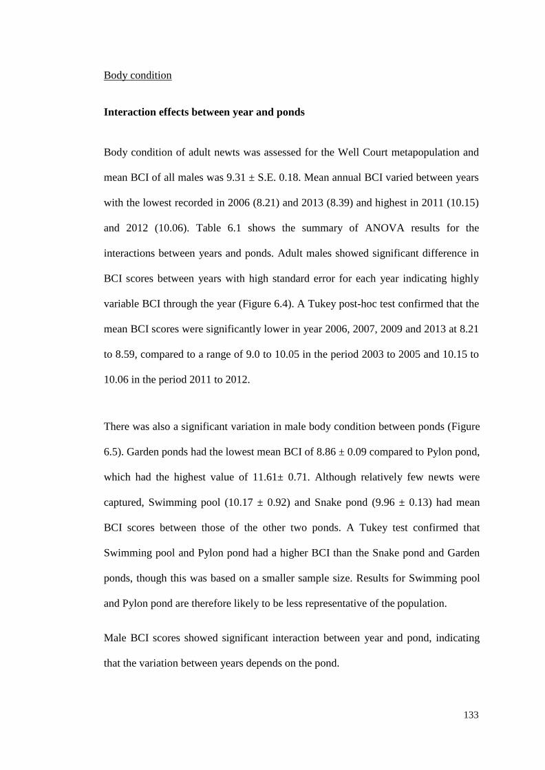
135

Body condition

Interaction effects between year and ponds

Body condition of adult newts was assessed for the Well Court metapopulation and

mean BCI of all males was 9.31 ± S.E. 0.18. Mean annual BCI varied between years

with the lowest recorded in 2006 (8.21) and 2013 (8.39) and highest in 2011 (10.15)

and 2012 (10.06). Table 6.1 shows the summary of ANOVA results for the

interactions between years and ponds. Adult males showed significant difference in

BCI scores between years with high standard error for each year indicating highly

variable BCI through the year (Figure 6.4). A Tukey post-hoc test confirmed that the

mean BCI scores were significantly lower in year 2006, 2007, 2009 and 2013 at 8.21

to 8.59, compared to a range of 9.0 to 10.05 in the period 2003 to 2005 and 10.15 to

10.06 in the period 2011 to 2012.

There was also a significant variation in male body condition between ponds (Figure

6.5). Garden ponds had the lowest mean BCI of 8.86 ± 0.09 compared to Pylon pond,

which had the highest value of 11.61± 0.71. Although relatively few newts were

captured, Swimming pool (10.17 ± 0.92) and Snake pond (9.96 ± 0.13) had mean

BCI scores between those of the other two ponds. A Tukey test confirmed that

Swimming pool and Pylon pond had a higher BCI than the Snake pond and Garden

ponds, though this was based on a smaller sample size. Results for Swimming pool

and Pylon pond are therefore likely to be less representative of the population.

Male BCI scores showed significant interaction between year and pond, indicating

that the variation between years depends on the pond.

133

136

Table 6.1 Summary of results of analysis of variance using a two-way ANOVA,

showing how body condition index of male great crested newts was

affected by the factors of pond and year of sampling

Sum of

squares

Mean

square

F

d.f.N

d.f.D

P

Year 44.707 10.14 4.53 11 193 0.0001

Pond 80.304 39.71 17.74 3 201 0.0001

Year x Pond 415.563 4.57 2.04 15 148 0.001

Figure 6.4 Mean of body condition index (BCI) of adult males in each study year,

2002–2013 at the Well Court. Error bars denote standard error

134

137

Figure 6.5 Mean of body condition index (BCI) of adult males in each study pond at

Well Court over the period 2002-2013. Error bars denote standard error

Effects of body conditions on survival

The male recapture data (2002–2013) were over-dispersed and the c-hat value was

adjusted to 1.52. The ΔQAICc weight values derived for each of the models showed

that the Phi(t) model fitted the data best (Table 6.2). The model with male BCI as a

covariate fitted the data second best, and following Burnham and Anderson (2002),

this model indicated less support (ΔQAICc 3-7). There were three remaining models

with ΔQAICc values within 3-7 which were Phi(MaleBCI+NAR), Phi(Male

BCI+SR) and, Phi(Male BCI+WT). There was no significant relationship between

male BCI scores and non-aquatic rainfall (BCI= 0.0014 NAR + 8.4301; R2 = 0.0178,

N = 7, P = 0.775), spring rainfall (BCI= -0.0007 SR + 9.2682; R2 = 0.0078, N = 7,

P= 0.851), or mean minimum winter temperature (BCI= -0.0532 WT + 9.2955; R2 =

135

138

0.0088, N = 7, P = 0.841). Therefore, body condition in spring was not affected by

climatic variables over the previous months. A regression analysis of survival using

model Phi(Male BCI) p(t) against male BCI (survival = 0.055 Male BCI + 0.1135

BCI, P = 0.679, R2 = 0.037; N = 7) showed that there was no relationship between

male BCI and survival.

136

Table 6.2 Model selection based on ΔQAICc values with the c-hat corrected as 1.52. Phi = survival, p = detection rate, t = time, (.) = constant,

and BCI = body condition index. Climatic variable; NAR = non-aquatic rainfall, SR = spring rainfall, and WT = winter temperature.

NP = number of parameters, and QAICc = quasi Akaike information criteria

Model QAICc ΔQAICc AICc

Model NP

QDeviance Weights Likelihood

Phi(t) p(t) 599.7267 0.0000 0.56556 1.0000 13 104.0596

Phi(BCI) p(t) 604.2161 4.4894 0.05993 0.1060 2 131.2679

Phi(BCI+NAR) p(t) 605.2667 5.5400 0.03544 0.0627 3 130.2945

Phi(BCI+SR) p(t) 605.7792 6.0525 0.02743 0.0485 3 130.8070

Phi(BCI+WT) p(t) 606.1014 6.3747 0.02335 0.0413 3 131.1292

Phi(.) p(t) 606.1189 6.3922 0.02314 0.0409 8 120.9037

Phi(t) p(.) 606.639 6.9123 0.01784 0.0315 8 121.4239

Phi(BCI+WT+NAR) p(t) 606.8292 7.1025 0.01623 0.0287 4 129.8248

Phi(BCI+NAR+SR) p(t) 607.2683 7.5416 0.01303 0.0230 4 130.2639

139 137

140

6.3.2 Field Site Population

Body size

A total number of 63 adult male great crested newts from 243 captures were

identified in the Field Site from 2003-2015. The highest number of new individuals

were recorded in 2013 (n = 28), followed by 2015 (n = 26) and 2014 (n=24). Figure

6.6 demonstrates the mean of annual SVL and body mass of males that were captured

between 2003 and 2015. The SVL average among adult males was74.95 ± S.E. 0.22

g and the body mass was 11.53 ± S.E. 0.09 g. The intraspecific regressions of male ln

Mass on ln SVL took the form of: ln Mass = 1.91 (± 0.061) ln SVL – 5.85 (± 0.261);

R2 = 0.56, P < 0.0001 (Figure 6.7).

Figure 6.6 Field Site annual March and April average of mass (g) and snout vent

length (SVL) for males. Error bars denote standard error

-5

0

5

10

15

20

25

30

35

2003 2004 2005 2006 2007 2008 2009 2010 2011 2012 2013 2014 2015

Nu

mb

er o

f in

div

idu

als

Year

Adult male

New adult male

138

141

Figure 6.7 The intraspecific allometric regression of ln body mass (m; g) on ln

snout-vent length (SVL; mm) in male newts at the Field Site. Error

bars denote standard error

Body condition

Differences in body condition between years

A one-way ANOVA was conducted that examined the effect of year on the Field Site

BCI. There was a significant difference between the annual BCI between years (F12,

232 = 9.123, P < 0.0001). The BCI scores fluctuated over the years with the highest

BCI scores in 2007 and the lowest in 2014 (Figure 6.8). The mean of the BCI scores

for thirteen years were 11.61 ± 0.18. A Tukey post-hoc ANOVA revealed a

significant difference in BCI scores between the years 2003 to 2007 and 2008 to

2015 (P < 0.001).

62

64

66

68

70

72

74

76

78

80

82

0

2

4

6

8

10

12

14

16

2003 2004 2005 2006 2007 2008 2009 2010 2011 2012 2013 2014 2015

SVL

(mm

)

Mas

s (g

)

Year

Mass SVL

139

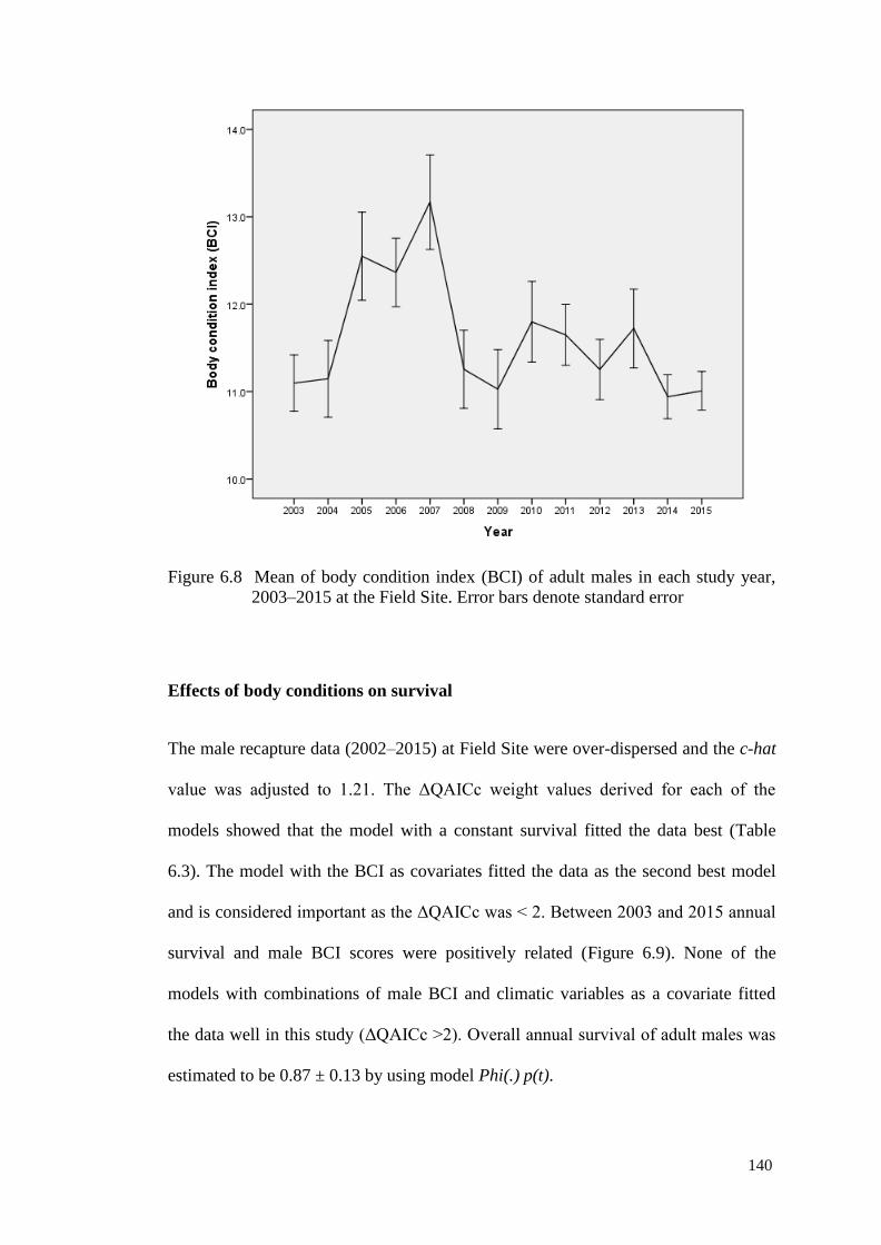
142

Figure 6.8 Mean of body condition index (BCI) of adult males in each study year,

2003–2015 at the Field Site. Error bars denote standard error

Effects of body conditions on survival

The male recapture data (2002–2015) at Field Site were over-dispersed and the c-hat

value was adjusted to 1.21. The ΔQAICc weight values derived for each of the

models showed that the model with a constant survival fitted the data best (Table

6.3). The model with the BCI as covariates fitted the data as the second best model

and is considered important as the ΔQAICc was < 2. Between 2003 and 2015 annual

survival and male BCI scores were positively related (Figure 6.9). None of the

models with combinations of male BCI and climatic variables as a covariate fitted

the data well in this study (ΔQAICc >2). Overall annual survival of adult males was

estimated to be 0.87 ± 0.13 by using model Phi(.) p(t).

140

Table 6.3 Model selection based on ΔQAICc values with the c-hat corrected as 1.21. Phi = survival, p = detection rate, t = time, (.) = constant,

and BCI = body condition index. Climatic variable; NAR = non-aquatic rainfall, SR = spring rainfall, and WT = winter temperature. NP

= number of parameters, and QAICc = quasi Akaike information criteria

Model

QAICc

ΔQAICc AICc

Weights Model

Likelihood

NP

QDeviance

Phi(.) p(.) 190.681 0.000 0.236 1.000 2 85.224

Phi(BCI) p(t) 192.322 1.641 0.104 0.440 2 86.865

Phi(BCI + WT) p(t) 192.790 2.109 0.082 0.348 3 85.273

Phi(BCI + NAR) p(t) 193.558 2.877 0.056 0.237 3 86.041

Phi( BCI + NAR + WT) p(t) 194.576 3.896 0.034 0.143 4 84.979

Phi( BCI +NAR + SR) p(t) 195.002 4.321 0.027 0.115 4 85.404

Phi(t) p(.) 207.652 16.972 0.000 0.000 14 76.044

Phi(.) p(t) 209.383 18.702 0.000 0.000 14 77.775

Phi(t) p(t) 226.660 35.979 0.000 0.000 25 68.000

144 141

144

Figure 6.9 Relationship between annual male survival, and body condition index

(BCI) in the previous year between 2003 and 2015 at the Field Site. The

fitted line was derived from a regression of survival male against BCI (F

= 19.03, R2 = 0.634, N = 13, P < 0.001)

6.3.3 Interaction Effects of Pond and Year

BCI scores of male newts at the Well Court metapopulation and Field Site population

were compared from 2003 till 2013, the years when both sites were monitored. A

two-way ANOVA was conducted that examined the effect of pond and year on BCI

scores. Male BCI scores did vary significantly between ponds (F1, 739 = 6.85, P <

0.0001). Male BCI scores also showed significant differences across year and pond

(F10, 739 = 11.92, P < 0.002), suggesting that variation between years depends on BCI

scores between ponds. The pattern of mean BCI scores was different to that exhibited

by males from each pond. Males at the Field Site had a significantly higher BCI

compared to the males at Well Court over the years (F10, 739 = 4.59, P < 0.0001)

(Figure 6.10). The BCI scores of Well Court and Field Site were not significantly

0.862

0.864

0.866

0.868

0.870

0.872

0.874

0.876

10.5 11 11.5 12 12.5 13

Surv

ival

rat

e (

Ph

i)

Body condition index (BCI)

142

145

correlated although there appeared to be a slight negative relationship (r = -0.519, n =

11, p = 0.102).

Figure 6.10 Comparison of male mean annual BCI scores at the Well Court

metapopulation, and Field Site population. Errors bars denote the 95%

confidence intervals

6.3.4 Interaction between Population and Body Condition

At Well Court, there was a non-significant relationship between male metapopulation

sizes with the mean annual BCI. However, an analysis just based on male

subpopulations at the Garden ponds indicated that the mean BCI increased as

population decreased (Figure 6.11). A regression analysis confirmed that there was a

negative significant relationship between male population size and the annual mean

BCI at the Garden ponds (Figure 6.12). In general, the trend at the Field Site was

143

146

towards an increase in number of adults after 2008. Male numbers at the Field Site

ponds doubled after the addition of the new four ponds in 2008 (Figure 6.13). There

was a negative significant relationship between male population size and BCI for the

Field Site ponds (Figure 6.14). This finding suggests that male population size may

explain BCI for the Field Site ponds and for the highest density subpopulation at

Well Court. BCI at the Well Court ponds were only affected by male subpopulation

at the Garden ponds over the duration of the study.

Figure 6.11 Population estimates for the Garden ponds population at Well Court by

year, based on detection rate using model Phi(t) p(t)

0

5

10

15

20

25

30

35

40

45

7.5

8

8.5

9

9.5

10

2002 2003 2004 2005 2006 2007 2008 2009 2010 2011 2012 2013P

op

ula

tio

n e

stim

ate

Bo

dy

con

dit

ion

ind

ex

(BC

I)

Year

BCI Male population

144

147

Figure 6.12 Linear regression analysis of body condition index (BCI) against male

population size for Garden ponds at Well Court (F = 8.36, R2 = 0.456,

N = 12, P < 0.016)

Figure 6.13 Population estimates for the Field Site population by year, based

on detection rate using model Phi(BCI) p(t)

8

8.2

8.4

8.6

8.8

9

9.2

9.4

9.6

9.8

20 25 30 35 40 45

Bo

dy

con

dit

ion

ind

ex

(BC

I)

Population estimate

5

10

15

20

25

30

35

7

8

9

10

11

12

13

14

2003 2004 2005 2006 2007 2008 2009 2010 2011 2012 2013 2014 2015

Po

pu

lati

on

est

imat

e

Bo

dy

con

dit

ion

ind

ex (

BC

I)

Year

BCI Male population

145

148

Figure 6.14 Linear regression analysis of body condition index (BCI) against male

population for Field Site ponds (F = 12.47, R2 = 0.305, N = 13, P <

0.046)

6.4 DISCUSSION

Both males at the Well Court and Field Site showed differences in body condition

over the years. Other studies of amphibians have shown that body condition can vary

over time (e.g. Wheeler et al. 2003; Bancila et al. 2010; Jarvis 2015) but few have

documented the effects of climatic variables on body condition. This study revealed

that there was no clear relationship between body condition of male crested newts

and the climatic variations since 2002. However, the relationship

between body condition with subsequent survival and population density of male

newts was strong at the Field Site. Annual survival at the Well Court was found not

to be influenced by body condition over the years and metapopulation density was

not affecting the body condition here. Male newts from the Field Site population

demonstrated a higher body condition compared to the metapopulation at the Well

10

10.5

11

11.5

12

12.5

13

13.5

0 5 10 15 20 25 30 35

Bo

dy

con

dit

ion

ind

ex (

BC

I)

Population estimate

146

149

Court.

Higher body condition in Field Site ponds was generally related to higher habitat

quality compared to the Well Court ponds that exist in agricultural areas. The results

of this study suggest that habitat attributes rather than climate may influence body

condition because none of the models provided good fits with climatic variables at

either site. This is supported by the fact that body condition differed between the two

study sites and showed different patterns over an 11 year period when they were

monitored simultaneously: this implies that local rather than regional factors are

driving the patterns observed. An increase in foraging activity in good surrounding

terrestrial habitat may lead to greater opportunities for the newts to feed and result in

a higher body condition. Body condition in amphibians during early spring is

remarkably associated with food intake during the preceding autumn (Sztatecsny &

Schabetsberger 2005). Body condition in this study probably depended on resource

intake during the terrestrial phase because newts were measured at the beginning of

the breeding season (March-April). However, both terrestrial and aquatic feeding

habitats need to be considered because newts do appear to take prey on arrival in the

aquatic environment (Griffiths & Mylotte 1987).

According to Johnson (2007), body condition is one potentially useful index

assessing habitat quality and its effects on individuals. Body condition may be a

reflection of access to resources; individuals with abundant resources are expected to

be in better condition than those occupying poor habitat. Janin et al. (2011)

demonstrated that reduced body condition in common toad (Bufo bufo) populations

was associated with decreased habitat suitability resulting from fragmentation.

Similarly, Sztatecsny and Schabetsberger (2005) found that body condition of the

common toad varied between sites and this was related to variation in habitat

147

150

conditions that determine resource availability. Karraker and Welsh (2006) reported

pronounced impacts of habitat degradation and loss on salamander body condition.

According to Pope and Matthews (2002), the body condition of an animal mainly

reflects food uptake in the previous year and is assumed to be indicative of habitat

quality.

Well Court ponds exist in an agricultural area where food may be limited.

Agricultural practices may affect the environment by reducing food availability of

newts. These changes can limit the resource uptake of newts, reducing their body

mass, which is reflected in a decrease in body condition (Brodeur et al. 2011; Zaya et

al. 2011; Wagner et al. 2014). From previous studies, it is apparent that the majority

of newts capture food prior to entering the hibernation period (e.g. Bogdan et al.

2011; Dimancea et al. 2011). Kuzmin (1995) lists earthworms, insects and their

larvae, and slugs as their main prey on land. In agricultural areas, glyphosate is

regularly applied as broad-spectrum systemic herbicide and crop desiccant. Verrell

and Van Buskirk (2004) found that earthworms avoid soils contaminated by a

glyphosate-based herbicide.

Higher body condition in newts from the Field Site ponds may also be related to the

shorter distance of newts moving from the terrestrial sites to the breeding ponds after

the winter hibernation. Newts that travel a shorter distance might utilize minimal

body reserves compare to the newts that travel longer distance. The terrestrial habitat

in the close vicinity of the Field Site ponds (< 200 m) usually consists of scrub, long

grass and woodland area and offers plenty of hiding places in the form of logs and

stones. It is noted that the habitats at this site changed little over the course of this

study. The newts might use logs, old stumps and piles of old leaves surrounding the

Field Site as these provide damp refugia during winter (Verrell 1985). A terrestrial

148

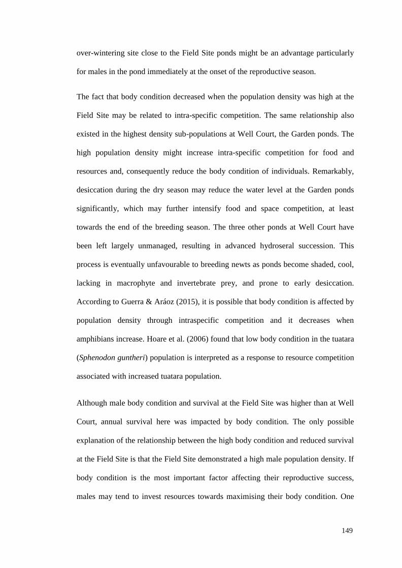
151

over-wintering site close to the Field Site ponds might be an advantage particularly

for males in the pond immediately at the onset of the reproductive season.

The fact that body condition decreased when the population density was high at the

Field Site may be related to intra-specific competition. The same relationship also

existed in the highest density sub-populations at Well Court, the Garden ponds. The

high population density might increase intra-specific competition for food and

resources and, consequently reduce the body condition of individuals. Remarkably,

desiccation during the dry season may reduce the water level at the Garden ponds

significantly, which may further intensify food and space competition, at least

towards the end of the breeding season. The three other ponds at Well Court have

been left largely unmanaged, resulting in advanced hydroseral succession. This

process is eventually unfavourable to breeding newts as ponds become shaded, cool,

lacking in macrophyte and invertebrate prey, and prone to early desiccation.

According to Guerra & Aráoz (2015), it is possible that body condition is affected by

population density through intraspecific competition and it decreases when

amphibians increase. Hoare et al. (2006) found that low body condition in the tuatara

(Sphenodon guntheri) population is interpreted as a response to resource competition

associated with increased tuatara population.

Although male body condition and survival at the Field Site was higher than at Well

Court, annual survival here was impacted by body condition. The only possible

explanation of the relationship between the high body condition and reduced survival

at the Field Site is that the Field Site demonstrated a high male population density. If

body condition is the most important factor affecting their reproductive success,

males may tend to invest resources towards maximising their body condition. One

149

152

generally accepted assumption is that an increase in animal fitness is countered by a

decrease in another life trait (Roff 1992).

On the contrary, Reading (2007) in his study of a common toad population showed

that survival and body condition were positively related, with both variables

declining in relation to increasing temperatures over a 27 year period. Abiotic factors

(climate) may be only affecting the body condition of newts without any relationship

with the inter-year survival rates. In the current study, climatic factors were not

strong covariates of body condition at either Well Court or the Field Site. Catlin et al.

(2014) found that body condition index does predict survival of pipping plover

shorebird (Charadrius melodus) during particularly challenging times. For example,

mass adjusted for structural body size predicted the survival of Florida scrub jays

(Aphelocoma coerulescens) through a disease epidemic (Wilcoxen et al. 2010) and

body condition predicted the survival of wintering Great tits (Parus major) when

they were food limited (Gosler 1996). Also, stress physiology predicted the survival

of marine iguanas during a starvation event (Romero & Wikelski 2010). During this

period of study, such notable selective events were not observed at the Field Site.

However, Chapter 4 in this thesis has explained how the non-aquatic rainfall together

with the spring rainfall affected the survival of newts at Well Court. Griffiths et al.

(2010) in their study at Well Court between 1995 and 2006 confirmed that non-

aquatic rainfall and winter minimum temperature impacted adult survival here.

Although climatic conditions affected survival, this was not strongly reflected in

body condition, suggesting that environmental conditions are not always ideal and

that some years may indeed be challenging. Yet body condition indices failed to

predict survival even during these years at the Well Court. Thus, the climatic

150

153

conditions prior to the breeding season at this study site may be important for

survival but not strong enough to impact the body condition of newts.

With respect to winter conditions, it appears that minimum winter temperatures and

non-aquatic rainfall had a very weak impact on survival and body condition at the

Field Site. Previous studies on amphibian populations suggest that mean winter

temperatures have an effect on survival (Anholt et al. 2003; Araujo et al. 2006) with

varying effects depending on location and species ecology. Several studies

demonstrate a negative relationship between mean winter temperature and body

condition the following spring. For example, Bancila et al. (2010) found that yellow-

bellied toads (Bombina variegata) emerged from winter hibernation in higher body

condition after colder winters. Earlier work by Reading and Clarke (1995) suggested

that a mild winter and warm pre-spawning period had a negative effect on the body

condition of hibernating anurans, through an elevated metabolic rate and the increase

in energy reserve utilization. Thus, amphibians are more likely to emerge from

hibernation in good condition after colder winters.

Apart from the colder winter, longer summers may increase body condition, because

newts have more time to forage, grow and fatten up for the winter. Alternatively, hot

dry summers may have negative impacts compared to hot wet summers (Reading &

Clarke 1995). Amphibians in such circumstances are likely to enter hibernation in

poor condition since high temperatures combined with low humidity increase the risk

of desiccation, affecting their foraging and thus the rebuilding of body reserves

(Tomasevic et al. 2007). The extreme environment may also result in catastrophic

mortality of adult newts. However, this factor could not be the main reason in this

study because survival rates do not suggest any catastrophic mortality.

151

154

In conclusion, the present study suggests that body condition is related to local rather

than regional or climatic factors. The local factor here - population density - had a

close relationship with body condition at both of the study sites. The study also

indicates a close relationship between survival and body condition of newts on

emergence from hibernation at the Field Site. Agricultural activity may be one of the

factors that negatively influence the body conditions of newts and might represent an

ongoing threat for its conservation.

152

155

CHAPTER 7

GENERAL DISCUSSION

7.1 POPULATION GROWTH AND REGULATION

The unprecedented long-term data of capture history and environmental variables on

multiple study sites (Well Court and Field Site) enable this study to understand the

relationship between local and regional factors on the population growth and

regulations of the great crested newts. In conclusion, the persistence of the two

populations relies on a combination of (1) local, population-specific factors - such as

population density and pond desiccation, and (2) regional factors, such as climate

that affect recruitment and survival from each pond. Firstly, this study is concerned

with the impact of local-specific demographic rates on population regulation of

newts at the Well Court metapopulation. Here, a small fraction of the individuals

may occasionally occur in ‘sink’ ponds, where within-pond reproduction is

insufficient to balance local mortality. Nevertheless, populations may persist in such

ponds, being locally maintained by continued immigration from a more-productive

‘source’ pond nearby.

Survival of adult great crested newts at Well Court differed between years, but there

was no variation in survival between subpopulations. Thus, asynchrony between

subpopulations in their dynamics was more likely due to variation in juvenile

dispersal and recruitment than variation in adult survival or dispersal. With only ca.

2% of adults moving between ponds, adult dispersal was too low to even out local

population densities or synchronise their trends. Fluctuations in adult population

153

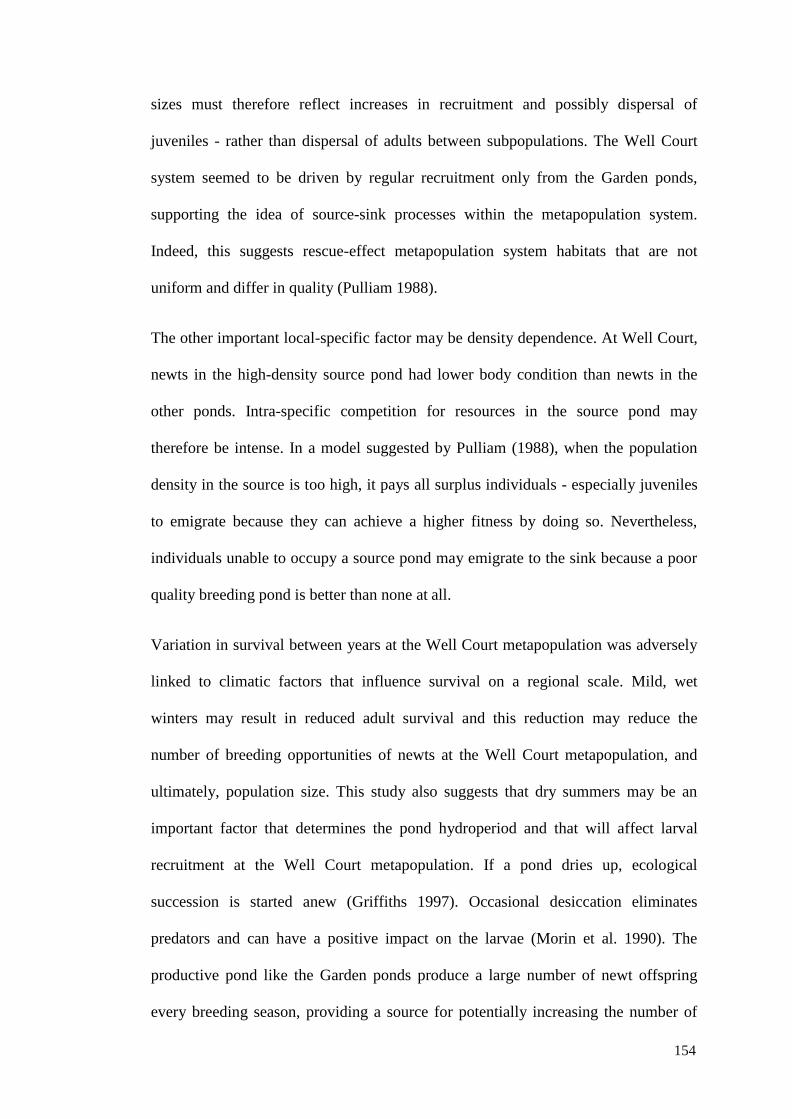
156

sizes must therefore reflect increases in recruitment and possibly dispersal of

juveniles - rather than dispersal of adults between subpopulations. The Well Court

system seemed to be driven by regular recruitment only from the Garden ponds,

supporting the idea of source-sink processes within the metapopulation system.

Indeed, this suggests rescue-effect metapopulation system habitats that are not

uniform and differ in quality (Pulliam 1988).

The other important local-specific factor may be density dependence. At Well Court,

newts in the high-density source pond had lower body condition than newts in the

other ponds. Intra-specific competition for resources in the source pond may

therefore be intense. In a model suggested by Pulliam (1988), when the population

density in the source is too high, it pays all surplus individuals - especially juveniles

to emigrate because they can achieve a higher fitness by doing so. Nevertheless,

individuals unable to occupy a source pond may emigrate to the sink because a poor

quality breeding pond is better than none at all.

Variation in survival between years at the Well Court metapopulation was adversely

linked to climatic factors that influence survival on a regional scale. Mild, wet

winters may result in reduced adult survival and this reduction may reduce the

number of breeding opportunities of newts at the Well Court metapopulation, and

ultimately, population size. This study also suggests that dry summers may be an

important factor that determines the pond hydroperiod and that will affect larval

recruitment at the Well Court metapopulation. If a pond dries up, ecological

succession is started anew (Griffiths 1997). Occasional desiccation eliminates

predators and can have a positive impact on the larvae (Morin et al. 1990). The

productive pond like the Garden ponds produce a large number of newt offspring

every breeding season, providing a source for potentially increasing the number of

154

157

individuals inhabiting a given pond network.

The Snake pond was very deep, and perhaps did not desiccate frequently enough to

reduce predators (Hecnar & M’Closkey 1997). In addition, the Snake pond is over-

shaded by trees, and may be colder and thereby retard amphibian larval growth,

suggesting that thermal characteristics play an important role in amphibian

development (Skelly et al. 2002). The Swimming pool and the Pylon pond are

example of sink ponds where great crested newt larvae were never captured,

indicating repeated reproductive failure. Infection of eggs by fungi, often linked to

cool weather conditions, and predation of larvae are likely the major drivers of the

reproductive failure in the Swimming pool. The Pylon pond on the other hand is too

isolated from the other three ponds and frequently displays hydroseral succession.

This process is eventually unfavourable to newts as ponds become shaded, cool,

lacking in macrophytes and invertebrate prey, and prone to early desiccation.

At the Field Site, survival was constantly high every year with some effect of wet,

mild winters. Pond management through periodic desiccation that removes

invertebrate predators combined with topping up of ponds to prevent desiccation

every year enhances recruitment and survival, and can offset potentially detrimental

climatic influences, especially desiccation risk during the hot summers.

Consequently, number of individuals increased significantly 2-3 years after ponds

were drained or new ponds installed (Lewis 2012). However, the Field Site

population still responds to a local-specific effect which is density dependence. The

analysis on the effect of body condition on survival suggested that survival at the

Field Site was related to decreasing body condition. However, there was no influence

of any climatic variables on the body condition of the crested newts. Further analysis

showed that population density was the main local factor influencing body condition.

155

158

At the Field Site, there may be increased competition for food that affects the body

condition of newts (Baker 1992). Features relevant to adult survivorship are naturally

selected on the basis of optimizing fitness/body condition, with a trade-off between

resource allocation into somatic growth or into germ cells (Beebee 1996). Assuming

the importance of adult survival as one of the drivers of crested newt population

dynamics, these potential effects of body condition on survival have substantial

effects for population dynamics (Stahl & Oli 2006). According to Rockwood (2006),

population regulation usually does occur in the presence of density dependence.

7.2 CONCLUSION: CONSERVATION IMPLICATIONS

The study of the four populations at the Well Court farm was an example of how

metapopulation dynamics can be driven by different factors at a small spatial scale.

Amphibians often form metapopulations (Gill 1979), and in these cases conservation

should occur at a landscape level, and extinction and re-colonisation dynamics may

become an important characteristic of these populations (Sjogren-Gulve 1994). Well

Court highlights the dynamic nature of population processes and illustrates how the

elimination of a few core sub-populations or reducing the potential for migration

could lead to the decline of a species over a much wider area. Sjogren (1991) showed

that the probability of extinction was increased either by obvious deterministic

factors (destruction of ponds) or just by distance from the nearest extant site. On the

other hand, both source and sink populations can be important to the long-term

survival of a source population, with sinks holding reservoirs of non-breeding adults.

Reproductive surpluses from productive source ponds may maintain populations in

sink ponds, where local reproductive success fails to keep pace with local mortality.

For the sink ponds, if the source population is susceptible to chaotic behaviour, or

156

159

shows great fluctuations such as drought or fire, the source population itself could be

rescued if connected to a sink (Gyllenberg et al. 1993).

The rescue-effect is based on the idea that emigrants from source areas regularly

supplement these small, extinction-prone populations. If the expected size of the

small population is increased through this supplementation it becomes less prone to,

or is rescued from extinction (Brown & Kodric Brown 1977). In a true sink habitat, a

population would decline to extinction if cut off from its source population. The

general trend within the Well Court metapopulation over a 19-year period was a slow

decline after 2001 with the Swimming pool and possibly Pylon pond sub-

populations going extinct (Griffiths et al. 2010). For the Snake pond, its function

alternated between sink and source depending on the pond condition prior to

breeding season such as pond desiccation. If adult survival in the metapopulation

remains low - especially in the source ponds - there will be fewer breeding

opportunities which can lead to greater vulnerability of repeated reproductive failure.

One of the assumptions for long-term metapopulation persistence is that source

ponds must produce large populations with positive growth rates, and are likely to be

a source of emigrants. Other ponds are of low quality, have small populations, and

consistently have negative growth rates (Pulliam 1988).

Metapopulation studies have traditionally highlighted the significance of habitat

connectivity (Hanski & Ovaskainen 2000, Eycott et al. 2012, Van Buskirk 2012).

Habitat connectivity is a conceptual framework that relates the spatial structure of a

landscape and the responses of species to it (Vuorio et al. 2016). In amphibians, the

enhancement of connectivity is of major importance because it assists recolonization

if a pond dries out during summer as a consequence of dry weather conditions

157

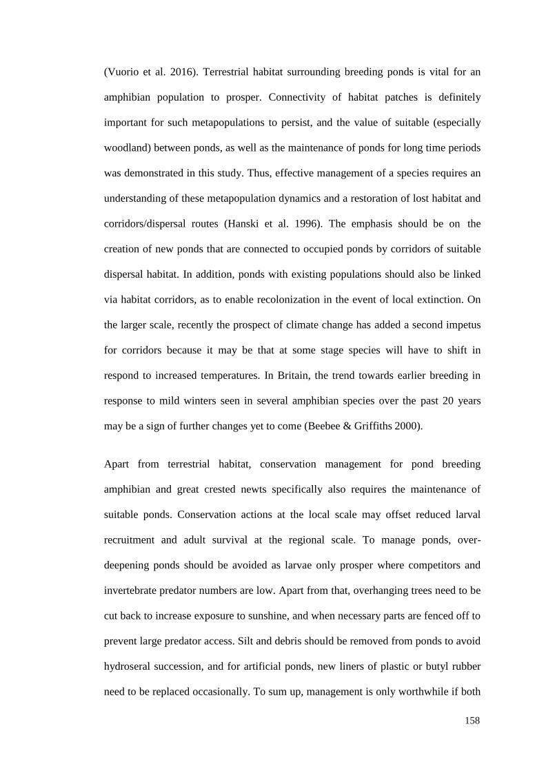
160

(Vuorio et al. 2016). Terrestrial habitat surrounding breeding ponds is vital for an

amphibian population to prosper. Connectivity of habitat patches is definitely

important for such metapopulations to persist, and the value of suitable (especially

woodland) between ponds, as well as the maintenance of ponds for long time periods

was demonstrated in this study. Thus, effective management of a species requires an

understanding of these metapopulation dynamics and a restoration of lost habitat and

corridors/dispersal routes (Hanski et al. 1996). The emphasis should be on the

creation of new ponds that are connected to occupied ponds by corridors of suitable

dispersal habitat. In addition, ponds with existing populations should also be linked

via habitat corridors, as to enable recolonization in the event of local extinction. On

the larger scale, recently the prospect of climate change has added a second impetus

for corridors because it may be that at some stage species will have to shift in

respond to increased temperatures. In Britain, the trend towards earlier breeding in

response to mild winters seen in several amphibian species over the past 20 years

may be a sign of further changes yet to come (Beebee & Griffiths 2000).

Apart from terrestrial habitat, conservation management for pond breeding

amphibian and great crested newts specifically also requires the maintenance of

suitable ponds. Conservation actions at the local scale may offset reduced larval

recruitment and adult survival at the regional scale. To manage ponds, over-

deepening ponds should be avoided as larvae only prosper where competitors and

invertebrate predator numbers are low. Apart from that, overhanging trees need to be

cut back to increase exposure to sunshine, and when necessary parts are fenced off to

prevent large predator access. Silt and debris should be removed from ponds to avoid

hydroseral succession, and for artificial ponds, new liners of plastic or butyl rubber

need to be replaced occasionally. To sum up, management is only worthwhile if both

158

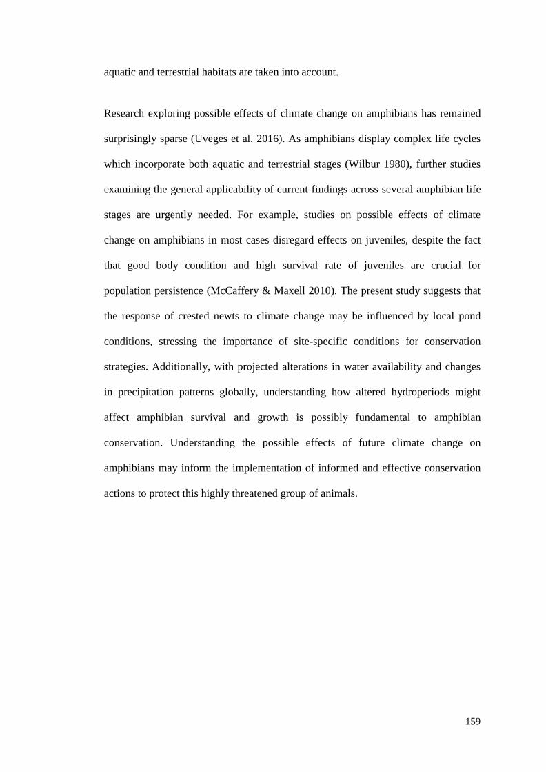
161

aquatic and terrestrial habitats are taken into account.

Research exploring possible effects of climate change on amphibians has remained

surprisingly sparse (Uveges et al. 2016). As amphibians display complex life cycles

which incorporate both aquatic and terrestrial stages (Wilbur 1980), further studies

examining the general applicability of current findings across several amphibian life

stages are urgently needed. For example, studies on possible effects of climate

change on amphibians in most cases disregard effects on juveniles, despite the fact

that good body condition and high survival rate of juveniles are crucial for

population persistence (McCaffery & Maxell 2010). The present study suggests that

the response of crested newts to climate change may be influenced by local pond

conditions, stressing the importance of site-specific conditions for conservation

strategies. Additionally, with projected alterations in water availability and changes

in precipitation patterns globally, understanding how altered hydroperiods might

affect amphibian survival and growth is possibly fundamental to amphibian

conservation. Understanding the possible effects of future climate change on

amphibians may inform the implementation of informed and effective conservation

actions to protect this highly threatened group of animals.

159

162

REFERENCES

Agler, B. 1992. The use of photographic identification for studying individual Fin

Whales (Balaenoptera physalus) in the Gulf of Maine. Report of the

International Whaling Commission 42: 711-722.

Alford, R.A., Dixon, P.M. & Pechmann, J.H.K. 2001. Global amphibian population

declines. Nature 412: 499-500.

Alldredge, M.W., Simons, T.R. & Pollock, K.H. 2007. A field evaluation of distance

measurement error in auditory avian point count surveys. Journal of Wildlife

Management 7: 2759-2766.

Anderson, D.R., Burnham, K.P & White, G.C. 1994. AIC model selection in

overdispersed capture-recapture data. Ecology 75: 1780-1793.

Anholt, B.R., Hotz, H., Guex, G.D. & Semlitsch, R.D. 2003. Overwinter survival of

Rana lessonae and its hemiclonal associate Rana esculenta. Ecology 84: 391-

397.

Antwis, R.E. Garcia, G., Fidgett, A.L. & Preziosi, R.F. 2014.Tagging frogs with

passive integrated transponders causes disruption of the cutaneous bacterial

community and proliferation of opportunistic fungi. Applied and

Environmental Microbiology 80: 4779-4784.

Araabi, B.N., Kehtarnavaz, N., McKinney, T., Hillman, G. & Wursig, B. 2000. A

string matching computer-assisted system for dolphin photoidentification.

Annuals of Biomedical Engineering 28: 1269-1279.

Araujo, M.B., Thuiller, W. & Pearson, R.G. 2006. Climate warming and the decline

of amphibians and reptiles in Europe. Journal of Biogeography 33: 1712-1728.

Arntzen, J.W. & Teunis, S.F.M. 1993. A six year study on the population dynamics

of the crested newt (Triturus cristatus) following the colonization of a newly

created pond. Herpetological Journal 3: 99-110.

Arntzen, J.W. 2002. Seasonal variation in sex ratio and asynchronous presence at

ponds of male and female Triturus newts. Journal of Herpetology 36: 30-35.

Arntzen, J.W., Goudie, I.B.J., Halley, J. & Jehle, R. 2004. Cost comparison of

marking techniques in long-term population studies: PIT-tags versus pattern

maps. Amphibia-Reptilia 25: 305-315.

Baker, J.M.R. & Halliday, T.R. 1999. Amphibian colonization of new ponds in an

agricultural landscape. Herpetological Journal 9: 55-63.

Baker, J.M.R. 1992. Body condition and tail height in great crested newts, Triturus

cristatus. Animal Behaviour 43: 157-159.

160

http://aem.asm.org/search?author1=Andrea%2BL.%2BFidgett&sortspec=date&submit=Submit

http://aem.asm.org/search?author1=Richard%2BF.%2BPreziosi&sortspec=date&submit=Submit

163

Baker, J.M.R. 1999. Abundance and survival rates of great crested newts (Triturus

cristatus) at a pond in central England: monitoring individuals. Herpetological

Journal 9: 1-8.

Bancila, R.I., Hartel, T., Plaia ̧R., Smets, J. & Cogalniceanu, D. 2010. Comparing

three body condition indices in amphibians: a case study of yellow-bellied toad

Bombina variegata. Amphibia-Reptilia 31: 558-562.

Băncilă, R.I., Ozgul, A., Hartel, T., Sos, T. & Schmidt, B.R. 2016, Direct negative

density-dependence in a pond-breeding frog population. Ecography, 39: 449-

455.

Beebee T.J.C. & Griffiths R.A. 2005. The amphibian decline crisis: a watershed for

conservation biology? Biological Conservation 125: 271-285.

Beebee, T.J.C. 2002. Amphibian phenology and climate change. Conservation

Biology 16: 1454-1455.

Beebee, T.J.C. & Griffiths, R.A. 2000. Amphibians and Reptiles: A Natural History

of the British Herpetofauna. Harper Collins New Naturalist, London.

Beebee, T.J.C. 1996. Ecology and Conservation of Amphibians. Chapman & Hall,

London.

Beebee, T.J.C. 1995. Amphibian breeding and climate. Nature 374: 219-220.

Begon, M. & Mortimer, A. 1981. Population Ecology. Sinauer Press, Sunderland,

Mass.

Benard, M.F. 2015. Warmer winters reduce frog fecundity and shift breeding

phenology, which consequently alters larval development and metamorphic

timing. Global Change Biology 21: 1058-1065.

Bendik, N.F., Morrison, T.A., Gluesenkamp, A.G., Sanders, M.S. & O'Donnell, L.J.

2013. Computer-assisted photo identification outperforms visible implant

elastomers in an endangered salamander, Eurycea tonkawae. PLoS One 8:

e59424.

Bishop, P.J., Angulo, A., Lewis, J.P., Moore, R.D., Rabb, G.B. & Moreno, J.G. 2012.

The amphibian extinction crisis - what will it take to put the action into the

Amphibian Conservation Action Plan? Surveys and Perspectives Integrating

Environment and Society 5: 97-111.

Blackwell, G.L. 2002. A potential multivariate index of condition for small

mammals. New Zealand Journal of Zoology 29: 195-203.

Blaustein A.R., Walls S.C., Bancroft B.A., Lawler J.J., Searle C.L. & Gervasi S.S.

2010. Direct and indirect effects of climate change on amphibian populations.

Diversity 2: 281-313.

161

164

Blaustein, A.R. & Kiesecker, J.M. 2002. Complexity in conservation: lessons from

the global decline of amphibian populations. Ecology Letters 5: 597-608.

Blaustein, A.R. & Wake, D.B. 1990. Declining amphibian populations: a global

phenomenon? Trends in Ecology and Evolution 5: 203-204.

Blaustein, A.R., Wake, D.B. & Sousa, W.P. 1994. Amphibian declines: Judging

stability, persistence, and susceptibility of populations to local and global

extinctions. Conservation Biology 8: 60-71.

Bogdan, H.V., Ianc, R.M., Pop, A.N., Söllösi R.S. & Popovici, A.M. 2011. Food

composition of an Ichthyosaura alpestris (Amphibia) population from the

Poiana Rusca Mountains, Romania. Herpetologica Romanica 5: 1-6.

Bolger, D.T., Morrison, T.A., Vance, B., Lee, D. & Farid, H. 2012. A computer-

assisted system for photographic mark–recapture analysis. Methods in Ecology

& Evolution 3: 813-822.

Bonetti, M. 1996. Geographical variation in growth, size and body condition between

amphibian populations. MSc thesis, Durrell Institute of Conservation and

Ecology, University of Kent.

Boone, M.D., Scott, D.E. & Niewiarowski, P.H. 2002. Effects of hatching time for

larval ambystomatid salamanders. Copeia 2002: 511-517.

Bosch, J., Carrascal, L.M., Duran, L., Walker, S. & Fisher, M.C. 2007. Climate

change and outbreaks of amphibian chytridiomycosis in a montane area of

Central Spain; is there a link? Proceeding of the Royal Society B Biological

Sciences 274: 253-260.

Bosch, J., Carrascal, L.M., Duran, L., Walker, S. & Fisher, M.C. 2007. Climate

change and outbreaks of amphibian chytridiomycosis in a montane area of

Central Spain; is there a link? Proceeding of the Royal Society B Biological

Sciences 274: 253-260.

Both, C. & Visser, M.E. 2005. The effect of climate change on the correlation

between avian life-history traits. Global Change Biology 11: 1606-1613.

Bradfield, K.S. 2004. Photographic identification of individual Archey’s frogs,

Leiopelma archeyi, from natural markings. DOC Internal Science Series 191.

Department of Conservation, Wellington.

Brenner, F.J. 1969. The role of temperature and fat deposition in hibernation and

reproduction in two species of frogs. Herpetologica 25: 105-113.

Brodeur, J.C., Suarez, R.P., Natale, G.S., Ronco, A.E. & Zaccagnini, E.M. 2011.

Reduced body condition and enzymatic alterations in frogs inhabit intensive

crop production areas. Ecotoxicology and Environmental Safety 74: 1370-

1380.

Brodie, E.D. 1989. Behavioral modification as a means of reducing the cost of

162

165

reproduction. American Naturalist 134: 225-238.

Brown, J.H. & Kodric-Brown, A. 1977. Turnover rates in insular biogeography:

effect of immigration on extinction. Ecology 58: 445-449.

Brown, J.L., Li, S.H. & Bhagabati, N. 1999. Ecology long-term trend toward earlier

breeding in an American bird: A response to global warming? Proceedings of

the National Academy Sciences 96: 5565-5569.

Buckley, L.B. & Jetz, W. 2007. Environmental and historical constraints on global

patterns of amphibian richness. Proceedings of the Royal Society B: Biological

Sciences 274: 1167-1173.

Burghardt, T. 2008 Visual animal biometrics. PhD thesis, University of Bristol, UK.

Burke, E.J., Brown, S.J. & Christidis, N. 2006. Modelling the recent evolution of

global drought and projections for the 21st century with the Hadley Centre

climate model. Journal of Hydrometeorology 7: 1113-1125.

Burnham, K.P. & Anderson, D.R. 1992. Data-based selection of an appropriate

biological model: the key to modern data analysis. In: McCullough, D.R. &

Barrett, R.H. (Eds.), Wildlife 2001: Populations. Elsevier, London.

Burrowes, P.A., Joglar, R.L. & Green, D.E. 2004. Potential causes for amphibian

declines in Puerto Rico. Herpetologica 60: 141-154.

Carey, C. 2003. Climate change and amphibian declines: is there a link? Diversity

and Distribution 9: 111-121.

Catlin, D.H., Milenkaya, O., Hunt, K.L., Friedrich, M.J. & Fraser, J.D. 2014. Can

river management improve the Piping Plover’s long-term survival on the

Missouri River? Biological Conservation 180:196-205.

Cayuela, H., Arsovski, D., Thirion, J.-M., Bonnaire, E., Pichenot, J., Boitaud, S.,

Miaud, C., Joly, P. & Besnard, A. 2016. Demographic responses to weather

fluctuations are context dependent in a long-lived amphibian. Global Change

Biology, 22: 2676–2687.

Cayuela, H., Joly, P., Schmidt, B.R., Pichenot, J., Bonnaire, E. Priol, P., Peyronel,

O., Laville, M. & Besnard, A. 2017. Life history tactics shape amphibians’

demographic responses to the North Atlantic Oscillation. Global Change

Biology, 23: 4620-4638

Chanson, J., Hoffmann, M., Cox, N. & Stuart, S. 2008. The state of the world’s

amphibians. In: Stuart, S., Hoffmann, M., Chanson, J., Cox, N., Berridge, R.,

Ramani, P. & Young B. (Eds.), Threatened Amphibians of the World. Lynx

Edicions/IUCN/Conservation International, Barcelona/Gland/Arlington.

Charland, M.B. & Gregory, T. 1995. Movements and habitat use in gravid and

nongravid female garter snakes (Colubridae: Thamnophis). Journal of Zoology

236: 543-561.

163

https://www.zora.uzh.ch/view/authors_for_linking_in_citation/Schmidt=3AB_R=3A=3A.html

https://www.zora.uzh.ch/id/eprint/140347/

https://www.zora.uzh.ch/id/eprint/140347/

166

Chase, F.W., Hardie, B.E., Kern, M.M., Pittman, S.E., Harden, L.A. & Dorcas, M.E.

2015. Evaluation of two individual identification techniques for Spotted

Salamanders (Ambystoma maculatum). Herpetological Review 46: 192-196.

Church, D.R., Bailey, L.L., Wilbur, H.M., Kendall, W.L. & Hines, J.E. 2007.

Iteroparity in the variable environment of the salamander Ambystoma tigrinum.

Ecology 88: 891-903.

Climate Change. 2001. Third Assessment Report of the Intergovernmental Panel on

Climate Change IPCC (WG I & II). Cambridge University Press, Cambridge.

Cohn, J.P. 2008. Citizen science: can volunteers do real research? Bioscience 58:

192-197.

Collins, J.P. & Storfer, A. 2003. Global amphibian declines: sorting the hypotheses.

Diversity and Distributions 2: 89-98.

Cooch, E.G. & White, G.W. 2001. Using MARK – A Gentle Introduction, 2nd ed.

Colorado State University, Fort Collins, Colorado, US.

Cooke, A.S. & Arnold, H.R. 2003. Night counting, netting and population dynamics

of crested newts (Triturus cristatus). Herpetological Bulletin 84: 5-14.

Cooke, A.S. 1974. Differential predation by newts on anuran tadpoles. British

Journal of Herpetology 5: 386-390.

Cooper, W.E., Vitt, L.J., Hedges, R. & Huey, R.B. 1990. Locomotor impairment and

defense in gravid lizards: behavioural shift in activity may offset cost of

reproduction in an active forager. Behavioral Ecology and Sociobiology 27:

153-157.

Corn, P.S. & Muths, E. 2002. Variable breeding phenology affects the exposure of

amphibian embryos to ultraviolet radiation. Ecology 83: 2958-2963.

Corn, P.S. 2005. Climate change and amphibians. Animal Biodiversity and

Conservation 28: 59-67.

Coulson, T., Albon, S., Pilkington, J. & Clutton-Brock, T. 1999. Small-scale spatial

dynamics in a fluctuating ungulate population. Journal of Animal Ecology 68:

658- 671.

Crombie, A.C. 1942. The effect of crowding upon the oviposition of grain-infesting

insects. Journal of Experimental Biology 19: 311-340.

Crombie, A.C. 1944. On intraspecific and interspecific competition in larvae of

graminivorous insects. Journal of Experimental Biology 20: 135-151.

Cummins, C.P. & Swan, M.J.S. 2000. Long-term survival and growth of free-living

great crested newts (Triturus cristatus) PIT-tagged at metamorphosis.

Herpetological Journal 10: 177-182.

163

164

167

Cushman, S. 2006. Effects of habitat loss and fragmentation on amphibians: a review

and prospectus. Biological Conservation 128: 231-240.

D’Amen, M. & Bombi, P. 2009. Global warming and biodiversity: Evidence of

climate-linked amphibian declines in Italy. Biological Conservation 142: 3060-

3067.

D’Amen, M., Bombi, P., Pearman, P.B., Schmatz, D.R., Zimmermann, N.E. &

Bologna, M.A. 2011. Will climate change reduce the efficacy of protected

areas for amphibian conservation in Italy? Biological Conservation 144: 989-

997.

Debinski, D.M., VanNimwegen, R.E. & Jakubauskas, M.E. 2006. Quantifying

relationships between bird and butterfly community shifts and environmental

change. Ecological Applications 16: 380-393.

DEFRA. 2009. The environment in your pocket 2009: Key facts and figures on the

environment of the United Kingdom. Department for Environment, Food and

Rural Affairs, London.

Denver, R.J. & Crespi, E.J. 2006. Stress hormones and human developmental

plasticity: lessons from tadpoles. Neoreviews 7:183-188.

Denver, R.J., Mirhadi, N. & Phillips, M. 1998. Adaptive plasticity in amphibian

metamorphosis: Response of Scaphiopus hammondii tadpoles to habitat

desiccation. Ecology 79: 1859-1872.

Dervo, B.K., Bærum, K.M., Skurdal, J. & Museth, J. 2016. Effects of temperature

and precipitation on breeding migrations of amphibian species in Southeastern

Norway. Scientifica 2016: 3161-3174.

Dimancea, N., Cicort-Lucaciu, A.Ş., Fazacas, R., Ianc, R., Boros, A. 2011. The

trophic spectrum analysis of a Mesotriton alpestris (Laurentus 1768)

population from Voineasa locality, Valcea County, Romania. South Western

Journal of Horticulture, Biology and Environment 2: 65-73.

Dodd, C.K. Jr. & Cade, B.S. 1998. Movement patterns and the conservation of

amphibians breeding in small, temporary wetlands. Conservation Biology 12:

331- 339.

Donnelly, M.A. & Crump, M.L. 1998. Potential effects of climate change on two

Neotropical amphibian assemblages. Climatic Change 39: 541-561.

Donovan, T.M., Thompson, F.R., Faaborg, J. & Probst, J.R. 1995. Reproductive

success of migratory birds in habitat sources and sinks. Conservation Biology

9: 1380-1395.

Drechsler. A., Helling, T. & Steinfartz, S. 2015. Genetic fingerprinting proves cross-

correlated automatic photo-identification of individuals as highly efficient in

large capture-mark-recapture studies. Ecology and Evolution 5: 141-151.

165

168

Duan, R.Y., Kong, X.Q., Huang, M.Y., Varela, S. & Ji, X. 2016. The potential

effects of climate change on amphibian distribution, range fragmentation and

turnover in China. PeerJ 4: e2185.

Duellman, W.E. & Trueb, L. 1986. Biology of Amphibians. McGraw-Hill, New

York.

Durigen, B. 1897. Deutschlands Amphibien und Reptilien- Magdeburg (Creutz).

Edgar P. & Bird D.R. 2005. Action Plan for the Conservation of the Sand Lizard

(Lacerta agilis) in Northwest Europe. Convention on the Conservation of

European Wildlife and Natural Habitats, Strasbourg 2005: 1-18.

Edgar, P. & Bird, D.R. 2006. Action plan for the conservation of the crested newt

Triturus cristatus species complex in Europe. Council of Europe, Strasbourg,

France.

English Nature. 2001. Great crested newt mitigation guidelines. The Creative

Company, Peterborough.

Feder, M.E. 1978. Environmental variability and thermal acclimation in neotropical

and temperate zone salamanders. Physiological Zoology 51: 7-16.

Finerty, S.E., Hillman, G.R., & Davis, R.W. 2007. Computer matching of sea otter

(Enhydra lutris) nose scars: A new method for tracking individual otters.

Aquatic Mammals 33: 349-358.

Finkler, M.S., Sugalski, M.T. & Claussen, D.L. 2003. Sex-related differences in

metabolic rate and locomotor performance in breeding spotted salamanders

(Ambystoma maculatum). Copeia 887-893.

Fisher, M.C., Garner, T.W.J. & Susan, F. 2009. Global emergence of

Batrachochytrium dendrobatidis and amphibian Chytridiomycosis in space,

time, and host. Annual Review of Microbiology 63: 291-310.

Forcada, J. & Aguilar, A. 2000. Use of photographic identification in capture-

recapture studies of Mediterranean monk seals. Marine Mammal Science 16:

767- 793.

Forchhammer, M.C., Post, E. & Stenseth, N.C. 1998. Breeding phenology and

climate. Nature 391: 29-30.

Forero-Medina, G., Joppa, L. & Pimm, S.L. 2011. Constraints to species’ elevational

range shifts as climate changes. Conservation Biology 25: 163-171.

Foster-Smith, J. & Evans, S.M. 2003. The value of marine ecological data collected by volunteers. Biological Conservation 113: 199-213.

Friday, N., Smith, T.D., Stevick, P.T. & Allen, J. 2000. Measurement of

photographic quality and animal distictiveness for the photographic

identification of humpback whales. Marine Mammal Science 16: 355-374.

166

169

Gaggiotti, O.E. 1996. Population genetic models of source-sink metapopulations.

Theoretical Population Biology 50: 178-208.

Gallant, A.L., Klaver, R.W., Casper, G.S. & Lannoo, M.J. 2007. Global rates of

habitat loss and implication for amphibian conservation. Copeia 2007: 965-

977.

Gamble, L., Ravela, S. & McGarigal, K. 2008. Multi-scale features for identifying

individuals in large biological databases: an application of pattern recognition

technology to the marbled salamander Ambystoma opacum. Journal of Applied

Ecology 45: 170-180.

Gao, X., Jin, C., Llusia, C. & Li, Y. 2015. Temperature-induced shifts in hibernation

behavior in experimental amphibian populations. Scientific Reports 5: 11580.

Gerlanc, N.M. & Kaufman, G.A. 2005. Habitat of origin and changes in water

chemistry influence development of western chorus frog. Journal of the

Herpetology 39: 254-265.

Gervasi, S.S. & Foufopoulos, J. 2008. Costs of plasticity: responses to desiccation

decrease post-metamorphic immune function in a pond-breeding amphibian.

Functional Ecology 22: 100-108.

Gibbs, J.P. & Breisch, A.R. 2001. Climate warming and calling phenology of frogs

near Ithaca, New York, 1900-1999. Conservation Biology 15: 1175-1178.

Gill, D.E. 1978. The metapopulation ecology of the red-spotted newt,

Notophthalmus viridescens (Rafinesque). Ecological Monographs 48: 145-166.

Gill, D.E. 1979. Density dependence and homing behaviour in adult red-spotted

newts Notophthalmus viridescens (Rafineque). Ecology 60: 800-813.

Gillooly, J.F., Brown, J.H., West, G.B., Savage, V.M. & Charnov, E.L. 2001. Effects

of size and temperature on metabolic rate. Science 293: 2248-2251.

Gosler, A.G. 1996. Environmental and social determinants of winter fat storage in

the Great Tit Parus major. Journal of Animal Ecology 65: 1-17.

Gouveia, S.F., Hortal, J., Cassemiro, F.A., Rangel, T.F. & Diniz-Filho, J.A.F. 2013.

Nonstationary effects of productivity, seasonality, and historical climate

changes on global amphibian diversity. Ecography 36: 104-113.

Gowans, S. & Whitehead, H. 2001. Photographic identification of northern

bottlenose whales (Hyperoodon ampullatus): Sources of heterogeneity from

natural marks. Marine Mammal Science 17: 76-93.

Grayson, K.L., Bailey, L.L. & Wilbur, H.M. 2011. Life history benefits of residency

in a partially migrating wetland-breeding amphibian. Ecology 92: 1236-1246.

Green, A.J. 2001. Mass/length residuals: measures of body condition or generators of

spurious results? Ecology 82: 1473-1483.

167

170

Green, D.M. 2003.The ecology of extinction: population fluctuation and decline in

amphibians. Biological Conservation 111: 331-343.

Griffiths, R. 1996. Newts and salamanders of Europe. Poyser Natural History,

London.

Griffiths, R.A. & Mylotte, V.J. 1987. Microhabitat selection and feeding relations of

smooth and warty newts, Triturus vulgaris and T. cristatus, at an upland pond

in mid-Wales. Holarctic Ecology 10: 1-7.

Griffiths, R.A. & Mylotte, V.J. 1988. Observations on the development of the

secondary sexual characters of male smooth and palmate newts, Triturus

vulgaris and T. helveticus. Journal of Herpetology 22: 476-480.

Griffiths, R.A. & Raper, S.J. 1994. A review of current techniques for sampling

amphibian communities. JNCC Report, No. 210. Joint Nature Conservation

Committee, Peterborough.

Griffiths, R.A. & Williams, C. 2001. Population modelling of great crested newts

(Triturus cristatus). Rana 4: 239-247.

Griffiths, R.A. 1985. A simple funnel trap for studying newt populations and an

evaluation of trap behaviour in smooth and palmate newts, Triturus vulgaris

and T. helveticus. Herpetological Journal 1: 5-10.

Griffiths, R.A. 1996. Newts and salamanders of Europe. Poyser/Academic Press,

London and San Diego.

Griffiths, R.A. 1997. Temporary ponds as amphibian habitats. Aquatic

Conservation: Marine Freshwater Ecosystems 7: 119-126.

Griffiths, R.A. 2004. Great crested newts in Europe; Effects of metapopulation

structure and juvenile dispersal on population persistence. In: Ackakaya, H.R.,

Burgman, M., Kindvall, O., Wood, C.C., Sjogren-Gulve, P., Hatfield, J.S. &

McCarthy, M.A. (Eds.), Species Conservation and Management: Case Studies.

Oxford University Press, New York.

Griffiths, R.A. & Williams, C. 2000. Modelling population dynamics of great crested

newts (Triturus cristatus): A population viability analysis. Herpetological

Journal 10: 157-163.

Griffiths, R.A., Raper, S.J. & Brady, L.D. 1996. Evaluation of a standard method for

surveying common frogs (Rana temporaria) and newts (Triturus cristatus, T.

helveticus and T. vulgaris). Report no. 259. Joint Nature Conservation

Committee, Peterborough, UK.

Griffiths, R.A., Sewell, D. & McCrea, R. 2010. Dynamics of a declining amphibian

metapopulation: Survival, dispersal and the impact of climate. Biological


Guerra, C. & Araoz, E. 2015. Amphibian malformations and body condition across

an agricultural landscape of northwest Argentina. Diseases of Aquatic

Organisms 121: 105-116.

168

171

Gyllenberg, M., Soderbacka, G. & Ericsson, S. 1993. Does migration stabilize local

population dynamics? Analysis of a discrete metapopulation model.

Mathematical Biosciences 118: 25-49.

Hagström, T. 1971. Stora vattensalamandern i Västsverige - en predator pâ sin

mindre släkting. Fauna Flora 66: 71-72.

Hagström, T. 1973. Identification of newt specimens (Urodela, Triturus) by

recording the belly pattern and a description of photographic equipment for

such registrations. British Journal of Herpetology 4: 321-326.

Hagström, T. 1979. Population ecology of Triturus cristatus and T. vulgaris

(Urodela) in SW Sweden. Holarctic Ecology 2: 108-114.

Halley, J.M., Oldham, R.S. & Arntzen, J.W. 1996. Predicting the persistence of

amphibian populations with the help of a spatial model. Journal of Applied

Ecology 33: 455-470.

Hamer, A.J. & Mcdonnell, M.J. 2008. Amphibian ecology and conservation in the

urbanizing world: a review. Biological Conservation 141: 2432-2449.

Hammond, P.S., Mizroch, S.A. & Donovan, G.P. 1990. Individual recognition of

cetaceans: use of photo - indentification and other techniques to estimate

population parameters. Report of the International Whaling Commission

(Special Issue 12). Cambridge, UK.

Hanski, I. & Gilpin, M.E. 1991. Metapopulation dynamics: brief history and

conceptual domain. In: Gilpin, M.E. & Hanski, I. (Eds.), Metapopulation

Dynamics. Academic Press, London.

Hanski, I., Moilanen, A. & Gyllenberg, M. 1996. Minimum viable metapopulation

size. The American Naturalist 147: 527-541.

Hanski, I. & Simberloff, D. 1997. The metapopulation approach, its history,

conceptual domain and application to conservation. In: Hanski, I. & Gilpin, M.

(Eds.), Metapopulation Biology. Academic Press, San Diego, CA, USA.

Hanski, I. 1997. Metapopulation dynamics: From concept and observations to

predictive models. In: Hanski, I.A. & Gilpin, M.E. (Eds.), Metapopulation

Biology: Ecology, Genetics and Evolution. Academic Press, London.

Hanski, I., Moilanen, A., Pakkala, T. & Kuussaari, M. 1996. The quantitative

incidence function model and persistence of an endangered butterfly

metapopulation. Conservation Biology 10: 578-590.

Harrison, S. & Taylor, A.D. 1997. Empirical evidence for metapopulation dynamics.

In: Hanski, I.A. & Gilpin, M.E. (Eds.), Metapopulation Biology: Ecology,

Genetics and Evolution. Academic Press, London.

Harting, A., Baker, J. & Becker, B. 2004. Non-metrical digital photo-identification

system for the Hawaiian monk seal. Marine Mammal Science 20: 886-895.

Hastings, K.K., Hiby, L.A. & Small, R.J. 2008. Evaluation of a computer-assisted

169

172

photograph-matching system to monitor naturally marked harbor seals at

Tugidak Island, Alaska. Journal of Mammalogy 89: 1201-1211.

Hayward, R., Oldham, R.S., Watt, P.J. & Head, S.M. 2000 Dispersion patterns of

young great crested newts (Triturus cristatus) Herpetological Journal 10: 129-

136.

Hecnar, S.J. & M’Closkey, R.T. 1996. Amphibian species richness and distribution

in relation to pond water chemistry in south-western Ontario, Canada.

Freshwater Biology 36: 7-15.

Hecnar, S.J. & M’Closkey, R.T. 1997. The effects of predatory fish on amphibian

species richness and distribution. Biological Conservation 79: 123-131.

Hedlund, L. & Robertson, J.G. 1989. Lekking behaviour in crested newts, Triturus

cristatus. Ethology 80: 111-119.

Hedlund, L. 1990. Reproductive ecology of crested newts, Triturus cristatus (Laur.).

PhD Thesis. Swedish Unversity of Agricultural Sciences.

Hellriegel, B. 2000. Single- or multistage regulation in complex life cycles: does it

make a difference? Oikos 88: 239-249.

Hoare, J.M., Pledger, S., Keall, S.N., Nelson, N.J., Mitchell, N.J. & Daugherty, C.H.

2006. Conservation implications of a long-term decline in body condition of

the Brothers Island tuatara (Sphenodon guntheri). Animal Conservation 9: 456-

462.

Hodgson, G. 1999. A global sssessment of human effects on coral reefs. Marine

Pollution Bulletin 38: 345-355.

Hoey, A.S. & McCormick, M.I. 2004. Selective predation for low body condition at

the larval-juvenile transition of a coral reef fish. Oecologia 139: 23-29.

Hof, C., Araújo, M.B., Jetz, W. & Rahbek, C. 2011. Additive threats from pathogens,

climate and land-use change for global amphibian diversity. Nature 480: 516-

519.

Hoffmann, A.A. & Parsons, P.A. 1997 Extreme Environmental Change and

Evolution. Cambridge University Press, UK.

Hoffmann, H. 2012. Studies on the mechanisms that affect the growth and

development rates of Leptodactylus melanonotus tadpoles (Anura:

Leptodactylidae) at different population densities. Salamandra 48: 213-223.

Hoque, S., Azhar, M.A.H.B. & Deravi, F. 2011. ZOOMETRICS - Biometric

identification of wildlife using natural body marks. International Journal of

Bio- Science and Bio-Technology 3: 45-54.

Houlahan, J.E., Findlay, C.S., Schmidt, B.R., Meyer, A.H. & Kuzmin, S.L. 2000.

Quantitative evidence for global amphibian population declines. Nature 404:

170

173

752- 755.

Hulme, M., Jenkins, G.J., Lu, X., Turnpenny, J.R., Mitchell, T.D., Jones, R.G.,

Lowe, J., Murphy, J.M., Hassell, D., Boorman, P., McDonald, R. & Hill, S.

2002. Climate change scenarios for the UK: the UKCIP02 scientific report.

Tyndall Centre, University of East Anglia, Norwich, UK.

Inouye, D.W., Barr, B., Armitage, K B. & Inouye, B.D. 2000. Climate change is

affecting altitudinal migrants and hibernating species. Proceedings of the

National Academy Sciences 97: 1630-1633.

Intergovernmental Panel on Climate Change (IPCC). 1996. Climate Change 1995:

The Science of Climate Change. World Meteorological Organization and

United Nations Environmental Program.

IPCC. 2001. Climate Change 2001: The Scientific Basis. Contribution of Working

Group I to the Third Assessment Report of the Intergovernmental Panel on

Climate Change (Eds. Houghton, J.T., Ding, Y., Griggs, D.J., Noguer, M., van

der Linden, P.J., Dai, X., Maskell, K. & Johnson, C.A.). Cambridge University

Press, Cambridge, United Kingdom and New York, NY, USA.

Jahn, P. 1995. Untersuchungen zur Populationsökologie von Triturus cristatus und T.

vulgaris am Friedeholzer Schlatt. Dipl.arb. Univ. Bremen, unveröff.

Jakob, E.M., Marshall, S.D. & Uetz, G. W. 1996. Estimating fitness: a comparison of

body condition indices. Oikos 77: 61-67.

Janin, A., Léna, J.P. & Joly, P. 2011. Beyond occurrence: body condition and stress

hormone as integrative indicators of habitat availability and fragmentation in

the common toad. Biological Conservation 144: 1008-1016.

Jarvis, L.E. 2015. Factors affecting body condition in a great crested newt Triturus

cristatus population. The Herpetological Bulletin 134: 1-5.

Jarvis, L.E. 2010. Population dynamics of the Great Crested Newt (Triturus

cristatus), High Beach, Epping Forest. The Essex Naturalist 27: 186-195.

Jehle, R. & Arntzen, J.W. 2000. Post-breeding migrations of newts (Triturus

cristatus and T. marmoratus) with contrasting ecological requirements. Journal

of Zoology 251: 297-306.

Jehle, R. & Arntzen, J.W. 2000. Post-breeding migrations of newts (Triturus

cristatus and T. marmoratus) with contrasting ecological requirements. Journal

of Zoology 251: 297-306.

Jehle, R., Thiesmeier, B. & Foster, J. 2011. The crested newt. Laurenti-Verlag,

Bielefeld.

Jehle, R., Wilson, G.A., Arntzen, J.W. & Burke, T. 2005. Contemporary gene flow

and the spatio-temporal genetic structure of subdivided newt populations

(Triturus cristatus, T. marmoratus). Journal of Evolutionary Biology 18: 619-

171

174

628.

Johnson, M.D. 2007. Measuring habitat quality: a review. Condor 109: 489-504.

Johnson, P.T.J., McKenzie, V.J., Peterson, A.C., Kerby, J.L., Brown, J., Blaustein,

A.R. & Jackson, T. 2011. Regional decline of an iconic amphibian associated

with elevation, land-use change, and invasive species. Conservation Biology

25(3): 556-566.

Joly, P. & Miaud, C. 1993. How does a newt find its pond? The role of chemical

cues in migrating newts (Triturus alpestris). Ethology Ecology and Evolution

5: 447- 455.

Jonas, M., Bowman, K.L. & Nazdrowicz, N.H. 2011. Using spot patterns to identify

individual long-tailed salamanders. Herpetological Review 42: 520-522.

Jones, P.D., Osborn, T.J., Briffa, K.R., Folland, C.K., Horton, E.B., Alexander, L.V.,

Parker, D.E. & Rayner, N.A. 2001. Adjusting for sampling density in grid box

land and ocean surface temperature time series. Journal of Geophysical

Research 106: 3371-3380.

Jørgensen, C.B. 1986. External and internal control of patterns of feeding, growth

and gonadal function in a temperate zone anuran, the toad Bufo bufo. Journal

of Zoology 210: 211-241.

Karlsson, T., Betzholtz, P.E. & Malmgren, J.C. 2007. Estimating viability and

sensitivity of the great crested newt Triturus cristatus at a regional scale. Web

Ecology 7: 63-76.

Karraker, N.E. & Welsh, H.H. 2006. Long-term impacts of even-aged timber

management on abundance and body condition of terrestrial amphibians in

Northwestern California. Biological Conservation 131: 132-140.

Kelly, M.J. 2001. Computer-aided photograph matching in studies using individual

identification: an example from Serengeti cheetahs. Journal of Mammalogy 82:

440- 449.

Kiesecker J.M., Blaustein A.R. & Belden L.K. 2001. Complex causes of amphibian

population declines. Nature 410: 681-684.

Kiesecker, J.M. & Blaustein, A.R. 1998. Effects of introduced bullfrogs and

smallmouth bass on microhabitat use, growth, and survival of native red-legged

frogs (Rana aurora). Conservation Biology 12: 776-787.

Kinkead, K.E. & Otis D.L. 2007. Estimating superpopulation size and annual

probability of breeding for pond-breeding salamanders. Herpetologica 63:151-

162.

Knox, C.D., Cree, A. & Seddon, P.J. 2013. Accurate identification of individual

geckos (Naultinus gemmeus) through dorsal pattern differentiation. New

172

175

Zealand Journal of Ecology 37: 60-66.

Kuhn, J. 1994. Lebensgeschichte und Demographie von Erdkrotenweibchen Bufo

bufo bufo (L.). Zeitschrift fur Feldherpetologie 1: 3-87.

Kundzewicz, Z.W., Mata, L.J., Arnell, N.W., Döll, P., Kabat, P., Jiménez, B., Miller,

K.A., Oki, T., Sen, Z. & Shiklomanov, I.A. 2007. Freshwater resources and

their management. In: Climate Change 2007: Impacts, Adaptation and

Vulnerability. Contribution of Working Group II to the Fourth Assessment

Report of the Intergovernmental Panel on Climate Change (Eds. Parry, M.L.,

Canziani, O.F., Palutikof, J.P., van derLinden, P.J. & Hanson, C.E.).

Cambridge University Press, Cambridge, UK.

Kupfer, A. & Kneitz, S. 2000. Population ecology of the great crested newt (Triturus

cristatus) in an agricultural landscape: dynamics, pond fidelity and dispersal.

Herpetological Journal 10: 165-171.

Kupfer, A. 1998. Wanderstrecken einzelner kammolche (Triturus cristatus) in einem

agrarlebensraum (In German with English abstract). Zeitschrift für

Feldherpetologie 5: 238-242.

Kuzmin, S.L. 1995. Die Amphibien Russlands und angrenzender Gebiete. Westarp

Wissenschaften, Magdeburg.

Laan, R. & Verboom, B. 1990. Effects of pool size and isolation on amphibian

communities. Biological Conservation 54: 251-262.

Lagtimm, C.A., Beck, C.A., Edwards, H.H, Fick-Child, K.J., Ackerman, B.B.,

Barton, S.L. & Hartley, C. 2004. Survival estimates for Florida Manatees from

the photo-identification of individuals. Marine Mammal Science 20: 438-463.

Langton, T., Beckett, C. & Foster, J. 2001. Great Crested Newt Conservation

Handbook. Froglife, Peterborough.

Lawler, J.J., Shafer, S.L., Bancroft, B.A. & Blaustein, A.R. 2009. Projected climate

impacts for the amphibians of the Western hemisphere. Conservation

Biology 24: 38-50.

Lebreton, J.D., Burnham, K.P., Clobert, J. & Anderson, D.R. 1992. Modelling

survival and testing biological hypotheses using marked animals: a unified

approach with case studies. Ecological Monographs 62: 67-118.

Lemckert, F. & Penman, T. 2012. Climate change and Australia's frogs: how much

do we need to worry? In: Lunney, D. & Hutchings, P. (Ed.), Wildlife & Climate

Change: Towards Robust Conservation Strategies for Australian Fauna. Royal

Zoological Society of New South Wales, Mosman, N.S.W.

Levins, R. 1969. Some demographic and genetic consequences of environmental

heterogeneity for biological control. Bulletin of the Entomological Society of

America 15: 237-240.

173

176

Lewis, B. 2012. An evaluation of mitigation actions for great crested newts at

development sites. PhD Thesis. Durell Institute of Conservation Biology,

University of Kent.

Lips, K.R. & Donnelly, M.A. 2013. What the tropics can tell us about declining

amphibian populations: Current patterns and future prospects. In: Lannoo, M.J.

(Ed.), North American Amphibians: Status and Conservation. University of

California Press, Berkeley.

Lips, K.R., Burrowes, P.A., Mendelson III, J.R. & Parra-Olea, G. 2005. Amphibian

declines in Latin America: Widespread population declines, extinctions, and

impacts. Biotropica 37: 163-165.

Lowe, D. 2004. Distinctive image features from scale-invariant keypoints.

International Journal of Computer Vision 60: 91-110.

Luiselli, L., Capizzi, D., Filippi, E., Anibaldi, D., Rugiero, L. & Capula, M. 2007.

Comparative diets of three populations of an aquatic snake (Natrix tessellata,

Colubridae) from Mediterranean streams with different hydric regimes. Copeia

2: 426-435.

Madison, D.M. & Farrand, L. 1998. Habitat use during breeding and emigration in

radio-implanted Tiger Salamanders, Ambystoma tigrinum. Copeia 1998: 402-

410.

Malmgren, J.C. 2002. How does a newt find its way from a pond? Migration patterns

after breeding and metamorphosis in great crested newts (Triturus cristatus)

and smooth newts (T. vulgaris). Herpetological Journal 12: 29- 35.

Malmgren, J.C. 2007. Åtgärdsprogram för bevarande av större vattensalamander och

dess livsmiljöer. Report No. 5636. Swedish Environmental Protection Agency,

Stockholm, Sweden. (In Swedish with English summary).

Markowitz, T.M., Harlin, A.D. & Würsig, B. 2003. Digital photography improves

efficiency of individual dolphin identification. Marine Mammal Science 19:

217- 223.

Marquez-Garcia, M., Correa-Solis, M., Sallaberry, M. & Mendez, M.A. 2009.

Effects of pond drying and life-history traits in the anuran Rhinella spinulosa

(Anura: Bufonidae). Evolutionary Ecology Research 11: 803-815.

Marra, P. & Holmes, R.T. 2001. Consequences of dominance-mediated habitat

segregation in American Redstarts during the nonbreeding season. The Auk

118: 92- 104.

Marsh, D.M. & Trenham, P.C. 2001. Metapopulation dynamics and amphibian

conservation. Conservation Biology 15: 40-49.

Matthé, M., Schönbrodt, T. & Berger, G. 2008. Computergestützte Bildanalyse von

Bauchfleckenmustern des Kammmolchs (Triturus cristatus). Zeitschrift für

Feldherpetologie 15: 89-94.

174

177

Matthews, J.H. 2010. Anthropogenic climate change impacts on ponds: A thermal

mass perspective. BioRisk 5: 193-209.

McCaffery, R.M. & Maxell, B.A. 2010. Decreased winter severity increases viability

of a montane frog. Proceedings of the National Academy of Sciences 107:

8644- 8649.

McMenamin, S.K., Hadly, E.A. & Wright, C.K. 2008. Climate change and wetland

desiccation cause amphibian decline in Yellowstone National Park.

Proceedings of the National Academy of Sciences USA 105: 16988-16993.

Menzel. A. & Estrella, N. 2001. Plant phenological changes. In: Walther, G.R.,

Burga, C.A. & Edwards, P.J. (Eds.), Fingerprints of Climate Change- Adapted

Behaviour and Shifting Species Ranges. Kluwer Academic/Plenum Publishers,

New York and London.

Mettouris, O., Megremis, G. & Giokas, S. 2016. A newt does not change its spots:

using pattern mapping for the identification of individuals in large populations

of newt species. Ecological Research 31: 483-489.

Miaud, C., Joly, P. & Castanet, J. 1993. Variation in age structures in a population of

Triturus cristatus. Canadian Journal of Zoology 71: 1874-1879.

Miles, D.B., Sinervo, B. & Frankino, W.A. 2000. Reproductive burden, locomotor

performance, and the cost of reproduction in free ranging lizards. Evolution 54:

1386-1395.

Morin, P.J., Lawler, S.P. & Johnson, E.A. 1990. Ecology and breeding phenology of

larval Hyla andersonii: the disadvantages of breeding late. Ecology 71: 1590-

1598.

Morris, C. 1992. Academic Press Dictionary of Science and

Technology. Academic Press, Inc. San Diego.

Morrison, T., Yoshizaki, J., Bolger, D. & Nichols, J. 2011. Estimating survival with

computer-assisted identification and mark–recapture: the problem of

misidentification error. Methods in Ecology and Evolution 2: 454-463.

Moya, O., Mansilla, P.L., Madrazo, S., Igual, J.M., Rotger, A., Romano, A. &

Tavecchia, G. 2015. APHIS: a new software for photo–matching in ecological

studies. Ecological Informatics 27: 64-70.

Müllner, A. 1991. Zur Biologie von Triturus cristatus und Triturus vulgaris unter

besonderer Berücksichtigung des Wanderverhaltens. Diplom thesis,

Zoologisches Institut, Universität Hamburg.

Mullner, A. 2001. Spatial patterns of migrating great crested newts and smooth

newts: the importance of the terrestrial habitat surrounding the breeding pond.

Rana 4: 279-293.

175

178

NAST. 2000. Climate Change Impacts on the United States: The Potential

Consequences of Climate Variability and Change, Overview. Cambridge

University Press.

Newman, C., Buesching, C.D. & Macdonald, D.W. 2003. Validating mammal

monitoring methods and assessing the performance of volunteers in wildlife

conservation ‘‘Sedquis custodiet ipsos custodies?’’ Biological Conservation

113: 189-197.

Newman, R.A. 1989. Developmental plasticity of Scaphiopus couchii tadpoles in an

unpredictable environment. Ecology 70: 1775-1787.

Newman, R.A. 1994. Effects of changing density and food level on metamorphosis

of a desert amphibian, Scaphiopus couchii. Ecology 75: 1085-1096.

Nichols, J.D. 1992. Capture–recapture models: using marked animals to study

population dynamics. Bioscience 42: 94-102.

Nietfeld, M.T., Barrett, M.W. & Silvy, N. 1994 Wildlife marking techniques. In:

Bookhout, T.K. (Ed.), Research and Management Techniques for Wildlife and

Habitats. The Wildlife Society, Bethesda.

Ochoa-Ochoa, L.M., Rodríguez, P., Mora, F., Flores-Villela, O. & Whittaker, R.J.

2012. Climate change and amphibian diversity patterns in Mexico. Biological


Odum, H.T. 1971. Environment, power, and society. Wiley-Interscience, New York.

Oldham R.S., Keeble J., Swan M.J.S. & Jeffcote M. 2000. Evaluating the suitability

of habitat for the Great Crested Newt (Triturus cristatus). Herpetological

Journal 10: 143-155.

Oldham, R.S. & Swan, M.J.S. 1997. Pond loss and amphibians; historical

perspective. In: Boothby, J. (Ed.), British Pond Landscapes. Action for

Protection and Enhancement. Proceedings of the UK Conference of the Pond

Life Project 3-16. Pond Life Project, Liverpool, UK.

Olsson, M., Wapstra, E., Madsen, T. & Silverin, B. 2000. Testosterone, ticks, and

travels: a test of the immunocompetence-handicap hypothesis in free ranging

male sand lizards. Proceedings of the Royal Society of London B 267: 2339-

2343.

Park, T. 1962. Beetles, competition, and populations. Science 138: 1369-1375.

Parmesan, C. & Yohe, G. 2003. A globally coherent fingerprint of climate change

impacts across natural systems. Nature 421: 37-42.

Parmesan, C. 2007. Influences of species, latitudes and methodologies on estimates

of phenological response to global warming. Global Change Biology 13: 1860-

1872.

176

179

Pearman, P.B. 1995. Effects of pond size and consequent predator density on two

species of tadpoles. Oecologia 102: 1-8.

Pearson, R.G. & Dawson, T.P. 2003. Predicting the impacts of climate change on the

distribution of species: are bioclimate envelope models useful? Global Ecology

and Biogeography 12: 361-371.

Pechmann, J.H.K. & Wilbur, H.M. 1994. Putting declining amphibian populations

into perspective: Natural fluctuations and human impacts. Herpetologica 50:

65-84.

Pechmann, J.H.K., Scott, D.E., Gibbons, J.W. & Semlitsch, R.D. 1989. Influence of

wetland hydroperiod on diversity and abundance of metamorphosing juvenile

amphibians. Wetlands Ecology & Management 1: 3-11.

Pechmann, J.H.K., Scott, D.E., Semlitsch, R.D., Caldwell, J.P., Vitt, L.J. & Gibbons,

J.W. 1991. Declining amphibian populations: the problem of separating human

impacts from natural fuctuations. Science 253: 892-895.

Peig, J. & Green, A.J. 2010. The paradigm of body condition: a critical reappraisal of

current methods based on mass and length. Functional Ecology 24: 1323-1332.

Peig, J. & Green, A.J. 2009. New perspectives for estimating body condition from

mass/length data: the scaled mass index as an alternative method. Oikos 118:

1883- 1891.

Pennycuick, C.J. 1978, Identification using natural markings. In: Stonehouse, B.

(Ed.), Animal Marking: Recognition Marking of Animals in Research.

Macmillan Publishers Limited.

Perry, G., Wallace, M.C., Perry, D., Curzer, H. & Muhlberger, P. 2011. Toe-clipping

of amphibians and reptiles: science, ethics, and the law. Journal of Herpetology

45: 547-555.

Petersen, J.C.B. 1972. An identification system for zebra (Equus burchelli, Gray).

African Journal of Ecology 10: 59-63.

Peterson, T.C. & Vose, R.S. 1997. An overview of the global historical climatology

network temperature data base. Bulletin of the American Meteorological

Society 78: 2837-2849.

Petranka, J.G. 1998. Salamanders of the United States and Canada. Smithsonian

Institution Press, Washington, DC.

Pope, K.L. & Matthews, K.R. 2002. Influence of anuran prey on the condition and

distribution of Rana mucosa in the Sierra Nevada. Herpetologica 58: 345-363.

Pounds, J.A. 2001. Climate and amphibian declines. Nature 410: 639-640.

Pounds, J.A., Fogden, M.P.L. & Campbell, J.H. 1999. Biological response to climate

change on a tropical mountain. Nature 398: 611-614.

177

180

Pounds, J.A., Bustamante, M.R., Coloma, L.A., Consuegra, J.A., Fogden,

M.P., Foster, P.N., La Marca, E., Masters, K.L., Merino-Viteri, A.,

Puschendorf, R., Ron, S.R., Sánchez-Azofeifa, G.A., Still, C.J. & Young, B.E.

2006. Widespread amphibian extinctions from epidemic disease driven by

global warming. Nature 439: 161-167.

Primack, R.B. 1998. Essentials of Conservation Biology. Sinauer Associaes,

Madison, USA.

Pulliam, H.R. 1988. Sources, sinks and population regulation. American Naturalist

132: 652-661.

Rannap, R., Lőhmus, A. & Briggs, L. 2009. Niche position, but not niche breadth,

differs in two coexisting amphibians having contrasting trends in Europe.

Diversity and Distributions 15: 692-700.

Raxworthy, C.J., Pearson, R.G., Rabibisoa, N., Rakotondrazafy, A.M.,

Ramanamanjato. J.B., Raselimanana, A.P., Wu, S., Nussbaum, R.A. & Stone,

D.A. 2008. Extinction vulnerability of tropical montane endemism from

warming and upslope displacement: a preliminary appraisal for the highest

massif in Madagascar. Global Change Biology 14: 1-18.

Reading, C.J. & Clarke, R.T. 1995. The effects of density, rainfall and environmental

temperature on body condition and fecundity in the common toad, Bufo bufo.

Oecologia 102: 453-459.

Reading, C.J. & Clarke, R.T. 1999. Impacts of climate and density on the duration of

the tadpole stage of the common toad Bufo bufo. Oecologia 121: 310-315.

Reading, C.J. 2007. Linking global warming to amphibian declines through its

effects on female body condition and survivorship. Oecologia 151: 125-131.

Reaser, J. 1995. Marking amphibians by toe-clipping; a response to Halliday.

Froglog 12: 1-2.

Redgrave, L. 2009. Marnel Park- accommodating great crested newts within

residential development. In Practice 6: 23-26.

Reyer, H.U. & Battig, I. 2004. Identification of reproductive status in female frogs- a

quantitative comparison of nine methods. Herpetologica 60: 349-356.

Rockwood, L.L. 2006. Introduction to Population Ecology. Blackwell Publishing,

Madison, USA.

Roff, D.A. 1992. The Evolution of Life Histories: Theory and Analysis. Chapman and

Hall, New York.

Romero, L.M. & Wikelski, M. 2010. Stress physiology as a predictor of survival in

Galapagos marine iguanas. Proceeding of the Royal Society of London 277:

3157- 3162.

Ron, S.R., Duellman, W.E., Coloma, L.A. & Bustamante, M.R. 2003. Population

178

181

decline of the Jambato toad Atelopus ignescens (Anura: Bufonidae) in the

Andes of Ecuador. Journal of Herpetology 37: 116-126.

Rovero, F., Zimmermann, F., Berzi, D. & Meek, P. 2013. Which camera trap type

and how many do I need?” A review of camera features and study designs for a

range of wildlife research applications. Italian Journal of Mammalogy 24: 148-

156.

Rowe, C.L. & Dunson, W.A. 1995. Impacts of hydroperiod on growth and survival

of larval amphibians in temporary ponds of Central Pennsylvania, USA.

Oecologia 102: 397-403.

Roy, D.B. & Sparks, T.H. 2000. Phenology of British butterflies and climate change.

Global Change Biology 6: 407-416.

Ruxton, G.D., Gonzalez-Andujar, J.L. & Perry, J.N. 1997. Mortality during dispersal

and the stability of a metapopulation. Journal of Theoretical Biology 186: 389-

396.

Sacchi, R., Scali, S., Pellitteri-Rosa, D., Pupin, F., Gentilli, A., Tettamanti, S.,

Cavigioli, L., Racina, L., Maiocchi, V., Galeotti, P. & Fasola, M. 2010.

Photographic identification in reptiles: a matter of scales. Amphibia-Reptilia

31: 489-502.

Scheele, B.C., Driscoll, D.A., Fischer, J. & Hunter, D.A. 2012. Decline of an

endangered amphibian during an extreme climatic event. Ecosphere 3: 101-

115.

Schmeller D.S., Henry, P.Y., Julliard, R., Gruber, B., Clobert, J., Dziock, F.,

Lengyel, S., Nowicki, P., Deri, E., Budrys, E., Kull, T., Tali, K., Bauch, B.,

Settele, J., Van Swaay, C., Kobler, A., Babij, V., Papastergiadou, E. & Henle,

K. 2009. Advantages of volunteer-based biodiversity monitoring in Europe.

Conservation Biology 23: 307-316.

Schmitt, E. & Sullivan, K. 1996. Analysis of a volunteer method for collecting fish

presence and abundance data in the Florida Keys. Bulletin of Marine Science

59: 404-416.

Schoener, T. 1984. Field experiments on interspecific competition. American

Naturalist 122: 240-285.

Scott, D.E. 1994. The effect of larval density on adult demographic traits in

Ambystoma opacum. Ecology 75: 1383-1396.

Sears, R., Williamson, J.M., Wenzel, F.W., Berube, M., Gendron, D. & Jones, P.

1990. Photographic identification of the blue whale (Balaenoptera musculus)

in the Gulf of St. Lawrence, Canada. Report of International Whaling

Commission (Special Issue12) 335-342.

Seigel, R.A, Huggins, M.M. & Ford, N.B. 1987. Reduction in locomotor ability as a

cost of reproduction in gravid snakes. Oecologia 73: 481-485.

179

182

Semlitsch R.D. 2008. Differentiating migration and dispersal processes for pond-

breeding amphibians. The Journal of Wildlife Management 72: 260-267.

Seneviratne, S.I., Nicholls, N., Easterling, D., Goodess, C.M., Kanae, S., Kossin, J.,

Luo, Y., Marengo, J., McInnes, K., Rahimi, M., Reichstein, M., Sorteberg, A.,

Vera, C. & Zhang, X. 2012. Changes in climate extremes and their impacts on

the natural physical environment. In: Field, C.B., Barros, V., Stocker, T.F.,

Qin, D., Dokken, D.J., Ebi, K.L., Mastrandrea, M.D., Mach, K.J., Plattner, G.-

K., Allen, S.K., Tignor, M. & Midgley, P.M. (Eds.), Managing the Risks of

Extreme Events and Disasters to Advance Climate Change Adaptation - A

Special Report of Working Groups I and II of the Intergovernmental Panel on

Climate Change (IPCC). Cambridge University Press, Cambridge, UK, and

New York, NY, USA.

Sewell, D.L. 2006. Great crested newt (Triturus cristatus) as indicators of pond

biodiversity. PhD thesis, Durrell Institute of Conservation and Ecology,

University of Kent.

Shine, R. 1980. Costs of reproduction in reptiles. Oecologia 46: 92-100.

Shine, R., Keogh, S., Doughty, P. & Giragossyan, H. 2008. Costs of reproduction

and the evolution of sexual dimorphism in a ‘flying lizard’ Draco

melanopogon (Agamidae). Journal of Zoology 246: 203-213.

Shirley, J.H., Dalton, J.B., Prockter, L.M. & Kamp, L.W. 2010. Europa's ridged

plains and smooth low albedo plains: Distinctive compositions and

compositional gradients at the leading side–trailing side boundary. Icarus 210:

358-384.

Shoemaker, V.H., Hillyard, S.D., Jackson, D.C., McClanahan, L.L., Withers, P.C. &

Wygoda, M.L. 1992. Exchange of water, ions, and respiratory gases in

terrestrial amphibians. In: Feder, M.E. & Burgen, W.W. (Eds.), Environmental

Physiology of the Amphibians. University of Chicago Press, Chicago.

Shoo, L.P., Olson, D.H., McMenamin, S.K., Murray, K.A., Sluys, M.V., Donnelly,

M.A., Stratford, D., Terhivu, J., Merino-Viteril, A., Herbert, S.M., Bishop, P.J.,

Corn, P.S., Dovey, L., Griffiths, R.A., Lowe, K., Mahony, M., McCallum, H.,

Shuker, J.D., Simpkins, C., Skerratt, L.F., Williams, S.E. & Hero, J. 2011.

Engineering a future for amphibians under climate change. Journal of Applied

Ecology 48: 487-492.

Silvertown, J. 2009. A new dawn for citizen science. Trends in Ecology & Evolution

24: 467-471.

Sinch, U., Lang, V., Wiemer, R. & Wirtz, S. 2003. Dynamik einer Kammolch-

Metapopulation (Triturus cristatus) auf militarischem Uebungsgelaende

(Schmittenhohe, Koblenz): 1 Phanologie Wettereinfluss und Orstreue.

Zeitschrift für Feldherpetologie 10: 193-210.

Sinervo, B., Hedges, R. & Adolph, S.C. 1991. Decreased sprint speed as a cost of

reproduction in the lizard Sceloporus occidentalis: variation among

180

183

populations. Journal of Experimental Biology 155: 323-336.

Sivan, J., Kam, M., Hadad, S., Degen, A.A. & Rosenstrauch, A. 2014. Body size and

seasonal body condition in two small coexisting desert snake species, the

Saharan sand viper (Cerastes vipera) and the crowned leafnose (Lytorhynchus

diadema). Journal of Arid Environments 114: 8-13.

Sjogren P. 1991. Extinction and isolation gradients in metapopulations. The case of

the pool frog (Rana lessonae). In: Gilpin, M. & Hanski, I. (Eds.),

Metapopulation Dynamics: Brief History and Conceptual Domain. Academic

Press, London.

Sjigren-Gulve, P. 1994. Distribution and extinction patterns within a Northern

metapopulation of the pool frog, Rana lessonae. Ecology 75: 1357-1367.

Skelly, D.K. & Werner, E.E. 1990. Behavioral and life historical responses of larval

American toads to an odonate predator. Ecology 71: 2313-2322.

Skelly, D.K., Freidenburg, L.K. & Kiesecker, J.M. 2002. Forest canopy and the

performance of larval amphibians. Ecology 83: 983-992.

Smith-Gill, S.J. & Berven, K.A. 1979. Predicting amphibian metamorphosis. The

American Naturalist 113: 563-585.

Solomon, S., Qin, D., Manning, M., Chen, Z., Marquis, M., Averyt, K.B., Tignor, M.

& H.L. Miller, H.L. 2007. Contribution of Working Group I to the Fourth

Assessment Report of the Intergovernmental Panel on Climate Change.

Cambridge University Press, Cambridge, United Kingdom and New York, NY,

USA.

Speed, C.W., Meekan, M.G. & Bradshaw, C.J.A. 2007. Spot the match – wildlife

photo-identification using information theory. Frontiers in Zoology 4: 1-11.

Stacey, P.B., Johnson, V.A. & Taper, M.L. 1997. Migration within metapopulations:

the impact upon local population dynamics. In: Hanski, I.A. & Gilpin, M.E.

(Eds.), Metapopulation Biology: Ecology, Genetics and Evolution. Academic

Press, London.

Stahl, J.T. & Oli, M.K. 2006. Relative importance of avian life-history variables to

population growth rate. Ecological Modelling 198: 23-39.

Stebbins, R.C. 1985. A Field Guide to Western Reptiles and Amphibians. Second

edition, revised. Houghton Mifflin Company, Boston, MA.

Still, C.J., Foster, P.N. & Schneider, S.H. 1999. Simulating the effects of climate

change on tropical montane cloud forests. Nature 398: 608-610.

Stoefer, M. 1997. Populationsbiologische Untersuchung an einer

Kammolchpopulation (Triturus cristatus) im Barnim (Brandenburg). Dipl.arb.

Univ. Potsdam, unveröff.

Stuart, S.N., Chanson, J.S., Cox, N.A., Young, B.E., Rodrigues, A.S.L., Fischman,

181

184

D.L. & Waller, R.W. 2004. Status and trends of amphibian declines and

extinctions worldwide. Science 306: 1783-1786.

Stuart, S.N., Hoffmann, M., Chanson, J.S., Cox, N.A., Berridge, R.J., Ramani, P. &

Young, B.E. 2008. Threatened Amphibians of the World. Lynx Edicions,

Barcelona, Spain; IUCN, Gland, Switzerland; and Conservation International,

Arlington, Virginia, USA.

Stuart, S.N., Chanson, J.S., Cox, N.A., Young, B.E., Rodrigues, A.S.L., Fischman,

D.L. & Waller, R.W. 2004. Status and trends of amphibian declines and extinctions

worldwide. Science 306: 1783-1786.

Sutcliffe, O.L., Thomas, C.D. & Moss, D. 1996. Spatial synchrony and asynchrony

in butterfly population dynamics. Journal of Animal Ecology 65: 85-95.

Swan, M.J.S. & Oldham, R.S. 1993. Herptile Sites. Volume 1: National Amphibian

Survey Final Report. English Nature Research Reports 38. English Nature,

Peterborough.

Szatecsay, M. & Schabetsberger, R. 2005. Into thin air: vertical migration, body

condition and quality of terrestrial habitats of alpine common toads, Bufo bufo.

Canadian Journal of Zoology 83: 788-796.

Teixeira J., Ferrand N. & Arntzen J.W. 2001. Biogeography of the golden-striped

salamander, Chioglossa lusitanica: a field survey and spatial modelling

approach. Ecography 24: 618-624.

Temple, H.J. & Cox, N.A. 2009. European red list of amphibians. Office for official

publications of the European communities, Luxembourg.

Terhivuo, J. 1988. Phenology of spawning for the common frog (Rana temporaria

L.) in Finland from 1846 to 1986. Annales Zoologici Fennici 25: 165-175.

Thomas, C.D. & Kunin, W.E. 1999. The spatial structure of populations. Journal of

Animal Ecology Volume 68: 647-665.

Todd, B.D. & Winne, C.T. 2006. Ontogenetic and interspecific variation in timing of

movement and responses to climatic factors during migrations by pond-

breeding amphibians. Candian Journal of Zoology 84: 715-722.

Todd, B.D., Scott, D.E., Pechmann, J.H.K. & Gibbons, J.W. 2010. Climate change

correlates with rapid delays and advancements in reproductive timing in an

amphibian community. Proceedings of the Royal Society B 278: 2191-2197.

Tomasevic, N., Cvetkovic, D., Aleksic, I. & Crnobrnja-Isailovic, J. 2007. Effect of

climatic con post-hibernation body vondition and reproductive traits of Bufo

Bufo Females. Archives of Biological Sciences 59: 51-52.

Turchin, P. 1999. Population regulation: a synthetic view. Oikos 84:153-159.

Tyler, M.J. 1976. Frogs. Collins, Sydney, Australia.

182

185

Uveges, B., Mahr, K., Szederkényi, M., Bókony, V., Hoi, H. & Hettyey, A. 2016.

Experimental evidence for beneficial effects of projected climate change on

hibernating amphibians. Scientific Reports 6: 26754.

Van Der Jeugd, H.P., Eichhorn, G., Litvin, K.E., Stahl, J., Larsson, K., Van Der

Graaf, A.J. & Drent, R.H. 2009. Keeping up with early springs: rapid range

expansion in an avian herbivore incurs a mismatch between reproductive

timing and food supply. Global Change Biology 15: 1057-1071.

Van Tienhoven, A.M., Den Hartog, J.E., Reijns, R.A. & Peddemors, V.M. 2007. A

computer-aided program for pattern-matching of natural marks on the spotted

raggedtooth shark Carcharias taurus. Journal of Applied Ecology 44: 273-280.

Verell, P. & Van Buskirk, E. 2004. As the worm turns: Eisenia fetida avoids soil

contaminated by a glyphosate-based herbicide. Bulletin of Environmental

Contamination and Toxicology 72: 219-224.

Verrell, P.A. & Halliday, T. 1985. Reproductive dynamics of a population of smooth

newts, Triturus vulgaris in southern England. Herpetologica 386-395.

Verrell, P.A. 1985. The emergence of postmetamorphic smooth newts from a pond in

southern England. British Journal of Herpetology 6: 430-432.

Vincent, C., Meynier, L. & Ridoux, V. 2001. Photo-identification in grey seals:

legibility and stability of natural markings. Mammalia 65: 363-372.

Vuorio, V., Reunanen, P. & Tikkanen, O-P. 2016. Spatial context of breeding ponds

and forest management affect the distribution and population dynamics of the

Great Crested Newt. Annales Zoologici Fennici 53(1-2):19-34.

Wagner, N., Züghart, W., Mingo, V. & Lötters, S. 2014. Are deformation rates of

anuran developmental stages suitable indicators for environmental pollution?

Possibilities and limitations. Ecological Indicators 45: 394-401.

Wake, D.B. 1991. Declining amphibian populations. Science 253: 860.

Walther, G.R., Post, E., Convey, P., Menzel, A., Parmesan, C., Beebee, T.J.C.,

Fromentin, J.M., Hoegh-Guldberg, O. & Bairlein, F. 2002 Ecological

responses to recent climate change. Nature 416: 389-395.

Waye, H.L. 2013. Can a tiger change its spots? A test of the stability of spot patterns

for identification of individual Tiger Salamanders (Ambystoma tigrinum).

Herpetological Conservation and Biology 8: 419-425.

Wells, K.D. 2007. The Ecology and Behavior of Amphibians. The University of

Chicago Press, Chicago.

Werner, E.E., Relyea, R.A., Yurewicz, K.L., Skelly, D.K. & Davis, C.J. 2009.

Comparative landscape dynamics of two anuran species: climate-driven

interaction of local and regional. Ecological Monographs 79: 503-521.

183

186

Wheeler, B.A., Prosea, E., Mathis, A. & Wilkinson, R.F. 2003. Population declines

of a long-lived salamander: a 20+ year study of hellbenders, Cryptobranchus

alleganiensis. Biological Conservation 109: 151-156.

White, G.C. & Burnham, K.P. 1999. Program MARK: survival estimation from

populations of marked animals. Bird Study 46:120-139.

Whittaker, K., Koo, M.S., Wake, D.B. & Vredenburg, V.T. 2013. Global declines of

amphibians. In: Levin, S.A. (Ed.), Encyclopedia of Biodiversity, 2nd ed.

Academic Press, USA.

Wilbur, H.M. & Collins, J.P. 1973. Ecological aspects of amphibian metamorphosis.

Science 182: 1305-1314.

Wilbur, H.M. 1980. Complex life cycles. Annual Review of Ecology and Systematics

11: 67-93.

Wilcoxen, T.E., Boughton, R.K. & Schoech, S.J. 2010. Selection on innate immunity

and body condition in Florida Scrub-Jays throughout an epidemic. Biological

Letters 6: 552-554.

Wilkinson, J.W., Wright, D., Arnell, A.P. & Driver, B. 2011. Assessing Population

Status of the Great Crested Newt in Great Britain. NE Commissioned Research

Report 1080.

Williams, B.K., Nichols, J.D. & Conroy, M.J. 2002. Analysis and Management of

Animal Populations: Modelling, Estimation, and Decision Making. Academic

Press, New York.

Williams, C. 1999. Metapopulation dynamics of the crested newt, Triturus cristatus.

PhD thesis, Durrell Institute of Conservation and Ecology, University of Kent.

Wood, P.J., Greenwood, M.T. & Agnew, M.D. 2003. Pond biodiversity and habitat

loss in the UK. Area 35: 206-216.

Woolrich-Piña, G.A., Smith, G.R. & Lemos-Espinal, J.A. 2015. Effects of salinity

and density on tadpoles of two anurans from the Río Salado, Puebla,

Mexico. Journal of Herpetology 49: 17-22.

Wright, A.R. 2009. Assessing the status of newts within ponds using bottle traps:

Colonisation, behavioural interactions and microhabitat preference. MSc thesis,

Durell Institute of Conservation Biology, University of Kent.

Yoshizaki, J., Pollock, K.H., Brownie, C. & Webster, R.A. 2009. Modeling

misidentification errors in capture–recapture studies using photographic

identification of evolving marks. Ecology 90: 3-9.

Young, S.L. 2002. Population ecology and behavioural interactions of smooth newts,

Triturus vulgaris, and common frog, Rana temporaria, in garden ponds. PhD

184

187

thesis, Durell Institute of Conservation Biology, University of Kent.

Zaya, R.M., Amini, Z., Whitaker, A.S., Kohler, S.L. & Ide, C.F. 2011. Atrazine

exposure affects growth, body condition and liver health in Xenopus laevis

tadpoles. Aquatic Toxicology 104: 243-253.

185

188

APPENDIX I

Published Paper in Scientific Reports

186

1 Scientific RepoRts | 7:46294 | DOI: 10.1038/srep46294

OPEN

Received: 04 August 2016

Accepted: 15 March 2017

Published: 10 April 2017

Seasonal variation in environmental DNA in relation to population size and environmental factors Andrew S. Buxton, Jim J. Groombridge, Nurulhuda B. Zakaria & Richard A. Griffiths

Analysing DNA that organisms release into the environment (environmental DNA, or eDNA) has enormous potential for assessing rare and cryptic species. At present the method is only reliably used to assess the presence-absence of species in natural environments, as seasonal influences on eDNA in relation to presence, abundance, life stages and seasonal behaviours are poorly understood. A naturally colonised, replicated pond system was used to show how seasonal changes in eDNA were influenced by abundance of adults and larvae of great crested newts (Triturus cristatus). Peaks in eDNA were observed in early June when adult breeding was coming to an end, and between mid-July and mid- August corresponding to a peak in newt larval abundance. Changes in adult body condition associated with reproduction also influenced eDNA concentrations, as did temperature (but not rainfall or UV). eDNA concentration fell rapidly as larvae metamorphosed and left the ponds. eDNA concentration may therefore reflect relative abundance in different ponds, although environmental factors can affect the concentrations observed. Nevertheless, eDNA surveys may still represent an improvement over unadjusted counts which are widely used in population assessments but have unreliable relationships with population size.

All living organisms continually expel DNA into the environment via faeces, urine, skin secretions, skin cells and gametes1–3. The emergence of techniques that are able to detect low levels of such environmental DNA (eDNA) has enormous potential to break new ground in areas such as invasive species research4–6, pathogen detection7, palaeoecology8, and forensics and law enforcement9. The use of eDNA to survey rare and cryptic species that are difficult to detect using traditional methods also has wide implications for biodiversity assessment and the protection of species10,11. A relationship between the amount of eDNA present and measures of abundance has been demonstrated in both natural and mesocosm systems6,12–18. Although some studies suggest peaks in eDNA associated with breeding16,19,20, the seasonal dynamics of eDNA in relation to population size are poorly understood. Consequently, eDNA is currently largely limited to surveys of presence and absence. Measures of abundance are more useful than presence-absence, but are often based on count data that are not adjusted for detection probability which can be misleading21. As such, producing reliable population, biomass or relative abundance estimates would be much more informative for conservation practitioners10. Before predicting abundance, the factors that influence eDNA concentration in relation to changes in population size and environmental factors need to be understood.

The concentration of eDNA at any point in time will depend on (1) the rate of production of eDNA by the species; and (2) how long eDNA persists in the environment22. eDNA release and accumulation rates depend on a number of factors including the density of individuals, their physiology, metabolism and temperature23. However, eDNA can be broken down by biotic and abiotic factors such as extracellular enzymes, high temperatures, UV, and chemicals22,24–29. In aquatic environments, eDNA can also become incorporated into sediment17. Persistence of eDNA in water after organisms are removed can range from less than one day30, to over three weeks22 depending on environmental conditions, whereas persistence in soil or sediment is likely to be much longer31. Despite this knowledge base, and the fact that eDNA concentration can vary seasonally19,20, to our knowledge no studies

Durrell Institute of Conservation and Ecology, School of Anthropology and Conservation, University of Kent, Marlowe Building, Canterbury, Kent, CT2 7NR, UK. Correspondence and requests for materials should be addressed to A.S.B. (email: [email protected])

http://www.nature.com/scientificreports

mailto:[email protected]


www.nature.com/scientificreports/

have identified how seasonal population dynamics impact eDNA concentration in relation to other factors that influence DNA release and degradation. Therefore, whilst eDNA surveys promises to redefine how biodiversity is monitored in the future, there is considerable uncertainty about the relationship between eDNA concentrations and seasonal changes in population size, because of the influence of other environmental factors.

In this study we examined the relationship between eDNA and the seasonal population dynamics of great crested newts (Triturus cristatus) using a replicated but naturally colonised system of eight ponds. Adult great crested newts migrate into ponds to breed in the spring, with most returning to land in early summer. Breeding occurs in water with females laying eggs that hatch into aquatic larvae that metamorphose and emerge in the late summer or, occasionally, overwinter32. All of these stages may release eDNA into the water. As a European Protected Species, great crested newt eDNA surveys are currently being used to assess the presence-absence of species, but how eDNA fluctuates over this aquatic phase is unknown33. To fill this knowledge gap, adult and larval abundance, adult body condition and environmental factors including temperature, rainfall and UV, were used to evaluate their influences on eDNA concentrations throughout the aquatic period.

Results Between 26 February 2015 and 29 October 2015, a total of 389 captures of 49 individuals were made across the eight ponds, with capture-mark-recapture models yielding an overall population size of between 53 and 60 individuals with a most likely population size of 57, although the numbers varied between ponds. Likewise, 408 larvae were captured between 28 May 2015 and 29 October 2015, with an estimated bottle trapping detectability of 0.39. Two distinct peaks were seen in eDNA concentration (Fig. 1). The first peak corresponded to the end of the adult breeding season in early June. The second peak was observed from mid-July to mid-August and corresponded with the peak in larval numbers. The influences on eDNA concentration over the breeding season (26 February to 18 June) were identified using the first set of models. The change in body condition measured by the Scaled Mass Index (SMI)34 fell from a peak on 6 March through the breeding season and continued to fall into the post-breeding season, with most of the decline occurring from 9 April through to 4 June. Both sexes showed declines in SMI score with females showing a slightly greater decrease than males (Fig. 1). The sharpest decline in body condition for both males and females occurred in the key breeding months of April and May. During the same core period of April and May the mean eDNA concentration rose considerably but adult population changed very little, and larvae were first identified in the ponds at the beginning of June. As would be expected, temperature and UV both increased as the breeding season progressed, from early spring into early summer. This resulted in the model with the greatest AIC support (∆AIC to second model= 0.5) comprising adult abundance, larval abundance, temperature, and male and female body condition as predictors of eDNA concentration (Table 1). Three other models were shown to have strong support (∆AIC ≤ 2) also detailed in Table 1.

Further analysis was undertaken on AIC importance weights for individual predictors over the breeding season, with female body condition (cumulative AIC weight = 0.99), larval abundance (cumulative AIC weight = 0.797) and air temperature (cumulative AIC weight = 0.79) strongly supported by the analysis, while male body condition (cumulative AIC weight= 0.428) and adult abundance (cumulative AIC weight = 0.44) were only somewhat supported by the analysis.

Influences on eDNA concentration after adult newts had finished breeding were examined through the second set of models, which included potential predictors from 18 June to 22 October. eDNA concentration increased dramatically between 18 June and 30 July, corresponding with an increase in mean larval abundance. During the same period adult abundance nearly halved, indicating that the increase in eDNA was more likely due to larval than adult influences. Temperature also increased through this period from a mean weekly temperature of 15.9 °C to over 19 °C for all of July. eDNA concentration remained high until the middle of August when it fell by over 90% between 13 August and 27 August, and continued to fall into the autumn. Metamorphosis of larvae from the ponds resulted in larval abundance falling over the same period. Temperature remained above 15 °C through August but then fell to below 10 °C in October. The model with the greatest AIC support (∆AIC= 4.82) included larval abundance and air temperature (Table 2) as predictors of eDNA concentration. No other models were shown to have strong support (∆AIC ≤ 2), but one was shown to have limited support (∆AIC ≤ 7) also detailed in Table 2.

Further analysis was undertaken on AIC importance weights for individual predictors for the post-breeding season, with larval abundance (cumulative AIC weight= 0.998), and temperature (cumulative AIC weight= 1.0) strongly supported by the analysis; no other variables were found to be strongly supported by the analysis. Sample collection method was not found to be a significant predictor of eDNA in any of the models.

Discussion Both laboratory and field studies have shown that an increase in abundance or density of target species can lead to an increase in either eDNA concentration6,12,13,17,23,35 or eDNA detectability36. Our results take this further by showing that the eDNA contribution from different life stages of a semi-aquatic species varies seasonally. Although it was artificially created, our replicated pond system was ideal for this work, as it allowed for truly replicated samples to be taken, with robust population estimates of naturally colonising newts obtained. eDNA concentration within the breeding season increases as females lose body condition through reproductive behaviour and laying eggs. Male body condition and adult abundance also have some influence on eDNA concentration during the breeding season but not to the same extent as other variables. After adult breeding activity has finished, eDNA increases again as larval abundance increases, but with temperature also having an influence at this time.

The amount of eDNA in the environment depends on both DNA release from organisms and eDNA degradation rate22. These rates are likely to vary seasonally in response to environmental changes and the ecology of the species17,25,37. Strong temporal increases in eDNA during months associated with breeding have been observed in the Eastern hellbender (Cryptobranchus alleganiensis alleganiensis)19 and Chinese and Japanese giant salamanders

http://www.nature.com/scientificreports/



Figure 1. Seasonal variations in eDNA concentration, in relation to adult and larval population size, adult body condition and temperature. (a) Shows Log10 (x + 0.0001) of the mean eDNA concentration (ngµ L−1), per pond (black line, solid circles collected using glass-microfiber filters, solid squares collected using precipitation in ethanol) with 95% confidence intervals (grey) across the eight ponds. (b) Shows the mean estimated population size per pond black (adults - solid line, larvae - broken line) with 95% confidence intervals (grey). (c) Shows mean body condition (males – solid line, females – dashed line) using the scaled mass index of adults caught each week throughout a survey season with 95% confidence intervals (grey). (d) Shows mean weekly temperatures in degrees Celsius through the study period. The vertical dotted line represents the end of the breeding season and the start of the post-breeding season, as related to the models described in Tables 1–2.




Predictor Random Value SE DF t-value p-value AIC AICc ∆AIC Weights

Adult Abundance

Pond

0.029 0.008 83 3.68 0.0004

97.91

99.6

0.00

0.263

Larval Abundance 0.043 0.021 83 2.01 0.0481

Male Body Condition −0.189 0.072 83 −2.61 0.0108

Female Body Condition −0.328 0.065 83 −5.02 <0.0001

Temperature −0.117 0.022 83 −5.32 <0.0001

Larval Abundance Pond

0.054 0.020 85 2.65 0.0095 99.13

100.1

0.50

0.204 Female Body Condition −0.398 0.063 85 −6.31 <0.0001

Temperature −0.101 0.023 85 −4.33 <0.0001

Adult Abundance Pond

0.026 0.008 84 −4.99 <0.0001 99.13

100.4

0.83

0.174

Larval Abundance 0.066 0.020 84 3.32 0.0013

Female Body Condition −0.404 0.061 84 −6.66 <0.0001

Temperature −0.113 0.0223 84 3.223 0.0018

Female Body Condition Pond −0.176 0.039 87 4.53 <0.0001 100.79 101.2 1.66 0.115

Table 1. Linear mixed effect models showing influences on eDNA concentration in the breeding season (26 February to 18 June). All models showing substantial support based on ∆AIC shown.

Predictor Random Value SE DF t-value p-value AIC AICc ∆AIC Weights

Larval Abundance Pond

0.013 0.002 94 5.36 <0.0001 100.74 101.4 0.00 0.898

Temperature 0.056 0.014 94 6.13 <0.0001

Collection Method Pond

0.065 0.079 93 0.82 0.4166 105.31

106.2

4.82

0.081 Larval Abundance 0.012 0.002 93 5.29 <0.0001

Temperature 0.088 0.014 93 6.16 <0.0001

Table 2. Linear mixed effect models showing influences on eDNA concentration post-breeding season (18 June to 22 October). All models showing substantial or some support based on ∆AIC shown.

(Andrias davidianus and A. japonicus respectively)20. Doi et al.16 found that seasonal variations in eDNA concentration were related to total biomass, rather than abundance or behaviour, in stream dwelling fish16. Our data support this with an increase in eDNA concentration associated with both peak breeding and peak larval abundance. Current eDNA survey protocols for great crested newts focus on the period adults are present in ponds33. In the past, positive great crested newt eDNA samples have been identified outside the breeding season38. We find a second period with high eDNA concentration at a time of year when adults are moving out of ponds into their terrestrial phase39. This post-breeding season spike can be attributed to other life stages, predominantly larvae, and the late August fall in eDNA, corresponds to the period larvae are metamorphosing and leaving the ponds39. Seasonal changes in eDNA therefore have implications for survey strategy. If the eDNA surveys are focused on assessing breeding rates, it may be more appropriate to attempt to target larvae by sampling over the post-breeding months. On the other hand, if surveys are aimed at determining occupancy by adults, this approach may be inappropriate. As with many other amphibians, great crested newts live in a metapopulations, where some ponds hold reservoirs of adults that are not breeding each year40. We have shown that one of the key influences on eDNA concentration after adults have finished breeding is larval abundance. Samples taken outside the core adult aquatic period may be useful in identifying successful breeding, due to the presence of larvae. However, in the cases of occupied but non-breeding ponds, samples in this period would likely return negative results, potentially missing important non-breeding sites for the species.

The relationship between eDNA water concentration and population size varies by season. For example, an increase in temperature is likely to influence both eDNA release, through higher activity levels6, and break- down rates, with an increase in DNA degradation25,28. We found that temperature had a significant influence on eDNA concentration during both breeding and non-breeding periods. During the breeding season, temperature increased as did eDNA concentration, while during the post-breeding season (late summer and autumn) both eDNA and temperature decreased. This suggests that the seasonal activity of newts outweighs any influence temperature has on DNA degradation. High levels of rainfall would potentially dilute ponds thereby reducing eDNA concentration. However, we found that rainfall had no influence on eDNA concentration in our system. Although UV has been found to influence DNA41, its impact on degradation rates appears to be variable3,28,42–45. In the present study the correlation of UV with other potential environmental predictors means that separating its precise effects is confounded.

During the breeding season newts expend energy in courtship and reproduction, releasing pheromones 46,47, spermatophores and eggs into the environment, all potentially directly or indirectly releasing DNA with them. The release of these products into the environment will not only lead to an increase in eDNA but it will reduce the mass of an individual and lead to a reduction in body condition. We observed a fall in both male and female body condition through the breeding season both of which were shown to be a significant influence on eDNA concentration. Reductions in male body condition were not as pronounced as for females and are likely to come




®

from the release of spermatophores and expenditure of energy during courtship. The greater decline in female body condition and influence on eDNA over that from males is likely to be related to the greater loss of body mass due to egg production and laying.

Great crested newt females lay between 200 and 400 eggs per year48, which take between 15 and 20 days to develop49. However, this species suffers from a development arrest syndrome, with a chromosomal abnormality causing 50% of eggs to abort during the first two weeks of development50. As a result, this mortality is likely to release a large amount of eDNA into the water as eggs decompose. As egg production, egg abortion and hatching would be difficult to measure without destructive sampling, we believe that female body condition was a proxy measure for egg laying.

Can eDNA concentration be used as an index of relative abundance of target organisms rather than just presence or absence ? Our analyses – which provide more accurate estimates of adult and larval numbers than widely used visual count or trap-based survey methods – demonstrate that factors other than newt abundance influence the amount of eDNA present seasonally. Using eDNA to map population trends would therefore be problemati- cal, although a relative abundance estimate between similar ponds, sampled concurrently under the same environmental conditions may be possible. Current traditional count-based population assessments from visual or trapping surveys for amphibians or other aquatic organisms suffer from the same issues, as detection rates may have poorly understood relationships to total population sizes and vary according to environmental conditions51. For stream fish, predictive models incorporating eDNA concentration are developing to identify detection probabilities, abundance, as well as eDNA production and discharge52. To apply this to population assessments of lentic, semi-aquatic amphibians, models would need to include seasonally variable DNA release and degradation rates, as well as taking into account multiple life stages. As these relationships become clearer, the role of eDNA in assessing populations is likely to become an increasingly valuable and cost-effective tool in assessing and mitigat- ing the challenging problem of global amphibian declines.

Methods Study Site. The study site was located at the University of Kent campus in Canterbury, UK. The site consists of eight identical ponds measuring 1 m× 2 m× 0.7 m deep constructed using PVC liner and a water volume when full of 600 L. The eight ponds are arranged in a grid pattern with approximately 3 m between each pond. All eight ponds can be considered to experience the same environmental conditions. All eight ponds had been in place for a minimum of six years at the time of the study and were allowed to be colonised naturally by the three species newts in the area53. All species could freely move from one pond to another and to immigrate or emigrate. Over the winter prior to the study, all eight ponds were drained, liners replaced and filled with tap water so that all ponds were identical at the start of the study.

eDNA sampling. eDNA samples were collected from the eight ponds every 14 days from 26 February through to 22 October 2015. To avoid contamination, on each occasion eDNA samples were collected prior to the population monitoring. Two eDNA collection methods were used: (1) filtration of 1 L of sample water using a 0.7 µm glass-microfiber syringe filter (Sterlitech Corporation , Kent Washington State, USA); and (2) precipitation of DNA from a 0.09 L sample volume in an ethanol, sodium acetate solution54. All field equipment was sterilised using 10% bleach, UV-Crosslinker or autoclave and sealed prior to transport to the study site, and a separate set of nitrile disposable gloves were used for each sample. Due to the small dimensions of each pond, a single 1 L surface sample, collected using a polypropylene wide mouth bottle, was deemed sufficient to provide a representative sample from each pond. The bottle was rinsed with pond water and used to stir the pond as suggested by Biggs et al.33 prior to being filled.

Filtered samples were collected using a 100 mL syringe. The sample was removed from the collection bottle, and then drawn through a 0.7 µm glass microfiber syringe filter. The process was repeated with the sample homogenised before filling each syringe. The process was repeated until 1 L had been filtered or two filter units had become blocked. Residual water was removed from the filter unit by passing two syringes of air through each unit. Both filter units were then sealed in bags prior to transport to the laboratory where they were stored at −20 °C until extraction.

Samples collected using precipitation in ethanol consisted of six, sterile 50 mL centrifuge tubes containing 33 mL of absolute ethanol and 1.5 mL of 3 M sodium acetate solution. All six tubes were filled from the collection bottle to make the volume in each up to 50 mL, using a sterile disposable plastic pipette. This equates to a total volume per sample of approximately 90 mL. Each sample was placed in a sealable bag for transport to the laboratory, where they were stored at −20 °C until extraction.

Population assessments. The population in each pond was assessed using aquatic funnel traps55. Trapping commenced in the last week of February 2015 and continued weekly until the end of October 2015, encompassing the period adult and larval great crested newts are active56. Traps were left in place for between 11 and 12 hours overnight depending on the season. Ventral patterns of all adults caught were photographed and used for individual identification to allow for Capture-Mark-Recapture analysis to provide weekly detection probabilities57. Each adult was weighed on each capture event to the nearest 0.1 g, and snout-vent and tail length measured to the nearest 1 mm to assess body condition. To avoid contamination between ponds, surveyors wore disposable nitrile gloves that were changed between ponds. Additionally all bottle trapping equipment was sterilised at the start of the season with 10% bleach and dedicated equipment was used for sampling each of the eight ponds.

Torchlight counts of larvae were also conducted from the beginning of July onwards. This allowed calibration of the counts of larvae captured in the bottle traps at the same time. Torchlight counts involve shining a 1 million candle power torch through the surface of the water after dark. The light was moved systematically from one end




®

® ®

® ®

of the pond to the other, counting all of individuals that could be seen within the water column. Due to the size of each of the study ponds and absence of vegetation, counts could be undertaken across the entire surface area and water column of each of the ponds.

Laboratory protocol. DNA extractions were conducted in a UV sterilisable work station in a laboratory with dedicated equipment. All extractions were based on the DNeasy Blood & Tissue Extraction kit (Qiagen , Hilden, Germany) with amended protocols as outlined in the Supplementary Material. Periodic extraction blanks for both methods were undertake through the laboratory phase of the project to check for equipment contamination, and were all negative.

Real-Time qPCR was performed on all samples in a separate lab from DNA extraction and in a dedicated UV-sterilisable work station. qPCR was performed using previously published primers and hydrolysis probe12 and qPCR assay and cycle condition54 using a CFX Connect Real-Time PCR detection system (BIO-RAD Hercules, California, USA). Eight qPCR replicates were performed per sample. qPCR standards were created from a serial dilution of a great crested newt tissue extract, quantified using a Qubit 2.0 flurometer (Life TechnologiesTM, Carlsbad, California, USA) with Double Stranded DNA High Sensitivity Kit following manufacturers’ instruc- tions, qPCR negative controls were also included in each run. The median value for the eight qPCR replicates was taken forward into the analysis for each sample. eDNA was found in all ponds, but not in each calendar week, with concentration varying between zero and 0.00845 ngµL−1. The mean R-squared value of all qPCR standard curves was 0.99 and the efficiency was 90.3%.

The limit of detection (LOD) and limit of quantification (LOQ) were calculated through qPCR from a serial dilution of a tissue extract from a great crested newt. The LOD related to the minimum concentration amplifica- tion was observed, while the LOQ was assigned to the minimum level that exhibited a high degree of conformity between qPCR replicates24. The LOD was found to be less than 10−7 ngµL−1, with an LOQ of 10−5 ngµL−1.

Great crested newt eDNA was detected in some or all ponds on each survey occasion. Eleven out of 200 eDNA samples analysed returned as negative. Negative results were split between both survey methods and were only found when eDNA concentrations were low either towards the start or end of the study.

Environmental Data. Mean temperature as well as UV levels for the 14 days between sampling were generated for the study site as a whole. Air temperature was recorded from the site hourly using a Tinitag Plus 2 – TGP-4017 (Gemini Data Loggers, Chichester, UK) commencing on the 30 January. UV was recorded on a TR-74Ui – Illuminance UV Recorder (T&D Corporation , Nagano, Japan) at hourly intervals, from 17 February. An indication of the level of rainfall that occurred between each survey period was collected using a standard rain gauge, emptied at the time of the visual surveys.

Analysis. Losses of body mass during the breeding season are associated with egg deposition (females), sper- matophore production (males) and utilization of fat reserves for breeding activity. Body condition estimates were generated using the Scaled Mass Index (SMI)34. The mean of the SMI values for all individuals caught each week were taken to produce each weekly value. SMI values could only be generated until the middle of July due to low adult numbers caught beyond that point. This was done for males and females separately as well as both sexes combined.

The Cormack-Jolly-Seber model and Program MARK57 were used to generate a detection probability each week for adults captured in traps. The best fitting model was phi(.)p(t), or constant survival with variable detection probability. Detectability varied each week and ranged from 0 to 1 with the majority of results falling between 0.3 and 0.6, with outliers from this range only found in weeks when few individuals were caught. A single detection probability was generated for the larvae, using torchlight counts, as using capture mark recapture was not a viable option for larvae. Using ponds with high visibility, which allowed the entire pond to be observed, the number of larvae captured in traps was divided by the number of larvae counted in the torchlight surveys. This approach is appropriate in the case of this study due to the small size of the ponds allowing the entire pond to be searched by torchlight. A fixed detection probability of 0.39 was used in all weeks for two reasons. Firstly, the low number of individuals in the last few weeks of the study skewed detectability estimates. Secondly, torchlight counts only started on 9 June, after the first larvae were caught in traps, therefore no detection probability could be generated for the weeks before the introduction of torchlight counts. The population size for each pond in each week was estimated by multiplying the number of newts caught in traps by the reciprocal of the detection prob- ability21. Population estimates and body condition scores are only included in the analysis for the weeks eDNA was collected.

Statistical analysis. eDNA concentrations were transformed prior to analysis using y = log10 (x + 0.0001) to ensure normality. All statistics were conducted using linear mixed effect models (LMM)58 using R version 3.1.359 and package nlme60, LMM were chosen to account for the repeated measures on the same ponds through the season (treated as a random effect). Akaike’s Information Criterion (AIC) was used to assess support for different models using package MuMIn61. Models with a ∆AIC of ≤2 were considered to have substantial support, while models with a ∆AIC of ≤7 were considered to have some support62. Using the full set of models, Akaike importance weights for predictors were calculated as measures of parameter importance, by summing the Akaike weights for each model containing that variable62,63. Parameters were classed as strongly supported by our models if they were significant in all strongly supported models (∆AIC of ≤2) and had a cumulative Akaike weight of > 0.7562. Parameters were considered somewhat supported if they were significant in any of the strongly supported models (∆AIC of ≤2) regardless of Akaike weight62.

Two models were run, because different factors potentially influence eDNA concentration at different times of year: (1) a model encompassing the core adult aquatic period (26 February to 18 June); and (2) a model




encompassing the post-breeding season when most adults will be on land (18 June to 22 October). A single model would be inappropriate because estimates for body condition were only available for those weeks when adults were in the ponds in high numbers, and would lead to a high degree of non-random missing data biasing the output. The first set of models therefore incorporated the breeding season (i.e. 26 February to 18 June), and comprised nine eDNA sampling occasions across 18 weeks. These models were constructed with “Pond” as the random variable to account for repeated sampling, and combinations of adult abundance, larval abundance, male body condition, female body condition, combined body condition, calendar week, collection method, air temperature, water temperature, rainfall and UV included as covariates. All variables were treated as continuous covariates with the exception of collection method which was nominal. Correlation coefficients were examined for covariates included in all strongly supported models (∆AIC of ≤2), a pair of covariates were considered to be highly correlated with a correlation coefficient of >0.764. This was found to be the case for UV and female body condition (r = 0.868 in the top model), and as a result UV was excluded from the analysis. No other pairs of covariates were found to be above this threshold.

The second set of models explored variation in eDNA concentration outside the breeding season (i.e. 18 June to the 22 October), including ten eDNA sampling occasions across 19 weeks, with “Pond” again used as the random variable to account for repeated sampling. Adult abundance, larval abundance, eDNA collection method, air temperature, rainfall, UV, and calendar week, were all included as covariates. All variables were treated as continuous covariates with the exception of collection method which was nominal. Correlation coefficients were examined for covariates included in all strongly supported models (∆AIC of ≤2), a pair of covariates were considered to be highly correlated with a correlation coefficient of >0.764.This was found to be the case for UV and calendar week (r = 0.960 in the top model), and as a result UV was excluded from the analysis, no other pairs of covariates were found to be above this threshold.

Collection method (i.e. ethanol precipitation versus glass-microfiber syringe filtration) was included as a variable in all of the models to check that there was no method-related bias. This was subsequently corroborated, with paired sample analysis showing no difference in eDNA extract concentration between the two methods (Buxton et al. in prep.).

Ethics Statement. The experimental procedure was approved by the School of Anthropology and Conservation (University of Kent) Research and Ethics Committee, with disturbance and handling of live animals undertaken under EPS Licence 2014-5025-CLS-CLS issued by Natural England, in accordance with the conditions of the licence.

Data accessibility statement. This statement confirms that, should the manuscript be accepted, then data supporting the results will be archived in the Kent Academic Repository.

References 1. Lydolph, M. C. et al. Beringian paleoecology inferred from permafrost-preserved fungal DNA. Appl. Environ. Microbiol. 71,

1012–1017 (2005). 2. Haile, J. et al. Ancient DNA reveals late survival of mammoth and horse in interior Alaska. Proc. Natl. Acad. Sci. 106, 22352–22357

(2009). 3. Waits, L. P. & Paetkau, D. Noninvasive genetic sampling tools for wildlife biologists: A review of applications and recommendations

for accurate data collection. J. Wildl. Manag. 69, 1419–1433 (2005). 4. Dejean, T. et al. Improved detection of an alien invasive species through environmental DNA barcoding: the example of the

American bullfrog Lithobates catesbeianus. J. Appl. Ecol. 49, 953–959 (2012). 5. Jerde, C. L. et al. Detection of Asian carp DNA as part of a Great Lakes basin-wide surveillance program. Can. J. Fish. Aquat. Sci. 70,

522–526 (2013). 6. Takahara, T., Minamoto, T., Yamanaka, H., Doi, H. & Kawabata, Z. ‘Ichiro. Estimation of fish biomass using environmental DNA.

PLOS One 7, e35868 (2012). 7. Walker, S. F. et al. Environmental detection of Batrachochytrium dendrobatidis in a temperate climate. Dis. Aquat. Organ. 77,

105–112 (2007). 8. Anderson-Carpenter, L. L. et al. Ancient DNA from lake sediments: Bridging the gap between paleoecology and genetics. BMC Evol.

Biol. 11, 30 (2011). 9. Mahon, A. R., Nathan, L. R. & Jerde, C. L. Meta-genomic surveillance of invasive species in the bait trade. Conserv. Genet. Resour. 6,

563–567 (2014). 10. Bohmann, K. et al. Environmental DNA for wildlife biology and biodiversity monitoring. Trends Ecol. Evol. 29, 358–367 (2014). 11. Ikeda, K., Doi, H., Tanaka, K., Kawai, T. & Negishi, J. N. Using environmental DNA to detect an endangered crayfish Cambaroides

japonicus in streams. Conserv. Genet. Resour. 8, 231–234 (2016). 12. Thomsen, P. F. et al. Monitoring endangered freshwater biodiversity using environmental DNA. Mol. Ecol. 21, 2565–2573 (2012). 13. Pilliod, D. S., Goldberg, C. S., Arkle, R. S. & Waits, L. P. Estimating occupancy and abundance of stream amphibians using

environmental DNA from filtered water samples. Can. J. Fish. Aquat. Sci. 70, 1123–1130 (2013). 14. Eichmiller, J. J., Bajer, P. G. & Sorensen, P. W. The relationship between the distribution of common carp and their environmental

DNA in a small lake. PLOS One 9, e112611 (2014). 15. Doi, H. et al. Use of droplet digital PCR for estimation of fish abundance and biomass in environmental DNA surveys. PLOS One 10,

e0122763 (2015). 16. Doi, H. et al. Environmental DNA analysis for estimating the abundance and biomass of stream fish. Freshw. Biol. n/a-n/a, doi:

10.1111/fwb.12846 (2016). 17. Lacoursière-Roussel, A., Côté, G., Leclerc, V. & Bernatchez, L. Quantifying relative fish abundance with eDNA: a promising tool for

fisheries management. J. Appl. Ecol., doi: 10.1111/1365-2664.12598 (2016). 18. Matsuhashi, S., Doi, H., Fujiwara, A., Watanabe, S. & Minamoto, T. Evaluation of the environmental DNA method for estimating

distribution and biomass of submerged aquatic plants. PLOS One 11, e0156217 (2016). 19. Spear, S. F., Groves, J. D., Williams, L. A. & Waits, L. P. Using environmental DNA methods to improve detectability in a hellbender

(Cryptobranchus alleganiensis) monitoring program. Biol. Conserv. 183, 38–45 (2015). 20. Fukumoto, S., Ushimaru, A. & Minamoto, T. A basin-scale application of environmental DNA assessment for rare endemic species

and closely related exotic species in rivers: a case study of giant salamanders in Japan. J. Appl. Ecol. 52, 358–365 (2015).




21. Schmidt, B. R. Count data, detection probabilities, and the demography, dynamics, distribution, and decline of amphibians. C. R. Biol. 326, Supplement 1, 119–124 (2003).

22. Dejean, T. et al. Persistence of environmental DNA in freshwater ecosystems. PLOS One 6, e23398 (2011). 23. Klymus, K. E., Richter, C. A., Chapman, D. C. & Paukert, C. Quantification of eDNA shedding rates from invasive bighead carp

Hypophthalmichthys nobilis and silver carp Hypophthalmichthys molitrix. Biol. Conserv. 183, 77–84 (2015). 24. Tréguier, A. et al. Environmental DNA surveillance for invertebrate species: advantages and technical limitations to detect invasive

crayfish Procambarus clarkii in freshwater ponds. J. Appl. Ecol. 51, 871–879 (2014). 25. Barnes, M. A. et al. Environmental conditions influence eDNA persistence in aquatic systems. Environ. Sci. Technol. 48, 1819–1827

(2014). 26. Piaggio, A. J. et al. Detecting an elusive invasive species: a diagnostic PCR to detect Burmese python in Florida waters and an

assessment of persistence of environmental DNA. Mol. Ecol. Resour. 14, 374–380 (2014). 27. Levy-Booth, D. J. et al. Cycling of extracellular DNA in the soil environment. Soil Biol. Biochem. 39, 2977–2991 (2007). 28. Pilliod, D. S., Goldberg, C. S., Arkle, R. S. & Waits, L. P. Factors influencing detection of eDNA from a stream-dwelling amphibian.

Mol. Ecol. Resour. 14, 109–116 (2014). 29. Strickler, K. M., Fremier, A. K. & Goldberg, C. S. Quantifying effects of UV-B, temperature, and pH on eDNA degradation in aquatic

microcosms. Biol. Conserv. 183, 85–92 (2015). 30. Thomsen, P. F. et al. Detection of a diverse marine fish fauna using environmental DNA from seawater samples. PLOS One 7, e41732

(2012). 31. Turner, C. R., Uy, K. L. & Everhart, R. C. Fish environmental DNA is more concentrated in aquatic sediments than surface water.

Biol. Conserv. 183, 93–102 (2015). 32. Beebee, T. J. C & Griffiths, R. A. Amphibians and Reptiles: A Natural History of the British Herpetofauna (HarperCollins, UK, 2000). 33. Biggs, J. et al. Analytical and methodological development for improved surveillance of the Great Crested Newt. Appendix 5.

Technical advice note for field and laboratory sampling of great crested newt (Triturus cristatus) environmental DNA (2014). 34. Peig, J. & Green, A. J. New perspectives for estimating body condition from mass/length data: the scaled mass index as an alternative

method. Oikos 118, 1883–1891 (2009). 35. Goldberg, C. S., Sepulveda, A., Ray, A., Baumgardt, J. & Waits, L. P. Environmental DNA as a new method for early detection of New

Zealand mudsnails (Potamopyrgus antipodarum). Freshw. Sci. 32, 792–800 (2013). 36. Mahon, A. R. et al. Validation of eDNA surveillance sensitivity for detection of asian carps in controlled and field experiments. PLOS

One 8, e58316 (2013). 37. Goldberg, C. S., Pilliod, D. S., Arkle, R. S. & Waits, L. P. Molecular detection of vertebrates in stream water: A demonstration using

Rocky Mountain tailed frogs and Idaho giant salamanders. PLOS One 6, e22746 (2011). 38. Rees, H. C. et al. The application of eDNA for monitoring of the Great Crested Newt in the UK. Ecol. Evol. 4, 4023–4032 (2014). 39. Jehle, R., Thiesmeier, B. & Foster, J. P. The Crested Newt (Laurenti, 2011). 40. Griffiths, R. A., Sewell, D. & McCrea, R. S. Dynamics of a declining amphibian metapopulation: Survival, dispersal and the impact

of climate. Biol. Conserv. 143, 485–491 (2010). 41. Ravanat, J.-L., Douki, T. & Cadet, J. Direct and indirect effects of UV radiation on DNA and its components. J. Photochem. Photobiol.

B 63, 88–102 (2001). 42. Dick, L. K., Stelzer, E. A., Bertke, E. E., Fong, D. L. & Stoeckel, D. M. Relative decay of bacteroidales microbial source tracking

markers and cultivated Escherichia coli in Freshwater Microcosms. Appl. Environ. Microbiol. 76, 3255–3262 (2010). 43. Green, H. C., Shanks, O. C., Sivaganesan, M., Haugland, R. A. & Field, K. G. Differential decay of human faecal Bacteroides in

marine and freshwater. Environ. Microbiol. 13, 3235–3249 (2011). 44. Bae, S. & Wuertz, S. Rapid decay of host-specific fecal Bacteroidales cells in seawater as measured by quantitative PCR with

propidium monoazide. Water Res. 43, 4850–4859 (2009). 45. Bae, S. & Wuertz, S. Survival of host-associated bacteroidales cells and their relationship with Enterococcus spp., Campylobacter

jejuni, Salmonella enterica serovar Typhimurium, and adenovirus in freshwater microcosms as measured by propidium monoazide- quantitative PCR. Appl. Environ. Microbiol. 78, 922–932 (2012).

46. Janssenswillen, S. & Bossuyt, F. Male courtship pheromones induce cloacal gaping in female newts (Salamandridae). PLOS One 11, e0144985 (2016).

47. Treer, D. et al. Love is blind: Indiscriminate female mating responses to male courtship pheromones in newts (Salamandridae). PLOS One 8, e56538 (2013).

48. Griffiths, R. A. Newts and Salamanders of Europe (Poyser, 1996). 49. Griffiths, R. A., de Wijer, P. & May, R. T. Predation and competition within an assemblage of larval newts (Triturus). Ecography 17,

176–181 (1994). 50. Horner, H. A. & Macgregor, H. C. Normal development in newts (Triturus) and its arrest as a consequence of an unusual

chromosomal situation. J. Herpetol. 19, 261–270 (1985). 51. Griffiths, R. A., Foster, J., Wilkinson, J. W. & Sewell, D. Science, statistics and surveys: a herpetological perspective. J. Appl. Ecol. 52,

1413–1417 (2015). 52. Wilcox, T. M. et al. Understanding environmental DNA detection probabilities: A case study using a stream-dwelling char Salvelinus

fontinalis. Biol. Conserv. 194, 209–216 (2016). 53. Lewis, B. An evaluation of mitigation actions for great crested newts at development sites. PhD Thesis. (Durrell Institute of

Conservation and Ecology, University of Kent, 2012). 54. Biggs, J. et al. Using eDNA to develop a national citizen science-based monitoring programme for the great crested newt (Triturus

cristatus). Biol. Conserv. 183, 19–28 (2015). 55. Griffiths, R. A. A simple funnel trap for studying newt populations and an evaluation in smooth and palmate newts, Triturus vulgaris

and Triturus helveticus. Herpetol. J. 1, 5–10 (1985). 56. Langton, T. E., Beckett, C. L. & Foster, J. P. Great Crested Newt Conservation Handbook (Froglife, 2001). 57. White, G. C. & Burnham, K. P. Program MARK: survival estimation from populations of marked animals. Bird Study 46, S120–S139

(1999). 58. Crawley, M. J. The R Book (Wiley-Blackwell, 2007). 59. R Development Core Team. R: language and environment for statistical computing (R Foundation for Statistical, 2008). 60. Pinheiro, J., Bates, D., DebRoy, S. & Sarkar, D. & R-Core Team. nlme: linear and nonlinear mixed effects models (2016). 61. Bartoń, K. MuMIn: Multi-Model Inference (2016). 62. Marchetti, M. P., Light, T., Moyle, P. B. & Viers, J. H. Fish Invasions in California watersheds: testing hypotheses using landscape

patterns. Ecol. Appl. 14, 1507–1525 (2004). 63. Johnson, P. T. J. et al. Regional decline of an iconic amphibian associated with elevation, land-use change, and invasive species.

Conserv. Biol. 25, 556–566 (2011). 64. Dormann, C. F. et al. Collinearity: a review of methods to deal with it and a simulation study evaluating their performance.

Ecography 36, 27–46 (2013).




Acknowledgements We would like to thank Debbie Fogell, Joseph Jones, Gail Austen, Victoria Johnston and Narissa Parry for assisting with the field work; and Jim Foster and Dr. John Wilkinson from Amphibian and Reptile Conservation, and Dr. Jeremy Biggs from Freshwater Habitats Trust for their advice. We would also like to thank the University of Kent for providing top-up funds to the privately funded wider project grant. The School of Marine and Environmental Science (PPSMS), University Malaysia Terengganu for provided funding for Nurulhuda Zakaria. We would finally like to thank two anonymous reviewers for their suggestions for the manuscript.

Author Contributions A.B., R.G. – experimental design, A.B., N.Z., R.G. – traditional field work, A.B. - eDNA field work, A.B., J.G. laboratory design, A.B. – laboratory bench work, A.B., R.G. statistical design, A.B., N.Z. analysis, A.B. Core Text, R.G., J.G. text review and input.

Additional Information Supplementary information accompanies this paper at http://www.nature.com/srep

Competing Interests: The authors declare no competing financial interests.

How to cite this article: Buxton, A. S. et al. Seasonal variation in environmental DNA in relation to population size and environmental factors. Sci. Rep. 7, 46294; doi: 10.1038/srep46294 (2017).

Publisher's note: Springer Nature remains neutral with regard to jurisdictional claims in published maps and institutional affiliations.

This work is licensed under a Creative Commons Attribution 4.0 International License. The images or other third party material in this article are included in the article’s Creative Commons license,

unless indicated otherwise in the credit line; if the material is not included under the Creative Commons license, users will need to obtain permission from the license holder to reproduce the material. To view a copy of this license, visit http://creativecommons.org/licenses/by/4.0/

© The Author(s) 2017


http://www.nature.com/srep

http://creativecommons.org/licenses/by/4.0/

Kent Academic Repository

Documents

Transcript of Kent Academic Repository