
Kanmantoo Copper Project Mining Lease Proposal
401
5000_2_v6 October 2007 Appendices Volume 1 Kanmantoo Copper Project Mining Lease Proposal
-
Upload
khangminh22 -
Category
Documents
-
view
1 -
download
0
Transcript of Kanmantoo Copper Project Mining Lease Proposal

5000_2_v6October 2007
AppendicesVolume 1
Kanmantoo Copper ProjectMining Lease Proposal

Kanmantoo Copper Project
Mining Lease Proposal
Appendices
Volume 1
October 20075000_2_v6
Prepared by:
Enesar Consulting Pty Ltd
Level 1, 2-3 Greenhill Road Wayville South Australia 3510
p 61-8-7221 3588 f 61-8-7221 3510
e [email protected] www enesar.com.au

Project Director David Browne
Project Manager Tara Halliday
Version/s: Distribution:
CR 5000_2_v6
October 2007
Hillgrove – 4 copies
Enesar – 4 copies
South Australian Agencies and other project stakeholders – 30 copies

Summary Information
Mine owner: Hillgrove Copper Pty Ltd and Kelaray Pty Ltd
Mine operator: Hillgrove Copper Pty Ltd
Contact person: Marty AdamsProject Manager
Contact details: Hillgrove Resources LimitedCallington Project Office42 Back Callington RoadCallington SA 5254
Telephone: 08 8538 5100Email: [email protected]
Tenements: MC 3510, MC 3833, MC 3834, MC 3835, MC 3836
Name of mining operation: Kanmantoo Copper Project
Commodity to be mined: Copper, gold, silver and garnet
MLP date: October 2007

Mining Lease Proposal Kanmantoo Copper Project
Enesar Consulting Pty Ltd 5000_App-Vo1_ToCv6.doc/October 9, 2007
Appendices1A Kanmantoo Copper Project Air Quality Assessment1B Kanmantoo Copper Project Odour Assessment1C Kanmantoo Copper Project Greenhouse Gas Assessment2 Kanmantoo Copper Project Visual Assessment Report3A Kanmantoo Copper Project Surface Water (Water Quality) Statistical
Summary3B Surface water quality data4 Kanmantoo Copper Project Groundwater Impact Assessment

Appendix 1A
Kanmantoo Copper Project Air Quality Assessment

����������� ���
Air Quality Assessment
Kanmantoo Copper Project
Principal Contacts
������ ����
�������������
June 2007
���������������

Table of Contents
Hillgrove Resources
Air Quality Assessment - Kanmantoo Copper Project
20060840RA3B Revision: B Date: 21/06/2007 Page: i
Table of Contents
Hillgrove Resources Air Quality Assessment Kanmantoo Copper Project
1. Executive Summary 1
2. Introduction 1
�!" #���������$%��������&���� " �!� ���'������( �
3. Existing Air Quality 4
�!" ) ��)&����*� �#�������� � �!� ) ��)&����*� ��� ��� � �!� )��� ���������) ��)&������$���� + �!� ���''�$���������) ��,��������� + �!�!" ) ��)&����*� �� + �!�!� ��-.��%�'&������/�����������,"� �
4. Government Regulations and Guidelines 9
�!" ���0 ����(* �$���� 1 �!� %&�������)������� "� �!� ���0 ����(�����'��2��� ������������ "�
5. Mobile Vehicle Emissions 12
6. Dust Emission Estimations 13
�!" ) ��2'��������������� "� �!� ) ��2'���������2���'�����,���$� "� �!� ) ��2'������%� ��� "� �!�!" ���%� ��� "� �!�!� 3������&������3,��$ "� �!�!� 4������5�����&�����4������5%����� "6 �!�!� �� ����� "6 �!�!6 ������������5 & "6
7. Dust Dispersion Modelling 16
+!" ����������)��&�����,�$� "� +!� ) ��)��&�����,�$�����,���$����( "� +!� ���'������(��$2��� �������*����$,�������()��� "+ +!� �� ��� ��
8. Conclusions and Recommendations 24
�!" ����� ����� �� �!� ���''�$������ ��
9. References 25

Table of Contents
Hillgrove Resources
Air Quality Assessment - Kanmantoo Copper Project
20060840RA3B Revision: B Date: 21/06/2007 Page: ii
Tables ��7��!" 8��'���������������������$����$�(� � ��7��!" * �$����������&��� �������������������� "� ��7��!� �����������������'���($ ��$&����������� "� Figures /�� ��!" 3����9����'������������$���������&���� � /�� ��!� 8��'�����4��$���:�&�������,�����+-61�1�� �� � /�� ��!" ) ��)&����*� ���� ����%��-#��5�������� � /�� ��!� ) ��)&����*� ����������%������;#��5���%4 � /�� ��!� ) ��)&����*� ���,������������!3�$%'������'�(��#�%��$��
2<&��������)���������$= �����������*� � 6 /�� ��!� ) ��)&����*� �����3�$�%/;#��5���4�� 6 /�� ��!6 ) ��)&����*� ��� ���>��'�?'�?$�(@ � /�� ��!" 3����9$ ���� ��� "� /�� �+!" ��'&������4��$����������,������$8��'���������?�+ "+ /�� �+!� ��'&��������4��$�������)�'7�A��� ��(B/7� ��( "� /�� �+!� ��'&��������4��$�������,����A�&���B,�( "� /�� �+!� ��'&������4��$�������� �A� �(B� � �� "1 /�� �+!6 ��'&������4��$�������%&�'7�A3���7�B���'7� "1 /�� �+!� ,�<�' '��$���$)���(���������������,"� �� /�� �+!+ ,�<�' '���� ����������������,"����� $����7��5��� �$����������������
C�?'�9�����6'�<�' '�������������<�� $$ �" /�� �+!� ��� ��,�<�' '���� ��%������������� �� /�� �+!1 )���() ��$&��������%�11!1&������ �� Appendices �&&�$�<� %��#�(� � �&&�$�< ) ��,����������� ��� �&&�$�<� 2'������/��������$2'����������


Executive Summary
Hillgrove Resources
Air Quality Assessment - Kanmantoo Copper Project
20060840RA3B Revision: B Date: 21/06/2007 Page:1
1. Executive Summary
������ $(�$$�������D ����(��� �A<�� $����$� �A����������'��&��&��$
��&��������8��'�������&&�,��!��&�����&�����D ����(��� ��$ ��A��
�����'�����&�������>�,"�@9���������������5A��$�����% �&�$$
������ ���>�%�@9������'�������'���(��� !,�7�������'�������9�
���������$�$7 �9��� �$��7������������������������7� �������$���
9�������$!
�������'�������(���5(&���'�������D ����(�� $��!��(������
'�����������$��������� ��(��� �����"�'����&���$9����'&��$ ����
�&�����������9����$ �� ��,�������(9����$���7���!�����(������
'�����������$����������$�������&����&�����$���$ ���������������
�������(����'�����!���(������$���7��9��������'&���7�������'��$
'�����������$���������$�����!
���$��&�����'�$�����9�������#�E//'�$���$����$�������'��$
'����������,"����'��'������&�������$��&��$��������'�<�' '��
�� �������,"�������������������������$��9���������6�C�?'�A
9������'&���9������&&��&��������$��$�����2�,!�$$����7��5��� �$
�,"�����������������C�?'�����������'&�����9������2�,A��������6
$�(�<�$�����6�C�?'�������9$!
,�$��$�%�$��&�������$����$��'&�����9������������ �$���������
����7� �������$���!2<���������D ����($��������������������"�'�������
$�������� � �$ ��$&������ �$������� ����������9�������'�����!,�����
��$�����$���������$ ����������������� ���������(!
��$ ��$&������ ���9��5�$���7<&��$$A��$'��$��������� � �
'�����(��'&�������'!������������������� �$7���$�$7(��������
��� ��������!��-.����'&�������,"���� �$7�� &������������������
>��'����������@��$&����7�(9��������$��-.�������� ����$��
8��'�������9����&!

Introduction
Hillgrove Resources
Air Quality Assessment - Kanmantoo Copper Project
20060840RA3B Revision: B Date: 21/06/2007 Page:1
2. Introduction
���5������ �����9����''������$7(2�������� �������7��������������
��� ����� �$���5�����D ����(�����'�������&��&��$8��'�����
��&&����=��!��������������8��'�������&&����=��������&���$��
<&��$��8��'�������&&�'�������&�� �'��!
�����D ����(�����'�������8��'�������&&����=�������$�����
'����������'��'������ ����$ ��'����������'��<����������$
&��������������$���$������9������5��$�����'����������''�7��
&����!
��$ ��'���������� �$����$ ��$��&�����'�$����������'��$ ����
'�������������!��$ ��'������������� �$������ $(������$���'��
E%2��'������������'�� ����-��F"G��$��� �������������������� ����
H������(>��H@'���������'����������D '�� �����'�����F�G!��$��&�����
'�$�������$ �������$����&��������I������������,"����������'&������$
������ �&�$$&����� ����>�%�@����������$�'���(�'&����9����������9���
'�$�����&�$�������:
� '�<�' '$���(���������������,"�J
� $���(���������������,"�9������$$�����������?'����,"����
7��5��� �$������������9�����6&�$���$�������������������
<�� $$J
� '�<�' '$���(���������������%�J��$
� 11!1&��������$���(�%�$ ��$&�������!
.����'����������''�7��&����9������$�$A7 ���'&�����'���
&��&������������������'����������'��&��=��!
2.1 Location and Sensitive Receptors
��8��'�������&&�,���������$"!�8'�� ��-�� ��9����8��'�������$
�!68'�����9��������������!�������9�������A��������������'��
��$������������������������&����>���$�����$9������@���������
&����$��/�� ��!"!
��'���������$����,� ��#���(�����������$�����������,��������
�����5'9������ �'�.���(��$�7� �"5'�������)�9��(��5!��
��&����&�(���������7��$����7$�� �$ ���������������$9����&���
���I���!��&��������&����9���7�����$= ������9����,������������9���
���&�� �'��&���9���7�����$����$��� �$��<������'���&��������$�

Introduction
Hillgrove Resources
Air Quality Assessment - Kanmantoo Copper Project
20060840RA3.doc Revision: B Date: 21/6/2007 Page: 2
of Macfarlane Hill. The outline of the mining site and the haul road network is
presented in Appendix A.
Figure 2.1 Overview mine location and sensitive receptors
2.2 Climatology
A weather station on the ridge top of Macfarlane Hill has been in operation since
April 2006. The location of the weather station is presented in
Figure 2.1. A wind rose of the 5949 hours of data logged from April 2006 to March
2007 is presented in Figure 1.2. The weather station has its wind speed and
direction sensor at the non-standard height of 2 m. About 117 days of data was
missing from a full year.
Weather Station

Introduction
Hillgrove Resources
Air Quality Assessment - Kanmantoo Copper Project
20060840RA3B Revision: B Date: 21/06/2007 Page:3
Figure 2.2 Kanmantoo Windrose: Apr 2006 to Mar 2007 - 5949 hours
NORTH
SOUTH
WEST EAST
3%
6%
9%
12%
15%
WIND SPEED
(m/s)
>= 11.0
8.8 - 11.0
5.1 - 8.8
3.6 - 5.1
2.1 - 3.6
0.5 - 2.1
Calms: 5.58%
��&��������9��$������ ''����������� ����(��7�I�9�����
&��������9��$�����9������������������-9����(��'&�����!%������
9��$������&����$��%�����+!�!
��������������������"�+������ �� ��,�������(�����������������
8��'�������&����$����7��!"!
Table 2.1 Kanmantoo Average Rainfalls and Raindays
Month Average Rain (mm) No of Raindays
��� ��( "1!� �!�
/7� ��( �"!� �!�
,���� ��!+ �!�
�&��� ��!" +!6
,�( �1!� "�!�
� � 6�!� "�!�
� �( 6�!� "�!�
� � �� 6�!� "�!�
%&�'7� 6�!1 "�!1
3���7� ��!1 �!�
���'7� �+!� 6!�
)�'7� �6!� �!�
Yearly Average ��+!+ ""�!�
% ''�'�������������(��($�(!3���������� ''��� �$�����'����
<�$��'�����(���������A9�����'$���(���������<�$���"��''!

Government Regulations and Guidelines
Hillgrove Resources Air Quality Assessment - Kanmantoo Copper Project 20060840RA3B Revision: B Date: 21/06/2007 Page: 4
3. Existing Air Quality
3.1 Dust Deposit Gauge Locations
A network of four dust deposition gauges was set up around the Kanmantoo mine
site in April 2006. The gauges are at:
1. Neutrog Fertilizer Factory site, just north of the plant
Figure 3.1 Dust Deposit Gauge at Neutrog Site - Looking North
2. Paringa Station, just south of the homestead
Figure 3.2 Dust Deposit Gauge at Paringa Station – Looking SW

Government Regulations and Guidelines
Hillgrove Resources Air Quality Assessment - Kanmantoo Copper Project 20060840RA3B Revision: B Date: 21/06/2007 Page: 5
3. Macfarlane Hill, on the ridgetop just near an old smelter chimney
Figure 3.3 Dust Deposit Gauge at Macfarlane Hill. Old Smelter Chimney to LHS and an Exploration Drilling Pad just North of the Gauge
4. Just west of the eastern embankment of the old Tailings Storage Facility
(TSF) on the dried tailings from the previous mine operations.
Figure 3.4 Dust Deposit Gauge at the Old TSF – Looking West

Government Regulations and Guidelines
Hillgrove Resources
Air Quality Assessment - Kanmantoo Copper Project
20060840RA3B Revision: B Date: 21/06/2007 Page:6
3.2 Dust Deposit Gauge Results
���7�� ''���������$ ��$&��������� ������������&&�$�< !���� �
���9���$ ��$&�����������&���$������$A<&���$��'�?'�?$�(A�����9���
/�� ��!6!
Figure 3.5 Dust Deposit Gauge Results (in mg/m2/day)
��$ ��$&��������� ������� ������$����$�%/������������(��9A��$��
����K� ���L���������$�������2��$ ������������9�����7��!�! ������
������������������������A�������&���I�����<&��������$�������
���������9�������'�����!
��,���������������������������(����K� ���L7��$<�&�����&���?� �
������$� �?� � �����+A9����������K���(��$ ������L���������$�����
�������������7��!�!����5��$�����������$����9$$��������������������
� �(����A��$����&����7�����������9��5������$����&�$�>�/�� ��!�@
9�$����'��'���&���?� �����!����'�(���� ����������($ ��������
�����'&��!

Government Regulations and Guidelines
Hillgrove Resources
Air Quality Assessment - Kanmantoo Copper Project
20060840RA3B Revision: B Date: 21/06/2007 Page:7
%�'�����(A��������� ����������%��������� �?� � ��������$,����?�&���
���+��$�&���?,�(���+'�(7��������$9�����&��$'���������
'��'��������������(����$ ��$&������ �!
��$ ��$&������� ����������&&�$�< ����������9�'��������� $�
��'��������(�������$&����$$ ��!��9� �$7<&��$A��'�=���'��
$���$����&&�A9����������I�����$����!����������&&���$��������
� ����A9������&&�'��&��������&����9���������("1+�M�A��$����
��$�%/!
3.3 Discussion of the Dust Deposit Readings
���9�$ �������� �������� ������$����$�%/�� �� ��������
������ $�&���������� ��� ����������'��!
��������������%������9���7����$7(9������5$ ������'�����!��
,���������������'�(79�������&����$&��� �����!�������9������7
������7�����������'�����!
��$ ��$&������ �7��������7�$&��($���&���$�����������'�"$�(�
����$�(�A9������&���7� ��957�9��������������7��������&���$
��$������������<�!�%?�N%�6��!"�!":����F�G�&�������������� ���
'���������&�����'���&���$��<&�� ����(&�����(��O��-�$�(�!>�%?�N%
�6��!"�!":����� &��$��%�+��!";"1��@!���'��&���������� ������
�����-���7�����A����$9���"�!�'#����&&�� �&���A�����$�����
'����M��7������������������� � ��7���������!H��������A���&&�������
������7����(������7����� �$A�������&7�9��7��������
&���$�!
3.4 Recommendations for Dust Monitoring
3.4.1 Dust Deposit Gauges
��� ���������$����$�%/������� �$7�����$!���$$���������������
��� �$7���7����$��� �$��&��'������'�����7���'�����
��''���!���������� �$7�����$��'������$ ��'��'�����''�����
�&������������7(���$���!
%����������������� ������ �$��5�����=�7�����������������'&�
7�������$$��&������� �$7����������������$��$��7������(���'����!
����'�(��������'��&����<&�$�� ��������$���$� ����?���&&��!%�'&�
7�����A&�-����$9�����&&�% �&���������$A9� �$7� &&��$7(��
��7������(!

Government Regulations and Guidelines
Hillgrove Resources
Air Quality Assessment - Kanmantoo Copper Project
20060840RA3B Revision: B Date: 21/06/2007 Page:8
3.4.2 Hi-Vol Samplers for Fine Particles PM10
�9���-.�������'&������'����������,"���� �$7���7����$!���(&����
��'&�������'����������� ������'&������(�$�(�!������ ���������
$�(����95����'&�$����&���������'!
��-.������� '����D �����.��������(!���7��� ��������������������
��������������&��&��$'����&��������&����!������������9� �$���
��'��$������������'� �������&�������$���������9��$���� �������� ��
��$�� ��9������'��!
�����$��-.����� �$7&�������$7�9���'����$���� ����<�����
����9����&��8��'�����!����'�(�D �������������&������� ��9��A
��$&����7�(��&������������(� &&�(��$�� ���(����������-.��A$&�$���
������������!
�������� '����� �$7� �7(����������� ��������9����&&��&����
��������A9���� &&�(��&�-9���$��������$&�����'&��������(���7(�����
����$��$��7������(!����������(A��9�����-.����'&����<������ �$7
��������$� �!

Government Regulations and Guidelines
Hillgrove Resources
Air Quality Assessment - Kanmantoo Copper Project
20060840RA3B Revision: B Date: 21/06/2007 Page:9
4. Government Regulations and Guidelines
���$��&�����'�$�����9�� �$���5���&�$���$ ������������������������
���$�������&����!��&�$�������9���'&��$9���������������$��$�
��$� �$��������7��9��$��'������ ������'&������''����������������
��8��'�������&&����=��!
4.1 Air Quality Guidelines
����������������'��&������������������D ����(��$���$������������
2������'�����������>�'7������0 ����(@,�� �>�2�,@F�G!��$���$
������'����� ���'�����2�,�����'7������D ����(��������9������
�$D ��&����������� '���������$9��-7���!��������'��&��������
����������������2�,���D ����(����9�������(�������''��'��!
�����D ����(�2�,9����� $��"11�A��$���2�,��� �����7�����$
7(����!
������$��$�2�,���D ����(���������&����� ����A�,"�A��6�C�?'������$
�������� �&���$9������<�$���$�(�����9$���(��F�G!������
���9�����7��!"!
H�����A���2�,9���'�$$���$$�$�����(�&������%���$��$����&�������
���,�!6���6��?'������$������� ��A��$���?'������$���"(��F6G!
�������������'�$'������������ �������$������������(���������������9
���,�!6����$��$�!��������(��'��������%� ��� ��������&���$7(��
2�����$���$!%����������� �����,�!6����$��$A����''�����'�$
������&���'��!
3���� �$���� �$7(��%�2��������$���������%�������������������
�'7����������������7��!"!
�������������D ����(�������������7��,���<�$�3A�������)��<�$�3���$
% �&� �)��<�$%3������������2�,F�G!����&��&��$'�����
��'&� �$���'����(��������$9���'�7�������'�������� ���!*�����
�'���� '7������������7 �$����8��'�������&&�,����'&��$9���
���$���$'���&���������A�����'���������D ����(���������������
��&���������8��'�����,��9������<�$���2�,����$ ��'�����
�������(!���� �$������$����$��$�����������7��!"!

Government Regulations and Guidelines
Hillgrove Resources
Air Quality Assessment - Kanmantoo Copper Project
20060840RA3B Revision: B Date: 21/06/2007 Page:10
Table 4.1 Guidelines for air pollutant concentration levels
Pollutant Averaging
period
Maximum
concentration
Maximum allowable
exceedances
Source
�,"� "$�( 6�C�?'� 6$�(�&�(�� �2�,
�%� "$�( "��C�?'� ����&&����7� 4�3
�%� "(�� 1�C�?'� ����&&����7� ��,��
�3 ��� �� 1!�&&' "$�(&�(�� �2�,
%3� "�� �
���� ��
"(��
�!��&&'
�!��&&'
�!��&&'
"$�(&�(��
"$�(&�(��
"$�(&�(��
�2�,
�3� "�� � �!"�&&' ����&&����7� �2�,
�����������$��$�����%�$&�������A7 ���%�2��&���� ��(��$
� �$��������'���(��'&������& �&�����$ ��$&���������'�� �$9�����
� ��������%���$��$$ ��$&������ �!������������������������$ ���������
&����$����7��!�!��'�$������� ���9���'&��$9�����$ ��$&����
$������'��8��'�����,�����&����$��%������!�!
Table 4.2 Classification of amenity dust deposition rates
Classification Dust fall (water insoluble solids) mg m-2 day-1
� ��� "�;�6
���$����� ��;1�
#����H�$ ������ "��;"��
���(H�$ ������ ���;�6�
4.2 Separation Distances
��������&����$�&�������$���������'�����7 ��������&�������
$��������6��'����%�2��)����* �$�������%&�������)����������
D ���(���?&��������?7�������9��������'��������9��5������F�G!������7(
���������&������'������6��'���''������&�������!
4.3 Air Quality Assessment Evaluation Criteria
���$��&�����'�$�����9�������$� �����������9���&������&��� ������������
��$���� ���9���'&��$9�����������%���$��$��* �$���:
� ��&�$���$$���(���� ��,"�$ ��������������9����� ��$�������
���2�,���D ����(������������'����������'&����!
� ��&�$���$$���(���� ��%�������������9����� ��$���������
4�3������������������$���(��������&���$����������'&����!

Government Regulations and Guidelines
Hillgrove Resources
Air Quality Assessment - Kanmantoo Copper Project
20060840RA3B Revision: B Date: 21/06/2007 Page:11
� ��&�$���$$ ��$&����������9����� ��$������������'�%�
2��$ ������� ���������������� �$��������������'����$ ������
�'���(��� A��$���������$ ��$&����$���&����$��%������!�!

Dust Emission Estimations
Hillgrove Resources
Air Quality Assessment - Kanmantoo Copper Project
20060840RA3B Revision: B Date: 21/06/2007 Page:12
5. Mobile Vehicle Emissions
���2�,F�G�����������������'�������������$9���'�7��������A��'�(
���7��,���<�$��$�������)��<�$!����������9�$���&$���
� �������������9���������� '7����������������$��������$�(�� �$
<�$��'������!
����������� ���������&��������� '7����������&����������'��
����9���7�������9�:
� �$ '&�� �5�;"���J
� �<���������;"���J
� ����)"�7 ��$�I��J
� "���111���$��$������� ���J
� "���"����$�J
� "���+�19�������J
� ���'���5""��$��������J
� �������������J
� � $� 7��� �5�;���;����������������������$���$J��$
� 2'&��(������!
2'&��(������9����&�$'�����'����'&��(���&��5!) '&�� �5�9���
7���������('��������'��&�������9������5$ '&������3,&�$!
������������'�����������8��'�������&&�,�����'���7��
��� ��������������������'&��$9���'����������'���$���$,���&������
��������!H����7����� $$�������2�,���������������'�������9���7
��'&��$9�����8��'�����9�����&��������7� �������$�������&����!
�7 ��$ &�������'�����������7�����&��'�(7��3�B%��� A��$
'�(�D ��'���������A7 �������� ���$����7����������� $(!

Dust Emission Estimations
Hillgrove Resources
Air Quality Assessment - Kanmantoo Copper Project
20060840RA3B Revision: B Date: 21/06/2007 Page:13
6. Dust Emission Estimations
�����'���������$ ��'�������������''�������������������$ ��
$��&�����'�$�������7��$�������$��$��$'���$�����'�����!
6.1 Dust Emission Rate References
��'���$�������'�����$ ��'����������$��&�����'�$�������7��$��
������D �����(���$ ��'�������������'��$���$ ��&��$ �������&���$
���������!���'���$���$����7$��E%2����-��F"G9������������
������'�����'�������������������$ ������&������!�������������� ����
H������(>��H@&����$����$�&����������E%2����-����� �����������$������
�����''��������������!/��$ ��'���������������8��'�������&&�
���=�����D ����(�� $(���'7���������$ ��'������������������'����-
����$��� ���������$�&�$����������2'������2���'����������D ,�� ��
���,�����F�G9� �$���7���&&������������'��������������������������
�����!���� �����$ ��'������������&����$���&&�$�<���
�&��$����9���'���������������$������!
6.2 Dust Emission Rate Estimation Methods
) ��'���������������� ���$���'$ ��'����������������9������ � ���(
�������'����5������'>5�@��$ ��>�,"����%�@&�������&��$ �����$�$A5�
��$ ��'���$&������5���'��������$>.8�@��5���$ ��'���$&� �����
���>'�@!���$ ��'���������������������� ���$7��$��$������
&���'���$&�$�������$ ���� ��!��''��&���'�����'������
'���� �������A�����9��$�&$�A������ '7���$�(�������A�����
9�����>���$$��$ ����$$@A� ��������������A��!)�� ����� ���&����$$
���'��(&���'���!
6.3 Dust Emission Sources
������������$ ��'�������� �������$��&�����'�$���&����$��
/�� ��!"!��<&��������������77��������������� ����'���
&����$���&&�$�<�9�����'���������������$����!
��$ ���� ����(� ���/�� ��!"����'&���$$ ������'��������������
$��&�����'�$���$&������'�������� ���!������� ��������9����$
��������A��$����<$���������� ���A� �������� ���������(���(��'A��
'���7��� ���A� ����7������������������9������5 ����$���&�����!!
���'���7��� ������7�&�������$���&������9�������$ ��
'��������������9����&��8��'�����!

Dust Emission Estimations
Hillgrove Resources Air Quality Assessment - Kanmantoo Copper Project 20060840RA3B Revision: B Date: 21/06/2007 Page: 14
Figure 6.1 Overview dust sources
6.3.1 Pit Sources
The dust emissions from drilling of blastholes, blasting and loading of dump trucks
with waste rock and ore were modelled. The north end of the pit was chosen as the
source. This was considered the worst case scenario for dust impacts on the
township of Kanmantoo. Furthermore, these sources were modelled at surface level
therefore excluding the ability of the pit to retain dust. The drilling and dump truck
loading was modelled with continuous emissions while the blasting was modelled as
a daily emission at noon. The dust emission from the loading of the dump trucks was
estimated with an emission factor for fractured rock. The blast emission was based
on a blasting volume of 25,000 tonnes. The loading rate of ore, 250 tonnes per hour
was based on an annual processing rate of 2,000,000 tonne of ore and 8000
operation hours. The loading rate of waste rock, 1172 tonnes per hour, was based
on an estimate of 75,000,000 tonnes of overburden waste rock, 8,000 hours of
operation per year and 8 years of operation.
6.3.2 Ore Transport to ROM Pad
The dust emissions for the transport of ore to the ROM pad was based on transport
with 100 tonne loading capacity dump trucks (weight of empty dump truck 120

Dust Emission Estimations
Hillgrove Resources
Air Quality Assessment - Kanmantoo Copper Project
20060840RA3B Revision: B Date: 21/06/2007 Page:15
�����@�� �&��$���$�!������&�&��� �9���� '$����$��������"!1
5'��������� � �'�������!��'��������������� ����$��������3,&�$9��
��� '$�������� �$���5!�������'���������'���� ����$��9��59��
&��&������������� '7���&����7(��$ '&�� �5���$��������������$
��9��5!�$ �������$ ��'�������9���� '$��7+6PA9���$ ��
� &&�����������$7(9����&��(������� ����$���������#?'�?�� ���
'��!
6.3.3 Waste Rock Transport to Waste Rock Storage
��$ ��'�����������������&�������9������5����9������5������9��
7��$�������&���9���"���������$�����&����($ '&�� �5�>9������'&�(
$ '&�� �5"�������@�� �&��$���$�!�9�����&�&��� �9���� '$���
�$���������!�5'��������� � �'�������!��������� �$���������!�5'
9����� '$7��$������I����9������5������!��'���������������
����$�������9������5������9����� '$�������� �$���5��$�����$���
9�����������������<&�� �������9����&��8��'�����!�������'������
����� ����9������5�� ���9������ ���$7��$��������������� �#�A#6A
#�A#+A#�A#1��$#"�9�����'�����������$&��&���������(��������������
���$������!�$ �������$ ��'�������9���� '$7(+6P�����$7($ ��
� &&������7(9����&��(��������� ����$��������<������#?'�?�� �!
6.3.4 Crushing
��$ ��'���������'���� ����������������$��'����������'�������$
���$����$������� ���A���� ����������$�������&��������'���� �����
���� ��$������5&��!��'�$���� '$$�(��'�&�������7�9��+:��
��$"1:��9����&��$ ����������6�������&��� �!�����������&�����
9��'�$��$��������� � ��&������9���������&����������$��������������
�������7�����'���������������� ���!) ��'����������'���� ���A
����(�7���������&�������$9��$���������'����5&���9��$ �$7(6�P
�����$7(9����&��(���!) ��'����������'�������9��$ �$7(�6P
�����$7(���$�����$�(�����!) ��'����������'������5&���9������
��� ����9��$�&$�D ������$���������6!�'?�9�����������$�$��
�������$���9��$&��5 &��$ ��!
6.3.5 Concentrate Pickup
��$ ��'����������'�����������&��5 &9��'�$��$���������&��5 &�
��($�(�� ��(7�9���:����$"�:��9���'�$������������$��������� �5�
��$�����$$ ��'�������������� �5���� �&��$���$�!

Dust Dispersion Modelling
Hillgrove Resources
Air Quality Assessment - Kanmantoo Copper Project
20060840RA3B Revision: B Date: 21/06/2007 Page:16
7. Dust Dispersion Modelling
7.1 Choice of Air Dispersion Model
��8��'�������&&�,���������$��������������$��7���������
��&����&�(!H�9��������(������������$��&�����'�$������� �$'�$�
�����&����&����������!����'&�� �&� '���$��&�����'�$���'��
� ��$������������( �$ ������������A��$��9���=��$!���%H�3'�$�
���,>��������� ����,�$�@��'��� ��$����������'�$�����������$
&� '����''�=��&�9�����������$�'����A��$9�������=��$!/������
���������#�E//���$��&�����'�$�9������������$A��������'�$���
��7�����'�$�����$��&����������(������������������(�'��������!
���%H�3���,����9��9���������$����9��'��������� ��(
'�����������$���A ���� �� ��,�������($�����A9���������$�������
9��$���$��� �$��'�����!���$���9����&�����$ ������#,2�
��������'� ���7����$����������#�E//���$��&�����'�$�!
7.2 Dust Dispersion Modelling Methodology
��8��'�����'���������$������(� ��� �$���������� ��,� ��#���(
�����9����� �'�.���(�����������'�����!%&������������9��
&��$��&���'�����$����������� �������'&�<������$��&��������$��������
������������'�����������$��������'�$�����!
%���&������ ������$ &&����$�������9������$ ���������,
����9����$$������!��$��&�����'�$�����9��&����'$9�����#�E//$
������'&�<������!
���,9���� &9���6���$���$�9��������$�&��������A���'A"�A���'A
�A���'A"A���'��$6��'�������$���"<�"���$&���������������������5'
7(��5'���������'������$!�������$��I���� $$��,� ��#���(�����
��$����7�����$����� �'�.���(��$����9$�����&� ���������$������
���9����� �'���$)�9��(��5����(�!%���'���� �������A$&����
�'&��� ��A��� �����'&��� ����$���$ �9���$= ��$������������
���$������'����� ����(������$�� ����� ��������,$���7��!������
� ������$ &&����$�������9�<�����$���'��6��'���$�&��������$
�����$��� �$�����$��&� ����5(��������������9��$���$!/������������
������#,2�'�����������$��������������$��"�"<"�"���$&�����9����
���$�&�������"�6'�������5'7(��5'$�'���9�� �$!�������$ �$����
���� ������&����&�($�������9�����#,2���$������������&����&�(
�$= ��'�������9��$���$A� �����$����������� �$�������� �$��$���$���

Dust Dispersion Modelling
Hillgrove Resources Air Quality Assessment - Kanmantoo Copper Project 20060840RA3B Revision: B Date: 21/06/2007 Page: 17
drainage. This methodology for generation of meteorological data ensured high
resolution recreation of the wind field of the dispersion modelling domain. The dust
dispersion modelling was conducted for a 3.8 km by 3.9 km grid.
The predicted maximum concentration of PM10 and concentration of PM10 including
an addition of 20 �g/m3 of PM10 for background concentration with the five predicted
highest concentrations excluded were evaluated against the NEPM air quality goal
for assessment of health impacts, which allows for five exceedances per year.
The predicted maximum TSP concentration is evaluated against the WHO
concentration for daily averaging periods for health impacts.
The predicted 99.9 percentile for dust deposition rate is evaluated against the former
SA EPA dust fallout classification guidelines for the assessment of dust as an
amenity issue.
7.3 Climatology and Evaluation of Generated Meteorology Data
The TAPM generated surface winds are for the standard height of 10 m above
ground. The Macfarlane Hill wind observations were taken at 2 m above ground
level. Figure 7.1 shows a lower frequency of winds in the top two wind speed
classes, >8.8m/s & >11.0, for the TAPM data compared with the observations from
Macfarlane Hill. The TAPM data predicts a higher frequency (33.4%) than the
observations (28.7%) for wind speeds greater than 5.1 m/s which is set as the
threshold for wind erosion emissions. The data set for Macfarlane Hill with 5949
hours of data is not a complete dataset, and not for the same year, and this would
explain some of the deviations between the two data sets.
Figure 7.1 Comparison Windroses for TAPM 2003 and Kanmantoo 2006/07
TAPM generated for 2003 (12 months) Macfarlane Hill observations 5949 hours
NORTH
SOUTH
WEST EAST
3%
6%
9%
12%
15%
WIND SPEED (m/s)
>= 11.0
8.8 - 11.0
5.1 - 8.8
3.6 - 5.1
2.1 - 3.6
0.5 - 2.1
Calms: 0.00%
NORTH
SOUTH
WEST EAST
3%
6%
9%
12%
15%
WIND SPEED (m/s)
>= 11.0
8.8 - 11.0
5.1 - 8.8
3.6 - 5.1
2.1 - 3.6
0.5 - 2.1
Calms: 5.58%

Dust Dispersion Modelling
Hillgrove Resources Air Quality Assessment - Kanmantoo Copper Project 20060840RA3B Revision: B Date: 21/06/2007 Page: 18
For summer conditions TAPM predicts a higher frequency of westerly components in
the prevailing southerly sea breezes than the Macfarlane Hill data inFigure 7.2.
There were 31 missing days from Macfarlane Hill observations.
Figure 7.2 Comparison of Windroses for December, January & February
TAPM generated 2003 Macfarlane Hill observations
NORTH
SOUTH
WEST EAST
4%
8%
12%
16%
20%
WIND SPEED (m/s)
>= 11.0
8.8 - 11.0
5.4 - 8.8
3.6 - 5.4
2.1 - 3.6
0.5 - 2.1
Calms: 0.00%
NORTH
SOUTH
WEST EAST
5%
10%
15%
20%
25%
WIND SPEED (m/s)
>= 11.0
8.8 - 11.0
5.4 - 8.8
3.6 - 5.4
2.1 - 3.6
0.5 - 2.1
Calms: 4.80%
Autumn wind conditions are shown in Figure 7.3. The Macfarlane Hill data is a
composite of 2006 and 2007 with 39 days of missing data, which might explain some
of the differences. The TAPM data does however contain a higher proportion of
south-westerly winds favouring exposure of Kanmantoo in the modelling.
Figure 7.3 Comparison of Windroses for March, April & May
TAPM generated 2003 Macfarlane Hill observations
NORTH
SOUTH
WEST EAST
3%
6%
9%
12%
15%
WIND SPEED (m/s)
>= 11.0
8.8 - 11.0
5.4 - 8.8
3.6 - 5.4
2.1 - 3.6
0.5 - 2.1
Calms: 0.00%
NORTH
SOUTH
WEST EAST
4%
8%
12%
16%
20%
WIND SPEED (m/s)
>= 11.0
8.8 - 11.0
5.4 - 8.8
3.6 - 5.4
2.1 - 3.6
0.5 - 2.1
Calms: 6.84%

Dust Dispersion Modelling
Hillgrove Resources Air Quality Assessment - Kanmantoo Copper Project 20060840RA3B Revision: B Date: 21/06/2007 Page: 19
During winter Figure 7.4 shows that TAPM predicts a higher proportion of north-
westerly winds with strong wind speeds than observed at Macfarlane Hill. Some of
this may be because Macfarlane Hill had 40 days of missing data for June/July 2006.
Figure 7.4 Comparison Windroses for June, July & August
TAPM generated 2003 Macfarlane Hill observations
NORTH
SOUTH
WEST EAST
5%
10%
15%
20%
25%
WIND SPEED (m/s)
>= 11.0
8.8 - 11.0
5.4 - 8.8
3.6 - 5.4
2.1 - 3.6
0.5 - 2.1
Calms: 0.00%
NORTH
SOUTH
WEST EAST
4%
8%
12%
16%
20%
WIND SPEED (m/s)
>= 11.0
8.8 - 11.0
5.4 - 8.8
3.6 - 5.4
2.1 - 3.6
0.5 - 2.1
Calms: 7.98%
Springtime winds in Figure 7.5 show a similar distribution of wind speeds and
directions. Macfarlane Hill had 7 days of missing data in September 2006.
Figure 7.5 Comparison Windroses for September, October & November
TAPM generated 2003 Macfarlane Hill observations
NORTH
SOUTH
WEST EAST
4%
8%
12%
16%
20%
WIND SPEED (m/s)
>= 11.0
8.8 - 11.0
5.4 - 8.8
3.6 - 5.4
2.1 - 3.6
0.5 - 2.1
Calms: 0.00%
NORTH
SOUTH
WEST EAST
3%
6%
9%
12%
15%
WIND SPEED (m/s)
>= 11.0
8.8 - 11.0
5.4 - 8.8
3.6 - 5.4
2.1 - 3.6
0.5 - 2.1
Calms: 3.43%

Dust Dispersion Modelling
Hillgrove Resources
Air Quality Assessment - Kanmantoo Copper Project
20060840RA3B Revision: B Date: 21/06/2007 Page:20
7.4 Results
��'�<�' '&�$���$�,"���������������&����$��/�� �+!�!���2�,
�����������'�<�' '���� ��,"���������������6�C�?'�9�����'������6
<�$����&�(�������<�$$����������(����������$��������$�����
��&����!
Figure 7.6 Maximum Predicted Daily Concentration of PM10

Dust Dispersion Modelling
Hillgrove Resources
Air Quality Assessment - Kanmantoo Copper Project
20060840RA3B Revision: B Date: 21/06/2007 Page:21
/�� �+!+���9���'�<�' '���� ��,"�������������9���������������(
����7��5��� �$����������������C�?'��$$$A7 �<�� $��������������
�,"�����������������!���'&�������'����$����������&�$���$'�<�' '
�,"���/�� �+!�!�������������$������&�$���������������������&���
9���7<&��$���,"��������������<�$������2�,������������!
Figure 7.7 Maximum 24 hour Concentration of PM10 including a background
concentration of 20 g/m3 with the 5 maximum concentrations
excluded

Dust Dispersion Modelling
Hillgrove Resources
Air Quality Assessment - Kanmantoo Copper Project
20060840RA3B Revision: B Date: 21/06/2007 Page:22
������'&���$9�������� �'�<�' '�%�������������<�$���"��
C�?'���/�� �+!����������$������9�������'����������$9��������'��
���'���'���� ����$�!��6�C�?'������ ����'�<�' '�%���$��6�
C�?'������ ����'�<�' '�,"�������'�������������9�������� �����'���
&�������������������,"���I�������������%�'�<� ��������$� �7���
������������������$��������������&����!
Figure 7.8 Annual Maximum 24 hour TSP Concentration

Dust Dispersion Modelling
Hillgrove Resources
Air Quality Assessment - Kanmantoo Copper Project
20060840RA3B Revision: B Date: 21/06/2007 Page:23
����&�$����� ��������$ ��&�������9�������'�����������������'$7(��
&�$���$�%�$&���������/�� �+!19�������9����������������$�����
���������&����9���7<&��$��$ ������� ����'��'����'&���7���
�(&����� ������$������!
Figure 7.9 Daily Dust deposition TSP 99.9 percentile

Dust Dispersion Modelling
Hillgrove Resources
Air Quality Assessment - Kanmantoo Copper Project
20060840RA3B Revision: B Date: 21/06/2007 Page:24
8. Conclusions and Recommendations
8.1 Conclusions
��$ ��$��&�����'�$��������9����������$��������������&���9���7
<&��$��$ ���������������<�$�������� ��$�2�,��$4�3�����
�������!��&�$��������$ ��$&����������9�������7��'���(�'&���������
����������$�������&����9���$ ����������� ���������(�����11!1
&������!
8.2 Recommendations
��������������� ����$ �������'��$�������������'�����'��'���
������ ����$�!�+6P&�����$ �����9����� '$����'�$�����7��$
��9����&��(�����<������#?�� �?'�F�G!H�������''�$���������9���
�&��(�����������( �$�� ����$���$��������� 7=������D �������
'��'�������������$A&����� ����(�����$�(9��$($�(�!
���������� �����(���$ �$�������� �$���(��'�$$�(!���������������
���$ ����'�$��&�����&��������9A����'�$$�($��&��������$����������
���$$��&�����!
��$ ��$&������ ���9��5��� �$7<&��$$�������� ��A���� $���
��������������<�������� ��!����������� ������ �$7�7���� �����
��9��59������� ������!
����������-����,"������'&��A��$&����7�(�9���'&������ �$7
$&��($!������7� �7(����������� ��������A����������$� �!

References
Hillgrove Resources
Air Quality Assessment - Kanmantoo Copper Project
20060840RA3B Revision: B Date: 21/06/2007 Page:25
9. References
F"G ��'&������������&��� ����'�������������A.�� '"A%��������(�������$���
�� ���A/����2$�����A��-��AE%2��"116
F�G 2'������2���'����������D ,�� �����,�����.������!�A������������ ����
H������(A)�'7����"
F�G �%?�N%�6��!"�!":����A,���$"�!":)��'���������&����� ���'����-
)&����$'����-*����'����'���$A%���$��$�� �������A"�&&
F�G ��������2������'�����������>�'7������0 ����(@,�� �>�2�,@A��� �
"11�A��������2������'������������� ����A"��&&
F6G ��������2������'�����������>�'7������0 ����(@,�� �>�2�,@��
�'�$$B� �(����A��������2������'������������� ����A"1&&
F�G ���� �������)����* �$�������%&�������)�������A%�2��A� � ������

Appendix A
Hillgrove Resources
Dust Impact Study Kanmantoo Copper Project
20060840RA3B Revision: A Date: 21/6/2007
Appendix A Site Layout
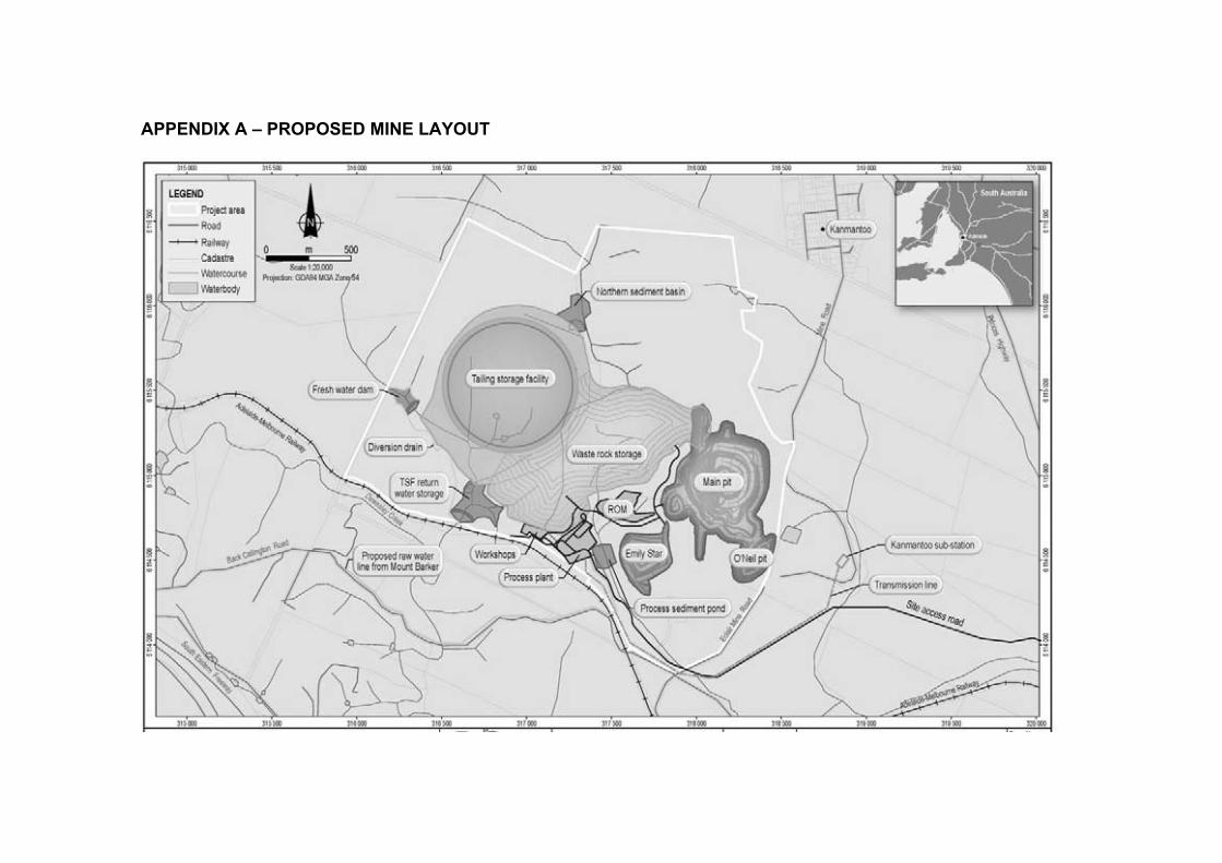
APPENDIX A – PROPOSED MINE LAYOUT

Appendix B
Hillgrove Resources
Dust Impact Study Kanmantoo Copper Project
20060840RA3B Revision: A Date: 21/6/2007
Appendix B Dust Monitoring Results
�


Appendix C
Hillgrove Resources
Dust Impact Study Kanmantoo Copper Project
20060840RA3B Revision: A Date: 21/6/2007
Appendix C Emission Factors and Emission Rates
�

���������
�� ��
����
���
�����������
�� ��
�����
��������� � ��
���������
���
��� ��
����� ������ ��
������
������ ��
�����
��� �����
�!��
"� ���
��
����
#$"���
"�%��
����
�!�����
"�%����
�!�����
%�&'������
�!�����
%�&'����
�!�����
"�%�!�����
%�&'�!�����
(������
�����
�� ��
(�����
�����
�)) � ��
��"�
%�!�����
%�&'�!�����
"�%�!�����
%�&'�!�����
�����
���
���
�� ��
����
������
��
����
����
����
����
������
����
����
����
�����
����
�����
���
���
����
���
���
�����
����
����
�����
�� !
�"��
#�$
����
����
�� ��
����
������
��
���
���
���
����
����#
�����
���
�����
!�"
��#�
$���
���#
���
����
�����
���
���
����
���
���
�����
����
����
�����
�� !
�"��
#�$
����
���#
�� ��
����
������
��
���
���
���
����
����#
�����
���
�����
!�"
��#�
$���
���#
���
����
�����
���
���
����
���
���
�����
����
����
�����
�� !
�"��
#�$
����
����
%�
�����
�&���
��
���
�� ��
����
�����
����
���&
�� !
���
����
����
�����
����
�#��
�����
����
����
����
�� ��
����
�����
����
���&
�� !
����
�����
�&��
#���
�����
����
����
�����
�� !
�"��
#�$
�����
����
�� ��
����
�����
����
���&
�� !
����
�����
�&��
#���
�����
�#��
����
�����
�� !
�"��
#�$
�����
����
�� ��
����
�����
����
���&
�� !
����
�����
�&��
#���
�����
����
����
�����
�� !
�"��
#�$
����
����
�� ��
����
�����
����
���&
�� !
�#��
�����
�&��
#���
�����
����
����
�����
�� !
�"��
#�$
�#���
����
�� ��
����
�����
����
���&
�� !
����
�����
�&��
#���
����#
����
����
�����
�� !
�"��
#�$
�����
���#
�� ��
����
�����
����
���&
�� !
����
�����
�&��
#���
�����
�#��
����
�����
�� !
�"��
#�$
�����
����
�� ��
����
�����
����
���&
�� !
���
����
����&
��#�
����
�����
�����
���
�����
!�"
��#�
$��
������
�
'���
�����
������
��
��'�
����
������
(�&�
��
����
�����
����
�����
)��*�
��)��
�����
����
��#���
������
������
�����
���
�����
!�"
��#�
$���
������
���
*������
(������
���
�� �� �� �� �� �� �# �� �� ���
+������������
�� ����
����
��,
��"� �
�+�
�����������
�� ��
������
�����"� ��
�����������
�� ����
���
���- ����
���������
�� ��
�����%
� &&./'�!�����
����
����
����
����
�����
�����
�����
�����
����
����
����
����
���- ����
���������
�� ��
�����%
� &'�!�����
����
����
��#�
���#
����
����
�����
�����


�����������
�������
���
���������������
������
���������
������
���������
���
��������
�������
���
�����
�������
���
���
������"��
���
���
�������� !
"
���
���
������
���
#�����
������
����
#����������
����������
���
�������
��!"�$%�&��'
����������
���
��������
��!!()"�$%�&��'
��������
���
��
�� ���
����
�����
�����
�����
���
������
����
����
� ���� ���
�� �
!����
"��
�����
"��
�� �
����
�����
#���
��#
$������
$��
""%&
'��+
�����,�
�����
����
����
����
����
� ���� ���
����
���-
����
.�� #"�
���.
�!"�
����
����
����
�.�#
.�
��
/������
�'�0
+1��
0��
"/�
��
�� ���
���
�����
�����
�����
���
������
����
����
����
� �
�� �
��.��
"��
!����
"��.
�� �
����
�����
����
���
�����
�����
���/
���
�� ���
���
�����
�����
�����
���
�����
� ��
���
���.
��"��
!����
"��.
�� �
����
�����
����
���
2���
������
�'����1���
2"�
""%&
'��+
�����,�
�����
����
���
�+�
213 �
�+
����.
"���
��#�
"���
�� �
4 �
�����
1���
�5
�����
����
���
/������
�'��
0 �
�6"
/���
�� ���
���
�����
�����
�����
���
�����
���
���
�#7
���3��
7����.
��"��
!����
"��.
�� �
����
�����
����
���
8�0 �
�8��
��
�� ���
���
�����
�����
�����
���
�����
���
���
�#7
���3��
7�����
��"���
�����
"��
�� �
�����
1���
�5
����
���#
���
/������
�'��
�,����
%���
��
�� ���
���.
�����
�����
�����
���
�����
���
���
�#7
���3��
7�����
��"��
#����
"���
�� �
�����
1���
�5
���!�
����
!��
8��,������
�1�'
'�����
�1���
%���
��
�� ���
���.
�����
�����
�����
���
�����
���
���
�#7
���3��
7�����
��"��
#����
"���
�� �
�����
1���
�5
���!�
����
!��
2���
������
�'����1���
2"�
""%&
'��+
�����,�
�����
����
���
��.
+�2
13 �
�+
����.
"���
��#�
"���
�� �
4 �
�����
1���
�5
����
#���
�#
/������
�'��
�,����
%��
��
�� ���
���.
�����
�����
�����
���
�����
� ��
���
����
��"��
#����
"���
�� �
�����
1���
�5
�����
����
���
���������
�'�
��1
���
��
�� ���
����
�����
�����
�����
���
�����
� ��
���
���!
��"���
�.��
"���
�� �
������
��� ��
�����
.
5��
��
��� �
����
�'��
������
�������
���
��
�� ���
����
�����
�����
�����
���
�����
� ��
���
���!
��"���
�.��
"���
�� �
������
��� ��
�����
.
5��
��
��� �
���
������
������
���
�/�
��
�� ���
���
�����
�����
�����
���
����
����
����#�
� �
�� �
��.��
"��
!����
"��.
�� �
����
�����
����
���
2���
������
�'����
�����0
+11���
2"
""%&
'��+
�����,�
���
�����
� ��
����
�� �
+�2
13 �
�+
����.
"���
��#�
"���
�� �
4 �
����
�����
#���
��#
/������
�'��
�������
��6"
/�""
%&'�
�+�����,�
�����
����4
�����
���������
��!
� �
! �!
7���3�.
7����
."���
���!
"���
�� �
����
����
.���
�.�

Appendix 1B
Kanmantoo Copper Project Odour Assessment

Hillgrove Resources
Odour Impact Assessment
Kanmantoo Copper Project
Principal Contacts
Chris Purton
Johan Torringer
June 2007
Ref No 20060840RA2B

Table of Contents
Odour Impact Assessment
Kanmantoo Copper Project
20060840RA2B (2) Revision: B Date: 13/06/2007 Page: i
Table of Contents
Hillgrove Resources Odour Impact Assessment Kanmantoo Copper Project
1. Introduction 4 1.1 Location and Sensitive Receptors 4 1.2 The Relationship Between Climatology and Dispersion of Odour 5 1.3 Climatology 6 1.4 Existing Air Quality 7
2. Government Regulations 8 2.1 Odour Guideline Criteria 8 2.2 Human Response to Odour 8 2.3 Odour Sampling Guidelines 9 2.4 Separation Distances 9
3. Odour Sampling 10 3.1 Description of Odorous Part of the Concentration Process 10 3.2 Odour Sampling 10 3.2.1 Description of the Sampling Mine 11 3.3 Odour Intensity Assessment at the Sampling Mine 11 3.4 Odour Sample Results 12
4. Odour Dispersion Modelling 13 4.1 Odour Dispersion Modelling Methodology 13 4.2 Evaluation Generated Meteorology Data 13 4.3 Odour Emission Rates 15 4.4 Dispersion Modelling Results 16 4.5 Discussion 17
5. Conclusions and Recommendations 18 5.1 Conclusions 18 5.2 Recommendations 18
6. References 19 Tables Table 2.1 EPA Odour Guideline Criteria [1] 8 Table 3.1 Comparison of flotation chemistries 11 Table 3.2 Odour sample concentrations and odour emission rates 12 Table 4.1 Odour emission rates from flotation process 15 Table 4.2 Odour emission rates from TSF 15 Figures Figure 1.1 Overview mine location and sensitive receptors 5 Figure 1.2 Apr 2006 to Mar 2007 5949 hours Figure 1.3 00:00 to 09:00 Apr 2006 to Mar 2007 6 Figure 1.4 10:00 to 14:00 Apr 2006 to Mar 2007 Figure 1.5 15:00 to 23:00 Apr 2006 to Mar 2007 7

Table of Contents
Odour Impact Assessment
Kanmantoo Copper Project
20060840RA2B (2) Revision: B Date: 13/06/2007 Page: ii
Figure 4.1 Evaluation of TAPM generated meteorology 14 Figure 4.2 Result odour dispersion modelling 16 Appendices Appendix A Mine Site Layout Appendix B Odour Sample Results Appendix C Odour Sample Photographs


Introduction
Odour Impact Assessment
Kanmantoo Copper Project
20060840RA2B (2) Revision: B Date: 13/06/2007 Page: 4
1. Introduction
Tonkin Consulting was commissioned by Enesar Consulting on behalf of Hillgrove
Resources to undertake the odour impact assessment for the proposed Kanmantoo
copper project. The intention of the Kanmantoo copper project is to reopen and
expand the existing Kanmantoo copper mine.
The odour impact assessment for the Kanmantoo copper project considers odours
from the processing plant and tailings storage facility (TSF), the two main odour
sources of the proposed activities. The odour samples for the study were taken at a
mine in NSW of similar size and with similar flotation reagent chemistry.
1.1 Location and Sensitive Receptors
The Kanmantoo copper mine is located 1.2 Km south southwest of Kanmantoo and
3.5 Km northwest of Callington. An overview of the area, the location of the mine
and the locations of the sensitive receptors in the area are presented in Figure 1.1.
Sensitive receptors are all residential dwellings outside the mining lease.
The mine is located in the Mount Lofty Ranges on the ridgeline north of Macfarlane
Hill 3 km west of the Bremer Valley and about 1 km north of Dawesley Creek. The
topography in the area is best described as undulating hills and with sparse grazing.
The processing plant and the TSF will be located just to the west of Macfarlane Hill.
The proposed layout of the mining site is presented in Appendix A.


Introduction
Odour Impact Assessment Kanmantoo Copper Project 20060840RA2B (2) Revision: B Date: 13/06/2007 Page: 6
1.3 Climatology
A weather station on Macfarlane Hill has been in operation since April 2006. The location of the weather station is shown in Figure 1.1. A wind rose of the 5949 hours of data logged from April 2006 to March 2007 is presented in Figure 1.2. Note that the wind speed and direction sensors are at the non-standard height of 2 m above ground level. Figure 1.3 presents a wind rose for the hours 00:00 to 09:00 for this data. The weather station is located on a hill and the winds for this time of day are mostly gradient winds. For the winter seasons the majority of the gradient winds are northerly to westerly. For the summer seasons the majority of the gradient winds are westerly to southerly.
Figure 1.2 Apr 2006 to Mar 2007 5949 hours Figure 1.3 00:00 to 09:00 Apr 2006 to Mar 2007
NORTH
SOUTH
WEST EAST
3%
6%
9%
12%
15%
WIND SPEED (m/s)
>= 11.0
8.8 - 11.0
5.1 - 8.8
3.6 - 5.1
2.1 - 3.6
0.5 - 2.1
Calms: 5.58%
NORTH
SOUTH
WEST EAST
4%
8%
12%
16%
20%
WIND SPEED (m/s)
>= 11.0
8.8 - 11.0
5.1 - 8.8
3.6 - 5.1
2.1 - 3.6
0.5 - 2.1
Calms: 9.72%
Figure 1.4 presents a wind rose for the hours 10:00 to 14:00. In the summer seasons for day times the proportion of southerly winds is higher than for the winter seasons. This proportion of southerly winds is most likely the early onset of sea breezes. Figure 1.5 presents a wind rose for the hours 15:00 to 23:00. For the winter seasons the majority of the winds have westerly components associated with gradient winds. For the summer seasons the winds are almost exclusively southerly or south south-westerly sea breezes.

Introduction
Odour Impact Assessment Kanmantoo Copper Project 20060840RA2B (2) Revision: B Date: 13/06/2007 Page: 7
Figure 1.4 10:00 to 14:00 Apr 2006 to Mar 2007 Figure 1.5 15:00 to 23:00 Apr 2006 to Mar 2007
NORTH
SOUTH
WEST EAST
3%
6%
9%
12%
15%
WIND SPEED (m/s)
>= 11.0
8.8 - 11.0
5.1 - 8.8
3.6 - 5.1
2.1 - 3.6
0.5 - 2.1
Calms: 1.53%
NORTH
SOUTH
WEST EAST
5%
10%
15%
20%
25%
WIND SPEED (m/s)
>= 11.0
8.8 - 11.0
5.1 - 8.8
3.6 - 5.1
2.1 - 3.6
0.5 - 2.1
Calms: 3.20%
As can be seen in Figure 1.3 overnight conditions produce 9.7% of calm stable conditions which are characterized as the kind of conditions giving the highest odour concentrations due to poor dispersion. The plant site and TSF are located west of Macfarlane Hilll and cold air drainage from the site carrying odour is expected to drain with the topography to the south from the site and then southeast along the creek line depression towards the Bremer Valley. Poor dispersion conditions of concern apart from the calm conditions are the light overnight winds with south-westerly components pushing odour towards Kanmantoo.
1.4 Existing Air Quality
The Neutrog fertilizer factory is located east of Macfarlane Hill at the site of the previous mine processing plant from the mine operations in the 1970’s and is shown in Figure 1.1. Neutrog is a significant odour source in the area. Discussions with Mr Chris Harris from the EPA revealed that odour complaints are mainly associated with cold air drainage situations draining odorous air eastward from the Neutrog site at the foot of the hill on the eastern side of Macfarlane Hill to nearby residences.

Government Regulations
Odour Impact Assessment
Kanmantoo Copper Project
20060840RA2B (2) Revision: B Date: 13/06/2007 Page: 8
2. Government Regulations
2.1 Odour Guideline Criteria
The SA EPA odour criteria are population density dependent and based on the
principle of the possibility of exposure of sensitive individuals and the potential for
odour complaints increase with population. The odour exposure is expressed as
Odour Units (OU) for a 3 minute averaging period for the 99.9 percentile which is
equal to the 9th highest concentration predicted for each receptor a year of hourly
data.
Table 2.1 EPA Odour Guideline Criteria [1]
Number of People Odour Units
(3 min avg, 99.9%)
2000 or more 2
350 or more 4
60 or more 6
12 or more 8
Single residence (less than 12) 10
There are 12 residential houses to the southwest of the mine site. Assuming 4
residents per house brings the population in this direction from the mine to 48
people. There are no population statistics for Kanmantoo but the town is about the
same size as Callington. In 2001 the population of Callington was 185 people Error!
Reference source not found.. The population of Kanmantoo does not exceed 350
people. According to the SA EPA Odour Guideline the assessment criteria to the
south west of the mine should be 8 OU and the assessment criteria in the direction
towards Kanmantoo should be 6 OU. As noted in Section 1.4 the Neutrog Fertilizer
Factory is a significant odour source, and provides a high background odour to the
area. Therefore the EPA has requested that the Kanmantoo Copper Mine achieves
an odour target of 2 OU (3 minute average, 99.9% non-exceedance level arising
from mining operations.
2.2 Human Response to Odour
An approximate guide to the average population response to odours measured in
accordance with AS/NZS 4323.3:2001 [2] is:
� 1 OU is where half the members of a calibrated Reference Panel [2] can
detect an odour with certainty when the odour is presented by an
olfactometer
� 2 OU – some people will smell something

Government Regulations
Odour Impact Assessment
Kanmantoo Copper Project
20060840RA2B (2) Revision: B Date: 13/06/2007 Page: 9
� 6 OU – most people will recognize an odour
� 10 OU – unpleasant odours may be considered offensive by most people
2.3 Odour Sampling Guidelines
In accordance with the EPA guidelines on odour assessments the odour sampling at
the NSW copper mine was carried out at full production and under normal operating
conditions [1]. The odour samples were analysed in accordance with AS/NZS
4323.3:2001 [2].
2.4 Separation Distances
There are no specified separation distances for mining in the SA EPA draft
separation guidelines [3] with respect to odour. However, the separation distance for
mining, due to dust, is 500 m from mining operations to the nearest dwelling.

Odour Sampling
Odour Impact Assessment
Kanmantoo Copper Project
20060840RA2B (2) Revision: B Date: 13/06/2007 Page: 10
3. Odour Sampling
Odour sampling was carried out at a copper mine in the Cobar Region in NSW. The
mine at which the sampling work was undertaken wished to remain anonymous. The
odour sampling results were used to derive odour emission rates representative of
the processes at the proposed Kanmantoo copper mine.
3.1 Description of Odorous Part of the Concentration Process
The odours of concern considered in this report derive from the reagents used in the
concentration flotation process. Flotation is the main means treatment which ore
particles are separated from gangue (unmineralised) material in the ore. Separation
is achieved in slurry containing the ground ore and specialised reagents. Ore
particles are carried to the top of the flotation tanks on the surface of air bubbles.
The collector reagent bonds with the metal surface of the ore granules and has a
hydrophobic end which repels the molecule from the water towards the air bubbles in
the slurry. At the surface in the flotation tank a layer of froth is formed by a frothing
agent creating a large surface area which carries the concentrated metal containing
ore over the rim of the flotation tank for collection and treatment in the next phase of
the concentration process.
Prior to the flotation step the reagents are mixed in a conditioning tank before
injection into the process slurry stream. The process stream undergoes primary,
secondary and tertiary flotation before the remaining waste is thickened and pumped
to the Tailings Storage Facility (TSF). The concentrated metal-containing ore is also
thickened before it is pressed dry.
The flotation ore slurry is dosed with lime to keep the pH at a level in which the
flotation reagents perform at their optimum with minimum waste. The concentration
of the odorous reagents is highest at the point of conditioning and declines through
the primary, secondary and tertiary flotation circuits leaving only trace amounts of
reagents in the thickened tailings stream.
3.2 Odour Sampling
The odour sampling program was put together based on previous experience of
odour sampling for the Angas Zinc Project in Strathalbyn. Odour samples were taken
of:
� the conditioning tank – point of highest reagent concentration;
� the primary flotation circuit – highest reagent concentration in the flotation
step;
� the dry surface of the TSF – replicate samples were taken;

Odour Sampling
Odour Impact Assessment
Kanmantoo Copper Project
20060840RA2B (2) Revision: B Date: 13/06/2007 Page: 11
� the wet surface of the TSF – replicate samples were taken.
Replicate samples were taken at the TSF. The TSF is the least odorous step in the
process but the largest in area and hence likely to be the most significant odour
source. Single samples were taken of the flotation process which is part of the
process with the highest odour concentration but the sources are small in area and
hence less significant compared to the TSF.
3.2.1 Description of the Sampling Mine
A copper mine with similar chemistry was selected for the odour sampling. The
sampling mine also had a similar production volume to the proposed Kanmantoo
mine. The concentration plant at the sampling location was located in the open and
not enclosed. The concentration plant was elevated on a steel structure allowing
gravity feed in the process stream. The concentration, primary, secondary, and
tertiary flotation, was carried out in 30 flotation cells. The open tops of the flotation
cells were 2.2 x 2.6m. The concentration of the reagent mix was 30 to 35 g per tonne
of ore. A comparison of the flotation chemistry at the two mines is given in Table 3.1.
Table 3.1 Comparison of flotation chemistries
Proposed Flotation Reagents
Kanmantoo copper mine
Reagents used at the NSW copper
mine
Collector 3418A – a dialkyl dithiophosphinate RTD 948 – a mixture of dithiophosphate
and carbamothic ester
Frother MIBC – methyl isobutyl carbinol MIBC – methyl isobutyl carbinol
Process conditions pH 9 to 11.5 depending on ore type pH 9 to 11.5 depending on ore type
3.3 Odour Intensity Assessment at the Sampling Mine
The odour intensity assessment was made accordingly to the self explanatory
German VDI standard [4] odour intensity scale:
0. Not detectable
1. Very weak
2. Weak
3. Distinct
4. Strong
5. Very strong
6. Extremely strong
At the time of the sampling an odour intensity assessment around the site of the
concentration plant and the TSF was undertaken. The odour intensity assessments
were taken in the morning when conditions were clear with calm to light winds, with
the wind picking up after sunrise. At the concentration plant standing immediately
next to or on top of the odour source tanks the odour strength varied in calm to 0.5

Odour Sampling
Odour Impact Assessment
Kanmantoo Copper Project
20060840RA2B (2) Revision: B Date: 13/06/2007 Page: 12
m/s light wind conditions between weak and strong. At about 50 m down wind from
the concentrate plant at ground level in light wind conditions the odour from the
reagents was dispersed to non detectable. At the TSF odour was only detectable as
intermittent non detectable to very weak to weak if kneeling down towards the mud
surface just at the edge downwind the TSF and downwind from a tailings outlet in 0.5
m/s light wind. 5m downwind from the edge of the TSF at 2 m above the ground the
odour had dispersed to non detectable to very weak. The concentrate storage at the
sampling mine was an open pad on to which a batch of pressed concentrate of 9 %
moisture level was dumped from the press above every 7 minutes. The odour from
this process and the concentrate it self were considered negligible compared to the
ambient odour in the concentrate plant.
3.4 Odour Sample Results
The odour samples were analysed by The Odour Unit in Sydney within the 30 hr
sampling holding time. The results of the odour concentration analysis according to
AS/NZS 4323.3:2001 [2] are presented in Table 3.2 and the analysis record is
attached in Appendix B. The odour emission rates are presented in the odour
dispersion modelling section in Table 4.1 and Table 4.2.
Photographs of the sampling operation are presented in Appendix C.
Table 3.2 Odour sample concentrations and odour emission rates
Odour sample Odour sample
Concentration
(OU/m3)
Sampling gas
flow rate
(L/min)
Flux hood
sampling
area (m2)
Odour
emission rate
(OU/m2s)
1. Flotation conditioning tank 166 5 0.13 0.11
2. Primary flotation tank 166 5 0.13 0.11
3. TSF dry surface 181 7 0.13 0.17
4. TSF dry surface
(replicate of sample no 3)
76 7 0.13 0.07
5. TSF wet surface 76 7 0.13 0.07
6. TSF wet surface
(replicate of sample no 5)
70 7 0.13 0.06

Odour Dispersion Modelling
Odour Impact Assessment
Kanmantoo Copper Project
20060840RA2B (2) Revision: B Date: 13/06/2007 Page: 13
4. Odour Dispersion Modelling
4.1 Odour Dispersion Modelling Methodology
The Kanmantoo mine is located in hilly surroundings in the south Mount Lofty
Ranges with the Bremer Valley to the east of the mine site. Special attention was
paid to the parameters and factors influencing complex terrain dispersion conditions
in the computer generation of meteorological data for the modelling.
Site specific surface and upper air data files were generated using the CSIRO TAPM
(The Air Pollution Model) software and datasets. The dispersion modelling was
performed with CALPUFF due to the complex terrain.
TAPM was set up with 5 nested grids with the grid spacings 30,000m, 10,000m,
3,000m, 1,000m and 500m for a grid of 41 x 41 grid points covering an area of 20 km
by 20 km for the innermost grid. This grid size included the Mount Lofty Ranges
ridges on both sides of the Bremer Valley and allowed for capturing of drainage flows
in the Bremer valley. Soil moisture content, deep soil temperatures and sea surface
temperatures were adjusted to local conditions and land use was adjusted with better
detail than provided in the default TAPM database. Thirteen surface and upper air
data files were extracted from the 500m grid spacing grid located around the grid
capturing key variations in the wind field. For the generation of the CALMET
meteorological data file a finer grid of 161 x 161 grid points with a grid spacing of
125m over the 20 km by 20 km domain was comprised of high resolution topography
data allowing CALMET to derive fine scale topography adjustments, such as
redirections around higher ground and cold air drainage, to the wind field. This
methodology ensured high resolution recreation of the wind field of the dispersion
modelling domain. The odour dispersion modelling was conducted for a 5 km by 5
km grid centred on the mine using the odour emission rates from the odour sampling.
The modelling assumed the initial ground level elevations for the odour sources of
the TSF. As the TSF rises and the odour source surface is elevated it is expected
that the dispersion will improve.
4.2 Evaluation Generated Meteorology Data
The TAPM generated wind speeds and directions were compared with the
Macfarlane Hill observations using wind roses for various times of day. These wind
rose comparisons are shown in Figure 4.1. Given that the Macfarlane Hill wind
observation were taken at the non-standard height of 2 m instead of 10 m, the
agreement between the two sets of wind roses is reasonable.

Odour Dispersion Modelling
Odour Impact Assessment Kanmantoo Copper Project 20060840RA2B (2) Revision: B Date: 13/06/2007 Page: 14
Figure 4.1 Evaluation of TAPM generated meteorology TAPM generated for 2003 12 months Macfarlane Hill Observations 5949 hours
NORTH
SOUTH
WEST EAST
3%
6%
9%
12%
15%
WIND SPEED (m/s)
>= 11.0
8.8 - 11.0
5.1 - 8.8
3.6 - 5.1
2.1 - 3.6
0.5 - 2.1
Calms: 0.00%
NORTH
SOUTH
WEST EAST
3%
6%
9%
12%
15%
WIND SPEED (m/s)
>= 11.0
8.8 - 11.0
5.1 - 8.8
3.6 - 5.1
2.1 - 3.6
0.5 - 2.1
Calms: 5.58%
00:00 to 09:00 00:00 to 09:00
NORTH
SOUTH
WEST EAST
3%
6%
9%
12%
15%
WIND SPEED (m/s)
>= 11.0
8.8 - 11.0
5.1 - 8.8
3.6 - 5.1
2.1 - 3.6
0.5 - 2.1
Calms: 0.00%
NORTH
SOUTH
WEST EAST
4%
8%
12%
16%
20%
WIND SPEED (m/s)
>= 11.0
8.8 - 11.0
5.1 - 8.8
3.6 - 5.1
2.1 - 3.6
0.5 - 2.1
Calms: 9.72% 10:00 to 14:00 10:00 to 14:00
NORTH
SOUTH
WEST EAST
3%
6%
9%
12%
15%
WIND SPEED (m/s)
>= 11.0
8.8 - 11.0
5.1 - 8.8
3.6 - 5.1
2.1 - 3.6
0.5 - 2.1
Calms: 0.00%
NORTH
SOUTH
WEST EAST
3%
6%
9%
12%
15%
WIND SPEED (m/s)
>= 11.0
8.8 - 11.0
5.1 - 8.8
3.6 - 5.1
2.1 - 3.6
0.5 - 2.1
Calms: 1.53% 15:00 to 23:00 15:00 to 23:00
NORTH
SOUTH
WEST EAST
4%
8%
12%
16%
20%
WIND SPEED (m/s)
>= 11.0
8.8 - 11.0
5.1 - 8.8
3.6 - 5.1
2.1 - 3.6
0.5 - 2.1
Calms: 0.00%
NORTH
SOUTH
WEST EAST
5%
10%
15%
20%
25%
WIND SPEED (m/s)
>= 11.0
8.8 - 11.0
5.1 - 8.8
3.6 - 5.1
2.1 - 3.6
0.5 - 2.1
Calms: 3.20%

Odour Dispersion Modelling
Odour Impact Assessment
Kanmantoo Copper Project
20060840RA2B (2) Revision: B Date: 13/06/2007 Page: 15
The TAPM generated meteorological data was then processed to give CALPUFF
meteorological files using the CALMET pre-processor. An evaluation of the
CALPUFF meteorological data file showed that CALMET processed the TAPM
generated 500 m grid space meteorological data well and adapted the wind field for
the finer 125 m grids space recreating topography induced wind diversions and slope
flows as would be expected to be observed.
4.3 Odour Emission Rates
The odour emission rates were calculated from the sample odour concentrations, the
sampling gas flow rate and the flux hood sampling area. For the odour emission
rates for the flotation process the highest odour concentration from the conditioning
tank was assumed for the conditioning tank, primary, secondary, tertiary and the
thickener. The odour emission rate from the TSF was averaged from the results of
the four samples taken on the wet and dry surface of the TSF. The three last
samples (samples No 4-6) showed a very good consistency in the result whereas
sample No 3 showed the highest concentration in the sampling. The difference in
concentration is however within the olfactometry error margin. This deviation was
accounted for by averaging of the sample concentrations for samples no 3 to 6 for
the calculation of the odour emission rates. The odour emission rates from the
flotation process and the TSF are presented in Table 4.1 and Table 4.2.
Table 4.1 Odour emission rates from flotation process
Odour source Size of area (m2) Odour emission rates
(OU/m2s)
Odour emission rates
(OU/s)
Conditioner, primary &
secondary flotation
79.1 0.11 8.7
Tertiary flotation 37.2 0.11 4.1
Thickener 278 0.11 30.6
Table 4.2 Odour emission rates from TSF
Odour source Size of area (m2) Odour emission rates
(OU/m2s)
Odour emission rates
(OU/s)
Average odour emission rate
from wet and dry surfaces
420,000 0.17 71,400

Odour Dispersion Modelling
Odour Impact Assessment
Kanmantoo Copper Project
20060840RA2B (2) Revision: B Date: 13/06/2007 Page: 16
4.4 Dispersion Modelling Results
Figure 4.2 Result odour dispersion modelling
The result of the odour dispersion modelling is presented in Figure 4.2. The units are
in Odour Units for 3 minute averages for the 99.9th percentile. Figure 4.2 shows that
out of the 16 sensitive rural receptors identified around the Kanmantoo mine the
predicted odour level is 2 OU for one receptor and 1 OU for three receptors. All
other residential receptors will have less than 1 OU (3 minute, 99.9%) attributable to
the mining operations.

Odour Dispersion Modelling
Odour Impact Assessment
Kanmantoo Copper Project
20060840RA2B (2) Revision: B Date: 13/06/2007 Page: 17
4.5 Discussion
The extent of the odour impact area is highly affected by the topography. Macfarlane
Hill, on which the pit of the existing mine is located, acts as a barrier sheltering the
sensitive residential receptors east of the mine from odour impacts from the mine
processing plant. The pattern of the mine odour impact shows no interference or
addition to the odours from the Neutrog plant which occasionally causes complaints
from residents to the east of Macfarlane Hill. Further, the odour impacted area to the
south of the TSF is caused by cold air drainage following the drainage lines.
The odour from the flotation process is negligible compared with the odour from the
larger TSF area, which is not particularly strong in any event.
Figure 4.2 indicates that one dwelling is predicted to experience 2 OU (3 minute
average, 99.9% non-exceedance level) while all other dwellings are less than 2 OU.
Section 2.2 shows that most people cannot recognise an odour of less than 6 OU.

Odour Dispersion Modelling
Odour Impact Assessment
Kanmantoo Copper Project
20060840RA2B (2) Revision: B Date: 13/06/2007 Page: 18
5. Conclusions and Recommendations
5.1 Conclusions
The EPA odour Guideline [1] is not exceeded at any neighbouring residence, neither
is the target of 2 OU suggested by the EPA. This reduced odour target is due to the
existing high odour background of the locality originating from the Neutrog Fertilizer
factory.
The odour impact study predicts that the highest odour level a sensitive residential
receptor (dwelling) would be subjected to due to mining operations is 2 OU (3 minute
average, 99.9%) at one house. Three other houses are predicted to experience
between 1 OU and 2 OU, 3 minute average, 99.9% non-exceedance level. All other
houses in the locality are less than 1 OU.
The definition of 1 OU is odour detectable by 50% of a calibrated Reference Panel
while 2 OU is a very weak barely detectable odour which is generally
unrecognisable. The modelling predicts this odour level for a 3 minute average
period to occur for 9 hours out of a year of 8760 hours.
The above predicted odour impacts do not include existing background odour in the
locality.
5.2 Recommendations
The odour modelling showed compliance by the mining operations with the EPA
target for the Kanmantoo Copper Mine. The odour modelling also showed that
surrounding dwellings would not detect recognisable odours from the mine.
Adherence to normal operation conditions will keep odour emissions stable and low.
Apart from that, the storage area of reagents is recommended to be well ventilated.

References
Odour Impact Assessment
Kanmantoo Copper Project
20060840RA2B (2) Revision: B Date: 13/06/2007 Page: 19
6. References
[1] Odour assessment using odour source modelling, EPA Guidelines, SA EPA, EPA
373/06, February 2006
[2] AS/NZS 4323.3:2001, Stationary source emissions – Determination of odour
concentration by dynamic olfactometry, Standards Australia, 55 pp
[3] Consultation Draft Guidelines for Separation Distances, SA EPA, August 2000
[4] VDI 3882/1, Olfactometry – Determination of odour intensity, Part 1, October
1992, VDI Handbuch Reinhaltung der Luft, Vol 1

Appendix A
Odour Impact Assessment
Kanmantoo Copper Project
20060840RA2B (2) Revision: B Date: 13/6/2007
Appendix A Mine Site Layout

Mine
Roa
d
PrincesHighway
Eclair
Mine
Roa
d
South Eastern Freeway
Back Callington Road
Adelaide-Melbourne Railway
Adelaide-Melbourne Railway
Dawesley Creek
Dawesl
ey Cree
kKanmantoo
Tailing storage facility
Waste rock storage
Main pit
Process sediment pond
Northern sediment basin
Fresh water dam
Diversion drain
Proposed raw waterline from Mount Barker
TSF returnwater storage
Workshops
Process plant
ROM
Transmission line
Kanmantoo sub-station
Site access road
O‘Neil pitEmily Star
N
Projection: GDA94 MGA Zone 54
0 500mScale 1:20,000
LEGEND
Project areaRoadRailwayCadastre
WaterbodyWatercourse
South Australia
Adelaide
315 000 315 500 316 000 316 500 317 000 317 500 318 000 318 500 319 000 319 500 320 000
315 000 315 500 316 000 316 500 317 000 317 500 318 000 318 500 319 000 319 500 320 000
6 114
000
6 114
500
6 115
000
6 115
500
6 116
000
6 116
500
6 114
000
6 114
500
6 115
000
6 115
500
6 116
000
6 116
500
Project layout 5HillgroveResources_KanmantooGIS
5000_02_F005_GIS_AI
22.08.2007Figure No:Date:
Job No:
MXD:
Kanmantoo Copper Project
Hillgrove Resources LtdSource:Cadastre, roads, rail and drainage from DEH (optimum scale 1:50,000)Project layout from Hillgrove Resources

Appendix B
Odour Impact Assessment
Kanmantoo Copper Project
20060840RA2B (2) Revision: B Date: 13/6/2007
Appendix B Odour Sample Results

THE ODOUR UNIT PTY LIMITEDSuite G03 Bay 16
Australian Technology Park Locomotive Street
Eveleigh NSW 1430
Phone: +61 2 9209 4420 Facsimile: +61 2 9209 4421 Email:[email protected]: www.odourunit.com.au ABN: 53 091 165 061
The Odour Unit Pty Ltd Issue Date: 13.11.2003 Revision: 3
ACN 091 165 061 Issued By: SB Revision Date: 12.07.2005
Form 06 – Odour Concentration Results Sheet (V02) Odour Measurement Manual Approved By: TJS
1
Form 06 - Sydney Laboratory
Odour Concentration Measurement Results
The measurement was commissioned by: Organisation Tonkin Consulting Telephone +61 (8) 8273 3100
Contact Johan Torringer Facsimile +61 (8) 8273 3110 Sampling Site Not supplied Email [email protected]
Sampling Method Isolation Flux Hood Sampling Team Tonkin Consulting
Order details: Order requested by J. Torringer Order accepted by S. Hayes
Date of order - TOU Project # 1273 Order number - Project Manager A. Balch
Signed by J. Torringer Testing operator D. Hepple
Investigated Item Odour concentration in odour units ‘ou’, determined by sensory odour concentration measurements, of an odour sample supplied in a sampling bag. Odour character is also assessed, however, this assessment is not covered by AS4323.3:2001.
Identification The odour sample bags were labelled individually. Each label recorded the testing laboratory, sample number, sampling location (or Identification), sampling date and time, dilution ratio (if dilution was used) and whether further chemical analysis was required.
Method The odour concentration measurements were performed using dynamic olfactometry according to the Australian Standard ‘Determination of Odour Concentration by Dynamic Olfactometry AS/NZS4323.3:2001. The odour perception characteristics of the panel within the presentation series for the samples were analogous to that for butanol calibration. Any deviation from the Australian standard is recorded in the ‘Comments’ section of this report.
Measuring Range The measuring range of the olfactometer is 22� � � 2
18 ou. If the measuring range was
insufficient the odour samples will have been pre-diluted. The machine is not calibrated beyond dilution setting 2
17. This is specifically mentioned with the results.
Environment The measurements were performed in an air- and odour-conditioned room. The room temperature is maintained between 22
oC and 25
oC.
Measuring Dates The date of each measurement is specified with the results.
Instrument Used The olfactometer used during this testing session was: ODORMAT SERIES V02
Instrumental Precision
The precision of this instrument (expressed as repeatability) for a sensory calibration must be
r � 0.477 in accordance with the Australian Standard AS/NZS4323.3:2001. ODORMAT SERIES V02: r = 0.2015 (9/10 August, 2006) Compliance – Yes
Instrumental Accuracy
The accuracy of this instrument for a sensory calibration must be A � 0.217 in accordance with the Australian Standard AS/NZS4323.3:2001. ODORMAT SERIES V02: A = 0.1882 (9/10 August, 2006) Compliance – Yes
Lower Detection Limit (LDL)
The LDL for the olfactometer has been determined to be 16 ou (four times the lowest dilution setting)
Traceability The measurements have been performed using standards for which the traceability to the national standard has been demonstrated. The assessors are individually selected to comply with fixed criteria and are monitored in time to keep within the limits of the standard. The results from the assessors are traceable to primary standards of n-butanol in nitrogen.
Date: Thursday, 22 March, 2007 Report Number / Panel Roster Number: SYD20070322_022
A. Balch Manager, Odour Impact Assessment
D. HeppleAuthorised Signatory

THE ODOUR UNIT PTY LIMITED
The Odour Unit Pty Ltd Issue Date: 13.11.2003 Revision: 3
ACN 091 165 061 Issued By: SB Revision Date: 12.07.2005
Form 06 – Odour Concentration Results Sheet Odour Measurement Manual Approved By: TJS
2
Odour Sample Measurement Results
Sample Location
TOU
Sample
ID
Sampling
Date &
Time
Analysis
Date &
Time
Panel
Size
Valid
ITEs
Nominal
Sample
Dilution
Actual
Sample
Dilution
(Adjusted for
Temperature)
Sample Odour
Concentration
(as received,
in the bag)
(ou)
Sample Odour
Concentration
(Final, allowing
for dilution)
(ou)
Odour Character
#1 – FlotationConditioning Tank
SC 7012621.03.200707:16
22.03.200711:09
4 8 -- -- 166 166 Fishy
#2 – PrimaryRougher
SC 7012721.03.200708:08
22.03.200711:39
4 8 -- -- 166 166 Oily
#3 – TailingsStorage Facility –Dry Surface
SC 7012821.03.200709:30
22.03.200712:10
4 8 -- -- 181 181 Dirty
#4 – TailingsStorage Facility –Dry Surface
SC 7012921.03.200709:43
22.03.200713:17
4 8 -- -- 76 76 Gassy
#5 – TailingsStorage Facility –Wet Surface
SC 7013021.03.200710:20
22.03.200713:48
4 8 -- -- 76 76 Gassy
#6 – Tailings Dam– Not specific
SC 7013121.03.200710:34
22.03.200714:21
4 8 -- -- 70 70 Gassy

THE ODOUR UNIT PTY LIMITED
The Odour Unit Pty Ltd Issue Date: 13.11.2003 Revision: 3
ACN 091 165 061 Issued By: SB Revision Date: 12.07.2005
Form 06 – Odour Concentration Results Sheet Odour Measurement Manual Approved By: TJS
3
Odour Panel Calibration Results
Reference Odorant
Reference Odorant
Panel Roster
Number
Concentration of
Reference gas
(ppb)
Panel Target Range
for n-butanol
(ppb)
Measured
Concentration
(ou)
Measured
Panel Threshold
(ppb)
Does this panel
calibration
measurement
comply with
AS/NZS4323.3:2001
(Yes / No)
n-butanol SYD20070322_022 49,600 20 � � � 80 724 69 Yes
Comments All samples were collected by Tonkin Consulting.There was no deviation from the analysis method prescribed in the Australian standard AS/NZS4323.3:2001.
Disclaimer Parties, other than TOU, responsible for collecting odour samples hereby certify that they have voluntarily furnished these odour samples, appropriately collected andlabelled, to The Odour Unit Pty Limited for the purpose of odour testing. The collection of odour samples by parties other than The Odour Unit Pty Limitedrelinquishes The Odour Unit Pty Limited from all responsibility for the sample collection and any effects or actions that the results from the test(s) may have.
Note This report shall not be reproduced, except in full, without written approval of The Odour Unit Pty Limited.
END OF DOCUMENT

Appendix C
Odour Impact Assessment
Kanmantoo Copper Project
20060840RA2B (2) Revision: B Date: 13/6/2007
Appendix C Odour Sample Photographs

Hillgrove ResourcesOdour sampling for Kanmantoo Copper Project
Odour Impact Assessment
JOB NO. : 2006.0840
Sample No2 Primary flotation
Date: 1/5/2007Drawn: JNTJob No 2006.0840
Sample No1 Conditioning tank
Sample No3-4 TSF dry surface Sample No5-6 TSF wet surface

Appendix 1C
Kanmantoo Copper Project Greenhouse Gas Assessment

Hillgrove Resources
Kanmantoo Copper Project
Greenhouse Gas Emissions
Principal Contacts
Chris Purton
June 2007
Ref No 20060840RA1B

Table of Contents
Hillgrove Resources
Kanmantoo Copper Project – Greenhouse Gas Emissions
20060840RA1B Revision: B Date: 13/06/2007 Page: i
Table of Contents
Hillgrove Resources Kanmantoo Copper Project Greenhouse Gas Emissions
1. Introduction 1
2. GHG Emissions Associated with Mine Construction 2
3. Mining Operations 3
4. Rehabilitation of the Mine 4
5. Total Greenhouse Gas Emissions over the Mine Life 5
6. Greenhouse Gas Mitigation Strategies 6
6.1 Government Policies 6
6.2 Internal Mine GHG Mitigation Stategies 6
7. References 7
8. Acknowledgements 8
Tables Table 3.1 Mining Operations: Greenhouse Gas Emissions for One Year and Eight Year Totals 3
Table 4.1 Rehabilitation GHG Emissions over the Total Mine Life. 4
Table 5.1 Estimates of Greenhouse Gas Emissions over Total Mine Life 5
Appendices Appendix A Greenhouse Gas Emissions from Mine Construction Processes Appendix B Greenhouse Gas Emissions from Annual Mining Operations


Introduction
Hillgrove Resources
Kanmantoo Copper Project – Greenhouse Gas Emissions
20060840RA1B Revision: A Date: 13/06/2007 Page: 1
1. Introduction
The Australian Government encourages Australian organisations to calculate and
report greenhouse gas emissions arising from their activities. To assist such
organisations, the Department of the Environment and Water Resources, Australian
Greenhouse Office, has published the AGO Factors and Methods Workbook[1]. The
latest edition of this publication was published in December 2006.
This report on estimated greenhouse gas (GHG) emissions from the proposed
Kanmantoo Copper Mine was based on the emission factors from the AGO
Workbook [1]. GHG emissions are reported in this study as tonnes of carbon dioxide
equivalent (tCO2-e).
This report calculates three types of emissions, called “Scopes” in the AGO
Workbook, from sources within the boundary of the mine.
� Scope 1 covers direct GHG emissions from within the boundary of the
mine. These are chiefly from fuel consumption by mobile sources. GHG
emissions from transport of concentrate to the shipping terminal are also
included;
� Scope 2 covers indirect GHG emissions from the consumption of
purchased electricity produced by an external organisation;
� Scope 3 includes all other indirect GHG emissions that are a consequence
of an organisation’s activities but are not from sources owned or controlled
by the organisation. Scope 3 GHG emissions are usually only reported by
organisations in the Greenhouse Challenge Plus programme.
Scope 3 emissions include estimates of GHG emissions for the following categories:
� Employees commuting to and from work;
� Emissions of the external electricity generator associated with losses of
electricity from the transmission and distribution network;
� Extraction, production and transport to the mine of purchased fuels
consumed at the mine;
There are a number of other minor Scope 3 categories which have not been included
in this report due to insufficient data.
The estimation of greenhouse gas emissions has been divided into the Construction,
Mining and Rehabilitation phases. GHG emissions for each Scope are reported for
each of these phases.

GHG Emissions Associated with Mine Construction
Hillgrove Resources
Kanmantoo Copper Project – Greenhouse Gas Emissions
20060840RA1B Revision: A Date: 13/06/2007 Page: 2
2. GHG Emissions Associated with Mine Construction
The construction of the Kanmantoo Copper Mine is expected to take about 12
months. During the construction of the mine, processing plant, tailing storage facility
(TSF) and internal haul roads, the following sources of GHG emissions were
estimated from fuel consumption estimates supplied by Hillgrove Resources:
� Transport of materials to the site was estimated to use 100,000L of fuel
(assumed to be 95,000L diesel and 5,000L petrol);
� Onsite construction was estimated to use 60,000L of petrol and 500,000L of
diesel;
� Construction subcontractors commuting to the site were estimated to use
180,000L of petrol (100 vehicles each using 1800L in a year of commuting).
These GHG emissions are Scope 3 emissions;
� Electricity use in offices, amenities, etc, was estimated to use 561 MWh
during the year of construction, based on 24 hour, 365 days continuous
operation.
The resulting construction greenhouse gas emissions were:
� 1,763 tCO2-e (Scope 1);
� 485 tCO2-e (Scope 2 – all electricity);
� 351 tCO2-e (Scope 3).
Where tCO2-e is tonnes of carbon dioxide equivalent.
Detailed GHG emission calculations and emission factor references for mine
construction emissions are given in Appendix A.

�
�
�
�
������������ ���
����� ���� ����
������� �� ���� ��������� ������������� ���
����� !��"#$%& �� ����� �'�"� (��'�# )��)���*� �����+�
+% ������������ ���
���������� ������ � �������� ���������������� �� ��� ���������� �
��������������� ������������������� �� ����������� ���� ���� ���� ��
���� � ���!���� ������ �������������� ����������������� ���"���#�
��������������� �����$����������������� �����������% �� ������ ������ �
��������������
�
& ����� ��� �� �� ���� �#!'''!'''� ���(�����%�����������������!���������
)'!'''� ���(�����%���������� �� ���&������ ���� �������������� ������
���� ��������� ����������� �� ����� �� ��*������+�� ����*�%��� ��%��� �,�
��������� ��� ��� �-)�� (���!�����--�� (�����������.!�����#�#�� (�����������)��
�
/��� ������� ���������������� �����%��������������0��1�����/2��
�
���� ��� ���������������%����� ���������!�����%��� ���� ����� �������%�
������� ��������������������3�-��
�
�
,�-��+%#������������� ��'���� ������������� ���. ����/����&�
������/��, �����
�
� tCO2-e (Scope 1)
tCO2-e (Scope 2)
tCO2-e (Scope 3)
"������0���� #3!.#3� 3)!)-)� -'!,#.�
, �����������1�.�2 �3��4�0���� -)4!.),� 3-'!563� )5!'-5�
�
�
����� ����� ��������������������������%���������� ��������������������
��������1�����/��
�
�

Rehabilitation of the Mine
Hillgrove Resources
Kanmantoo Copper Project – Greenhouse Gas Emissions
20060840RA1B Revision: A Date: 13/06/2007 Page: 4
4. Rehabilitation of the Mine
Rehabilitation will be progressive throughout the life of the mine. After mining
ceases, the remaining mine workings will be shaped, covered with top soil and re-
vegetated. Rehabilitation work is expected to be completed about three months after
cessation of mining.
The greenhouse gas emissions from the rehabilitation works, based on estimated
fuel usage to cover and revegetate the site, are given in Table 4.1.
Table 4.1 Rehabilitation GHG Emissions over the Total Mine Life.
Fuel Type Fuel Use
(L)
tCO2-e
(Scope 1)
tCO2-e
(Scope 3)
Diesel 1,500,000 4,050 450


Greenhouse Gas Mitigation Strategies
Hillgrove Resources
Kanmantoo Copper Project – Greenhouse Gas Emissions
20060840RA1B Revision: A Date: 13/06/2007 Page: 6
6. Greenhouse Gas Mitigation Strategies
6.1 Government Policies
The Kanmantoo Copper Mine is most likely to be affected by the carbon trading
schemes proposed by the Australian Commonwealth Government and the various
Australian State Governments.
All State and Territory Governments have formed a National Emissions Trading
Taskforce (NETT) to formulate a carbon trading scheme to be introduced at the end
of 2010. No details of this scheme are available at the present time.
The Commonwealth Gorvernment has also proposed a carbon trading scheme to
start in 2014. No details of this scheme are available.
The South Australian Government has a Climate Change and Greenhouse
Emissions Reduction Bill before State Parliament at the time of writing. The Bill will,
if passed, set a target to reduce greenhouse emissions to 60% of emissions at 1990
by 2050. An interim target of no greater than 108% of 1990 emissions during the
period 2008 to 2012 is also proposed. A secondary target of 20% of all electricity
consumed to be generated from renewable sources by 2014 is also proposed.
Overseas experience suggests that energy prices will increase at more than the rate
of inflation when carbon trading schemes are introduced.
6.2 Internal Mine GHG Mitigation Stategies
Possible Greenhouse Gas Emission mitigation strategies include:
� The normal commercial imperative to reduce fuel and energy inputs to the mining process
� Trading in carbon credits (when such a scheme is in place in Australia)
� Use efficient siting and design of power efficient lighting
� Ensuring that equipment is correctly sized for supply to the job site to reduce transmission losses
� Reducing haul distances
� Participation in revegetation programmes
� Ensuring that vehicles and equipment are mechanically sound, serviced regularly and fitted with appropriate emission control equipment
� Changing to low carbon fuels such as compressed natural gas (CNG) or Aquadiesel if practical

References
Hillgrove Resources
Kanmantoo Copper Project – Greenhouse Gas Emissions
20060840RA1B Revision: A Date: 13/06/2007 Page: 7
7. References
1. AGO Factors and Methods Workbook, Australian Government, Department of the
Environment and Heritage, Australian Greenhouse Office, December 2006, 49pp.

Acknowledgements
Hillgrove Resources
Kanmantoo Copper Project – Greenhouse Gas Emissions
20060840RA1B Revision: A Date: 13/06/2007 Page: 8
8. Acknowledgements
Estimates of mining production tonnages and electricity and fuel consumption totals
for mining operations at the Kanmantoo Copper Mine were supplied by Hillgrove
Resources.

Appendix A
Hillgrove Resources
Kanmantoo Copper Project – Greenhouse Gas Emissions
20060840RA1B Revision: B Date: 13/06/2007
Appendix A Greenhouse Gas Emissions from Mine Construction Processes

Appendix A
Hillgrove Resources
Kanmantoo Copper Project – Greenhouse Gas Emissions
20060840RA1B Revision: B Date: 13/06/2007
Construction Phase (12 Months)
Transport Materials to Site:
Fuel Type
Fuel Use
(L)
tCO2-e
per Year
(Scope 1)
tCO2-e
per Year
(Scope 3)
Petrol 5,000 12 2
Diesel 95,000 257 29
Ref [1]: AGO Factors and Methods Workbook - December 2006
GHG EF for Transport Fuels in Table 3
Onsite Construction:
Fuel Type
Fuel Use
(L)
tCO2-e
per Year
(Scope 1)
tCO2-e
per Year
(Scope 3)
Petrol 60,000 144 18
Diesel 500,000 1,350 150
Ref [1]: AGO Factors and Methods Workbook - December 2006
GHG EF for Transport Fuels in Table 3
Electricity (Onsite Offices):
Plant
Installed
kW excl.
stand-by
Utilisation
%
Load
Factor
Average
kWh
Consumed
Yrly MWh
Consumed
(8760 hrs)
tCO2-e
per Year
(Scope 2)
tCO2-e
per Year
(Scope 3)
Office and Amenities, etc 64 100 1 64 561 485 99
Ref [1]: AGO Factors and Methods Workbook - December 2006
GHG EF for Electricity generated in SA in Table 5: Scope 2 (0.865) and Scope 3 (0.177)
Construction Subcontractor Commuting:
Fuel Type
Fuel Use
(L)
tCO2-e
per Year
(Scope 1)
tCO2-e
per Year
(Scope 3)
Petrol 180,000 0 54
No of Subcontractors: 100 Fuel/yr (L): 1800
Ref [1]: AGO Factors and Methods Workbook - December 2006
GHG EF for Transport Fuels in Table 3 [1]
Construction GHG Emission Summary:
tCO2-e
(Scope 1)
tCO2-e
(Scope 2)
tCO2-e
(Scope 3)
1,763 485 351

Appendix B
Hillgrove Resources
Kanmantoo Copper Project – Greenhouse Gas Emissions
20060840RA1B Revision: B Date: 13/06/2007
Appendix B Greenhouse Gas Emissions from Annual Mining Operations


Appendix 2
Kanmantoo Copper Project Visual Assessment Report

1
������������� ���������� �������� ����������� ���������
Prepared for Enesar Consulting Pty Ltd 28 August 2007
WAX DESIGN Ltd Pty ACN 117 346 264
41 Regent Street Kensington Adelaide 5068 SA
T 08 8463 0886 F 08 8364 0821
Contact: Warwick Keates and Brett Grimm
© August 2007

Content
3
Section
01 Executive Summary 4
02 Methodology 5
03 Landscape Character 7
04 Viewpoint Assessment Quantified Visual Effect 14
05 Viewer Sensitivity 27
06 Conclusion and Opinion 28
Appendices
Appendix A: Assessment Mapping (topography, viewpoint locations and photo graphic
survey reference, viewshed)
Appendix B: Photomontages
Appendix C: Methodology and Project Scoping
Appendix D: GRIMKE Matrix (based on the HASSELL Matrix, 2001 and WAX Matrix, 2006)
Appendix E: Glossary
Appendix F: Relevant Experience (Warwick Keates and Brett Grimm)
Appendix G: References and Endnotes

01 Executive Summary
4
This report has been prepared by WAX Design in association with Brett Grimm for Enesar
Consulting Pty Ltd to assess the potential visual impact of the proposed redevelopment of
the Kanmantoo Copper mine. The aim of the report is to evaluate the existing visual
character of the proposed mine development and provide an assessment of the potential
visual effect.
Hillgrove Resources Limited (HRL) is proposing to redevelop the old Kanmantoo Copper
Mine, 1.5 km South West of Kanmantoo Township, 44 km East of Adelaide in South Australia.
The Indicated and Inferred Resources at Kanmantoo are 33.44 Mt at 0.9% copper and 0.2 g/t
gold within the proposed project area. The current scope of the project is for mining and
processing of the copper - gold mineralisation to produce concentrate over an initial mine
life of eight years.
The landscape character surrounding the proposed mine has a defined agricultural land use.
There is limited vegetation, with isolated tree groups to creeks and valleys and extensive
grazing creating a bare land cover to the ridges and hills, punctuated with powerlines,
roads, buildings and small scale quarrying operation. Surrounding the mine are a number of
small townships including, Kanmantoo, Callington and Dawesley which are connected with
numerous roads, both sealed and unsealed.
The topography of the area is defined by a series of ridgelines that run in multiple directions
to the north, east and west, with wider valley forms to the south. The topography visually
encloses the landscape restricting views to the development mine from location greater
than 10km and only allowing views from elevated location within the surrounding landscape.
The proposed mine will consist of one main open pit, a small satellite pit, waste rock
storage facility, tailing facility (Integrated Waste Landform) and associated infrastructure.
Processing of the ore is proposed to be by conventional crushing, grinding and flotation.
Figure 1 represents the concept plan of the proposed redevelopment of the mine site.
Figure 1 Proposed redevelopment of the Kanmantoo mine (produced by Enesar Consulting Pty Ltd)

01 Executive Summary
5
A detailed assessment has quantified the degree of visual change within the context of the
existing landscape and visual impact created by the existing waste rock dump. Therefore,
the proposed redevelopment does not result in the introduction of a new visual effect
(mining) within an agricultural landscape, rather a proportional increase in an existing visual
effect.
Generally, the visual effect of the proposed mine is defined as slight (increasing to
moderate). This is measured as a visual change of 22.5% to 35% that would be experienced
in areas to the north, west, west, south and south west. Taking account of the visual impact
produced by the existing mine, the actual degree of additional visual impact caused by the
mine expansion is likely to be in the range of 7.5% (or negligible referring to table 4.1).
This visual effect will be further reduced by progressive mitigation measures to the
Integrated Waste Landform, including rounding the leading angle of repose (western edge)
to from a convex form to provide landscape integration and reduce the defined visual edge
that is created by the IWL. The IWL design will consider rounding the profile of the top of
the waste rock area to provide a landform that reflects the undulating landscape of low
rises and saddles between valleys and creeks. Extensive tree planting will be considered at
the base of IWL as well as any benching areas and promontories to provide a contextual
landscape character to the IWL and surrounding areas.

02 Methodology
6
This assessment report provides a detailed overview of the landscape character of the
surrounding area in order to articulate an impression, sufficient to assess the suitability of
the development with regards to the visual effect within the local (1-5km), sub-regional (5-
15km) and regional areas (>15km). The assessment considers the development as an
extension of an existing mine facility. Consequently the base line landscape character is
inclusive of the existing open cut pit and waste rock dump and tailing storage facility
landscape modifications.
2.1 Detailed Visual Effect Assessment
The assessment of the visual effect on the surrounding environment is undertaken using the
GrimKe Matrix (Appendix D) and photomontages (Appendix B) to simulate the visual
character of the mine expansion in the landscape. The assessment methodology has been
produced with detailed reference to other visual assessment criteria being used within
Australia and worldwide.
The extent of visual effect was identified on site, using a Global Positioning System (GPS).
Using the GPS, the location and extent of the mine proposal is plotted as a series of
'waypoints', using longitude and latitude, elevation and distances to provide geo-referenced
data. The surrounding area was then surveyed for landscape character zones. A hand held
GPS and bearing compass was used to calculate the bearing and distance between the
viewpoint and the mine area (open cut pit, Integrated Waste Landform, and associated
infrastructure). This methodology is used to assess where the development is in the
landscape and whether it is visible. Other references are used, such as buildings, trees and
landmarks to confirm the location of the proposed development in the landscape (refer to
appendix D for a detailed illustrated example of the process).
To provide an understanding of the overall visual effect of the proposal on the landscape,
the following criteria are used to quantify the landscape character and visual effect from
specific key viewpoints. Photomontages are also analysed on site, to assist with the
assessment of the visual effect on the existing environment. The following aspects of
landscape character and visual effect are assessed as part of the GrimKe Matrix:
1 Topographic Relief (the complexity of the land that exists as part of the underlying
landscape character)
2 Vegetation Cover (the extent to which vegetation is present and its potential to
screen and filter views)
3 Infrastructure and Built Form (the impact of development on landscape and visual
character)
4 Cultural and Landscape Value (quantification of recognised planning overlays)
5 Percentage of visual absorption (ability of landscape to absorb and screen the visual
change).
6 Horizontal visual effect (spread of the development in the visual landscape).
7 Vertical visual effect (height of the development in the active visual landscape).
8 Distance of visual effect (distance between viewpoint and closest waypoint of the
proposed development).
Two separate assessments are conducted. Firstly items 1-4 above are assessed for the
existing landscape character. The values out of 5 are aggregated to form a baseline figure

02 Methodology
7
out of 20. The higher the value the more sensitive the landscape is to changes in the
existing visual character.
Items 5- 8 above are rated from 1 to 5 with 1 being minimal visual effect and 5 significant
visual change caused by the proposed development. The scores are than aggregated out of
20 to provide an indication of the significance of the visual effect from selected viewpoints
and the degree of visual change on the landscape. This figure is then represented as a
coefficient to be multiplied by the existing landscape character value.
Appendix D contains a detailed explanation of the GrimKe Matrix including the methodology,
criteria of assessment and techniques used to calculate the measured values.
2.2 Field Work Study
The detailed site assessment was conducted on 29 March and 18 April 2007. During both
visits, weather conditions were cloudy (low level) with some rain, overcast and occasional
periods of sunshine.

03 Landscape Character
8
3.1 Surrounding General Landscape Character
The surrounding landscape character is described as a highly modified agricultural
landscape, punctuated with powerlines, roads, buildings and small scale quarrying
operation. Throughout the subregional area there is limited vegetation cover, with sporadic
tree groups to creeks and valleys and extensive grazing creating a bare land cover to the
ridges and hills in the area. Within the local and sub-regional areas are a number of small
townships including, Kanmantoo, Callington and Dawesley. Numerous roads, both sealed and
unsealed, that provide access through the surrounding landscape, link these towns.
The underlying topography of the area is defined by a complex series of dominant ridgelines
that run in multiple directions around the site (Figure 2 Appendix A). To the north are a
series of closely spaced narrow ridges running east to west. To the east are two dominant
parallel ridges, wider in form, that run the entire length of the local, sub-regional area. The
wider valleys, which lie in between these ridges, contain large areas of vegetation, which
provide screening to the wider landscape. Kanmantoo is located within one of the low lying
valley forms, visually enclosed by vegetation and topographic relief.
To the south are a complex series of ridges and valleys around the Old Princes Highway road
corridor. The predominant alignment of the ridgelines is in an east west direction with
numerous creeks running north south connecting to the Bremer Valley. To the west are
north south ridges and the engineered road corridor of the South Eastern Freeway (Princes
Highway).
This varied topography creates an enclosed sub-regional landscape and visual envelope
surrounding the development site. This ensures that views to the development site do not
exist from more distant locations (beyond 10km).
The development site is visible in the landscape due to the previous mining operations that
have taken place. These operations include an open cut pit, waste rock dump, tailing
storage facility, buildings and other associated infrastructure. The visual effect produced by
the mine and existing waste rock dump is experienced to the north west, west, south west
and south east. This is due to minimal vegetation coverage, framed views along valley
corridors from the south east and elevated viewpoints from the north west, which allow
views across the landscape to and from the mine site.
The sub regional and regional area has a distinct horizontal undulating visual and physical
landscape character. The rolling context of the wider ridges contrast with the more incised
valleys and creeks to the west of the development site. The over riding horizontal forms are
reinforced by the remnant vegetation, which extend along creeks and valleys. Figure 2
Appendix A illustrates the undulating complex nature of the topography within the sub
regional area.
3.2 North
(Refer to Figure 3, Appendix A for geographic locations of photographic survey).
The dominant land use to the north is pastoral in character with grazed paddocks creating
cleared hillsides with small groups of vegetation to valleys and creeks. The sub regional area
is open in visual character to the north with little screening provided by remnant
vegetation. The topography to the north is defined by closely spaced narrow ridgelines that
run east west. These ridges have an undulating form with low lying valleys formed between
elevated ridges, which enclose the field of view.

03 Landscape Character
9
Around the intersection of Sawpit Gully Road and Harrogate Road [North] the landscape character of undulating ridges punctuated with remnant vegetation continues. While the ridges around the Harrogate Road area are elevated, the layering of surrounding ridges and vegetation produces a visually enclosed landscape to the south.
North of Kanmantoo [North East of the development site] the landscape between ridges is visually enclosed. This is demonstrated by the visual landscape around Proctor Road and the Kanmantoo Bluestone Quarry (Figure 4). The visual character of the surrounding landscape is defined by the adjacent topography with no views to the existing mine and development site (Figure 5). Only from elevated locations within agricultural paddocks and private land is the site visible (Figure 6).
Figure 4 Proctor Rd, view to bluestone quarry. Figure 5 Screened views towards the development
Dawesley is located (North West) of the development site on The Old Princes Highway. Residential properties are positioned towards the road with street trees and garden boundary vegetation, screening views beyond the framed road corridor. Around the township of Dawesley the topography is complex with interconnected ridges and valleys creating a dynamic landscape with fi ltered views as a result of the relationship between topography and vegetation.
Ironstone Range Road is an unsealed road located to the west within the sub-regional area. The elevation of the road produces an open visual aspect with views across the low-lying ridges and valleys to the south and east . From the road the mine site and particularly the waste rock dump are visible from a number of locations (Figure 7).
Figure 6 View to the development site from private land. Figure 7 Long distant views to the development site

03 Landscape Character
10
3.3 South
The landscape of the Bremer Valley defines the southern sub-regional area. The topography
has a complex undulating landform that creates a dynamic visual character of open and
enclosed views. The land cover is grazed open paddocks with isolated stands of vegetation
or individual trees, particularly associated with watercourses.
The town of Callington is located within the Bremer Valley. The low lying location of the
town and surrounding vegetation creates an enclosed visual context, with no views to the
existing mine site. The town has a dense urban form with small plots and a tight road grid.
There is no discernible Main Street or town centre with numerous destinations throughout
the town, including a hotel, local store and petrol station, tea room and other dispersed
businesses. The properties are typically located facing towards the roads with few views or
elevated positions to appreciate the surrounding landscape (Figure 8).
North of the town, towards the existing mine, the vegetation associated with the town
diminishes being replaced by an open rolling agricultural landscape that is typical of the
sub-regional area.
From the edge of Callington at the intersection of Callington Road and The Old Princes
Highway [South East] part of the existing open pit wall is visible. This creates a defined
visual effect, producing a human modified scarring of the landscape, which has been subject
to mining and extraction operations (Figure 9). The road corridor between Callington and
Kanmantoo (The Old Princes Highway) runs over a series of ridges creating elevated views
towards the existing mine site. However the local ridges, particularly MacFarlane Hill screen
the existing waste rock dump.
Further north east of Callington is a wide valley basin between the major north south ridges
of the surrounding Mount Lofty Ranges. The lack of tree cover within the area means that
the mine and the resulting visual effect are visible through the local and the sub regional
area.
The extent of buildings and impact of infrastructure within the south eastern sub-regional
area increases with numerous farm buildings, powerlines, roads and fence lines crisscrossing
and punctuating the modified pastoral landscape. Small quarrying operations create notable
visual elements creating contrasting forms, colours and land use to the agricultural
landscape.

03 Landscape Character
11
Figure 8 Callington streetscape character Figure 9 View towards mine site with open pit visible
3.4 East
To the east around Kanmantoo the amount of vegetation increases along the Kanmantoo Valley. There are notable stands of remnant vegetation to hillsides and creeks as well as numerous large plantations. The low-lying landscape means that remnant trees screen the local area with few views to the wider area and the surrounding ridges.
The town of Kanmantoo is physically and visually enclosed (due to the topography and vegetation screening). This landscape character continues to the northern edge of the town (Figure 10). The southern edge of the town is also enclosed by the interrelation of landform and vegetation. Properties are orientated east west perpendicular to the main road alignment and the underlying residential grid. The majority of properties are located within the wide low lying, well vegetated valleys of the eastern sub-regional area, where the relationship of elevation, ridges and vegetation limits views to the mine.
From elevated sect ions east of Kanmantoo the existing excavated face of the open pit is visible (Figure 11). This landscape element is seen as a discrete colouration within the hillside surrounded by heavily vegetated slopes and escarpments. The main residential development of Kanmantoo is located within the Valley and does not extend to the surrounding ridges where the open pit is visible. It is only from more exposed ridges that the open pit and surrounding landscape is evident.
Figure 10 Enclosed views towards the mine site Figure 11 Filtered views from elevated aspects of Kanmantoo

03 Landscape Character
12
To the East is an extremely modified landscape devoid of signif icant vegetation. The landscape is punctuated with small areas of open cut mining (quarrying) farm buildings, roads and pipeline infrastructure. Views to the west are enclosed by the rising topography of the dominant ridgeline adjacent to Kanmantoo. The landscape has a more wooded character with numerous stands of eucalypts associated with the hillside and revegetation work conducted on the existing tailings storage facility.
Of note, particularly around Kanmantoo, is the impact of the (Murray River Pipeline) water pipeline, pump stations and powerlines, which combined with the residential and urban character of the town, creates a highly modified rural/rural township character (Figures 12 and 13).
Figure 12 Water pipeline infrastructure Figure 13 Highly modified human influence landscape
3.5 West
The topography to the west is defined by north south oriented ridges and the engineered landscape of the South Eastern Freeway (Princes Highway). The surrounding landscape character is defined by the pronounced undulating ridges, which produce topographic variat ions forming promontories and rolling hills that extend over the landscape. This landform is punctuated by numerous valleys and creeks creating a complex visual field (Figure 14).
The layering of remnant trees combines to provide a patchwork of vegetation, interspersed with open areas of pasture. The intensity of the vegetation increases along creeks and where areas of revegetation have been undertaken, with limited vegetation to ridgelines (Figure 15).

03 Landscape Character
13
Figure 14 Complex visual foreground and mid ground. Figure 15 Limited vegetation except for creeks and valleys.
In some of the low lying valleys views are contained to a short field of view. Extensive vegetation within these valleys along creek lines provide a natural landscape amenity (Figure 16)
Figure 16 Lower- lying creek valleys.
The existing waste rock dump is visible within the landscape, primarily because of the western escarpment of the dump. The angle of repose and plateau to the top of the dump, form a distinct visual contrast to the surrounding rolling undulated landscape. The revegetat ion of the waste rock dump provides some mitigation to the north of the existing development, reducing in part the engineered form of the waste rock dump construction. To a lesser extent the dump is visible due to its colouration. The variation in colour to the surrounding landscape does provide a visual cue to its location. These factors enable viewers to identify the waste rock dump within the landscape.

03 Landscape Character
14
The elevated location of Ironstone Ridge Road provides panoramic views across the adjacent
ridges and valleys to the south and towards the existing mine site. The visual envelope to
the east is defined by the distant ridgelines that mark the eastern edge of the Mount Lofty
Ranges. These dominant ridges, which extend south, create a defined horizon line. The
topographic features of the local and sub-regional area are below the elevation of the
Mount Lofty Ranges. The result of this relationship is a defined visual envelope where the
local landscape elements (ridges, hills, the waste rock dump and pit walls) are set against
an elevated landscape backdrop. This removes the potential for sky-lining to occur and
reduces potential visual effects.
The South Eastern Freeway provides a major access corridor from which the existing mine
can be seen. Numerous cuttings and embankments define the visual character along the
road alignment. The associated roadside vegetation and engineered topography creates a
dynamic visual environment, with distant views along the road corridor enclosed by the
roadside vegetation in some areas and expansive glimpsed views as the road crosses
embankments. The mine is visible travelling south within two sections of about 800-1000m
of the road corridor, due to the speed of travel being approximately 100 kilometers per hour
(legal speed limit), the time of visual effect would be in the order of 30 to 40 seconds for
each visible portion. The combination of low ridges, limited tree cover and an elevated road
alignment provides opportunities to see the existing waste rock dump. This visual effect
needs to be considered in terms of the existing landscape character, which is highly
modified with extensive grazing, limited vegetation coverage, various powerlines, train
tracks and pipelines crisscrossing the landscape and the occasional farm building
punctuating the underlying topography.
The landscape character remains consistent throughout the western sub-regional area,
particularly along Ironstone Range Road. The landscape to the west shares the same
topographic variations as other local and sub-regional areas; however the distinct lack of
trees produces panoramic views from elevated locations. Any screening of views and
resulting visual character is not produced by the interrelationship of vegetation and
topography, but by the landform alone.
3.6 Local (Mine Area)
Within the local area in and around Back Callington Road, numerous ridges orientated north
west to south east; provide elevated vantage points from where the waste rock dump
becomes a dominant landscape feature due to its scale, form, lack of vegetation and
proximity on the southern side. The closely spaced ridges and valleys of the area create a
dynamic visual context. The visual character rapidly changes depending on the relationship
of topography and viewpoint. Consequently, expansive views occur along ridges, contrasted
by visually enclosed low lying valleys with views focused along secondary creeks and
tributaries.
Travelling along Back Callington Road, within close proximity to the mine lease, the waste
rock dump forms a dominant visual element. Due to the lack of revegetation and angle of
repose on the southern side of the waste rock dump, the angular form and flat plateau on
top contrast with the surrounding landforms. The colouration of the rock also provides a
contrast to the dry grassland typical of the area (Figure 17).

03 Landscape Character
15
Figure 17 Contrast in form and colour of the waste rock dump and undulating topography
The local landscape is typical of the area having an undulating topographic form and little vegetation cover. The landscape is defined by the distant ridgelines of the Mount Lofty Ranges to the east. Pockets of vegetation are scattered throughout the local area, predominantly to the north of the waste rock dump along, creeks and plantation areas to the north east associated with remediation works to the tailings facility of the existing mine.
To the south and west is a rail corridor that passes to the edge of the site. The relative posit ion of the rail track and waste rock dump (approximately 300 meters) ensures that visual impact will be experienced along the majority of the south western side of the site. Macfarlane Hill provides screening of the open pit, which is not visible from the western sub regional area.

04 Viewpoint Assessment Quantified Visual Effect
16
As part of the landscape assessment four viewpoints were identified as typical
representations of the landscape and visual character of the area. Photomontages were
developed from each viewpoint to demonstrate the potential visual effect that will result
from the development of the Kanmantoo Copper Project and the degree of visual change
that will occur. These viewpoints were assessed using the GrimKe Matrix as discussed in
section 2 and detailed in Appendix D. The matrix is used to quantify both the existing
landscape character and the visual effect of the development. Refer to Appendix A for the
location of viewpoints and GPS geographic coordinates and Appendix B for the
photomontages.
The matrix considers key aspects of the existing landscape such as relief, vegetation, built
form and infrastructure; as well as cultural and landscape value. These aspects produce an
assessment value out of 20. This provides a baseline measurement of the landscape
character from which the degree of visual effect can be assessed. The matrix also provides a
framework by which to quantify key aspects of the visual impact such as absorption,
horizontal and vertical effect; and distance to the development form, from the viewpoint.
Aspects such as horizontal and vertical impact and distances are surveyed on site.
Absorption is measured using Photoshop are an area measure of the absorption
characteristics of the landscape. For clarity, the photomontages in Sections 4.2 to 4.5 have
be coloured to illustrate the relative positions and absorption of the existing waste rock
dump, the proposed Integrated Waste Landform and the proposed pits.
The visual assessment is then combined with the landscape value to produce a measurement
that represents the degree of visual change, that is to say, the extent to which the
development will alter the landscape. This is measured as a percentage change (see below)
and is accompanied by a descriptive reference to qualify the visual effect.
Table 4.1
Descriptive Qualification of Visual Effect Percentage Value of Visual Change
Severe (80-100%)
Substantial (60-80%)
Moderate (40-60%)
Slight (20-40%)
Negligible* (0-20%)
The following illustrates the landscape assessment and visual effect resulting from the
Kanmantoo Copper Project (more detailed information regarding the GrimKe Matrix is
provided in appendix D).
4.1 Viewshed analysis
As illustrated and discussed the landscape of the sub regional area is complex in topographic
relief. Undulating ridges and valley forms, which contain the fields of view to approximately
3-4 kilometers, with a few exceptions, encircles the development site. To the north west of
the site some elevated aspects provide expansive views towards the south, south east
towards the development site.

04 Viewpoint Assessment Quantified Visual Effect
17
To assess the field of view in relation to topographic relief (vegetation can not be modelled
due to inconsistencies in modelling densities of canopy structures) a digital terrain model
was produced and a viewshed mapped using GIS software (Figure 18). From this assessment
it is possible to predict likely areas that will experience considerable visual impact. Further
ground truthing enables the selection of ‘typical worse case scenario’ viewpoints for the
detailed assessment.
Figure 18 (Appendix A) illustrates the geographic location of the viewpoints and viewshed
analysis. As can be seen, the extent of the visual impact is localised around the mine lease
project area and from elevated ridges. The four viewpoints selected represent areas of
public access, within close proximity to dwellings, which may be subject to visual effects
and are typical of the sub regional area. The detailed assessment is based on the 8 year life
time of the project hence the photomontages represent the evolution of the project with
possible revegetation.
4.2 Viewpoint 1 (Ironstone Range Road – South of Petwood)
(Refer to Appendix B for photomontage plates)
From Viewpoint 1, the existing waste rock dump can be identified in the landscape due to
its linear profile and the angle of repose of the western escarpment. The proposed
Integrated Waste Landform (waste rock and tailing facility) will produce a gentle slope
profile of 15-20� and will be seen as an expansion to the existing landform. The current
height of the waste rock dump is 245 metres above sea level. The IWL expansion will also
result in an increase in height from the current waste rock dump of 20 meters. This
increases the potential for the IWL to project above the existing horizon line, in event sky-
lining and will require careful consideration of the profile to minimise visual impact (see
Section 4.5.1). The expansion of the mining operations will also result in a proportional
removal of Macfarlane Hill, adjusting the depth of field and developing a series of pit walls,
which will be visible from Viewpoint 1 and the wider western sub-regional area. The
removal of a proportion of Macfarlane Hill will allow distant views to the background
landscape south of Callington.
The visual effect created by the mine expansion will appear in the landscape as a
progressive alteration of the physical and visual character of the area. The full extent of
visual change will only be experienced at the completion of the project. Even then, the full
impact of the mine and IWL will be mitigated by the landform design and the progressive
revegetation of the site. Figure 19 and 20 show the change in visual effect and the
landscapes ability to absorb (Table 4.1) the existing mine and proposed redevelopment.
Figure 19 Existing mine site visual effect and landscape absorption (refer to table 4.3).

04 Viewpoint Assessment Quantified Visual Effect
18
Figure 20 Proposed redevelopment visual effect and landscape absorption capacity (refer to table 4.4).
Table 4.2 Existing landscape character
Assessment Value Description
Relief 3 56%. of the existing mine facility is screened by the complexity
of the local and sub-regional (foreground mid-ground)
topography, which provides a dynamic interesting view.
Vegetation Coverage 1 15% of the field of view is remnant vegetation
Infrastructure and Built Form 5 15-20% transmission line and rail corridor as well as farming
infrastructure built form.
Cultural and Landscape Value 1 3.5% due to heritage properties through out the sub-regional
area, including a number of State heritage Listed building
within an 8km radius. Of note there is no heritage listed
buildings on the lease hold mine site.
Landscape Character 10
Table 4.3 Existing mine facility visual effect
Landscape Absorption 4 33% of the development is screened from this elevated
viewpoint.
Horizontal 1 85˚-94˚= 9˚ This equates to a visual effect of 7.5%
Vertical 1 1.2˚, which equates to 2.2%, extremely minimal from this
distance.
Distance 4 3.35km from the closest edge of the existing development
Visual Effect 10
Coefficient 0.5
Degree of Visual Change 25%

04 Viewpoint Assessment Quantified Visual Effect
19
Table 4.4 Proposed mine expansion visual effect
Landscape Absorption 3 Localized topographic elevated ridges screen 48% of the
development form.
Horizontal 2 73˚-100˚= 27˚ This equates to 22.5% of the active field of view
Vertical 1 1.3˚= 2.4% of the active field of view.
Distance 4 2.29km from the closest point of the proposed development
Visual Effect 10
Coefficient 0.5
Degree of Visual Change 25
Degree of additional visual change
from the existing mine facility
0% The proposed expansion will provide a slight
modification to the visual character of the region due
to increased horizontal effect and minimal vertical. In
relation to the existing visual effect this will be
insignificant due to increased landscape absorption
offsetting the increase in horizontal effect.
4.3 Viewpoint 2 (Princes Highway – North of Callington)
From Viewpoint 2 the existing mine is notable due to the excavated pit walls of the open
cut mine. The visual effect created by the existing waste rock dump and tailing storage
facility is not apparent due to the screening that is provided by Macfarlane Hill. The lack of
vegetation to the foreground and generally within the southern sub-regional area ensures
that the visual effect is seen when travelling along The Old Princes Highway, between
Callington and Kanmantoo. To the north, the existing vegetation associated with the
ridgelines adjacent to Kanmantoo provides a significant screen, creating a vegetated
backdrop to the area and reducing the visual effect of the pit walls.
The proposed expansion of the Kanmantoo mine will result in a modification of the landform
around the existing pit. The expansion of the pit to the west results in a proportional
removal of Macfarlane Hill. This will modify the landscape altering physically the landform
and visually the depth of field, resulting in the exposure of some distant views. This will
have the added effect of increasing the perceived extent of the mine, in terms of the
exposure to views of the open pit walls extending to the south. Evidently the process of the
mine cutting into Macfarlane Hill will provide a contrasting colour and texture associated to
the cutting of the rock face.
As with Viewpoint 1, the mine expansion is seen as a proportional increase of the existing
visual effect. Although, the proposal can be considered as a proportional increase, small-
scale mining, low grade ore stockpiles and other industrial operations have impacted the
majority of the existing Macfarlane Hill escarpment. The expansion will formalise the
existing processes that already occur on Macfarlane Hill and this will be mitigated to some

04 Viewpoint Assessment Quantified Visual Effect
20
extent following revegetation of the site. The ultimate visual impact is a proportional
increase, rather than the introduction of a new visual effect within the landscape.
The issues, described in relation to the visual effect experienced at Viewpoint 2, will
continue throughout the local and sub regional areas to the south, south east and south
west. Again this visual effect is considered in the context of a modified landscape
containing road and railway corridors, powerlines, farms and small scale quarrying
operations. Figures 21 and 22 refer to the existing visual effect of the mine site and the
proposed redevelopment respectively.
Figure 21 Existing mine site visual effect and landscape absorption (refer to table 4.6)
Figure 22 Proposed redevelopment visual effect and landscape absorption capacity assessment. (Refer to table 4.7)
Table 4.5 Existing landscape character
Assessment Value Description
Relief 4 67%, the landscape visual field has moderate variations
throughout the foreground, mid-ground and background.
Vegetation Coverage 2 20% of the field of view is composed of stands of remnant
eucalypt along the low lying valleys and small clusters along
ridgelines provide some sense of scale and form to the
landscape.
Infrastructure and Built Form 4 25-30%, the landscape is heavily modified from this aspect
with dwellings, the rail corridor and fence lines prominent in
the view.
Cultural and Landscape Value 1 3.5% due to heritage properties through out the sub-regional
area, including a number of State heritage Listed buildings. Of
note there are no heritage listed buildings within the mine
development project site.
Landscape Character 11

04 Viewpoint Assessment Quantified Visual Effect
21
Table 4.6 Existing mine facility visual effect
Landscape Absorption 3 57% of the existing open pit and waste rock dump is screened
by Macfarlane Hill and re vegetation to the top of the tailings
storage facility
Horizontal 1 (280˚-289˚=9˚) The horizontal visual effect from this aspect
equates to 7.5% of the field of view
Vertical 1 Minimal vertical effect within the active field of view. 2˚
Distance 4 2.72 km relatively close to the development form however the
undulating topography and Macfarlane Hill screen the waste
rock dump.
Visual Effect 9
Coefficient 0.45
Degree of Visual Change 24.75%
Table 4.7 Proposed mine expansion visual effect
Assessment Value Description
Landscape Absorption 3 52% of the development is screened. This is due to the
localized ridge line mitigating any perspective views into the
open cut pit.
Horizontal 2 268˚-291˚=23˚ This equates to a 19% horizontal visual effect.
Vertical 1 2.3˚= 4% vertical visual effect.
Distance 4 2.67km due to the excavation of Macfarlane Hill the open cast
pit will become slightly closer to the viewpoint with the waste
rock dump becoming a more dominant element in the mid
ground.
Visual Effect 10

04 Viewpoint Assessment Quantified Visual Effect
22
Coefficient 0.5
Degree of Visual Change 27.5%
Degree of additional visual change
from the existing mine facility
2.75% The new mine facility will have minimal change on the
visual amenity of the landscape from this viewpoint.
Due to the existing pit wall and waste rock dump being
prominent, the development will be seen as a slight
increase in visual effect. The horizontal effect will be
particularly evident. The ability of the landscape to
absorb the development will mitigate the potential of
the expansion to significantly impact the landscape
amenity.
4.4 Viewpoint 3 (Ironstone Range Road – South of Dawesley)
The proposed IWL will be seen as an extension of the existing mine landform. The current
angle of repose of the waste rock dump is visible. This notable landscape element will be
replaced by a more elongated landform, with a lower batter angle that mimics the existing
landscape character surrounding the mine site. The proposed 20 meter increase in height
will result in moderate sky-lining. This impact will be reduced through profiling, and doming
of the IWF to decrease the visual mass in response to the topographic context of the area.
The proposed IWL is located 5.4 km from the viewpoint within the undulating landscape
associated with the north western sub-regional area. The visual effect of the proposed IWL
is seen as a proportional expansion of the visual character produced by the existing waste
rock dump. From the north the impact of the open cut mining operation is minimal; and the
associated removal or modification of landform limited, due to the distance between the
viewpoint and the project site.
Extensively the IWL is seen as a narrow elongated visual element within the landscape. The
visual effect is reduced by vegetation to ridges and the screening provided by trees in and
around the viewpoint and adjacent to the road corridor. The patchwork effect created by
the surrounding landscape (background) in terms of colouration, patterning and form assists
in reducing the notability of the proposed waste rock dump expansion. The colouration of
the IWL from this distance is similar to the summer dry land grass of the paddocks due to
light and shade. This also provides continuity in relation to colouration. Figure 23 and 24
illustrate the existing landscape visual effects of the waste rock dump, whereas Figure 24
provides a representation of the proposed visual effect and landscape absorption capacity.
Figure 23 Existing visual effect and landscape absorption capacity (refer to table 4.9)

04 Viewpoint Assessment Quantified Visual Effect
23
Figure 24 Proposed redevelopment visual effect and landscape absorption capacity (refer to table 4.10)
Table 4.8 Existing landscape character
Assessment Value Description
Relief 3 The foreground and mid-ground are moderately complex in
topographic variety. The background becomes more uniform.
55%
Vegetation Coverage 2 25-35% of the field of view is occupied with vegetation
coverage typically eucalypt planting
Infrastructure and Built Form 4 20-25% of the field of view is occupied by built form and linear
infrastructure including fence lines and transmission lines.
Cultural and Landscape Value 1 3.5% due to heritage properties through out the sub-regional
area, including a number of State heritage Listed buildings
Landscape Character 10
Table 4.9 Existing mine facility visual effect
Landscape Absorption 2 Vegetation and topographic relief screen 67% of the existing
waste rock dump.
Horizontal 1 115˚-122˚= 7˚ this equates to a 6% horizontal visual effect.
Vertical 1 3.4˚ of the vertical field. This equates to 6%
Distance 3 The distance to the existing development waste rock dump is
5.67km.
Visual Effect 7
Coefficient 0.35
Degree of Visual Change 17.5%

04 Viewpoint Assessment Quantified Visual Effect
24
Table 4.10 Proposed mine expansion visual effect
Assessment Value Description
Landscape Absorption 3 55% of the proposed development will be screened by the
undulating topography.
Horizontal 1 114˚-126˚= 12˚ which equates to 10% of the horizontal field of
view.
Vertical 1 3.6˚ which equates to 6.5% of the vertical visual field
Distance 3 The development form will become closer to the viewpoint
corresponding to the expansion of the Integrated Waste
Landform. The distance from the viewpoint to the IWL will be
4.93km.
Visual Effect 8
Coefficient 0.40
Degree of Visual Change 2.5%
Degree of additional visual change
from the existing mine facility
5% The expansion of the mine to the west and north west
will bring the development closer to the viewpoint
limiting the landscapes ability to absorb the Integrated
Waste Landform. This increases the visual effect in
relation to the existing mine facility.
4.5 Viewpoint 4 (Back Callington Road – North of St Ives)
To the west the existing waste rock dump forms a distinct landscape feature within the local and sub regional area. The uniformity of the physical form and angle of repose, as well as the junction between the existing landform and the waste rock dump at its base, create an engineered landform that does not blend naturally with the surrounding landscape character. The revegetation that has occurred at the base of the dump does provide some mitigation especially in terms of its junction with the existing landscape. The limited vegetation cover on the top of the dump provides some mitigation reducing the linear effect and providing a vegetated skyline.
As described previously, the more elevated distant landscape of the Adelaide Hills and Mount Lofty Ranges assist in removing the potential sky-lining of the waste rock dump limiting the existing visual impact.
The lack of surrounding vegetation within the western landscape increases the visibility with variations in landform and elevations providing the most significant screening of the site.
Generally, the landscape character of the western areas around Viewpoint 4 is described as being complex in topographic relief with a uniform land cover and landform punctuated by undulating promontories and creek lines. The existing waste rock dump is seen as a different landscape character, in relation to the angle of repose of the waste rock dump, its materiality, texture, colour and form; and the applied engineering characteristics of the

04 Viewpoint Assessment Quantified Visual Effect
25
existing development. This appears as a notable contrast to the uniform colour and texture of the surrounding landscape character. The proposed redevelopment will be an extension to the visual effect of the waste rock dumps engineered form, however the open pit will be visible in the foreground, providing an additional form, colour and texture. Figures 25 and 26 illustrate the visual effect and landscape absorption capacity of the existing landscape and the proposed redevelopment respectively.
Figure 25 Existing mine site visual effect and absorption capacity calculation (refer to table 4.12).
Figure 26 Proposed redevelopment visual effect and landscape absorption calculation refer to table (refer to table 4.13).
Table 4.11 Existing landscape character
Assessment Value Description
Relief 3 The foreground and mid-ground view from this viewpoint is
relatively complex with north south oriented undulating
ridgelines and valley forms. Due to the elevated view, long
distant views provide a uniform backdrop. (55%)
Vegetation Coverage 2 30% of the landform is covered with remnant eucalypt copses
scattered across the ridgelines and low-lying depressions.
Infrastructure and Built Form 4 35% of the field of view is occupied with human modification.
The existing waste rock dump and scattered dwellings are
evident within the view.
Cultural and Landscape Value 1 3.5% due to heritage properties through out the sub-regional
area, including a number of State heritage Listed buildings,
however there is no heritage listed buildings on the project
site
Landscape Character 10
Table 4.12 Existing mine facility visual effect

04 Viewpoint Assessment Quantified Visual Effect
26
Landscape Absorption 4 39% of the existing development is softened and screened by
vegetation.
Horizontal 1 57˚-77˚=20˚ this equates to a 17% change to the visual field.
Vertical 1 1.8˚, which equates to 3% change to the vertical visual field.
The minimal vertical effect is relative to the elevated view
and adjacent valley, limiting the sky lining of the development
Distance 5 The viewpoint is 1.66km to the development.
Visual Effect 11
Coefficient 0.55
Degree of Visual Change 27.5%
Table 4.13 Proposed mine expansion visual effect
Assessment Value Description
Landscape Absorption 5 Vegetation and topographic relief screen 18% of the
development. Due to the close proximity and extent of
horizontal effect, there are minimal opportunities for
mitigating screening.
Horizontal 3 33˚-99˚=66˚ This is equivalent to 55% of the HOV
Vertical 1 2.3˚, which equates to 4.2% of the vertical visual field.
Distance 5 The development proposal will be considerably closer to the
viewpoint. The distance will be 1.10km
Visual Effect 14
Coefficient 0.7
Degree of Visual Change 35%
Degree of additional visual change
from the existing mine facility
7.5% The expansion of the mine will bring about a
considerable change in the horizontal visual effect. In
addition the limited existing vegetation in the
foreground limits the ability of the landscape to absorb
the proposed development.

04 Viewpoint Assessment Quantified Visual Effect
27
4.6 Degree of Visual Change
The scale and mass of the surrounding landscape is similar to the existing waste rock dump
and proposed IWL. This provides a physical and visual context for the mine operations,
which in turn affects the degree of visual impact
The degree of visual change is considered within the context of the existing landscape. This
is a highly modified agricultural landscape extending across a complex topographic relief
with limited or no tree cover. Within this landscape, the existing waste rock dump already
creates a noticeable visual effect. Consequently, the proposed redevelopment does not
result in the introduction of a new visual effect (mining) within an agricultural landscape,
rather a proportional increase in an existing visual character. For this reason, both the
existing and proposed mining projects have been assessed. Hence the proposed effects have
been assessed relative to the existing waste rock dump and mine.
Generally, the direct visual effect of the proposed development is defined as slight
(increasing to moderate) from the selected viewpoints in the sub-regional area. This is
measured as a visual change ranging from 22.5% to 35%. The landscape assessment would
suggest that this degree of visual effect would be experienced in local and sub-regional
areas to the north west, west, south and south west. The consistent landscape character,
as described in Section 3, ensures that the visual effect will only have minor variations as a
result of local topography and vegetation.
Referring to the existing mine visual effect, the actual degree of additional visual impact
caused by the mine expansion is likely to range to 7.5% (negligible referring to table 4.1).
This represents a more accurate assessment of the visual effect, as the measured degree of
visual impact is compared against an existing post mining landscape.
The elevation of the existing waste rock dump ensures that no sky lining occurs within the
sub regional area. The wider landscape of the Murray River basin and surrounding horizontal
rolling land forms a dominant backdrop, rather than the flat engineered profile of the
dump. This assists in reducing the existing visual effect of Integrated Waste Facility.
The expansion of the mine will result in an increased visual effect of the IWL within the sub regional area to the west. The development of the IWL will result in the screening of some of the adjacent vegetation associated with the ridgelines adjacent to Kanmantoo. The prominence of engineered structures and landforms associated with the IWL will proportionally alter the visual character of the area.
This visual effect is further compounded by the open cut pit development, which removes a proportion of Macfarlane Hill to the south of the IWL. The removal of a proportion of Macfarlane Hill which is generally unaffected by the existing mine operations will produce a considerable visual change within the sub regional area especially to the west. It has the effect of increasing the depth of field and providing more distant views to the surrounding Mount Lofty ranges in the distance. The total visual effect is a combination of both introducing an engineered landform and rock escarpment and the removal of an existing landscape feature (ridgeline).
4.7 Lighting Impact
The potential impact of lighting to the northern and western sides of the IWl will need to be
considered and evaluated in detail. It is anticipated that from the elevated aspect of
Ironstone Range Road as well as the adjacent properties to the road and potentially the
Princess Highway, the IWL will be clearly visible at night if lighting is used on the northern,

04 Viewpoint Assessment Quantified Visual Effect
28
north western side of the IWL. The elevated aspects on the north western side of the site
and lack of vegetation and landform to block or mitigate the light spill will potentially
attract visual interest. The final location of the lights will need to be carefully assessed in
order to minimise the impact on northern and western edges of the IWF. Recommendations
would include light specifications that reduce light spill at night by means of controlling the
vertical beam, orientated towards the southern aspects of the proposed development site.
4.8 Rail Corridor
The Adelaide to Melbourne rail link runs to the south of the mine site along a winding
alignment that traverses the local ridges and valleys of the area. The relationship of
topography, rail corridor alignment and visibility, means significant views from the
surrounding areas to the mine are no appreciated by passages. It is only when traveling
along the southern boundary of the mine, in close proximity to the IWL and processing
plant, that people on the train will experience any visual effect.
Depending on the direction to travel, the rock wall of the IWL will be seen forming the
dominant visual character to the north side of the rail corridor. This effect is likely to last
for a duration of 1 to 1.5 km, and is then replaced a combined view of the processing plant
and the pit walls of the proposed cut areas of the mine. The scale of both the IWL and pits
will dominate the landscape and visual character with only the processing plant providing a
human (industrial scale). Again, the duration of the visual effect contain to distance of 1 to
1.5 km.
The visual effect form the rail corridor will be confined. The surrounding topography and
rail alignment removes distant views of the mine. Travelers will experience a brief period
of visual effect (1-2 mins) depending on speed that will consist of large mine related
landforms (IWL and pits) and the processing plant.
4.9 Mitigation
The IWL will be a prominent element within the surrounding landscape. Opportunities to
help mitigate the IWL need to be considered in terms of reducing the visual mass and
providing visual relief to the walls of the IWL. Proposals need to assist the integration of the
landform and these include:
• doming the top of IWL to mimic the undulating landform of the surrounding
landscape.
• extensive tree/ shrub planting should be undertaken to the base of the IWL as well
as any benching areas or promontories that may be created as part of the final
design. There are also opportunities to plant on the western and northern edge of
the project site to assist the integration of the IWL and revegetation work as it
matures during the staging of the mining process.
• creating a series of inundations, gullies and valleys in the face of the IWL walls to
increase the extent of light and shadow on the rock walls of the IWL breaking up the
visual mass of the structure.

04 Viewpoint Assessment Quantified Visual Effect
29
• develop gullies and valleys as refuges for vegetation and fauna habitat towards the
lower levels of the IWL.
• form concave grading to the low section of the IWL to create a sense of weathering
and assimilation into the existing landscape. Convex slopes should be formed on the
top of the IWL to facilitate the integration of the landform to the surrounding
landscape topography.
• select lighting that minimise light-spill. Use of mobile lighting unit to enable
specific lighting of work areas at night.
• consider colouration of built form material. Reduce the visual impact and mass of
other facilities through appropriate colour selection of cladding and paint. Suggest
using colourbond, colour range -Pale Eucalypt, Mist Green (blue-green) or Bushland
(straw-brown) for the processing plant on the north western side of the site. This
will reduce the contrast of the built form. The colour range of the landscape will
help assimilate the infrastructure.
Mitigation measures to be considered from the northern and western areas would include
rounding the leading angle of repose (western edge) to a more convex form to provide
additional landscape integration and reduce the defined visual edge that is created by the
IWL. The IWL design should also consider rounding the profile of the top of the waste rock
dump to provide a landform that reflects the undulating landscape of low rises and saddles
between valleys and creeks. Extensive tree planting should be undertaken at the base of
IWL as well as any benching areas and promontories that may be created as part of the final
design.

05 Viewer Sensitivity
30
5.1 Viewer Sensitivity
The fundamental consideration of viewer sensitivity is the degree to which change is
perceived or experienced and whether this is seen as a positive or negative visual effect.
Generally, the local community will experience change, knowing the landscape prior to the
proposed mine extension. The implementation of the development can be compared against
the existing landscape character and the degree of visual modification (change) assessed by
the viewer. Conversely, the majority of visitors will experience little change, as the
landscape (including the mine expansion) may be experienced for the first time and is seen
as part of the existing visual environment. Due to the landscape character being a modified
agricultural landscape with numerous signs of human modification and infrastructure
implementation, it would be foreseen that the effect would be slight to moderate
Therefore, it is concluded that the local community will experience an increased level of
visual change, while the visitors may experience little or no change to the landscape
character. In the case of the proposed Kanmantoo mine extension, this is reinforced by the
fact that visitors will experience the visual effect from the surrounding arterial road
network which is typically located 5 km from the proposed site, while residents using the
local roads around the mine will experience a larger degree of visual change due to
proximity and awareness of the existing landscape character.
The final level of viewer sensitivity becomes the personal preference of the viewer as to
whether the visual change is positive or negative. An assessment of preferences within
social or demographic groups can only be subjective and it does not form part of this
discussion.

06 Conclusion and Opinion
31
The landscape character surrounding the Kanmantoo Copper Project is described as a highly
modified agricultural landscape, punctuated with powerlines, roads, buildings and small
scale quarrying operations. The land cover is a mixture of grazed paddocks and sporadic
trees, creating a barren landscape, of dry grassland.
The underlying topography is a complex series of ridgelines that run in multiple directions
around the site. This varied topography creates an enclosed sub-regional landscape and
visual envelope surrounding the development site, ensuring that views from more distant
locations (beyond 15km) do not exist.
The development site is visible in the landscape due to the existing mine operations that
have taken place. These operations include an open cut mine, pit walls, waste rock dump,
tailing storage facility, buildings and associated infrastructure. The visual effect produced
by the mine and existing waste rock dump is experienced to the north west, west, south
west and south east.
The expansion of the mine and the development of the IWL will result in additional visual effects within the sub regional area. To the west there will be an extension of the existing waste rock dump and the modification of landforms to the south, namely the mining of Macfarlane Hill. These proposals have the effect of altering the existing visual containment within the local area. The removal of a proportion of a localised ridgeline and the replacement of existing landforms with an engineered IWL will change the visual landscape predominantly from the east to south eastern side of the project site.
This report has measured and illustrated the additional visual impact that will be produced by the project. The degree of visual effect on the landscape character resulting from the proposed mining development is in the order of 22.5% to 35%. However, the relative change, in terms of the existing waste rock dump and proposed IWL, is far lower and is described as negligible (measured as 7.5%). The total visual effect is a combination of an expanded engineered landform (IWL) and the removal of an existing landscape feature (Macfarlane Hill) occurring within the context of an existing mine site.
Through a considered programme of progressive remediation, responsive IWL design and
revegetation, the visual effect of the Kanmantoo Copper Project can be further reduced. It
can be argued that due to proposed rehabilitation programmes of revegetation and the
detailed design consideration mentioned in (4.8), the ultimate visual effect may in fact
improve the amenity of the local landscape character. This combined with the low visual
impact enables this report to conclude that the degree of visual change would not cause a
significant adverse visual effect.

Appendices
Appendix A Assessment Mapping- Figure 2, Figure 3 and Figure 18 (topography, viewpoint locations and sub-regional view shed analysis)

Appendices

Appendices

Appendices

Appendices
Appendix B
Photomontages (illustrating ‘worst case scenario’ – no mitigation at end of mine life)

Appendices
Viewpoint 1 (Ironstone Range Road – South of Petwood)
Viewpoint 2 (Princes Highway – North of Callington)

Appendices
Viewpoint 3 (Ironstone Range Road – South of Dawesley)
Viewpoint 4 (Back Callington Road – North of St Ives)

Appendices
Appendix C
Project Methodology and Scope

Appendices
Landscape Assessment Scope
The assessment considers both the existing landscape quality and visual character with
review of the potential visual effects. The analysis considers the landscape composition
through forms, lines, colours and textures and their interrelationships. The landscape scene
is assessed for the composition of the landform with respect to topography, vegetation
coverage, existing human occupation and the patterning of the colouration, horizon line and
depth of foreground, mid ground and background. The following flow chart illustrates the
method used for the assessment process. This method is based on a suggested process
recommended by Ginivan, J (2004), Victorian Coastal Council Submission.

Appendices
Visualise the Project – Define its size, scale, clustering and location. Consider
significance of local, sub regional and
regional context.
Preliminary Landscape Assessment
(Existing Visual Environment) Define the potential view shed and describe the landscape character and scenic quality. Identify significant viewpoints for detailed assessment. Assess landscape character,
local, sub-regional, regional zones considering specific criteria:
— Relief — Vegetation Coverage — Built form and Infrastructure — Cultural and landscape Value
Assess and quantify degree of visual modification likely to be caused at the key
viewpoints.
Quantitative Objective Assessment
Quantify Visual Effects of proposed development considering specific
criteria:
— Visual Absorption — Horizontal Visual Effect — Vertical Visual Effect
— Distance
Qualitative Subjective Assessment Consider viewer sensitivity at key
viewpoints and determine
importance of viewpoint
Detailed Visual Effect Assessment (Assessment of Visual Impact)

Appendices
Appendix D GrimKe Assessment Matrix

Appendices
The GRIMKE Matrix has been based on the WAX (2006) and HASSELL Matrix (2005), and with
reference to The Visual Management System (VMS) produced by Litton (1968) primarily used
for the U.S. Forest Service (1973) and the US Bureau of Land Management (1980). These
models are based on a professional consultant (Landscape Architect) quantifying potential
changes to landscape composition through “forms, lines, colours and textures and their
interrelationships”1. Other factors such as compositional qualities, dominance, variety,
animation and sensitivity to potential receptors are also considered.
The extent of visual impact was identified on site, using a GPS with a Wide Area
Augmentation System (WAAS) that provides positional accuracy to within 3 metres.i Using
the GPS, the location and extent of the development was plotted as 'waypoints', using
longitude and latitude, elevation and distances to provide geographic referenced data. The
surrounding area was then surveyed with the GPS and a SILVAii bearing compass to calculate
the bearing and distance between the viewpoint and the subject area. This methodology
was used to assess where the development is in the landscape and whether it is visible.
The GrimKe Matrix considers two key aspects in terms of understanding visual impact and
the resulting visual assessment. The initial assessment is a quasi-objective measurement,
where a landscape architect considers the landscape character of the site and particularly
in relation of this landscape to the viewpoints that have been selected as part of the
assessment criteria. Each viewpoint is then assessed in terms of:
� Relief (the complexity of the land that exists as part of the underlying landscape
character)
� Vegetation Cover (the extent to which vegetation is present and its potential to
screen and filter views)
� Infrastructure and Built Form (the impact of development on landscape and visual
character)
� Cultural and Landscape Value (quantification of recognised planning overlays)
Assessing each viewpoint and the regional context (cultural and landscape value) a
quantified value is generated for landscape character. This value then forms the baseline
assessment value which will be modified by the impact of the development within the
landscape, which in turn will be measured as part of the visual assessment).
This two-tiered assessment methodology ensures the degree of visual impact is assessed
against a quantified landscape character value. Enabling, the GrimKe Matrix to accurately
quantify the degree of visual impact that it is experienced as a result of implementing the
development.
The assessment considers the landscape as three distinct zones based on the distance from
the proposed development. The three zones were defined as; local (0-1km), sub-regional (1-
5km) and regional (5-30km). (Planning South Australia, 2002). Specific landscape characters
are also identified to provide a complete assessment of the landscape context.
1 Daniel, T C & Vining, J (1980) p49

Appendices
Landscape Assessment
Relief
This is an assessment of the landscape complexity in terms of the underlying topography.
The relationship of relief assists in defining the landscape and the visual character of an
area. This is relevant in terms of the position and elevation of a proposed development
within the landscape and the viewpoint.
The topography is assessed both on site (from each viewpoint) and as part of a desktop
review (topography mapping). The assessment considers the topographical complexity in
terms of local, sub regional and regional. Within each zone an assessment is made of the
topography and the complexity of landscape features.
The assessment is concerned with landscape complexity and how it impacts on the visual
character. The assessment considers landform patterns, dominant elements and other
distinguishing topographical features that will impact on the visual context.
Relief (expressed as percentage)
Value Description of Landscape Relief
80-100% 5 Substantial landscape relief. The landscape possesses significant topographic variations, features and prominent elements creating a dynamic landscape context.
60-79% 4 Increasing relief. Due to the scale of the topography and frequency of features.
40-59% 3 Moderate relief. Medium level of change to the landscape. Occasional landscape features and topographic variation.
20-39% 2 Limited relief. Small amount of topographic variation in the landscape.
0-19% 1 No or minor relief within the landscape. The landscape is considered feature less, without noticeable elements or patterns.
Vegetation Coverage
Vegetation coverage is a measurement of the extent, character and frequency of vegetation
that exists at each viewpoint and within the local, sub regional and regional zones. The
extent of vegetation provides the potential for screening and to reduce the visual effect of
development. Conversely, a lack of vegetation results in an increase in the visual
significance of a development.
This measurement responds to the potential visual absorption of the landscape as measured
by the visual matrix. Again, this assessment considers the dominant vegetation patterns
within each zone and in relation to each viewpoint.

Appendices
Vegetation Coverage (expressed as percentage)
Value Description of Vegetation Coverage
80-100% 5 Natural or non-harvested commercial forests. Significant areas of treed vegetation creating an arboreal landscape.
60-79% 4 Bushland or woodlands. Major areas of vegetation that define the landscape character of an area
40-59% 3 Tree groups, copse, screens, shelter belts. Defined areas of vegetation creating a layered landscape character.
20-39% 2 Sporadic trees producing a punctuated vegetation character.
0-19% 1 No trees scrub or low ground cover. Limited vegetation cover.
Infrastructure and Built Form
This assessment considers the interrelationship of landscape character and human
development. The assessment considers how development and infrastructure can create a
counterpoint to the existing landscape character (vegetation and topography).
Alternatively, development within the landscape may assist with the assimilation of
development.
Infrastructure and Built Form (expressed as percentage)
Value Description of Infrastructure and Built Form
0-19% 5 No objects within the landscape. The landscape has a high natural or remote rural character.
20-39% 4 Isolated objects in the landscape. Single elements with limited visual impact on the landscape. Small farm building, telephone towers or houses.
40-59% 3 Small clusters of development. Increasing presence of development within the landscape.
60-79% 2 Medium scale linear infrastructure or development. More significant development within the landscape. Minor roads, culverts, warehouses, transmission lines and residential areas.
80-100% 1 Large scale infrastructure. The landscape is significantly affected by development. Freeways, power stations and opencast mining

Appendices
Cultural and Landscape Value
The cultural and landscape value assessment is a survey of the regional area around the
development up to 20 kilometres. The measurement considers the recognised cultural,
heritage, natural and social overlays that exist within the landscape. This assessment is
predominantly a desktop survey and only measures recognised designations.
The measurement is then represented as a percentage based of the area of designation
compare to the area occupied by the regional zone.
The landscape value is the aggregate value from each of the assessment criteria. Either, as
a value for each viewpoint or as a baseline value for the landscape surrounding the
development. This Landscape Value in then used to assess the percentage of visual change
created by the introduction of development within the landscape.
Cultural and Landscape (expressed as percentage)
Value Description of Cultural and Landscape Value
80-100% 5 Majority of regional zone is affected by planning designations or overlays. Highly values culture, natural and social landscape.
60-79% 4 Planning designations impacts a significant area of the regional zone.
40-59% 3 Moderate impact from planning designations
20-39% 2 Limited affect
0-19% 1 None to negligible affect of planning designations
Visual Assessment Each viewpoint was then assessed with respect to the following aspects of visual effect
� Percent of landscape absorption (the landscapes ability to absorb and screen the development form).
� Horizontal visual effect (percentage spread of the development in the field of view).
� Vertical visual effect (height of the development as a percentage of the field of view).
� Distance of visual effect (distance between viewpoint and development).
Using the following GRIMKE matrixiii formula, the development was quantified and
aggregated to provide an assessment of the visual effect for each viewpoint.
Percent of Visual Absorption (PVA)
This is an assessment of the landscape’s ability to absorb or screen the visual effect. Due to
the comprehension of the landscape and development being holistic, the area that is
visually affected includes the space between the turbines.

Appendices
Using Adobe Photoshop™ the amount to which the landscape screens the development is
described as a percent of pixel absorption. Foreground contrasting pixels are selected within
the vertical and horizontal extents of the development (area A), figure 6. This area is
divided by the total area occupied by the development within the active field of view (area
B) and expressed as a percentage of visual absorption. The assessment takes into
consideration, visual sky lining and screening from existing vegetation and other physical
forms.
Figure 2 Photo with wire line model draped on top. Courtesy Wind Farm Developments (2004)
Figure 3 Wire line of showing extent of photomontage. Adapted from Wind Farm Development (2004)
Figure 4 Detailed view of the landscape absorption (area A) and development extents (area B). Adapted from Wind Farm Development (2004)

Appendices
Percent of Visual Absorption (expressed as percentage of change)
Value Description of Visual Absorption
80-100% 1 Substantial landscape absorption capacity. The landscape possesses sufficient vegetation and topography to screen any effect of the development, maintaining the visual character.
60-79% 2 Increasing absorption capacity. Due to the scale of the topography and density of vegetation the landscape is able to screen the development.
40-59% 3 Moderate absorption capacity. Medium level of change to the landscape. The landscape is less able to absorb change due to the scale, distance and extent of the development.
20-39% 4 Limited absorption. The development is noticeable within the landscape; however through vegetation and topography the landscape fragments and filters views of the development.
0-19% 5 No or minor absorption within the landscape. The development is considered to be prominent within the visual landscape.
Horizontal Visual Effect (HVE)
The field of vision (FOV) experienced by the human eye is described as an angle of 200-208
degrees horizontallyiv. This field of view includes the peripheral (monocular) vision, which is
described as 40 degrees to each eye; within this zone colour and depth of field are not
registered. For the purposes of the assessment the angle of peripheral vision has been
subtracted from the field of view producing a binocular, ‘active field of view’ of 120
degrees. Using this fixed visual reference, an assessment of the possible impact of
development within this measurable area is undertaken. The centre of the development is
established and an angle of 60 degrees each side is defined. The overall assessment is made
of the entire development, rather than of the individual objects that may form the
proposal. The angle is measured using a GPS and a bearing compass with known waypoints
(geographic coordinates). Using GPS the extent of the horizontal visual field is calculated by
the difference in bearing between the widest waypoints from a particular viewpoint. This
measurement of effect is then described as a percentage of the 120 degrees active field of
view

Appendices
Figure 5 Active field of view is defined as the binocular field equating to 120-124 degreesv. On the right is an illustration of horizontal measured angle as percent of active field 120 degrees. Photo Brett Grimm
Degree of Horizontal Visual Impact (expressed as an angle of impact and percentage of change)
Value Description of Visual Modification
80-100% of the panorama measure at 120˚FOV)
5 Substantial horizontal visual impact. Visual impact throughout the entire active field of view.
60-80% of the panorama measure at 120˚FOV)
4 Increasing visual effect. A large proportion of the active field of view is affected.
40-60% of the panorama
Measure at 120˚FOV
3 Moderate visual effect.
20-40% of the panorama measure at 120˚FOV)
2 Limited effect. The visual impact is a small part of the active field of view.
0-20% of the panorama measure at 120˚FOV)
1 No or minor visual effect.
Vertical Visual Effect (VVE)
The vertical visual effect is measured in a similar way to the assessment of horizontal visual
effect, with the field of view described as 120 degrees (based on 50 degrees above the
horizontal plane and 70 degrees below). This assessment ensures that the visual effect takes
into consideration the proximity and vertical scale of the proposed development. It is
measured as the percentage change within the vertical field of view.
The angle is measured on site using a clinometer. For this case study a SUUNTO PM 5
clinometer was used. Keeping both eyes open the instrument is placed in front of the
reading eye. The hairline is targeted towards the baseline of the development and a
measurement reading is taken. By raising the instrument until the hairline is sighted against
the top of the turbine another measurement is recorded. The difference between the two

Appendices
measurements is the angle of effected view. This is then calculated as a percentage of the
vertical field of view.
Figure 6 The vertical field of view is described as 120 degrees.vi Illustration on the right shows the angle of measurement. Photo Brett Grimm
Degree of Vertical Visual Impact (expressed as an angle of impact and percentage of change)
Value Description of Visual Modification
80-100% of the panorama measure at 150oFOV
5 Substantial visual impact.
60-80% of the panorama measure at 150oFOV)
4 Increasing visual impact
40-60% of the panorama measure at 150oFOV)
3 Moderate visual impact.
20-40% of the panorama measure at 150oFOV)
2 Limited impact
0-20% of the panorama measure at 150oFOV)
1 No or minor visual impact within the landscape
Distance of Visual Effect
This is a measurement of how visual impact is modified by distance. The effect of scale,
topography, vegetation and weather, changes with distance, and in turn changes the degree
of visual effect. The distance to the development from each viewpoint is recorded using the

Appendices
GPS. Standing onsite at each viewpoint the exact distance can be calculated by selecting
the closest waypoint function (all the turbine locations are stored as waypoints in the GPS).
The distance categories outlined in the table below have been based on empirical research
University of Newcastle (2002), Sinclair (2001), Bishop (2002).
Location of Development (from viewpoint)vii
Value Description
0 to 2 km (80-100%) 5 Adjacent: Dominant impact due to large scale, movement, proximity and number
2 to 4 km (60-80%) 4 Foreground: Major impact due to proximity:
capable of dominating landscape
4 to 6 km (40-60%) 3 Middle ground: Clearly visible with moderate impact:
potentially intrusive
6 to 8 km (20-40%) 2 Distant middle ground: Clearly visible with moderate impact becoming less distinct
8 km and greater (0-20%)
1 Background: Less distinct: size much reduced
Degree of Visual Impact (Percentage of Visual Change)
Degree of Visual Impact
The degree of Visual Impact is expressed as a coefficient of visual change to the baseline
Landscape Value (general or viewpoint specific). This calculation directly expresses the
effect of the development on the landscape, the change to the visual character and the
reciprocal visual impact.
� Baseline Landscape Character : express as a value between 4 and 20)
� Coefficient of Visual Impact : calculated as the 20 divided by visual assessment
value
Calculation of degree of Visual Impact
Coefficient x landscape character value expressed as a percentage = Visual Impact on
Landscape Character

Appendices
Example:
(a) Visual Impact Assessment
Horizontal visual effect 3
Vertical visual effect 1
Absorption capacity 3
Distance 2
Total visual effect 9 (0.45)
9/20 equated to a coefficient of 0.45
(b) Landscape Character Assessment
Relief 3
Vegetation coverage 3
Infrastructure built form 2
Cultural landscape overlays 2
Total landscape character 10
(c) 10 x 0.45 = 4.5
(d) 4.5/20 = 0.225
(e) 0.225 x 100 = 22.5% Visual Change to the Landscape
Final Aggregated Visual Effect
Degree of Visual Effect Value (total of previous criteria)
Severe (80-100%)
Substantial (60-80%)
Moderate (40-60%)
Slight (20-40%)
Negligible* (0-20%)

Appendices
Appendix E Glossary

Appendices
����������������� The field of view excluding peripheral vision, which is
described as 40° to each eye, within this zone colour, shapes
and forms are not registered. The active field of view
removes the angle of peripheral vision from the field of view
producing an angle of 120 - 160°
�!!�!!"�#�$�%#�!�%&�' An umbrella term for description, classification and analysis
of landscape.
(�&�)������� The distance between the nearest point (viewpoint) and
farthest objects (visual envelope) which is visible within the
field of view.
��"�#� A component part of the landscape or visual composition.
�����$�%#�!�%&��*��!+%�' These occur as a broad culmination of one or more impacts,
incorporating professional judgement to extrapolate and/or
generalise on the nature of these.
��*�,�#�%���!+%������ This term is used to describe the field of view occupied by
the visible part of a wind farm.
�"&%��$�%#�!�%&��*��!+%�' Impacts occur to a particular element of the environment
and they can be described factually by the nature and
degree of change.
�%#�!�%&� Human perception of the land conditioned by knowledge and
identity with a place.
�%#�!�%&��)%*%���* The distinct and recognizable pattern of elements that
occurs consistently in a particular type of landscape, and
how people perceive this. It reflects particular combinations
of geology, landform, soils, vegetation, land use and human
settlement. It creates the particular sense of place of
different areas of the landscape.
�%#�!�%&���%�+*� A prominent eye-catching element, for example, wooded
hilltop, isolated trees or grain silo.
����-%���# Measures, including any process, activity or design to avoid,
reduce, remedy or compensate for adverse landscape and
visual impacts of a development project.
�%#�*%"% A view, covering a wide field of view.
�)���"�#�%-� A visualisation based on the superimposition of an image
onto a photograph for the purpose of creating a realistic

Appendices
representation of proposed or potential changes to a view.
These are now mainly generated using computer software.
��#!������.$�%#�!�%&��*��!+%�' The extent to which a landscape or visual composition can
accommodate of a particular type and scale without adverse
effects on its character or value.
��!+%��"�#��. The value of a particular area or view in terms of what is
seen.
��!+%�#����&� Extent of potential visibility to or from a specific area,
viewpoint or feature.
%#���% Candlepower, or Candela is a measure of how much light the
bulb produces, measured at the bulb, rather than how
much falls upon the object one wants to light up.
����/�%#��� A foot-candle is how bright the light is one foot away from
the source.
�+0 The energy density striking is given in lumens per square
meter, generally known as lux.
�+"�# The total amount of photons emitted by a light source at
any given time. Lumens are not the same as brightness,
which is the maximum concentration of photons on a given
location.
�1./��#�#- The projection of a land form or visual element above the
viewpoints horizon line.
�22*���%���#!
EIS- Environmental Impact Statement
DTM- Digital Terrain Model
�#��*!��#!
1 lux = 1 lumen/m�

Appendices
Appendix F Relevant Experience

Appendices
Warwick Keates and Brett Grimm have worked
together for the last 3 years, developing visual
assessment methodologies for wind farms and
other infrastructure projects. Warwick and
Brett are co-authors of the GrimKe Visual
Assessment Matrix
Warwick Keates is currently a director of WAX
Design. Previously, he was a Senior Associate
with HASSELL for five years, and has over 19
years experience in Landscape Architecture
practising in South Australia, Australia, Middle
East and the United Kingdom. During this
period of time, Warwick has prepared
numerous visual impact and landscape
assessments for Planning Appeals, Expert
Witness Statements and Environmental Impact
Assessments including:
� Olympic Dam Mine Expansion Visual
Impact Assessment SA
� Drysdale Wind Farm Assessment VIC
� Woolsthorpe Wind Farm Assessment
VIC
� Berrimal Wind Farm VIC
� Gulnare Wind Farm Landscape
Assessment SA
� Taralga Wind Farm Peer Review NSW
� Naroghid Wind Farm Assessment VIC
� Waitpinga Wind Farm Visual Impact Assessment SA
� Myponga Wind Farm Visual Impact
Assessment SA
� Telstra Telephone Tower Visual Impact
Assessment SA
� IKEA Totem Visual Assessment SA
� Hutchinson 3G Phone Tower Visual
Impact Assessment SA
Warwick has provided evidence for a variety of
developments, including major road corridors,
telecommunication towers, residential
developments, significant trees, wind farms
and mine expansions. During the course of his
employment, he has appeared as an expert
witness before the Environment, Resources
and Development Court of South Australia, and
appeared before the Development Assessment
Commission in South Australia on numerous
occasions and has presented expert evidence
at the Planning Panel Hearing for the Naroghid
Wind Farm in Victoria. Warwick has also made
presentations at Parliamentary Hearings, both
in Australia and the United Kingdom.
Brett Grimm is a Landscape Architect with
five years experience in visual assessment.
Brett has worked in both Australia and the
United Kingdom since graduating in 2002 with
fist class honours. Since 2002, Brett has
worked on the visual assessment of numerous
wind farms, mine expansions and associated
road corridor infrastructure, including:
� Olympic Dam Mine Expansion Visual
Impact Assessment
� Drysdale Wind Farm Assessment VIC
� Woolsthorpe Wind Farm Assessment
VIC
� Naroghid Wind Farm Assessment VIC
� Waitpinga Wind Farm Visual Impact
Assessment
Brett has significant experience in GIS and
landscape modelling as well as other facets of
digital media. Additionally Brett’s knowledge
and expertise of visual assessment
methodologies and understanding of landscape
processes provides a credible and valued
intellectual rigour to visual assessment
projects.
Brett Grimm is also currently researching for a
PhD as part of a postgraduate scholarship at
Adelaide University. Brett’s PhD topic is
“Landscape Visual Assessment- Quantifying the
Visual Effects of Wind Farms within the
Landscape”.
The objective of Brett’s research is to provide
a new approach to assess the visual effects of
wind farms, which can be used in practice for
strategic planning and site-specific
assessments. The method to be developed
will be credible, replicable, reliable, and
measurable for cross comparison of potential
sites.

Appendices
Appendix G References and Endnotes

Appendices
i The GPS used was a Garmin X12 which differential-ready 12 parallel channel receiver continuously tracks and uses up to twelve satellites to compute and update a position ii The SILVA precision M80 with a parallax free prismatic magnification-bearing compass. A magnetic bearing compass with a ± 0.5˚ from true magnetic course. iii The matrix outlined in this paper and techniques used to quantify the visual effect are copyright under the name GRIMKE Matrix. iv Pirenne, M.H. (1967). Vision and the Eye. London: Chapman and Hall v Panero,J. & Zelnik, M. (1979) Human Dimension & Interior Space- A source Book of Design Reference Standards. The Architectural Press Ltd. London. vi Ibid vii The distance zones have been developed Sinclair Thomas Matrix, which has cited field observations of the visual extents. The classification zones have been based on projected 90-100m high turbines.
References
Bell, S. (1999). Landscape: Pattern, Perception and Process, E & FN Spon, London.
Brown, T. J. (1991). Visual Analysis: Mappable predictors of environmental preference. Council of Educators in Landscape
Architecture, East Lansing, MI.
Buhyoff, G. J., P. A. Miller, et al. (1992). An Expert System for Landscape Assessments. Ai Applications 6(4): 38-38.
Daniel, T. C. (2001). Whither scenic beauty? Visual landscape quality assessment in the 21st century. Landscape and Urban
Planning 54(1-4): 267-281.
Daniel, T. C. and R. S. Boster (1976). Measuring landscape aesthetics: the scenic beauty estimation method. USDA Forest
Service, Rocky Mountain Forest and Range Experiment Station.
Daniel, T. C. and J. Vining (1983). Methodological Issues in the Assessment of Landscape Quality. Behavior and the Natural
Environment. I. Altman and J. F. Wohlwill. New York, Plenum Press: 39-83.
Lee, J. T., M. J. Elton, et al. (1999). "The role of GIS in landscape assessment: using land-use-based criteria for an area of the
Chiltern Hills Area of Outstanding Natural Beauty." Land Use Policy 16(1): 23-32.
Ginivan, J (2004) Victorian Coastal Landscape Forum.
Peccol, E., A. C. Bird, et al. (1996). GIS as a tool for assessing the influence of countryside designations and planning policies
on landscape change. Journal of Environmental Management 47(4): 355-367.
Scottish Natural Heritage (2005) Visual Analysis of Windfarms Good Practice Guidance

Appendix 3A
Kanmantoo Copper Project Surface Water (WaterQuality) Statistical Summary

Mining Lease Proposal Kanmantoo Copper Project
Site pH TDS EC at 25ºC SO4
pH unit mg/L μS/cm mg/L
LOD 0.1 1 1 1
Dawesley Creek (upstream of confluence with Mount Barker Creek)
Average 5.5 1800 2820 706
Count 5 5 5 5
Minimum 5.2 1800 2800 630
Maximum 6.3 1800 2900 800
1st Quartile 5.3 1800 2800 650
Median 5.4 1800 2800 690
3rd Quartile 5.5 1800 2800 760
Mount Barker Creek (upstream of confluence with Dawesley Creek)
Average 7.2 1068 2000 79
Count 5 5 5 5
Minimum 6.8 940 1900 64
Maximum 7.5 1100 2100 92
1st Quartile 7.2 1100 1900 71
Median 7.3 1100 2000 81
3rd Quartile 7.3 1100 2100 89
Mount Barker Creek (downstream of confluence with Dawesley Creek)
Average 7.5 1309 2268 154
Count 22 22 22 22
Minimum 6.8 1200 2100 90
Maximum 8.2 1500 2500 310
1st Quartile 7.3 1225 2200 94
Median 7.6 1300 2300 96
3rd Quartile 7.7 1400 2300 270
ANZECC/ARMCANZA1 6.5–9 – 100-5000 –
State water quality criteriaB1
Freshwater aquatic 6.5–9 B2 B2 –
Potable water 6.5–8.5 – – 500
Irrigation 4.5–9 – – –
Livestock – – – 1000
*Source:Burtt and Gum, 2000a.
A1 ANZECC/ARMCANZ (2000). Australian and New Zealand Water Quality Guidelines for Fresh and Marine Waters (for slightly-moderately disturbed aquatic ecosystems and 95% species protection).
B2 10% variation.
Values in exceedence of ANZECC/ARMCANZ water quality criteria for freshwater ecosystem protection are shown in italics.
Values in exceedence of state water quality criteria are shown in bold.
Table 1 Dawesley Creek and Mount Barker Creek water quality – general parameters*
B1 EPA (2003). Environmental Protection (Water Quality) Policy (Schedule 2).
Enesar Consulting Pty Ltd 5000_2_v1.doc

Mining Lease Proposal Kanmantoo Copper Project
Site Al As Ba Cd Cr Co Cu Fe Mn Mo Ni Pb Znmg/L mg/L mg/L mg/L mg/L mg/L mg/L mg/L mg/L mg/L mg/L mg/L mg/L
LOD 0.002 0.01 0.001 0.0001 0.001 0.001 0.001 0.05 0.001 0.001 0.001 0.001 0.002
Dawesley Creek (upstream of confluence with Mount Barker Creek)Average 0.633 0.0025 0.028 0.010 – 0.088 0.011 – 3.50 0.001 0.10 0.01 1.25Count 5 5 5 5 – 5 5 – 5 1 5 4 5
Minimum 0.46 0.0025 0.027 0.009 – 0.079 0.008 – 3.43 0.001 0.087 0.004 1.17Maximum 0.93 0.0025 0.028 0.012 – 0.1 0.013 – 3.55 0.001 0.114 0.02 1.321st Quartile 0.47 0.0025 0.027 0.01 – 0.081 0.011 – 3.49 0.001 0.09 0.012 1.22Median 0.61 0.0025 0.028 0.01 – 0.083 0.011 – 3.51 0.001 0.095 0.017 1.253rd Quartile 0.7 0.0025 0.028 0.011 – 0.095 0.012 – 3.54 0.001 0.111 0.02 1.27Mount Barker Creek (upstream of confluence with Dawesley Creek)Average 0.0088 0.0025 0.061 – 0.0025 – 0.002 – 0.0058 0.002 0.003 – 0.004
Count 5 5 5 – 5 – 5 – 5 5 5 – 5
Minimum 0.004 0.0025 0.059 – 0.0025 – 0.002 – 0.003 0.002 0.003 – 0.003
Maximum 0.014 0.0025 0.063 – 0.0025 – 0.002 – 0.009 0.002 0.003 – 0.004
1st Quartile 0.005 0.0025 0.061 – 0.0025 – 0.002 – 0.004 0.002 0.003 – 0.003
Median 0.008 0.0025 0.062 – 0.0025 – 0.002 – 0.005 0.002 0.003 – 0.004
3rd Quartile 0.013 0.0025 0.062 – 0.0025 – 0.002 – 0.008 0.002 0.003 – 0.004
Mount Barker Creek (downstream of confluence with Dawesley Creek)Average 0.050 0.0025 0.0545 0.0004 0.0025 0.0018 0.0025 0.06 0.044 0.0012 0.007 0.001 0.015
Count 22 22 22 17 22 6 22 1 22 20 22 1 22
Minimum 0.022 0.0025 0.049 0 0.0025 0.001 0.002 0.06 0.004 0.001 0.006 0.001 0.004
Maximum 0.090 0.0025 0.059 0.001 0.0025 0.004 0.005 0.06 0.18 0.002 0.012 0.001 0.0651st Quartile 0.035 0.0025 0.053 0 0.0025 0.001 0.002 0.06 0.019 0.001 0.006 0.001 0.007
Median 0.047 0.0025 0.055 0 0.0025 0.001 0.002 0.06 0.031 0.001 0.006 0.001 0.01
3rd Quartile 0.060 0.0025 0.056 0.001 0.0025 0.0025 0.003 0.06 0.059 0.001 0.007 0.001 0.015
Table 2 DawesleyCreek and Mount Barker Creek water quality – metals
Filtered metals (0.45 μm)
Enesar Consulting Pty Ltd 5000_2_v1.doc

Mining Lease Proposal Kanmantoo Copper Project
Site Al As Ba Cd Cr Co Cu Fe Mn Mo Ni Pb Znmg/L mg/L mg/L mg/L mg/L mg/L mg/L mg/L mg/L mg/L mg/L mg/L mg/L
LOD 0.02 0.01 0.005 0.0005 0.005 0.005 0.005 0.05 0.005 0.005 0.005 0.002 0.01
Dawesley Creek (upstream of confluence with Mount Barker Creek)Average 0.74 0.0025 – 0.011 – 0.09 0.013 0.05 3.7 – 0.108 0.016 1.4Count 5 5 – 5 – 5 5 1 5 – 5 4 5
Minimum 0.56 0.0025 – 0.009 – 0.09 0.011 0.05 3.6 – 0.097 0.005 1.3Maximum 1.07 0.0025 – 0.012 – 0.11 0.014 0.05 4.0 – 0.12 0.022 1.51st Quartile 0.64 0.0025 – 0.011 – 0.09 0.012 0.05 3.6 – 0.1 0.013 1.3Median 0.65 0.0025 – 0.011 – 0.09 0.013 0.05 3.7 – 0.10 0.019 1.33rd Quartile 0.77 0.0025 – 0.011 – 0.10 0.014 0.05 3.8 – 0.12 0.022 1.4Mount Barker Creek (upstream of confluence with Dawesley Creek)Average 0.28 0.0045 – – – – – 0.512 0.078 – – 0.004 0.01
Count 5 5 – – – – – 5 5 – – 5 1
Minimum 0.16 0.0025 – – – – – 0.32 0.066 – – 0.003 0.01
Maximum 0.37 0.005 – – – – – 0.79 0.094 – – 0.007 0.01
1st Quartile 0.22 0.005 – – – – – 0.35 0.072 – – 0.003 0.01
Median 0.29 0.005 – – – – – 0.55 0.073 – – 0.003 0.01
3rd Quartile 0.34 0.005 – – – – – 0.55 0.084 – – 0.005 0.01
Mount Barker Creek (downstream of confluence with Dawesley Creek)Average 0.55 0.004 – 0.0013 – 0.012 0.006 0.361 0.56 – 0.013 0.005 0.095Count 22 22 – 18 – 8 6 22 22 – 22 13 22
Minimum 0.13 0.0025 – 0.0005 – 0.006 0.005 0.12 0.18 – 0.008 0.002 0.02
Maximum 1.19 0.01 – 0.0028 – 0.02 0.008 0.91 1.35 – 0.026 0.009 0.31st Quartile 0.36 0.0025 – 0.0005 – 0.008 0.005 0.23 0.33 – 0.009 0.003 0.04
Median 0.46 0.0025 – 0.001 – 0.01 0.006 0.36 0.52 – 0.01 0.005 0.063rd Quartile 0.68 0.005 – 0.0018 – 0.017 0.007 0.45 0.66 – 0.016 0.006 0.13
ANZECC/ARMCANZA1 0.055 A2 0.024A3; 0.012A4 – 0.00058A5 0.001 0.0039A5 0.0039A5 – 1.9 – 0.031A5 0.0157A5 0.022A5
State water quality criteriaB1
Freshwater aquatic 0.1B2 0.05 – 0.002 B3 – 0.01 1 – – 0.15 0.005 0.05
Potable water – 0.007 0.7 0.002 B3 – 2 – 0.5 0.05 0.02 0.01 0.05
Irrigation 1 – – 0.01 1 0.05 0.2 1 2 0.01 0.2 0.2 2
Livestock 5 – – 0.01 1 – 0.5 – – 0.01 1 0.1 20
A1 ANZECC/ARMCANZ (2000). Australian and New Zealand Water Quality Guidelines for Fresh and Marine Waters (for slightly-moderately disturbed aquatic ecosystems and 95% species protection).A3 As(III).A4 As(V).
A5 Calculated for a water hardness of 100 mg CaCO3/L.
B2 Applies to soluble form, filterable through a 0.1 μm filter.B3 Cr(VI). Insufficient data exists to establish a trigger value for Cr(III).
South Australian water quality criteria apply to total metal concentrations, whereas ANZECC/ARMCANZ values apply to filterable metal concentrations.
Exceedences of ANZECC (2000) guidelines are shown in italics.
Exceedences of state water quality criteria are shown in bold.
B1 EPA (2003). Environmental Protection (Water Quality) Policy (Schedule 2).
Total metals
Table 2 DawesleyCreek and Mount Barker Creek water quality – metals (cont.)
A2 If pH>6.5 insufficient data exists to establish a trigger value for waters with pH<6.5.
Enesar Consulting Pty Ltd 5000_2_v1.doc

Mining Lease Proposal Kanmantoo Copper Project
Conductivity* TDSª pH Temperature DO Turbidity oxidised N TKN Total N P (sol as P) Total P Organic C Hardnessμs/cm mg/L pH units ºC mg/L NTU mg N/L mg N/L mg/L mg/L mg P/L mg/L mg CaCO3/L
Highest LOD – – – – – >400 <0.01 <0.05 – <0.005 – – –Average 3188.4 1720.9 7.8 15.1 8.2 16.9 0.83 1.17 2.0 0.017 0.1 9.3 482.4Count 200 112 163 178 116 141 112 112 112 112 113 103 104Count < DL – – – – – – 30 1 – 54 – – –Min 635 348.9 6.3 0 3.4 0.6 0.0025 0.025 0.516 0.0025 0.018 0.7 96.8Max 9580 5450 8.9 28.5 14.2 440 6.45 4.6 7.65 0.178 1.11 21.3 10401st Quartile 2246 1281.5 7.7 12 6.6 3.8 0.003 0.85 1.1 0.0025 0.043 7.6 384.8Median 3005 1627.3 7.81 14 8.3 6.0 0.20 1.07 1.4 0.0058 0.07 9.1 458.53rd Quartile 3940.3 2007.4 8.0 18.0 9.5 9.9 1.3 1.3 2.6 0.0173 0.1 10.7 565.4ANZECC/ARMCANZ B1 100-5000 – 6.5-9 – 90% 1-50 0.1 – 1 – 0.04 – –State water quality criteria#
Freshwater aquatic º º 6.5–9 – – 20 0.5 – 5 0.1 0.5 15 –Potable water – – 6.5–8.5 – – 5 – – – – – – –Irrigation – – 4.5–9 – – – – – – – – – –Livestock – – – – – – – – – – – – – **Source: EPA, 2006b.* Measurement at 25ºC.ª Measured by electrical conductivity.# Criteria described in Schedule 2 of the Environment Protection (Water Quality Policy) 2003.º 10% variation.
Cd Cu Hg Ni Pb Znmg/L mg/L mg/L mg/L mg/L mg/L
Highest LOD <0.001 <0.03 <0.0005 <0.01 <0.005 <0.01Average 0.0006 0.0078 0.0002 0.0066 0.0012 0.0844Count 26 106 22 26 106 106Count < DL 22 40 22 5 76 4Minimum 0.00025 0.0005 0.0001 0.00025 0.00025 0.003Maximum 0.005 0.063 0.00025 0.04 0.026 0.4961st Quartile 0.00025 0.0025 0.00015 0.0026 0.0005 0.02Median 0.00025 0.0049 0.00015 0.0049 0.0005 0.05983rd Quartile 0.0005 0.0139 0.00015 0.0076 0.0011 0.1218ANZECC/ARMCANZ B1 0.00058B11 0.0039B11 0.0006B9 0.031B1 0.0157B11 0.022B11
State water quality criteria#
Freshwater aquatic 0.002 0.01 0.0001 0.15 0.005 0.05Potable water 0.002 2 0.001 0.02 0.01 0.05Irrigation 0.01 0.2 0.002 0.2 0.2 2Livestock 0.01 0.5 0.002 1 0.1 20**Source: EPA, 2006b.B1 ANZECC/ARMCANZ (2000). Australian and New Zealand Water Quality Guidelines for Fresh and Marine Waters (for slightly-moderately disturbed aquatic ecosystems and 95% species protection).Australian and New Zealand Environment and Conservation Council and the Agricultural and Resource Management Council of Australia and New Zealand. October 2000. B11 Calculated for a water hardness of 100 mg CaCO3/L.# Criteria described in Schedule 2 of the Environment Protection (Water Quality) Policy 2003.Exceedences of ANZECC/ARMCANZ (2000) guidelines are shown in italics.Exceedences of state water quality criteria (Schedule 2) guidelines are shown in bold.
Table 3 Bremer River (near Hartley site GS426533) water quality summary statistics - general parameters**
Table 4 Bremer River (near Hartley site GS426533) water quality summary statistics - total metals**
Enesar Consulting Pty Ltd 5000_2_v1.doc

Mining Lease Proposal Kanmantoo Copper Project
DateConductivity# TDS* pH Temp DO Turbidity Oxidised N TKN Total N P (sol) Total P Organic carbon chlorophyll (a) Enterococci
μs/cm mg/L pH units ºC mg/L NTU mg N/L mg N/L mg N/L mg P/L mg P/L mg/L μg/L per 100mLPoltalloch plainsAverage 1004 553 8.4 16.2 10.1 51.7 0.0037 1.4 1.4 0.0047 0.1 – 35.2 125.2Count 90 90 24 24 15 90 90 90 90 90 24 – 88 24Minimum 384 211 7.9 9 6.8 13.7 0.0025 0.63 0.6 0.0025 0.04 – 9.27 0Maximum 1664 918 8.8 22 11.8 185 0.0230 4.99 5 0.0721 0.62 – 121.7 8001st quartile 783 430 8.3 13 9.2 26.6 0.0025 1.03 1.0 0.0025 0.08 – 23.1 9Median 1100 605 8.4 16 10.3 44.8 0.0025 1.2 1.2 0.0025 0.12 – 31.1 433rd Quartile 1241 684 8.6 19.3 11.2 69.5 0.0025 1.4 1.4 0.0025 0.16 – 43.1 61Milang (GS426524)Average 746 406 8.3 16.4 9.5 77.0 0.027 1.3 1.3 0.026 0.2 7.3 30.9 119.0Count 1077 1025 1026 792 667 894 412 450 388 440 399 123 93 23Minimum 269 148 7 9 0 0.31 0.0025 0.03 0.04 0.0025 0.005 2.8 6.5 1Maximum 1750 820 10 27 81 390 0.59 2.77 2.99 0.336 0.713 15 244.2 5501st Quartile 541 297 8.1 13 8.5 33 0.008 0.96 0.98 0.0025 0.097 6 17.1 25Median 683 375 8.3 16 9.6 58 0.01 1.19 1.2 0.007 0.148 7 24 493rd Quartile 913 497 8.5 20 10.4 103 0.02 1.5 1.5 0.033 0.223 8 32.3 120Goolwa BarrageAverage 2213 1228 8.6 16.3 9.0 18.6 0.006 1.1 1.1 0.0034 0.1 – 22.9 9.4Count 87 87 23 24 15 87 87 87 87 87 23 – 85 23Minimum 448 246 8.3 10 6.8 2.5 0.0 0.7 0.69 0.0025 0.04 – 3.3 0Maximum 8460 4792 8.9 23 10.8 91.5 0.15 2.3 2.29 0.024 0.11 – 56.3 321st Quartile 1386 763 8.48 13.8 8.5 12.0 0.0025 0.9 0.89 0.0025 0.05 – 16.4 3.5Median 1828 1009 8.6 16.3 9.1 15.6 0.0025 1.1 1.06 0.0025 0.06 – 22.6 83rd Quartile 2574 1425 8.7 18.3 9.7 20 0.0025 1.2 1.2 0.0025 0.08 – 26.2 10
1) 300-1000 – 6.5-9 – 90% 1-100 0.1 – 1 0.01 0.025 – – –2) – – 8-8.5 – – 0.5-10 0.05 – 1 0.01 0.1 – – –State water quality criteriaªFreshwater aquatic º º 6.5–9 – – 20 0.5 – 5 0.1 0.5 15 – –Potable water – – 6.5–8.5 – – 5 – – – – – – – –Irrigation – – 4.5–9 – – – – – – – – – – –Livestock – – – – – – – – – – – – – –**Source: EPA, 2006b.# At 25 ºC.* By EC.ª Criteria described in Schedules 2 of the Environment Protection (Water Quality Policy) 2003.º No greater than 10% variation.1) ANZECC/ARMCANZ (2000) default trigger values for freshwater lakes and reservoirs in South Central Australia (for slightly-moderately disturbed aquatic ecosystems and 95% species protection).2) ANZECC/ARMCANZ (2000) default trigger values for marine ecosystems in South Central Australia (for slightly-moderately disturbed aquatic ecosystems and 95% species protection).
Table 5 Lake Alexandrina water quality statistical summary – general parameters**
Enesar Consulting Pty Ltd 5000_2_v1.doc

Mining Lease Proposal Kanmantoo Copper Project
pH EC Ag As Au Ba Be Bi Cd Co Cr Cu Mn Mo Ni Pb Sb Sn ZnpH unit μS/cm mg/kg mg/kg mg/kg mg/kg mg/kg mg/kg mg/kg mg/kg mg/kg mg/kg mg/kg mg/kg mg/kg mg/kg mg/kg mg/kg mg/kg
DL 0.01 1 0.1 0.5 0.001 20 0.5 0.1 0.1 0.2 20 0.5 50 0.1 2 0.5 0.5 10 0.5Dawesley/Mount Barker CreekRange 3.5–10.2 66–2100 <DL–400 0.5–2350 <DL–1.13 90–4650 0.2–9.5 <DL–2.7 <DL–54 0.90–360 <DL–270 2–700 100-5600 0.03–11 2–320 2–42400 <DL–2350 <DL–140 5–5850Average 7.4 641 2.0 21.58 0.007 465 2.5 0.43 4.3 25.5 69.6 36.3 600 9.2 34.4 216.8 10.9 1.5 590.2Median 7.4 568 0.3 10 0.002 460 2 0.4 1.95 13.5 70 27.5 5000 0.7 24 35 1 <DL 33Langhorne CreekRange 5.9–10.3 121–1500 <DL–0.8 1.0–19.5 <DL–0.006 280–700 <DL–5.5 <DL–1.8 <DL–2.1 2.2–27.5 <DL–130 6.5–130 2000–8000 0.2–1.2 6–58 7.5–9.5 <DL–1.5 <DL–25 18–400Average 7.7 335 0.23 5.4 0.0016 426 1.7 0.43 0.22 8.41 41.7 33.6 3000 0.56 19.13 37.67 0.21 0.921 79.0Median 7.6 276 0.2 3.5 0.001 390 1.5 0.3 0.2 7 40 20.5 300 0.5 15.5 16.5 <DL <DL 49.8Kanmantoo mineRange 3.9–9.3 138–5000 0.1–2.2 4.0–14.5 0.005–0.14 190–600 1–4.5 3.5–100 <DL–0.3 11–100 90–180 140–13500 700–2700 0.7–2.2 16–105 14.5–89 <DL–0.5 <DL 40–185Average 7.4 1667 0.6 7.2 0.0274 374 2.33 28 0.2 32.5 147 2131 1100 1.3 40 38.5 0.5 – 103Median 7.9 679 0.4 5.5 0.011 310 2.5 18.5 0.2 21.5 150 310 900 1.2 26 27 0.5 – 78ISQG-High** – 70 – – – – 10 – 370 270 – – 52 220 – – 410
– 20 – – – – 1.5 – 80 65 – – 21 20 – – 200
0.07 1.5 – 500 2.6 – 0.11 20 100 50 950 1.5 80 14 0.2 2.2 750.11 5 – 460 3 – – 13 60 56 850 1 35 – – 2 92
*Source: Burtt and Gum, 2000b.ª Salomons and Forstner, 1984.** Interim Sediment Quality Guideline, ANZECC/ARMCANZ, 2000.Exceedences of ISQG-High guidelines are shown in bold.
Table 6 Bremer catchment bed sediment statistical summary – pH, EC and metals*
ISQG-Low**
Average crustal abundanceªShallow water sedimentª
Enesar Consulting Pty Ltd 5000_2_v1.doc

Mining Lease Proposal Kanmantoo Copper Mine
Site Date pH CN As Cd Cr Co Cu Fe Pb Mn Hg Mo Ni Se ZnpH unit mg/kg mg/kg mg/kg mg/kg mg/kg mg/kg mg/kg mg/kg mg/kg mg/kg mg/kg mg/kg mg/kg mg/kg
PB01 4-Apr-06 7.1 1.9 4.0 <2.0 47 13 75 28,000 12 370 0.02 <2.0 25 <2.0 52Kan01 May-00 3.86 – 12 0.2 150 100 2200 96400 47 650 – 2.2 105 1.0 160PB02 4-Apr-06 4.90 <0.1 2.5 <2.0 40 16 360 21,000 8.6 240 0.02 <2.0 29 <2.0 40Kan02 May-00 8.30 – 4 <0.1 180 15 260 50,900 25 1300 – 0.7 23 <0.5 78PB03 4-Apr-06 7.10 <0.1 5.7 <2.0 87 54 1,200 62,000 38 520 0.06 <2.0 68 2.2 120Kan03 May-00 7.70 – 8.5 0.2 160 41 2,000 90,500 89 800 – 1.2 68 <0.5 180PB04 4-Apr-06 8.20 <0.1 4.9 <2.0 100 54 1,200 65,000 61 700 0.08 <2.0 68 <2.0 120Kan04 May-00 5.50 – 5.0 0.1 180 51 13,500 106,000 66 2650 – 2 31 6 185PB05 4-Apr-06 5.80 <0.1 2.2 <2.0 29 32 5,800 38,000 28 180 0.07 <2.0 18 6.3 40Kan05 May-00 8.30 – 5.5 <0.1 90 22 240 42,800 22 900 – 0.8 26 <0.5 58PB06 4-Apr-06 7.30 <0.1 3.1 <2.0 43 13 190 31,000 10 360 <0.01 <2.0 19 <2.0 26Kan06 May-00 8.40 – 5.0 <0.1 180 12 310 41,800 21 1200 – 1.0 16 <0.5 66PB07 4-Apr-06 7.90 <0.1 3.0 <2.0 33 10 120 23,000 13 280 <0.01 <2.0 15 <2.0 28Kan07 May-00 9.30 – 4.0 <0.1 140 11 140 36,500 15 850 – 1.4 22 <0.5 40PB08 4-Apr-06 8.40 <0.1 8.2 <2.0 100 29 250 61,000 29 640 0.08 <2.0 58 <2.0 100Kan09 May-00 6.90 – 6.5 0.3 100 22.5 380 48,300 27 850 – 1.10 25 <0.5 59PB10 4-Apr-06 8.30 <0.1 4.1 <2.0 42 12 92 25,000 8.5 390 <0.01 <2.0 21 <2.0 37
ISQG-High** 70 10 370 – 270 – 220 – 1 – 52 – 41020 1.5 80 – 65 – 20 – 0.15 – 21 – 200
1.5 0.11 100 20 50 41,000 14 950 0.05 1.5 80 – 755 – 60 13 56 65,000 – 850 – 1 35 – 92
*Source: PB, 2006b.** Interim Sediment Quality Guideline, ANZECC/ARMCANZ, 2000ª Salomons and Forstner, 1984.Exceedences of ISQG-High guidelines are shown in bold.
Table 7 Kanmantoo project area stream bed sediment results – pH, CN and metals*
Average crustal abundanceªShallow water sedimentª
ISQG-Low
Enesar Consulting Pty Ltd 5000_2_v1.doc

Appendix 3B
Surface water quality data

Mining Lease Proposal Kanmantoo Copper Project
Site pH TDS EC at 25ºC SO4
pH unit mg/L μS/cm mg/LLOD 0.1 1 1 1Dawesley Creek (upstream of confluence with Mount Barker Creek)B47-1 5.4 1800 2800 650B48-3 5.2 1800 2800 800B49-3 5.5 1800 2800 690B50-1 5.3 1800 2800 760B55-1 6.3 1800 2900 630Mount Barker Creek (upstream of confluence with Dawesley Creek)B26-3 7.3 1100 1900 64B51-1 6.8 940 1900 71B52-1 7.2 1100 2000 81B53-1 7.3 1100 2100 89B54-1 7.5 1100 2100 92Mount Barker Creek (downstream of confluence with Dawesley Creek)B25-3 7.3 1400 2400 290B56-1 6.8 1300 2300 270B57-1 7 1400 2400 310B58-1 7 1400 2300 290B59-1 7.7 1400 2400 280B60-1 7.1 1500 2500 270B61-1 7.1 1300 2300 270B62-1 7.5 1200 2200 91B63-1 7.4 1200 2100 90B64-1 7.5 1300 2200 91B65-1 7.6 1200 2200 92B66-1 7.9 1200 2200 92B67-1 8.2 1200 2100 97B68-1 7.7 1200 2200 94B69-1 7.6 1300 2200 97B70-1 7.6 1400 2200 96B71-1 7.4 1300 2200 96B72-1 8.1 1300 2300 97B73-1 7.9 1300 2300 96B74-1 7.6 1300 2300 95B75-1 8.1 1400 2300 96B76-1 7.6 1300 2300 95*Siource: Burtt and Gum, 2000a.
Table 8 DawesleyCreek and Mount Barker Creek water quality – general parameters*
Enesar Consulting Pty Ltd 5000_2_v1.doc

Mining Lease Proposal Kanmantoo Copper Project
Site Al As Ba Cd Cr Co Cu Fe Mn Mo Ni Pb Znmg/L mg/L mg/L mg/L mg/L mg/L mg/L mg/L mg/L mg/L mg/L mg/L mg/L
LOD 0.002 0.01 0.001 0.0001 0.001 0.001 0.001 0.05 0.001 0.001 0.001 0.001 0.002Dawesley Creek (upstream of confluence with Mount Barker Creek)B47-1 0.93 <0.005 0.028 0.009 – 0.095 0.013 – 3.43 – 0.114 – 1.25B48-3 0.7 <0.005 0.028 0.01 – 0.1 0.012 – 3.54 – 0.111 0.004 1.32B49-3 0.458 <0.005 0.028 0.012 – 0.083 0.011 – 3.55 – 0.095 0.02 1.27B50-1 0.613 <0.005 0.027 0.011 – 0.081 0.011 – 3.51 0.001 0.09 0.02 1.22B55-1 0.466 <0.005 0.027 0.01 – 0.079 0.008 – 3.49 – 0.087 0.014 1.17Mount Barker Creek (upstream of confluence with Dawesley Creek)B26-3 0.008 <0.005 0.061 – <0.005 – 0.002 – 0.003 0.002 0.003 – 0.004B51-1 0.005 <0.005 0.059 – <0.005 – 0.002 – 0.004 0.002 0.003 – 0.003B52-1 0.004 <0.005 0.062 – <0.005 – 0.002 – 0.005 0.002 0.003 – 0.004B53-1 0.014 <0.005 0.062 – <0.005 – 0.002 – 0.009 0.002 0.003 – 0.004B54-1 0.013 <0.005 0.063 – <0.005 – 0.002 – 0.008 0.002 0.003 – 0.003Mount Barker Creek (downstream of confluence with Dawesley Creek)B25-3 0.048 <0.005 0.053 0.001 <0.005 0.001 0.005 – 0.051 – 0.007 – 0.017B56-1 0.034 <0.005 0.049 0.001 <0.005 0.004 0.004 – 0.131 0.001 0.012 – 0.065B57-1 0.072 <0.005 0.051 0.001 <0.005 0.003 0.003 0.06 0.18 – 0.009 0.001 0.058B58-1 0.04 <0.005 0.053 0.001 <0.005 – 0.003 – 0.025 0.001 0.007 – 0.027B59-1 0.034 <0.005 0.052 0.001 <0.005 – 0.003 – 0.019 0.001 0.007 – 0.015B60-1 0.055 <0.005 0.053 0.001 <0.005 0.001 0.004 – 0.023 0.001 0.008 – 0.015B61-1 0.039 <0.005 0.054 0.001 <0.005 – 0.004 – 0.021 0.001 0.007 – 0.026B62-1 0.09 <0.005 0.059 0 <0.005 0.001 0.002 – 0.054 0.001 0.007 – 0.012B63-1 0.047 <0.005 0.057 0 <0.005 – 0.002 – 0.005 0.001 0.006 – 0.01B64-1 0.059 <0.005 0.057 0 <0.005 – 0.002 – 0.007 0.001 0.006 – 0.006B65-1 0.06 <0.005 0.056 0 <0.005 – 0.002 – 0.004 0.001 0.006 – 0.01B66-1 0.074 <0.005 0.054 – <0.005 – 0.002 – 0.007 0.001 0.006 – 0.004B67-1 0.071 <0.005 0.056 – <0.005 0.001 0.002 – 0.042 0.001 0.007 – 0.005B68-1 0.047 <0.005 0.056 0 <0.005 – 0.002 – 0.037 0.001 0.006 – 0.005B69-1 0.03 <0.005 0.056 – <0.005 – 0.002 – 0.02 0.001 0.006 – 0.008B70-1 0.026 <0.005 0.057 – <0.005 – 0.002 – 0.017 0.001 0.006 – 0.005B71-1 0.022 <0.005 0.055 0 <0.005 – 0.002 – 0.024 0.001 0.006 – 0.008B72-1 0.041 <0.005 0.055 – <0.005 – 0.002 – 0.064 0.001 0.006 – 0.005B73-1 0.055 <0.005 0.054 0 <0.005 – 0.002 – 0.061 0.002 0.006 – 0.008B74-1 0.029 <0.005 0.054 0 <0.005 – 0.002 – 0.049 0.002 0.006 – 0.01B75-1 0.078 <0.005 0.053 0 <0.005 – 0.002 – 0.06 0.001 0.006 – 0.009B76-1 0.042 <0.005 0.055 0 <0.005 – 0.002 – 0.066 0.002 0.006 – 0.01
Table 9 DawesleyCreek and Mount Barker Creek water quality – metals*
Filtered metals (0.45 μm)
Enesar Consulting Pty Ltd 5000_2_v1.doc

Mining Lease Proposal Kanmantoo Copper Project
Site Al As Ba Cd Cr Co Cu Fe Mn Mo Ni Pb Znmg/L mg/L mg/L mg/L mg/L mg/L mg/L mg/L mg/L mg/L mg/L mg/L mg/L
LOD 0.02 0.01 0.005 0.0005 0.005 0.005 0.005 0.05 0.005 0.005 0.005 0.002 0.01Dawesley Creek (upstream of confluence with Mount Barker Creek)B47-1 1.07 <0.005 0.028 0.0093 – 0.098 0.014 – 3.63 – 0.119 – 1.4B48-3 0.77 <0.005 0.028 0.011 – 0.108 0.014 0.05 3.6 – 0.12 0.005 1.47B49-3 0.56 <0.005 0.028 0.012 – 0.09 0.012 – 3.66 – 0.102 0.022 1.32B50-1 0.64 <0.005 0.027 0.011 – 0.088 0.013 – 3.98 – 0.1 0.022 1.29B55-1 0.65 <0.005 0.029 0.011 – 0.086 0.011 – 3.75 – 0.097 0.015 1.29Mount Barker Creek (upstream of confluence with Dawesley Creek)B26-3 0.37 <0.01 0.071 – – – – 0.79 0.084 – – 0.007 0.01B51-1 0.22 <0.005 0.065 – – – – 0.35 0.066 – – 0.005 –B52-1 0.16 <0.01 0.069 – – – – 0.32 0.073 – – 0.003 –B53-1 0.29 <0.01 0.073 – – – – 0.55 0.094 – – 0.003 –B54-1 0.34 <0.01 0.073 – – – – 0.55 0.072 – – 0.003 –Mount Barker Creek (downstream of confluence with Dawesley Creek)B25-3 0.69 <0.01 0.064 0.0026 – 0.016 0.008 0.46 1.35 – 0.023 0.009 0.19B56-1 0.29 0.005 0.056 0.0026 – 0.019 0.005 0.25 0.9 – 0.026 0.005 0.3B57-1 0.45 <0.01 0.061 0.0017 – 0.02 0.005 0.36 1.21 – 0.024 0.006 0.23B58-1 1.17 <0.005 0.065 0.0028 – 0.011 0.007 0.56 0.893 – 0.019 0.008 0.2B59-1 0.76 <0.005 0.063 0.0018 – 0.008 – 0.4 0.709 – 0.016 0.005 0.13B60-1 0.87 <0.005 0.064 0.0018 – 0.007 0.005 0.39 0.639 – 0.015 0.005 0.12B61-1 1.19 <0.01 0.064 0.0026 – 0.009 0.006 0.61 0.66 – 0.016 0.006 0.17B62-1 0.4 <0.01 0.069 0.0005 – – – 0.23 0.278 – 0.009 0.002 0.05B63-1 0.62 <0.01 0.068 0.001 – – – 0.36 0.323 – 0.01 0.003 0.08B64-1 0.39 <0.01 0.065 0.0005 – – – 0.24 0.259 – 0.009 – 0.05B65-1 0.65 <0.01 0.068 0.001 – – – 0.36 0.319 – 0.011 0.003 0.07B66-1 0.21 <0.01 0.064 – – – – 0.12 0.182 – 0.008 – 0.02B67-1 0.35 0.005 0.065 0.0005 – – – 0.22 0.34 – 0.01 – 0.05B68-1 0.43 <0.01 0.070 0.0005 – – – 0.26 0.501 – 0.01 – 0.04B69-1 0.47 <0.005 0.069 0.001 – – – 0.33 0.54 – 0.01 0.002 0.06B70-1 0.13 <0.005 0.064 – – – – 0.13 0.218 – 0.009 – 0.02B71-1 0.5 <0.005 0.067 0.0005 – – – 0.46 0.45 – 0.01 – 0.06B72-1 0.23 <0.005 0.065 – – – – 0.2 0.386 – 0.009 – 0.03B73-1 0.57 <0.005 0.068 0.0005 – – – 0.48 0.567 – 0.01 0.002 0.06B74-1 0.23 <0.005 0.064 – – – – 0.22 0.377 – 0.008 – 0.02B75-1 1.03 <0.005 0.069 0.0011 – 0.006 – 0.91 0.649 – 0.012 0.003 0.1B76-1 0.44 <0.005 0.065 0.0005 – – – 0.39 0.578 – 0.011 – 0.04*Source: Burtt and Gum, 2000b.
Table 9 DawesleyCreek and Mount Barker Creek water quality – metals (cont.)*
Total metals
Enesar Consulting Pty Ltd 5000_2_v1.doc

Mining Lease Proposal Kanmantoo Copper Mine
Date Conductivity* TDSª pH Temp DO Turbidity Oxidised N TKN Total N P (sol as P) Total P Organic C Hardnessus/cm mg/L pH units ºC mg/L NTU mg N/L mg N/L mg/L mg/L mg P/L mg/L mg CaCO3/L
Highest LOD – – – – – >400 <0.01 <0.05 – <0.005 – – -20-10-06 2240 1200 8.6 18.6 9.47 2.8 <0.005 0.59 0.595 0.006 0.034 7.7 38529-09-06 1960 1100 7.7 13 7.7 5.1 1.63 1.23 2.86 <0.005 0.071 7.2 37314-08-06 2680 1500 7.9 11 9.7 4.8 1.33 0.98 2.31 <0.005 0.028 7.9 43017-07-06 1410 777 7.5 10 11.6 66 2.72 1.73 4.45 0.031 0.213 8.8 26830-06-06 2390 1320 7.8 8 6.6 0.96 2.55 0.72 3.27 <0.005 0.018 6.6 44719-05-06 1480 816 7.5 12 6.8 9.2 0.404 0.8 1.204 0.007 0.038 7.3 27128-04-06 3320 1840 7.9 13 8.6 5.7 <0.005 1.03 1.035 0.009 0.067 11.3 53021-03-06 4370 2440 8.0 17 4.6 6.3 <0.005 1.12 1.125 <0.005 0.144 12.9 77020-02-06 3520 1960 7.9 19 3.7 5.4 <0.005 1.12 1.125 0.026 0.106 12.4 64004-01-06 2130 1180 7.7 20 9.01 5 <0.005 1.1 1.105 <0.005 0.106 9.9 38407-12-05 2090 1150 8.5 21 12.7 5.7 0.304 2.46 2.764 0.016 0.098 10.8 34209-11-05 1260 – 7.4 19 4.7 17.1 0.013 2.01 2.023 0.08 0.164 21.3 18805-10-05 2308 1280 7.7 16 7.6 5.22 0.301 1.24 1.541 <0.005 0.043 10.2 39609-09-05 1661 916 7.8 15 8.2 15.3 0.592 <0.05 0.642 0.018 0.076 14.5 26403-08-05 3436 1910 8.0 13 9.2 3.61 1.317 0.97 2.287 <0.005 0.024 8.9 54706-07-05 3133 1740 7.6 10 9.4 9.89 2.801 1.12 3.921 0.018 0.051 9.2 50208-06-05 4570 2550 8.0 12 5.8 4.09 0.006 0.51 0.516 0.018 0.072 8.5 75204-05-05 8170 4620 8.2 16 6.9 11.3 <0.005 1.71 1.715 <0.005 0.106 11.5 104015-04-05 9580 5450 8.6 16 9.1 21.8 <0.005 1.87 1.875 <0.005 0.175 12.7 102016-03-05 4700 2620 8.1 18 3.4 9.3 0.005 0.93 0.935 0.026 0.091 9.8 80009-02-05 4320 2410 8.0 – – 10.1 <0.005 1.11 1.115 0.019 0.126 11.2 68905-01-05 4280 2390 8.1 18.6 5.64 13.9 <0.005 1.41 1.415 <0.005 0.118 11.9 62207-12-04 2365 1300 7.7 20.2 5.59 8.44 0.013 1.01 1.023 <0.005 0.103 9.3 392.803-11-04 3032 1700 7.9 17 6.45 5.45 0.012 1.14 1.152 <0.005 0.035 9.1 539.115-10-04 2854 1581.9 7.9 17 7.9 5.85 0.034 0.94 0.974 <0.005 0.036 10.4 492.608-09-04 2944 1632.3 8.0 12 9.8 4.42 0.306 1.08 1.386 <0.005 0.035 10.9 493.725-08-04 2293 1268.1 7.7 12 11 5.21 1.13 1.03 2.16 <0.005 0.034 12.7 372.207-07-04 1875 1035.2 7.5 – – 14 2.1 1.13 3.23 0.022 0.071 – 376.123-06-04 997 548.5 7.4 10.6 7.7 110 1.22 1.13 2.35 0.039 0.168 8.9 199.205-05-04 3481 1934.2 7.7 16 8 6.17 <0.005 1.42 1.425 <0.005 0.088 12.4 590.203-03-04 3650 2029.4 7.7 24 4.6 5.04 <0.005 1.22 1.225 0.01 0.059 12 558.504-02-04 3920 2181.8 7.9 20 5.1 5.98 0.008 1.26 1.268 0.016 0.08 10.8 67614-01-04 3082 1709.8 8.1 25 6.2 8.27 <0.005 1.1 1.105 0.006 0.06 – 512.727-11-03 2930 1624.5 7.7 21.3 6.7 5.34 <0.005 1.05 1.055 <0.01 0.036 9.8 468.122-10-03 2625 1453.6 8.0 16 10.2 6.09 0.11 1.11 1.22 0.008 0.05 10 461.810-09-03 2103 1162.2 7.9 13 8.2 6.81 0.68 0.94 1.62 0.011 0.049 11.7 356.513-08-03 2564 1419.5 7.7 13 8.4 17 1.43 1.09 2.52 0.029 0.085 10.2 435.923-07-03 8380 4745.5 8.1 10 7.4 2.2 0.005 1.04 1.045 0.033 0.068 11.3 777.112-06-03 1398 770.4 7.5 11 6.1 38.15 1.14 1.15 2.29 0.042 0.141 8.4 244.914-05-03 3956 2202.2 7.9 16 6.66 8.71 <0.005 1.21 1.215 0.008 0.119 7.5 68308-01-03 2900 1607.7 8.1 23 8.4 15.9 <0.005 1.14 1.145 0.007 0.11 9.8 512.204-12-02 2675 1481.6 7.8 19 6.8 9.01 <0.005 1.24 1.245 <0.005 0.074 12 44916-10-02 2363 1307.2 8.0 18 7.9 6.3 <0.005 0.84 0.845 <0.005 0.042 7.6 410.311-09-02 2138 1181.7 8.1 14 9.5 5.58 <0.005 0.79 0.795 <0.005 0.026 7.5 419.414-08-02 2322 1284.3 8.5 12 12.3 9.815 0.133 1.88 2.013 0.0055 0.135 8.4 412.4
Table 10 Bremer River (near Hartley site GS426533) water quality - general parameters**
Enesar Consulting Pty Ltd 5000_2_v1.doc

Mining Lease Proposal Kanmantoo Copper Mine
Date Conductivity* TDSª pH Temp DO Turbidity Oxidised N TKN Total N P (sol as P) Total P Organic C Hardnessus/cm mg/L pH units ºC mg/L NTU mg N/L mg N/L mg/L mg/L mg P/L mg/L mg CaCO3/L
10-07-02 1419 782 7.4 10 9 54.3 1.701 1.27 2.971 0.0237 0.116 7.9 281.512-06-02 2735 1515.2 7.8 – – 5.61 0.0054 0.95 0.9554 <0.005 0.064 8.7 457.816-05-02 4310 2402.6 8.0 16 8.2 8.44 <0.005 0.9 0.905 0.0118 0.08 10.5 690.113-02-02 2940 1630.1 7.7 17 4.5 4.7 <0.005 0.72 0.725 <0.005 0.027 8.1 344.524-10-01 2193 1212.3 7.9 17 8.4 5.48 0.122 0.87 0.992 0.005 0.045 10 420.819-09-01 1916 1058 7.7 16 8.5 9.28 0.964 1.55 2.514 0.009 0.069 11.9 309.215-08-01 3935 2190.3 7.9 12 9.5 5.74 2.12 0.85 2.97 <0.005 0.032 6.4 58618-07-01 2318 1282.1 7.6 – – 3.15 0.811 0.67 1.481 <0.005 0.022 6.7 507.607-06-01 1841 1016.3 7.7 12.1 9.8 6.74 0.4831 0.78 1.2631 0.0055 0.057 6.9 350.130-05-01 1917 1058.6 7.6 12 6.5 6.84 0.5539 0.82 1.3739 0.022 0.094 6.9 373.117-01-01 4150 2311.9 8.3 22 – 10.2 0.0054 0.98 0.9854 <0.005 0.08 10.2 69706-12-00 3110 1725.5 8.0 25 4.4 8.06 0.0273 1.36 1.3873 <0.005 0.059 8.1 543.306-11-00 2690 1490 7.9 0 6.1 8.5 0.0094 0.76 0.7694 <0.005 0.045 0.7 447.211-10-00 2780 1540.4 8.1 15 6.3 6.96 0.0067 1.1 1.1067 0.0085 0.068 8.7 455.506-09-00 1381 761 7.7 13 8.9 19.5 0.5148 1.39 1.9048 0.0392 0.15 14 219.307-08-00 2330 1288.8 7.8 10 9.4 6.03 0.777 0.92 1.697 0.0067 0.047 9 382.603-07-00 3210 1781.7 7.8 11 8.3 44.8 1.18 1.1 2.28 0.041 0.171 7.4 41706-06-00 2186 1208.4 7.6 11 10.1 3.77 2.62 0.75 3.37 <0.005 0.036 4.1 388.101-05-00 3180 1764.8 7.9 16 9 5.51 <0.005 0.85 0.855 <0.005 0.043 8.4 495.603-04-00 3690 2052 7.7 17 6 14.2 0.009 1.09 1.099 <0.005 0.072 11.1 599.115-03-00 3550 1973 7.4 18 – 10.8 0.023 0.65 0.673 0.007 0.116 11.7 521.922-12-99 2686 1487.8 7.8 19 3.8 6.69 0.031 1.71 1.741 0.01 0.122 9.2 480.315-11-99 2950 1635.7 7.6 – – 12.4 0.121 0.85 0.971 0.005 0.065 7.6 429.920-10-99 2700 1495.6 7.8 17 5.9 63.2 0.539 2.02 2.559 0.015 0.126 9.8 387.604-10-99 2920 1618.9 7.8 17 7.7 9.04 0.265 1.06 1.325 <0.005 0.052 9.1 438.502-08-99 2870 1590.8 7.6 13 7.3 12.2 1.94 0.98 2.92 <0.005 0.072 5.9 540.607-07-99 2140 1182.8 7.7 13 – 9.53 3.78 0.85 4.63 0.012 0.054 6.4 342.113-05-99 – – – 15 5.6 – – – – – – – –19-11-98 3180 1764.8 7.9 19 4.9 3.67 0.006 0.72 0.726 <0.005 0.032 7.6 500.324-09-98 2620 1450.8 7.9 16 10.6 2.7 2.92 1.28 4.2 <0.005 0.07 7.9 445.413-08-98 2890 1602 7.7 13 6.1 8.79 1.89 1.1 2.99 <0.005 0.04 8.8 443.823-07-98 3430 1905.4 8.0 10 11.9 6 2.52 0.67 3.19 <0.005 0.028 5.5 494.425-06-98 2470 1400 7.8 10 8.3 4.9 2.13 0.45 2.58 0.019 0.048 5.7 43806-05-98 2580 1400 7.7 13 6.8 5.8 0.43 0.7 1.13 <0.005 0.223 6.9 37429-04-98 2960 1600 8.4 14 7.9 7.4 2.12 2.02 4.14 <0.005 0.097 9.9 44017-12-97 4070 2300 7.9 22 7.4 9.4 0.006 1.22 1.226 0.012 0.084 10.5 60120-11-97 3100 1719.9 7.8 19 7 6.1 0.007 0.95 0.957 <0.005 0.054 11.5 463.423-10-97 4010 2200 7.7 – – 5.6 0.026 1.35 1.376 0.009 0.099 9.9 60517-09-97 3490 1900 7.8 13 12.7 6.5 1.88 0.99 2.87 <0.005 0.051 7.2 49711-08-97 2150 1200 7.5 11 9.2 24 4.73 2.92 7.65 0.082 0.203 6.7 32024-07-97 3480 1900 7.9 11 11.4 2.5 6.45 0.98 7.43 0.015 0.059 7.2 49316-06-97 3730 2100 8.0 12 8.2 3 3.32 1.61 4.93 <0.005 0.105 8.9 50522-05-97 5900 3300 8.0 13 6.4 3.8 0.013 1.19 1.203 <0.005 0.062 12.3 81012-02-97 4630 2600 7.8 24 5.4 4 0.01 1.28 1.29 0.015 0.094 9.8 74212-12-96 3880 2200 7.9 23 6 2.5 <0.005 0.86 0.865 0.009 0.033 9.8 60407-11-96 3560 2000 8.1 15 7.2 3.1 <0.005 0.9 0.905 <0.005 0.043 9.1 503
Table 10 Bremer River (near Hartley site GS426533) water quality - general parameters (cont.)**
Enesar Consulting Pty Ltd 5000_2_v1.doc

Mining Lease Proposal Kanmantoo Copper Mine
Date Conductivity* TDSª pH Temp DO Turbidity Oxidised N TKN Total N P (sol as P) Total P Organic C Hardnessus/cm mg/L pH units ºC mg/L NTU mg N/L mg N/L mg/L mg/L mg P/L mg/L mg CaCO3/L
24-10-96 2890 1600 8.2 – 6.8 6.7 0.024 1.54 1.564 <0.005 0.093 9.4 45312-09-96 2700 1500 8.2 13 8.4 5 1.14 1.04 2.18 0.033 0.085 9.6 45622-08-96 1360 750 7.8 11 9.9 31 0.6 1.49 2.09 0.034 0.191 11.8 21011-07-96 3160 1800 7.6 – 9 11 2.7 1.24 3.94 0.046 0.106 6.4 47627-06-96 1150 630 7.4 10 8.4 440 2.07 4.6 6.67 0.103 1.11 7.1 –23-05-96 3700 2100 8.0 – 8.2 4.1 <0.01 0.64 0.65 <0.005 0.025 9.1 –07-12-95 3840 2100 7.4 – 4.2 2.3 0.01 1.17 1.18 <0.005 0.086 8.4 –16-11-95 3380 1900 7.8 – 9.2 3.2 <0.01 1.45 1.46 0.178 0.297 8.4 –19-10-95 3620 2000 8.4 19 5.7 4.6 0.03 0.88 0.91 <0.005 0.102 7.3 –07-09-95 3470 1900 8.2 – 11.3 4 0.31 0.77 1.08 <0.005 0.026 6.5 –31-08-95 3190 1800 8.2 13 10.6 5 2.06 0.79 2.85 <0.005 0.038 8.1 –22-06-95 – – – – 9.4 5 – – – – – – –01-06-95 3380 1900 7.9 11 – 1.5 0.45 0.83 1.28 0.166 0.242 8.4 –26-07-94 4020 – 8.2 12 – 2.8 – – – – – – –09-11-93 3470 – 6.6 15 – 0.7 – – – – – – –01-07-93 4030 – 7.8 12 – 5.3 – – – – – – –18-03-93 5480 – – – – 6 – – – – – – –15-12-92 2430 – 7.5 18 – 2 – – – – – – –04-09-92 768 – 6.6 12 – 59 – – – – – – –05-06-92 3300 – 7.6 10 – 0.8 – – – – – – –28-08-91 1087 – 6.8 12 – 240 – – – – – – –11-12-90 4970 – 8.1 22 – 6.5 – – – – – – –20-07-90 3030 – 8.0 13 – 3.2 – – – – – – –13-12-89 2860 – 7.7 – – 3.1 – – – – – – –13-09-89 1059 – 7.3 15 – 34 – – – – – – –02-06-89 3560 – 8.9 12 – 4.1 – – – – – – –12-12-88 4190 – 8.1 23 – 0.6 – – – – – – –08-09-88 2430 – 8.5 15 – 2.5 – – – – – – –22-06-88 2190 – 7.6 12.5 – 7.7 – – – – – – –24-05-88 850 – 7.1 13 – >400 – – – – – – –30-11-87 3750 – 8.3 28 – 2.1 – – – – – – –04-09-87 2200 – – 12.5 11.7 – – – – – – – –03-09-87 2160 – 8.3 12 – 1.3 – – – – – – –03-07-87 2340 – 7.5 11 – 3.3 – – – – – – –24-06-87 808 444.2 6.8 – – – 1.34 2.66 4 0.032 0.574 8.9 124.916-12-86 1795 – 8.2 18 – 0.8 – – – – – – –22-09-86 1695 – 7.8 15.5 – 4.9 – – – – – – –04-07-86 3000 1663.7 7.6 – – – 3.26 1.71 4.97 0.144 0.335 – –13-06-86 5400 – 8.0 13.5 – 2.6 – – – – – – –17-12-85 5560 – 8.1 19.5 8.2 – – – – – – – –11-09-85 1550 – 7.1 12.4 9.6 29 – – – – – – –20-08-85 2610 – 7.4 10.2 8.8 14 – – – – – – –09-08-85 1810 – 7.3 10.6 10 46 – – – – – – –05-06-85 4080 – 7.8 11.8 9.5 2.5 – – – – – – –03-06-85 4320 2408.3 7.6 9 – 1.1 <0.01 0.73 0.74 <0.005 0.023 7.7 673.9
Table 10 Bremer River (near Hartley site GS426533) water quality - general parameters (cont.)**
Enesar Consulting Pty Ltd 5000_2_v1.doc

Mining Lease Proposal Kanmantoo Copper Mine
Date Conductivity* TDSª pH Temp DO Turbidity Oxidised N TKN Total N P (sol as P) Total P Organic C Hardnessus/cm mg/L pH units ºC mg/L NTU mg N/L mg N/L mg/L mg/L mg P/L mg/L mg CaCO3/L
27-03-85 7205 – 8.1 23.8 7 7 – – – – – – –15-10-84 3230 – 7.7 18 6.4 4 – – – – – – –14-08-84 2500 1383.7 7.6 11 9.3 10 0.5 0.98 1.48 0.017 0.04 – 392.027-06-84 4170 – 7.8 11 10.2 – – – – – – – –13-01-84 3700 – 7.7 25 8.8 – – – – – – – –16-11-83 3502 – 8.5 17 9.2 – – – – – – – –07-09-83 1104 611 7.5 14 8.6 37 0.3 2.36 2.66 0.05 0.333 16.5 176.213-07-83 4305 2425.3 8.0 9 11.4 1 0.93 0.99 1.92 0.011 0.036 – 655.702-06-83 3583 – 8.1 11 12.2 – – – – – – – –07-10-82 5126 – 8.1 18 – – – – – – – – –24-08-82 5210 2914.5 7.9 – – 1.9 0.84 0.89 1.73 <0.005 0.021 – 777.508-06-82 4687 2510.4 7.9 5.5 11.2 1.3 <0.01 0.67 0.68 <0.005 0.025 – 722.116-06-81 4166 2450.2 8.1 10.5 14.2 0.64 2.4 2.37 4.77 <0.005 0.045 – 620.820-11-80 4000 – 8.7 24 14.2 – – – – – – – –22-10-80 2397 – 8.7 20.6 13.5 – – – – – – – –16-09-80 4186 – 8.0 16.8 9.2 – – – – – – – –30-07-80 3453 – 7.9 11 10.8 – – – – – – – –25-06-80 4736 – 8.1 12.8 – – – – – – – – –19-12-79 4456 – 8.3 21 8.3 – – – – – – – –20-11-79 3673 – 8.2 24 – – – – – – – – –04-10-79 – – 7.6 15.5 – – – – – – – – –23-08-79 3010 1669.4 8.1 – – 3 4.1 0.4 4.5 0.011 0.053 – 459.119-07-79 5428 – 8.2 9.5 – – – – – – – – –11-06-79 5291 – 7.7 11.5 – – – – – – – – –14-12-78 6756 – 7.8 19 – – – – – – – – –21-11-78 4888 – – 19.5 – – – – – – – – –24-10-78 4105 – 8.0 22 – – – – – – – – –28-09-78 1890 – 7.8 16.5 – – – – – – – – –22-08-78 1856 – 6.7 12.5 – – – – – – – – –17-07-78 3194 – 7.5 10.7 – – – – – – – – –03-07-78 3513 – – 11 – – – – – – – – –25-05-78 5597 – 7.6 15 – – – – – – – – –14-12-77 6415 – – 28.5 – – – – – – – – –12-10-77 4687 – – 21 – – – – – – – – –04-08-77 3684 – – 11.8 – – – – – – – – –17-05-77 7582 – – 15.2 – – – – – – – – –06-12-76 5294 – – 24 – – – – – – – – –25-10-76 2965 – – 17.5 – – – – – – – – –15-09-76 5060 – – 15.8 – – – – – – – – –26-08-76 3974 – – 13.5 – – – – – – – – –28-07-76 5223 – – 12.8 – – – – – – – – –15-07-76 4605 – – 11 – – – – – – – – –17-06-76 2250 – – 13 – – – – – – – – –25-10-75 825 – – 14 – – – – – – – – –24-10-75 635 348.9 6.3 – – 93 – – – – 0.228 – 96.8
Table 10 Bremer River (near Hartley site GS426533) water quality - general parameters (cont.)**
Enesar Consulting Pty Ltd 5000_2_v1.doc

Mining Lease Proposal Kanmantoo Copper Mine
Date Conductivity* TDSª pH Temp DO Turbidity Oxidised N TKN Total N P (sol as P) Total P Organic C Hardnessus/cm mg/L pH units ºC mg/L NTU mg N/L mg N/L mg/L mg/L mg P/L mg/L mg CaCO3/L
06-10-75 3207 – – 17.8 – – – – – – – – –05-09-75 2641 – – 12.5 – – – – – – – – –07-08-75 2375 – – 12.8 – – – – – – – – –10-07-75 4922 – – 11.8 – – – – – – – – –11-06-75 3717 – – 11 – – – – – – – – –04-11-74 2141 – – 17 – – – – – – – – –08-10-74 1440 – – 16.4 – – – – – – – – –11-09-74 2400 – – 15.2 – – – – – – – – –15-08-74 1833 – – 13 – – – – – – – – –01-08-74 985 – – 11.5 – – – – – – – – –25-07-74 1576 – – 12 – – – – – – – – –02-07-74 2248 – – 10.8 – – – – – – – – –04-06-74 2692 – – 12.6 – – – – – – – – –29-03-74 2040 – – – – – – – – – – – –01-02-74 3655 – – 22 – – – – – – – – –02-01-74 2500 – – 21 – – – – – – – – –31-10-73 2075 – – 23.5 – – – – – – – – –24-10-73 637 – – 13.5 – – – – – – – – –17-09-73 1267 – – – – – – – – – – – –01-08-73 2276 – – – – – – – – – – – –04-07-73 2428 – – – – – – – – – – – –24-05-73 3827 – – – – – – – – – – – –**Source: EPA, 2006b.Note that "–" indicates that an analytical result could not be obtained on that occasion.* Measurement at 25ºC.ª Measured by electrical conductivity.
Table 10 Bremer River (near Hartley site GS426533) water quality - general parameters (cont.)**
Enesar Consulting Pty Ltd 5000_2_v1.doc

Mining Lease Proposal Kanmantoo Copper Project
Date Cd Cu Hg Ni Pb Znmg/L mg/L mg/L mg/L mg/L mg/L
Highest LOD <0.001 <0.03 <0.0005 <0.01 <0.005 <0.01� 0.00058ª 0.0039ª 0.0006 0.031ª 0.0157ª 0.022ª20/10/06 <0.0005 <0.001 <0.0003 0.0021 <0.0005 0.00629/09/06 <0.0005 0.0019 <0.0003 0.0048 <0.0005 0.01514/08/06 <0.0005 0.0017 <0.0005 0.003 <0.0005 0.02217/07/06 0.0014 0.0068 <0.0005 0.0066 0.005 0.11430/06/06 <0.0005 <0.001 <0.0005 0.0042 <0.0005 0.01319/05/06 <0.0005 0.0017 <0.0003 0.0025 0.0006 0.01628/04/06 <0.0005 0.0021 <0.0003 0.0083 <0.0005 0.03221/03/06 <0.0005 <0.001 <0.0003 0.0021 <0.0005 0.00620/02/06 <0.0005 <0.001 <0.0003 0.0021 <0.0005 <0.00304/01/06 <0.0005 0.001 <0.0003 <0.0005 <0.0005 0.01207/12/05 <0.0005 0.002 <0.0003 0.0039 <0.0005 0.01709/11/05 <0.0005 0.0066 <0.0003 0.0076 0.0015 0.0105/10/05 <0.0005 0.0035 <0.0003 0.0061 <0.0005 0.023109/09/05 <0.0005 0.0049 <0.0003 0.0074 0.0011 0.043403/08/05 <0.0005 0.0027 <0.0003 0.0038 <0.0005 0.0306/07/05 0.0017 0.0039 <0.0003 0.0098 <0.0005 0.188808/06/05 <0.0005 0.0015 <0.0003 <0.0005 <0.0005 0.006604/05/05 <0.0005 0.0041 <0.0003 0.0011 <0.0005 0.013515/04/05 <0.0005 0.0069 <0.0003 0.0032 0.0014 0.025316/03/05 <0.0005 0.0018 <0.0003 0.0138 <0.0005 0.009709/02/05 0.0011 0.0016 <0.0003 0.0084 <0.0005 0.008405/01/05 – 0.0034 – – 0.0012 0.020107/12/04 – 0.003 – – <0.0005 0.013303/11/04 – 0.005 – – 0.001 0.016515/10/04 – 0.0052 – – 0.0009 0.029208/09/04 – 0.0032 – – <0.0005 0.042525/08/04 – 0.0048 – – 0.0007 0.102723/06/04 – 0.0085 – – 0.0034 0.04705/05/04 – 0.0127 – – 0.0011 0.018303/03/04 – 0.0047 – – 0.0007 0.008704/02/04 – 0.0049 – – 0.0031 0.024927/11/03 – 0.0024 – – <0.0005 0.010622/10/03 – 0.0022 – – 0.0006 0.026610/09/03 – 0.0035 – – 0.0011 0.106113/08/03 – 0.0021 – – 0.001 0.14523/07/03 – 0.004 – – <0.0005 0.006412/06/03 – 0.0047 – – 0.0027 0.050914/05/03 – <0.001 – – 0.0005 0.010708/01/03 – 0.0046 – – 0.001 0.024104/12/02 – 0.013 – – 0.0016 0.042216/10/02 – 0.0042 – – <0.0005 0.029611/09/02 – 0.0012 – – 0.001 0.019914/08/02 – 0.0051 – – <0.0005 0.062510/07/02 – 0.0045 – – 0.0025 0.12112/06/02 – 0.0017 – – <0.0005 0.033516/05/02 – 0.0031 – – <0.0005 0.016513/02/02 – 0.0051 – – 0.0011 0.010424/10/01 – 0.004 – – 0.001 0.055419/09/01 – 0.0142 – – 0.0016 0.16715/08/01 – 0.0065 – – 0.0007 0.28618/07/01 – 0.0054 – – 0.0019 0.49607/06/01 – 0.0182 – – 0.0017 0.11330/05/01 – 0.0119 – – 0.002 0.29617/01/01 – <0.03 – – 0.0011 0.152206/12/00 – <0.03 – – 0.001 0.146206/11/00 – <0.03 – – 0.0009 0.096311/10/00 – <0.03 – – <0.001 0.07706/09/00 – <0.03 – – 0.002 0.13807/08/00 – <0.03 – – 0.001 0.1983
Table 11 Bremer River (near Hartley GS426533) water quality - total metals**
Enesar Consulting Pty Ltd 5000_2_v1.doc

Mining Lease Proposal Kanmantoo Copper Project
Date Cd Cu Hg Ni Pb Znmg/L mg/L mg/L mg/L mg/L mg/L
03/07/00 – <0.03 – – <0.001 0.123906/06/00 – <0.03 – – <0.001 0.119501/05/00 – <0.03 – – <0.001 0.027703/04/00 – <0.03 – – <0.001 <0.0115/03/00 – <0.03 – – <0.001 0.096822/12/99 – <0.03 – – <0.001 0.042415/11/99 – <0.03 – – <0.001 0.050920/10/99 – <0.03 – – <0.001 <0.0104/10/99 – <0.03 – – <0.001 0.010502/08/99 – <0.03 – – <0.001 <0.0107/07/99 – <0.03 – – <0.001 0.06313/05/99 – <0.03 – – <0.001 0.105619/11/98 – <0.005 – – <0.001 0.124/09/98 – <0.005 – – <0.001 0.15713/08/98 – 0.005 – – <0.001 0.24623/07/98 – <0.005 – – <0.001 0.24725/06/98 – 0.006 – – <0.001 0.13106/05/98 – <0.005 – – <0.001 0.10429/04/98 – 0.01 – – 0.003 0.12217/12/97 – 0.006 – – <0.001 0.08120/11/97 – <0.005 – – <0.001 0.08623/10/97 – 0.016 – – <0.001 0.12517/09/97 – <0.005 – – <0.001 0.16311/08/97 – 0.009 – – 0.002 0.16424/07/97 – <0.005 – – <0.001 0.14116/06/97 – 0.007 – – <0.001 0.11222/05/97 – <0.005 – – <0.001 0.12212/02/97 – 0.005 – – <0.001 0.05712/12/96 – <0.005 – – <0.001 0.04307/11/96 – <0.005 – – <0.001 0.04124/10/96 – <0.005 – – <0.001 0.03712/09/96 – 0.063 – – <0.001 0.15422/08/96 – 0.01 – – 0.004 0.12211/07/96 – <0.005 – – <0.001 0.29927/06/96 – 0.018 – – 0.015 0.2323/05/96 – <0.005 – – 0.001 0.07107/12/95 – 0.012 – – <0.001 0.06416/11/95 – 0.02 – – <0.001 0.07619/10/95 – 0.01 – – <0.001 0.07707/09/95 – 0.011 – – <0.001 0.17931/08/95 – 0.017 – – <0.001 0.10801/06/95 – 0.01 – – <0.001 0.07403/06/85 0.005 0.006 <0.0001 <0.01 0.026 0.07507/09/83 <0.001 0.009 – 0.014 <0.005 0.1214/10/81 <0.001 0.024 – 0.01 <0.005 0.0419/08/81 <0.001 0.015 – 0.04 <0.005 0.3323/08/79 <0.001 0.009 – <0.01 <0.005 0.12**Source: EPA, 2006b.� ANZECC/ARMCANZ (2000)ªValues calculated using a hardness of 100 mg CaCO3/L.Note that "–" indicates that an analytical result could not be obtained on that occasion.
Table 11 Bremer River (near Hartley GS426533) water quality - total metals (cont.)**
Enesar Consulting Pty Ltd 5000_2_v1.doc

Mining Lease Proposal Kanmantoo Copper Project
Date Conductivityª DO* pH Temp DO Turbidity Oxidised N TKN Total N P (sol) Total P chlorophyll a Enterococciμs/cm mg/L pH units ºC mg/L NTU mg N/L mg N/L mg/L mg P/L mg P/L ug/L per 100mL
17-01-07 1530 840.0 8.6 22 6.8 50 0.007 1.33 1.337 <0.005 0.125 50.0 28020-12-06 1430 790.0 8 21 9 16 <0.005 1.22 1.225 <0.005 0.104 14.2 1015-11-06 1300 720.0 8.5 16 9.4 99 <0.005 1.74 1.745 <0.005 0.19 63.1 3418-10-06 1120 620.0 8.2 16 8.8 55 0.006 1.28 1.286 <0.005 0.146 23.0 6427-09-06 1160 640.0 8.4 13 11.6 54 <0.005 1.16 1.165 <0.005 0.124 35.3 4616-08-06 907 500.0 8.3 11 10.1 120 <0.005 2.4 2.405 <0.005 0.348 46.6 4420-07-06 1230 677.0 8.3 9 10.8 15 <0.005 0.73 0.735 <0.005 0.05 19.2 1223-06-06 1070 589.0 7.9 11 – 53 0.007 1.41 1.417 <0.005 0.123 23.8 6017-05-06 1140 628.0 8.3 14 – 13.7 <0.005 0.75 0.755 0.005 0.04 16.3 627-04-06 1130 622.0 8.4 13 – 33.3 <0.005 1.69 1.695 0.006 0.092 22.9 4222-03-06 1120 617.0 8.4 19 – 18.1 0.008 1.35 1.358 <0.005 0.055 16.3 3216-02-06 1110 611.0 8.3 20 – 19.7 <0.005 1.33 1.335 0.008 0.063 20.4 6003-01-06 1190 655.0 8.4 20 – 35.5 <0.005 0.92 0.925 <0.005 0.095 30.1 307-12-05 1090 600.0 8 22 – 105 <0.005 1.83 1.835 <0.005 0.242 51.9 80009-11-05 1260 694.0 8.3 – – 55.1 <0.005 1.85 1.855 <0.005 0.166 39.1 4605-10-05 1376 758.0 8.68 17 8.4 41.1 <0.005 1.28 1.285 <0.005 0.126 41.9 5814-09-05 1243 685.0 8.72 16 10.3 54.6 0.006 4.99 4.996 <0.005 0.619 52.9 44010-08-05 1664 918.0 8.38 11 11.3 79.2 <0.005 1.8 1.805 <0.005 0.16 48.0 72013-07-05 1139 627.0 8.41 10 11.8 43.7 <0.005 1.05 1.055 <0.005 0.132 37.0 3922-06-05 1134 624.0 8.26 13 11.1 102 <0.005 1.81 1.815 <0.005 0.208 56.0 20011-05-05 1487 820.0 8.6 16 11.1 16.8 <0.005 0.87 0.875 <0.005 0.059 19.7 413-04-05 1109 610.0 8.78 21 11.7 18.1 <0.005 0.63 0.635 <0.005 0.055 25.1 023-03-05 1322 728.0 8.55 19 – 19 <0.005 1.07 1.075 <0.005 0.08 30.2 116-02-05 1376 758.0 8.8 19 9.5 23.1 <0.005 1.07 1.075 <0.005 0.083 44.9 312-01-05 1297 714.0 – – – 48.9 <0.005 1.17 1.175 <0.005 – 41.2 –15-12-04 1309 720.0 – – – 24.6 <0.005 0.96 0.965 <0.005 – 18.0 –10-11-04 1161 640.0 – – – 29.2 <0.005 1.28 1.285 0.014 – 38.0 –20-10-04 1150 633.1 – – – 42.7 <0.005 1.06 1.065 0.005 – 25.0 –22-09-04 1288 709.5 – – – 16.2 <0.005 1.09 1.095 <0.005 – 34.0 –11-08-04 1380 760.4 – – – 48 <0.005 1.69 1.695 <0.005 – 32.0 –21-07-04 1365 752.1 – – – 40.3 <0.005 1.33 1.335 <0.005 – 29.8 –16-06-04 1248 687.3 – – – 51.9 <0.005 1.37 1.375 <0.005 – 45.0 –12-05-04 1190 655.2 – – – 26 <0.005 1.19 1.195 <0.005 – 22.8 –14-04-04 1249 687.9 – – – 36.8 <0.005 1.37 1.375 <0.005 – 49.8 –10-03-04 1270 699.5 – – – 19.6 <0.005 0.91 0.915 <0.005 – 32.0 –14-01-04 1235 680.1 – – – 26.4 <0.005 1.21 1.215 <0.005 – 24.0 –12-11-03 1160 638.6 – – – 29.6 <0.005 1.08 1.085 0.015 – 22.8 –15-10-03 1212 667.4 – – – 47.6 0.023 1.47 1.493 <0.005 – 34.2 –17-09-03 1340 738.3 – – – 19 <0.005 2.76 2.765 <0.005 – 53.3 –13-08-03 1174 646.4 – – – 34.6 <0.005 1.01 1.015 <0.005 – 21.4 –
Table 12 Lake Alexandrina (Poltalloch plains) water quality – general parameters**
Enesar Consulting Pty Ltd 5000_2_v1.doc

Mining Lease Proposal Kanmantoo Copper Project
Date Conductivityª DO* pH Temp DO Turbidity Oxidised N TKN Total N P (sol) Total P chlorophyll a Enterococciμs/cm mg/L pH units ºC mg/L NTU mg N/L mg N/L mg/L mg P/L mg P/L ug/L per 100mL
16-07-03 1196 658.6 – – – 32.6 <0.005 1.13 1.135 <0.005 – 27.6 –11-06-03 1280 705.0 – – – 62.8 <0.005 1.42 1.425 <0.005 – 42.6 –14-05-03 1028 565.7 – – – 23.5 <0.005 1.13 1.135 <0.005 – 29.2 –16-04-03 1371 755.4 – – – 27.1 0.016 1.46 1.476 <0.005 – 32.7 –12-03-03 1331 733.3 – – – 15.5 <0.005 1.15 1.155 <0.005 – 25.7 –12-02-03 1269 699.0 – – – 23.7 <0.005 1.046 1.051 <0.005 – 22.9 –15-01-03 1152 634.2 – – – 34.4 <0.005 1.26 1.265 <0.005 – 37.0 –11-12-02 1213 668.0 – – – 55.8 0.015 1.71 1.725 <0.005 – 39.0 –13-11-02 1109 610.4 – – – 84.4 <0.005 2.23 2.235 <0.005 – 60.0 –16-10-02 1017 559.6 – – – 61.8 <0.005 1.42 1.425 <0.005 – 63.6 –17-09-02 1062 584.5 – – – 114 <0.005 2.85 2.855 0.0058 – 121.7 –14-08-02 918 504.9 – – – 33.7 0.0168 1.06 1.0768 <0.005 – 44.7 –10-07-02 1003 551.9 – – – 61.4 <0.005 1.46 1.465 <0.005 – 52.0 –13-06-02 891 490.0 – – – 103 <0.005 1.96 1.965 <0.005 – 65.5 –15-05-02 865 475.7 – – – 90.9 <0.005 2.66 2.665 <0.005 – 70.5 –10-04-02 865 475.7 – – – 17.2 <0.005 0.79 0.795 <0.005 – 23.1 –12-03-02 884 486.1 – – – 27.1 <0.005 1.02 1.025 <0.005 – 29.4 –13-02-02 810 445.3 – – – 24.3 <0.005 1.02 1.025 <0.005 – 24.0 –16-01-02 841 462.4 – – – 38.3 <0.005 1.14 1.145 <0.005 – 27.1 –12-12-01 667 366.5 – – – 30.35 <0.005 1.35 1.355 0.0721 – 15.2 –14-11-01 678 372.6 – – – 19.5 <0.005 0.7 0.705 <0.005 – 9.3 –10-10-01 661 363.2 – – – 137 <0.005 2.26 2.265 <0.005 – 81.1 –14-09-01 856 470.7 – – – 78.3 <0.005 1.37 1.375 <0.005 – 33.0 –15-08-01 540 296.6 – – – 82.2 <0.005 1.19 1.195 <0.005 – 38.9 –11-07-01 556 305.4 – – – 67.5 <0.005 1.24 1.245 0.011 – 37.7 –13-06-01 537 294.9 – – – 89.3 0.0073 1.34 1.3473 0.0087 – 37.3 –22-05-01 601 330.1 – – – 46 <0.005 0.85 0.855 <0.005 – 14.4 –11-04-01 603 331.2 – 19 – 88.3 <0.005 1.41 1.415 0.016 – 28.6 –14-03-01 547 300.4 – – – 38.1 <0.005 0.89 0.895 <0.005 – 13.0 –14-02-01 510 280.1 – – – 45.8 <0.005 1.15 1.155 <0.005 – 21.8 –10-01-01 384 210.8 – – – 73.6 <0.005 1.12 1.125 0.0063 – 17.6 –13-12-00 424 232.7 – – – 75.9 <0.005 1.05 1.055 <0.005 – 24.2 –15-11-00 429 235.5 – – – 72.2 <0.005 0.84 0.845 <0.005 – 17.7 –12-10-00 715 392.9 – – – 70.1 <0.005 1.02 1.025 <0.005 – 28.8 –13-09-00 807 443.7 – – – 57.3 <0.005 1.23 1.235 <0.005 – 35.3 –16-08-00 848 466.3 – – – 47.9 <0.005 1.16 1.165 <0.005 – 29.3 –12-07-00 789 433.7 – – – 47.7 0.006 1.03 1.036 <0.005 – 24.6 –14-06-00 888 488.4 – – – 47.4 <0.005 1.64 1.645 <0.005 – 35.9 –10-05-00 857 471.3 – – – 27.6 <0.005 0.96 0.965 <0.005 – 23.6 –12-04-00 799 439.3 – – – 40.3 <0.005 1.03 1.035 <0.005 – 36.1 –
Table 12 Lake Alexandrina (Poltalloch plains) water quality – general parameters (cont.)**
Enesar Consulting Pty Ltd 5000_2_v1.doc

Mining Lease Proposal Kanmantoo Copper Project
Date Conductivityª DO* pH Temp DO Turbidity Oxidised N TKN Total N P (sol) Total P chlorophyll a Enterococciμs/cm mg/L pH units ºC mg/L NTU mg N/L mg N/L mg/L mg P/L mg P/L ug/L per 100mL
15-03-00 779 428.2 – – – 16.8 <0.005 0.79 0.795 <0.005 – 24.8 –16-02-00 858 471.8 – – – 19 0.014 0.8 0.814 <0.005 – 23.4 –12-01-00 781 429.3 – – – 120 0.005 2.48 2.485 <0.005 – 70.1 –15-12-99 722 396.8 – – – 94.5 <0.005 1.45 1.455 <0.005 – 47.0 –10-11-99 683 375.3 – – – 37.4 <0.005 0.88 0.885 0.011 – 14.0 –14-10-99 609 334.5 – – – 40 <0.005 0.75 0.755 <0.005 – 15.4 –16-09-99 698 383.6 – – – 185 0.007 2.27 2.277 0.049 – 76.0 –12-08-99 626 343.9 – – – 105 <0.005 1.08 1.085 <0.005 – – –15-07-99 527 289.4 – – – 48 <0.005 0.74 0.745 0.007 – – –01-07-99 653 358.8 – – – 94 <0.005 1.38 1.385 0.005 – 37.1 –**Source: EPA, 2006b.ª At 25 ºC.* By EC.
Table 12 Lake Alexandrina (Poltalloch plains) water quality – general parameters (cont.)**
Enesar Consulting Pty Ltd 5000_2_v1.doc

Appendix 4
Kanmantoo Copper Project Groundwater Impact Assessment

Final Report
Kanmantoo Copper Project-
Groundwater Impact Assessment
Prepared for
Hillgrove Resources Limited
42 Back Callington RoadCALLINGTON, SA 5254
31 August 2007

P:\Hillgrove Resources (EZ)\03 (Additional Works)\deliverables\final\EZ03-R002.doc
Document Title
Final Report, Kanmantoo Copper Project – Groundwater Impact Assessment
Document Author(s)
Emily Picken – Resource and Environmental Management Pty Ltd Todd Hodgkin – Resource and Environmental Management Pty Ltd
Distribution List
Copies Distribution Contact Name 2 Hillgrove Resources Limited Marty Adams 2 REM Todd Hodgkin 1 Lycopodium – pdf Mike Warren 1 Enesar – pdf David Browne
Document Status
Doc. No. EZ03-R002 Approved for Issue
Rev No. Name Signature Date
A Project Manager T Hodgkin
Peer Reviewer P Howe/ D McCarthy
Resource & Environmental Management Pty Ltd ABN 47 098 108 877 Suite 9, 15 Fullarton Road, KENT TOWN SA 5067 Telephone: (08) 8363 1777 Facsimile: (08) 8363 1477

Executive Summary
ES - 1
ES.1 BACKGROUND
Since late 2006, Resource & Environmental Management Pty Ltd has undertaken field and desktop hydrogeological investigations to provide assistance to Hillgrove Resources Limited for the preparation of the Definitive Feasibility Study and Mining Lease Proposal for the Kanmantoo Copper Project. These investigations have included water sampling from surrounding wells and on-site monitoring wells for laboratory analyses to investigate the impacts of previous mining activities upon groundwater quality and the potential for groundwater supplies to be developed from aquifers beneath the mine lease. These studies have been reported previously and have led to further field investigations, the results of which are presented in this report.
Various studies have improved the hydrogeological understanding of the project area and have been used to:
develop a site conceptual hydrogeological model;
establish baseline conditions;
undertake analytical groundwater flow and solute transport modeling; and
assess the potential impacts of past and proposed mining activities upon surrounding groundwater users and beneficial water uses.
Investigations show that the groundwater system beneath the Kanmantoo site consists of a fractured rock aquifer, with most groundwater occurring within the fresh bedrock profile in discrete fracture zones. The predominant source of recharge to the fractured rock aquifer is rainfall, although some localised recharge may also occur along the ephemeral watercourses present on-site following significant rainfall runoff events. Groundwater is discharged from the site as evaporation from the existing mine pond and also as groundwater flow across the southern and eastern site boundaries towards the lower lying parts of the Bremer catchment.
ES.2 BASELINE GROUNDWATER CONDITIONS
Baseline groundwater conditions have been established and show that:
Groundwater used by surrounding landholders is typically brackish and used mainly for livestock. Detailed chemical analyses indicate that:
- levels of cadmium, copper, manganese, mercury and zinc in groundwater sampled from several wells occurs at levels marginally above SA EPA (2003) Freshwater Ecosystem or Potable use criteria and probably reflect natural elevated backgrounds associated with the base-metal mineralisation of the area;
- groundwater sampled from three monitoring wells reported iron concentrations above the SA EPA (2003) Irrigation criteria; and

Executive Summary
ES - 2
- concentrations of fluoride were reported above the SA EPA (2003) Livestock and Potable use criteria in groundwater sampled from six of the eight targeted regional wells and most likely are reflective of natural background levels.
- Historical mining impacts on groundwater quality have been identified from wells in the close vicinity of the existing open-pit, waste rock dump and tailings dam seepage pond. In each of these areas, where concentrations of heavy metals have been identified above the SA EPA (2003) water quality policy, concentrations are observed to decline significantly down hydraulic-gradient to either below limit of resolution or relevant criteria values.
Should the proposed mining not proceed, groundwater down-gradient of the pre-existing tailings dam seepage pond will continue to migrate off-site to the east with elevated levels of metals. However, the modelling indicates that levels of copper, nickel and zinc will diminish down-gradient and not exceed SA EPA (2003) Fresh Water Ecosystem criteria beyond about 620 m from the seepage pond. If mining does proceed, it is possible that groundwater flow directions from near the seepage pond will be altered, with groundwater flow towards the Main Pit during and post-mining.
ES.3 POTENTIAL IMPACTS ASSOCIATED WITH FUTURE MINING
To assess potential groundwater impacts of the proposed mining operations, analytical groundwater flow modeling was undertaken. Analytical modeling was adopted in preference to a numerical groundwater flow model as it is considered appropriate for the current stage of hydrogeological understanding and also suitable for the level of technical assessment that the Mining Lease Proposal and Definitive Feasibility Study represents. The analytical modeling undertaken indicates that:
The fractured rock aquifer responds to pumping in a leaky confined bounded manner, with the leakage arising from either an overlying aquitard or from the fractured rock matrix.
Groundwater inflows to the proposed open-pits will progressively increase over time as they become larger and deeper, possibly ranging between 5 and 20 L/s.
Yields from groundwater supply wells near the open-pits are likely to be compromised by pit dewatering over time.
Potential groundwater supplies for process water demand from supply wells and pit dewatering are expected to range between 9 and 15 L/s.
Groundwater drawdowns of 1.0 m are predicted to extend to a maximum of about 1,300 m from the southern and eastern project boundary and to lesser distances to the north and west of the project site. The state well database indicates there may be up to 18 existing groundwater wells within this area of influence.
Following completion of mining, water levels in the Main and O’Neil pit voids are unlikely to recover to pre-mining groundwater levels and will form groundwater sinks that capture a significant proportion of groundwater throughflow and recharge that

Executive Summary
ES - 3
currently occurs on site, consistent with existing conditions. The Main Pit void should become a permanent groundwater sink, with a zone of influence of about 1,200 m.
ES.4 CONCLUSIONS
In terms of the potential impacts from proposed mining activities, the results of the investigations undertaken done to date and analytical modeling indicate that the:
Predicted drawdowns associated with pit dewatering and abstraction from groundwater supply wells may compromise the yield of several existing groundwater wells on neighbouring properties, depending on well depths and pump depth settings. Drawdowns predicted from groundwater supply wells are a worst-case scenario given the potential for developing process water supplies from alternative sources;
Predicted drawdowns and reduced groundwater throughflows are not likely to have any adverse impact on local watercourses as baseflow is not considered to be present or significant in these watercourses; and
Main Pit will become a major groundwater sink and provide hydraulic containment to any adverse groundwater quality changes created during or following mining within about 1,200 of the Main Pit.
There are not expected to be any significant groundwater impacts associated with the proposed TSF, as the design incorporates a clay liner and underdrainage system which willprevent any significant seepage to groundwater.
ES.5 RECOMMENDATIONS
To further assess the potential impacts of groundwater drawdowns, it is recommended that:
A census of landholders within the area defined by the predicted life-of-mine 1.0 m drawdown contour be undertaken to establish if the wells indicated by the State database are actually active, and record details of their location, construction and use.
Additional groundwater monitoring wells be installed at several locations near and beyond the site boundary, principally to monitor the actual drawdown effects of dewatering and supply well pumping near areas where existing groundwater users occur. Any new monitoring well sites should be reviewed after undertaking the well census.
A Groundwater Monitoring and Management Plan (GMMP) be prepared for the site to derive an effective monitoring, evaluation and reporting framework for water supply and pit dewatering development impacts during and post-mining, in addition to monitoring contaminant concentrations in groundwater beneath and down hydraulic gradient of the site and to verify predictive modeling outcomes. The GMMP willdetail trigger levels for water level drawdowns and concentrations of contaminants of concern beneath the site above which intervention may be warranted and will also

Executive Summary
ES - 4
detail contingency plans to ensure the protection of the beneficial uses of groundwater down gradient of the site.
Further investigate the proposed backfilling design of the Emily Star Pit to better understand the potential for full pit water level recovery and any adverse effects on water quality from rainfall seepage through the backfill.

P:\HILLGROVE RESOURCES (EZ)\03 (ADDITIONAL WORKS)\DELIVERABLES\FINAL\EZ03-R002.DOC\31-AUG-07 i
Table of Contents
EXECUTIVE SUMMARY
1 INTRODUCTION............................................................................................ 1
1.1 Background 1
1.2 Previous Investigations 1
1.3 Objectives 3
1.4 Scope of Works 3
2 ADDITIONAL GROUNDWATER INVESTIGATIONS .................................... 5
2.1 Approach and Methodology 5
2.2 Results 6
2.2.1 Groundwater Occurrence and Flow 6
2.2.2 Groundwater Analytical Results 7
2.2.3 Analytical Data Quality 10
2.2.4 Aquifer Testing 11
3 CONCEPTUAL HYDROGEOLOGICAL MODEL......................................... 12
4 ANALYTICAL MODELING .......................................................................... 14
4.1 Overview 14
4.2 Aquifer Response to Pumping 14
4.3 Mine Pit Development 15
4.3.1 Overview 15
4.3.2 During Mining 17
4.3.3 Following Closure 18
4.4 Contaminant Transport Modeling 20
4.4.1 Overview 20
4.4.2 Baseline Conditions 20
4.4.3 Forward Predictions 23
4.5 Water Supply Sources 25
5 POTENTIAL IMPACTS ASSESSMENT....................................................... 26
5.1 Overview 26
5.2 Baseline Conditions 26
5.2.1 Regional 26
5.2.2 Historical Mining Impacts 27
5.3 During Mining 27

P:\HILLGROVE RESOURCES (EZ)\03 (ADDITIONAL WORKS)\DELIVERABLES\FINAL\EZ03-R002.DOC\31-AUG-07 ii
5.3.1 Groundwater Levels 27
5.3.2 Groundwater Discharge and Recharge 28
5.3.3 Groundwater Quality 28
5.3.4 Tailings Storage Facility 29
5.4 Post-Mining 29
5.4.1 Groundwater Levels 29
5.4.2 Groundwater Discharge and Recharge 29
5.4.3 Groundwater Quality 30
6 CONCLUSIONS AND RECOMMENDATIONS ............................................ 31
6.1 Conclusions 31
6.2 Recommendations 32
7 REFERENCES............................................................................................. 34
8 STATEMENT OF LIMITATIONS.................................................................. 35

Final Report, Kanmantoo Copper Project – Groundwater Impact Assessment
P:\HILLGROVE RESOURCES (EZ)\03 (ADDITIONAL WORKS)\DELIVERABLES\FINAL\EZ03-R002.DOC\31-AUG-07 iii
List of Tables, Figures, Appendices TABLES
Table 3.1 Summary of the Kanmantoo Site Conceptual Hydrogeological Model Table 4.1 Summary of Simulated Aquifer Parameters – Clark Groundwater Model Table 4.2 Estimated Groundwater Inflows During Mining (L/s) Table 4.3 Existing Pit Model Calibration – Observed vs. Predicted Concentrations (mg/L) Table 4.4 Tailings dam seepage pond Model Calibration – Observed vs Predicted Concentrations (mg/L) Table 4.5 Estimated Groundwater Supplies for Process Water Demand (L/s)
FIGURES
Figure 1 Site Location Plan Figure 2 Groundwater Well Location Plan Figure 3 Heavy Metal Concentrations in Groundwater Near the Open-pit Figure 4 Monitoring Wells Targeted for Hydraulic Conductivity and Pumping Tests Figure 5 Inferred Groundwater Levels (mAHD) June 2007 Figure 6 Heavy Metal Concentrations in Groundwater Across the Site Figure 7 Piper Plot – Groundwater Geochemistry Figure 8 Conceptual Hydrogeologic Section Figure 9 Estimated Main Pit Dimensions at Year 3 and Year 8 of Mining Schedule Figure 10 Estimated Emily Star Dimensions at Year 1 and Year 3 of Mining Schedule Figure 11 Estimated O’Neil Pit Dimensions at Year 5 and Year 8 of Mining Schedule Figure 12 Predicted Groundwater Drawdown at the End of Year 3 of Mining Schedule Figure 13 Predicted Groundwater Drawdown at the End of Mining Development Figure 14 Main Pit – Predicted Copper, Nickel and Zinc Concentrations for 100 Year Simulation Period Figure 15 Tailings Pond – Predicted Copper, Nickel and Zinc Concentrations for 100
Year Simulation Period Figure 16 Estimated Groundwater Supplies During Mining Figure 17 Recommended Long Term Groundwater Monitoring Sites
APPENDICES
Appendix A Methodology of Field Investigations Appendix B Groundwater Level and Quality Summary Appendix C Certified Laboratory Analytical Reports – Groundwater Appendix D Groundwater Data Quality Assessment Appendix E Hydraulic Conductivity Methodology and Solutions Appendix F Pumping Test Methodology and Solutions Appendix G Groundwater Flow Analytical Modelling Estimates

Final Report, Kanmantoo Copper Project – Groundwater Impact Assessment
P:\HILLGROVE RESOURCES (EZ)\03 (ADDITIONAL WORKS)\DELIVERABLES\FINAL\EZ03-R002.DOC\31-AUG-07 1
1 INTRODUCTION
1.1 Background Resource & Environmental Management Pty Ltd (REM) was commissioned by Hillgrove Resources Limited (Hillgrove) in late 2006 to assist in the feasibility assessment process for a mining and processing operation at the Kanmantoo Mine site (Figure 1). These works were commissioned following the completion of a Pre-Feasibility Study (PFS) by Hillgrove in October 2006 which identified that the proposed operation warranted further assessment.
The information contained in this groundwater impact assessment report will assist in the preparation of the Definitive Feasibility Study (DFS) and Mining Lease Proposal (MLP) documentation. The DFS document covers all aspects of the proposed project and will be used to secure funding and company commitment for the project. The MLP is a regulatory document required by the lead government agency (Department of Primary Industries and Resources South Australia - PIRSA) to formally obtain stakeholder comment on the mining proposal.
This groundwater impact assessment report presents the findings of hydrogeological investigations undertaken by REM, including:
provision of a conceptual hydrogeological model;
establishment of baseline conditions; and
analytical groundwater flow and solute transport modeling;
assessment of the potential impacts of the proposed mining operation upon surrounding groundwater users and beneficial water uses.
The Kanmantoo mine site represents a ‘brownfields’ development, with mining from open-pit and underground operations having previously occurred between 1972 and 1976. The establishment of baseline conditions has thus involved determining natural background levels as well as changes as a result of the previous mining activities.
1.2 Previous Investigations The development of a site hydrogeological model, establishment of baseline conditions and prediction of potential impacts by REM has occurred in several stages since November 2006.
Initially, REM installed four groundwater monitoring wells (KMB001 to KMB004; Figure 2) near the existing pit and waste rock dump to investigate groundwater quality impacts associated with past mining (REM, 2006). Subsequent to this work, REM was engaged by Hillgrove in January 2007 to provide additional hydrogeological assessments that would contribute to the preparation of the DFS and MLP by:
estimating on-site surface water and groundwater supplies for the proposed mining operation;

Final Report, Kanmantoo Copper Project – Groundwater Impact Assessment
P:\HILLGROVE RESOURCES (EZ)\03 (ADDITIONAL WORKS)\DELIVERABLES\FINAL\EZ03-R002.DOC\31-AUG-07 2
improving the understanding of the impacts of previous mining operations on current groundwater quality conditions; and
developing a site conceptual hydrogeological model that could be used as the basis for assessing the potential impacts of the proposed mining operations on surrounding water resources and users.
This work involved the installation of six groundwater supply investigation wells in March 2007 (KMB005 - KMB010), and further groundwater level and quality monitoring. This work was reported in REM (2007a) and included recommendations for further field investigations to develop the conceptual-level hydrogeological model so that analytical models could be used to make semi-quantitative estimates of the impacts of previous and proposed mining activities. Most of these recommended activities have recently been undertaken and are documented in Section 2 of this report.
In May 2007, REM also completed a groundwater sampling program of nearby stock and domestic wells. These results were documented in REM (2007b) and have contributed to an improved understanding of baseline hydrogeologic conditions. Some of the key findings from these previous investigations include:
Elevated heavy metal concentrations and acidic pH in groundwater sampled from wells KMB001 and KMB002 near the current open-pit (Figure 3) may result from historical mining activities. Concentrations of heavy metals further away from the pit (KMB003; Figure 3 decrease significantly.
Elevated metal concentrations in groundwater sampled from monitoring well KMB004 (Figure 3) may be a result of seepage through the existing waste rock dump. Groundwater from KMB007, installed approximately 260 m down-gradient of KMB004, did not report metal concentrations exceeding the relevant criteria, suggesting that the down hydraulic extent of potentially impacted groundwater identified at KMB004 has been delineated in this area.
Analytical data from the groundwater supply investigation wells indicate that minor heavy metals are naturally present in the groundwater system at concentrations reflective of the mineralisation of the parent rock at these locations. Groundwater sampled from these wells at the highest yielding water cut is of sufficient quality for use in mineral processing but not for potable use.
Groundwater flow across the site is likely to be strongly compartmentalised, heterogeneous and fracture-flow dominated.
At least since 2004, the existing open-pit has acted as a groundwater sink, with general radial flow of groundwater towards the pit.
A significant portion of the process water demand could possibly be accessed from on-site groundwater resources.
Abstraction from individual groundwater supply wells at rates of 3 L/s could induce drawdown in the surrounding aquifer of between 1 and 18 m within one kilometre of individual wells after one year of continuous pumping.

Final Report, Kanmantoo Copper Project – Groundwater Impact Assessment
P:\HILLGROVE RESOURCES (EZ)\03 (ADDITIONAL WORKS)\DELIVERABLES\FINAL\EZ03-R002.DOC\31-AUG-07 3
Pit inflows during future mining could range between about 1and 10 L/s.
1.3 Objectives The key objective of this groundwater impact assessment is to assess the level of potential impact(s) that past or proposed mining activities may have on surrounding water resources and third party users, and to provide Hillgrove with recommendations to meet the likely regulatory obligations arising from these potential impacts. Work involved in meeting the study objectives include:
refinement of the existing site conceptual hydrogeological model recently developed (REM, 2007a);
development of analytical groundwater flow and solute models;
establishing baseline hydrogeological conditions across the site; and
undertaking predictive analytical modeling and assessment against baseline conditions.
1.4 Scope of Works To meet project objectives the following scope of work was undertaken between May and July 2007:
Installation of five additional groundwater monitoring wells (KMB011 – KMB015).
Groundwater elevation gauging in all existing monitoring and water supply wells located on-site.
Groundwater sampling of the five newly installed groundwater monitoring wells and four additional open hole RC monitoring wells (KMB016 – KMB019) installed by Hillgrove during the sterilisation drilling program of the proposed waste rock storage and tailings storage facilities.
Pumping tests on groundwater supply wells KMB005 and KMB006, including step drawdown tests and 24 hour constant rate tests with associated recovery testing.
Hydraulic conductivity testing (slug tests) in selected groundwater monitoring and water supply wells across the site (Figure 4) to assist in assessing aquifer properties for input into analytical groundwater flow and contaminant fate and transport modeling.
Refinement of the existing conceptual hydrogeological model with the additional data obtained
Development of analytical groundwater flow and contaminant transport models to assist in assessing the following:
- Local and off-site impacts to groundwater and beneficial uses of groundwater from mining development.

Final Report, Kanmantoo Copper Project – Groundwater Impact Assessment
P:\HILLGROVE RESOURCES (EZ)\03 (ADDITIONAL WORKS)\DELIVERABLES\FINAL\EZ03-R002.DOC\31-AUG-07 4
- Fate and transport of elevated dissolved metals of groundwater associated with past and proposed mining activities.
- Post-mining groundwater impacts.
Development of a transient pit water balance model to assess pit water level responses following proposed mining activities.
Preparation of a report detailing the findings of the above investigation program and analytical modeling with respect to groundwater impacts including historical, during and post mining development of the site.

Final Report, Kanmantoo Copper Project – Groundwater Impact Assessment
P:\HILLGROVE RESOURCES (EZ)\03 (ADDITIONAL WORKS)\DELIVERABLES\FINAL\EZ03-R002.DOC\31-AUG-07 5
2 ADDITIONAL GROUNDWATER INVESTIGATIONS
2.1 Approach and Methodology To assist identification of potential groundwater impacts of past and proposed mining activities, a number of additional groundwater field investigations were undertaken during May and June 2007 which build on previous investigations undertaken in 2006 and 2007 (REM, 2006, 2007a and 2007b), which included:
Installation of five additional groundwater monitoring wells (refer to Figure 2) including:
- Two monitoring wells (KMB014 and KMB015) in a south to south east transect of the existing open-pit to delineate heavy metal impacts from historical mining activities;
- Two monitoring wells (KMB011 and KMB012) down hydraulic gradient (to east) of the tailings dam seepage pond which contains acidic water with elevated concentrations of heavy metals in excess of the SA EPA (2003) Environmental Protection Water Quality Policy criteria; and
- One monitoring well (KMB013) down gradient (to south east) of the old tailings dam to assist in assessing groundwater flow patterns in this area and any potential groundwater impacts emanating from the tailings dam.
Groundwater elevation gauging of all existing and newly installed monitoring wells to characterise groundwater flow patterns and direction across the site.
Groundwater sampling of all newly installed monitoring wells and RC drillholes (KMB016-KMB019) installed at the proposed TSF and waste rock storage facility area by Hillgrove in June 2007 to assess groundwater quality in these areas and delineate the potential extent of heavy metal contamination from historical mining activities.
Hydraulic conductivity tests on selected monitoring wells (KMB002, KMB003, KMB004 KMB011, KMB012, KMB013 and KMB015), water supply wells (KMB007, KMB009) and RC drillholes installed by Hillgrove (KMB016, KMB017, KMB018, KMB019) to assist in assessing aquifer properties for input into analytical groundwater flow and contaminant fate and transport modeling (Figure 3).
Pumping tests on water supply wells KMB005 and KMB006, which included step drawdown tests and a 24 hour constant rate test with associated recovery testing to assess the specific capacity of both wells and the transmissivity and storage values of the aquifer.
The additional information obtained in May and June 2007 including installation of additional groundwater monitoring wells, groundwater elevation gauging and sampling, and hydraulic conductivity and pumping testing combined with previous data (REM, 2006, 2007a and 2007b)

Final Report, Kanmantoo Copper Project – Groundwater Impact Assessment
P:\HILLGROVE RESOURCES (EZ)\03 (ADDITIONAL WORKS)\DELIVERABLES\FINAL\EZ03-R002.DOC\31-AUG-07 6
have been incorporated into the analytical flow and contaminant transport modeling (Section 4) to assess the following:
Estimates of groundwater inflows into the pits and subsequent dewatering requirements during each year of the proposed mining development.
Groundwater impacts both on and off-site from groundwater abstraction and pit dewatering.
Estimates of on-site groundwater supplies during mining.
Prediction on the migration timeframes of heavy metal concentrations in the watertable aquifer beneath the site based on historical mining activities, proposed mining development and post mining and site closure.
Appendix A details the methodology of field investigations undertaken in May and June 2007.
2.2 Results
2.2.1 Groundwater Occurrence and Flow Groundwater levels were gauged at each new and existing monitoring well on the 7 July 2007 using an electronic dip meter. Water levels are summarised in Appendix B and ranged between 3.75 m below the top of the casing (bTOC) in KMB010 to 35.47 m bTOC in KMB001 (Table B.1).
Groundwater level data were reduced relative to m AHD (Table A.1) and used to interpret groundwater contours and flow directions (Figure 5). Figure 5 indicates that the regional groundwater flow direction to occur in a general east direction across the site and south to south easterly direction in the southern portion of the site consistent with the undulating topography.
Consistent with previous data collected in November and December 2006 and March and June 2007, the water elevation provided to REM by Hillgrove for the pit (105 m AHD) was lower than the groundwater measured in surrounding monitoring wells suggesting that the pit is acting as a groundwater sink with groundwater flow in the vicinity of the pit occurring in a radial direction towards the pit.
The groundwater elevation for monitoring well KMB002 located close to the shallow tailings dam used for copper extraction increased significantly from 17.3 m bTOC observed in December 2006 and March 2007 to 5.7 (May 2007), 6.6 (June 2007) and 4.6 m bTOC in July 2007. The May and June 2007 gauging rounds were undertaken following significant rainfall events however the water levels in wells located in the close vicinity of KMB002 did not increase significantly suggesting that the 13 m water level rise at KMB002 is most likely the result of stormwater entering conduits near KMB002.
Groundwater elevation data for monitoring well KMB014 located further south to south east of the pit may be influenced by injection of water (estimated to be around 10 to 15 kL/d) into this area while exploration diamond drilling was being undertaken at the time of monitoring.

Final Report, Kanmantoo Copper Project – Groundwater Impact Assessment
P:\HILLGROVE RESOURCES (EZ)\03 (ADDITIONAL WORKS)\DELIVERABLES\FINAL\EZ03-R002.DOC\31-AUG-07 7
2.2.2 Groundwater Analytical Results Field Parameters
Field parameters measured during the groundwater sampling program undertaken in June 2007 are summarised in Appendix B (Table B.2) and indicate the following hydro-geochemical conditions exist in groundwater sampled from newly installed wells sampled at the watertable (including KMB016 to KMB019 installed by Hillgrove):
pH values ranged from 6.34 (KMB011) to 8.32 (KMB012). This is consistent with ranges previously reported at the site (REM, 2006 and 2007a) with the exception of highly acidic conditions reported in groundwater sampled from wells (KMB001 and KMB002) in the close vicinity of the open-pit. Parson Brinckerhoff (July, 2006) reported a pH of 2.6 and 2.8 and for water sampled from the tailings dam seepage pond and open-pit (respectively). REM measured a pH value of 2.2 from water sampled from the tailings dam seepage pond on the 7 July 2007.
Electrical conductivity (EC) of sampled groundwater ranged from 2.27 mS/cm (estimated TDS: 1,473 mg/L) at KMB014 to 24.86 mS/cm (TDS: 16,159 mg/L) at monitoring well KMB013. This is consistent with EC ranges reported in previous groundwater sampling programs at the site (REM, 2006 and 2007a).
Redox potential ranges from -64 mV (KMB013) to 144 mV (KMB017) which is consistent with the range of redox values previously observed in groundwater across the site. For this sampling round reducing conditions were only identified in groundwater sampled from monitoring well KMB013.
Temperature of sampled groundwater ranged from 14.4oC at KMB017 to 16.0oC at KMB019.
Based on the previous groundwater salinity measurements, groundwater is potentially suitable for irrigation and industrial purposes and marginally suitable for livestock uses with the exception of groundwater sampled from KMB006, KMB011, KMB013, KMB017, KMB018 and KMB019. This is consistent with previous groundwater investigations undertaken by REM (2006 and 2007a).
Heavy Metals
Groundwater analytical results for all groundwater monitoring events undertaken by REM at the Hillgrove site are summarised contained in Table B.3 of Appendix B, whilst full laboratory analytical reports for the June 2007 monitoring event are contained in Appendix C. The results of groundwater sampling undertaken in June 2007 in addition to historical analytical results for existing monitoring wells are presented below.
Near the Main Pit
Elevated heavy metals including cadmium, cobalt, copper, zinc, lead, nickel and manganese which exceed the SA EPA (2003) water quality policy criteria are observed in groundwater sampled from monitoring wells KMB001 and KMB002 installed closest to the current open-pit. Heavy metal concentrations and acidic field pH observed in groundwater sampled from these monitoring wells was similar to that measured from the pit suggesting that historical mining activities and potential leakage from the shallow tailings dams located near KMB002 have

Final Report, Kanmantoo Copper Project – Groundwater Impact Assessment
P:\HILLGROVE RESOURCES (EZ)\03 (ADDITIONAL WORKS)\DELIVERABLES\FINAL\EZ03-R002.DOC\31-AUG-07 8
impacted groundwater quality in this area. An increase in groundwater elevation at KMB002 (around 13 m) following a significant rainfall event indicates indicates that the shallow tailings dams may be impacting KMB002 with stormwater was potentially recharging groundwater at this location.
The concentrations of heavy metals further east from the pit (KMB003) decrease significantly with only arsenic and nickel reported to exceed the SA EPA (2003) criteria for Potable Use. Concentrations of cobalt, copper and manganese decreased below the SA EPA (2003) criteria in April 2007 compared to the results reported for November 2006.
New monitoring wells (KMB014 and KMB015) installed in a south to south east transient from the pit indicate that groundwater has been impacted further down hydraulic gradient then that observed directly east of the pit. Elevated concentrations of cadmium, cobalt, copper, lead, manganese, nickel and zinc were identified in excess of the SA EPA (2003) water quality policy criteria in groundwater sampled from KMB015. Iron, lead and manganese concentrations were the only heavy metal concentrations reported above the SA EPA (2003) water quality policy in groundwater sampled from KMB014 located between the pit and KMB015. The lower concentrations of heavy metals in groundwater sampled from this well maybe influenced by the injection of water during exploration diamond coring in the area.
Tailings dam seepage pond
Elevated concentrations of heavy metals including aluminium, cadmium, cobalt, iron, manganese, nickel and zinc exceeding the SA EPA (2003) Water Quality Policy criteria were reported in newly installed monitoring well KMB011 located approximately 150 m down hydraulic gradient of the tailings dam seepage pond however concentrations significantly decreased to either below limits of reporting (LOR) or relevant criteria values in monitoring well KMB012 located a further 200 m down hydraulic gradient (Figure 6).
Waste Rock Dump
Groundwater sampled from monitoring well KMB004 installed near the creek line and adjacent to the waste rock dump reported a number of elevated heavy metals exceeding the SA EPA (2003) relevant criteria indicating that groundwater may have been impacted in this area from the historical placement of this material. The additional groundwater monitoring well (KMB007) installed in March 2007 approximately 260 m down hydraulic gradient of KMB004 did not report elevated concentrations exceeding the SA EPA (2003) criteria with the exception of nickel for potable use. This suggests that the down hydraulic extent of potentially impacted groundwater identified in the vicinity of KMB004 has been delineated in this area.
Background Water Quality On-site
Groundwater sampled from background monitoring wells installed within the boundary of the site have reported concentrations of heavy metals including arsenic, cadmium, copper, nickel, manganese, selenium and zinc marginally above the SA EPA (2003) water quality policy criteria.
Groundwater sampled from newly installed monitoring wells (KMB016-KMB019) installed into the watertable aquifer by Hillgrove in the proposed TSF and waste rock area reported elevated concentrations of selenium (KMB016 and KMB019), cadmium (KMB017 and KMB019), manganese (KMB017 and KMB018), copper (KMB019) and zinc (KMB017) marginally above the

Final Report, Kanmantoo Copper Project – Groundwater Impact Assessment
P:\HILLGROVE RESOURCES (EZ)\03 (ADDITIONAL WORKS)\DELIVERABLES\FINAL\EZ03-R002.DOC\31-AUG-07 9
SA EPA (2003) water quality criteria. These concentrations marginally reported above criteria most likely reflect naturally present concentrations from the parent rock at that location.
Groundwater monitoring well KMB006 located up hydraulic gradient of the site to assess background groundwater quality of the watertable aquifer reported concentrations of copper (0.186 mg/L) exceeding the SA EPA (2003) Fresh Water criteria and nickel exceeding the SA EPA (2003) Potable Use criteria. Parsons Brinckerhoff (2006) undertook an assessment of background groundwater quality data and found that copper concentrations in groundwater in the region ranged between below LOR (0.005 mg/L) to 0.24 mg/L. Regional wells up hydraulic gradient of the old Kanmantoo Mine site reported concentrations ranging from below LOR (0.005 mg/L) to 0.042 mg/L.
Background monitoring wells KMB007 and KMB008 sampled at the watertable reported all heavy metal concentrations either below LOR or below criteria with the exception of manganese in KMB007 which was reported above the SA EPA (2003) Potable Use criteria.
Analytical data from background wells indicate that minor concentrations of heavy metals are naturally present in the groundwater system at concentrations reflective of the mineralisation of the parent rock at that location.
Groundwater sampled from water supply wells installed on the site in March 2007 (KMB005, KMB006, KMB007 and KMB008) at the highest yielding water cut identified concentrations of arsenic and nickel marginally exceeding SA EPA (2003) Potable Use criteria in KMB005 and KMB007 and copper marginally above the SA EPA (2003) Fresh Water criteria at KMB006. The groundwater quality based on the April 2007 analytical data at these water cuts is of sufficient quality for use in mining production but not for potable use at the site.
Major Ions
Major ions of calcium, magnesium, sodium, potassium, chloride, bicarbonate, carbonate and sulphate were analysed from groundwater sampled from each groundwater monitoring well. Groundwater analytical results for major ions are presented in Table 3 in the certified laboratory analytical reports in Appendix C. The following results for major ions were identified;
Sulphate concentrations exceeding the SA EPA (2003) Environmental Protection Water Quality Policy for Potable Use (500 mg/L) and Livestock Use (1,000 mg/L) were reported in groundwater sampled from KMB011 (7,050 mg/L), KMB012 (2,520 mg/L), KMB013 (1,960 mg/L) and KMB015 (1,120 mg/L). Sulphate concentration exceeding the SA EPA (2003) Environmental Protection Water Quality Policy for Potable Use (500 mg/L) only was identified in groundwater sampled from KMB017 (703 mg/L). Reported sulphate concentrations are consistent with other monitoring wells sampled across the site.
Piper diagram plots showing the composition of the major cations and anions for groundwater sampled from existing and newly installed monitoring wells are illustrated in Figure 7. This figure also contains analytical results for regional background wells (REM, June 2007). The piper plot represents the ratio of different major cations and anions in milliequivalents per litre and can be used to characterise groundwater and mixing patterns between different groundwater bodies.
Consistent with previous piper plots reported in REM (2006) and REM (2007a) the plot shows the ionic composition in groundwater to be calcium, magnesium and sulphate dominant for groundwater monitoring wells KMB001 and KMB002 (located close to the pit) with the ionic

Final Report, Kanmantoo Copper Project – Groundwater Impact Assessment
P:\HILLGROVE RESOURCES (EZ)\03 (ADDITIONAL WORKS)\DELIVERABLES\FINAL\EZ03-R002.DOC\31-AUG-07 10
composition in groundwater sampled from KMB003, KMB004, KMB011, KMB014 and KMB015 observed to be more variable but tend to be more sulphate, calcium, magnesium and chloride dominant.
The piper plot illustrates that mixing of water derived from the pit and groundwater in the close vicinity of it (near KMB001 and KMB002) and to a lesser extent further away at KMB003, KMB014 and KMB015 has occurred. This suggests that historical groundwater flow patterns most likely occurred in a south easterly direction from beneath the pit and that historical mining activities undertaken in the vicinity of the pit has potentially impacted the groundwater quality which historically flowed down hydraulic gradient towards KMB003 and KMB015.
The ionic composition of groundwater sampled from KMB003, KMB004, KMB011, KMB012, KMB014 and KMB015 compared to background wells suggest that these wells have been impacted by the open-pit (KMB003, KMB014 and KMB015), tailings dam seepage pond (KMB011 and KMB012) and waste rock dump (KMB004) but to a lesser extent compared to groundwater sampled from KMB001 and KMB002. The geochemical signature of background monitoring wells sampled from the watertable aquifer reports an ionic composition dominated by sodium and chloride.
The ionic composition of the open-pit and tailing pond water measured and reported by PB (2006) is most similar to that of KMB001 and KMB002.
Total Cyanide
Total cyanide concentration sampled from each newly installed monitoring well was reported below the LOR (Table B.3 and Appendix C).
2.2.3 Analytical Data Quality The quality of analytical data produced for this project has been assessed with reference to the following issues:
sampling technique;
preservation and storage of samples upon collection and during transport to the laboratory;
sample holding times;
analytical procedures;
laboratory limits of reporting;
field duplicate agreement;
laboratory quality assurance/quality control (QA/QC) procedures; and
the occurrence of apparently unusual or anomalous results.
Laboratory QA/QC procedures and results are detailed in the certified laboratory results contained in Appendix C. A summary of the data quality assessment and a summary of the field duplicate sample relative percentage differences are included as Appendix D.

Final Report, Kanmantoo Copper Project – Groundwater Impact Assessment
P:\HILLGROVE RESOURCES (EZ)\03 (ADDITIONAL WORKS)\DELIVERABLES\FINAL\EZ03-R002.DOC\31-AUG-07 11
All samples were collected, stored and transported to the laboratory in accordance with standard REM Chain of Custody protocols which are consistent with the requirements of Schedule B(2) of the NEPM (NEPC,1999). Laboratory analysis was undertaken within specified holding times and in accordance with National Association of Testing Authorities (NATA) accepted analytical procedures and the requirements of Schedule B(3) of the NEPM (NEPC,1999).
Laboratory quality control information from the primary laboratory indicates an acceptable degree of QA/QC information was collected and reported with the data providing confidence in the accuracy and precision of reported results.
2.2.4 Aquifer Testing Hydraulic conductivity tests
Falling and rising head tests were conducted on numerous monitoring wells to provide near well estimates of aquifer hydraulic conductivity, the locations of the tested wells are shown on Figure 4. Details of the methodology and results from analyses of the hydraulic conductivity tests are presented as Appendix E.
In summary, the analyses of the test data indicate that aquifer hydraulic conductivities range between 0.0006 and 1.54 m/day with a geometric mean of 0.056m/day.
Pumping tests
Aquifer (pumping) tests were conducted on wells KMB005 and KMB006 in May and comprised step-drawdown, 24 hour constant rate and recovery tests. The results of these tests and the methodology used to analyse the data are presented in detail in Appendix F.
Analysis of the tests indicate aquifer transmissivity values ranging between 7 and 31 m2/day.The drawdown observed in both KMB005 and KMB006 suggest the tested aquifer (at this location) is leaky confined with a possible recharge boundary effect. Recovery data are consistent with these observations and, importantly, KMB005 show the aquifer to be extensive (with recovery trending to t/t’ greater than 1). No significant drawdowns were observed in the surrounding groundwater monitoring wells during the testing of both KMB005 and KMB006 and the results presented in Appendix G are based on the groundwater level responses within the pumped well.

Final Report, Kanmantoo Copper Project – Groundwater Impact Assessment
P:\HILLGROVE RESOURCES (EZ)\03 (ADDITIONAL WORKS)\DELIVERABLES\FINAL\EZ03-R002.DOC\31-AUG-07 12
3 CONCEPTUAL HYDROGEOLOGICAL MODEL
The groundwater system beneath the Kanmantoo site area comprises of a fractured rock aquifer, with groundwater predominantly occurring within discrete fracture zones within mineralised and un-mineralised fresh bedrock units of the Kanmantoo Group. The overlying shallower weathered bedrock profiles tend to form a confining unit to this aquifer, and the shallow Quaternary sediments associated with drainage lines, if saturated, would be too thin to form useful aquifers but may form perched aquifers that support remnant vegetation.
The predominant source of recharge in the area of the exploration lease is rainfall, which probably occurs at an average rate of around 30 mm/yr based on previous regional studies (Zulfic and Barnett, 2003). Some recharge may also occur along watercourses during rainfall runoff events. Groundwater discharge from beneath the site occurs via groundwater flow toward lower lying parts of the Bremer River catchment and via evaporation from the existing mine pond.
At the very local-scale, groundwater flow directions may be influenced by the expected contrast in hydraulic conductivity between discrete fracture intervals and the less permeable surrounding bedrock (rock matrix). Groundwater flow may be strongly compartmentalised into discrete ‘strip aquifers’ in at least three locations across the site (near KMB005, KMB006 and KMB010), and may also be a subdued reflection of site topography. The inferred groundwater contour plan for the site (see Figure 5) shows:
pre-mining groundwater probably flowed toward the Bremer River valley in the southeast, and Nairne/Dawseley Creek in the south; and
the existing mine pit now intercepts the south easterly groundwater flow field beneath the site (i.e. the mine pit is now acting as a local-scale groundwater sink).
Analytical modeling of pumping tests conducted at the Kanmantoo site suggest the aquifer responds to pumping in a leaky confined and bounded manner. The boundary apparent in pumping test data is a recharge boundary, which may be consistent with groundwater leakage from an overlying aquitard or from the fractured rock matrix. What ever the source of leakage, it appears that groundwater system response to pumping and mine pit development may be consistent with that of a uniform porous media, at the sub-regional scale, even though local-scale response might demonstrate a degree of heterogeneity within the fractured rock aquifer.
Groundwater discharge to the mine pit has likely imposed itself on the local groundwater system in a manner consistent with what might be expected from a large diameter well. Despite the heterogeneous nature of the fractured rock aquifer at the local-scale (as discussed above), it is reasonable to assume that a cone of depression will have developed around the existing mine pit, the extent of which is related to the bulk hydraulic properties of the aquifer and the gradient established between the mine pond and the water table.
Watercourses within and immediately adjacent to the lease are ephemeral, only flowing during and following rainfall events that generate runoff. Typically, when flowing the streams will act as losing streams, i.e. they lose water to the unsaturated and saturated soils and rocks that underlie the stream beds, and baseflow is not expected to contribute to sustained stream flow following rainfall runoff events, except in the case where local flow systems occur.

Final Report, Kanmantoo Copper Project – Groundwater Impact Assessment
P:\HILLGROVE RESOURCES (EZ)\03 (ADDITIONAL WORKS)\DELIVERABLES\FINAL\EZ03-R002.DOC\31-AUG-07 13
Figure 8 presents the key features of the conceptual hydrogeological model of the Kanmantoo site. Table 3.1 presents details of the conceptual hydrogeological model.
Table 3.1 Summary of the Kanmantoo Site Conceptual Hydrogeological Model
Groundwater Mechanism
Description Basis for developing Analytical Groundwater Models
Response to Stresses
Aquifer responds to stresses such as pumping consistent with a semi-bounded confined and leaky aquifer.
Assumption of uniform porous media is valid for this level of assessment
Assumption that mine pit will behave as a large diameter well is valid for this level of assessment
Recharge Primarily sourced from rainfall. Minor recharge along watercourses might occur during stream flow events
Rainfall recharge will constrain pumping and mine pit zone of influence
Discharge Groundwater flow to the south and east, and inflows to the mine pond from where evaporative losses occur
Mine pit influence on discharge processes can be assumed as the dominant mechanism
One dimensional solute transport modeling, assuming uniform porous media is valid for this level of assessment

Final Report, Kanmantoo Copper Project – Groundwater Impact Assessment
P:\HILLGROVE RESOURCES (EZ)\03 (ADDITIONAL WORKS)\DELIVERABLES\FINAL\EZ03-R002.DOC\31-AUG-07 14
4 ANALYTICAL MODELING
4.1 Overview Based on the current levels of hydrogeological understanding of the site and the level of assessment considered appropriate for preparation of the DFS and MPL, groundwater impacts have been modeled by analytical solutions instead of developing a numerical groundwater flow model. At this stage, a numerical model would not be expected to be any more accurate than a series of analytical solutions due to the complexity of site hydrogeological conditions. In addition, acceptance of numeric model outputs depends strongly on the model being suitably calibrated, which is not possible due to the lack of historical groundwater level or flow data for the mine site or surrounding area.
The analytical modeling is described below, and Appendix F provides complete details:
use of groundwater well equation solution software (Clark, 1988) to match observed pumping test data with different aquifer type models;
application of the Dupuit-Thiem equation for estimating groundwater inflows to open-pits and surrounding drawdown levels (Armstrong, 1996);
estimation of drawdown from pumping of groundwater supply wells using the Theis equation; and
one-dimensional groundwater solute modeling based on the Theis groundwater flow equation.
4.2 Aquifer Response to Pumping The Clark Groundwater Program (Clark, 1988) has been used to analyse the pumping test data presented as Appendix F. The software allows the user to simulate well test data for a number of aquifer types with various geometries (eg. confined, unconfined, bounded), and is particularly useful in the interpretation of data for complex non-uniform groundwater systems.
The large number of unknown variables required as input for the Clark analytical programs (transmissivity, storativity, leakage co-efficient, aquifer thickness, vertical hydraulic conductivity of the confining layer etc.) means there is no unique solution for analyses undertaken. Consequently, it is necessary to constrain the solution by assigning values to certain parameters, based on reasonably well defined data such as transmissivity (determined from the various solutions presented in Appendix F), and only varying these values within an acceptable range.
To test the hypothesis and conceptual models presented in Section 3, the constant rate test drawdown data for production wells KMB005 and KMB006 were analysed using the Clark program. The results of the hydraulic testing simulations are presented as Appendix F, whilst Table 4.1 presents a summary of the results.

Final Report, Kanmantoo Copper Project – Groundwater Impact Assessment
P:\HILLGROVE RESOURCES (EZ)\03 (ADDITIONAL WORKS)\DELIVERABLES\FINAL\EZ03-R002.DOC\31-AUG-07 15
Table 4.1 Summary of the Simulated Aquifer Parameters – Clark Groundwater Model
Aquifer Test Site
Aquifer Description Parameters [1]
KMB005 Leaky single semi boundary T = 9 m2/day
L = 169.17 m
T2 = 11.13 m2/day
Image Well = 9.47 m
RMS = 0.173
KMB006 Leaky semi bounded strip T = 22.89 m2/day
L= 6.01
T2 = 18.43 m2/day
Image Well 1.269m
RMS = 0.141
Notes: 1. T is transmissivity; S is storativity; T2 is transmissivity beyond boundary; L is leakage co-efficient; RMS is root mean square error
Simulations carried out for KMB005 and KMB006 indicates the aquifer responds to pumping in a leaky confined bounded manner, and that significant transmissivity exists beyond the aquifer boundary.
4.3 Mine Pit Development
4.3.1 Overview Estimates of potential groundwater level drawdowns associated with the groundwater supply wells and pit dewatering have been undertaken using the results of the slug and pumping tests conducted in May and June 2007. Groundwater inflows into the Main Pit, Emily Star and O’Neil Pits during each year of mining development have been estimated using modifications of the Dupuit-Thiem equations. The Dupuit-Theim equation approximates groundwater inflows (or discharge from) to a circular pit in porous media as:
Q = .K.Ho2 / ln (r0 / rpit)
Where is 3.142, K is hydraulic conductivity (m/d), Ho is the head of water above the pit floor (m), ro is the radius of influence (m) and rpit is the effective radius of the pit floor with circular area.
The mining schedule and pit designs provided by Hillgrove have been used to generate approximated pit outlines at different years of mining in order to calculate the required inputs to the pit inflow solution. These approximations and assumptions used in applying the Dupuit-Theim equation comprise:
Main Pit
o Mining development occurs for 8 years.

Final Report, Kanmantoo Copper Project – Groundwater Impact Assessment
P:\HILLGROVE RESOURCES (EZ)\03 (ADDITIONAL WORKS)\DELIVERABLES\FINAL\EZ03-R002.DOC\31-AUG-07 16
o Pit perimeter of around 251,000 m2 with a circular pit base ranging from 11,825 m2 at the end of Year 1 to 2,178 m2 at the end of Year 8.
o Head of water above the pit floor ranging from 61 (year 3) to 196 m (year 8).
o Groundwater level pre-mining development of 1,150 m RL.
Emily Star
o Mining development occurs for 3 years.
o Pit perimeter of around 69,700 m2 with a circular pit base ranging from 23,719 m2 at the end of Year 1 to 337 m2 at the end of Year 3.
o Head of water above the pit floor ranging from 31 (year 1) to 86 m (year 3).
o Groundwater level pre-mining development of 1,170 m RL
O’Neil Pit
o Mining development occurs for four years from year 5 to year 8.
o Pit perimeter of around 68,900 m2 with a circular pit base ranging from 36,490 m2 at the end of Year 4 to 4,530 m2 at the end of Year 8.
o Head of water above the pit floor of 19 m at year 4. It was assessed that the influence of drawdown from the Main Pit, Emily Star and water supply wells would lower the watertable below the excavated pit bottom for the first three years of mining of O’Neil Pit.
o Groundwater level pre-mining development of 1,144 m RL.
Figures 9, 10 and 11 illustrate the approximate pit dimensions at the end of Year 3 and 8 for the Main Pit, Emily Star and O’Neil Pit, respectively.
The groundwater flow modeling uses the local mine datum for levels (mRL), which represents mAHD plus 1,000.
Actual groundwater inflows, besides being controlled by aquifer properties, are influenced by the rate of vertical mining advance below the watertable and the interference effects from dewatering of nearby pits and the abstraction from nearby water supply wells. These effects have been incorporated into the analytical modeling by estimating groundwater inflows for each pit on annual basis during the active mining phase. The effects of drawdown interference were then accounted for by determining the cumulative drawdown interference at one pit from all the other pits and wells for different times before recalculating groundwater inflows with a revised (reduced) value of Ho.
The radius of influence for each pit was estimated by adopting a storativity value of 0.01 and a transmissivity value of 4 m2/d (based on the hydraulic conductivity geometric mean of 0.056 m/d and an average aquifer thickness of 73 m).

Final Report, Kanmantoo Copper Project – Groundwater Impact Assessment
P:\HILLGROVE RESOURCES (EZ)\03 (ADDITIONAL WORKS)\DELIVERABLES\FINAL\EZ03-R002.DOC\31-AUG-07 17
Sensitivity analyses were undertaken on a number of parameters described above with results reported in Appendix G.
The Theis analytical model (1935) was utilised to estimate drawdowns over the life of the mining development at the three highest yielding water supply wells (KMB005, KMB006 and KMB010). The Theis equation assumes that the aquifer is isotropic, uniform and receives no recharge during the period of estimation as:
s = (Q / 4. T). W(u); and u = r2.S/ 4.T.t
Where s is the drawdown, Q is the pumping rate of the well (m3/d), is 3.142, T is transmissivity (m2/d), W(u) is the well function, t is the time since pumping began (days) and r is the distance from the pumping well to the point of where drawdown is observed (m).
4.3.2 During Mining Groundwater inflows into each of the three pits were estimated for each year based on pit footprints provided by Hillgrove during the life of the mine development.
Table 4.2 summarises the estimated groundwater inflows into each of the three pits assuming that groundwater supply wells at the KMB005 and KMB010 sites are continuously pumping water at 2 L/s with KMB006 abstracting water at 3 L/s.
The predicted drawdown contours after Year 3 and 8 of mining are presented in Figures 12 and 13 and were generated with WellZ software (Zhang and Schwartz, 1995) that predicts the interference effects of multiple pumping sources assuming uniform aquifer parameters. Average abstraction rates have been approximated for input into the software and the aquifer was simulated as a leaky confined aquifer, which is consistent with the conceptual hydrogeological model (Section 3). The contours show a semi-circular pattern which reflects the assumption that the aquifer behaves as an isotropic porous medium, however, at least on a local scale, actual drawdown contours may be elongated along higher conductivity fracture zones and narrower in perpendicular directions to such structures.
Table 4.2 Estimated Groundwater Inflows During Mining (L/s)
Time Main Pit Emily Star O’Neil Pit Total
Year 1 4.5 1.0 - 5.5
Year 2 3.5 3.1 - 6.6
Year 3 2.7 3.3 - 6.0
Year 4 4.8 - - 4.8
Year 5 6.9 - 0 6.9
Year 6 13.1 - 0 13.1
Year 7 18.1 - 0 18.1
Year 8 19.0 - 0.2 19.2

Final Report, Kanmantoo Copper Project – Groundwater Impact Assessment
P:\HILLGROVE RESOURCES (EZ)\03 (ADDITIONAL WORKS)\DELIVERABLES\FINAL\EZ03-R002.DOC\31-AUG-07 18
Table 4.2 shows that the majority of inflows will occur within the largest and deepest pit (Main Pit) and are expected to gradually increase with time as the pit is deepened. The limited inflows to the O’Neil Pit reflect its relatively shallow depth and close proximity to the Main Pit; it is effectively a sub-set of the Main Pit that will be ‘dewatered’ by the deeper Main Pit.
Groundwater inflows to the Emily Star Pit are only shown for the active mining period in Years 1 to 3. Upon completion of mining, groundwater will continue to flow into the pit, but as the pit is scheduled to be backfilled (discussed in following section), continued dewatering of the pit void is not envisaged.
The estimated groundwater inflows presented in Table 4.2 are considered semi-quantitative and are sensitive to the value of hydraulic conductivity (K) used (Table 4.2 uses an adopted value of 0.056 m/day). Appendix G provides details of the sensitivity analyses undertaken and shows that for a range of K values from approximately 0.01 – 0.1 estimated inflows to the Main Pit at the end of Year 8 would vary between about 6 and 42 L/s.
The adoption of the lower-bound K value in the sensitivity analyses has been influenced by the water balance developed for the historic period since mining of the open-pit concluded in 1976. This historic water balance is presented in Appendix G and shows that the current day pit water level of about 1105 mRL is ‘achieved’ with a K value of about 0.01.
4.3.3 Following Closure A transient water balance was undertaken for each proposed pit to estimate water level recovery following completion of mining using long-term estimates of average evaporation, rainfall and recharge values. The water balance for the pits can simplistically be expressed as:
Inflows = Outflow + change in Storage
The following parameters and assumptions were adopted for each pit water balance:
Long term median annual rainfall of 370 mm (sourced from Bureau of Meteorology Callington Climate Station 24508) was applied to determine the volume of incident rainfall falling onto the pit void water body.
A rainfall-runoff coefficient of 0.5 was applied to the annual rainfall to estimate the volume of runoff generated within the pit from the pit crest down to the water body near the base of the pit.
A mean annual evaporation rate of 1,469 mm (sourced from the Bureau of Meteorology Wellington Climate Station 24562 located about 40 km to the south-east of the project site) and a pan evaporation factor of 0.8.
Groundwater inflows estimated using an averaged hydraulic conductivity of 0.056 m/day and storativity of 0.01.
A recharge rate of 30 mm/yr was adopted from regional studies of the Eastern Mount Lofty Ranges (Zulfic and Barnett, 2003) to estimate the zone of influence of the Main Pit void when water levels recover to a steady state.
Simple volume-area-pit level relationships were determined using the approximate pit base and perimeter areas outlined in Section 4.2.1. The pit water balance results and a full description of the methodology used as well as sensitivity analyses completed are included as Appendix G.

Final Report, Kanmantoo Copper Project – Groundwater Impact Assessment
P:\HILLGROVE RESOURCES (EZ)\03 (ADDITIONAL WORKS)\DELIVERABLES\FINAL\EZ03-R002.DOC\31-AUG-07 19
The results of the post-mining pit water balances show that water levels do not fully recover to the pre-mining groundwater level in the Main or O’Neil pits:
Within the Main Pit, pit water levels rise relatively rapidly in the first few years following cessation of mining (about 110 m of recovery after ten years), then approach steady-state conditions near 1124 mRL after about 70 years before reaching a maximum recovery level of about 1129 mRL after about 130 years. This final pit water level is about 22 m below the average pre-mining groundwater level.
Within the O’Neil Pit, pit water levels rise relatively steadily in the first few years following cessation of mining (30 m of recovery in the first ten years), then approach steady-state conditions near 1129 mRL after about 35 years before reaching a maximum recovery level of 1131 mRL after about 50 years. This final pit water level is about 13 m below the average pre-mining groundwater level.
The water balance for each pit was completed assuming that the surrounding open-pits do not affect the groundwater inflows and pit water levels significantly. However, it is likely that groundwater inflows to each pit following mining will be less than those estimated as a result of ‘interference’ effects, especially in the O’Neil Pit, which is close to the Main Pit but much shallower. The effect of this will be that the pits are likely to recover to levels lower than those indicated above and that the time to reach the steady-state recovery level may be longer, assuming rainfall run-off from outside of the pits is diverted from the pits.
Sensitivity analyses were completed on the Main Pit water balance by examining variations to water inflows and outflows by changing the pan evaporation factor between 0.7 to 0.9, the rainfall runoff coefficient between 0.3 to 0.7, and by doubling and halving estimated groundwater inflows. These analyses show that the evaporation and runoff factors do not significantly affect the pit water balance results, with final Main Pit water levels ranging between 1117 to 1127 mRL, compared with the 1122 mRL ‘base-case’ result. Doubling the groundwater inflows results in a final pit water level of 1136 mRL, which is still below the pre-mining groundwater level. Halving the groundwater inflows produces a final pit water level of about 1099 mRL.
For the Emily Star Pit, current mine scheduling indicates that the pit will be backfilled with waste rock after mining of the pit is concluded in Year 3 of the project. A water balance completed on the assumption that the pit is not backfilled indicates that the pit water level recovers fairly close to pre-mining levels; recovering about 60 m in the first ten years, then approaching steady-state conditions near 1150 mRL after about 38 years before reaching a maximum recovery level of 1153 mRL after about 55 years (17 m below the average pre-mining groundwater level). The pit water level recovery will be significantly altered by the process of backfilling. Initial water inflows to the completed (empty) pit are of the order of 120,000 to 130,000 m3/year, which is likely to be significantly less than the backfilling rate of waste rock, which may preclude the formation of a pit water pond. Consequently, the rate of pit water level recovery rise would be greater than for an empty pit as evaporation losses will likely be less and there will be lower water storage volumes available within the pit, even though groundwater inflow rates would be diminished. Thus, backfilling the Emily Star Pit is likely to result in the pit water level fully recovering to the pre-mining groundwater level.

Final Report, Kanmantoo Copper Project – Groundwater Impact Assessment
P:\HILLGROVE RESOURCES (EZ)\03 (ADDITIONAL WORKS)\DELIVERABLES\FINAL\EZ03-R002.DOC\31-AUG-07 20
4.4 Contaminant Transport Modeling
4.4.1 Overview Contaminant transport modeling was undertaken to assess the fate and transport of selected heavy metals in groundwater associated with historical mining activities. The one dimensional solute transport model applies an analytical solution to the one dimensional solute transport equation applied in a uniform flow field. The modeling process requires:
estimates of aquifer hydraulic conductivity, effective porosity and hydraulic gradients to allow calculation of groundwater flow velocity;
estimates of source concentrations of heavy metals and lifetimes; and
estimates of the retardation of contaminants of concern on natural aquifer constituents.
The groundwater flow conditions observed beneath the site in November, March and June 2007 indicate that the open-pit is currently acting as a groundwater sink with relatively high evaporation rates lowering the watertable, compensating for incident rainfall and groundwater inflow. Simplistically, it appears groundwater drawdown in response to the pit is radial, However, past groundwater flow may have occurred down hydraulic gradient of the pit during parts of the initial mining program with a reversal in hydraulic gradient occurring as the pit excavation became deeper. For the purpose of modeling the “worst-case” it was assumed that the pit was not acting as a groundwater sink and that groundwater flow would occur east to southeast consistent with the topography. The observed groundwater flow pattern across other portions of the site is consistent with the undulating topography
Concentrations of aluminium, cadmium, cobalt, copper, iron, lead, nickel, manganese and zinc have been identified in groundwater above the SA EPA (2003) water quality policy criteria in the vicinity and down hydraulic gradient of the current pit (near KMB001) and also the tailings dam seepage pond located in the northern portion of the site (near KMB011). The concentrations of heavy metals in groundwater further away from the pit (i.e. KMB003) and tailings dam seepage pond (i.e. KMB012), however, decrease significantly.
Copper, nickel and zinc concentrations were identified to exceed the most relevant sensitive SA EPA (2003) criteria (aquatic fresh water ecosystems) by the greatest amount and were subsequently adopted for fate and transport modeling for both the current pit and tailings dam seepage pond models.
4.4.2 Baseline Conditions For the purpose of modeling heavy metal transport in groundwater, the following assumptions were made prior to calibration:
Existing pit:
o Groundwater flow direction is in an east to southeast direction based on topography.

Final Report, Kanmantoo Copper Project – Groundwater Impact Assessment
P:\HILLGROVE RESOURCES (EZ)\03 (ADDITIONAL WORKS)\DELIVERABLES\FINAL\EZ03-R002.DOC\31-AUG-07 21
o A maximum concentration of 230 mg/L for copper, 26 mg/L for nickel and 32 mg/L for zinc (based on concentrations reported in water sampled from the open-pit in April 2006; Parson Brinkerhoff, 2006).
o Historical information provided by Hillgrove indicates that mining occurred from 1971 to 1976 at the site.
o For modeling purposes an ongoing one hundred year source life was simulated.
o Average linear velocity of 0.23 m/d was applied based on the geometric mean hydraulic conductivity of 0.026 m/d (measured from aquifer tests undertaken on monitoring wells KMB002, KMB003 and KMB013 located in the vicinity of the open-pit), effective porosity of 0.01 and a hydraulic gradient of 0.092 m/m.
o A dispersivity coefficient of 5.6 m2/d was used based on 5% of the flow path between the source (open-pit) and KMB003 and the average linear velocity of 0.23 m/d.
o Analytical results obtained from groundwater sampling event undertaken on the 3 April 2007 (most recent for these monitoring wells) and 12 April 2006 (open-pit) were used to calibrate the model.
o One of the key (typical) characteristics of metals in groundwater is the ability to sorb to charged surfaces of natural aquifer constituents such as aluminium, iron or coated clay particles. Retardation coefficients of 51 (copper), 42 (nickel) and 32 (zinc) were adopted during the calibration process for each of the contaminant models.
Tailings dam seepage pond
o Groundwater flow is interpreted to be in an east to southerly direction based on groundwater elevation gauging undertaken in June 2007.
o A maximum concentration of 48 mg/L for copper, 6.2 mg/L for nickel and 2.3 mg/L for zinc based on concentrations reported in water sampled from the tailings dam seepage pond in April 2006 (Parson Brinkerhoff, 2006).
o Historical information provided by Hillgrove indicates that the mining occurred from 1971 to 1976 at the site. It is assumed that the tailings dam was operational from 1972, one year after commencement of mining.
o For modeling purposes an ongoing source life for a hundred year was simulated.
o Average linear velocity of 0.17 m/d was applied based on the geometric hydraulic conductivity of 0.028 m/d (measured from aquifer tests undertaken on monitoring wells KMB011 and KMB012 located down hydraulic gradient of the tailings dam seepage pond), effective porosity of 0.01 and a hydraulic gradient of 0.062.

Final Report, Kanmantoo Copper Project – Groundwater Impact Assessment
P:\HILLGROVE RESOURCES (EZ)\03 (ADDITIONAL WORKS)\DELIVERABLES\FINAL\EZ03-R002.DOC\31-AUG-07 22
o A dispersivity coefficient of 3.0 m2/d was used based on 5% of the flow path between the source (tailings dam seepage pond) and KMB012 and the average linear velocity of 0.17 m/d.
o Analytical results obtained from groundwater sampling event undertaken on the 4 June 2007 (most recent in this area) and 12 April 2006 (tailings dam seepage pond).
o Retardation coefficients of 69 (copper), 22 (nickel) and 27 (zinc) were adopted during the calibration process for each of the contaminant models.
As the estimates of hydraulic conductivity using the slug test methods are constrained by the fact that the tests reflect the permeability near the tested well and are generally within an order of magnitude of actual values the use of the values listed above is considered representative of general site conditions.
Model calibration was based on making reasonable adjustments to model parameters to achieve a close match between predicted and observed heavy metal concentrations at monitoring wells located down gradient of the source areas (main-pit and tailings dam seepage pond).
Contaminant fate and transport modeling that has been undertaken is considered highly conservative as geochemical modeling has not been undertaken to provide information on the behaviour and migration of heavy metals in groundwater beneath the site and whether elevated metal concentrations remain in solution following natural buffering of groundwater by increases in pH.
Existing Pit
Table 4.3 presents the comparison of observed heavy metal concentrations at each monitoring well and the predicted concentration. Retardation was the key model parameter adjusted to assist in achieving model calibration.
Table 4.3 Existing Pit Model Calibration – Observed vs. Predicted Concentrations (mg/L)
Copper Model Nickel Model Zinc Model Location
Observed Predicted Observed Predicted Observed Predicted
Main Pit 230 230 26 26 32 32
KMB001 14.8 14.57 4.94 4.69 16.4 (8.1)* 8.29
KMB003 0.01 0.01 0.026 0.03 0.009 0.12
Note: The observed zinc concentration varied significantly between the November 2006 (8.1 mg/L) and the April 2007 (16.4 mg/L) sampling events. To simulate observed concentrations reported in April 2007 at monitoring well KMB003 the November 2006 concentration of 8.1 mg/L was adopted at KMB001. The variable zinc concentration reported at KMB001 will be confirmed in subsequent sampling rounds.
Modeling predicts that, at present day, nickel in groundwater has not migrated off-site at concentrations in excess of the SA EPA (2003) water quality policy criteria. Groundwater sampled from monitoring well KMB003 in April 2007 indicate that concentrations of copper and zinc are below the SA EPA (2003) water quality policy criteria.

Final Report, Kanmantoo Copper Project – Groundwater Impact Assessment
P:\HILLGROVE RESOURCES (EZ)\03 (ADDITIONAL WORKS)\DELIVERABLES\FINAL\EZ03-R002.DOC\31-AUG-07 23
Tailings dam seepage pond
Calibration to present day conditions down hydraulic gradient of the tailings dam seepage pond was also achieved by adjusting the retardation coefficient to achieve a close match between predicted and observed concentrations in groundwater. Table 4.4 presents the comparison of observed heavy metal concentrations at each monitoring well and the predicted concentration for the tailings dam seepage pond.
Table 4.4. Tailings dam seepage pond Model Calibration – Observed vs. Predicted Concentrations (mg/L)
Copper Model Nickel Model Zinc Model Location
Observed Predicted Observed Predicted Observed Predicted
Main Pit 48 48 6.2 6.2 2.3 2.3
KMB011 0.016 0.016 1.5 1.63 0.312 0.32
KMB012 0.01 0.0 0.002 0.0 0.011 0.0
Contaminant transport modeling has predicted the following at present day:
Copper concentrations exceed: – SA EPA (2003) fresh water ecosystem criteria of 0.01 mg/L approximately 20 m down hydraulic gradient of the site boundary.
Nickel concentrations exceed: – SA EPA (2003) fresh water ecosystem criteria of 0.01 mg/L approximately 145 m down hydraulic gradient of the site boundary.
– SA EPA (2003) potable use criteria of 0.02 mg/L approximately 135 m down hydraulic gradient of the site boundary.
– SA EPA (2003) irrigation use criteria of 0.2 mg/L approximately 90 m down hydraulic gradient of the site boundary.
– SA EPA (2003) livestock use criteria of 1 mg/L approximately 90 m down hydraulic gradient of the site boundary.
Zinc concentrations exceed: – SA EPA (2003) fresh water ecosystem criteria of 0.05 mg/L approximately 70 m down hydraulic gradient of the site boundary.
4.4.3 Forward Predictions The fate and transport of copper, nickel and zinc in groundwater beneath the site has been simulated to run forward in time for 100 years to predict the down hydraulic gradient extent of heavy metal migrating in groundwater down gradient of the source areas (i.e. open-pit and tailings dam seepage pond). An ephemeral watercourse is located approximately 685 m down hydraulic gradient of the open-pit with monitoring wells KMB011 and KMB012 located on an

Final Report, Kanmantoo Copper Project – Groundwater Impact Assessment
P:\HILLGROVE RESOURCES (EZ)\03 (ADDITIONAL WORKS)\DELIVERABLES\FINAL\EZ03-R002.DOC\31-AUG-07 24
ephemeral watercourse draining the northern portion of the site. The nearest down gradient fresh water ecosystem is the Bremer River located between 2,500 to 3,000 m east of the site boundary.
Main Pit Simulations
Figure 14 shows XY plots of copper, nickel and zinc concentrations over time for the 100 year simulation with results predicted the following:
Copper in groundwater is not predicted to migrate more than approximately 630 m down hydraulic gradient of the main pit at concentrations exceeding the SA EPA (2003) Fresh Water Ecosystem criteria of 0.01 mg/L.
Nickel in groundwater is not predicted to migrate more than approximately 625 m down hydraulic gradient of the main pit at concentrations exceeding the SA EPA (2003) Fresh Water Ecosystem criteria of 0.15 mg/L.
Zinc in groundwater is not predicted to migrate more than approximately 650 m down hydraulic gradient of the main pit at concentrations exceeding the SA EPA (2003) Fresh Water Ecosystem criteria of 0.05 mg/L.
Tailings dam seepage pond
Figure 15 shows XY plots of copper, nickel and zinc concentrations over time for the 100 year simulation with results predicting the following:
Copper in groundwater is not predicted to migrate more than approximately 360 m down hydraulic gradient of the tailings dam seepage pond at concentrations exceeding the SA EPA (2003) Fresh Water Ecosystem criteria of 0.01 mg/L.
Nickel in groundwater is not predicted to migrate more than approximately 625 m down hydraulic gradient of the tailings dam seepage pond at concentrations exceeding the SA EPA (2003) Fresh Water Ecosystem criteria of 0.15 mg/L.
Zinc in groundwater is not predicted to migrate more than approximately 540 m down hydraulic gradient of the tailings dam seepage pond at concentrations exceeding the SA EPA (2003) Fresh Water Ecosystem criteria of 0.05 mg/L.
Post Mining Predictions
The post mining water balances estimate that the water level in the Main Pit will approach steady state conditions near 1,124 m RL after about 70 years before reaching a maximum recovery level of about 1,129 m RL after around 130 years. Based on this final steady state pit level of 1,129 mRL, the hydraulic capture zone of the proposed Main Pit expanded pit post mining is predicted to be about 1,200 m from the centre of the pit (Figure 13). This indicates that post mining, impacted groundwater observed in the vicinity of the main pit and tailings dam seepage pond will be hydraulically contained with groundwater flow directions towards the main pit

Final Report, Kanmantoo Copper Project – Groundwater Impact Assessment
P:\HILLGROVE RESOURCES (EZ)\03 (ADDITIONAL WORKS)\DELIVERABLES\FINAL\EZ03-R002.DOC\31-AUG-07 25
4.5 Water Supply Sources A summary of the estimated groundwater yields available for process water supplies during mining is presented in Table 4.5 and Figure 16 for each year of mining development. The estimated yields from pit dewatering have been conservatively halved to allow for water ’losses’ from pit dewatering such as water diverted to dust suppression and for evaporative losses from pit walls and any storage facilities.
Table 4.5 Estimated Groundwater Supplies for Process Water Demand (L/s)
Time Pit Dewatering Supply Wells Total Contribution Required from alternative sources
Year 1 2.8 7.0 9.8 10.2
Year 2 3.3 7.0 10.4 9.6
Year 3 3.0 7.0 10.0 10.0
Year 4 2.4 7.0 9.4 10.6
Year 5 3.5 7.0 10.5 9.5
Year 6 6.6 7.0 13.5 6.5
Year 7 9.2 6.0 15.2 4.8
Year 8 9.6 5.0 14.6 5.4
Table 4.5 shows that a significant proportion of the 20 L/s steady-state process water demand willbe required from sources other than on-site groundwater resources, especially during the first five years of operation.
Pit dewatering may affect the sustainability of groundwater supply wells at the KMB005 and KMB010 sites. Peak drawdowns at these individual well sites due to pit dewatering and other supply well pumping reach about 20 and 30 m at the end of mining (Year 8). At these levels of drawdown interference, the 2.0 L/s yields assigned to these wells may not be sustainable in the final few years of mining, hence they have been reduced as shown in Table 4.5.
Only minor drawdown interference impacts are expected at KMB006 from pit dewatering and the other supply wells, and are not likely to affect the sustainable yield of 3.0 L/s assigned to this well site

Final Report, Kanmantoo Copper Project – Groundwater Impact Assessment
P:\HILLGROVE RESOURCES (EZ)\03 (ADDITIONAL WORKS)\DELIVERABLES\FINAL\EZ03-R002.DOC\31-AUG-07 26
5 POTENTIAL IMPACTS ASSESSMENT
5.1 Overview Hydrogeological investigations have been undertaken to assess baseline groundwater conditions, including the impact of historical mining activities at the Kanmantoo Copper mine on groundwater quality, and pit groundwater capture. Additional hydraulic investigations were undertaken to assess aquifer characteristics to allow the implementation of analytical groundwater modeling to predict the impact of proposed mine pit development on groundwater elevations, pit dewatering volumes and past mining groundwater elevations. One dimensional contaminant transport modeling was also undertaken to predict changes in groundwater quality associated with historical and the current proposed mining approaches. The contaminant modeling represents a conservative assessment of potential contaminant impact with no consideration to changes in geochemical conditions down hydraulic gradient of the source areas due to the natural buffering capacity of the groundwater system.
5.2 Baseline Conditions
5.2.1 Regional Regional groundwater flow conditions in the fractured rock aquifer of the Kanmantoo region are likely to be strongly influenced by the undulating topography with local flow directions towards deeply incised drainage lines and more regionally from west to east towards the lower-lying Bremer River valley.
The assessment of regional wells conducted in May 2007 (and also in April 2006) in the vicinity of the old Kanmantoo Mine was undertaken to establish background groundwater quality prior to the proposed recommencement of mining by Hillgrove at the Old Kanmantoo mine site. The groundwater investigation targeted eight nearby regional groundwater wells, and found:
The salinity of groundwater sampled from the regional wells indicates that the likely beneficial uses of groundwater include industrial and livestock water supply. Aquatic ecosystems are an additional potential beneficial use of groundwater when discharging to down hydraulic gradient creek lines, but only if they are baseflow dependent.
Groundwater analytical testing for groundwater sampled from one or more targeted wells reported concentrations of cadmium, copper, manganese, mercury and zinc marginally above either the SA EPA (2003) Freshwater Ecosystem or Potable use criteria.
Groundwater sampled from three monitoring wells reported iron concentrations above the SA EPA (2003) irrigation criteria. In addition, concentrations of fluoride were reported above the SA EPA (2003) Livestock and Potable use criteria in groundwater sampled from six of the eight targeted regional wells and most likely are reflective of natural background levels.

Final Report, Kanmantoo Copper Project – Groundwater Impact Assessment
P:\HILLGROVE RESOURCES (EZ)\03 (ADDITIONAL WORKS)\DELIVERABLES\FINAL\EZ03-R002.DOC\31-AUG-07 27
5.2.2 Historical Mining Impacts Groundwater flow conditions observed beneath the site indicate that the open-pit is acting as a groundwater sink with relatively high evaporation rates lowering the watertable. The current groundwater flow to the pit is inferred as occurring in a radial manner. However, past groundwater flow may have occurred down hydraulic gradient of the pit during parts of the initial mining program with a reversal in hydraulic gradient occurring as the pit excavation became deeper.
Groundwater salinity beneath the site indicates that the beneficial uses of groundwater on-site potentially include industrial, limited irrigation, livestock and aquatic ecosystem use with groundwater generally unsuitable for potable use.
Based on groundwater investigations undertake to date at the site, historical mining impacts on groundwater quality have been identified in the close vicinity of the existing open-pit (KMB001 and KMB002), waste rock dump (KMB004) and tailings dam seepage pond (KMB011) located in the northern portion of the site. In each of these areas where concentrations of heavy metals have been identified above the SA EPA (2003) water quality policy, concentrations have declined significantly down hydraulic gradient to either below limit of resolution LOR or relevant criteria values, including:
KMB003 located within the site boundary 235 m from the existing pit.
KMB012 located 220 m down gradient of the site boundary and 350 m from the tailings dam seepage pond.
KMB007 located within the site boundary 260 m down gradient of KMB004 and the waste rock dump.
Conservative groundwater flow and contaminant transport modeling indicates that if the pit was not acting as a groundwater sink and groundwater was flowing east to southeast, consistent with the undulating topography, copper, nickel and zinc would not migrate more than approximately 350 to 375 m from the site boundary within a 100 year timeframe at concentrations exceeding the SA EPA (2003) fresh water aquatic ecosystem criteria.
Conservative modeling undertaken to assess potential future impacts down gradient of the former tailings dam seepage pond predict that copper, nickel and zinc will not migrate further than 500 m down hydraulic gradient of the site boundary at concentrations exceeding the SA EPA (2003) Fresh Water Aquatic Ecosystems over a 100 year timeframe
Contaminant fate and transport modeling is considered highly conservative as modeling does not take into account the behaviour of heavy metals in groundwater beneath the site and whether elevated metal concentrations remain in solution following natural buffering of groundwater.
5.3 During Mining
5.3.1 Groundwater Levels Figure 13 shows the predicted maximum groundwater level drawdowns arising from open-pit dewatering and groundwater pumping from three water supply wells showing:

Final Report, Kanmantoo Copper Project – Groundwater Impact Assessment
P:\HILLGROVE RESOURCES (EZ)\03 (ADDITIONAL WORKS)\DELIVERABLES\FINAL\EZ03-R002.DOC\31-AUG-07 28
Major drawdowns in excess of 10 m are mainly limited to within the project area but also within about 300 m of the southeastern project boundary.
The extent of the 1.0 m drawdown contour (inferred as the outer extent of drawdowns in response to mine pit development) extends to between around 1,200 to 1,300 m from the eastern and southern project boundaries and between around 600 and 800 m from the northern and western boundaries.
Figure 13 also displays the location of water wells as defined by the state water well database and indicates that there about 18 water wells located within the influence of the 1.0 m drawdown contour, with most of them occurring within the 1 to 4 m drawdown interval. A drawdown of this magnitude is unlikely to significantly affect the supply potential of individual wells, unless the wells are of limited depth, or the pump is set at a relatively shallow depth below the watertable. Several of the wells form part of the Hillgrove regional monitoring network and have been previously verified. However, the other well sites may be non-existent, abandoned or in entirely different locations, as the state database is not entirely accurate.
The lower groundwater levels that develop during the operating phase of the mine are unlikely to have any significant impacts on vegetation, as groundwater dependent terrestrial vegetation is unlikely to occur within the project area, except possibly along drainage lines, and even then it is expected that riparian vegetation are dependent on perched water tables and higher soil water content in alluvial sediments, rather than the regional water table Most of the site and adjacent area has depths to groundwater in excess of five metres and in the north and west areas of the site, where much of the uncleared native vegetation occurs, the regional watertable is typically greater than 10 to 15m, and these vegetation are expected to be vadophytes (plants dependent on moisture held within the soil profile but not accessing the water table).
5.3.2 Groundwater Discharge and Recharge Based on the site surface water and groundwater investigations completed, there are no known groundwater baseflows to watercourses within or immediately adjacent to the project site. These watercourses are ephemeral, only flowing during and following rainfall events that generate runoff and probably interflow (as opposed to baseflow). Typically, when flowing the streams willact as losing streams, i.e. they lose water to the unsaturated and saturated soils and rocks that underlie the stream beds, and baseflow is not expected to contribute to sustained stream flow following rainfall runoff events, except in the case where local flow systems occur. Consequently there is unlikely to be any significant impacts on watercourses associated with pit dewatering and abstraction from groundwater supply wells.
Dewatering of the open-pits and pumping from the supply wells will intercept a higher proportion of groundwater throughflow and recharge than is currently being intercepted by the existing open-pit.
5.3.3 Groundwater Quality Based on the estimated drawdown extent from pit dewatering and water supply abstraction after 3 and 8 years of mining (Figures 12 and 13), any adverse groundwater quality impacts caused by historical or proposed mining activities would be hydraulically contained by the mine pits.

Final Report, Kanmantoo Copper Project – Groundwater Impact Assessment
P:\HILLGROVE RESOURCES (EZ)\03 (ADDITIONAL WORKS)\DELIVERABLES\FINAL\EZ03-R002.DOC\31-AUG-07 29
5.3.4 Tailings Storage Facility Figure 17 shows the proposed footprint of the integrated waste landform (tailings storage facility (TSF) and waste rock storage facility). The landform covers a large area that has been investigated by Hillgrove with a series of sterilisation drill holes to determine if any potentially economic mineralisation occurs beneath the proposed structure. As seepage of process water beneath TSFs at many mine sites has the potential to impact off-site groundwater quality, several of the sterilisation drillholes were completed as monitoring wells to help characterise the hydrogeology of this part of the lease area (Figure2) and provide information to support analytical modeling.
To mitigate seepage, the TSF design at Kanmantoo incorporates an extensive underdrainage and clay liner system such that no significant seepage from beneath the TSF to underlying groundwater systems occurs. At the end of mining and processing, the top of the TSF will be capped with a clay or HDPE liner to prevent any potential long-term seepage into and beneath the TSF.
Underdrainage and decant water from the TSF will be transferred to a HDPE-lined dam that meets EPA criteria. Thus there are no adverse impacts to the groundwater system expected from operation of the proposed TSF during mining or post-closure.
5.4 Post-Mining
5.4.1 Groundwater Levels Groundwater levels are expected to commence recovering immediately after cessation of mining and processing, in response to cessation of active dewatering and pumping. Levels should recover relatively quickly around the supply wells and also initially within the pit voids. With time, the recovery rate of pit water levels will reduce, as groundwater inflows reduce (due to the reduced head of water above the pit water level) and evaporative losses from an increasing void water surface area increase.
As outlined in Section 4.2.3, water levels in the Main and O’Neil pits are not expected to fully recover to pre-mining groundwater levels at any stage. Based on sensitivity analyses completed, water levels are expected to stabilise about 15 to 50 m below surrounding pre-mining groundwater levels in the Main Pit. If the Emily Star Pit is backfilled, it is likely that water levels in the pit will recover to near pre-mining levels. It may be possible for perching or elevated water levels to occur within the backfilled pit if excessive seepage from large rainfall events enters the pit backfill, which may influence the quality of groundwater within or near the backfilled pit. However, based on the steady-state capture zone predicted for the Main Pit of about 1,200 m, any potential contamination would be hydraulically contained (Figure 13).
5.4.2 Groundwater Discharge and Recharge The Main Pit and O’Neil pits are predicted to act as groundwater sinks into the future, consistent with the existing site condition, with a combined long-term groundwater inflow to these pits of about 4 to 5 L/s. The ongoing capture of groundwater throughflow and recharge by these pit voids will intercept groundwater leaving the eastern and southern site boundaries.

Final Report, Kanmantoo Copper Project – Groundwater Impact Assessment
P:\HILLGROVE RESOURCES (EZ)\03 (ADDITIONAL WORKS)\DELIVERABLES\FINAL\EZ03-R002.DOC\31-AUG-07 30
5.4.3 Groundwater Quality Within the Main and O’Neil pits, the quality of the pit water is expected to decline with time. Water salinity is expected to increase with time as evaporation increases, whilst an increase in acidity and dissolved metals is expected as groundwater and rainfall runoff enters the pit and slowly oxidises sulphide minerals on and behind the open-pit walls. However, these impacts on pit water quality will be hydraulically contained to within the pit void as the post-mining water balance indicates the main pit will only recover to about 1,122 mRL and have a capture zone (or radius of influence) of about 1,200 m.

Final Report, Kanmantoo Copper Project – Groundwater Impact Assessment
P:\HILLGROVE RESOURCES (EZ)\03 (ADDITIONAL WORKS)\DELIVERABLES\FINAL\EZ03-R002.DOC\31-AUG-07 31
6 CONCLUSIONS AND RECOMMENDATIONS
6.1 Conclusions Key conclusions from the recent field investigations and analytical modeling comprise:
Elevated concentrations of heavy metals exceeding the SA EPA (2003) Water Quality Policy criteria were reported in groundwater sampled from monitoring well KMB011 located approximately 150 m down hydraulic gradient of the tailings dam seepage pond. However, concentrations significantly decreased to either below LOR or relevant criteria values down hydraulic gradient of the mine pit.
Monitoring wells (KMB014 and KMB015), installed in a south to south east transient from the pit, indicate that groundwater has been impacted further down hydraulic gradient than that observed directly east of the pit.
Groundwater sampled from four monitoring wells (KMB016 to KMB019), installed in the area of the proposed Integrated Waste Landform, reported marginally elevated concentrations of heavy metals consistent with other background monitoring wells located on the site and most likely reflects naturally present concentrations of metals reflective of the mineralisation of the parent rock.
Inferred groundwater flow occurs in a general east direction across the site and south to southeasterly direction in the southern portion of the site, consistent with topography.
Consistent with previous data collected, the current pit water level is lower than groundwater measured in surrounding monitoring wells indicating that it acts as a groundwater sink with groundwater flow in the vicinity of the pit occurring in an approximately radial direction towards the pit.
The fractured rock aquifer is expected to behave as a leaky confined aquifer in response to the stresses that will be imparted by proposed pumping and dewatering associated with the proposed mining operation.
Groundwater inflows during mining will range between 5 and 19 L/s, typically increasing with time as the pits become deeper.
Groundwater supply wells (KMB005, KMB006 and KMB010) will be initially capable of yielding at least 7.0 L/s, but after about five years of mining the effects of drawdown interference from pit dewatering and well pumping is likely to decrease the combined yield of the three wells to about 5 L/s over time.
Estimated groundwater inflows to the pit are considered to be only semi-quantitative and for the purpose of securing alternative process water supplies, it should be conservatively assumed that only 50% of the estimated pit inflows are actually ‘available’ as a process water supply source, allowing for ‘losses’ to evaporation in storage facilities and other uses such as dust suppression.

Final Report, Kanmantoo Copper Project – Groundwater Impact Assessment
P:\HILLGROVE RESOURCES (EZ)\03 (ADDITIONAL WORKS)\DELIVERABLES\FINAL\EZ03-R002.DOC\31-AUG-07 32
Groundwater drawdowns of 1.0 m are predicted to extend to a maximum of about 1,300 m from the southern and eastern project boundary and to lesser distances to the north and west of the project site. The predicted drawdowns may compromise the yield of several existing groundwater wells on neighbouring properties, depending on well depths and pump depth settings. However, the predicted drawdowns from groundwater supply wells are a worst-case scenario given the potential for developing process water supplies from alternative sources.
The local watercourses are ephemeral and likely to be net-losing streams, providing recharge to the aquifer after major runoff events. Thus, groundwater drawdowns associated with mining activities are unlikely to adversely impact on the environmental values of these watercourses.
Following completion of mining, water levels in the Main and O’Neil pit voids are unlikely to recover to pre-mining groundwater levels and will form groundwater sinks that willcapture a significant proportion of the existing groundwater throughflow and recharge that currently occurs on site, consistent with existing conditions.
The Main Pit void should become a permanent groundwater sink, and provide hydraulic containment (with a radius of about 1,200 m) preventing off-site migration of any groundwater associated with the proposed pits and possibly even the old tailings dam.
Any adverse groundwater quality impacts potentially created by the proposed backfilling of the Emily Star Pit with waste rock should be mitigated by the hydraulic capture zone created by the Main Pit void.
6.2 Recommendations Based on the findings of the additional investigations and analytical groundwater flow and contaminant transport modeling, the following recommendations are provided:
Undertake a census of landholders within the area defined by the predicted 1.0 m drawdown contour (arising from mine water management activities) after eight years to establish if the wells indicated by the State database are active, and record details of their location, construction and use.
Installation of additional groundwater monitoring wells at several locations near and beyond the site boundary, principally to monitor the actual drawdown effects of dewatering and supply well pumping near areas where existing groundwater users occur. Figure 17 shows the potential location of four new wells, but these sites should be reviewed after undertaking the well census.
Prepare a Groundwater Monitoring and Management Plan (GMMP) for the site to derive an effective monitoring, evaluation and reporting framework for water supply and pit dewatering development impacts during and post-mining, in addition to monitoring contaminant concentrations in groundwater beneath and down hydraulic gradient of the site and to verify predictive modeling outcomes. The GMMP will detail trigger levels for water level drawdowns and concentrations of contaminants of concern beneath the site, above which intervention may be warranted and will also detail contingency plans to ensure the protection of the beneficial uses of groundwater down gradient of the site.

Final Report, Kanmantoo Copper Project – Groundwater Impact Assessment
P:\HILLGROVE RESOURCES (EZ)\03 (ADDITIONAL WORKS)\DELIVERABLES\FINAL\EZ03-R002.DOC\31-AUG-07 33
Further investigate the proposed backfilling design of the Emily Star Pit to better understand the potential for full pit water level recovery and any adverse effects on water quality from rainfall seepage through the backfill.

Final Report, Kanmantoo Copper Project – Groundwater Impact Assessment
P:\HILLGROVE RESOURCES (EZ)\03 (ADDITIONAL WORKS)\DELIVERABLES\FINAL\EZ03-R002.DOC\31-AUG-07 34
7 REFERENCES
Armstrong, D. 1996. Mine Dewatering. Course Notes prepared for Woodward-Clyde.
Clark, D. 1988. Groundwater Discharge test simulation and analysis. Developments in Water Science, 37. Elsevier, Amsterdam, Oxford, New York, Tokyo.
Parsons Brinckerhoff, 2006. Kanmantoo Mine – Background Groundwater Quality Investigation. Prepared for Hillgrove Resources. Report prepared for Hillgrove Resources. July 2006.
REM. 2006. Initial Groundwater Assessment of Old Kanmantoo Mine, Callington, South Australia. 22 December 2006.
REM. 2007a. Draft Report - Kanmantoo Copper Project, Water Resources Investigation. 5 June 2007.
REM. 2007b. Background Groundwater Quality Investigation of Regional Bores – Kanmantoo Copper Project, South Australia. 29 June 2007.
South Australian Environmental Protection Authority. 2003. Environment Protection (Water Quality) Policy and Explanatory Report. 2003.
Zhang, H., and Schwartz, F.W., 1995. Wellz program, Version 1.0, 1995. Department of Geological Sciences, Ohio State University.
Zulfic, D., and Barnett, S.R., 2003. Eastern Mount Lofty Ranges Groundwater Assessment. South Australia. Department of Water, Land and Biodiversity Conservation, Report DWLBC 2003/25. not seen as a reference!

Final Report, Kanmantoo Copper Project – Groundwater Impact Assessment
P:\HILLGROVE RESOURCES (EZ)\03 (ADDITIONAL WORKS)\DELIVERABLES\FINAL\EZ03-R002.DOC\31-AUG-07 35
8 STATEMENT OF LIMITATIONS
The services provided by Resource & Environmental Management Pty Ltd in preparing this report and undertaking the various studies contributing to the findings of the report have been conducted in a manner consistent with the level of quality and skill generally exercised by members of its profession and consulting practice.
This report has been prepared solely for use by Hillgrove Resources and may not contain sufficient information for the purposes of other parties or for other uses. Any reliance on this report by third parties shall be at such parties’ sole risk.
The information in this report is based on conditions encountered at the time field investigations were undertaken, as well as readily available data and information that has been assumed as accurate and complete, and any conclusions are based on the data and information available at the time of report preparation. As significant spatial variability can occur in hydrogeological conditions over small distances, future investigations in the Study Area may require re-analysis of data and re-evaluation of the findings presented in this report.

Figures

Hillgrove Resources Groundwater Impact Assessment
FIGURE 1
Site Location Plan
R:\GIS\Hillgrove Resources\02 (water supply)\maps
EZ-03 July 2007
¯
0 1 2Kilometres
Site Boundary Area
STURT HIGHWAY
DU
KE
SH
IGH
WA
YPR
INC
ES
HIG
HW
AY
MA
INN
OR
TH
RO
AD
PO
RT
WA
KEFIE
LD
RO
AD
SOUTH EASTERN FREEWAY
ADELAIDE
Kanmantoo

Project: EZ-03 JULY 2007
File: R:\GIS\Hillgrove Resources\03 \maps\Figure2-Well Location Plan.mxd
!A
!A
!A
!A
!A
!A
!A!A
!A
!A
!A!A
!A
!A!A
!A
!A
!A
!A
Tailings Dam
Waste RockDump
SeepagePond
KMB019
KMB018
KMB017
KMB016
KMB015
KMB014
KMB013
KMB012
KMB011
KMB004
KMB003KMB002
KMB001
KMB010
KMB009
KMB008
KMB007
KMB006
KMB005
Hillgrove Resources Groundwater Impact AssessmentGroundwater Well Location Plan
FIGURE 2
!A Newly Installed Monitoring Wells (May/ June 2007)
!A Exisiting Monitoring Wells
!A Water Supply Investigation Wells
Site Boundary Area
¯
0 0.6 1.20.3Kilometres

!A
!A
!A
!A
!A
!A!A
!A
!A
!A
!A
!A
KMB010
KMB009
FIGURE 3EZ-03 May 2007
¯
0 125 250Meters
Exceeding SelectedSA EPA (2003) Guideline
SA EPA (2003) Potable
SA EPA (2003) Aquatic Ecosystems - Fresh
SA EPA (2003) Livestock
SA EPA (2003) Irrigation
KMB015 Jun-07
Aluminium 0.18
Arsenic 0.002
Cadmium 0.0114Chromium <0.001
Cobalt 2.31Copper 9.95
Iron 0.24
Lead 0.025
Manganese 10.1
Mercury <0.0001
Nickel 0.69
Selenium <0.010
Vanadium <0.01
Zinc 1.63
KMB001 Nov-06 Apr-07
Aluminium 15 -Arsenic 0.041 0.004Beryllium - 0.056
Barium - 0.036Cadmium 0.051 0.126
Chromium <0.001 0.001Cobalt 9.4 14.7
Copper 14 14.8
Iron 120 -Lead 0.06 0.449
Manganese 21 25.8
Mercury 0.0003 0.0001Nickel 3 4.94
Selenium 0.24 -Vanadium - <0.01Zinc 8.1 16.4
KMB002 Nov-06 Apr-07
Aluminium 91 -Arsenic 0.006 0.003Beryllium - 0.051
Barium - 0.016Cadmium 0.024 4.16
Chromium <0.001 0.004Cobalt 3.6 4.4
Copper 10 118
Iron 1.2 -Lead 0.23 0.045
Manganese 17 20.5
Mercury <0.0005 <0.0001Nickel 2.5 1.91
Selenium 0.039 -Vanadium - <0.01Zinc 1.3 1.8
KMB003 Nov-06 Apr-07
Aluminium <0.005 -Arsenic 0.009 0.01
Beryllium - <0.001Barium - 0.039Cadmium <0.0002 0.0003Chromium <0.001 <0.001Cobalt 0.096 0.011Copper 0.09 0.01Iron 1.7 -
Lead <0.001 <0.001Manganese 0.71 0.219Mercury <0.0001 <0.0001Nickel 0.023 0.026
Selenium 0.063 -Vanadium - <0.01Zinc 0.013 0.009
KMB004 Nov-06 Apr-07
Aluminium <0.005 -Arsenic 0.008 0.003Beryllium - 0.001Barium - 0.039Cadmium 0.0057 0.0058
Chromium <0.001 <0.001Cobalt 0.29 0.101
Copper 0.14 0.039
Iron 3.8 -Lead <0.001 0.002Manganese 1.8 1.01
Mercury <0.0001 <0.0001Nickel 0.27 0.158
Selenium 0.074 -Vanadium - <0.01Zinc 0.066 0.053
KMB005 54 m bgl
Aluminium -Arsenic 0.008
Beryllium 0.004Barium 0.021Cadmium <0.0001Chromium <0.001Cobalt 0.022Copper 0.002Iron -Lead <0.001Manganese 0.176Mercury <0.0001Nickel 0.049
Selenium -Vanadium <0.01Zinc 0.033
KMB008 Watertable
Aluminium -Arsenic 0.002Beryllium 0.003Barium 0.042Cadmium 0.0003Chromium <0.001Cobalt 0.007Copper 0.001Iron -Lead <0.001Manganese 0.119Mercury <0.0001Nickel 0.011Selenium -Vanadium <0.01Zinc 0.022
KMB007 Watertable 54 m bgl
Aluminium - -Arsenic <0.001 0.005Beryllium <0.001 0.003Barium 0.033 0.044Cadmium <0.0001 <0.0001Chromium <0.001 <0.001Cobalt 0.005 0.013Copper 0.002 <0.001Iron - -Lead <0.001 <0.001Manganese 0.654 0.312Mercury <0.0001 <0.0001Nickel 0.012 0.036
Selenium - -Vanadium <0.01 <0.01Zinc 0.011 0.018
KMB014 Jun-07
Aluminium 0.02
Arsenic 0.003
Cadmium 0.0001
Chromium <0.001
Cobalt 0.015
Copper 0.004
Iron 6.27
Lead 0.008
Manganese 0.625
Mercury <0.0001
Nickel 0.013
Selenium <0.010
Vanadium <0.01
Zinc 0.01
KMB015 Jun-07
Aluminium 0.18
Arsenic 0.002
Cadmium 0.0114Chromium <0.001
Cobalt 2.31Copper 9.95
Iron 0.24
Lead 0.025
Manganese 10.1
Mercury <0.0001
Nickel 0.69
Selenium <0.010
Vanadium <0.01
Zinc 1.63
!A Existing Groundwater Monitoring Well
!A Water Supply/Monitoring Well
!A New Groundwater Monitoring Well (May 2007)
!A RC Well Installed by Hillgrove Resources (June 2007)
SIte Boundary
Main Pit Apr-06Arsenic <0.005Beryllium -
Barium -
Cadmium 0.062
Chromium 0.2Cobalt 47
Copper 230
Iron 200
Lead <0.005Manganese 110
Mercury <0.001Nickel 26
Selenium 0.081
Vanadium -
Zinc 32
R:/GIS/Hilgrove Resources\03 New Wells - Sampling May 03/EZ03/Figure 6.mxd
Hillgrove Resources Groundwater Impact AssessmentHeavy Metal Concentrations in Groundwater Near the Open Pit

!>
!>
!>!>
!>
!>!>
!>
!>
!>
!>
!>
!>
!>
!>
KMB019
KMB018
KMB017
KMB016
KMB015
KMB013
KMB012KMB011
KMB004
KMB003KMB002
KMB009
KMB007
KMB006
KMB005
!> Aquifer Pumping Test
!> Hydraulic Conductivity Test
Site Boundary
Hillgrove Resources Groundwater Impact Assessment
FIGURE 4
Monitoring Wells Targeted for Hydraulic Conductivity
and Pumping Tests
R:/GIS/Hilgrove Resources\03 New Wells - Sampling May 03/EZ03/Figure 3.mxd
EZ-02 July 2007
0 430 860Meters

!?
!?
!?
!?
!?
!?
!?!?
!?
!?
!?
!?
!?
!?
!?
!?
!?
!?
!?
KMB005
KMB008
KMB006
170
160
150
180
190
200
140
105
150
190
KMB010163
KMB019164.5
KMB018191.9
KMB015152.3KMB014
159.9
KMB013200.3
KMB012158.3
KMB004168.3
KMB003143.2
KMB009143.7
KMB008156.2
KMB007169.8
KMB006198.3
KMB005146.4
Hillgrove Resources Groundwater Impact Assessment
FIGURE 5
Inferred Groundwater Levels (mAHD)
June 2007
R:/GIS/Hilgrove resources/03 New Wells - Sampling May 03/EZ03 Maps/Fig 5.mxd
EZ-02 July 2007
¯
0 570 1,140Meters
!?
!?
!?
!?
!?
!?
165
170
150
160
140
105
KMB015152.3
KMB014159.9
KMB003143.2
KMB001134.8
KMB009143.7
ENLARGEMENT
0 130 26065Meters
Groundwater flow direction
Site area!? Monitoring Well with June 2007 rswl
Inferred Groundwater Level Contours (mAHD)

!A
!A
!A
!A
!A
!A
!A!A
!A!A
!A!A
!A
!A!A
!A
!A
!A
!AKMB019
KMB018KMB017
KMB016
KMB015KMB014
KMB013
KMB012KMB011
KMB004KMB003KMB002
KMB010
KMB009
KMB008
KMB007
KMB006
KMB005
FIGURE 6EZ-03 May 2007
¯
0 0.3 0.6Kilometres
KMB016 Jun-07
Aluminium 0.02
Arsenic 0.002
Cadmium 0.0001
Chromium <0.001
Cobalt 0.004
Copper 0.001
Iron 0.01
Lead <0.001
Manganese 0.105
Mercury <0.0001
Nickel 0.019
Selenium 0.038
Vanadium <0.01
Zinc 0.008
KMB012 Jun-07
Aluminium 0.01
Arsenic 0.002
Cadmium 0.0001
Chromium <0.001
Cobalt 0.003
Copper 0.006
Iron 0.08
Lead <0.001
Manganese 0.291
Mercury <0.0001
Nickel 0.002
Selenium <0.010
Vanadium <0.01
Zinc 0.011
KMB013 Jun-07
Aluminium 0.01
Arsenic 0.004
Cadmium 0.0441
Chromium <0.001
Cobalt 0.005
Copper 0.01
Iron 5.65
Lead 0.004
Manganese 2.54
Mercury <0.0001
Nickel 0.009
Selenium <0.010
Vanadium <0.01
Zinc 0.014
KMB017 Jun-07
Aluminium 0.01
Arsenic <0.001
Cadmium 0.0088
Chromium <0.001
Cobalt 0.013
Copper 0.003
Iron <0.01
Lead <0.001
Manganese 0.8
Mercury <0.0001
Nickel 0.02
Selenium <0.010
Vanadium <0.01
Zinc 0.091
KMB018 Jun-07
Aluminium 0.02
Arsenic 0.001
Cadmium 0.0004
Chromium <0.001
Cobalt 0.005
Copper 0.004
Iron 0.02
Lead <0.001
Manganese 0.507
Mercury <0.0001
Nickel 0.008
Selenium 0.011
Vanadium <0.01
Zinc 0.005
KMB019 Jun-07
Aluminium <0.01
Arsenic <0.001
Cadmium 0.0021
Chromium <0.001
Cobalt 0.008
Copper 0.024
Iron <0.01
Lead <0.001
Manganese 0.17
Mercury <0.0001
Nickel 0.008
Selenium <0.010
Vanadium <0.01
Zinc 0.034
KMB011 Jun-07
Aluminium 0.12
Arsenic 0.002
Cadmium 0.0036
Chromium <0.001
Cobalt 7.49Copper 0.016
Iron 149
Lead <0.001
Manganese 171
Mercury <0.0001
Nickel 1.5
Selenium <0.010
Vanadium <0.01
Zinc 0.312
Exceeding SelectedSA EPA (2003) Guideline
SA EPA (2003) Potable
SA EPA (2003) Aquatic Ecosystems - Fresh
SA EPA (2003) Livestock
SA EPA (2003) Irrigation
KMB005 54 m bgl
Aluminium -Arsenic 0.008
Beryllium 0.004Barium 0.021Cadmium <0.0001Chromium <0.001Cobalt 0.022Copper 0.002Iron -Lead <0.001Manganese 0.176Mercury <0.0001Nickel 0.049
Selenium -Vanadium <0.01Zinc 0.033
KMB007 Watertable 54 m bgl
Aluminium - -Arsenic <0.001 0.005Beryllium <0.001 0.003Barium 0.033 0.044Cadmium <0.0001 <0.0001Chromium <0.001 <0.001Cobalt 0.005 0.013Copper 0.002 <0.001Iron - -Lead <0.001 <0.001Manganese 0.654 0.312Mercury <0.0001 <0.0001Nickel 0.012 0.036
Selenium - -Vanadium <0.01 <0.01Zinc 0.011 0.018
KMB011 Jun-07
Aluminium 0.12
Arsenic 0.002
Cadmium 0.0036
Chromium <0.001
Cobalt 7.49Copper 0.016
Iron 149
Lead <0.001
Manganese 171
Mercury <0.0001
Nickel 1.5
Selenium <0.010
Vanadium <0.01
Zinc 0.312
KMB004 Nov-06 Apr-07
Aluminium <0.005 -Arsenic 0.008 0.003Beryllium - 0.001Barium - 0.039Cadmium 0.0057 0.0058
Chromium <0.001 <0.001Cobalt 0.29 0.101
Copper 0.14 0.039
Iron 3.8 -Lead <0.001 0.002Manganese 1.8 1.01
Mercury <0.0001 <0.0001Nickel 0.27 0.158
Selenium 0.074 -Vanadium - <0.01Zinc 0.066 0.053
KMB008 Watertable
Aluminium -Arsenic 0.002Beryllium 0.003Barium 0.042Cadmium 0.0003Chromium <0.001Cobalt 0.007Copper 0.001Iron -Lead <0.001Manganese 0.119Mercury <0.0001Nickel 0.011Selenium -Vanadium <0.01Zinc 0.022
KMB006 Watertable 48 m bgl
Aluminium - -Arsenic 0.005 0.005Beryllium 0.003 0.004Barium 0.042 0.044Cadmium 0.0014 0.0014Chromium <0.001 <0.001Cobalt 0.014 0.008Copper 0.186 0.02
Iron - -Lead <0.001 <0.001Manganese 0.21 0.208Mercury <0.0001 <0.0001Nickel 0.049 0.02Selenium - -Vanadium <0.01 <0.01Zinc 0.014 0.021
!A Existing Groundwater Monitoring Well
!A Water Supply/Monitoring Wells
!A New Groundwater Monitoring Wells (May 2007)
!A RC Wells Installed by Hillgrove Resources (June 2007)
Site Boundary
Pond Water Apr-06Arsenic <0.005Beryllium -
Barium -
Cadmium 0.01
Chromium 0.006Cobalt 29
Copper 48
Iron 15,000
Lead <0.005Manganese 140
Mercury <0.001Nickel 6.2
Selenium 0.028
Vanadium -
Zinc 2.3
Hillgrove Resources Groundwater Impact AssessmentHeavy Metal Concentrations in Groundwater Across the Site
R:/GIS/Hilgrove Resources\03 New Wells - Sampling May 03/EZ03/Figure 5.mxd

Hillgrove Resources Groundwater Impact Assessment
FIGURE 7
Piper Plot - Groundwater Geochemistry
EZ-03 July 2007
R:/GIS/Hilgrove Resources\03 New Wells - Sampling May 03/EZ03/Figure 7.mxd

Hillgrove Resources Groundwater Impact Assessment
FIGURE 8
Conceptual Hydrogeologic Section
EZ-03 July 2007
R:/GIS/Hilgrove resources/03 New Wells - Sampling May 03/EZ03 Maps/Fig 4.mxd
R:/GIS/Hilgrove resources/03 New Wells - Sampling May 03/EZ03 Maps/Fig 8.mxd


Hillgrove Resources Groundwater Impact Assessment
FIGURE 14
Main Pit - Predicted Copper, Nickel and Zinc Concentrations for 100 Year Simulation Period
R:/GIS/Hilgrove\Water Supply\Fig 15.mxd
EZ-03\ July 2007
Predicted Nickel Concentrations Down Gradient of Pit
0
5
10
15
20
25
30
0 100
200
300
400
500
600
700
Distance (m)
Con
cent
ratio
n (m
g/L)
Present Day Year 2012 (after 5 years)Year 2017 (after 10 years) Year 2027 (after 20 years)Year 2057 (after 50 years) Year 2082 (after 75 years)Year 2107 (after 100 years) Aquatic Ecosystem Criteria
Predicted Copper Concentrations Down Gradient of Pit
0
50
100
150
200
250
0 100
200
300
400
500
600
700
Distance (m)
Con
cent
ratio
n (m
g/L)
Present Day Year 2012 (after 5 years) Year 2017 (after 10 years)
Year 2027 (after 20 years) Year 2057 (after 50 years) Year 2082 (after 75 years)
Year 2107 (after 100 years) Aquatic Ecosystem Criteria
KMB001 KMB003
SOURCE: PIT
Predicted Copper Concentrations Down Gradient of Pit
0
0.05
0.1
0.15
0.2
0 100
200
300
400
500
600
700Distance (m)
Con
cent
ratio
n (m
g/L)
Water CourseKMB003KMB001
SOURCE: PIT
ZOOM
KMB001 KMB003
Water Course
SOURCE: PIT
Water Course
Predicted Nickel Concentrations Down Gradient of Pit
0
1
2
3
4
5
0 100
200
300
400
500
600
700
Distance (m)
Con
cent
ratio
n (m
g/L)
SOURCE: PIT
Water CourseKMB003KMB001
ZOOM
Predicted Zinc Concentrations Down Gradient of Pit
0
5
10
15
20
25
30
35
0 100
200
300
400
500
600
700
Distance (m)
Conc
entra
tion
(mg/
L)
Present Day Year 2012 (after 5 years)Year 2017 (after 10 years) Year 2027 (after 20 years)Year 2057 (after 50 years) Year 2082 (after 75 years)Year 2107 (after 100 years) Aquatic Ecosystem Criteria
KMB001 KMB003
Water Course
SOURCE: PIT
Predicted Zinc Concentrations Down Gradient of Pit
0
0.5
1
1.5
2
0 100
200
300
400
500
600
700
Distance (m)
Conc
entra
tion
(mg/
L)
Water Course
SOURCE: PIT
KMB001 KMB003
ZOOM

Hillgrove Resources Groundwater Impact Assessment
FIGURE 15
Tailings Pond - Predicted Copper, Nickel and Zinc Concentrations for 100 Year Simulation Period
R:/GIS/Hilgrove\Water Supply\Fig 16.mxd
EZ-03\ July 2007
Predicted Zinc Concentrations Down Gradient of Pond
0
0.5
1
1.5
2
2.5
0 100
200
300
400
500
600
700
800
900
1000
1100
1200
1300
1400
1500
Distance (m)
Con
cent
ratio
n (m
g/L)
Present Day Year 2012 (after 5 years) Year 2017 (after 10 years)
Year 2027 (after 20 years) Year 2057 (after 50 years) Year 2082 (after 75 years)Year 2107 (after 100 years) Aquatic Ecosystem Criteria
KMB011 KMB012
SOURCE: POND
Predicted Copper Concentrations Down Gradient of Pond
0
5
10
15
20
25
30
35
40
45
50
0 100
200
300
400
500
600
700
800
900
1000
1100
1200
1300
1400
1500
Distance (m)
Con
cent
ratio
n (m
g/L)
Present Day Year 2012 (after 5 years) Year 2017 (after 10 years)
Year 2027 (after 20 years) Year 2057 (after 50 years) Year 2082 (after 75 years)
Year 2107 (after 100 years) Aquatic Ecosystem Criteria
Predicted NIckel Concentrations Down Gradient of Pond
0
1
2
3
4
5
6
7
8
0 100 200 300 400 500 600 700 800 900 1000 1100 1200 1300 1400 1500
Distance (m)
Conc
entra
tion
(mg/
L)
Present Day Year 2012 (after 5 years) Year 2017 (after 10 years)
Year 2027 (after 20 years) Year 2057 (after 50 years) Year 2082 (after 75 years)
Year 2107 (after 100 years) Aquatic Ecosystem Criteria
KMB011 KMB012
SOURCE: POND
KMB011 KMB012
SOURCE: POND
Predicted Copper Concentrations Down Gradient of Pond
0
0.05
0.1
0.15
0.2
0.25
0.3
0 100
200
300
400
500
600
700
800
900
1000
1100
1200
1300
1400
1500
Distance (m)
Con
cent
ratio
n (m
g/L)
Predicted NIckel Concentrations Down Gradient of Pond
00.20.40.60.8
11.21.41.61.8
2
0 100
200
300
400
500
600
700
800
900
1000
1100
1200
1300
1400
1500
Distance (m)
Conc
entra
tion
(mg/
L)
SOURCE: POND
KMB011
KMB012
Predicted Zinc Concentrations Down Gradient of Pond
0
0.2
0.4
0.6
0.8
1
0 100
200
300
400
500
600
700
800
900
1000
1100
1200
1300
1400
1500
Distance (m)
Conc
entra
tion
(mg/
L)
KMB011
KMB012
KMB011
KMB012
SOURCE: POND
SOURCE: POND
ZOOM
ZOOM
ZOOM

Hillgrove Resources Groundwater Impact Assessment
FIGURE 16
Estimated Groundwater Supplies During Mining
EZ-03 July 2007
R:/GIS/Hi lgrov e resourc es/03 New Wel ls - S ampling May 03/EZ03 Maps/Fig 14.m xd
0
1
2
3
4
5
6
7
8
9
10Fl
ow(L
/s)
1 2 3 4 5 6 7 8Mining Year
KMB005 KMB006 KMB010 Main Pit Emily Star Pit O'Neils Pit

!.
!.
!.
!.
!.
!.
!.
!.
!.
[_
[_
[_
[_
1.0m
KMB005
KMB008
KMB010
KMB007
KMB013
KMB011
KMB012
KMB003
KMB009
Hillgrove Resources Groundwater Impact Assessment
FIGURE 17
Recommended Long Term Groundwater Monitoring Sites
R:/GIS/Hilgrove/03 New Wells-Sampling May07/EZ03 Maps/Fig 17.mxd
EZ-03 July 2007
¯
0 0.7 1.4Kilometres
[_
Site Boundary
!. Recommended Monitoring Site - Existing Well
Recommended Monitoring Site - New Well Required
Water Courses
Approximate Footprint of Intergrated Waste Landform
Extent of pit development at 8 years
1.0m Predicted Groundwater Drawdown contour at 8 years
[_

Appendix A
Field Investigations

Appendix A.1
Methodology

Final Report, Kanmantoo Copper Project – Groundwater Impact Assessment
P:\HILLGROVE RESOURCES (EZ)\03 (ADDITIONAL WORKS)\DELIVERABLES\FINAL\APPENDIX A.DOC\31-AUG-
07 1
A.1.1 GROUNDWATER MONITORING WELL INSTALLATION
Five groundwater monitoring wells were installed at the Kanmantoo Mine site between the 14 and 17 May 2007. All sites were service cleared prior to the commencement of drilling.
Rotary air blade and/ or air hammer was utilised for the drilling of all groundwater monitoring wells into the Kanmantoo Formation. All drilling equipment was thoroughly cleaned before the commencement of drilling and between sites to minimise the potential for cross-contamination between locations.
Well construction details for each groundwater monitoring well is presented in Table 1. All groundwater monitoring wells were constructed using DN 50 mm Class 18 uPVC with screen intervals of 6 m (KMB011), 9 m (KMB014) and 12 m (KMB012, KMB013 and KMB015).
The borehole’s were backfilled with clean, washed, well graded, predominantly silica sand/ gravel pack (filter material) of a size compatible with the screened geological unit so that no significant loss of filter material from the well annulus occurred during development. The gravel pack extended from the base of the monitoring well to 0.5 m (KMB013, KMB015), 1.0 m (KMB011 and KMB014) and 1.35 (KMB012) m above the screen. A bentonite plug was placed above the gravel pack followed by a cement slurry grout to the surface. Each well was completed at the surface with lockable enviro-caps either lockable standpipe or gatic cover. The lithological logs and well construction details for the newly installed wells are provided as Appendix A.1 with well construction permits presented in Appendix A.2.
Groundwater monitoring well materials were supplied by the drilling contractor. All materials were new and undamaged. All equipment and materials (except for new materials such as sand and cement grouts) were decontaminated and stored in a fashion that provided adequate protection from contamination or damage prior to use.
Drilling and the installation of all groundwater monitoring wells was supervised by an experienced REM Environmental Scientist.
A.1.2 SURVEYING
Groundwater monitoring wells were surveyed into the Australian Height Datum (m AHD) and GDA coordinates by Hillgrove Resource’s licensed surveyor. This data was used to assist in assessing the direction of groundwater flow. Survey data for each well is contained in Table B.1 of Appendix B.
A.1.3 GROUNDWATER SAMPLING
Groundwater sampling of newly installed monitoring wells KMB011 to KMB015 in addition to the RC drillholes (KMB016-KMB019) installed at the proposed TSF and waste rock storage facility acres by Hillgrove in June 2007 occurred on the 5 and 7 June 2007.
Sampling of all newly installed monitoring wells occurred at least one week following well installation and development.
Groundwater levels were gauged at each new and existing monitoring well on the 7 July 2007 using an electronic dip meter. Water levels ranged between 3.75 m below the top of the casing (bTOC) in KMB010 to 35.47 m bTOC in KMB001 (Table B.1).

Final Report, Kanmantoo Copper Project – Groundwater Impact Assessment
P:\HILLGROVE RESOURCES (EZ)\03 (ADDITIONAL WORKS)\DELIVERABLES\FINAL\APPENDIX A.DOC\31-AUG-
07 2
Groundwater levels at all new and existing operational monitoring wells were measured prior to sampling using an electronic water level probe. Water level data corrected to m AHD are presented in Table B.1.
Monitoring wells were purged and sampled using the low flow sample technique with the exception. For low flow sampling a micro purge bladder pump was utilised, which is a submersible stainless steel tube with an internal bladder controlled by compressed air. LDPE tubing and internal bladders were dedicated to each monitoring well. The water level in each monitoring well was assessed during the micro purging so as to ensure that the water level did not fall by more than 10 cm (based on US EPA adopted low flow sampling methodology) and that water was being sampled from the targeted depth. Field chemical parameters were recorded every five minutes and once stable geochemical conditions were achieved for two consecutive readings then groundwater was sampled from the monitoring well. Stable field parameters indicates that the groundwater sample collected was representative of groundwater in the aquifer at that location. The pH, redox, electrical conductivity and temperature meters were calibrated prior to the commencement of purging.
Table B.2 presents results of the groundwater field parameters with groundwater purge sheets presented in Appendix A.3.
Groundwater samples were placed in laboratory cleaned bottles containing appropriate preservatives, and then placed into a chilled esky for transport to Australian Laboratory Services (ALS), a National Association of Testing Authorities (NATA) registered laboratory. Intra-duplicate and inter-duplicate groundwater samples were also collected and sent to ALS and MGT Environmental Consulting (MGT), (another NATA registered laboratory). Groundwater samples analysed for metals were filtered in the field using dedicated 0.45 micron filters for each sample and were placed into pre-acidified containers.
A.1.4 ANALYTICAL PROGRAM AND CRITERIA
Each groundwater monitoring well was analysed for the following:
Major Ions including Ca, Na, Mg, K, SO4, Cl and HCO3/ CO3;
Metals (Al, As, Cd, Cr, Co, Cu, Fe, Pb, Mn, Hg, Ni, Se, Vn and Zn); and
Total cyanide.
Quality assurance/quality control samples included 10% inter-laboratory and 10% intra-laboratory duplicate sample analysis and rinsate blanks (undertaken on the micro-purge bladder pump) for both days of the field program.
Based on the potential beneficial uses of groundwater, analytical data for groundwater samples have been compared against the following published criteria:
SA EPA Environment Protection Policy (2003) – Water Quality Potable Use.
SA EPA Environment Protection Policy (2003) – Water Quality Irrigation Use.
SA EPA Environment Protection Policy (2003) – Water Quality Livestock Use.
SA EPA Environment Protection Policy (2003) – Water Quality Aquatic Ecosystems (Fresh Waters).

Appendix A.2
Groundwater Monitoring Well Lithological Logs

(no
resi
stan
ce)
FIELD BOREHOLE / WELL BOREHOLE / WELL NUMBER
PROJECT NUMBER:PROJECT NAME:LOCATION:DRILLING CO:DRILLING METHOD:
DATE COMPLETED:
TOTAL DEPTH (m bgl):
STATIC WATER LEVELD
EP
TH (m
)
MO
ISTU
RE
CO
NS
ISTE
NC
Y
MATERIAL DESCRIPTION
GR
AP
HIC
LO
G
WEL
L
INS
TALL
ATI
ON
0.0
-0.5
-1.0
-1.5
-2.0
-2.5
-3.0
-3.5
-4.0
-4.5
-5.0
-5.5
LOGGED:
Page 1 of 2
CHECKED:
LOG
CO
ND
ITIO
N
RE
L. D
EN
SIT
Y
FIELD RECORDS / CONSTRUCTION INFO.
MET
HO
D
DRILLING INFO.
PE
NE
TRA
TIO
N(r
efus
al)
MATERIAL PROPERTIES
SAM
PLE
ID
WEL
LD
ES
CR
IPTI
ON
DATE:
DATE:
REFERENCE POINT (m AHD):
EASTING: NORTHING:
MOISTURE
W = WetM = MoistD = Dry
STRENGTHFine Grain Coarse GrainS = SoftF = FirmH = Hard VD = Very Dense
D = DenseL = Loose
Depth (m bgl):Date:PROJECTION:
PID
(ppm
)
WELL PERMIT NUMBER:
DATE STARTED:BOREHOLE DIAMETER:
Gatic
PVC Casing
Bentonite Plug
Bentonite / CementSlurry
GRASS
WEATHERED SILTSTONE: Red/brown, fine tomedium grained sands, some mica/schist, angulargravels up to 10mm in diameter, no odour/staining
WEATHERED SILTSTONE: Light brown, fine tomedium grained sands, some mica/schist, angulargravels up to 10mm in diameter, no odour/staining
WEATHERED SILTSTONE: Light brown, fine tomedium grained sands, moderate mica/schist,some quartz gravels, angular gravels up to 10mmin diameter, no odour/staining
WEATHERED SILTSTONE: Red/brown, fine tomedium grained sands, some mica/schist, angulargravels up to 10mm in diameter, no odour/stainingSome quartz gravels less than 10mm in diameterat 6.0m depth
KMB011
Rotary Airblade/Rock Roller
Hillgrove ResourcesEZ-03
KanmantooGeodrill Pty Ltd
14/05/07
11.0m
L/D
L/D
L/D
L/D
D/M
D
D
D
5.728
D.N. 14/05/07
173.94
318388 6116001
15/05/07GDA
130678
14/05/076 1/4" / 4"

(no
resi
stan
ce)
FIELD BOREHOLE / WELL BOREHOLE / WELL NUMBER
PROJECT NUMBER:PROJECT NAME:LOCATION:DRILLING CO:DRILLING METHOD:
DATE COMPLETED:
TOTAL DEPTH (m bgl):
STATIC WATER LEVELD
EP
TH (m
)
MO
ISTU
RE
CO
NS
ISTE
NC
Y
MATERIAL DESCRIPTION
GR
AP
HIC
LO
G
WEL
L
INS
TALL
ATI
ON
-6.0
-6.5
-7.0
-7.5
-8.0
-8.5
-9.0
-9.5
-10.0
-10.5
-11.0
-11.5
LOGGED:
Page 2 of 2
CHECKED:
LOG
CO
ND
ITIO
N
RE
L. D
EN
SIT
Y
FIELD RECORDS / CONSTRUCTION INFO.
MET
HO
D
DRILLING INFO.
PE
NE
TRA
TIO
N(r
efus
al)
MATERIAL PROPERTIES
SAM
PLE
ID
WEL
LD
ES
CR
IPTI
ON
DATE:
DATE:
REFERENCE POINT (m AHD):
EASTING: NORTHING:
MOISTURE
W = WetM = MoistD = Dry
STRENGTHFine Grain Coarse GrainS = SoftF = FirmH = Hard VD = Very Dense
D = DenseL = Loose
Depth (m bgl):Date:PROJECTION:
PID
(ppm
)
WELL PERMIT NUMBER:
DATE STARTED:BOREHOLE DIAMETER:
End Cap
PVC Screen
Sand
EOH @ 11.0m
WEATHERED SILTSTONE: Red/brown, fine tomedium grained sands, some mica/schist, angulargravels up to 10mm in diameter, some ironstaining
WEATHERED SILTSTONE: Red/brown, fine tomedium grained sands, some mica/schist, angulargravels up to 10mm in diameter, no odour/staining
WEATHERED SILTSTONE: Red/brown, fine tomedium grained sands, some mica/schist, angulargravels up to 5mm in diameter, no odour/staining
WEATHERED SILTSTONE: Red/brown, fine tomedium grained sands, some quartz andmica/schist gravels up to 5mm in diameter, noodour/staining
WEATHERED SILTSTONE: Red/brown, fine tomedium grained sands, some quartz gravels up to5mm in diameter, some tan weathered schist, noodour/staining
WEATHERED SILTSTONE: Red/brown, fine tomedium grained sands, some weathered schist(flakes), some quartz gravels up to 2mm indiameter, no odour/staining
KMB011
Rotary Airblade/Rock Roller
Hillgrove ResourcesEZ-03
KanmantooGeodrill Pty Ltd
14/05/07
11.0m
L/D
L/D
L/D
D
D
L/D
M
M
D/M
D
D/M
D/M
5.728
D.N. 14/05/07
173.94
318388 6116001
15/05/07GDA
130678
14/05/076 1/4" / 4"

(no
resi
stan
ce)
FIELD BOREHOLE / WELL BOREHOLE / WELL NUMBER
PROJECT NUMBER:PROJECT NAME:LOCATION:DRILLING CO:DRILLING METHOD:
DATE COMPLETED:
TOTAL DEPTH (m bgl):
STATIC WATER LEVELD
EP
TH (m
)
MO
ISTU
RE
CO
NS
ISTE
NC
Y
MATERIAL DESCRIPTION
GR
AP
HIC
LO
G
WEL
L
INS
TALL
ATI
ON
0.5
0.0
-0.5
-1.0
-1.5
-2.0
-2.5
-3.0
-3.5
-4.0
-4.5
-5.0
-5.5
-6.0
-6.5
-7.0
-7.5
-8.0
-8.5
-9.0
-9.5
-10.0
-10.5
-11.0
-11.5
LOGGED:
Page 1 of 2
CHECKED:
LOG
CO
ND
ITIO
N
RE
L. D
EN
SIT
Y
FIELD RECORDS / CONSTRUCTION INFO.
MET
HO
D
DRILLING INFO.
PE
NE
TRA
TIO
N(r
efus
al)
MATERIAL PROPERTIES
SAM
PLE
ID
WEL
LD
ES
CR
IPTI
ON
DATE:
DATE:
REFERENCE POINT (m AHD):
EASTING: NORTHING:
MOISTURE
W = WetM = MoistD = Dry
STRENGTHFine Grain Coarse GrainS = SoftF = FirmH = Hard VD = Very Dense
D = DenseL = Loose
Depth (m bgl):Date:PROJECTION:
PID
(ppm
)
WELL PERMIT NUMBER:
DATE STARTED:BOREHOLE DIAMETER:
Gatic
PVC Screen
PVC Casing
Bentonite Plug
Bentonite / CementSlurry
Gravel Pack
GRASS
WEATHERED SILTSTONE: Red/brown, fine tomedium grained sands, some mica/schist gravelsup to 50mm in diameter, no odour/staining
WEATHERED SILTSTONE: Red/brown, fine tomedium grained sands, abundant quartz gravelsup to 5mm in diameter, some mica/schist gravelsup to 5mm in diameter, no odour/staining
WEATHERED SILTSTONE: Red/brown, fine tomedium grained sands, few mica/schist gravels up to 50mm in diameter, no odour/staining
WEATHERED SILTSTONE: Red/brown, fine tomedium grained sands, abundant quartz gravelsup to 10mm in diameter, some mica/schist gravelsup to 5mm in diameter, no odour/staining
WEATHERED SILTSTONE: Light brown, finegrained sands, no quartz, no odour/staining
WEATHERED SILTSTONE: Brown, fine tomedium grained sands, abundant quartz gravelsup to 10mm in diameter, some mica/schist gravelsup to 5mm in diameter, no odour/staining
SCHIST: Orange/brown, fine grained, noodour/staining
KMB012
4" Rotary Air Blade
Hillgrove ResourcesEZ-03
KanmantooGeodrill Pty Ltd
14/05/07
17.6m mPVC
L/D
L/D
L/D
L/D
L
D
F
D/M
D
D
D
D/M
D
D
16.139
D.N. 14/05/07
158.307
318589 6115955
14/5GDA
130679
14/05/074"

(no
resi
stan
ce)
FIELD BOREHOLE / WELL BOREHOLE / WELL NUMBER
PROJECT NUMBER:PROJECT NAME:LOCATION:DRILLING CO:DRILLING METHOD:
DATE COMPLETED:
TOTAL DEPTH (m bgl):
STATIC WATER LEVELD
EP
TH (m
)
MO
ISTU
RE
CO
NS
ISTE
NC
Y
MATERIAL DESCRIPTION
GR
AP
HIC
LO
G
WEL
L
INS
TALL
ATI
ON
-12.0
-12.5
-13.0
-13.5
-14.0
-14.5
-15.0
-15.5
-16.0
-16.5
-17.0
-17.5
-18.0
-18.5
-19.0
-19.5
-20.0
-20.5
LOGGED:
Page 2 of 2
CHECKED:
LOG
CO
ND
ITIO
N
RE
L. D
EN
SIT
Y
FIELD RECORDS / CONSTRUCTION INFO.
MET
HO
D
DRILLING INFO.
PE
NE
TRA
TIO
N(r
efus
al)
MATERIAL PROPERTIES
SAM
PLE
ID
WEL
LD
ES
CR
IPTI
ON
DATE:
DATE:
REFERENCE POINT (m AHD):
EASTING: NORTHING:
MOISTURE
W = WetM = MoistD = Dry
STRENGTHFine Grain Coarse GrainS = SoftF = FirmH = Hard VD = Very Dense
D = DenseL = Loose
Depth (m bgl):Date:PROJECTION:
PID
(ppm
)
WELL PERMIT NUMBER:
DATE STARTED:BOREHOLE DIAMETER:
End Cap
Gravel Pack
EOH @ 20.2m
SCHIST: Tan/grey, fine grained, weathered, noodour/staining
Band of orange colouration at 14m
SCHIST: Grey, fine grained, weathered, noodour/staining
Some mica/schist gravels up to 2mm in diameterat 20m
KMB012
4" Rotary Air Blade
Hillgrove ResourcesEZ-03
KanmantooGeodrill Pty Ltd
14/05/07
17.6m mPVC
F/H
F/H
D
D
D/M
16.139
D.N. 14/05/07
158.307
318589 6115955
14/5GDA
130679
14/05/074"

(no
resi
stan
ce)
FIELD BOREHOLE / WELL BOREHOLE / WELL NUMBER
PROJECT NUMBER:PROJECT NAME:LOCATION:DRILLING CO:DRILLING METHOD:
DATE COMPLETED:
TOTAL DEPTH (m bgl):
STATIC WATER LEVELD
EP
TH (m
)
MO
ISTU
RE
CO
NS
ISTE
NC
Y
MATERIAL DESCRIPTION
GR
AP
HIC
LO
G
WEL
L
INS
TALL
ATI
ON
1.0
0.5
0.0
-0.5
-1.0
-1.5
-2.0
-2.5
-3.0
-3.5
-4.0
-4.5
-5.0
-5.5
-6.0
-6.5
-7.0
-7.5
-8.0
-8.5
-9.0
-9.5
-10.0
-10.5
-11.0
-11.5
-12.0
-12.5
-13.0
-13.5
-14.0
-14.5
-15.0
-15.5
-16.0
-16.5
-17.0
-17.5
-18.0
LOGGED:
Page 1 of 2
CHECKED:
LOG
CO
ND
ITIO
N
RE
L. D
EN
SIT
Y
FIELD RECORDS / CONSTRUCTION INFO.
MET
HO
D
DRILLING INFO.
PE
NE
TRA
TIO
N(r
efus
al)
MATERIAL PROPERTIES
SAMPLE ID
WEL
LD
ES
CR
IPTI
ON
DATE:
DATE:
REFERENCE POINT (m AHD):
EASTING: NORTHING:
MOISTURE
W = WetM = MoistD = Dry
STRENGTHFine Grain Coarse GrainS = SoftF = FirmH = Hard VD = Very Dense
D = DenseL = Loose
Depth (m bgl):Date:PROJECTION:
WELL PERMIT NUMBER:
DATE STARTED:BOREHOLE DIAMETER:
Stand Pipe
PVC Casing
Bentonite / CementSlurry
SILTY SANDY GRAVEL: Red/brown, gravelsup to 10mm in diameter, fine to mediumgrained sands, no odour/staining
SILTY SANDY GRAVEL: Cream, limestonegravels up to 25mm in diameter, fine tomedium grained sands, no odour/staining
GRAVELLY SILTY SAND: Light brown, fineto medium grained sands, limestone gravelsup to 10mm in diameter, no odour/staining
SILTSTONE: Brown, fine grained, mica/schist flakes, no odour/staining
SCHIST: Tan brown, fine grained, abundantmica/schist flakes, no odour/staining
Orange/brownat 7m
Brown at 8m
Tan/grey at 11m
Becoming grey at 15m
KMB013
Rotary Air Blade / Air Hammer
Hillgrove ResourcesEZ-03
Kanmantoo MineGeodrill Pty Ltd
15/05/07
33.0m
L/DD/VD
D
F/H
F/H
H
H
H
DD
D
D
D
D
D/M
D
30.85
D.N. 15/05/07
200.349
318071 3115583
15/06/07GDA
128139
15/05/074"

(no
resi
stan
ce)
FIELD BOREHOLE / WELL BOREHOLE / WELL NUMBER
PROJECT NUMBER:PROJECT NAME:LOCATION:DRILLING CO:DRILLING METHOD:
DATE COMPLETED:
TOTAL DEPTH (m bgl):
STATIC WATER LEVELD
EP
TH (m
)
MO
ISTU
RE
CO
NS
ISTE
NC
Y
MATERIAL DESCRIPTION
GR
AP
HIC
LO
G
WEL
L
INS
TALL
ATI
ON
-18.5
-19.0
-19.5
-20.0
-20.5
-21.0
-21.5
-22.0
-22.5
-23.0
-23.5
-24.0
-24.5
-25.0
-25.5
-26.0
-26.5
-27.0
-27.5
-28.0
-28.5
-29.0
-29.5
-30.0
-30.5
-31.0
-31.5
-32.0
-32.5
-33.0
-33.5
LOGGED:
Page 2 of 2
CHECKED:
LOG
CO
ND
ITIO
N
RE
L. D
EN
SIT
Y
FIELD RECORDS / CONSTRUCTION INFO.
MET
HO
D
DRILLING INFO.
PE
NE
TRA
TIO
N(r
efus
al)
MATERIAL PROPERTIES
SAMPLE ID
WEL
LD
ES
CR
IPTI
ON
DATE:
DATE:
REFERENCE POINT (m AHD):
EASTING: NORTHING:
MOISTURE
W = WetM = MoistD = Dry
STRENGTHFine Grain Coarse GrainS = SoftF = FirmH = Hard VD = Very Dense
D = DenseL = Loose
Depth (m bgl):Date:PROJECTION:
WELL PERMIT NUMBER:
DATE STARTED:BOREHOLE DIAMETER:
End Cap
PVC Screen
Bentonite Plug
Sand
EOH @ 33.0m
Some quartz gravels at 26m
Black, abundant quartz gravels at 27m
Black/grey, some quartz gravels at 28m (lowreturns)
Grey, some quartz gravels at 29m (lowreturns)
Abundant quartz gravels at 30m
Grey/black at 31m
KMB013
Rotary Air Blade / Air Hammer
Hillgrove ResourcesEZ-03
Kanmantoo MineGeodrill Pty Ltd
15/05/07
33.0m
H
H
H
H
H
H
H
D/M
D
D
D/M
D/M
D
M
30.85
D.N. 15/05/07
200.349
318071 3115583
15/06/07GDA
128139
15/05/074"

(no
resi
stan
ce)
FIELD BOREHOLE / WELL BOREHOLE / WELL NUMBER
PROJECT NUMBER:PROJECT NAME:LOCATION:DRILLING CO:DRILLING METHOD:
DATE COMPLETED:
TOTAL DEPTH (m bgl):
STATIC WATER LEVELD
EP
TH (m
)
MO
ISTU
RE
CO
NS
ISTE
NC
Y
MATERIAL DESCRIPTION
GR
AP
HIC
LO
G
WEL
L
INS
TALL
ATI
ON
1.0
0.5
0.0
-0.5
-1.0
-1.5
-2.0
-2.5
-3.0
-3.5
-4.0
-4.5
-5.0
-5.5
-6.0
-6.5
-7.0
-7.5
-8.0
-8.5
-9.0
-9.5
-10.0
-10.5
-11.0
-11.5
-12.0
-12.5
LOGGED:
Page 1 of 2
CHECKED:
LOG
CO
ND
ITIO
N
RE
L. D
EN
SIT
Y
FIELD RECORDS / CONSTRUCTION INFO.
MET
HO
D
DRILLING INFO.
PE
NE
TRA
TIO
N(r
efus
al)
MATERIAL PROPERTIES
SAM
PLE
ID
WEL
LD
ES
CR
IPTI
ON
DATE:
DATE:
REFERENCE POINT (m AHD):
EASTING: NORTHING:
MOISTURE
W = WetM = MoistD = Dry
STRENGTHFine Grain Coarse GrainS = SoftF = FirmH = Hard VD = Very Dense
D = DenseL = Loose
Depth (m bgl):Date:PROJECTION:
PID
(ppm
)
WELL PERMIT NUMBER:
DATE STARTED:BOREHOLE DIAMETER:
Stand Pipe
PVC Casing
Bentonite / CementSlurry
SCHIST: Tan brown, fine grained, noodour/staining
SCHIST: Grey, fine grained, some quartz gravels,no odour/staining
SCHIST: Orange/brown, fine grained, some quartz gravels, no odour/staining
SCHIST: Grey, fine grained, some quartz gravels,no odour/staining
QUARTZITE: Light grey, some mica flakes, noodour/staining
SCHIST: Grey, fine grained, very low returns, noquartz, no odour/staining
Dark grey, some quartz gravels at 12 m
KMB014
Air Hammer
Hillgrove ResourcesEZ-03
Kanmantoo MineGeodrill Pty Ltd
16/05/07
24.0m
H
H
H
H
H
H
D
D
D/M
D
D
D
19.105
D.N. 16/05/07
159.949
318330 6114792
16/5/07GDA
128141
16/05/074"

(no
resi
stan
ce)
FIELD BOREHOLE / WELL BOREHOLE / WELL NUMBER
PROJECT NUMBER:PROJECT NAME:LOCATION:DRILLING CO:DRILLING METHOD:
DATE COMPLETED:
TOTAL DEPTH (m bgl):
STATIC WATER LEVELD
EP
TH (m
)
MO
ISTU
RE
CO
NS
ISTE
NC
Y
MATERIAL DESCRIPTION
GR
AP
HIC
LO
G
WEL
L
INS
TALL
ATI
ON
-13.0
-13.5
-14.0
-14.5
-15.0
-15.5
-16.0
-16.5
-17.0
-17.5
-18.0
-18.5
-19.0
-19.5
-20.0
-20.5
-21.0
-21.5
-22.0
-22.5
-23.0
-23.5
-24.0
-24.5
LOGGED:
Page 2 of 2
CHECKED:
LOG
CO
ND
ITIO
N
RE
L. D
EN
SIT
Y
FIELD RECORDS / CONSTRUCTION INFO.
MET
HO
D
DRILLING INFO.
PE
NE
TRA
TIO
N(r
efus
al)
MATERIAL PROPERTIES
SAM
PLE
ID
WEL
LD
ES
CR
IPTI
ON
DATE:
DATE:
REFERENCE POINT (m AHD):
EASTING: NORTHING:
MOISTURE
W = WetM = MoistD = Dry
STRENGTHFine Grain Coarse GrainS = SoftF = FirmH = Hard VD = Very Dense
D = DenseL = Loose
Depth (m bgl):Date:PROJECTION:
PID
(ppm
)
WELL PERMIT NUMBER:
DATE STARTED:BOREHOLE DIAMETER:
End Cap
PVC Screen
Bentonite Plug
Sand
EOH @ 24.0m
Grey, some purple colouration at 14 m
Grey/dark grey at 18m
Orange/brown colouration from 20-21m
Dark grey at 23m
Grey at 23.5m
KMB014
Air Hammer
Hillgrove ResourcesEZ-03
Kanmantoo MineGeodrill Pty Ltd
16/05/07
24.0m
H
H
H
H
H
H
H
H
H
D
D/M
D
D/M
D
D
D/M
D
D/M
19.105
D.N. 16/05/07
159.949
318330 6114792
16/5/07GDA
128141
16/05/074"

(no
resi
stan
ce)
FIELD BOREHOLE / WELL BOREHOLE / WELL NUMBER
PROJECT NUMBER:PROJECT NAME:LOCATION:DRILLING CO:DRILLING METHOD:
DATE COMPLETED:
TOTAL DEPTH (m bgl):
STATIC WATER LEVELD
EP
TH (m
)
MO
ISTU
RE
CO
NS
ISTE
NC
Y
MATERIAL DESCRIPTION
GR
AP
HIC
LO
G
WEL
L
INS
TALL
ATI
ON
1.0
0.5
0.0
-0.5
-1.0
-1.5
-2.0
-2.5
-3.0
-3.5
-4.0
-4.5
-5.0
-5.5
-6.0
-6.5
-7.0
-7.5
-8.0
-8.5
-9.0
-9.5
-10.0
-10.5
-11.0
-11.5
-12.0
-12.5
-13.0
-13.5
LOGGED:
Page 1 of 2
CHECKED:
LOG
CO
ND
ITIO
N
RE
L. D
EN
SIT
Y
FIELD RECORDS / CONSTRUCTION INFO.
MET
HO
D
DRILLING INFO.
PE
NE
TRA
TIO
N(r
efus
al)
MATERIAL PROPERTIES
SAM
PLE
ID
WEL
LD
ES
CR
IPTI
ON
DATE:
DATE:
REFERENCE POINT (m AHD):
EASTING: NORTHING:
MOISTURE
W = WetM = MoistD = Dry
STRENGTHFine Grain Coarse GrainS = SoftF = FirmH = Hard VD = Very Dense
D = DenseL = Loose
Depth (m bgl):Date:PROJECTION:
PID
(ppm
)
WELL PERMIT NUMBER:
DATE STARTED:BOREHOLE DIAMETER:
Stand Pipe
PVC Casing
Bentonite / CementSlurry
FILL: Silty sandy clay, red/brown, low plasticity,abundant weathered schist, no odour/staining
SCHIST: Grey, some orange/brown colour, finegrained, no odour/staining
SCHIST: Grey, fine grained, no odour/staining
Some tan/brown colouration at 3-4m
Light grey at 4-5m
Some discoloured (brown) quartz gravels at 5-7m
Some quartz gravels at 7m
No quartz gravels from 8m
Some tan colouration at 12m
KMB015
Rotary Air Blade / Air Hammer
Hillgrove ResourcesEZ-03
Kanmantoo MineGeodrill Pty Ltd
17/05/07
27.0m
S
H
H
H
H
H
H
H
D/M
D
D
D
D
D/M
D
D
24.525
D.N. 16/05/07
152.314
318367 6114710
17/6GDA
128142
16/05/074"

(no
resi
stan
ce)
FIELD BOREHOLE / WELL BOREHOLE / WELL NUMBER
PROJECT NUMBER:PROJECT NAME:LOCATION:DRILLING CO:DRILLING METHOD:
DATE COMPLETED:
TOTAL DEPTH (m bgl):
STATIC WATER LEVELD
EP
TH (m
)
MO
ISTU
RE
CO
NS
ISTE
NC
Y
MATERIAL DESCRIPTION
GR
AP
HIC
LO
G
WEL
L
INS
TALL
ATI
ON
-14.0
-14.5
-15.0
-15.5
-16.0
-16.5
-17.0
-17.5
-18.0
-18.5
-19.0
-19.5
-20.0
-20.5
-21.0
-21.5
-22.0
-22.5
-23.0
-23.5
-24.0
-24.5
-25.0
-25.5
-26.0
-26.5
-27.0
-27.5
LOGGED:
Page 2 of 2
CHECKED:
LOG
CO
ND
ITIO
N
RE
L. D
EN
SIT
Y
FIELD RECORDS / CONSTRUCTION INFO.
MET
HO
D
DRILLING INFO.
PE
NE
TRA
TIO
N(r
efus
al)
MATERIAL PROPERTIES
SAM
PLE
ID
WEL
LD
ES
CR
IPTI
ON
DATE:
DATE:
REFERENCE POINT (m AHD):
EASTING: NORTHING:
MOISTURE
W = WetM = MoistD = Dry
STRENGTHFine Grain Coarse GrainS = SoftF = FirmH = Hard VD = Very Dense
D = DenseL = Loose
Depth (m bgl):Date:PROJECTION:
PID
(ppm
)
WELL PERMIT NUMBER:
DATE STARTED:BOREHOLE DIAMETER:
End Cap
PVC Screen
Bentonite Plug
Sand
EOH @ 27.0m
Tan/grey at 15m
Grey, moderate quartz gravels at 16m
Grey, cream siltstone, moderate quartz gravels at17m
Grey, no quartz gravels from18m
Some quartz gravels, abundant mica flakes at 21m
KMB015
Rotary Air Blade / Air Hammer
Hillgrove ResourcesEZ-03
Kanmantoo MineGeodrill Pty Ltd
17/05/07
27.0m
H
H
H
H
H
H
H
H
D/M
D
D
D
D
D
D
D
D/M
D
24.525
D.N. 16/05/07
152.314
318367 6114710
17/6GDA
128142
16/05/074"

Appendix A.3
Well Construction Permits


Appendix A.4
Groundwater Purge Sheets


Appendix B
Groundwater Level and Quality Summary

Table B.1. Monitoring Well Construction Details and Water Level Elevation DataHillgrove Resources - Kanmantoo Copper Project
Well Purpose Eastings Northings Depth of Well (m PVC)
WatertableIntersected
(m bgl)
Depth of Casing(m bgl)
Reduced Levelm AHD
(top of PVC)
Water Levels(m PVC)
20 Nov 2006
Reduced Water Levels
(m AHD)
Water Levels(m PVC)
21 Nov 2006
Reduced Water Levels
(m AHD)
Water Levels(m PVC)
14 Dec 2006
ReducedWater Levels
(m AHD)
Water Levels (m PVC)
30 Mar 2007
ReducedWater Levels
(m AHD)
Water Levels(m PVC)
18 May 2007
ReducedWaterLevels
(m AHD)
WaterLevels
(m PVC)5 June 2007
ReducedWaterLevels
(m AHD)
Water Levels (m PVC)
7 July 2007
Reduced Water Levels
(m AHD)
KMB001 Monitoring Well 318378.334 6114920.623 57.73 55 - 170.324 55.177 115.147 54.831 115.493 51.203 119.121 39.970 130.354 38.558 131.766 37.325 132.999 35.470 134.854KMB002 Monitoring Well 318343.319 6114865.801 34.43 17 - 169.667 17.224 152.443 17.099 152.568 17.312 152.355 17.330 152.337 5.742 163.925 6.630 163.037 4.608 165.059KMB003 Monitoring Well 318473.823 6114903.458 30.83 23 - 167.054 23.564 143.490 23.556 143.498 23.567 143.487 23.705 143.349 23.774 143.280 23.815 143.239 23.824 143.230KMB004 Monitoring Well 317435.026 6114805.44 16.52 8 - 177.715 8.423 169.292 8.421 169.294 8.526 169.189 9.320 168.395 - - 9.240 168.475 9.401 168.314KMB005 Water Supply 317865.277 6113863.304 120 8 18 151.748 - - - - - - 5.390 146.358 - - - - 5.374 146.374KMB006 Water Supply 316957.307 6115911.231 96 15 6 211.33 - - - - - - 12.435 198.895 - - - - 12.978 198.352KMB007* Water Supply 317653.206 6114651.134 138 54 6 189.981 - - - - - - 19.010 170.971 - - 20.153 169.828 20.211 169.770KMB008* Water Supply 317647.21 6114060.999 120 60 10 159.985 - - - - - - 5.885 154.100 - - - - 3.786 156.199KMB009 Water Supply 318467.979 6114559.949 66 - 54 167.215 - - - - - - 23.315 143.900 - - 23.290 143.925 23.522 143.693KMB010 Water Supply 317546 - GPS 6114396 - GPS 120 21 6 166.795 - - - - - - 4.970 161.825 - - 3.745 163.050 3.754 163.041KMB011** Monitoring Well 318388 6116001 11.04 6 - 179.347 - - - - - - - - 5.712 173.635 5.640 173.707 5.407 173.940KMB012** Monitoring Well 318589 6115955 17.6 16 - 174.508 - - - - - - - - 16.179 158.329 16.220 158.288 16.201 158.307KMB013** Monitoring Well 318071 3115583 33.92 31 - 231.039 - - - - - - - - 30.452 200.587 30.600 200.439 30.690 200.349KMB014** Monitoring Well 318330 6114792 24.93 18 - 177.921 - - - - - - - - 18.324 159.597 18.330 159.591 17.972 159.949KMB015** Monitoring Well 318367 6114710 27.92 24 - 173.272 - - - - - - - - 24.013 149.259 21.565 151.707 20.958 152.314KMB016*** RC Holes 316718 6115752 60 223.75 - - - - - - - - - - 25.395 198.355 25.442 198.308KMB017*** RC Holes 316864 6115540 60 220.25 - - - - - - - - - - - - 27.146 193.104KMB018*** RC Holes 317074 6115639 60 213.4 - - - - - - - - - - 21.396 192.004 21.473 191.927KMB019*** RC Holes 50 180.13 - - - - - - - - - - 15.100 165.030 15.640 164.490BH01 Old TSF- Coffeys 317511.803 6116073.063 8.05 199.185 - - - - - - - - - - 6.000 193.185 7.480 191.705BH02 Old TSF- Coffeys 317656.865 6115941.306 200.248 - - - - - - - - - - 3.200 197.048 - -BH03 Old TSF- Coffeys - - - - - - - - - - - - - -BH04 Old TSF- Coffeys 317801.805 6116059.648 11.12 202.631 - - - - - - - - - - 8.500 194.131 11.013 191.618
Note:Water level in pit was approximately 105 m AHD on the 6 December 2006 (data provided to REM by Hillgrove Resources). * Only water supply wells which have not been cased over the watertable.** Wells drilled in May 2007 by REM***RC wells installed in June 2007 by Hillgrove Resources
Table B.2. Summary of Groundwater Field Parameters Hillgrove Resources - Kanmantoo Copper Project
Well Temperature (ºCTemperature (ºC)
Nov-2006 Apr-2007 Jun-2007 Nov-2006 Apr-2007 Jun-2007 Nov-2006 Apr-2007 Jun-2007 Nov-2006 Apr-2007 Jun-2007 Nov-06 Apr-07 Jun-07KMB001 40 4.94 5.15 - 5.96 5.98 - 3,874 3,887 - 193 188 - 14.0 18.5 -KMB002 18 3.94 4.17 - 3.98 1.98 - 2,587 1,287 - 396 252 - 17.1 21.3 -KMB003 24 6.71 7.51 - 3.61 3.35 - 2,347 2,178 - 42 18 - 13.7 21.3 -KMB004 10 6.8 7.97 - 5.92 6.11 - 3,848 3,972 - 86 15 - 13.7 19.1 -KMB005 54 - 7.35 - 5.39 - - 3,504 - - -24 - - 22.0 -KMB006 - watertable 13 - 7.55 - 12.94 - - 8,411 - - 50 - - 19.3 -KMB006 - at depth 48 - 7.89 - 13.05 - - 8,483 - -41 - - 19.8 -KMB007 - watertable 20 - 7.96 - 2.74 - - 1,781 - - 37 - - 21.6 -KMB007 - at depth 54 - 7.57 - 4.23 - - 2,750 - 14 - - 19.3 -KMB008 60 - 7.12 - 5.83 - - 3,790 - - -55 - - 21.6 -KMB011 7 - - 6.34 - - 9.27 - - 6,026 - - 14 - - 15.7KMB012 17 - - 8.32 - - 7.69 - - 4,999 - - 131 - - 15.7KMB013 32 - - 7.87 - - 24.86 - - 16,159 - - -64 - - 15.9KMB014 20 - - 6.99 - - 2.27 - - 1,473 - - 52 - - 15.7KMB015 23 - - 6.87 - - 3.12 - - 2,028 - - 115 - - 15.6KMB016 27 - - 7.81 - - 6.69 - - 4,349 - - 56 - - 15.2KMB017 28 - - 7.63 - - 16.39 - - 10,654 - - 144 - - 14.4KMB018 23 - - 7.78 - - 10.64 - - 6,916 - - 20 - - 14.6KMB019 16 - - 7.35 - - 9.46 - - 6,149 - - 73 - - 16.0Note:TDS calculated by multiplying EC by a factor of 650
Total Dissolved Solids (mg/L) Redox ( mV)Sampling
Depth(m bPVC)
pH Electrical Conductivity (mS/cm)
Page 1 of 1 P:\Hillgrove Resources (EZ)\03 (Additional Works)\Data\Water levels& Parameters.xls

Table B.3. Summary of Historical Groundwater Analytical Results Hillgrove Resources - Kanmantoo Copper Project
Location Pit Water* Pond Water* KMB001 KMB001 KMB002 KMB002 KMB003 KMB003 KMB004 KMB004 KMB006SDate Sampled 12/04/2006 12/04/2006 21/11/2006 3/04/2007 21/11/2006 3/04/2007 21/11/2006 3/04/2007 21/11/2006 2/04/2007 2/04/2007Sample Depth Surface Water Surface Water Watertable Watertable Watertable Watertable Watertable Watertable Watertable Watertable WatertableLaboratory Amdel Amdel MGT ALS MGT ALS MGT ALS MGT ALS ALS
Chemical ALS LOR MGT LOR UnitsSA EPA EPP (Water
Quality) 2003 POTABLE USE
SA EPA EPP (Water Quality) 2003 IRRIGATION
SA EPA EPP (Water Quality)
2003 LIVESTOCK
SA EPA EPP (Water Quality) 2003 - Aquatic Ecosystems
(Fresh)
MAJOR IONSCalcium 1 0.5 mg/L 520 530 520 487 240 188 150 139 400 395 142Magnesium 1 0.5 mg/L 1400 980 410 445 230 168 140 144 430 417 355Potassium 1 0.5 mg/L 3.3 25 140 75 52 34 48 38 66 50 134Sodium 1 0.5 mg/L 700 430 420 403 280 143 470 492 740 768 2430Chloride 1 0.01 mg/L 880 310 220 376 150 285 590 712 310 441 4010Nitrate as N 0.01 0.02 mg/L 10 30 <0.5 <0.5 0.2 <0.010 9.6 14.4 2.4 10.2 6.3 5.82 <0.010Sulphate as SO4 2- 1 1 mg/L 500 1000 11,000 7,400 1300 3910 870 1750 340 948 1100 3090 612Hydroxide Alkalinity as CaCO3 1 mg/L - - - <1 - <1 - <1 - <1 <1Bicarbonate Alkalinity as CaCO3 1 10 mg/L <10 <10 <0.5 <1 <0.5 <1 240 226 430 374 717Carbonate Alkalinity as CaCO3 1 10 mg/L <10 <10 <0.5 <1 <0.5 <1 <0.5 <1 <0.5 <1 6Total Alkalinity as CaCO3 1 20 mg/L - - - <1 - <1 - 226 - 374 723Total Cyanide 0.005 0.01 mg/L 0.08 <0.005 <0.005 <0.01 0.014 <0.01 <0.005 <0.01 <0.005 <0.01 0.017 <0.005Total Anions 0.01 meq/L - - - 92 - 44.4 - 44.3 - 84.2 140Total Cations 0.01 meq/L - - - 80.4 - 35.5 - 41.2 - 88.7 146Ionic Balance 0.01 % - - - 6.77 - 11.2 - 3.65 - 2.59 1.87HEAVY METALSAluminium 0.01 0.005 mg/L 1 5 0.1 - - 15 - 91 - <0.005 - <0.005 - -Arsenic 0.001 0.001 mg/L 0.007 0.1 0.5 0.05 <0.005 <0.005 0.041 0.004 0.006 0.003 0.009 0.01 0.008 0.003 0.005Beryllium 0.001 0.001 mg/L 0.1 0.1 0.004 - - - 0.056 - 0.051 - <0.001 - 0.001 0.003Barium 0.001 mg/L 0.7 - - - 0.036 - 0.016 - 0.039 - 0.039 0.042Cadmium 0.0001 0.0002 mg/L 0.002 0.01 0.01 0.002 0.062 0.01 0.051 0.126 0.024 4.16 <0.0002 0.0003 0.0057 0.0058 0.0014Chromium 0.001 0.001 mg/L 1 1 0.2 0.006 <0.001 0.001 <0.001 0.004 <0.001 <0.001 <0.001 <0.001 <0.001Cobalt 0.001 0.001 mg/L 0.05 1 47 29 9.4 14.7 3.6 4.4 0.096 0.011 0.29 0.101 0.014Copper 0.001 0.001 mg/L 2 0.2 0.5 0.01 230 48 14 14.8 10 118 0.09 0.01 0.14 0.039 0.186Iron 0.01 0.05 mg/L 1 1 200 15,000 120 - 1.2 - 1.7 - 3.8 - -Lead 0.001 0.001 mg/L 0.01 0.2 0.1 0.005 <0.005 <0.005 0.06 0.449 0.23 0.045 <0.001 <0.001 <0.001 0.002 <0.001Manganese 0.001 mg/L 0.5 2 110 140 21 25.8 17 20.5 0.71 0.219 1.8 1.01 0.21Mercury 0.0001 0.0001 mg/L 0.001 0.002 0.002 0.0001 <0.001 <0.001 0.0003 0.0001 <0.0005 <0.0001 <0.0001 <0.0001 <0.0001 <0.0001 <0.0001Nickel 0.001 0.001 mg/L 0.02 0.2 1 0.15 26 6.2 3 4.94 2.5 1.91 0.023 0.026 0.27 0.158 0.049Selenium 0.01 0.001 mg/L 0.01 0.02 0.02 0.005 0.081 0.028 0.24 - 0.039 - 0.063 - 0.074 - -Vanadium 0.01 mg/L 0.1 0.1 - - - <0.01 - <0.01 - <0.01 - <0.01 <0.01Zinc 0.005 0.001 mg/L 2 20 0.05 32 2.3 8.1 16.4 1.3 1.8 0.013 0.009 0.066 0.053 0.014
Notes:
Sample Concentration in Excess of Adopted Guidelinena - not applicableLOR - Limits of Reporting
Page 1 of 2 P:\Hillgrove Resources (EZ)\01\02-Additional Contam Investigations March 2007\Data\Analytical GW Results-April07.xls

Table B.3. Summary of Historical GroundwatHillgrove Resources - Kanmantoo Copper P
Chemical ALS LOR MGT
MAJOR IONSCalcium 1 0.Magnesium 1 0.Potassium 1 0.Sodium 1 0.Chloride 1 0.0Nitrate as N 0.01 0.0Sulphate as SO4 2- 1 1Hydroxide Alkalinity as CaCO3 1Bicarbonate Alkalinity as CaCO3 1 10Carbonate Alkalinity as CaCO3 1 10Total Alkalinity as CaCO3 1 20Total Cyanide 0.005 0.0Total Anions 0.01Total Cations 0.01Ionic Balance 0.01HEAVY METALSAluminium 0.01 0.0Arsenic 0.001 0.0Beryllium 0.001 0.0Barium 0.001Cadmium 0.0001 0.00Chromium 0.001 0.0Cobalt 0.001 0.0Copper 0.001 0.0Iron 0.01 0.0Lead 0.001 0.0Manganese 0.001Mercury 0.0001 0.00Nickel 0.001 0.0Selenium 0.01 0.0Vanadium 0.01Zinc 0.005 0.0
Notes:
Sample Concentration in na - not applicableLOR - Limits of Reporting
KMB006D KMB007S KMB007D KMB008 KMB011 KMB012 KMB013 KMB014 KMB015 KMB016 KMB017 KMB018 Intra-DUP1 Inter-DUP1 KMB0192/04/2007 3/04/2007 3/04/2007 2/04/2007 4/06/2007 4/06/2007 4/06/2007 4/06/2007 4/06/2007 7/06/2007 7/06/2007 7/06/2007 7/06/2007 7/06/2007 7/06/200748 m bgl Watertable 54 m bgl 60 m bgl Watertable Watertable Watertable Watertable Watertable Watertable Watertable Watertable Watertable Watertable Watertable
ALS ALS ALS ALS ALS ALS ALS ALS ALS ALS ALS ALS ALS MGT ALS
143 35 45 56 440 93 120 71 196 52 98 61 60 47 129360 68 99 115 1080 99 448 48 134 97 321 176 184 120 214135 45 52 50 114 44 211 41 67 70 159 92 96 91 752440 441 679 1020 707 1440 5350 286 297 1130 3250 2030 2100 2000 15103850 690 1170 1890 602 682 8560 367 361 1360 4910 2680 2720 2800 2510
<0.010 5.36 <0.010 <0.010 - - - - - - - - - - -624 315 403 299 7050 2520 1960 380 1120 286 703 438 467 130 419<1 <1 <1 <1 <1 <1 <1 <1 <1 <1 <1 <1 <1 - <1732 239 301 371 71 475 253 162 150 668 569 746 746 610 524
4 24 35 52 <1 <1 <1 <1 <1 <1 <1 <1 <1 - <1736 262 336 423 71 475 253 162 150 668 569 746 746 - 524
0.006 0.008 <0.005 0.009 0.0263 0.0064 0.0051 <0.0050 <0.0050 0.0144 0.007 0.0086 0.0084 < 0.005 0.0098136 31.3 48.1 68.1 165 81.1 287 21.5 36.5 57.6 164 99.5 101 - 89.9147 27.6 41.2 58 165 76.6 281 20.9 35.4 61.4 177 108 112 - 91.73.69 6.2 7.67 8 0.07 2.92 1.11 1.33 1.42 3.15 3.59 4.08 4.96 - 1.01
- - - - 0.12 0.01 0.01 0.02 0.18 0.02 0.01 0.02 0.02 < 0.005 <0.010.005 <0.001 0.005 0.002 0.002 0.002 0.004 0.003 0.002 0.002 <0.001 0.001 0.001 0.014 <0.0010.004 <0.001 0.003 0.003 - - - - - - - - - - -0.044 0.033 0.044 0.042 - - - - - - - - - - -0.0014 <0.0001 <0.0001 0.0003 0.0036 0.0001 0.0441 0.0001 0.0114 0.0001 0.0088 0.0004 0.0005 < 0.0002 0.0021<0.001 <0.001 <0.001 <0.001 <0.001 <0.001 <0.001 <0.001 <0.001 <0.001 <0.001 <0.001 <0.001 0.025 <0.0010.008 0.005 0.013 0.007 7.49 0.003 0.005 0.015 2.31 0.004 0.013 0.005 0.005 0.004 0.0080.02 0.002 <0.001 0.001 0.016 0.006 0.01 0.004 9.95 0.001 0.003 0.004 0.004 0.003 0.024
- - - - 149 0.08 5.65 6.27 0.24 0.01 <0.01 0.02 0.02 0.66 <0.01<0.001 <0.001 <0.001 <0.001 <0.001 <0.001 0.004 0.008 0.025 <0.001 <0.001 <0.001 <0.001 < 0.001 <0.0010.208 0.654 0.312 0.119 171 0.291 2.54 0.625 10.1 0.105 0.8 0.507 0.508 0.58 0.17
<0.0001 <0.0001 <0.0001 <0.0001 <0.0001 <0.0001 <0.0001 <0.0001 <0.0001 <0.0001 <0.0001 <0.0001 <0.0001 <0.005 <0.00010.02 0.012 0.036 0.011 1.5 0.002 0.009 0.013 0.69 0.019 0.02 0.008 0.008 0.009 0.008
- - - - <0.010 <0.010 <0.010 <0.010 <0.010 0.038 <0.010 0.011 0.01 0.046 <0.010<0.01 <0.01 <0.01 <0.01 <0.01 <0.01 <0.01 <0.01 <0.01 <0.01 <0.01 <0.01 <0.01 0.01 <0.010.021 0.011 0.018 0.022 0.312 0.011 0.014 0.01 1.63 0.008 0.091 0.005 0.006 < 0.001 0.034
RC Wells Installed by Hillgrove Resources
Page 2 of 2 P:\Hillgrove Resources (EZ)\01\02-Additional Contam Investigations March 2007\Data\Analytical GW Results-April07.xls

Appendix C
Certified Laboratory Analytical Reports – Groundwater

CERTIFICATE OF ANALYSISRESOURCE & ENVIRON MANGMNT
P/L
1 of 5 Page :Laboratory :Client : Environmental Division Melbourne
Contact :Address :
Contact :Address :UNIT 9, 15 FULLARTON RD KENT TOWN SA
AUSTRALIA 5067
:MS EMILY PICKEN Paul Loewy EM07041684 Westall Rd Springvale VIC Australia 3171
Work Order
E-mail : E-mail :[email protected] [email protected]
Telephone :Facsimile :
Telephone :Facsimile :
8363 1777 61-3-8549 9600
8363 1477 61-3-8549 9601
6 Jun 2007ME/122/06Quote number :EZ-03Project :
- Not provided -Order number :- Not provided -C-O-C number :
- Not provided -Site : Analysed :Received :
6
6No. of samples -14 Jun 2007Date issued :
Date received :
ALSE - Excellence in Analytical Testing
NATA Accredited Laboratory
825
This document is issued in
accordance with NATA's
accreditation requirements.
Accredited for compliance with
ISO/IEC 17025.
This document has been electronically signed by those names that appear on this report and are the authorised signatories. Electronic signing has been carried out in compliance with procedures specified in 21 CFR Part 11.
Signatory DepartmentPosition
Dilani Fernando Inorganics - NATA 825 (13778 - Melbourne)Senior Inorganic Instrument Chemist
Herman Lin Inorganics - NATA 825 (13778 - Melbourne)Senior Inorganic Chemist
Terrance Hettipathirana Inorganics - NATA 825 (13778 - Melbourne)Senior ICP/MS Chemist

RESOURCE & ENVIRON MANGMNT P/LClient :EM0704168
2 of 5 Page Number :
:Work Order
CommentsThis report for the ALSE reference EM0704168 supersedes any previous reports with this reference. Results apply to the samples as submitted. All pages of this report have been checked and approved for release.
This report contains the following information:
l Analytical Results for Samples Submitted
l Surrogate Recovery Data
The analytical procedures used by ALS Environmental have been developed from established internationally-recognized procedures such as those published by the US EPA, APHA, AS and NEPM. In house developed procedures are employed in the absence of documented standards or by client request. The following report provides brief descriptions of the analytical procedures employed for results reported herein. Reference methods from which ALSE methods are based are provided in parenthesis.
When moisture determination has been performed, results are reported on a dry weight basis. When a reported 'less than' result is higher than the LOR, this may be due to primary sample extracts/digestion dilution and/or insuffient sample amount for analysis. Surrogate Recovery Limits are static and based on USEPA SW846 or ALS-QWI/EN38 (in the absence of specified USEPA limits). Where LOR of reported result differ from standard LOR, this may be due to high moisture, reduced sample amount or matrix interference. When date(s) and/or time(s) are shown bracketed, these have been assumed by the laboratory for process purposes. Abbreviations: CAS number = Chemical Abstract Services number, LOR = Limit of Reporting. * Indicates failed Surrogate Recoveries.

Client : RESOURCE & ENVIRON MANGMNT P/L
EM0704168
3 of 5 Page Number :
Work Order :
Analytical Results KMB015KMB014KMB013KMB012KMB011Client Sample ID :Sample Matrix Type / Description :
Sample Date / Time :
Laboratory Sample ID :
WATER4 Jun 2007
15:00
WATER4 Jun 2007
15:00
WATER4 Jun 2007
15:00
WATER4 Jun 2007
15:00
WATER4 Jun 2007
15:00
EM0704168-001 EM0704168-002 EM0704168-003 EM0704168-004 EM0704168-005Analyte CAS number LOR Units
ED037P: Alkalinity by PC Titrator
<1 <1 <1 <1 <1DMO-210-001 mg/L1Hydroxide Alkalinity as CaCO3<1 <1 <1 <1 <13812-32-6 mg/L1Carbonate Alkalinity as CaCO371 475 253 162 15071-52-3 mg/L1Bicarbonate Alkalinity as CaCO371 475 253 162 150mg/L1Total Alkalinity as CaCO3
ED040F: Dissolved Major Anions
7050 2520 1960 380 112014808-79-8 mg/L1Sulphate as SO4 2-
ED045P: Chloride by PC Titrator
602 682 8560 367 36116887-00-6 mg/L1Chloride
ED093F: Dissolved Major Cations
440 93 120 71 1967440-70-2 mg/L1Calcium1080 99 448 48 1347439-95-4 mg/L1Magnesium707 1440 5350 286 2977440-23-5 mg/L1Sodium114 44 211 41 677440-09-7 mg/L1Potassium
EG005F: Dissolved Metals by ICP-AES
149 0.08 5.65 6.27 0.247439-89-6 mg/L0.01Iron
EG020F: Dissolved Metals by ICP-MS
0.12 0.01 0.01 0.02 0.187429-90-5 mg/L0.01Aluminium0.002 0.002 0.004 0.003 0.0027440-38-2 mg/L0.001Arsenic0.0036 0.0001 0.0441 0.0001 0.01147440-43-9 mg/L0.0001Cadmium<0.001 <0.001 <0.001 <0.001 <0.0017440-47-3 mg/L0.001Chromium
7.49 0.003 0.005 0.015 2.317440-48-4 mg/L0.001Cobalt0.016 0.006 0.010 0.004 9.957440-50-8 mg/L0.001Copper
<0.001 <0.001 0.004 0.008 0.0257439-92-1 mg/L0.001Lead171 0.291 2.54 0.625 10.17439-96-5 mg/L0.001Manganese1.50 0.002 0.009 0.013 0.6907440-02-0 mg/L0.001Nickel
<0.010 <0.010 <0.010 <0.010 <0.0107782-49-2 mg/L0.010Selenium<0.01 <0.01 <0.01 <0.01 <0.017440-62-2 mg/L0.01Vanadium0.312 0.011 0.014 0.010 1.637440-66-6 mg/L0.005Zinc
EG035F: Dissolved Mercury by FIMS
<0.0001 <0.0001 <0.0001 <0.0001 <0.00017439-97-6 mg/L0.0001Mercury
EK026G: Total Cyanide By Discrete Analyser
0.0263 0.0064 0.0051 <0.0050 <0.005057-12-5 mg/L0.0040Total Cyanide
EN055: Ionic Balance
165 81.1 287 21.5 36.5meq/L0.01Total Anions165 76.6 281 20.9 35.4meq/L0.01Total Cations0.07 2.92 1.11 1.33 1.42%0.01Ionic Balance
A Campbell Brothers Limited Company

Client : RESOURCE & ENVIRON MANGMNT P/L
EM0704168
4 of 5 Page Number :
Work Order :
Analytical Results RINSATE 1Client Sample ID :Sample Matrix Type / Description :
Sample Date / Time :
Laboratory Sample ID :
WATER4 Jun 2007
15:00
EM0704168-006Analyte CAS number LOR Units
ED037P: Alkalinity by PC Titrator
<1DMO-210-001 mg/L1Hydroxide Alkalinity as CaCO3<13812-32-6 mg/L1Carbonate Alkalinity as CaCO3171-52-3 mg/L1Bicarbonate Alkalinity as CaCO31mg/L1Total Alkalinity as CaCO3
ED040F: Dissolved Major Anions
<114808-79-8 mg/L1Sulphate as SO4 2-
ED045P: Chloride by PC Titrator
<116887-00-6 mg/L1Chloride
ED093F: Dissolved Major Cations
<17440-70-2 mg/L1Calcium<17439-95-4 mg/L1Magnesium<17440-23-5 mg/L1Sodium<17440-09-7 mg/L1Potassium
EG005F: Dissolved Metals by ICP-AES
0.017439-89-6 mg/L0.01Iron
EG020F: Dissolved Metals by ICP-MS
0.017429-90-5 mg/L0.01Aluminium<0.0017440-38-2 mg/L0.001Arsenic
<0.00017440-43-9 mg/L0.0001Cadmium<0.0017440-47-3 mg/L0.001Chromium<0.0017440-48-4 mg/L0.001Cobalt0.0017440-50-8 mg/L0.001Copper
<0.0017439-92-1 mg/L0.001Lead0.0047439-96-5 mg/L0.001Manganese
<0.0017440-02-0 mg/L0.001Nickel<0.0107782-49-2 mg/L0.010Selenium<0.017440-62-2 mg/L0.01Vanadium<0.0057440-66-6 mg/L0.005Zinc
EG035F: Dissolved Mercury by FIMS
<0.00017439-97-6 mg/L0.0001Mercury
EK026G: Total Cyanide By Discrete Analyser
<0.005057-12-5 mg/L0.0040Total Cyanide
EN055: Ionic Balance
<0.01meq/L0.01Total Anions<0.01meq/L0.01Total Cations<0.01%0.01Ionic Balance
A Campbell Brothers Limited Company

Client : RESOURCE & ENVIRON MANGMNT P/L
EM0704168
5 of 5 Page Number :
Work Order :
Surrogate Control Limitsl No surrogates present on this report.
A Campbell Brothers Limited CompanyReport version : COANA 3.02

QUALITY CONTROL REPORT1 of 8 Page :Laboratory :Client : Environmental Division MelbourneRESOURCE & ENVIRON MANGMNT P/L
Contact :
Address :
Contact :
Address : Work order :
Amendment No. :
MS EMILY PICKEN4 Westall Rd Springvale VIC Australia 3171
EM0704168Paul Loewy
UNIT 9, 15 FULLARTON RD KENT TOWNSA AUSTRALIA 5067
6 Jun 2007ME/122/06Quote number :EZ-03 Date received :Project :
Date issued :- Not provided -Order number :
C-O-C number : - Not provided -- Not provided -Site :
[email protected] E-mail :E-mail :
8363 1777 Telephone :Telephone :
8363 1477 Facsimile :Facsimile : Analysed :
Received :
No. of samples
14 Jun 2007
[email protected] 960061-3-8549 9601
6 6
Results apply to the samples as submitted. All pages of this report have been checked and approved for release.This report contains the following information:
l Laboratory Duplicates (DUP); Relative Percentage Difference (RPD) and Acceptance Limitsl Method Blank (MB) and Laboratory Control Samples (LCS); Recovery and Acceptance Limitsl Matrix Spikes (MS); Recovery and Acceptance Limits
This final report for the ALSE work order reference EM0704168 supersedes any previous reports with this reference.
ALSE - Excellence in Analytical Testing
NATA Accredited Laboratory - 825 This document has been electronically signed by those names that appear on this report and are the authorised signatories. Electronic signing has been carried out in compliance with procedures specified in 21 CFR Part 11.
Signatory Department
Dilani Fernando Inorganics - NATA 825 (13778 - Melbourne)Herman Lin Inorganics - NATA 825 (13778 - Melbourne)Terrance Hettipathirana Inorganics - NATA 825 (13778 - Melbourne)
This document is issued in accordance with NATA's
accreditation requirements.
Accredited for compliance with ISO/IED 17025

Project :
Client : Work Order :
ALS Quote Reference :
Page Number :
Issue Date :
2 of 8 EZ-03 ME/122/06 14 Jun 2007RESOURCE & ENVIRON MANGMNT P/L EM0704168
Quality Control Report - Laboratory Duplicates (DUP)The quality control term Laboratory Duplicate refers to an intralaboratory split sample randomly selected from the sample batch. Laboratory duplicates provide information on method precision and sample heterogeneity. - Anonymous - Client Sample IDs refer to samples which are not specifically part of this work order but formed part of the QC process lot. Abbreviations: LOR = Limit of Reporting, RPD = Relative Percent Difference. * Indicates failed QC. The permitted ranges for the RPD of Laboratory Duplicates (relative percent deviation) are specified in ALS Method QWI-EN/38 and are dependent on the magnitude of results in comparison to the level of reporting:- Result < 10 times LOR, no limit - Result between 10 and 20 times LOR, 0% - 50% - Result > 20 times LOR, 0% - 20%
Matrix Type: WATER Laboratory Duplicates (DUP) Report
LOR RPDDuplicate ResultOriginal ResultAnalyte nameClient Sample IDLaboratory Sample ID
ED037P: Alkalinity by PC Titrator
%ED037P: Alkalinity by PC Titrator - ( QC Lot: 425281 ) mg/L mg/L
1 mg/L 0.0<1Hydroxide Alkalinity as CaCO3EM0704087-001 Anonymous <1
1 mg/L 0.0<1Carbonate Alkalinity as CaCO3 <1
1 mg/L 0.014Bicarbonate Alkalinity as CaCO3 14
1 mg/L 0.014Total Alkalinity as CaCO3 14
1 mg/L 0.0<1Hydroxide Alkalinity as CaCO3EM0704146-001 Anonymous <1
1 mg/L 0.0<1Carbonate Alkalinity as CaCO3 <1
1 mg/L 1.0525Bicarbonate Alkalinity as CaCO3 531
1 mg/L 1.0525Total Alkalinity as CaCO3 531
ED040F: Dissolved Major Anions
%ED040F: Dissolved Major Anions - ( QC Lot: 426007 ) mg/L mg/L
1 mg/L 0.013Sulphate as SO4 2-EM0704156-001 Anonymous 13
1 mg/L 0.52520Sulphate as SO4 2-EM0704168-002 KMB012 2500
ED045P: Chloride by PC Titrator
%ED045P: Chloride by PC Titrator - ( QC Lot: 425280 ) mg/L mg/L
1 mg/L 0.1250000ChlorideEM0704075-001 Anonymous 250000
1 mg/L 4.32050ChlorideEM0704146-001 Anonymous 1970
%ED045P: Chloride by PC Titrator - ( QC Lot: 425284 ) mg/L mg/L
1 mg/L 3.4361ChlorideEM0704168-005 KMB015 349
ED093F: Dissolved Major Cations
%ED093F: Dissolved Major Cations - ( QC Lot: 426009 ) mg/L mg/L
1 mg/L 0.09CalciumEM0704156-001 Anonymous 9
1 mg/L 0.08Magnesium 8
1 mg/L 0.0145Sodium 144
1 mg/L 0.04Potassium 4
1 mg/L 0.093CalciumEM0704168-002 KMB012 93
A Campbell Brothers Limited Company

Project :
Client : Work Order :
ALS Quote Reference :
Page Number :
Issue Date :
3 of 8 EZ-03 ME/122/06 14 Jun 2007RESOURCE & ENVIRON MANGMNT P/L EM0704168
Matrix Type: WATER Laboratory Duplicates (DUP) Report
LOR RPDDuplicate ResultOriginal ResultAnalyte nameClient Sample IDLaboratory Sample ID
ED093F: Dissolved Major Cations - continued
%mg/L mg/LED093F: Dissolved Major Cations - ( QC Lot: 426009 ) - continued
1 mg/L 0.099MagnesiumEM0704168-002 KMB012 99
1 mg/L 0.81440Sodium 1450
1 mg/L 0.044Potassium 45
EG005F: Dissolved Metals by ICP-AES
%EG005F: Dissolved Metals by ICP-AES - ( QC Lot: 426242 ) mg/L mg/L
0.01 mg/L 0.0<0.01IronEM0704111-001 Anonymous <0.01
0.01 mg/L 26.80.13IronEM0704162-007 Anonymous 0.10
EG020F: Dissolved Metals by ICP-MS
%EG020F: Dissolved Metals by ICP-MS - ( QC Lot: 426132 ) mg/L mg/L
0.01 mg/L 13.10.16AluminiumEM0704156-001 Anonymous 0.14
0.001 mg/L 0.0<0.001Arsenic <0.001
0.0001 mg/L 0.0<0.0001Cadmium <0.0001
0.001 mg/L 0.0<0.001Chromium <0.001
0.001 mg/L 0.0<0.001Cobalt <0.001
0.001 mg/L 0.00.003Copper 0.003
0.001 mg/L 0.0<0.001Lead <0.001
0.001 mg/L 0.00.003Manganese 0.003
0.001 mg/L 0.00.005Nickel 0.005
0.010 mg/L 0.0<0.010Selenium <0.010
0.01 mg/L 0.0<0.01Vanadium <0.01
0.005 mg/L 1.40.092Zinc 0.093
0.01 mg/L 0.00.18AluminiumEM0704168-005 KMB015 0.18
0.001 mg/L 0.00.002Arsenic 0.002
0.0001 mg/L 3.10.0114Cadmium 0.0118
0.001 mg/L 0.0<0.001Chromium <0.001
0.001 mg/L 1.22.31Cobalt 2.34
0.001 mg/L 0.29.95Copper 9.96
0.001 mg/L 0.00.025Lead 0.025
0.001 mg/L 0.0310.1Manganese 10.1
A Campbell Brothers Limited Company

Project :
Client : Work Order :
ALS Quote Reference :
Page Number :
Issue Date :
4 of 8 EZ-03 ME/122/06 14 Jun 2007RESOURCE & ENVIRON MANGMNT P/L EM0704168
Matrix Type: WATER Laboratory Duplicates (DUP) Report
LOR RPDDuplicate ResultOriginal ResultAnalyte nameClient Sample IDLaboratory Sample ID
EG020F: Dissolved Metals by ICP-MS - continued
%mg/L mg/LEG020F: Dissolved Metals by ICP-MS - ( QC Lot: 426132 ) - continued
0.001 mg/L 0.40.690NickelEM0704168-005 KMB015 0.693
0.010 mg/L 0.0<0.010Selenium <0.010
0.01 mg/L 0.0<0.01Vanadium <0.01
0.005 mg/L 0.61.63Zinc 1.64
EG035F: Dissolved Mercury by FIMS
%EG035F: Dissolved Mercury by FIMS - ( QC Lot: 426631 ) mg/L mg/L
0.0001 mg/L 0.0<0.0001MercuryEM0704156-005 Anonymous <0.0001
0.0001 mg/L 0.0<0.0001MercuryEM0704174-015 Anonymous <0.0001
EK026G: Total Cyanide By Discrete Analyser
%EK026G: Total Cyanide By Discrete Analyser - ( QC Lot: 425805 ) mg/L mg/L
0.0040 mg/L 0.0<0.0050Total CyanideEM0704152-001 Anonymous <0.0050
A Campbell Brothers Limited Company

Project :
Client : Work Order :
ALS Quote Reference :
Page Number :
Issue Date :
5 of 8 EZ-03 ME/122/06 14 Jun 2007RESOURCE & ENVIRON MANGMNT P/L EM0704168
Quality Control Report - Method Blank (MB) and Laboratory Control Samples (LCS)The quality control term Method / Laboratory Blank refers to an analyte free matrix to which all reagents are added in the same volumes or proportions as used in standard sample preparation. The purpose of this QC type is to monitor potential laboratory contamination. The quality control term Laboratory Control Sample (LCS) refers to a known, interference free matrix spiked with target analytes or certified reference material. The purpose of this QC type is to monitor method precision and accuracy independent of sample matrix. Dynamic Recovery Limits are based on statistical evaluation of actual laboratory data. Flagged outliers on control limits for inorganics tests may be within the NEPM specified data quality objective of recoveries in the range of 70 to 130%. Where this occurs, no corrective action is taken. Abbreviations: LOR = Limit of reporting.
Matrix Type: WATER Method Blank (MB) and Laboratory Control Samples (LCS) Report
Analyte name Low
Recovery Limits
Dynamic Recovery LimitsHighLCS
Spike Recovery
Actual Results
Spike concentration
Methodblankresult
LOR
ED037P: Alkalinity by PC Titrator
ED037P: Alkalinity by PC Titrator - ( QC Lot: 425281 ) mg/L mg/L %%%
1 mg/L ---- 80 120114Total Alkalinity as CaCO3 20
ED040F: Dissolved Major Anions
ED040F: Dissolved Major Anions - ( QC Lot: 426007 ) mg/L mg/L %%%
1 mg/L <1 ---- --------Sulphate as SO4 2- 11 mg/L ---- 90.3 116102300
ED045P: Chloride by PC Titrator
ED045P: Chloride by PC Titrator - ( QC Lot: 425280 ) mg/L mg/L %%%
1 mg/L <1 ---- --------Chloride ----1 mg/L ---- 89 11710850
ED045P: Chloride by PC Titrator - ( QC Lot: 425284 ) mg/L mg/L %%%
1 mg/L <1 ---- --------Chloride ----1 mg/L ---- 89 117105500
ED093F: Dissolved Major Cations
ED093F: Dissolved Major Cations - ( QC Lot: 426009 ) mg/L mg/L %%%
1 mg/L ---- 85 115104Calcium 51 mg/L <1 ---- ------------1 mg/L <1 ---- --------Magnesium ----1 mg/L ---- 84.8 11510251 mg/L <1 ---- --------Potassium ----1 mg/L ---- 83.5 11692.9501 mg/L <1 ---- --------Sodium ----1 mg/L ---- 88.5 11395.450
EG005F: Dissolved Metals by ICP-AES
A Campbell Brothers Limited Company

Project :
Client : Work Order :
ALS Quote Reference :
Page Number :
Issue Date :
6 of 8 EZ-03 ME/122/06 14 Jun 2007RESOURCE & ENVIRON MANGMNT P/L EM0704168
Matrix Type: WATER Method Blank (MB) and Laboratory Control Samples (LCS) Report
Analyte name Low
Recovery Limits
Dynamic Recovery LimitsHighLCS
Spike Recovery
Actual Results
Spike concentration
Methodblankresult
LOR
EG005F: Dissolved Metals by ICP-AES - continued
EG005F: Dissolved Metals by ICP-AES - ( QC Lot: 426242 ) mg/L mg/L %%%
0.01 mg/L <0.01 ---- --------Iron ----0.05 mg/L ---- 80 1201031.00
EG020F: Dissolved Metals by ICP-MS
EG020F: Dissolved Metals by ICP-MS - ( QC Lot: 426132 ) mg/L mg/L %%%
0.01 mg/L ---- 83 119101Aluminium 0.50.01 mg/L <0.01 ---- ------------
0.001 mg/L ---- 84 11198.7Arsenic 0.10.001 mg/L <0.001 ---- ------------0.0001 mg/L <0.0001 ---- --------Cadmium ----0.0001 mg/L ---- 85.8 1201070.10.001 mg/L ---- 84.3 11899.2Chromium 0.10.001 mg/L <0.001 ---- ------------0.001 mg/L <0.001 ---- --------Cobalt ----0.001 mg/L ---- 81.2 1151000.10.001 mg/L ---- 81.8 11898.6Copper 0.10.001 mg/L <0.001 ---- ------------0.001 mg/L ---- 84.4 11696.9Lead 0.10.001 mg/L <0.001 ---- ------------0.001 mg/L <0.001 ---- --------Manganese ----0.001 mg/L ---- 82.5 11797.10.10.001 mg/L ---- 81.8 118100Nickel 0.10.001 mg/L <0.001 ---- ------------0.010 mg/L <0.010 ---- --------Selenium ----0.01 mg/L ---- 80.4 11298.80.10.01 mg/L ---- 86.1 11899.1Vanadium 0.10.01 mg/L <0.01 ---- ------------
0.005 mg/L <0.005 ---- --------Zinc ----0.005 mg/L ---- 87.4 1191010.1
EG035F: Dissolved Mercury by FIMS
A Campbell Brothers Limited Company

Project :
Client : Work Order :
ALS Quote Reference :
Page Number :
Issue Date :
7 of 8 EZ-03 ME/122/06 14 Jun 2007RESOURCE & ENVIRON MANGMNT P/L EM0704168
Matrix Type: WATER Method Blank (MB) and Laboratory Control Samples (LCS) Report
Analyte name Low
Recovery Limits
Dynamic Recovery LimitsHighLCS
Spike Recovery
Actual Results
Spike concentration
Methodblankresult
LOR
EG035F: Dissolved Mercury by FIMS - continued
EG035F: Dissolved Mercury by FIMS - ( QC Lot: 426631 ) mg/L mg/L %%%
0.0001 mg/L ---- 80.2 12086.2Mercury 0.01000.0001 mg/L <0.0001 ---- ------------
EK026G: Total Cyanide By Discrete Analyser
EK026G: Total Cyanide By Discrete Analyser - ( QC Lot: 425805 ) mg/L mg/L %%%
0.0040 mg/L <0.0050 ---- --------Total Cyanide ----0.004 mg/L ---- 80 1201040.5
A Campbell Brothers Limited Company

Project :
Client : Work Order :
ALS Quote Reference :
Page Number :
Issue Date :
8 of 8 EZ-03 ME/122/06 14 Jun 2007RESOURCE & ENVIRON MANGMNT P/L EM0704168
Quality Control Report - Matrix Spikes (MS)The quality control term Matrix Spike (MS) refers to an intralaboratory split sample spiked with a representative set of target analytes. The purpose of this QC type is to monitor potential matrix effects on analyte recoveries. Static Recovery Limits as per laboratory Data Quality Objectives (DQO's). 'Ideal' recovery ranges stated may be waived in the event of sample matrix interferences. - Anonymous - Client Sample IDs refer to samples which are not specifically part of this work order but formed part of the QC process lot. Abbreviations: LOR = Limit of Reporting, RPD = Relative Percent Difference.* Indicates failed QC
Matrix Type: WATER Matrix Spike (MS) Report
Analyte name Client Sample ID
Actual Results Recovery Limits
Static LimitsSpike RecoverySpike ConcentrationLaboratory Sample ID HighLowMSLOR
Sample Result
ED045P: Chloride by PC Titrator
ED045P: Chloride by PC Titrator - ( QC Lot: 425280 ) %%%mg/Lmg/L
6821 mg/LChloride 70 130490AnonymousEM0704075-002 105
ED045P: Chloride by PC Titrator - ( QC Lot: 425284 ) %%%mg/Lmg/L
<11 mg/LChloride 70 130490RINSATE 1EM0704168-006 99.3
EG005F: Dissolved Metals by ICP-AES
EG005F: Dissolved Metals by ICP-AES - ( QC Lot: 426242 ) %%%mg/Lmg/L
0.030.01 mg/LIron 70 1301.00AnonymousEM0704111-004 92.1
EG020F: Dissolved Metals by ICP-MS
EG020F: Dissolved Metals by ICP-MS - ( QC Lot: 426132 ) %%%mg/Lmg/L
<0.0010.001 mg/LArsenic 70 1300.2AnonymousEM0704156-001 111
<0.00010.0001 mg/LCadmium 70 1300.05 118
<0.0010.001 mg/LChromium 70 1300.2 108
<0.0010.001 mg/LCobalt 70 1300.2 113
0.0030.001 mg/LCopper 70 1300.2 110
<0.0010.001 mg/LLead 70 1300.2 98.0
0.0030.001 mg/LManganese 70 1300.2 106
0.0050.001 mg/LNickel 70 1300.2 114
<0.010.01 mg/LVanadium 70 1300.2 109
0.0920.005 mg/LZinc 70 1300.2 111
EG035F: Dissolved Mercury by FIMS
EG035F: Dissolved Mercury by FIMS - ( QC Lot: 426631 ) %%%mg/Lmg/L
<0.00010.0001 mg/LMercury 70 1300.0100AnonymousEM0704162-001 86.0
EK026G: Total Cyanide By Discrete Analyser
EK026G: Total Cyanide By Discrete Analyser - ( QC Lot: 425805 ) %%%mg/Lmg/L
<0.00500.004 mg/LTotal Cyanide 70 1300.5AnonymousEM0704158-009 110A Campbell Brothers Limited CompanyReport version : QC_NA 3.03

INTERPRETIVE QUALITY CONTROL REPORTEnvironmental Division Melbourne 1 of 6 Page :Laboratory :RESOURCE & ENVIRON MANGMNT P/LClient :
Contact :
Address :
Contact :
Address :
Paul Loewy4 Westall Rd SpringvaleVIC Australia 3171
MS EMILY PICKENUNIT 9, 15 FULLARTON RD KENT TOWN SA AUSTRALIA 5067
Work order : EM0704168
Amendment No. :
6 Jun 2007ME/122/06Quote number :EZ-03 Date received :Project :
Date issued :- Not provided -Order number :
C-O-C number : - Not provided -- Not provided -Site :
[email protected] [email protected] :E-mail :
8363 1777 61-3-8549 9600Telephone :Telephone :
8363 1477 61-3-8549 9601Facsimile :Facsimile : 66
Analysed :
Received :
No. of samples
14 Jun 2007
This Interpretive Quality Control Report was issued on 14 Jun 2007 for the ALS work order reference EM0704168 and supersedes any previous reports with this reference.This report contains the following information:
l Analysis Holding Time Compliancel Quality Control Type Frequency Compliancel Summary of all Quality Control Outliersl Brief Method Summaries
ALSE - Excellence in Analytical Testing

Project :
Client : RESOURCE & ENVIRON MANGMNT P/L Work Order :
ALS Quote Reference :
Page Number :
Issue Date :
EM0704168 2 of 6 EZ-03 ME/122/06 14 Jun 2007
Interpretive Quality Control Report - Analysis Holding TimeThe following report summarises extraction / preparation and analysis times and compares with recommended holding times. Dates reported represent first date of extraction or analysis and preclude subsequent dilutions and reruns. Information is also provided re the sample container (preservative) from which the sample aliquot was taken. Elapsed time to analysis represents time from sampling where no extraction / digestion is involved or time from extraction / digestion where this is present. For composite samples, sampling date/time is taken as that of the oldest sample contributing to that composite. Sample date/time for laboratory produced leaches are taken from the completion date/time of the leaching process. Outliers for holding time are based on USEPA SW846, APHA, AS and NEPM (1999). Failed outliers, refer to the 'Summary of Outliers'.
Matrix Type: WATER Analysis Holding Time and Preservation
AnalysisExtraction / Preparation
Due for analysisDate analysedDue for extractionDate extractedDate SampledMethod
Container / Client Sample ID(s) Pass? Pass?
ED037-P: Alkalinity by PC TitratorClear Plastic Bottle - Natural
---- Pass18 Jun 2007----KMB011, KMB012,KMB013, KMB014,KMB015, RINSATE 1
6 Jun 2007----4 Jun 2007
ED040F: Major Anions - FilteredClear Plastic Bottle - Natural
---- Pass2 Jul 2007----KMB011, KMB012,KMB013, KMB014,KMB015, RINSATE 1
13 Jun 2007----4 Jun 2007
ED045-P: Chloride by PC TitratorClear Plastic Bottle - Natural
---- Pass2 Jul 2007----KMB011, KMB012,KMB013, KMB014,KMB015, RINSATE 1
6 Jun 2007----4 Jun 2007
ED093F: Major Cations - FilteredClear Plastic Bottle - Natural
---- Pass2 Jul 2007----KMB011, KMB012,KMB013, KMB014,KMB015, RINSATE 1
13 Jun 2007----4 Jun 2007
EG005F: Dissolved Metals by ICP-AESClear Plastic Bottle - Nitric Acid; Filtered
---- Pass1 Dec 2007----KMB011, KMB012,KMB013, KMB014,KMB015, RINSATE 1
7 Jun 2007----4 Jun 2007
EG020A-F: Dissolved Metals by ICP-MS - Suite AClear Plastic Bottle - Nitric Acid; Filtered
---- Pass1 Dec 2007----KMB011, KMB012,KMB013, KMB014,KMB015, RINSATE 1
8 Jun 2007----4 Jun 2007
EG035F: Dissolved Mercury by FIMSClear Plastic Bottle - Nitric Acid; Filtered
---- Pass2 Jul 2007----KMB011, KMB012,KMB013, KMB014,KMB015, RINSATE 1
12 Jun 2007----4 Jun 2007
EK026G: Total Cyanide By Discrete Analyser
A Campbell Brothers Limited Company

Project :
Client : RESOURCE & ENVIRON MANGMNT P/L Work Order :
ALS Quote Reference :
Page Number :
Issue Date :
EM0704168 3 of 6 EZ-03 ME/122/06 14 Jun 2007
Matrix Type: WATER Analysis Holding Time and Preservation
AnalysisExtraction / Preparation
Due for analysisDate analysedDue for extractionDate extractedDate SampledMethod
Container / Client Sample ID(s) Pass? Pass?
EK026G: Total Cyanide By Discrete Analyser - continued
White Plastic Bottle - NaOH/Cadmium Nitrate
Pass Pass18 Jun 200718 Jun 2007KMB011, KMB012,KMB013, KMB014,KMB015, RINSATE 1
8 Jun 20077 Jun 20074 Jun 2007
A Campbell Brothers Limited Company

Project :
Client : RESOURCE & ENVIRON MANGMNT P/L Work Order :
ALS Quote Reference :
Page Number :
Issue Date :
EM0704168 4 of 6 EZ-03 ME/122/06 14 Jun 2007
The following report summarises the frequency of laboratory QC samples analysed within the analytical lot(s) in which this work order was processed. Actual rate should be greater than or equal to the expected rate.
Interpretive Quality Control Report - Frequency of Quality Control Samples
Matrix Type: WATER Frequency of Quality Control Samples Quality Control Sample Type Count Rate (%) Quality Control Specification
QC Actual ExpectedRegularMethod
Laboratory Duplicates (DUP)ED037-P: Alkalinity by PC Titrator 2 20 10.0 10.0 NEPM 1999 Schedule B(3) and ALSE QCS3 requirementED040F: Major Anions - Filtered 2 18 11.1 10.0 NEPM 1999 Schedule B(3) and ALSE QCS3 requirementED045-P: Chloride by PC Titrator 3 25 12.0 10.0 NEPM 1999 Schedule B(3) and ALSE QCS3 requirementED093F: Major Cations - Filtered 2 14 14.3 10.0 NEPM 1999 Schedule B(3) and ALSE QCS3 requirementEG005F: Dissolved Metals by ICP-AES 2 20 10.0 10.0 NEPM 1999 Schedule B(3) and ALSE QCS3 requirementEG020A-F: Dissolved Metals by ICP-MS - Suite A 2 20 10.0 10.0 NEPM 1999 Schedule B(3) and ALSE QCS3 requirementEG035F: Dissolved Mercury by FIMS 2 10 20.0 10.0 NEPM 1999 Schedule B(3) and ALSE QCS3 requirementEK026G: Total Cyanide By Discrete Analyser 1 8 12.5 10.0 NEPM 1999 Schedule B(3) and ALSE QCS3 requirement
Laboratory Control Samples (LCS)ED037-P: Alkalinity by PC Titrator 1 20 5.0 5.0 NEPM 1999 Schedule B(3) and ALSE QCS3 requirementED040F: Major Anions - Filtered 1 18 5.6 5.0 NEPM 1999 Schedule B(3) and ALSE QCS3 requirementED045-P: Chloride by PC Titrator 2 25 8.0 5.0 NEPM 1999 Schedule B(3) and ALSE QCS3 requirementED093F: Major Cations - Filtered 1 14 7.1 5.0 NEPM 1999 Schedule B(3) and ALSE QCS3 requirementEG005F: Dissolved Metals by ICP-AES 2 20 10.0 10.0 NEPM 1999 Schedule B(3) and ALSE QCS3 requirementEG020A-F: Dissolved Metals by ICP-MS - Suite A 1 20 5.0 5.0 NEPM 1999 Schedule B(3) and ALSE QCS3 requirementEG035F: Dissolved Mercury by FIMS 1 10 10.0 5.0 NEPM 1999 Schedule B(3) and ALSE QCS3 requirementEK026G: Total Cyanide By Discrete Analyser 1 8 12.5 5.0 NEPM 1999 Schedule B(3) and ALSE QCS3 requirement
Method Blanks (MB)ED040F: Major Anions - Filtered 1 18 5.6 5.0 NEPM 1999 Schedule B(3) and ALSE QCS3 requirementED045-P: Chloride by PC Titrator 2 25 8.0 5.0 NEPM 1999 Schedule B(3) and ALSE QCS3 requirementED093F: Major Cations - Filtered 1 14 7.1 5.0 NEPM 1999 Schedule B(3) and ALSE QCS3 requirementEG005F: Dissolved Metals by ICP-AES 1 20 5.0 5.0 NEPM 1999 Schedule B(3) and ALSE QCS3 requirementEG020A-F: Dissolved Metals by ICP-MS - Suite A 1 20 5.0 5.0 NEPM 1999 Schedule B(3) and ALSE QCS3 requirementEG035F: Dissolved Mercury by FIMS 1 10 10.0 5.0 NEPM 1999 Schedule B(3) and ALSE QCS3 requirementEK026G: Total Cyanide By Discrete Analyser 1 8 12.5 5.0 NEPM 1999 Schedule B(3) and ALSE QCS3 requirement
Matrix Spikes (MS)ED045-P: Chloride by PC Titrator 2 25 8.0 5.0 NEPM 1999 Schedule B(3) and ALSE QCS3 requirementEG005F: Dissolved Metals by ICP-AES 1 20 5.0 5.0 NEPM 1999 Schedule B(3) and ALSE QCS3 requirementEG020A-F: Dissolved Metals by ICP-MS - Suite A 1 20 5.0 5.0 NEPM 1999 Schedule B(3) and ALSE QCS3 requirementEG035F: Dissolved Mercury by FIMS 1 10 10.0 5.0 NEPM 1999 Schedule B(3) and ALSE QCS3 requirementEK026G: Total Cyanide By Discrete Analyser 1 8 12.5 5.0 NEPM 1999 Schedule B(3) and ALSE QCS3 requirement
A Campbell Brothers Limited Company

Project :
Client : RESOURCE & ENVIRON MANGMNT P/L Work Order :
ALS Quote Reference :
Page Number :
Issue Date :
EM0704168 5 of 6 EZ-03 ME/122/06 14 Jun 2007
Interpretive Quality Control Report - Summary of OutliersOutliers : Quality Control SamplesThe following report highlights outliers flagged on the 'Quality Control Report'. Surrogate recovery limits are static and based on USEPA SW846 or ALS-QWI/EN/38 (in the absence of specific USEPA limits). Flagged outliers on control limits for inorganics tests may be within the NEPM specified data quality objective of recoveries in the range of 70 to 130%. Where this occurs, no corrective action is taken. - Anonymous - Client Sample IDs refer to samples which are not specifically part of this work order but formed part of the QC process lot.
Non-surrogates
l For all matrices, no RPD recovery outliers occur for the duplicate analysis.
l For all matrices, no method blank result outliers occur.
l For all matrices, no laboratory spike recoveries breaches occur.
l For all matrices, no matrix spike recoveries breaches occur.
Surrogates
l For all matrices, no surrogate recovery outliers occur.
Outliers : Analysis Holding TimeThe following report highlights outliers within this 'Interpretive Quality Control Report - Analysis Holding Time'.
l No holding time outliers occur.
Outliers : Frequency of Quality Control SamplesThe following report highlights outliers within this 'Interpretive Quality Control Report - Frequency of Quality Control Samples'.
l No frequency outliers occur.
A Campbell Brothers Limited Company

Project :
Client : RESOURCE & ENVIRON MANGMNT P/L Work Order :
ALS Quote Reference :
Page Number :
Issue Date :
EM0704168 6 of 6 EZ-03 ME/122/06 14 Jun 2007
Method Reference SummaryThe analytical procedures used by ALS Environmental are based on established internationally-recognized procedures such as those published by the US EPA, APHA, AS and NEPM. In house procedure are employed in the absence of documented standards or by client request. The following report provides brief descriptions of the analytical procedures employed for results reported herein. Reference methods from which ALSE methods are based are provided in parenthesis.
Matrix Type: WATER Method Reference Summary
Preparation Methods
EK026-PR : Total Cyanide - APHA 21st ed., 4500 CN- C&N. The sample is distilled with H2SO4 releasing all bound cyanides as HCN. The CN is trapped in a caustic solution, and quanitified by colourimetry on FIA. This method is compliant with NEPM (1999) Schedule B(3) (Appdx. 2)
Analytical Methods
ED037-P : Alkalinity by PC Titrator - APHA 21st ed., 2320 B This procedure determines alkalinity by both manual measurement and automated measurement (e.g. PC Titrate) using pH 4.5 for indicating the total alkalinity end-point. This method is compliant with NEPM (1999) Schedule B(3) (Appdx. 2)
ED040F : Major Anions - Filtered - APHA 21st ed., 3120 Sulphur and Silcon content is determined by ICP/AES and reported as Sulphate after conversion by gravimetric factor.
ED045-P : Chloride by PC Titrator - APHA 21st ed., 4500 Cl - B. Automated Silver Nitrate titration.
ED093F : Major Cations - Filtered - APHA 21st ed., 3120; USEPA SW 846 - 6010 The ICPAES technique ionises filtered sample atoms emitting a characteristic spectrum. This spectrum is then compared against matrix matched standards for quantification. This method is compliant with NEPM (1999) Schedule B(3) (Appdx. 2)
EG005F : Dissolved Metals by ICP-AES - APHA 21st ed., 3120; USEPA SW 846 - 6010 The ICPAES technique ionises the 0.45um filtered samples, emitting a characteristic spectrum which is compared against matrix matched standards. This method is compliant with NEPM (1999) Schedule B(3) (Appdx. 2)
EG020A-F : Dissolved Metals by ICP-MS - Suite A - (APHA 21st ed., 3125; USEPA SW846 - 6020, ALS QWI-EN/EG020): The ICPMS technique utilizes a highly efficient argon plasma to ionize selected elements. Ions are then passed into a high vacuum mass spectrometer, which separates the analytes based on their distinct mass to charge ratios prior to their measurement by a discrete dynode ion detector.
EG035F : Dissolved Mercury by FIMS - AS 3550, APHA 21st ed. 3112 Hg - B (Flow-injection (SnCl2)(Cold Vapour generation) AAS) FIM-AAS is an automated flameless atomic absorption technique. A bromate/bromide reagent is used to oxidise any organic mercury compounds in the filtered sample. The ionic mercury is reduced online to atomic mercury vapour by SnCl2 which is then purged into a heated quartz cell. Quantification is by comparing absorbance against a calibration curve. This method is compliant with NEPM (1999) Schedule B(3) (Appdx. 2)
EK026G : Total Cyanide By Discrete Analyser - APHA 21st ed., 4500-CN-C & N Total Cyanide is determined from aqueous solutions after distillation with sulphuric acid. The resultant distillate is then captured in a caustic absorber solution followed by Seal. This method is compliant with NEPM (1999) Schedule B(3) (Appdx. 2)
EN055 : Ionic Balance - APHA 21st Ed. 1030F. This method is compliant with NEPM (1999) Schedule B(3) (Appdx. 2)
A Campbell Brothers Limited CompanyReport version : 1QCINA 2.08


CERTIFICATE OF ANALYSISRESOURCE & ENVIRON MANGMNT
P/L
1 of 4 Page :Laboratory :Client : Environmental Division Melbourne
Contact :Address :
Contact :Address :UNIT 9, 15 FULLARTON RD KENT TOWN SA
AUSTRALIA 5067
:MS EMILY PICKEN Paul Loewy EM07042324 Westall Rd Springvale VIC Australia 3171
Work Order
E-mail : E-mail :[email protected] [email protected]
Telephone :Facsimile :
Telephone :Facsimile :
8363 1777 61-3-8549 9600
8363 1477 61-3-8549 9601
8 Jun 2007ME/122/06Quote number :EZ-03Project :
- Not provided -Order number :- Not provided -C-O-C number :
- Not provided -Site : Analysed :Received :
5
5No. of samples -18 Jun 2007Date issued :
Date received :
ALSE - Excellence in Analytical Testing
NATA Accredited Laboratory
825
This document is issued in
accordance with NATA's
accreditation requirements.
Accredited for compliance with
ISO/IEC 17025.
This document has been electronically signed by those names that appear on this report and are the authorised signatories. Electronic signing has been carried out in compliance with procedures specified in 21 CFR Part 11.
Signatory DepartmentPosition
Dilani Fernando Inorganics - NATA 825 (13778 - Melbourne)Senior Inorganic Instrument Chemist
Herman Lin Inorganics - NATA 825 (13778 - Melbourne)Senior Inorganic Chemist
Terrance Hettipathirana Inorganics - NATA 825 (13778 - Melbourne)Senior ICP/MS Chemist

RESOURCE & ENVIRON MANGMNT P/LClient :EM0704232
2 of 4 Page Number :
:Work Order
CommentsThis report for the ALSE reference EM0704232 supersedes any previous reports with this reference. Results apply to the samples as submitted. All pages of this report have been checked and approved for release.
This report contains the following information:
l Analytical Results for Samples Submitted
l Surrogate Recovery Data
The analytical procedures used by ALS Environmental have been developed from established internationally-recognized procedures such as those published by the US EPA, APHA, AS and NEPM. In house developed procedures are employed in the absence of documented standards or by client request. The following report provides brief descriptions of the analytical procedures employed for results reported herein. Reference methods from which ALSE methods are based are provided in parenthesis.
When moisture determination has been performed, results are reported on a dry weight basis. When a reported 'less than' result is higher than the LOR, this may be due to primary sample extracts/digestion dilution and/or insuffient sample amount for analysis. Surrogate Recovery Limits are static and based on USEPA SW846 or ALS-QWI/EN38 (in the absence of specified USEPA limits). Where LOR of reported result differ from standard LOR, this may be due to high moisture, reduced sample amount or matrix interference. When date(s) and/or time(s) are shown bracketed, these have been assumed by the laboratory for process purposes. Abbreviations: CAS number = Chemical Abstract Services number, LOR = Limit of Reporting. * Indicates failed Surrogate Recoveries.

Client : RESOURCE & ENVIRON MANGMNT P/L
EM0704232
3 of 4 Page Number :
Work Order :
Analytical Results DUP1KMB019KMB018KMB017KMB016Client Sample ID :Sample Matrix Type / Description :
Sample Date / Time :
Laboratory Sample ID :
WATER7 Jun 2007
15:00
WATER7 Jun 2007
15:00
WATER7 Jun 2007
15:00
WATER7 Jun 2007
15:00
WATER7 Jun 2007
15:00
EM0704232-001 EM0704232-002 EM0704232-003 EM0704232-004 EM0704232-005Analyte CAS number LOR Units
ED037P: Alkalinity by PC Titrator
<1 <1 <1 <1 <1DMO-210-001 mg/L1Hydroxide Alkalinity as CaCO3<1 <1 <1 <1 <13812-32-6 mg/L1Carbonate Alkalinity as CaCO3668 569 746 524 74671-52-3 mg/L1Bicarbonate Alkalinity as CaCO3668 569 746 524 746mg/L1Total Alkalinity as CaCO3
ED040F: Dissolved Major Anions
286 703 438 419 46714808-79-8 mg/L1Sulphate as SO4 2-
ED045P: Chloride by PC Titrator
1360 4910 2680 2510 272016887-00-6 mg/L1Chloride
ED093F: Dissolved Major Cations
52 98 61 129 607440-70-2 mg/L1Calcium97 321 176 214 1847439-95-4 mg/L1Magnesium
1130 3250 2030 1510 21007440-23-5 mg/L1Sodium70 159 92 75 967440-09-7 mg/L1Potassium
EG005F: Dissolved Metals by ICP-AES
0.01 <0.01 0.02 <0.01 0.027439-89-6 mg/L0.01Iron
EG020F: Dissolved Metals by ICP-MS
0.02 0.01 0.02 <0.01 0.027429-90-5 mg/L0.01Aluminium0.002 <0.001 0.001 <0.001 0.0017440-38-2 mg/L0.001Arsenic0.0001 0.0088 0.0004 0.0021 0.00057440-43-9 mg/L0.0001Cadmium<0.001 <0.001 <0.001 <0.001 <0.0017440-47-3 mg/L0.001Chromium0.004 0.013 0.005 0.008 0.0057440-48-4 mg/L0.001Cobalt0.001 0.003 0.004 0.024 0.0047440-50-8 mg/L0.001Copper
<0.001 <0.001 <0.001 <0.001 <0.0017439-92-1 mg/L0.001Lead0.105 0.800 0.507 0.170 0.5087439-96-5 mg/L0.001Manganese0.019 0.020 0.008 0.008 0.0087440-02-0 mg/L0.001Nickel0.038 <0.010 0.011 <0.010 0.0107782-49-2 mg/L0.010Selenium<0.01 <0.01 <0.01 <0.01 <0.017440-62-2 mg/L0.01Vanadium0.008 0.091 0.005 0.034 0.0067440-66-6 mg/L0.005Zinc
EG035F: Dissolved Mercury by FIMS
<0.0001 <0.0001 <0.0001 <0.0001 <0.00017439-97-6 mg/L0.0001Mercury
EK026G: Total Cyanide By Discrete Analyser
0.0144 0.0070 0.0086 0.0098 0.008457-12-5 mg/L0.0040Total Cyanide
EN055: Ionic Balance
57.6 164 99.5 89.9 101meq/L0.01Total Anions61.4 177 108 91.7 112meq/L0.01Total Cations3.15 3.59 4.08 1.01 4.96%0.01Ionic Balance
A Campbell Brothers Limited Company

Client : RESOURCE & ENVIRON MANGMNT P/L
EM0704232
4 of 4 Page Number :
Work Order :
Surrogate Control Limitsl No surrogates present on this report.
A Campbell Brothers Limited CompanyReport version : COANA 3.02

QUALITY CONTROL REPORT1 of 8 Page :Laboratory :Client : Environmental Division MelbourneRESOURCE & ENVIRON MANGMNT P/L
Contact :
Address :
Contact :
Address : Work order :
Amendment No. :
MS EMILY PICKEN4 Westall Rd Springvale VIC Australia 3171
EM0704232Paul Loewy
UNIT 9, 15 FULLARTON RD KENT TOWNSA AUSTRALIA 5067
8 Jun 2007ME/122/06Quote number :EZ-03 Date received :Project :
Date issued :- Not provided -Order number :
C-O-C number : - Not provided -- Not provided -Site :
[email protected] E-mail :E-mail :
8363 1777 Telephone :Telephone :
8363 1477 Facsimile :Facsimile : Analysed :
Received :
No. of samples
18 Jun 2007
[email protected] 960061-3-8549 9601
5 5
Results apply to the samples as submitted. All pages of this report have been checked and approved for release.This report contains the following information:
l Laboratory Duplicates (DUP); Relative Percentage Difference (RPD) and Acceptance Limitsl Method Blank (MB) and Laboratory Control Samples (LCS); Recovery and Acceptance Limitsl Matrix Spikes (MS); Recovery and Acceptance Limits
This final report for the ALSE work order reference EM0704232 supersedes any previous reports with this reference.
ALSE - Excellence in Analytical Testing
NATA Accredited Laboratory - 825 This document has been electronically signed by those names that appear on this report and are the authorised signatories. Electronic signing has been carried out in compliance with procedures specified in 21 CFR Part 11.
Signatory Department
Dilani Fernando Inorganics - NATA 825 (13778 - Melbourne)Herman Lin Inorganics - NATA 825 (13778 - Melbourne)Terrance Hettipathirana Inorganics - NATA 825 (13778 - Melbourne)
This document is issued in accordance with NATA's
accreditation requirements.
Accredited for compliance with ISO/IED 17025

Project :
Client : Work Order :
ALS Quote Reference :
Page Number :
Issue Date :
2 of 8 EZ-03 ME/122/06 18 Jun 2007RESOURCE & ENVIRON MANGMNT P/L EM0704232
Quality Control Report - Laboratory Duplicates (DUP)The quality control term Laboratory Duplicate refers to an intralaboratory split sample randomly selected from the sample batch. Laboratory duplicates provide information on method precision and sample heterogeneity. - Anonymous - Client Sample IDs refer to samples which are not specifically part of this work order but formed part of the QC process lot. Abbreviations: LOR = Limit of Reporting, RPD = Relative Percent Difference. * Indicates failed QC. The permitted ranges for the RPD of Laboratory Duplicates (relative percent deviation) are specified in ALS Method QWI-EN/38 and are dependent on the magnitude of results in comparison to the level of reporting:- Result < 10 times LOR, no limit - Result between 10 and 20 times LOR, 0% - 50% - Result > 20 times LOR, 0% - 20%
Matrix Type: WATER Laboratory Duplicates (DUP) Report
LOR RPDDuplicate ResultOriginal ResultAnalyte nameClient Sample IDLaboratory Sample ID
ED037P: Alkalinity by PC Titrator
%ED037P: Alkalinity by PC Titrator - ( QC Lot: 428381 ) mg/L mg/L
1 mg/L 0.0<1Hydroxide Alkalinity as CaCO3EM0704221-001 Anonymous <1
1 mg/L 0.0<1Carbonate Alkalinity as CaCO3 <1
1 mg/L 2.2428Bicarbonate Alkalinity as CaCO3 419
1 mg/L 2.2428Total Alkalinity as CaCO3 419
ED040F: Dissolved Major Anions
%ED040F: Dissolved Major Anions - ( QC Lot: 428406 ) mg/L mg/L
1 mg/L 4.53320Sulphate as SO4 2-EM0704200-001 Anonymous 3180
1 mg/L 0.04Sulphate as SO4 2-EM0704216-001 Anonymous 4
ED045P: Chloride by PC Titrator
%ED045P: Chloride by PC Titrator - ( QC Lot: 428382 ) mg/L mg/L
1 mg/L 2.0131ChlorideEM0704221-001 Anonymous 128
ED093F: Dissolved Major Cations
%ED093F: Dissolved Major Cations - ( QC Lot: 428405 ) mg/L mg/L
1 mg/L 3.6493CalciumEM0704200-001 Anonymous 476
1 mg/L 4.41590Magnesium 1520
1 mg/L 4.312400Sodium 11900
1 mg/L 3.0538Potassium 522
1 mg/L 0.011CalciumEM0704216-001 Anonymous 11
1 mg/L 0.0<1Magnesium <1
1 mg/L 0.056Sodium 56
1 mg/L 0.03Potassium 3
EG005F: Dissolved Metals by ICP-AES
%EG005F: Dissolved Metals by ICP-AES - ( QC Lot: 428804 ) mg/L mg/L
0.01 mg/L 0.00.06IronEM0704204-001 Anonymous 0.06
0.01 mg/L 0.00.01IronEM0704232-001 KMB016 0.01
A Campbell Brothers Limited Company

Project :
Client : Work Order :
ALS Quote Reference :
Page Number :
Issue Date :
3 of 8 EZ-03 ME/122/06 18 Jun 2007RESOURCE & ENVIRON MANGMNT P/L EM0704232
Matrix Type: WATER Laboratory Duplicates (DUP) Report
LOR RPDDuplicate ResultOriginal ResultAnalyte nameClient Sample IDLaboratory Sample ID
EG020F: Dissolved Metals by ICP-MS
%EG020F: Dissolved Metals by ICP-MS - ( QC Lot: 429180 ) mg/L mg/L
0.01 mg/L 0.00.02AluminiumEM0704232-001 KMB016 0.02
0.001 mg/L 0.00.002Arsenic 0.002
0.0001 mg/L 0.00.0001Cadmium 0.0002
0.001 mg/L 0.0<0.001Chromium <0.001
0.001 mg/L 0.00.004Cobalt 0.004
0.001 mg/L 0.00.001Copper 0.001
0.001 mg/L 0.0<0.001Lead <0.001
0.001 mg/L 0.00.105Manganese 0.104
0.001 mg/L 0.00.019Nickel 0.019
0.010 mg/L 0.00.038Selenium 0.039
0.01 mg/L 0.0<0.01Vanadium <0.01
0.005 mg/L 0.00.008Zinc 0.008
0.01 mg/L 0.00.02AluminiumEM0704293-006 Anonymous 0.02
0.001 mg/L 0.0<0.001Arsenic <0.001
0.0001 mg/L 0.0<0.0001Cadmium <0.0001
0.001 mg/L 0.00.002Chromium 0.002
0.001 mg/L 0.0<0.001Cobalt <0.001
0.001 mg/L 0.0<0.001Copper <0.001
0.001 mg/L 0.0<0.001Lead <0.001
0.001 mg/L 0.00.002Manganese 0.002
0.001 mg/L 0.0<0.001Nickel <0.001
0.010 mg/L 0.0<0.010Selenium <0.010
0.01 mg/L 0.0<0.01Vanadium <0.01
0.005 mg/L 0.00.014Zinc 0.014
EG035F: Dissolved Mercury by FIMS
%EG035F: Dissolved Mercury by FIMS - ( QC Lot: 430873 ) mg/L mg/L
0.0001 mg/L 0.0<0.0001MercuryEM0704232-001 KMB016 <0.0001
0.0001 mg/L 0.0<0.0001MercuryEM0704304-001 Anonymous <0.0001
EK026G: Total Cyanide By Discrete Analyser
A Campbell Brothers Limited Company

Project :
Client : Work Order :
ALS Quote Reference :
Page Number :
Issue Date :
4 of 8 EZ-03 ME/122/06 18 Jun 2007RESOURCE & ENVIRON MANGMNT P/L EM0704232
Matrix Type: WATER Laboratory Duplicates (DUP) Report
LOR RPDDuplicate ResultOriginal ResultAnalyte nameClient Sample IDLaboratory Sample ID
EK026G: Total Cyanide By Discrete Analyser - continued
%EK026G: Total Cyanide By Discrete Analyser - ( QC Lot: 428774 ) mg/L mg/L
0.0040 mg/L 1080.0167Total CyanideEM0704200-001 Anonymous <0.0050
0.0040 mg/L 18.60.0098Total CyanideEM0704232-004 KMB019 0.0118
A Campbell Brothers Limited Company

Project :
Client : Work Order :
ALS Quote Reference :
Page Number :
Issue Date :
5 of 8 EZ-03 ME/122/06 18 Jun 2007RESOURCE & ENVIRON MANGMNT P/L EM0704232
Quality Control Report - Method Blank (MB) and Laboratory Control Samples (LCS)The quality control term Method / Laboratory Blank refers to an analyte free matrix to which all reagents are added in the same volumes or proportions as used in standard sample preparation. The purpose of this QC type is to monitor potential laboratory contamination. The quality control term Laboratory Control Sample (LCS) refers to a known, interference free matrix spiked with target analytes or certified reference material. The purpose of this QC type is to monitor method precision and accuracy independent of sample matrix. Dynamic Recovery Limits are based on statistical evaluation of actual laboratory data. Flagged outliers on control limits for inorganics tests may be within the NEPM specified data quality objective of recoveries in the range of 70 to 130%. Where this occurs, no corrective action is taken. Abbreviations: LOR = Limit of reporting.
Matrix Type: WATER Method Blank (MB) and Laboratory Control Samples (LCS) Report
Analyte name Low
Recovery Limits
Dynamic Recovery LimitsHighLCS
Spike Recovery
Actual Results
Spike concentration
Methodblankresult
LOR
ED037P: Alkalinity by PC Titrator
ED037P: Alkalinity by PC Titrator - ( QC Lot: 428381 ) mg/L mg/L %%%
1 mg/L ---- 80 120101Total Alkalinity as CaCO3 20
ED040F: Dissolved Major Anions
ED040F: Dissolved Major Anions - ( QC Lot: 428406 ) mg/L mg/L %%%
1 mg/L ---- 90.3 116101Sulphate as SO4 2- 3001 mg/L <1 ---- --------1
ED045P: Chloride by PC Titrator
ED045P: Chloride by PC Titrator - ( QC Lot: 428382 ) mg/L mg/L %%%
1 mg/L ---- 89 117100Chloride 10001 mg/L <1 ---- ------------
ED093F: Dissolved Major Cations
ED093F: Dissolved Major Cations - ( QC Lot: 428405 ) mg/L mg/L %%%
1 mg/L <1 ---- --------Calcium ----1 mg/L ---- 85 11511051 mg/L ---- 84.8 115106Magnesium 51 mg/L <1 ---- ------------1 mg/L <1 ---- --------Potassium ----1 mg/L ---- 83.5 11695.4501 mg/L <1 ---- --------Sodium ----1 mg/L ---- 88.5 11397.850
EG005F: Dissolved Metals by ICP-AES
EG005F: Dissolved Metals by ICP-AES - ( QC Lot: 428804 ) mg/L mg/L %%%
0.01 mg/L <0.01 ---- --------Iron ----0.05 mg/L ---- 80 1201031.00
EG020F: Dissolved Metals by ICP-MS
A Campbell Brothers Limited Company

Project :
Client : Work Order :
ALS Quote Reference :
Page Number :
Issue Date :
6 of 8 EZ-03 ME/122/06 18 Jun 2007RESOURCE & ENVIRON MANGMNT P/L EM0704232
Matrix Type: WATER Method Blank (MB) and Laboratory Control Samples (LCS) Report
Analyte name Low
Recovery Limits
Dynamic Recovery LimitsHighLCS
Spike Recovery
Actual Results
Spike concentration
Methodblankresult
LOR
EG020F: Dissolved Metals by ICP-MS - continued
EG020F: Dissolved Metals by ICP-MS - ( QC Lot: 429180 ) mg/L mg/L %%%
0.01 mg/L ---- 83 119106Aluminium 0.50.01 mg/L <0.01 ---- ------------
0.001 mg/L <0.001 ---- --------Arsenic ----0.001 mg/L ---- 84 11199.60.10.0001 mg/L ---- 85.8 120103Cadmium 0.10.0001 mg/L <0.0001 ---- ------------0.001 mg/L ---- 84.3 118100Chromium 0.10.001 mg/L <0.001 ---- ------------0.001 mg/L ---- 81.2 115101Cobalt 0.10.001 mg/L <0.001 ---- ------------0.001 mg/L ---- 81.8 118101Copper 0.10.001 mg/L <0.001 ---- ------------0.001 mg/L <0.001 ---- --------Lead ----0.001 mg/L ---- 84.4 11699.30.10.001 mg/L <0.001 ---- --------Manganese ----0.001 mg/L ---- 82.5 11792.40.10.001 mg/L ---- 81.8 118100Nickel 0.10.001 mg/L <0.001 ---- ------------0.01 mg/L ---- 80.4 11296.1Selenium 0.1
0.010 mg/L <0.010 ---- ------------0.01 mg/L <0.01 ---- --------Vanadium ----0.01 mg/L ---- 86.1 11898.40.1
0.005 mg/L <0.005 ---- --------Zinc ----0.005 mg/L ---- 87.4 11999.40.1
EG035F: Dissolved Mercury by FIMS
EG035F: Dissolved Mercury by FIMS - ( QC Lot: 430873 ) mg/L mg/L %%%
0.0001 mg/L <0.0001 ---- --------Mercury ----0.0001 mg/L ---- 80.2 12089.50.0100
EK026G: Total Cyanide By Discrete Analyser
A Campbell Brothers Limited Company

Project :
Client : Work Order :
ALS Quote Reference :
Page Number :
Issue Date :
7 of 8 EZ-03 ME/122/06 18 Jun 2007RESOURCE & ENVIRON MANGMNT P/L EM0704232
Matrix Type: WATER Method Blank (MB) and Laboratory Control Samples (LCS) Report
Analyte name Low
Recovery Limits
Dynamic Recovery LimitsHighLCS
Spike Recovery
Actual Results
Spike concentration
Methodblankresult
LOR
EK026G: Total Cyanide By Discrete Analyser - continued
EK026G: Total Cyanide By Discrete Analyser - ( QC Lot: 428774 ) mg/L mg/L %%%
0.004 mg/L ---- 80 120114Total Cyanide 0.50.0040 mg/L <0.0050 ---- ------------
A Campbell Brothers Limited Company

Project :
Client : Work Order :
ALS Quote Reference :
Page Number :
Issue Date :
8 of 8 EZ-03 ME/122/06 18 Jun 2007RESOURCE & ENVIRON MANGMNT P/L EM0704232
Quality Control Report - Matrix Spikes (MS)The quality control term Matrix Spike (MS) refers to an intralaboratory split sample spiked with a representative set of target analytes. The purpose of this QC type is to monitor potential matrix effects on analyte recoveries. Static Recovery Limits as per laboratory Data Quality Objectives (DQO's). 'Ideal' recovery ranges stated may be waived in the event of sample matrix interferences. - Anonymous - Client Sample IDs refer to samples which are not specifically part of this work order but formed part of the QC process lot. Abbreviations: LOR = Limit of Reporting, RPD = Relative Percent Difference.* Indicates failed QC
Matrix Type: WATER Matrix Spike (MS) Report
Analyte name Client Sample ID
Actual Results Recovery Limits
Static LimitsSpike RecoverySpike ConcentrationLaboratory Sample ID HighLowMSLOR
Sample Result
ED045P: Chloride by PC Titrator
ED045P: Chloride by PC Titrator - ( QC Lot: 428382 ) %%%mg/Lmg/L
1141 mg/LChloride 70 130490AnonymousEM0704222-001 99.9
EG005F: Dissolved Metals by ICP-AES
EG005F: Dissolved Metals by ICP-AES - ( QC Lot: 428804 ) %%%mg/Lmg/L
0.620.01 mg/LIron 70 1301.00AnonymousEM0704204-002 106
EG020F: Dissolved Metals by ICP-MS
EG020F: Dissolved Metals by ICP-MS - ( QC Lot: 429180 ) %%%mg/Lmg/L
0.0020.001 mg/LArsenic 70 1300.2KMB016EM0704232-001 118
0.00010.0001 mg/LCadmium 70 1300.05 112
<0.0010.001 mg/LChromium 70 1300.2 104
0.0040.001 mg/LCobalt 70 1300.2 119
0.0010.001 mg/LCopper 70 1300.2 110
<0.0010.001 mg/LLead 70 1300.2 98.7
0.1050.001 mg/LManganese 70 1300.2 96.7
0.0190.001 mg/LNickel 70 1300.2 117
<0.010.01 mg/LVanadium 70 1300.2 109
0.0080.005 mg/LZinc 70 1300.2 109
EG035F: Dissolved Mercury by FIMS
EG035F: Dissolved Mercury by FIMS - ( QC Lot: 430873 ) %%%mg/Lmg/L
<0.00010.0001 mg/LMercury 70 1300.0100KMB017EM0704232-002 71.2
EK026G: Total Cyanide By Discrete Analyser
EK026G: Total Cyanide By Discrete Analyser - ( QC Lot: 428774 ) %%%mg/Lmg/L
0.01070.004 mg/LTotal Cyanide 70 1300.5AnonymousEM0704200-002 99.5
A Campbell Brothers Limited CompanyReport version : QC_NA 3.03

INTERPRETIVE QUALITY CONTROL REPORTEnvironmental Division Melbourne 1 of 6 Page :Laboratory :RESOURCE & ENVIRON MANGMNT P/LClient :
Contact :
Address :
Contact :
Address :
Paul Loewy4 Westall Rd SpringvaleVIC Australia 3171
MS EMILY PICKENUNIT 9, 15 FULLARTON RD KENT TOWN SA AUSTRALIA 5067
Work order : EM0704232
Amendment No. :
8 Jun 2007ME/122/06Quote number :EZ-03 Date received :Project :
Date issued :- Not provided -Order number :
C-O-C number : - Not provided -- Not provided -Site :
[email protected] [email protected] :E-mail :
8363 1777 61-3-8549 9600Telephone :Telephone :
8363 1477 61-3-8549 9601Facsimile :Facsimile : 55
Analysed :
Received :
No. of samples
18 Jun 2007
This Interpretive Quality Control Report was issued on 18 Jun 2007 for the ALS work order reference EM0704232 and supersedes any previous reports with this reference.This report contains the following information:
l Analysis Holding Time Compliancel Quality Control Type Frequency Compliancel Summary of all Quality Control Outliersl Brief Method Summaries
ALSE - Excellence in Analytical Testing

Project :
Client : RESOURCE & ENVIRON MANGMNT P/L Work Order :
ALS Quote Reference :
Page Number :
Issue Date :
EM0704232 2 of 6 EZ-03 ME/122/06 18 Jun 2007
Interpretive Quality Control Report - Analysis Holding TimeThe following report summarises extraction / preparation and analysis times and compares with recommended holding times. Dates reported represent first date of extraction or analysis and preclude subsequent dilutions and reruns. Information is also provided re the sample container (preservative) from which the sample aliquot was taken. Elapsed time to analysis represents time from sampling where no extraction / digestion is involved or time from extraction / digestion where this is present. For composite samples, sampling date/time is taken as that of the oldest sample contributing to that composite. Sample date/time for laboratory produced leaches are taken from the completion date/time of the leaching process. Outliers for holding time are based on USEPA SW846, APHA, AS and NEPM (1999). Failed outliers, refer to the 'Summary of Outliers'.
Matrix Type: WATER Analysis Holding Time and Preservation
AnalysisExtraction / Preparation
Due for analysisDate analysedDue for extractionDate extractedDate SampledMethod
Container / Client Sample ID(s) Pass? Pass?
ED037-P: Alkalinity by PC TitratorClear Plastic Bottle - Natural
---- Pass21 Jun 2007----KMB016, KMB017,KMB018, KMB019,DUP1
12 Jun 2007----7 Jun 2007
ED040F: Major Anions - FilteredClear Plastic Bottle - Natural
---- Pass5 Jul 2007----KMB016, KMB017,KMB018, KMB019,DUP1
14 Jun 2007----7 Jun 2007
ED045-P: Chloride by PC TitratorClear Plastic Bottle - Natural
---- Pass5 Jul 2007----KMB016, KMB017,KMB018, KMB019,DUP1
12 Jun 2007----7 Jun 2007
ED093F: Major Cations - FilteredClear Plastic Bottle - Natural
---- Pass5 Jul 2007----KMB016, KMB017,KMB018, KMB019,DUP1
14 Jun 2007----7 Jun 2007
EG005F: Dissolved Metals by ICP-AESClear Plastic Bottle - Nitric Acid; Filtered
---- Pass4 Dec 2007----KMB016, KMB017,KMB018, KMB019,DUP1
13 Jun 2007----7 Jun 2007
EG020A-F: Dissolved Metals by ICP-MS - Suite AClear Plastic Bottle - Nitric Acid; Filtered
---- Pass4 Dec 2007----KMB016, KMB017,KMB018, KMB019,DUP1
14 Jun 2007----7 Jun 2007
EG035F: Dissolved Mercury by FIMSClear Plastic Bottle - Nitric Acid; Filtered
---- Pass5 Jul 2007----KMB016, KMB017,KMB018, KMB019,DUP1
18 Jun 2007----7 Jun 2007
EK026G: Total Cyanide By Discrete Analyser
A Campbell Brothers Limited Company

Project :
Client : RESOURCE & ENVIRON MANGMNT P/L Work Order :
ALS Quote Reference :
Page Number :
Issue Date :
EM0704232 3 of 6 EZ-03 ME/122/06 18 Jun 2007
Matrix Type: WATER Analysis Holding Time and Preservation
AnalysisExtraction / Preparation
Due for analysisDate analysedDue for extractionDate extractedDate SampledMethod
Container / Client Sample ID(s) Pass? Pass?
EK026G: Total Cyanide By Discrete Analyser - continued
White Plastic Bottle - NaOH/Cadmium Nitrate
Pass Pass21 Jun 200721 Jun 2007KMB016, KMB017,KMB018, KMB019,DUP1
14 Jun 200713 Jun 20077 Jun 2007
A Campbell Brothers Limited Company

Project :
Client : RESOURCE & ENVIRON MANGMNT P/L Work Order :
ALS Quote Reference :
Page Number :
Issue Date :
EM0704232 4 of 6 EZ-03 ME/122/06 18 Jun 2007
The following report summarises the frequency of laboratory QC samples analysed within the analytical lot(s) in which this work order was processed. Actual rate should be greater than or equal to the expected rate.
Interpretive Quality Control Report - Frequency of Quality Control Samples
Matrix Type: WATER Frequency of Quality Control Samples Quality Control Sample Type Count Rate (%) Quality Control Specification
QC Actual ExpectedRegularMethod
Laboratory Duplicates (DUP)ED037-P: Alkalinity by PC Titrator 1 6 16.7 10.0 NEPM 1999 Schedule B(3) and ALSE QCS3 requirementED040F: Major Anions - Filtered 2 15 13.3 10.0 NEPM 1999 Schedule B(3) and ALSE QCS3 requirementED045-P: Chloride by PC Titrator 1 7 14.3 10.0 NEPM 1999 Schedule B(3) and ALSE QCS3 requirementED093F: Major Cations - Filtered 2 17 11.8 10.0 NEPM 1999 Schedule B(3) and ALSE QCS3 requirementEG005F: Dissolved Metals by ICP-AES 2 20 10.0 10.0 NEPM 1999 Schedule B(3) and ALSE QCS3 requirementEG020A-F: Dissolved Metals by ICP-MS - Suite A 2 20 10.0 10.0 NEPM 1999 Schedule B(3) and ALSE QCS3 requirementEG035F: Dissolved Mercury by FIMS 2 20 10.0 10.0 NEPM 1999 Schedule B(3) and ALSE QCS3 requirementEK026G: Total Cyanide By Discrete Analyser 2 13 15.4 10.0 NEPM 1999 Schedule B(3) and ALSE QCS3 requirement
Laboratory Control Samples (LCS)ED037-P: Alkalinity by PC Titrator 1 6 16.7 5.0 NEPM 1999 Schedule B(3) and ALSE QCS3 requirementED040F: Major Anions - Filtered 1 15 6.7 5.0 NEPM 1999 Schedule B(3) and ALSE QCS3 requirementED045-P: Chloride by PC Titrator 1 7 14.3 5.0 NEPM 1999 Schedule B(3) and ALSE QCS3 requirementED093F: Major Cations - Filtered 1 17 5.9 5.0 NEPM 1999 Schedule B(3) and ALSE QCS3 requirementEG005F: Dissolved Metals by ICP-AES 2 20 10.0 10.0 NEPM 1999 Schedule B(3) and ALSE QCS3 requirementEG020A-F: Dissolved Metals by ICP-MS - Suite A 1 20 5.0 5.0 NEPM 1999 Schedule B(3) and ALSE QCS3 requirementEG035F: Dissolved Mercury by FIMS 1 20 5.0 5.0 NEPM 1999 Schedule B(3) and ALSE QCS3 requirementEK026G: Total Cyanide By Discrete Analyser 1 13 7.7 5.0 NEPM 1999 Schedule B(3) and ALSE QCS3 requirement
Method Blanks (MB)ED040F: Major Anions - Filtered 1 15 6.7 5.0 NEPM 1999 Schedule B(3) and ALSE QCS3 requirementED045-P: Chloride by PC Titrator 1 7 14.3 5.0 NEPM 1999 Schedule B(3) and ALSE QCS3 requirementED093F: Major Cations - Filtered 1 17 5.9 5.0 NEPM 1999 Schedule B(3) and ALSE QCS3 requirementEG005F: Dissolved Metals by ICP-AES 1 20 5.0 5.0 NEPM 1999 Schedule B(3) and ALSE QCS3 requirementEG020A-F: Dissolved Metals by ICP-MS - Suite A 1 20 5.0 5.0 NEPM 1999 Schedule B(3) and ALSE QCS3 requirementEG035F: Dissolved Mercury by FIMS 1 20 5.0 5.0 NEPM 1999 Schedule B(3) and ALSE QCS3 requirementEK026G: Total Cyanide By Discrete Analyser 1 13 7.7 5.0 NEPM 1999 Schedule B(3) and ALSE QCS3 requirement
Matrix Spikes (MS)ED045-P: Chloride by PC Titrator 1 7 14.3 5.0 NEPM 1999 Schedule B(3) and ALSE QCS3 requirementEG005F: Dissolved Metals by ICP-AES 1 20 5.0 5.0 NEPM 1999 Schedule B(3) and ALSE QCS3 requirementEG020A-F: Dissolved Metals by ICP-MS - Suite A 1 20 5.0 5.0 NEPM 1999 Schedule B(3) and ALSE QCS3 requirementEG035F: Dissolved Mercury by FIMS 1 20 5.0 5.0 NEPM 1999 Schedule B(3) and ALSE QCS3 requirementEK026G: Total Cyanide By Discrete Analyser 1 13 7.7 5.0 NEPM 1999 Schedule B(3) and ALSE QCS3 requirement
A Campbell Brothers Limited Company

Project :
Client : RESOURCE & ENVIRON MANGMNT P/L Work Order :
ALS Quote Reference :
Page Number :
Issue Date :
EM0704232 5 of 6 EZ-03 ME/122/06 18 Jun 2007
Interpretive Quality Control Report - Summary of OutliersOutliers : Quality Control SamplesThe following report highlights outliers flagged on the 'Quality Control Report'. Surrogate recovery limits are static and based on USEPA SW846 or ALS-QWI/EN/38 (in the absence of specific USEPA limits). Flagged outliers on control limits for inorganics tests may be within the NEPM specified data quality objective of recoveries in the range of 70 to 130%. Where this occurs, no corrective action is taken. - Anonymous - Client Sample IDs refer to samples which are not specifically part of this work order but formed part of the QC process lot.
Non-surrogates
l For all matrices, no RPD recovery outliers occur for the duplicate analysis.
l For all matrices, no method blank result outliers occur.
l For all matrices, no laboratory spike recoveries breaches occur.
l For all matrices, no matrix spike recoveries breaches occur.
Surrogates
l For all matrices, no surrogate recovery outliers occur.
Outliers : Analysis Holding TimeThe following report highlights outliers within this 'Interpretive Quality Control Report - Analysis Holding Time'.
l No holding time outliers occur.
Outliers : Frequency of Quality Control SamplesThe following report highlights outliers within this 'Interpretive Quality Control Report - Frequency of Quality Control Samples'.
l No frequency outliers occur.
A Campbell Brothers Limited Company

Project :
Client : RESOURCE & ENVIRON MANGMNT P/L Work Order :
ALS Quote Reference :
Page Number :
Issue Date :
EM0704232 6 of 6 EZ-03 ME/122/06 18 Jun 2007
Method Reference SummaryThe analytical procedures used by ALS Environmental are based on established internationally-recognized procedures such as those published by the US EPA, APHA, AS and NEPM. In house procedure are employed in the absence of documented standards or by client request. The following report provides brief descriptions of the analytical procedures employed for results reported herein. Reference methods from which ALSE methods are based are provided in parenthesis.
Matrix Type: WATER Method Reference Summary
Preparation Methods
EK026-PR : Total Cyanide - APHA 21st ed., 4500 CN- C&N. The sample is distilled with H2SO4 releasing all bound cyanides as HCN. The CN is trapped in a caustic solution, and quanitified by colourimetry on FIA. This method is compliant with NEPM (1999) Schedule B(3) (Appdx. 2)
Analytical Methods
ED037-P : Alkalinity by PC Titrator - APHA 21st ed., 2320 B This procedure determines alkalinity by both manual measurement and automated measurement (e.g. PC Titrate) using pH 4.5 for indicating the total alkalinity end-point. This method is compliant with NEPM (1999) Schedule B(3) (Appdx. 2)
ED040F : Major Anions - Filtered - APHA 21st ed., 3120 Sulphur and Silcon content is determined by ICP/AES and reported as Sulphate after conversion by gravimetric factor.
ED045-P : Chloride by PC Titrator - APHA 21st ed., 4500 Cl - B. Automated Silver Nitrate titration.
ED093F : Major Cations - Filtered - APHA 21st ed., 3120; USEPA SW 846 - 6010 The ICPAES technique ionises filtered sample atoms emitting a characteristic spectrum. This spectrum is then compared against matrix matched standards for quantification. This method is compliant with NEPM (1999) Schedule B(3) (Appdx. 2)
EG005F : Dissolved Metals by ICP-AES - APHA 21st ed., 3120; USEPA SW 846 - 6010 The ICPAES technique ionises the 0.45um filtered samples, emitting a characteristic spectrum which is compared against matrix matched standards. This method is compliant with NEPM (1999) Schedule B(3) (Appdx. 2)
EG020A-F : Dissolved Metals by ICP-MS - Suite A - (APHA 21st ed., 3125; USEPA SW846 - 6020, ALS QWI-EN/EG020): The ICPMS technique utilizes a highly efficient argon plasma to ionize selected elements. Ions are then passed into a high vacuum mass spectrometer, which separates the analytes based on their distinct mass to charge ratios prior to their measurement by a discrete dynode ion detector.
EG035F : Dissolved Mercury by FIMS - AS 3550, APHA 21st ed. 3112 Hg - B (Flow-injection (SnCl2)(Cold Vapour generation) AAS) FIM-AAS is an automated flameless atomic absorption technique. A bromate/bromide reagent is used to oxidise any organic mercury compounds in the filtered sample. The ionic mercury is reduced online to atomic mercury vapour by SnCl2 which is then purged into a heated quartz cell. Quantification is by comparing absorbance against a calibration curve. This method is compliant with NEPM (1999) Schedule B(3) (Appdx. 2)
EK026G : Total Cyanide By Discrete Analyser - APHA 21st ed., 4500-CN-C & N Total Cyanide is determined from aqueous solutions after distillation with sulphuric acid. The resultant distillate is then captured in a caustic absorber solution followed by Seal. This method is compliant with NEPM (1999) Schedule B(3) (Appdx. 2)
EN055 : Ionic Balance - APHA 21st Ed. 1030F. This method is compliant with NEPM (1999) Schedule B(3) (Appdx. 2)
A Campbell Brothers Limited CompanyReport version : 1QCINA 2.08


CERTIFICATE OF ANALYSIS
Resource and Environmental Management Pty LtdSuite 9 15 Fullarton RoadKent TownSA 5067Site: E6-03
Report Number: 209425 Page 1 of 3Order Number:Date Received: Jun 8, 2007Date Sampled: Jun 7, 2007Date Reported: Jun 20, 2007Contact: Emily Picken
Methods• USEPA 6020 Heavy Metals• APHA 4500-Cl Chloride by FIA• USEPA 9010B Cyanide• APHA 4500-SO4 Sulfate by FIA• APHA 2320 Alkalinity by Titration
Comments
Notes
1. The results in this report supersede any previously corresponded results.2. All Soil Results are reported on a dry basis.3. Samples are analysed on an as received basis.
ABBREVIATIONSmg/kg : milligrams per kilograms, mg/L : milligrams per litre, ppm : parts per million,LOR : Limit of ReportingRPD : Relative Percent DifferenceCRM : Certified Reference MaterialLCS : Laboratory Control Sample
Report Number: 209425
3 Kingston Town Close, Oakleigh, Victoria 3166, AustraliaPostal address: P. O. Box 276, Oakleigh, Victoria 3166, Australia
Telephone: (03) 9564 7055Fax: (03) 9564 7190
Email: [email protected]
Authorised
Michael WrightNATA SignatoryLaboratory Manager
NATA AccreditedLaboratory Number 1261The tests, calibrations or measurements covered by this document have been performed in accordance with NATA requirements which include therequirements of ISO/IEC 17025 and are traceable to national standards of measurement. This document shall not be reproduced, except in full.

Resource and Environmental Management Pty Ltd Client Sample ID DUP 1
Suite 9 15 Fullarton Road Lab Number 07-JN02910Kent Town Matrix WaterSA 5067 Sample Date Jun 7, 2007
Analysis Type LOR Units
Heavy Metals
Calcium 0.5 mg/L 47
Magnesium 0.5 mg/L 120
Potassium 0.5 mg/L 91
Sodium 0.5 mg/L 2000
Chloride 0.01 mg/L 2800
Cyanide (total) 0.005 mg/L < 0.005
Sulphate (S) 1 mg/L 130
Alkalinity
Bicarbonate Alkalinity-mg CaCO3/L 10 mg/L 610
Heavy Metals
Aluminium 0.005 mg/L < 0.005
Arsenic 0.001 mg/L 0.014
Cadmium 0.0002 mg/L < 0.0002
Chromium 0.001 mg/L 0.025
Cobalt 0.001 mg/L 0.004
Copper 0.001 mg/L 0.003
Iron 0.05 mg/L 0.66
Lead 0.001 mg/L < 0.001
Manganese 0.005 mg/L 0.58
Mercury 0.0001 mg/L <0.005
Nickel 0.001 mg/L 0.009
Selenium 0.001 mg/L 0.046
Vanadium 0.005 mg/L 0.010
Zinc 0.001 mg/L < 0.001
MGT Report No. 209425Page 2 of 3
COMMENTS:
3 Kingston Town Close, Oakleigh, Victoria 3166, AustraliaPostal address: P. O. Box 276, Oakleigh, Victoria 3166, Australia
Telephone: (03) 9564 7055Fax: (03) 9564 7190
Email: [email protected]

Resource and Environmental Management Pty Ltd Client SampleID
DUP 1 DUP 1 DUP 1 DUP 1 Method blank
Suite 9 15 Fullarton Road Lab Number 07-JN02910 07-JN02910 07-JN02910 07-JN02910 BatchKent Town QA
DescriptionDuplicate Duplicate %
RPDSpike %Recovery
SA 5067 Matrix Water Water Water Water WaterSample Date Jun 7, 2007 Jun 7, 2007 Jun 7, 2007 Jun 7, 2007 Jun 7, 2007
Analysis Type Units % RPD % Recovery mg/L
Chloride 2800 2800 <1 - < 0.01
Cyanide (total) - - <1 109 < 0.005
Sulphate (S) 130 130 1.4 94 < 1
Heavy MetalsAluminium < 0.005 0.005 13 95 < 0.005
Arsenic - - <1 95 < 0.001
Cadmium < 0.0002 0.0002 <1 79 < 0.0002
Calcium - - 3.2 101 < 0.5
Chromium 0.025 0.022 14 86 < 0.001
Cobalt 0.004 0.004 4.4 87 < 0.001
Copper 0.003 0.003 8.2 81 < 0.001
Iron - - 7.4 98 < 0.05
Lead < 0.001 < 0.001 <1 89 < 0.001
Magnesium - - 3.2 98 < 0.5
Manganese - - 8.0 99 < 0.005
Nickel 0.009 0.009 <1 82 < 0.001
Potassium - - <1 118 < 0.5
Selenium 0.046 0.044 3.8 92 < 0.001
Sodium - - - - < 0.5
Vanadium 0.010 0.010 <1 88 < 0.005
Zinc < 0.001 < 0.001 <1 70 < 0.001
AlkalinityBicarbonate Alkalinity-mg CaCO3/L - - - - < 10
MGT Report No. 209425Page 3 of 3
COMMENTS:
3 Kingston Town Close, Oakleigh, Victoria 3166, AustraliaPostal address: P. O. Box 276, Oakleigh, Victoria 3166, Australia
Telephone: (03) 9564 7055Fax: (03) 9564 7190
Email: [email protected]


Appendix D
Groundwater Data Quality Assessment

DATA QUALITY SUMMARY REPORT - GROUNDWATER
Project No: EZ-03Site: HILLGROVE RESOURCES - Old Kanmantoo Mine SiteMatrix: GROUNDWATERPrimary Laboratory: ALS (Batch No:EM0704168 & EM0704�3�)Secondary Laboratory: MGT (Batch No: �094��)No. of Tests Requested/ Reported: 9 primary samplesFrequency of QA/QC undertaken: 1 in 9 samples was undertakenFrequency of QA/QC Required: 1 in 10 samples is required to be duplicated
Data Quality Issue Assessed Issue Reviewed Results Acceptable Comments
Sampling Technique
Sample Holding Times
Analytical Procedures
Laboratory Limits of Reporting(below relevant guideline value)
Field Duplicate Agreement (RPD%) see Note 1
Blank Sample Analysis
Method BlankRinsate Blank see Note �
Laboratory Duplicate Agreement (RPD%) see Note 3
Matrix Spikes/Matrix Spike Duplicates
Recovery PercentagesDuplicate Agreement (RPD%)
Surrogate Recoveries
Other Issues (i.e Trip Blanks) NA NA
Other Observations:
Note 1: One inter and intra-laboratory duplicate was undertaken during the June �007 sampling program at well KMB018.Elevated RPDs were identified between the primary sample and the inter-laboratory duplicate for sulphate, total cyanide, aluminium, arsenic, cadmium, chromium, iron, selenium and zinc.
The elevated RPDs for cyanide, aluminium, cadmium, chromium, selenium and zinc are not considered as significant to the overall interpretation of the results as either:
- the RPD% only marginally exceeds the acceptable difference; and/or - the reported concentrations are close to LOR where precision and accuracy are compromised
The elevated RPDs for arsenic, iron and sulphate will need to be confirmed in subsequent sampling rounds however reported concentrations for both the primary and inter-laboratory duplicate are below the relevant criteria with exception of arsenic which marginally exceeds the SA EPA (�003) Potable use criteria however the salinity levels beneath the site preclude this beneficial water use.
Note �: A micro purge bladder pump was used for purging all wells. Dedicated LPDE tubing and bladder was used for each monitoring well with the submersiblepump washed and rinsed throughly between well locations and prior to taking a rinsate blank. A rinsate blank was taken on 4 June �007 however mistakenlynot on the 7 June �007. For the rinsate blank taken on the 4 July a number of analytes including total alkalinity, copper, iron and manganese were reported equal to or above LOR. These results are not considered significant as the reported concentrations are close to the LOR where laboratory precision and accuracy on determining values is compromised.
Note 3: EM0707�3� reported an elevated laboratory RPD for total cyanide (108%) on an anomymous sample. This is not considered significant in terms of overall interpretation of the results as the reported concentration is close to LOR where precision and accuracy is compromised.
Summary Comments:
Groundwater analytical data can be used as a basis of interpretation, subject to the limitations outlined above.
Recommended Corrective Action:
none
1 of 1 P:\Hillgrove Resources (EZ)\03 (Additional Works)\Data\Analytical GW Results-June07

Appendix E. Summary of Relative Percentage Duplicates and Rinsate BlankHillgrove Resources - Old Kanmantoo Mine Site
Location KMB018 Intra-DUP1 Inter-DUP1 Rinsate BlankDate Sampled 7/06/2007 7/06/2007 7/06/2007 4/06/2007Comment EM0704232 EM0704232 209425 EM0704168
Chemical Units
MAJOR IONSCalcium mg/L 61 60 1.7 47 25.9 <1Magnesium mg/L 176 184 4.4 120 37.8 <1Potassium mg/L 92 96 4.3 91 1.1 <1Sodium mg/L 2030 2100 3.4 2000 1.5 <1Chloride mg/L 2680 2720 1.5 2800 4.4 <1Nitrate as N mg/L - - - - - -Sulphate as SO4 2- mg/L 438 467 6.4 130 108.5 <1Hydroxide Alkalinity as CaCO3 mg/L <1 <1 0.0 - - <1Bicarbonate Alkalinity as CaCO3 mg/L 746 746 0.0 610 20.1 1Carbonate Alkalinity as CaCO3 mg/L <1 <1 0.0 - - <1Total Alkalinity as CaCO3 mg/L 746 746 0.0 - - 1Total Cyanide mg/L 0�0086 0�0084 2.4 <0.005 52.9 <0.0050Total Anions meq/L 99�5 101 1.5 - - <0.01Total Cations meq/L 108 112 3.6 - - <0.01Ionic Balance % 4�08 4�96 19.5 - - <0.01HEAVY METALSAluminium mg/L 0�02 0�02 0.0 <0.005 120.0 0.01Arsenic mg/L 0�001 0�001 0.0 0.014 173.3 <0.001Beryllium mg/L - - - - - -Barium mg/L - - - - - -Cadmium mg/L 0�0004 0�0005 22.2 <0.0002 66.7 <0.0001Chromium mg/L <0�001 <0�001 0.0 0.025 184.6 <0.001Cobalt mg/L 0�005 0�005 0.0 0.004 22.2 <0.001Copper mg/L 0�004 0�004 0.0 0.003 28.6 0.001Iron mg/L 0�02 0�02 0.0 0.66 188.2 0.01Lead mg/L <0�001 <0�001 0.0 < 0.001 0.0 <0.001Manganese mg/L 0�507 0�508 0.2 0.58 13.4 0.004Mercury mg/L <0�0001 <0�0001 0.0 <0.005 - <0.0001Nickel mg/L 0�008 0�008 0.0 0.009 11.8 <0.001Selenium mg/L 0�011 0�01 9.5 0.046 122.8 <0.010Vanadium mg/L <0�01 <0�01 0.0 0.01 0.0 <0.01Zinc mg/L 0�005 0�006 18.2 <0.001 133.3 <0.005
Notes:Relative percentage difference >50% for field duplicateLOR - Limits of Reporting
RPD% RPD%
Page 1 of 1 P:\Hillgrove Resources (EZ)\03 (Additional Works)\Data\Analytical GW Results-June07

Appendix E
Hydraulic Conductivity Methodology and Solutions

Final Report, Kanmantoo Copper Project – Groundwater Impact Assessment
P:\HILLGROVE RESOURCES (EZ)\03 (ADDITIONAL WORKS)\DELIVERABLES\FINAL\APPENDIX E.DOC\31-AUG-
07 1
E.1 HYDRAULIC CONDUCTIVITY TESTS
Hydraulic conductivity (falling and rising head tests) were undertaken on monitoring wells KMB002, KMB003, KMB004, KMB007, KMB009, KMB011, KMB012, KMB013, KMB015, KMB016, KMB017, KMB018 and KMB019 (Figure 4) between the 5 and 8 June 2007 to provide estimates of aquifer hydraulic conductivity and transmissivity. Hydraulic conductivity tests were undertaken by an experienced REM Environmental Scientist.
Hydraulic conductivity testing comprised the removal of a volume of water followed by monitoring of the water level recovery using a pressure inducer data logger. The removal of water (slug) from each well was achieved by a bailer for wells completed with 50mm diameter PVC and a submersible pump for larger diameter wells. The recovery data was then analysed using published solutions. At monitoring well KMB007 where the slug was removed via a bailer, a subsequent falling head test was carried out by re introducing the same slug of water back into the well once water levels had recovered to pre test levels.
Time series groundwater level data was downloaded from the logger and imported into an Excel spreadsheet template for the Bouwer and Rice solution (Bouwer 1989), which is suitable for providing near well estimates of unconfined aquifer hydraulic conductivity. Appendix E details data sheets for each hydraulic conductivity test.
Hydraulic conductivities derived from falling head tests range from 0.02 to 1.54m/day (Table E.1).
Table E.1. Summary of Estimated Hydraulic Conductivity Values
Well Aquifer Test Method Well Depth (mPVC) Screened over Watertable
K (m/d)
KMB002 slug test - bailer 34.4 Y 0.002 KMB003 slug test - bailer 30.8 Y 0.247 KMB004 slug test - bailer 16.5 Y 0.135 KMB007 slug test - pump (IN) 138.0 Y 0.086 KMB007 slug test - pump (OUT) 138.0 Y 0.093 KMB009 slug test - pump 66.0 N 0.0006 KMB011 slug test - bailer 11.0 Y 0.065 KMB012 slug test - bailer 17.6 Y 0.163 KMB013 slug test - pump 33.9 Y 0.030 KMB015 slug test - bailer 27.9 Y 0.037 KMB016 slug test - pump 60.0 Y 0.99 KMB017 slug test - pump 60.0 Y 1.080 KMB018 slug test - pump 60.0 Y 1.540
KMB019 slug test - pump 50.0 Y 0.408


Appendix F
Pumping Test Methodology and Solutions

Final Report, Kanmantoo Copper Project – Groundwater Impact Assessment
P:\HILLGROVE RESOURCES (EZ)\03 (ADDITIONAL WORKS)\DELIVERABLES\FINAL GW REPORT\APPENDIX
F.DOC\30-AUG-07 1
F.1 PUMPING TEST METHODOLOGY
Pumping tests were conducted at wells KMB005 and KMB006 by the Department for Water, Land and Biodiversity Conservation (DWLBC) Technical Services Group between 17 to 25 May 2007. The tests were undertaken in accordance with the standards outlined in Land and Water Biodiversity Committee (2003), and the resultant drawdown and pumping rate data provide the basis for estimating a broader range of hydraulic parameters than is achievable from falling head tests.
Pumping was undertaken using an electric-submersible pump powered by a portable generator. The pumps were set at approximately 70 m depth to provide sufficient available drawdown during the test. Groundwater pumped from KMB005 was transferred through lay-flat hose to a pre-existing dam located a few hundred metres to the north west of the well. At KMB006, pumped water was released into a nearby drainage line which fed into a pre-existing stock dam.
Tests undertaken at each of the production wells comprised:
four 60 minute mulit-rate tests, which can be used to assess well efficiency at different pumping rates and to provide an estimate of pumping rates that can be sustained for the period of a constant rate test;
a 24 hour constant rate test; which provide drawdown data from which to estimate aquifer hydraulic parameters; and
a recovery test following completion of the constant rate test, which also provides data to assist in estimating aquifer hydraulic parameters, and the extent of the tested aquifer.
Groundwater levels in the pumped (production) well were measured at routine intervals using a water level probe and also in surrounding wells. Pump discharge was measured at regular intervals using calibrated flow meters.
A suite of published solutions (Kruseman and de Ridder, 1991) have been used to analyse the pumping test data from the test production wells. The following methods have been used in this analysis:
Jacob’s straight-line method derived for unsteady flow in a confined aquifer. The method is used here to analyse mid-time data, after well storage effects become negligible.
Theis’s curve fitting method, which is derived for non-leaky confined aquifers.
Theis’s Recovery solution, which is derived for confined aquifers.
Aquifer transmissivity was calculated using pumping well data only, as the surrounding wells did not show any significant reponse to pumping. Hydraulic properties estimated from an observation well are considered to be more representative of an aquifer than those estimated from pumping well data. Despite this, pumping well drawdown and recovery data still provides useful information on aquifer behaviour, extent and geometry.

Final Report, Kanmantoo Copper Project – Groundwater Impact Assessment
P:\HILLGROVE RESOURCES (EZ)\03 (ADDITIONAL WORKS)\DELIVERABLES\FINAL GW REPORT\APPENDIX
F.DOC\30-AUG-07 2
F.2 STEP DRAWDOWN TESTS
Step-drawdown tests were performed on each pumping well to determine a pumping rate that could be sustained for the duration of the constant rate test and to enable assessment of any wells losses. The testing consisted of four 60 minutes steps, without waiting for water level recovery between each step. The data is presented in Figure F1. Based on this data, pumping rates of 2L/s and 4L/s were selected for the constant rate test for pumping wells KMB005 and KMB006 respectively.
F.3 CONSTANT RATE TEST
A summary of the aquifer hydraulic parameters is presented in Table F.1 and the graphical solutions and calculations from which these values were derived are included in Figures F2 to F5.
Table F.1. Estimated Aquifer Parameters derived from Pumping Tests
Well Solution T (m2/day) K
(m/day)
Constant rate tests KMB005 Jacob Straight Line - CRT early 7.81 0.07
Jacob Straight Line - CRT mid ^ 10.37 0.09 Jacob Straight Line - CRT late 8.43 0.07 Theis Curve Fitting ^ 9.48 0.08
KMB006 Jacob Straight Line - CRT mid ^ 19.77 0.24 Jacob Straight Line - CRT late 24.33 0.29 Theis Curve Fitting ^ 22.92 0.27
Recovery tests KMB005 Theis - recovery mid ^ 8.11 0.07
Theis - recovery late - - KMB006 Theis - recovery mid ^ 22.59 0.27
Theis - recovery late 30.85 0.37 Geometric Mean ^ KMB005 9.27 0.08 KMB006 21.71 0.26
^Geometric mean calculated based on Theis curve, Theis recovery and Jacob mid time values
The pumping test KMB005 and KMB006 (pumped wells) suggest the tested aquifer is leaky confined with a possible recharge boundary effect.
The log linear plot of drawdown observed in the production wells shows a change in flow dynamics at 100minutes which may resemble induced leakage from an overlaying aquitard or a delayed yield effect from the fractured rock matrix (Figure F3 and F5). Transmissivities calculated during this later period are slightly higher (10m2/day and 24.3 m2/day) compared to the transmissivities calculated during the early time data (7.8 m2/day and 19.77 m2/day) for both KMB005 and KMB006 respectively.
F.4 RECOVERY TEST
The Theis recovery method was used to analyse early to late time recovery data measured in the production wells at each test site. This method is valid for confined aquifers that are fully penetrated by a well pumping at a constant rate, but can be used to estimate the transmissivity of leaky confined aquifers.

Final Report, Kanmantoo Copper Project – Groundwater Impact Assessment
P:\HILLGROVE RESOURCES (EZ)\03 (ADDITIONAL WORKS)\DELIVERABLES\FINAL GW REPORT\APPENDIX
F.DOC\30-AUG-07 3
A summary of aquifer transmissivity data is presented in Table 1 and the graphical solutions and calculations from which these values were derived are included in igure 4. The transmissivity values derived by the Theis recovery solution are in close agreement with transmissivity derived by other solutions.
Figures F6 and F7 present the recovery test data. In general, the characteristic shapes of recovery curves are consistent with the theoretical aquifer model identified for both the test sites and, importantly, KMB005 shows the aquifer to be extensive (with recovery tending to t/t’ greater than 1).
F.5 Aquifer Simulations
The Clark Groundwater Program (Clark, 1988) has been used to further analyse the pumping test data by simulating the raw data against a number of different aquifer types with various geometries and boundary conditions (eg. confined, unconfined, bounded). It is particularly useful in the interpretation of data for complex non-uniform groundwater systems.
The large number of unknown variables required as input for the Clark analytical programs (transmissivity, storativity, leakage co-efficient, aquifer thickness, vertical hydraulic conductivity of the confining layer etc.) means there is no unique solution for analyses undertaken. Consequently, it is necessary to constrain the solution by assigning values to certain parameters, based on reasonably well defined data such as transmissivity (determined from the various solutions presented above), and only varying these values within an acceptable range.
The simulations completed are shown on Figures F8 and F9 and indicate that the aquifer near KMB005 behaves as a leaky confined aquifer with a single semi boundary and that the aquifer near KMB006 behaves as a leaky semi-bounded strip aquifer.

0.1 1 10 100 1000Time (minutes)
12
8
4
0D
raw
dow
n (m
)STEP DRAWDOWN
TEST
P:\Hillgrove Resources (EZ)\03 (Additional Works)\Data\pumping tests\Step Test.grf
Reduced: .............................
Checked: .............................
Date: ..............................
Date: .............................
Calculated Parameters:
Observation Well:
Date of Test: 23-24/05/07
Pumping Rate (Q):
Production Well:ID: KMB5
Reso
urce
& E
nviro
nmen
tal M
anag
emen
t Pty
Ltd
Solution:
Figure F1
ID: KMB6
1 L/s
2 L/s
3 L/s
4 L/s
0.5 L/s
1 L/s
1.5 L/s
2.0 L/s

0.01 0.1 1 10 100 1000 10000Time (minutes)
0.01
0.1
1
10
100
1000D
raw
dow
n (m
)
CONSTANT RATEPUMPING TEST
P:\Hillgrove Resources (EZ)\03 (Additional Works)\Data\pumping tests\KMB5_Theis.grf
Reduced: .............................
Checked: .............................
Date: ..............................
Date: .............................
Calculated Parameters:KD = 9.48 m2/d
Solution: Theis
1/u = 103
W(u) = 1t = 50 mins = 1.45 m
KD = Q W(u) (4 SA)
S = 4uKDt r2
Observation Well:
Dist. from production well : 0 m
ID: KMB5
Date of Test: 23-24/05/07
Pumping Rate (Q): 172.8 m3/d, 2.0 L/s
Production Well:
ID: KMB5
Reso
urce
& E
nviro
nmen
tal M
anag
emen
t Pty
Ltd
Oxian
a
Figure F2

0.01 0.1 1 10 100 1000 10000Time (minutes)
4
8
12
16
20D
raw
dow
n (m
)CONSTANT RATEPUMPING TEST
P:\Hillgrove Resources (EZ)\03 (Additional Works)\Data\pumping tests\KMB5_Jacob.grf
Reduced: .............................
Checked: .............................
Date: ..............................
Date: .............................
Calculated Parameters:
Observation Well:
Dist. from production well : 0 m
ID: KMB5
Date of Test: 23-24/05/07
Pumping Rate (Q): 172.8 m3/d, 2.0 L/s
Production Well:
ID: KMB5
Reso
urce
& E
nviro
nmen
tal M
anag
emen
t Pty
Ltd
Oxian
a
Solution: Jacob
searly = 4.05msmid = 3.05m
slate = 3.75m
KD = 2.3Q 4 s)
S = 2.25KDt r2
KDearly = 7.81 m2/dKDmid = 10.37 m2/dKDlate = 8.43 m2/d
Figure F3

0.01 0.1 1 10 100 1000 10000Time (minutes)
0.01
0.1
1
10
100
1000D
raw
dow
n (m
)
CONSTANT RATEPUMPING TEST
P:\Hillgrove Resources (EZ)\03 (Additional Works)\Data\pumping tests\KMB6_Theis.grf
Reduced: .............................
Checked: .............................
Date: ..............................
Date: .............................
Calculated Parameters:
KD = 22.92 m2/d
Solution: Theis
1/u = 103
W(u) = 1t = 320 mins = 1.2 m
KD = Q W(u) (4 SA)
S = 4uKDt r2
Observation Well:
Dist. from production well : 0 m
ID: KMB6
Date of Test: 19-20/05/07
Pumping Rate (Q): 345.6 m3/d, 4.0 L/s
Production Well:
ID: KMB6
Reso
urce
& E
nviro
nmen
tal M
anag
emen
t Pty
Ltd
O xian
a
Figure F4

0.01 0.1 1 10 100 1000 10000Time (minutes)
4
8
12
16
20D
raw
dow
n (m
)CONSTANT RATEPUMPING TEST
P:\Hillgrove Resources (EZ)\03 (Additional Works)\Data\pumping tests\KMB6_Jacob.grf
Reduced: .............................
Checked: .............................
Date: ..............................
Date: .............................
Calculated Parameters:
Observation Well:
Dist. from production well : 0 m
ID: KMB6
Date of Test: 19-20/05/07
Pumping Rate (Q): 345.6 m3/d, 4.0 L/s
Production Well:
ID: KMB6
Reso
urce
& E
nviro
nmen
tal M
anag
emen
t Pty
Ltd
O xian
a
Solution: Jacob
smid = 3.2mslate = 2.6m
KD = 2.3Q 4 s)
S = 2.25KDt r2
KDmid = 19.77 m2/dKDlate = 24.33 m2/d
Figure F5

0.01 0.1 1 10 100 1000 10000t/t'
4
8
12
16
20R
esid
ual D
raw
dow
n (m
)
RECOVERY
P:\Hillgrove Resources (EZ)\03 (Additional Works)\Data\pumping tests\KMB5_Theis Recovery.grf
Reduced: .............................
Checked: .............................
Date: ..............................
Date: .............................
Calculated Parameters:KD = 8.11 m2/d
Solution: Theis
s'early =s'mid = 3.9ms'late =
KD = 2.3Q (4 S')
Observation Well:
Dist. from production well : 0 m
ID: KMB5
Date of Test: 23-24/05/07
Pumping Rate (Q): 172.8 m3/d, 2.0 L/s
Production Well:
ID: KMB5
Reso
urce
& E
nviro
nmen
tal M
anag
emen
t Pty
Ltd
Oxian
a
Figure F6

0.01 0.1 1 10 100 1000 10000t/t'
2
4
6
8
10R
esid
ual D
raw
dow
n (m
)
RECOVERY
P:\Hillgrove Resources (EZ)\03 (Additional Works)\Data\pumping tests\KMB6_Theis Recovery.grf
Reduced: .............................
Checked: .............................
Date: ..............................
Date: .............................
Calculated Parameters:KD mid = 22.59 m2/dKDlate = 30.85 m2/d
Solution: Theis
s'early =s'mid = 2.80ms'late = 2.05m
KD = 2.3Q (4 S')
Observation Well:
Dist. from production well : 0 m
ID: KMB6
Date of Test: 23-24/05/07
Pumping Rate (Q): 345.6 m3/d, 4.0 L/s
Production Well:
ID: KMB6
Reso
urce
& E
nviro
nmen
tal M
anag
emen
t Pty
Ltd
Figure F7

Hillgrove Resources Groundwater Impact Assessment
FIGURE F8
Clarke Conceptual ModelsWell KMB005
R:/GIS/Hilgrove\Water Supply\Fig 7.mxd
EZ-02 July 2007
KMB005 Conceptual Model Tested:
Leaky, Semi-bounded strip
0
2
4
6
8
10
12
14
16
0.0001 0.001 0.01 0.1 1
Time (days)
Dra
wd
ow
n (
m)
Clarke ModelKMB5 CRT
T = 8.09m2/dayL = 50.44mW = 3.615T2 = 10.6RMS Error = 0.109
KMB005 Conceptual Model Tested:
Leaky, Single Semi Boundary
0
2
4
6
8
10
12
14
16
0.0001 0.001 0.01 0.1 1
Time (days)
Dra
wd
ow
n (
m)
Clarke ModelKMB5 CRT
T = 8.097m2/dayL = 32.08mW = 3.63T2 = 12.59RMS Error = 0.119
KMB005 Conceptual Model Tested:
Leaky, Single Semi Boundary
0
2
4
6
8
10
12
14
16
0.0001 0.001 0.01 0.1 1
Time (days)
Dra
wd
ow
n (
m)
Clarke ModelKMB5 CRT
T = 8.99m2/dayL = 169mImage well 9.47T2 = 11.132RMS Error = 0.173

Hillgrove Resources Groundwater Impact Assessment
FIGURE F9
Clarke Conceptual ModelsWell KMB006
R:/GIS/Hilgrove\Water Supply\Fig 7.mxd
EZ-02 July 2007
KMB006 Conceptual Model Tested:
Leaky, Semi-bounded strip
0
2
4
6
8
10
12
14
16
0.0001 0.001 0.01 0.1 1
Time (days)
Dra
wd
ow
n (
m)
Clarke ModelKMB6 CRT
KMB006 Conceptual Model Tested:
Leaky, Single Semi Boundary- Discharge
0
2
4
6
8
10
12
14
16
0.0001 0.001 0.01 0.1 1
Time (days)
Dra
wd
ow
n (
m)
Clarke ModelKMB6 CRT
KMB006 Conceptual Model Tested:
Leaky, Semi Bounded strip
0
2
4
6
8
10
12
14
16
0.0001 0.001 0.01 0.1 1
Time (days)
Dra
wd
ow
n (
m)
Clarke ModelKMB6 CRT
T = 22.89m2/dayL = 6mW = 1.2T2 = 18.4RMS Error 0.141
T = 35.18m2/dayL = 8.06mImage Well = 1.15T2 = RMS Error 0.056
T = 59.69m2/dayL = 17.9mW = 1.05T2 = 17.12RMS Error = 0.04761

Appendix G
Groundwater Flow Analytical Modeling Estimates

Final Report, Kanmantoo Copper Project – Groundwater Impact Assessment
P:\HILLGROVE RESOURCES (EZ)\03 (ADDITIONAL WORKS)\DELIVERABLES\FINAL GW REPORT\APPENDIX
G.DOC\27-AUG-07 1
G.1 PIT INFLOWS DURING MINING
G.1.1 Approach and Inputs
Groundwater inflows into the Main Pit, Emily Star and O’Neil Pits during each year of mining development have been estimated using modifications of the Dupuit-Thiem equations. The Dupuit-Theim equation approximates groundwater inflows (or discharge from) to a circular pit in porous media as:
Q = .K.Ho2 / ln (r0 / rpit)
Where is 3.142, K is hydraulic conductivity (m/d), Ho is the head of water above the pit floor (m), ro is the radius of influence (m) and rpit is the effective radius of the pit floor with circular area.
The mining schedule and pit designs provided by Hillgrove have been used to generate approximated pit outlines at different years of mining in order to calculate the required inputs to the pit inflow solution. These approximations and assumptions used in applying the Dupuit-Theim equation comprise:
Main Pit
Mining development occurs for 8 years.
Pit perimeter of around 251,000 m2 with a circular pit base ranging from 11,825 m2 at the end of Year 1 to 2,178 m2 at the end of Year 8.
Head of water above the pit floor ranging from 61 (year 3) to 196 m (year 8).
Groundwater level pre-mining development of 1,150 m RL.
Emily Star
Mining development occurs for 3 years.
Pit perimeter of around 69,700 m2 with a circular pit base ranging from 23,719 m2 at the end of Year 1 to 337 m2 at the end of Year 3.
Head of water above the pit floor ranging from 31 (year 1) to 86 m (year 3).
Groundwater level pre-mining development of 1,170 m RL.
O’Neil Pit
Mining development occurs for four years from year 5 to year 8.
Pit perimeter of around 68,900 m2 with a circular pit base ranging from 36,490 m2 at the end of Year 4 to 4,530 m2 at the end of Year 8.
Head of water above the pit floor of 19 m at year 4. It was assessed that the influence of drawdown from the Main Pit, Emily Star and water supply wells would

Final Report, Kanmantoo Copper Project – Groundwater Impact Assessment
P:\HILLGROVE RESOURCES (EZ)\03 (ADDITIONAL WORKS)\DELIVERABLES\FINAL GW REPORT\APPENDIX
G.DOC\27-AUG-07 2
lower the watertable below the excavated pit bottom for the first three years of mining of O’Neil Pit.
Groundwater level pre-mining development of 1,144 m RL.
Figures 9, 10 and 11 illustrate the approximate pit dimensions at the end of Year 3 and 8 for the Main Pit, Emily Star and O’Neil Pit, respectively.
The groundwater flow modeling uses the local mine datum for levels (mRL), which represents mAHD plus 1,000.
Actual groundwater inflows, besides being controlled by aquifer properties, are influenced by the rate of vertical mining advance below the watertable and the interference effects from dewatering of nearby pits and the abstraction from nearby water supply wells. These effects have been incorporated into the analytical modelling by estimating groundwater inflows for each pit on annual basis during the active mining phase. The effects of drawdown interference were then accounted for by determining the approximate cumulative drawdown interference at one pit from all the other pits and wells for different times before recalculating groundwater inflows with a revised (reduced) value of Ho. The effects of drawdown interference during each year of mining development is summarised below in Table G.1.
Table G.1. Summary of Approximate Drawdown Interferences (m)
Total Drawdown
Main Pit Emily Star O’Neil Pit KMB005 KMB006 KMB010
Year 1 0 9 NA 1 0 10
Year 2 3 14 NA 4 0 23
Year 3 9 19 NA 8 0 26
Year 4 7 NA NA 5 0 8
Year 5 7 NA 24 5 0 10
Year 6 11 NA 36 10 1 18
Year 7 15 NA 44 14 1 24
Year 8 19 NA 45 19 4 29
The radius of influence for each pit was estimated by adopting a storativity value of 0.01 and a transmissivity value of 4 m2/d (based on the hydraulic conductivity geometric mean of 0.056 m/d and an average aquifer thickness of 73 m).
The Theis analytical model (1935) was utilised to estimate drawdown’s over the life of the mining development at the three highest yielding water supply wells (KMB005, KMB006 and KMB010). The Theis equation assumes that the aquifer is isotropic, uniform and receives no recharge during the period of estimation as:
s = (Q / 4. T). W(u); and u = r2.S/ 4.T.t

Final Report, Kanmantoo Copper Project – Groundwater Impact Assessment
P:\HILLGROVE RESOURCES (EZ)\03 (ADDITIONAL WORKS)\DELIVERABLES\FINAL GW REPORT\APPENDIX
G.DOC\27-AUG-07 3
Where s is the drawdown, Q is the pumping rate of the well (m3/d), is 3.142, T is transmissivity (m2/d), W(u) is the well function, t is the time since pumping began (days) and r is the distance from the pumping well to the point of where drawdown is observed (m).
G.1.2 Results
Groundwater inflows into each of the three pits were estimated for each year based on pit footprints provided by Hillgrove during the life of the mine development.
Table G.2 summarises the estimated groundwater inflows into each of the three pits assuming that groundwater supply wells at the KMB005 and KMB010 sites are continuously pumping water at 2 L/s with KMB006 abstracting water at 3 L/s. Theis analytical solutions for the water supply wells are detailed in Appendix G.1
The predicted drawdown contours after Year 3 and 8 of mining are presented in Figures 12 and 13 and were generated with WellZ software (Zhang and Schwartz, 1995) that predicts the interference effects of multiple pumping sources assuming uniform aquifer parameters. Average abstraction rates have been approximated for input into the software and the aquifer was simulated as a leaky confined aquifer, which is consistent with the conceptual hydrogeological model (Section 3). The contours show a semi-circular pattern which reflects the assumption that the aquifer behaves as an isotropic porous medium, however, at least on a local scale, actual drawdown contours may be elongated along higher conductivity fracture zones and narrower in perpendicular directions to such structures.
Table G.2 Estimated Groundwater Inflows During Mining (L/s)
Time Main Pit Emily Star O’Neil Pit Total
Year 1 4.5 1.0 - 5.5
Year 2 3.5 3.1 - 6.6
Year 3 2.7 3.3 - 6.0
Year 4 4.8 - - 4.8
Year 5 6.9 - 0 6.9
Year 6 13.1 - 0 13.1
Year 7 18.1 - 0 18.1
Year 8 19.0 - 0.2 19.2
Table G.2 shows that the majority of inflows will occur within the largest and deepest pit (Main Pit) and are expected to gradually increase with time as the pit is deepened. The limited inflows to the O’Neil Pit reflect its relatively shallow depth and close proximity to the Main Pit; it is effectively a sub-set of the Main Pit that will be ‘dewatered’ by the deeper Main Pit.
Groundwater inflows to the Emily Star Pit are only shown for the active mining period in Years 1 to 3. Upon completion of mining, groundwater will continue to flow into the pit, but as the pit is scheduled to be backfilled (discussed in following section), continued dewatering of the pit void is not envisaged.
The estimated groundwater inflows presented in Table G.2 are considered semi-quantitative and are sensitive to the value of hydraulic conductivity (K) used (Table F.2 uses an adopted value of 0.056 m/day).

Final Report, Kanmantoo Copper Project – Groundwater Impact Assessment
P:\HILLGROVE RESOURCES (EZ)\03 (ADDITIONAL WORKS)\DELIVERABLES\FINAL GW REPORT\APPENDIX
G.DOC\27-AUG-07 4
Appendix G.2 presents the Dupuit -Theim analytical solutions.
G.1.3 Sensitivity Analysis
A sensitivity analysis was conducted to identify the sensitivity of the model predictions to hydraulic parameters of transmissivity and storativity. The following sensitivity analyses were undertaken:
Varying the adopted transmissivity to 1 and 10 m/d from 4 m/d.
Varying the adopted storativity to 0.001 and 0.02 from 0.01.
The effect (sensitivity) of increasing and decreasing these parameters on inflows into the Main Pit, Emily Star and O’Neil Pit during the mine development is presented in Tables G.3, G.4 and G.5 and Figure G.1 in Appendix G.3. Appendix G.3 also presents the Dupuit -Theim analytical solutions for the sensitivity analysis.
Table G.3 shows that for a range of transmissivity values (1 – 10 m2/d) estimated inflows to the Main Pit at the end of Year 8 would vary between about 6 and 42 L/s with storativity values (0.001 to 0.02) reported to be less sensitive with estimated pit inflows at year 8 ranging from 14.8 to 20.7 L/s.
Table G.3. Summary of Main Pit Inflows – Sensitivity Analysis
Time Adopted Model T = 4m2/d, S = 0.01
T = 1 m2/d, S = 0.01
T = 10 m2/d,S = 0.01
T = 4 m2/d, S = 0.02
T = 4 m2/d, S = 0.001
Year 1 4.5 1.6 9.2 5.3 2.9
Year 2 3.5 0.1 7.5 4.1 2.4
Year 3 2.7 0.9 5.8 3.1 1.9
Year 4 4.8 1.7 9.9 5.7 3.2
Year 5 6.9 2.6 14.0 8.3 4.4
Year 6 13.1 4.6 27.3 15.3 8.8
Year 7 18.1 5.9 38.7 20.5 12.9
Year 8 19.0 5.6 42.4 20.7 14.8
For Emily Star, Table G.4 shows that for a range of transmissivity values (1 – 10 m2/d) estimated inflows at the end of Year 8 would vary between about 1 and 7 L/s. The range of storativity values (0.001 to 0.02) are less sensitive with estimated pit inflows at year 8 ranging from 2.6 to 3.2 L/s.
Table G.4. Summary of Emily Star Inflows – Sensitivity Analysis
Time Adopted Model T = 4m/d, S = 0.01
T = 1 m/d, S = 0.01
T = 10 m/d, S = 0.01
T = 4 m/d, S = 0.02
T = 4 m/d, S = 0.001
Year 1 1.0 0.40 2.1 1.0 0.6
Year 2 3.1 1.0 6.6 2.9 2.2
Year 3 3.3 1.0 7.4 3.2 2.6

Final Report, Kanmantoo Copper Project – Groundwater Impact Assessment
P:\HILLGROVE RESOURCES (EZ)\03 (ADDITIONAL WORKS)\DELIVERABLES\FINAL GW REPORT\APPENDIX
G.DOC\27-AUG-07 5
Table G.5 shows that for a range of transmissivity values (1 – 10 m2/d) estimated inflows to the O’Neil Pit at the end of Year 8 would vary between about 0.18 and 0.25 L/s. The estimated pit inflows for a range of storativity values (0.001 to 0.02) at year 8 range from 0.16 to 0.24 L/s.
Table G.5. Summary of O’Neil Inflows – Sensitivity Analysis
Time Adopted Model T = 4m/d, S = 0.01
T = 1 m/d, S = 0.01
T = 10 m/d, S = 0.01
T = 4 m/d, S = 0.02
T = 4 m/d, S = 0.001
Year 5 0 0 0 0 0
Year 6 0 0 0 0 0
Year 7 0 0 0 0 0
Year 8 0.22 0.26 0.18 0.24 0.16
G.2 HISTORICAL PIT WATER BALANCE
A historical annual water balance for the existing open-pit following closure in 1976 has been prepared to investigate the potential broad hydraulic conductivity of the pit area. The balance is only considered semi-quantitative as there are no historic datasets, apart from rainfall, regarding pit water levels or inflows and outflows. In preparing the historic water balance, average annual rainfall data has been used and we have assumed that;
there was no significant rainfall runoff generated from outside of the pit perimeter that provided inflows to the pit;
the base of the pit is at 1,080 mRL;
the area of the base of the pit is 3,000 m2 (and the top is 163,200 m2); and
pan evaporation factor of 0.8 for the mine pond and a runoff-coefficient of 0.5 for rainfall runoff within the pit
The water balance is presented in Appendix G.4 and shows that the recent pit water levels (between 1105 – 1107 mRL) are ‘achieved’ by using a hydraulic conductivity of 0.01. This value is lower than the geometric mean of 0.056 m/day adopted from the recent field investigations and was subsequently used as a lower bound value in undertaking sensitivity analyses of the groundwater inflows during the proposed mining.
G.3 FOLLOWING CLOSURE
A transient water balance was undertaken for each proposed pit to estimate water level recovery following completion of mining using long-term estimates of average evaporation, rainfall and recharge values. The water balance for the pits can simplistically be expressed as:
Inflows = Outflow + change in Storage
The following parameters and assumptions were adopted for each pit water balance:
Long term median annual rainfall of 370 mm (sourced from Bureau of Meteorology Callington Climate Station 24508) was applied to determine the volume of incident rainfall falling onto the pit void water body.

Final Report, Kanmantoo Copper Project – Groundwater Impact Assessment
P:\HILLGROVE RESOURCES (EZ)\03 (ADDITIONAL WORKS)\DELIVERABLES\FINAL GW REPORT\APPENDIX
G.DOC\27-AUG-07 6
A rainfall-runoff coefficient of 0.5 was applied to the annual rainfall to estimate the volume of runoff generated within the pit from the pit crest down to the water body near the base of the pit.
A mean annual evaporation rate of 1,469 mm (sourced from the Bureau of Meteorology Wellington Climate Station 24562 located about 40 km to the south-east of the project site) and a pan evaporation factor of 0.8.
Groundwater inflows estimated using an averaged hydraulic conductivity of 0.056 m/day and storativity of 0.01.
A recharge rate of 30 mm/yr was adopted from regional studies of the Eastern Mount Lofty Ranges (Zulfic and Barnett, 2003) to estimate the zone of influence of the Main Pit void when water levels recover to a steady state.
Simple volume-area-pit level relationships were determined using the approximate pit base and perimeter areas outlined in Section 4.2.1 and are shown on Figures G.2 and G.3 in Appendix G.5, which also presents the transient water balance spreadsheet assessments for each of the three pits post mining development.
The results of the post-mining pit water balances show that water levels do not fully recover to the pre-mining groundwater level in the Main or O’Neil pits:
Within the Main Pit, pit water levels rise relatively rapidly in the first few years following cessation of mining (about 110 m of recovery after ten years), then approach steady-state conditions near 1124 mRL after about 70 years before reaching a maximum recovery level of about 1129 mRL after about 130 years. This final pit water level is about 22 m below the average pre-mining groundwater level.
Within the O’Neil Pit, pit water levels rise relatively steadily in the first few years following cessation of mining (30 m of recovery in the first ten years), then approach steady-state conditions near 1129 mRL after about 35 years before reaching a maximum recovery level of 1131 mRL after about 50 years. This final pit water level is about 13 m below the average pre-mining groundwater level.
The water balance for each pit was completed largely by assuming that the surrounding open-pits do not affect the groundwater inflows and pit water levels significantly. However, it is likely that groundwater inflows to each pit following mining will be less than those estimated as a result of ‘interference’ effects, especially in the O’Neil Pit, which is close to the Main Pit but much shallower. The effect of this will be that the pits are likely to recover to levels lower than those indicated above and that the time to reach the steady-state recovery level may be longer, assuming rainfall run-off from outside of the pits is diverted from the pits.
For the Emily Star Pit, current mine scheduling indicates that the pit will be backfilled with waste rock after mining of the pit is concluded in Year 3 of the project. A water balance completed on the assumption that the pit is not backfilled indicates that the pit water level recovers fairly close to pre-mining levels; recovering about 60 m in the first ten years, then approaching steady-state conditions near 1150 mRL after about 38 years before reaching a maximum recovery level of 1153 mRL after about 55 years (17 m below the average pre-mining groundwater level). The pit

Final Report, Kanmantoo Copper Project – Groundwater Impact Assessment
P:\HILLGROVE RESOURCES (EZ)\03 (ADDITIONAL WORKS)\DELIVERABLES\FINAL GW REPORT\APPENDIX
G.DOC\27-AUG-07 7
water level recovery will be significantly altered by the process of backfilling. Initial water inflows to the completed (empty) pit are of the order of 120,000 to 130,000 m3/year, which is likely to be significantly less than the backfilling rate of waste rock, which may preclude the formation of a pit water pond. Consequently, the rate of pit water level recovery rise would be greater than for an empty pit as evaporation losses will likely be less and there will be lower water storage volumes available within the pit, even though groundwater inflow rates would be diminished. Thus, backfilling the Emily Star Pit is likely to result in the pit water level fully recovering to the pre-mining groundwater level.
Sensitivity analyses were completed on the Main Pit water balance by examining variations to water inflows and outflows by changing the pan evaporation factor between 0.7 to 0.9, the rainfall runoff coefficient between 0.3 to 0.7, and by doubling and halving estimated groundwater inflows. These analyses show that the evaporation and runoff factors do not significantly affect the pit water balance results, with final Main Pit water levels ranging between 1117 to 1127 mRL, compared with the 1122 mRL ‘base-case’ result. Doubling the groundwater inflows results in a final pit water level of 1136 mRL, which is still below the pre-mining groundwater level. Halving the groundwater inflows produces a final pit water level of about 1099 mRL.
Figures G.4 in Appendix G.6 presents the sensitivity analysis for the transient water balance assessment post mining development.

Appendix G.1
Theis Analytical Solutions


Applicant:Calculate Drawdown (s) for known Discharge (Q) THEIS Analytical Solution (Theis, 1935)
KMB005 INPUTS NOTE 1: Estimating 'T' from specific capacity data use:
3 YEARS Pumping rate of well (m3/day): 172.8 [ log t = -2.31 +0.81 log (spec cap) ]
NOTE 2: If using 'T', divide by saturated thickness to give
Storage coefficient (s) of aquifer: 0.01 hydraulic conductivity (T=kB)
Transmissivity (m2/day): 4 NOTE 3: Estimates of s (conservative): Unconfined=0.05,
Time since pumping started (days): 1095 Semi=0.005, Confined=0.00005
NOTE 4: To convert Gallons/minute to litres/sec, divide by 13.2
NOTE 5: To convert litres/sec to cubic metres/day, multiply by 86.4
Distance(m) u W(u) Drawdown
(m)1 5.71E-07 1.38E+01 47.43770532 2.28E-06 1.24E+01 42.67198223 5.14E-06 1.16E+01 39.88421935 1.43E-05 1.06E+01 36.3720724
100 5.71E-03 4.59E+00 15.7944794500 1.43E-01 1.51E+00 5.18279245620 2.19E-01 1.15E+00 3.9450367680 2.64E-01 1.00E+00 3.44588877720 2.96E-01 9.16E-01 3.14874136840 4.03E-01 6.98E-01 2.398950651000 5.71E-01 4.82E-01 1.657703361152 7.57E-01 3.36E-01 1.154005341250 8.92E-01 2.64E-01 0.907285952500 3.5673516 4.31E-03 0.01480052
Applicant:Calculate Drawdown (s) for known Discharge (Q) THEIS Analytical Solution (Theis, 1935)
INPUTS NOTE 1: Estimating 'T' from specific capacity data use:
4 YEARS Pumping rate of well (m3/day): 172.8
NOTE 2: If using 'T', divi [ log t = -2.31 +0.81 log (spec cap) ]
Storage coefficient (s) of aquifer: 0.01Transmissivity (m2/day): 4 NOTE 3: Estimates of s hydraulic conductivity (T=kB)
Time since pumping started (days): 1460
NOTE 4: To convert Gal Semi=0.005, Confined=0.00005
NOTE 5: To convert litres/sec to cubic metres/day, multiply by 86.4
Distance(m) u W(u) Drawdown
(m)1 4.28E-07 1.41E+01 48.42668292 1.71E-06 1.27E+01 43.66095843 3.85E-06 1.19E+01 40.8731935 1.07E-05 1.09E+01 37.3610383
100 4.28E-03 4.88E+00 16.7785642500 1.07E-01 1.76E+00 6.05647918620 1.65E-01 1.39E+00 4.76243779680 1.98E-01 1.23E+00 4.23231333720 2.22E-01 1.14E+00 3.91365776840 3.02E-01 9.01E-01 3.096174671000 4.28E-01 6.58E-01 2.26045491152 5.68E-01 4.85E-01 1.666812721450 9.00E-01 2.60E-01 0.894433873200 4.38E+00 -1.71E-02 #NUM!
Distance vs Drawdown
0
5
10
15
20
25
30
35
40
45
50
0 500 1000 1500 2000 2500 3000 3500 4000 4500 5000
Distance (m)
Dra
wdo
wn
(m)
Distance vs drawdown
0
5
10
15
20
25
30
35
40
45
50
0 500 1000 1500 2000 2500 3000 3500 4000 4500 5000
Distance (m)
Dra
wdo
wn
(m)

Applicant:Calculate Drawdown (s) for known Discharge (Q) THEIS Analytical Solution (Theis, 1935)
KMB005 INPUTS NOTE 1: Estimating 'T' from specific capacity data use:
5 YEARS Pumping rate of well (m3/day): 172.8 [ log t = -2.31 +0.81 log (spec cap) ]
NOTE 2: If using 'T', divide by saturated thickness to give
Storage coefficient (s) of aquifer: 0.01 hydraulic conductivity (T=kB)
Transmissivity (m2/day): 4 NOTE 3: Estimates of s (conservative): Unconfined=0.05,
Time since pumping started (days): 1825 Semi=0.005, Confined=0.00005
NOTE 4: To convert Gallons/minute to litres/sec, divide by 13.2
NOTE 5: To convert litres/sec to cubic metres/day, multiply by 86.4
Distance(m) u W(u) Drawdown
(m)1 3.42E-07 1.43E+01 49.19379372 1.37E-06 1.29E+01 44.42806823 3.08E-06 1.21E+01 41.64030145 8.56E-06 1.11E+01 38.1281419
100 3.42E-03 5.10E+00 17.5427376500 8.56E-02 1.96E+00 6.75344042620 1.32E-01 1.58E+00 5.42438697680 1.58E-01 1.42E+00 4.87475861720 1.78E-01 1.32E+00 4.54245707840 2.42E-01 1.07E+00 3.681434861000 3.42E-01 8.10E-01 2.783283281152 4.54E-01 6.19E-01 2.128081511600 8.77E-01 2.71E-01 0.931573663550 4.31592466 -1.39E-02 #NUM!
Applicant:Calculate Drawdown (s) for known Discharge (Q) THEIS Analytical Solution (Theis, 1935)
INPUTS NOTE 1: Estimating 'T' from specific capacity data use:
6 YEARS Pumping rate of well (m3/day): 172.8
NOTE 2: If using 'T', divi [ log t = -2.31 +0.81 log (spec cap) ]
Storage coefficient (s) of aquifer: 0.01Transmissivity (m2/day): 4 NOTE 3: Estimates of s hydraulic conductivity (T=kB)
Time since pumping started (days): 2190
NOTE 4: To convert Gal Semi=0.005, Confined=0.00005
NOTE 5: To convert litres/sec to cubic metres/day, multiply by 86.4
Distance(m) u W(u) Drawdown
(m)1 2.85E-07 1.45E+01 49.82056882 1.14E-06 1.31E+01 45.05484283 2.57E-06 1.23E+01 42.2670755 7.13E-06 1.13E+01 38.7549124
100 2.85E-03 5.28E+00 18.1675539500 7.13E-02 2.13E+00 7.33303659620 1.10E-01 1.74E+00 5.98010881680 1.32E-01 1.58E+00 5.41707964720 1.48E-01 1.48E+00 5.07535729840 2.01E-01 1.22E+00 4.184017661000 2.85E-01 9.43E-01 3.241647261152 3.79E-01 7.39E-01 2.541873551800 9.25E-01 2.49E-01 0.857182693900 4.34E+00 -1.50E-02 #NUM!
Distance vs Drawdown
0
5
10
15
20
25
30
35
40
45
50
0 500 1000 1500 2000 2500 3000 3500 4000 4500 5000
Distance (m)
Dra
wdo
wn
(m)
Distance vs drawdown
0
5
10
15
20
25
30
35
40
45
50
0 500 1000 1500 2000 2500 3000 3500 4000 4500 5000
Distance (m)
Dra
wdo
wn
(m)

Applicant:Calculate Drawdown (s) for known Discharge (Q) THEIS Analytical Solution (Theis, 1935)
KMB005 INPUTS NOTE 1: Estimating 'T' from specific capacity data use:
7 YEARS Pumping rate of well (m3/day): 172.8 [ log t = -2.31 +0.81 log (spec cap) ]
NOTE 2: If using 'T', divide by saturated thickness to give
Storage coefficient (s) of aquifer: 0.01 hydraulic conductivity (T=kB)
Transmissivity (m2/day): 4 NOTE 3: Estimates of s (conservative): Unconfined=0.05,
Time since pumping started (days): 2555 Semi=0.005, Confined=0.00005
NOTE 4: To convert Gallons/minute to litres/sec, divide by 13.2
NOTE 5: To convert litres/sec to cubic metres/day, multiply by 86.4
Distance(m) u W(u) Drawdown
(m)1 2.45E-07 1.46E+01 50.35049972 9.78E-07 1.33E+01 45.58477323 2.20E-06 1.24E+01 42.79700475 6.12E-06 1.14E+01 39.2848399
100 2.45E-03 5.44E+00 18.6960852500 6.12E-02 2.28E+00 7.829064620 9.40E-02 1.88E+00 6.45881691680 1.13E-01 1.71E+00 5.88601558720 1.27E-01 1.61E+00 5.53740083840 1.73E-01 1.34E+00 4.623749191000 2.45E-01 1.06E+00 3.648453211152 3.25E-01 8.48E-01 2.914984781900 8.83E-01 2.68E-01 0.921265564200 4.31506849 -1.39E-02 #NUM!
Applicant:Calculate Drawdown (s) for known Discharge (Q) THEIS Analytical Solution (Theis, 1935)
INPUTS NOTE 1: Estimating 'T' from specific capacity data use:
8 YEARS Pumping rate of well (m3/day): 172.8
NOTE 2: If using 'T', divi [ log t = -2.31 +0.81 log (spec cap) ]
Storage coefficient (s) of aquifer: 0.01Transmissivity (m2/day): 4 NOTE 3: Estimates of s hydraulic conductivity (T=kB)
Time since pumping started (days): 2920
NOTE 4: To convert Gal Semi=0.005, Confined=0.00005
NOTE 5: To convert litres/sec to cubic metres/day, multiply by 86.4
Distance(m) u W(u) Drawdown
(m)1 2.14E-07 1.48E+01 50.80954672 8.56E-07 1.34E+01 46.04381993 1.93E-06 1.26E+01 43.25605095 5.35E-06 1.16E+01 39.7438844
100 2.14E-03 5.57E+00 19.1540823500 5.35E-02 2.40E+00 8.26257098620 8.23E-02 2.00E+00 6.8791868680 9.90E-02 1.83E+00 6.29894488720 1.11E-01 1.73E+00 5.94506964840 1.51E-01 1.46E+00 5.014315271000 2.14E-01 1.17E+00 4.013564491152 2.84E-01 9.46E-01 3.253757161960 8.22E-01 2.98E-01 1.025878364500 4.33E+00 -1.47E-02 #NUM!
Distance vs Drawdown
0
5
10
15
20
25
30
35
40
45
50
0 500 1000 1500 2000 2500 3000 3500 4000 4500 5000
Distance (m)
Dra
wdo
wn
(m)
Distance vs drawdown
0
5
10
15
20
25
30
35
40
45
50
0 500 1000 1500 2000 2500 3000 3500 4000 4500 5000
Distance (m)
Dra
wdo
wn
(m)

Applicant:Calculate Drawdown (s) for known Discharge (Q) THEIS Analytical Solution (Theis, 1935)
KMB006 INPUTS NOTE 1: Estimating 'T' from specific capacity data use:
1 YEAR Pumping rate of well (m3/day): 259.2 [ log t = -2.31 +0.81 log (spec cap) ]
NOTE 2: If using 'T', divide by saturated thickness to give
Storage coefficient (s) of aquifer: 0.01 hydraulic conductivity (T=kB)
Transmissivity (m2/day): 4 NOTE 3: Estimates of s (conservative): Unconfined=0.05,
Time since pumping started (days): 365 Semi=0.005, Confined=0.00005
NOTE 4: To convert Gallons/minute to litres/sec, divide by 13.2
NOTE 5: To convert litres/sec to cubic metres/day, multiply by 86.4
Distance(m) u W(u) Drawdown
(m)1 1.71E-06 1.27E+01 65.49143762 6.85E-06 1.13E+01 58.34287063 1.54E-05 1.05E+01 54.161255710 1.71E-04 8.10E+00 41.745198350 4.28E-03 4.88E+00 25.167846475 9.63E-03 4.08E+00 21.013684785 1.24E-02 3.83E+00 19.7368975
100 1.71E-02 3.51E+00 18.0851237500 4.28E-01 6.58E-01 3.39068235690 8.15E-01 3.02E-01 1.558316531000 1.71E+00 7.34E-02 0.378277161025 1.80E+00 6.48E-02 0.334241821200 2.47E+00 2.60E-02 0.134295282500 10.7020548 -2.60E+02 #NUM!
Applicant:Calculate Drawdown (s) for known Discharge (Q) THEIS Analytical Solution (Theis, 1935)
INPUTS NOTE 1: Estimating 'T' from specific capacity data use:
2 YEARS Pumping rate of well (m3/day): 259.2
NOTE 2: If using 'T', divi [ log t = -2.31 +0.81 log (spec cap) ]
Storage coefficient (s) of aquifer: 0.01Transmissivity (m2/day): 4 NOTE 3: Estimates of s hydraulic conductivity (T=kB)
Time since pumping started (days): 730
NOTE 4: To convert Gal Semi=0.005, Confined=0.00005
NOTE 5: To convert litres/sec to cubic metres/day, multiply by 86.4
Distance(m) u W(u) Drawdown
(m)0.1 8.56E-09 1.80E+01 92.81283891 8.56E-07 1.34E+01 69.065729910 8.56E-05 8.79E+00 45.319053650 2.14E-03 5.57E+00 28.7311235
100 8.56E-03 4.19E+00 21.6155535200 3.42E-02 2.83E+00 14.5980013350 1.05E-01 1.78E+00 9.17842375500 2.14E-01 1.17E+00 6.02034673975 8.14E-01 3.03E-01 1.562096731000 8.56E-01 2.81E-01 1.448782871200 1.23E+00 1.50E-01 0.77563291400 1.68E+00 7.71E-02 0.397402971450 1.80E+00 6.47E-02 0.33373463
Distance vs Drawdown
0
10
20
30
40
50
60
70
0 500 1000 1500 2000
Distance (m)
Dra
wdo
wn
(m)
Distance vs drawdown
0
10
20
30
40
50
60
70
80
90
100
0 1000 2000 3000 4000 5000 6000 7000 8000
Distance (m)
Dra
wdo
wn
(m)

Applicant:Calculate Drawdown (s) for known Discharge (Q) THEIS Analytical Solution (Theis, 1935)
KMB006 INPUTS NOTE 1: Estimating 'T' from specific capacity data use:
3 YEARS Pumping rate of well (m3/day): 259.2 [ log t = -2.31 +0.81 log (spec cap) ]
NOTE 2: If using 'T', divide by saturated thickness to give
Storage coefficient (s) of aquifer: 0.01 hydraulic conductivity (T=kB)
Transmissivity (m2/day): 4 NOTE 3: Estimates of s (conservative): Unconfined=0.05,
Time since pumping started (days): 1095 Semi=0.005, Confined=0.00005
NOTE 4: To convert Gallons/minute to litres/sec, divide by 13.2
NOTE 5: To convert litres/sec to cubic metres/day, multiply by 86.4
Distance(m) u W(u) Drawdown
(m)1 5.71E-07 1.38E+01 71.1565582 2.28E-06 1.24E+01 64.00797343 5.14E-06 1.16E+01 59.82632910 5.71E-05 9.19E+00 47.409735950 1.43E-03 5.98E+00 30.818277275 3.21E-03 5.17E+00 26.645805285 4.12E-03 4.92E+00 25.3596683
100 5.71E-03 4.59E+00 23.691719500 1.43E-01 1.51E+00 7.774188681200 8.22E-01 2.99E-01 1.539761681500 1.28E+00 1.39E-01 0.71581971650 1.55E+00 9.24E-02 0.476265241780 1.81E+00 6.40E-02 0.329800715000 14.2694064 -5.33E+03 #NUM!
Applicant:Calculate Drawdown (s) for known Discharge (Q) THEIS Analytical Solution (Theis, 1935)
INPUTS NOTE 1: Estimating 'T' from specific capacity data use:
4 YEARS Pumping rate of well (m3/day): 259.2
NOTE 2: If using 'T', divi [ log t = -2.31 +0.81 log (spec cap) ]
Storage coefficient (s) of aquifer: 0.01Transmissivity (m2/day): 4 NOTE 3: Estimates of s hydraulic conductivity (T=kB)
Time since pumping started (days): 1460
NOTE 4: To convert Gal Semi=0.005, Confined=0.00005
NOTE 5: To convert litres/sec to cubic metres/day, multiply by 86.4
Distance(m) u W(u) Drawdown
(m)0.1 4.28E-09 1.87E+01 96.38713561 4.28E-07 1.41E+01 72.640024410 4.28E-05 9.48E+00 48.893129550 1.07E-03 6.26E+00 32.299906
100 4.28E-03 4.88E+00 25.1678464200 1.71E-02 3.51E+00 18.0851237350 5.24E-02 2.42E+00 12.4926591500 1.07E-01 1.76E+00 9.084718761380 8.15E-01 3.02E-01 1.558316531527 9.98E-01 2.20E-01 1.134835122200 2.07E+00 4.43E-02 0.228418092300 2.26E+00 3.41E-02 0.175776168000 2.74E+01 -4.64E+06 #NUM!
Distance vs Drawdown
0
10
20
30
40
50
60
70
80
0 100 200 300 400 500 600 700 800 900 1000
Distance (m)
Dra
wdo
wn
(m)
Distance vs drawdown
0
20
40
60
80
100
120
0 1000 2000 3000 4000 5000 6000 7000 8000
Distance (m)
Dra
wdo
wn
(m)

Applicant:Calculate Drawdown (s) for known Discharge (Q) THEIS Analytical Solution (Theis, 1935)
KMB006 INPUTS NOTE 1: Estimating 'T' from specific capacity data use:
5 YEARS Pumping rate of well (m3/day): 259.2 [ log t = -2.31 +0.81 log (spec cap) ]
NOTE 2: If using 'T', divide by saturated thickness to give
Storage coefficient (s) of aquifer: 0.01 hydraulic conductivity (T=kB)
Transmissivity (m2/day): 4 NOTE 3: Estimates of s (conservative): Unconfined=0.05,
Time since pumping started (days): 1825 Semi=0.005, Confined=0.00005
NOTE 4: To convert Gallons/minute to litres/sec, divide by 13.2
NOTE 5: To convert litres/sec to cubic metres/day, multiply by 86.4
Distance(m) u W(u) Drawdown
(m)1 3.42E-07 1.43E+01 73.79069052 1.37E-06 1.29E+01 66.642102410 3.42E-05 9.70E+00 50.043751950 8.56E-04 6.49E+00 33.4494693
100 3.42E-03 5.10E+00 26.3141065250 2.14E-02 3.29E+00 16.9563205500 8.56E-02 1.96E+00 10.1301606750 1.93E-01 1.25E+00 6.463775531527 7.99E-01 3.11E-01 1.605952631570 8.44E-01 2.87E-01 1.479942371970 1.33E+00 1.30E-01 0.667910523000 3.08E+00 1.13E-02 0.058442534000 5.48E+00 -2.13E-01 #NUM!5000 8.56164384 -2.47E+01 #NUM!
Applicant:Calculate Drawdown (s) for known Discharge (Q) THEIS Analytical Solution (Theis, 1935)
INPUTS NOTE 1: Estimating 'T' from specific capacity data use:
6 YEARS Pumping rate of well (m3/day): 259.2
NOTE 2: If using 'T', divi [ log t = -2.31 +0.81 log (spec cap) ]
Storage coefficient (s) of aquifer: 0.01Transmissivity (m2/day): 4 NOTE 3: Estimates of s hydraulic conductivity (T=kB)
Time since pumping started (days): 2190
NOTE 4: To convert Gal Semi=0.005, Confined=0.00005
NOTE 5: To convert litres/sec to cubic metres/day, multiply by 86.4
Distance(m) u W(u) Drawdown
(m)1 2.85E-05 9.89E+00 50.983885510 7.13E-04 6.67E+00 34.388896850 2.85E-03 5.28E+00 27.2513308
100 1.78E-02 3.47E+00 17.8782673250 7.13E-02 2.13E+00 10.9995549500 6.65E-01 3.99E-01 2.059372531527 6.65E-01 3.99E-01 2.059372531570 7.03E-01 3.71E-01 1.91488521617 7.46E-01 3.43E-01 1.767481541700 8.25E-01 2.97E-01 1.531915721960 1.10E+00 1.87E-01 0.964885392000 1.14E+00 1.74E-01 0.896815632500 1.78E+00 6.62E-02 0.34160516
Distance vs Drawdown
0
10
20
30
40
50
60
70
80
0 100 200 300 400 500 600 700 800 900 1000
Distance (m)
Dra
wdo
wn
(m)
Distance vs drawdown
0
10
20
30
40
50
60
0 1000 2000
Distance (m)
Dra
wdo
wn
(m)
2

Applicant:Calculate Drawdown (s) for known Discharge (Q) THEIS Analytical Solution (Theis, 1935)
KMB006 INPUTS NOTE 1: Estimating 'T' from specific capacity data use:
7 YEARS Pumping rate of well (m3/day): 259.2 [ log t = -2.31 +0.81 log (spec cap) ]
NOTE 2: If using 'T', divide by saturated thickness to give
Storage coefficient (s) of aquifer: 0.01 hydraulic conductivity (T=kB)
Transmissivity (m2/day): 4 NOTE 3: Estimates of s (conservative): Unconfined=0.05,
Time since pumping started (days): 2555 Semi=0.005, Confined=0.00005
NOTE 4: To convert Gallons/minute to litres/sec, divide by 13.2
NOTE 5: To convert litres/sec to cubic metres/day, multiply by 86.4
Distance(m) u W(u) Drawdown
(m)10 2.45E-05 1.00E+01 51.77876150 6.12E-04 6.82E+00 35.1832679
100 2.45E-03 5.44E+00 28.0441278150 5.50E-03 4.63E+00 23.8782049250 1.53E-02 3.62E+00 18.6601324500 6.12E-02 2.28E+00 11.743596
1000 2.45E-01 1.06E+00 5.472679811527 5.70E-01 4.83E-01 2.488559661570 6.03E-01 4.52E-01 2.329237331617 6.40E-01 4.20E-01 2.165760481700 7.07E-01 3.69E-01 1.902263771850 8.37E-01 2.91E-01 1.498300871960 9.40E-01 2.43E-01 1.252956473000 2.20156556 3.71E-02 0.1913961
Applicant:Calculate Drawdown (s) for known Discharge (Q) THEIS Analytical Solution (Theis, 1935)
INPUTS NOTE 1: Estimating 'T' from specific capacity data use:
8 YEARS Pumping rate of well (m3/day): 259.2NOTE 2: If using 'T', divid[ log t = -2.31 +0.81 log (spec cap) ]
Storage coefficient (s) of aquifer: 0.01Transmissivity (m2/day): 4 NOTE 3: Estimates of s ( hydraulic conductivity (T=kB)
Time since pumping started (days): 2920
NOTE 4: To convert Gall Semi=0.005, Confined=0.00005
NOTE 5: To convert litres/sec to cubic metres/day, multiply by 86.4
Distance(m) u W(u) Drawdown
(m)0.1 2.14E-09 1.94E+01 99.96143231 2.14E-07 1.48E+01 76.21432
10 2.14E-05 1.02E+01 52.467315950 5.35E-04 6.96E+00 35.8714445
150 4.82E-03 4.76E+00 24.563237250 1.34E-02 3.75E+00 19.3389186500 5.35E-02 2.40E+00 12.3938565
1000 2.14E-01 1.17E+00 6.020346731527 4.99E-01 5.61E-01 2.892346831570 5.28E-01 5.28E-01 2.72090671617 5.60E-01 4.93E-01 2.544234541700 6.19E-01 4.38E-01 2.257635071850 7.33E-01 3.52E-01 1.812918181960 8.22E-01 2.98E-01 1.538817543000 1.93E+00 5.42E-02 0.27939943
Distance vs Drawdown
0
10
20
30
40
50
60
0 100 200 300 400 500 600 700 800 900 1000
Distance (m)
Dra
wdo
wn
(m)
Distance vs drawdown
0
20
40
60
80
100
120
0 1000 2000 3000 4000 5000 6000 7000 8000
Distance (m)
Dra
wdo
wn
(m)


Applicant:Calculate Drawdown (s) for known Discharge (Q) THEIS Analytical Solution (Theis, 1935)
KMB010 INPUTS NOTE 1: Estimating 'T' from specific capacity data use:
3 YEARS Pumping rate of well (m3/day): 172.8 [ log t = -2.31 +0.81 log (spec cap) ]
NOTE 2: If using 'T', divide by saturated thickness to give
Storage coefficient (s) of aquifer: 0.01 hydraulic conductivity (T=kB)
Transmissivity (m2/day): 4 NOTE 3: Estimates of s (conservative): Unconfined=0.05,
Time since pumping started (days): 1095 Semi=0.005, Confined=0.00005
NOTE 4: To convert Gallons/minute to litres/sec, divide by 13.2
NOTE 5: To convert litres/sec to cubic metres/day, multiply by 86.4
Distance(m) u W(u) Drawdown
(m)1 5.71E-07 1.38E+01 47.43770532 2.28E-06 1.24E+01 42.671982250 1.43E-03 5.98E+00 20.5455182
100 5.71E-03 4.59E+00 15.7944794184 1.93E-02 3.39E+00 11.6485584500 1.43E-01 1.51E+00 5.18279245630 2.27E-01 1.12E+00 3.8570117680 2.64E-01 1.00E+00 3.44588877830 3.93E-01 7.14E-01 2.45425951856 4.18E-01 6.73E-01 2.312891821000 5.71E-01 4.82E-01 1.657703361152 7.57E-01 3.36E-01 1.154005341620 1.50E+00 1.00E-01 0.344947832500 3.5673516 4.31E-03 0.01480052
Applicant:Calculate Drawdown (s) for known Discharge (Q) THEIS Analytical Solution (Theis, 1935)
INPUTS NOTE 1: Estimating 'T' from specific capacity data use:
4 YEARS Pumping rate of well (m3/day): 172.8
NOTE 2: If using 'T', divi [ log t = -2.31 +0.81 log (spec cap) ]
Storage coefficient (s) of aquifer: 0.01Transmissivity (m2/day): 4 NOTE 3: Estimates of s hydraulic conductivity (T=kB)
Time since pumping started (days): 1460
NOTE 4: To convert Gal Semi=0.005, Confined=0.00005
NOTE 5: To convert litres/sec to cubic metres/day, multiply by 86.4
Distance(m) u W(u) Drawdown
(m)1 4.28E-07 1.41E+01 48.42668292 1.71E-06 1.27E+01 43.660958450 1.07E-03 6.26E+00 21.5332707
100 4.28E-03 4.88E+00 16.7785642184 1.45E-02 3.67E+00 12.6210682500 1.07E-01 1.76E+00 6.05647918630 1.70E-01 1.36E+00 4.66936716680 1.98E-01 1.23E+00 4.23231333830 2.95E-01 9.18E-01 3.15726906856 3.14E-01 8.73E-01 3.000816921000 4.28E-01 6.58E-01 2.26045491152 5.68E-01 4.85E-01 1.666812721620 1.12E+00 1.79E-01 0.615575872500 2.68E+00 1.97E-02 0.06780088
Distance vs Drawdown
0
5
10
15
20
25
30
35
40
45
50
0 500 1000 1500 2000 2500 3000 3500 4000 4500 5000
Distance (m)
Dra
wdo
wn
(m)
Distance vs drawdown
0
10
20
30
40
50
60
0 500 1000 1500 2000 2500 3000 3500 4000 4500 5000
Distance (m)
Dra
wdo
wn
(m)

Applicant:Calculate Drawdown (s) for known Discharge (Q) THEIS Analytical Solution (Theis, 1935)
KMB010 INPUTS NOTE 1: Estimating 'T' from specific capacity data use:
5 YEARS Pumping rate of well (m3/day): 172.8 [ log t = -2.31 +0.81 log (spec cap) ]
NOTE 2: If using 'T', divide by saturated thickness to give
Storage coefficient (s) of aquifer: 0.01 hydraulic conductivity (T=kB)
Transmissivity (m2/day): 4 NOTE 3: Estimates of s (conservative): Unconfined=0.05,
Time since pumping started (days): 1825 Semi=0.005, Confined=0.00005
NOTE 4: To convert Gallons/minute to litres/sec, divide by 13.2
NOTE 5: To convert litres/sec to cubic metres/day, multiply by 86.4
Distance(m) u W(u) Drawdown
(m)1 3.42E-07 1.43E+01 49.19379372 1.37E-06 1.29E+01 44.428068250 8.56E-04 6.49E+00 22.2996462
100 3.42E-03 5.10E+00 17.5427376184 1.16E-02 3.89E+00 13.3782792500 8.56E-02 1.96E+00 6.75344042630 1.36E-01 1.55E+00 5.32815117680 1.58E-01 1.42E+00 4.87475861830 2.36E-01 1.09E+00 3.74628717856 2.51E-01 1.04E+00 3.58002211000 3.42E-01 8.10E-01 2.783283281152 4.54E-01 6.19E-01 2.128081511620 8.99E-01 2.61E-01 0.896417482500 2.14041096 4.03E-02 0.13865762
Applicant:Calculate Drawdown (s) for known Discharge (Q) THEIS Analytical Solution (Theis, 1935)
INPUTS NOTE 1: Estimating 'T' from specific capacity data use:
6 YEARS Pumping rate of well (m3/day): 172.8
NOTE 2: If using 'T', divi [ log t = -2.31 +0.81 log (spec cap) ]
Storage coefficient (s) of aquifer: 0.01Transmissivity (m2/day): 4 NOTE 3: Estimates of s hydraulic conductivity (T=kB)
Time since pumping started (days): 2190
NOTE 4: To convert Gal Semi=0.005, Confined=0.00005
NOTE 5: To convert litres/sec to cubic metres/day, multiply by 86.4
Distance(m) u W(u) Drawdown
(m)1 2.85E-07 1.45E+01 49.82056882 1.14E-06 1.31E+01 45.054842850 7.13E-04 6.67E+00 22.9259312
100 2.85E-03 5.28E+00 18.1675539184 9.66E-03 4.07E+00 13.9984465500 7.13E-02 2.13E+00 7.33303659630 1.13E-01 1.71E+00 5.88170331680 1.32E-01 1.58E+00 5.41707964830 1.97E-01 1.24E+00 4.25150282856 2.09E-01 1.19E+00 4.078356091000 2.85E-01 9.43E-01 3.241647261152 3.79E-01 7.39E-01 2.541873551620 7.49E-01 3.41E-01 1.172286542500 1.78E+00 6.62E-02 0.22773677
Distance vs Drawdown
0
10
20
30
40
50
60
0 500 1000 1500 2000 2500 3000 3500 4000 4500 5000
Distance (m)
Dra
wdo
wn
(m)
Distance vs drawdown
0
10
20
30
40
50
60
0 500 1000 1500 2000 2500 3000 3500 4000 4500 5000
Distance (m)
Dra
wdo
wn
(m)

Applicant:Calculate Drawdown (s) for known Discharge (Q) THEIS Analytical Solution (Theis, 1935)
KMB010 INPUTS NOTE 1: Estimating 'T' from specific capacity data use:
7 YEARS Pumping rate of well (m3/day): 172.8 [ log t = -2.31 +0.81 log (spec cap) ]
NOTE 2: If using 'T', divide by saturated thickness to give
Storage coefficient (s) of aquifer: 0.01 hydraulic conductivity (T=kB)
Transmissivity (m2/day): 4 NOTE 3: Estimates of s (conservative): Unconfined=0.05,
Time since pumping started (days): 2555 Semi=0.005, Confined=0.00005
NOTE 4: To convert Gallons/minute to litres/sec, divide by 13.2
NOTE 5: To convert litres/sec to cubic metres/day, multiply by 86.4
Distance(m) u W(u) Drawdown
(m)1 2.45E-07 1.46E+01 50.35049972 9.78E-07 1.33E+01 45.584773250 6.12E-04 6.82E+00 23.4555119
100 2.45E-03 5.44E+00 18.6960852184 8.28E-03 4.22E+00 14.5236536500 6.12E-02 2.28E+00 7.829064630 9.71E-02 1.85E+00 6.35883174680 1.13E-01 1.71E+00 5.88601558830 1.69E-01 1.37E+00 4.69318014856 1.79E-01 1.31E+00 4.514944171000 2.45E-01 1.06E+00 3.648453211152 3.25E-01 8.48E-01 2.914984781620 6.42E-01 4.18E-01 1.43712572500 1.52886497 9.58E-02 0.32948279
Applicant:Calculate Drawdown (s) for known Discharge (Q) THEIS Analytical Solution (Theis, 1935)
INPUTS NOTE 1: Estimating 'T' from specific capacity data use:
8 YEARS Pumping rate of well (m3/day): 172.8
NOTE 2: If using 'T', divi [ log t = -2.31 +0.81 log (spec cap) ]
Storage coefficient (s) of aquifer: 0.01Transmissivity (m2/day): 4 NOTE 3: Estimates of s hydraulic conductivity (T=kB)
Time since pumping started (days): 2920
NOTE 4: To convert Gal Semi=0.005, Confined=0.00005
NOTE 5: To convert litres/sec to cubic metres/day, multiply by 86.4
Distance(m) u W(u) Drawdown
(m)1 2.14E-07 1.48E+01 50.80954672 8.56E-07 1.34E+01 46.043819950 5.35E-04 6.96E+00 23.9142963
100 2.14E-03 5.57E+00 19.1540823184 7.25E-03 4.36E+00 14.9791557500 5.35E-02 2.40E+00 8.26257098630 8.50E-02 1.97E+00 6.77800026680 9.90E-02 1.83E+00 6.29894488830 1.47E-01 1.48E+00 5.0852423856 1.57E-01 1.43E+00 4.903091441000 2.14E-01 1.17E+00 4.013564491152 2.84E-01 9.46E-01 3.253757161620 5.62E-01 4.91E-01 1.688881782500 1.34E+00 1.28E-01 0.4393742
Distance vs Drawdown
0
10
20
30
40
50
60
0 500 1000 1500 2000 2500 3000 3500 4000 4500 5000
Distance (m)
Dra
wdo
wn
(m)
Distance vs drawdown
0
10
20
30
40
50
60
0 500 1000 1500 2000 2500 3000 3500 4000 4500 5000
Distance (m)
Dra
wdo
wn
(m)

Appendix G.2
Adopted Dupuit-Theim Analytical Solutions

OPEN MINE PITS IN POROUS MEDIA- circular pits NOTES:
- water level of pit = 105 RL or 1105 RL (Hillgrove RL's). Estimate that the pit floor is around 1080 RL.
Key: indicates operator input required A = area of pit floor (m2) - area of base of pit estimated to be 18,232m2 (for first three yearsT = transmissivity (m3/d/m) rpit = calculated radius of circular pit with area A HoS = storage coefficient h0 = head of water above pit floor (m - the bottom pit elevation: after 1 yr = 1080 RL = 80 25r0 = radius of influence (m) K = hydraulic conductivity (m/d after 2 yrs = 1080 RL = 80 25t = time (days) after 3 yrs = 1080 RL = 80 25
after 4 yrs = 1070 RL = 70 35This sheet can be used to assess various pit dimensions (eg. pit floor area or depths), or a series of pits in an area after 5 yrs = 1060 RL = 60 45
after 6 yrs = 1015 RL = 15 90after 7 yrs = 975 RL = -25 130
SOLVING FOR RADIUS OF INFLUENCE (r0) after 8 yrs = 930 RL = -70 175Description Simulation 1: Description Simulation 2: - use K value of 0.056 m/d with aquifer thickness of 42 m.
T = 4 Enter days elapsed here (eg. 100) T =S = 0.01 S =
1. r0 = (2.25Tt/S)0.5 t(i) = 365 days 1 YR r0 = (2.25Tt/S)0.5
= 573 m = #DIV/0! m
2. r0 = (2.25Tt/S)0.5 t(ii) = 730 days 2 YR r0 = (2.25Tt/S)0.5
= 811 m = #DIV/0! m
3. r0 = (2.25Tt/S)0.5 t(iii) = 1095 days 3 YR r0 = (2.25Tt/S)0.5
= 993 m = #DIV/0! m
4. r0 = (2.25Tt/S)0.5 t(iv) = 1460 days 4 YR r0 = (2.25Tt/S)0.5
= 1146 m = #DIV/0! m
5. r0 = (2.25Tt/S)0.5 t(v) = 1825 days 5 YR r0 = (2.25Tt/S)0.5
= 1282 m = #DIV/0! m
6. r0 = (2.25Tt/S)0.5 t(v) = 2190 days 6 YR r0 = (2.25Tt/S)0.5
= 1404 m = #DIV/0! m
7. r0 = (2.25Tt/S)0.5 t(v) = 2555 days 7 YR r0 = (2.25Tt/S)0.5
= 1516 m = #DIV/0! m
8 r0 = (2.25Tt/S)0.5 t(v) = 2920 days 8 YR r0 = (2.25Tt/S)0.5
= 1621 m = #DIV/0! m
SOLVING FOR RADIUS OF PIT (rpit) - 4 pit sizes availableDescription:
1. rpit = (A/p)0.5 A(i) = 11,825 m2
61.3 m
2. rpit = (A/p)0.5 A(ii) = 11,825 m2
61.3 m
3. rpit = (A/p)0.5 A(iii) = 11,825 m2
61.3 m
4. rpit = (A/p)0.5 A(iv) = 44,863 m2
119.5 m
5. rpit = (A/p)0.5 A(i) = 88,769 m2
168.1 m
6. rpit = (A/p)0.5 A(ii) = 52,408 m2
129.2 m
7. rpit = (A/p)0.5 A(iii) = 22,581 m2
84.8 m
8. rpit = (A/p)0.5 A(iv) = 2,178 m2
26.3 m
ESTIMATION OF DISCHARGE
Q = pKh02/ln(r0/rpit)
0.112Simulation 1
K = 0.056 m/d h0 = m INFLOWS WITHOUT RECHARGE Ho r0 573 811 993 1146 1282 1404 1516 1621 t 365 730 1095 1460 1825 2190 2555 2920
Kh02 - 8.62E+02 70 yr1 ln(r0/rpit) - rpit Q(m3/d)(i) rpit
7.90E+02 67 yr2 61 2.23459 2.58116 2.784 2.928 3.039 3.130 3.208 3.274 61 386 306 235 320 399 864 1404 20646.55E+02 61 yr3 61 2.23459 2.58116 2.7839 2.928 3.039 3.130 3.208 3.274 61 386 306 235 320 399 864 1404 20649.38E+02 73 yr4 61 2.23457 2.58115 2.78388 2.92772 3.039 3.130 3.208 3.274 61 386 306 235 320 399 864 1404 20641.21E+03 83 yr5 119 1.56789 1.91447 2.1172 2.26104 2.37261 2.464 2.541 2.608 119 550 413 309 415 511 1098 1773 25922.71E+03 124 yr6 168 1.22668 1.57325 1.77599 1.91983 2.0314 2.123 2.200 2.266 168 703 502 369 488 597 1274 2048 29824.50E+03 160 yr7 129 1.49017 1.83674 2.03947 2.18332 2.29489 2.386 2.463 2.530 129 578 430 321 429 528 1134 1828 26716.76E+03 196 yr8 85 1.91114 2.25772 2.46045 2.60429 2.71586 2.807 2.884 2.951 85 451 350 266 360 446 964 1562 2290
26 3.08049 3.42707 3.6298 3.77364 3.88521 3.976 4.053 4.120 26 280 230 180 248 312 680 1111 1640
Simulation 2K = 0.056 m/d 99 m
r0 #DIV/0! #DIV/0! #DIV/0! #DIV/0! #DIV/0! t 365 730 1095 1460 1825
pKh02 - 1.72E+03 ln(r0/rpit) - rpit Q(m3/d)(i) rpit
61 #DIV/0! #DIV/0! #DIV/0! #DIV/0! #DIV/0! 61 #DIV/0! #DIV/0! #DIV/0! #DIV/0! #DIV/0!61 #DIV/0! #DIV/0! #DIV/0! #DIV/0! #DIV/0! 61 #DIV/0! #DIV/0! #DIV/0! #DIV/0! #DIV/0!61 #DIV/0! #DIV/0! #DIV/0! #DIV/0! #DIV/0! 61 #DIV/0! #DIV/0! #DIV/0! #DIV/0! #DIV/0!
119 #DIV/0! #DIV/0! #DIV/0! #DIV/0! #DIV/0! 119 #DIV/0! #DIV/0! #DIV/0! #DIV/0! #DIV/0!
MAIN PIT
P:\Hillgrove Resources (EZ)\03 (Additional Works)\Data\Analytical-Solutions\main pit without recharge

OPEN MINE PITS IN POROUS MEDIA- circular pits NOTES:
- depth to water near proposed Emily Star Pit is 20 m- area of base of pit estimated to be 29,172m2 (after
Key: indicates operator input required A = area of pit floor (m2) 816 m2 (3 yrs) and 816m2 (5 yrs).T = transmissivity (m3/d/m) rpit = calculated radius of circular pit with area A - the bottom pit elevation: after 1 yr = 1130S = storage coefficient h0 = head of water above pit floor (m) after 2 yrs = 1090r0 = radius of influence (m) K = hydraulic conductivity (m/d after 3 yrs = 1065t = time (days) after 5 yrs = 1065
- K value near Emily Star is 0.093 m/d (KMB007).This sheet can be used to assess various pit dimensions (eg. pit floor area or depths), or a series of pits in an area
SOLVING FOR RADIUS OF INFLUENCE (r0)Description Simulation 1: Description Simulation 2:
T = 4 Enter days elapsed here (eg. 100) T =S = 0.01 S =
1. r0 = (2.25Tt/S)0.5t(i) = 365 days 1 YR r0 = (2.25Tt/S)0.5
= 573 m = #DIV/0! m
2. r0 = (2.25Tt/S)0.5t(ii) = 730 days 2 YR r0 = (2.25Tt/S)0.5
= 811 m = #DIV/0! m
3. r0 = (2.25Tt/S)0.5t(iii) = 1095 days 3 YR r0 = (2.25Tt/S)0.5
= 993 m = #DIV/0! m
4. r0 = (2.25Tt/S)0.5t(iv) = days 4 YR r0 = (2.25Tt/S)0.5
= 0 m = #DIV/0! m
5. r0 = (2.25Tt/S)0.5t(v) = days 5 YR r0 = (2.25Tt/S)0.5
= 0 m = #DIV/0! m
SOLVING FOR RADIUS OF PIT (rpit) - 4 pit sizes availableDescription:
1. rpit = (A/p)0.5A(i) = 23,719 m2
86.9 m
2. rpit = (A/p)0.5A(ii) = 6,376 m2
45.0 m
3. rpit = (A/p)0.5A(iii) = 337 m2
10.4 m
4. rpit = (A/p)0.5A(iv) = m2
m
ESTIMATION OF DISCHARGE
Q = pKh02/ln(r0/rpit)
Simulation 1K = 0.056 m/d h0 = m
revised Ho r0 573 811 993 0 0 t 365 730 1095
Kh02 - 1.69E+02 31 yr1 ln(r0/rpit) - rpit Q(m3/d)(i) rpit
7.66E+02 66 yr2 87 1.88656 2.23313 2.436 no sol'n no sol'n 87 90 343 5341.30E+03 86 yr3 45 2.54343 2.89 3.09273 no sol'n no sol'n 45 66 265 421
10 4.01353 4.36011 4.56284 no sol'n no sol'n 10 42 176 2850 #DIV/0! #DIV/0! #DIV/0! #DIV/0! #DIV/0! 0 #DIV/0! #DIV/0! #DIV/0!
K = 0.1 m/d 105 mr0 #DIV/0! #DIV/0! #DIV/0! #DIV/0! #DIV/0! t 365 730 1095 0 0
pKh02 - 3.46E+03 ln(r0/rpit) - rpit Q(m3/d)(i) rpit
87 #DIV/0! #DIV/0! #DIV/0! #DIV/0! #DIV/0! 87 #DIV/0! #DIV/0! #DIV/0! #DIV/0! #DIV/0!45 #DIV/0! #DIV/0! #DIV/0! #DIV/0! #DIV/0! 45 #DIV/0! #DIV/0! #DIV/0! #DIV/0! #DIV/0!
34.7 10 #DIV/0! #DIV/0! #DIV/0! #DIV/0! #DIV/0! 10 #DIV/0! #DIV/0! #DIV/0! #DIV/0! #DIV/0!73 0 #DIV/0! #DIV/0! #DIV/0! #DIV/0! #DIV/0! 0 #DIV/0! #DIV/0! #DIV/0! #DIV/0! #DIV/0!97
EMILY STAR
P:\Hillgrove Resources (EZ)\03 (Additional Works)\Data\Analytical-Solutions\emily star without recharge

OPEN MINE PITS IN POROUS MEDIA NOTES:- circular pits - depth to water near proposed O'Neil Pit is 23 mPVC = 1
- area of base of pit estimated to be 41,720m2 (at yr 5) an- O'Neil Pit is development at year 5
Key: indicates operator input required A = area of pit floor (m2) - the bottom pit elevation: after 5 yrs = 1140T = transmissivity (m3/d/m) rpit = calculated radius of circular pit with area A after 6 yrs= 1120S = storage coefficient h0 = head of water above pit floor (m) after 7 yrs = 1100r0 = radius of influence (m) K = hydraulic conductivity (m/d after 8 yrs = 1080t = time (days) - K value near Emily Star is 0.000647 m/d (KMB009). Que
This sheet can be used to assess various pit dimensions (eg. pit floor area or depths), or a series of pits in an area
SOLVING FOR RADIUS OF INFLUENCE (r0)Description Simulation 1: Description Simulation 2:
T = 4 Enter days elapsed here (eg. 100) T =S = 0.01 S =
1. r0 = (2.25Tt/S)0.5t(i) = 365 days 1 YR r0 = (2.25Tt/S)0.5
= 573 m = #DIV/0! m
2. r0 = (2.25Tt/S)0.5t(ii) = 730 days 2 YR r0 = (2.25Tt/S)0.5
= 811 m = #DIV/0! m
3. r0 = (2.25Tt/S)0.5t(iii) = 1095 days 3 YR r0 = (2.25Tt/S)0.5
= 993 m = #DIV/0! m
4. r0 = (2.25Tt/S)0.5t(iv) = 1460 days 4 YR r0 = (2.25Tt/S)0.5
= 1146 m = #DIV/0! m
5. r0 = (2.25Tt/S)0.5t(v) = days r0 = (2.25Tt/S)0.5
= 0 m = #DIV/0! m
SOLVING FOR RADIUS OF PIT (rpit) - 4 pit sizes availableDescription:
1. rpit = (A/p)0.5A(i) = 36,493 m2
107.8 m
2. rpit = (A/p)0.5A(ii) = 24,189 m2
87.7 m
3. rpit = (A/p)0.5A(iii) = 12,852 m2
64.0 m
4. rpit = (A/p)0.5A(iv) = 4,534 m2
38.0 m
ESTIMATION OF DISCHARGE
Q = pKh02/ln(r0/rpit)
Simulation 10 K = 0.056 m/d h0 = 0 m
revised Ho r0 573 811 993 1146 0 t 365 730 1095 1460 0
Kh02 - 0.00E+00 0 yr1 ln(r0/rpit) - rpit Q(m3/d)(i) rpit
0.00E+00 0 yr2 108 1.67114 2.01771 2.220 2.364 no sol'n 108 0 0 0 27 no sol'n0.00E+00 0 yr3 88 1.87675 2.22332 2.42606 2.570 no sol'n 88 0 0 0 25 no sol'n6.35E+01 19 yr4 64 2.19295 2.53952 2.74225 2.8861 no sol'n 64 0 0 0 22 #######
38 2.7139 3.06047 3.2632 3.40704 no sol'n 38 0 0 0 19 #######
K = m/d mr0 #DIV/0! #DIV/0! #DIV/0! #DIV/0! #DIV/0! t 365 730 1095 1460 0
pKh02 - 0.00E+00 ln(r0/rpit) - rpit Q(m3/d)(i) rpit
108 #DIV/0! #DIV/0! #DIV/0! #DIV/0! #DIV/0! 108 #DIV/0! #DIV/0! #DIV/0! #DIV/0! #DIV/0!88 #DIV/0! #DIV/0! #DIV/0! #DIV/0! #DIV/0! 88 #DIV/0! #DIV/0! #DIV/0! #DIV/0! #DIV/0!64 #DIV/0! #DIV/0! #DIV/0! #DIV/0! #DIV/0! 64 #DIV/0! #DIV/0! #DIV/0! #DIV/0! #DIV/0!38 #DIV/0! #DIV/0! #DIV/0! #DIV/0! #DIV/0! 38 #DIV/0! #DIV/0! #DIV/0! #DIV/0! #DIV/0!
O'NEIL PIT
P:\Hillgrove Resources (EZ)\03 (Additional Works)\Data\Analytical-Solutions\oneil pit without recharge

Appendix G.3
Sensitivity Analysis Pit Inflows

FIGURE
PROJECT EZ-03 July-07
SENSITIVITY ANALYSIS OF PARAMETERS USED TO ESTIMATE
PIT INFLOWS F.1
MAIN PIT
0
5
10
15
20
25
30
35
40
45
1 2 3 4 5 6 7 8
Time (years)
Pit I
nflo
ws
(L/s
)
Adopted Model T = 4m2/d, S = 0.01
T = 1 m2/d, S = 0.01
T = 10 m2/d, S = 0.01
T = 4 m2/d, S = 0.02
T = 4 m2/d, S = 0.001
EMILY STAR PIT
0
1
2
3
4
5
6
7
8
1 1.2 1.4 1.6 1.8 2 2.2 2.4 2.6 2.8 3Time (years)
Pit I
nflo
ws
(L/s
)
Adopted Model T = 4m2/d, S = 0.01
T = 1 m2/d, S = 0.01
T = 10 m2/d, S = 0.01
T = 4 m2/d, S = 0.02
T = 4 m2/d, S = 0.001
O'NEIL PIT
0
0.05
0.1
0.15
0.2
0.25
0.3
5 5.5 6 6.5 7 7.5 8Time (years)
Pit I
nflo
ws
(L/s
)
Adopted Model T = 4m2/d, S = 0.01T = 1 m2/d, S = 0.01T = 10 m2/d, S = 0.01T = 4 m2/d, S = 0.02T = 4 m2/d, S = 0.001

OPEN MINE PITS IN POROUS MEDIA- circular pits NOTES:
- water level of pit = 105 RL or 1105 RL (Hillgrove RL's). Estimate that the pit floor is around 1080 RL.
Key: indicates operator input required A = area of pit floor (m2) - area of base of pit estimated to be 18,232m2 (for first three yearsT = transmissivity (m3/d/m) rpit = calculated radius of circular pit with area A HoS = storage coefficient h0 = head of water above pit floor (m - the bottom pit elevation: after 1 yr = 1080 RL = 80 25r0 = radius of influence (m) K = hydraulic conductivity (m/d after 2 yrs = 1080 RL = 80 25t = time (days) after 3 yrs = 1080 RL = 80 25
after 4 yrs = 1070 RL = 70 35This sheet can be used to assess various pit dimensions (eg. pit floor area or depths), or a series of pits in an area after 5 yrs = 1060 RL = 60 45
after 6 yrs = 1015 RL = 15 90after 7 yrs = 975 RL = -25 130
SOLVING FOR RADIUS OF INFLUENCE (r0) after 8 yrs = 930 RL = -70 175Description Simulation 1: Description Simulation 2: - use K value of 0.056 m/d with aquifer thickness of 42 m.
T = 1 Enter days elapsed here (eg. 100) T =S = 0.01 S =
1. r0 = (2.25Tt/S)0.5 t(i) = 365 days 1 YR r0 = (2.25Tt/S)0.5
= 287 m = #DIV/0! m
2. r0 = (2.25Tt/S)0.5 t(ii) = 730 days 2 YR r0 = (2.25Tt/S)0.5
= 405 m = #DIV/0! m
3. r0 = (2.25Tt/S)0.5 t(iii) = 1095 days 3 YR r0 = (2.25Tt/S)0.5
= 496 m = #DIV/0! m
4. r0 = (2.25Tt/S)0.5 t(iv) = 1460 days 4 YR r0 = (2.25Tt/S)0.5
= 573 m = #DIV/0! m
5. r0 = (2.25Tt/S)0.5 t(v) = 1825 days 5 YR r0 = (2.25Tt/S)0.5
= 641 m = #DIV/0! m
6. r0 = (2.25Tt/S)0.5 t(v) = 2190 days 6 YR r0 = (2.25Tt/S)0.5
= 702 m = #DIV/0! m
7. r0 = (2.25Tt/S)0.5 t(v) = 2555 days 7 YR r0 = (2.25Tt/S)0.5
= 758 m = #DIV/0! m
8 r0 = (2.25Tt/S)0.5 t(v) = 2920 days 8 YR r0 = (2.25Tt/S)0.5
= 811 m = #DIV/0! m
SOLVING FOR RADIUS OF PIT (rpit) - 4 pit sizes availableDescription:
1. rpit = (A/p)0.5 A(i) = 11,825 m2
61.3 m
2. rpit = (A/p)0.5 A(ii) = 11,825 m2
61.3 m
3. rpit = (A/p)0.5 A(iii) = 11,825 m2
61.3 m
4. rpit = (A/p)0.5 A(iv) = 44,863 m2
119.5 m
5. rpit = (A/p)0.5 A(i) = 88,769 m2
168.1 m
6. rpit = (A/p)0.5 A(ii) = 52,408 m2
129.2 m
7. rpit = (A/p)0.5 A(iii) = 22,581 m2
84.8 m
8. rpit = (A/p)0.5 A(iv) = 2,178 m2
26.3 m
ESTIMATION OF DISCHARGE
Q = pKh02/ln(r0/rpit)
0.112Simulation 1
K = 0.014 m/d h0 = m INFLOWS WITHOUT RECHARGE Ho r0 287 405 496 573 641 702 758 811 t 365 730 1095 1460 1825 2190 2555 2920
Kh02 - 2.14E+02 70 yr1 ln(r0/rpit) - rpit Q(m3/d)(i) rpit
1.96E+02 67 yr2 61 1.54144 1.88802 2.091 2.235 2.346 2.437 2.514 2.581 61 139 104 78 104 128 275 444 6491.62E+02 61 yr3 61 1.54144 1.88802 2.09075 2.235 2.346 2.437 2.514 2.581 61 139 104 78 104 128 275 444 6492.33E+02 73 yr4 61 1.54143 1.888 2.09073 2.23457 2.346 2.437 2.514 2.581 61 139 104 78 104 128 275 444 6493.01E+02 83 yr5 119 0.87474 1.22132 1.42405 1.56789 1.67946 1.771 1.848 1.914 119 244 160 114 148 179 379 605 8766.71E+02 124 yr6 168 0.53353 0.88011 1.08284 1.22668 1.33825 1.429 1.506 1.573 168 401 223 150 190 225 469 742 10661.12E+03 160 yr7 129 0.79702 1.14359 1.34633 1.49017 1.60174 1.693 1.770 1.837 129 268 171 121 156 188 396 631 9131.68E+03 196 yr8 85 1.218 1.56457 1.7673 1.91114 2.02272 2.114 2.191 2.258 85 176 125 92 122 149 317 510 742
26 2.38735 2.73392 2.93665 3.08049 3.19207 3.283 3.360 3.427 26 90 72 55 75 94 204 332 489
Simulation 2K = 0.056 m/d 99 m
r0 #DIV/0! #DIV/0! #DIV/0! #DIV/0! #DIV/0! t 365 730 1095 1460 1825
pKh02 - 1.72E+03 ln(r0/rpit) - rpit Q(m3/d)(i) rpit
61 #DIV/0! #DIV/0! #DIV/0! #DIV/0! #DIV/0! 61 #DIV/0! #DIV/0! #DIV/0! #DIV/0! #DIV/0!61 #DIV/0! #DIV/0! #DIV/0! #DIV/0! #DIV/0! 61 #DIV/0! #DIV/0! #DIV/0! #DIV/0! #DIV/0!61 #DIV/0! #DIV/0! #DIV/0! #DIV/0! #DIV/0! 61 #DIV/0! #DIV/0! #DIV/0! #DIV/0! #DIV/0!
119 #DIV/0! #DIV/0! #DIV/0! #DIV/0! #DIV/0! 119 #DIV/0! #DIV/0! #DIV/0! #DIV/0! #DIV/0!
MAIN PIT
P:\Hillgrove Resources (EZ)\03 (Additional Works)\Data\Analytical-Solutions\main pit without recharge

OPEN MINE PITS IN POROUS MEDIA- circular pits NOTES:
- water level of pit = 105 RL or 1105 RL (Hillgrove RL's). Estimate that the pit floor is around 1080 RL.
Key: indicates operator input required A = area of pit floor (m2) - area of base of pit estimated to be 18,232m2 (for first three yearsT = transmissivity (m3/d/m) rpit = calculated radius of circular pit with area A HoS = storage coefficient h0 = head of water above pit floor (m - the bottom pit elevation: after 1 yr = 1080 RL = 80 25r0 = radius of influence (m) K = hydraulic conductivity (m/d after 2 yrs = 1080 RL = 80 25t = time (days) after 3 yrs = 1080 RL = 80 25
after 4 yrs = 1070 RL = 70 35This sheet can be used to assess various pit dimensions (eg. pit floor area or depths), or a series of pits in an area after 5 yrs = 1060 RL = 60 45
after 6 yrs = 1015 RL = 15 90after 7 yrs = 975 RL = -25 130
SOLVING FOR RADIUS OF INFLUENCE (r0) after 8 yrs = 930 RL = -70 175Description Simulation 1: Description Simulation 2: - use K value of 0.056 m/d with aquifer thickness of 42 m.
T = 10 Enter days elapsed here (eg. 100) T =S = 0.01 S =
1. r0 = (2.25Tt/S)0.5 t(i) = 365 days 1 YR r0 = (2.25Tt/S)0.5
= 906 m = #DIV/0! m
2. r0 = (2.25Tt/S)0.5 t(ii) = 730 days 2 YR r0 = (2.25Tt/S)0.5
= 1282 m = #DIV/0! m
3. r0 = (2.25Tt/S)0.5 t(iii) = 1095 days 3 YR r0 = (2.25Tt/S)0.5
= 1570 m = #DIV/0! m
4. r0 = (2.25Tt/S)0.5 t(iv) = 1460 days 4 YR r0 = (2.25Tt/S)0.5
= 1812 m = #DIV/0! m
5. r0 = (2.25Tt/S)0.5 t(v) = 1825 days 5 YR r0 = (2.25Tt/S)0.5
= 2026 m = #DIV/0! m
6. r0 = (2.25Tt/S)0.5 t(v) = 2190 days 6 YR r0 = (2.25Tt/S)0.5
= 2220 m = #DIV/0! m
7. r0 = (2.25Tt/S)0.5 t(v) = 2555 days 7 YR r0 = (2.25Tt/S)0.5
= 2398 m = #DIV/0! m
8 r0 = (2.25Tt/S)0.5 t(v) = 2920 days 8 YR r0 = (2.25Tt/S)0.5
= 2563 m = #DIV/0! m
SOLVING FOR RADIUS OF PIT (rpit) - 4 pit sizes availableDescription:
1. rpit = (A/p)0.5 A(i) = 11,825 m2
61.3 m
2. rpit = (A/p)0.5 A(ii) = 11,825 m2
61.3 m
3. rpit = (A/p)0.5 A(iii) = 11,825 m2
61.3 m
4. rpit = (A/p)0.5 A(iv) = 44,863 m2
119.5 m
5. rpit = (A/p)0.5 A(i) = 88,769 m2
168.1 m
6. rpit = (A/p)0.5 A(ii) = 52,408 m2
129.2 m
7. rpit = (A/p)0.5 A(iii) = 22,581 m2
84.8 m
8. rpit = (A/p)0.5 A(iv) = 2,178 m2
26.3 m
ESTIMATION OF DISCHARGE
Q = pKh02/ln(r0/rpit)
0.112Simulation 1
K = 0.139 m/d h0 = m INFLOWS WITHOUT RECHARGE Ho r0 906 1282 1570 1812 2026 2220 2398 2563 t 365 730 1095 1460 1825 2190 2555 2920
Kh02 - 2.14E+03 70 yr1 ln(r0/rpit) - rpit Q(m3/d)(i) rpit
1.96E+03 67 yr2 61 2.69274 3.03931 3.242 3.386 3.497 3.589 3.666 3.732 61 794 645 501 687 860 1870 3047 44911.62E+03 61 yr3 61 2.69274 3.03931 3.24204 3.386 3.497 3.589 3.666 3.732 61 794 645 501 687 860 1870 3047 44912.33E+03 73 yr4 61 2.69272 3.03929 3.24202 3.38587 3.497 3.589 3.666 3.732 61 794 645 501 687 860 1870 3047 44913.01E+03 83 yr5 119 2.02604 2.37261 2.57534 2.71918 2.83076 2.922 2.999 3.066 119 1055 826 630 855 1062 2296 3725 54686.71E+03 124 yr6 168 1.68483 2.0314 2.23413 2.37797 2.48954 2.581 2.658 2.725 168 1269 964 727 978 1208 2600 4203 61531.12E+04 160 yr7 129 1.94831 2.29489 2.49762 2.64146 2.75303 2.844 2.921 2.988 129 1097 854 650 880 1092 2359 3824 56101.68E+04 196 yr8 85 2.36929 2.71586 2.9186 3.06244 3.17401 3.265 3.342 3.409 85 902 721 556 759 947 2055 3342 4917
26 3.53864 3.88521 4.08795 4.23179 4.34336 4.435 4.512 4.578 26 604 504 397 550 692 1513 2476 3661
Simulation 2K = 0.056 m/d 99 m
r0 #DIV/0! #DIV/0! #DIV/0! #DIV/0! #DIV/0! t 365 730 1095 1460 1825
pKh02 - 1.72E+03 ln(r0/rpit) - rpit Q(m3/d)(i) rpit
61 #DIV/0! #DIV/0! #DIV/0! #DIV/0! #DIV/0! 61 #DIV/0! #DIV/0! #DIV/0! #DIV/0! #DIV/0!61 #DIV/0! #DIV/0! #DIV/0! #DIV/0! #DIV/0! 61 #DIV/0! #DIV/0! #DIV/0! #DIV/0! #DIV/0!61 #DIV/0! #DIV/0! #DIV/0! #DIV/0! #DIV/0! 61 #DIV/0! #DIV/0! #DIV/0! #DIV/0! #DIV/0!
119 #DIV/0! #DIV/0! #DIV/0! #DIV/0! #DIV/0! 119 #DIV/0! #DIV/0! #DIV/0! #DIV/0! #DIV/0!
MAIN PIT
P:\Hillgrove Resources (EZ)\03 (Additional Works)\Data\Analytical-Solutions\main pit without recharge

T=4 S=0.02
OPEN MINE PITS IN POROUS MEDIA- circular pits NOTES:
- water level of pit = 105 RL or 1105 RL (Hillgrove RL's). Estimate that the pit floor is around 1080 RL.
Key: indicates operator input required A = area of pit floor (m2) - area of base of pit estimated to be 18,232m2 (for first three yearsT = transmissivity (m3/d/m) rpit = calculated radius of circular pit with area A HoS = storage coefficient h0 = head of water above pit floor (m - the bottom pit elevation: after 1 yr = 1080 RL = 80 25r0 = radius of influence (m) K = hydraulic conductivity (m/d after 2 yrs = 1080 RL = 80 25t = time (days) after 3 yrs = 1080 RL = 80 25
after 4 yrs = 1070 RL = 70 35This sheet can be used to assess various pit dimensions (eg. pit floor area or depths), or a series of pits in an area after 5 yrs = 1060 RL = 60 45
after 6 yrs = 1015 RL = 15 90after 7 yrs = 975 RL = -25 130
SOLVING FOR RADIUS OF INFLUENCE (r0) after 8 yrs = 930 RL = -70 175Description Simulation 1: Description Simulation 2: - use K value of 0.056 m/d with aquifer thickness of 42 m.
T = 4 Enter days elapsed here (eg. 100) T =S = 0.02 S =
1. r0 = (2.25Tt/S)0.5 t(i) = 365 days 1 YR r0 = (2.25Tt/S)0.5
= 405 m = #DIV/0! m
2. r0 = (2.25Tt/S)0.5 t(ii) = 730 days 2 YR r0 = (2.25Tt/S)0.5
= 573 m = #DIV/0! m
3. r0 = (2.25Tt/S)0.5 t(iii) = 1095 days 3 YR r0 = (2.25Tt/S)0.5
= 702 m = #DIV/0! m
4. r0 = (2.25Tt/S)0.5 t(iv) = 1460 days 4 YR r0 = (2.25Tt/S)0.5
= 811 m = #DIV/0! m
5. r0 = (2.25Tt/S)0.5 t(v) = 1825 days 5 YR r0 = (2.25Tt/S)0.5
= 906 m = #DIV/0! m
6. r0 = (2.25Tt/S)0.5 t(v) = 2190 days 6 YR r0 = (2.25Tt/S)0.5
= 993 m = #DIV/0! m
7. r0 = (2.25Tt/S)0.5 t(v) = 2555 days 7 YR r0 = (2.25Tt/S)0.5
= 1072 m = #DIV/0! m
8 r0 = (2.25Tt/S)0.5 t(v) = 2920 days 8 YR r0 = (2.25Tt/S)0.5
= 1146 m = #DIV/0! m
SOLVING FOR RADIUS OF PIT (rpit) - 4 pit sizes availableDescription:
1. rpit = (A/p)0.5 A(i) = 11,825 m2
61.3 m
2. rpit = (A/p)0.5 A(ii) = 11,825 m2
61.3 m
3. rpit = (A/p)0.5 A(iii) = 11,825 m2
61.3 m
4. rpit = (A/p)0.5 A(iv) = 44,863 m2
119.5 m
5. rpit = (A/p)0.5 A(i) = 88,769 m2
168.1 m
6. rpit = (A/p)0.5 A(ii) = 52,408 m2
129.2 m
7. rpit = (A/p)0.5 A(iii) = 22,581 m2
84.8 m
8. rpit = (A/p)0.5 A(iv) = 2,178 m2
26.3 m
ESTIMATION OF DISCHARGE
Q = pKh02/ln(r0/rpit)
0.112Simulation 1
K = 0.056 m/d h0 = m INFLOWS WITHOUT RECHARGE Ho r0 405 573 702 811 906 993 1072 1146 t 365 730 1095 1460 1825 2190 2555 2920
Kh02 - 8.62E+02 70 yr1 ln(r0/rpit) - rpit Q(m3/d)(i) rpit
7.90E+02 67 yr2 61 1.88802 2.23459 2.437 2.581 2.693 2.784 2.861 2.928 61 457 353 269 363 450 972 1574 23086.55E+02 61 yr3 61 1.88802 2.23459 2.43732 2.581 2.693 2.784 2.861 2.928 61 457 353 269 363 450 972 1574 23089.38E+02 73 yr4 61 1.888 2.23457 2.43731 2.58115 2.693 2.784 2.861 2.928 61 457 353 269 363 450 972 1574 23081.21E+03 83 yr5 119 1.22132 1.56789 1.77062 1.91447 2.02604 2.117 2.194 2.261 119 706 504 370 490 598 1278 2053 29892.71E+03 124 yr6 168 0.88011 1.22668 1.42941 1.57325 1.68483 1.776 1.853 1.920 168 979 644 458 596 719 1523 2430 35204.50E+03 160 yr7 129 1.14359 1.49017 1.6929 1.83674 1.94831 2.039 2.117 2.183 129 754 530 387 510 622 1326 2128 30966.76E+03 196 yr8 85 1.56457 1.91114 2.11388 2.25772 2.36929 2.460 2.538 2.604 85 551 413 310 415 512 1099 1775 2595
26 2.73392 3.08049 3.28323 3.42707 3.53864 3.630 3.707 3.774 26 315 256 199 274 342 745 1215 1791
Simulation 2K = 0.056 m/d 99 m
r0 #DIV/0! #DIV/0! #DIV/0! #DIV/0! #DIV/0! t 365 730 1095 1460 1825
pKh02 - 1.72E+03 ln(r0/rpit) - rpit Q(m3/d)(i) rpit
61 #DIV/0! #DIV/0! #DIV/0! #DIV/0! #DIV/0! 61 #DIV/0! #DIV/0! #DIV/0! #DIV/0! #DIV/0!61 #DIV/0! #DIV/0! #DIV/0! #DIV/0! #DIV/0! 61 #DIV/0! #DIV/0! #DIV/0! #DIV/0! #DIV/0!61 #DIV/0! #DIV/0! #DIV/0! #DIV/0! #DIV/0! 61 #DIV/0! #DIV/0! #DIV/0! #DIV/0! #DIV/0!
119 #DIV/0! #DIV/0! #DIV/0! #DIV/0! #DIV/0! 119 #DIV/0! #DIV/0! #DIV/0! #DIV/0! #DIV/0!
MAIN PIT
P:\Hillgrove Resources (EZ)\03 (Additional Works)\Data\Analytical-Solutions\main pit without recharge-recovered

OPEN MINE PITS IN POROUS MEDIA- circular pits NOTES:
- water level of pit = 105 RL or 1105 RL (Hillgrove RL's). Estimate that the pit floor is around 1080 RL.
Key: indicates operator input required A = area of pit floor (m2) - area of base of pit estimated to be 18,232m2 (for first three yearsT = transmissivity (m3/d/m) rpit = calculated radius of circular pit with area A HoS = storage coefficient h0 = head of water above pit floor (m - the bottom pit elevation: after 1 yr = 1080 RL = 80 25r0 = radius of influence (m) K = hydraulic conductivity (m/d after 2 yrs = 1080 RL = 80 25t = time (days) after 3 yrs = 1080 RL = 80 25
after 4 yrs = 1070 RL = 70 35This sheet can be used to assess various pit dimensions (eg. pit floor area or depths), or a series of pits in an area after 5 yrs = 1060 RL = 60 45
after 6 yrs = 1015 RL = 15 90after 7 yrs = 975 RL = -25 130
SOLVING FOR RADIUS OF INFLUENCE (r0) after 8 yrs = 930 RL = -70 175Description Simulation 1: Description Simulation 2: - use K value of 0.056 m/d with aquifer thickness of 42 m.
T = 4 Enter days elapsed here (eg. 100) T =S = 0.001 S =
1. r0 = (2.25Tt/S)0.5 t(i) = 365 days 1 YR r0 = (2.25Tt/S)0.5
= 1812 m = #DIV/0! m
2. r0 = (2.25Tt/S)0.5 t(ii) = 730 days 2 YR r0 = (2.25Tt/S)0.5
= 2563 m = #DIV/0! m
3. r0 = (2.25Tt/S)0.5 t(iii) = 1095 days 3 YR r0 = (2.25Tt/S)0.5
= 3139 m = #DIV/0! m
4. r0 = (2.25Tt/S)0.5 t(iv) = 1460 days 4 YR r0 = (2.25Tt/S)0.5
= 3625 m = #DIV/0! m
5. r0 = (2.25Tt/S)0.5 t(v) = 1825 days 5 YR r0 = (2.25Tt/S)0.5
= 4053 m = #DIV/0! m
6. r0 = (2.25Tt/S)0.5 t(v) = 2190 days 6 YR r0 = (2.25Tt/S)0.5
= 4440 m = #DIV/0! m
7. r0 = (2.25Tt/S)0.5 t(v) = 2555 days 7 YR r0 = (2.25Tt/S)0.5
= 4795 m = #DIV/0! m
8 r0 = (2.25Tt/S)0.5 t(v) = 2920 days 8 YR r0 = (2.25Tt/S)0.5
= 5126 m = #DIV/0! m
SOLVING FOR RADIUS OF PIT (rpit) - 4 pit sizes availableDescription:
1. rpit = (A/p)0.5 A(i) = 11,825 m2
61.3 m
2. rpit = (A/p)0.5 A(ii) = 11,825 m2
61.3 m
3. rpit = (A/p)0.5 A(iii) = 11,825 m2
61.3 m
4. rpit = (A/p)0.5 A(iv) = 44,863 m2
119.5 m
5. rpit = (A/p)0.5 A(i) = 88,769 m2
168.1 m
6. rpit = (A/p)0.5 A(ii) = 52,408 m2
129.2 m
7. rpit = (A/p)0.5 A(iii) = 22,581 m2
84.8 m
8. rpit = (A/p)0.5 A(iv) = 2,178 m2
26.3 m
ESTIMATION OF DISCHARGE
Q = pKh02/ln(r0/rpit)
0.112Simulation 1
K = 0.056 m/d h0 = m INFLOWS WITHOUT RECHARGE Ho r0 1812 2563 3139 3625 4053 4440 4795 5126 t 365 730 1095 1460 1825 2190 2555 2920
Kh02 - 8.62E+02 70 yr1 ln(r0/rpit) - rpit Q(m3/d)(i) rpit
7.90E+02 67 yr2 61 3.38588 3.73246 3.935 4.079 4.191 4.282 4.359 4.426 61 255 212 166 230 289 632 1033 15276.55E+02 61 yr3 61 3.38588 3.73246 3.93519 4.079 4.191 4.282 4.359 4.426 61 255 212 166 230 289 632 1033 15279.38E+02 73 yr4 61 3.38587 3.73244 3.93517 4.07901 4.191 4.282 4.359 4.426 61 255 212 166 230 289 632 1033 15271.21E+03 83 yr5 119 2.71918 3.06576 3.26849 3.41233 3.5239 3.615 3.692 3.759 119 317 258 200 275 344 748 1220 17982.71E+03 124 yr6 168 2.37797 2.72455 2.92728 3.07112 3.18269 3.274 3.351 3.418 168 363 290 224 305 381 826 1344 19784.50E+03 160 yr7 129 2.64146 2.98803 3.19077 3.33461 3.44618 3.537 3.614 3.681 129 326 264 205 281 352 765 1246 18366.76E+03 196 yr8 85 3.06244 3.40901 3.61174 3.75558 3.86716 3.958 4.035 4.102 85 281 232 181 250 313 683 1116 1648
26 4.23179 4.57836 4.78109 4.92493 5.03651 5.128 5.205 5.272 26 204 172 137 190 241 528 865 1282
Simulation 2K = 0.056 m/d 99 m
r0 #DIV/0! #DIV/0! #DIV/0! #DIV/0! #DIV/0! t 365 730 1095 1460 1825
pKh02 - 1.72E+03 ln(r0/rpit) - rpit Q(m3/d)(i) rpit
61 #DIV/0! #DIV/0! #DIV/0! #DIV/0! #DIV/0! 61 #DIV/0! #DIV/0! #DIV/0! #DIV/0! #DIV/0!61 #DIV/0! #DIV/0! #DIV/0! #DIV/0! #DIV/0! 61 #DIV/0! #DIV/0! #DIV/0! #DIV/0! #DIV/0!61 #DIV/0! #DIV/0! #DIV/0! #DIV/0! #DIV/0! 61 #DIV/0! #DIV/0! #DIV/0! #DIV/0! #DIV/0!
119 #DIV/0! #DIV/0! #DIV/0! #DIV/0! #DIV/0! 119 #DIV/0! #DIV/0! #DIV/0! #DIV/0! #DIV/0!
MAIN PIT
P:\Hillgrove Resources (EZ)\03 (Additional Works)\Data\Analytical-Solutions\main pit without recharge-recovered

OPEN MINE PITS IN POROUS MEDIA- circular pits NOTES:
- depth to water near proposed Emily Star Pit is 20 m- area of base of pit estimated to be 29,172m2 (after 1
Key: indicates operator input required A = area of pit floor (m2) 816 m2 (3 yrs) and 816m2 (5 yrs).T = transmissivity (m3/d/m) rpit = calculated radius of circular pit with area A - the bottom pit elevation: after 1 yr = 1130S = storage coefficient h0 = head of water above pit floor (m after 2 yrs = 1090r0 = radius of influence (m) K = hydraulic conductivity (m/d after 3 yrs = 1065t = time (days) after 5 yrs = 1065
- K value near Emily Star is 0.093 m/d (KMB007).This sheet can be used to assess various pit dimensions (eg. pit floor area or depths), or a series of pits in an area
SOLVING FOR RADIUS OF INFLUENCE (r0)Description Simulation 1: Description Simulation 2:
T = 1 Enter days elapsed here (eg. 100) T =S = 0.01 S =
1. r0 = (2.25Tt/S)0.5 t(i) = 365 days 1 YR r0 = (2.25Tt/S)0.5
= 287 m = #DIV/0! m
2. r0 = (2.25Tt/S)0.5 t(ii) = 730 days 2 YR r0 = (2.25Tt/S)0.5
= 405 m = #DIV/0! m
3. r0 = (2.25Tt/S)0.5 t(iii) = 1095 days 3 YR r0 = (2.25Tt/S)0.5
= 496 m = #DIV/0! m
4. r0 = (2.25Tt/S)0.5 t(iv) = days 4 YR r0 = (2.25Tt/S)0.5
= 0 m = #DIV/0! m
5. r0 = (2.25Tt/S)0.5 t(v) = days 5 YR r0 = (2.25Tt/S)0.5
= 0 m = #DIV/0! m
SOLVING FOR RADIUS OF PIT (rpit) - 4 pit sizes availableDescription:
1. rpit = (A/p)0.5 A(i) = 23,719 m2
86.9 m
2. rpit = (A/p)0.5 A(ii) = 6,376 m2
45.0 m
3. rpit = (A/p)0.5 A(iii) = 337 m2
10.4 m
4. rpit = (A/p)0.5 A(iv) = m2
m
ESTIMATION OF DISCHARGE
Q = pKh02/ln(r0/rpit)
Simulation 1K = 0.014 m/d h0 = m
revised Ho r0 287 405 496 0 0 t 365 730 1095
Kh02 - 4.19E+01 31 yr1 ln(r0/rpit) - rpit Q(m3/d)(i) rpit
1.90E+02 66 yr2 87 1.19341 1.53999 1.743 no sol'n no sol'n 87 35 123 1853.23E+02 86 yr3 45 1.85028 2.19685 2.39959 no sol'n no sol'n 45 23 87 134
10 3.32039 3.66696 3.86969 no sol'n no sol'n 10 13 52 830 #DIV/0! #DIV/0! #DIV/0! #DIV/0! #DIV/0! 0 #DIV/0! #DIV/0! #DIV/0!
K = 0.1 m/d 105 mr0 #DIV/0! #DIV/0! #DIV/0! #DIV/0! #DIV/0! t 365 730 1095 0 0
pKh02 - 3.46E+03 ln(r0/rpit) - rpit Q(m3/d)(i) rpit
87 #DIV/0! #DIV/0! #DIV/0! #DIV/0! #DIV/0! 87 #DIV/0! #DIV/0! #DIV/0! #DIV/0! #DIV/0!45 #DIV/0! #DIV/0! #DIV/0! #DIV/0! #DIV/0! 45 #DIV/0! #DIV/0! #DIV/0! #DIV/0! #DIV/0!
34.7 10 #DIV/0! #DIV/0! #DIV/0! #DIV/0! #DIV/0! 10 #DIV/0! #DIV/0! #DIV/0! #DIV/0! #DIV/0!73 0 #DIV/0! #DIV/0! #DIV/0! #DIV/0! #DIV/0! 0 #DIV/0! #DIV/0! #DIV/0! #DIV/0! #DIV/0!97
EMILY STAR
P:\Hillgrove Resources (EZ)\03 (Additional Works)\Data\Analytical-Solutions\emily star without recharge

OPEN MINE PITS IN POROUS MEDIA- circular pits NOTES:
- depth to water near proposed Emily Star Pit is 20 m- area of base of pit estimated to be 29,172m2 (after
Key: indicates operator input required A = area of pit floor (m2) 816 m2 (3 yrs) and 816m2 (5 yrs).T = transmissivity (m3/d/m) rpit = calculated radius of circular pit with area A - the bottom pit elevation: after 1 yr = 1130S = storage coefficient h0 = head of water above pit floor (m) after 2 yrs = 1090r0 = radius of influence (m) K = hydraulic conductivity (m/d after 3 yrs = 1065t = time (days) after 5 yrs = 1065
- K value near Emily Star is 0.093 m/d (KMB007).This sheet can be used to assess various pit dimensions (eg. pit floor area or depths), or a series of pits in an area
SOLVING FOR RADIUS OF INFLUENCE (r0)Description Simulation 1: Description Simulation 2:
T = 10 Enter days elapsed here (eg. 100) T =S = 0.01 S =
1. r0 = (2.25Tt/S)0.5t(i) = 365 days 1 YR r0 = (2.25Tt/S)0.5
= 906 m = #DIV/0! m
2. r0 = (2.25Tt/S)0.5t(ii) = 730 days 2 YR r0 = (2.25Tt/S)0.5
= 1282 m = #DIV/0! m
3. r0 = (2.25Tt/S)0.5t(iii) = 1095 days 3 YR r0 = (2.25Tt/S)0.5
= 1570 m = #DIV/0! m
4. r0 = (2.25Tt/S)0.5t(iv) = days 4 YR r0 = (2.25Tt/S)0.5
= 0 m = #DIV/0! m
5. r0 = (2.25Tt/S)0.5t(v) = days 5 YR r0 = (2.25Tt/S)0.5
= 0 m = #DIV/0! m
SOLVING FOR RADIUS OF PIT (rpit) - 4 pit sizes availableDescription:
1. rpit = (A/p)0.5A(i) = 23,719 m2
86.9 m
2. rpit = (A/p)0.5A(ii) = 6,376 m2
45.0 m
3. rpit = (A/p)0.5A(iii) = 337 m2
10.4 m
4. rpit = (A/p)0.5A(iv) = m2
m
ESTIMATION OF DISCHARGE
Q = pKh02/ln(r0/rpit)
Simulation 1K = 0.139 m/d h0 = m
revised Ho r0 906 1282 1570 0 0 t 365 730 1095
Kh02 - 4.19E+02 31 yr1 ln(r0/rpit) - rpit Q(m3/d)(i) rpit
1.90E+03 66 yr2 87 2.34471 2.69128 2.894 no sol'n no sol'n 87 179 706 11153.23E+03 86 yr3 45 3.00157 3.34815 3.55088 no sol'n no sol'n 45 140 568 909
10 4.47168 4.81825 5.02099 no sol'n no sol'n 10 94 395 6430 #DIV/0! #DIV/0! #DIV/0! #DIV/0! #DIV/0! 0 #DIV/0! #DIV/0! #DIV/0!
K = 0.1 m/d 105 mr0 #DIV/0! #DIV/0! #DIV/0! #DIV/0! #DIV/0! t 365 730 1095 0 0
pKh02 - 3.46E+03 ln(r0/rpit) - rpit Q(m3/d)(i) rpit
87 #DIV/0! #DIV/0! #DIV/0! #DIV/0! #DIV/0! 87 #DIV/0! #DIV/0! #DIV/0! #DIV/0! #DIV/0!45 #DIV/0! #DIV/0! #DIV/0! #DIV/0! #DIV/0! 45 #DIV/0! #DIV/0! #DIV/0! #DIV/0! #DIV/0!
34.7 10 #DIV/0! #DIV/0! #DIV/0! #DIV/0! #DIV/0! 10 #DIV/0! #DIV/0! #DIV/0! #DIV/0! #DIV/0!73 0 #DIV/0! #DIV/0! #DIV/0! #DIV/0! #DIV/0! 0 #DIV/0! #DIV/0! #DIV/0! #DIV/0! #DIV/0!97
EMILY STAR
P:\Hillgrove Resources (EZ)\03 (Additional Works)\Data\Analytical-Solutions\emily star without recharge
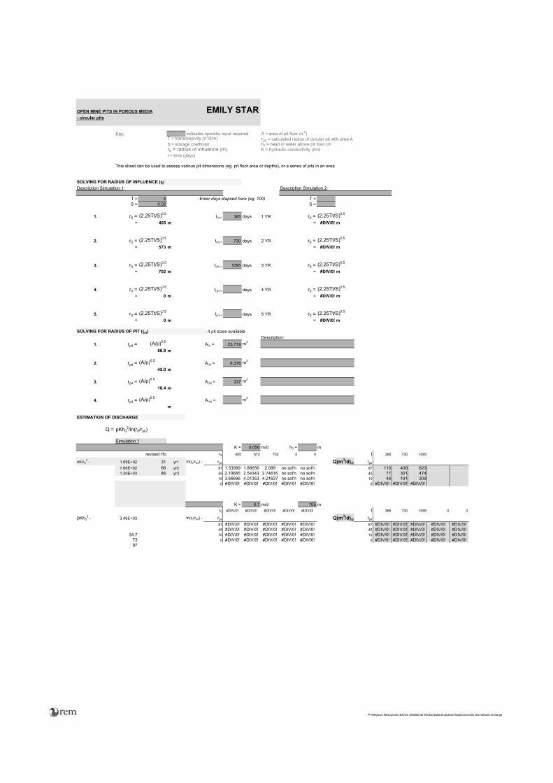
OPEN MINE PITS IN POROUS MEDIA- circular pits NOTES:
- depth to water near proposed Emily Star Pit is 20 m- area of base of pit estimated to be 29,172m2 (after
Key: indicates operator input required A = area of pit floor (m2) 816 m2 (3 yrs) and 816m2 (5 yrs).T = transmissivity (m3/d/m) rpit = calculated radius of circular pit with area A - the bottom pit elevation: after 1 yr = 1130S = storage coefficient h0 = head of water above pit floor (m) after 2 yrs = 1090r0 = radius of influence (m) K = hydraulic conductivity (m/d after 3 yrs = 1065t = time (days) after 5 yrs = 1065
- K value near Emily Star is 0.093 m/d (KMB007).This sheet can be used to assess various pit dimensions (eg. pit floor area or depths), or a series of pits in an area
SOLVING FOR RADIUS OF INFLUENCE (r0)Description Simulation 1: Description Simulation 2:
T = 4 Enter days elapsed here (eg. 100) T =S = 0.02 S =
1. r0 = (2.25Tt/S)0.5t(i) = 365 days 1 YR r0 = (2.25Tt/S)0.5
= 405 m = #DIV/0! m
2. r0 = (2.25Tt/S)0.5t(ii) = 730 days 2 YR r0 = (2.25Tt/S)0.5
= 573 m = #DIV/0! m
3. r0 = (2.25Tt/S)0.5t(iii) = 1095 days 3 YR r0 = (2.25Tt/S)0.5
= 702 m = #DIV/0! m
4. r0 = (2.25Tt/S)0.5t(iv) = days 4 YR r0 = (2.25Tt/S)0.5
= 0 m = #DIV/0! m
5. r0 = (2.25Tt/S)0.5t(v) = days 5 YR r0 = (2.25Tt/S)0.5
= 0 m = #DIV/0! m
SOLVING FOR RADIUS OF PIT (rpit) - 4 pit sizes availableDescription:
1. rpit = (A/p)0.5A(i) = 23,719 m2
86.9 m
2. rpit = (A/p)0.5A(ii) = 6,376 m2
45.0 m
3. rpit = (A/p)0.5A(iii) = 337 m2
10.4 m
4. rpit = (A/p)0.5A(iv) = m2
m
ESTIMATION OF DISCHARGE
Q = pKh02/ln(r0/rpit)
Simulation 1K = 0.056 m/d h0 = m
revised Ho r0 405 573 702 0 0 t 365 730 1095
Kh02 - 1.69E+02 31 yr1 ln(r0/rpit) - rpit Q(m3/d)(i) rpit
7.66E+02 66 yr2 87 1.53999 1.88656 2.089 no sol'n no sol'n 87 110 406 6231.30E+03 86 yr3 45 2.19685 2.54343 2.74616 no sol'n no sol'n 45 77 301 474
10 3.66696 4.01353 4.21627 no sol'n no sol'n 10 46 191 3090 #DIV/0! #DIV/0! #DIV/0! #DIV/0! #DIV/0! 0 #DIV/0! #DIV/0! #DIV/0!
K = 0.1 m/d 105 mr0 #DIV/0! #DIV/0! #DIV/0! #DIV/0! #DIV/0! t 365 730 1095 0 0
pKh02 - 3.46E+03 ln(r0/rpit) - rpit Q(m3/d)(i) rpit
87 #DIV/0! #DIV/0! #DIV/0! #DIV/0! #DIV/0! 87 #DIV/0! #DIV/0! #DIV/0! #DIV/0! #DIV/0!45 #DIV/0! #DIV/0! #DIV/0! #DIV/0! #DIV/0! 45 #DIV/0! #DIV/0! #DIV/0! #DIV/0! #DIV/0!
34.7 10 #DIV/0! #DIV/0! #DIV/0! #DIV/0! #DIV/0! 10 #DIV/0! #DIV/0! #DIV/0! #DIV/0! #DIV/0!73 0 #DIV/0! #DIV/0! #DIV/0! #DIV/0! #DIV/0! 0 #DIV/0! #DIV/0! #DIV/0! #DIV/0! #DIV/0!97
EMILY STAR
P:\Hillgrove Resources (EZ)\03 (Additional Works)\Data\Analytical-Solutions\emily star without recharge

OPEN MINE PITS IN POROUS MEDIA- circular pits NOTES:
- depth to water near proposed Emily Star Pit is 20 m- area of base of pit estimated to be 29,172m2 (after
Key: indicates operator input required A = area of pit floor (m2) 816 m2 (3 yrs) and 816m2 (5 yrs).T = transmissivity (m3/d/m) rpit = calculated radius of circular pit with area A - the bottom pit elevation: after 1 yr = 1130S = storage coefficient h0 = head of water above pit floor (m) after 2 yrs = 1090r0 = radius of influence (m) K = hydraulic conductivity (m/d after 3 yrs = 1065t = time (days) after 5 yrs = 1065
- K value near Emily Star is 0.093 m/d (KMB007).This sheet can be used to assess various pit dimensions (eg. pit floor area or depths), or a series of pits in an area
SOLVING FOR RADIUS OF INFLUENCE (r0)Description Simulation 1: Description Simulation 2:
T = 4 Enter days elapsed here (eg. 100) T =S = 0.001 S =
1. r0 = (2.25Tt/S)0.5t(i) = 365 days 1 YR r0 = (2.25Tt/S)0.5
= 1812 m = #DIV/0! m
2. r0 = (2.25Tt/S)0.5t(ii) = 730 days 2 YR r0 = (2.25Tt/S)0.5
= 2563 m = #DIV/0! m
3. r0 = (2.25Tt/S)0.5t(iii) = 1095 days 3 YR r0 = (2.25Tt/S)0.5
= 3139 m = #DIV/0! m
4. r0 = (2.25Tt/S)0.5t(iv) = days 4 YR r0 = (2.25Tt/S)0.5
= 0 m = #DIV/0! m
5. r0 = (2.25Tt/S)0.5t(v) = days 5 YR r0 = (2.25Tt/S)0.5
= 0 m = #DIV/0! m
SOLVING FOR RADIUS OF PIT (rpit) - 4 pit sizes availableDescription:
1. rpit = (A/p)0.5A(i) = 23,719 m2
86.9 m
2. rpit = (A/p)0.5A(ii) = 6,376 m2
45.0 m
3. rpit = (A/p)0.5A(iii) = 337 m2
10.4 m
4. rpit = (A/p)0.5A(iv) = m2
m
ESTIMATION OF DISCHARGE
Q = pKh02/ln(r0/rpit)
Simulation 1K = 0.056 m/d h0 = m
revised Ho r0 1812 2563 3139 0 0 t 365 730 1095
Kh02 - 1.69E+02 31 yr1 ln(r0/rpit) - rpit Q(m3/d)(i) rpit
7.66E+02 66 yr2 87 3.03785 3.38443 3.587 no sol'n no sol'n 87 56 226 3631.30E+03 86 yr3 45 3.69472 4.04129 4.24403 no sol'n no sol'n 45 46 190 307
10 5.16483 5.5114 5.71413 no sol'n no sol'n 10 33 139 2280 #DIV/0! #DIV/0! #DIV/0! #DIV/0! #DIV/0! 0 #DIV/0! #DIV/0! #DIV/0!
K = 0.1 m/d 105 mr0 #DIV/0! #DIV/0! #DIV/0! #DIV/0! #DIV/0! t 365 730 1095 0 0
pKh02 - 3.46E+03 ln(r0/rpit) - rpit Q(m3/d)(i) rpit
87 #DIV/0! #DIV/0! #DIV/0! #DIV/0! #DIV/0! 87 #DIV/0! #DIV/0! #DIV/0! #DIV/0! #DIV/0!45 #DIV/0! #DIV/0! #DIV/0! #DIV/0! #DIV/0! 45 #DIV/0! #DIV/0! #DIV/0! #DIV/0! #DIV/0!
34.7 10 #DIV/0! #DIV/0! #DIV/0! #DIV/0! #DIV/0! 10 #DIV/0! #DIV/0! #DIV/0! #DIV/0! #DIV/0!73 0 #DIV/0! #DIV/0! #DIV/0! #DIV/0! #DIV/0! 0 #DIV/0! #DIV/0! #DIV/0! #DIV/0! #DIV/0!97
EMILY STAR
P:\Hillgrove Resources (EZ)\03 (Additional Works)\Data\Analytical-Solutions\emily star without recharge

OPEN MINE PITS IN POROUS MEDIA NOTES:- circular pits - depth to water near proposed O'Neil Pit is 23 mPVC = 1
- area of base of pit estimated to be 41,720m2 (at yr 5) an- O'Neil Pit is development at year 5
Key: indicates operator input required A = area of pit floor (m2) - the bottom pit elevation: after 5 yrs = 1140T = transmissivity (m3/d/m) rpit = calculated radius of circular pit with area A after 6 yrs= 1120S = storage coefficient h0 = head of water above pit floor (m) after 7 yrs = 1100r0 = radius of influence (m) K = hydraulic conductivity (m/d after 8 yrs = 1080t = time (days) - K value near Emily Star is 0.000647 m/d (KMB009). Que
This sheet can be used to assess various pit dimensions (eg. pit floor area or depths), or a series of pits in an area
SOLVING FOR RADIUS OF INFLUENCE (r0)Description Simulation 1: Description Simulation 2:
T = 1 Enter days elapsed here (eg. 100) T =S = 0.01 S =
1. r0 = (2.25Tt/S)0.5t(i) = 365 days 1 YR r0 = (2.25Tt/S)0.5
= 287 m = #DIV/0! m
2. r0 = (2.25Tt/S)0.5t(ii) = 730 days 2 YR r0 = (2.25Tt/S)0.5
= 405 m = #DIV/0! m
3. r0 = (2.25Tt/S)0.5t(iii) = 1095 days 3 YR r0 = (2.25Tt/S)0.5
= 496 m = #DIV/0! m
4. r0 = (2.25Tt/S)0.5t(iv) = 1460 days 4 YR r0 = (2.25Tt/S)0.5
= 573 m = #DIV/0! m
5. r0 = (2.25Tt/S)0.5t(v) = days r0 = (2.25Tt/S)0.5
= 0 m = #DIV/0! m
SOLVING FOR RADIUS OF PIT (rpit) - 4 pit sizes availableDescription:
1. rpit = (A/p)0.5A(i) = 36,493 m2
107.8 m
2. rpit = (A/p)0.5A(ii) = 24,189 m2
87.7 m
3. rpit = (A/p)0.5A(iii) = 12,852 m2
64.0 m
4. rpit = (A/p)0.5A(iv) = 4,534 m2
38.0 m
ESTIMATION OF DISCHARGE
Q = pKh02/ln(r0/rpit)
Simulation 10 K = 0.056 m/d h0 = 0 m
revised Ho r0 287 405 496 573 0 t 365 730 1095 1460 0
Kh02 - 0.00E+00 0 yr1 ln(r0/rpit) - rpit Q(m3/d)(i) rpit
0.00E+00 0 yr2 108 0.97799 1.32456 1.527 1.671 no sol'n 108 0 0 0 38 no sol'n0.00E+00 0 yr3 88 1.1836 1.53018 1.73291 1.877 no sol'n 88 0 0 0 34 no sol'n6.35E+01 19 yr4 64 1.4998 1.84637 2.04911 2.19295 no sol'n 64 0 0 0 29 #######
38 2.02075 2.36732 2.57005 2.7139 no sol'n 38 0 0 0 23 #######
K = m/d mr0 #DIV/0! #DIV/0! #DIV/0! #DIV/0! #DIV/0! t 365 730 1095 1460 0
pKh02 - 0.00E+00 ln(r0/rpit) - rpit Q(m3/d)(i) rpit
108 #DIV/0! #DIV/0! #DIV/0! #DIV/0! #DIV/0! 108 #DIV/0! #DIV/0! #DIV/0! #DIV/0! #DIV/0!-12.2 88 #DIV/0! #DIV/0! #DIV/0! #DIV/0! #DIV/0! 88 #DIV/0! #DIV/0! #DIV/0! #DIV/0! #DIV/0!-0.4 64 #DIV/0! #DIV/0! #DIV/0! #DIV/0! #DIV/0! 64 #DIV/0! #DIV/0! #DIV/0! #DIV/0! #DIV/0!11.7 38 #DIV/0! #DIV/0! #DIV/0! #DIV/0! #DIV/0! 38 #DIV/0! #DIV/0! #DIV/0! #DIV/0! #DIV/0!29.5
O'NEIL PIT
P:\Hillgrove Resources (EZ)\03 (Additional Works)\Data\Analytical-Solutions\oneil pit without recharge

OPEN MINE PITS IN POROUS MEDIA NOTES:- circular pits - depth to water near proposed O'Neil Pit is 23 mPVC = 1
- area of base of pit estimated to be 41,720m2 (at yr 5) an- O'Neil Pit is development at year 5
Key: indicates operator input required A = area of pit floor (m2) - the bottom pit elevation: after 5 yrs = 1140T = transmissivity (m3/d/m) rpit = calculated radius of circular pit with area A after 6 yrs= 1120S = storage coefficient h0 = head of water above pit floor (m) after 7 yrs = 1100r0 = radius of influence (m) K = hydraulic conductivity (m/d after 8 yrs = 1080t = time (days) - K value near Emily Star is 0.000647 m/d (KMB009). Que
This sheet can be used to assess various pit dimensions (eg. pit floor area or depths), or a series of pits in an area
SOLVING FOR RADIUS OF INFLUENCE (r0)Description Simulation 1: Description Simulation 2:
T = 10 Enter days elapsed here (eg. 100) T =S = 0.01 S =
1. r0 = (2.25Tt/S)0.5t(i) = 365 days 1 YR r0 = (2.25Tt/S)0.5
= 906 m = #DIV/0! m
2. r0 = (2.25Tt/S)0.5t(ii) = 730 days 2 YR r0 = (2.25Tt/S)0.5
= 1282 m = #DIV/0! m
3. r0 = (2.25Tt/S)0.5t(iii) = 1095 days 3 YR r0 = (2.25Tt/S)0.5
= 1570 m = #DIV/0! m
4. r0 = (2.25Tt/S)0.5t(iv) = 1460 days 4 YR r0 = (2.25Tt/S)0.5
= 1812 m = #DIV/0! m
5. r0 = (2.25Tt/S)0.5t(v) = days r0 = (2.25Tt/S)0.5
= 0 m = #DIV/0! m
SOLVING FOR RADIUS OF PIT (rpit) - 4 pit sizes availableDescription:
1. rpit = (A/p)0.5A(i) = 36,493 m2
107.8 m
2. rpit = (A/p)0.5A(ii) = 24,189 m2
87.7 m
3. rpit = (A/p)0.5A(iii) = 12,852 m2
64.0 m
4. rpit = (A/p)0.5A(iv) = 4,534 m2
38.0 m
ESTIMATION OF DISCHARGE
Q = pKh02/ln(r0/rpit)
Simulation 10 K = 0.056 m/d h0 = 0 m
revised Ho r0 906 1282 1570 1812 0 t 365 730 1095 1460 0
Kh02 - 0.00E+00 0 yr1 ln(r0/rpit) - rpit Q(m3/d)(i) rpit
0.00E+00 0 yr2 108 2.12928 2.47586 2.679 2.822 no sol'n 108 0 0 0 23 no sol'n0.00E+00 0 yr3 88 2.33489 2.68147 2.8842 3.028 no sol'n 88 0 0 0 21 no sol'n6.35E+01 19 yr4 64 2.65109 2.99767 3.2004 3.34424 no sol'n 64 0 0 0 19 #######
38 3.17204 3.51861 3.72135 3.86519 no sol'n 38 0 0 0 16 #######
K = m/d mr0 #DIV/0! #DIV/0! #DIV/0! #DIV/0! #DIV/0! t 365 730 1095 1460 0
pKh02 - 0.00E+00 ln(r0/rpit) - rpit Q(m3/d)(i) rpit
108 #DIV/0! #DIV/0! #DIV/0! #DIV/0! #DIV/0! 108 #DIV/0! #DIV/0! #DIV/0! #DIV/0! #DIV/0!-12.2 88 #DIV/0! #DIV/0! #DIV/0! #DIV/0! #DIV/0! 88 #DIV/0! #DIV/0! #DIV/0! #DIV/0! #DIV/0!-0.4 64 #DIV/0! #DIV/0! #DIV/0! #DIV/0! #DIV/0! 64 #DIV/0! #DIV/0! #DIV/0! #DIV/0! #DIV/0!11.7 38 #DIV/0! #DIV/0! #DIV/0! #DIV/0! #DIV/0! 38 #DIV/0! #DIV/0! #DIV/0! #DIV/0! #DIV/0!29.5
O'NEIL PIT
P:\Hillgrove Resources (EZ)\03 (Additional Works)\Data\Analytical-Solutions\oneil pit without recharge

OPEN MINE PITS IN POROUS MEDIA NOTES:- circular pits - depth to water near proposed O'Neil Pit is 23 mPVC = 1
- area of base of pit estimated to be 41,720m2 (at yr 5) an- O'Neil Pit is development at year 5
Key: indicates operator input required A = area of pit floor (m2) - the bottom pit elevation: after 5 yrs = 1140T = transmissivity (m3/d/m) rpit = calculated radius of circular pit with area A after 6 yrs= 1120S = storage coefficient h0 = head of water above pit floor (m) after 7 yrs = 1100r0 = radius of influence (m) K = hydraulic conductivity (m/d after 8 yrs = 1080t = time (days) - K value near Emily Star is 0.000647 m/d (KMB009). Que
This sheet can be used to assess various pit dimensions (eg. pit floor area or depths), or a series of pits in an area
SOLVING FOR RADIUS OF INFLUENCE (r0)Description Simulation 1: Description Simulation 2:
T = 4 Enter days elapsed here (eg. 100) T =S = 0.02 S =
1. r0 = (2.25Tt/S)0.5t(i) = 365 days 1 YR r0 = (2.25Tt/S)0.5
= 405 m = #DIV/0! m
2. r0 = (2.25Tt/S)0.5t(ii) = 730 days 2 YR r0 = (2.25Tt/S)0.5
= 573 m = #DIV/0! m
3. r0 = (2.25Tt/S)0.5t(iii) = 1095 days 3 YR r0 = (2.25Tt/S)0.5
= 702 m = #DIV/0! m
4. r0 = (2.25Tt/S)0.5t(iv) = 1460 days 4 YR r0 = (2.25Tt/S)0.5
= 811 m = #DIV/0! m
5. r0 = (2.25Tt/S)0.5t(v) = days r0 = (2.25Tt/S)0.5
= 0 m = #DIV/0! m
SOLVING FOR RADIUS OF PIT (rpit) - 4 pit sizes availableDescription:
1. rpit = (A/p)0.5A(i) = 36,493 m2
107.8 m
2. rpit = (A/p)0.5A(ii) = 24,189 m2
87.7 m
3. rpit = (A/p)0.5A(iii) = 12,852 m2
64.0 m
4. rpit = (A/p)0.5A(iv) = 4,534 m2
38.0 m
ESTIMATION OF DISCHARGE
Q = pKh02/ln(r0/rpit)
Simulation 10 K = 0.056 m/d h0 = 0 m
revised Ho r0 405 573 702 811 0 t 365 730 1095 1460 0
Kh02 - 0.00E+00 0 yr1 ln(r0/rpit) - rpit Q(m3/d)(i) rpit
0.00E+00 0 yr2 108 1.32456 1.67114 1.874 2.018 no sol'n 108 0 0 0 31 no sol'n0.00E+00 0 yr3 88 1.53018 1.87675 2.07948 2.223 no sol'n 88 0 0 0 29 no sol'n6.35E+01 19 yr4 64 1.84637 2.19295 2.39568 2.53952 no sol'n 64 0 0 0 25 #######
38 2.36732 2.7139 2.91663 3.06047 no sol'n 38 0 0 0 21 #######
K = m/d mr0 #DIV/0! #DIV/0! #DIV/0! #DIV/0! #DIV/0! t 365 730 1095 1460 0
pKh02 - 0.00E+00 ln(r0/rpit) - rpit Q(m3/d)(i) rpit
108 #DIV/0! #DIV/0! #DIV/0! #DIV/0! #DIV/0! 108 #DIV/0! #DIV/0! #DIV/0! #DIV/0! #DIV/0!-12.2 88 #DIV/0! #DIV/0! #DIV/0! #DIV/0! #DIV/0! 88 #DIV/0! #DIV/0! #DIV/0! #DIV/0! #DIV/0!-0.4 64 #DIV/0! #DIV/0! #DIV/0! #DIV/0! #DIV/0! 64 #DIV/0! #DIV/0! #DIV/0! #DIV/0! #DIV/0!11.7 38 #DIV/0! #DIV/0! #DIV/0! #DIV/0! #DIV/0! 38 #DIV/0! #DIV/0! #DIV/0! #DIV/0! #DIV/0!29.5
O'NEIL PIT
P:\Hillgrove Resources (EZ)\03 (Additional Works)\Data\Analytical-Solutions\oneil pit without recharge

OPEN MINE PITS IN POROUS MEDIA NOTES:- circular pits - depth to water near proposed O'Neil Pit is 23 mPVC = 1
- area of base of pit estimated to be 41,720m2 (at yr 5) an- O'Neil Pit is development at year 5
Key: indicates operator input required A = area of pit floor (m2) - the bottom pit elevation: after 5 yrs = 1140T = transmissivity (m3/d/m) rpit = calculated radius of circular pit with area A after 6 yrs= 1120S = storage coefficient h0 = head of water above pit floor (m) after 7 yrs = 1100r0 = radius of influence (m) K = hydraulic conductivity (m/d after 8 yrs = 1080t = time (days) - K value near Emily Star is 0.000647 m/d (KMB009). Que
This sheet can be used to assess various pit dimensions (eg. pit floor area or depths), or a series of pits in an area
SOLVING FOR RADIUS OF INFLUENCE (r0)Description Simulation 1: Description Simulation 2:
T = 4 Enter days elapsed here (eg. 100) T =S = 0.001 S =
1. r0 = (2.25Tt/S)0.5t(i) = 365 days 1 YR r0 = (2.25Tt/S)0.5
= 1812 m = #DIV/0! m
2. r0 = (2.25Tt/S)0.5t(ii) = 730 days 2 YR r0 = (2.25Tt/S)0.5
= 2563 m = #DIV/0! m
3. r0 = (2.25Tt/S)0.5t(iii) = 1095 days 3 YR r0 = (2.25Tt/S)0.5
= 3139 m = #DIV/0! m
4. r0 = (2.25Tt/S)0.5t(iv) = 1460 days 4 YR r0 = (2.25Tt/S)0.5
= 3625 m = #DIV/0! m
5. r0 = (2.25Tt/S)0.5t(v) = days r0 = (2.25Tt/S)0.5
= 0 m = #DIV/0! m
SOLVING FOR RADIUS OF PIT (rpit) - 4 pit sizes availableDescription:
1. rpit = (A/p)0.5A(i) = 36,493 m2
107.8 m
2. rpit = (A/p)0.5A(ii) = 24,189 m2
87.7 m
3. rpit = (A/p)0.5A(iii) = 12,852 m2
64.0 m
4. rpit = (A/p)0.5A(iv) = 4,534 m2
38.0 m
ESTIMATION OF DISCHARGE
Q = pKh02/ln(r0/rpit)
Simulation 10 K = 0.056 m/d h0 = 0 m
revised Ho r0 1812 2563 3139 3625 0 t 365 730 1095 1460 0
Kh02 - 0.00E+00 0 yr1 ln(r0/rpit) - rpit Q(m3/d)(i) rpit
0.00E+00 0 yr2 108 2.82243 3.169 3.372 3.516 no sol'n 108 0 0 0 18 no sol'n0.00E+00 0 yr3 88 3.02804 3.37462 3.57735 3.721 no sol'n 88 0 0 0 17 no sol'n6.35E+01 19 yr4 64 3.34424 3.69081 3.89355 4.03739 no sol'n 64 0 0 0 16 #######
38 3.86519 4.21176 4.41449 4.55834 no sol'n 38 0 0 0 14 #######
K = m/d mr0 #DIV/0! #DIV/0! #DIV/0! #DIV/0! #DIV/0! t 365 730 1095 1460 0
pKh02 - 0.00E+00 ln(r0/rpit) - rpit Q(m3/d)(i) rpit
108 #DIV/0! #DIV/0! #DIV/0! #DIV/0! #DIV/0! 108 #DIV/0! #DIV/0! #DIV/0! #DIV/0! #DIV/0!-12.2 88 #DIV/0! #DIV/0! #DIV/0! #DIV/0! #DIV/0! 88 #DIV/0! #DIV/0! #DIV/0! #DIV/0! #DIV/0!-0.4 64 #DIV/0! #DIV/0! #DIV/0! #DIV/0! #DIV/0! 64 #DIV/0! #DIV/0! #DIV/0! #DIV/0! #DIV/0!11.7 38 #DIV/0! #DIV/0! #DIV/0! #DIV/0! #DIV/0! 38 #DIV/0! #DIV/0! #DIV/0! #DIV/0! #DIV/0!29.5
O'NEIL PIT
P:\Hillgrove Resources (EZ)\03 (Additional Works)\Data\Analytical-Solutions\oneil pit without recharge

Appendix G.4
Historical Pit Water Balance

HISTORICAL TRANSIENT WATER BALANCE - MAIN PIT
year
post-mining
yearopening pit water level
opening pit water volume
openingwater body area (m2)
rain onto pit water
bodyrain runoff
into pit
rain runoff from outside
of pit gw inpumping
out evap out change in
volumeclosing pit
water volumeclosing pit
level hw Q (kL/day)1977 1 980 3000 3,000 1,110 29,637 0 15,600 3,526 42,821 45,821 1,086 0 42.71978 2 1,086 45,821 10,120 3,744 28,320 0 15,485 11,893 35,656 81,477 1,089 6 42.41979 3 1,089 81,477 13,680 5,062 27,661 0 15,342 16,077 31,988 113,465 1,091 9 42.01980 4 1,091 113,465 16,053 5,940 27,222 0 15,214 18,866 29,510 142,975 1,093 11 41.71981 5 1,093 142,975 18,427 6,818 26,783 0 15,061 21,655 27,007 169,982 1,094 13 41.31982 6 1,094 169,982 19,613 7,257 26,564 0 14,976 23,050 25,746 195,729 1,095 14 41.01983 7 1,095 195,729 20,800 7,696 26,344 0 14,883 24,444 24,479 220,208 1,096 15 40.81984 8 1,096 220,208 21,987 8,135 26,124 0 14,785 25,839 23,205 243,413 1,097 16 40.5 1985 9 1,097 243,413 23,173 8,574 25,905 0 14,679 27,233 21,925 265,338 1,098 17 40.21986 10 1,098 265,338 24,360 9,013 25,685 0 14,568 28,628 20,639 285,977 1,099 18 39.91987 11 1,099 285,977 25,547 9,452 25,466 0 14,450 30,022 19,346 305,323 1,100 19 39.61988 12 1,100 305,323 26,733 9,891 25,246 0 14,326 31,417 18,047 323,370 1,100 20 39.21989 13 1,100 323,370 26,733 9,891 25,246 0 14,326 31,417 18,047 341,417 1,101 20 39.21990 14 1,101 341,417 27,920 10,330 25,027 0 14,196 32,812 16,741 358,158 1,102 21 38.91991 15 1,102 358,158 29,107 10,769 24,807 0 14,059 34,206 15,429 373,587 1,102 22 38.51992 16 1,102 373,587 29,107 10,769 24,807 0 14,059 34,206 15,429 389,016 1,103 22 38.51993 17 1,103 389,016 30,293 11,209 24,588 0 13,915 35,601 14,111 403,127 1,103 23 38.11994 18 1,103 403,127 30,293 11,209 24,588 0 13,915 35,601 14,111 417,238 1,104 23 38.11995 19 1,104 417,238 31,480 11,648 24,368 0 13,766 36,995 12,786 430,024 1,104 24 37.71996 20 1,104 430,024 31,480 11,648 24,368 0 13,766 36,995 12,786 442,811 1,104 24 37.71997 21 1,104 442,811 31,480 11,648 24,368 0 13,766 36,995 12,786 455,597 1,105 24 37.71998 22 1,105 455,597 32,667 12,087 24,149 0 13,610 38,390 11,455 467,052 1,105 25 37.31999 23 1,105 467,052 32,667 12,087 24,149 0 13,610 38,390 11,455 478,507 1,106 25 37.32000 24 1,106 478,507 33,853 12,526 23,929 0 13,447 39,784 10,118 488,625 1,106 26 36.82001 25 1,106 488,625 33,853 12,526 23,929 0 13,447 39,784 10,118 498,743 1,106 26 36.82002 26 1,106 498,743 33,853 12,526 23,929 0 13,447 39,784 10,118 508,861 1,106 26 36.82003 27 1,106 508,861 33,853 12,526 23,929 0 13,447 39,784 10,118 518,979 1,107 26 36.82004 28 1,107 518,979 35,040 12,965 23,710 0 13,279 2,000 41,179 6,774 525,753 1,107 27 36.42005 29 1,107 525,753 35,040 12,965 23,710 13,279 4,500 41,179 4,274 530,027 1,107 27 36.42006 30 1,107 530,027 35,040 12,965 23,710 13,279 6,000 41,179 2,774 532,801 1,107 27 36.4
P:\Hillgrove Resources (EZ)\03 (Additional Works)\Data\Analytical-Solutions\final pit water balance with revised ros

Appendix G.5
Transient Water Balance Spreadsheets – Post Mining Development

FIGURE
PROJECT EZ-03 July-07
MAIN PIT VOLUME -AREA-LEVEL RELATIONSHIPS F.2
Pit RL - Area
930
950
970
990
1,010
1,030
1,050
1,070
1,090
1,110
1,130
1,150
1,170
1,190
1,210
1,230
0 50,000 100,000 150,000 200,000 250,000 300,000
Pit Area (m2)
Pit L
evel
(mR
L)
Pit RL - Volume
930
950
970
990
1,010
1,030
1,050
1,070
1,090
1,110
1,130
1,150
1,170
1,190
1,210
1,230
0.0E+00 5.0E+06 1.0E+07 1.5E+07 2.0E+07 2.5E+07 3.0E+07 3.5E+07 4.0E+07
Cumulative Pit Volume (m3)
Pit L
evel
(mR
L)

FIGURE
PROJECT EZ-03 July-07
O'NEIL AND EMILY STAR PIT VOLUME -AREA-LEVEL RELATIONSHIPS F.3
Pit RL - Area
1,050
1,070
1,090
1,110
1,130
1,150
1,170
1,190
1,210
0 10,000 20,000 30,000 40,000 50,000 60,000 70,000 80,000
Pit Area (m2)
Pit L
evel
(mR
L)
Emily Star PitO'Neil Pit
Pit RL - Volume
1,050
1,070
1,090
1,110
1,130
1,150
1,170
1,190
1,210
0.0E+00 5.0E+05 1.0E+06 1.5E+06 2.0E+06 2.5E+06 3.0E+06 3.5E+06 4.0E+06 4.5E+06 5.0E+06
Cumulative Pit Volume (m3)
Pit L
evel
(mR
L)
Emily Star PitO'Neil Pit

POST CLOSURE PIT WATER BALANCE - MAIN PIT
post-miningyear
opening pit water level
opening pit water volume
opening water body area (m2)
rain onto pit water body
rain runoff into pit gw in evap out
change in volume
closing pit water volume closing pit level hw Q (kL/day)
1 935 2178 2,178 806 46,034 627,000 2,560 671,280 673,458 971 0 1,967.8
2 971 673,458 33,768 12,494 40,189 627,000 39,684 639,999 1,313,457 986 36 1,912.6
3 986 1,313,457 47,838 17,700 37,586 627,000 56,219 626,067 1,939,525 998 51 1,857.1
4 998 1,939,525 59,094 21,865 35,504 627,000 69,447 614,922 2,554,446 1,008 63 1,798.8
5 1,008 2,554,446 68,474 25,335 33,769 627,000 80,471 605,634 3,160,080 1,016 73 1,740.9
6 1,016 3,160,080 75,978 28,112 32,381 616,301 89,289 587,505 3,747,584 1,024 81 1,688.5
7 1,024 3,747,584 83,482 30,888 30,992 595,170 98,108 558,942 4,306,526 1,031 89 1,630.6
8 1,031 4,306,526 90,048 33,318 29,778 575,048 105,824 532,319 4,838,845 1,036 96 1,575.5
9 1,036 4,838,845 94,738 35,053 28,910 559,743 111,336 512,370 5,351,215 1,042 101 1,533.5
10 1,042 5,351,215 100,366 37,135 27,869 540,351 117,950 487,405 5,838,621 1,047 107 1,480.4
11 1,047 5,838,621 105,056 38,871 27,001 523,337 123,462 465,747 6,304,368 1,051 112 1,433.8
12 1,051 6,304,368 108,808 40,259 26,307 509,167 127,871 447,861 6,752,229 1,055 116 1,395.0
13 1,055 6,752,229 112,560 41,647 25,613 494,499 132,281 429,478 7,181,707 1,059 120 1,354.8
14 1,059 7,181,707 116,312 43,035 24,919 479,333 136,690 410,598 7,592,305 1,063 124 1,313.2
15 1,063 7,592,305 120,064 44,424 24,225 463,671 141,099 391,220 7,983,526 1,066 128 1,270.3
16 1,066 7,983,526 122,878 45,465 23,704 451,598 144,406 376,361 8,359,886 1,069 131 1,237.3
17 1,069 8,359,886 125,692 46,506 23,183 439,245 147,713 361,222 8,721,108 1,072 134 1,203.4
18 1,072 8,721,108 128,506 47,547 22,663 426,613 151,020 345,803 9,066,910 1,075 137 1,168.8
19 1,075 9,066,910 131,320 48,588 22,142 413,701 154,327 330,104 9,397,015 1,077 140 1,133.4
20 1,077 9,397,015 133,196 49,283 21,795 404,937 156,532 319,483 9,716,498 1,080 142 1,109.4
21 1,080 9,716,498 136,010 50,324 21,275 391,559 159,839 303,318 10,019,816 1,082 145 1,072.8
22 1,082 10,019,816 137,886 51,018 20,928 382,485 162,044 292,387 10,312,203 1,084 147 1,047.9
23 1,084 10,312,203 139,762 51,712 20,581 373,286 164,248 281,330 10,593,533 1,086 149 1,022.7
24 1,086 10,593,533 141,638 52,406 20,233 363,963 166,453 270,150 10,863,683 1,088 151 997.2
25 1,088 10,863,683 143,514 53,100 19,886 354,516 168,658 258,845 11,122,528 1,090 153 971.3
26 1,090 11,122,528 145,390 53,794 19,539 344,945 170,862 247,416 11,369,944 1,092 155 945.1
27 1,092 11,369,944 147,266 54,488 19,192 335,249 173,067 235,863 11,605,807 1,094 157 918.5
28 1,094 11,605,807 149,142 55,183 18,845 325,429 175,272 224,185 11,829,992 1,095 159 891.6
29 1,095 11,829,992 150,080 55,530 18,672 320,472 176,374 218,300 12,048,292 1,097 160 878.0
30 1,097 12,048,292 151,956 56,224 18,325 310,466 178,579 206,436 12,254,727 1,098 162 850.6
31 1,098 12,254,727 152,894 56,571 18,151 305,416 179,681 200,457 12,455,184 1,099 163 836.8
32 1,099 12,455,184 153,832 56,918 17,978 300,335 180,783 194,447 12,649,631 1,101 164 822.8
33 1,101 12,649,631 155,708 57,612 17,631 290,080 182,988 182,334 12,831,966 1,102 166 794.7
34 1,102 12,831,966 156,646 57,959 17,457 284,906 184,090 176,231 13,008,197 1,103 167 780.6
35 1,103 13,008,197 157,584 58,306 17,283 279,701 185,193 170,097 13,178,295 1,104 168 766.3
36 1,104 13,178,295 158,522 58,653 17,110 274,464 186,295 163,932 13,342,227 1,105 169 752.0
37 1,105 13,342,227 159,460 59,000 16,936 269,197 187,397 157,736 13,499,963 1,106 170 737.5
38 1,106 13,499,963 160,398 59,347 16,763 263,898 188,500 151,509 13,651,471 1,107 171 723.0
39 1,107 13,651,471 161,336 59,694 16,589 258,569 189,602 145,250 13,796,722 1,108 172 708.4
40 1,108 13,796,722 162,274 60,041 16,416 253,208 190,704 138,961 13,935,683 1,109 173 693.7
41 1,109 13,935,683 163,212 60,388 16,242 247,816 191,807 132,640 14,068,323 1,110 174 678.9
42 1,110 14,068,323 164,150 60,736 16,069 242,394 192,909 126,289 14,194,612 1,111 175 664.1
43 1,111 14,194,612 165,088 61,083 15,895 236,940 194,011 119,906 14,314,518 1,112 176 649.2
44 1,112 14,314,518 166,026 61,430 15,722 231,455 195,114 113,492 14,428,011 1,112 177 634.1
45 1,112 14,428,011 166,026 61,430 15,722 231,455 195,114 113,492 14,541,503 1,113 177 634.1
46 1,113 14,541,503 166,964 61,777 15,548 225,939 196,216 107,048 14,648,551 1,114 178 619.0
47 1,114 14,648,551 167,902 62,124 15,375 220,392 197,318 100,572 14,749,122 1,114 179 603.8
48 1,114 14,749,122 167,902 62,124 15,375 220,392 197,318 100,572 14,849,694 1,115 179 603.8
49 1,115 14,849,694 168,840 62,471 15,201 214,814 198,421 94,065 14,943,759 1,115 180 588.5
50 1,115 14,943,759 168,840 62,471 15,201 214,814 198,421 94,065 15,037,823 1,116 180 588.5
51 1,116 15,037,823 169,778 62,818 15,028 209,204 199,523 87,527 15,125,350 1,117 181 573.2
52 1,117 15,125,350 170,716 63,165 14,854 203,564 200,625 80,958 15,206,308 1,117 182 557.7
53 1,117 15,206,308 170,716 63,165 14,854 203,564 200,625 80,958 15,287,265 1,118 182 557.7
54 1,118 15,287,265 171,654 63,512 14,680 197,893 201,728 74,357 15,361,623 1,118 183 542.2
55 1,118 15,361,623 171,654 63,512 14,680 197,893 201,728 74,357 15,435,980 1,118 183 542.2
56 1,118 15,435,980 171,654 63,512 14,680 197,893 201,728 74,357 15,510,337 1,119 183 542.2
57 1,119 15,510,337 172,592 63,859 14,507 192,190 202,830 67,726 15,578,063 1,119 184 526.5
58 1,119 15,578,063 172,592 63,859 14,507 192,190 202,830 67,726 15,645,790 1,120 184 526.5
59 1,120 15,645,790 173,530 64,206 14,333 186,457 203,932 61,064 15,706,853 1,120 185 510.8
60 1,120 15,706,853 173,530 64,206 14,333 186,457 203,932 61,064 15,767,917 1,120 185 510.8
61 1,120 15,767,917 173,530 64,206 14,333 186,457 203,932 61,064 15,828,981 1,121 185 510.8
62 1,121 15,828,981 174,468 64,553 14,160 180,692 205,035 54,370 15,883,351 1,121 186 495.0
63 1,121 15,883,351 174,468 64,553 14,160 180,692 205,035 54,370 15,937,721 1,121 186 495.0
64 1,121 15,937,721 174,468 64,553 14,160 180,692 205,035 54,370 15,992,092 1,122 186 495.0
65 1,122 15,992,092 175,406 64,900 13,986 174,896 206,137 47,646 16,039,738 1,122 187 479.2
66 1,122 16,039,738 175,406 64,900 13,986 174,896 206,137 47,646 16,087,383 1,122 187 479.2
67 1,122 16,087,383 175,406 64,900 13,986 174,896 206,137 47,646 16,135,029 1,123 187 479.2
68 1,123 16,135,029 176,344 65,247 13,813 169,070 207,239 40,890 16,175,919 1,123 188 463.2
69 1,123 16,175,919 176,344 65,247 13,813 169,070 207,239 40,890 16,216,810 1,123 188 463.2
70 1,123 16,216,810 176,344 65,247 13,813 169,070 207,239 40,890 16,257,700 1,123 188 463.2
71 1,123 16,257,700 176,344 65,247 13,813 169,070 207,239 40,890 16,298,590 1,124 188 463.2
72 1,124 16,298,590 177,282 65,594 13,639 163,212 208,342 34,104 16,332,694 1,124 189 447.2
73 1,124 16,332,694 177,282 65,594 13,639 163,212 208,342 34,104 16,366,797 1,124 189 447.2
74 1,124 16,366,797 177,282 65,594 13,639 163,212 208,342 34,104 16,400,901 1,124 189 447.2
75 1,124 16,400,901 177,282 65,594 13,639 163,212 208,342 34,104 16,435,004 1,124 189 447.2
76 1,124 16,435,004 177,282 65,594 13,639 163,212 208,342 34,104 16,469,108 1,125 189 447.2
77 1,125 16,469,108 178,220 65,941 13,466 157,323 209,444 27,286 16,496,394 1,125 190 431.0
78 1,125 16,496,394 178,220 65,941 13,466 157,323 209,444 27,286 16,523,680 1,125 190 431.0
79 1,125 16,523,680 178,220 65,941 13,466 157,323 209,444 27,286 16,550,966 1,125 190 431.0
80 1,125 16,550,966 178,220 65,941 13,466 157,323 209,444 27,286 16,578,251 1,125 190 431.0
81 1,125 16,578,251 178,220 65,941 13,466 157,323 209,444 27,286 16,605,537 1,125 190 431.0
82 1,125 16,605,537 178,220 65,941 13,466 157,323 209,444 27,286 16,632,823 1,126 190 431.0
83 1,126 16,632,823 179,158 66,288 13,292 151,403 210,546 20,437 16,653,260 1,126 191 414.8
84 1,126 16,653,260 179,158 66,288 13,292 151,403 210,546 20,437 16,673,697 1,126 191 414.8
main pit future P:\Hillgrove Resources (EZ)\03 (Additional Works)\Data\Analytical-Solutions\final pit water balance with revised ros

POST CLOSURE PIT WATER BALANCE - MAIN PIT
post-miningyear
opening pit water level
opening pit water volume
opening water body area (m2)
rain onto pit water body
rain runoff into pit gw in evap out
change in volume
closing pit water volume closing pit level hw Q (kL/day)
85 1,126 16,673,697 179,158 66,288 13,292 151,403 210,546 20,437 16,694,134 1,126 191 414.8
86 1,126 16,694,134 179,158 66,288 13,292 151,403 210,546 20,437 16,714,571 1,126 191 414.8
87 1,126 16,714,571 179,158 66,288 13,292 151,403 210,546 20,437 16,735,008 1,126 191 414.8
88 1,126 16,735,008 179,158 66,288 13,292 151,403 210,546 20,437 16,755,445 1,126 191 414.8
89 1,126 16,755,445 179,158 66,288 13,292 151,403 210,546 20,437 16,775,882 1,126 191 414.8
90 1,126 16,775,882 179,158 66,288 13,292 151,403 210,546 20,437 16,796,319 1,126 191 414.8
91 1,126 16,796,319 179,158 66,288 13,292 151,403 210,546 20,437 16,816,756 1,127 191 414.8
92 1,127 16,816,756 180,096 66,636 13,119 145,452 211,649 13,557 16,830,314 1,127 192 398.5
93 1,127 16,830,314 180,096 66,636 13,119 145,452 211,649 13,557 16,843,871 1,127 192 398.5
94 1,127 16,843,871 180,096 66,636 13,119 145,452 211,649 13,557 16,857,428 1,127 192 398.5
95 1,127 16,857,428 180,096 66,636 13,119 145,452 211,649 13,557 16,870,985 1,127 192 398.5
96 1,127 16,870,985 180,096 66,636 13,119 145,452 211,649 13,557 16,884,542 1,127 192 398.5
97 1,127 16,884,542 180,096 66,636 13,119 145,452 211,649 13,557 16,898,099 1,127 192 398.5
98 1,127 16,898,099 180,096 66,636 13,119 145,452 211,649 13,557 16,911,657 1,127 192 398.5
99 1,127 16,911,657 180,096 66,636 13,119 145,452 211,649 13,557 16,925,214 1,127 192 398.5
100 1,127 16,925,214 180,096 66,636 13,119 145,452 211,649 13,557 16,938,771 1,127 192 398.5
101 1,127 16,938,771 180,096 66,636 13,119 145,452 211,649 13,557 16,952,328 1,127 192 398.5
102 1,127 16,952,328 180,096 66,636 13,119 145,452 211,649 13,557 16,965,885 1,127 192 398.5
103 1,127 16,965,885 180,096 66,636 13,119 145,452 211,649 13,557 16,979,442 1,128 192 398.5
104 1,128 16,979,442 181,034 66,983 12,945 139,470 212,751 6,646 16,986,089 1,128 193 382.1
105 1,128 16,986,089 181,034 66,983 12,945 139,470 212,751 6,646 16,992,735 1,128 193 382.1
106 1,128 16,992,735 181,034 66,983 12,945 139,470 212,751 6,646 16,999,381 1,128 193 382.1
107 1,128 16,999,381 181,034 66,983 12,945 139,470 212,751 6,646 17,006,027 1,128 193 382.1
108 1,128 17,006,027 181,034 66,983 12,945 139,470 212,751 6,646 17,012,673 1,128 193 382.1
109 1,128 17,012,673 181,034 66,983 12,945 139,470 212,751 6,646 17,019,320 1,128 193 382.1
110 1,128 17,019,320 181,034 66,983 12,945 139,470 212,751 6,646 17,025,966 1,128 193 382.1
111 1,128 17,025,966 181,034 66,983 12,945 139,470 212,751 6,646 17,032,612 1,128 193 382.1
112 1,128 17,032,612 181,034 66,983 12,945 139,470 212,751 6,646 17,039,258 1,128 193 382.1
113 1,128 17,039,258 181,034 66,983 12,945 139,470 212,751 6,646 17,045,904 1,128 193 382.1
114 1,128 17,045,904 181,034 66,983 12,945 139,470 212,751 6,646 17,052,551 1,128 193 382.1
115 1,128 17,052,551 181,034 66,983 12,945 139,470 212,751 6,646 17,059,197 1,128 193 382.1
116 1,128 17,059,197 181,034 66,983 12,945 139,470 212,751 6,646 17,065,843 1,128 193 382.1
117 1,128 17,065,843 181,034 66,983 12,945 139,470 212,751 6,646 17,072,489 1,128 193 382.1
118 1,128 17,072,489 181,034 66,983 12,945 139,470 212,751 6,646 17,079,135 1,128 193 382.1
119 1,128 17,079,135 181,034 66,983 12,945 139,470 212,751 6,646 17,085,782 1,128 193 382.1
120 1,128 17,085,782 181,034 66,983 12,945 139,470 212,751 6,646 17,092,428 1,128 193 382.1
121 1,128 17,092,428 181,034 66,983 12,945 139,470 212,751 6,646 17,099,074 1,128 193 382.1
122 1,128 17,099,074 181,034 66,983 12,945 139,470 212,751 6,646 17,105,720 1,128 193 382.1
123 1,128 17,105,720 181,034 66,983 12,945 139,470 212,751 6,646 17,112,366 1,128 193 382.1
124 1,128 17,112,366 181,034 66,983 12,945 139,470 212,751 6,646 17,119,013 1,128 193 382.1
125 1,128 17,119,013 181,034 66,983 12,945 139,470 212,751 6,646 17,125,659 1,128 193 382.1
126 1,128 17,125,659 181,034 66,983 12,945 139,470 212,751 6,646 17,132,305 1,128 193 382.1
127 1,128 17,132,305 181,034 66,983 12,945 139,470 212,751 6,646 17,138,951 1,128 193 382.1
128 1,128 17,138,951 181,034 66,983 12,945 139,470 212,751 6,646 17,145,597 1,129 193 382.1
129 1,129 17,145,597 181,972 67,330 12,772 133,456 213,853 -296 17,145,302 1,129 194 365.6
130 1,129 17,145,302 181,972 67,330 12,772 133,456 213,853 -296 17,145,006 1,128 194 365.6
131 1,128 17,145,006 181,034 66,983 12,945 139,470 212,751 6,646 17,151,652 1,129 193 382.1
132 1,129 17,151,652 181,972 67,330 12,772 133,456 213,853 -296 17,151,356 1,129 194 365.6
133 1,129 17,151,356 181,972 67,330 12,772 133,456 213,853 -296 17,151,060 1,129 194 365.6
134 1,129 17,151,060 181,972 67,330 12,772 133,456 213,853 -296 17,150,765 1,129 194 365.6
135 1,129 17,150,765 181,972 67,330 12,772 133,456 213,853 -296 17,150,469 1,129 194 365.6
136 1,129 17,150,469 181,972 67,330 12,772 133,456 213,853 -296 17,150,173 1,129 194 365.6
137 1,129 17,150,173 181,972 67,330 12,772 133,456 213,853 -296 17,149,877 1,129 194 365.6
138 1,129 17,149,877 181,972 67,330 12,772 133,456 213,853 -296 17,149,581 1,129 194 365.6
139 1,129 17,149,581 181,972 67,330 12,772 133,456 213,853 -296 17,149,285 1,129 194 365.6
140 1,129 17,149,285 181,972 67,330 12,772 133,456 213,853 -296 17,148,990 1,129 194 365.6
141 1,129 17,148,990 181,972 67,330 12,772 133,456 213,853 -296 17,148,694 1,129 194 365.6
142 1,129 17,148,694 181,972 67,330 12,772 133,456 213,853 -296 17,148,398 1,129 194 365.6
143 1,129 17,148,398 181,972 67,330 12,772 133,456 213,853 -296 17,148,102 1,129 194 365.6
144 1,129 17,148,102 181,972 67,330 12,772 133,456 213,853 -296 17,147,806 1,129 194 365.6
145 1,129 17,147,806 181,972 67,330 12,772 133,456 213,853 -296 17,147,510 1,129 194 365.6
146 1,129 17,147,510 181,972 67,330 12,772 133,456 213,853 -296 17,147,215 1,129 194 365.6
147 1,129 17,147,215 181,972 67,330 12,772 133,456 213,853 -296 17,146,919 1,129 194 365.6
148 1,129 17,146,919 181,972 67,330 12,772 133,456 213,853 -296 17,146,623 1,129 194 365.6
149 1,129 17,146,623 181,972 67,330 12,772 133,456 213,853 -296 17,146,327 1,129 194 365.6
150 1,129 17,146,327 181,972 67,330 12,772 133,456 213,853 -296 17,146,031 1,129 194 365.6
151 1,129 17,146,031 181,972 67,330 12,772 133,456 213,853 -296 17,145,735 1,129 194 365.6
152 1,129 17,145,735 181,972 67,330 12,772 133,456 213,853 -296 17,145,439 1,129 194 365.6
153 1,129 17,145,439 181,972 67,330 12,772 133,456 213,853 -296 17,145,144 1,128 194 365.6
154 1,128 17,145,144 181,034 66,983 12,945 139,470 212,751 6,646 17,151,790 1,129 193 382.1
155 1,129 17,151,790 181,972 67,330 12,772 133,456 213,853 -296 17,151,494 1,129 194 365.6
156 1,129 17,151,494 181,972 67,330 12,772 133,456 213,853 -296 17,151,198 1,129 194 365.6
157 1,129 17,151,198 181,972 67,330 12,772 133,456 213,853 -296 17,150,902 1,129 194 365.6
158 1,129 17,150,902 181,972 67,330 12,772 133,456 213,853 -296 17,150,607 1,129 194 365.6
159 1,129 17,150,607 181,972 67,330 12,772 133,456 213,853 -296 17,150,311 1,129 194 365.6
160 1,129 17,150,311 181,972 67,330 12,772 133,456 213,853 -296 17,150,015 1,129 194 365.6
161 1,129 17,150,015 181,972 67,330 12,772 133,456 213,853 -296 17,149,719 1,129 194 365.6
162 1,129 17,149,719 181,972 67,330 12,772 133,456 213,853 -296 17,149,423 1,129 194 365.6
163 1,129 17,149,423 181,972 67,330 12,772 133,456 213,853 -296 17,149,127 1,129 194 365.6
164 1,129 17,149,127 181,972 67,330 12,772 133,456 213,853 -296 17,148,832 1,129 194 365.6
165 1,129 17,148,832 181,972 67,330 12,772 133,456 213,853 -296 17,148,536 1,129 194 365.6
166 1,129 17,148,536 181,972 67,330 12,772 133,456 213,853 -296 17,148,240 1,129 194 365.6
167 1,129 17,148,240 181,972 67,330 12,772 133,456 213,853 -296 17,147,944 1,129 194 365.6
168 1,129 17,147,944 181,972 67,330 12,772 133,456 213,853 -296 17,147,648 1,129 194 365.6
main pit future P:\Hillgrove Resources (EZ)\03 (Additional Works)\Data\Analytical-Solutions\final pit water balance with revised ros

POST CLOSURE PIT WATER BALANCE - EMILY STAR
post-miningyear
opening pit water level
opening pit water volume
opening water body area (m2)
rain onto pitwater body
rain runoff into pit gw in evap out
change in volume
closing pit water volume closing pit level hw Q (kL/day)
1 1065 337 337 125 12,863 104,069 396 116,661 116,998 1,085 0 421.8
2 1,085 116,998 10,638 3,936 10,958 104,069 12,502 106,461 223,459 1,093 20 406.5
3 1,093 223,459 14,758 5,461 10,195 104,069 17,344 102,381 325,840 1,099 28 391.8
4 1,099 325,840 17,849 6,604 9,624 104,069 20,976 99,321 425,161 1,104 34 377.6
5 1,104 425,161 20,424 7,557 9,147 104,069 24,002 96,771 521,932 1,109 39 363.6
6 1,109 521,932 22,999 8,510 8,671 104,069 27,029 94,221 616,153 1,113 44 347.8
7 1,113 616,153 25,059 9,272 8,290 104,069 29,450 92,181 708,334 1,116 48 333.7
8 1,116 708,334 26,605 9,844 8,004 104,069 31,266 90,651 798,984 1,120 51 322.3
9 1,120 798,984 28,665 10,606 7,623 104,069 33,687 88,611 887,595 1,123 55 306.1
10 1,123 887,595 30,210 11,178 7,337 104,069 35,503 87,081 974,676 1,125 58 293.1
11 1,125 974,676 31,240 11,559 7,146 103,692 36,713 85,684 1,060,360 1,128 60 284.1
12 1,128 1,060,360 32,785 12,131 6,860 98,539 38,529 79,000 1,139,360 1,130 63 270.0
13 1,130 1,139,360 33,815 12,512 6,670 94,964 39,740 74,405 1,213,765 1,133 65 260.2
14 1,133 1,213,765 35,361 13,083 6,384 89,391 41,556 67,303 1,281,069 1,134 68 244.9
15 1,134 1,281,069 35,876 13,274 6,289 87,478 42,161 64,880 1,345,949 1,136 69 239.7
16 1,136 1,345,949 36,906 13,655 6,098 83,568 43,372 59,950 1,405,898 1,138 71 229.0
17 1,138 1,405,898 37,936 14,036 5,908 79,546 44,582 54,908 1,460,806 1,139 73 217.9
18 1,139 1,460,806 38,451 14,227 5,812 77,493 45,187 52,345 1,513,151 1,141 74 212.3
19 1,141 1,513,151 39,481 14,608 5,622 73,303 46,398 47,135 1,560,286 1,142 76 200.8
20 1,142 1,560,286 39,996 14,799 5,527 71,167 47,003 44,489 1,604,775 1,143 77 195.0
21 1,143 1,604,775 40,511 14,989 5,431 69,002 47,609 41,814 1,646,588 1,144 78 189.0
22 1,144 1,646,588 41,026 15,180 5,336 66,810 48,214 39,111 1,685,700 1,145 79 183.0
23 1,145 1,685,700 41,541 15,370 5,241 64,589 48,819 36,381 1,722,081 1,146 80 177.0
24 1,146 1,722,081 42,056 15,561 5,145 62,341 49,424 33,622 1,755,703 1,146 81 170.8
25 1,146 1,755,703 42,056 15,561 5,145 62,341 49,424 33,622 1,789,326 1,147 81 170.8
26 1,147 1,789,326 42,571 15,751 5,050 60,064 50,030 30,836 1,820,162 1,148 82 164.6
27 1,148 1,820,162 43,086 15,942 4,955 57,760 50,635 28,022 1,848,184 1,149 83 158.2
28 1,149 1,848,184 43,601 16,133 4,860 55,428 51,240 25,180 1,873,363 1,149 84 151.9
29 1,149 1,873,363 43,601 16,133 4,860 55,428 51,240 25,180 1,898,543 1,150 84 151.9
30 1,150 1,898,543 44,116 16,323 4,764 53,068 51,846 22,310 1,920,853 1,150 85 145.4
31 1,150 1,920,853 44,116 16,323 4,764 53,068 51,846 22,310 1,943,162 1,151 85 145.4
32 1,151 1,943,162 44,631 16,514 4,669 50,680 52,451 19,412 1,962,574 1,151 86 138.8
33 1,151 1,962,574 44,631 16,514 4,669 50,680 52,451 19,412 1,981,985 1,152 86 138.8
34 1,152 1,981,985 45,147 16,704 4,574 48,264 53,056 16,486 1,998,471 1,152 87 132.2
35 1,152 1,998,471 45,147 16,704 4,574 48,264 53,056 16,486 2,014,956 1,152 87 132.2
36 1,152 2,014,956 45,147 16,704 4,574 48,264 53,056 16,486 2,031,442 1,153 87 132.2
37 1,153 2,031,442 45,662 16,895 4,478 45,820 53,661 13,532 2,044,973 1,153 88 125.5
38 1,153 2,044,973 45,662 16,895 4,478 45,820 53,661 13,532 2,058,505 1,153 88 125.5
39 1,153 2,058,505 45,662 16,895 4,478 45,820 53,661 13,532 2,072,037 1,154 88 125.5
40 1,154 2,072,037 46,177 17,085 4,383 43,348 54,267 10,550 2,082,586 1,154 89 118.8
41 1,154 2,082,586 46,177 17,085 4,383 43,348 54,267 10,550 2,093,136 1,154 89 118.8
42 1,154 2,093,136 46,177 17,085 4,383 43,348 54,267 10,550 2,103,686 1,154 89 118.8
43 1,154 2,103,686 46,177 17,085 4,383 43,348 54,267 10,550 2,114,236 1,154 89 118.8
44 1,154 2,114,236 46,177 17,085 4,383 43,348 54,267 10,550 2,124,785 1,155 89 118.8
45 1,155 2,124,785 46,692 17,276 4,288 40,848 54,872 7,540 2,132,325 1,155 90 111.9
46 1,155 2,132,325 46,692 17,276 4,288 40,848 54,872 7,540 2,139,865 1,155 90 111.9
47 1,155 2,139,865 46,692 17,276 4,288 40,848 54,872 7,540 2,147,405 1,155 90 111.9
48 1,155 2,147,405 46,692 17,276 4,288 40,848 54,872 7,540 2,154,945 1,155 90 111.9
49 1,155 2,154,945 46,692 17,276 4,288 40,848 54,872 7,540 2,162,485 1,155 90 111.9
50 1,155 2,162,485 46,692 17,276 4,288 40,848 54,872 7,540 2,170,025 1,156 90 111.9
51 1,156 2,170,025 47,207 17,466 4,193 38,321 55,477 4,502 2,174,528 1,156 91 105.0
52 1,156 2,174,528 47,207 17,466 4,193 38,321 55,477 4,502 2,179,030 1,156 91 105.0
53 1,156 2,179,030 47,207 17,466 4,193 38,321 55,477 4,502 2,183,532 1,156 91 105.0
54 1,156 2,183,532 47,207 17,466 4,193 38,321 55,477 4,502 2,188,034 1,156 91 105.0
55 1,156 2,188,034 47,207 17,466 4,193 38,321 55,477 4,502 2,192,537 1,156 91 105.0
56 1,156 2,192,537 47,207 17,466 4,193 38,321 55,477 4,502 2,197,039 1,156 91 105.0
57 1,156 2,197,039 47,207 17,466 4,193 38,321 55,477 4,502 2,201,541 1,156 91 105.0
58 1,156 2,201,541 47,207 17,466 4,193 38,321 55,477 4,502 2,206,043 1,156 91 105.0
59 1,156 2,206,043 47,207 17,466 4,193 38,321 55,477 4,502 2,210,546 1,157 91 105.0
60 1,157 2,210,546 47,722 17,657 4,097 35,765 56,083 1,437 2,211,982 1,157 92 98.0
61 1,157 2,211,982 47,722 17,657 4,097 35,765 56,083 1,437 2,213,419 1,157 92 98.0
62 1,157 2,213,419 47,722 17,657 4,097 35,765 56,083 1,437 2,214,855 1,157 92 98.0
63 1,157 2,214,855 47,722 17,657 4,097 35,765 56,083 1,437 2,216,292 1,157 92 98.0
64 1,157 2,216,292 47,722 17,657 4,097 35,765 56,083 1,437 2,217,729 1,157 92 98.0
65 1,157 2,217,729 47,722 17,657 4,097 35,765 56,083 1,437 2,219,165 1,157 92 98.0
66 1,157 2,219,165 47,722 17,657 4,097 35,765 56,083 1,437 2,220,602 1,157 92 98.0
67 1,157 2,220,602 47,722 17,657 4,097 35,765 56,083 1,437 2,222,039 1,157 92 98.0
68 1,157 2,222,039 47,722 17,657 4,097 35,765 56,083 1,437 2,223,475 1,157 92 98.0
69 1,157 2,223,475 47,722 17,657 4,097 35,765 56,083 1,437 2,224,912 1,157 92 98.0
70 1,157 2,224,912 47,722 17,657 4,097 35,765 56,083 1,437 2,226,348 1,157 92 98.0
71 1,157 2,226,348 47,722 17,657 4,097 35,765 56,083 1,437 2,227,785 1,157 92 98.0
72 1,157 2,227,785 47,722 17,657 4,097 35,765 56,083 1,437 2,229,222 1,157 92 98.0
73 1,157 2,229,222 47,722 17,657 4,097 35,765 56,083 1,437 2,230,658 1,157 92 98.0
74 1,157 2,230,658 47,722 17,657 4,097 35,765 56,083 1,437 2,232,095 1,157 92 98.0
75 1,157 2,232,095 47,722 17,657 4,097 35,765 56,083 1,437 2,233,532 1,157 92 98.0
76 1,157 2,233,532 47,722 17,657 4,097 35,765 56,083 1,437 2,234,968 1,157 92 98.0
77 1,157 2,234,968 47,722 17,657 4,097 35,765 56,083 1,437 2,236,405 1,157 92 98.0
78 1,157 2,236,405 47,722 17,657 4,097 35,765 56,083 1,437 2,237,841 1,157 92 98.0
79 1,157 2,237,841 47,722 17,657 4,097 35,765 56,083 1,437 2,239,278 1,157 92 98.0
80 1,157 2,239,278 47,722 17,657 4,097 35,765 56,083 1,437 2,240,715 1,157 92 98.0
81 1,157 2,240,715 47,722 17,657 4,097 35,765 56,083 1,437 2,242,151 1,157 92 98.0
82 1,157 2,242,151 47,722 17,657 4,097 35,765 56,083 1,437 2,243,588 1,157 92 98.0
emily star P:\Hillgrove Resources (EZ)\03 (Additional Works)\Data\Analytical-Solutions\final pit water balance with revised ros
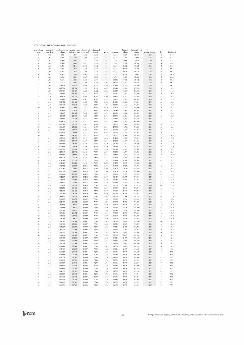
POST CLOSURE PIT WATER BALANCE - O'NEIL PIT
post-miningyear
opening pit water level
opening pit water volume
opening water body area (m2)
rain onto pit water body
rain runoff into pit gw in evap out
change in volume
closing pit water volume closing pit level hw Q (kL/day)
1 1080 4534 4,534 1,678 11,908 0 5,328 8,257 12,791 1,082 0 211.5
2 1,082 12,791 5,607 2,075 11,710 0 6,589 7,195 19,986 1,083 2 211.3
3 1,083 19,986 6,143 2,273 11,610 0 7,219 6,664 26,650 1,084 3 211.1
4 1,084 26,650 6,680 2,471 11,511 0 7,850 6,133 32,783 1,085 4 210.7
5 1,085 32,783 7,216 2,670 11,412 0 8,480 5,602 38,385 1,086 5 210.3
6 1,086 38,385 7,752 2,868 11,313 0 9,111 5,070 43,455 1,086 6 209.7
7 1,086 43,455 7,752 2,868 11,313 0 9,111 5,070 48,525 1,087 6 209.7
8 1,087 48,525 8,289 3,067 11,213 0 9,741 4,539 53,065 1,087 7 209.0
9 1,087 53,065 8,289 3,067 11,213 0 9,741 4,539 57,604 1,088 7 209.0
10 1,088 57,604 8,825 3,265 11,114 0 10,371 4,008 61,612 1,088 8 208.2
11 1,088 61,612 8,825 3,265 11,114 38,003 10,371 42,011 103,623 1,092 8 208.2
12 1,092 103,623 10,971 4,059 10,717 37,249 12,893 39,133 142,756 1,096 12 204.1
13 1,096 142,756 13,116 4,853 10,320 36,193 15,414 35,952 178,709 1,098 16 198.3
14 1,098 178,709 14,189 5,250 10,122 35,553 16,675 34,249 212,958 1,100 18 194.8
15 1,100 212,958 15,262 5,647 9,923 34,836 17,936 32,471 245,429 1,102 20 190.9
16 1,102 245,429 16,335 6,044 9,725 34,044 19,197 30,617 276,045 1,104 22 186.5
17 1,104 276,045 17,408 6,441 9,526 33,177 20,457 28,687 304,732 1,106 24 181.8
18 1,106 304,732 18,480 6,838 9,328 32,235 21,718 26,682 331,415 1,107 26 176.6
19 1,107 331,415 19,017 7,036 9,229 31,735 22,349 25,652 357,067 1,109 27 173.9
20 1,109 357,067 20,090 7,433 9,030 30,680 23,609 23,534 380,600 1,110 29 168.1
21 1,110 380,600 20,626 7,632 8,931 30,124 24,240 22,447 403,047 1,111 30 165.1
22 1,111 403,047 21,162 7,830 8,832 29,549 24,870 21,340 424,387 1,112 31 161.9
23 1,112 424,387 21,699 8,029 8,733 28,955 25,500 20,216 444,603 1,113 32 158.7
24 1,113 444,603 22,235 8,227 8,633 28,342 26,131 19,072 463,675 1,113 33 155.3
25 1,113 463,675 22,235 8,227 8,633 28,342 26,131 19,072 482,746 1,114 33 155.3
26 1,114 482,746 22,772 8,425 8,534 27,711 26,761 17,909 500,655 1,115 34 151.8
27 1,115 500,655 23,308 8,624 8,435 27,060 27,392 16,728 517,383 1,116 35 148.3
28 1,116 517,383 23,844 8,822 8,336 26,391 28,022 15,527 532,910 1,116 36 144.6
29 1,116 532,910 23,844 8,822 8,336 26,391 28,022 15,527 548,437 1,117 36 144.6
30 1,117 548,437 24,381 9,021 8,236 25,703 28,652 14,308 562,745 1,118 37 140.8
31 1,118 562,745 24,917 9,219 8,137 24,996 29,283 13,070 575,815 1,118 38 137.0
32 1,118 575,815 24,917 9,219 8,137 24,996 29,283 13,070 588,885 1,119 38 137.0
33 1,119 588,885 25,454 9,418 8,038 24,270 29,913 11,813 600,698 1,119 39 133.0
34 1,119 600,698 25,454 9,418 8,038 24,270 29,913 11,813 612,512 1,120 39 133.0
35 1,120 612,512 25,990 9,616 7,939 23,526 30,543 10,537 623,049 1,120 40 128.9
36 1,120 623,049 25,990 9,616 7,939 23,526 30,543 10,537 633,586 1,120 40 128.9
37 1,120 633,586 25,990 9,616 7,939 23,526 30,543 10,537 644,124 1,121 40 128.9
38 1,121 644,124 26,526 9,815 7,839 22,762 31,174 9,243 653,366 1,121 41 124.7
39 1,121 653,366 26,526 9,815 7,839 22,762 31,174 9,243 662,609 1,121 41 124.7
40 1,121 662,609 26,526 9,815 7,839 22,762 31,174 9,243 671,852 1,122 41 124.7
41 1,122 671,852 27,063 10,013 7,740 21,980 31,804 7,929 679,781 1,122 42 120.4
42 1,122 679,781 27,063 10,013 7,740 21,980 31,804 7,929 687,710 1,122 42 120.4
43 1,122 687,710 27,063 10,013 7,740 21,980 31,804 7,929 695,640 1,123 42 120.4
44 1,123 695,640 27,599 10,212 7,641 21,179 32,435 6,597 702,237 1,123 43 116.0
45 1,123 702,237 27,599 10,212 7,641 21,179 32,435 6,597 708,834 1,123 43 116.0
46 1,123 708,834 27,599 10,212 7,641 21,179 32,435 6,597 715,431 1,123 43 116.0
47 1,123 715,431 27,599 10,212 7,641 21,179 32,435 6,597 722,028 1,124 43 116.0
48 1,124 722,028 28,136 10,410 7,542 20,359 33,065 5,246 727,273 1,124 44 111.6
49 1,124 727,273 28,136 10,410 7,542 20,359 33,065 5,246 732,519 1,124 44 111.6
50 1,124 732,519 28,136 10,410 7,542 20,359 33,065 5,246 737,765 1,124 44 111.6
51 1,124 737,765 28,136 10,410 7,542 20,359 33,065 5,246 743,011 1,124 44 111.6
52 1,124 743,011 28,136 10,410 7,542 20,359 33,065 5,246 748,257 1,125 44 111.6
53 1,125 748,257 28,672 10,609 7,443 19,520 33,695 3,876 752,133 1,125 45 107.0
54 1,125 752,133 28,672 10,609 7,443 19,520 33,695 3,876 756,008 1,125 45 107.0
55 1,125 756,008 28,672 10,609 7,443 19,520 33,695 3,876 759,884 1,125 45 107.0
56 1,125 759,884 28,672 10,609 7,443 19,520 33,695 3,876 763,760 1,125 45 107.0
57 1,125 763,760 28,672 10,609 7,443 19,520 33,695 3,876 767,636 1,125 45 107.0
58 1,125 767,636 28,672 10,609 7,443 19,520 33,695 3,876 771,512 1,125 45 107.0
59 1,125 771,512 28,672 10,609 7,443 19,520 33,695 3,876 775,388 1,125 45 107.0
60 1,125 775,388 28,672 10,609 7,443 19,520 33,695 3,876 779,263 1,126 45 107.0
61 1,126 779,263 29,208 10,807 7,343 18,662 34,326 2,487 781,750 1,126 46 102.3
62 1,126 781,750 29,208 10,807 7,343 18,662 34,326 2,487 784,237 1,126 46 102.3
63 1,126 784,237 29,208 10,807 7,343 18,662 34,326 2,487 786,724 1,126 46 102.3
64 1,126 786,724 29,208 10,807 7,343 18,662 34,326 2,487 789,211 1,126 46 102.3
65 1,126 789,211 29,208 10,807 7,343 18,662 34,326 2,487 791,698 1,126 46 102.3
66 1,126 791,698 29,208 10,807 7,343 18,662 34,326 2,487 794,185 1,126 46 102.3
67 1,126 794,185 29,208 10,807 7,343 18,662 34,326 2,487 796,672 1,126 46 102.3
68 1,126 796,672 29,208 10,807 7,343 18,662 34,326 2,487 799,159 1,126 46 102.3
69 1,126 799,159 29,208 10,807 7,343 18,662 34,326 2,487 801,646 1,126 46 102.3
70 1,126 801,646 29,208 10,807 7,343 18,662 34,326 2,487 804,133 1,126 46 102.3
71 1,126 804,133 29,208 10,807 7,343 18,662 34,326 2,487 806,620 1,127 46 102.3
72 1,127 806,620 29,745 11,006 7,244 17,786 34,956 1,079 807,699 1,127 47 97.5
73 1,127 807,699 29,745 11,006 7,244 17,786 34,956 1,079 808,779 1,127 47 97.5
74 1,127 808,779 29,745 11,006 7,244 17,786 34,956 1,079 809,858 1,127 47 97.5
75 1,127 809,858 29,745 11,006 7,244 17,786 34,956 1,079 810,937 1,127 47 97.5
76 1,127 810,937 29,745 11,006 7,244 17,786 34,956 1,079 812,017 1,127 47 97.5
77 1,127 812,017 29,745 11,006 7,244 17,786 34,956 1,079 813,096 1,127 47 97.5
78 1,127 813,096 29,745 11,006 7,244 17,786 34,956 1,079 814,175 1,127 47 97.5
79 1,127 814,175 29,745 11,006 7,244 17,786 34,956 1,079 815,254 1,127 47 97.5
80 1,127 815,254 29,745 11,006 7,244 17,786 34,956 1,079 816,334 1,127 47 97.5
81 1,127 816,334 29,745 11,006 7,244 17,786 34,956 1,079 817,413 1,127 47 97.5
82 1,127 817,413 29,745 11,006 7,244 17,786 34,956 1,079 818,492 1,127 47 97.5
83 1,127 818,492 29,745 11,006 7,244 17,786 34,956 1,079 819,571 1,127 47 97.5
84 1,127 819,571 29,745 11,006 7,244 17,786 34,956 1,079 820,651 1,127 47 97.5
oneil P:\Hillgrove Resources (EZ)\03 (Additional Works)\Data\Analytical-Solutions\final pit water balance with revised ros

POST CLOSURE PIT WATER BALANCE - O'NEIL PIT
post-miningyear
opening pit water level
opening pit water volume
opening water body area (m2)
rain onto pit water body
rain runoff into pit gw in evap out
change in volume
closing pit water volume closing pit level hw Q (kL/day)
85 1,127 820,651 29,745 11,006 7,244 17,786 34,956 1,079 821,730 1,127 47 97.5
86 1,127 821,730 29,745 11,006 7,244 17,786 34,956 1,079 822,809 1,127 47 97.5
87 1,127 822,809 29,745 11,006 7,244 17,786 34,956 1,079 823,889 1,127 47 97.5
88 1,127 823,889 29,745 11,006 7,244 17,786 34,956 1,079 824,968 1,127 47 97.5
89 1,127 824,968 29,745 11,006 7,244 17,786 34,956 1,079 826,047 1,127 47 97.5
90 1,127 826,047 29,745 11,006 7,244 17,786 34,956 1,079 827,126 1,127 47 97.5
91 1,127 827,126 29,745 11,006 7,244 17,786 34,956 1,079 828,206 1,127 47 97.5
92 1,127 828,206 29,745 11,006 7,244 17,786 34,956 1,079 829,285 1,127 47 97.5
93 1,127 829,285 29,745 11,006 7,244 17,786 34,956 1,079 830,364 1,127 47 97.5
94 1,127 830,364 29,745 11,006 7,244 17,786 34,956 1,079 831,443 1,127 47 97.5
95 1,127 831,443 29,745 11,006 7,244 17,786 34,956 1,079 832,523 1,127 47 97.5
96 1,127 832,523 29,745 11,006 7,244 17,786 34,956 1,079 833,602 1,127 47 97.5
97 1,127 833,602 29,745 11,006 7,244 17,786 34,956 1,079 834,681 1,127 47 97.5
98 1,127 834,681 29,745 11,006 7,244 17,786 34,956 1,079 835,761 1,128 47 97.5
99 1,128 835,761 30,281 11,204 7,145 16,890 35,586 -347 835,413 1,128 48 92.5
100 1,128 835,413 30,281 11,204 7,145 16,890 35,586 -347 835,066 1,127 48 92.5
101 1,127 835,066 29,745 11,006 7,244 17,786 34,956 1,079 836,145 1,128 47 97.5
102 1,128 836,145 30,281 11,204 7,145 16,890 35,586 -347 835,798 1,128 48 92.5
103 1,128 835,798 30,281 11,204 7,145 16,890 35,586 -347 835,451 1,128 48 92.5
104 1,128 835,451 30,281 11,204 7,145 16,890 35,586 -347 835,103 1,127 48 92.5
105 1,127 835,103 29,745 11,006 7,244 17,786 34,956 1,079 836,183 1,128 47 97.5
106 1,128 836,183 30,281 11,204 7,145 16,890 35,586 -347 835,835 1,128 48 92.5
107 1,128 835,835 30,281 11,204 7,145 16,890 35,586 -347 835,488 1,128 48 92.5
108 1,128 835,488 30,281 11,204 7,145 16,890 35,586 -347 835,141 1,127 48 92.5
109 1,127 835,141 29,745 11,006 7,244 17,786 34,956 1,079 836,220 1,128 47 97.5
110 1,128 836,220 30,281 11,204 7,145 16,890 35,586 -347 835,873 1,128 48 92.5
111 1,128 835,873 30,281 11,204 7,145 16,890 35,586 -347 835,526 1,128 48 92.5
112 1,128 835,526 30,281 11,204 7,145 16,890 35,586 -347 835,178 1,127 48 92.5
113 1,127 835,178 29,745 11,006 7,244 17,786 34,956 1,079 836,258 1,128 47 97.5
114 1,128 836,258 30,281 11,204 7,145 16,890 35,586 -347 835,910 1,128 48 92.5
115 1,128 835,910 30,281 11,204 7,145 16,890 35,586 -347 835,563 1,128 48 92.5
116 1,128 835,563 30,281 11,204 7,145 16,890 35,586 -347 835,216 1,127 48 92.5
117 1,127 835,216 29,745 11,006 7,244 17,786 34,956 1,079 836,295 1,128 47 97.5
118 1,128 836,295 30,281 11,204 7,145 16,890 35,586 -347 835,948 1,128 48 92.5
119 1,128 835,948 30,281 11,204 7,145 16,890 35,586 -347 835,600 1,128 48 92.5
120 1,128 835,600 30,281 11,204 7,145 16,890 35,586 -347 835,253 1,127 48 92.5
121 1,127 835,253 29,745 11,006 7,244 17,786 34,956 1,079 836,332 1,128 47 97.5
122 1,128 836,332 30,281 11,204 7,145 16,890 35,586 -347 835,985 1,128 48 92.5
123 1,128 835,985 30,281 11,204 7,145 16,890 35,586 -347 835,638 1,128 48 92.5
124 1,128 835,638 30,281 11,204 7,145 16,890 35,586 -347 835,291 1,127 48 92.5
125 1,127 835,291 29,745 11,006 7,244 17,786 34,956 1,079 836,370 1,128 47 97.5
126 1,128 836,370 30,281 11,204 7,145 16,890 35,586 -347 836,023 1,128 48 92.5
127 1,128 836,023 30,281 11,204 7,145 16,890 35,586 -347 835,675 1,128 48 92.5
128 1,128 835,675 30,281 11,204 7,145 16,890 35,586 -347 835,328 1,128 48 92.5
129 1,128 835,328 30,281 11,204 7,145 16,890 35,586 -347 834,981 1,127 48 92.5
130 1,127 834,981 29,745 11,006 7,244 17,786 34,956 1,079 836,060 1,128 47 97.5
131 1,128 836,060 30,281 11,204 7,145 16,890 35,586 -347 835,713 1,128 48 92.5
132 1,128 835,713 30,281 11,204 7,145 16,890 35,586 -347 835,365 1,128 48 92.5
133 1,128 835,365 30,281 11,204 7,145 16,890 35,586 -347 835,018 1,127 48 92.5
134 1,127 835,018 29,745 11,006 7,244 17,786 34,956 1,079 836,097 1,128 47 97.5
135 1,128 836,097 30,281 11,204 7,145 16,890 35,586 -347 835,750 1,128 48 92.5
136 1,128 835,750 30,281 11,204 7,145 16,890 35,586 -347 835,403 1,128 48 92.5
137 1,128 835,403 30,281 11,204 7,145 16,890 35,586 -347 835,056 1,127 48 92.5
138 1,127 835,056 29,745 11,006 7,244 17,786 34,956 1,079 836,135 1,128 47 97.5
139 1,128 836,135 30,281 11,204 7,145 16,890 35,586 -347 835,788 1,128 48 92.5
140 1,128 835,788 30,281 11,204 7,145 16,890 35,586 -347 835,440 1,128 48 92.5
141 1,128 835,440 30,281 11,204 7,145 16,890 35,586 -347 835,093 1,127 48 92.5
142 1,127 835,093 29,745 11,006 7,244 17,786 34,956 1,079 836,172 1,128 47 97.5
143 1,128 836,172 30,281 11,204 7,145 16,890 35,586 -347 835,825 1,128 48 92.5
144 1,128 835,825 30,281 11,204 7,145 16,890 35,586 -347 835,478 1,128 48 92.5
145 1,128 835,478 30,281 11,204 7,145 16,890 35,586 -347 835,130 1,127 48 92.5
146 1,127 835,130 29,745 11,006 7,244 17,786 34,956 1,079 836,210 1,128 47 97.5
147 1,128 836,210 30,281 11,204 7,145 16,890 35,586 -347 835,862 1,128 48 92.5
148 1,128 835,862 30,281 11,204 7,145 16,890 35,586 -347 835,515 1,128 48 92.5
149 1,128 835,515 30,281 11,204 7,145 16,890 35,586 -347 835,168 1,127 48 92.5
150 1,127 835,168 29,745 11,006 7,244 17,786 34,956 1,079 836,247 1,128 47 97.5
151 1,128 836,247 30,281 11,204 7,145 16,890 35,586 -347 835,900 1,128 48 92.5
152 1,128 835,900 30,281 11,204 7,145 16,890 35,586 -347 835,553 1,128 48 92.5
153 1,128 835,553 30,281 11,204 7,145 16,890 35,586 -347 835,205 1,127 48 92.5
154 1,127 835,205 29,745 11,006 7,244 17,786 34,956 1,079 836,285 1,128 47 97.5
155 1,128 836,285 30,281 11,204 7,145 16,890 35,586 -347 835,937 1,128 48 92.5
156 1,128 835,937 30,281 11,204 7,145 16,890 35,586 -347 835,590 1,128 48 92.5
157 1,128 835,590 30,281 11,204 7,145 16,890 35,586 -347 835,243 1,127 48 92.5
158 1,127 835,243 29,745 11,006 7,244 17,786 34,956 1,079 836,322 1,128 47 97.5
159 1,128 836,322 30,281 11,204 7,145 16,890 35,586 -347 835,975 1,128 48 92.5
160 1,128 835,975 30,281 11,204 7,145 16,890 35,586 -347 835,627 1,128 48 92.5
161 1,128 835,627 30,281 11,204 7,145 16,890 35,586 -347 835,280 1,127 48 92.5
162 1,127 835,280 29,745 11,006 7,244 17,786 34,956 1,079 836,359 1,128 47 97.5
163 1,128 836,359 30,281 11,204 7,145 16,890 35,586 -347 836,012 1,128 48 92.5
164 1,128 836,012 30,281 11,204 7,145 16,890 35,586 -347 835,665 1,128 48 92.5
165 1,128 835,665 30,281 11,204 7,145 16,890 35,586 -347 835,318 1,128 48 92.5
166 1,128 835,318 30,281 11,204 7,145 16,890 35,586 -347 834,970 1,127 48 92.5
167 1,127 834,970 29,745 11,006 7,244 17,786 34,956 1,079 836,050 1,128 47 97.5
168 1,128 836,050 30,281 11,204 7,145 16,890 35,586 -347 835,702 1,128 48 92.5
oneil P:\Hillgrove Resources (EZ)\03 (Additional Works)\Data\Analytical-Solutions\final pit water balance with revised ros

Appendix G.6
Sensitivity Analysis for the Transient Water Balance Assessment Post Mining Development

FIGURE
PROJECT EZ-03 July-07
SENSITIVITY ANALYSIS - MAIN PIT POST CLOSURE WATER BALANCE F.4
940
960
980
1,000
1,020
1,040
1,060
1,080
1,100
1,120
1,140
1,160
0 10 20 30 40 50 60 70 80 90 100 110 120 130 140 150
Years Since Stop Mining
Pit W
ater
Lev
el (m
RL)
Base CaseEvap factor 0.7evap factor 0.9Rain runoff factor 0.3Rain runoff factor 0.7Groundwater inflow halvedGroundwater inflow doubled
current watertable