ADVERTIMENT. Lʼaccés als continguts dʼaquesta tesi doctoral i la seva utilització ha de respectar els drets de lapersona autora. Pot ser utilitzada per a consulta o estudi personal, així com en activitats o materials dʼinvestigació idocència en els termes establerts a lʼart. 32 del Text Refós de la Llei de Propietat Intel·lectual (RDL 1/1996). Per altresutilitzacions es requereix lʼautorització prèvia i expressa de la persona autora. En qualsevol cas, en la utilització delsseus continguts caldrà indicar de forma clara el nom i cognoms de la persona autora i el títol de la tesi doctoral. Nosʼautoritza la seva reproducció o altres formes dʼexplotació efectuades amb finalitats de lucre ni la seva comunicaciópública des dʼun lloc aliè al servei TDX. Tampoc sʼautoritza la presentació del seu contingut en una finestra o marc alièa TDX (framing). Aquesta reserva de drets afecta tant als continguts de la tesi com als seus resums i índexs.

ADVERTENCIA. El acceso a los contenidos de esta tesis doctoral y su utilización debe respetar los derechos de lapersona autora. Puede ser utilizada para consulta o estudio personal, así como en actividades o materiales deinvestigación y docencia en los términos establecidos en el art. 32 del Texto Refundido de la Ley de PropiedadIntelectual (RDL 1/1996). Para otros usos se requiere la autorización previa y expresa de la persona autora. Encualquier caso, en la utilización de sus contenidos se deberá indicar de forma clara el nombre y apellidos de la personaautora y el título de la tesis doctoral. No se autoriza su reproducción u otras formas de explotación efectuadas con fineslucrativos ni su comunicación pública desde un sitio ajeno al servicio TDR. Tampoco se autoriza la presentación desu contenido en una ventana o marco ajeno a TDR (framing). Esta reserva de derechos afecta tanto al contenido dela tesis como a sus resúmenes e índices.

WARNING. The access to the contents of this doctoral thesis and its use must respect the rights of the author. It canbe used for reference or private study, as well as research and learning activities or materials in the terms establishedby the 32nd article of the Spanish Consolidated Copyright Act (RDL 1/1996). Express and previous authorization of theauthor is required for any other uses. In any case, when using its content, full name of the author and title of the thesismust be clearly indicated. Reproduction or other forms of for profit use or public communication from outside TDXservice is not allowed. Presentation of its content in a window or frame external to TDX (framing) is not authorized either.These rights affect both the content of the thesis and its abstracts and indexes.

Johannes Petrus Antonius Maria Groen

Doctoral Thesis

PhD in Chemistry

Directors

Dr. Eva Pereiro López

Tutor

Dr. Félix Busqué Sánchez

Dr. Aitziber López Cortajarena

Department de Quimica

Facultat de Ciències

2021

Studying the fate and action of a designed

therapeutic protein-nanomaterial in vivo

utilizing a novel correlative cryo-3D-SIM and

cryo soft X-ray tomography approach

The present thesis, entitled “Studying the fate and action of a designed therapeutic protein-

nanomaterial in vivo utilizing a novel correlative cryo-3D-SIM and cryo soft X-ray

tomography approach” is submitted by Johannes Petrus Antonius Maria Groen as a partial

fulfilment of the requirements for the Doctor of Philosophy degree in Chemistry.

This thesis was carried out at the Alba Synchrotron, at the Mistral Beamline, under supervision

of Dr. Eva Pereiro López, Beamline responsible at Mistral, and Dr. Aitziber López Cortajarena,

Ikerbasque Research Professor at the Biomolecular Nanotechnology group in Donostia/ San

Sebastian

This thesis project has received funding from the European Union’s Horizon 2020 research and

innovation programme under the Marie Skłodowska-Curie grant agreement No 754397

With the approval of

Dr. Eva Pereiro López

(Director)

Dr. Aitziber López Cortajarena

(Director)

Johannes Petrus Antonius Maria Groen

(Author)

Submitted: 16.09.2021, Bellaterra

2

Acknowledgments Acknowledgements… where to even begin. It has been more than 3 years since I started this

project and what an adventure it was. I have never been so long and so far from friends and

family and the culture shock I experienced in the beginning was intense. Then, just as I got

accustomed to this new life, the pandemic hit and everything changed again. One thing I can say

for sure is that it was never boring. Overall, that the whole experience was a positive one and

that is for a big part thanks to the many people in my life, old ones, but also new ones. I want to

take this opportunity to express my gratitude.

First of all, I would like to thank both of my supervisors, Eva Pereiro and Aitziber Cortajarena.

One of the worst nightmares of every PhD candidate is to have bad supervisors. I can say without

a doubt, this was not the case for me at all. No matter how little time they had, they would

always make some for me if needed. Without their guidance I do not think if I would be here

now where I am: submitting my PhD manuscript. Without a doubt, I am a better researcher now

thanks to their guidance, expertise and trust.

Because this project was a collaboration, I want to mention everyone involved: Javi Conesa,

Antonio Aires, Ana Villar, Ana Palanca and David Maestro, apart from the previously mentioned

Eva and Aitziber of course. The combined knowledge of everyone is what enabled the successful

completion of this project.

The Mistral team, who made me feel welcome from the very start, always providing help when

I was stuck.

Everyone that was somehow involved in any of my experiments, Maria Harkiolaki, Ilias

Kounatidis and Chidinma Okolo for their help during our visit to Diamond Synchrotron, Tanja

and Nuria for their help with the Miras experiment. And Robert Oliete for his help in the biolab.

To everyone else I met at Alba, from the people at the Bio-lab, from the other beamlines or the

other sections.

The people from DocFam: Laura Cabana and Christopher Albornoz, who were always there to

clear doubts about the bureaucracy part of the PhD, and all the other fellows, who I wish I could

have spent more time with.

Thanks also to the European Commission for its funding without which none of this would have

happened. The European Union’s Horizon 2020 research and innovation programme under the

Marie Skłodowska-Curie grant agreement No 754397 is what made everything possible.

The beamtimes that were allocated by Alba: 2018093181, 2018093099, 2019013245,

2019093739, 2020034355; and by Diamond: BI23046 and BI25162

To all my old friends, from both Germany and from the Netherlands. None of you thought I

would be the type to do a PhD. Look at me now!

All the new people that I have met during these last years and that I am now able to call friends.

3

To my family. Far away yet always there to support me when I needed it, cheering me on from

afar.

Lastly and most importantly, I want to mention my wonderful girlfriend, Roser. We met during

my second year and during all the pandemic we lived together. She always kept me on my toes,

made sure I would do my work when I was lacking motivation, and made sure I was taking

enough breakes when times were stressful. I am super happy I found you during this adventure.

I love you.

4

Contents Acknowledgments ......................................................................................................................... 2

Abstract ......................................................................................................................................... 6

List of abbreviations ...................................................................................................................... 8

1 Introduction ........................................................................................................................ 10

1.1 Societal background .................................................................................................... 10

1.1.1 Cardiac diseases .................................................................................................. 10

1.2 Tetratricopeptide repeat (TPR) proteins ..................................................................... 13

1.2.1 Metal Nanoclusters ............................................................................................. 14

1.3 Objective ..................................................................................................................... 15

2 Approach ............................................................................................................................. 16

2.1 Visible light fluorescence microscopy ......................................................................... 17

2.1.1 VLFM in biology ................................................................................................... 17

2.1.2 Super-resolution microscopy .............................................................................. 18

2.1.3 Correlative Microscopy ....................................................................................... 20

2.1.4 Cryo-fixation in biology ....................................................................................... 20

2.1.5 Requirements ...................................................................................................... 22

2.1.6 Cryo-3D-SIM ........................................................................................................ 24

2.2 X-ray microscopy ......................................................................................................... 27

2.2.1 X-ray light sources ............................................................................................... 27

2.2.2 X-ray Properties ................................................................................................... 28

2.2.3 Trends in X-ray microscopy ................................................................................. 29

2.2.4 Soft X-ray tomography at Mistral ........................................................................ 29

2.2.5 Cryo-SXT data of cells .......................................................................................... 35

2.3 Correlative microscopy ............................................................................................... 39

2.3.1 Current trends ..................................................................................................... 39

2.3.2 Cryo-3D-SIM and cryo-SXT .................................................................................. 40

2.3.3 Future developments using cryo-SXT correlatively ............................................. 41

3 Experimental procedure ...................................................................................................... 43

3.1 Samples ....................................................................................................................... 44

3.2 Summarized workflow protocol .................................................................................. 45

3.3 Trial and error: optimizing the protocol ...................................................................... 47

3.3.1 Confocal imaging at room temperature .............................................................. 47

3.3.2 Sample fixation as a possible solution? ............................................................... 49

3.3.3 Cryo-3D-SIM ........................................................................................................ 50

4 Methods .............................................................................................................................. 54

4.1 TPR preparation .......................................................................................................... 54

4.1.1 Protein Isolation .................................................................................................. 54

5

4.1.2 AuNC formation................................................................................................... 54

4.1.3 Alexa 488 nm labelling ........................................................................................ 55

4.2 Primary mouse fibroblast isolation ............................................................................. 55

4.3 Sample preparation for CLXT ...................................................................................... 55

4.4 Cryo-3D-SIM ................................................................................................................ 56

4.5 Cryo soft X-ray tomography ........................................................................................ 56

4.6 Fluorescence and immunofluorescence assays .......................................................... 57

4.7 Data processing ........................................................................................................... 57

4.8 Statistical Analysis of organelles ................................................................................. 58

5 Preliminary Results .............................................................................................................. 59

5.1 1st Experiment, March 2019 ........................................................................................ 59

5.2 2nd Experiment, May 2019........................................................................................... 60

5.3 3rd Experiment, March 2020 ........................................................................................ 62

6 Main results ......................................................................................................................... 64

6.1 Correlation .................................................................................................................. 64

6.2 Co-localization studies by confocal microscopy .......................................................... 72

6.3 Studying treatment-induced morphological differences ............................................ 76

6.3.1 NIH-3T3 cells ........................................................................................................ 76

6.3.2 Myocardial primary mouse fibroblasts ............................................................... 79

6.3.3 Other morphological changes ............................................................................. 81

6.4 Collagen visualization with cryo-SXT ........................................................................... 82

6.5 FTIR measurements of NIH-3T3 cells .......................................................................... 83

7 Discussion ............................................................................................................................ 85

7.1 General Discussion ...................................................................................................... 85

7.2 Future optimization ..................................................................................................... 89

8 Future studies and conclusion ............................................................................................ 93

9 References ........................................................................................................................... 96

10 ANNEX ............................................................................................................................... 111

Protocol Workflow ................................................................................................................ 111

Sample preparation ........................................................................................................... 111

Sample imaging ................................................................................................................. 114

Data Processing ................................................................................................................. 119

Correlation ........................................................................................................................ 121

6

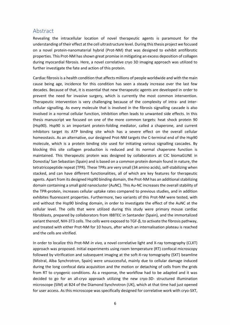
Abstract Revealing the intracellular location of novel therapeutic agents is paramount for the

understanding of their effect at the cell ultrastructure level. During this thesis project we focused

on a novel protein-nanomaterial hybrid (Prot-NM) that was designed to exhibit antifibrotic

properties. This Prot-NM has shown great promise in mitigating an excess deposition of collagen

during myocardial fibrosis. Here, a novel correlative cryo 3D imaging approach was utilized to

further investigate the fate and action of this protein.

Cardiac fibrosis is a health condition that affects millions of people worldwide and with the main

cause being age, incidence for this condition has seen a steady increase over the last few

decades. Because of that, it is essential that new therapeutic agents are developed in order to

prevent the need for invasive surgery, which is currently the most common intervention.

Therapeutic intervention is very challenging because of the complexity of intra- and inter-

cellular signalling. As every molecule that is involved in the fibrosis signalling cascade is also

involved in a normal cellular function, inhibition often leads to unwanted side effects. In this

thesis manuscript we focused on one of the more common targets: heat shock protein 90

(Hsp90). Hsp90 is an important protein-folding mediator, called a chaperone, and current

inhibitors target its ATP binding site which has a severe effect on the overall cellular

homeostasis. As an alternative, our designed Prot-NM targets the C-terminal end of the Hsp90

molecule, which is a protein binding site used for initiating various signalling cascades. By

blocking this site collagen production is reduced and its normal chaperone function is

maintained. This therapeutic protein was designed by collaborators at CIC biomaGUNE in

Donostia/ San Sebastian (Spain) and is based on a common protein domain found in nature, the

tetratricopeptide repeat (TPR). These TPRs are very small (34 amino acids), self-stabilizing when

stacked, and can have different functionalities, all of which are key features for therapeutic

agents. Apart from its designed Hsp90 binding domain, the Prot-NM has an additional stabilizing

domain containing a small gold nanocluster (AuNC). This Au-NC increases the overall stability of

the TPR-protein, increases cellular uptake rates compared to previous studies, and in addition

exhibites fluorescent properties. Furthermore, two variants of this Prot-NM were tested, with

and without the Hsp90 binding domain, in order to investigate the effect of the AuNC at the

cellular level. The cells that were utilized during this study were primary mouse cardiac

fibroblasts, prepared by collaborators from IBBTEC in Santander (Spain), and the immortalized

variant thereof, NIH-3T3 cells. The cells were exposed to TGF-β, to activate the fibrosis pathway,

and treated with either Prot-NM for 10 hours, after which an internalisation plateau is reached

and the cells are vitrified.

In order to localize this Prot-NM in vivo, a novel correlative light and X-ray tomography (CLXT)

approach was proposed. Initial experiments using room temperature (RT) confocal microscopy

followed by vitrification and subsequent imaging at the soft-X-ray tomography (SXT) beamline

(Mistral, Alba Synchrotron, Spain) were unsuccessful, mainly due to cellular damage induced

during the long confocal data acquisition and the motion or detaching of cells from the grids

from RT to cryogenic conditions. As a response, the workflow had to be adapted and it was

decided to go for an all-cryo approach utilizing the new cryo-3D- structured illumination

microscope (SIM) at B24 of the Diamond Synchrotron (UK), which at that time had just opened

for user access. As this microscope was specifically designed for correlative work with cryo-SXT,

7

sample preparation and imaging proved to be straightforward. However, due to its novelty, no

fiducialisation strategy, nor correlation protocols were available at the time. The development

of a working protocol for the complete process became therefor a large part of this thesis work.

After several visits to B24 for cryo 3D-SIM data collection, refining the sample preparation each

time, we were able to collect the data that allowed us to unambiguously localize the Prot-NM

within the 3D cellular space of both vitrified cell-types with a correlation accuracy down to 70

nm. This newly established correlative workflow placed the fluorescent visible light signal from

the Prot-NM within specific multivesicular bodies (MVB) and showed distinct differences when

comparing the two cell-types. While primary fibroblasts seemed rather unaffected, apart from

the natural reaction towards the fibrosis pathway activation, NIH-3T3 cells showed clear signs

of stress towards the treatments. Furthermore, the MVB themselves showed different

morphological features for either cell-type, which suggests different ways of uptake and

processing of the Prot-NM by the cells. This was also confirmed by an immunofluorescence assay

and confocal imaging in which different co-localisation was observed depending on the cell-type.

This correlative super-resolution and X-ray imaging strategy joins high specificity, by the use of

fluorescence, with high spatial resolution at 30 nm (half pitch) provided by cryo-SXT in whole

cells, without the need of staining or fixation, and can be of particular benefit to locate specific

molecules in the native cellular environment in bio-nanomedicine research. The data presented

in this manuscript highlights the development of this new workflow, and its ability to shed light

on complex drug-cell interactions. The Prot-NM studied here has shown great promise in

preventing myocardial fibrosis events without inducing side effects in primary cardiac mouse

fibroblasts. Meanwhile, a strong negative reaction towards the treatment, revealed by

ultrastructure morphological changes, was observed in the immortalized NIH-3T3 cell-type,

which is an important finding for biomedical studies as immortalized cell-lines are supposed to

exhibit similar behaviour as the primary ones.

8

List of abbreviations

(d)STORM (direct) Stochastic Optical Reconstruction Microscopy

2D 2 Dimensional

3D 3 Dimensional

ALS Advanced Light source

ART algebraic reconstruction technique

AuNC Gold Nanocluster

AVG Average

BESSY Berlin Electron Storage Ring Society for Synchrotron Radiation

CCD Charce-coupled Device

CLEM Correlative Light and Electron Microscopy

CLXT Correlative Light and X-ray tomography

CMS Cryo Microscopy Stage

CTPR consensus tetratricopeptide repeat

DMEM Dulbecco's Modified Eagle's Medium

DOF Depth of Field

DT Dual tilt

EBS Extra Brilliant Lightsource

EM Electron Microscopy

ES Entrance Slit

ESRF European Synchrotron Radiation Facility

ET Electron tomography

FBS Fetal Bovine Serum

FF Flat Field

FIB Focussed Ion Beam

FOV Field of view

FSCe/o Fourier Shell Correlation (equal/ odd)

FTIR Fourier Transform Infrared

FWHM Full Width Half Maximum

GFP Green Fluorescent Protein

HFM Horizontal Focussing Mirror

Hop Hsp70/90 organizing protein

Hsp90 Heat shock protein 90

IPTG Isopropyl β-d-thiogalactoside

LAC Linear Absorption Coefficient

LN2 Liquid Nitrogen

Med Median

MVB Multivesicular body

NA Numerical Aperture

NP Nano-particle

9

ON Over-night

OTF Optical transfer function

PALM Photoactivated localization Microscopy

PBS Phosphate Buffered Saline

Pen/Strep Penicillin/ Streptomycin

PFA Paraformaldehyde

PLL Poly-L-lysine

PPE Personal Protective Equipment

Prot-NM Protein Nanomaterial hybrid

rER rough endoplasmic reticulum

ROS Reactive Oxygen Species

RPS3 Ribosomal protein S3

RT Room temperature

S/N Signal to Noise ratio

SEM Scanning Electron Microscopy

sER smooth endoplasmic reticulum

SIM Structured Illumination Microscopy

SIRT Simultaneous iterations reconstruction technique

SLM Spatial Light Modulator

SMLM Single Molecule Localization Microscopy

SR Super Resolution

STED Stimulated Emission Depletion

SXT Soft X-ray tomography

TEM Transmission Electron Microscopy

TGF-β Transforming growth factor

THMS Temperature and Humidity controlled Microscopy Stage

TPR Tetratricopeptide repeat

TPS Taiwan Photon Source

TXM Transmission X-ray Microscope

UK United Kingdom

VFM Vertical Focussing Mirror

VLF Visible light Fluorescence

VLFM Visible Light Fluorescence Microscopy

VLM Visible Light Microscope

VRFM Vertical Re-Focussing Mirror

XRF X-ray fluorescence

XS Exit Slit

ZP Fresnel Zone Plate

10

1 Introduction

1.1 Societal background

In the last century a huge shift in the age demographic has occurred. This is mainly due to two

reasons: medical developments increasing the overall life expectancy, and increased birth-rates

after the Second World War, especially in developed countries. This so-called baby-boomer

generation, which are people born between 1946 and 1964, is now reaching an age where age-

related illnesses, such as arthritis, neurodegenerative and cardiovascular diseases, become a

major problem (Figure 1). This gives rise to an increased demand of related therapies, which are

still mainly treating symptoms, rather than the origin of the diseases. When consulting current

age demographic tables, it can be seen, that this baby-boomer group is just starting to reach the

medical-relevant age, meaning that the demand for specific therapeutic agents will increase

even further in the near future.

1.1.1 Cardiac diseases

One of the most prominent age-related conditions is connected to the cardiovascular function

(Jaul & Barron, 2017). Stress and an unhealthy lifestyle are the most important factors, in

addition to age, that increase the risk of cardiovascular dysfunction. In this work, we focused on

one specific event, called cardiac fibrosis. Cardiac fibrosis is a condition that affects millions of

people worldwide and is negatively affecting the progression of many other heart diseases

(Porter & Turner, 2009). The main characteristic of this condition is an excess (pathological)

deposition of collagen on the cardiac muscle which leads to myocardial stiffness and a reduced

overall heart function (Hinderer & Schenke-Layland, 2019). While this increased collagen

deposition alleviates some of the problems in the short-term, it reduces the life-span of the

Figure 1: Age demographic of the more developed regions of the world in 2020 according to the United Nations.

https://population.un.org/wpp/Graphs/DemographicProfiles/Pyramid/901 accessed 17.06.2021.

11

patient in the long-term. In addition, in most cases, (invasive) surgery is needed to prevent

further complications related to cardiac fibrosis (Porter & Turner, 2009). Currently there are no

preventive or curative treatments for cardiac fibrosis, due to the elusive mechanism and the lack

of specific targets (Colunga Biancatelli et al., 2020; M. Liu et al., 2021).

This lack of specific targets comes from the fact that affected cells release a large number of

cytokines, however none of which is solely responsible for fibrosis. The main cytokine that is

excreted during pro-inflammatory and pro-fibrotic processes and promotes the synthesis of

collagen fibres is the transforming growth factor (TGF-β) (Dobaczewski et al., 2011;

Doetschman et al., 2012). This cytokine initiates various signalling cascades upon binding

simultaneously to TGF-β receptor-I and II (Barnette et al., 2013; Chen et al., 1998; Isono et al.,

2002; Massagué & Wotton, 2000; Rodríguez-Vita et al., 2005; Yuan & Jing, 2010). In addition, it

initiates other cascades by independently binding to either receptor alone (Akhurst & Hata,

2012; Bujak & Frangogiannis, 2007; Derynck & Zhang, 2003; Massagué & Chen, 2000; Takekawa

et al., 2002). These molecular processes and cascades are tightly regulated and any external

interference can affect cell homeostasis. For this reason, targeting TGF-β directly unavoidably

leads to unwanted side-effects. As previously mentioned, there is no preventative or curative

treatment for fibrosis due to, among other, the lack of specific targets. This is the main reason

why recent efforts have been made towards identifying new target molecules for fibrosis

treatment, including those involved in the TGF-β induced pathway that leads to fibrosis (Figure

2).

One of the molecules that is currently investigated as potential target is the heat shock protein

90 (Hsp90) (Datta et al., 2015). Hsp90 is a chaperone, an enabler protein, whose role is to bind

Figure 2: Simplified schematic of the fibrosis pathway. Damaged cells upregulate TGF-β transcription and excretion

which in turn upregulates Hsp90 transcription. These effects together create a positive reinforcement and increase

the inflammation in the affected area, activating surrounding cells. When coming together to form a complex, TGF-

β, Hsp90 and CDC37 initiate the pro-fibrotic pathway, which leads to the collagen deposition on the affected area.

12

to so-called client proteins. When bound to ATP, Hsp90 facilitates protein folding and

stabilization of a wide variety of proteins, one of which is TGF-β (Wrighton et al., 2008). On the

contrary, when bound to ADP and a co-chaperone, it can facilitate the degradation of the

respective client protein (Eckl et al., 2013; Pratt & Toft, 2003). In the case of a fibrosis event, the

ATP-bound Hsp90 makes use of the co-chaperone CDC37 to stabilize the client (Eckl et al., 2013;

Pratt & Toft, 2003), which is in this case TGF-β (Figure 2). Because Hsp90 has been shown to be

up-regulated in the heart (Lee et al., 2010), Hsp90-inhibition has already been investigated in a

variety of pre-clinical studies targeting fibrosis (García et al., 2016; Noh et al., 2012; Sun et al.,

2009; Tomcik et al., 2014). However, the inhibitors investigated in these studies block the

ATPase domain, which is a key functional element in its protein folding activity, therefore giving

rise to side effects.

13

1.2 Tetratricopeptide repeat (TPR) proteins

An engineered Hsp90 inhibiting module was developed based on natural tetratricopeptide

repeat (TPR) domains (Cáceres et al., 2018; Cortajarena et al., 2004; Cortajarena, Yi, et al., 2008;

Main et al., 2003). This molecule has shown great potential inhibiting Hsp90, since this inhibition

results in a reduction of collagen overproduction (Cáceres et al., 2018). Unlike other Hsp90

inhibiting molecules, it does not act at the ATPase domain, instead it binds to the co-chaperone

binding site at the C-terminal end. This enables a normal chaperone function which is of vital

importance when trying to minimize unwanted side effects. While the Hsp70/90 organizing

protein (Hop) is the most common Hsp90 co-chaperone, during a fibrosis event the previously

mention CDC37 is one of the co-chaperones that binds to this site and facilitates the collagen

(over-) production (Datta et al., 2015).

The TPR was already described in 1990 and is a domain usually found in different protein

scaffolds of varying lengths (Hirano et al., 1990; Lamb et al., 1995; Sikorski et al., 1990). These

tandem repeats are small sequences (34 amino acids), stabilized by local interactions within

itself, but also between the repeated modules (Cortajarena et al., 2011). The number of

repeats in a scaffold varies, from only a single domain, up to 16 repeats, although most well-

described TPR proteins contain three repeats (D’Andrea & Regan, 2003). One of the best

characterized TPRs at that time was the Hop TPR domain which is why this was used to further

investigate TPR-target recognition (Scheufler et al., 2000). A consensus TPR (CTPR) sequence

was designed based on a large amount of TPR sequences to optimize stability, and CTPR

proteins with different numbers of repeats resulted in well-folded super stable TPR scaffolds.

Mimicking the natural TPR-based binding domains, a TPR was build containing three repeats

(CTPR3), on which specific binding functional sites could be introduced. The original Hop has

two functional TPR sites: TPR1 and TPR2A, which bind Hsp70 and Hsp90, respectively. For

therapeutic purposes, Hsp90 inhibition was more interesting compared to the former as it has

been shown that Hsp90 overexpression is involved in many diseases, including cancer (Bisht et

al., 2003; Cortajarena, Yi, et al., 2008; Neckers et al., 1999; Workman, 2005) and various

fibrosis events (Datta et al., 2015; Noh et al., 2012; Tomcik et al., 2014). A consensus sequence

from the identified binding residues from Hop TPR2A and other Hsp90-binding TPR domains

was grafted onto the CTPR3 scaffold (Cortajarena et al., 2004), to obtain the CTPR390 protein

(Cortajarena, Yi, et al., 2008), and it has shown great promise in specifically binding the C-

terminal end of Hsp90 (Aires et al., 2021; Cáceres et al., 2018).

The main advantage of these TPR-based proteins is their large variety and thus application

possibilities. The CTPR390 described previously has been specifically designed with the purpose

of binding to Hsp90. The three domains used in this version were needed to create the specific

binding pocket. However, by changing the appearance of the protein, i.e. by introduction of

more repeated modules or creating point mutations to change their electrochemical properties,

new binding pockets can be created and these proteins can encode a wide range of new

functions (Cortajarena et al., 2010).

14

1.2.1 Metal Nanoclusters

Another recent development has been metal nanomaterials, which often show size-dependent

properties, for various technological applications (Cobley et al., 2011; Guo & Wang, 2011; Sau &

Rogach, 2010). When comprising of only very few atoms, these metal-nanomaterials display

fluorescent properties but usually need a stabilizing agent to maximize these. This has already

been done with a variety of biological structures (Bao et al., 2010; Chevrier, 2012; G. Liu et al.,

2013; Slocik et al., 2002; Varnavski et al., 2001) and now has also been applied to the CTPR390

protein (Aires et al., 2019, 2021). A new TPR domain was designed with two strategically placed

His molecules that enable the binding of a gold nanocluster (AuNC) on an α-helix of a repeat

module and this module was fused to the CTPR390 protein scaffold, creating a protein-

nanomaterial hybrid (Prot-NM), see Figure 3 left (Aires et al., 2019, 2021). This Prot-NM, which

in the scope of this thesis manuscript will be called CTPR390-AuNC, showed high stability and

good fluorescent properties from the AuNC, in addition to the Hsp90 binding capabilities. The

excitation peak for the AuNC was found at 370 nm, with an emission optimum between 440 and

450 nm (Figure 3 right). Furthermore, when tested in vivo, it showed no toxicity and increased

internalization capabilities when compared to the CTPR390 without the AuNC. Especially the

improved cellular uptake rate is an immense improvement for biological studies and in

combination with the fluorescent properties makes these protein-metal complexes very useful

for live cell imaging and labelling.

Figure 3: Left, structural representation of the CTPR390-AuNC protein hybrid showing the base CTPR3 in green with

the Hsp90 binding ligand attached to it, and the AuNC stabilizing module in blue, with the AuNC attached. Taken

from (Aires et al., 2021). Right, excitation (blue) and emission (orange) spectra of this CTPR390-AuNC.

15

1.3 Objective

In this project, an optimized version of the Hsp90 inhibiting CTPR390 protein, described in

(Cáceres et al., 2018) was used. This improved version contains the AuNC which has shown to

increase cellular uptake and exhibits fluorescent properties (Aires et al., 2019, 2021), which

would allow the protein localization without the need of the labelling with a fluorescent

molecule, as was required in the previous study (Cáceres et al., 2018). As mentioned before,

previous studies found that CTPR390 can efficiently inhibit Hsp90, and thereby reduce collagen

deposition, in vivo and in vitro without affecting overall health of the cell (Cáceres et al., 2018).

With the introduction of new components onto the protein, as in this case the AuNC and its

stabilizing domain, it is expected that the pharma-kinetic properties have changed. In order for

it to become a therapeutic agent it does need more studies highlighting its beneficial effects.

Herein we intended to investigate the effect of the hybrid protein including AuNCs at a cellular

level using a high-resolution correlative microscopy approach. Due to the introduction of the

AuNC we intended to replicate the findings of this previous study, and then build on top, further

highlighting its beneficial effects and lack of negative effects. The initial goals of this research

were:

1. To study the intracellular fate of this novel protein nanomaterial hybrid.

2. To study the effect of the treatment on the cell at an ultrastructural level.

Both goals will deepen our knowledge and understanding of the molecular processes related to

the cellular uptake as well as the effects triggered by the therapeutic agent at the cellular level.

This information is indispensable for further practice in the clinic.

One of the techniques suited to achieve this is cryo soft X-ray tomography (cryo-SXT) (Schneider

et al., 2010; Weiß et al., 2000) as it allows revealing the structure of whole cells in close-to-

native conditions at high spatial resolution (Carrascosa et al., 2009; Chiappi et al., 2016; Chichón

et al., 2012; Duke et al., 2014; Groen et al., 2019; Hagen et al., 2012; Kepsutlu et al., 2020; Pérez-

Berná et al., 2016; Weinhardt et al., 2020). Initially there was not yet a clear idea on which

specific technique to use in conjunction. Still, as we intended to localize molecules within the

cellular space, visible light fluorescence microscopy (VLFM) was the go-to approach, although

other techniques, such as hard X-ray fluorescence (Conesa, Carrasco, et al., 2020), were also

considered. Because such an abundance of VLFM techniques are available we had to perform

some tests to find a suitable workflow that would allow us to address the previously mentioned

questions accurately.

In what follows, we discuss the methodology used, as well as the advantages and limitations of

our approach.

16

2 Approach To answer the research questions raised for this project, a correlative imaging approach was

proposed: visible light fluorescence microscopy (VLFM) to locate specifically the CTPR390-AuNC,

and cryo-SXT to visualize the cellular ultrastructure and place this fluorescence signal within the

cellular environment to understand the fate of the CTPR390-AuNC and its effect. Due to the

availability of instrumentation we had at hand, we started with a combination of room

temperature VLFM followed by sample vitrification and cryo X-ray imaging. Unfortunately, this

hybrid temperature approach was unsuccessful. Therefore, a complete cryo approach was

undertaken, using the newly in house developed cryo 3D structured illumination microscope

(cryo-3D-SIM) at B24 at Diamond Synchrotron (UK). This type of cryo correlative visible light and

soft X-ray tomography (CLXT) approach is very novel and unique, and a recent Nature Protocol

paper was published in collaboration with B24 to allow future users to choose the best possible

strategy for their research (Okolo et al., 2021). This approach is summarised in Figure 4, after

sample preparation and vitrification, samples are first screened using cryo epifluorescence and

the best ones are then imaged at the cryo-3D-SIM followed by cryo-SXT to finally correlate the

3D datasets.

It is worth mentioning that currently suitable equipment allowing for cryogenic studies is scarce

and this cryo approach could only be pursued using prototype instrumentation developed by

specific academic research groups outside Spain. Therefore, our choice had a clear drawback:

the restricted access to the cryo-3D-SIM instrumentation which implied travelling to a foreign

country a limited number of times, not to mention the currently still ongoing pandemic which

was not expected when this work started.

This chapter will first focus on an introduction to VLFM, highlighting our choice for the cryo-3D-

SIM, then on X-ray microscopy, highlighting cryo-SXT, and finally on correlative microscopy

including a discussion on the advantages and limitations.

Figure 4: Schematic representation of the workflow. Cells are cultured on top of EM grids, followed by the

treatment and fluorescent labelling. Then, the grids are vitrified and visualized using cryo-epifluorescence to

determine the quality of each sample. The best samples are then imaged using the cryo-3D-SIM, followed by cryo-

SXT on the same cells. After various post-processing steps the datasets belonging to the same cell can be correlated

and combined. Field of view of the three datasets: 10 x 10 µm.

17

2.1 Visible light fluorescence microscopy

VLFM has been used for decades to find structures of interest and is one of the preferred tools

in most laboratories worldwide as it allows live cell imaging of the tagged features. Thanks to its

high compatibility and complementarity with other techniques, VLFM is usually included in

correlative approaches, the most common being correlative light and electron microscopy

(CLEM, (Deerinck et al., 1994; Svitkina et al., 1995)). This chapter will first give a general

introduction into VLFM, highlighting its versatility and limitations, followed by short

introductions to three topics, relevant to this project: super resolution VLFM, VLFM within

correlative approaches and cryo VLFM. The final part describes the requirements for this project

in particular, and a more detailed description on the technique that was utilized in this work.

2.1.1 VLFM in biology

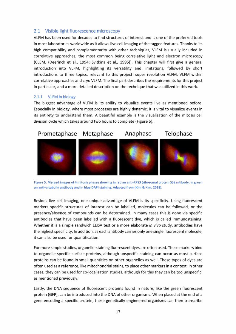
The biggest advantage of VLFM is its ability to visualize events live as mentioned before.

Especially in biology, where most processes are highly dynamic, it is vital to visualize events in

its entirety to understand them. A beautiful example is the visualization of the mitosis cell

division cycle which takes around two hours to complete (Figure 5).

Besides live cell imaging, one unique advantage of VLFM is its specificity. Using fluorescent

markers specific structures of interest can be labelled, molecules can be followed, or the

presence/absence of compounds can be determined. In many cases this is done via specific

antibodies that have been labelled with a fluorescent dye, which is called immunostaining.

Whether it is a simple sandwich ELISA test or a more elaborate in vivo study, antibodies have

the highest specificity. In addition, as each antibody carries only one single fluorescent molecule,

it can also be used for quantification.

For more simple studies, organelle-staining fluorescent dyes are often used. These markers bind

to organelle specific surface proteins, although unspecific staining can occur as most surface

proteins can be found in small quantities on other organelles as well. These types of dyes are

often used as a reference, like mitochondrial stains, to place other markers in a context. In other

cases, they can be used for co-localization studies, although for this they can be too unspecific,

as mentioned previously.

Lastly, the DNA sequence of fluorescent proteins found in nature, like the green fluorescent

protein (GFP), can be introduced into the DNA of other organisms. When placed at the end of a

gene encoding a specific protein, these genetically engineered organisms can then transcribe

Figure 5: Merged images of 4 mitosis phases showing in red an anti-RPS3 (ribosomal protein S3) antibody, in green

an anti-α-tubulin antibody and in blue DAPI staining. Adapted from (Kim & Kim, 2018).

18

these fluorescent proteins. Compared to fluorescent dyes, this technique is much more accurate

as no un-specific labelling can occur. This creation of recombinant strains is usually done to

answer gene-activity studies or to identify recombinant strains.

Regardless the type of labelling, VLFM has enabled answering many research questions.

Nonetheless it has some flaws that limit its use. The first disadvantage to mention would be the

lack of context. As only the fluorescently labelled structures can be seen, no information is given

on the rest of the cellular environment. Especially in the field of cell-/molecular biology, the

ultrastructural organisation is missing. Using just the fluorescent signal will give an incomplete

picture of a complex system. Related to this, the number of structures that can be labelled at

the same time is limited by the available markers, excitation lasers and emission filters. Although

using spectral imaging, which is a method to split light based on wavelength, it is possible to

select a specific range of wavelengths for collection. However, narrowing the spectral collection

window also reduces the amount of signal, leading to reduced contrast. In addition, if

fluorescent markers are chosen that have their emission wavelengths too close together,

bleeding of the signal into the other range will be observed. For this reason, a maximum of 4

different fluorescent markers are used per sample in most cases.

Another limitation in fluorescence microscopy is the bleaching effect of the fluorophores. High

illumination power and long exposure times can severely reduce the lifetime of a fluorophore.

Depending on the type of experiment this is something to be considered. In addition to the

bleaching effect, extended illumination will induce the formation of reactive oxygen species

(ROS) in cells. While these do not directly affect the fluorophore, the generated ROS will cause

damage to the cell which, in itself can provoke artefacts.

While all previously mentioned points must be taken into consideration when designing an

experimental approach, the main limitation of visible light has yet to be addressed: the

resolution limit. The achievable resolution using any spectrum range of light is determined by

the diffraction limit of the wavelength used (Abbe, 1873). The lateral resolution is given by

/2NA (where is the wavelength used and NA is the numerical aperture) and is, for green light

emission at 500 nm, set at 250 nm for NA=1 while the axial resolution, given by 2/NA2, is set at

1 µm. While this resolution has long been sufficient, it quickly became an insurmountable

obstacle as increasingly small objects had to be visualized.

2.1.2 Super-resolution microscopy

Until a few decades ago this diffraction limit could not be surpassed. Since then, various

techniques emerged that utilize “tricks” and post-processing techniques to circumvent these

limits, which are caused by the inherent properties of using visible light wavelengths (400-700

nm). These newly developed techniques were coined super-resolution (SR) (Sezgin, 2017) and

the efforts of Professors S. Hell, E. Betzig and W.E. Moerner to develop super-resolution imaging

even deserved the Chemistry Nobel Prize in 2014. The techniques mentioned here do not

represent the full list but, within the scope of this project, were techniques that could possibly

answer our research questions.

SR techniques were developed because there was a need to localize and study increasingly small

features or molecules. Some of the most commonly used super-resolution techniques are

stimulated emission depletion (STED) microscopy (Hell & Wichmann, 1994), photoactivated

19

localization microscopy (PALM) (Betzig et al., 2006; Hess et al., 2006) and stochastic optical

reconstruction microscopy (STORM) (Heilemann et al., 2008; Rust et al., 2006). The basic

principle behind these three techniques is the visualization of a single or few fluorophores at a

time in order to calculate the exact centre of the collected signal. The main advantage of these

techniques is the achievable resolution well below the diffraction limit. However, in order to

reach resolutions down to 20 nm, for example in the case of dSTORM (Heilemann et al., 2008),

the samples need to fulfil multiple and stringent requirements (thickness, fixation, buffer-

solution…) which can severely limit its applications. Within these SR techniques, a new term was

created to distinguish those that can locate single molecules: Singe Molecule Localization

Microscopy (SMLM). But ultimately, what these techniques gain in lateral resolution, they lose

in axial resolution meaning only the light emitted from very thin in-depth sections of the cell are

commonly used. Furthermore, STORM and PALM in particular need long acquisition times which

make imaging of live cells and their dynamic intracellular processes challenging.

When looking at whole cells, 3D information is vital and one of the most common technique

worldwide is confocal microscopy (Elliott, 2020). The main usage of confocal microscopy is 3D

imaging by using a pinhole that blocks light coming from outside the focal plane. This means that

no further processing is needed as the light that reaches the detector only contains information

of a single but thick focal plane of about 1 µm. By moving the sample stage, cells can be

visualized rapidly in 3D. Because it is such an easy-to-use technique, many developments have

been made, both hardware and software, which allowed for more specific functional research.

Examples are the Airy scan module, which does give it a space in the group of SR techniques, or

the previously mentioned spectral imaging, which allows the collection of specific wavelengths.

However, the fact that light, and thus valuable information, is excluded enforces the need of

having a high fluorophore yield coming from the imaged planes, which makes identifying scarce

molecules or events difficult.

The last technique to be mentioned here is structured illumination microscopy (SIM)

(Gustafsson, 2000). This technique uses two diffracted beam orders from a coherent light beam

generated by a grating or a spatial light modulator, which interfere on the specimen producing

a structured light pattern that varies laterally. Using the collected emission signal and the

structured excitation light pattern, the final image can be reconstructed, giving a 2-time increase

in resolution, thereby surpassing the diffraction limit. In 2008, the Gustafsson’s group managed

to incorporate the zero-order beam that allowed distinguishing the signal axially too, which

means a 2-fold spatial resolution increase in all 3 dimensions (Gustafsson et al., 2008). This

technique is a high throughput full-field technique where acquisition and reconstruction of the

data can be done in less than 15 minutes. Furthermore, it has very good out-of-focus light

suppression which allows imaging thick samples (10 µm) with good contrast and low intensities

(Phillips et al., 2020). The main limitation is the fact that the 2-fold increase in resolution cannot

be further improved.

For structural molecular biology it is essential to obtain intracellular information. The

aforementioned techniques are able to do that and thus are the most commonly used for these

studies. However, by circumventing the resolution limitation, another, previously mentioned

limitation became the new main obstacle: the lack of context. To compensate for this problem,

correlative microscopy was created.

20

2.1.3 Correlative Microscopy

Current trends in biology are going mostly towards the development of correlative approaches.

The idea behind correlative microscopy is to visualize the same sample using different

techniques, which combined give more information than either technique alone. This also

includes compensating the weaknesses of the different techniques. The most commonly known

correlative technique is correlative light and electron microscopy (CLEM) which has been a major

asset in the field of biology for decades. VLFM provides the specificity to identify an event or

structure of interest and electron microscopy (most commonly transmission EM (TEM))

provides, in nanometric resolution, the ultrastructural information of that same structure.

Nowadays, almost every electron microscope has an integrated light microscope for correlative

purposes. While these integrated visible light microscopes are in most cases not able to perform

single molecule studies, they do guide the user to particular areas of interest, which is indeed a

very important asset.

Something that needs to be mentioned when considering correlative microscopy, specifically for

CLEM, is the fact that the samples have to be fixed prior to imaging. Apart from an alteration of

the natural cellular structure, chemical fixatives are known to induce quenching of the

fluorescent signal. For this reason, two different approaches can be utilized: fluorescent imaging

prior to fixation, or post-fixation staining. Imaging prior to fixation allows more options regarding

labelling, however, the time between imaging and fixation can give rise to problems. This is not

the case for post-fixation labelling and imaging as molecules or structures will not move.

However, as after-fixation-labelling is performed with specific antibodies, issues can still arise as

they might not be able to reach all sites. In addition, specific antibodies need to be readily

available, which can be a challenge when novel proteins need to be marked.

As mentioned before, the ability to perform live cell imaging is what makes VLFM such an

excellent tool for addressing many biological questions. This is also the reason why it is such a

great partner in many correlative microscopy approaches. However, if this approach implies an

alteration of the sample, i.e. by exposing it to chemicals, this benefit is to a certain extent lost.

Observing something in their native state should always be preferred over any fixed sample and

for that reason a new approach was developed that does not require any chemical fixation and

thus offers an unperturbed view of a cell in near-native conditions: cryogenic fixation.

2.1.4 Cryo-fixation in biology

Cryogenic fixation is currently not a new development. For standard EM in biology, the most

common sample preparation approach is cryo-fixation, for example by high pressure freezing,

followed by freeze substitution, which is a slow process (several days) in which the water is

exchanged with an organic solvent containing the chemical fixation agents (Giddings, 2003).

However, using the frozen sample itself is a relatively new approach, especially for EM, mainly

due to the hardware requirements that are involved in working with cryo-fixed samples

(Dubochet et al., 1987; Dubochet & Sartori Blanc, 2001). For a successful cryopreservation,

samples need to be frozen completely and rapidly. The main hurdle during this process is the

formation of ice crystals, which occurs when water freezes “slowly”. In the case of cellular

samples, these crystals destroy the sample from within as the cellular cytoplasm consists mostly

of water. However, if the water is cooled to 130 K in a fraction of a second, so-called non-

crystalline (amorphous) ice is formed, as the water does not have time to form ice crystals. This

21

process of rapidly freezing a sample is called vitrification which is done by the previously

mentioned high pressure freezing or plunge freezing devices, among others. The challenge with

cryogenically frozen samples is that they need to be permanently maintained in a cryogenic

environment, because an increase in temperature above 130 K will result in the formation of ice

crystals, which is coincidently the most common artefact in cryogenic samples (Dubochet et al.,

1987).

An area that had a major breakthrough recently, the so-called “resolution revolution”

(Kühlbrandt, 2014), is the field of cryo-electron microscopy (cryo-EM), which was awarded a

Nobel prize in 2017 in the area of single particle analysis. In the area of cell biology, cryo-electron

tomography (cryo-ET) was developed to obtain high resolution 3D information of thin cryo

focussed ion beam (FIB) milled lamellae. Contrary to classical EM, cryo-EM and cryo-ET do not

require chemical fixation or staining and therefore, samples can be fluorescently labelled prior

to cryo-fixation and imaged in cryogenic conditions. This opened up new possibilities, like using

the previously mentioned fluorescent proteins, as no quenching of the fluorescent signal is

induced by fixation chemicals. Furthermore, as the samples for cryo-ET needed to be very thin,

which is also a requirement for some SR techniques like PALM or STORM, interest in cryo-

fluorescence got re-ignited.

While in itself cryo-fluorescence is an old approach, it has been used primarily for

epifluorescence studies (Sartori et al., 2007; Schwartz et al., 2007), as it is very challenging,

mainly due to temperature stability and hardware restriction (specific objectives, humidity

control, stable sample stage etc.). Low resolution cryo epifluorescence however, had been

possible thanks to academic developments (Schwartz et al., 2007) and, shortly after, commercial

developments from Linkam Scientific Instruments in particular, made it available to the global

scientific community. A prototype based on the Temperature and Humidity control Microscopy

Stage (THMS) became available in 2009, followed by a first fully dedicated Cryo-Microscopy

Stage (CMS) in 2012. This manual cryo stage has progressively improved and their most recent

CMS196 motorised unit is a staple element in many current setups. Unfortunately, all these

stages at the moment use a long-distance air objective with NA<1, which has a direct effect on

the resolving power. With the development of cryogenic approaches in other fields and an

increasing interest on correlative imaging, particularly in cryo-ET, there is a high demand for high

resolution cryo VLFM. Lately, commercial companies are pushing towards producing suitable

instrumentation for correlative cryo-microscopy approaches and some of these developments

have benefitted from the Linkam CMS196 cryo stage, as mentioned before. While in theory most

visible light fluorescence microscopy techniques could be used in cryogenic conditions, cryo

condition capabilities are not easily achievable due to the varying requirements of each specific

technique and the progress is slower than expected.

The development of super resolution under cryo conditions is currently still in progress

(Dahlberg et al., 2020). It has been shown that some fluorescent markers perform better under

cryo condition due to increased photo stability and decreased bleaching (Schwartz et al., 2007;

van Driel et al., 2009), which is detrimental for techniques like PALM or STORM that rely on

fluorophore longevity. The main hurdle for cryo super-resolution fluorescence is the fact that no

immersion objectives are available yet, meaning 100x 0.9 NA long distance air objectives give,

for the moment, the best results. As already mentioned, another relevant development in

22

progress is the cryo-stage, which is indirectly also tied to the objective. While some of the major

companies are working on the development of proprietary stages, it seems that the integration

of the Linkam stage for the moment is the only available option. Meanwhile, the development

of a cryo immersion objective for higher numerical apertures is still a challenge that might take

time to be overcome. At this moment, the main issue related to the development of a cryo

immersion objective is that the process of cooling and heating has an immense toll on the

objective lens. These repeated temperature gradients and changes put an increased strain on

the objective, increasing the risk of damaging parts and thereby reducing its lifespan. There is

currently a short distance cryo objective that has been developed by Leica, however it is also

not an immersion objective. It is expected that with the development of stable cryo immersion

objectives the development of a better compatible cryo stage will shortly follow.

The transmission X-ray microscope (TXM) at Mistral beamline operates in complete cryogenic

conditions and thus utilizes well established plunge freezing protocols for sample preparation.

The development of cryo-SR-VLFM is a major step forward, not only in the field of VLFM but also

for correlative microscopy, in general, with already well-established cryo-imaging techniques.

Cryo fixation is nowadays considered the gold standard for sample preparation and while in this

case it cannot be called live cell imaging anymore, it will give a close-to-native representation of

the cell, practically frozen in time.

2.1.5 Requirements

The best correlative approach ideally depends on the research question. In our case, we needed

to fulfil several requirements to be fully compatible with cryo-SXT (see Table 1: Comparison of

the three main super resolution techniques for a comparison of key parameters). These include:

1) using the same sample support (EM grids); 2) the ability to perform the imaging in cryo; 3)

avoid using chemical fixatives; 4) full field 3D imaging; 5) match as best as possible the 3D

resolution; and 6) fast acquisition and processing of the data to be able to image cell

populations. Additionally, the availability to access the proper instrumentation can be

considered the 7th requirement.

As mentioned before, a hybrid approach with live cell imaging at RT, followed by vitrification

and cryo-SXT was unsuccessful. With the need for cryo, SMLM techniques were discarded as an

option for this project. The main factor here was that a working and open for user access cryo-

SMLM setup does not yet exist. Furthermore, the disability of SMLM to image deeper than a few

microns, as well as the extensive acquisition and processing requirements are additional reasons

why it was discarded. Both options, cryo 3D-SIM and cryo confocal microscopy, were viable as

each had, depending on the criterion, specific advantages over the other. Ultimately, the key

factor on which the decision was based was the availability. A working and open for user-access

cryo-3D-SIM was available at B24 of the Diamond Synchrotron (UK) while at that time, only few

cryo-confocal systems were installed in specific laboratories. To our knowledge, the only

available system in Spain today is located at CNB-CSIC in Madrid and is currently still under

commissioning. Note that the field of fluorescence microscopy is highly versatile and

continuously evolving. In the future some of the mentioned techniques could potentially adapt

and conform to our requirements, providing new information. In what follows, a short and more

in-depth explanation of the cryo-3D-SIM is given.

23

Table 1: Comparison of the three main super resolution techniques

Requirement Specifics Compatibility level Explanation

Sample

support

SXT requires EM

grids (typically

Au Finder with a

Quantifoil

support layer)

3D-SIM

Confocal Microscopy

SMLM

(STORM/PALM)

➢ Yes

➢ Yes

➢ Needs either very thin or very

flat samples, due to low axial

resolution

Cryo-imaging

development

Availability 3D-SIM

Confocal Microscopy

SMLM

(STORM/PALM)

➢ Yes

➢ Yes

➢ In development

3D imaging Ability to obtain

the data

through the

whole cell

3D-SIM

Confocal Microscopy

SMLM

(STORM/PALM)

➢ Yes

➢ Yes

➢ Only up to 250 nm accurately,

although up to few microns is being

developed

Resolution Matching 30 nm

half pitch SXT

resolution

3D-SIM

Confocal Microscopy

SMLM

(STORM/PALM)

➢ Capped at 125 nm lateral under

ideal conditions

➢ Sub-diffraction limit using

special equipment

➢ <50 nm

Time Acquisition and

post-processing

time

3D-SIM

Confocal Microscopy

SMLM

(STORM/PALM)

➢ Fast acquisition time, but needs

different angles and phases and

processing time reconstruction

➢ Very fast

➢ Long acquisition and processing

Availability Both

commercial

instrument or

internal

developments

3D-SIM

Confocal Microscopy

SMLM

(STORM/PALM)

➢ Open for user experiments since

2019

➢ Commercial instruments

available but only few open for user

access

➢ Not in cryo

Level of compatibility: Green – High; Orange – requires work; Red – Low

24

2.1.6 Cryo-3D-SIM

As mentioned above a cryo-3D-SIM was developed at B24 at Diamond synchrotron (UK) (Phillips

et al., 2020), which is another cryo soft X-ray tomography beamline. Their cryo-3D-SIM set-up

was specifically designed with the purpose of performing correlative visible light and X-ray

tomography (CLXT) (see Figure 6). As mentioned previously, SIM is a technique able to surpass

Figure 6 Top: Schematic of the cryo-3D-SIM at B24, Diamond. For more details see (Phillips et al., 2020). Bottom:

Some pictures of the microscope. A shows the laser sources and the SLM, B shows a number of mirrors, C shows

more mirrors and the 2 cameras, and D shows the complete closed setup with the CMS196 Linkam stage.

25

the diffraction limit, although only 2-fold, meaning the maximum theoretical resolution

achievable is 91 nm (NA=1.4) or 142 nm (NA=0.9) laterally and 260 nm (NA=1.4) or 629 nm

(NA=0.9) axially for 510 nm emission (GFP). Due to the objective lens limitation, this also

represents the current resolution difference when comparing room temperature (NA=1.4) and

cryo conditions (NA=0.9), thus further highlighting the need to develop proper cryo (immersion)

objectives.

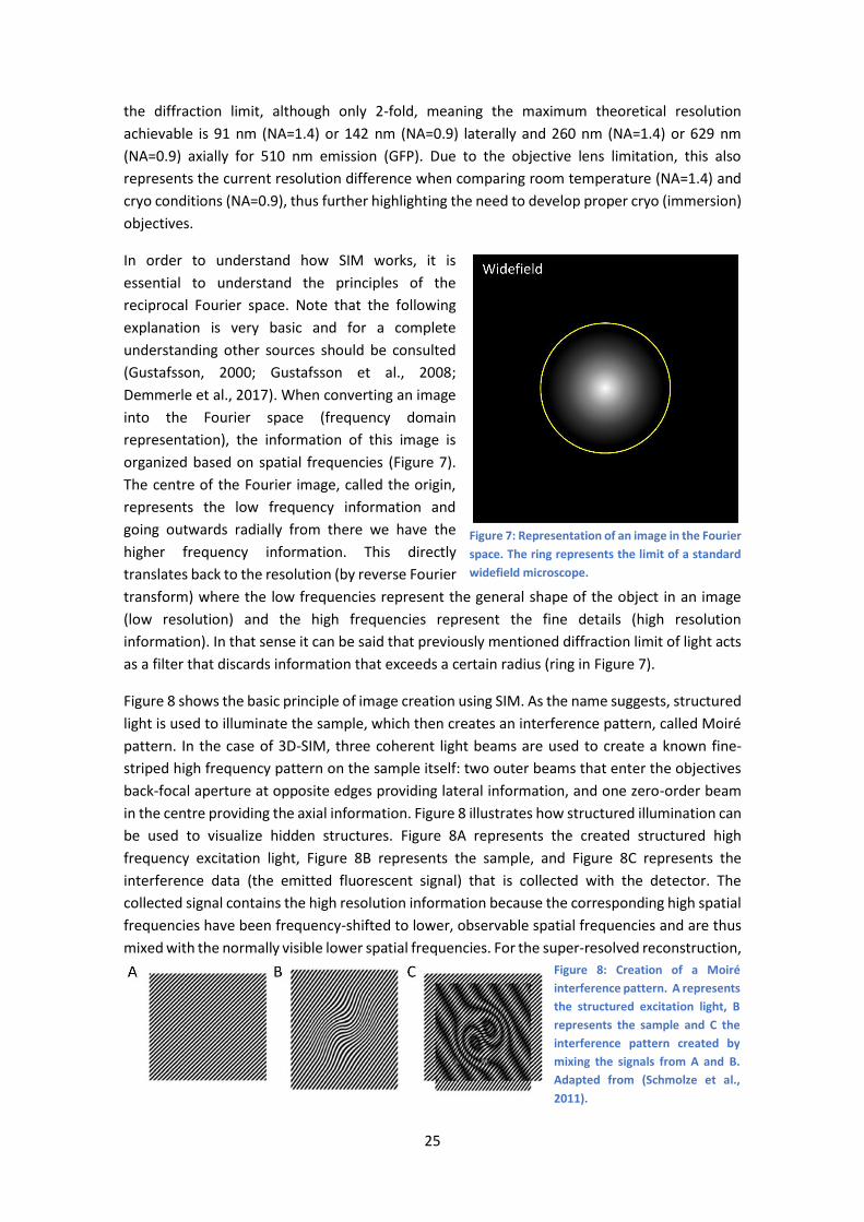
In order to understand how SIM works, it is

essential to understand the principles of the

reciprocal Fourier space. Note that the following

explanation is very basic and for a complete

understanding other sources should be consulted

(Gustafsson, 2000; Gustafsson et al., 2008;

Demmerle et al., 2017). When converting an image

into the Fourier space (frequency domain

representation), the information of this image is

organized based on spatial frequencies (Figure 7).

The centre of the Fourier image, called the origin,

represents the low frequency information and

going outwards radially from there we have the

higher frequency information. This directly

translates back to the resolution (by reverse Fourier

transform) where the low frequencies represent the general shape of the object in an image

(low resolution) and the high frequencies represent the fine details (high resolution

information). In that sense it can be said that previously mentioned diffraction limit of light acts

as a filter that discards information that exceeds a certain radius (ring in Figure 7).

Figure 8 shows the basic principle of image creation using SIM. As the name suggests, structured

light is used to illuminate the sample, which then creates an interference pattern, called Moiré

pattern. In the case of 3D-SIM, three coherent light beams are used to create a known fine-

striped high frequency pattern on the sample itself: two outer beams that enter the objectives

back-focal aperture at opposite edges providing lateral information, and one zero-order beam

in the centre providing the axial information. Figure 8 illustrates how structured illumination can

be used to visualize hidden structures. Figure 8A represents the created structured high

frequency excitation light, Figure 8B represents the sample, and Figure 8C represents the

interference data (the emitted fluorescent signal) that is collected with the detector. The

collected signal contains the high resolution information because the corresponding high spatial

frequencies have been frequency-shifted to lower, observable spatial frequencies and are thus

mixed with the normally visible lower spatial frequencies. For the super-resolved reconstruction,

Figure 7: Representation of an image in the Fourier

space. The ring represents the limit of a standard

widefield microscope.

Figure 8: Creation of a Moiré

interference pattern. A represents

the structured excitation light, B

represents the sample and C the

interference pattern created by

mixing the signals from A and B.

Adapted from (Schmolze et al.,

2011).

26

several images have to be collected, with this striped pattern shifted laterally (usually in 5 steps

with a step size of 2π/5). The acquired phase-shifted images are used to calculate the relative

contribution of the low- and high spatial frequencies in order to separate them (mathematically

deconvolving the interference signal). The high frequencies are then extracted and shifted to

the correct position. However, this only provides information on one axis, depending on the

angle of the structured excitation light. In order to create an isotropic resolution increase,

images have to be acquired using three different angles with steps of 60˚, creating different

interference patterns. This is shown in Figure 9. The three images on the left represent the added

high spatial frequency information per angle in Fourier space, which is then combined in the

large panel. Furthermore, these 15 images (3 angles x 5 phases) must be acquired for each focal

plane (z steps of 125 nm).

The advantage that SIM has compared to other super resolution techniques is its ability to

perform fast imaging in 3D with high out of focus light suppression and low excitation intensities.

With cryo-SXT having a resolution of 30 nm (half-pitch) laterally (Otón et al., 2016; Reineck et

al., 2021), the higher the resolution of the fluorescent signal, the better the spatial correlation

accuracy. At the moment, all available cryo stages have similar limitations as they use a long

working distance 100X objective with a NA of 0.9. This severely limits achievable resolutions

compared to immersion objectives. Accounting for this fact, the difference in spatial resolution

in the axial direction between the cryo-3D-SIM and its main competitor, the cryo confocal

microscope with Airy scanning unit from Zeiss, is therefore substantial, even though in the

lateral direction both instruments will provide similar performances. Even so, it should be

mentioned that usually a commercial instrument might be more user-friendly and this can also

be an advantage when used in imaging facilities.

Figure 9: Representation of

the Fourier space of a 3D-

SIM image. The small

images on the left represent

the individual angles, which

are combined to give the

complete image in Fourier

space. Note the FOV is the

same as in Figure 7 which

shows the actual 2-fold

increase of spatial

frequency.

27

2.2 X-ray microscopy

X-ray microscopy is one of the major players in the world of microscopy. On the electromagnetic

spectrum, X-rays are located between ultraviolet and gamma rays, having a very small

wavelength ranging from 10 nm to 10 pm which corresponds to an energy range of 0.1 to 100

keV. X-rays are a form of electromagnetic radiation originating from electrons when they lose

kinetic energy. This energy loss can be due to a hard stop, directly hitting a wall, or more softly

when the path of electrons travelling at speeds close to the speed of light is slightly changed

through so-called bending magnets. The hard stop is usually used in small tabletop sources,

which will not be discussed in this manuscript. As the work described here was performed in a

synchrotron, the techniques discussed here are all synchrotron-based. This chapter will first

explain the concept of a synchrotron, discuss some general properties of X-rays, followed by the

current trends and ending with a description of soft X-ray tomography at the Mistral beamline

(Alba, Spain).

2.2.1 X-ray light sources

Wilhelm Röntgen is usually credited as the discoverer of X-rays in 1895 because he was the first

to systematically study them, hence the reason why they are often referred to as Röntgen rays.

He quickly discovered that X-rays are able to pass through a wide variety of materials, while not

being able to penetrate others. This was a breakthrough for medicine as they are able to

penetrate tissue. Within a few years, X-rays were used in hospitals to locate broken bones,

swallowed objects and more within the body. Interest in X-rays skyrocketed, which even lead to

Röntgen being awarded the first Nobel Prize in Physics in 1901. Back then a so-called X-ray tube

was used as a source. The big limitation for this type of source is that the produced rays are

Figure 10: Schematic representation of Alba Synchrotron. In blue the four sections of the ring are named and in

yellow the endstations available or in construction at Alba. Obtained from:

https://www.cells.es/en/about/welcome accessed 06-08-21.

28

going off in all directions. Combined with the fact that X-rays can only be reflected with specific

mirrors, this severely limited the use of these machines. When during the 1930s higher particle

physics began doing experiments in so-called cyclotrons, they quickly discovered that their

experiments produced X-rays as a side-product, and in addition, those X-rays were far more

brilliant than what was possible using X-ray tubes. This led to the development of the first

synchrotron in the 1960s with the sole purpose of producing X-rays and performing X-ray

experiments (see Figure 10 for a layout of the Alba synchrotron). The way that a synchrotron

functions is as follows: electrons are injected with an electron gun into a linear accelerator up

to 100 MeV and then they are accelerated further in a Booster ring (internal ring of the tunnel

in Figure 10) up to 99.99% of the speed of light. Finally, they are stored in the so-called Storage

Ring (external ring Figure 10) at a final energy of 3 GeV in the case of the Alba synchrotron. Using

bending magnets, the electrons path is changed repeatedly, so that a ring is obtained. The lost

energy at each bend travels straight further in the forms of X-rays. As the ring is basically a

repetition of straight sections and bending magnets X-rays are spawned at many points which

allow different end-stations or small laboratories (see in yellow the names of the end stations

at Alba (Figure 10), each with their respective specialisation. Over the years, developments have

led to even brighter light, mainly by increasing the number of magnets (undulators and wigglers)

along the straight sections.

2.2.2 X-ray Properties

X-rays are basically high energy light and interact with matter through photoelectric absorption,

and coherent- (Rayleigh) and incoherent (Compton) scattering. Depending on the chosen

wavelength, X-rays will get absorbed, or pass through an object. As was mentioned before, X-

rays span from 0.1 eV to 100 keV. This range can be divided into soft (0.1 eV – 2 keV) tender (2

keV-5 keV) and hard X-rays (5 keV – 100 keV). During this thesis, soft X-rays were used to

elucidate the cellular ultrastructure in 3D. Because in the soft X-ray energy range, photoelectric

absorption governs, there will be no further details regarding X-ray scattering. When the energy

of the incoming photon is absorbed by an atom, its energy will be transmitted to an inner

electron shell (K, L etc.). This electron will thus be expelled from the atom leaving the atom

ionized. The hole will be subsequently filled by another electron from an outer shell with

simultaneous photon emission (X-ray fluorescence) or Auger electron emission. One advantage

of X-rays is that they are in the energy range of absorption edges of individual elements. By

tuning the energy to specific absorption edges, a selective absorption contrast of the specific

element will occur with respect to other elements (Conesa et al., 2016). For soft X-ray

tomography at Mistral, for example, the samples are imaged at 520 eV. At this energy carbon is

highly absorbing while oxygen is not. This creates a natural contrast in cells where the

membranes absorb the light and the water from the cytoplasm does not. Another example

would be computed tomography (CT) scanners in hospitals, where the energy is chosen based

on the feature to be imaged (bone, tumor etc.) and the penetration required depending on the

location. It must be noted that with increasing energy (i.e. decreasing wavelength) the

penetration depth increases accordingly. For this reason, it is possible to scan an entire human

body in a hospital with hard X-rays, while with soft X-rays sample thickness is limited to a few

microns.

Regardless of the energy, all X-rays need to be reflected or focused using specific mirrors or

lenses. Using silicon (Si)-mirrors at specific incidence angles X-rays can be reflected and focused

29

with very high efficiency. In addition, specific reflectivity coatings are used to discard parts of

the light. For instance, nickel is used to discard high energy photons (E> 4 keV) at Mistral.

Similarly, specific lenses are needed to focus the light before or after passing through the

sample, depending on the type of microscope. At Mistral, a full field Transmission soft X-ray

Microscope (TXM), the lenses used are called Fresnel zone plates (ZP). Although they have a low

efficiency of around 20% or less, they are currently the best option for soft X-ray imaging

(Schmahl et al., 1996).

2.2.3 Trends in X-ray microscopy

Current synchrotron developments are mostly related to the design and construction of the next

generation synchrotrons: the 4th generation. These new facilities will have more coherent and

brilliant light, which will mainly benefit coherent-based techniques. While the increased

brilliance of these new synchrotrons will allow for higher flux, it will also imply higher doses

unless very short exposure times are used. This is especially problematic for sensitive samples

as issues with radiation damage will need to be faced. The first 4th generation synchrotron, MAX

IV, was built in Sweden (Castelvecchi, 2015) and since then there is an effort to upgrade many

existing 3rd generation synchrotron, like the European Synchrotron Radiation Facility (ESRF,

France), a 6 GeV machine, for example, which finished its upgrade after 2 years of downtime in

2020 (Chenevier & Joly, 2018).

Together with these upgrades, most developments are done to improve current beamline

hardware. Dealing with higher power loads due to the higher brilliance and trying to focus the

beam in a stable manner to nanometre sizes implies optical, mechanical and electronic

challenges that need to be faced, when the goal is to be able to use all possible photons coming

from 4th generation machines.

Regarding specifically X-ray microscopy applied to biological research, it is of outmost

importance to develop correlative and multimodal approaches. X-ray microscopy techniques

can provide structural information in 3D at a wide range of spatial resolutions (30 nm to few

microns) and of specimen sizes (cells, tissues etc.) (Conesa, Sevilla, et al., 2020; Kuan et al., 2020;

Pérez-Berná et al., 2016), but can also provide chemical information by using X-ray

spectromicroscopy (Kahil et al., 2020; Sorrentino et al., 2021) and element specific location and

quantification by X-ray fluorescence microscopy (Conesa, Carrasco, et al., 2020; Domart et al.,

2020). In addition, the correlation of X-ray microscopy with VLFM has proven to be very useful

(Domart et al., 2020; Kounatidis et al., 2020). Overall, the combination of these capabilities will

provide more information on a concrete specimen or system than any of them alone. Specific

examples of these efforts are the combination of cryo X-ray fluorescence tomography and cryo

soft X-ray tomography (Conesa, Carrasco, et al., 2020), but also the combination of cryo-3D-SIM

and cryo soft X-ray tomography (Kounatidis et al., 2020). Finally, cryogenic capabilities are

mandatory in biology and beamlines at synchrotron facilities have evolved lately to provide this

gold standard in biological sample preparation.

2.2.4 Soft X-ray tomography at Mistral

Mistral is one of the phase I beamlines at ALBA that started operating in 2013 (Figure 11, Figure

12 and Figure 13). It is a full field Transmission X-ray microscope (TXM) that specializes in

tomography in the water window (soft X-ray spectrum) of cryo-preserved samples at a

30

nanometric resolution for biological applications, but also spectromicroscopy can be performed.

Worldwide, it is the 3rd beamline of its kind that became operational for users after the one at

BESSY I (Berlin, Germany) and at the Advanced Light Source (ALS Berkeley, USA). Currently, two

more beamlines have been added to the portfolio: the one at Diamond (Didcot, UK) and the one

at TPS (Hsinchu, Taiwan).

Figure 11: Picture of Mistral beamline.

Figure 12: View inside the

TXM showing the glass

capillary condenser, the

holder of the ZP, the shield

around the sample stage

and the objective lens of the

on-line VLFM.

31

The energy range in which the microscope can operate is from 290 eV to 1200 eV.

Monochromatic light illuminates the sample at cryo temperature and is then focused by a

Fresnel zone plate lens (ZP) (25 or 40 nm

outermost zone widths) on a back illuminated CCD

camera (Pixies XO by Princeton Instruments).

Because soft X-rays are absorbed by air, the whole

system operates in high vacuum (10-8 – 10-7 mbar).

The layout and specifics concerning the optics

design and instrumentation is well documented in

(Pereiro et al., 2009; Sorrentino et al., 2015). To

summarize the main characteristics (see Figure

13): the incoming beam first passes the vertical

and horizontal focusing mirrors (M1 and M2 in

Kirkpatrick-Baez geometry (Kirkpatrick & Baez,

1948), respectively), with M1 focussing onto the

entrance slit of the plane grating monochromator

(containing M3 and a variable line spacing

grating). After exiting the monochromator, the

Figure 14: Representation of the flat-field image

(unperturbed beam) with a drawing of the Lissajous

pattern overlaid. FOV: 11 x 11 µm.

Figure 13: Schematic of the beamline. After leaving the storage ring (source), the X-rays are both vertically and

horizontally focused by the 2 first mirrors, M1 and M2. M1 focuses at the entrance slit (ES) of the monochromator

while M2 focuses directly to the exit slit (XS). The light then enters the monochromator, which chromatically shifts

the incoming beam in order to create monochromatic light of the desired wavelength (energy). After leaving the

monochromator, the beam is refocused vertically on the exit slit with another mirror (M4). From the M4, it enters

the TXM chamber and ultimately reaches the CCD camera. The box at the bottom shows the path that the light

takes (top view). Taken from (Sorrentino et al., 2015).

32

beam is re-focussed one last time vertically (M4) onto the exit slit. Horizontally the beam is

focused directly to the exit slit by M2. From the exit slit, the beam diverges and fills a glass

capillary condenser lens (Figure 12). The condenser follows a Lissajous pattern (wobbling) to fill

the whole field of view (FOV) homogenously with light as the focus achieved is around 1.5-2

microns (Figure 14) (Rudati et al 2011). A central stop located before the capillary condenser

prevents direct light reaching the sample which would decrease the contrast. After the light,

reflected by the condenser, passes through the sample, it is focussed with a ZP on a direct-

illumination CCD of 1024 pixels 1024 pixels, as mentioned before. One attribute of SXT that

should be mentioned is the relatively large FOV. Because the light-beam is moved over the

sample with a frequency of 1 Hz to completely fill it with light, as described before, a FOV

between 1010 and 1616 µm2 can be achieved depending on the magnification (the CCD can

be moved closer or away from the sample a certain amount). Especially in the case of

intracellular studies, this provides information regarding the cellular ultrastructure, which can

provide key information about the overall health of the cell. In general, full-field microscopes

(regardless of the probe) are more time-efficient than scanning ones, as for the later the sample

has to be moved under the beam to reach the same FOV, which is inherently more time

consuming. But, scanning X-ray microscopes in particular are more sensitive, as more flux is

condensed in a smaller spot.

Soft X-rays are particularly useful when imaging cellular structures. Within the soft X-ray energy

range there is an abundance of elemental absorption edges. The main mode of operation is in

the so-called water window energy range (Figure 15) which spans from the carbon K absorption

edge (284 eV) to the oxygen K absorption edge (543 eV). In this window, carbon-based structures

absorb strongly and water-based components absorb very little (Wolter, 1952). For imaging

Figure 15: Representation of the water window. (Groen et al., 2019).

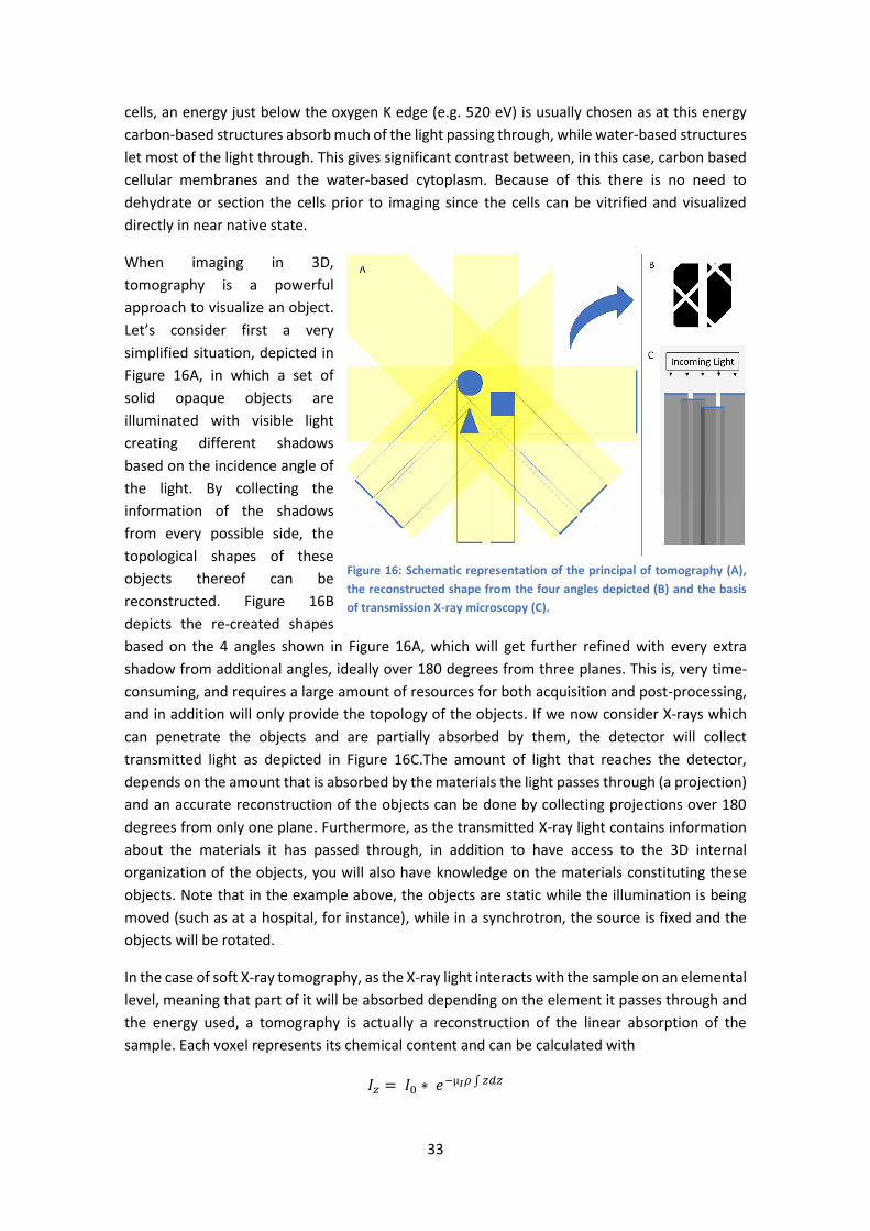
33

cells, an energy just below the oxygen K edge (e.g. 520 eV) is usually chosen as at this energy

carbon-based structures absorb much of the light passing through, while water-based structures

let most of the light through. This gives significant contrast between, in this case, carbon based

cellular membranes and the water-based cytoplasm. Because of this there is no need to

dehydrate or section the cells prior to imaging since the cells can be vitrified and visualized

directly in near native state.

When imaging in 3D,

tomography is a powerful

approach to visualize an object.

Let’s consider first a very

simplified situation, depicted in

Figure 16A, in which a set of

solid opaque objects are

illuminated with visible light

creating different shadows

based on the incidence angle of

the light. By collecting the

information of the shadows

from every possible side, the

topological shapes of these

objects thereof can be

reconstructed. Figure 16B

depicts the re-created shapes

based on the 4 angles shown in Figure 16A, which will get further refined with every extra

shadow from additional angles, ideally over 180 degrees from three planes. This is, very time-

consuming, and requires a large amount of resources for both acquisition and post-processing,

and in addition will only provide the topology of the objects. If we now consider X-rays which

can penetrate the objects and are partially absorbed by them, the detector will collect

transmitted light as depicted in Figure 16C.The amount of light that reaches the detector,

depends on the amount that is absorbed by the materials the light passes through (a projection)

and an accurate reconstruction of the objects can be done by collecting projections over 180

degrees from only one plane. Furthermore, as the transmitted X-ray light contains information

about the materials it has passed through, in addition to have access to the 3D internal

organization of the objects, you will also have knowledge on the materials constituting these

objects. Note that in the example above, the objects are static while the illumination is being

moved (such as at a hospital, for instance), while in a synchrotron, the source is fixed and the

objects will be rotated.

In the case of soft X-ray tomography, as the X-ray light interacts with the sample on an elemental

level, meaning that part of it will be absorbed depending on the element it passes through and

the energy used, a tomography is actually a reconstruction of the linear absorption of the

sample. Each voxel represents its chemical content and can be calculated with

𝐼𝑧 = 𝐼0 ∗ 𝑒−µ𝐼𝜌 ∫ 𝑧𝑑𝑧

Figure 16: Schematic representation of the principal of tomography (A),

the reconstructed shape from the four angles depicted (B) and the basis

of transmission X-ray microscopy (C).

34

where I0 and Iz are the incoming flux and the transmitted flux, µl is the linear absorption

coefficient (cm2/g), ρ the density (g/cm3) and z is the thickness of the sample. The linear

absorption coefficient (LAC) in this formula is the parameter that is used for characterization.

Furthermore, by imaging just before and at a specific absorption edge, specific elements

contained in a voxel can be made visible, as was done previously to visualize calcium in algae

(Gal et al., 2018) or in primary mesenchyme cells of urchin larvae (Kahil et al., 2020). In addition,

this can also be applied to elements outside of the water window, although the sample

preparation has to be adjusted as was done by Conesa et al (Conesa et al., 2016). Note that the

reconstruction of the linear absorption coefficient is only possible in native samples, as in the

case of chemical fixation the absorption will not come anymore from the elemental composition

of the sample but from the later together with the chemical fixative, and the staining efficiency

cannot be considered equal throughout the sample, hence quantification is not possible

anymore but even voxel values cannot be compared.

The main advantage of SXT however is its ability to obtain high resolution 3D information of cells

up to 10 microns thick without the need to section the sample nor to use any staining reagents.

This is achieved by rotating the sample and acquiring images at many different angles which can

in turn be tomographically reconstructed, as was already explained previously. The main

limitation for the achievable spatial resolution in soft X-ray tomography currently is the ZP lens

which is made from consecutive clear and opaque (metallic) areas with decreasing width going

outwards while keeping the same area size. ZPs are usually defined by their outermost zone-

width as this last zone defines the maximum achievable resolution when the NA of the lenses

(condenser and ZP) matches. At Mistral two Ni ZPs are available: a 40 nm and a 25 nm. These

lenses are fabricated using a process called lithography and are exceptionally fragile and

expensive, mainly due to their size (150 µm diameter). The main disadvantage with these types

of lenses is the depth of field (DoF), which decreases with decreasing outermost zone-width.

Even though it is possible to image up to 10 µm thick samples because the transmission signal

allows for it, using a high resolution ZP, the depth of field is less than the thickness of a typical

cell (3 - 5 µm for the cytoplasm, 6-10 µm nucleus). Indeed, the 40 nm ZP has a measured DoF at

Mistral of 3.3 µm, while the 25 nm one has 1.6 µm (Otón et al., 2016). This is especially visible

at high tilt angles as the light has to pass through more material. There have been efforts to

overcome this DoF limitation by imaging the same FOV at different focal planes but this

methodology (XTEND, (Otón et al., 2017)), for the moment, only gives proper results for an

incoherent optical system, that is when the numerical apertures of the lenses match, which is

energy dependent and rarely the case. More methodological developments are needed

considering partially coherent optical systems (mismatch of NAs) which are the usual working

conditions.

Another limitation which reduces the final volume resolution in addition to prevent 3D isotropic

resolution stems from the focal length of the ZP, in combination with the flat sample support

that is used at Mistral. At 520 eV the focal lengths are 2.52 mm and 1.57 mm for the 40 nm and

the 25 nm ZP, respectively. Due to geometrical constrains, this allows tilting the sample support

from -70 to + 70 degrees in the case of the 40 nm ZP, and from -65 to +65 degrees for the 25 nm

ZP. These missing angles (up to ±90 degrees) cause a phenomenon called the missing wedge

which produces an elongation along the beam direction in the final reconstruction (see Figure

17) as the resolution achieved is anisotropic, in addition to the blurring due to missing

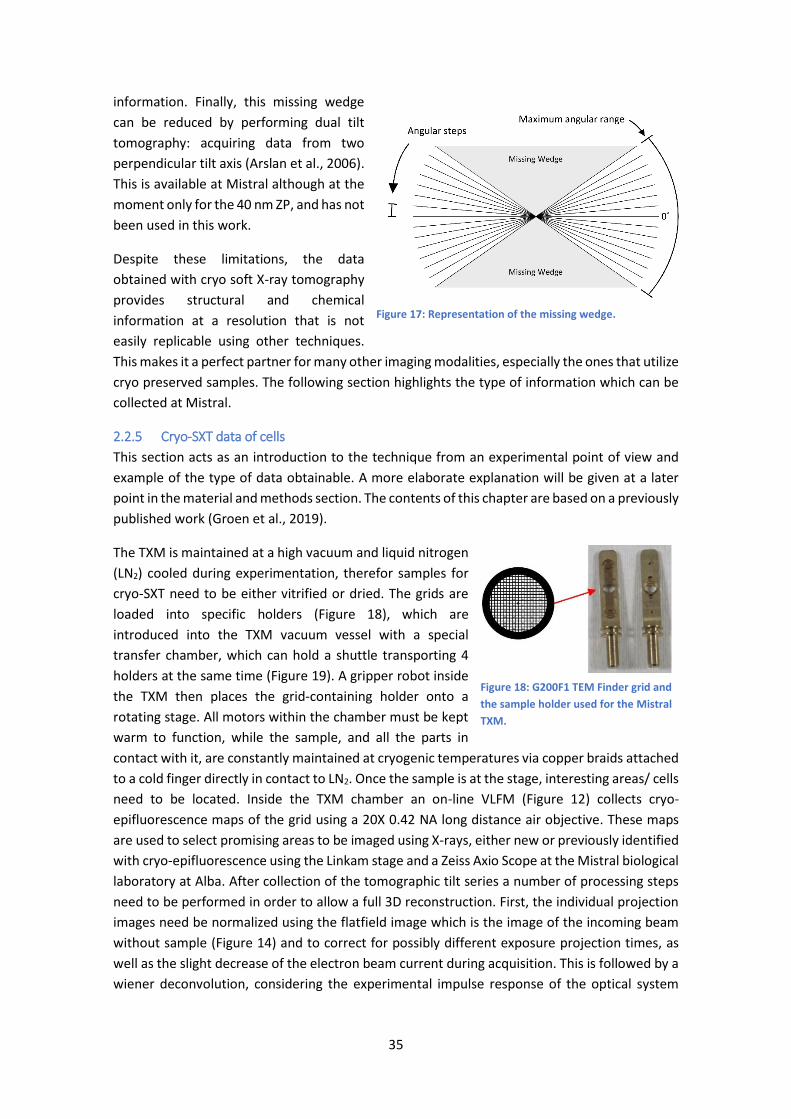
35

information. Finally, this missing wedge

can be reduced by performing dual tilt

tomography: acquiring data from two

perpendicular tilt axis (Arslan et al., 2006).

This is available at Mistral although at the

moment only for the 40 nm ZP, and has not

been used in this work.

Despite these limitations, the data

obtained with cryo soft X-ray tomography

provides structural and chemical

information at a resolution that is not

easily replicable using other techniques.

This makes it a perfect partner for many other imaging modalities, especially the ones that utilize

cryo preserved samples. The following section highlights the type of information which can be

collected at Mistral.

2.2.5 Cryo-SXT data of cells

This section acts as an introduction to the technique from an experimental point of view and

example of the type of data obtainable. A more elaborate explanation will be given at a later

point in the material and methods section. The contents of this chapter are based on a previously

published work (Groen et al., 2019).

The TXM is maintained at a high vacuum and liquid nitrogen

(LN2) cooled during experimentation, therefor samples for

cryo-SXT need to be either vitrified or dried. The grids are

loaded into specific holders (Figure 18), which are

introduced into the TXM vacuum vessel with a special

transfer chamber, which can hold a shuttle transporting 4

holders at the same time (Figure 19). A gripper robot inside

the TXM then places the grid-containing holder onto a

rotating stage. All motors within the chamber must be kept

warm to function, while the sample, and all the parts in

contact with it, are constantly maintained at cryogenic temperatures via copper braids attached

to a cold finger directly in contact to LN2. Once the sample is at the stage, interesting areas/ cells

need to be located. Inside the TXM chamber an on-line VLFM (Figure 12) collects cryo-

epifluorescence maps of the grid using a 20X 0.42 NA long distance air objective. These maps

are used to select promising areas to be imaged using X-rays, either new or previously identified

with cryo-epifluorescence using the Linkam stage and a Zeiss Axio Scope at the Mistral biological

laboratory at Alba. After collection of the tomographic tilt series a number of processing steps

need to be performed in order to allow a full 3D reconstruction. First, the individual projection

images need be normalized using the flatfield image which is the image of the incoming beam

without sample (Figure 14) and to correct for possibly different exposure projection times, as

well as the slight decrease of the electron beam current during acquisition. This is followed by a

wiener deconvolution, considering the experimental impulse response of the optical system

Figure 17: Representation of the missing wedge.

Figure 18: G200F1 TEM Finder grid and

the sample holder used for the Mistral

TXM.

36

(Otón et al., 2016) in order to increase the image quality and finally the linear absorption

coefficient is reconstructed using the Naperian logarithm. The resulting stacks are then loaded

into IMOD software (Kremer et al., 1996) in which, using the fiducial markers (100 nm Au beads),

the individual projections are aligned to the common tilt axis. The aligned stacks are then

reconstructed using either the SIRT (Gilbert, 1972) or the ART (Gordon et al., 1970) algorithm. It

has to be mentioned that the SIRT used from Tomo3d (Agulleiro & Fernandez, 2011), which is

very convenient because it is very fast, had up to recently incorporated the “long object

compensation” (Xu et al., 2010) which produced a re-scaling of the voxel values which was not

conserving the absolute values of the linear absorption coefficient. Therefore, ART was

preferred when quantification was required. Doing so however required extra computational

resources and time (5 minutes and 1.5 hours for SIRT in Tomo3d and ART in TomoJ (MessaoudiI

et al., 2007) respectively). Nonetheless, the SIRT with “long object compensation”

reconstruction is often preferred as it is visually more pleasing, showing less extreme contrast

differences. For this reason, a reconstruction with SIRT in Tomo3d is performed initially to obtain

a fast visualisation of the reconstructed volume, followed by an ART reconstruction from TomoJ

of a few select tomograms. The developer of Tomo3d, José Jesús Fernández, has recently

modified the code to allow us to perform SIRT without the “long object compensation”, which

should allow quantitative reconstruction, however, unfortunately this was only available after

analysing the data presented in this manuscript.

As was already explained before, cryo-SXT offers a near-native representation of the cell in

which the obtained contrast values are comparable. Figure 20 shows example data from NIH-

3T3 and primary mouse fibroblast cells, presenting the different types of organelles and

structures that can be made visible. Figure 20A shows an X-ray mosaic of square mesh within

the grid. Figure 20B shows a single slice from the collected tomographic reconstruction of the

yellow square in Figure 20A, presenting most of the organelles shown in the other panels. Figure

20C and D show Nucleus specific structures: Nucleolus, Nuclear membrane channels,

Heterochromatin, the nuclear double membrane and even some nuclear membrane blebbing.

Looking at the cytoplasm, a variety of organelles can be discerned. Apart from the larger ones,

like mitochondria (E and F) and lipid droplets (G), very small features can be recognized, based

on structure but also based on visibility (contrast). Smooth and rough endoplasmic reticulum

(sER and rER, respectively) and the Golgi apparatus are examples for morphology-based

Figure 19: Left, transfer chamber connected to the workstation for sample loading. Right, zoom into the work

chamber with the shuttle that goes into the TXM.

37

differentiation (H, I, and J in Figure 20). Examples for differentiation based on contrast are the

various endocytic vesicles (K, L, M and N Figure 20) because their nature is usually determined

based on their content/intra-vesicular organization.

In conclusion, cryo-SXT is a very powerful tool to investigate cellular morphology as is highlighted

by the examples shown here. Furthermore, in terms of samples preparation, only vitrification is

required and the imaging itself is non-destructive. As such, it is easily included in existing

workflows, to provide additional data.

Figure 20 next page: An overview of cryo soft X-ray data of mammalian cells (fibroblast and NIH-3T3 cells). The

different structures have been labelled as follows: N – Nucleus, NMC – Nuclear membrane channel, Nu –

Nucleolus, Mi – Mitochondria, He – Heterochromatin, G – Golgi apparatus, rER – rough Endoplasmic reticulum,

sER – smooth endoplasmic reticulum, Fid – Fiducial markers, Ld – Lipid droplets, V – Vesicles, Ly – Lysosome, En –

Endosome, Aut – Autophagosome.

A. A mosaic overview of a square within the grid with a cell of interest. Within the mosaic, areas for acquiring tilt

series are selected. The yellow box represents the field of view of the camera.

B. One slice of the reconstructed volume from the yellow box shown in A.

C & D. One slice of a reconstructed volume showing the N of two different cells. In C, two Nu are visible, as well

as some NMC. The white arrows aim at pores within the double nuclear membrane. In D, Nu are visible and He

structures can be seen close to the nuclear membrane. The white arrowheads point to the double membrane.

The black arrows point to a detachment of the outer layer of the nuclear membrane, which is called nuclear

blebbing.

E & F. Two Mi forms we were able to observe. E shows a small and elongated form and F shows some swollen Mi.

G. The two forms Ld usually appear as, filled or with an empty core.

H & I. ER can be found between other organelles. While rER is elongated and usually easy to find, sER membranes

are thinner and appear to be randomly distributed.

J. The G is usually surrounded by low absorbing V and appears as parallel oriented elongated structures close to

the N.

K, L, M & N. Endocytic vesicles in different stages. Depending of the developmental and metabolic state of the

cell, different forms can be found.

Scale bars: A 20 µm; B 5 µm; C and D 2 µm; E, F, G, H, I and J 1 µm; K, L, M and N 0.5 µm.

Image reproduced from from (Groen, Conesa, Valcárcel, & Pereiro, 2019).

38

39

2.3 Correlative microscopy

As already mentioned, using microscopic techniques in a correlative manner can greatly improve

the understanding of a system when compared to using the individual techniques without

correlation of the data. This holds true for all types of correlative approaches. While many

combinations are possible and can provide very specific information, provided the same sample

can be used, some combinations have become very prominent within the structural cell biology

scientific community. In what follows, we will highlight two of the most similar approaches to

CLXT, followed by an explanation of the combination that was used during this project: cryo-3D-

SIM and cryo-SXT. While the individual techniques have been explained in the previous sections,

now we will focus on the correlative aspect.

2.3.1 Current trends

CLEM is the most commonly used methodology when talking about correlative strategies in cell

biology. Using VLFM alone to identify cells or structures of interest has been used since the

advent of the technique while using it in a correlative manner, mainly to place a certain

fluorescence signal within the cellular context, is more recent (Deerinck et al., 1994; Svitkina et

al., 1995). Nowadays most commercial electron microscopes come with a build-in light

microscope and some of the newer even have automated correlation based on build-in markers,

either on the support or on the support holder, which has been called integrated correlation.

Because of this, these techniques also do not need fiducial markers to perform a low-resolution

correlation. On the other hand, to reach resolution accuracies below 100 nm, fiducial-based

correlation is needed (Kukulski et al., 2011; Mohammadian et al., 2019)

Compared to cryo-SXT, electron microscopy, regardless the modality, will always give higher

resolution. However, following the classical approach of chemical fixation, sectioning and

fluorescent labelling using antibody-conjugates, a complete 3D correlation of a cell volume

requires an immense amount of time and resources. One advantage of this approach would be

that the thin sections (<250 nm) are ideal for SMLM, which is often very challenging in whole

cells. In recent years a more automated manner was developed: FIB-SEM (Focused Ion Beam –

Scanning Electron Microscopy). Here the sample is chemically fixed and fluorescently labelled,

but not sectioned. The whole sample is then introduced into the microscope and imaged using

a VLFM and a SEM. The FIB follows the Ga ion beam and mills the already imaged layer. This

process is repeated throughout the cell which gives a full 3D view of the FOV. While still being a

scanning technique, which are inherently slower compared to full field techniques, this

approach has increased the speed of 3D SEM acquisitions substantially.

More recently cryo-electron tomography (cryo-ET) was developed (Kürner et al., 2004). This

technique is similar to cryo-SXT and is able to provide 3D data of cryo-preserved cells without

the need for staining. While higher resolutions compared to SXT are achievable, it is limited by

the low penetration depth of the electrons to thin sections ( 100 nm). This technique is widely

used for studying proteins i.e. membrane proteins, macromolecular complexes, viruses and

more. Furthermore, using a process called sub-tomogram averaging, sub-nm resolutions have

been achieved (Wan & Briggs, 2016; Zhang, 2019). The production of the thin lamellae by cryo-

FIB-SEM also uses VLFM for locating the region of interest. Cryo-ET has become one of the most

interesting techniques nowadays in structural biology.

40

Another approach that, for the first time, has shown to give high resolution information on the

same cell is cryo-SXT and cryo hard X-ray fluorescence tomography (cryo-XRF) (Conesa, Carrasco,

et al., 2020). In this work epifluorescence VLM was used to tag relevant organelles, followed by

cryo-SXT to obtain the cellular ultrastructure, and lastly cryo-XRF to locate the iridium specific

signal from an iridium organometallic drug related to the research of new cancer therapeutic

agents. While this approach is able to obtain high resolution information of specific elements, it

needs a very tight dose control as well as long data collection times as XRF tomography is a

scanning technique, which for the moment does not allow imaging cell populations although 4th

generation sources (such as the new EBS machine at ESRF (Chenevier & Joly, 2018)) should

improve this actual limitation allowing going from one tomogram collected a day to few of them.

The advantage is that 2D and 3D element-specific mapping of endogenous and exogenous

elements as well as trace elements sensitivity (ppm) in biological samples under cryo conditions

can be obtained.

Of course, there are many more possible combinations and, as mentioned previously, the

techniques of choice are highly dependent on the research question that needs to be answered.

Cryo-SXT is a technique that can provide an abundance of information without affecting the

integrity of the cell. For example, it is possible to include it in existing cryo-CLEM approaches.

Especially now, with the development of cryo-ET, it could be envisaged to include cryo-SXT after

VLFM and before cryo-ET as in terms of sample preparation the same support and strategy is

used, although the dose would need to be tightly controlled to be able to obtain high resolution

cryo-ET (better than 4 Å). In any case, the sample would need to be trimmed to conform to the

depth limitations of ET. The “low” resolution volume provided by cryo-SXT could yield the

coordinates of an event of interest within the 3D cellular space, which would be immensely

helpful for creating the corresponding lamella of that specific specimen region.

Overall, the more techniques are included in a workflow, the more care has to be taken

regarding the radiation dose delivered to the specimen, as was already mentioned previously.

As such it is not always recommended to add more techniques to existing workflows but one

should critically evaluate the added benefit versus the possible loss of detail.

2.3.2 Cryo-3D-SIM and cryo-SXT

Finally, a novel approach which has been used in this work is the combination of cryo-3D-SIM

and cryo soft X-ray tomography. Each technique has been described previously but let us quickly

mention again the main advantages that make them highly compatible: both techniques are

working at cryo conditions, utilize the same sample support, provide high resolution 3D data

that are highly complementary in terms of information and finally they are both high-

throughput, allowing for cell population imaging. The only cryo-3D-SIM currently available is

located at B24 at Diamond synchrotron (UK), although there are efforts to have it developed at

more places, such as at Alba.

Correlative microscopy can be hampered due to technical differences or different sample

processing for each of the techniques. The case of cryo-3D-SIM and cryo-SXT is clearly an easy

combination, as after the initial sample preparation step, samples can be used for both imaging

modalities without any further intervention. In terms of achievable resolutions, there is still a

clear difference with cryo-SXT, the latter having an almost 3x increase in resolving power.

41

However, for the correlation itself this difference is not really an issue as spatial correlation

accuracies down to 70 nm can still be achieved laterally with proper fiducial strategies, as will

be shown in the results below.

The main advantage that this combination has over other similar workflows is the speed of data

collection, which is a reality for both techniques individually, as well as for the combination. An

actual limiting step is the transfer from the cryo-3D-SIM to the TXM as this step adds risk of

damaging or losing the sample grid. This is a problem that most modern CLEM setups do not

have as the visible light fluorescence microscope is integrated in the TEM. Nonetheless, EM,

especially when collecting 3D data, is low throughput. Moreover, at synchrotron facilities, the

priority is focused on using the X-ray beam as efficiently as possible as the beamtime allocated

is very precious and few instruments are available worldwide (currently only five in the case of

cryo-SXT). Therefore, the strategy of having separated instruments, despite the added risk, is

preferred.

2.3.3 Future developments using cryo-SXT correlatively

Correlative microscopy is an ever-expanding field. Laboratories are progressing in developing

new methodologies and instrumentation to answer increasingly difficult and complex biological

questions. This process is also fuelled by the technical individual innovations that initially might

not have a direct connection. For our project, we used this novel correlative cryo-3D-SIM and

cryo soft X-ray tomography approach as it had the ideal features for our goals. Apart from the

3D aspect, which is imperative when it comes to the unambiguous localization of an object in a

whole cell (without sectioning), and the high throughput, the size of the field of view that both

techniques allow is also an advantage, although in a minor degree for cryo-SXT. Having a full

overview of a cell, when tackling treatment-induced morphological changes, was especially

useful for statistical evaluation.

Something else that has to be mentioned here is the fact that this correlative workflow does not

exclude further experiments with other techniques as the sample is preserved all along the

workflow. If deemed necessary or desired, the samples can, for example, be imaged using cryo-

electron microscopy provided cryo-FIB milling is used, as already mentioned above. Having the

exact location of the feature of interest in 3D can greatly increase the lamellae production

efficiency, which is one of the bottlenecks in cryo-ET. While this would require a stricter control

of the dose it should not be a major issue. Another technique which could also be used, as

already mentioned, is hard X-ray fluorescence although a different sample support would be

needed for all the workflow (silicon nitride windows, for instance). An additional possibility

would be to freeze-dry or to freeze substitute the samples, to allow non-cryo techniques to be

consecutively used on the same specimen, such as classical EM for higher resolution on specific

section (Chichón et al., 2012), infrared microscopy to link the structure to the chemical

composition or even specific antibody labelling with additional visible light fluorescence

microscopy.

As CLXT is a novel methodology, we had to refine the full workflow steps, as well as the

fiducialisation strategy to be able to reach the highest possible spatial correlation accuracy.

Although this was not a goal by itself, it did represent most of the experimental work required

42

to successfully achieve the aim of this work. Therefore, summarizing here again the goals of this

work and adding this new one:

1. To study the intracellular fate of this novel protein nanomaterial hybrid.

2. To study the effect of the treatment on the cell at an ultrastructural level.

3. To create a correlative cryo-3D-SIM and cryo-SXT workflow that gives high resolution 3D

information of the whole cell.

In what follows, we will detail the experimental procedure.

43

3 Experimental procedure Choosing the right experimental procedure is an essential part of any project. As already

mentioned, it should be chosen based on the research question, but also on the availability of

specific equipment. In any case, the starting strategy might not produce results and flexibility

will be required to adapt to the results progressively obtained. Optimizing the strategy is

therefore a dynamic process of trial and error until a path is found that is: a) able to address the

research question(s) and b) is feasible and reproducible.

This section first shows a condensed version of the final protocol used before presenting a more

detailed description of each step. The complete step by step version can be found in the

appendix or in the previously published protocols (Groen et al., 2021; Okolo et al., 2021; Vyas et

al., 2021). In this section, the first part will focus on the samples and the initial experiments of

the project, as well as on the description and discussion about what went wrong during those

experiments. The second part will follow the path towards the final protocol in a chronological

order, highlighting the thought-processes. After that, a future outlook is given, mainly focussing

on the protocol itself and what parts thereof can most likely be optimized in future

developments and work.

44

3.1 Samples

As mentioned before, our goal was to locate the CTPR390-AuNC within the cell and understand

the treatment-induced changes. To this aim a total of four different sample conditions were

prepared and imaged. Apart from the necessary non-treated control, we imaged cells after

activation with TGF-β, cells activated and treated with the CTPR390-AuNC and finally cells

activated and treated with a control version of CTPR390-AuNC lacking the Hsp90 binding site.

For the purpose of differentiating between the two CTPR390-AuNC treatments, they will be

named TPR-Hsp90-AuNC and TPR-AuNC, respectively. TGF-β was used to simulate external

stress and thus activating the fibrosis pathway. For this reason, we activated also the cells that

were treated with either protein nanomaterial hybrid. The expectations for the different groups

were:

- TGF-β: an increased mitochondrial and ER activity and an onset of collagen production.

- TPR-Hsp90-AuNC: a similar effect as for the TGF-β group, except for the increased

collagen production. As the nanomaterial binds the Hsp90 C-terminal site it inhibits the

Hsp90-TGF-β fibrotic pathway without affecting its chaperone functionality. Therefore,

the cell should show increased activity with regard to the TGF-β-activation, but a clear

lack of collagen production normally associated with the fibrosis.

- TPR-AuNC: similar to the TGF-β group. As this nanomaterial cannot bind to Hsp90, we

do not expect it to have any effect on the cell, however it will report on potential non-

specific effects of the systems.

In addition, two different cell lines were tested: NIH-3T3 cells and primary fibroblasts extracted

from mice hearts. The primary fibroblasts were the obvious final choice but as we had to test

sample preparation and workflows, we first used NIH-3T3 cells, which is the immortalized

variant of this cell line. The first reason for this was ethical, as for every set of samples a mouse

had to be sacrificed. Apart from that, growing and keeping a healthy primary mouse heart cell-

culture is more complicated and takes more time than an immortalized version. Initial

experiments were then performed solely on NIH-3T3 cells as we expected them to react in a

similar manner as the primary fibroblasts. Contrary to our expectations, we did observe clear

differences towards the treatment between the two cell types. This added a fourth goal to this

work, and for completion we summarize all of them here again:

1. To study the intracellular fate of this novel protein nanomaterial hybrid.

2. To study the effect of the treatment on the cell at an ultrastructural level.

3. To create a correlative cryo-3D-SIM and cryo-SXT workflow that gives high resolution 3D

information of the whole cell.

4. To describe and compare the behaviour of primary and immortalized cardiac fibroblasts

when treated with a designed therapeutic nanomaterial.

45

3.2 Summarized workflow protocol

The protocol written here is a very condensed version of a correlative cryo-3D-SIM and cryo-SXT

approach. As the following chapters will detail specific steps, this protocol serves as an

introduction for the reader to the workflow. For a complete guide see Annex 1.

1. Sample preparation

a. Culture the cells until a sufficient density is reached .

b. Deposit cells on top of TEM Au finder grids (Quantifoil) giving them time to settle

and attach (around 24 hours).

c. Add the treatment and leave to incubate 12 h or 48 h (depending on the

experiment done).

d. Once the grids are ready to be vitrified:

i. Cool down the vitrification device.

ii. Prepare the fiducial markers following manufacturers protocols.

iii. Add organelle fluorescent trackers to the samples, following manufacturers

protocols.

e. Add the fiducials, blot using a Whatman #1 filter paper and vitrify the grids.

f. Store the grids in LN2.

g. Check grid quality using a Linkam CMS196 cryo stage.

i. Make a priority list per treatment based on quality of the grid (damage, ice,

confluence, etc.) and cellular appearance (healthy, correct phenotype, etc.).

ii. Pre-select suitable cells for the correlative imaging.

2. Cryo-3D-SIM at B24, Diamond Synchrotron

a. Cool down the Linkam CMS196 cryo stage and leave to stabilize.

b. Load the high priority grids and acquire at least 3-4 cells per grid. It is advised

that this is done for more than one grid per treatment in case the grid is lost in

subsequent manipulation.

c. Repeat for each treatment.

d. Reconstruct the cryo-3D-SIM stack using the SoftWorx software available on

site.

3. Cryo-SXT at Mistral beamline, Alba Synchrotron

a. Load the grids into sample holders in the workstation and then transfer them to

the transfer chamber that will finally allow loading the samples into the TXM

high vacuum chamber.

b. Collect the on-line fluorescence data and re-locate the cells imaged prior by

cryo-3D-SIM.

c. Acquire the X-ray mosaic images of the cells of interest and select areas for the

tilt series collection.

d. Collect 4-5 tomographic tilt series for each cell that has been imaged prior by

cryo-3D-SIM.

e. Select additional cells to collect tilt series for statistical data on the cellular

morphology.

f. Repeat for each treatment

4. Data processing

46

a. Normalize the acquired tilt series with the incoming flux impinging the specimen

and deconvolve the measured point spread function of the optical system taking

into account the ZP used and the working energy (Otón et al., 2016) .

b. Calculate the natural logarithm to obtain the linear absorption coefficient (µ)

for the whole tilt series as described previously.

c. Align the tilt series to a common rotation axis (IMOD) and reconstruct (SIRT

and/or ART) the tilt series to obtain the absorbance.

d. [Optional] Stitch the tomograms together.

5. Correlation

a. Correct possible shifts between the fluorescent channels of the cryo-3D-SIM if

required.

b. Perform a rough 2D correlation (fluorescence data with the X-ray mosaic) using

the ecCLEM plugin (Paul-Gilloteaux et al., 2017) of ICY (de Chaumont et al.,

2011, 2012) by selecting clearly visible features (holes in quantifoil, Lipid

droplets, cell- or organelle deformities, …).

c. Perform the fine 3D correlation using the ecCLEM plugin of ICY by strategically

selecting small structures, equally spread throughout the 3D volume (preferably

fiducial markers, otherwise organelles or other clearly identifiable structures).

d. Merge the transformed data in Fiji (Schindelin et al., 2012) to assess the quality

of the correlated data.

6. Segmentation

a. Using SURVOS (Luengo et al., 2017) or AMIRA (ThermoFisher Scientific, 2021a)

to segment the different organelles for statistical evaluation of their numbers,

shapes and volumes.

47

3.3 Trial and error: optimizing the protocol

Protocol optimization is a constant iterative feedback process. In our case, we did not start with

a correlative cryo workflow from the beginning due to the lack of 3D cryo VLFM instrumentation

in the immediate accessible institutes. Therefore, we first evaluated if live cell VLF imaging with

subsequent vitrification and finally cryo-SXT was fulfilling our goals. More specifically, confocal

imaging using an Airyscan high resolution module was used followed by immediate vitrification.

During these first experiments several problems surfaced which forced us to rethink our

approach, and ultimately led us to the final protocol described in this work.

3.3.1 Confocal imaging at room temperature

For the initial experiments with live confocal imaging we tagged the mitochondria and the

nuclear membrane using mitotracker red (564 nm) and Syto13 (488 nm), respectively (both from

ThermoFisher). During this experiment, we did not use the TPR-AuNC treatment yet. In order to

localize TPR-Hsp90-AuNC we intended to

use the fluorescent properties of the AuNC

(405 nm; see Table 2).

The first problem we faced was that

many of the imaged cells with confocal

microscopy were not located at the

same place when X-ray imaging was

performed, or even the cells had

completely disappeared after

vitrification. Interestingly enough, we could relocate all cells (white arrows Figure 21) except the

ones that were imaged in 3D stacks with the confocal microscope (blue arrows Figure 21). This

suggested that the acquisition duration was too long, which had a negative effect on cellular

adhesion to the quantifoil support. However, as we did not observe an effect on the cell

adhesion during the confocal microscopy acquisition (Figure 21B), there may be additional

reasons. Due to logistical and safety issues, vitrification was performed in a different part of the

institute. Imaged samples had to be moved from the room with the confocal microscope to the

other laboratory where the vitrification device was located. As the grids are constantly

Table 2: Fluorescent channel occupation during the

confocal experiment.

Excitation wavelength Fluorescent element

405 nm AuNC

488 nm Syto 13

564 nm Mitochondrial tracker

Figure 21: Comparison of the same area on a sample grid with NIH-3T3 cells treated with TPR-Hsp90-AuNC. A and

B show a projection image acquired with confocal microscopy, before the 3D stack was acquired (A) and after (B).

Panel C shows the same area using the in-line VLM at Mistral. Scale bar 20 µm

48

submerged in medium, which moves over the grid

during transport, the already by the exposure affected

cells were most likely washed away due to the motion.

But even without the transfer from one room to the

other, from live cell imaging to vitrification a time lapse

is unavoidable and motion or/and changes in the

sample should be expected. One thing to consider when

comparing the data from the confocal and from the on-

line VLFM within the vacuum chamber (Figure 21C) of

the TXM is that in the confocal microscope the grid was

imaged from the other side which makes clear

identification difficult. Nonetheless it was possible to

observe the fluorescence through the carbon quantifoil

support layer, as is the case for the two small cells

marked with the white arrows at the bottom of Figure 21. The two large cells marked with the

blue arrows where imaged with the confocal microscope and could not be found in the final

vitrified grid, as can be seen from the cryo epifluorescence on line microscope inside the TXM

(Figure 21C). This is also confirmed by cryo-SXT, as is seen in Figure 22. The cell in the white circle

is the same cell as the one in the white circle of Figure 21, which can be faintly seen in the

confocal data as well. This was a clear indication that the acquisition of the confocal stacks

induced stress or damage that causes the cells to detach.

The second problem that was observed, which is directly tied to the first, was related to the

irradiation. After transferring the samples to Mistral for cryo-SXT, we could observe major

radiation damage in the cells that we were able to relocate. Some of this damage was already

present prior to X-ray imaging, while in some cases it would appear shortly after the tilt series

acquisition commenced indicating a previous excessive irradiation dose. Radiation damage is a

complex phenomenon which includes radiolysis and bond ionization depending on the photon

energy used (Shinohara & Ito, 1991). Hence, special care needs to be taken when a sample is to

be imaged using multiple imaging modalities as it has to stand the total given dose. Prolonged

illumination or/and incorrect laser power when imaging with confocal at low resolution can have

consequences afterwards, even if the damage is not immediately visible with this technique (as

it cannot be detected with the achievable confocal resolution). In the reconstructed cryo-SXT

data, radiation damage showed as bubbles throughout the cells, indicating H-bond breaking.

Even though some of the major cellular structures such as the nucleus or even mitochondria

could still be discerned when they were large enough, all the fine detail was lost. In our case, as

we were interested in the location of small molecules, this approach was not successful.

As previously mentioned, the AuNC has fluorescent properties with an optimum excitation

wavelength at 370 nm (Figure 3). Initially we intended to use this feature for the intracellular

tracking of the protein-AuNC nanomaterial; however, due to the unavailability of a suitable laser

the signal was too low. At 405 nm, which was the closest available laser source, the obtained

signal did not exceed the cellular autofluorescence (30 mW, 3.3 sec/frame). While we wanted

to mitigate the radiation damage, we could not lower the excitation power at the confocal

microscope without losing the nanocluster fluorescent signal. For this reason, after observing

the radiation damage, we tried to mitigate it to some degree by reducing the total exposure

Figure 22: SXT mosaic of the area shown in

Figure 21. Scale bar 10 micron.

49

time or the total number of tilt angles used at Mistral. However, this was not enough to prevent

further radiation damage. In addition, when trying to correlate the data from both imaging

modalities, a third problem became apparent: organelles were not found at the same position

in confocal imaging and after vitrification. The most likely explanation is the fact that

intracellular processes are highly dynamic and the time required for the confocal imaging and

the time between this acquisition and the cryo-fixation was sufficient for the organelles to move.

This is supported by the fact that we already saw a change of the overall cell shape. Another

explanation could be that some of the displacement was passively caused by the radiation

damage. The way that organelles keep their position, or move through the cell, is through,

among others, actin filaments that transport the organelle via the cytoskeleton to their position

(S Mogre et al., 2020). If these actin filaments or even the tubulin of the cytoskeleton that

anchors the organelles are damaged by the radiation, the organelles would float aimlessly

throughout the cell, thereby explaining the displacement.

3.3.2 Sample fixation as a possible solution?

The first two problems, movement of the cells and radiation damage, could be mitigated by a

tighter control of the dose. However, there is no study directly documenting the effect of

illumination time, wavelength or power and how much each attribute contributes to the

appearance of radiation damage and at which scale this radiation damage occurs. There is a

general consensus that the effect is not linear with respect to the laser power and the chosen

parameters are usually based on previous experience. As a result, creating new workflows

involving more than one imaging modality can be very challenging as optimal parameters are

determined through experimentation. The third problem, the dislocation of organelles, could

for instance be resolved by fixation, but unfortunately this solution brought additional problems.

The two main issues with chemical fixation are that the fixatives quench fluorescence and that

they are carbon based, increasing evenly the absorption within the soft X-ray water window. In

order to be able to image the samples, a minimal fixation approach was investigated. This

included a very short (soft) fixation time of 5 minutes using a low concentration of 1% PFA in

order to fixate the cell itself and its major organelles. In addition, PFA was freshly made following

the advice of other scientists in the field (Purdue University forum:

https://lists.purdue.edu/pipermail/cytometry/1997-April/006859.html), making sure to not

surpass 59°C when preparing the solution from powder. This avoids the formation of

formaldehyde which is argued to be at least partially responsible for the observed

autofluorescence. While we were able to improve the results, this approach was still

unsuccessful. The already low fluorescence from the AuNC was further masked by some induced

autofluorescence and the cryo-SXT data showed increased absorbance everywhere and

therefore lost the “natural” contrast, as expected. This observation, in combination with the fact

that at this point we were able to apply the newly developed cryo-3D-SIM at the Diamond

synchrotron was key to abandon the strategy of trying to make live cell imaging and chemical

fixation work, and move to a full cryogenic approach.

A full cryogenic approach was possible using either cryo-confocal or cryo-3D-SIM. Recently cryo-

confocal microscopy has become available although no such instrument was available in Spain

yet when this work started. If it were available for user operation it would have been an

alternative to be considered, instead of live imaging or chemically fixed cells. However, the lack

of axial resolution, which is worsened by the fact that no immersion lenses can be used in cryo,

50

and the exclusion of valuable information because of it, was decisive to focus on the cryo-3D-

SIM alternative, as explained in previous sections.

3.3.3 Cryo-3D-SIM

When starting the PhD-project in 2018, high resolution 3D cryo-fluorescence techniques were

being developed in some laboratories worldwide (e.g. Stanford University and Diamond among

others). To be compatible with cryo-SXT at Mistral, the new approach chosen had to fulfil the

requirements discussed previously (chapter 2.1.5 Requirements). Coincidently, in 2018 a cryo-

3D-SIM set-up opened for proposal-based user access at B24 at Diamond synchrotron. The cryo-

3D-SIM at Diamond was specifically designed for cryo-SXT correlation, as B24 is also a cryo-SXT

beamline.

From there on, we visited the facility three times. Note that this section focusses on the

problems encountered during the acquisition and subsequent processing. The results will be

discussed in the following chapters. During our first visit we encountered problems with the cryo

sample delivery which resulted in the allocated time being cancelled. The samples ultimately

arrived on the last half-day allocated, which did allow us to have a first look at them. Afterwards

we returned two more times for a total of 6 days. This measurement time was needed to collect

all the data presented in this manuscript and more would have been useful for instance, to

evaluate different time points, but travelling between countries with finite access and measuring

time did not allow for this, in addition to the pandemic situation that started mid-March 2020.

As was mentioned, during the

first visit only half a day could

be used to acquire the first

test-data. The obtained results

were clearly better than any of

the confocal imaging we had

done up until that point,

although some problems arose

right away. The main issue,

which we already observed

after analysing the Airyscan

confocal data, was that the

fluorescent signal of the AuNC

was not as good as expected.

Again, a suboptimal excitation

wavelength at 405 nm was faced. Because of this it was difficult to differentiate between actual

real signal and background autofluorescence. As this was already anticipated, an Alexa647

fluorescent dye was attach to the protein nanomaterial hybrid (Prot-NM). Previous studies

(Aires et al., 2019, 2021; Cáceres et al., 2018) showed that the AuNC is necessary for an improved

uptake of the Prot-NM by the cell, apart from contributing to its stability (as mentioned in

chapter 1.2 Tetratricopeptide repeat (TPR) proteins p. 13). For this reason, the fluorescent

marker did not replace, but rather would confirm the presence of the Prot-NM presence by an

overlapping fluorescence emission signal. In addition, we used a mitochondrial tracker in the

green channel (Mitotracker Green, 488 nm), and a mix of two fiducial markers that were

Table 3: 1st visit to the cryo-3D-SIM with primary mouse fibroblasts.

Excitation

wavelength

Fluorescent element

405 nm AuNC

488 nm Mitochondrial tracker

561 nm Ursa Bioscience 80 nm Ag with a red

fluorescent dye (594 nm)

647 nm Alexa 647 on CTPR390 and CD

Bioparticles 250 nm Au with a far-red

fluorescent dye (Alexa 647)

51

recommended and donated by Dr. Maria Harkiolaki from B24: 80 nm silver core with red

fluorescent molecule (547 nm) embedded in a silica gel (Ursa Bioscience) and 250 nm gold core

with far-red fluorescent molecule (647 nm) conjugated on top (CD Bioparticles) (see Table 3).

The fluorescent gold nanoparticles had a double role: to allow 3D data correlation and to align

the cryo-SXT tilt series projection images prior to reconstruction Note that there was still no

properly characterized fiducialisation strategy yet, as it was still being developed by the staff of

B24 at the same time. Because we already had the Alexa 647 conjugated to the Prot-NM, the

use of these two fiducial markers meant that there were two different signals in the far-red

channel. It was thought that, as the nanomaterial would be located inside the cell and the

fiducial marker would be outside it, we would be able to differentiate between the two. In

addition, we expected the signal coming from the AuNC to overlap with the Alexa647, as well as

that the signal from the Prot-NM would not to be as uniform and spherical as the fiducial signal.

Ultimately, neither of the tested fluorescent fiducial markers performed as expected. Apart from

their non-uniform fluorescent signals, which made differentiating between Prot-NM and fiducial

difficult, the fluorescent gold fiducials did not spread evenly, tending to aggregate, which also

made aligning the tomographic tilt series very difficult. For this reason, we discarded the Ag

particles and exchanged the far-red gold fiducials with red gold fiducials of 250 nm, also from

CD Bioparticles, and prepared new samples for the following session.

During this second cryo-3D-

SIM session (see Table 4) the

data collected improved and

were clearly more promising.

We could confirm the

presence of the nanomaterial

intracellularly using both the

405 nm and the 647 nm

excitation, and were able to

identify the 250 nm gold

fluorescent fiducials although

not all of them showed

fluorescent signal as the commercial batch was suboptimal. However, during this visit we

encountered a new problem: a chromatic shift between the different fluorescent channels used.

This prevented us from performing accurate correlations as we needed all the channels to be

perfectly referenced. In addition, we found that the fluorescence yield from the Alexa647

attached to the Prot-NM was lower than expected (Figure 23 Left). While we could clearly

determine a difference between the treatments, thus confirming the presence of the

nanomaterials with Hsp90 binding site intracellularly, the emitted signal was still very low. One

advantage of using the far-red signal was the absence of cellular auto-fluorescence in control

samples, although some could be seen if there was, for example, ice contamination. For this

reason, we decided to switch to Alexa488, which has a higher fluorescence quantum yield and

therefore resulted in a brighter signal (Figure 23 Right). One last thing that we observed was that

the correlative 250 nm gold fiducials were not working as expected, mainly because they were

also not spreading evenly (such as the Ag ones), which rendered them hardly beneficial for the

Table 4: 2nd visit to the cryo-3D-SIM with NIH-3T3 cells

Excitation

wavelength

Fluorescent Element

405 nm AuNC

488 nm Mitochondrial tracker

564 nm CD Bioparticles 250 nm Au – Alexa594

647 nm TPR-Alexa647

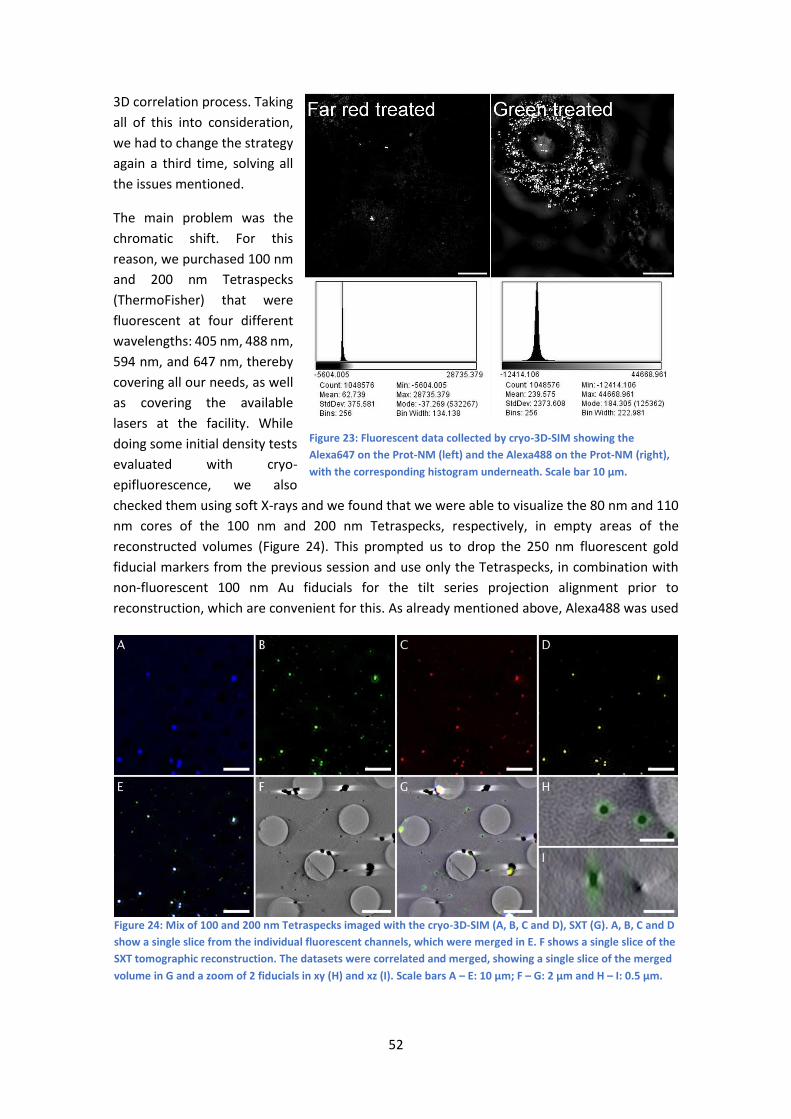
52

3D correlation process. Taking

all of this into consideration,

we had to change the strategy

again a third time, solving all

the issues mentioned.

The main problem was the

chromatic shift. For this

reason, we purchased 100 nm

and 200 nm Tetraspecks

(ThermoFisher) that were

fluorescent at four different

wavelengths: 405 nm, 488 nm,

594 nm, and 647 nm, thereby

covering all our needs, as well

as covering the available

lasers at the facility. While

doing some initial density tests

evaluated with cryo-

epifluorescence, we also

checked them using soft X-rays and we found that we were able to visualize the 80 nm and 110

nm cores of the 100 nm and 200 nm Tetraspecks, respectively, in empty areas of the

reconstructed volumes (Figure 24). This prompted us to drop the 250 nm fluorescent gold

fiducial markers from the previous session and use only the Tetraspecks, in combination with

non-fluorescent 100 nm Au fiducials for the tilt series projection alignment prior to

reconstruction, which are convenient for this. As already mentioned above, Alexa488 was used

Figure 23: Fluorescent data collected by cryo-3D-SIM showing the

Alexa647 on the Prot-NM (left) and the Alexa488 on the Prot-NM (right),

with the corresponding histogram underneath. Scale bar 10 µm.

Figure 24: Mix of 100 and 200 nm Tetraspecks imaged with the cryo-3D-SIM (A, B, C and D), SXT (G). A, B, C and D

show a single slice from the individual fluorescent channels, which were merged in E. F shows a single slice of the

SXT tomographic reconstruction. The datasets were correlated and merged, showing a single slice of the merged

volume in G and a zoom of 2 fiducials in xy (H) and xz (I). Scale bars A – E: 10 µm; F – G: 2 µm and H – I: 0.5 µm.

53

linked to the nanomaterial to increase the fluorescence output, and the mitochondrial marker

was changed to the mitotracker red CXMRos fluorescent marker for reference purposes. We

returned one last time to perform cryo-3D-SIM imaging and finally we were able to collect data

that we could correlate in 3D successfully.

The last experimental session at B24 was just before the global lockdown due to the pandemic

from March 4th to 6th 2020. Although we were able to collect enough data to perform accurate

3D correlations, the amount of data was very limited. As discussed previously, one risk factor in

this type of experiments is the sample preparation and handling aspect. Due to the limited time,

we could not image as many cells on different sample supports as desirable to avoid handling

risks. Unfortunately, we did lose some grids and in other cases, a lack of fiducial markers resulted

in a suboptimal alignment and reconstruction of the SXT data. Nonetheless, we obtained enough

data to draw statistically relevant conclusions, as is shown in this work.

54

4 Methods This chapter describes in more detail the workflow utilized for preparing the latest set of samples

of the final workflow achieved. For completion, let us summarize here the previously set goals

of this PhD-work:

1. To study the intracellular fate of this novel protein-nanomaterial hybrid.

2. To study the effect of the treatment on the cells at an ultrastructural level.

3. To create a correlative cryo-3D-SIM and cryo-SXT workflow that gives high resolution 3D

information of the whole cell.

4. To describe and compare the behaviour of primary and immortalized cardiac fibroblasts

when treated with a designed therapeutic nanomaterial.

In order to answer the research questions 1, 2 and 4 a working cryo-CLXT protocol was required

and therefore this is the first step that needed to be achieved. While the TPR preparation, the

primary mouse cell isolation and the immunofluorescence assays detailed below were project

specific, the sections after those are the fulfilment of this 3rd goal. Note that during this PhD-

project, a protocol has been published in collaboration with B24 staff (Okolo et al., 2021). The

differences between this workflow and the published one in 2021 are minute and are mostly

related to hard- and software availability or individual preference.

4.1 TPR preparation

4.1.1 Protein Isolation

The TPR variants were prepared and shipped to Alba by Dr. Antonio Aires from the Biomolecular

Nanotechnology group at CIC biomaGUNE in San Sebastián/Donostia (Spain). For each

experiment they were freshly prepared following previously described protocols (Aires et al.,

2021; Cortajarena, Yi, et al., 2008) and shipped in dry ice. The His-tagged proteins have been

purified by affinity chromatography following standard protocols. C41 (DE3) cells transfected

with the pProEx-HTA plasmid encoding the desired TPR gene, were grown in an orbital shaker

at 37 °C to an optical density of 0.6-0.8. Then the protein expression was induced with 1 mM

isopropyl β-d-thiogalactoside (IPTG) and the cell were left for 16 hours at 20 °C. The cells were

centrifuged and lysed by sonication in 500 mM NaCl, 50 mM Tris pH 8.0. Proteins were purified

from the supernatant using a 5 mL HisTrap Q column (GE Healthcare). Then, the his-tag was

removed by TEV protease cleavage and purified by gel filtration chromatography (HiLoad 16/60

Superdex 200 column).

4.1.2 AuNC formation

AuNCs were synthesized and stabilized in the protein scaffolds using a protocol based on

previously reported procedures at CIC biomaGUNE in San Sebastián/Donostia (Spain) (Aires et

al., 2019, 2021). A protein at 20 µM was incubated with HAuCl4 (30 eq. with respect to protein)

for 1 hour at 20 °C. After, a reduction step is applied by adding 100 eq. with respect to the Au

concentration of sodium ascorbate and left to incubate at 50 °C for 72 h. Finally, the Prot-NM

were purified by gel filtration (Sephadex G-25 column).

55

4.1.3 Alexa 488 nm labelling

Alexa Fluor 488 NHS ester was used to label the TPR-Hsp90-AuNC and TPR-AuNC proteins as

described previously (Cortajarena, Lois, et al., 2008). Both Prot-NM versions were first reduced

before the dye was added dropwise to the protein to bind through their primary amines at a 1:2

stoichiometry to avoid over-labelling and potential disruption of the protein recognition activity.

The reaction was allowed to proceed for 4 h at RT under constant stirring and under a non-

reducing atmosphere (N2) in the dark. Once the labelling reaction was completed, the labelled

proteins were purified using two consecutive buffer exchange columns (PD-10) and

concentrated and washed using a Centriprep YM-3 filtration unit (Millipore) in PBS buffer.

4.2 Primary mouse fibroblast isolation

Primary fibroblasts were harvested and shipped to Alba by David Maestro Lavin from the “Nano

and Molecular Treatments Against (Cardiac) Fibrosis” research group at IBBTEC in Santander

(Spain). Adult cardiac fibroblasts from mice C57BL6 strain (wildtype) were isolated directly from

enzymatically digested hearts (collagenase, trypsin and DNase) followed by centrifugation and

filtration. They were maintained in Dulbecco's Modified Eagle's Medium (DMEM) containing 10

% FBS and 100 U/ml penicillin-streptomycin. For shipping, the cells were initially cultured in

standard cell culture flasks (50 ml) and shipped to Alba using the “same day arrival” option to

minimize stress due to, for example, temperature fluctuations and movement of the container.

After arrival, the cells were washed, supplied with fresh medium and kept at 37 °C in 5% CO2 for

24 h to stabilize.

4.3 Sample preparation for CLXT

As already mentioned, the sample preparation protocol was based on previously published

procedures (Groen et al., 2021; Okolo et al., 2021). As the procedure involves cryogenic liquids,

appropriate safety measures are required. Both NIH-3T3 and primary myocardial mouse

fibroblasts were grown in complete culture medium (DMEM with 10% FBS and 1% Penicilin/

Streptomycin) at 37 °C and 5% CO2 until a confluence of 70-80% was reached (Figure 25A). At

this point the cells were ready for subculture, or for sample preparation. As sample support,

gold quantifoil R 2/2 holey carbon-film microscopy grids (Au-G200F1) were used. Before cell

deposition, grids were placed in P60 Petri-dishes, already separated by type of treatment, and

UV-sterilized (Figure 25B). Spreading the grids at this stage minimized grid handling and possible

damaging thereof. Cells were washed in phosphate buffer saline (PBS) and seeded on top of the

grids at a concentration of circa 2-3 x105 cells per ml (3 ml total in the case of a P60 Petri dish)

(Figure 25C). After the cells were allowed to settle and stabilized on the surface for around 24

Figure 25: A: 80% confluence in a Petri dish. B: Grid before vitrification showing good cellular confluence C: Grids

submerged in compete medium in a P60 Petri dish.

56

hours, they were treated. Both the NIH-3T3 and primary fibroblasts were divided in 4 groups:

control, TGF-β activated, TGF-β activated and treated with TPR-Hsp90-AuNC, and lastly TGF β

activated and treated with TPR-AuNC, lacking the Hsp90 inhibitory domain. Cells were activated

with 1 ng/ml TGF-β final concentration and for the TPR-Hsp90-AuNC, as well as TPR-AuNC

groups, the activated cells were treated with their respective CTPR390 variant at a final

concentration of 0.8 μM. After overnight (ON) incubation, Mitotracker Red CMXRos

(ThermoFisher) was added to the grids, following manufacturer recommendations. After the

incubation time of the fluorescent dye had passed, a mix of 100 nm gold fiducial markers (BBI

Solutions; 10x concentrated) and 200 nm Tetraspecks (ThermoFisher; 5x diluted) was prepared

and 3 μl thereof was deposited on the grid followed by 2 s of blotting using a Whatman #1 filter

paper and vitrification through plunge freezing in liquid ethane precooled by liquid nitrogen in

a Leica EM-CPC. Special care has to be taken as grids have to be kept at cryogenic temperatures

from this point on at all times. The vitrified grids were pre-screened using a Linkam CMS196

cryo-stage on a Zeiss Axio Scope fluorescence microscope. A grid-priority list is prepared based

on the integrity of each grid, in terms of damage to the grid, ice thickness, cell confluence, etc.)

and cells of interest are marked for later correlation.

4.4 Cryo-3D-SIM

The previously selected highest priority grids, at least two per cell-type and condition, were sent

to B24 at the Diamond Synchrotron (UK). The grids were imaged with their home-build cryo-3D-

SIM following a previously described protocol (Vyas et al., 2021) to collect the green signal

coming from the Alexa488 on the Prot-NM proteins (λexc 488/ λem 525, 40 mW, 100 ms), and red

signal coming from mitotracker Red CMXRos (λexc 561/ λem 605, 40 mW, 50-100 ms depending

on staining efficiency) using a 100X 0.9 NA long distance air objective lens achieving a lateral

resolution of roughly 210 nm full width at half maximum (FWHM) at an emission wavelength of

488 nm (Phillips et al., 2020). For each sample-type three to six cells, preferably from different

grids, were imaged and the collected data was processed on site using the Softworx software

(GE Healthcare).

4.5 Cryo soft X-ray tomography

The grids were then sent back to Mistral at ALBA (Spain) for data collection using cryo soft X-ray

tomography (Groen et al., 2021; Pereiro et al., 2009; Sorrentino et al., 2015). The grids were

loaded into the transmission X-ray microscope (TXM) chamber and the cells that were imaged

prior with the cryo-3D-SIM were identified using the on-line visible light fluorescence

microscope inside the TXM vacuum vessel with a long distance 20X objective. Once the areas

were found, first an X-ray mosaic of the grid square was collected at a photon energy of 520 eV

to obtain a general view of the area containing the cell of interest. Afterwards, together with

the fluorescence data from the cryo-3D-SIM, specific areas for tilt series are selected and the

data is collected. After collection of the data required for the correlation, additional cells for

each cellular type and condition (NIH-3T3 and primary myocardial mouse fibroblasts) were

imaged for morphological data evaluation, comparison and statistics. Note that up to 5 tilt-series

were collected in cells that were previously imaged by cryo-3D-SIM. This was done to cover as

much of the cell as possible, as the field of view (FOV) of the TXM was 10 µm10 µm and the

cells are larger, as well as for easier 3D correlation later. For cells for which no cryo-3D-SIM was

acquired, only 1 or 2 tilt-series were collected to be able to obtain the morphological information

57

from as many cells as possible. All data was collected using a Ni Fresnel zone plate lens with an

outermost zone width of 25 nm (courtesy of S. Rebhein, HZB-Bessy II), giving an effective voxel

size of 10 nm3. Depending on the sample and the position of the cell on the grid, projections

were collected covering a maximum angular range of -65° to +65° (or less) with a constant step

size of 1° at a magnification of 1300x. While for the lower tilt angles an exposure time of 1-2

seconds was used, at higher tilt angles the exposure time was increased to 3-4 seconds, as tilting

makes the effective sample thickness for X-ray transmission higher and therefore increasing the

signal-to-noise ratio is advisable while taking care to not oversaturate the CCD camera. Note

that when tilting, empty cell areas might appear in the FOV.

4.6 Fluorescence and immunofluorescence assays

The following fluorescence and immunofluorescence assays were performed by Dr. Ana Palanca

from the “Nano and Molecular Treatments Against (Cardiac) Fibrosis” research group at IBBTEC

in Santander (Spain). Cells were seeded onto 60 mm cell culture dishes and treated as described

previously. Then samples were fixed (4% paraformaldehyde), permeabilized (20-30 min

0.05%Triton-X in PBS 1x) and incubated overnight at 4˚C with different primary antibodies: anti-

Alix (1:100, sc53540), anti-Flotillin-1 (1:100, sc74566), anti-CD9 (1:100, donation from Sanchez-

Madrid), which are markers for different endosomal vesicle processes, anti-LC3-II (Cell Signaling

#2775), which is an autophagy marker, and lastly anti-caspase-2 (ab182657), which is an

apoptosis marker. The samples were washed with 0.05% Tween 20 in PBS, incubated for 30 min

in the specific secondary antibody conjugated with Alexa-568 (ThermoFisher), washed in PBS

and mounted with the Vectashield antifade mounting medium (Vector). Confocal images were

obtained in the microscopy facility at IDIVAL (Santander, Spain) with a confocal microscope

NIKON A1R spectral (405nm, 488nm, 514nm, 561nm, 638nm) and Fiji (Schindelin et al., 2012)

was used for data visualization.

4.7 Data processing

The tilt-series were pre-processed by normalization with the collected flatfield signal (flux

impinging the sample) and the corresponding machine current, followed by deconvolution of

the measured PSF of the TXM at the corresponding energy and for the corresponding ZP lens

(Otón et al., 2016). Afterwards, the linear absorption was calculated for the whole tilt series

before they were aligned using the 100 nm Au fiducials and the IMOD software (Kremer et al.,

1996). A first reconstruction was performed using the SIRT algorithm (Gilbert, 1972) in tomo3d

with “long object compensation” (Agulleiro & Fernandez, 2011; Xu et al., 2010) for a fast

reconstruction (about 6 minutes with 30 iterations), which is for visualization purposes only to

check the quality of the cell region measured, as well as the alignment accuracy. Then, the final

reconstruction was performed using the ART algorithm (Gordon et al., 1970) with tomoJ

(MessaoudiI et al., 2007) for linear absorption coefficients recovery (about 1 h 30 min with 15

iterations and a relaxation coefficient of 0.01). Note that SIRT with “long object compensation”

is not quantitative, this is why it is used only for fast visualization purposes (as explained in

section 2.2.5). The tomographic reconstruction of each of the cells that were previously imaged

using the cryo-3D-SIM were then further post-processed using Fiji (Schindelin et al., 2012) to

ensure they are aligned to each other by flattening and cropping in the z-direction to adjust the

height, based on the carbon quantifoil support layer. The 3D correlation was done using the ICY

plugin (de Chaumont et al., 2012) in ecCLEM (Paul-Gilloteaux et al., 2017). First, the cryo-SXT

58

reconstructions were 2D transformed to overlay them on the X-ray mosaic to place them in the

context of the whole cell as each tomogram only covers an area of 10 µm2 of the cell. To prevent

excessively large files, cropping of the X-ray mosaic to the area containing the reconstructions is

advised. The transformed tomographic reconstructions could then be combined into one file for

subsequent 3D correlation. Because of the chromatic shift of the cryo-3D-SIM, the fluorescent

channels were first aligned to each other using the 200 nm Tetraspecks fluorescent fiducials.

After this, the aligned fluorescent channels were roughly transformed in 2D to locate and overlay

them on the X-ray mosaic using large feature, like for example the holes in the quantifoil film or

using large organelles, like mitochondria. After this the fluorescent data was transformed in 3D

using more fine features such as Tetraspecks or recognizable organelle shapes, and finally the

transformed data was merged and inspected with Fiji.

4.8 Statistical Analysis of organelles

The tomographic reconstructions were segmented using the Amira software (ThermoFisher

Scientific, 2021a). Volume and sphericity measurements on the segmentation were performed

using the Amira module Label Analysis. For the volume, the native measure is used but for the

sphericity a custom measure had to be created using the formula:

Sphericity =π

13 ∗ (6V)

23

A

with V being the volume of the label, and A being the surface area. For each condition, four

tomographic reconstructions belonging to four different cells were segmented and measured.

The statistical analysis was performed using Excel 2016s Data Analysis add-in. First, the datasets

were tested for equal or unequal variance, followed by the corresponding two-tailed t-test using

a cut-off value of 0.05 to test for significance or 0.01 for extreme significance between the

groups.

59

5 Preliminary Results As was mentioned before, we collected data at the cryo-3D-SIM a total of 3 times. This section

will first go systematically and chronologically through each visit, highlighting the main findings

and problems, before showing the main results which were obtained during the last visit.

5.1 1st cryo 3D-SIM Experiment, March 2019

Due to difficulties with the sample

shipment, as already mentioned in

chapter 3.3.3, we could only use few

hours to perform a first feasibility test.

Figure 26 shows a first correlation

between cryo-3D-SIM and cryo-SXT. For

this experiment we used the Alexa-647

dye on the Prot-NM, mitotracker green

(488 nm) as a reference and a mixture of

two fiducial nanoparticles for

correlation, provided by Dr. Maria

Harkiolaki from B24: 250 nm Au particles

coated with Alexa647 from CD

Bioparticles and 80 nm Ag nanoparticles

with Rhodamine B fluorescent dye from

Ursa Bioscience. In addition, during this

first visit only primary myocardial mouse

fibroblasts samples (control, TGF-β, and

TPR-Hsp90-AuNC treated) were

prepared. Unfortunately, due to some

problems with the cell-culture the cells

were not looking as healthy as they should (and as they did during our latest measurements) as

can be seen in Figure 26 where the cell shows clear vacuolization (see arrows Figure 26).

Nonetheless, the data quality was already superior to the confocal microscope one thanks to

the full cryo workflow. Firstly, we were able to re-locate every cell imaged with the cryo-3D-SIM

by cryo-SXT. In addition, all the cells looked exactly the same with the cryo-3D-SIM as when the

grids were screened with the cryo epifluorescence immediately after vitrification (see Figure 27).

Having the cells embedded within a thin layer of ice was clearly an improvement in terms of

stabilisation, which was expected. Even though, the correlation accuracy was suboptimal due to

the correlation strategy or registration process. We found that the correlative fiducial makers

used did not spread well over the field of view which led to most areas being free of them. As a

result, these areas were impossible to correlate with the needed accuracy. Regarding the

vacuolization of the cells, we believe the quality of the isolated cells can differ and a bad batch

could react negatively to the shipment to Alba which might have caused cellular stress. Although

the delay in the dewar arrival containing the grids was a drawback, the few hours of data

collection allowed us to evaluate how to improve sample preparation for a future second visit.

Figure 26: Correlated reconstructed slice of a primary

fibroblast collected with the cryo-3D-SIM and cryo-SXT during

our first visit. The green signal comes from the mitotracker

green, Red from the Alexa647 labelled TPR-Hsp90-AuNC, and

blue from the AuNC on the TPR-Hsp90-AuNC. White arrows

indicate clear vacuolization. Scale bar 5 microns.

60

5.2 2nd cryo-3D-SIM Experiment, May 2019

During the second visit only NIH-3T3 cells were prepared: control, TGF-β treated and treated

with the same nanomaterial (TPR-Hsp90-AuNC with Alexa-647) as the previous visit. However,

this time different fiducial nanoparticles were used: 250 nm Au nanoparticles coated with

Alexa594. In addition, the samples were sent a week in advance to avoid having unexpected

courier delays. While this should have been enough, the samples still arrived one day late.

However, this time it was due to the samples going to the wrong UK distribution centre. Note

that these types of samples are sent at liquid nitrogen temperature in specific dry shipping

containers that, in general, can only hold the proper temperature for 6 days. Fortunately, no

damage to the samples from the shipping was observed and it was possible to extend the stay

for 1 additional day, which allowed us to collect data during 3 consecutive days. The data

acquired during this visit showed a clear improvement compared to the previous visit.

The higher concentration of fluorescent nanoparticles showed a better spread compared to data

from the previous visit, which made correlation much easier. In Figure 28 a single slice from the

correlation of two tomographic reconstructions with the cryo-3D-SIM data is shown. Most

correlation was performed using the mitochondrial (green) signal, hence the high correlation

accuracy that can be seen in the 3D overlay with the cryo-SXT data. The blue and red signals

correspond to the AuNC (blue) and the Alexa-647 (red), respectively. When looking at the XZ

view (bottom of Figure 28), it can be observed that most of the fluorescent red and blue

fluorescent signal of the nanomaterial is located at the bottom of the cell. These results could

be explained since the collagen is usually deposited between surfaces, in nature between cells,

and in our case the surface between cell and the quantifoil support. However, we did not

observe any apparent association or co-localization between the nanomaterial and a specific

organelle or cellular feature. Interestingly, however, after correlating several volumes, we found

that some features and artefacts which were visible in more than one channel, which were

mostly quantifoil or ice artifacts, did not align properly. These results suggested a chromatic shift

Figure 27: Comparison of an area collected with cryo epifluorescence signal from the mitotracker green at Alba

(Left) and a single slice from a cryo-3D-SIM reconstruction of cell number 1 (right). The other numbers mark the

surrounding cells highlighting the fact that no movement of cells is observed. Scale bars: Left 25 µm, Right 10 µm

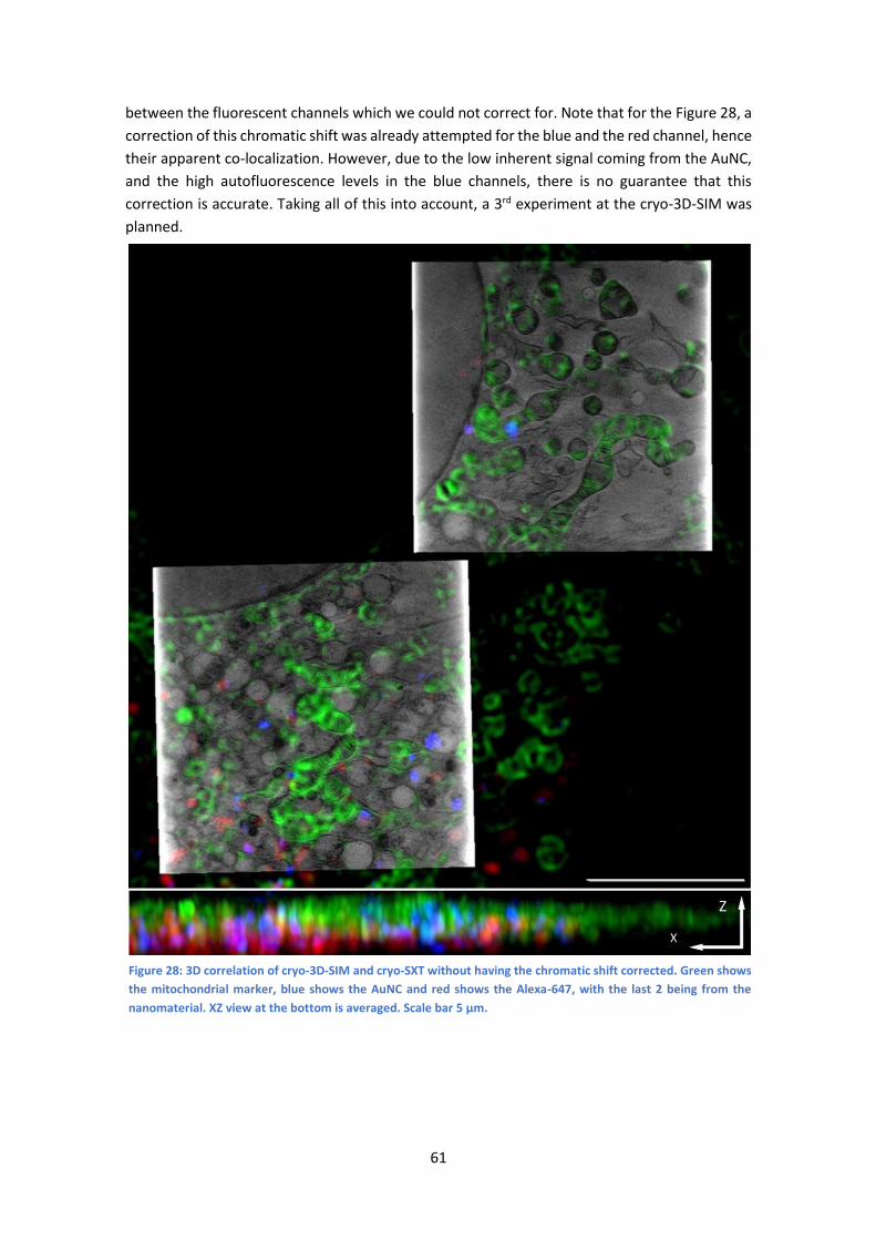
61

between the fluorescent channels which we could not correct for. Note that for the Figure 28, a

correction of this chromatic shift was already attempted for the blue and the red channel, hence

their apparent co-localization. However, due to the low inherent signal coming from the AuNC,

and the high autofluorescence levels in the blue channels, there is no guarantee that this

correction is accurate. Taking all of this into account, a 3rd experiment at the cryo-3D-SIM was

planned.

Figure 28: 3D correlation of cryo-3D-SIM and cryo-SXT without having the chromatic shift corrected. Green shows

the mitochondrial marker, blue shows the AuNC and red shows the Alexa-647, with the last 2 being from the

nanomaterial. XZ view at the bottom is averaged. Scale bar 5 µm.

62

5.3 3rd cryo-3D-SIM Experiment, March 2020

As new, optimized samples had to be prepared, we also decided to prepare new nanomaterials.

As previously discussed, the fluorescent yield coming from the far-red Alexa dye was low. Even

though we could distinguish its signal in most cases, it was sometimes difficult. In addition, the

spatial resolution has an inverse relationship with the wavelengths (see chapter 2.1.1 VLFM in

biology), which means that in order to improve the localization accuracy for the Prot-NM, a

fluorophore with a lower excitation wavelength is preferred. For both of these reasons and as

already mentioned in chapter 3.3.3, we replaced the Alexa647 with Alexa488 which has a 3-fold

higher fluorescence quantum yield (0.33 and 0.92 for Alexa647 and Alexa488, respectively

(ThermoFisher Scientific, 2021b)). The chromatic shift was overcome by using 200 nm

Tetraspecks from ThermoFisher, which are fluorescent in the 4 different channels (405 nm, 488

nm, 561 nm and 647 nm). Finally, Mitotracker green was used instead of Mitotracker Red

CMXRos (p.XX). During the 3 days of data acquisition, we imaged a total of 40 cells, from both

cell types and from each treatment (Table 5). The fact that at B24 they work only 1 shift of 8

hours per day (for comparison, at Alba, users have the possibility to do 3 shifts/day as is common

in all synchrotron facilities worldwide) did limit our efficiency substantially. Had we been able to

work more shifts, we could have obtained much more data.

Figure 29 shows the correlation overlay of a single reconstructed slice from a NIH-3T3 cell

treated with TPR-Hsp90-AuNC. Using the previously mentioned Tetraspecks we were able to

accurately correct for the chromatic shift. This showed that the previous correlation with the

nanomaterial signal near the carbon quantifoil was in reality not accurate. All the 3D data

correlations that are shown in what follows were prepared using data from this last visit. The

next section will describe and discuss the main results regarding the 3D correlation. Ultimately,

additional visits would have been useful as we had many samples prepared and not enough time

Table 5: Number of cells imaged per visit.

Visit 1st 2nd 3rd

Cell type

Treatment

NIH-3T3 Primary

fibroblast

NIH-

3T3

Primary

fibroblast

NIH-3T3 Primary

fibroblast

Control - 4 6 - 3 3

TGF-β - - 3 - 5 3

TPR-Hsp90-AuNC - 8 15 - 10 9

TPR-AuNC - - - - 4 3

63

to image all of them. In addition, acquiring data at different treatment times would have been

extremely interesting to follow the dynamics of the process.

Figure 29: One slice out of a 3D stack of correlated cryo-3D-SIM and cryo-SXT data. The 5 tomograms were

collected to show a bigger area of the cell and stitched together. The fluorescence data was transformed to fit the

SXT data and overlayed. Red signal comes from the mitochondria and green signal comes from the TPR-Hsp90-

AuNC. Scale bar 10 µm.

64

6 Main results These main results also include complementary immunofluorescence studies which were

performed by Dr. Ana Palanca at IBBTEC in Santander (Spain).

6.1 Correlation

The following results are the main results of this project and have been submitted for

publication. We prepared both myocardial primary mouse fibroblasts and NIH-3T3 cells and the

samples are the same that were described earlier: the control group, TGF-β activated group,

TGF-β activated and treated with TPR-Hsp90-AuNC (TPR-Hsp90-AuNC group), and finally TGF-β

activated and treated with the TPR-AuNC, lacking the Hsp90 inhibitory domain (TPR-AuNC

group). As mentioned in chapter 1.2.1 Metal Nanoclusters, comparing previous studies, it

became apparent that the synthesized AuNC has a positive effect on the internalization of the

nanomaterial (Aires et al., 2019, 2021; Cáceres et al., 2018). Based on this experience we did not

include a control group that is lacking the AuNC.

The fluorescence super-resolution signal in the Alexa-488 specific channel (λexc = 488 nm/ λem

= 525 nm) was intense and well-defined in specific locations for the TPR-Hsp90-AuNC group,

confirming that the observed fluorescence signal corresponded indeed to the internalized TPR-

Hsp90-AuNC. Nonetheless, some auto-fluorescence signal could be observed in the control and

the TGF-β groups at both excitation wavelengths (405 nm and 488 nm). In the case of the TPR-

AuNC group a low but distinct signal was also found which indicates the presence of TPR-AuNC

at significantly lower concentrations than TPR-Hsp90-AuNC in the cell (Figure 30 and Figure 31).

These results suggest that the Hsp90 binding site has a functional role in the uptake of the TPR-

Hsp90-AuNC. Although the mode of internalization of the nanomaterials is still unknown, it is

hypothesized that the nanomaterial enters the cell bound to extracellular Hsp90. The

comparison of the maximum fluorescence signal value collected between the treatment groups

showed a slight increase of TPR-AuNC signal compared to the

Figure 30: Single slice from a cryo-3D-SIM stack of different NIH-3T3 cells comparing the blue (405 nm excitation,

top) and green (488 nm excitation, bottom) channels to show the levels of autofluorescence and the intracellular

concentration of TPR-AuNC compared to TPR-Hsp90-AuNC signal. From left to right it shows control (A and E), TGF-

β (B and F), TPR-Hsp90-AuNC (C and G) and TPR-AuNC (D and H). Scale bars 20 µm.

65

Figure 31: Comparison of the histogram of the cryo 3D-SIM signal for each treatment in NIH-3T3 cells. The

red circle shows the measured area. Control, TGF-β and TPR-AuNC are contrast corrected, TPR-Hsp90-AuNC

has its upper limit increased for visualization purposes. Scale bars 20 µm.

66

autofluorescence signal of the control (2-fold) and TGF-β (1.5-fold), and a 6-fold increase in value

for the TPR-Hsp90-AuNC compared to the TPR-AuNC (12-fold increase compared to the control,

Figure 31). This small increase of observed emission for the TPR-AuNC group would not have

been visible with the nanomaterial containing the far-red fluorescent dye.

After cryo-3D-SIM imaging, cryo-SXT was performed on the same cells at the Mistral beamline.

Figure 32 presents the correlated data of a NIH-3T3 cell. Figure 32A shows the 2D X-ray

projection mosaic of the full cell and Figure 32B its overlay with the 2D SIM data projection. The

red fluorescence signal comes from mitotracker Red CMXRos (ThermoFisher) and the green

from the Alexa488-labelled TPR-Hsp90-AuNC. For this cell, five areas within the cytoplasm

surrounding the nucleus were chosen for tomography collection, and a single slice of the

resulting combined reconstructions is shown in Figure 32C, superimposed on top of the X-ray

2D mosaic. In Figure 32D a single slice from the correlated 3D datasets is shown. Correlating

both 3D datasets, the TPR-Hsp90-AuNC signal was unambiguously located in multivesicular

bodies (MVB) which were homogenous in size (0.5 - 1 μm in diameter) and distributed

throughout the cytoplasm. These MVBs were found in both NIH-3T3 and primary mouse

Figure 32: Correlation of a TPR-Hsp90-AuNC treated NIH-3T3 cell using cryo-3D-SIM showing the mitochondria in

red (CMXRos mitotracker) and the TPR-Hsp90-AuNC in green (Alexa-488) and cryo-SXT showing the reconstructed

linear absorption coefficient. A: X-ray projection mosaic; B: cryo-3D-SIM signal projection overlaid on X-ray mosaic;

C: single slice of the tomographic reconstructions of 5 areas overlaid on the X-ray mosaic; D: Single slice of the

tomographic reconstruction overlaid with a single slice of the cryo-3D-SIM. See S5 for the correlation accuracy

map. Scale bar: A B C & D 10 μm.

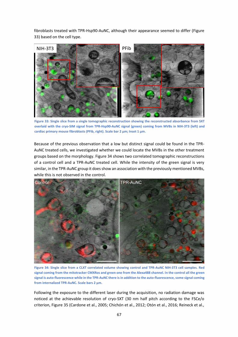
67

fibroblasts treated with TPR-Hsp90-AuNC, although their appearance seemed to differ (Figure

33) based on the cell type.

Because of the previous observation that a low but distinct signal could be found in the TPR-

AuNC treated cells, we investigated whether we could locate the MVBs in the other treatment

groups based on the morphology. Figure 34 shows two correlated tomographic reconstructions

of a control cell and a TPR-AuNC treated cell. While the intensity of the green signal is very

similar, in the TPR-AuNC group it does show an association with the previously mentioned MVBs,

while this is not observed in the control.

Following the exposure to the different laser during the acquisition, no radiation damage was

noticed at the achievable resolution of cryo-SXT (30 nm half pitch according to the FSCe/o

criterion, Figure 35 (Cardone et al., 2005; Chichón et al., 2012; Otón et al., 2016; Reineck et al.,

Figure 34: Single slice from a CLXT correlated volume showing control and TPR-AuNC NIH-3T3 cell samples. Red

signal coming from the mitotracker CMXRos and green one from the Alexa488 channel. In the control all the green

signal is auto-fluorescence while in the TPR-AuNC there is in addition to the auto-fluorescence, some signal coming

from internalized TPR-AuNC. Scale bars 2 µm.

Figure 33: Single slice from a single tomographic reconstruction showing the reconstructed absorbance from SXT

overlaid with the cryo-SIM signal from TPR-Hsp90-AuNC signal (green) coming from MVBs in NIH-3T3 (left) and

cardiac primary mouse fibroblasts (PFib, right). Scale bar 2 μm; Inset 1 μm.

68

2021)) after cryo-3D-SIM. Apart from the clear improvement compared to the confocal data, it

enabled studying the (near-native) environment of the cells, and allowed high accuracy

correlation between the two modalities. Using the displacement of the manually selected

correlative point and the point in the final transformed volume, a correlation heat-map was

calculated depicting correlation accuracies of up to 70 nm in specific areas (see Figure 36).

Furthermore, these types of compartmentalized vesicles were found in all sample groups

imaged, but in a greater number in the case of cells treated with TPR-Hsp90-AuNC (85% increase

for NIH-3T3 and 74% for primary mouse fibroblasts, with respect to the control group, see Table

6). As can be observed in the tomographic reconstruction (Figure 32), the green fluorescence

signal from TPR-Hsp90-AuNC overlapped with MVBs for both NIH-3T3 and cardiac primary

mouse fibroblasts. These MVBs showed vesicle-like compartments with different morphology

and higher absorbance in the case of the later, which might indicate a different mechanism of

processing this TPR-Hsp90-AuNC accumulation by the cell (Figure 37). Note that SXT directly

reconstructs the linear absorption coefficient value of the elemental composition within each

voxel; hence it can be quantified and compared (Weiß et al., 2000). As mentioned above, these

MVBs were found in all cell groups (with a higher presence in the TPR-Hsp90-AuNC group) and

likely play a functional role in cell homeostasis, which is investigated below. Four cells per

Table 6: Statistical analysis of MVBs

NIH-3T3 Primary Mouse Fibroblast

Average Number

per tomogram

Average

Volume [µm3]

Median

Volume

[µm3]

Average Number

per tomogram

Average

Volume [µm3]

Median

Volume

[µm3]

Control 10.25 ± 5.2 204.8 ± 23 172.1 13.25 ± 3.8 216.8 ± 16.9 209.1

TGF-β 9 ± 3.4 211.2 ± 31.8 136.4 12.25 ± 4.6 213.3 ±16.8 192.9

TPR-Hsp90-AuNC 19 ± 3.6 221 ± 17.3 190 23 ± 14.8 176.5 ± 12 149.2

TPR-AuNC 13.25 ± 1.9 149.2 ± 10.5 125.3 14.75 ± 7.6 155.5 ± 15.8 130

Comparison of the main characteristics of MVBs for the different treatments and the two cell types measured from the segmented volumes using Amira software. For each sample 4 tomograms were segmented, except for the NIH-3T3 TPR-Hsp90-AuNC group which had 5 tomograms. For more details see Figure 38.

Figure 35: Resolution

estimation of one of the

cryo-SXT volumes shown

in Figure 29 following the

FSCe/o criterion (0.25

cutoff frequency).

(Cardone et al., 2005)

69

Figure 36: Correlation accuracy map of the CLXT figure shown at the bottom (from Figure 29 in text). The map

was calculated with the build in feature in the ecCLEM plugin (Paul-Gilloteaux et al., 2017) of ICY (de Chaumont

et al., 2012). The colour-scale bar varies from 70.71 nm to 189.04 nm; the squares show the location of the

tomographic reconstructions. Scale bars 10 µm.

70

condition have been segmented with the Amira software (ThermoFisher Scientific, 2021a) and

the number and size of the MVBs was calculated (see Table 6 for a summary and Figure 38 for a

more detailed description), yielding similar sizes for all NIH-3T3 groups considered except for

the TPR-AuNC group, which presents significantly smaller vesicles (*t<0.05) compared to

control. For cardiac primary mouse fibroblasts, a similar trend was observed, with the TPR-AuNC

group having significantly smaller vesicles (**t<0.01) compared to control. In both cell types a

slight increase in the number of MVBs can be observed for TPR-AuNC compared to the control

and TGF-β, although not significant. This small increase in numbers together with the estimated

smaller volume might suggest that the cell is forming new vesicles. When the two cell types were

compared directly, a difference in MVB size for the TPR-Hsp90-AuNC group was observed. NIH-

3T3 cells treated with TPR-Hsp90-AuNC showed the largest size variety of MVBs, also presenting

the highest average volume compared to the respective control groups, while for the cardiac

primary fibroblasts the highest variability, and average volume, was observed in the control

cells. Despite the different appearance, an almost 2-fold increase in the number of MVBs was

observed in both cell types compared to the control groups. The TPR-AuNC groups for both cell

types were the most similar to each other, having similar median and average volumes, while

the TGF-β group showed the same spread, but higher median for the primary mouse fibroblasts.

The TPR-Hsp90-AuNC group of the primary fibroblasts showed a lower median volume of MVBs

(while the average stayed similar) but almost double the number compared to the control,

suggesting the recent formation of new vesicles. It has to be mentioned that the total volumes

of the cell-types are not the same; hence we do not make a direct comparison of the organelle

volumes.

Figure 37: Comparison of MVB morphology for NIH-3T3 (A, B, C & D) and primary mouse fibroblasts (E, F, G & H)

collected by SXT. M = Mitochondria and the arrows point at the MVBs. Scale bars 1 µm.

71

Figure 38: Comparison of MVB volumes measured after segmentation using AMIRA (ThermoFisher Scientific,

2021a). Avg # represents the average number of segmented MVBs in a tomogram, Avg V stands for average volume

and Med V stands for median volume (both in µm3). The measured data was tested for variance and the

corresponding t-test was used to determine statistically relevant differences between groups, the results of which

are shown in the table below.

72

6.2 Co-localization studies by confocal microscopy

To determine the type of the vesicles that contain TPR-Hsp90-AuNCs within the fibroblasts, we

chose different biomarkers to test their spatial association with the Alexa488-labelled Prot-NM.

This part of the experiment was performed by our collaborator Dr. Ana Palanca from Dr. Villar’s

group at IBBTEC, Santander. However, it is part of the investigation and therefore deserves to

be elaborated upon as it answers some additional questions regarding the origin of the MVBs.

The biomarker targets were: Alix, Flotillin-1, CD9 and LC3-II associated to different cellular

vesicles as we explained below. All assays were performed on cells fixed with paraformaldehyde

(PFA) (see specific sample preparation chapter 4.6 Fluorescence and immunofluorescence

assays) and imaged by confocal microscopy.

Figure 39 shows the comparison of NIH-3T3 and primary fibroblasts for the Alix (Figure 39A and

Figure 39B), Flotillin-1 (Figure 39C and Figure 39D) and CD-9 (Figure 39E and Figure 39F) co-

localization study with TPR-Hsp90-AuNC. Both anti-Alix and anti-Flotillin-1 are markers for MVB

biogenesis while anti-CD9 (anti-tetraspanin CD9) is associated with adhesion, motility,

membrane fusion, signal trafficking vesicles and cargo transfer from cellular vesicles (Andreu &

Yáñez-Mó, 2014; Santos et al., 2019). In NIH-3T3 cells a spatial co-localization (at the achievable

confocal resolution) with anti-Alix and anti-CD9 was observed. In addition, some very low anti-

Flotillin-1 signal was detected although there was no spatial association. In the case of primary

mouse fibroblasts, some spatial association was observed with anti-Alix, although the signal was

lower compared to the NIH-3T3 cells. Similar to NIH-3T3, some signal can also be detected from

anti-Flotillin-1, although it appears diffused. Finally, some foci can be seen from the anti-CD9,

but there is no association with the TPR-Hsp90-AuNC. With the above observations, the two cell

types appear to have the same tendency with the exception of CD9 biomarker that showed co-

localization with TPR-Hsp90-AuNC in NIH-3T3 and not in primary fibroblasts. We also tested

these same biomarkers with TPR-AuNC. The TPR-AuNC group showed the same associations

with anti-Alix for both cell types and a co-localization with anti-CD9 in NIH-3T3, however none

in primary fibroblasts similarly to TPR-Hsp90-AuNC. Moreover, and contrary to TPR-Hsp90-

AuNC, we observed a clear spatial association between Flotillin-1 and TPR-AuNC, especially in

primary fibroblasts. Few foci were also observed in NIH-3T3 cells. Previous studies pointed at

Alix, as an accessory protein of the endosomal sorting complex required for transport, to be

involved in the biogenesis of trafficking vesicles, such as extracellular vesicles (Iavello et al.,

2016) The cellular trafficking-related protein Flotillin-1 (Otto & Nichols, 2011) has been related

to endocytosis and endosomal trafficking events. In addition, lipid raft-dependent endocytosis

can be mediated by Flotillin-1 that would be recruited to the surface forming pre-endocytic

clusters. The lack of association with Flotillin-1 for TPR-Hsp90-AuNC could suggest that the

protein hybrid does not enter via endocytosis. The ability of TPR-Hsp90-AuNC to bind to

extracellular Hsp90 may allow it to enter the cell bound to this chaperone through a different

route than TPR-AuNC which is unable to bind to Hsp90.

Once the nanomaterials are inside the fibroblasts, trafficking vesicles presenting Alix could then

be the route of moving both nanomaterials, with and without binding site. The difference

between NIH-3T3 and primary mouse fibroblasts concerning the association with CD9, which we

saw in both TPR-Hsp90-AuNC and TPR-AuNC treated cells, can be related to exocytosis events

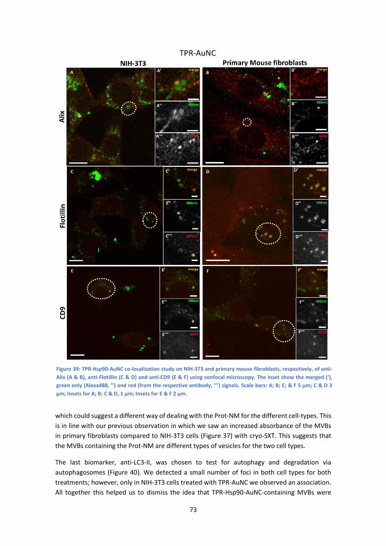
73

which could suggest a different way of dealing with the Prot-NM for the different cell-types. This

is in line with our previous observation in which we saw an increased absorbance of the MVBs

in primary fibroblasts compared to NIH-3T3 cells (Figure 37) with cryo-SXT. This suggests that

the MVBs containing the Prot-NM are different types of vesicles for the two cell types.

The last biomarker, anti-LC3-II, was chosen to test for autophagy and degradation via

autophagosomes (Figure 40). We detected a small number of foci in both cell types for both

treatments; however, only in NIH-3T3 cells treated with TPR-AuNC we observed an association.

All together this helped us to dismiss the idea that TPR-Hsp90-AuNC-containing MVBs were

Figure 39: TPR-Hsp90-AuNC co-localization study on NIH-3T3 and primary mouse fibroblasts, respectively, of anti-

Alix (A & B), anti-Flotillin (C & D) and anti-CD9 (E & F) using confocal microscopy. The inset show the merged (‘),

green only (Alexa488, ’’) and red (from the respective antibody, ’’’) signals. Scale bars: A; B; E; & F 5 μm; C & D 3

μm; Insets for A; B; C & D, 1 μm; Insets for E & F 2 μm.

74

involved in the autophagosome pathway. The possibility of an enhancement of programmed cell

death- apoptosis- events caused by stress upon treatment was also tested using the activated

caspase-3 (cleaved caspase-3 Asp175). No increments where seen for TPR-AuNC, TPR-Hsp90-

AuNC nor TGF-β cells which indicates that we are not inducing apoptosis with the TGF-β

concentration used in this study, similar to previous assays that describe different

concentrations of TGF (data not shown) (Petrov et al., 2002). Moreover, the control cells were

also labelled and imaged and showed no foci with any of the tested biomarkers (Figure 41).

Figure 40: Co-localization study of LC3 with TPR-AuNC (A & B) and TPR-Hsp90-AuNC (C & D) using confocal

microscopy showing some foci however no co-localization. The inset show the merged (‘), green only (Alexa488, ’’)

and red (from the respective antibody, ’’’) signal. Scale bars: A – D 5 μm, insets 1 μm.

75

Figure 41: Testing the four

biomarkers in the control

cells using confocal

microscopy. The images

are 488 nm and 561 nm

emission channels

merged together and

show, apart from some

individual foci, no

increased biomarker

signal. The figures show

anti-Alix (A & B), anti-

Flotillin (C & D) and anti-

CD9 (E and F). No signal in

the 488 nm channel is

observed, which is in

accordance with the lack

of protein hybrid

nanomaterial. Scale bars:

A – G 5 μm; H 2 μm.

76

6.3 Studying treatment-induced morphological differences

6.3.1 NIH-3T3 cells

In addition to elucidating the intracellular fate of the Prot-NM, cryo-SXT allowed gathering

information regarding the possible changes in the cellular ultrastructure upon treatment (Figure

42 and Figure 43). For example, organelle abundance gives information regarding cellular

homeostasis (Cole, 2016). Of special interest was the mitochondrial morphology as their

appearance is directly related to the cellular health, as was mentioned previously. In order to

obtain statistical information about morphological changes of the different cell groups

compared to the control one, and to understand the effect of the treatment, the mitochondria

were segmented using Amira software (ThermoFisher Scientific, 2021a) as already done for the

MVBs. This segmentation allowed evaluating the number, volume and shape dependence of

these organelles for each treatment with respect to the control cells. In the case of the NIH-3T3

cells, the TGF-β group presented an increased number of mitochondria (78% more compared to

Figure 42: Single slice out of a representative tomographic reconstruction for each NIH-3T3 sample showing

the reconstructed absorbance value to compare the morphology of the cell after treatment. * = MVB; M =

Mitochondria; N = Nucleus; V = Vacuole; LD = Lipid Droplet; arrow = Nuclear double membrane. Scale bar 2

μm.

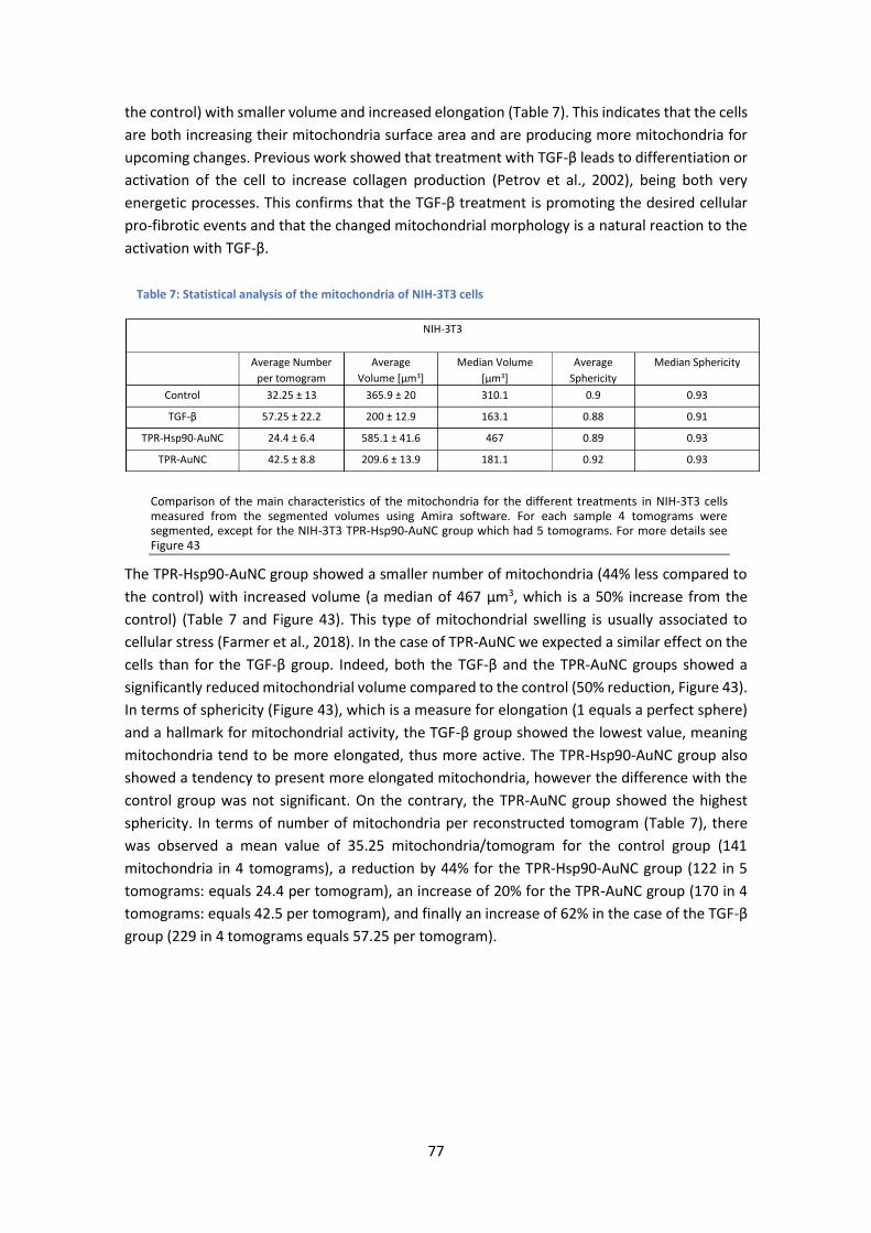
77

the control) with smaller volume and increased elongation (Table 7). This indicates that the cells

are both increasing their mitochondria surface area and are producing more mitochondria for

upcoming changes. Previous work showed that treatment with TGF-β leads to differentiation or

activation of the cell to increase collagen production (Petrov et al., 2002), being both very

energetic processes. This confirms that the TGF-β treatment is promoting the desired cellular

pro-fibrotic events and that the changed mitochondrial morphology is a natural reaction to the

activation with TGF-β.

The TPR-Hsp90-AuNC group showed a smaller number of mitochondria (44% less compared to

the control) with increased volume (a median of 467 µm3, which is a 50% increase from the

control) (Table 7 and Figure 43). This type of mitochondrial swelling is usually associated to

cellular stress (Farmer et al., 2018). In the case of TPR-AuNC we expected a similar effect on the

cells than for the TGF-β group. Indeed, both the TGF-β and the TPR-AuNC groups showed a

significantly reduced mitochondrial volume compared to the control (50% reduction, Figure 43).

In terms of sphericity (Figure 43), which is a measure for elongation (1 equals a perfect sphere)

and a hallmark for mitochondrial activity, the TGF-β group showed the lowest value, meaning

mitochondria tend to be more elongated, thus more active. The TPR-Hsp90-AuNC group also

showed a tendency to present more elongated mitochondria, however the difference with the

control group was not significant. On the contrary, the TPR-AuNC group showed the highest

sphericity. In terms of number of mitochondria per reconstructed tomogram (Table 7), there

was observed a mean value of 35.25 mitochondria/tomogram for the control group (141

mitochondria in 4 tomograms), a reduction by 44% for the TPR-Hsp90-AuNC group (122 in 5

tomograms: equals 24.4 per tomogram), an increase of 20% for the TPR-AuNC group (170 in 4

tomograms: equals 42.5 per tomogram), and finally an increase of 62% in the case of the TGF-β

group (229 in 4 tomograms equals 57.25 per tomogram).

Comparison of the main characteristics of the mitochondria for the different treatments in NIH-3T3 cells measured from the segmented volumes using Amira software. For each sample 4 tomograms were segmented, except for the NIH-3T3 TPR-Hsp90-AuNC group which had 5 tomograms. For more details see Figure 43

Table 7: Statistical analysis of the mitochondria of NIH-3T3 cells

NIH-3T3

Average Number

per tomogram

Average

Volume [µm3]

Median Volume

[µm3]

Average

Sphericity

Median Sphericity

Control 32.25 ± 13 365.9 ± 20 310.1 0.9 0.93

TGF-β 57.25 ± 22.2 200 ± 12.9 163.1 0.88 0.91

TPR-Hsp90-AuNC 24.4 ± 6.4 585.1 ± 41.6 467 0.89 0.93

TPR-AuNC 42.5 ± 8.8 209.6 ± 13.9 181.1 0.92 0.93

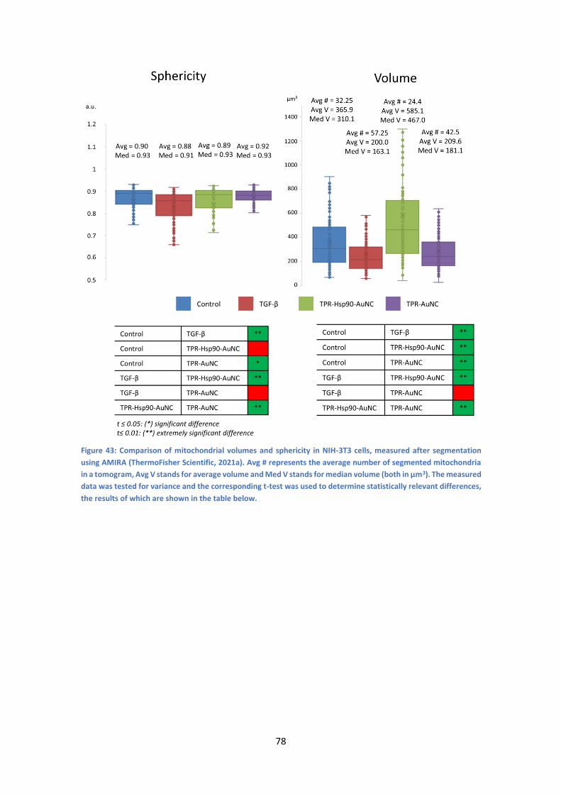
78

Figure 43: Comparison of mitochondrial volumes and sphericity in NIH-3T3 cells, measured after segmentation

using AMIRA (ThermoFisher Scientific, 2021a). Avg # represents the average number of segmented mitochondria

in a tomogram, Avg V stands for average volume and Med V stands for median volume (both in µm3). The measured

data was tested for variance and the corresponding t-test was used to determine statistically relevant differences,

the results of which are shown in the table below.

79

6.3.2 Myocardial primary mouse fibroblasts

When analysing the cardiac primary mouse fibroblast morphology results, significant differences

compared to the NIH-3T3 cells were observed (see Table 8, Figure 44 and Figure 45). First, the

number of mitochondria was similar in all four groups ((23.5; 21.5; 19; and 20.75 per tomogram

for control, TGF-β, TPR-Hsp90-AuNC and TPR-AuNC, respectively see Table 8), although the TPR-

Hsp90-AuNC group had a decrease in mitochondria of 20% compared to the control, following

the same tendency than for NIH-3T3. Second, the mitochondria volume was very similar for all

the groups except for the TGF-β one which showed a significantly higher mean volume

compared to the control. In terms of sphericity, there were significant differences between most

of the groups. Contrary to what was seen in the NIH-3T3 cells, the control group had the most

diverse shapes consistent with the expected continuous fission and fusion of mitochondria

(Youle & van der Bliek, 2012). For both TGF-β and the TPR-AuNC groups, mitochondria appeared

rather spherical, while the TPR-Hsp90-AuNC group showed slightly greater variety of shapes, but

still leaning towards spherical mitochondria. Mitochondrial morphological changes in fibroblasts

due to fission and fusion are beneficial under conditions of high-energy demand (Westermann,

2012) as it is in the case of TGF-β induced collagen production. Note that apart from the control,

all groups have been activated with TGF-β and therefore higher mitochondrial activity demand

is expected in these cells.

Table 8: Statistical analysis of the mitochondria of primary mouse fibroblasts

Primary Mouse Fibroblasts

Average Number per

tomogram

Average Volume

[µm3]

Median Volume

[µm3]

Average

Sphericity

Median

Sphericity

Control 23.5 ± 10.7 382.5 ± 24.8 292.3 0.83 0.89

TGF-β 21.5 ± 10.4 478.3 ± 29.3 411.6 0.9 0.92

TPR-Hsp90-

AuNC

19 ± 3.6 393.1 ± 32 306.7 0.87 0.91

TPR-AuNC 20.75 ± 6.4 353.7 ± 21.9 325.1 0.91 0.93

Comparison of the main characteristics of the mitochondria for the different treatments in primary mouse fibroblasts cells measured from the segmented volumes using Amira software. For each sample 4 tomograms were segmented, except for the NIH-3T3 TPR-Hsp90-AuNC group which had 5 tomograms. For more details see Figure 45

80

Figure 44: Single slice out of a representative tomographic reconstruction for each primary fibroblast sample

showing the reconstructed absorbance value to compare the morphology of the cell after treatment. * = MVB;

M = Mitochondria; N = Nucleus; V = Vacuole; LD = Lipid Droplet; arrow = Nuclear double membrane. Scale bar

2 μm.

81

6.3.3 Other morphological changes

It is worth mentioning that, apart from the mitochondria and MVBs, no additional structural

change has been observed regarding cell nuclei, lipid droplets or other types of vesicle. Neither

the number of lipid droplets nor vacuoles has changed. In the case of the ER, some opening

thereof could be observed in the treated groups for both cell types with respect to their

respective control cells. This type of ER enlargement is normal in cardiac fibroblasts in which

fibrosis events have been triggered, as is also stimulated with the TGF-β treatment. This effect

was already shown previously (Cáceres et al., 2018) and was here confirmed. However, it does

seem that in the NIH-3T3 TPR-AuNC group this effect is even larger than for the TGF-β group

(Figure 42 and Figure 44). This is in line with the mitochondria swelling observation mentioned

above. More research is needed to investigate the cause of these alterations. In the case of the

primary mouse fibroblasts similarities with the TGF-β group are found for both TPR treatments,

which hints towards primary mouse fibroblasts being more resilient towards the treatment.

Figure 45: Comparison of mitochondrial volumes and sphericity of primary mouse fibroblasts, measured after

segmentation using AMIRA (ThermoFisher Scientific, 2021a). Avg # represents the average number of segmented

mitochondria in a tomogram, Avg V stands for average volume and Med V stands for median volume (both in µm3).

The measured data was tested for variance and the corresponding t-test was used to determine statistically

relevant differences, the results of which are shown in the table below.

82

6.4 Collagen visualization with cryo-SXT

Apart from the cryo correlation workflow experiments, we wanted to confirm the findings of

previous studies that Prot-NM can indeed inhibit collagen production. To evaluate this

inhibition, we incubated our samples for 48 h followed by vitrification. As we did not have a

fluorescent marker for collagen available when the samples were prepared, nor did we know

whether we would be able to see it with SXT, we initially only prepared NIH-3T3 cells. Note that

we collected tomograms only in areas between cells where collagen bundles are expected.

Previous studies (Cáceres et al., 2018) have shown that when cultured on a flat surface with TGF-

β, collagen fibres spread evenly underneath the cells. We collected data on one big fibre bundle

on top of the quantifoil in the TGF-β treated grids (Figure 46). In most areas however, the formed

collagen was very thin and hardly visible in 2D projections when looking for specific areas in X-

ray mosaics. Due to the limited depth of field of the ZP it is possible that we did not focus in the

right place. The more likely explanation however is that the achievable resolution is not able to

resolve the individual fibres of the collagen bundle. Using a fluorescent marker for collagen

might help identifying areas with higher collagen concentration. Nonetheless, we could confirm

that a complete inhibition of extracellular collagen production in NIH-3T3 cells was not achieved

upon treatment, but a substantial reduction was indeed visible. In future work it might be

interesting to investigate further, with cryo-SXT but perhaps even better with EM for the higher

resolution. Some tests were already performed by our collaborators from IBBTEC. They found

some structured and un-structured collagen in TGF-β and the Prot-NM containing the Hsp

binding site (TPR-Hsp90-AuNC) but without the fluorescent dye, treated, respectively (data not

shown).

Figure 46: A single slice of the 3D reconstructed absorbance by cryo-SXT showing a comparison of NIH-3T3 cells

treated with TGF-β (left) and TPR-Hsp90-AuNC (right) after 48 h incubation showing collagen on top of the

quantifoil support. TGF-β treated cells show structured collagen bundles, while cells treated with TPR-Hsp90-AuNC

show some signs of unstructured collagen, although in most cases none can be found. Scale bars 2 μm.

83

6.5 FTIR measurements of NIH-3T3 cells

An initial test using Fourier Transform Infrared (FTIR) spectroscopy was performed at Miras

beamline at Alba. FTIR is a technique that measures chemical bond- or group specific vibrational

changes and is a powerful tool to determine chemical compositions. By using synchrotron light

as a source, high resolutions can be achieved that can help determining protein confirmations,

especially secondary structures (Barth, 2007; Goormaghtigh et al., 2006, 2009). The main goal

was investigating whether we could measure biochemical differences that would indicate

cellular stress. For this initial test we prepared new grids of NIH-3T3 cells (control, TGF-β and

TPR-Hsp90-AuNC), the same way as described before, by cryogenically preserving. Because at

Miras samples are imaged at room temperature, after epifluorescence characterization, the

cryogenically preserved samples were rapidly plunged in a 5% PFA solution to quickly fix them

chemically. During this initial test we used the global source of the spectrometer and because

of that the resolution was not as high as it would have been with the synchrotron-based IR light.

Note that when preparing the samples, we did not have the TPR-AuNC lacking the Hsp90

inhibiting group.

As can be seen in the spectrum (Figure 47) we were able to find differences between the three

treatment groups. Especially in the fingerprint region (< 1300 cm-1) we could observe a clear

difference for the TPR-Hsp90-AuNC compared to both the control and the TGF groups, which

showed a similar behaviour.

Figure 47: 2nd derivative of part of the spectra acquired using FTIR spectroscopy on NIH-3T3 cells. The TPR-Hsp90-

AuNC (Green), TGF-β (Red) and control (blue) signals are overlaid to show shifts between them, marked with red

arrows.

84

In the case of FTIR, every peak represents a group and the size of the peak represents the

amount. Simultaneously, the exact position of this peak might shift depending on side groups or

conformational changes of the protein itself. Very prominent peaks when measuring cells for

example are at 2960 cm-1 and 2920 cm-1, which represent CH3 and CH2 respectively. Lipid

content, which comes mainly from the long lipid chains in cellular membranes, can be

approximated by calculating the ratio between these two peaks. Lipid oxidation was estimated

by calculating the ratio between the 1740 cm-1 carbonyl band and the CH2 at 2921 cm-1. The last

ratio that was calculated was the amide I band at 1652 cm-1 and the peak at 2991 cm-1

representing CH stretching, which gives information regarding protein content and in our case,

this also includes information about the presence of collagen.

During this test only a very small number of cells were imaged (5 control, 16 TGF-β and 15 TPR-

Hsp90-AuNC) hence the results show a large variety in most of the cases. As we only had five

control cells we could not use it as a reference, instead only TGF- and TPR-Hsp90-AuNC are

compared. The main reason for this experiment was that we suspected oxidative stress to be

the reason why we saw the morphological changes, especially the mitochondrial swelling

observed in the NIH-3T3 cells. The ratio 1740/2921 gives an indication regarding lipid oxidation.

Figure 48A shows a clear increase in the TPR-Hsp90-AuNC treated group, confirming our

hypothesis. When looking at the lipid content (2960/2920 ratio), which is an indication of overall

cell activity, there seemed to be slightly less in the treated group, however there is no significant

difference (Figure 48B). In the case of protein content, a clear increase in the TGF- group was

observed (Figure 48C). This is most likely the collagen deposited due to the fibrosis being

triggered. This result is another confirmation that TPR-Hsp90-AuNC is able to reduce the

formation of collagen, and in addition, it also suggests that overall cell activity is lower, likely

due to the absence of the Hsp90 triggered signalling cascades.

A proposal to access the Miras beamline for an official experiment using the synchrotron-based

light, was prepared and got accepted. Samples were prepared from both NIH-3T3 and primary

fibroblasts, with the four different treatments described before. Unfortunately, these samples

were contaminated by some bacteria, which made all of the acquired data unusable. Due to

time restrictions it was not possible to write another proposal and repeat the experiment.

Nonetheless it would be very interesting to re-apply for an additional beamtime and repeat this

experiment as there are clear observable differences and the higher resolution achievable using

synchrotron light source will definitely help to identify differences between the treatments, and

possibly also between the cell types. In addition, this experiment could be done with the same

samples measured in cryo-SXT, so that data can be correlated.

Figure 48: Ratios between the values under specific peaks collected by FTIR spectroscopy. These ratios can be used

to draw conclusions regarding processes within cells.

85

7 Discussion

7.1 General Discussion

CLXT at cryogenic temperatures has allowed locating unambiguously the designed therapeutic

agent inhibiting Hsp90 in the 3D cellular environment after being internalized by two different

types of fibroblasts. This novel methodology enables evaluating the effects of the different

treatments at the cellular level which is essential for a future practical usage at the clinical level.

Cryo-3D-SIM provides excellent specificity using a wide range of common dyes and fluorescent

proteins and adequate 3D resolution for correlative purposes, although higher sensitivity at the

single molecule level and resolution (in particular axial resolution) would be desirable. Cryo-SXT

in turn reveals the environmental context and the ultrastructural detail, which allows identifying

the designed protein nanomaterial hybrid containing organelles and describing the

morphological differences accompanying the different treatments. In both cases, the TPR-AuNC

with and without Hsp90 binding module were found in specific multivesicular bodies (MVBs),

although in significantly higher numbers in the TPR-Hsp90-AuNC treated cells. These MVBs likely

play a functional role in cell homeostasis as described in chapter 6.1: Correlation(p. 64) and in

chapter 6.2: Co-localization studies by confocal microscopy (p. 72).

Several visits to the cryo-3D-SIM instrument were required to optimize the protocol described

in Preliminary Results (p. 59) to obtain the results presented in the main results chapter 5. The

main hurdle was the fiducialisation process as a successful high accuracy correlation requires

well distributed and defined fiducial markers which should be ideally detectable by both imaging

techniques. In collaboration with the team from B24 beamline at Diamond we produced a

protocol published in a methods manuscript (Okolo et al., 2021) that highlights the main

requirements and problems when deciding which fiducial to use, and how to use it. As is

described there, fiducial batch-variability is a major problem when it comes to reproducibility as

it can have a severe negative impact on the experiment, without a way to circumvent or

overcome the problem. Note that fiducial markers are expensive (up to 1000€ per ml) and

distributors hardly offer any refund. Fortunately, it is possible to perform the 3D correlation also

using organelles, thus it is always recommended to use at least one organelle tracker. Apart from

having the organelle tracker as a backup-fiducial, it can also act as reference to judge the quality

of the correlation. Moreover, from our experience the combination of extracellular- and

intracellular fiducials allows for better 3D correlation accuracy as fiducialisation can happen

throughout the full volume (in depth) and not only on the external parts of it.

As was explained before (see chapter 4.3 Sample preparation for CLXT), we utilized a mix of non-

fluorescent gold fiducials (100 nm, BBI solutions) and Tetraspecks (200 nm, Thermofischer)

which show fluorescence at four different wavelengths (405 nm, 488 nm, 594 nm, and 635 nm).

The first are needed for projection alignment prior to reconstruction and ideally, it would be

better to have one fiducial only which would fulfil the two requirements: high fluorescence

signal and high absorption contrast. While we did try fluorescent Au fiducial markers to avoid

adding the 100 nm non-fluorescent gold beads, the batch we obtained was useless, showing low

fluorescence emission. At the same time, we discovered that we were able to reconstruct the

Tetraspecks in the cryo-SXT volumes although these were not visible in the tilt series projections.

Unfortunately, using the Tetraspecks for the 3D correlation proved impossible unless they were

86

in a very thin cell area as they would fall outside the depth of field of the TXM when on top of

the cell. Ultimately, for this thesis project, all successful correlations were performed using the

fluorescent signal from mitochondria (Mitotracker red CMXRos). The obtained correlation

accuracy was, depending on the area, down to 70 nm using a minimum of 10 strategically placed

points in the centre of evenly spread mitochondria (in 3D). Considering the larger size of

mitochondria compared to standard fiducial markers, the accuracy could have been better if, in

addition, the latter would have been used. This is arguably not as important for our approach

due to the limited resolution mainly from the cryo-3D-SIM in this case, however if at some point

cryo single molecule localization microscopy (SMLM) techniques are available, such as cryo-

dSTORM, small fiducial markers are an unavoidable need, as is already seen for classical CLEM

that involves techniques surpassing the 50 nm resolution (Mohammadian et al., 2019). In our

case, this might have helped locating our designed protein within the specific compartments of

the MVB.

As already mentioned, in our case having better fiducial markers would most likely not improve

the results, due to the large resolution gap between cryo-3D-SIM and cryo-SXT. As such, the

correlation accuracy of 70 nm might be near the achievable limit, although, using more well

distributed fiducials, the area that shows this highest accuracy could have probably been

increased (see the correlation accuracy heatmap Figure 36 p.69). As such, the only way to obtain

additional information, for example a more specific location of the protein inside the MVBs,

would be to utilize higher resolution techniques to measure the very same samples using, for

example cryo-ET after cryo-FIB milling correlatively with a cryo super resolution technique, or

by preparing new samples and utilizing different means to obtain the data, like non-cryo

workflows. A workflow involving cryo-ET would require a tight dose control, however it is

expected that doses below 108 Gy would still produce high resolution cryo-ET results (better

than 1 nm). In general, doses delivered in cryo-SXT are of the order of 107 – 108 Gy (2.5 x 108 has

been reported previously after acquisition of two tiltseries (Conesa et al., 2016)). In addition,

strategies to minimize dose can be adopted including decreasing the number of projections

collected and using algorithms appropriate for sampling sparsity (Jiang et al., 2018), and thus

still allowing further experimentation. Note that during our experiments we did control the dose

as no further techniques were used.

In addition to achieve high accuracy in the location of the proteins within the MVBs, obtaining

information on the specific cellular processes is required for a more complete understanding of

the system. One example of this, which has already been done during this project, is the

fluorescence co-localization study. To obtain information regarding the origin of the MVBs,

collaborators from IBBTEC performed an immunofluorescence assay using confocal microscopy

(see chapter 6.2 Co-localization studies by confocal microscopy) on chemically fixed samples,

which allowed obtaining valuable information regarding the function and origin of these MVBs

in relatively short time using specific antibodies for different endosomal marker targets. While

these results did not answer the question about the identity of the vesicles, nor about their

function, they shed light on the process of how the different cell-types are dealing with the

nanomaterial. It must be said that the co-localization achieved of specific events (co-localization

of the fluorescent signal from the therapeutic agent with the antibody) by confocal microscopy

has a poor axial resolution and the results can be misleading. While a co-localisation in X-Y has

87

an accuracy of 200 nm and most probably indicate real events, the axial resolution of 800-900

nm might not, although an apposition or association could be claimed.

Based on their appearance in the cryo-SXT volumes, it was postulated that the MVBs could be

related to lysosomes, and their role would be to remove the nanomaterial from the cell. The

four chosen antibodies specifically target different key proteins in different processes related to

our hypothesis. Alix is an accessory protein of the endosomal sorting complex required for

transport and has been related to the biogenesis of trafficking vesicles, such as extracellular

vesicles (Iavello et al., 2016). The cellular trafficking-related protein Flotillin-1 (Otto & Nichols,

2011) has been related to endocytosis and endosomal trafficking events. In addition, lipid raft-

dependent endocytosis can be mediated by Flotillin-1 that would be recruited to the surface

forming pre-endocytic clusters (Otto & Nichols, 2011). The difference between TPR-Hsp90-AuNC

and TPR-AuNC with regard to Flotillin-1 suggests that the latter enters the cell by endocytosis,

while the TPR-Hsp90-AuNC enters differently. Based on previous publications it was

hypothesized that it binds to extracellular Hsp90 and enters the cells in conjunction with it. This

proposed mechanism will explain the lower intracellular TPR-AuNC concentration as this

suggests a slower, passive, incorporation via the endocytic pathway compared to the active

incorporation bound to Hsp90. After uptake of the nanomaterials, trafficking vesicles presenting

Alix, which showed association with both nanomaterials, could then be used for transport. The

difference concerning the association with CD9 for both nanomaterials, for which an association

was observed only in NIH-3T3 cells, can be related to exocytosis events and may suggest a

different, cell-dependent, way of dealing with the nanomaterial. This hypothesis is in line with

our observation of an increased absorbance of the MVBs in primary fibroblasts compared to

NIH-3T3 cells (Figure 37) by cryo-SXT. Overall, these results suggest that the MVBs are mainly

related to endosomal trafficking events, however the origin of the endosomal trafficking seems

to differ depending, not only on cell type, but also on the presence of the Hsp90 binding module.

Cryo-SXT also allowed the evaluation of the cellular response towards the treatment. As

highlighted before, a clear difference was already observed for the MVBs. This trend was also

observed throughout the whole cell, specifically for the cells treated with TPR-Hsp90-AuNC. NIH-

3T3 cells showed clear signs of stress in the form of mitochondrial swelling. As this swelling was

not observed in the TPR-AuNC group, it is thought to be directly linked to the molecular changes

promoted by the binding of the hybrid functional protein to the C-terminal end of Hsp90 (Aires

et al., 2021). Still, it could be argued that the lower intracellular TPR-AuNC concentration could

explain the apparent lack of reaction. Other studies have already reported that stress, especially

oxidative stress, induces mitochondrial swelling, which would support our first hypothesis

(Rossignol et al., 2004). Whether the stress is induced only by the Hsp90 inhibition (Li et al.,

2015; Sable et al., 2018) or also because of the presence of the AuNC (Jawaid et al., 2020; Tay et

al., 2014) is still to be answered by performing for instance additional cryo-SXT experiments on

cells treated with the CTPR390 (with and without the Hsp90 binding domain) without the AuNC.

FTIR spectroscopy would also be useful combined with the cryo-SXT results in particular if the

same grids are used as specific morphological observations can be correlated with biochemical

changes within the cell.

Oxidative stress in particular is a clear sign of an adverse effect of a treatment and mitochondria

are clear markers for this effect, as previously explained. However, even without considering

88

mitochondria, both cell types were affected by a low intracellular TPR-AuNC concentration, as

shown by the extra ER enlargement, especially in NIH-3T3 cells. This type of ER enlargement is

normal in cardiac fibroblasts in which fibrosis events have been triggered as shown previously

(Cáceres et al., 2018) and confirmed here. Nonetheless, the fact that TPR-AuNC treatment has a

noticeable effect on the cells, while missing the Hsp90 inhibitory domain, suggests that the

observed effect for the NIH-3T3 TPR-Hsp90-AuNC group is probably not entirely due to the

Hsp90 inhibition. These effects could stem from the AuNC, the metallic component of the

protein nanomaterial as was suggested before. However, note that the increased Hsp90

production is not the only effect induced by the TGF-β activation. Another possibility could

therefore be related to a different signalling cascade induced by the TGF-β. This hypothesis is

supported by our observation in the TGF-β group, which showed a drastic morphological change

compared to the control group. Ultimately, more research will be needed to investigate these

observations and to determine which aspect of the treatment is causing the morphological

changes observed. Finally, it is worth mentioning that these results reinforce the need of

evaluating systematically the cellular structure upon application of specific treatments with

adequate imaging techniques to be able to assess the cellular response.

All the previously mentioned observations about adverse reactions towards the different

treatments were mostly visible in the NIH-3T3 groups. Primary mouse fibroblasts, on the other

hand, did not exhibit these symptoms of stress after overnight TPR-Hsp90-AuNC treatment,

indicating that the cells had time to recover or adapt to the new conditions. Furthermore, the

fact that the number of mitochondria is similar in every treatment group, is in line with other

work that related organelle size to cellular homeostasis(Cole, 2016), arguing that every cell type

has an optimum number of organelles and a deviation from this number suggests a change in

gene expression. While previous studies (Aires et al., 2021; Cáceres et al., 2018) already

highlighted the lack of negative effects in primary cardiac mouse fibroblasts, we now confirm

that at the ultrastructural level TPR-Hsp90-AuNC is a viable option to inhibit the Hsp90 protein

in primary cardiac mouse fibroblasts while also ensuring its ATPase activity and thereby keeping

the cell in homeostasis. Despite the side effects in NIH-3T3 cells, we confirm here that Hsp90

inhibition at the C-terminal end reduces collagen overproduction in both cell types.

Furthermore, we conclude that the immortalized version of a cell type may not always be a good

functional alternative when studying molecular processes as deviations from primary cells can

occur.

89

7.2 Future optimization

As mentioned before, experimental procedures are often adapted to fit the need of the research

question. However, some parts of the protocol are already well established, i.e. the cell culture

part. The imaging itself will in theory also not change significantly, although, with software

upgrades and developments, the sample preparation and data acquisition mode will become

easier and more user-friendly. The main developments that can happen in the near future are

therefore expected to be in the image processing workflow. This section will focus on possible

future developments that could have a major impact on the workflow utilized in this thesis

project.

One of the major developments that will be required is fiducial-less alignment of the

tomographic projections. At the moment these developments are mainly happening in the field

of electron microscopy (Castaño-Díez et al., 2007) and hard X-ray micro-tomography which is

less demanding, but also in X-ray nano-tomography (Gürsoy et al., 2017; Guzzi et al., 2021).

However, it is expected that these developments will be implemented with the needed

specificities for SXT as well, although the depth of field limitation of the Fresnel zone plate lens

intrinsically renders this fiducial-less alignment much more complicated than in the ET field.

Currently IMOD patch-tracking (Mastronarde, 1997) is used for tomographic tilt series that do

not have sufficient fiducial markers. However, this script does not detect features. Rather, it

calculates the position based on the tilt-angles and the cosine-stretching of high angle images.

While this can result in very accurate alignments, a manual intervention often improves these

results substantially (sub pixel alignment is needed). The points that are being tracked are

created by overlapping patches of predetermined sizes and subsequent tracking of the

intersections of said patches. Small mistakes during the first cosine stretching step can be

amplified at the more extreme angles. This actually does not happen for all intersections,

meaning that with a small intervention, mainly by deleting wrong points, the resulting alignment

can substantially improve the final reconstruction. This manual intervention is very subjective

and will never replace an alignment based on fiducial markers. A fiducial-less alignment

facilitated by machine learning or artificial intelligence might in the future make fiducialisation

obsolete, or at least offer a viable alternative (Amat et al., 2008, 2010; Castaño-Díez et al., 2010;

Noble & Stagg, 2015). Note that the patch-tracking supposes that the run-out of the stage is

mainly mechanical and can be somehow predicted. This is not true for Mistral and B24 as on top

of the run-out of the stage, the cooling Cu braids that keep the sample around 100 K adds

irreproducible displacements which are difficult to foresee or calculate.

Regarding the cryo-3D-SIM, software development can improve the acquisition part and the

reconstruction. The current acquisition software, cockpit (SOFTWORX, GE Healthcare), was

chosen for historical reasons: re-using existing software was favoured as a complete

development would have slowed down the operation of this novel cryo-3D-SIM instrument. In

the case of the software for data reconstruction new developments are in progress such as 3D

FairSIM (Markwirth et al., 2019), for instance. The reconstruction of SIM data is straight forward

when proper optical transfer function (OTF) measurements are done and the calibration of the

instrument is maintained properly (Demmerle et al., 2017), which means there is no way of

improving the reconstruction itself. However, software developments may improve user

experience, as well as speed of the reconstruction. FairSIM (Müller et al., 2016) is an open source

90

Fiji-plugin, and it shows some impressive results. However, as of writing this manuscript, only

2D SIM reconstructions are possible with FairSIM. A new version that allows 3D reconstruction

is currently still under development.

The correlation of the cryo-3D-SIM and cryo-SXT data is done using Icy (de Chaumont et al.,

2011, 2012) plugin ecCLEM (Paul-Gilloteaux et al., 2017). This plugin works as intended but is

still under development, and currently presents bugs that impair overall user experience.

Looking at commercial products, Zeiss’s CLEM products, for example, offer automatic

correlation. This is expected to be available in the future too although the efforts towards this

of few specific laboratories are inevitably slow.

Finally, the development of an automated pipeline however will be the most important

improvement. Currently, the data processing of the acquired cryo-3D-SIM data at B24 Diamond

is preferentially performed at the end of the day, after an experimental session, meaning, in the

worst case, wrong experimental parameters could lead to unusable data. Ideally the data should

be processed in real time so that the experimental procedure and settings can be adjusted

during the experiment, especially when the cryo-3D-SIM reconstruction process will take about

10 minutes for each 3D stack. In the case of cryo-SXT, this depends on the user’s choice: an

automatic, possibly low-quality alignment and fast reconstruction using SIRT after acquisition,

or high-quality alignment based on user input after the experimental session. The first option,

which takes in total less than 10 minutes, is available although the quality will highly depend on

the available 100 nm Au fiducials used to align the projections to a common rotation axis.

Although this is useful in order to decide if it is worth collecting more tomograms on the imaged

cell, the manual alignment refinement done by the user will be still required and is time-

consuming. Performing the automatic alignment does have the advantage that at the end of a

session, in which hundreds of tomograms could be collected, a priority list can be determined

for the subsequent manual refinement of the automatically aligned stacks. In any case, full

automation of both data processing types including the correlation would greatly make the

experimental sessions more time-efficient, which is of utmost importance considering the

limited allocated time at a synchrotron facility.

Regardless the software and processing pipelines, there are also issues that came up which are

related to the sample preparation. The first issue to be mentioned is the variability of the cell

confluence on the sample support. While in culture plates an even spread is usually observed,

on EM grids there is more variability. One phenomenon commonly observed is cells growing on

top of, or very close to the Au bars of the grids. In order to record a maximum angular range in

the tilt series, it is important that the cells are located in the centre of the grid squares, far from

any bar. There has been recently some development in the accurate deposition of single cells,

from a suspension, in previously designated positions (Toro-Nahuelpan et al., 2020) but it can

be argued that this procedure does not recreate a natural distribution, also considering that

most cells like to be in direct contact to each other. However, being able to actively deposit cells

at specific locations would greatly increase the reproducibility and success rate of experiments,

mainly because suboptimum samples are the main reason for failed measurements during

beamtimes.

91

The second issue is the timing of organelle staining and vitrification. Organelle stains are not

completely organelle specific. If the recommended incubation time is exceeded, unspecific

(over-)staining can occur. This is due to the nature of the stain, which for example targets specific

membrane proteins and if all targets are labelled, the stain will target similar membrane

proteins. Over-staining increases background fluorescence, which can create problems at a later

stage, especially during the correlation as it can be difficult to identify clear features. Even for

trained users, 3 minutes to vitrify and store one single grid should be considered. By adding the

staining reagent to 4 grids every 15 minutes, for the number of available slots in a grid box (4

grids) and exchange of the grid box, overstaining can be avoided. Furthermore, related to the

vitrification itself, the thickness of the ice-layer in which the cells are embedded can have a

negative impact on the sample. Too thick ice can reduce the amount of transmitted light, which

has an effect on the achievable resolution, while too thin ice can affect the cells themselves by

either exposing them or compressing them. Before the samples are vitrified, excess liquid

(mostly water) is removed by a process called blotting. A filter paper is pressed against the

backside of the EM grid (to avoid touching the cells) and absorbs the liquid until only a thin layer

is left, equal on the whole grid. The efficiency of this process is related to the blotting time, but

also the confluence of the cells or the presence of other materials on the grid has an influence.

High-speed interferometry has been used to assess the ice thickness of vitrified macromolecules

(Armstrong et al., 2020). An integration of such a device into a vitrification setup could greatly

improve overall vitrification reproducibility, although this can be more difficult when having

whole cells compared to the macromolecule samples reported there.

The third issue is more of a recommendation and is related to the cryo epifluorescence imaging

to select the best samples. Apart from evaluating the quality of the sample in terms of ice

thickness, confluence and grid preservation (cracks, broken foil etc.), it is worth to already select

cells during this screening step for the cryo-3D-SIM correlative imaging to be more efficient later.

The issue to consider here is that the quality of the sample can be assessed at low magnification

(10x). At the same time, the field of view is very large, making it easy to identify suitable cells.

Instead of writing down the location of the cells in the finder grids, or going to a higher

magnification (100x), it is easier to collect low magnification (10x) maps of several areas to

recreate a mosaic view of the grid. Acquiring high magnification images at this stage does not

make sense as it takes time, the sample could be lost during transport, and better-quality images

can be acquired using the cryo-3D-SIM setup. In addition, switching between low and high

magnification, and then re-locating the cells is time consuming and usually, several tens of grids

need to be screened. Having instead a mosaic view of the grid allows the selection of cells after

the cryo epifluorescence imaging. In addition, having a mosaic is especially useful when the

previously selected cells become unusable, for example due to the accidental introduction of

artefacts, like ice contamination or cracks in the ice from mechanical stress, and new cells have

to be found on a short notice once already at the cryo-3D-SIM.

The last thing to be discussed in this section should be hardware and its availability. With

upgrades to the hardware, experiments will become easier. One example here is the Linkam

CMS196 cryo stage which needs a bake out every two hours due to the prevention of any ice

crystal formation. Most of the current commercial high-resolution cryo 3D fluorescence setups

utilize this cryo stage, which highlights how difficult the design of an open cryo stage like this is.

A way to overcome ice contamination would be to have a humidity-controlled chamber around

92

the sample stage so that very low humidity can be set and maintained during all the

measurements.

Another possible future hardware development related to cryo-SXT would be dual tilt

tomography for all lenses available at Mistral. As already mentioned, dual tilt tomography

(Arslan et al., 2006) is a technique where, first, a tilt series is acquired followed by a 90-degree

rotation of the sample and the acquisition of a second tilt series. This reduces the effect from

the missing wedge, in turn increasing the visibility of hidden feature due to their orientation

with respect to the axis of rotation and the resolution in the XZ and YZ planes. Note that the

resolution of a reconstructed tomogram is not isotropic due to the missing wedge. In addition,

as the sample is placed in an autogrid, sample handling will become slightly easier, as the

autogrid is sturdier than the grid, thereby avoiding mechanical stress when handling the sample

although mounting a vitrified grid on an autogrid requires expertise. A hardware development

is currently available for the 40 nm ZP lens at Mistral (Valcarcel et al., 2018) but is still in progress

for the 25 nm one which was the used lens for these data. The challenge here is the available

space for designing a holder as the available rotation range, which is reduced for this last lens

as the focal length is smaller (1.52 mm). It has to be mentioned that dual tilt tomography (DT)

implies extra data collection. Therefore, a choice is required during a given beamtime: either

collecting the maximum possible number of tomograms on different cells, or collecting less in

order to perform DT. Either approach has its benefits and ultimately each user has to decide by

itself.

In terms of availability, having all equipment available at the same institute and even in the same

laboratory would be a major advantage. Except for the cryo-3D-SIM, every step of the workflow

was performed at Alba. This was a major bottleneck as we were able to prepare many samples

but were only able to visit the cryo-3D-SIM two times for 3 days, 8 hours per day. At the moment

of writing this manuscript, a similar cryo-3D-SIM setup is being developed at Alba. Having it

available on-site will allow more data acquisition and better data once good sample preparation

is achieved.

All the developments mentioned in this section will undoubtedly improve many current

workflows, not just the one used during this project. As every current experimental procedure

is a derivation, mixture, or improvement of older protocols, many nowadays unrelated fields

have to deal with similar problems concerning specific parts of a protocol. Developments in one

field can therefore have an immense impact on other fields as well. Nonetheless, the amount of

information, already obtainable using current equipment, is immense. This methodology creates

exciting prospects for the future.

93

8 Future studies and conclusion To summarize, the goals of this work were:

1. To study the intracellular fate of this novel protein nanomaterial hybrid.

2. To study the effect of the treatment on the cell at an ultrastructural level.

3. To create a correlative cryo-3D-SIM and cryo-SXT workflow that gives high resolution 3D

information of the whole cell.

4. To describe and compare the behaviour of primary and immortalized cardiac fibroblasts

when treated with a designed therapeutic nanomaterial.

Creating a workflow, as was specified for goal number three, was fundamental for answering

the other research questions. Specially the decision to focus on a full cryogenic approach was

what ultimately enabled us to study the protein nanomaterial in vivo to the extent that was

needed and the techniques selected in our correlative approach prove to be adequate. The

protein-nanomaterial hybrid was unambiguously located within specific multivesicular bodies

(MVB). The nature of these MVBs was determined by confocal microscopy using additional

samples and with the a priori knowledge provided by cryo-SXT. The MVBs are related to the

endosomal pathway and the immunostaining assay showed a clear difference depending on the

cell-type. This different reaction towards the treatment depending on the cell-type was also

seen using cryo-SXT, in which MVBs showed higher absorption in the case of the myocardial

primary mouse fibroblasts which suggests a different way of dealing with the nanomaterial.

Furthermore, a distinct difference between the two cell-types was observed regarding the

cellular reaction towards the treatment with the Prot-NM. Our results show that the primary

mouse cardiac fibroblasts are inherently more stable and resilient towards the treatment

compared to the immortalized NIH-3T3 cells which presented clear signs of stress. This is an

important observation for the study of novel therapeutic agents as in many cases an initial study

is performed on immortalized cells, due to the extra costs, effort and bioethical considerations

that are involved in obtaining and working with the primary version. A more detailed study,

comparing the primary and immortalized versions of other cells, and their reaction towards

various treatments, could shed more light on this phenomenon. But in any case, it would be

advisable to evaluate both type of cells in this type of research, as seen here.

During this thesis project the main focus was the development of the workflow that would allow

answering the other research questions. This process was limited by the availability of super

resolution techniques in cryogenic conditions and, in particular, of our ability to access the only

available instrument at the time, the cryo-3D-SIM itself in the UK, and collect the needed data.

The obtained result, while already providing very useful information, could still be considered

incomplete. Especially in the case of novel therapeutic agents, it is of utmost importance that

the complete dynamic process, from uptake to breakdown, is well documented. Our data

provides information about the cell when the intracellular concentration has reached its

maximum (10 h after treatment), however, this peak has been shown to last up to 48 h (Cáceres

et al., 2018), after which the intracellular concentration has shown to subside. Additionally, after

48 h, collagen deposition commenced in TGF-β samples, as was also shown in that same study.

While some experiments with 48 h samples have been performed during this project, the main

interest during these sessions was the visualization of collagen fibres. For this reason, there is

94

not sufficient data regarding intracellular organization of the cells at this stage. This should

definitely be addressed in future studies.

Other time points, which would provide important information, could be shortly after

treatment, to investigate uptake, and once the intracellular concentration starts decreasing, to

investigate the fate of the protein nanomaterials. Current hypotheses are that TPR-Hsp90-AuNC

enters via an active transportation, bound to the Hsp90, and TPR-AuNC enters passively through

endocytosis. This is based on previously found uptake-rates, as well as the immunofluorescence

assays that were performed. If the hypotheses are correct, it could be expected that the

formation of MVB for the TPR-AuNC starts at the cellular membrane, while in the case of TPR-

Hsp90-AuNC the vesicles would be formed throughout the cell. To visualize this event using the

cryo-CLXT workflow developed here might be difficult due the lack of knowledge regarding the

actual onset of the internalization and the fact that it may be an elusive event. To capture this

event a live-cell imaging approach would be more suited as the formation of vesicles could be

visualized in real time. As the nanomaterial itself is too small to be visualized (<20 atoms), it

would be visible only once a sufficient amount of aggregation would happen or using single

molecule super resolution techniques, although the latter brings its own difficulties as discussed

previously. The same live-cell imaging approach could be used to determine what happens to

the nanomaterial. A slow disappearance within the cell would suggest degradation, while

transport towards the cellular membrane would suggest exocytosis events. Once the

information regarding the onset of either process is available, cryo-CLXT could be used to

capture the event in more detail in its cellular environment.

One process for which cryo-SXT is lacking resolving power to provide detailed information is the

collagen deposition as the collagen fibre itself cannot be resolved and only large bundles were

clearly seen. The dataset showing the collagen bundle made from individual fibres (Figure 46)

should be considered a “lucky find” as most of the collected data did not show anything similar,

even though previous EM studies on thin sections have shown the presence of collagen after 48

h (Cáceres et al., 2018). Although in some cases collected data presented an observable

unidentifiable shadow that could be due to the suspected extracellular collagen, we could not

confirm its origin with the needed certainty. This is mainly due to the small size of the fibres, its

low inherent absorption contrast compared to the rest of the cell with thicknesses of several

microns, as well as probably due to the depth of field (DOF) of cryo-SXT which implies that the

full cell thickness will not be in focus. Because setting up the collection of a tomographic tilt

series requires having a feature in focus throughout the entire angular range, this is usually done

with clearly visible feature, like nuclear- or mitochondrial membranes or lipid droplets. For this

reason, the collagen might have fallen outside the DOF if the thickness of the cell exceeds it.

Also, having a fluorescent marker to pinpoint the collagen location would have certainly helped,

but this was not the case. In order to ensure obtaining high quality information, EM is the best

option in this case. Especially FIB-SEM (Knott et al., 2008) could provide the 3D organization of

the collagen bundles.

The integration of cryo-ET into the existing cryo-CLXT workflow, which has been mentioned

several times throughout this manuscript, would be yet another great advance within the field

of correlative microscopy. In the scope of this research project it is arguably not necessary at

this stage as the structural changes and the Prot-NM accumulation within vesicles can be

95

visualized using cryo-SXT. Note that a great number of tomograms has been needed to tackle

the problem for the different sample conditions. Imaging of the same number of samples and

cells would be very time consuming if it were to be repeated with cryo-ET. However, research

involving low-abundance accumulation of fluorescent entities or rare events, would need EM to

further elucidate higher level of structural information. For example, an accurate localization of

these features or events first by cryo-SXT at better than 100 nm resolution would greatly

improve the process to guide the user to locate the site for the lamellae production. Even for

our project, cryo-ET might in the future, provide additional information to, for example,

determine the aggregation of the therapeutic agent within the MVBs or to determine the mode

of internalization.

In conclusion, the work presented in this thesis highlights the development of a novel cryo

correlative microscopy approach and shows impressive results, not only localizing a specific

molecule within the 3D space of a cell but also providing ultrastructural information of the cell

itself. Especially in the field of therapeutics development, this sort of information is vital to

ensure a full understanding of the mode of action of the compound under study. Furthermore,

working in cryogenic conditions has the added benefit that the samples are frozen in time,

meaning even dynamics through particular time points and/or elusive events can be visualized

with ease once their presence has been confirmed. Apart from the clear technological progress

of integrating the fluorescence specificity in the 3D native cell structure, it was possible to

deepen our knowledge on novel designed protein-nanomaterial hybrids. The obtained data

clearly points towards an efficient and specific therapeutic mode of action, without any

apparent negative effect in myocardial mouse primary fibroblasts. Due to the nature of these

designed proteins, changing its functionalization is straightforward and could lead to a wide

range of novel therapeutic agents. The here reported findings might incentivize others to build

and study novel therapeutic agents based on the Prot-NM studied here, or on alternative

protein-nanomaterials hybrids.

Ultimately, our findings have raised additional questions and more research will be needed to

address them. With the development of a cryo-3D-SIM setup at Alba, it is expected that further

studies will proceed faster, mainly because access to the cryo-3D-SIM was the largest constraint

during this project. Nonetheless, the results presented here already show great promise and

provide a solid basis for future work. The expertise of all people involved in the project, cardiac

cell biology from IBBTEC, the protein-nanomaterial from CIC biomaGUNE and the imaging aspect

from Alba, enabled the optimization of the workflows and resulted in achieving the

aforementioned goals.

96

9 References Abbe, E. (1873). Beiträge zur Theorie des Mikroskops und der mikroskopischen Wahrnehmung.

Archiv Für Mikroskopische Anatomie, 9(1). https://doi.org/10.1007/bf02956173

Agulleiro, J. I., & Fernandez, J. J. (2011). Fast tomographic reconstruction on multicore

computers. Bioinformatics, 27(4), 582–583.

https://doi.org/10.1093/bioinformatics/btq692

Aires, A., Llarena, I., Moller, M., Castro‐Smirnov, J., Cabanillas‐Gonzalez, J., & Cortajarena, A. L.

(2019). A Simple Approach to Design Proteins for the Sustainable Synthesis of Metal

Nanoclusters. Angewandte Chemie International Edition, 58(19), 6214–6219.

https://doi.org/10.1002/anie.201813576

Aires, A., Maestro, D., Ruiz del Rio, J., Palanca, A. R., Lopez-Martinez, E., Llarena, I., Geraki, K.,

Sanchez-Cano, C., Villar, A. v., & Cortajarena, A. L. (2021). Engineering multifunctional

metal/protein hybrid nanomaterials as tools for therapeutic intervention and high-

sensitivity detection. Chemical Science, 12(7), 2480–2487.

https://doi.org/10.1039/D0SC05215A

Akhurst, R. J., & Hata, A. (2012). Targeting the TGFβ signalling pathway in disease. In Nature

Reviews Drug Discovery (Vol. 11, Issue 10). https://doi.org/10.1038/nrd3810

Amat, F., Castaño-Diez, D., Lawrence, A., Moussavi, F., Winkler, H., & Horowitz, M. (2010).

Alignment of cryo-electron tomography datasets. In Methods in Enzymology (Vol. 482,

Issue C). https://doi.org/10.1016/S0076-6879(10)82014-2

Amat, F., Moussavi, F., Comolli, L. R., Elidan, G., Downing, K. H., & Horowitz, M. (2008). Markov

random field based automatic image alignment for electron tomography. Journal of

Structural Biology, 161(3). https://doi.org/10.1016/j.jsb.2007.07.007

Andreu, Z., & Yáñez-Mó, M. (2014). Tetraspanins in Extracellular Vesicle Formation and

Function. Frontiers in Immunology, 5(SEP). https://doi.org/10.3389/fimmu.2014.00442

Armstrong, M., Han, B. G., Gomez, S., Turner, J., Fletcher, D. A., & Glaeser, R. M. (2020).

Microscale Fluid Behavior during Cryo-EM Sample Blotting. Biophysical Journal, 118(3).

https://doi.org/10.1016/j.bpj.2019.12.017

Arslan, I., Tong, J. R., & Midgley, P. A. (2006). Reducing the missing wedge: High-resolution dual

axis tomography of inorganic materials. Ultramicroscopy, 106(11-12 SPEC. ISS.).

https://doi.org/10.1016/j.ultramic.2006.05.010

Bao, Y., Yeh, H. C., Zhong, C., Ivanov, S. A., Sharma, J. K., Neidig, M. L., Vu, D. M., Shreve, A. P.,

Dyer, R. B., Werner, J. H., & Martinez, J. S. (2010). Formation and stabilization of

fluorescent gold nanoclusters using small molecules. Journal of Physical Chemistry C,

114(38). https://doi.org/10.1021/jp909580z

97

Barnette, D. N., Hulin, A., Ahmed, A. S. I., Colige, A. C., Azhar, M., & Lincoln, J. (2013). Tgfβ-Smad

and MAPK signaling mediate scleraxis and proteoglycan expression in heart valves. Journal

of Molecular and Cellular Cardiology, 65. https://doi.org/10.1016/j.yjmcc.2013.10.007

Barth, A. (2007). Infrared spectroscopy of proteins. In Biochimica et Biophysica Acta -

Bioenergetics (Vol. 1767, Issue 9). https://doi.org/10.1016/j.bbabio.2007.06.004

Betzig, E., Patterson, G. H., Sougrat, R., Lindwasser, O. W., Olenych, S., Bonifacino, J. S., Davidson,

M. W., Lippincott-Schwartz, J., & Hess, H. F. (2006). Imaging intracellular fluorescent

proteins at nanometer resolution. Science. https://doi.org/10.1126/science.1127344

Bisht, K. S., Bradbury, C. M., Mattson, D., Kaushal, A., Sowers, A., Markovina, S., Ortiz, K. L., Sieck,

L. K., Isaacs, J. S., Brechbiel, M. W., Mitchell, J. B., Neckers, L. M., & Gius, D. (2003).

Geldanamycin and 17-Allylamino-17-demethoxygeldanamycin Potentiate the in Vitro and

in Vivo Radiation Response of Cervical Tumor Cells via the Heat Shock Protein 90-Mediated

Intracellular Signaling and Cytotoxicity. Cancer Research, 63(24).

Bujak, M., & Frangogiannis, N. G. (2007). The role of TGF-β signaling in myocardial infarction and

cardiac remodeling. In Cardiovascular Research (Vol. 74, Issue 2).

https://doi.org/10.1016/j.cardiores.2006.10.002

Cáceres, R. A., Chavez, T., Maestro, D., Palanca, A. R., Bolado, P., Madrazo, F., Aires, A.,

Cortajarena, A. L., & Villar, A. V. (2018). Reduction of cardiac TGFβ-mediated profibrotic

events by inhibition of Hsp90 with engineered protein. Journal of Molecular and Cellular

Cardiology, 123, 75–87. https://doi.org/10.1016/j.yjmcc.2018.08.016

Cardone, G., Grünewald, K., & Steven, A. C. (2005). A resolution criterion for electron

tomography based on cross-validation. Journal of Structural Biology, 151(2), 117–129.

https://doi.org/10.1016/j.jsb.2005.04.006

Carrascosa, J. L., Chichón, F. J., Pereiro, E., Rodríguez, M. J., Fernández, J. J., Esteban, M., Heim,

S., Guttmann, P., & Schneider, G. (2009). Cryo-X-ray tomography of vaccinia virus

membranes and inner compartments. Journal of Structural Biology.

https://doi.org/10.1016/j.jsb.2009.07.009

Castaño-Díez, D., Al-Amoudi, A., Glynn, A. M., Seybert, A., & Frangakis, A. S. (2007). Fiducial-less

alignment of cryo-sections. Journal of Structural Biology, 159(3).

https://doi.org/10.1016/j.jsb.2007.04.014

Castaño-Díez, D., Scheffer, M., Al-Amoudi, A., & Frangakis, A. S. (2010). Alignator: A GPU

powered software package for robust fiducial-less alignment of cryo tilt-series. Journal of

Structural Biology, 170(1). https://doi.org/10.1016/j.jsb.2010.01.014

Castelvecchi, D. (2015). Next-generation X-ray source fires up. Nature, 525(7567).

https://doi.org/10.1038/nature.2015.18253

Chenevier, D., & Joly, A. (2018). ESRF: Inside the Extremely Brilliant Source Upgrade. In

Synchrotron Radiation News (Vol. 31, Issue 1).

https://doi.org/10.1080/08940886.2018.1409562

98

Chen, Y. G., Hata, A., Lo, R. S., Wotton, D., Shi, Y., Pavletich, N., & Massagué, J. (1998).

Determinants of specificity in TGF-β signal transduction. Genes and Development, 12(14).

https://doi.org/10.1101/gad.12.14.2144

Chevrier, D. M. (2012). Properties and applications of protein-stabilized fluorescent gold

nanoclusters: short review. Journal of Nanophotonics, 6(1).

https://doi.org/10.1117/1.jnp.6.064504

Chiappi, M., Conesa, J. J., Pereiro, E., Sorzano, C. O. S., Rodríguez, M. J., Henzler, K., Schneider,

G., Chichón, F. J., & Carrascosa, J. L. (2016). Cryo-soft X-ray tomography as a quantitative

three-dimensional tool to model nanoparticle:cell interaction. Journal of

Nanobiotechnology, 14(1), 15. https://doi.org/10.1186/s12951-016-0170-4

Chichón, F. J., Rodríguez, M. J., Pereiro, E., Chiappi, M., Perdiguero, B., Guttmann, P., Werner,

S., Rehbein, S., Schneider, G., Esteban, M., & Carrascosa, J. L. (2012). Cryo X-ray nano-

tomography of vaccinia virus infected cells. Journal of Structural Biology.

https://doi.org/10.1016/j.jsb.2011.12.001

Cobley, C. M., Chen, J., Chul Cho, E., Wang, L. v., & Xia, Y. (2011). Gold nanostructures: A class of

multifunctional materials for biomedical applications. Chemical Society Reviews, 40(1).

https://doi.org/10.1039/b821763g

Cole, L. W. (2016). The Evolution of Per-cell Organelle Number. Frontiers in Cell and

Developmental Biology, 4(AUG). https://doi.org/10.3389/fcell.2016.00085

Colunga Biancatelli, R. M. L., Solopov, P., Gregory, B., & Catravas, J. D. (2020). Hsp90 inhibition

and modulation of the proteome: Therapeutical implications for idiopathic pulmonary

fibrosis (ipf). In International Journal of Molecular Sciences (Vol. 21, Issue 15).

https://doi.org/10.3390/ijms21155286

Conesa, J. J., Carrasco, A. C., Rodríguez-Fanjul, V., Yang, Y., Carrascosa, J. L., Cloetens, P., Pereiro,

E., & Pizarro, A. M. (2020). Unambiguous Intracellular Localization and Quantification of a

Potent Iridium Anticancer Compound by Correlative 3D Cryo X-Ray Imaging. Angewandte

Chemie - International Edition, 59(3). https://doi.org/10.1002/anie.201911510

Conesa, J. J., Otón, J., Chiappi, M., Carazo, J. M., Pereiro, E., Chichon, F. J., & Carrascosa, J. L.

(2016). Intracellular nanoparticles mass quantification by nearedge absorption soft X-ray

nanotomography. Scientific Reports. https://doi.org/10.1038/srep22354

Conesa, J. J., Sevilla, E., Terrón, M. C., González, L. M., Gray, J., Pérez-Berná, A. J., Carrascosa, J.

L., Pereiro, E., Chichón, F. J., Luque, D., & Montero, E. (2020). Four-Dimensional

Characterization of the Babesia divergens Asexual Life Cycle, from the Trophozoite to the

Multiparasite Stage . MSphere, 5(5). https://doi.org/10.1128/msphere.00928-20

Cortajarena, A. L., Kajander, T., Pan, W., Cocco, M. J., & Regan, L. (2004). Protein design to

understand peptide ligand recognition by tetratricopeptide repeat proteins. Protein

Engineering Design and Selection, 17(4), 399–409.

https://doi.org/10.1093/protein/gzh047

99

Cortajarena, A. L., Liu, T. Y., Hochstrasser, M., & Regan, L. (2010). Designed proteins to modulate

cellular networks. ACS Chemical Biology, 5(6). https://doi.org/10.1021/cb9002464

Cortajarena, A. L., Lois, G., Sherman, E., O’Hern, C. S., Regan, L., & Haran, G. (2008). Non-random-

coil Behavior as a Consequence of Extensive PPII Structure in the Denatured State. Journal

of Molecular Biology, 382(1). https://doi.org/10.1016/j.jmb.2008.07.005

Cortajarena, A. L., Mochrie, S. G. J., & Regan, L. (2011). Modulating repeat protein stability: The

effect of individual helix stability on the collective behavior of the ensemble. Protein

Science, 20(6). https://doi.org/10.1002/pro.638

Cortajarena, A. L., Yi, F., & Regan, L. (2008). Designed TPR Modules as Novel Anticancer Agents.

ACS Chemical Biology, 3(3), 161–166. https://doi.org/10.1021/cb700260z

Dahlberg, P. D., Saurabh, S., Sartor, A. M., Wang, J., Wang, J., Mitchell, P. G., Chiu, W., Chiu, W.,

Shapiro, L., & Moerner, W. E. (2020). Cryogenic single-molecule fluorescence annotations

for electron tomography reveal in situ organization of key proteins in Caulobacter.

Proceedings of the National Academy of Sciences of the United States of America, 117(25).

https://doi.org/10.1073/pnas.2001849117

D’Andrea, L. D., & Regan, L. (2003). TPR proteins: The versatile helix. In Trends in Biochemical

Sciences (Vol. 28, Issue 12). https://doi.org/10.1016/j.tibs.2003.10.007

Datta, R., Bansal, T., Rana, S., Datta, K., Chattopadhyay, S., Chawla-Sarkar, M., & Sarkar, S. (2015).

Hsp90/Cdc37 assembly modulates TGFβ receptor-II to act as a profibrotic regulator of TGFβ

signaling during cardiac hypertrophy. Cellular Signalling, 27(12), 2410–2424.

https://doi.org/10.1016/j.cellsig.2015.09.005

de Chaumont, F., Dallongeville, S., Chenouard, N., Hervé, N., Pop, S., Provoost, T., Meas-Yedid,

V., Pankajakshan, P., Lecomte, T., le Montagner, Y., Lagache, T., Dufour, A., & Olivo-Marin,

J.-C. (2012). Icy: an open bioimage informatics platform for extended reproducible

research. Nature Methods, 9(7), 690–696. https://doi.org/10.1038/nmeth.2075

de Chaumont, F., Dallongeville, S., & Olivo-Marin, J. C. (2011). ICY: A new open-source

community image processing software. Proceedings - International Symposium on

Biomedical Imaging. https://doi.org/10.1109/ISBI.2011.5872395

Deerinck, T. J., Martone, M. E., Lev-Ram, V., Green, D. P. L., Tsien, R. Y., Spector, D. L., Huang, S.,

& Ellisman, M. H. (1994). Fluorescence photooxidation with eosin: A method for high

resolution immunolocalization and in situ hybridization detection for light and electron

microscopy. Journal of Cell Biology, 126(4). https://doi.org/10.1083/jcb.126.4.901

Demmerle, J., Innocent, C., North, A. J., Ball, G., Müller, M., Miron, E., Matsuda, A., Dobbie, I.

M., Markaki, Y., & Schermelleh, L. (2017). Strategic and practical guidelines for successful

structured illumination microscopy. Nature Protocols, 12(5).

https://doi.org/10.1038/nprot.2017.019

Derynck, R., & Zhang, Y. E. (2003). Smad-dependent and Smad-independent pathways in TGF-β

family signalling. In Nature (Vol. 425, Issue 6958). https://doi.org/10.1038/nature02006

100

Dobaczewski, M., Chen, W., & Frangogiannis, N. G. (2011). Transforming growth factor (TGF)-β

signaling in cardiac remodeling. In Journal of Molecular and Cellular Cardiology.

https://doi.org/10.1016/j.yjmcc.2010.10.033

Doetschman, T., Barnett, J. v., Runyan, R. B., Camenisch, T. D., Heimark, R. L., Granzier, H. L.,

Conway, S. J., & Azhar, M. (2012). Transforming growth factor beta signaling in adult

cardiovascular diseases and repair. Cell and Tissue Research, 347(1), 203–223.

https://doi.org/10.1007/s00441-011-1241-3

Domart, F., Cloetens, P., Roudeau, S., Carmona, A., Verdier, E., Choquet, D., & Ortega, R. (2020).

Correlating sted and synchrotron xrf nano-imaging unveils cosegregation of metals and

cytoskeleton proteins in dendrites. ELife, 9. https://doi.org/10.7554/ELIFE.62334

Dubochet, J., Adrian, M., Chang, J.-J., Lepault, J., & McDowall, A. W. (1987). Cryoelectron

Microscopy of Vitrified Specimens. In Cryotechniques in Biological Electron Microscopy.

https://doi.org/10.1007/978-3-642-72815-0_5

Dubochet, J., & Sartori Blanc, N. (2001). The cell in absence of aggregation artifacts. Micron,

32(1). https://doi.org/10.1016/S0968-4328(00)00026-3

Duke, E. M. H., Razi, M., Weston, A., Guttmann, P., Werner, S., Henzler, K., Schneider, G., Tooze,

S. A., & Collinson, L. M. (2014). Imaging endosomes and autophagosomes in whole

mammalian cells using correlative cryo-fluorescence and cryo-soft X-ray microscopy (cryo-

CLXM). Ultramicroscopy, 143, 77–87. https://doi.org/10.1016/j.ultramic.2013.10.006

Eckl, J. M., Rutz, D. A., Haslbeck, V., Zierer, B. K., Reinstein, J., & Richter, K. (2013). Cdc37 (cell

division cycle 37) restricts Hsp90 (heat shock protein 90) motility by interaction with N-

terminal and middle domain binding sites. Journal of Biological Chemistry, 288(22).

https://doi.org/10.1074/jbc.M112.439257

Elliott, A. D. (2020). Confocal Microscopy: Principles and Modern Practices. Current Protocols in

Cytometry, 92(1). https://doi.org/10.1002/cpcy.68

Farmer, T., Naslavsky, N., & Caplan, S. (2018). Tying trafficking to fusion and fission at the mighty

mitochondria. Traffic, 19(8), 569–577. https://doi.org/10.1111/tra.12573

Gal, A., Sorrentino, A., Kahil, K., Pereiro, E., Faivre, D., & Scheffel, A. (2018). Native-state imaging

of calcifying and noncalcifying microalgae reveals similarities in their calcium storage

organelles. Proceedings of the National Academy of Sciences.

https://doi.org/10.1073/pnas.1804139115

García, R., Merino, D., Gómez, J. M., Nistal, J. F., Hurlé, M. A., Cortajarena, A. L., & Villar, A. v.

(2016). Extracellular heat shock protein 90 binding to TGFβ receptor I participates in TGFβ-

mediated collagen production in myocardial fibroblasts. Cellular Signalling, 28(10), 1563–

1579. https://doi.org/10.1016/j.cellsig.2016.07.003

Giddings, T. H. (2003). Freeze-substitution protocols for improved visualization of membranes

in high-pressure frozen samples. Journal of Microscopy, 212(1).

https://doi.org/10.1046/j.1365-2818.2003.01228.x

101

Gilbert, P. (1972). Iterative methods for the three-dimensional reconstruction of an object from

projections. Journal of Theoretical Biology, 36(1), 105–117. https://doi.org/10.1016/0022-

5193(72)90180-4

Goormaghtigh, E., Gasper, R., Bénard, A., Goldsztein, A., & Raussens, V. (2009). Protein

secondary structure content in solution, films and tissues: Redundancy and

complementarity of the information content in circular dichroism, transmission and ATR

FTIR spectra. Biochimica et Biophysica Acta - Proteins and Proteomics, 1794(9).

https://doi.org/10.1016/j.bbapap.2009.06.007

Goormaghtigh, E., Ruysschaert, J. M., & Raussens, V. (2006). Evaluation of the information

content in infrared spectra for protein secondary structure determination. Biophysical

Journal, 90(8). https://doi.org/10.1529/biophysj.105.072017

Gordon, R., Bender, R., & Herman, G. T. (1970). Algebraic Reconstruction Techniques (ART) for

three-dimensional electron microscopy and X-ray photography. Journal of Theoretical

Biology, 29(3), 471–481. https://doi.org/10.1016/0022-5193(70)90109-8

Groen, J., Conesa, J. J., Valcárcel, R., & Pereiro, E. (2019). The cellular landscape by cryo soft X-

ray tomography. Biophysical Reviews, 11(4), 611–619. https://doi.org/10.1007/s12551-

019-00567-6

Groen, J., Sorrentino, A., Aballe, L., Oliete, R., Valcárcel, R., Okolo, C., Kounatidis, I., Harkiolaki,

M., Pérez-Berná, A. J., & Pereiro, E. (2021). A 3D Cartographic Description of the Cell by

Cryo Soft X-ray Tomography. Journal of Visualized Experiments, 2021(169).

https://doi.org/10.3791/62190

Gürsoy, D., Hong, Y. P., He, K., Hujsak, K., Yoo, S., Chen, S., Li, Y., Ge, M., Miller, L. M., Chu, Y. S.,

de Andrade, V., He, K., Cossairt, O., Katsaggelos, A. K., & Jacobsen, C. (2017). Rapid

alignment of nanotomography data using joint iterative reconstruction and reprojection.

Scientific Reports, 7(1). https://doi.org/10.1038/s41598-017-12141-9

Guo, S., & Wang, E. (2011). Noble metal nanomaterials: Controllable synthesis and application

in fuel cells and analytical sensors. In Nano Today (Vol. 6, Issue 3).

https://doi.org/10.1016/j.nantod.2011.04.007

Gustafsson, M. G. L. (2000). Surpassing the lateral resolution limit by a factor of two using

structured illumination microscopy. Journal of Microscopy, 198(2).

https://doi.org/10.1046/j.1365-2818.2000.00710.x

Gustafsson, M. G. L., Shao, L., Carlton, P. M., Wang, C. J. R., Golubovskaya, I. N., Cande, W. Z.,

Agard, D. A., & Sedat, J. W. (2008). Three-dimensional resolution doubling in wide-field

fluorescence microscopy by structured illumination. Biophysical Journal, 94(12).

https://doi.org/10.1529/biophysj.107.120345

Guzzi, F., Kourousias, G., Gianoncelli, A., Pascolo, L., Sorrentino, A., Billè, F., & Carrato, S. (2021).

Improving a Rapid Alignment Method of Tomography Projections by a Parallel Approach.

Applied Sciences, 11(16). https://doi.org/10.3390/app11167598

102

Hagen, C., Guttmann, P., Klupp, B., Werner, S., Rehbein, S., Mettenleiter, T. C., Schneider, G., &

Grünewald, K. (2012). Correlative VIS-fluorescence and soft X-ray cryo-

microscopy/tomography of adherent cells. Journal of Structural Biology, 177(2), 193–201.

https://doi.org/10.1016/j.jsb.2011.12.012

Heilemann, M., van de Linde, S., Schüttpelz, M., Kasper, R., Seefeldt, B., Mukherjee, A.,

Tinnefeld, P., & Sauer, M. (2008). Subdiffraction-resolution fluorescence imaging with

conventional fluorescent probes. Angewandte Chemie - International Edition, 47(33).

https://doi.org/10.1002/anie.200802376

Hell, S. W., & Wichmann, J. (1994). Breaking the diffraction resolution limit by stimulated

emission: stimulated-emission-depletion fluorescence microscopy. Optics Letters, 19(11).

https://doi.org/10.1364/ol.19.000780

Hess, S. T., Girirajan, T. P. K., & Mason, M. D. (2006). Ultra-high resolution imaging by

fluorescence photoactivation localization microscopy. Biophysical Journal, 91(11).

https://doi.org/10.1529/biophysj.106.091116

Hinderer, S., & Schenke-Layland, K. (2019). Cardiac fibrosis – A short review of causes and

therapeutic strategies. Advanced Drug Delivery Reviews, 146, 77–82.

https://doi.org/10.1016/j.addr.2019.05.011

Hirano, T., Kinoshita, N., Morikawa, K., & Yanagida, M. (1990). Snap helix with knob and hole:

Essential repeats in S. pombe nuclear protein nuc2 +. Cell, 60(2).

https://doi.org/10.1016/0092-8674(90)90746-2

Iavello, A., Frech, V. S. L., Gai, C., Deregibus, M. C., Quesenberry, P. J., & Camussi, G. (2016). Role

of Alix in miRNA packaging during extracellular vesicle biogenesis. International Journal of

Molecular Medicine, 37(4), 958–966. https://doi.org/10.3892/ijmm.2016.2488

Isono, M., Chen, S., Won Hong, S., Carmen Iglesias-de la Cruz, M., & Ziyadeh, F. N. (2002). Smad

pathway is activated in the diabetic mouse kidney and smad3 mediates TGF-β-induced

fibronectin in mesangial cells. Biochemical and Biophysical Research Communications,

296(5). https://doi.org/10.1016/S0006-291X(02)02084-3

Jaul, E., & Barron, J. (2017). Age-Related Diseases and Clinical and Public Health Implications for

the 85 Years Old and Over Population. Frontiers in Public Health, 5.

https://doi.org/10.3389/fpubh.2017.00335

Jawaid, P., Rehman, M. U., Zhao, Q.-L., Misawa, M., Ishikawa, K., Hori, M., Shimizu, T., Saitoh, J.,

Noguchi, K., & Kondo, T. (2020). Small size gold nanoparticles enhance apoptosis-induced

by cold atmospheric plasma via depletion of intracellular GSH and modification of oxidative

stress. Cell Death Discovery, 6(1), 83. https://doi.org/10.1038/s41420-020-00314-x

Jiang, Y., Padgett, E., Hovden, R., & Muller, D. A. (2018). Sampling limits for electron tomography

with sparsity-exploiting reconstructions. Ultramicroscopy, 186.

https://doi.org/10.1016/j.ultramic.2017.12.010

103

Kahil, K., Varsano, N., Sorrentino, A., Pereiro, E., Rez, P., Weiner, S., & Addadi, L. (2020). Cellular

pathways of calcium transport and concentration toward mineral formation in sea urchin

larvae. Proceedings of the National Academy of Sciences of the United States of America,

117(49). https://doi.org/10.1073/pnas.1918195117

Kepsutlu, B., Wycisk, V., Achazi, K., Kapishnikov, S., Pérez-Berná, A. J., Guttmann, P., Cossmer,

A., Pereiro, E., Ewers, H., Ballauff, M., Schneider, G., & McNally, J. G. (2020). Cells Undergo

Major Changes in the Quantity of Cytoplasmic Organelles after Uptake of Gold

Nanoparticles with Biologically Relevant Surface Coatings. ACS Nano, 14(2), 2248–2264.

https://doi.org/10.1021/acsnano.9b09264

Kim, J., & Kim, Y. S. (2018). Effect of HIV-1 Tat on the formation of the mitotic spindle by

interaction with ribosomal protein. Scientific Reports, 8(1).

https://doi.org/10.1038/s41598-018-27008-w

Kirkpatrick, P., & Baez, A. v. (1948). Formation of optical images by X-rays. Journal of the Optical

Society of America, 38(9). https://doi.org/10.1364/JOSA.38.000766

Knott, G., Marchman, H., Wall, D., & Lich, B. (2008). Serial section scanning electron microscopy

of adult brain tissue using focused ion beam milling. Journal of Neuroscience, 28(12).

https://doi.org/10.1523/JNEUROSCI.3189-07.2008

Kounatidis, I., Stanifer, M. L., Phillips, M. A., Paul-Gilloteaux, P., Heiligenstein, X., Wang, H.,

Okolo, C. A., Fish, T. M., Spink, M. C., Stuart, D. I., Davis, I., Boulant, S., Grimes, J. M., Dobbie,

I. M., & Harkiolaki, M. (2020). 3D Correlative Cryo-Structured Illumination Fluorescence

and Soft X-ray Microscopy Elucidates Reovirus Intracellular Release Pathway. Cell, 182(2),

515-530.e17. https://doi.org/10.1016/j.cell.2020.05.051

Kremer, J. R., Mastronarde, D. N., & McIntosh, J. R. (1996). Computer Visualization of Three-

Dimensional Image Data Using IMOD. Journal of Structural Biology, 116(1), 71–76.

https://doi.org/10.1006/jsbi.1996.0013

Kuan, A. T., Phelps, J. S., Thomas, L. A., Nguyen, T. M., Han, J., Chen, C. L., Azevedo, A. W., Tuthill,

J. C., Funke, J., Cloetens, P., Pacureanu, A., & Lee, W. C. A. (2020). Dense neuronal

reconstruction through X-ray holographic nano-tomography. Nature Neuroscience, 23(12).

https://doi.org/10.1038/s41593-020-0704-9

Kühlbrandt, W. (2014). The resolution revolution. In Science (Vol. 343, Issue 6178).

https://doi.org/10.1126/science.1251652

Kukulski, W., Schorb, M., Welsch, S., Picco, A., Kaksonen, M., & Briggs, J. A. G. (2011). Correlated

fluorescence and 3D electron microscopy with high sensitivity and spatial precision. Journal

of Cell Biology, 192(1). https://doi.org/10.1083/jcb.201009037

Kürner, J., Medalia, O., Linaroudis, A. A., & Baumeister, W. (2004). New insights into the

structural organization of eukaryotic and prokaryotic cytoskeletons using cryo-electron

tomography. In Experimental Cell Research (Vol. 301, Issue 1).

https://doi.org/10.1016/j.yexcr.2004.08.005

104

Lamb, J. R., Tugendreich, S., & Hieter, P. (1995). Tetratrico peptide repeat interactions: to TPR

or not to TPR? Trends in Biochemical Sciences, 20(7). https://doi.org/10.1016/S0968-

0004(00)89037-4

Lee, K. H., Jang, Y., & Chung, J. H. (2010). Heat shock protein 90 regulates IκB kinase complex

and NF- κB activation in angiotensin II-induced cardiac cell hypertrophy. Experimental and

Molecular Medicine, 42(10). https://doi.org/10.3858/emm.2010.42.10.069

Li, J., Csibi, A., Yang, S., Hoffman, G. R., Li, C., Zhang, E., Yu, J. J., & Blenis, J. (2015). Synthetic

lethality of combined glutaminase and Hsp90 inhibition in mTORC1-driven tumor cells.

Proceedings of the National Academy of Sciences, 112(1), E21–E29.

https://doi.org/10.1073/pnas.1417015112

Liu, G., Shao, Y., Wu, F., Xu, S., Peng, J., & Liu, L. (2013). DNA-hosted fluorescent gold

nanoclusters: Sequence-dependent formation. Nanotechnology, 24(1).

https://doi.org/10.1088/0957-4484/24/1/015503

Liu, M., López de Juan Abad, B., & Cheng, K. (2021). Cardiac fibrosis: Myofibroblast-mediated

pathological regulation and drug delivery strategies. Advanced Drug Delivery Reviews, 173,

504–519. https://doi.org/10.1016/j.addr.2021.03.021

Luengo, I., Darrow, M. C., Spink, M. C., Sun, Y., Dai, W., He, C. Y., Chiu, W., Pridmore, T., Ashton,

A. W., Duke, E. M. H., Basham, M., & French, A. P. (2017). SuRVoS: Super-Region Volume

Segmentation workbench. Journal of Structural Biology, 198(1).

https://doi.org/10.1016/j.jsb.2017.02.007

Main, E. R. G., Xiong, Y., Cocco, M. J., D’Andrea, L., & Regan, L. (2003). Design of stable α-helical

arrays from an idealized TPR motif. Structure, 11(5). https://doi.org/10.1016/S0969-

2126(03)00076-5

Markwirth, A., Lachetta, M., Mönkemöller, V., Heintzmann, R., Hübner, W., Huser, T., & Müller,

M. (2019). Video-rate multi-color structured illumination microscopy with simultaneous

real-time reconstruction. Nature Communications, 10(1). https://doi.org/10.1038/s41467-

019-12165-x

Massagué, J., & Chen, Y. G. (2000). Controlling TGF-beta signaling. Genes & Development, 14(6).

Massagué, J., & Wotton, D. (2000). Transcriptional control by the TGF-β/Smad signaling system.

The EMBO Journal, 19(8). https://doi.org/10.1093/emboj/19.8.1745

Mastronarde, D. N. (1997). Dual-axis tomography: An approach with alignment methods that

preserve resolution. Journal of Structural Biology. https://doi.org/10.1006/jsbi.1997.3919

MessaoudiI, C., Boudier, T., Sorzano, C., & Marco, S. (2007). TomoJ: tomography software for

three-dimensional reconstruction in transmission electron microscopy. BMC

Bioinformatics, 8(1), 288. https://doi.org/10.1186/1471-2105-8-288

Mohammadian, S., Fokkema, J., Agronskaia, A. v., Liv, N., de Heus, C., van Donselaar, E., Blab, G.

A., Klumperman, J., & Gerritsen, H. C. (2019). High accuracy, fiducial marker-based image

105

registration of correlative microscopy images. Scientific Reports, 9(1).

https://doi.org/10.1038/s41598-019-40098-4

Müller, M., Mönkemöller, V., Hennig, S., Hübner, W., & Huser, T. (2016). Open-source image

reconstruction of super-resolution structured illumination microscopy data in ImageJ.

Nature Communications, 7. https://doi.org/10.1038/ncomms10980

Neckers, L., Schulte, T. W., & Mimnaugh, E. (1999). Geldanamycin as a potential anti-cancer

agent: Its molecular target and biochemical activity. In Investigational New Drugs (Vol. 17,

Issue 4). https://doi.org/10.1023/A:1006382320697

Noble, A. J., & Stagg, S. M. (2015). Automated batch fiducial-less tilt-series alignment in Appion

using Protomo. Journal of Structural Biology, 192(2).

https://doi.org/10.1016/j.jsb.2015.10.003

Noh, H., Kim, H. J., Yu, M. R., Kim, W. Y., Kim, J., Ryu, J. H., Kwon, S. H., Jeon, J. S., Han, D. C., &

Ziyadeh, F. (2012). Heat shock protein 90 inhibitor attenuates renal fibrosis through

degradation of transforming growth factor-β type II receptor. Laboratory Investigation,

92(11). https://doi.org/10.1038/labinvest.2012.127

Okolo, C. A., Kounatidis, I., Groen, J., Nahas, K. L., Balint, S., Fish, T. M., Koronfel, M. A.,

Cortajarena, A. L., Dobbie, I. M., Pereiro, E., & Harkiolaki, M. (2021). Sample preparation

strategies for efficient correlation of 3D SIM and soft X-ray tomography data at cryogenic

temperatures. Nature Protocols, 16(6), 2851–2885. https://doi.org/10.1038/s41596-021-

00522-4

Otón, J., Pereiro, E., Conesa, J. J., Chichón, F. J., Luque, D., Rodríguez, J. M., Pérez-Berná, A. J.,

Sorzano, C. O. S., Klukowska, J., Herman, G. T., Vargas, J., Marabini, R., Carrascosa, J. L., &

Carazo, J. M. (2017). XTEND: Extending the depth of field in cryo soft X-ray tomography.

Scientific Reports. https://doi.org/10.1038/srep45808

Otón, J., Pereiro, E., Pérez-Berná, A. J., Millach, L., Sorzano, C. O. S., Marabini, R., & Carazo, J. M.

(2016). Characterization of transfer function, resolution and depth of field of a soft X-ray

microscope applied to tomography enhancement by Wiener deconvolution. Biomedical

Optics Express, 7(12), 5092. https://doi.org/10.1364/BOE.7.005092

Otto, G. P., & Nichols, B. J. (2011). The roles of flotillin microdomains – endocytosis and beyond.

Journal of Cell Science, 124(23), 3933–3940. https://doi.org/10.1242/jcs.092015

Paul-Gilloteaux, P., Heiligenstein, X., Belle, M., Domart, M.-C., Larijani, B., Collinson, L., Raposo,

G., & Salamero, J. (2017). eC-CLEM: flexible multidimensional registration software for

correlative microscopies. Nature Methods, 14(2), 102–103.

https://doi.org/10.1038/nmeth.4170

Pereiro, E., Nicolás, J., Ferrer, S., & Howells, M. R. (2009). A soft X-ray beamline for transmission

X-ray microscopy at ALBA. Journal of Synchrotron Radiation, 16(4), 505–512.

https://doi.org/10.1107/S0909049509019396

106

Pérez-Berná, A. J., Rodríguez, M. J., Chichón, F. J., Friesland, M. F., Sorrentino, A., Carrascosa, J.

L., Pereiro, E., & Gastaminza, P. (2016). Structural Changes In Cells Imaged by Soft X-ray

Cryo-Tomography During Hepatitis C Virus Infection. ACS Nano, 10(7), 6597–6611.

https://doi.org/10.1021/acsnano.6b01374

Petrov, V. v., Fagard, R. H., & Lijnen, P. J. (2002). Stimulation of Collagen Production by

Transforming Growth Factor-β1 During Differentiation of Cardiac Fibroblasts to

Myofibroblasts. Hypertension, 39(2), 258–263. https://doi.org/10.1161/hy0202.103268

Phillips, M. A., Harkiolaki, M., Susano Pinto, D. M., Parton, R. M., Palanca, A., Garcia-Moreno,

M., Kounatidis, I., Sedat, J. W., Stuart, D. I., Castello, A., Booth, M. J., Davis, I., & Dobbie, I.

M. (2020). CryoSIM: super-resolution 3D structured illumination cryogenic fluorescence

microscopy for correlated ultrastructural imaging. Optica, 7(7), 802.

https://doi.org/10.1364/OPTICA.393203

Porter, K. E., & Turner, N. A. (2009). Cardiac fibroblasts: At the heart of myocardial remodeling.

Pharmacology & Therapeutics, 123(2), 255–278.

https://doi.org/10.1016/j.pharmthera.2009.05.002

Pratt, W. B., & Toft, D. O. (2003). Regulation of signaling protein function and trafficking by the

hsp90/hsp70-based chaperone machinery. In Experimental Biology and Medicine (Vol. 228,

Issue 2). https://doi.org/10.1177/153537020322800201

Reineck, P., Abraham, A. N., Poddar, A., Shukla, R., Abe, H., Ohshima, T., Gibson, B. C., Dekiwadia,

C., Conesa, J. J., Pereiro, E., Gelmi, A., & Bryant, G. (2021). Multimodal Imaging and Soft X‐

Ray Tomography of Fluorescent Nanodiamonds in Cancer Cells. Biotechnology Journal,

16(3), 2000289. https://doi.org/10.1002/biot.202000289

Rodríguez-Vita, J., Sánchez-López, E., Esteban, V., Rupérez, M., Egido, J., & Ruiz-Ortega, M.

(2005). Angiotensin II activates the Smad pathway in vascular smooth muscle cells by a

transforming growth factor-β-independent mechanism. Circulation, 111(19).

https://doi.org/10.1161/01.CIR.0000165133.84978.E2

Rossignol, R., Gilkerson, R., Aggeler, R., Yamagata, K., Remington, S. J., & Capaldi, R. A. (2004).

Energy Substrate Modulates Mitochondrial Structure and Oxidative Capacity in Cancer

Cells. Cancer Research, 64(3), 985–993. https://doi.org/10.1158/0008-5472.CAN-03-1101

Rust, M. J., Bates, M., & Zhuang, X. (2006). Sub-diffraction-limit imaging by stochastic optical

reconstruction microscopy (STORM). Nature Methods. https://doi.org/10.1038/nmeth929

Sable, A., Rai, K. M., Choudhary, A., Yadav, V. K., Agarwal, S. K., & Sawant, S. v. (2018). Inhibition

of Heat Shock proteins HSP90 and HSP70 induce oxidative stress, suppressing cotton fiber

development. Scientific Reports, 8(1), 3620. https://doi.org/10.1038/s41598-018-21866-0

Santos, M. F., Rappa, G., Karbanová, J., Vanier, C., Morimoto, C., Corbeil, D., & Lorico, A. (2019).

Anti‐human CD 9 antibody Fab fragment impairs the internalization of extracellular vesicles

and the nuclear transfer of their cargo proteins. Journal of Cellular and Molecular Medicine,

23(6), 4408–4421. https://doi.org/10.1111/jcmm.14334

107

Sartori, A., Gatz, R., Beck, F., Rigort, A., Baumeister, W., & Plitzko, J. M. (2007). Correlative

microscopy: Bridging the gap between fluorescence light microscopy and cryo-electron

tomography. Journal of Structural Biology, 160(2).

https://doi.org/10.1016/j.jsb.2007.07.011

Sau, T. K., & Rogach, A. L. (2010). Nonspherical noble metal nanoparticles: Colloid-chemical

synthesis and morphology control. In Advanced Materials (Vol. 22, Issue 16).

https://doi.org/10.1002/adma.200901271

Scheufler, C., Brinker, A., Bourenkov, G., Pegoraro, S., Moroder, L., Bartunik, H., Hartl, F. U., &

Moarefi, I. (2000). Structure of TPR domain-peptide complexes: Critical elements in the

assembly of the Hsp70-Hsp90 multichaperone machine. Cell, 101(2).

https://doi.org/10.1016/S0092-8674(00)80830-2

Schindelin, J., Arganda-Carreras, I., Frise, E., Kaynig, V., Longair, M., Pietzsch, T., Preibisch, S.,

Rueden, C., Saalfeld, S., Schmid, B., Tinevez, J.-Y., White, D. J., Hartenstein, V., Eliceiri, K.,

Tomancak, P., & Cardona, A. (2012). Fiji: an open-source platform for biological-image

analysis. Nature Methods, 9(7), 676–682. https://doi.org/10.1038/nmeth.2019

Schmahl, G., Rudolph, D., Schneider, G., Thieme, J., Schliebe, T., Kaulich, B., & Hettwer, M.

(1996). Diffraction optics for X-ray imaging. Microelectronic Engineering, 32(1-4 SPEC. ISS.).

https://doi.org/10.1016/0167-9317(95)00177-8

Schmolze, D. B., Standley, C., Fogarty, K. E., & Fischer, A. H. (2011). Advances in microscopy

techniques. In Archives of Pathology and Laboratory Medicine (Vol. 135, Issue 2).

https://doi.org/10.5858/135.2.255

Schneider, G., Guttmann, P., Heim, S., Rehbein, S., Mueller, F., Nagashima, K., Heymann, J. B.,

Müller, W. G., & McNally, J. G. (2010). Three-dimensional cellular ultrastructure resolved

by X-ray microscopy. Nature Methods, 7(12), 985–987.

https://doi.org/10.1038/nmeth.1533

Schwartz, C. L., Sarbash, V. I., Ataullakhanov, F. I., Mcintosh, J. R., & Nicastro, D. (2007). Cryo-

fluorescence microscopy facilitates correlations between light and cryo-electron

microscopy and reduces the rate of photobleaching. Journal of Microscopy.

https://doi.org/10.1111/j.1365-2818.2007.01794.x

Sezgin, E. (2017). Super-resolution optical microscopy for studying membrane structure and

dynamics. In Journal of Physics Condensed Matter (Vol. 29, Issue 27).

https://doi.org/10.1088/1361-648X/aa7185

Shinohara, K., & Ito, A. (1991). Radiation damage in soft X‐ray microscopy of live mammalian

cells. Journal of Microscopy, 161(3). https://doi.org/10.1111/j.1365-2818.1991.tb03104.x

Sikorski, R. S., Boguski, M. S., Goebl, M., & Hieter, P. (1990). A repeating amino acid motif in

CDC23 defines a family of proteins and a new relationship among genes required for

mitosis and RNA synthesis. Cell, 60(2). https://doi.org/10.1016/0092-8674(90)90745-Z

108

Slocik, J. M., Moore, J. T., & Wright, D. W. (2002). Monoclonal Antibody Recognition of Histidine-

Rich Peptide Encapsulated Nanoclusters. Nano Letters, 2(3).

https://doi.org/10.1021/nl015706l

S Mogre, S., Brown, A. I., & Koslover, E. F. (2020). Getting around the cell: Physical transport in

the intracellular world. In Physical Biology (Vol. 17, Issue 6). https://doi.org/10.1088/1478-

3975/aba5e5

Sorrentino, A., Malucelli, E., Rossi, F., Cappadone, C., Farruggia, G., Moscheni, C., Perez-Berna,

A. J., Conesa, J. J., Colletti, C., Roveri, N., Pereiro, E., & Iotti, S. (2021). Calcite as a precursor

of hydroxyapatite in the early biomineralization of differentiating human bone-marrow

mesenchymal stem cells. International Journal of Molecular Sciences, 22(9).

https://doi.org/10.3390/ijms22094939

Sorrentino, A., Nicolás, J., Valcárcel, R., Chichón, F. J., Rosanes, M., Avila, J., Tkachuk, A., Irwin,

J., Ferrer, S., & Pereiro, E. (2015). MISTRAL: a transmission soft X-ray microscopy beamline

for cryo nano-tomography of biological samples and magnetic domains imaging. Journal of

Synchrotron Radiation, 22(4), 1112–1117. https://doi.org/10.1107/S1600577515008632

Sun, J. M., Yoon, J. H., Bo, H. K., Lee, J. H., Eun, U. J., & Lee, H. S. (2009). Heat shock protein 90

inhibitor induces apoptosis and attenuates activation of hepatic stellate cells. Journal of

Pharmacology and Experimental Therapeutics, 330(1).

https://doi.org/10.1124/jpet.109.151860

Svitkina, T. M., Verkhovsky, A. B., & Borisy, G. G. (1995). Improved procedures for electron

microscopic visualization of the cytoskeleton of cultured cells. Journal of Structural Biology,

115(3). https://doi.org/10.1006/jsbi.1995.1054

Takekawa, M., Tatebayashi, K., Itoh, F., Adachi, M., Imai, K., & Saito, H. (2002). Smad-dependent

GADD45β expression mediates delayed activation of p38 MAP kinase by TGF-β. EMBO

Journal, 21(23). https://doi.org/10.1093/emboj/cdf643

Tay, C. Y., Yu, Y., Setyawati, M. I., Xie, J., & Leong, D. T. (2014). Presentation matters: Identity of

gold nanocluster capping agent governs intracellular uptake and cell metabolism. Nano

Research, 7(6), 805–815. https://doi.org/10.1007/s12274-014-0441-z

ThermoFisher Scientific. (2021a). Amira for Life & Biomedical Sciences.

https://www.thermofisher.com/es/es/home/industrial/electron-microscopy/electron-

microscopy-instruments-workflow-solutions/3d-visualization-analysis-software/amira-

life-sciences-biomedical.html

ThermoFisher Scientific. (2021b). Fluorescence Quantum Yields and Lifetimes for Alexa Fluor

Dyes. https://www.thermofisher.com/es/es/home/references/molecular-probes-the-

handbook/tables/fluorescence-quantum-yields-and-lifetimes-for-alexa-fluor-dyes.html

Tomcik, M., Zerr, P., Pitkowski, J., Palumbo-Zerr, K., Avouac, J., Distler, O., Becvar, R., Senolt, L.,

Schett, G., & Distler, J. H. (2014). Heat shock protein 90 (Hsp90) inhibition targets canonical

109

TGF-β signalling to prevent fibrosis. Annals of the Rheumatic Diseases, 73(6).

https://doi.org/10.1136/annrheumdis-2012-203095

Toro-Nahuelpan, M., Zagoriy, I., Senger, F., Blanchoin, L., Théry, M., & Mahamid, J. (2020).

Tailoring cryo-electron microscopy grids by photo-micropatterning for in-cell structural

studies. Nature Methods, 17(1). https://doi.org/10.1038/s41592-019-0630-5

Valcarcel, R., Gonzalez, N., Colldelram, C., Pérez-Berná, A. J., Sorrentino, A., & Pereiro, E. (2018).

New Holder for Dual-Axis Cryo Soft X-Ray Tomography of Cells at the Mistral Beamline.

Mechanical Eng. Design of Synchrotron Radiation Equipment and Instrumentatio.

van Driel, L. F., Valentijn, J. A., Valentijn, K. M., Koning, R. I., & Koster, A. J. (2009). Tools for

correlative cryo-fluorescence microscopy and cryo-electron tomography applied to whole

mitochondria in human endothelial cells. European Journal of Cell Biology.

https://doi.org/10.1016/j.ejcb.2009.07.002

Varnavski, O., Ispasoiu, R. G., Balogh, L., Tomalia, D., & Goodson, T. (2001). Ultrafast time-

resolved photoluminescence from novel metal-dendrimer nanocomposites. Journal of

Chemical Physics, 114(5). https://doi.org/10.1063/1.1344231

Vyas, N., Perry, N., Okolo, C. A., Kounatidis, I., Fish, T. M., Nahas, K. L., Jadhav, A., Koronfel, M.

A., Groen, J., Pereiro, E., Dobbie, I. M., & Harkiolaki, M. (2021). Cryo-Structured

Illumination Microscopic Data Collection from Cryogenically Preserved Cells. Journal of

Visualized Experiments, 2021(171). https://doi.org/10.3791/62274

Wan, W., & Briggs, J. A. G. (2016). Cryo-Electron Tomography and Subtomogram Averaging. In

Methods in Enzymology (Vol. 579). https://doi.org/10.1016/bs.mie.2016.04.014

Weinhardt, V., Chen, J.-H., Ekman, A. A., Guo, J., Remesh, S. G., Hammel, M., McDermott, G.,

Chao, W., Oh, S., le Gros, M. A., & Larabell, C. A. (2020). Switchable resolution in soft x-ray

tomography of single cells. PLOS ONE, 15(1), e0227601.

https://doi.org/10.1371/journal.pone.0227601

Weiß, D., Schneider, G., Niemann, B., Guttmann, P., Rudolph, D., & Schmahl, G. (2000).

Computed tomography of cryogenic biological specimens based on X-ray microscopic

images. Ultramicroscopy, 84(3–4), 185–197. https://doi.org/10.1016/S0304-

3991(00)00034-6

Westermann, B. (2012). Bioenergetic role of mitochondrial fusion and fission. Biochimica et

Biophysica Acta (BBA) - Bioenergetics, 1817(10), 1833–1838.

https://doi.org/10.1016/j.bbabio.2012.02.033

Wolter, H. (1952). Spiegelsysteme streifenden Einfalls als abbildende Optiken für

Röntgenstrahlen. Annalen Der Physik, 445(1–2).

https://doi.org/10.1002/andp.19524450108

Workman, P. (2005). Overview: Translating Hsp90 Biology into Hsp90 Drugs. Current Cancer

Drug Targets, 3(5). https://doi.org/10.2174/1568009033481868

110

Wrighton, K. H., Lin, X., & Feng, X. H. (2008). Critical regulation of TGFβ signaling by Hsp90.

Proceedings of the National Academy of Sciences of the United States of America, 105(27).

https://doi.org/10.1073/pnas.0800163105

Xu, W., Xu, F., Jones, M., Keszthelyi, B., Sedat, J., Agard, D., & Mueller, K. (2010). High-

performance iterative electron tomography reconstruction with long-object compensation

using graphics processing units (GPUs). Journal of Structural Biology, 171(2).

https://doi.org/10.1016/j.jsb.2010.03.018

Youle, R. J., & van der Bliek, A. M. (2012). Mitochondrial Fission, Fusion, and Stress. Science,

337(6098), 1062–1065. https://doi.org/10.1126/science.1219855

Yuan, S. M., & Jing, H. (2010). Cardiac pathologies in relation to Smad-dependent pathways.

Interactive Cardiovascular and Thoracic Surgery, 11(4).

https://doi.org/10.1510/icvts.2010.234773

Zhang, P. (2019). Advances in cryo-electron tomography and subtomogram averaging and

classification. In Current Opinion in Structural Biology (Vol. 58).

https://doi.org/10.1016/j.sbi.2019.05.021

111

10 ANNEX

Protocol Workflow

The protocol described here until the correlation step (11) is a concoction of three previously

published protocols (Groen et al., 2021; Okolo et al., 2021; Vyas et al., 2021), adapted to this

thesis work. The correlation process is based on personal experience and has not been reported

previously. Note that certain parameters mentioned here are specific for this project and might

differ depending on the sample (incubations times, blotting times, exposure times, etc.) Any of

the original publications can be consulted for a more general description.

Sample preparation

All sample preparation was performed in a flow cabinet within a P2 bio safety laboratory.

Everything coming into contact with the cells has been sterilized using either 98% ethanol and/or

UV light. Both primary mouse cardiac fibroblasts and NIH-3T3 cells were grown in DMEM

medium supplemented with 10% Fetal Bovine Serum (FBS) and 1% Penicillin/ Streptomycin.

Washing was done with 1x phosphate buffer saline (PBS buffer). Appropriate personal protective

equipment (PPE) was used.

1. Preparing the Grid support

1.1. Place the grids in P60 Petri dishes, already separated by the different sample groups (cell-types, treatments, …)

1.2. Irradiate the Au finder grids (Quantifoil) with UV light for 3 hours with the carbon film facing upward for sterilization.

1.3. Optional: In case of problems with cells not attaching to the grid, the grids can be pre-treated either by hydrophilization of the carbon support foil by plasma treatment or by functionalisation with either poly-L-lysine (PLL) or FBS.

2. Growing adherent cells on grids

2.1. Grow cells in a P100 Petri dish until 80-90% confluency is reached.

2.2. Seed 1-2 x 105 cells/mL on top of the Au grids in a P60 Petri dish (3 mL total).

Note: The addition of the cell suspension has to be done very carefully with the carbon film of the grid facing upward in the Petri dish P60. Prepare several grids per condition.

2.3. Allow the cells to settle until the confluency on the grid reaches several cells (1 to 10

depending on the cell size) in each mesh square (depending on the cell line, this can take up to 24 h).

Note: Prior to freezing, the grids should be checked with a Visible light microscope (VLM), evaluating the carbon film integrity as well as cell confluency in each grid. Wait until the proper cell density on the grid is reached. If the grid is too confluent or too broken, start over.

112

2.4. Optional: If the cells do not attach properly to the carbon support, the grids can be

functionalized to aid this problem (Step 1.3)

3. Fluorescent tagging of the samples It can be beneficial to fluorescently label some part of the sample, like the mitochondria or

nucleus. This allows easy detection of cells using cryo-epifluorescence microscopy and aids

finding cells of interest before the actual imaging. Furthermore, for the correlation we found

that using intracellular correlation markers can greatly improve the correlation accuracy. In fact,

the correlations performed during this thesis project were done using only the mitochondria,

but also lipid droplets, if present, can be excellent correlative markers (Okolo et al. 2021).

3.1. Prepare a working solution for your fluorophore(s) (see manufacturers recommendation)

3.2. Add the fluorophore(s) to the cells and mix by gently shaking the Petri dish.

3.3. Leave to incubate, taking care to not exceed the recommended incubation time.

Note: Make sure to be ready for immediate vitrification after the incubation time passed as overstaining can negatively affect the dye specificity (a-specific binding can occur), thus reducing the ability to use it for correlation.

4. Fiducials preparation Note: During this project, a mix of standard Au fiducials (100 nm) and fluorescent Tetraspecks

(size: 200 nm, fluorescent in four channels) were used. The Tetraspecks can be made visible after

the reconstruction of the SXT tilt-series, however only when within the depth of field (DOF). In

our case, they were located on top of the cells, outside the DOF and therefore could only be

used for the correction of the chromatic shift and not for the actual correlation. See Okolo et al.,

2021 for more details on how to choose the right fiducial.

4.1. The final fiducial mixture of the Au fiducials and the Tetraspecks had the Au fiducials 10 times concentrated and the Tetraspecks 5 times diluted, with respect to their original. Calculate the needed amount for each (considering 3 µL per grid).

4.2. Take the appropriate amount of Au fiducial nano particle (NP) and centrifuge to pellet.

Note: If possible, it is preferred to leave the fiducials settle naturally overnight, to avoid aggregation.

4.3. Remove the supernatant and re-suspend the NPs in serum free medium or buffer

solution to obtain a homogeneous solution.

4.4. Dilute the Tetraspecks in the same serum free medium or buffer solution as the Au NP.

4.5. Mix the two NP to obtain the final mixture.

Note: sonication and vortexing is recommended to help homogenize the solution. However, it should be tested if it has an effect on the fluorescent properties of the fluorescent NP. Sonication in particular often shows a negative effect on the fluorescent properties of NP,

113

due to breaking of linker molecules and subsequent loss of the fluorescent molecule.

5. Plunge-freezing grids. Caution: Liquid nitrogen can cause cold-burns and proper protective equipment should be worn

(long labcoat, safety glasses, gloves, long pants and closed shoes). Ethan is highly explosive and

should be kept away from any sparks or open fire.

5.1. Follow the manufacturer's instructions to prepare and use the plunge freezer instrument.

NOTE: Humidity is usually set to 80%-90%; temperature will depend on cell type (yeast 30 °C maximum, mammalian cells 37 °C, insect cells 28 °C, etc.).

5.2. Take a grid with the mounting tweezers from the Petri dish by the rim, taking great care

not to bend the grid and mount it on the plunge freezer device. Ensure that the cells face away from the blotting paper.

5.3. Add 3 μL of fiducials mix on top of the cells (through the hole on the right side of the chamber) and leave to settle for 30 s before blotting and plunging the grid.

Note: From this point on the Grid should be kept at cryogenic temperatures at all times to prevent devitrification.

5.4. Transfer the grid fast into the cryo grid box. The cryo grid box is then transferred under

liquid nitrogen and stored in a cryogenic storage dewar.

6. Screening grids with cryo-optical microscopy

6.1. Transfer the grids under liquid nitrogen from the cryo-boxes to a standard cryo-cassette (three positions for 3 mm TEM grids) inside a pre-cooled cryo-stage (see instructions from the manufacturer).

6.2. The cryo-cassette is placed onto the bridge and the cryo-stage is mounted on a wide field epifluorescence light microscope.

6.3. Image the grids at -196.5 °C using a long working distance objective (10x, 50x, 100x) in order to locate suitable cells for imaging and assess the grid quality (presence of thick ice, integrity of the carbon support film, presence of fluorescent signal etc.).

6.4. Localize the cells of interest using bright field or/and fluorescence imaging. Note: At this stage, capture the images if a linked camera is present on the microscope. Use it for image correlation.

6.5. After screening, return the grids to the cryo-boxes in a liquid nitrogen storage dewar.

Note: If no good samples are found, repeat the sample preparation steps modifying any of the parameters.

114

Sample imaging

7. Cryo-3D-SIM imaging at B24 Diamond

Note: It is assumed that interesting areas have been identified previously (step 6). If this is the

case, the initial mosaic acquisition has to be done to re-locate those areas. If no areas have been

identified previously, mosaic acquisition can take more time as a larger area needs to be scanned

to identify cells of interest.

7.1. Cool down the Linkam cryo stage, fill the refill-dewar and leave to stabilize for 30 min.

7.2. Transfer a single grid under liquid nitrogen from the cryo boxes to the cryo-cassette and place the cassette onto the bridge.

7.3. Using the condenser light of the cryo-stage to focus the sample until the grid support film is in focus.

7.4. Use the “Run mosaic” option to acquire tiles of visible light images spiralling outwards from the centre.

Note: If the grid is bent the mosaic acquisition has to be repeated in several areas, focusing anew for each area.

7.5. Once all cells of interest have been found, switch off the brightfield light and turn on

the appropriate excitation laser (405, 488, 561, or 647) and select the corresponding camera and filter, initially at 50 mW, for 50 s exposure time.

7.6. Re-focus on the cell to be imaged and check the counts reaching the camera and adjust laser power and exposure time accordingly.

Note: 10.000 – 20.000 counts are optimal, although lower counts are acceptable if there is a good contrast. The excitation power should be kept below 100 mW to prevent possible thawing.

7.7. Select the upper and lower limit of the acquisition (Z, corresponding to the thickness of

the cell)

7.8. Make sure all the settings are correct (spatial light modulator (SLM) number of angles, exposure time, laser power, filter, camera, etc.) and that the refilling process has just finished.

Note: Refilling of the stages happens automatically every 15-20 min (depends on the LN2 level in the refill dewar) and induces vibrations that render the acquired data useless. Acquisition of the data can take up to 10 minutes (depending on the parameters), thus care has to be taken that there is no overlap.

7.9. Switch off the laser and return to the ambient light to collect a brightfield z-stack of the

same FOV.

7.10. Repeat steps 7.6 to 7.9 for each cell of interest.

115

Note: The Linkam cryo stage should be warmed every 2 hours to prevent build-up of ice inside the stage chamber. Depending on the number of cells to be imaged, this results in 1 or 2 grids that can be imaged in between bake-outs.

7.11. Reconstruct the acquired stacks using the channel specific optical transfer

function (OTF) and the available software on site (most commonly SoftWorx (GE Healthcare)).

8. Cryo SXT imaging at Mistral Alba

8.1. Loading into the TXM.

8.1.1. Cool the transfer chamber and the workstation with liquid nitrogen until it reaches <100 K (boiling of LN2 stops). Make sure the transfer shuttle and the holders are cooled.

8.1.2. Place the gridbox in its designated position and load the previously imaged grids into the sample holders. Load the holders into the shuttle and protect them with the covers.

8.1.3. Load the shuttle into the transfer chamber and pump it down to low vacuum.

8.1.4. Attach the transfer chamber to the Transmission X-Ray Microscope (TXM) and load the shuttle from the transfer chamber into the TXM following the vacuum procedure on the screen.

8.1.5. Once the samples are inside, the TXM robot arm can bring one sample holder at a time to the sample stage.

8.2. Grid mapping with the on-line VLFM.

Note: This on-line microscope can be used in both bright field and in fluorescent modes.

8.2.1. Bright field mosaic acquisition.

8.2.1.1. Select the VLM camera and turn on the VLM light source for bright field imaging (Exposure time 1 sec).

8.2.1.2. Rotate the sample to -60 degrees in order to face the VLM objective (20X). Focus on the sample until the cells and/or the holes of the carbon foil are in focus. Start in step of 50 µm and refine it down to step of 5 µm.

8.2.1.3. Start the acquisition of a full mosaic map of the grid in bright field mode.

Note: A mosaic map is made out of single images. The number of images (number of columns, rows, and the step size in X and Y) should be set to visualize the whole grid. The step size depends on the size of the field of view (FOV).

8.2.1.4. Optional: If the grid is bend, refocus in the out-of-focus area, return to

the centre position of the grid and repeat the mosaic acquisition.

116

8.2.2. Fluorescence mode mosaic acquisition.

8.2.2.1. Turn off the VLM led source for bright field imaging.

8.2.2.2. Select the LED light source corresponding to the desired wavelength (red, green or blue) and the corresponding optical filter.

8.2.2.3. Refine the focus on the fluorescence image, and then acquire a mosaic map retaining the positional parameters (X and Y) from the bright field mosaic.

Note: If the grid is bend, refocus the same way as was done for the brightfield mosaic acquisition.

8.2.2.4. Switch off the LED light-source.

8.3. Optional: Mark the mesh squares previously imaged by cryo-3D-SIM and select other regions of interest (ROI) based on the bright field and fluorescence mosaic maps for additional data collection.

Note: As the VLM and the TXM cameras are aligned, X and Y coordinates will remain the same for all imaging modes.

9. X-ray imaging

9.1. X-ray mosaic acquisition.

9.1.1. Select the CCD X-rays detector, bring the sample to 0-degree rotation and move the X-rays optics (Condenser and Zone Plate (ZP)) to the aligned positions.

Note: Cool down the CCD chip to -65 ˚C before imaging.

9.1.2. Move the sample to the centre of the mesh square of one of the ROI.

9.1.3. Using binning 2 and exit slit at 5 µm (to minimize irradiation), adjust the focus using sample Z translation. Start in step of 5 µm and refine it down to step of 0.5 µm, until the carbon coating holes are well in focus.

9.1.4. Acquire a mosaic map of the complete mesh square.

Note: Mosaic acquisition parameters can be determined the same way as for the VLM mosaics (8.2.1.3). The step size depends on the magnification used.

9.1.5. Move the sample to a Flat-Field (FF) position (an empty area within the grid,

preferably a hole in the carbon support).

9.1.6. Set the exposure time to 1 second and acquire a single image.

9.1.7. Normalize (divide) the acquired mosaic by the FF image to obtain the transmission (with values between 0 and 1) and save the normalized mosaic.

117

Note: The FF has to be acquired only once per sample, provided the beam is stable, and can be used for normalizing all X-ray mosaics from the same sample.

9.2. Collecting X-ray tilt-series

9.2.1. Select areas within the X-ray mosaic to perform the tomography, i.e by placing a square shape the size of the FOV in the X-ray mosaic map.

Note: When selecting areas consider the distance from the border (≥ 10 µm) and to other cells, to avoid overlap of cells during rotation. In addition, check the condition of the cell (expected cell shape, ice thickness, success of vitrification, fiducial spread, etc.)

9.2.2. Align the sample to the rotation axis.

Note: this procedure has to be done for every tilt series.

9.2.2.1. Set camera binning 2, exposure time 1 second, exit slit set to 5 µm to

minimize the dose as much as possible.

9.2.2.2. With the rotation at 0˚, move to the previously selected area using the sample X and sample Y translation and focus on the feature of the cell you want to put in the rotation axis using the sample Z translation.

9.2.2.3. Rotate the sample to the positive and negative maximum angular position (with the here used 25 nm ZP the maximum is ± 65˚ although this might be lower depending on the position of cell on the grid)

9.2.2.4. Ensure that the previously selected feature of interest stays in focus in the centre of the FOV. If needed, move the Sample X position to move the in-focus area back to the centre of the FOV.

9.2.2.5. Note: This process is iterative. If the in-focus area moves out of the FOV during rotation, a first adjustment at lower angles is advised. At higher magnification the displacement error becomes larger, thus the fine refinement should be done at the maximum achievable angles.

9.2.3. Re-optimize ZP Z position with respect to the new rotation axis.

9.2.3.1. Move the sample back to 0˚ rotation and record a ZP Z focal series (collections of images at different ZP Z positions, usually in steps of 0.3 μm) and move the ZP Z to the position where the sample is in focus.

9.2.4. Set the parameters for the tilt series acquisition.

Note: The maximum angular range is ultimately limited by the focal length of the ZP (±70 or ±65 degrees for a 40 nm or 25 nm ZP for a flat sample, respectively). Exposure time should be defined optimizing signal to noise ratio (S/N) and radiation damage. For tomography use different exposure times at different angular ranges.

9.2.4.1. Determine the highest rotation angular range, in case shadowing occurs

118

before maximum rotation angle is reached.

9.2.4.2. Set the camera binning to 1 and open the exit slit to 15 µm.

9.2.4.3. Acquire a single image with an exposure time of 1 s and estimate the exposure time required for the tomography.

Note: As a rule of thumb for normal tilt series acquisition of 131 projections, counting 20.000 on the detector throughout the whole tilt series will not lead to radiation damage while giving sufficient S/N. In order to optimize the exposure time for different angular ranges, this step should be repeated at different angles and an appropriate exposure-time correction table should be used.

9.2.5. Tomography acquisition:

9.2.5.1. Move to the negative maximum angle +0.1 (for example for ZP 25 go to -65.1°)

9.2.5.2. Set the number of images as total number of angles (considering also the image at angle 0).

9.2.5.3. Set the defined exposure time and start the acquisition.

9.2.5.4. Move to the FF position and acquire 10 FF images.

119

Data Processing

The cryo-3D-SIM data post processing is straightforward and done using only one piece of

software and as such is not included in this section. Cryo-SXT data requires more elaborate post-

processing using different algorithms and processing software to ultimately recover the

quantitative information which makes SXT such a powerful technique.

10. Cryo-SXT post processing

Note: Pipelines mentioned here are Mistral specific. While they use open-source software to

perform the processing, other SXT beamline might have their own, inhouse developed pipelines.

10.1. An automated pipeline converts tomography stacks from txrm extension (TXM software extension) to hdf5 (open source hierarchical data format) with all needed metadata, then normalizes the stack by the FF average and machine current, and finally deconvolves the stacks by the measured point spread function of the optical system for a specific Fresnel zone plate (ZP) lens and energy. For deconvolution, find the proper k = 1/ S/N value (depends on sample thickness). This pipeline also includes an automated tilt-series alignment utilizing the IMOD software, followed by a reconstruction using the SIRT algorithm in tomo3D (30 iterations).

Note: This process takes less than 15 minutes to complete and can be initiated directly after

the FF acquisition is finished. The quality of the reconstruction is highly dependent on the

fiducial marker spread and the visibility of the fiducials throughout the entire tilt-series.

10.2. Evaluate the reconstructed volumes with Fiji. Create a priority list for the manual refined of the alignment and reconstructed.

10.3. Manual alignment

10.3.1. Start the IMOD software and load the deconvolved and normalized tilt series.

10.3.2. Note: By opening the project file (edf file format) from the automatic alignment

process, the work can be continued instead of starting completely over (i.e. by

refining the previously generated fiducial model instead of creating a new one). In

that case go directly to step 10.3.5.

10.3.3. Specify the pixel size, fiducial diameter and load the tilt-angle information.

10.3.4. Calculate the cross-correlation and generate a coarse aligned stack

10.3.5. Generate a seed model and open it to check.

Note: The seed model should contain a minimum of 4 (better 8-10) seeds, evenly spread on fiducial markers, or other clearly identifiable structures (for example lipid droplets). Better results are achieved if the seeds are on the outer edges of the X-axis (avoiding the rotation axis), as the displacement with respect to the other tilt angles is highest.

10.3.6. Track the seed model to create the fiducial model. Fix the fiducial model by filling gaps.

120

Note: If the fiducial model contains many gaps, a first look at the model view will give a

good first overview of the fiducial paths. Large errors can result in a failed complete

fiducial model creation. Thus, by fixing these large errors first and tracking again using

the repaired fiducial model as seed can save a lot of time as it can enable the software

to fill most of the gaps itself. The last gaps need to be filled manually

10.3.7. Set the parameters for the fine alignment to: One rotation, Fixed magnification, Fixed tilt-angles and disabled distortion solution. Compute the alignment.

10.3.8. View the computed alignment and check if the fiducial model is indeed following the fiducial marker. Refine the positions.

Note: IMOD will give suggestions to move a marker that shows different positional

coordinated compared to the calculated ideal. If the suggested position is wrong, the

whole fiducial path (or the path of the other fiducials) should be checked as there is

probably a larger mistake at a different point. Fix all the residual errors and recalculate

the alignment until the calculated residual error falls below 0.3, at which point the

alignment can be considered good.

10.4. Create the full aligned stack and exit IMOD.

10.5. Reconstruct the aligned full aligned stack using SIRT (30 iterations) in tomo3D.

10.6. In order to retain the absorption values and thus be able to stitch the tomographic reconstructions together, the aligned tilt series belonging to the cells which are to be correlated, are reconstructed using the ART algorithm of tomoJ (15 iterations, relaxation coefficient 0.01) in Fiji.

Note: During this thesis project, SIRT in tomo3D was only available using the long objective

compensation. This changed the reconstructed signal values of the voxels. Recently, the

developer of the software has included the option to not use the compensation which allows

the retainment of the original absorption coefficient values, thus making the long ART

reconstruction using tomoJ obsolete.

10.7. The visualization and segmentation of the final volumes is carried out using

Survos (Luengo et al., 2017) , Amira 3D (ThermoFisher Scientific, 2021a) or Chimera

software (Pettersen et al., 2004).

121

Correlation

Icy is an open source image analysis tool that uses various plugins based on the required process.

As it is still in development, a number of bugs were encountered, which are elaborated upon in

notes at the correct step in this section of the protocol. As Icy and its plugins are updated

regularly, these bugs might get fixed in the near future.

Furthermore, specifically for this work, whenever a transformation is performed in ecCLEM, it is

a rigid transformation and the option to “update myself” (found when selecting 2D or 3D

transformation) is used.

11. Correlation 11.1. Stitching of the tomograms

Note: Stitching of the tomograms is not required but a full view of the cell provides more

information and a larger FOV makes the correlation easier, and more accurate.

11.1.1. Flatten the volumes

11.1.1.1. Open the reconstructed tomogram in Fiji.

11.1.1.2. Use the reslice function to obtain the XZ view, find the quantifoil layer and rotate the sample to put the quantifoil in a flat horizontal position.

11.1.1.3. Reslice to get the YZ view and repeat.

11.1.1.4. In the XY view, check the result and if satisfactory, save the flattened volume.

11.1.1.5. Repeat for each reconstruction.

11.1.2. Crop the flattened volumes in the Z direction so that the quantifoil is at the same position (height) for all 3D volumes.

11.1.3. Open the X-ray mosaic with Fiji and crop it to an area that just fits the tomographic reconstructions. Save the cropped file.

11.1.4. Open the flattened 3D volumes, the cropped X-ray mosaic and the ecCLEM plugin. Perform a 2D transformation of each 3D volume, using the X-ray mosaic as reference, using clearly visible features like fiducials, organelles or the holes in the quantifoil. This transformation increases the canvas size of the 3D volumes and places the 3D volume at the correct position.

Note: ICY is not able to read the correct pixel size from the our reconstructed SXT data metadata (from the reconstructed SIM data it can in most cases). Whenever a new file is opened it has to be checked if these values are still correct.

11.1.5. Repeat the transformation for each volume and save the transformed 3D stacks.

122

Note: these volumes can be extremely large (> 10 GB) which can make it difficult to work

with these volumes. This is why it is essential to crop the 3D volume in Z (step 11.1.2.)

and to crop the X-ray mosaic in X and Y (step 11.1.3) to reduce the size of these volumes

as much as possible without excluding essential information.

11.1.6. The transformed 3D volumes are combined using a custom written matlab script that adds the volumes too each other and halves areas were both volumes show a value other than 0 (overlapping regions).

Note: In some cases, tomographic tilt series have a small overlapping area. In order to

return to the original values, the added signals are halved. In the transformed 3D

volumes, the empty areas have a value of 0, thus the value from a tomogram stays

original and no halving is required.

Note: This script requires 32-bit MRC files of exactly the same dimensions. Furthermore,

only 2 volumes can be combined at the same time and the output is rotated by 90˚. Both

Fiji and ICY work with tif files, thus care has to be taken that the file extensions are

correct (using the export function in Fiji). There are efforts to improve this script.

11.1.7. Repeat this step, adding 1 by 1 all to 3D volumes together.

Note: ICY has a plugin (smartMerge) that is able to combine 3D volumes. However, it

works by creating a new file with 3 channels, the first and second containing the original

volumes without the overlapping areas, and the third channel containing only the

overlapping area. As we want to stitch volumes together, most areas are empty in our

volumes, thus the third channel will be empty as well. This can be “tricked” by adding

an extremely small value to the whole volume (0.000001) of every transformed 3D

volume, which will result in the plugin combining everything (channels 1 and 2 empty,

and the 3rd containing all the information) without affecting the linear absorption values.

While this approach does not require a change of the file format, it still needs more time

to complete compared to the custom matlab script (step 11.1.6)

11.1.8. Check the final stitched 3D volume, confirming that the quantifoil support is flat

and at the same height for all the volumes. If there is a mismatch, repeat.

11.2. Preparing the cryo-3D-SIM data for correlation.

11.2.1. Optional: Correct the chromatic shift.

Note: During our visits at the cryo-3D-SIM a chromatic shift was observed which is why

we included the Tetraspecks as fiducial markers. Since then an automatic chromatic shift

correction has been included as part of the SIM-data processing pipeline, which removes

the need to do this manually (Vyas et al., 2021)

11.2.1.1. Open all the needed cryo-3D-SIM channel files of the same cell in ICY and start the ecCLEM plugin. Choose one channel to be the reference and 2D-

123

transform all other fluorescent channels to this reference using the signal from the Tetraspecks, which is visible in all 4 available channels.

11.2.1.2. Open the reference, and the 2D transformed files in Fiji and correct in the Z direction by cropping the volumes to place the Tetraspeck signal at the same height for all volumes

Note: It is essential that the files for the fluorescent data are identical as ecCLEM has

the possibility to repeat previously computed transformations. However, this is only

possible if the file dimensions (X, Y and Z) are identical. Additionally, this will only give

an accurate result if the correction is accurate as well.

11.2.2. Fitting the fluorescence data to the X-ray mosaic

11.2.2.1. Open the cropped X-ray mosaic, all the fluorescent channels and ecCLEM in ICY

11.2.2.2. Choose one fluorescent channel and perform a 2D transformation using features visible in both datasets (fiducials, mitochondria, holes in the quantifoil ..)

Note: This transformation does not need to be 100% accurate. This is done mainly to ease the later 3D transformation as the FOV will be exactly the same (all datasets are transformed to the X-ray mosaic) and all the data has the same pixel size.

11.2.2.3. Apply this transformation to the other fluorescent channels

11.2.3. 3D correlation

11.2.3.1. Open the stitched 3D volume, the (transformed) fluorescent channel containing the feature used for correlation (fluorescent fiducial marker, mitochondrial signal …) and ecCLEM in ICY.

Note: During the selection of correlation points, a bug has been observed wgere previously set points jump to other Z-planes when new points are selected. It is recommended to note the Z-position of each point (on a paper or by renaming the points in the fluorescent dataset to include the Z-slice number in the name) and correct the Z-position before performing the transformation. This includes noting the new Z-position after the transformation finished as the Z-position might have changed.

11.2.3.2. Use the “Monitor a target point” feature and place the target point in

the centre of the fluorescence data file.

11.2.3.3. Perform a first rough correlation of the fluorescence dataset by selecting few (4-6) strategically placed correlation points and transform with the SXT volume as the reference

Note: The two datasets show an extreme discrepancy in terms of Z-slices (fluorescence dataset usually between 20 and 40 with thickness of 125 nm, and SXT

124

dataset usually between 250 and 350 with a thickness of 10 nm). This first rough correlation is mostly to increase the number of slices for the fluorescence dataset. For this reason, it is more important to choose correlation point that are far apart in Z, rather than far in X or Y, although it is preferred to do both.

11.2.3.4. Perform the fine correlation by first revisiting the previously set

correlation points, confirming the accurate placement thereof after the elongation of the dataset in Z. Add a few more points, strategically placed in not-yet represented areas.

11.2.3.5. Check the transformed file by merging it with the stitched SXT datafile in Fiji. If not good, add more points and repeat.

11.2.3.6. Use the “Apply previously transformation” option to transform all the fluorescent files.

Note: ecCLEM will convert the files used for the refinement of the correlation to 8-bit. When applying a previous transformation, this is not done, thus to obtain the final 32-bit transformed fluorescence data, also use it on the file that was originally used for point selection.

11.2.3.7. Compute the whole predicted error map to obtain the correlation

accuracy heatmap.

11.2.3.8. Save all the files correctly.

11.2.3.9. Use Fiji to merge all the fluorescent channels and the stitched SXT volume and confirm the accuracy.