Journal - WSCG

ISSN 1213-6972 Volume 20, Number 1-3, 2012

Journal of

WSCG

An international journal of algorithms, data structures and techniques for

computer graphics and visualization, surface meshing and modeling, global

illumination, computer vision, image processing and pattern recognition,

computational geometry, visual human interaction and virtual reality,

animation, multimedia systems and applications in parallel, distributed and

mobile environment.

EDITOR – IN – CHIEF

Václav Skala

Vaclav Skala – Union Agency

Journal of WSCG

Editor-in-Chief: Vaclav Skala

c/o University of West Bohemia

Faculty of Applied Sciences

Univerzitni 8

CZ 306 14 Plzen

Czech Republic

http://www.VaclavSkala.eu

Managing Editor: Vaclav Skala

Printed and Published by:

Vaclav Skala - Union Agency

Na Mazinach 9

CZ 322 00 Plzen

Czech Republic

Hardcopy: ISSN 1213 – 6972

CD ROM: ISSN 1213 – 6980

On-line: ISSN 1213 – 6964

ISBN 978-80-86943-78-7

http://www.vaclavskala.eu/

Journal of WSCG

Editor-in-Chief

Vaclav Skala

c/o University of West Bohemia

Centre for Computer Graphics and Visualization

Univerzitni 8

CZ 306 14 Plzen

Czech Republic

http://www.VaclavSkala.eu

Journal of WSCG URLs: http://www.wscg.eu or http://wscg.zcu.cz/jwscg

Editorial Advisory Board

MEMBERS

Baranoski,G. (Canada)

Bartz,D. (Germany)

Benes,B. (United States)

Biri,V. (France)

Bouatouch,K. (France)

Coquillart,S. (France)

Csebfalvi,B. (Hungary)

Cunningham,S. (United States)

Davis,L. (United States)

Debelov,V. (Russia)

Deussen,O. (Germany)

Ferguson,S. (United Kingdom)

Goebel,M. (Germany)

Groeller,E. (Austria)

Chen,M. (United Kingdom)

Chrysanthou,Y. (Cyprus)

Jansen,F. (The Netherlands)

Jorge,J. (Portugal)

Klosowski,J. (United States)

Lee,T. (Taiwan)

Magnor,M. (Germany)

Myszkowski,K. (Germany)

Pasko,A. (United Kingdom)

Peroche,B. (France)

Puppo,E. (Italy)

Purgathofer,W. (Austria)

Rokita,P. (Poland)

Rosenhahn,B. (Germany)

Rossignac,J. (United States)

Rudomin,I. (Mexico)

Sbert,M. (Spain)

Shamir,A. (Israel)

Schumann,H. (Germany)

Teschner,M. (Germany)

Theoharis,T. (Greece)

Triantafyllidis,G. (Greece)

Veltkamp,R. (Netherlands)

Weiskopf,D. (Canada)

Weiss,G. (Germany)

Wu,S. (Brazil)

Zara,J. (Czech Republic)

Zemcik,P. (Czech Republic)

http://www.vaclavskala.eu/

http://www.wscg.eu/

http://wscg.zcu.cz/jwscg

Journal of WSCG 2012

Board of Reviewers

Abad,F. (Spain)

Adzhiev,V. (United Kingdom)

Ariu,D. (Italy)

Assarsson,U. (Sweden)

Aveneau,L. (France)

Barthe,L. (France)

Battiato,S. (Italy)

Benes,B. (United States)

Benger,W. (United States)

Bengtsson,E. (Sweden)

Benoit,C. (France)

Beyer,J. (Saudi Arabia)

Biasotti,S. (Italy)

Bilbao,J. (Spain)

Biri,V. (France)

Bittner,J. (Czech Republic)

Bosch,C. (Spain)

Bouatouch,K. (France)

Bourdin,J. (France)

Bourke,P. (Australia)

Bruckner,S. (Austria)

Bruder,G. (Germany)

Bruni,V. (Italy)

Buriol,T. (Brazil)

Cakmak,H. (Germany)

Capek,M. (Czech Republic)

Cline,D. (United States)

Coquillart,S. (France)

Corcoran,A. (Ireland)

Cosker,D. (United Kingdom)

Daniel,M. (France)

Daniels,K. (United States)

de Geus,K. (Brazil)

De Paolis,L. (Italy)

Debelov,V. (Russia)

Dingliana,J. (Ireland)

Dokken,T. (Norway)

Drechsler,K. (Germany)

Durikovic,R. (Slovakia)

Eisemann,M. (Germany)

Erbacher,R. (United States)

Erleben,K. (Denmark)

Essert,C. (France)

Faudot,D. (France)

Feito,F. (Spain)

Ferguson,S. (United Kingdom)

Fernandes,A. (Portugal)

Flaquer,J. (Spain)

Flerackers,E. (Belgium)

Fuenfzig,C. (Germany)

Galo,M. (Brazil)

Garcia Hernandez,R. (Spain)

Garcia-Alonso,A. (Spain)

Gavrilova,M. (Canada)

Giannini,F. (Italy)

Gobron,S. (Switzerland)

Gonzalez,P. (Spain)

Gudukbay,U. (Turkey)

Guérin,E. (France)

Hall,P. (United Kingdom)

Hansford,D. (United States)

Haro,A. (United States)

Hasler,N. (Germany)

Hast,A. (Sweden)

Havran,V. (Czech Republic)

Hege,H. (Germany)

Hernandez,B. (Mexico)

Herout,A. (Czech Republic)

Hicks,Y. (United Kingdom)

Horain,P. (France)

House,D. (United States)

Chaine,R. (France)

Chaudhuri,D. (India)

Chmielewski,L. (Poland)

Choi,S. (Korea)

Chover,M. (Spain)

Chrysanthou,Y. (Cyprus)

Ihrke,I. (Germany)

Jansen,F. (Netherlands)

Jeschke,S. (Austria)

Jones,M. (United Kingdom)

Juettler,B. (Austria)

Kanai,T. (Japan)

Kim,H. (Korea)

Klosowski,J. (United States)

Kohout,J. (Czech Republic)

Krivanek,J. (Czech Republic)

Kurillo,G. (United States)

Kurt,M. (Turkey)

Lay Herrera,T. (Germany)

Lien,J. (United States)

Liu,S. (China)

Liu,D. (Taiwan)

Loscos,C. (France)

Lucas,L. (France)

Lutteroth,C. (New Zealand)

Maciel,A. (Brazil)

Madeiras Pereira,J. (Portugal)

Magnor,M. (Germany)

Manak,M. (Czech Republic)

Manzke,M. (Ireland)

Mas,A. (Spain)

Masia,B. (Spain)

Masood,S. (United States)

Matey,L. (Spain)

Matkovic,K. (Austria)

Max,N. (United States)

McDonnell,R. (Ireland)

McKisic,K. (United States)

Mestre,D. (France)

Molina Masso,J. (Spain)

Molla Vaya,R. (Spain)

Montrucchio,B. (Italy)

Muller,H. (Germany)

Murtagh,F. (Ireland)

Myszkowski,K. (Germany)

Niemann,H. (Germany)

Okabe,M. (Japan)

Oliveira Junior,P. (Brazil)

Oyarzun Laura,C. (Germany)

Pala,P. (Italy)

Pan,R. (China)

Papaioannou,G. (Greece)

Paquette,E. (Canada)

Pasko,A. (United Kingdom)

Pasko,G. (United Kingdom)

Pastor,L. (Spain)

Patane,G. (Italy)

Patow,G. (Spain)

Pedrini,H. (Brazil)

Peters,J. (United States)

Peytavie,A. (France)

Pina,J. (Spain)

Platis,N. (Greece)

Plemenos,D. (France)

Poulin,P. (Canada)

Puig,A. (Spain)

Reisner-Kollmann,I. (Austria)

Renaud,c. (France)

Reshetov,A. (United States)

Richardson,J. (United States)

Rojas-Sola,J. (Spain)

Rokita,P. (Poland)

Rudomin,I. (Mexico)

Runde,C. (Germany)

Sacco,M. (Italy)

Sadlo,F. (Germany)

Sakas,G. (Germany)

Salvetti,O. (Italy)

Sanna,A. (Italy)

Santos,L. (Portugal)

Sapidis,N. (Greece)

Savchenko,V. (Japan)

Sellent,A. (Germany)

Sheng,B. (China)

Sherstyuk,A. (United States)

Shesh,A. (United States)

Schultz,T. (Germany)

Sirakov,N. (United States)

Skala,V. (Czech Republic)

Slavik,P. (Czech Republic)

Sochor,J. (Czech Republic)

Solis,A. (Mexico)

Sourin,A. (Singapore)

Sousa,A. (Portugal)

Sramek,M. (Austria)

Staadt,O. ()

Stroud,I. (Switzerland)

Subsol,G. (France)

Sunar,M. (Malaysia)

Sundstedt,V. (Sweden)

Svoboda,T. (Czech Republic)

Szecsi,L. (Hungary)

Takala,T. (Finland)

Tang,M. (China)

Tavares,J. (Portugal)

Teschner,M. (Germany)

Theussl,T. (Saudi Arabia)

Tian,F. (United Kingdom)

Tokuta,A. (United States)

Torrens,F. (Spain)

Triantafyllidis,G. (Greece)

TYTKOWSKI,K. (Poland)

Umlauf,G. (Germany)

Vavilin,A. (Korea)

Vazquez,P. (Spain)

Vergeest,J. (Netherlands)

Vitulano,D. (Italy)

Vosinakis,S. (Greece)

Walczak,K. (Poland)

WAN,L. (China)

Wang,C. (Hong Kong SAR)

Weber,A. (Germany)

Weiss,G. (Germany)

Wu,E. (China)

Wuensche,B. (New Zealand)

Wuethrich,C. (Germany)

Xin,S. (Singapore)

Xu,D. (United States)

Yang,X. (China)

Yoshizawa,S. (Japan)

YU,Q. (United Kingdom)

Yue,Y. (Japan)

Zara,J. (Czech Republic)

Zemcik,P. (Czech Republic)

Zhang,X. (Korea)

Zhang,X. (China)

Zillich,M. (Austria)

Zitova,B. (Czech Republic)

Zwettler,G. (Austria)

Journal of WSCG

Vol.20

Contents

Movania,M.M., Lin,F., Qian,K., Chiew,W.M., Seah,H.S.: Coupling between

Meshless FEM Modeling and Rendering on GPU for Real-time Physically-based

Volumetric Deformation

1

Ivanovska,T., Hahn,H.K., Linsen,L.: On global MDL-based Multichannel Image

Restoration and Partitioning

11

Akagi,Y., Kitajima,K.: Study on the Animations of Swaying and Breaking Trees

based on a Particle-based Simulation

21

Huang,G., Kim,J., Huang,X., Zheng,G., Tokuta,A.: A Statistical Framework for

Estimation of Cell Migration Velocity

29

Tandianus,B., Johan,H., Seah,H.S.: Caustic Object Construction Based on

Multiple Caustic Patterns

37

Knecht,M., Tanzmeister,G., Traxler,C., Wimmer,W.: Interactive BRDF Estimation

for Mixed-Reality Applications

47

Brambilla,A., Viola,I., Hauser,H.: A Hierarchical Splitting Scheme to Reveal

Insight into Highly Self-Occluded Integral Surfaces

57

Krajicek,V., Dupej,J., Veleminska,J., Pelikan,J.: Morphometric Analysis of Mesh

Asymmetry

65

Walek,P., Jan,J., Ourednicek,P., Skotakova,J., Jira,I.: Preprocessing for

Quantitative Statistical Noise Analysis of MDCT Brain Images Reconstructed

Using Hybrid Iterative (iDose) Algorithm

73

Congote,J., Novo,E., Kabongo,L., Ginsburg,D., Gerhard,S., Pienaar,R., Ruiz,O.:

Real-time Volume Rendering and Tractography Visualization on the Web

81

Navrátil,J., Kobrtek,J., Zemcík,P.: A Survey on Methods for Omnidirectional

Shadow Rendering

89

Bernard,J., Wilhelm,N., Scherer,M., May,T., Schreck,T.: TimeSeriesPaths:

Projection-Based Explorative Analysis of Multivarate Time Series Data

97

Kozlov,A., MacDonald,B., Wuensche,B.: Design and Analysis of Visualization

Techniques for Mobile Robotics Development

107

Yuen,W., Wuensche,B., Holmberg,N.: An Applied Approach for Real-Time Level-

of-Detail Woven Fabric Rendering

117

Amann,J., Chajdas,M.G., Westermann,R.: Error Metrics for Smart Image

Refinement

127

Recky,M., Leberl, F., Ferko, A.: Multi-View Random Fields and Street-Side

Imagery

137

Anjos,R., Pereira,J., Oliveira,J.: Collision Detection on Point Clouds Using

a 2.5+D Image-Based Approach

145

Karadag,G., Akyuz,A.O.: Color Preserving HDR Fusion for Dynamic Scenes

155

Kanzok,Th., Linsen,L., Rosenthal,P.: On-the-fly Luminance Correction for

Rendering of Inconsistently Lit Point Clouds

161

Chiu,Y.-F., Chen,Y.-C., Chang,C.-F., Lee,R.-R.: Subpixel Reconstruction 171

Antialiasing for Ray Tracing

Verschoor,M., Jalba,A.C.: Elastically Deformable Models based on the Finite

Element Method Accelerated on Graphics Hardware using CUDA

179

Aristizabal,M., Congote,J., Segura,A., Moreno,A., Arregui,H., Ruiz,O.:

Visualization of Flow Fields in the Web Platform

189

Prochazka,D., Popelka,O., Koubek,T., Landa,J., Kolomaznik,J.: Hybrid SURF-

Golay Marker Detection Method for Augmented Reality Applications

197

Hufnagel,R., Held,M.: STAR: A Survey of Cloud Lighting and Rendering

Techniques

205

Hucko,M., Sramek,M.: Interactive Segmentation of Volume Data Using

Watershed Hierarchies

217

Ritter,M., Benger,W.: Reconstructing Power Cables From LIDAR Data Using

Eigenvector Streamlines of the Point Distribution Tensor Field

223

Engel,S., Alda,W., Boryczko,K.: Real-time Mesh Extraction of Dynamic Volume

Data Using GPU

231

Schedl,D., Wimmer,M.: A layered depth-of-field method for solving partial

occlusion

239

Coupling between Meshless FEM Modeling and

Rendering on GPU for Real-time Physically-based

Volumetric Deformation

Muhammad Mobeen Movania

Nanyang Technological University, Singapore

[email protected]

Feng Lin


[email protected]

Kemao Qian


[email protected]

Wei Ming Chiew


[email protected]

Hock Soon Seah


[email protected]

ABSTRACT For real-time rendering of physically-based volumetric deformation, a meshless finite element method (FEM) is

proposed and implemented on the new-generation Graphics Processing Unit (GPU). A tightly coupled

deformation and rendering pipeline is defined for seamless modeling and rendering: First, the meshless FEM

model exploits the vertex shader stage and the transform feedback mechanism of the modern GPU; and secondly,

the hardware-based projected tetrahedra (HAPT) algorithm is used for the volume rendering on the GPU. A

remarkable feature of the new algorithm is that CPU readback is avoided in the entire deformation modeling and

rendering pipeline. Convincing experimental results are presented.

Keywords Volumetric deformation, physically based deformation, finite element method, meshless model, GPU transform

feedback, volume rendering

1. INTRODUCTION Interactive visualization of physically-based

deformation has been long pursued as it plays a

significant role in portraying complex interactions

between deformable graphical objects. In many

applications, such subtle movements are necessary,

for example, surgical simulation systems in which a

surgeon's training experience is directly based on the

feedback he/she gets from the training system.

Prior to the advent of the Graphics Processing Unit

(GPU), such interactions were only restricted to

sophisticated hardware and costly workstations.

Thanks to the massive processing capability of

modern GPUs, such interactions can now be carried

out on a consumer desktop or even a mobile device.

However, even with such high processing capability,

it is still difficult to simultaneously deform and

visualize a volumetric dataset in realtime. Several

promising volumetric deformation techniques have

been proposed, but they have mostly favored a

specific stage of the programmable graphics pipeline.

Therefore, these approaches could not utilize the full

potential of the hardware efficiently.

With new hardware releases, new and improved

features have been introduced into the modern GPU.

One such feature is transform feedback in which the

GPU feedbacks the result from the geometry shader

stage back to the vertex shader stage. While this

method was usually used for dynamic tessellation and

level-of-detail (LOD) rendering, we have proposed to

use this mode for an efficient deformation pipeline.

Since this deformation uses the vertex shader stage,

we may streamline the fragment shader stage for

volume rendering, forming a coupled graphics

pipeline.

Permission to make digital or hard copies of all or part

of this work for personal or classroom use is granted

without fee provided that copies are not made or

distributed for profit or commercial advantage and that

copies bear this notice and the full citation on the first

page. To copy otherwise, or republish, to post on

servers or to redistribute to lists, requires prior specific

permission and/or a fee.

Journal of WSCG, Vol.20 1 http://www.wscg.eu

In Section 2, we report a comprehensive survey on

deformation algorithms and GPU acceleration

technologies. Then, we describe our new meshless

FEM approach and the formulation of the physical

model in Section 3. In Section 4, we present the

techniques for coupling between the novel

deformation pipeline and the GPU-based volume

rendering. Experimental results and comparisons of

the performance are given in Section 5. And finally,

Section 6 concludes this paper.

2. PREVIOUS WORK Up to now, physically-based deformation can be

broadly classified into mesh-based and meshless

methods. Mesh-based methods include finite element

method (FEM), boundary element method (BEM),

and mass spring system. Meshless methods include

smoothed point hydrodynamics (SPH), shape

matching and Lagrangian methods. We refer the

reader for meshless methods to [ST99], [HF00]

[BBO03], [NRBD08] and for physically-based

deformation approaches in computer graphics to

[NMK06].

One of the first mass spring methods for large

deformation on the GPU for surgical simulators is

attributed to Mosegaard et al. [MHSS04], in which

Verlet integration is implemented in the fragment

shader. Using the same technique, Georgii et al.

[GEW05] implemented a mass spring system for soft

bodies. The approach by Mosegaard et al. [MHSS04]

requires transfer of positions in each iteration.

Georgii et al. [GEW05] thus focused on how to

minimize this transfer by exploiting the ATI

Superbuffers extension. They described two

approaches for implementation: an edge centric

approach (ECA) and a point centric approach (PCA).

A CUDA-based mass spring model has been

proposed recently [ADLETG10].

All of the mass spring models and methods discussed

earlier used explicit integration schemes which are

only conditionally stable. For unconditional stability,

implicit integration could be used as demonstrated for

the GPU-based deformation by Tejada et al. [TE05].

The mass spring models are fast but inaccurate. FEM

methods have been proposed for more accurate

simulation and animation. The model assumes linear

elasticity so the deformation model is limited to small

displacements. In addition, the small strain

assumption produces incorrect results unless the

corotational formulation is used [MG04] which

isolates the per-element rotation matrix when

computing the strain.

With the increasing computational power, non-linear

FEM has been explored, in which both material and

geometric non-linearities are taken into consideration

[ML03], and [ZWP05]. The fast numerical methods

for solving FEM systems for deformable bodies are

based on the multi-grid scheme. These approaches

have been extended in animation [SB09] and medical

applications for both the tetrahedral [GW05] [GW06]

and hexahedral FEM [DGW10].

In addition to the above approaches, explicit non-

linear methods have been proposed using the

Lagrangian explicit dynamics [MJLW07] which are

especially suitable for real-time simulations. A single

stiffness matrix could be reused for the entire mesh.

Especially with the introduction of the CUDA

architecture, the Lagrangian explicit formulation has

been applied for both the tetrahedral FEM [TCO08]

as well as the hexahedral FEM [CTA08].

The problem with explicit integration is that it is only

conditionally stable, that is, for convergence, the time

step value has to be very small. In addition, such

integration schemes may not be suitable during

complex interactions as in surgery simulations and

during topological changes (for example, cutting of

tissues). Allard et al. [ACF11] circumvent these cons

by proposing an implicitly integrated GPU-based

non-linear corotational model for laparoscopic

surgery simulator. They use the pre-conditioned

Conjugate Gradient (CG) solver for solving the FEM.

They solve the stiffness matrices directly on the mesh

vertices rather than building the full stiffness

assembly. Ill-conditioned elements may be generated

in the case of cutting or tearing which may produce

numerical instabilities.

3. THE MESHLESS FEM APPROACH Although there have been significant achievements in

deformable models, a few difficulties in the mesh-

based models still exist in real-time volumetric

deformation, as highlighted in the followings:

Approximating a volumetric dataset requires a

large number of finite tetrahedral elements.

Numerical solution of such a large system would

require a large stiffness matrix assembly. This

makes the model unsuitable for real-time

volumetric deformation. In addition, the corotated

formulation is needed which further increases the

computational burden.

The solution of the tetrahedral FEM requires an

iterative implicit solver for example Newton

Raphson (Newton) or Conjugate Gradient (CG)

method. These methods converge slowly.

Moreover, the implicit integration solvers reduce

the overall energy of the system causing the

physical simulation to dampen excessively.

Even though multi-grid schemes are fast, they have

to update the deformation parameters across

different grid hierarchy levels. This requires

considerable computation. Moreover, the number


of grid levels required is subjective to the dataset at

hand and there is no rule to follow for accurate

results.

On the other hand, we have noticed that the meshless

FEM approach has not been applied for volumetric

deformation in the literature. Our preliminary study

shows that the meshless formulation possesses a few

advantages:

It supports deformations without the need for

stiffness warping (the corotated formulation).

The solution of meshless FEM is based on a semi-

implicit integration scheme which not only is stable

but also converges faster as compared to the

implicit integration required by the tetrahedral

FEM solver. In addition, it does not introduce

artificial damping.

It does not require an iterative solver such as

conjugate gradient (CG) method which is required

for conventional FEM.

Therefore, in this study, we are interested in

exploiting the meshless FEM approach for volumetric

deformation, coupled with simultaneous GPU-based

real-time visualization.

Formulation of the Physical Model We base our deformation modeling and rendering on

the continuum elasticity theory. Key parameters in

the physical model are stress, strain and

displacement. Strain (ε) is defined as the relative

elongation of the element. Assuming an element

undergoing a displacement (ΔL) having length (l), the

strain may be given as:

l

L

For a three-dimensional problem, the strain (ε) is

represented as a symmetric 3×3 tensor. There are two

popular choices for the strain tensor in computer

graphics, the linear Cauchy strain tensor given as

)][(2

1 T

Cauchy UU (1)

and the non-linear Green strain tensor given as

)][][(2

1UUUU TT

Green (2)

In Eq. (1) and (2), the ∇U is the gradient of the

displacement field U. Similar to the strain, in the

three-dimensional problem, the stress tensor (σ) is

also given as a 3×3 tensor. Assuming that the material

under consideration is isotropic and it undergoes

small deformations (geometric linearity), the stress

and strain may be linearly related (material linearity)

using Hooke’s law, given as

D (3)

Since stress and strain are symmetric matrices, there

are six independent elements in each of them. This

reduces the isotropic elasticity matrix (D) to a 6×6

matrix as follows:

)21)(1(

2

2100000

02

210000

002

21000

0001

0001

0001

EB

BD

where, E is the Young's modulus of the material

which controls the material's resistance to stretching

and ν is the Poisson's ratio which controls how much

a material contracts in the direction transverse to the

stretching.

In a finite element simulation, we try to estimate the

amount of displacement due to the application of

force. There are three forces to consider (see Fig. 1):

Stress force (σ) which is an internal force,

Nodal force (q) which is an external force applied

to each finite element node, and

Loading force (t) which is an external force applied

to the boundary or surface of the finite element.

For the finite element to be in static equilibrium, the

amount of work done by the external forces must be

equal to that of the internal forces, given as

ee A

t

V

q dAWWdVW (4)

where, Wσ is the internal work done per unit volume

by stress σ, Wq is the external work done by the nodal

force q on the element’s node and Wt is the external

work done by the loading force t on the element per

unit area. Ve is the volume and A

e is the area of the

finite element e. Wσ is given as

Stress Force (Internal)

Nodal Force (External)

Loading Force (External)

(a) (b)

Figure 1. Different forces acting on a finite

tetrahedral element (a), with (b) its cross

sectional view highlighting the different

internal and external forces acting on the finite

element


TW

where, δε is the strain produced by the stress σ.

Similarly, Wq is given as

eTe

q quW

where, δue is the displacement of the finite element e

produced by the force qe. Wt is given as

tuWT

t

Substituting these in Eq. (4), we get

ee A

T

V

eTeTtdAuqudV (5)

Since δue provides the displacement of node e at

vertices only, to get the displacement at any point

within the finite element, we can interpolate it with

the shape function N. After applying a differential

operator S to the shape functions, we get the change

in strain (δε). The matrix product (SN) can be

replaced by B

euB

Substituting (δε) in Eq. (5), we get

ee A

Te

V

eTeTe tdAuNqudVuB (6)

Simplifying Eq. (6), taking the constant terms out of

the equation and solving integral (see Appendix)

gives

eA

TeeeT dAtNqVDBuB )( (7)

The left side is replaced by the element stiffness

matrix (Ke=B

TDBV

e) and the right by the element

surface force (f e), which gives us the stiffness matrix

assembly equation:

eeee fquK (8)

The Meshless FEM The conventional FEM methods discretize the whole

body into a set of finite elements. Calculation of the

element stiffness matrix in Eq. (8) requires the

volume of the body which is represented as the sum

of the finite elements' volume. For instance, the

widely used corotated linear FEM [MG04] has to

construct the global stiffness matrix for each

deformation frame, and the matrix is then solved

using an iterative solver such as the conjugate

gradients (CG). This makes the implementation

inefficient for a large volume.

In our meshless FEM, the whole body is sampled at a

finite number of points. The typical simulation

quantities such as the position (x), velocity (v) and

density (ρ) are all stored with the points, and the

displacement field is estimated from the volume of

the point and its mass distribution. The gradient of

the displacement field is then estimated to obtain the

Jacobian. Finally, the Jacobian is used to calculate

the stresses and strains. These, in turn, allow us to

obtain the internal forces. Since the meshless FEM

uses the moving least square approximation, it does

not require the stiffness matrix assembly, enabling a

much better execution performance.

To ascertain that our proposed meshless FEM is able

to produce the same deformation as that in the

conventional FEM such as the corotated linear FEM,

we conducted a computational experiment on a

horizontal beam as shown in Fig. 2. The two results

show a horizontal beam having Young's modulus of

500,000 psi and the Poisson ratio of 0.33. The

dimensions of the two beams are the same. The beam

in Fig. 2 (a) contains 450 tetrahedra for the corotated

linear FEM whereas its equivalent one in Fig. 2 (b)

contains 176 points for the meshless FEM.

While the two computations yield the same

deformation under the given load, our meshless FEM

has a significantly improved execution performance:

40 msecs per frame by the corotated linear FEM,

compared to 1.25 msecs per frame with the meshless

FEM. These timings include both the deformation as

well as rendering time.

In a dynamic simulation, we are to solve the

following system:

extffxcxm int (9)

The first term on the right is the velocity damping

term with c being the damping coefficient. For an

infinitesimal element, the mass is approximated using

density (ρ). This changes Eq. (9) to

extffxcx int (10)

(a)

(b)

Figure 2. Comparison of deformation of a

horizontal beam using (a) linear FEM and (b)

meshless FEM


The external forces (fext) are due to gravity, wind,

collision and others. Since our system assumes

geometric and material linearity, Eq. (10) becomes a

linear PDE that may be solved by discretizing the

domain of the input dataset using finite differences

over finite elements. This system may be solved using

either explicit or implicit integration schemes.

Smoothing Kernel In the conventional FEM, the volume of the body is

estimated from the volume of its constituent finite

elements. Calculation of the element stiffness matrix

requires the volume of the body which is usually

represented as the sum of the finite elements volume.

In the case of the meshless FEM, it is approximated

from the point's neighborhood. For each point, its

mass is distributed into its neighborhood by using a

smoothing kernel (w)

else

hrifrhhhrw

0

)()(64

313

),(322

9

(11)

where, r is the distance between the current particle

and its neighbor, and h is the kernel support radius.

The density is approximated by summing the product

of the current point's mass with the kernel.

We analyzed the effect of varying the smoothing

kernel [MCG03]. These kernels include the normal

smoothing kernel (as given in Eq. (11)) the spiky

kernel given as

hr

hrrhhhrw

0

0)(15

),(3

6

(12)

and the blobby kernel given as

hr

hrr

h

h

r

h

r

hhrw

0

0)122

(2

15

),( 2

2

3

3

3

(13)

The deformation results on a horizontal beam

containing 176 points are shown in Fig. 3. Note that

for all the beams shown in Fig. 3, the Young’s

modulus of 500,000 psi and the Poisson ratio of 0.33

are used. As can be seen, changing the smoothing

kernel alters the stiffness of the soft body. This is

because each kernel has a distinct support radius

which influences the neighboring points. Moreover,

each of these kernels has a different falloff (or,

different derivative) which gives a different

deformation result even though the rest of the

simulation parameters are the same.

Propagation of Deformation For propagating the stress, strain and body forces in

the meshless FEM, we compute the gradient of the

displacement field (U) by a moving least square

interpolation between the displacement values at the

current point (ui) and its neighbor (uj) as given by

ij

i

ij wuue2

)( (14)

where, wij is the kernel function given in Eq. (11).

The displacement values (uj) are given using the

spatial derivatives approximated at point (i) as

).( ijij xxuuu

We want to minimize the error (e) in Eq. (14) so we

differentiate e with respect to X, Y and Z and set the

derivatives equal to zero. This gives us three

equations for three unknowns

ij

i

ijijx wxxuuAu ))((| 1

where, A=Σi(xj-xi)(xj-xi)Twij is the moment matrix that

can be pre-calculated since it is independent of the

current position and displacement. Once ∇u is

obtained, the strain (ε) is obtained using Eq. (2).

Using this strain, the stress (σ) may be obtained using

Eq. (3). The internal forces (fint) in Eq. (10) are

calculated as the divergence of the strain energy

which is a function of the particle's volume

).(2

1iiii vU

where, vi is the volume of the particle. The force

acting on neighboring particle (j) due to particle (i) is

given as

iiiij vUf .

2

1

To sum up, the internal forces acting on the particles i

and j may be given as

jjjj

iiii

dJvf

dJvf

2

2

(15)

(a)

(b)

(c)

Figure 3. Effects of different smoothing

kernels on the deformation: (a) the normal

smoothing kernel (Eq. 11), (b) the spiky kernel

(Eq. 12) , and (c) the blobby kernel (Eq. 13)


where, di=M-1

(Σi(xj-xi)wij) and dj=M-1

(xj-xi)wij, J is the

Jacobian, v is the volume of the point and σ is the

stress at the given point.

Note that in the case of point masses, the volume may

be calculated from the mass density in the point’s

neighborhood. The mass (mi) of the point (i) is

calculated using

3

ii srm

where, ri is the average distance between the mass

point and its neighbors, ρ is the material density and s

is a scaling constant which is calculated as

ns

wr

i

i

j

jj

j

3

1

where, n is the total number of points. Once the mass

is obtained, the per-point density is then obtained by

summing the product of the mass of its neighbor (mj)

with the kernel evaluated at the neighbor j (wj), as

follow:

j

jji wm

This density can then be used to obtain the volume of

the point which is given as

i

ii

mvol

During the force evaluation, the internal forces are

scattered in the neighborhood of the point using Eq.

(15). Since scattering cannot be implemented in a

GPU shader program, therefore, for parallel

processing, we convert the scatter operation into a

gather operation by reformulation [Buc05]. First, the

sum of force matrices (Fe and Fv) is obtained )( vei FFsumF

Instead of calculating the force on the point i as given

in Eq. (15), we multiply the matrix (sumFi) with (di)

iiii dsumFFF

where di is obtained as in Eq. (15). The internal force

due to the neighbor points is then given as

jjii dsumFFF

where, Fi is the net internal force, j loops for each

neighbor of the current point i and dj is obtained as in

Eq. (15). This allows us to run the program in parallel

on all points simultaneously.

4. COUPLING BETWEEN

VOLUMETRIC DEFORMATION AND

RENDERING Prior rendering algorithms have resorted to the

GPGPU-based techniques for evaluating the position

and/or velocity integration on the fragment shader

[GEW05], [GW06], [GW08], [TE05], [VR08]. This

involves rendering a screen sized quad with the

appropriate textures setup and then the fragment

shader is invoked to solve the integration for each

fragment. The output from the fragment shader is

written to another texture. On the contrary, we adopt

a different approach (see Fig. 4).

We implement the meshless deformation by using the

transform feedback mechanism of the modern GPU.

The original unstructured mesh vertices are used

directly in our implementation. Our deformable

pipeline is implemented in the vertex shader stage

and it outputs to the buffer object registered to the

transform feedback. We use a pair of buffer objects

for both the positions and velocities to avoid the

simultaneous read/write race condition [ML12a]. So

when we are reading from a pair of position and

velocity buffers, we write to another pair. In each

iteration, the pair is swapped.

Attribute Setup for Transform Feedback All the per-point attributes such as the current

position (xi), previous position (x0

i), and velocity (vi)

are passed to the transform feedback vertex shader as

per-vertex attributes.

The inverse mass matrices of individual nodes are

stored in a texture (texMinv) and the rest distances are

stored in an attribute (rdist); The point neighbor

distance (ri), support radius (hi), the point mass (mi)

and volume (voli) are pre-computed and stored into a

set of textures: the neighborCountsTexture and the

neighborListTexture.

A pair of position and velocity buffer objects is

bound as a transfer feedback buffer. This enables the

vertex shader to output the results to a buffer object

directly without CPU readback.

Vertex shader

Buffer objects

Rasterizer

Tessellationshader

Attributes(position/

pre. position)

Fragment shader

Rasteroperations

Frame buffer

)(

)(

ttx

tx

i

i

,2

)(

2

1

211

1

2

1

taa

vv

m

Fa

tatvxx

iiii

i

ii

iiii

Transfo

rm

feedb

ack

CPU

GPU

Primitive assembly

Geometryshader

Figure 4. Proposed deformation pipeline using

transform feedback


Dataflow Referring to Fig. 5, for each rendering cycle, we swap

between the two buffers to alternate the read/write

pathways. Before the transform feedback can

proceed, we need to bind the update array objects.

Once the update array object is bound, we bind the

appropriate buffer objects (for reading the current

positions and velocities) to the transform feedback.

The draw point call is issued to allow the writing of

vertices to the buffer object. The transform feedback

is then disabled. Following the transform feedback,

the rasterizer is enabled and then the points are

drawn. This time, the render array objects are bound.

This renders the deformed points on screen.

Evaluation of Forces The forces are evaluated per-vertex. Rather than

storing the isotropic elasticity matrix (D) as a 6×6

matrix, we store it into a single vec3 attribute

containing the three non-zero entries. The inverse

mass matrix is pre-calculated at initialization on the

CPU and then transferred to the GPU as a per-vertex

attribute.

At initialization, the nearest K neighbors of the point

are found using a neighborhood search. For the

examples shown in this paper, the K is set as 10. This

value was arrived at after some experiments. Large

size of K generally makes the object stiffer. For fast

and efficient search, we use a Kd-tree extracted from

the given point set. The found points become the

neighbors of the current point. Then, the mass,

volume, weights and moment matrices are calculated

for each point.

We first calculate the external forces such as the

gravity force and the velocity damping force. We

then calculate the Jacobians, the stresses and the

internal forces using the neighbor node attributes.

Numerical Integration Following the calculation of the forces, we perform

the leap frog integration. The leap frog integration

works by evaluating the velocities at 1/2 time step

offset from the position. Mathematically, the leap

frog integration is given as

taa

vv

tatvxx

ii

ii

iiii

2

2

1

1

2

1 (16)

The advantage that we obtain from this integration

scheme is that it conserves the overall energy of the

system. The expressions given in Eq. (16) may be

converted directly into shader statements. The current

position (xi) and velocity (vi) are passed in as per-

vertex attributes whereas the next position (xi+1) and

velocity (vi+1) are written using the transform

feedback mechanism.

Cell Projection of Transformed Volume In view of the various aspects of modeling and

rendering requirements for fast rendering of

transformed points, we use the hardware assisted

projected tetrahedra (HAPT) algorithm [MMF10].

The deformation pipeline outputs a pair of buffer

objects. These are used directly as positions for cell

projection. Thus, we do not need to transfer the

deformation results to CPU.

The nonrigid transformation is incorporated in the

HAPT pipeline by streaming our deformed points

directly. The HAPT algorithm stores positions in

texture objects. In our implementation, we reuse the

buffer objects output from our deformation pipeline

directly. This involves no CPU readback, and thus,

the data can be visualized directly.

User Interaction and Collision Detection

with Deformed Volume In a simulation system, it is often necessary to

interact with the volume in realtime. In our proposed

pipeline, we can interact with the volume in two

ways: by modifying the vertex positions directly and

by modifying the tetrahedra. In either case, we map

the GPU memory to obtain the pointer to the GPU

memory, index to the appropriate value and modify

the value directly [ML12b].

Collision detection and response can be handled

directly in the integration vertex shader by applying

constraints to the calculated positions. For example,

Update VAO 0

Position VBO

Pre. Pos. VBO

)(txi

)( ttxi

Update VAO 1

Position VBO

Pre. Pos. VBO

)(txi

)( ttxi

.)(

,)()()(2)(

),(

,)(

)(

,)()(

)()())()(()(

2

tmpttx

ttattxtxtx

txtmp

m

tfta

txtx

txtxltxtxktf

i

iiii

i

i

ii

ji

ji

ijiii

Vertex shader + Transform Feedback

Figure 5. The vertex array object and vertex

buffer object setup for transform feedback:

the blue/solid rectangles show the attributes

written to and the red/dotted rectangles show

the attributes being read simultaneously from

another vertex array object


if we have a mass point xi, a sphere with a radius r

and center C, the collision constraint may be given as

elsex

rCxifCx

rCxC

x

i

i

i

i

i

).(

1

Likewise, other constraints may be integrated directly

in the proposed pipeline using the vertex or geometry

shader.

5. EXPERIMENTAL RESULTS AND

PERFORMANCE ASSESSMENT The coupled deformation and rendering pipeline has

been implemented on a Dell Precision T7500 desktop

with an Intel Xeon E5507 @ 2.27 MHz CPU. The

machine is equipped with an NVIDIA Quadro FX

5800 graphics card. The viewport size for the

renderings is 1024×1024 pixels.

The output results with deformation and rendering are

shown in Fig. 6. We applied the meshless FEM to

two volumetric datasets, the spx dataset (containing

2896 points and 12936 tetrahedra) and the liver

dataset (1204 points and 3912 tetrahedra).

For all our experiments, the normal smoothing kernel

Eq. (11) is used. We allowed the spx dataset to fall

under gravity while the liver dataset was manipulated

by the user. The time step value (dt) used for this

experiment is 1/60. Thanks to the convenience of our

proposed deformation pipeline, we can integrate our

deformation pipeline directly into the HAPT

algorithm.

In the second experiment, to assess the performance

of the proposed method, we compare our GPU-based

meshless FEM with an already optimized CPU

implementation that utilized all available cores of our

CPU platform. For this experiment, the bar model

containing varying number of points (from 250 to

10000) was used with the time step value (dt) of 1/60.

These timings only include the time for deformation

using a single iteration and they do not include the

time for rendering. These results are given in Fig. 7.

The results clearly show that the performance of the

meshless FEM scales up well with the large datasets

and we gain an acceleration of up to 3.3 times

compared to an optimized CPU implementation.

From this graph, it is clear that the runtime for CPU

would be exponentially increased for larger datasets

and the performance gap between the CPU and the

GPU would be widened further.

It is the first time a meshless FEM model is applied to

unstructured volumetric datasets. Our method uses

the leap-frog integration which is semi-implicit

whereas the existing mesh based FEM approaches

use implicit integration schemes. The amount of time

required for convergence in the case of implicit

integration schemes is much more as compared to

semi-implicit integration.

Moreover, the simulation system built using such

formulation requires the stiffness matrix assembly

which is then solved using an iterative solver such as

Newton Raphson method or Conjugate Gradients

(CG) method. Such stiffness assemblies are not

required in meshless FEM. Therefore, ours converges

much faster.

Nevertheless, for completeness, in the third

experiment, we compared the performance of

meshless FEM with an implicit tetrahedral FEM

[ACF11]. These results are presented in Table 1.

0

0.1

0.2

0.3

0.4

0.5

0.6

0.7

Number of points

250

1250

5000

1000

0

Tim

e (m

secs

)

Performance comparison

CPU

GPU

Figure 7. Performance of meshless FEM on

GPU and CPU

(a)

(b)

Figure 6. Two frames of deformation of (a) the

spx dataset falling due to gravity on the floor

and (b) the liver dataset manipulated by the

user


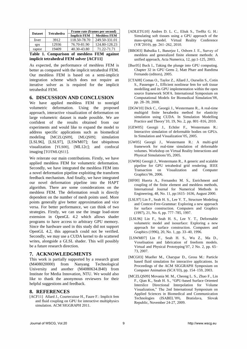
Dataset Tetrahedra Frame rate (frames per second)

Implicit FEM Meshless FEM

liver 3912 118.50-78.70 249.50-331.01

spx 12936 76.70-81.90 124.80-128.23

raptor 19409 40.30-43.80 71.22-71.71

Table 1. Comparison of meshless FEM against

implicit tetrahedral FEM solver [ACF11]

As expected, the performance of meshless FEM is

better as compared with the implicit tetrahedral FEM.

Our meshless FEM is based on a semi-implicit

integration scheme which does not require an

iterative solver as is required for the implicit

tetrahedral FEM.

6. DISCUSSION AND CONCLUSION We have applied meshless FEM to nonrigid

volumetric deformation. Using the proposed

approach, interactive visualization of deformation on

large volumetric dataset is made possible. We are

confident of the results obtained from our

experiments and would like to expand the model to

address specific applications such as biomedical

modeling [MCZLQS09], [MLQS09]; simulation

[LSL96], [LSL97], [LSWM07]; fast ubiquitous

visualization [YLS00], [ML12c]; and confocal

imaging [TOTMLQS11].

We reiterate our main contributions. Firstly, we have

applied meshless FEM for volumetric deformation.

Secondly, we have integrated the meshless FEM into

a novel deformation pipeline exploiting the transform

feedback mechanism. And finally, we have integrated

our novel deformation pipeline into the HAPT

algorithm. There are some considerations on the

meshless FEM. The deformation result is directly

dependent on the number of mesh points used. More

points generally give better approximation and vice

versa. For better performance, we can think of two

strategies. Firstly, we can use the image load-store

extension in OpenGL 4.2 which allows shader

programs to have access to arbitrary GPU memory.

Since the hardware used in this study did not support

OpenGL 4.2, this approach could not be verified.

Secondly, we may use a CUDA kernel to do scattered

writes, alongside a GLSL shader. This will possibly

be a future research direction.

7. ACKNOWLEDGMENTS This work is partially supported by a research grant

(M408020000) from Nanyang Technological

University and another (M4080634.B40) from

Institute for Media Innovation, NTU. We would also

like to thank the anonymous reviewers for their

helpful suggestions and feedback.

8. REFERENCES [ACF11] Allard J., Courtecuisse H., Faure F.: Implicit fem

and fluid coupling on GPU for interactive multiphysics

simulation. ACM SIGGRAPH 2011.

[ADLETG10] Andres D. L. C., Eliuk S., Trefftz G. H.:

Simulating soft tissues using a GPU approach of the

mass-spring model. Virtual Reality Conference

(VR’2010), pp. 261–262, 2010.

[BBO03] Babuška I., Banerjee I., Osborn J. E., Survey of

meshless and generalized finite element methods: A

unified approach, Acta Numerica, 12, pp:1-125, 2003.

[Buc05] Buck I., Taking the plunge into GPU computing.

Chapter 32 in GPU Gems 2, Matt Pharr and Randima

Fernando (editors), 2005.

[CTA08] Comas O., Taylor Z., Allard J., Ourselin S., Cotin

S., Passenger J., Efficient nonlinear fem for soft tissue

modelling and its GPU implementation within the open

source framework SOFA. International Symposium on

Computational Models for Biomedical Simulation’08,

pp. 28–39, 2008.

[DGW10] Dick C., Georgii J., Westermann R., A real-time

multigrid finite hexahedra method for elasticity

simulation using CUDA. In Simulation Modelling

Practice and Theory’10, 19, No. 2, pp. 801–816, 2010.

[GEW05] Georgii J., Echtler F., Westermann R.:

Interactive simulation of deformable bodies on GPUs.

In Simulation and Visualization’05, 2005.

[GW05] Georgii J., Westermann R.: A multi-grid

framework for real-time simulation of deformable

volumes. Workshop on Virtual Reality Interactions and

Physical Simulations’05, 2005.

[GW06] Georgii J., Westermann R., A generic and scalable

pipeline for GPU tetrahedral grid rendering. IEEE

Transaction on Visualization and Computer

Graphics’06, 2006.

[HF00] Huerta A., Fernandez M. S., Enrichment and

coupling of the finite element and meshless methods,

International Journal for Numerical Methods in

Engineering, 48, No. 11, pp:1615–1636, August 2000.

[LSL97] Lin F., Seah H. S., Lee Y. T., Structure Modeling

and Context-Free-Grammar: Exploring a new approach

for surface construction. Computers and Graphics

(1997), 21, No. 6, pp. 777–785, 1997.

[LSL96] Lin F., Seah H. S., Lee Y. T., Deformable

volumetric model and isosurface: Exploring a new

approach for surface construction. Computers and

Graphics (1996), 20, No. 1, pp. 33–40, 1996.

[LSWM07] Lin F., Seah H. S., Wu Z., Ma D.,

Voxelisation and fabrication of freeform models.

Virtual and Physical Prototyping’07, 2 No. 2, pp. 65–

73, 2007.

[MCG03] Mueller M., Charypar D., Gross M.: Particle

based fluid simulation for interactive applications. In

Proceedings of the ACM SIGGRAPH Symposium on

Computer Animation (SCA’03), pp. 154–159, 2003.

[MCZLQS09] Movania M. M., Cheong L. S., Zhao F., Lin

F., Qian K., Seah H. S., “GPU-based Surface Oriented

Interslice Directional Interpolation for Volume

Visualization,” The 2nd International Symposium on

Applied Sciences in Biomedical and Communication

Technologies (ISABEL’09), Bratislava, Slovak

Republic, November 24-27, 2009.


[MG04] Mueller M., Gross M., Interactive virtual

materials. Proceedings of Graphics Interface (GI’04),

pp. 239–246, 2004.

[MHSS04] Mosegaard J., Herborg P., Sangild Sorensen T.:

A GPU accelerated spring mass system for surgical

simulation. Health Technology and Informatics’04, pp.

342–348, 2004.

[MJLW07] Miller K., Joldes G., Lance D., Wittek A.,

Total Lagrangian explicit dynamics finite element

algorithm for computing soft tissue deformation.

Communications in Numerical Methods in

Engineering‘07, 23, No. 1, pp. 801–816, 2007.

[ML03] Mendoza C., Laugier C., Simulating soft tissue

cutting using finite element models. IEEE International

Conference on Robotics and Automation’03, pp. 1109–

1114, 2003.

[ML12a] Movania M. M., Lin F., A novel GPU-based

deformation pipeline. ISRN Computer Graphics, vol.

2012 (2012), p. 8.

[ML12b] Movania M. M., Lin F., Real-time physically-

based deformation using transform feedback. Chapter

17 in The OpenGL Insights, Christophe, Riccio and

Patrick, Cozzi (Ed.), AK Peters/CRC Press, 2012, pp.

233-248.

[ML12c] Movania M. M., Lin F., High-Performance

Volume Rendering on the Ubiquitous WebGL

Platform, 14th IEEE International Conference on High

Performance Computing and Communications

(HPCC’12), Liverpool, UK, 25-27 June, 2012.

[MLQS09] Movania M. M., Lin F., Qian K., Seah H. S.,

“Automated Local Adaptive Thresholding for Real-

time Feature Detection and Rendering of 3D

Endomicroscopic Images on GPU,” The 2009

International Conference on Computer Graphics and

Virtual Reality (CGVR'09), Las Vegas, US, July 13-16,

2009.

[MMF10] Maximo A., Marroquim R., Farias R., Hardware

assisted projected tetrahedra. Computer Graphics

Forum, 29, No. 3, pp: 903–912, 2010.

[NMK06] Nealen A., Mueller M., Keiser R., Boxermann

E., Carlson M., Physically based deformable models in

computer graphics. In STAR Report Eurographics

2006 vol. 25, pp. 809–836, 2006.

[NRBD08] Nguyena V. P., Rabczukb T., Bordasc S.,

Duflotd M., Meshless methods: A review and computer

implementation aspects, Mathematics and Computers

in Simulation, 79, No. 3, pp:763–813, December 2008.

[SB09] Sampath R., Biros G., A parallel geometric

multigrid method for finite elements on octree meshes.

In review, available online accessed in 2012

http://www.cc.gatech.edu/grads/r/rahulss/, 2009.

[ST99] Shapiro V., Tsukanov I., Meshfree Simulation of

Deforming Domains," Computer Aided Design, 31,

No. 7, pp: 459–471, 1999.

[TCO08] Taylor Z., Cheng M., Ourselin S., High-speed

nonlinear finite element analysis for surgical simulation

using graphics processing units. IEEE Trans. Medical

Imaging, vol. 27, pp. 650–663, 2008.

[TE05] Tejada E., Ertl T., Large steps in GPU-based

deformable bodies simulations. In Simulation

Modeling Practice and Theory, 13 No. 8, Elsevier, pp.

703–715, 2005.

[TOTMLQS11] Thong P. S. P, Olivo M., Tandjung S. S.,

Movania M. M., Lin F., Qian K., Seah H. S., Soo K.

C., “Review of Confocal Fluorescence

Endomicroscopy for Cancer Detection,” IEEE

Photonics Society (IPS) Journal of Selected Topics in

Quantum Electronics, Vol. PP, Issue 99, 2011. DOI:

10.1109/JSTQE.2011.2177447.

[VR08] Vassilev T., Rousev R., Algorithm and data

structures for implementing a mass-spring deformable

model on GPU. Research and Laboratory University

Ruse 2008 (2008), pp. 102–109, 2008.

[YLS00] Yang Y. T., Lin F. and Seah H. S., “Fast Volume

Rendering,” Chapter 10 in Volume Graphics, Springer,

January 2000.

[ZWP05] Zhong H., Wachowiak M., Peters T.: A real time

finite element based tissue simulation method

incorporating nonlinear elastic behavior. Computer

Methods Biomechan. Biomed. Eng., 6, No. 5, pp. 177–

189, 2005.

9. APPENDIX

e e

e e

e e

V A

TeT

V A

TeTeTTe

V A

TeeTeTe

tdANqdVB

tdANqudVBu

tdAuNqudVuB

)()()(

)()()(

Substitution using Eq. (3)

e

e e

e e

e e

A

TeeeT

V A

TeeT

V A

TeeT

V A

TeT

tdANqVDBuB

tdANqdVDBuB

tdANqdVDBuB

tdANqdVDB


http://www.cc.gatech.edu/grads/r/rahulss/

On Global MDL-based Multichannel Image Restoration andPartitioning

Tetyana IvanovskaUniversity of Greifswald, Germany

[email protected]

Horst K. HahnFraunhofer MEVIS,

[email protected]

Lars LinsenJacobs University, Germany

[email protected]

ABSTRACTIn this paper, we address the problem of multichannel image partitioning and restoration, which includes simulta-neous denoising and segmentation processes. We consider a global approach for multichannel image partitioningusing minimum description length (MDL). The studied model includes a piecewise constant image representationwith uncorrelated Gaussian noise. We review existing single- and multichannel approaches and make an extensionof the MDL-based grayscale image partitioning method for the multichannel case. We discuss the algorithm’sbehavior with several minimization procedures and comparethe presented method to state-of-the-art approachessuch as Graph cuts, greedy region merging, anisotropic diffusion, and active contours in terms of convergence,speed, and accuracy, parallelizability and applicabilityof the proposed method.

Keywords: Segmentation, Denoising, Minimum Description Length, Energy Minimization, Multichannel images.

1 INTRODUCTION

The goal of image partitioning is to detect and extractall regions of an image which can be distinguished withrespect to certain image characteristics. A special formof image partitioning is image segmentation, where oneor a few regions of given characteristics are separatedfrom the rest of the image. If the underlying image issupposed to be piecewise constant, image partitioningis equivalent to the restoration of that image, which isoften obtained using denoising algorithms. Althoughthere exist plenty of methods for solving image parti-tioning, segmentation, and restoration problems, manyof them are task-specific or require intensive user inter-action and triggering of a large number of parameters.

In this paper, we restrict ourselves to generic solutionsusing automatic methods based on energy minimiza-tion. Hence, two tasks need to be tackled: First, oneneeds to formulate an energy functional based on someassumptions and, second, one needs to find an appro-priate and computationally feasible minimization algo-rithm. The main emphasis of this work is put on anal-ysis and discussion of an energy functional, based onthe assumption that the processed image is multichan-nel, piecewise constant, and affected by white Gaussiannoise. We analyse and compare several minimization

Permission to make digital or hard copies of all or part ofthis work for personal or classroom use is granted withoutfee provided that copies are not made or distributed for profitor commercial advantage and that copies bear this notice andthe full citation on the first page. To copy otherwise, or re-publish, to post on servers or to redistribute to lists, requiresprior specific permission and/or a fee.

procedures and draw analogies to other approaches.Color images are used as examples, as they documentthe algorithmic behavior in an intuitive manner. How-ever, all steps work are applicable for any multichan-nel image data. The paper is organized as follows. InSection 2 the related work in this area is described. InSection 3 we formulate the energy functional and de-scribe two minimization procedures. Our findings arepresented and discussed in Section 4.

2 RELATED WORKGlobal energy minimization approaches originatefrom such seminal works as the ones by Mumfordand Shah [24] and Blake and Zisserman [2]. TheMarkov Random Fields (MRF) framework (see theseminal work of Geman and Geman [8]) is a stochasticbranch of the energy minimization approaches. In thelast years a great breakthrough has been done in thedirection of Markov random fields methods [19]. Suchmethods as Graph Cuts [5] are mathematically welldescribed and allow to find a solution that lies close tothe global optimum.

The minimum description length (MDL) based ap-proach [15] uses basic considerations from informationtheory [19] in the formulation of the energy term, in thesense that the best image partitioning is equivalent toobtaining the minimum description length of the imagewith respect to some specific description language.

There exist two main tendencies in further develope-ment of this approach. The first one consists in extend-ing the functional to be minimized. These extentionsinclude either different noise models (not only whiteGaussian noise), or elimination of the model parame-ters that must be manually tuned by a user.


Kanungo [12] et al. formulated the functional for multi-band and polynomial images. Lee [17] considered cor-related noise. Galland [7] et al. considered speckle,Poisson, and Bernoulli noise. Zhu and Yuille [31] pro-posed an algorithm combining region growing, merg-ing, and region competition which permits one to seg-ment complex images. In several approaches [20, 16],an extended version of the functional is used and alluser-defined parameters are eliminated. For example,Luo and Khoshgoftaar [20] propose to use the wellknown Mean-Shift method [6] to obtain the initial seg-mentation and start the MDL-based region mergingprocedure from it.

These approaches utilize region growing, as theminimization of the extended functional is infeasible.However, such an iterative technique, generally, doesnot lead to a stable local minimum and can givemuch coarser results, when compared to the relaxationtechnique, if the procedure of region merging is non-reversible. Moreover, the authors state, for instance,in [20], that the initial region selection has a strongimpact on the efficiency and effectiveness of the regionmerging.

The second direction is to use a simplified or lim-ited model with some user-defined parameters, but ap-ply a global minimization procedure, which allows oneto find at least a stable local minimum. Kerfoot andBresler [13] formulated a full MDL-based criterion forpiecewise constant image partitioning, but the class ofimages is limited to the class of simply-connected ones.For minimization such methods as Graph Cuts [5] havegained in popularity in the last years.

3 METHODS3.1 Multichannel Model DescriptionThe fundamental idea behind the Minimum DescriptionLength (MDL) [19, 23] principle is that any regularityin the given data can be used to compress the data.

The image partitioning problem with respect to theMDL principle can be formulated as follows: Usinga specified descriptive language, construct the descrip-tion of an image (code) that is simplest in the sense ofbeing shortest (when coded, needs the least number ofbits) [15]. LetL(M) denote the language for describinga modelM andL(D|M) the language for describing dataD given modelM. Moreover, let|.| denote the numberof bits in the description. The goal is to find the modelM that minimizes the code lengthCl = |L(M)|+ |L(D|M)|

. This corresponds to the two-part MDL code [9]. If thea priori probabilitiesP(M) of the described models areknown, then the number of bits in the description equalsthe negative base-two logarithm of the probability ofthe described models [19]:|L(M)|=− log2P(M).

In terms of image partitioning and restoration the codelength can be written asCl = |L(u)|+ |L(z−u)| ,where

the model we are looking for is the underlying im-age representation (or partitioning)u that minimizes thecode length. The termz describes the initial (or given)image, and the differencer = (z−u) between the givenimagez and the partitioningu corresponds to the noisein the image. The noise describes the data with respectto modelu.

A simple implementation of the MDL principle for im-age partitioning was presented by Leclerc [15, 23]: heassumed a piecewise constant model and derived thefunctional (or energy term)

Cl =b2 ∑

i∈I∑j∈Ni

(

1−δ(

ui −u j))

+a∑i∈I

(

zi −ui

σ

)2

, (1)

whereu denotes the underlying image,z the given im-age, andσ2 the noise variance. Moreover,δ (ui−u j)denotes the Kronecker delta (1 if(ui = u j), else 0),Idenotes the range of the image, andNi is the neigh-bourhood of theith pixel, a andb are constants. Thefirst term in Equation (1) encodes the boundaries of theregions, whereas the second term encodes the noise inform of uncorrelated white Gaussian noise.

One can observe the similarities between the functionalin Equation (1) with constantsa,b,σ and the energyconsidered in different MRF approaches, namely in theGraph Cut methods (see [5] for more details):E( f ) =λ ∑

(p,q)∈N

Vp,q( fp, fq) + ∑p∈I

Dp( fp), where the interaction

potentialV between pixelsp,q having labels (colors)fp, fq is taken from the Potts model (which correspondsto the Kronecker deltas),D is the distance between theinitial and current colors of the pixelp (which corre-sponds to the noise values), andλ is a constant.

We expand on this approach to derive a multichannelimage description length. For encoding the model,i.e., derivingL(u), we have to encode the boundariesof the regions. To do so, we calculate the numberof pixels that contribute to the boundary. Hence,the codelength for the boundary encoding is given

by |L(u)| = b2 ∑

i∈I∑j∈Ni

(

1− ∏k∈Ch

δ(

uki −uk

j

)

)

, where

k denotes the channel,Ch is the range of channels(e.g., RGB in the three-channel color case), and othernotations are as above. To encode the data that donot fit the model, i.e., the noise, we deriveL(z− u)assuming that the values in each channel are subject towhite Gaussian noise with parameters(0,(σk)2). Thisassumption implies that the noise between channels isnot correlated. Such an assumption allows for betterunderstanding of the underlying processes and is oftensufficient for many applications, since the uncorrelatednoise can appear during the transmission, storing, ormanipulation of images [1]. Moreover, the assumptionholds when a multichannel image is combined fromdifferent independent modalities for processing.


The codelength of the noise is derived as

|L(z−u)|=−∑i∈I

∑k∈Ch

log2 P(rki ) (2)

=−∑i∈I

∑k∈Ch

log2

(

q√

2π(σk)2exp

(

−

(

rki

)2

2(σk)2

))

=1

2ln2∑i∈I

∑k∈Ch

(

rki

σk

)2

+const

whereq = 1 is the pixel precision,const is an addi-

tive constant, which is discarded, if(

σk)2

is consideredconstant and equal for all channels.

The resulting codelength functional becomesCl =

b2 ∑

i∈I∑j∈Ni

(

1− ∏k∈Ch

δ(

uki −uk

j

)

)

+1

2ln2∑i∈I

∑k∈Ch

(

rki

σk

)2

.

This functional corresponds to the one considered inthe Graph cuts method up to the constant weights.

3.2 MinimizationHaving formulated the energy functionals, one needs tominimize them for a given image in order to computethe image partitioning. As it has been shown that com-puting the global optimum even of the simplest func-tional is an NP-hard problem [5], in practice one has tolook for efficient approximations for it.

In the current paper, we will deal with two optimizationapproaches for energy minimization: a discrete one anda continuous one, namely, theα-expansion Graph Cutalgorithm, introduced by Boykov [5], and the GNC-like approach, introduced by Leclerc [15], with severalmodifications, which have been done to check the con-vergence.

Graph cuts is an efficient minimizing technique that al-lows for finding a local minimum within a known factorof the global one. This algorithm belongs to the classof discrete optimization. Here, we give the outline ofthe algorithm and refer the reader to the original paperby Boykov et al [5] for further details. LetS andL

denote image pixels (lattice) and the palette (set of allpossible colors), correspondingly. The labelingu is de-scribed asSl |l ∈L , whereSl = p∈ S|up = l is asubset of pixels with assigned colorl . Given a labelα amove from a labelingu to a new labelingu

′is called an

α- expansion ifSα ⊂S′

α andS′

l ⊂Sl for any labell 6=α. In other words, anα-expansion move allows anyset of image pixels to change their labels toα [5]. Theminimum of the energyE for each labelα is found byconstructing a graph and finding the minimum cut forit. It is efficiently done by the algorithm developed byBoykov and Kolmogorov [3].

Start with an arbitrary partitioningurepeat

Setsuccess← 0for all α ∈L do

Find u = argminE(u′) among u

′within one

α-expansion ofu

if E(u)< E(u) thenu← usuccess← 1

end ifend for

until success6= 0Returnu

A Relaxation method using ideas of Graduated NonConvexity (GNC) by Blake and Zisserman [2] was pro-posed by Leclerc [15]. This is a continuous optimiza-tion method, where the labelingu is not selected fromthe given palette, as in the Graph Cuts case, but is it-eratively computed. Here,u ∈ R

n. The basic con-cept of the minimization procedure is to replace thenon-convex codelength functionalCl (u) by an embed-ding in a family of continuous functionsCl (u,s), wheres ∈ R is a user-defined parameter, that converge to-wards the target functionalCl (u) whens goes to zero.lims→0Cl (u,s) =Cl (u). For the starting value ofs, thefunctional Cl (u,s) is convex such that standard con-vex minimization procedures can compute the singleminimum. Whens approaches zero, number and po-sitions of the local minima ofCl (u,s) become those ofCl . The minimization procedure iterates overs, whichsteadily decreases, and minimizesCl (u,s) for the re-spective value ofs in each iteration step.

To obtain a continuous embedding, the discontinuousparts in functionalCl need to be replaced by a continu-ous approximation. The discontinuity ofCl is due tothe use of the functionδ . Hence, functionδ is re-placed by a continuous approximation that converges toδ whens goes to zero [15]. We use the approximation

δ(

uki −uk

j

)

≈ exp

(

−(uk

i −ukj)

2

(sσ k)2

)

= eki j .

The minimization iteration starts with a sufficientlylarge values= s0 and computes the (global) minimumu0 of the convex functionalCl (u,s0). In each iterationstepT + 1, we setsT+1 = rsT , where 0< r < 1, andcompute the local minimum ofCl (u,sT+1) starting fromminimum uT of the previous iteration step. The itera-tion is repeated untils is sufficiently small, i.e., untils< ε with ε being a small positive threshold.

To compute the local minimumu on each iteration weapply Jacobi iterations [26]. The functionalCl (u,s) isconvex, if we choose a value fors that satisfies(xk

i −

xkj )

2≤ 0.5(

sσk)2

for all pixelsi and j with i 6= j) and allchannelsk. Hence, when this condition is met, the localminimum must be a global one. The condition needsto be fulfilled for the starting values= s0. Then, thecondition ∂Cl (u,sT )

∂uki

= 0for the local minimum at iteration

stepT becomes

2a(

uki −zk

i

)

(

σk)2 +

b2 ∑

j∈Ni

2(

uki −uk

j

)

(

sTσk)2 ∏

l∈Chel

i j

= 0, (3)


where constanta = (2ln2)−1. As Equation (3) can-not be solved explicitly, we use an iterative approach,where at each iteration stept +1 we compute

uk,t+1i =

zki +

b

a(sT)2∑j∈Ni

uk,tj ∏

l∈Chelt

i j

1+b

a(sT)2∑j∈Ni

∏l∈Ch

elti j

. (4)

In total, we have two nested iterations. The outer itera-tion denoted byT iterates oversT , while the inner iter-ation denoted byt iterates overuk,t+1

i . Considering thebehavior of the exponential function, the termination

criterion for the inner loop is given by∣

∣

∣uk,t+1

i −uk,ti

∣

∣

∣<

sTσk, ∀i ∈ I . Starting withu = z, the minimizationprocedure can be summarized by the following pseudo-code:

while s≥ ε dostart with local minimum foru found in previous itera-tionwhile termination criterion foru is not metdo

recalculateu using Equation (4)end whileupdates

end while

Comparison to Anisotropic Diffusion.The derived iter-ative scheme for computingut+1

i in the single-channelcase, cf. [15], is similar to the iteration in the well-known anisotropic diffusion approach. The continuousform of the Perona-Malik equation [25] for anisotropicdiffusion is given by

∂ I∂ t

= div(g(‖∇I‖) ·∇I) , (5)

whereI denotes the image and functiong is defined by

g(‖∇I‖)= exp

(

−

(

‖∇I‖K

)2)

with flow constantK. The

discrete version of Equation (5) is given byI t+1i − I t

i +

λ ∑ j∈Ni

(

I ti − I t

j

)

exp

−

(

I ti − I t

j

K

)2

= 0, whereλ is a

normalization factor.

The local minimum of the MDL-based energyCl insingle-channel notation (for a fixeds) is defined bysolving ∂Cl (u,s)

∂ui= 0, which leads to

(ui −zi)+α ∑j∈Ni

[

(

ui −u j)

exp

(

−

(

ui −u j)2

(sσ)2

)]

= 0.

The continuous version of this equation can be writtenas

∫ tend

0

∂u∂ t

dt = div(g(‖∇u‖) ·∇u) , (6)

whereu0 = z and utend describes the image values atthe current steptend. Comparing the continuous formof the Perona-Malik equation (5) with the continuous

form of the MDL-based equation (6), one can immedi-ately observe the similarity. The main difference is theintegral on the left-hand side of Equation (6). The inte-gral represents the changes between the current imageand the initial image. Thus, this version of the MDL-based minimization algorithm can be considered as an“anisotropic diffusion algorithm with memory”.

In general, the assumptions about the convexity ofCl (u,s) do not hold anymore, whens is small. Hence,the relaxation method with Jacobi iterations can givean inadequate result. To check this we implementedthe steepest descent minimization scheme [26] andcompared the results.

4 RESULTS AND DISCUSSIONThe presented algorithm belongs to the class of algo-rithms that are not purely for denoising or segmenta-tion, but can be treated as an elegant combination ofboth approaches. Usually, some part of meaningful im-age data might be lost on the denoising step, whichaffects the subsequent segmentation results. Here, onthe contrary, the complete information is used both forboundary preservation and noise exclusion, which is re-ferred in the literature as image restoration [28] or re-construction [25].

The algorithm ( minimization procedures with Jacobiiterations, Gradient descent, and Graph cuts) was im-plemented using C/C++ programming language, opti-mized appropriately, and was compiled under gcc4.4.The Graph cuts code for grayscale images was kindlyprovided on the Vision.Middlebury web-site [22].

Figure 1 documents the general behavior of the Relax-ation scheme. Starting with a synthetic 100×100 im-age with manually added noise, we apply the Jacobiiteration minimization procedure. The three rows inFigure 1 show (intermediate) results at iterationT = 4,T = 600, andT = 1484, respectively. The first col-umn shows the currently detected underlying image andthe second column the currently removed noise, i.e.,the difference between the initial image and the cur-rently detected underlying image (first column of Fig-ure 1). For the generation of the images in columnthree, we picked one row of the image, i.e., a horizontalcut through the image, and show the current values ofufor that single row. The third column in Figure 1 docu-ments nicely, how individual values (first row) start as-similating and grouping together (second row) to even-tually form a piecewise constant representation (thirdrow).

To qualitatively describe the restoration results,we evaluated the difference between the resultingand initial (not noisy) images using two mea-sures. The first one is the mean squared error(MSE) estimator [18], which is suitable to showwhether the colors were reconstructed as close to


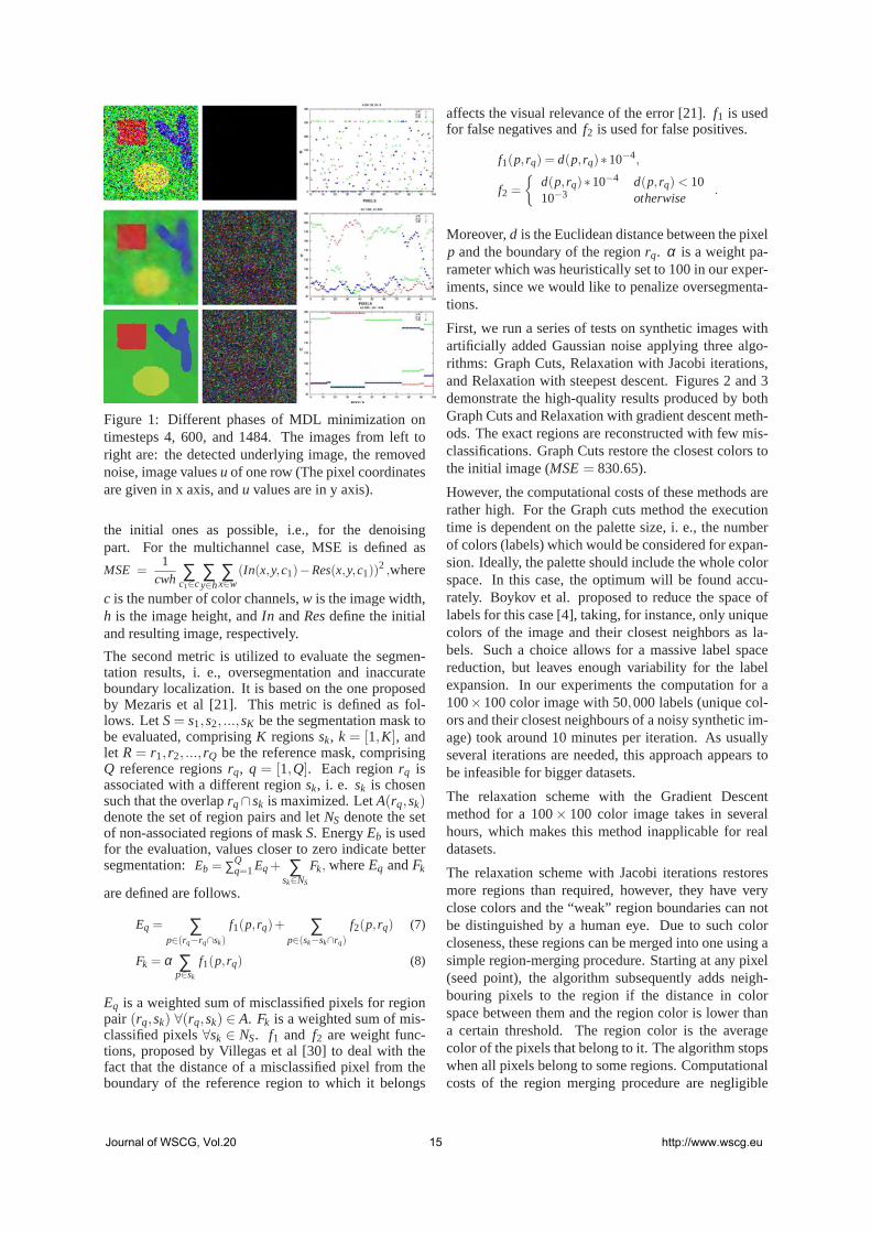
Figure 1: Different phases of MDL minimization ontimesteps 4, 600, and 1484. The images from left toright are: the detected underlying image, the removednoise, image valuesu of one row (The pixel coordinatesare given in x axis, andu values are in y axis).

the initial ones as possible, i.e., for the denoisingpart. For the multichannel case, MSE is defined as

MSE =1

cwh ∑c1∈c

∑y∈h

∑x∈w

(In(x,y,c1)−Res(x,y,c1))2,where

c is the number of color channels,w is the image width,h is the image height, andIn andResdefine the initialand resulting image, respectively.

The second metric is utilized to evaluate the segmen-tation results, i. e., oversegmentation and inaccurateboundary localization. It is based on the one proposedby Mezaris et al [21]. This metric is defined as fol-lows. LetS= s1,s2, ...,sK be the segmentation mask tobe evaluated, comprisingK regionssk, k = [1,K], andlet R= r1, r2, ..., rQ be the reference mask, comprisingQ reference regionsrq, q = [1,Q]. Each regionrq isassociated with a different regionsk, i. e. sk is chosensuch that the overlaprq∩sk is maximized. LetA(rq,sk)denote the set of region pairs and letNS denote the setof non-associated regions of maskS. EnergyEb is usedfor the evaluation, values closer to zero indicate bettersegmentation:Eb = ∑Q

q=1Eq+ ∑sk∈NS

Fk, whereEq andFk

are defined are follows.

Eq = ∑p∈(rq−rq∩sk)

f1(p, rq)+ ∑p∈(sk−sk∩rq)

f2(p, rq) (7)

Fk = α ∑p∈sk

f1(p, rq) (8)

Eq is a weighted sum of misclassified pixels for regionpair (rq,sk) ∀(rq,sk) ∈ A. Fk is a weighted sum of mis-classified pixels∀sk ∈ NS. f1 and f2 are weight func-tions, proposed by Villegas et al [30] to deal with thefact that the distance of a misclassified pixel from theboundary of the reference region to which it belongs

affects the visual relevance of the error [21].f1 is usedfor false negatives andf2 is used for false positives.

f1(p, rq) = d(p, rq)∗10−4,

f2 =

d(p, rq)∗10−4 d(p, rq)< 1010−3 otherwise

.

Moreover,d is the Euclidean distance between the pixelp and the boundary of the regionrq. α is a weight pa-rameter which was heuristically set to 100 in our exper-iments, since we would like to penalize oversegmenta-tions.

First, we run a series of tests on synthetic images withartificially added Gaussian noise applying three algo-rithms: Graph Cuts, Relaxation with Jacobi iterations,and Relaxation with steepest descent. Figures 2 and 3demonstrate the high-quality results produced by bothGraph Cuts and Relaxation with gradient descent meth-ods. The exact regions are reconstructed with few mis-classifications. Graph Cuts restore the closest colors tothe initial image (MSE= 830.65).

However, the computational costs of these methods arerather high. For the Graph cuts method the executiontime is dependent on the palette size, i. e., the numberof colors (labels) which would be considered for expan-sion. Ideally, the palette should include the whole colorspace. In this case, the optimum will be found accu-rately. Boykov et al. proposed to reduce the space oflabels for this case [4], taking, for instance, only uniquecolors of the image and their closest neighbors as la-bels. Such a choice allows for a massive label spacereduction, but leaves enough variability for the labelexpansion. In our experiments the computation for a100×100 color image with 50,000 labels (unique col-ors and their closest neighbours of a noisy synthetic im-age) took around 10 minutes per iteration. As usuallyseveral iterations are needed, this approach appears tobe infeasible for bigger datasets.

The relaxation scheme with the Gradient Descentmethod for a 100× 100 color image takes in severalhours, which makes this method inapplicable for realdatasets.

The relaxation scheme with Jacobi iterations restoresmore regions than required, however, they have veryclose colors and the “weak” region boundaries can notbe distinguished by a human eye. Due to such colorcloseness, these regions can be merged into one using asimple region-merging procedure. Starting at any pixel(seed point), the algorithm subsequently adds neigh-bouring pixels to the region if the distance in colorspace between them and the region color is lower thana certain threshold. The region color is the averagecolor of the pixels that belong to it. The algorithm stopswhen all pixels belong to some regions. Computationalcosts of the region merging procedure are negligible


when compared to the ones of the Relaxation method.When the simple region merging is applied, we obtainEb = 0.0021, which is slightly better than the other re-sults.

The main advantage of the Jacobi iteration approach isits independence of the palette size and straightforwardparallelizability, such that computations only take sec-onds [11], which makes this method attractive for realapplications.

Next, we would like to compare the presented methodto other (similar) approaches, namely, anisotropic dif-fusion, region merging, and a combination of these twoprocedures. Although anisotropic diffusion is primarilyused to remove noise from digital images without blur-ring edges, it can be used in edge detection algorithms.By running the diffusion with an edge seeking diffusioncoefficient for a certain number of iterations, the im-age can be evolved towards a piecewise constant imagewith the boundaries between the constant componentsbeing detected as edges [25]. We compared our ap-proach to the anisotropic diffusion algorithm for multi-channel images, presented by Sapiro and Ringach [27].This method similarly to ours considers the influenceof all image channels at once, which allows for betterboundary preservation when compared to the methodstreating each image channel separately. However, ourapproach has a “memory”, as it always refers to the ini-tial image instead of iterating from the result obtainedon the previous time step. Such a behavior should guar-antee a better boundary preservation and initial colorrestoration if the parameters are properly chosen. Fig-ure 4 demonstrates that Sapiro’s method successfullyeliminates the noise (except from some mistakes onthe image boundaries) and preserves most of the objectboundaries. Our approach appears to be stable to noise,preserves object boundaries, restores the colors close tothe initial ones, and produces the most uniformly col-ored background.

Due to the energy functional complexity, which arisesfor the models with no manually adjustable parametersor for more complicated noise models, it is often dif-ficult to find a feasible minimization procedure. Thus,many authors follow a "greedy" region merging strat-egy [12, 20, 14, 16]. The idea of the algorithm is asfollows. It starts from some initial oversegmentation.Then at each timestep it chooses two neighbouring re-gions and merges them to form a new region. Thesetwo regions are chosen in such a way that, when theyare merged, it provides the largest energy reductionamongst all other possible merges. Although this pro-cedure is very fast, it has several drawbacks. First, itdoes not guarantee convergence to a stable local mini-mum, especially, in the presence of noise. Second, theway the initial oversegmentation is chosen also affectsthe results.

Although Kanungo et al. [12], Luo and Khoshgof-taar [20], Lee [16], and Koepfler et al. [14] propose touse different functionals for color image segmentation,the region merging procedures are similar to eachother. We assume that a more complicated functionalcould lead to a more adequate result. However, thereis no guarantee about the convergence to a stable localminimum, and this issue stays unresolved.

We compared our approach to the algorithm proposedby Koepfler et al. [14]. They use the Mumford-Shahfunctional for the piecewise constant case, which co-incides with the MDL-based functionalCl . Here, wecomputed both metrics to evaluate the results. As itcan be observed in Figure 5, the iterative region merg-ing produces results with some misclassified bound-aries, which appears due the fact that the merging al-gorithm did not land close to the minimum, and notcompletely erased noise when compared to Figure 4.The relaxation approach can be approximated with apipeline that utilizes several algorithms, namely, de-noising, boundaries sharpening, and region merging.We constructed a pipeline from Sapiro’s anisotropic dif-fusion and Koepfler’s region merging. As it can be ob-served in Figure 5, the pipeline produces the best resultin terms of boundary preservation and noise elimina-tion when compared to the independent application ofthese methods. However, in general, each method in thepipeline requires additional adjustment of the parame-ters for each image.

Our comparison shows that the proposed approach pro-duces the best results in terms of color (the lowestMSE = 377.628) and region restoration (the lowestEb = 0.0008) for the test image.

We also compared our results to the results obtainedwith the Active contours without edges [29] method in-troduced by Chan and Vese. This is a variational ap-proach based on energy minimization, and the energy isformulated using the Mumford-Shah functional for thepiecewise constant case. For our tests, we applied the 4-phase version of the algorithm for color piecewise con-stant images with the parameters for each phase:λ1,2 =1, ν = 0, as it is recommended by the authors. We ex-perimented with different values of parameterµ andinitial contour locations. We executed the algorithmwith max. 2000 iterations with thetimestep= 0.5. Fig-ure 6 documents that it is problematic to obtain decentresults for images with low signal-to-noise ratio for thereasonable amount of time and the prior denoising isneeded.

When applied to real images, our approach allowsfor obtaining the results with different levels of de-tail, which reminds one of the multi-scale theory ofpiecewise image modeling, introduced by Guigues etal. [10]. In Figure 7 the results illustrate this effect.Increasing the value ofb allows us to reduce the


Figure 2:First: Input diamand image with manually added noiseN(0,702). Second: Graph cuts result.MSE=830.65. Eb = 0.0027Third: Relaxation (Steepest descent on inner iterations) result. MSE= 2273.8096. Eb =0.0031Fourth: Relaxation (Jacobi iterations) result.MSE= 2418.262. No region mergingEb = 651.287. Withregion mergingEb = 0.0021

Figure 3: First: True image with 8 regions (5 unique colors).Second: Piecewise-constant regions are markedwith random different colors on the Graph cuts result. The image consists of 8 regions (7 unique colors).Third:Regions are marked with random different colors on the Relaxation (Descent) result. The image consists of 8regions.Fourth and Fifth: Piecewise-constant regions are marked with random different colors on the Relaxation(Jacobi) result. The image consists of 49 regions (before region merging) and 8 regions (after region merging).

Figure 4:First: Initial synthetic image.Second: Synthetic image with added noiseN(0,702). Third: Result for ourapproach with subsequent region merging.MSE= 377.628.Eb = 0.0008.Fourth: Result for Sapiro’s anisotropicdiffusion with parameters:edge= 49,numStep= 45. MSE= 447.83.

Figure 5:First: Result for iterative region merging withλ = 106. Noise is not erased completely. Further in-creasing the parameterν0 does not improve the result.MSE= 436.538. Eb = 6.5369Second: Result for thepipeline consisting of the anisotropic diffusion and re-gion merging based on the Mumford-Shah functional.MSE= 419.7864.Eb = 0.26

number of details, i.e., the number of regions, and leaveonly the "strongest" edges.

Figure 6:First: Result for Active contours. The result-ing contours are still noisy.Second: Initial contours.

5 CONCLUSION AND FUTUREWORK

We generalized the existing single-channel MDL-basedmethod to a multichannel one and applied it to colorimage partitioning and restoration. For synthetic colorimages, the results were compared to the ones obtainedwith Graph cuts, anisotropic diffusion, greedy regionmerging with energy, and active contours approaches.Our method produces best results in terms of color


Figure 7: Results with differentb for the "woman" im-age. The initial image is the leftmost one. The param-eterb is selected: 2, 5, 20 for the images from left toright, correspondingly.

restoration and boundary accuracy for our test cases.Moreover, the relaxation scheme with Jacobi iterationscombined with a simple region merging procedure al-lows for fast computations due to straightforward par-allelizability, which is important when applied to real-world problems.

We believe that this approach has potential in solvingproblems of image restoration. The future work di-rections include studying different noise models (e. g.correlated noise) for piecewise constant and piecewisesmooth images as well as the models based on otherMDL codes.

6 REFERENCES[1] D. Baez-Lopez, F. H. Mendoza, and J. M.

Ramirez. Noise in color digital images.Cir-cuits and Systems, Midwest Symposium on, 0:403,1998.

[2] A. Blake and A. Zisserman.Visual Reconstruc-tion. MIT Press, 1987.

[3] Y. Boykov and V. Kolmogorov. An experimen-tal comparison of min-cut/max-flow algorithmsfor energy minimization in vision.IEEE Trans-actions on Pattern Analysis and Machine Intelli-gence, 26(9):1124–1137, 2004.

[4] Y. Boykov, O. Veksler, and R. Zabih. Efficientrestoration of multicolor image with independentnoise. Technical report, 1998.

[5] Y. Boykov, O. Veksler, and R. Zabih. Fast approx-imate energy minimization via graph cuts.IEEETransactions on Pattern Analysis and MachineIntelligence, 23(11):1222–1239, 2001.

[6] D. Comaniciu and P. Meer. Mean shift: A robustapproach toward feature space analysis.IEEETransactions on Pattern Analysis and MachineIntelligence, 24(5):603–619, 2002.

[7] F. Galland, N. Bertaux, and P. Refregier. Multi-component image segmentation in homogeneousregions based on description length minimization:Application to speckle, poisson and bernoulli

noise. Pattern Recognition, 38(11):1926 – 1936,2005.

[8] S. Geman and D. Geman. Stochastic relaxation,gibbs distributions, and the bayesian restorationof images.IEEE Transactions on Pattern Analysisand Machine Intelligence, (6):721–741, 1984.

[9] P. Grunwald.A tutorial introduction to the mini-mum description length principle. 2004.

[10] L. Guigues, J. Cocquerez, and H. Le Men. Scale-sets image analysis.International Journal ofComputer Vision, 68:289–317, 2006.

[11] T. Ivanovska, L. Linsen, H. K. Hahn, andH. Voelzke. Gpu implementations of a relax-ation scheme for image partitioning: Glsl vs.cuda. Computing and Visualization in Science,14(5):217–226, 2012.

[12] T. Kanungo and B. Dom et al. A fast algorithmfor mdl-based multi-band image segmentation.Computer Vision and Pattern Recognition, pages609–616, 1994.

[13] I.B. Kerfoot and Y. Bresler. Theoretical analy-sis of multispectral image segmentation criteria.Image Processing, IEEE Transactions, 8(6):798–820, 1999.

[14] G. Koepfler, C. Lopez, and M. Morel. A multi-scale algorithm for image segmentation by varia-tional method.SIAM Journal of Numerical Anal-ysis, 31:282–299, 1994.

[15] Y.G. Leclerc. Constructing simple stable descrip-tions for image partitioning.International Journalof Computer Vision, 3(1):73–102, 1989.

[16] T. C. M. Lee. A minimum description length-based image segmentation procedure, and itscomparison with a cross-calidation-based seg-mentation procedure.Journal of the AmericanStatistical Association, 95(449):259–270, 2000.

[17] T. C. M. Lee and T. Lee. Segmenting images cor-rupted by correlated noise.IEEE Transactionson Pattern Analysis and Machine Intelligence,20:481–492, 1998.

[18] E. L. Lehmann and George Casella.Theory ofPoint Estimation (Springer Texts in Statistics).Springer, 2003.

[19] S. Z. Li. Markov random field modeling in imageanalysis. Springer-Verlag New York, Inc., 2001.

[20] Q. Luo and T.M. Khoshgoftaar. Unsupervisedmultiscale color image segmentation based onmdl principle. IEEE Transactions on Image Pro-cessing, 15(9):2755–2761, 2006.

[21] V. Mezaris, I. Kompatsiaris, and M. G. Strintzis.Still image objective segmentation evaluation us-ing ground truth. InIn Proceedings of the FifthCOST 276 Workshop on Information and Knowl-


edge Management for Integrated Media Commu-nication, 2003.

[22] http://vision.middlebury.edu/MRF/ Middle-bury Vision.

[23] A. Mitiche and I. B. Ayed.Variational and LevelSet Methods in Image Segmentation. SpringerBerlin Heidelberg, 2011.

[24] D. Mumford and J. Shah. Boundary detectionby minimizing functionals. InProc. IEEE Conf.Computer Vision and Pattern Recognition, 1985.

[25] P. Perona and J. Malik. Scale-space and edge de-tection using anisotropic diffusion.IEEE Trans.Pattern Anal. Mach. Intell., 12(7):629–639, 1990.

[26] W. H. Press, S. A. Teukolsky, W. T. Vetterling,and B. P. Flannery.Numerical Recipes in C++:The Art of Scientific Computing. Cambridge Uni-versity Press, 2002.

[27] G. Sapiro and D. L. Ringach. Anisotropic diffu-sion of multivalued images with applications tocolor filtering. Image Processing, IEEE Transac-tions on, 5(11):1582–1586, 1996.

[28] R. Szeliski, R. Zabih, D. Scharstein, O. Vek-sler, V. Kolmogorov, A. Agarwala, M. Tappen,and C. Rother. A comparative study of energyminimization methods for markov random fieldswith smoothness-based priors.Pattern Analysisand Machine Intelligence, IEEE Transactions on,30(6):1068–1080, 2008.

[29] L. A. Vese and T. F. Chan. A multiphase levelset framework for image segmentation using theMumford and Shah model.International Journalof Computer Vision, 50(3):271–293, December2002.

[30] P. Villegas, X. Marichal, and A. Salcedo. Ob-jective evaluation of segmentation masks in videosequences. InIn Proceedings of Workshop om Im-age Analysis for Multimedia Interactive Services,1999.

[31] S.C. Zhu and A.L. Yuille. Region competition:unifying snakes, region growing, and bayes/mdlfor multiband image segmentation.IEEE Trans.on PAMI, 1996.


A Study on the Animations of Swaying and Breaking Trees based on a Particle-based Simulation

Yasuhiro AKAGI

Tokyo University of Agriculture and Technology Naka-cho 2-24-16

184-8588, Koganei, Tokyo

[email protected]

Katsuhiro KITAJIMA

Tokyo University of Agriculture and Technology Naka-cho 2-24-16

184-8588, Koganei, Tokyo

[email protected]

ABSTRACT In this paper, we propose a particle-based simulation method to create the animations of swaying and breaking

trees. Since the shapes of trees and their realistic motions are usually complex, it is difficult for us to create an

animation of a swaying tree manually. Therefore, to produce films and image contents which contain a natural

scene of swaying and breaking trees, it takes a lot of work to create the animation. To solve this problem, it is

important that how to calculate interactions between a tree and wind to automatically generate the swaying and

breaking motions of a tree by using a physical simulation. We model both a tree and wind as particles to simulate

the interactions. The advantage of the particle-based method is that the method is robust for changing of the

topology of wind and the branching structure of a tree. Our results show that the proposed method can naturally

represent the breaking behavior of a tree and the wind flow around the tree by using the particle-based

simulation of the wind.

Keywords Tree animation, Breaking branches, Fallen leaves, Particle-based simulation, SPH method, Elastic deformation

1. INTRODUCTION The 3D modeling and creation of animations of

natural scenes is one of the most time-consuming

works of producing films and videos[Chn11]. It is

difficult to manually create an animation of swaying

trees that has realistic movements of branches and

leaves in an environment having a complex wind

flow. Therefore, there are many studies on the

animation of swaying trees on the basis of tree

dynamics and wind simulations. We propose a

practical method of generating tree animations that

simulate the swaying motions and breaking behaviors

of trees by using a particle-based model. We

represent both the trees and wind by particles and

links to be able to simulate the breaking behaviors of

trees. The most advantage of the method using the

particles is that the simulation method can freely

divide the tree structure into broken branches and

fallen leaves. This method also represents the change

of the movement which is caused by the breaking and

changing the shape of the tree.

Previous work Most of these studies propose a method of

simulating the dynamics of branches by using beam

structures[AWZ09]. These methods simulate the

bending motions of the beam structures (branches) on

the basis of external forces (wind). For instance,

Habel [HKW09] and Yang[YHY+10] proposed a

method of automatically animating swaying trees

using beam structures. Diener [DRB+09] proposed a

simpler method of simulating bending branches. This

method divides a tree into the sections and simulates

the movements of branches only by the rotation of

these sections. The method enables us to generate

tree animations that contain thousands of trees in real

time. Then, our method simulates the deformation of

the beam structure of a branch by using the particles

and connection of the particles.

In recent years, there are several studies on the

simulation of the breaking behaviors of branches and

falling leaves for generating tree animations

[BCN+10]. Saleem[SCZ+07] proposed a method that

simulates the breaking behaviors of branches. In this

method, the breaking positions of a branch are

decided on the basis of the threshold velocity, which

is the velocity of the wind around the branch. When

the breaking position of a branch is detected, the

method detaches the broken branch from the tree and

simulates the falling motion of the branch. Since the

threshold velocities are set by the users beforehand, it

takes a considerable amount of time to create the tree

animations[Chn11]. Moreover, this method cannot

Permission to make digital or hard copies of all or part of

this work for personal or classroom use is granted without

fee provided that copies are not made or distributed for

profit or commercial advantage and that copies bear this

notice and the full citation on the first page. To copy

otherwise, or republish, to post on servers or to

redistribute to lists, requires prior specific permission

and/or a fee.


detect the broken positions of branches and cannot

generate the cross-sectional shape of a broken branch

automatically.

On the other hand, to generate fluid animations,

many studies on the simulation of complex

movements such as broken waves, splashing, and

pouring have been conducted [AT11][CBP05]. These

studies are based on the SPH method[Luc77], which

is a particle-based fluid dynamics method. One of the

features of the SPH method is that it represents a

fluid as a set of particles that makes it easy to

simulate the separation and fusion of the fluid.

Another feature of the SPH method is that it is easy

to parallelize. With the use of this method,

Goswami[GSS+10] succeeded in accelerating the

generation of fluid animations by using GPUs. Stava

et.al.[SBB+08] proposed “Surface particles” to

simulate the erosion of a terrain by defining the

relationship between particles and terrain.

Moreover, there are several studies based on the

particle method for simulating the deformations of

elastic objects. Muller[MC11] proposed a particle-

based simulation method for elastic objects. One of

the features of this method is that it effectively

represents elastic objects by using ellipsoid particles.

Gerszewski[GBB09] also succeeded in deforming

elastic objects robustly by using particle-based

models. Since the particle-based approach has the

advantage of geometric changes, there are several

studies on the destruction simulation of solid objects.

Pauly[PKA+05] succeeded in simulating the

destruction of solid objects by replacing the finite

element meshes of an object with particles.

[WRK+10] proposed a method for simulating

deformation and fracturing of elastic objects. This

method efficiently simulates the elastic objects with

remeshing technique. Since the trees have complexly

branched structures and intersections, we use the

particle-based method to simulate the deformation

and fracturing of trees to prevent the miss generation

of meshes.

2. PHYSICAL SIMULATION OF

SWAYING AND BREAKING TREES In this section, we propose a simulation method to

create an animation of swaying and breaking trees.

This method is based on a particle-based simulation

of wind and elastic deformations. We model both

wind and trees as particles that have the same

physical parameters in order to handle the

interactions between the wind and the trees

independently. The advantages of using the particle-

based method are as follows:

1. If the physical parameters of the particles, such as

position and velocity, are discrete, the interactions

between the particles can be simply simulated as a

particle-to-particle problem.

2. The particle-based structure has an advantage with

respect to a breaking behavior that contains a

topology change.

3. As the particles are discrete, it is easy to speed-up

the simulation by using a parallel processing

technique.

Parameter Symbol

Particle

Position

Velocity

Acceleration

Interaction Radius

Mass

Table 1. Physical parameters of a particle

In the following sections, we describe the equations

of our simulation by using the symbols given in

Table 1.

Types of interaction models When we perform a particle-based physical

simulation, it is important to define the interactions

between particles. In order to distinguish between the

physical characteristics and interactions of the wind

and the trees, we define the following four types of

particles:

Wind : wind particle

Branch: particle for a part of a branch

Leaf : leaf particle

Bone : particle for the bone structure of a tree

We define three of the abovementioned types of

particles for representing a tree. Two of these three

are the types that help distinguish between the

branches and the leaves. The fourth one represents

the structure of a tree, such as the bone structure for a

CG character. This bone particle is used for

calculating the restoring force. We will describe the

effect of this type of particles in Section 2.

Figure 1. Generation process of the particle and

link-structure based tree model form a polygon-

based tree model

Next, we define the four type.

.


Particle-based tree modeling In this section, we describe a method of modeling

trees on the basis of the abovementioned four types

of particles. To simulate the swaying motions and

breaking behaviors of a tree, we define a link

structure of the particles that are used for replacing

the 3D tree model. The link structure represents the

relationships between the particles for detecting an

interaction force between two particles. In the

proposed method, we require two types of

information for the 3D tree model. One is the

information regarding the differences between

branches and leaves, and the other is the information

regarding the tree structure and the positions of the

branching points. By using the information of the tree,

the proposed method generates the particles and link

structures by following steps:

(a) Define central axis

We use the links that are named the “central axis”

[TMW02]. The central axis connects two particles to

form the bone structure of a tree. We generate these

links on the basis of the information regarding the

positions of the branching points of the 3D tree

model. Then, the proposed method generates

subdivision particles at regular intervals in order to

calculate the bending of a branch.

(b) Replace branches and leaves with particles

The particles for representing branches are generated

on the circumference of a circle whose center is

formed by the particles of the central axis generated

in step (a). The radius of the circle is the same as that

of the branch, and the normal vector of the circle is

the same as the direction of the central axis. The

particles for representing the branches are generated

on the central position of the leaf.

(c) Generate link structure

We generate the link structure of a tree on the basis

of the particles that are generated in the previous step.

Particles for various parts of a branch are linked side

by side on the circumference of the circle and are

linked to the particles of the central axis, which are

the center particles of the circle. These particles are

also linked to particles that are linked to the

neighboring circles. The leaf particles are linked to

the nearest particles of the parent branch.

(d) Define particles and links for wind

We define the cubic area for simulating the wind, and

the wind particles are generated in this area at regular

intervals. The links from a wind particle are

generated on the basis of the influence radius of the

particle, and the links are updated in each time step

of the simulation. Next, we define the four types of interaction forces as

follows:

: Force of the wind from the fluid simulation

: Internal force of a tree based on a mass-

spring system

: Restoring force from the central axis

: Shear stress from the structure of a branch

Table 2 shows the relationships between the four

types of particles and the four types of interaction

forces. The names of the types in the first column are

the source of the interaction force, and those in the

second row from the top are the destination.

The wind particles affect all types of interactions. We

calculate the interaction force using the Navier-

Stokes equations. Further, we simulate the elastic

deformations of a tree by using three types of

interaction forces. We will describe the method for

simulating the elastic deformations in fifth Section.

Wind simulations The interactions from the wind particles are

calculated using the Navier-Stokes equations, which

are one of the fundamental equations in the field of

fluid dynamics. We apply the SPH method, which is

a numerical solution of fluid dynamics, to simulate

the airflow around a tree. Since the SPH method

handles both fluids and objects as particles, it can be

used for simulating the interactions between the wind

and the trees. Equation (1) gives the interaction force

, which is the force exerted by all types of

particles on particle .

(1)

: viscosity, : pressure,

: density, : external force

The first factor on the right side of equation 1 is the

viscosity factor and the second factor is the pressure

factor. The following equations are the differential

equations for each factor.

(2)

(3)

The variable denotes the kernel function of the

SPH method[MC11] between and .

Destination

Wind Branch Leaf Bone

So

urc

e

Wind

Branch

Leaf - -

Bone -

Table 2. Interaction model


By using these equations, we simulate the

interactions between the wind and the trees on the

basis of the particle definitions. Then all of the

relationships between wind and trees are detected

based on the radius of the particles. In this process,

since we deal with the particles of trees as same as

the particles of wind, the two-way effect are

calculated by the SPH method. When we implement

the SPH method, we set the natural density of the air

for the parameter and the mass of the tree is

calculated with .

Interaction models for branches and

leaves We described the link structures of branches and

leaves for simulating elastic deformations of a tree in

the second section. In this section, we describe the

three types of interaction forces that affect the

particles for representing a tree. Figure 2 shows the

link structure and the interaction forces of a branch.

The first interaction force is the internal force

of a tree based on a mass-spring system. The value of

is given by equation 4.

(4)

: Spring constant between and

: Initial length between and

The second interaction force is the restoring

force from the central axis. Now, there are two

particles for representing the central axis, (top)

and (bottom). Then, we define the direction

vector of the central axis . When

we determine the restoring force, we require the

relative rotation angle of the central axis to be against

the initial rotation. To determine the rotation angle,

we calculate the quaternion , which represents the

rotation from to on the basis of the

initial position of the tree beforehand.

= (5)

Then, we define the interaction force as

follows:

(6)

: Elastic modulus

The third interaction force is the shear stress

from the structure of a branch. This force moves for representing branches on the circle whose center

is formed by the particles of the central axis . The

normal vector of the circle is given by equation 7:

(7)

By using the normal vector, we can determine the

distance and the direction from to the circle.

Equation 8 gives the relationship between both the

distance and the direction and the interaction force

.

(8)

: Modulus of rigidity

We simulate the elastic deformations of trees by

using these three types of interaction forces.

Breaking conditions of a tree In this section, we describe the determination of the

broken locations of a tree. We represent the breaking

behavior of a tree by erasing the links between the

particles that compose the particle-based model of

the tree. We assign the limitation length of a stretch

and a compress to each link of the tree model.

Usually the breaking conditions are detected based

on the stress of an object. In our method, the stress of

a link can be calculated with . Since the value of

simply proportion the length between particles,

we use the length to detect the broken position to be

easy to set the threshold parameters by users. To

determine the broken link between and , we

use the strain measure of the link .

(9)

If the strain rate of the link is greater than or

lesser than , the link is erased from the tree model.

(10)

The threshold parameters and are given by

the users. Then, if half of the links that are generated

along the central axis are erased, the link of the

central axis is erased.

Figure 2. Three types of interaction forces for

simulation of the elastic deformation of a branch


3. GENERATION OF BROKEN

BRANCH In this section, we describe a method of modeling a

broken shape of a branch. This method automatically

generates a polygon model that represents a cross-

sectional shape of a broken branch on the basis of the

link structure of a tree described in Section 2.

Internal model of a branch A branch is constructed by a bundle of fibers, and the

cross-sectional shape of a broken branch is uneven.

We define the internal model of a branch that

represents the difference in the density, radius, and

color of fibers in order to generate the unevenness.

This internal model consists of three layers: core,

wood, and bark. By controlling the thickness of each

layer, this model can handle a branch that has an

internal cavity, such as a bamboo.

Polygon model for broken branch In this section, we describe the generation of a

polygon model for a broken branch on the basis of

the internal model of a branch (Figure 3). The

generation procedure is as follows:

(a) The layered structure of a branch.

(b) The vertices that represent the fibers are placed

randomly into the area of each layer according to

its density.

(c) By using the Delaunay triangulation, we connect

the vertices to form triangles.

(d) The triangles generated in step (c) are expanded

to form triangle poles.

In our implementation, the broken shape is

dynamically generated when the branch is broken. In

our preliminary experiment, the computation time of

the generation process is match faster than other

simulations (< 0.005sec.).

Cross-section of a broken branch In this section, we describe the division of the

polygon model generated in Section 3. When a

natural branch is broken at an arbitrary position on

the surface of the branch, the breaking process

proceeds to the other side. Then, the cross-sectional

shape of the branch forms a curve that goes down to

the bottom gradually. Therefore, we define the side

curve of the cross-sectional shape on the basis of

equation 11. This equation gives the drop rate of

the side curve (Figure 4 upper-side).

(11)

: Length of central axis, Brittleness,

: Position of central axis, : Starting position

of the breaking.

The bottom side of the figure 4 shows the cross-

sectional shape of the branch.

4. Results and Discussions

Particle-based tree modeling We generate a particle- and link-based tree model by

using the method described in Section 2. Figure 5

shows the polygon-based model and the particle-

based model of a tree. One of the advantages of this

method is that since the intervals between the

particles can be changed, the users can freely change

the details of the simulation of the tree.

Figure 3. Generating process of a polygon

model for broken branch.

Figure 5. Result of generating particle-

based model from a 3D model of a tree.

Figure 4. Cross-sectional shapes of a branch.

Upper-side: Braking goes down to the bottom.

Bottom-side: Braking behavior in a scene.


Interactions between wind and tree In this section, we present the results of the tree

animations that contain the breaking behaviors of

branches and falling leaves.

4.1.1 Swaying branches and leaves Figure 6 shows the comparison of the wind flow

according to the differences in the shapes of trees.

The color dots on the images are the particles used

for representing the wind. Since the branches and

leaves of the trees block the wind particles, the larger

and denser tree the more wind flows around the tree.

These results show that the proposed method can

represent the natural interactions between the tree

and the wind.

4.1.2 Breaking branches and falling leaves Figure 7 shows the Comparison of the broken

conditions of branches according to the differences in

the velocity of the wind. The red circles are the signs

of the broken branches. In the previous study, Saleem

et.al. [SCZ+07] enable to visualize the flying effect

of the branches. However, this method calculates the

broken conditions by using the angle of the branch

and velocity of wind. Therefore the Salem’s method

could not visualize the difference of the broken

position of a tree according with the velocity of wind.

In our result, the image on the top of figure 7 is the

result of the lowest velocity of the wind. This results

show that there are any broken branches and a few

fallen leaves. The faster the velocity of the wind

causes the more number of the broken branches and

fallen leaves. This result shows that the proposed

method can visualize the difference of the broken

position according with the velocity of the wind and

the structure of the tree.

4.1.3 Implementation and performance In this section we discuss the simulation performance

of our method. We measured the processing time on

a 2.66Ghz Xeon PC with 8GB RAM. We set the

radius of the particles for wind 0.05m and place the

particles for the trees every 0.1m. The time-step of

our simulation is 0.01sec. Table3 shows the results to

compare the time scaling according to the number of

the particles for trees. This result shows that the

increase of the number of the particles causes the

increase of both the time for simulating wind and the

tree. Since our method calculates the relationship

between a tree and wind in the process of SPH

method, the processing time for SPH method also

increase according to the particles of a tree. The table

4 shows the results to compare the time scaling

according to the number of the particles for wind.

This result shows that since the relationship between

the tree and wind are considered in the process of

SPH method, the processing time for computing the

tree deformation is not changed according to the

number of the particle of wind. Since the processing

times are not real-time,

Number of

particles Calculation time per fame (sec.)

Wind Tree SPH Tree

Deformation Total

7680

16877 0.225 0.134 0.360

22319 0.356 0.178 0.535

31812 0.565 0.264 0.829

44222 0.958 0.367 1.325

72759 2.412 0.617 3.028

102282 4.350 0.869 5.219

Table 3. The time scaling according to the

number of the particles for trees.

Number of

particles Calculation time per fame (sec.)

Wind Tree SPH Tree

Deformation Total

2560

21900

0.262 0.177 0.439

5120 0.310 0.174 0.484

9984 0.395 0.174 0.569

17664 0.610 0.176 0.787

25088 1.096 0.175 1.270

35072 2.312 0.181 2.492

Table 4. The time scaling according to the

number of the particles for wind.

5. CONCLUSIONS We proposed the particle-based simulation method to

create the animations of swaying and breaking trees.

We obtained the following results:

(1) We defined the four types of particles (wind,

branch, leaf and bone) and the four types of

interaction forces (wind, internal force, restoring

Figure 6. Comparison of the interaction

between a tree and wind flow according to

the differences in the shapes of trees.


force and shear stress) between the particles. By

using the models, we can simulate the swaying and

breaking behaviors of trees.

(2) We proposed the generation method of a polygon

model for a broken branch. This method is able to

generate the cross-sectional shape of a broken branch

on the basis of the link structure of a tree.

(3) Our results show that the animation of swaying

and breaking trees is automatically generated by the

proposed method. By using the particle-based

simulation of the wind, the proposed method can

represent that the wind flow naturally around the tree.

In a future work, we will accelerate our simulation

method to be able to generate animations in real-time

by using parallel processing on GPU.

6. ACKNOWLEDGMENTS This research was supported by Adaptable and

Seamless Technology Transfer Program through

Target-driven R&D (A-Step), Japan Science and

Technology Agency.

7. REFERENCES [AT11]Ando, R., Tsuruno, R., A particle-based

method for preserving fluid sheets, In

Proceedings of the 2011 ACM

SIGGRAPH/Eurographics Symposium on

Computer Animation (SCA '11), pp.7-16, 2011.

[AWZ09]Ao, X., Wu, Y., Zhou, M., Real time

animation of trees based on BBSC in computer

games, International Journal of Computer Games

Technology, Article 5, 2009.

[BCN+10]Baxter, R., Crumley, Z., Neeser, R., Gain,

J., Automatic addition of physics components to

procedural content, In Proceedings of the 7th

International Conference on Computer Graphics,

Virtual Reality, Visualisation and Interaction in

Africa (AFRIGRAPH '10), pp.101-110, 2010.

[CBP05]Clavet, S., Beaudoin, P., Poulin, P., Particle-

based viscoelastic fluid simulation, In

Proceedings of the 2005 ACM

SIGGRAPH/Eurographics symposium on

Computer animation (SCA '05), pp.219-228,

2005.

[Chn11]Chng. E., Realistic Placement of Plants for

Virtual Environments. IEEE Comput. Graph.

Appl. 31, 4, pp.66-77, 2011.

[DRB+09]Diener, J., Rodriguez, M., Baboud, L.,

Reveret, L., Wind projection basis for real-time

animation of trees, Computer Graphics Forum

(Proceedings EUROGRAPHICS 2009), 28, 2, pp.

533-540, 2009.

[GSS+10]Goswami, P., Schlegel, P., Solenthaler, B.,

Pajarola, R., Interactive SPH simulation and

rendering on the GPU, In Proceedings of the 2010

ACM SIGGRAPH/Eurographics Symposium on

Computer Animation (SCA '10), pp.55-64, 2010.

[GBB09]Gerszewski, D., Bhattacharya, H., Bargteil,

W.A., A point-based method for animating

elastoplastic solids, In Proceedings of the 2009


Computer Animation (SCA '09), pp.133-138,

2009.

[HKW09]Habel, R., Kusternig, A., Wimmer, M.,

Physically Guided Animation of Trees, Computer

Graphics Forum (Proceedings EUROGRAPHICS

2009), 28, 2, pp.523-532, 2009.

[Luc77]Lucy, L., A numerical approach to the testing

of the fission hypothesis, 82, pp.1013-1024, 1977.

[MC11]Muller, M., Chentanez, N., Solid simulation

with oriented particles, ACM Trans. Graph., 30, 4,

Article 92, 2011.

[PKA+05]Pauly, M., Keiser, R., Adams, B., Dutr, P.,

Gross, M., Guibas, J.L., Meshless animation of

fracturing solids, ACM Trans. Graph. 24, 3,

pp.957-964, 2005.

[SBB+08]Stava, O., Benes, B., Brisbin, M.,

Krivánek, J., Interactive Terrain Modeling Using

Hydraulic Erosion. In Proceedings of Symposium

on Computer Animation. pp.201-210, 2008.

[SCZ+07]Saleem, K., Chen, S., Zhang, K.,

Animating Tree Branch Breaking and Flying

Effects for a 3D Interactive Visualization System

for Hurricanes and Storm Surge Flooding, In

Proceedings of the Ninth IEEE International

Symposium on Multimedia Workshops (ISMW

'07), pp.335-341, 2007.

[TMW02]Tobler, F. R., Maierhofer, S., Wilkie, A., A

multiresolution mesh generation approach for

procedural definition of complex geometry. In

Shape Modeling International 2002, 11, 15,

pp.35-43, 2002.

[WRK+10]Wicke, M., Ritchie, D., Klingner,M. B.,

Burke, S., Shewchuk, R. J., O'Brien, F. J,

Dynamic Local Remeshing for Elastoplastic

Simulation, In Proceedings of ACM SIGGRAPH

2010, pp. 49:1–11, 2010.

[YHY+10]Yang, M., Huang, M., Yang, G., Wu, E.,

Physically-based animation for realistic

interactions between tree branches and raindrops,

In Proceedings of the 17th ACM Symposium on

Virtual Reality Software and Technology (VRST

'10), pp.83-86, 2010.


Figure 7. Comparison of the broken conditions of branches according

to the differences in the velocity of the wind.


A Statistical Framework for Estimation of Cell Migration Velocity

Guangming Huang Jiwoong Kim Xinyu Huang Gaolin Zheng Alade Tokuta

Department of Mathematics and Computer Science

North Carolina Central University

1801 Fayetteville Street

Durham, NC 27707, USA

ghuang, jkim7, huangx, gzheng, [email protected]

ABSTRACT Migration velocity of cell populations in vitro is one of important measurements of cell behaviors. As there are massive amount of cells in one image that share similar characteristics and are highly deformable, it is often computational expensive to track every individual cell. It is also difficult to track cells over a long period of time due to propagation of segmentation and tracking errors. This paper presents an algorithm to estimate migration velocity of cell populations observed by time-lapse microscopy. Instead of tracking cells individually, our proposed algorithm computes mutual information between image blocks of consecutive frames. The migration velocity is then estimated by a linear regression, with mutual information and foreground area ratio as input. Experiments on a variety of image sequences verified that our algorithm can give accurate and robust estimation under different situations in real-time.

Keywords Cell Migration, Mutual Information, Linear Regression.

1. INTRODUCTION It is important to measure cell migration velocity in many biomedical applications, such as wound healing assay of cell monolayers [YPW+04] and analysis of red blood cell in microcirculation [WZH+09]. For cell populations, there are mainly two obstacles to estimate the migration velocity accurately and robustly. First, all the cells in a population have very similar characteristic, such as shape and intensity. Second, cells are often highly deformable. For example, two cells could merge into one cell, and one cell could divide to two or more cells. As a result, it could be difficult and computational expensive to track every cell in image sequences. Figure 1 shows three examples of cell populations. Cells in some types of images even have very similar intensities to the background as shown in figure 1(b). Thus, the segmentation algorithms based

on intensity values would easily fail. In this paper, we present an efficient and novel algorithm to estimate cell migration velocity. Our algorithm first computes mutual information and foreground ratio between image blocks of two consecutive frames. A linear regressor is then trained and applied to estimate migration velocity. Mutual information has been widely used to align two images in many medical applications [PMV03] in order to reduce the error during the image acquisition (e.g., finger jigging). However, to our knowledge, there is no work that uses mutual information as an input variable of regression for the estimation of cell migration velocity. As there are no individual cells involved in the estimation process, our algorithm contains no accumulated segmentation and tracking errors. Therefore, the proposed algorithm has several advantages. First, accurate segmentation and data association of cell contours are not required. Second, it can be performed in real-time without using motion trackers for all the cells. Third, since tracking accuracy is not an issue (e.g., there are no accumulation errors), it can be used to estimate migration velocity for a long period.

Permission to make digital or hard copies of all or part of this work for personal or classroom use is granted without fee provided that copies are not made or distributed for profit or commercial advantage and that copies bear this notice and the full citation on the first page. To copy otherwise, or republish, to post on servers or to redistribute to lists, requires prior specific permission and/or a fee.


The remainder of this paper is organized as follows. Section 2 describes related work. Our proposed algorithm is given in section 3. Section 4 shows the experiments using three different datasets. The conclusion is given in section 5.

2. RELATED WORK Wu et al. proposed an approach to measure velocity of red blood cell from capillary video using the optical flow technique [WZH+09]. In order to apply the optical flow technique, the skeleton of vessel needs to be extracted first based on a set of pre-processing steps, such as connected component labeling, thinning, and length pruning. These pre-processing processes may not be applied to other types of cells in general due to occlusions, deformations, and even varying illuminations. More importantly, the velocity determination in this approach is based on two assumptions: a) intensity of each cell does not change over time; b) the surrounding area of the cell move in a similar manner. These two assumptions are fundamental to apply the optical flow on the skeletons. They however, are too restricted and cannot be extended in general. Other approaches [DSA+08, LGM04] that based on detection and graph extraction of vessel shapes also have similar problems.

In [LMC+08], Li et al. proposed an automated tracking algorithm to track hundreds to thousands of cells and construct lineages simultaneously. This tracking system first segments candidate cell regions and tracks them over frames by forming a minimization problem with a topological constraint. Then this system predicts and filters the cell motion dynamics using interacting multiple model filters, and construct lineages by checking the entire tracking history. The proposed system can be used to analyze a number of cell behaviors including migration, division, death, and so on. According to [MDI+09], tracking in cell can be divided into two stages, segmenting individual cells and connecting cells over time. However, since each possible candidate cell needs to be considered, the whole process could be computational expensive. For the purpose of estimating migration velocity, the algorithms based on tracking individual cells could be complicated and hence may not be the best choice. Moreover, common used segmentation algorithms based on intensity values could easily fail to distinguish between background areas and candidate cells.

Figure 1. Examples of microcopy images of cell populations: (left) primary keratinocytes [Cel09]. (middle) cancer cells captured spinning disc confocal microscope [Mar09]. (right) human umbilical vein endothelial cells (HUVEC) [Yam09].

Contrast Stretching

Top-hat Filter

Median Filter

Otsu Thresholding

Mutual Information

Offline Training

Migration Velocity

w

Figure 2. Overview of our methodology


3. METHODOLOGY Our algorithm can be divided into three modules, 1) image enhancement and foreground detection; 2) computation of mutual information between image blocks; 3) velocity estimation using linear regression. Figure 2 gives an overview of the algorithm. 3.1 Image Enhancement and Foreground Detection The purpose of image enhancement is to reduce noise and enhance the image contrast. For simplicity, we assume two image frames has been aligned. This can be achieved by an affine transformation based on an estimated homography [HZ04], or a non-linear transformation using mutual information [PMV03]. First, we enhance the image by a linear contrast stretch that enlarges the range of intensity values to the entire available range. If the cells appear darker than the background, the images are inverted so that the cell interior areas are brighter. Next, the enhanced image is convolved with a 7 7 top-hat filter, which is often used to detect bright features on a dark background. A 3 3median filter is then applied

twice to remove small grey objects that could be noise or artifacts caused by the top-hat filter. The output image after the median filter is the input image for the computation of mutual information. We further detect the foreground by using Otsu thresholding [Otu79] to obtain a binary image where the white pixels indicate the foreground. Figure 3 visualizes these image processing steps. Unlike many algorithms that require fairly accurate foreground and cell detections, we only need to detect a rough foreground as shown in Figure 3(f). Moreover, there are no accumulated segmentation errors. 3.2 Computation of Mutual Information Mutual information is usually used to test the independence between two random variables x and y. If two random variables are independent, the joint probability , can be factorized into the product of their marginals . In our application, the random variables x and y are two same image blocks from two consecutive image frames.

Figure 3. Image enhancement and foreground detection. (a) Original color image. (b) Grayscale image. (c) Result after intensity inversion and contrast stretching. (d) Result of top-hat filtering. (e) Output of median filtering. (f) Foreground detection by Otsu thresholding.

(a) (b) (c)

(d) (e) (f)


We do not use the entire image frames as the random variables. This is mainly because that the majority of an image could be the background, in which case, when the entire images are used, the mutual information between them could mainly reflect the differences between backgrounds. Furthermore, when the captured image has a high resolution, it also could be inefficient since the memory storage is increased. Therefore, we divide each frame into a set of image blocks with overlapping areas. The size of the image block is determined by the maximum of cell migration velocity, which can be easily estimated by the visual inspection. For many types of cells, the size of an image block is often around a few times that of a single cell. Let us denote an image block as x and the same image block in the next image frame as y. The mutual information between the variables x and y is defined as , KL , ||

, ln,

where KL ∙ is known as the Kullback-Leibler divergence, and and are histogram distributions of two image blocks. We can see that

, 0 if and only if two image blocks are independent, which indicates a very large migration. The larger the , , the more similar two image blocks are, which indicate a small migration. 3.3 Velocity Estimation using Linear Regression For each pair of image blocks x and y, we describe the cell migration using two features: the mutual information I and the difference between foregrounds of x and y. The mutual information I measures independence between two image blocks including both foreground and background. The difference between two foregrounds is measured by the ratio of non-overlapping foreground to the union of the two foregrounds, which is defined by

| ∪ ∩ || ∪ |

where subscript F indicates the foreground. In general, the smaller the ratio, the more similar two image blocks are. Thus, the inputs for the regression are the mutual information I and area ratio D, and the output is the cell migration velocity v. Since there could exist multiple moving cells in one image block, the maximum velocity is chosen as output.

In order to avoid over-fitting problem, we only consider the second order of the inputs. Therefore, the possible variables include , , , , and . We adopt the forward selection to select a suitable model for the data. In this model selection approach, we add one variable that results in the largest reduction in sum squared errors (SSE), and then carry out a hypothesis test to determine whether this reduction in SSE is significant. If the reduction is significant, we continue the adding process and stop otherwise. The results show that the full model is the most suitable regression model when the area ratio can be robustly estimated. The regression model is given by

, , 1

where , … , . In order to estimate the parameters w, we first developed an interactive user interface to measure the velocities of a set of sample cells ( 30) by manually clicking centroids of the same cells in two image frames. Then the parameters w can be estimated by the normal equations

where is 6 design matrix given by

11

⋮ ⋮1

⋮ ⋮

⋮

⋮

It could be very difficult to estimate the area ratio D for some types of microcopy images. For example, for the image type shown in figure 1(b), the intensities of both foreground and background are very similar and illumination conditions also change when cells are moving. Therefore, the most exiting cell segmentation algorithms based on intensity values would fail to detect foreground and moving cells accurately. For these types of images, we discard the area ratio D in our regression model and only use the mutual information. Thus, the model could be changed to a polynomial regression with order 3, which is given by

, 1 where , … , . The normal equations remain same and the 4 design matrix is defined by


11

⋮ ⋮1

⋮ ⋮

During the prediction stage, we divide each image frame into blocks and estimate the migration velocity for each block using the linear regression. We can then plot the velocity distribution over time. The expectation of the migration velocity can also be estimated for each frame by

1

where is the velocity in each block.

4. EXPERIEMNTS 4.1 Datasets Our proposed algorithm is tested on three microcopy image sequences. A few frames of the same cell type are used for estimation of parameters w. Dataset A has one sequence of human umbilical vein endothelial cells (HUVEC) that are isolated from normal umbilical vein [Cel09]. The images are cropped to 474 364.

Dataset B includes image sequences that show cell migration of primary keratinocytes before and after calcium switch [Yam09]. These images have a dimension cropped to 642 449 pixels. Dataset C contains one image sequence taken overnight by using a spinning disc confocal microscope [Mar09]. It shows motility of cancer cells. This image sequence has 111 frames with 472 360 pixels/frame. 4.2 Estimation of Parameters The parameters w for the linear regression are learned from the training data. For each dataset, the parameters are learned using a set of samples marked by our interactive graphic interface. The image block size is set to 64 64, which is around 2 times larger than a typical cell length The training sets include 20~40 samples from each dataset. Figure 4-7 show the scatterplot matrix of the 34 training samples from dataset A, and 25 training samples from dataset C. It is easy to see the strong correlation among mutual information, area ratio, and migration. The training samples from the dataset B have the distribution similar to the figure 4 and 5 from the dataset A.

The area ratio distribution in figure 7 is more dispersed than the distribution shown in figure 5. This is mainly because that the cell intensity is very close to the background intensity as shown figure 1(b). The segmentation based on intensity tends to fail. In this case, the regression with only mutual information can provide a more stable result. Table 1 gives a summary of parameters for dataset A and C.

Figure 4. Mutual information I versus migration using 34 training samples from dataset A.

Figure 5. Area ratio D versus migration using 34 training samples from dataset A.

Figure 6. Mutual information I versus migration using 25 training samples from dataset C.


Figure 7. Area ratio D versus migration using 25 training samples from dataset C.

Table 1. Summary of parameters for dataset A and database C.

4.3 Estimation of Migration Velocity After the training stages, we compute the migration velocity over the whole range of each dataset.

Figure 8 shows the result from the dataset A. We computed migration velocity using our algorithm for every 50 frames over 4271 image frames captured over 70 hours and 37 minutes. This velocity distribution with the bell shape is same as our expectation. At the beginning of the captured image sequences, the number of cells is relatively small and the cell growth rate is high. After the growth rate reaches its peak, the cells are very crowded and touch each other in the limited space. As a result, the growth rate decreases. Figure 9 shows two image frames at the beginning and at the end of the dataset A.

Figure 8. Velocity distribution for the dataset A.

(a) 92th Frame at 01m00s

(b) 4,250th Frame at 68h46m30s

Figure 9. Two image frames from the dataset A that could be used to further verify the cell growth rate.

For the dataset B, as the concentration of calcium was increased from low to high, cell migration velocity is prevented by the maturation of cell-cell adhesion after the calcium switch. Therefore, the velocity decreases shown in figure 10 is also same as our expectation. Here we take every 3 frames to compute velocity over 73 frames that are captured using 6 hours.

Figure 10. Velocity distribution for the dataset B.

Figure 11 shows the velocity distribution for the dataset C over 111 frames using more than 18 hours.

DB Block Size

A 0.202 0.246 0.039 0.349 0.016 0.031 64 64C 0.114 0.041 0.019 0.010 N/A N/A 64 64


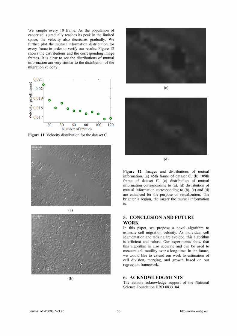
We sample every 10 frame. As the population of cancer cells gradually reaches its peak in the limited space, the velocity also decreases gradually. We further plot the mutual information distribution for every frame in order to verify our results. Figure 12 shows the distributions and the corresponding image frames. It is clear to see the distributions of mutual information are very similar to the distribution of the migration velocity.

Figure 11. Velocity distribution for the dataset C.

(a)

(b)

(c)

(d)

Figure 12. Images and distributions of mutual information. (a) 45th frame of dataset C. (b) 109th frame of dataset C. (c) distribution of mutual information corresponding to (a). (d) distribution of mutual information corresponding to (b). (c) and (d) are enhanced for the purpose of visualization. The brighter a region, the larger the mutual information is.

5. CONCLUSION AND FUTURE WORK In this paper, we propose a novel algorithm to estimate cell migration velocity. As individual cell segmentation and tacking are avoided, this algorithm is efficient and robust. Our experiments show that this algorithm is also accurate and can be used to measure cell motility over a long time. In the future, we would like to extend our work to estimation of cell division, merging, and growth based on our regression framework.

6. ACKNOWLEDGMENTS The authors acknowledge support of the National Science Foundation HRD 0833184.


7. REFERENCES [Cel09] Cell Applications, Inc., Human Endothelial

Cells, http://www.cellapplications.com/endothelial-cells.

[DSA+08] J. G. G. Dobbe, G. J. Streekstra, B. Atasever, R. van Zijderveld, and C. Ince, Measurement of functional microcirculatory geometry and velocity distributions using automated image analysis. Journal of Medical and Biological Engineering and Computing, Volume 46, Number 7, Pages 659-670, 2008.

[HZ04] Hartley, R. and Zisserman, A., Multiple

View Geometry in Computer Vision, 2nd Edition, Cambridge University Press, ISBN: 0521540518, 2004

[LGM04] Lamberti, F., Gamba, A., and

Montrucchio, B, Computer-assisted analysis of in-vitro vasculogenesis and angiogenesis processes. Journal of WSCG, Volume 12, Number 1-3, Pages 237-244, 2004.

[LMC+08] Kang Li, Eric D. Miller, Mei Chen, Takeo

Kanade, Lee E. Weiss, and Phil G. Campbell, Cell population tracking and lineage construction with spatiotemporal context. Journal of Medical Image Analysis, Volume 12, Issue 5, Pages 546-566, 2008.

[Mar09] Charles Marcus, Cancer cell migration and

movement, http://marcuslab.harvard.edu/index.shtml, Department of Physics, Harvard University.

[MDI+09] E. Meijering, O. Dzyubachyk, I. Smal,

and W.A. van Cappellen, Tracking in Cell and Developmental Biology. Seminars in Cell and Developmental Biology, Volume 20, Issue 8, Pages 894-902, 2009.

[Otu79] Otsu, N., A threshold selection method from

gray level histograms. IEEE Transactions on Systems, Man, and Cybernetics - Part B, Volume 9, pages 62–66, 1979.

[PMV03] Pluim, J.P.W., Maintz, J.B.A., and

Viergever, M.A., Mutual-information-based registration of medical images: a survey, IEEE Transactions on Medical Imaging, Volume 22, Issue 8, Pages 986-1004, 2003.

[WZH+09] Chih-Chieh Wu, Geoffrey Zhang, Tzung-

Chi Huang, and Kang-Ping Lin, Red blood cell

velocity measurements of complete capillary in finger nail-fold using optical flow estimation. Journal of Microvascular Research, Volume 78, Issue 3, Pages 319-324, 2009.

[Yam09] Soichiro Yamada, Keratinocyte migration,

http://yamadalab.ucdavis.edu/, Biomedical Engineering, University of California at Davis.

[YPW+04] Justin C Yarrow, Zachary E Perlman,

Nicholas J Westwood, and Timothy J Mitchison, A high-throughput cell migration assay using scratch wound healing, a comparison of image-based readout methods, BMC Biotechnology, Volume 4, Number 1, 21, 2004


Caustic Object Construction Based onMultiple Caustic Patterns

Budianto TandianusNanyang TechnologicalUniversity, [email protected]

Henry JohanNanyang TechnologicalUniversity, Singapore

[email protected]

Hock Soon SeahNanyang TechnologicalUniversity, Singapore

[email protected]

ABSTRACTInverse caustic problem, that is computing the geometry of a reflector and/or refractor based on a given causticpattern, is currently not widely studied. In this paper, we propose a technique to solve the inverse caustic problemin which we compute the geometry of a semi-transparent homogeneous refractive object (caustic object) given adirectional light source and a set of caustic patterns (each pattern is considered to be formed at a specified distancefrom the caustic object). We validate the results by using mental ray (software rendering). The novelty of ourresearch is that we consider a set of caustic patterns whereas existing techniques only consider one caustic pattern.We employ a stochastic approach to simulate the refracted light beam paths that can approximately reconstruct theinput caustic patterns. Working backward, from the computed refracted light beam paths we compute the geometryof the caustic object that can produce such light beam paths. Due to having multiple caustic patterns as the inputs,it is a challenge to reconstruct the input caustic patterns because of the differences in their shapes and intensities.We solve this problem by using a two-step optimization algorithm in which we adjust the position and size ofthe caustic regions in the first step and we adjust the caustic shapes in the second step. Our technique is able toconstruct a caustic object for a various types of input caustic patterns.

Keywords: caustics, photon, reconstruction, inverse problem, stochastics

1. INTRODUCTIONRecently, there is a growing interest in inverse problemresearch in Computer Graphics due to the possibility ofcontrolling the creation of visual effects. By using theinverse techniques, the design process becomes easieras the artists can just specify the intended effects di-rectly instead of performing the iterative trial-and-errorprocess. However, inverse problem is generally difficultas in most cases there is no unique bijective relationshipbetween the output and the input (i.e., given an output,there are many input possibilities that can generate suchoutput).

In the inverse caustic problem, given an input causticpattern (shape, intensity, and location from the caus-tic object) and a light source, we have to compute thegeometry of the caustic object that can produce a caus-tic pattern similar to the input caustic pattern. Inversecaustic problem is hard to solve because the input caus-tic pattern only contains the irradiance magnitude and itdoes not have incident light direction information (and


also the reflected and/or refracted light paths). Up tonow, the inverse caustic problem is not widely studiedand the existing work only consider a single input caus-tic pattern.

In this paper, we propose a new inverse caustic problem,that is computing the caustic object given multiple inputcaustic patterns formed on a caustic receiver (diffuseand non-transparent surface) at various distances fromthe caustic object. We show an example in Figure 1.

Our basic idea for solving this problem is as follows.We subdivide one side of the caustic object and alsothe caustic patterns into regular cells. The light beamrefracted by each caustic object cell will pass throughone caustic cell of each caustic pattern. We try to com-pute the orientation of each caustic object cell such thatthe combination of the refracted light beams of all caus-tic object cells can approximately reconstruct the inputcaustic patterns.

We use a stochastic approach in our technique and werepresent each input caustic pattern as a 2D probabilitymass function (pmf) by considering the brightness of acaustic cell as the probability of a light beam might passthrough it (i.e., the brighter the caustic cell is, the higherprobability or the more likely a light beam is consideredto pass through it). Hence, for each cell of the causticobject, we use the pmfs of the caustic patterns to deter-mine to which direction the caustic object cell refractsa light beam. From the determined refracted light beam


(a) Scene setup. (b) Computed caustic object and approximately reconstructed caustic patterns.

Figure 1: (a) Scene setup. We compute a caustic object (the leftmost box), specifically the surface geometry of theside (shown in red color) facing the caustic patterns, given three caustic patterns (WSCG, 2012, and Europe) to beformed on a caustic receiver at three distances from the caustic object, with a directional light source orthogonalto the caustic object illuminates from the left. (b) mental ray renderings of caustics produced by our computedcaustic object (final output). Input caustic patterns are shown in the insets at each image. The computational timeis 9.0 hours.

direction, we can compute the orientation of the causticobject cell.

Due to differences of the input caustic patterns (interms of shapes and intensities), it is hard to computethe caustic object that can satisfy all the input caus-tic patterns. Thus, we relax the input requirements byslightly adjusting the sizes, positions, and shapes of thenon-zero intensity regions of the input caustic patterns.Moreover, we also allow a small amount of light beamwhich has passed through several caustic patterns tomiss or overshoot the rest of the caustic patterns. Wecompute these adjustments by using optimization tech-niques. We validate our results by performing renderingsimulation using mental ray [men12a], a robust indus-try standard rendering engine.

2. RELATED WORKUnknown Input Given only the output, the inputthat can produce such output is computed. This is ahard problem since the a priori knowledge of the inputis not available. One example is the work presentedby Bottino et al. [Bot01a] and Mitra et al. [Mit09a].They compute a 3D geometry that can satisfy the inputswhich consist of a set of silhouettes or shadow patterns.

Inverse Caustics One of the earliest work in inversecaustic is presented by Patow and Pueyo [Pat04a]. Theycompute the reflector shape in an optical set (consists ofa reflector, light source, and diffusor) given the radiancedistribution as an input. They represent the reflector asgrids and they iteratively adjust the grid vertices such aspositions and number of vertices based on the similar-ity with the intended radiance distributions. The wholeprocess took many days even though they can obtain ra-diance distribution similar to the input. They improvethe work by allowing the user to set the range of thesolution space [Pat07a] (the lower bound and the upperbound of the reflector shape). Hence, a user has morecontrol in determining the reflector shape. They laterincrease the performance by using GPU [Mas09a] and

they can reduce the processing time into magnitude ofhours.

In parallel with the aforementioned work, Anson etal. [Ans08a] represent the reflector as a NURBS sur-face and Finckh et al. represent the reflector as a B-Spline surface [Fin10a]. As a result, during the opti-mization they optimize the control points instead of gridvertices which in the end can produce smooth reflectorsin a relatively fast speed (due to the small number ofparameters to be optimized). However, as Papas et al.also mention [Pap11a], the parameterized technique hasa difficulty with highly complex caustic images, thusFinckh et. al [Fin10a] cannot reproduce all frequenciesof the caustic pattern and Anson et. al [Ans08a] assumethe shape of the caustic pattern to be circular.

Weyrich et al. generate a microgeometry reflector givena single reflected caustic pattern input [Wey09a]. Thecaustic object is subdivided into uniform cells (facets),and they compute the optimized orientation of each cellthat can produce a caustic pattern similar to the inputpattern. Papas et al. [Pap11a] improve the work ofWeyrich et al. [Wey09a] by generating a refractor caus-tic object on a larger scale. Moreover, they are ableto prevent noise on the reconstructed caustic pattern bycomputing the surface of each facet based on the Gaus-sian distribution. Similar to Weyrich et al. [Wey09a],they employ several optimization costs in order to gen-erate the caustic objects. In the most recent develop-ment, Yue et al. [Yue12a] emphasize on modularity byreconstructing an input caustic pattern from a causticobject which consists of many smaller pieces of causticobject cells. Their caustic object cells are divided intoten types with each type refracts light to a predefineddirection.

Comparison In all these work, the input is only a sin-gle caustic pattern. On the other hand, in this paper wepropose a new challenge in which we compute the ge-ometry of a caustic object based on a set of input causticpatterns.


Figure 2: Scene setup. Our algorithm computes thenormal/orientation of each caustic object cell. Caus-tic pattern ’1’ is formed when the caustic receiver is atdistance d0 from the caustic object and similarly causticpattern ’2’ at d1.

3. BASIC IDEA OF OUR METHODScene Setup The scene setup is shown in Figure 2. Thescene consists of three components, a caustic object (ofa box shape), a caustic receiver (a planar surface wherethe caustic patterns are formed), and a directional lightsource (whose direction is orthogonal to the caustic ob-ject). Both the caustic receiver and the caustic objectare positioned coplanar, with the caustic receiver is onone side of the caustic object (assumed to be the backface of the caustic object, facing (0, 0, -1) direction)and incoming light direction is on the other face of thecaustic object (assumed to be the front face of the caus-tic object, facing (0, 0, 1) direction). We assume thecaustic receiver and the caustic object to have the samespatial dimension (i.e. same width and height) and ori-entation. Therefore, the extent of the region of interestof each caustic pattern is bounded by the shape of thecaustic receiver

The caustic patterns and the back face of the causticobject are subdivided into a regular grid of cells. Eachcell of a caustic pattern stores the total caustic intensityon that particular cell. We call cells of caustic patternswhich have non-zero caustic intensity as caustic cellsand cells with zero caustic intensity as empty cells. Thecollection of caustic cells of a caustic pattern is collec-tively called as a caustic region. For each cell of thecaustic object (caustic object cell), we compute its ori-entation such that it can produce a refracted light beamto a specific direction. In the rest of this paper, we referto each refracted light beam as light and we representeach light beam in the following Figures 3 and 4 as anarrow.

Problem Formulation We compute the back face of acaustic object C given a set of p grayscale caustic pat-terns such that each caustic pattern j will be formed onthe caustic receiver when the receiver is located at theuser-input distance d j from the caustic object. Specif-ically, we compute the orientation of each caustic ob-

(a) (b)

Figure 3: Problem formulation. (a) Given two caus-tic patterns at two different locations (with the intensityof each caustic cell is denoted by the size of the cell),compute light refraction direction (red arrow) of eachcaustic object cell such that the refracted light collec-tively can generate caustic patterns similar to the inputcaustic patterns. (b) Light refraction combination thatcan satisfy the input caustic patterns.

ject cell at the back face of the caustic object such thatthe cell refracts the incoming light into a direction thatpasses through parts of the caustic regions. Collec-tively, the light refracted from all caustic object cells isexpected to pass through all the input caustic cells thusreconstructing the input caustic patterns. As mentionedin Section 1, the input caustic patterns only providethe estimate of the amount of refracted light arrivingat caustic receiver cells, not the light directions. Hence,the main challenge is to compute refracted light pathsthat can approximately reconstruct all the given causticpatterns. This problem is illustrated in Figure 3. Theorientation of each cell can then be determined basedon the path of its refracted light.

Solution As explained above, the task is to compute re-fracted light direction combinations such that they canapproximately reconstruct the input caustic patterns. Inthis case, more light is expected to pass through brightercaustic cells compared to darker caustic cells. Hence,to solve this, we simulate the direction of the refractedlight of each caustic object cell by using a stochasticapproach. The idea is to use the caustic intensity ineach caustic cell as the probability that we will refract alight to that caustic cell (i.e. the brighter the input caus-tic pattern is, the more likely it is chosen as a refractedlight target).

We represent the set of caustic patterns as a setof normalized 2D probability mass functionsP = fP0 , fP1 , fP2 , . . . fPp−1 (each in P is the pmfof the user-input caustic pattern on the caustic receiverwhen the receiver is located at the user-input distancefrom the caustic object). The pmf of each caustic pat-tern is defined by using the grayscale value (intensity)of the caustic pattern in which the probability at eachcaustic cell is the grayscale value of that particular cellin the caustic pattern. Each pmf fPj is normalized by


Figure 4: Each numbered arrow denotes the refractedlight from the cells of the caustic object C and the grayblocks denote the probability of caustic cells. Light #1and #2 have joint pmf of zero since their paths passthrough at least one empty cell. Each light in #3 hasthe probability greater than zero since the light passthrough non-zero cells. Light #4 is allowed even thoughit misses some of the caustic patterns. We will explainthis further in Section 4.2. Light #5 is not valid becauseit does not intersect any caustic patterns

dividing the probability of each of its cell with the totalprobability of all cells of fPj .We assign a random variable Xi for each i-th cell ofthe caustic object. For each Xi, the probability value ofeach possible refracted light direction x is computed bymultiplying the probability of each caustic cell passedby the light refracted to direction x (see Figure 4), asshown in Equation 1.

fXi(x) =p−1

∏j=0

fPj(gij(x)), (1)

with gij(x) is a mapping function. The mapping func-

tion is basically a ray casting function in which the lightis shot from the i-th caustic object cell to the caustic pat-tern j with the direction of x and return the intersectedcell (of caustic pattern j). Then, for each caustic objectcell or each Xi we assign a refracted light direction byusing the Acceptance-Rejection method [vN51a] withthe distribution based on the sampled joint probabilitymass function of all caustic patterns (Equation 1).Once we obtain the refracted light direction for eachcaustic object cell, we compute its normal or orienta-tion based on the user-input index of refraction of thecaustic object, incoming light direction (orthogonal tothe caustic object), and the obtained refracted light di-rection by solving the Snell’s Equation (see AppendixA). Afterward, we perform rendering simulation usingthe mental ray to asses the approximate reconstructedcaustic patterns (as shown in Figure 6a).Note that our technique can also be applied topoint light sources and directional light sources non-orthogonal to the caustic object. In the rest of the paper,

the terms caustic patterns and pmfs are interchangeableas we use the term pmfs when we emphasize on themathematical representation of the caustic patterns.

4. IMPROVING THE RECON-STRUCTED CAUSTICS

The solution in Section 3 may not be able to reconstructthe caustic patterns very well if the input consists ofmultiple patterns. If we only have a single caustic pat-tern (shown in Figure 5a), then we can reconstruct itvery well. However, if we add two additional causticpatterns, then some parts of the input caustic patternsare missing (Figure 5b).

Reconstruction problem As explained in Section 3(and shown in Figure 4), some refraction directionshave zero joint pmf when they pass through at leastone empty caustic cell. As a result, if all possible re-fraction directions from every caustic object cell passthrough a caustic cell of a caustic pattern but they alsopass through the empty cells of other caustic patterns,then the aforementioned caustic cell cannot be recon-structed (we call such cell as a missing caustic cell).As seen in Figure 4, the top and bottom caustic cellsin fP1 are missing caustic cells since the refracted lightthat pass through these caustic cells also pass throughempty cells in the other caustic patterns.

Proposed solution Based on the given input causticpatterns and their configurations (positions and sizes),it might not be possible to compute the caustic objectthat can well reconstruct the original input caustic pat-terns. Thus, we propose a method to relax the input re-quirement by allowing slight changes to the positions,sizes, and shapes of the caustic regions. Our proposedmethod consists of two steps. In the first step, we op-timize the size and position of the caustic regions byslightly adjusting the size and position given by the user(Section 4.1). In the second step, the boundaries of eachcaustic region are adaptively extended such that theyenable the reconstruction of the missing caustic cells onthe other caustic patterns (Section 4.2). We also com-pute the amount of light that is allowed to overshoot orto miss some caustic patterns.

In both optimization steps, we use Simulated Anneal-ing [Kir83a]. The main reason we use Simulated An-nealing is because the problem cannot be solved analyt-ically. However, there are also some possible optimiza-tion techniques such as Particle Swarm, Ant Colony,and Genetic Algorithm. However, those techniques re-quire keeping the record of multiple possible solutionsat once, hence it is not efficient for our case (as seen inEquation 3, the cost computation requires reconstruc-tion of the caustic patterns multiple times using the ad-justed input caustic patterns). Moreover, in some ofthe related work [Wey09a, Fin10a, Pap11a], SimulatedAnnealing is also used. After applying our proposed


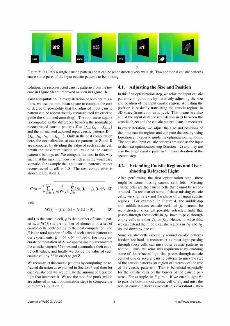
(a) (b)

Figure 5: (a) Only a single caustic pattern and it can be reconstructed very well. (b) Two additional caustic patternscause some parts of the input caustic patterns to be missing.

solution, the reconstructed caustic patterns from the testcase in Figure 5b are improved as seen in Figure 1b.

Cost computation In every iteration of both optimiza-tions, we use the root mean square to compute the costor degree of possibility that the adjusted input causticpattern can be approximately reconstructed (in order toguide the simulated annealing). The root mean squareis computed as the difference between the normalizedreconstructed caustic patterns Z = fZ0 , fZ1 , . . . fZp−1and the normalized adjusted input caustic patterns D = fD0 , fD1 , fD2 , . . . fDp−1. Only in the cost computationhere, the normalization of caustic patterns in Z and Dare computed by dividing the value of each caustic cellt with the maximum caustic cell value of the causticpattern t belongs to. We compute the cost in this waysuch that the maximum cost (which is in the worst casescenario, for example the input caustic patterns are notreconstructed at all) is 1.0. The cost computation isshown in Equation 3.

Cost =1p

p−1

∑j=0

1n(W( j))

β

∑i=0

( fD j(ti)− fZ j(ti))2, (2)

with

W( j) = t| fD j(t)+ fZ j(t)> 0, (3)

and t is the caustic cell, p is the number of caustic pat-terns, n(W( j)) is the number of elements of a set ofcaustic cells contributing to the cost computation, andβ is the total number of cells of each caustic pattern (inour experiments, β = 64× 64 = 4096). For more ac-curate computation of Z, we approximately reconstructthe caustic patterns 32 times and accumulate their caus-tic cell values, and finally we divide the value of eachcaustic cell by 32 in order to get Z.

We reconstruct the caustic patterns by computing the re-fracted direction as explained in Section 3 and then foreach caustic cell we accumulate the amount of refractedlight that intersects it. We use the modified pmfs (whichare adjusted in each optimization step) to compute thejoint pmfs (Equation 1).

4.1. Adjusting the Size and PositionIn this first optimization step, we relax the input causticpattern configurations by iteratively adjusting the sizeand position of the input caustic region. Adjusting theposition is basically translating the caustic regions in3D space (translation in x, y, z). This means we alsoadjust the input distance (translation in z) between thecaustic object and the caustic pattern (caustic receiver).

In every iteration, we adjust the size and positions ofthe input caustic regions and compute the cost by usingEquation 2 in order to guide the optimization iterations.The adjusted input caustic patterns are used as the inputto the next optimization step (Section 4.2) and they arealso the target caustic patterns for every iteration of thesecond step.

4.2. Extending Caustic Regions and Over-shooting Refracted Light

After performing the first optimization step, theremight be some missing caustic cells left. Missingcaustic cells are the caustic cells that cannot be recon-structed. To reconstruct some of these missing causticcells, we slightly extend the shape of all input causticregions. For example, in Figure 4, the middle-topand middle-bottom caustic cells of fP1 cannot bereconstructed since all possible refracted light thatpasses through these cells in fP1 have to pass throughempty cells in either fP0 or fP2 . Hence, to solve this,we can extend the middle caustic regions in fP0 and fP2up and down by one cell.

Some caustic cells especially around caustic patternsborders are hard to reconstruct as most light passingthrough these cells can miss other caustic patterns inbehind. Thus, we relax this requirement by enablingsome of the refracted light that passes through causticcells of one or several caustic patterns to miss the restof the caustic patterns (or region of interests of the restof the caustic patterns). This is beneficial especiallyfor the caustic cells on the border of the caustic pat-terns. For example, in Figure 4, if we enable light #4to pass the bottommost caustic cell of fP0 and miss therest of caustic patterns (we call this overshoot), then


(a) Results without optimization. Cost : 4.45×10−1

(b) Results after 1st optimization (Section 4.1). Cost : 4.08×10−1

(c) Results after 1st and 2nd optimization (Section 4.2). Cost: 2.64×10−1

Figure 6: Mental ray rendering results of the optimiza-tion steps. Input caustic patterns are shown at the bot-tom right of each screenshot in (a). We also show themissing caustic cell maps at the below right of each im-age (green cells show the missing caustic cells, graycells show the caustic cells that can be reconstructed,and cyan cells show the extended caustic cells). Forthe visualization of the differences between the targetand the reconstructed caustic patterns, we also show thecaustic irradiance difference maps (assuming the totalirradiance of each target caustic pattern is 1.0 and thetotal light emitted to the scene is 1.0, i.e. each caus-tic object cell refracts the light with the amount of 1.0divided by the number of caustic object cells) at the be-low left of each image (from the darkest pixels with theleast errors to the brightest pixels with the most errors).For the sake of visual clarity, we scale up the differencevalues by 5000. The computational time is 5.7 hours.

the bottommost caustic cell of fP0 can be reconstructed.However, we still do not allow the refracted light of onecaustic object cell to miss all of the caustic patterns (asin light #5).

Fully extending the caustic regions can deform the orig-inal caustics too much, and likewise if we allow toomuch light to overshoot the caustic patterns then the ap-proximate reconstructed caustic patterns will have verylow intensity. Hence, in this step, we apply an optimiza-

tion to determine the appropriate caustic regions exten-sions amount k = k0,k1, . . .kp−1 and light overshootamount o= o0,o1, . . . ,op−1 with k and o ∈ [0,1] (i.e.,a k and an o value for each caustic pattern).

(a) (b)

Figure 7: (a) A simple example of missing caustic cellprojection (is explained in Section 4.2). Gray cells arethe caustic cells and the green cell is the missing causticcell. (b) We extend the second caustic pattern (two cellsaway) with gradually decreasing intensity.

Extending Caustic Regions To enable the missingcaustic cells of a caustic pattern j to be reconstructed,we have to firstly compute at most how many sb unitcells away the caustic region boundaries of the othercaustic patterns b (0 ≤ b ≤ p−1,b = j) have to be ex-tended. Afterward, for every caustic pattern b, we ex-tend its caustic region with the amount of sb · kb. In or-der to enable smooth extension, we extend the causticregions with linearly decreasing intensity (or probabil-ity value).

To do this, for every missing caustic cell of the causticpattern j, we project it from every caustic object cellto the empty cells of other caustic patterns b (0 ≤ b ≤p− 1,b = j). We perform this projection for the miss-ing caustic cells of all caustic patterns. This projectionexample is shown in Figure 7a in which we project themissing caustic cell (shown in green color). Afterward,for each caustic pattern b, we obtain the maximum dis-tance (sb) between its caustic region boundaries and itsempty cells that receive the projections of the missingcaustic cells (of other caustic patterns). In Figure 7a ex-ample, it is five cells (sb = 5) away for the second caus-tic pattern and in Figure 7b the caustic region boundaryis extended two cells away (if kb = 0.4).

Some of the missing caustic cell projections might missthe other caustic patterns b. For example, if the missingcaustic cell in Figure 7a is one or two cells to the right,then some of the projections will overshoot or will nothit the second caustic pattern. We use this informationto control the possibility of the refracted light to over-shoot each caustic pattern.

Overshooting Refracted Light To improve the re-sults, we also enable the refracted light to overshootsome of the caustic patterns. Thus, during the missingcaustic cells projections, we also compute the ratio (eb)between the amount of these projections that do not hitcaustic pattern b and the total amount of these projec-


tions toward caustic pattern b (i.e. sum of the missingcaustic cell projections that hit and do not hit causticpattern b). eb is essential since it provides the informa-tion on the amount of probability that the refracted lightmiss plane b. Hence, the probability hb that we will re-fract the light to miss the caustic pattern b is shown inEquation 4.

hb = eb ·ob · fPb(tmax), (4)

with ob is the coefficient to control the probability ofovershooting b-th caustic pattern and tmax is a cell offPb with the highest probability value.

We show the optimization progression in Figure 6.

5. GEOMETRY CONSTRUCTIONAs explained in Section 3 we use the joint pmf (Equa-tion 1) of the caustic patterns to compute the refractiondirection of each caustic object cell. From the refrac-tion direction, we can obtain the normal of the partic-ular caustic object cell. However, if we perform theoptimizations in Section 4, then we use the modifiedpmfs (output from both optimization steps) to computethe joint pmf (and ultimately the normal of each causticobject cell).

Based on the computed orientation of each caustic ob-ject cell, we can obtain the caustic object geometry bycomputing the x,y,z coordinates of the four corners ofeach caustic object cell. The x,y coordinates of eachcaustic object cell corner can be easily found as thecaustic object is uniformly subdivided. To computethe z coordinates of the caustic object cell corners, wefirstly assume that the z coordinate of all caustic objectcell middle points to be the same (z = 0.0). Next, we usethe dot product operation, i.e. dot product between thenormal of the caustic object cell and the vector fromthe caustic object cell middle point (we know its x,ycoordinates from the uniform subdivision and also its zcoordinate which is 0.0) to each caustic object cell cor-ner (we know its x,y coordinates) must be equal to zero.In this case, the only unknown value is z of the causticobject cell corner.

Since the edges of the neighbouring caustic object cellsdo not have the same slope or the same z coordinate onboth endpoints, there are vertical open spaces betweencaustic object cells (shaded with lighter gray in Fig-ure 8), we generate additional polygons to close thosegaps.

6. RESULTSWe present some results computed using our techniquein Figures 1, 6, 10. In all of the test cases, the index ofrefraction of the caustic objects are 1.5, the resolutionof the caustic objects are 128× 128 and the resolutionof the caustic receiver is 64× 64. Resolution refers to

Figure 8: Caustic object geometry (inset) of Figure 6cwith a zoom-in view. In the zoom-in view, each causticobject cell consists of two co-planar triangles shadedwith darker gray. We also generate additional verticalpolygons (shaded with lighter gray) to close the gapsbetween caustic object cells.

the number of cells. If we assume the spatial size tobe 1.0×1.0, then the size of each caustic object cell is1.0/128× 1.0/128 and the size of each caustic cell is1.0/64×1.0/64.

We use higher resolution for caustic object cells sincewe want to have more variations on the refracted lightpaths so that we can better reconstruct the contrast (orintensity variations) of the given caustic patterns. Weshow a difference example with a single caustic patterncase in Figure 9, a simple caustic pattern (resolution64×64) reconstructed with a resolution 64 x 64 causticobject and a resolution 128 x 128 caustic object.

(a) (b)

Figure 9: A simple test case (one caustic pattern, withresolution 64×64) reconstructed with different causticobject resolutions. (a) Resolution 64 x 64 caustic ob-ject. (b) Resolution 128 x 128 caustic object.

We use the same parameters for the simulation anneal-ing for both optimization steps in all experiments, i.e.10 cycles of 10 iterations, Boltzmann’s constant of 1.0,and temperature reduction factor of 0.5.

The experiments were performed on two comparablePCs. The specification of the first PC is Intel i7 9202.67 GHz (CPU) with NVIDIA GeForce GTX 285


(GPU) and the specification of the second PC is Intel i7880 3.07 GHz (CPU) with NVIDIA GeForce GT 330(GPU). In the implementations, we calculate the jointpmf by rendering each caustic pattern and then we mul-tiply them by using alpha blending (hence the use ofGPU). For the rest of the computations such as Simu-lated Annealing and Acceptance-Rejection method, weperform them on CPU.

From the results, we can observe that the caustic ob-jects generated using our technique can approximatelyreconstruct various types of input caustic patterns, es-pecially for the WSCG (Figure 1b), fruits (Figure 10a),and rotating star (Figure 10c) test cases. The degree ofdifficulty in reconstructing the caustic patterns mostlydepends on the number of caustic patterns, similaritybetween shapes, and the number of caustic cells in theinput caustic patterns. As shown in Equation 4, due tothe multiplication in computing the joint pmf, the prob-ability of a particular refraction direction can becomezero if the refracted light passes through empty cells.With the increasing number of caustic patterns espe-cially the ones with different shapes, the chances thatwe have many refraction directions with zero probabil-ity also increase. We can see this from the results inFigures 1 and 6 (three input caustic patterns) where wecan reconstruct better compared to the results in Fig-ures 10 (four or more caustic patterns).

The shapes and orientations of caustic patterns can alsoaffect the reconstruction difficulty. The test cases withsimilar caustic patterns, can be approximately recon-structed pretty well since similar refracted light pathsare sufficient to reconstruct the caustic patterns. This isevident by comparing Figure 10a and Figure 10b. Thecaustic patterns in Figure 10a have near round shapesand approximately the same orientations. In contrast,the test case in Figure 10b have pretty different shapes(and orientations). Hence, there are few light that canpass through the endpoints of the bars compared to themiddle regions of the bars.

Note the difficult test case shown in Figure 10b, fourbar caustic patterns with alternating orientations. Aswe can see, the hardest parts to reconstruct are the onesnear the two endpoints of the bars and on the other handthe parts around the centers are the easiest. This is dueto the alternating shapes which cause the light paths toalways pass through the center of the caustic regions.As we allow the refracted light to miss some of thecaustic patterns, we are able to approximately recon-struct the top and bottom parts of the first caustic pat-tern. However, the consequence is that the last causticpattern appears much dimmer.

In many cases, light tends to converge to the middlecaustic patterns and as a result the center regions ofthese caustic patterns become relatively brighter com-pared to the other caustic patterns (for example, the Ar-

madillo caustic pattern in Figure 6 exhibits this effect).This is due to two reasons. First, the caustic regionsare positioned approximately at the center of the caus-tic patterns. Second, because the size of the caustic re-gions are mostly smaller than the caustic object. There-fore, some caustic object cells have to refract the lightin the diagonal directions. This is illustrated in Figure 4in which some of the light grouped to #3 have to berefracted in the diagonal directions.

Note that the relative depth of caustic patterns also af-fects the quality, as it is very difficult to reconstruct ifthe caustic patterns are located very near to each other.This is because the refracted light paths will intersectthe patterns at similar locations and thus it is difficult toreconstruct caustic patterns with different shapes.

Please refer to the submitted video to see the progres-sive changes of the caustic patterns as the caustic re-ceiver is moved.

7. APPLICATIONSThe inverse caustics has several potential applications.

Arts As shown in Figure 10, our technique can gener-ate caustic objects that can produce several interestingcaustic effects (similar to the intention in the inverseshadow [Mit09a]). Therefore, we hope that our workcan encourage more exploration in caustic arts.

Information Encoding Information (such as serialnumbers, passwords) can be encoded as caustic patternsof encrypted 2D images. Only when the requirements(such as light direction and caustic receiver distance)are known, we can recover the original information.We show an example in Figure 11 in which we encryptWSCG and 2012 into two QR barcode patterns.

Validation Tests By using the computed caustic ob-ject, we can validate some processes such as renderingprocess (validating the correctness of caustics render-ing algorithm) or manufacturing (validating the qualityof produced glasses or light sources).

8. CONCLUSIONS AND FUTUREWORK

We have presented an inverse caustic problem and anovel technique which computes a caustic object givena set of caustic patterns with each pattern is positionedat a user-input distance from the caustic object. Ourproposed technique is based on a stochastic approach,and it is augmented with two optimization steps thatcan alleviate the missing caustic problems. We havevalidated our results by performing physically render-ing simulation using mental ray, and the caustic ob-ject generated using our technique can approximatelyreconstruct various types of input caustic patterns.

In the future, we would like to improve the quality ofthe reconstructed caustics in terms of smoothness. It


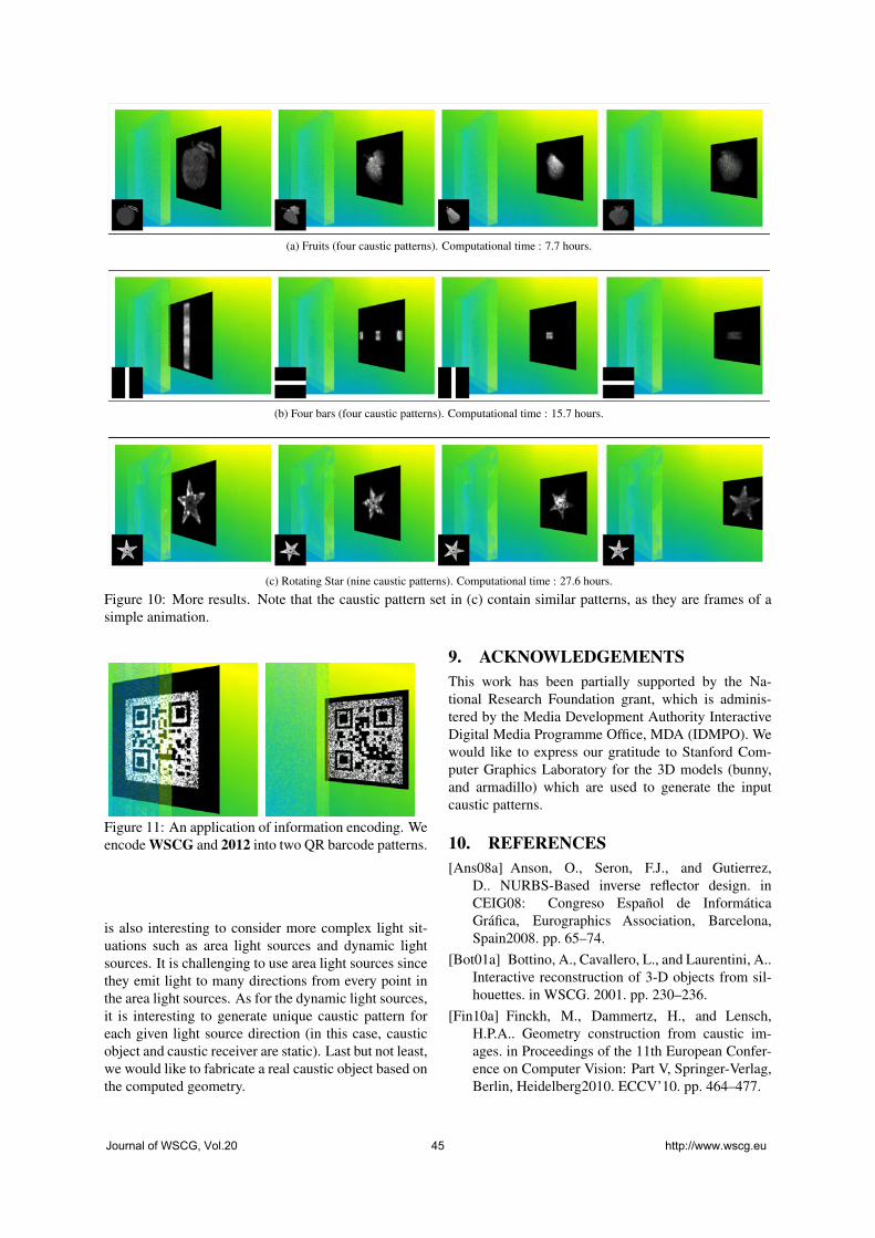
(a) Fruits (four caustic patterns). Computational time : 7.7 hours.

(b) Four bars (four caustic patterns). Computational time : 15.7 hours.

(c) Rotating Star (nine caustic patterns). Computational time : 27.6 hours.

Figure 10: More results. Note that the caustic pattern set in (c) contain similar patterns, as they are frames of asimple animation.

Figure 11: An application of information encoding. Weencode WSCG and 2012 into two QR barcode patterns.

is also interesting to consider more complex light sit-uations such as area light sources and dynamic lightsources. It is challenging to use area light sources sincethey emit light to many directions from every point inthe area light sources. As for the dynamic light sources,it is interesting to generate unique caustic pattern foreach given light source direction (in this case, causticobject and caustic receiver are static). Last but not least,we would like to fabricate a real caustic object based onthe computed geometry.

9. ACKNOWLEDGEMENTSThis work has been partially supported by the Na-tional Research Foundation grant, which is adminis-tered by the Media Development Authority InteractiveDigital Media Programme Office, MDA (IDMPO). Wewould like to express our gratitude to Stanford Com-puter Graphics Laboratory for the 3D models (bunny,and armadillo) which are used to generate the inputcaustic patterns.

10. REFERENCES[Ans08a] Anson, O., Seron, F.J., and Gutierrez,

D.. NURBS-Based inverse reflector design. inCEIG08: Congreso Español de InformáticaGráfica, Eurographics Association, Barcelona,Spain2008. pp. 65–74.

[Bot01a] Bottino, A., Cavallero, L., and Laurentini, A..Interactive reconstruction of 3-D objects from sil-houettes. in WSCG. 2001. pp. 230–236.

[Fin10a] Finckh, M., Dammertz, H., and Lensch,H.P.A.. Geometry construction from caustic im-ages. in Proceedings of the 11th European Confer-ence on Computer Vision: Part V, Springer-Verlag,Berlin, Heidelberg2010. ECCV’10. pp. 464–477.


[Kir83a] Kirkpatrick, S., Gelatt, C.D., and Vecchi,M.P.. Optimization by simulated annealing. Sci-ence. vol. 220, no. 4598, pp. 671–680, 1983.

[Mas09a] Mas, A., Martín, I., and Patow, G.. Fast in-verse reflector design (FIRD). Computer GraphicsForum. vol. 28, no. 8, pp. 2046–2056, 2009.

[men12a] mental ray.http://www.mentalimages.com/products/mental-ray.html, 2012.

[Mit09a] Mitra, N.J., and Pauly, M.. Shadow art. ACMTrans. Graph.. vol. 28, pp. 156:1–156:7, 2009.

[Pap11a] Papas, M., Jarosz, W., Jakob, W.,Rusinkiewicz, S., Matusik, W., and Weyrich,T.. Goal-based caustics. Computer GraphicsForum. vol. 30, no. 2, pp. 503–511, 2011.

[Pat04a] Patow, G., Pueyo, X., and Vinacua, A.. Re-flector design from radiance distributions. WorldScientific. vol. 10, no. 2, pp. 211–235, 2004.

[Pat07a] Patow, G., Pueyo, X., and Vinacua, A..User-guided inverse reflector design. Computers &Graphics. vol. 31, no. 3, pp. 501–515, 2007.

[vN51a] von Neumann, J.. Various techniques used inconnection with random digits. monte carlo meth-ods. vol. 12, pp. 36–38, 1951.

[Wey09a] Weyrich, T., Peers, P., Matusik, W., andRusinkiewicz, S.. Fabricating microgeometry forcustom surface reflectance. ACM Trans. Graph..vol. 28, pp. 32:1–32:6, 2009.

[Yue12a] Yue, Y., Iwasaki, K., Chen, B., Dobashi, Y.,and Nishita, T.. Pixel art with refracted light byrearrangeable sticks. Computer Graphics Forum.vol. 31, no. 2, pp. 575–582, 2012.

A. NORMAL COMPUTATION

Given the Snell’s Equation

η1 sinθ1 = η2 sinθ2,

η

1− cos2 θ1 =

1− cos2 θ2,

η

1− (−N ·M)2 =

1− (N ·R)2,

A1NxNx +A2NxNy +A3NyNy = 1, (5)

with η1 is the index of refraction of the caustic object,η2 is the index of the refraction of air, N is the normal,M is the inverse incoming light direction, R is the re-fracted light direction, θ1 is the angle between M andthe inverse normal, θ2 is the angle between M and thenormal, and

η = η1η2

A1 =η2MxMx−RxRx

η2−1

A2 = 2 η2MxMy−RxRyη2−1 A3 =

η2MyMy−RyRyη2−1

Since the normal vector N is normalized, the solutionlies on a unit circle and as a result Nx = cosφ and Ny =sinφ . Hence, Equation 5 can be simplified to

(2A3 −2) tan2φ +2A2 tanφ +(2A1 −2) = 0. (6)

Equation 6 is basically a quadratic equation and the an-gle φ can be obtained by solving the quadratic equation.


Interactive BRDF Estimation for Mixed-Reality Applications

Martin KnechtVienna University of

[email protected]

Georg TanzmeisterVienna University of

[email protected]

Christoph TraxlerVRVis Zentrum für Virtual

Reality undVisualisierung

[email protected]

Michael WimmerVienna University of

[email protected]

ABSTRACTRecent methods in augmented reality allow simulating mutual light interactions between real and virtual objects.These methods are able to embed virtual objects in a more sophisticated way than previous methods. However,their main drawback is that they need a virtual representation of the real scene to be augmented in the form ofgeometry and material properties. In the past, this representation had to be modeled in advance, which is very timeconsuming and only allows for static scenes.We propose a method that reconstructs the surrounding environment and estimates its Bidirectional ReflectanceDistribution Function (BRDF) properties at runtime without any preprocessing. By using the Microsoft Kinect sen-sor and an optimized hybrid CPU & GPU-based BRDF estimation method, we are able to achieve interactive framerates. The proposed method was integrated into a differential instant radiosity rendering system to demonstrate itsfeasibility.

KeywordsBRDF estimation, reconstruction, augmented reality

1 INTRODUCTIONMany mixed-reality applications require or at leastdesire a consistent shading between virtual and realobjects. Examples are product presentations, virtualprototyping, architectural and urban visualizationsand edutainment systems. Here virtual objects shouldsmoothly blend into the real environment and providea plausible illusion for users. They need to be renderedin a way that makes them hard to distinguish from realobjects. Some recently published methods [14, 7]consider the mutual light interaction between real andvirtual objects, so that they indirectly illuminate orshadow each other.

Beside the geometry of the scene and the real lightingconditions, the BRDFs of real objects are needed tosimulate these mutual shading effects. Acquiring thisdata in a pre-processing step would diminish the dy-


namic and interactive nature of mixed-reality systems,and would also make it necessary to track the previ-ously modeled movable real objects. In this paper, weintroduce a BRDF estimation method that runs at in-teractive frame rates. It is based on real-time recon-struction using the structural light scanner provided byMicrosoft’s Kinect sensor [11]. The real lighting con-ditions are captured by a camera with a fish-eye lensfrom which light sources are derived.

Our contribution is best characterized by the uniquefeatures of our BRDF estimation approach, which are:

• It runs at interactive frame rates.

• It does not need any pre-processing.

• It utilizes a novel K-Means implementation exe-cuted on the GPU.

2 RELATED WORKBRDF estimation has a long history of research and avariety of methods have been presented. Our approachbelongs to the class of image-based methods, whichare sometimes synonymously called Inverse Render-ing. These methods try to fit parameters of an un-derlying, sometimes rather simple, BRDF model, like


the Phong [15] or Ward model [20], from images of ascene. Yu et al. introduced Inverse Global Illumina-tion [23], where reflectance properties are derived froma sparse set of HDR images considering also indirectillumination. The geometry is pre-modeled and par-titioned into surfaces with similar materials. The di-rect light sources must also be known. An optimizationalgorithm then calculates diffuse and specular compo-nents separately. Although the concept is sound andforms the basis of newer algorithms, it needs a lot ofmanual pre-processing. Sato et al. [17] presented amethod that also performs a reconstruction of the ob-ject’s geometry from range images, which is then usedto estimate diffuse and specular parameters from thesame images.

Boivin and Gagalowicz [2] use a single LDR image inaddition to a geometric model including light sources.Starting with a Lambertian model, they iteratively com-pare renderings with the original image and considermore and more complex reflectance models as long asthe difference is too large. Though their solution is scal-able with regard to accuracy, it is still time consumingand requires pre-processing. Mercier et al. [10] werethe first to present a fully automatic method to recoverthe shape and reflectance properties of a single objectand the position of light sources from a set of cali-brated images. For that purpose, the object and lightsources are fixed on a turntable, and photographs aretaken every 5 degrees. The geometry is approximatedby Shape From Silhouette (SFS) from Szeliski [19].The method is very accurate and does not need any pre-processing, but the special setup makes it unsuitable formixed-reality. Xu and Wallace [22] used a depth sen-sor and a stereo intensity image to acquire an object’sreflectance properties and parameters for multiple lightsources. Although using a depth map comes close toour approach, their method is restricted to a single ob-ject. Furthermore, calculating light source parametersfrom intensity images introduces inaccuracies for flatsurfaces.

Zheng et al. [25] presented a solution that is similar tothat of Mercier et al. [10]. One big difference is thatthey use measured lighting conditions instead of deriv-ing this information from the images, which minimizesthe estimation error. They then apply the highlight re-moval algorithm from Ortiz and Torres [13] before clus-tering images into regions with similar diffuse materialsusing K-Means. The parameters of the Ward model arethen obtained for each cluster by non-linear optimiza-tion. Their algorithm is very robust, since after estimat-ing specular factors, diffuse factors are re-estimated inorder to compensate for errors caused by wrong clus-tering or inaccurate geometry.

Like Mercier’s method, the approach is based on acontrolled setup, which does not meet our require-

ments. This especially concerns reconstruction by SFSand measurement of the light source. Their estimationpipeline however is very efficient and so we based ourwork on it. For example we also use an adaptationof the highlight removal technique from Ortiz andTorres [13] and we also use K-Means [9] for clustering.

Several efficient implementations of the K-Means algo-rithm on the GPU already exist. Almost all of themuse a hybrid GPU/CPU approach, where the new clus-ter centers in each iteration are either entirely or at leastpartially calculated on the CPU [5, 8, 24, 21]. In allof the aforementioned papers CUDA is used to performthe calculations on the GPU.

To our knowledge there is only one method which wasproposed by Dhanasekaran and Rubin [4] where thewhole K-Means algorithm is done entirely on the GPUeliminating the need of continuously copying data viathe PCIe bus. However, in contrast to Dhanasekaranand Rubin’s work which relies on OpenCL, we use adifferent approach that utilizes mipmaps to calculate thecenter of each cluster using DirectX.

Generally speaking, all these previous image-basedBRDF estimation methods work off-line and have run-ning times ranging from a couple of minutes to severalhours. Furthermore they are restricted to static scenes.Mixed-reality applications are highly interactive anddynamic according to Azuma’s definition [1]. Henceour motivation was to design and develop a methodthat runs at interactive frame rates and can thus handlehighly dynamic scenes.

3 OVERVIEWEstimating material characteristics for mixed-realityapplications is a challenging task, due to several con-straints. On top of it, is the time constraint, since theapplications have to be interactive. Then the observeredscenes usually exhibit a certain degree of dynamics andmaterials that just appeared in the camera frustum needto be estimated immediately. As described in the intro-duction several methods for BRDF estimation exist butall of them are designed for offline purposes. They alltry to get a very accurate BRDF estimation. In our casethis goal must be lowered to achieve interactive framerates. The resulting diffuse and specular reflectancemaps are used in a differential instant radiosity (DIR)system where the goal is to get visually plausibleimages instead of physically correct ones. Mappingthis idea to our BRDF estimation method, our goal isto find BRDFs that emphasize the same visual cues tothe user as the real materials would do.

Our BRDF estimation algorithm is mainly influencedby the ideas of Zheng et al. [25]. Their method wasdesigned to work offline and had thus different require-ments. As an adaption we modified their approachwhere necessary and made extensive use of the GPU


to gain interactive frame rates. The presented methodcan be divided into two main parts:

• Data acquisition: Capture data from the MicrosoftKinect sensor and a fish-eye lens camera to obtaincolor, geometry and lighting information.

• BRDF Estimation: Enhance the RGB input data andestimate diffuse and specular material characteris-tics.

Figure 1 illustrates the separate steps in the context ofthe two main parts of the method. Section 4 describesthe data acquisition. Here normals are obtained withthe use of the depth map we get from the Kinect andthe lighting environment is approximated with the inputstream of the fish-eye lens camera. The BRDF estima-tion is described in Section 5 where after intermediatesteps the final diffuse and specular reflectance param-eters are estimated. The output of our method is inte-grated into a DIR rendering system [7] and we directlyrender the fully defined geometry (including materialcharacteristics) into a G-Buffer which stores the 3D po-sition, the normal, the color and the material parametersneeded for Phong shading.

4 DATA ACQUISITIONThe Microsoft Kinect sensor is a relatively cheap deviceto capture a video and a depth stream simultaneously.The resolution of both streams is 640×480 pixels at aframe rate of 30Hz. Surrounding objects can be cap-tured in a range between 0.45 and 10 meters. Figure 2shows the input data provided by the Kinect sensor. Theother source of input data is a IDS uEye camera with afish-eye lens attached to capture the incident illumina-tion.

4.1 Normal EstimationWe implemented two methods for normal estimation.The first one uses the Point Cloud Library (PCL) [16].While the normals are of high quality, their compu-tation takes too much time. The PCL functions need223 milliseconds for one normal estimation step with asmoothing factor of 10. The estimation is performed onthe CPU and therefore we implemented our own GPUnormal estimation method that exploits temporal coher-ence (TC) between adjacent frames in a similar way asdone by Scherzer et al. [18].

Our normal estimation is based on two render passes.The first pass performs subsampling and averaging ofthe normals from the previous frame. Furthermore, acurvature coefficient is calculated. The subsamplingcauses a smoothing on the normals of the previousframe. Let (i, j) be the row and the column of a givenpixel in the previous frame. The average normal is

Figure 1: Shows the main steps in the BRDF estima-tion pipeline. Operations related to data acquisition areshown in the blue box (Section 4). Steps belonging toBRDF estimation and are shown in the green box (Sec-tion 5).

Figure 2: The left image shows the video input stream.The right image shows the normalized depth inputstream. Both streams have a resolution of 640× 480with a frame rate of 30Hz.

then calculated by averaging over (i− 1, j), (i+ 1, j),(i, j−1) and (i, j+1). Note that if no normal is avail-able at a given pixel location, it will be discarded fromthe calculation. The curvature coefficient is calculatedas follows:

curvH(i, j) = Ni−1, j ·Ni+1, j (1)curvV (i, j) = Ni, j−1 ·Ni, j+1 (2)


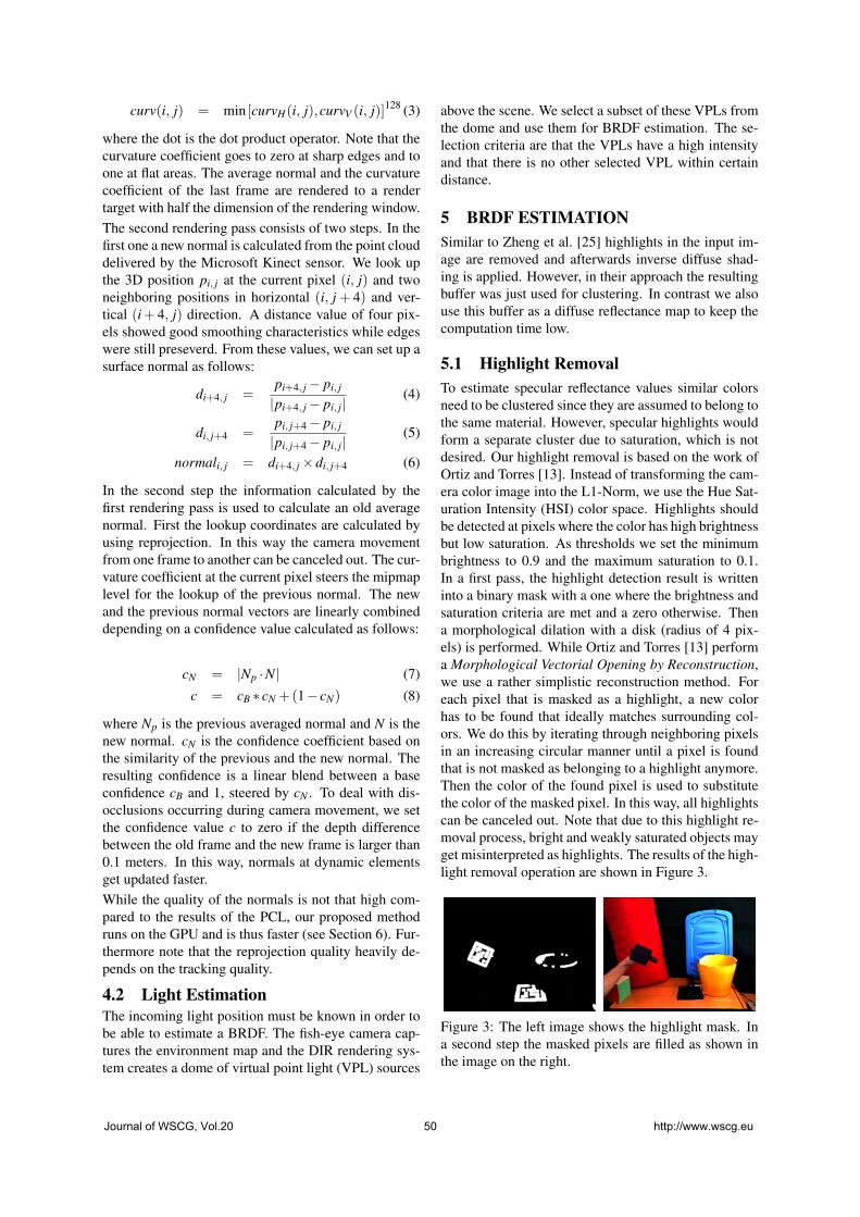
curv(i, j) = min [curvH(i, j),curvV (i, j)]128 (3)

where the dot is the dot product operator. Note that thecurvature coefficient goes to zero at sharp edges and toone at flat areas. The average normal and the curvaturecoefficient of the last frame are rendered to a rendertarget with half the dimension of the rendering window.The second rendering pass consists of two steps. In thefirst one a new normal is calculated from the point clouddelivered by the Microsoft Kinect sensor. We look upthe 3D position pi, j at the current pixel (i, j) and twoneighboring positions in horizontal (i, j + 4) and ver-tical (i+ 4, j) direction. A distance value of four pix-els showed good smoothing characteristics while edgeswere still preseverd. From these values, we can set up asurface normal as follows:

di+4, j =pi+4, j− pi, j

|pi+4, j− pi, j|(4)

di, j+4 =pi, j+4− pi, j

|pi, j+4− pi, j|(5)

normali, j = di+4, j×di, j+4 (6)

In the second step the information calculated by thefirst rendering pass is used to calculate an old averagenormal. First the lookup coordinates are calculated byusing reprojection. In this way the camera movementfrom one frame to another can be canceled out. The cur-vature coefficient at the current pixel steers the mipmaplevel for the lookup of the previous normal. The newand the previous normal vectors are linearly combineddepending on a confidence value calculated as follows:

cN = |Np ·N| (7)c = cB ∗ cN +(1− cN) (8)

where Np is the previous averaged normal and N is thenew normal. cN is the confidence coefficient based onthe similarity of the previous and the new normal. Theresulting confidence is a linear blend between a baseconfidence cB and 1, steered by cN . To deal with dis-occlusions occurring during camera movement, we setthe confidence value c to zero if the depth differencebetween the old frame and the new frame is larger than0.1 meters. In this way, normals at dynamic elementsget updated faster.While the quality of the normals is not that high com-pared to the results of the PCL, our proposed methodruns on the GPU and is thus faster (see Section 6). Fur-thermore note that the reprojection quality heavily de-pends on the tracking quality.

4.2 Light EstimationThe incoming light position must be known in order tobe able to estimate a BRDF. The fish-eye camera cap-tures the environment map and the DIR rendering sys-tem creates a dome of virtual point light (VPL) sources

above the scene. We select a subset of these VPLs fromthe dome and use them for BRDF estimation. The se-lection criteria are that the VPLs have a high intensityand that there is no other selected VPL within certaindistance.

5 BRDF ESTIMATIONSimilar to Zheng et al. [25] highlights in the input im-age are removed and afterwards inverse diffuse shad-ing is applied. However, in their approach the resultingbuffer was just used for clustering. In contrast we alsouse this buffer as a diffuse reflectance map to keep thecomputation time low.

5.1 Highlight RemovalTo estimate specular reflectance values similar colorsneed to be clustered since they are assumed to belong tothe same material. However, specular highlights wouldform a separate cluster due to saturation, which is notdesired. Our highlight removal is based on the work ofOrtiz and Torres [13]. Instead of transforming the cam-era color image into the L1-Norm, we use the Hue Sat-uration Intensity (HSI) color space. Highlights shouldbe detected at pixels where the color has high brightnessbut low saturation. As thresholds we set the minimumbrightness to 0.9 and the maximum saturation to 0.1.In a first pass, the highlight detection result is writteninto a binary mask with a one where the brightness andsaturation criteria are met and a zero otherwise. Thena morphological dilation with a disk (radius of 4 pix-els) is performed. While Ortiz and Torres [13] performa Morphological Vectorial Opening by Reconstruction,we use a rather simplistic reconstruction method. Foreach pixel that is masked as a highlight, a new colorhas to be found that ideally matches surrounding col-ors. We do this by iterating through neighboring pixelsin an increasing circular manner until a pixel is foundthat is not masked as belonging to a highlight anymore.Then the color of the found pixel is used to substitutethe color of the masked pixel. In this way, all highlightscan be canceled out. Note that due to this highlight re-moval process, bright and weakly saturated objects mayget misinterpreted as highlights. The results of the high-light removal operation are shown in Figure 3.

Figure 3: The left image shows the highlight mask. Ina second step the masked pixels are filled as shown inthe image on the right.


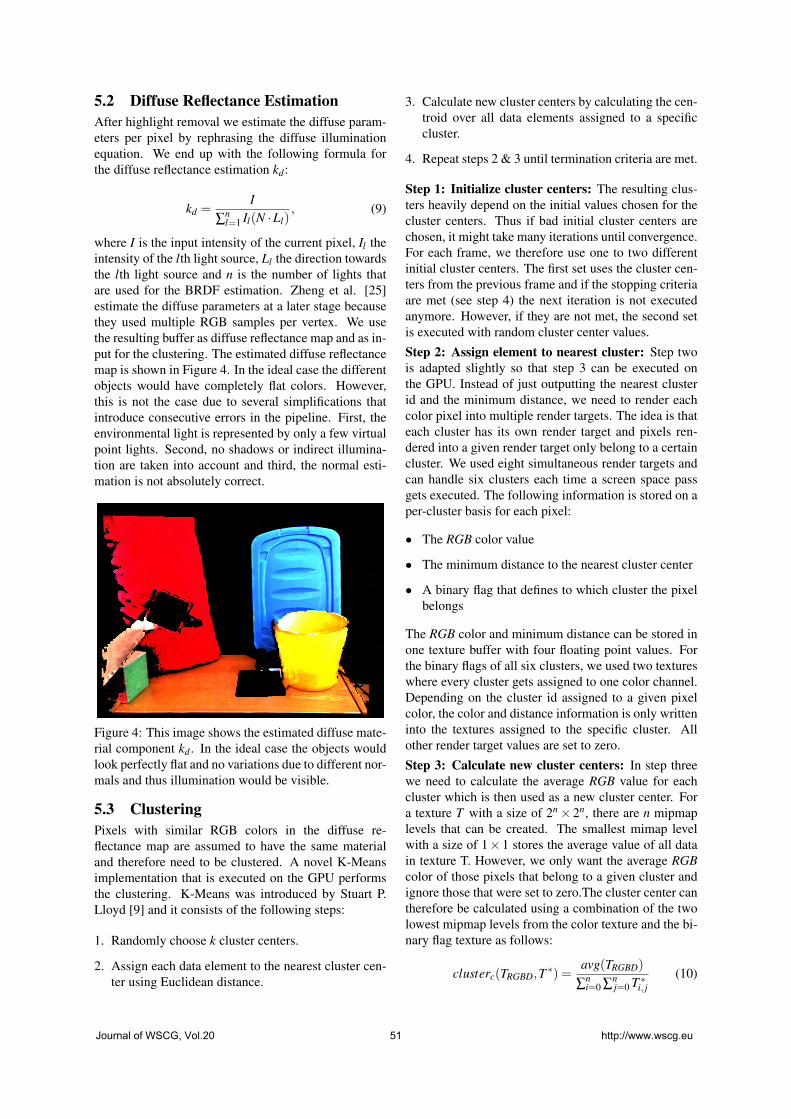
5.2 Diffuse Reflectance EstimationAfter highlight removal we estimate the diffuse param-eters per pixel by rephrasing the diffuse illuminationequation. We end up with the following formula forthe diffuse reflectance estimation kd :

kd =I

∑nl=1 Il(N ·Ll)

, (9)

where I is the input intensity of the current pixel, Il theintensity of the lth light source, Ll the direction towardsthe lth light source and n is the number of lights thatare used for the BRDF estimation. Zheng et al. [25]estimate the diffuse parameters at a later stage becausethey used multiple RGB samples per vertex. We usethe resulting buffer as diffuse reflectance map and as in-put for the clustering. The estimated diffuse reflectancemap is shown in Figure 4. In the ideal case the differentobjects would have completely flat colors. However,this is not the case due to several simplifications thatintroduce consecutive errors in the pipeline. First, theenvironmental light is represented by only a few virtualpoint lights. Second, no shadows or indirect illumina-tion are taken into account and third, the normal esti-mation is not absolutely correct.

Figure 4: This image shows the estimated diffuse mate-rial component kd . In the ideal case the objects wouldlook perfectly flat and no variations due to different nor-mals and thus illumination would be visible.

5.3 ClusteringPixels with similar RGB colors in the diffuse re-flectance map are assumed to have the same materialand therefore need to be clustered. A novel K-Meansimplementation that is executed on the GPU performsthe clustering. K-Means was introduced by Stuart P.Lloyd [9] and it consists of the following steps:

1. Randomly choose k cluster centers.

2. Assign each data element to the nearest cluster cen-ter using Euclidean distance.

3. Calculate new cluster centers by calculating the cen-troid over all data elements assigned to a specificcluster.

4. Repeat steps 2 & 3 until termination criteria are met.

Step 1: Initialize cluster centers: The resulting clus-ters heavily depend on the initial values chosen for thecluster centers. Thus if bad initial cluster centers arechosen, it might take many iterations until convergence.For each frame, we therefore use one to two differentinitial cluster centers. The first set uses the cluster cen-ters from the previous frame and if the stopping criteriaare met (see step 4) the next iteration is not executedanymore. However, if they are not met, the second setis executed with random cluster center values.

Step 2: Assign element to nearest cluster: Step twois adapted slightly so that step 3 can be executed onthe GPU. Instead of just outputting the nearest clusterid and the minimum distance, we need to render eachcolor pixel into multiple render targets. The idea is thateach cluster has its own render target and pixels ren-dered into a given render target only belong to a certaincluster. We used eight simultaneous render targets andcan handle six clusters each time a screen space passgets executed. The following information is stored on aper-cluster basis for each pixel:

• The RGB color value

• The minimum distance to the nearest cluster center

• A binary flag that defines to which cluster the pixelbelongs

The RGB color and minimum distance can be stored inone texture buffer with four floating point values. Forthe binary flags of all six clusters, we used two textureswhere every cluster gets assigned to one color channel.Depending on the cluster id assigned to a given pixelcolor, the color and distance information is only writteninto the textures assigned to the specific cluster. Allother render target values are set to zero.

Step 3: Calculate new cluster centers: In step threewe need to calculate the average RGB value for eachcluster which is then used as a new cluster center. Fora texture T with a size of 2n× 2n, there are n mipmaplevels that can be created. The smallest mimap levelwith a size of 1×1 stores the average value of all datain texture T. However, we only want the average RGBcolor of those pixels that belong to a given cluster andignore those that were set to zero.The cluster center cantherefore be calculated using a combination of the twolowest mipmap levels from the color texture and the bi-nary flag texture as follows:

clusterc(TRGBD,T ∗) =avg(TRGBD)

∑ni=0 ∑

nj=0 T ∗i, j

(10)


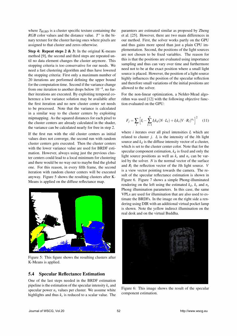
where TRGBD is a cluster specific texture containing theRGB color values and the distance value. T ∗ is the bi-nary texture for the cluster having ones where pixels areassigned to that cluster and zeros otherwise.

Step 4: Repeat steps 2 & 3: In the original K-meansmethod [9], the second and third steps are repeated un-til no data element changes the cluster anymore. Thisstopping criteria is too conservative for our needs. Weneed a fast clustering algorithm and thus have loweredthe stopping criteria: First only a maximum number of20 iterations are performed defining the upper boundfor the computation time. Second if the variance changefrom one iteration to another drops below 10−4, no fur-ther iterations are executed. By exploiting temporal co-herence a low variance solution may be available afterthe first iteration and no new cluster center set needsto be processed. Note that the variance is calculatedin a similar way to the cluster centers by exploitingmipmapping. As the squared distances for each pixel tothe cluster centers are already calculated in the shader,the variance can be calculated nearly for free in step 2.

If the first run with the old cluster centers as initialvalues does not converge, the second run with randomcluster centers gets executed. Then the cluster centerswith the lower variance value are used for BRDF esti-mation. However, always using just the previous clus-ter centers could lead to a local minimum for clusteringand there would be no way out to maybe find the globalone. For this reason, in every fifth frame, the seconditeration with random cluster centers will be executedanyway. Figure 5 shows the resulting clusters after K-Means is applied on the diffuse reflectance map.

Figure 5: This figure shows the resulting clusters afterK-Means is applied.

5.4 Specular Reflectance EstimationOne of the last steps needed in the BRDF estimationpipeline is the estimation of the specular intensity ks andspecular power ns values per cluster. We assume whitehighlights and thus ks is reduced to a scalar value. The

paramters are estimated similar as proposed by Zhenget al. [25]. However, there are two main differences inour method. First, the solver works partly on the GPUand thus gains more speed than just a plain CPU im-plementation. Second, the positions of the light sourcesare not chosen to be fixed variables. The reason forthis is that the positions are evaluated using importancesampling and thus can vary over time and furthermoreneed not to be at the exact position where a small lightsource is placed. However, the position of a light sourcehighly influences the position of the specular reflectionand therefore small variations of the initial positions areallowed to the solver.

For the non-linear optimization, a Nelder-Mead algo-rithm was used [12] with the following objective func-tion evaluated on the GPU:

Fj = ∑i

[Ii−

n

∑l=1

Ilkd(N ·Ll)+ Ilks(V ·Rl)ns]2

(11)

where i iterates over all pixel intensities Ii which arerelated to cluster j. Il is the intensity of the lth lightsource and kd is the diffuse intensity vector of a cluster,which is set to the cluster center color. Note that for thespecular component estimation, kd is fixed and only thelight source positions as well as ks and ns can be var-ied by the solver. N is the normal vector of the surfaceand Rl the reflection vector of the lth light source. Vis a view vector pointing towards the camera. The re-sult of the specular reflectance estimation is shown inFigure 6. Figure 7 shows a simple Phong-illuminatedrendering on the left using the estimated kd , ks and nsPhong illumination parameters. In this case, the sameVPLs are used for illumination that are also used to es-timate the BRDFs. In the image on the right side a ren-dering using DIR with an additional virtual pocket lampis shown. Note the yellow indirect illumination on thereal desk and on the virtual Buddha.

Figure 6: This image shows the result of the specularcomponent estimation.


Figure 7: The left image shows a simple Phong render-ing with the VPLs used for BRDF estimation. In theright image a virtual pocket lamp illuminates the realscene. Note the yellow color bleeding on the real deskand on the virtual Buddha.

6 RESULTSOur computer system consists of an Intel Core 2 QuadCPU at 2.83 GHz and an NVIDIA GeForce GTX 580with 1.5 GB of dedicated video memory. The softwareis running on Windows 7 64-bit and implemented in C#and DirectX 10. Cameras used in this scenario are theMicrosoft Kinect sensor and an IDS uEye camera tocapture the environment map.

6.1 Normal estimationThe two methods used for normal estimation differin quality and computation time. Figure 8 shows aside-by-side comparison of the normal maps. The leftnormal map is calculated with the PCL library and asmoothing factor of 10. The average computation timeis 223 milliseconds. The right normal map is computedwith our proposed method in about 0.57 milliseconds.The PCL based normal map has a lot of holes, shown ingrey color. In our method these holes are filled with thenormals of the neighboring pixels. Even though thesenormals are not correct from a reconstruction point ofview, they reduce the visible artifacts a lot. Furthermorenote that our method produces sharper edges.

Figure 8: Comparison of the two implemented normalestimation methods. Left: Normals estimated using thePCL library [16] in 223 milliseconds. In grey areas nonormal could be estimated by the PCL. Right: Our pro-posed method which takes 0.57 milliseconds.

6.2 K-Means clusteringWe compared the proposed K-Means clustering imple-mentation against the OpenCV library [3]. In the testsetup a data set of 640×480 3-vector elements neededto be clustered. We ran both algorithms 5 times each

time with different initial cluster centers. The inter-action count of each run was set to 20. Note that notemporal coherence was exploited in order to get com-parable results. The measured times include all the 5runs and do not include the setup of the random dataelements. Table 1 shows the execution times in secondsfor 6 and 12 clusters.

Clusters OpenCV GPU K-Means6 3.94s 0.33s

12 7.07s 0.44sTable 1: Shows a comparison between the K-Meansimplementation from OpenCV [3] and our GPU imple-mentation. Both algorithms ran 5 times with 20 itera-tions. Timings show the total execution of the 5 runs inseconds.

Table 2 shows the average iteration count needed for thefirst 50 frames to get below the variance change thresh-old. The columns show the average number of itera-tions for 6 clusters (6C) and for 12 clusters (12C). Therows show if the cluster centers from the previous framewere used (frame−1) or if the cluster centers where cho-sen randomly (random). We set the maximum iterationcount to 30, which was never reached during this test.

Initials Avg. Iter., 6C Avg. Iter., 12Crandom 9.00 11.47frame−1 7.53 6.98

Table 2: Shows the average iteration count whenreusing the cluster centers from the previous frame ortaking random new ones.

6.3 Performance AnalysisThe BRDF estimation pipeline has several steps. Ta-ble 3 gives an overview on the time spent for each one.In this setup, 6 clusters and 4 VPLs were used to ap-proximate the BRDFs.

Stage Time in msNormal Estimation 0.57msHighlight Removal 0.94msDiffuse estimation 0.23msK-Means 39.08msSpecular estimation 315.76msTotal time: 356.58ms

Table 3: Shows the time spent on each pipeline stage.

It clearly shows that the specular estimation step con-sumes by far most of the time. However, if it is possi-ble not only to use a hybrid CPU / GPU version for theoptimization but a complete GPU solution, the perfor-mance should increase a lot.

Two main parameters can be tweaked to get a betterperformance for a given scenario. One parameter is thenumber of materials that are estimated every frame. The


second parameter is the number of virtual point lightsthat are used to approximate the surrounding illumina-tion. Table 4 shows the impact of different cluster andVPL settings with a fixed maximum iteration count forthe specular estimation set to 50.

VPLs 6 Cluster (fps) 12 Cluster (fps)1 3.82 2.418 2.23 1.30

128 1.70 1.01256 0.99 0.59

Table 4: Shows the average fps with different VPL andcluster settings.

We also investigated how the maximum iteration countfor the specular estimation solver reduces the total er-ror. Interestingly, the change of the error was extremelysmall regardless how large the value was set. We thinkthat this has to do with the large amount of pixels thatare available in a cluster. Compared to that the area ofa specular highlight is relatively small and thus correctestimations will only have a small impact on the totalerror.

Furthermore it turned out that the solver has difficultiesin finding appropriate values in certain cases. Some-times there is simply no highlight due to a given VPL.We therefore introduced a threshold value for a maxi-mum error. If the error is too large, we set the specu-lar intensity ks to zero. Another problem could be thatthe solver just has one single point of view per framewhereas Zheng et al. [25] used several photographsto perform a specular estimation. Recently upcomingtechniques, however, promise to greatly improve theproblem of temporal coherent BRDF estimation (seeSection 8).

6.4 Critical ScenarioA critical scenario is shown in Figure 9 on the left. Itshows a blue notebook and a horse made from porcelainplaced on a wooden box. The light is mainly comingfrom the direction of the spotlight partially visible onthe left side of the image, causing specular highlights onthe blue notebook envelope and the wooden box. Thenumber of clusters used in this scenario is six, and fourvirtual point lights are used to estimate the surroundingillumination. The average frame rate is 2.3 fps.

In this scenario, the clustering is not as distinct regard-ing the objects compared to the first scenario. Due tothe highlights caused by the spotlight, the clusteringstep creates different clusters for the same material asshown in Figure 9 (right). Furthermore, the Kinect sen-sor has troubles finding depth values at the white bor-ders of the tracking marker, resulting in holes in theestimations (see Figure 10 (left)). Figure 11 shows theresulting diffuse (left) and specular (right) estimations.The Phong-shaded result is shown in Figure 12.

Figure 9: The left image shows the video input capturedby the Kinect sensor. On the right side, the clusteringresult is shown.

Figure 10: This figure shows the depth values acquiredby the Kinect sensor on the left. Note that it failedto measure depth at the white borders of the track-ing marker and the black fish-eye lense camera. Onthe right side the normal estimation from our proposedmethod is shown.

Figure 11: This figure shows the scene rendered withjust the diffuse estimation (left) and specular estimation(right).

Figure 12: This figure shows the Phong-shaded resultcombining the diffuse and specular estimations.

7 LIMITATIONS AND DISCUSSIONSome limitations of our method are imposed by the Mi-crosoft Kinect sensor, which is a structural light scan-ner. In general, depth values cannot be calculated whenthe light pattern is not recognized by the system. This


happens when objects are very glossy, reflective, trans-parent or absorb too much of the infrared light. Theinfrared pattern also vanishes in direct sunlight, mak-ing the approach unsuitable for outdoor mixed-reality.Furthermore, the border of curved objects is also oftenmissing from the depth map because the projected lightpattern is too distorted there.

Since bright pixels are assumed to be highlights dueto specular reflections, bright and weakly saturated ob-jects may be misinterpreted as highlights. Furthermore,shadows are not considered directly in the current im-plementation. Pixels with a brightness value below acertain threshold are simply discarded.

The K-Means clustering approach uses a variance valueto decide whether further iterations are needed or not.However, there is no estimation of the optimal amountof clusters right now. This number must be specified bythe user in advance and highly depends on the materialsavailable in the scene.

Although temporal coherence is exploited at severalstages in the pipeline, we do not continuously integratealready-seen geometry data. This would be helpful as agiven point in the scene could be viewed under differentviewing angles, leading to a better BRDF estimation,but could also lead to problems with moving objects.

Due to the real-time constraints several simplificationsare introduced. The environmental illumination is ap-proximated using a few virtual point lights, the nor-mals have a lower quality compared to the PCL libraryand the clustering therefore also introduces some errors.All these simplifications lower the quality of the finalBRDF estimation. However, since DIR mainly triesto compute visually plausible results rather than beingphysically correct, the estimated BRDFs should have asufficient quality for mixed-reality scenarios.


We introduced a method to estimate the BRDFs of anaugmented scene at interactive frame rates. The methoddoes not need any precomputation, which makes itsuitable for mixed-reality applications. The MicrosoftKinect sensor serves as a data input source to recon-struct the surrounding environment in the form of ge-ometry and material properties. First, normals are es-timated using a screen-space method exploiting tempo-ral coherence. In the next pipeline stage we proposean adapted K-Means implementation that is speciallytailored towards BRDF estimation and fast executionon the GPU. Temporal coherence is exploited here too,which allows us to find clusters faster than with a con-ventional implementation. The Phong parameter esti-mation is performed using a hybrid CPU / GPU varia-tion of the Nelder-Mead optimization algorithm. The

results demonstrate the feasibility of this method formixed-reality applications.

In the future, we plan to enhance the quality and speedof this BRDF estimation method. It should be possi-ble to gain a lot of speed by porting the Nelder-Meadoptimization method to the GPU. Furthermore, recenttechniques like KinectFusion [6] could greatly enhancethe quality of the BRDF estimation.

9 ACKNOWLEDGEMENTSThis work was supported by a grant from the FFG-Austrian Research Promotion Agency under the pro-gram “FIT-IT Visual Computing” (project no. 820916).Studierstube Tracker is kindly provided by ImaginationComputer Services GmbH.

10 REFERENCES[1] Ronald T. Azuma. A survey of augmented real-

ity. Presence: Teleoperators and Virtual Environ-ments, 6(4):355–385, August 1997.

[2] Samuel Boivin and Andre Gagalowicz. Image-based rendering of diffuse, specular and glossysurfaces from a single image. In Proceedings ofthe 28th annual conference on Computer graph-ics and interactive techniques, SIGGRAPH ’01,pages 107–116, New York, NY, USA, 2001.ACM.

[3] G. Bradski. The OpenCV Library. Dr. Dobb’sJournal of Software Tools, 2000.

[4] Balaji Dhanasekaran and Norman Rubin. A newmethod for gpu based irregular reductions and itsapplication to k-means clustering. In Proceedingsof the Fourth Workshop on General Purpose Pro-cessing on Graphics Processing Units, GPGPU-4,pages 2:1–2:8, New York, NY, USA, 2011. ACM.

[5] Bai Hong-tao, He Li-li, Ouyang Dan-tong,Li Zhan-shan, and Li He. K-means on commod-ity gpus with cuda. In Proceedings of the 2009WRI World Congress on Computer Science andInformation Engineering - Volume 03, CSIE ’09,pages 651–655, Washington, DC, USA, 2009.IEEE Computer Society.

[6] Shahram Izadi, David Kim, Otmar Hilliges,David Molyneaux, Richard Newcombe, Push-meet Kohli, Jamie Shotton, Steve Hodges, DustinFreeman, Andrew Davison, and Andrew Fitzgib-bon. Kinectfusion: real-time 3d reconstructionand interaction using a moving depth camera. InProceedings of the 24th annual ACM symposiumon User interface software and technology, UIST’11, pages 559–568, New York, NY, USA, 2011.ACM.


[7] Martin Knecht, Christoph Traxler, Oliver Mat-tausch, Werner Purgathofer, and Michael Wim-mer. Differential instant radiosity for mixed real-ity. In Proceedings of the 9th IEEE InternationalSymposium on Mixed and Augmented Reality, IS-MAR ’10, pages 99–108, 2010.

[8] You Li, Kaiyong Zhao, Xiaowen Chu, and JimingLiu. Speeding up k-means algorithm by gpus. InProceedings of the 2010 10th IEEE InternationalConference on Computer and Information Tech-nology, CIT ’10, pages 115–122, Washington,DC, USA, 2010. IEEE Computer Society.

[9] S. Lloyd. Least squares quantization in PCM.IEEE Transactions on Information Theory,28(2):129–137, March 1982.

[10] Bruno Mercier, Daniel Meneveaux, and AlainFournier. A framework for automatically recov-ering object shape, reflectance and light sourcesfrom calibrated images. International Journal ofComputer Vision, 73:77–93, June 2007.

[11] Microsoft. Kinect sdk:research.microsoft.com/en-us/um/redmond/projects/kinectsdk/.

[12] J. A. Nelder and R. Mead. A simplex methodfor function minimization. Computer Journal,7:308–313, 1965.

[13] F Ortiz and F Torres. Automatic detection andelimination of specular reflectance in color im-ages by means of ms diagram and vector con-nected filters. IEEE Transactions on Systems Manand Cybernetics Part C Applications and Reviews,36(5):681–687, 2006.

[14] Saulo A. Pessoa, Guilherme de S. Moura, Veron-ica Teichrieb, and Judith Kelner. Photorealisticrendering for augmented reality: A global illumi-nation and brdf solution. In Virtual Reality, pages3–10, 2010.

[15] Bui Tuong Phong. Illumination for computer gen-erated pictures. Communications of the ACM,18:311–317, June 1975.

[16] Radu Bogdan Rusu and Steve Cousins. 3D ishere: Point Cloud Library (PCL). In IEEE Inter-national Conference on Robotics and Automation(ICRA), Shanghai, China, May 9-13 2011.

[17] Yoichi Sato, Mark D. Wheeler, and KatsushiIkeuchi. Object shape and reflectance model-ing from observation. In Proceedings of the 24thannual conference on Computer graphics andinteractive techniques, SIGGRAPH ’97, pages379–387, New York, NY, USA, 1997. ACMPress/Addison-Wesley Publishing Co.

[18] Daniel Scherzer, Stefan Jeschke, and MichaelWimmer. Pixel-correct shadow maps with tem-poral reprojection and shadow test confidence. In

Jan Kautz and Sumanta Pattanaik, editors, Ren-dering Techniques 2007 (Proceedings Eurograph-ics Symposium on Rendering), pages 45–50. Eu-rographics, Eurographics Association, June 2007.

[19] Richard Szeliski. Rapid octree constructionfrom image sequences. CVGIP: Image Underst.,58:23–32, July 1993.

[20] Gregory J. Ward. Measuring and modelinganisotropic reflection. In Proceedings of the 19thannual conference on Computer graphics andinteractive techniques, SIGGRAPH ’92, pages265–272, New York, NY, USA, 1992. ACM.

[21] Ren Wu, Bin Zhang, and Meichun Hsu. Clus-tering billions of data points using gpus. In Pro-ceedings of the combined workshops on UnCon-ventional high performance computing workshopplus memory access workshop, UCHPC-MAW’09, pages 1–6, New York, NY, USA, 2009. ACM.

[22] S. Xu and A. M. Wallace. Recovering surfacereflectance and multiple light locations and in-tensities from image data. Pattern Recogn. Lett.,29:1639–1647, August 2008.

[23] Yizhou Yu, Paul Debevec, Jitendra Malik, andTim Hawkins. Inverse global illumination: re-covering reflectance models of real scenes fromphotographs. In Proceedings of the 26th annualconference on Computer graphics and interac-tive techniques, SIGGRAPH ’99, pages 215–224,New York, NY, USA, 1999. ACM Press/Addison-Wesley Publishing Co.

[24] M. Zechner and M. Granitzer. Accelerating k-means on the graphics processor via cuda. InIntensive Applications and Services, 2009. IN-TENSIVE ’09. First International Conference on,pages 7 –15, april 2009.

[25] Zuoyong Zheng, Lizhuang Ma, Zhong Li, andZhihua Chen. Reconstruction of shape and re-flectance properties based on visual hull. In Pro-ceedings of the 2009 Computer Graphics Inter-national Conference, CGI ’09, pages 29–38, NewYork, NY, USA, 2009. ACM.


A Hierarchical Splitting Scheme to Reveal Insight intoHighly Self-Occluded Integral Surfaces

Andrea Brambilla

University of BergenBergen, Norway

[email protected]

Ivan Viola


[email protected]

Helwig Hauser


[email protected]

AbstractIn flow visualization, integral surfaces are of particular interest for their ability to describe trajectories of masslessparticles. In areas of swirling motion, integral surfaces can become very complex and difficult to understand.Taking inspiration from traditional illustration techniques, such as cut-aways and exploded views, we propose asurface analysis tool based on surface splitting and focus+context visualization. Our surface splitting scheme ishierarchical and at every level of the hierarchy the best cut is chosen according to a surface complexity metric. Inorder to make the interpretation of the resulting pieces straightforward, cuts are always made along isocurves ofspecific flow attributes. Moreover, a degree of interest can be specified, so that the splitting procedure attempts tounveil the occluded interesting areas. Through practical examples, we show that our approach is able to overcomethe lack of understanding originating from structural occlusion.

Keywords: flow visualization, illustrative visualization, occlusion management.

1 INTRODUCTION

Flow phenomena are present at very different scales inour world, and they influence many aspects of our dailylife: winds and water currents determine weather andclimate, the stream of air around vehicles affects theirspeed and stability, the flow of blood in our vesselsis fundamental for our good health condition. Under-standing their behaviour is therefore highly relevant inmany fields, and several years of research in flow visual-ization have produced a wide set of tools to accomplishthis difficult task [PVH+02].

Flow behaviour can be analyzed from different pointsof view, according to the specific needs of the user.In particular, field experts are often interested in thetrajectories of massless particles that are advected bythe flow, which are commonly visualized using integralcurves. Specifically, a path line represents the trajectoryof a massless particle seeded from a specific starting lo-cation. Similarly, a path surface conveys the trajecto-ries of a set of particles seeded along a 1D curve.

Integral surfaces are very expressive, but have a ma-jor downside: in correspondence with areas of swirling


motion, like vortices and eddies, they tend to fold andtwist, becoming very intricate and difficult to under-stand (Figures 2, 7, and 8). In this paper, we presenta procedure which aims at solving this issue using tech-niques from traditional handcrafted illustration, such ascutting and splitting (Figure 1). These concepts havebeen frequently applied in medical visualization scenar-ios, but their application in the context of flow visual-ization has been limited. This is probably due to thefact that identifying well defined objects in flow data isvery challenging. An overview of related approaches ispresented in Section 2.

We propose a general surface splitting methodologybased on two main concepts: a cut space defines pos-sible ways to split a surface so that the resulting pieceshave a clear meaning, while a complexity measure de-

Figure 1: (left) Example of a cut-away view in a tradi-tional illustration by Leonardo da Vinci [dV11]. (right)Illustration of a stream surface with cuts and clippingplanes, by Abraham and Shaw [AS82].


termines a degree of occlusion at every point on the sur-face. We iteratively split the surface according to a cutfrom the cut space, so that the complexity is reducedthe most. To improve the versatility of our approach,we allow the user to specify a degree of interest (DoI)function over the surface, which is combined with thecomplexity measure when the cut is chosen. Details onthe splitting algorithm can be found in Section 3.

The resulting pieces of the surface are presented in atree-like structure, and pieces of interest can be visual-ized either separated from the rest of the flow structure,or with a semi-transparent context (Figure 2). We usea stream surface extracted from the ABC flow to illus-trate our method. We then show the application of ourmethod on two datasets from application fields. Section4 describes this process and provides a short discussionon timings and computational complexity.

Compared to the current state of the art, the main con-tributions of our work are:

• a general methodology for the design of surface cuts

• the first (to the best of our knowledge) splitting ap-proach for integral surfaces

• a novel complexity measure for surfaces, which cantake into account the importance of the data

• a helpful tool for the analysis of stream surfaces.

2 RELATED WORKAccording to one of the most well-known categoriza-tions [PVH+02], flow visualization techniques can beclassified in four groups: direct, texture-based, geomet-ric and feature-based visualization. Our work is relatedto the third category. Geometric approaches in fact aimat visualizing flow data through integral structures. Themost common types of 1D integral curves are

• streamlines: curves tangent to the flow field in everypoint at a specific time instant

• path lines: the trajectories of massless particles insteady or unsteady flows

• streak lines: formed by particles continuously re-leased in the velocity field from a specific location

• time lines: curves connecting a set of particles si-multaneously released along a seeding curve.

These concepts can be extended to 2D and 3D, obtain-ing surfaces and volumes respectively. Interested read-ers can refer to to the excellent survey by McLoughlinet al. [MLP+10] for more details.

Flow datasets are often multidimensional, multivari-ate and very dense. In these cases, traditional flow vi-sualization approaches often suffer from cluttering and

Figure 2: A stream surface extracted from a simulationof a gas leak on an oil platform. Top image: the initialsurface with the position of the leak (red arrow) and theobjects placed in the room (gray structures). Bottomthree images: the surface pieces obtained after two cuts.

occlusion problems, which are commonly addressedwith simple techniques, such as clipping, slicing or con-ventional transparency. A novel visualization researchdirection, called illustrative visualization [RBGV08],aims at solving these perceptual issues taking inspira-tion from traditional handcrafted illustrations.

Cutting an object to reveal its inner parts is a com-mon approach in illustrative visualization, and it can beapplied in different ways. A typical example are ex-ploded views: Li et al. [LACS08] apply this conceptto show how composite objects are built. Ruiz et al.[RVB+08] suggest to subdivide a volume into orientedslabs according to the amount of information conveyed.More recently, Karpenko et al. [KLMA10] propose an


Surface Pieces Importance

Cut Space

Cut Selection and Splitting

Complexity Measure

Visualization and User Interaction

Figure 3: An overview of the splitting algorithm.

explosion strategy for mathematical surfaces based onsurface symmetries.

If an importance measure is defined over the data, thevisualization could be guided by these values. For in-stance, Viola et al. [VKG05] describe a volume render-ing technique which discards the low-importance (con-text) portions of the volume occluding the relevant ones(focus). Similarly, Bruckner and Gröller [BG06] pro-pose an exploded view strategy, where the occludingcontext is not discarded, but displaced in an intuitiveway. Bruckner and Gröller also presented a conciseoverview of basic focus+context approaches in 2005[BG05]. An effective combination of splitting and fo-cus+context visualization has been presented by Bala-banian et al. [BVG10]. Their work is focused on med-ical volumetric data and the splitting is based on a pre-computed segmentation. The resulting pieces are dis-played in a navigable graph, which was the main inspi-ration for our subdivision hierarchy.

Illustrative principles have been mainly adopted inmedical visualization, but, especially in recent years,they are spreading to other contexts as well. For flow vi-sualization, a fair number of illustrative techniques havebeen proposed [BCP+12]. The self-occlusion problemof integral surfaces have been initially addressed in anearly paper by Löffelman et al. [LMGP97]: their ap-proach cuts away pieces of the surface, generating re-sults similar to the illustrations by Abraham and Shaw(Figure 1, right).

Two relevant focus+context approaches have beenproposed in 2005 and 2007 respectively. The Eyeletparticle tracing approach [WS05] shows integral sur-faces passing through a specific point of high inter-est. In contrast, the technique by Correa et al. [CSC07]computes a deformation of the low importance data sothat the focus is not occluded. More recently, two note-

worthy approaches [HGH+10, BWF+10] propose toaddress the self-occlusion problem of stream surfacesthrough a smart use of transparency. They also adoptad-hoc shading and texturing in order to improve depthperception and convey local flow behaviour.

Outside the context of flow visualization, similar is-sues have been investigated in connection with isosur-faces of scalar volumes. In this field, many techniqueshave been proposed (the contour spectrum [BPS97],Reeb graphs [FTAT00] and similarity maps [BM10],just to mention a few), but their applicability to flowdata is still uncertain.

3 SURFACE SPLITTINGIn the case of 3D flow fields, a stream surface is a 2Dmanifold. Our algorithm assumes it is represented by atriangular mesh. The mesh is defined by a set of pointsP ⊂ R3, and a set of triangles T . Flow data is sampledat each point in P: for instance, the velocity at a pointp ∈ P is v(p). Linear interpolation is used to determineflow attributes over the triangles.

The structure of our general splitting framework issummarized in Figure 3. The splitting process is itera-tive and begins when the user requests to generate a cut.At this point two independent steps are performed: thecomplexity measure cpx(·) is computed for every p∈ Pand a set of potential cuts (the cut space) is generated.The complexity measure can take into account a degreeof interes doi(·) defined over the points.

Notice that, regardless of how a cut is defined, it is al-ways possible to reduce it to a cutting curve on the sur-face, i.e., the line along which a cut would split the sur-face. Therefore, for every potential cut, the complexityvalues are integrated along the corresponding cuttingcurve, and the cut with the highest overall complexityCPX(·) is chosen. The surface is finally split along thechosen cut, and the resulting pieces are inserted in thesubdivision hierarchy (a binary tree) as children of theinitial surface. The user can explore the tree and possi-bly request a new cut, executing again the whole proce-dure over all the leaves of the tree.

This is a general scheme to design effective splittingapproaches, every step of the process can be customizedaccording to the kind of surface of interest and to thedesired results. In the following, we describe all theoperations in detail and explain how we have tuned thisframework in order to effectively split stream surfaces.

3.1 The Complexity MeasureThe complexity measure cpx(·) is a function that asso-ciates a certain complexity value to every p ∈ P. Themeaning of this value depends on how the function iscomputed. Since our goal is to reduce occlusion, we de-fine the complexity so that cpx(p) represents how muchp conceals the rest of the surface. However, to accu-rately evaluate such a measure, all the possible view-


3 21

2

1

0

0

*

Figure 4: The typical visualization scenario. The cam-era (in green) moves circularly around the surface (inblue). The complexity measure, shown for a few points,is computed counting the intersections between the sur-face and the point-to-pivot line segment (in red).

points should be considered, which is too expensive toallow for user interaction. We opted for an approxi-mation based on a simple consideration: datasets arefrequently shown using a polar view, with the cameramoving circularly around a pivoting point o placed atthe center of the object of interest. Thus, we considerthe amount of occlusion generated by p when the cam-era is looking directly at it, i.e., when it lies exactlybetween the camera and the pivot. Let r = o−p be thevector from p to o, we set

cpx(p) = ‖X‖ (1)

where X is the set of intersection points between r andthe surface mesh.

There is however an issue to solve: if r is tangentto portions of the surface, cpx(p) can easily degenerate(Figure 4, middle red line). To attenuate this effect, weadditionally take into account the angle between r andthe surface normals nrm(·) at the intersection points

cpx(p) = ∑x∈X

∣∣∣∣nrm(x) · r‖r‖

∣∣∣∣ (2)

Including the importance measure is straightforward.We have to modify the complexity function so that, ifthe occluded area is highly important, the complexity ofthe occluding points has to be high as well. We assumethat the degree of interest function is a generic attributedoi(·) defined for every p ∈ P:

cpx(p) = ∑x∈X

doi(x)∣∣∣∣nrm(x) · r

‖r‖

∣∣∣∣ (3)

For the moment, we assume that doi(·) is defined at thebeginning and never changes during the analysis phase;inclusion of interactive brushing techniques will be in-vestigated in the future.

3.2 The Cut SpaceThe set of potential cuts can be defined in several ways.For example, Karpenko et al. [KLMA10] define it asa set of planes orthogonal to an explosion axis. Li etal. [LACS08], instead, define cuts as the boundaries ofthe components of the initial object. The fundamen-tal requirement is that the elements of the cut spacesplit the surface in meaningful and easily understand-able pieces. In the case of flow data, defining such aspace is not trivial: arbitrary cuts with a fixed geome-try, such as planes or cubes, can reduce cluttering butthe resulting pieces would be of difficult interpretation.Moreover, integral surfaces are not aggregate objects,so their building blocks cannot be easily defined.

One of the main characteristics of stream surfaces isthat they have a semantically meaningful parametriza-tion: every point on the surface lies in fact on the trajec-tory of one of the advected particles. Therefore, everypoint p can be associated with two parameters

• the seeding point s(p): the location where the re-lated particle has been seeded, expressed as a per-centage of the length of the seeding line

• the integration time t(p): the time needed by the re-lated particle to travel from the seeding point to p.

The isocurves of these two attributes are actuallystreamlines and time lines respectively. When a streamsurface is split along one of these curves, the resultingpieces are stream surfaces as well. Therefore we definethe cut space as the set of streamlines and time lines,corresponding to regular samples of their value ranges.

Notice that s(·) and t(·) are bijections. Therefore, inparameter coordinates, the surface is simply a portionof the 2D space, and the cuts become straight line seg-ments parallel to the axis (Figure 5, left).

To improve the versatility of our system, we also pro-vide the possibility of considering isocurves of arbitraryparameters. An example is shown in Figure 5, right,where the integration time has been replaced by the in-tegration length, i.e., the arc length of the trajectory.

Figure 5: A stream surface from the ABC flow shownin parameter space, with three cuts. (left) parametriza-tion given by the seeding point and the integration time.(right) The integration distance is used instead of the in-tegration time.


Figure 6: The tree obtained cutting two times a streamsurface from the ABC flow. The first cut is made alonga streamline (in green) and the second one along a timeline (in yellow).

3.3 Surface CuttingGiven the space of potential cuts, we have to determinewhich cut would result in the most effective reductionof structural occlusion. Recall that the complexity mea-sure has been already evaluated for every point on thesurface. Then, we define the overall complexity CPX(·)of a cut Ω as the average complexity along it:

CPX(Ω) =1

length(Ω)

∫x∈Ω

cpx(x) (4)

An approximation of this integral is computed in the 2Dparameter space as explained in Section 5.

The final step consists in selecting the cut with thehighest overall complexity and using it to split the sur-face. However, the proposed complexity measure doesnot take into account the size of the resulting pieces.Usually, removing a relatively small piece from a largesurface does not lead to a significant occlusion reduc-tion. Therefore, we bias the cut selection in two ways:firstly we discard cuts that are shorter than a specifiedthreshold. Then we adjust the complexity of the cutsaccording to the area ratio of the resulting pieces.

After the optimal cut is selected, the stream surface issplit and the resulting pieces are inserted in the subdivi-sion hierarchy as children of the split surface. We neverhad to modify the mesh structure to get well definedcuts, but, for low resolution models, a triangle splittingprocedure may be required.

Notice that, if the surface has already been subdi-vided, the cut evaluation is performed on all the current

pieces. Then, only the piece with the highest complex-ity cut is split.

The subdivision hierarchy is presented to the user asin Figure 6. At every node of the tree, the correspondingsurface piece is displayed. The user can interact withthis view to get an overall idea of the generated cuts.Then a single piece can be selected and visualized ina separate view in a focus+context manner: the pieceof interest is rendered completely opaque while the restof the surface can be optionally shown with variabletransparency, as in Figure 7, bottom row.

4 DEMONSTRATIONIn order to show the capabilities of our visualizationsystem, we used it to explore stream surfaces extractedfrom one synthetic and two CFD datasets. In the fol-lowing, we give details about the considered datasetsand discuss the most relevant results.

4.1 ABC flowThe ABC flow is a synthetic dataset well known in flowvisualization [DFH+86]. It is defined as a vector fieldover the domain [0,2π]3 ∈ R3 and the velocities aregiven by:

v(x,y,z) =

Asin(z)+Bcos(y)Bsin(x)+C cos(z)C sin(y)+Acos(x)

(5)

which are solutions of the Euler equation for inviscidflow. We set A = sqrt(3), B = sqrt(2), and C = 1. An

Figure 7: (top left) Overview of the ABC flow dataset,with a stream surface we extracted. (top right) A slicefrom the ABC flow where the velocity is depicted withglyphs. (bottom) The two pieces obtained by cuttingthe surface once, using the magnitude of the velocity asDoI. The complementary pieces of surface are shownsemi-transparent to provide the context.


Figure 8: CFD simulation of a fluid flow in a box. The leftmost picture gives an overview of the dataset with theextracted stream surface. The other pictures show the surface after the first and the second cut.

overview of the dataset is given in Figure 7: the topleft picture shows the boundaries of the domain and oneexpressive stream surface we extracted; the top rightpicture depicts the flow behaviour on the z = π plane.

The stream surface under consideration has two al-most overlapping areas in the bottom part, one on theleft and one on the right. If we do not take into accountany DoI, we expect that the splitting procedure sepa-rates these areas of the surface. That is exactly whathappens after the first cut in Figure 6. The situation iseven more interesting if we set the DoI proportional tothe velocity magnitude: as can be seen in Figure 7, bot-tom row, the first cut is made so that the high velocityareas at the bottom right are clearly visible.

4.2 Flow in a boxThe second dataset we investigated using our frame-work is a CFD simulation of fluid flow in a box-likestructure. As illustrated in Figure 8, left, the inlet isplaced on the far upper side, while the outlet is situ-ated on the front plane, adjacent to both the right andthe bottom wall. Vortices and eddies are expected closeto where the inlet connects to the box, so we seeded astream surface in that area.

The surface adequately conveys the rotational be-haviour, but, due to self occlusion, it is very difficultto understand what is actually happening in the innerpart. After applying a first cut, the more stable pieceof the surface is separated from the swirling one, effec-tively showing the inner vortex (Figure 8, second andthird pictures from the left). Requesting an additionalcut, the twisting piece is split again (Figure 8, fourthand fifth pictures). This exposes the inner part of thesurface and let us analyze the swirling behaviour closeto the core of the vortex. Achieving the same goals withtraditional techniques, such as transparency or clipping,would have been substantially more difficult.

4.3 Gas leak simulationThe last dataset is a CFD simulation of a gas leak ina closed room on an oil platform. An overview of thearchitectural structure is given in Figure 2, top. The

left and right walls are semi-permeable and, in normalcondition, there is an almost constant flow of air in theroom, from right to left. After the gas begins leaking, itmixes with air and affects the regular air flow.

The gas/air mixture is described by the equivalenceratio (ER), which roughly represents the ratio betweenfuel and oxidant. In our scenario, where ER is between0.5 and 1.7 the mixture is flammable, while ER greaterthan 1.7 means that the mixture cannot burn but it isnot breathable either. One of the aspects of interest inthis dataset is identifying the locations where there ismixing between air and gas.

We seeded a stream surface in front of the gas leakand observed its behaviour. Two vortices can be eas-ily identified in the top part of the spatial domain and,given their proximity to the leak, they may have astrong influence on the mixing process. Our splittingapproach, already at the first cut, correctly separates thebranch with the two vortices from the rest of the sur-face (Figure 2). Figure 9 shows the effect of subsequentcuts: the swirling areas of the surface are effectively

Figure 9: Pieces of stream surface extracted from thegas leak dataset. Iteratively cutting the surface with theproposed approach allows for an easy investigation ofthe inner areas of the vortices.


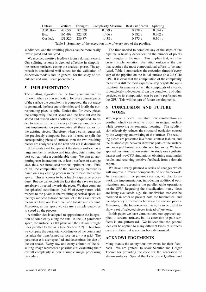
Dataset Vertices Triangles Complexity Measure Best Cut Search SplittingABC flow 42 050 82 329 0.379 s 0.278 s 0.094 sBox 166 499 322 931 1.466 s 0.582 s 0.362 sGas leak 151 320 286 874 1.438 s 0.475 s 0.301 s

Table 1: Summary of the execution time of every step of the pipeline.

subdivided, and the resulting pieces can be more easilyinvestigated and analyzed.

We received positive feedback from a domain expert.Our splitting scheme is deemed effective in simplify-ing stream surfaces, easing the analysis phase. The ap-proach is considered well suited for the validation ofdispersion models and, in general, for the study of tur-bulence and small scale phenomena.

5 IMPLEMENTATIONThe splitting algorithm can be briefly summarized asfollows: when a cut is requested, for every current pieceof the surface the complexity is computed, the cut spaceis generated, the best cut is identified and finally the cor-responding piece is split. Notice that for every piece,the complexity, the cut space and the best cut can bestored and reused when another cut is requested. In or-der to maximize the efficiency of our system, the cur-rent implementation precomputes all these values forthe existing pieces. Therefore, when a cut is requested,the previously computed best cut is used to split thecorresponding piece of surface, then the two resultingpieces are analyzed and the next best cut is determined.

If the mesh used to represent the stream surface has alarge number of vertices and triangles, determining thebest cut can take a considerable time. We aim at sup-porting user interaction on, at least, surfaces of averagesize, thus, we introduced various optimizations. Firstof all, the computation of the complexity measure isbased on a ray casting process in the three-dimensionalspace. This is known to be a highly expensive proce-dure. But we can exploit the fact that the rays we traceare always directed towards the pivot. We then computethe spherical coordinates (r,φ ,θ) of every vertex withrespect to the pivot: in the resulting spherical space, allthe rays we need to trace are parallel to the r axis, whichmeans we have one less dimension to take into account.Moreover, in this space we can use a simple quad-treeto speed up the process.

A similar idea is adopted to approximate the integra-tion of complexity along the cuts. In the 2D parameterspace, the surface is a flat plane and the cuts are straightlines parallel to the axis (see Section 3.2). Thereforewe compute the parameter coordinates of the points andrasterize the transformed surface on a n× n grid. Theparameter n is user specified and determines the size ofthe cut space. Every row and every column of the re-sulting image represents a possible cut: evaluating theiroverall complexity is now a simple image processingprocedure.

The time needed to complete any of the steps of thepipeline is heavily dependent on the number of pointsand triangles of the mesh. This implies that, with thecurrent implementation, the initial surface is the onethat requires the most computational efforts to be ana-lyzed. Table 1 summarizes the execution times of everystep of the pipeline on the initial surface on a 2.8 GHzCPU. It is clear that the computation of the complexitymeasure is still the most expensive step despite the opti-mization. As a matter of fact, the complexity of a vertexis completely independent from the complexity of othervertices, so its computation can be easily performed onthe GPU. This will be part of future developments.


We propose a novel illustrative flow visualization al-gorithm which can iteratively split an integral surfacewhile preserving its semantic meaning. The subdivi-sion effectively reduces the structural occlusion causedby the wrapping and twisting of the surface. The result-ing pieces are presented in a focus+context fashion, andthe relationships between different parts of the surfaceare conveyed through a subdivision hierarchy. We haveapplied our visualization system to study one syntheticdataset and two CFD simulations, obtaining meaningfulresults and receiving positive feedback from a domainexpert.

We have already planned a series of changes whichwill improve different components of our framework.As mentioned in the previous section, we plan to re-work the implementation, introducing additional opti-mizations and executing the parallelizable operationson the GPU. Regarding the visualization, many ideasare being evaluated: e.g., the subdivision tree can bemodified in order to present both the hierarchical andthe adjacency information between the surface pieces.Moreover, in the focus+context view, it can be useful toshow a set of selected pieces instead of just one.

In this paper we have demonstrated our approach ap-plied to stream surfaces, but its extension to path sur-faces is straightforward. We believe that the generalidea can be applied to many different kinds of surfacesonce a suitable cut space has been determined.

ACKNOWLEDGEMENTSMany thanks the anonymous reviewers for their feed-back. We are grateful to Maik Schulze and HolgerTheisel for providing the code for the generation ofstream surfaces. Special thanks to Josué Quilliou and


GexCon AS for providing the gas leak dataset. Thanksalso to AVL for provinding the dataset of the flow in abox. This report has been worked out within the scopeof the SemSeg project and we acknowledge the finan-cial support of the Future and Emerging Technologies(FET) programme within the Seventh Framework Pro-gramme for Research of the European Commission, un-der FET-Open grant number 226042.

REFERENCES

[AS82] R. Abraham and C. D. Shaw. Dynamics–the geometry of behavior. Aerial Press,1982.

[BCP+12] A. Brambilla, R. Carnecky, R. Peikert,I. Viola, and H. Hauser. Illustrative flowvisualization: State of the art, trends andchallenges. In Eurographics 2012 State-of-the-Art Reports, pages 75–94, 2012.

[BG05] S. Bruckner and M. E. Gröller. Vol-umeshop: an interactive system for directvolume illustration. In IEEE Visualization2005, pages 671–678, 2005.

[BG06] S. Bruckner and M. E. Gröller. Explodedviews for volume data. IEEE Transactionson Visualization and Computer Graphics,12(5):1077–1084, 2006.

[BM10] S. Bruckner and T. Möller. Isosurface sim-ilarity maps. Computer Graphics Forum,29(3):773–782, 2010.

[BPS97] C. L. Bajaj, V. Pascucci, and D. R.Schikore. The contour spectrum. In IEEEVisualization ’97, pages 167–ff., 1997.

[BVG10] J.-P. Balabanian, I. Viola, and M. E.Gröller. Interactive illustrative visualiza-tion of hierarchical volume data. In Pro-ceedings of Graphics Interface 2010, pages137–144, 2010.

[BWF+10] S. Born, A. Wiebel, J. Friedrich,G. Scheuermann, and D. Bartz. Illus-trative stream surfaces. IEEE Transactionson Visualization and Computer Graphics,16:1329–1338, 2010.

[CSC07] C. D. Correa, D. Silver, and Min Chen.Illustrative deformation for data explo-ration. IEEE Transactions on Visualiza-tion and Computer Graphics, 13(6):1320–1327, 2007.

[DFH+86] T. Dombre, U. Frisch, M. Henon, J. M.Greene, and A. M. Soward. Chaoticstreamlines in the abc flows. Journal ofFluid Mechanics, 167:353–391, 1986.

[dV11] L. da Vinci. The babe in the womb, c.1511.

[FTAT00] I. Fujishiro, Y. Takeshima, T. Azuma, andS. Takahashi. Volume data mining using3d field topology analysis. IEEE ComputerGraphics and Applications, 20(5):46–51,2000.

[HGH+10] M. Hummel, C. Garth, B. Hamann, H. Ha-gen, and K. I. Joy. Iris: Illustrative ren-dering for integral surfaces. IEEE Trans-actions on Visualization and ComputerGraphics, 16:1319–1328, 2010.

[KLMA10] O. Karpenko, W. Li, N. Mitra, andM. Agrawala. Exploded view diagrams ofmathematical surfaces. IEEE Transactionson Visualization and Computer Graphics,16(6):1311–1318, 2010.

[LACS08] W. Li, M. Agrawala, B. Curless, andD. Salesin. Automated generation of inter-active 3d exploded view diagrams. pages101:1–101:7, 2008.

[LMGP97] H. Löffelmann, L. Mroz, M. E. Gröller,and W. Purgathofer. Stream arrows: En-hancing the use of streamsurfaces for thevisualization of dynamical systems. TheVisual Computer, 13:359–369, 1997.

[MLP+10] T. McLoughlin, R. S. Laramee, R. Peikert,F. H. Post, and M. Chen. Over two decadesof integration-based, geometric flow vi-sualization. Computer Graphics Forum,29(6):1807–1829, 2010.

[PVH+02] F. H. Post, B. Vrolijk, H. Hauser,R. Laramee, and H. Doleisch. Featureextraction and visualization of flow fields.In Eurographics 2002 State-of-the-Art Re-ports, pages 69–100, 2002.

[RBGV08] P. Rautek, S. Bruckner, M. E. Gröller, andI. Viola. Illustrative visualization: newtechnology or useless tautology? ACMSIGGRAPH Computer Graphics Quar-terly, 42:4:1–4:8, 2008.

[RVB+08] M. Ruiz, I. Viola, I. Boada, S. Bruckner,M. Feixas, and M. Sbert. Similarity-basedexploded views. In Smart Graphics, vol-ume 5166, pages 154–165. 2008.

[VKG05] I. Viola, A. Kanitsar, and M. E. Gröller.Importance-driven feature enhancement involume visualization. IEEE Transactionson Visualization and Computer Graphics,11(4):408–418, 2005.

[WS05] A. Wiebel and G. Scheuermann. Eyeletparticle tracing - steady visualization of un-steady flow. In IEEE Visualization 2005,pages 607–614, 2005.


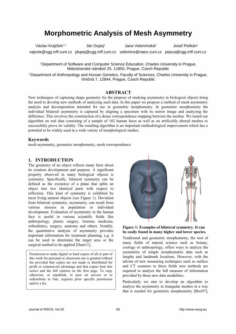
Morphometric Analysis of Mesh Asymmetry

Václav Krají ekč 1,2

[email protected]

Ján Dupej1

[email protected]

Jana Velemínská2

[email protected]

Josef Pelikán1

[email protected]

1 Department of Software and Computer Science Education, Charles University in Prague, Malostranské nám stí 25, 11800, Prague, Czech Republicě

2 Department of Anthropology and Human Genetics, Faculty of Sciences, Charles University in Prague, Vini ná 7, 12844, Prague, Czech Republicč

ABSTRACTNew techniques of capturing shape geometry for the purpose of studying asymmetry in biological objects bring the need to develop new methods of analyzing such data. In this paper we propose a method of mesh asymmetry analysis and decomposition intended for use in geometric morphometry. In geometric morphometry the individual bilateral asymmetry is captured by aligning a specimen with its mirror image and analyzing the difference. This involves the construction of a dense correspondence mapping between the meshes. We tested our algorithm on real data consisting of a sample of 102 human faces as well as on artificially altered meshes to successfully prove its validity. The resulting algorithm is an important methodological improvement which has a potential to be widely used in a wide variety of morphological studies.

Keywordsmesh asymmetry, geometric morphometry, mesh correspondence

1. INTRODUCTIONThe geometry of an object reflects many facts about its creation development and purpose. A significant property observed in many biological objects is symmetry. Specifically, bilateral symmetry can be defined as the existence of a plane that splits an object into two identical parts with respect to reflection. This kind of symmetry is exhibited by most living natural objects (see Figure 1). Deviation from bilateral symmetry, asymmetry, can result from various stresses in population or individual development. Evaluation of asymmetry in the human face is useful in various scientific fields like anthropology, plastic surgery, forensic medicine, orthodintics, surgery, anatomy and others. Notably, the quantitative analysis of asymmetry provides important information for treatment planning; e.g. it can be used to determine the target area or the surgical method to be applied [Dam11].

Traditional and geometric morphometry, the tool of many fields of natural science such as botany, zoology or anthropology, offers ways to analyze the asymmetry of simple morphometric data such as lengths and landmark locations. However, with the advent of new measuring techniques such as surface and CT scanners to these fields new methods are required to analyze the full measure of information provided by these new data modalities.

Particularly we aim to develop an algorithm to analyze the asymmetry in triangular meshes in a way that is needed for geometric morphometry [Boo97],

Figure 1: Examples of bilateral symmetry. It can be easily found in many higher and lower species.



which includes its decomposition into directional and fluctuating asymmetry [Val62] [Pal94] [Kli02]. Before we analyze the group tendency to asymmetry we have to formulate how to interpret individual asymmetry.

Individual asymmetry is the quantified difference in a particular feature from its paired counterpart. Directional asymmetry is then the average of these differences across the studied sample. The statistical significance of this average can be evaluated using standard statistical tools such as the t-test. In other words, directional asymmetry describes the tendency to a certain deviation from the symmetry of the whole group or population. On the other hand, fluctuating asymmetry is defined as the difference between individual asymmetry and directional asymmetry and thus represents the random presence of asymmetry in the individual. Fluctuating asymmetry traits are normally distributed around the mid-sagittal plane. The overall magnitude of the fluctuating asymmetry is generally more significant than its spatial distribution. The process of such decomposition is visualized in the Figure 2.

In geometric morphometry, asymmetry is evaluated on paired features, i.e. paired landmarks and distances. The correspondence of particular features in traditional and geometric morphometry across the sample is known by definition from the homology of the features. Such correspondence is, however, not implicitly defined on triangular mesh data.

In the following chapter, some existing work related to mesh asymmetry analysis and extraction will be introduced. In Chapter 3 we will present the basis of our approach, namely the dense correspondence

algorithm introduced by Hutton [Hut01]. Next, in Chapter 4 we thoroughly explain our procedure. We then we demonstrate its results in three scenarios in Chapter 5. Finally, Chapter 6 concludes our work and discusses future extensions.

2. RELATED WORKSymmetry and asymmetry is an important feature of the human brain which was intensively studied in the past. In the modern era there have been many attempts [Fou11] to analyze MRI images and interpret brain asymmetry with respect to its connection to illnesses, functional abilities or genetics.

There have not been many attempts at automatic analysis of asymmetries in mesh data. One particular approach [Liu03] maps objects of interest onto a surrounding cylindrical surface. In the reference cylindrical coordinate system, the corresponding symmetric points are found with the help of manually placed landmarks. Asymmetry is then deduced from these pairs. This approach obviously works only for simple shapes that can be unambiguously projected onto a cylinder.

A different method [Ola07] assumes the existence of an ideally symmetric template and then maps each subject in the study onto this template using B-spline based non-rigid registration. Construction of the ideal or any symmetric template for a certain group is not trivial. Constructing that template requires the so called mid-sagittal plane about which the template is bilaterally symmetrical.

Another approach [Com08b] constructs a mid-sagittal plane using a modified EM algorithm [Com08a] and uses it to mirror the studied shapes. Asymmetry is then represented as the distance between the corresponding points on the original and mirror shape. Correspondence is found using non-rigid registration, bending the mirror shape to the original.

In geometric morphometry [Boo97], asymmetry was analyzed on landmark datasets [Sch06] by mirroring the landmark configuration and reordering the landmarks so that the mirror and the original can be realigned. The asymmetry is then defined as the difference of an ideally superimposed mirror and the original. More importantly, the approach decomposes the asymmetry in the traditional way studied in biological sciences [Val62] [Pal94].

We used some of these ideas in our proposed method.

3. DENSE CORRESPONDENCEThe individual asymmetry can be computed from the knowledge of matching counterpart features in a mirrored mesh. To calculate the directional and

Figure 2: Decomposition of individual asymmetry (IA) into directional (DA) and fluctuating (FA) asymmetry components.


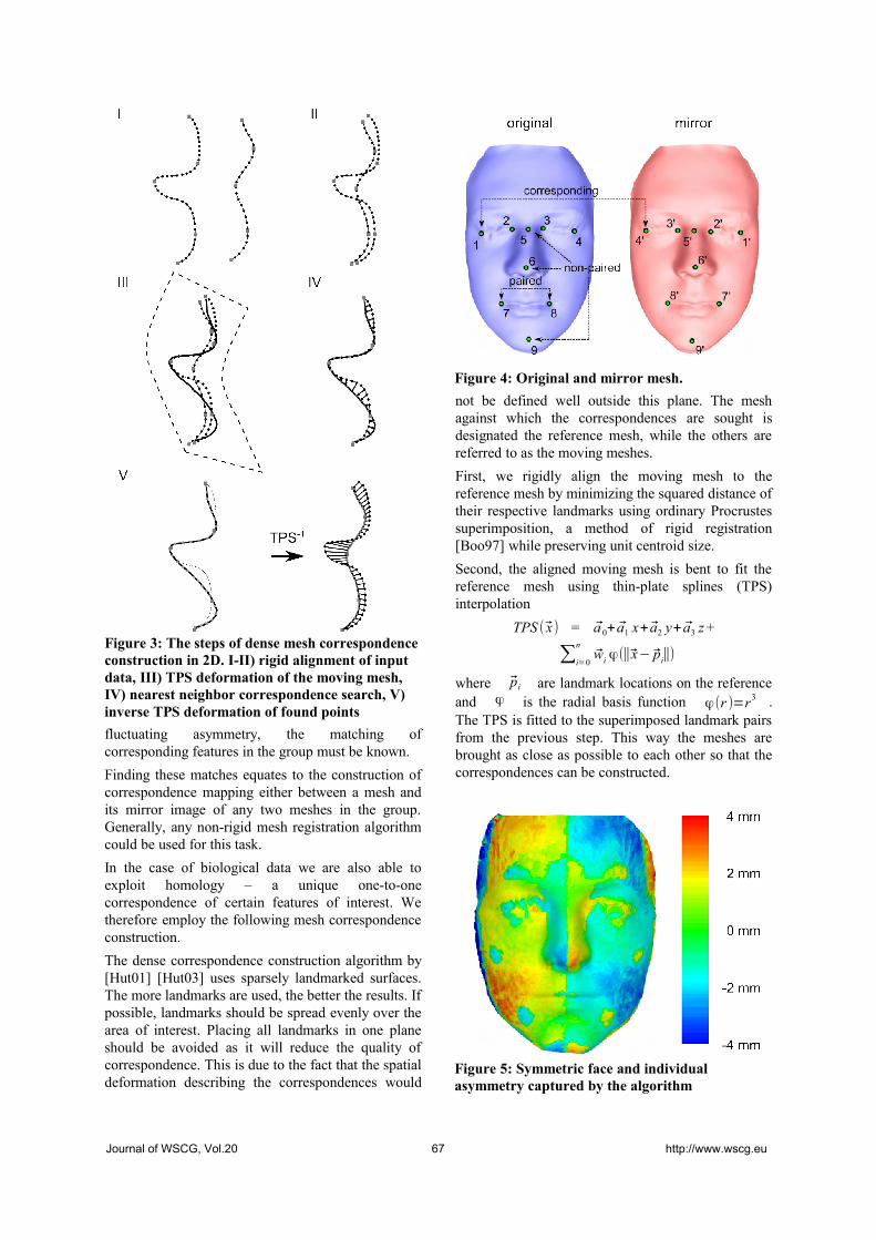
fluctuating asymmetry, the matching of corresponding features in the group must be known.

Finding these matches equates to the construction of correspondence mapping either between a mesh and its mirror image of any two meshes in the group. Generally, any non-rigid mesh registration algorithm could be used for this task.

In the case of biological data we are also able to exploit homology – a unique one-to-one correspondence of certain features of interest. We therefore employ the following mesh correspondence construction.

The dense correspondence construction algorithm by [Hut01] [Hut03] uses sparsely landmarked surfaces. The more landmarks are used, the better the results. If possible, landmarks should be spread evenly over the area of interest. Placing all landmarks in one plane should be avoided as it will reduce the quality of correspondence. This is due to the fact that the spatial deformation describing the correspondences would

not be defined well outside this plane. The mesh against which the correspondences are sought is designated the reference mesh, while the others are referred to as the moving meshes.

First, we rigidly align the moving mesh to the reference mesh by minimizing the squared distance of their respective landmarks using ordinary Procrustes superimposition, a method of rigid registration [Boo97] while preserving unit centroid size.

Second, the aligned moving mesh is bent to fit the reference mesh using thin-plate splines (TPS) interpolation

TPS ( x) = a 0+ a1 x+ a2 y+ a3 z +

∑i=0

nwi ϕ(∥x− pi∥)

where pi are landmark locations on the reference and ϕ is the radial basis function ϕ(r )=r3 . The TPS is fitted to the superimposed landmark pairs from the previous step. This way the meshes are brought as close as possible to each other so that the correspondences can be constructed.

Figure 3: The steps of dense mesh correspondence construction in 2D. I-II) rigid alignment of input data, III) TPS deformation of the moving mesh, IV) nearest neighbor correspondence search, V) inverse TPS deformation of found points

Figure 4: Original and mirror mesh.

Figure 5: Symmetric face and individual asymmetry captured by the algorithm


In the last step the reference mesh is used to construct a new mesh with the same topology as the reference but the shape of the moving mesh, which is referred to as the correspondence mesh. This is done by finding the closest point (not necessarily vertex) in the reference mesh to each vertex of the moving mesh. The search efficiency can be enhanced with acceleration structures. A kd-tree on all mesh triangles has proven very effective. This process yields the correspondence between the reference mesh's points and the deformed moving mesh. We now need to transform these vertex locations to the space of the original moving mesh. Because the deformed mesh was created with a TPS the original is obtained by inverting that TPS. Since TPS has no analytically defined inversion it must be computed numerically as the solution of the following minimization problem.

arg minx∈R 3

∥TPS ( x)− y∥2

This could be solved by any optimization procedure. Because in this case the second derivatives can be easily analytically expressed, the Newton's method is suitable for the problem.

An alternative to the numeric TPS inversion computation is an approximation using barycentric coordinates. The correspondence points in the deformed moving mesh are expressed in barycentric coordinates inside their respective triangles. The same barycentric coordinates are then used to compute the point in the corresponding face of the original moving mesh. A scheme of the correspondence construction procedure is described in Figure 3.

Sometimes the corresponding point is located too far from the vertex in the reference. Then it is not likely that it is a proper correspondence. We can define a threshold distance beyond which the correspondence is not accepted. In that case we simply omit this vertex from the mesh with identical topology.

In order to analyze a group of meshes the correspondences across the whole sample must be constructed. One mesh from the sample is chosen as the reference and the remaining meshes are used as moving meshes to construct correspondences to the reference.

The choice of the reference mesh may have a significant influence on the result. It should be chosen so that it is not too different from the rest of the group. Ideally, it lies in the middle of the group, hence the other moving shapes need to be bent less to align with the reference. The authors of the original algorithm [Hut01] claim that if the input data is random, choosing the first mesh as the reference for the group is as good as choosing any other.

4. MESH ASYMMETRY ANALYSISIn our approach to capture a group mesh asymmetry we use the concept of decomposing the asymmetry into directional and fluctuating components. Concurrently, dense triangular meshes allow us to express the asymmetry on a very localized level.

Before we can compare the local asymmetries in all meshes, we need to have them transformed into a common coordinate space. This is done by applying a group-wise rigid landmark-based registration, specifically generalized Procrustes superimposition has been used. The meshes' vertices are transformed the same way as the landmarks in the Procrustes superimposition.

The next step is to recompute the meshes to the same number of vertices and the same topology. We used the dense correspondence construction algorithm from the previous section.

Now, the individual mesh asymmetry is computed. The result is the list of directions for every vertex. If every vertex were moved by their respective displacement the mesh would become ideally symmetric. The mirror mesh must be constructed by

Figure 6: An ideally symmetric face and the artificially added asymmetry (left). Individual asymmetry of artificial test subject detected by the algorithm (right).


negating one of the vertex coordinates (see Figure 4). The same is done with landmarks placed on the mesh.

The landmarks are then used to align the mirror mesh back to the original mesh. In order to do that the landmarks must be reordered as they have changed their homologous meaning after the mirroring. e.g. some landmarks on the left side of a bilaterally symmetric mesh became the landmarks on the right side of the mirror mesh. These are the so called paired landmarks; they swap their positions with their mirror counterparts, while the others, the non-paired landmarks are not affected by mirroring.

After mirroring and landmark reordering the mirror meshes are realigned by ordinary Procrustes superimposition and deformed by TPS in order to get mirror meshes closer to the original ones and allow for subsequent correspondence searching. The closest points on the mirror meshes to each vertex of the original correspondence meshes are found using search acceleration structures. Again, we opted for a kd-tree.

The vectors defined by the difference of the original mesh vertices and their closest mirror mesh points is the local measures of asymmetry. Completely symmetrical shapes have identical mirrors and when aligned the distances between the original mesh vertices and the closest points are zero. If asymmetries occur on the mesh the difference between the left and right part of the mesh appears and the distance between a part of the mesh and its mirrored counterpart becomes non-zero. Furthermore, the associated vector holds the information about the direction of the asymmetry, i.e. how the part of the mesh was moved to form the asymmetry. This information is exhibited on either side of a bilaterally symmetrical mesh in the opposite directions. Hence it cannot be said which part of the mesh originated from a symmetric shape and which was altered, if this is the way the analyzed asymmetric shape was created. It can be said that

bilateral asymmetry is a symmetric feature. The vector field that represents the displacement of a point on a mesh from where it would lie if the mesh were ideally symmetric is called individual asymmetry.

We visualize the aforementioned vector field on the original mesh with color-coded signed distances (see Figure 5). The sign is the same as that of the dot product of the mesh normal and the vector of individual asymmetry in that point. The color images could be simply interpreted in the following way: red areas lie in the front of the corresponding mirrored counterpart which means that they are larger than the corresponding paired counterpart while blue areas are smaller and lie behind the aligned mirrored counterpart. The areas that are close to green are not significantly larger or smaller. This interpretation does not include any information about the direction

Figure 7: Directional asymmetry (left) and significance map of the asymmetry (right) on 102 human faces.

Figure 8: Directional asymmetry of male (left) and female (right) subgroups.


of the asymmetry. This sort of visualization is also known as clearance vector mapping and is useful in quantifying the facial surface asymmetries in the areas where anthropometric landmarks are scarce. The volume of detected asymmetry is potentially significant in patients who may have their unilateral facial deficiencies corrected using injections or implants [OGr99].

All individual asymmetries are already aligned group-wise, therefore, directional asymmetry is computed as the average of all corresponding individual asymmetry vectors. The length of the respective individual asymmetry vectors is the same for all the meshes and they correspond to each other per element as the meshes were reconstructed to have the same topology. The directional asymmetry is visualized the same way as individual asymmetry.

Fluctuating asymmetry is computed as the difference of individual asymmetry and directional asymmetry. Its visualization is also based on color coded distances without the consideration of the sign for direction as was done for individual and directional asymmetry above. As stated in the previous chapter, we are more interested in the overall magnitude of the fluctuating asymmetry which is computed as the sum of squared distances of the fluctuating asymmetry vectors. It can be compared across the group and if normalized by the number of vectors, or between groups just as well.

To prove that the directional asymmetry reflects the global trend of the group, and is not the result of randomness in the group, it has to be tested statistically. A standard t-test is performed on the signed lengths of corresponding individual asymmetry vectors. The significance map can then also be visualized. This way of interpretation is especially important for particular research in biological sciences.

The direction of the individual asymmetry vector is also important property that should be taken into account. In order to do so we define the local

orientation difference asymmetry measure which is equal to cosine of angle between corresponding individual asymmetry vectors.

The lengths of individual asymmetry vectors and local orientation difference asymmetry measure can be summarized into total asymmetry and total orientation asymmetry.

TA=1N ∑i=0

N

∥ai∥2

TOA=1N ∑i=0

Nni⋅mi

5. RESULTSOur semiautomatic landmark-based approach reflects the needs of scientists from fields like archaeology and anthropology where the homology of certain feature points is advantageous. It is often the case that mesh datasets together with their respective landmark configurations already exist and the results of landmark-only based studies have already been published so some comparison of results can be done. All these facts are the motivation supporting our solution over completely autonomous algorithms, e.g. employing nonrigid mesh registration.

In the first test it will be demonstrated how the proposed algorithm approximates individual asymmetry on an artificial dataset where the ground truth is well known. A symmetric face model was created by cutting a real face in half approximately along its medial axis mirroring one of the halves and stitching it to its original. Then the symmetric face was locally deformed, bulged on the left side of the forehead. Shell distance measured by a software tool, RapidForm XOS in our case, was used as the ground truth (see the left side of Figure 6). In this case, if the deformation does not affect the areas with landmarks, the algorithm can uncover the asymmetry perfectly (see the right side of Figure 6). If the location of a landmark is distorted by a nearby asymmetry the error of alignment by the generalized Procrustes superimposition will be distributed among all

Figure 9: Difference in total orientation asymmetry of male and female subgroups is statistically significant (p < 0.05). The orientation the asymmetry is locally unevenly distributed on the male faces while being uniform almost everywhere on female faces.


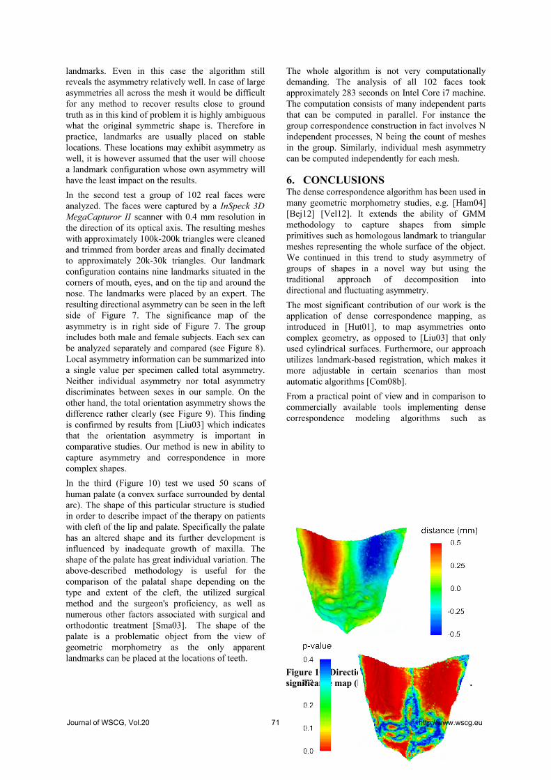
landmarks. Even in this case the algorithm still reveals the asymmetry relatively well. In case of large asymmetries all across the mesh it would be difficult for any method to recover results close to ground truth as in this kind of problem it is highly ambiguous what the original symmetric shape is. Therefore in practice, landmarks are usually placed on stable locations. These locations may exhibit asymmetry as well, it is however assumed that the user will choose a landmark configuration whose own asymmetry will have the least impact on the results.

In the second test a group of 102 real faces were analyzed. The faces were captured by a InSpeck 3D MegaCapturor II scanner with 0.4 mm resolution in the direction of its optical axis. The resulting meshes with approximately 100k-200k triangles were cleaned and trimmed from border areas and finally decimated to approximately 20k-30k triangles. Our landmark configuration contains nine landmarks situated in the corners of mouth, eyes, and on the tip and around the nose. The landmarks were placed by an expert. The resulting directional asymmetry can be seen in the left side of Figure 7. The significance map of the asymmetry is in right side of Figure 7. The group includes both male and female subjects. Each sex can be analyzed separately and compared (see Figure 8). Local asymmetry information can be summarized into a single value per specimen called total asymmetry. Neither individual asymmetry nor total asymmetry discriminates between sexes in our sample. On the other hand, the total orientation asymmetry shows the difference rather clearly (see Figure 9). This finding is confirmed by results from [Liu03] which indicates that the orientation asymmetry is important in comparative studies. Our method is new in ability to capture asymmetry and correspondence in more complex shapes.

In the third (Figure 10) test we used 50 scans of human palate (a convex surface surrounded by dental arc). The shape of this particular structure is studied in order to describe impact of the therapy on patients with cleft of the lip and palate. Specifically the palate has an altered shape and its further development is influenced by inadequate growth of maxilla. The shape of the palate has great individual variation. The above-described methodology is useful for the comparison of the palatal shape depending on the type and extent of the cleft, the utilized surgical method and the surgeon's proficiency, as well as numerous other factors associated with surgical and orthodontic treatment [Sma03]. The shape of the palate is a problematic object from the view of geometric morphometry as the only apparent landmarks can be placed at the locations of teeth.

The whole algorithm is not very computationally demanding. The analysis of all 102 faces took approximately 283 seconds on Intel Core i7 machine. The computation consists of many independent parts that can be computed in parallel. For instance the group correspondence construction in fact involves N independent processes, N being the count of meshes in the group. Similarly, individual mesh asymmetry can be computed independently for each mesh.

6. CONCLUSIONSThe dense correspondence algorithm has been used in many geometric morphometry studies, e.g. [Ham04] [Bej12] [Vel12]. It extends the ability of GMM methodology to capture shapes from simple primitives such as homologous landmark to triangular meshes representing the whole surface of the object. We continued in this trend to study asymmetry of groups of shapes in a novel way but using the traditional approach of decomposition into directional and fluctuating asymmetry.

The most significant contribution of our work is the application of dense correspondence mapping, as introduced in [Hut01], to map asymmetries onto complex geometry, as opposed to [Liu03] that only used cylindrical surfaces. Furthermore, our approach utilizes landmark-based registration, which makes it more adjustable in certain scenarios than most automatic algorithms [Com08b].

From a practical point of view and in comparison to commercially available tools implementing dense correspondence modeling algorithms such as

Figure 10: Directional asymmetry (top) and significance map (bottom) of 50 human palates.


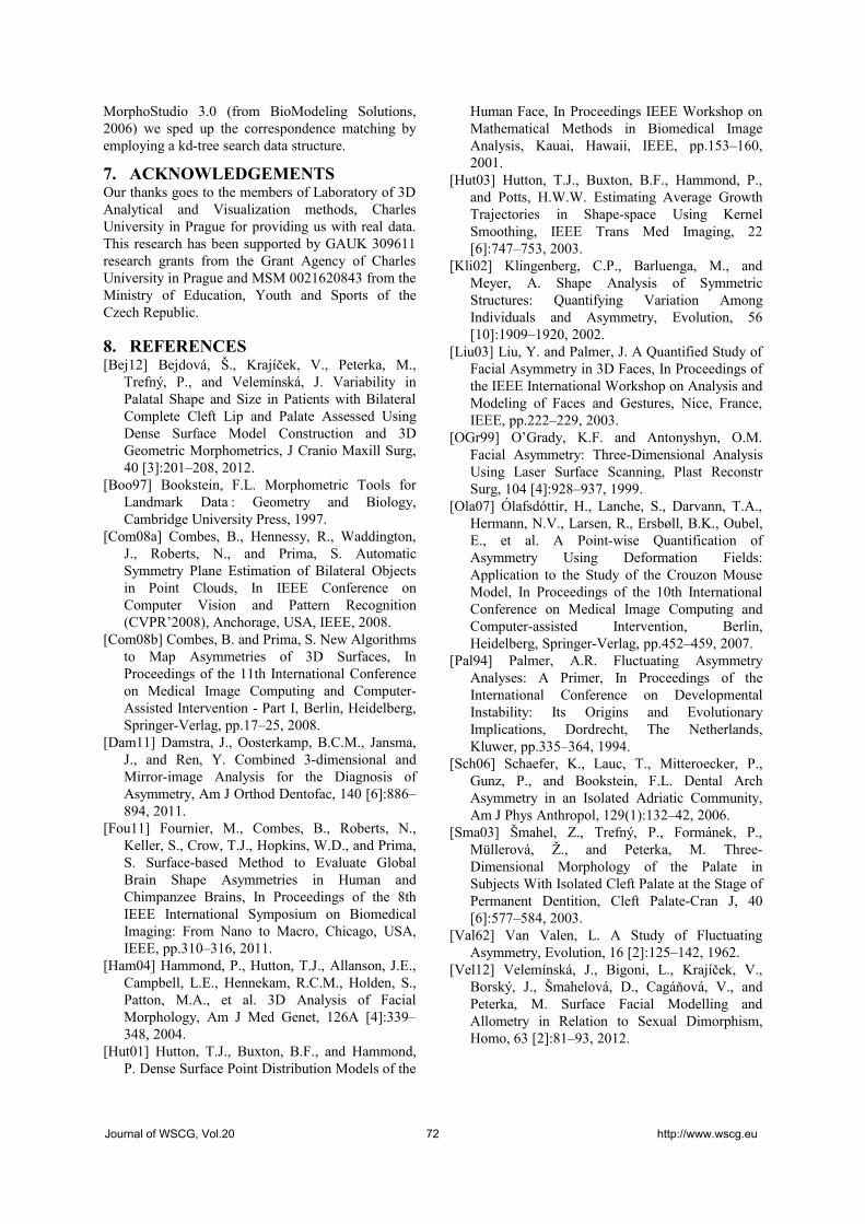
MorphoStudio 3.0 (from BioModeling Solutions, 2006) we sped up the correspondence matching by employing a kd-tree search data structure.

7. ACKNOWLEDGEMENTSOur thanks goes to the members of Laboratory of 3D Analytical and Visualization methods, Charles University in Prague for providing us with real data. This research has been supported by GAUK 309611 research grants from the Grant Agency of Charles University in Prague and MSM 0021620843 from the Ministry of Education, Youth and Sports of the Czech Republic.

8. REFERENCES[Bej12] Bejdová, Š., Krajíček, V., Peterka, M.,

Trefný, P., and Velemínská, J. Variability in Palatal Shape and Size in Patients with Bilateral Complete Cleft Lip and Palate Assessed Using Dense Surface Model Construction and 3D Geometric Morphometrics, J Cranio Maxill Surg, 40 [3]:201–208, 2012.

[Boo97] Bookstein, F.L. Morphometric Tools for Landmark Data : Geometry and Biology, Cambridge University Press, 1997.

[Com08a] Combes, B., Hennessy, R., Waddington, J., Roberts, N., and Prima, S. Automatic Symmetry Plane Estimation of Bilateral Objects in Point Clouds, In IEEE Conference on Computer Vision and Pattern Recognition (CVPR’2008), Anchorage, USA, IEEE, 2008.

[Com08b] Combes, B. and Prima, S. New Algorithms to Map Asymmetries of 3D Surfaces, In Proceedings of the 11th International Conference on Medical Image Computing and Computer-Assisted Intervention - Part I, Berlin, Heidelberg, Springer-Verlag, pp.17–25, 2008.

[Dam11] Damstra, J., Oosterkamp, B.C.M., Jansma, J., and Ren, Y. Combined 3-dimensional and Mirror-image Analysis for the Diagnosis of Asymmetry, Am J Orthod Dentofac, 140 [6]:886–894, 2011.

[Fou11] Fournier, M., Combes, B., Roberts, N., Keller, S., Crow, T.J., Hopkins, W.D., and Prima, S. Surface-based Method to Evaluate Global Brain Shape Asymmetries in Human and Chimpanzee Brains, In Proceedings of the 8th IEEE International Symposium on Biomedical Imaging: From Nano to Macro, Chicago, USA, IEEE, pp.310–316, 2011.

[Ham04] Hammond, P., Hutton, T.J., Allanson, J.E., Campbell, L.E., Hennekam, R.C.M., Holden, S., Patton, M.A., et al. 3D Analysis of Facial Morphology, Am J Med Genet, 126A [4]:339–348, 2004.

[Hut01] Hutton, T.J., Buxton, B.F., and Hammond, P. Dense Surface Point Distribution Models of the

Human Face, In Proceedings IEEE Workshop on Mathematical Methods in Biomedical Image Analysis, Kauai, Hawaii, IEEE, pp.153–160, 2001.

[Hut03] Hutton, T.J., Buxton, B.F., Hammond, P., and Potts, H.W.W. Estimating Average Growth Trajectories in Shape-space Using Kernel Smoothing, IEEE Trans Med Imaging, 22 [6]:747–753, 2003.

[Kli02] Klingenberg, C.P., Barluenga, M., and Meyer, A. Shape Analysis of Symmetric Structures: Quantifying Variation Among Individuals and Asymmetry, Evolution, 56 [10]:1909–1920, 2002.

[Liu03] Liu, Y. and Palmer, J. A Quantified Study of Facial Asymmetry in 3D Faces, In Proceedings of the IEEE International Workshop on Analysis and Modeling of Faces and Gestures, Nice, France, IEEE, pp.222–229, 2003.

[OGr99] O’Grady, K.F. and Antonyshyn, O.M. Facial Asymmetry: Three-Dimensional Analysis Using Laser Surface Scanning, Plast Reconstr Surg, 104 [4]:928–937, 1999.

[Ola07] Ólafsdóttir, H., Lanche, S., Darvann, T.A., Hermann, N.V., Larsen, R., Ersbøll, B.K., Oubel, E., et al. A Point-wise Quantification of Asymmetry Using Deformation Fields: Application to the Study of the Crouzon Mouse Model, In Proceedings of the 10th International Conference on Medical Image Computing and Computer-assisted Intervention, Berlin, Heidelberg, Springer-Verlag, pp.452–459, 2007.

[Pal94] Palmer, A.R. Fluctuating Asymmetry Analyses: A Primer, In Proceedings of the International Conference on Developmental Instability: Its Origins and Evolutionary Implications, Dordrecht, The Netherlands, Kluwer, pp.335–364, 1994.

[Sch06] Schaefer, K., Lauc, T., Mitteroecker, P., Gunz, P., and Bookstein, F.L. Dental Arch Asymmetry in an Isolated Adriatic Community, Am J Phys Anthropol, 129(1):132–42, 2006.

[Sma03] Šmahel, Z., Trefný, P., Formánek, P., Müllerová, Ž., and Peterka, M. Three-Dimensional Morphology of the Palate in Subjects With Isolated Cleft Palate at the Stage of Permanent Dentition, Cleft Palate-Cran J, 40 [6]:577–584, 2003.

[Val62] Van Valen, L. A Study of Fluctuating Asymmetry, Evolution, 16 [2]:125–142, 1962.

[Vel12] Velemínská, J., Bigoni, L., Krajíček, V., Borský, J., Šmahelová, D., Cagáňová, V., and Peterka, M. Surface Facial Modelling and Allometry in Relation to Sexual Dimorphism, Homo, 63 [2]:81–93, 2012.


Preprocessing for Quantitative Statistical Noise Analysis ofMDCT Brain Images Reconstructed Using Hybrid Iterative

(iDose) Algorithm

Petr WalekDept. of Biomedical

EngineeringBrno University of Technology612 00, Brno, Czech republic

[email protected]

Jiri JanDept. of Biomedical

EngineeringBrno University of Technology612 00, Brno, Czech republic

[email protected]

Petr OurednicekPhilips Czech Republic155 00 Prague, Czech

[email protected]

Jarmila SkotakovaChildren’s Hospital - Faculty

HospitalMasaryk University

625 00, Brno, Czech [email protected]

Igor JiraChildren’s Hospital - Faculty

HospitalMasaryk University

625 00, Brno, Czech [email protected]

ABSTRACTRadiation dose reduction is a very topical problem in medical X-ray CT imaging and plenty of strategies havebeen introduced recently. Hybrid iterative reconstruction algorithms are one of them enabling dose reduction up to70 %. The paper describes data preprocessing and feature extraction from iteratively reconstructed images in orderto assess their quality in terms of image noise and compare it with quality of images reconstructed from the samedata by the conventional filtered back projection. The preprocessing stage consists in correction of a stair-stepartifact and in fast, precise bone and soft tissue segmentation. Noise patterns of differently reconstructed imagescan therefore be examined separately in these tissue types. In order to remove anatomical structures and to obtainthe pure noise, subtraction of images reconstructed by the iterative iDose algorithm from images reconstructed bythe filtered back projection is performed. The results of these subtractions called here residual noise images andare the used to further extract parameters of the noise. The noise parameters, which are intended to serve as inputdata for consequent multidimensional statistical analysis, are the standard deviation and power spectrum of theresidual noise. This approach enables evaluation of noise properties in the whole volume of real patient data, incontrast to noise analysis performed in small regions of interest or in images of phantoms.

KeywordsX-ray computed tomography, dose reduction, skull segmentation, noise power spectrum.

1 INTRODUCTIONMultidetector X-ray computed tomography (MDCT)imaging is very important for medical diagnostics andquantity of pathological states diagnosed by a MDCTis steadily increasing. This fact causes, in conjunctionwith rising accessibility of MDCT examinations,increase of the average population radiation exposurewhich, in spite of unexceptionable diagnostics out-come, constitutes certain health risk especially for


pediatrics patients. Effective dose introduced by eachMDCT scan depends on many factors and nowadaysusually falls within range from 1 to 14 mSv which canbe considered as a high value in comparison with theannual dose received from natural sources in the CzechRepublic (2.5 mSv).

In order to be compliant with the ALARA principleeach of the major MDCT manufacturers have focusedtheir research on as large radiation dose reduction aspossible. As a result of this increased effort there havebeen introduced new strategies for reducing radiationdose, for example tube current modulation (in both an-gular and longitudinal directions), elimination of over-ranging effect, dual energy scanning, bowtie filteringand replacement of a filtered back projection (FBP) byiterative reconstruction algorithm [MPB+09], [Goo12].Among a range of mentioned methods the iterative re-


(a) (b) (c)

Figure 1: Saggital slice of brain image (with magnified sections): (a) original slice, (b) slice after registration byphase correlation, (c) slice after registration by gradient descent optimization.

construction one takes exceptional position by produc-ing quality images, even when drastic radiation dose re-duction (up to 70%) is applied [FB11]. Such a dosereduction is alowed by inclusion of photon countingstatistics and models of acquisition process into re-construction. So far, each of the available iterativereconstructions are vendor specific and further detailsabout used algorithms are unknown. General descrip-tion of iterative reconstruction methods can be found in[BKK12] and references therein.

Many studies dealing with problem of quality evalua-tion of iteratively reconstructed images have been pro-posed recently. These studies are targeted either to as-sessment of image quality in small regions of interest inreal patient data [MNS+10] or to evaluation of imagesacquired by scanning of phantoms [MGB+12]. Formerapproach utilizes information only from spatially lim-ited range and thus can not affect whole complexity ofimage noise, e.g. differences between noise in anatom-ical structures. The phantom approach analyzes noiseproperties in homogeneous regions of artificial imagesand there is difficulty to relate results obtained by thisapproach to clinical practice. In order to overcome pre-viously mentioned drawbacks a new way of extractionof noise parameters from whole volume of real patientdata is presented in this paper.

2 DATA ACQUISITIONOur study is targeted to head MDCT images, acquiredby the Philips Brilliance CT 64-channel scanner andreconstructed by a prototype of the Philips iterativereconstruction method called iDose during ordinaryoperation of radiological center in Children’s hospitalin Brno. Acquired raw data were once reconstructed bythe conventional filtered back projection and four timesusing the iDose algorithm, every time with differently

adjusted parameters. The parameters adjusted beforeeach reconstruction are inclusion level of iDose recon-struction expressed in percents (chosen to be 30 %,50 % and 70 % and in this paper labeled as an ID30,ID50 and ID70), and Multi Resolution which wasturned on only together with the iDose level ID70 (inthis paper labeled as an ID70MR). Meaning of iDoselevels is folowing, images reconstructed by FBP haveequal standard deviation of noise as images acquiredwith 30 % less dose and reconstructed by ID30.

A statistical data set contains forty patients uniformlydivided into male and female, aged in range from threemonths to sixty years. A certain group of patients wasscanned with regular dose according to a scanning pro-tocol, other group also with regular dose but in a highquality imaging mode (HQ) and the last group in a highquality mode with radiation dose reduced about 30 %(30HQ). Note that dose reduction was obtained by auniform reduction of tube current.

3 CORRECTION OF A STAIR-STEPARTIFACT

Acquired images suffer from the very severe stair-stepartifact especially after three-dimensional reformattingto a sagittal plane as can be clearly seen in Fig. 1a.In general a stair-step artifact is caused by using widecollimation and a non-overlapping reconstruction in-terval especially using multisection scanning [BK04].Artifact introduces translational shift into sub-volumeslocated identically according to sections acquired inone gantry rotation during multisection scanning. Sucha shift cause many artificial edges in a sagittal planewhich are able to harm further noise power spectra anal-ysis by introducing artificial high frequencies.


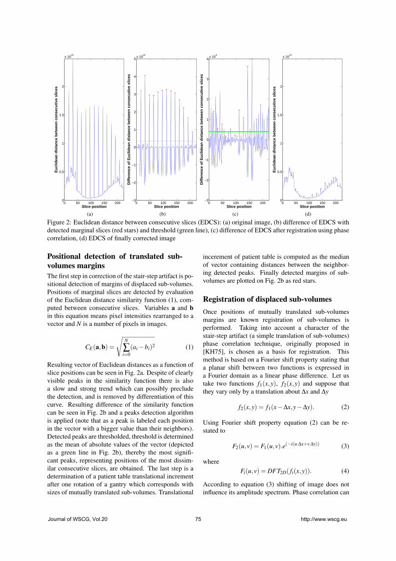
0 50 100 150 2000

0.5

1

1.5

2

x 1010

Slice position

Eu

clid

ean

dis

tan

ce b

etw

een

co

nse

cuti

ve s

lices

(a)

0 50 100 150 200−3

−2

−1

0

1

2

3

4

5x 10

10

Slice position

Dif

fere

nce

of

Eu

clid

ean

dis

tan

ce b

etw

een

co

nse

cuti

ve s

lices

(b)

0 50 100 150 200−3

−2

−1

0

1

2

3

4x 10

9

Slice positionD

iffe

ren

ce o

f E

ucl

idea

n d

ista

nce

bet

wee

n c

on

secu

tive

slic

es

(c)

0 50 100 150 2000

0.5

1

1.5

2

x 1010

Slice position

Eu

clid

ean

dis

tan

ce b

etw

een

co

nse

cuti

ve s

lices

(d)

Figure 2: Euclidean distance between consecutive slices (EDCS): (a) original image, (b) difference of EDCS withdetected marginal slices (red stars) and threshold (green line), (c) difference of EDCS after registration using phasecorrelation, (d) EDCS of finally corrected image

Positional detection of translated sub-volumes marginsThe first step in correction of the stair-step artifact is po-sitional detection of margins of displaced sub-volumes.Positions of marginal slices are detected by evaluationof the Euclidean distance similarity function (1), com-puted between consecutive slices. Variables a and bin this equation means pixel intensities rearranged to avector and N is a number of pixels in images.

CE(a,b) =

√N

∑i=0

(ai−bi)2 (1)

Resulting vector of Euclidean distances as a function ofslice positions can be seen in Fig. 2a. Despite of clearlyvisible peaks in the similarity function there is alsoa slow and strong trend which can possibly precludethe detection, and is removed by differentiation of thiscurve. Resulting difference of the similarity functioncan be seen in Fig. 2b and a peaks detection algorithmis applied (note that as a peak is labeled each positionin the vector with a bigger value than their neighbors).Detected peaks are thresholded, threshold is determinedas the mean of absolute values of the vector (depictedas a green line in Fig. 2b), thereby the most signifi-cant peaks, representing positions of the most dissim-ilar consecutive slices, are obtained. The last step is adetermination of a patient table translational incrementafter one rotation of a gantry which corresponds withsizes of mutually translated sub-volumes. Translational

incerement of patient table is computed as the medianof vector containing distances between the neighbor-ing detected peaks. Finally detected margins of sub-volumes are plotted on Fig. 2b as red stars.

Registration of displaced sub-volumesOnce positions of mutually translated sub-volumesmargins are known registration of sub-volumes isperformed. Taking into account a character of thestair-step artifact (a simple translation of sub-volumes)phase correlation technique, originally proposed in[KH75], is chosen as a basis for registration. Thismethod is based on a Fourier shift property stating thata planar shift between two functions is expressed ina Fourier domain as a linear phase difference. Let ustake two functions f1(x,y), f2(x,y) and suppose thatthey vary only by a translation about ∆x and ∆y

f2(x,y) = f1(x−∆x,y−∆y). (2)

Using Fourier shift property equation (2) can be re-stated to

F2(u,v) = F1(u,v).e(−i(u.∆x+v.∆y)) (3)

whereFi(u,v) = DFT2D( fi(x,y)). (4)

According to equation (3) shifting of image does notinfluence its amplitude spectrum. Phase correlation can


be calculated as a inverse Fourier transform of a nor-malized cross power spectrum

p(x,y) = DFT−12D

[F2(u,v).F1(u,v)∗

|F2(u,v).F1(u,v)|

]. (5)

This phase correlation matrix contains a strong impulsein position [∆x,∆y] which is detected as the strongestpeak. Vector of translation parameters [∆x,∆y]′ for eachsub-volume is known and alignment can be performedin a very simple manner as [x,y]′+[∆x,∆y]′. Phase cor-relation, in its basic form, cannot determine sub-pixelshifts and registration therefore cannot be sufficient, seeFig. 1b. After registration of sub-volumes by phase cor-relation, difference of Euclidean distance between con-secutive slices is computed and thresholded again, seeFig. 2c. Euclidean distances between sub-volumes mar-gins (labeled as red stars) above threshold are then min-imized by gradient descent optimization method, pro-viding final correction of stair-step artifact, see Fig. 1cand Fig. 2d.

4 SEGMENTATION OF SKULL ANDSOFT TISSUE

Very interesting findings may be done if noise prop-erties of differently reconstructed images are exam-ined separately for hyperdense and hypodense struc-tures (i.e. bones and soft tissue). An automatic, reliableand fast segmentation algorithm is therefore neededwhich should be capable to distinguish between bonesand soft tissue even in a complex structure of a basiscranii and segment not only cortical however also tra-becular parts of bones. Distinction between soft tissueand bones is carried out in the following manner:

0 0.1 0.2 0.3 0.4 0.5 0.6 0.7 0.8 0.9 10

1

2

3

4

5

6

x 106

Normalized pixel intensity

Pix

el c

ou

nts

Histogram countsBefore optimizationAfter optimizationThresholds

0.32 0.33 0.34 0.35 0.36 0.37 0.380

0.5

1

1.5

2

2.5

x 106


Pix

el c

ou

nts

Figure 3: Brightness histogram of the whole brain vol-ume (blue bar graph). Initial Gaussian curve (red plot)is fitted on soft tissue peak (green plot) and final thresh-olds are depicted as the black lines

• Segmentation of cortical bones.

• Adding trabecular bones parts into segmentation.

• Segmentation of surrounding air and sinuses.

• Segmentation of soft tissue by calculating a comple-ment to segmented bones and surrounding air.

Only the first and the second steps deserves closer atten-tion and are in detail discussed in next two subsections,on the other hand the third step is very similar to thefirst and the fourth is simple computation of a comple-ment to two binary images (bones and surrounding airsegmentations).

Segmentation of cortical bonesThe simplest and fastest method for segmenting corti-cal bones parts is the intensity thresholding. A thresh-old is needed for this operation and probably the bestway for its automatic determination is evaluation of theimage histogram. A typical brightness histogram of thewhole brain volume comprises only two distinct peaks,and can be seen in Fig. 3 plotted as a blue bar graph,note that pixel intensities are normalized to be in in-terval 〈0,1〉. The peak situated at lower intensities be-longs to representation of surrounding air and sinuses,while second significant peak belongs to a representa-tion of soft tissue. Intensities belonging to bones arespread over a wide range hence there is no distinct de-tectable peak. Threshold for cortical bones segmenta-tion is therefore derived from a position of soft tissuepeak which is detected in similar way as peaks in chap-ter 3. Peak with the second highest value is consideredto be representation of soft tissue. Detected position ofthe soft tissue peak serves as a mean µ and magnitudeas parameter a of initial Gaussian function (6) used toapproximate properties of soft tissue lobe (variance σ

is initially selected as 0.01).

f (x) = a.e(−0.5( x−µ

σ )2)

(6)

The initial Gaussian curve is depicted in Fig. 3 (pleasenotice detailed plot) as a red curve and is optimizedby a least-squares curve fitting algorithm in orderto find optimal parameters µ and σ (green curve inFig. 3). Thresholds for segmentation are empiricallydetermined as µ − 25.σ for surrounding air andµ + 20.σ for bones (black lines in Fig. 3). In this waythresholds for bones and surrounding air segmentationare determined automatically and independently on theinput data.

Classification of trabecular bonesIntensities (i.e. Hounsfield units or tissue density) intrabecular parts of bones are partially overlapped withintensities of soft tissue, therefore simple thresholdingis only capable to segment cortical parts of bones as canbe seen in Fig. 4b (note that resulting binary masks 4b,


(a) Original slice (b) After intensity thresholding (c) Final bones segmentation (d) Soft tissue segmentation

Figure 4: Example of skull and soft tissue segmentation

0.32 0.34 0.36 0.38 0.4 0.42 0.440

20

40

60

80


Pix

el c

ou

nts

(a) Histogram of trabecular bone

0.32 0.34 0.36 0.38 0.4 0.42 0.440

200

400

600

800

1000

1200


Pix

el c

ou

nts

(b) Histogram of Soft tissue

Figure 5: Typical histograms of holes manually classi-fied as soft tissue and trabecular bone

4c and 4d are in this view multiplied with the originalslice 4a) and because of that areas being zero fully sur-rounded by values of one (in this paper called "holes")appears instead trabecular parts of bones. Separationof holes by a boundary tracking technique is thereforenext step followed by decision if particular hole repre-sents soft tissue or trabecular bone. As stated beforeintensities of soft tissue and trabecular bones are par-tially overlapping, nevertheless their histograms differin shapes, typical histograms of soft tissue hole and tra-becular bone are depicted in Fig. 5. Histograms of tra-becular bones parts are, in comparison with soft tissueones, more compact (histogram counts are smoother)and skewed towards higher intensities. Shape of a par-ticular histogram is objectified by five parameters: en-tropy (7), compactness (8), relative position of the his-togram mean according to position of soft tissue peak inhistogram of whole volume (9), skewness (10) and kur-tosis (11). In each of the following equations N meanssum of all counts in bins (i.e. number of pixels in hole),i is a bin mark and xi means counts in the bin markedas i.

S =− 1N

n−1

∑i=0

xi log(xi). (7)

C =1N

n−1

∑i=0

xi

max(x)(8)

Prel =Ppos

µ; µ =

1N

n−1

∑i=0

xii. (9)

γ1 =

1N

n−1∑

i=0(i−µ)3

[1N

n−1∑

i=0(xii)2−µ2

] 32. (10)

γ2 =

1N

n−1∑

i=0(i−µ)4

[1N

n−1∑

i=0(xii)2−µ2

]2 −3. (11)

Classification of the holes is done by a simple neuralnetwork, trained by set of 300 exemplary vectors, eachvector is composed of histogram parameters resultingfrom equations 7 - 11. Each exemplary vector is man-ually classified and this classification is verified by anexperienced radiologist. Final segmentation of bones incomplex structure of basis cranii can be seen in Fig. 4c.

5 EXTRACTION OF PARAMETERSFOR STATISTICAL ANALYSIS

By means of the segmentation algorithm proposed insection 4 two binary masks is obtained representingbones and soft tissue. In order to compare noise proper-ties of images reconstructed by the iDose with respectto the conventional FBP technique, anatomical struc-tures must be removed. Removing of anatomical struc-tures is done by subtraction of image reconstructed bythe FBP from images reconstructed by the iDose (i.e.images marked by ID30, ID50, ID70 and ID70MR) us-ing binary masks for bones and soft tissue. Resultsof these subtractions are called residual noise imageswhich can be seen in Fig. 6.

Standard deviation of residual noiseFirst group of parameters extracted from residual noiseimages are standard deviations computed from a wholeimage volume (results can be seen in Fig. 6). Mean-ing of this parameter is explained considering follow-ing thought. A region of interest (ROI) is selected fromeach reconstructed image (before subtraction) in order


ID30 minus FBP; STD = 2.6349 HU ID50 minus FBP; STD = 4.5007 HU ID70 minus FBP; STD = 6.639 HU ID70MR minus FBP; STD = 6.0105 HU

ID30 minus FBP; STD = 3.0471 HU ID50 minus FBP; STD = 5.394 HU ID70 minus FBP; STD = 8.2288 HU ID70MR minus FBP; STD = 7.8183 HU

Figure 6: Residual noise images depicted separately for bones (upper row) and soft tissue (bottom row)

Figure 7: ROI selected from image reconstructed byID70

to select an area of brain, which should be consideredhomogeneous. Therefore intensity changes in theseROIs are considered being only random noise patterns,see sample in Fig. 7.Two parameters are computed from each ROI, a crosscovariance with the ROI selected form the FBP recon-struction (CX ,FBP) and a standard deviation in each ROI(σ2

X ), see Tab. 1 and note that both parameters decreaseswith increasing iDose level. Subtracting of two randomvariables FBP and X (X is meant as a particular re-construction), having variances σ2

FBP and σ2X and cross-

covariance CX ,FBP, results in new random variable witha standard deviation equal to equation (12).

σ(X−FBP) =√

σ2FBP +σ2

X −2.CX ,FBP (12)

Recon. (X) CX ,FBP σ2X σ(X−FBP) σE(X−FBP)

FBP 276.64 16.63 0.41 0

ID30 234.09 14.12 2.78 2.77

ID50 200.31 12.19 4.95 4.95

ID70 158.81 9.97 7.64 7.64

ID70MR 155.11 9.46 7.47 7.48

Table 1: Noise parameters of selected ROI

A standard deviation of residual noise in investigatedROI σE(X−FBP) is computed from real data and com-pared with value obtained from equation (12), seeTab. 1. Assuming that anatomical structures are identi-cal in reconstructed images and completely suppressedby subtraction, the standard deviation of residual noise,therefore depends only on a standard deviation of noisein image X and a cross-covariance function betweennoises in images FBP and X . The standard deviationof residual noise increases with decreasing cross-covariance CFBP,X and increasing difference betweenσ2

FBP and σ2X and thus can be considered as a valuable

measure indicating improvement of noise propertiesin images reconstructed by the iDose according toimages reconstructed by the filtered back projection.Advantage of this parameter lies in independence on animaged object and therefore can be directly applicableto real patient data not only to phantoms. On the otherhand it provides only relative improvement of noiseproperties according to the filtered back projection.


By means of the segmentation algorithm proposed insection 4 two binary masks is obtained representingbones and soft tissue. In order to compare noise proper-ties of images reconstructed by the iDose with respectto the conventional FBP technique, anatomical struc-tures must be removed. Removing of anatomical struc-tures is done by subtraction of image reconstructed bythe FBP from images reconstructed by the iDose (i.e.images marked by ID30, ID50, ID70 and ID70MR) us-ing binary masks for bones and soft tissue. Resultsof these subtractions are called residual noise imageswhich can be seen in Fig. 6

Power spectrum of residual noiseStandard deviation provides information only on noisemagnitude, however no less important is knowledgeabout its frequency content. Such an information maybe obtained by a noise power spectrum, routinelyused as quality measure of MDCT imaging systems[YKH+08], [YKH+08] and [BMG07]. In this studyresidual noise images (Fig. 6), both for segmentedbones and soft tissue, serves as input images for anoise power spectral analysis. Determination of a noisepower spectra (NPS) is carried out by a direct digitaltechnique as proposed in [SCJ02] and is computedaccording to equation (13).

S( fx, fy) =bxby

LxLy·⟨∣∣DFT2D

D(x,y)−D f ilt(x,y)

∣∣2⟩ (13)

Each slice is considered to be the one realization of arandom noise and is denoted as D(x,y). Individual real-izations must be zero mean detrended before NPS cal-culation, therefore an image filtered by a lowpass Gaus-sian filter (D f ilt(x,y)) is subtracted from each slice. Ap-plying a two-dimensional Fourier transform and squar-ing an absolute value of a result (||2), individual noisepower spectrum is obtained. Individual noise powerspectra suffer from a very large variance between real-izations, power spectrum of a stochastic field (i.e. a pro-cess generating random noise) is therefore calculated asa mean value of individual power spectra (in equation(13) outlined by 〈〉 operator). Fraction in this equationis a normalization term consisting of bx by representingsampling periods and Ly Lx representing sizes in direc-tions x and y, respectively.

Residual noise power spectra are determined in trans-verse S( fx, fy), coronal S( fx, fz) and sagittal planeS( fy, fz) as can be seen in Fig. 8. A set of an annularsector shaped binary frequency filters, covering inpiecewise sense the whole spectrum, is used to extractthe final parameters from residual noise power spectra.Filters are used to select a segment of a NPS and themean of this segment is the sought noise pattern, 36

Noise power spectrum S [fx,f

y]

Spatial frequency fx (rad.mm−1)

Spa

tial f

requ

ency

f y (ra

d.m

m−

1 )

−7.31 −5.48 −3.66 −1.83 0 1.83 3.66 5.48 7.31

7.31

5.48

3.66

1.83

0

−1.83

−3.66

−5.48

−7.31

S [fx,f

z]

Spatial frequency fz (rad.mm−1)

Spa

tial f

requ

ency

f x (ra

d.m

m−

1 )

−5.03 −2.51 0 2.51 5.03

7.31

5.48

3.66

1.83

0

−1.83

−3.66

−5.48

−7.31

S [fy,f

z]

Spatial frequency fz (rad.mm−1)

Spa

tial f

requ

ency

f y (ra

d.m

m−

1 )−5.03 −2.51 0 2.51 5.03

7.31

5.48

3.66

1.83

0

−1.83

−3.66

−5.48

−7.31

Figure 8: Example of power spectra of residual noisefor transverse (upper), coronal (bottom left) and sagittal(bottom right) planes

parameters are extracted from each single residualnoise power spectrum.

6 CONCLUSIONS AND FUTUREWORK

Preprocessing of reconstructed image data and ex-traction of parameters for further statistical analysisof noise in MDCT images reconstructed by the iDoseiterative algorithm is proposed in this paper. Thepreprocessing includes a correction of the stair-stepartifact, which may harm further noise feature ex-traction and segmentation of bones and soft tissue.The proposed algorithm for segmenting bones in headimages is fast and reliable even in complex structureof basis cranii, however there are certain drawbacks ofthis method. Segmentation of cortical bones, especiallythe ones with weak borders, may not result in areasof zeros fully surrounded by ones in locations of tra-becular bones. Therefore boundary tracking algorithmcan not label them as a "holes" and such a trabecular


bones remains unsegmented. Another difficulty isthe lack of a trabecular structure in bones, especiallyin images of pediatrics patients. Considering that atrabecular structure in bones causes difference in theshapes of histograms of holes, the lack of this structurecan negatively influence reliability of the resultingsegmentation.

The parameters used for further statistical analysis arethe standard deviation and noise power spectrum of theresidual noise. The images formed by the residual noiseare obtained by subtracting the images reconstructedby the filtered back projection from the images recon-structed by the iDose algorithm. When obtained by thissubtraction, the noise properties can be evaluated in thewhole volume of real patient data, on the other hand, theobtained parameters do not reflect the absolute level ofthe image noise but only the relative improvement withrespect to image reconstructed by the FBP.

In order to assess different nature of noise and provedifferent behavior of the iterative reconstruction in softtissue and bones the images of residual noise are multi-plied with the binary masks obtained by segmentation.According to a convolution property of Fourier trans-form multiplying of signals results in convolution oftheir spectra therefore each of the residual noise powerspectrum is affected by spectrum of the used binarymask which is moreover varying with respect to theslice position. Statistical inference of general resultsfrom such modified spectra may be incorrect and ourfuture goal will be to analyze how strong is this influ-ence and how to overcome this problem.

Considering the separate evaluation of the noise param-eters from bones and soft tissue, taking into accountthe number of iDose reconstructions and the count ofparameters extracted from three residual noise powerspectra (for transverse, coronal and sagittal plane), weobtain 392 noise parameters per patient. The vectors ofthe parameters for forty patients can be arranged to ma-trix of size forty rows and 392 columns where each rowcan be considered as a single realization of a randomprocess. Multidimensional statistical analysis such asprincipal component analysis or factor analysis can beused to reveal hidden relations in this matrix. Statisti-cal analysis of the whole matrix can be rather compli-cated due to high number of the extracted parametersin comparison with quantity of scanned patients there-fore selections of groups of parameters must be done(for example selection of low frequency noise). Resultsof future statistical analysis are expected to clarify re-lation between dose reduction, iDose level and quantityof image noise and differences between noise propertiesin soft tissue and bones. In future research proposedalgorithms will be adapted to abdominal and thoracicimages and typical noise properties of these body partswill be analyzed.

7 ACKNOWLEDGMENTSLending of the iDose reconstructor prototype pro-gramme package from Philips Healthcare is highlyacknowledged as well as the long term data acquisitionenabled by the Brno Faculty Hospital, Children’sHospital.

8 REFERENCES[BK04] Julia F. Barrett and Nicholas Keat. Artifacts in CT:

recognition and avoidance. Radiographics : a review pub-lication of the Radiological Society of North America, Inc,24(6):1679–91, 2004.

[BKK12] Marcel Beister, Daniel Kolditz, and Willi A.Kalender. Iterative reconstruction methods in X-ray CT.Physica medica : PM : an international journal devotedto the applications of physics to medicine and biology :official journal of the Italian Association of BiomedicalPhysics (AIFB), 28(2):94–108, April 2012.

[BMG07] K. L. Boedeker and M. F. McNitt-Gray. Appli-cation of the noise power spectrum in modern diagnosticMDCT: part II. Noise power spectra and signal to noise.Physics in medicine and biology, 52(14):4047–61, 2007.

[FB11] Dominik Fleischmann and F. Edward Boas. Com-puted tomography–old ideas and new technology. Euro-pean radiology, 21(3):510–7, March 2011.

[Goo12] Hyun Woo Goo. CT Radiation Dose Optimiza-tion and Estimation: an Update for Radiologists. Koreanjournal of radiology : official journal of the Korean Radi-ological Society, 13(1):1–11, January 2012.

[KH75] C. D. Kuglin and D. C. Hines. The phase correlationimage alignment method. IEEE Conference on Cybernet-ics and Society, pages 163–165, 1975.

[MGB+12] Frédéric A. Miéville, François Gudinchet, Fran-cis Brunelle, François O. Bochud, and Francis R. Verdun.Iterative reconstruction methods in two different MDCTscanners: Physical metrics and 4-alternative forced-choicedetectability experiments - A phantom approach. PhysicaMedica, January 2012.

[MNS+10] Daniele Marin, Rendon C. Nelson, Sebastian T.Schindera, Samuel Richard, Richard S. Youngblood,Terry T. Yoshizumi, and Ehsan Samei. Low-tube-voltage,high-tube-current multidetector abdominal CT: improvedimage quality and decreased radiation dose with adaptivestatistical iterative reconstruction algorithm–initial clinicalexperience. Radiology, 254(1):145–53, January 2010.

[MPB+09] Cynthia H. McCollough, Andrew N. Primak, Na-talie Braun, James Kofler, Lifeng Yu, and Jodie Christner.Strategies for reducing radiation dose in CT. Radiologicclinics of North America, 47(1):27–40, January 2009.

[SCJ02] J. H. Siewerdsen, I. A. Cunningham, and D. A. Jaf-fray. A framework for noise-power spectrum analysis ofmultidimensional images. Medical Physics, 29(11):2655,2002.

[YKH+08] Kai Yang, Alexander L. C. Kwan, Shih-YingHuang, Nathan J. Packard, and John M. Boone. Noisepower properties of a cone-beam CT system for breastcancer detection. Medical Physics, 35(12):5317, 2008.


Real-time Volume Rendering and Tractography Visualization onthe Web

John Congote1, Esther Novo, Luis Kabongo

Vicomtech Research CenterDonostia - San Sebastian, Spain

jcongote,enovo,[email protected]

Dan Ginsburg

Children’s HospitalBoston, United States

[email protected]

Stephan Gerhard

Institute of NeuroinformaticsUni/ETH Zurich, Switzerland

[email protected]

Rudolph Pienaar

Harvard Medical SchoolBoston, United States

[email protected]

Oscar E. Ruiz1Universidad EAFITMedellin, Antioquia

[email protected]

ABSTRACTIn the field of computer graphics, Volume Rendering techniques allow the visualization of 3D datasets, and specif-ically, Volume Ray-Casting renders images from volumetric datasets, typically used in some scientific areas, suchas medical imaging. This article aims to describe the development of a combined visualization of tractographyand volume rendering of brain T1 MRI images in an integrated way. An innovative web viewer for interactivevisualization of neuro-imaging data has been developed based on WebGL. This recently developed standard en-ables the clients to use the web viewer on a wide range of devices, with the only requirement of a compliantweb-browser. As the majority of the rendering tasks take place in the client machine, the effect of bottlenecksand server overloading are minimized. The web application presented is able to compete with desktop tools, evensupporting high graphical demands and facing challenges regarding performance and scalability. The developedsoftware modules are available as open source code and include MRI volume data and tractography generatedby the Diffusion Toolkit, and connectivity data from the Connectome Mapping Toolkit. Our contribution for theVolume Web Viewer implements early ray termination step according to the tractography depthmap, combiningvolume images and estimated white matter fibers. Furthermore, the depthmap system extension can be used forvisualization of other types of data, where geometric and volume elements are displayed simultaneously.

KeywordsWebGL, Volume Rendering, Ray Casting, DVR, dMRI

1 INTRODUCTION

Three-dimensional data can be found in several scien-tific fields, coming from simulation, sampling or mod-eling processes. Regarding the biomedical scope, sev-eral scanning techniques, such as magnetic resonance(MRI) or computerized tomography (CT), are used forstoring body imaging samples as volumetric datasetsformed by groups of parallel slices, where the term vol-umetric dataset refers to a scalar field. These datasetsare usually visualized in three dimensions in order tofacilitate specialists to interpret information.


Figure 1: Combined visualization of volume renderingand tractography information on the web


Visualization of medical volumetric datasets can suit-ably be performed by the use of Direct Volume Render-ing algorithms. These methods show important charac-teristics of datasets, even though rendering is not usu-ally photo-realistic.The problem addressed in this pa-per is the visualization of tractography information ob-tained from dMRI (diffusion MRI) together with vol-ume data corresponding to MRI or CT images.

In order to represent the volumetric datasets, volumerendering techniques allow the visualization of all in-ner characteristics of volumes at once, by projectingdata into 2D images, according to the correspondingposition of a virtual camera. The main idea of the ray-casting algorithm is to launch rays from the camera intothe volume, calculating the volume rendering integralalong the rays. Thus, in this method, the colour andopacity of each pixel in the final image is evaluated bylaunching a ray in the scene from the view position,sampling the volume at discrete points along the rayand accumulating the contribution of each sample.

Our contribution is an implementation of a webrendering system for medical images, which integratesvolume rendering and geometric objects within acompliant WebGL browser, based on the volume raycasting algorithm and built on previous developments[CSK11]. Due to the technology limitations of Webgl,the improvements developed allow us to create aweb application for combined visualization of volumerendering and tractography, as shown in Figure 1, beingable to compete with desktop tools, supporting highgraphical demands and facing challenges regardingperformance and scalability.

The article is organized as follows. Section 2 presentsthe work related to this article, including a descriptionof volume rendering techniques, visualization of med-ical images and geometry intersection. The methodol-ogy of the developed work is explained in Section 3.Then, the results accomplished are presented, and fi-nally, Section 5 states the conclusions and future devel-opments.

2 RELATED WORK2.1 Volume RenderingIn computer graphics, Ray Casting is a well known di-rect volume rendering technique that was designed byKajiya and Herzen [KVH84] as one of the initial devel-opments in this area. Traditionally, three dimensionalobjects have been created by using surface representa-tions, drawing geometric primitives that create polygo-nal meshes [Lev88], hence provoking the loss of infor-mation from one dimension.

Further developments [DCH88] accomplished themathematical modeling of the ray casting process,based on the light’s behaviour equations. Thus, the

volume rendering integral was defined. A comparativebetween different direct volume rendering algorithms,such as Texture Mapping, Ray Casting, Splatting orShear Warp, was presented [MHB00]. Ray casting isa flexible algorithm that allows the implementationof acceleration methods, such as Empty Space Skip-ping [KW03] or Early Ray Termination. Early raytermination is an optimization process that establishescertain limitations in the volume, so that the samplesencountered after them do not contribute to the valueof the pixel.

Ray casting suitably fits GPUs’ operating mode[Sch05], because of the independence of each ray thatis launched to the scene, making this algorithm highlyparallelizable and allowing the exploitation of GPUs’parallel architecture. For GPU ray casting, the volumeelement is stored in the GPU memory as a 3D textureand a fragment shader program is used in order toimplement the ray casting algorithm.

A quality evaluation model was developed for compar-ing the different Direct Volume Rendering techniques[BBD07]. These methods handle a higher amount ofdata than surface rendering techniques, therefore, thecomplexity of the algorithms is increased, as well as thenecessary rendering time [Bru08]. Optimized volumerendering methods avoid empty spaces by introducinga volume proxy geometry [MRH08].

Web 3D Rendering

The use of the recently released WebGL standard[Mar11] leads to new methods for web 3D visualiza-tion, where most part of the computational processesare performed in vertex and fragment shaders thatrun on the GPU hardware. WebGL is a softwarelibrary that enables HTML5-based browsers to identifyclients’ graphics hardware. HTML5, the latest Internetstandard propose, provides native elements for audioand video. WebGL consists of a low-level imperativegraphic programming API based on OpenGLES 2.0for Javascript that enables flexibility and exploitsthe characteristics of advanced graphics cards. Dueto the constant improvement of the performance ofJavascript interpreters, the management of scene ele-ments behaves similarly to the ones obtained by usingnatively compiled languages. Moreover, some WebGLextensions have been implemented in order to achievea friendly interaction, such as SpiderGL [DBPGS10].

Several standards and proprietary solutions are cur-rently being developed in order to fulfil the necessityof moving 3D visualization into the web [BA01], suchas X3D, a standard derived from VRML that stores3D information in a scenegraph format using XML(Extensible Markup Language). This model has beenimplemented in a declarative form, as an extension ofHTML; X3DOM presents a framework for integrating


X3D nodes into HTML5 DOM content [BEJZ09]and other alternatives have also been developed, e.g.XML3D [SKR10]. Finally, there is a standardizationfor X3D in the MedX3D volume rendering model[JAC08, PWS11].

2.2 Visualization of Medical ImagesMedical visualization is a challenging scientific fieldbecause interpretation of images may lead to clinicalintervention. Therefore, quality and fast interactive re-sponse are important features in this domain. Remark-able advances have occurred in medical imaging tech-nology and applications in the past few years, support-ing the possibility of sharing imaging data online acrossclinical and research centres and among clinicians andpatients. The development of these kind of applicationsis influenced by connectivity, security and resources’heterogeneity concerns.On-server rendering can be considered a partial solutionfor Medical Imaging [BM07]. Moreover, several webimplementations for volumetric visualization have al-ready been presented [JAC08], although many of thesesolutions require third party systems to allow visual-ization or their scalability is limited by the renderingserver.As medical volumetric imaging requires high fidelityand high performance, several rendering algorithmshave been analyzed, leading to thread- and data-parallelimplementations of ray casting [SHC09]. Thus, ar-chitectural trends of three modern commodity parallelarchitectures are exploited: multi-core, GPU, and IntelLarrabee. Other approaches describe the developmentof web-based 3D reconstruction and visualizationframeworks for medical data [SAO10]. Such appli-cations based on X3D technology allow extendingcross-platform, inter-application data transfer ability.Several applications have been implemented usingweb 3D rendering techniques, for example, evaluationsystems at the educational level [Joh07] or medicaltraining simulations [JROB08].

dMRIDiffusion Magnetic Resonance Imaging (dMRI) relieson the visualization of water diffusion using data fromMRI. Diverse methodologies have been presented overthe last years and can be classified into two categories:Image based and Object based techniques. The firstmethodology divides the space in voxels and the as-signed colour represents the principal diffusion direc-tion [MAA03]. However, tracks can not be easily iden-tified since no segmentation of the visualization is per-formed, and therefore direction information is difficultto observe since voxel colour mapping is not one-to-one, i.e., different directions might be represented bythe same colour. Otherwise, in object based method-ologies, objects, such as ellipsoids and lines, are used

together with colour mapping in order to enhance visu-alization and give a direction sense to the representa-tion.

Visualization of brain white matter cortical tracks is oneof the most important applications of dMRI, since it al-lows to non-invasively visualize white matter anatomy,and detecting of anomalies [NVLM07, GKN11]. Trac-tography, which refers specifically to the representationof the white matter tracks based on the water diffusioninformation, employs lines to represent the diffusiondirection and to visualize the white matter paths. Ingeneral, lines are generated using randomly distributedseed points; together with the principal diffusion infor-mation and a prescribed interval of time, the differentpaths are generated. However, this representation be-comes dependent on the amount and location of seedpoints to correctly visualize tracks [EKG06] because er-roneous connections might be produced between tracksdue to the existing error in data. Incorrect visualizationof branching of tracks is another drawback, since onlyone path is generated per each seed point.

Probabilistic methodologies have been proposed[EKG06] to represent branching of white matter tracks,in which secondary seed points are included in regionsin which branching is assumed. Therefore, a denservisualization is performed in those regions. An algo-rithm was proposed for path visualization [RSDH10],in which the different global paths are simplified byone simple curve, clustering the different paths andthen using average curves to obtain one simple curvethat summarizes each cluster.

2.3 Geometry IntersectionThe application described in this article requires rep-resenting volume rendering and tractography together,i.e., both volumetric and polygonal data have to be dis-played in the same scene. There are several models forcombining polygonal geometry and volume rendering.Some methods identify the intersection between rayslaunched in the volume rendering process and geome-try [SMF00]. This technique can be optimized by creat-ing octrees for dividing the geometric space and proveintersections correctly.

Other models try to achieve a correct visibility or-der for the intersections between volume and geome-try [HLSR09]. Geometry has to be rendered in the firstplace to correctly look at the intersections of the geom-etry and the volume. Besides, parts that are occludedby the geometry should not contribute to the final im-age, not performing any ray casting at all. In order toachieve this feature, rays should terminate when theyhit a polygonal object, accordingly modifying the raylength image if a polygonal object is closer to the viewpoint than the initial ray length.


3 METHODOLOGYIn our project, the results of the Connectome Mapperare directly loaded in the browser using WebGL andJavaScript. The FreeSurfer cortical surface reconstruc-tion binary files are loaded and processed in JavaScriptand converted to WebGL vertex buffer objects for ren-dering. The surfaces are overlaid with per-vertex cur-vature values computed during the FreeSurfer process-ing stream. The tractography data is likewise parsedin the JavaScript code and rendered as line primitivescoloured based on direction. Finally, the structural net-work itself is converted to JSON (JavaScript ObjectNotation) as an offline preprocess and loaded into thebrowser using JavaScript. The networks are visualizedin 3D along with the fiber tracts and volumes enablingexploration of connectivity information in real-time.

The work described in this paper has been developedusing volume ray casting, a widely used algorithm forgeneration of 2D representations from three dimen-sional volumetric datasets. The obtained images are 2-dimensional matrices I : [1,h]× [1,w]→ R4 (w: widthand h: height, both in pixels). Each pixel is representedby a colour expressed by a four-tuple of red, green, blueand alpha real-valued components, (R,G,B,A ∈ [0,1]).

An entire volume is represented by a 3-dimensional ar-ray of real values V : [1,H]× [1,W ]× [1,D]→ [0,1] (H:Height, W: Width, D: Depth of the represented volume,all of them in positive integer coordinates). Therefore,V (x,y,z) ∈ [0,1]. The projection model used in thiswork is called pin-hole camera [HZ03]. The pin-holecamera technique uses intrinsic K ∈M3×4 and extrinsicR ∈M4×4 real-valued matrices in order to project every3D point p ∈ P3 onto a 2D point p′ ∈ P2.

The volume ray casting algorithm defines the colour foreach pixel (i, j) in the image, which is also known asprojection screen, I, according to the values of a scalarfield V (x,y,z). This scalar field is associated to thepoints (x,y,z) reached by rays that are originated at acertain pixel or camera, represented as C in Figure 2. Acuboid geometry is generated with coordinates (0,0,0)to (1,1,1). This cube represents the boundary estab-lished for the volumetric dataset. Each ray intersectswith the cuboid volume V at points p(i, j)(x,y,z) andq(i, j)(x,y,z), which represent the input and output co-ordinates of the ray into and out from the volume, re-spectively.

Then, each obtained ray pq is equi-parametrically sam-pled. For every sampled point s(x,y,z) over the ray,an approximation of the scalar field V (s) is calculated,commonly by using trilinear interpolation. The sam-pled points also influence the colour of the originatingpixel, due to the use of a composition function (Equa-tions 1-4), where the accumulated colour Argb is thecolour of the point s in the volume V , and Aa is thetransparency component of the pixel, which has a value

of 1 at the end of the rendering process. Given a cer-tain set of coordinates (x,y,z) in the volume and a raystep k, Va is the scalar value of the volume V , Vrgb isthe colour defined by the given transfer function Va, Srepresents the sampled values over the ray and O f , L fare the general Opacity and Light factors.

Sa =Va×O f ×(

1s

)(1)

Srgb =Vrgb×Sa×L f (2)

Akrgb = Ak−1

rgb +(

1−Ak−1a

)×Srgb (3)

Aka = Ak−1

a +Sa (4)

In the ray casting process performed in this work, ge-ometry G is formed by a set of segment lines L (al-though G could also be represented as a set of pointsP or triangles T ). Each segment L is defined by twopoints in the space. Lines are projected through projec-tion matrices onto a different image, where the valuesof colour (r,g,b,a) and depth (depth) are defined foreach pixel (x,y).

p

q

C

V

V1

V2

V3

G1

G2

Figure 2: 2D representation of the ray casting algorithmperformance (types of ray termination)

Each pq ray traverses the cuboid volume V , where bothvolume elements Vi and geometries Gi are rendered inthe same process by modifying the early ray termina-tion method, as depicted in Figure 2. This techniquechecks the alpha value for each sample of the trans-parency colour of the ray. If the value Va is equal to 1,which means that the ray has reached the final colour,the remaining steps of the ray are not evaluated. Raysmight terminate due to several reasons: when encoun-tering a very dense volume (such as V1 in fig. 2), whenintersecting with a geometric element (e.g. with G1) orwhen exiting the boundary cube, at point q.

The early ray termination model is also used to checkthe length of the ray and compare it to the depthmap ofthe figure. In conclusion, a projection of the geometry is


obtained, as well as the colour and depth for each pixelin the image. This information can be compared to thelength of the ray, terminating the ray when the alphavalue is 1 or when the depth is equal to the geometrydepth.

4 RESULTSThis section describes the accomplished implementa-tion of a real-time web viewer for both direct volumerendering and tractography visualization. This work isbased on the WebGL standard and performs the raycasting algorithm with an early ray termination opti-mization.

4.1 TractographyThe Connectome Mapper [GDL11] is a publicly avail-able software that provides a pipeline to automaticallygenerate structural networks from raw dMRI data ofthe brain. Gray and white matter segmentations areobtained by processing T1 MPRAGE MRI using theFreesurfer set of tools. The Diffusion Toolkit is usedlater for reconstruction. A deterministic streamline al-gorithm is used to obtain tractography, by generatingfiber tracts of the same subject. For cortical and sub-cortical regions of interest, a parcellation is performed.Finally, these datasets are coregistered and a networkis generated by weighting the connectivity between re-gions based on the fiber tracts [GGCP11].

4.2 Data Processing and Volume Interpo-lation

For the developed work, all the slices that correspond toa certain volume are composed into a single image, asshown in Figure 3. This image is generated by placingslices in a matrix configuration as a preprocessing stepof the rendering algorithm. The size of the image storedin GPU memory could range from 4096×4096 on a PC(which can contain up to 2563 volume) to 1024x1024on other devices (which can contain up to 128×128×64). The screen resolutions being reduced on mobiledevices it seems reasonable to scale down or even cropthe volumes original dimensions in order to match themaximum GPU available memory.

In medical imaging, the sample bit depth is usuallyhigher than 8 bits per pixel. This is a drawback thathas to be handled for the development of web applica-tions, where commonly supported formats are limitedto 8 bits per sample. In the described experiment, infor-mation from medical datasets was reduced to 8 bits persample.

Identification of Ray CoordinatesAccording to the ray casting algorithm, the displayedcolours of the boundary cuboid geometry represent

Figure 3: Brain dataset in mosaic form, read by theshader

the coordinates at each point (x,y,z). Coordinatesare stored as r,g,b colour components for each pixel.Then, the cube can be rendered in the scene from thedesired view point. In order to achieve volume visu-alization, several steps are followed in the renderingprocess. First of all, the rendering of the colour cube isperformed according to the depth function change.

Taking this into account, rays are defined for each pointof the cube, starting at the front faces, where the vir-tual camera is located, and ending at the back region.The colour of every point of the cube represents the ex-act coordinates of the ray for each pixel in the image.The colour information is stored as 24 bit RGB values.The range of values that can be represented may seemsmall or imprecise for large images, but colour inter-polation provides precision enough for ray coordinates.The depth information is stored in different buffers inorder to obtain the corresponding depth value for eachray. Finally, the geometry is rendered and the colourand depth buffers are stored to be processed in the vol-ume shader.

4.3 VisualizationThe previously presented GPU implementation of vol-ume rendering based on WebGL was used to developa real-time online tractography and volume renderingviewer, accordingly to Table 1, proving this standard tobe a valid technology for real-time interactive applica-tions on the web. The results shown in the table be-low were accomplished when interacting with the webviewer from several computers, using the same webbrowser (Chrome) and the same number of steps, 50.For every graphic card tested, the application can becompletely considered to have a real-time behaviour.


Graphic card model Frame rateNVidia GeForce GTX480 60 fpsNVidia GeForce GTX285 60 fpsNVidia 9600GT 28 fpsNVidia Quadro FX 3800M 20 fpsNVidia Quadro FX 880M 15 fps

Table 1: Performance of the developed viewer for dif-ferent graphic cards, using Chrome as web browser, thenumber of steps equal to 50

(a) Tractography

(b) Volume Rendering

(c) Combined visualization

Figure 4: Tractography, volume rendered image ofbrain T1 MPRAGE MRI and combined visualizationon the web

In the developed work, the web viewer shows tractogra-phy information obtained from dMRI in the first place,represented in Figure 4(a). These organized fiber tracksin the white matter connect various cortical regions toeach other. The tractography is represented using We-bGL line primitives, where each fiber track is renderedby a set of points. The colour is assigned based on theabsolute value of the unit vector pointing in the direc-tion from the start point to the end point of the tract.The length value of each tract is stored in a per-vertexattribute together with the position and colour. Theminimum tract length value is placed in a uniform vari-able in the vertex shader. The vertex shader determineswhether the tract is longer than the minimum length torender. The entire tractrography set for the brain is effi-ciently rendered using a single draw call with one ver-tex buffer object. Thus, no dynamic geometry genera-tion is performed in JavaScript.

Direct volume rendering of MRI data (Figures 4(b)) isdeveloped simultaneously with the tractography. Thevolume renderer loads the MRI dataset from the serverinto a tiled 2D texture. Then, ray-tracing is performedin the shader in order to obtain the volume render-ing. This implementation of a volume rendering sys-tem for the Web is based on the Volume Ray-Castingalgorithm. Since the algorithm is implemented in We-bGL, the reached visualization speed is similar to na-tive applications, due to the use of the same acceleratedgraphic pipeline. The algorithm simulates 3D data byusing a 2D tiling map of the slices from the volumemaintaining trilinear interpolation and runs entirely inthe client.

In the developed Web viewer, shown in Figure 5, thetractography and the volume rendering from brain MRIdata can be represented separate or simultaneously, asdepicted in Figures 4(c). Several features can be modi-fied at runtime, by adjusting the provided sliders. Trac-tography’s position can be changed according to thethree main axes and fiber tracks can be seen moreclearly by reducing the volume opacity. Finally, theminimum tract length can also be modified.


This paper describes the successful implementation ofremote visualization of medical images based on We-bGL1. Interaction with remote medical images was lim-ited by many technical requirements, but the emergenceof recent standards such as WebGL and HTML5 allowthe development of applications that enable clients toaccess images without downloading them, maintaining

1 http://www.volumerc.org/demos/brainviewer/webgl/brain_viewer/brain_viewer.html


Figure 5: Volume rendering and tractography webviewer (sliders available for configuration)

data in a secure server and being able to perform func-tions, e.g. registration, segmentation, etc., in a webcontext. These technologies empower web browsers tohandle 3D graphics naturally. Thus, modern browserssupport a wide range of applications, from simple ren-dering of two dimensional images to complex manipu-lation of 3D models.

The achieved visualization of volume rendering andtractography on the web, used for the implementationthe presented viewer (shown in Figure 5), has demon-strated the capabilities of complex volume rendering vi-sualization in web browsers, as well as the potentialof WebGL for interactive visualization of neuroimag-ing data. Combined representation of volume render-ing of brain T1 MRI images and tractography in realtime has been accomplished. The main strength of theWebGL standard used here is the ability to provide effi-cient access to GPU rendering hardware with no specialclient-side software requirements, except for a compat-ible browser. Thus, this platform has great potential forimaging tools, particularly those providing web-basedinterfaces for automatic pipelining of image data pro-cessing.

In the work explained herein, the early ray termina-tion algorithm was modified in order to combine vol-ume and geometric elements in a seamless way. Thus,the developed software modules, which are available asopen source code, successfully implement early ray ter-mination step according to the tractography depthmap,performing a combination between volume images andestimated white matter fibers.

6 ACKNOWLEDGMENTSThis work was partially supported by CAD/CAM/CAELaboratory at EAFIT University and the ColombianCouncil for Science and Technology -COLCIENCIAS-. Everyone who has contributed to this work is alsogratefully acknowledged.

7 REFERENCES[BA01] Johannes Behr and Marc Alexa. Volume vi-

sualization in vrml. In Proceedings of the sixthinternational conference on 3D Web technology,Web3D ’01, pages 23–27, New York, NY, USA,2001. ACM.

[BBD07] Christian Boucheny, Georges-Pierre Bon-neau, Jacques Droulez, Guillaume Thibault, andStéphane Ploix. A perceptive evaluation of vol-ume rendering techniques. In Proceedings of the4th symposium on Applied perception in graphicsand visualization, APGV ’07, pages 83–90, NewYork, NY, USA, 2007. ACM.

[BEJZ09] Johannes Behr, Peter Eschler, Yvonne Jung,and Michael Zöllner. X3dom: a dom-basedhtml5/x3d integration model. In Proceedingsof the 14th International Conference on 3D WebTechnology, Web3D ’09, pages 127–135, NewYork, NY, USA, 2009. ACM.

[BM07] Bojan Blazona and Zeljka Mihajlovic. Visu-alization service based on web services. 29th In-ternational Conference on, pages 673–678, 2007.

[Bru08] S. Bruckner. Efficient Volume Visualizationof Large Medical Datasets: Concepts and Algo-rithms. VDM Verlag, 2008.

[CSK11] John Congote, Alvaro Segura, LuisKabongo, Aitor Moreno, Jorge Posada, and OscarRuiz. Interactive visualization of volumetric datawith webgl in real-time. In Proceedings of the16th International Conference on 3D Web Tech-nology, Web3D ’11, pages 137–146, New York,NY, USA, 2011. ACM.

[DBPGS10] Marco Di Benedetto, Federico Ponchio,Fabio Ganovelli, and Roberto Scopigno. Spi-dergl: a javascript 3d graphics library for next-generation www. In Proceedings of the 15thInternational Conference on Web 3D Technol-ogy, Web3D ’10, pages 165–174, New York, NY,USA, 2010. ACM.

[DCH88] Robert A. Drebin, Loren Carpenter, and PatHanrahan. Volume rendering. In Proceedings ofthe 15th annual conference on Computer graph-ics and interactive techniques, SIGGRAPH ’88,pages 65–74, New York, NY, USA, 1988. ACM.

[EKG06] H.H. Ehricke, U. Klose, and W. Grodd. Visu-alizing mr diffusion tensor fields by dynamic fibertracking and uncertainty mapping. Computers &Graphics, 30(2):255–264, 2006.

[GDL11] S. Gerhard, A. Daducci, A. Lemkaddem,R. Meuli, J.P. Thiran, and P. Hagmann. The con-nectome viewer toolkit: an open source frame-work to manage, analyze, and visualize connec-tomes. Frontiers in Neuroinformatics, 5, 2011.


[GGCP11] Daniel Ginsburg, Stephan Gerhard,John Edgar Congote, and Rudolph Pienaar. Re-altime visualization of the connectome in thebrowser using webgl. Frontiers in Neuroinfor-matics, October 2011.

[GKN11] A.J. Golby, G. Kindlmann, I. Norton,A. Yarmarkovich, S. Pieper, and R. Kikinis. In-teractive diffusion tensor tractography visualiza-tion for neurosurgical planning. Neurosurgery,68(2):496, 2011.

[HLSR09] Markus Hadwiger, Patric Ljung,Christof R. Salama, and Timo Ropinski. Ad-vanced illumination techniques for gpu-basedvolume raycasting. In ACM SIGGRAPH 2009Courses, pages 1–166. ACM, 2009.

[HZ03] Richard Hartley and Andrew Zisserman. Mul-tiple View Geometry in Computer Vision. Cam-bridge University Press, Cambridge, UK, secondedition, 2003.

[JAC08] N W John, M Aratow, J Couch, D Evestedt,A D Hudson, N Polys, R F Puk, A Ray, K Victor,and Q Wang. Medx3d: Standards enabled desk-top medical 3d. Studies In Health Technology AndInformatics, 132:189–194, 2008.

[Joh07] Nigel W. John. The impact of web3d technolo-gies on medical education and training. Comput-ers and Education, 49(1):19 – 31, 2007. Web3DTechnologies in Learning, Education and Train-ing.

[JROB08] Yvonne Jung, Ruth Recker, Manuel Ol-brich, and Ulrich Bockholt. Using x3d for medicaltraining simulations. In Web3D ’08: Proceedingsof the 13th international symposium on 3D webtechnology, pages 43–51, New York, NY, USA,2008. ACM.

[KVH84] James T. Kajiya and Brian P Von Herzen.Ray tracing volume densities. SIGGRAPH Com-put. Graph., 18:165–174, January 1984.

[KW03] J. Kruger and R. Westermann. Accelerationtechniques for gpu-based volume rendering. InProceedings of the 14th IEEE Visualization 2003(VIS’03), VIS ’03, pages 38–, Washington, DC,USA, 2003. IEEE Computer Society.

[Lev88] Marc Levoy. Display of surfaces from volumedata. IEEE Comput. Graph. Appl., 8:29–37, May1988.

[MAA03] Y. Masutani, S. Aoki, O. Abe, N. Hayashi,and K. Otomo. Mr diffusion tensor imaging: re-cent advance and new techniques for diffusiontensor visualization. European Journal of Radiol-ogy, 46(1):53–66, 2003.

[Mar11] Chris Marrin. WebGL Specification. Khronos

WebGL Working Group, 2011.[MHB00] M. Meißner, J. Huang, D. Bartz, K. Mueller,

and R. Crawfis. A practical evaluation of popularvolume rendering algorithms. In Proceedings ofthe 2000 IEEE symposium on Volume visualiza-tion, pages 81–90. Citeseer, 2000.

[MRH08] Jörg Mensmann, Timo Ropinski, and KlausHinrichs. ccelerating volume raycasting usingocclusion frustums. In IEEE/EG Volume andPoint-Based Graphics, pages 147–154, 2008.

[NVLM07] P.G.P. Nucifora, R. Verma, S.K. Lee, andE.R. Melhem. Diffusion-tensor mr imaging andtractography: Exploring brain microstructure andconnectivity. Radiology, 245(2):367–384, 2007.

[PWS11] Nicholas Polys, Andrew Wood, and PatrickShinpaugh. Cross-platform presentation of inter-active volumetric imagery. Departmental Tech-nical Report 1177, Virginia Tech, Advanced Re-search Computing, 2011.

[RSDH10] N. Ratnarajah, A. Simmons, O. Davydov,and A. Hojjat. A novel white matter fibre track-ing algorithm using probabilistic tractography andaverage curves. Medical Image Computing andComputer-Assisted Intervention–MICCAI 2010,pages 666–673, 2010.

[SAO10] S. Settapat, T. Achalakul, and M. Ohkura.Web-based 3d visualization and interaction ofmedical data using web3d. In SICE Annual Con-ference 2010, Proceedings of, pages 2986–2991.IEEE, 2010.

[Sch05] Henning Scharsach. Advanced gpu raycast-ing. Proceedings of CESCG, 5:67–76, 2005.

[SHC09] Mikhail Smelyanskiy, David Holmes, JatinChhugani, Alan Larson, Douglas M. Carmean,Dennis Hanson, Pradeep Dubey, Kurt Augustine,Daehyun Kim, Alan Kyker, Victor W. Lee, An-thony D. Nguyen, Larry Seiler, and Richard Robb.Mapping high-fidelity volume rendering for med-ical imaging to cpu, gpu and many-core architec-tures. IEEE Transactions on Visualization andComputer Graphics, 15:1563–1570, November2009.

[SKR10] Kristian Sons, Felix Klein, Dmitri Rubin-stein, Sergiy Byelozyorov, and Philipp Slusallek.Xml3d: interactive 3d graphics for the web. InProceedings of the 15th International Conferenceon Web 3D Technology, Web3D ’10, pages 175–184, New York, NY, USA, 2010. ACM.

[SMF00] Marcelo Rodrigo Maciel Silva, Isabel HarbManssour, and Carla Maria Dal Sasso Freitas. Op-timizing combined volume and surface data raycasting. In WSCG, 2000.


A Survey on Methods for Omnidirectional ShadowRendering

Jan Navrá[email protected]

Faculty of InformationTechnology

Brno University of Technology,Brno, Czech Republic

Jozef [email protected]



Pavel Zemcí[email protected]



ABSTRACT

This paper focuses on methods of rendering shadows cast by point light sources. The goal is to summarize advantages anddisadvantages of methods based on shadow mapping. We compare the traditional approach that exploits cube maps with theDual–Paraboloid mapping. All of the methods are implemented on the latest hardware and they exploit capabilities of currentGPUs. We also implemented optimization techniques which decrease the computational time. We examine the time the methodsspent in particular rendering passes and we evaluate their overall performance. Finally, we conclude the comparison with somerecommendations for typical applications in which the methods of interest can be exploited. We also suggest some direction offuture investigation.

Keywords: shadow mapping, rendering, GPU, performance, cube maps, Dual–Paraboloid mapping

1 INTRODUCTION

Shadows play very important role in modern graphicsapplications as they increase overall visual cue froma rendered image. The shadow mapping algorithm[Wil78] and the technique based on shadow volumes[Cro77] are the most popular techniques for addingshadows to 3D scenes.

A well known disadvantage of the shadow mappingalgorithm is the limited resolution of textures whichstore the depth information. Furthermore, it is also dif-ficult to render shadows cast from point light sources.The basic shadow mapping algorithm cannot cover thewhole environment with a single texture and thus addi-tional computations are required. Such additional com-putations decrease the performance especially in sceneswith a complex geometry.

The technique based on shadow volumes can eas-ily render shadows from point light sources with perpixel accuracy. However, a high fill rate rapidly reducesthe computational performance even for moderate sizedscenes. Even though some optimization approaches ex-ist [LWGM04], interactive applications mostly use theshadow mapping algorithm.

In this paper, we investigate several approaches forrendering shadows cast from point light sources basedon the shadow mapping algorithm. Our contribution isthe evaluation of the advantages and disadvantages of

Permission to make digital or hard copies of all or part of this workfor personal or classroom use is granted without fee provided thatcopies are not made or distributed for profit or commercial advantageand that copies bear this notice and the full citation on the first page.To copy otherwise, or republish, to post on servers or to redistributeto lists, requires prior specific permission and/or a fee.

the approaches. We compare the existing methods es-pecially with respect to their performance. We presentsome figures related to the time spent on generationof shadow maps on GPUs [MGR+05, Gru07] and alsosome frame times related to a camera view. We willalso discuss the efficiency of all of the presented meth-ods and potential implementation problems related toGPUs. Since the paper is restricted to the specific caseof the shadow mapping algoritm we do not consider theshadow volumes approaches [LWGM04, VBGP09] aswell as techniques that increase visual quality of shad-ows [WSP04]. Because they add some additional pro-cessing steps that might influence the results.

In Section 2, we refer to some techniques related toshadow rendering. We also mention some existing sur-veys. Section 3 introduces some issues that may arisewhen implementing the presented methods. We demon-strate all of the methods and their optimization in Sec-tion 4 and in Section 5, we present our experiments anddiscuss their results. We conclude our work in Section6 where we also suggest some areas of future investiga-tion.

2 RELATED WORKFor high quality shadow rendering, techniques such asray tracing can be used. However, the shadow volumesalgorithm or the shadow mapping approach are the mostfrequently used in interactive applications. The shadowvolume technique [Cro77] provides per-pixel accuracy,its main disadvantage is a huge required fill rate. Thisfact does not allow for its common use in interactive ap-plications. We can, however, find some methods that re-duce the fill rate [LWGM04]. Nevertheless, the shadowmapping is the most popular algorithm for shadow ren-


dering. Basically, two approaches exist to render shad-ows cast from omnidirectional light sources using theshadow mapping algorithm. Firstly, shadow maps canbe represented by faces of a cube map [Ger04]. Inthis case, six render passes are needed to fill the datainto the cube map faces. Secondly, the Dual–Parabo-loid mapping technique [BAS02, OBM06] can be used.It is capable of capturing the whole environment intwo render passes. However, the mapping is not linearand thus not fully supported by contemporary graphicshardware. Recently, different techniques have been in-troduced [CVM11, HWL+11] that discuss other typesof parametrizatons.

All of the above mentioned methods are capable ofrendering shadows cast from omnidirectional (point)light sources. However, they all have some limitationsand their usage may depend on the application and onscene complexity. Some surveys of shadow renderinghave already been published, but they generally com-pare visual quality of the shadows with respect to thealiasing error [SWP10] or they address problem of softshadow rendering [HLHS03]. In these cases, mostlydirectional light sources have been taken into account.The omnidirectional light sources need an extra treat-ment for creating shadow maps but also for reducingthe aliasing error. Vanek et al. [VNHZ11] did someexperiments with Dual–Paraboloid mapping techniquebut they did not work with the cube maps approach atall. They considered the cube map approach ineffectivefor omnidirectional light sources.

3 ISSUES OF THE SHADOW MAP-PING ALGORITHM

3.1 Overview of the AlgorithmThe first step of the shadow mapping algorithm is cre-ation of the shadow map. A virtual camera is placedin the position of a light source. Then the scene is ren-dered as viewed from the virtual camera and the depthinformation is captured in the shadow map. In the sec-ond step, the scene is rendered from a camera point ofview and the rendered pixels are compared with valuesstored in the shadow map.

During the process of the creation of the shadow map,the geometry has to be transformed to the light spacecoordinate system. For this purpose, the transforma-tion matrix has to provide an appropriate transformationbased on the type of the light source.

3.2 Linear Transformation and Interpo-lation

In case of directional light sources, orthogonal projec-tion is used since all of the light rays have the samedirection. For spotlights, perspective projection is usedsince the spotlights cover only certain part of the scene.

a) b)

Figure 1: (left)A virtual camera for spotlights createsthe view frustum. The frustum covers only a part ofthe scene based on a direction of the spotlight. (right)Directional lights use orthographic projection, becausedirection the light rays are parallel.

Then, the field-of-view in perspective projection is sim-ilar to the concept of falloff angle in spotlights. (seeFigure 1). The perspective projection has a limitedfield-of-view range and thus it can not cover the wholeenvironment. However, both projections are linear andthus they do not allow for covering the 180 degree field-of-view appropriately. To cover the whole environment,multiple linear projections are required. This meansthat if we want to use the basic shadow mapping algo-rithm for omnidirectional light sources, multiple renderpasses are necessary to create the shadow map (see Fig-ure 2). Otherwise, a non-linear transformation has to beused.

...

Figure 2: Multiple frusta have to be placed next to eachother to cover the whole environment.

When we apply a projection, represented by a ma-trix, on vertices in the vertex shader, the fragments inthe fragment shader are linearly interpolated. Instead ofmultiple linear projections, we can apply a non-lineartransformation. The non-linear transformation, how-ever, does not work well with the interpolation schemeused in graphics hardware. Straight lines are curvedafter the transformation (see Figure 3). It causes un-wanted artifact for large polygons. The solution forthese artifacts is to refine tessellation of the scene. Forsmall polygons, the artifacts are not noticeable.

3.3 Limited ResolutionStamminger et al. [SD02] described two types of alias-ing: perspective and projection. Perspective aliasingis caused by limited resolution of shadow texture when


linear nonlinear

Vertex

shader

Fragment

shader

Figure 3: Fragments, that have to be rasterized be-tween two vertices, are linearly interpolated in frag-ment shaders. Nonlinear parameterization can causethat fragments do not lie on a line.

the shadow map is undersampled while projection alias-ing appears when the direction of light rays is parallelto the surface. Some methods exist that try to reducethe perspective aliasing artifacts on shadow boundaries.The shadow map can be filtered to make the shadowsmooth [Fer05].

4 OVERVIEW OF METHODSIn this section, we present an overview of various meth-ods for rendering shadows cast from omnidirectionallight sources. We describe principles of each of themethods and we discuss their advantages and disadvan-tages. Furthermore, we present some optimization tech-niques that eliminate some of the disadvantages in orderto achieve the best results for each of the methods. Forour purpose, we only deal with omnidirectional lightsources. It means that the light is emitted from a singlepoint in space: therefore, we neglect an extent of thelight source.

4.1 Cube Shadow Maps TechniqueIn Section 3, we mentioned how problematic it is tocover the whole environment with traditional projectiontransformations. In order to create shadow maps foran omnidirectional light source, it is necessary to pointthe virtual camera into six directions. The view direc-tion of the virtual camera should point toward directionsdefined by the axes of the local coordinate system ofthe cube: positive X, negative X, positive Y, negative Y,positive Z and negative Z. This is almost identical to theway how a cube map for environment mapping is gen-erated except that in this case depth values are storedinstead of color.

Basics of the Cube Shadow Maps

The faces of the cube represent shadow maps and di-rections of the faces shows the particular direction forthe virtual camera (see Figure 4). In order to cover thewhole environment, the traditional shadow mapping al-gorithm exploits cube maps to visualize shadows castfrom point lights. To fill the data in the cube shadow

map, six render passes have to be performed. The GPUsgenerally support the cube shadow maps which are thuseasy to implement.

The biggest disadvantage of the cube shadow mapsis that six render passes are often too expensive. Thisfact can cause rapid decrease of performance for com-plex scenes with high number of polygons. Even if per-object frustum culling is applied, rendering of shadowsis still very expensive compared to rendering of the restof the scene.

Figure 4: Illustration of the cube shadow maps tech-nique. Each face of the cube stores depth values fora certain part of the scene.

Efficient Cube Face Frustum Culling

The methods of reduction of the number of passes havebeen investigated [KN05]. If the light source is outsidethe view frustum, then we can skip rendering of at leastone face of the shadow map. This leads to the mostnoticeable effect on the performance

For our experiments, we use the following techniquefor efficient culling of cube map faces. A camera viewfrustum and each cube map frustum are tested for theirmutual intersection. Those frusta that do not inter-sect can be discarded for further rendering because theydo not affect the final image. The efficient cullingof arbitrary frustum F against the camera view frus-tum V works as follows. The frusta are defined by8 boundary points and 12 boundary edges. To deter-mine whether the two frusta intersect, two symmetrictests have to be performed. Firstly, it should be testedwhether a boundary point of one frustum lies insideother frustum (see Figure 5a). Secondly, it should betested whether a boundary edge of one frustum inter-sects one or more clip planes of other frustum (see Fig-ure 5b) [KN05].

For each face of the cube shadow map, we investigatewhether the camera view frustum intersects the shadowface frustum and vice versa. If it is not the case, theshadow face frustum does not affect the scene and wecan skip the additional processing (see Figure 6).

It is also necessary to take into account shadow cast-ers outside the view frustum. If we cull the shadowcaster against the view frustum, the projected shadowmay still be visible in the view frustum. On the other


a) b)

V V

FF

Figure 5: A frustum consists of boundary points andboundary edges. Two frusta intersect when (a) at leastone boundary point of the frustum F lies inside otherthe frustum V or (b) at least one boundary edge of thefrustum F intersects a face of the frustum V .

hand, culling the shadow caster against the cube mapfrustum draws invisible shadows as well. King et al.[KN05] suggest to use frustum-frustum intersection testdescribed above for the shadow casters as well. Sincewe use point light sources, rays are emitted from a sin-gle point towards all shadow casters. This is analogousto the perspective projections. If the shadow casters areenclosed by bounding objects, frusta representing theprojected shadows can be created [KN05] and then thefrustum-frustum test can be applied in this case as well.These tests are performed once per frame.

Cullable frustaCullable frusta

Cullable frusta

Figure 6: If the light source lies outside the camera viewfrustum, at least one face is cullable.

4.2 Dual–Paraboloid Mapping AlgorithmIn the following text, we will discuss the Dual–Parab-oloid Mapping algorithm (DPSM) [BAS02]. The map-ping is based on two paraboloids attached back-to-back,each capturing one hemisphere:

f (x,y) =12− 1

2(x2 + y2), x2 + y2 ≤ 1 (1)

In principle, a single hemisphere mapping can beimagined as an exploitation of a totally reflective mir-ror which reflects incident rays from the hemisphereinto the direction of the paraboloid (see Figure 7). Therays may carry some information about the environ-ment (mostly distance to the light) and the informationcan be stored into a texture. The texture coordinates are

computed according to coordinates of the point wherethe ray is reflected. The Dual–Paraboloid mapping ba-sically maps 3D space to 2D which is represented bythe shadow map.

The algorithm needs only two render passes to cap-ture the whole environment. Thus, it is more efficientthan the cube shadow maps technique. Other parame-terization can be certainly found (spherical, cube map-ping etc.) but the proposed parabolic parameterizationmaintains its simplicity and performance, e.g. in GPUimplementation [OBM06]. It minimizes the amount ofused memory and the number of render passes that arenecessary to cover the whole environment.

Figure 7: Two paraboloids attached back-to-back cancapture the environment from all directions.

Nevertheless, the DPSM algorithm has also some dis-advantages. While in the cube shadow map approach,all the transformations needed to create the shadowmap are linear, they do not need any extra treatmenton GPUs. This mainly concerns interpolation processbetween vertex and fragment shader (see Sec 3). Whenusing the DPSM algorithm, the rendered scene needs tobe finely tessellated because the mapping is not linearand thus it does not work well for large polygons. Itmay, however, introduce new bottlenecks.

4.3 Limitations of Geometry ShaderIt is also possible to exploit both shadow mappingmethods utilizing a geometry shader in order to reducethe number of render passes from six (two in Dual–Pa-raboloid mapping algorithm) to a single one [Eng08].In this case, we exploited capablities of the frequentlyused graphics card, i.e., NVIDIA GeForce GTX560Ti,which supports geometry shaders.

The core of this method is usage of multiple rendertargets for and rendering all of the six cube map facesat once. The geometry shader transforms each of theincoming triangles with view-projection matrix of thecorresponding cube. A naive approach sends all theincoming geometry data to all render targets, produc-ing three to five times more geometry data than neces-sary. Such data is, however, anyhow discarded in thefollowing rendering phases by the rasterizer. This leadsto a massive performance penalty, as seen in Table 1.The results were measured on the same scene with theshadow map resolution set to 10242.


avg. FPSCube6 6.19Cube6Optim 20.3DP 18.81DPOptim 30.90

Table 1: All the methods exploit geometry shader andrender the shadow maps in one pass.

This method was further optimized by testing eachobject bounding sphere against view frusta of the cubemap faces, or, in case of Dual–Paraboloid mapping al-gorithm, against plane dividing scene in place of bothparaboloids. Cube shadow mapping method was spedup by 227%, but still resulting in a very poor perfor-mance. Dual–Paraboloid mapping approach did notbenefit that much from optimization, resulting in only64% increase of performance, but also scoring far lessthan multi-pass methods.

Despite the optimizations, these methods did notovercome above mentioned optimized 6-pass tech-niques (described in Section 4.1). The core problem ofthe geometry shader is its execution model. It outputsdata in a serial fashion with no parallelism used.Utilizing vertex shader and multiple passes overcomesthe above mentioned geometry shader solutions despiteswitching of the render targets and updating resourcesbetween render calls.

5 EXPERIMENTAL RESULTSWe implemented the experimental framework inDirectX11 on an Intel Core i5 CPU 661 running at3.33GHz using NVIDIA GeForce GTX560Ti GPU.The rendered images have resolution of 1024× 768.We used the 32bit render target for the shadowmaps. The resulting graphs were generated froman experimental walkthrough of a demo scene. Thebenchmarking scene had approximately 3 millions ofvertices.

Our implementation does not introduce any hardwarespecific features. We can assume that the difference be-tween the approaches would not be principally differ-ent.

5.1 Frame Time in WalkthroughThe first measurement shows dependence of the frametime for the walkthrough of the scene for all of the im-plemented methods. The unoptimized variants of thecube shadow maps and the Dual–Paraboloid shadowmapping (DPSM) show the worst results. In this ap-proach, for every pass, all the geometry is rendered.Naturally, six render passes of the cube shadow mapslead into the highest frame time.

The basic optimization technique provided thebounding object frustum culling against the view frus-tum, the cube shadow maps frustum and the clipping

plane for paraboloids. In this case, the same amountof geometry is rendered in both approaches. Theoverhead for increased number of the render passes forthe cube shadow maps had no effect on an overall timefor a single frame and thus the resulting frame timesare similar.

0 5 10 15 20 25 30 350

10

20

30

40

50

60

Animation Time [s]

FrameTime[ms]

Cube6

Cube6 Optim

Cube6 Optim + EFC

Dual Paraboloid

Dual Paraboloid Optim

Dual Paraboloid Optim + PC

Figure 8: Frame times for the walkthrough of the scenefor all implemented methods.

The cube shadow maps approach exhibits the best re-sult with the effective cube face frustum culling - EFC(see Section 4.1). The plot shown in Figure 8 shows thatthe DPSM increased the performance only by skippingone paraboloid wherever appropriate (using plane clip-ping - PC). Otherwise, all of the geometry had to be ren-dered in two passes. The cube shadow maps approachcan skip up to five render passes and thus it achieved thebest results (e.g. in 25th second of the walkthrough).The frame time in the DPSM depends mainly on theamount of rendered geometry and also the amount ofgeometry in the given hemisphere. As can be seen inthe plot, the DPSM saved only 50% of the computationtime when rendering the scene only for one side. How-ever, the cube shadow maps saved up to 83% of the per-formance. Furthermore, Figure 9 shows that the DPSMuses only one paraboloid most of the time and also thatthe cube shadow map rarely performed all six passes.This is mainly because the light source lied outside thecamera view frustum.

5.2 Timings of Render PassesSince the shadow mapping algorithm renders shadowsin two passes, we investigated frame times for thepasses for all implemented methods. The time forfinal shadow rendering showed to be equivalent forall methods, because it mainly depends on number ofrendered geometry. Here, the view frustum culling wasemployed. The most noticeable differences were intimes for generation of the shadow map.

As shown in Figure 10, the methods without any opti-mization had to render all the geometry six times in caseof the cube shadow maps (blue) or two times in case of


0 5 10 15 20 25 30 350

1

2

3

4

5

6

7

Animation Time [s]

Fru

stra

/Pla

nes

Use

d

Cube6 Optim + EFCDP Optim + PC

Figure 9: The plot shows the number of processedcube faces (blue) and the number of rendered parabo-loid sides (red).

0 5 10 15 20 25 30 350.2

0.4

0.6

0.8

1

1.2

1.4

1.6

1.8

2

2.2

Animation Time [s]

Sha

dow

Map

Cre

atio

n T

ime

[ms]

Cube6 OptimCube6 Optim + EFCDual Paraboloid OptimDual Paraboloid Optim + PC

Figure 10: Evaluation of the times which all methodsspent on the shadow map generation. For better illus-tration, unoptimized methods are not visible, becausethey had very poor results as compared to optimizedtechniques.

the DPSM algorithm (yellow). There are also some dif-ferences between methods where a frustum and planeculling is applied. The DPSM algorithm was fastercompared to the cube shadow maps. An overall amountof rendered geometry was equivalent in both cases sothere seems to be some additional overhead in the cubeshadow maps technique.

Generally, the DPSM algorithm was faster when onlyone paraboloid was processed. The cube shadow maptechnique reached the similar times when only 2 faceswere processed. The plot in Figure 10 also shows that intime 25 s, the cube shadow maps technique achieved thebest results. In this case, only one face was processedwhich is mainly based on the position of a light sourcesrelative to a camera (see Figure 11).

5.3 Effect of Shadow Map ResolutionWe also investigated how the shadow map resolution af-fects the frame rate. In Table 2 and Table 3 you can seethe results for various shadow map sizes. As you can

Processed face

Discarded

faces

Figure 11: An illustration of the situation when onlyone face is processed during shadow map generationpass. Figure shows that only one cube face frustum in-tersects with the camera view frustum.

see, the optimization techniques brought an increase inframe rate.

Considering shadow map as a texture storing single32-bit value per texel, memory consumption of the cubeshadow maps was from 24MB (1024×1024) to 384MB(4096×4096). Whereas the Dual–Paraboloid mappingapproach uses one third of memory compared to thecube shadow maps (8MB to 128MB), it is more compu-tationally intensive. Utilizing efficient frustum cullingmethods, we can save computation time by reducingnumber of the render passes and size of the geometrydata, which also reduces memory utilization (less num-ber of values stored due to frustum culling).

When taking 10242 resolution of shadow map as100% performance for each method, switching to20482 causes performance drop off only by 6.54% inaverage, but greatly increases shadow quality. Choos-ing 40962 resolution for shadow map takes 25.76%performance penalty in average.

Image quality of the result of Dual–Paraboloid map-ping technique depends on the geometry of the occlud-ing object. As described in [BAS02, OBM06], theDual–Paraboloid mapping causes low-polygonal cast-ers to produce incorrect shadows. Increasing shadowmap resolution does improve shadow quality, but stillcan not match the quality of details achieved by thecube shadow maps approach (see Figure 12).

10242 20482 40962

Cube6 75.71 70.04 47.9Cube6Optim 150.43 116.76 64.04Cube6Opt+EFC 188.71 151.67 89.68DP 167.95 146.62 97.52DPOptim 207.24 178.67 109.4DPOptim+PC 208.15 180.24 110.95

Table 2: FPS of low-poly scene (600K vertices)

5.4 Position of a Light Source Relative toGeometry

We also performed an experiment where we focusedon position of a light source relative to the geometry.This experiment was inspired by techniques for com-putation of interactive global illumination [RGK+08].


5122 10242 20482 40962

Cu

be

Sh

ad

ow

Ma

ps

DP

SM

Figure 12: Figure shows how the shadow map resolution influences the shadow quality. Since a single paraboloidcovers one hemisphere, one shadow map texel is projected on the large area in the scene (as compared to the cubeshadow maps). This leads to worse quality of shadows.

10242 20482 40962

Cube6 19.11 18.38 16.21Cube6Optim 57.15 51.23 36.50Cube6Opt+EFC 127.47 114.21 83.38DP 41.50 39.74 33.17DPOptim 57.47 54.32 42.85DPOptim+PC 90.56 86.08 69.58Table 3: FPS of high-poly scene (3M vertices)

In this case, Virtual Point Lights (VPLs) are generatedon the surface to approximate indirect lighting. The re-flected light is scattered into all directions. Therefore,some method is required to handle shadows from thereflected light. For this purpose, all the geometry datais positioned into one hemisphere relative to the lightsource. When the geometry is distributed around thelight sources, it is useful to use the cube shadow mapstechnique, because it has better optimization strategyand it can easily manage the number of processed cubemap faces. However, when we need to render only onehemisphere, the DPSM algorithm is more sufficient.

We measured times for generation of the shadowmap in both of the presented techniques. Ritschel etal. [RGK+08] employed the Dual–Paraboloid mappingalgorithm in their approach. They generated shadowmaps for multiple VPLs (256 and more) from simpli-fied geometry. We compared timings for the DPSM andthe cube map technique.

In Figure 13, it can be seen that the DPSM algorithmis approximately two times faster than the cube shadowmaps approach. The results are similar for various lev-els of the scene complexity. The Dual–Paraboloid map-ping algorithm can be used despite its worse accuracy,because indirect lighting produces low-frequency shad-ows. In this case, the artifacts are blurred.

0 5 10 15 20 25 30 35

1.4

1.6

1.8

2

2.2

2.4

2.6

Animation Time [s]

Sha

dow

Map

Cre

atio

n T

ime

[ms]

Cube6 OptimDP Optim

0 5 10 15 20 25 30 350.8

1

1.2

1.4

1.6

1.8

2

Animation Time [s]

Sha

dow

Map

Cre

atio

n T

ime

[ms]

Cube6 OptimDP Optim

Figure 13: Figure illustrates times that the methods ofinterest spent on generation of the shadow map. In thiscase, the geometry is placed into one direction from thelight source. The scene was represented by points only:3 millions points (Top) and 100k points (Bottom).

6 CONCLUSION AND DISCUSSION

The goal of the work presented in this paper was to in-vestigate the shadow mapping algorithm and techniquesbased on this algorithm as well as their capabilities torender shadows cast from point light sources. We ex-


amined two techniques that are based on the shadowmapping algorithm. The cube shadow maps approachexploits the traditional shadow mapping algorithm andrenders the shadow map on cube faces. The Dual–Pa-raboloid shadow mapping uses nonlinear parameteriza-tion to render one hemisphere in one render pass.

The initial assumption was that multiple renderpasses performed by the cube shadow maps techniqueshould be very time consuming process. The result ofthe measurement is that an unoptimized version of thecube shadow maps exhibits the worst performance ofthe examined algorithms. When a simple optimizationtechnique was used significantly increased perfor-mance was reached, in fact, the best of the examinedalgorithms. The performance and the visual quality ofthe cube shadow maps is better compared to the Dual–Paraboloid algorithm. However, the Dual–Paraboloidalgorithm produces better results if we consider thespecific position of a light source related to a geometry,e.g., when computing illumination using VPLs.

Future work includes the complexity study that willimprove the quality of measurements but since the tim-ings depend mainly on the rendered geometry, however,as the complexity class is similar for all approaches, nosignificant differences are expected. It might be inter-esting to compare the implementation using the currenthardware capabilities, e.g. CUDA. Evaluation of visualquality of the presented methods and their ability to dealwith the aliasing problem in the shadow mapping algo-rithm is also subject of future work.

ACKNOWLEDGMENTThis work was supported by the European Regional De-velopment Fund in the IT4Innovations Centre of Excel-lence project CZ.1.05/1.1.00/02.0070 and the ArtemisJU project R3-COP, grant no. 100233.

REFERENCES[AM00] Ulf Assarsson and Tomas Möller. Optimized view frus-

tum culling algorithms for bounding boxes. J. Graph.Tools, 5(1):9–22, January 2000.

[BAS02] Stefan Brabec, Thomas Annen, and Hans-Peter Sei-del. Shadow mapping for hemispherical and omnidi-rectional light sources. In Proceedings of ComputerGraphics International, pages 397–408, 2002.

[Cro77] Franklin C. Crow. Shadow algorithms for computergraphics. SIGGRAPH Comput. Graph., 11(2):242–248,1977.

[CVM11] Marcel Stockli Contreras, Alberto José RamírezValadez, and Alejandro Jiménez Martínez. Dual sphere-unfolding method for single pass omni-directionalshadow mapping. In ACM SIGGRAPH 2011 Posters,SIGGRAPH ’11, pages 69:1–69:1, New York, NY,USA, 2011. ACM.

[Eng08] Wolfgang Engel, editor. Programming Vertex, Geome-try, and Pixel Shaders. Charles River Media; 2 edition,2008.

[Fer05] Randima Fernando. Percentage-closer soft shadows.In ACM SIGGRAPH 2005 Sketches, SIGGRAPH ’05,New York, NY, USA, 2005. ACM.

[Ger04] Philipp Gerasimov. Omnidirectional shadow mapping.In Randima Fernando, editor, GPU Gems: Program-ming Techniques, Tips and Tricks for Real-Time Graph-ics, pages 193–203. Addison Wesley, 2004.

[Gru07] Holger Gruen. Performance profiling with amd gputools: A case study. AMD Sponsored Session, GDC,March 2007.

[HLHS03] Jean-Marc Hasenfratz, Marc Lapierre, NicolasHolzschuch, and François Sillion. A survey of real-time soft shadows algorithms. Computer GraphicsForum, 22(4):753–774, dec 2003.

[HWL+11] Tze-Yiu Ho, Liang Wan, Chi-Sing Leung, Ping-ManLam, and Tien-Tsin Wong. Unicube for dynamic envi-ronment mapping. IEEE Transactions on Visualizationand Computer Graphics, 17(1):51–63, January 2011.

[KN05] Gary King and William Newhall. Efficient omni-directional shadow maps. In Wolfgang Engle, edi-tor, ShaderX3: Advanced Rendering with DirectX andOpenGL, pages 435–448. Charles River Media, Hing-ham, MA, 2005.

[LWGM04] Brandon Lloyd, Jeremy Wendt, Naga Govindaraju, andDinesh Manocha. Cc shadow volumes. In ACM SIG-GRAPH 2004 Sketches, SIGGRAPH ’04, pages 146–,New York, NY, USA, 2004. ACM.

[MGR+05] Victor Moya, Carlos Gonzalez, Jordi Roca, AgustinFernandez, and Roger Espasa. Shader performanceanalysis on a modern gpu architecture. In Proceed-ings of the 38th annual IEEE/ACM International Sym-posium on Microarchitecture, MICRO 38, pages 355–364, Washington, DC, USA, 2005. IEEE Computer So-ciety.

[OBM06] Brian Osman, Mike Bukowski, and Chris McEvoy.Practical implementation of dual paraboloid shadowmaps. In Proceedings of the 2006 ACM SIGGRAPHsymposium on Videogames, pages 103–106. ACM,2006.

[RGK+08] T. Ritschel, T. Grosch, M. H. Kim, H.-P. Seidel,C. Dachsbacher, and J. Kautz. Imperfect shadow mapsfor efficient computation of indirect illumination. InSIGGRAPH Asia ’08: ACM SIGGRAPH Asia 2008 pa-pers, pages 1–8. ACM, 2008.

[SD02] Marc Stamminger and George Drettakis. Perspectiveshadow maps. In Proceedings of the 29th annual confer-ence on Computer graphics and interactive techniques,pages 557–562. ACM, 2002.

[SWP10] Daniel Scherzer, Michael Wimmer, and Werner Pur-gathofer. A survey of real-time hard shadow mappingmethods. In EUROGRAPHICS 2010 State of the ArtReports, 2010.

[VBGP09] Forest Vincent, Loïc Barthe, Gael Guennebaud, andMathias Paulin. Soft Textured Shadow Volume. Com-puter Graphics Forum, 28(4):1111–1120, 2009.

[VNHZ11] Juraj Vanek, Jan Navrátil, Adam Herout, and PavelZemcík. High-quality shadows with improved parab-oloid mapping. In Proceedings of the 7th internationalconference on Advances in visual computing - VolumePart I, ISVC’11, pages 421–430, Berlin, Heidelberg,2011. Springer-Verlag.

[Wil78] Lance Williams. Casting curved shadows on curvedsurfaces. SIGGRAPH Comput. Graph., 12(3):270–274,1978.

[WSP04] M. Wimmer, D. Scherzer, and W. Purgathofer. Lightspace perspective shadow maps. In the EurographicsSymposium on Rendering, 2004.


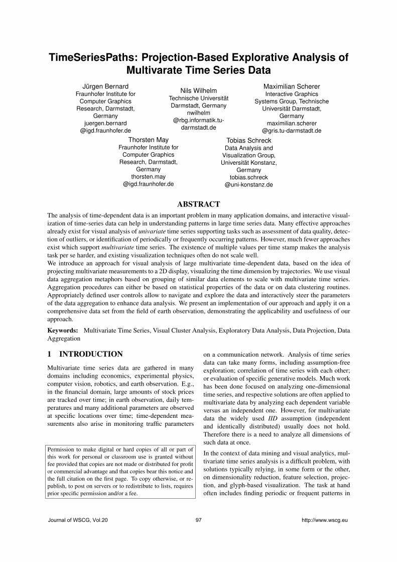
TimeSeriesPaths: Projection-Based Explorative Analysis ofMultivarate Time Series Data

Jürgen BernardFraunhofer Institute for

Computer GraphicsResearch, Darmstadt,

Germanyjuergen.bernard

@igd.fraunhofer.de

Nils WilhelmTechnische UniversitätDarmstadt, Germany

[email protected]

darmstadt.de

Maximilian SchererInteractive Graphics

Systems Group, TechnischeUniversität Darmstadt,

Germanymaximilian.scherer

@gris.tu-darmstadt.de

Thorsten MayFraunhofer Institute for

Computer GraphicsResearch, Darmstadt,

Germanythorsten.may

@igd.fraunhofer.de

Tobias SchreckData Analysis and

Visualization Group,Universität Konstanz,

Germanytobias.schreck

@uni-konstanz.de

ABSTRACTThe analysis of time-dependent data is an important problem in many application domains, and interactive visual-ization of time-series data can help in understanding patterns in large time series data. Many effective approachesalready exist for visual analysis of univariate time series supporting tasks such as assessment of data quality, detec-tion of outliers, or identification of periodically or frequently occurring patterns. However, much fewer approachesexist which support multivariate time series. The existence of multiple values per time stamp makes the analysistask per se harder, and existing visualization techniques often do not scale well.We introduce an approach for visual analysis of large multivariate time-dependent data, based on the idea ofprojecting multivariate measurements to a 2D display, visualizing the time dimension by trajectories. We use visualdata aggregation metaphors based on grouping of similar data elements to scale with multivariate time series.Aggregation procedures can either be based on statistical properties of the data or on data clustering routines.Appropriately defined user controls allow to navigate and explore the data and interactively steer the parametersof the data aggregation to enhance data analysis. We present an implementation of our approach and apply it on acomprehensive data set from the field of earth observation, demonstrating the applicability and usefulness of ourapproach.

Keywords: Multivariate Time Series, Visual Cluster Analysis, Exploratory Data Analysis, Data Projection, DataAggregation

1 INTRODUCTION

Multivariate time series data are gathered in manydomains including economics, experimental physics,computer vision, robotics, and earth observation. E.g.,in the financial domain, large amounts of stock pricesare tracked over time; in earth observation, daily tem-peratures and many additional parameters are observedat specific locations over time; time-dependent mea-surements also arise in monitoring traffic parameters


on a communication network. Analysis of time seriesdata can take many forms, including assumption-freeexploration; correlation of time series with each other;or evaluation of specific generative models. Much workhas been done focused on analyzing one-dimensionaltime series, and respective solutions are often applied tomultivariate data by analyzing each dependent variableversus an independent one. However, for multivariatedata the widely used IID assumption (independentand identically distributed) usually does not hold.Therefore there is a need to analyze all dimensions ofsuch data at once.

In the context of data mining and visual analytics, mul-tivariate time series analysis is a difficult problem, withsolutions typically relying, in some form or the other,on dimensionality reduction, feature selection, projec-tion, and glyph-based visualization. The task at handoften includes finding periodic or frequent patterns in


Figure 1: Main display: data analysis of a multivariate time series of 10 years length is always challenging dueto overview problems and visual cluttering. This is the starting point of our data exploration. The Time SeriesPath System provides visual structures and interactive functionality to address the implied challenges. In thisexample, we aggregate a weather scenario by its temperature values and receive 5 well-distributed data clustersfrom cold (blue) on the left to warm (yellow) on the right. This is a qualified starting point for selection andfiltering approaches to detect periodicity, dense data regions and outliers. Confer our case study in Section 5 fordetails about the 2D projection.

the data, relating multiple variables to each other, ordetecting outliers or anomalies. Visual-interactive ap-proaches can help to tackle these challenging tasks byclosely involving the user in the exploration process,addressing the typically difficult parameter selectionproblem, which could be more complicated to solve re-lying on purely automatic methods.

Several works propose to visually analyze multivariatetime-dependent data by dimensionality reduction [26,12]. Multivariate data is visualized as two-dimensionaltime series paths obtained by dimensionality reduction(projection to 2D). While these works visually comparesections of labeled multivariate time-dependent data,they do not consider exploratory search in unknowndata sets. Furthermore, these works do not focus on ag-gregation efforts to reduce over-plotting problems. Tothis end, we introduce interactively steerable data ag-gregation, supporting handling of multivariate time se-ries data. In particular, the user is able to group datapoints according to data-specific characteristics like sta-tistical calculations based on value and time, or cluster-ing results.

Our approach supports an effective overview of fre-quent and infrequent states in multivariate time seriesdata even in cases of very large data. Furthermore, userscan interactively select meaningful path line subsets

for detailed exploration and for visual clutter reductionpurposes. Understanding of aggregated data groups issupported by showing a comprehensive cluster glyphmetaphor, wherever data aggregation visualization isrequired within the exploration process. We directlyinvolve the user in the exploration process, combiningdata exploration with interactive steering of the auto-matic analysis methods, such as searching for appropri-ate clustering parameters, in particular.

We demonstrate the usefulness of our approach by anapplication to earth observation data. There, long timeseries of many parameters arise, and users want to un-derstand periodicities, trends, and anomalies. We showhow our set of interactive views allows for interactivelyexploring weather patterns of different lengths and pa-rameters. Due to our data aggregations, domain userscan explore multivariate weather data in a single dis-play, giving an overview of all data aspects at once.

The remainder of this paper is structured as follows.In Section 2 we discuss related work in several areas.In Section 3 and 4 we motivate our approach, explainour system design and describe user interaction tech-niques. In Section 5 we apply our implementation to areal-world data set, demonstrating the usefulness of theapproach. Finally, we summarize this paper and discussfuture extensions in Sections and 6 and 7.


Figure 2: Visual comparison SOM, PCA and MDS projection technique. A k-means clustering result is shown.

2 RELATED WORKOur work is related to analysis methods for time-dependent data and multivariate data. Time seriesanalysis in general is conducted to understand thebehavior of systems, to distinguish regular fromextraordinary characteristics [14] and to predict futuredevelopment [13].

Visualization of Time Series Data

The visualization of time series is often helpful for ex-ploratory analysis. Traditionally, time series can be vi-sualized by line charts [24]. However, using line chartsis typically not effective for large time series data,as many and long time series lead to over-plotting ifpacked into a given display or would require excessiveuser navigation (cf. the problem specification in Fig-ure 1). The pixel paradigm [2] for visualization of timeseries suggests to map the quantitative values of a timeseries to an appropriate color scale. Ultimately, eachvalue can be represented by a single pixel. The Recur-sive Pattern technique [2] employs the pixel paradigmto arrange time series in a generic proximity-preservingway, allowing to arrange between row-by-row up tomore complex patterns following space-filling curves.The comparison of many time series can be supportedby rendering them next to each other in an appropriatedisplay.

Besides side-by-side schemes, e.g., TreeMap-like lay-outs have been proposed [10]. An alternative to thepixel paradigm is to map the time axis to a spiral, ef-fectively using more length, which is particularly use-ful for analysis of periodic data [27]. For domain-specific visualization tasks, e.g., atomistic simulationdata, specialized techniques have been proposed [6].An overview of time series visualization can be foundin the textbook by Aigner et al. [1]

Automatic Support

Automatic analysis techniques are often used in timeseries visualization. E.g., the size of the data to be vi-sualized may be reduced by aggregation [5] or dimen-sionality reduction [8].

In [25] prototypical time series patterns are found bycluster analysis, and linked to occurrence on the timescale by color-coding. In [17] a discretization approach

is applied to support visual analysis of frequent subse-quences in a node-link-diagram. Often, the similaritydefinition between time series or subsequences thereofis important to support exploratory search. In [28] so-called Perception Points of Interest are identified to sorta large number of time series for effective overview-ing. Various other systems support the interactive re-trieval of time series by defining appropriate similar-ity notions and query interfaces [9, 11, 3]. A visual-interactive approach to analyzing different families offunctions is presented in [16]. Here, the authors allowthe user to highlight data patterns of interest and pro-vide linked views of the multidimensional data and theuser-selected highlights.

Multivariate Time Series

The above methods mainly consider univariate time se-ries. Yet, multivariate time series analysis is of impor-tance in many domains. A number of approaches in-clude small multiple displays for showing all variablesover time next to each other. They may rely on linecharts, pixel displays, or any other appropriate basetechnique. Also, automatic analysis methods for ex-ploratory analysis in multivariate time series have beenconsidered. E.g., in [19] a frequent-pattern-based ap-proach is used to find interesting time series patternsalong several levels of abstraction.

Recently, a number of authors have considered the visu-alization of multivariate time series data based on pro-jection. The basic idea is to project discrete points intime to a 2D display, which in turn allows for analysis ofthe time series for regularities and irregularities [23]. In[22, 12] multivariate observation measures from motiontracking are projected using the Self-Organizing Map(SOM) method [15]. Individual observations are con-nected by lines, and glyphs illustrating the particularconfigurations of the motion are shown. In [18] mul-tivariate time series are extracted from text, by com-putation of certain text features for discrete intervalsalong the sequence of the text. A PCA-based displaywas used to assess the development of the text content,by analysis of feature trajectories observed in the dis-play. In [26] the authors use PCA-based projection toexplore the sequence of small fixed-size intervals (so-called n-grams) of long univariate time series data. Theapproach was applied to stock market data and shown toprovide an informative overview over long time series


Figure 3: Aggregation of multivaritate time series data based on a variety of statistical data properties. Most of thefunctionality can either be performed on a single, or all dimensions.

data. In particular, the authors proposed their methodto support the following analysis cases: Detection ofcyclic behaviors; visual identification of base patternsand outliers; and analysis for trends.

3 SYSTEM DESIGNIn this work we present TimeSeriesPaths, a system forthe analysis of multivariate time series data. The PCAprojection algorithm is applied to arrange multivariatetime-series on the (2D) display screen (the Time SeriesPath Map). We connect temporally adjacent data ele-ments and receive a sequentially ordered set of points –a so called time series path. By default, such a visual-ization suffers from severe over-plotting and overviewproblems. In order to make such a visualization under-standable for domain-experts and to counter the impliedchallenges, our approach comprises three contributions:

1. We apply semi-automatic data aggregation function-ality, either derived from statistical data calculation,or from visual-interactive data clustering (cf. Sub-section 3.2). This helps the user to get an overviewto the dataset.

2. We present a cluster visualization technique thatincorporates multiple information about the aggre-gated data (cf. Subsection 3.2). This supports datainterpretation and cluster comparison approaches.

3. We propose a multi-view system with broad visual-interactive analysis functionality (cf. Subsection 4).Selection and highlighting modalities of data pathsubsets counter the challenge of over-plotting andallow for comprehensive detail on demand perspec-tives.

3.1 Visualizing Multivariate Time SeriesData Projection

We apply a projection technique to visualize multivari-ate time series data on 2D displays. An applicability

consideration between visualizations based on projec-tion and the multiple linechart technique is given inSection 6.

A general requirement concerning projection is thepreservation of data topology, by means that similardata in the multivariate input space is also arrangedclose to each other in the display space. Due to theirpopularity and their diversity in arithmetical mannerwe chose PCA, SOM and Multidimensional ScalingMDS [7] as promising candidates. After an evaluationof our requirement criteria and a visual comparison inFigure 2, we choose the PCA algorithm as a default forprospective projection needs in the TimeSeriesPathssystem. The non-linear MDS proves to be rather un-suitable for our approach, solely because it has troublesin separating k-means clusters. The SOM algorithmsuffers in respect to the calculation speed and a majordifficult (fully automatic) parametrization. Yet the keybenefit of PCA derives from the ability to project datapoints in a linear manner, by means that the projectionresults do not lack on local distortions and thus allowfor a more straight forwarded interpretation. Further-more, the visual comparison of the three projectiontechniques shows a good cluster separation by PCA.We accept that PCA does not exploit the completedisplay space as well as the SOM projection. Howeverlater in this section, we will present our cluster glyphand show how our glyph visualization mitigates thisproblem.

Visualizing Time Series Paths

The visualization of time series paths is provided bythe Time Series Path Map in the center of the display.Based on our data projection method, we connect indi-vidual data points by their chronological order to formpaths. The projection arranges similar data points closeto each other and reflects the data point distances of themultivariate data input space. Accordingly, if path se-quences are similar to each other, their possibly close


Figure 4: The “Rollercoaster Animation”. By dragging the time slider, the user can explore the temporal devel-opment of the time series path. The cursor position and time series path neighbors are animated with circularshapes.

positions on the display space help the user with pro-found analysis approaches.

3.2 Multivariate Time Series AggregationStatistics Calculation and Aggregation

We integrate automatically generated statistical data in-formation into the visualization to counter the overviewproblem and support the analysis process. So far, re-lated approaches color-code data points for time-basedand value-based changes or class labeling [12, 26]. Ourapproach generalizes this by a variety of statistical datameasurements that provide additional important infor-mation, an overview is given in Figure 3. Altogether,our system provides four different properties of statisti-cal data information for color coding:

• (a) occurrence within the time line (time-based)

• (b) nearest neighbor distance (NN-based)

• (c) speed of value change to adjacent time stamps(gradient-based)

• (d) cluster membership (clustering-based)

Except for (a), all statistical data information can eitherbe calculated on a single dimension or on all dimen-sions of the data set. Thus, we are also able to performdomain-specific exploration tasks due to the level of de-tail in the aggregation setup. The number of data groupsk can be specified by the user for all properties, (a)-(d).

Data color codings according to group affiliations aredisplayed on the Time Series Path Map, our time axisdisplay at the bottom (called Color Time Bar), and theData Aggregation List on the right, respectively. Show-ing multiple aspects of the data enables to find an ap-propriate aggregation level, to interpret groups of dataand derive mutual characteristics, to detect outliers andto explore periodic behavior in the data.

In our case study (cf. Section 5), we will show that dis-tributions of aggregated statistical data information onthe Time Series Path Map and the Color Time Bar givevaluable information about dense data regions, dataanomalies and the periodicity of time series paths.

Generic Cluster Glyph

The aggregation of data into groups requires a mean-ingful cluster visualization method (cf. Figure 5). Themain requirement is genericity in order to suit to agreat variety of multivariate time series data. Addition-ally, averages, minima and maxima, variances, num-ber of elements and cluster quality indices are needed.Each data dimension is displayed with an error barchart glyph metaphor and labeled with the correspond-ing physical unit. Additionally, we include the distribu-tion of time stamps on a time axis to monitor chrono-logical data characteristics to detect periodic behavioror anomalies. Finally we demand the cluster glyph toshow the cluster color coding for linking, and a headlinefor user-centered data labeling purposes.

Earlier we argued that PCA does not capitalize the en-tire border areas of the display space. We benefit fromthis instance due to the fact that we have free space re-maining to position cluster glyphs for data aggregationoperations. Four black concentrical lines connect thecluster glyph with the appropriate display coordinatewithout producing too much occlusion (see Figures 1,6, 7 and 8).

Figure 5: Generic Cluster Glyph. A boxplot-like visu-alization shows the distribution of data elements in eachdimension of the dataset, transparency is used to showdata frequency. Cluster centroid values are displayed asred bars, just like gray variance bands mapped laterallyfor each dimension. Statistical information about thedata cluster is shown at the center, the data distributionon the global time axis is shown at the bottom.

4 INTERACTION TECHNIQUESTimeSeriesPaths includes a set of linked user interac-tion modalities which work across the three different


Figure 6: Data aggregation on single input data dimensions: Distribution of relative humidity values (color map:blue means wet, yellow means dry). We constitute rainy weather states to be located left on the Time Series PathMap. By exploring the Color Time Bar, we discover rainy weathers dominating the winter periods. Composingthese two findings, we reason that (wet) winter climates are located on the left of the Time Series Path Map.

views. We give a short introduction to the major visual-interactive capabilities of the TimeSeriesPaths system.

Tooltipping

An important user requirement is detail on demand vi-sualization. By hovering above data elements on theTime Series Path Map and the Color Time Bar, tooltipsshow the multivariate data information and the positionof the respective data elements on the time axis (cf. Fig-ures 9 and 10).

Selection, Interactive Grouping and Highlighting

The selection of data is supported in each of our threeviews. The user can (1) select single data points, (2)time series paths or subsequences thereof, (3) the selec-tion of data within a distinct display region in the TimeSeries Path Map is possible (cf. Figure 7). The usersketches an arbitrarily polygonal shape on the map, andthe surrounded data points will be selected.

Data selections can subsequently be added to the DataAggregation List for additional information about theselection and for future re-selection. The respective se-lection is highlighted in all three views to allow the userthe detection of interesting patterns. For example, whenthe user selects a data cluster from the Data Aggrega-tion List (cf. Figures 9 and 8), respective data points arehighlighted in the Time Series Path Map and the Color

Time Bar. Thus, the user has three different scopes forthe exploration of the selected data: (a) the distribu-tion of the data on the Time Series Path Map, (b) occur-rences of data elements along the time line in the ColorTime Bar and (c) cluster value distributions in the DataAggregation List (cf. Figure 8).By means of transparency and plotting size, the usercan counter over-plotting on his own by reducing thevisibility of elements that are not selected.

Rollercoaster Animation

The Color Time Bar also contains a Time Slider for ani-mated time series analysis. We can drag the Time Sliderto a specific point or interval in time, and correspond-ing subsequences are highlighted with circular shapesin real-time on the Time Series Path Map. A schemat-ical demonstration of our so called “Rollercoaster Ani-mation” is given in Figure 4, an application is shown inFigure 10. This interactive animation allows a detailedexploration of the distribution of projected values overtime, and also to detect periodic patterns on the TimeSeries Path Map. The latter is especially helpful in caseof over-plotted displays, where a large amount of dataelements is visualized on the display.

5 CASE STUDYWe apply our system to a data set from earth obser-vation research. Based on consultation with domain re-searchers, we explore weather phenomena hidden in the


Figure 7: Data aggregation on single input data dimensions: Air pressure development. Selection of the left half ofthe paths (winter weathers). We discover a color gradient from high (top, yellow) to low (bottom, blue) air pressurevalues.

data like periodic patterns, frequent ’weather states’ andabnormal behavior that can be found with our system.

5.1 Data Set and Application Domain

Our considered data set is acquired from the open datarepository PANGAEA [21], operated by the AlfredWegener Insitute (AWI) for Polar and Marine Researchin Bremerhaven. PANGAEA archives and publishesgeo-referenced scientific earth observation data inthe research areas of water, ice, sediment and atmo-sphere. Our data set focuses on atmospheric weathermeasurements, gathered in the scope of the BaselineSurface Radiation Network (BSRN) [20] PANGAEAcompartment. These measurements are multivariateatmospheric observations of radiation-related physicalparameters) which were recorded every minute. Wefocus on a dataset of ten years duration, originatedfrom the BSRN station in Payerne (Switzerland) inthe time period of January 1st, 1994 to December31th, 2003 [4]. Payerne is located in the center ofthe triangle Lyon, Milan and Fribourg at 491 metersabove sea level. The climate of Payerne is temperate,semi-continental with average minimum temperaturesat about -2C in January and about 18C in July. Theaverage daily sunshine duration varies between 2 hoursin January and 8 hours in July. Hence, the researchersaffirm a yearly climate periodicity to the data thatserves as ground truth and primary analysis goal.Beyond that, the so called “summer of the century”in 2003 produced temperature values up to 40C and

motivates us finding this and yet other anomalies in thedata set.We consulted researchers from BSRN to select a suit-able parameter subset for detecting interesting weatherscenarios. Besides temperature, relative humidity andair pressure, we incorporate the short-wave downwardradiation (SWD) and the long-wave downward radia-tion (LWD). The SWD is well suited to give statementsabout cloud occurrences. Most radiation is measured atthe so called clear-sky condition, even when there areno clouds in the sky. It is used for climate research ingeneral and in applied sciences, e.g., in land surface as-similation models, surface energy budget models, andocean assimilation models. In agriculture, the short-wave downward radiation is used as an input for cropmodeling and the solar industry applies it for estima-tions where to build solar power plants. The LWD isanother important factor in the energetic exchange be-tween atmosphere and the earth surface. While the so-lar dependent short-wave downward radiation is nearzero at night, the long-wave downward radiation canbe measured all night long. The long-wave downwardradiation is higher when the sky is clear. By applyingthese five measurements as our data set, we are ableto make statements about different weather states thatpossibly change within a seasonal cycle.Due to the long time period of ten years, we determineeach single day as one data point, periodic behaviorswithin single days are also discovered in the data setand possible to analyze with our system, but not in thefocus in this case study. In order to remain on a uni-


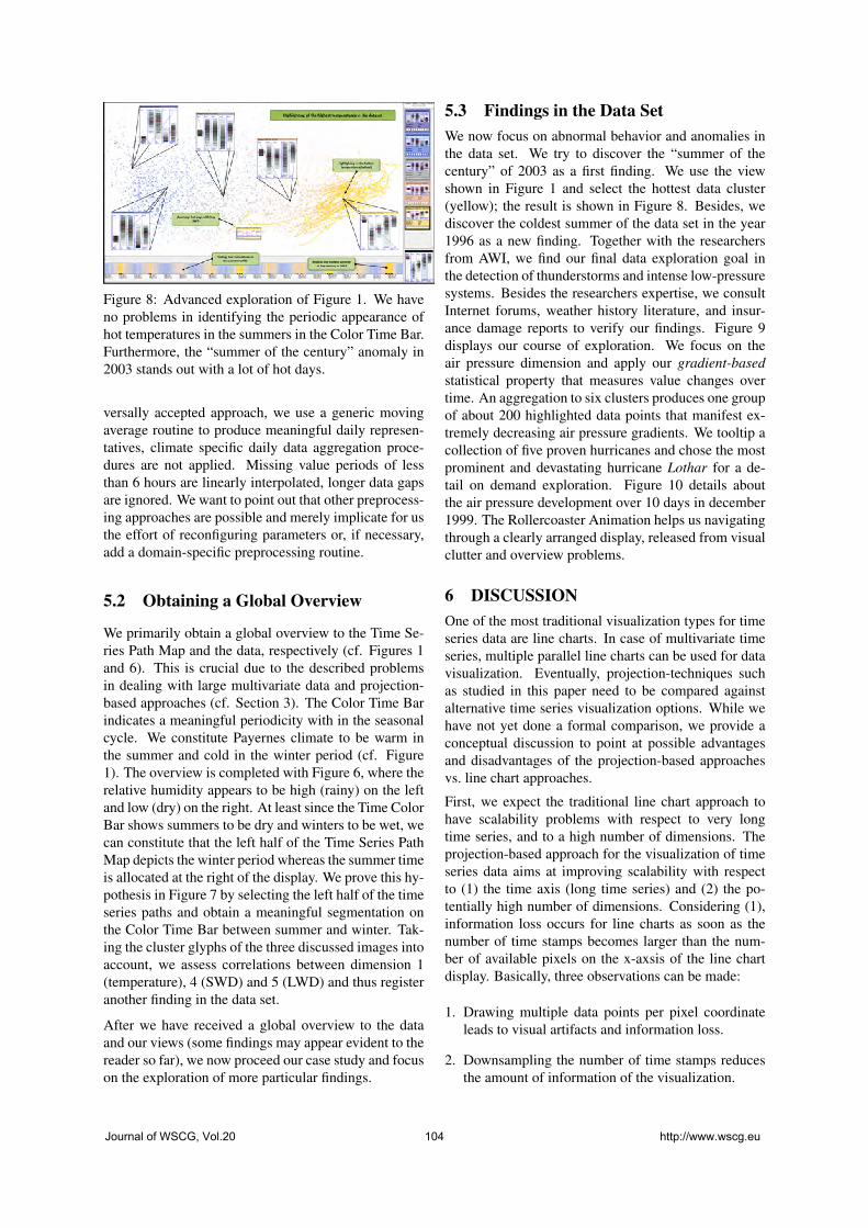
Figure 8: Advanced exploration of Figure 1. We haveno problems in identifying the periodic appearance ofhot temperatures in the summers in the Color Time Bar.Furthermore, the “summer of the century” anomaly in2003 stands out with a lot of hot days.

versally accepted approach, we use a generic movingaverage routine to produce meaningful daily represen-tatives, climate specific daily data aggregation proce-dures are not applied. Missing value periods of lessthan 6 hours are linearly interpolated, longer data gapsare ignored. We want to point out that other preprocess-ing approaches are possible and merely implicate for usthe effort of reconfiguring parameters or, if necessary,add a domain-specific preprocessing routine.

5.2 Obtaining a Global Overview

We primarily obtain a global overview to the Time Se-ries Path Map and the data, respectively (cf. Figures 1and 6). This is crucial due to the described problemsin dealing with large multivariate data and projection-based approaches (cf. Section 3). The Color Time Barindicates a meaningful periodicity with in the seasonalcycle. We constitute Payernes climate to be warm inthe summer and cold in the winter period (cf. Figure1). The overview is completed with Figure 6, where therelative humidity appears to be high (rainy) on the leftand low (dry) on the right. At least since the Time ColorBar shows summers to be dry and winters to be wet, wecan constitute that the left half of the Time Series PathMap depicts the winter period whereas the summer timeis allocated at the right of the display. We prove this hy-pothesis in Figure 7 by selecting the left half of the timeseries paths and obtain a meaningful segmentation onthe Color Time Bar between summer and winter. Tak-ing the cluster glyphs of the three discussed images intoaccount, we assess correlations between dimension 1(temperature), 4 (SWD) and 5 (LWD) and thus registeranother finding in the data set.

After we have received a global overview to the dataand our views (some findings may appear evident to thereader so far), we now proceed our case study and focuson the exploration of more particular findings.

5.3 Findings in the Data SetWe now focus on abnormal behavior and anomalies inthe data set. We try to discover the “summer of thecentury” of 2003 as a first finding. We use the viewshown in Figure 1 and select the hottest data cluster(yellow); the result is shown in Figure 8. Besides, wediscover the coldest summer of the data set in the year1996 as a new finding. Together with the researchersfrom AWI, we find our final data exploration goal inthe detection of thunderstorms and intense low-pressuresystems. Besides the researchers expertise, we consultInternet forums, weather history literature, and insur-ance damage reports to verify our findings. Figure 9displays our course of exploration. We focus on theair pressure dimension and apply our gradient-basedstatistical property that measures value changes overtime. An aggregation to six clusters produces one groupof about 200 highlighted data points that manifest ex-tremely decreasing air pressure gradients. We tooltip acollection of five proven hurricanes and chose the mostprominent and devastating hurricane Lothar for a de-tail on demand exploration. Figure 10 details aboutthe air pressure development over 10 days in december1999. The Rollercoaster Animation helps us navigatingthrough a clearly arranged display, released from visualclutter and overview problems.

6 DISCUSSIONOne of the most traditional visualization types for timeseries data are line charts. In case of multivariate timeseries, multiple parallel line charts can be used for datavisualization. Eventually, projection-techniques suchas studied in this paper need to be compared againstalternative time series visualization options. While wehave not yet done a formal comparison, we provide aconceptual discussion to point at possible advantagesand disadvantages of the projection-based approachesvs. line chart approaches.

First, we expect the traditional line chart approach tohave scalability problems with respect to very longtime series, and to a high number of dimensions. Theprojection-based approach for the visualization of timeseries data aims at improving scalability with respectto (1) the time axis (long time series) and (2) the po-tentially high number of dimensions. Considering (1),information loss occurs for line charts as soon as thenumber of time stamps becomes larger than the num-ber of available pixels on the x-axsis of the line chartdisplay. Basically, three observations can be made:

1. Drawing multiple data points per pixel coordinateleads to visual artifacts and information loss.

2. Downsampling the number of time stamps reducesthe amount of information of the visualization.


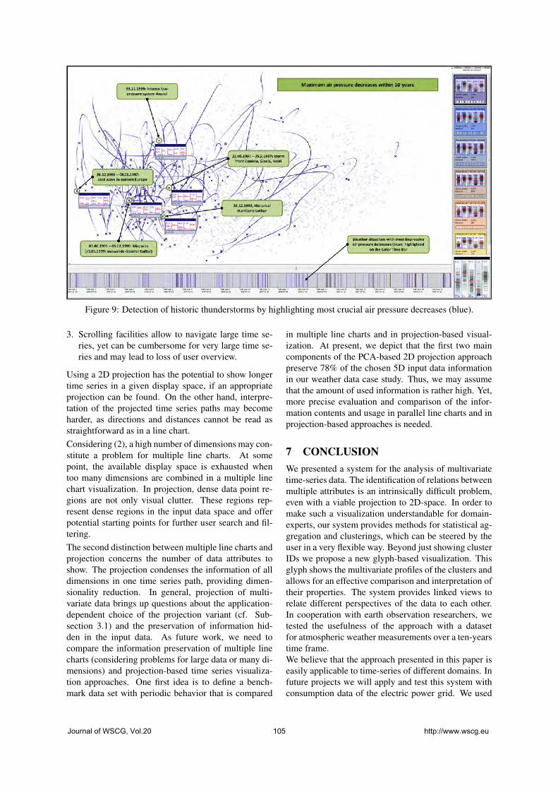
Figure 9: Detection of historic thunderstorms by highlighting most crucial air pressure decreases (blue).

3. Scrolling facilities allow to navigate large time se-ries, yet can be cumbersome for very large time se-ries and may lead to loss of user overview.

Using a 2D projection has the potential to show longertime series in a given display space, if an appropriateprojection can be found. On the other hand, interpre-tation of the projected time series paths may becomeharder, as directions and distances cannot be read asstraightforward as in a line chart.Considering (2), a high number of dimensions may con-stitute a problem for multiple line charts. At somepoint, the available display space is exhausted whentoo many dimensions are combined in a multiple linechart visualization. In projection, dense data point re-gions are not only visual clutter. These regions rep-resent dense regions in the input data space and offerpotential starting points for further user search and fil-tering.The second distinction between multiple line charts andprojection concerns the number of data attributes toshow. The projection condenses the information of alldimensions in one time series path, providing dimen-sionality reduction. In general, projection of multi-variate data brings up questions about the application-dependent choice of the projection variant (cf. Sub-section 3.1) and the preservation of information hid-den in the input data. As future work, we need tocompare the information preservation of multiple linecharts (considering problems for large data or many di-mensions) and projection-based time series visualiza-tion approaches. One first idea is to define a bench-mark data set with periodic behavior that is compared

in multiple line charts and in projection-based visual-ization. At present, we depict that the first two maincomponents of the PCA-based 2D projection approachpreserve 78% of the chosen 5D input data informationin our weather data case study. Thus, we may assumethat the amount of used information is rather high. Yet,more precise evaluation and comparison of the infor-mation contents and usage in parallel line charts and inprojection-based approaches is needed.

7 CONCLUSIONWe presented a system for the analysis of multivariatetime-series data. The identification of relations betweenmultiple attributes is an intrinsically difficult problem,even with a viable projection to 2D-space. In order tomake such a visualization understandable for domain-experts, our system provides methods for statistical ag-gregation and clusterings, which can be steered by theuser in a very flexible way. Beyond just showing clusterIDs we propose a new glyph-based visualization. Thisglyph shows the multivariate profiles of the clusters andallows for an effective comparison and interpretation oftheir properties. The system provides linked views torelate different perspectives of the data to each other.In cooperation with earth observation researchers, wetested the usefulness of the approach with a datasetfor atmospheric weather measurements over a ten-yearstime frame.We believe that the approach presented in this paper iseasily applicable to time-series of different domains. Infuture projects we will apply and test this system withconsumption data of the electric power grid. We used


Figure 10: Rollercoaster Animation on hurricaneLothar. Air pressure coloring (blue means low).

projection techniques as an overview because of theirpopularity as a method for multivariate analysis. How-ever, the methods to calculate, steer and explore theclusters are not restricted to a specific type of overview.In future, we will extend the linked views by other vi-sualizations for multivariate time-series to test for themost effective combination of domain, overview andaggregation methods.

ACKNOWLEDGMENTSWe thank the Alfred Wegener Insitute (AWI) in Bre-merhaven, particularly Rainer Sieger, Hannes Grobeand Gert König-Langlo, and everyone involved withPANGAEA for supporting this research effort.

8 REFERENCES[1] W. Aigner, S. Miksch, H. Schumann, and C. Tominski. Visual-

ization of Time-Oriented Data. Springer-Verlag New York Inc,2011.

[2] Mihael Ankerst, Daniel A. Keim, and Hans-Peter Kriegel. Re-cursive pattern: A technique for visualizing very large amountsof data. In Proceedings of Visualization ’95, Atlanta, GA, pages279–286, 1995.

[3] Jürgen Bernard, Jan Brase, Dieter W. Fellner, Oliver Koepler,Jörn Kohlhammer, Tobias Ruppert, Tobias Schreck, and IrinaSens. A visual digital library approach for time-oriented sci-entific primary data. In Proc. European Conference on DigitalLibraries, pages 352–363, 2010.

[4] Jürgen Bernard, Nils Wilhelm, Maximilian Scherer, ThorstenMay, and Tobias Schreck. Reference list of 120 datasetsfrom time series station payerne used for exploratory search.doi:10.1594/pangaea.783598, 2012.

[5] Lior Berry and Tamara Munzner. Binx: Dynamic explorationof time series datasets across aggregation levels. In Proc. IEEESymposium on Information Visualization, 2004.

[6] D. Bhattarai and B.B. Karki. Visualization of atomistic simu-lation data for spatio-temporal information. In The 14th Int’l.Conf. on Central Europe in Computer Graphics, Visualizationand Computer Vision (WSCG’06), 2006.

[7] Trevor F. Cox and M.A.A. Cox. Multidimensional Scaling,Second Edition. Chapman and Hall/CRC, 2 edition, 2000.

[8] Tim Dwyer and David R. Gallagher. Visualising changes infund manager holdings in two and a half-dimensions. Informa-tion Visualization, 3:227–244, December 2004.

[9] Ming C. Hao, Umeshwar Dayal, Daniel A. Keim, DominikMorent, and Jörn Schneidewind. Intelligent visual analytics

queries. In IEEE Symposium on Visual Analytics Science andTechnology, pages 91–98, 2007.

[10] Ming C. Hao, Umeshwar Dayal, Daniel A. Keim, and To-bias Schreck. Importance driven visualization layouts for largetime-series data. In Proc. IEEE Symposium on InformationVisualization. IEEE Computer Society, 2005.

[11] Harry Hochheiser and Ben Shneiderman. Dynamic query toolsfor time series data sets: Timebox widgets for interactive ex-ploration. Information Visualization, 3(1):1–18, 2004.

[12] Yueqi Hu, Shuangyuan Wu, Shihong Xia, Jinghua Fu, andWei Chen 0001. Motion track: Visualizing variations of humanmotion data. In PacificVis, pages 153–160, 2010.

[13] N.K. Kasabov and Q. Song. Denfis: Dynamic evolving neural-fuzzy inference system and its application for time-series pre-diction. Fuzzy Systems, IEEE Transactions on, 2002.

[14] E. Keogh, J. Lin, and A. Fu. Hot sax: Efficiently finding themost unusual time series subsequence. In Data Mining, FifthIEEE International Conference on, pages 226 – 233. Ieee, 2005.

[15] Teuvo Kohonen. Self-Organizing Maps. Springer, Berlin, 3rdedition, 2001.

[16] Zoltan Konyha, Kresimir Matkovic, Denis Gracanin, MarioJelovic, and Helwig Hauser. Interactive visual analysis of fam-ilies of function graphs. IEEE Transactions on Visualizationand Computer Graphics, 12(6):1373–1385, November 2006.

[17] J. Lin, E. Keogh, S. Lonardi, J.P. Lankford, and D.M. Nystrom.VizTree: a tool for visually mining and monitoring massivetime series databases. In Proc. of the int. conf. on Very LargeData Bases, pages 1269–1272. VLDB Endowment, 2004.

[18] Yi Mao, Joshua Dillon, and Guy Lebanon. Sequential docu-ment visualization. IEEE Transactions on Visualization andComputer Graphics, 13:1208–1215, 2007.

[19] Fabian Mörchen and Alfred Ultsch. Efficient mining of under-standable patterns from multivariate interval time series. DataMin. Knowl. Discov., 15(2):181–215, 2007.

[20] A. Ohmura, E. G. Dutton, B. Forgan, C. Fröhlich, H. Gilgen,H. Hegner, A. Heimo, G. König-Langlo, B. mcarthur,G. Müller, R. Philipona, R. Pinker, C. H. Whitlock,K. Dehne, and M. Wild. Baseline surface radiation network(BSRN/WCRP): New precision radiometry for climate re-search. Bull. Amer. Met. Soc., 79:2115–2136, 1998.

[21] PANGAEA - Data Publisher for Earth and Environmental Sci-ence. http://www.pangaea.de/. Last accessed on April 5, 2012.

[22] Y. Sakamoto, S. Kuriyama, and T. Kaneko. Motion map:image-based retrieval and segmentation of motion data. In Proc.2004 ACM SIGGRAPH/Eurographics symposium on computeranimation. Eurographics Association, 2004.

[23] Geoffroy Simon, Amaury Lendasse, Marie Cottrell, and Uni-versité Paris. Long-term time series forecasting using self-organizing maps: the double vector quantization method, 2003.

[24] Edward R. Tufte. The visual display of quantitative informa-tion. Graphics Press, Cheshire, CT, USA, 1986.

[25] Jarke J. Van Wijk and Edward R. Van Selow. Cluster and cal-endar based visualization of time series data. In Proc. IEEESymposium on Information Visualization, pages 4–9. IEEEComputer Society, 1999.

[26] Matthew O. Ward and Zhenyu Guo. Visual exploration of time-series data with shape space projections. Eurographics / IEEESymposium on Visualization (EuroVis), 30(3), 2011.

[27] M. Weber, M. Alexa, and W. Müller. Visualizing time-series onspirals. In proceedings of the IEEE Symposium on InformationVisualization, pages 7 – 13, 2001.

[28] H. Ziegler, M. Jenny, T. Gruse, and D.A. Keim. Visual marketsector analysis for financial time series data. In Visual Ana-lytics Science and Technology (VAST), IEEE Symposium on,pages 83–90, 2010.


Design and Analysis of Visualization Techniques for MobileRobotics Development

Alex KozlovThe University of Auckland, New

[email protected]

Bruce A. MacDonaldThe University of Auckland,

New [email protected]

Burkhard C. WünscheThe University of Auckland,


ABSTRACTSimultaneous localization and mapping (SLAM) algorithms are of vital importance in mobile robotics. This paperpresents novel Augmented Reality (AR) visualization techniques for SLAM algorithms, with the purpose of assist-ing algorithm development. We identify important algorithm invariants and parameters and combine research inuncertainty visualization and AR, to develop novel AR visualizations, which offer an effective perceptual and cog-nitive overlap for the observation of SLAM systems. A usability evaluation compares the new techniques with thestate-of-the-art inferred from the SLAM literature. Results indicate that the novel correlation and color-mappingvisualization techniques are preferred by users and more effective for algorithm observation. Furthermore theAR view is preferred over the non-AR view, while being at least similarly effective. Since the visualizations arebased on general algorithm properties, the results can be transferred to other applications using the same class ofalgorithms, such as Particle Filters.

KeywordsAlgorithm visualisation, augmented reality, robot programming, human-robot interfaces

1 INTRODUCTIONSimultaneous Localization and Mapping (SLAM)[SSC90, LDW91] is a popular and important classof estimation algorithms, addressing the challengeof autonomous map-building for mobile robots. Arobot must have a model, or a map, of the physicalenvironment in order to carry out useful navigationtasks. The robot must additionally localize itself withinthe environment. In SLAM the robot autonomouslyexplores and maps its environment with its sensorswhile localizing itself at the same time. Despiteconsiderable research, open challenges in SLAMinclude implementations in unstructured, difficult,and large scale environments [BFMG07], multi-robotSLAM [NTC03] as well as SLAM consistency andconvergence [MCDFC07].

SLAM development is made more difficult by its prob-abilistic nature. In SLAM, neither the robot locationnor the environment map are known in advance. How-ever, in order to map the environment the robot locationneeds to be known with accuracy, and in order to local-ize the robot the environment map needs to be known


with accuracy. Visualizations aid the development andtesting of SLAM algorithms by revealing relationshipsbetween robot and algorithm states and environmentalparameters. Existing SLAM visualization techniquesare purely virtual and limited to basic state information,thus lacking perceptual and cognitive overlap betweenthe robot and the human developer [BEFS01].

Augmented Reality (AR) involves spatially registeringvirtual objects in real time within a view of a real scene[BR05, Azu97]. AR has been used in robotics to en-hance the human-robot interface, but has never been ap-plied to SLAM visualization. This paper presents andevaluates novel AR visualization techniques for SLAMwith the purpose of assisting algorithm developmentand debugging. The introduced concepts and lessonslearned are applicable to other estimation algorithms inrobotics and related fields.

Section 2 outlines the SLAM algorithms for which thevisualizations have been developed. Section 3 presentsa review of fields we draw on. Section 4 summarizesthe visualization requirements. Section 5 explains thevisualization techniques. Section 6 presents the evalu-ation of the visualizations, and section 7 concludes ourpaper.

2 SLAM BACKGROUNDThe two most popular SLAM algorithm archetypes,the Extended Kalman Filter (EKF) SLAM[GL06, DWB06] and FastSLAM [MTKW03, Mon03],are both based on recursive Bayesian estimation. These


algorithms were targeted for visualization because theyare the two most important and prevalent SLAM solu-tion methods [DWB06]. The visualizations presentedin this paper would also be relevant for any modifiedKalman Filter or Particle Filter based algorithm.

2.1 EKF SLAMIn feature-based EKF SLAM the state is represented bya multivariate Gaussian distribution with mean x andcovariance P:

x =

xrx f1...

x fn

(1)

P =

Pr Pr, f1 . . . Pr, fn

Pf1,r Pf1 . . . Pf1, fn...

.... . .

...Pfn,r Pfn, f1 . . . Pfn

(2)

xr is the estimated robot pose and x fi , i = 1, . . . ,n is theestimated position of an environment feature fi. Themain diagonal elements Pr,Pf1 , . . . ,Pfn are error covari-ance matrices of the robot pose and the landmark loca-tions. The off-diagonal elements are cross-covariancematrices between the robot and feature positions. Therecursive estimation steps of the algorithm are motionprediction, data association, observation update andfeature initialization.

2.2 FastSLAMIn FastSLAM, which is based on Rao-BlackwellizedParticle Filters, the state is represented by a set of Nparticles:

w(i),X (i)r ,µ

(i)f1, . . . ,µ

(i)fn ,Σ

(i)f1, . . . ,Σ

(i)fn

Ni (3)

where for particle i, w(i) is the particle weight, X (i)r is

the sampled robot path, and each map feature f j is rep-resented independently by a Gaussian distribution withmean µ

(i)f j

and covariance Σ(i)f j

. The recursive estimationsteps of the algorithm are motion prediction, weight up-date, resampling and map update.

3 LITERATURE REVIEWA number of Robotics Development Environments(RDEs) are available for use in robotics programming,but none offers visualizations for SLAM. Examplesinclude Player [GVS+01], CARMEN (CarnegieMellon robot navigation toolkit) [MRT] and Pyro(Python Robotics) [BKMY03]. These offer purelyvirtual sensor data visualizations. Possibly the most

flexible support for visualizations is offered by ROS(Robot Operating System) [QGC+09], which includesa variety of data-types such as point clouds, geometricprimitives, robot poses and trajectories.

No formal studies have been done for visualizationtechniques in SLAM. The SLAM visualization stateof the art is inferred from the visual representa-tions of SLAM systems and data in the literature.The current “conventional” method of visualizingEKF-style SLAM is by showing the mean estimatesfor the robot and features, along with the covari-ance ellipsoids showing the individual uncertainties(e.g. [BNG+07, NCMCT07]). For Particle Fil-ter type SLAM, all current robot poses and meanfeature locations are shown for all particles (e.g.[MTKW03, Mon03]). Perhaps the most interestingexample of an existing SLAM visualization is the 3Dgraphical representation of the robot in relation to themapped obstacles, with the uncertainties shown bydotted lines around the objects [NLTN02]. Martinez-Cantin et al. visualized a constructed 3D map from therobot’s point of view [MW03].

None of the basic SLAM visualizations suggested sofar employs an AR environment. However, AR sys-tems have been developed and used in robotics. Anexample is ARDev [CM06, CM09]. It provides per-ceptual overlap between the human and the robot byvisualizing sensor data within the robot’s real world en-vironment. Nunez et al. use AR for supervision ofsemi-autonomous robot navigation tasks [NBPLS06].A topological map is generated online and visualizedwith AR. Daily et al. use AR to supervise a swarm of 20robots for search and rescue scenarios [DCMP03]. Vir-tual arrows above every swarm member in view conveythe intention and direction of travel. AR has also seenconsiderable application in mobile robot tele-operation[BOGH+03] and manipulator robotics [NCE+07].

4 VISUALIZATION REQUIREMENTSThe underlying requirement for all of the visualiza-tions is to embed information within the context of thereal world environment the mobile robot operates in.This provides a qualitative comparison between the es-timates and the ground truth, and shows sources of po-tential errors within the real environment.

4.1 EKF SLAM RequirementsThe fundamental EKF SLAM requirement is to visual-ize the state and the individual uncertainty covariances.The state consists of 2D robot and feature locations, andthe robot orientation in the ground plane. The 2 by 2covariance matrices for the robot and each feature indi-cate the positional uncertainty, together with the robotorientation variance.


(a) (b) (c)

Figure 1: Conventional AR EKF Visualization: EKF-SLAM state and covariance visualization in AR, showing progressionover time. The AR view provides a direct comparison of the estimates against the ground truth in the real world environment;this shows the discrepancies between the truth and the estimates.

Correlations between features are well known to be im-portant for correct SLAM operation [DWRN96]. In[DNC+01] feature correlations are defined as follows.Let di j be the relative position between any two featureestimates fi and f j. Let Pdi j be the covariance of di j asfollows:

di j = x fi − x f j (4)

Pdi j = Pfi +Pf j −Pfi, f j −PTfi, f j

(5)

Pdi j is a measure of relative error between the twofeatures, and is therefore also a measure of their cor-relation. The expected convergence property [HD07,DNC+01] is that correlations strengthen as observa-tions are made over time, i.e. the volume of uncertaintyin Pdi j is non-increasing. Visualization of the correla-tion behaviour is essential. Violations of this behaviour(i.e. weakening correlations) indicate problems in theSLAM system, and therefore must be detected by theuser. Specifically, the 2 by 2 covariance matrix Pdi j

must be visualized for all feature pairs, together withits non-increasing volume of uncertainty trend. Viola-tions must be exemplified.

4.2 FastSLAM RequirementsThe fundamental FastSLAM requirement is to visualizethe state represented by the set of particles. This meansvisualizing 2D points for the robot and Gaussian meanfeature locations, for all particles. Additionally robotorientations for all particles must be visualized.

Due to the Rao-Blackwellized structure of FastSLAM,sampling is only done on the robot path. The error inthe map estimation for a given particle is dependenton the accuracy of the robot path. For this reason, itis important to visualize the relationship between therobot path and map estimates within particles, or intra-particle associations. Specifically, this refers to visu-ally linking estimates from the same particle, and dis-tinguishing these from other particles. Visualization ofthe individual weight for each particle is also important

in order to gain insight into the resampling phase of thealgorithm.

Lastly, a more qualitative and more intuitive representa-tion of the SLAM solution produced by the filter wouldbe useful. This needs to show a better overall picture ofthe solution, possibly at the cost of lower informationcontent or being less exact.

5 AR VISUALIZATION TECHNIQUES5.1 EKF SLAM Visualizations5.1.1 Conventional EKF SLAM Visualization

Fig. 1 presents the state-of-the-art conventional EKFvisualization implemented in AR. The underlying realworld images present an overhead view of the robotand its environment. The robot is a PIONEER 3-DX[Rob08]. The map the robot is building consists of twodimensional points in the ground plane represented bywhite cardboard cylinders. The cylinders are the onlyphysical objects being mapped and are extracted fromraw laser rangefinder data. The robot drives around andperforms SLAM in a small 1 by 1 meter loop. Thegraphical icons augmenting the video frames representSLAM information:

• Cyan Marker - The cyan downward pointed conerepresents the estimated robot position. The cyan el-lipsoid underneath is the robot position covariance.The cyan line is the robot path.

• Green Marker - The green downward pointed conerepresents the estimated feature position. The greenellipsoid underneath is the feature position covari-ance.

• Yellow Marker - The yellow triangular pointer rep-resents the robot orientation estimate. A semitrans-parent yellow circular wedge represents the orienta-tion variance.


(a) (b)

Figure 2: EKF SLAM Correlations Clustering. (a) shows all inter-cluster correlations, (b) shows only the maximum, mean,and minimum inter-cluster correlations. Green wireframe circles represent spatial clusters.

The markers represent the SLAM estimates for qual-itative real-time visual comparison against the groundtruth presented in the real image, i.e. the green mark-ers correspond to the white cardboard cylinders and theblue marker to the physical robot. For the orientation an“arrow” type marker was chosen, as commonly used inSLAM and robotics visualizations. For the covariance,the common tensor ellipsoid glyph was used, which issuperior to line or arrow type ellipsoid glyphs. Colourwas used to define specifically what the estimate refersto, i.e. robot or features. The design follows the “Natu-ral Scene Paradigm”, which is based on humans’ abilityto immediately perceive complex information in a nat-ural scene [WL01].

5.1.2 Correlations Visualization

In previous work [KMW09] we presented the novel fea-ture correlation visualization shown in Fig. 2a. It sat-isfies the requirements discussed earlier. For every pairof features fi, f j the visualization contains:

• A line linking the feature estimates fi and f j

• A yellow tensor “correlation ellipsoid” for Pdi j ren-dered at the half-way point on the line

As Pdi j is a two-dimensional covariance, it produces a2D tensor ellipsoid. However, the problem of visualcluttering becomes evident when many such ellipsoidsgrow in size and overlap. It becomes difficult to discernany individual ellipsoids. To mitigate this issue the el-lipsoids were inflated to a shaded 3D shape. The sec-ond eigenvalue is used for the length of the axis intothe third dimension. Giving a 3D shaded volume tothe correlation ellipsoids provides better visual distinc-tion to overlapping ellipsoids, however a limitation of

this method is that it occludes more of the backgroundworld image.Strengthening correlations show up as decreasing vol-umes of the correlation ellipsoids. If the volume ofthe correlation ellipsoid increases (i.e. the correlationweakens), this is considered a violation of the expectedbehaviour. This occurrence is exemplified in the visu-alization by changing the colour of the ellipsoid to red.Thus, the visualization allows the observation of the ex-pected correlations trend, and the detection of its viola-tions.The problem of visual cluttering is resolved by spatialclustering using the standard single-linkage hierarchi-cal clustering method [LL98]. Features are divided intospatial clusters, and only the correlations between fea-tures in different clusters are shown. The green wire-frame circles exemplify the clusters computed by thealgorithm. This image demonstrates a pure virtual sim-ulation of the SLAM algorithm, and hence no physicalrobot and environment is shown.In order to further reduce the number of correlationsin view the user can select to only see the minimum(yellow), mean (orange), and maximum (yellow) inter-cluster correlations (Fig 2b). The expected correla-tion convergence can be observed through the non-increasing size of the minimum correlation ellipsoid[Koz11].

5.2 FastSLAM Visualizations5.2.1 Conventional FastSLAM VisualizationFig. 3 presents the conventional state-of-the-art Fast-SLAM visualization implemented for the first time inAR. The underlying real world images present an over-head view of the robot and the environment the robot isworking in. The graphical icons augmenting the videoframes represent SLAM information:


(a) (b) (c)

Figure 3: Conventional FastSLAM AR Visualization: particle representation for the robot pose and features, showing thejoint SLAM posterior distribution computed by the particle filter and its progression over time.

• Cyan Marker - The cyan downward pointed conerepresents the sampled robot location for a givenparticle.

• Yellow Marker - The yellow arrow-type markerrepresents the sampled robot orientation for a givenparticle.

• Green Marker - The green downward pointed conerepresents a Gaussian mean feature location for agiven particle.

The visualization shows the joint SLAM posteriorprobability distribution of the robot pose and thefeature map. As for the EKF, the markers representthe SLAM state for qualitative visual comparisonagainst the ground truth presented in the real image, i.e.the green markers correspond to the white cardboardcylinders and the blue marker to the physical robot.

5.2.2 Colour Mapping VisualizationsFig. 4 presents a colour-mapping visualization tech-nique addressing the requirements of intra-particle as-sociations and particle weights, as discussed earlier.First the centroid and maximum distance from the cen-troid are computed for the current robot positions in theparticles. This creates a local polar coordinate frame forthe robot positions (and thus the particles they belongto), originating at the centroid. Then each particle’s po-lar coordinates are mapped directly onto the Hue andSaturation parameters in the HSV colour model. Thus,each particle which has a unique robot position is as-signed a unique colour. This colour is used to encodemembers of the same particle (intra-particle associa-tions), e.g. a red feature and a red robot pose belongto the same particle. This shows the important rela-tionship between the map and robot path estimations.In the final step, the particle weight is encoded intothe Value (brightness) parameter of the HSV model.Lighter coloured markers indicate higher weights, anddarker colours indicate lower weights. Fig. 5 shows the

Figure 4: The colour-mapping technique.

colour-mapping visualization applied in SLAM. Thecolour-coded relationship between the robot positionand feature errors is clearly visible.

5.2.3 Surface Density Visualization

Fig. 6 presents a novel surface density visualizationtechnique developed for FastSLAM. The purpose ofthis visualization is to present a better overall qualita-tive picture of the SLAM solution produced by the filter.Here the joint SLAM posterior probability of the robotand the features is represented by a smooth, shaded 3Dsurface. The mapping area is divided into an uniform(customizable) grid, where the density of a given cell isgiven by the number of particle members (robot pose orfeatures) within that cell. Then the surface is interpo-lated over the grid using a Radial Basis Function (RBF)[Buh03], with the density giving the surface height. Ifcolour-mapping is enabled, the colour for each cell isthe average of the particle colours within it. Other-wise, the cyan surface represents the robot pose and thegreen surfaces the features. In addition, a single arrowis drawn above each cell of the robot pose surface. Thisis the average robot orientation within the cell.


(a) (b) (c)

Figure 5: Intra-particle Associations Visualization: colour-mapping used to show members belonging to the same givenparticle, showing progression over time. Brightness indicates particle weights.

Figure 6: The surface colour-mapping technique.

Fig. 7 shows the surface density visualization with-out the colour mapping. Intuitively the height of thesurface indicates the SLAM posterior probability. Theshape of the surface provides a good qualitative pictureof the uncertainty spread of the distribution, as com-pared to rendering each individual marker. Fig. 8 showsthe colour-mapped surface density visualization. Thisoffers the benefits of both the surface and the colour-mapping techniques. The visualization shows both theshape of the uncertainty spread and the colour-mappedintra-particle associations.

6 EVALUATION6.1 Experimental SetupThe visualization system was implemented with a ceil-ing mounted Prosilica EC 1350C Firewire camera forimage capture. Registration was done using ARToolK-itPlus and a fiducial marker mounted on the robot. Therobot’s initial position is registered in the AR coordi-nate frame as the origin of the SLAM map. This allowsthe registration of the SLAM data in the AR coordinateframe. Videos were taken of the robots SLAM per-formance using different visualization techniques forcorrectly implemented SLAM algorithms and versionswith typical errors we inferred from the literature and aprevious user survey [Koz11].

6.2 MethodologyWe performed five experiments summarised in table 1in order to investigate the effectiveness of the visual-

Fault Detection ExperimentsExperiment Vis 1 Vis 2EKF Exp 1 Conventional

ARConventionalnon-AR

EKF Exp 2 Correlations AR ConventionalAR

FastSLAMExp 1

ConventionalAR

Conventionalnon-AR

FastSLAMExp 2

Colour-mappingAR

ConventionalAR

FastSLAMExp 3

Surface densityAR

ConventionalAR

Table 1: Fault detection experiments summary. Each experi-ment compared Vis 1 with Vis 2.

izations for assisting SLAM development. In partic-ular we evaluated AR-based visualisation techniquesversus non-AR visualisation techniques and novel ARvisualisation versus AR-implementations of techniquesconsidered current state-of-the-art. The purpose of thestudy was to compare the effectiveness of the visualiza-tion techniques for SLAM algorithm development, i.e.fault detection and fault correction.

The experiments were performed as a web-basedsurvey questionnaire. Participants were invited overemail, through the major international robotics mailinglists. These included Robotics Worldwide, AustralianRobotics and Automation Association (ARAA) andEuropean Robotics Research Network (EURON).Ideally the desired population of the participants wouldbe SLAM developers; but in practice to obtain suffi-cient participants the population scope was widened torobotics developers. The experiments involved partici-pants watching online videos of the visualizations andanswering questions about the visualizations.

Within the questionnaire document, the concepts ofSLAM and AR were first explained, along with in-


(a) (b) (c)

Figure 7: Surface Density Visualization: the surface density visualization without the colour-mapping, showing progressionover time. The shape and height of the surface conveys the joint SLAM posterior distribution computed by the particle filter.

(a) (b) (c)

Figure 8: Colour Mapped Surface Visualization: the surface density visualization with the colour-mapping, showing pro-gression over time. The visualization shows both the shape of the joint SLAM posterior distribution and the associations withinparticles.

troductory videos and explanations about the visual-izations. Each AR visualization was presented with avideo of it being used for SLAM with a real robot andcylindrical point features, along with a written explana-tion. To present the non-AR visualization, two videoswere used. One was the virtual SLAM visualization,and the other was the video of the physical robot per-forming SLAM corresponding to the SLAM visualiza-tion.

After showing correct operation, artificial faults wereintroduced into the SLAM systems. Within each exper-iment the same fault was used to compare the visual-izations, however the visualizations showed the fault indifferent ways. For each visualization, the participantswere asked as a multi choice question what SLAM faultis present in the visualization (if any). For each pairof visualizations compared, the participants were alsoasked in a short answer question which visualizationthey felt was more effective (Vis 1, Vis 2, or neither)and why. Details of the study are found in [Koz11].

6.3 ResultsThere were 24 participants in the EKF evaluation, and14 participants in the FastSLAM evaluation.

In EKF Exp 1 users detected 75% of errors with the ARvisualization and 70% of errors with the non-AR visual-ization. Users liked that the AR visualization combineda view of the real environment with the SLAM infor-mation. Reasons for prefering non-AR were perceptiondifficulties in AR due to the 3D camera perspective,deformation, depth and projection, and the real-worldcamera image. In FastSLAM Exp 1 all of the partic-ipants preferred the AR visualization. In terms of ef-fectivness both visualisations resulted in 57% of errorsbeing detected.

In EKF Exp 2 our new correlation visualization allowedusers to detect 79% of errors, whereas the traditionalvisualization only allowed detection of 50% of errors.Users liked in the correlation visualization the explicitrepresentation of correlation faults enabling a faster de-tection. Reasons for prefering the conventional AR vi-sualization were clearer, more intuitive representationof robot pose/landmarks and faults therein, the correla-tion ellipsoids being hard to understand and occludingthe landmark/robot markers, and robot/landmark co-variances being more representative of the estimationprocess.


In FastSLAM Exp 2 users were able to detect 64% oferrors using colour mapped particles and 35% of er-rors using the conventional visualization. Users likedabout colour-mapping the clear representation of par-ticle weighting and the resampling process, and thatcolour mapping offers more information in a compactrepresentation allowing for better fault detection.

In FastSLAM Exp 3 users identified 42% of errors us-ing the surface density visualization and 71% of errorsusing the conventional visualization. Users liked thecompact and effective representation of the particle setdistribution in the surface density AR visualization, andthat the peak of the surface indicates the most likely es-timate position whereas the spread shows the amountof divergence in the estimates. However, users com-plained that the surface representation is too opaque andobscures the true landmarks, and that the surface viewdoes not show the robot orientation clearly. Users statedthat the conventional AR visualization is easier to ana-lyze in order to detect errors.

7 CONCLUSIONSThis paper presented novel AR visualization techniquesfor SLAM algorithms. The visualization requirementswere challenging because SLAM algorithms are de-tailed, complex, and must address real world uncertain-ties. To address the requirements, visualizations weredeveloped in AR to target the most important aspects ofthe SLAM algorithms, including feature correlations,particle weights and relationships.

Our Evaluation shows that AR visualizations are pre-ferred over non-AR visualizations, and that the noveltechniques for feature correlations is more effectivethan the existing state of the art for SLAM fault de-tection. The visualizations are effective because theytarget specific aspects of the algorithm and becauseAR enables visualization of the real world and asso-ciated uncertainties. The correlation visualization canbe adapted to any application requiring representationof correlations between physical entities. Care must betaken that visualization icons do not obscure relevantreal-world information in the camera view and that vi-sual complexity does not put undue stress on the user.Hence small point based icons are preferable over morecomplex and information rich surface representations.The presented visualizations perform differently wellfor different types of errors. Ideally the user should beable to swap interactively between all of the presentedtechniques.

8 REFERENCES[Azu97] R.T. Azuma. A survey of augmented

reality. Presence: Teleoperators and Vir-tual Environments, 6(4):355–385, 1997.

[BEFS01] C. Breazeal, A. Edsinger, P. Fitzpatrick,and B. Scassellati. Active vision for so-ciable robots. IEEE Trans. Syst., Man,Cybern., 31(5):443–453, 2001.

[BFMG07] J.L. Blanco, J.A. Fernandez-Madrigal,and J. Gonzalez. A New Approach forLarge-Scale Localization and Mapping:Hybrid Metric-Topological SLAM.In IEEE International Conference onRobotics and Automation (ICRA), pages2061–2067, 2007.

[BKMY03] D. Blank, D. Kumar, L. Meeden, andH. Yanco. Pyro: A python-based versa-tile programming environment for teach-ing robotics. Journal on Educational Re-sources in Computing (JERIC), 3(4):1–15, 2003.

[BNG+07] T. Bailey, J. Nieto, J. Guivant,M. Stevens, and E. Nebot. Consis-tency of the EKF-SLAM algorithm. InIntelligent Robots and Systems, 2006IEEE/RSJ International Conference on,pages 3562–3568. IEEE, 2007.

[BOGH+03] V. Brujic-Okretic, J.Y. Guillemaut, L.J.Hitchin, M. Michielen, and G.A. Parker.Remote vehicle manoeuvring using aug-mented reality. In International Confer-ence on Visual Information Engineering,pages 186–189, 2003.

[BR05] O. Bimber and R. Raskar. Spatial Aug-mented Reality : Merging Real and Vir-tual Worlds. A K Peters, Limited, 2005.

[Buh03] M. Buhmann. Radial basis functionstheory and implementations. CambridgeUniversity Press, 2003.

[CM06] T.H.J. Collett and B.A. MacDonald. De-veloper oriented visualisation of a robotprogram. In ACM SIGCHI/SIGARTHuman-Robot Interaction, pages 49–56,2006.

[CM09] T. H. J. Collett and B. A. MacDonald. Anaugmented reality debugging system formobile robot software engineers. Journalof Software Engineering for Robotics,1(1):1–15, 2009.

[DCMP03] M. Daily, Y. Cho, K. Martin, and D. Pay-ton. World embedded interfaces forhuman-robot interaction. In AnnualHawaii International Conference on Sys-tem Sciences, pages 6–12, 2003.

[DNC+01] M. W. M. Gamini Dissanayake, PaulNewman, Steven Clark, Hugh F.Durrant-Whyte, and M. Csorba. A so-lution to the simultaneous localization


and map building (slam) problem. IEEETRANSACTIONS ON ROBOTICS ANDAUTOMATION, 17(3):229–241, 2001.

[DWB06] H. Durrant-Whyte and T. Bailey. Simul-taneous localisation and mapping: Part1. IEEE Robotics and Automation Mag-azine, 13(2):99–108, 2006.

[DWRN96] H. Durrant-Whyte, D. Rye, and E. Nebot.Localisation of automatic guided vehi-cles. In Robotics Research: The 7th In-ternational Symposium (ISRR’95), pages613—-625, 1996.

[GL06] S. Ge and F. Lewis. Autonomous mobilerobots : sensing, control, decision- mak-ing, and applications. Boca Raton, FLCRC/Taylor and Francis, 2006.

[GVS+01] B.P. Gerkey, R.T. Vaughan, K. Stoy,A. Howard, G.S. Sukhatme, and M.J.Mataric. Most valuable player: a robotdevice server for distributed control. InIEEE/RSJ International Conference onIntelligent Robots and Systems, pages1226–1231, 2001.

[HD07] Shoudong Huang and Gamini Dis-sanayake. Convergence and consistencyanalysis for extended kalman filter basedslam. Robotics, IEEE Transactions on,23(5):1036–1049, 2007.

[KMW09] Alex Kozlov, Bruce MacDonald, andBurkhard C. Wünsche. Covariance Visu-alisations for Simultaneous Localisationand Mapping. In Proceedings of the Aus-tralasian Conference on Robotics andAutomation (ACRA 2009), pages 1 – 10,December 2009. http://www.cs.auckland.ac.nz/~burkhard/Publications/ACRA2009_KozlovMacDonaldWuensche.pdf.

[Koz11] Alex Kozlov. Augmented Reality Tech-nologies for the Visualisation of SLAMSystems. PhD thesis, The University ofAuckland, 2011.

[LDW91] J.J. Leonard and H.F. Durrant-Whyte.Simultaneous map building and localisa-tion for an autonomous mobile robot. InProc. IEEE Int. Workshop Intell. RobotsSyst. (IROS), pages 1442–1447, 1991.

[LL98] Pierre Legendre and Louis Legendre.Numerical ecology. New York : Else-vier, 1998.

[MCDFC07] R. Martinez-Cantin, N. De Freitas, andJ.A. Castellanos. Analysis of particlemethods for simultaneous robot localiza-

tion and mapping and a new algorithm:Marginal-slam. In IEEE InternationalConference on Robotics and Automation(ICRA), pages 2415–2420, 2007.

[Mon03] M. Montemerlo. FastSLAM: A factoredsolution to the simultaneous localiza-tion and mapping problem with unknowndata association. PhD thesis, CarnegieMellon University, 2003.

[MRT] M. Montemerlo, N. Roy, and S. Thrun.Carmen, Robot Navigation Toolkit.Retrieved June 2007 from http://carmen.sourceforge.net/.

[MTKW03] M. Montemerlo, S. Thrun, D. Koller,and B. Wegbreit. Fast-slam 2.0: An im-proved particle filtering algorithm forsimultaneous localization and mappingthat provably converges. In Proceedingsof the International Joint Conference onArtificial Intelligence, pages 1151–1156,2003.

[MW03] I. Mahon and S. Williams. Three-dimensional robotic mapping. In Aus-tralasian Conference on Robotics andAutomation (ACRA), 2003.

[NBPLS06] R. Nunez, J.R. Bandera, J.M. Perez-Lorenzo, and F. Sandoval. A human-robot interaction system for navigationsupervision based on augmented reality.In IEEE Mediterranean ElectrotechnicalConference, pages 441–444, 2006.

[NCE+07] A. Nawab, K. Chintamani, D. Ellis,G. Auner, and A. Pandya. Joystickmapped Augmented Reality Cues forEnd-Effector controlled Tele-operatedRobots. In IEEE Virtual Reality Confer-ence, pages 263–266, 2007.

[NCMCT07] J. Neira, J.A. Castellanos, R. Martinez-Cantin, and J.D. Tardos. Robocentricmap joining: Improving the consis-tency of EKF-SLAM. Robotics and Au-tonomous Systems, 55(1):21–29, 2007.

[NLTN02] P. Newman, J. Leonard, J.D. Tardos, andJ. Neira. Explore and return: experi-mental validation of real-time concurrentmapping and localization. In IEEE In-ternational Conference on Robotics andAutomation (ICRA), pages 1802–1809,2002.

[NTC03] J. Neira, J.D. Tardos, and J.A. Castel-lanos. Linear time vehicle relocationin SLAM. In IEEE International Con-ference on Robotics and Automation(ICRA), pages 427–433, 2003.


[QGC+09] M. Quigley, B. Gerkey, K. Conley,J. Faust, T. Foote, J. Leibs, E. Berger,R. Wheeler, and A. Ng. ROS: an open-source Robot Operating System. In IEEEInternational Conference on Roboticsand Automation (ICRA), 2009.

[Rob08] ActivMedia Robotics. PIONEER P3-DX. Retrieved January 2008 fromhttp://www.activrobots.com/ROBOTS/p2dx.html, 2008.

[SSC90] R. Smith, M. Self, and P. Cheeseman. Es-timating uncertain spatial relationshipsin robotics. Autonomous Robot Vehicles,pages 167–193, 1990.

[WL01] Burkhard C. Wünsche and RichardLobb. A scientific visualiza-tion schema incorporating percep-tual concepts. In Proceedings ofIVCNZ ’01, pages 31–36, 2001.http://www.cs.auckland.ac.nz/~burkhard/Publications/IVCNZ01_WuenscheLobb.pdf.


An Applied Approach for Real-Time Level-of-Detail Woven FabricRendering

Wallace YuenThe University of Auckland,


Burkhard C. WünscheThe University of Auckland,


Nathan Holmberg77-Pieces Ltd,New Zealand

[email protected]

ABSTRACTPhotorealistic rendering of fabric is essential in many applications ranging from movie special effects to e-commerce and fashion design. Existing techniques usually render the fabric’s microscale structure. However,this can result in severe aliasing and is unsuitable for interactive cloth simulation and manipulation. In this pa-per we describe a novel real-time level-of-detail fabric rendering technique. The algorithm adjusts geometry andtexture details with changing viewpoint by using a mipmapping approach, in order to obtain a perceptually con-sistent representation on the screen. Compared to previous work we also introduce more parameters allowing thesimulation of a wider range of fabrics. Our evaluation demonstrates that the presented approach results in realis-tic renderings, increases the shader’s run-time speed, and reduces aliasing artifacts by hiding the underlying yarngeometry.

Keywords: fabric rendering, anisotropic materials, real-time rendering, cloth simulation, anti-aliasing, level-of-detail methods

1 INTRODUCTIONRealistic fabric rendering addresses many different ar-eas and industries in computer games and fashion ap-plications. It is a challenging research field due to thecomplexity of the underlying fabric structure, textures,and materials, which results in complex light interac-tions and aliasing problems when using a raster rep-resentation. Fabric structures vary depending on themanufacturing process, such as weaving and knitting,and the desired fiber properties. Previous research inthis field has explored different aspects of this problem,such as rendering complex weaving and knitting pat-terns, and developing specialized lighting models thatsimulate light interaction with the yarn geometry andits microstructure.

The modeling of complex weaving patterns and yarngeometry can result in aliasing when the screen resolu-tion is lower than the perceived color variations on thematerial (caused by the geometry, lighting and texture).This is particularly problematic when animating thefabric using cloth simulations, which creates conspic-uous temporal aliasing artifacts. In recent years, manyhardware anti-aliasing techniques have been developedfor real-time applications such as computer games, but


are mainly used as a post-processing remedy. In this pa-per, we describe a level-of-detail fabric rendering tech-nique for reducing the aliasing artifacts with minimalimpact on computation time. This method can be usedin conjunction with post-processing anti-aliasing tech-niques to further reduce the aliasing artifacts.

We want to create a parameterized fabric shaders forfashion design and e-commerce applications. This fun-damentally requires fast interactive speed, high mem-ory efficiency, and high robustness to support for a widerange of woven fabrics. We found that the model pro-posed by Kang [Kan10] would be the most suitable forour needs with several extensions and modifications tothe original algorithm [YW11]. We adopted this modeland implemented it in OpenGL Shading Language tosupport real-time parameterization of weaving patternand yarn geometry.

Section 2 reviews existing fabric rendering techniques.Section 3 introduces previously presented techniquesfor modeling light interaction and rendering fabric,which form the foundation of our fabric renderingframework. Section 4 proposes our level-of-detailalgorithm and improvements to the existing algorithmfor real-time fabric rendering. Section 5 presents anevaluation of our framework and Section 6 drawsconclusions and suggests directions for future work.

2 LITERATURE REVIEWFabric rendering techniques have been an active areaof research since the early 1990s. We classify exist-ing techniques into two categories, example-based and


procedural-based models. Example-based models fo-cus on capturing reflectance information of specific ma-terial and use the captured data for rendering virtualfabrics. Procedural-based models are empirical math-ematical models that use various parameters to controlthe appearance of fabrics.

2.1 Example-Based ModelsExample-based cloth rendering techniques requirethe capturing of reflectance information of materials.This usually requires modification of the lightings,sensors, and planar examples of the correspondingmaterials. The reflectance properties of a materialfor different viewpoints and light directions can beencoded in a Bidirectional Reflectance DistributionFunction (BRDF), which is often obtained with agonioreflectometer [War92].Daubert et al. [DLH01] proposed a Spatially-VaryingBi-directional Reflection Distribution Function(SVBRDF) specifically for cloth rendering usingthe Lafortune reflection model. It is designed torender clothes with repeating patterns such as knittingand weaving patterns. A texture map is used as alook-up table, for storing precomputed parameters ofthe Lafortune reflection model. This method worksfor both knitted and woven clothes by modeling thestructure explicitly through the generation of newtriangle meshes, but the computation consists ofseveral rendering passes. Even though many methodshave been proposed to obtain a SVBRDF using only asingle view of a material sample [WZT+08], SVBRDFis generally very memory intensive, which makes itimpractical for real-time applications where materialparameters are interactively changed.Another popular example-based model is the Bidirec-tional Texture Function (BTF), which captures a ma-terial’s light interaction for varying light source andcamera positions. The BTF captures more effects thanthe SVBRDF including self-shadowing, occlusion, andinter-reflection effects, and is used for many surface re-flectance data measurements. The actual textures of thecloth samples are used and stored as texture maps, andthey are used at render time with different parameterssuch as the illumination, camera position, and the tex-ture coordinates of the object. Due to the higher num-ber of parameters, the BTF suffers from high memoryrequirements and acquisition costs. Kautz [Kau05] in-troduced a compression method for the BTFs. He ac-quires a lower number of images and interpolates be-tween them. Despite these compression approaches,example-based methods still require an over-abundantstorage capacity for practical use, and they do not of-fer enough flexibility for rendering different types ofclothes with different weaving patterns.A volumetric approach that uses the microflake modelwas proposed by Zhao et al. [ZJMB11]. The ap-

proach acquires a volume model of the material thatneeds to be rendered using a X-ray computed tomog-raphy (CT) scanner. The volumetric data acquired ispost-processed for orientation extraction and noise re-moval, and is matched to a photograph of the same ma-terial captured to obtain the optical properties for fab-ric rendering [ZJMB11]. This approach suffers fromhigh memory requirements, due to the size of volumet-ric data, where each fabric sample takes approximately7.26GB [ZJMB11]. It is also difficult to acquire equip-ments for this approach, due to the cost of CT scanners,thus making it difficult to capture different fabrics.

2.2 Procedural-Based ModelsProcedural-based cloth rendering techniques are mod-els that are designed based on the analysis of fabricstructure. Yasuda et al. [YYTI92] developed shadingmodels for woven cloth by analyzing fiber propertiesand weaving patterns. The authors proposed a tiny facetmodel for fabric materials taking into consideration re-flection and refraction of multiple fabric layers. Usinga multiple layer model, they simulated the scattering ef-fects of fabrics by calculating the light refraction at dif-ferent layers [YYTI92]. The reflection model assumesa simple percentage of warp and weft yarns in wovenclothes and used a non yarn-based reflection. The lightinteraction with a small area of fabric is calculated byobtaining the total reflections [YYTI92]. Hence, thisapproach does not explicitly model the weaving pat-terns, but simulates the appearance of the fabric at ahigher level where the weaving patterns are not visible.Ashikhmin et al. [AS00] developed a microfacet-basedanisotropic model that can be used for general materi-als, and was tested by simulating satin and velvet. Theauthors take into account the weaving pattern of satinand velvet. For example, satin is modeled by weight-ing the BRDF values of weft and warp yarns [AS00].Due to a lack of self-shadowing and light interactionat the yarn-level, this microfacet anisotropic model istoo generic to be used directly for fabric rendering, butit formed the foundation for many subsequently devel-oped techniques.Adabala et al. [AMTF03] use a weaving pattern inputdefined by the user, and generate a correspondingAnisotropic BRDF, texture, and horizon map forthe clothing material. The authors render the fabricbased on the weaving pattern input provided by theuser to generate the overall appearance of the cloth[AMTF03]. This approach extends previous fabricmodels and allows more complicated weaving patternsto be defined. However, the authors applied theAshikhmin-Shirley BRDF [AS00] on the object-levelrather than the yarn-level, thus the modeling of lightinteraction with the fabric lacks realism compared totechniques which calculate light interaction based onyarn material and weaving patterns.


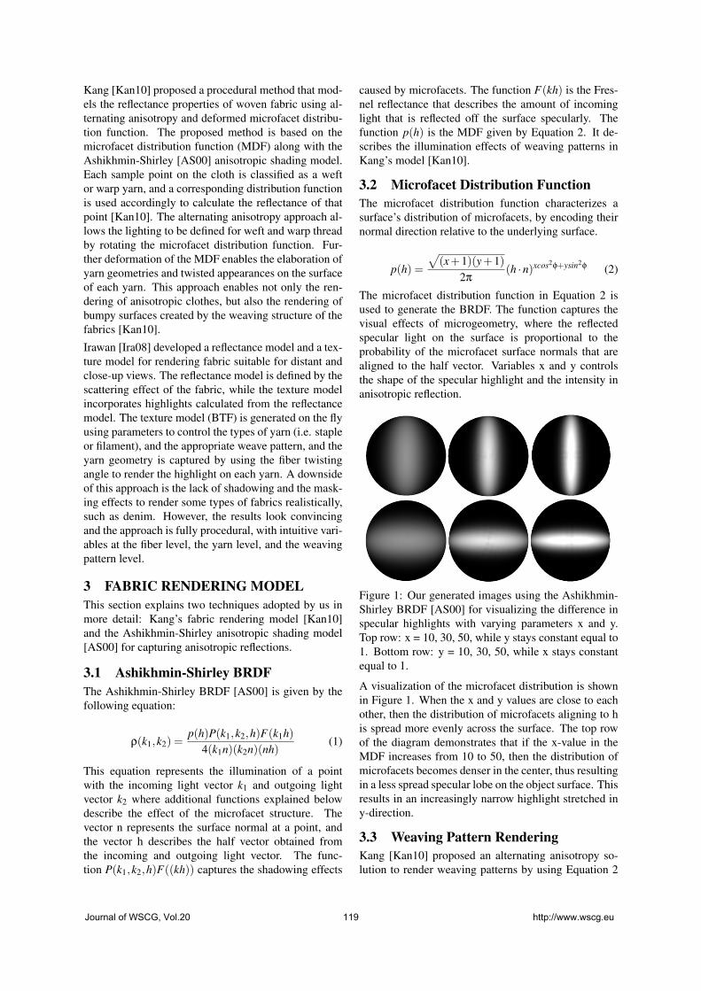
Kang [Kan10] proposed a procedural method that mod-els the reflectance properties of woven fabric using al-ternating anisotropy and deformed microfacet distribu-tion function. The proposed method is based on themicrofacet distribution function (MDF) along with theAshikhmin-Shirley [AS00] anisotropic shading model.Each sample point on the cloth is classified as a weftor warp yarn, and a corresponding distribution functionis used accordingly to calculate the reflectance of thatpoint [Kan10]. The alternating anisotropy approach al-lows the lighting to be defined for weft and warp threadby rotating the microfacet distribution function. Fur-ther deformation of the MDF enables the elaboration ofyarn geometries and twisted appearances on the surfaceof each yarn. This approach enables not only the ren-dering of anisotropic clothes, but also the rendering ofbumpy surfaces created by the weaving structure of thefabrics [Kan10].

Irawan [Ira08] developed a reflectance model and a tex-ture model for rendering fabric suitable for distant andclose-up views. The reflectance model is defined by thescattering effect of the fabric, while the texture modelincorporates highlights calculated from the reflectancemodel. The texture model (BTF) is generated on the flyusing parameters to control the types of yarn (i.e. stapleor filament), and the appropriate weave pattern, and theyarn geometry is captured by using the fiber twistingangle to render the highlight on each yarn. A downsideof this approach is the lack of shadowing and the mask-ing effects to render some types of fabrics realistically,such as denim. However, the results look convincingand the approach is fully procedural, with intuitive vari-ables at the fiber level, the yarn level, and the weavingpattern level.

3 FABRIC RENDERING MODELThis section explains two techniques adopted by us inmore detail: Kang’s fabric rendering model [Kan10]and the Ashikhmin-Shirley anisotropic shading model[AS00] for capturing anisotropic reflections.

3.1 Ashikhmin-Shirley BRDFThe Ashikhmin-Shirley BRDF [AS00] is given by thefollowing equation:

ρ(k1,k2) =p(h)P(k1,k2,h)F(k1h)

4(k1n)(k2n)(nh)(1)

This equation represents the illumination of a pointwith the incoming light vector k1 and outgoing lightvector k2 where additional functions explained belowdescribe the effect of the microfacet structure. Thevector n represents the surface normal at a point, andthe vector h describes the half vector obtained fromthe incoming and outgoing light vector. The func-tion P(k1,k2,h)F((kh)) captures the shadowing effects

caused by microfacets. The function F(kh) is the Fres-nel reflectance that describes the amount of incominglight that is reflected off the surface specularly. Thefunction p(h) is the MDF given by Equation 2. It de-scribes the illumination effects of weaving patterns inKang’s model [Kan10].

3.2 Microfacet Distribution FunctionThe microfacet distribution function characterizes asurface’s distribution of microfacets, by encoding theirnormal direction relative to the underlying surface.

p(h) =

√(x+1)(y+1)

2π(h ·n)xcos2φ+ysin2φ (2)

The microfacet distribution function in Equation 2 isused to generate the BRDF. The function captures thevisual effects of microgeometry, where the reflectedspecular light on the surface is proportional to theprobability of the microfacet surface normals that arealigned to the half vector. Variables x and y controlsthe shape of the specular highlight and the intensity inanisotropic reflection.

Figure 1: Our generated images using the Ashikhmin-Shirley BRDF [AS00] for visualizing the difference inspecular highlights with varying parameters x and y.Top row: x = 10, 30, 50, while y stays constant equal to1. Bottom row: y = 10, 30, 50, while x stays constantequal to 1.

A visualization of the microfacet distribution is shownin Figure 1. When the x and y values are close to eachother, then the distribution of microfacets aligning to his spread more evenly across the surface. The top rowof the diagram demonstrates that if the x-value in theMDF increases from 10 to 50, then the distribution ofmicrofacets becomes denser in the center, thus resultingin a less spread specular lobe on the object surface. Thisresults in an increasingly narrow highlight stretched iny-direction.

3.3 Weaving Pattern RenderingKang [Kan10] proposed an alternating anisotropy so-lution to render weaving patterns by using Equation 2


to generate the specular highlight that can be seen onweaving pattern [Kan10]. Using the fact that weavingpatterns are only made of weft and warp yarns, the spec-ular highlight of weft yarns must therefore be obtainedby rotating the microfacet distribution by 90. This isagain shown in Figure 1. The rotated microfacet dis-tribution is seen on the second row, and is done by ex-changing the values of x and y to create such rotation.

Figure 2: Weave pattern generated by using the alter-nating anisotropy method showing the closer view (left)and distant view (right).

An example of a weaving pattern generated using thealternating anisotropy method is shown in Figure 2.Without the yarn geometry the weaving pattern lookslike a checkerboard pattern, thus the yarn geometry hasto be defined for close-up viewpoints.

3.4 Yarn GeometryThe yarn geometry is generated after the weaving pat-tern by normal perturbation at run-time. Kang [Kan10]proposed that the yarn geometry can be specified byseveral parameters including: number of threads foreach strand of yarn Nξ, fiber curvature of each strandc f , and the yarn curvature cy. Therefore, the normalof each point is altered using these parameters and itssampling position on the weft or warp yarn [Kan10].

weft:(δx,δy) = (c f (2fract(Nξ(uw− s f σu))−1,cyσ

v)(3)

warp:(δx,δy) = (cyσu,c f (2fract(Nξ(vw− s f σ

v))−1)(4)

Equations 3 and 4 show the changes made to the x-and y-coordinates of the normal. The z-coordinateof the perturbed normal is generated by calculating√

1.0−δx−δy. This achieves yarn based lighting bytaking into account different user-defined parametersincluding: fiber curvature (c f ), yarn curvature (cy),slope of fibers (s f ), offsets in yarn space (σu and σv),and number of fiber strands (Nξ) used to make up eachyarn. The variables uv and vw are texture coordinates ofthe model, and the function fract() calculates the frac-tion component of a floating point.

Figure 3 shows a fabric model with weaving pattern andyarn geometry. The image on the left of Figure 3 shows

a rendering of the fabric seen from a distance, with themicroscale details well below an individual pixel size.The results are not significantly different to the versionof rendering without yarn geometry as shown in Fig-ure 2. The difference between the two fabric modelsbecomes more visible when rendering a close-up view.The image on the right of Figure 3 illustrates that eachyarn is constructed by several threads, as specified bythe variable Nξ, with a high yarn curvature resulting inlarge shaded areas on the sides of the yarns.

4 DESIGNFabric rendering techniques often suffer from strongaliasing effects if the resolution of the fabric mi-crostructure is higher than the screen resolution it isdisplayed on. While post-processing can soften theseeffects, the solution is inefficient and artifacts canremain, especially for interactive applications such ascloth simulations. Some solutions use large weavesizes to reduce aliasing effects, but this is not suitablefor fashion applications where realism is essential.We analyzed existing cloth rendering techniques andfound that the method from Kang [Kan10] is the mostpromising one [YW11]. A major advantage of thisalgorithm is its speed, which was shown to be only1.846 time more expensive than Gouraud shading[Kan10]. The approach also displays a high level ofrealism, as the results of rendered woven fabrics lookrealistic in close-up. However, this approach lacks acoloring scheme at the yarn level to render fabrics suchas denim, and it also displays blatant aliasing artifactson the fabric surface.

4.1 Level-of-detail Fabric RenderingWe propose a level-of-detail design for the fabric modelproposed by Kang [Kan10], which removes unneces-sary detail, and only renders the detailed fabric struc-ture in close-up views.

Our design consists of two levels of visually perceiv-able fabric details: weave structure and yarn geome-try. The visibility of yarn geometry is determined bythe mipmap level, which is calculated with the use ofderivative functions on texture coordinates. We explic-itly render two mipmap levels for the general weavestructure and the underlying yarn geometry. We limitthe mipmap levels to between 0 and 1, and uses it asan alpha value for blending between the two layers ofmipmap. This concept is shown in Figure 4, for thosefragments that are highlighted in lighter colors, theyare rendered with the general weave structure, whereasfor those that are highlighted in darker colors, theyare rendered with more detailed yarn geometry. Thismeans that if the texture coordinates between neighbor-ing fragments are changing quickly, then a higher level


Figure 3: Rendering of weave pattern with yarn geometry seen from distance (left), and from close-up (right).

mipmap (less detail) is used, thus avoiding the render-ing of unnecessary detail when the fabric is observed ina larger distance.

Figure 4: Visualization of mipmap level selection fromfar view point to close view point (left to right).

In essence, two MDFs are calculated, one using the pre-perturbed normals for weaving pattern rendering, andthe other using the perturbed normals for yarn geome-try rendering. The yarn geometry is obtained from thenormal perturbation using Equations 3 and 4, which isthen used as an input to the MDF. In practice, however,only the dot product between the halfway vector h andthe normal vector n has to be recalculated two times foreach values, with the rest of the calculations in Equation2 only calculated once. Equation 5 shows the calcula-tion of the final MDF, which is done by using the twopreviously mentioned MDFs, and weighting them withthe α value obtained from the mipmap calculation thatdetermines which level of mipmap should be used forrendering.

p(h) = (1.0−α)p(h1)+αp(h2) (5)

4.2 Extensions for Real-time applicationsWe also extend the model developed by Kang [Kan10]to support more types of fabrics.

4.2.1 Extended Fabric Coloring Scheme

For our system, we require the visualization of fabricssuch as denim. Denim is often constructed from fiberusing the twill-weaved weaving pattern. In contrast toordinary cotton twill, denim uses different colors for theweft and warp yarn, with the most popular combinationbeing white for the warp yarn and blue for the weft yarn.

We define extra parameters to specify the base color ofindividual weft and warp yarns, both in terms of diffuseand specular colors. Using these base colors, we applyKang’s algorithm [Kan10] to generate the proceduraltextures with weaving patterns and yarns to simulate thevirtual fabrics.

4.2.2 Ambient Occlusion

The original method by Kang [Kan10] introduced anambient occlusion term defined by the z value of theperturbed normal. Since the perturbed normal is gen-erated to define the yarn geometry at the micro-level,the ambient occlusion term only works for scalingthe anisotropic reflection at the yarn level to create ashadow effect on the reflection.

The self-shadowing effects at a higher level are not cap-tured due to the lack of indirect lighting involved in cal-culating the overall reflectance of the fabric. However,self-shadowing is common in practice, e.g. when clothis folded. Hence, we use Screen-Space Ambient Occlu-sion (SSAO) [Mit07] as a real-time ambient occlusionmethod to introduce self-shadowing effects to the exist-ing fabric rendering method.

In the initial pass, we render our fabric at the same timeas normal buffer and position buffer to avoid render-ing the same object in multiple passes. We store fabricrendering results in a color buffer, and the color bufferis referred to for scaling its values using the calculated


ambient occlusion from the normal buffer and positionbuffer.

ao = max(0.0,dot(N,V )

1.0+d) (6)

Equation 6 describes the calculation of the ambient oc-clusion of a pixel. A point (occluder) occludes anotherpoint (occludee) if the dot product between the normalof the ocludee and the vector from the ocludee to oc-cluder is greater than zero, i.e if the point is located atthe front face of the occludee, then it contributes someamount of occlusion scaled by the dot product and thedistance between two points. In order to calculate theambient occlusion at each pixel of the screen, neighbor-ing pixels are sampled randomly using a noise functionand the ambient occlusion value is averaged accordingto the number of sample points [Mit07].

4.2.3 Anti-AliasingThe original implementation of the renderer producedclearly visible aliasing effects and moire patterns due tohigh frequency textures. These artifacts are caused bythe microscopic details of the procedural textures gen-erated in real-time. When the object is in motion, thealiasing artifacts become even more visible to temporalaliasing.

Figure 5: Aliasing of weave patterns. Comparison offabric being viewed from a distance (left) and fromclose-up (right). The fabric was rendered with the orig-inal implementation by Kang [Kan10] without any anti-aliasing or level-of-detail algorithm

The left image of Figure 5 displays the distortion ofweaving patterns when the viewpoint is located faraway from the object. The moire patterns on the sur-face of the fabric are clearly visible as distorted curvelines. The fabric on the right in Figure 5 shows theweaving pattern when the viewpoint is at a closer dis-tance to the object - no moire pattern is visible. Anotherexample is given by Figure 6, which shows a denim fab-ric rendered without any underlying textures, but usingblue colored weft yarns and white colored warp yarns.When the fabric is viewed from a distance (left imageof Figure 6), the aliasing artifacts are more visible withthis fabric due to the highly contrasted yarn colors be-tween weft and warp yarns, also causing moire patternsto appear on the surface of the fabric. Furthermore, the

twill-weave on the denim fabric is clearly distorted andunrecognizable from this distance. The aliasing arti-facts are significantly reduced on the right of Figure 6,but still exist in high frequency areas such as regionswhere the fabric is bent around the underlying cuboidobject.

Figure 6: Aliasing of weave patterns of denim fab-ric. Comparison of distant viewpoint in magnified view(left) and close viewpoint (right)

An anti-aliasing method is required to reduce the moireeffects on the surface of the fabric. While a level-of-detail scheme was proposed in Section 4.1, the size ofthe weaving patterns still introduces a high level of tex-ture frequency on the fabric surface.Traditionally, oversampling methods such as su-persampling anti-aliasing (SSAA) and its variation,multisampling anti-aliasing (MSAA) were used tohandle aliasing for graphics applications and computergames. SSAA is known to incur large bandwidth andshading cost, due to multiple numbers of samples beingtaken inside each pixel [HA90, Mam89], while MSAAimproves on SSAA’s performance by only evaluatingeach fragment value once and only supersamplingdepth and stencil values [Ake93].Recently, post-processing anti-aliasing methods havebecome more popular for reducing aliasing artifacts.Methods such as morphological anti-aliasing (MLAA)[Res09] and fast approximation anti-aliasing (FXAA)[Lot09] have the advantage that they are independent tothe rendering pipeline. The methods are applied at thelast stage as an image-based post-processing technique.While MLAA resolves many edge aliasing problems,it is unable to handle pixel-sized features, and fails toreduce the moire-effects from high frequency textures[Res09]. FXAA employs a similar anti-aliasing pro-cedure, where the image is used to detect edges usinghighly contrasting areas of each pixel, with an addi-tional sub-pixel offset from the detected edge for low-pass filtering to achieve anti-aliasing in the sub-pixellevel [Lot09]. Therefore, FXAA can be considered asa sub-pixel anti-aliasing technique and is hence poten-tially useful for our fabric shader. However, MSAA isthe preferred choice due to its proven anti-aliasing per-formance over the entire object surface.Despite the popularity of these methods, we found thatthey did not alleviate the high frequency aliasing prob-


lem we faced with texture aliasing from our imple-mentations. Therefore, we decided to simply use anadaptive prefiltering approach [Ros05] inside our GLSLshader for averaging the pixel with its neighbors. Thefilter is adaptive such that the number of surroundingcolors it calculates depends on the degree of similar-ity in each iteration. This algorithm is shown in Al-gorithm 1, which shows an overview of the algorithmfor each fragment in calculating its final color. Essen-tially, the final color is iterated until its difference withother colors between neighboring fragments is less thana threshold, defined by the inverse distance of the frag-ment from the view point.

Algorithm 1 Prefiltering for fabric shadercount← 1ddx← dFdx(worldPos)∗0.5ddy← dFdy(worldPos)∗0.5while true do

lastColor← colorcolor← color + calcFragmentColor(worldPos

+ ddx∗ rand()+ddy∗ rand())count← count +1if count > 5 then

δcolor← lastColor− colorif length(δcolor)< (1 / viewDistance) then

breakend if

end ifend whilef inalColor← color/count

5 RESULTSThis section evaluates the effectiveness and efficiencyof the improvements proposed by us. The followingtests were performed:

• LOD fabric rendering quality test

• LOD fabric rendering performance test

• Denim Rendering

With rendering quality, we compare and contrast thequality of several images with real fabrics. To com-pare the effects of using level-of-detail rendering, wecompare rendering results with and without the im-provements, and we also compare their effects on alias-ing artifacts. For rendering performance we comparethe frame rates achieved with the different implemen-tations. All tests were performed on a PC with In-tel Core i7 2600k,12 GB memory at 1600 MHz withan AMD Radeon HD 6950 graphics card with 2GByteGPU memory.

5.1 Level-of-Detail Rendering5.1.1 Rendering QualityThe level-of-detail rendering of woven fabric was testedby comparing the rendering quality of fabrics with andwithout our level-of-detail fabric rendering algorithm.Figure 7 shows that without level-of-detail rendering(left) many aliasing artifacts are seen, which they arenot visible using level-of-detail rendering (right). Theobservations are confirmed by a second example shownin Figure 8, which represents a red twill-weaved wovenfabric.

Figure 7: Level-of-detail rendering, without LOD (left)and with LOD (right).

Figure 8: Level-of-detail rendering, without LOD (top)and with LOD (bottom).

The denim fabric still displays some aliasing artifactswith high frequency weaving pattern that is renderedon polygons facing away from the screen. This is dueto the high contrast in color in the underlying weavingconstruct, coupled with the projection of weaving pat-tern to a much smaller projected area, thus making itdifficult to smooth the high frequency changes in colorat the micro-level. An example of this problem is shownin Figure 9, where the left image is a magnificationof the small rectangle section in the right image. Theleft image illustrates some aliasing artifacts close to theedge of the fabric, with white lines going against theflow of the twill-weaved weaving pattern. These arti-facts are not clearly noticeable in static images, but they


Implementation Performance (ms) Std. dev (ms)Original 5.9302 0.0346LOD 4.4037 0.04115

Table 1: Table comparing performance and standard de-viation of the two algorithms in milliseconds per frame.

become very conspicuous in temporal aliasing when thefabric is in motion.

Figure 9: An example of aliasing problem due to textureprojection. The left image is a magnification of the redsquare in the right image.

5.1.2 Performance AnalysisThe performance of the two algorithms (the originalalgorithm and the LOD algorithm) was analyzed us-ing an identical camera position and view, cloth model,texture, and input parameters for the rendering model.Both algorithms were tested along with the prefilteringapproach, as we have decided to incorporate it to reducethe procedural texture aliasing.

Table 1 shows the results of the two algorithms, per-formed with a 3D model as shown in Figures 7 and 8,which contains 18892 vertices and 37566 triangles. Ourlevel-of-detail fabric rendering algorithm is faster thanthe original algorithm. Given the improved renderingquality and reduced artifacts our new approach is hencepreferable.

5.2 Denim RenderingBy extending the model to allow the specification ofcoloring of yarns, we managed to procedurally generatefabrics such as denim using the twill-weaved weavingpattern coupled with blue colored weft yarns and whitecolored warp yarns. Figure 10 provides a comparisonbetween our results and a close-up of real worn denimfabric. The rendering results look realistic in terms offabric structure, but more randomness and tear and wearneeds to be incorporated into our model in the future.

We adopted the noise function proposed by Kang[Kan10]. The noise function generates random illumi-nation at different yarns, which enhances the realism ofour rendering. Note that some white warp yarns lookbrighter than others as is the case for real denim. So farour framework does not simulate washed denim fabric

Figure 10: Denim fabric rendered with our framework(left) and a photo of real denim (right).

and hence we cannot replicate the random whitishpatches in the image of real denim fabric.

Figure 11: Close-up view of denim fabric rendered withour framework.

Figure 11 shows a close-up view of our rendering re-sults. Our model renders the twill-weave too uniformly,lacking the natural imperfection found in real denim.When the denim is being viewed from a larger distance,the yarn geometry and weaving pattern gets aggregatedand only the dominating color in the weaving pattern isvisible to the user.

Figure 12 shows another close-up appearance of thedenim fabric using a model of a pair of jeans.. Theweaving pattern is defined to closely simulate the struc-ture of a pair of real jeans. In order to render jeans re-alistically, we modified our fabric shader so that it sup-ports the input of wash maps. Wash maps are used todefine the patterns of washes for a pair of jeans, wherewashes are patterns of white patches on the jeans asshown in Figure 12. In Figure 12, a pair of renderedjeans is shown on the left with a pair of real jeans on theright. This close-up view demonstrates that the weav-ing pattern of the rendered jeans closely resembles theweaving pattern of the real jeans, as they are both sim-ilar in structure and size relative to the jeans model.Furthermore, at this viewing distance, the appearanceof both jeans is very similar to each other.

A comparison of an entire pair of real jeans and our ren-dered jeans using a distance view is shown in Figure 13.


Figure 12: Jeans comparison when viewed from close-up: rendered jeans (left) and real jeans (right).

The rendered jeans (left) in Figure 13 closely resemblesthe real jeans (right) in Figure 13. From this distance,the weaving pattern is completely invisible to the ob-server, and aliasing artifacts are also unrecognizable onthe fabric surface with the use of our LOD algorithmand prefiltering approach.

Figure 13: Jeans comparison when viewed from a dis-tance: rendered jeans (left) and real jeans (right).

In our results, we found that that the use of direct light-ing often makes the resulting rendered object too brightin areas that are occluded by the object itself. An ex-ample is shown in Figure 14, where the left image is

Figure 14: Effect of ambient occlusion, before ambientocclusion (left), and after ambient occlusion (right)

the rendered jeans without ambient occlusion, and theright image is the rendered jeans with ambient occlu-sion. In this scene, the light is positioned to the left ofthe jeans, hence the inner thigh area should be dark asit is not directly illuminated by the light source. How-ever, without ambient occlusion the rendered jeans stillseems to be too bright around this area, and we foundthat the SSAO approach results in a more natural ap-pearance of occluded areas.

6 CONCLUSIONIn this paper, we analyzed several existing fabric ren-dering techniques. We chose to use the method pro-posed by Kang [Kan10] as a basis for our fabric shader,due to its rendering quality and performance. Severalextensions were proposed to improve the robustness ofthe model and for supporting fabrics such as denim, and


ambient occlusion for enhancing the realism of self-occlusion of the cloth model. Furthermore, we pro-posed a level-of-detail approach in visualizing the ag-gregation of details with the use of a mipmap LOD se-lection mechanism, to help reduce aliasing artifacts re-sulting from high frequency textures. Overall, our ex-tension to the model enabled us to successfully renderdenim fabric with an unwashed look and it significantlyreduced aliasing problems. With the incorporation ofwash maps to specify areas of washes, we have success-fully replicated the overall and close-up appearance ofactual jeans.

7 FUTURE WORKThe weave-based level-of-detail algorithm only reducesparts of the aliasing caused by high frequency textures.It still suffers from aliasing from small scaled weav-ing pattern and highly contrasting weft and warp yarns’colors, such as for denim fabric, depending on the sizeof weft and warp segments. Our approach rectified thealiasing problem that is often seen in weave-based fab-ric rendering approaches, but a better algorithm can beinvestigated in the future to reconstruct the appearanceof high-detail level from lower levels, rather than filter-ing these details away.

8 REFERENCES[Ake93] Kurt Akeley. Reality engine graphics. In

Proceedings of the 20th annual confer-ence on Computer graphics and interactivetechniques, SIGGRAPH ’93, pages 109–116, New York, NY, USA, 1993. ACM.

[AMTF03] N. Adabala, N. Magnenat-Thalmann, andG. Fei. Real-time rendering of wovenclothes. In Proceedings of the ACM sympo-sium on Virtual reality software and tech-nology, pages 41–47. ACM, 2003.

[AS00] M. Ashikhmin and P. Shirley. Ananisotropic phong BRDF model. Jour-nal of graphics tools, 5(2):25–32, 2000.

[DLH01] K. Daubert, H.P.A. Lensch, and W. Hei-drich. Efficient cloth modeling and ren-dering. In Rendering techniques 2001:proceedings of the Eurographics work-shop in London, United Kingdom, June 25-27, 2001, page 63. Springer Verlag Wien,2001.

[HA90] Paul Haeberli and Kurt Akeley. The ac-cumulation buffer: hardware support forhigh-quality rendering. SIGGRAPH Com-put. Graph., 24(4):309–318, September1990.

[Ira08] Piti Irawan. Appearance of woven cloth.PhD thesis, Ithaca, NY, USA, 2008.AAI3295837.

[Kan10] Y.M. Kang. Realtime rendering of real-istic fabric with alternation of deformedanisotropy. Motion in Games, pages 301–312, 2010.

[Kau05] J. Kautz. Approximate bidirectional tex-ture functions. GPU Gems, 2:177–187,2005.

[Lot09] T. Lottes. FXAA. 2009. Also available ashttp://developer.download.nvidia.com/assets/gamedev/files/sdk/11/FXAA_WhitePaper.pdf.

[Mam89] Abraham Mammen. Transparency and an-tialiasing algorithms implemented with thevirtual pixel maps technique. IEEE Com-put. Graph. Appl., 9(4):43–55, July 1989.

[Mit07] Martin Mittring. Finding next gen:Cryengine 2. In ACM SIGGRAPH 2007courses, SIGGRAPH ’07, pages 97–121,New York, NY, USA, 2007. ACM.

[Res09] A. Reshetov. Morphological antialiasing.In Proceedings of the Conference on HighPerformance Graphics 2009, pages 109–116. ACM, 2009.

[Ros05] R.J. Rost. OpenGL (R) shading language.Addison-Wesley Professional, 2005.

[War92] G.J. Ward. Measuring and modelinganisotropic reflection. ACM SIGGRAPHComputer Graphics, 26(2):265–272, 1992.

[WZT+08] J. Wang, S. Zhao, X. Tong, J. Snyder, andB. Guo. Modeling anisotropic surface re-flectance with example-based microfacetsynthesis. In ACM SIGGRAPH 2008 pa-pers, pages 1–9. ACM, 2008.

[YW11] W. Yuen and B. Wünsche. An eval-uation on woven cloth rendering tech-niques. In Proceedings of the 26th In-ternational Image and Vision Comput-ing New Zealand Conference (IVCNZ2011), pages 7–12, Auckland, NewZealand, November 2011. Also availableas http://www.cs.auckland.ac.nz/~burkhard/Publications/IVCNZ2011_YuenWuensche.pdf.

[YYTI92] T. Yasuda, S. Yokoi, J. Toriwaki, andK. Inagaki. A shading model for clothobjects. Computer Graphics and Applica-tions, IEEE, 12(6):15–24, 1992.

[ZJMB11] S. Zhao, W. Jakob, S. Marschner, andK. Bala. Building volumetric appearancemodels of fabric using micro ct imaging.ACM Trans. Graph, 30(44):1–44, 2011.


Error Metrics for Smart Image Refinement

Julian Amann Matthäus G. Chajdas Rüdiger WestermannCG/Vis Group, CS DepartementTechnische Universität München

Boltzmannstrasse 385748 Garching, Germany

[email protected] [email protected] [email protected]

ABSTRACTScanline rasterization is still the dominating approach in real-time rendering. For performance reasons, real-time ray tracing is only used in special applications. However, ray tracing computes better shadows, reflections,refractions, depth-of-field and various other visual effects, which are hard to achieve with a scanline rasterizer.A hybrid rendering approach benefits from the high performance of a rasterizer and the quality of a ray tracer.In this work, a GPU-based hybrid rasterization and ray tracing system that supports reflections, depth-of-fieldand shadows is introduced. The system estimates the quality improvement that a ray tracer could achieve incomparison to a rasterization based approach. Afterwards, regions of the rasterized image with a high estimatedquality improvement index are refined by ray tracing.

Keywordshybrid rendering, reflection error metric, depth-of-field error metric

1 INTRODUCTIONNowadays, rasterization based graphic pipelines domi-nate real-time 3D computer graphics, because graphicshardware is highly optimized for this rendering algo-rithm. Many years of research have been spent on de-veloping massive parallel processing units that are ableto process complete pixel quads in a fast way by ex-ploiting frame buffer locality and coherence [KMS10].

Even though rasterization has a lot of advantages, it alsohas some limitations. It performs well evaluating localillumination models, however there are problems withglobal effects like reflections. Because rasterization islimited to local illumination models, it is hard to com-pute physically correct reflections of the environment.For that reason, approximations like environment maps[Gre86] are used, which can result in visually plausiblereflections.

Shadows are also a very challenging problem forrasterization. Although there are numerous shadowmapping and shadow volume techniques, they all havesome inherent problems that arise from the local viewof shading in the rasterization process. For example,


most shadow mapping techniques suffer from thewell-known biasing problems or have shadow mappingartifacts due to a too small shadow map resolution[ESAW11]. The number of annually appearing publi-cations to shadow topics proves that the generation ofshadows is still a challenging subject.

Besides reflections and shadows, it is also hard to simu-late a correct thin-lens camera with rasterization. Mostdepth-of-field techniques which are rasterization basedcompute the circle of confusion and then just blur theimage with the computed radius, which results in an in-correct depth-of-field effect [Pot81].

Secondary effects, like shadows or reflections are hardto achieve with a rasterization approach. A ray tracercan natively handle shadows and multiple reflectionsjust by sending additional secondary rays. With a raytracer it is not hard to simulate these effects. A thin-lens camera model can also be easily implemented in aray tracer to get a nice depth-of-field effect.

2 MOTIVATIONBecause ray tracing is computationally very expensive,rasterization is still used for games today. Another rea-son is that under some circumstances a rasterizer canproduce exactly the same image as a ray tracer could.Figure 1 compares a scene rendered with ray tracing toa scene rendered with rasterization.

Remarkable is the fact that the rasterized image tookabout 7 ms to render with precomputed environmentmaps on commodity hardware (NVIDIA GeForce GTX


(c) Difference image

(a) Rasterized image

(b) Ray traced image

HighError

LowError

Figure 1: A difference image of scene (a) that has been rendered with rasterization (b) and ray tracing (c). Thetemperature scale on the left shows how to interpret the colors of the difference image. Blue colors mean a lowdifference and red colors mean a high difference. For example high differences can be seen in the reflecting objectin the center of scene.

460) at a resolution of 762 x 538 pixels with no scenegraph optimizations. However, the ray traced imagewith the same image quality and resolution and a highlyoptimized scene graph took roughly 976 ms to render(the performance measurements were made with therender system described in section 7).

Being given the choice of those techniques, one has toweigh the speed up against the high image quality. Inorder to profit from the advantages of rasterization andray tracing, a hybrid approach is preferable. For ex-ample, a hybrid technique can just use ray tracing tocompute reflections while the rest of the scene can beconservatively rasterized. This helps to get high qualityreflections at the cost of only ray tracing the parts of thescene that have reflecting materials.

Ideally, one would estimate beforehand how big the dif-ference between the rasterized and ray traced image is.This difference (see Figure 1c) could be used as a hintto find out where it is most appropriate to send somerays to improve the image quality.

3 CONTRIBUTIONSThis paper describes an error metric for reflections,shadow mapping and depth-of-field, which estimatesthe expected pixel error between the rasterized and theray traced scene. The error metric is a heuristic one,which yields an expected but not an absolutely correcterror value. During the rasterization of the scene, theerror value is calculated and stored in an additional ren-der target. After a first approximation of the currentscene by rasterization, the error value of each pixel can

be used to find out where it is most appropriate to refinethe rasterized image by ray tracing.This paper also presents a scheduling strategy that de-termines in which order the parts of the image are get-ting refined via ray tracing, so the scene convergesquickly. This means that parts of the scene with higherror get ray traced first and more often than parts of thescene with a low error. This helps to prevent wasting alot of computation time on parts of the image where nodifference or only a slight difference between the raytraced and the rasterized version is observable.Furthermore, the implementation of a hybrid raster-ization and ray tracing framework that is based onMicrosoft Direct3D 11, NVIDIA CUDA Toolkit andNVIDIA OptiX 2.51 ray tracing engine is described,which demonstrates the feasibility of the describedsmart image refinement system. The system is calledsmart, because it refines the image according to theerror estimate.

4 RELATED WORKIn the following section related work is briefly pre-sented. Contributions made by other researchers reachfrom simple hybrid rendering systems to sophisticatedperceptually-based techniques.

1 NVIDIA OptiX is a freely available low level ray tracingengine that runs entirely on the GPU. Currently OpitX isonly supported by NVIDIA GPUs. Similar as Direct3D orOpenGL provides an interface to an abstract rasterizer whichcan be used to implement various rasterization-based algo-rithms, OptiX provides an interface to an abstract ray tracer.


Perceptually-based techniques try to shortcut the renderprocess by computing a perceptually indistinguishablesolution instead of a fully converged one. In [YPG01],a perceptually-based technique is described that calcu-lates a spatio–temporal error tolerance map. The com-putation of the error map takes a few seconds and istargeted at offline renderers. Each pixel of the errormap indicates how much effort should be spent on therespective pixel. The error value is determined by har-nessing knowledge about the human visual system anda model which predicts visual attention. For example,the eye is less sensitive to areas with high spatial fre-quency patterns or movements. Alongside with a pre-diction on where the viewer directs his or her attention,an estimate is computed that describes how importanta pixel will be. This estimate is saved in the error mapand is used during the render process to spend moretime on important regions of the image. The paper’sauthors achieved on their test rendering system a 6× to8× speedup.

[Cab10] uses a simple error metric. The metric consistsof only a binary decision if ray tracing or rasterizationis to be used. If the rasterizer renders a triangle witha transparent or reflecting material, a flag is set in aray casting buffer. Afterwards all pixels marked withthe flag get ray traced and combined with the rasterizedimage. They use a CPU-based ray tracer.

In [KBM10], a hybrid approach is shown that combinesshadow mapping and ray tracing to render shadows. Ina direct render pass and from a small number of shadowmaps that are used to approximate an area light sourceby several point lights, a shadow refinement mask is de-rived. The mask is used to identify the penumbra regionof an area light source. A pixel is classified as inside thepenumbra when it cannot be seen from all point lights.Afterwards, the penumbra pixels are dilated by a 5×5structuring element. The dilated region is then renderedby a CPU-based ray tracer to compute accurate shad-ows.

5 ERROR METRICSThis section describes different error metrics for reflec-tions, depth-of-field and soft shadows. The presentederror metrics are used by the smart image refinementsystem to find out in which regions refinement by raytracing is most appropriate. An error value is estimatedfor each pixel and is stored in an additional render tar-get. The error metric is used as a heuristic that indicateshow likely the calculated pixel is wrong in comparisonto a pure ray traced version of the scene.

A high error value indicates that the approximation bythe rasterizer contains a high error, whereas a small er-ror value indicates low errors in the approximation bythe rasterizer. The error value is just based on heuris-tics, which means that in certain circumstances, a high

error value refers to a pixel that has only a small real orno approximation error at all compared to the ray tracedscene. Conservative error metrics were chosen, so nopixels get estimated as correctly approximated, even ifthey are not correct.

Each error metric is normalized, which means it gener-ates an error value in the range of [0,1].

ReflectionsReflections can be approximated by environment mapsin a rasterization based environment. Figure 2 com-pares reflections rendered by rasterization to reflectionsrendered by a recursive ray tracer.

(a) Rasterized

(b) Ray traced (c) Difference

Figure 2: The rasterized image (a) approximates reflec-tion with an environment of the scene. Figure (b) showsthe same scene rendered with a recursive ray tracer. Thedifference image (c) visualizes the difference betweenFigure a and b. A red value indicates a high differenceand a blue value a small difference.

As can be seen from the difference image, the approx-imated rasterized image is far from perfect. It containsseveral regions with wrong reflections.

The simplest to think of error heuristic is one that justmakes a binary decision, depending on the criterion ifa fragment is part of a reflection object or not [Cab10].Assuming it is part of the reflecting material, the errormetric returns 1, in all other cases it returns 0:

Ere f lection1 =

1 : reflecting material0 : else

The previous classification is a very simple one. A moresophisticated error metric can be derived, if we try tounderstand why the approximation of an environmentis wrong. Figure 3 shows two major problems of envi-ronment mapping.

Put the case that we want to rasterize a reflecting spherewith the help of environment mapping. For a point P


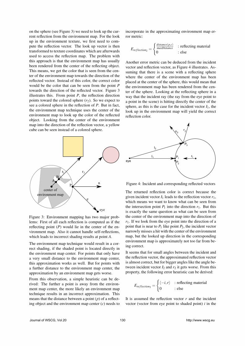
on the sphere (see Figure 3) we need to look up the cur-rent reflection from the environment map. For the lookup in the environment texture, we first need to com-pute the reflection vector. The look up vector is thentransformed to texture coordinates which are afterwardsused to access the reflection map. The problem withthis approach is that the environment map has usuallybeen rendered from the center of the reflecting object.This means, we get the color that is seen from the cen-ter of the environment map towards the direction of thereflected vector. Instead of this color, the correct colorwould be the color that can be seen from the point Ptowards the direction of the reflected vector. Figure 3illustrates this. From point P, the reflection directionpoints toward the colored sphere (r2). So we expect tosee a colored sphere in the reflection of P. But in fact,the environment map technique uses the center of theenvironment map to look up the color of the reflectedobject. Looking from the center of the environmentmap into the direction of the reflection vector, a yellowcube can be seen instead of a colored sphere.

n

eye

e

r

center of environment map

AB

r

P

1 2

Figure 3: Environment mapping has two major prob-lems: First of all each reflection is computed as if thereflecting point (P) would lie in the center of the en-vironment map. Also it cannot handle self-reflections,which leads to incorrect shading results at point A.

The environment map technique would result in a cor-rect shading, if the shaded point is located directly inthe environment map center. For points that only havea very small distance to the environment map center,this approximation works as well. But for points witha further distance to the environment map center, theapproximation by an environment map gets worse.From this observation, a simple heuristic can be de-rived: The further a point is away from the environ-ment map center, the more likely an environment maptechnique results in an incorrect approximation. Thismeans that the distance between a point (p) of a reflect-ing object and the environment map center (c) needs to

incorporate in the approximating environment map er-ror metric:

Ere f lection2 =

distance(p,c)maxDistance : reflecting material0 : else

Another error metric can be deduced from the incidentvector and reflection vector, as Figure 4 illustrates. As-suming that there is a scene with a reflecting spherewhere the center of the environment map has beenplaced at the center of the sphere, this would mean thatthe environment map has been rendered from the cen-ter of the sphere. Looking at the reflecting sphere in away that the incident ray (the ray from the eye point toa point in the scene) is hitting directly the center of thesphere, as this is the case for the incident vector I1, thelook up in the environment map will yield the correctreflection color.

I1

2

eye

n

r1

2r

I2

P

P

P

2

1

3

Figure 4: Incident and corresponding reflected vectors

The returned reflection color is correct because thegiven incident vector I1 leads to the reflection vector r1,which means we want to know what can be seen fromthe intersection point P1 into the direction r1. But thisis exactly the same question as what can be seen fromthe center of the environment map into the direction ofr1. If we look from the eye point into the direction of apoint that is near to P1 like point P2, the incident vectornarrowly misses a hit with the center of the environmentmap, but the looked up direction in the correspondingenvironment map is approximately not too far from be-ing correct.

It seems that for small angles between the incident andthe reflection vector, the approximated reflection vectoris almost correct, but for bigger angles like the angle be-tween incident vector I2 and r2 it gets worse. From thisproperty, the following error heuristic can be derived:

Ere f lection3 =

〈−i,r〉 : reflecting material0 : else

It is assumed the reflection vector r and the incidentvector (vector from eye point to shaded point) i in the


above equation are normalized. The angle between thevector r and −i is always in the range [0,90]. Sincethe angle can be in the range [0,180) the dot productfails for greater than 90 angles. To circumvent thisproblem instead of considering the reflected vector thenormal can be considered which leads to the followingequation:

Ere f lection4 =

〈−i,n〉 : reflecting material0 : else

This works because the angle between the incident andreflected vector is directly proportional to angle be-tween the reflected and the incident vector. The anglebetween the negative incident vector and the normal cannever exceed 90.

E reflection1

Ereflection2

E reflection4

Ereflection 5Figure 5: Displays the different reflection error metricsapplied to a scene with sphere (left) and a scene with amore complex shape (right)

Another not yet considered problem of the error met-ric that is also related with environment maps are self-reflections. Concave objects are displayed incorrectlyby an environment map technique. Figure 3 shows thereason for this. Assuming we want to compute the re-flection of the point A in Figure 3 given the reflectionvector r1. In a look up in the environment, the yel-low color from the yellow cube is returned. Howeverin fact the reflection ray intersects the reflecting objectitself (a so-called self-reflection) in point B and despiteof this, the yellow color from the environment map isnonsense. Self-reflections can probably not be handledby environment maps. We can take care of this in ourerror metric by using an ambient occlusion map. Theambient occlusion map can be interpreted as a descrip-tion of the curvature of the reflecting object. This infor-mation can be directly used in a heuristic that estimatesthe possibility of self-reflections:

Ere f lection5 =

ka(p) : reflecting material0 : else

ka(p) refers here to the ambient occlusion term.

Figure 5 shows the different error metrics applied to twosample scenes.

Depth-of-FieldMost rasterization based depth-of-field techniques areimage based and use only the depth buffer and colorbuffer to compute a depth-of-field effect. Thereby, theinformation about the scene is lost. In a ray tracer, thelens is sampled at different locations. Each sample onthe lens has a different view of the current scene. In therasterizer approach, we have only one view at the scenefrom the center of the lens. This can lead to missingobjects, because in some cases from some points on thelens, objects can be seen that cannot be seen from thecenter of the lens.

Another problem of most depth-of-field techniques iscolor leaking. Color leaking can be seen around sharpedges that are in focus in which other blurry objectsfrom the background bleed into [LU08]. The other wayaround, objects in the foreground can bleed into objectsin the background. Figure 6 shows this effect.

As demonstrated in Figure 7, rasterization based depth-of-field have problems in regions with high depth dis-continuities. This knowledge can be exploited to con-struct an error metric for the depth-of-field.

To find depth discontinuities, an edge filter, like the So-bel filter, can be applied. A problem with this approachis that the founded edges have to be dilated by a struc-turing element, since the artifacts do not only occur atthe identified edge pixels, but also in the neighborhoodof the edge pixel according the circle of confusion. The


(a) Rasterized (b) Raytraced

Figure 6: A blurry foreground object bleeds into thefocused background object.

(b) Rasterized

(c) Ray traced(a) Difference

Figure 7: Difference image of scene (with applied depthof field effect) (a) that has been rendered with rasteri-zation (b) and ray tracing (c). Regions with high depthdiscontinuities are problematic for rasterization basedrendering techniques.

maximal radius of the circle of confusion Cmax for thedilation can be determined for a point p by the follow-ing equation with image distance VP, focal length F andaperture number n (zp is the distance between the pointp and the image plane):

Cmax(p) = max(C(zp),C∞)

C∞ = limz→∞

C(z) = |F−Vp| 1n

For simplicity reasons, we use a quad shape structuringelement in our implementation to approximate the cir-cle of confusion. Figure 8 shows the error metric fordepth-of-field.

The Error metric for depth of field can be expressed as:

Edo f =

1 : Vicinity of a depth discontinuity0 : else

The described error metric is not absolutely conserva-tive, which means that errors can also occur in regions

(a) Rasterized (b) Dilated

Figure 8: After the depth discontinues have beenmarked, they need to be dilated according to the circleof confusion.

that were not classified with an error value of 0. How-ever, it can give a smart image refinement system a goodhint where to start the refinement process.

ShadowsIn [GBP06], an algorithm has been described that canbe modified to estimate where the penumbra of a givenarea source light will be projected onto the scene. InFigure 9, the estimated penumbra region is shown ingreen color.

Figure 9: The estimated penumbra region is shown ingreen color.

The algorithm described in [GBP06] makes a conserva-tive estimation of the penumbra region, and is thereforeperfectly appropriate to be used as an error metric. Thedifference between the shadow generated by the ras-terization system and the ray tracer is only notable inthe penumbra region. In umbra regions and in regionswhere the area light source is not occluded by other ob-jects (so that the scene is fully lit by the light source) nodifference between the rasterizer and ray tracer is no-ticeable (see Figure 1 - only the penumbra region needsto be refined).

In [Mic07], an improved algorithm is presented whichcan estimate a tighter, conservative penumbra estima-tion than the algorithm described by [GBP06]. Eventhough it requires more memory, the tighter estimationreduces the amount of pixels that have to be refined,resulting in an overall improved performance.

The corresponding error metric for soft shadow is there-fore quite simple:


Eshadow =

1 : Pixel resides in penumbra region0 : else

Combination of Error MetricsThe different error metrics can be combined in multipleways. A naive idea is to calculate an averaged sum:

Ecombined1 =∑

ni=1 Ei(p)

n

Figure 10 shows the quality of the average sum metric.

(a) (b) (c)

Figure 10: Quality of averaged sum metric. (a) showsthe real error, (b) the estimated error and (c) the differ-ence image.

For a better estimation, a more complex combinationis required. A simple, yet effective approach is touse a linear combination of the different error metrics(i.e. Ere f lectioni , Edo f , Eshadow) and let the smart imagerefinement system automatically determine the coeffi-cients λi by rendering multiple views of a scene withthe goal of minimizing the difference between the esti-mated and the real error:

Ecombined2 = ∑ni=1 λiEi(p)

The determination of the factors λi is done as a pre-process for each different scene. In this pre-process acertain number of screenshots from the scene is taken(with pure rasterization and pure ray tracing). Then arandom tuple of λi coefficients is chosen and the com-bined metric Ecombined2 is then compared with the realerror. We repeat this step multiple times and choose theλi coefficients which result in the best approximationfor all test images.

6 SCHEDULING STRATEGYThis section describes how the error value is used todirect the rendering process of the smart image refine-ment system.

First the scene is rasterized by the rasterization system.During rasterization, an error value is also computedas described in the previous section about error met-rics. After the rasterization pass, the color buffer andthe error color buffer are filled. Now post-processingeffects are applied to the previously rendered scenery.The post-processing result is written to the post-processcolor buffer; after this, the post-process error buffer is

computed. Then the error buffer and the post-processerror buffer get composed in a combined error buffer.For each pixel, an error value is computed and storedin the combined error buffer. After composing the er-ror buffers, the next step is to sort the pixels. The errorbuffer also stores, besides the error value, the positionfor each pixel. The position is needed to find out towhich pixel a corresponding error value belongs to af-ter reordering them according their error values. Aftersorting the error pixels, they are gathered in the requestbuffer. Additionally to the position, a sample countvalue is also stored in the request buffer for each pixelthat determines how many rays should be traced for thecorresponding pixel. The sample count is determinedby an estimation pass that fills the request buffer. Af-ter the request buffer is filled, it is handed over to theray tracing system. The ray tracing system reads thefirst entry from the request buffer and samples the cor-responding pixel according to the sample count. Theray tracer proceeds this process for a user-defined max-imum number of pixels. After the maximum numberis reached, the ray tracing process stops and the smartimage refinement system continues with blending thecurrent ray traced image with the computed rasterizedimage. The blending factor of each pixel depends onthe total number of samples that were computed for thecorresponding pixel by this time. Figure 11 gives anoverview of this process. This process is repeated untilthe whole image is refined.

7 IMPLEMENTATIONFor the implementation of the smart image refine-ment system Direct3D 11, CUDA 4.1 and OptiX 2.5([Ste10]) have been used. Direct3D is used for therasterization part and analogously OptiX is used for theray tracing part. Thus all rendering is done on the GPU.Optionally the system can perform pure rasterizationwith Direct3D or pure ray tracing with OptiX. Inthe case of pure ray tracing Direct3D is needed onlyto show the generated OptiX output buffer. Pureray tracing and rasterization is used for comparisonpurposes like the time measurements in section 2 or intable 1.The ray tracing subsystem uses a SBVH accelerationstructure [SFD09] provided by OptiX to accelerate ray-triangle intersections. The rasterizer subsystem renderswithout any scene graph optimizations in a brute forcemanner.A pixel shader is used to write the error values dur-ing rasterization to an additional render target (the errorbuffer). Some error values can be only determined af-ter post-processing so there is an additional error buffer(post-process error buffer) which stores the error valuesdetermined during applying post-processing effects likedepth-of-field. The combined error buffer which con-tains the unsorted error values is shared with CUDA.


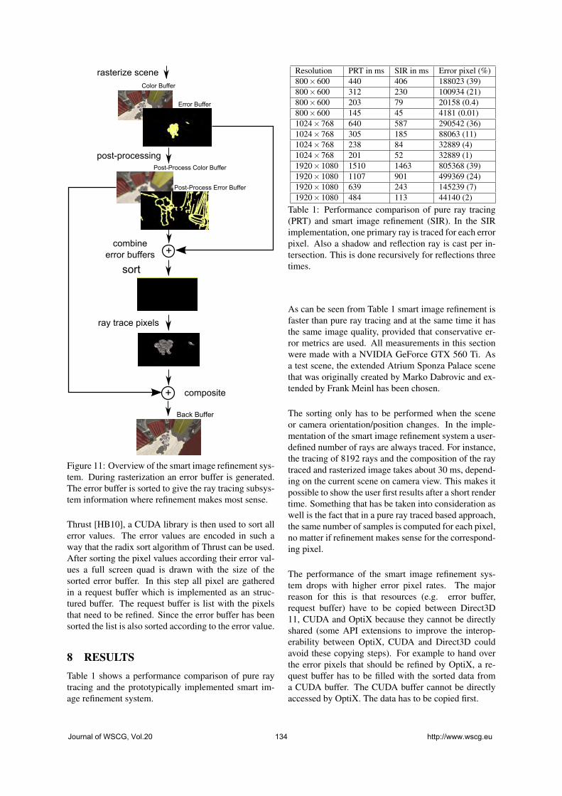
Color Buffer

Error Buffer

rasterize scene

Post-Process Error Buffer

post-processingPost-Process Color Buffer

+ combine error buffers

sort

ray trace pixels

Back Buffer

+ composite

Figure 11: Overview of the smart image refinement sys-tem. During rasterization an error buffer is generated.The error buffer is sorted to give the ray tracing subsys-tem information where refinement makes most sense.

Thrust [HB10], a CUDA library is then used to sort allerror values. The error values are encoded in such away that the radix sort algorithm of Thrust can be used.After sorting the pixel values according their error val-ues a full screen quad is drawn with the size of thesorted error buffer. In this step all pixel are gatheredin a request buffer which is implemented as an struc-tured buffer. The request buffer is list with the pixelsthat need to be refined. Since the error buffer has beensorted the list is also sorted according to the error value.

8 RESULTSTable 1 shows a performance comparison of pure raytracing and the prototypically implemented smart im-age refinement system.

Resolution PRT in ms SIR in ms Error pixel (%)800×600 440 406 188023 (39)800×600 312 230 100934 (21)800×600 203 79 20158 (0.4)800×600 145 45 4181 (0.01)1024×768 640 587 290542 (36)1024×768 305 185 88063 (11)1024×768 238 84 32889 (4)1024×768 201 52 32889 (1)1920×1080 1510 1463 805368 (39)1920×1080 1107 901 499369 (24)1920×1080 639 243 145239 (7)1920×1080 484 113 44140 (2)

Table 1: Performance comparison of pure ray tracing(PRT) and smart image refinement (SIR). In the SIRimplementation, one primary ray is traced for each errorpixel. Also a shadow and reflection ray is cast per in-tersection. This is done recursively for reflections threetimes.

As can be seen from Table 1 smart image refinement isfaster than pure ray tracing and at the same time it hasthe same image quality, provided that conservative er-ror metrics are used. All measurements in this sectionwere made with a NVIDIA GeForce GTX 560 Ti. Asa test scene, the extended Atrium Sponza Palace scenethat was originally created by Marko Dabrovic and ex-tended by Frank Meinl has been chosen.

The sorting only has to be performed when the sceneor camera orientation/position changes. In the imple-mentation of the smart image refinement system a user-defined number of rays are always traced. For instance,the tracing of 8192 rays and the composition of the raytraced and rasterized image takes about 30 ms, depend-ing on the current scene on camera view. This makes itpossible to show the user first results after a short rendertime. Something that has be taken into consideration aswell is the fact that in a pure ray traced based approach,the same number of samples is computed for each pixel,no matter if refinement makes sense for the correspond-ing pixel.

The performance of the smart image refinement sys-tem drops with higher error pixel rates. The majorreason for this is that resources (e.g. error buffer,request buffer) have to be copied between Direct3D11, CUDA and OptiX because they cannot be directlyshared (some API extensions to improve the interop-erability between OptiX, CUDA and Direct3D couldavoid these copying steps). For example to hand overthe error pixels that should be refined by OptiX, a re-quest buffer has to be filled with the sorted data froma CUDA buffer. The CUDA buffer cannot be directlyaccessed by OptiX. The data has to be copied first.



In this work, a GPU-based hybrid rasterization and raytracing system was presented that is able to direct therender processes to regions with high relevance. Re-gions with a high error are getting refined first and moreoften than regions with a small error value. This helpsto converge fast to a stable image and avoids at the sametime the waste of computing time in regions that do notneed any refinement.

There is some scope for improvements of the describederror metrics.

Besides reflections, shadows and depth-of-field, itwould also be interesting to see how other effects likeambient occlusion (AO) or refractions can be integratedinto a smart image refinement system. In the caseof AO, a screen based ambient occlusion techniquecan be employed in the rasterizer to compute a fastapproximation of an occlusion term.

Another interesting aspect that has not been consideredin this work is global illumination. Global illuminationcould be approximated with light propagation volumesand refined with a more sophisticated ray tracing tech-nique like path tracing.

There are several real-time perceptually based ap-proaches like [CKC03] which try to cut downrendering time by focusing on important parts. Theseideas can be combined with our approach.

10 REFERENCES[Cab10] Cabeleira Joao. Combining Rasteriza-

tion and Ray Tracing Techniques to Ap-proximate Global Illumination in Real-Time.http://www.voltaico.net/files/article.pdf, 2010.

[CKC03] Cater, K., Chalmers, A., and Ward, G. Detailto attention: exploiting visual tasks for selectiverendering. Proceedings of the 14th Eurographicsworkshop on Rendering, Eurographics Associa-tion, 270-280, 2003.

[ESAW11] Eisemann, E.; Schwarz, M.; Assarsson, U.& Wimmer, M., Real-Time Shadows A. K. Peters,Ltd., 2011.

[GBP06] Gaël Guennebaud, Loïc Barthe, and Math-ias Paulin. Real-time soft shadow mapping bybackprojection. In Eurographics Symposium onRendering (EGSR), Nicosia, Cyprus, 26/06/2006-28/06/2006, pages 227-234. Eurographics, 2006.

[Gre86] Ned Greene. Environment mapping and otherapplications of world projections. IEEE Comput.Graph. Appl., 6:21-29, November 1986.

[HB10] Jared Hoberock and Nathan Bell. Thrust:A parallel template library, Version 1.3.0.http://www.meganewtons.com/, 2010.

[KBM10] Erik Knauer, Jakob Bärz, and Stefan Müller.A hybrid approach to interactive global illumina-tion and soft shadows. Vis. Comput., 26(6-8):565-574, 2010.

[KMS10] Jan Kautz Kenny Mitchell, Christian Ober-holzer and Peter-Pike Sloan. Bridging Ray andRaster Processing on GPUs. High-PerformanceGraphics 2010 Poster, 2010.

[LU08] Per Lönroth and Mattias Unger. AdvancedReal-time Post-Processing using GPGPU tech-niques, Technical Report, No. 2008-06-11,Linköping University, 2008.

[Mic07] Michael Schwarz and Marc Stamminger. Bit-mask soft shadows. Computer Graphics Forum,Vol. 26, No. 3, pages 515-524, 2007.

[Pot81] Potmesil, Michael and Chakravarty, Indranil.A lens and aperture camera model for syntheticimage generation. In SIGGRAPH 81: Proceed-ings of the 8th annual conference on Computergraphics and interactive techniques, pages 297-305, New York, NY, USA, 1981. ACM.

[SFD09] Martin Stich, Heiko Friedrich, and AndreasDietrich. Spatial splits in bounding volume hierar-chies. In Proceedings of the Conference on HighPerformance Graphics 2009, HPG 09, pages 7-13,New York, NY, USA, 2009. ACM.

[Ste10] Steven G. Parker, James Bigler, Andreas Di-etrich, Heiko Friedrich, Jared Hoberock, DavidLuebke, David McAllister, Morgan McGuire,Keith Morley, Austin Robison and Martin Stich.OptiX: A General Purpose Ray Tracing Engine.ACM Transactions on Graphics, August 2010.

[YPG01] Hector Yee, Sumanita Pattanaik, and DonaldP. Greenberg. Spatiotemporal sensitivity and vi-sual attention for efficient rendering of dynamicenvironments. ACM Trans. Graph., 20:39-65,January 2001.


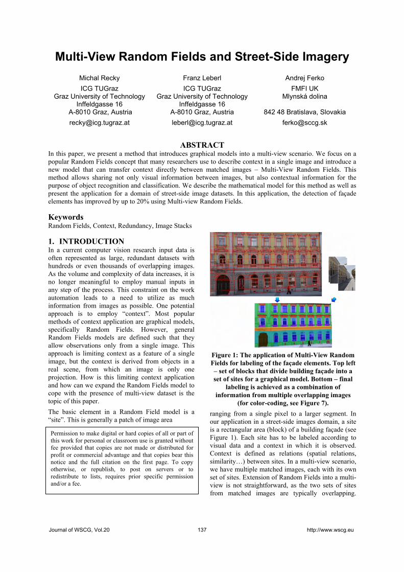
Multi-View Random Fields and Street-Side Imagery

Michal Recky ICG TUGraz

Graz University of Technology Inffeldgasse 16

A-8010 Graz, Austria [email protected]

Franz Leberl ICG TUGraz

Graz University of Technology Inffeldgasse 16

A-8010 Graz, Austria [email protected]

Andrej Ferko FMFI UK

Mlynská dolina

842 48 Bratislava, Slovakia [email protected]

ABSTRACT In this paper, we present a method that introduces graphical models into a multi-view scenario. We focus on a popular Random Fields concept that many researchers use to describe context in a single image and introduce a new model that can transfer context directly between matched images – Multi-View Random Fields. This method allows sharing not only visual information between images, but also contextual information for the purpose of object recognition and classification. We describe the mathematical model for this method as well as present the application for a domain of street-side image datasets. In this application, the detection of façade elements has improved by up to 20% using Multi-view Random Fields.

Keywords Random Fields, Context, Redundancy, Image Stacks

1. INTRODUCTION In a current computer vision research input data is often represented as large, redundant datasets with hundreds or even thousands of overlapping images. As the volume and complexity of data increases, it is no longer meaningful to employ manual inputs in any step of the process. This constraint on the work automation leads to a need to utilize as much information from images as possible. One potential approach is to employ “context”. Most popular methods of context application are graphical models, specifically Random Fields. However, general Random Fields models are defined such that they allow observations only from a single image. This approach is limiting context as a feature of a single image, but the context is derived from objects in a real scene, from which an image is only one projection. How is this limiting context application and how can we expand the Random Fields model to cope with the presence of multi-view dataset is the topic of this paper. The basic element in a Random Field model is a “site”. This is generally a patch of image area

Figure 1: The application of Multi-View Random Fields for labeling of the façade elements. Top left – set of blocks that divide building façade into a set of sites for a graphical model. Bottom – final

labeling is achieved as a combination of information from multiple overlapping images

(for color-coding, see Figure 7). ranging from a single pixel to a larger segment. In our application in a street-side images domain, a site is a rectangular area (block) of a building façade (see Figure 1). Each site has to be labeled according to visual data and a context in which it is observed. Context is defined as relations (spatial relations, similarity…) between sites. In a multi-view scenario, we have multiple matched images, each with its own set of sites. Extension of Random Fields into a multi-view is not straightforward, as the two sets of sites from matched images are typically overlapping.



Simple merging of these two sets would cause double detections of same objects and unresolved relations between sites. To solve both problems, we introduce a new concept – Multi-View Random Fields. In this paper, the “Background” and “Graphical Models” sections are outlining a context of our work in a computer vision community and in a Random Fields models research. The “Context in Multi-View” section explains what type of context is relevant in multi-view and how it can be utilized. In the “Multi-View Random Fields” section the new graphical model is introduced and the “Application of MVRF” section present the illustrational application of the model in a street-side images domain.

2. BACKGROUND The last decade saw growing interest in multi-view methods. With the introduction of a new generation of high resolution digital cameras and with rapid improvements in storage and computing hardware, multi-view imagery advanced from a source for the computation of point clouds by two-image stereo methods to a broad range of vision problems employing thousands of overlapping images. Open online image hosting sites (Flickr, Picasa, Photobucket…) have added interesting vision opportunities. While the basic principles for matching images remain applicable to such datasets [Har04a] [Leo00a], new problems needed to get solved, such as the organization and alignment of images without any knowledge about camera poses [Sna06a]. The resulting resource need in computing gets addressed by means of graphical processing units GPUs, or with distributed approaches [Fra10a]. Therefore current computer vision can cope with this avalanche of imagery and multi-views are becoming a common reality. Extending the concept of Random Fields into such multi-view scenario comes from an idea that given more images of the same scene, more contextual relations can be examined. In this work, we present a mathematical model for Multi-View Random Fields that allows transferring contextual relations between matched images. We also present the application of Multi-View Random Fields in a domain of street-side images. This domain is useful for a demonstration, as there are large datasets of matched street-side images for the purpose of urban modeling (virtual cities, GIS, cultural heritage reconstruction) that establish a multi-view scenario. Urban scenes also exhibit strong contextual relations, as man-made objects adhere to an inherent organization. We show how façade elements can be classified, using both context and multi-view principles in one model.

Figure 2. The typical application of MRF in computer vision. At each node (site) i, the

observed data is denoted as yi and the corresponding label as xi. For each node, only local observations are possible. Generally each

node represents a pixel in an image and observed data pixel’s features.

3. GRAPHICAL MODELS The most common non-causal graphical models in computer vision are Markov Random Fields (MRF). MRF have been used extensively in labeling problems for classification tasks in computer vision [Vac11a] and for image synthesis problems. In a labeling task, MRF are considered to be probabilistic functions of observed data in measured sites of the image and labels assigned to each site. Given the observed data y = yiiϵS from the image, and corresponding labels x = xiiϵS, where S is the set of sites, the posterior distribution over labels for MRF can be written as:

( ) ( ) ⎟⎟⎠

⎞⎜⎜⎝

⎛+= ∑ ∑∑

∈ ∈ ∈Si Si Njjimii

m i

xxxpZ

P β|logexp1| yyx ,(1)

where Zm is the normalizing constant, βm is the interaction parameter of the MRF and Ni is the set of neighbors of a site i. The pairwise term βmxixj in MRF can be seen as a smoothing factor. Notice that the pairwise term in MRF uses only labels as variables, but not the observed data from an image. In this arrangement, the context in a form of MRF is limited to be a function of labels, thus allowing for semantic context (context between classes) and limiting geometric context to a structure of MRF graph (see Figure 2). This makes the MRF applicable mainly for simpler forms of local context. To cope with such limitations, the concept of Conditional Random Fields (CRF) was proposed by J. Lafferty [Laf01a] for the segmentation and labeling of text sequences. The CRF are discriminative models that represent the conditional distribution over labels. Using the Hammersley-Clifford theorem [Ham71a], assuming only pairwise cliques potentials to be nonzero, the conditional distribution in CRF over all labels x given the observation y can be written as


( ) ( ) ( )⎟⎟⎠

⎞⎜⎜⎝

⎛+= ∑ ∑∑

∈ ∈ ∈Si si Njjiijii

i

xxIxAZ

P yyyx ,,,exp1| ,(2)

where Z is the normalizing constant, -Ai is the unary and -Iij pairwise potential. The two principal differences between conditional model (2) and MRF distribution (1) are that the unary potential Ai(xi, y) is a function of all observations instead of only one observation yi in a specific site i and the pairwise potential in (2) is also the function of observation, not only labels as in MRF. In CRF, the unary potential Ai(xi, y) is considered to be a measure of how likely a site i will take label xi given the observation in a image y. The pairwise term is considered to be a measure of how the labels at neighboring sites i and j should interact given the observed image y. This concept of CRF allows for use of more complex context derived from larger sets of observations in the image and employing geometric context (e.g. spatial relations between objects). It is extended even more in a concept of Discriminative Random Fields [Kum06a], where an arbitrary discriminative classifier can be applied in a form of unary/pairwise potential. However, in all concepts of Random Fields, the set of sites S (and thus the observations) is limited to a single image. How to extend these models into a multi-view is explained in subsequent sections.

4. CONTEXT IN MULTI-VIEW Before the definition of a new Random Field model in multi-view, we must consider what type of context can be transferred between images. The most common type of context applied for classification is a local pixel context. In general, a small neighborhood around an examined pixel is taken as a context area and a graph structure of a model is placed in this neighborhood (one node per pixel). However, this approach is not suitable for multi-views, as neighborhoods around matched pixels in two images are in general uniform and will not present much useful additional information. Alternatively we can consider global context, which examines relationships between all objects in the images. In this type of context, we can observe different relations in different images, thus transferring such context would provide additional information for recognition and classification (see Figure 3). If spatial relations between objects are examined in this manner, graphical models are approximating spatial relations between objects in a real 3D scene. In a standard Random Fields (RF) model, each image is considered a unique unit of information. Thus, we can consider a global context to be a specific feature of each image - the global context is a set of relations between all sites detected in a single image.

Figure 3. Building façade projected in slightly

different views. Red lines (graph edges) represent spatial relationships between objects detected in the images, indicating different context in two

projections for the same objects. For better overview, only some relations are visualized.

Typically, sites are either pixels or segments. Construction of a global model with node in each pixel would significantly increase the complexity of computation; therefore we consider segments as the representation of sites in our model. Subsequently a site is represented by a specific area (segment) in a digital image. Such area represents an object (or part of object) and areas from two sites are not overlapping. In a general RF model, a set of all sites in one graph is denoted as S. In a local model, one set S include sites from a small patch of the image, however in a global model, S includes all sites from the entire image. Visual features of the area assigned to a specific site are denoted as image observation ys from site sϵS. In a graphical model, if there is an edge between nodes assigned to sites s1 and s2, let’s denote this relation as Φ(s1, s2) = 1 and consequently if there is no edge between s1 and s2, denote this as Φ(s1, s2) = 0.

Transferable Sites Consider one image from the dataset as “examined image” to which we would like to transfer context from other matched images. Let’s call any site sϵS from an examined image a “native site”. If the image matching is established in a dataset (we have a set of corresponding points that link images), we can look for any sites from other images that are corresponding to native sites. In most cases, sparse point cloud of matched points is enough to establish correspondence between site. Relative poses between images and camera parameters are not required. Definition of corresponding sites can vary in different applications. In general, corresponding sites are two sites from different images that share some subset of corresponding points;


Figure 4. Transfer of sites from the image lϵ I to the image kϵI, as presented in Definition 1. Only

sites from l that are not corresponding to any sites from k are transferred. This figure demonstrates

only transfer between two images. each site from matched images can have only one corresponding site in the examined image – the example of this relation is provided in the application section of this paper. Given that corresponding sites usually represent the same objects, transferring such information between images would be redundant. Therefore we transfer sites that have no correspondences in the examined images to provide new information. We denote such sites as “transferable sites”. For a single, examined image from the image stack, let’s define the set of transferable sites as:

Definition 1: If Sk = s1, s2, … , sn is the set of sites for single image kϵ I, where I is the set of images and correspondences have been established between the images from I such that ϵS'

is l is a site from image lϵ I-k corresponding to a site si. Than the Rk = r1, r2, … , rm is the set of transferable sites for the image k if and ( ) 1SR =∈∃∈∀ ',Φ| ijkikj srsr

kjkj rr SR ∈¬∃∈∀ ' . Rk is constructed such that

kji rr R∈∀ , , ri and rj are not correspondent to each other in any two images from I Thus the Rk is the set of sites from other images than k, that are in the relationship in graphical model with some corresponding site to sites from Sk, but themselves have no correspondences in Sk (see Figure 4). The set of transferable sites can be seen as a context information, that is available in the image stack, but not in the examined image. If sites are the representations of objects, than in a transferable set, there are objects in context with the scene of the image that are currently not located in the projection,

thus are occluded, out of the view or in different timeframe. This also means that the visual information from the sites in Rk are not present in the image k. If the sites from Rk are included in the vision process, they can provide additional context and visual information that is not originally present in the examined image. Note that a transferable site is not equivalent to a native site in an examined image. Even though transferable sites have the same set of visual features as sites native to the image and they can be assigned the same set of spatial and contextual relations in a graphical model, transferable sites lost all original contextual relationships except the relationships to the sites they are connected within the examined image. This makes them harder to label. But the labeling of transferable sites is not the aim in the case of examined image (the goal is to label only native sites), thus transferable sites can contribute information for image labeling, but the labeling of themselves is usually irrelevant.

5. MULTI-VIEW RANDOM FIELDS Given a non-equality of transferable sites to native sites, standard RF models are not compatible with this extended set. For this reason, we introduce a new model denoted as Multi-View Random Fields (MVRF). This model is derived from a CRF, described in Section 2; however we extend the posterior probability distribution into MVRF model framework as follows:

Given the observed data y = yiiϵS from the image, corresponding labels x = xiiϵS, where S is the set of native sites from the image and observations from transferable set z = ziiϵR with corresponding labels

R∈= iix~~x , where R is the set of transferable sites, the posterior distribution over labels is defined as:

,(3) where Z is the normalizing constant, Ni is the set of native sites neighboring site i and Ki is the set of transferable sites neighboring site i. - Ai and - are

unary potentials, - I

'iA

ij and - are pairwise potentials (for native sites and transferable sites respectively). The differences between potentials for transferable sites and for native sites are as follows:

'ijI

- In the unary potential for a transferable site, only observations from the site itself are


considered, instead of observation from the entire image for native sites. This is due to the fact, that a transferable site does not have any connections to the image except for the site it is neighboring. Even if other connections exist (with other sites in the image), it is a hard task to establish relationships. For native site, there are no changes to a standard conditional model.

- In the pairwise potential, in addition to observation from the image, local observation from the transferable site is considered, when relations are examined between a native site and transferable site. The inclusion of all image observation grant at least the same level of information in pairwise computation as in a standard CRF model and the additional observation form transferable site represent extended context for native image observation. The pairwise potential for two native sites is the same as in a standard CRF model.

This model has some additional unique characteristics. For example, no pairwise relations are considered between two transferable sites. This is based on the construction of transferable sites set. A site from such set can be neighboring several native sites, but not any other transferable site. This can be seen as a limitation for the model, however without additional high frequency information about the scene (as a prior knowledge), it is virtually impossible to establish relationships for transferable sites. The computational complexity of the model is not increased significantly. Pairwise potentials are computed only for native sites, as it is in the standard CRF model. The difference is in the number of neighbors for each site, however even this number should not increase significantly. When considering a global model, each new neighbor (transferable site in relation to the native site) represents a new object in the projection. This is dependent on the differences between projection parameters – camera positions, optical axes…, but even for very different parameters, the number of objects should not differ significantly for the same scene. From the general observation, the number of neighboring transferable sites is notably lower than the number of neighboring native sites.

Potentials Modifications Unary potential for native image sites, similar to a standard CRF is a measure of how likely a site i will take label xi given the observations in image y. A standard approach described in a work of S. Kumar is to apply Generalized Linear Models (GLM) as

local class conditional [Kum06]. In that case, given the model parameter w and a transformed feature vector at each site hi(y), the unary potential can be written as:

( ) ( )( )( )ywy iT

iii xxA hlog, σ= ,(4)

For the transferable sites, the feature vector is limited to the observations from single site. This limitation defines a new expression for unary potential, exclusive to transferable sites as

( ) ( ( ))( )iiT

iiii xxA zwz h~log,~' σ= ,(5)

The feature vector hi(zi) at the transferable site i is defined as a nonlinear mapping of site feature vectors into high dimensional space. The model parameter w = w0, w1 is composed of bias parameter w0 and model vector w1. σ(.) is a local class conditional, that can be any probabilistic discriminative classifier. The pairwise potential for two native sites from the image remains the same as in CRF model, given the GLM are applied to compute the class conditional: ( ) ( ) ( )( )( )( )121 −−+= yvy ij

Tjijijiij xxKxKxxxI µ,, σβ

,(6) where 0 ≤ K ≤ 1, v and β are the model parameters and µij(y) is a feature vector. For transferable sites, we introduce the additional feature vector in a form of observations from specific site:

( ) ( ) ( )( )( )( )121 −−+= jijT

jijijjiij xxKxKxxxI zyvzy ,µ~~,,~,' σβ

,(7) where µij(y,zi) is a feature vector defined in a domain

such that observations are mapped from the image/sites related to site s into a feature vector with dimension γ. Note that the smoothing term is the same as in a standard CRF definition. Thus if K = 1, the pairwise potential still performs the same function as in a MRF model, however given new transferable sites, the smoothing function will depend also on their classification . In this case, visual information from transferable sites is not involved in the pairwise term and is only applied in the unary term. If K<1 the data-dependent term

qµ ℜ→ℜ×ℜ γγ:

ji xKx ~

jx~

( )( ) 12 −jijT

ji xx zyv ,µ~σ is included in a pairwise potential. Observations from the image related to the examined native site and observation from transferable site are transformed into feature vector and involved in computation.

Parameter Learning and Inference In this work, we constructed an MVRF model to be as compatible with other RF models as possible. This approach is observed also in a parameter learning process, as any standard method used for learning of


CRF model can be also used for MRVF model. To further simplify the process, we observed that learning from single (un-matched) images is feasible without the loss of strength of the model. This is due to the construction of potentials - in a unary potential, visual features do not change for transferable sites, therefore they can be learned directly from single images in training dataset. The spatial relations defined for a pairwise potential also do not change significantly for the pair native-transferable site. For such reasons, we can assume that the MVRF model can be learned even directly from single images without dataset matching. Therefore, methods such as pseudo-likelihood can be applied for learning. Similarly, parameter inference can be performed, using any standard method applied in CRF. In our application, we use Belief Propagation, but other possible methods are Tree-Based Reparameterization or Expectation Propagation for example.

6. APPLICATION OF MVRF In this section we present the application of MVRF in the building façades dataset for the purpose of façade elements detection and classification. This application is based on the dataset provided by a vehicle-based urban mapping platform. Sparse image matching is applied (see Figure 5), using the Structure-from-Motion method [Irs07a]. We selected the left camera subset, since it provides a clear view of the building façades, not distorted by the perspective (which, however, is easy to rectify) and with good visual cues. This setting will demonstrate the advantages of MVRF in cases when a site was misdetected and presents lost contextual information in standard models. In most images, the building façade is not projected in its entirety and parts are located in other images. Therefore in such cases, the MVRF will also provide new contextual and visual information in a form of transferable sites based on the objects that are not located in the original image. In each image, separate facades are detected. This can be achieved when the wire-frame models of the scene are available, or using visual cues, such as repetitive patterns [Rec11a]. Subsequently, a modified gradient projection is applied to segment each façade into a set of blocks. This method is based on a standard gradient projection approach [Lee04a] designed for the detection of windows with following modifications: First, we vertically project gradients to establish a horizontal division of the façade into levels (level borders are located at the spikes of the projection). Subsequently, we compute horizontal gradient projections in each level separately.

Figure 5. Top row: two examples of the same

façade, matched with a sparse point cloud (red dots). Middle row: set of blocks located in each façade (left image show façade detail for better

overview, right image entire facade). Bottom row: set of blocks from the first image projected into a

second image and a set of transferable sites (highlighted blocks) that is derived from the

projection (as sites that have no correspondence in second set).

This process will yield a set of blocks bordered by level borders horizontally and spikes in projection vertically (see Figure 5). Second, we consider each block as a site for a graphical model, thus we compute visual features for each block and consider spatial relationships between blocks. Visual features, such as texture covariance, or clustering in a color space are used for classification [Rec10a]. For example, clusters in a CIE-Lab color space are computed for each block and are compared to class descriptors. When the segmentation of a façade into a set of block is established, we can define a global graphical model in this structure. Each block is considered a site, thus each node of the graph is placed in a separate block. We define neighborhood relation such that for each block, its neighbors are all blocks located in areas above, below, left and right from itself (see Figure 6). This definition allows considering all objects at the same level and column to be involved in contextual relations, accounting for relations, such as rows and columns of windows, or window-arch. An edge of a graphical model is placed between each two neighboring blocks. In this approach, a separate graph is created for each façade in the image.


Figure 6. Example of site neighborhood, as

defined in this application. Green block is the examined site and highlighted blocks are defined

as its neighborhood.

Multi-View Scenario To establish a multi-view, we use a sparse point cloud. We match blocks between images such that we interpolate between detected corresponding points to achieve rough point-to-point matching. If two blocks in different images share at least 2/3 of matched points (detected and interpolated), we define these as corresponding blocks. Given one image as “examined”, we can label all blocks from the same façade in other images as either corresponding or non-corresponding. Subsequently, transferable sites are blocks that are from the same façade as in an examined image, but are non-corresponding to any block from the examined set (see Figure 5). Establishing the relations between native and transferable sites is straightforward, as we can still consider up, down, left, right directions. With these definitions, we can construct the MVRF model from our dataset.

Experiments We use the described model for the purpose of façade elements detection and classification. The set of classes with corresponding color coding is displayed in Figure 7. Our testing dataset consists of 44 matched images. This dataset covers three full building façades and one half façade. A sparse point cloud of 1429 3D points is used to match images. Approximately 800 points are projected into each image. In the testing process, we compare the number of façade elements to the number of detected elements with the applied method. We counted overall numbers of elements through the entire dataset, as displayed in Table 1. For example, total number of 536 “window centre” elements can be observed in all images, that is approximately 12 “window centers” per image.

Figure 7. Set of classes: a) clear façade; b) brick

façade; c) window centre; d) window top; e) window bottom; f) window margins; g) arch top; h) arch bottom; i) basement window; j) door; k) ledge; l) ledge ornament; On the right side, color

representation of each class is displayed. Each façade was processed separately, that is if there were two façades in one image, such image was processed two times (each time for different façade). After running the algorithm, a number of detected elements is counted visually. The façade element is defined as detected, if at least 2/3 of its area is labeled with the corresponding class. For the training purpose, we used the subset of 3 images from the dataset and other 5 unrelated images as labeled ground truth. This proved to be sufficient, as the spatial relations between classes are in general stable through different facades and a certain visual features variability

Class # el single multi /native

multi/trans

clear façade 61 61 61 61 brick façade 54 54 54 54 win. centre 536 485 531 531 window top 311 270 303 308 win. bottom 300 227 273 288 win. margin 683 572 618 654

Arch top 199 176 189 192 Arch bottom 199 184 194 194 Basem. win 121 98 115 117

Door 34 32 33 33 Ledge 90 90 90 90

Ledge orna. 34 32 34 34 Table 1. The Results for the MVRF application. “# el” displays the overall number of each class for entire dataset (44 images). “single” displays

detected elements in MVRF single image scenario (equivalent to CRF), “multi/native” displays

results for multi-view scenario with only native sites in results and “multi/trans” display results for multi-view scenario with transferable sites labels in results. Numbers displayed are the

detected façade elements in all images of dataset.


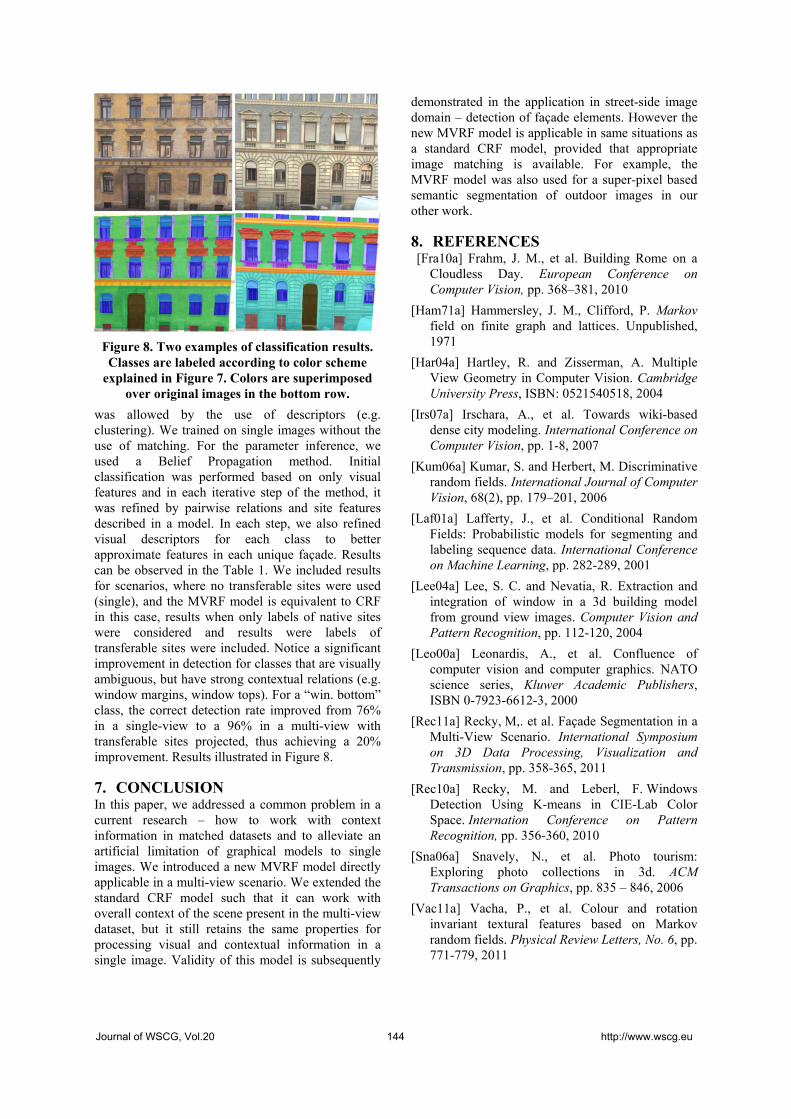
Figure 8. Two examples of classification results. Classes are labeled according to color scheme

explained in Figure 7. Colors are superimposed over original images in the bottom row.

was allowed by the use of descriptors (e.g. clustering). We trained on single images without the use of matching. For the parameter inference, we used a Belief Propagation method. Initial classification was performed based on only visual features and in each iterative step of the method, it was refined by pairwise relations and site features described in a model. In each step, we also refined visual descriptors for each class to better approximate features in each unique façade. Results can be observed in the Table 1. We included results for scenarios, where no transferable sites were used (single), and the MVRF model is equivalent to CRF in this case, results when only labels of native sites were considered and results were labels of transferable sites were included. Notice a significant improvement in detection for classes that are visually ambiguous, but have strong contextual relations (e.g. window margins, window tops). For a “win. bottom” class, the correct detection rate improved from 76% in a single-view to a 96% in a multi-view with transferable sites projected, thus achieving a 20% improvement. Results illustrated in Figure 8.

7. CONCLUSION In this paper, we addressed a common problem in a current research – how to work with context information in matched datasets and to alleviate an artificial limitation of graphical models to single images. We introduced a new MVRF model directly applicable in a multi-view scenario. We extended the standard CRF model such that it can work with overall context of the scene present in the multi-view dataset, but it still retains the same properties for processing visual and contextual information in a single image. Validity of this model is subsequently

demonstrated in the application in street-side image domain – detection of façade elements. However the new MVRF model is applicable in same situations as a standard CRF model, provided that appropriate image matching is available. For example, the MVRF model was also used for a super-pixel based semantic segmentation of outdoor images in our other work.

8. REFERENCES [Fra10a] Frahm, J. M., et al. Building Rome on a

Cloudless Day. European Conference on Computer Vision, pp. 368–381, 2010

[Ham71a] Hammersley, J. M., Clifford, P. Markov field on finite graph and lattices. Unpublished, 1971

[Har04a] Hartley, R. and Zisserman, A. Multiple View Geometry in Computer Vision. Cambridge University Press, ISBN: 0521540518, 2004

[Irs07a] Irschara, A., et al. Towards wiki-based dense city modeling. International Conference on Computer Vision, pp. 1-8, 2007

[Kum06a] Kumar, S. and Herbert, M. Discriminative random fields. International Journal of Computer Vision, 68(2), pp. 179–201, 2006

[Laf01a] Lafferty, J., et al. Conditional Random Fields: Probabilistic models for segmenting and labeling sequence data. International Conference on Machine Learning, pp. 282-289, 2001

[Lee04a] Lee, S. C. and Nevatia, R. Extraction and integration of window in a 3d building model from ground view images. Computer Vision and Pattern Recognition, pp. 112-120, 2004

[Leo00a] Leonardis, A., et al. Confluence of computer vision and computer graphics. NATO science series, Kluwer Academic Publishers, ISBN 0-7923-6612-3, 2000

[Rec11a] Recky, M,. et al. Façade Segmentation in a Multi-View Scenario. International Symposium on 3D Data Processing, Visualization and Transmission, pp. 358-365, 2011

[Rec10a] Recky, M. and Leberl, F. Windows Detection Using K-means in CIE-Lab Color Space. Internation Conference on Pattern Recognition, pp. 356-360, 2010

[Sna06a] Snavely, N., et al. Photo tourism: Exploring photo collections in 3d. ACM Transactions on Graphics, pp. 835 – 846, 2006

[Vac11a] Vacha, P., et al. Colour and rotation invariant textural features based on Markov random fields. Physical Review Letters, No. 6, pp. 771-779, 2011


Collision Detection on Point Clouds Using a 2.5+D Image-Based Approach

Rafael Kuffner dos Anjos

Inesc-ID Av. Prof. Dr Anibal Cavaco Silva Portugal 2744-016, Porto Salvo

[email protected]

João Madeiras Pereira

IST/Inesc-ID Rua Alves Redol, 9

Portugal 1000-029, Lisboa,

[email protected]

João Fradinho Oliveira

C3i/Inst. Politécnico de Portalegre Praça do Município

Portugal 7300, Portalegre

[email protected]

ABSTRACT

This work explores an alternative approach to the problem of collision detection using images instead of

geometry to represent complex polygonal environments and buildings derived from laser scan data, used in an

interactive navigation scenario. In a preprocessing step, models that are not point clouds, are sampled to create

representative point clouds. Our algorithm then creates several 2.5+D maps in a given volume that stacked

together form a 3D section of the world. We show that our new representation allows for realistic and fast

collision queries with complex geometry such as stairs and that the algorithm is insensitive to the size of the

input point cloud at run-time.

Keywords Collision Detection, Point-based Graphics, Navigation

1. INTRODUCTION Collision detection is normally a bottleneck in the

visualization and interaction process, as collisions

need to be checked at each frame. Traditionally, the

more complicated and crowded is our scene, the

more calculations need to be done, bringing the

frame-rate down. Therefore the optimization of this

process, gaining speed without losing quality in the

simulation, is something that has been researched for

years. Although several different techniques and

approaches have been developed, and showed good

performance in specific scenarios, these approaches

rely on object topology information which is easily

extracted from polygonal models. However with

point cloud models, the classical approaches either

will not work, or will have to heavily adapt to this

specific scenario, compromising their optimizations.

Using images as an alternative way of executing the

task of collision detection might just be the answer.

Image-based techniques can have their precision

easily controlled by the resolution of the used

images, and the algorithms are completely

independent of the object's topology and complexity

at run-time. It does not matter whether an object has

sharp features, round parts, or even whether it is a

point cloud, as all we are dealing with is the object's

image representation. Being a scalable and promising

technique, Image-based collision detection seems to

be a plausible alternative to the classical approaches.

Our approach focuses in a virtual reality navigation

scenario, where the scene is derived from the real

world via devices such as laser scanners, which tend

to generate enormous point clouds. Also, the

hardware at hand might not fit the basic requirements

for most algorithms and techniques, a situation that

commonly will happen in tourism hotspots,

museums, or other places where we would like

ordinary people to be able to interact with the system.

The developed application enables them to control an

avatar on a static environment, a point cloud or

polygonal model.

The main contribution of our research is a new 3D

world representation for environment and buildings

which is completely image-based with information

that enables realistic and robust collision detection

with underlying complex geometry such as slopes

and stairs. Slicing a given structure along the Z axis

(Using Cartesian coordinates as illustrated in Figure

1); we create a discrete set of images containing

height information about the surface, and possible

collidable frontiers. It is a flexible format that is able

to represent either point clouds or polygonal models.

This representation allows us to perform collision

detection with user chosen precision, and high

scalability.

Permission to make digital or hard copies of all or part of

this work for personal or classroom use is granted without

fee provided that copies are not made or distributed for

profit or commercial advantage and that copies bear this

notice and the full citation on the first page. To copy

otherwise, or republish, to post on servers or to

redistribute to lists, requires prior specific permission

and/or a fee.


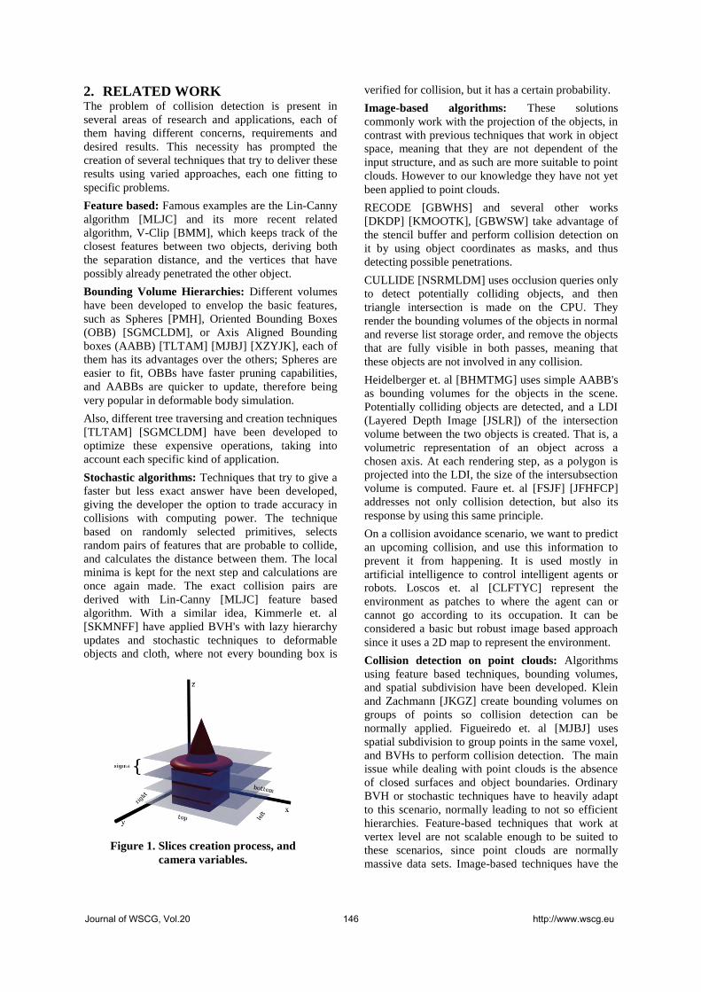
2. RELATED WORK The problem of collision detection is present in

several areas of research and applications, each of

them having different concerns, requirements and

desired results. This necessity has prompted the

creation of several techniques that try to deliver these

results using varied approaches, each one fitting to

specific problems.

Feature based: Famous examples are the Lin-Canny

algorithm [MLJC] and its more recent related

algorithm, V-Clip [BMM], which keeps track of the

closest features between two objects, deriving both

the separation distance, and the vertices that have

possibly already penetrated the other object.

Bounding Volume Hierarchies: Different volumes

have been developed to envelop the basic features,

such as Spheres [PMH], Oriented Bounding Boxes

(OBB) [SGMCLDM], or Axis Aligned Bounding

boxes (AABB) [TLTAM] [MJBJ] [XZYJK], each of

them has its advantages over the others; Spheres are

easier to fit, OBBs have faster pruning capabilities,

and AABBs are quicker to update, therefore being

very popular in deformable body simulation.

Also, different tree traversing and creation techniques

[TLTAM] [SGMCLDM] have been developed to

optimize these expensive operations, taking into

account each specific kind of application.

Stochastic algorithms: Techniques that try to give a

faster but less exact answer have been developed,

giving the developer the option to trade accuracy in

collisions with computing power. The technique

based on randomly selected primitives, selects

random pairs of features that are probable to collide,

and calculates the distance between them. The local

minima is kept for the next step and calculations are

once again made. The exact collision pairs are

derived with Lin-Canny [MLJC] feature based

algorithm. With a similar idea, Kimmerle et. al

[SKMNFF] have applied BVH's with lazy hierarchy

updates and stochastic techniques to deformable

objects and cloth, where not every bounding box is

verified for collision, but it has a certain probability.

Image-based algorithms: These solutions

commonly work with the projection of the objects, in

contrast with previous techniques that work in object

space, meaning that they are not dependent of the

input structure, and as such are more suitable to point

clouds. However to our knowledge they have not yet

been applied to point clouds.

RECODE [GBWHS] and several other works

[DKDP] [KMOOTK], [GBWSW] take advantage of

the stencil buffer and perform collision detection on

it by using object coordinates as masks, and thus

detecting possible penetrations.

CULLIDE [NSRMLDM] uses occlusion queries only

to detect potentially colliding objects, and then

triangle intersection is made on the CPU. They

render the bounding volumes of the objects in normal

and reverse list storage order, and remove the objects

that are fully visible in both passes, meaning that

these objects are not involved in any collision.

Heidelberger et. al [BHMTMG] uses simple AABB's

as bounding volumes for the objects in the scene.

Potentially colliding objects are detected, and a LDI

(Layered Depth Image [JSLR]) of the intersection

volume between the two objects is created. That is, a

volumetric representation of an object across a

chosen axis. At each rendering step, as a polygon is

projected into the LDI, the size of the intersubsection

volume is computed. Faure et. al [FSJF] [JFHFCP]

addresses not only collision detection, but also its

response by using this same principle.

On a collision avoidance scenario, we want to predict

an upcoming collision, and use this information to

prevent it from happening. It is used mostly in

artificial intelligence to control intelligent agents or

robots. Loscos et. al [CLFTYC] represent the

environment as patches to where the agent can or

cannot go according to its occupation. It can be

considered a basic but robust image based approach

since it uses a 2D map to represent the environment.

Collision detection on point clouds: Algorithms

using feature based techniques, bounding volumes,

and spatial subdivision have been developed. Klein

and Zachmann [JKGZ] create bounding volumes on

groups of points so collision detection can be

normally applied. Figueiredo et. al [MJBJ] uses

spatial subdivision to group points in the same voxel,

and BVHs to perform collision detection. The main

issue while dealing with point clouds is the absence

of closed surfaces and object boundaries. Ordinary

BVH or stochastic techniques have to heavily adapt

to this scenario, normally leading to not so efficient

hierarchies. Feature-based techniques that work at

vertex level are not scalable enough to be suited to

these scenarios, since point clouds are normally

massive data sets. Image-based techniques have the

Figure 1. Slices creation process, and

camera variables.


Figure 2. Points Coloring and Obstacle

Detection Algorithm

disadvantage of sometimes requiring special graphic

card capabilities, but only for some implementations.

Overall, their properties make them the best suited

for the proposed scenario of the tourism kiosk.

For further information on collision detection and

avoidance techniques we suggest the following

surveys: [NMAS] [SKTGKICB] [MT].

3. IMPLEMENTATION Image-based algorithms that have been presented in

the community ([NSRMLDM] [GBWHS] [DKDP]

[NBJM] [JFHFCP] [FSJF]) perform very well in

various kinds of scenarios, but some features of our

set scenario (described on Section 1) make them hard

or impossible to be applied (e.g. our data is

unstructured, not all objects are closed or convex).

Our work extends the idea of a 2.5D map presented

on the work of Loscos et. al [CLFTYC] by using

enhanced height-maps, where the pixel color not only

represents the height on that point, but also contains

obstacle information, while at the same time

overcoming the limitations of only supporting single

floor environments. We call these enhanced maps,

2.5+D maps. Instead of having just one height map,

we create a series of enhanced maps along intervals

sized on the axis, thus enabling the storage of

more than a single value for each ( ) pair.

Unlike LDI’s, our representation does not combine

several images into a volumetric representation, but

separates each slice into a single image so we can

easily perform memory management, and apply

image comparison and compression techniques to

have a better performance. Using the color of each

pixel as a representation of a voxel, we write height

information on the red channel, and identify

obstacles on the blue channel. By adding these

variables, we can determine not only the height level

where the avatar should be standing, but also if he is

colliding with any obstacle in several different

heights.

Slices Creation The creation of this representation is executed in a

pre-processing stage, which is composed of several

steps that must be performed from the input of the

model until the actual rendering to create the

snapshots that will be the used as collision maps.

These slices are created as following. The camera is

first set up according to the previously calculated

bounding boxes of the input model on an orthogonal

projection. After rendering that projection, a snapshot

sized is created and saved into the disk for further

use. The camera then is moved along the axis, and

the process is repeated until the whole extension of

the model has been rendered into images. A visual

representation of the described variables along with

the slices computed on an example model can be

seen on Figure 1 and two real slices can be seen on

Figure 4.

Polygonal Model Oversampling We aim for a solution that accepts both polygonal

models and point clouds. However these

representations are inherently different and cannot be

processed initially in the same way. Hence we

created a solution that approximates the polygon

models with a synthetic point cloud thus enabling

later steps to be processed in the same way. We apply

a simple oversampling operation that operates at

triangle level transforming a polygonal model into a

point cloud with a user-choice level of precision.

After oversampling and discarding the polygons, the

rendering of the produced point cloud has exactly the

same shape and fill as if rendering the polygonal

representation to the height map.

Information Processing and Encoding Since all of our collision information will be written

on collision maps as colors, we must assign each

point on the point cloud a color representing its

collision information. This will not replace the

original color of that point in question. When writing

these points on the output image, each pixel will

represent a voxel sized ( ) on object space. So

the painted color on that pixel will represent all the

points contained in that volume. The algorithm on

Figure 2 performs both the operation of height map

information encoding, and obstacle detection. We

define as , so as to ensure that one has more than

one point on each slice, to properly perform the

obstacle detection, as will be described later.

The first operation is executed as follows: We

calculate the difference between the current point

coordinate and the model's lower bounding box ,

and apply the modulo operator with . This

remainder represents the points coordinate on an


Figure 3. Technique for surface orientation

detection. Red points belong to a vertical

structure, grey points to the floor.

Figure 4. Two slices of an office environment,

where walls (white/blue) and floor (green) are

clearly distinguished, as well as a subsection

of a roof (green to yellow) on the entrance.

interval . To be used as a color value, this

difference must belong to the interval , so we

calculate ⁄ thus deriving finally the red channel

value. The simplified formula is given by

( )

As navigation on a real-world scenario is normally

performed horizontally on the plane, we classify

an obstacle as a surface that is close to being

perpendicular to , parallel to . So our obstacle

collision technique simply estimates how parallel to

the axis a certain surface is. Figure 3 illustrates how

potential obstacles and floor are classified using the

coloring algorithm (Figure 2). Points lined up

vertically on the same pixel most likely belong to a

vertical surface. Diagonal structures like ramps are

climbable up to a certain degree. The closer to a wall

they are, the greater the probability is that its points

are considered to be obstacles.

In order to keep track of point information that will

be stored in the slices we use an auxiliary structure, a

3D array , after processing each point,

we keep its color value on the position of the array

representing the voxel on object space from where it

came from. If there is already a stored value in this

voxel, the difference between both red values is

calculated, and transformed into an object-space

distance ( )

.

If this difference is bigger than a certain small

percentage (e.g. 7%) of the size of the slice, we

assume that the points are vertically aligned,

belonging to a vertical surface. These points are

marked on their blue channel with the value 1, and

we slightly increase its coordinate so that the point

is not occluded when rendering the maps. Typical

output slices produced in the pre-processing stage

can be seen in Figure 4, an office environment, where

the floor has been correctly labeled as green, and all

the walls are labeled as white or light blue.

Collision Detection The developed representation provides us with

enough information to perform quick collision

detection on the navigation scenario given on section

1 where we consider point clouds as a viable input. In

the accompanying video we show precise collision

detection between rigid bodies and point clouds.

We divide the task of collision detection into two

steps: a first step, that we call Broad phase, where we

verify the occurrence of collisions between any

objects in the scene, and a second step called narrow

phase, where we perform collision response.

3.1.1 Broad Phase and Collision Detection This task consists on identifying possible collisions

between all objects on the scene. By representing the

avatar that will be navigating on the environment by

an Axis Aligned Bounding Box (AABB), we first

calculate its size in pixels by calculating

and

, where threshold is calculated as

the pixel size. This will be the number of pixels

checked for collision on each slice, around the center

of the avatar. If any checked pixel is not black, we

mark the object as colliding, and they will be further

processed in a narrow phase.

The only images we will need to load into the

memory at the same time in order to perform

collision detection between the given avatar and the

environment are the ones located between

and

, where

represents the z coordinate of the avatar. These slices

contain collision detection information about the

location where the pawn currently is.

New slices that are needed, are loaded into memory

until a user defined constant of number of slices

( ) is reached. New slices beyond this point,

replace an already loaded slice that has the furthest

value from the avatar's own value, meaning it is not

needed at this point of the execution. In practice we

found that six slices covered well the avatar's


potential waist, shoulders, head, knees, and feet

collisions with the scene.

3.1.2 Narrow Phase and Collision Response In our current version, the sole purpose of our

collision response algorithm was to simply avoid

objects from overlapping, and provide a basic

navigation experience on the given environment. Any

other more complex technique could be applied here,

but this simple solution fulfills the requirements for

our navigation scenario. We focused on an efficient

broad phase algorithm, and a flexible representation

so we could apply any chosen image-based technique

on the narrow phase. This was achieved with a

straightforward extension of our broad-phase

algorithm, by applying the concepts of collision

response from height maps, and collision avoidance

[CLFTYC]. Instead of simply returning true when we

find pixels that are not black, we gather information

for collision response each time we find colored

pixels. Pixels with the blue channel set to always

represent an obstacle, except on applications where

we want to enable the avatar to climb small

obstacles, as the agents from Loscos et.al [CLFTYC].

On these situations, we may ignore these pixels up

until the height we want to be considered as

climbable. As our avatar moves on fixed length steps,

and each time it collides we correct it to the place it

was on the previous check, we thus ensure that the

avatar is always on a valid position. We apply this

( ) correction each time an obstacle pixel is found

until all the pixels representing the avatar's bounding

box are verified.

Height is defined exactly as it is when precomputing

height maps. By multiplying the coded height

information on the red channel by and adding the

base coordinate of the given slice, we have precise

information about a given point's height. Collision

response can be made by setting the final height to

the average height of the points on the base of the

bounding box, or by the adopted strategy, the

maximum value. Here we also check for surface

height values from the first slice until the height we

want to consider as climbable.

The complexity of this operation is exactly ( ) where and are the number of

pixels ocuppied by the base of the avatar and is the

number of slices encompassed by the avatar's height.

We point however, that these checks are already

performed in the broad phase, and hence can be re-

used in the narrow phase without adding any extra

operations.

4. EXPERIMENTAL RESULTS We have implemented the whole algorithm using

OpenGL 2.1.2, C and the OpenGL Utility Toolkit

(GLUT) to deal with user input and the base

application loop management. The platform used for

tests was a computer with an Intel core 2 Duo CPU at

2 GHz with 2GB of RAM, a NVIDIA GeForce 9400

adapter, running Microsoft Windows Seven x86.

Table 2 shows the time taken on the whole

preprocessing stage for each model and

configuration. Polygon sampling during the

preprocessing of polygonal models is clearly the

most computationally intensive task in the pipeline,

as the two higher complexity point cloud models

(Entrance and Room as seen on Table 1 and Figure

7) that did not require sampling had a faster

performance. In the preprocessing phase the increase

on processing time with point clouds is linear to point

complexity. This linear growth is expected since each

point must be checked for coloring once, and also for

common input processing tasks such as file reading

and display list creation.

Regarding the results of the overall memory cost

specifically in the preprocessing phase, Table 2

shows that memory scales almost linearly according

to the input size of the point cloud (Entrance versus

Room in Table 1). This memory is needed

temporarily for allocating the auxiliary 3D array for

obstacle detection in the slice creation phase.

Similarly, tests have shown that this memory

consumption also grows linearly with the number of

points produced in the polygon sampling phase.

During the application runtime, the average memory

consumption varies according to the number of

loaded slices into RAM, and according to the size of

the loaded model used for rendering (Figure 5 and

Table 1). On a 700x700 resolution, the peak minimal

value found in any model we experimented was

50,07MB (Office) and the peak maximum 168,08MB

(Street), with 6 slices loaded in memory. Table 2

shows how much memory the application consumes

when only rendering the models and the total

memory with collision detection, while having 6

slices loaded in memory. By controlling we

can avoid this value from going over the memory we

wish the Figure 5. Memory load at a given moment

during runtime on a 700x700 configuration, 6

slices, with and without collision detection.


application to consume, since all other memory

required for the application is for tasks unrelated to

collision detection.

We were interested in studying the direct behavior of

our algorithm and did not wish to mask performance

with asynchronous I/O threads. Results on collision

detection have been verified through establishing a

fixed route to navigate with the pawn avatar where it

goes through different situations and scenarios, such

as "climbing" single steps, "traversing" planar areas,

going "near" cylindrical or square shaped columns

and "falling" from a height. Whilst the number of

created collision maps for a scene can affect collision

results, the actual number of buffer slices will

only affect potentially the performance, as the system

checks all slices at the avatar´s current height. Tests

on Cathedral 700x700 with 130 slices and set

to 10 have showed us that reading from the disk at

runtime has a bigger impact on efficiency than

storing a higher number of images on commodity

RAM. For instance, when using a maximum buffer

of 10 slices and reading a high resolution image from

the disk, we notice a sudden drop in frame-rate

(Figure 6), and this can also be noticed when the

pawn falls from a higher structure, and needs to

rapidly load a series of maps on his way to the

ground. By increasing to 16 on this scenario,

we ensure the storage of enough slices to represent

the ground floor and the platform on top of the steps

(Experiment B in the accompanying video). Little

difference was noticed on memory load (5,33MB),

and the interaction was much smoother.

Results also show that our algorithm did not affect in

any way the rendering speed of the interactive

application. Figure 6 shows that the frame-rate was

nearly identical in the same scenario with and

without collision detection using 16 slices.

Although we did not aim for high precision on

collision response, our technique has presented

precise results on different resolutions. We note that

point clouds are themselves approximations to

surfaces, and as such a collision amongst points is an

unlikely event, Figueiredo et. al use the average

closest point to point distance divided by two to

establish a conservative bounding box around each

point, which can generate false collisions when close.

With our approach, instead of a box, we use the

pixels of a zoomed out view which is also

conservative. Precision results with the different

algorithms were verified empirically by changing the

Model Type Original

Complexity Details

Office Polygonal 17.353 pts. Office environment with cubicles and hallways

Church Polygonal 26.721 pts. Simple church with stairs and columns

Sibenik Polygonal 47.658 pts. Cathedral of St. James on Sibenik, Croatia

Columns Polygonal 143.591 pts. Big environment with localized complexity.

Room 3D laser scan 271.731 pts. 3D Scan of a room with chairs and several objects.

Street Polygonal 281.169 pts. Outside street environment with an irregular floor,

houses, and several objects

Entrance 3D laser scan 580.062 pts. Entrance of the Batalha monastery in Portugal.

Model Time

(s)

Total

Complexity

Memory

Office 41,23 9.349.585 pts 610,3 MB

Church 58,14 6.475.125 pts 536,58 MB

Sibenik 78,87 5.199.093 pts 532,48 MB

Columns 42,92 2.612.303 pts 241,66 MB

Street 114,75 7.142.361 pts 598,02 MB

Entrance 13,9 580.062 pts. 122,88 MB

Room 6,96 271.731 pts. 67,58 MB

Table 1. Features of the models used for evaluation

.

Table 2. Time, Total complexity (with

generated points) and Memory consumption

on the pre-processing stage for a 700x700

resolution.

Figure 6. Average frame rate and memory

consumption comparison between different

𝒏𝒔𝒍𝒊𝒄𝒆𝒔 configurations with 700x700 images,

and no collision detection scenario.

(Experiment B, Cathedral)


color of the avatar when a collision occurs. We found

that using collision maps with a resolution of

700x700 enabled one to lower the number of false

collisions from other methods when close to

obstacles.

Floor collision has been performed perfectly in all

resolutions, since its precision is defined by the rgb

value of the point. Collisions with obstacles are more

affected by resolution as is to be expected, since we

rely on pixel finesse to precisely know the position of

a given surface. Tests on office and street (Figure 7)

have showed the same errors of small object

interference or fake collisions due to diffuse

information about object boundaries. These are more

noticeable on the interactions with round objects on

Street (Figure 7) where we can notice the aliasing

creating invisible square barriers around a perfectly

round object.

Table 3 compares our technique with the work from

Figueiredo et. al [MJBJ], which has been tested on

one of our experimental scenarios (Figure 7), the

walkthrough in the point cloud of the Batalha

Monastery (Experiment A in the accompanying

video, 700x700 resolution set to 10), on a

machine with a slightly faster processing speed and

RAM than the one used for our walkthroughs. We

compared our results with their best performance

alternative, that bases the surface partition on 4096

cells of the octree.

Frame-rate was disturbed during the collision

detection process on the R-tree approach, while it

remained steady at the 30 fps during the whole

execution of our application. Also, the image-based

technique has required much less memory to be

executed, even with a significantly high number of

slices loaded in memory. The biggest difference is in

the pre-processing times. Our approach was executed

107 times faster than the BVH approach. The pre-

processing stage must only be performed once for

each configuration, since the representation is written

and loaded to the hard-drive for further interactions.

As stated in section 2 the research on point cloud

collision detection is recent, and non-existent

regarding image-based techniques. Our pioneer

solution has presented excellent results, not only

performing better than other works on point clouds

published in the scientific community, but also being

flexible enough to be applied on models from CAD,

or combined with precise collision response

techniques. Our technique can be performed with our

representation on any computer that can render the

input model at an acceptable frame-rate, without

requiring much processing from the CPU or GPUs.

5. CONCLUSION AND FUTURE

WORK A new image-based environment representation for

collision detection has been presented, using 2.5+D

slices of an environment or buildings across the

axis. These images contain at each pixel, information

about a given voxel, representing i's contents with

colors. Height map information is stored on the red

channel, and obstacles are indicated on the blue

channel. This allows us to have a Broad phase

collision detection stage that is performed with high

efficiency and scalability, where the user can choose

the precision according to the computing power at

hand by simply adjusting the resolution of the

produced images. Point clouds and polygonal models

are ubiquitously processed, making our approach

currently the best suited for fast interaction with

massive laser-scan data. This work fills a gap in the

area of collision detection, exploring a scenario that

has been receiving more attention recently.

Future Work Using graphic card capabilities such as the stencil

buffer for broad-phase collision detection and vertex

shaders for point coloring could greatly speed up

these operations, and also, calculations would be

moved to the GPU, taking away some work from the

CPU. Applying this representation of environments

also on objects of the scene, or even applying it to the

avatars we're using on the interaction, could present

interesting results. Using non-uniform resolution

images on environments where we do not have a

uniform complexity, would also help us achieve

more precision on our narrow phase, or on these

presented situations.

Image comparison techniques and compression can

also be applied to the generated images in order to

decrease the number of times we need to load a slice,

and also the number of collision detection checks we

must do. In several man-made structures such as

buildings, many slices tend to be identical; intra-slice

compression also presents itself as an interesting

avenue of research.

6. ACKNOWLEDGMENTS We would like to thank Artescan for the point clouds

provided.

Image-based

(700x700)

BVH Oct 4096

Frame-rate 30 fps 16 to 30 fps

Total

Memory

143.36 MB 225,44 MB

Pre. proc.

time

13.9 s 1500 s

Table 3. Comparison between point-cloud

techniques (Experiment A)


7. REFERENCES [BHMTMG] Bruno Heidelberger, Matthias

Teschner, and Markus Gross, Real-Time

Volumetric Intersections of Deforming Objects,

Proceedings of Vision, Modeling, and

Visualization 2003,461-468,2003

[BMM] Brian Mirtich, V-clip: fast and robust

polyhedral collision detection, ACM Trans.

Graph., 17:177--208, July 1998.

[CLFTYC] Céline Loscos, Franco Tecchia, and

Yiorgos Chrysanthou, Real-time shadows for

animated crowds in virtual cities, In Proceedings

of the ACM symposium on Virtual reality

software and technology, VRST '01, pages 85--

92, New York, NY, USA, 2001. ACM.

[DKDP] Dave Knott and Dinesh K. Pai, Cinder -

collision and interference detection in real-time

using graphics hardware, Proceedings of Graphics

Interface, pages 73--80, 2003.

[FSJF] François Faure, Sébastien Barbier, Jérémie

Allard, and Florent Falipou, Image-based

collision detection and response between arbitrary

volume objects, In Proceedings of the 2008


Computer Animation, SCA '08, pages 155--162,

Aire-la-Ville, Switzerland, Switzerland, 2008.

Eurographics Association.

[GBWHS] G. Baciu, Wingo Sai-Keung Wong, and

Hanqiu Sun, Recode: an image-based collision

detection algorithm, In Computer Graphics and

Applications, 1998. Pacific Graphics '98. Sixth

Pacific Conference on, pages 125 --133, oct 1998.

[GBWSW] George Baciu and Wingo Sai-Keung

Wong, Hardware-assisted self collision for

deformable surfaces, Proceedings of the ACM

symposium on Virtual reality software and

technology, 2002.

[JFHFCP] Jérémie Allard, François Faure, Hadrien

Courtecuisse, Florent Falipou, Christian Duriez,

and Paul G. Kry, Volume contact constraints at

arbitrary resolution, ACM Trans. Graph.,

29:82:1--82:10, July 2010.

[JKGZ] Jan Klein and Gabriel Zachmann, Point

cloud collision detection, Computer Graphics

Forum, 23(3):567--576, 2004.

[JSLR] Jonathan Shade, Steven Gortler, Li wei He,

and Richard Szeliski, Layered depth images,

Proceedings of the 25th annual conference on

Computer graphics and interactive techniques,

1998.

[KMOOTK] Karol Myszokowski, Oleg G. Okunev,

and Tosiyasu L. kunii, Fast collision detection

between complex solids using rasterizing

graphics hardware, The Visual Computer,

11(9):497 -- 512, 1995.

[MJBJ] Mauro Figueiredo, João Oliveira, Bruno

Araújo, and João Pereira, An efficient collision

detection algorithm for point cloud models, 20th

International conference on Computer Graphics

and Vision, 2010.

[MLJC] M.C. Lin and J.F. Canny, A fast algorithm

for incremental distance calculation, In Robotics

and Automation, 1991. Proceedings., 1991 IEEE

International Conference on, pages 1008 --1014

vol.2, apr 1991.

[MT] M. Teschner, S. Kimmerle, G. Zachmann, B.

Heidelberger, Laks Raghupathi, A. Fuhrmann,

Marie-Paule Cani, François Faure, N. Magnetat-

Thalmann, and W. Strasser, Collision detection

for deformable objects, Computer Graphics

Forum,24(1):61--81,2005

[NBJM] Niels Boldt and Jonas Meyer, Self-

intersections with cullide, Eurographics, 23(3),

2005.

[NMAS] Noralizatul Azma Bt Mustapha Abdullah,

Abdullah Bin Bade, and Sarudin Kari, A review

of collision avoidance technique for crowd

simulation, 2009 International Conference on

Information and Multimedia Technology,

(2004):388--392, 2009.

[NSRMLDM] Naga K. Govindaraju, Stephane

Redon, Ming C. Lin, and Dinesh Manocha,

Cullide: interactive collision detection between

complex models in large environments using

graphics hardware, In Proceedings of the ACM

SIGGRAPH/EUROGRAPHICS conference on

Graphics hardware, HWWS '03, pages 25--32,

Aire-la-Ville, Switzerland, Switzerland, 2003.

Eurographics Association.

[PMH] Philip M. Hubbard, Approximating polyhedra

with spheres for time-critical collision detection,

ACM Transactions on Graphics, 15(3):179--210,

July 1996.

[SGMCLDM] S. Gottschalk, M. C. Lin, and D.

Manocha. 1996. OBBTree: a hierarchical

structure for rapid interference detection. In

Proceedings of the 23rd annual conference on

Computer graphics and interactive techniques

(SIGGRAPH '96). ACM, New York, NY, USA,

171-180.

[SKMNFF] Stephan Kimmerle, Matthieu Nesme, and

François Faure, Hierarchy Accelerated Stochastic

Collision Detection, In 9th International

Workshop on Vision, Modeling, and

Visualization, VMV 2004, pages 307-312,

Stanford, California, États-Unis, November 2004.


(a) Church

[SKTGKICB] S. Kockara, T. Halic, K. Iqbal, C.

Bayrak, and Richard Rowe, Collision detection:

A survey, In Systems, Man and Cybernetics,

2007. ISIC. IEEE International Conference on,

pages 4046 --4051, oct. 2007.

[TLTAM] Thomas Larsson and Tomas Akenine-

Möller, Collision detection for continuously

deforming bodies, Eurographics 2001.

[XZYJK] Xinyu Zhang and Y.J. Kim, Interactive

collision detection for deformable models using

streaming aabbs, Visualization and Computer

Graphics, IEEE Transactions on, 13(2):318 --329,

march-april 2007.

(b) Street

(c) Sibenik (d) Room

(e) Columns (f) Office

(e) Batalha

Figure 7. Pictures of all the tested input

polygonal models and point clouds. Environments

with different topologies were chosen for this

purpose.


Color Preserving HDR Fusion for Dynamic Scenes

Gökdeniz KaradagMiddle East Technical University, Turkey

[email protected]

Ahmet Oguz AkyüzMiddle East Technical University, Turkey

[email protected]

ABSTRACTWe present a novel algorithm to efficiently generate high quality high dynamic range (HDR) images. Our methodis based on the idea of expanding the dynamic range of a reference image at granularity of tiles. In each tile, weuse data from a single exposure, but different tiles can comefrom different exposures. We show that this approachis not only efficient and robust against camera and object movement, but also improves the color quality of theresulting HDR images. We compare our method against the commonly used HDR generation algorithms.

Keywords: High dynamic range imaging, image fusion, color quality

1 INTRODUCTIONThe interest in HDR imaging has rapidly gained pop-ularity in recent years. This has been accompanied bythe development of various methods to create HDR im-ages. While it is believed that using dedicated HDRcapture hardware will be the de-facto way of generat-ing HDR images in future [Rei10a], software solutionsare still commonly used in today’s systems. Amongthese multiple exposure techniques (MET) are the mostdominant [Man95a, Deb97a].

In METs, several images of the same scene are capturedby varying the exposure time between the images. Thisensures that each part of the captured scene is properlyexposed in at least one image. The individual imagesare then merged to obtain the HDR result. Althoughvariations exist, the equation below is typically used forthe merging process:

I j =N

∑i=1

f−1(pi j )w(pi j )

ti

/ N

∑i=1

w(pi j ). (1)

HereN is the number of LDR images,pi j is the valueof pixel j in imagei, f is the camera response function,ti is the exposure time of imagei, andw is a weightingfunction used to attenuate the contribution of poorly ex-posed pixels.

In Equation 1, a weighted average is computed for ev-ery pixel. While this may be desirable for attenuatingnoise, it introduces unwanted artifacts due to ghostingand misalignment problems. In this paper, we show thatthis approach also results in the desaturation of colors


making the HDR image less saturated than the its con-stituent exposures.

Computing a weighted average for every pixel also re-quires that the individual pixels are perfectly aligned.Otherwise, pixels belonging to different regions in thescene will be accumulated resulting ghosting and align-ment artifacts.

In this paper, we propose a method that largely avoidsboth of these problems. Our method is underpinned bythe idea that instead of computing an average for ev-ery pixel, one can use the pixels from a single properlyexposed image. A different image can be used for dif-ferent regions ensuring that the full dynamic range iscaptured. We also introduce the concept of working intiles instead of pixels to make the algorithm more robustagainst local object movements.

2 PREVIOUS WORKStarting with the pioneering works of Mad-den [Mad93a] and Mann and Picard [Man95a], variousalgorithms have been developed to create HDR images.The early work focused on recovering the camera re-sponse function and choosing an appropriate weightingfunction [Deb97a, Mit99a, Rob03a, Gro04a]. Thesealgorithms assumed that the exposures that are usedto create an HDR image are perfectly aligned and thescene is static.

Ward developed a method based on median thresh-old bitmaps (MTBs) to allow photographers usehand-held images of static scenes in HDR imagegeneration [War03a]. His alignment algorithm provedto be very successful and is used as an initial stepof more advanced alignment and ghost removalalgorithms [Gro06a, Jac08a, Lu09a].

In another alignment algorithm, Cerman and Hlavác es-timated the initial shift amounts by computing the cor-relation of the images in the Fourier domain [Cer06a].This, together with the initial rotational estimate which


was assumed to be zero, was used as a starting point forthe subsequent iterative search process.

Tomaszewska and Mantiuk employed a modified scaleinvariant feature transform (SIFT) [Low04a] to extractlocal features in the images to be aligned [Tom07a].The prominent features are then selected by theRANSAC algorithm [Fis81a]. This refined set offeatures are then used to compute a homographybetween the input images.

Several methods have been proposed to deal with ghost-ing artifacts. These algorithms usually pre-align the in-put exposures using MTB or other algorithms to sim-plify the ghost detection process. Some of these algo-rithms avoid merging suspicious regions where there ishigh variance [Kha06a, Gal09a, Ram11a]. Other algo-rithms try to detect the movement of pixels and performpixel-wise alignment [Zim11a]. A recent review ofHDR ghost removal algorithms can be found in Srikan-tha and Sidibé [Sri12a].

There are also existing algorithms that attempt tocombine data from multiple exposures for the purposeof generating a single low dynamic range (LDR)image. Among these, Goshtasby first partitions theimages into tiles [Gos05a]. For each tile, he thenselects the image that has the highest entropy. Thetiles are blended using smooth blending functions toprevent seams. Mertens et al., on the other hand, donot use tiles but utilize three metrics namely contrast,saturation, and well-exposedness to choose the bestimage for each pixel [Mer07a]. Similar to Goshtasby,Várkonyi-Kóczy et al. propose a tile based algorithmwhere tiles are selected to maximize detail using imagegradients [Var08a]. In another tile based algorithm,Vavilin and Jo use three metrics; mean intensity,intensity deviation, and entropy to choose the bestexposure for each tile [Vav08a]. In contrast to previoustile based studies, they choose tile size adaptivelybased on local contrast. Finally, Jo and Vavilin proposea segmentation based algorithm which allows choosingdifferent exposures for different clusters [Jo11a].Unlike previous methods they use bilateral filteringduring the blending stage.

It is important to note that existing tile-based algorithmsattempt to generate LDR images with more details andenhanced texture information, whereas our goal is togenerate HDR images with natural colors. Our ap-proach alleviates the need for explicit ghost detectionand removal procedures. If the dynamic parts of a scenedo not span across regions with significantly differentluminance levels, no ghost effects will occur in the out-put. Also, we avoid redundant blending of pixels thatcan result in reduced color saturation.

L LL

LLL

L L L

S

S

SS

S SS

Figure 1: We partition the images into tiles and deter-mine which exposure to use for each tile.

3 ALGORITHM

The first step of our algorithm is to align the input expo-sures using the MTB algorithm [War03a]. In this part,both the original MTB or the MTB with the rotationsupport can be used.

Once the images are aligned, we partition each expo-sure into tiles. Our goal then becomes to choose thebest image that represents the area covered by each tile.A sample image is shown in Figure 1 to illustrate thisidea. In this image, the under-exposed tiles are markedwith L indicating that these tiles should come from alonger exposure. Similarly, over-exposed regions aremarked byS suggesting that shorter exposures shouldbe used for these tiles. Unmarked tiles can come fromthe middle exposures.

To make these decisions, we need to define a qualitymetric that indicates whether a tile is well-exposed. Tothis end, we experimented with the mean intensity aswell as the number of under- and over-exposed pixelswithin a tile as potential metrics. Our results suggestedthat using the mean intensity gives better results. There-fore, we marked a tile as agoodtile if its mean intensityis in the range[Imin, Imax]. Imin andImax are user param-eters, but we found thatImin= 50 andImax= 200 can beused as reasonable defaults.

Based on this criteria, we compute the number of goodtiles for each exposure. We choose the exposure withthe maximum number of good tiles as the reference ex-posure. This exposure serves as thedonor which pro-vides data for all tiles whose mean intensity stays inthe aforementioned limits. This leniency allows us touse the same image as much as possible and providesgreater spatial coherency. For the remaining tiles, wechoose the second reference exposure and fill in thetiles which are valid in this exposure. This process is


(a) Standard MET (b) LDR reference (c) Our result

Figure 2: (a) HDR image created by using the standard MET. (b)Selected individual exposure from the bracketedsequence. (c) HDR image created using our algorithm. The toprow shows the full images. The middle row showsthe close-up view of a selected region. The bottom row shows the color of a single pixel from the region indicatedin the middle row. Both HDR images are tone mapped using the photographic tone mapping operator [Rei02a].As can be seen in the zoomed views, the color quality of our result is closer to the selected reference image.

recursively executed until a source image is found forall tiles1. This process can be represented as:

I j =N

∑i=1

f−1(pi j )Wi j

ti, (2)

Wi j =

1 if pixel j comes from imagei,

0 otherwise.(3)

Note that we no longer have thew(pi j ) term from Equa-tion 1 as we do not compute a weighted average.

Finally, we use a blending strategy to prevent the visi-bility of seams at tile boundaries. For this purpose, wecreate Gaussian pyramids of weights (Wi j ) and Lapla-cian pyramids of source images. We then merge theimages by using Equation 2 at each level of the pyra-mid and collapse the pyramid to obtain the final HDRimage. We refer the reader to Burt and Adelson’s orig-inal paper for the details of this process [Bur83a].

Since the tiles are not overlapping our algorithm en-sures that within each tile data from only a single sourceimage is used. As we demonstrate in the next section,this improves the color saturation of the resulting HDRimages. A second observation is that each tile is spa-tially coherent. This means that motion related artifacts

1 It is possible that the a tile is under- or over-exposed in allinput images. In this case, we choose the longest exposure ifthe tile is under-exposed and shortest exposure otherwise.

will not occur within tiles. However, such artifacts canstill occur across tiles. Thus our algorithm reduces theeffect of motion artifacts but does not completely elim-inate them.

4 RESULTS AND ANALYSIS

We present the results of our color preserving HDR fu-sion algorithm under three categories namely: (1) Fixedcamera & static scene, (2) hand-held camera & staticscene, and (3) hand-held camera & dynamic scene. Forthe first configuration, we illustrate that the color qual-ity of the HDR image created by our method is supe-rior to the output of the standard HDR fusion algorithmshown in Equation 1. A sample result for this case isdepicted in Figure 2 where the output of the standardMET is shown on the left and our result is shown on theright. A selected exposure from the bracketed sequenceis shown in the middle for reference.

For the image on the left, we used the tent weight-ing function proposed by Debevec and Malik [Deb97a].We used the sRGB camera response function for bothimages, and a tile size of 64×64 for our result. It can beseen that, due to the pixel-wise averaging process, theoutput of the standard MET has a washed-out appear-ance. Our result, on the other hand, is colorimetricallycloser to the selected exposure. This is a consequenceof avoiding unnecessary blending between images.


Figure 3: The colors show the correspondence between the tiles in the HDR image and the source images thatthey were selected from. We can see that most tiles were selected from the fourth image. Figure courtesy of ErikReinhard [Rei10a].

Figure 3 shows which tiles in the output HDR imagecame from which images in the exposure sequence. Thecorrespondence is shown by color coding the individualexposures. As we can see from this figure, the major-ity of the tiles were selected from the fourth exposure.The tiles that correspond to the highlights on the plantscame from the darker exposures. On the other hand, thetiles that correspond to the crevices on the rock and theshadow of the lizard came from the lighter exposures.We can also see that the last three exposures were notused at all.

At this point, it would be worthwhile to discuss whythe standard MET gives rise to a washed-out appear-ance and our algorithm does not. We would not ex-pect to see this problem if all exposures were perfectrepresentations of the actual scene. However, in real-ity, there are slight differences between exposures thatare not only due to changing the exposure time. Slightcamera movements, noise, and inaccuracies in the cam-era response curve can all cause variations between theactual observations. The combined effect of these vari-ations result in reduced color saturation. By avoidingunnecessary blending, we also avoid this artifact.

The second test group consists of images of a staticscene captured by a hand-held camera (Figure 4). Inthis figure, the left column shows the unaligned resultcreated by directly merging five bracketed exposures.The middle column shows the tone mapped HDR out-put after the exposures are aligned by using the MTB al-gorithm. The right column shows our result obtained byfirst aligning the exposures using the MTB algorithm,and then merging them using our tile-based technique.As can be seen from the fence and the sign in the in-sets, our result is significantly sharper than that of theMTB algorithm. However, we also note that small ar-tifacts are visible in our result on the letters “R” and“E”. Further examination reveals that these artifacts aredue to using tiles from different exposures that are notperfectly aligned.

As the color map indicates, the majority of the finalHDR image is retrieved from the exposure coded byred (exposures not shown). The darker regions retrieveddata from the lighter (gray) exposure. The highlights atthe top left corner received data from the darker (green)exposure. In fact, in this example, all five exposurescontributed to the final image but the majority of thecontribution came from these three exposures.

In the final category, we demonstrate the performanceof our algorithm using scenes that have both global andlocal movement. To this end, we used the hdrgen soft-ware2 which implements the MTB alignment algorithmand a variance based ghost removal method explainedin Reinhard et al. [Rei10a]. In Figure 5, the left columnshows the output obtained by only image alignment butwithout ghost removal. The middle column shows theresult of alignment and ghost removal. Although themajority of the ghosts are removed, some artifacts arestill visible on the flag as shown in the close-ups. Theright column shows our result where these artifacts areeliminated. The color map indicates the source imagesfor different regions of the HDR image.

We also demonstrate a case where our algorithm intro-duces some unwanted artifacts in high contrast and highfrequency image regions as the window example in Fig-ure 6. The bright back light and window grates causehigh contrast. If the tile size is large, blending tiles fromdifferent exposures produces sub-par results. A reducedtile size eliminates these artifacts.

Our choice of prioritizing the reference image increasessuccess in image sets where ghosting effects would nor-mally occur. If the object movements are located inregions with similar lighting conditions, our algorithmprefers the image closer to reference image while con-structing tiles, preventing ghosting effects. It is possi-ble that an object moves between regions of differentlighting conditions, and our algorithm may choose tiles

2 http://www.anyhere.com


Figure 4: Left: Unaligned HDR image created from hand-held exposures. Middle: Exposures aligned using theMTB algorithm. Right: Our result. The close-ups demonstrate that our algorithm produces sharper images. Thecolor map shows the source exposures for different regions of the HDR image.

(a) Alignment (b) Alignment and ghost removal (c) Our result

Figure 5: Left: Aligned HDR image created from hand-held exposures using the MTB algorithm. Middle: Alignedand ghost removed HDR image. Right: Our result. The insets demonstrate that ghosting artifacts are eliminated inour result. The color map shows the source exposures for different regions of the HDR image.

from different images where the moving object can beseen. In this case different copies of the object may bepresent in multiple locations in the output image.

Finally, we report the running times of our algorithm.An unoptimized C++ implementation of our algorithmwas able to create high resolution (18 MPs) HDR im-ages from 9 exposures within 30 seconds including alldisk read and write times. We conducted all of ourtest on an Intel Core i7 CPU running at 3.20 GHz andequipped with 6 GBs of memory. This suggests that ouralgorithm is practical and can easily be integrated intoexisting HDRI workflows.

5 CONCLUSIONS

We presented a simple and efficient algorithm that im-proves the quality of HDR images created by usingmultiple exposures techniques. By not redundantly av-eraging pixels in low dynamic regions, our algorithm

preserves the color saturation of the original exposures,and reduces the effect of ghosting and alignment arti-facts. As future work, we are planning to make thetiling process adaptive instead of using a uniform grid.This would prevent artifacts that can be caused bysudden illumination changes between neighboring tilescoming from different exposures. We are also planningto perform blending using edge-aware Laplacian pyra-mid [Par11a] to avoid blending across sharp edges. Im-proved quality of our results can also be validated by auser study.

ACKNOWLEDGMENTSThis work was partially supported by METU BAP-08-11-2011-123.

6 REFERENCES[Bur83a] P. Burt and E. Adelson. The laplacian pyramid as a com-

pact image code.Communications, IEEE Transactions on,31(4):532 – 540, apr 1983.


Figure 6: Top: A tone-mapped HDR image with128x128 tile size. Tile boundaries are highly visible inthe close-up. Middle: Changing the tile size to 32x32removes most of the artifacts, but some remain in di-agonal lines. Bottom: Using a 2x2 tile size eliminatesremaining artifacts.

[Cer06a] Lukáš Cerman and Václav Hlavác. Exposure time estima-tion for high dynamic range imaging with hand held camera.In Computer Vision Winter Workshop, Czech Republic, 2006.

[Deb97a] Paul E. Debevec and Jitendra Malik. Recovering highdynamic range radiance maps from photographs. InSIG-GRAPH 97 Conf. Proc., pages 369–378, August 1997.

[Fis81a] Martin A. Fischler and Robert C. Bolles. Random sampleconsensus: a paradigm for model fitting with applications toimage analysis and automated cartography.Commun. ACM,24(6):381–395, 1981.

[Gal09a] O. Gallo, N. Gelfandz, Wei-Chao Chen, M. Tico, andK. Pulli. Artifact-free high dynamic range imaging. InCom-putational Photography (ICCP), 2009 IEEE InternationalConference on, pages 1 –7, april 2009.

[Gos05a] A. Ardeshir Goshtasby. Fusion of multi-exposure images.Image and Vision Computing, 23(6):611 – 618, 2005.

[Gro04a] M.D. Grossberg and S.K. Nayar. Modeling the space ofcamera response functions.Pattern Analysis and MachineIntelligence, IEEE Trans. on, 26(10):1272 –1282, 2004.

[Gro06a] Thorsten Grosch. Fast and robust high dynamic rangeim-age generation with camera and object movement. InProc.of Vision Modeling and Visualization, pages 277–284, 2006.

[Jac08a] Katrien Jacobs, Celine Loscos, and Greg Ward. Automatichigh-dynamic range image generation for dynamic scenes.IEEE CG&A, 28(2):84–93, 2008.

[Jo11a] K.H. Jo and A. Vavilin. Hdr image generation based on in-tensity clustering and local feature analysis.Computers inHuman Behavior, 27(5):1507–1511, 2011.

[Kha06a] Erum Arif Khan, Ahmet Oguz Akyüz, and Erik Rein-hard. Ghost removal in high dynamic range images.IEEEInternational Conference on Image Processing, 2006.

[Low04a] David G. Lowe. Distinctive image features from scale-invariant keypoints.Int. J. Comput. Vision, 60(2):91–110,2004.

[Lu09a] Pei-Ying Lu, Tz-Huan Huang, Meng-Sung Wu, Yi-TingCheng, and Yung-Yu Chuang. High dynamic range imagereconstruction from hand-held cameras. InCVPR, pages509–516, 2009.

[Mad93a] B. C. Madden. Extended dynamic range imaging. Techni-cal report, GRASP Laboratory, Uni. of Pennsylvania, 1993.

[Man95a] S Mann and R Picard. Being ’undigital’ with digitalcam-eras: Extending dynamic range by combining differentlyexposed pictures, 1995.

[Mer07a] T. Mertens, J. Kautz, and F. Van Reeth. Exposure fusion.In Computer Graphics and Applications, 2007. PG ’07. 15thPacific Conference on, pages 382 –390, 29 2007-nov. 2 2007.

[Mit99a] T. Mitsunaga and S. K. Nayar. Radiometric self calibra-tion. In Proceedings of CVPR, volume 2, pages 374–380,June 1999.

[Par11a] Sylvain Paris, Samuel W. Hasinoff, and Jan Kautz. Locallaplacian filters: edge-aware image processing with a lapla-cian pyramid.ACM Trans. Graph., 30(4):68:1–68:12, July2011.

[Ram11a] Shanmuganathan Raman and Subhasis Chaudhuri. Re-construction of high contrast images for dynamic scenes.The Visual Computer, 27(12):1099–1114, 2011.

[Rei02a] Erik Reinhard, Michael Stark, Peter Shirley, and Jim Fer-werda. Photographic tone reproduction for digital images.ACM Transactions on Graphics, 21(3):267–276, 2002.

[Rei10a] Erik Reinhard, Greg Ward, Sumanta Pattanaik, and PaulDebevec.High Dynamic Range Imaging: Acquisition, Dis-play and Image-Based Lighting. Morgan Kaufmann, SanFrancisco, second edition edition, 2010.

[Rob03a] Mark A. Robertson, Sean Borman, and Robert L. Steven-son. Estimation-theoretic approach to dynamic range en-hancement using multiple exposures.Journal of ElectronicImaging 12(2), 219 228 (April 2003)., 12(2):219–228, 2003.

[Sri12a] Abhilash Srikantha and Désiré Sidibé. Ghost detection andremoval for high dynamic range images: Recent advances.Signal Processing: Image Communication, (0):–, 2012.

[Tom07a] Anna Tomaszewska and Radoslaw Mantiuk. Image reg-istration for multi-exposure high dynamic range image ac-quisition. InWSCG: Proc. of the 15th Intl. Conf. in CentralEurope on Computer Graphics, Visualization and ComputerVision, 2007.

[Var08a] A. R. Varkonyi Koczy, A. Rovid, and T. Hashimoto.Gradient-based synthesized multiple exposure time colorhdr image.Instrumentation and Measurement, IEEE Trans-actions on, 57(8):1779 –1785, aug. 2008.

[Vav08a] A. Vavilin and K.H. Jo. Recursive hdr image generationfrom differently exposed images based on local image prop-erties. InControl, Automation and Systems, 2008. ICCAS2008. International Conference on, pages 2791–2796. IEEE,2008.

[War03a] Greg Ward. Fast, robust image registration for composit-ing high dynamic range photographs from hand-held expo-sures.Journal of Graphics Tools, 8(2):17–30, 2003.

[Zim11a] Henning Zimmer, Andrés Bruhn, and Joachim Weickert.Freehand hdr imaging of moving scenes with simultane-ous resolution enhancement.Computer Graphics Forum,30(2):405–414, 2011.


On-the- y Luminance Correction for Rendering offlInconsistently Lit Point Clouds

Thomas Kanzok

Chemnitz University of Technology

Department of Computer ScienceVisual Computing Laboratory

Straße der Nationen 62 09111 Chemnitz, Germany

[email protected]

Lars Linsen

Jacobs University

School of Engineering & Science Visualization and Computer

Graphics LaboratoryCampus Ring 1

28759 Bremen, Germany

[email protected]

Paul Rosenthal

Chemnitz University of Technology

Department of Computer ScienceVisual Computing Laboratory

Straße der Nationen 62 09111 Chemnitz, Germany

[email protected]

ABSTRACTScanning 3D objects has become a valuable asset to many applications. For larger objects such as buildings or bridges, a scanner is positioned at several locations and the scans are merged to one representation. Nowadays, such scanners provide, beside geometry, also color information. The different lighting conditions present when taking the various scans lead to severe luminance artifacts, where scans come together. We present an approach to remove such luminance inconsistencies during rendering. Our approach is based on image-space operations for both luminance correction and point-cloud rendering. It produces smooth-looking surface renderings at interactive rates without any preprocessing steps. The quality of our results is similar to the results obtained with an object-space luminance correction. In contrast to such an object-space technique the presented image-space approach allows for instantaneous rendering of scans, e.g. for immediate on-site checks of scanning quality.

KeywordsPoint-cloud Rendering, Image-space Methods, Luminance Correction, Color-space Registration

1. INTRODUCTIONIn the field of civil engineering large structures like bridges have to be surveyed on a regular basis to document the present state and to deduct safety recommendations for repairs or closures. Typically this is done by measuring the structures manually or semiautomatically at predefined measuring points and adding detailed photographs or by using completely automatic 3D scanning techniques.Nowadays, both dominant surface digitalization techniques, laser scanning [BR02] as well as photogrammetry [SSS06,TS08], produce colored point clouds where the color of each point matches

the color of the respective surface part under the lighting conditions at the time of scanning. Many photographs become redundant with this additional information. However, when dealing with large structures one has to do several scans from different points of view in order to generate a complete building model of desired resolution. As in most cases only one 3D scanner is used and relocated for each scan, the time of day and therefore the lighting conditions may differ significantly between adjacent scans or, on a cloudy day, even within one scan.When combining the different scans to one object representation and using a standard geometry-based registration approach, the resulting point cloud may have severe inconsistencies in the luminance values. Because of the scanning inaccuracies in the geometric measures, the renderings of registered scans exhibit disturbing patterns of almost randomly changing luminance assignment in regions where scans with different lighting conditions overlap. We present an approach to correct the luminance and create a consistent rendering. "Consistent" in this context



means that no local luminance artifacts occur; it does not mean that the global illumination in the rendering is consistent.A simple, yet effective approach to adjust the luminance is to average the luminances locally within neighborhoods in object space, as outlined in Section 4. We use this approach as a reference to the image-space approach we propose in Section 5. The reason for introducing the image-space approach is that the luminance correction in object space is rather time-consuming and needs to be done in a preprocessing step. The engineers, however, would like to get an immediate feedback during their field trip whether the scans they have taken are capturing all important details and are of sufficient quality. Hence, an immediate rendering of the combined scans is required. Our image-space approach allows for such an instantaneous investigation of the scans since it is capable of producing high-quality renderings of inconsistently lit point clouds at interactive framerates.

2. RELATED WORKToday both the amount and size of generated surface data are steadily increasing. Beginning with the Digital Michelangelo project [LPC+00], which was the first one generating massive point clouds, the scanning hardware was getting significantly cheaper while producing results of increasing resolution and quality. The datasets that are typically generated these days range from hundreds of million to several billion surface points [WBB+08].In this setting it is obvious, that global reconstruction of the surface becomes infeasible and the use of local reconstruction techniques, like splatting [LMR07, PzvBG00, RL00] or implicit reconstruction [AA03, ABCO+03, GG07], has become state of the art. However, these approaches still need some preprocessing steps, constricting instant preview of generated data. With the advent of image-space point-cloud rendering techniques [DRL10, MKC07, RL08, SMK07] it became possible to interactively render and explore scanned datasets on the fly without any preprocessing.These new possibilities open up a whole set of new applications, but also induce new challenges. The sampling of the generated point clouds can be highly varying, making the use of several rendering approaches difficult. This can be circumvented by using level-of-detail methods conveying a nearly uniform sampling in image space [BWK02, GZPG10, RD10].Registration of color scans, produced under different light conditions, can result in luminance inconsistencies of the resulting colored point cloud. Consequently, renderings of such point clouds exhibit

significant high-frequency noise. Removing such noise has always been an important topic in image processing. There exists a vast amount of approaches in this field [BC04, BJ10, KS10, WWPS10], which typically try to remove noise in an image by analyzing the spatial neighborhood of a pixel and adjusting the pixel value accordingly. Adams et al. [AGDL09] propose a kd-tree-based filtering which is also able to handle geometry if connectivity information is given. This is not the case for point clouds resulting from standard scanning techniques. The aforementioned approaches are specialized on denoising images and do not utilize the particular nature of point-cloud renderings. A notable example of denoising that was explicitly designed for point clouds was presented by Kawata and Kanai [KK05], but it suffers from the restriction to only two different points for denoising.We will show how to effectively exploit the whole amount of surface points that project to a pixel for interactively generating smooth renderings of inconsistently lit point clouds.

3. GENERAL APPROACHLet P be a colored point cloud, i.e. a finite set of points p∈ℝ

3 where each point is enhanced with RGB color information. Furthermore, we assume that colors stored at the surface points approximate the respective surface color except for luminance correctly. Our goal is to produce an interactive rendering of the point cloud with smoothly varying luminance, following the assumption that neighboring points represent surface parts with similar luminance.To adjust the luminance of the point cloud we decided to use the HSV color model, since it naturally describes the luminance of a point p in its V component. Thus, we are able to manipulate luminance without interfering with hue and saturation. The basic approach is to convert the colors of all points to the HSV model, average the V component between selected surface points and convert the colors back to the RGB format for final rendering.As a first idea one could think of prefiltering the whole point cloud in object space to achieve this goal. We implement this idea by generating a space partition for the point cloud, enabling the efficient generation of neighborhood information. Luminance of neighboring surface points is smoothed to generate a point cloud with smoothly varying luminance, see Section 4. This approach can effectively eliminate the luminance noise in point clouds when choosing a sufficiently large neighborhood. However, it takes a significant amount of precomputation time, especially for massive point clouds with hundreds of million


points, which inhibits the instant rendering of generated point clouds.To avoid this preprocessing step, we propose a GPU-assisted image-space luminance correction working on the fly. The approach utilizes the fact, that in most cases multiple surface points get projected to one pixel during rendering, as illustrated in Figure 1. When restricting the surface points to those representing non-occluded surface parts, a good approximation for the desired luminance can be obtained by averaging the luminance of the respective surface points. This is done in two rendering steps. In a first pass the scene is rendered to the depth buffer generating a depth mask. Following the idea of a soft z-buffer [PCD+97], an additional threshold ϵ is ad-ded to the depth mask, which defines the minimal distance between different consecutive surfaces. In a second render pass the depth mask is utilized to accumulate the luminance of all surface points, effectively contributing to a pixel. A detailed des-cription of the method is given in Section 5. After this step we apply image-space filters to fill pixels incorrectly displaying background color or occluded surface parts, as proposed by Rosenthal and Linsen [RL08]. The final rendering with associated depth buffer can be used to approximate surface normals per fragment, which opens up several possibilities for calculating postprocessing effects.

4. OFFLINE LUMINANCE CORRECTIONLuminance correction in object space requires the definition of a certain neighborhood for each surface point. We use the n nearest neighbors for each point as neighborhood. For fast detection of these neighborhoods, a three-dimensional kd-tree is built for the point cloud. Since luminance correction is done utilizing the HSV color space, all point colors are converted to this space. Then for each point we compute its neighbors and average their luminance. Finally the complete point cloud is converted back to RGB for rendering.Note, that for weighted averaging also a kernel function can be used. However, several tests, e.g. with a Gaussian kernel, revealed no significant differences. Regarding the neighborhood size a value of n=40 has proven to produce appealing results. However, the precomputation time increases significantly with the number of points and number of neighbors. The luminance correction of a point cloud with 150 million surface points takes for example nearly six hours in an out-of-core implementation. Also when using an in-core implementation, the computation times are far too long for allowing instant views of generated point clouds.

Figure 1. Image-space rendering of a real world point cloud. The number of projected points per pixel is color coded between 1 (green) and 150 (red), which is also emphasized by the isolines. The image was produced with applied depth thresholding and shading to enhance geometry perception.


5. IMAGE-SPACE LUMINANCECORRECTION

Following the main idea of image-space point-cloud rendering, we propose an algorithm that facilitates high-quality point-cloud inspection without preprocessing, utilizing luminance correction in image space. The algorithm takes advantage of the fact that many points are projected to one pixel in models with high point densities, as already shown in Figure 1. Usually a large fraction of these points describe nearly the same geometric position on the surface. The other points belong to parts of the scene which are occluded by the surface closest to the viewer.

Our algorithm for correcting luminance in image space consists of two main rendering steps. In a first rendering pass a (linearized) depth map, selecting all points which represent visible surface parts, is generated (see Figure 2). In a second pass luminance is corrected for each pixel, taking all surface points into account which pass the depth-mask test.For the first rendering pass all points are rendered resulting in a preliminary depth map and a texture Twith the preliminary rendering result. The depth map is extended fragment-wise by the z-threshold, gen-erating the desired, slightly displaced depth mask. Afterwards, we prohibit writing operations to the depth buffer such that every surface point that is closer than the value stored in the depth mask is drawn in the next render pass while farther points are discarded.

In the second render pass we accumulate the luminance of the rendered points using the OpenGL blending with a strictly additive blending function. All surface points are rendered to a non-clamped RGB floating point texture using the depth test. In the fragment shader we set the color of each fragment to (luminance,0,1), which produces a texture T with the accumulated luminances in the R component and the number of blended points in the B component. Finally, we combine the blended texture T with the preliminary rendering result T by converting T to the HSV color space, applying

T HSV :=(T H , T S ,T RT B

)

and converting the result back to the RGB color space. The result per pixel is a color with averaged luminance over all surface points, which passed the depth test, i.e. which belong to the visible surface.Note that one can also easily average colors in RGB space by using a four-channel texture for T and blending (R,G,B,1) for each fragment. Then the resulting color would be given by

T RGB :=(T RT A,TGT A,T BT A

)

The difference between traditional z-buffering and our approach is depicted in Figure 3. Although our algorithm requires two rendering passes and therefore basically halves the framerate, we are able to produce smooth lighting much faster than with the prepro-cessing algorithm, making on-site preview feasible. An enhancement to the base algorithm is to correct luminance not only in one pixel but to additionally use points from neighboring pixels. We do this by summing the luminance of a fragment in the final step over its 8-neighborhood and dividing by the total number of points. A Gaussian kernel can be used as additional weight for the points of the neighboring fragments to take their distances into account. This produces even smoother results than the simple

a) b)

Figure 3. Comparison of the rendering results with (a) normal z-buffering and (b) depth masked luminance correction. The change of predominant luminance at the surface points from top to bottom is rendered much smoother with luminance correction.

Figure 2. 2D illustration of point projection. The traditional z-buffer test renders only the nearest points (light green). Points representing occluded surface parts (red) but also redundant points on the same surface (dark green) are discarded. By increasing a fragment's z-value by a threshold ϵ(dotted lines) we still discard points from occluded surface parts but are able to blend the luminance of the remaining points for each pixel. (The view plane is the dashed line on the left-hand side.)


averaging per fragment while not overblurring the image.The advantage of using the HSV space lies in the error tolerance when applying the Gaussian. While RGB averaging produces smoother transitions in the image, it tends to blur away details in the rendering. HSV averaging in contrast preserves even small features and sharp edges if this is desired (Figure 4).The amount of points necessary to successfully use this approach can be roughly approximated by the following calculation: Assume that a spherical volume element with a volume of 1cm3 is projected to the center of a Full HD screen. Then the volume element gets projected to a spherical disc with the absolute (world-space) radius r= 3√ 3

4π. Now let α be

the vertical field of view of the virtual camera. The projected area of the volume element in distance dfrom the camera is then given by

A=π⋅( 1080 r2d tan(α))

2

.

Our experiments have shown that a number of seven to ten points per pixel usually suffice to yield smooth transitions. Therefore, in order to view a model from a given distance d , the resolution k of the dataset in terms of points per cm 3 has to satisfy k≥10⋅A,which corresponds to around 50 points per cm 3 for a view from a distance of 5 meters with =35 ° . If this requirement is met the angle from which the point cloud is viewed is not of great importance since the geometric measuring accuracy is usually very high, producing only minor inconsistencies in the point-to-pixel mapping in adjacent views. It can only pose problems in the immediate vicinity of edges, when the depth threshold is so high that occluded points are included during blending. This, however, can be mitigated by a sufficiently low threshold and did not induce visible errors in our experiments.

a) b) c)

d) e)

Figure 4. (a) - (c) Comparison of averaging in HSV colorspace without (left) and with Gaussian neighborhood (middle) and RGB space with Gaussian neighborhood (right). A part of the wall is visible between the viewer and the street. While in HSV space the wall is only brightened up but still visible, in RGB space it is smoothed away.(d) - (e) HSV smoothing (left) preserves sharp corners and the structure of the road in the rendering while using RGB (right) produces an antialiased image. In both cases the 3 × 3 neighborhood has been used.


Having normalized the luminance of our points we can fill remaining small holes in the rendering using the image-space filters proposed by Rosenthal and Linsen [RL08]. Finally we apply a simple trian-gulation scheme over a pixel's 8-connected neigh-borhood in image space to achieve a satisfying rendering enhanced with lighting and ambient occlusion (See Figure 8).

6. RESULTS AND DISCUSSIONWe have tested our luminance correction approach in terms of quality and speed with the help of two types of datasets: unaltered real world data (Hinwil) and real world data with artificial noise (Lucy, dataset courtesy of the Stanford 3D Scanning Repository). We implemented the method using C++ and GLSL on an Intel Core i7-970 machine with an NVIDIA Quadro 4000 graphics card. All results were obtained by rendering to a viewport of 1920 × 1080 pixels.The Hinwil dataset was acquired by scanning a bridge with several stationary high-resolution laser scanners. Two directly adjacent scans, each one containing about 30 million points, were registered using a geometry-based approach to obtain a dataset with 59 million points. The two scans were taken at different times of the day, resulting in different lighting conditions. An image-space rendering of the data is shown in Figure 6. It exhibits three common problems in such data that are highlighted and magnified:

1. Scattering: A part of the object was scanned from different scanners, but the point cloud from one scanner is significantly more dense in that region than the other's. The result is a noisy appearance of the surface because single points are scattered over the surface.

2. Shadowing: A part of the object can be seen from only one scanner, resulting in aliased lighting borders.

3. Border regions: These are the regions, where the point density of two scanners is nearly equal, causing sharp borders when applying a median filter.

Figure 5. Image-space point-cloud rendering of the Hinwil dataset with closeup views of three problematic regions (left column). The application of standard image filters, like a Gaussian filter (middle column) or a median filter (right column) is not producing satisfying results.

The first problem can, in many cases, be satisfyingly handled by a median filter, which fails at the border regions since it produces a sharp border between the scans. Smoothing with a Gaussian filter yields slightly better results in border regions, but it keeps most of the scattered specks and leads to an overall blurry appearance of the rendered image, as illustrated in Figure 5. The shadowing problem is not easy to solve in image space, since we would have to correct the lighting over larger planar parts of the object.

a) b) c)

Figure 6. Detail view of the Hinwil dataset using different approaches. For each approach, the overview and three closeup views are presented. (a) Image-space point-cloud rendering, exhibiting typical artifacts in regions with inconsistent lighting. (b) Image-space point-cloud rendering of the complete dataset with offline luminance correction (n=50). The preprocessing effectively eliminates the artifacts. (c) Image-space point-cloud rendering with image-space luminance correction. The visual quality is comparable to the offline method.


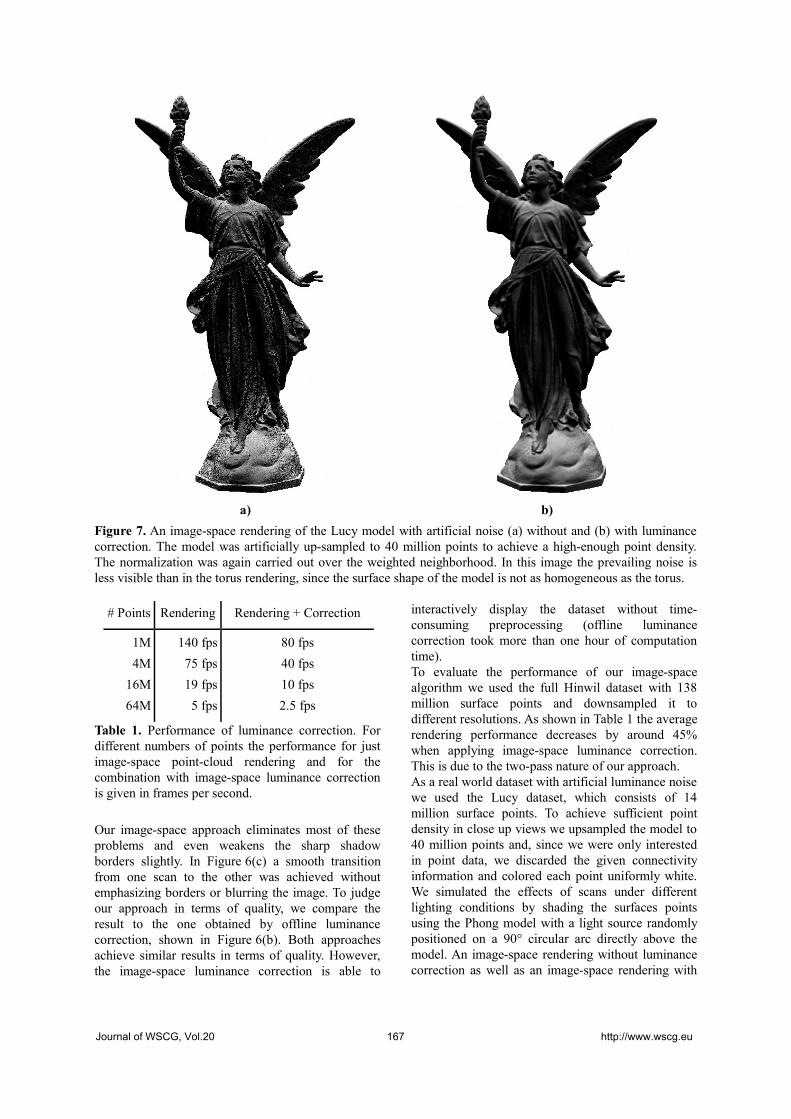
# Points Rendering Rendering + Correction

1M

4M

16M

64M

140 fps

75 fps

19 fps

5 fps

80 fps

40 fps

10 fps

2.5 fps

Table 1. Performance of luminance correction. For different numbers of points the performance for just image-space point-cloud rendering and for the combination with image-space luminance correction is given in frames per second.

Our image-space approach eliminates most of these problems and even weakens the sharp shadow borders slightly. In Figure 6(c) a smooth transition from one scan to the other was achieved without emphasizing borders or blurring the image. To judge our approach in terms of quality, we compare the result to the one obtained by offline luminance correction, shown in Figure 6(b). Both approaches achieve similar results in terms of quality. However, the image-space luminance correction is able to

interactively display the dataset without time-consuming preprocessing (offline luminance correction took more than one hour of computation time).To evaluate the performance of our image-space algorithm we used the full Hinwil dataset with 138 million surface points and downsampled it to different resolutions. As shown in Table 1 the average rendering performance decreases by around 45% when applying image-space luminance correction. This is due to the two-pass nature of our approach.As a real world dataset with artificial luminance noise we used the Lucy dataset, which consists of 14 million surface points. To achieve sufficient point density in close up views we upsampled the model to 40 million points and, since we were only interested in point data, we discarded the given connectivity information and colored each point uniformly white. We simulated the effects of scans under different lighting conditions by shading the surfaces points using the Phong model with a light source randomly positioned on a 90° circular arc directly above the model. An image-space rendering without luminance correction as well as an image-space rendering with

a) b)

Figure 7. An image-space rendering of the Lucy model with artificial noise (a) without and (b) with luminance correction. The model was artificially up-sampled to 40 million points to achieve a high-enough point density. The normalization was again carried out over the weighted neighborhood. In this image the prevailing noise is less visible than in the torus rendering, since the surface shape of the model is not as homogeneous as the torus.


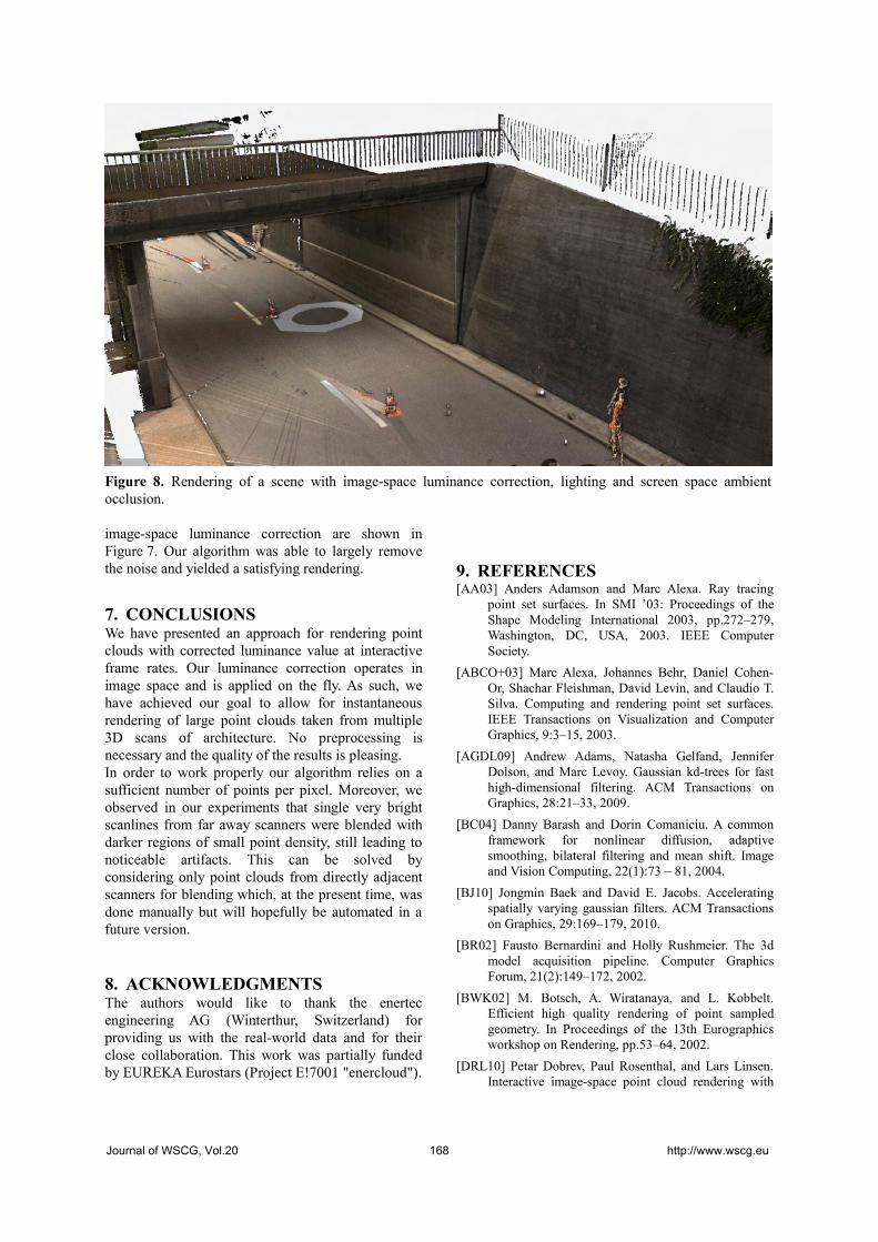
image-space luminance correction are shown in Figure 7. Our algorithm was able to largely remove the noise and yielded a satisfying rendering.

7. CONCLUSIONSWe have presented an approach for rendering point clouds with corrected luminance value at interactive frame rates. Our luminance correction operates in image space and is applied on the fly. As such, we have achieved our goal to allow for instantaneous rendering of large point clouds taken from multiple 3D scans of architecture. No preprocessing is necessary and the quality of the results is pleasing.In order to work properly our algorithm relies on a sufficient number of points per pixel. Moreover, we observed in our experiments that single very bright scanlines from far away scanners were blended with darker regions of small point density, still leading to noticeable artifacts. This can be solved by considering only point clouds from directly adjacent scanners for blending which, at the present time, was done manually but will hopefully be automated in a future version.

8. ACKNOWLEDGMENTSThe authors would like to thank the enertec engineering AG (Winterthur, Switzerland) for providing us with the real-world data and for their close collaboration. This work was partially funded by EUREKA Eurostars (Project E!7001 "enercloud").

9. REFERENCES[AA03] Anders Adamson and Marc Alexa. Ray tracing

point set surfaces. In SMI ’03: Proceedings of the Shape Modeling International 2003, pp.272–279, Washington, DC, USA, 2003. IEEE Computer Society.

[ABCO+03] Marc Alexa, Johannes Behr, Daniel Cohen-Or, Shachar Fleishman, David Levin, and Claudio T. Silva. Computing and rendering point set surfaces. IEEE Transactions on Visualization and Computer Graphics, 9:3–15, 2003.

[AGDL09] Andrew Adams, Natasha Gelfand, Jennifer Dolson, and Marc Levoy. Gaussian kd-trees for fast high-dimensional filtering. ACM Transactions on Graphics, 28:21–33, 2009.

[BC04] Danny Barash and Dorin Comaniciu. A common framework for nonlinear diffusion, adaptive smoothing, bilateral filtering and mean shift. Image and Vision Computing, 22(1):73 – 81, 2004.

[BJ10] Jongmin Baek and David E. Jacobs. Accelerating spatially varying gaussian filters. ACM Transactions on Graphics, 29:169–179, 2010.

[BR02] Fausto Bernardini and Holly Rushmeier. The 3d model acquisition pipeline. Computer Graphics Forum, 21(2):149–172, 2002.

[BWK02] M. Botsch, A. Wiratanaya, and L. Kobbelt. Efficient high quality rendering of point sampled geometry. In Proceedings of the 13th Eurographics workshop on Rendering, pp.53–64, 2002.

[DRL10] Petar Dobrev, Paul Rosenthal, and Lars Linsen. Interactive image-space point cloud rendering with

Figure 8. Rendering of a scene with image-space luminance correction, lighting and screen space ambient occlusion.


transparency and shadows. In Vaclav Skala, editor, Communication Papers Proceedings of WSCG, The 18th International Conference on Computer Graphics, Visualization and Computer Vision, pp.101–108, Plzen, Czech Republic, 2010. UNION Agency – Science Press.

[GG07] Gaël Guennebaud and Markus Gross. Algebraic point set surfaces. ACM Transactions on Graphics, 26, 2007.

[GZPG10] P. Goswami, Y. Zhang, R. Pajarola, and E. Gobbetti. High quality interactive rendering of massive point models using multi-way kd-Trees. In Pacific Graphics Poster Papers, 2010.

[KK05] Hiroaki Kawata and Takashi Kanai. Direct point rendering on gpu. In George Bebis, Richard Boyle, Darko Koracin, and Bahram Parvin, editors, Advances in Visual Computing, volume 3804 of Lecture Notes in Computer Science, pp.587–594. Springer Berlin / Heidelberg, 2005.

[KS10] Michael Kass and Justin Solomon. Smoothed local histogram filters. ACM Transactions on Graphics, 29:100–110, 2010.

[LMR07] Lars Linsen, Karsten Müller, and Paul Rosenthal. Splat-based ray tracing of point clouds. Journal of WSCG, 15:51–58, 2007.

[LPC+00] Marc Levoy, Kari Pulli, Brian Curless, Szymon Rusinkiewicz, David Koller, Lucas Pereira, Matt Ginzton, Sean Anderson, James Davis, Jeremy Ginsberg, Jonathan Shade, and Duane Fulk. The digital michelangelo project: 3d scanning of large statues. In Proceedings of the 27th annual conference on Computer graphics and interactive techniques, SIGGRAPH ’00, pp.131–144, New York, NY, USA, 2000. ACM Press/Addison-Wesley Publishing Co.

[MKC07] Ricardo Marroquim, Martin Kraus, and Paulo Roma Cavalcanti. Efficient point-based rendering using image reconstruction. In Proceedings of the Symposium on Point-Based Graphics, pp.101–108, 2007.

[PZvBG00] Hanspeter Pfister, Matthias Zwicker, Jeroen van Baar, and Markus Gross. Surfels: surface elements as rendering primitives. In SIGGRAPH ’00: Proceedings of the 27th annual conference on Computer graphics and interactive techniques, pp.335–342, New York, NY, USA, 2000. ACM Press/Addison-Wesley Publishing Co.

[RD10] R. Richter and J. Döllner. Out-of-core real-time visualization of massive 3D point clouds. In Proceedings of the 7th International Conference on Computer Graphics, Virtual Reality, Visualisation and Interaction in Africa, pp.121–128, 2010.

[RL00] S. Rusinkiewicz and M. Levoy. QSplat: a multiresolution point rendering system for large meshes. In Proceedings of the 27th annual conference on Computer graphics and interactive techniques, pp.343–352, 2000.

[RL08] Paul Rosenthal and Lars Linsen. Image-space point cloud rendering. In Proceedings of Computer Graphics International, pp.136–143, 2008.

[SMK07] R. Schnabel, S. Moeser, and R. Klein. A parallelly decodeable compression scheme for efficient point-cloud rendering. In Proceedings of Symposium on Point-Based Graphics, pp.214–226, 2007.

[SSS06] Noah Snavely, Steven M. Seitz, and Richard Szeliski. Photo tourism: exploring photo collections in 3D. ACM Transactions on Graphics, 25:835–846, 2006.

[TS08] Thorsten Thormählen and Hans-Peter Seidel. 3D-modeling by ortho-image generation from image sequences. ACM Transactions on Graphics, 27:86:1–86:5, 2008.

[WBB+08] Michael Wand, Alexander Berner, Martin Bokeloh, Philipp Jenke, Arno Fleck, Mark Hoffmann, Benjamin Maier, Dirk Staneker, Andreas Schilling, and Hans-Peter Seidel. Processing and interactive editing of huge point clouds from 3D scanners. Computers & Graphics, 32(2):204–220, 2008.

[WWPS10] Z. Wang, L. Wang, Y. Peng, and I. . Shen. Edge-preserving based adaptive icc method for image diffusion. In Proceedings of the 3rd International Congress on Image and Signal Processing, CISP 2010, volume 4, pp.1638–1641, 2010.


Subpixel Reconstruction Antialiasing for Ray Tracing

Chiu, Y.-FNational Tsing HuaUniversity, Taiwan

[email protected]

Chen, Y.-CNational Tsing HuaUniversity, Taiwan

[email protected]

Chang, C.-FNational Taiwan

Normal University,Taiwan

[email protected]

Lee, R.-RNational Tsing HuaUniversity, Taiwan

[email protected]

ABSTRACTWe introduce a practical antialiasing approach for interactive ray tracing and path tracing. Our method is inspiredby the Subpixel Reconstruction Antialiasing (SRAA) method which separates the shading from visibility and ge-ometry sampling to produce antialiased images at reduced cost. While SRAA is designed for GPU-based deferredshading renderer, we extend the concept to ray-tracing based applications. We take a hybrid rendering approachin which we add a GPU rasterization step to produce the depth and normal buffers with subpixel resolution. Byutilizing those extra buffers, we are able to produce antialiased ray traced images without incurring performancepenalty of tracing additional primary rays. Furthermore, we go beyond the primary rays and achieve antialiasingfor shadow rays and reflective rays as well.

Keywords: antialiasing, ray tracing, path tracing.

1 INTRODUCTION

With the abundance of computation power and paral-lelism in multicore microprocessors (CPU) and graph-ics processors (GPU), achieving interactive photoreal-istic rendering on personal computers is no longer afantasy. Recently, we have seen the demonstration ofreal-time ray tracing [6, 17] and the emergence of real-time path tracing with sophisticated global illumination[2, 20]. Though real-time path tracing can producerendering of photorealistic quality that include com-plex lighting effects such as indirect lighting and softshadow, the illusion of a photograph-like image breaksdown quickly when jaggy edges are visible (Figure 1shows an example).

Jaggy edges are one of the typical aliasing artifactsin computer generated images. A straightforward an-tialiasing technique is to increase the sampling rate bytaking multiple samples uniformly at various subpixelpositions. However this approach induces significantperformance penalty that makes it an afterthought inreal-time ray tracing. A more practical approach isto increase subpixel samples adaptively for image pix-els where discontinuity is detected. Although adaptivesampling approach avoids the huge performance hit ofthe multisampling approach, it still requires additional


subpixel samples and introduces large variation to theestimation of rendering time.In this work, we introduce an antialiasing approach thatworks well for real-time ray tracing and path tracing.We take a hybrid rendering approach in which we add aGPU rasterization step to produce the depth and normalbuffers with subpixel resolution. By utilizing those ex-tra buffers, we are able to produce antialiased ray tracedimages without incurring performance penalty of trac-ing additional primary rays. Our method is inspired bythe Subpixel Reconstruction Antialiasing (SRAA) [3]which combines per-pixel shading with subpixel vis-ibility to produce antialiased images. While SRAAis designed for GPU-based deferred shading renderer,we extend the concept to ray-tracing based applica-tions. Furthermore, we apply our antialiasing approachto shadow and reflection which SRAA cannot resolvewith its subpixel buffers.Our main contributions in this work are:

• We propose an efficient antialiasing technique whichimproves the perception of photorealism in interac-tive or real-time ray tracing without sacrificing itsperformance.

• Unlike adaptive sampling or subpixel sampling, ourapproach does not penalize the performance of aCPU ray tracer because no additional primary rayneeds to be traced. Our hybrid rendering approachobtains the necessary subpixel geometric informa-tion by leveraging the GPU rasterization pipeline.

• While SRAA works well for improving the sam-pling on image plane, we extend its application be-yond the primary rays and achieve antialiasing forshadow rays and reflective rays as well.


Figure 1: Antialiasing can improve the rendering quality in interactive ray tracing. The left image is rendered with-out applying any antialiasing method. The right image is rendered with our method using relatively inexpensivegeometric information to improve expensive shading results.

2 RELATED WORK2.1 Real-time Ray TracingWith the rapid improvement of computation power andparallelism in multicore microprocessors (CPU) andgraphics processors (GPU), various works have beenpublished on speeding up the ray tracing, either onCPUs [1, 19], GPUs [5], or special-purpose platforms[21]. Recently, we have seen the demonstration of real-time ray tracing with Whitted-style reflection and re-fraction (a.k.a. specular rays) [6, 17] and the emergenceof real-time path tracing with sophisticated global illu-mination [2, 20]. The NVIDIA OptiX acceleration en-gine [12] elevates rendering applications to a new levelof interactive realism by greatly increasing ray tracingspeeds with GPU solutions. While real-time ray tracingis now feasible, most renderers still rely on Monte Carlopath tracing to obtain more sophisticated global illumi-nation effects such as soft shadow and indirect light-ing. Noisy preview images are usually produced firstat interactive rates and then gradually converge to highquality images. Therefore, antialiasing often becomesan afterthought as it further slows down the rendering.

2.2 Adaptive SamplingThe ray tracing algorithm is basically a loop over allscreen pixels to find the nearest visible object in thescene. We can consider ray tracing as a point samplingbased rendering method in signal processing view.However, point sampling makes an all-or-nothingchoice in each pixel and thus leads to jaggies. An-tialiasing of ray-traced images could be achieved bysupersampling the image. However the supersam-pling approach demands significantly larger amountof computation resource. Therefore antialiasing bysupersampling is rarely adopted by software renderers.Adaptive sampling [10, 11] reduces the overheadby casting additional rays only if significant colorvariation across image samples is detected. Variations

of the adaptive sampling techniques have also beenproposed in [8].

2.3 Post Filter AntialiasingA small disadvantage of adaptive sampling is that someimage pixels still need additional subpixel samples to befully shaded or traced. It would be desirable if expen-sive shading could be avoided at additional subpixel lo-cations. Reshetov [16] proposes an image filtering ap-proach, Morphological antialiasing (MLAA) to recoveredges from input image with per-pixel color informa-tion. However, this sort of color-only information couldfail to identify some geometry edges, especially thoseedges without high contrast. Geometric Post-processAnti-Aliasing (GPAA) [13] and Geometry Buffer Anti-Aliasing (GBAA) [14] extend the MLAA ideas and useextra edge information explicitly to eliminate the jaggyedges. Normal Filter Anti-Aliasing (NFAA) [18] re-duces aliasing by searching for contrasting luminositychanges in the final rendering image. It builds a nor-mal displacement map to apply a per-pixel blur filter inhighly contrast aliased areas. However, it softens theimage due to the filtering of textures. More filter-basedapproaches are discussed in [7].

2.4 Shading Reconstruction FilterDecoupled sampling [9, 15] presents an approach togenerate shading and visibility samples at differentrates in GPU pipelines to speed up the rendering inapplications with stochastic supersampling, depth offield, and motion blur. Yang et al. [22] present ageometry-aware framebuffer level of detail (LOD) ap-proach for controlling the pixel workload by renderinga subsampled image and using edge-preserving upsam-pling to the final resolution. Subpixel ReconstructionAntialiasing (SRAA) [3] takes a similar decoupledsampling approach and applies a cross-bilateral filter(as in the geometry-aware framebuffer LOD method) to


upscale shading information using subpixel geometricinformation that is obtained from the GPU rasterizationpipeline. It is based on the assumption that the subpixelgeometric information could be obtained much moreeasily without fully going through the expensive shad-ing stage. SRAA can produce good edge antialiasingbut it cannot resolve shading edges in texture, shadow,reflection and refraction. Our work follows the sameassumption by avoiding emitting subpixel samples forthe primary rays. This maintains the advantage overadaptive sampling because no subpixel ray needs to betraced.

3 ANTIALIASINGSRAA [3] relies on the fact that shading often changesmore slowly than geometry in screen space and gen-erates shading and visibility at different rates. SRAAperforms high-quality antialiasing in a deferred render-ing framework by sampling geometry at higher reso-lution than the shaded pixels. It makes three modifi-cations to a standard rendering pipeline. First, it mustproduce normal and depth information at subpixel res-olution. Second, it needs to reconstruct the shading val-ues of sampled geometric subpixel from neighboringshaded samples with bilateral filter using the subpixelgeometric (normal and depth) information. Finally, thesubpixel shading values are filtered into an antialiasedscreen-resolution image.

SRAA detects the geometric edges with geometric in-formation to resolve aliasing problem. However, theedges of shadow and reflection/refraction could not bedetected by the subpixel geometric information gener-ated from the eye position. For example, the shadowedges mostly fall on other continuous surfaces that haveslowly changing subpixel depths and normals. To ex-tend the SRAA concept to ray-tracing based applica-tions, we perform antialiasing separately for primaryrays, shadow rays and secondary rays to resolve thisissue. The following subsections offer the detail.

3.1 Primary RayLike SRAA, our goal is to avoid the performancepenalty of shading subpixel samples. In Figure 2,geometric information and shading are generated atdifferent rates. Each pixel has 4 geometric sampleson a 4× 4 grid and one of those geometric samplesis also a shaded sample. The shading value at eachgeometric sample is reconstructed by interpolating allshaded neighbors in a fixed radius using the bilateralweights. We take both depth and normal change intoaccount when compute the bilateral weight. A neigh-boring sample with significantly different geometry isprobably across a geometric edge and hence receives alow weight.

wi j = G(σz(z j− zi))G(σn(1− sat(n j ·ni))) (1)

In Equation 1, G(x) is the Gaussian function of the formexp(−x2). zi and ni are the depth and normal of the ith

subpixel sample. σz and σn are the scaling factors forcontrolling how quickly the weights fall off and allow-ing us to increase the importance of the bilateral filter.We set σz to 10 and σn to 0.25 in all our testing. Thesat(x) function is implemented as max(0,min(1,x)).The result wi j is the weight associated with the jth sub-pixel sample while performing shading reconstructionfor the ith subpixel sample.

For tracing the primary rays that are emitted from theeye position, we use a hybrid rendering approach thatutilizes the GPU to generate the subpixel geometric in-formation including position, normal and depth. Wecreate 3 auxiliary geometric buffers to store position,normal and depth by GPU rasterization with the sameresolution as the shaded buffer. Each geometric bufferis rendered with a subpixel offset applied to the pro-jection matrix. The subpixel offset is applied not onlyto form a 4× rotated-grid but also to do pixel align-ment between rasterization and ray tracing rendering.Since the GPU rasterization pipeline produces the sub-pixel geometric information very efficiently, this over-head is insignificant when compared to the ray tracingstage.

3.2 Shadow RayAs mentioned above in Section 3, the shadow edgescannot be detected by the geometric information thatis generated from the eye position alone. What we needis subpixel information that is more meaningful to theshadow edges. The naive solution for shadow antialias-ing is through a shadow map drawn at a higher reso-lution. However, this approach is inefficient becausethe increased resolution of the shadow map (from thelight’s view) does not contribute directly to the subpix-els at the screen space. Therefore, we generate subpixelshadow information by ray casting and combine thisshadow value with the bilateral filter weighting equa-tion as shown in Equation 2. The subpixel shadow raysare generated by utilizing the position information inthe geometric buffer as mentioned in Section 3.1.

Figure 2 shows our algorithm reconstructs the colorvalue of a geometric sample in a non-shadowed areanot only by taking the Euclidean distance and the nor-mal change between the source and the target samplesbut also under the influence of shadow boundaries to ex-clude the neighboring samples in shadowed area. Thisis the reason why the original SRAA adds excessiveblur to the shadow boundaries, yet our method achievesa better quality that is comparable to 16× supersam-pling.


wi j =

G(σz(z j− zi))G(σn(1− sat(n j ·ni))), if si = s j

0, if si 6= s j

(2)

In Equation 2, si is the shadow value of the ith subpixelsample and is equal to 1 if it is in shadowed area. Oth-erwise it is equal to 0. If s j is different from si, then thejth subpixel falls on the other side of a shadow edge.Therefore we set the weight wi j associated with the jth

subpixel to 0 to exclude it from the shading reconstruc-tion for the ith subpixel sample.

3.3 Secondary RayIn the original SRAA framework, it uses geometric in-formation to detect geometric edges in the subpixel re-construction process. However, the edge of secondaryshading (such as those from the reflection) cannot bedetected by this geometric information generated fromthe eye position. Take the reflection rays for an exam-ple as shown in Figure 5 (c), if we perform subpixelshading reconstruction as shown in Equation 1 with thegeometric information generated from the eye position,it will not be able to detect the edges of the reflectedobjects, and in consequence add excessive blur to thereflected colors.

Therefore we must take geometric information that isgenerated from the hit points of primary rays to performsubpixel-level bilateral filer when computing the shad-ing value of the secondary rays that originate from theprimary hit point. The subpixel secondary rays for hitpoints are generated by utilizing the position and nor-mal information in the geometric buffer. Our methodwhich performs subpixel reconstruction separately forprimary and secondary shading achieves better qualitythan the original SRAA approach. Please see our re-sults in Section 4 and Figure 5.

4 RESULTOur algorithm is implemented using NVIDIA CUDA4.0, the raytracer is built with OptiX 2.0 and rasteriza-tion with OpenGL. All results shown in this paper wereobtained using an Intel Xeon E5504 processor and anNVIDIA Geforce GTX 570 GPU.

4.1 QualityFigure 4 shows the quality comparison between ourmethod and other antialiasing techniques in a Cornellbox scene. The original SRAA adds excessive blur tothe shadow, yet our method achieves similar quality to16× supersampling.

Figure 5 highlights some interesting cases for primaryshading, shadow and secondary shading in the Sponzascene. For the shading from primary rays, both our

Figure 2: Here we add shadow edge into considerationto perform subpixel shading reconstruction. Each pixelhas 4 geometric samples on a 4× 4 grid. One of thosegeometric samples is also a shaded sample. Shadingvalue for each geometric sample in non-shadowed areais reconstructed from nearby shaded samples except theshaded samples in shadowed area and weighted by theirdistance and the normal change between the source andthe target sample.

method and SRAA use the geometric information toimprove image quality and the results are almost iden-tical between ours and SRAA. For the shadow, ourmethod uses both the geometry and the shadow edge in-formation to perform subpixel reconstruction, thus pro-duces better shadow line in the highlighted area thanSRAA. For secondary shading, we perform subpixelreconstruction separately for primary and secondaryshading, while SRAA uses only the final color of eachsampled subpixel for this purpose. This results in overblurring for secondary shading in SRAA.

To summarize, we observe that antialiasing with geo-metric information from primary rays could be prob-lematic in some difficult cases and our method offers asolution to the highlighted cases in Figure 5.

Our method does have a limitation in handling mate-rial variation or textured surfaces. Figure 6 shows suchan example where the floor contains patches of differ-ent colors. Since the extra subpixel depth and normalinformation does not help us detect the edges betweenpatches of different colors, jagged edges could still ap-pear on the floor.

4.2 PerformanceThere are two rendering passes in our current imple-mentation. The first pass is the geometric informationgeneration step and the second pass is the antialiasingprocess. Table 1 shows that the geometric informationgeneration step with raytracer solution takes about 70percent of the total processing time for rendering theSponza scene [4] in Figure 5. This overhead to generategeometric information for primary rays can be reducedwith a GPU hybrid solution. Figure 3 shows that ourmethod maintains the interactive rate while renderingthe Sponza scene in Figure 5 with a GPU hybrid solu-


Rendering PassResolution 1st 2nd Total256x256 18 5 23512x512 35 14 49768x768 69 28 97

1024x1024 116 49 165unit: millisecond

Table 1: Time measurement of our method for render-ing the Sponza scene in Figure 5.The first pass is ge-ometric information generation and the second pass isantialiasing process. Note that the time shown in firstpass is measured with raytracer solution.

Figure 3: Performance comparison between NoAA (noantialiasing applied ), our method with GPU hybrid ap-proach, and SSAA (16× supersampling antialiasing)for rendering the Sponza scene under various outputresolutions. The vertical axis is the rendering timein millisecond. The overall rendering performance ofour method with a GPU hybrid approach is about 6×speedup in average compared to the 16× supersamplingapproach.

tion and achieves about 6× speedup in average com-pared to the 16× supersampling approach.

5 CONCLUSION

We introduce the concept in SRAA to path-tracingbased rendering methods for antialiasing. Our methodextends the subpixel geometric sampling conceptbeyond the primary rays and achieves antialiasing forshadow rays and reflective rays as well. By adoptinga hybrid approach, our method improves the imagequality without incurring performance penalty oftracing additional primary rays. We hope our methodencourages the adoption of antialiasing even for thecomputationally constrained real-time ray tracing orpath tracing.

6 ACKNOWLEDGEMENTSThis work is supported in part under the “Embeddedsoftware and living service platform and technology de-velopment project” of the Institute for Information In-dustry which is subsidized by the Ministry of Econ-omy Affairs (Taiwan), and by National Science Council(Taiwan) under grant NSC 100-2219-E-003-002.

7 REFERENCES[1] Carsten Benthin. Realtime Ray Tracing on Cur-

rent CPU Architectures. PhD thesis, SaarlandUniversity, 2006.

[2] Jacco Bikker. Arauna real-time ray tracer andBrigade real-time path tracer.

[3] Matthäus G. Chajdas, Morgan McGuire, andDavid Luebke. Subpixel reconstruction antialias-ing for deferred shading. In Symposium on Inter-active 3D Graphics and Games, I3D ’11, pages15–22, 2011.

[4] Marko Dabrovic. Sponza atrium,http://hdri.cgtechniques.com/ sponza/files/, 2002.

[5] Johannes Gunther, Stefan Popov, Hans-Peter Sei-del, and Philipp Slusallek. Realtime ray tracing ongpu with bvh-based packet traversal. In Proceed-ings of the 2007 IEEE Symposium on InteractiveRay Tracing, pages 113–118, 2007.

[6] Daniel Reiter Horn, Jeremy Sugerman, MikeHouston, and Pat Hanrahan. Interactive k-d treegpu raytracing. In Proceedings of the 2007 sym-posium on Interactive 3D graphics and games,I3D ’07, pages 167–174, 2007.

[7] Jorge Jimenez, Diego Gutierrez, Jason Yang,Alexander Reshetov, Pete Demoreuille, TobiasBerghoff, Cedric Perthuis, Henry Yu, MorganMcGuire, Timothy Lottes, Hugh Malan, EmilPersson, Dmitry Andreev, and Tiago Sousa. Fil-tering approaches for real-time anti-aliasing. InACM SIGGRAPH Courses, 2011.

[8] Bongjun Jin, Insung Ihm, Byungjoon Chang,Chanmin Park, Wonjong Lee, and Seokyoon Jung.Selective and adaptive supersampling for real-time ray tracing. In Proceedings of the Confer-ence on High Performance Graphics 2009, HPG’09, pages 117–125, 2009.

[9] Gábor Liktor and Carsten Dachsbacher. Decou-pled deferred shading for hardware rasterization.In Proceedings of the ACM SIGGRAPH Sympo-sium on Interactive 3D Graphics and Games, I3D’12, pages 143–150, New York, NY, USA, 2012.ACM.

[10] Don P. Mitchell. Generating antialiased imagesat low sampling densities. In Proceedings ofthe 14th annual conference on Computer graph-


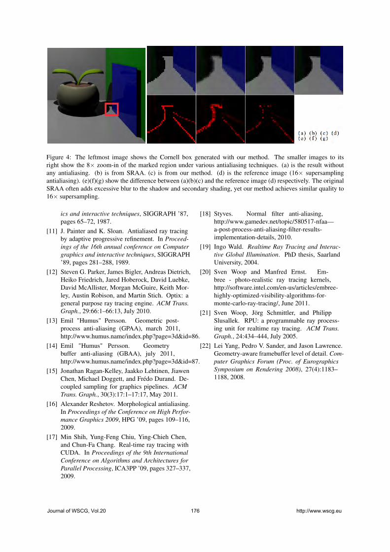
Figure 4: The leftmost image shows the Cornell box generated with our method. The smaller images to itsright show the 8× zoom-in of the marked region under various antialiasing techniques. (a) is the result withoutany antialiasing. (b) is from SRAA. (c) is from our method. (d) is the reference image (16× supersamplingantialiasing). (e)(f)(g) show the difference between (a)(b)(c) and the reference image (d) respectively. The originalSRAA often adds excessive blur to the shadow and secondary shading, yet our method achieves similar quality to16× supersampling.

ics and interactive techniques, SIGGRAPH ’87,pages 65–72, 1987.

[11] J. Painter and K. Sloan. Antialiased ray tracingby adaptive progressive refinement. In Proceed-ings of the 16th annual conference on Computergraphics and interactive techniques, SIGGRAPH’89, pages 281–288, 1989.

[12] Steven G. Parker, James Bigler, Andreas Dietrich,Heiko Friedrich, Jared Hoberock, David Luebke,David McAllister, Morgan McGuire, Keith Mor-ley, Austin Robison, and Martin Stich. Optix: ageneral purpose ray tracing engine. ACM Trans.Graph., 29:66:1–66:13, July 2010.

[13] Emil "Humus" Persson. Geometric post-process anti-aliasing (GPAA), march 2011,http://www.humus.name/index.php?page=3d&id=86.

[14] Emil "Humus" Persson. Geometrybuffer anti-aliasing (GBAA), july 2011,http://www.humus.name/index.php?page=3d&id=87.

[15] Jonathan Ragan-Kelley, Jaakko Lehtinen, JiawenChen, Michael Doggett, and Frédo Durand. De-coupled sampling for graphics pipelines. ACMTrans. Graph., 30(3):17:1–17:17, May 2011.

[16] Alexander Reshetov. Morphological antialiasing.In Proceedings of the Conference on High Perfor-mance Graphics 2009, HPG ’09, pages 109–116,2009.

[17] Min Shih, Yung-Feng Chiu, Ying-Chieh Chen,and Chun-Fa Chang. Real-time ray tracing withCUDA. In Proceedings of the 9th InternationalConference on Algorithms and Architectures forParallel Processing, ICA3PP ’09, pages 327–337,2009.

[18] Styves. Normal filter anti-aliasing,http://www.gamedev.net/topic/580517-nfaa—a-post-process-anti-aliasing-filter-results-implementation-details, 2010.

[19] Ingo Wald. Realtime Ray Tracing and Interac-tive Global Illumination. PhD thesis, SaarlandUniversity, 2004.

[20] Sven Woop and Manfred Ernst. Em-bree - photo-realistic ray tracing kernels,http://software.intel.com/en-us/articles/embree-highly-optimized-visibility-algorithms-for-monte-carlo-ray-tracing/, June 2011.

[21] Sven Woop, Jörg Schmittler, and PhilippSlusallek. RPU: a programmable ray process-ing unit for realtime ray tracing. ACM Trans.Graph., 24:434–444, July 2005.

[22] Lei Yang, Pedro V. Sander, and Jason Lawrence.Geometry-aware framebuffer level of detail. Com-puter Graphics Forum (Proc. of EurographicsSymposium on Rendering 2008), 27(4):1183–1188, 2008.


Inpu

t

No

AA

Out

put SR

AA

Our

s

Ref

eren

ce

16sa

mpl

es

(a) Primary Shading (b) Shadow (c) Reflection (d) Reflected Shadow

Figure 5: Quality comparison between our method and the other antialiasing techniques in highlighted areas ofprimary shading, shadow, reflection, and reflected shadow. (Row 1) No antialiasing, (Row 2) SRAA: one subpixelwith shading value and 4 subpixels with primary geometric information, (Row 3) Ours: one subpixel with shadingvalue and 4 subpixels with geometric information for primary, shadow and secondary rays, (Row 4) Referenceimage: 16× supersampling.


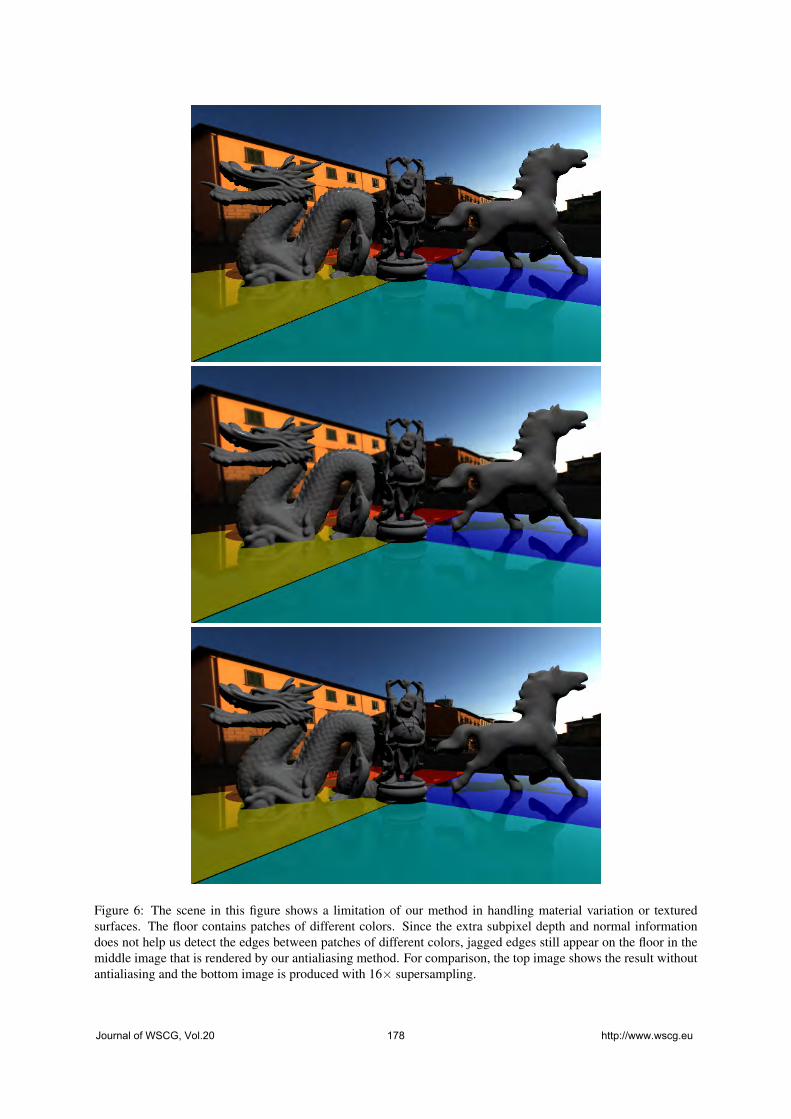
Figure 6: The scene in this figure shows a limitation of our method in handling material variation or texturedsurfaces. The floor contains patches of different colors. Since the extra subpixel depth and normal informationdoes not help us detect the edges between patches of different colors, jagged edges still appear on the floor in themiddle image that is rendered by our antialiasing method. For comparison, the top image shows the result withoutantialiasing and the bottom image is produced with 16× supersampling.


Elastically Deformable Models based on the Finite Element

Method Accelerated on Graphics Hardware using CUDA

Mickeal VerschoorEindhoven University of Technology,

The Netherlands

[email protected]

Andrei C. JalbaEindhoven University of

Technology, The Netherlands

[email protected]

Abstract

Elastically deformable models have found applications in various areas ranging from mechanical sciences and engineering tocomputer graphics. The method of Finite Elements has been the tool of choice for solving the underlying PDE, when accuracyand stability of the computations are more important than, e.g., computation time. In this paper we show that the computationsinvolved can be performed very efficiently on modern programmable GPUs, regarded as massively parallel co-processorsthrough Nvidia’s CUDA compute paradigm. The resulting global linear system is solved using a highly optimized ConjugateGradient method. Since the structure of the global sparse matrix does not change during the simulation, its values are updatedat each step using the efficient update method proposed in this paper. This allows our fully-fledged FEM-based simulator forelastically deformable models to run at interactive rates. Due to the efficient sparse-matrix update and Conjugate Gradientmethod, we show that its performance is on par with other state-of-the-art methods, based on e.g. multigrid methods.

Keywords: Elastically deformable models, Finite Elements, sparse-matrix update, GPU.

1 INTRODUCTION

Mathematical and physical modeling of elastically de-formable models has been investigated for many years,especially within the fields of material and mechanicalsciences, and engineering. In recent years, physically-based modeling has also emerged as an important ap-proach to computer animation and graphics modeling.As nowadays graphics applications demand a growingdegree of realism, this poses a number of challenges forthe underlying real-time modeling and simulation al-gorithms. Whereas in engineering applications model-ing of deformable objects should be as accurate as pos-sible compared to their physical counterparts, in graph-ics applications computational efficiency and stabilityof the simulation have most often the highest priority.

The Finite Element Method (FEM) constitutesone of the most popular approaches in engineeringapplications which need to solve Partial DifferentialEquations (PDEs) at high accuracies on irregulargrids [PH05]. Accordingly, the (elastically) deform-able object is viewed as a continuous connectedvolume, and the laws of continuum mechanics providethe governing PDE, which is solved using FEM.Other popular methods are the Finite DifferenceMethod (FDM) [TPBF87], the Finite Volume Method

Permission to make digital or hard copies of all or part of thiswork for personal or classroom use is granted without fee providedthat copies are not made or distributed for profit or commercialadvantage and that copies bear this notice and the full citation on thefirst page. To copy otherwise, or republish, to post on servers or toredistribute to lists, requires prior specific permission and/or a fee.

(FVM) [TBHF03] and the Boundary Element Method(BEM) [JP99] (see [NMK∗06, GM97]). FDM is theeasiest to implement, but as it needs regular spatialgrids, it is difficult to approximate the boundary of anarbitrary object by a regular mesh. FVM [TBHF03]relies on a geometrical framework, making it more in-tuitive than FEM. However, it uses heuristics to definethe strain tensor and to calculate the force emergingat each node. BEM performs the computations onthe surface of the model, thus achieving substantialspeedups as the size of the problem is proportionalto the area of the model’s boundary as opposed to itsvolume. However, this approach only works for objectswhose interior is made of homogeneous material.Furthermore, topological changes are more difficult tohandle than in FEM methods [NMK∗06].

In this paper we present a fully-fledged FEM-basedsimulator for elastically-deformable models, runningsolely on GPU hardware. We show that the involvedcomputations can be performed efficiently on mod-ern programmable GPUs, regarded as massively par-allel co-processors through Nvidia’s CUDA computeparadigm. Our approach relies on the fast GPU Conjug-ate Gradient (CG) method of [VJ12] to solve the result-ing linear system. Since the topology of the deformedmesh does not change during the simulation, the struc-ture of the sparse-matrix describing the linear system isreused throughout the simulation. However, during thesimulation, the matrix values have to be updated effi-ciently. To achieve this, we propose a method that up-dates the sparse-matrix entries respecting the orderingof the data, as required by the CG method of [VJ12],see Sect. 5.4. Thanks to the optimized CG method andthe efficient sparse-matrix update procedure, we ob-


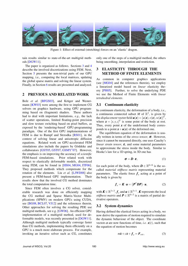
Figure 1: Effect of external (stretching) forces on an ’elastic’ dragon.

tain results similar to state-of-the-art multigrid meth-ods [DGW11].

The paper is organized as follows. Sections 3 and 4describe the involved discretizations using FEM. Next,Section 5 presents the non-trivial parts of our GPUmapping, i.e., computing the local matrices, updatingthe global sparse matrix and solving the linear system.Finally, in Section 6 results are presented and analyzed.

2 PREVIOUS AND RELATED WORK

Bolz et al. [BFGS03], and Krüger and Wester-mann [KW03] were among the first to implement CGsolvers on graphics hardware, using GPU program-ming based on (fragment) shaders. These authorshad to deal with important limitations, e.g., the lackof scatter operations, limited floating-point precisionand slow texture switching based on pixel buffers, asexposed by the ‘rendering-based’ GPU-programmingparadigm. One of the first GPU implementations ofFEM is due to Rumpf and Strzodka [RS01], in thecontext of solving linear and anisotropic diffusionequations. Related work on GPU-accelerated FEMsimulations also include the papers by Göddeke andcollaborators [GST05, GST07, GSMY∗07]. However,the emphasis is on improving the accuracy of scientific

FEM-based simulations. Prior related work withrespect to elastically deformable models, discretizedusing FEM, can be found in [HS04, MG04, ITF06].They proposed methods which compensate for therotation of the elements. Liu et al. [LJWD08] alsopresent a FEM-based GPU implementation. Theirresults show that the involved CG method dominatesthe total computation time.

Since FEM often involves a CG solver, consid-erable research was done on efficiently mappingthe CG method and Sparse Matrix-Vector Multi-plications (SPMV) on modern GPUs using CUDA,see [BG08, BCL07, VJ12] and the references therein.Other approaches for solving the resulting PDE usemultigrid methods, see e.g. [GW06]. An efficient GPUimplementation of a multigrid method, used for de-formable models, was recently presented in [DGW11].Although multigrid methods typically converge fasterthan CG methods, implementing them efficiently on aGPU is a much more elaborate process. For example,invoking an iterative solver such as CG, constitutes

only one of the steps of a multigrid method, the othersbeing smoothing, interpolation and restriction.

3 ELASTICITY THROUGH THE

METHOD OF FINITE ELEMENTS

As common in computer graphics applications(see [MG04] and the references therein), we employa linearized model based on linear elasticity the-ory [PH05]. Further, to solve the underlying PDEwe use the Method of Finite Elements with linear

tetrahedral elements.

3.1 Continuum elasticity

In continuum elasticity, the deformation of a body, i.e.,a continuous connected subset M of R

3, is given bythe displacement vector field uuu(xxx)= [u(xxx),v(xxx),w(xxx)]T ,where xxx = [x,y,z]T is some point of the body at rest.Thus, every point xxx of the undeformed body corres-ponds to a point xxx+uuu(xxx) of the deformed one.

The equilibrium equation of the deformation is usu-ally written in terms of the stress tensor, σσσ . However,since it cannot be measured directly, one uses Cauchy’slinear strain tensor, εεε , and some material parametersto approximate the stress inside the body. Similar toHooke’s law for a 1D spring, in 3D one has

σσσ = DDD · εεε , (1)

for each point of the body, where DDD ∈ R6×6 is the so-

called material stiffness matrix representing materialparameters. The elastic force fff e acting at a point ofthe body is given by

fff e = KKK ·uuu =(

PPPT DDDPPP)

·uuu, (2)

with KKK ∈R3×3, fff e and uuu∈R

3×1. KKK represents the localstiffness matrix and PPP ∈ R

6×3 is a matrix of partial de-rivative operators.

3.2 System dynamics

Having defined the elastical forces acting in a body, wenow derive the equations of motion required to simulatethe dynamic behaviour of the object. The coordinatevectors xxx are now functions of time, i.e. xxx(t), such thatthe equation of motion becomes

mxxx+ cxxx+ fff e = FFFext , (3)


where m is the mass of a body particle at position xxx,c the damping coefficient, fff e the elastic force and FFFext

the vector of external forces, i.e., the gravitational force.We approximate Eq. (3) using a semi-implicit method,i.e.,

m

(

vvvi+1 − vvvi)

∆t+ cvvvi+1 +KKK ·uuui+i = FFF i

ext . (4)

xxxi+1 = xxxi +∆t vvvi+1, (5)

with uuui+1 = ∆tvvvi+1 + xxxi − xxx0, which can be rearrangedas

(

m+∆tc+∆t2KKK)

· vvvi+1 =

mvvvi −∆t(

KKK · xxxi −KKK · xxx0 −FFF iext

)

. (6)

3.3 Discretization using FEM

Within FEM, the continuous displacement field uuu isreplaced by a discrete set of displacement vectors uuu

defined only at the nodes of the elements. Within eachelement e the displacement field is approximated by

uuu = ΦΦΦe · uuu, (7)

where ΦΦΦe ∈ R3×12 is the matrix containing the element

shape functions and uuu = [u1,v1,w1, . . . ,u4,v4,w4]T is

the vector of the nodal displacement approximations.Next, Galerkin’s method of weighted residuals is ap-plied over the whole volume V , in which the weighting

functions are equal to the shape functions. Each termin Eq. (6) is weighted and approximated as in Eq. (7),which results in

∫

VΦΦΦT

(

m+∆tc+∆t2KKK)

ΦΦΦ · vvvi+1dV =∫

VmΦΦΦT ΦΦΦvvvidV−

∆t

∫

VΦΦΦT

(

KKKΦΦΦ · xxxi −KKKΦΦΦ · xxx0 −ΦΦΦ · FFFiext

)

dV, (8)

with ΦΦΦT the weighting functions. The equation aboveis defined for each individual element and generatesone matrix consisting of the local mass (MMMe), damp-ing (CCCe) and element stiffness (KKKe) matrices. Addition-ally, a local force matrix (FFFe) is generated, representingthe net external force applied to the object. These localmatrices are given by

MMMe = ρe

∫

V ΦΦΦTe ΦΦΦe dV

CCCe = c∫

V ΦΦΦTe ΦΦΦe dV

KKKe =∫

V ΦΦΦT PPPT DDDPPPΦΦΦdV

FFFe =∫

V ΦΦΦTe ΦΦΦe · FFFext dV,

(9)

with ρe the density of element e. See [PH05] for moredetails on computing these matrices.

Finally, the global matrix KKK ∈ R3n×3n (with n the

number of mesh vertices) is ‘assembled’ from indi-vidual element matrices. This resulting system is then

solved using the Conjugate Gradient method for theunknown velocity vvvi+1, which is then used to updatethe positions of the nodes, see Eq. (5). Eq. (5) showsa first order method for updating the positions whichcan be replaced by higher order methods as describedin [ITF06].

Unfortunately, the above equations for simulatingelastic deformation only work fine as long as the modeldoes not undergo large rotations. This is because lin-earized elastic forces are used, which are only ’valid’close to the initial configuration. Therefore we usethe so-called Element-based Stiffness Warping or Coro-

tational Strain method [MG04, HS04] to compensatefor the rotation of the elements. To extract the rota-tion part of the deformation, we use the polar decom-position method proposed in [Hig86]. The rotation-free element stiffness matrix KKKre then becomes KKKre =RRReKKKeRRR−1

e , with RRRe ∈R12×12 the rotation matrix for ele-

ment e. Note that this gives rise to an initial elastic forcefff e0 = RRReKKKe · xxx0, which replaces the term KKKΦΦΦ · xxx0 in theright-hand-side of Eq. (8).

4 OVERVIEW OF THE ALGORITHM

Algorithm 1 gives an overview of the simulation ofelastically deformable models as described in Section 3.First, a tetrahedralization of the polygonal mesh rep-resenting the surface of the object is computed, seeSection 5.5. Each tetrahedron is considered as an ele-ment in FEM. Then, the initial stiffness-matrices ofthe elements are computed (line 3); these matrices donot change during the simulation and thus are pre-computed. Additionally, as the shape functions are con-stant during the simulation, we can pre-calculate mostmatrices from Eq. (9), using NNN1 = ΦΦΦT

e ΦΦΦe. This matrixis identical for all elements and is therefore only com-puted once.

Algorithm 1 Simulation algorithm.1: Compute NNN1 see Eq. (9)2: foreach element e

3: Compute KKKe see Eq. (9)4: loop of the simulation

5: foreach element e

6: Compute volume ve

7: Compute RRRe see Section 3.38: Compute KKKre = RRReKKKeRRR−1

e ve

9: Compute MMMe = ρeNNN1ve

10: Compute CCCe = cNNN1ve

11: Compute fff e0 = RRReKKKe · xxx0ve

12: Compute FFFe = NNN1 · FFFext ve see Eq. (9)13: Compute FFF te = MMMe · vvv

i −∆t(

fff e0 −KKKre · xxxi −FFFe

)

14: Compute KKKte = MMMe +∆tCCCe +∆t2KKKre

15: Assemble global KKK and FFF using KKKte and FFF te of elements16: Solve KKK · vvvi+1 = FFF for vvvi+1

17: Update xxxi+1 = xxxi +∆tvvvi+1 see Section 3.2

After all local matrices have been computed andstored (line 14), the global matrix is assembled


(line 15). The resulting linear system of equations issolved for velocities (line 16), which are then used toadvance the position vectors (line 17).

5 GPU MAPPING USING CUDA

In this section we describe our GPU mapping ofthe simulation on NVida GeForce GPUs usingCUDA [NVI]. First we shall give details aboutimplementing the rotation extraction through polardecomposition. Then, we describe the computation ofthe local stiffness matrices which are used to assemblethe global (sparse) stiffness matrix (matrix KKK inAlgorithm 1). The resulting system of linear equationsis solved using a Jacobi-Preconditioned CG Method.

5.1 Rotation extraction

As mentioned in subsection 3.3 we have to estimate therotation of each element in order to calculate displace-ments properly. Finding the rotational part of the de-formation matrix is done using a Polar Decompositionas described in [MG04,HS04,Hig86]. Although a largenumber of matrix inversions is involved, this can bedone efficiently because small 4× 4 matrices are used.Since each matrix contains 16 elements, we chose tomap the computations of 16 such matrices to a singleCUDA thread-block with 256 threads.

For computing the inverse of a 4 × 4 matrix weperform a co-factor expansion. Each thread within athread-block computes one co-factor of the assignedmatrix. Since the computation of a co-factor requiresalmost all values of the matrix, memory accesseshave to be optimized. In order to prevent for possiblebank-conflicts during the computation of the co-factors,each matrix is stored in one memory bank of sharedmemory. Accordingly, the shared-memory segment (ofsize 16×16 locations) is regarded as a matrix stored inrow-major order, where each column represents a 4×4local matrix. Therefore, each column (local matrix)maps exactly to one memory-bank. Since a largenumber of rotation matrices are computed in parallel, alarge performance boost is obtained.

5.2 Local stiffness matrices

Solving a specific problem using FEM starts with de-scribing the problem locally per element. Since a typ-ical problem consists of a large number of elements, thecomputations involved per element can be easily paral-lelized. Further, since the matrices used to constructKKKe are in R

12×12, we map the computation of eachindividual local element stiffness matrix to a thread-block containing 12 × 12 threads. The inner loop inAlgorithm 1 is implemented using one or two CUDAkernels, depending on the architecture version. Insteadof creating kernels for each individual matrix operation,we combine a number of them into one larger kernel.Since data from global memory can be reused multiple

times, less global memory transactions are required,which improves the overall performance.

5.3 Solving the linear system

Given the local element matrices and load vectors,the global stiffness matrix of the system is assembled.Next, the system has to be solved for the unknownvelocity vvvi+i. The (Jacobi-Preconditioned) CG methodperforms a large number of sparse matrix-vectormultiplications and other vector-vector operations.Therefore, solving a large linear system efficiently,requires a fast and efficient implementation of sparsematrix-vector multiplications, which is highly-dependent on the layout used for storing the sparsematrix. Since three unknown values (componentsof the velocity vector) are associated to each meshvertex, a block with 3×3 elements in the global matrixcorresponds to each edge of the tetrahedral mesh.Therefore, a Block-Compressed Sparse Row (BCSR)format is very well suited for storing the global matrix,and thus improving the speed of the CG method.

Furthermore, since the vertex degree of internalnodes is constant in a regular tetrahedralization (seesect 5.5), the variation of the number of elements perrow in the global matrix is minimal. Therefore, we usethe optimized BCSR format from [VJ12]. This methodefficiently stores a large sparse-matrix in BCSR formatand reorders the blocks in memory to improve theefficiency of the memory transactions. This fact isvery important since the main bottleneck of the CGmethod is the memory throughput. In [VJ12], throughextensive experiments, it is shown that their optimizedBCSR layout outperforms other storage formats forefficient matrix-vector multiplication on the GPU.

5.4 Global matrix update

Each local matrix represents a set of equations for eachindividual tetrahedron. To obtain the global system ofequations, each component of each local matrix is ad-ded to the corresponding location of the global matrix.The location is obtained using the indices of the ver-tices for that specific element. Since the structure ofthe underlying mesh does not change during the sim-ulation, also the structure of the global matrix remainsunchanged. Therefore we assemble the global matrixonly once and updates its values every time step. In thissection, we propose an extension of [VJ12] which al-lows us to efficiently update a sparse matrix stored inthe BCSR format.

For updating the global matrix, two approaches arepossible. Within the first approach (scatter), all valuesof a local matrix are added to their corresponding valuesin the global matrix. When the local matrices are pro-cessed on the GPU, many of them are processed in par-allel. Therefore, multiple threads can update the same


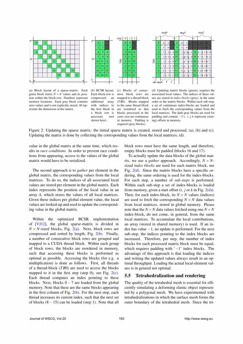
0 1

2 3

4 5 6

7 8 9

10 11 12

13 14 15

16 17 18

19 20 21

M

M

(a) Block layout of a sparse-matrix: Eachgreen block stores N ×N values and its posi-tion within the block-row. Numbers representmemory locations. Each gray block containszero-values and is not explicitly stored. M rep-resents the dimension of the matrix.

0 1

2 3

4 5 6

7 8 9

10 11 12

13 14 15

16 17 18

19 20 21

M

(b) BCSR layout:Each block-row iscompressed; anadditional arraywith indices tothe first block ina block row isnecessary (notshown here).

0 8

1 9

2 10 18

3 11 19

4 12 20

5 13 21

6 14 22

7 15 23

16

17

0 1 2step

TB0

(c) Blocks of consec-utive block rows aremapped to a thread block(T B0). Blocks mappedto the same thread blockare reordered so thatblocks processed in thesame step are continuousin memory. Padding isrequired (gray blocks).

16

17

18

19

20

21

22

23

TB0

step0 s step2

0

2

3

4

5

6

7

i

i

i

i

i

i

i

i

i

i

i

i

i

i

i

i

i

i

i

i

i

i

i

i

8

9

1

4

5

j

j

j

j

j

j

j

j

j

j

j

j

j

j

j

j

j

j

j

j

j

j

j

j

k

k

k

k

k

k

k

k

k

k

k

k

k

k

k

k

k

k

k

k

k

k

k

k

2ss1

(d) Updating matrix blocks (green), requires theassociated local values. The indices of these val-ues are stored in index blocks (gray), in the sameorder as the matrix blocks. Within each sub-step,a set of continuous index-blocks are loaded andused to fetch the corresponding values from thelocal matrices. The dark-gray blocks are used forpadding and contain −1’s. i, j,k represent (start-ing) offsets in memory.

Figure 2: Updating the sparse matrix: the initial sparse matrix is created, stored and processed, (a), (b) and (c).Updating the matrix is done by collecting the corresponding values from the local matrices, (d).

value in the global matrix at the same time, which res-ults in race conditions. In order to prevent race condi-tions from appearing, access to the values of the globalmatrix would have to be serialized.

The second approach is to gather per element in theglobal matrix, the corresponding values from the localmatrices. To do so, the indices of all associated localvalues are stored per element in the global matrix. Eachindex represents the position of the local value in anarray A, which stores the values of all local matrices.Given these indices per global element value, the localvalues are looked-up and used to update the correspond-ing value in the global matrix.

Within the optimized BCSR implementationof [VJ12], the global sparse-matrix is divided inN × N-sized blocks, Fig. 2(a). Next, block rows arecompressed and sorted by length, Fig. 2(b). Finally,a number of consecutive block rows are grouped andmapped to a CUDA thread block. Within each groupof block rows, the blocks are reordered in memory,such that accessing these blocks is performed asoptimal as possible. Accessing the blocks (for e.g. amultiplication) is done as follows. First, all threadsof a thread-block (T B0) are used to access the blocksmapped to it in the first step (step 0), see Fig. 2(c).Each thread computes an index pointing to theseblocks. Next, blocks 0− 7 are loaded from the globalmemory. Note that these are the same blocks appearingin the first column of Fig. 2(b). For the next step, eachthread increases its current index, such that the next setof blocks (8−15) can be loaded (step 1). Note that all

block rows must have the same length, and therefore,empty blocks must be padded (blocks 16 and 17).

To actually update the data blocks of the global mat-rix, we use a gather approach. Accordingly, N × N-sized index blocks are used for each matrix block, seeFig. 2(d). Since the matrix blocks have a specific or-dering, the same ordering is used for the index-blocks.For each step, a number of sub-steps is performed.Within each sub-step a set of index-blocks is loadedfrom memory, given a start offset (i, j or k in Fig. 2(d)).Then, for each index-block, its N ×N values (indices)are used to fetch the corresponding N ×N data valuesfrom local matrices, stored in global memory. Pleasenote that the N×N data values fetched using one N×N

index-block, do not come, in general, from the samelocal matrices. To accumulate the local contributions,an array (stored in shared memory) is used. If an in-dex has value −1, no update is performed. For the nextsub-step, the indices pointing to the index blocks areincreased. Therefore, per step, the number of indexblocks for each processed matrix block must be equal,which requires padding with ’−1’ index blocks. Theadvantage of this approach is that loading the indicesand writing the updated values always result in an op-timal throughput. Loading the actual local-element val-ues is in general not optimal.

5.5 Tetrahedralization and rendering

The quality of the tetrahedral mesh is essential for effi-ciently simulating a deforming elastic object represen-ted by a polygonal mesh. We have experimented withtetrahedralizations in which the surface mesh forms theouter boundary of the tetrahedral mesh. Since the tri-


angles of the surface mesh can have a high variety insize, the generated tetrahedralization also contains tet-rahedral elements with a high variation in size and con-figuration. This can have a negative effect on the qualityof the tetrahedralization. Therefore, we chose to createa tetrahedral mesh, using equi-sized elements, whichhowever, may result in a rather rough approximation ofthe original surface mesh. We tackle this problem bycoupling the input polygonal mesh to the (deforming)tetrahedral mesh, as follows.

First, a regular 3D grid of N3 voxels is created, inwhich each voxel containing a part of the surface ismarked as important; typical values for N are 32,64 or128. Next, a regular tetrahedralization of the grid iscreated using equi-sized tetrahedral elements, and eachelement containing at least one important vertex of thegrid, is stored. Further, the inner volume of the objectis tetrahedralized using the same equi-sized tetrahedralelements. Next, in order to reduce the amount of ele-ments, those elements belonging to the inner volumeare merged together into fewer larger ones. This re-duces the total amount of elements and thus the totalcomputation time. Note however that this approachis most useful with models which have large internalvolumes, similar to the bunny in Figure 5. Finally, theoriginal surface mesh is coupled with the tetrahedralone similar to [MG04]: each vertex in the original sur-face mesh is mapped to exactly one tetrahedron, andits barycentric coordinates in that tetrahedron are storedalong with the vertex coordinates.

When the new positions of the tetrahedra are com-puted, the surface mesh is also updated. To computenew positions of the deformed surface mesh, for eachvertex of the input mesh, the positions of the four ver-tices of the corresponding tetrahedron are looked-upand interpolated using the barycentric coordinates ofthe original vertex.

6 RESULTS

All experiments have been performed on a machineequipped with an Intel Q6600 quad-core processor anda GeForce GTX 570 with 1.2 Gb of memory.

Figure 3 shows the performances obtained for com-puting the local element matrices (Matrix), the rota-tion matrices (Rotation), solving the resulting linearsystem (CG), performing a single SpMV (SpMV), andthe total performance (Total) as a function of the num-ber of elements. Steps/sec is the corresponding num-ber of simulation steps performed per second. Simil-arly, Figure 4 shows the computation time per simula-tion time-step. For each model, we have used the fol-lowing material parameters: Young’s modulus of elasti-city, E = 5×105N/m2; Poisson’s ratio, µ = 0.2; dens-ity, ρ = 1000KG/m3. Furthermore, the time step ofthe simulation ∆t = 0.001 and the volume of each ini-tial element ve = 1.65× 10−6m3. Each model used in

0

20

40

60

80

100

120

140

160

1000 10000

100000

0

100

200

300

400

500

600

700

800

Per

form

ance

(G

FL

OP

S)

Per

form

ance

(S

teps/

sec)

Number of elements

CGMatrix

RotationTotal

Steps/secSpMV

Figure 3: Performance results with different numbersof elements. CG represents the performance of theCG solver, Matrix – the performance for computingthe local element matrices, Rotation – the performanceof the rotation extraction procedure, SpMV – the per-formance of the SpMV operation; Total represents theoverall performance. Steps/sec represents the numberof simulation steps per second. The global-matrix up-date was performed with an effective throughput of 50GB/sec.

10

100

1000

10000

100000

1000 10000

100000

Tim

e (M

icro

seco

nd

s)

Number of elements

CGMatrix

RotationUpdate

Total

Figure 4: Timing results with different numbers of ele-ments, per time step. CG represents the time of theCG solver, Matrix – the time for computing the localelement matrices, Rotation – the time of the rotationextraction procedure; Total represents the total elapsedtime per time-step.

this paper is scaled such that each dimension is at most66 cm and is tetrahedralized as described in Section 5.5.With these settings, the CG solver found a solution foreach model in 5 to 18 iterations. In order to obtain ageneric performance picture, we have fixed the numberof iterations to 18, which resulted in the performancesfrom Fig. 3.

Within Figure 3 a number of interesting patterns canbe seen. First, the performance for computing thelocal element matrices reaches its maximum very soon.Since each matrix is mapped to exactly one thread-


block, a large amount of thread-blocks is created, res-ulting in a ’constant’ performance. Second, the per-formance figures for computing the rotation matricesshow a larger variation. Since 16 rotation matrices areprocessed by one thread-block, a significantly smal-ler amount of thread-blocks is used. Finally, the per-formance of the CG method seems to be low comparedto the other operations. The CG method operates ona global sparse-matrix and performs a large numberof sparse-matrix vector multiplications (SPMVs) andvector-vector operations, for which the performancesare mainly bound by the memory throughput. However,the CG performances from Figure 3 agree with thosefrom [VJ12], given the dimensions of the problem.

The measured, effective throughput for updating theglobal matrix was about 50 GB/sec, in all cases withmore than 5k elements. Since this operation transfersa large amount of data, the memory bus is saturatedvery soon, resulting in a good throughput. However,since not all transactions can be coalesced, the max-imum throughput is not reached. This operation is verysimilar to an SPMV with 1× 1 blocks, but now for amatrix containing d× more elements, with d the degreeof internal nodes in the model. This observation showsthat the measured throughput is close to the expectedone, according to the results in [VJ12].

As expected, the total performance increases with thenumber of elements. This shows that the computationalresources are used efficiently for larger models. Thenumber of elements, for which the maximum perform-ance is reached, depends on the actual GPU mappingof the computations. For example, the CG solver doesnot reach its maximum performance for 100k elements,while the computation of the local element matricesreaches its peak at 5k elements. Due to this, one canexpect better performances for the CG method whenlarger models are used. Furthermore, for models havingless than 30k elements, the total computation is domin-ated by the time spent by the CG solver. For larger mod-els, more time is spent on computing the local matrices,see Figure 4.

The measured overall performance is based on thetotal time needed per simulation step, which includesall operations performed, except the rendering of themodel. Figure 3 also shows the number of simulationsteps performed per second, given the number of ele-ments; these numbers are based on the total compu-tation time. Accordingly, even for large models, in-teractive frame rates can be reached. A rough com-parison of the obtained performance and frame ratewith other state-of-the-art multigrid GPU implement-ations [DGW11] shows that, even if in theory the CGmethod converges slower than multigrid, comparableresults can be obtained for similar models. We assumethat memory transactions in our method are more effi-cient, despite of transferring more data. However, more

research is required to get a full understanding of thedifferences between both methods performed on mod-ern GPUs, with respect to performance figures. Finally,Figures 1, 5, 6, 7, 8 and 9 show example results fromour simulations.

Figure 5: Material properties and collision handling.Left: flexible material (E = 5×104). Right: stiffer ma-terial (E = 5× 105). Simulation rate: 120 frames persecond.

Figure 6: Left: stretching and deforming a model usingexternal forces. Right: deformation after releasing ex-ternal forces. Simulation rate: 118 frames per second.

Figure 7: Bunny bouncing on the floor. Simulation rate:120 frames per second.

7 CONCLUSIONS

We have presented an efficient method for simulat-ing elastically deformable models for graphics applica-tions, accelerated on modern GPUs using CUDA. Ourmethod relies on a fast Conjugate Gradient solver andan efficient mapping of the SPMV operation on modernGPUs [VJ12]. Since the topology of the underlying grid


Figure 9: Other simulation results. Simulation rate: 160 frames per second.

Figure 8: Left: applying external forces on the wings.Right: after releasing the external forces. Simulationrate: 116 frames per second.

does not change during the simulation, data structuresare reused for higher efficiency. To further improve theperformance, we proposed a scheme which allows toefficiently update the sparse matrix, during the simula-tion.

In future work we will investigate the performance ofthis method when multiple GPUs are used. Further-more, we will investigate the performance differencebetween traditional CG methods and multigrid methodsperformed on modern GPUs. Also, we plan to enhancethe simulation to allow for plastic behaviour as well asbrittle and fracture of stiff materials.

REFERENCES

[BCL07] BUATOIS L., CAUMON G., LÉVY B.:Concurrent Number Cruncher: An Effi-cient Sparse Linear Solver on the GPU. InHigh Perf. Comp. Conf. (HPCC) (2007).2

[BFGS03] BOLZ J., FARMER I., GRINSPUN E.,SCHRÖDER P.: Sparse matrix solvers onthe GPU: Conjugate gradients and multi-grid. In Proc. SIGGRAPH’03 (2003). 2

[BG08] BELL N., GARLAND M.: Efficient

Sparse Matrix-Vector Multiplication on

CUDA. Tech. Rep. NVR-2008-004,NVidia, 2008. 2

[DGW11] DICK C., GEORGII J., WESTERMANN

R.: A real-time multigrid finite hexa-hedra method for elasticity simulation us-

ing CUDA. Simulation Modelling Prac-

tice and Theory 19, 2 (2011), 801–816. 2,7

[GM97] GIBSON S., MIRTICH B.: A Survey

of Deformable Modeling in Computer

Graphics. Tech. Rep. TR-97-19, MERL,Cambridge, MA, 1997. 1

[GSMY∗07] GÖDDEKE D., STRZODKA R., MOHD-YUSOF J., MCCORMICK P., BUIJSSEN

S. H., GRAJEWSKI M., TUREK S.: Ex-ploring weak scalability for FEM calcula-tions on a GPU-enhanced cluster. Parallel

Computing 33, 10–11 (2007), 685–699. 2

[GST05] GÖDDEKE D., STRZODKA R., TUREK

S.: Accelerating double precision FEMsimulations with GPUs. In Proc. ASIM

2005 - 18th Symp. on Simul. Technique

(2005). 2

[GST07] GÖDDEKE D., STRZODKA R., TUREK

S.: Performance and accuracy ofhardware-oriented native-, emulated- andmixed-precision solvers in FEM simula-tions. Int. Journal of Parallel, Emergent

and Distributed Systems 22, 4 (2007),221–256. 2

[GW06] GEORGII J., WESTERMANN R.: Amultigrid framework for real-time simu-lation of deformable bodies. Computers

& Graphics 30, 3 (2006), 408–415. 2

[Hig86] HIGHAM N. J.: Computing the polar de-composition – with applications. SIAM

Journal of Scientific and Statistical Com-

puting 7 (1986), 1160–1174. 3, 4

[HS04] HAUTH M., STRASSER W.: Corota-tional simulation of deformable solids. InWSCG (2004), pp. 137–144. 2, 3, 4

[ITF06] IRVING G., TERAN J., FEDKIW R.: Tet-rahedral and hexahedral invertible finiteelements. Graph. Models 68, 2 (2006),66–89. 2, 3

[JP99] JAMES D. L., PAI D. K.: ArtDefo: ac-curate real time deformable objects. InProc. SIGGRAPH’99 (1999), pp. 65–72.


1

[KW03] KRÜGER J., WESTERMANN R.: Linearalgebra operators for gpu implementationof numerical algorithms. In Proc. SIG-

GRAPH’03 (2003), pp. 908–916. 2

[LJWD08] LIU Y., JIAO S., WU W., DE S.: Gpuaccelerated fast fem deformation simula-tion. In Circuits and Systems, 2008. AP-

CCAS 2008. IEEE Asia Pacific Confer-

ence on (30 2008-dec. 3 2008), pp. 606–609. 2

[MG04] MÜLLER M., GROSS M.: Interactive vir-tual materials. In Proc. Graphics Inter-

face 2004 (2004), pp. 239–246. 2, 3, 4,6

[NMK∗06] NEALEN A., MÜLLER M., KEISER R.,BOXERMANN E., CARLSON M.: Phys-ically based deformable models in com-puter graphics. Computer Graphics

Forum 25 (2006), 809–836. 1

[NVI] NVIDIA CORPORATION: Compute

Unified Device Architecture program-

ming guide. Available at http://

developer.nvidia.com/cuda. 4

[PH05] PEPPER D. W., HEINRICH J. C.: The

Finite Element Method: Basic Concepts

and Applications. Taylor and Francis,2005. 1, 2, 3

[RS01] RUMPF M., STRZODKA R.: Usinggraphics cards for quantized FEM com-putations. In Proc. IASTED Vis., Imaging

and Image Proc. (2001), pp. 193–202. 2

[TBHF03] TERAN J., BLEMKER S., HING V. N. T.,FEDKIW R.: Finite volume methods forthe simulation of skeletal muscle. In In

SIGGRAPH/Eurographics symposium on

Computer Animation (2003), pp. 68–74.1

[TPBF87] TERZOPOULOS D., PLATT J., BARR A.,FLEISCHER K.: Elastically deformablemodels. In Proc. SIGGRAPH’87 (1987),pp. 205–214. 1

[VJ12] VERSCHOOR M., JALBA A. C.: Ana-lysis and performance estimation of theconjugate gradient method on multiplegpus. Parallel Computing (2012). (inpress). 1, 2, 4, 5, 7


http://developer.nvidia.com/cuda

http://developer.nvidia.com/cuda

VISUALIZATION OF FLOW FIELDS IN THE WEB PLATFORMMauricio Aristizabal

Universidad EAFIT1CAD/CAM/CAE Laboratory

Carrera 49 # 7 Sur - 50Colombia (050022), Medellin,

Antioquia

[email protected]

John Congote1

Vicomtech Research CenterMikeletegi Pasealekua, 57

Parque tecnológicoSpain (20009), Donostia - San

Sebastian, Guipuzcoa

[email protected]

Alvaro Segura




[email protected]

Aior Moreno




[email protected]

Harbil Arregui




[email protected]

Oscar E. Ruiz

Universidad EAFITCAD/CAM/CAE Laboratory

Carrera 49 # 7 Sur - 50Colombia (050022), Medellin,

Antioquia

[email protected]

ABSTRACTVisualization of vector fields plays an important role in research activities nowadays. Web applications allow afast, multi-platform and multi-device access to data, which results in the need of optimized applications to be im-plemented in both high and low-performance devices. The computation of trajectories usually repeats calculationsdue to the fact that several points might lie over the same trajectory. This paper presents a new methodology tocalculate point trajectories over a highly-dense and uniformly-distributed grid of points in which the trajectoriesare forced to lie over the points in the grid. Its advantages rely on a highly parallel computing implementationand in the reduction of the computational effort to calculate the stream paths since unnecessary calculations areavoided by reusing data through iterations. As case study, the visualization of oceanic streams in the web platformis presented and analyzed, using WebGL as the parallel computing architecture and the rendering engine.

KeywordsStreamlines, Trajectory, Hierarchical Integration, Flow Visualization, WebGL.

1 INTRODUCTION

Vector field visualization plays an important role in theautomotive and aero-spatial industries, maritime trans-port, engineering activities and others. It allows the de-tection of particularities of the field such as vortexes oreddies in flow fields, but also permits exploring the en-tire field behavior, determining flow paths.

In particular, ocean flow visualization is important inmaritime navigation and climate prediction, since themovement of sea water masses produces variations inair temperature and wind currents. Therefore, flowvisualization becomes determinant to represent theocean’s behavior.


Figure 1: flow visualization of Atlantic ocean currentsin WebGL. Hierarchical integration was used to reducethe total number of iterations required to calculate thepaths.


With the growth of a great diversity of devices, develop-ment of multi-platform applications has become a com-mon goal for developers. The Web is de-facto a univer-sal platform to unify the development and execution ofapplications. However, challenges arise since applica-tions must be optimized in order to be useful as well ason high as on low-performance devices.The development of parallel computing hardware for allthe different devices is increasing and the developmentof applications and computer-based procedures are tak-ing in advance this capability. The contribution of thispaper is a new methodology to calculate point trajecto-ries of a highly dense grid of points over n-dimensionalvector fields, in which the trajectories are forced to passover the grid points (Figure 1). This allows to imple-ment a hierarchical integration procedure ([HSW11]),which takes advance of previously calculated data inorder to avoid repetitive and unnecessary calculations,and reduces the complexity of the algorithm from lin-ear to logarithmic. The procedure is suitable to be im-plemented over highly parallel computing architecturesdue to independent calculations and the number of com-putations to be performed. We employ WebGL as theparallel computing engine to calculate the iterations, us-ing the inherently parallel rendering procedure, and im-ages are used to store the data through the iterations.Different from other procedures, in which the calcula-tion of the trajectories is performed for each point inparticular, our methodology allows to merge its calcu-lation for all the points in which the field is discretized.Therefore, the number of unnecessary computations iscritically reduced.This paper is organized as follows: Section 2 presentsthe related work. Section 3 exposes the methodology inwhich the contribution of this work is explained. Sec-tion 4 presents a case of study in oceanic currents andfinally section 5 concludes the article.

2 LITERATURE REVIEW2.1 Flow VisualizationA great amount of methodologies to visualize vectorfields (flow fields) has been developed among the lastdecades. Geometric-based approaches draw iconson the screen whose characteristics represent thebehavior of the flow (as velocity magnitude, vorticity,etc). Examples of these methodologies are arrowgrids ([KH91]), streamlines ([KM92]) and streaklines([Lan94]). However, as these are discrete approaches,the placement of each object is critical to detect theflow’s anomalies (such as vortexes or eddies), andtherefore, data preprocessing is needed to perform anillustrative flow visualization. An up-to-date survey ongeometric-based approaches is presented by [MLP10].However, in terms of calculating those trajectories fordetermined points in the field, the procedures usually

compute for each point the integrals, and, as a result, theprocedures are computationally expensive for highlydense data sets.

On the other hand, texture-based approaches representboth a more dense and a more accurate visualization,which can easily deal with the flow’s feature represen-tation as a dense and semi-continuous (instead of sparseand discrete) flow visualization is produced. A deepsurvey in the topic on texture-based flow visualizationtechniques is presented by [LHD04].

An animated flow visualization technique in which anoise image is bended out by the vector field, and thenblended with a number of background images is pre-sented by [VW02]. Then, in [VW03] the images aremapped to a curved surface, in which the transformedimage visualizes the superficial flow.

Line Integral Convolution (LIC), presented by [CL93],is a widely implemented texture-based flow visualiza-tion procedure. It convolves the associated texture-pixels (texels) with some noise field (usually a whitenoise image) over the trajectory of each texel in somevector field. This methodology has been extended torepresent animated ([FC95]), 3D ([LMI04]) and timevarying ([LM05, LMI04]) flow fields.

An acceleration scheme for integration-based flow vi-sualization techniques is presented by [HSW11]. Theoptimization relies on the fact that the integral curves(such as LIC) are hierarchically constructed using pre-viously calculated data, and, therefore, avoid unneces-sary calculations. As a result, the computational effortis reduced, compared to serial integration techniques,from O(N) to O(logN), where N refers to the numberof steps to calculate the integrals. Its implementationis performed on Compute Unified Device Architecture(CUDA), which allows a parallel computing schemeperformed in the Graphics Processing Unit (GPU), andtherefore the computation time is critically reduced.However, it requires, additionally to the graphic Appli-cation Programming Interface (API), the CUDA API inorder to reuse data, and hence, execute the procedure.

2.2 WebGL literature reviewThe Khronos Group released the WebGL 1.0 Specifi-cation in 2011. It is a JavaScript binding of OpenGLES 2.0 API and allows a direct access to GPU graphicalparallel computation from a web-page. Calls to the APIare relatively simple and its implementation does notrequire the installation of external plug-ins, allowingan easy deployment of multi-platform and multi-deviceapplications. However, only images can be transferedbetween rendering procedures using framebuffer ob-jects (FBOs).

Several WebGL implementations of different applica-tions have been done such as volume rendering, pre-sented by [CSK11] or visualization of biological data,


presented by [CADB10]. A methodology to implementLIC flow visualization with hierarchical integration, us-ing only WebGL, was presented by [ACS12], in whichFBOs are used to transfer data between different ren-dering procedures, and therefore allowing to take in ad-vance the parallel computing capabilities of the render-ing hardware, in order to perform the different calcula-tions. However, for the best of our knowledge, no otherimplementation that regards to streamline flow visual-ization on WebGL has been found in the literature or inthe Web.

2.3 Conclusion of the Literature ReviewWebGL implementations allow to perform appli-cations for heterogeneous architectures in a widerange of devices from low-capacity smart phones tohigh-performance workstations, without any externalrequirement of plug-ins or applets. As a result, opti-mized applications must be developed. In responseto that, this work optimizes the calculation of pointtrajectories in n-dimensional vector fields over highlydense set of points, forcing the trajectories to lie overthe points in the set. As a consequence, previouslycalculated data can be reused using hierarchicalintegration, avoiding unnecessary calculations andreducing the complexity of the algorithm.

3 METHODOLOGYThe problem that we address is stated as: given a setof points and a vector field that exists for all of thesepoints, the goal is to find the finite trajectory that eachpoint will reproduce for a certain period of time.

Normal calculation of point trajectories in n-dimensional vector fields, requires to performnumerical integration for each particular point in orderto reproduce the paths. In the case of a dense set ofpoints, the procedures suffer from unnecessary stepcalculations of the integrals, since several points inthe field might lie over the same trajectory of others.Hence, some portions of the paths might be shared.Figure 2 illustrates this situation.

syj=xj(0)

xj(1)xj(2)

f(xj(0))f(xj(1)) f(xj(2))

Figure 2: Trajectory overlapping in several point paths.

In order to avoid repeated computations, we propose amethodology to calculate trajectories of highly densegrid of points, in which the paths are forced to lie over

the points in the grid, i.e., the paths are generated as aPiecewise Linear (PL) topological connection betweena set of points that approximates the trajectory. Withthis, hierarchical integration [HSW11] is employed toiteratively compute the paths and reuse data through theiterations.

3.1 Hierarchical IntegrationSince line integration over n-dimensional vector fieldssuffers from repeated calculations, hierarchical integra-tion [HSW11] only calculates the necessary steps andthen iteratively grows the integrals reusing the data.This reduces the computational complexity of the algo-rithm from O(N), using serial integration, to O(logN).The procedure is summarized as follows.For an arbitrary point in the field y ∈ Y with Y ⊆ Rn,let us define f : Y → Rm, as an arbitrary line integralbounded by its trajectory cy. Consider its discrete ap-proximation as described in equation 1.

f (y) =∫

cy

w(x(s))ds≈t

∑i=1

w(x(i∗∆s))∆s (1)

where t is the maximum number of steps required toreproduce cy with ∆s the step size. x(0) = y is the start-ing point of the trajectory to be evaluated and w is thefunction to be integrated. The integration procedure isperformed for all points y ∈ Y in parallel.We assume that ∆s = 1 , ∀y ∈ Y and therefore f (y) ≈

t∑

i=1w(x(i)). The algorithm starts with the calculation of

the first integration step for all the points in the field.Namely,

f0(y) = w(x(1)) (2)

It is required to store the last evaluated point x(1) overthe growing trajectory and the partial value of the in-tegral for all the points y in order to reuse them in thefollowing steps to build the integral. With this, the nextaction is to update the value of the integral, using thesum of the previously calculated step at y and the stepevaluated at its end point (x(1)). Namely,

f1(y) = f0(x(0))+ f0(x(1)) (3)

In this case, the end point of f1(x(0)) is x(2) as thecalculation evaluates f0(x(1)). Therefore, the next iter-ation must evaluate f1 at x(0) and x(2) in order to growthe integral. In general, the k’th iteration of the proce-dure is calculated as follows:

fk(y) = fk−1(x(0))+ fk−1(x(end)) (4)

It is important to remark that each iteration of this pro-cedure evaluates two times the integration steps eval-uated in the previous iteration. As a result, the to-tal number of integration steps t is a power of two,


and the hierarchical iterations required to achieve thisevaluations is reduced by a logarithmic scale, i.e., k =log2 t. Also notice that the evaluation of the vectorfield is performed only once, in the calculation of thefirst step, which avoids unnecessary evaluations of thevector field, which are computationally demanding forcomplex vector fields. Figure 3 illustrates the procedureup to four hierarchical steps.

Step 0

Step 1

Step 2

Step 3

Step 4

f0(y)

f1(y)

f3(y)

f3(y)

f4(y)

Figure 3: Exponential growth of hierarchical integra-tion methodology. At step 3, the procedure evaluates 8serial integration steps, meanwhile at step 4 it evaluates16 serial integration steps.

3.2 Stream Path CalculationIn order to perform the visualization of a vector field us-ing trajectory paths, lets assume a homogeneously dis-tributed set of points

Y = y, z ∈ Rn|y− z = ∆y,

∆y is constant ∀z adjacent to y (5)

and a n-dimensional vector field F : Rn→Rn. The goalis to calculate for each point y ∈ Y , the PL approxi-mation of the trajectory that the point will describe ac-cording to F , defined by the topological connection ofa particular set of points Ay ⊂Y . Figure 4 illustrates theapproximation.

y

Figure 4: PL approximation of the trajectory by the pro-cedure.

The trajectory cy of an arbitrary point y in the field isdefined as

cy = xy(s) =∫

lF(xy(s))ds (6)

where l represents a determined length of integration.

Using hierarchical integration, for each point in the fieldthe first step of the PL trajectory is calculated, this is,the corresponding end point of the first step of the in-tegral is computed using a local approximation of thepoint in the set of points.

xy(0) = y (7)

y′ = xy(0)+ γF(xy(0)) (8)

xy(1) = argxy

min(Y − y′) (9)

where y′ is the first iteration result of the Euler inte-gration procedure, γ is a transformation parameter toadjust the step given by the vector field to the local sep-aration of the set of points and xy(1) is defined as theclosest point in Y that approximates y′. The value ofxy(1) is then associated (and stored) to y. The set Aycontains the reference to the points of the trajectory thatdescribes y, and therefore for equation 8, Ay is definedas:

A0y = xy(1) (10)

Similarly to the hierarchical integration procedure, thenext steps are performed to join the calculated steps inorder to grow the trajectories. Therefore, for each pointy, its computed trajectory is joint with its last point’strajectory, this is, for the step in equation 8.

A1y = A0

y ∪A0xy(1) = xy(1),xy(2) (11)

Note that each iteration of the procedure will increasethe number of points in the trajectory by a power oftwo. Therefore, the growth of the paths is exponential.In general, the k’th iteration is calculated as

Aky = Ak−1

y ∪Ak−1xy(2k)

= xy(1),xy(2), . . . ,xy(2(k+1))(12)

The accuracy of the procedure is strongly determinedby the discretization (density) of Y , since it is directlyrelated to the step size in the integration procedure, i.e.,the approximation of the first step end-point is deter-minant. In order to increase the accuracy of the proce-dure, the computation of the first step can be calculatedwith e.g., a 4th order Runge Kutta numerical integra-tion, however, it might significantly increase the com-putation time of the procedure if the computation timeof the vector field function is relevantly high.

3.3 Time-Varying DataIn terms of unsteady flow fields, i.e., time-varying vec-tor fields, the generation of the trajectories might seemdifficult. In that case, as proposed in [HSW11], timeis considered another dimension of the vector field.


Therefore, the set of points is formed with the posi-tion coordinates of the points and discretized time steps,producing an n+1-dimensional grid of points.

It is also determinant for the accuracy of the procedurethat the density of the discretization set is high, in orderto increase the precision of the approximated trajecto-ries.

3.4 AnimationDynamic scenes are demanding in most of the visu-alization procedures. We consider in this section twokinds of dynamic scenes. A first kind of proceduresrefers to when the vector field is steady, i.e., it remainsconstant through the time. In this case, the goal is tovisualize the motion of the particle all across the field.

Since the paths for all the points in the field are cal-culated, the representation of the particle’s trajectorythrough the frames is simple. Consider a point y and itsapproximated trajectory given by the set of points Ay.Notice, as described in section 3.2, that the first pointof the set Ay [1], i.e., xy(1), represents the next pointin which y will lie in a determined period of time. Asa result, at a posterior frame, the displayed trajectoryshould be Axy(1).

The second type of procedure refers when vector fieldis varying with the time. Complementary to the ani-mation stated before, a second kind of dynamic sceneis comprised since it is also important to visualize thechanges that a trajectory suffers in the time. In the caseof time varying data, as in the steady case, all the pointshave an associated trajectory. In order to animate thechange of one trajectory, from one frame to another, thetrajectory that will be represented refers to the one ofthe point with the same point coordinate, but the nexttime coordinate. i.e., Ay,t+∆t .

4 CASE STUDYIn this section the visualization of 2D oceanic currentsusing the proposed methodology is performed. The im-plementation has been done in WebGL, so the method-ology’s parallel computing capabilities are fully used.WebGL offers the possibility to use the rendering pro-cedure to calculate images (textures) through Frame-buffer Objects, and then use those rendered textures asinput images for other rendering procedures. As a con-sequence, for this implementation we associate the pix-els of an image to the points in the field, and therefore,the rendering procedure is used to compute the differenthierarchical iterations, which are stored in the color val-ues of the pixels. Finally, the trajectories are hierarchi-cally constructed. The implementation was performedon an Intel Core2Quad 2.33 GHz with 4 GB of RAMand with a nVidia GeForce 480.

4.1 ImplementationFor a w×h grid of points (w and h being its width andheight respectively in number of elements), images ofsize w×h in pixels are used, in which a particular pixel(i, j) is associated with the point (i, j) in the grid. Sincefor each particular pixel, a four component vector isassociated, i.e., a vector of red, green, blue and alphavalues, each value can be associated as a particular po-sition of another pixel. This is, if the value of a pixel isr, then its associated pixel coordinates are given by

i = r mod w (13)

j =r− i

w(14)

where mod represents the remainder of the division ofr by w. As a result, if for each hierarchical integration,only the last point of the trajectory is to be stored, thenone image can store four hierarchical iterations.

For the zero’th hierarchical iteration, and the image I tostore its calculation, the value of a pixel (i, j) is givenby

i0 = i+ kFi(i, j) (15)j0 = j+ kFj(i, j) (16)

(17)

where the parameter ’0’ refers to the hierarchical step0, k represents the scaling factor of the vector field, andFi(i, j) represents the component of the vector field overthe direction of i, evaluated at the point (i, j). The vec-tor field used in this case study is shown in figures 5(a)for the direction of i and 5(b) for the direction of j.

In general, the k’th step is calculated as follows,

inext = I(i, j,k−1) mod w (18)

jnext =I(i, j,k−1)− inext

w(19)

I(i, j,k) = I(inext , jnext ,k−1) (20)

In the case that k is greater than four, then more imagesare used to store the values of the hierarchical iterations.

With that, all the desired steps are stored in the neces-sary images. In order to build the trajectories from thoseimages, a generic line, formed by k2 points, is required.Each point in the trajectory needs to have an associatedvalue, that refers to its order in the trajectory, i.e., thefirst point in the trajectory has an index 0, the secondpoint the value 1 and so on. With this index associ-ated to each point of the trajectory of the point y, theposition of each point is calculated as described in Al-gorithm 1, where HL is the hierarchical level that needsto be evaluated and the function evalHL() returns thenew position of the point y, for a particular hierarchicallevel.


(a)

(b)

Figure 5: Oceanic currents information. Color-scale of the oceanic currents magnitude in the (a) longitudinal and(b) latitudinal directions, of the 1st January of 2010. Images generated using data from the NASA’s ECCO2 project.

Require:

index Index referring to the elementposition into the line.

y Position of the initial point ofthe trajectory.

Ensure: yend Position of the i’th element of theline in the space.

Finished = f alsewhile not Finished do

HL = floor(log2(index))index = index−2HL

y = evalHL(HL,y)if index == 0 then

yend = yFinished = true

Algorithm 1: Procedure to reconstruct the streamlinesusing the already calculated hierarchical levels.

4.2 ResultsA general grid of 2048× 2048 points is used as theworld’s discretization. The vector field information was

acquired from the NASA’s ECCO2 project (see figure5), in which high-resolution data is available. Only sixhierarchical levels, i.e., 26 = 64 points in the trajectoryare used for each point in the field, as a result only 2images are required to calculate the trajectories.

The time needed to compute all the hierarchical levels(from 0 to 6) was 3 ms. The trajectory computation wasperformed to 10000 equally-distributed points all overthe field, which means that 64000 points need to betransformed by the trajectory computation. The com-putation time of those trajectories was 670 ms (Finalresults are shown in Figure 6).

In order to compare the visualization using the pro-posed methodology, the LIC visualization of the vectorfield using the methodology proposed in [ACS12] wasinserted below the stream line visualization. It showsthat for this level of discretization (2048× 2048), thevisualization is correct and accurate. However, sparsedata might produce inaccurate results.


(a) (b)

(c) (d)

Figure 6: Different view points of the final visualization of the oceanic currents using hierarchically calculatedstreamlines. Six hierarchical steps were used to achieve this visualization. The LIC visualization of the flow isused below the streamlines in order to visually compare the different methods and to enhance the visualization


This article presents a novel methodology to calculatepoints trajectories in highly dense point sets, in whichthe trajectories are formed as piecewise-linear connec-tions of the points in the set. This allows to merge thecalculation of the different trajectories and use itera-tively the data to avoid repeated and unnecessary calcu-lations, hence, accelerating the process. The procedureis suitable to be implemented in parallel architecturessuch as WebGl, OpenCL or CUDA, since the calcula-tions of the integrals for one point are independent fromthe calculation of the other points.

As a result, thanks to the use of hierarchical integration,the procedure reduces the computational complexity ofthe calculation of the trajectories from linear to loga-rithmic. The methodology deals with n-dimensionaland time-varying data and animated visualization canbe easily achieved due to the fact that the trajectoriesare calculated for all the points in the set.

Since the procedure performs an approximation ofthe trajectories using a piecewise-linear connectionof the points in the set, the accuracy of the algorithmis strongly influenced by the discretization distancebetween the points, because this distance determines alower bound in the integration step to be used.


Ongoing research focuses on the adaptation of thismethodology to require less computational effort(processing and memory effort), so that extremelylow-performance devices such as smart-phones andtablets might be able to perform an accurate andcomplete flow visualization using streamlines. Relatedfuture work includes the adjustment of the grid pointpositions along the iterations and the increase in theaccuracy of the calculated trajectories.

ACKNOWLEDGEMENTSThis work was partially supported by the Basque Gov-ernment’s ETORTEK Project (ITSASEUSII) researchprogram and CAD/CAM/CAE Laboratory at EAFITUniversity and the Colombian Council for Science andTechnology COLCIENCIAS. The vector field infor-mation was acquired form NASA’s ECCO2 project inhttp://ecco2.jpl.nasa.gov/.

6 REFERENCES[ACS12] Mauricio Aristizabal, John Congote, Al-

varo Segura, Aitor Moreno, Harbil Arriegui, andO. Ruiz. Hardware-accelerated web visualizationof vector fields. case study in oceanic currents.In Robert S. Laramee Paul Richard, Martin Krausand José Braz, editors, IVAPP-2012. InternationalConference on Computer Vision Theory and Ap-plications, pages 759–763, Rome, Italy, February2012. INSTICC, SciTePress.

[CADB10] M. Callieri, R.M. Andrei, M. Di Benedetto,M. Zoppè, and R. Scopigno. Visualization meth-ods for molecular studies on the web platform. InProceedings of the 15th International Conferenceon Web 3D Technology, pages 117–126. ACM,2010.

[CL93] B. Cabral and L.C. Leedom. Imaging vectorfields using line integral convolution. In Proceed-ings of the 20th annual conference on Computergraphics and interactive techniques, pages 263–270. ACM, 1993.

[CSK11] J. Congote, A. Segura, L. Kabongo,A. Moreno, J. Posada, and O. Ruiz. Interac-tive visualization of volumetric data with webglin real-time. In Proceedings of the 16th Interna-tional Conference on 3D Web Technology, pages137–146. ACM, 2011.

[FC95] L.K. Forssell and S.D. Cohen. Using line inte-gral convolution for flow visualization: Curvilin-ear grids, variable-speed animation, and unsteady

flows. Visualization and Computer Graphics,IEEE Transactions on, 1(2):133–141, 1995.

[HSW11] M. Hlawatsch, F. Sadlo, and D. Weiskopf.Hierarchical line integration. Visualization andComputer Graphics, IEEE Transactions on,(99):1–1, 2011.

[KH91] R.V. Klassen and S.J. Harrington. Shadowedhedgehogs: A technique for visualizing 2d slicesof 3d vector fields. In Proceedings of the 2ndconference on Visualization’91, pages 148–153.IEEE Computer Society Press, 1991.

[KM92] D.N. Kenwright and G.D. Mallinson. A 3-dstreamline tracking algorithm using dual streamfunctions. In Proceedings of the 3rd conferenceon Visualization’92, pages 62–68. IEEE Com-puter Society Press, 1992.

[Lan94] D.A. Lane. Ufat: a particle tracer for time-dependent flow fields. In Proceedings of the con-ference on Visualization’94, pages 257–264. IEEEComputer Society Press, 1994.

[LHD04] R.S. Laramee, H. Hauser, H. Doleisch,B. Vrolijk, F.H. Post, and D. Weiskopf. Thestate of the art in flow visualization: Dense andtexture-based techniques. In Computer GraphicsForum, volume 23, pages 203–221. Wiley OnlineLibrary, 2004.

[LM05] Z. Liu and R.J. Moorhead. Accelerated un-steady flow line integral convolution. IEEE Trans-actions on Visualization and Computer Graphics,pages 113–125, 2005.

[LMI04] Z. Liu and R.J. Moorhead II. Visualizingtime-varying three-dimensional flow fields us-ing accelerated uflic. In The 11th InternationalSymposium on Flow Visualization, pages 9–12.Citeseer, 2004.

[MLP10] T. McLoughlin, R.S. Laramee, R. Peikert,F.H. Post, and M. Chen. Over two decades ofintegration-based, geometric flow visualization.In Computer Graphics Forum, volume 29, pages1807–1829. Wiley Online Library, 2010.

[VW02] J.J. Van Wijk. Image based flow visualiza-tion. In ACM Transactions on Graphics (TOG),volume 21, pages 745–754. ACM, 2002.

[VW03] J.J. Van Wijk. Image based flow visualizationfor curved surfaces. In Proceedings of the 14thIEEE Visualization 2003 (VIS’03), page 17. IEEEComputer Society, 2003.


Hybrid SURF-Golay Marker Detection Method for Augmented Reality Applications

David Prochazka, Ondrej Popelka, Tomas Koubek, Jaromir Landa, Jan Kolomaznik

Mendel University in Brno

Zemedelska 1

61300, Brno, Czech Republic

[email protected]

ABSTRACT Augmented reality is a visualization technique widely used in many applications including different design tools. These tools are frequently based on tracking artificial objects such as square markers. The markers allow users to add a 3D model into the scene and adjust its position and orientation. Nevertheless, there are significant problems with marker occlusions caused by users or objects within the scene. The occlusions usually cause a disappearance of the 3D model. Such behavior has substantial negative impact on the application usability. In this article we present a hybrid marker detection approach. With this approach, markers are detected using the well-known SURF method. This method is able to recognize complex natural objects and deal with partial occlusions. Further, we overcome the problem of distinguishing similar markers by using the Golay error correction code patterns. The described approach represents a robust method that is able to identify even significantly occluded markers, differentiate similar markers, and it works in a constant time regardless of the amount of used markers.

Keywords Augmented reality, augmented prototyping, SURF, Golay error correction code.

1. INTRODUCTION The augmented reality (AR) research has been running for almost two decades. Nevertheless, it is possible to find just a few applications for common users. There are several principal reasons. One of the key problems is the inability to deal with occlusions of markers that are used for scene augmentation. During the work with an AR application, a marker is frequently obstructed by different solid objects, e.g. users´ hands. Inability to identify such a partially occluded marker leads to frequent disappearances of a visualized 3D model. Despite the obvious importance, this problem is unsolved even in many well-known AR toolkits (e.g. ARToolKitPlus).

The presented approach is implemented in the AR application AuRel that is focused on an augmented prototyping process. The application is developed in cooperation with an automotive company. It allows a car designer to extend a physical car model by selected virtual objects (3D models of car spare parts

(see Fig. 1)). The usage of AR for industrial design is mentioned in many papers, e.g. in [FAM*02], [BKF*00] and [VSP*03].

Although there is a substantial amount of existing augmented reality frameworks (ARToolkit, ARTag, Studierstube, etc.), OpenCV library has been used for the implementation [Lag11]. Principal reasons being active OpenCV development, cross-platform


Figure 1: 3D model of a spoiler inserted onto a rear car hood


deployment, 64bit systems support, a wide range of implemented computer vision algorithms and the amount of documentation (books, tutorials, etc.) [PK11].

There are briefly summarized current methods used for recognition of possible markers in the section 2. Two approaches focused on identification of geometric features are compared with the advanced technique usually used for natural object detection. Further, the section 3 outlines our method that is composed of SURF marker detection and Golay error correction code identification. Finally, the section 4 presents our results and concentrates on the ability to deal with occlusions.

2. MARKER RECOGNITION METHODS The process of marker recognition is usually divided in two parts: marker detection and marker identification. The former involves recognition of video frame regions that may represent markers. The latter concentrates on verifying the identity of the markers. The marker identity defines which 3D model will be displayed to the user.

2.1 Marker Detection Approaches The registration process of all further described methods is influenced by many negative factors, e.g. low image resolution, camera distortion (caused by lens), various light conditions or marker occlusions. The methods endeavor to compensate most of these factors. For the purpose of the article, the methods are distinguished into three general groups according to their basic principles. In detail the description of object recognition methods can be found e.g. in [Sze11].

2.1.1 Morphology-based marker detection These methods are based on recognition of shapes in preprocessed images. An approach described in [HNL96] uses a system of concentric contrast circles (CCC). The marker is composed of a black circle around a white middle or vice versa. The detection process starts with image thresholding and noise removal. Further, connected components are found, and their centers are determined. The results are two sets of centers: centers of white connected components and centers of black connected components. CCC marker position is given by the cross section of black and white centers.

An example of another approach is implemented in the frequently used ARToolKit [KB99]. In this case, square markers with black borders and black-and-white inner pictures are detected. A camera image is thresholded and connected components contours are found. Further, quadrangles are selected from the

contours set. These quadrangles represent potential markers [KTB*03].

The obvious limitation of these methods is their inability to deal with occlusions. Such occlusion causes a change in the image morphology. Therefore, the required shape cannot be detected.

2.1.2 Edge-based marker detection These methods are more flexible with regard to the marker occlusions than the image morphology-based methods. One solution that is based on this principle is the ARTag system [Fia05]. Although the ARTag markers are similar to the ARToolKit markers (significant is a thick black border), the implemented detection method is completely different. The ARTag method is based on detection of edgels (edge pixels) of an object. Further, a set of lines is constructed from the found edgels. It is not necessary to detect all line edgels; therefore, the edge could be partially occluded. Finally, four corresponding lines represent edges of a potential marker.

The same detection principle is used also in StudierStube project [Hir08] and many others.

2.1.3 Feature-based marker detection These methods are based on key points detection. The key points are various regions of interest: edges, corners, blobs. To identify whether a given key point really represents a part of a marker, it is necessary to match it with a key point in a marker template. This matching process requires that both key points to be matched are described by gradient changes in their neighborhood. The process of key point

Figure 2: Markers used with different detection methods. Detected features are

highlighted with a red color. From left: a) Match template, b) Golay error correction

code, c) SURF and d) S-G detection

a) b)

c) d)


neighborhood description is usually called feature extraction. The output of this process is a set of feature descriptors vectors. The feature descriptors are later compared and their distance is computed [Low04]. This enables to match points of interest between a template and a camera image.

There are several approaches for feature-based detection. Widely used are e.g. SIFT [CHT*09] and SURF [BTG06]. A thorough comparison of selected methods is described in [TM08]. The SURF (Speeded Up Robust Features) algorithm has a good ratio between detection capabilities and performance. The SURF algorithm application is composed of three steps: detection of key points (points of interest), feature extraction and key point matching.

The detection of image key points that are used for the image description is based on gradient changes in the grayscale version of the image. Each key point is identified by position and radius that specifies the size of the key point neighborhood. Then the process of feature extraction is performed.

During this process, each key point neighborhood is described using 64-dimensional or 128-dimensional vector that describes the gradient changes of each key point neighborhood. The descriptors are produced both for a template and a camera image, so that the corresponding key points are identified.

The SURF main advantage is the scale and rotation invariance [BTG06]. This allows the SURF to work even with low resolution images or small objects. Another advantage is that the algorithm compares only the points; therefore, the object can be partially occluded. Although the SURF method is usually used for natural object identification (see e.g. [BCP*08]), it can be used also for marker detection as described in our method outlined in section 3.

2.2 Marker Identification Approaches Morphological and edge-based detection methods are commonly used with following marker identification approaches: template matching and decoding of various binary codes.

Match template identification is based on computation of a pixel value correlation between a potential marker and a list of templates. In case the correlation fulfills a given threshold, the marker is identified. Obviously, the method has a linear time complexity. It is necessary to compute correlations with all templates until the required one is found or all templates are tested. Moreover, it is difficult to choose a threshold that allows to distinguish a large amount of markers [Bru09]. Therefore, methods based on different binary codes are frequently used to compensate this problem. One of the possible codes is the Golay error correction code.

A marker based on the Golay error correction code (ECC) can be composed of a large white square in the top left corner and e.g. 24 black or white squares that encode a number. The large square provides information about the marker orientation (see Fig. 2-b).

In the first step, a Golay ECC decoder for such a marker detects the position of the large white square. Further, it divides the code area into 24 blocks and calculates an average pixel value in all segments. Finally, the average value is thresholded to zero or one and the binary code is reconstructed. Possible implementation of the code reconstruction is outlined in [MZ06].

A significant advantage of this approach is that the binary code is reconstructed in a constant time. Another important advantage is the ability to correct errors caused by occlusions or an image corruption. Finally, the amount of distinguishable markers is limited just by the binary code length.

A feature-based method, such as the SURF is, is capable of both marker detection and marker identification. Therefore, it is not usually used with an identification method. As mentioned above, the method relies on searching for distinctive key points in a camera image that are then matched against image template descriptors. This process has linear time complexity because all template descriptors must be tested until the required one is found.

2.3 Summary of the Marker Recognition In general, there are three approaches for marker recognition. The first one is based on image morphology. Detection can be fast and precise. However, it cannot deal with marker occlusions. The edge-based methods can detect partially occluded markers. Nevertheless, this ability is limited. Larger occlusions of the edges are problematic. Both detection methods can be accompanied by a binary code identification method that is able to work in a constant time and reliably distinguish a substantial amount of markers.

Feature-based approaches are able to detect and identify even substantially occluded markers. However, they work in a linear time. This complexity is usually problematic for real-time applications with larger amounts of markers. Even more, feature-based methods have problems with distinguishing of similar markers [SZG*09].

3. S-G HYBRID RECOGNITION METHOD The proposed identification method combines the positive properties of two previously mentioned methods. We take advantage of robustness of the SURF feature-based object identification and


combine it with high reliability and effectiveness of the Golay error correction code detection, hence the name S-G hybrid detection method.

3.1 Marker design As described in section 2.1.3, the SURF algorithm is suitable especially for natural objects identification. However, many applications use this method to identify only a single object in an image. This is marker may appear in a scene.

The most problematic part of the SURF marker identification is the matching of corresponding marker key points in both images. The key points similarity is determined by gradient changes in the key points neighborhoods (these are represented by feature descriptors). If the image contains areas with similar gradient changes, then such areas will be identified as the same or similar key points.

Therefore, it is important to design markers so that the key points identified in them have distinctive gradient changes. Furthermore, these key points must be distinguishable both from the scene image and from other markers.

We use artificial markers very distinctive from the scene objects. Acceptable results are obtained using complex asymmetric markers composed of arbitrary geometric shapes (see Fig. 2–c). These markers are easily detected because they contain a substantial amount of features which can be tracked. The development of such marker, however, requires a lot of manual work. Even with a thorough testing it seems that only a very low number (approx. 3) of these markers could be reliably distinguished in an image.

Therefore, to ensure the correct marker identification we propose a hybrid detection method – S-G Detection – in which we combine the SURF algorithm with the Golay error correction code. In this case, the marker template is divided into two parts: the marker border and marker content. These two parts of a template may be combined independently.

Marker content is composed solely of a Golay code image. Only the marker content is used for marker identification. This has the advantage of very high identification reliability and allows to distinguish large number of markers – see section 2.2.

Marker border is composed of different geometric shapes selected so that they are distinctive from real scene objects. However, the border is no longer used for identification of the markers. This is possible because each marker border may be combined with any number of Golay codes to identify the marker. This combination solves the problem of distinguishing between marker templates while maintaining great robustness against template occlusion (see Fig. 4). Different marker borders may be used in the application. However, it is not necessary. We use the same border for all markers.

3.2 Marker Detection As been described in the previous section, we use the SURF method to identify key points only in the marker border (see Fig. 2–d). This border is the same for all markers. A strong advantage of this approach is that the time complexity of the whole algorithm is not a function of a number of templates (see section 2.1). Therefore, we can use a high number of markers without a performance hit. This is an important usability feature.

A common approach [Lag11] in matching the template and video frame points of interest is: find the best matches of key points using a defined metric, filter out false positives (invalid matches), repeat filtering until a sufficient number of adequately reliable points are obtained.

Errors in matched points may occur when a template key point is matched to an unrelated video frame key point because it happens to have similar neighborhood. Another source of errors occurs when a video frame contains two or more markers and template points are matched to correct points but on different marker borders (two or more physical markers).

Figure 3: S-G hybrid method. From left: a) key points are detected and filtered b) angle filter is applied so that the key points on both markers are distinguished c) marker specified in application

configuration is detected.

a) b) c)


For many applications, it is enough to identify if the template is present in the image, other applications require approximate template positions. Our application requires the exact position (translation and rotation) of the marker so that the virtual object may be inserted to the real scene.

The first step of marker matching feature extractor is to discover key points in the processed image. Then a descriptor vector for each key point is found using a feature extractor. These vectors are matched by computation of Euclidean distance between each pair of points. Moreover, we use symmetric matching filter for the key points.

First, template key points are matched against video frame image and the best matches are selected. Then the frame key points are matched against template key points, and best matches are selected. The intersection of these two sets is a set of matched points [Lag11].

Further, we filter the set of key points by application of an angle filter. The idea behind the angle filter is to take advantage of the information stored in a SURF key point itself. Each SURF key point contains an angle value, which defines the direction of the most significant gradient descent in the neighborhood of the key point. In our application, we use artificial markers; therefore we search for a set of predefined objects. This means that relative differences in rotation of the matched key point must be similar for all matched key points. That is – if the template has two key points and their rotation is 45° and 70°, then the two key points matched in the frame must have the rotation difference approximately 25°. Due to perspective deformations, the differences can be computed only approximately. An example of this filtering is shown in Fig. 3 – each set of differently colored points maintains the same relative rotation differences between points (in other words the same rotation difference between a template and a video frame).

A difficult part of the angle filtering algorithm is defining initial conditions. This is caused by the fact that until the marker is identified, its key points, their rotations and order are all unknown. To overcome this problem, the angle filter algorithm is implemented by marshaling all possible rotations into overlapping intervals of a defined width (rotation difference tolerance – RT). Each interval overlaps half of neighboring intervals so that there are no artificial boundaries. Key points in each interval are then processed individually as if it was a standalone key point set. This introduces a performance hit as another loop iterating over sets of key point has to be processed. Fortunately this is upper bounded – maximum number of iterations is 360 / (RT · 2). This

upper bound is hardly reached because only sets containing at least four points need to be processed. A minimum of four points is required for a correct positioning of a 3D model which will be added to the image later in the process. The angle filter algorithm may be described by the following pseudo-code: FOR each matched_point

difference =

matched_point_template->angle -

matched_point_frame->angle;

div = difference / RT

angles[div * RT]->add(matched_point)

angles[(div + 1) * RT]

->add(matched_point)

END FOR

FOR each angle

find homography

identify Golay marker

IF marker identified THEN

display 3D object

END FOR

3.3 Marker Identification For each set of points detected by the angle filter, we compute homography matrix so that the Golay code can be identified. By applying the homography transformation to the camera image we compensate the perspective deformation. This image transformed

Figure4: Examples of S-G method capability of occluded marker identification from a close

distance.


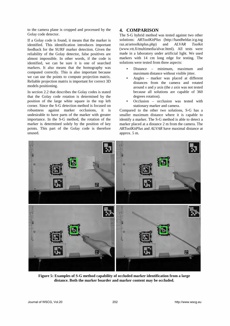
to the camera plane is cropped and processed by the Golay code detector.

If a Golay code is found, it means that the marker is identified. This identification introduces important feedback for the SURF marker detection. Given the reliability of the Golay detector, false positives are almost impossible. In other words, if the code is identified, we can be sure it is one of searched markers. It also means that the homography was computed correctly. This is also important because we can use the points to compute projection matrix. Reliable projection matrix is important for correct 3D models positioning.

In section 2.2 that describes the Golay codes is stated that the Golay code rotation is determined by the position of the large white square in the top left corner. Since the S-G detection method is focused on robustness against marker occlusions, it is undesirable to have parts of the marker with greater importance. In the S-G method, the rotation of the marker is determined solely by the position of key points. This part of the Golay code is therefore unused.

4. COMPARISON The S-G hybrid method was tested against two other solutions: ARToolKitPlus (http://handheldar.icg.tug raz.at/artoolkitplus.php) and ALVAR Toolkit (www.vtt.fi/multimedia/alvar.html). All tests were made in a laboratory under artificial light. We used markers with 14 cm long edge for testing. The solutions were tested from three aspects:

• Distance – minimum, maximum and maximum distance without visible jitter.

• Angles – marker was placed at different distances from the camera and rotated around x and y axis (the z axis was not tested because all solutions are capable of 360 degrees rotation).

• Occlusion – occlusion was tested with stationary marker and camera.

Compared to the other two solutions, S-G has a smaller maximum distance where it is capable to identify a marker. The S-G method is able to detect a marker placed at a distance 2 m from the camera. The ARToolKitPlus and ALVAR have maximal distance at approx. 5 m.

Figure 5: Examples of S-G method capability of occluded marker identification from a large distance. Both the marker boarder and marker content may be occluded.


In the angles comparison, measured results are influenced by the SURF algorithm limitations. The S-G method is able to detect a marker that is under 55° angle to the camera axis. (0° represents a marker perpendicular to the camera axis. The maximal theoretical angle is therefore 90°.) The other two solutions have maximal angles ranging from 74° to 85°.

Neither ARToolKitPlus nor ALVAR can deal with any type of occlusion. This is the most important disadvantage of these solutions. The S-G method can deal with significant marker occlusion. Because S-G works with key points instead of morphological operations or e.g. edgels, it is able to withstand a substantial number of different occlusions. We tested several of them (see Fig. 4).

The marker border can be obstructed up to 50 %. It is irrelevant what part of marker border is obstructed (all corners, two whole sides, etc.). The marker content (the Golay error correction code) must be visible at least from 75 % in case the large white square is obstructed. In case the obstruction is in other part of the Golay code, maximum allowed occlusion is approx. 15 %. This occlusion is limited by the Golay code redundancy.

This is the most important contribution of our solution in comparison to other used methods.

Because of the nature of the detection, the solutions capable of occlusion (e.g. ARTag) need at least three visible marker corners to detect and identify the marker. Our method is capable of the identification of a marker with all corners or sides covered. Our method has capability even of overcoming of the occlusion of marker contents. This is possible because of the Golay error correction code usage.

5. CONCLUSION Our application aims to improve the car design process. Therefore, several criteria must be fulfilled: Our marker detection and identification methods must be able to distinguish several hundred markers (one marker represents one spare part). Further, it must be possible to compute the precise position and rotation of the marker. Finally, the methods must be able to deal with occlusions that are common in real situations.

The SURF detection method as well as the Golay error correction code is able to deal with the occlusions. The proposed S-G registration method is slower than other frequently used approaches (e.g. image morphology approach with the Golay error correction codes). Still, it works in a constant time that is significant for real-time applications.

Nevertheless, in case of very good lighting conditions and absence of occlusions we recommend techniques based on the image morphology. With these methods, the video stream processing speed is substantially improved. Our AuRel application supports both approaches; therefore, registration technique is chosen according to the current conditions. By default, the morphology-based method (16 fps) is used. In case a marker detected in previous frame is missing, we switch to the S-G method (4 fps). Following frame is again processed by morphology-based method. Frame rates are measured on 640×480 px camera stream processed by Intel Core i5 2.6 GHz, 4 GB RAM, HDD 7200 rpm.

We consider our approach very promising. Nonetheless, there must be further research focused on several technical aspects. Particularly, the marker detector performance should be optimized (on the reference hardware configuration, ARToolKitPlus and ALVAR have above 20 fps). This could be done by reducing the number of key points in exchange for

Figure 6: Marker occlusion. The marker is approx. 2 m distant from the camera.

Figure 7: Key points detected by the S-G method and augmented 3D model.


lower reliability. Also the maximum detection distance needs to be improved. Possible solution can be to improve marker design so that the marker detector response is increased as outlined in [Sch*09].

SURF method can be easily used to design a marker-less tracking method as outlined in many articles. The absence of markers can substantially improve the application usability. Nevertheless, there could be a problem with selection of a correct 3D model and its manual position adjustment.

6. ACKNOWLEDGMENTS This paper is written as a part of a solution of the project IGA FBE MENDELU 7/2012 and FBE MENDELU research plan MSM 6215648904.

7. REFERENCES [BCP*08] Barandiaran, I., Cottez, Ch., Paloc, C.,

Grana, M.: Comparative Evaluation of Random 159 Forest and Ferns Classifiers for Real-Time Feature Matching in WSCG 2008 Full Papers Proceedings, Plzen: University of West Bohemia, 2008, pp. 159-166.

[Bru09] Brunelli, R.: Template Matching Techniques in Computer Vision: Theory and Practice, Wiley, 2009, ISBN 978-0-470-51706-2.

[BKF*00] Balcisoy, S., Kallmann, M., Fua, P., Thalmann, D.: A framework for rapid evaluation of prototypes with Augmented Reality. In Proceedings of the ACM symposium on Virtual reality software and technology, pp. 61-66. 2000. ISBN:1-58113-316-2.

[BTG06] Bay, H., Tuytelaars, T., Gool, L. V.: Surf: Speeded up robust features. In ECCV, 2006, pp. 404–417.

[CHT*09] Cui, Y., Hasler, N., Thormahlen, T., Seidel, H.: Scale Invariant Feature Transform with Irregular Orientation Histogram Binning. In Proceedings of Image Analysis and Recognition: 6th International Conference, pp. 258-267, 2009. ISBN: 978-3-642-02610-2.

[FAM*02] Fiorentino, M., De Amicis, R., Monno, G., Stork, A.: Spacedesign: A Mixed Reality Workspace for Aesthetic Industrial Design. In Proceedings of International Symposium on Mixed and Augmented Reality, p. 86. 2002. ISBN:0-7695-1781-1.

[Fia05] Fiala, M.: ARTag, a fiducial marker system using digital techniques. Computer Vision and Pattern Recognition, 2, June, 2005.

[Hir08] Hirzer, M.: Marker detection for augmented reality applications, 2008. Inst. for Computer

Graphics and Vision, Graz University of Technology, Austria.

[HNL96] Hoff, W. A., Nguyen, K., Lyon T.: Computer vision-based registration techniques for augmented reality. In Intelligent Robots and Computer Vision, XV, 1996, pp. 538–548.

[KB99] Kato, H., Billinghurst, M.: Marker Tracking and HMD Calibration for a Video-based Augmented Reality Conferencing System. In Proceedings of the 2nd IEEE and ACM International Workshop on Augmented Reality. 1999, s. 85-94.

[KTB*03] Kato, H., Tachibana, K., Billinghurst, M., Grafe, M.: A registration method based on texture tracking using artoolkit. In Augmented Reality Toolkit Workshop, 2003. IEEE International, 2003, IEEE, pp. 77–85.

[Lag11] Laganiere, R.: OpenCV 2 Computer Vision Application Programming Cookbook. Packt Publishing, 2011.

[Low04] Lowe, D. G.: Distinctive image features from scale-invariant keypoints. International Journal of Computer Vision, 60, 2004, pp. 91–110.

[MZ06] Morelos-Zaragoza, R. H.: The Art of Error Correcting Coding (Second Edition). John Wiley & Sons, 2006.

[PK11] Prochazka, D., Koubek, T.: Augmented Reality Implementation Methods in Mainstream Applications. Acta of Mendel University of agriculture and forestry Brno 59, 4,. 2011, p. 257.

[Sch*09] Schweiger, F. et al.: Maximum Detector Response Markers for SIFT and SURF, Proceedings of the Vision, Modeling, and Visualization Workshop 2009, Germany.

[SZG*09] Schweiger, F., Zeisl, B., Georgel, P., Schroth, G., Steinbach, E., Navab, N.: Maximum Detector Response Markers for SIFT and SURF. In Int. Workshop on Vision, Modeling and Visualization (VMV), 2009.

[Sze11] Szeliski, R.: Computer Vision: Algorithms and Applications, Springer, 2011.

[TM08] Tuytelaars T., Mikolajczyk K.: Local invariant feature detectors: a survey, Foundations and Trends® in Computer Graphics and Vision archive, Volume 3 Issue 3, 2008, pp. 177-280.

[VSP*03] Verlinden, J. C., Smit, A. D., Peeters, A. W. J., Gelderen, M. H. V.: Development of a flexible augmented prototyping system. Journal of WSCG, 11, 2003, pp. 496-503


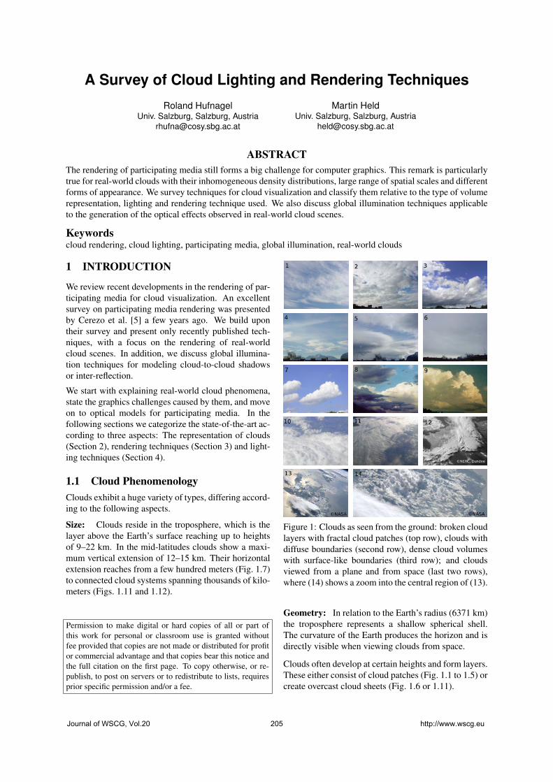
A Survey of Cloud Lighting and Rendering Techniques

Roland HufnagelUniv. Salzburg, Salzburg, Austria

[email protected]

Martin HeldUniv. Salzburg, Salzburg, Austria

[email protected]

ABSTRACTThe rendering of participating media still forms a big challenge for computer graphics. This remark is particularlytrue for real-world clouds with their inhomogeneous density distributions, large range of spatial scales and differentforms of appearance. We survey techniques for cloud visualization and classify them relative to the type of volumerepresentation, lighting and rendering technique used. We also discuss global illumination techniques applicableto the generation of the optical effects observed in real-world cloud scenes.

Keywordscloud rendering, cloud lighting, participating media, global illumination, real-world clouds

1 INTRODUCTION

We review recent developments in the rendering of par-ticipating media for cloud visualization. An excellentsurvey on participating media rendering was presentedby Cerezo et al. [5] a few years ago. We build upontheir survey and present only recently published tech-niques, with a focus on the rendering of real-worldcloud scenes. In addition, we discuss global illumina-tion techniques for modeling cloud-to-cloud shadowsor inter-reflection.

We start with explaining real-world cloud phenomena,state the graphics challenges caused by them, and moveon to optical models for participating media. In thefollowing sections we categorize the state-of-the-art ac-cording to three aspects: The representation of clouds(Section 2), rendering techniques (Section 3) and light-ing techniques (Section 4).

1.1 Cloud PhenomenologyClouds exhibit a huge variety of types, differing accord-ing to the following aspects.

Size: Clouds reside in the troposphere, which is thelayer above the Earth’s surface reaching up to heightsof 9–22 km. In the mid-latitudes clouds show a maxi-mum vertical extension of 12–15 km. Their horizontalextension reaches from a few hundred meters (Fig. 1.7)to connected cloud systems spanning thousands of kilo-meters (Figs. 1.11 and 1.12).


Figure 1: Clouds as seen from the ground: broken cloudlayers with fractal cloud patches (top row), clouds withdiffuse boundaries (second row), dense cloud volumeswith surface-like boundaries (third row); and cloudsviewed from a plane and from space (last two rows),where (14) shows a zoom into the central region of (13).

Geometry: In relation to the Earth’s radius (6371 km)the troposphere represents a shallow spherical shell.The curvature of the Earth produces the horizon and isdirectly visible when viewing clouds from space.

Clouds often develop at certain heights and form layers.These either consist of cloud patches (Fig. 1.1 to 1.5) orcreate overcast cloud sheets (Fig. 1.6 or 1.11).


Local upward motions emerging from the ground (con-vective plumes) create clouds with a sharp cloud baseand a cauliflower-like structure above, so-called Cumu-lus (Figs. 1.7 to 1.9). Their vertical extension reachesup to several kilometers (Fig. 1.9).For low clouds also mixed forms of convective and lay-ered clouds exist, where the convective plumes are ver-tically bound and form a layer (Fig. 1.3).Clouds formed in connection with frontal systems usu-ally show a large vertical extension and can span thou-sands of kilometers (Fig. 1.12).Boundary Appearance: The appearance of cloudsmainly depends on the cloud volume’s constituents:droplets of different size or ice particles. While largewater droplets produce a determined, surface-likeboundary (Figs. 1.7 to 1.9), smaller droplets create adiffuse or fractal boundary (Figs. 1.2 to 1.6). Ice parti-cles often form hair-like or fiber-like clouds, so-calledCirrus (Fig. 1.1), or diffuse clouds, the anvil-like topsof convective clouds (Fig. 1.13).The appearance of a cloud is strongly influenced bythe distance to its observer: While distant clouds oftenshow a distinct surface and sharp contours (Figs. 1.12and 1.13), a closer look reveals diffuse or fractal struc-tures (Fig. 1.14).

Optical Phenomena: Clouds consist of water dropletsand ice crystals which scatter light mostly independentof wavelength. Clouds are therefore basically white.Spectral colors appear only at certain angular constella-tions but generally do not influence their overall appear-ance. However, several optical phenomena determinetheir characteristic, natural appearance:Self-Shadowing: The attenuation of light within acloud creates gray tones and is proportional to theoptical depth of the volume. The self-shadowingprovides the cue to perceive clouds as volumetricobjects.Multiple scattering slightly attenuates the effect ofself-shadowing by distributing light within the cloudvolume in a diffusion-like process; see e.g. [4, 27, 33].Inter-Cloud Shadows: Clouds cast shadows onto otherclouds, like in Fig. 1.11, where a high cloud layer on theright-hand side shadows a low cloud layer.The Earth’s Shadow: Clouds can be shadowed by theEarth; see Fig. 1.8 showing an evening scene, where thelow clouds lie in the shadow of a mountain range.Indirect Illumination: Light inter-reflection betweendifferent clouds or between different parts of the samecloud brighten those regions, as, e.g., in Fig. 1.9, wherethe cloud seems to gloom from the inside.Light Traps: Light inter-reflection at a smaller scaleoccurs on determined cloud surfaces (Neyret [29]) andlets concavities appear brighter (Figs. 1.7 and 1.10).

Corona: The corona effect occurs when the cloud islit from behind. The strong forward scattering at theboundary produces a bright silhouette (silver-lining).

Atmospheric Scattering: Clouds often appear in vividcolors. This is caused by the scattering of light outsidethe cloud volume on air molecules and aerosols. Cloudsare therefore often lit by yellowish to reddish sunlight(Fig. 1.9). Different paths of light in the atmosphere letthe high clouds in Fig. 1.14 appear bright white and thelow clouds yellowish. Atmospheric scattering also cre-ates blue skylight which in some situations representsthe main source of lighting (Fig. 1.8).

Ground Inter-Reflection: For low-level clouds theinter-reflection with the ground creates subtle tones de-pending on the type of the ground; see e.g. [3].

1.1.1 Summary

From a computer graphics point of view we identifythe following volume properties, in addition to the formof the clouds as created by cloud modeling techniques,which are out of the scope of this survey: thin cloudsthat show no self-shadowing; cloud patches that repre-sent a mixture of slightly dense cores and optically thinboundaries, usually forming horizontally extensive lay-ered clouds; and dense cloud volumes of different sizesand extensions with a sharp or surface-like boundary.The boundary of clouds exhibits either a fractal, dif-fuse or sharp appearance.

1.2 Computer Graphics ChallengesA realistic visualization of clouds requires to tackle thefollowing challenges:

Heterogeneity: Real-world cloud scenes typically con-sist of a very heterogeneous collection of clouds withdifferent appearances, sizes and forms. Different cloudtypes require different volume representations, lightingand rendering techniques.

Atmospheric Scattering: For creating a cloud’snatural appearance the lighting model employed has toreproduce its typical optical phenomena (see Sec. 1.1),including atmospheric scattering which is the mainsource for color in the sky. This requires the inclusionof atmospheric models (which are not discussed in thissurvey) in the lighting process of clouds.

Curved volume: The spherical atmosphere makes itdifficult to take advantage of axis-aligned volumes ifclouds are viewed on a large or even global scale, as inFigs. 1.12 or 1.13.

Huge domain: The sheer size of the volume of real-world cloud scene, especially when viewed from above,like in Figs 1.11 to 1.13, requires sophisticated and ef-ficient lighting and rendering techniques.


1.3 Participating MediaA cloud volume constitutes a participating medium ex-hibiting light attenuation and scattering. This sectionuses the terminology of [5] to provide a short introduc-tion to the radiometry of participating media.

While light in vacuum travels along straight lines, thisis not the case for participating media. Here photons in-teract with the medium by being scattered or absorbed.From a macroscopic point of view light spreads in par-ticipating media, gets blurred and attenuated, similar toheat diffusion in matter.

Participating media are characterized by a particle den-sity ρ , an absorption coefficient κa, a scattering coeffi-cient κs, and a phase function p(~ω, ~ω ′) which describesthe distribution of light after scattering.

Absorption is the process where radiation is trans-formed to heat. The attenuation of a ray of light withradiance L and direction ~ω at position x (within an in-finitesimal ray segment) is described by

(~ω ·∇)L(x, ~ω) = −κa(x)L(x, ~ω).

In the atmosphere absorption is mainly due to water va-por and aerosols. Cloud droplets or ice crystals showlittle absorption which means that the light distributionin clouds is dominated by scattering.

Scattering is the process where radiance is absorbedand re-emitted into other directions. Out-scatteringrefers to the attenuation of radiance along direction ~ωdue to scattering into other directions:

(~ω ·∇)L(x, ~ω) =−κs(x)L(x, ~ω).

In-scattering refers to the scattering of light into thedirection ~ω from all directions (integrated over thesphere) at a point x:

(~ω ·∇)L(x, ~ω) =κs(x)4π

∫4π

p(~ω ′, ~ω)L(x, ~ω ′)dω′,

Extinction is the net effect of light attenuation due to ab-sorption and out-scattering described by the extinctioncoefficient κt = κa +κs.

Emission contributes light to a ray:

(~ω ·∇)L(x, ~ω) = κa(x)Le(x, ~ω).

It is usually not relevant for cloud rendering sinceclouds do not emit light. (An exception is lightninginside a cloud.)

Radiative Transfer Equation (RTE): Putting all termstogether yields the RTE which describes the change ofradiance within a participating medium at a point x:

(~ω ·∇)L(x, ~ω) = κa(x)Le(x, ~ω) +

κs(x)4π

∫4π

p(~ω ′, ~ω)L(x, ~ω ′)dω′ −

κa(x)L(x, ~ω) − κs(x)L(x, ~ω).

L(x, ~ω) L(x0, ~ω)x′

x x0

Ls(~ωs)

L(x, ~ω) L(x0, ~ω)

x′x x0

xsLs(~ωs)

Figure 2: Multiple scattering (left), and the single scat-tering approximation (right).

By using the single scattering albedo Ω = κs/κt andnoting that κa can be expressed as κa = κt (1−Ω), wecan re-write the RTE as

(~ω ·∇)L(x, ~ω) = κt(x)J(x, ~ω) − κt(x)L(x, ~ω), (1)

with the source radiance J:

J(x, ~ω) = (1−Ω(x))Le +

Ω(x)4π

∫4π

p(~ω ′, ~ω)L(x, ~ω ′)dω′.

The source radiance describes all contributions of ra-diance to a ray (x, ~ω) at a point x inside the medium.In high-albedo media, like clouds, the source term ismainly due to in-scattering, while the extinction is dom-inated by out-scattering: κt ≈ κs.

Integrating the RTE along a ray from x0 to x yields theradiance reaching point x from direction−~ω (see Fig. 2,left):

L(x, ~ω)= T (x,x0)L(x0, ~ω)+∫ x

x0

T (x,x′)κt(x′)J(x′)dx′,

(2)with the transmittance T (x1,x2) = exp(−∫ x2

x1κt(x)dx).

The boundary condition of the integral is L(x0, ~ω), rep-resenting the light coming from the background, an en-vironment map, or from scene objects.

Note that the coefficients κ∗ depend on the wavelength.Therefore, three versions of Eqn. 2 have to be solvedwith appropriate coefficients κ∗,λ for each wavelengthcorresponding to the RGB color components.

Single Scattering Approximation: A difficulty insolving Eqn. 2 is that L appears (implicitly through J)on both sides of the equation. A common approxima-tive solution is to account only for a certain number ofscattering events and apply extinction on the paths inbetween. Considering only the first order of scatteringyields the single scattering approximation: The sourceradiance JSS is given by the light from the light sourceLs attenuated on its way between xs and x′, see Fig. 2(right), thus eliminating L:

JSS(x′, ~ω) = Ω(x′)T (x′,xs) p(x′, ~ωs, ~ω)Ls(xs, ~ωs).

The single scattering approximation simulates the self-shadowing of a volume. Higher order scattering ac-counts for the “more diffuse” distribution of light withinthe volume.


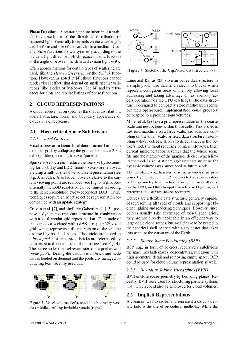
Phase Function: A scattering phase function is a prob-abilistic description of the directional distribution ofscattered light. Generally it depends on the wavelength,and the form and size of the particles in a medium. Usu-ally phase functions show a symmetry according to theincident light direction, which reduces it to a functionof the angle θ between incident and exitant light p(θ).

Often approximations for certain types of scattering areused, like the Henyey-Greenstein or the Schlick func-tion. However, as noted in [4], those functions cannotmodel visual effects that depend on small angular vari-ations, like glories or fog-bows. See [4] and its refer-ences for plots and tabular listings of phase functions.

2 CLOUD REPRESENTATIONSA cloud representation specifies the spatial distribution,overall structure, form, and boundary appearance ofclouds in a cloud scene.

2.1 Hierarchical Space Subdivision2.1.1 Voxel Octrees

Voxel octrees are a hierarchical data structure built upona regular grid by collapsing the grid cells of a 2×2×2cube (children) to a single voxel (parent).

Sparse voxel octrees reduce the tree size by account-ing for visibility and LOD: Interior voxels are removed,yielding a hull- or shell-like volume representation (seeFig. 3, middle). Also hidden voxels (relative to the cur-rent viewing point) are removed (see Fig. 3, right). Ad-ditionally the LOD resolution can be limited accordingto the screen resolution (view-dependent LOD). Thesetechniques require an adaptive octree representation ac-companied with an update strategy.

Crassin et al. [7], and similarly Gobetti et al. [13], pro-pose a dynamic octree data structure in combinationwith a local regular grid representation. Each node ofthe octree is associated with a brick, a regular 323 voxelgrid, which represents a filtered version of the volumeenclosed by its child nodes. The bricks are stored ina brick pool of a fixed size. Bricks are referenced bypointers stored in the nodes of the octree (see Fig. 4).The octree nodes themselves are stored in a pool as well(node pool). During the visualization brick and nodedata is loaded on demand and the pools are managed byupdating least recently used data.

Figure 3: Voxel volume (left), shell-like boundary vox-els (middle), culling invisible voxels (right).

N0

N0.2

N0.2.3

brick pool

N0.2.3

N0.2

N0node pooloctree bricks

Figure 4: Sketch of the GigaVoxel data structure [7].

Laine and Karras [25] store an octree data structure ina single pool. The data is divided into blocks whichrepresent contiguous areas of memory allowing localaddressing and taking advantage of fast memory ac-cess operations on the GPU (caching). The data struc-ture is designed to compactly store mesh-based scenesbut their open-source implementation could probablybe adapted to represent cloud volumes.Miller et al. [28] use a grid representation on the coarsescale and nest octrees within those cells. This providesfast grid marching on a large scale, and adaptive sam-pling on the small scale. A fixed data structure, resem-bling 4-level octrees, allows to directly access the oc-tree’s nodes without requiring pointers. However, theircurrent implementation assumes that the whole scenefits into the memory of the graphics device, which lim-its the model size. A streaming-based data structure fordynamic volumes was announced as future work.The real-time voxelization of scene geometry, as pro-posed by Forester et al. [12], allows to transform raster-izable geometry to an octree representation on-the-flyon the GPU, and thus to apply voxel-based lighting andrendering to a surface-based geometry.Octrees are a flexible data structure, generally capableof representing all types of clouds and supporting effi-cient lighting and rendering techniques. However, sinceoctrees usually take advantage of axis-aligned grids,they are not directly applicable in an efficient way tolarge-scale cloud scenes, but would have to be nested inthe spherical shell or used with a ray caster that takesinto account the curvature of the Earth.

2.1.2 Binary Space Partitioning (BSP)BSP, e.g., in form of kd-trees, recursively subdividesthe space into half-spaces, concentrating at regions withhigh geometric detail and removing empty space. BSPcould be used for cloud volume representation as well.

2.1.3 Bounding Volume Hierarchies (BVH)BVH enclose scene geometry by bounding planes. Re-cently, BVH were used for structuring particle systems[14], which could also be employed for cloud volumes.

2.2 Implicit RepresentationsA common way to model and represent a cloud’s den-sity field is the use of procedural methods. While the


Figure 5: Perlin noise [31] and “fractal sum” [11] func-tions (left). A hypertexture applied to a surface (right).

overall structure is usually specified by simple geomet-ric primitives, like spheres or ellipsoids, the internal,high-resolution structure is modeled by a function.

Perlin and Hoffert [31] introduce space-filling shapes,based on procedural functions, so-called hypertextures.Ebert et al. [11] propose many additional noise func-tions (see Fig. 5, left), and create various natural pat-terns applicable also for clouds.

The sampling of implicitly defined densities can be-come expensive and harm rendering performance. Sch-pok et al. [36] propose to evaluate the procedural func-tions on-the-fly on the GPU during the rendering by us-ing a fragment shader program and a 3D texture con-taining Perlin noise.

Kniss et al. [22] use procedural functions for geomet-ric distortion which adds a fractal appearance to regularshapes by changing the vertex positions of the geometryrendered. They apply this distortion during the render-ing process by using vertex shader programs.

Bouthors et al. [4] use hypertextures in combinationwith surface-bounding volumes for creating a fractalboundary appearance; see Fig. 5, right.

Implicitly specifying a volume via procedural functionsis a compact volume representation. The computationalcost can be mitigated by employing parallel process-ing on the GPU and taking advantage of hardware-supported tri-linear interpolation of 3D textures. Pro-cedural techniques are perfect for clouds with a frac-tal boundary appearance. However, they only providethe fine-scale volume structure while the overall cloudshape has to be modeled by other techniques.

2.3 Particle SystemsThe volume is represented by a set of particles with apre-defined volume. Usually spherical particles with aradial density function are used.

Nishita et al. [30] promote the use of particles witha Gaussian density distribution, so-called metaballs.While the metaballs in [30] are used only to create avolume density distribution, Dobashi et al. [10] directlylight and render the metaballs and visualize medium-size cloud scenes of Cumulus-like clouds with a diffuseboundary appearance.

Bouthors and Neyret [2] use particles to create a shell-like volume representation for Cumulus-like clouds.

Their algorithm iteratively places particles at the in-terface of a cloud volume, with smaller particles beingplaced upon the interface of larger particles. This cre-ates a hierarchy of particles with decreasing radius andspecifies the cloud’s surface, which can be transformed,e.g., to a triangle mesh.

Efficient transformation algorithms were developed tomatch the favored lighting and rendering approaches.Cha et al. [6] transform the density distribution givenby a particle system to a regular grid by using the GPU,while Zhou et al. [44] propose the inverse process trans-forming a density field to radial basis function (RBF)representation. This low-resolution particle system isaccompanied by a high-resolution grid, which storesdeviations of the particles’ density distribution from theinitial density field in a so-called residual field. Perfectspatial hashing allows a compact storage of this field.

Particles systems are a compact volume representationand directly support many cloud modeling techniques.Spherical particles are well suited for Cumulus-likeclouds or dense cloud volumes, but less appropriate forstratified cloud layers with a large horizontal extensionor for thin, fiber-like clouds.

2.4 Surface-Bounded VolumesThe cloud volume is represented by its enclosing hull,usually given as a triangle mesh. Since no informationon the internal structure is available, usually a homoge-neous volume is assumed.

Bouthors et al. [4] demonstrate the use of surface-bounded volumes for visualizing single Cumulusclouds. A triangle mesh is used in combinationwith a hypertexture to add small-scale details at theboundaries. A sophisticated lighting model reproducesa realistic appearance (see Sec. 4.1.4).

Porumbescu et al. [32] propose shell maps to create avolumetric texture space on a surface. A tetrahedralmesh maps arbitrary volumetric textures to this shell.

Surface-bounded volumes are a very compact represen-tation of cloud volumes, allowing for efficient renderingand for incorporating sophisticated lighting techniques.However, they are only applicable if a quick saturationof a ray entering the volume may be assumed. Whilethis is valid for dense clouds it does not apply to thinor layered clouds with their optically thin boundaries.Also special rendering techniques have to be developedfor allowing perspectives from within the clouds.

2.5 Clouds as LayersClouds represented by a single layer, usually renderedas a textured triangle mesh, allow fast rasterization-based rendering and are the traditional technique topresent clouds, e.g., during weather presentations [24].


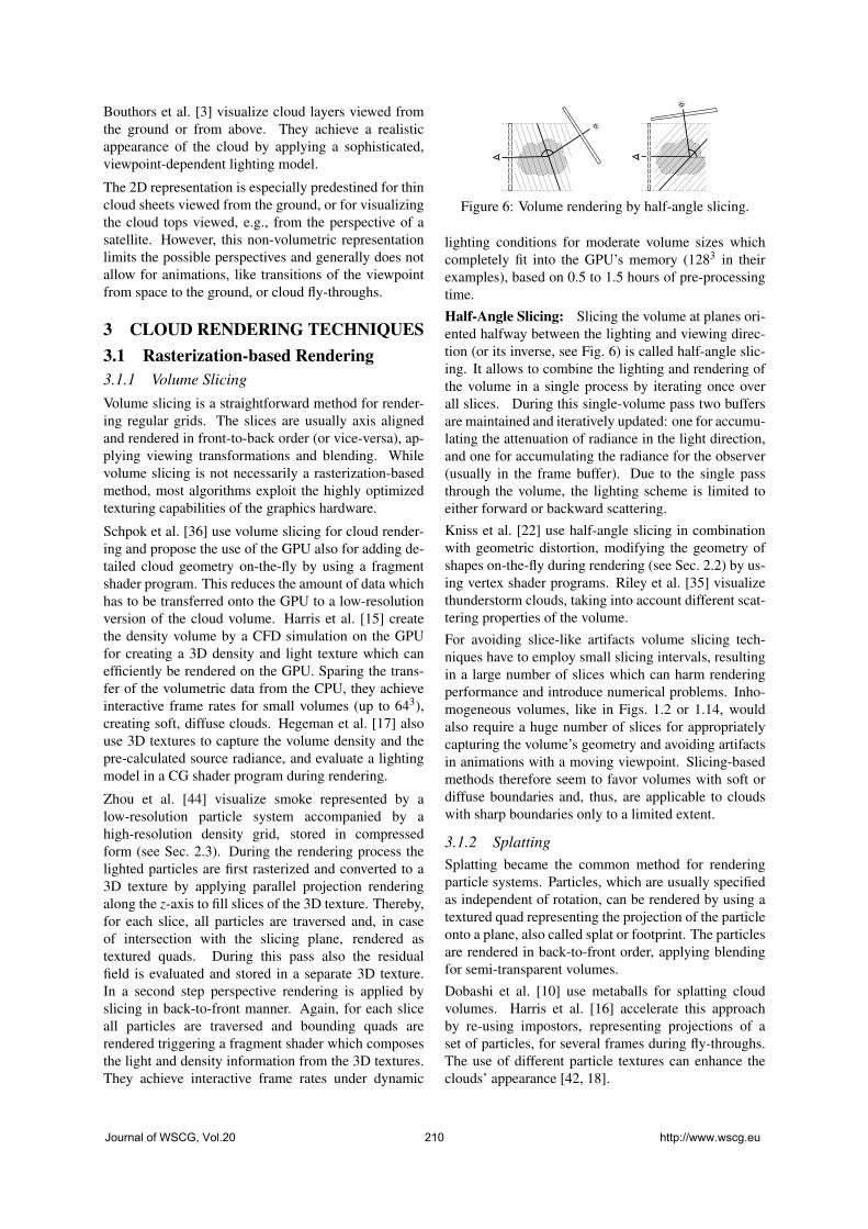
Bouthors et al. [3] visualize cloud layers viewed fromthe ground or from above. They achieve a realisticappearance of the cloud by applying a sophisticated,viewpoint-dependent lighting model.

The 2D representation is especially predestined for thincloud sheets viewed from the ground, or for visualizingthe cloud tops viewed, e.g., from the perspective of asatellite. However, this non-volumetric representationlimits the possible perspectives and generally does notallow for animations, like transitions of the viewpointfrom space to the ground, or cloud fly-throughs.

3 CLOUD RENDERING TECHNIQUES3.1 Rasterization-based Rendering3.1.1 Volume SlicingVolume slicing is a straightforward method for render-ing regular grids. The slices are usually axis alignedand rendered in front-to-back order (or vice-versa), ap-plying viewing transformations and blending. Whilevolume slicing is not necessarily a rasterization-basedmethod, most algorithms exploit the highly optimizedtexturing capabilities of the graphics hardware.

Schpok et al. [36] use volume slicing for cloud render-ing and propose the use of the GPU also for adding de-tailed cloud geometry on-the-fly by using a fragmentshader program. This reduces the amount of data whichhas to be transferred onto the GPU to a low-resolutionversion of the cloud volume. Harris et al. [15] createthe density volume by a CFD simulation on the GPUfor creating a 3D density and light texture which canefficiently be rendered on the GPU. Sparing the trans-fer of the volumetric data from the CPU, they achieveinteractive frame rates for small volumes (up to 643),creating soft, diffuse clouds. Hegeman et al. [17] alsouse 3D textures to capture the volume density and thepre-calculated source radiance, and evaluate a lightingmodel in a CG shader program during rendering.

Zhou et al. [44] visualize smoke represented by alow-resolution particle system accompanied by ahigh-resolution density grid, stored in compressedform (see Sec. 2.3). During the rendering process thelighted particles are first rasterized and converted to a3D texture by applying parallel projection renderingalong the z-axis to fill slices of the 3D texture. Thereby,for each slice, all particles are traversed and, in caseof intersection with the slicing plane, rendered astextured quads. During this pass also the residualfield is evaluated and stored in a separate 3D texture.In a second step perspective rendering is applied byslicing in back-to-front manner. Again, for each sliceall particles are traversed and bounding quads arerendered triggering a fragment shader which composesthe light and density information from the 3D textures.They achieve interactive frame rates under dynamic

Figure 6: Volume rendering by half-angle slicing.

lighting conditions for moderate volume sizes whichcompletely fit into the GPU’s memory (1283 in theirexamples), based on 0.5 to 1.5 hours of pre-processingtime.Half-Angle Slicing: Slicing the volume at planes ori-ented halfway between the lighting and viewing direc-tion (or its inverse, see Fig. 6) is called half-angle slic-ing. It allows to combine the lighting and rendering ofthe volume in a single process by iterating once overall slices. During this single-volume pass two buffersare maintained and iteratively updated: one for accumu-lating the attenuation of radiance in the light direction,and one for accumulating the radiance for the observer(usually in the frame buffer). Due to the single passthrough the volume, the lighting scheme is limited toeither forward or backward scattering.Kniss et al. [22] use half-angle slicing in combinationwith geometric distortion, modifying the geometry ofshapes on-the-fly during rendering (see Sec. 2.2) by us-ing vertex shader programs. Riley et al. [35] visualizethunderstorm clouds, taking into account different scat-tering properties of the volume.For avoiding slice-like artifacts volume slicing tech-niques have to employ small slicing intervals, resultingin a large number of slices which can harm renderingperformance and introduce numerical problems. Inho-mogeneous volumes, like in Figs. 1.2 or 1.14, wouldalso require a huge number of slices for appropriatelycapturing the volume’s geometry and avoiding artifactsin animations with a moving viewpoint. Slicing-basedmethods therefore seem to favor volumes with soft ordiffuse boundaries and, thus, are applicable to cloudswith sharp boundaries only to a limited extent.

3.1.2 SplattingSplatting became the common method for renderingparticle systems. Particles, which are usually specifiedas independent of rotation, can be rendered by using atextured quad representing the projection of the particleonto a plane, also called splat or footprint. The particlesare rendered in back-to-front order, applying blendingfor semi-transparent volumes.Dobashi et al. [10] use metaballs for splatting cloudvolumes. Harris et al. [16] accelerate this approachby re-using impostors, representing projections of aset of particles, for several frames during fly-throughs.The use of different particle textures can enhance theclouds’ appearance [42, 18].


Since usually a single color (or luminance) is assignedto each particle and the particles do not represent a dis-tinct geometry, but a spherical, diffuse volume (due tothe lack of self-shadowing within a particle), the splat-ting approach is limited to visualizing clouds with asoft, diffuse appearance. Clouds with a distinct surfacegeometry, like Cumulus clouds, cannot be reproducedrealistically.

3.1.3 Surface-Based Volume Rendering

Nowadays, rendering clouds as textured ellipsoids isno more regarded as realistic. The same applies to thesurface-bounded clouds of [41]. A triangle mesh is cre-ated by surface subdivision of an initial mesh, createdby a marching cubes algorithm applied on weather fore-cast data. The rendering of the semi-transparent mesh,however, is prone to artifacts on the silhouette.

Bouthors et al. [4] resurrected surface-based cloud ren-dering by using fragment shader programs which cal-culate the color for each fragment of a triangle meshat pixel-basis. This allows to apply a sophisticatedvolume lighting scheme and the sampling of a hyper-texture superposed onto the surface on-the-fly for eachpixel. They achieve a realistic, real-time visualizationof dense clouds with fractal and sharp boundaries.

3.2 Ray Casting-Based Rendering3.2.1 Ray Marching

Ray marching casts rays into the scene and accumulatesthe volume densities at certain intervals. For renderingparticipating media volumes, like clouds, the illumina-tion values of the volume have to be evaluated, eitherby applying a volume lighting model on-the-fly or byretrieving the illumination from a pre-computed light-ing data structure.

Grids: Cha et al. [6] transform a particle-based volumerepresentation to a regular density grid for applying raymarching. The volume density is sampled within a 3Dtexture, combined with the illumination, stored in a sep-arate 3D texture, and accumulated along the viewingrays. Geometric detail is added to the low-resolutionvolume representation on-the-fly by slightly distortingthe sampling points of the ray march according to a pre-computed 3D procedural noise texture. For volumes fit-ting into the memory of the GPU (around 2563 in theirexamples), they achieve rendering times of a few sec-onds (including the lighting calculation).

BVHs: A particle system stored within a kd-treestructure is proposed by Gourmel et al. [14] for fast raytracing. The technique could be used for cloud render-ing, e.g., by ray marching through the particle volumesand adding procedural noise as proposed in [4] or [6].

Octrees: The huge amount of data caused by volu-metric representations can be substantially reduced byusing ray-guided streaming [7, 13, 25]. The GigaVoxelalgorithm [7] is based on an octree with associatedbricks (Sec. 2.1.1) which are maintained in a pool andstreamed on demand. The bricks at different levels ofthe octree represent a multi-resolution volume, similarto a mip-map texture. Sampling densities at differentmip-map resolutions simulates cone tracing (see Fig. 4,right). The octree is searched in a stack-less manner,always starting the search for a sampling position at theroot node. This supports the cone-based sampling ofthe volume since the brick values at all levels can becollected during the descent. The implementation em-ploys shader programs on the GPU, and achieves 20–90fps, with volumetric resolutions up to 160k.

4 LIGHTING TECHNIQUES4.1 Participating Media LightingWe review recent volume lighting approaches and referto [5] for a survey of traditional, mainly off-line lightingmodels.

4.1.1 Single-Scattering ApproximationSlice-Based: Schpok et al. [36] use volume slicingfor creating a low-resolution volume storing the sourceradiances. This so-called light volume is oriented suchthat light travels along one of the axes, which allowsa straightforward light propagation from slice to slice.The light volume storing the source radiance is calcu-lated on the CPU and transferred to a 3D texture on theGPU for rendering.

In the half-angle slicing approach by Kniss etal. [22, 23] the light is propagated from slice to slicethrough the volume by employing the GPU’s texturingand blending functionalities. A coarser resolution canbe used for the 2D light buffer (Fig. 6), thus savingresources and accelerating the lighting process.

Particle-Based: Dobashi et al. [10] use shadow cast-ing as a single-scattering method for lighting a particlesystem. The scene is rendered from the perspective ofthe light source, using the frame buffer of the GPU asa shadow map. The particles are sorted and processedin front-to-back manner relative to the light source. Foreach particle the shadow value is read back from theframe buffer before proceeding to the next particle andsplatting its shadow footprint. This read-back operationforms the bottleneck of the approach which limits eitherthe model size or the degree of volumetric detail. Har-ris and Lastra [16] extend this approach by simulatingmultiple forward scattering and propose several lightingpasses for accumulating light contributions from differ-ent directions including skylight.

Bernabei et al. [1] evaluate for each particle the opti-cal depth towards the boundary of the volume for a set


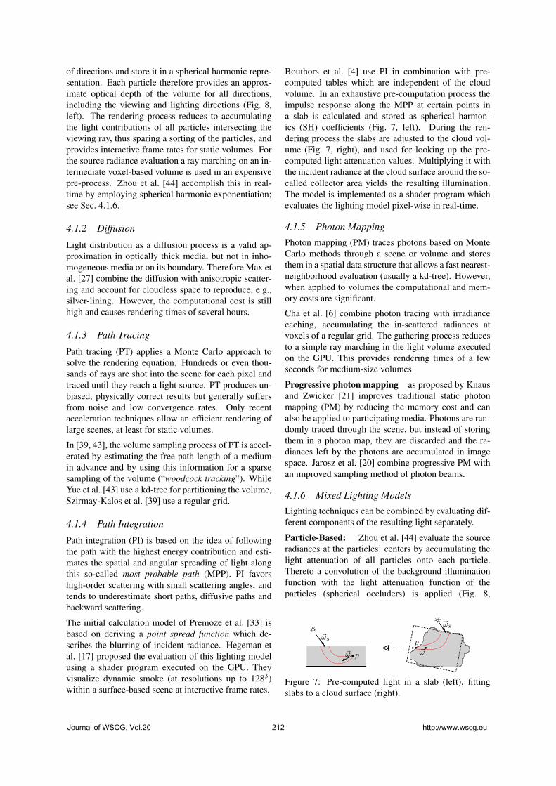
of directions and store it in a spherical harmonic repre-sentation. Each particle therefore provides an approx-imate optical depth of the volume for all directions,including the viewing and lighting directions (Fig. 8,left). The rendering process reduces to accumulatingthe light contributions of all particles intersecting theviewing ray, thus sparing a sorting of the particles, andprovides interactive frame rates for static volumes. Forthe source radiance evaluation a ray marching on an in-termediate voxel-based volume is used in an expensivepre-process. Zhou et al. [44] accomplish this in real-time by employing spherical harmonic exponentiation;see Sec. 4.1.6.

4.1.2 Diffusion

Light distribution as a diffusion process is a valid ap-proximation in optically thick media, but not in inho-mogeneous media or on its boundary. Therefore Max etal. [27] combine the diffusion with anisotropic scatter-ing and account for cloudless space to reproduce, e.g.,silver-lining. However, the computational cost is stillhigh and causes rendering times of several hours.

4.1.3 Path Tracing

Path tracing (PT) applies a Monte Carlo approach tosolve the rendering equation. Hundreds or even thou-sands of rays are shot into the scene for each pixel andtraced until they reach a light source. PT produces un-biased, physically correct results but generally suffersfrom noise and low convergence rates. Only recentacceleration techniques allow an efficient rendering oflarge scenes, at least for static volumes.

In [39, 43], the volume sampling process of PT is accel-erated by estimating the free path length of a mediumin advance and by using this information for a sparsesampling of the volume (“woodcock tracking”). WhileYue et al. [43] use a kd-tree for partitioning the volume,Szirmay-Kalos et al. [39] use a regular grid.

4.1.4 Path Integration

Path integration (PI) is based on the idea of followingthe path with the highest energy contribution and esti-mates the spatial and angular spreading of light alongthis so-called most probable path (MPP). PI favorshigh-order scattering with small scattering angles, andtends to underestimate short paths, diffusive paths andbackward scattering.

The initial calculation model of Premoze et al. [33] isbased on deriving a point spread function which de-scribes the blurring of incident radiance. Hegeman etal. [17] proposed the evaluation of this lighting modelusing a shader program executed on the GPU. Theyvisualize dynamic smoke (at resolutions up to 1283)within a surface-based scene at interactive frame rates.

Bouthors et al. [4] use PI in combination with pre-computed tables which are independent of the cloudvolume. In an exhaustive pre-computation process theimpulse response along the MPP at certain points ina slab is calculated and stored as spherical harmon-ics (SH) coefficients (Fig. 7, left). During the ren-dering process the slabs are adjusted to the cloud vol-ume (Fig. 7, right), and used for looking up the pre-computed light attenuation values. Multiplying it withthe incident radiance at the cloud surface around the so-called collector area yields the resulting illumination.The model is implemented as a shader program whichevaluates the lighting model pixel-wise in real-time.

4.1.5 Photon Mapping

Photon mapping (PM) traces photons based on MonteCarlo methods through a scene or volume and storesthem in a spatial data structure that allows a fast nearest-neighborhood evaluation (usually a kd-tree). However,when applied to volumes the computational and mem-ory costs are significant.

Cha et al. [6] combine photon tracing with irradiancecaching, accumulating the in-scattered radiances atvoxels of a regular grid. The gathering process reducesto a simple ray marching in the light volume executedon the GPU. This provides rendering times of a fewseconds for medium-size volumes.

Progressive photon mapping as proposed by Knausand Zwicker [21] improves traditional static photonmapping (PM) by reducing the memory cost and canalso be applied to participating media. Photons are ran-domly traced through the scene, but instead of storingthem in a photon map, they are discarded and the ra-diances left by the photons are accumulated in imagespace. Jarosz et al. [20] combine progressive PM withan improved sampling method of photon beams.

4.1.6 Mixed Lighting Models

Lighting techniques can be combined by evaluating dif-ferent components of the resulting light separately.

Particle-Based: Zhou et al. [44] evaluate the sourceradiances at the particles’ centers by accumulating thelight attenuation of all particles onto each particle.Thereto a convolution of the background illuminationfunction with the light attenuation function of theparticles (spherical occluders) is applied (Fig. 8,

~ωs

p~ω

p~ω

~ωs

Figure 7: Pre-computed light in a slab (left), fittingslabs to a cloud surface (right).


Figure 8: Pre-computed optical density at a particlecenter (left). Convolution of background illuminationwith the light attenuation by spherical occluders (right).

right). The functions are represented by low-orderspherical harmonics (SH) and the convolution is donein logarithmic space where the accumulation reducesto summing SH coefficients; a technique called SHexponentiation (SHEXP), introduced by Ren et al. [34]for a shadow calculation. For multiple scattering aniterative diffusion equation solver is used on the basisof the source radiance distribution. This includessolving linear systems of dimension n, with n beingthe number of particles. The approximation of thesmoke density field by a small number of particles(around 600 in their examples) allows interactive framerates under dynamic lighting conditions. However,the super-quadratic complexity in terms of the particlenumber prohibits the application to large volumes.

Surface-Based: Bouthors et al. [3] separately cal-culate the single and multiple-scattering componentsof light at the surface of a cloud layer. The single-scattering model reproduces silver lining at the silhou-ettes of clouds and back-scattering effects (glories andfog-bows). Multiple-scattering is evaluated by using aBRDF function, pre-calculated by means of path trac-ing. Inter-reflection of the cloud layer with the groundand sky is taken into account by a radiosity model. Theyachieve real-time rendering rates by executing the light-ing model on the GPU as a shader program.

4.1.7 Heuristic Lighting Models

Neyret [29] avoids costly physical simulations whena-priori knowledge can be used to simulate well-known lighting effects. He presents a surface-basedshading model for Cumulus clouds that simulatesinter-reflection in concave regions (light traps) and thecorona at the silhouette.

Wang [42] does not employ a lighting model at all, butlets an artist associate the cloud’s color to its height.

4.1.8 Acceleration Techniques

Pre-Computed Radiance Transfer: The lightingdistribution for static volumes under changing lightingconditions can be accelerated by pre-computing the ra-diance transfer through the model.

Lensch et al. [26] pre-compute the impulse response toincoming light for a mesh-based model. Local lightingeffects are simulated by a filter function applied to a

light texture. Looking up the pre-computed vertex-to-vertex throughput yields global lighting effects.Sloan et al. [38] use SH as emitters, simulate their dis-tribution inside the volume and store them as transfervectors for each voxel. The volume can be rendered ef-ficiently in combination with a shader-based local light-ing model under changing light conditions.Radiance Caching: Jarosz et al. [19] use radiancecaching to speed up ray marching rendering process.Radiance values and radiance gradients are stored as SHcoefficients within the volume and re-used.

4.2 Global IlluminationInter-cloud shadowing and indirect illumination cannotbe efficiently simulated by participating media lightingmodels. These effects require global illumination tech-niques, usually applied in surface-based scenes.

4.2.1 ShadowsSphere-based scene representations allow a fast shadowcalculation, either, e.g., by using SH for representingthe distribution of blocking geometries [34] (Fig. 8,right), or by accumulating shadows in image space [37].The CUDA implementation of the GigaVoxel algorithm[8] allows to render semi-transparent voxels and to castshadow rays. Employing the inherent cone tracing ca-pability produces soft shadows.

4.2.2 Indirect IlluminationVoxel cone tracing applied to a sparse octree on theGPU is used by Crassin et al. [9] for estimating indi-rect illumination. The illumination at a surface point isevaluated by sampling the neighborhood along a smallnumber of directions along cones.A fast ray-voxel intersection test for an octree-basedscene representation is used in Thiedemann et al. [40]for estimating near-field global illumination.

5 SUMMARY AND OUTLOOKIn the following table we summarize efficient lightingand rendering techniques for clouds with different typesof volume (rows) and boundary appearances (columns).

diffuse fractal sharpdense [6, 7, 10, 15] [4, 7, 11] [4, 42]

[16, 35, 44] [17, 22]thin [22, 36, 44] [11, 17, 36] do not existlayer [3]

The approaches surveyed represent a set of impres-sive but specialized solutions that employ fairly diversetechniques. However, all known approaches cover onlysome of the phenomena found in nature (see Sec. 1.1).Extensive memory usage or the algorithm’s complexityoften limit the size of a cloud volume. Thus, the realis-tic visualization of real-world cloud scenes still is andwill remain widely open for future research for years tocome.


Major future challenges to be tackled include theefficient handling of

• heterogeneous cloud scene rendering, i.e., the simul-taneous visualization of different cloud types, eachfavoring a specific cloud representation, lighting andrendering technique;

• large-scale cloud scenes, e.g., clouds over Europe;• cloud-to-cloud shadows and cloud inter-reflection,

i.e., the combination of global illumination tech-niques with participating media rendering;

• the inclusion of atmospheric scattering models forlighting clouds;

• cloud rendering at different scales, i.e., views ofclouds from close and far, and seamless transitionsin between, requiring continuous LOD techniques;

• temporal cloud animations implying dynamic vol-umes and employing cloud simulation models.

ACKNOWLEDGEMENTSWork supported by Austrian FFG Grant #830029.

6 REFERENCES[1] D. Bernabei, F. Ganovelli, N. Pietroni, P. Cignoni,

S. Pattanaik, and R. Scopigno. Real-time single scat-tering inside inhomogeneous materials. The VisualComputer, 26(6-8):583–593, 2010.

[2] A. Bouthors and F. Neyret. Modeling clouds shape. InEurographics, Short Presentations, 2004.

[3] A. Bouthors, F. Neyret, and S. Lefebvre. Real-time re-alistic illumination and shading of stratiform clouds. InEG Workshop on Natural Phenomena, Vienna, Austria,2006. Eurographics.

[4] A. Bouthors, F. Neyret, N. Max, É. Bruneton, andC. Crassin. Interactive multiple anisotropic scatter-ing in clouds. In Proc. ACM Symp. on Interactive 3DGraph. and Games, 2008.

[5] E. Cerezo, F. Perez-Cazorla, X. Pueyo, F. Seron, andF. X. Sillion. A survey on participating media renderingtechniques. The Visual Computer, 2005.

[6] D. Cha, S. Son, and I. Ihm. GPU-assisted high qualityparticle rendering. Comp. Graph. Forum, 28(4):1247–1255, 2009.

[7] C. Crassin, F. Neyret, S. Lefebvre, and E. Eisemann.GigaVoxels: Ray-guided streaming for efficient and de-tailed voxel rendering. In Proc. ACM SIGGRAPH Symp.on Interactive 3D Graph. and Games (I3D), Boston,MA, Etats-Unis, February 2009. ACM, ACM Press.

[8] C. Crassin, F. Neyret, M. Sainz, and E. Eisemann. GPUPro, chapter X.3: Efficient Rendering of Highly De-tailed Volumetric Scenes with GigaVoxels, pages 643–676. AK Peters, 2010.

[9] C. Crassin, F. Neyret, M. Sainz, S. Green, and E. Eise-mann. Interactive indirect illumination using voxel conetracing. Comp. Graph. Forum (Proc. Pacific Graph.2011), 30(7), 2011.

[10] Y. Dobashi, K. Kaneda, H. Yamashita, T. Okita, andT. Nishita. A simple, efficient method for realistic ani-mation of clouds. In Comp. Graphics (SIGGRAPH ’00Proc.), pages 19–28, 2000.

[11] D. S. Ebert, F. Musgrave, P. Peachey, K. Perlin, andS. Worley. Texturing & Modeling: A Procedural Ap-proach. Morgan Kaufmann, 3rd edition, 2003.

[12] V. Forest, L. Barthe, and M. Paulin. Real-time hierar-chical binary-scene voxelization. Journal of Graphics,GPU, & Game Tools, 14(3):21–34, 2009.

[13] E. Gobbetti, F. Marton, and J. A. Iglesias Guitián. Asingle-pass GPU ray casting framework for interactiveout-of-core rendering of massive volumetric datasets.The Visual Computer, 24(7-9):797–806, 2008. Proc.CGI 2008.

[14] O. Gourmel, A. Pajot, M. Paulin, L. Barthe, andP. Poulin. Fitted BVH for fast raytracing of metaballs.Comp. Graph. Forum, 29(2):281–288, May 2010.

[15] M. J. Harris, W. V. Baxter, Th. Scheuermann, andA. Lastra. Simulation of cloud dynamics on graph-ics hardware. In Proc. SIGGRAPH/Eurographics ’03Conference on Graph. Hardware, pages 92–101. Euro-graphics Association, 2003.

[16] M. J. Harris and A. Lastra. Real-time cloud rendering.Comput. Graph. Forum (Proc. IEEE Eurographics ’01),20(3):76–84, 2001.

[17] K. Hegeman, M. Ashikhmin, and S. Premože. A light-ing model for general participating media. In Proc.Symp. on Interactive 3D Graph. and Games (I3D ’05),pages 117–124, New York, NY, USA, 2005. ACM.

[18] R. Hufnagel, M. Held, and F. Schröder. Large-scale,realistic cloud visualization based on weather forecastdata. In Proc. IASTED Int. Conf. Comput. Graph. andImaging (CGIM’07), pages 54–59, February 2007.

[19] W. Jarosz, C. Donner, M. Zwicker, and H. W. Jensen.Radiance caching for participating media. ACM Trans.Graph., 27(1):1–11, 2008.

[20] W. Jarosz, D. Nowrouzezahrai, R. Thomas, P. P. Sloan,and M. Zwicker. Progressive photon beams. ACMTrans. Graph. (SIGGRAPH Asia 2011), 30(6):181:1–181:12, December 2011.

[21] C. Knaus and M. Zwicker. Progressive photon map-ping: A probabilistic approach. ACM Trans. Graph.,30(3):25:1–25:13, May 2011.

[22] J. M. Kniss, S. Premože, Ch. D. Hansen, and D. S.Ebert. Interactive translucent volume rendering andprocedural modeling. In Proc. IEEE Visualization ’02,pages 109–116. IEEE Comput. Society Press, 2002.

[23] J. M. Kniss, S. Premože, Ch. D. Hansen, P. Shirley, andA. McPherson. A model for volume lighting and mod-eling. IEEE Trans. Visualiz. Comput. Graph., 9(2):150–162, 2003.

[24] H.-J. Koppert, F. Schröder, E. Hergenröther, M. Lux,and A. Trembilski. 3d visualization in daily operationat the dwd. In Proc. ECMWF Worksh. on Meteorolog.Operat. Syst., 1998.

[25] S. Laine and T. Karras. Efficient sparse voxel octrees.


In Proc. ACM SIGGRAPH Symp.on Interactive 3DGraph.and Games (I3D ’10), pages 55–63, New York,NY, USA, 2010. ACM.

[26] H. P. A. Lensch, M. Goesele, Ph. Bekaert, J. Kautz,M. A. Magnor, J. Lang, and H.-P. Seidel. Interactiverendering of translucent objects. In Proc. Pacific Conf.on Comp. Graph. and Appl. (PG ’02), pages 214–. IEEEComputer Society, 2002.

[27] N. Max, G. Schussman, R. Miyazaki, and K. Iwasaki.Diffusion and multiple anisotropic scattering for globalillumination in clouds. Journal of WSCG 2004,12(2):pp. 277, 2004.

[28] A. Miller, V. Jain, and J. L. Mundy. Real-time renderingand dynamic updating of 3-d volumetric data. In Proc.Worksh. on General Purpose Process. on Graph. Pro-cess. Units (GPGPU-4), pages 8:1–8:8, New York, NY,USA, 2011. ACM.

[29] F. Neyret. A phenomenological shader for the renderingof cumulus clouds. Technical Report RR-3947, INRIA,May 2000.

[30] T. Nishita, Y. Dobashi, and E. Nakamae. Display ofclouds taking into account multiple anisotropic scatter-ing and skylight. Comput. Graphics (SIGGRAPH ’96Proc.), pages 379–386, 1996.

[31] K. Perlin and E. M. Hoffert. Hypertexture. In Comp.Graph. (SIGGRAPH ’89 Proc.), volume 23 (3), pages253–262, July 1989.

[32] S. D. Porumbescu, B. Budge, L. Feng, and K. I. Joy.Shell maps. ACM Trans. Graph., 24:626–633, July2005.

[33] S. Premože, M. Ashikhmin, R. Ramamoorthi, andSh. K. Nayar. Practical rendering of multiple scatteringeffects in participating media. In Proc. EurographicsWorksh. on Render. Tech., pages 363–373. EurographicsAssociation, June 2004.

[34] Z. Ren, R. Wang, J. Snyder, K. Zhou, X. Liu, B. Sun,P. P. Sloan, H. Bao, Q. Peng, and B. Guo. Real-time softshadows in dynamic scenes using spherical harmonicexponentiation. In ACM Trans. Graph. (SIGGRAPH’06 Proc.), pages 977–986, 2006.

[35] K. Riley, D. S. Ebert, Ch. D. Hansen, and J. Levit. Visu-ally accurate multi-field weather visualization. In Proc.IEEE Visualization (VIS’03), pages 37–, Washington,DC, USA, 2003. IEEE Computer Society.

[36] J. Schpok, J. Simons, D. S. Ebert, and Ch. D. Hansen.A real-time cloud modeling, rendering, and animationsystem. In Proc. SIGGRAPH/Eurographics ’03 Symp.Computer Anim., pages 160–166. Eurographics Associ-ation, July 2003.

[37] P. P. Sloan, N. K. Govindaraju, D. Nowrouzezahrai, andJ. Snyder. Image-based proxy accumulation for real-time soft global illumination. In Proc. Pacific Conf. onComp. Graph. and Appl., pages 97–105, Washington,DC, USA, 2007. IEEE Computer Society.

[38] P. P. Sloan, J. Kautz, and J. Snyder. Precomputed radi-ance transfer for real-time rendering in dynamic, low-frequency lighting environments. In ACM Trans. Graph.

(SIGGRAPH ’02 Proc.), pages 527–536, July 2002.

[39] L. Szirmay-Kalos, B. Tóth, and M Magdics. Free pathsampling in high resolution inhomogeneous participat-ing media. Comp. Graph. Forum, 30(1):85–97, 2011.

[40] S. Thiedemann, N. Henrich, Th. Grosch, and St.Mueller. Voxel-based global illumination. In ACMSymp. on Interactive 3D Graph. and Games (I3D),2011.

[41] A. Trembilski and A. Broßler. Surface-based efficientcloud visualisation for animation applications. Journalof WSCG, 10(1–3), 2002.

[42] N. Wang. Realistic and fast cloud rendering in com-puter games. In SIGGRAPH ’03: ACM SIGGRAPH2003 Sketches & Applications, pages 1–1, New York,NY, USA, 2003. ACM.

[43] Y. Yue, K. Iwasaki, B. Y. Chen, Y. Dobashi, andT. Nishita. Unbiased, adaptive stochastic sampling forrendering inhomogeneous participating media. ACMTrans. Graph. (SIGGRAPH Asia 2010), 29:177:1–177:8, December 2010.

[44] K. Zhou, Z. Ren, St. Lin, H. Bao, B. Guo, and H. Y.Shum. Real-time smoke rendering using compensatedray marching. ACM Trans. Graph., 27(3):36:1–36:12,August 2008.


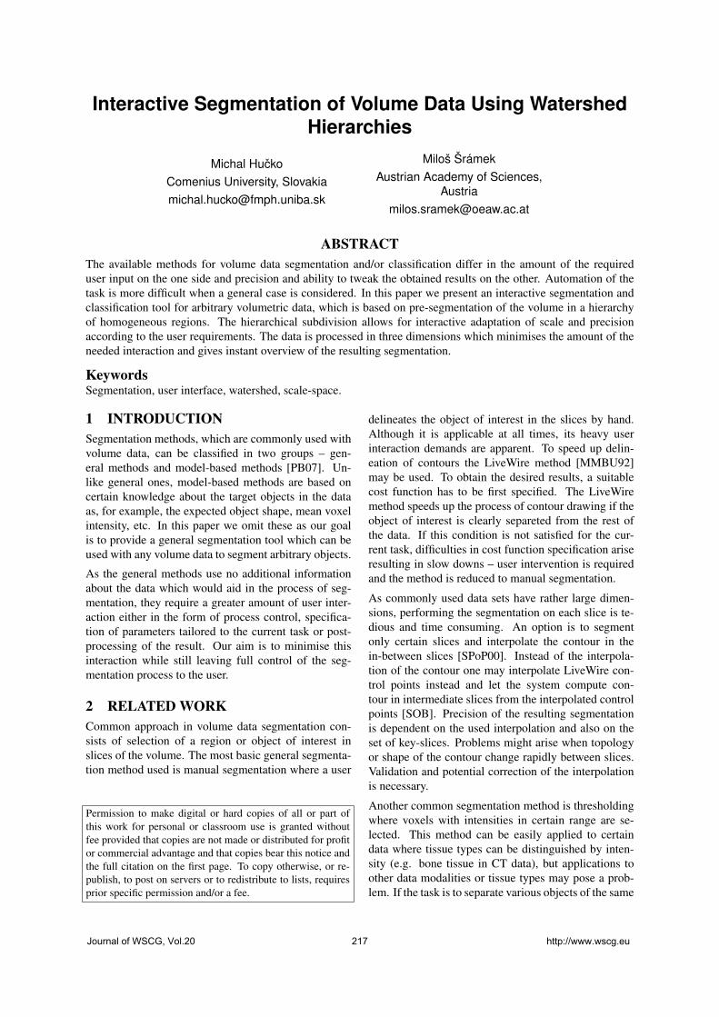
Interactive Segmentation of Volume Data Using WatershedHierarchies

Michal HuckoComenius University, [email protected]

Miloš ŠrámekAustrian Academy of Sciences,

[email protected]

ABSTRACTThe available methods for volume data segmentation and/or classification differ in the amount of the requireduser input on the one side and precision and ability to tweak the obtained results on the other. Automation of thetask is more difficult when a general case is considered. In this paper we present an interactive segmentation andclassification tool for arbitrary volumetric data, which is based on pre-segmentation of the volume in a hierarchyof homogeneous regions. The hierarchical subdivision allows for interactive adaptation of scale and precisionaccording to the user requirements. The data is processed in three dimensions which minimises the amount of theneeded interaction and gives instant overview of the resulting segmentation.

KeywordsSegmentation, user interface, watershed, scale-space.

1 INTRODUCTIONSegmentation methods, which are commonly used withvolume data, can be classified in two groups – gen-eral methods and model-based methods [PB07]. Un-like general ones, model-based methods are based oncertain knowledge about the target objects in the dataas, for example, the expected object shape, mean voxelintensity, etc. In this paper we omit these as our goalis to provide a general segmentation tool which can beused with any volume data to segment arbitrary objects.

As the general methods use no additional informationabout the data which would aid in the process of seg-mentation, they require a greater amount of user inter-action either in the form of process control, specifica-tion of parameters tailored to the current task or post-processing of the result. Our aim is to minimise thisinteraction while still leaving full control of the seg-mentation process to the user.

2 RELATED WORKCommon approach in volume data segmentation con-sists of selection of a region or object of interest inslices of the volume. The most basic general segmenta-tion method used is manual segmentation where a user


delineates the object of interest in the slices by hand.Although it is applicable at all times, its heavy userinteraction demands are apparent. To speed up delin-eation of contours the LiveWire method [MMBU92]may be used. To obtain the desired results, a suitablecost function has to be first specified. The LiveWiremethod speeds up the process of contour drawing if theobject of interest is clearly separeted from the rest ofthe data. If this condition is not satisfied for the cur-rent task, difficulties in cost function specification ariseresulting in slow downs – user intervention is requiredand the method is reduced to manual segmentation.

As commonly used data sets have rather large dimen-sions, performing the segmentation on each slice is te-dious and time consuming. An option is to segmentonly certain slices and interpolate the contour in thein-between slices [SPoP00]. Instead of the interpola-tion of the contour one may interpolate LiveWire con-trol points instead and let the system compute con-tour in intermediate slices from the interpolated controlpoints [SOB]. Precision of the resulting segmentationis dependent on the used interpolation and also on theset of key-slices. Problems might arise when topologyor shape of the contour change rapidly between slices.Validation and potential correction of the interpolationis necessary.

Another common segmentation method is thresholdingwhere voxels with intensities in certain range are se-lected. This method can be easily applied to certaindata where tissue types can be distinguished by inten-sity (e.g. bone tissue in CT data), but applications toother data modalities or tissue types may pose a prob-lem. If the task is to separate various objects of the same


tissue type thresholding may be used for preprocessingto reject clearly non-target voxels and thus localise thearea of interest.

Two methods based on detection of homogeneousregions instead of contours are worth mentioning.General region growing requires user specified seedpoints and a suitable homogeneity criterion. Data isflooded from the seed points as long as the homo-geneity criterion is satisfied, creating a homogeneousregion. The watershed segmentation [VS91] is usuallyperformed on a gradient image, which is treated asa topographic height map. Homogeneous regionswith voxels with small gradient magnitude formvalleys having voxels with high gradient magnitude onregion borders as ridges. Although there exist variousalgorithms for computing the watershed transform,variants of two approaches are common – simulationof downhill water flow for each voxel or immersingof the relief into water. Exhaustive study of existingwatershed algorithms is provided by Roedink andMeijster [RM00].

A broader overview and more detailed descriptionof the existing segmentation methods can be foundin [PB07].

2.1 Interaction techniquesAll of the previously mentioned segmentation ap-proaches differ in the way how a user can interact withthe data to modify a partial result until the desired seg-mentation is achieved. For example, when delineatinga contour the user directly sees the partial result andcan undo recent steps if the contour starts to divergefrom the desired position.

Thresholding requires numeric input – the threshold.Usually, a user is provided with a histogram from whichthe most suitable threshold value can be estimated.Clean separation of various tissue types based only onvoxel intensity is rare and thus it may be difficult to findan optimal threshold value. Usage of other methods forrefining the segmentation from thresholding (morpho-logic operations, connected component labeling, etc) istherefore convenient [STBH92].

Watershed segmentation produces a highly over-segmented result, especially if the data is spoiled bynoise. Some methods allow merging of neighbour-ing regions if the shared border is weak (gradientmagnitude is low). This situation is illustrated infigure 1 which shows gradient magnitude image of aCT head dataset slice – the corresponding watershedsegmentation can be seen in figure 3 (red borders).The aim is to create segmentation in which the targetobject is labeled by a unique label. If this is nothappening user intervention is usually required. Forexample, an interaction technique called marker-basedwatershed segmentation can be used [HP03], where a

Figure 1: Slice from the Visible human male [Ack98]CT dataset with corresponding gradient magnitude im-age on right.

user specifies special include and exclude points in thedata which prohibit merging of neighbouring regions ifnew region would contain markers of both types.

Watershed hierarchies [Beu94] were used in a tech-nique based on interaction with slice views by Cateset al [CWJ05]. In such hierarchy, the order in whichregions are merged defines a binary merge tree. Orig-inal regions form leaves and non-leaf nodes representregions formed by merging of two regions – its childrennodes. This tree may be used to segment an object froma data with a possibility to select large parts of the ob-ject by specification of high-positioned tree nodes andto refine the border by adding/removing low-positionednodes.

In the paper by Armstrong et al [APB07] an extensionof LiveWire or Intelligent Scissors called Live Surfacewas proposed. Data is presegmented into hierarchy ofregions. Initial regions are computed using toboggan-ing [MB99] creating result equivalent to watershed seg-mentation (depends on the used watershed definition).For merging of the regions for higher levels in the hi-erarchy a special metric is used, which is based on themean voxel intensity/colour and intensity/colour vari-ance of a region. Segmentation is done by specifyingtwo types of markers – inner and outer – which are thenused to create a graph-cut in the region neighbourhoodgraph with minimal cost. Markers can be entered onan arbitrary cross section of the volume or directly inthe 3D view allowing to add/remove parts to/from theborder of an already segmented object.

3 THE SEGMENTATION TOOLAll of the segmentation approaches mentioned in theprevious section were either proposed for two dimen-sional images or, if targeted to segmentation of 3D data,were used only for interaction in two dimensional space– on respective slices – or provided limited possibilitiesto modify the resulting segmentation directly in the 3Dvisualisation of the data. In our approach we let the userdirectly control the segmentation process by selectingfragments of the target object in 3D space. As manualsegmentation by pixels/voxels is too cumbersome, data


Figure 2: Measured dependency of mean region size onthe Gaussian filter sigma. Three data sets were used– an MRI head, VHP male CT head and VHP femalecolour head dataset. Measured was diameter of mini-mal bounding sphere centered at the region’s centre ofmass.

is pre-segmented by the watershed transform as it cre-ates homogeneous regions which can be used instead ofsingle voxels.

3.1 PreprocessingThe watershed segmentation produces highly over-segmented results, because for each local minimum inthe (usually gradient image of) original data a regionis created. This can be a serious problem especiallyif noise is present in the data. To cope with this,data is usually first smoothed by the Gaussian filter.Smoothing, however, also shifts edges and removesweak edges, resulting in merging of regions which auser might desire in certain cases separated. Therefore,we perform the watershed segmentation on a sequenceof derived data sets where each one is produced fromthe original by smoothing with a gradually increasingdegree (increasing of the Gaussian sigma). As Koen-derink showed [Koe84] this produces a set of imageswhere on each image details smaller than certain sizeare increasingly ignored (the scale-space approach).As can be seen in figure 2, measurements on three dif-ferent head datasets showed that dependency of meanbounding sphere diameter of regions on used Gaussianfilter sigma can be approximated with function 1.

d(σ) = 5(σ −1)+10 (1)

To further reduce the starting number of regions, regionmerging based on mean region intensity or some othercriterion can be used.

In order to correct position of the shifted edges, causedby smoothing, to the original position specified by theunsmoothed data or at least data at the lowest level ofsmoothing, an aligned region hierarchy is build. Spa-tial alignment of borders of corresponding regions ondifferent hierarchy levels is achieved by the techniquebased on the maximum number of spatially overlappingvoxels [SD02]. Thus, if later required, aligned regions

Figure 3: Three levels of watershed segmentation onvisible human – male CT dataset. In the red channelare boundaries of regions for Gaussian smoothing withsigma 3, in green for sigma 5 and in blue for sigma 7.Overlapping boundaries are blended. On the left are theoriginal watersheds, on the right the regions are alignedshowing only red, yellow (red plus green) and white (allthree levels) boundaries.

positioned higher in the hierarchy can be unambigu-ously decomposed to multiple smaller regions on somelower level.

As the last step of preprocessing the relevant neigh-bour information is extracted from the original voxeldata and stored in a file. The described technique worksequally well for scalar data (CT and MRI scans) as wellas for multi-field data (dual energy CT, T1, T2 and PDMRI data etc). In the second case the watershed trans-form is performed on a gradient volume obtained asmaximum of individual gradient fields.

3.2 GUI interactionGUI of the segmentation application is shown in Fig-ure 4. In this section all parts of the application as wellas the segmentation workflow will be explained.

After the hierarchy is loaded into the application it isdisplayed in a tree widget allowing the user to navi-gate through it. Hovering or selecting a node highlightsthe corresponding region in a 3D visualisation window(Figure 5). This allows the user to choose an initialfragment of the region of interest. Depending on the tar-get object and created hierarchy, regions on higher lev-els might consist of multiple target objects (e.g. variousbones of skull). As pre-segmentation was performed atvarious scale levels, there is no need to repeat the pro-cess when the aforementioned problem arises – movingto lower levels in the hierarchy until the objects are sep-arated is possible.

After the initial region is selected it is possible to dis-play neighbouring regions which satisfy certain similar-ity criteria (Figure 6, also see section 3.3). The user canthen select either one neighbour belonging to the targetobject by clicking into the 3D view or by selecting theneighbour in the list or can select all neighbors. De-selection of an undesired region is possible in a similarway, too. Once a neighbour is added/removed to/from


Figure 4: The segmentation tool: the region hierarchy is on the right. Left side from top to bottom: the list ofselected regions, classification classes, the list similar neighbours of the regions in selection. At centre-bottomsimilarity criteria can be specified and above is the 3D visualisation and interaction window.

Figure 5: Selection of objects using the tree widget.The scene consist of concentric spheres/ellipsoids withdifferent density and was intentionally spoiled by noiseand superimposed low frequency density variation tomake segmentation of the ellipsoids by thresholdingimpossible. Left: A region on the highest hierarchylevel (white) was selected. One can see that it is com-posed of pieces of several ellipsoids. I we go down inthe hierarchy (bottom row, in this case by two levelsof the hierarchy), these pieces are separated and can beindividually selected. The yellow region is a partiallysegmented and labeled part of the central sphere.

the selection, updated neighbours of the new selectionare displayed. This allows traversal of the target objectuntil all fragments are in the selection. Now classifica-tion class for the object can be created and all selectedregions can be classified (Figure 6 right). Already clas-sified regions are during selection refining displayeddimmed to provide context whereas the current selec-tion is always highlighted.

3.3 Similarity criteriaTo decide whether neighbouring regions are similar weimplemented five different similarity criteria. Each cri-terion can be turned on or off and has a separate thresh-old value. When deciding whether two neighboring re-gions are similar all criteria which are turned on haveto return a positive answer. Detailed description of thesimilarity criteria can be found below.

When searching for similar neighbours all neighbour-ing regions of the regions in the current selection arevisited. As the selection might contain regions on dif-ferent levels in the hierarchy we have to prevent multi-ple inclusion of same region – once directly and secondtime by including parent of the region. Naturally, re-gions positioned higher in the hierarchy are accepted infavor of the lower positioned child.

A second issue arises from the fact that we would liketo move to a lower level of the hierarchy and to repeatthe search for similar neighbors there, if we were notsuccessful on a higher level. In this case, first, all re-gions in the selection are decomposed to regions onthe lowest level – some lowest-level regions were di-rectly present in the selection and some were selectedindirectly by selection of its ancestor. Now we iteratethrough all pairs of the selected lowest-level regionsand their neighbours (also at the lowest level). Forboth regions in the pair we ascend as many levels upin the hierarchy, until the original region in the selec-tion which was decomposed to the currently processedlowest-level region is found. This leaves us with a listof pairs – (indirectly) selected region with its neighbour


– for each level not higher than level of the original se-lected region. Subsequently we start with the similaritytests. If a region and its neighbor on the higher leveldo not pass the selected similarity test we descent byone level and again perform the tests. By this higherpositioned similar neighbours are found first.A detailed description of the different similarity criteriafollows:

Mean intensity Simple criterion comparing mean in-tensities of neighbouring regions. Difference in theintensities have to be in the specified interval for thetest to pass. If the data contains multiple bands, thetest must pass for all bands to be considered success-ful.

Similar neighbors In this criterion the prevalent di-rections of intensities in the region’s neighborhoodare compared. All neighbors of a region are vis-ited and their center of mass is computed by aver-aging their geometric centroids weighted by theirmean intensity. Subsequently, the direction vector,which points in the direction of growing intensity, isobtained by subtracting the center of mass from thegeometric centroid of the region. Comparison of anangle between such vectors of two neighboring re-gions against a user defined threshold yields resultof the similarity test.

Surface to volume ratio As working directly withthe volume data would be slow and would increasememory requirements significantly, only derivedinformation is used – mean intensity of a region,voxel count, etc. To compare region shapes ratioof the number of region’s surface voxels to itstotal voxel count is used. The computed value isnormalized to the [0,1] range where 0 representssphere-like objects and 1 string-like objects.

Weak borders For two regions to be similar in this cri-terion their border should have small mean gradi-ent magnitude. Unlike the mean intensity criterionwhich compares mean values for whole regions, thiscriterion uses the original gradient data which wereused during the creation of the most-detailed water-shed segmentation. Intensity of the regions is n thiscriterion irrelevant.

Continuous border This criterion tries to find borderin the data which spans multiple region boundaries.For two regions to pass this test they have to havea common neighbor. Both faces – first region withthe common neighbor and second region with thecommon neighbor – have to be similar. For this, theangle between mean normal/gradient vectors of thefaces is examined. Faces which are too small areignored as their mean gradient vectors are based ontoo small set of values.

4 RESULTSThe application was implemented in C++ and usesOpenGL with GLSL. It was tested on the VHP dataset(the male head CT dataset). Individual bones of theskull, which are connected without a well defined bor-der, were successfully segmented (figure 7 left). Wealso tested the application on an MRI scan of a humanhead. Figure 7 right shows segmentation of the braincortex with certain gyri labeled as separate objects.Preprocessing with three levels of watershed hierar-chies and 3 additional levels of merging by density sim-ilarity took about 10 minutes. Both segmentations wereproduced in about 30 minutes.In contrast to other methods, we intentionally omittedthe possibility to interact through slices or cross sec-tions to investigate the possibility for interaction onlythrough the 3D view. If desired, display of the slicesor cross sections can be easily added to the application,which may be then used for an initial selection.If compared to traditional segmentation approaches,our method is most similar to region growing – assum-ing that mean intensity criterion is used. Neighboursto selected regions having similar intensity can be iter-atively added to the selection until only regions withlarge difference in intensity remain. Because of themanual operation, user can omit regions which evaluatesimilar, but are not part of the target object. This can beessential when separating two or more objects of sameor similar intensity, but different shape (as exemplifiedby segmentetion of the brain cortex in individual gyri).Automatic, or semi-automatic methods fail to separatethese, if the interface is too weak or not present due topartial volume effect.

5 CONCLUSIONThe presented segmentation and classification tool al-lows fast insight into data and fast segmentation of tar-get structures while still leaving full control of the seg-mentation in user’s hands. The amount of user interac-tion depends on data properties – resolution, presenceof noise or other artefacts. Different similarity criteriawere presented which should simplify and thus speed-up localisation of similar neighbouring regions in thedata. Still, the user interaction is mainly done directlyin the 3D visualisation window instead of slices. Opera-tion in the visualisation window also gives direct visualfeedback.The concept was tested on the VHP dataset by segmen-tation of the bones of human skull and on MRI data bysegmentation of respective gyri of the brain cortex.

6 ACKNOWLEDGEMENTSThis work was supported by the Slovak Research andDevelopment Agency under the contract No. APVV-20-056105, Science Grant Agency (VEGA, Slovakia)


Figure 6: From left: selection of similar neighbors starting from an initial region. The blue regions are selectioncandidates (density similarity was used). White objects are already selected objects, the green color means that theobject has already been labeled. The highlighted blue candidate object can be individually added to the selectionor all candidates can be added at once.

Figure 7: Left: segmentation of skull bones of the VHP male CT head dataset. Right: segmentation of brain andgyri in the MRI head dataset.

under contract No. 1/0631/11, FWF Austria under con-tract No. TRP-67-N23 and Comenius University undercontract No. UK/229/2012. Miloš Šrámek is currentlyon leave at the the Institute of Computer Graphics andAlgorithms, Vienna University of Technology, Vienna,Austria.

7 REFERENCES[Ack98] M.J. Ackerman, The visible human project, Proceed-

ings of the IEEE 86 (1998), no. 3, 504–511.

[APB07] Christopher J. Armstrong, Brian L. Price, andWilliam A. Barrett, Interactive segmentation of imagevolumes with live surface, Comput. Graph. 31 (2007),no. 2, 212–229.

[Beu94] S. Beucher, Watershed, hierarchical segmentation andwaterfall algorithm, Mathematical morphology and itsapplications to image processing (J. Serra and P. Soille,eds.), Kluwer Academic Publishers, 1994, pp. 69–76.

[CWJ05] Joshua E. Cates, Ross T. Whitaker, and Greg M. Jones,Case study: an evaluation of user-assisted hierarchi-cal watershed segmentation., Medical Image Analysis(2005), 566–578.

[HP03] Horst K. Hahn and Heinz-Otto Peitgen, Iwt-interactivewatershed transform: a hierarchical method for effi-cient interactive and automated segmentation of multi-dimensional gray-scale images, vol. 5032, SPIE, 2003,pp. 643–653.

[Koe84] J.J. Koenderink, The structure of images, BiologicalCybernetics 50 (1984), no. 5, 363–370.

[MB99] E.N. Mortensen and W.A. Barrett, Toboggan-based in-telligent scissors with a four parameter edge model,

Proceedings of the IEEE Computer Vision and PatternRecognition (CVPR ’99), vol. II, 1999, pp. 452–458.

[MMBU92] Eric Mortensen, Bryan Morse, William Barrett, and Ja-yaram Udupa, Adaptive boundary detection using Live-Wire two-dimensional dynamic programming, IEEEComputers in Cardiology (1992), 635–638.

[PB07] B. Preim and D. Bartz, Visualization in medicine: the-ory, algorithms, and applications, The Morgan Kauf-mann series in computer graphics, Morgan Kaufmann,2007.

[RM00] Roerdink and Meijster, The watershed transform: Def-initions, algorithms and parallelization strategies,FUNDINF: Fundamenta Informatica 41 (2000).

[SD02] M. Sramek and L. I. Dimitrov, Segmentation of to-mographic data by hierarchical watershed transform,Journal of Medical Informatics and Technologies 3(2002), 161–169.

[SOB] Zein Salah, Jasmina Orman, and Dirk Bartz, Live-wirerevisited.

[SPoP00] Andrea Schenk, Guido Prause, and Heinz otto Peit-gen, Efficient semiautomatic segmentation of 3d objectsin medical images, In Proc. of Medical Image Com-puting and Computer-assisted Intervention (MICCAI,Springer, 2000, pp. 186–195.

[STBH92] T. Schiemann, U. Tiede, M. Bomans, and K. H. Höhne,Interactive 3D-segmentation, Visualization in Biomed-ical Computing 1992, Proc. SPIE 1808 (R. A. Robb,ed.), SPIE, Chapel Hill, NC, 1992, pp. 376–383.

[VS91] L. Vincent and P. Soille, Watersheds in digital spaces:An efficient algorithm based on immersion simulations,IEEE Transactions on Pattern Analysis and MachineIntelligence 13 (1991), 583–598.


Reconstructing Power Cables From LIDAR Data

Using Eigenvector Streamlines of the

Point Distribution Tensor Field

Marcel Ritter

Institute of Basic Sciences in Civil Engineering2

University of Innsbruck

[email protected]

Werner Benger

Center for Computation & Technology1

Institute for Astro- and Particle Physics2

[email protected]

[email protected]

ABSTRACT

Starting from the computation of a covariance matrixof neighborhoods in a point cloud, streamlines are uti-lized to reconstruct lines of linearly distributed pointsfollowing the major Eigenvector of the matrix. Thistechnique is similar to fiber tracking in diffusion ten-sor imaging (DTI), but in contrast is done mesh-free.Different weighting functions for the computation ofthe matrix and for the interpolation of the vector in thepoint cloud have been implemented and compared onartificial test cases. A dataset stemming from light de-tect and ranging (LIDAR) surveying served as a testbedfor parameter studies where, finally, a power cable wasreconstructed.Keywords: tensor-field visualization; streamlines;mesh-free methods; particle systems; point cloud; co-variance matrix; fiber tracking; LIDAR; DT-MRI

1 INTRODUCTION

Reconstructing lines from point clouds has an impor-tant application in light detection and ranging applica-tions (LIDAR). The surveying of power lines and theirgeometrical analysis is of great interest for companiesthat transmit electrical energy. Large networks of elec-tric facilities have to be maintained to guarantee stableelectrical power supply and prevent power outages. LI-DAR surveying is a suitable technique to either detectdamages on the electrical facilities or detect high grow-ing vegetation in power line corridors [19] [15]. We

Permission to make digital or hard copies of all or part ofthis work for personal or classroom use is granted withoutfee provided that copies are not made or distributed for profitor commercial advantage and that copies bear this noticeand the full citation on the first page. To copy otherwise,or republish, to post on servers or to redistribute to lists,requires prior specific permission and/or a fee.

1 Louisiana State University, Baton Rouge, LA-70803, USA2 University of Innsbruck, Technikerstraße 13/4, A-6020 Innsbruck,

Austria

experiment on a new method to reconstruct linear struc-tures, stemming from airborne LIDAR surveying. Weutilize a method inspired by diffusion tensor imaging(DTI) fiber tracking developed, originally, for magneticresonance imaging (MRI) to track neuronal structuresin the human brain [5].

1.1 Related Work

Current algorithms for reconstructing power lines areusually based on data filtering followed by a segmen-tation of the filtered and reduced point cloud either di-rectly on the point cloud data or on a rastered 2D im-age. Melzer [18] first computes a digital terrain model(DTM) by using the method by Kraus [14] to removeterrain points. The remaining points are projected ontoa 2D gray-scale raster (image). A Hough-Transform(e.g. [11]) is utilized iteratively to detect straight lines.Later, Melzer [17] improved the segmentation of LI-DAR data also for power cables, based on the so calledmean shift clustering, originally developed for patternrecognition [9]. Liu et al. [16] introduced a methodol-ogy based on statistical analysis to first remove groundpoints. Then, they project points onto a 2D gray-scale raster (image) and do a Hough-Transform simi-lar to Melzer [18], but use a different technique for theHough-Transform [8] to detect straight lines. Jwa etal. [13] developed a four step method. First they se-lect power-line candidates, by utilizing a voxel basedHough-Transform to recognize linear regions. After afiltering process they construct line segments based ongeometric orientation rules and, finally, use a voxel-based piece-wise line detector to reconstruct the linegeometries.

Weinstein et al. [23] worked on tracking linear struc-tures in diffusion tensor data stemming from MRI. Be-sides following the major Eigenvector they developedsome rules for overcoming areas of not linear diffusion.The flow of Eigenvectors was also used for segmen-tation and clustering in brain regions as, for example,shown in [6] and [20]. Jones discusses the study of con-nections in human brains. He states that tracking the


diffusion directions is still not solved a in stable wayand is an active research area [12].

Our work is based on previous work on the direct vi-sualization of the covariance matrix describing the lo-cal geometric properties of a neighborhood distributionwithin in a point cloud, the so called point distributiontensor [21].

1.2 Our Approach

In our method we do not want to remove any pointsbut operate on the entire dataset to avoid artifacts dueto a complex point removal method. Instead, we firstcompute the point distribution tensor for each point.Eigen-analysis of the tensor yields the major Eigenvec-tor, which indicates the dominant orientation of a pointdistribution. We may follow this orientation by comput-ing streamlines along this dominant Eigenvector field inregions where one Eigenvalue dominates, so-called lin-ear regions. In contrast, regions where the points aredistributed more isotropic, are indicated by the pointdistribution tensor’s Eigenvalues becoming more simi-lar values. We want to avoid these regions, as they willnot correspond to power cables. This approach is verysimilar to the fiber-tracking approach in medical visu-alization, but in our case the integration of the Eigen-vectors needs to be done in a mesh-free way, merelyon a point distribution rather than uniform grids. Thus,it can be applied to airborne LIDAR data without re-sampling to uniform grids (which would reduce dataresolution and introduce artifacts due to the chosen re-sampling method).

1.3 Overview of the Paper

Section 2 presents the mathematical background anddescribes the implementation of the algorithm in sec-tion 2.2. Section 2.3 shows verifications by means ofsimple artificial point distributions. Here, the influenceof different weighting functions on the tensor computa-tion and the vector field interpolation during streamlineintegration is investigated. Also, two different numeri-cal integration schemes are tested. In section 3 one setof power cables is reconstructed from a LIDAR data setstemming from actual observations. We then explorethe available parameter space for weighting and inte-gration in order to identify the best values for the givenscenario.

2 ALGORITHM

2.1 Background

In [21] we defined the “point distribution tensor” of aset of N points Pi : i = 1, ...,N as

S(Pi) =1N

N

∑k=1

ωn(|tik,r|)(tik ⊗ tτ

ik), (1)

whereby ⊗ denotes the tensor product, τ the transposeand tik = Pi −Pk. ωn(|tik|,r) is a weighting function de-pendent on the distance of a point sample to a centerpoint Pi and a radius of a neighborhood r, which canbe constant or defined by a scalar field on the points:r(Pi). We did not find a generally optimal solution forthe weighting function, but implemented seven choicesfor our first investigations:

ω1 = 1 (2)

ω2 = 1− x/r (3)

ω3 = 1− (x/r)2 (4)

ω4 = r/x2 (5)

ω5 =

1− 32 a2 + 3

4 a3 0 ≤ a < 114 (2−a)3 1 ≤ a < 2

0 otherwise(6)

ω6 =

( 52 −b)4 −5( 3

2 −b)3 +10( 12 − v)b [0, 1

2 )

( 52 −b)4 −5( 3

2 −b)3 [ 12 ,

32 )

( 52 −b)4 [ 3

2 ,52 )

0 [ 52 ,∞)

(7)

ω7 =

(3− c)5 −6(2− c)5 +15(1− c)5 [0,1)(3− c)5 −6(2− c)5 [1,2)

(3− c)5 [2,3)0 [3,∞)

(8)

with a := 2xr

, b := 2.5xr

and c := 3.0xr

, illustrated in Fig-ure 1. The three functions ω5, ω6 and ω7 are typi-cal Gauss-like spline kernel functions used in smoothparticle hydrodynamics (SPH) [10]. We use the sameweighting functions for interpolating the vector fieldduring Eigenvector integration. Even though, interpo-lation of Eigenvectors and interpolating tensors and lo-cally computing its Eigenvectors lead to different re-sults, we utilize the interpolation of the Eigenvector asa simpler implementation.

0 0.5 1 1.5 2

0

0.02

0.04

0.06

0.08

0.1

0.12

0.14

0.16

1-average

2-slinear

3-ssquare

4-square

5-sphcubic

6-sphquadratic

7-sphquintic

Distance

Wei

ght

Figure 1: Different weighting functions of the distance interval 0.0 to 2.0,r = 2.0. Different slopes and characteristics are visualized. The square function(green) was clamped for axis scaling reasons and would grow further quadrat-ically to the origin. The weights were normalized regarding to the integral ofthe curve in the interval. The curve numbers match the index of the weightingfunction: 1-average illustrates ω1, 2-slinear illustrates ω2, ...

We utilize tensor splats [1] for direct visualization ofthe tensor field. Figure 2 illustrates a point distributionalong the edges of a rectangle and the correspondingtensor visualization with a neighborhood being 1/5 ofthe longer rectangle edge. We then use Westin’s shape


analysis method [24] to determine the so-called linear,planar and spherical shape factors. Points having a lin-early distributed neighborhood are displayed as greenoriented splats. Planar distributions are displayed as reddisks. The linearity of the distribution tensor is shownin Figure 4 and Figure 5.

Figure 2: Distribution tensor visualization of a rectangular point distribution.Top: Points on a rectangle. Bottom: Tensor splats [1] of the point distributiontensor [21]. At each point one splat, a small textured and oriented disk, is drawnto represent the properties of the tensor’s shape.

Visualizing streamlines is a common method to studyvector fields. Starting from some seeding point, or ini-tial condition, a curve q(s) is computed which is alwaystangent to the vector field, solving the equation:

q(s) =V (q(s)) (9)

with s the curve parameter and V the vector field. Solv-ing the differential equation at an arbitrary coordinatelocation Q within in the discretized data domain re-quires interpolation of the vector field. For mesh-freeinterpolation within a point cloud we use weightingfunctions parameterized with a specific radius of influ-ence:

v(Q) =∑

Ni=1 v(Pi)ω(|Q−Pi|,r)

∑Ni=1 ω(|Q−Pi|,r)

, (10)

with v(Pi) representing the vector at point Pi.

2.2 Software Engineering Aspects

The algorithm was implemented using C++ within theVISH visualization shell [2]. The implementation ex-tends a framework for computing integral geometriesin vector fields, such as streamlines, pathlines or timesurfaces. The streamline integration and visualizationis separated into three different components: seeding,integration and displaying. The first component definesthe initial conditions or seeding geometry. For com-puting streamlines within vector fields seeding points

are sufficient. However, for streamlines of Eigenvec-tor fields also an initial direction must be specified, be-cause the Eigenvector is undirected. Integration basedon an orientation continuing an user-chosen directionmust be possible. Thus, requiring also a vector field oninitial seeding points to disambiguate the Eigenvectors’orientations into unique directions.

Two new integration modules were developed. Thefirst one extends the original streamline module, whichwas designed for vector field integration in uniform andcurvilinear multi-block grids [4], to Eigenvector fieldintegration. The second module expands this methodfurther to allow integrating Eigenvector fields on mesh-free grids. One of the seven weighting functions (Equa-tions 2, 3, 4, 5, 6, 7 and 8) and the radial influenceweighting parameter can be specified for the interpo-lation of the Eigenvector inside the field domain. Arange query on a KD-tree returns the points and theirdistances within the neighborhood of radius r. Equa-tion 10 is utilized and Eigenvectors are aligned in ori-entation with respect to the Eigenvector of the closestneighbor. The Eigenvector is reversed if the dot prod-uct is negative. The integration of the streamline stopswhen the neighborhood becomes empty. Both integra-tion modules support two different numeric schemes forthe integration: explicit Euler and DOP853 [7]. ExplicitEuler is used to get a fast yet inaccurate result. DOP853is more expensive due to its adaptive stepsize but giveshighly accurate results. When aiming at the same accu-racy, DOP853 is faster than the Euler method by ordersof magnitude. It is a Runge Kutta method of order eightusing order five and three for error estimation and adap-tive step size control, providing dense output. Accuracymeasures and timing measures comparing the two inte-gration methods were done, e.g., in [3].

The display module utilized here is reused from ear-lier development and implements color-coded illumi-nated lines utilizing OpenGL, allowing interactive nav-igation through the generated streamlines. Other mod-ules, such as displaying ribbons [3] are also available.

2.3 Test Cases

We investigate the two Eigenvector integration moduleson an uniform grid and on mesh-free grids. The Eigen-vector field of a DTI-MRI scan [1], originally given on auniform grid (128x128x56), was converted into a mesh-free grid, a point cloud holding the same Eigenvectors:Figure 3 (a) shows a volume rendering of the trace ofthe diffusion tensor along with the streamlines, reveal-ing some brain structure and the location of the stream-lines. Figure 3 (b) shows the comparison of Eigenvec-tor streamlines computed on the uniform grid (blue) andEigenvector streamlines computed in the point cloud(white). Both integrations were done with explicit Eu-ler and a step size of 0.05. The size of a uniformgrid cell is about 0.2, thus, utilizing about four integra-


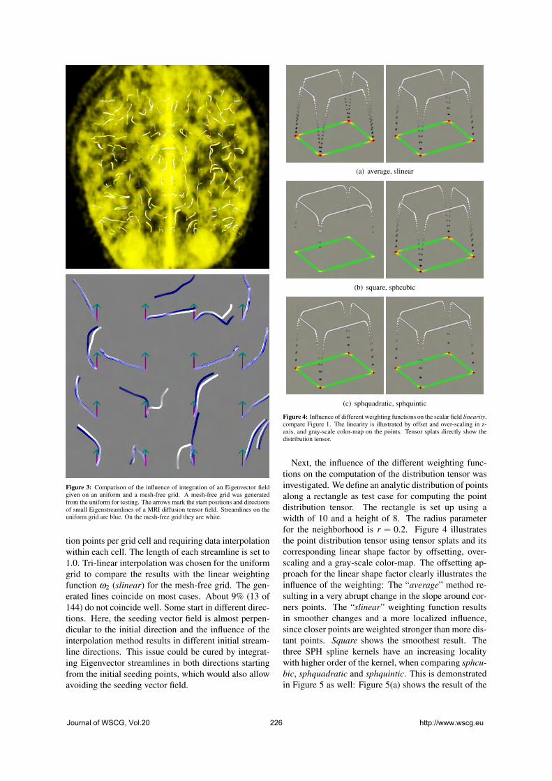
Figure 3: Comparison of the influence of integration of an Eigenvector fieldgiven on an uniform and a mesh-free grid. A mesh-free grid was generatedfrom the uniform for testing. The arrows mark the start positions and directionsof small Eigenstreamlines of a MRI diffusion tensor field. Streamlines on theuniform grid are blue. On the mesh-free grid they are white.

tion points per grid cell and requiring data interpolationwithin each cell. The length of each streamline is set to1.0. Tri-linear interpolation was chosen for the uniformgrid to compare the results with the linear weightingfunction ω2 (slinear) for the mesh-free grid. The gen-erated lines coincide on most cases. About 9% (13 of144) do not coincide well. Some start in different direc-tions. Here, the seeding vector field is almost perpen-dicular to the initial direction and the influence of theinterpolation method results in different initial stream-line directions. This issue could be cured by integrat-ing Eigenvector streamlines in both directions startingfrom the initial seeding points, which would also allowavoiding the seeding vector field.

(a) average, slinear

(b) square, sphcubic

(c) sphquadratic, sphquintic

Figure 4: Influence of different weighting functions on the scalar field linearity,compare Figure 1. The linearity is illustrated by offset and over-scaling in z-axis, and gray-scale color-map on the points. Tensor splats directly show thedistribution tensor.

Next, the influence of the different weighting func-tions on the computation of the distribution tensor wasinvestigated. We define an analytic distribution of pointsalong a rectangle as test case for computing the pointdistribution tensor. The rectangle is set up using awidth of 10 and a height of 8. The radius parameterfor the neighborhood is r = 0.2. Figure 4 illustratesthe point distribution tensor using tensor splats and itscorresponding linear shape factor by offsetting, over-scaling and a gray-scale color-map. The offsetting ap-proach for the linear shape factor clearly illustrates theinfluence of the weighting: The “average” method re-sulting in a very abrupt change in the slope around cor-ners points. The “slinear” weighting function resultsin smoother changes and a more localized influence,since closer points are weighted stronger than more dis-tant points. Square shows the smoothest result. Thethree SPH spline kernels have an increasing localitywith higher order of the kernel, when comparing sphcu-

bic, sphquadratic and sphquintic. This is demonstratedin Figure 5 as well: Figure 5(a) shows the result of the


cubic and quadratic SPH kernel function. When the ra-dius of the neighborhood is increased to match the ker-nels there is no visible difference between the sphcubic

in Figure 5(a), sphquadratic and sphquintic in Figure5(b) in the resulting linearity.

(a) sphcubic r = 0.2, sphquadratic r = 0.2

(b) sphquadratic r = 0.25, sphquintic r = 0.3

Figure 5: Different orders of the SPH kernel functions are compared, see Fig-ure 1. (a) sphcubic and shpquintic using the same radius for the neighborhood.(b) sphquadratic and shpquintic, with adjusted neighborhood radius, have asimilar result as the sphcubic (a)-left.

The influence of the integration scheme on the Eigen-streamline integration is demonstrated in Figure 6. Thedistribution tensor of a circular point distribution wascomputed using the ssquare weighting function. Ten-sor splats show the undirected Eigenvector, vector ar-rows show how the vector is directed within the internalvector representation. One Eigenstreamline is seededdownwards at the rightmost point of the circular pointdistribution and follows the undirected vectors. The topimage shows Euler integration. Decreasing the step sizewould result in a more accurate integration. But, clos-ing the gap of the integrated circle requires such a smallstep size, that the Runge Kutta method outperforms theEuler method. The 8th order Runge Kutta method suc-cessfully closes the gap and reconstructs a circle fromthe circular point distribution, as shown in the bottomimage. Also, a square-shaped point distribution wastested as shown in Figure 7. The length of a side is10. Here, the influence of different weighting functionson the interpolation of the Eigenvector field was inves-tigated. The distribution tensor was computed usingthe ssquare weighting function with r = 2. An Eigen-streamline is seeded downwards in the mid of the rightedge. It follows the undirected vectors and flows aroundthe corners of the rectangle. At each corner some erroris introduced and the streamline is moving apart from

Figure 6: Comparison of different numerical integration schemes in a circu-lar point distribution. One streamline (white) is seeded at the east-pole of thecircle pointing southwards. Tensor splats and vector arrows illustrate the pointdistribution tensor and major Eigenvector. Note, that the Eigenvectors changeorientation at north-east and south-west. Top: explicit Euler. Bottom: DOP853.

the original point distribution. Integration was doneusing the DOP853 method. Different weighting func-tions, mostly with r = 1, were tested for vector fieldinterpolation. The length of the horizontal gap betweenthe end and the start of the streamline was used as ameasure for the integration error. Figure 8 shows thedifferent errors in a bar diagram. The two best resultswere achieved using the ssquare and average weightingfunction.

Figure 7: Comparison of Euler and DOP853 streamline integration on asquare-shaped point distribution. Tensor splats and Eigenvectors are visual-ized besides the streamline (white) seeded downwards at the center of the rightedge of the rectangle.


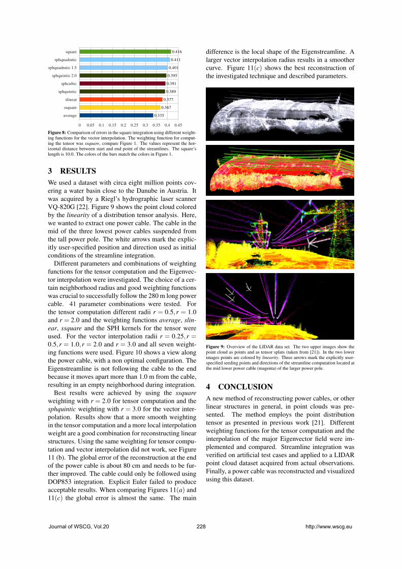
average

ssquare

slinear

sphquintic

sphcubic

sphquintic 2.0

sphquadratic 1.5

sphquadratic

square

0 0.05 0.1 0.15 0.2 0.25 0.3 0.35 0.4 0.45

0.335

0.367

0.377

0.389

0.391

0.395

0.401

0.411

0.416

Figure 8: Comparison of errors in the square integration using different weight-ing functions for the vector interpolation. The weighting function for comput-ing the tensor was ssquare, compare Figure 1. The values represent the hor-izontal distance between start and end point of the streamlines. The square’slength is 10.0. The colors of the bars match the colors in Figure 1.

3 RESULTS

We used a dataset with circa eight million points cov-ering a water basin close to the Danube in Austria. Itwas acquired by a Riegl’s hydrographic laser scannerVQ-820G [22]. Figure 9 shows the point cloud coloredby the linearity of a distribution tensor analysis. Here,we wanted to extract one power cable. The cable in themid of the three lowest power cables suspended fromthe tall power pole. The white arrows mark the explic-itly user-specified position and direction used as initialconditions of the streamline integration.

Different parameters and combinations of weightingfunctions for the tensor computation and the Eigenvec-tor interpolation were investigated. The choice of a cer-tain neighborhood radius and good weighting functionswas crucial to successfully follow the 280 m long powercable. 41 parameter combinations were tested. Forthe tensor computation different radii r = 0.5,r = 1.0and r = 2.0 and the weighting functions average, slin-

ear, ssquare and the SPH kernels for the tensor wereused. For the vector interpolation radii r = 0.25,r =0.5,r = 1.0,r = 2.0 and r = 3.0 and all seven weight-ing functions were used. Figure 10 shows a view alongthe power cable, with a non optimal configuration. TheEigenstreamline is not following the cable to the endbecause it moves apart more than 1.0 m from the cable,resulting in an empty neighborhood during integration.

Best results were achieved by using the ssquare

weighting with r = 2.0 for tensor computation and thesphquintic weighting with r = 3.0 for the vector inter-polation. Results show that a more smooth weightingin the tensor computation and a more local interpolationweight are a good combination for reconstructing linearstructures. Using the same weighting for tensor compu-tation and vector interpolation did not work, see Figure11 (b). The global error of the reconstruction at the endof the power cable is about 80 cm and needs to be fur-ther improved. The cable could only be followed usingDOP853 integration. Explicit Euler failed to produceacceptable results. When comparing Figures 11(a) and11(c) the global error is almost the same. The main

difference is the local shape of the Eigenstreamline. Alarger vector interpolation radius results in a smoothercurve. Figure 11(c) shows the best reconstruction ofthe investigated technique and described parameters.

Figure 9: Overview of the LIDAR data set. The two upper images show thepoint cloud as points and as tensor splats (taken from [21]). In the two lowerimages points are colored by linearity. Three arrows mark the explicitly user-specified seeding points and directions of the streamline computation located atthe mid lower power cable (magenta) of the larger power pole.

4 CONCLUSION

A new method of reconstructing power cables, or otherlinear structures in general, in point clouds was pre-sented. The method employs the point distributiontensor as presented in previous work [21]. Differentweighting functions for the tensor computation and theinterpolation of the major Eigenvector field were im-plemented and compared. Streamline integration wasverified on artificial test cases and applied to a LIDARpoint cloud dataset acquired from actual observations.Finally, a power cable was reconstructed and visualizedusing this dataset.


Figure 10: Power cable reconstruction via streamlines. The distribution tensorwas computed using the average r = 2.0 weighting and the vector interpolationwas done with the ssquare r = 1.0 weighting. Top: Points colored by linearity.Bottom: Tensor splats illustrate the distribution tensor. Streamlines are movingapart from the power cable and break before they can reconstruct the full 280m of cable.

(a) Tensor: ssquare r=2, Vectorfield: sphquintic r=1

(b) Tensor: sphquintic r=2, Vectorfield: sphquintic r=2

(c) Tensor: ssquare r=2, Vectorfield: sphquintic r=3

Figure 11: Comparison of different parameters and weighting function com-binations of the computation, finally resulted in a successfully reconstructedpower cable. The LIDAR point cloud is colored by linearity of the distributiontensor. The three Eigenvector streamlines reconstruct a 280 m long cable.

5 FUTURE WORK

Other weighting functions for computing the tensor anddoing the interpolation during the streamline integra-tion need to be tested. Automatic determination of theoptimal combination of weighting functions and alsotheir parameters will be the goal of further investiga-tions. Seeding points and directions for computingthe streamlines need also to be chosen automatically,for example, by taking tensor properties into account.Following the major Eigenvector of points with highplanarity or sphericity needs to be prevented duringstreamline integration. Finally, more datasets should beexplored to stabilize the method. Furthermore, minorchanges of the algorithm would enable streamline inte-gration in datasets stemming from SPH simulations.

ACKNOWLEDGMENT

Many thanks to Frank Steinbacher for proving the LI-DAR data. This work was supported by the Aus-trian Science Foundation FWF DK+ project Compu-

tational Interdisciplinary Modeling (W1227) and grantP19300. This research employed resources of the Cen-ter for Computation and Technology at Louisiana StateUniversity, which is supported by funding from theLouisiana legislature’s Information Technology Initia-tive. This work was supported by the Austrian Ministryof Science BMWF as part of the UniInfrastrukturpro-gramm of the Forschungsplattform Scientific Comput-ing at LFU Innsbruck.

REFERENCES

[1] W. Benger, H. Bartsch, H.-C. Hege, H. Kitzler,A. Shumilina, and A. Werner. Visualizing Neu-ronal Structures in the Human Brain via Diffu-sion Tensor MRI. International Journal of Neu-

roscience, 116(4):pp. 461–514, 2006.

[2] W. Benger, G. Ritter, and R. Heinzl. The Con-cepts of VISH. In 4th High-End Visualization

Workshop, Obergurgl, Tyrol, Austria, June 18-

21, 2007, pages 26–39. Berlin, Lehmanns Media-LOB.de, 2007.

[3] W. Benger and M. Ritter. Using geometric algebrafor visualizing integral curves. In E. M. S. Hitzerand V. Skala, editors, GraVisMa 2010 - Computer

Graphics, Vision and Mathematics for Scientific

Computing. Union Agency - Science Press, 2010.

[4] W. Benger, M. Ritter, S. Acharya, S. Roy, andF. Jijao. Fiberbundle-based visualization of a stirtank fluid. In 17th International Conference in

Central Europe on Computer Graphics, Visualiza-

tion and Computer Vision, pages 117–124, 2009.

[5] T. E. Conturo, N. F. Lori, T. S. Cull, E. Akbu-dak, A. Z. Snyder, J. S. Shimony, R. C. Mckinstry,H. Burton, and M. E. Raichle. Tracking neuronal


fiber pathways in the living human brain. Proc

Natl Acad Sci U S A, 96(18):10422–10427, Aug.1999.

[6] M. Descoteaux, L. Collins, and K. Siddiqi. Amulti-scale geometric flow for segmenting vascu-lature in mri. In In Medical Imaging Computing

and Computer-Assisted Intervention, pages 500–507, 2004.

[7] S. N. E. Hairer and G. Wanner. Solving ordi-

nary differential equations I, nonstiff problems,

2nd edition. Springer Series in ComputationalMathematics, Springer-Verlag, 1993.

[8] L. A. Fernandes and M. M. Oliveira. Real-time line detection through an improved houghtransform voting scheme. Pattern Recognition,41(1):299 – 314, 2008.

[9] K. Fukunaga and L. Hostetler. The estimation ofthe gradient of a density function, with applica-tions in pattern recognition. Information Theory,

IEEE Transactions on, 21(1):32 – 40, jan 1975.

[10] D. A. Fulk and D. W. Quinn. An analysis of 1Dsmoothed particle hydrodynamics kernels. Jour-

nal of Computational Physics, 126(1):165–180,1996.

[11] R. C. Gonzalez and R. E. Woods. Digital Im-

age Processing. Addison-Wesley Longman Pub-lishing Co., Inc., Boston, MA, USA, 2nd edition,2001.

[12] D. K. Jones. Studying connections in the livinghuman brain with diffusion mri. Cortex, 44(8):936– 952, 2008.

[13] Y. Jwa, G. Sohn, and H. B. Kim. Automatic3d powerline reconstruction using airborne lidardata. IAPRS, XXXVIII(2004):105–110, 2009.

[14] K. Kraus and N. Pfeifer. Determination of terrainmodels in wooded areas with airborne laser scan-ner data. ISPRS Journal of Photogrammetry and

Remote Sensing, 53(4):193 – 203, 1998.

[15] Z. Li, R. Walker, R. Hayward, and L. Mejias. Ad-vances in vegetation management for power linecorridor monitoring using aerial remote sensingtechniques. In Applied Robotics for the Power

Industry (CARPI), 2010 1st International Confer-

ence on, pages 1 –6, oct. 2010.

[16] Y. Liu, Z. Li, R. F. Hayward, R. A. Walker, andH. Jin. Classification of airborne lidar intensitydata using statistical analysis and hough transformwith application to power line corridors. In Digital

Image Computing : Techniques and Applications

Conference (DICTA 2009), Melbourne, Victoria,December 2009. IEEE Computer Society.

[17] T. Melzer. Non-parametric segmentation of alspoint clouds using mean shift. Journal of Applied

Geodesy, 1(3):159–170, 2007.

[18] T. Melzer and C. Briese. Extraction and modelingof power lines from als point clouds. In Proceed-

ings of 28th Workshop, pages 47–54. Österreichis-che Computer Gesellschaft, 2004. talk: AustrianAssociation for Pattern Recognition (ÖAGM),Hagenberg; 2004-06-17 – 2004-06-18.

[19] S. Mills, M. Gerardo, Z. Li, J. Cai, R. F. Hay-ward, L. Mejias, and R. A. Walker. Evaluationof aerial remote sensing techniques for vegetationmanagement in power line corridors. IEEE Trans-

actions on Geoscience and Remote Sensing, Oc-tober 2009.

[20] M. Persson, J. Solem, K. Markenroth, J. Svens-son, and A. Heyden. Phase contrast mri segmen-tation using velocity and intensity. In R. Kimmel,N. Sochen, and J. Weickert, editors, Scale Space

and PDE Methods in Computer Vision, volume3459 of Lecture Notes in Computer Science, pages119–130. Springer Berlin - Heidelberg, 2005.

[21] M. Ritter, W. Benger, B. Cosenza, K. Pullman,H. Moritsch, and W. Leimer. Visual data miningusing the point distribution tensor. In IARIS Work-

shop on Computer Vision and Computer Graphics

- VisGra 2012, Feb-Mar 2012.

[22] F. Steinbacher, M. Pfennigbauer, A. Ulrich, andM. Aufleger. Vermessung der Gewassersohle - ausder Luft - durch das Wasser. In Wasserbau in Be-

wegung ... von der Statik zur Dynamik. Beitrage

zum 15. Gemeinschaftssymposium der Wasserbau

Institute TU München, TU Graz und ETH Zürich,2010.

[23] D. Weinstein, G. Kindlmann, and E. Lundberg.Tensorlines: advection-diffusion based propaga-tion through diffusion tensor fields. In Proceed-

ings of the conference on Visualization ’99: cel-

ebrating ten years, VIS ’99, pages 249–253, LosAlamitos, CA, USA, 1999. IEEE Computer Soci-ety Press.

[24] C. Westin, S. Peled, H. Gudbjartsson, R. Kikinis,and F. Jolesz. Geometrical diffusion measures formri from tensor basis analysis. In Proceedings of

ISMRM, Fifth Meeting, Vancouver, Canada, page1742, Apr. 1997.


Real-time Mesh Extraction of Dynamic Volume Data UsingGPU

Szymon EngelAGH, Krakow, Poland

[email protected]

Witold AldaAGH, Krakow, Poland

[email protected]

Krzysztof BoryczkoAGH, Krakow, [email protected]

ABSTRACTIn the paper an algorithm of triangle mesh generation for a full three-dimensional volumetric data is presented.Calculations are performed in real time using graphics processors. The method is very well suited for the visu-alization of dynamic data, as the calculations use only the current frame data (not including data from previousframes). Due to high performance of the algorithm, it can be practically applied in programs for digital sculpting,simulators and games which require editable geometries.

Keywordsmesh generation, iso-surface, volume data, real-time, GPU computation

1 INTRODUCTIONNowadays, visualization of volumetric data is very of-ten applied in practice. Both in medicine, e.g. for theMRI, PET, or CT data presentation in medical imag-ing, nondestructive inspection of materials (industrialCT), digital sculpting software, as well as in computergames. Often the visualization itself is not sufficientand a three-dimensional mesh is required for a physi-cal calculations, such as collision detection, calculationof material properties or stress. Moreover, the advan-tage of representing models with triangle meshes is thatmodern GPUs are optimized for efficient rendering oftriangles.

Another issue is that volumetric data can change dy-namically. When modeling is performed in a programfor sculpting a virtual material, a three-dimensionalmesh generated in real time is needed in order to dis-play the results. In video games or simulators of earth-moving machineries, we have to deal with the terrain,which cannot be fully represented by height maps. Wemay require a visualization of structures such as tun-nels, caves, overhangs of the land as well as other mod-ifications caused as a result of a player actions, such asexplosions, vehicle interactions with the terrain or othergameplay activities.

Currently available methods often do not allow to gen-erate a mesh for a large amount of data in real time.


Sometimes the resulting effect is described as "interac-tive" which usually means ability to carry out calcu-lations giving a few frames per second. This speed,however, is not sufficient for the smooth operation ofapplications such as computer games.

In response to these problems, a mesh generation al-gorithm for a fully three-dimensional volumetric datahas been developed. All calculations are performed onGPU in real time by which we understand the actualmean speed of computations above 30 frames per sec-ond. Another advantage of the presented algorithm isits independence of the volumetric data representation;therefore, scalar fields, implicit functions, or metaballobjects can be used.

The rest of this article is organized as follows. Thenext section presents previous work on mesh generationmethods of volumetric data. The third part briefly de-scribes the possible methods of data representation. Itthen shows the subsequent steps of the algorithm whilein the following passage detailed information on howto implement the algorithm using graphics processorsis included. The last section presents a description andsummary of results.

2 RELATED WORKThe subject of this paper is to visualize an iso-surfacegenerated for the volumetric data using triangle mesh.Mesh-based methods allow their easy integration withother algorithms or modules, e.g. physics engines, thatrequire mesh as an input. Thanks to this approach ouralgorithm can be used in real-time applications.

Therefore, discussion of previous works does notinclude ray-tracing and view-dependent visualization;however, information on the methods of these typescan be found e.g. in [OBA05, LK10, GDL+02].


GPU-based methods which allows to interactiveor real-time calculations were presented e.g. in[KOKK06, CNLE09, KOR08, TSD07].

One of the basic methods of generating a mesh on thebasis of volumetric data is the Marching Cubes algo-rithm [LC87] developed in the 1980s. It consists in di-viding the visualized space into equal cubes and gen-erating a polygon within each cube, which is then sub-jected to triangulation. The position and shape of thepolygon are dependent on the values of an implicitfunction in eight vertices of each cube. A commonissue with this method is that it requires generating amesh in the entire space of visualized data. In responseto this, several hierarchical and adaptive versions ofthe Marching Cubes algorithm have been developed[OR97, Blo88, WKE99, KKDH07] using octal trees toreduce the area for which calculations were carried outand which reduce the number of triangles by generatingthem in different densities depending on the distance ofthe camera. Implementations of of the Marching Cubesalgorithm using GPUs are presented in [JC06, Gei07].

Another, possibly less popular, method is the Sur-faceNets method [Gib98] which originally was usedto visualize binary medical data. This method is dualto the marching cubes algorithm and, as in the latterone, visualized space is divided into cubes of the samedimensions. In its base version, the method consistedof selecting the nodes belonging to the surface in a waythat a certain node has been selected, if among the eightvertices of the cube were those that had a differentsign. These nodes were linked with adjacent ones thuscreating a net, which was then smoothed by movingthe nodes so as to minimize the energy between themwhile maintaining the restriction that a node could notleave the cube, to which it originally belonged. Thefinal step was a triangulation of the network, whichgave the resulting mesh of triangles. The next methodwhich belongs to the group of "dual algorithms" is theone by [Nie04], which generates a mesh very similarto SurfaceNets, but its implementation is more likethe Marching Cubes algorithm. One of the importantdifferences between this method and the SurfaceNetsis that the mesh generated by the former is a propertwo-dimensional manifold.

In addition to the methods outlined above, there arealso: the marching tetrahedra method [TPG99], whoseoperating principle is based on the marching cubes al-gorithm, the marching triangles method based on theDelaunay triangulation [HSIW96] which generates anirregular mesh, or the method based on marching cubeswhich allows one to obtain sharp edges, described inthe work [JLSW02].

We follow the existing approach of dual marchingcubes, however, our algorithm is implemented exclu-sively on GPU and it efficiently exploits geometry

shaders. Thanks to the use of dual methods, the result-ing mesh contains fewer triangles and is regular due tothe number of generated triangles within each of thecubes. The latter allows the method to be implementedin a very efficient way using graphics processors.Former GPU-accelerated mesh extraction algorithms(e.g. [KW05], [Goe05], [JC06]) are based on bothCPU and GPU computations, using vertex or fragmentshaders only. Although meshes generated using ourmethod are not proper two-dimensional manifolds, ourapproach is extremely efficient and can be used fordynamic data which change on random every frame.

3 VOLUMETRIC DATAThe basic method of describing three-dimensional vol-umetric data is the implicit function. By setting the val-ues of the contour we obtain surface limiting the de-sired area. If the values of this function represent theEuclidean distances from a given contour and we savethem as an array, then we get a three dimensional signeddistance field D : R3 → R, representing the iso-surfaceS, defined for point p ∈ R

3 as:

D(p) = sgn(p) ·min|p−q| : q ∈ S, (1)

where

sgn(p) =

−1 if p is inside+1 if p is outside (2)

This representation can be stored in graphics card mem-ory as a three-dimensional texture. Thanks to this rep-resentation, smoothing of the resulting mesh using nor-mals computed directly from distance fields and vertexdistances from the surface, is very effective.

Also, most medical data is stored in the form of three-dimensional arrays. For such data combined with con-tour values we can generate a mesh. Another, lesscommon way to represent the volumetric data, is usingmetaball objects which, with adequate representation,can be converted to distance fields.

4 ALGORITHM OVERVIEWDue to the GPU architecture and the way they carry outcalculations, the developed algorithm is based on dualmethods. They allow to obtain a regular mesh consist-ing of squares, so one doesn’t need expensive triangula-tion of polygons generated inside a cube, as is the caseof marching cubes method. The algorithm has beenadapted to carry out calculations on GPUs, and highlyparallelized, which allows it to achieve very high per-formance.

Input data block, of size n3, where n of a form 2k, isdivided into equal cubes. This is shown in Figure 1.


0 1 2 n

1

2

n

0 1 n-1

1

n-1

0 1 2 3 n+2 n+3

1

2

3

n+2

n+3

Figure 1: Data organization (2D view)

The image represents a two-dimensional version, butthe three-dimensional one is similar.Calculation points marked with "•" symbol are placedin the centers of cubes and their coordinates are usedto calculate the distance from the contour, based onthe volumetric data. Distance field values are stored inpoints marked "+", while points marked "×" representvertices of quadrangles generated by the algorithm.The calculations of the algorithm are processed in twosteps. At the beginning, for each calculation pointp ∈ R

3, marked with the symbol "•", such that p ∈[0,n − 1]× [0,n − 1]× [0,n − 1], there are gener-ated three points q,r,s ∈ R

3 such that for p = (x,y,z):q = (x − 1,y,z), r = (x,y − 1,z), s = (x,y,z − 1). Ineach of these points p,q,r,s an implicit function valuedp = f (p) is calculated and three edges defined by pairsof calculation points pq, pr, ps are created. Then, foreach edge – if its endpoints have different signs (lie ondifferent sides of the contour) – a quadrangle located onthe border of the cubes is generated. Its orientation isdetermined by the direction of the edge, which is con-sistent with the direction of the normal to the surface ofthe quadrangle. A set of squares, generated in this way,approximates the iso-surface for input volumetric data,and is smoothed in the next stage. As a result of con-version of each square to a pair of triangles, a trianglemesh is obtained.Due to the fact that during the calculation the signchanges, zero is treated differently depending on thedirection of the edge, the condition 3, under whichquadrilaterals are generated is presented as follows:

( f (q)≥ 0∧ f (p)< 0)∨ ( f (q)< 0∧ f (p)≥ 0) (3)

The first step in the algorithm, described above, is ide-ally suited for parallelization, because the calculations

for computing the individual points can be carried outindependently. Despite the fact that the distance fieldsare calculated for each point twice, it is possible to ob-tain a high-performance computing algorithm, becauseit is not a costly operation.

The second stage of the algorithm is a smoothing ofgenerated mesh by moving its vertices in the directionof the surface represented by the distance fields values.For this purpose, at each vertex of the distance field, anormal vector n is calculated on the basis of the gradi-ent and the distance d to the surface. Then, the vertexis moved in the direction of the normal, by the valuecalculated according to formula 4.

p′ = p+dn (4)

In the case that the resulting mesh is used only for dis-playing a surface, this step can be implemented directlyduring rendering. Otherwise, it is possible to smooththe mesh only and use it for subsequent calculations,such as collision detection.

The advantage of the developed algorithm over march-ing cubes method consists partly in that for creating aquad for the cube we generate exactly four indices andthere is no need for triangulation of polygons gener-ated. This allows the calculations to be successfullyperformed on the GPU.

5 IMPLEMENTATION DETAILSThe algorithm was implemented using the OpenGLgraphics library; however, DirectX library can be usedas well.

Input volumetric data, for which a mesh is generated,is divided into equal blocks, for which fragments of themesh are generated independently. This approach waschosen because of the GPU hardware limitations on themaximum size of supported textures, as well as for op-timization purposes. To be specific: not all parts of dy-namic data need to be modified at the same time, andhence there is no need for mesh regeneration in theseblocks. Generated meshes merge together in continu-ous blocks along borders.

The algorithm is carried out equally for each datablock. All calculations are done on the GPU, so thedata are not transferred between main memory andgraphics card memory. Calculations are carried out intwo phases, the algorithm flowchart is shown in Figure2.

In both passes of the rendering shaders refer to the vol-umetric data.

5.1 Volume RepresentationThree-dimensional floating-point texture is used fordistance field representation in each block of data.


SAMPLE

VOLUME

GENERATE

TRIANGLESRENDER

ADJUST

POSITIONS

GENERATE

INDICES

TRANSFORM

FEEDBACK

PA

SS

2P

AS

S 1

VERTEX SHADER FRAGMENT SHADERGEOMETRY SHADER

Figure 2: Algorithm flowchart

Texture size is (n+ 3)3, 2 bytes per texel. Although4-byte floating point numbers can be applied for theprecision improvement, no need for that has beenfound during testing. To avoid communication betweenneighboring blocks, block’s data size is enlarged andoverlaps adjacent blocks; for each common quadranglebetween two adjacent blocks of size (n+3)3 each, 2n2

of voxels are duplicated. This allows parts of the meshin each block to be generated independently of theothers.

In the texture, we used a single GL_RED channel,where the data is stored in GL_FLOAT16 format. Inorder to allow reading distance field values, each pointof the texture is sampled using linear filtering. This isdone automatically, and the values are calculated on thebasis of neighboring texels. Mipmaps for the texturesare not generated.

5.2 Mesh Generation (Pass 1)

In the first pass calculations are performed using ver-tex shader and geometry shader. Then, using a trans-form feedback, generated indices are stored in the out-put buffer. Input and output data are presented in Table1.

INVertex buffer containing calculation points p ∈[0,n−1]× [0,n−1]type: GL_ARRAY_BUFFERsize: (n−1)2

sharing: one per all blocksTexture with volumetric datatype: GL_TEXTURE_3Dsize: (n+3)3

sharing: one per single blockOUTBuffer with indices of generated quadstype: GL_ELEMENT_ARRAY_BUFFERsharing: one per single block

Table 1: Input and output data of the first pass

The subsequent steps of the algorithm are as follows:

1. Data from the vertex buffer containing the calcula-tion points is rendered n−1 times, using the instancerendering.

2. For a calculation point p three points q,r,s are cre-ated in the vertex shader.

3. For each of the points p,q,r,s a volumetric texture issampled in order to retrieve implicit function value.Texture coordinates t are calculated according to for-mula 5.

t =p+2n+3

(5)

4. Subsequently three edges pq, pr, ps are created andaccording to formula 3 it is checked whether the val-ues of implicit function at the endpoints have differ-ent signs.

5. For each edge, if the sign changes, there is a flag set,which specifies whether the quadrilateral is gener-ated or not, and what is its orientation (zero meansthat the quadrilateral is not generated). Generatedflags along with the coordinates of the point p areforwarded to the geometry shader.

6. In the geometry shader, for each non-zero flag therea vertex containing four indices of generated quad-rangles is established. Indices are calculated on thebasis of the flag f and coordinates p. For example,quadrangle, which normal is consistent with the di-rection of the edge pq, is defined by (i1, i2, i4, i3),where

i1 = pxn2 + pyn+ pz+1i2 = pxn2 + py+1n+ pz+1i3 = pxn2 + py+1n+ pzi4 = pxn2 + pyn+ pz

7. Using the feedback transformation these indices arestored directly in the index buffer, used in the nextpass. Number of saved indices is queried using anOpenGL query mechanism.

5.3 Rendering (pass 2)The second pass is responsible for smoothing of thegenerated mesh and its rendering. All programmableshader units, i.e. vertex, fragment and geometry shadersare used. The input data is presented in Table 2.

Subsequent steps of the second pass of the algorithmare as follows:

1. The data from the vertex buffer is ren-dered using the indices as primitives of theGL_LINES_ADJACENCY type. This type waschosen because it is the only type that can render


INVertex buffer which contains all potential vertices,such as: u ∈ [0,n]× [0,n]× [0,n].type: GL_ARRAY_BUFFERsize: n3

sharing: one per all blocksBuffer with indices for generated quadranglestype: GL_ELEMENT_ARRAY_BUFFERsharing: one per single blockTexture with volumetric datatype: GL_TEXTURE_3Dsize: (n+3)3

sharing: one per single blockTable 2: Input data for the second pass of the algorithm

primitives indexed by four indices (in OpenGLversion 3.0 or higher it is not possible to renderquadrangles).

2. Then in the vertex shader for each vertex u, a nor-mal vector n is calculated, on the basis of the gradi-ent map. Normal value is obtained by sampling thevolumetric data texture in the neighboring six texelsin x,y,z directions.

3. On the basis of the direction of the normal and thedensity function value, the point u is moved in thedirection of the contour, according to formula 4.Due to the fact that the value of the density func-tion is calculated as the average of neighboring tex-els at the point u, for small values of n it is requiredto perform a smoothing of the mesh in an iterativemanner.

4. Vertices calculated in this way are sent to the geom-etry shader, in which there is a change of type done,from "lines adjacency" into "triangle strip".

5. The last step is to display a completed mesh, duringwhich the associated shading calculations are per-formed in the fragment shader. In case when meshrendering is not required, but the mesh is needed forfurther calculations, smoothed values of the verticescan be stored in the output buffer using a transformfeedback.

6 RESULTSAll calculations were performed on an AMD PhenomII X6 1090T 3.2GHz computer with an nVidia GeForceGTX 460 graphics card. Figure 3 presents datasets usedin tests; Armadillo and Asian Dragon from The Stan-ford 3D Scanning Repository, Engine and Skull fromhttp://www.volvis.org/. In addition, three-dimensional animated Perlin noise has been used as adynamic, time-dependent data. All tests were run fordifferent n on one block of data.

(a) Armadillo (b) Asian Dragon

(c) Engine (d) Skull

Figure 3: Datasets used for tests

Table 3 lists times for mesh generation and renderingfor different block sizes and different data sets. Allmeshes were regenerated from volumetric data eachframe; moreover, calculations for time-dependent Per-lin noise data were also performed before mesh gener-ation every frame. Generated meshes for the Armadillodataset for different block sizes are presented on figure4, results for noise dataset are presented on figure 6.

dataset n triangle count fpsArmadillo 64 14180 1100Armadillo 128 91958 208Armadillo 256 494880 28Asian Dragon 64 5864 1180Asian Dragon 128 41578 234Asian Dragon 256 229840 30Engine 256 592884 29Skull 256 1699526 23.6Perlin Noise 128 180k-246k 60

Table 3: Results for different block sizes and data sets

Table 4 presents results for our method compared to[Goe05, JC06]. The Engine and Skull datasets wereused, no preprocessing were performed for these data.As it can be seen our algorithm performs much faster,however, if all methods would be run on the same hard-ware configuration, the difference could be less signifi-cant. Both methods of [Goe05] and [JC06] were testedon nVidia GeForce 6800GT graphics card.

The Marching Cubes algorithm described in [Gei07]seems to execute faster than [Goe05, JC06] methodsbut no measurable results were published. Authors of[Gei07] claims that their algorithm executes in interac-


(a) n = 64 (b) n = 128 (c) n = 256

Figure 4: Generated mesh for the Armadillo dataset

tive frames but mesh generation are not performed eachframe.

dataset size method fpsengine 256x256x110 [Goe05] 3.6engine 256x256x128 [JC06] 2.8engine 256x256x256 our method 29skull 256x256x225 [Goe05] 2.4skull 256x256x256 [JC06] 1.5skull 256x256x256 our method 23.6

Table 4: Results compared to previous GPU-basedmethods

7 MESH IMPROVEMENTSThe presented method works well for smooth surfaces,such as the ones presented in figure 6. In case of sur-faces with sharp edges we see artifacts as it is shown infigure 5(a).

(a) Artifacts on sharp edges

(b) Smoothed mesh

Figure 5: Mesh improvements due to smoothing

In order to improve visual quality of the generated sur-face, in the second pass of the algorithm a smoothing

process based on normals is performed about 10 times.Next, during transforming quadrangles into strips of tri-angles, the quadrangles are divided along the shorterdiagonal. The last step of smoothing the mesh is com-putation of normals for every pixel in fragment shader,on the basis of volumetric data. Normals are calculatedin the same way as for the mesh vertices. The smoothedmesh is presented in Figure 5(b).


In this paper we present a real-time algorithm for gener-ating a three-dimensional mesh fully based on volumet-ric data. This method has been optimized for graphicsprocessors and provides a significant advantage over thealready existing solutions for conventional processors.The presented algorithm is also very well suited for thevisualization of dynamic data, because the calculationscarried out do not need to know the state of the algo-rithm from previous time steps.With the resulting performance, practical applicationof the algorithm in digital sculpting software, earth-moving machineries simulators and computer games isfully possible. The tests show a significant advantageof GPUs. The volumetric data representation that hasbeen used allows also for efficient data modification us-ing GPUs.As part of further work on the algorithm it would be rea-sonable to add support for levels of detail (LOD), so asto enable the process to connect continuously adjacentblocks containing cubes of different sizes and densities.The second issue is to optimize the algorithm by anadditional parallelization and simultaneous calculationcarried out for 4 blocks. It would be possible in thecase of using all four available texture channels. As aresult, it would be possible to generate meshes for thefour blocks at the same time.

9 ACKNOWLEDGEMENTSThe work described in this paper was partially sup-ported by The European Union by means of European


Social Fund, PO KL Priority IV: Higher Education andResearch, Activity 4.1: Improvement and Developmentof Didactic Potential of the University and IncreasingNumber of Students of the Faculties Crucial for theNational Economy Based on Knowledge, Subactivity4.1.1: Improvement of the Didactic Potential of theAGH University of Science and Technology “HumanAssets”, No. UDA-POKL.04.01.01-00-367/08-00.

One of us (WA) kindly acknowledges partial support byMinistry of Science and Higher Education in Poland,project No. N N519 443039.

10 REFERENCES[Blo88] J. Bloomenthal. Polygonization of im-

plicit surfaces. Comput. Aided Geom. Des.,5(4):341–355, 1988.

[CNLE09] Cyril Crassin, Fabrice Neyret, SylvainLefebvre, and Elmar Eisemann. Gigavox-els: ray-guided streaming for efficient anddetailed voxel rendering. In I3D ’09: Pro-ceedings of the 2009 symposium on In-teractive 3D graphics and games, pages15–22, New York, NY, USA, 2009. ACM.

[GDL+02] Benjamin Gregorski, Mark Duchaineau,Peter Lindstrom, Valerio Pascucci, andKenneth I. Joy. Interactive view-dependentrendering of large isosurfaces. In VIS ’02:Proceedings of the conference on Visual-ization ’02, pages 475–484, Washington,DC, USA, 2002. IEEE Computer Society.

[Gei07] Ryan Geiss. Generating Complex Proce-dural Terrains using the GPU, chapter 1.GPU Gems. Addison Wesley, 2007.

[Gib98] Sarah F. Frisken Gibson. Constrainedelastic surface nets: Generating smoothsurfaces from binary segmented data. InMICCAI ’98: Proceedings of the FirstInternational Conference on Medical Im-age Computing and Computer-Assisted In-tervention, pages 888–898, London, UK,1998. Springer-Verlag.

[Goe05] F. et al. Goetz. Real-time marching cubeson the vertex shader. In In Proceedings ofEurographics 2005, Dublin, Ireland , pp.5-8, 2005.

[HSIW96] A. Hilton, A. J. Stoddart, J. Illingworth,and T. Windeatt. Marching triangles:range image fusion for complex objectmodelling. In Proc. Conf. Int Image Pro-cessing, volume 1, pages 381–384, 1996.

[JC06] Gunnar Johansson and Hamish Carr. Ac-celerating marching cubes with graphicshardware. In In CASCON ’06: Proceed-ings of the 2006 conference of the Center

for Advanced Studies on Collaborative re-search, ACM, page 378. Press, 2006.

[JLSW02] Tao Ju, Frank Losasso, Scott Schaefer, andJoe Warren. Dual contouring of hermitedata. In SIGGRAPH ’02: Proceedings ofthe 29th annual conference on Computergraphics and interactive techniques, pages339–346, New York, NY, USA, 2002.ACM.

[KKDH07] Michael Kazhdan, Allison Klein, Ke-tan Dalal, and Hugues Hoppe. Uncon-strained isosurface extraction on arbitraryoctrees. In SGP ’07: Proceedings of thefifth Eurographics symposium on Geom-etry processing, pages 125–133, Aire-la-Ville, Switzerland, Switzerland, 2007. Eu-rographics Association.

[KOKK06] Takashi Kanai, Yutaka Ohtake, HiroakiKawata, and Kiwamu Kase. Gpu-basedrendering of sparse low-degree implicitsurfaces. In Proceedings of the 4th inter-national conference on Computer graph-ics and interactive techniques in Australa-sia and Southeast Asia, GRAPHITE ’06,pages 165–171, New York, NY, USA,2006. ACM.

[KOR08] John Kloetzli, Marc Olano, and PennyRheingans. Interactive volume isosurfacerendering using bt volumes. In I3D ’08:Proceedings of the 2008 symposium on In-teractive 3D graphics and games, pages45–52, New York, NY, USA, 2008. ACM.

[KW05] P. Kipfer and R. Westermann. Gpu con-struction and transparent rendering of iso-surfaces. In Vision, Modeling, and Visual-ization (VMV 2005), Erlangen, Germany,Nov. 16-18, 2005.

[LC87] William E. Lorensen and Harvey E. Cline.Marching cubes: A high resolution 3d sur-face construction algorithm. SIGGRAPHComput. Graph., 21:163–169, August1987.

[LK10] Samuli Laine and Tero Karras. Efficientsparse voxel octrees. In I3D ’10: Pro-ceedings of the 2010 ACM SIGGRAPHsymposium on Interactive 3D Graphicsand Games, pages 55–63, New York, NY,USA, 2010. ACM.

[Nie04] Gregory M. Nielson. Dual marchingcubes. In Proceedings of the conferenceon Visualization ’04, VIS ’04, pages 489–496, Washington, DC, USA, 2004. IEEEComputer Society.

[OBA05] Yutaka Ohtake, Alexander Belyaev, and


Figure 6: Generated meshes for Perlin noise dataset for 15 frames

Marc Alexa. Sparse low-degree implicitsurfaces with applications to high qualityrendering, feature extraction, and smooth-ing. In Proceedings of the third Euro-graphics symposium on Geometry process-ing, SGP ’05, Aire-la-Ville, Switzerland,Switzerland, 2005. Eurographics Associa-tion.

[OR97] M. Ohlberger and M. Rumpf. Hierarchicaland adaptive visualization on nested grids.Computing, 59(4):365–385, 1997.

[TPG99] G. M. Treece, R. W. Prager, and A. H.Gee. Regularised marching tetrahedra:improved isosurface extraction. Comput-ers and Graphics, 23:583–598, 1999.

[TSD07] Natalya Tatarchuk, Jeremy Shopf, andChristopher DeCoro. Real-time isosurfaceextraction using the gpu programmablegeometry pipeline. In ACM SIGGRAPH2007 courses, SIGGRAPH ’07, pages122–137, New York, NY, USA, 2007.ACM.

[WKE99] R. Westermann, L. Kobbelt, and T. Ertl.Real-time exploration of regular volumedata by adaptive reconstruction of iso-surfaces. The Visual Computer, 15:100–111, 1999.


A Layered Depth-of-Field Method for Solving PartialOcclusion

David C. Schedl*[email protected]

Michael Wimmer*

[email protected]

*Vienna University of Technology, Austria

ABSTRACTDepth of field (DoF) represents a distance range around a focal plane, where objects on an image are crisp. DoFis one of the effects which significantly contributes to the photorealism of images and therefore is often simulatedin rendered images. Various methods for simulating DoF have been proposed so far, but little tackle the issue ofpartial occlusion: Blurry objects near the camera are semi-transparent and result in partially visible backgroundobjects. This effect is strongly apparent in miniature and macro photography. In this work a DoF method ispresented which simulates partial occlusion. The contribution of this work is a layered method where the sceneis rendered into layers. Blurring is done efficiently with recursive Gaussian filters. Due to the usage of Gaussianfilters big artifact-free blurring radii can be simulated at reasonable costs.

Keywords:depth of field, rendering, real-time, layers, post-processing

1 INTRODUCTIONDoF represents a distance range around a focal planein optic systems, such as camera lenses. Objects out ofthis range appear to be blurred compared to sharp ob-jects in focus. This effect emphasizes objects in focusand therefore is an important artistic tool in pictures andvideos.

People in the field of computer graphics aim for theambitious goal of generating photo-realistic render-ings. Depth of Field is one effect which significantlycontributes to the photorealism of images becauseit is an effect that occurs in most optical systems.In computer renderings, the pinhole-camera model,which relies upon the assumption that all light-raystravel through one point before hitting the imageplane, is used. Therefore, there is no focus rangeand no smearing occurs, resulting in a crisp image.However, in real-life optical systems—such as theeye or photographic cameras—sharp images are onlyproduced if the viewed object is within a certain depthrange: the depth of field.

DoF can be simulated very accurately by ray tracing,but the rendering of accurate DoF effects is far from in-teractive frame rates. For interactive applications, the


(a) (b)Figure 1: A pinhole rendering of the scene Dragons resulting in acrisp image (a). Simulating shallow depth-of-field with the proposedmethod partly reveals occluded scene content (b). Note how thetongue of the dragon almost vanishes.

effect has to be approximated in real time. Therefore,most approaches use fast post-processing techniquesand sacrifice visual quality, causing artifacts. Com-mon techniques to produce the DoF effect use an ap-proach where pixels get smeared according to their cir-cle of confusion (CoC) [25]. The CoC depends on thedistance of objects and the lens parameters. One arti-fact in post-processing approaches is partial occlusion:An object in-focus occluded by an out-of-focus objectshould be partly visible at the blurred object borders ofthe front object. In computer graphics, the used pin-hole camera model in combination with depth testingleads to a dismissing of background pixels. Real opticalsystems use a finite aperture camera model where lightrays from occluded objects can hit the image sensor.Figure 1 shows this effect next to a pinhole rendering.

In this paper, we present an approach to tackling thepartial occlusion problem. By rendering the scene withdepth peeling [11], occluded pixels can be retrieved(Section 3.1). This occluded scene information is used


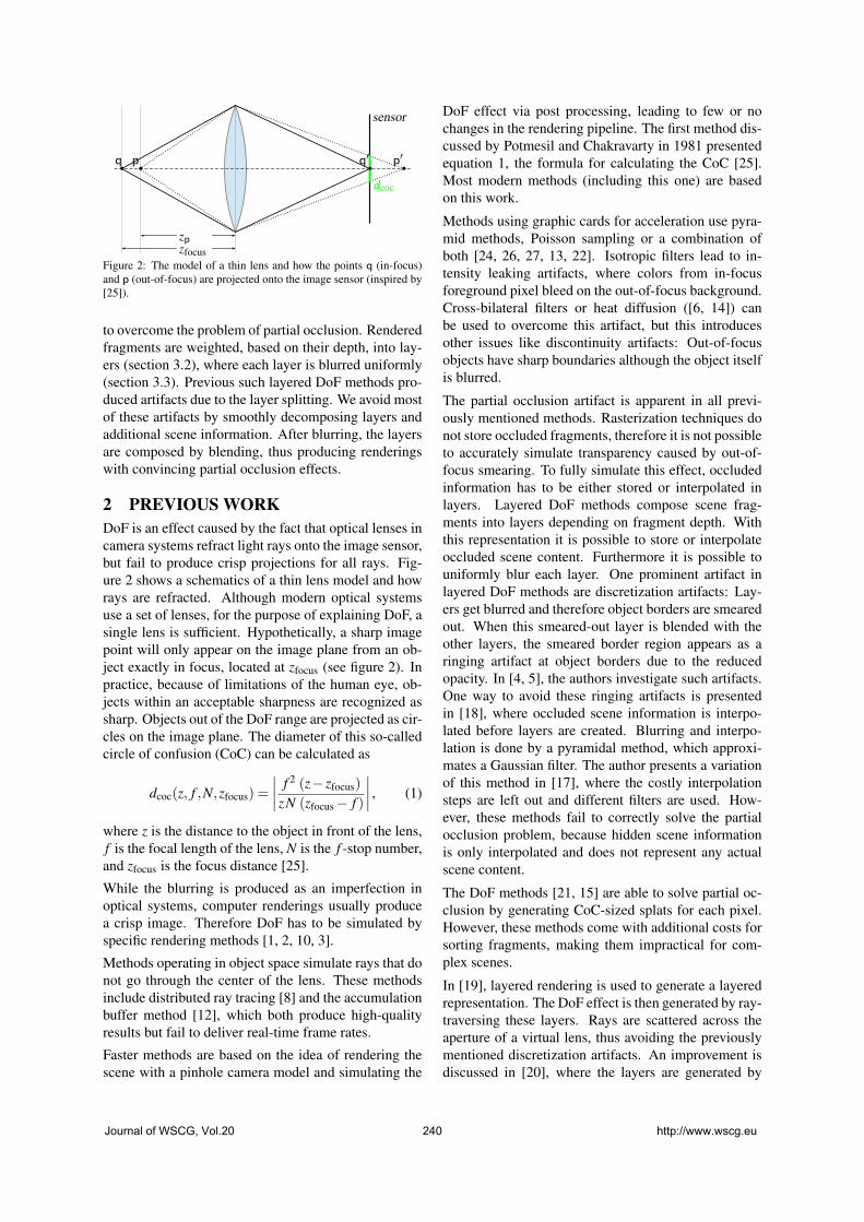
zfocuszp

sensor

p p′

dcoc

q q′

Figure 2: The model of a thin lens and how the points q (in-focus)and p (out-of-focus) are projected onto the image sensor (inspired by[25]).

to overcome the problem of partial occlusion. Renderedfragments are weighted, based on their depth, into lay-ers (section 3.2), where each layer is blurred uniformly(section 3.3). Previous such layered DoF methods pro-duced artifacts due to the layer splitting. We avoid mostof these artifacts by smoothly decomposing layers andadditional scene information. After blurring, the layersare composed by blending, thus producing renderingswith convincing partial occlusion effects.

2 PREVIOUS WORKDoF is an effect caused by the fact that optical lenses incamera systems refract light rays onto the image sensor,but fail to produce crisp projections for all rays. Fig-ure 2 shows a schematics of a thin lens model and howrays are refracted. Although modern optical systemsuse a set of lenses, for the purpose of explaining DoF, asingle lens is sufficient. Hypothetically, a sharp imagepoint will only appear on the image plane from an ob-ject exactly in focus, located at zfocus (see figure 2). Inpractice, because of limitations of the human eye, ob-jects within an acceptable sharpness are recognized assharp. Objects out of the DoF range are projected as cir-cles on the image plane. The diameter of this so-calledcircle of confusion (CoC) can be calculated as

dcoc(z, f ,N,zfocus) =

∣∣∣∣ f 2 (z− zfocus)

zN (zfocus− f )

∣∣∣∣ , (1)

where z is the distance to the object in front of the lens,f is the focal length of the lens, N is the f -stop number,and zfocus is the focus distance [25].

While the blurring is produced as an imperfection inoptical systems, computer renderings usually producea crisp image. Therefore DoF has to be simulated byspecific rendering methods [1, 2, 10, 3].

Methods operating in object space simulate rays that donot go through the center of the lens. These methodsinclude distributed ray tracing [8] and the accumulationbuffer method [12], which both produce high-qualityresults but fail to deliver real-time frame rates.

Faster methods are based on the idea of rendering thescene with a pinhole camera model and simulating the

DoF effect via post processing, leading to few or nochanges in the rendering pipeline. The first method dis-cussed by Potmesil and Chakravarty in 1981 presentedequation 1, the formula for calculating the CoC [25].Most modern methods (including this one) are basedon this work.

Methods using graphic cards for acceleration use pyra-mid methods, Poisson sampling or a combination ofboth [24, 26, 27, 13, 22]. Isotropic filters lead to in-tensity leaking artifacts, where colors from in-focusforeground pixel bleed on the out-of-focus background.Cross-bilateral filters or heat diffusion ([6, 14]) canbe used to overcome this artifact, but this introducesother issues like discontinuity artifacts: Out-of-focusobjects have sharp boundaries although the object itselfis blurred.

The partial occlusion artifact is apparent in all previ-ously mentioned methods. Rasterization techniques donot store occluded fragments, therefore it is not possibleto accurately simulate transparency caused by out-of-focus smearing. To fully simulate this effect, occludedinformation has to be either stored or interpolated inlayers. Layered DoF methods compose scene frag-ments into layers depending on fragment depth. Withthis representation it is possible to store or interpolateoccluded scene content. Furthermore it is possible touniformly blur each layer. One prominent artifact inlayered DoF methods are discretization artifacts: Lay-ers get blurred and therefore object borders are smearedout. When this smeared-out layer is blended with theother layers, the smeared border region appears as aringing artifact at object borders due to the reducedopacity. In [4, 5], the authors investigate such artifacts.One way to avoid these ringing artifacts is presentedin [18], where occluded scene information is interpo-lated before layers are created. Blurring and interpo-lation is done by a pyramidal method, which approxi-mates a Gaussian filter. The author presents a variationof this method in [17], where the costly interpolationsteps are left out and different filters are used. How-ever, these methods fail to correctly solve the partialocclusion problem, because hidden scene informationis only interpolated and does not represent any actualscene content.

The DoF methods [21, 15] are able to solve partial oc-clusion by generating CoC-sized splats for each pixel.However, these methods come with additional costs forsorting fragments, making them impractical for com-plex scenes.

In [19], layered rendering is used to generate a layeredrepresentation. The DoF effect is then generated by ray-traversing these layers. Rays are scattered across theaperture of a virtual lens, thus avoiding the previouslymentioned discretization artifacts. An improvement isdiscussed in [20], where the layers are generated by


depth peeling and ray-tracing is done differently. Fur-thermore various lens effects (e.g., chromatic aberra-tion and lens distortion) can be simulated. However,the method needs preprocessing previously to ray in-tersecting and needs back faces to be rendered. If thenumber of rays is not sufficient both methods producesnoise and aliasing artifacts. Especially for strong blursmany rays have to be used, resulting in non-interactiverates.

For a solid approximation of partial occlusion, a lay-ered scene representation, storing occluded fragments,has to be used. The approach presented in the followingsection is a layered DoF method which produces con-vincing partial occlusion effects while vastly avoidingthe discussed issues.

3 METHODThe method proposed in this paper decomposes thescene into depth layers, where each layer contains pix-els of a certain depth range. The resulting layers arethen blurred with a filter that is sized according to thedistance from the focal point, and then composited.This approach handles partial occlusion, because hid-den objects are represented in more distant layers andcontribute to the compositing.

One way to generate the K layers would be to renderthe scene K times, with near- and far planes adjustedto cover the desired depth range of the layer. However,this leads to two problems: first, rendering the scene Ktimes is too expensive for interactive applications, andsecond, discretization artifacts would appear due to thehard layer borders. In this paper, we solve both prob-lems:

In order to avoid rendering the scene K times, we usedepth peeling to generate a number M of occlusion lay-ers (also named buffers in the following), where M <K.Note that each occlusion layer can contain fragmentsfrom the full depth range of the scene, while a depthlayer is bound by its associated depth range. We thengenerate the depth layers by decomposing the occlusionlayers into the depth ranges, which is much faster thanrendering each depth layer separately.

To avoid discretization artifacts, we do not use hardboundaries for each depth layer, but a smooth transitionbetween the layers, given by matting functions.

Furthermore, we also propose a method for efficientlycomputing both the blur and the layer composition inone step.

Our method consists of the following steps:

1. Render the scene into M buffers, where I0 and Z0contain the color and depth from an initial pinholerendering. The buffers I1 . . . IM−1 and Z1 . . .ZM−1store peeled fragments from front to back.

Z0

I0

Z1

I1

L0 L1 LK−1

. . .

L′0 L′1 L′K−1

. . .

Matting

Rendering/Depth peeling

Blurring

Compositing

I′

. . .

. . .

ZM−1

IM−1

Figure 3: A overview of the proposed method in this work: The sceneis rendered into color buffers I0 to IM−1 and depth buffers Z0 to ZM−1by depth peeling . The color buffers are decomposed into K layersL0 to LK−1 by a depth-dependent matting function. The decomposedlayers get blurred by their CoC and composed. Note that the finalalgorithm combines the blurring and composing step, which is sim-plified in this figure.

2. Decompose the fragments of the input buffers into Kdepth layers L0 to LK−1, based on a matting functionand the fragments’ depth.

3. Blend and blur each layer Lk onto the buffers I′front,I′focus or I′back, which are composed back-to-front af-terwards.

Figure 3 outlines the above described algorithm.

3.1 RenderingRendering is done by depth peeling [11]. For depthpeeling, first a 3D scene is rendered into a buffer stor-ing the color I0 and the depth Z0 of a rendering, shownin figure 3. Then the scene is rendered a second time


into new buffers Im and Zm while projecting the pre-vious depth buffer Zm−1 onto the scene. A fragmentp gets rejected if its depth zp has the same or smallerdepth than the previously rendered fragment, stored inIm−1 and Zm−1. This means that only previously oc-cluded fragments are stored in Im and Zm. This is doneiteratively until M layers are retrieved. If a fragment isrejected, it is “peeled away,” revealing objects behindthe first layer. Although there are faster peeling meth-ods (e.g., [23]), we rely on [11], because peeling can bedone iteratively from front to back.

3.2 Scene decompositionThe input images I0 . . . IM−1 are decomposed into K lay-ers L0 . . .L(K−1) by matting functions ω(z) and ω:

Lk =(

I0 ·ωk(Z0))⊕(

I1 · ωk(Z1)). . .

⊕(

IM−1 · ωk(ZM−1))

. (2)

The functions ωk(z) and ωk(z) denote the matting func-tion for the layer Lk and A⊕B denotes alpha-blendingA over B.

3.2.1 Matting functionsThe matting function ωk was introduced in [18] andguarantees a smooth transition of objects between lay-ers, while ωk retains a hard cut at the back layer bound-aries to avoid situations where background fragmentswould be blended over foreground layers. The formu-las are

ωk(z) =

z−zk−2

zk−1−zk−2for zk−2 < z < zk−1,

1 for zk−1 ≤ z≤ zk,0 otherwise,

(3)

and

ωk(z) =

zk−z

zk−zk+1for zk < z < zk+1,

ωk(z) otherwise,(4)

where zk−2 to zk+1 defines anchor points for the layerboundaries. A plot of the functions is shown in figure4. Special care has to be taken when matting the frontL0 and back LK−1 layer, where the boundaries are set toz−2 = z−1 = z0 =−∞ and zK−1 = zK = ∞, respectively.

3.2.2 Layer boundariesThe layer matting relies on anchor points. Similarly to[18], the boundaries are spaced according to the filtersize of the blurring method (further explained in sec-tion 3.3). Potmesil’s formula for calculating the CoC(equation 1) can be rearranged to calculate a depth zbased on a given CoC d. Since dcoc is non-injective,there are two possible results of this inversion:

d−1coc(d) =

(D1(d),D2(d)

)(5)

0

1

zk−2 zk−1 zk zk+1

ωk(

z)

z0

1

zk−2 zk−1 zk zk+1

ωk(

z)

z

(a) (b)

Figure 4: The matting functions ωk (a) and ωk (b) with exemplarydepth coordinates zk−2 to zk+1.

with

D1(d) =zfocus · f 2

f 2 +d ·N · (zfocus− f ), (6)

D2(d) =zfocus · f 2

f 2−d ·N · (zfocus− f ). (7)

With equation 5, the depth of anchor points can be cal-culated by using dcocas input parameter, calculated bythe filter size of the blurring method. Note that D2(d),d ∈ R+ is only applicable as long as

d <f 2

N · (zfocus− f ). (8)

The anchor point furthest away from the camera, zK−1,is limited by this constraint. An anchor pointzk is placedat the average CoC of the layers Lk and Lk+1. Thus

zk =

D1

(dk+dk+1

2

)for k < kfocus,

D2

(dk+dk+1

2

)for k ≥ kfocus,

(9)

where kfocus is the index of the layer in focus and dkand dk+1 are the CoCs of the layers Lk and Lk+1 respec-tively. The layer’s CoC dk is given by the blur radius fora discrete layer Lk, determined by the blurring method(see section 3.3).

3.2.3 Determining the number of layersThe depth of rendered fragments in the scene shouldlie within the depth range of the closest and furthestanchor points (zK−1 and z0). Therefore enough an-chor points to cover the scene have to be generated.This can be done manually or automatically. One naiveautomatic approach would be to use the near and farclipping planes, resulting in the highest possible depthrange, which usually is not present in a scene. A betterapproach is to use hierarchical N-Buffers for determin-ing the minimum and maximum depth values within theview frustum [9].

3.3 Blurring and CompositionWe use Gaussian filters for blurring, because they canbe separated, recursively applied and produce smoothresults. The mapping from CoC to the standard devia-tion σ of a Gaussian kernel is chosen empirically as

dpix = 4σ . (10)


L0

L0 L1

⊕

L1

∗H0

∗H1

⊕

L2...

LK−1

LK−1LK−2

⊕

LK−2

∗HK−1

∗HK−2

⊕

LK−3

Lkfocus−1 Lkfocus

⊕

Lkfocus+1

⊕

I′

...

Figure 5: Overview of the combined blurring and composition steps:The layers L0 to LK−1 are blended iteratively. Between each blendingstep the composition is blurred. Layers in front of the focus layerLkfocus and layers behind the focus layer are composed separately.Those are combined in a final step into the result I′.

Note that dpix is the dcoc in screen coordinates and has tobe transformed into the world coordinate system. Eachlayer is blurred by a Gaussian kernel Hk with the stan-dard deviation σk as

L′k = Lk ∗Hk, (11)

where ∗ denotes a convolution.

Instead of convolving each layer separately (shown infigure 3 for illustrative reasons), a cascaded approach ischosen. Between each blur, one layer is blended ontothe composition.

Layers in front and behind the in-focus layer have to becomposed and blurred separately. Otherwise it is notpossible to keep the correct depth ordering of the lay-ers. The composition of the front layer starts by takingthe layer closest to the camera (i.e., L0) and blurring itwith the filter kernel H0. In the next step this blurredlayer is blended over the next closest layer (i.e., L1) andafterwards blurred with H1. A schematic of the compo-sition steps is shown in figure 5. Since a blurred layerLk is blended over Lk+1 and then blurred again, the ef-fect of this method is that Lk is blurred by Hk and byHk+1. The iteration continues until the layer in-focusLkfocus is reached. In general, such recursive Gaussianfilters produce the same result as blurring with one bigGaussian. The resulting filter sizes can be calculated by

the Euclidean distance [7, chapter 8]. However, in ourapplication the results differ due to occlusions withinthe layers.

Back layers are blurred similarly, starting with LK−1.To keep the correct layer ordering, the layer closer tothe camera (i.e., LK−2) has to be blended over the pre-viously blurred layer. The iteration is again continueduntil the layer in-focus is reached.

The number of blurring iterations for a layer Lk is givenby |k− kfocus|. Calculating the final composition I′ isdone by

I′ = Lkfocus−1⊕ (Lkfocus ⊕ Lkfocus+1), (12)

where

Lk =

Lk for k = kfocus

Lk ∗ Hk for k = 0 and k = K−1(Lk−1⊕Lk)∗ Hk for k < kfocus

(Lk⊕ Lk+1)∗ Hk for k > kfocus

(13)

Results in section 4 are produced with a Gaussian filterkernel Hk with a standard deviation of σk:

σk = |k− kfocus|. (14)

Various methods for calculating the filter size can beused. For Gaussians, the adequate (non-recursive) σkcan be calculated by

σk =

0 for k = kfocus,√

σ2k +σ2

k+1 for k < kfocus,√σ2

k +σ2k−1 for k > kfocus,

(15)

where k is in the interval [0,K−1].

3.3.1 NormalizationDue to the usage of matting functions ω and ω , result-ing in expanded depth layers, and the usage of depthpeeling, discretization artifacts as discussed in [5, 4]are mostly avoided. However, in some circumstances(e.g., almost perpendicular planes) such artifacts maystill appear. We use premultiplied color values whilematting and filtering. Therefore the composition can benormalized (divided by alpha), thus further minimizingdiscretization artifacts.

4 RESULTSThe proposed method was implemented in OpenGL andthe shading language GLSL. Performance benchmarksare done on an Intel Core i7 920 CPU with a GeforceGTX 480 graphics card. Depth peeling uses a 32bit


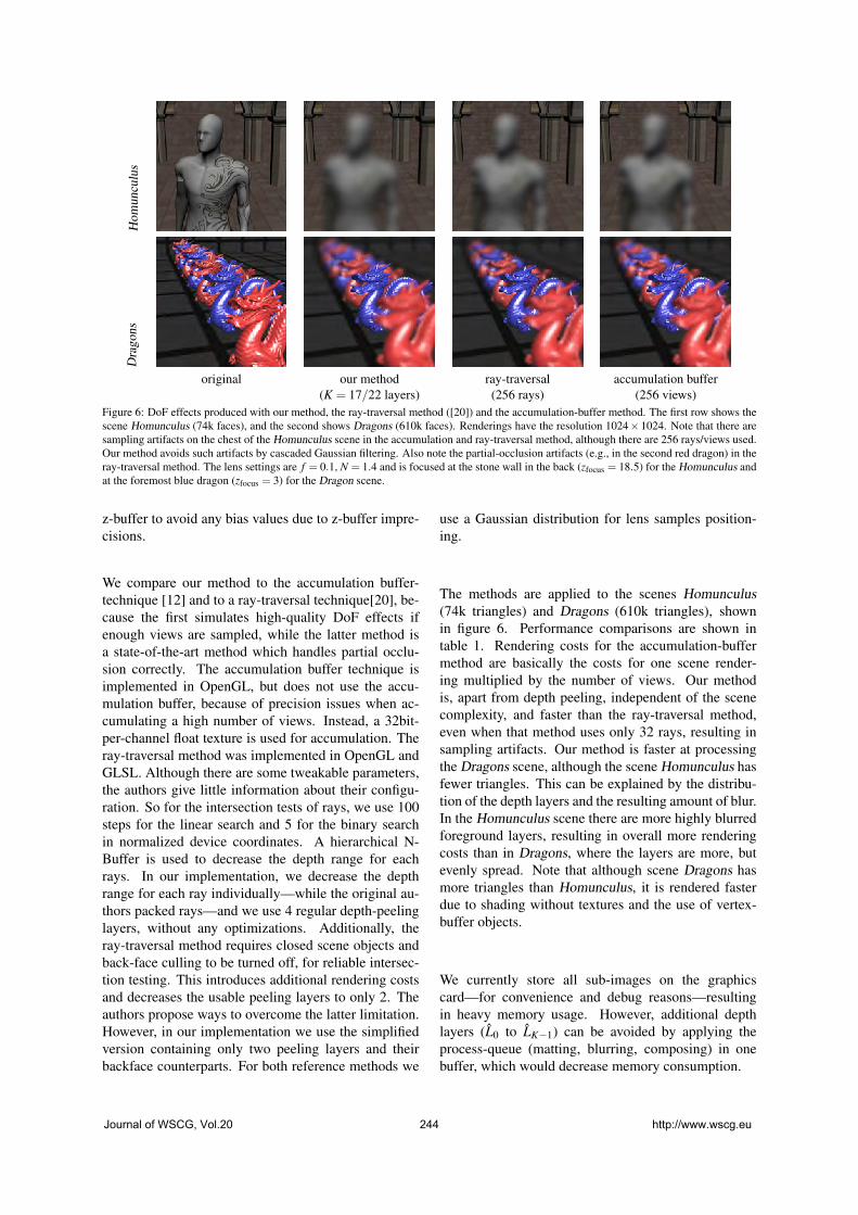
Hom

uncu

lus

Dra

gons

original our method ray-traversal accumulation buffer(K = 17/22 layers) (256 rays) (256 views)

Figure 6: DoF effects produced with our method, the ray-traversal method ([20]) and the accumulation-buffer method. The first row shows thescene Homunculus (74k faces), and the second shows Dragons (610k faces). Renderings have the resolution 1024×1024. Note that there aresampling artifacts on the chest of the Homunculus scene in the accumulation and ray-traversal method, although there are 256 rays/views used.Our method avoids such artifacts by cascaded Gaussian filtering. Also note the partial-occlusion artifacts (e.g., in the second red dragon) in theray-traversal method. The lens settings are f = 0.1, N = 1.4 and is focused at the stone wall in the back (zfocus = 18.5) for the Homunculus andat the foremost blue dragon (zfocus = 3) for the Dragon scene.

z-buffer to avoid any bias values due to z-buffer impre-cisions.

We compare our method to the accumulation buffer-technique [12] and to a ray-traversal technique[20], be-cause the first simulates high-quality DoF effects ifenough views are sampled, while the latter method isa state-of-the-art method which handles partial occlu-sion correctly. The accumulation buffer technique isimplemented in OpenGL, but does not use the accu-mulation buffer, because of precision issues when ac-cumulating a high number of views. Instead, a 32bit-per-channel float texture is used for accumulation. Theray-traversal method was implemented in OpenGL andGLSL. Although there are some tweakable parameters,the authors give little information about their configu-ration. So for the intersection tests of rays, we use 100steps for the linear search and 5 for the binary searchin normalized device coordinates. A hierarchical N-Buffer is used to decrease the depth range for eachrays. In our implementation, we decrease the depthrange for each ray individually—while the original au-thors packed rays—and we use 4 regular depth-peelinglayers, without any optimizations. Additionally, theray-traversal method requires closed scene objects andback-face culling to be turned off, for reliable intersec-tion testing. This introduces additional rendering costsand decreases the usable peeling layers to only 2. Theauthors propose ways to overcome the latter limitation.However, in our implementation we use the simplifiedversion containing only two peeling layers and theirbackface counterparts. For both reference methods we

use a Gaussian distribution for lens samples position-ing.

The methods are applied to the scenes Homunculus(74k triangles) and Dragons (610k triangles), shownin figure 6. Performance comparisons are shown intable 1. Rendering costs for the accumulation-buffermethod are basically the costs for one scene render-ing multiplied by the number of views. Our methodis, apart from depth peeling, independent of the scenecomplexity, and faster than the ray-traversal method,even when that method uses only 32 rays, resulting insampling artifacts. Our method is faster at processingthe Dragons scene, although the scene Homunculus hasfewer triangles. This can be explained by the distribu-tion of the depth layers and the resulting amount of blur.In the Homunculus scene there are more highly blurredforeground layers, resulting in overall more renderingcosts than in Dragons, where the layers are more, butevenly spread. Note that although scene Dragons hasmore triangles than Homunculus, it is rendered fasterdue to shading without textures and the use of vertex-buffer objects.

We currently store all sub-images on the graphicscard—for convenience and debug reasons—resultingin heavy memory usage. However, additional depthlayers (L0 to LK−1) can be avoided by applying theprocess-queue (matting, blurring, composing) in onebuffer, which would decrease memory consumption.


our (DP/matting/blur) Total (DP/ray-traversal) Total accum.cascaded non-cascaded 256 128 32 rays 256 views

Homunculus (74k tri.) (46/5/51)102 (46/5/95)146 (58/1290)1348 (48/643)691 (48/140)188 4809Dragons (610k tri.) (40/7/51)98 (40/8/85)133 (69/1374)1443 (69/685)754 (59/152)211 4163

Table 1: Performance comparisons, in ms, of our method (cascaded and non-cascaded blurring) with the ray-traversal method ([20]) andthe accumulation-buffer method for the scenes Homunculus and Dragons. Renderings have the resolution 1024× 1024 and 4 Depth-peelingiterations (DP) have been used.


We have presented a depth-of-field post-processingmethod with the aim of overcoming the partial occlu-sion artifact. The contribution of this work is a simple,efficient and GPU-friendly method. We combinedepth-peeling with improved matting functions toavoid the overhead of rendering to a high numberof depth layers. Furthermore we use high-qualityGaussian filters in a recursive way, which has not beendone—to our knowledge—in DoF methods before.With the usage of Gaussian filters, high blur radii canbe simulated, where even the reference methods startto produce sampling artifacts. We have shown thatthose DoF effects can be produced at frame rates thatare significantly higher than previous methods, makinghigh-quality DoF available for interactive applications.

One important step for the correct handling of partialocclusion is depth peeling, which is frequently used toresolve transparency issues, thus making the methodhardly usable for interactive applications like games.

Currently we use Gaussian filters, which are separa-ble and can be computed efficiently while deliveringartifacts-free images. The usage of cascaded filterswhile composing the DoF effect slightly alters the pro-duced image, but results in better performance. Ifhigher frame rates are needed and visual quality can besacrificed faster blurring methods (e.g., box, pyramidfilters) can be used.

The composition by alpha-blending is simple and effi-cient, thus leading to faster results when compared tocurrent methods like [20]. Layering discretization arti-facts known from other methods are mostly avoided bymatting, depth peeling and normalization.

Wide-spread anti-aliasing methods (i.e., MSAA)cannot be easily enabled for our method. However,image-based anti-aliasing methods (such as MLAA orFXAA)—which are becoming more popular due to thewide usage of deferred shading—can be applied.

Currently, layers are split based on the dcoc of fragmentsand on the chosen blurring method. This might resultin empty layers. Decomposition could be optimized byusing clustering methods, such as k-means clustering,as proposed in [21, 16]. With the use of clustering, layerborders could be tailored to the pixel density in scenesand empty layers could be avoided. However, cluster-

ing is a costly process and therefore only applicable foroff-line rendering.

One further field of investigation would be the impactof correct partial occlusion rendering on human percep-tion. We think that a correct handling of partial oc-clusion in combination with gaze-dependent focusing(e.g., with an eye-tracker) would result in deeper im-mersion of the user.

6 ACKNOWLEDGMENTSThanks to Juergen Koller for providing the Homunculusmodel. The used Dragon and Sponza models are cour-tesy of Stanford Computer Graphics Laboratory andMarko Dabrovic.

7 REFERENCES[1] Brian A. Barsky, Daniel R. Horn, Stanley A.

Klein, Jeffrey A. Pang, and Meng Yu. Cam-era models and optical systems used in computergraphics: Part I, Object based techniques. Tech-nical report, University of Berkeley, California,USA, 2003.

[2] Brian A. Barsky, Daniel R. Horn, Stanley A.Klein, Jeffrey A. Pang, and Meng Yu. Cam-era models and optical systems used in computergraphics: Part II, Image-based techniques. Tech-nical report, University of Berkeley, California,USA, 2003.

[3] Brian A. Barsky and Todd J. Kosloff. Algorithmsfor rendering depth of field effects in computergraphics. In Proceedings of the 12th WSEASinternational conference on Computers, pages999–1010, Stevens Point, Wisconsin, USA, 2008.World Scientific and Engineering Academy andSociety (WSEAS).

[4] Brian A. Barsky, Daniel R. Tobias, MichaelJ.and Horn, and Derrick P. Chu. Investigatingocclusion and discretization problems in imagespace blurring techniques. In First InternationalConference on Vision, Video and Graphics, pages97–102, University of Bath, UK, July 2003.

[5] Brian A. Barsky, Michael J. Tobias, Derrick P.Chu, and Daniel R. Horn. Elimination of artifactsdue to occlusion and discretization problems inimage space blurring techniques. Graphics Mod-els, 67(6):584–599, November 2005.


[6] Marcelo Bertalmio, Pere Fort, and DanielSanchez-Crespo. Real-time accurate depth of fieldusing anisotropic diffusion and programmablegraphics cards. In Proceedings of the 3D DataProcessing, Visualization, and Transmission, 2ndInternational Symposium, 3DPVT ’04, pages767–773, Washington, DC, USA, 2004.

[7] Wilhelm Burger and Mark J. Burge. Principles ofDigital Image Processing: Advanced Techniques.To appear, 2011.

[8] Robert L. Cook, Thomas Porter, and Loren Car-penter. Distributed ray tracing. In Proceed-ings of the 11th annual conference on Computergraphics and interactive techniques, SIGGRAPH’84, pages 137–145, New York, NY, USA, 1984.ACM.

[9] Xavier Décoret. N-buffers for efficient depth mapquery. Computer Graphics Forum, 24(3), 2005.

[10] J. Demers. Depth of field: A survey of tech-niques. In Fernand Randima, editor, GPU Gems,chapter 23, pages 375–390. Pearson Education,2004.

[11] C. Everitt. Interactive order-independent trans-parency. Technical report, NVIDIA, 2001.

[12] Paul Haeberli and Kurt Akeley. The accumulationbuffer: hardware support for high-quality render-ing. SIGGRAPH Computer Graphics, 24:309–318, September 1990.

[13] Earl J. Hammon. Practical post-process depthof field. In Hubert Nguyen, editor, GPU Gems3: Programming Techniques for High-Perfor-mance Graphics and General-Purpose Computa-tion, chapter 28, pages 583–606. Addison-Wesley,2007.

[14] Michael Kass, Lefohn Aaron, and John Owens.Interactive depth of field using simulated diffu-sion on a GPU. Technical report, Pixar AnimationStudios, 2006.

[15] Todd J. Kosloff, Michael W. Tao, and Brian A.Barsky. Depth of field postprocessing for layeredscenes using constant-time rectangle spreading.In Proceedings of Graphics Interface 2009, pages39–46, Toronto, Canada, 2009.

[16] Todd Jerome Kosloff. Fast Image Filters forDepth of Field Post-Processing. PhD thesis,EECS Department, University of California,Berkeley, May 2010.

[17] Martin Kraus. Using Opaque Image Blur for Real-Time Depth-of-Field Rendering. In Proceedingsof the International Conference on ComputerGraphics Theory and Applications : GRAPP2011, pages 153–159, Portugal, 2011. Institutefor Systems and Technologies of Information,Control and Communication.

[18] Martin Kraus and Magnus Strengert. Depth-of-field rendering by pyramidal image processing.Computer Graphics Forum, 26(3):645–654, 2007.

[19] Sungkil Lee, Elmar Eisemann, and Hans-PeterSeidel. Depth-of-field rendering with multiviewsynthesis. ACM Transactions on Graphics (TOG),28(5):1–6, 2009.

[20] Sungkil Lee, Elmar Eisemann, and Hans-PeterSeidel. Real-time lens blur effects and focuscontrol. ACM Transactions on Graphics (TOG),29(4):65:1–65:7, July 2010.

[21] Sungkil Lee, Gerard Jounghyun Kim, and Seung-moon Choi. Real-time depth-of-field renderingusing splatting on per-pixel layers. ComputerGraphics Forum (Proc. Pacific Graphics’08),27(7):1955–1962, 2008.

[22] Sungkil Lee, Gerard Jounghyun Kim, and Seung-moon Choi. Real-time depth-of-field renderingusing anisotropically filtered mipmap interpola-tion. IEEE Transactions on Visualization andComputer Graphics, 15(3):453–464, 2009.

[23] Fang Liu, Meng-Cheng Huang, Xue-Hui Liu,and En-Hua Wu. Single pass depth peeling viacuda rasterizer. In SIGGRAPH 2009: Talks, SIG-GRAPH ’09, New York, NY, USA, 2009. ACM.

[24] Jurriaan D. Mulder and Robert van Liere. Fastperception-based depth of field rendering. In Pro-ceedings of the ACM symposium on Virtual Re-ality Software and Technology, VRST ’00, pages129–133, Seoul, Korea, October 2000. ACM.

[25] Michael Potmesil and Indranil Chakravarty. Alens and aperture camera model for synthetic im-age generation. In Proceedings of the 8th AannualConference on Computer Graphics and Interac-tive Techniques, SIGGRAPH ’81, pages 297–305,Dallas, Texas, USA, 1981. ACM.

[26] Guennadi Riguer. Real-time depth of field simu-lation. In Wolfgang F. Engel, editor, ShaderX2:Shader Programming Tips and Tricks with Di-rectX 9, pages 529–556. Wordware Publishing,October 2003.

[27] Thorsten Scheuermann and Natalya Tatarchuk.Improved depth of field rendering. In WolfgangEngel, editor, ShaderX3: Advanced RenderingTechniques in DirectX and OpenGL, pages 363–378. Charles River Media, 2004.


Journal of WSCG

Index

Akagi,Y. 21 Akyuz,A.O. 155 Alda,W. 231 Amann,J. 127 Anjos,R. 145 Aristizabal,M. 189 Arregui,H. 189 Benger,W. 223 Bernard,J. 97 Boryczko,K. 231 Brambilla,A. 57 Congote,J. 81 189

Dupej,J. 65 Engel,S. 231 Ferko, A. 137 Gerhard,S. 81 Ginsburg,D. 81 Hahn,H.K. 11 Hauser,H. 57 Held,M. 205 Holmberg,N. 117 Huang,G. 29 Huang,X. 29 Hucko,M. 217 Hufnagel,R. 205 Chajdas,M.G. 127 Chang,C.-F. 171 Chen,Y.-C. 171 Chiew,W.M. 1 Chiu,Y.-F. 171 Ivanovska,T. 11 Jalba,A.C. 179 Jan,J. 73 Jira,I. 73 Johan,H. 37 Kabongo,L. 81 Kanzok,Th. 161 Karadag,G. 155

Kim,J. 29 Kitajima,K. 21 Knecht,M. 47 Kobrtek,J. 89 Kolomaznik,J. 197 Koubek,T. 197 Kozlov,A. 107 Krajicek,V. 65 Landa,J. 197 Leberl, F. 137 Lee,R.-R. 171 Lin,F. 1 Linsen,L. 11 161

MacDonald,B. 107 May,T. 97 Moreno,A. 189 Movania,M.M. 1 Navrátil,J. 89 Novo,E. 81 Oliveira,J. 145 Ourednicek,P. 73 Pelikan,J. 65 Pereira,J. 145 Pienaar,R. 81 Popelka,O. 197 Prochazka,D. 197 Qian,K. 1 Recky,M. 137 Ritter,M. 223 Rosenthal,P. 161 Ruiz,O. 81 189

Seah,H.S. 1 37

Segura,A. 189 Schedl,D. 239 Scherer,M. 97 Schreck,T. 97 Skotakova,J. 73 Sramek,M. 217

Tandianus,B. 37 Tanzmeister,G. 47 Tokuta,A. 29 Traxler,C. 47 Veleminska,J. 65 Verschoor,M. 179 Viola,I. 57 Walek,P. 73 Westermann,R. 127 Wilhelm,N. 97 Wimmer,M. 239 Wimmer,W. 47 Wuensche,B. 107 117

Yuen,W. 117 Zemcík,P. 89 Zheng,G. 29

Journal - WSCG

Documents

Transcript of Journal - WSCG