Journal of Networks - CiteSeerX

Journal of Networks ISSN 1796-2056

Volume 8, Number 3, March 2013

Contents

REGULAR PAPERS Real-time-service-based Distributed Scheduling Scheme for IEEE 802.16j Networks Kuo-Feng Huang and Shih-Jung Wu The Measurement of Optimization Performance of Managed Service Division with ITIL Framework using Statistical Process Control Kasman Suhairi and Ford Lumban Gaol On Varying Network Coding Forwarding Ratio in Vector Based Wireless Sensor Networks Mohammed Halloush and Tasneem Dawahdeh Optimized Energy Management for Mixed Uplink Traffic in LTE UE Vinod Mirchandani and Peter Bertok A Framework for Automated Security Proof and its Application to OAEP Guang Yan, Zhu Yue-Fei, Gu Chun-Xiang, Fei Jin-long, and He Xin-Zheng A Review of Routing Protocols in Wireless Body Area Networks Samaneh Movassaghi, Mehran Abolhasan, and Justin Lipman On Sensor Data Verification for Participatory Sensing Systems Diego Mendez and Miguel A. Labrador Infrastructure Based Chord Structure for P2P File Sharing over Vehicular Network Hung-Chin Jang and Tzu-Yao Hsu Downlink Power Control for CDMA Satellite Cognitive Radio Peng Chen, Lede Qiu, and Feng Xu CloudProxy: A NAPT Proxy for Vulnerability Scanners based on Cloud Computing Yulong Wang and Jiakun Shen Adaptive Clustering for Maximizing Network Lifetime and Maintaining Coverage Luqiao Zhang, Qinxin Zhu, and Juan Wang A Leakage-Based Beamforming Algorithm for Cognitive MIMO Systems via Game Theory Feng Zhao, Xuezhi Lv, and Hongbin Chen A SNR-based Multi-channel Multicast Scheme for Popular Video in Wireless Networks Ting T. Liu, Wei Yang, Chang L. Xu, and Young-Il Kim A Novel Multi-layered Immune Network Intrusion Detection Defense Model: MINID Xufei Zheng, Yonghui Fang, Yanhui Zhou, and Jing Zhang Enhancing Node Cooperation in Mobile Ad Hoc Network S. Kami Makki and Keenan B. Bonds

513

518

530

537

552

559

576

588

598

607

616

623

628

636

645

Design of Three-dimensional Interchange Network Based on IPv4/IPv6 Network Yange Chen, Zhili Zhang, and Qingfang Cui Wireless Position Scheme based on ZigBee Network in the Freeway ETC System Baishun Su and Baoding Zhang Multiple Antennas Spectrum Sensing for Cognitive Radio Networks Yang Ou and Yi-Ming Wang An Efficient Parallel Anomaly Detection Algorithm Based on Hierarchical Clustering Ren Wei-wu, Hu Liang, Zhao Kuo, and Chu Jianfeng Improving K-means Clustering Method in Fault Diagnosis based on SOM Network Anhua Chen, Yang Pan, and Lingli Jiang Research on Web Information Retrieval based on Vector Space Model Zhang Ji Bo Ning Detecting Protein Complexes through Micro-Network Comparison in Protein-Protein Interaction Networks Haihong Li, Luo Zhong, and Huaxiong Yao Stability of Impulsive Cellular Neural Networks with Time-varying Delays Yuanqiang Chen Spectrum Allocation Based on Game Theory in Cognitive Radio Networks Qiufen Ni, Rongbo Zhu, Zhenguo Wu, Yongli Sun, Lingyun Zhou, and Bin Zhou A Workflow-based RBAC Model for Web Services in Multiple Autonomous Domains Zhenwu WANG, Xuejun ZHAO, Benting WAN, Jun XIE, and Pengfei BAI Blocking DoS Attack Traffic in Network with Locator/Identifier Separation Jianqiang Tang, Ying Liu, Ming Wan, and Hongke Zhang Optimality and Duality for Minimax Fractional Semi-Infinite Programming Xiaoyan Gao

650

658

665

672

680

688

696

704

712

723

731

739

Real-time-service-based Distributed Scheduling Scheme for IEEE 802.16j Networks

Kuo-Feng Huang1, Shih-Jung WuTaipei College of Maritime Technology/Visual Communication Design, New Taipei City, Taiwan

2*

Tamkang University/Innovative Information and Technology, New Taipei City, Taiwan1

Email: [email protected]

1, [email protected]

2

Abstract—Supporting Quality of Service (QoS) guarantees for diverse multimedia services is the primary concern for IEEE802.16j networks. A scheduling scheme that satisfies the QoS requirements has become more important for wireless communications. We proposed an adaptive nontransparent-based distributed scheduling scheme (ANDS) for IEEE 802.16j networks. ANDS comprises three major components: Priority Assignment, Resource Allocation, Preserved Bandwidth Adjustment. Different service-type connections primarily depend on their QoS requirements to adjust priority assignments and dispatch bandwidth resources dynamically. Meanwhile, we promote the connections, which do not satisfy QoS requirements, to avoid the delay and starvation. Simulation results show that our APS methodology outperforms the representative scheduling approaches in both QoS satisfaction and maintains fairness in starvation prevention.

Index Terms—Distributed Scheduling, IEEE 802.16, Relay, Real-time, Non-Transparent

I. INTRODUCTION The internet service has become the necessity of

modern society. The demand of internet results in spreading internet constructions no matter in urban area or countryside. The wired network system meets more restrictions and suffers more difficulties. To save the cost of construction time and decrease the construction complexity when deploying wired network in a developed city, the wireless network system seems a better solution. WiMAX (Worldwide Interoperability for Microwave Access) system is the mainstream of wireless network technology [9-14]. The IEEE 802.16 standard is developed as the guideline for WiMAX system. The main object of the standard is to ensure that the device from different manufacturers won’t cause the compatibility problems [4, 8].

For the convenience of using internet resource, the goal of wireless network system is to provide network service as possible as it could. However, providing network service to a blind spot or a sparsely populated area by a BS usually substantially increases the cost to system suppliers. The RS architecture which is specified in the IEEE 802.16j, as the extension of IEEE 802.16, could overcome these problems by multi-hop relaying technology [6].

II. RELATED WORKS To overcome the compatibility problems to the

existing WiMAX system and unify the specifications from different manufacturers, the IEEE 802.16j working group is dedicated to establish the standard of multi-hop relay technology. The relay technology is a new issue because of the integration of relay station and the existing network system.

Relay stations can be classified into two classes by whether the Preamble and UL/DL MAP being broadcasted. The non-transparent RS supports the broadcasting of Preamble and UL/DL MAP but the transparent RS doesn’t.

A. Transparent RS The frame structure of a transparent RS is based on the

two-hop transparent relaying specified in the IEEE 802.16j standard. It includes the MR-BS frame structure and the transparent RS frame structure. One transmission frame could be divided into DL sub-frame and UL sub-frame.

The DL sub-frame of MR-BS is divided into two zones. One is DL Access Zone for MS and RS, and another one is DL Transparent Zone in Silent Mode. The UL sub-frame of MR-BS is divided into UL Access Zone and UL Relay Zone. The DL sub-frame of transparent RS is divided into DL Access Zone in Receiving Mode and DL Transparent Zone. The UL sub-frame of transparent RS is divided into UL Access Zone and UL Relay Zone in Transmitting Mode. The RS supports the relaying when the transmission between BS and MS is decided to use two-hop relaying. The packet from BS is delivered to RS by and relay to MS in downlink transmission, and the packet from MS is delivered to RS and relay to BS in uplink transmission.

B. Non-Transparent RS The frame structure of a non-transparent RS is based

on the two-hop transparent relaying specified in the IEEE 802.16j standard. It includes the MR-BS frame structure and the non-transparent RS frame structure. The DL sub-frame of MR-BS is divided into DL Access Zone and DL Relay Zone. The UL sub-frame of MR-BS is divided into UL Access Zone for MS and UL Relay Zone. The DL sub-frame of non-transparent RS is divided into DL Access Zone for MS and DL Relay Zone in Receiving Mode. The UL sub-frame of non-transparent RS is divided

JOURNAL OF NETWORKS, VOL. 8, NO. 3, MARCH 2013 513

© 2013 ACADEMY PUBLISHERdoi:10.4304/jnw.8.3.513-517

into UL Access Zone for MS and UL Relay Zone in Transmitting Mode.

In the network system with non-transparent RS architecture, the non-transparent RS supports the relaying when the transmission between BS and MS is decided to use two-hop relaying. The relay station architecture which is added to the new standard, IEEE 802.16j, gives more challenges to the scheduling issue. Because of the difference in RS’s functionality the scheduling scheme could be classified into two modes, that is centralized scheduling and distributed scheduling. In centralized scheduling mode, the BS needs to handle all of the scheduling information in a cell and decide the order how system serves each MS. However, the BS will share the scheduling overhead with RSs in distributed scheduling mode. For the network system with non-transparent RS, the system could schedule in both centralized and distributed mode since the non-transparent RS is capable of dealing with scheduling information. On the other hand, the network system with transparent RS should only schedules in centralized mode. Nevertheless, no matter which scheduling mode and RS is used, the BS is always has the authority to manage all of the MSs in a cell [1, 7].

The scheduling issue in wireless network system is close to resource management and the main purpose of scheduling is for QoS guaranteed. However, the IEEE 802.16j doesn’t make any provision about the scheduling mechanism hence the issue leaves discussion for later researches [2, 3, 5].

III. ADAPTIVE NONTRANSPARENT-BASED DISTRIBUTED SCHEDULING (ANDS)

ANDS

Priority Assignment Resource Allocation Preserved Bandwidth Adjustment

Service Type Ranking

Priority Adjustment

BandwidthRequirementCalculation

BandwidthAllocation

BandwidthStatus Report

PreservedBandwidth

Re-Allocation Figure 1. RTDS architecture

Our research proposes an adaptive real-time-service-based distributed scheduling scheme (RTDS) for IEEE 802.16j network system. RTDS will guarantee the QoS of the users and enhance the efficiency of the network system by assigning and adjusting bandwidth dynamically. The main goal of RTDS is to satisfy all connections’ requests as far as possible.

Figure 1 is the scheduling architecture of RTDS. In this paper, we divide chapter three into three parts to make a detail description of RTDS. Part (A): Priority Assignment. Part (B): Resource Allocation. Part (C): Preserved Bandwidth Adjustment.

A. Priority Assignment TABLE 1. IEEE 802.16J DEFINED SERVICE TYPE

UGS (Unsolicited

Grant Service)

Maximum Sustained Traffic Rate, Minimum Reserved Traffic Rate,

Maximum Latency, Unsolicited Grant Interval,

Tolerated Jitter ertPS

(Extended Real-Time

Polling Service)


Maximum Latency, Unsolicited Grant Interval,

Tolerated Jitter rtPS

(Real-Time Polling Service)


Maximum Latency

nrtPS (Non-Real-

Time Polling Service)

Maximum Sustained Traffic Rate, Minimum Reserved Traffic Rate

BE (Best Effort) Maximum Sustained Traffic Rate

RTDS quantifies five classes of traffic type which are specified in the IEEE 802.16j to give an initial priority value for scheduling order. Table 1 shows the initial priority value for five classes of traffic type. These values match our goal that is enhancing the QoS of real time service connections. There are five traffic types specified in the IEEE 802.16j, which are UGS, ertPS, rtPS, nrtPS and BE, and the initial priority value are 5, 4, 3, 2 and 1 respectively. Since UGS, ertPS and rtPS are real time services, the initial priority values of UGS, ertPS and rtPS are higher then nrtPS and BE.

After the initial priority value of each connection is set, RTDS adjust the initial priority value to the different condition and request of each connection. The section of priority adjustment is divided into three phases which are Priority Promotion by Packet Delay Tolerance Rating, Priority Promotion by Packet Critical Rating and Priority Diminution, respectively.

Phase one of priority adjustment is Priority Promotion by Packet Delay Tolerance Rating. The main idea of this phase is to promote the priority value of a connection by its case of packet delay.

Arrival Timeof the Packet

Current Timeof System

Overdue Timeof the PacketT S

Maximum Latency of the Packet

TW T H

Time

ω

Arrival Timeof the Packet

Current Timeof System

Overdue Timeof the PacketT S

Maximum Latency of the Packet

TW T H

Time

ω

Figure 2. Packet delay time diagram

Figure 2 depicts the delay time of a packet. The packet arrival time, denoted by T

A

, means the time when a packet arrives in an access station, such as BS and RS. The calculation of T

W

is defined as: )()( jj TTT A

iSW

i −= (1)

)( jTWi is packet waiting time of the j’th packet of

connection i.

T S

is the current time of the system.

514 JOURNAL OF NETWORKS, VOL. 8, NO. 3, MARCH 2013

© 2013 ACADEMY PUBLISHER

)( jT Ai is packet arrival time of the j’th packet of

connection i.

Our research defines the packet remaining halt time, denoted by T

H

, to indicate the legal halting time for a packet. Let the maximum latency of packet minuses its packet waiting time to obtain T

H

, which means the packet will be a out of date packet after the time T

H

and dropped. The calculation of T

H

is defined as: )()( jj TT W

iiHi −=ω (2)

)( jT Hi : packet remaining halt time of the j’th packet of

connection i. ω i : maximum latency of service type i.

Our research defines the packet delay tolerance rating, denoted by RD

i , to represent the average value of the packet remaining halt time from the same connection i. The formula is defined as:

∑=

=N

ji

ji

Hi

Di NTR

1/)(

(3)

N i : number of packets from connection i. In general speaking, the connections with a lower

value of RDi means most of the packets will be out of date

soon and should be scheduled first. On the other hand, the

connections with a higher value of RDi means the

connections could suffer more waiting time. Thus, our research defines a parameter for priority promotion,

denoted by PCi . The function of normalization is defined

as: )/(1 _RRP MAXD

iDi

Di −=

(4)

Phase two of priority adjustment is Priority Promotion by Packet Critical Rating. The main idea of phase two is to promote the priority value of the connections which with packets are going to be out of date on the next transmission frame. Thus, the RTDS could satisfy the QoS of these connections. To distinguish a packet which is going to be out of date, the estimation formula is defined as:

TT FWi ≤−ω (5)

T F

: time duration of a transmission frame. If formula (5) stands, it means the packet will be out of

date if it is not transmitted at the scheduling frame. And under this circumstance, the QoS of users will be decreased. In our research, we define these packets as critical packet. In general speaking, a connection with more critical packets will generate much more unsatisfied QoS and should be served earlier. We define critical packet rating to represent the critical degree of a connection, and as follows:

∑=

=N

jCi

j

Wi

Ci TR

1)( (6)

N C

i : number of critical packets in connection i.

RCi : critical packet rating of connection i.

And we also normalize the critical packet rating to get the priority value to promote. The function is defined as:

RRP MAXCi

Ci

Ci

_/= (7)

PCi : priority value to promote.

R MAXCi

_

: maximum value of the critical packet rating with the same service type as connection i.

The final phase, phase three, of priority adjustment is Priority Diminution. RTDS will decrease the priority value of the connections which get priority promoted twice by critical packet condition. The main idea of this phase is to offer fairness among the connections. The diminution function is defined as:

γ*PP Di

Fi = (8)

PFi : priority value to decrease.

γ : fairness parameter, from 0% to 100%. To obtain the final priority value, RTDS sums up all

priority parameters in one total priority value. The final priority value of each connection i is defined as:

PPPPP Fi

Ci

Di

Ii

Ti −++= (9)

B. Resource Allocation After RTDS obtains the final priority value of each

connection, the following step is to allocate bandwidth to each connection. First of all, RTDS calculates the upper bound and the lower bound of bandwidth request for each connection. The upper bound of bandwidth request for

connection i is denoted by bi

max

, and the lower bound of bandwidth request for connection i is denoted by bi

min

. The definitions of these two functions are defined as follow:

)*,*min( maxmax TRNb Fiiii β=

(10)

)*,*min( minmin TRNb Fiiii β=

(11)

N i : number of packets which are waiting for scheduling in connection i.

β i : size of a packet.

Rimax

: maximum sustained traffic rate of connection i.

Rimin

: minimum reserved traffic rate of connection i.

T F

: duration of a transmission frame. The lower bound and upper bound of bandwidth

request for all connections and the total bandwidth of the system will divide resource allocation into three conditions: (1) System bandwidth is greater than the upper bound. (2) System bandwidth is between the upper bound and the lower bound. (3) System bandwidth is smaller than the lower bound.



In situation (1), RTDS will allocate the upper bound of bandwidth to each connection since the system has plenty of resource.

In situation (2), RTDS allocates the lower bound of bandwidth to each connection to meet the basic requirement of QoS. After satisfying the basic requirement of Qos, RTDS will look for the connections which have got priority promoted by critical packet rating. For these connections, RTDS will allocate the upper bound of request by their priority value. Last, RTDS will allocate the remainder to each connection by the ratio of bandwidth request.

In situation (3), RTDS must make decision to sacrifice some connections’ QoS provision since the total system bandwidth couldn’t even afford the lower bound of bandwidth request of every connection. RTDS will allocate the lower bound of bandwidth request to each connection by its priority value until there is no longer any system bandwidth left.

C. Preserved Bandwidth Adjustment The feature of distributed scheduling is that the BS

doesn’t need to realize how RS making its own scheduling. This feature will bring lesser overhead to the BS but also bring some disadvantages such as the non-real time service handled by the BS may obtain more resource than the real time service handled by the RS since the BS only have the announcement of total bandwidth request for each RS. Therefore, RTDS builds a preserved bandwidth mechanism to protect the QoS of connections which are scheduled by RS.

RTDS defines the bandwidth status report which is send by the RS in order to notify the BS of the lower bound of bandwidth request for real time service connections. The BS collects all of the bandwidth status reports and then adjusts the preserved bandwidth of each RS by its ratio of bandwidth request.

IV. SIMULATION AND RESULTS ANALYSIS The simulation model refers to the IEEE 802.16j

standard and the simulation environment is in a cell. A BS is in the center of the cell and its transmission range is 8 km. 6 RSs are spreading among the cell and the transmission range of a RS is 3 km. The BS and RSs are in line of sight and at the distance of 5 km. The simulation model is depicted as figure 3.

3 km 8 km

BS

RS 2

RS 3

RS 4

RS 5RS 1

RS 6

3 km 8 km

BS

RS 2

RS 3

RS 4

RS 5RS 1

RS 6

Figure 3. Simulation model

We assume the buffer of the BS and the RS is unlimited and the packet size of UGS, ertPS, rtPS, nrtPS and BE are 160 bytes, 160 bytes, 240 bytes, 120 bytes and 120 bytes, respectively. The time duration of a transmission frame is 5 ms. The generation model of calls which are made by the MSs refers to Poisson Distribution function in order to meet the actual environment. The simulation time is 30000 frames, which is 150 seconds.

We use a simple call admission control (CAC) to decide whether a connection should be accepted by the system. If the system could not afford the minimum bandwidth request for a new connection, the system will reject the request for connecting.

Figure 4 shows the average delay time of real time service connections. RTDS suffers about 1.9 ms delay time in average. However, DFPQ and PQ suffer more on average delay time, about additionally 0.6 and 0.8 ms respectively.

Figure 4. Average delay time of real time service

Figure 5. Average delay time growth by difference system load

Figure 5 shows the average delay time growth by different system load. PQ and DFPQ will obviously increase the delay time when the system load is at the percentage of 50%. However, RTDS increases the delay time until the system load is at the percentage of 70%

Figure 6 shows the packet drop rate growth according to different system load. PQ will dramatically increase the drop rate when the system load is at the percentage of 40%. DFPQ will dramatically increase the drop rate when the system load is at the percentage of 60%. RTDS also increases the drop rate when the system load is at the percentage of 70%. RTDS could afford much more



system load against to the drop rate and the growth curve is flatter than others.

Figure 6. The packet loos arte growth by different system load

V. CONCLUSION AND FUTURE WORK Our research proposed a distributed scheduling

scheme, RTDS, for IEEE 802.16j networks. RTDS will allocate bandwidth dynamically for different types of connections to meet each connection’s QoS requirement. RTDS primary guarantees the QoS of real time service connections and additionally provides the fairness to every connection. The simulation results show that RTDS will suffer less packet delay time and packet loss rate than other representative researches.

In future works, we are going to take uplink scheduling into consideration to obtain a more completely and precisely scheduling scheme. Furthermore, we will provide more fairness to the non-real time service connections to enhance the overall QoS performance.

REFERENCES [1] Jianfeng Chen, Wenhua Jiao and Hongxi Wang, “A

Service Flow Management Strategy for IEEE 802.16 Broadband Wireless Access Systems in TDD Mode.” IEEE International Conference on Communications, ICC 2005, Volume 5, Page(s):3422 – 3426, 16-20 May 2005.

[2] Fen Hou, Pin-Han Ho, Xuemin Shen and An-Yi Chen , “A Novel QoS Scheduling Scheme in IEEE 802.16 Networks.” IEEE Wireless Communications and Networking Conference, WCNC 2007, Page(s):2457 – 2462 , 11-15 March 2007.

[3] Safa H., Artail H., Karam M., Soudan R. and Khayat S , “New Scheduling Architecture for IEEE 802.16 Wireless Metropolitan Area Network.” IEEE/ACS International Conference Computer Systems and Applications, AICCSA 2007., Page(s):203 - 210 13-16 May 2007.

[4] IEEE 802.16-2004, IEEE Standard for Local and Metropolitan Area Networks, Part 16: Air Interface for fixed and mobile broadband wireless access systems, amendment for physical and medium access control layers for combined fixed and mobile operation in licensed bands,“ February 2006.

[5] Sun J., Yanling Yao and Hongfei Zhu, “Quality of Service Scheduling for 802.16 Broadband Wireless Access Systems.” IEEE Vehicular Technology Conference,VTC 2006, Volume 3, Page(s):1221 – 1225, 7-10 May 2006.

[6] Qiang Ni, Vinel A., Yang Xiao, Turlikov A. and Tao Jiang , “Wireless Broadband Access: WIMAX And Beyond -

Investigation of Bandwidth Request Mechanisms under Point-to-Multipoint Mode of WiMAX Networks.” IEEE Communication H Magazine, Volume 45, Issue 5H, Page(s):132 – 138, May 2007.

[7] Genc V., Murphy S., Yang Yu and Murphy J, “IEEE 802.16J Relay-based Wireless Access Networks: an Overview.” IEEE Wireless Communications, Volume 15, Issue 5, Page(s):56 – 63, October 2008.

[8] Hui Zeng and Chenxi Zhu, “System-Level Modeling and Performance Evaluation of Multi-Hop 802.16j Systems.” International Wireless Communications and Mobile Computing Conference, IWCMC '08. Page(s):354 – 359, 6-8 Aug. 2008.

[9] IEEE 802.16j-2009, “Draft Amendment to IEEE Standard for Local and Metropolitan Area Networks, Part 16: Air Interface for Fixed and Mobile Broadband Wireless Access System,” 4 February, 2009.

[10] Ntagkounakis K., Dallas P., Sharif B., Valkanas A., “Adaptive TDD Synchronization for WiMAX Access Networks,” IET Communications, Volume 1, Issue 6, Page(s): 1218 – 1223, Dec. 2007.

[11] Po-Chun Ting, Chia-Yu Yu, Chilamkurti N., Tung-Hsien Wang, Ce-Kuen Chieh, “A Proposed RED-based Scheduling Scheme for QoS in WiMAX Networks,” International Symposium on Wireless Pervasive Computing, ISWPC 2009. Page(s):1 – 5, 11-13 Feb. 2009.

[12] Thaliath J., Joy M., Priya John E., Das D., “Service Class Downlink Scheduling in WiMAX,” International Conference on Communication Systems Software and Workshops, COMSWARE 2008. Page(s):196 – 199, 6-10 Jan. 2008.

[13] Bhatt T., Sundaramurthy V., Jian-Zhong Zhang, McCain D., “Initial Synchronization for 802.16e Downlink,” Asilomar Conference on Signals, Systems and Computers, ACSSC 2006. Page(s):701 – 706, Oct.29 2006.

[14] Peters S.W., Heath R.W., “The Future of WiMAX: Multihop Relaying With IEEE 802.16j,” IEEE Communications Magazine, Page(s):558 – 574, Volume 47, Issue 1, January 2009.

Kuo-Feng Huang received the B.S., M.S., and Ph.D. degrees in Computer Science and Information Engineering from the Tamkang University in 2003, 2007, and 2011, respectively. From September 1st

, 2011, he was an assistant professor in department of computer and communication engineering of Taipei College of Maritime Technology. His

current research interests are Wireless Communication, Mobile Communication, Wireless Sensor Networks and Embedded System.

Shih-Jung Wu was born in Taipei, Taiwan (R.O.C.), on Oct. 25, 1976. He received his B.C. degree from Department of Business Administration, Yuan Ze University, Taiwan (R.O.C.) in 1998. He received M.S. degree from Department of Computer Science and Information Engineering, Tamkang University, Taiwan (R.O.C.) in 2001. And he received his Ph.D. degree in the Department of Computer Science and Information Engineering, Tamkang University, Taiwan (R.O.C.) in 2006. Presently, he is working at Department of Innovative Information and Technology, Tamkang University in Taiwan (R.O.C.). His major research interests in high speed communications, mobility, QoS guarantees, and parallel algorithms.



The Measurement of Optimization Performance of Managed Service Division with ITIL

Framework using Statistical Process Control

Kasman Suhairi Graduate Program in Information Technology, Bina Nusantara University, Indonesia


Ford Lumban Gaol Graduate Program in Information Technology, Bina Nusantara University, Indonesia


Abstract— The purpose of the Configuration Management process is carrying and all IT assets, status, configuration, and relationship between each other being well documented. This documentation is useful, among others, for some purposes. The first objective is to create clarity in the relationship between key performance indicators (KPI) an IT services with the infrastructure. Changes to the configuration of those devices would obviously very disturbing the performance of IT services. The second objective is the accuracy of the information which will be used by the Service Delivery processes. So a Service Desk staff who need to get information about how a user at a branch office to connect to the network's headquarters, linked to issues of access to certain applications. Accurate network configuration information will be helpful Service Desk staff in helping the user solve the problem. The third objective is the accuracy of the information will be used for the IT audit.PT. XYZ is a telecommunications company which relatively new and aware of the increasing competitive competition in the telecommunications industry. PT. XYZ was starting its operation in 2006. The company's ambition is to develop progressively by increasing operational performance which closely linkages between operational performance improvements company with a bottom line of the company. Thus, it is a necessity / obligation for companies in the global era of integrated telecommunications services, to focus on Quality of services (QoS) provided to its customers, in order to survive in an increasingly competitive telecommunications business. (KS) Index Terms— Managed Service, ITIL, and Configuration management

I. INTRODUCTION

Information Technology Infrastructure Library (ITIL) is a collection of best practices for Information Technology Service Management (ITSM). While the Information Technology Service Management (ITSM) itself is a guide to the processes of IT service that exists in the organization, which wraps all the functional types of IT, which was previously more oriented to an application or infrastructure. ITSM approach aimed at

reducing disparities between the language of IT with business unit managers who use IT services, so that the alignment between business and IT can be realized from the very beginning of the IT life cycle [2].

In the world of cellular telecommunications services, the use of ITIL Service Management in the management of telecommunications networks continues to experience growth. The development of mobile telecommunications technology affects the cellular operators to continue to adapt in order to continue to expand its network capabilities that improve service to customers can be improved in order to achieve customer satisfaction.

One of the mobile operators who wish to enhance customer satisfaction is the PT. XYZ, developed a radio network capacity to accommodate 3G services to customer through upgrading BR10, which is implemented by PT. Nokia Siemens Networks as one of the mobile vendors. Prior to that PT. XYZ has a few problems in the network BSS on vendor. Therefore, the vendor implements BR10 software upgrade to resolve the issue. Use of ITIL Service Management is one of its components is Configuration management is used by PT. XYZ in managing this upgraded BR10. Assessment of the success of the activity of BR10 upgrade is done by looking at Key Performance Indicator (KPI), which translates as the level of quality expected after the upgrade BR10 (radio signal quality), so that the cellular customer satisfaction can be achieved. Apart from that the monitoring of cellular networks continues to be done as an embodiment of the process of Continuous Improvement efforts.

The rest of this paper organized as follows: Part 2 will discussed about development of GSM. next the Methodology and conclusion.

II. GLOBAL SYSTEM FOR MOBILE COMMUNICATION



A. The development of GSM (Global System for Mobile Communication)

Global System for Mobile Communication (GSM) was first recognized in 1982 and is the name of a committee under the umbrella Conference Europeenne des Postes et Telecommunications (CEPT) formed to define a new standard of mobile telecommunications to replace a wide range of mobile telecommunications standard that is widely used analog in several European countries. Telecommunications standards are designed to use digital technologies that are different from previous standards where analog technology is no longer used.

The first GSM network was launched in 1991 and shortly after its launch, soon most countries in Europe apply to the accompaniment of the spread of GSM technology GSM countries outside Europe. Because of the very rapid development, a term later changed to GSM Global System for Mobile Communications and the GSM standard proved to be the most widely applied on this planet.

At the beginning of the GSM standard is set, only operates on GSM 900-MHz frequency band, where most of the GSM network operates using the frequency band. The use of another frequency band occurred in England in 1993 which uses 1800 MHz frequency band with the commercial name of DCS (Digital Cellular System). Meanwhile, GSM was introduced in North America with the commercial name of the PCS (Personal Communication System) operating at 1900 MHz frequency band. [4].

B. GSM Network Topology GSM network topology using a cell structure as listed

in Figure 1. and on GSM cellular networks are included distribution of frequency bands into small parts and use the frequency spectrum in several Base Transceiver Station (BTS) that represents a cell that serves the Mobile Station (MS). Definition of BTS and the MS are clear that a cell covers an area of mobile telecommunications services. Air interface is the interface between the BTS and MS. Meanwhile, a device that handles multiple cell service is called a Base Station Subsystem (BSS) integrated with the core network to perform functions in the voice service (Circuit Switched) and data services (Packet Switched).

Figure 1. GSM Cell Structure [3]

C. GSM Network Components In Figure 1 shows that a GSM network system consists

of several subsystem elements are: Network Switching Subsystem (NSS), Base Station Subsystem (BSS), Network Management Subsystem (NMS). On the customer side there is a Mobile Station (MS) which is the tissue that is needed to establish a call consists of NSS and BSS. BSS function to control its radio network (Radio Network) and NSS serves to control the functions of control, therefore all calls would go through the NSS [2].

D. The GSM network subsystems and components Mobile Station (MS) Mobile Station (MS) is a telecommunication device on

the network users. MS consists of terminal equipment called a Mobile Equipment (ME) and customer data stored in a module called a Subscriber Identity Module (SIM). Valid driver's license as a database containing user identification number and a list of available networks. SIM is also a component to the process of checking the authenticity (authentication) and encryption (chipering). There is also a memory space to store messages and phone numbers.

Base Station Subsystem (BSS) Base Station Subsystem (BSS) is a

telecommunications device that serves to regulate the radio network. A BSS consists of BTS, BSC, TRAU and covering a wide area and comprises many cells with functions as follows:

Base Transceiver Station (BTS) Base Transceiver Station (BTS) is a

telecommunications device that regulates air interface and minimizing disruption for air interface transmission is very sensitive to disturbance.

To solve this problem BTS has 120 parameters that define the exact type of a BTS and how MS can know the network when moving into the area of BTS. The parameters of base stations to handle things as follows: the type of handover (when and why), paging settings, radio power level control, and identification of BTS. Some of the BTS processes undertaken include:

1. Air interface signaling Several signaling related calls and non calls must be

made for the system to work. Examples include when the MS is turned on for the first time, shipping and receiving much needed information to the BTS before you can make and receive phone calls. Signaling is required for initiating a call. Then the signaling is necessary to perform handovers.

2. The encryption (ciphering) MS and base stations must be able to perform the

encryption and cryptanalysis of conversation and information to protect data sent over the air interface.

3. Conversations Signal Processing (speech processing) Speech signal processing includes functions such as

speech coding in the digital to analog and analog to the digital downlink on uplink direction, channel coding for



protection against damage information, interleaving to improve the security of transmission, and burst formation.

Transcoding Rate and Adaptation Unit (TRAU) Transcoding Rate and Adaptation Unit (TRAU) is

telecommunication device that does the conversion between the two compression formats performed between base stations and the central network. At the air interface, radio frequency is the carrier of information. To produce a digital information transmission effective conversation over the air interface, the digital speech signal is undergoing a process of compression (compression). GSM networks also must be able to communicate with the PSTN network (wired telephone network) in which the speech compression format used is different.

Base Station Controller (BSC) Base Station Controller (BSC) is a central component

of the BSS network that serves to control the radio network base stations and TRAU.

Network Switching Subsystem (NSS) NSS is a telecommunications device that consists of

network components Mobile services Switching Centre (MSC), Visitor Location Register (VLR), Home Location Register (HLR), Authentication Center (AC) and Equipment Identity Register (EIR).

Mobile services Switching Center (MSC) MSC is responsible for controlling calls in a GSM

network. MSC is to identify the origin and destination of a call from MS or a landline as well as the type of call. An MSC acts as a bridge between GSM and the phone cable is called the Gateway MSC (GMSC). MSC is responsible for several important functions as follows:

1. Call settings MSC identifies the type of call, destination and origin

of a call. He is also responsible for the establishment, supervision, and cleanup call.

2. Originator of the paging process. Paging is the process of determining the location of an

MS call destination. 3. Billing data collection services. Visitor Location Register (VLR) Visitor Location Register (VLR) is a database that

contains information about customers who are in a service area. Information that include:

1. Identification number of the customer. 2. Authentication security information for the process

of driver's license and for encryption (ciphering). 3. Customer service that can be used. VLR register (registration) and site updates. When an

MS enters a new VLR service area, the MS did an update location. VLR database is temporary, in the sense that the data about the customer stored in the VLR for the customer is located in the VLR service area. VLR HLR also contains the addresses of those customers.

Home Location Register (HLR) Home Location Register (HLR) is a device for

managing data telecommunication keep from customers such as customer identification numbers. Besides the fixed data, the HLR also update the location of the customer at any time. This information is used to locate the MS MSC is the destination of a call.

Authentication Centre (AUC) Authentication Centre (AUC) is a telecommunications

device that provides security information to the network. With that information the network can check / test the validity of the SIM card (the process of authentication between MS and VLR) and encode information emitted via the air interface (between MS and BTS).

Equipment Identity Register (EIR) Equipment Identity Register (EIR) is a

telecommunications device that also has a network security functions such as AUC. However, if the AUC provides information to check the SIM card, then the EIR serves to check the International Mobile Equipment Identity (IMEI). At the checking process, the MS was asked to provide the IMEI number. This number contains a code of type approval (type approval code), the final assembly code (the final assembly code) and serial number (serial number) from your mobile phone (Mobile Equipment). The EIR has three categories of ME:

1. ME in the white list (white list) is allowed to operate normally.

2. ME in the list of gray (gray list) can be controlled if the suspected damage to him.

3. ME in the black list (black list) is not permitted to operate within the network.

Network Management Subsystem (NMS) Network Management Subsystem (NMS) is a

telecommunications device that serves to monitor the various functions and components of the network. Operator workstation connected to the database server communication via a Local Area Network (LAN). Server database stores information about network management. Communications server is responsible for data communication between the NMS and the equipment in the GSM network, known as network components. Communication is done via a Data Communications Network (DCN), which is connected to the NMS via a router.

Functions of the NMS can be divided into three categories:

1. Management failure (fault management). The goal of fault management is to ensure the smooth

running of the network operation and rapid correction of various problems that are detected. Fault management notifies the operator about the status of harmful events and manages a database that contains signs of danger.

2. Configuration management (configuration management).

The purpose of configuration management is to manage the information up-to-date information about



operating status and configuration of network components.

3. Performance Management (management on performance).

In performance management, NMS collects data HSIL measurement of each network component and saved in a Database. Based on these data, network operators can compare the actual performance of the network with the planned performance and detect areas of good performance and is not well in the network.

Figure 2 GSM subsystems [5]

E. Information Technology Infrastructure Library (ITIL) Information Technology Infrastructure Library (ITIL)

is a collection of best practices for Information Technology Service Management (ITSM). While the Information Technology Service Management (ITSM) itself is a guide to the processes of IT service that exists in the organization, which wraps all the functional types of IT, which was previously more oriented to an application or infrastructure. ITSM approach aimed at reducing disparities between the language of IT with business unit managers who use IT services, so that the alignment between business and IT can be realized from the very beginning of the IT life cycle.

In a cellular telecommunications network management, PT. XYZ uses ITIL as its network management technology. ITIL or Information Technology Infrastructure Library, is a framework that created and developed by the Office of Government Commerce (OGC) in England. ITIL is a collection of best practice corporate governance of information technology services in various fields and industries, from manufacturing to financial, industrial large and small, private and government, including the mobile telecommunications sector.

ITIL has grown along with the development of information technology. Figure 3 shows the components contained in ITIL version 3. Fundamental changes in this version is from the perspective of IT management, which in version 2 of ITIL service management as a set of processes and functions while in ITIL version 3 as a life-cycle services [7].

Figure 3. ITIL version 3 [16]

Difference in perspective between ITIL version 2 and

ITIL version 3 is only a reorganization and restructuring of the groove, where IT and the business no longer have different views that must be bridged and aligned (alignment), but is expected to IT and business has been directed to view the services as end of all existing processes. Therefore, recycling services starting from the definition hidur strategy, design, transition, operations and continuous improvements made can be done together as well as from the same angle between business and IT. Thus, conceptually no longer required an effort to harmonize between IT and business outlook, because it should have been aligned.

For companies that have implemented ITIL version 2 and intend to implement ITIL version 3, it is advisable to create a blueprint and roadmap as well as identifying quick win from the whole process and the functions contained in ITIL version 3, for further mapping of the processes of ITIL version 2 which has now implemented. Then the implementation process became more focused and unambiguous. In ITIL version 3 more processes and functions involved and, if not structured implementation strategy and clear objectives from the beginning of the implementation will not be so successful.

Broadly speaking, ITIL version 3 consists of five sections and more emphasis on life cycle management services provided by IT. The five sections are:

1. Service Strategy 2. Service Design 3. Service Transition 4. Service Operation 5. Continual Service Improvement 2.4.1 ITIL Service Cycle The five parts of ITIL above are also called as part of a

cycle. Also known as ITIL Service Cycle. Briefly, each piece is described in the section below.

Service Strategy The core of the ITIL Service Lifecycle is the Service

Strategy. Service Strategy provides guidance to implementers on how to look ITSM concepts not only as



an organizational capability (to provide, manage and operate the IT services), but also as a strategic asset of the company. This guide is presented in the form of the basic principles of ITSM concepts, references and processes that operate in the whole core ITIL Service Lifecycle stages.

The topics discussed in this lifecycle stage includes the establishment of a market for selling services, the types and characteristics of internal and external service providers, service assets, the concept of service portfolio and implementation strategy for the overall ITIL Service Lifecycle. The processes covered in Service Strategy, in addition to the above topics are:

1. Service Portfolio Management 2. Financial Management 3. Demand Management For the new IT organization will implement ITIL,

Service Strategy is used as a guide to determine goals / objectives and expectations of the value of performance in managing IT services and to identify, select and prioritize a variety of operational and organizational improvement plans within the IT organization.

For IT organizations today have implemented ITIL, Service Strategy is used as a guide to conduct a strategic review of all processes and devices (roles, responsibilities, supporting technologies, etc.) ITSM in the organization are to enhance the capabilities of all the ITSM processes and tools.

Service Design In order for IT services can provide benefits to the

business, the IT services it must first be designed with reference to the business goals of customers. Service Design provides guidance to IT organizations to systematically and best practices to design and build services that IT or ITSM implementations itself. Service Design contains the principles and methods of design for converting strategic objectives into IT organizations and business portfolio / collection of IT services and service assets, such as servers, storage and so on.

The scope of Service Design is not solely to design new IT services, but also the processes of change and improvement of service quality, continuity of service or performance of services. The processes covered in Service Design, namely:

1. Service Catalog Management 2. Service Level Management 3. Supplier Management 4. Capacity Management 5. Availability Management 6. IT Service Continuity Management 7. Information Security Management Service Transition Figure 4 shows the functions of Configuration

Management in Service Transition. Service Transition provides guidance to IT organizations to develop and the ability to change the design of both new IT services and IT services that changed the specifications to the operational environment. Lifecycle phases provide an

overview of how a requirement defined in the Service Strategy is then formed in Service Design to further effectively realized in Service Operation. The processes included in Transition Service are:

1. Transition Planning and Support 2. Change Management 3. Configuration management 4. Release & Deployment Management 5. Service Validation 6. Evaluation 7. Knowledge Management

Figure 4. Service Transition of ITIL version 3 [5] Service Operation Service Operation is the stage lifecycle that includes

all activities of daily operational management of IT services. Inside are various guides on how to manage IT services efficiently and effectively and ensure the level of performance that has been agreed with the previous customers. These guidelines include how to maintain the operational stability of IT services and management of design changes, the scale, scope and target performance of IT services.

The processes included in Transition Service are: 1. Event Management 2. Incident Management 3. Problem Management 4. Request fulfillment 5. Access Management. Continual Service Improvement Continual Service Improvement (CSI) provides

important guidance in developing and maintaining quality of service of process design, transition and operation. CSI combines principles and methods of quality management, one of which is the Plan-Do-Check-Act (PDCA) or which is known as the Deming Quality Cycle.

F. Configuration management This paper analyzes focus on configuration

management in ITIL framework used by the PT. XYZ. Configuration Management Database or better known as the CMDB is a repository of IT infrastructure or a component called a Configuration Item (CI) is interconnected with each other to form an infrastructure configuration. CMDB in ITIL is a single point of truth that is expected to be the only valid reference for the



configuration of the IT infrastructure for all parties, including the processes and other ITIL functions.

The question that often arises is “what is the difference between Configuration, Asset and Inventory Management?” Basically this process has a third and manage the same data, but there is a difference of purpose of each process. Configuration management is intended to manage the data infrastructure or IT components and their relationships with others. Thus in Configuration Management, Relationships between IT components to the other one gets the emphasis. While aimed more Asset Management in managing the financial aspects of the Asset-IT assets. While the Inventory Management is a process that is intended to manage the stock level of inventory, in this case are goods included into consumable items or goods consumables.

The third difference of this process must be understood clearly, especially during implementation so that the scope of the CMDB implementation of the goals is not to be biased CMDB itself. However, in practice it should also be considered with selective requirements relating to the Asset and Inventory Management so that the CMDB can be more informative for users of the CMDB itself or an interest against the company's Asset and Inventory.

Building a CMDB CMDB or Configuration Database management is a

strategic repository used by the cross-section within the company. Not only IT, but also business, customers and vendors have an interest in the CMDB data. Strategic value of the CMDB can be obtained if part or all of the CI can be mapped into a CMDB that defines the relationship and the relationship between CI. CMDB can help companies and organizations in the management of IT infrastructure components, including conduct assessment on the impact of changes to be made (Change Request / RFC), find out what components are affected by an incident including location, users, and other components that can be affected impact, knowing that some or all of the infrastructure company involved in business services, and management decision making [8].

However, creation of the CMDB is not as easy to build a database and populate the database with data. The following things need to be considered in making the CMDB, especially for companies and organizations that have a lot of service and supported by the infrastructure in large numbers: • Obtain commitment and support from

management, if possible not only the support of IT management but also from Business Management

• Getting the commitment and together with the data owners, data users and data responsibility in maintaining the validity, accuracy and regency of data

• Conducted in several phases to prevent the collection, population and data management that are too large at a time

• Any changes to the data contained in the CMDB, should be managed through the Change Request (Request for Change - RFC). Thus any change, all

interested parts of the data to know the change. Therefore the process of Change Management and Configuration management must first or jointly implemented by making the CMDB

• After the implementation process, should be a mechanism of Internal Audit (every 3 or 6 months) to keep the discrepancy of data between the CMDB, RFC and physical data is not too large

• Choosing the right tools to manage the CMDB and other ITSM processes (Incident Management, Problem Management, Service Level Management, Change Management, Release Management, Availability Management, Capacity Management, IT Service Continuity Management, Financial Management for IT, and Service Desk).

G. Key Performnce Indicators We used data Key performance indicators (KPI) to

analyze the performance of BSS network of PT XYZ. KPI is an indicator that defines a series of measures to determine performance and provide information to us how far we managed to achieve the performance targets imposed on us. KPIs can be a numerical value of the existing resource capability. One example is the BSS network KPI on Call Setup Success Ratio (CSSR).

There are a number of things that must be observed when we want to implement the KPI-based telecommunications projects. Ideally, each company can develop a kind of catalog of KPIs for each area of telecommunications, for example [6]:

Call Centre - Waiting Times - The average speed in answering

customer calls - Number of calls - A large number of customer complaints received - Revenue per call - The quality of the average phone call - The number of calls to be diverted - Average call duration - Customer satisfaction

- A large number of customer calls answered in 10 seconds - Efficiency agents.

Systems and Network Performance Analysis / Capacity Planning

- Availability of Services - Level of Service - The lifetime of the device - Bit error rate (BER) - Data Rate - Time of service when they fall - The level of telephone service - Cost of service system - Operational Costs - The average length of time the conversation - The level of data bottlenecks in service - Phone calls are dropped.

Revenue / Financial Analysis - The average revenue per telephone user (ARPU) -

Number of prepaid customer ARPU - Total ARPU by contract - Revenue per minute talks - Percentage of revenue for services beyond voice - Average revenue realization (ARR) - Amount of time the customer usage - Average revenue per employee (ARPE) - Average revenue per customer (Arps).

Achievement of KPI monitoring system needs to be done. Many companies have set KPI quite well but stopped midway due to lack of support systems and good



monitoring. For example, the company already has a KPI of Score Systems and Network Performance Analysis / Capacity Planning, but apparently they do not have the tools to measure it. Or another example, the KPIs of IT has an average duration of the repair servers, but do not have monitoring tables to record how long the average of their improvement process. Take another example, a section has a KPI on the number of customer complaints that can be completed thoroughly; but then did not develop mechanisms to measure the process. The above examples show the importance of monitoring and supporting system for the realization of data documenting the KPI. Only with the support of this monitoring scheme, the achievement of KPI every month or every quarter can be managed and controlled to the optimum.

Without good monitoring systems, performance improvement can ultimately culminate in what is referred to as "IEC Gaming" or KPI game. And this gaming is usually susceptible to parts or the administrative support function. KPIs should be recognized dimensions usually boils down to two things: the level of accuracy of reporting and timeliness of report preparation.

Without a monitoring system is neat, the achievement of KPI data can be filled with not careful. As a result, which is often visible achievement of KPI data they tend to always be "good" (e.g., always 100% accuracy, and timeliness is always stated on time; timeliness own criteria when they may not have the default standard).

In this paper used a performance measurement by using one of the components of the IBC on the network BSS Call Setup Success Ratio (CSSR). CSSR is a comparison between the calls that managed to occupy the traffic channels (call seizure) with the number of attempted calls (call Attempt). CSSR CSSR is good with high scores. At minimum standard GSM operators CSSR used was 98%. The greater the CSSR obtained from the data traffic (> 98%) show more and more calls that managed to occupy the canal. If CSSR <98% then the number of calls that are not managed to occupy the canal will be many more.

CSSR data in this paper are taken from Inspur system, according to the time of the incident to be retrieved daily, weekly, or monthly. Of the CSSR data is then analyzed the extent to which influence the activity of BR10 software upgrades on the performance of PT. XYZ.

H. Statistical Process Control (SPC) SPC began 1920 by Steward concerned that

management processes to produce a favorable situation for businesses and consumers, promote the importance of SPC control chart. Harold, Eugene, Deming develop SPC process. Formation Control chart limits have been transformed from initially limits the original concept of economic profitability of limits, based on variations of the group. Problems arising from the complexity of modern processes and variable polynomial, which will make the technologies grow more sophisticated. Therefore, controlling the future models should consider the number and the correlation relationship between

variables, characterized by the co-variance matrix, caused by the relationship between variables and the process [7].

False Alarms are used in SPC in a batch processes. Such problems can be solved with the help of multi variance SPC. M-SPC multidimensional compresses into a few variables that explain the diversity of variables to be measured, including relation to one another. This chapter will discuss the use of SPC and the M-SPC by using some components parameters.

Normal distribution in this paper is used to determine the sample from the process to be observed under controlled conditions or beyond the control of the system, namely by carrying out statistical sample calculations and to plot the sample into the normal distribution graph regularly. If the resulting distribution patterns do not change over time, it can be said that the process is in a phase controlled statistically. Pierre Simon LaPlace said the central limit theorem that if there is a random sample for a number of n observations selected from a population of data (any probability distribution) with the average value / mean value μ and standard deviation σx-bar = σ / √ n . The larger the size of a sample of the better forecasts will be generated for the sample average value.

The goal is about to find out when the time of a process that is beyond control (out of control) so that adjustments can be done at the right time. The whole process has variability, which causes the incurrence of costs and conditions that are not desirable; therefore, these conditions must be suppressed as much as possible. Process adjustment requires additional costs due to the slow throughput and requires no small amount of resources. Measurement process is also not cheap because it does not take a short.

Therefore, it is important to determine what should be measured from a process and when it is appropriate to make changes to the process.

Control charts Control chart consisting of the y axis and the x-axis,

dashed lines depict the standard deviation of the sample (below and above the interval), center line which is the average value of the distribution of samples will be used to show the picture of the processes that are observed in the period with some specific rules that can be used are:

1. One point which is outside the standard deviation than a third are upper control limit (UCL) and lower control limit (LCL), which has a probability of 100% up to 99.7% or 0.003 or 3 possibilities in every 1000.

2. Two points are located between the second and third deviations are on the same side of the center line, ie the square root of the reduction of 99.7% and 95.5% divided by two equals 0.0004.

3. Seven pieces of adjacent point which is entirely located above or below the average value (every point has a probability of 50%).

4. If there are five points up or down sequentially forming a pattern, it indicates the change process.

2.7.2 Attributes and Variables There are many kinds of control chart is used, but must

be selected in accordance with what is to be measured



and statistically calculated. One way to determine the appropriate chart is the first to define the method used, i.e. qualitative or quantitative, where both methods use numbers.

Numerical values are to qualitative data is the number of defects / damaged data is calculated as a percentage or fraction defect. Both are used to measure the attributes, characteristics of the quality of a discrete value, for example, is a measurement process that defect versus non-defect. In this case use c-chart obtained from the errors that appear on the sample data or the p-chart obtained from the percentage of errors in the data sample.

After that these quantitative data which is the variable data is calculated and the data is ongoing (continuous data) and use rational values. Rational values are values that can be expressed in terms of comparison / ratio. (For example, a 4.4 foot long board is 2:1 than 2.2 foot board. The same can be used for the thickness, length, weight, etc.). When it comes to control variables, c and p charts should be used because it requires X chart to see if there is a shift in central tendency, while the R-chart notify changes in the spread that must be done in a range of standard deviation to measure the magnitude of the spread which is an estimate derived from the collection data.

Trouble Ticket System and Inspur (TT) Inspur system is a network management tool PT. XYZ

in the Network Management Subsystem (NMS). How it works Inspur system refers to the ITIL concept which includes incident management and configuration management. The data used in this paper was collected using Inspur system. Inspur system has been used by PT. XYZ during the three years since April 2008.

Inspur is a system to support the operation of the NMS that can be divided into three categories namely:

Figure 5 Inspur system [9]

1. Management failure (fault management). The goal of fault management is to ensure the smooth

running of the network operation and rapid correction of various problems that are detected. Fault management notifies the operator about the status of harmful events and managing a database that contains signs of danger. In the system used the term Inspur Trouble Ticket (TT). TT is a tool in the system Inspur as a record for any problems / failures that arise in telecommunication networks of PT. XYZ.

2. Configuration management (configuration management).

The purpose of configuration management is to manage the information up-to-date information about operating status and configuration of network components.

3. Performance management (on performance management).

In performance management, NMS collects data HSIL measurement of each network component and saved in a Database. Based on these data, network operators can compare the actual performance of the network with the planned performance and detect areas of good performance and is not well in the network [11].

TT data is part of incident management (fault management), are used to support the analysis in the paper . So one goal of this paper is to determine and analyze the extent of the influence of the BSS software upgrades on the performance of PT. XYZ can be achieved. Furthermore, TT data is processed by the method of Statistical Process Control (SPC), and analyzed based on the results obtained.

The relationship between ITSM with TT in the PT. XYZ is that ITSM which is the manual processes that exist within the organization in this case PT. XYZ with the aim of providing customer satisfaction in the IT services / network in accordance with Service Level Agreement (SLA), use the TT as a tool to monitor effectively and efficiently some IT or network problems that arise. So the management can follow the development process of the IT or network problem solving and follow up to the parties involved in the process of solving the problem in order to meet SLA expectations.

III. THE RESEARCH METHODOLOGY

In this paper the authors identify problems with the Managed Services division of PT. XYZ and collect problem data in the form of Trouble Ticket (TT) obtained from observations carried out comprehensively in the past nine months. The type of TT include regional problems that occurred in south Sumatra, central Sumatra, Bodetabek, Jakarta, North Sumatra, Central Java, East Java and West Java. The problems are obtained, grouped in two categories based on the transmission and total TT (TT + TT transmission BSS). In writing this paper Inspur system used to obtain data from the second TT in the above categories, which the system is a system that has been used PT. XYZ for five years.

Inspur System is integrated into the radio system commander so that the data obtained is most accurate data.

Furthermore, the author uses methods Statistical Process Control (SPC) to process the data obtained from Inspur system. In the SPC method, the data is processed based on the timing of the problem and then calculated the mean (average) and range of data. After that, do the calculations to find the upper control limit (UCL) and lower control limit (LCL). UCL and LCL obtained mapped into a graph with all observational data in the can.



So it can be observed clearly chart pattern that occurs to see if the problem is still controlled or out-of-control.

Having obtained the results of the analysis of these problems, the authors provide recommendations for process improvement solutions Managed Service by first find the root cause of each problem that out-of-control.

Model and Analysis Method The first thing to do is determine the central line and

control limits using data already collected during the observation time on the process conditions in controlled circumstances. A process cannot be determined that in controlled conditions, until it made by control chart of the process. Thus, when the control chart is made first time, the center line and control limits is a trial value which will be experiencing adjustment.

In this paper used as many as 8 samples for Managed Service covers the operational areas of regional South Sumatra, Central Sumatra, North Sumatra, Bodetabek, Jakarta, Central Java, East Java and West Java for each of the Trouble Ticket (TT), then do the calculation in samples that expressed in the chart and determine the control limits based on these statistics, then the authors performed statistical values obtained plotting. If the eight samples taken from a deviation occurs, it is necessary to investigate certain cases, followed by process improvement and re-measurement.

So the first step to create a control chart there are three main considerations that need to be decided, namely:

1. Determining the quality characteristics need to be measured.

2. Determining the sampling plan will be created. 3. Establish how much error will be tolerated on the

evaluation of control, quality characteristics to be measured are a very important factor, considering closely related to the costs that will result from the output obtained. Meanwhile, the sampling plan is designed to accommodate random data and obtained from a different time each week.

Therefore, fault tolerance (risk of error) is used for ± 3σ, then the risk of errors that will occur is at 100% -99.7% which is equivalent to 0.3%. The following are the steps taken to make the control chart, namely:

1. Collect as many as eight or more samples (n samples) for n scale measurements.

2. Calculate the statistical sample to be used in a control chart.

3. Determining the center line on the average value / mean of n statistical sample.

4. Estimate the standard deviation (σ) of a process. Estimated value of σ will vary and depend on the type of chart used.

5. Determine upper and lower control limits on the ± 3σ control limits (approximate).

6. Doing all samples plotting on the chart statistics on a regular basis.

IV. RESEARCH RESULT

The author reinforces the importance of using ITIL methods in the management of BSS network of PT. XYZ.

because it supports the performance of services to its customers. At this stage the transition is a performed configuration management service to support the development of an existing BSS network, in order to continue to accommodate the needs of customers PT. XYZ increasing.

Based on observations on the operation of the network of PT. XYZ is known that the interplay between one subsystem to another subsystem. Thus we need a reliable Network Management System. Configuration Management conducted by PT. XYZ must be well planned, as well as in the implementation stage should be controlled to the optimum.

In this paper used data network that supports the analysis of the activity of BR10 software upgrades that support the performance of PT. XYZ. There are constraints that look at the implementation of planning in configuration management activities. Based on data obtained from these constraints, conducted Further analysis to be drawn a conclusion and a recommendation was made to the performance of PT. XYZ can be Increased. Here is the data in question:

1. The number of events (Trouble Ticket / TT) was recorded, caused by transmission problems in a period of 7 months (September 2010 - April 2011). The total is the sum of TT transmission with BSS.

2. Total events within a period of 7 months (September 2010 - April 2011).

3. Time plans are made to perform a software upgrade activities BR10.

Throughout the above data is processed using the method of Statistical Process Control (SPC), so it can be known at the time when a process is out of control. Then it can be drawn a conclusion and recommendations with the aim to Improve company performance.

In accordance with one of the goals of this paper , namely to know and analyze the extent of the influence of the BSS software upgrades on the performance of PT. XYZ based data processing with the SPC method, as the data in the form of 8 samples, the data for areas of Java and Sumatra, which includes the regional South Sumatra, Central Sumatra, North Sumatra, Bodetabek, Jakarta, Central Java, East Java and West Java.

The following steps to create control charts: 1. Collect as many as eight samples. 2. Calculate the statistical sample to be used in a

control chart. 3. Determining the center line on the value of 8

samples rata-rata/mean statistics. 4. Estimate the standard deviation (σ) of the

transmission process. 5. Determine upper and lower control limits on the ±

3σ control limits (approximate). 6. Plot on the chart makes the entire statistical sample. We get the calculation result obtained can be seen in

Table 1 below.

TABLE 1. TROUBLE TICKET DATA CALCULATION RESULTS



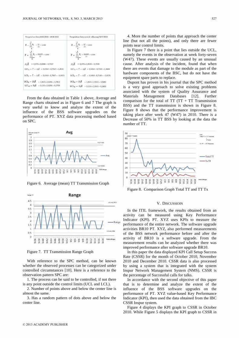
From the data obtained in Table 1 above, Average and

Range charts obtained as in Figure 6 and 7 The graph is very useful to know and analyze the extent of the influence of the BSS software upgrades on the performance of PT. XYZ data processing method based on SPC.

Figure 6. Average (mean) TT Transmission Graph

Figure 7. TT Transmission Range Graph With reference to the SPC method, can be known

whether the observed processes can be categorized under controlled circumstances [10]. Here is a reference to the observation pattern SPC are:

1. The process can be said to be controlled, if not there is any point outside the control limits (UCL and LCL).

2. Number of points above and below the center line is almost the same.

3. Has a random pattern of dots above and below the center line.

4. More the number of points that approach the center line (but not all the points), and only there are fewer points near control limits.

In Figure 7 there is a point that lies outside the UCL, namely the events in the observation at week forty-seven (W47). These events are usually caused by an unusual cause. After analysis of the incident, found that when there are events that damage to the module as part of the hardware components of the BSC, but do not have the equipment spare parts to replace.

Dupont has proven in his journal that the SPC method is a very good approach to solve existing problems associated with the system of Quality Assurance and Materials Management Databases [12]. Further comparison for the total of TT (TT + TT Transmission BSS) and the TT transmission is shown in Figure 8. Figure 8 shows that the performance improvement is taking place after week 47 (W47) in 2010. There is a Decrease of 50% in TT BSS by looking at the data the number of TT.

Figure 8. Comparison Graph Total TT and TT Tx

V. DISCUSSIOIN

In the ITIL framework, the results obtained from an activity can be measured using Key Performance Indicator (KPI). PT. XYZ uses KPIs to measure the performance of the entire network. The software upgrade activities BR10 PT. XYZ, also performed measurements of the BSS network performance before and after the activity of BR10 is a software upgrade. From the measurement results can be analyzed whether there was improved performance after software upgrade BR10.

In this paper the data displayed KPI Call Setup Success Rate (CSSR) for the month of October 2010, November 2010 and December 2010. CSSR data is also processed by using a system that is integrated with the system Inspur Network Management System (NMS). CSSR is the percentage of Successful calls for talks.

In accordance with the second objective of this paper that is to determine and analyze the extent of the influence of the BSS software upgrades on the performance of PT. XYZ value-based Key Performance Indicator (KPI), then used the data obtained from the IBC CSSR Inspur system.

Figure 4 displays the KPI graph to CSSR in October 2010. While Figure 5 displays the KPI graph to CSSR in



November 2010. And Figure 6 displays the KPI charts for the CSSR in December 2010. According to the graph, it was found that there was BSS network performance improvements on KPI CSSR occurred in November 2010 and December 2010. In the activity of BR10 software upgrades have been done on some network BSS PT. XYZ. In addition the Inspur system also had taken CSSR data on average in October 2010, November 2010 and December 2010.

The results of performance analysis is used to meet the expected network operating conditions and also can provide a guide in designing the development of BSS networks in the future. In addition to this performance analysis can be obtained accurately from the last condition that the customer needs so the company can optimally determine the next steps in terms of further development of the BSS network [14].

Under the second objective of this paper that is to determine and analyze the extent of the influence of the BSS software upgrades on the performance of PT. XYZ in accordance with the Key Performance Indicator (KPI), it is used as Tables contains average CSSR data obtained in Inspur system. CSSR data this average to support the KPI analysis of the BSS network. Of the CSSR data is obtained average performance improvement that occurred BSS network of 0.8% in the CSSR. With the increasing value of CSSR, the more calls from customers who succeeded in occupying the BSS network. Thus customer satisfaction in using the services of PT. XYZ can be increased.

VI. CONCLUSION

From the results of the discussion and analysis of the data processed by SPC and data analysis method IEC CSSR, it can be concluded in accordance with the purpose of this thesis are:

1. Activity BR10 software upgrade provides a positive effect for the performance of PT BSS network. XYZ. This is shown by a reduced number of Trouble Ticket (TT) of 50% in the operations of PT BSS network. XYZ. This indicated that the BR10 software as new software that replaces the old software, reducing some of the problems that exist in the BSS network.

2. The results of data processing and analysis using Statistical Process Control (SPC), show that there is a process in the Managed Services division of PT. XYZ needs to be improved based on the ITIL framework. That process is management of spare parts. There is an event of unavailability of replacement parts for the hardware module of the BSS network.

3. The results of data analysis based on the value of PT BSS KPI CSSR network. XYZ indicates that the BSS network performance improvement occurs with increasing value of CSSR. With the increasing value of CSSR, the more calls from customers who succeeded in occupying the BSS network. Increasing the value of CSSR in this thesis by 0.8%. Thus customer satisfaction in using the services of PT. XYZ can be increased.

4. As a guideline to direct the organization's IT and IS firms toward fulfilling the needs of customers better then

the development of PT BSS network capabilities. XYZ to address the existing experiences to the BSS network can be done by software upgrades BR10, which is implemented by Nokia Siemens Network (NSN) as one of the mobile vendors. Activity BR10 software upgrade has been managed effectively and efficiently through the ITIL framework, especially in the configuration management so that the results obtained in accordance with the expected value of the KPI.

BR10 solution software upgrades as part of the ITIL framework in the configuration management, undertaken to improve the performance of BSS Network PT. XYZ. Monitoring Network BSS still needs to be continued, to find out if there is a new symptom related to software or hardware problems BSS. For the BSS performance monitoring needs to be done simultaneously and if the new problems arise can be quickly acted upon. So That the BSS’s significant performance degradation can be avoided. In addition management of spare parts as part of configuration management activities, needs to be done properly to avoid problems due to unavailability of spare parts at the time it takes for the network BSS in order to function properly. So it needs to be done as a spare part dimensioning parts availability plan in all areas of the BSS network in accordance with its needs of each area.

Preventive Maintenance is needed in the operations of PT. XYZ for all network elements that are either BSS Network, Transmission Network, Core Network, Datacom Network and VAS Network. From the Preventive Maintenance activities can be prevented at an early stage, problems that require considerable time to mitigate them. To obtain the results of Key Performance Indicator (KPI) is good.

Future studies can be performed on an already unstable situation after the software upgrade process is complete, at a certain time. Researchers are advised to use SPC as a tool for controlling operational processes that exist in the Managed Service PT. XYZ. So that it can be seen on which the process in PT. XYZ out of control, to then be taken a number of steps to improve the process.

ACKNOWLEDGMENT

The authors wish to thank Bina Nusantara University for the support of this research.

REFERENCES

[1] EE Dwinells and JP Sheffer. "The Performance Adavantage" March 1992: P30-p31, APICS

[2] Isabel González , Ismael Sánchez . "Variable Selection for Multivariate Statistical Process Control ". Journal of Quality Technology . Milwaukee: July 2010 . Vol. 42, ISS. 3; p. 242,

[3] Nokia Siemens Network's, "GSM / EDGE Mobile D850/D900/D1800/D1900 Communication System ", 2009, NSN, Finland

[4] Rick Sloop. "Preventive Maintenance your SPC" Journal of Quality Technology , Automated Precision Inc.., Dec 2010

[5] M Siegmund Redl, Matthias K Webber, Malcolm W. Oliphant: "GSM and Personal Communications Handbook", 1998, Artech House London, UK.



[6] Toni Toni Anwar & Lim Wern Li, "Performance Analysis of 3G Communication Network "ITB J. ICT Vol. 2, No. 2, 2008, p130-p157

[7] Thuntee Sukchotrat , Seoung Bum Kim , Fugee Tsung . "One-class-based classification Control charts for multivariate process monitoring " IIE Transactions . Norcross: Feb 2010. Vol. 42, ISS. 2, P107

[8] Finch, BJ., Luebe, RL., "Operations Management: Competing in a Changing Environment", 1995, Harcourt Brace & Co.

[9] Galin, Daniel., "Software Quality Assurance: From Theory to Implementation", 2004, Pearson, UK.

[10] James R. Evans, William M. Lindsay, "The Management and Control of Quality", 2005,

[11] Thomson South Western Mayer, Silvian, "Impact of GPRS on the Signalling of a GSM- Based Network", 1999, University of Sttutgart: Institute of Communication Networks and Computer Engineering.

[12] Nokia Siemens Network's, "GSM / EDGE Mobile D850/D900/D1800/D1900 Communication System ", 2009, NSN, Finland

[13] Ram TS Ramakrishnan, Anjan V. Thakor. "The Review of Economic Studies: 51 Information Reliability and a Theory of financial intermediation", Vol.51, No. 3, p.415-432, 1984.

[14] Rick Sloop. "Preventive Maintenance your SPC" Journal of Quality Technology, Automated Precision Inc.., Dec 2010

[15] M Siegmund Redl, Matthias K Webber, Malcolm W. Oliphant: "GSM and Personal Communications Handbook", 1998, Artech House London, UK.

[16] TSO (The Stationary Office), "The Official Introduction to the ITIL Service Lifecycle" 2007, ISBN 9780113310616, UK.

[17] William, R., Kinney, JR., "Information Quality Assurance and Internal Control", 2000, McGraw-Hill, USA.

Kasman Suhairi is the System Engineer. He has Master Degree in Information Technology and Bachelor Degree in Electrical Engineering.

Ford Lumban Gaol received the B.Sc. in Mathematics, Master of Computer Science. and the Doctor in Computer Science from the University of Indonesia, Indonesia in 1997, 2001 and 2009, respectively. He is currently Associate Professor Informatics Engineering and Information System, Bina Nusantara University www.binus.ac.id. He is the Chair of PhD Program and Research Interest Group Leader Advance System in Computational Intelligence & Knowledge Engineering (IntelSys) Bina Nusantara University. Dr Ford is Vice Chair of IEEE Indonesia section for International and Professional Activities http://ieee.web.id/indonesia/officers/. He is the Chair SERSC: Science & Engineering Research. Support soCiety Indonesia Section. http://www.sersc.org/organization.php Dr Ford involved with some project relate with Technology Alignment in some of multinational company like Astra, United Tractors, Telkom, Sony Erickson. For International collaboration, Dr Ford is the recipient of IEEE Visiting Professor to Hong Kong University in 2011. For 2012, Dr Ford already received confirmation form Hong Kong Institute to collaborate with R&D with some Manufacturing Companies in HongKong..



On Varying Network Coding Forwarding Ratio in Vector Based Wireless Sensor Networks

Mohammed Halloush Department of Computer Engineering

Yarmouk University, Irbid, Jordan [email protected]

Tasneem Dawahdeh Department of Computer Engineering

Yarmouk University, Irbid, Jordan [email protected]

Abstract—Transmissions are costly in wireless sensor networks due to energy constraints in sensor nodes. In this work we apply network coding in WSNs that use Vector Based Forwarding (VBF) as a routing protocol. The goal is to decrease the total number of transmissions performed to deliver data. The proposed forwarding mechanism is location based. This means that the number of transmissions performed by a node depends on the location of that node within the VBF routing vector. Through simulations we evaluate the proposed forwarding mechanism. Results indicate major improvements in the total number of transmissions needed and the amount of traffic generated while propagating data to destination reliably.

Index Terms—Keywords- Network coding; wireless sensor networks; vector based forwarding; variable forwarding; forwarding ratio

I. INTRODUCTION

Network Coding (NC) has shown major improvements when applied in wireless sensor networks [1-4, 11-12]. With network coding nodes forward encoded packets [5-6]. Each encoded packet is a linear combination of previously received packets. Unlike conventional store and forward networks (networks that do not apply network coding), with network coding, it is necessary for the destination to receive a number of linearly independent encoded packets equals the number of source (original) packets.

With conventional store and forward networks, forwarding nodes forward all received packets. Each forwarding node forwards every packet received. With network coding, received packets are not forwarded. What

is forwarded is a linear combination of the received packets. Hence, with network coding what is important is not the specific packets received but the number of encoded packets received [6].

The number of encoded packets to be generated and sent by a forwarding node is a decision the node has to make. The source node has to generate a number of encoded packets that is greater than or equal the number of original packets (non-encoded source packets). This is to ensure that all source information is sent. Sending a number of encoded packets that is greater than the number of original packets enhances the reliability in case of packet loss.

On the other hand, and in a wireless network scenario each node’s transmission is heard by all of its neighbors. If each neighboring node generates and sends an encoded packet for every packet received, a huge amount of traffic will be generated. The forwarding nodes have to generate and send a number of encoded packets that are sufficient to enable the destination to recover source packets. Hence, a forwarding node can generate and send a number of encoded packets that is either less than, equal or greater than the number of encoded packets received.

With conventional store and forward networks, successful delivery is achieved when all source packets are received by destination. On the other hand, with network coding successful delivery is achieved when the number of linearly independent encoded packets received equals the number of source packets [6].

So the question is: with network coding, how many encoded packets a forwarding node has to send in order to achieve successful delivery? Sending less number of encoded packets means more energy savings. On the other hand, sending less number of encoded packets may sacrifice the reliability of delivering data to the destination.



In [7] NC was applied in wireless sensor networks that use Vector Based Forwarding (VBF) as a routing protocol. With VBF [8, 12], a vector of forwarding nodes is formed between the source and destination. The vector has a specific width. Nodes within the VBF routing vector are forwarding nodes. On the other hand nodes outside the VBF routing vector are not. By increasing and decreasing the width of the VBF vector the number of forwarding nodes is controlled. Increasing the width of the VBF routing vector increases the number of forwarding nodes. On the other hand decreasing the width of the VBF routing vector decreases the number of forwarding nodes. Figure 1 shows a VBF routing vector of width w. In Figure 1 nodes within the VBF routing vector are forwarders. Forwarders participate in forwarding source packets to destination. Nodes outside the VBF routing vector do not participate in forwarding any of the source packets.

In [7], NC was applied in such a way that nodes within the VBF routing vector encode and send encoded packets to destination. In [7], the number of encoded packets sent by a forwarding node (node inside the VBF routing vector) equals the number of encoded packets received by that node.

In this work, we vary the number of encoded packets sent by a forwarding node. More specifically, we allow a forwarding node to send a number of encoded packets that is less than or equals the number of encoded packets it has received. The goal is to decrease the overall number of packets encoded and sent by all forwarding nodes. Decreasing the overall number of packets encoded and sent means less traffic generated and less number of transmissions. Transmissions are costly in wireless sensor networks due to energy constraints in sensor nodes. Decreasing the number of transmissions means improved power savings and hence, extended network life.

In this paper, we define a Forwarding Ratio (FR) as the ratio between the number of encoded packets sent to the number of encoded packets received by a node. For example: FR=1 means that the forwarding node encodes and sends a number of encoded packets that is equal to the number of encoded packets received by that node. FR=0.5 means that the forwarding node encodes and sends a number of encoded packets equals half of the number of encoded packets received by that node.

The rest of the paper is organized as follows: In Section II Network coding is reviewed and variable forwarding is described. In Section III the variable forwarding ratio is explained. In Section IV variable forwarding ratio as a function of node location within the VBF routing vector is explained. In Section V the performance of network coding with the different variable forwarding ratio functions (explained in Section IV) is evaluated with extensive simulations. In Section VI the paper is concluded and future work is highlighted.

II. NETWORK CODING AND VARIABLE FORWARDING

Source as well as forwarding nodes encode and generate linearly independent encoded packets. At the source, an encoded packet is generated by linearly

combining k original packets. This is performed by randomly generating an encoding vector from finite field of sufficient size (GF(28) or GF(216

A forwarding node on the other hand, generates encoded packets out of the k’ encoded packets received. A forwarding node randomly generates a number of coefficients equals the number of encoded packets received. Each of the k’ encoded packets received is multiplied by a coefficient and the resultants packets are added to produce an encoded packet [5, 6].

)) [5]. The size of the encoding vector equals the number of packets to be encoded. To generate an encoded packet at the source each original packet (out of the k original packets) is multiplied by a coefficient from the encoding vector and the resultant packets are added to produce one encoded packet [5, 6].

Source as well as forwarding nodes need to decide on the number of encoded packets to be generated and sent. Source has to generate a number of encoded packets that is at least equals the number of original packets (k). This is necessary to ensure that the encoded packets generated and sent by the source carry the information of the k original packets. Producing a number of encoded packets that is greater than k has the advantage of improving reliability in case of packet loss.

On the other hand forwarding nodes can generate and send any number of encoded packets. The number of encoded packets produced and sent by a forwarding node can be less than, equals or greater than the number of packets received by that node.

In a wireless network, each packet sent is heard by all neighboring nodes. If each forwarding node generates and sends an encoded packet for every packet it receives a huge amount of traffic is generated which consumes bandwidth and transmission power. On the other hand, decreasing the number of encoded packets generated by a node to be less than the number of encoded packets improves bandwidth and transmission power consumption. At the same time, decreasing the number of encoded packets generated and sent may sacrifice the reliability of delivering data to the destination.

In this paper the number of encoded packets generated and sent by each forwarding node is decreased according

Figure1: VBF route with variable FR.



to some predefined forwarding function. The goal is to show that even by decreasing the number of encoded packets forwarded by a forwarding node to be less than the number of packets received by that node, reliable delivery of source data is achievable.

III. VARIABLE FORWARDING RATIO

Conventionally, nodes employ the store and forward mechanism when propagating packets from source to destination. Forwarding nodes are the nodes responsible for forwarding packets until they are delivered to the destination. Due to the broadcast nature of WSN transmission, one node transmission is heard by all neighboring nodes within a particular transmission radius. Depending on the routing protocol used, some of the neighboring nodes are forwarders and the others are not. With Vector Based Forwarding (VBF), in order to save transmission energy the number of forwarding nodes is controlled to prevent generating large amount of traffic. This is accomplished by varying the width of the forwarding vector. Increasing the width of VBF routing vector increases the number of forwarding nodes. On the other hand decreasing the width of the VBF routing vector decreases the number of forwarding nodes.

Even by limiting the width of the VBF vector, several copies of each source packet may exist at forwarding nodes (due to the broadcast transmission). Having several copies of each packet is useful to overcome the problem of rare packets in WSN [3]. On the other hand, multiple copies of each packet means more transmissions and duplicate reception at destination and hence, more transmission power consumption.

With network coding, forwarding nodes send encoded packets. Each encoded packet is a combination of previously received packets. Usually, the number of encoded packets sent by a forwarding node equals the number of encoded packets received by that node [7].

With network coding it is not necessary for each node to send a number of encoded packets that is equal to the number of encoded packets received. This is true because each encoded packet carries information from more than one source packet. This leads to the important question: how many encoded packets a forwarding node should send to ensure full delivery of source packets to destination? The lower the number of encoded packets sent by a forwarding node the less traffic generated in the WSN and the less number of transmission power consumed and hence extended network life. On the other hand, decreasing the number of packets forwarded beyond some level may sacrifice the reliability of delivering source data to destination.

We define a Forwarding Ratio (FR) for node n as the ratio between the numbers of packets transmitted to the number of packets received by that node. The maximum value of FR for node n is one and the minimum value is zero. An FR value of one is when the number of encoded packets transmitted by node n equals the number of encoded packets it received. While, an FR value of zero is when node n does not transmit any encoded packets regardless of the number of encoded packets received.

Next, we investigate different FR values for the different forwarding nodes (nodes within the VBF routing vector). Non-forwarding nodes (nodes outside the VBF routing vector) are assigned an FR value of zero. Non-forwarding nodes do not send any encoded packets regardless of the number of encoded packets heard. We propose and evaluate different functions for assigning FR values to forwarding nodes.

IV. VARIABLE FORWARDING RATIO AND NODE LOCATION

Our goal in this paper is to answer the question: Can we employ NC to decrease the number of packets forwarded by forwarding nodes with the goal of decreasing the overall number of transmissions performed without sacrificing the reliability of delivering source data to destination? To answer this question we propose and evaluate several FR functions. FR functions are used to assign different FR values for the different forwarding nodes (nodes inside the VBF routing vector). The FR functions proposed in this section provide FR values for forwarding nodes given the node’s relative position within the VBF vector.

An FR value is assigned to a forwarding node according to the node’s position within the VBF vector. The FR function assigns FR values for the different forwarding nodes, so that the maximum FR value is one. The different FR functions investigated in this paper are:

- Constant FR: constant FR value of one is assigned to all forwarding nodes within the VBF vector. This is the case of conventional forwarding applied in [7].

- Linear FR: forwarding nodes are assigned FR values that change linearly among nodes in different locations within the VBF routing vector.

- Quadratic FR: forwarding nodes are assigned FR values that change quadratically among nodes in different locations within the VBF routing vector.

- Cubic FR: forwarding nodes are assigned FR values that change cubically among nodes in different locations within the VBF routing vector.

- Exponential FR: forwarding nodes are assigned FR values that change exponentially among nodes in different locations within the VBF routing vector.

FR values of nodes within the routing vector are assigned according to the FR function selected (constant, linear…) and the node location within the vector. Nodes outside the routing vector are assigned a zero FR; since they do not send any encoded packets.

For the case of constant FR, all nodes within the routing vector are assigned the same FR value of one. This is the case of conventional NC forwarding applied in [7] where each node sends a number of encoded packets equals the number of encoded packets it has received.

For all other FR functions (other than constant FR), nodes are assigned FR values that vary according to the node location within the VBF vector. The FR value decreases as the distance between the node and the center of the routing vector increases. In other words, the FR



values of nodes decrease as nodes get farther away from the direct line between source and destination.

Nodes on the direct line between source and destination are assigned FR value of one. FR values assigned for nodes not on the direct line between source and destination decrease (linearly, quadratically, …) as nodes get farther away from the direct line toward the edges of the VBF routing vector. Figure 1 shows that nodes on the direct line have the darkest color which means highest FR (FR=1). The color gets lighter as regions get farther away from the direct line toward the edges of the VBF routing vector. This means smaller FR values are assigned to nodes in lighter colored regions.

Table 1 lists the different FR functions employed. In Table 1 x is the relative distance of a forwarding node from the direct path between source and destination. The relative distance (x) for nodes within the VBF vector has values between zero and one. The minimum value of x is zero for a node on the direct path between source and destination. The maximum value of x is one for a node on the border of the VBF vector.

According to the FR functions in Table 1, the FR value for a forwarding node is maximum (one) when x is zero (the node is on the direct path). On the other hand for all FR functions in table 1, the FR value for a node is minimum (zero) for a node when x is one (the node is on the border of the VBF vector). All nodes outside the VBF vector are non-forwarding nodes and hence these nodes are not going to forward any packets. A node outside the VBF vector is assigned an FR value of zero.

Figure 2 depicts the FR functions of Tables 1. As explained previously the relative position zero is for a

node on the direct line between source and destination while relative position one is for a node located on the edges of the VBF routing vector. As shown in Figure 2, a node with relative position zero is assigned an FR value of one while a node with relative position one is assigned an FR value of zero. Nodes with relative positions between zero and one are assigned FR values that decrease (linearly, quadratically, …) as the relative position increases. In other words, nodes with relative positions between zero and one are assigned FR values that decreases as nodes get farther away from the direct line between source and destination to reach zero for nodes at the edges of the VBF routing vector.

The motivation behind decreasing FR values as nodes get farther away from the direct line between source and destination is to decrease the total number of transmissions performed to have source data delivered to destination. Also, decreasing FR values for nodes as they get farther toward the edges of the VBF routing vector decreases the number of packets heard by non-forwarding nodes (nodes outside the routing vector. Packets heard by non-forwarding nodes can contradict with the transmissions performed by the non-forwarding nodes as they are forwarders in other forwarding vectors. In this paper, we call packets heard by non-forwarding nodes as useless packets. Decreasing the number of useless packets decreases unneeded traffic and allows other nodes outside the routing vector to communicate more efficiently by having less conflicting traffic.

The protocol by which nodes are assigned FR values is out of the scope of this paper and is part of ongoing research. In this paper, we show the advantages of varying FR on decreasing the amount of traffic generated and hence decreasing the overall transmissions needed to deliver data to destination reliably.

V. SIMULATION RESULTS

The performance of variable forwarding is evaluated in this section using simulations. In the simulations, network coding is applied in a wireless sensor network. The area in which the sensor network is deployed is one unit squared. Nodes are distributed randomly in each 0.04 X 0.04 unit area. A source and destination nodes are selected such that the distance between the two nodes is greater than 1.2. A VBF vector of forwarding nodes is formed between source and destination. Performance is evaluated for different values of vector width, network density, and node transmission range.

We used the simulator of [9] with the full implementation of network coding encoding and decoding operations at source, intermediate nodes and destination. The simulator is enhanced to implement the proposed variable forwarding scheme.

According to the variable forwarding function selected, each node forwards a number of encoded packets that is proportional to the number of encoded packets received by that node. The number of encoded packets generated and sent by a forwarding node decreases as the node distance from the direct path between source and destination increases (as explained previously).

Table 1: FR functions. x is the relative position of a node within the VBF routing vector (0 ≤ x ≤ 1)

Constant 1 Linear 1-x

Quadratic (1-x)2 Cubic (1-x)3

Exponential e-x-(x.e-1)

Figure 2: Different FR functions versus node's relative position within the forwarding vector.



The key performance metrics in the evaluation are the total number of transmissions in the network before the destination recovers source data. The larger the number of transmissions performed the more transmission power consumed. The other performance evaluation metrics are

the number of useless packets generated and communication time.

As explained previously, useless packets are the packets received by non-forwarding nodes. Useless packets cause inefficient utilization of network bandwidth

Figure 3: Number of transmissions vs. node's transmission range for

different FR functions.

Figure 4: Number of useless packets vs. node's transmission range

for different FR functions.

Figure 5: Communication time vs. node's transmission range for


Figure 6: Number of transmissions vs. number of nodes for different

FR functions.

Figure 7: Number of useless packets vs. number of nodes for


Figure 8: Communication time vs. number of nodes for different FR

functions.



and result in unneeded transmissions that consume sensor nodes power. Hence, useless packets are dropped once received by non-forwarding nodes.

The different Forwarding Ratio (FR) functions are applied and results are averaged over 100 simulation runs.

Figures 3, 4 and 5 show the total number of transmissions, useless packets, and communication time needed to achieve full data recovery at destination in the WSN with VBF route width of 0.24.

Figure 3 shows the total number of transmissions required to achieve full data recovery at destination for the different variable forwarding functions. The total number of transmissions is measured for different node's transmission ranges. As shown in the figure, a decrease in the number of transmissions is achieved by applying variable forwarding. For example, in the scenario where the transmission range is 0.06, Linear FR achieves full data recovery with 82% of the total transmissions of conventional VBF (without variable forwarding). Exponential FR achieves full data recovery with, 78% of the total transmissions of conventional VBF. At the same time, Quadratic FR achieves full data recovery with 66% of the total transmissions of conventional VBF. Cubic FR achieves full data recovery with only 55% of the total transmissions of conventional VBF.

Variable forwarding decreases the number of useless packets. This is shown in Figure 4. Again, the different

FR functions vary in their performance. Figure 4 shows the total number of useless packets vs. node's transmission range. As shown in the figure, as the node's transmission range increases, the total number of useless packets increases. This is because increasing transmission range increases the number of reachable nodes, part of which are outside the routing vector (non-forwarding nodes).

Figure 4 shows that the total number of useless packets decreases for all FR functions over conventional forwarding. For Linear FR and for the different transmission range values there is a decrease in the total number of useless packets from 16% to 65% of the useless packets of conventional forwarding. For Exponential FR the reduction is from 27% to 70% of conventional VBF. For Quadratic FR the reduction is from 40% to 93%. And finally for Cubic FR the reduction is from 46% to almost complete elimination of useless packets at transmission range of 0.06.

Although variable forwarding improves the total number of transmissions needed to achieve successful delivery and decreases the generated traffic while propagating data to destination (Figures 3 and 4), it has little impact on the communication time (delay) as shown in Figure 5.

Figures 6, 7, and 8 show the performance of variable forwarding for different values of network density. We referred network density to the number of nodes per each

Figure 9: Number of transmissions vs. route width for different FR

functions.

Figure 10: Number of useless packets vs. route width for different

FR functions.

Figure 11: Communication time vs. route width for different FR functions.



0.04x0.04 area. The performance of the various FR functions is evaluated on networks of a route width of 0.24, and node's transmission range of 0.06.

Figure 6 shows the number of transmissions needed to achieve full delivery at destination vs. network density for the different FR functions. As shown in the figure, variable forwarding achieves an improvement in the total number of transmissions needed to achieve full delivery for the different network densities. In comparison with conventional VBF there is a decrease in the total number of transmissions of approximately 22% for Linear FR, 32% for Exponential FR, 35% for Quadratic FR, and 45% for Cubic FR.

Figure 7 shows a reduction in the total number of useless packets achieved by variable forwarding for different network densities. The improvement in Figure 7 in the total number of transmissions needed to deliver data to destination (over conventional forwarding) is achieved for all FR functions and for the different densities. The communication time is slightly affected by variable forwarding as shown in Figure 8.

Moreover, variable forwarding improvements are achieved for different route width values for a transmission range of 0.06, and a network density of two nodes per each .04x.04 area. Figure 9 shows the improvement of variable forwarding in terms of the total number of transmissions needed for different values of route width. The improvement is achieved for the different FR functions and for the different values of route width.

The improvement in the number of useless packets generated persists for all FR functions when changing the route width as shown in Figure 10. At the same time, and with the improvements of variable forwarding, the communication time is slightly affected as shown in Figure 11.

Simulation results show major improvements achieved by variable forwarding. The results are consistent for different values of route width, transmission ranges and network densities.

VI. CONCLUSION

In this paper, we evaluated the effect of varying network coding forwarding ratio at VBF forwarding nodes on the overall number of transmissions needed to deliver source data to destination. Results presented show that by applying variable forwarding the total number of transmissions needed to achieve full delivery of source data to destination is decreased. At the same time, results showed that varying network coding forwarding ratio decreases the amount of useless traffic generated while forwarding traffic to the destination.

As part of our ongoing research, we are working on a variable forwarding protocol. The goal is to establish a distributed mechanism by which a forwarding vector is constructed where FR values are assigned to forwarding

nodes in a way that decreases the overall number of transmissions without sacrificing the reliability of data delivery.

REFERENCES

[1] R Ahlswede, N Cai, S Li, and R Yeung, "Network Information Flow," IEEE Transactions in Information Theory, July 2000.

[2] Abhinav Kamra, Vishal Misra, Jon Feldman, and Dan Rubenstein, "Growth codes: maximizing sensor network data persistence," SIGCOMM Comput. Commun. Rev., vol. 36, pp. 255-266 2006

[3] C. Fragouli, J. Widmer, and J.Le Boudec, "A network coding approach to energy efficient broadcasting: from theory to practice," INFOCOM pp. 1-11, 2006.

[4] C Fragouli, J Le Boudec, and J Widmer, "Network coding: an instant primer," Computer Communication Review, ACM SIGCOMM, Jan 2006.

[5] C Gkantsidis, and P Rodriguez, "Network Coding for Large Scale Content Distribution," INFOCOM, Miami, 2005.

[6] P Chou, Y Wu, and K Jain, "Practical network coding," Allerton Conference on Communication, Control, and Computing, Monticello, IL, October 20, 2003.

[7] Zheng Guo, Bing Wang and Jun-Hong Cui, "Efficient Error Recovery with Network Coding in Underwater Sensor Networks," UCONN CSE, Tech. Rep. UbiNet-TR05-05, Dec 2006.

[8] P. Xie, J. Cui and L. Li, "VBF: Vector-Based Forwarding Protocol for Underwater Sensor Networks," UCONN CSE Technical Report: UbiNet-TR05-03 (BECAT/CSETR-05-6), February 2005.

[9] Anwar Al Hamra, Chadi Barakat, and Thierry Turletti.”Network coding for wireless mesh networks: A case study”, Proc. of International Symposium on a World of Wireless, Mobile and Multimedia Networks (WoWMoM), 2006.

[10] Muhammad Azhar Iqbala, Bin Daia, Benxiong Huanga, A. Hassana, Shui Yub, "Survey of network coding-aware routing protocols in wireless networks," Journal of Network and Computer Applications, vol. 34, pp. 1956–1970, November 2011.

[11] Takahiro Matsuda, Taku Noguchi, Tetsuya Takine, "Survey of Network Coding and its applications," IEICE Transactions on Communications, vol. E94-B No. 3, 2011.

[12] Ayaz M, Imran Baig, Azween Abdullah, Ibrahima Faye, "A survey on routing techniques in underwater wireless sensor networks," Journal of Network and Computer Applications, 2011.



Optimized Energy Management for Mixed Uplink Traffic in LTE UE

Vinod Mirchandani and Peter Bertok

School of Computer Science & IT, RMIT University, Melbourne, Australia Email: {vinod.mirchandani, peter.bertok}@rmit.edu.au

Abstract

—Battery life is a major issue for any mobile equipment, and reducing energy consumption via energy management in 3G LTE user equipment (UE) will be essential for the delivery of a variety of services. Discontinuous transmission (DTX) and reception (DRX) have been designed to facilitate power management, but they can provide energy savings only via proper tuning. Relevant work in the literature mainly pertains only to discontinuous reception mode (DRX) for downlink data. However, today’s increasingly powerful UEs can generate and upload significant amount of data. This paper proposes an energy management framework applicable to both discontinuous transmission (DTX) and DRX power saving modes. In particular, in DTX mode it can reduce UE energy consumption for uplink intensive applications like telemedicine or social networking. The proposed novel energy management framework is based on jointly using a-priori analytical evaluation of a M/G/1/K finite uplink queue system for mixed traffic with an optimized DTX/DRX algorithm. DTX mode is modeled by an expression, through which the impact of quality of service (QoS) parameters on the UE’s mean energy consumption for uplink transfer is determined. The model extracts and operates on the values computed for the M/G/1/K queue. Finally, a dynamic energy management algorithm for DRX/DTX modes is proposed for energy consumption optimization based on an integrated Analytical Hierarchy Process (AHP) and Grey Relational Analysis (GRA). Analytical evaluation has shown that using our algorithm to tune DTX can achieve 49-73% energy saving over not using DTX.

Index Terms

— Energy management, Performance evaluation, LTE, M/G/1/K, AHP, GRA, DTX

I. INTRODUCTION

3G Long Term Evolution (LTE) is the first true next generation mobile network (NGMN) alliance compliant mobile network technology [1]. It is a high capacity all IP based wireless network that is expected to dominate for many years to come [2]. Notable attributes of 3G LTE are: uplink and downlink peak data rates of 50 Mb/s and 100 Mb/s respectively, better spectrum efficiency [3] and

flexibility, cost effectiveness of infrastructure, low power requirement by wireless terminals such as mobile phone or laptop computer, robustness to channel variations etc [4]. These attributes make 3G LTE network a strong candidate for the support of mission critical and commercial services such as m-health, e-commerce, m-gaming and smart grids.

In 3G LTE systems, there will be a high prevalence of diverse mobile terminals such as smart phones, laptops and iPads. Each one of these devices has a different battery capacity to support different applications over varying lengths of time. In the development of mobile communications technology battery performance has not kept pace with the advancements made in computing power. The wide variety of applications that may run simultaneously on 3G LTE handsets necessitates the UE to be used over prolonged periods of time. Reducing power consumption by switching off the UE transmitter has been a commonly accepted method, as transmitting circuits waste little power during switch-on/switch-off [5]. There is an increasing motivation for the UE to make use of the DRX/DTX (discontinuous reception/ transmission) framework feature provided by 3GPP to conserve battery power and cope with energy requirements of the applications. The main aim of our work was the creation of a dynamic algorithm based on DTX/DRX, for effective energy savings by the UE.

Our work is client-centered i.e. based on UE, and can be applied both to the DRX and DTX modes. We will explain our work in the context of DTX mode for uplink traffic transfer, because: (i) the emergence of applications, such as those related to telemedicine and social networking are expected to generate substantial uplink traffic and (ii) not much work to date seems to have addressed DTX mode. Our work will facilitate the conservation of battery power in the UE, and for this it focuses on using the DTX feature along with the quality of service (QoS) metrics computed for the finite M/G/1/K uplink queue system that serves traffic mixes of video, VoIP, and general TCP. (Note: In section III, we justify the assumption for M/G/1/K model in our work.) Specifically, the expected waiting time, blocking probability and throughput of the mixed traffic are determined through an analytical method. These computed parameters are then used to modulate the DTX cycle i.e. ON/OFF times, by taking into account the QoS bounds of the traffic – number of packets that can be



dropped, how long the packets can be buffered i.e. delay. By estimating these parameters, we can dynamically shape the traffic i.e. increase delay, blocking probability within the allowable bounds of QoS, even prior to the arrival of the traffic packets in the UE buffer. We then optimize the duty cycle of the DTX mode by applying an integrated analytical hierarchy process (AHP) and grey relational analysis (GRA), which to our knowledge has not been applied so far in this area. (Note: DTX cycles consist of power ON/OFF periods i.e. periods during which the UE goes into active (awake) and sleep modes.)

An indispensable part of the uplink communication in the UE is the mobile RAM of finite capacity that buffers the packets for transmission to the base station (eNodeB) in LTE. Mobile RAMs are expensive [6] and consume power, so a simple, cost-effective and power efficient strategy will be to have a single buffer of suitable size to serve the mix of heterogeneous services’ packets originating from the UE instead of having multiple RAMs to buffer each traffic type or have an arbitrarily large size RAM. The traffic for heterogeneous services generated by the UE has a characteristic packet inter-arrival distribution, packet size distribution and ON/OFF duration distribution. TCP traffic burstiness is generally characterized by long-range dependent (LRD) distribution such as Pareto or lognormal. Thus, if Poisson arrival of packets are assumed then we can consider the queue system formed in a finite buffer that stores a mix of TCP and UDP data traffic to have a generalized service time distribution and be of M/G/1/K type [7].

Motivated by observations on the M/G/1/K buffer and in particular its limitations [8], we have conducted a study of the M/G/1/K finite buffer for a mix of VoIP, video and TCP data. Although the buffer size study presented in this paper is directly applicable to LTE UE uplink buffer, it can also be suitably applied to other wireless technologies. The results of our work can lead to cost savings of mobile RAMs through proper dimensioning as well as in the savings of the limited power supply that is generally available in the UE. To the best of our knowledge, no one else has conducted such a study for a M/G/1/K queue system formed of composite heterogeneous traffic in an uplink UE buffer of a wireless network. Also, most of the work in the literature is not client (UE) centered.

Our work, in so far as M/G/1/K queue systems are concerned, is based on an embedded Markov chain that uses traffic models for VoIP, video and TCP data as specified by 3rd generation partnership project (3GPP), NGMN alliances or made use of in widely acknowledged literature. Our contributions in this paper are listed below; they complement the work of [9, 10].

i) An equation to obtain the transition probabilities and hence obtain transition probability matrix ‘P’ in a M/G/1/K queue has been derived based on [9] analytical framework. Our analysis is much deeper and exhaustive than that carried out in [9], as in our work we consider a mix of three flows i.e. VoIP, video and TCP data.

ii) With the help of steady state probabilities Лn (n=0, 1….K) obtained by solving the vector equation Лn = Лn

• Mean delay of a packet in the UE’s M/G/1/K uplink queue.

P of a system in state ‘n’, we compute:

• Combined blocking probability of VoIP and video traffic as a function of buffer size.

• TCP throughput as a function of buffer sizes for a round trip time (RTT) and packet error rate (PER).

iv) Analysis and study of the impact of different percentage compositions of data, video and VoIP traffic ratios on the performance. These results also help to obtain the impact of real-time traffic on TCP throughput.

v) An expression has been created for power consumed by the UE, while the packets are waiting in the queue and being transmitted. From this expression, we obtain (a) the impact of increase in average waiting time of a packet in the queue on energy consumption (b) the impact of increase in blocking probability of the traffic on energy consumption and (c) the impact of increase in transmitter’s (RF Modem) ON time on energy consumption.

vi) An algorithm for efficient energy management of the DTX mode for UE uplink data transfer. The algorithm is based on the combination of Analytical Hierarchy Process (AHP) and Grey Relational Analysis (GRA).

The rest of the paper is organized as follows: Section II reviews the related literature associated with mixed traffic performance in wireless networks and with energy management. Section III explains the assumption for M/G/1/K model, our analytical model for heterogeneous traffic mix in a M/G/1/K queue system as well as simulation models. It also presents and discusses the results of the M/G/1K study. Section IV presents our analytical expression for power usage in UE LTE and discusses key results obtained from it and simulations. It also explains our energy management algorithm and demonstrates the effectiveness of the integrated AHP and GRA approach in our algorithm to accomplish energy optimization. Section V concludes the paper.

II. LITERATURE REVIEW

Below, we first discuss significant literature on the performance of mixed traffic primarily in cellular wireless networks, after which we discuss the literature for energy management in wireless networks including 3G LTE.

A. Performance of Mixed Traffic in Wireless Networks Chatterjee et al. [11] conducted a system wide

performance study of the mixed services in a CDMA2000 cellular network to determine that both voice and data can be effectively supported. Since their work the traffic models have evolved, for example more recently the



NGMN recommends web traffic packet sizes to be Pareto distributed in sharp contrast to [11] who have considered the inter-arrival time to be Pareto distributed and not the packet sizes. Their study also neither considers video traffic in the mix nor carries out an analytical/simulation study to evaluate the implications of buffer size in the UE on the performance.

Huang et al. [12] conducted a thorough simulation study of the feasibility of CDMA2000 to support the co-existence of voice, data and streaming video in the traffic. They progressively determined the performance of the system for each type of traffic present individually in the system, and then extended their study for mixed traffic. Their study lacks any evaluation of the impact of buffer size, either by analysis or by simulations. Also, it must be pointed out that the streaming video model is different from a live video model and hence their study is not valid for uplink traffic, as generally video streaming occurs over the downlink.

A notable and a detailed study of UDP and TCP traffic mix for Internet optical switches was carried out by Vishwanath et al. [9]. A key finding of their work is that they observe an anomalous behavior of UDP packet losses with an increase in buffer size, the anomaly being that in the range of 9KB-24KB the UDP packet loss surprisingly increases with an increase in the core routers buffer size. On the downside, the authors of [9] did not consider any specific traffic models for the UDP traffic and they considered the FTP file durations to be Pareto distributions, which is contrary to the recommendations of NGMN [1] and 3GPP [13]. These shortcomings in [9] provided us with an opportunity to: (i) carry out the performance study for a more likely M/G/1/K queue system serving a traffic mix in the UE uplink (ii) consider a mix of three heterogeneous flows - VoIP, video and TCP data, (iii) carefully adopt traffic models that have been recommended by 3GPP and NGMN and (iv) Evaluate the TCP performance over 3G LTE uplink.

The interaction between Web traffic and VoIP traffic in a 1X EVDO (3G) network was studied by Sun et al. [14] and the results obtained are used as a basis for a suitable scheduling and call admission control mechanism. Their traffic model encompasses a hierarchical construction of the traffic in terms of user session, TCP session (for web traffic only), bursts within TCP/UDP connection and the packets inside the burst. They approach the study by first obtaining the performance for the VoIP and web traffic individually in the system and then obtain the mixed VoIP and web traffic performance. The system performance for the mixed traffic is measured in terms of the user perceived end-to-end VoIP packet delay and TCP throughput. Their findings suggest that within a certain traffic load range the performance of Web and VoIP traffic do not affect each other. As stated earlier, the focus of their work is on performance at the system level rather than at the queue level, and their mix of traffic does not include video. Also, their work falls short on detailed analysis.

The work of Alexiou et al [15] focused on obtaining the system wide performance of TCP traffic over the

UMTS (3G) air interface in terms of end-to-end packet delay, throughput over the wireless link and delay in the radio access network (RAN). The two main traffic types considered were conversation voice and FTP with the maximum packet size limited to 210 bytes, though no details of the FTP or the voice model were provided. Their study did not include any performance analysis and the traffic mix did not contain video.

B. Energy Management in Wireless Networks The literature pertaining to DRX/DTX mechanism for

energy management of the UE is fairly limited as it is still an emerging area for research. Almost all the work found so far in the literature pertains to the DRX mechanism to conserve power. DRX operates on the downlink data sent from eNodeB and received by the UE. The parameters to operate the DRX mechanism at the receiver are evaluated by eNodeB and passed on to the receiver through radio resource control (RRC) signaling [16]. This in turn requires interaction with the scheduling mechanism to meet the QoS requirements of the traffic for different applications.

The topic of energy/power management in the client wireless devices has gained popularity due to the widespread prevalence of IEEE WLANs, WiMax, UMTS (3G) networks. The main hardware responsible for a significant use of power in client handheld devices is the wireless network interface card (WNIC) [6]. A fundamental approach to decrease energy consumption in a mobile handheld is to transmit the data in bursts, which increases the packet transfer delay as the periodic transmitter ON (TX/RX active) state is punctuated with an OFF (Tx/Rx sleep) state(s).

The issue of energy/power management in wireless networks is a challenging one, which will continue to be an important area of research. In [6] the focus is on creating an energy efficient approach for streaming applications running from a server on the Internet via a proxy to the handheld client. The architecture is server/proxy/client and the proxy can be located at the access point. The main issue here is meeting the real-time constraints of the streaming application. Here the proxy is used for maintaining an ON/OFF schedule and for informing the client of the time when there will not be any transmission, so that the client can enter a sleep period. The proxy also adjusts the schedule based on the dynamic conditions of the channel i.e. the available bandwidth and the buffer size available at the client.

A number of techniques for power management have been created around this approach, such as power saving mode (PSM) for 802.11b [17], dynamic voltage scaling [17] and disk spindown [17]. PSM is not effective when application data is received at a frequent and steady rate, and it also increases the RTT to multiples of 100ms [17].

Efforts have been made earlier to achieve power savings by controlling the TCP sender’s behavior. For example, Chan et al in [17] have proposed regulation of ACKs back to the sender in 3G networks. One solution is based on TCP congestion control, and it creates a burst of TCP data by the receiver’s advertising to the sender a TCP buffer size of zero to delay the transfer of packets.



The receiver indicating the appropriate buffer space to the sender later, the sender can release the packets in a burst. This way a smooth TCP stream is manipulated into a bursty stream that generates many sleep periods, which results in energy savings. Their scheme performs 64% better as compared to the baseline TCP in terms of Energy*Delay product. The Energy*Delay product is used in [17] as a metric to compare different energy management schemes. This seems to be a valid performance metric for energy management schemes in view of the fact that in general increasing the energy savings results in additional delay.

Complex circuitry in the 3G LTE UE is a major power drain affecting battery life [18]. Discontinuous Reception (DRX) is a method in 3G LTE to increase battery lifetime by powering down most of its circuitry when packets are not transferred. Furthermore, the discontinuous nature of the DRX mechanism over the air interface helps to make resource utilization more efficient for applications that operate in an ON/OFF manner [18]. There is a tradeoff between the energy savings achieved due to the DRX mode and the delay that results, due to prolonging the transfer of data during the OFF periods. Therefore, it is vital to select the ON/OFF duration of the DRX cycle to decrease the impact on the QoS of the application. DRX has two cycles: Short and Long. Once the UE enters into DRX mode, the optional short DRX cycle is used for a predefined time and is succeeded with a constant long DRX cycle. Details of DRX in the context of timers and their values are well explained and given in [16, 18].

Predicting the behavior of the traffic was also proposed to reduce power in 3G LTE without affecting the user’s experience in terms of delay and throughput QoS [16]. This prediction information could then be used to switch the RF modem of the 3G LTE UE into ON (active) and OFF (sleep) periods. This may be feasible for constant bit rate (CBR) traffic such as Voice, as it is fairly predictable. However, other traffic, such as web browsing, is less predictable, and the varying traffic characteristics combined with changing traffic load in the network makes the prediction difficult. Three network algorithms have been proposed to adapt the various DRX parameters and have been shown that with prudent setting of parameters and their adaptation efficient power savings can be achieved [16]. The three algorithms proposed are Static, Semi-Static and Dynamic DRX. In Static DRX, the DRX parameters and DRX cycle length are kept constant for the entire web-browsing session. In the Semi-Static case the DRX cycle is kept constant but the DRX ON duration parameters are optimized. Finally, in case of Dynamic DRX the inactivity timer is used and the ON duration is set to one transmission time interval (TTI). It has been shown that Dynamic DRX is the most effective amongst the three algorithms, as it involves the use of the inactivity timer [16].

In [19] the use of short DRX is proposed in addition to the regular DRX cycle. The short DRX cycle essentially is a cycle with a shorter period than the regular DRX cycle, while ON duration is the same for both. By

adjusting the short DTX cycle to the burstiness of the data, optimal result for energy saving can be achieved.

A study has also been conducted to evaluate the performance of DRX to achieve energy savings for VoIP traffic under two different scheduling strategies – Dynamic scheduling and Semi-Persistent scheduling (SPS) [20]. In dynamic scheduling, the scheduler determines the users to multiplex and their assignments in the frequency domain during each transmission time interval (TTI). Whereas, in the case of SPS, that is introduced by 3GPP, the frequency resources are assigned for a period longer than one TTI, i.e. in a persistent fashion. The main advantage of SPS is a decrease in signaling overhead. The authors of [20] do not recommend the use of short DRX for VoIP call, as it will result in packets being dropped and incur higher downlink delays.

III. PERFORMANCE EVALUATION–COMPOSITE TRAFFIC M/G/1/K

A. Analytical Modelling Although, M/G/1/K system has been well studied and

analyzed for an individual traffic type in [8,23], we have analyzed it for a mix of heterogeneous traffic i.e. VoIP, video and TCP. To the best of our knowledge this has not been done so in the literature.

Markov chain representing states of a M/G/1/K queue system for composite heterogeneous traffic mix is shown below in Fig. 1. Dark thick curved lines show the bunch of transitions occurring from state 1 onwards to each of the successive states. In LTE UE the traffic will be a mix of TCP data traffic with UDP traffic such as VoIP or video or interactive video telephony.

Figure 1. Markov chain transitions in M/G/1/K composite traffic queue

As seen from Fig 1, the arrival of a VoIP, video or TCP packet that causes a change of state of the buffer system is well embedded in the Markov chain. This prevents any decoupling between traffic types and is also accounted for in the calculation of the transition probabilities later in this section.

The traffic models adopted by us are: (i) TCP- Poisson arrival and Pareto/Log normal service time distributions [21, 22] (ii) Video- ON/OFF with Poisson packet arrivals and deterministic service time distributions (fixed packet size) [30] and (iii) VoIP- ON/OFF talk spurts and silence periods [1]. Although VoIP traffic is CBR, it can be considered as Poisson arrival based on the impact of the approximation, and aggregation level of VoIP flows e.g. in Internet [9]. We consider VoIP traffic to have Poisson

0 1 2 3 4 K

P0,,K

P1,0

PK-1,,K

Pk,k-1

P0,4 P0,3 P0 2

P2,1 P3,2 P0,0 P1,1 P2,2 P3,3 P4,4 PK,K

P4,3

P0,1 P1,2 P2,3 P3,4

P5,4

P4,5



arrival [32] and deterministic service time distributions (fixed packet size). It is shown later in section III (C) that this approximation has a negligible impact on the performance results (Fig. 3 and Fig 4). This is because the graphs for G/G/1/K queue system (VoIP arrival deterministic, video and TCP Poisson arrivals) and M/G/1/K (VoIP, video and TCP data as Poisson arrivals) overlap. This is fairly plausible in our model, because (i) VoIP traffic intensity that we have used is much lower than either TCP or video traffic and (ii) VoIP packet sizes are much smaller than either TCP or video packets and (iii) our work is not concerned with computing the jitter of VoIP packets that is influenced by packet inter-arrival distribution. In order to assess the performance of such traffic mixes in a finite size buffer, we consider the queue system to be modeled as M/G/1/K. The TCP protocol transports the http data (web traffic) and as such TCP application traffic is representative of the web traffic that is considered herein. The truncated Pareto service time distribution for web traffic model as stipulated in [1,21,22] uses the maximum packet size ‘m’ in equation (5) to be 66,666 bytes. Equation (5) is used to obtain the mean TCP packet size that is transporting the web data. The probability sj

( ) dttbejts t

t

j

j )(!0

λλ −∞

=∫=

of j job arrivals during a service time is given by [23]:

where b(t) =service time probability density function. We represent the transition probabilities for a traffic mix by

( ) ( ) ( )

= −

∞

=

−∞

=

−∞

=∫∫∑ ∑ ∫∑ dttbe

atdttbe

vtdttbe

dtp t

t

at

t

v

D A

t

t

d

Vji )(

!)(

!)(

! 000,

λλλ λλλ

where D denotes TCP packets, V is video packets and A is audio/VoIP packets in the mix. The indices of the summations are suitably adjusted so as to generate all different combinations of packet mixes based on the final state j that the transition ‘pi,j’ in the Markov chain (refer Fig. 1) passes into on arrival of j jobs (packets). For TCP data, b(t) =Pareto service time distribution given by [21]:

b(t) = )1( α

αα+tk

where k≤ t < n , the shape parameter α = 1.5, k is the location parameter. Shape parameter of 1.5 results in a Hurst parameter H > 0.5, which is a condition for burstiness [24]. For traffic that have a deterministic service time distribution, such as fixed packet size voice or video b(t) = 1 for t =

µ1 where µ is the service time

and b(t) = 0 elsewhere i.e. for other times. The value of ‘k’ in equation (3) was obtained to be 0.0017 sec from equation (5) for a typical mean TCP packet size of 1000 bytes [9] and the uplink transmission rate of 1.6 Mbps. For TCP component in equation (2) the integration was carried over the range from 0.0017 to infinity instead of from 0 to infinity. This is because of the condition stated in equation (3) that t ≥ k.

Based on literature [25], the packet sizes for VoIP and video traffic were considered to be 100 and 400 bytes (mean size), respectively and TCP mean packet size to be 1000 bytes [9]. Permissible packet sizes were carefully selected to be an integral multiple of the VoIP packet size so as to represent any packet size as a multiple of a VoIP packet. This facilitates combinations between heterogeneous service packets when the system transits from one state to another. Further, we have considered two cases for the proportion of VoIP, video and TCP data traffic intensities (0.04:0.16:0.79 and 0.10:0.40:0.49) to illustrate the influence of real-time traffic on throughput. The mean packet size of a Pareto distributed packet is [21]:

∫∞

∞−

= dxxxf )(µ = ∫∫∞−

+m

m

k

dxxxfdxxxf )()(

where, =)(xf)1( α

αα+xk

and k≤ x< m and ‘m’ is the maximum allowed packet size 66,666 bytes [21] and the shape parameter α = 1.5, ‘k’ is the location parameter.

µ = ( )1−

−

α

αα

mkmk

From equation (5), we obtain the location parameter ‘k’ to be 2666 bits for a TCP mean packet size of 1000 bytes.

We denote the state of system as the number of packets (jobs) left in the system after a departing packet (job) has been served. As such, state zero means that zero packets are left after a departing job (packet). The probabilities of packet (job) arrivals are calculated distinctly for each traffic type from equation (1), which is a standard equation for a M/G/1/K queue system. The arrival rates for the TCP, VoIP and video traffic are considered to be mutually independent Poisson arrival processes. This helps to express the packet arrivals of each traffic type as an independent event. The change of state of a system (Fig. 1) can occur due to different combinations of traffic type arrivals, thus we have to take all possible combinations into account for calculating the transition probabilities. Note: As stated earlier the change of state of the queue system was represented through combinations of different packet types expressed as an integral multiple of VoIP packet size of 100 bytes.

We first obtained the transition probability square matrix ‘P’ by calculating the transition probabilities from equation (2) for a mix of traffic flows. Note: In equation (1) and (2) a job arrival corresponds to a packet size of 100 bytes i.e. 1 VoIP packet. Thus, we can express 1 TCP packet = 10 VoIP packets= 10 job arrivals and 1 Video packet=4 VoIP packets= 4 job arrivals. We denote A=Audio/VoIP packet, D=TCP packet and V=Video packet: Transition probabilities were computed as follows: p0,0 = P(A in state 0) x P(D=0) x P(V=0) => probability that a Audio packet arrives in state 0 and while being served, probability that NO TCP and NO Video packets arrive.

(1)

(2)

(3)

(4)

(5)



p0,1 = P(A in state 0) x P(A=1) x P (D=0) x P (V=0) => while A is being served, probability that exactly one A arrives but no V and D packets arrive. p0,2 and p0,3 can be computed similarly. However, for transition to higher states such as p0,4 means that either while an A is being served, A=4 and D=V=0 OR V=1 and A=D=0 (Because one Video packet is 4X audio packet size hence 4 jobs). As the number of job arrivals i.e. j increases, with increasing buffer size, then the number of tri-modal packet combinations to consider increases, and is non-trivial. For example transitions occurring from state i=1 say to j=11 where j<K means the 11 arrivals could be A=11 and V=D =0 OR V=1 and A=7 and D=0 OR V=2, A=3 and D=0 OR D=1 and A=1 and V=0. From Fig. 1, pi,j = 0 if i-j >1. Also, transition probability from state i ≥ 1 to state K is

∑−

−=

−1

1,1

K

ijjip and p0,K = ∑

−

=

−1

0,01

K

iip

In the calculations of the transition probabilities, we have accounted for the arrival of VoIP/video packet’s ON/OFF characteristic by multiplying the probability of voice/video packets arrivals obtained from equation (1) with the estimated activity factors i.e. the ratio of ON time to the sum of ON and OFF times. The values of these parameters for voice were obtained from [1] and for video from [30]. The packet size distribution of the packet that is undergoing service is accounted for in equation (1) by the term b(t).

After computing the transition probability matrix, we used it in πi= πiP [26] to compute the steady-state probability vector πi. for each state in buffer size of ‘K’ states. For this step, we used MATLAB to obtain the Eigen vector and Eigen value of the transpose of matrix ‘P’ from which we got the steady-state probabilities of the probability vector [27]. We then normalized the steady-state vector to obtain the normalized steady-state probabilities. This process helped us to solve the equations for steady-state vector probability quickly and efficiently even for a large number of states. The normalized steady-state probabilities are then used in equation (6) to compute the average delay of a packet in the M/G/1/K queue and equation (7) is used to compute the combined blocking probability of voice and video traffic [23]. The average delay of a packet in the M/G/1/K queue system is given by [23]:

( )

λ

ρππ 10

1

1−++

=∑−

=

KkT

K

kk

0

11πρ +

−=BP

where, π0 is the steady-state probability of state 0. In our case, λ = λVoIP + λVideo + λTCP because the arrival rates of VoIP, video and TCP data are mutually independent Poisson processes.

One of the main challenges is to create the transition probability matrix for large number of states, which occurs progressively with an increase in buffer size. (Note: 1KB of buffer size corresponds to K=10, as each state represents 100 bytes of VoIP packet. The corresponding transition probability matrix for 1 KB buffer size thus has 10X10=100 transition probabilities).

The dense and sparse functions in MATLAB helped us to first generate the matrix as per required buffer size (i.e. value of K states). However, values of transition probabilities of the order of 10-4

B. Simulation Modelling

or less were approximated to zero. We limited the buffer size to 15 KB, which on one hand kept the complexity of evaluating the transition probability matrix within tractable limits. On the other hand, as shown later in Fig.3, a buffer size of 15 KB, the mean packet delay is limited to around 12 ms, and this is conducive in providing quality of service (QoS) support for real-time services such as VoIP that are sensitive to end-to-end packet latency. Larger buffer sizes would not result in QoS improvement, so the cost to benefit ratio does not justify increasing the buffer size further. There is also literature [28-29] on approximate methods for the analysis of large state Markov chains, but none seemed available for the composite traffic analysis of embedded Markov chain with a large number of states.

The simulation plays a vital role in determining any spikes in waiting times/delays that cannot be obtained otherwise, such as through steady-state based analysis. We used OPNET 16.1 Modeler to validate all the key results via exhaustive simulations. In our simulations, we used the traditional dumbbell shaped simulation topology as shown in Fig. 2.

Figure 2. Simulation Topology

Most of our simulations for M/G/1/K buffer size performance for a mix of TCP and UDP traffic are confined to the shaded block and its elements, as our work is focusing on the User Equipment. For TCP performance, we also included the eNodeB protocol stack.

1) M/G/1/K Model We have modeled and validated the performance of

composite traffic belonging to the (i) Interactive class in two cases: continuous uplink data and FTP, and (ii) Conversational class: live video and VoIP. We considered the arrival rates of the data (TCP) packets to be generated by a Poisson process with exponentially distributed inter-arrival times [9],the arrival process is Markovian in the M/G/1/K system. To generate a general service time schedule for the traffic mix of different traffic types, we considered the data packet sizes to be Pareto distributed for http traffic [1,21]. The expression for truncated Pareto distribution is given in equation (4). In the simulation, we have generated TCP truncated Pareto distributed packets with a mean size of 1000 bytes and VoIP packets of fixed size 100 bytes and video packets of fixed size 400 bytes [30]. The TCP packet sizes are generated by using the following parameters of P(k, α) from equation (5) - Pareto (2666, 1.5). The traffic

(6) (7)

Channel

Source Processes – UDP/TCP

UE Buffer and Server Peer

Receiver Processes

User Equipment Base station (eNodeB)



models and their key parameters used in the performance evaluation are summarized in Table I. For data traffic, we consider two scenarios to carry out the performance evaluation: (i) full load in which the traffic is produced continuously, such as for bulk data transfer at the end of business hours to the head quarters and (ii) batch mode, such as FTP traffic uploading individual files. Note: We ensured that the combined utilization of VoIP, video and TCP traffic in the system was < 1, so that steady state condition of the queue was maintained.

TABLE I. KEY SIMULATION PARAMETERS FOR TCP, VIDEO AND VOIP TRAFFIC

Video VoIP TCP

Continuous FTP Duration

Distribution ON/OFF duration Exp. (H.265 Codec)[30]

ON/OFF duration Pareto

Packet size-

Pareto

File size Lognormal Exp. read time

Arrival Distribution

Poisson arrival, inter-

arrival exponential

Poisson arrival, inter-arrival exp.

Poisson arrival, inter-arrival exp.

-NA-

Distribution parameters

6.53 x 10-3

4.766 x 10

sec (ON

state) -2

P(0.144, 1.7) -ON State

sec (OFF

State)

P (0.127, 1.02)OFF State

P (2666, 1.5)

2MB avg file size, 0.722MB std dev. Avg read time 180s

Mean packet size

(bytes)

400 includes RTP/UDP/IP

headers

100 with RTP / UDP/IP hdrs

1000 1000 Pareto dist.

Source rate 200 kb/s min 64 kb/s 1.26 Mbps

-

C. Results and Discussion In this sub-section, we present the analytical and

simulation results for performance evaluation of a mix of VoIP, video and TCP data traffic obtained by using OPNET for its validation. The analysis becomes more and more complex with larger buffer sizes, because an increase in the number of states in the embedded Markov chain results in a squared increase in the size of the transition probability matrix. To overcome this, two steps were taken. First, low transition probabilities (below 10-

4)

Fig. 3 shows the impact of buffer size on the mean packet delay in a mix of TCP, video and VoIP traffic when the traffic intensity proportions are 0.79:0.16:0.04. It can be seen that as the buffer size increases the mean delay time monotonically increases as well, due to the increase in queue length. We can also observe that the mean delay is higher in case of 0.79 TCP data in the mix (Fig. 3) than for 0.49 TCP data in the mix (Fig 5a.). This is because the TCP packet size is ten times the VoIP packet size and 2.5

times the video packet size and the TCP traffic intensity is higher, which increases the overall occupancy of the buffer relative to the case for 0.49 TCP proportion for the same buffer size. As Fig.3 shows, the analytical result from equation (6) closely follows the simulation result.

were approximated to zero, which reduced the accuracy of the analysis as opposed to the simulation results. This can be observed as a gap between the simulation and analytical results, particularly in Fig. 4. Second, the buffer size range was limited to 15 KB, which did not affect QoS parameters adversely, as stated earlier. The simulation not having such limits, larger buffer sizes were also examined.

Figure 3. Mean packet delay vs Buffer size.

The blocking probabilities for VoIP and video packets in the traffic mix when the traffic intensity proportions are 0.79:0.16:0.04 is shown in Fig, 4.

Figure 4. VoIP and Video packet blocking probability (shown in Log scale)

It can be seen that as the buffer size increases the blocking probability decreases. It is worth noting that Fig. 4 does not indicate any anomalous behavior in the blocking probability, i.e. we can not observe blocking probability increase when buffer size increase in the range around 9 KB, which was reported in [9].

However, [9] considered hundreds to a thousand of TCP flows in an optical network based core router. Whereas, in our case, we have considered only 3 flows of which only one is TCP, as the UE is unlikely to generate many more flows. From this observation, we can infer that it needs a very large number (hundreds) of bursty TCP flows to result in anomalous blocking probability behavior.

The analytical result trend is similar to the simulation results in Fig. 4 and is obtained by using equation (7). The disparity between the simulation and the analytical results in Fig. 4 increases with an increase in the buffer size due to transition probability matrix becoming more approximate with a higher number of states in the Markov chain. The traffic intensity used in equation (7) is the combined traffic intensities for VoIP and video traffic mix, and the steady state probability for state zero is for the traffic mix of VoIP, video and TCP data traffic.

Parameters

Traffic



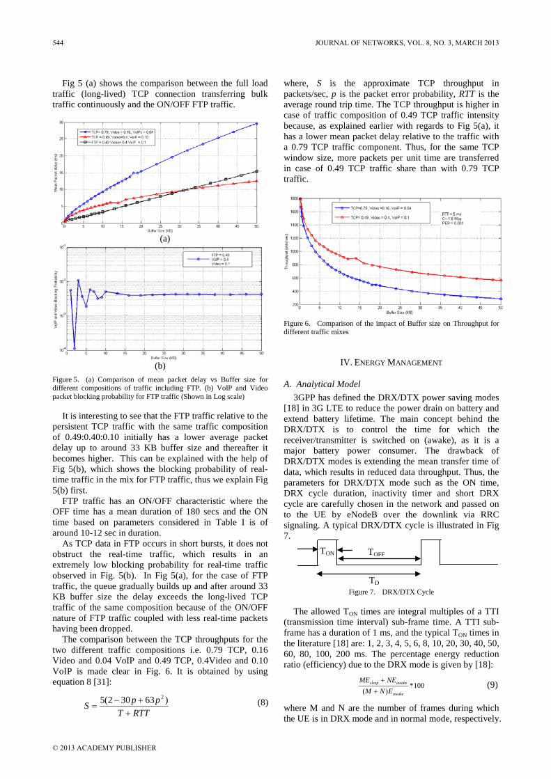
Fig 5 (a) shows the comparison between the full load traffic (long-lived) TCP connection transferring bulk traffic continuously and the ON/OFF FTP traffic.

(a)

(b)

Figure 5. (a) Comparison of mean packet delay vs Buffer size for different compositions of traffic including FTP. (b) VoIP and Video packet blocking probability for FTP traffic (Shown in Log scale)

It is interesting to see that the FTP traffic relative to the persistent TCP traffic with the same traffic composition of 0.49:0.40:0.10 initially has a lower average packet delay up to around 33 KB buffer size and thereafter it becomes higher. This can be explained with the help of Fig 5(b), which shows the blocking probability of real-time traffic in the mix for FTP traffic, thus we explain Fig 5(b) first.

FTP traffic has an ON/OFF characteristic where the OFF time has a mean duration of 180 secs and the ON time based on parameters considered in Table I is of around 10-12 sec in duration.

As TCP data in FTP occurs in short bursts, it does not obstruct the real-time traffic, which results in an extremely low blocking probability for real-time traffic observed in Fig. 5(b). In Fig 5(a), for the case of FTP traffic, the queue gradually builds up and after around 33 KB buffer size the delay exceeds the long-lived TCP traffic of the same composition because of the ON/OFF nature of FTP traffic coupled with less real-time packets having been dropped.

The comparison between the TCP throughputs for the two different traffic compositions i.e. 0.79 TCP, 0.16 Video and 0.04 VoIP and 0.49 TCP, 0.4Video and 0.10 VoIP is made clear in Fig. 6. It is obtained by using equation 8 [31]:

RTTT

ppS+

+−=

)63302(5 2

where, S is the approximate TCP throughput in packets/sec, p is the packet error probability, RTT is the average round trip time. The TCP throughput is higher in case of traffic composition of 0.49 TCP traffic intensity because, as explained earlier with regards to Fig 5(a), it has a lower mean packet delay relative to the traffic with a 0.79 TCP traffic component. Thus, for the same TCP window size, more packets per unit time are transferred in case of 0.49 TCP traffic share than with 0.79 TCP traffic.

Figure 6. Comparison of the impact of Buffer size on Throughput for different traffic mixes

IV. ENERGY MANAGEMENT

A. Analytical Model 3GPP has defined the DRX/DTX power saving modes

[18] in 3G LTE to reduce the power drain on battery and extend battery lifetime. The main concept behind the DRX/DTX is to control the time for which the receiver/transmitter is switched on (awake), as it is a major battery power consumer. The drawback of DRX/DTX modes is extending the mean transfer time of data, which results in reduced data throughput. Thus, the parameters for DRX/DTX mode such as the ON time, DRX cycle duration, inactivity timer and short DRX cycle are carefully chosen in the network and passed on to the UE by eNodeB over the downlink via RRC signaling. A typical DRX/DTX cycle is illustrated in Fig 7.

Figure 7. DRX/DTX Cycle

The allowed TON times are integral multiples of a TTI (transmission time interval) sub-frame time. A TTI sub-frame has a duration of 1 ms, and the typical TON times in the literature [18] are: 1, 2, 3, 4, 5, 6, 8, 10, 20, 30, 40, 50, 60, 80, 100, 200 ms. The percentage energy reduction ratio (efficiency) due to the DRX mode is given by [18]:

100*)( awake

awakesleep

ENMNEME

+

+

where M and N are the number of frames during which the UE is in DRX mode and in normal mode, respectively.

(8)

(9)

TON

TD

TOFF



We propose analytical equation (10) to model the DTX cycle operation on the M/G/1/K uplink queue system for composite traffic mix and to obtain the power/energy consumed by the uplink queue system. Equation (10), uses the fundamental concept behind equation (9) i.e. power consumption is based on the awake/sleep states of the UE and the number of frames (bits) in each state.

The effective traffic entering the queue system i.e. the throughput after taking into consideration the blocking probability is given by the numerator of the first term (outside the brackets) in equation (10). Under steady state conditions of the queue system, the effective throughput divided by the channel capacity is the utilization of the system. The multiplication of the first term within the brackets with the utilization represents the energy that is consumed by the packets (frames) that are awaiting service i.e. during the sleep period of the DTX cycle. The second term within the brackets after multiplication by utilization represents the energy that is consumed while serving the frames during the ON (awake) period of the DTX cycle i.e. duty cycle, by the transmitter. Equation 10 will follow the non-linear characteristic of the waiting time of packets (frames) for an increase with buffer size (refer Fig 3) and is valid under steady state condition of the queue system. The significance of our equation (10) is that it expresses the power/energy consumed by the UE in terms of QoS factors, namely blocking probability and mean waiting time of a packet in the M/G/1/K queue. It also takes into account the service time and the utilization of the traffic. In the literature, we could not find any similar equation expressing DRX/DTX power consumption in terms of QoS and other related key factors.

( ) ( ) ( )( )

+∆−∆−

+∆+++

− XETtTtT

tWEC

P awakeOFFON

ONqsleep

DAvB **1

λλλ

Further, in equation (10), we assume that the arrival rates for all the traffic generated in UE are independent and follow Poisson distribution. This assumption enables us to add the arrival rates for all three independently generated traffic flows in the UE i.e. audio (VoIP), video and TCP data. Also, it can be noticed in equation (10) that whatever amount of time we decrease TON by, we increase the mean waiting time of a packet in the M/G/1/K queue by the same amount. That is, essentially we decrease the TON time to decrease the power consumed, but at the cost of an increase in the mean waiting time of the packet in the M/G/1/K queue system. As stated earlier, this is the underlying principle behind the DTX/DRX power saving mode in 3G LTE, and our equation (10) satisfies it.

We investigate equation (10) by using typical values of the parameters as shown in Table II. We determine how energy consumption in the M/G/1/K queue system of LTE UE is governed by the factors such as blocking probability, increment in waiting time and DTX/DRX TON time in the DTX mode equation (10).

TABLE II. PARAMETERS AND THEIR TYPICAL VALUES FOR EQUATION (10)

Vλ = Arrival rate of Video traffic 384 kb/s

=Aλ Arrival Rate of VoIP traffic 12.2 kb/s

=Dλ Arrival Rate of TCP data 256 kb/s

=qW Mean waiting time in Queue 5 ms

=awakeE Energy spent per TTI during Normal mode 3000mW [20]

=sleepE Energy spent per TTI during DRX/DTX 11mW [20]

=BP Blocking Probability 0.03

=ONT On duration of DRX/DTX cycle As in [18]

DT = Total Length of DRX/DTX Cycle 80 ms [20] C= Channel data rate 1.6 Mbps

=∆t Increment in time. 0 to 40 ms

=X Mean service time per packet based on application or their combination.

ms

While [10, 20, 32] focused on energy consumption solely by VoIP transmission over the air interface, they did not evaluate the impact of QoS factors on energy consumption in the UE uplink/downlink system.

Energy consumed by a UE in terms of mWh (milli Watt hour) is primarily determined by the transmitter power-on time and secondarily by QoS factors. TON duration affects the time for which the transmitter will be in the active state, and the longer the transmitter is in the active state then more number of TTIs (sub-frames) can be transmitted resulting in an increase in energy consumption by the UE. This is observed in Fig. 8, which shows two graphs of the energy consumption as a function of (i) TON time indicated in red color and (ii) effect of mean packet waiting time (top X-axis) indicated in black color. From equation (10) it can easily be seen that a progressive increase in mean waiting time of a packet causes the net TON time to decrease by the same amount. As the net TON time decreases, the energy consumption by the UE for the uplink traffic decreases.

Figure 8. Influence of variation in Transmit ON time (Red color graph) and mean packet delay (black color graph) on energy consumption by UE for uplink traffic.

We found that the blocking probability did not impact much in the steady-state probability range (refer Fig. 4).

B. Simulation Modelling We made use of OPNET Modeler 16.1 to conduct a

simulation study of the energy consumption by UE uplink transmission (RF modem) in the 3G LTE system over a 600 second simulation time. We focused on the energy

(10)



consumed by the transmitter, and ignored other components, such as display, CPU, memory. The 3G LTE system simulated consists of detailed models of eNodeB, UE, evolved packet core (EPC) and application server, all of which closely replicate the functionality of protocol stacks used in the LTE system. In the analytical model’s equation (10) we considered the main traffic’s energy requirement only, without the power consumed in a UE for signaling, scheduling, hybrid ARQ and other inherent routine activities in the 3G LTE system.

The simulation model plays a key role in complementing the analytical study by way of taking into consideration a number of attributes that are difficult to model analytically, such as path loss and fading due to distance separating the UE from eNodeB, modulation and coding scheme (MCS) used, signaling information exchanged and the topology of the scenario: regular hexagonal, grid or random layout.

1) Simulation Scenario We considered a realistic scenario of the 3G LTE system consisting of eNodeB, UEs, EPC and a server in a hexagonal layout as shown in Fig. 9. The main objectives of the simulation study were to evaluate the:

• energy consumed by the UE for different commonly used applications-VoIP, Video, Email, web-browsing and FTP

• energy consumed by the UE in different locations within the hexagonal cell – closest to the eNodeB and at the cell edge.

Figure 9. Simulation Topology

Some of the general parameters and their values used for LTE physical layer and that for the UE are shown in Table III

TABLE III. LTE AND UE KEY SIMULATION PARAMETERS AND VALUES

eNodeB UE Uplink – LTE 1.4 MHz FDD. 1920 MHz base frequency

-1 dBi Antenna Gain

1.4 MHz Bandwidth MCS index (Initial) 9 Downlink – 2110 MHz, 1.4 MHz

bandwidth

Free Space path loss

Unlimited Power 0.05 W battery capacity Cyclic Prefix type: 7 symbols per slot

-200 dBm Receiver sensitivity

2) Results and Discussion We present and discuss some of the key results

obtained through simulations. Fig. 10 shows the energy consumed for different commonly used applications in UE located closest (refer Fig 9) to the eNodeB during 600 seconds simulation run.

Figure 10. Energy consumed by variety of applications

In order to assess the impact of commonly used applications available in mobile handhelds on the energy consumed by the UE, we used models for applications such as VoIP, HTTP and FTP that have been recommended by 3GPP and NGMN [1,21,22]. We can see from Fig. 10 that a persistent and high bandwidth application like FTP has the highest energy consumed whereas bursty lower rate application like interactive VoIP has the lowest power consumed. It must be mentioned here that a VoIP packet is generated every 20 ms and so the power is spread over 20 TTIs. Therefore, the energy consumed by VoIP shown in Fig. 10 is after dividing it by 20. We also observed that an interactive application such as two-way conversation voice consumes more power than one-way voice communication. This is because the transmitter does not go much into the sleep mode.

Fig. 11 shows the energy consumed by the UE for uplink transfer of TCP data at different commonly used rates, when the UE is located closest to the eNodeB and when it is at the cell edge boundary (refer Fig. 9). It can be observed that for lower rates the UE at the cell edge consumes more power than the UE closer to eNodeB. The reason for this lies in the physical layer, a 3G LTE - UE at the cell edge uses a lower modulation and coding scheme (MCS) index than the UE closer to eNodeB. This is because of lower signal power received from the eNodeB due to attenuation. The lower MCS index corresponds to lower transport block size [33] and thus more number of TTIs need to be used, which results in more power being consumed to transmit the data.

Another, interesting observation is that the power consumed by the UE at the cell edge decreases at higher

Server

UE UE

EPC

eNodeB



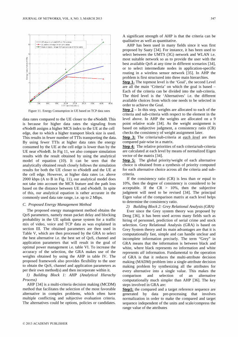
Figure 11. Energy Consumption in UE based on TCP data rates

data rates compared to the UE closer to the eNodeB. This is because for higher data rates the signaling from eNodeB assigns a higher MCS index to the UE at the cell edge, due to which a higher transport block size is used. This results in fewer number of TTIs transporting the data. By using fewer TTIs at higher data rates the energy consumed by the UE at the cell edge is lower than by the UE near eNodeB. In Fig 11, we also compare simulation results with the result obtained by using the analytical model of equation (10). It can be seen that the analytically obtained result closely follows the simulation results for both the UE closer to eNodeB and the UE at the cell edge. However, at higher data rates i.e. above 2000 kbps (A to B in Fig. 11), our analytical model does not take into account the MCS feature and the path loss based on the distance between UE and eNodeB. In spite of this, our analytical equation is rather accurate in the commonly used data rate range, i.e. up to 2 Mbps.

C. Proposed Energy Management Method The proposed energy management method obtains the

QoS parameters, namely mean packet delay and blocking probability in the UE uplink queue system for a traffic mix of video, voice and TCP data as was explained in section III. The obtained parameters are then used in Table V, which are then processed by the GRA to select the best alternative i.e. the best set of QoS, channel and application parameters that will result in the goal of optimal power management i.e. table VI. To increase the accuracy of the selection, the GRA makes use of the weights obtained by using the AHP in table IV. The proposed framework also provides flexibility to the user to obtain the QoS, channel and application parameters as per their own method(s) and then incorporate within it.

1) Building Block 1: AHP (Analytical Hierachy Process)

AHP [34] is a multi-criteria decision making (MCDM) method that facilitates the selection of the most favorable alternative in complex problems, which often have multiple conflicting and subjective evaluation criteria. The alternatives could be options, policies or candidates.

A significant strength of AHP is that the criteria can be qualitative as well as quantitative.

AHP has been used in many fields since it was first proposed by Saaty [34]. For instance, it has been used to select between the UMTS (3G) network and WLAN i.e. most suitable network so as to provide the user with the best available QoS at any time in different scenarios [34], or to select intermediate nodes in application-specific routing in a wireless sensor network [35]. In AHP the problem is first structured into three main hierarchies. Step 1- The topmost level is the ‘Goal’, the second Level are all the main ‘Criteria’ on which the goal is based – Each of the criteria can be divided into the sub-criteria. The third level is the ‘Alternatives’ i.e. the different available choices from which one needs to be selected in order to achieve the Goal. Step 2 – In this step, weights are allocated to each of the criteria and sub-criteria with respect to the element in the level above. In AHP the weights are allocated on a 9 point relative scale [34]. As the weight assignment is based on subjective judgment, a consistency ratio (CR) checks the consistency of weight assignment later. Step 3: The criteria/sub-criteria at each level are then compared pair-wise in a matrix. Step 4: The relative priorities of each criteria/sub-criteria are calculated at each level by means of normalized Eigen vector of the matrix [34]. Step 5:

If the consistency ratio (CR) is less than or equal to 10%, then the degree of consistency is considered to be acceptable. If the CR > 10%, then the subjective judgment will need to be revised [34]. The principal Eigen value of the comparison matrix at each level helps to determine the consistency ratio.

The global priority/weight of each alternative choice is obtained from a synthesis of priority computed for each alternative choice across all the criteria and sub-criteria.

2) Building Block 2: Grey Relational Analysis (GRA) Ever since the Grey system theory was proposed by

Deng [36], it has been used across many fields such as hiring of personnel, prediction of serial crime and stock selection. Grey Relational Analysis (GRA) is based on Grey System theory and its main advantages are that it is computationally fast, simple and can handle unclear and incomplete information precisely. The term “Grey” in GRA means that the information is between black and white, where black represents no information and white represents all information. Fundamental to the operation of GRA is that it reduces the multi-attribute decision making (MADM) problem into a single-attribute decision making problem by synthesizing all the attributes for every alternative into a single value. This makes the comparison and selection of an alternative computationally much simpler than AHP [36]. The key steps involved in GRA are: Step1: the compared and a target reference sequence are generated by data pre-processing that involves normalization in order to make the compared and target sequence independent of the units and scale/compress the range value of the attributes



Step2: the Grey relational coefficient (GRC) between the reference sequence and the sequences that it is compared with is calculated. It essentially determines the closeness of each attribute to that of the corresponding attribute in the reference sequence. Step 3:

D. Proposed Energy Management Algorithm – Key Steps

the degree of Grey coefficient (Grey relational grade) ranks the alternatives and the alternative that has the highest Grey relational grade is selected. The highest Grey relational grade signifies the closeness of a comparability sequence for an alternative to the ideal sequence. The Grey Relational Grade is calculated by taking into account the weight of each attribute. If all the attributes have equal significance then the weight of each attribute is 1/n, where n is the number of attributes for each alternative. In general, however, all the attributes may not have same weight and we obtain the weight of each attribute through AHP. This is called an integrated AHP and GRA approach, and has been shown to be reliable and practically feasible [37].

Step 1 – A software agent operating within the UE will inform the UE energy management algorithm regarding the applications that are currently active in it, such as VoIP, interactive video or FTP. Step 2: The mean waiting time of a packet in the M/G/1/K queue system of the UE will be determined by our analytical method, as explained in section III Step 3: If the difference between the standard QoS parameter values (such as mean packet delay, blocking probability) and the corresponding estimated values for the actual traffic is lower than a particular threshold then no power management will be conducted. If the difference is higher than the threshold, then our energy management technique will be initiated. Step 4: The DTX cycle ON time is modulated by the value of mean packet delay in UE’s M/G/1/K queue system and the blocking probability. That is, to reduce energy consumption, the value of mean packet delay and blocking probability are increased but within limits such that the resulting mean packet delay and the blocking probability will still be below the maximum values allowed by the QoS of the application. As explained earlier with regard to equation (10), if the mean packet delay value is increased by 1 unit of time, the TON time of the DTX cycle is decreased by the same amount and energy consumption is reduced. Step 5: Generate a AHP matrix and compute the weights of all the pre-defined criteria and sub-criteria. We assume that the DTX duty cycle can dynamically switch between the following three alternative types defined by us: long (TON=40ms), medium (TON=30 ms) and short (TON=20ms). We considered, short TON=20ms because this corresponds to the size of VoIP frame/TTI size [32]. It is stressed here, that the alternative types and the criteria/sub-criteria are entirely left at the implementer’s discretion. The weights in the AHP matrices may need to be slightly adjusted so that the consistency ratio is kept below 10%. Step 6

– GRA is used to determine the degree of Grey coefficients (Grey relational grade) for each of the

alternatives. The GRC gives the deviation of the attributes (parameters) of each alternative from the ideal reference. The weights obtained from the AHP for each of the criteria/sub-criteria are used in the computation of the degree of GRCs. Step 7- If the degree of GRCnew of an alternative duty

cycle is greater than the degree of GRCcurrent of the currently used duty cycle, then the currently used DTX duty cycle will be replaced with this alternative. Step 8 –

The algorithm explained above is summarized through a flow chart in Fig . 12.

The algorithm then goes back to Step 1 and the repeats the process periodically.

Figure 12. Proposed power/energy management algorithm

Fig. 13 shows the decrease in energy consumption achieved by the UE when it is operating for 600 sec, as a result of using DTX mode in Step 5 of the above algorithm for long, medium and short duty cycle types.

Figure 13. Comparison of energy consumption by traffic mixes with and without DTX mode

Determine currently active applications

Std. QoS values – Est. QoS values > Threshold

Generate AHP matrices to compute weights of criteria and global weights of sub criteria

Compute degree of GRC using AHP

Select the alternative with highest deg. of GRC

Modulate DRX/DTX cycle in terms of mean waiting time, Blocking prob. for

the selected alternative

Compute mean waiting, time, blk prob, throughput

Computed deg of GRC > Currently used alternative’s deg. of GRC

Periodically repeat the algorithm

NO

NO



It compares the energy consumed by UE for (i) VoIP only (iii) combination of VoIP and video traffic and (iii) combination of VoIP, video and data traffic with the corresponding energy consumed by UE when DTX mode is not used for these traffic for 600 sec. The results have been by obtained by using DTX analytical model equation (10). Fig. 13 also helps to determine the impact of the DTX mode on the energy saving at the UE. We calculated the energy savings as: VoIP only traffic approx. 73%; VoIP and video traffic 62%; and VoIP, video and data traffic 49%.

a) Power Optimization We explain the power optimization feature in our

algorithm for UE DTX mode by computing the parameters that pertain to AHP and GRC. To do this, the problem is first translated into an AHP hierarchy as shown Fig 14. Level 2 of the AHP represents the three alternatives from which one has to be selected for optimized energy management, and which results from a trade-off between the different criteria. We follow steps 2-5 stated under AHP, discussed earlier, to obtain the weights for the three criteria and the global priorities (weights) for the three sub-criteria. For this we use equations (11) and (12).

[ ] ( )AeigW =λ,

In equation (11), the eigen value of the square matrix ‘A’ for AHP is obtained. The priority vector i.e. weights for the matrix criteria and sub-criteria are also obtained [34].

1max

−−

=n

nCI λ and RICICR =

CI is the consistency index, ‘n’ is the number of comparisons made at each level in the square matrix, RI is the random consistency index that is 0.58 for n=3 and

=maxλ is principal Eigen value. We confirmed that our AHP matrices are consistent by checking that CR < 10%.

Table IV shows the weights obtained for the criteria and sub-criteria as a result of computations made for AHP. Table V gives the attributes and their values used for each alternative. We consider three scenarios corresponding to the applications used i.e. (i) VoIP only, (ii) VoIP and Video and (iii) VoIP, Video and Data. For each of these three scenarios there are three choices for DTX/DRX cycle defined by us i.e. short, medium or long (Refer step 5 of our algorithm). Table VI shows the degree of GRC obtained after following Steps 1- 3 in the earlier discussion on GRA. The ranks in Table VI are based on the degree of closeness to the ideal operating condition to achieve the goal of optimized energy management, for the attributes specified in Table V. The table confirms that the most optimal energy saving mode is for Voice application with a short duty cycle i.e. short ON time. The Grey relation coefficient χ is obtained from equation (14) [36,38]

max)(maxmin

∆+∆∆+∆

=ζζχ

joi

)(maxmaxmax joiji∆=∆ , )(minminmin joiji

∆=∆ [ ]1,0∈ζ

In our calculations we consider 5.0=ζ [36] The degree of Grey coefficient (Grey relational grade) is shown in the right most column and it is obtained by using equation (15) [36,38]

[ ] )(*)(1

jjW oi

n

jioi χ∑

=

=Γ

We have obtained the weights )( jWi for each of the

attribute’s sub-criteria and criteria by using AHP (Table IV). Therefore, our approach of integrating the AHP with GRA is much more accurate than would be the case if we had considered all the attributes to be of equal weight.

Figure 14. AHP Hierarchy for our optimized power management algorithm

TABLE IV. WEIGHTS OBTAINED FOR CRITERIA AND SUB-CRITERIA USING AHP

Criteria QoS Channel Condition Power Usage-Applications Weights of Criteria 0.5769 .0811 0.3420 Sub-Criteria S Delay Blk Prob λ Frame size TON

Global Wt. of Sub-criteria 0.1614 0.3615 0.0540 0.0511 0.0291 0.0925 0.2203

Blocking Prob. Throughput

Level 0

QoS Channel Condition (BER) Power Usage - Applications

Optimized Power Management

Delay

Short Duty Cycle Med. Duty Cycle

TON time Frame size

Arrival Rate

Level 1

Level 2 Long Duty Cycle

(12) (13)

(14)

(15)

(11)



TABLE V. ATTRIBUTE VALUES OF CRITERIA/SUB-CRITERIA FOR DIFFERENT APPLICATIONS

QoS Channel Power Usage - Applications ‘S’ pk/s Delay(ms) Blk Prob PER Average λ (kb/s) Avg. pkt size TON(ms)

Short Cycle (Voice) 881 1 .01 2x10 12.2 -3 40 bytes 20 Med Cycle 881 1 .01 2x10 12.2 -3 40 30 Long Cycle 881 1 .01 2x10 12.2 -3 40 40 Short Cycle (Voice+Video) 808 2 .02 2x10 (12.2+384)/2=198 -3 220 bytes 20 Med Cycle 808 2 .02 2x10 198 -3 220 30 Long Cycle 808 2 .02 2x10 198 -3 220 40 ShortCycle(Voice+Video+Data) 692 4 .03 2x10 (12.2+384+256)/3=218 -3 480 bytes 20 Med Cycle 692 4 .03 2x10 218 -3 480 30 Long Cycle 692 4 .03 2x10 218 -3 480 40

TABLE VI. GREY RELATIONAL COEFFICIENTS FOR APPLICATIONS WITH DIFFERENT DTX DUTY CYCLE TYPES

QoS Channel Power Usage - Applications Degree of Grey Coefficient ‘S’ Delay Pb PER λ Frame .

size TON

Short Cycle (Voice) 1 1 1 1 0.33 0.33 1 0.9184(Rank 1) Med Cycle 1 1 1 1 0.33 0.33 0.54 0.8171(Rank 2) Long Cycle 1 1 1 1 0.33 0.33 0.33 0.7708(Rank 3) Short Cycle (Voice+Video) 0.56 0.6 .5 1 0.83 0.45 1 0.7015(Rank 5) Med Cycle 0.56 0.6 .5 1 0.83 0.45 0.54 0.60(Rank 7) Long Cycle 0.56 0.6 .5 1 0.83 0.45 0.33 0.5539(Rank 9) ShortCycle(Voice+Video+Data) 1 0.33 .33 1 1 1 1 0.7215(Rank 4) Med Cycle 1 0.33 .33 1 1 1 0.54 0.620(Rank 6) Long Cycle 1 0.33 .33 1 1 1 0.33 0.5739(Rank 8)

V. CONCLUSIONS

Work on energy management in 3G LTE has been limited, and deals with download traffic via discontinuous reception (DRX). Increasingly powerful user devices can upload significant amount of data, which requires the use of discontinuous transmission (DTX). This paper proposed a energy management framework that can be used for both DRX and DTX modes. The framework has two main parts – (i) Evaluation of QoS metrics in M/G/1/K uplink queue system and (ii) algorithm for optimal energy management. First, using our analytical method for the evaluation of M/G/1/K queue system for heterogeneous traffic, we compute the QoS metrics, namely delay, blocking probability and throughput. These a-priori estimated values are periodically passed on to our energy management algorithm, which considers the tradeoffs between these parameters for the application and makes an optimal selection of the duty cycle for the DTX. The optimization of energy management is carried out via multi-criteria decision making provided by AHP and GRA. As part of our algorithm, we have also proposed an approximate analytical expression for energy consumption in terms of QoS metrics. We have validated this expression and the analytical model of M/G/1/K queue system by means of simulations. Our results will help to conserve the energy in UE and select buffer size accordingly.

ACKNOWLEDGMENT

The authors wish to thank the anonymous reviewers for their constructive comments. Furthermore, the authors acknowledge the role of OPNET Technologies in providing them with an Educational license for OPNET Modeler 16.1 to conduct simulations.

REFERENCES

[1] A White Paper by NGMN Alliance, “Next Generation Mobile Networks Radio Access Performance Evaluation Methodology,”http://www.ngmn.org/uploads/media/NGMN_Radio_Access_Performance_Evaluation_Methodology.pdf last retrieved on 11/08/2011

[2] LTE – The Global Opportunity – UMTS Forum Report – http://www.3gpp.org/LTE-the-Global-Opportunity-UMTS last retrieved on 11/04/2012.

[3] H. Ekström,”Technical solutions for the 3G Long-Term Evolution,” IEEE Comm. Mag., pp. 38-45, March 2006.

[4] 3GPP TS 25.913. ver 8.0.0. September 2008. http://www.3gpp.org/ftp/Specs/html-info/25913.htm last retrieved on 11/04/2012.

[5] E-UTRA Base Station Transmit ON/OFF Power Measurement,http://cp.literature.agilent.com/litweb/pdf/5990-5989EN.pdf last retrieved on 23/06/2012.

[6] G. Anastasi and A. Passarella, “An energy-efficient protocol for multimedia streaming in a mobile environment,” J. of Pervasive Comput & Comm. 1 (1), March 2005.

[7] H. Zhai, Y. Kwon, and Y. Fang, “Performance analysis of IEEE 802.11 MAC protocols in wireless LANs,” Wireless Communications and Mobile Computing (WCMC), vol 4. pp. 917-931, 2004.

[8] J.M. Smith, “Properties and performance modelling of finite buffer M/G/1/K networks,” Journal Computers and Operations Research, vol 38 Issue 4, Elsevier Science Ltd. Oxford, UK,, pp. 740-754, 2011.

[9] A.Vishwanath, V. Sivaraman, and G. N. Rouskas, “Considerations for sizing buffers in optical packet switched networks”, IEEE INFOCOM, pp. 1323 – 1331, April 2009.

[10] D. Vinella and M. Polignano, “Discontinuous Reception and Transmission (DRX/DTX) Strategies in long term Evaluation (LTE) for Voice over IP (VOIP) Traffic under Both Full-Dynamic and Semi-Persistent Packet Scheduling Policies”,Report,2009,http://projekter.aau.dk/projekter/files/18664711/Report_Vinella_Polignano.pdf last retrieved on 29/11/2011.



[11] M. Chatterjee and S.K. Das, “Resource optimization of CDMA systems for supporting integrated voice and data traffic,” J. of High Speed Networks - Special issue: Wireless and wired multimedia, vol. 11 Issue 3-4, 2002.

[12] J. Huang, R.Q. Yao, Y. Bai, and S.W. Wang, “Performance of a mixed-traffic CDMA2000 wireless network with scalable streaming video,”IEEE Transactions on Circuits and Systems for Video Technology, vol: 13, Issue: 10, pp. 973-981, Oct 2003.

[13] 3GPP TR 25.892 V2.0.0 (2004-06), http://www.3gpp.org/ftp/tsg_ran/tsg_ran/TSGR_24/Docs/PDF/RP 040221.pdf last retrieved on 20/082011.

[14] H.Sun and C. Williamson, “Downlink performance for mixed Web/VoIP traffic in 1xEVDO revision A networks,” IEEE ICC, pp.125 – 130,2008.

[15] A. Alexiou, C. Bouras, and V. Igglesis, “Performance Evaluation of TCP over UMTS Transport Channels,” http://ru6.cti.gr/ru6/publications/21901104.pdf last retrieved on 11/11/2011

[16] T. Kolding, J. Wigard, and L. Dalsgaard, “Balancing power saving and single user experience with discontinuous reception in LTE,” IEEE ISWCS, pp. 713-717, 2008.

[17] H. Yan, R. Krishnan, S. A. Watterson, D. K. Lowenthal, K. Li, and L. L. Peterson, “Client-Centered Energy and Delay Analysis for TCP Downloads,”Twelfth IEEE Int Workshop on Quality of Service, IWQOS pp. 255 – 264, 2004.

[18] C. Bontu and E. Illidge, “DRX Mechanism for Power Saving in LTE,” IEEE Comm. Magazine, vol. 47, Issue: 6 pp 48 – 55, June 2009.

[19] J. Wigard, T. Kolding, L. Dalsgaard, and C. Coletti, “On the User Performance of LTE UE Power Savings Schemes with Discontinuous Reception in LTE,” IEEE International Conference on Communications Workshops, pp. 1-5, 2009.

[20] M. Polignano, D. Vinella, D. Laselva, J. Wigard, and B. T. B. Sørensens, “Power Savings and QoS Impact for VoIP Application with DRX / DTX Feature in LTE,” IEEE VTC Spring, pp. 1-5, 2011.

[21] RACH Capacity Analysis-Packet 1,TSGR1#6(99)818, http://www.3gpp.org/ftp/tsg_ran/WG1_RL1/TSGR1_06/docs/Pdfs/r1-99818.pdf last retrieved on 20/02/2012.

[22] A. Silva and A. Gameiro, "Detailed scenario definition and business analysis of CODIV diversity technologies on cellular systems," EU, FP7 ICT-2007-215477, Jan., 2009

[23] S.K. Bose, Introduction to Queuing Systems, Kluwer/Plenum Publishers, 2001.

[24] X. Tang, J. Xu, S. T. Chanson, Web content delivery, Springer, 2005.

[25] 3GPP TS 26.236 V8.0.0 http://www.3gpp.org/ftp/Specs/archive/26_series/26.236/ last retrieved on 11/04/2012.

[26] F.Azimi and P. Bertók, “An analytical model of TCP flow in multi-hop wireless networks,”. IEEE 35th Conference on Local Computer Networks (LCN), pp. 88-95, 2010.

[27] B. Sinclair, “Solving discrete-time Markov chains,” http://cnx.org/content/m10835/2.3/ last retrieved on 19/072011.

[28] R.B. Sidje, “Inexact uniformization and GMRES methods for large Markov chains.,” Numerical Linear Algebra with Applications, vol. 18, Issue 6, John Wiley & Sons, 2011, pp. 947–960

[29] P. Buchholz, “Structured analysis techniques for large Markov chains,” SMCtools workshop on Tools for solving structured Markov chains, 2006.

[30] C. V. Seshaiah and K. Senbagam,” Mathematical modelling and bandwidth allocation for video

teleconference service traffic,” European Journal of Scientific Research, vol.60 No.4, pp. 619-629, 2011.

[31] K. Anand and V.Sharma,“Computing TCP throughput in a UMTS network,” IEEE WCNC , pp. 2507 – 2512, 2008.

[32] S. Fowler, “Study on Power Saving Based on Radio Frame in LTE Wireless Communication System Using DRX,” IEEE GLOBECOM Workshops, pp.1062 - 1066, 2011.

[33] 3GPP TS 36.213 http://www.3gpp.org/ftp/Specs/archive/36_series/36.213/ last retrieved on 15/05/2012.

[34] Q. Song and A. Jamalipour, “Network selection in an integrated wireless LAN and UMTS environment using mathematical modeling and computing techniques,” IEEE Wireless Communications, vol: 12 , Issue: 3 pp.: 42 - 48, June 2005.

[35] M.A. Azim, M.R. Kibria, and A. Jamalipour, “Designing an Application-Aware Routing Protocol for Wireless Sensor Networks,” IEEE GLOBECOM, pp. 1-5, 2008

[36] Y Kuoa, T Yangb and G-W Huangb, “The use of grey relational analysis in solving multiple attribute decision-making problems,” Computers & Industrial Engineering vol. 55, Issue 1, pp. 80–93, Aug 2008.

[37] H. Li, C. Z., D. Zhao, “Stock Investment Value Analysis Model Based on AHP and Gray Relational Degree,” Management Science and Engineering vol. 4, No. 4, pp. 01-06, 2010.

[38] H. Wu, “A Comparative Study of Using Grey Relational Analysis in Multiple Attribute Decision Making Problems,” Quality Engineering, vol 15, No. 2, pp. 209-217, 2002

Vinod Mirchandani was born in India. He has earned PhD degree in Computer Communications from the University of Melbourne, Australia in 1998, MS in EE from the University of Saskatchewan, Canada, BE in ECE from IISc, India and BSc degree from the University of Poona, India.

He has worked (i) as a Senior Research Engineer at Motorola Labs,

Australia in the area of WLANs and Performance Evaluation (ii) at the University of Sydney in the area of B3G networks (iii) at the University of Technology, Sydney (UTS) on collaborative projects with Alcatel-Lucent, Bell Labs (Paris) in the areas Self organization of Wireless mesh networks and Grid Computing (iv) at the RMIT University, Melbourne in 3GPP LTE wireless network and data privacy. He has authored more than 35 IEEE/ACM and other international publications, 3 book chapters and one US Patent.

Dr. Mirchandani has received numerous research awards and University Fellowships.

Peter Bertok received his PhD from the University of Tokyo, Japan in the area of Computer Control, and his Master of Engineering from the Technical University Budapest, Hungary in the field of data and computer communication. Currently, he is an Associate Professor at the School of Computer Science & IT, RMIT University, Melbourne, Australia. He has worked in industry as well as at research institutions.

He is a member of IEEE and ACM and has over 100 scientific publications.



A Framework for Automated Security Proof and its Application to OAEP

Guang Yana, Zhu Yue-Feia, Gu Chun-Xianga, Fei Jin-longa, He Xin-Zhengb

aZhengzhou Information Science and Technology Institute, Zhengzhou 450002, China b

[email protected] College of Computer and Information Engineer, Henan University, Kaifeng 475000, China

Abstract—OAEP is a widely used public-key encryption scheme based on trapdoor permutation. Its security proof has been scrutinized and amended repeatedly. In this paper we present a automatically proof for IND-CCA2 security of OAEP, which is completed by a framework for mechanized security proof, without any human intervention. The framework is built on the base of probabilistic polynomial-time process calculus, and capable of dealing with padding-based encryption schemes. We provide an overview of the proof instance and explain several crucial steps of the game transformation.

Index Terms—provable security; automated security

proof; OAEP; IND-CCA2; partial-domain one-wayness;

I. INTRODUCTION

Optimal Asymmetric Encryption Padding (OAEP) [1] is a prominent and widely deployed asymmetric encryption scheme based on a trapdoor permutation, most commonly used in combination with the RSA and Rabin functions. OAEP is standardized in RSA’ s PKCS #1 V2.1 and several variants of it are recommended by many other standards, including IEEE P1363, ISO 18033-2, ANSI X9, CRYPTREC and SET.

In their original 1994 paper, Bellare and Rogaway proved that OAEP is semantically secure under chosen-ciphertext adversaries (IND-CCA) under the hypothesis that the underlying trapdoor permutation family is one-way. In 2001, Shoup [2] discovered that this proof only established the security of OAEP against non-adaptive chosen-ciphertext adversaries, and not against the adaptive chosen-ciphertext adversaries, in which the adversaries are given access to the decryption oracle both before and after observing the challenge ciphertexts (This kind of security is named as IND-CCA2 security). Shoup suggested a modified scheme, OAEP+, and gave a proof of IND-CCA2 security under the one-wayness of the underlying permutation. Shoup’s paper stimulated great interest in analyzing and improving the security of OAEP, to make it stronger to resist the adaptive chosen-ciphertext adversaries, as well as efficient enough to meet practicality [3,4]. Subsequently, Fujisaki et al. [5] proved that OAEP in its original formulation is indeed secure against adaptive

adversaries, assuming the underlying permutation family to be partial-domain one-way. Since the latter assumption is no stronger than one-wayness in the particular case of RSA, this ultimately established the IND-CCA2 security of RSA-OAEP.

Most of the findings listed above are based on provable security, a popular approach for analyzing the security of cryptographic schemes. In this method, the adversaries are probabilistic polynomial-time Turing machines and try to win a game specifying certain security properties of the cryptographic scheme. The method is usually in the reduction sense: if the adversaries win the game with non-negligible probability, then a well-defined computational assumption about cryptographic primitive would be invalid. However, most of the existing security proofs are complex and error-prone, and their correctness relies heavily on the skill of the provers, and is difficult to check.

In this paper we presented an automatic security proof framework, which is an improvement of the framework in [6]. Our framework introduces the notion of union term to construct the security proof of padding-based encryption schemes. We also use a new criterion for IND-CCA2 security, depending on the notion of adversary’s view, which is inspired by Shoup’s approach [7]. To prove the IND-CCA2 security of OAEP, we designed and proved the observational equivalence of partial-domain one-way permutation.

Differing from the former results, this paper reports an automated game-based proof of the IND-CCA2 security of OAEP, under the assumption that the underlying permutation family is partial-domain one-way. The proof is completed by an automatic security proof framework, which is an improvement of the framework in [8]. In this new framework we introduces the union terms for structuring the security proof of padding-based encryption schemes, as well as a new criterion for IND-CCA2 security, depending on the notion of adversary’s view, which is inspired by the approach of [7]. We also introduce and proved the observational equivalence of partial-domain one-way permutation.

The rest of this paper is organized as follow: in section 2, we summarize the related work; in section 3, we introduce our framework, including its calculus, game-based proof strategy and criterion for security; in section 4 we review the scheme of OAEP and the definition of its IND-CCA2 security; in section 5, we

This work is supported by the Municipal Science and Technology Innovation Team Project of Zhengzhou [10CXTD150].



present the formal statement of the initial game and the observational equivalence of partial-domain one-wayness, and show how the framework manages to prove the IND-CCA2 security of OAEP by explaining several critical game transformations. Section 6 concludes the paper.

II. RELATED WORK

After Shoup’s discussion about structuring provable security proofs as sequence of games, Halevi [9] explained the implementation of an automatic tool based on compiler techniques to build security proofs with game sequence, and suggested ideas in this direction, but did not implemented one.

Bellare and Rogaway [10] showed how to prove triple encryption with code-based game-playing proofs. Backes et al. [11] formalize a language for such code-based games, in the Isabelle proof assistant [12]; however, no specific example is reported. Later, Nowak [13], and Affeldt et al. [14] separately reported on preliminary experiments with such kind of proofs on top of the proof assistant Coq

Recently, G. Barthe et al. [16] present a framework called Certicrypt, which enables the machine-checked construction and verification of code-based proofs. Certicrypt is also based on Coq, and has been used previously to build the proof of IND-CCA2 security of OAEP. Recently, they further improve their work and present a new automated tool for elaborating security proofs of cryptographic systems from proof sketches. This tool, which is called EasyCrypt [17], can be used together with Certicrypt to build a complete security proof. One of the main benefits of this method is to ensure that each step of the proof is machine-checked. However, structuring security proofs on top of proof assistant requires manual intervention, and thus sacrifices efficiency to some degree.

[15]. Nowak gives a game-based proof of ElGamal semantic security in Coq, his framework ignores complexity issues, and thus has limited support for proof automation. Affeldt et al. formalize a game-based proof of the switching lemma in Coq. However, their formalization is tailored towards the particular example they consider, and deals with a weak (non-adaptive) adversary model.

On the other hand, in 2006, Blanchet and Pointcheval [6] presented a framework based on process calculus and its relevant software called Cryptoverif. Instead of using proof assistant, this framework adopts an axiomatization of cryptographic primitives based on term rewriting. Cryptoverif focuses on automatically inferring the sequences of games, with the correctness of proofs partially relying on the mutually proof of axioms. Courant et al. [18] have also developed an automated prover for proving asymptotic security of encryption schemes based on one-way functions. Both of the provers are able to handle some schemes from the literature, but they can not handle OAEP. More recently, Gu Chunxiang et al. [8] present a framework for automated security proof of cryptographic schemes and protocols. This framework is based on a calculus inspired by Blanchet’s and introduces algebraic properties with observational equivalence.

Nowak and Yu Zhang [19] also present a probabilistic lambda-calculus for game-based security proofs and provide cryptographic constructions for public-key encryption and pseudorandom bit generation. However, by now there is no tool implemented for this calculus.

III. FRAMEWORK FOR AUTOMATED SECURITY PROOF

This section advocates the framework for automated security proof with sequences of game. Compared with the traditional provable security method completed by human being, our framework constructs mechanized security proof on the base of process equivalence and semantic congruence, and thus avoids the potential artificial errors in the proving process.

Our framework consists of three parts: a probabilistic polynomial-time process calculus to describe the cryptographic schemes and the games; a set of game transformating rules called observational consequence and a criteria to judge the winning probability for the adversary in each game.

The automated game-based security proof is conducted as below. On the input of an initial game describe by the process calculus, the framework executes a sequence of game transformations on it, and eventually gets a game in which the security can be judged clearly by the pre-defined criteria. These game transformations should guarantee that the difference of the adversary’s advantage in the consecutive games be negligible. The framework employs a proof strategy based on depth-first spanning tree. The initial game is transformed continuously by any available transformations, until there is no such transformation existed. Then it goes back to the prior game in the current sequence, excludes the latest transformation and tries another one. The proof terminates if the criteria for security is satisfied in any of the games or if the whole spanning tree is traversed.

A. The probabilistic polynomial-time process calculus The process calculus of our framework is inspired by

the calculus in [6] and [8]. It uses terms and processes to represent oracles and permutations in the games. And we denote by η the security parameter, which determines in particular the length of keys.

The calculus uses types to describe some special properties of the terms, such as randomicity or collision-resistance. For each value of the security parameterη , type T corresponds to a subset )(TIη of

Bitstring ∪ { ⊥ }, where Bitstring is the set of all bitstrings and ⊥ represents the terminal of Turing machine. The set )(TIη must be recognizable in polynomial time, that is, there exists an algorithm that decides whether x belongs to )(TIη in time polynomial in the length of x and the value ofη .



function ),,( union term |...||

access variable ][index

Term :

1

21

m

m

MMfMMM

Mxi

M

=

timesn replicatio ncompositio parallel '|

lookupbranch )

),,(

][,,][(branch lconditiona '

),,(assignment :random ;:][output ;],[input );:][],[(

channel private ; processevent ;

process nil Process :

1

1111

1

nPPP

PelsePthen

MMMdefinedsuchthat

niuniufindPelsePthen

MMMdefinedifPinMTNlet

PTixnewNMcout

PTixMcinPcnewChannel

xevent

P

ni

j

jjlj

jmmjmjjmj

l

j

jjj

≤

=

∧

≤≤⊕

∧=

=

θ

In this calculus, terms represent computations on bitstrings. And the calculus distinguishes four kinds of terms. The replication index i is an integer which serves in distinguishing different copies of a replicated process. The variable access x[M] returns the content of the cell of index M of the array variable x. We use x, y, z, u as variable names. Noticeably, this calculus use one-dimensional array variables instead of multi-dimensional array variables of [6] to make the syntax more laconic. This kind of arrays is used together with terms named union term to denote the complex multi-dimensional array variables. The union term M1|M2|…|Mm

The calculus uses processes to represent Turing machines. The nil process occurs in game transformations as the intermediate results of process reduction. The event process marks the occurrence of some particular events, such as the adversary successfully forging a legal signature. The input process waits on channel c[M] for an input variable of type T; while the output process outputs term N on channel c[M]. The output process doesn’t have formally successor. After matching with some input processes by the term parameter M, it probabilistically takes an input process as its successor. The input and output process are designed to represent the input and output tapes of Turing machine. Each Turing machine begins with an input process and ends with several potential output processes. The random process

uniformly chooses a fresh random number in

describes linking and padding of bitstrings and plays a vital role in dealing with the cryptographic schemes with message padding, such as OAEP. Union terms are also used as the parameters of functions in our calculus so that we can unify the form of all the functions, and moreover build a standard library of transforming rules in our framework.

)(TIη to be stored in x[i], and executes P. In our calculus, all the random numbers must be produced by random process. The assignment process stores the value of M (which must be in )(TIη ) in term N, and then executes P. The conditional process executes P if M1,…,Mk are defined and M evaluates to true. Otherwise, it executes P0. The find process tries to find an index u such that x[u] is defined and x[u] = a, and when such u is found, it executes P0

B. Observational Equivalence

with that value of u; otherwise, it executes P. In other words, the find process looks for the value a in the array x, and when a is found, it stores in u an index such that x[u] = a.

Before giving the definition of observational equivalence, we need to describe the formal adversaries first. In our framework, the adversary is described as the context in which the processes are running. And the adversary plays the game through controlling the intercourse between the processes.

Definition 1 [6] (context). A context is a process containing a hole [], denoted by

C[]. The [] could be substituted by certain process P, the variables in P would be re-evaluated according to the value of terms in C[].

Our framework distinguishes two kinds of game transformations: syntactic transformations and transformations from observational equivalence. The former kind includes the syntax simplification and reduction of the processes, while the later kind is mainly comes from properties of cryptographic primitives. The observational equivalence is a kind of bi-simulation equivalence between processes. In our calculus it is defined on the base of probabilistic semantics and therefore can be used to construct the game sequences with negligible probability difference.

Definition 2 [6] (observational equivalence). Let P and P’ be two processes, and V a set of variables.

The variables of V occurring in P and P’ are settled in the same type. An context C is said to be acceptable for P, P’, V if and only if var(C)∩ (var(P)∪ var(P’))⊆V. We say that P and P’ are observationally equivalent with public variables V, written P≈V

c

P’, and abbreviated as P≈P’, when for all contexts C acceptable for P, P’, V, for all channels and bitstrings a , |Pr[C[P] ac

] －

Pr[C[P’] ac

]| is negligible.

C. Criterion for Security In a game-based security proof, the criteria for

indistinguishability security are normally defined by probabilistic negligibility: the security property is satisfied when the probability of the adversary winning the game is negligible. To explain the criterion used in our framework specifically, we need to introduce the definition of adversary’s view, which is proposed by Shoup in [7].

Definition 3 (adversary’s view) The adversary’s view is the information being leaked to

the adversary during the game playing. It is a sequence of



variables View = < x0, x1, x2

The x…>; (3)

0 is normally the public key of the encryption scheme, and each xi 1≥i for consists of a response to either the result of oracle queries or the calculation on them. It should be noted that the adversary’s view changes after each game transformation.

Then the criterion for ciphertext indistinguishability security of encryption schemes can be described as the situation in which the coin toss of the messages corresponding to the challenger cipher doesn’t occur in the adversary’s View. In contrast with the criteria used in some similar tools [8, 10, 16], ours reaches closer to the essence of provable security and in the meantime makes the mechanized judging of security more precise.

IV. REVIEW OF OAEP

Let us first give a formal definition of OAEP: Definition 4 (OAEP encryption scheme) [1] Let (Kf, f, f-1) be a family of trapdoor permutations on

{0,1}k

G:{0,1}, and two hash functions

k0→{0,1}n+k1 H:{0,1}n+k1→{0,1}Where there is k=n+k

k0 0+k1

),( ),(),( )( skpkreturnskpk f ηη Κ←=Κ

. The Optimal Asymmetric Encryption Padding (OAEP) scheme is composed of the following triple of algorithms:

(4)

)||,( ;)(

);0||()(;}1,0{),( 10

tspkfreturnrsHt

mrGsrmpk kkrandom

⊕←⊕← ←=Ε

(5)

⊥=

⊕←⊕←←= −

else ][ then 0][ );();(

);,()||( ),(

1

1

1

returnmreturnmifrGsmsHtr

cskftscskD

nkk

(6)

where [x]n (resp. [x]n

In their original paper, Bellare and Rogaway build OAEP with one-way trapdoor permutation. However in this paper, we prove the security under the assumption that the underlying permutation is partial-domain one-way. So we present the definition of partial-domain one-wayness [3] here.

) denotes the n least (resp. most) significant bits of x.

Definition 5 (partial-domain one-wayness) Consider permutation kkf }1,0{}1,0{: → , which can

also be seen as 0101 }1,0{}1,0{}1,0{}1,0{: kknkknf ×→× ++

with k=n+k0+k1(

. τε , )-Partial-Domain One-Wayness of f means that

for any adversary A whose running time is bounded by τ , the success probability Succpd-ow τ( ) is upper-bounded by ε , where in time of τ

Succpd-ow τ( )=Prs,t τ[A(f(s,t))=t, in time of ] (7) In this paper, we present an automated proof of the

IND-CCA security of OAEP constructed by our framework, the proof conclusion is described by Theorem 1:

Theorem 1 (IND-CCA2 security of OAEP) Let A be an adversary against the IND-CCA2 security

of OAEP that makes at most qG and qH queries to the hash oracles G and H respectively, and at most qD queries to the decryption oracle D.

If the underlying trapdoor permutation scheme is partial-domain one way, then OAEP is secure against adaptive chosen ciphertext attack in the random oracle model. And the advantage of adversary is bounded by

)(2 game ofcontext 0

tSuccqDqHg owpdk

−++ (8)

where tcontext of gameWe give the detailed proof of this theorem in section 4,

with a sequence of game transformations.

is the total time of game running.

V. PROVING THE IND-CCA2 SECURITY OF OAEP

Our framework has been implemented in C++ environment, on an Intel 2.9 GHz Core i7 system with 4 MB cache, 1 GHz EPCI bus, and 8 GB of RAM. And the security proof of OAEP is completed in 4.5 seconds. Before the last game in which the criterion of IND-CCA2 security is clearly satisfied, there are totally 233 games produced and judged. And as a result of the proof, the framework outputs a game sequence of 16 games.

A. The Initial Game The formal statement of the IND-CCA2 security of

OAEP is displayed in Fig.1. The initial game is composed of five parallel processes, which are the process of initialization, the process of challenger, and the processes of oracle: two hash function and the decryption oracles. The potential context C[] plays as the adversary A.

This parallel structure of initial game allows the adversary to query both of the hash oracles during the game playing, with qG, qH bounding the number of queries. The game starts when the process start is executed. It produces the public key pk and private key sk using a fresh random value r0, and then discloses the former. Immediately after the execution of process start, there are two parallel groups of processes. One is the decryption oracle, which waits for a ciphertext y and responds with the relevant plaintext. It should be noted that the challenge ciphertext can not be used as the input of the decryption oracle. The other is the major part of initial game, which receives two plaintexts selected by the adversary and randomly chooses one to encrypt and output, depending to the internal coin toss b*

game G

. By making the process of decryption oracle parallel with the process of the challenger, we give the adversary access to the decryption oracle even after it gets the challenge ciphertext.

0

≦qHg is

in(c1, x1:bitstringk0

out(c);

2, hashg(x1

| )).

≦qHh in(c3, x2

out(c:bitstringn);

4, hashh(x2

| )).

start();



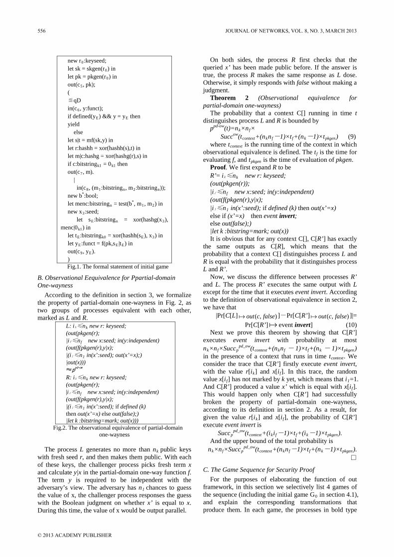
new r0

let sk = skgen(r:keyseed;

0

let pk = pkgen(r) in

0

out(c) in

5

( , pk);

≦qD in(c6

if defined(y, y:funct);

E) && y = yE

yield then

else let s|t = mf(sk,y) in let r:hashh = xor(hashh(s),t) in let m|c:hashg = xor(hashg(r),s) in if c:bitstringk1 = 0k1

out(c then

7

| , m).

in(c8, (m1:bitstringn, m2:bitstringn

new b));

*

let menc:bitstring:bool;

n = test(b*, m1, m2

new x) in

3

let s:seed;

E:bitstringn = xor(hashg(x3), menc|0k1

let t) in

E:bitstringk0 = xor(hashh(sE), x3

let y) in

E:funct = f(pk,sE|tE

out(c) in

9, yE

) ).

Fig.1. The formal statement of initial game

B. Observational Eequivalence for Ppartial-domain One-wayness

According to the definition in section 3, we formalize the property of partial-domain one-wayness in Fig. 2, as two groups of processes equivalent with each other, marked as L and R.

L: ik≤nk(out(pkgen(r);

new r: keyseed;

|if≤nf(out(f(pkgen(r),y|x);

new x:seed; in(y:independent)

|(i1≤n1|out(x)))

in(x’:seed); out(x’=x);)

≈ppd-ow

R: i

k≤nk(out(pkgen(r);

new r: keyseed;



|(i1≤n1then out(x’=x) else out(false);)

in(x’:seed); if defined (k)

|let k :bitstring=mark; out(x))) Fig.2. The observational equivalence of partial-domain

one-wayness The process L generates no more than nk public keys

with fresh seed r, and then makes them public. With each of these keys, the challenger process picks fresh term x and calculate y|x in the partial-domain one-way function f. The term y is required to be independent with the adversary’s view. The adversary has n1

On both sides, the process R first checks that the queried x’ has been made public before. If the answer is true, the process R makes the same response as L dose. Otherwise, it simply responds with false without making a judgment.

chances to guess the value of x, the challenger process responses the guess with the Boolean judgment on whether x’ is equal to x. During this time, the value of x would be output parallel.

Theorem 2 (Observational equivalence for partial-domain one-wayness)

The probability that a context C[] running in time t distinguishes process L and R is bounded by

ppd-ow(t)=nk×nf

Succ×

ow(tcontext+(nknf－1)×tf+(nk－1)×tpkgenwhere t

) (9) context is the running time of the context in which

observational equivalence is defined. The tf is the time for evaluating f, and tpkgen

Proof. We first expand R to be is the time of evaluation of pkgen.

R’= ik≤nk(out(pkgen(r));

new r: keyseed;



|i1≤n1else if (x’=x) then event invert;

in(x’:seed); if defined (k) then out(x’=x)

else out(false);) |let k :bitstring=mark; out(x)) It is obvious that for any context C[], C[R’] has exactly

the same outputs as C[R], which means that the probability that a context C[] distinguishes process L and R is equal with the probability that it distinguishes process L and R’.

Now, we discuss the difference between processes R’ and L. The process R’ executes the same output with L except for the time that it executes event invert. According to the definition of observational equivalence in section 2, we have that

|Pr[C[L] ),( falsecout

]－Pr[C[R’] ),( falsecout

]|= Pr[C[R’] event invert] (10)

Next we prove this theorem by showing that C[R’] executes event invert with probability at most nk×nf×Succp

pd_ow(tcontext+(nknf － 1)×tf+(nk － 1)×tpkgen) in the presence of a context that runs in time tcontext. We consider the trace that C[R’] firstly execute event invert, with the value r[ik] and x[if]. In this trace, the random value x[if] has not marked by k yet, which means that i1=1. And C[R’] produced a value x’ which is equal with x[if]. This would happen only when C[R’] had successfully broken the property of partial-domain one-wayness, according to its definition in section 2. As a result, for given the value r[ik] and x[if

Succ

], the probability of C[R’] execute event invert is

ppd_ow(tcontext+(ikif－1)×tf+(ik－1)×tpkgen

And the upper bound of the total probability is ).

nk×nf×Succppd_ow(tcontext+(nknf－1)×tf+(nk－1)×tpkgen

C. The Game Sequence for Security Proof

). □

For the purposes of elaborating the function of out framework, in this section we selectively list 4 games of the sequence (including the initial game G0 in section 4.1), and explain the corresponding transformations that produce them. In each game, the processes in bold type



are newly produced by the transformations, and the unchanged parts are respectively abbreviated as Process of initialization, hashg, hashh and decryption.

game G1

≦qHg is


find i);

1<qHg suchthat defined(x1[i1], r1[i1]) && (x1[i1] = x1

out(c) then

2, r1[i1

Orfind suchthat defined(x]).

3,r3) && (x3 = x1

out(c

) then

2, r3

else ).

new r1:bitstringk1

out(c;

2, r1

| ).

≦qHh Process of hashh; | Process of initialization; ( ≦qD in(c6

if defined(y, y:funct);

E) && y = yE

yield then

else let s|t = mf(sk,y) in let r:hashh = xor(hashh(s),t) in find i2<qD suchthat defined(r[i2], r2[i2]) &&

(r[i2

let m|c:hashg = xor(r] = r) then

2[i2

if c:bitstring],s) in

k1 = 0k1

out(c then

7

else , m).

new r2:bitstringk1

let m|c:hashg = xor(r;

2

if c:bitstring,s) in

k1 = 0k1

out(c then

7

| , m).

in(c8, (m1:bitstringn, m2:bitstringn

new b));

*


n = test(b*, m1, m2

new x) in

3

new r:seed;

3:bitstringk1

let s;

E:bitstringn = xor(r3, menc|0k1

let t) in

E:bitstringk0 = xor(hashh(sE), x3

let y) in

E:funct = f(pk,sE|tE

out(c) in

9, yE

) ).

Fig. 3. Game G

1

From the initial game G0 to game G1, the observational equivalence of hash function [6] is applied. By the definition of random oracle model, the hash function hashg is replaced by a branch lookup process, and the term hashg(x3) is transformed to x3, since x3 is fresh and independent with the adversary’s view. The difference of

adversary’s advantage between G0 and G1

0

01

2kGA

GA

qDqHgAdvAdv +=−

is calculated automatically:

(11)

game G2

≦qHg is

Process of hashg; | ≦qHh Process of hashh; | Process of initialization; ( ≦qD Process of decryption; | in(c8, (m1:bitstringn, m2:bitstringn

new b));

*


n = test(b*, m1, m2

new x) in

3

new r:seed;

3:bitstringk1

let s;


let t) in

E:bitstringk0 = x3

let y in

E:funct = f(pk,sE|x3

out(c) in

9, yE)

).

Fig. 4. Game G

2

Game G2 is transformed from game G1 by applying the observational equivalence of xor [6]. Since the fresh term x_14 is independent with the adversary’s view when tE is calculated, the assignment process let tE:bitstringk0 = xor(hashh(sE), x3) is replaced by let let tE:bitstringk0 = x3. The adversary’s advantage in game G1 and G2

game G

remains constant.

3

≦qHg is


find i);

1<qHg suchthat defined(x1[i1], r1[i1]) && (x1[i1] = x1

out(c) then

2, r1[i1

Orfind defined(x]).

3,r3) && (false) then out(c2, r3

else ).

new r1:bitstringk1

out(c;

2, r1

| ).

≦qHh Process of hashh; | Process of initialization; ( ≦qD Process of decryption; | in(c8, (m1:bitstringn, m2:bitstringn

new b));

*


n = test(b*, m1, m2

new x) in

3:seed;



new r3:bitstringk1

let s;


let t) in

E:bitstringk0 = x3

let y in

E:funct = f’(pk’,sE|x3

out(c) in

9, yEFig. 5. Game G

).

3

In game G1 and G2, there exist a process out(c2, r3) that might output r3, resulting in the term xor(r3, menc|0k1) as well as the coin toss b* dependent with the adversary’s view. So the game transformation continues. After the former transformations, the parameter of the permutation f in game G2 has been altered to sE|x3 while x3 being a fresh value independent with the adversary’s view. As a result, the condition of applying the equivalence of partial-domain one-wayness is satisfied. The result of this transformation is that several equations which have x3 involved are substituted by false, including one of the necessary conditions of executing out(c2, r3

)(2

23 ofcontext G

owpdGA

GA tSuccAdvAdv −=−

). The probability difference of this transformation is counted as below:

(12) Thus far r3 has been moved away from the adversary’s

view, so the observational equivalence of xor can be applied on the term xor(r3, menc|0k1) and terns it to r3. Since the term menc no longer occurs in the adversary’s view, so does b*

, by the criterion of our framework, the IND-CCA2 security of OAEP is proved. And the adversary’s advantage is bounded by the sum of the probability differences of all the game transformations, which here is:

)(2 game ofcontext 0

tSuccqDqHg owpdk

−++ (13)

VI. CONCLUSIONS

Provable security is an efficient method to analyze the security of cryptographic schemes. But many of the proofs are truly complex, error-prone and difficult to check. In this paper we present a framework for constructing mechanized game-based security proof, and build a full mechanized proof of IND-CCA2 security of OAEP. To achieve this, the framework makes use of the properties of partial-domain one-wayness and some other cryptographic primitives, in the form of observational equivalence. This proof instance was completed in seconds on a 1-CPU 32bit machine. And the framework can be easily extended for many other cryptographic schemes and security properties, through introducing the corresponding criterion and observational equivalences.

REFERENCES

[1] M. Bellare and P. Rogaway. Optimal asymmetric encryption. In Advances in Cryptology – EUROCRYPT 1994, volume 950 of Lecture Notes in Computer Science, pages 92–111, Berlin, 1994. Springer.

[2] V. Shoup. OAEP reconsidered. In Advances in Cryptology – CRYPTO 2001, volume 2139 of Lecture Notes in Computer Science, pages 239–259, Berlin, 2001. Springer.

[3] K. Kobara and H. Imai. OAEP++: A very simple way to

apply OAEP to deterministic OW-CPA primitives. Cryptology ePrint Archive, Report 2002/130, 2002.

[4] DH. Phan and D. Pointcheval. OAEP 3-Round: A Generic and Secure Asymmetric Encryption Padding. in Asiacrypt'04, LNCS 3329, pages 63-77, Springer- Verlag, 2004.

[5] E. Fujisaki, T. Okamoto, D. Pointcheval, and J. Stern. RSA-OAEP is secure under the RSA assumption. Journal of Cryptology, 17(2):81–104, 2004.

[6] Bruno Blanchet and D. Pointcheval. Automated Security Proofs with Sequences of Games. In Proceedings of CRYPTO. 2006, 537-554.

[7] V. Shoup. Sequences of games: a tool for taming complexity in security proofs. Cryptology ePrint Archive, Report 2004/332, 2004.

[8] Gu Chunxiang, Guang Yan, and Zhu Yuefei. Game-based Automated Security Proofs for Cryptographic Protocols. China Communications, 2011(7):50–57, 2011.

[9] S. Halevi. A plausible approach to computer-aided cryptographic proofs. Cryptology ePrint Archive,Report 2005/181, June 2005.

[10] M. Bellare and P. Rogaway. The security of triple encryption and a framework for code-based game-playing proofs. In Advances in Cryptology – EUROCRYPT 2006, volume 4004 of Lecture Notes in Computer Science, pages 409–426, Berlin, 2006. Springer.

[11] M. Backes, M. Berg, and D. Unruh. A formal language for cryptographic pseudocode. In 15th International Conference on Logic for Programming, Artificial Intelligence and Reasoning, LPAR 2008, volume 5330 of Lecture Notes in Computer Science, pp 353–376. Springer, 2008.

[12] Clemens Ballarin. Introduction to the Isabelle Proof Assistant. http: //www4.in.tum.de/~ballarin/Belgrade08tu. 2008-1-29/2012 -7-30

[13] David Nowak and Yu Zhang. A calculus for game-based security proofs. In Provable Security - 4th International Conference, ProvSec 2010, Malacca, Malaysia, October 13-15, 2010.

[14] R. Affeldt, M. Tanaka, and N. Marti. Formal proof of provable security by game-playing in a proof assistant. In Proceedings of International Conference on Provable Security, ser. Lecture Notes in Computer Science, vol. 4784. Springer-Verlag, 2007. 151–168.

[15] Adam Koprowski. Introduction to Coq - Proving with computer assistance. http://www.win.tue.nl/~akoprows/teaching/Coq.2007- 2-12/2012-7-30

[16] G. Barthe, B.Gregoire, S.Zanella Beguelin. Formal certification of code-based cryptographic proofs. In Proceedings of the 36th ACM Symposium on Principles of Programming Languages, ACM Press,2009. 90–101.

[17] G Barthe, B Gregoire, S Heraud and and S Zanella Beguelin. Computer-Aided Security Proofs for the Working Cryptographer. In Advances in Cryptology - CRYPTO 2011, volume 6841 of Lecture Notes in Computer Science, pages 71-90, Springer, 2011.

[18] J. Courant, M. Daubignard, C. Ene, P. Lafourcade, and Y. Lakhnech. Towards automated proofs for asymmetric encryption in the random oracle model. Computer and Communications Security. ACM Press, 2008.

[19] David Nowak, Yu Zhang. A calculus for game-based security proofs. Lecture Notes in Computer Science Volume 6402, 2010, pp 35-52.



A Review of Routing Protocols in WirelessBody Area Networks

Samaneh Movassaghi, Mehran AbolhasanSchool of Communication and Computing, University of Technology, Sydney, Australia

Email: [email protected] and [email protected]

Justin LipmanIntel IT Labs, China


Abstract—Recent technological advancements in wire-less communication, integrated circuits and Micro-Electro-Mechanical Systems (MEMs) has enabled miniaturized, low-power, intelligent, invasive/ non-invasive micro and nano-technology sensor nodes placed in or on the human bodyfor use in monitoring body function and its immediateenvironment referred to as Body Area Networks (BANs).BANs face many stringent requirements in terms of delay,power, temperature and network lifetime which need to betaken into serious consideration in the design of differentprotocols. Since routing protocols play an important role inthe overall system performance in terms of delay, powerconsumption, temperature and so on, a thorough studyon existing routing protocols in BANs is necessary. Also,the specific challenges of BANs necessitates the design ofnew routing protocols specifically designed for BANs. Thispaper provides a survey of existing routing protocols mainlyproposed for BANs. These protocols are further classifiedinto five main categories namely, temperature based, cross-layer, cluster based, cost-effective and QoS-based routing,where each protocol is described under its specified category.Also, comparison among routing protocols in each categoryis given.

Index Terms—IEEE 802.15.6, Body Area Networks,BANs, Wireless Sensor Networks, Mobile Ad Hoc Networks

I. INTRODUCTION

Sensors in BANs can either be implanted in the humantissue (in-body) or strategically placed on the body (on-body). Either approach requires considering the effect ofradiation emitted by wireless transceivers on the bodytissue for human safety. In the in-body case, relayingor transmission of data to neighbor nodes may lead toaverage temperature rise which may have undesirableeffects on human tissue given prolonged operation ofthe sensor nodes [1]. One solution is to disseminate datatransmission in the entire network instead of relaying onsome predefined routes. This avoids a dramatic increasein the temperature of sensors located in specific areas.However, such a solution increases overall system over-head and system complexity that should be minimizedfor BAN. Additionally, the severe path loss of radiosignals in the surrounding of a human body necessitatesthe need of multihop communication in BANs as their

direct transmission will come at high communicationcosts [1, 2].

Routing protocols in WSNs [3] and MANETs [4]have been excessively studied in the past few years.However, the stringent requirements of BANs imposescertain constraints on the design of their routing protocolwhich leads to novel challenges in routing which havenot been met through routing protocol in WSNs andMANETs. WSNs consider minimal routing overhead andmaximal throughput more significant than minimal energyconsumption [5]. On the other hand, energy efficientrouting protocols in MANETs consider finding routesto minimize energy consumption in cases with smallenergy resources. Unfortunately, they do not consider therequired energy to receive and transmit a symbol over awireless link and operations required for memory access,data processing and measurements [5]. WSNs assumehomogeneous nodes comprise the network, whereas BANnodes are heterogeneous and have varying capability withrespect to data rate and available energy [6]. Mobilityin WSNs may be on the order of meters to tens ofmeters, whereas in BANs movement is on the order oftens of centimeters [5, 6]. Additionally, BAN routing mustconsider variations in body movement, effects of radiationon tissue heating and limited energy resources to provideefficient usage of available resources to further reduce theintervals of battery charging, enhance network lifetimeand develop a user-friendly system. Hence, even thoughthe general characteristics of BANs are somehow similarto MANETs and WSNs, the unique differences amongstthem with BANs requires novel solutions in their routingprotocols.

In the past decade, several routing protocols have beenproposed for BANs that can be classified with respectto their aims. The first category is temperature basedrouting protocols which are mainly designed to minimizethe local or overall system temperature rise. In fact, theidea behind these protocols is to route data from differentroutes to avoid a dramatic temperature rise in somesensors leading to human tissue damage and depletion ofthe node. However, these protocols suffer from systemcomplexity and overhead which dramatically increaseswith higher number of nodes. The second class is cluster-



based routing protocols which try to divide nodes inBANs into different clusters and assign a cluster-head foreach cluster and route data from sensor to the sink throughthe cluster-heads. These protocols aim to minimize thenumber of direct transmissions from sensors to the basestation. However, the large amount of overhead and delayrequired for cluster selection are main drawbacks of theseprotocols.

Cross layer routing which is the third category ofBAN routing protocols discussed in this paper, combinesthe challenges in routing with medium access issues.Although these protocols achiever high throughput, lowenergy consumption and a relatively fixed end-to-enddelay, they cannot provide high performance in casesof body motion and high path loss in some scenarios.Cost-effective routing protocols periodically update a costfunction based on cost-effective information and find theirroute amongst routes with minimum cost. These protocolssuffer from large number of transmissions required forupdating cost-effective information. The last categoryis QoS-based routing protocol which mainly providesseparate modules for different QoS metrics that operate incoordination with each other. Hence, they provide higherreliability, lower end-to-end delay and higher packetdelivery ratio. These protocols mainly suffer from highcomplexity due to the design of several modules basedon different QoS metrics.

We provide a detailed review of each protocol in itsspecified category, compare protocols within each cate-gory and describe their main advantages and drawbacks.As temperature routing protocols try to minimize theoverall or local temperature rise in BANs and do notconsider link quality or other system parameters, they maynot satisfy all the requirements in BAN routing. Cross-layer and cluster based protocols require a large amountof overhead to exchange network information betweennodes and do not consider temperature effects of theprotocol on the skin and so do not fulfill all requirementsof routing in BANs. Cost-effective protocols can notprovide high throughput without minimum overhead andenergy consumption. QoS routing protocols require toomuch information that leads to high energy consumptionand huge overhead. In fact, each classification of routingprotocols only tries to satisfy a specific requirement inBANs. This encourages us to find new routing protocolsthat meet all requirements of BANs. This paper takes thefirst step in this regard by providing a detailed review onexisting routing protocols in BANs which is essential togain the overall knowledge of challenges in BAN routingand possible solutions in each case.

The rest of this paper is organized as follows. SectionII provides background information on BANs. Section IIIdescribes challenges of routing in BANs. BAN specifictemperature routing protocols are described in SectionIV. Section V describes cluster based routing protocolsin BANs. Cross-layer routing protocols are describedin Section VI. Section VII and Section VIII describescost-effective and QoS-based routing protocols in BANs,

respectively. In Section IX, we provide a comparison ofrouting in BANs with WSN and MANET routing. SectionX concludes the paper.

II. BACKGROUND

BANs have a huge potential to revolutionize the futureof health care monitoring by diagnosing many life threat-ening diseases and providing real-time patient monitoring[7]. Demographers have predicted that people age 65and over in 2025 will double the 357 million populationin 1901 and become 761 million. This implies the factthat by mid-century, medical care will become a majorissue. By 2009, the health care expenditure in the UnitedStates was about 2.9 trillion and is estimated to become4 trillion by 2015, almost 20% of the gross domesticproduct. Moreover, based on the advances in technologyin microelectronic miniaturization, integration, sensors,the Internet and wireless networking; the deployment andservice of health care services will be fundamentallychanged and modernized. Via the use of BANs, healthcare systems can be augmented to manage illness andreact to crisis rather than just wellness [8, 9].

A node in a body area network is referred to anindependent device with communication capability. Nodesin BANs can be classified into three different categoriesbased on their functionality, implementation and role inthe network. In terms of functionality, there are the threetypes of nodes: a) Sensors that measure certain parametersin one’s body internally or externally and gather and re-spond to data on a physical stimuli, process necessary dataand provide wireless response to information. b) Actuatorwhich interacts with the user once it receives data fromthe sensors [6]. c) Personal Device (PD) which collectsall information received from sensors and actuators andhandles interaction with other users.

In terms of implementation nodes are classified intothree classes of Implant Node, Body Surface Node andExternal Node; which are implanted in the human bodyand, 2cm away from the body and farther away fromthe it, respectively [10, 11]. Nodes in BANs can alsobe classified into three types based on their role in thenetwork: a) Coordinator which is a gateway to the outsideworld or another BAN, b) End Nodes which are onlycapable of performing their embedded application, c)Routers are intermediate nodes which have a parent nodeand a few child nodes through which they relay messages.

Based on the IEEE 802.15.6 working group nodes inBANs are considered to operate in either a one-hop ortwo-hop star topology with the node in the center of thestar being placed on a location like the waist [12, 13]. Asfor communication architecture, BANs can be separatedinto three different tiers as follows: Intra-BAN (tier-1),Inter-BAN (tier-2) and Extra-BAN (tier-3) shown in Fig.1. These communication tiers cover multiple design issuesin facilitating an efficient, component-based system forBANs [14]. As shown in Fig.1, the devices of BANsare scattered all over the body in a centralized network



Fig. 1. Communication Tiers in a Body Area Network

architecture where the precise location of a device isapplication specific [14].

III. ROUTING CHALLENGES IN BANS

BANs span a wide area of medical and non-medicalapplications from sport and entertainment to ubiquitoushealth care, military and many more. The main goal ofall BAN applications is to improve one’s quality of life.However, BANs applications have different architectures,technological requirements, constraints and goals. ThisSection covers a general view of challenges in differentBAN applications.

1) Postural Body Movements: The link quality be-tween nodes in BANs varies as a function of time dueto postural body movements [15]. Thus, the proposedrouting algorithm should be adaptive to different topol-ogy changes. In this regard, the authors of [16] haveconsidered BANs to be in the category of Delay Toler-ant Networks (DTN) due to disconnection and frequentpartitioning concluded from postural body movements.Moreover, body segments and clothing have been shownto negatively intensify RF attenuation to signal blockage.

2) Efficient Transmission Range: Low RF transmissionrange leads to disconnection and frequent partitioningamong sensors in BANs which leads to similar perfor-mance to DTNs [16]. More specifically, if the transmis-sion range of sensor nodes in a BAN is less than athreshold value, the choice of the next sensors for routingis reduced which causes higher number of transmissionsto obtain a route leading to an overall average temperaturerise. Moreover, the lower the number of neighbors theless the probability for packets to arrive at the destina-tion within a certain hop count. Hence, packets wouldtake longer to arrive at the destination and the averagetemperature of the network will increase [1].

3) Limitation of Resources: The bandwidth in BANsis limited and varies with interference, noise and fading.Hence, the proposed routing protocol needs to be awareof the limitation on network control, energy and datagathered as the nodes in BANs may deplete due tounavailable memory, battery and bandwidth which mayaffect Quality of Service (QoS) [5].

4) Interference and Temperature Rise: In terms ofcomputing power and available energy, the energy levelof nodes needs to be taken into account in the proposedrouting protocol. The transmission power of nodes needsto be extremely low in order to avoid tissue heating andminimize interference [5].

5) Limitation of Packet Hop Count: Based on theIEEE standard draft of IEEE 802.15.6 [17], only one-hop or two-hop communication is defined for BANs.Multi-hopping will increase overall system reliability byproviding stronger links. However, the larger numberof hops the higher the energy consumption [2]. Mostproposed BAN routing protocols have not considered thelimitation of number of hops.

6) Local Energy Awareness: The proposed routingalgorithm should not rely on one route and one node inthe network but has to further disperse its communicationdata to avoid total power usage of a specific nodes leadingto node failure.

7) Global Network Lifetime: Network lifetime inBANs is defined as the time interval between which thenetwork starts working to the time the first node dies[15]. Network lifetime is of greater importance in BANscompared to WSNs and Personal Area Networks (PAN) asdevices are expected to operate over a longer period e.g.charging and battery replacement is not feasible in im-plantable medical devices [12]. In this regard, simulationresults in various papers have clarified the improvementof network lifetime through multihop relay networks [18].

8) Heterogenous Environment: Nodes in BANs can beheterogenous. More specifically the memory and powerconsumption of nodes may be different from one another,which imposes several challenges to QoS in BANs [6].

IV. TEMPERATURE BASED ROUTING

Radio signals generated through wireless communica-tion generate magnetic and electric fields. The exposureof electromagnetic fields results in radiation absorptionof the human tissue leading to temperature rise [19]. Thiswill reduce blood flow and cause thermal damage to moresensitive organs. Prolonged temperature rise inside thehuman body tissue can lead to damage, growth of certaintypes of bacteria, effect enzymatic reactions and reduceblood flow in some organs [20]. The amount of radiationenergy absorbed by human tissue given in (1) is referredas the Specific Absorption Rate (SAR) [19].

SAR =σ|E|2

ρ(W/kg) (1)

where σ is the electrical conductivity of tissue, E is theelectric field induced by radiation and ρ is the densityof tissue. Experiments have shown exposure to SARof 8 W/kg for 15 minutes can cause significant tissuedamage [19]. Hence, BAN routing protocols must activelydecrease temperature and radiation emission. More specif-ically, even routes with short delay and light traffic mightnot be efficient in terms of temperature which makesrouting and forwarding intolerable for the nodes. The



common objective of all temperature routing protocolsreviewed in this section is to maintain low temperatureamong sensor nodes by avoiding routing on hot spots.

A. Thermal-aware routing algorithm (TARA)

The TARA [19] protocol has been considered for in-body sensor networks and considers sensor locationsand cluster leadership history to minimize the hazardouseffects of temperature rise on the human tissue. It mea-sures temperature changes of its neighboring sensor nodesthrough monitoring neighbors packet count, calculation ofcommunication radiation and power consumption. TARAaims to reduce the possibility of overheating and han-dles packet transmission in temperature rise by defininghotspots as areas that exceed a certain temperature dueto data communication. Accordingly, it aims to specifypaths to detour around the hotpots. As can be seen inFig.2, in cases where packets arrived at nodes surroundedby hot spots, they are sent back to the sender and analternate path is specified to detour the routes. Afterthe hot spots have been cooled down to a certain limit,they can be considered in later routing. TARA uses theFinite-Difference Time-Domain (FDTD) [21, 22] methodto measure the Specific Absorption Rate (SAR) andtemperature rise of each node. This protocol measurestemperature rise by using the FDTD and Pennes bioheatEquation shown in (2) [23], by which it discretizes theproblem space into small grids with a pair of coordinates(i, j).

In (2), σ is the discretized space step (size of grid),σt is the discretized time step, b is the blood perfusionconstant, ρ is the mass density, Cp is the specific tissueheat, K is the thermal conductivity of the tissue, Tb isthe temperature of the tissue and the blood; and Pc is theheat generated from power dissipation of circuitry. Basedon (2), the temperature of grid point (i, j) at time m+ 1is a function of the temperature of its surrounding gridpoints (i+1, j), (i, j+1), (i− 1, j) and (i, j− 1) at timem. TARA has shown to have low maximum temperaturerise and small average temperature rise which makes ita safe routing protocol for use in in-body BANs. Also,the thermal-aware capability of TARA leads to better loadbalancing and less traffic congestion [19].

However, since TARA withholds packets from hot spotregions and finds routes through alternate paths, there isan average increase in the number of transmissions andoverall network temperature. Additionally, TARA onlyconsiders temperature as a metric, has low network life-time, high end-to-end delay, low reliability, high packetloss ratio and does not consider power efficiency and linkprobability.

B. Least Temperature Routing (LTR)

Bag et. al [24], have proposed the LTR protocol whichis a thermal aware routing protocol for BANs. LTR defineshot spots as areas which have high temperature due to datacommunication focus. Each node in LTR is assumed to

Fig. 2. TARA

Fig. 3. LTR

have knowledge of the temperature of its neighbor nodes,similar to TARA. As shown in Fig. 3, unlike TARA, LTRchooses its routes from neighbor nodes with the lowesttemperature. Hence, it sets its path to the coolest neighborwithout involving routing loops. In fact, a hop-count isspecified for each packet and is incremented by the valueof one each time a node forwards a packet. In order tomaintain the network bandwidth constraint, the packetis discarded if it has exceeded the threshold value ofMAX HOPS, which is relative to the diameter of thenetwork. LTR also provides its packets with tables thatkeep track of the sensor nodes through which the packetshave passed and avoids getting into infinite loops.

However, as nodes in LTR forward packets to nodeswith lowest temperature until the destination is reached,there is potential for significant power consumption, over-all temperature rise and waste of bandwidth throughoutthe network as most nodes will be involved in routing.Also, LTR does not ensure that packets are forwarded inthe direction of the destination, consequently the routetowards the destination is less optimal. Additionally, thetemperature of sensor nodes is variable over time whichwill increase the end to end delay. LTR is considered agreedy approach to routing that is not globally optimal,but may be locally optimal [1].

C. Adaptive least temperature routing (ALTR)

Another temperature based routing scheme was re-cently proposed in [24], namely ALTR. It is similarto LTR in specifying MAX HOPs COUNT for packetsbeing routed to not exceed the MAX HOPs ADAPTIVE.If the number of hops is less than or equal toMAX HOPs ADAPTIVE, the same rules as the LTR



Tm+1(i, j) = [1− σtb

ρCp− 4σtK

ρCpσ2]Tm(i, j) +

σtCpSAR+

σtb

ρCpTb +

σ

ρCpPc

+σtK

ρCpσ2[Tm(i+ 1, j) + Tm(i, j + 1) + Tm(i− 1, j) + Tm(i, j − 1)] (2)

Fig. 4. ALTR

algorithm apply. Whereas, in cases where the hop count ishigher than MAX HOPs ADAPTIVE, the Shortest Hopalgorithm (SHR) is used [24]. An example of routingin ALTR is shown in Fig. 4. ALTR also differs fromLTR in being adaptive to different topologies, as it uses aproactive delay strategy to cool down the temperature ofnodes in a ring topology which tends to increase rapidlyby passing the same path repeatedly. In cases where anode receives a packet when even its coolest neighborhas a high temperature, the node delays the packet byone unit of time before sending it to its coolest neighbor.Thus, a minor increase in packet delivery delay is tradedoff for the average temperature of the network. Even witha hop count specification in ALTR, network bandwidth iswasted when routes calculated from SHR go through hotspots. Also, as ALTR sends packets to neighbors withminimum temperature, the overall network temperatureand number of hops will eventually increase. In fact,this algorithm does not guarantee that packets are routedtowards the destination which leads to increase in sensortemperature and hop count.

ALTR, LTR and TARA do not optimize routing interms of reliability, delay or efficiency. More specifically,the excessive hop count leads to more than 50% packetloss ratio which results in average network temperaturerise, energy wastage and low packet delivery ratio.

LTR and ALTR have shown to have lower temperaturerise at all packet arrival rates compared to TARA andSHR. SHR has higher temperature rise as it ignores tem-perature rise and aims to find the shortest route whereasLTR and ALTR have better performance even at highpacket arrival rates as they route packets through coolernodes from the start [24].

LTR and ALTR have better end-to-end delay thanTARA at higher packet arrival rate. However, ALTR hasconsiderably lower delay than LTR due to its adaptivenature. Also, TARA has the highest power consumptioncompared to LTR and ALTR as it withdraws packets from

heated regions and detours them which leads to higherpower consumption [24]. Additionally, TARA experienceslarger number of hops and higher packet loss comparedto LTR and ALTR as it reroutes data from heated regions.

D. Least Total Route Temperature (LTRT)

LTRT is a temperature aware routing protocol proposedin [1] which basically is a smart hybrid of LTR andSHR. LTRT aims to optimize issues related total tem-perature rise and redundant hops. Hence, it is designedto reduce hop count to maintain network bandwidth andselect routes with minimum temperature from sender todestination. LTRT uses the single source shortest path(SSSP) algorithms of graph theory, Dijkstra’s algorithm,to calculate its routes and uses the routes for furthertransmission. Basically, LTRT translates the temperatureof sensors into graph weights which eventually lead tominimum temperature routes. The temperature of eachsensor node is assigned as the weight of that sensornode. It then transfers the weight of its sensor throughpredefined outgoing edges that connect the nodes (Fig. 5).The step by step procedure of route allocation in LTRTis as follows:

a. Observe communication activity of neighbor sensornodes to assign the temperature of sensor nodes asthe weight of each sensor node.

b. Transfer weight of the sensor nodes to the weight ofoutgoing edges connected to the node.

c. Find least temperature routes from sender to destina-tion nodes by applying single shortest path algorithmto the configured graph.

d. Update routes periodically to avoid excessive tem-perature rise of sensor nodes and maintain topologychanges related to node mobility.

Simulation results in [1] have shown LTRT to havelower average temperature rise, hop count per packetcompared to ALTR and LTR. This is because of spec-ifying a route to the destination in LTRT before packettransmission which affects the maximum number of hopsrequired to reach the destination node and the averagetemperature rise in the network. Since LTRT and ALTRare designed to not drop any packets in the routingprocedure, their packet loss ratio is nearly zero. Whereas,LTR has a higher packet loss as it discards some packetsand the packets take more time to reach the destinationnode which inevitably exceeds the maximum hop countthreshold. Even with increasing the number of nodes,LTRT has lower average temperature rise compared toALTR and LTR.



Fig. 5. LTRT [1]

LTR provides better energy efficiency and lower tem-perature rise compared to the aforementioned algorithms.However, overhead is a major drawback as each node hasto have knowledge of the temperature of all other nodes.Unfortunately, energy consumption is not investigated inthe LTRT.

E. Hotspot Preventing Routing (HPR)

HPR [20] is a biomedical sensor network routing pro-tocol for delay sensitive applications like medical moni-toring. It aims to avoid hotspot formation and decreaseaverage packet delay. HPR routes packets through theshortest hop from the sender node to the destinationvia minimum hops unless a hotspot exists in that path.However, the packet is discarded if the hopcount ex-ceeds MAX HOPs. Packets also maintain a list of mostrecently visited nodes to avoid loops. Temperature changeof neighbor nodes is computed through overhearing thenumber of transmissions of neighbors and estimation ofnumber of packets transmitted in a certain time interval.

The procedure of route calculation in HPR is completedthrough a setup phase and a routing phase. In the setupphase, information exchange relative to the initial tem-perature of the nodes and shortest path is provided androuting tables are built. The routing phase considers thefollowing:

• If a neighbor node is the destination of a packet, thepacket is directly forwarded to the destination

• Else If (temperature of next hop in shortest path todestination ≤ current node temperature + thresh-old): packet is routed through next hop in the shortestpath to destination.

• Else If (temperature of next hop in shortest path todestination ≥ current node temperature + thresh-old): The node realizes that this path faces a hotspotin its route and routes the packet such that it bypassesthe hotspot. Hence, the packet is forwarded to aneighbor node with the least temperature (coolestneighbor).

The threshold value is dynamically calculated in (3)from the temperature of neighbor nodes (C1) and the localload (number of packets routed by a node over a pasttime window). Hence, the threshold value depends on theequal weight of these two components. So, the load is

handled through a node’s temperature which is based onthe number of packets routed over a past window (C2).

threshold value = 0.5× C1 + 0.5× C2 (3)

where C1 = K1√avgn, C2 = K2

√tempn, avgn is the

average temperature of the node’s neighbors, tempn isthe temperature of a node, K1 and K2 are constants setthrough experiments.

Simulations in [20] have compared HPR to TARAand SHR. TARA has shown to have better performancethan HPR and SHR at high packet arrival rates buthas significantly high packet loss and packet deliverydelay. Whereas HPR has almost zero packet loss, verylow packet delivery delay and decreases the maximumtemperature rise of the nodes. TARA withdraws packetsfrom hot spot regions and detours them through alternatepaths which results in more communication in the net-work that creates more hotspots, higher packet loss andhigher packet delivery delay. HPR chooses its routes viabypassing the high temperature regions and choosing theshortest path from the sender node to the destination node.Routes are dynamically established based on networktraffic conditions. Hence, HPR has low packet deliverydelay, prevents the formation of hotspots and avoidstemperature rise.

HPR is further extended for use in Networks-on-Chip(NoC) in [25] as a hotspot preventing adaptive routingalgorithm for Networks-on-Chip, namely HPAR. The pro-cedure of route calculation in HPAR is similar to HPR andis completed through a setup phase and a routing phase.However, information exchange is done among routersrelated to the associate routers and unique module idsassigned to modules or components. HPAR calculates itsthreshold value from (3).

F. Routing algorithm for networks of homogenous andId-less biomedical sensor nodes (RAIN)

The authors of [26] have proposed the RAIN rout-ing algorithm for networks of homogeneous and Id-lessbiomedical sensor nodes. RAIN is fault tolerant andoperates efficiently even though some of its nodes dieas their energy depletes. RAIN operates in three phases:setup phase, routing phase and status update phase. In thesetup phase, each node uses a random number generatorto originate a random number which is assigned as node-id in the operational lifetime of the node. All nodesdistribute their ids throughout the network through theirHello messages.The id = 0 is given to the sink node. Theidea of the routing phase is to assign a unique packet-id to each packet generated by a node with the format[N,T,R], where N is the node-id of the node that thispacket originated from, T is the time the packet has beengenerated and R is a random number. A hop-count is alsospecified which is incremented by 1 at each hop. Once apacket reaches a node its hop-count is checked and routecalculation is done as follows:



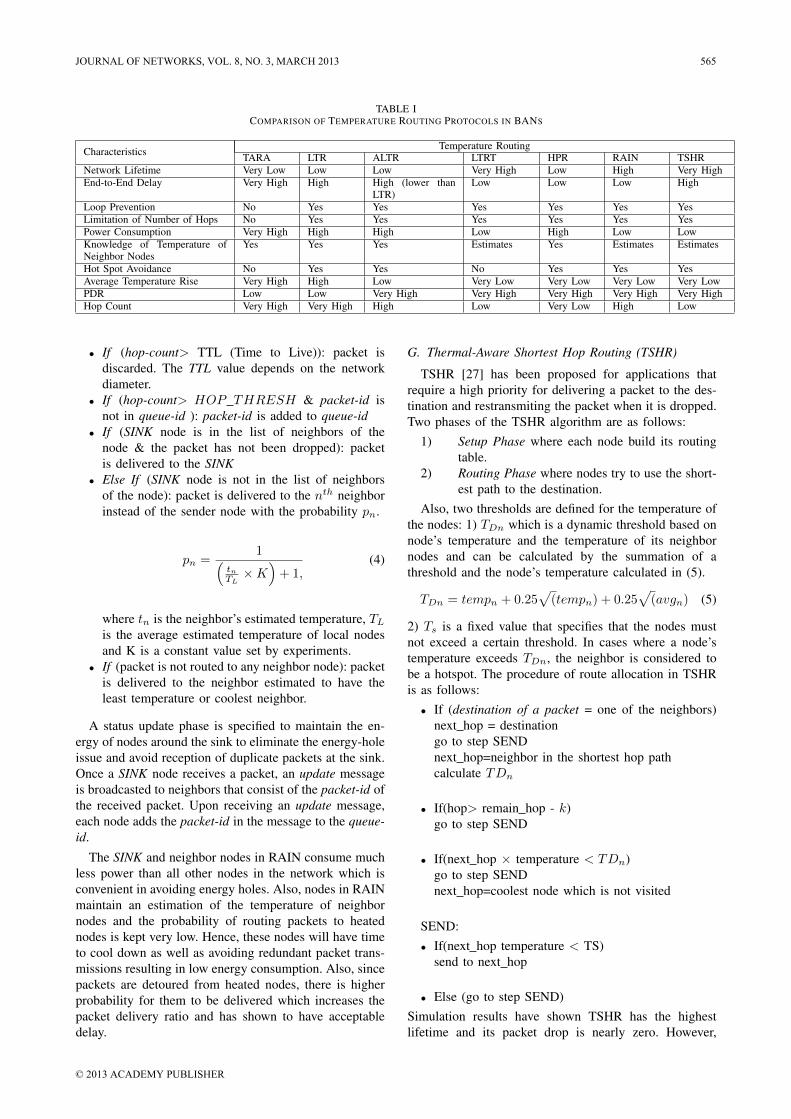
TABLE ICOMPARISON OF TEMPERATURE ROUTING PROTOCOLS IN BANS

Characteristics Temperature RoutingTARA LTR ALTR LTRT HPR RAIN TSHR

Network Lifetime Very Low Low Low Very High Low High Very HighEnd-to-End Delay Very High High High (lower than

LTR)Low Low Low High

Loop Prevention No Yes Yes Yes Yes Yes YesLimitation of Number of Hops No Yes Yes Yes Yes Yes YesPower Consumption Very High High High Low High Low LowKnowledge of Temperature ofNeighbor Nodes

Yes Yes Yes Estimates Yes Estimates Estimates

Hot Spot Avoidance No Yes Yes No Yes Yes YesAverage Temperature Rise Very High High Low Very Low Very Low Very Low Very LowPDR Low Low Very High Very High Very High Very High Very HighHop Count Very High Very High High Low Very Low High Low

• If (hop-count> TTL (Time to Live)): packet isdiscarded. The TTL value depends on the networkdiameter.

• If (hop-count> HOP THRESH & packet-id isnot in queue-id ): packet-id is added to queue-id

• If (SINK node is in the list of neighbors of thenode & the packet has not been dropped): packetis delivered to the SINK

• Else If (SINK node is not in the list of neighborsof the node): packet is delivered to the nth neighborinstead of the sender node with the probability pn.

pn =1(

tnTL×K

)+ 1,

(4)

where tn is the neighbor’s estimated temperature, TLis the average estimated temperature of local nodesand K is a constant value set by experiments.

• If (packet is not routed to any neighbor node): packetis delivered to the neighbor estimated to have theleast temperature or coolest neighbor.

A status update phase is specified to maintain the en-ergy of nodes around the sink to eliminate the energy-holeissue and avoid reception of duplicate packets at the sink.Once a SINK node receives a packet, an update messageis broadcasted to neighbors that consist of the packet-id ofthe received packet. Upon receiving an update message,each node adds the packet-id in the message to the queue-id.

The SINK and neighbor nodes in RAIN consume muchless power than all other nodes in the network which isconvenient in avoiding energy holes. Also, nodes in RAINmaintain an estimation of the temperature of neighbornodes and the probability of routing packets to heatednodes is kept very low. Hence, these nodes will have timeto cool down as well as avoiding redundant packet trans-missions resulting in low energy consumption. Also, sincepackets are detoured from heated nodes, there is higherprobability for them to be delivered which increases thepacket delivery ratio and has shown to have acceptabledelay.

G. Thermal-Aware Shortest Hop Routing (TSHR)

TSHR [27] has been proposed for applications thatrequire a high priority for delivering a packet to the des-tination and restransmiting the packet when it is dropped.Two phases of the TSHR algorithm are as follows:

1) Setup Phase where each node build its routingtable.

2) Routing Phase where nodes try to use the short-est path to the destination.

Also, two thresholds are defined for the temperature ofthe nodes: 1) TDn which is a dynamic threshold based onnode’s temperature and the temperature of its neighbornodes and can be calculated by the summation of athreshold and the node’s temperature calculated in (5).

TDn = tempn + 0.25√(tempn) + 0.25

√(avgn) (5)

2) Ts is a fixed value that specifies that the nodes mustnot exceed a certain threshold. In cases where a node’stemperature exceeds TDn, the neighbor is considered tobe a hotspot. The procedure of route allocation in TSHRis as follows:

• If (destination of a packet = one of the neighbors)next hop = destinationgo to step SENDnext hop=neighbor in the shortest hop pathcalculate TDn

• If(hop> remain hop - k)go to step SEND

• If(next hop × temperature < TDn)go to step SENDnext hop=coolest node which is not visited

SEND:• If(next hop temperature < TS)

send to next hop

• Else (go to step SEND)Simulation results have shown TSHR has the highestlifetime and its packet drop is nearly zero. However,



packet delivery delay and packet arrival rate is higher thanHPR, but TSHR has lower maximum temperature rise.

A comparison on temperature routing algorithms inBANs is given in Table I where LTRT has shown tohave comparatively better performance amongst all theproposed protocols.

V. CLUSTER-BASED ROUTING

A. Anybody

Anybody [28] is a cluster-based routing protocol thatuses clusters to gather data instead of making directcommunication with their base station. The clusters arechosen randomly in time which spreads energy dissipationthrough the entire network as cluster heads collect all dataand then send it to the base station. Anybody furtherconsiders a virtual backbone network of cluster headsby which it changes the cluster head selection. The stepby step procedure of route allocation in Anybody is asfollows:(1). Neighbor Discovery:In stage 1, each node broadcasts hello1 messages consist-ing of its unique identifier, waits for hello1 messages in agiven time frame, and relays hello1 messages of its one-hop neighbors via sending hello2 messages in the secondtime frame. At this stage, each node has gained knowledgeof its two-hop neighbors and builds its connectivity graph.(2). Density Calculation:In stage 2, each node calculates its density from (6) andsends it via hello3 messages throughout the network andreceives the density of other nodes in the network.

density =number of links

number of 2-hop neighbors(6)

(3). Contacting Clusterhead:In stage 3, each node sends a join message along with thelist of its one hop neighbors to its neighbor with highestdensity. The join messages are continuously relayed untilthey reach the node with highest density. These pathsform an intra-cluster gradient and will be used for intra-cluster communication. Hence, clusters and cluster headsare formed among local nodes. The cluster heads haveknowledge of the nodes attached to them as well theneighbor list of each one.(4). Setting up the backbone:In stage 4, some nodes will be chosen as Gateway (GW)nodes to connect the independent clusters with each other.Each clusterhead checks its cluster members and selectsthose that have a neighbor outside the cluster. Hence, aGW inform message will be sent to the elected nodes.GW nodes are responsible for communication amongthe clusters and build a virtual backbone through theirvirtual communication. Each GW node sends messagesit receives from its clusterhead to the gateway node itis connected with and messages its receives from anothercluster to its clusterhead through its intra-cluster gradient.(5). Setting up the routing paths:

Fig. 6. ANYBODY [28]

In stage 5 (the last stage), routing paths are formed viagradient setup messages: gradient setup1 from sinknode to its clusterhead, gradient setup2 from clusterhead to its connected backbone links, gradient setup3from other clusters till all clusterheads have sent agradient setup message which sets up inter-cluster-gradients (Fig. 6). Therefore the route for a messageflow in Anybody is in the following order: sender node,sender’s clusterhead, other clusterheads, sink’s cluster-head and finally the sink.

The features of Anybody can be extended for use inheterogenous networks by assigning different tasks todifferent nodes, enhancing energy efficiency by switchingoff redundant nodes and using data aggregation methodsto eliminate and buffer the messages.

Anybody has the major advantage of keeping thenumber of clusters low with increase in number ofnodes. However, reliability and energy efficiency has notbeen thoroughly investigated. Also, this protocol is notoptimized for BANs and has high delay and significantoverhead which is inconvenient for BANs due their strin-gent constraints in bandwidth, computational power andenergy.

B. Hybrid Indirect Transmission (HIT)

Culpepper et al [29, 30] have proposed a cluster-based data gathering protocol that reduces the number ofdirect transmissions to the base station and uses parallelmultihop indirect transmissions both within a cluster andamong multiple adjacent clusters. The analysis of HITand HITm (HIT with multiple clusters) have shown smallnetwork delay, high energy efficiency and high networklifetime.

The procedure of route calculation in HIT is describedas follows: In the initial stage, one or multiple cluster-heads are chosen. The cluster-heads then send out theirstatus throughout the network. Next, the upstream anddownstream relation of the clusters are formed. Accord-ingly, multiple routes are setup within a cluster to thecluster-head. Then each node calculates its blocking set.The blocking set of node i is the list of nodes that arenot allowed to transmit simultaneously with node i. Morespecifically, node i blocks node j only if

d(i, ui) > d(i, uj) (7)



Fig. 7. WASP [2]

where uj is the upstream neighbors of node j. Then, aTDMA schedule is computed for each node which allowsmaximum communication amongst nodes with paralleltransmissions. Finally, nodes transmit to their upstreamneighbors through the TDMA schedule previously as-signed. Unfortunately, HIT requires more communicationenergy in dense networks, does not consider reliabilityand has conflicting interaction issues among the desiredroutes for specific applications and its communicationroutes [5].

VI. CROSS LAYER ROUTING

A. Wireless Autonomous Spanning Tree Protocol (WASP)

The WASP [2] protocol sets up a spanning tree anddivides the time axis in slots, referred as WASP-cycles,in a distributed manner to provide traffic routing andmedium access coordination using the same spanning treewhich results in lower energy consumption and higherthroughput (Fig. 7). Each node assigns a unique WASP-scheme message and sends to its child nodes informingthem when they are allowed to use the link. Hence,these messages allow traffic control and increase resourcerequest from parents of children which minimizes the co-ordination overhead. The children respond to the schemeby sending their own WASP-scheme based on the thesink WASP-scheme and the child node’s requirements. Itis important that the nodes are synchronized to avoidshifting. The WASP-scheme messages are different forsink and child nodes, but they usually consist of thefollowing: (1) address of sender node (2) slots assignedto the children of the parent node where they send theirWASP-scheme (3) silent period duration (4) forwardingreceived data to the sink (5) Contention slot (6) Acknowl-edgment sequence. WASP achieves up to 94% throughput,high packet delivery ratio, low energy consumption andfixed end to end delay. However, WASP does not considerlink quality, mobility, load and does not support two waycommunication. Also overhead is a drawback which canbe reduced with data aggregation techniques.

B. Controlling Access with Distributed slot Assignmentprotocol (CICADA)

CICADA [18, 31] is a low energy cross layer routingprotocol specifically designed for BANs based on multi-hop TDMA scheduling and improves reliability through

the definition of a lognormal distribution for link prob-ability instead of a circular coverage region. It is animprovement to the WASP protocol as it considers twoway communication. In CICADA, each node calculatestwo parameters for sending data and sends it to its parentnode. One is the number of slots required to send data,αn and the other is number of slots the node has to waituntil it has received all data from its children, βn. Basedon these parameters, all nodes know when to send data.Additionally, each transmission cycle is divided into dataand control subcycles which enhance mobility support asit provides the detection of parent or child loss, lowerdelays for joining a node and allows a maximum of 3cycles to join the parent node.

In the data subcycles, each node sends its data basedon the allocated time. In the control subcycle, the parentnodes broadcast a scheme to their child nodes to informthem of when to transmit data. Unlike WASP, the bottomnodes of the spanning tree are the first nodes to sendtheir data. Hence, CICADA has been designed such thatall packets reach the source in one cycle which leadsto lower delay and routes data packets up its spanningtree to control medium access without the requirementof control packets. Also CICADA has much simplercomputations for calculating the data period and waitingperiod compared to WASP which is significant for use innetworks with scarce resources.

CICADA has modeled reliability by using scheme ran-domization and increasing the number of retransmissions[18]. Additionally, CICADA can be enhanced to supporthigh traffic BANs which require low delay by sendingdata more often instead of local buffering [31]. In terms ofenergy efficiency, CICADA avoids collision, idle listeningand overhearing via assigning slots in the control subcycleand using them in the data subcycle. Hence, all nodes willknow of their sleep time, when to receive data, when tosend data and when to switch on their radio.

However, CICADA has shown to have a high sleepratio in cases with 50% or lower duty cycle. Also,longer duty cycles have higher packet loss in high packetgeneration rates and a major increase in number ofretransmissions. Therefore, a tradeoff exists between en-ergy efficiency and the desired throughput [18]. Also, allcommunication information in CICADA is sent in plaintext instead of being protected and unauthorized nodesare capable of joining the network without authorization.An updated version of CICADA, namely CICADA-Shas been designed in [32] to encounter the privacy andsecurity issues that had not been considered in CICADA.CICADA-S has four main states in terms of security:secure initialization phase, sensor (re) joining the BAN,key update procedure within the BAN and a sensorleaving the BAN. These phases have little impact on thethroughput and power consumption [32].

C. Timezone Coordinated Sleeping Mechanism (TICOSS)

TICOSS [33] sets all nodes as Full Functional Devices(FDD) and provides improvements to the IEEE 802.15.4



standard by offering configurable shortest path routingto the BAN coordinator, preserving energy and reducinghidden terminal collisions through V-scheduling (due toV-shape communication flow). This results in doublethe operation lifetime of IEEE 802.15.4 for high trafficscenarios and the extending IEEE 802.15.4 to supportmobility. The idea of TICOSS is to provide timezonedivisions based on the minimum hops required for packetsto reach the coordinator when all nodes have joined thenetwork. Both synchronization and timezone division cantake place in the initialization phase as follows: an initialzone message is sent by the coordinator to neighboringnodes that consists of timing information and zone of thetransmitter (TxZone). The nodes receiving this messageset their timezone to TxZone+1, renew their internal clockand send a new zone message which consists of newtiming information and TxZone+1 as the transmitter zone.Further receiving nodes continue this process.

TICOSS considers mobility, replacement and node de-ployment through setting a preset expiration time for anode’s timezone when no zone update message is receivedby the node. The updates are stored in a table along withthe sender’s node ID, to discard and identify stale zonemessages, and a timestamp to associate corrupt entries.The V-scheduling table assigns periods of node inactivityand activity to nodes timeslots which allows transmissionand reception to occur in the same interval. Nodes in thesame time slot are capable of using the same time slotfor transmission.

D. Cross Layer MAC and Routing Protocol Co-Designfor Biomedical Sensor Networks (BIOCOMM)

BIOCOMM [34] is a cross layer routing protocol de-signed based on the interaction of the MAC and networklayer in biomedical sensor networks to optimize overallnetwork performance. This interaction is achieved througha Cross-layer Messaging Interface (CMI) via which theMAC layer sends its status information to the networklayer and vice-versa. More specifically, the network layerkeeps track of the vacant space in it Buffer Space (BS)and this information is sent to the MAC layer through theCMI by which MAC layer becomes capable of assigninghigher frame transmission priority to congested nodes toeliminate packet loss ratio in the network layer due tobuffer overflow. Both the MAC and network layer eachmaintain Neighbor Status Table which is set to Blocked(B) or Free (F) via the MAC logic. Each modificationin the Block and Free message is generated and sent viaCMI to the network layer through which the network layerupdates its status in its Neighbor State Table.

Each node tries to route packets to the destinationvia the least number of hops unless a sleeping nodeor a hotspot exists in the path. The procedure of routeallocation in BIOCOMM is as follows:

• If (hop count > Time To Live (TTL)): The packetis dropped.

• Else If (Status of next-hop node in shortest path tosink is Free in Neighbor Status Table): 1) increment

hop count, 2) Send packet to next-hop node.• Else If (Status of next-hop node in shortest path

to sink is Blocked in Neighbor Status Table): 1)Increment hop count, 2) Send packet to Last Activenode (LA).

BIOCOMM-D provides certain modifications to BIO-COMM to reduce the average packet delay in delaysensitive applications. Both Biocomm and Biocomm-Dhave very low temperature rise for nodes in its network.However, Biocomm-D has comparatively higher temper-ature rise than Biocomm due to its attempt to reduceaverage packet delay.

Both Biocomm and Biocomm-D have significantlylower energy consumption (one-forth the energy con-sumption of HPR) which is due turning the radio of nodesoff when they are asleep. In terms of delay, Biocommhas slightly higher delay than HPR which is resolved inBicomm-D which has lower delay than both Biocommand HPR as it drops packets that have been circulating inthe network for a long time.

VII. COST-EFFECTIVE ROUTING

A. Opportunistic routing

In [15], the moving nature of the body is consideredin the routing protocol through an opportunistic schemethat ensures high communication probability with thesink at all times. This protocol uses a simple systemmodel where the sink node is placed on the wrist andmoves forward and backward while running and walking.A relay node exists on the waist and a sensor nodeon the chest. Consequently, for the sensor node to beable to communicate with the sink node, there are twopossibilities. When the wrist is at the back of the body,non line of sight (NLOS) communication is consideredwhere the sensor node will send data to the relay nodeand then the sink node. Whereas, in cases where thewrist is in the front, line of sight (LOS) communicationexists between the sensor node and sink. The data measurethrough these sensor nodes needs to be periodically sentto an external server through the sink. The probability forLOS and NLOS communication is considered 0.5 and 0.5.

Once a node wants to send data through LOS commu-nication it sends a Request to Send (RTS) signal witha power level that only nodes in its LOS can receiveit. The nodes in LOS position will reply by sending anACK (Acknowledge) signal in a specified time slot. Thesender node will now be able to directly send its packetto the node in its LOS position. In cases where no nodeexists in the LOS position of the sender node the RTSsignal will not be received and no ACK signal will besent in the time out interval. After the timeout perioda wakeup signal will be sent to identify when the nodeis ready to start the communication. In the end of thecommunication, a Receive Acknowledge (RAck) signalwill be sent to the sender node to announce successfulcommunication. In cases where the RAck signal is notreceived, the mentioned procedure will be repeated.



The proposed opportunistic routing scheme aims toincrease network lifetime and is compared to one-hopor two-hop communication and shown to have the sameenergy consumption for multihop transmission in the sen-sor node but has approximately half the energy consump-tion of multihop communication at the relay node. Theresults have shown the capability of decreasing energyconsumption to increase network lifetime in the relay andsensor via preserving the same Bit Error (BER) of one-hop and two-hop communication. Moreover, the energyconsumption of the relay nodes have shown to decreasedramatically via the proposed opportunistic scheme whichleads to overall decrease in overhead energy consumptionas relay nodes are major consumers of overhead in thenetwork.

The overall energy consumption of the proposed rout-ing algorithm lies in between one-hop and multihop com-munication where multihop communication costs doublethe energy of one hop. However, this protocol does notconsider the energy level of nodes and is not scalable dueto increase of traffic on the relay node from an increasein the overall number of nodes.

B. Prediction-based Secure and Reliable routing (PSR)

Liang et. al [35] have proposed the distributed (PSR)routing framework for BANs where each node ni main-tains the matrix Mi (s× p) which stores the link qualitymeasurements between itself and all other nodes in thenetwork during the past p time slots (p is a predefined pa-rameter and the initial matrix is empty). Each row belongsto a unique node where the k-th column corresponds tothe link quality between ni and other nodes in Tc−p+k−1

(Tc is the current time slot). Link quality is determinedthrough the received signal at the receiver side. The valuesof the matrix at two time slots Tc and Tc+1 are shownin Fig. 8. ni generates an order-p auto-regressive modelthrough which node ni is capable of predicting its linkquality at time Tc with every other node and picks anode closer to the sink with better link quality. Datatransmission of node ni is heard by all neighboring nodeswhere the received signal power is measured. Then, anACK consisting of their intention to be a receiver or notis replied to ni through which Mi is updated. However,this protocol is not scalable and is only suitable for BANapplications with few number of nodes due to the hugeoverhead for maintaining the table.

C. Probabilistic routing with postural link costs (PRPLC)

PRPLC [36] sets a Link Likelihood Factor (LLF)namely P t

ij (0 ≤ P tij ≤ 1) which denotes the likelihood

for link Lij between node i and j to be connected over adiscrete time slot t. LLF is determined to be dynamicallyupdated after the tth time slot as follows:

P tij =

{P t−1ij + (1− P t−1

i,j )ω if Lij is connectedP t−1ij ω if Lij is disconnected

Fig. 8. Link quality matrix Mi of node ni [35]

When the link is connected, P tij is determined to

increase with a constant rate ω plus the difference ofits maximum value which is 1 and its current value,P tij . For low values of ω, P t

ij rises slowly when thelink is connected and degrades fast when the link is notconnected. On the other hand, for high values of ω, P t

ij

rises fast when the link is connected and degrades slowlywhen the link is not connected. P t

ij is expected to risefast and degrade slowly for a historically good link andto rise slow and degrade fast for a historically bad link.Hence, ω should be capable of gaining knowledge of along-term history of the link which is described throughthe definition of Historical Connectivity Quality (HCQ)for an on-body link Lij in (8) as follows:

ωti,j =

t∑r=t−Twindow

Lri,j

Twindow(8)

where Twindow is the measurement window (number ofslots) over which the connectivity quality is averaged. Lij

is 0 if the link is not connected over time slot r, and 1when the link is connected. All nodes observe and main-tain their LLF to be in one-hop contact with each otherat all times. The aim of PRPLC is to choose high link-likelihoods to reduce end-to-end delay and intermediatestorage delay relative to packets getting stuck at nodeswith low link likelihood.

When a node i wants to route data to a node d (sinknode) and meets node j, node i forwards the packetto node j if and only if P t

i,d ≤ P tj,d is valid. More

specifically, in such cases node j is more likely to meetnode i as it has a higher link likelihood which explainsthe reduction in end-to-end delay via transferring a packetfrom node i to node j. Also, each node updates its P t

ij

values with all nodes in the network through its periodicHello messages which are also used to send the P t

id valueswith the common destination node d.

In cases where packets are stored in node-i’s buffer,node-i finds out if there is a node that has a higher LLFto node d . In cases where there is a node with a higherLLF to the destination node, packets are forwarded to thatnode. Otherwise, node-i continues to store its packet inits own buffer if it has the highest LLF to the destinationnode.



TABLE IICOMPARISON OF COST-EFFECTIVE ROUTING PROTOCOLS IN BANS

Characteristics Cost-effective RoutingOpportunistic Routing PRPLC DVRPLC OBSFR PSR ETPA

Delay Low High High Low High HighNetwork Lifetime High High High Low Low HighLink Probability LOS and NLOS X X X X X

PDR 100% up to 88% up to 89% up to 92% up to 80% up to 95%GPS X × × × × ×

Mobility X X X X X XEnergy Usage Low Low Low High High Low

D. Distance vector routing with postural link costs (DVR-PLC)

DVRPLC [16] proposes that all nodes preserve thecumulative path cost to the common sink node. As withPRPLC, this protocol chooses high likelihood paths todecrease end-to-end packet delivery delay and decreaseintermediate storage delay relative to storing packets atnodes with low link likelihood. DVRPLC specifies a LinkCost Factor (LCF) of Ct

ij(0 ≤ Ctij ≤ Cmax) which stands

for the routing cost of link Lij in a discrete time slot t.LCF is defined to be updated dynamically after the tthtime slot as follows:

Ctij =

{Ct−1

ij (1− ωti,j) if Lij is connected

ωtij(C

t−1ij − 1) + 1 if Lij is disconnected

Ctij decreases at a fixed rate of (1 − ωt

i,j) whereωti,j(0 ≤ ωt

i,j ≤ 1) is the HCQ described in (8). Asin PRPLC, both short and long term link localities areshown to minimize delay with the same routing procedurewith the difference of choosing links of lower costs.DVRPLC aims to minimize end-to-end cumulative costwhich outperforms PRPLC that has considered LLF toonly be in the link level.

E. On-Body Store and Forward Routing (OBSFR)

OBSFR [37] attempts to avoid network partitioningwhich may arise by allowing each node to maintain itssource id, seq No and list of node-ids that demonstrateits path so far from the source node. Hence, once a packetarrives at a node for the first time, the node continues tostore the packet until it meets at least one node that is notlisted in the node-ids of the packet. In such cases, node ibroadcasts the packet to the node it has encountered anddeletes the packet from its buffer. As in regular flooding,node i will ignore the reception of the same packet.However, this routing scheme is only applicable to smallnetworks of few nodes and not scalable to large networksdue to the requirement of tens of ids being added to thepackets.

OBSFR has shown to have a packet delivery ratio ofup to 92 % which is due to multi-packet forwarding thatleads to lower packet loss. However, there is a uniquetype of packet loss in OBSFR relative to partition packetsaturation. Also, OBSFR and DVRPLC have been shownto have higher packet hop count leading to longer routescompared to PRPLC.

Fig. 9. Route Allocation in ETPA

F. Energy Efficient Thermal and Power Aware (ETPA)Routing

Movassaghi et. al [38] have proposed an energy ef-ficient, thermal and power aware routing algorithm forBANs named Energy Efficient Thermal and Power Awarerouting (ETPA). This protocol calculates a cost functionfor route allocation based on a nodes temperature, energylevel and received power from adjacent nodes. In order toavoid idle listening and decrease interference, the framesare considered to be divided into time slots by the numberof nodes in the network, N, where each node is allowed totransmit in the time slot it has been assigned (i.e TDMA).In each cycle (every four frames), each node, j, broadcastsits temperature, Tj and its available energy level, Ej ,through a HELLO message in its allocated time slot to allits adjacent nodes. Next, each node estimates the receivedpower from its adjacent nodes (Fig. 9). Hence node ibecomes capable of calculating the cost of transmissionto node j through (9) as follows:

Ci,j = α1(Pm − P j

i

Pm) + α2(

TjTm

) + α3(Em − Ej

Em) (9)

where α1, α2 and α3 are non-negative coefficients, P ji

is the received power at node i from node j, Pm isthe maximum received power at each nodes, Em is themaximum available energy at each nodes and Tm is themaximum temperature allowed. In the next frame, eachnode which has a packet to send, finds the node withminimum cost and forwards the packet to that node.Otherwise, the packet is stored at the node itself. Forexample in Fig. 9, C1,3 is less than C1,2 and C1,4, so,node 3 is selected as the next node. Also, packets thathave been stored for more than 2 frames are consideredto be dropped.

ETPA has shown to significantly decrease temperature



rise and power consumption and provide a more efficientusage of the available resources. Additionally, it has aconsiderably high depletion time that guarantees a longerlasting communication among nodes.

A comparison of the cost-effective routing protocolsin BANs is provided in Table II. As in all cost-effectiveprotocols, the cost-effective relation between all nodesneeds to be periodically updated and stored, a largeamount of transmissions and overhead is required to findroutes which also adds complexity to the system.

VIII. QOS BASED ROUTING

A. LOCALMOR

A novel QoS-based routing protocol has been proposedin [39] for biomedical applications of sensor networksvia traffic diversity namely LOCALMOR. The proposedprotocol functions in a localized, distributed, computationand memory efficient way. It also classifies data trafficinto several categories based on the required QoS metricswhere different techniques and routing metrics are pro-vided for each category. LOCALMOR deploys diversityof data traffic whilst considering reliability, latency andresidual energy in sensor nodes and transmission powerbetween sensor nodes as QoS metrics of the multi-objective issue. Additionally, the proposed protocol canbe used with any MAC protocol if an ACK mechanismis employed.

Four modules exist in the proposed protocol as itfollows a modular approach explained in the following:

• Delay-sensitive Module: This module deals withrouting packets that are required to be deliveredby a given deadline. It deploys the packet velocityapproach provided in [40] that does not require anysynchronization amongst the nodes.

• Power-efficiency Module: This module handles reg-ular packets and can be used by other modules incases where the required data-related metrics needto be optimized by several nodes.

• Reliability-sensitive Module: This module deals withrouting packets requiring high reliability to enhancethe chances of delivering a packet by sending a copyto both the primary and secondary sinks. Thus, amulti-sink single path is chosen instead of a single-sink multipath approach which leads to convergenceof data packets close by or at the sink and results inincrease of collision and traffic congestion.

• Neighbor Manager: This module executes HELLOmessages, implements estimation methods, managesneighbor tables and provides other modules withtheir expected information based on their packettype.

However, scalability has not been investigated in theproposed protocol and a high number of nodes need to beconfigured as well as a real sensor network using motes.

B. Data-centric Multi-objective QoS-aware routing(DMQoS)

Razzaque et. al [41] have proposed a data-centric multi-objective QoS-aware routing protocol, namely DMQoS,for delay and reliability domains in BANs. The proposedprotocol provides customized QoS services for each trafficcategory based on their generated data types. It employs amodular design architecture that consists of different unitsthat operate in coordination with each other to supportmultiple QoS services. More specifically, it consists ofthe following five modules:

• Reliability Control: Reliable data delivery to thedestination can be effected via link/node failure,congestion, node mobility, link quality degradation,etc. This module uses the greedy approach for itsreliability control algorithm. First, a candidate down-stream node j is identified at each node i for eachsink s ∈ S with maximum reliability ri,j and storesit in the NHr variable. The packet is immediatelydropped in cases where NHr returns a Null. Incases where only one node is returned, the packetwill be forwarded to the next hop if its reliability ishigher than the required reliability R and droppedotherwise.

• Delay Control: This module controls on-time deliv-ery for time critical emergency packets where thelife-time of a packet (tlife) bounds the maximumallowable latency for delay-guaranteed service re-quired by the application. The end-to-end packetlatency at the network layer is the sum of thepropagation delay, queuing delay, processing delayand transmission delay where the queuing delay hasthe most significant amount of the latency followedby the transmission delay.

• QoS-aware Queuing and Scheduling Modules: Thismodule considers four individual queues in a sensornode where the highest priority is given to criticalpackets (CP), the second highest probability is givento delay-constrained packets (DP), the third priorityis for reliability-constrained packets (RP) and theleast priority is given to ordinary packets (OP).

• The Dynamic Packet Classifier: This module de-fines four separate classes of packets as follow:ordinary packets (OP), critical packets (CP), delay-constrained packets (DP), reliability-constrainedpackets (RP),

• Energy-aware Geographic Forwarding (EAGF): Thismodule deploys a localized packet forwarding thatuses hop-by-hop routing instead of traditional end-to-end path discovery routing. Thus, a packet willhave numerous choices in choosing a path to thedestination. The aim is to choose a downstream nodewith higher geographic progress and higher residualenergy towards the destination where the first ap-proach leads to lower number of hop between thesource and destination and the second one provides abalance of energy consumption amongst the potentialdownstream nodes. This tradeoff is further managed



via the multiobjective Lexicographic Optimization(LO) approach.

Additionally, a homogenous energy dissipation rate isensured for all routing nodes in the network using a mul-tiobjective Lexicographic Optimization-based geographicforwarding that uses a localized hop-by-hop routing basedon the QoS performance and geographic locations of theneighbor nodes.

In summary, DMQoS provides a better performancecompared to LOCALMOR in terms of end-to-end delayand packet delivery ratio.

C. Reinforcement Learning Based Routing Protocol withQoS support (RL-QRP)

A reinforcement learning based routing protocol withQoS support (RL-QRP) has been proposed in [42] whichuses the basic idea of location information where sensornodes can of compute the available QoS routes basedon the link qualities of the available routes and the QoSrequirements of the data packet, and forward data packetsto one of the neighbor nodes. This procedure is continuedin forwarding the data packets to the sink node and iteratesat each relaying node till the packets reach the sinknode. Thus, a distributed reinforcement learning algorithmis used for the computation and selection of the QoSroutes where each of the sensor nodes individually andgraphically calculate the route.

The major issue with shortest path routing, geographicrouting and other pre-defined routing protocols are rela-tive to congestion avoidance and network load balance.More specifically, in these networks a sensor nodes for-wards its data packets to nodes that are geographicallycloser to the sink without considering their communi-cation and computation load, duty cycle, their bufferstatus, etc. This challenge is taken into considerationwith the design of adaptive QoS routes that considersneighbor nodes’ state information, and link quality. But,the prediction and maintenance of such information inhighly dynamic environments is quite challenging. Thus,the RL-QRP algorithm uses the independent distributedreinforcement learning (IndRL) approach for QoS routecalculation where a sensor node does not consider theinteraction among itself and other sensor nodes and onlyconsiders itself capable of changing the state of the envi-ronment. However, the proposed approach is not efficientfor global optimization in large scale networks.

D. QoS framework

Liang et. al [43] have proposed a QoS-aware routingprotocol for biomedical sensor networks with the aim ofproviding differential QoS support and prioritized routingservice in the network . This procedure is accomplishedvia the following tasks: establishment and maintenanceof QoS-aware routes, prioritized packet routing, feed-back on network conditions to user application, adaptivenetwork traffic balance and Application ProgrammingInterfaces (API). The routing module is in charge of route

maintenance and establishment through proactive table-driven algorithms where each node preserves its routinginformation to the sink node and stores all possible routesto the sink in its routing table by indexing the node IDsof its one-hop neighbors. In the route setup phase, thesink node indicates its existence by sending broadcast sinkadvertisement (ADV) packets. These packets are receivedand stored by sensor nodes in the communication rangeof the sink node. Next, the sensor nodes broadcast RouteInformation (RI) packets to its neighbor nodes indicatingthey can be used as routers to the sink node. The neighbornodes will also set up their own routing tables andbroadcast RI packets to their neighbors. Therefore, allsensor nodes will establish a path to the sink nodes aftera while.

Due to topological changes relative to change in thewireless channel and node or link failure, network infor-mation needs to be periodically updated. The sink nodesbroadcast ADV packets in a fixed period. All sensor nodescheck route information in the packet upon receiving aADV or RI packet, update their routing tables and broad-cast RI packets accordingly. Additionally, the proposedQoS framework provides prioritized packet routing byproviding a classification for all the packets including datapackets and control packets.

IX. ROUTING IN BANS VS. OTHERS

Energy consumption and network lifetime are two ofthe major challenges in BANs as recharging and replacingbatteries of devices attached to a human body may leadto one’s discomfort. Moreover, the surrounding area ofthe human body is considered as a lossy medium for datacommunication. Hence, electromagnetic waves around thebody are considerably attenuated leading to high data pathloss and delay spread due to placement on different bodysides and constraining data transmission over an arbitrarydistance around the body. In cases with too much datatransmission around the body, temperature rise and tissueheating can cause significant issues [44].

Literature has shown many power-aware and QoS-aware routing protocols described for WSNs, MANETswhich are not applicable to in-body and on-body BANsgiven their stringent constraints. Much of the researchin MANETs has focused on improving scalability[45–47], whereas in BANs currently its more about energyefficiency. More specifically, power dissipation and com-munication radiation of implanted sensors may lead tosevere health hazards [19, 48]. QoS is important in manyBAN applications such as artificial retinas and in otherapplications large delays could be fatal. Therefore BANrouting protocols need to ensure they can address the QoSconstraints of the respective applications [1]. Hence, therouting protocols designed for BANs must also considerthe delay specifications in communication of the senseddata to the base-station [20].

A number of energy efficient routing protocols havebeen proposed for MANETs that aim to find routes thatminimize energy consumption in terminals with little



energy resources and ignore the load of operations inmemory access, data processing, measurement and alsothe required energy to receive or transmit data over awireless link [4]. Moreover, the loss of a device or sensoris not considered an issue [5].

Routing protocols designed for WSNs mainly focuson delay constraints and energy-efficiency whereas notconsidering the effects of power dissipation and commu-nication radiation of the implanted sensors. Two types ofhotspot routing issues have been stated to exist in thenetworking field, namely, link hot spot and area hot spot[19]. Area hot spot refers to the entire region arounda node as hot and all of its surrounding links to bedisconnected which leads to node isolation. Link hot spotrefers to disconnection of a link. However, the proposedsensor network and ad hoc routing protocols mainly focuson link hot spot whereas other links of the node may beavailable [19].

Heterogenous devices are required in BANs with dif-ferent data rates, whereas WSNs consider homogenoussensors throughout the network. However, some applica-tions in BANs support non-real time data communication.The mobility pattern in BANs changes in the order ofmovements within tens of centimeters whereas the scaleof mobility in WSNs is in the order of meters and tens ofmeters [5]. In WSNs, traffic flow is amongst the sensorsand their sinks and between any two pair of nodes inMANETs.

X. CONCLUSION AND FUTURE DIRECTIONS

We have classified routing protocols in BANs into fivecategories: temperature based, cluster-based, cross layer,cost-effective and QoS-based. We have described thedesign and constraints of the individual routing protocolswith respect to their category and their application inBANs. The temperature-based routing protocols used forin-body BANs only consider temperature as a metricfor choice of routes that would either avoid hot regionsor detour after reaching a hot region. The cost-effectiverouting protocols calculate a probability for a link tobe connected based on knowledge from certain char-acteristics in the network. However, none of the cost-effective routing protocols consider temperature rise in thenodes and the path loss among sensor nodes around thebody. The cluster based and cross layer routing protocolsare mainly reactive and need to gain knowledge of theconnectivity of all nodes in the network and their otherfeatures which leads to significant overhead. QoS-basedrouting protocols aim to accomplish the required QoSmetrics.

Some of the challenges of routing in BANs are consid-ered in different categories of routing protocols proposedbut still a lot more work needs to be done. The proposedrouting protocols either do not consider postural bodymovements with mobility or are not as energy efficient.Also, most of the aforementioned routing protocols havenot considered reliability and QoS. The future vision of

BANs is to provide energy efficient and reliable communi-cation among sensors in both real-time and non real-timeapplications. Also, more accurate propagation models arerequired that consider mobility, latency, reliability, mutualinterference and energy consumption that construct amore efficient architecture for better routing protocols inBANs.

Future routing protocols for BANs should be capableof obtaining the required QoS as well as maintaininga well balanced low power energy consumption. Thiscan be achieved by jointly designing the MAC layerand the routing protocol in order to satisfy both energyand QoS requirements. Such a procedure can be foundin the excessive body of research in the field of WSNsand MANETS that should be considered to be used inBANs. However, these protocols need to be modified andoptimized to be efficiently used in BANs.

REFERENCES

[1] D. Takahashi, Y. Xiao, F. Hu, J. Chen, and Y. Sun, “Temperature-aware routing for telemedicine applications in embedded biomed-ical sensor networks,” EURASIP Journal on Wireless Communi-cations and Networking, vol. 2008, Jan. 2008.

[2] B. Braem, B. Latre, I. Moerman, C. Blondia, and P. Demeester,“The wireless autonomous spanning tree protocol for multihopwireless body area networks,” In proceeding of the Third AnnualInternational Conference on Mobile and Ubiquitous Systems:Networking Services, pp. 1 –8, July 2006.

[3] K. Akkaya and M. Younis, “A survey on routing protocols forwireless sensor networks,” Ad Hoc Networks, vol. 3, pp. 325–349,2005.

[4] M. Abolhasan, “A review of routing protocols for mobile ad hocnetworks,” Ad Hoc Networks, vol. 2, no. 1, pp. 1–22, 2004.

[5] S. Ullah, H. Higgins, B. Braem, B. Latre, C. Blondia, I. Moerman,S. Saleem, Z. Rahman, and K. Kwak, “A Comprehensive Surveyof Wireless Body Area Networks,” Journal of Medical Systems,pp. 1–30, 2010.

[6] B. Latre, B. Braem, I. Moerman, C. Blondia, and P. Demeester,“A survey on wireless body area networks,” Wirel. Netw., vol. 17,pp. 1–18, Jan. 2011.

[7] K. Kwak, S. Ullah, and N. Ullah, “An overview of IEEE 802.15.6standard,” in 3rd International Symposium on Applied Sciences inBiomedical and Communication Technologies (ISABEL), pp. 1 –6,Nov. 2010.

[8] C. Otto, A. Milenkovic’, C. Sanders, and E. Jovanov, “Systemarchitecture of a wireless body area sensor network for ubiquitoushealth monitoring,” J. Mob. Multimed., vol. 1, pp. 307–326,January 2005.

[9] E. Dishman, “Inventing wellness systems for aging in place,”Computer, vol. 37, pp. 34 – 41, May. 2004.

[10] K. Y. Yazdandoost and K. Sayrafian-Pour, “Channel model forbody area network (BAN),” Networks, p. 91, 2009.

[11] J. Xing and Y. Zhu, “A survey on body area network,” in 5th In-ternational Conference on Wireless Communications, Networkingand Mobile Computing, 2009. WiCom ’09., pp. 1 –4, Sept. 2009.

[12] C. Tachtatzis, F. Di Franco, D. Tracey, N. Timmons, and J. Mor-rison, “An energy analysis of IEEE 802.15.6 scheduled accessmodes,” IEEE GLOBECOM Workshops (GC Wkshps), pp. 1270–1275, Dec. 2010.

[13] R. Shah and M. Yarvis, “Characteristics of on-body 802.15.4networks,” 2nd IEEE Workshop on Wireless Mesh Networks(WiMesh), pp. 138 –139, Sep. 2006.

[14] D. Domenicali and M.-G. Di Benedetto, “Performance analysisfor a body area network composed of ieee 802.15.4a devices,” 4thWorkshop on Positioning, Navigation and Communication (WPNC’07), pp. 273 –276, Mar. 2007.

[15] A. Maskooki, C. B. Soh, E. Gunawan, and K. S. Low, “Op-portunistic routing for body area network,” in IEEE ConsumerCommunications and Networking Conference (CCNC), pp. 237 –241, Jan. 2011.

[16] M. Quwaider and S. Biswas, “DTN routing in body sensor



networks with dynamic postural partitioning,” Ad Hoc Networks,vol. 8, no. 8, pp. 824–841, 2010.

[17] “IEEE p802.15.6/d0 draft standard for body area network,” IEEEDraft, 2010.

[18] B. Braem, B. Latre, C. Blondia, I. Moerman, and P. Demeester,“Improving reliability in multi-hop body sensor networks,” Pro-ceedings of the 2008 Second International Conference on SensorTechnologies and Applications, pp. 342–347, 2008.

[19] R. Shah and M. Yarvis, “TARA: Thermal-aware routing algorithmfor implanted sensor networks,” 1st IEEE International Confer-ence on Distributed Computing in Sensor Systems (DCOSS05),vol. 3560, p. 206217, June.-July. 2005.

[20] A. Bag and M. Bassiouni, “Hotspot preventing routing algo-rithm for delay-sensitive biomedical sensor networks,” IEEEInternational Conference on Portable Information Devices(PORTABLE07), pp. 1 –5, May. 2007.

[21] D. M. Sullivan, “Electromagnetic simulation using the FDTDmethod,” IEEE Press series on RF and microwave technology,p. 165, 2000.

[22] M. Chari and S. J. Salon, Numerical methods in electromagnetism.Academic Press, 2000.

[23] H. H. Pennes, “Analysis of tissue and arterial blood temperatures inthe resting human forearm,” Journal of Applied Physiology, vol. 1,no. 2, pp. 93–122, 1948.

[24] A. Bag and M. A. Bassiouni, “Energy efficient thermal awarerouting algorithms for embedded biomedical sensor networks,”IEEE International Conference on Mobile Adhoc and SensorSystems (MASS), pp. 604 –609, Oct. 2006.

[25] A. Bag and M. A. Bassiouni, “Hotspot preventing adaptiverouting algorithm for networks-on-chip.,” in High PerformanceComputing, Networking and Communication Systems Conference(HPCNCS’07), pp. 171–177, 2007.

[26] A. Bag and M. Bassiouni, “Routing algorithm for network ofhomogeneous and id-less biomedical sensor nodes (RAIN),” IEEESensors Applications Symposium (SAS), pp. 68 –73, Feb. 2008.

[27] F. Ahourai, M. Tabandeh, M. Jahed, and S. Moradi, “A ther-malaware shortest hop routing algorithm for in vivo biomedicalsensor networks,” in Third International Conference on Informa-tion Technology : New Generations, p. 16121613, Sept. 2009.

[28] T. Watteyne, S. Auge-Blum, M. Dohler, and D. Barthel, “Any-body: a self-organization protocol for body area networks,” in theProc. of Second International Conference on Body Area Networks(BODYNETS 2007).

[29] B. J. Culpepper, L. Dung, and M. Moh, “Design and analysis ofhybrid indirect transmissions (HIT) for data gathering in wirelessmicro sensor networks,” SIGMOBILE Mob. Comput. Commun.Rev., vol. 8, pp. 61–83, Jan. 2004.

[30] M. Moh, B. Culpepper, L. Dung, T.-S. Moh, T. Hamada, and C.-F. Su, “On data gathering protocols for in-body biomedical sensornetworks,” Global Telecommunications Conference (GLOBECOM’05), vol. 5, Dec. 2005.

[31] B. Latre, B. Braem, I. Moerman, C. Blondia, E. Reusens,W. Joseph, and P. Demeester, “A low-delay protocol for multihopwireless body area networks,” Fourth Annual International Con-ference on Mobile and Ubiquitous Systems: Networking Services,pp. 1 –8, Aug. 2007.

[32] D. Singele, B. Latr, B. Braem, M. Peeters, M. De Soete,P. De Cleyn, B. Preneel, I. Moerman, and C. Blondia, “A securecross-layer protocol for multi-hop wireless body area networks,” inAd-hoc, Mobile and Wireless Networks (D. Coudert, D. Simplot-Ryl, and I. Stojmenovic, eds.), vol. 5198 of Lecture Notes inComputer Science, pp. 94–107, Springer Berlin / Heidelberg, 2008.

[33] A. G. Ruzzelli, R. Jurdak, G. M. O’Hare, and P. Van Der Stok,“Energy-efficient multi-hop medical sensor networking,” Proceed-ings of the 1st ACM SIGMOBILE international workshop onSystems and networking support for healthcare and assisted livingenvironments, pp. 37–42, 2007.

[34] A. Bag and M. A. Bassiouni, “Biocomm - a cross-layer mediumaccess control (mac) and routing protocol co-design for biomedicalsensor networks,” International Journal of Parallel, Emergent andDistributed Systems, vol. 24, Feb. 2009.

[35] X. Liang, X. Li, Q. Shen, R. Lu, X. Lin, X. Shen, and W. Zhang,“Exploiting Prediction to Enable Secure and Reliable Routing inWireless Body Area Networks,” in The 31st IEEE InternationalConference on Computer Communications (INFOCOM), (Orlando,United States), 2012.

[36] M. Quwaider and S. Biswas, “Probabilistic routing in on-body

sensor networks with postural disconnections,” Proceedings of the7th ACM international symposium on Mobility management andwireless access, pp. 149–158, 2009.

[37] M. Quwaider and S. Biswas, “On-body packet routing algorithmsfor body sensor networks,” First International Conference onNetworks and Communications (NETCOM ’09), pp. 171 –177,Dec. 2009.

[38] S. Movassaghi, M. Abolhasan, and J. Lipman, “Energy efficientthermal and power aware (ETPA) routing in body area networks,”in 23rd IEEE International Symposium on Personal Indoor andMobile Radio Communications (PIMRC), Sept. 2012.

[39] D. Djenouri and I. Balasingham, “New qos and geographicalrouting in wireless biomedical sensor networks,” in Sixth Interna-tional Conference on Broadband Communications, Networks, andSystems (BROADNETS), pp. 1 –8, Sept. 2009.

[40] O. Chipara, Z. He, G. Xing, Q. Chen, X. Wang, C. Lu,J. Stankovic, and T. Abdelzaher, “Real-time power-aware routingin sensor networks,” in 14th IEEE International Workshop onQuality of Service (IWQoS), pp. 83 –92, June. 2006.

[41] M. A. Razzaque, C. S. Hong, and S. Lee, “Data-centric multi-objective qos-aware routing protocol for body sensor networks,”Sensors, Jan. 2011.

[42] X. Liang, I. Balasingham, and S.-S. Byun, “A reinforcement learn-ing based routing protocol with qos support for biomedical sensornetworks,” in First International Symposium on Applied Scienceson Biomedical and Communication Technologies (ISABEL ’08),pp. 1 – 5, Oct. 2008.

[43] X. Liang and I. Balasingham, “A qos-aware routing service frame-work for biomedical sensor networks,” in Wireless CommunicationSystems, 2007. ISWCS 2007. 4th International Symposium on,pp. 342 –345, oct. 2007.

[44] B. Braem, B. Latr, I. Moerman, C. Blondia, E. Reusens, W. Joseph,L. Martens, and P. Demeester, “The need for cooperation andrelaying in short-range high path loss sensor networks,” Inter-national Conference on Sensor Technologies and Applications(SENSORCOMM), 2007.

[45] M. Abolhasan and T. Wysocki, “Dynamic zone topology routingfor manets,” the Wiley Interscience, European Transactions onTelecommunications, vol. 18, pp. 351–368, June. 2007.

[46] M. Abolhasan, T. A. Wysocki, and E. Dutkiewicz, “Lpar: An adap-tive routing strategy for manets,” Journal of Telecommunicationand Information Technology, pp. 28–37, Feb. 2003.

[47] M. Abolhasan, T. Wysocki, and E. Dutkiewicz, “Scalable rout-ing strategy for dynamic zones-based manets,” in IEEE GlobalTelecommunications Conference (GLOBECOM), vol. 1, pp. 173–177, 2002.

[48] L. Schwiebert, S. K. Gupta, and J. Weinmann, “Research chal-lenges in wireless networks of biomedical sensors,” Proceedingsof the 7th annual international conference on Mobile computingand networking, pp. 151–165, 2001.

Samaneh Movassaghi received a B.Sc. fromUniversity of Tehran in 2009 and a Master byResearch in Telecommunication Engineeringfrom the University of Technology, Sydney in2012. She is currently a PhD student at theUniversity of Technology, Sydney and is con-ducting research in the field of Wireless BodyArea Networks. She has authored 9 papers inthe area of wireless body area networks andis currently an IEEE Student member. She hasbeen the reviewer of a number of conference

papers and journals. Her research interests are in Body Area Networks,Address Allocation, Routing Schemes, Sensor Networks, MIMO Com-munications, Traffic control (Queing Theory) and QoS provisioning inwireless sensor networks.



Mehran Abolhasan completed his B.E inComputer Engineering and PhD in Telecom-munications on 1999 and 2003 respectivelyat the University of Wollongong. From July2003, he joined the Smart Internet TechnologyCRC and Office of Information and Com-munication Technology within the Departmentof Commerce in NSW, where he proposeda major status report outlining strategies andnew projects to improve the communicationsinfrastructure between the NSW Emergency

Services Organizations. In July 2004, he joined the Desert knowledgeCRC and Telecommunication and IT Research Institute to work on ajoint project called the Sparse Ad hoc network for Deserts project (Alsoknown as the SAND project). During 2004 to 2007 Dr. Abolhasanled a team of researchers at TITR to develop prototype networkingdevices for rural and remote communication scenarios. Furthermore,he led the deployment of a number of test-beds and field studies inthat period. In 2008, Dr. Abolhasan accepted the position of Director ofEmerging Networks and Applications Lab (ENAL) at the ICTR institute.During his time as the Director of ENAL, Dr. Abolhasan won a numberof major research project grants including an ARC DP project and anumber of CRC and other government and industry-based grants. Healso worked closely with the Director of ICTR in developing futureresearch directions in the area wireless communications. In March 2010,Dr. Abolhasan accepted the position of Senior Lecturer at the School ofComputing and Communications within the faculty of Engineering andIT (FEIT) at the University of Technology Sydney .

Dr. Abolhasan has authored over 70 international publications and haswon over one million dollars in research funding. His Current researchInterests are in Wireless Mesh, Wireless Body Area Networks, 4thGeneration Cooperative Networks and Sensor networks. He is currentlya Senior Member of IEEE.

Justin Lipman received a Ph.D. Telecommu-nications Engineering from the University ofWollongong and a B.E. Computer Engineeringin 1999 and 2004 respectively. He is currentlya Senior Research Scientist at Intel IT Labsbased in Shanghai, China. Prior to Intel, Dr.Lipman was Program Manager for Researchand Innovation at Alcatel Research and Inno-vation. Dr. Lipman has over forty internationalpublications and has been a reviewer and tech-nical program committee member of more than

fifty international conferences and journals. His recent research interestsvary from the small (Nano Networking, Molecular Communication andNear Field Communication) to the large (Location Aware Networkingand Internet of Things with specific emphasis on enterprise environ-ments).



On Sensor Data Verification for ParticipatorySensing Systems

Diego MendezDepartment of Electronics Engineering. Pontificia Universidad Javeriana, Bogota, Colombia.

Email: [email protected] A. Labrador

Department of Computer Science and Engineering. University of South Florida, Tampa FL, USA.Email: [email protected]

Abstract— In this paper we study the problem of sensor dataverification in Participatory Sensing (PS) systems using anair quality/pollution monitoring application as a validationexample. Data verification, in the context of PS, consistsof the process of detecting and removing spatial outliers toproperly reconstruct the variables of interest. We propose,implement, and test a hybrid neighborhood-aware algorithmfor outlier detection that considers the uneven spatial densityof the users, the number of malicious users, the level ofconspiracy, and the lack of accuracy and malfunctioningsensors. The algorithm utilizes the Delaunay triangulationand Gaussian Mixture Models to build neighborhoods basedon the spatial and non-spatial attributes of each location.This neighborhood definition allows us to demonstrate thatit is not necessary to apply accurate but computationallyexpensive estimators to the entire dataset to obtain goodresults, as equally accurate but computationally cheapermethods can also be applied to part of the data and obtaingood results as well. Our experimental results show that ourhybrid algorithm performs as good as the best estimatorwhile reducing the execution time considerably.

Index Terms— Spatial-outliers, Data-mining, Kriging, Delau-nay, Gaussian Mixture Models.

I. INTRODUCTION

Participatory Sensing (PS) systems aim to collectenough data to measure and monitor variables of interestin a community, city, country, or even worldwide withthe participation or collaboration of many cellular users.PS takes advantage of the always increasing number ofcellular phone users with powerful mobile devices withembedded or integrated sensors to collect data that wewere not able to collect before. This new data collectionparadigm provides the opportunity to address large-scalesocietal problems in a cost-effective manner [1]. In thispaper, we utilize a PS system to monitor the environment,in particular, the level of air pollution measuring theair quality and some important gases such as carbonmonoxide and carbon dioxide, and other parameters suchas temperature and humidity.

A PS system for environmental monitoring presentsimportant advantages and challenges compared to current

This paper is based on “Removing Spatial Outliers in PS Appli-cations,” by D. Mendez and M. Labrador, which appeared in theProceedings of the International Conference on Selected Topics inMobile and Wireless Networking (iCOST), Avignon, France, 2-4 July2012. c© 2012 IEEE.

measurement systems. Currently, government-managedmeasuring stations are located in most cities around thecountry. These stations, equipped with very expensivesensors, are located in very few strategic and secureplaces. Compared to these static expensive stations, a PSsystem for environmental monitoring offers the possibilityof having many of these stations moving around at a verylow cost. The mobility and the large number of cellularphone users makes it possible to collect a considerablelarger amount of samples and from places we had nochance before, providing real-time environmental infor-mation in a very granular manner.

Precise and localized pollution information could beused by organizations and individuals like never before.For example, government officials could used these datato monitor and control the Air Quality Index (AQI) [2]of a city, state, or country, and more precise informationabout the amount of pollution being sent to the environ-ment by a particular factory; doctors should be able tocorrelate respiratory problems of their patients to the AQIthey are exposed to during their daily activities, in theplaces they work and live; county officials, communitydevelopers, and realtors could have precise data to deter-mine the best places where to build a new school, hospital,or community and advertise properties according to theAQI of the locations.

PS systems present some important challenges as well.From a system viewpoint, a PS system should be ableto handle massive amounts of data. Processing thesedata requires more storage and computational power thantraditional systems. New ways to aggregate or summarizedata and process data quicker are in much need. Anotherimportant challenge comes from the fact that now themeasuring stations are cheaper –of lesser quality– andthey are in the hands of the users. This means that 1) thequality of the individual samples might not be as goodas the quality of the samples of those expensive staticstations; 2) the sensors may fail with higher frequency,and 3) the data are more prone to being intentionallytampered.

In this work we present a framework to address theproblem of sensor data verification, i.e., the detectionand removal of invalid data, whether intentionally orunintentionally produced, in a computationally efficient



manner. The computational problem is very challenginggiven the large amounts of data and the fact that currentinference tools use all samples to produce estimatesin other locations. In order to address this issue, weclassify the data in neighborhoods considering spatial(location of the samples) and non-spatial (environmentalvariables) information. This classification allow us toreduce the computational time applying computationallyexpensive techniques for invalid data detection only inthose neighborhoods that make sense while using veryinexpensive and simple techniques in the rest of theneighborhoods. Our results show a considerable reductionin the execution time of the proposed approach comparedto current techniques.

The detection and removal of outliers as a result ofa malfunctioning sensor that generates abnormal valuesis fairly simple if multiple measurements for the samelocation are available. A solution to this problem is pro-posed based on the Mahalanobis distance on multivariatedata [3], [4]. Our results show that this technique is verysuccessful removing this type of outliers.

Intentional modifications to the data by the users areharder to detect. This case can occur in scenarios wherepolluters must comply with certain maximum levels ofemitted pollutants to the atmosphere in order to avoidpenalty fees; these polluters (companies, countries, etc.)would like to report modified values of the collectedpollution data. To address this problem, we use knownspatial data mining techniques for spatial outlier detectionand removal and propose a hybrid method based on theclassification of the data in neighborhoods. An observa-tion is considered a spatial outlier if its value is notablydifferent compared to the values of the locations aroundit [5]. This new method considers different characteristicsof a typical PS application, such as the density of theneighborhood of each location and the behavior of thevariables to reconstruct the original variables regardlessof the intrusion of malicious users modifying their mea-surements. Our results indicate that our hybrid approachdetects malicious modifications of the data in a veryefficient manner with conspiracy levels of up to 22% ofthe total number of users.

The problem of wrong data detection and removal isalso important because of the strong connection betweenthis problem of sensor data verification and the problemof sensor data visualization and analysis. Visualization islargely used to find spatial patterns on the variables [6]. Ingeneral, inconsistent data can make us get an incorrect (orbiased) analysis of the global status of the variable due tothe strong influence of a small set of data in the statisticalmodel [7]. Figure 1 shows this problem when the sameinterpolation technique is applied to the data with andwithout the removal of the outliers. From the graph, it canbe seen how the variable of interest, in this case the spatialinterpolation of carbon monoxide data collected in theUniversity of South Florida (USF) campus, is completelydifferent when the outliers are detected and removed (left)than when data verification is not performed (right).

Figure 1. CO interpolated using real data collected at the USF campus.On the left, the spatial interpolation using data verification, and on theright, without data verification.

Although one could argue that particular outliers couldbe visually detected and manually removed from the data,it is better if an automated procedure can take care ofthese problems. Further, in some cases, such as thosemaliciously introduced by the users, the visual detectionmight not be so obvious. This also shows the importanceof creating an application that automatically detects andremoves outliers using not only the location informationbut also the behavior of the variables [8].

The rest of the paper is organized as follows. Section IIpresents the details of our PS system for environmentalmonitoring and Section III describes how we generateinvalid data. Section IV introduces the proposed hybridalgorithm for data verification and removal. Section Vpresents the results of our experiments and their corre-sponding analysis. Section VI reviews the related workin the area of neighborhood generation and spatial outlierdetection. Finally, Section VII concludes the paper.

II. P-SENSE

P-Sense [9] is a PS system for air pollution monitoringand control. P-Sense provides large amounts of pollutiondata in time and space with different granularities in asimple and cost-effective manner. P-Sense is based on theG-Sense system architecture presented in [10].

In P-Sense, the gas sensors are integrated using a Blue-tooth capable board, which then transmits the collectedmeasurements to a first-level integrator device, in thiscase an Android cellular phone with GPS and Bluetoothcapabilities. Similarly, wireless sensor networks made ofstatic environmental sensors can be integrated into thesystem. An example of such an scenario is the use ofthe sensor data from the traditional air pollution stationsas part of the P-Sense system. P-Sense measures CO(ppm), CO2 (ppm), combustible gases (ppm), air quality(4 discrete levels), temperature (F), and relative humidity(%), through the integration of the following externalsensors:

• The Arduino BT development board1: a Bluetooth-capable AVR based board that integrates digital andanalog sensors.

1Arduino, Open-source electronics,www.arduino.cc/en/



• Gas sensors by Figaro Sensors2: carbon dioxide(CDM4161), combustible gas (FCM6812), carbonmonoxide (TGS 5042), and air quality (AM 1-2602).

• Temperature and relative humidity sensor by Sen-sirion3: SHT-75 digital sensor.

The first-level integrator collects the measurementscoming from the sensor board and sends the data tothe central server where most of the processing is done.Nevertheless, the first-level integrator implements featureslike local visualization of collected values in real time.The campus of the University of South Florida, in Tampa,Florida was the location for the collection of the data. Thearea of the campus is approximately 3.9 km2. Duringthree months data were collected 3 times a day for onehour, 3 to 4 days a week.

Figure 2 shows the measurements of the six envi-ronmental variables after applying a spatial interpolationusing a multivariate approach with the combination ofthe widely-known ordinary kriging technique and PCA(Principal Component Analysis) and ICA (IndependentComponent Analysis) [11]. The figure shows the finegranularity of the measurements provided by P-Sense,definitively not attainable by static expensive stationslocated miles away from the campus. This is one ofthe most important advantages of a PS system whencompared with current measuring systems. In our case,we were able to identify that the peaks in the CO2 plotcorresponded to parking lot areas, definitively with higherlevels of the gas compared to the rest of the campus.

III. MODELING THE GENERATION OF INVALID DATA

This section describes the models used to generateerroneous data due to sensor malfunctioning and lack ofaccuracy and malicious attacks.

A. Sensor Malfunctioning and Lack of Accuracy

The original measurements of the sensors are modifiedin two ways, due to lack of accuracy and malfunctioning.In order to model the lack of accuracy of the sensors,once a location is selected, we add some noise to all sixvariables using an uniform distribution with parametersgiven by the accuracy of each sensor. In order to modela malfunctioning sensor, we randomly select a set oflocations and change one of the sensor’s measurementsto a random value chosen with an uniform distributionwith parameters given by the range of the sensor. Thevalues for the accuracy and range are taken from themanufacturers’ datasheets, after the characterization of thesensor, or by considering the natural range of the variables(see Table I).

After all locations are selected and the noise model isapplied to the sensors, a process takes place in which animaginary grid divides the area in small cells and an ag-gregation mechanism is applied. The aggregation processis essential to reduce data redundancy, to improve data

2Figaro, Gas Sensors, www.figarosensor.com/3Sensirion, General Sensors, www.sensirion.com

TABLE I.THE ACCURACY AND RANGE OF THE POLLUTION SENSORS.

Variable Range AccuracyTemperature [0 : 150] ±0.54◦FRH [0 : 100] ±1.8%Air Quality [0 : 31] ±0.2CO2 [200 : 9000] ±5ppmCO [0 : 1000] ±1ppmComb Gases [0 : 14000] ±80ppm

accuracy, and to reduce the computational requirementsof our posterior processing [12]. After the aggregationprocess, a local outlier removal algorithm is executed(see Section IV) and the average for each variable foreach cell is left. For our purposes the size of the cell isapproximately 50× 50 meters.

B. Malicious Attacks

We also model the case where users maliciously changethe values of their measurements. We consider two cases,one completely random, in which users do not know ifanyone else is forging the data, and one scenario in whichusers attack the system in a cooperative manner.

1) Random Attacks: In order to model random attacks,two parameters are used: conspiracy percentage and con-spiracy level, both in a range of [0 : 1]. The conspiracypercentage is the number of malicious users comparedwith the total number N of participants in the system. Avalue of 0 represents a system with no malicious users anda value of 1 means that all users are conspiring against thesystem. Therefore, a conspiracy ratio of 0.3 means thatthirty percent of the users are modifying their originalmeasurements. After the data have been aggregated, werandomly select a set of locations to comply with theratio defined by the conspiracy percentage parameter andreduce the corresponding measurements by an amountdefined by the conspiracy level.

The conspiracy level determines the amount of reduc-tion that the users apply to the acquired measurements.For instance, a value of 0 implies no change to theoriginal measurements whereas a value of 0.4 impliesthat the measurements of all sensors are reduced by40% their original values. We chose to reduce the valuesonly because this is what makes sense in a pollutionapplication, i.e., no one would like to cheat increasingthe pollution level.

2) Cooperative Attacks: In cooperative attacks, weconsider the more complex case where users forge theirdata in a more intelligent way, cooperating in order toconfuse the data verification system and succeed in theirobjective. In order to model this scenario, we introducethe concepts of center of conspiracy, as the point withthe maximum level of conspiracy that the attackers willuse, and the area of influence, as the region where themalicious users are conspiring. For example, the center ofconspiracy might be the location of a factory that wouldlike to fake the pollution values around it in order to avoidpenalty fees.



Figure 2. A snapshot of the variables of interest over the USF campus.

In order to confuse the verification system, the mali-cious users surrounding this center will cooperate, modi-fying their values in a decreasing way with respect to thedistance to the center of conspiracy. In other words, thecloser a user is to the center, the higher the conspiracyvalue she uses, considering the conspiracy level of thecenter, as the maximum allowable value. In this way,the closest users will decrease their values in an amountsimilar to the center of conspiracy, while the furthest userswill decrease their value in a really small amount.

Additionally, we consider two possible situations. In thefirst one, some of the surrounding users will cooperatewith the center of conspiracy, while others will not.This implies that some trusted users will be mixed withmalicious users, as shown in Figure 3a. For the dataverification process, this is a simpler condition since thevalues reported by the trusted users will help detectingthe malicious users. The second scenario considers thatall surrounding nearby users will cooperate and conspireagainst the system. This situation, shown in Figure 3b, ismore difficult for the data verification system.

IV. THE HYBRID ALGORITHM FOR DATAVERIFICATION AND REMOVAL

In this section we describe the hybrid algorithm pro-posed in this work for the reduction of the computationsand the detection and removal of invalid data. The stepsof the entire algorithm are shown in Figure 4.

Initially, the data are aggregated in space using animaginary grid, as explained before. On this new dataset,we apply a local outlier detection algorithm in order toremove the outliers due to sensor malfunctioning. Withthe resulting measurements, we calculate the average percell leaving one valid value per variable per cell.

The next stage is crucial. We propose a techniqueto classify each location as Dense or Sparse. A Sparselocation implies either distant neighbors or a stronglyheterogeneous neighborhood, i.e., neighbors with verydifferent measurement values of the same variables. Onthe other hand, a Dense location implies either nearbyneighbors or an homogeneous neighborhood. This classi-fication is achieved using the Delaunay triangulation andGaussian Mixture Models.

Using this new classification of the locations, the hybridalgorithm calculates the neighborhood function, whichestimates the value of a location based on its neighbors.This is one of the fundamental contributions of this work.

(a) Some neighbors cooperate to conspire.

(b) All neighbors cooperate to conspire.

Figure 3. The generation of the areas of influence. The crosses representthe locations of the users participating in the system. The centers ofconspiracy are represented with a circle, and the malicious neighborswith squares.

If the location is classified as Dense, a simple algorithm,such as the median, is used to detect and remove theoutliers. Otherwise, multivariate local kriging is used.Finally, after the hybrid algorithm removes the suspiciouslocations, the remaining locations are used to interpolatethe data and measure the quality of the interpolation using



Figure 4. The hybrid algorithm for data verification and removal.

the coefficient of determination (R2).

A. Local Outlier Detection Algorithm

Traditional statistical outlier detection methods can beeither univariate or multivariate. Multivariate statisticalmethods are more robust and selective than univariatemethods [4]. As presented in [3], [4], a widely usedmultivariate method is based on the Mahalanobis distance.

In our case, once the data have been aggregated per cell,we calculate the Mahalanobis distance for each measure-ment in the same cell and remove the measurements thatdo not satisfy χ2

d(α), the upper 100αth percentile of achi-square distribution with d degrees of freedom. In ourcase d = 6 (the number of variables), and after exhaustivetests, we found α = 0.05 as the optimal parameter todetect between 80% to 90% of the local outliers becauseof sensors malfunctioning.

B. Neighborhood Definition

The input data for a spatial data mining algorithm havetwo different types of attributes: spatial, i.e., locations,coordinates, and the like, and non-spatial attributes, e.g.,the values of the measured variables of interest. In ourapproach, we consider both attributes to define a neigh-borhood and calculate the neighborhood function for theoutlier detection algorithm. It is important to emphasizethat most approaches found in the literature consider afixed size of K-closest neighbors for each location. Ourapproach is more realistic since it does not assume an apriori known number of neighbors per location.

To classify each location as dense or sparse accordingto its neighborhood, we need to create or define theneighborhoods first. Our technique executes in two steps:First, the Delaunay triangulation is used to cluster the databased on the spatial attributes. Second, Gaussian MixtureModels are applied to cluster the data based on the non-spatial attributes of the dataset.

The use of these two clustering methods is very impor-tant since the classification of the locations is not straight-forward. A location can have really close neighbors,

but if the measurements of the neighbors are stronglyheterogeneous, i.e., very dissimilar values of the variablesof interest, the use of a median algorithm might not be theright choice to detect the outliers. This can be the resultwhen using only a distance-based classification, such asthe Delaunay triangulation. To solve this problem, anadditional classification stage that considers the behaviorof the measurements in the neighborhood, is required.In our case, this is performed by the Gaussian MixtureModels.

1) Delaunay Triangulation: The Delaunay triangula-tion (a dual graph of the Voronoi diagram) has been usedbefore to determine the natural neighbors [13], [14]. ADelaunay triangulation is the set of edges connecting aset of points such that each location is joined to its near-est/natural neighbors. We use the Delaunay triangulationas our first estimate to classify each location, which isbased only on the spatial attributes of the dataset.

Using this triangulation, for each location we calculatethe average distance to all neighbors. This will gives us Naverages, one per location. We now classify a location i ashaving a Sparse neighborhood if its average distance to itsneighbors µdi complies with µdi > (µavg +σavg), whereµavg and σavg are the mean and standard deviation ofthe average distance of all locations. Figure 5a shows theinitial classification of the locations as Sparse or Denseafter using this technique.

2) Gaussian Mixture Models: The second step clustersthe data based on the non-spatial attributes of the dataset.For this purpose, we train a Gaussian Mixture Model(GMM) on the variables without using the location infor-mation. This clusters the locations based upon how similartheir measurements are. Normally, we expect nearbylocations to have similar measurements. The Expectation-Maximization (EM) algorithm is utilized with an initialestimation of the means and covariance matrices usingK-means.

As any other clustering technique, we need to define thenumber of components kc to be used. For this, we used thedistortion metric and the jump criterion presented in [15].Applying this technique on different scenarios on oursystem always generated consistent results. We found that5 or 6 components for the GMM creates a good clusteringof the locations in the sense that it allows us to classifythe neighbors into homogeneous or heterogeneous. Youcan see the result of the GMM clustering technique inFigure 5b.

The homogeneity of each neighbor is determined bya metric based on the mode component of each neigh-borhood. We define the mode component (the componentwith the highest frequency of appearance) of the neigh-borhood of location i as mBi, the number of neighborsas nei, and the number of neighbors that belong tocomponent mBi as nmi. If nmi < (0.4 ·nei) we classifyi as a Sparse location. The previous criterion establishesthat at least 40% of the locations must belong to themode component to classify a location as Dense. Afterexperimenting, we found that using a threshold greater



than 0.5 (the existence of a majority component) is avery strong condition and most locations would end upbeing classified as Sparse. After applying this additionalclassification criterion, we include those additional Sparselocations to the previous classification shown in Figure 5a.The final classification (Figure 5c) clearly shows how af-ter applying this additional density metric, more locationsare classified as Sparse.

Up to this point, we have classified each location asDense or Sparse. Now the neighbors for each locationneed to be selected to calculate the neighborhood func-tion. In the case of Sparse locations, we use local krigingto calculate the neighborhood function. For this, we usedthe K-closest neighbors to each Sparse location, whereK = N

10 has been found as a minimum value to createa good regression using a spherical model for the semi-variogram.

In the case of Dense locations, a location j is a neighborof location i if two conditions hold. First, the distancebetween j and i, denoted as dji, is such that dji < (µavg−σavg). And second, if γ(j,mBi) > 1 × 10−3, whereγ(j,mBi) is the probability that the location j belongsto component mBi. Even though the value 1 × 10−3

seems small, we found that it is a good threshold toconsider nearby locations that do not belong to the samecomponent but “similar”. Figure 6 presents the neighborsfor each location, Sparse and Dense. You can see how theDense neighborhoods cluster following the informationfrom the GMM components (see Figure 5b).

The final purpose of this two-stage procedure is to havea classification that is sensitive to the level of conspiracyin the system. Figure 7 shows the ratio between Dense andSparse locations versus the conspiracy percentage. Whenthere is no conspiracy, the ratio depends only on the dis-tance, and ultimately, on the Delaunay triangulation. Asexpected, when the conspiracy percentage is incremented,the number of Sparse locations also increments since theheterogeneity of the locations in the same neighborhoodalso increases. This special behavior is what allows ouralgorithm to adapt to an increasing number of malicioususers.

C. Spatial Outlier Detection for Multiple Attributes

After the neighborhood for each location is defined,a spatial outlier removal algorithm is needed. There aretwo alternatives to detect outliers using spatial statistics:a quantitative or a graphical approach [6]. The graphicalapproach basically highlights the outliers for a later inter-pretation of the user. Some examples of these methods arevariogram clouds and Moran scatterplots. The graphicaltests lack a precise criterion to decide on the outliers andit strongly depends on the perception of the analyst.

For our purposes, we consider a multivariate (multiplenon-spatial attributes) quantitative approach to detect theoutliers. Our hybrid algorithm is based upon the workof Lu et al. in [3], [16], [17] about local differences.Given a set of points X = {x1, x2, . . . xN}, we definea multivariate attribute function F = {F1, F2, . . . , F6}

(a) Classification based on only spatial attributes (dis-tance). Locations classified as Dense are 69.6% and asSparse are 30.4%.

(b) Classification of the location by using GMM with 5components.

(c) Classification based on distance and the similarityof the measurements. Dense locations are 55.7% andSparse are 44.3%.

Figure 5. The two steps of the Hybrid approach. A first classificationstage based only on distance, followed by a stage based on distance andthe classification using GMM. Dense locations are represented as bluetriangles and Sparse locations as red dots.



Figure 6. The neighborhood for the Sparse (top) and Dense (bottom)locations.

Figure 7. The ratio between dense and sparse locations versus theconspiracy percentage. The conspiracy level is fixed to 0.4.

representing the measurements for all 6 variables in all Nlocations. We also define a neighborhood function gi(j)and a comparison function hi(j) = Fi(j)−gi(j) for eachattribute i and every location j.

Almost all previous work in the area of spatial outlierdetection considers one neighborhood function. However,our approach is different, as we select the proper algo-rithm based on the classification of the neighborhood.

Proper in the sense of finding a good trade-off betweencomputational requirements and quality of the final fit ofthe spatial interpolation. The idea is to use a simple localmethod (iterative r, iterative Z, or median algorithms) [3],[17] when a location has a Dense neighborhood, and usea linear estimation of the local value using the krigingtechnique, which is considered the best linear unbiasedspatial predictor [5], for the Sparse case. This combinationwill provide us with the best accuracy and executiontime of the algorithms compared to existing methods,as we apply the most appropriate detection algorithmfor each neighborhood, i.e., a simple method in denseneighborhoods and a costly but more accurate method insparse neighborhoods only.

For the case of locations in dense neighborhoods, afterinitial tests, we chose the median algorithm over theiterative r or Z algorithms due to its higher detectionratio, simplicity, and lower computational complexity. Thereader may find and use similar algorithms and probablyobtain similar results; however, our main interest here is toshow that our hybrid algorithm improves the final resultsof a single gi(.) approach.

For the sparse case, we do not use a global estimationusing kriging, but instead we utilize local kriging. Localkriging is a kriging estimation that only uses a subset(nearby locations) of the total number of locations toreduce the computational complexity. For this local esti-mation, we utilized Ordinary kriging since Simple krigingdoes not adapt well to local trends [18]. Ordinary kriginguses a local mean µz to re-estimate the mean at eachgrid node from the data within the search neighborhood.In order to have a multivariate criterion, we used eitherPCA or ICA (depending on the variable of interest) as aprevious stage to the interpolation process [11].

Algorithm 1 presents the proposed hybrid approachin pseudocode. As it can be seen, the hybrid approachremoves a location and all its attributes if the estimationof at least one of the attributes (either using the medianor local kriging) is considered a spatial outlier. Theparameter θ can vary between 2.5 and 3.0, corroboratingthe results presented in [3].

D. Computational Complexity

Our algorithm will be compared against the medianalgorithm, and a pure local Ordinary kriging approach.To ease the analysis, we consider a number of neighborsC for each location and the number of spatial outliersas ms = cons perc × N . For a dataset of l points, themedian requires O(l) time and Ordinary kriging requiresO(l2) [19]. For the general spatial outlier removal algo-rithm, the strongest computational requirement consists ofthe initial calculation of the gi(.) function for all N loca-tions. Using the median algorithm for this stage requiresO(CN) time, while the kriging approach takes O(C2N).Ideally, the algorithm will remove one spatial outlier percycle, therefore, executing additional ms cycles. Whenremoving one spatial outlier, the algorithm recalculates



Algorithm 1: The Hybrid Algorithm.Input: Aggregated dataOutput: Spatial outlier-free dataforeach attribute Fi do

foreach location j doCalculate gi(j) using the median or the localkriging estimation depending on theneighborhood classification;Calculate hi(j) = Fi(j)− gi(j);

endhn(.) = Normalize(hi(.));find a location b with maximum hn(.);while hn(b) > θ do

Remove location b and all its attributes Fi(b);Update gi(x) and hi(x) for location x thathas b in its neighborhood;Find a new location b with maximum hn(.);

endend

gi(.) for C locations, requiring O(Cms) for the medianand O(C2ms) for the kriging case.

The Delaunay triangulation requires O(NlogN) [20],the training of a GMM using the EM algorithm re-quires O(kcNd) [21], and applying the classification cri-teria (spatial and non-spatial) requires O(N). Therefore,the complete neighborhood definition stage executes inO(NlogN) time.

Our hybrid algorithm has the median and the krigingalgorithm as lower and upper execution bounds, respec-tively. Ideally, when the system has no malicious users(ms ≈ 0), the hybrid algorithm depends on the initialcalculation of gi(.) for all N using the median (O(CN)),but no outliers are removed. Therefore, the total complex-ity would be O(NlogN + CN) = O(NlogN). On theother hand, when all users are conspiring (ms → N ),the hybrid algorithm would calculate the gi(.) for all Nusing kriging (O(C2N)) and additionally would removeN outliers (O(C2N)). The total complexity would beO(NlogN + C2N + C2N) = O(C2N). In practice, thehybrid algorithm would be somewhere in between thesetwo computational bounds, as it will be corroborated withthe experimental results later.

V. EXPERIMENTS AND ANALYSIS

In this section we compare the performance of threealgorithms for spatial outlier detection: the median al-gorithm alone, the local kriging algorithm alone, andthe proposed hybrid algorithm. For the median and thelocal kriging algorithms, we have a structure similar toAlgorithm 1, but we used the median and the local krigingestimation for the gi(.) neighborhood function, respec-tively, regardless of the classification of the neighborhood,in a similar way as presented in [3], [16], [17].

We will first present the results for the maliciousrandom attacks, for different conspiracy levels and per-centages. After this, we measure the execution time of

Figure 8. R2 versus the conspiracy level (left) and the conspiracypercentage (right) for carbon dioxide (CO2) for all three algorithms.

these three algorithms and compare the results. Finally,the case for cooperative attacks is presented and analyzed.

A. Random Attacks

The evaluation consists of two different scenarios. Thefirst scenario fixes the conspiracy level and increases theconspiracy percentage. The second scenario uses a fixedconspiracy percentage and increases the conspiracy level.In both cases the execution time was measured to showthat our algorithm is faster than a pure kriging approach.Table II shows the parameters used in the experiments.

TABLE II.PARAMETERS USED IN THE EXPERIMENTS.

Parameter RangeNumber of Locations (N) 100Conspiracy Level [0.1 : 0.70]Conspiracy Percentage [0.0 : 0.25]Local Outliers 10Repetitions 4

For each instance of the experiment, the coefficient ofdetermination is calculated, and since every experimentis repeated 4 times, the average of R2 is reported asthe final performance metric. As explained before, thedetection ratio for the local outliers is around 80% to 90%,and no more results are presented here since our finalobjective is the quality of the final interpolation, measuredthrough R2. Due to space restrictions, we only report theresults for carbon dioxide (CO2), but the performance ofthe algorithms is similar for the remaining 5 variables(Temperature, Relative Humidity, CO, Combustible Gasesand Air Quality).

1) Conspiracy Level: We first present the results whenvarying the conspiracy level while maintaining a fixedvalue of the conspiracy percentage (0.15). The results ofthese experiments are shown in the left part of Figure 8.

In general, a negative value of R2 represents a model-fitting procedure for a completely different data. One ofthe most notable results is the behavior of the median al-gorithm for this conspiracy percentage. Regardless of theconspiracy level, the median algorithm always producesa negative coefficient of determination, which implies apoor result for the final spatial interpolation process. Theonly exception is in the case of the carbon monoxide(CO), which presents similar results to local kriging and



the hybrid algorithm. This is because CO presents reallylow values across the map and the conspiracy of the userdoes not affect this variable much.

On the other hand, the local kriging and the hybridalgorithms generate similar and almost constant perfor-mance for the complete range of the conspiracy level.This clearly proves how robust and resilient the localkriging algorithm is, but also that our hybrid approachmatches this performance. The reader must remember thatkriging is, statistically speaking, the best linear unbiasedspatial predictor [5]. Achieving a performance close tokriging is optimal, and above this value could imply overfitting of the data. Nevertheless, as it will be shown later,our algorithm not only matches this accuracy, but alsooutperforms the local kriging approach in the executiontime.

2) Conspiracy Percentage: In this set of experiments,the conspiracy level is fixed at 0.5 and the conspiracypercentage is varied. The results of these experiments areshown in the right part of Figure 8. The median algorithmachieves a poor performance when the conspiracy percent-age is greater than 0.10 (1 out of 10 users is modifyingthe measurements). Even though its performance is reallygood before this point, we cannot assume this conditionas the worst case scenario for a real PS system.

Nevertheless, the local kriging and hybrid algorithmsagain outperform the median algorithm. As expected, theaccuracy of the final spatial interpolation suffers withthe number of malicious users. However, both algorithmspresent a good coefficient of determination up to a con-spiracy level of 0.22, a notable result compared to the casefor the median algorithm. As in the previous experiment,the hybrid algorithm has a similar performance comparedto the local kriging, but with a faster execution time.

B. Execution Time

Finally, it is important to compare the execution time ofthe three algorithms. Figure 9 plots the different executiontimes for both experiments: variation of conspiracy leveland conspiracy percentage. As it can be seen from thefigure, the execution times are roughly constant for allinstances of the experiments. As expected, the medianalgorithm is the fastest of all three because of the simplic-ity in the calculation of the median; however, we alreadyknow the performance limitations of this algorithm.

On the other hand, the figure shows how the hybridalgorithm executes in less than half the time of thelocal kriging, but still matching its performance. Underthe simulated conditions and after extensive experiments,we found that the neighborhood generation is quite fast,and the bulk of the computation becomes the spatialoutlier detection and removal. These results corroborateour theoretical analysis of the execution time of thesethree algorithms.

C. Cooperative Attacks

This section evaluates the proposed algorithms in thecase of cooperative attacks. Two different conditions are

Figure 9. The execution time of the three algorithms. On the left,the conspiracy level is varied while the conspiracy percentage is fixedat 0.20. On the right, the conspiracy percentage is varied while theconspiracy level is fixed at 0.40.

considered: one where all of the users surrounding thecenter of conspiracy cooperate, and another where onlysome of these users cooperate. In both cases two centersof conspiracy are considered and 5 surrounding users co-operate, as shown in Figure 3. The experiments considervalues of the conspiracy level of the center between 0.1and 0.8.

Figure 10 presents the coefficient of determinationcorresponding to the case where only some of the userssurrounding the centers of conspiracy cooperate. As ex-pected, the Hybrid algorithm achieves a better perfor-mance compared with the median case and really closeto the optimal estimator (local kriging). Also, the medianalgorithm decreases its accuracy as the conspiracy levelincreases, something that does not happen to the Hybridand local kriging cases, as they exhibit an almost stableperformance. Although not shown here, the quality of thespatial estimation for the rest of the variables without dataverification is also very poor for conspiracy levels above0.1.

Figure 11 now presents the case where all users sur-rounding the centers of conspiracy are cooperating toconfuse the verification system even further. Again, localkriging achieves the best results, followed really close bythe Hybrid algorithm, while the median approach has amediocre performance. If these results are compared withthe ones shown in Figure 10, it is easy to see that thiscase is more demanding for the data verification systemthan the case where not all users conspire. In addition, itcan be observed how this cooperative attack affects moreas the conspiracy level increases.

Finally, Figure 12 shows the effect and importanceof the verification process. For the non-verified case,it is clear how the spatial estimation is very poor andthe visualization can be misleading. On the other hand,the quality of the spatial estimation after the verificationprocess is quite good and reconstructs the original variablein such a way that it can extract the details and most ofthe meaningful information.

VI. RELATED WORK

Although the problem of sensor data validation has notbeen addressed yet in the context of PS applications, here



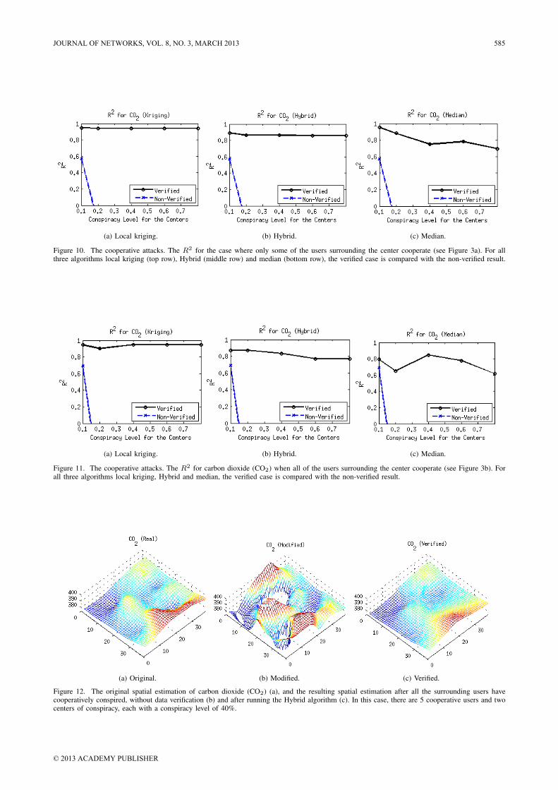
(a) Local kriging. (b) Hybrid. (c) Median.

Figure 10. The cooperative attacks. The R2 for the case where only some of the users surrounding the center cooperate (see Figure 3a). For allthree algorithms local kriging (top row), Hybrid (middle row) and median (bottom row), the verified case is compared with the non-verified result.

(a) Local kriging. (b) Hybrid. (c) Median.

Figure 11. The cooperative attacks. The R2 for carbon dioxide (CO2) when all of the users surrounding the center cooperate (see Figure 3b). Forall three algorithms local kriging, Hybrid and median, the verified case is compared with the non-verified result.

(a) Original. (b) Modified. (c) Verified.

Figure 12. The original spatial estimation of carbon dioxide (CO2) (a), and the resulting spatial estimation after all the surrounding users havecooperatively conspired, without data verification (b) and after running the Hybrid algorithm (c). In this case, there are 5 cooperative users and twocenters of conspiracy, each with a conspiracy level of 40%.



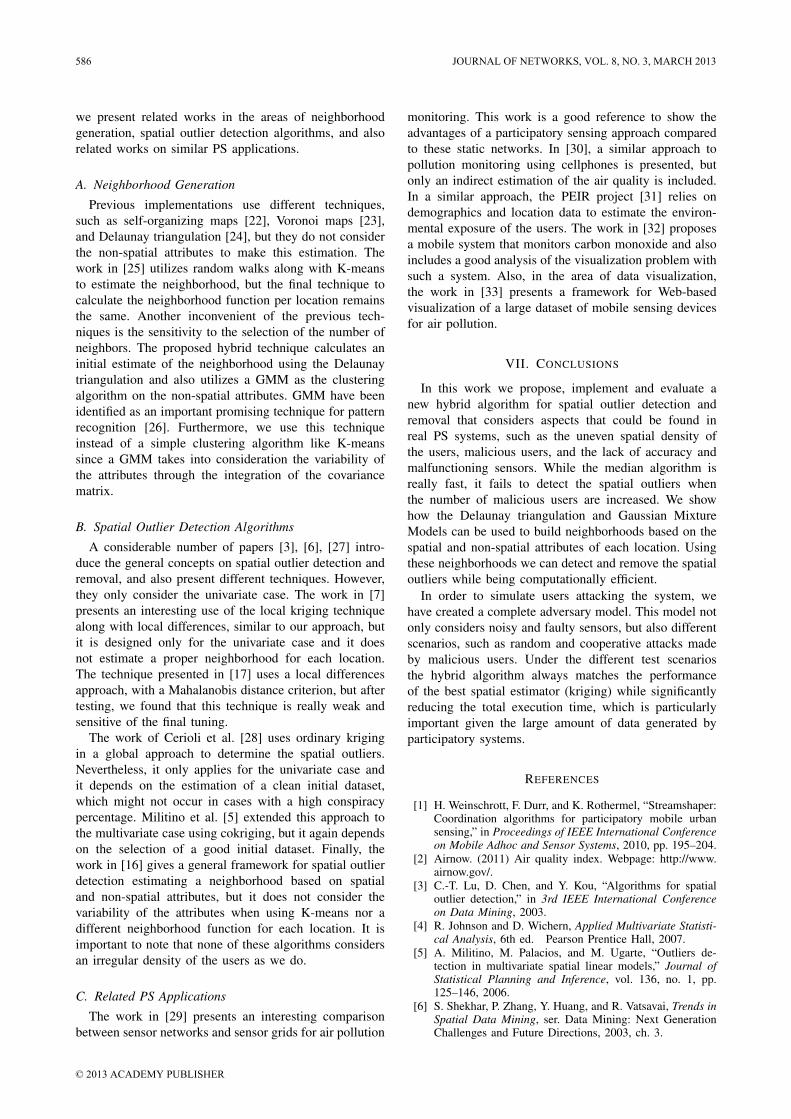
we present related works in the areas of neighborhoodgeneration, spatial outlier detection algorithms, and alsorelated works on similar PS applications.

A. Neighborhood Generation

Previous implementations use different techniques,such as self-organizing maps [22], Voronoi maps [23],and Delaunay triangulation [24], but they do not considerthe non-spatial attributes to make this estimation. Thework in [25] utilizes random walks along with K-meansto estimate the neighborhood, but the final technique tocalculate the neighborhood function per location remainsthe same. Another inconvenient of the previous tech-niques is the sensitivity to the selection of the number ofneighbors. The proposed hybrid technique calculates aninitial estimate of the neighborhood using the Delaunaytriangulation and also utilizes a GMM as the clusteringalgorithm on the non-spatial attributes. GMM have beenidentified as an important promising technique for patternrecognition [26]. Furthermore, we use this techniqueinstead of a simple clustering algorithm like K-meanssince a GMM takes into consideration the variability ofthe attributes through the integration of the covariancematrix.

B. Spatial Outlier Detection Algorithms

A considerable number of papers [3], [6], [27] intro-duce the general concepts on spatial outlier detection andremoval, and also present different techniques. However,they only consider the univariate case. The work in [7]presents an interesting use of the local kriging techniquealong with local differences, similar to our approach, butit is designed only for the univariate case and it doesnot estimate a proper neighborhood for each location.The technique presented in [17] uses a local differencesapproach, with a Mahalanobis distance criterion, but aftertesting, we found that this technique is really weak andsensitive of the final tuning.

The work of Cerioli et al. [28] uses ordinary krigingin a global approach to determine the spatial outliers.Nevertheless, it only applies for the univariate case andit depends on the estimation of a clean initial dataset,which might not occur in cases with a high conspiracypercentage. Militino et al. [5] extended this approach tothe multivariate case using cokriging, but it again dependson the selection of a good initial dataset. Finally, thework in [16] gives a general framework for spatial outlierdetection estimating a neighborhood based on spatialand non-spatial attributes, but it does not consider thevariability of the attributes when using K-means nor adifferent neighborhood function for each location. It isimportant to note that none of these algorithms considersan irregular density of the users as we do.

C. Related PS Applications

The work in [29] presents an interesting comparisonbetween sensor networks and sensor grids for air pollution

monitoring. This work is a good reference to show theadvantages of a participatory sensing approach comparedto these static networks. In [30], a similar approach topollution monitoring using cellphones is presented, butonly an indirect estimation of the air quality is included.In a similar approach, the PEIR project [31] relies ondemographics and location data to estimate the environ-mental exposure of the users. The work in [32] proposesa mobile system that monitors carbon monoxide and alsoincludes a good analysis of the visualization problem withsuch a system. Also, in the area of data visualization,the work in [33] presents a framework for Web-basedvisualization of a large dataset of mobile sensing devicesfor air pollution.

VII. CONCLUSIONS

In this work we propose, implement and evaluate anew hybrid algorithm for spatial outlier detection andremoval that considers aspects that could be found inreal PS systems, such as the uneven spatial density ofthe users, malicious users, and the lack of accuracy andmalfunctioning sensors. While the median algorithm isreally fast, it fails to detect the spatial outliers whenthe number of malicious users are increased. We showhow the Delaunay triangulation and Gaussian MixtureModels can be used to build neighborhoods based on thespatial and non-spatial attributes of each location. Usingthese neighborhoods we can detect and remove the spatialoutliers while being computationally efficient.

In order to simulate users attacking the system, wehave created a complete adversary model. This model notonly considers noisy and faulty sensors, but also differentscenarios, such as random and cooperative attacks madeby malicious users. Under the different test scenariosthe hybrid algorithm always matches the performanceof the best spatial estimator (kriging) while significantlyreducing the total execution time, which is particularlyimportant given the large amount of data generated byparticipatory systems.

REFERENCES

[1] H. Weinschrott, F. Durr, and K. Rothermel, “Streamshaper:Coordination algorithms for participatory mobile urbansensing,” in Proceedings of IEEE International Conferenceon Mobile Adhoc and Sensor Systems, 2010, pp. 195–204.

[2] Airnow. (2011) Air quality index. Webpage: http://www.airnow.gov/.

[3] C.-T. Lu, D. Chen, and Y. Kou, “Algorithms for spatialoutlier detection,” in 3rd IEEE International Conferenceon Data Mining, 2003.

[4] R. Johnson and D. Wichern, Applied Multivariate Statisti-cal Analysis, 6th ed. Pearson Prentice Hall, 2007.

[5] A. Militino, M. Palacios, and M. Ugarte, “Outliers de-tection in multivariate spatial linear models,” Journal ofStatistical Planning and Inference, vol. 136, no. 1, pp.125–146, 2006.

[6] S. Shekhar, P. Zhang, Y. Huang, and R. Vatsavai, Trends inSpatial Data Mining, ser. Data Mining: Next GenerationChallenges and Future Directions, 2003, ch. 3.



[7] Z. Shuyu and Z. Zhongying, “Detection of outliers in spa-tial data by using local difference,” in Intelligent Mecha-tronics and Automation, International Conference on, 26-31, 2004, pp. 400–405.

[8] D. Holland, R. Scheffe, W. Cox, A. Cimorelli, D. Nychka,and P. Hopke, “Spatial prediction of air quality data,”Environmental Manager, 2003.

[9] D. Mendez, A. Perez, M. Labrador, and J. Marron, “P-sense: A participatory sensing system for air pollutionmonitoring and control,” in Proceedings of IEEE Inter-national Conference on Pervasive Computing and Com-munications, 2011, pp. 344–347.

[10] A. Perez, M. Labrador, and S. Barbeau, “G-sense: ascalable architecture for global sensing and monitoring,”Network, IEEE, vol. 24, no. 4, 2010.

[11] D. Mendez, M. Labrador, and K. Ramachandran, “Datainterpolation for participatory sensing systems,” Summer2012, submitted to the Pervasive and Mobile Computingjournal.

[12] S. Ozdemir and H. Cam, “Integration of false data detec-tion with data aggregation and confidential transmission inwireless sensor networks,” Networking, IEEE/ACM Trans-actions on, vol. 18, pp. 736–749, 2010.

[13] K. F. Mulchrone, “Application of delaunay triangulation tothe nearest neighbour method of strain analysis,” Journalof Structural Geology, vol. 25, no. 5, pp. 689–702, 2003.

[14] S. Li, K. Liu, S. Long, and G. Li, “The natural neigh-bour petrov-galerkin method for thick plates,” EngineeringAnalysis with Boundary Elements, vol. 35, no. 4, pp. 616–622, 2011.

[15] C. A. Sugar and G. M. James, “Finding the number ofclusters in a dataset: An information-theoretic approach,”Journal of the American Statistical Association, vol. 98,no. 463, pp. 750–763, 2003.

[16] F. Chen, C.-T. Lu, and A. P. Boedihardjo, “Gls-sod: ageneralized local statistical approach for spatial outlierdetection,” in Proceedings of the international conferenceon Knowledge discovery and data mining. ACM, 2010.

[17] C.-T. Lu, D. Chen, and Y. Kou, “Detecting spatial outlierswith multiple attributes,” in Tools with Artificial Intelli-gence. IEEE International Conference on, 2003, pp. 122–128.

[18] D. Ginsbourger, D. Dupuy, A. Badea, L. Carraro, andO. Roustant, “A note on the choice and the estimation ofkriging models for the analysis of deterministic computerexperiments,” Appl. Stoch. Model. Bus. Ind., vol. 25, pp.115–131, March 2009.

[19] N. Memarsadeghi, V. Raykar, R. Duraiswami, andD. Mount, “Efficient kriging via fast matrix-vector prod-ucts,” in Aerospace Conference, IEEE, 2008.

[20] M. de Berg, O. Cheong, M. van Kreveld, and M. Overmars,Computational Geometry, 3rd ed. Springer, 2008.

[21] Y. Li, M. Dong, and J. Hua, “A gaussian mixture modelto detect clusters embedded in feature subspace,” Commu-nications in Information and Systems, vol. 7, no. 4, pp.337–352, 2007.

[22] Q. Cai, H. He, and H. Man, “Somso: A self-organizingmap approach for spatial outlier detection with multipleattributes,” in Neural Networks. International Joint Con-ference on, 2009.

[23] N. R. Adam, V. P. Janeja, and V. Atluri, “Neighborhoodbased detection of anomalies in high dimensional spatio-temporal sensor datasets,” in Proceedings of the ACMsymposium on Applied computing, 2004.

[24] Z. Min-qi, C. Chong-cheng, L. Jia-xiang, F. Ming-hui, andJ. Tamas, “An algorithm for spatial outlier detection basedon delaunay triangulation,” in International Conference onComputational Intelligence and Security, 2008, pp. 102–107.

[25] X. Liu, C.-T. Lu, and F. Chen, “Spatial outlier detection:random walk based approaches,” in Proceedings of the18th International Conference on Advances in GeographicInformation Systems. ACM, 2010.

[26] S. Chandrakala and C. Sekhar, “Classification of varyinglength time series using example-specific adapted gaussianmixture models and support vector machines,” in Interna-tional Conference on Signal Processing and Communica-tions, 2010.

[27] S. Shekhar, C.-T. Lu, and P. Zhang, “A unified approachto detecting spatial outliers,” Geoinformatica, vol. 7, pp.139–166, June 2003.

[28] A. Cerioli and M. Riani, “The Ordering of Spatial Data andthe Detection of Multiple Outliers,” Journal of Computa-tional and Graphical Statistics, vol. 8, no. 2, pp. 239–258,1999.

[29] M. Ghanem, Y. Guo, J. Hassard, M. Osmond, andM. Richards, “Sensor grids for air pollution monitoring,”in Proc. 3rd UK e-Science All Hands Meeting, 2004.

[30] M. Demirbas, C. Rudra, A. Rudra, and M. Bayir, “Imap:Indirect measurement of air pollution with cellphones,” inIEEE International Conference on Pervasive Computingand Communications, 2009.

[31] CENS. Personal environmental impact report. Webpage:http://urban.cens.ucla.edu/projects/peir/.

[32] P. Rudman, S. North, and M. Chalmers, “Mobile pollutionmapping in the city,” in UK-UbiNet workshop on eScienceand ubicomp, 2005.

[33] W. Hedgecock, P. Volgyesi, A. Ledeczi, and X. Kout-soukos, “Dissemination and presentation of high resolutionair pollution data from mobile sensor nodes,” in Proceed-ings of the 48th Annual Southeast Regional Conference.ACM, 2010.

Diego Mendez received his B.Eng. in Electronics Engineer-ing from the Universidad Nacional de Colombia in 2005, hisM.Eng. in Microelectronics from the Universidad de Los Andes,Colombia in 2008, and his M.Sc. and Ph.D in Computer Scienceand Engineering from the University of South Florida, USA, in2011 and 2012 respectively. Since 2012, he has been with thePontificia Universidad Javeriana, Bogota, Colombia, where he iscurrently an Assistant Professor in the Department of ElectronicsEngineering. His research interests include participatory sens-ing, wireless sensor networks, digital systems design, parallelarchitectures, embedded systems, and co-design techniques.

Miguel A. Labrador received the M.S. in Telecommunicationsand the Ph.D. degree in Information Science with concentrationin Telecommunications from the University of Pittsburgh, in1994 and 2000, respectively. Since 2001, he has been with theUniversity of South Florida, Tampa, where he is currently anAssociate Professor in the Department of Computer Scienceand Engineering. His research interests are in design and per-formance evaluation of computer networks and communicationprotocols for wired, wireless, and optical networks, energy-efficient mechanisms for wireless sensor networks, bandwidthestimation techniques, ubiquitous sensing and allocation-basedservices.



Infrastructure Based Chord Structure for P2P File Sharing over Vehicular Network

Hung-Chin Jang and Tzu-Yao Hsu

Department of Computer Science, National Chengchi University, Taipei, Taiwan Email: [email protected]

Abstract—Vehicular network is different from wired network due to its network environment changes rapidly. The connection lifetime between vehicles is usually short because vehicles move in high speeds. Hence, deploy peer-to-peer (p2p) applications over vehicular network is a challenging research issue. There are many problems confronted in p2p file sharing over vehicular network. Therefore, how to search files effectively, how to share files with distant vehicles, how to fully utilize the limited bandwidth, etc. have became important issues. In this paper, we propose an infrastructure-based Urban Multi-Layered Chord (UML-Chord) architecture for p2p file sharing over an urban vehicular network. In this architecture, vehicles are grouped into clusters. A multi-layer chord is employed to manage both files information and clustered vehicles locations. Connection lifetime between vehicles is estimated on a traffic aware basis. Target vehicle selection considers connection lifetime, bandwidth, and vehicle transmission status. Simulations results show that UML-Chord outperforms Chord, clustered organization and overlay based approaches in terms of number of hops (per query), control message overhead, query delay time, average download time, and file complete ratio. Index Terms—vehicular network, vehicle to road side unit (V2R), peer-to-peer (P2P), multi-layer chord

I. INTRODUCTION

In recent years, with the rapid development of wireless networks and global positioning technology, vehicular network has become a feasible and popular research area. In a vehicular network, vehicles use wireless communication to enhance vehicle efficiency and safety. Vehicles communicate with either vehicles or RSUs (Road Side Unit) through OBU (On-Board Unit). Where RSU serves as an access point or gateway. There are three modes of communications identified in a vehicular network.

• Inter-Vehicle Communication (IVC): information is transmitted either directly between vehicles within their communication ranges (one hop), or indirectly through the relay of intermediate vehicles (multi-hop) given the end to end distance is beyond their direct communication range.

• Road to Vehicle Communication (RVC): vehicles are able to access the information on the Internet through RSUs.

• Hybrid of IVC and RVC: it offers the flexibility of IVC and RVC types of data transmission, and thus extends network coverage. This communication mode is able to retrieve more resources from either vehicles or Internet.

Peer-to-peer (p2p) architecture is different from that

of client-server. In p2p, there is no need of a server to store and manage all the resources. Each peer serves as a client as well as a server, so each peer can easily share its resources (computation capability, storage, bandwidth, etc.) with other peers. Therefore, the more peers added to a p2p network, the more capable the network is. Gnutella, BitTorrent and Napster are well known examples of p2p systems.

The p2p architectures can be either centralized or distributed. Napster is an example of centralized architecture. In a centralized p2p system, there is a server managing all the resources shared among peers. Each peer has to register and provide the server with its shared resource list. When a peer (source peer) would like to obtain a certain resource form the p2p system, it looks up the server for those peers that own the resource. The server then replies with the candidate peers list that the source peer can communicate with directly. The major problem of centralized architectures is the server may become a bottleneck of bandwidth and capacity. Gnutella is an example of distributed architecture. In a distributed p2p system, there is no server intervention required. Each peer serves as a server as well as a client. The source peer broadcasts query of resource to its neighbor peers. Those peers that receive the query should check themselves for the query and then broadcast the query to their neighbor peers. The major problem of distributed architectures is the possible broadcast storm due to flooding. TTL (Time To Live) is usually employed to limit the number of hops of each broadcast. However, this limits the search space to a limited area. It is possible that a target resource does exist in the p2p network but cannot be found.

The p2p architectures can be classified into structured or unstructured architectures by different taxonomy. Structured p2p architectures usually build an overlay network on top of the bottom plane of peers. Peers information is abstracted into an upper plane. It facilitates resource management, however, it adds extra overhead and delay to the overlay network. With the maturity of vehicular network technology, p2p file sharing on



vehicular network becomes feasible though challenging. The motivation of this research is as follows. Vehicular network is different from wired network due to its network environment changes rapidly. There are many problems confronted in p2p file sharing over vehicular network. How to search files effectively, how to share files with distant vehicles, how to fully utilize the limited bandwidth, etc. have became important issues. In this paper, we propose an infrastructure-based Urban Multi-Layered Chord (UML-Chord) architecture to enhance p2p file sharing over an urban vehicular network.

II. RELATED WORK

A. Chrod Structured DHT (Distributed Hash Table) based p2p protocols

have been paid much attention these years. Stoica et al. [1] proposed a DHT based Chord structure for lookup service over a distributed p2p architecture. To build an overlay network, Chord adds each node into the system by generating a node ID using m-bit key space SHA-1, MD4, or MD5 hashing functions. The generated node ID is then placed on the identifier circle as shown in Figure 1 [1]. In the figure, the nodes on the Chord are projected onto the bottom plane. The system has to maintain the key space information to manage the Chord structure. For example, the successor(i) of node(i) has the minimum key that is greater than the key of node(i). Similarly, the predecessor(i) of nod(i) has the maximum key that is less than the key of nod(i). In addition, each node has to maintain a finger table to ensure each query can be completed in O(log N) time.

Figure 1. Chord architecture.

Chord is scalable in service lookup, however, its

maintenance overhead is heavy due to structured p2p architecture. To reduce the overhead, Lu et al. [2] proposed a ML-Chord (Multi-Layered Chord) by separating Chord into category layers instead of a single ring as shown in Figure 2. Each category layer represents a special domain. Each peer is mapped to one to many category layers according to the resources it has. The Bridge Peer (BP) goes across all category layers and forms a BP layer providing cross-layer lookup. Assume

that there are T category layers, the query complexity can be reduced to O(𝑙𝑜𝑔 𝑁 𝑇⁄ ), which is better than that of Chord.

In a wireless network, there are two problems in deploying a Chord based p2p system. First, the query packet transmission path of an overlay network is different from that of the real network since the neighbor nodes of an overlay network are usually not the neighbors of the real network. Second, it usually takes a longer time to come to network steady state when a new node added into an overlay network. To reduce the number of finger table ping messages, Lang et al. [3] proposed to use knowledge table rather than finger table to store one-hop neighbors information of the overlay network. The knowledge tables are broadcasted to neighbors to keep node information updated.

Figure 2. ML-Chord architecture [2].

B. Infrastructure-based P2P Architecture In an inter-vehicle communication (IVC) network,

nodes exchange messages only if they meet within their radio communication range. In a sparse IVC environment, if there is not enough number of peers participating p2p, it will be difficult to share files with other peers. Kchiche et al. [4] proposed an infrastructure based architecture for inter-vehicles file sharing. Peers are able to search entire vehicular network through overlay network. Files are thus easier to be found. Kchiche uses chord architecture to build a p2p network and classify vehicles into different RSUs based on k-medoid clustering algorithm in order to reduce message overhead. Furthermore, considering frequent traffic change affects chord performance, Kchiche separates the workload of managing vehicle locations from cluster heads.

II. METHODOLOGY

A. Infrastructure-based Multi-Layered Chord Architecture

Ad-hoc based p2p network uses flooding to search files resulting in message overhead. Besides, it often fails to find the wanted files due to the number of peers is limited in such network. On the other hand, single ring



based chord usually has too many finger table faults. In this paper we propose an infrastructure based UML-Chord (Urban Multi-layered Chord) that is constructed by grouping RSUs into a cluster (a single ring chord), selecting a cluster head for each single ring chord, linking these cluster heads into a super ring. The super ring is used for cross-cluster file search. The UML-Chord is proved to be able to reduce the number of hops of each query and maintenance cost in an urban environment.

Figure 3 shows the UML-Chord architecture. The dotted line separates the real network (lower part) from the overlay network (upper part). In the real network part, the triangles represent RSUs. There are four clusters in the overlay network part. All the RSUs in a cluster are linked by blue circle to form a chord ring. Each RSU maintains the (file, vehicle) entries of those vehicles belonging to it. The pink RSU node represents the cluster head of each cluster. All pink nodes are linked into a super chord that is responsible for query across clusters. The green RSU node is cp-head (car-position head), which is responsible for managing vehicle locations. The operation flow is illustrated using the following example: car1 would like to search file Rebirth.mp3 over p2p network. In the first step, car1 looks up the file from the UML-Chord through RSU. According to the key of Rebirth.mp3, the system does not find the file in the current cluster. The search query is then forwarded to the other clusters through RSU C. Finally, car2 and car3 are found to have Rebirth.mp3 in RSU M. In the next step, cp-head E tracks the locations of car2 and car3. At last, car1 sends query to car2 and car3 for file Rebirth.mp3 download.

Figure 3. UML-Chord architecture.

B. Management Architecture for Clustered Vehicle Locations

After the system found those vehicles that own the wanted files, the next step is to locate those vehicles. As mentioned above, the cluster heads (the red nodes in Figure 4) usually have heavy overhead, we select a cp-head (brown node) from the RSUs of the same cluster to manage vehicle locations. Each cp-head has to maintain

the location and connection lifetime information of each vehicle of the cluster. When there are queries forwarded from other clusters (yellow arrows), the cp-head is responsible for vehicle information provisioning. Similarly, vehicles in the current cluster can query other clusters for vehicle information (green arrows).

Figure 4. Clustered vehicle locations.

C. Traffic Aware Connection Lifetime Estimation Connection lifetime implies the duration of steady

transmission and is useful for selecting target vehicles for file download. The longer the connection time is, the better the target vehicle is. In estimating connection lifetime between vehicles in a dense urban area, we have to consider driving path, speed limit, and the time being blocked by traffic light. Before estimating connection lifetime, we make the following assumptions and parameters definitions. We assume all communications are single-hop vehicle to RSU communications. Let the coordinates of vehicle i is (xi,yi) and the coordinates of its RSUj is (xj,yj). Let the intersection k ahead of vehicle i is located at (xk,yk

). The rest of the parameters are defined as follows:

• 𝑣𝑖：the moving speed of vehicle i • 𝜃𝑖： the angle between the moving direction of

vehicle i and x-axis • 𝑇𝑖： the time spent in accelerating up to speed

limit for vehicle i • 𝑉𝑆：the speed limit of the route • 𝑇𝑛𝑜𝑤：the current time • 𝑇𝑠𝑡𝑜𝑝_𝑠𝑡𝑎𝑟𝑡：the time the red light begins • 𝑇𝑠𝑡𝑜𝑝_𝑒𝑛𝑑：the time the red light ends • D：the distance between vehicle i and intersection

k

⎩⎪⎨

⎪⎧ vi�Tstop_start − Tnow� < 𝐷, if ai = 0

12

(VS + vi)Ti + VS�Tstop_start − Tnow − Ti� < 𝐷, if Ti < Tstop_start − Tnow

vi2 +12

ai(Tstop_start − Tnow)2 < 𝐷, 𝑖𝑓 Ti ≥ Tstop_start − Tnow

�

First, we estimate whether the vehicle will be blocked by the stop light.

(1)



The three formulae show the three conditions the vehicle will be blocked by the red light at the intersection: case1: vehicle moves at constant speed, case 2: vehicle accelerates up to the speed limit and then moves at speed limit, case 3: vehicle accelerates but not reaches speed limit.

The next step is to estimate the connection lifetime between vehicle i and RSUk. Let ai, aj be the accelerations of vehicles i and j, respectively; Ti and Tj

be the time elapsed the vehicles i and j reach speed limit, respectively. The connection lifetime can be estimated by the following formula:

connection lifetime =

⎩⎪⎨

⎪⎧ �[(a − b)c + (d − e)f]2 − (c2 + f 2)[(a− b)2 + (d− e)2 − r2] − [(a− b)c + (d− e)f]

c2 + f 2

(Tstop_end − Tnow) +�[(a− b)c + (d− e)f]2 − (c2 + f 2)[(a− b)2 + (d − e)2 − r2] − [(a − b)c + (d − e)f]

c2 + f 2

�

where 𝑎 = 𝑥𝑖 − 𝑥𝑗, 𝑑 = 𝑦𝑖 − 𝑦𝑗

𝑐 = (𝑣𝑖 𝑐𝑜𝑠 𝜃𝑖 + 𝑎𝑖 𝑐𝑜𝑠 𝜃𝑖 𝑇𝑖)

𝑓 = (𝑣𝑖 𝑠𝑖𝑛 𝜃𝑖 − 𝑎𝑖 𝑠𝑖𝑛 𝜃𝑖 𝑇𝑖)

𝑏 = 12𝑎𝑖 𝑐𝑜𝑠 𝜃𝑖 𝑇𝑖2, 𝑒 = 1

2𝑎𝑖 𝑠𝑖𝑛 𝜃𝑖 𝑇𝑖2

(2)

The first formula shows the case the vehicle passes the intersection without being blocked by the traffic light. In this case, connection lifetime counts only the time elapsed after the vehicle left the current RSU. The second formula shows the case the vehicle being blocked by the traffic light. In this case, we should consider additional waiting time being blocked. Since RSUs have to manage Multi-Layered Chord and vehicles locations, the workload of connection lifetime estimation is assigned to vehicles. The vehicles have to record the estimated results into RSUs.

D. Multi-layered Chord Based File Search and Vehicle Localization

After a vehicle (source vehicle) sent out a query to the multi-layered chord to search a file, the system will then return a vehicle list showing all those vehicles (target vehicles) that own the file. All the target vehicles information will then be sent to the network immediately for locations tracking. Finally, all the vehicles locations hopefully be found and returned to the source vehicle. To reduce the search latency, we set a time threshold, say 0.5 sec. The source vehicle does not need to wait until collecting all the target vehicles information. The source vehicle begins to download file from those found vehicles once the time threshold is reached. The time threshold is adaptive to change, say 1 sec., if there are very few vehicles found. On the other hand, if there are too many target vehicles, the system selects only the five vehicles with the largest connection lifetimes.

E. Transmission Status Based Target Vehicles Selection

Before a peer is going to upload or download a file, the estimated transmission time is stored in RSU. Once a source vehicle plans to download a file from a target vehicle, it checks the RSU to see if the target vehicle is under transmission. If yes, the system deducts the remained transmission time from the connection lifetime and sends the update to RSU. The updated connection lifetime will be used for afterward target vehicle selection.

RSU side:

when receiving car msg

if msg is query

search in Chord;

end if;

if msg is position update

if self RUS is cp-head

update CLtime;

end if;

else

send this msg to cp-head of this cluster;

end if;

Car side：

getCarList to download;

if sizeof(CarList) = 1

setwait_threshold to 1 ;

storeCarList in list SendList;

end if;

else if sizeof(CarList) > 5

setwait_threshold to 0.5 ;

select the five highest CLtime node of

CarList ;

store in list SendList;

end if;

else if 5 >= sizeof(CarList) > 0

begin

setwait_threshold to 0.5;

store CarList in list SendList;



when catching RSUj

begin

’s broadcast beacon

calculate CLtime

if this car has current download traffic

CLtime←CLtime– remained download

time;

return CLtime to RSUj

end if;

;

F. File Transmission Based on Both Connection Lifetime and Bandwidth There are two extreme cases in file transmission. If

each query requests only one file block, it wastes too much bandwidth. At the other end, if each query requests all file blocks, it affects the overall system performance due to overwhelming packets consuming large bandwidth. Therefore, considering both connection lifetime and bandwidth in selecting target vehicles for file transmission may enhance transmission efficiency. Assume that there are two vehicles, vehicle s plans to download files from vehicle i. We define some parameters prior to further analysis. Among these parameters, the number of the requested

set of blocks ( 𝛱𝑅𝐸𝑄 ), block size (P), and the number of blocks transmitted between vehicles during connection lifetime (B) can be optimized using simulation optimization to obtain optimal performance.

• N: the set of vehicles that are able to provide files to vehicle s

• 𝛱𝑅𝐸𝑄: the requested set of blocks by vehicle s • 𝐴𝑖: the set of blocks that can be offered by vehicle

i • 𝑇𝑖;𝑆 : the connection lifetime between vehicles i

and s • 𝑇𝐵𝑖 : the transmission bandwidth that vehicle s

downloads files from vehicle i last time • P: block size • 𝐵𝑖: number of blocks transmitted between vehicle

s and i during connection lifetime

𝐵𝑖 = max (𝑇𝑖;𝑆 × 𝑇𝐵𝑖

𝑃, 1)

• 𝐺𝑖: estimated number of blocks that vehicle s can

download files from vehicle i during connection lifetime

𝐺𝑖 = Π𝑅𝐸𝑄 ∩ 𝐴𝑖 ∩ 𝐵𝑖

Assume vehicle k is the vehicle of the N vehicles that

may offer the largest number of blocks to vehicle s. In this case, vehicle s will select vehicle k to download file.

𝐺𝑘 ≧ 𝐺𝑖 where 𝑖 ∈ 𝑁

G. System Architecture The system architecture as shown in Figure 5 can be

decomposed into three parts: multi-layered Chord construction, connection lifetime calculation and file transmission.

Figure 5. System architecture.

Figure 6 shows multi-layered Chord construction. When a node would like to search a file from vehicular network, it queries the first layer single ring Chord of its RSU. It it fails, the query is sent to the super ring through cluster head. If it fails again, it implies that there is no such file in the vehicular network. If the queried file is found, the source node will get the (file, vehicle) entries stored in RSU for file download.

Figure 6. Multi-layered Chord construction.

Figure 7 shows connection lifetime calculation. The node calculates the connection lifetime with its RSU according to the formulae stated above. The node sends its update of position, file list and download status to RUS for latter use. Figure 8 shows the file transmission. The source node downloads target nodes list from RSU and selects the top nodes according to connection lifetime and transmission status, etc. Then the source node sends transmission requests to those nodes and starts file transmission.



Figure 7. Connection lifetime calculation.

Figure 8. File transmission.

III. SIMULATIONS

A. Simulation Environment Simulations are performed by Network Simulator 2.35

(NS-2) with Iango Purushothaman's IEEE802.11 infrastructure mode. In addition, we use SUMO (Simulation of Urban MObility) and MOVE (MObility model generator for Vehicular Networks) to generate two-way four lanes grid map with traffic lights and vehicle flows. The parameter setting is shown in Table I.

TABLE I. PARAMETERS SETTING

B. Performance Index The proposed UML-Chord is compared to Chord,

clustered organization and overlay-based methods in terms of number of hops (per query), control message overhead, query delay time, average download time, and file complete ratio.

• Number of hops: number of hops of each query • Control message overhead: the overhead of

overlay network maintenance, file query, management of vehicle location and file download

• Query delay time: the time between query a file and beginning of file download

• Download time: the time between query a file and completion of file transmission

• File complete ratio: the ratio of how many files are completely download

C. Results and Analysis The performance evaluations are classified into two

categories: file search and file transmission. • Comparisons of file search

Figure 9 shows the comparisons of no. of hops (per

query) against different number of RSUs. The file search complexity of Chord is O(log n). As the number of RSUs for Chord increases, the number of query hops increases. Due to the use of multi-layer Chord for UML-Chord, the average number of query hops is less than that of Chord by 17%. On the other hand, the structure of overlay-based approach is inefficient for file search. At this, UML-Chord outperforms overlay-based approach by 25% in average.

Figure 9. Comparisons of no. of hops vs. no. of RSUs.

TABLE II.

COMPARISONS OF NO. OF HOPS VS. NO. OF RSUS

No. of RSUs

UML-Chord Chord Overlay-based

40 3.70 4.50 17.78% 4.80 22.92% 60 4.00 4.90 18.37% 5.70 29.82% 80 4.40 5.40 18.52% 6.00 26.67%

100 5.00 6.40 21.88% 7.80 35.90%

Figure 10 shows the comparisons of no. of hops (per query) against different number of cars. Due to multi-layer architecture, UML-Chord has less number of query hops than that of Chord and overlay-based approaches by 15% and 26%, respectively. In addition, the number of hops does not increase significantly as the number of cars increases for UML-Chord. This is because UML-Chord is based on RSUs. Each RSU manages a key value, so the number of RSUs is fixed. Therefore, the number of query hops won’t be affected even if the numbers of vehicles or files increase.

Parameter Value No. of vehicles 200,300,400,500,600,700,800 Network coverage 2,500m x 2,500m No. of lanes 4 lanes (two-way) Radio transmission radius 250m Driving speed (km/hr) 0-60 km/hr Simulation time 3,600 sec Transmission rate BPSK 6Mbps No. of files 200 different files No. of files owned by each vehicle

1-10 (initialization)

No. of file queries by each vehicle

1-3

File size 5, 10, 15 MB



Figure 10. Comparisons of no. of hops vs. no. of cars.

TABLE III.

COMPARISONS OF NO. OF HOPS VS. NO. OF CARS

No. of cars

UML-Chord Chord Overlay-based

200 3.50 4.10 14.63% 4.60 23.91%

400 3.70 4.20 11.90% 4.80 22.92%

600 3.60 4.50 20.00% 5.10 29.41%

800 3.80 4.40 13.64% 5.22 27.20%

Figure 11 shows the comparisons of control message overhead against different number of cars. The overhead consists of overlay network maintenance, file query, vehicle location management, allocation of file download, etc. Clustered organization uses RSU to monitor vehicle traffic in order to dynamically manage the cluster members. This results in increase of message exchange among RUSs. On the other hand, UML-Chord moves all the updates to cp-head and can thus reduce the number of control messages by 13%. Overlay-based has the least message overhead in this comparison.

Figure 11. Comparisons of control message overhead vs. no. of cars.

TABLE IV. Comparisons of control message overhead vs. no. of cars

No. of cars

UML-Chord Clustered organization Overlay-based

200 18015 21002 14.22% 14786 -21.84% 400 19150 23110 17.14% 17153 -11.64% 600 23130 26654 13.22% 19121 -20.97% 800 25135 29150 13.77% 22021 -14.14%

Since overlay-based approach does not have an

effective file and vehicle management mechanism, the query delay time is relatively high. UML-Chord transmits the query results to RSU rather than the source vehicle, and thus saves much delay time. Figure 12 shows that UML-Chord outperforms clustered organization and overlay-based approaches by 14% and 23%, respectively. In addition, the query delay time increases as the number of cars increases. This is because the system has to collect information from many vehicles.

Figure 12. Comparisons of query delay time vs. no. of cars.

TABLE V. COMPARISONS OF QUERY DELAY TIME VS. NO. OF CARS

No. of cars

UML-Chord Clustered organization Overlay-based

200 0.5022 0.5825 13.79% 0.6003 28.27%

400 0.532 0.612 13.07% 0.6315 20.53%

600 0.5364 0.6341 15.41% 0.6131 31.42%

800 0.5912 0.718 17.66% 0.7765 23.86%

• Comparisons of file transmission

Figure 13 shows the comparisons of average download

time against different number of cars. Both UML-Chord and clustered organization approaches have more file sources to download from when there are many vehicles



in the network. As to overlay-based approach, there is only one download source. In comparison with clustered organization, UML-Chord has better performance by 12%.

Figure 13. Comparisons of average download time (N=200, 500, 800).

TABLE VI. COMPARISONS OF AVERAGE DOWNLOAD TIME (N=200, 500, 800)

time (sec) UML-Chord Clustered

organization

200 55.20 61.89 10.81%

500 51.61 59.45 13.18%

800 45.53 53.76 15.32%

Figure 14-16 show the comparisons of average download time against different simulation time for N=200, 500, 800, respectively. With these comparisons, we can have more detailed observations as time varies.

Figure 14. Comparisons of average download time (N=200).

TABLE VII. COMPARISONS OF AVERAGE DOWNLOAD TIME (N=200)

time (sec)

UML-Chord Clustered organization

600 64.7 78.0 17.12%

1500 60.5 65.9 8.20%

2400 48.2 60.0 19.75%

3300 48.9 55.5 11.89%


TABLE VIII. COMPARISONS OF AVERAGE DOWNLOAD TIME (N=500)

time (sec)


600 60.3 64.7 6.73%

1500 51.9 60.6 14.36%

2400 48.6 56.3 13.60%

3300 45.6 53.9 15.32%




TABLE IX. COMPARISONS OF AVERAGE DOWNLOAD TIME (N=800)

time (sec)


600 57.3 61.5 6.83%

1500 47.0 54.8 14.25%

2400 39.8 51.9 23.41%

3300 37.4 48.6 23.15%

Only 100% download of a file that counts a successful download. Figure 17 shows the comparisons of file complete ratio against different number of cars. Since UML-Chord has less average download time than that of clustered organization, it implicitly implies UML-Chord has higher file complete ratio than that of clustered organization. We observe that as the number of cars increases from 200 to 800, the file complete ratio decreases. This is because the number of queries increases as the number of cars increases. This implies more files are under p2p transmission resulting file complete ratio decreases.

Figure 17. Comparisons of file complete ratio vs. no. of cars (N=200, 500, 800).

TABLE X. COMPARISONS OF FILE COMPLETE RATIO VS. NO. OF CARS

(N=200, 500, 800)

time (sec)


200 76.05% 72.88% 4.34%

500 68.73% 65.72% 4.58%

800 67.36% 64.65% 4.18%

Figure 18-20 show the comparisons of file complete ratio against different simulation time for N=200, 500, 800, respectively. With these comparisons, we can have more detailed observations as time varies.

Figure 18. Comparisons of file complete ratio vs. no. of cars (N=200).

TABLE XI. COMPARISONS OF FILE COMPLETE RATIO VS. NO. OF CARS (N=200)

time (sec)


600 72.10% 69.20% 4.19%

1500 76.20% 72.20% 5.54%

2400 78.20% 74.60% 4.83%

3300 78.30% 75.90% 3.16%

Figure 19. Comparisons of file complete ratio vs. no. of cars (N=500).

TABLE XII. COMPARISONS OF FILE COMPLETE RATIO VS. NO. OF CARS (N=500)

time (sec)


600 64.10% 62.40% 2.72%

1500 67.00% 64.40% 4.04%

2400 70.20% 67.00% 4.78%

3300 73.00% 70.00% 4.29%



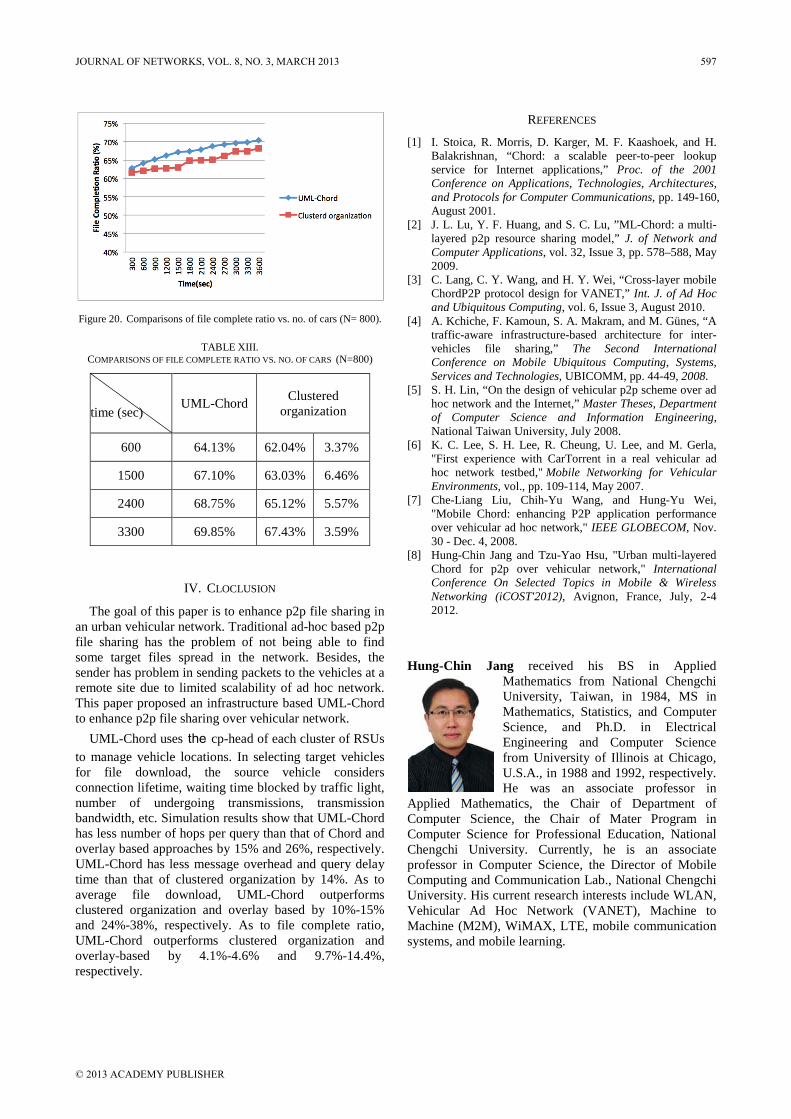
Figure 20. Comparisons of file complete ratio vs. no. of cars (N= 800).

TABLE XIII. COMPARISONS OF FILE COMPLETE RATIO VS. NO. OF CARS (N=800)

time (sec)


600 64.13% 62.04% 3.37%

1500 67.10% 63.03% 6.46%

2400 68.75% 65.12% 5.57%

3300 69.85% 67.43% 3.59%

IV. CLOCLUSION

The goal of this paper is to enhance p2p file sharing in an urban vehicular network. Traditional ad-hoc based p2p file sharing has the problem of not being able to find some target files spread in the network. Besides, the sender has problem in sending packets to the vehicles at a remote site due to limited scalability of ad hoc network. This paper proposed an infrastructure based UML-Chord to enhance p2p file sharing over vehicular network.

UML-Chord uses the cp-head of each cluster of RSUs to manage vehicle locations. In selecting target vehicles for file download, the source vehicle considers connection lifetime, waiting time blocked by traffic light, number of undergoing transmissions, transmission bandwidth, etc. Simulation results show that UML-Chord has less number of hops per query than that of Chord and overlay based approaches by 15% and 26%, respectively. UML-Chord has less message overhead and query delay time than that of clustered organization by 14%. As to average file download, UML-Chord outperforms clustered organization and overlay based by 10%-15% and 24%-38%, respectively. As to file complete ratio, UML-Chord outperforms clustered organization and overlay-based by 4.1%-4.6% and 9.7%-14.4%, respectively.

REFERENCES

[1] I. Stoica, R. Morris, D. Karger, M. F. Kaashoek, and H. Balakrishnan, “Chord: a scalable peer-to-peer lookup service for Internet applications,” Proc. of the 2001 Conference on Applications, Technologies, Architectures, and Protocols for Computer Communications, pp. 149-160, August 2001.

[2] J. L. Lu, Y. F. Huang, and S. C. Lu, ”ML-Chord: a multi-layered p2p resource sharing model,” J. of Network and Computer Applications, vol. 32, Issue 3, pp. 578–588, May 2009.

[3] C. Lang, C. Y. Wang, and H. Y. Wei, “Cross-layer mobile ChordP2P protocol design for VANET,” Int. J. of Ad Hoc and Ubiquitous Computing, vol. 6, Issue 3, August 2010.

[4] A. Kchiche, F. Kamoun, S. A. Makram, and M. Günes, “A traffic-aware infrastructure-based architecture for inter-vehicles file sharing,” The Second International Conference on Mobile Ubiquitous Computing, Systems, Services and Technologies, UBICOMM, pp. 44-49, 2008

[5] S. H. Lin, “On the design of vehicular p2p scheme over ad hoc network and the Internet,” Master Theses, Department of Computer Science and Information Engineering, National Taiwan University, July 2008.

.

[6] K. C. Lee, S. H. Lee, R. Cheung, U. Lee, and M. Gerla, "First experience with CarTorrent in a real vehicular ad hoc network testbed," Mobile Networking for Vehicular Environments, vol., pp. 109-114, May 2007.

[7] Che-Liang Liu, Chih-Yu Wang, and Hung-Yu Wei, "Mobile Chord: enhancing P2P application performance over vehicular ad hoc network," IEEE GLOBECOM, Nov. 30 - Dec. 4, 2008.

[8] Hung-Chin Jang and Tzu-Yao Hsu, "Urban multi-layered Chord for p2p over vehicular network," International Conference On Selected Topics in Mobile & Wireless Networking (iCOST'2012), Avignon, France, July, 2-4 2012.

Hung-Chin Jang received his BS in Applied

Mathematics from National Chengchi University, Taiwan, in 1984, MS in Mathematics, Statistics, and Computer Science, and Ph.D. in Electrical Engineering and Computer Science from University of Illinois at Chicago, U.S.A., in 1988 and 1992, respectively. He was an associate professor in

Applied Mathematics, the Chair of Department of Computer Science, the Chair of Mater Program in Computer Science for Professional Education, National Chengchi University. Currently, he is an associate professor in Computer Science, the Director of Mobile Computing and Communication Lab., National Chengchi University. His current research interests include WLAN, Vehicular Ad Hoc Network (VANET), Machine to Machine (M2M), WiMAX, LTE, mobile communication systems, and mobile learning.



http://portal.acm.org/citation.cfm?id=383071&CFID=32942346&CFTOKEN=69665867�



Downlink Power Control for CDMA Satellite Cognitive Radio

Peng Chen

China Academy of Space Technology (Xi’an), Xi’an, P. R. China E-mail: [email protected]

Lede Qiu, and Feng Xu

China Academy of Space Technology (Xi’an), Xi’an, P. R. China

Abstract—In this paper, we consider power control for a code-division-multiple-access (CDMA)-based satellite cognitive radio network where the satellite acts as the common transmitter of primary users and secondary users. Specially, we assume that primary users are willing to share resource with secondary users by means of leasing spectrum, while secondary users have to pay for the shared spectrum. In addition, secondary users are allowed to transmit on any sub-channel provided that the resulting interference to any primary users is below a critical threshold. We focus on the downlink. The objective is to maximize the throughput in the licensed frequency band of the satellite network. We formulate the problem as a game theoretic problem with all users as the players. We propose a tow-phase control scheme that can be accepted willingly by both types of users and can maximize the throughput of the satellite network. In the first phase, the Nash Equilibrium point is calculated with an iterative method, the existence of the Nash Equilibrium point is also proved. In the second phase, Payoff Dominance Selection is used to choose the optimal power allocation under the constraints including quality of service protections of all users and maximum transmission power of the onboard power amplifier. Simulation is performed to study the parameters of the system and of each user. By simulation, we find that the throughput is greatly increased by the proposed scheme compared with traditional satellite networks where fixed power is allocated to only primary users. Onboard complexity is also analyzed. Index Terms—Satellite Cognitive Communication; Power Control; Dynamic Spectrum Access; Downlink; Nash Equilibrium

I. INTRODUCTION

As reported by the Federal Communications Commission (FCC), spectrum utilization in many bands is very low [1]. For satellite communications, especially, spectrum resource is more precious than any other ingredients. However, satellites perform service to different area with dissimilar work states. Furthermore, traditional approaches of fixed spectrum allocation to licensed networks lead to spectrum underutilization. Actually, the fact that only a few licensed users access the satellite network does underutilizes the licensed spectrum. This motivates the concept of spectrum sharing that

allows secondary cognitive radio networks [2]-[4] to exploit the under-utilized spectrum. More importantly, the profound significance for a satellite network to support both primary communications and secondary cognitive radios should be appreciated.

In this paper, we consider a downlink power control (PC) problem for a point-to-multipoint cognitive satellite network. Specifically, we consider a code-division-multiple-access (CDMA)-based cognitive network with one satellite as the common transmitter and multiple primary and secondary users as the downlink receivers that communicate with the satellite in a single hop.

The spread spectrum CDMA system consists of orthogonal pseudo-codes, where a pseudo-code can be thought of as an orthogonal sub-channel though this is not explicitly assumed. The secondary system may transmit on any of the orthogonal sub-channels provided that the interference created to a primary user (PU) is below a predefined threshold to guarantee the Quality of Service (QoS) of the PU.

We assume that perfect information of PU and secondary user (SU) is gathered by satellite at the beginning of every frame. We also assume that instantaneous fading gains are perfectly known at the satellite since each user can estimate channel gains and report to the common transmitter. As a result, for each user, a transmission power is decided at the satellite that ensures that both types of users receive signals without harmful interference created to any user by the satellite transmitting power on the downlink.

More precisely, we are interested in the idea of Dynamical Spectrum Leasing (DSL) [5] that allows PU and SU communicate cooperatively by means of payment from SUs to PUs. On one hand, an SU has to pay a certain cost for receiving signals from the satellite. On the other hand, a PU is willing to reap additional benefit from SUs by leasing spectrum.

We then propose a game model with all users as the players and define utility functions of both types of users. Naturally, the utility functions imply that every SU pursues maximum throughput at low cost while every PU obtains maximum benefit by sharing spectrum with SUs. A power allocation scheme that maximizes both the utilities can be obtained by calculating Nash Equilibrium



mailto:[email protected]�

(NE) of the game model. Of course, the existence of NE should be also proved. After that, we achieve the optimal power allocation scheme that maximizes the spectrum efficiency by using Payoff Dominance Selection (PDS) [6].

A practical application, where our formulation can be useful, is the CDMA satellite network that licenses a wideband to offer service with insufficient communications because of high price. The benefit of our scheme is the improvement of spectrum efficiency and enhancement of income of network provider.

The rest of this paper is organized as follows: In section II, we review work that is related to this paper. In section III, the system model is described and the power allocation problem is formulated. The game model and the solution of optimal scheme are presented in section IV. In section V, numerical results are presented and complexity is analyzed. We state conclusion in section VI.

II. RELATED WORKS

Downlink resource allocation of femto-cell aims at increasing the utilization of the available macro-cell bandwidth for users located indoors. In [7], time slot is treated as the resource to be allocated as the time division duplex (TDD) operation is proposed. The sensing is performed on the uplink channel and the transmission is carried out in the corresponding slot of the downlink channel. The outage probabilities of both PU and SU are discussed in [8]. In [9], mixed primal and dual decomposition methods are employed to solve the downlink spectrum sharing problem with the aim of maximizing throughput. The optimization question is divided into two subproblems including a channel allocation problem and a power control problem on each channel. In [10], OFDMA is operated in both maro- and femto-cells, and the optimal power allocation on downlink is obtained according to Karush-Kunh-Tucker (KKT) condition. And in [11], downlink power control is accomplished in a game model with sum throughput of maro- and femto- cells as the utility function.

Resource allocation in OFDM-based wireless networks has been an active research topic. In [12], the optimal power control problem that aims at maximizing throughput is divided into four subproblems including: throughput computation, transmission power allocation, channel allocation and Lagrange multipliers calculation. In [13], a downlink channel/power allocation scheme that maximizes the number of supported fixed-location wireless subscriber with opportunistic spectrum access is obtained by solving a mixed-integer linear programming. A suboptimal scheme that can be obtained at a lower complexity based on local knowledge is also introduced in [13]. In [14], a joint cross-layer scheduling and spectrum sensing design framework that adapts the power allocation and subcarrier assignment across the secondary users is proposed to optimize a system utility. A distributed implementation for the cross-layer sensing and scheduling design using primal-dual decomposition is also introduced in [14]. An optimal and two suboptimal algorithms are proposed in [15]. The optimal one at a

higher complexity is to find a power profile that holds KKT conditions so that the maximum throughput can be achieved. To reduce complexity, one of the suboptimal algorithms is to allocate power for a particular CR user by considering the effect only on the PU band where the CR user causes the most amount of interference. The other takes the step size of the ladder to be inversely proportional to the primary signal energy in the licensed spectrum. In [16], a primary radio network willingness-based framework for coexistence and sub-channel sharing is designed, where PU determines its interference margin and broadcasts to CR users while CR users optimize their sum data rate by implementing water-filling.

Game theory is a useful tool to study the strategic behavior of network participants in cognitive radios. In [17], a game theoretic approach for downlink power control to solve the resource allocation problem from a set of base stations (BSs) to a number of CR users. In the game model, BSs and users act as the players and the pricing mechanism motivates the BS to provide service to users. As forementioned, a game model is established in [11].

Finding a power vector/matrix which holds KKT condition is another available approach to deal with the resource allocation problem. In [18], a solution to uplink and downlink power allocations according to KKT conditions is presented in a CR system including a BS and multi-users with perfect channel state information. In [19], the problem which takes into account the uncertainty of the primary users’ location is modeled as a mixed integer nonlinear programming problem. KKT condition is applied to find the optimal assignment of channel and power to each user to maximize the downlink average throughput by means of decomposition of the dual optimization problem into a number of sub-problems. As mentioned earlier, KKT condition is used in OFDMA case in [10].

There are also several other methods to allocate downlink power/channel. In [20], a fair spectrum allocation approach to maximize throughput is introduced. However, the study object is fixed device, not cognitive users. The fairness is also discussed in [21]. Besides, an optimal solution for jointly controlling data rate, transmission power, and sub-band allocation to optimize the sum throughput in a relay-assisted cognitive cellular downlink system accessing a spectrum licensed to a primary network is presented in [21]. An optimal resource allocation for multi-BS working in identical frequency band is proposed in [22]. In [23], a compressed sensing (CS) –based algorithm is presented according to the sparsity of difference between fore-and-aft power allocation vectors of PU and SU, i.e. pprior pnextP P and

sprior snextP P , and the power control procedure is completed by announcing sensed results to BS. An integration-based model to contain the correlation in shadow fading is modified and the definition of coverage area and protection area are also introduced in [24]. In [25], device-to-device communication as a potential resource reuse technique underlaying the cellular network is addressed. In [26], a power allocation scheme that



maximizes the throughput in scene including a CR BS and multi fixed-location CR user is presented. The contribution of this paper is that transmission power should be calculated at first. After that power/channel allocations of both uplink and downlink are achieved by broadcasting the channel information to all users. In [27], a max-min problem based downlink resource allocation in a fair and efficient fashion is formulated for an OFDMA-based cognitive radio point-to-multipoint network with fixed users according to the backlog of each user. A model to compute the allowed maximum transmission power for CR is introduced in [28].

Compared to all these related works, our paper focuses on the satellite cognitive radio network downlink which has never been mentioned so far. As stated earlier, indeed, the insufficiency of spectrum utilization of traditional satellite communication is an imperative. We believe that the spectrum efficiency can be improved by introducing secondary users into the traditional satellite networks. By considering spectrum leasing from PU to SU, the proposed scheme in this paper can greatly increase the throughput in licensed frequency band.

III. PROBLEM DEFINITION

A. System Model In this section, we propose a dynamic spectrum leasing

CDMA satellite cognitive network architecture in which the primary network which has the license of the available spectrum is co-located with the secondary network and is willing to share its spectrum with secondary systems. We assume that the satellite works as a common transmitter of both networks. Let L and K denote the numbers of PUs and SUs respectively. Obviously leasing would mean that the secondary system will have to pay certain compensation to the primary system for this spectrum access. An SU could receive data from downlink only if the QoS of primary system has been protected. The primary system has an incentive to allow SUs to access the licensed spectrum in order to maximize the possible compensation from SUs. Meanwhile, the SUs are interested in maximum throughput under certain payment.

Let skh be the channel gain between satellite and

SU k and plh be the channel gain between satellite and

PU l . The primary user can adapt its interference cap denoted by lQ , which is the maximum tolerable interference from all secondary transmissions. Let lP and

kp respectively denote the transmission power from satellite to PU l and SU k .

B. Operational Requirements We assume that both types of users in the satellite

networks have same communication conditions and spreading code length. In other words, each user has equal CDMA gain G , and s p

k lh h h . There are many phenomena that lead to signal loss on transmission through the earth’s atmosphere. h changes in different

weather conditions and so does lQ . Under a specific weather condition, lQ is determined by lP while QoS is unchanged. In our model, satellite lease licensed spectrum by adjusting lP and QoS of PU must be protected at the same time.

For the PU system, the SINR of l th downlink can be calculated as:

( )2 2

1 1,

P l ll K L p

lk i

k i i l

Gh P Gh PI Nhp hP N

γ

= = ≠

= =++ +∑ ∑

(1)

where plI is the total interference suffered by PU l ,

1, 1

L Kp

l i ki i l k

I hP hp= ≠ =

= +∑ ∑ , and N is the noise. For a PU to

protect its QoS, the target SINR is defined as lγ , and the interference gap lQ on the l th downlink with lP as the transmission power can be calculated as:

ll

l

GhPQ N

γ= − (2)

For the SU system, the received SINR of k th downlink can be calculated as:

( )

1, 1

S k kk K L s

ki l

i i k l

Ghp GhpI Nhp hP N

γ

= ≠ =

= =++ +∑ ∑

(3)

where skI is the total interference suffered by SU k ,

1, 1

K Lsk i l

i i k lI hp hP

= ≠ =

= +∑ ∑ . To receive data from satellite, SU

which consume transmission power should be charged. Cost factor kλ is defined as the amount charged by satellite when the satellite transmits per unit power on k th downlink to SU k . In other words, SU k should pay

k kpλ to receive data from satellite on k th downlink, and the payment can be seen as the compensation (benefit) of PU system. The total benefit of PU can be calculated as:

1

K

k kk

B pλ=

= ∑ (4)

We assume that, for appropriate performance of the primary network, the received SINR at each PU receiver must be above a predefined value of lγ . For the same reason, SU receiver also requires the received SINR to be above a predefined threshold minΓ . Both of the assumptions can be expressed as:

( )Pl lγ γ≥ (5)

( )min

Skγ ≥ Γ (6)



C. Users’ Utility For the whole satellite communication system,

developing a scheme that maximizes spectrum efficiency is the aim. It means maximum system throughput that includes both PU’s and SU’s throughput. As the license holder, PU system aims at maximizing B , that means the satellite transmit lowest power to each PU with the confine of PU’s target SINR. For a specific PU, PU l could be satisfied only if p

l lQ I≥ . Meanwhile, as tenants, SUs are seeking to receive maximum data after a certain payment. Thus, the utility functions of PU l and SU k are given respectively by:

( ) ( ) ( )( )( ) ( )

2

1

2

,

1p

ll

p p p pl l l l l l l l

I Q pl l

U Q Q Q I Q I

e I Q

µ ε

µ ε

−

−

= − − − − − −

P

(7)

( ) ( )( ), ln 1

ln 1

Ss sk k k k k k

kk ks

k

U p p

Ghpp

I N

γ λ

λ

− = + −

= + − +

p (8)

where the transmit power vector of all SUs except SU k is denoted by ps

k− and the transmit power vector of all PUs except PU l is denoted by P p

l− . ( )ε ⋅ is the step

function with ( ) 1xε = for 0x > and ( ) 0xε = for

0x ≤ and 1µ and 2µ are positive punishment coefficients. Note that the second and third terms in (7) are introduced to ensure that QoS required by PU l is satisfied. If a PU downlink instantaneous SINR is less than the target SINR, i.e. if p

l lQ I< , the PU downlink should be strictly punished because it can not satisfy PU’s reception. On the contrary, if a PU downlink instantaneous SINR is greater than the target SINR, i.e. if p

l lQ I> , the PU downlink also should be penalized because it is unnecessary for the satellite to transmit higher power when PU’s reception is satisfied. Higher transmit power means greater interference to other users and lower benefit, and especially, for satellite communication it makes energy wasted. We also note that the first term in (8) is the Shannon capacity for secondary user, where ln replaces 2log for the sake of expedite computation. The second term in (8) is the total amount charged on SU k for receiving data. It is easy to see that the goal of secondary user is to achieve the most energy efficient transmission from the utility function in (8).

D. Objective We are interested in finding a downlink power

allocation schemes that maximize the spectrum efficiency in a satellite DSL Cognitive network. In other words, the aim of this paper is to maximize the satellite network throughput in its licensed frequency band. As mentioned

above, the throughput of the satellite network including both PUs’ and SUs’ throughput is calculated as:

( ) ( )( ) ( )( )1 1

, ln 1 ln 1L K

P Sl k l k

l kT P p γ γ

= =

= + + +∑ ∑ (9)

The optimal power allocation scheme must be an equilibrium at which all the primary and the secondary users act the optimal response to each other. Also, the scheme must maximize the system throughput. Thus, we formulate the spectrum efficiency maximization problem as a game model and select the equilibrium which meets the following conditions:

( ) ( )( ) ( )( )

( )

0 1 1

max1 1

min

max , ln 1 ln 1

1. 0

2.

3.

k

L KP S

l k l kl k

K L

k lk l

p sp ppl l l l

Sk

T P p

subject to

p P p

I I I Q

λγ γ

γ

≥= =

= =

= + + +

≤ + + ≤

= + ≤

≥ Γ

∑ ∑

∑ ∑ (10)

Where maxp is the maximum power that the on board power amplifier (PA) could transmit.

IV. GAME MODEL AND OPTIMAL POWER ALLOCATION

A. The Proposed Game Model In practice, the satellite parameters, such as:

G , h , kλ , minΓ , lγ and N , are known. Thus, the game model is as follows:

Players: Let be the closet of players which include L PUs and K SUs, and each player is rational and has common knowledge. All players are waiting to receive data from satellite.

Action set: 1 2 1 2A ... ...L KP P P p p p= × × × × × × × , where [ ]max0,lP p= is the action set of PU l and

l lP P∈ is the power that the satellite transmit to PU l ,

[ ]max0,kp p= is the action set of SU k and k kp p∈ is the power that the satellite transmit to SU k . An action vector can be expressed as: [ ]1 1p ,..., , ,...,L KP P p p= , where p A ∈ .

The utility functions of PU and SU are (7) and (8) respectively. The outcome of the game is that each user could receive data with required QoS and that the satellite network achieves maximum throughput.

B. Nash Equilibrium Existence of Nash Equilibrium: We note that the

constrain 2. in (10) is pl lI Q≤ which makes the third tern

in (7) be zero. Thus, equations (7) and (8) are continuous functions of p and strictly quasi-concave with respect to

lP and kp . Furthermore, since the set of admissible power allocation strategies of each player is nonempty, convex and compact, we can conclude that this game



model has a pure Nash Equilibrium by using Kakutani Fixed Point Theory[29][30].

Calculating Nash Equilibrium: Recall the utility of each PU, as mentioned in (7). In the Nash point of the game model, each PU tries to maximize its utility. For PU l , we can achieve its optimal interference gap ne

lQ by setting the derivative of (7) to zero. The equivalent consequence is that the satellite transmits power ne

lP to PU l . Both of ne

lQ and nelP can be calculated as:

1

12

ne pl lQ I

µ= + (11)

( )

1 1, 1

12

nel lne

l

K Ll

k ik i i l

Q NP

GhNp P

G h h

γ

γµ= = ≠

+=

= + + +

∑ ∑

(12)

Similarly, each SU tries to achieve its maximum utility. However, the QoS of PU should be perfectly protected and SUs will acquire their optimal power allocations under that condition. As mentioned above, the utility of each SU will be maximum when the derivative of (8) equals to zero. For a given SU k , the optimal power allocation ne

kp can maximize its utility and nekp can be

calculated as:

1, 1

1

1 1

ne sk k

k

K L

i li i k lk

Ghp I NGh

Np PG h

λ

λ = ≠ =

= ⋅ − −

= − ⋅ + +

∑ ∑ (13)

When an action vector pne satisfies (11) and (13), the action of each PU or each SU is best-response to others’ actions. Therefore, the power allocation vector pne is an equilibrium strategy. To maximize the satellite network throughput, finding the equilibrium strategy pne which satisfies (10) is the goal of this paper. Let (10) be the utility function of the satellite communication system, then we can achieve the unique power allocation strategy by using PDS [6].

Application to satellite cognitive communication: In satellite cognitive networks, the licensed users play the role of primary users which are willing to lease their downlink spectrum to cognitive users which are considered as secondary users. All users are regarded as players. Utility function of each type of users is given by (7) and (8) respectively. To achieve the outcome that throughput of the satellite network is maximized, the optimal power allocation should be searched from action set.

In a single game, the numbers of both PUs and SUs are constant. Equilibrium strategies can be gained after iteratively calculating (11), (12) and (13). If the result is unique, the equilibrium strategy is the optimal power

allocation vector pne . Otherwise, the optimal power allocation pne can be achieved by using PDS with (10) as the utility function. Since the PU and SU may enter or quit the network, the number of players will be variable and the power control scheme should be updated whenever any user enters or exits the satellite network. To keep the network stable, the information of users’ entrance and exit should be refreshed periodically. In practice, the satellite collects all the users’ information and on board processor builds the game model and calculates the optimal power allocation vector. After that, the satellite transmits data to all users at the optimal power level.

V. PERFORMANCE EVALUATION

In this section, we discuss the performance of the proposed scheme in DSL game model by simulation. Firstly, the maximum numbers of PUs and SUs that the satellite network could afford should be considered. Secondly, individual action of each user is modeled and the optimal action strategy of each user is selected after iteration and optimization. Thirdly, the maximum throughput that the network could achieve is analyzed and results in normal situation and in the proposed scheme are also compared. Finally, the utility of each user is shown. Furthermore, computing complexity of the scheme which is substantial since the algorithm is completed on board is given in this section.

A. Simulation Model The satellite is assumed to work in geostationary earth

orbit and carry a C-band transmitter with a bandwidth of 100MHz. To simplify the simulation process, both types of users are considered to be uniformly configured respectively. In other words, all PUs have the same configuration parameters and all SUs are identical. Other parameter assumptions are shown as follows:

Simulation parameters

( )30 dBsG = Tx-Rx antenna gain= ( )70 dB

( )max 20 dBWp = Path loss = ( )196.5 dB−

2kλ = Noise temperature = ( )75 K

( )12 dBlγ = ( )126.5 dBh = −

( )min 10 dBΓ = ( )129.8 dBWN = −

21 10/ h sµ = 2

2 100/ hµ =

B. System Capacity to Accept SUs In a scenario with N as the noise power, relation

between SUs’ and PUs’ number is shown in Fig.1. In particular, in view of the interference to PUs produced by SUs’ transmission, Fig.1 depicts the maximum number of SUs that the satellite CDMA network can afford with existence of PUs when both types of users achieve their required SINR. Each curve in the picture denotes a different ratio between satellite transmission power to each PU and that to each SU. On one hand, it can be observed intuitionally from this picture that the largest numbers of SUs in different power ratio are equal to 100,



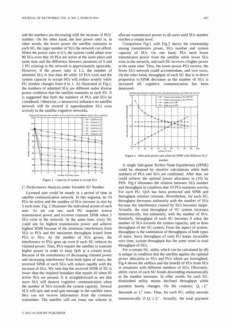
and the numbers are decreasing with the increase of PUs’ number. On the other hand, the less power ratio is, in other words, the lower power the satellite transmits to each SU, the lager number of SUs the network can afford. When the power ratio is 0.5, the system could admit over 80 SUs even that 10 PUs are active at the same place and same time and the difference between situations of 0 and 1 PU existing in the network is approximately ignorable. However, if the power ratio is 1.5, the number of admitted SUs is less than 40 while 10 PUs exist and the system capacity to accept SUs will reduce acutely while PU number changes from 0 to 1. As illustrated in Fig.1, the numbers of admitted SUs are different under diverse power condition that the satellite transmits to each SU. It is suggested that both the numbers of PUs and SUs be considered. Otherwise, a destructive influence on satellite network will be exerted if superabundant SUs exist actively in the satellite cognitive networks.

0 1 2 3 4 5 6 7 8 9 1030

40

50

60

70

80

90

100

110

120

number of primary users

num

ber o

f sec

onda

ry u

sers

relationship between the numbers of PUs and SUs under different power ratio conditions

SU/PU=0.5SU/PU=0.7SU/PU=0.9SU/PU=1.1SU/PU=1.3SU/PU=1.5

Figure 1. Capacity of system to accept SUs

C. Performance Analysis under Variable SU Number Licensed user could be steady in a period of time in

satellite communication network. In this segment, let 10 PUs be active and the number of SUs increase in size by 5 each time. Fig. 2 illustrates the individual action of each user. As we can see, each PU requires lowest transmission power and receives constant SINR when 5 SUs exist in the network. At the same time, every SU could ask for highest transmission power and achieve highest SINR because of the minimum interference from SUs to PUs and the maximum throughput leased from PUs to SUs. As the number of SUs grows, the interference to PUs goes up even if each SU reduces its claimed power. Thus, PUs require the satellite to transmit higher power in order to keep QoS at a certain level. Because of the simultaneity of decreasing claimed power and increasing interference from both types of users, the received SINR of each SUs will reduce rapidly with the increase of SUs. We note that the received SINR of SU is lower than the required boundary that equals 10 when 85 active SUs are present. It is straightforward to see that more SUs will destroy cognitive communication when the number of SUs exceeds the system capacity. Several SUs will quit and send quit message to the satellite since they can not receive information from the common transmitter. The satellite will not reuse our scheme to

allocate transmission power to all users until SUs number reaches a certain level.

Comparison Fig.1 with Fig.2 shows the relationship among transmission power, SUs number and system capacity of SUs. On one hand, PUs need lower transmission power from the satellite while fewer SUs exist in the network, and each SU receives a higher power at the same time. Thus, the lower power PUs receive, the fewer SUs network could accommodate, and vice versa. On the other hand, throughput of each SU that is in direct proportion to SINR decreases as the number of SUs is increased till cognitive communication has been destroyed.

0 10 20 30 40 50 60 70 80 90 1000

5

10

15

20

25

number of SUs

allo

cate

d po

wer

and

SIN

R/(m

W),(

dB)

Relationship between number of SUs and allocated power and SINR with 10 PUs

Power transmitted to PU（*50mW ）

Power transmitted to SU（*50mW ）

SINR of PU（dB）SINR of SU（dB）

Figure 2. Allocated power and achieved SINR with different SUs’

number

A single Sub-game Perfect Nash Equilibrium (SPNE) could be obtained by iterative calculations while both numbers of PUs and SUs are confirmed. After that, we could achieve the optimal power allocation in (10) by PDS. Fig.3 illustrates the relation between SUs number and throughput in condition that 10 PUs maintain activity. For each PU, QoS has been protected and SINR and throughput remains constant. Nevertheless, for each SU, throughput decreases unlinearly with the number of SUs because the interference caused by SUs becomes larger. Actually, the total throughput of SU system increases monotonically, but unlinearly, with the number of SUs. Similarly, throughput of each SU becomes 0 when the number of SUs exceeds the system capacity, and so does throughput of the SU system. From the aspect of system, throughput is the summation of throughputs of both types of users. Since throughput of each PU keeps invariable over time, system throughput has the same trend as total throughput of SUs.

For a certain SU, utility which can be calculated by (8) is unique in condition that the satellite applies the optimal power allocation to SUs and PUs which are foresighted. Fig.4 shows the utilities and the benefit of PUs from SUs in situations with different numbers of SUs. Obviously, utility curve of each SU trends descending monotonically as the number increases. In other words, for each SU, diminished utility means declined throughput while payment barely changes. On the contrary, p

l lQ I− descends as p

lI rises. Thus, for each PU, utility ascends monotonically if p

l lQ I≥ . Actually, the total payment



from SUs to PUs, namely 1

K

k kk

B pλ=

= ∑ , will be on the

rise as the number of SUs is increased. And this is the prime motive for PUs to lease spectrum to SUs.

0 10 20 30 40 50 60 70 80 90 1000

100

200

300

400

500

600

number of SUs

thro

ughp

ut/(b

its)

Relationship between number of SUs and throughput with 10 PUs

total throughput of PUtotal throughput of SUtotal throughput of networkaverage throughput of single PU(*20)average throughput of single SU(*20)

Figure 3. Relationship between throughput and Sus’ number

0 10 20 30 40 50 60 70 80 90 1000

1

2

3

4

5

6

7

8

9

10

number of SUs

utili

ty a

nd b

enef

it

Relationship between number of SUs and utility with 10 PUs

utility of PUutility of SUbenefit of PU(minification is 10)

Figure 4. Relationship between utility and SUs’ number

D. Performance Analysis under Variable SINR PU Required

In this segment, by varying PU required SINR from 2 to 20, we discuss the performance of the proposed scheme in a scene where numbers of PUs and SUs are regarded to be 10 and 30 respectively. Fig.5 illustrates the relation among allocated power, actual SINR and minimum SINR that PUs required. As can be verified, for an individual PU, to claim a higher transmission power is necessary in order to achieve a greater SINR. However, the claimed power is against constraint 1 in (10) when the required SINR is greater than 18dB. That is to say, in the same condition, the satellite can not afford the total transmission power even if no SU exists. At this point, communications of both types of users have been broken. And before this point, transmission power to PUs and actually received SINR of each PU ascends monotonically as the minimum required SINR increase. On the contrary, the same parameters of each SU descend monotonically under the same condition till the required SINR reaches 18dB.

0 2 4 6 8 10 12 14 16 18 20 220

10

20

30

40

50

60

70

80

SINR constraint of PU receiver/(dB)

allo

cate

d po

wer

and

SIN

R /(

mW

),(dB

)

Relationship between QoS of PU and allocated power and SINR with 10 PUs and 30SUs

Power transmitted to PU（*50mW ）

Power transmitted to SU（*50mW ）

SINR of PU（dB）SINR of SU（dB）

Figure 5. Allocated power and achieved SINR with different SINR

required by PU Fig.6 shows the relationship between throughputs and

the required SINR. As can be observed, average throughput of single PU ascends as the required SINR increases till it reaches 18dB, and so does the total throughput of PUs. For SU system, by contrast, the same parameters descend monotonically in the same situation. However, the total throughput of network is not a monotonic function. Before the required SINR reaches 14dB, network throughput ascends, and after that, it descends statically in the range from 14dB to 16dB. As the required SINR continues increasing, network throughput will decrease at large scale when PU required SINR exceeds 16dB. As can be concluded from this figure, the network will achieve maximum throughput if the minimum SINR required by PUs is within [ ]12dB,16dB .

0 2 4 6 8 10 12 14 16 18 20 220

50

100

150

200

250

300

350

400


thro

ughp

ut/(b

its)

Relationship between QoS of PU and throughput with 10 PUs and 30SUs

total throughput of PUtotal throughput of SUtotal throughput of networkaverage throughput of single PU(*20)average throughput of single SU(*20)

Figure 6. Relationship between throughputs and the required SINR

The relation between utilities and the required SINR is illustrated by Fig.7. The utility of PU reaches vertex when the required SINR is 18dB. However, as aforementioned, it is impossible for the satellite to support such a power allocation. In addition, the utility of SU descends sharply and the benefit from SUs becomes less when PU required SINR is greater than 16dB. Furthermore, as we can deduce from this picture, SUs are unwilling to pay more cost for less communication capacity as PU required SINR increases.



0 2 4 6 8 10 12 14 16 18 20 220

1

2

3

4

5

6

7

8

9

10


utili

ty a

nd b

enef

it

Relationship between QoS of PU and utility with 10 PUs and 30SUs

utility of PUutility of SUbenefit of PU(minification is 10)

Figure 7. Relationship between utilities and the required SINR

E. Complexity Analysis In practice, whenever the number of SUs varies or

required SINR of PUs changes, the optimal power allocation has to be updated. Thus, complexity of single calculation circle is an important parameter which is restricted by onboard processor. Let us assume L PUs and K SUs be active in a calculation circle, simulation results show that Nash Equilibrium will be achieved after 6 iterative calculations. Thus, the complexity brought by (11), (12) and (13) is ( )K Lο + in a circle. Then,

selection accomplished by (10) needs ( )K Lο +

multiplications and ( )K Lο + additions. Therefore, computation complexity in an updating circle is bounded by ( )K Lο + . Another important parameter for the onboard processor is the number of memory elements. When iterative calculation occurs, both series of variables before and after computation should be stored. In detail, variables such as 2 kKp , 2 lLP , 2 lLQ , kKλ , lLγ and constants such as G , h , minΓ , N , 1µ , 2µ , maxP , maxp have to be memorized. Therefore, onboard processor approximately needs ( )3 2K L+ memory elements in total to complete an updating circle. Naturally, the size of memory element depends on the required precision of each variable. On account of the current technology level, it is sufficient for a satellite to accomplish the proposed scheme.

VI. CONCLUSION

In this paper, we introduce underlay cognitive radio into satellite CDMA communication network and consider the problem of downlink power allocation to maximize spectrum efficiency in a DSL scene where SUs pay PUs for transmission power from satellite. Using game theory, we propose a centralized power control scheme implemented by onboard processor to protect the communication of primary users while providing maximum possible throughput for secondary users. The simulation results have shown the performance of the proposed scheme. The complexity of the scheme has been also analyzed.

REFERENCES

[1] Federal Communication Commission Spectrum Policy Task Force. Report of the spectrum efficiency working group. FCC 02-155, Nov.2002

[2] J. III. Mitola, G. Q. Maguire. Cognitive radio: making software radios more personal. IEEE. Personal Communications, 1999, 6(4): 13–18

[3] S. Haykin. Cognitive radio: brain-empowered wireless communication, IEEE, Journal on SAC, 2005, 23(2): 201-220.

[4] A. Goldsmith, S. A. Jafar, I. Maric, et al. Breaking spectrum gridlock with cognitive radios-an information theoretic perspective. IEEE, Proceedings of the IEEE. 2009, 97(5): 894-914

[5] S. K. Jayaweera, T. M. Li. Dynamic spectrum leasing in cognitive radio networks via primary-secondary user power control games. IEEE. Transactions on wireless communications, 2009, 8(6): 3300-3310

[6] J. Harsanyi, R. Selten. A general theory of equilibrium selection in games. Cambridge, Massachusetts: The MIT Press, 1988

[7] R. Berangi, S. Saleem, M. Faulkner, et al. TDD cognitive radio femtocell network (CRFN) operation in FDD downlink spectrum. IEEE., 22nd International Symposium on Personal, Indoor and Mobile Radio Communications, 2011: 482-486

[8] W. Ahmed, J. Gao, S. Saleem, et al. An access technique for secondary network in downlink channels. IEEE., 22nd International Symposium on Personal, Indoor and Mobile Radio Communications, 2011 : 423-427

[9] J. Xiang, Y. Zhang, T. Skeie, et al. Downlink spectrum sharing for cognitive radio femtocell networks. IEEE., Systems journal, 2010, 4(4): 524-534

[10] D. L. Sun, X. N. Zhu, Z. M. Zeng, et al. Downlink power control in cognitive femtocell networks. IEEE., International conference on wireless communications and signal processing, 2011: 1-5

[11] Q. Li, Z. Y. Feng, W. Li, et al. Joint access and power control in cognitive femtocell networks, 2011 International conference on wireless communications and signal processing, 2011: 1-5

[12] K. W. Choi, E. Hossain, D. I. Kim. Downlink subchannel and power allocation in multi-cell OFDMA cognitive radio networks. IEEE., Transactions on wireless communications, 2011, 10(7): 2259-2271

[13] A. T. Hoang, Y. C. Liang. Downlink channel assignment and power control for cognitive radio networks. IEEE., Transactions on wireless communications, 2008, 7(8): 3106-3117

[14] R. Wang, V. K. N. Lau, L. J. Lv, et al. Joint cross-layer scheduling and spectrum sensing for OFDMA cognitive radio systems. Transactions on wireless communications, 2009, 8(5): 2410-2416

[15] G. Bansal, M. J. Hossain, V. K. Bhargava. Optimal and suboptimal power allocation schemes for OFDM-based cognitive radio systems. IEEE., Transactions on wireless communications, 2008, 7(11):4710-4718

[16] Y. Ma, D. I. Kim, Z. Q. Wu. Optimization of OFDMA-based cellular cognitive radio networks. IEEE., Transactions on communications, 2010, 58(8):2265-2276

[17] N. Omidvar, B. H. Khalaj. A game theoretic approach for power allocation in the downlink of cognitive radio networks. IEEE., 16th CAMAD, 2011:158-162

[18] D. Xu, Z. Y. Feng, Y. Z. Li, et al. Fair Channel allocation and power control for uplink and downlink cognitive radio



http://ieeexplore.ieee.org/xpl/mostRecentIssue.jsp?punumber=6093625�




networks. IEEE., Workshop on mobile computing and emerging communication networks, 2011:591-596

[19] W. Q. Yao, Y. Wang, T. Wang. Joint optimization for downlink resource allocation in cognitive radio cellular networks. IEEE., 8th Annual IEEE consumer communications and networking conference, 2011:664-668

[20] S. H. Tang, M. C. Chen, Y. S. Sun, et al. A spectral efficient and fair user-centric spectrum allocation approach for downlink transmissions. IEEE., Globecom.,2011:1-6

[21] R. Wang, V. K. N. Lau, C. Ying, et al. Decentralized fair resource allocation for relay-assisted cognitive cellular downlink systems. IEEE., ICC’09, 2009:1-5

[22] M. Yang, D. Grace. Interaction and coexistence of multicast terrestrial communication systems with area optimized channel assignments, 3rd International conference on communications and networking in China, 2008:1190-1194

[23] H. Ganapathy, C. Caramanis, L. Ying. Limited feedback for cognitive radio networks using compressed sensing. IEEE., 48th Annual allerton conference, 2010:1090-1097

[24] K. Ruttik, K. Koufos, R. Janttir. Model for computing aggregate interference from secondary cellular network in presence of correlated shadow fading. IEEE., 22nd International symposium on personal, indoor and mobile radio communications, 2011: 433-437

[25] C. H. Yu, O. Tirkkonen, K. Doppler, et al. On the performance of device-to-device underlay communication with simple power control, IEEE 69th Vehicular technology conference, 2009: 1-5

[26] A. T. Hoang, Y. C. Liang, M. H. Islam. Power control and channel allocation in cognitive radio networks with primary users’ cooperation. IEEE., Transactions on mobile computing, 2010, 9(3): 348-360

[27] P. Mitran, L. B. Le, C. Rosenberg. Queue-aware resource allocation for downlink OFDMA cognitive radio networks. IEEE. Transactions on wireless communications, 2010, 9(10): 3100-3111

[28] J. Naereddine, J. Riihijarvi, P. Mahonen. Transmit power control for secondary use in environments with correlated shadowing. IEEE, ICC2011 Proceedings, 2011:1-6

[29] S. Kakutani. A generalization of Brouwer’s fixed point theorem. Duke mathematical journal, 1941, 8(3): 457-459

[30] J. F. Nash. Jr. Equilibrium points in N-person games. Proceedings of the national academy of sciences of the United State of America, 1950, 36(1):48-49

Peng Chen was born in Xi’an, Shaanxi province, in1981. Since 2009 he has been working towards his Ph.D. degree in spacecraft design in China Academy of Space Technology, his main interest is spacecraft communication.

Lede QIU was born in Shangdong Province, in 1964. He works as Research Fellow and Tutor for Doctor Degree at China Academy of Space Technology (Xi’an). His research interests focus on Satellite Communications.

Feng Xu, male, was born in Gaomi, Shandong province, China, in 1979. Since 2009 he has been working towards his Ph. D. degree in spacecraft design in China Academy of Space Technology. His current research work concerns the communications technology of spacecraft.





CloudProxy: A NAPT Proxy for VulnerabilityScanners based on Cloud Computing

Yulong Wang, Jiakun ShenState Key Laboratory of Networking and Switching Technology, Beijing University of Posts and

Telecommunications, Beijing, ChinaEmail: {wyl, moretea sjk}@bupt.edu.cn

Abstract—Security-as-a-service (SaaS) is an outsourcingmodel for security management in cloud computing. Vul-nerability scanners based on cloud computing is becomingone of the killer applications in SaaS due to the pay-per-usemanner and powerful scanning capability. When performingvulnerability scanning through network, the scanner needsto establish a large number of TCP connections with thetarget host. To deal with the problem of IPv4 addressshortening and to protect the hosts within the organization,the target hosts are almost always deployed behind aNAPT(Network Address and Port Translation) device, TCPpackets sent by the scanner outside the network isolated bythe NAPT device will be blocked, thus unable to complete thevulnerability scanning task when the scanners are deployedin the cloud. While there exists NAPT traversal methods,they support TCP poorly and therefore is not ready for thevulnerability scanning scenario where a large number ofTCP connections needs to be established. In this paper weproposed a NAPT proxy named CloudProxy for adoptingvulnerability scanners in cloud computing by combiningthe TURN extension protocol and the Socks5 protocol. Weintegrated function of Socks5 into the TURN client, sothat the destination port of all scanning packets will beaggregated before passing through the TURN server, lessenthe burden of the TURN server. The experimental resultsshow that CloudProxy can relay packets for the vulnerabilityscanner based on cloud computing in a transparent way andits scalability is sufficient for practical use.

Index Terms—vulnerability scanning, cloud computing,NAPT traversal, proxy

I. INTRODUCTION

A. Security Issue

According to the 2011 Global Security Stats and Trendsreport [1], during the past two years, individuals becameeasily identifiable to attackers. Malicious tools becamemore sophisticated. New attack vectors like mobile, socialnetworking and web-based are introduced as we innovatewhile old vectors like normal applications never die. Andin 2011, one of the most notable trends was that 89%of the attacks were focused on obtaining personally iden-tifiable information and other customer data, exploitingsystem vulnerability of individuals and organizations. At

This work was supported in part by the Independent Research Projectfor the Base (N2012002), the Innovative Research Groups of the Na-tional Natural Science Foundation of China (61121061), the DisciplinaryJoint Construction Project of the Beijing Municipal Commission ofEducation, and the Important national science & technology specificprojects: Next-generation broadband wireless mobile communicationsnetwork (2011ZX03002-002-01).

the same time, the Computer Emergency Response Team(CERT) also says in the report of Network Monitoringfor Web-Based Threats [2], that web-based vulnerabilitieshave made the web into a wonderfully powerful yet verydangerous place. The vulnerabilities will no doubt onlyincrease as the web continues to grow.

At the U.S. National Vulnerability Database (NVD),there are a total of 50049 vulnerabilities when this paperis written, 14364 of which are documented in the lastthree years. And since March 2012, there are about 1332new vulnerability records, which involves authenticationissues, code injection, credentials management, designerror, OS command injection, SQL injection and a varietyof other different categories of vulnerability.

On the other hand, the global outbreak of a variety ofsecurity events has proved that network security is underserious threat. For example, in 2010 and 2011, the NASAagency had 5,408 computer security incidents and othersecurity vulnerabilities that resulted in the installation ofmalicious software or unauthorized access. Some of theseintrusions have affected thousands of NASA computers,caused significant disruption to mission operations, andresulted in the theft of sensitive data, with an estimatedcost for NASA of more than $7 million [3]. It is obviousthat even the most recognized agencies and companiesare being threatened by serious network security prob-lems all the time. Thus, security issues have becomeincreasingly important. However, security assessment isvery costly due to the fact that new vulnerabilities arefound from time to time and the skills for managingnetwork vulnerability, such as developing vulnerabilityscanning plug-ins, comparing scanning results, assessingthe risk of security and providing appropriate securityenhancement recommendations, are complicated. How tosecure networks in a costly manner is a big challenge.Recently, cloud computing, the new IT paradigm, isconsidered to be a promising direction for solving thechallenge.

B. SaaS and Cloud Based Vulnerability Scanning

Security as a service (SaaS) is an outsourcing model forsecurity management. It involves application such as anti-virus software and intrusion detection systems providedby an external organization. SaaS is regularly proposedas the most promising approach for realizing security



functions. SaaS allows service clients and the providernot to pay attention to security components but devotemore time to their core business logic [4].

Vulnerability scanning is a kind of SaaS. Using it, theservice provider is able to scan the customer’s network forvulnerabilities and poor configurations without exploitingthem. Each and every enterprise, whether large, mediumor small, is concerned about data leakage, data theftand overall IT security problems. The best way to avoidsecurity attacks is to use vulnerability scanning to checkyour network and systems, keeping dangers outside yourdoor.

However, because of the large numbers of IP nodes andhigh security requirements of the Internet, it is usuallyinfeasible to meet the time and efficiency requirementsusing only one single vulnerability scanner to scan alarge network. The rise of cloud computing is pushingvulnerability scanning into a new horizon cloud-basedvulnerability scanning. Cloud-based vulnerability scan-ning is the use of scanning resources (scanning engines,plug-ins and management modules) that are deliveredas a service over a network (typically the Internet) bydeploying a large number of network-based vulnerabilityscanners on the cloud platform. And it is the cloud man-agement platform that dispatches and schedules all of thescanning resources. There are compelling advantages ofusing cloud based vulnerability scanning services. Sincecloud computing can provide service in an automatic andpay-per-use manner, cloud-based vulnerability scanningwill support customized security services with much lesscosts. It is also a more professional way to assess thesecurity of customers’ networks than the conventionallocal-network-based one since it is equipped with highquality scanning plug-ins that are developed by securityexports working for the cloud provider. It will providemore in-depth scanning reports and effective recommen-dations since the cloud platform has enormous computingresources for supporting the large scale scanning resultsanalysis. The enormous computing resources are also veryhelpful for finding new kind of vulnerabilities, whichmeans cloud-based vulnerability scanning will updatesmore timely so as to mitigate new threats in time.

Thus, cloud-based vulnerability scanning has becomeone of the killer applications in SaaS.

II. MOTIVATING EXAMPLE

A. Problem

Limitations imposed by NAPT. On February 3rd of2011, the Internet Assigned Numbers Authority (IANA)allocated the remaining IPv4 address space in accordancewith the Global Policy for the Allocation of the Re-maining IPv4 Address Space. With this action, the poolof available IPv4 addresses is now fully depleted [5].Using IPv6 instead of IPv4 is a way to acquire moreaddresses. However, it will take a long time until IPv6prevails. To provide more IPv4 addresses, NAPT [6] hadbeen used widely. Another reason for using NAPT and

relating equipments is to hide the IP addresses of theinternal hosts, so as to reduce the possibility of beingattacked directly by the potential attackers from outsidethe network. But NAPT, unlike IDS or firewall, is notequipment that is dedicated to provide security protection.A private network with NAPT is still facing variety ofsecurity threats. For example, malwares, such as computerviruses, worms, trojan horses and rootkits, can still spreadinto private networks through web browsing, emails orremovable storage devices. Once the vulnerabilities of thehosts in the private network are exploited by the threats,it would lead to major security loss to the organization.Therefore, it is significantly important to scan a privatenetwork for vulnerabilities.

There are two variations to traditional NAT, namely Ba-sic NAT and NAPT (Network Address Port Translation).[6] Basic NAT is the simplest type of NAT provides aone-to-one translation of IP addresses. NAPT extends thenotion of translation one step further by also translatingthe transport identifier (e.g., TCP and UDP port numbers).This allows the transport identifiers of a number of privatehosts to be multiplexed into the transport identifiers of asingle external address. NAPT allows a set of hosts toshare a single external address.

Using NAPT, several private IP addresses can multiplexone public IP address, thus alleviates the shortage ofavailable IPv4 addresses. On the down-side, however,when NAPT is used, a host in the public network cannotaccess the internal hosts isolated by the NAPT equipment,because the former is assigned with a private IP addresswhich is not routable in the public network.

If the scanning target is behind NAPT equipment, thereis no way that the TCP packets sent by the scanner willreach the target, thus it is impossible to complete thescanning task. Apart from the aforementioned reason, thisis due to the strict restrictions imposed by some strictNAPTs, such as port restricted or symmetric NAPT, onaccess from the external network. For an external host,knowing the mapped IP address(i.e. the public IP addressof the NAPT equipment) and mapped port of the internalhost on the NAPT equipment is not sufficient for it toconnect the internal host. The internal host must accessthe external host once before the NAPT equipment allowsthe external host to connect the internal host using themapped IP address and port.

Characteristics of Vulnerability Scanning. Figure.1shows the deployment of cloud-based vulnerability scan-ning. The scanners are installed on virtual machines. Allthe virtual machines are in the cloud and dynamicallyscheduled by the scanning management platform. Andthere may be a NAT equipment deployed on the entranceof the target network, blocking the scanning packets fromreaching the target hosts.

The cloud-based vulnerability scanning involves twomajor phases: preparation and scanning. The most signif-icant activities are port scanning and service detectionin the preparation phase, and the plug-in detection inthe scanning phase. The purpose of port scanning and



Scanner(Virtual machine)



……

Management Platform

Cloud

Target Network(Behind NAPT)

NAPT

…… Target Host

Resource pool

Fig. 1. Cloud-based Vulnerability Scanning Deployment

ScannerIP: ip1

TargetIP: ip2

Port Scanning and Service Detecting

TCP ip1 portS1 ip2 portT1

ip1:portS1 ip2:portT1

TCP ip1 portS2 ip2 portT2

ip1:portS2 ip2:portT2

……TCP ip1 portSn ip2 portTn

ip1:portSn ip2:portTn

TCP ip1 portSx ip2 3306 Mysql Connect Request

Mysql Service Plugin Testing

TCP ip1 portSx ip2 3306 Mysql “Show Database”

……ip1:portSx

ip1:portSx

ip2:3306

ip2:3306

Fig. 2. How Vulnerability Scanner Works

service detection is to check the status of certain ports(e.g.the well-known ports) and identify the services providedthrough them. The scanner will record the set of portsin open state and the identified services on the hostsunder scanning. Then, according to the identified services,the scanner will select appropriate plug-ins, which areencapsulated scripts dedicated for scanning particularkinds of services, to detect the potential vulnerabilitiesof the target in the scanning phase. Figure.2 illustrateshow a vulnerability scanner works.

In the example shown in Figure.2, the scanner usesits ports portS1 − portSn to establish TCP connectionswith the targets ports portT1 − portTn, respectively, todetect the port status(e.g. open, closed or filtered) andthe services that run on portT1 − portTn. Then, it findsout that the MySQL service is running on port 3306 ofthe target host. So the scanner runs the MySQL plug-in to detect the existence of MySQL vulnerabilities onthe target host. The detection process is still carried outby sending and receiving TCP packets. Besides MySQL,typical network services, such as FTP, HTTP and Telnet,

are all TCP-oriented, therefore vulnerability scanning forthese services also requires establishing a large numberof TCP connections.

In addition, it can be seen from Figure.2 that theTCP connections established between the scanner and thetarget share some common features: the destination IPis the IP address of the target host and the destinationport may be any port (portT1 − portTn) of the targetthat may provide a vulnerable service. Thus if the targethost is behind NAPT, to complete one scanning task,the scanner needs to know the real IP address andall target ports that will be involved. Apparently, it isimpossible for the scanner to finish this task withoutadditional mechanism. However, if it uses some NAPTport prediction algorithms such as Port Analysis andPrediction Algorithm (PCAP) [7], it requires the scannerto predict the entire set of target ports (portT1− portTn)before starting the scanning task, and then use the PCAPalgorithm several times which would take up a lot of CPUresources and cause serious delay. It also results in highadoption costs since the scanner needs to be modified tosupport the port prediction algorithms. In addition, sincethe source port of the TCP packets sent by the scanner areconstantly changing (portS1−portSn), it is infeasible forthe scanner to make every packet (with different sourceport) sent by itself acquire access permission to the NAPTisolated network when the NAPT is a symmetric one.

In summary, with the limitation imposed by NAPT andthe characteristics of vulnerability scanning, vulnerabilityscanning is difficult to be directly applied to the cloudcomputing environment.

B. Purpose

The purpose of this paper is to design a cloud-basedvulnerability scanning proxy CloudProxy, to solve theproblem of scanners unable to scan target hosts behindNAPT. With the help of CloudProxy, the following goalscan be achieved:

(1) The vulnerability scanner can be directly applied tothe cloud computing environment without any modifica-tion.

(2) The vulnerability scanner can complete scanningthe target hosts behind NAPT.

(3) Compared to NAPT port prediction algorithms andother methods, our method requires less CPU resources,thus is more suitable for vulnerability scanning.

(4) The CloudProxy will enable vulnerability scanningto be used more widely, for instance, scanning the internalnetwork of large enterprises from the outside.

III. OVERVIEW

TURN(Traversal Using Relay NAT) extension supportsTCP NAT traversal. It works in the C/S mode by settingthe TURN client inside the NAPT network and the TURNserver outside. For traversing NAPT, the TURN clientfirst sends a TURN request to the TURN server, usingits IP address IP-c and port port-x. After the TURN



server has verified the identity of the TURN client, itwill allocate a relay port, for example port-y, to the TURNclient. Then, the TURN client needs to provide the TURNserver with a list of IP addresses of the external peersthat will be granted the permission to access the internalNAPT network. In this way, all the privileged externalpeers could communicate with port-x of the TURN clientthrough the relay port port-y of the TURN server. Thus,TURN established a channel for NAPT traversal betweenexternal and internal peers.

According to the principle of TURN, TURN onlychecks the access permission of peers with their IPaddresses, which will help the scanner avoid the needto make every packet (with different source port) sent byitself acquire access permission to the NAPT network.However, the relay port port-y on the TURN servercorresponds to the source port port-x of the TURN clientthat sent the TURN request. If we apply TURN directlyto cloud-based vulnerability scanning and suppose thatwe scan portT1 − portTn of a host inside the NAPT,then the TURN client wound need to send n TURNrequests to the TURN server, using its portC1 − portCn

respectively, to establish n channels for NAPT traversal.This won’t work for two reasons. The first one is thatbefore executing the scanning task, the scanner may notbe able to determine the set of target destination ports.Another is that the destination ports of a scan task mayrange from 1 to 65535, therefore the TURN client wouldneed to establish 65535 TCP channels with the TURNserver, which, on one hand, will cause too much overheadin channel establishment, on the other hand, is limited bythe number of ports available on the TURN server.

To solve these two problems, we present a method toenable the CloudProxy to aggregate destination ports ofall scanning packets into one. The CloudProxy wouldestablish only one NAPT traversal channel correspondingto the internal port-x on the TURN client and relayport-y on the TURN server. And all of the consecutivescan packets will be sent to port-y. After port-x receivesthe packets, the TURN client will then carry out portdisaggregation, forwarding the packets to the scanningtarget hosts.

We adopt Socks5 protocol [8] in CloudProxy to com-plete the aggregation of destination ports. The Socks5protocol sets a shim socks-layer between the transport andapplication layer and takes the C/S mode. The way to ap-ply Socks5 to vulnerability scanning port aggregation is:(1) Install Socks5 client where the scanner is; (2) Socks5client captures all packets sent by the scanner from NICand re-package them by taking the application data of theoriginal packet and put them into the application layer ofthe new packet. The destination IP address and port of thenew packet should be set as the IP address and port of theSocks5 server. The destination IP address and port of theoriginal packet will be contained in the shim socks-layerof the new packet.

In this way, we combine Socks5 and TURN into theCloudProxy which solves the above problem. The main

idea is: (1) following TURN, the CloudProxy establishesa TCP traversal channel between port-x of the TURNclient and relay port-y of the TURN server; (2) theSocks5 client encapsulates the original packets sent bythe scanner and forwards them to port-y; (3) when theencapsulated packets are received by the TURN client,the client will take the data out of the shim socks-layerand the application layer, process the data and forward itto the Socks5 server; (4) the Socks5 server decapsulatesthe packets and forwards them to the target host, thuscompleting the proxy work of the vulnerability scanning.

IV. BACKGROUND AND RELATED WORK

The STUN(Session traversal Utilities for NAT) pro-tocol is defined in RFC5389 [9]. It allows applicationsoperating through a NAPT to discover the presence ofNAPT and to obtain the mapped IP address (public, NAPTaddress) and port number that the NAPT has allocated forthe application’s UDP connections to remote hosts. STUNdoes not work with symmetric NAPT which is often foundin the networks of large companies. It doesn’t supportTCP either.

TURN, defined in RFC5766 [10], is a way to traversesymmetric NAPTs. TURN is a client-server protocol.It allows a host behind a NAPT to request the TURNserver outside the NAPT to act as a relay server. Thus,TURN is an effective solution for traversing symmetricNAPTs. The extended protocol of TURN, defined inRFC6062 [11], supports TCP NAPT traversal. However,a TURN server has to process all packets which are sentvia a symmetric NAPT.

There are existing methods of NAPT traversal basedon the above two protocols [12] [13] [14]. Various otherspecific methods, such as UDP multi-hole punching [15]and Port Prediction [7] have already been developed.However, these methods are unable to meet the require-ments of vulnerability scanning, which requires a largenumber of TCP connections to traverse NAPT duringone single scanning task, because the target inside NAPTneeds to send a large number of TURN requests to theTURN server, and the TURN server needs to allocatecorresponding relay ports for the target.

At first glance, it seems that VPN (Virtual Private Net-work) is also an alternative method to aid the vulnerabilityscanner in accessing the NAPT network. However, VPNis mainly used to provide secure remote access to internalresources. Commonly used VPN technologies, such asPPTP and IPSec VPN, work on the data link layer ornetwork layer, thus lack port information. Therefore, itis difficult for them to realize NAPT traversal. TLS/SSLVPN is above the transport layer and encrypts the seg-ments of network connections at the application layer. Itis mainly used to access servers from outside and requiresthe target server to allocate dedicated ports for TLS/SSLconnection. This is not the case for most of the targetrequiring vulnerability scanning. Therefore VPN is notsuitable for NAPT traversal in vulnerability scanning.



Fig. 3. Overall Structure of CloudProxy

V. CASE STUDY

A. Server and Client Design of CloudProxy

The overall structure of CloudProxy is shown in Fig-ure. 3. CloudProxy consists of two modules: server andclient. The server module is composed of a Socks5 serverand a TURN client. These two parts are both deployedin the private target network(i.e. the NAPT network). TheSocks5 server is responsible for dispatching the aggre-gated packets to their respective targets. The TURN clientis responsible for NAPT traversal. To achieve the goal ofthis paper, the CloudProxy modifies the TURN client insuch a way: (1) adding a Socks5 packet process modulein the TURN client; (2) re-packaging TURN packetsand forwarding them to the Socks5 server. The processmodule needs to distinguish different packets based onthe IP addresses and ports of the peers that sent themand record their indications (i.e. the identity of the peerdenoted by the source and destination IP addresses andports), so as to ensure that the TURN client could forwardthe packets that returned from the Socks5 server backto the corresponding peers correctly. In addition, becauseTCP is a stream-oriented protocol, CloudProxy adds apre-process module in the TURN client, to buffer the TCPdata streams containing the TURN packets, then divideand insert them into the TURN packet list according tothe TURN protocol format.

The client module contains two parts: Socks5 clientand TURN server. The Socks5 client is bundled withthe scanner, which is deployed in the public network oranother NAPT network. The TURN server is deployed inthe public network. The Socks5 client is responsible foraggregating the destination ports of the scanning packets.The TURN server is responsible for NAPT traversal, incooperation with the TURN client.

B. CloudProxy Message Flow

PreparationsFigure.4 shows the preparation phase of CloudProxy,

which is establishing the channel for TCP NAPT traversal.The detailed steps are described as follows:

1-1. The TURN client randomly chooses a port-x, anduses port-x to send a relay port allocation request to theTURN server.

TURN client TURN server

1-3

1-6

1-2

1-5

1-1

1-4

Note: 1-1 AllocateRequest(port-x) 1-2 CreateAllocate() 1-3 AllocateResponse(IP-s, port-y) 1-4 CreatePermission(port-y,IP-Peer1, IP-Peer2, …) 1-5 SetPermissionList(port-y) 1-6 CreatePermissionSuccess()

Fig. 4. Message Flow in Preparation Phase

Scanner SocksClient TURNserver TURNclient SocksServer

2-1

Target

2-2

2-3

2-4

2-5

2-6

2-7

2-8

2-9

2-10

ip-tport-t

2-1 ScanPack(data,ip-t,port-t)2-2 SocksPack(socks_data,port-y)2-3 TurnPack(id,socks_data,port-x)2-4 SocksPack(socks_data,1080)2-5 ScanPack(data,ip-t,port-t)2-6 ScanResponse(data',ip-t,port-t)2-7 SocksPack(socks_data')2-8 TurnPack(id,socks_data')2-9 SocksPack(socks_data')2-10 ScanPack(data')

Fig. 5. Message Flow in Scanning Phase

1-2. The TURN server verifies the identity of theTURN client, and then allocates a relay transport portport-y for the TURN client.

1-3. The TURN server sends the response to the TURNclient, containing the allocated port-y in the packet. Therelay port-y is recorded as the port of the Socks5 serverand filled in the configure file of the Socks5 client.

1-4. The TURN client sends the IP addresses list ofthe peers that are permitted to communicate with port-yof the TURN Server.

1-5. The TURN server sets the above permission listfor the relay port-y.

1-6. The TURN server returns a success response forestablishing the channel.

Vulnerability scanningIn Figure.5, we suppose that the scanner will scan port-

t of the target host with IP address ip-t inside the NAPTnetwork. The scanning process from the scanner to thetarget is described as follows:



2-1. The scanner sends scanning packets to the target(ip-t: port-t).

2-2. The Socks5 client intercepts the scanning packets.It encapsulates the targets IP address and port in thesocks data field of the Socks5 packet, then sends thepacket to the corresponding relay port-y of the TURNserver.

2-3. The TURN server receives the Socks5 packet,tagging it with an ID idx based on its source IP addressand port. Then, the TURN server forwards the packet tothe TURN client through source port port-idx.

2-4. The pre-reception thread of the TURN client firststores the TCP data stream retrieved from the socketbuffer. And the pre-process thread of the TURN client, atthe same time, splits the data stream into TURN packetsbased on the TURN protocol format and inserts theminto a TURN packet list. The TURN packets in the listwill be processed by the main thread of the TURN clientsynchronously in accordance with the TURN protocol.Moreover, the main thread also performs socks relatedtasks: (1) check the ID of the Socks5 packets; (2) re-package the one with ID idx without changing the socksdata part; (3) replace the target IP address and port withthe Socks5 servers IP address and port. At the same time,the main thread needs to check whether it is the first timethat the TURN client receives packets with ID idx. TheTURN client will send Socks5 requests to the Socks5server if it is, do nothing otherwise.

2-5. The Socks5 server receives the Socks5 packet.Then it unpacks the target IP address and port from thesocks data field, and forwards the data in the applicationlayer to the target host.

The above are the steps of the scanner sending scanningpackets to a target. After these steps, if the target has itsport-t opened, it will return a scanning response back tothe scanner. The detailed steps are as follows:

2-6. The target host generates the response data andsends it to the Socks5 server.

2-7. The Socks5 server encapsulates the data into thesocks data field and forwards it to the TURN client.

2-8. The TURN client receives the Socks5 packet. Be-sides processing the TURN packet in accordance with theTURN protocol, it has the following extended function:check the destination IP address of the Socks5 packet. If itmatches a certain recorded ID idx, then the TURN clientwill forward the packet to the corresponding port-idx ofthe TURN server.

2-9. The TURN server forwards the Socks5 packet tothe corresponding port of port-idx on the Socks5 client.

2-10. The Socks5 client receives the Socks5 packet. Itunpacks and submits the data in socks data to the upperapplication(i.e. the scanner).

At this point, the entire message flow for one portscanning from the scanner to the target using CloudProxycompletes. When multiple scanners at different nodes scanmultiple targets in one NAPT network at the same time,each scanner will use its own Socks5 client and share thesame TURN server. If the targets are in large quantities,

TABLE IHOST CONFIGURATION OF THE EXPERIMENT

Host Location ConfigurationTarget Target

Network,SymmetricNAPT,192.168.131.0

Virtual Machine (Microsoft VirtualPC), Windows XP SP1, Intel(R)Pentium(R) Dual CPU [email protected], Memory 512MB

CloudProxyServer

TargetNetwork,SymmetricNAPT,192.168.131.0

Virtual Machine (Microsoft VirtualPC), Fedora, Intel(R) Pentium(R)Dual CPU E2160 @1.80GHz, Mem-ory 1G

CloudProxyClient

Public Physical machine, CentOS, Intel(R)Xeon(R) CPU E5520 @2.27GHz,Memory 14.8G, 100Mb/s

Scanner(InstalledwithCloud-ProxyClient)

ScannerNetwork,Cone NAPT,172.16.129.0

Virtual Machine (VMware), Fedora,Intel(R) Xeon(R) CPU [email protected], Memory 1G

Target Network

192.168.131.0/24

Scanner Network

172.16.129.0/24

ScannerWith CloudProxy

Client-SocksClient

installed

Targets

CloudProxyServer

SymmetricNAPT

CloudProxyClient-TURNserver

CoreNAPT

Internet

(Public IP)

Fig. 6. Network configuration of the experiment

CloudProxy can use more than one TURN client toestablish multiple NAPT traversal channels, which willwork in parallel to improve the proxy efficiency. Messageflows among each 6-tuple group ¡scanner, Socks5 client,TURN server, TURN client, Socks5 server, target¿, arethe same as the ones described in Figure.4 and Figure.5.

VI. EVALUATION

In this section, we will evaluate the performance of theproposed CloudProxy and analyze the results.

A. Experiment Setup

The hosts and network environment which were usedto evaluate CloudProxy are listed and shown in Table Iand Figure.6.

As is shown in Figure.6, we set up a symmetric NAPTnetwork as the target network using Window Virtual PC.The target and the CloudProxy server are both in thetarget network. The CloudProxy client is in the publicnetwork and it has a public IP address which can berouted in the Internet. Then, we set up another core NAPTnetwork as the scanner network using VMware. Thevulnerability scanner, pre-installed with the CloudProxyclient component, is deployed in it.

B. Experiments and Result Analysis

FunctionFirst, we tested the connectivity of the scanning without

CloudProxy. The result is the same as we expected: all



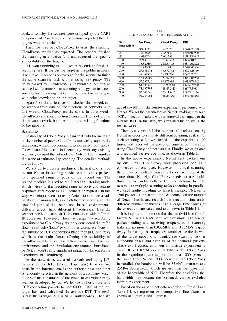
packets sent by the scanner were dropped by the NAPTequipment of Private-1, and the scanner reported that thetargets were unreachable.

Then, we used our CloudProxy to assist the scanning.CloudProxy worked as expected. The scanner finishedthe scanning task successfully and reported the specificvulnerability of the targets.

It is worth noticing that it takes 20 seconds to finish thescanning task. If we put the target in the public network,it will take 12 seconds on average for the scanner to finishthe same scanning task without using any proxy. Thedelay caused by CloudProxy is unavoidable, but can bereduced with a more smart scanning strategy, for instance,sending less scanning packets to achieve the same goalwith prior knowledge on the target.

Apart from the differences on whether the network canbe scanned from outside, the functions of networks withand without CloudProxy are the same. In other words,CloudProxy adds one function (scannable from outside) tothe private network, but doesn’t hurt the existing functionsof the network.

ScalabilityScalability of CloudProxy means that with the increase

of the number of peers, CloudProxy can easily support theincrement, without becoming the performance bottleneck.To evaluate this metric independently with any existingscanners, we used the network tool Netcat [16] to simulatethe scene of vulnerability scanning. The detailed methodsare as follows.

We set up two server machines. The first one is usedto run Netcat in sending mode, which sends packetsto a specified range of ports of the second one. Thesecond machine is used to run Netcat in listening mode,which listens to the specified range of ports and returnsresponses after receiving TCP connection requests. In thisway, we setup a scenario using Netcat to simulate a vul-nerability scanning task, in which the first server scans thespecified ports of the second one. In real environments,different targets have different IP addresses. Thus thescanner needs to establish TCP connection with differentIP addresses. However, when we design the scalabilityexperiment for CloudProxy, we only considered the trafficflowing through CloudProxy. In other words, we focus onthe amount of TCP connections made though CloudProxywhich is the main factor affecting the scalability ofCloudProxy. Therefore, the difference between the realenvironment and the simulation environment introducedby Netcat won’t cause significant impact on the scalabilityexperiment of CloudProxy.

At the same time, we used network tool hping [17]to measure the RTT (Round Trip Time) between twohosts in the Internet, one is the author’s host, the otheris randomly selected in the network of a company whichis one of the consumers of the cloud based vulnerabilityscanner developed by us. We let the author’s host sendTCP connection packets to port 6000 - 7000 of the realtarget host and calculated the average RTT. The resultis that the average RTT is 81.90 milliseconds. Then we

TABLE IIAVERAGE EXECUTION TIME INCLUDING RTT (S)

TCPconnections

No Proxy Cloud Proxy Diff

10 0.928232 1.457575 1.57027014820 1.842699 2.887150 1.56680499650 4.610504 7.091599 1.538139648100 9.213162 15.060583 1.634681231150 13.820406 22.136175 1.601702222200 18.408603 28.917091 1.570846576300 27.646171 46.877542 1.695625119400 37.058839 59.183716 1.597020241500 46.138107 75.357783 1.633308948600 55.337350 89.977399 1.625979542700 64.504925 104.902701 1.626274288800 73.697793 118.458449 1.60735409900 83.341048 133.113415 1.5972131161000 92.264051 146.283200 1.585484253

added the RTT in the former experiment performed withNetcat. We set the parameters of Netcat, making it to sendTCP connection packets with an interval that equals to theaverage RTT. In this way, we simulated the delays in thereal network.

Then, we controlled the number of packets sent byNetcat in order to simulate different scanning scales. Foreach scanning scale, we carried out the experiment 100times, and recorded the execution time in both cases ofusing CloudProxy and not using it. Finally, we calculatedand recorded the average time, as shown in Table II.

In the above experiments, Netcat sent packets oneby one. Thus, CloudProxy only processed one TCPconnection of one peer. However, in a real scanning,there may be multiple scanning tasks executing at thesame time. Namely, CloudProxy needs to use multi-threading to handle multiple TCP connections. In orderto simulate multiple scanning tasks executing in parallel,we used multi-threading to launch multiple Netcats tosend packets at the same time. We controlled the numberof Netcat threads and recorded the execution time underdifferent number of threads. The average time values ofthe executions are calculated and shown in Table III.

It is important to mention that the bandwidth of Cloud-Proxys NIC is 100Mb/s, in full-duplex mode. The generalpacket sending and receiving frequencies of scanningtasks are no more than 0.033Mb/s and 0.25Mb/s respec-tively. Increasing the frequency would cause the firewallof the target network to identify the scanning task asa flooding attack and filter all of the scanning packets.These two frequencies in our simulation experiment inTable III are 0.022Mb/s and 0.017Mb/s. The CloudProxyin the experiment can support at most 1000 peers atthe same time. When 1000 peers use the CloudProxyin parallel, the bandwidth will be 33Mb/s upstream and25Mb/s downstream, which are less than the upper limitof the bandwidth of NIC. Therefore the possibility thatbandwidth may become the bottleneck can be excludedfrom our experiment.

Based on the experiment data recorded in Table II andTable III, we represent two comparison line charts, asshown in Figure.7 and Figure.8.



TABLE IIIAVERAGE EXECUTION TIME MULTI-PEERS (S)

TCP connections Number of peers Average Time10 1 1.457575

2 1.4986265 2.98456010 3.22018415 5.44773420 7.62947430 10.83312440 19.84303750 20.342757100 43.806441200 85.516066300 152.184318400 174.748115500 227.226585

20 1 2.8871502 3.00623410 6.84875120 14.374395100 95.745792200 206.645147

50 1 7.0915992 8.69616110 22.17923520 51.718310100 280.803423200 523.595370

100 1 15.06058310 49.602241100 493.530402

0

20

40

60

80

100

120

140

160

0 200 400 600 800 1000

CloudProxy

No Proxy

Number of peers

Exe

cu

tio

n tim

e(s

)

Fig. 7. Execution Time Trend with Growth of TCP connections

It can be seen from Figure.7 that with the growth of thenumber of TCP connections (i.e. the scanning scale), theexecution time with or without CloudProxy both growslinearly. The average execution time with CloudProxyis 1.6 times more than the case without it (Average ofDiff, which is the ratio of the slopes of lines in Figure.7).This ratio does not grow with the growth of the scanningscale, which means CloudProxy scales well. It can beseen from Figure.8 that when using multi-threading tosimulate multi-peers, with the growing number of peers,for the same TCP connection scale, the average executiontime increases linearly. Thus, we can conclude that withthe growth of the scanning scale, it would be hard forCloudProxy to become the performance bottleneck inpractice since it has a relatively high scalability.

0

50

100

150

200

250

300

350

400

450

500

550

0 50 100 150 200 250 300 350 400 450 500

10 TCP

20 TCP

50 TCP

100 TCP

Number of peers

Exe

cu

tio

n tim

e(s

)

Fig. 8. Execution Time Trend with Growth of Peer Numbers

VII. CONCLUSION

This paper proposed a NAPT proxy called CloudProxyfor vulnerability scanners based on cloud computing.CloudProxy combines the TURN extension protocol andthe Socks5 protocol. The CloudProxy integrates Socks5function into the TURN client, so that the destination portof all scanning packets will be aggregated into one beforepassing through the TURN server, lessening the burdenfor the TURN server.

We have set up a testing environment in which wedeployed CloudProxy between two private NAPT net-works and performed related tests. The results show thatCloudProxy is functional and scalable . As the scale ofscanning becomes larger, execution time for CloudProxyincreases linearly. Since we have taken the real networkdelay into consideration, the testing results imply thatCloudProxy would be practical in real application.

For future works, we will improve the adaptabilityof CloudProxy, so that it can tune the relaying speedaccording to the sensed situation of the target network.We also plan to strengthen the coordination betweenCloudProxy and the scanner, so that the scanner can adjustits sending speed in accordance with the relaying speed ofCloudProxy. In this way, we would be able to minimizethe involvement of the administrator and provide a moreelastic scanning service in the cloud.

ACKNOWLEDGMENT

We thank professors and colleagues for numerousdiscussions concerning this work, State Key Laboratoryof Networking and Switching Technology for assistance,and the reviewers for their detailed comments.

REFERENCES

[1] C. Henderson, “2011 Global Security Statistics and Trends,”Trustwave Spider Labs,” Technical Report, 2011.

[2] M. Heckathorn, “Network Monitoring for Web-Based Threats,”Carnegie Mellon University, SEI Administrative Agent,” TechnicalReport, Feb. 2011.

[3] P. K. Martin, “NASA Cyber security: An Ex-amination of the Agency’s Information Security,”U.S. House of Representatives, Feb. 2012. [On-line]. Available: http://democrats.science.house.gov/hearing/nasa-cybersecurity-examination-agencys-information-security

[4] C. Fritsch and G. Pernul, “Security for Dynamic Service-OrientedeCollaboration,” Lecture Notes in Computer Science, vol. 6264,no. 214, 2010.

[5] “The IANA IPV4 Address Free Pool Is Now Depleted,”https://www.arin.net/announcements/2011/20110203.html.



[6] “IP Network Address Translator (NAT) Terminology and Consid-erations,” http://tools.ietf.org/html/rfc2663.

[7] L. Zhang, W. Jia, and X. Xiao, “Research of TCP NAT Traver-sal Solution Based on Port Correlation Analysis and PredictionAlgorithm,” Proceedings of the 6th International Conference onWireless Communications Networking and Mobile Computing(WiCOM), no. 1, 2010.

[8] “Socks Protocol Version 5,” http://www.ietf.org/rfc/rfc1928.txt.[9] “Session Traversal Utilities for NAT (STUN),”

http://www.ietf.org/rfc/rfc5389.txt.[10] “Traversal Using Relays around NAT (TURN): Relay Ex-

tensions to Session Traversal Utilities for NAT (STUN),”http://www.ietf.org/rfc/rfc5766.txt.

[11] “Traversal Using Relays around NAT (TURN) Extensions for TCPAllocations,” http://www.ietf.org/rfc/rfc6062.txt.

[12] J. Kuroday, “STUN-based connection sequence through symmetricNATs for TCP connection,” Network Operations and ManagementSymposium (APNOMS), pp. 1–4, Sept. 2011.

[13] Z. Lin and T. You, “TT-STUN protocol design for effective TCPNAT traversal,” Broadband Network and Multimedia Technology(IC-BNMT), pp. 970–974, Oct. 2010.

[14] J. Huang, J. Min, and W. Cheng, “Design and Implementation of aTURN Based Solution to Symmetric NAT,” Microelectronics andComputer, vol. 26, no. 4, Apr. 2009.

[15] Y.Wei, D.Yamada, S.Yoshida, and S.Goto, “A New Method forSymmetric NAT Traversal in UDP and TCP,” APAN NetworkResearch Workshop, pp. 11–18, 2008.

[16] “The GNU Netcat,” http://netcat.sourceforge.net/.[17] “Hping - Active Network Security Tool,” http://www.hping.org/.Yulong Wang received his Ph.D. degree in computer sciencefrom the Beijing University of Posts and Telecommunications,China, in 2010. He is currently a lecturer at the Beijing Uni-versity of Posts and Telecommunications. His research interestsinclude security and cloud computing.

Jiakun Shen is currently a MS candidate at the Beijing Uni-versity of Posts and Telecommunications, China. Her researchinterests include security and network.



Adaptive Clustering for Maximizing Network Lifetime and Maintaining Coverage

Luqiao Zhang1, 2, Qinxin Zhu1, Juan Wang 2

1 University of Electronic Science and Technology of China/School of Computer Science and Engineering, Chengdu, China

2

[email protected] University of Information Technoloy/School of Network Engineering, Chengdu, China

, [email protected], [email protected]

Abstract—In Wireless Sensor Network (WSN), cluster-based topology is believed to be an effective way for balancing energy consumption and prolonging the network lifespan. However, the clustering process itself can be an energy cost behavior, especially when it is executed periodically. Moreover, little attention has been paid to combine sleeping scheduling with topology formation. In order to solve the above problem, a novel distributed clustering algorithm called Adaptive Energy Efficient Clustering (AEEC) is proposed to maximize network lifetime in this study. Optimizations including the restricted global re-clustering, intra-cluster node sleeping scheduling and adaptive transmission range adjustment are introduced to fulfill the task of energy conservation, while connectivity and coverage is guaranteed. Simulation demonstrates that a great amount of energy is saved for sensed data transmission rather than control packet broadcast, and thus the network lifetime is extended significantly. Index Terms—wireless sensor network, topology control, clustering, energy efficiency

I. INTRODUCTION

Wireless Sensor Network (WSN) [1] is composed of hundreds even thousands of micro-sensors empowered by batteries. And it has already found its application in battle field surveillance [2], wild animal protection [3], volcano monitoring [4] and other fields. Sensors are usually scattered in harsh or hostile regions and left unattended once deployed, which makes battery replacement or recharging impossible. Due to the above fact, additional attention has to be paid to energy conservation.

After deployment, sensor nodes setup communication links with each other autonomously, and then they work in a coordinate manner to relay sensed data back to the base station or observer. Topology control [5] plays a key role in the process of network setup and maintenance.

A lot of work has been done in how to create optimized topology. However, not much attention has been paid to the energy cost of topology formation itself. Furthermore, combining sleeping scheduling with topology control has yet to be investigated.

In order to solve the above problems, we propose a distributed cluster-based topology control algorithm, which aims to maximize the network lifetime while fulfilling other goals.

The rest of the paper is organized as follows. First of all, the classification of topology control algorithm, and the most typical ones, especially the cluster-based algorithms, will be introduced. Secondly, the network model, notations and problem statement is given. Thirdly, a detail description of our approach is presented. Afterwards, the analysis and simulation of our method is provided. At last, conclusion is made.

II. RELATED WORK

A lot of topology control algorithms with very different design goals have been presented in past years. Reference [6]-[9] can be good reference for those who are interested in this area.

Topology control in WSN can be classified into non-hierarchical and hierarchical due to the network structure. Typical non-hierarchical topology control methods include GG (Gabriel Graph) [10], RNG (Relative Neighbor Graph) [11], LMST (Localized Minimum Spanning Tree) [12] and so on. Besides the non-hierarchical structure, hierarchical structure is believed to be a more efficient solution, especially for large scale WSNs. However, hierarchical approaches are more complicated than the non-hierarchical ones in terms of the topology formation and maintenance. We focus on hierarchical methods in this study, more specifically, cluster-based algorithms.

In cluster-based approaches, a bunch of nodes are selected to be cluster head (CH) and responsible for coordinating the cluster’s operation, like time slot allocation, data fusion and inter-cluster communication. However, clustering algorithms can be very different in many ways, as listed below.

1) CH selection. The common criteria for CH selection include residual energy [13], multi-criteria [14], node’s ID [15] and so forth. And the clustering process is also based on quite different assumptions, for example, reference [16] requires that sensors are equipped with location-aware equipment; reference [17] assumes that nodes have long-haul communication capability;

Manuscript received November 2, 2012; accepted January 28, 2013. Corresponding author: Luqiao Zhang, University of Electronic

Science and Technology of China (UESTC), 610000, Chengdu, China.





reference [18] allows the existence of mobile nodes and so on.

2) Centralized or distributed. Clusters can be formed in either centralized or distributed manner. It is quite clear that the distributed method is a better choice for WSNs, because in WSN, it is very hard for a single node to get a full picture of the overall network. For such reason, most of the existed algorithms are designed to be executed in distributed manner. But centralized algorithms, like LEACH-C [19], find their application in some particular scenarios.

3) Single-hop or multi-hop. Choice has to be made between single-hop link and multi-hop link for both intra-cluster and inter-cluster communication. It is widely accepted that CHs should communicate with the base station through a multi-hop route, because some CHs can be very far from the base station, and their battery will be quickly drain out if they communicate with base station directly. Moreover, sensors are not equipped with long-haul communication module in many cases. As for intra-cluster communication, the distance between non-CHs and CHs is not very far, single-hop solution becomes the most popular choice. Multi-hop solutions, e.g. DWECH (Distributed Weight-based Energy-efficient Hierarchical clustering protocol) [20] is proved can further reduce energy consumption for its hierarchical intra-cluster communication model, but additional computation is inevitable.

4) Topology Maintenance. After setup, the topology maintenance, which is an important mechanism for dealing with node failure and balancing energy consumption among sensors, has to be considered. Triggering global network reformation periodically is the simplest and most common solution. However, this can be disaster for energy conservation, if the reformation can be restricted to only part of the network, it would be preferred.

There are still more characteristics which can be used to classify clustering methods, and readers can refer to [9] for more information.

III. PRELIMINARY

A. Network Model and Notation A number of sensor nodes are randomly dispersed on a

square field and all nodes are quasi-stationary once deployed. Those nodes are the same in terms of initial battery level, Critical Transmission Range (CTR) and sensing range.

A unique ID is given for each node, for example i for the ith node. Besides that, the distance between node i and node j, i.e. dist(i,j), can be estimated by the RSSI (Received Signal Strength Index). And only bi-directional links are taken into consideration. Noticing that we do not assume any location-aware mechanism like GPS.

BS is used as an abbreviation for the Base Station. R intra and R inter

E

stands for intra-cluster communication range and inter-cluster communication range in following sections.

residualHop(i) denotes node i’s minimum hop distance to the

BS.

(i) denotes the residual energy of node i.

Other notations will be explained while the detail of the algorithm is explored.

B. Problem Statement The typical process for clustering is listed as follow. 1) Transmission range assignment and neighbor

discovery The base station will trigger the network

initialization by broadcast a beacon message, and other nodes will relay that message, so that global settings, like transmission range, can be spread throughout the whole network. Moreover, neighbor discovery can be done simultaneously in this phase.

2) CH election According to the algorithm, a bunch of nodes will be

elected as CH to be responsible for both intra-cluster and inter-cluster communication.

3) Cluster formation After the CH selection, nodes other than CHs have

to choose a cluster to join and act as cluster members, i.e. non-CHs.

4) Backbone network setup A backbone network has to be setup among CHs, so

that the sensed data can be relayed to base station in a multi-hop manner.

5) Intra-cluster optimization Mechanisms like sleeping scheduling and using

multi-hop scheme can be adopted for optimizing intra-cluster communication.

6) Topology maintenance Topology has to be reconfigured due to node failure,

load-balancing and so on. The proposed algorithm follows the above illustrated

steps, and for each step, we will introduce some new mechanisms for performance optimization, which will be discussed in section IV.

IV. ALGORITHM DESCRIPTION

In this section, the steps of the proposed algorithm and the mechanisms used in each step will be discussed.

Step 1: Initialization In this phase, the setting of global parameters and

neighbor discovery has to be done. For most existed approaches, intra-cluster and inter-

cluster communication range are fixed values. However, as node fails or new node joins, the density of the network changes, so it is reasonable that both intra-cluster and inter-cluster communication range adapt as the number of living nodes changes, shown as (1) and (2).



( )intra

2 2min[ , ]

dR CTR

Na

∗=

(1)

( )inter intramin[3* , 2 2 ]R R d= ∗

(2)

In (1) and (2), NaFor R

is the number of nodes alive. intra, smaller transmission range can be used

while only a few nodes fail. And it should be increased to guarantee connectivity when the number of active nodes decreases. Of course, the upper bound for Rintra

For R

is CTR.

inter, it should be large enough so that inter-cluster communications can be carried out simultaneously for neighboring clusters [21]. Moreover, the upper bound for Rinter

Base Station

d

d

MaximumDistance

is set to the maximum distance between base station and certain node is (sqrt(2)/2)*d, as shown in Fig. 1.

Figure 1. Maximum distance between the base station and node

The base station initializes the clustering process, by broadcasting beacon message, carrying Rintra and Rinter, with different power level. Node i, who receives such beacon, will relay the message with the sender ID, Hop(i) and Eresidual

Notice that a node may receive several beacon messages from its neighbors, so the beacon should be relayed until all beacon messages are received. In practice, this can be achieved by setting a timer T

(i) updated. By the received beacon message, every node knows its neighbor within one-hop range.

w

Step 2: Clustering

, when the timer expires, node stops waiting and starts beacon broadcasting.

In this step, CHs will be selected, and clusters will be formed. And only the nodes with more residual energy than the average energy level of its neighbors can become candidates for CHs, as (3) shows.

( ) 1( )residual

residual

nE j

jE in

∑=

≥ (3)

However, there can be more than one CH candidate in the same neighboring area, to deal with such dilemma, each CH candidate waits for a time Tc before it announce itself to be a CH. If any CH announcement is received during Tc

Furthermore, T

, the candidate CH will step back to be cluster member.

c is set to be inversely proportional to Cost(i). The computation of Tc

Nodes with greater Cost(i) will have a better chance to be CH due to the setting of T

and Cost(i) is shown in (4) and (5), where t is an application determined constant. And Cost(i) is a multi-criteria index [14],

which denotes the centrality of a node and the cost for its neighbor to communicate with it.

c

( )ct

TCost i

=

, thereafter denser cluster with smaller cluster radius will be formed, which can be very helpful for increasing the network throughput. Moreover, as there is no repetition in the process, it terminates in O(1) iteration.

(4)

1

1( )

( , )

nCost i

j dist i j= ∑

= where intra( , )dist i j R≤ (5)

The information needed for computation of Eresidual

Once a node decides to be a CH, it broadcast its ID. Those nodes, who receive such announcements, will choose a cluster to join and the CH i with smaller dist(i, j) would be favored.

(i) and Cost(i) has already been collected in step 1.

Base Station Cluster

Head j

Node i

Figure 2. Node covered by both the base station and CH

One more problem has to be solved, considering the situation illustrated in Fig. 2. It is not hard to tell that a direct link should be setup between i and the base station for energy efficiency. Unfortunately, to the best of our knowledge, only CHs are allowed to communicate with the base station in existed approaches. In this study, such restraint is removed, and node i can choose the base station to be its parent when the distance between i and the base station is smaller than any CH.

Step 3: Backbone network setup Once the clustering process ends, inter-cluster

communication links have to be setup between CHs, so that sensed data can be sent to base station. Compared to clustering, the backbone network setup among CHs is straightforward. For each CH i, it selects CH j with the smallest Hop(j) to be its parent (Notice that Hop(j) is initialized in Step 1). If there lies multiple options, then CH j with smaller dist(i, j) would be chosen. A tree-shaped backbone network can be formed among CHs under such criteria.

Step 4: Intra-cluster communication optimization The intra-cluster communication is scheduled

according to the sensing range overlapping rate of the nodes within the same cluster. Once two nodes stays too close to each other, which means that they will detect the same event with very high probability. In such cases, the one with larger ID can switch to sleep mode. After that, the rest active cluster members



communicate with their CH in allocated TDMA slots. Following is the detail of how sleeping decision is made.

R

α Di j.

Figure 3. Example of sensing area overlapping

Assuming that the sensing range of nodes is Rs, the distance between node i and j is d (0≤ d＜Rs), and the probability for i to successfully detect certain event happening inside its sensing range is P, as shown in Fig. 3. Then the probability for j to detect the same event can be computed by (6), in which So

2

oj

SP P

Rπ= ×

denotes the area of overlapping sensing area.

(6)

Moreover, the computation of So is listed in (7) (8) (9), in which the Ss stands for the area of the sector while St

2 ( )o s tS S S= × −

stands for the area of the triangle, illustrated in Fig. 3.

(7)

2

2sS Rα

ππ

= × where2 2 2

2arccos( )

2

R R D

Rα

+ −= (8)

2

2

2 2t

d dS R= −

(9)

Finally, if Pj≥ Pr, Pr is an application determined constant, then j can switch to sleep mode. And node i and node j are defined as substitutable nodes. Moreover, Pr

Step 5: Topology maintenance

is set to 0.9 in our work, in order to guarantee the coverage.

Unlike former clustering algorithms, for example [13], [14] and [17], the clustering process is not triggered periodically. The global topology reset is only needed when a CH dies, which can be detect if the report has not been received for several consecutive rounds from certain CH. Once CH failure is detected, the base station can trigger global re-clustering by broadcasting a beacon as discussed in Step 1.

Only intra-cluster topology adjustment is needed when the dead node is a non-CH node. If the dead non-CH node i can not be replaced by any sleeping node, the CH simply deletes i from its member list and broadcast the adjusted TDMA time slot information. If i has a sleeping substitutable node j, then j will be awaken in the beginning of next round. Therefore, a great amount of energy can be saved for sensed data transmission rather than used for control message relay.

However, the node dies earlier in our approach than

other algorithms, because periodical CH rotation is not available. However, we believe this is a reasonable trade-off, which can lead to longer lifespan and more graceful downgrade of the service quality. The further explanation will be given in section V.

Finally, a sample topology resulted by AEEC is shown in Fig. 4, in which ‘.’ denotes cluster members, ’o’ denotes CHs, ’x’ denotes dead nodes and ‘☆’ denotes sleeping nodes.

As Fig. 4 shows, firstly, connectivity is guaranteed. Secondly, some nodes switch to sleeping mode because of the sensing area overlapping. At last, the coverage and the lifespan will be discussed in section V.

Figure 4. A sample topology of AEEC

V. ANALYSIS AND SIMULATION

A. Settings As former discussed design goals, analysis and

simulation will be focused on the network lifetime, coverage and scalability of AEEC. The energy mode used in simulation is a widely accepted one, which can be referred in [17]. Other parameters are listed in TABLE. I. All simulation is done by using Matlab, and all results are the average of ten experiments.

TABLE I. PARAMETERS

Parameter Value Deploy region From (0,0) to (100,100) Base station At (50,50)

Number of nodes 100 Initial energy for each node 0.2J

E 50 nJ/bit elec ε 10 pJ/bit/mfs ε

2 0.0013 pJ/bit/mmp

E4

5 nJ/bit/signal fusion Control packet size 25 bytes

Data packet size 100 bytes Threshold distance (d0 75 m )

P 0.97 P 0.9 r

B. Network Lifetime AEEC can greatly prolong the network’s lifetime, in

term of round, as compared to LEACH and HEED, depicted in Fig. 5. And this is achieved by the sleeping



scheduling and the topology maintenance, especially the topology maintenance strategy, which reduces the energy consumption remarkably.

Figure 5. Comparison of network lifetime

In LEACH, HEED and most of the current clustering methods, the role of CH is rotated among nodes in order to balancing the energy consumption. However, global re-clustering can be expensive, in terms of energy consumption, which can be seen from the abrupt changes in red dotted curve in Fig. 8.

Figure 6. Comparison of times of global re-clustering

Figure 7. Energy consumed for control message transmission

And frequent global topology reformation, which forces sensors to use their energy for control packet transmission rather than data collection. A great amount of energy is saved for data collection by

restricting the scope of topology reformation in AEEC, when compared to LEACH and HEED, as illustrated in Fig. 6 and Fig. 7. It can be seen from Fig. 6, AEEC has the least count of global topology reformation, which lead to least energy consumption for control packet transmission shown in Fig. 7.

Figure 8. Detailed energy consumption for AEEC

C. Coverage

Figure 9. Sample topology without sleeping nodes

Figure 10. Sample topology with sleeping nodes

The central concept of our sleeping mechanism is to eliminate coverage redundancy without introducing any ‘cavity’ in sensing coverage area. Shown by



massive simulation, our sleeping mechanism does satisfy the above requirement. And a sample contrast of topology structure and coverage with or without sleeping node is given in Fig. 9, Fig. 10, Fig. 11 and Fig. 12.

Figure 11. Sample coverage contour without sleeping nodes

Figure 12. Sample coverage contour with sleeping nodes

Fig. 9 and Fig. 10 depict the samples of nodes and links between nodes with or without sleeping mechanism. While the coverage of the above two cases is shown in Fig. 11 and Fig. 12. And no ‘cavity’ is introduced by applying the sleeping scheduling.

Moreover, as TABLE II shows, while the density of sensor grows, the sleeping strategy does a better job in energy saving. Such phenomenon can be explained by that the denser the network, the more sleeping nodes, and the more energy will be saved.

TABLE II. THE EFFECT OF SLEEPING SCHEDULING

Number of nodes 100 200 300 400 500 Lifetime increase ratio by applying sleeping strategy

(%) 25.4 26.8 65.9 77.4 79.5

D. Scalability Our approach is suitable for large scale WSNs, as its

complexity has nothing to do with the number of nodes and it can be run on each node separately with neighboring information just within one-hop range.

Besides the above, simulation shows that the ratio of CHs, active non-CHs and sleeping non-CHs is quiet stable as the number of nodes grows, which is illustrated in Fig. 13.

Figure 13. Ratio of different nodes

VI. CONCLUSION

Gathering from the above, conclusion can be made that the AEEC algorithm has many salient features. Firstly, it is fully distributed, localized and scalable, moreover, its convergence time is O(1). Therefore it is suitable for large scale WSNs. Moreover, with the help of intra-cluster sleeping, adaptive transmission range assignment and topology maintenance schemes, it is a highly energy efficient clustering algorithm while coverage and connectivity is not jeopardized.

ACKNOWLEDGMENT

This work was supported by Education Department of Department of Sichuan Province, China (NO. 10ZB093, Scientific Research Fund of SiChuan Provincial Education Department) and Science and Technology Department of Sichuan Province, China (NO. 2011GZ0195, Science and Technology Support Program of SiChuan Province)

REFERENCES

[1] Akyildiz, I.F., Su W., Sankarasubramaniam Y., and Cayirci E., “Wireless Sensor Networks: A Survey,” Computer Networks, vol.38, no.4, pp. 393-422, Mar. 2002.

[2] Tatiana Bokareva, Wen Hu, Salil Kanhere, Branko Ristic, Neil Gordon, Travis Bessell, Mark Rutten and Sanjay Jha, “Wireless Sensor Networks for Battlefield Surveillance,” Proc. Land Warfare Conference 2006, Brisbane, Australia, 2006.

[3] Szewczyk R., Osterweil, E. Polastre, J. Hamilton, M. Mainwaring A. and Estrin D., “Habitat Monitoring with Sensor Networks,” Communications of the ACM, vol.47, no.6, pp. 34-40, Jun. 2004.

[4] Werner-Allen, Geoffrey, Lorincz, Konrad, Welsh, Matt, Marcillo, Omar, Johnson, Jeff, Ruiz, Mario, Lees and Jonathan, “Deploying a Wireless Sensor Network on an Active Volcano,” IEEE Internet Computing, vol.10, no.2, pp. 18-25, Mar.-Apr. 2006.



http://www.engineeringvillage.com/controller/servlet/Controller?CID=quickSearchCitationFormat&searchWord1=%7bAkyildiz%2C+I.F.%7d&section1=AU&database=3&yearselect=yearrange&sort=yr�

http://www.engineeringvillage.com/controller/servlet/Controller?CID=quickSearchCitationFormat&searchWord1=%7bSu%2C+W.%7d&section1=AU&database=3&yearselect=yearrange&sort=yr�

http://www.engineeringvillage.com/controller/servlet/Controller?CID=quickSearchCitationFormat&searchWord1=%7bSankarasubramaniam%2C+Y.%7d&section1=AU&database=3&yearselect=yearrange&sort=yr�

http://www.engineeringvillage.com/controller/servlet/Controller?CID=quickSearchCitationFormat&searchWord1=%7bCayirci%2C+E.%7d&section1=AU&database=3&yearselect=yearrange&sort=yr�

http://www.sciencedirect.com/science/article/pii/S1389128601003024�

http://www.engineeringvillage.com/controller/servlet/Controller?CID=quickSearchCitationFormat&searchWord1=%7bSzewczyk%2C+R.%7d&section1=AU&database=3&yearselect=yearrange&sort=yr�

http://www.engineeringvillage.com/controller/servlet/Controller?CID=quickSearchCitationFormat&searchWord1=%7bOsterweil%2C+E.%7d&section1=AU&database=3&yearselect=yearrange&sort=yr�

http://www.engineeringvillage.com/controller/servlet/Controller?CID=quickSearchCitationFormat&searchWord1=%7bPolastre%2C+J.%7d&section1=AU&database=3&yearselect=yearrange&sort=yr�

http://www.engineeringvillage.com/controller/servlet/Controller?CID=quickSearchCitationFormat&searchWord1=%7bHamilton%2C+M.%7d&section1=AU&database=3&yearselect=yearrange&sort=yr�

http://www.engineeringvillage.com/controller/servlet/Controller?CID=quickSearchCitationFormat&searchWord1=%7bMainwaring%2C+A.%7d&section1=AU&database=3&yearselect=yearrange&sort=yr�

http://www.engineeringvillage.com/controller/servlet/Controller?CID=quickSearchCitationFormat&searchWord1=%7bEstrin%2C+D.%7d&section1=AU&database=3&yearselect=yearrange&sort=yr�

http://dl.acm.org/citation.cfm?id=990704�


http://www.engineeringvillage.com/controller/servlet/Controller?CID=quickSearchCitationFormat&searchWord1=%7bWerner-Allen%2C+Geoffrey%7d&section1=AU&database=3&yearselect=yearrange&sort=yr�

http://www.engineeringvillage.com/controller/servlet/Controller?CID=quickSearchCitationFormat&searchWord1=%7bLorincz%2C+Konrad%7d&section1=AU&database=3&yearselect=yearrange&sort=yr�

http://www.engineeringvillage.com/controller/servlet/Controller?CID=quickSearchCitationFormat&searchWord1=%7bWelsh%2C+Matt%7d&section1=AU&database=3&yearselect=yearrange&sort=yr�

http://www.engineeringvillage.com/controller/servlet/Controller?CID=quickSearchCitationFormat&searchWord1=%7bMarcillo%2C+Omar%7d&section1=AU&database=3&yearselect=yearrange&sort=yr�

http://www.engineeringvillage.com/controller/servlet/Controller?CID=quickSearchCitationFormat&searchWord1=%7bJohnson%2C+Jeff%7d&section1=AU&database=3&yearselect=yearrange&sort=yr�

http://www.engineeringvillage.com/controller/servlet/Controller?CID=quickSearchCitationFormat&searchWord1=%7bRuiz%2C+Mario%7d&section1=AU&database=3&yearselect=yearrange&sort=yr�

http://www.engineeringvillage.com/controller/servlet/Controller?CID=quickSearchCitationFormat&searchWord1=%7bLees%2C+Jonathan%7d&section1=AU&database=3&yearselect=yearrange&sort=yr�

http://www.engineeringvillage.com/controller/servlet/Controller?CID=quickSearchCitationFormat&searchWord1=%7bLees%2C+Jonathan%7d&section1=AU&database=3&yearselect=yearrange&sort=yr�

[5] Santi Paolo, “Topology Control in Wireless Ad hoc and Sensor Networks,” ACM Computing Surveys, vol. 37, no. 2, pp. 164-194, Jun. 2005.

[6] Jardosh, Sunil, Ranjan and Prabhat, “A Survey: Topology Control for Wireless Sensor Networks,” Proc. ICSCN 2008, Chennai, India 2008, pp. 422-427.

[7] Banner, R. and Orda, A., “Multi-Objective Topology Control in Wireless Networks,” Proc. IEEE INFOCOM 2008, Phoenix, AZ., USA. 2008, pp. 1121-1129.

[8] Abbasi, Ameer Ahmed and Younis, Mohamed, “A Survey on Clustering Algorithms for Wireless Sensor Networks,” Computer Communications, vol.30, no.14-15, pp. 2826-2841, Oct. 2007.

[9] Xu Rui, Wunsch II and Donald, “Survey of clustering algorithms,” IEEE Transactions on Neural Networks, vol.16, no. 3, pp. 645-678, May. 2005.

[10] Gabriel KR. and Sokal RR., “A New Statistical Approach to Geographic Variation Analysis,” Systematic Zoology, vol. 18, no. 3, pp. 259-278, 1969.

[11] Toussaint GT, “The Relative Neighborhood Graph of A Finite Planar Set,” Pattern Recognition, vol.12, no. 4, 1980, pp. 261-268.

[12] Li, Ning, Hou Jennifer C, Sha Lui, “Design and Analysis of an MST-Based Topology Control Algorithm,” Proc. IEEE INFOCOM 2003, San Francisco, CA, USA. 2003, pp. 1702-1712.

[13] Younis O, Fahmy S, “HEED: A Hybrid, Energy-efficient, Distributed Clustering Approach for Ad hoc Sensor Networks,” IEEE Transactions on Mobile Computing, vol.3, no. 4, pp. 366-379, Oct.-Dec. 2004.

[14] Neamatollahi P., Taheri H., Naghibzadeh M., Yaghmaee M.H., “DESC: Distributed Energy Efficient Scheme to Cluster Wireless Sensor Networks,” Proc. The 9th IFIP TC 6 International Conference 2011, pp. 234-246, Jun. 2011.

[15] Lin C.R.,Gerla M., “Adaptive Clustering for Mobile Wireless Networks,” IEEE Journal on Selected Areas Communications, no. 15, vol. 7, pp. 1265–1275, 1997.

[16] Hongwei Zhang, Arora, A., “GS3: Scalable Self-configuration and Self-healing in Wireless Networks,” Computer Networks, vol. 43, no. 4, pp. 459-480, Jul. 2002.

[17] Heinzelman W.R., Chandrakasan A., Balakrishnan H., “Energy-efficient Communication Protocol for Wireless Microsensor Networks,” Proc. The 33rd Annual Hawaii International Conference on System Sciences, Maui, HI, USA, 2000, p.10.

[18] K. Xu, M. Gerla, “A Heterogeneous Routing Protocol Based on a New Stable Clustering Scheme,” Proc. IEEE Military Communications Conference, Anaheim, CA, Oct. 2002, pp.838-843.

[19] Heinzelman W.B., Chandrakasan A.P., Balakrishnan H., “An Application-specific Protocol Architecture for Wireless Microsensor Networks,” IEEE Transactions on Wireless Communications, vol. 1, no. 4, pp. 660-670, Oct. 2002.

[20] Ping Ding, Holliday, J., Celik, A., “Distributed Energy Efficient Hierarchical Clustering for Wireless Sensor Networks,” Proc. The IEEE International Conference on Distributed Computing in Sensor Systems 2005, Marina Del Rey, CA, Jun. 2005, pp. 322-339.

[21] Ning Xu, Aiping Huang, Ting-Wei Hou, Hsiao-Hwa Chen, “Coverage and Connectivity Guaranteed Topology Control Algorithm for Cluster-based Wireless Sensor Networks,” Wireless Communications and Mobile Computing, vol. 12, no. 1, pp. 23-32, Jan. 2012.

Luqiao Zhang received B.S. degree and M.S. degree in computer science from University of Electronics and Technology of China (UESTC) in 2003 and 2006, respectively. He is now a Ph.D. candidate in University of Electronics and Technology of China (UESTC). His research interests include wireless sensor network and mobile wireless P2P.

Qingxin Zhu

got his B.S. degree on Math in the Math Department of Sichuan Normal University, Chengdu, P. R. C. He was admitted by the Applied Math Department of the Beijing University of Technology in 1982 and got his master’s degree there. In 1988, he went to Math and Electrical Engineering Department of the Ottawa University, Canada for his doctor’s degree. From May 1993 to March 1995, he did postgraduate research in

the Electrical Engineering Department of the Ottawa University and the Computer Department of the Carlton University. Currently he is a professor and doctoral supervisor at the University of Electronic Science and Technology of China. His major research fields are Computer Networks, Bio-informatics, Optimization and Search Theory.

Juan Wang received her M.S. degree of Computer Architecture and Ph. D degree of Information Security from University of Electronics and Technology of China (UESTC) in 2006 and 2010. And being a visiting scholar at University of North Carolina at Charlotte (UNCC) from 2007.9 to 2008.9.Her research interests include network security and grid storage.



http://www.engineeringvillage.com/controller/servlet/Controller?CID=quickSearchCitationFormat&searchWord1=%7bSanti%2C+Paolo%7d&section1=AU&database=3&yearselect=yearrange&sort=yr�



http://www.engineeringvillage.com/controller/servlet/Controller?CID=quickSearchCitationFormat&searchWord1=%7bJardosh%2C+Sunil%7d&section1=AU&database=3&yearselect=yearrange&sort=yr�

http://www.engineeringvillage.com/controller/servlet/Controller?CID=quickSearchCitationFormat&searchWord1=%7bRanjan%2C+Prabhat%7d&section1=AU&database=3&yearselect=yearrange&sort=yr�

http://www.engineeringvillage.com/controller/servlet/Controller?CID=quickSearchCitationFormat&searchWord1=%7bBanner%2C+R.%7d&section1=AU&database=3&yearselect=yearrange&sort=yr�

http://www.engineeringvillage.com/controller/servlet/Controller?CID=quickSearchCitationFormat&searchWord1=%7bOrda%2C+A.%7d&section1=AU&database=3&yearselect=yearrange&sort=yr�

http://www.engineeringvillage.com/controller/servlet/Controller?CID=quickSearchCitationFormat&searchWord1=%7bAbbasi%2C+Ameer+Ahmed%7d&section1=AU&database=3&yearselect=yearrange&sort=yr�

http://www.engineeringvillage.com/controller/servlet/Controller?CID=quickSearchCitationFormat&searchWord1=%7bYounis%2C+Mohamed%7d&section1=AU&database=3&yearselect=yearrange&sort=yr�



http://www.engineeringvillage.com/controller/servlet/Controller?CID=expertSearchCitationFormat&searchWord1=%7bXu%2C+Rui%7d+WN+AU&database=3&yearselect=yearrange&searchtype=Expert&sort=yr�

http://www.engineeringvillage.com/controller/servlet/Controller?CID=expertSearchCitationFormat&searchWord1=%7bWunsch+II%2C+Donald%7d+WN+AU&database=3&yearselect=yearrange&searchtype=Expert&sort=yr�

http://ieeexplore.ieee.org/xpls/abs_all.jsp?arnumber=1427769�


http://www.engineeringvillage.com/controller/servlet/Controller?CID=quickSearchCitationFormat&searchWord1=%7bLi%2C+Ning%7d&section1=AU&database=3&yearselect=yearrange&sort=yr�

http://www.engineeringvillage.com/controller/servlet/Controller?CID=quickSearchCitationFormat&searchWord1=%7bHou%2C+Jennifer+C.%7d&section1=AU&database=3&yearselect=yearrange&sort=yr�

http://www.engineeringvillage.com/controller/servlet/Controller?CID=quickSearchCitationFormat&searchWord1=%7bSha%2C+Lui%7d&section1=AU&database=3&yearselect=yearrange&sort=yr�

http://www.engineeringvillage.com/controller/servlet/Controller?CID=quickSearchCitationFormat&searchWord1=%7bFahmy%2C+S.%7d&section1=AU&database=3&yearselect=yearrange&sort=yr�




http://www.engineeringvillage.com/controller/servlet/Controller?CID=quickSearchCitationFormat&searchWord1=%7bNeamatollahi%2C+P.%7d&section1=AU&database=3&yearselect=yearrange&sort=yr�

http://www.engineeringvillage.com/controller/servlet/Controller?CID=quickSearchCitationFormat&searchWord1=%7bTaheri%2C+H.%7d&section1=AU&database=3&yearselect=yearrange&sort=yr�

http://www.engineeringvillage.com/controller/servlet/Controller?CID=quickSearchCitationFormat&searchWord1=%7bNaghibzadeh%2C+M.%7d&section1=AU&database=3&yearselect=yearrange&sort=yr�

http://www.engineeringvillage.com/controller/servlet/Controller?CID=quickSearchCitationFormat&searchWord1=%7bYaghmaee%2C+M.H.%7d&section1=AU&database=3&yearselect=yearrange&sort=yr�

http://www.engineeringvillage.com/controller/servlet/Controller?CID=quickSearchCitationFormat&searchWord1=%7bYaghmaee%2C+M.H.%7d&section1=AU&database=3&yearselect=yearrange&sort=yr�

http://www.engineeringvillage.com/controller/servlet/Controller?CID=quickSearchCitationFormat&searchWord1=%7bLin%2C+C.R.%7d&section1=AU&database=3&yearselect=yearrange&sort=yr�

http://www.engineeringvillage.com/controller/servlet/Controller?CID=quickSearchCitationFormat&searchWord1=%7bGerla%2C+M.%7d&section1=AU&database=3&yearselect=yearrange&sort=yr�

http://www.engineeringvillage.com/controller/servlet/Controller?CID=quickSearchCitationFormat&searchWord1=%7bHongwei+Zhang%7d&section1=AU&database=3&yearselect=yearrange&sort=yr�

http://www.engineeringvillage.com/controller/servlet/Controller?CID=quickSearchCitationFormat&searchWord1=%7bArora%2C+A.%7d&section1=AU&database=3&yearselect=yearrange&sort=yr�

http://www.engineeringvillage.com/controller/servlet/Controller?CID=quickSearchCitationFormat&searchWord1=%7bHeinzelman%2C+W.R.%7d&section1=AU&database=3&yearselect=yearrange&sort=yr�

http://www.engineeringvillage.com/controller/servlet/Controller?CID=quickSearchCitationFormat&searchWord1=%7bChandrakasan%2C+A.%7d&section1=AU&database=3&yearselect=yearrange&sort=yr�

http://www.engineeringvillage.com/controller/servlet/Controller?CID=quickSearchCitationFormat&searchWord1=%7bBalakrishnan%2C+H.%7d&section1=AU&database=3&yearselect=yearrange&sort=yr�



http://www.engineeringvillage.com/controller/servlet/Controller?CID=quickSearchCitationFormat&searchWord1=%7bHeinzelman%2C+W.B.%7d&section1=AU&database=3&yearselect=yearrange&sort=yr�

http://www.engineeringvillage.com/controller/servlet/Controller?CID=quickSearchCitationFormat&searchWord1=%7bChandrakasan%2C+A.P.%7d&section1=AU&database=3&yearselect=yearrange&sort=yr�

http://www.engineeringvillage.com/controller/servlet/Controller?CID=quickSearchCitationFormat&searchWord1=%7bBalakrishnan%2C+H.%7d&section1=AU&database=3&yearselect=yearrange&sort=yr�



http://www.engineeringvillage.com/controller/servlet/Controller?CID=quickSearchCitationFormat&searchWord1=%7bPing+Ding%7d&section1=AU&database=3&yearselect=yearrange&sort=yr�

http://www.engineeringvillage.com/controller/servlet/Controller?CID=quickSearchCitationFormat&searchWord1=%7bHolliday%2C+J.%7d&section1=AU&database=3&yearselect=yearrange&sort=yr�

http://www.engineeringvillage.com/controller/servlet/Controller?CID=quickSearchCitationFormat&searchWord1=%7bCelik%2C+A.%7d&section1=AU&database=3&yearselect=yearrange&sort=yr�

http://www.engineeringvillage.com/controller/servlet/Controller?CID=quickSearchCitationFormat&searchWord1=%7bNing+Xu%7d&section1=AU&database=3&yearselect=yearrange&sort=yr�

http://www.engineeringvillage.com/controller/servlet/Controller?CID=quickSearchCitationFormat&searchWord1=%7bAiping+Huang%7d&section1=AU&database=3&yearselect=yearrange&sort=yr�

http://www.engineeringvillage.com/controller/servlet/Controller?CID=quickSearchCitationFormat&searchWord1=%7bTing-Wei+Hou%7d&section1=AU&database=3&yearselect=yearrange&sort=yr�

http://www.engineeringvillage.com/controller/servlet/Controller?CID=quickSearchCitationFormat&searchWord1=%7bHsiao-Hwa+Chen%7d&section1=AU&database=3&yearselect=yearrange&sort=yr�

A Leakage-Based Beamforming Algorithm for Cognitive MIMO Systems via Game Theory

Feng Zhao

Key Laboratory of Cognitive Radio and Information Processing (Guilin University of Electronic Technology), Ministry of Education, Guilin, China


Xuezhi Lv and Hongbin Chen Key Laboratory of Cognitive Radio and Information Processing (Guilin University of Electronic Technology), Ministry

of Education, Guilin, China Email: {[email protected], [email protected]}

Abstract—Cognitive radio has been recently proposed as a promising technology to achieve efficient use of spectrum resources. In this paper, we consider spectrum sharing in a MIMO system where several secondary users (SUs) share spectrum with a primary user (PU). A leakage-based beamforming algorithm is proposed via game theory. The objective is to maximize the sum throughput of SUs subject to the signal-to-leakage-and-noise ratio (SLNR) constraint of SUs and PU interference constraint. The sum-throughput maximization problem is formulated as a non-cooperative game, where the SUs compete with each other over the resources offered by the PU. Nash equilibrium is considered as the solution of this game. Simulation results show that the proposed algorithm can achieve a high sum throughput and converge to a locally optimal beamforming vector. Index Terms—beamforming, cognitive radio, MIMO, game theory, Nash equilibrium 1

I. INTRODUCTION

Cognitive radio (CR), as a promising technology to advocate efficient use of radio spectrum, has been a topic of increasing research interest in recent years [1]. Cognitive radio has been recently proposed as a smart and agile technology which allows non-legitimate users to utilize licensed bands opportunistically [2]. By detecting licensed spectrum holes and jumping into them rapidly, the CR can dramatically improve the spectrum utilization. To guarantee a high spectral-efficiency while avoiding the interference to the licensed users, the CR should be able to adapt to electromagnetic conditions flexibly. Hence, some important abilities should be provided by the CR network which include spectrum sensing, spectrum sharing [3]. A key feature of the CR network is to allow a SU to simultaneously share a licensed spectrum as long as the secondary transmission does not interfere with the primary transmission. The challenge of the CR network is to protect the PUs from

Manuscript received October 17, 2012; revised February 24, 2013;

accepted March, 2013. Corresponding author: Hongbin Chen.

harmful interference induced by the SUs as well as to meet the quality of service (QoS) requirements of SUs.

In the past decade, multiple-input multiple-output (MIMO) technique is fast becoming the most popular technology in wireless systems due to its performance benefits [4]. Therefore, most wireless systems use multiple antennas at the transmitter and the receiver. As a result, it is important to study cognitive radio systems in a MIMO setting. This technological combination results in the so-called cognitive MIMO radio [5].

For traditional fixed-spectrum-allocation-policy based wireless communications systems, beamforming and power control are recognized as effective approaches to mitigate co-channel interference and thus increase the system capacity. For traditional wireless multiuser systems, power control and beamforming algorithms were widely studied [6][7]. The multiuser downlink problem was discussed in two different scenarios of spectrum sharing [8]. In the first case, the primary network cooperates with the secondary network to jointly optimize the transmit beamforming weights and total transmission power in both networks subject to signal-to-interference-plus-noise ratio (SINR) constraints of both primary and secondary users. In the second case, the secondary network jointly optimizes the transmit beamforming weights and its total transmission power satisfying the SINR constraint of the secondary users and maximum tolerable interference constraint of the primary user. The beamforming problem with individual SINR constraints was discussed in [9], where the goal of designing beamformers is to maximize the SINR.

In this paper, we focus on the problem of beamforming based on the signal-to-leakage-and-noise ratio (SLNR) [9] via game theory in cognitive MIMO systems. Game theory is suitable for analyzing cooperative and non-cooperative behaviors among rational decision makers. It has been applied to solve the problem of beamforming for providing the maximum throughput in CR networks. Our aim is to maximize the sum rate of SUs by optimizing the beamforming vectors of the secondary users jointly when the channel state information is known at the transmitter.



Figure 1. Cognitive MIMO system model.

Note that the authors in [10] considered both power and rate control using a game-theoretical approach, where the SUs were considered as active players in the game. Therein, both theoretic analysis and algorithm were carefully investigated. However, the problem of joint beamforming and power allocation for cognitive MIMO systems is different from the traditional radio networks and to the best of our knowledge, few studies have been performed to the beamforming problem in a cognitive MIMO radio environment.

We consider a CR system where several SUs are operating in the same frequency band as the PU. In this case, the SUs who compete for the spectrum offered by the PU and the cost of using the spectrum is determined by a pricing function. A non-cooperative game model is adopted to analyze this situation and the Nash equilibrium is considered as the solution of this game. In [11], we proposed a joint beamforming and power allocation algorithm for cognitive MIMO systems via game theory. However, it did not consider the SLNR and the formulation of the optimization problem is different from the one in this paper. When incorporating the SLNR, the SINRs of SUs are more balanced, which indicates the improvement of fairness of SUs.

II. SYSTEM MODEL AND PROBLEM FORMULATION

In the system model, the primary network consists of a primary transmitter (PBS) that transmits signals to a single primary user (PU). Within the area of the primary network, a secondary network is deployed which shares the same spectrum resource with the primary network. The secondary network has a single base station (CBS), equipped with M antennas, serving K secondary users (SUs). Throughout this paper, we consider the downlink of the cognitive radio network in which CBS transmits independent signals to K SUs using a uniformly spaced M-element antenna array. The PBS is equipped with an L-element antenna array. A block diagram of the system is shown in Fig. 1. The transmitted signal vector of SUs is compactly written as

1

K

j jj=

= ∑x sf , (1)

where js denotes the transmitted data intended for user j,

[ ]1, , K=f f f is a beamforming vector. In this paper, we assume that all the SUs are homogeneous and experience independent fading.

The received signal at the i-th SU is given by

1

K

p i j p ii i i j iij=

= + + = + +∑xy W G W s Gx z f x z , (2)

where [ ]1, , K=W W W denotes the M K× channel matrix from the CBS to the SUs. Its entry is i.i.d., complex Gaussian, with zero mean and unit variance, iG represents the channel coefficient between the PBS and the i-th SU, px represents the transmitted signal from the PBS, iz is a vector of additive noises whose entries are i.i.d., complex Gaussian, with zero mean and variance

2kσ . The received signal at the primary user is given by

1

K

j p pp j ppj=

= + +∑y W s Gf x z (3)

where pG denotes the channel coefficient between the PU and the PBS, pW is an M K× channel matrix representing the channel between the CBS and the PU,

pz denotes the additive noise and is assumed to be i.i.d.,

complex Gaussian, with zero mean and variance 2pσ .

Each SU treats the signals intended for other SUs as interference. Then, the SINR of the i-th SU is

2

2 2 2

1,

iii K

ki i i ik k i

SINRN σ

= ≠

=+ +∑

W f

W Gf. (4)

For each user i, we expect that its signal power 2

iiW f is large compared to the noise power at its

receiver (i.e., 2i iN σ ). We also expect 2

iiW f is large compared to the power leaked from user i to all other

users, i.e., 2

1,

K

ikk k i= ≠∑ W f . These considerations motivate

us to introduce a metric called signal-to-leakage-noise ratio (SLNR), which is defined as

2

22 2

1,

iii K

i ik p i ik k i

SLNRN σ

= ≠

=+ +∑

W f

W Wf f. (5)

Using this notion of leakage, we can formulate an optimization problem which instead of dealing with the total interference of all users on user i as in (4), but deals with the total interfering power that user i causes on all other users. Specifically, we would like to select beamforming vectors if , 1, ,i K= , such that (5) is maximized over if .

In order to allow the SUs to share the spectrum with the PU, we should investigate appropriate beamforming weights to distribute them among the users so that the sum throughput of SUs is maximized, and the interference caused to the PU is as small as possible.



Thus, the optimization problem can be formally stated as follows:

( )21

arg max 1logK

ii

C SINR=

= +∑ , (6)

2

1. .

K

i thpi

i

Is tSLNR γ=

≤

≥

∑ W f , (7)

where thI and γ are the given values with respect to the interference power and SLNR, respectively.

III. NON-COOPERATIVE GAME

A. Utility Function Game theory is used in the hypothesis that players act

rationally, in the sense that each player has a payoff function that it tries to optimize, it is an effective tool to analyze competitive optimization problems. The SU selfishly chooses a strategy to increase its own utility, Thereby, the strategies chosen by different SUs depend on each other. Based on the system model described above, a non-cooperative game can be formulated as follows:

( ){ }, ,iG K uSINR = ⋅ , (8)

where 1, ,i K= is the set of players corresponding to the SUs. The strategy of each of the players is the beamforming weights (denoted by if for secondary user i), which is non-negative. The resulting utility (payoff) function of SU i is denoted as ( )u ⋅ . SINR can be taken as the optimization variable. Due to greediness, each player focuses on the forming of its own beam without nulling the interference to the PU. To prevent this selfish circumstance, pricing has been used as an effective tool to give distributed players incentives to cooperate in resource usages. Therefore, the payoff function should consist of revenue and cost. Specifically, the new utility function of the i-th SU with pricing is rewritten as follows:

( ) 2iii i

i

SINRu SINRSINR

λα

= −+

f , (9)

where λ and α are constant, λ is the price factor. α is an adjustable parameter, which lets the curve of the utility function to be steep. Thus, a non-cooperative game is formulated as:

1max

K

ii

u=∑ . (10)

Here, each SU competes against the others by choosing its beamforming vector if to maximize its own utility function.

B. Nash Equilibrium A Nash equilibrium (NE) is a stable outcome of a

game. At the NE point, no user has any incentive to change its strategy with its own action. According to the fundamental game theory result, the existence conditions of Nash Equilibrium are given in [11][12]: (1) 2

if is a

non-empty, convex, and compact subset of the Euclidean space; (2) ( )i iu SINR is continuous in if and quasi-concave in if . The detailed proof is omitted due to space limitation.

By taking the first derivative of ( )ku ⋅ with respect to

if , respectively, we get

( )( )2 2

2 2ii i

ii i

SINRu uSINR

λ∂∂ ∂

= −∂∂ ∂f f

. (11)

By setting these first derivatives to zero, we get

2 2 22

1,2

2

2 2 2

1,2

K

ki i i ik k i

i

K

ki i ik k i

i

N

i

N

αλσ

λ

α σ

= ≠

= ≠

+ +

=

+ +

−

∑

∑

W G Wff

W

W Gf

W

.

(12) Moreover, by taking the second derivative of ( )ku ⋅ with respect to if , respectively, we get

( ) ( )42

2 222 2 2

1,

4

4

2

2 2 2

1,

2

2

ii

Ki

ki i ik k i

i

iiK

ki i ik k i

u

N

N

α

σ

α

ασ

= ≠

= ≠

∂= −

∂ + +

×

++ +

∑

∑

W

f W Gf

W

W f

W Gf

. (13)

It is easy to check that ( )

2

220i

i

u∂ ≤∂ f

. Consequently, the

existence of the Nash equilibrium is proven for the proposed strategic non-cooperative game.

C. The Beamforming Algorithm In the following, in order to maximize the sum rate of

SUs while not degrading QoS for the PU, we present an iterative algorithm that repeats the beamforming steps until convergence [14].

The iterative algorithm is summarized as follows: 1. Set : 0n = and ( ): 1, 2A K= . Initialize beamforming

vectors ( )0if , i A∈ .

At each iteration, set 0 : nn = , i A∈ . Repeat { For each user i A∈ calculate the interference

2 2 2

1,

Kni ki i i i

k k iNI σ

= ≠

= + +∑ W Gf . (14)

Set : 1n n= + , ( ) ( )1n ni i

−=f f for each i A∈ . } until 0n Nn= + . 2. For each user i A∈ compute the beamforming

vector, these are generalized eigenvalue problems as



( )

1arg max

H Sn k

i H Ik

MM=

=x

xxf xx, (15)

where 2Sk iM = H and

2 2 2

1,

KIk i i i i

k k iNM σ

= ≠

= + +∑ IGH . (16)

3. Repeat Steps 1 and 2 until convergence.

D. Convergence of the Algorithm The beamforming algorithm can be interpreted as best-

responses in a beamforming game. The existence of Nash equilibrium point follows directly from the results of game theory. The beamforming guarantees the convergence of the algorithm to the Nash equilibrium while minimum interference to the PU is guaranteed.

IV. SIMULATION RESULTS

Computer simulation results are presented in this section to evaluate the performance of the proposed algorithms. Specifically, we show the convergence properties of the beamforming algorithm with respect to beamforming weight of each link. For simplicity, we consider two base stations with a single antenna (one PBS, one CBS), a CR network with three SUs, and a single PU. All channel knowledges are perfectly known. We choose three different pricing factors λ , the noise power

2σ =0.05W, the interference threshold thI =60, the i-th SU maximum SLNR constraint γ = 0.2 dB, respectively. The channel coefficients are drawn from the Rayleigh distribution.

Firstly, we examine the convergence of the beamforming algorithm with respect to beamforming weight. Fig. 2 shows the convergence of beamforming weight of each secondary link, in which the weight vector initialization is the same as 0. It is observed that the beamforming weight converges to the optimal values in a few iterations. In Fig. 3 we plot the utility of SU1 when the interference to PU caused by SUs is restricted. Moreover, Fig. 4 plots the sum utility of the SUs disparate the pricing factor λ . We observe that the utility of the SUs converges in Figs. 3 and 4, and decreases as λ increases.

V. CONCLUSIONS

In this paper, we have studied a beamforming problem via game theory in a cognitive MIMO system. The goal is to maximize the sum throughput of SUs under the SLNR constraint of SUs and the PU interference constraint. The sum throughput maximization problem is formulated as a non-cooperative game. We choose a proper utility function with pricing to characterize the data transmission of all SUs. Moreover, we propose an iterative algorithm that computes locally optimal beamforming vectors. Simulation results show that the proposed algorithm can achieve a high sum throughput.

Figure 2. Convergence of beamforming weights for three users.

Figure 3. SU1' utility for different λ .

Figure 4. SUs' sum utility for different λ .

ACKNOWLEDGMENT

This research was supported by the National Natural Science Foundation of China (61172055, 61162008), the Key Project of Chinese Ministry of Education (212131), the Foundation of Department of Education of Guangxi Province (201202ZD045), and the Open Research Fund



of Guangxi Key Lab of Wireless Wideband Communication & Signal Processing (12103, 12106).

REFERENCES

[1] S. Haykin, “Cognitive radio: brain-empowered wireless communications,” IEEE J. Sel. Areas Commun., vol. 23, pp. 201–220, February 2005.

[2] T. A. Weiss and F. K. Jondral, “Spectrum pooling: an innovative strategy for the enhancement of spectrum efficiency,” IEEE Commun. Maga., vol. 42, pp. S8–14, March 2004.

[3] I. F. Akyildiz, W. Y. Lee, M. C. Vuran, and S. Mohanty, “Next generation/dynamic spectrum access/cognitive radio wireless networks: a survey,” Comput. Netw., vol. 50, pp. 2127–2159, October 2006.

[4] D. Gesbert, M. Shafi, D. Shiu, P. J. Smith, and A. Naguib, “From theory to practice: an overview of MIMO space-time coded wireless systems,” IEEE J. Sel. Areas Commun., vol. 21, pp. 281–302, April 2003.

[5] G. Scutari, D. P. Palomar, and S. Barbarossa, “Cognitive MIMO radio,” IEEE Signal Process. Maga., vol. 25, pp. 46–59, November 2008.

[6] F. Rashid-Farrokhi, L. Tassiulas, and K. J. R. Liu, “Joint optimal power control and beamforming in wireless networks using antenna arrays,” IEEE Trans. Commun., vol. 46, pp. 1313–1324, October 1998.

[7] H. Islam, Y. C. Liang, and A. T. Hoang, “Joint power control and beamforming for cognitive radio networks,”

IEEE Trans. Wireless Commun., vol. 7, pp. 2415–2419, July 2008.

[8] H. Islam, Y. C. Liang, and A. T. Hoang, “Joint beamforming and power control in the downlink of cognitive radio networks,” in Proc. IEEE Int. Conf. Commun., 2007, pp. 21–26.

[9] M. Sadek, A. Tarighat, and A. H. Sayed, “A leakage-based precoding scheme for downlink multi-user MIMO channels,” IEEE Trans. Wireless Commun., vol. 6, pp. 1711–1721, May 2007.

[10] P. Zhou, W. Yuan, W. Liu, and W. G. Cheng, “Joint power and rate control in cognitive radio networks: a game-theoretical approach,” in Proc. IEEE Int. Conf. Commun., 2008, pp.3296–3301.

[11] F. Zhao, B. Li, and H. Chen, “Joint beamforming and power allocation algorithm for cognitive MIMO systems via game theory,” in Lecture Notes in Computer Science: Wireless Algorithms and Applications, 2012, pp. 166–177.

[12] R. D. Yates, “A framework for uplink power control in cellular radio systems,” IEEE J. Sel. Areas Commun., vol. 13, pp. 1341–1347, September 1995.

[13] R. H. Gohary and T. N. Davidson, “On rate-optimal MIMO signaling with mean and covariance feedback,” IEEE Trans. Wireless Commun., vol. 8, pp. 912–921, Febuary 2009.

[14] M.-P. Chrisanthopoulou and K. P. Tsoukatos, “Joint beamforming and power control for CDMA uplink throughput maximization,” in Proc. IEEE Int. Symp. Personal, Indoor and Mobile Radio Commun., 2007, pp. 1–5.



A SNR-based Multi-channel Multicast Scheme for Popular Video in Wireless Networks

Ting T. Liu

School of Electronic and Information Engineering, Beijing Jiaotong University, Beijing, China Email: [email protected]

Wei Yang and Chang L. Xu and Young-Il Kim

National Mobile Communications Research Laboratory, Southeast University, Nanjing, China/ National Mobile Communications Research Laboratory, Southeast University, Nanjing, China / School of Electronic and Information

Engineering, Beijing Jiaotong University, Beijing, China & Wireless System Research Group, Electronics and Telecommunications Research Institute, Daejoon, Korea

Email: {[email protected], [email protected]，[email protected] }

Abstract

—Multi-channel multicast/broadcast solution is used to improve Quality of Service (QoS) /Quality of Experience (QoE) of Video-on-Demand (VoD) service in mobile Internet Protocol Television (IPTV) applications. In this paper, a SNR-based multi-channel multicast scheme (SBMM) for popular video in wireless networks is proposed. Different from the existing fast data broadcasting scheme (FB), the wireless channel Signal Noise Ratio (SNR) is taken into account in SBMM. The higher-SNR channel is assigned with a higher channel rate. The higher-rate channel is used to transmit higher priority chunks, through which users’ waiting time is reduced and bandwidth utilization is improved. Simulation results show that 22.11% of FB’s start-up delay is reduced in average by SBMM and 49.52% at most. Moreover, 4.01% of FB’s download time is reduced in average by SBMM and 8.25% at most in the price of a small increase in buffer requirements. The additional space taken is 2.11% of the total video size in average and 6.19% at most. At the same time, SBMM can use bandwidth effectively through delivering chunks according to different priorities. As hardware technology develops, it is reasonable to reduce users’ waiting time further in the price of a small increase in buffer requirements.

Index Terms

—VoD, waiting time, buffer requirements, bandwidth utilization.

I. INTRODUCTION

As the development of wired and wireless Internet, a lot of multimedia applications are provided for millions of users. Internet Protocol Television (IPTV) has become the most popular application to meet the demand of entertainment in metropolitan areas. It enables people to transmit and receive multimedia streaming including video, audio, graphics, texts, and television signals through IP-based wired and wireless networks [1]. Among various IPTV services, Video-on-Demand (VoD) service is in high-profile because it allows users to select and watch their favorite programs on demand anytime and anywhere, even when they are on move. As multi-channel technology and routing schemes develop in wireless networks [2-3]

The most important factor to influence users’ QoE in multicast service for VoD traffic is users’ waiting time whether in wired or wireless communication networks

, multicast schemes which based on

that have been used widely to support VoD service and some schemes such as Weight Pick in [4] was proposed to reduce multicast retransmission delay in order to improve service performance in wireless communication environments.

[5]. Therefore, previous works such as [6-13, 15-16] focus on how to reduce users’ waiting time. Among that, papers [6-13] are based on wired networks such as cable TV and papers [14-16] are based on wireless networks such as mobile TV [17-18] and WiMAX [19]

b i

. Literatures [6] and [13] proposed a fast data broadcasting and receiving scheme (FB) to reduce waiting time and used fewer bandwidths under the condition of the same waiting time simultaneously. An efficient recursive frequency-splitting (RFS) scheme is proposed in [12], which can significantly reduce the users’ waiting time in cable TV applications as compared to [6] by replacement chunks based on slot sequence. Literature [14] proposed an adaptive hybrid transmission mechanism based on FB scheme in wireless networks (WiMAX) to reduce the blocking probability. Literature [15-16] has combined FB scheme and Patching algorithm in mobile IPTV environment in order to support continuous playback and reduce the waiting time. However, the transmission rates of multiple channels in [6-10] and [12-16] are identical and fixed with the video consumption rate. Though in [11] channels are divided into different transmission rates, they are also fixed with the value where b represents

the consumption rate and i is the channel number. The proposed scheme is originally motivated from FB

scheme in [6,13] and improve it to adapt to wireless environment such as WiMAX .The essential difference between wired and wireless networks is the channel conditions of latter vary over time, such as bandwidth, channel capacities , Signal-Noise-Ratio (SNR) and so on. Fixed data delivery strategy in wired environment can not be adopted directly in wireless environment. Therefore,




mailto:Young-il%20Kim%20%[email protected]%3e�

taking the dynamic channel attribute in wireless networks into account, this paper focuses on how to dynamically adjust the video data distribution strategy according to different channel conditions, in order to maximize the total utilization of channel bandwidth.

FB divides the resources into K identical-rate channels and divides the VoD content into N identical chunks, then puts them into K channels in the order of 1,2,4,8…2K and repeatedly broadcasts these chunks in multiple channels. Thus, anytime when users request the video they can download the first chunk within the shortest time and the total download time is not more than the download time of 2K chunks in the last channel. However, different channels have different (SNR) in wireless environment so that the channel capacities are different. The channel capacities of some low-SNR channels maybe lower than the video consumption rate and that of the other high-SNR channels maybe higher than the video consumption rate. FB scheme fixed the channel rate with the video consumption rate without regard of the SNR so that the theoretical optimal waiting time maybe not reached in wireless scene. Therefore, a major concern of this paper is how to delivery VoD chunks based on SNR to further reduce users’ waiting time and improve utilization of bandwidth resources. The proposed scheme use SNR as channel feedback to evaluate the corresponding channel rates, then put the high-priority chunks into high-rate channels, through which users’ start-up delay and download time can be reduced and the utilization of bandwidth resources can be improved.

The paper is organized as follows. In section II, we briefly describe existing FB scheme and propose a SNR based multi-channel multicast (SBMM) scheme. Details on analysis and simulation results are discussed in section III. Conclusions are drawn In section IV.

II. THE EXISTING FB SCHEME AND THE PROPOSED SBMM SCHEME

A. The Existing FB Scheme The existing FB scheme is illustrated in Fig. 1 and Fig.

2. In FB scheme, fixed-length video with length D is

given. The consumption rate of the video is b and the total bandwidth that we can assign for the video is B . The total channel rates can be reached FB

rB B . The bandwidth and video content are equally divided into K channels and ( 2 1)KN N chunks respectively.

Thus, the size of the video 1 2* NS D b S S S

and each channel rate , 1,2,FB FBi rR B K i K .

According to Shannon formula

2/ log (1 )FB FB FBi r iR B K B K SNR , the SNR of

the thi channel FBiSNR is 1dB in default. Under the

theoretical assumptions of FB that each channel rate is not less than the consumption rate, the number of logical

channels K B b . Then put 2i continuous data

chunks ( )p qS S repeatedly on the thi channel. At the client end, users start to download the first

chunk from channel 1C , then to download the other

chunks from channel 2,... KC C , and stop download from

channel iC when they have received 12i chunks. When is an integer, the number of channels K is

equal to , then the channel rate is equal to the video consumption rate b and fixed. When is not an integer,

the number of channels K B b , then the channel rate

is a little more than the video consumption rate b and is fixed with the value /B K .

Figure 1. FB scheme model when β is an integer.

Figure 2. FB scheme model when β is not an integer.

B. The Proposed SBMM Scheme When all channel rates are more than or equal to the

consumption rate and are identical, FB could meet the users’ waiting time demand in theory. However, the channel capacity is influenced by SNR so that the channel capacities of some low-SNR channels maybe lower than b and that of the other high-SNR channels maybe higher than b . The theoretical optimal value maybe not reached in the former situation, and the bandwidth utilization is decreased in the later situation. Furthermore, some scattered channel resources may exist in the system which has low channel rates. Thus, the low-SNR channels and the scattered bandwidth resources are wasted in FB according to the theoretical conditions of FB. Therefore, we propose a SNR based multi-channel multicast (SBMM) scheme in this part to reduce the impact of time-varying wireless channels on users’ waiting time and make use of bandwidth resources effectively.

Fig. 3 depicts the proposed service procedures. In wireless networks such as WiMAX, the MBS server

performs Membership management, MBS Zone management, Video segment and Security functions [14]



and so on. When a user sends a VoD request to MBS server, MBS server authorizes the user to activate an MBS service. Then the user joins a multicast group to receive video data. Generally, there is a group leader in each group, which is responsible for manage group members. In order to reflect the channel conditions, the group leader’s receiver sends the channel feedback including SNR to the base station transmitter periodically. Then the scheduler multicasts the video segments based on channel feedback through multi-channels to the user.

Figure 3. The proposed service procedures.

Suppose the bandwidth given is newB , the consumption rate is b (unit: Mbps) and the total channel rate is new

rB . The bandwidth is divided into K channels

in the system, thus new newK B b . The movie

with length D (unit: minutes) is segmented to N ( 2 1KN ) identical length chunks which are represented by 1 2, ,... NS S S respectively. The SNR fed

back by channel iC is newiSNR , thus

2 2log (1 ) / log (1 )new new new new newi i i r iR W SNR B K SNR ,

where newiW is the bandwidth taken by channel iC .

Obviously, it is waste to delivery the same size of chunks using higher-rate channels compared to lower-rate channels. Therefore, we sort them in descending order first and assign a higher speed for the higher-SNR channel. Therefore, new new

i jR R when i j , where newiR (unit: Mbps) represents channel rate of iC ,

1,2,...i K . We assume newiSNR for each channel is

constant within the download time of the video. For a given video 1 2 NS S S S , the priority of

iS is more than that of jS when i j because users

watch the video in the order of 1 2, , NS S S . Thus, we assign high-priority chunks to high-rate channel which

can decrease the receive time of the first chunk. At the same time, the higher-rate channel can transmit more chunks than FB does within fixed time and fewer channels were used due to the following reason. We use represents the time a chunk is transmitted by the last channel KC . In the period of , iC can transmit

12 /i new newi minR R

chunks, 1,2,..., ( )i M M K .

Among that, minnew new

KR R . For the reason that all N chunks need K channels in the order of

1 11,2, 4,...2 ,...2i K , when we transmit 12 /i new new

i minR R ( 1 12 / 2i new new i

i minR R ) chunks

on channel iC , only M out of K channels are needed. Therefore, the procedure of our proposed scheme is as

follows.

• Put the beginning 1 /new newminR R

continuous chunks

on the first channel repeatedly.

• Put the followed 112 /i new new

minR R continuous

chunks on the thi channel repeatedly when 1i M .

• Put the final 1

1

1

2 /M

i new newi min

i

N R R

continuous

chunks into the last channel repeatedly.

At client end, users accept 12 /i new newi minR R

chunks

from channel , 1,2, 1iC i M while accept 1

11

1

2 /M

i new newmin

i

N R R

chunks from the last channel.

Fig. 4 gives the details of our proposed multi-channel multicast scheme when 1 1

new new new newM M M MN R N R

(which we called case 1), where newiN represents the

number of chunks transmitted by channel iC . The

situation of 1 1new new new newM M M MN R N R (which we

called case 2) are similar to it and is given in next section.

Fig. 4 The proposed scheme in case 1

III. ANALYSIS AND SIMULATION RESULTS

We analyze the performance of SBMM scheme from the following aspects: users’ start-up delay, total download time, users’ buffer requirements and bandwidth utilization. The VoD file with playback speed of 3Mbps



was transmitted on wireless channels, where ranges from 1 to 8 with intervals of 0.1. The VoD file’s playback time is 100 minutes and the total file size is 2.25GB.For SBMM scheme, we assume the SNR feedback by channels range from 0.1dB to 9dB. For FB scheme, all channels’ SNR are the same. We simulated the above four factors of SBMM and FB and analyzed them as followes.

A. Users’ Start-up Delay Suppose the client end has sufficient buffer space to

store the video. A user starts to play the video when 1S is

being downloaded. 1S with another 1 / 1new newminR R

chunks are transmitted on the first channel. The worst situation is that the user access the channel just after 1S begins to be transmitted on the channel, as shown in Fig.5.

Figure 5. The maximum start-up delay

Thus the maximum start-up delay is equal to the

download time of 1 /new newminR R

chunks on channel 1C .

The size of 1S is /D b N . Therefore, on the condition of enough buffer space, the maximum start-up delay of our scheme is:

/1

1

/ /1

1

newR D b Nnewsdnew newR Rminnew new newR D B N

rnew newR Rmin

(1)

Fig. 6 depicts the relationship between bandwidth and maximum start-up delay (unit:D). It is seen that the start-up delay of SBMM is much smaller than that of FB. The average start-up delay of our scheme is 0.2092 while 0.2686 for FB scheme. The start-up delay reduction is 0.0594 in average and 0.3716 at most. This means, the proposed scheme reduces 22.11% of FB’s start-up delay in average and 49.52% of FB’s at most. For a video with length 100 minutes, there are 5.94 minutes reduced in average and 37.16 minutes reduced at most in terms of start-up delay.

Under the influence of SNR, channel capacities are different in size, some low-SNR channel resources limit the theoretical value of FB and the other high-SNR channel resources are not used efficiently in FB. However, SBMM can make full use of them to transmit chunks in different priorities. In FB scheme, the number of chunks must be decreased and the size of each chunk must be increased in order to make use of low-capacity channel resources. As we can know from formula (1), the start-up delay is proportional to the chunk size. Therefore, the

start-up delay of FB increases with the spread of chunk size.

Figure 6. The relationship between bandwidth and maximum start-

up delay.

The proposed scheme makes users choose a video and start to watch it within a shorter period, which reduces the probability that users leave or reconnect again. Thus, in dynamic wireless networks, the system overhead used for user access can be greatly reduced by our scheme.

B. Total Download Time Suppose the client end has sufficient buffer to store the

video. For the reason that the last two channels take the longest time to download continuous chunks, so the total download time of MCM scheme is divided into two cases: • If the transmission time of chunks transmitted by

channel MC are more than that transmitted by

1MC , i.e. 1 1new new new newM M M MN R N R , then the

total download time:

1 1( 2 ) / /1

1 1 =( 2 ) / / /1

newRM i newiT N D b N RMnewi R

minnewRM i new new newiN D B N R

r Mnewi Rmin

(2)

• If the transmission time of chunks transmitted by channel MC are less than that transmitted by 1MC ,

i.e. 1 1new new new newM M M MN R N R , as shown in Fig. 7,

then the total download time:

2 12 / /1

2 1 = 2 / / /1

newRM newMT D b N R

MnewRmin

newRM new new newM D B N R

r MnewRmin

(3)

Fig. 8 depicts the relationship between bandwidth and total download time (unit: D). It is seen that the total download time of SBMM is much smaller than that of FB. The average download time of our scheme is 0.5053



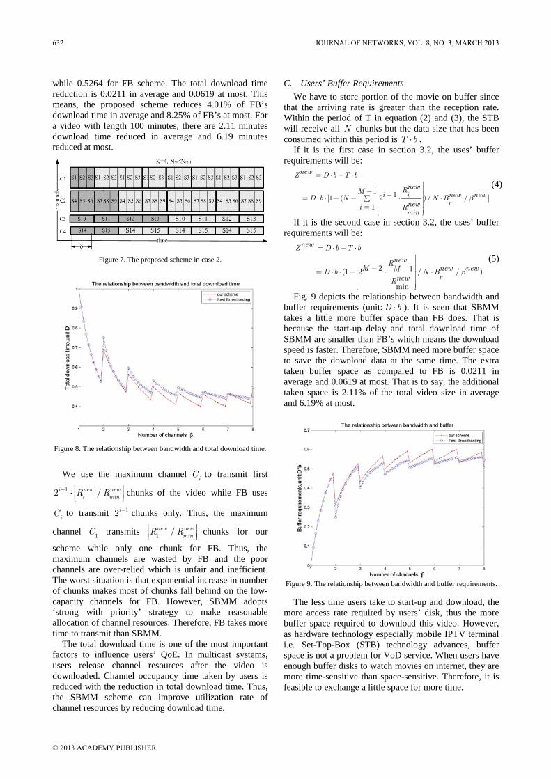
while 0.5264 for FB scheme. The total download time reduction is 0.0211 in average and 0.0619 at most. This means, the proposed scheme reduces 4.01% of FB’s download time in average and 8.25% of FB’s at most. For a video with length 100 minutes, there are 2.11 minutes download time reduced in average and 6.19 minutes reduced at most.

Figure 7. The proposed scheme in case 2.

Figure 8. The relationship between bandwidth and total download time.

We use the maximum channel iC to transmit first 12 /i new new

i minR R chunks of the video while FB uses

iC to transmit 12i chunks only. Thus, the maximum

channel 1C transmits 1 /new newminR R

chunks for our

scheme while only one chunk for FB. Thus, the maximum channels are wasted by FB and the poor channels are over-relied which is unfair and inefficient. The worst situation is that exponential increase in number of chunks makes most of chunks fall behind on the low-capacity channels for FB. However, SBMM adopts ‘strong with priority’ strategy to make reasonable allocation of channel resources. Therefore, FB takes more time to transmit than SBMM.

The total download time is one of the most important factors to influence users’ QoE. In multicast systems, users release channel resources after the video is downloaded. Channel occupancy time taken by users is reduced with the reduction in total download time. Thus, the SBMM scheme can improve utilization rate of channel resources by reducing download time.

C. Users’ Buffer Requirements We have to store portion of the movie on buffer since

that the arriving rate is greater than the reception rate. Within the period of T in equation (2) and (3), the STB will receive all N chunks but the data size that has been consumed within this period is T b .

If it is the first case in section 3.2, the uses’ buffer requirements will be:

1 1 [1 ( 2 ) / / ]1

newZ D b T b

newRM i new newiD b N N Brnewi R

min

(4)

If it is the second case in section 3.2, the uses’ buffer requirements will be:

2 1 (1 2 / / )

min

newZ D b T b

newRM new newMD b N B

rnewR

(5)

Fig. 9 depicts the relationship between bandwidth and buffer requirements (unit: D b ). It is seen that SBMM takes a little more buffer space than FB does. That is because the start-up delay and total download time of SBMM are smaller than FB’s which means the download speed is faster. Therefore, SBMM need more buffer space to save the download data at the same time. The extra taken buffer space as compared to FB is 0.0211 in average and 0.0619 at most. That is to say, the additional taken space is 2.11% of the total video size in average and 6.19% at most.

Figure 9. The relationship between bandwidth and buffer requirements.

The less time users take to start-up and download, the

more access rate required by users’ disk, thus the more buffer space required to download this video. However, as hardware technology especially mobile IPTV terminal i.e. Set-Top-Box (STB) technology advances, buffer space is not a problem for VoD service. When users have enough buffer disks to watch movies on internet, they are more time-sensitive than space-sensitive. Therefore, it is feasible to exchange a little space for more time.



D. Bandwidth Utilization

According to section 2.2, iC can transmit 12 /i new new

i minR R chunks, 1,2,..., ( )i M M K ,

only M out of K channels are used in SBMM. Thus, the total bandwidth requirements taken by the proposed

scheme is newBW , then 1

Mnew new

ii

BW W

. For FB

scheme, the bandwidth requirements FBBW are equal to

FBi

FBi

W b

W

.

In actual scene, the given bandwidth resources may discrete. Some scattered channel rates may be lower than the video consumption rate. In FB scheme, these channels must be discarded otherwise the theoretical value of FB can’t be reached. While in our proposed scheme, we make use of these channels to transmit low-priority chunks. Therefore, we define bandwidth utilization here as the ratio between bandwidth used for transmission and total given bandwidth. It represents the bandwidth can be used by the scheme. Thus, for a given bandwidth newB , the bandwidth utilization newU for our scheme is:

1

Mnewinew

new inew new

WBW

UB B

(6)

For FB scheme, for a given bandwidth B the bandwidth utilization FBU is equal to the sum of all bandwidth which is not less than the consumption rate, then

FBi

FBi

W bFB

W

UB

(7)

Fig. 10 depicts the bandwidth utilization of our scheme compared with that of FB. Obviously, bandwidth utilization of our scheme is much larger than that of FB. Due to different SNR of wireless link lead to different channel capacities, there are some low-capacity channels in wireless system. Any channel resources regardless of channel capacities can be used by SBMM; however, the channels whose capacities are smaller than the consumption rate could not be used by FB scheme according to the assumption of FB. Thus, SBMM can make use of bandwidth resources effectively.

We also simulate the proposed scheme and FB scheme under the same bandwidth utilization. The simulation results are shown in table 1. As we can see from table 1, the start-up delay and total download time of our scheme are 47.92% and 20.22% fewer than that of FB in average, while the buffer requirements are 23.08% more than that of FB. Therefore, the start-up delay, download time and buffer requirements results under the same bandwidth utilization are similar to that under the same SNR. Therefore, the proposed scheme performs better in terms of user’s waiting time than FB under the same bandwidth utilization.

Figure 10. The bandwidth utilization

TABLE 1 PERFORMANCE COMPARISON UNDER THE SAME BANDWIDTH

UTILIZATION

IV. CONCLUSIONS

In current mobile IPTV such as VoD services, 80% of users request for 20% contents, thus multicast mechanism is a feasible solution for the hot videos. Users in the same multicast group can share common channels to access and download. However, different channel conditions such as channel capacities reflected by SNR are not considered in previous works. In this paper, we proposed the SBMM scheme that taken SNR as channel feedback. From numerical analysis and simulations, we can see that the proposed scheme reduces 22.11% of FB’s start-up delay in average and 49.52% of FB’s at most, while reduced 4.01% of FB’s download time in average and 8.25% of FB’s at most in the price of a small increase in buffer requirements. For a video with size of 2.25GB, 48.61MB more size are taken by SBMM in average and 142.62MB at most. At the same time, SBMM can use bandwidth effectively through delivering chunks by priority. As hardware technology especially STB technology develops, disk space is enough for users to watch and download VoD contents, even high definition videos. Therefore, it is reasonable to further reduce users’ start-up delay and total download time in the price of a small increase in buffer requirements. Future work needs to consider how to improve QoS/QoE in VoD service when the channel condition is poor.

ACKNOWLEDGMENT

This work was supported by the Natural Science Foundation of China under Grant (51274018), the

Times Start-up

Delay (D)

Total Download Time (D)

Bandwidth Utilization (%)

Buffer Require- ments (D*b)

SBMM FB SBMM FB SBMM FB SBMM FB 1 0.1045 0.1120 0.5274 0.5650 75.00 75.00 0.4726 0.4350 2 0.1064 0.1140 0.4747 0.5086 75.00 75.00 0.5253 0.4914 3 0.0259 0.0536 0.3851 0.4898 80.00 80.00 0.6149 0.5102 4 0.0252 0.0521 0.3334 0.5011 80.00 80.00 0.6666 0.4989 5 0.0929 0.2168 0.388 0.4526 66.67 66.67 0.6120 0.5474 6 0.0806 0.1881 0.3304 0.5140 66.67 66.67 0.6696 0.4860



National Science & Technology Pillar Program (2013BAK06B03), and National Mobile Communications Research Laboratory (2010D11), Southeast University.

REFERENCES

[1] http://en.wikipedia.org/wiki/Mobile IPTV. [2] Hongjiang Lei, Chao Gao, Yongcai Guo, Zhi Ren& Jun

Huang.(2012). Wait-Time-based Multi-channel MAC Protocol for Wireless Mesh Networks. Journal of Networks, Academy Publisher, 7(8):1208-1213.

[3] Yingying Qin & Rongbo Zhu. (2010). Efficient Routing Algorithm Based on Decision-making Sequence in Wireless Mesh Networks. Journal of networks, Academy Publisher,7(3):502-509.

[4] Qiang H. & Jun Z. (2012). Weight Pick: an efficient packet selection algorithm for network coding based multicast retransmission in mobile communication networks. Wireless Networks, Springer, DOI: 10.1007/s11276-012-0472-x

[5] Knud, E. S. & Reza, T. (2006). Future networks and user requirements – A techno-economic analysis. Wireless Personal Communications, Springer, 38(1):89-101.

[6] Li, S. J. & Li, M. T. (1998). Fast data broadcasting and receiving scheme for popular video service. IEEE Trans. On Broadcasting, 44(1): 100-105.

[7] Sheu, J. P., Han, L. W., Chi, H. C., & Yu, C. T. (2004). A fast video-on-demand broadcasting scheme for popular videos. IEEE Trans. On Broadcasting, 50(2): 120-125.

[8] Azad, S. A., Murshed, M. (2007). An efficient transmission scheme for minimizing user waiting time in video-on-demand systems. IEEE Communication Letters, 17(3): 285-287

[9] Kien, A. H., Ying, C., & Simon, S. (1994). Patching: a multicast technique for true video-on-demand services. In: Proceeding of ACM Multimedia, (pp.191-200)

[10] Yoshihisa, T., Tsukamoto, M., & Nishio, S. (2006). A scheduling scheme for continuous media data broadcasting with a single channel. IEEE Trans. on Broadcasting, 52(1): 1–10.

[11] Hung, C. Y., Hsiang, G. Y., Li, M. T. & Yi, M.C. (2005). An efficient staircase-harmonic scheme for broadcasting popular videos. In: IEEE Consumer Communications and Networking Conference, (pp.122-127).

[12] Yu, C.T., Ming, H. Y. & Chi, H. C. (2002). A recursive frequency-splitting scheme for broadcasting hot videos in VoD service. IEEE Trans. On Communications, 50(8):1348-1355.

[13] Li, S. J. & Li, M.T. (1997). Fast Broadcasting for Hot Video Access. In: Fourth Int. Workshop on Real-Time Computing Systems and Applications Proceeding, (pp.237-243.)

[14] Jong, M.L., Hyo, J. P., Seong, G. C. & Jun, K.C. (2009). Adaptive hybrid transmission mechanism for on-demand mobile IPTV over WiMAX. IEEE Trans. on Broadcasting, 55(2): 468-477.

[15] Sung, S. M., Kyung, T. K., Seongwoo, L., Hee, Y. Y., & Ohyoung, S. (2011). An efficient VoD scheme combining fast broadcasting with patching. In: IEEE Parallel and Distributed Processing with Applications Symposium, (pp.189-194).

[16] Sun, S. P., Myung, J, H., Sung, S. M. & Hee, Y. Y. (2010). An efficient VoD scheme providing service continuity for mobile IPTV in heterogeneous networks. In: IEEE Int.

Computer and Information Technology Conference, (pp.2589-2595)

[17] Reza, T., Anders, H.& Knud, E. S. (2008). Mobile TV as part of IMT advanced: technology, market development, business models and regulatory chanllenges. Wireless personal communications, Springer, 45(4):585-595.

[18] Soohong, P. & Seong, H. J. (2009). Mobile IPTV: Approaches, challenges, standards, and QoS support. IEEE Internet Computing, 13(3):23-31.

[19] IEEE Standard for local and metropolitan area network, part 16. Air interface for fixed broadband wireless access system, (Feb 2006).

Ting T. Liu was born in Shandong, China in 1986. She received the B.S. degree in Qufu Normal University in 2007 and M.S. degree in Beijing Jiaotong University in 2009. She serves as a PhD candidate in Beijing Jiaotong University since 2009. Her research interests are in the areas of wireless communication and networks including streaming media

service in wireless networks, wireless mesh networks and WLAN.

Wei Yang was born in Liaoning, China in 1964. He received the B. S. and M. S. degree, in Electronic Engineering from Liaoning Technical University in 1986 and 1988, and the Ph.D. degree in Electronic Engineering from China University of Mining & Technology in 2000. From Feb. 2000 to Jan. 2002, he was a postdoctoral research fellow at the National Mobile

Communications Research Laboratory, Southeast University, Nanjing, China. Since Feb. 2002, he has been with Beijing Jiaotong University, where he is currently a Professor in the School of Electronics and Information Engineering, Beijing Jiaotong University, China. His main research interests are digital communication system, spread spectrum system and communication signal processing.

Chang L. Xu received the B.E., M.E. and Ph.D degrees in Applied Physics, Signal and Information systems, and Communication and Electronic systems all from Southeast University, Nanjing, China, in 1995, 1998, and 2002, respectively. From April 2002 to August 2003, he was with Beijing Samsung Telecom R&D Institute as a senior engineer. From

September 2003 to October 2004, he served as a research fellow at School of Electrical and Electronic Engineering, Nanyang Technological University, Singapore. He was research scientist with Institute for InfoComm Research, Singapore since October 2004. He joined Intel labs China in February 2008. His research interests are in the areas of digital wireless communication systems and communication theory including CDMA, OFDM, MIMO, channel coding, and space-time coding techniques. Dr. Xu has published over 30 international journal and conference paper and is a Senior Member of IEEE. Young-Il Kim (M’06) received the B.S., M.S., and



http://en.wikipedia.org/wiki/Mobile_IPTV�

http://www.springerlink.com/content/cln6837526j21286/�

http://www.springerlink.com/content/cln6837526j21286/�

Ph.D. degrees in electronic engineering from Kyung-Hee University, Seoul, Korea, in 1985, 1988, and 1996, respectively. Since 1988, he has been with the Electronics and Telecommunication Research Institute,

Daejeon, Korea, where he is currently the Team Leader of the WiBro System Research Team. He is also currently an Adjunct Professor with the Beijing Jiaotong University, Beijing, China. His current research interests include PHY/MAC layer and system architecture of the WiMax/WiBro system.



A Novel Multi-layered Immune NetworkIntrusion Detection Defense Model: MINID

Xufei Zhenga, Yonghui Fangb, Yanhui Zhoua, Jing Zhangba Faculty of Computer and Information Science, Southwest University, Chongqing 400715, China

Email: {zxufei, xiaohui}@swu.edu.cnb Faculty of Electronic and Information Engineering, Southwest University, Chongqing 400715, China

Email: {fyhui, zhangj}@swu.edu.cn

Abstract— Today network security has become an everydayproblem with virtually all computers connected to theInternet. Intrusion detection serves the important functionof identifying malicious activities and determining theirnature, origin, and seriousness. Inspired by the many excel-lent characteristics of biological immune System (BIS), thenetwork intrusion detection system (NIDS) which based onartificial immune system (AIS) has become one of the focusof the intelligent NIDS research and achieved many goodresults in the past studies. However, there are still manyproblems existed in traditional AIS-based NIDS, such aslow detector generation efficiency, low detection true positiverate and high detection false positive rate, etc. Currently, theAIS-based NIDS mainly learn from the adaptive immunemechanism of BIS, but ignoring the rapid response andco-stimulatory mechanism of the innate immune of BIS,thus cause these problems discussed above. In this paper,we combine the innate and adaptive immune mechanismsin BIS and map them to AIS, and propose a novel multi-layered immune network intrusion detection model (MINID)which based on pattern recognition receptor (PRR) theory.Theoretical analysis shows that the MINID model effective-ly integrates the misuse detection and anomaly detectiontechnologies to quickly respond to known network intrusionattacks and discover unknown network intrusion attacks innetwork intrusion detection application.

Index Terms— network intrusion detection, innate immune,adaptive immune, pattern recognition receptor theory, arti-ficial immune system, dual negative selection algorithm

I. INTRODUCTION

ABOUT 20 years ago in November 1988, the Morrisworm spread through the Internet, taking down

thousands of computers [1]. 20 years later, in November2008, the Conficker worm spotted and quickly becameone of the most notorious worms in the history. TheConficker worm owned the worlds largest cloud networkthat the Conficker worm controls 6.4 million computersystems in 230 countries at 230 top level domains globally[2]. Network security was understandably not one of thehigh priority concerns of the Internet designers 20 yearsago, but the consequences of an open public Internet arenow apparent.

Manuscript received December 25, 2012; revised January 2, 2012;accepted April 16, 2012. c⃝ 2005 IEEE.

Project supported by the doctoral fund of southwestern university,china (NO. SWU112038), and the Fundamental Research Funds for theCentral Universities (XDJK2010C025).

Corresponding author: Yonghui Fang, [email protected]

Today network security has become an everyday prob-lem with virtually all computers connected to the Internet.The average Internet user must be constantly vigilantagainst a number of network threats such as virus, spam,worms, Trojans, bots, spyware, and phishing. Intrusiondetection system (IDS) has been a critical componentof network security since the 1980s. Intrusion detectionserves the important function of identifying maliciousactivities and determining their nature, origin, and seri-ousness.

Currently, there are two general categories of intrusiondetection technologies - anomaly detection and misusedetection [3]. Anomaly detection identifies activities thatvary from established patterns for users, or groups ofusers. Anomaly detection typically involves the creationof knowledge bases that contain the profiles of themonitored activities. Misuse detection is the process ofattempting to identify instances of network attacks bycomparing current activity against the attack signatures ofan attacker. Most current approaches to misuse detectioninvolve the use of rule-based expert systems to identifyindications of known attacks. Essentially, the IDS looksfor a specific attack that has already been documented.Like a virus detection system, misuse detection softwareis only as good as the database of attack signatures that ituses to compare packets against. While anomaly detectiontypically utilizes threshold monitoring to indicate when acertain established metric has been reached, misuse detec-tion techniques frequently utilize a rule-based approach.However, anomaly detection is less efficient in identifyingknown attacks, misuse detection is less successful inidentifying attacks which vary from expected patterns.

Biological immune system (BIS) has many excellentcharacteristics, such as diversity, tolerance, memory, dis-tribution, adaptability, robustness, etc., and be able toresist constantly changing pathogens in a distributed andresource-constrained environment. Inspired by the manyexcellent characteristics of BIS, more and more computersecurity researchers integrate biological immune mech-anism into the network intrusion detection technologies[4]–[7], the network intrusion detection system (NIDS)which based on artificial immune system (AIS) has be-come one of the focus of the intelligent NIDS researchand achieved many good results in the past studies. Theproblems faced by NIDS and BIS are highly similar.



TABLE I.THE CORRESPONDENCE BETWEEN BIS AND NIDS

Biological Immune System Network Intrusion Detection Systemself antigens normal programs, network behaviornon-self antigens malicious programs, network attacksartificial T-Cells T-Cell detectorsimmature antibodies immature detectorsmature antibodies mature detectorsmemory antibodies memory detectorsantigen presenting cells APC detectorscell clonal expansion mature detectors’ replicationself tolerance process negative selection processco-stimulation message activation of negative selectionantigens’ immune response recognition anomaly by detectors

Both of them are required to ensure the health of thesystem and to maintain the stability of the system ina changing environment. Specifically, NIDS and BIShaving the following three similarities. Table I shows thecomparative relationship of NIDS and BIS.

1) The task of NIDS and BIS is similar. The main taskof NIDS is able to timely and accurate detect theintrusion attacks within the system or from network,and to take appropriate defensive measurements, butnot do any interventions to the normal behaviorswithin the system or from network. The main func-tion of BIS is to distinguish between self antigenand non-self antigen cells, and to eliminate harmfulnon-self antigen cells, but to self tolerant with selfantigen cells, thus ensuring the normal and orderlywork of biological organisms.

2) The living environment of NIDS and BIS is similar.NIDS being existed in a complex and changingenvironment of Internet network, there is a widerange of computer viruses, worms, trojan horses,and a variety of intrusions, and faced with all kindsof ever-changing invasion means, various levelsof poor software vulnerabilities as well as attacksagainst these vulnerabilities. The BIS is also existedin a complex and changing biological world sur-round with a variety of evolving pathogens withinitself or from outside.

3) The main defense methods used by NIDS and BISis similar. Misuse detection and anomaly detectionare the main detection methods of current NIDS.There are two main biological pathogen defensemechanisms in BIS. One method is the use ofantigen presenting cells to eradication of harmfulpathogens in the innate immune system accordingto the pathogen associated molecular patterns (suchas inflammation, fever, etc.). Another method isthe use of T-cell antibodies which are self-toleratedfrom self antigens’ negative selection process in theadaptive immune system to clear the non-self anti-gens. The NIDS which based on artificial immunesystem (AIS) maps the biological self-tolerance andcell clonal expansion mechanisms to the networkintrusion detection research.

Forrest first introduced the biological immune mech-anism to network intrusion detection research. She pro-

posed the negative selection algorithm (NSA) which sim-ulates the lymphocytes’ self-tolerance process in 1994,and applied to computer virus detection [8]. This pio-neering research has greatly promoted the study of AIS.Hofmeyr further proposed the AIS model “ARTIS” basedon NSA and applied to network intrusion detection [9].Forrest and Hofmeyr laid a good basis of AIS research,after this, a large number of domestic and foreign re-searchers launched a sustained and in-depth studies ofthe theories and methods of the AIS and the AIS-basedintrusion detection technology. Dasgupta applied NSA tofault detection and achieved better results [10]. Gonzalezfirst proposed real-valued negative selection algorithm togenerate detectors [11]. Ji further proposed real-valuednegative selection algorithm with variable-size detectors[12], [13]. Stibor verified the validity of the negativeselection algorithm in the computer virus and networkintrusion detection applications [14]. Williams studied adistributed computer immune system CDIS [15]. Aickelinapplied danger theory to network intrusion detection ap-plication [16], [17]. Twycross put forward the Libtissueframework which integrated innate and adaptive artificialimmune systems and applied to process anomaly detection[5], [18]. Greensmith proposed the DCA algorithm incombination of the innate immune and applied to thedetection of network scanning, computer viruses, Torjanhorses and network worms [19], [20].

The research of network intrusion detection based onAIS is still in constant development. Many researchershave proposed a variety of intrusion detection algorithms,technologies and models which based on AIS, and appliedto computer virus detection, network intrusion detection,spam filtering, fault detection and other fields. However,there are still many problems to be solved:

• The AIS-based NIDS mainly using traditional low-efficient NSA to generate detectors. The inefficien-cy problem of NSA was discussed in refs. [21],the probability of candidate detectors to maturedby passing the negative selection process is P =(1− Pm)

Ns , where Pm is the match probability ofcandidate detector and antigen, Ns is the training setsize; thus with the increase of Ns, P will tend to be 0ultimately; moreover, N0 =

− ln(Pf )

Pm·(1−Pm)Nscandidate

detectors are needed to reach the given failure prob-ability Pf ≈ e−Pm·Nd , which means that the countof candidate detectors N0 is exponentially related tothe count of training set Ns, and the time complexityof NSA is O (N0 ·Ns) = O

(− ln(Pf )·Ns

Pm·(1−Pm)Ns

). The

extreme low detector generation efficiency limitedthe application of NSA [14], [21].

• The AIS-based NIDS exist the shortcoming of highfalse positive detection rate. The mathematical verifi-cation of it. As indicated in refs. [22], the traditionalNSAs inherited from the BIS that the self antigensand detectors keep relatively stable, thus these N-SAs use a statically definition of the antigens anddetectors. However, the normal and abnormal stateconstantly changes in the actual network intrusion



detection applications, and these traditional NSAsdid not consider the detectors’ dynamic update, thusresulting in a high false positive rate of these NSAs.The false positive rate of traditional NSAs is Pf =1 − (1− Pm)|D|, where |D| is the number of de-tectors and Pm is the match probability of candidatedetector and antigen. Pm = (l−r)·2r/3 in the stringrepresented NSAs [8] and Pm = rd ·

∏d/2/Γ(d/2+

1) in the real-valued NSAs [13], where Pm is aconstant when string length l, matching bits r, datadimensions d and detector radius r are determined.

• The NIDS which based on danger theory,TLR and DCA algorithms which inspiredfrom innate immune system is still difficultto achieve satisfactory detection rate. Thedetection rate of DCA is mainly determinedby the signal processing equation Output =(∑

(Pn · Pw) +∑

(Dn ·Dw) +∑

(Sn · Sw)) ·(1 + I) [17], [19], where Pn, Dn and Sn are theinput signal value of category PAMP (P ), danger(D), and safe (S) for all signals (n), Pw, Dw andSw are the related weights of category PAMP (P ),danger (D), and safe (S) for all signals (n), and Irepresents the inflammation signal.

The defects of the current AIS-based intrusion detectionalgorithms, technologies and models greatly hinder thedevelopment of the AIS-based network intrusion detectiontechnologies. Forrest and Timmis have pointed out thatthe lack of metaphors for some key biological immunemechanism is the main cause of these poor performancealgorithms and models [23], [24]. Therefore, it is animportant theoretical and applied research issue that thefurther extract effective immune mechanism from BIS tobuild and/or improve novel AIS-based network intrusiondetection algorithms and models.

The theory of pattern recognition receptors (PRR) isan important theory that connect the innate and adaptiveimmune mechanism in BIS [25]. The validation of thePRR theory obtained the 2011 Nobel Prize in Physiologyor Medicine [26]. Currently, the AIS-based NIDS mainlylearn from the adaptive immune mechanism of BIS, butignoring the rapid response and co-stimulatory mechanis-m of the innate immune of BIS, thus cause these problemsdiscussed above.

In this paper, we combine the innate and adaptiveimmune mechanisms in BIS and map them to AIS, andpropose a novel multi-layered immune defense archi-tecture based on PRR theory, and build an intelligent,distributed and multi-layered network intrusion detectionmodel to solve and/or improve the current AIS-basedintrusion detection technologies.

The rest of this paper is organized as follows. Insection 2 we discuss some design principles of AIS-based NIDS. In section 3 we propose the multi-layeredimmune network intrusion detection model (MINID). Theconclusions are given in section 4.

II. DESIGN PRINCIPLES OF MINID MODEL

Stepney et al. proposed a conceptual framework basedon bio-inspired, and discussed some important features ofthe conceptual framework, such openness, diversity, inter-action, structure, scalability, and etc. [27]. De Castro et al.proposed a general AIS framework based on the adaptiveimmune system in BIS [28]. Based on the characteristicsof the adaptive immune system, Knight et al. put forward6 design principles for AIS, which mainly focus on theinstantiation problem of idiotypic immune network [29].Based on comprehensive synthesize of previous studies,Twycross presented 9 design principles of the secondgeneration artificial immune system which combined theinnate immune with the adaptive immune system, andproposed the Libtissue system architecture [7], [18].

Figure 1. An outline conceptual framework for a bio-inspired compu-tational domain [27].

Figure 2. The engineered artificial immune system framework [28].

As Forrest and Timmis have pointed out, the lack ofmetaphors for some key biological immune mechanismis the main cause of these poor performance algorithmsand models [23], [24]. The theory of pattern recognitionreceptors (PRR) is an important theory that connect theinnate and adaptive immune mechanism in BIS [25]. Thevalidation of the PRR theory obtained the 2011 NobelPrize in Physiology or Medicine [26].

In 1989, the famous immunologist Janeway first pro-posed the PRR theory [25]. In biology, the PRR modeladded additional layer of pathogen-associated molecularpatterns (PAMP) to the self-nonself model [30]. The PRRmodel assumes that antigen presenting cell (APC) arequiescent until they are activated via encoded patternrecognition receptors that recognize conserved PAMPs.

Inspired by this metaphor, we put forward the multi-layered immune defense model (MINID) which integrate



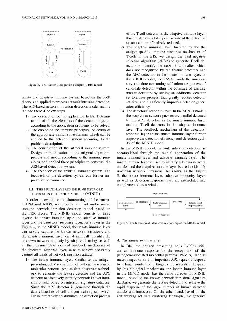
PAMP

APC

recogn

ate

activ

ate

antigen

T-cell

co-stimulate

recogn

ate

signal 2 signal 1

Figure 3. The Pattern Recognition Receptor (PRR) model.

innate and adaptive immune system based on the PRRtheory, and applied to process network intrusion detection.The AIS-based network intrusion detection model mainlyinclude these 4 below steps.

1) The description of the application fields. Determi-nation of all the elements of the detection systemaccording to the application problems to be solved.

2) The choice of the immune principles. Selection ofthe appropriate immune mechanisms which can beapplied to the detection system according to theproblem description.

3) The construction of the artificial immune system.Design or modification of the original algorithm,process and model according to the immune prin-ciples, and applied these principles to construct theAIS-based detection system.

4) The feedback of the artificial immune system. Thefeedback of the detection system can further im-prove its performance.

III. THE MULTI-LAYERED IMMUNE NETWORKINTRUSION DETECTION MODEL: (MINID)

In order to overcome the shortcomings of the curren-t AIS-based NIDS, we propose a novel multi-layeredimmune network intrusion detection model based onthe PRR theory. The MINID model consists of threelayers: the innate immune layer, the adaptive immunelayer and the detectors’ response layer. As shown as theFigure 4, in the MINID model, the innate immune layercan rapidly capture the known network intrusions, andthe adaptive immune layer can dynamically identify theunknown network anomaly by adaptive learning, as wellas the dynamic detection and feedback mechanism ofthe detectors’ response layer, so as to achieve accuratelycapture all kinds of network intrusion attacks.

1) The innate immune layer. Similar to the antigenpresenting cells’ recognition of pathogen-associatedmolecular patterns, we use data clustering technol-ogy to generate the feature detector and the APCdetector to effectively identify network known intru-sion attacks based on intrusion signature database.Since the APC detector is generated through thedata clustering of self antigen training set, whichcan be effectively co-stimulate the detection process

of the T-cell detector in the adaptive immune layer,thus the detection false positive rate of the detectionsystem can be effectively reduced.

2) The adaptive immune layer. Inspired by the theantigen-specific immune response mechanism ofT-cells in the BIS, we design the dual negativeselection algorithm (2NSA) to generate T-cell de-tectors to identify the network anomalies whichdoes not recognized by the feature detectors andthe APC detectors in the innate immune layer. Inthe MINID model, the 2NSA avoids the unneces-sary and time-consuming self-tolerance process ofcandidate detector within the coverage of existingmature detectors by adding an additional detectorset tolerance process, thus greatly reduces detectorset size, and significantly improves detector gener-ation efficiency.

3) The detectors’ response layer. In the MINID model,the suspicious network packets are parallel detectedby the APC detectors in the innate immune layerand the T-cell detectors in the adaptive immunelayer. The feedback mechanism of the detectors’response layer to the innate immune layer furtherimprove the detection efficiency and detection qual-ity of the MINID model.

In the MINID model, network intrusion detection isaccomplished through the mutual cooperation of theinnate immune layer and adaptive immune layer. Theinnate immune layer is used to identify a known networkattacks, and the adaptive immune layer is used to identifyunknown network intrusions. As shown as the Figure5, the innate immune layer, adaptive immunity layer,as well as detection response layer are interrelated andcomplemented as a whole.

innate immune

layer

co-stimulate activate

memory feedback

rapid response

adaptive immune

layer

detection and

response layer

Figure 5. The hierarchical interactive relationship of the MINID model.

A. The innate immune layer

In BIS, the antigen presenting cells (APCs) initi-ate an immune response by the recognition of thepathogen-associated molecular patterns (PAMPs), such asmacrophages (a kind of important APC) quickly respondto a large number of pathogens are identified. Inspiredby this biological mechanism, the innate immune layerin the MINID model has the same purpose. In MINIDmodel, based on the known network intrusions signaturedatabase, we generate the feature detectors to achieve therapid response of the large number of known networkattacks and intrusions. On the other hand, based on theself training set data clustering technique, we generate



generation of the

APC detectors

generation of feature detectors

based on intrusions’ signature

database

generation of Self antigen

training set

computer program,

network data package

antigen presenting

data clustering

randomly generate

candidate detectors

selection of T-cell

candidate detector

generation of T-cell

semi-mature detector

generation of T-cell

mature detector

pass the 1st

negative

selection process

pass the 2nd

negative

selection process

dual negative

selection process

mature detector set

death

not activate in life cycle

failu

re of th

e neg

ativ

e selection

pro

cess

memory

detector set

clone expansion

high quality

detectors

the adaptive

immune layer

detection

rapid response

feedback of the detected network intrusions

detection of the T-cell

mature detectors

detection of the memory detectors

detection of the feature

and APC detectors

co-stim

ula

tion

antigen

presenting

the undetermined network data packages further

submitted mature detectors and memory detectors

add new attack signature to database

Figure 4. the multi-layered immune defense architecture of the MINID model.

the APC detectors to co-simulate the adaptive immunelayer and thus to avoid the high false positive problem oftraditional negative selection algorithms (NSAs).

The innate immune layer is a kind of non-specificdefense strategy, which does not require time-consumingself-tolerance process and thus have a rapid responseability. On the other hand, for the APC detector is theself data clustering results and thus can effectively avoidmisidentification of self elements (that is the false positiveproblem existed NSAs). Specifically, the main functionmodule of the innate immune layer are as follows.

• Antigen presenting module. The antigen presentingprocess is the data normalization process to generatethe self antigen set based on normal data in theretrieved network connection data package.

• Feature detectors’ generation module. The featuredetector set generation process is the process togenerate feature detectors based on the known net-work intrusion signature database, that is the misusedetection technology.

• APC detectors’ generation module. The APC detec-tor set generation process is the process to generatethe APC detectors based on self antigen set dataclustering, the complete cluster generation processof the APC detector is shown as the Figure 6.

begin

select self antigens

training set

self-clustering According to

the default parameters

generate the APC detectors

according to the clustering results

APC detector radius is

appropriate or not?

end

adjust data clustering

parameters

N

Y

Figure 6. The APC detector generation process in innate immune layer.

B. The adaptive immune layer

In BIS, T cells’ maturation process in the bone mar-row is achieved through self-tolerance to eliminate self-reaction, and is based on the recognition of self/non-selfto achieve the immune response to pathogens. Inspiredthis biological adaptive immune mechanism, the negativeselection algorithm was firstly proposed by Forrest in



1994 [8]. It was designed by modeling the biologicalprocess in which T-cells mature in thymus through beingcensored against self cells. The Real-valued representa-tion NSA (RNSA) [11] encodes antigens and antibodiesusing normalized real-valued range [0, 1], and affinity wascalculated by the Minkowski distance function in unithypercube of n−dimensional real-valued space [0, 1]

n .The RNSA with Variable-sized Detector algorithm (V-Detector) was proposed in refs. [12] [13], in which thedetector radius was dynamically determined by the nearestself margin. The V-Detector achieved better detectionresults than RNSA in simulation experiments.

Both RNSA and V-Detector algorithm employed oncenegative selection process to eliminate the self-recognizedinvalid detectors by matching candidate detector with thewhole self training set. In the negative selection process,it is only considered the relationship between candidatedetector and training set but without any consideration ofrepetitive coverage of candidate detector with detector set,which bring about the unnecessary and time-consumingself-tolerance of the candidate detector which repetitivecovered. Thus, the unnecessary and time-consuming self-tolerance of these candidate detectors resulted in an ex-cessive count of detectors and extremely lowered detectorgeneration efficiency, and increased the computation timecomplexity of these NSAs. Stibor et al. [21] point out thatthe unacceptable high time cost of NSAs is caused by theinefficiency of the detector generation process, and whichsignificantly limited the applications of AIS.

The dual negative selection algorithm (2NSA) is adopt-ed in this paper, which includes two negative selectionprocesses to generate detector set. The 1st negative s-election process: the randomly generated candidate de-tector tolerates with detector set, and eliminated it whenrecognized by any mature detector. The successful tol-erated candidate detector becomes semi-mature detector,whose center is located outside the coverage of existingdetector set. The 2nd negative selection process: thesemi-mature detector self-tolerates with the training set,and eliminated it when recognized by any self element.The successful tolerated semi-mature detector becomesmature detector and joins to the detector set. The 2NSAalgorithm effectively avoids the unnecessary and time-consuming self-tolerance of candidate detector whosecenter is located in the coverage of existing detector set,which greatly reduces detector set size, improves detectorgeneration efficiency, and decreases time complexity ofcurrent RNSAs. The complete negative selection processof the 2NSA is shown as the Figure 7.

The 1st negative selection process: every randomlygenerated candidate detector dnew tolerates with maturedetector set and becomes semi-mature detector whenit does not match any existing mature detector. Thecandidate detector dnew was randomly generated withcenter X(x1, x2, ..., xn) firstly, and then calculated theEuclidean distance dis(dnew, di) between the candidatedetector and every mature detector di in the detectorset D. The candidate detector successfully tolerated with

the 2

nd

negativ

e sele

ction

process

the 1

stn

egativ

e selection

pro

cess

begin

initialize the training set,

and detector set

randomly generate the

candidate detector dnew

Is the candidate detector dnew

recognized by detector set D?

pass the 1st

negative selection

process, and generate the

semi-mature detector dsemi

Is the semi-mature detector dsemi

recognized by any self training element?

pass the 2nd

negative selection process, and

generate the mature detector dmat

expC C

end

N

Y

D !

" #matD D d !

Y

N

N

Y

Figure 7. The dual negative selection process in adaptive immune layer.

the detector set and becomes a semi-mature detectordsemi if the dnew satisfies the formula (dis(dnew, di) >rdi i = 1, 2, ..., Nd). Otherwise, the candidate de-tector dnew will be eliminated if it been recognized byany mature detector, and a new candidate detector dnewwill be randomly generated and the 1st negative selectionprocess be restarted again.

The 2nd negative selection process: the semi-maturedetector dsemi tolerates with self set and becomes maturedetector when it does not match any self element. Theshortest distance dismin(dsemi, sj) between the centerY (y1, y2, ..., yn) of semi-mature detector dsemi and everyself element of training set was calculated according to theEuclidean distance. The dsemi successfully tolerated withthe training set and becomes a mature detector dmat if theformula (dismin(dsemi, sj) > rs j = 1, 2, ..., Ns) besatisfied, the mature detector dmat joins to the detectorset D, that is D ← D ∪ {dmat}, the radius of dmat isrd = dismin(dsemi, sj)− rs. Otherwise, the semi-maturedetector dsemi will be eliminated if it been recognized byany self element, and the 1st negative selection process



will be restarted again.

C. The detectors’ response layer

The detectors’ response layer is the control and feed-back center of entire MINID model. The detectors’ gen-erated in the innate and adaptive immune layer performparallel and dynamic detection of the coming networkdata packages in the detectors’ response layer, and providethe feedback to the innate and adaptive immune layer,as well as coordinate the various modules in the MINIDmodel. In the MINID model, different kind of detectorsare generated at different immune layer (the feature andAPC detectors are generated in the innate immune layer,and the T-cell detectors are generated through negativeselection algorithm in the adaptive immune layer), thusthe detection of network data packages are performedin parallel and dynamic manner. The complete detectionprocess of the detectors’ response layer is shown as theFigure 8.

begin

input samples

match with any

APC detector?

generate co-stimulation

of T-cell detectors

match with any

T-cell detector?

anomaly

end

normal

Y

Y

N

Y

Nwithin the scope of APC

detectors co-stimulation?

N

Y

match with any

feature detector?

Y

N

Figure 8. The detection process in detectors’ response layer.

IV. THE CHARACTERISTIC OF THE MINID MODEL

The MINID model is a multi-layered immune defensenetwork intrusion detection model which integrated innateand adaptive immune systems. Through the analysis of themodel, we summary the MINID model has the following

excellent features: hierarchy, rapid response, adaptability,distributivity and robustness.

A. HierarchyIn the MINID model, the detector generation and the

detection of the network suspicious packets are hierar-chical. The innate immune layer is used to generate thefeature detectors and the APC detectors, the adaptiveimmune layer is used to generate the T-cell detectors,as well as the detectors’ response layer is used to thedetection of network intrusions. The innate immunitylayer has the capability of rapid response and can effectiveresponse to known network attacks according to theintrusion signature database. However, the innate immunelayer does not have the adaptive learning ability, thuscan not generate detectors to identify unknown networkattacks and intrusions. The adaptive immune layer hasadaptive learning ability to constantly evolve and adapt tothe changes of network environment, and can effectivelydetect unknown attacks and network intrusions.

B. Rapid responseIn the MINID model, the innate immunity layer can

effective response to a large number of known networkattacks and intrusions according to the network intrusionsignature database. On the other hand, the feedback mech-anism of the detectors’ response layer can add the newlyidentified network intrusions to the network intrusionsignature database.

C. AdaptabilityTraditional signature-based intrusion detection methods

does not have adaptability that they can only detectknown attacks and intrusions, but unable to detect theunknown intrusions or the variant of known intrusions,which resulting in these systems with high false negativerate. In the MINID model, the adaptive immune layer hasadaptive learning ability to constantly evolve and adaptto the changes of network environment by means of self-tolerance, and thus can effectively detect unknown attacksand network intrusions. In addition, the mutual conversionbetween the memory detector and mature detector, aswell as the dynamic updates of memory detector furtherimprove the system’s adaptability and reduce the falsenegative rate.

D. DistributivityThe distribution of the MINID model is primarily

gained through the following three mechanisms: neg-ative selection, co-stimulatory, and detectors’ dynamicevolution. In the negative selection algorithm, the self-tolerated T-cell detectors do not need to communicatewith each other to achieve network intrusion detection(distributed detection). The co-stimulatory signal con-trol the T-cell detectors’ detection of network intrusions(distributed control). Detectors’ replication, mutation andclear provide the resource allocation and control of theentire detection system (distributed evolution).



E. Robustness

Robustness is defined as “the ability of a system toresist change without adapting its initial stable config-uration” [31]. The robustness of the MINID model isimplemented in a distributed manner, every detector isindependent and their interaction together to provideglobal protection. There is no control center to achievethe control of detectors, and any detector’s failure willnot affect the whole detection system.

V. CONCLUSIONS

The defects of the current AIS-based intrusion detectionalgorithms, technologies and models greatly hinder thedevelopment of the AIS-based network intrusion detectiontechnologies. The lack of metaphors for some key biolog-ical immune mechanism is the main cause of these poorperformance algorithms and models. The innate immunesystem co-stimulate the adaptive immune system to formorganic whole immune protection mechanism in BIS.

The theory of pattern recognition receptors (PRR) isan important theory that connect the innate and adap-tive immune mechanism in BIS. Based on PRR theory,the multi-layered immune network intrusion detection(MINID) model which integrate innate and adaptive im-mune system is proposed in this paper. We illustratehow the innate immune layer, adaptive immune layer anddetectors’ response layer defend the network intrusionsin detail. Theoretical analysis shows that the MINIDmodel effectively integrates the misuse detection andanomaly detection technologies to quickly respond toknown network intrusion attacks and discover unknownnetwork intrusion attacks in network intrusion detectionapplication.

REFERENCES

[1] H. Orman, “The morris worm: A fifteen-year perspective,”IEEE Security and Privacy, vol. 1, no. 5, pp. 35–43, Sept.2003.

[2] G. Lawton, “On the trail of the conficker worm,” Comput-er, vol. 42, no. 6, pp. 19–22, June 2009.

[3] O. Depren, M. Topallar, E. Anarim, and M. K. Ciliz, “Anintelligent intrusion detection system (ids) for anomalyand misuse detection in computer networks,” Expert Syst.Appl., vol. 29, no. 4, pp. 713–722, Nov. 2005.

[4] P. Musilek, A. Lau, M. Reformat, and L. Wyard-Scott,“Immune programming,” Inf. Sci., vol. 176, no. 8, pp. 972–1002, Apr. 2006.

[5] J. Twycross and U. Aickelin, “Biological inspiration forartificial immune systems,” in Proceedings of the 6thinternational conference on Artificial immune systems, ser.ICARIS’07. Berlin, Heidelberg: Springer-Verlag, 2007,pp. 300–311.

[6] Z. Ma and X. Zheng, “Multi-layer intrusion detection anddefence mechanisms based on immunity,” in Proceedingsof the 2008 Second International Conference on Geneticand Evolutionary Computing, ser. WGEC ’08. Washing-ton, DC, USA: IEEE Computer Society, 2008, pp. 281–284.

[7] J. Twycross and U. Aickelin, “Information fusion in theimmune system,” Inf. Fusion, vol. 11, no. 1, pp. 35–44,Jan. 2010.

[8] S. Forrest, A. S. Perelson, L. Allen, and R. Cherukuri,“Self-nonself discrimination in a computer,” in Proceed-ings of the 1994 IEEE Symposium on Security and Privacy,ser. SP ’94. Washington, DC, USA: IEEE ComputerSociety, 1994, pp. 202–212.

[9] S. A. Hofmeyr and S. A. Forrest, “Architecture for anartificial immune system,” Evol. Comput., vol. 8, no. 4,pp. 443–473, Dec. 2000.

[10] D. Dasgupta and S. Forrest, “Artificial immune systems inindustrial applications,” in Proceedings of the InternationalConference on Intelligent Processing and Manufacturingof Materials, 1999, pp. 257–267.

[11] F. A. Gonzalez and D. Dasgupta, “Anomaly detection usingreal-valued negative selection,” Genetic Programming andEvolvable Machines, vol. 4, no. 4, pp. 383–403, Dec. 2003.

[12] J. Zhou, “Negative selection algorithms: from the thymusto v-detector,” Ph.D. dissertation, The University of Mem-phis, 2006.

[13] J. Zhou and D. Dasgupta, “V-detector: An efficient nega-tive selection algorithm with “probably adequate” detectorcoverage,” Information Science, vol. 19, no. 9, pp. 1390–1406, 2009.

[14] T. Stibor, J. Timmis, and C. Eckert, “A comparative studyof real-valued negative selection to statistical anomaly de-tection techniques,” in Proceedings of the 4th internationalconference on Artificial Immune Systems, ser. ICARIS’05.Berlin, Heidelberg: Springer-Verlag, 2005, pp. 262–275.

[15] P. D. Williams, K. P. Anchor, J. L. Bebo, G. H. Gunsch,and G. D. Lamont, “Cdis: Towards a computer immunesystem for detecting network intrusions,” in Proceedingsof the 4th International Symposium on Recent Advancesin Intrusion Detection, ser. RAID ’00. London, UK:Springer-Verlag, 2001, pp. 117–133.

[16] U. Aickelin, P. Bentley, S. Cayzer, J. Kim, and J. McLeod,“Danger theory: The link between ais and ids?” in ArtificialImmune Systems, ser. Lecture Notes in Computer Science.Springer Berlin Heidelberg, 2003, vol. 2787, pp. 147–155.

[17] U. Aickelin and J. Greensmith, “Sensing danger: Innateimmunology for intrusion detection,” Inf. Secur. Tech. Rep.,vol. 12, no. 4, pp. 218–227, Sept. 2007.

[18] J. P. Twycross, “Integrated innate and adaptive artificialimmune systems applied to process anomaly detection,”Ph.D. dissertation, The University of Nottingham, 2007.

[19] J. Greensmith, U. Aickelin, and S. Cayzer, “Detectingdanger: The dendritic cell algorithm,” Robust IntelligentSystems, vol. 12, pp. 89–112, 2008.

[20] J. Greensmith, U. Aickelin, and G. Tedesco, “Informationfusion for anomaly detection with the dendritic cell algo-rithm,” Inf. Fusion, vol. 11, no. 1, pp. 21–34, Jan. 2010.

[21] T. Stibor, P. Mohr, J. Timmis, and C. Eckert, “Is negativeselection appropriate for anomaly detection?” in Proceed-ings of the 2005 conference on Genetic and evolutionarycomputation, ser. GECCO ’05. New York, USA: ACM,2005, pp. 321–328.

[22] T. Stibor, J. Timmis, and C. M. Eckert, “On the ap-propriateness of negative selection defined over hammingshape-space as a network intrusion detection system,”in Proceedings of the IEEE Congress on EvolutionaryComputation, CEC 2005, Edinburgh, UK. IEEE, 2005,pp. 995–1002.

[23] S. Forrest and C. Beauchemin, “Computer immunology,”Immunological Reviews, vol. 216, pp. 176–197, 2007.

[24] J. Timmis, A. Hone, T. Stibor, and E. Clark, “Theoreticaladvances in artificial immune systems,” Theor. Comput.Sci., vol. 403, no. 1, pp. 11–32, Aug. 2008.

[25] C. A. Janeway, “Approaching the asymptote? evolutionand revolution in immunology,” in Cold Spring Harborsymposia on quantitative biology, vol. 54, no. part 1, 1989,pp. 1–13.



[26] Nobelprize.org, “The nobel prize in physiology ormedicine 2011,” http://www.nobelprize.org/nobel prizes/medicine/laureates/2011/, Dec 2012.

[27] S. Stepney, R. E. Smith, J. Timmis, A. M. Tyrrell, M. J.Neal, and A. N. W. Hone, “Conceptual frameworks forartificial immune systems,” Int. Journ. of UnconventionalComputing, vol. 1, no. 3, pp. 315–338, 2005.

[28] L. N. de Castro and F. J. Von Zuben, “Learning andoptimization using the clonal selection principle,” Trans.Evol. Comp, vol. 6, no. 3, pp. 239–251, June 2002.

[29] T. Knight and J. Timmis, “A multi-layered immune in-spired approach to data mining,” in Proceedings of the4th International Conference of Recent Advances in SoftComputing, 2003, pp. 266–271.

[30] R. Medzhitov and C. Janeway Jr, “Decoding the patternsof self and nonself by the innate immune system.” Science,vol. 296, no. 5566, pp. 298–300, 2002.

[31] A. Wieland and C. M. Wallenburg, “Dealing with supplychain risks: Linking risk management practices and strate-gies to performance,” International Journal of PhysicalDistribution and Logistics Management, vol. 42, no. 10,pp. 887–905, 2012.

Xufei Zheng received his Ph.D degree in the College ofComputer Science in Sichuan University, China, in 2012. From2004 to now, he is a lecturer in the School of Computer andInformation Science in Southwest University, China. His currentresearch interests include computer network security, artificialimmune system and software testing theory.

Yonghui Fang received her Master degree in Computer Sciencefrom Southwest China Normal University in 2004. Currently,she is a Ph.D student in the College of Electronic Engineeringin Chongqing University, China. From 2002 to now, she is alecturer in the School of Electronic and Information Engineeringat Southwest University, China. Her current research interests in-clude Intelligent Information Processing and computer networksecurity.

Yanhui Zhou received his Bachelor and Master degree insoftware engineering from Southwest University, China. He iscurrently an associate professor and a PhD student in the Facultyof Computer and Information Science at Southwest University.His research interests include Information Security and testing,artificial intelligence in software engineering, and automationtechnologies in software testing.

Jing Zhang received her Master of engineering in ComputerApplication from Southwest China Normal University in 2002.As a visiting scholar, she studied in North East Wales Institute ofHigher Education, United Kingdom in 2004. She is currently anassociate professor in the Faculty of Electronic and InformationEngineering at Southwest University. Her research interestsinclude software engineering, database and cloud computing.



Enhancing Node Cooperation in Mobile Ad Hoc Network

S. Kami Makki

Department of Computer Science, Lamar University, Beaumont, Texas, USA Email: [email protected]

Keenan B. Bonds

Department of Computer Science, Norfolk State University, Norfolk, Virginia, USA Email: [email protected]

Abstract—Mobile Ad Hoc Networks (MANET) have been a research interest over the past few years, yet, node cooperation has continually been a recognized issue for researchers. Because of their lack of infrastructure, MANETS depend on the cooperation of intermediate nodes in order to forward or send packets of their own to other nodes in the network. Therefore, nodes located in the central area of the network are used more frequently than the nodes located on the outer boundary. The inner nodes have to forward the packets of other nodes and if there is no payoff for forwarding the packets, the nodes may start to refrain from forwarding the packets of others to save their energy. The Community Enforcement Mechanism has been proposed to force the cooperation of among the nodes and reduce their misbehavior. Although, it provides cooperation among the nodes, it does not essentially increase the network life. In this paper, we present an efficient algorithm to improve the longevity of a MANET based upon more structured nodes cooperation. Index Terms—Mobile Ad Hoc Network, Selfish, Cooperation, Misbehavior

I. INTRODUCTION

A Mobile Ad Hoc Network is a self-configurable wireless network made up of mobile devices, such as laptops, PDAs, smart phones etc.,. MANETS lack infrastructure, meaning that they have no central coordinator [13]. Given that they have no infrastructure, they require multi-hop relays. This means that a packet may be forwarded by more than one node until it reaches its destination. If a node desires to send a packet to a further node that is not in its communication range, it must depend on the intermediate nodes cooperation, which can forward its packets. Nodes adjacent to each other can communicate directly if they are in communication range. With the absence of a fixed infrastructure, the cooperation of nodes is more difficult to be managed since the nodes can move freely around

the network, causing constant link breakage. Therefore, it is not guaranteed that the packets will arrive to their destination.

There are numerous applications that Mobile Ad Hoc Networks are associated with, including military communication, emergency services, commercial products, etc [1]. In order for the applications to operate correctly, each node is required to forward packets for the others. A node can refuse to forward a packet if it does not get any valuable gain from doing so. Therefore, to maintain a functional network, a node must not behave in this manner.

While dealing with Mobile Ad hoc Networks, one faces a plethora of challenges. These include constant link breakage, insufficient node battery power, low bandwidth, and security [13]. As stated earlier, each node is in constant motion, so it is quite common for the links between the nodes to be broken. If a node does not have sufficient battery power, it will fail to forward packets to other nodes. Along with these challenges, the node can refrain from cooperation. Therefore, in MANETS uncooperative nodes are classified into three types: malicious nodes, faulty nodes, and selfish nodes [13]. Malicious nodes can enter networks without authenticating themselves, launching a range of attacks on other nodes such as “blackhole” or “denial of service” (DoS) [2, 12]. Faulty nodes because of hardware malfunctions or software errors will withdraw from the participation of the network. Selfish nodes do not forward packets since they want to save their own resources, such as battery power, for their own sending of packets.

In this paper, the main objective is to label the issues of selfish nodes and introduce an algorithm which encourages nodes to evenly distribute their resources, leading to a functional network. In section II we will introduce related work and different cooperation schemes used in MANETS. Section III will present our proposed algorithm. In Section IV, we will explain the simulation environment and the results from our experiments, followed by our conclusion in Section V.

II. RELATED WORK

A large amount of research has been done to tackle the issue of node cooperation in multi-hop networks. The

This material is based upon the work supported by the National Science Foundation under Grant No. 0851912.

Any opinions, findings, and conclusions or recommendations expressed in this material are those of the author(s) and do not necessarily reflect the views of the National Science Foundation.



cooperation of nodes in MANETS can be classified and divided into two schemes: Virtual currency based schemes and Reputation based schemes. Virtual currency based schemes offer an incentive to the nodes that help to cooperate and forward packets in the network [5, 6, 8]. A node will not receive any help if it does not have any incentives to offer. Reputation based scheme uses the behavior or reputation of the node to mitigate the selfish behavior [3, 4, 7, 9]. In order to attain the reputation of a node, reputation messages can be exchanged with other nodes or it can be obtained through direct observation. We describe these schemes in more detail below.

A. Virtual Currency based Schemes When forwarding a packet for another node, a node

has to use own resources, such as battery life. Without any gain, a node will be hesitant to cooperate to relay packets. To address this problem, uncooperative nodes will be given an incentive in order to forward packets for the other nodes. The incentives are also used to motivate nodes for future cooperation. To reward a node for its services, the virtual currency system [5, 6, 8] uses credit or micro payments. Therefore, virtual currency is used to charge the nodes sending or receiving a message and to reward the nodes that forward these messages. Two examples of the virtual currency system which are discussed below in more detail are Nuglets [6, 8] and Sprite [5].

A.1. Nuglets The virtual currency, Nuglets, developed by Buttyan

and Hubaux, is used to reward/charge for the forwarding of packets [6, 8]. There are two types of models that use Nuglets: Packet purse model, where the source of the packet is charged, and the Packet trade model, in which the destination of packet is charged. In the packet purse model, the source loads the packet with Nuglets equal to at least the number of hops that it takes to reach the destination. Each intermediate node takes the same amount of Nuglets and forwards the packet until it reaches the destination. In the packet trade model, the intermediate nodes use the “trading system”. An intermediate node purchases the packet from the prior node and then trades it to the next node for more Nuglets. This continues until it reaches the destination, where it purchases the packet for the total cost. This system would only function if each node has a valid counter so that the increments/decrements of the Nuglets can be managed equally

A.2. Sprite Sprite uses a credit-based system to offer incentives for

nodes in MANETS to cooperate. This credit-based system manages the rewards and credit charges for each node participating in the forwarding of packets [5]. A receipt is given to a node that receives a message, later reporting it to the credit system when they are come in contact. A node that attempts to forward a packet is benefited, but the amount of credit received depends on if the forwarding was successful. It is only considered successful if the node at the next hop has a receipt to give

the credit system. This method is assumed to have a centralized server to manage these rewards and credit charges.

B. Reputation Based Schemes Reputation based schemes are based on the

performance of nodes in a network. A node is monitored by neighboring nodes, calculating its reputation value. There have several models developed that focuses on a nodes reputation. Three examples that we will discuss are: CONFIDANT [3], CORE [4, 7], and OCEAN [9].

B.1. CONFIDANT In Dynamic Ad-hoc Network, the assessment of nodes’

reputation makes misbehavior of the nodes unattractive [3]. This reputation model focuses on finding the uncooperative nodes and isolating them from the network. Doing this makes the node unattractive, making other nodes want to participate in the network; since no node wants to be established as unattractive. Every node watches the activity of their neighbors, reporting any unusual behavior to a reputation system. If an unusual event occurred too many times, the reputation system deletes all of the routes containing the misbehaving node and notifies its neighbors.

B.2. CORE In Collaborative Reputation, or CORE, a node receives

its reputation based on their contribution to the network [4]. A node that has good reputation, always forwarding other nodes’ packets, it can use the resources of the other nodes. However, nodes that don’t cooperate in the forwarding of packets often get excluded from the network, not being able to send their own packets. There are two components that each node contains [4, 7]: a watchdog mechanism that watches the next node’s transmission to verify that it forwards the packet, and a reputation table that contains the information based from the watchdog mechanism.

B.3. OCEAN In OCEAN [9], which stands for Observation-based

Cooperation Enforcement in Ad- hoc Networks, every node starts off with the rating of zero (0). Every time a node cooperates in the network, their rating increments by plus one (+1). If a node does not forward a packet, their rating goes down by minus two (-2). The node is added to a misbehaving list if it reaches the set threshold, which is negative forty (-40). Traffic that comes from any misbehaving nodes will be rejected; however, they do receive a second-chance after a certain timeout period. The rating does not change, so that if it continues to misbehave, it can be quickly added back onto the faulty list.

B.4. Classes Reputation based schemes can be broken into three

classes: Trust vs. Reputation, Direct vs. Indirect Trust, and Global vs. Local Reputation.

- Trust vs. Reputation [10]: Trust represents the honesty of a node, deciding if it is trustworthy to



forward packets, while reputation represents the behavior of a node, deciding if it is misbehaving or cooperative.

- Direct vs. Indirect Reputation: Direct reputation occurs when a node observes the behavior of a direct neighboring node (one-hop), while indirect reputation occurs when a node receives information about a nodes’ reputation from the other nodes in the network.

- Global vs. Local Reputation [11]: In global reputation, the reputation of a node is shared throughout the network indirectly, while in local reputation, the reputation information of a node is solely based on the direct observation of a neighboring node. CONFIDANT and CORE are examples of both local and global reputation, while OCEAN is an example of only local reputation

C. Community Enforcement Mechanism A functional network should include full cooperation

of nodes within the network. To achieve this, a few characteristics should be present in the network, which are [12]:

- Autonomy: Every node in the network has the option to cooperate.

- Local Views: Every node should observe the behavior of its neighboring nodes regularly and directly [11].

- Decentralization: The network is self-configured, meaning that it does not include a central authority.

- Mobility: The nodes in the network can be either mobile or static.

Based on the characteristics presented above, a community enforcement mechanism would be best suitable for a MANET. With this mechanism, the nodes are able to monitor each other’s behavior. A node is considered to be misbehaving if it does not participate in the forwarding of a packet. In one strategy discussed about the community enforcement mechanism [12], there are two types of nodes that exist in a network, a node type “c", which is not a defected node, and a node type “d”, which is a defected node. Every node uses a contagious strategy, where if a node with no defection (type c) identifies a defected node (type d) in its transmission range, it will also become a defected node. This ultimately leads to a complete network failure, since every node will become defected. This forces nodes to cooperate because a node does not want to be the one that starts the process of contaminating the network, ruining their future gain.

III. PROPOSED ALGORITHM

The community enforcement mechanism considers a node to be misbehaving if it does not cooperate. A node does not cooperate because of early depletion of their battery life for forwarding other‘s packets. We propose an algorithm called the Measured Defection strategy, which is developed with the attention to the level of depletion of the battery of each node. It is considered that each node

has an initial battery power X, and the energy that it spends to forward one packet is Y. Hence, a node is able to forward or send in its life time X/Y packets.

The longevity for a network can be achieved by preventing the quick depletion of an individual node. Therefore, a threshold value, Z, is set for the battery power of a node. In which, a node can send/forward packets as long as the battery power of a node does not fall below the threshold value Z. If the battery power of a node falls below the threshold Z, then the node does not need to cooperate with the other nodes for forwarding their packets. Therefore, this node will not be considered defective/selfish by the other nodes. The neighbor nodes instead will find an alternative route for forwarding their packets. This agreement among the nodes helps to maintain the battery life of a node and therefore such nodes do not affect the life of entire network. Eventually, after a certain point of time, most of the nodes energy level will be depleted, causing the network to break down. Although the network eventually fails, its lifetime will effectively become extended.

The Measured Defection strategy proved to be a beneficial progression of the Community Enforcement Mechanism; however, the internal nodes of the network are used much more frequently than nodes lying on the outer boundary. Consequently, they may not be able to send packets of their own since their battery life is being diminished faster than the other nodes. In order for a network to have the best performance, each node’s battery power should be used discreetly.

IV. SIMULATION

This experiment was performed in the Network Simulator 3 (NS-3), applying the AODV routing protocol to the node cooperation.

A. Network Simulator-3 NS-3 is a discrete event simulator that is written in C++. It was developed for educational purposes, primarily used for research involving networking. It is a refurbished version of the NS-2 simulator. The NS-2 is written using two languages, C++ and Object Oriented Tool Command Language (OTcl). The combination of two languages makes it difficult to correct possible errors that lie within the coding, and therefore it is not appropriate for large simulations, as it does not scale well. The NS-3 simulator was best suited for the development of the experiment. However, it is not backward compatible with its predecessor, the NS2 simulator. It contains a Random Waypoint Mobility model that allows nodes to move throughout the network freely, demonstrating a realistic effect of Mobile Ad Hoc Networks. The NS3 supports the use of a pyviz python simulator for viewing the actual flow of packets in a network. The NS3 also provides support for the global routing protocols and OLSR; various types of internet stacks such as Ipv4, Ipv6 and transport protocols like TCP, UDP implementations along with the support for implementation of some NetDevice such as WIFI, CSMA, etc. Some of the key features supported by the NS3 are: Virtualization, Tracing Model



and Statistical Framework, Object Aggregation Model, Attribute System, Updated Models. B. AODV Routing Protocol

AODV or Ad Hoc On-Demand Distance Vector is a common routing protocol used for mobile and wireless ad hoc networks. This routing protocol finds a route from the source to destination as needed (on demand). A broadcast system is used in order to establish a route between the source node and the destination node (route discovery function). A source node broadcasts RREQ messages to its neighbors [13]. This process repeats with the intermediate nodes. If the node is the intended destination, it replies sending back a RREP message. Once the RREP message follows the path back to source node, the route has been established and the packet can be sent. Since wireless networks are susceptible to link breakages, the responsibility of the route maintenance function is to discover if any link between nodes is broken while a RREQ or RREP is in process, a RERR message is sent to the source node if a timeout occurs and another route has to be established.

C. Environment The simulation area was set to be 800m x 800m on a

plain surface. 80 nodes were randomly placed all over the simulation area. As explained above, the Random Waypoint Mobility model was applied to the simulation. Therefore, the nodes were able to move through the area at different speeds of 1, 2, 5, 10, and 20 m/sec. When a node moves toward the boundary line, it bounces off and continues to move throughout the area. The communication range between the nodes was set to 128m, meaning they are considered neighboring nodes if they are 128m or less next to each other. However, if they are more than 128m, a multi-hop is required. A simulation lasts for 1000 seconds. In each simulation run, 20 random nodes were selected as the source nodes, and each of these nodes sends 5 packets to a destination. For each source node, five destination nodes were selected randomly within the network. So a total of 100 connections were established with both source and destination chosen randomly.

D. Results and Analysis The Measured Defection strategy is assumed to

elongate the network when compared to the community enforcement mechanism. The Measured Defection strategy focuses on the battery life of nodes, and with the community enforcement mechanism, a node is turned defected if a defected node is in its vicinity. Figure 1 is a comparison between the community enforcement mechanism and the Measured Defection strategy. It clearly shows that within the time span of 15 seconds, the community enforcement mechanism has all 80 nodes defected, however only 24 nodes are defected in Measured Defection strategy. As Figure 1 shows, our proposed algorithm has increased the life of the network.

Figure 2 also shows the minimum, average and maximum time for defection of nodes from the whole network from the time that the first node was defected.

0102030405060708090

0 5 10 15

Community Enforcement

Measured Defection

Figure 1. Node defection comparison between the community enforcement and Measured Defection

Strategies

Community Enforcement

strategy

Measured Defection strategy

Minimum 9 54 Average 15 85 Maximum 17 127

Figure 2: Minimum, average and maximum time to

defect from the whole network.

V. CONCLUSION

In this paper, we analyzed and tested node cooperation pertaining mobile ad-hoc networks using the NS-3 simulator. We studied the network behavior containing the community enforcement mechanism and proposed an algorithm, which can prolong the life of an ad-hoc network. Based on the results from our simulation, this algorithm shows fewer nodes defection in comparison with the community enforcement mechanism in the same amount of time, hence increasing the lifetime of the network.

ACKNOWLEDGMENT

The authors wish to thank Divya Rani Bhat and Yogesh Sanghi Lamar Students for the implementation of the algorithm.

REFERENCES

[1] Pravin Ghosekar, Girish Katkar, Pradip Ghorpade, Mobile ad hoc networking: imperatives and challenges. Mobile Ad Hoc Networks, 1(1), 2003, pp. 155.

[2] A. Jangra1, Goel, Priyanka N. and, K. Bhati, Security Aspects in Mobile Ad Hoc Networks (MANETs): A Big Picture, International Journal of Electronics Engineering, pp. 189-196, 2010.



[3] Sonja Buchegger and Jean-Yves Le Boudec., Performance Analysis of the CONFIDANT Protocol (Cooperation Of Nodes: Fairness in Dynamic Ad-hoc NeTworks). In Proceedings of IEEE/ACM Symposium on Mobile Ad Hoc Networking and Computing (MobiHOC), Lausanne, CH, June 2002.

[4] Pietro Michiardi, Rek Molva, Core: A Collaborative Reputation mechanism to enforce node cooperation in Mobile Ad Hoc Networks, IFIP Communication and Multimedia Security Conference 2002.

[5] Sheng Zhong, Jiang Chen, and Yang Richard Yang, Sprite: A simple, Cheatproof, Credit-based System for Mobile Ad hoc Networks, in Proceedings of IEEE INFOCOM '03, San Francisco, CA, April 2003.

[6] L. Buttyan and J.-P. Hubaux, Enforce Service Availability in Mobile Ad-Hoc WANs, in proceedings of MobiHoc, 2000.

[7] Sergio Marti, T. J. Giuli, Kevin Lai, and Mary Baker, Mitigating routing misbehavior in mobile ad hoc networks, in proceedings of MOBICOM 2000, pp. 255-265, 2000.

[8] L. Buttyan and J. P. Hubaux, Stimulating Cooperation in Self Organizing Mobile Ad Hoc Networks, Technical

Report No. DSC/2001/046, Swiss Federal Institute of Technology, Lausanne, August 2001.

[9] S. Bansal and M. Baker, Observation-based Cooperation Enforcement in Ad Hoc Networks, http://arxiv.org/pdf/cs.NI/0307012, July 2003.

[10] George Theodorakopoulos and John S. Baras, Trust Evaluation in Ad Hoc Networks, In Proceedings of the 2004 ACM workshop on Wireless security, 2004.

[11] Sonja Buchegger, Jean-Yves Le Boudec, Robust Reputation System for P2P and Mobile Ad-hoc Networks, in Proceedings of the Second Workshop on the Economics of Peer-to-Peer Systems,2004.

[12] Charles A. Kamhoua, Niki Pissinou, S. Kami Makki. Game theoretic Analysis of Cooperation in Autonomous Multi Hop Networks: The Consequences of Unequal Traffic Load. IEEE Globecom 2010 FUSECO Workshop. Florida, 2010.

[13] Charles A. Kamhoua, , Niki Pissinou, S. Kami Makki. Mitigating Routing Misbehavior in Multi-hop Networks Using Evolutionary Game Theory. IEEE Globecom 2010 FUSECO Workshop, Florida, 2010.



Design of Three-dimensional Interchange Network Based on IPv4/IPv6 Network

Yange Chen, Zhili Zhang

Xuchang University /College of Computer Science & Technology, Xuchang, China Email: [email protected]

Qingfang Cui

Henan Xuji XJ POWER, Henan Xuji Company Group, Xuchang, China Email:[email protected]

Abstract—the present universities are deploying IPv6 campus network actively, protecting the existing investment and equipment need a gradual transition process safely. In order to achieve the fast communication between IPv4 /IPv6 hybrid network ， a BRT three-dimensional interchange system is proposed. By introducing kinds of technologies and communication solutions in this paper, the system is realized by building the BRT IPv6 channel in Dual-stack network， and finally designed that achieves the network fast intercommunication in IPv4 and IPv6 hybrid campus network, as well as resolves IPv6 occupying IPv4 communication channel in dual-stack network to increase the network burden question. Index Terms—dual-stack, NAT-PT, three-dimensional interchange, BRT fast channel, network burden

I. INTRODUCTION

IPv6 is a mature standard at present, migration to IPv6 within a very short period would require a world-wide IPv6 addressing application, the installation of IPv6 protocol on every router and host, both and modifications of all existing applications to run over IPv6. It is inevitable to deploy IPv6-based networks on a large scale. The challenge currently is to push IPv6 deployment into the universities in the academic networks. The most delicate issue of deploying IPv6 on campus network is to build an IPv6-capable network, but to realize the full IPv6 network that must consider the existing network resource in setting up the network process.

From the IPv6 experiment network to a wide range of IPv6 network application is gradually transited. Low-speed transition model Such as the original ISATAP tunnel, Configuration Tunnel already can't satisfy the growing IPv6 access demand, so the Dual-stack access network and comprehensive IPv6 campus network have become an irreversible trend.

At present, the realization of IPv6 campus network includes Access Realization and Internal Realization two parts. Among them, IPv6 Access Realization is access to IPv6 network on the education network through existing IPv4 network, achieving to access the world network resources; IPv6 Internal Realization is able to access IPv6 internal applications through a network mechanism in the campus network.

In the analysis original IPv4 network's foundation, this

paper carries the plan on the IPv4/v6 network from basic service, intercommunication technology, considering the campus network's internal network and the exterior network situation, in the original equipment's foundation, we realize the comprehensive IPv6 deployment and the promotion to Three-dimensional Interchange campus Network.

The rest of the paper is organized as follows: Section II introduces IPv6 basic service, Section III presents intercommunication technology solutions, Section IV describes comprehensive deployment scheme, and Section V discusses Pure IPv6 network deployment. Finally, conclusions are drawn in Section VI.

II. IPV6 BASIC SERVICE

A. Address Assignment Address Allocation is the first consideration question

on IPv6 evolution process. IPv6 address can be divided into experiments address (3ffe: prefix), commercial address (2001: prefix) etc. IP address planning mainly involves the use of network resources and convenient and effective management; IPv6 address can distribute the address space of 64bit IPv6 prefix. It has two kinds of way, one way is IP address representation of the prefix + interface identifier; Another way is use the prefix to present DNS through cancelling interface identifier’s way.

In the stage of IPv4/v6 coexist, DNS server is suggested Double protocol configuration, and provides IPv4 and IPv6 network users’ queries; for the pure IPv6 network, it forwards queries to Dual-stack server.

For an Anycast service which is connected to IPv6 networks, using IPv6 address auto-configuration scheme which does not need the address duplication detection. When an Anycast mobile member moves it can keep the existing communications with its corresponding nodes to continue providing the Anycast services.

B. Routing Service On the IPv6 campus, it adopts dynamic routing with

RIPng and BGP4+ agreement, and the node routers set up the default routing to aggregation layer equipment of the higher level, while the core layer and the aggregation layer routers can be point to network equipment at the lower level with polymerizing address by block. Specific



IP address planning and partition should consider the requirements of the network development. Different stages, IPv4 network address and gateway is different from IPv6 network.

C. DNS Using sub-interface technology of DNS server

configures one IPv6 address and two IPv4 addresses in one network card (one of IPv4 addresses is designated as IPv4 address of IPv6 DNS server). Domain Name Server is proposed allocation of Dual-stack that it can provide IPv4 and IPv6 network users’ query.

Building IPv6 network, it needs update DNS server to support IPv6, which can record AAAA records. DNS domain name service’s main function is to realize the mapping of Host Name and IP address. IPv4 and IPv6 can share the unified domain name space, which correspond to more IPv4 and IPv6 address, and use the inverted tree structure.

In IPv6 transition stage, by joining AAAA, IPv4 domain configuration environment requires that DNS server can resolve IPv6 address, and PC points to IPv4 DNS. IPv6 domain configuration environment also requires that can add AAAA type IPv6 address and resolve IPv6 addresses, PC pointing to IPv6 network structure is clear, and can use the dynamic routing protocols including RIPng, BGP4+, ISISv6, and OSPFv3. For the large scale campus network, routing distribution protocol should be considered with dynamic routing protocol.

IPv6 network mainly adopts BGP4+ agreement to achieve the best routing protocol choice, more protocol support, and self-control system alliance, routing filtering, smooth reboot and aggregation etc. Function. The node routers need set Default Route to the convergence layer equipment, but convergence layer and core layer equipment can gather the address and pointing to the next level network equipment.

The above service is IPv6 network of the most basic service, and also realizes the basic functions that IPv6 network can realize the interconnection and intercommunication.

III. INTERCOMMUNICATION TECHNOLOGY SOLUTIONS

The various stages of IPv6 and IPv4 network intercommunication must be taken into account from IPv4 to IPv6 transition process.

A.IPv4/v6 Intercommunication Technology (1) IPv6 based-IPv4 network interconnection In the initial IPv4 to IPv6 transition period, IPv4 is the

mainstream network and IPv4/v6 network coexistence. In the period the main solution question is IPv6 based-IPv4 interconnection. This stage’s intercommunication technologies solves IPv6 network traversing IPv4 network intercommunication question, the main technology is Tunnel technology, including IPv6 over IPv4 Tunnel, 6PE Tunnel and Deliberation Tunnel and so on.

(2) IPv4/IPv6 transparent interconnection

With the expansion of IPv6 networks, IPv6 obtains the large-scale application, and presents the IPv6 backbone network, and still has a large number of IPv4 networks. At this point, this stage’s technologies provide how IPv4 network and IPv6 network intercommunicate. At present the main technology has 4over6 mechanism, IVI, BRT, the Network Layer protocol conversion, the Transport Layer protocol conversion, the Application program interface protocol conversion and the Application Layer protocol conversion and so on.

(3) IPv4 based-IPv6 network interconnection With IPv4 address's exhaustion and IPv6 unceasing

strength, IPv6 will gradually replace IPv4’s dominant status, and IPv6 network becomes the backbone network. This stage’s technologies have 4over6 transition mechanism, the IPv6 General Packet tunnel standard, GRE and DSTM and so on, which can solve IPv4 network with IPv6 network and the node interconnection and intercommunication.

B. IPv4/v6 Coummunication Solutions By above learning about

(1) Dual-stack mode

different transition phase using different techniques, and the present network mainly use the following communication scheme.

Dual-stack mode is that IPv4 and IPv6 protocols have been enabled at the same time. The important consideration of Dual-stack model is to ensure that hardware support IPv6 protocol on campus network such as routers and switches. Its implementation needs not only upgrade the network layer software and hardware to support IPv4 and IPv6 protocol, but also end-users need to install IPv6 protocol. IPv4 and IPv6 Control Planes and Data Planes must not impact each other, and the routing protocol is set up using EIGRP for IPv4 network and OSPFv3 for IPv6 network.

(2) NAT-PT technology Network address/protocol conversion mechanism and

protocol Technology, also is abbreviated as NAT-PT, named transparent conversion mechanism, which transforms two kinds of different protocol message to corresponding directly, so as to achieve the purpose which IPv4 and IPv6 can communicate each other. The transition gateway as two kinds of different protocol communication’s intermediate equipment carries on address translation (NAT) between the IPv4 and IPv6 networks, and also carries on translation between the IPv4 and IPv6 packets header format and its corresponding semantic translation (PT) simultaneously. Providing the transparent route between IPv4 and IPv6 nodes is the effective solution that pure IPv4 and pure IPv6 network can intercommunicate.

NAT-PT in IPv4 and IPv6 networks provides transparent routing, and converses directly the corresponding fields reported from the data in two different protocols in order to make the two of them interpenetration, which is an effective way to solve the communication between the pure IPv4 and pure IPv6 network. Therefore, we can realize the interconnection between IPv4 network and IPv6 network through NAT-PT gateway. However, some network protocols store the



address information in the packet while the NAT-PT mechanisms can’t get the information in it unless through the help of ALG. To achieve basic communication between the two networks, it is essential to the support of Application Layer Gateway (ALG) such as DNS-ALG, FTP-ALG and SIP-ALG etc. In addition, DNS-ALG is the key point to achieve the interoperability between IPv6 and IPv4 single-protocol network node.

(3) BRT Interchanges Network Bus Rapid Transit (BRT) mode is a elevated

interchanges network which mainly realizes IPv6 and IPv6 high speed communication in hybrid network. This solution builds elevated BRT IPv6 rapid channels to solve IPv6 big flow problems between IPv6 experimental network and double-stack network. BRT Interchanges Network mode still uses the three, three and two network structure, namely the Core Layer and Convergence Layer are three layer switches, Access Layer is two layer switches.

In a network with IPv4/v6 mixed network, pure IPv4 network, and pure IPv6 network, IPv4/v6 mixed network and pure IPv6 network realize the high speed communication via the BRT IPv6 channel. The Three-dimensional interchanges network reaches the rapid communication between IPv6 and IPv6 through IPv4 network, namely for pure IPv6 network across an IPv4 network and IPv6 network in the other end of the IPv4 network also can realize the communication using a BRT high speed IPv6 channels, pure IPv4 network and pure IPv6 network realize the communication using NAT-PT or IVI, as in figure 1.

Figure 1. BRT Three-dimensional Interchange Network

BRT Three-dimensional Interchange Network realizes mutual communication, and solve "download" a large number of data to affect network speed, and due to the presence of IPv6 to affect IPv4 network speed problems.

D. IVI Technology IV is four and VI is six in Roman, and IVI was

improved on basis of SIIT (stateless IP/ICMP translation technology) and NAT-PT technology. For IVI technology, using special IPv6 address and IPv4 address realize mapping and stateless address translation, which supports IPv4 and IPv6 launched communication. With IVI, it makes IPv6 separating a small part of address as the IVI address, and goes on the address mapping of one-to-one or one-to-more, directly in a IVI gateway to find IPv4 and IPv6 mapping address, and realizing IPv4 address reuse and communication between IPv4 hosts and IPv6 host. IVI gateway doesn’t need DNS to lookup IPv4 and IPv6

mapping relation, but passes through one-on-one mapping finding the corresponding address. IVI technology supports multicast modes, and can realize Reverse Path Forward mechanism, and its corresponding ALG, and the establishment of DHCPv6 server implements of stateless address conversion, so it can realize completely communications during IPv6 network and IPv4 network. At present this scheme is already implemented in some colleges and universities.

IV. COMPREHENSIVE DEPLOYMENT SCHEME

A. Original IPv4 Deployment Scheme School’s IPv4 network construction has begun to take

shape, in the protection of the existing network investment, our school access to the Zhengzhou University IPv6 experimental platform on Henan Education Network through the tunnel way. Xuchang University through the main nodes of North China connect to CERNET, because there is no direct line with the CERNET2, so using the fiber or

The original campus network multi-export router equipment implements Netcom and education network access LAN(Local area network) at the same time; Gateway is a server equipment which achieves the communications during network, meanwhile, it can provide filtering, conversion and security features; flow control device is GM-AFM 12000, GM-AFM is a high performance Application Layer network traffic analysis and control products; BD-12804 is network core switches, and Network Center and Activity Center (dormitory) are SB4008 switch models; Convergence Layer network uses three-tier network equipment for each Department, Family Area, Dormitory to provide network services. That is the original campus network topology in Figure 2.

tunnel mode to connect CERNET2, then can visit the world IPv6 network resources.

Figure 2. The old topology of Xuchang University

At present, the transition technologies have Dual-stack, Network Address Translation technology (NAT-PT) or IVI and BRT in our school, which adopt above-mixed methods achieving IPv6 deployment on the whole campus network. Dual-stack mode deploys IPv4 and IPv6 protocol both on the campus backbone equipment,



making the network node to support two kinds of protocol simultaneously. At the same time, it makes switch support IPv6 protocol and relies on IPv6 DNS equipment building the pure IPv6 network environment, the devices with NAT-PT or IVI implement IPv4 and IPv6’s interconnection and intercommunication, which solves the pure IPv6 network and IPv4 network intercommunication.BRT realizes IPv6 and IPv6 high speed communication.

B. IPv4/v6 Hybrid Networks Deployment Scheme Xuchang College IPv4/v6 mixed Network has the

overall structure for dual-stack and three-tier exchange. We propose using the three-tier switch as a core Dual-stack equipment, aggregation layer using Dual-stack mode to link up the campus network through several different levels of high-end routers and switches, if aggregation layer devices use ordinary IPv4 switches, all on IPv6 packets are handled by Core layer without aggregation layer. The primary campus implementation is the access and distribution layer devices to support IPv6 protocol, and IPv6 routing and forwarding must be performed in Core layer and distribution layer hardware. For IPv6 clients can access IPv4 server, but can’t be upgraded to dual stack, we should use NAT-PT or IVI mechanism.

In the basic of original campus network, startuping IPv6 function of the core department make support dual-stack. The core equipment of campus network BD-12804C supports the Dual-stack and other function, IPv6 function actived on BD-12804C becomes Dual Stack equipment. The various convergence departments which some support IPv6 function, and some don’t support. Convergence for supporting IPv6 can be formed hierarchical IPv6 network, at this time, it needs activate Convergence three-level switch's IPv6 functions. Convergence for not supporting IPv6, IPv6 packets are treated by the core equipment through the VLAN across the Aggregation layer directly, using BD-12804 gateway function, not through the Convergence three-layer switches to communicate. When the IPv4/v6 campus network is implemented, the routing access program is applied to the Access layer and Aggregation layer configuration, simultaneously actualizing the IPv6 route on the Core level and Aggregation level's hardware. While on the hardware of the Core layer and Aggregation layer implement IPv6 routing.

School original SB4008 switches do not support IPv6 network, ensuring all users accessed IPv6 networks, to replace the original equipment SB4008 for dual-stack switches. Currently the core switch BD12804 implements IPv4 and IPv6 Dual-stack functionality, by which all IPv6 users on campus network can access CERNET2. BD12804 Dual-stack core switches bear the exchange jobs between IPv6 and IPv4 network, BD12804 switches and IPv4/IPv6 distribution switches connect by Trunk technology. The pure IPv6 network is connected to this core equipment by NAT-PT equipment, which realizes IPv6 and the IPv4 network intercommunication.

With regard to the existing users, we install IPv6 protocol on their machines, different operating systems

use different installation methods, and set the network-centric allocation’s IPv6, DNS, routing address respectively. Such completes the user's transformation job, and fulfills the access successfully at two different network protocols.

Faculties, Research Departments and quarters can access IPv4 and IPv6 dual-stack protocol through buildings’ switches on the existing campus network. School is currently all the users which can use the IPv6 protocol.

Separately IPv6 or IPv4 protocol users to access the network, the use of static routing connects with the external network. When the user uses IPv4 applications, it realizes IPv4 connection via the campus network with CERNET Network. When the user employs IPv6 application, the Network is the link with CERNET2 through IPv6 routing.

C. Pure IPv4 Network and Pure IPv6 Network Incommunication

In order to better test and research IPv6 protocol, the design implemented a pure IPv6 network. Building pure IPv6 network, the core technical subject includes three parts, first it has built IPv6 application server group on the IPv6 network, the second is to connect the IPv6 campus network and the core network CERNET2, and finally followed by the IPv4 to IPv6 transition seamless. In CERNET2, the IPv6 Source Address Validation

Architecture (SAVA) is used, to enhance the Internet with IP source address validation. Software and hardware platform and IPv6 routing equipment build the pure IPv6 network environment, testing IPv6 address allocation, and IPv6 dynamic address management, setting up IPv6 network resources, and IPv6 network users provide access services for IPv4/v6 network, eventually realizing IPv4 and IPv6 network secure communications.

(1) NAT-PT mode The school network through Quidway NetEngine 80E

core router which support NAT-PT, IPv6 routing protocols, and MPLS network protocol etc. function implements interconnection and intercommunication between IPv4 and IPv6 network.

If one side of the network in NAT-PT gateway is hybrid network, it will appear communication problems of the same protocol in NAT-PT two sides. This paper combines NAT-PT and ALG to realize IPv4 and IPv6 network communication, to solve the communication of different protocols in NAT-PT two sides. Meanwhile, it uses the BRT interchange network to resolve the same protocols communication in NAT-PT two sides.

At present our university uses two NAT-PT equipments between IPv4 and IPv6 network. Two equipments placed in two places respectively. In the campus during pure IPv6 network and internal pure IPv4 network placed NAT-PT equipment, realizing the communication between internal pure IPv6 network and IPv4 network. Between the external network and the internal network placed NAT-PT equipment can realize the communication between pure IPv6 network and external network.



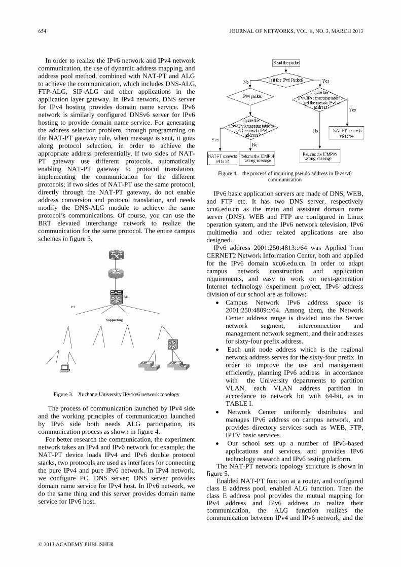
In order to realize the IPv6 network and IPv4 network communication, the use of dynamic address mapping, and address pool method, combined with NAT-PT and ALG to achieve the communication, which includes DNS-ALG, FTP-ALG, SIP-ALG and other applications in the application layer gateway. In IPv4 network, DNS server for IPv4 hosting provides domain name service. IPv6 network is similarly configured DNSv6 server for lPv6 hosting to provide domain name service. For generating the address selection problem, through programming on the NAT-PT gateway rule, when message is sent, it goes along protocol selection, in order to achieve the appropriate address preferentially. If two sides of NAT-PT gateway use different protocols, automatically enabling NAT-PT gateway to protocol translation, implementing the communication for the different protocols; if two sides of NAT-PT use the same protocol, directly through the NAT-PT gateway, do not enable address conversion and protocol translation, and needs modify the DNS-ALG module to achieve the same protocol’s communications. Of course, you can use the BRT elevated interchange network to realize the communication for the same protocol. The entire campus schemes in figure 3.

BD-

PT

Supporting

Figure 3. Xuchang University IPv4/v6 network topology

The process of communication launched by IPv4 side and the working principles of communication launched by IPv6 side both needs ALG participation, its communication process as shown in figure 4.

For better research the communication, the experiment network takes an IPv4 and IPv6 network for example; the NAT-PT device loads IPv4 and IPv6 double protocol stacks, two protocols are used as interfaces for connecting the pure IPv4 and pure lPv6 network. In IPv4 network, we configure PC, DNS server; DNS server provides domain name service for IPv4 host. In IPv6 network, we do the same thing and this server provides domain name service for IPv6 host.

Figure 4. the process of inquiring pseudo address in IPv4/v6

communication

IPv6 basic application servers are made of DNS, WEB, and FTP etc. It has two DNS server, respectively xcu6.edu.cn as the main and assistant domain name server (DNS). WEB and FTP are configured in Linux operation system, and the IPv6 network television, IPv6 multimedia and other related applications are also designed.

IPv6 address 2001:250:4813::/64 was Applied from CERNET2 Network Information Center, both and applied for the IPv6 domain xcu6.edu.cn. In order to adapt campus network construction and application requirements, and easy to work on next-generation Internet technology experiment project, IPv6 address division of our school are as follows:

• Campus Network IPv6 address space is 2001:250:4809::/64. Among them, the Network Center address range is divided into the Server network segment, interconnection and management network segment, and their addresses for sixty-four prefix address.

• Each unit node address which is the regional network address serves for the sixty-four prefix. In order to improve the use and management efficiently, planning IPv6 address in accordance with the University departments to partition VLAN, each VLAN address partition in accordance to network bit with 64-bit, as in TABLE I.

• Network Center uniformly distributes and manages IPv6 address on campus network, and provides directory services such as WEB, FTP, IPTV basic services.

• Our school sets up a number of IPv6-based applications and services, and provides IPv6 technology research and IPv6 testing platform.

The NAT-PT network topology structure is shown in figure 5.

Enabled NAT-PT function at a router, and configured class E address pool, enabled ALG function. Then the class E address pool provides the mutual mapping for IPv4 address and IPv6 address to realize their communication, the ALG function realizes the communication between IPv4 and IPv6 network, and the



site needs the domain name resolution

TABLE I. VLAN AND ADDRESS PARTITION

. The communication schematic diagram is shown in Figure 6.

VLAN IPv4 address IPv6 address Rem

ark

10 211.67.191.0/24 2001:250:4813:::/64 Equipment

20 211.67.198.0/24 2001:250:4813:1::1/64 Server

51 222.21.126.0/24 2001:250:4813:51::1/64

52 222.21.127.0/24 2001:250:4813:52::1/64

53 222.21.128.0/24 2001:250:4813:53::1/64

54 222.21.129.0/24 2001:250:4813:54::1/64

55 222.21.130.0/24 2001:250:4813:55::1/64

56 222.21.131.0/24 2001:250:4813:56::1/64

57 222.21.132.0/24 2001:250:4813:57::1/64

58 222.21.133.0/24 2001:250:4813:58::1/64

… … … …

Figure 5. the topology of experimental network

Figure 6. the schematic diagram of DNS-ALG working model

In order to improve the efficiency of the domain name resolution, it needs to make configuration of DNS server according to the use of IPv6 site. If the site is oriented to access to IPv6 network, treat IPv6 DNS server as the main DNS server, set the PRIFIX_IPv4_DNS as the secondary DNS server. Thus the most DNS query

messages will directly communicate in IPv6 network without through the NAT-PT gateway. When the domain name resolution

For the problem of protocol selection in the existence of hybrid network, considering the three ways above and the best selection scheme, simultaneously paying attention to make some correction records at IPv4 network and IPv6 network DNS server.

cannot get IPv6 address, then enable the secondary DNS server; go to IPv4 DNS server through NAT-PT gateway to look for the domain name. When the site is oriented to access to IPv4 network, just exchange the main and auxiliary address of DNS server, this can also improve the query efficiency.

What’s more, it resolves the ALG problems such as FTP-ALG, SIP-ALG and so on, in the process of implementation, realizes the communication of the current hybrid network and resolves the loading balance problems in experiments.

(2) IVI mode Due to the network's complexity, NAT-PT gateway are

still many problems, and not suitable to deploy a large scale of IPv6 network. With the IPv6 network expansion, we can choose to use IVI technology deployment. IVI mode can also realize IPv4/IPv6 network intercommunication.

IVI technology is a improve technology with SIIP and NAT-PT technology. In IVI, IVI gateway with address conversion and ALG function to realize the hybrid network intercommunication.

In large-scale IPv6 network, it needs to use at least two IVI gateway equipments. IVI gateway is placed between the external network and the school Dual-stack core switch, realizing the campus network and external network communication. The other IVI gateway placed between pure IPv6 network and mixed network in campus network, make the network to establish route relationship, so as to realize the interconnection between the mixed networks.

In order to facilitate the automatic distribution IPv6 address consistent with the requirements of IVI, we need to configure a DHCPv6 server to automatically obtain IPv6 address; at the same time, ensure the original IPv4 and IPv6 DNS configuration to realize domain name resolution of two network address, and can achieve the communication between IPv4 and IPv6 network finally.

1) When the host of IPv6 network to the host of IPv4 network sends out requesting the communication, DHCPv6 server automatically obtain an IPv6 address, and from the IPv6 DNS server to obtain a corresponding IVI IPv6 address, the address routing to the IVI gateway device, when the IVI IPv6 source address and destination address pass IVI gateway, in the gateway these addresses are converted to IPv4 address identified by the IPv4 address, and then forwarded to the IPv4 network. When the address is returning, in IVI gateway the source address and destination address are converted to IVI IPv6 address, forwarded to the IPv6 network, thus realizing IPv6 host to IPv4 network access.

2) When the IPv4 host accesses IPv6 network, in IVI gateway IPv4 address is converted into IVI IPv6 address,



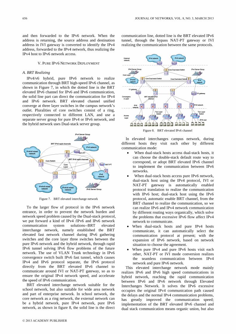
and then forwarded to the IPv6 network. When the address is returning, the source address and destination address in IVI gateway is converted to identify the IPv4 address, forwarded to the IPv4 network, thus realizing the IPv4 host to IPv6 network access.

V. PURE IPV6 NETWORK DEPLOYMENT

A. BRT Realizing IPv4/v6 hybrid, pure IPv6 network to realize

communication through BRT high-speed IPv6 channel, as shown in Figure 7, in which the dotted line is the BRT elevated IPv6 channel for IPv6 and IPv6 communication, the solid line part can direct the communication for IPv4 and IPv6 network. BRT elevated channel unified converge at three layer switches in the campus network’s outlet. Pluralities of core switches consist of a ring, respectively connected to different LAN, and use a separate server group for pure IPv4 or IPv6 network, and the hybrid network uses Dual-stack server group.

BRT IPv6 rapid channels

Core Layer

NAT-PT

NAT-PT

IPv4 network

IPv4/v6 mixed network

IPv4/v6 mixed network

IPv4 Server Group

Core Switch

IPv6 netwrok

BRT IPv6 rapid channels

IPv6 Server GroupIPv4/v6 mixed

network

Figure 7. BRT elevated interchange network

To the larger flow of protocol in the IPv6 network entrance, in order to prevent the network burden and network speed problem caused by the Dual-stack protocol, we put forward a kind of IPv4 /IPv6 and IPv6 network communication system solutions--BRT elevated interchange network, namely established the BRT elevated fast network channel during IPv6 gathering switches and the core layer three switches between the pure IPv6 network and the hybrid network, through rapid IPv6 tunnel solving IPv6 flow problems of the future network. The use of VLAN Trunk technology in IPv6 convergence switch built IPv6 fast tunnel, which causes IPv4 and IPv6 protocol separate, the IPv6 protocol directly from the BRT elevated IPv6 channel to communicate around IVI or NAT-PT gateway, so as to ensure the original IPv4 network speed, and accelerate the speed of IPv6 communication.

BRT elevated interchange network suitable for the school network, but also suitable for wide area network and part of enterprise network. In school network, the core network as a ring network, the external network can be a hybrid network, pure IPv4 network, pure IPv6 network, as shown in figure 8, the solid line is the direct

communication line, dotted line is the BRT elevated IPv6 tunnel, through the bypass NAT-PT gateway or IVI realizing the communication between the same protocols.

IPv4/v6 network

IPv4 network

IVI gateway

IPv6 netwrok

BRT elevated IPv6 channel

IPv6 Server Group

Core Dual-stack Switch

Core Layer

Externalnetwork

Convergence Layer

Access Layer

Two Layer Switch

IPv6 user

IVI gateway

IPv6 network



Two Layer Switch

IPv4 Server Group

IPv4 network IPv6 network

Figure 8. BRT elevated IPv6 channel

In elevated interchanges campus network, during different hosts they visit each other by different communication mode:

• When dual-stack hosts access dual-stack hosts, it can choose the double-stack default route way to correspond, or adopt BRT elevated IPv6 channel to implement the communication between IPv6 networks.

• When dual-stack hosts access pure IPv6 network, dual-stack host using the IPv4 protocol, IVI or NAT-PT gateway is automatically enabled protocol translation to realize the communication with IPv6 host; dual-stack host using the IPv6 protocol, automatic enable BRT channel, from the BRT channel to realize the communication, so we can realize IPv6 and IPv4 network communication by different routing ways organically, which solve the problems that excessive IPv6 flow affect IPv4 network to communicate.

• When dual-stack hosts and pure IPv4 hosts communicate, it can automatically select the communication protocol at present; with the expansion of IPv6 network, based on network situation to choose the agreement.

• When pure IPv4 and pure IPv6 hosts visit each other, NAT-PT or IVI mode conversion realizes the seamless communication between IPv4 network and pure IPv6 network.

This elevated interchange network mode mainly realizes IPv6 and IPv6 high speed communications in hybrid network, reaching the rapid communication between IPv6 and IPv6 network through Elevated Interchanges Network. It solves the IPv6 excessive occupies the original IPv4 communication path caused the delays and the normal IPv4 communication problems, has greatly improved the communication speed; implementation of the BRT elevated IPv6 channel and dual stack communication means organic union, but also



protects the IPv4 and IPv6 network security communication. This rapid elevated communication mode greatly eases the dual stack communication pressure on the basis of meeting IPv4 and IPv6 seamless access, and avoids some security problems. For WiMAX, different architectures to consider deploying IPv6 over wireless broadband network.

VI. CONCLUSION

This paper explains several existing and new IPv4 / IPv6 interchange technology, combined with the actual situation of campus network. Meanwhile the warranty does not affect the existing IPv4 network normal application, through the core equipment, gathering equipment gradually upgrade to IPv6’s process, which put forward a safe IPv6 transition scheme.

The planning and deployment of the IPv4/v6 network, setting up the entire IPv6 network successes, which provide a good test platform for IPv6 related technical research.

Based on the realization of IPv4 network and IPv6 networks communication, this system put forward mixed network and IPv6 network communication rapid solution – BRT mode, the scheme has run IPv6 speed quickly, low investment and so on, to solve the IPv6 in dual stack network occupying IPv4 channel, and increasing the network burden, affecting network communication question, so as to achieve the IPv6 fast communication without affecting IPv4 communication situations. The scheme will be likely to use as a kind of important mode of the next generation of Internet development process.

ACKNOWLEDGEMENT

This work is supported by Henan Science and Technology Research Foundation (122102210544, 122102210425) and Henan Education Department Natural Science Foundation (12A510022).

REFERENCES

[1] Jun Bi, Guang Yao and Jianping Wu. An IPv6 Source Address Validation Testbed andPrototype Implementation. Journal of Networks, 2009,4(2).

[2] Wang Xiaonan, Qian Huanyan etal. Design and Implementation of Anycast Services in Ad Hoc Networks Connected to IPv6 Networks. Journal of Networks, 2010,5(4).

[3] G. Wu, M. Mizuno, and P. J. M. Havinga, “MIRAI architecture for heterogeneous network,” IEEE Commun. Mag., vol. 40, no. 2, pp. 126–134, Feb. 2008.

[4] Adlen Ksentini. IPv6 over IEEE 802.16 (WiMAX) networks:Facts and challenges. Journal of communications, 2008,7.

[5] Lishen Yang, Yange Chen. IPv4/v6 tunnel problems and the deployment scheme Research [J].Computer Development and Application, 2008, 21 (1):43-45.

[6] Wang Kuifu,Chen Yange. Research of IPv6 transition technology and its department on campus network. ICISCI2011,EI retrieval.

[7] N. Montavont and T. Noel, “Handover management for mobile nodes in IPv6 networks,” IEEE Commun. Mag., vol. 40, no. 8, pp. 38–43, Aug. 2008.

[8] Yange Chen,Hui Ma. Design of BRT Three-dimensional Interchange Network Based on IPv4/IPv6 Hybrid Network[J]. Television Technology,2011,35(19):86-92.

[9] Zhifeng Chen, Qiaoming Zhu. IPv6-Based Dynamic Quality of Service Control Strategy for Wireless Network. Journal of Networks, 2010,9(5).

[10] Chen Yange, Ma Hui.Study on safe transition scheme for IPv6 campus networks[J]. Study on optical communications, 2010,12(6):26-29.

[11] Y.g. Ch.., Z.l. Zh...Intercommunication Strategy about IPv4/IPv6 co-existence networks based on Application Layer Gateway. The International Conference on Communication Systems and Network Technologies(CSNT),2013,1.

[12] R. Braden, D. Clark, and S. Shenker, “Integrated services in the Internet architecture: An overview,” IETF, RFC 1663,2008.

Yange Chen received the MS degree in computer science and Technology from Henan Polytechnic University in 2008. Her dissertation focused on IPv6 networks. She is currently working at College of Computer Science & Technology, Xuchang University in China as a lecturer. She is involved in several projects, which aim at realizing a large-scale testbed supporting IPv6 technology and Internet of Things. Her research interests include the next-generation network and Internet of Things. He is a coauthor of more than 20 technical journal papers and international conference papers. Zhili Zhang received the MS degree in maths department from Zhengzhou University and the PhD degree in computer science in 2006 from South China University of Technology. Currently he is a full professor and director of College of Computer Science & Technology, Xuchang University in China, where he is also a member of the Henan Education and Research Network. He is presiding over several projects, which aim at realizing a large-scale IPv6 testbed and Internet of Things. .His research interests include the next-generation network and Web Accelerator. He is a coauthor of more than 30 technical journal papers and international conference papers.

Qingfang Cui received the MS degree in computer science and Technology from Henan Polytechnic University in 2006, he is currently working at Henan Xuji XJ POWER, Henan Xuji Company Group.His research interests are the next-generation network architecture and protocol.



doi:10.4304/jnw.8.3.658-664

Wireless Position Scheme based on ZigBee Network in the Freeway ETC System

Baishun Su

School of computer science and technology, Henan Polytechnic University, 454000, Jiaozuo, China Email: [email protected]

Baoding Zhang

School of computer science and technology, Henan Polytechnic University , 454000, Jiaozuo, China Email: [email protected]

Abstract—Based on the review of the development situation of the ETC home and abroad and the ETC key technology, this paper put forward to apply ZigBee network in the freeway ETC system. CC2431 wireless location function is used in the high speed highway ETC system to realize data transmission between network centre node and terminal node safely, which records passing information of the vehicle terminal by the wireless data transmission between the coordinator and vehicle terminal. To improve the position accuracy, a weighted centroid position algorithm is introduced combination the RSSI with centroid position algorithm. The test results of the wireless communication between vehicle terminal and coordinator show that CC2431 wireless position system can realize vehicle omnibearing position and real time monitor in the super-speed highway. Index Terms—ZigBee; coordinator; vehicle terminal; electronic toll collection

I. INTRODUCTION

With the development of the freeway, at present electronic toll collection (ETC) system more and more is used in the freeway management system, Which can finish identification of the vehicle and vehicle toll without parking automatic.Freewway business enterprise can get good economic and social benefits in the aspect of the operating management mode and running cost and vehicle traffic capacity by this means [1] [2]. With the development of the short wireless communication technologies, such as RFID, WiFi, UWB and Bluetooth reveal the great application prospects in the freeway ETC system and promote the new ETC system research and development.

Radio Frequency Identification (RFID) is a grown automatic identification technology and is widely used in the ECT system now with the advantage of the short transmission distance, no-touching and fast response. In view of the disadvantage of short transmission distance, electronic tag damage easily, vehicle position and tracking for the RFID.

This paper put forward the ZigBee technology to use in the vehicle localization to improve the efficiency of the freeway ETC system [3] [4].

To improve traffic capacity of the toll gate and finish toll process efficiently and reliably, lane control system usually include three key systems as followings [5].

1) Automatic vehicle identification system Automatic vehicle identification system’s function is to

inquire the stored vehicle-mounted information in the RFID. Such as ID, vehicle type and owner to ascertain if the vehicle can pass through the no parking charge lane.

2) Automatic vehicle classfication system Automatic vehicle classification system can measure

the vehicle type by the sensor equipments in the lane or near the lane and check the vehicle type information provided by the electronic tag to prevent human in card and make assure normal charging according to the corresponding models.

3) Video enforcement system Video enforcement system can capture the picture of

the license plate without effective identification card when car is passing through the no parking charging lane to determine the owners with the fled fee and give his notice of fee.

ZigBee (IEEE 802.15.4 standard) is a rising wireless network technology which is of short space, low complicacy, low power consumption, low data rate and low cost. ZigBee technology can be introduced to satisfy the function of the vehicle position and tracking, through which highway management system can get the more information of the vehicle and effectively reduce the Vehicles blocking rate.

IEEE

802

.15.

4

Application (APL) Layer

Network (NWK) Layer

Medium Access Control (MAC) Layer

868/915MHzPhysical

(PHY) Layer

2.4GHzPhysical

(PHY) Layer

ZigB

ee A

llian

ce

Figure 1. ZigBee stack architecture

The ZigBee stack architecture is made up of a set of block called layers. Each layer performs a specific set of services for the layers. The IEEE802.15.4 standard



defines the two lower layers: the physical (PHY) layer and the medium access control (MAC) sub-layer. The ZigBee Alliance builds on this foundation by providing the network (NWK) and the framework for the application layer. Which includes the application support sub-layer (APS), the ZigBee device objects (ZDO) and the manufacture defined application objects [6] [7]. The outline ZigBee stack architecture can be shown in fig. 1.

The freeway electronic toll gate system is composed of the vehicle terminal, coordinator and toll gate system, which can collect automatically, analyze and handle every ZigBee node data on the basis of the IEEE802.15.4/ZigBee protocol. Record and gain vehicle detailed information when passing through toll station. Data request of the vehicle terminal can transmit to ZigBee coordinator by the wireless information) channel and transmit data to toll gate system to handle.

Two different type devices are a full-function device (FFD) and a reduced-function device (RFD) in ZigBee networks. The FFD can operate in three modes serving as a personal area network (PAN) coordinator, a coordinator or a device. An FFD can talk to RFDs or other FFDs, while an RFD can talk only to an FFD. An RFD is intended for end device that are extremely simple such as sensor. They do not have the need to send large amounts of data and may only associate with a single FFD at a time.

Electromagnetic wave propagation loss not only is related to propagation distance d, but also is related to the obstacle. Signal strength can decrease with the increasing distance. RSSI(Received signal strength indicator) can evaluate the node distance according to the signal attenuation in the transmission [8]. The RSSI value will decrease when the distance increases.

Figure 2. Location system diagram

Fig. 2 shows a simplified system for location detection. Reference node is a static node placed at a known position. The reference node knows its own position and can transmit the position to other nodes when it is requested. Since a reference node does not need to implement the hardware used for location detection, it will not perform any calculation at all. A mobile node will collect signals from all reference nodes responding to a request, read out the respective RSSI values, feed the collected values into the hardware engine, and then it reads out the calculated position and sends the position information to a control application. The minimum data contained in a packet sent from a reference node to a mobile node should be the parameters Xi and Yi of the

reference node. The RSSI values are calculated by the mobile node.

The location engine utilizes an extremely simple inter face seen from the software layer, writes parameters in, waits for the calculation to be performed, and reads out the calculated position[9][10].

The arrangement and the scope of the wireless sensor nodes constantly change on the march of car and advancement, which can cause serious power consumption of node in long-distance data transmission. In order to ensure the network data transmission efficiently and save energy consumption, we use the cluster tree network is a special case of a peer-to-peer network in which most devices are FFDs. An RFD may connect to a cluster tree network as a leave node at the end of a branch, because it may only associate with one FFD at a time. Any of the FFDs may act as a coordinator and provide synchronization services to other devices or other coordinators[11].The network topology is can be shown in fig. 3.

Figure 3. Cluster tree network topology

II. SYSTEM ARCHITECTURE

A. ZigBee wireless network Highway vehicle position system mainly consists of

vehicle terminal, coordinator and toll gate computer. The wireless mobile position technology can measure the vehicle position and vehicle speed in the highway or toll station.

ZigBee wireless network includes two categories of nodes: the coordinator and vehicle terminal, according to ZigBee Stack and networks character, and its network architecture can be shown in Fig. 4.

Figure 4. System architecture of the ZigBee network

AS can be shown in fig.4, vehicle terminal state information can be obtained by coordinator and sent toll



gate computer, the toll gate computer can communicate with the coordinator by RS232 interface through which can give the command and sent to coordinator, coordinator analyze control signals and make the appropriate response to control the implementation. The vehicle terminal collect the car type, position information and sent to coordinator by ZigBee network, and coordinator finally send data to PC monitoring centre[3].toll gate computer can transmit car information to the toll gate database server by internet through which can store and analyze relevant information.

Vehicle terminal is a mobile node in the wireless network in the high speed highway. This can join the network or exit at any time. And allocate an only ID to identify vehicle terminal in a known ZigBee network, vehicle terminal nodes can transmit ID to coordinator. Coordinator then transmits to the toll gate computer. Management system can search and obtain vehicle type parameter according to the ID database so that can provide the vehicle position and calculate vehicle fee.

III. ALGORITHM MODEL

A. RSSI Postion Model Wireless information channel mathematical model can

be expressed in the following equation:

0

0

( ) ( ) 10 logr rd

P d P d n Xd σ= − −

(1)

In this formula: d is the receiver and transmitter direct distance(m). d0 n is path loss index. Normal can be 2; 4, a related

environment factor.

is the reference distance(m). Generally take 1m.

Xσ is a gauss random noise variables of average for 0(Bm).

Pr(d) is receiver receive signal power(dBm). Pr(d0Wireless path loss has great influence on the positional

accuracy. Its model can also be expressed as followings:

) is reference distance receive signal power(dBm).

32.44 10 lg 10 lgLb f n F n D= + + (2) where Lbf is the free space loss(dB); D is distance (km); F is frequency (MHz); n is path loss index. From (2) we can get the received signal strength as the followings.

RSSI Pt Gt Gr Lc Lbf= + + − − (3) where Pt is the power of the sending signal .Gt is Transmittion antenna gain. Gr is the receiving antenna gain. Lc is line loss. In view of the multipath, diffraction and obstacle factors, wireless propagation path loss have some change compared with the theoretical value. Convert it with formula 3 into 2 and simplify it in the followings.

lgRSSI b k D= + (4) where b= Pt+Gt+Gr-Lc-32.44-10nlgF,k=-n/2.from (4)it can be seen that RSSI have linear relationship with the 20lgD. Environmental signal transmission model can be determined by the calculation of b and k for the preparation of the position.

From above the analysis, RSSI can decrease with the distance increasing .the experiments show that the

calculating distance of the bigger RSSI value will near to the real value. The bigger error between calculating value and real value will appear for the smaller RSSI value. From equation (1) the distance can be calculated.

At present localization algorithm can be divided into range-based algorithm and range-free algorithm. Range-based algorithm calculates node information mainly by measuring the distance of the nodes and the angle [12]. Common range-based technology including RSSI, TOA, TDOA and AOA. Range-free algorithm doesn’t need distance and angle information and it can achieve the RSSI position algorithm by the network connectedness. Out of doors environment factor n change greatly when the weather changes. To reduce the vehicle position error, an improved localization algorithm based on RSSI called weighted centroid algorithm is put forward [13].

B. Weighted centroid algorithm The weighted centriod algorithm is centered with the

weighting factor which can reveal the influence of the beacon node on the mass center and the internal relation. Weighted centroid localization algorithm is simple and no communication is needed while locating. Assume three the signal strength of the near to d0

Weighting factor can reveal signal node’s function to decision. Weighting equation can be defined as following equation 2.

to transmission。We can calculate the distance d. yet signal channel be affected by the multi-path fading and non-of-sight blockage with the time [14].

31 2

1 2 3

1 2 3

1 1 1

xx xd d d

X

d d d

+ +=

+ +,

31 2

1 2 3

1 2 3

1 1 1

yy yd d d

Y

d d d

+ +=

+ + (5)

As can be seen in fig.5, Where x1, x2 and x3 are the signal nodes coordinate. The distance between undetermined node and known node are d1,d2 and d3. According to the equation (5), we can get the unknown coordinate. Factor can reveal the signal node’s function to decision. d1,d2 and d3

(x1,y1)

(x2,y2) (x3,y3)(X,Y)

d1d2 d3

can be obtained by the RSSI wireless module.

Figure 5. weighting centroid algorithm

Reference node and mobile reference get the unknown coordinate. Factor can reveal signal node’s function to decision. Weighting equation can be defined as followings. d1,d2 and d3

IV. HARDWARE DESIGN

can be obtained by the RSSI wireless module.



All ZigBee node of the system use CC2431 as the wireless controller. The CC2431 is a true system-on-chip (Soc) for wireless networking ZigBee including location detection hardware based on RSSI values. The CC2431 combines the excellent performance of the leading CC2420 RF transceiver with an industry-standard enhanced 8051MCU.Combined with the industry leading ZigBee protocol stack.

A. Coordinator Node Coordinator node is composed of power supply module,

communication Module, keyboard module and LCD display module, the specific hardware architecture can be shown in Fig. 5.

CC2431 ControllerPower

Management

LCD Display

Keyboard Control

RS232 Communication

Alarm Figure 5. Block diagram of coordinator Hardware architecture

1) Power management Power supply voltage of CC2431 is 3.3V, and we can

realize 5V and 3.3V interface level translation byTPS79533 which is a low-dropout, low-power linear voltage regulators features with 3.3V voltage output. Power supply circuit can be seen in fig.6.

1K

R?

0.1uF

C3

0.1uFC1

100pF

C2Vin3 Vout 2

GND

1

U1

LM1117

+5V 3.3V

LED

Figure 6. Power supply

2) RS485 communication In order to communicate between coordinator and the

PC monitoring centre，The coordinator communicates the data with the wired workstation by RS485 interface. So we choose MAX485 to realize communication. MAX485 is a 5V low power the RS-485 transceiver and can meet the RS-485 serial protocol requirements. The RS485 communication can be shown in fig.7.

U1

TLP521-1

5V

U3

TLP521-2

U4

TLP521-32.2K

R9

RO1/RE2DE3DI4 GND 5A 6

VCC 8B 7

U2

MAX485

510R5

2.2KR1

120R6

510R8

510R2

+5V

5V20

R4

20

R7

3.3V

3.3V

12

P1

2.2KR3

RXD

TXD 3.3V

CTRL

Figure 7. RS485 communication

3) LCD display module OCM12864-9 is a 128×64 dot-matrix liquid crystal

display modules with controller by ST7565P produced by Gold Palm Electronics CO.,Ltd, which can show the current terminal node parameters from data collection terminal, such as device type, network ID.

VSS1VDD2NC3AO4R/W5E6DB07DB18DB29DB310DB411DB512DB613DB714CS15NC16RST17NC18LED+19LED-20

OCM12864-9

OCM12864-9

3.3V

R350K

R2

220Q1

9015

D0D1D2D3D4D5D6D7

AORW

E

CS

10uFC1100K

R13.3V

3.3V

LED+

Figure 8. LCD display

4) Keyboard control Keyboard control is designed by 4×4 matrix key array

including number key and function key. Number key can set the environmental parameters upper and lower limits of the end device, group number while functional key can provide configuration and inquiring information of data collection terminal.

1 42 3

R6470

R7470

R8470

R5470

5 6 7 8

9 OK CANCEL0

OPTION SEARCH UP DOWN

4.7K

R1

4.7K

R2

4.7KR3

4.7K

R4

3.3V

K1

K2

K3

K4

K5 K6 K7 K8

Figure 9. LCD display

5) Alarm control Once the data collection terminal parameters exceed

setvalue by number key, it will give an alarm.

B. Terminal node Terminal node not only measure vehicle speed, vehicle

position, but also including some node connecting with actuator. Different kinds of mobile vehicle nodes can share wireless communication module in common use or in exclusive use, the number and configuration of the sensors depend on vehicle type and the lane conditions.

V. SOFTWARE DESIGN

Software of system uses IAR Embedded Workbench (EW)for MCS-51 produced by IAR System company which is a set of high sophisticated and easy-to-use development tools for programming embedded application. Software system use ZigBee 2007/PRO



http://www.iciba.com/and/�

Zstack-2.0.0 of TI Company, Which can be managed by adding the operating system (OS).

The OS Abstraction Layer (OSAL) API allows the software components in the Z-stack to be written independently of the specifics of the operating system, kernel or tasking environment. OSAL is independent of ZigBee stack. But it whole stack can run based on OSAL System build a task and allocate task ID and functions.

A. Software Design of the Coordinator The coordinator automatically build network after

initialization and allows vehicle terminal to join the network. Firstly it can receive the configuration data of the reference nodes and position node provided by the monitoring PC, Send data to according node with the different manner. Secondly it receives feedback data of the nodes and sends to the monitoring PC. The flow chart of its software design can be shown in fig.10.

start

Receive PC data？ Receive every node data？

Check is correct？

Send to the node

Send through serial port

Calculate the check value and send it through

serial port

end

YY

Y

NN

N

Figure 10. Position node software flow

B. Software Design of the Reference Node Reference mode is a stationary node which knows its

position and can transmit signal bag including x, y coordinate and RSSI to position node. This node must configure in the position area. The plane position coordinate of the reference node should be set when Firstly be used. Reference node can remember its position after setting.

The flow chart of its software design can be shown in fig.3.As can be seen in fig.11, reference node includes g the following four input ID.

1) RSSI request RSSI request can transmit RSSI average value to

position node. 2) Reference node configuration Configure the reference node coordinate according to

the coordinator and then data written into flash. 3) Reference node request configuration Transmit the reference node its own information

coordinates to coordinator. 4) RSSI Collection The RSSI value collection between the its own and

position nodes. When the reference node receives the information, it

can handle the information according to the string ID and

implement the function. The flow chart of its software design can be shown in fig.11.

C. Software Design of the Position Node The position node automatically can randomly move in

the area of the reference node surrounding. To improve the measurement precision, we can add the number of the reference node. When the reference node sends its own position coordinate, Reference node receive signal and reply an answer signal. The flow chart of its software design can be shown in fig.12.

N

start

receive data？

XY-RSSI request？

Reference node configuration？

Reference node request configuration？

Collect RSSI?

N

N

N

Y

N

end

Transmit RSSI average value

configuration information writing

flash

Y

Y

Y Configuration information transmit

coordinator

Collect RSSIY

Figure 11. Reference node software flow

N

Start

Receive data？

Position node finding request？

Position configuration？

Position node request configuration ？

Collect RSSI response?

N

N

N

Y

N

end

Forceful position finding

Configuration write to flash

Y

Y

Y Configuration information transimt to coordinator

Receive RSSI average value

Y

XY-RSSI request？ Forceful position finding

Y

Figure 12. Position node software flow

IEEE 64 bit address can be defined by user and be written into EEPROM.when the position node enter into the network, the coordinator can ZigBee node can allocate a sixteen bit short address.



D. PC Monitoring Software Software Design of Host Computer Control Centre is

based on VC ++6.0 to achieve serial communication with coordinator provided by the control of MSComm ActiveX. MSComm in serial programming extremely convenient programmer does not have to spend time to understand the more complex API functions. The software is connected with coordinator to achieve serial receiving data and sending data control data communication combining SQL2000 database programming software, finally establish visual man-machine interactive interface. Its main functions are as follows:

a) Software contains the integrity function of users increase, delete and the cipher modification .

b) Software can set baudrate,commPort,the address parameter of the terminal sensors and alarm parameters .

c) Software can read stored data in the coordinator and extract working parameters and conditions information,which can be stored to corresponding database table and conduct data backups. Also can analyze and process data to determine whether actuator is activated according to site environment.

d) The system administrator can not only monitor the real-time running state of vehivles parameters and display data on screen dynamically in curve or chart way, but also manage effectively the system resources and tune the system parameters to improve system performance. such as parameter enactment,instruction control; fault annunciation .

e) The system provide the inquiry, analysis and calling function of historical data such as statistics, historical curves for various periods of observation, Automatically generating, storing, querying and print-out the reports.

VI. CENTROID ALGORITHM SIMULATION

. A. Simulation process 1) Beacon node sends its information periodically

including its ID and position information. 2) When normal node receives the information, it

records the only same beacon node’s RSSI average [15]. 3) When normal node receive m beacon information

exceeding the threshold value, collate beacon from bigger to small according to the RSSI vale and establish the mapping from RSSI to the distance between unknown node and beacon node. Including three set:

One: Beacon node set can be defined as { }1 2, , , mBeacon set a a a− =

Two: Distance set between unknown node and beacon node can be defined as

{ }1 2 1 2tan , , , ,m mDis ce set d d d d d d− = < < (6) Three: Beacon node position set

( ) ( ) ( ){ }1 1 2 2, , , , , ,m mPosition set X Y X Y X Y− = (7) 4) Apply the first beacon with bigger RSSI value to

calculate itself position. According to analysis of the wireless transmission path loss model, selecting the

beacon node with the bigger RSSI value to assembly the following triangle set to improve the position accuracy.

( ) ( )( ) ( )

1 2 3 1 2 4

1 3 4 1 3 5

{ , , , , , , ,

, , , , , }

Triangle set a a a a a a

a a a a a a

− =

(8)

5) For any a triangle ( , , )ii jj kka a a , unknown node coordinate 1 1( , )i k kk x y can be calculated with equation by weighted centroid algorithm. Distance from beacon node ( , , )ii jj kka a a to unknown node calculated by the RSSI value can be expressed (1) ( ) (2) ( ) (3) ( )( , , )k i k i k id d d for the sake for convenience. Figure up repeatly above every triangle in the triangle set and will get the unknown node approximate position coordinate set 1 2 3,{ , , , }pk k k k .

6) Approximate position coordinate set 1 2 3,{ , , , }pk k k k can determine unknown node coordinate

by the weighted centroid algorithm as follows.

(1)( ) (2)( ) (3)( )1

(1)( ) (2)( ) (3)( )1

(1)( ) (2)( ) (3)( )1

(1)( ) (2)( ) (3)( )1

[ / ( )]

[1 / ( )]

[ / ( )]

[1 / ( )]

i i i

i i i

i i i

i i i

p

ki k k ki

p

k k kip

ki k k ki

p

k k ki

x d d dx

d d d

y d d dy

d d d

=

=

=

=

+ +=

+ +

+ +=

+ +

∑

∑

∑

∑

(9)

VII. EXPERIMENTAL VERIFICATION

The whole experiment is carried through in the open air. On the ground eight node position marks fixed locate in the table I. coordinator fixed in the 0m. Every location node’s RSSI value is measured for five times and uses its average. When Node sending power is 0dB, Reference node send data periodically and coordinator receive the data and collect RSSI value.

TABLE I. RSSI VALUE CHANGE CHART WITH DIFFERENT DISTANCE

Distance(m) 1 6 11 16 21 26 31 36

RSSI(dB) -2 -12 -19 -22 -30 -33 -34 -34

Numerical analysis of the RSSI and correction theory

model combination is with the wireless transmission loss model. According to the equation (1), we can get the relationship between receiving power and distance for the mobile vehicle [16].

The real distance value and experimental distance value can be seen in fig.13. It shows that in the range of 10m RSSI value have good linear relationship with the distance and good uniformity with theory model. RSSI value changes slowly with the growing gap towards the model and with certain randomness. To improve the position accuracy, on the basis of the RSSI model we can adopt the weighted centriod algorithm to improve the RSSI model, according to the simulation process of the weighted centriod algorithm. The simulation results show that the weighted-centroid algorithm has better estimation error and node localization coverage than common RSSI algorithm.



http://www.iciba.com/real-time/�

Figure 13. Minimum curve fitting

VIII. CONCLUSION

In this paper, we introduce a weighted centroid position algorithm to solve mobile node change on the basis of the RSSI, through which we can know of the relationship between position accuracy and nodes number. It shows that position algorithm have important effect on the position accuracy with the complex environment [17], unfortunately the node have poor uniformity and RSSI random component change greatly with the environment So many times experiments should be done near the area of the toll station by appropriate reference nodes number selection and the selection of the distance between reference nodes and coordinator. With the position algorithm’s improvement, the vehicle information can be accurately obtained by the ZigBee wireless network.

ACKNOWLEDGMENT

This work is supported by the key scientific and technological project grants of china (No.102102210032) and is supported by Henan Education Department National Science Research Project under Grant 2010B510013.

REFERENCES

[1] Wang wei-jie, Huang Shou-zhi, Zhao Xue-zeng. Research on highway inter-vehicle communication technology based on ZigBee. Journal of Dalian Jiaotong university.2009, 30(6): 90~94

[2] Fu De-yu, Wu Ping, Mao Wan-hua. Application of the ZigBee Technology in the high speed highway ETC System. Microcontrollers & Embedded systems. 2008, (3): 50~52

[3] Fan Li, Guizhong Liu, Lijun He. Cross-layer approach to multiuser H.264 Video Transmission over wireless networks. Journal of multimedia. 2010,5(2),110-117

[4] Aslam.Nauman, Philips.William, Robertson.William. Effective location management of mobile actor in wireless sensor and actor networks. Journal of networks. 2009,4(1), 1-8.

[5] Jian Wu, Zhiming Cui, Jianming Chen. Guangming Zhang. A survey on video-based vehicle behavior analysis algorithms. Journal of multimedia. 2012,7(3), 223-230

[6] IEEE.IEEE standard 802.15.4-Wireless Medium Access Control (MAC) and Physical Layer (PHY) Specifications

for Low-Rate Wireless Personal Area Networks (LR-WPANs),IEEE2003,Online,Available:http://standards.ieee.org/getieee802/download/802.15.4-2003.pdf

[7] Paolo Baronti, Prashant Pillai, Vince W.C.Chook, Stefano Chessa, Alberto Gotta, Y.Fun.Hu. Wireless sensor networks: A survey on the state of the art and 802.15.4 and ZigBee Standards. Computer and Communications. 2007,30,1655-1695

[8] Fang Zhen, Zhao Zhan, Guo peng, Zhang Yu-guo. Analysis of distance measurement based on RSSI. Chinese Journal of sensor and actuators ,2007,20(11):2526－2530.

[9] Zhou Yan, Li Hai-cheng. Space localization algorithm based RSSI in wireless sensor networks. Journal on communications.2009, 30(6):75~79

[10] Wang Yang, Huang Liu-sheng, Xiao Ming-jun, Xu Hong-li. Localization algorithm for wireless sensor network based on RSSI-verify. Journal of Chinese computer systems. 2009, 30(1):59~62

[11] Wang Gicheol, Kim Seunghae, Kang Daewook, Choi Deokjai, Cho Gihwan. Lightweight key renewals for clustered sensor networks. Journal of networks. 2011,5(3),300-312

[12] Shaoping Zhang, Guohui Li, Wei Wei, Bing Yang. A novel iterative multiateral localization algorithm for wireless sensor networks. Journal of networks. 2010,5(1),112-119

[13] Wang Fu-bao, Shi Long,Ren Feng-yuan.Self-localization systems and algorithms for wireless sensor networks. Journal of software. 2005, 16(5):857~868

[14] Chen Wei-ke, Li Wen-feng,Shou Heng, Yuan Bing. Weighted centroid localization algorithm based on RSSI for wireless sensor networks. Journal of Wuhan university of technology (Transportation Science&Engineering).2006, 30(2):265~268

[15] Yang xiang, Lu Chao-ze, Pan wei. A ZigBee-based highway vehicles prevent collision warning system research. 2011 fourth international symposium on computational intelligence and design. 270~273

[16] Raul Morais,Miguel A.Fernandes, Samuel G.Matos, Carlos serôdio, P.J.S.G. Ferreira, M.J.C.S. Reis. A ZigBee multi-powered wireless acquisition device for remote sensing application in precision viticulture. Computer and Electronics in Agriculture. 2008,62,94-106

[17] Hanjiang Luo, Zhongwen Guo, Wei Dong, Feng Hong, Yiyang Zhao. Localization with directional beacons for sparse 3D underwater Acoustic sensor network. Journal of networks. 2010,5(1), 28-38

Bai-Shun Su obtained his bachelor degree in power system automation from Jiaozuo institute of technology in 1999; He was conferred with MS degree in control theory and engineering from Henan Polytechnic University in 2006. And he obtained his PhD degree in China University of Mining & Technology, Beijing. He’s main research areas include Embedded system, wireless sensor network and fiber sensor technology. He is presently a teacher in school of computer science and technology of Henan Polytechnic University.

Bao-ding Zhang graduated in Computer Application Technology from the University of Shenyang Ligong, China in 2006 and got his Master’s degree at the same university. Currently he is a teacher of College of Computer Science and Technology in Henan Polytechnic University. His research topics include wireless sensor networks and the design of embedded electronic system in water meters.



doi:10.4304/jnw.8.3.665-671

Multiple Antennas Spectrum Sensing for Cognitive Radio Networks

Yang Ou

Soochow University, Department of Electronics and Information Engineering, Suzhou, China University of Science and Technology of Suzhou, Department of Electronic Engineering, Suzhou, China


Yi-Ming Wang Soochow University, Department of Electronics and Information Engineering, Suzhou, China


Abstract—Performance of cooperative spectrum sensing with multiple antennas at each cognitive radio is discussed in this paper. A new algorithm based on auto-correlation is proposed in which the optimal weights are obtained for each antenna in case little priori knowledge of channel characteristics as well as noise is known. In multiple antennas spectrum sensing, As long as the antenna characteristics are similar, the detection probability can be improved if more antennas are involved. However, if the antenna characteristics are quite different or the number of poorly performed antenna is large the detection probability deteriorates. Therefore, the well-performed antennas are selected in order to improve the detection probability. The performance of an antenna is obtained to determine whether it is deployed to sense the spectrum. A criterion is proposed to select the well-performed antennas to sense spectrum. Simulations are used to verify the method. The results indicate that the proposed antenna weighting and selection algorithm can be able to optimize network performance. Index Terms—spectrum sensing, cognitive radio, antenna selection, detection performance, optimization

I. INTRODUCTION

According to the recent report published by Spectrum Policy Task Force within Federal Communications Commission (FCC), most of the spectrum is under-utilized for significant periods of time [1]. It indicates that the scarcity of spectrum is mainly due to inefficient spectrum allocation rather than physical spectrum inadequacy. Therefore, the technology of cognitive radio (CR) was proposed in order to implement efficient spectrum utilization [2]. This technology allows an unlicensed user (secondary user) to access a spectrum unoccupied by licensed user (primary user). The fundamental requirement for secondary user is to avoid interference with potential primary users in their vicinity. One of the most critical tasks of cognitive radio is spectrum sensing. Spectrum sensing is currently one of

the most challenging tasks in CR design and implementation.

As described in the deployment scenario of the IEEE 802.22 wireless regional area network (WRAN), secondary systems should be located sufficiently far from primary systems to protect primary receivers from occasional interference caused by secondary transmitters. Under that scenario, of course, the signal-to-noise ratio (SNR) of the primary signal is low at the secondary sensing node. Moreover, in a fading environment, spectrum sensing is challenged by the channel uncertainty such as deep fading or shadowing [3]. In such a low SNR region with the fading channel recent research has focused on overcoming this poor performance by utilizing spatial diversity employing multi-antenna techniques at the secondary sensing node [4-7]. With these techniques, multiple antennas are used to perform spectrum sensing simultaneously. The sensing performance gain achieved in this case, however, is the tradeoff of increased complexity [8], where all the radio frequency (RF) chains have to be used at the same time to exploit full spatial diversity. Different MTM-multi- antenna based techniques are proposed in [9]. [10] investigates a new spectrum sharing algorithm based on price in cognitive radio networks. [11] analyzes the performance of multi-hop relay cooperative spectrum sensing.

The idea of antenna selection, which uses a subset of antennas selected from all of the available antennas, has been discussed extensively for the purpose of improving data transmission in MIMO systems [8][12]. Nevertheless, the application of antenna selection in spectrum sensing for a cognitive radio network has remained largely unexplored. An antenna selection based sensing scheme is proposed in [13]. However it didn’t give actual selection method for antenna. In this paper a new algorithm is proposed for selecting the antenna with the best detection performance so as to maximize the spectrum sensing sensitivity.

The proposed algorithm is able to select the antenna with the best performance in case channel coefficient and noise power are unknown. Meanwhile this algorithm can

Corresponding author: Yang Ou, Email: [email protected]



distinguish the necessity for selecting antenna so as to optimize spectrum sensing performance.

The rest of this paper is organized as follows. In section two, general model for spectrum sensing is introduced. In section three, a multiple antenna spectrum sensing model based on cyclic auto-correlation (CA) function is described. Then the algorithm for selecting the antenna with the best detection performance is proposed. In section four, simulations are used to evaluate and compare the methods and finally we conclude the whole paper in section five.

II. GENERAL MODEL FOR SPECTRUM SENSING

In this section, we first present the general model for spectrum sensing, then review the cyclic auto-correlation detection scheme and analyze the relationship between the probability of detection and the probability of false alarm.

A. Sensing Model Suppose that we are interested in the frequency band

with carrier frequency cf and bandwidth W and the received signal is sampled at sampling frequency. When the primary user is active, the discrete received signal at the secondary user can be represented as

( ) ( ) ( ) ( )x n h n s n w n= + (1) which is the output under hypothesis 1H . When the primary user is inactive, the received signal is given by

( ) ( )x n w n= (2) This case is referred to as hypothesis 0H . There are some assumptions. ·The noise ( )w n is a Gaussian, independent and

identically distributed (i.i.d) random process with mean zero and variance 2 2[ ( ) ] wE w n σ= . ·The primary signal ( )s n is an i.i.d random process

with mean zero and variance 2 2[ ( ) ] sE s n σ= . ·The primary signal ( )s n is independent of the noise ( )w n . Two probabilities are of interest for spectrum sensing:

probability of detection, which defines, under hypothesis 1H , the probability of the algorithm correctly detecting

the presence of primary signal, and probability of false alarm, which defines, under hypothesis 0H , the probability of the algorithm falsely declaring the presence of primary signal. From the primary user’s perspective, the higher the probability of detection is, the better protection it receives. From the secondary user’s perspective, however, the lower the probability of false alarm is, there are more chances for which the secondary users can use the frequency bands when they are available. Obviously, for a good detection algorithm, the probability of detection should be as high as possible while the probability of false alarm should be as low as possible.

B. Cyclic Auto-correlation (CA) Detector The probability of successful detection of primary

users in given frequency bands largely depends on the knowledge of signal & noise. Energy detection is a fundamental method which requires the knowledge of accurate noise power. However, it is very difficult to obtain the accurate noise power in practice, leading to the degradation of the detection quality.

Cyclostationarity feature detection is a method for detecting primary user transmissions by exploiting the cyclostationarity features of the received signals. These features can be used to discriminate the noise from modulated signal. In this paper, a spectrum sensing detector based on cyclic auto-correlation (CA) is used.

The numerical cyclic auto-correlation estimation of ( )x n is defined as [14]

* 2

1

1ˆ ( , ) ( ) ( )N j n

xn

R x n x n eN

παα τ τ −

== +∑ (3)

where N is the number of observations and τ is time delay. α is called cycle frequency. There are many cyclic frequencies and cyclic frequencies can be assumed to be known or they can be extracted, which can be used as features for identifying transmitted signals. In the case of signal classification is not necessary while testing the presence of primary user is needed only, special cyclic frequency 0α = can be used to sense spectrum. So the test statistic γ for spectrum sensing is written as

ˆ (0, ) 0xRγ τ τ= ≠ (4) According to [14-15], under hypothesis 0H , the test static ˆ ( , )xR α τ is a random variable whose probability density function (PDF) is approximated by a complex Gaussian Normal distribution with mean 0 0µ = and variance

2 40

1wN

σ σ= (5)

If we choose the detection threshold as λ , the probability of false alarm faP is then given by

0 2( )

/faw

P P H QN

λγ λσ

= > =

(6)

where ( )Q ⋅ is the complementary distribution function of the standard Gaussian, i.e.,

2

21( )2x

Q x e dµ

µπ

−∞= ∫ (7)

If the probability of false alarm of sensing system is given, according to (6), threshold λ is set as

( )2

1wfaQ P

Nσ

λ − =

(8)

where 1( )Q− ⋅ denotes the inverse function of ( )Q x . Under hypothesis 1H , the PDF of the test static γ can

be approximated by a Gaussian distribution with mean

0ˆ (0, )sRµ α= (9)

and variance



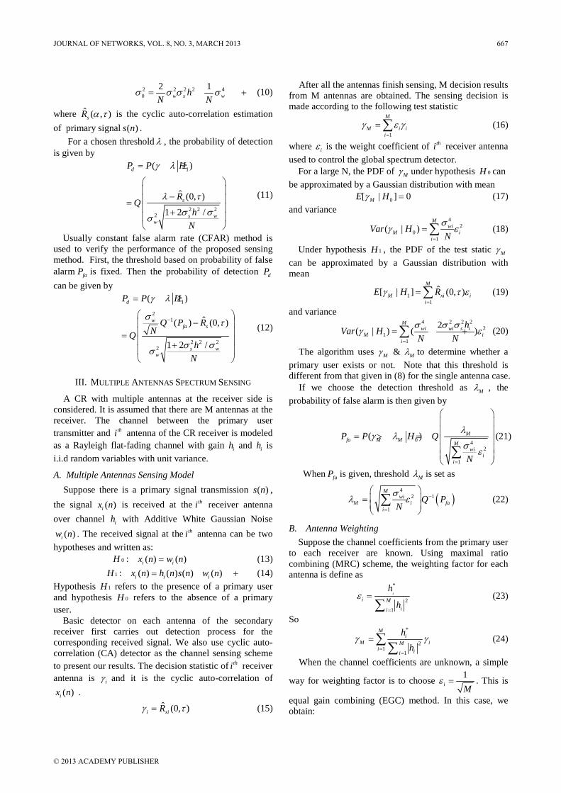
2 2 2 2 40

2 1w s wh

N Nσ σ σ σ= + (10)

where ˆ ( , )sR α τ is the cyclic auto-correlation estimation of primary signal ( )s n . For a chosen threshold λ , the probability of detection is given by

1

2 2 22

( )

ˆ (0, )

1 2 /

d

s

s ww

P P H

RQ

hN

γ λ

λ τ

σ σσ

= ≥

− = +

(11)

Usually constant false alarm rate (CFAR) method is used to verify the performance of the proposed sensing method. First, the threshold based on probability of false alarm faP is fixed. Then the probability of detection dP can be given by

1

21

2 2 22

( )

ˆ( ) (0, )

1 2 /

d

wfa s

s ww

P P H

Q P RNQ

hN

γ λ

στ

σ σσ

−

= ≥

−

= +

(12)

III. MULTIPLE ANTENNAS SPECTRUM SENSING

A CR with multiple antennas at the receiver side is considered. It is assumed that there are M antennas at the receiver. The channel between the primary user transmitter and thi antenna of the CR receiver is modeled as a Rayleigh flat-fading channel with gain ih and ih is i.i.d random variables with unit variance.

A. Multiple Antennas Sensing Model Suppose there is a primary signal transmission ( )s n ,

the signal ( )ix n is received at the thi receiver antenna over channel ih with Additive White Gaussian Noise

( )iw n . The received signal at the thi antenna can be two hypotheses and written as:

0H : ( ) ( )i ix n w n= (13) 1H : ( ) ( ) ( ) ( )i i ix n h n s n w n= + (14)

Hypothesis 1H refers to the presence of a primary user and hypothesis 0H refers to the absence of a primary user.

Basic detector on each antenna of the secondary receiver first carries out detection process for the corresponding received signal. We also use cyclic auto-correlation (CA) detector as the channel sensing scheme to present our results. The decision statistic of thi receiver antenna is iγ and it is the cyclic auto-correlation of

( )ix n . ˆ (0, )i xiRγ τ= (15)

After all the antennas finish sensing, M decision results from M antennas are obtained. The sensing decision is made according to the following test statistic

1

M

M i ii

γ ε γ=

= ∑ (16)

where iε is the weight coefficient of thi receiver antenna used to control the global spectrum detector.

For a large N, the PDF of Mγ under hypothesis 0H can be approximated by a Gaussian distribution with mean

0[ | ] 0ME Hγ = (17) and variance

42

01

( | )M

wiM i

iVar H

Nσ

γ ε=

= ∑ (18)

Under hypothesis 1H , the PDF of the test static Mγ can be approximated by a Gaussian distribution with mean

11

ˆ[ | ] (0, )M

M xi ii

E H Rγ τ ε=

= ∑ (19)

and variance

4 2 2 2

21

1

2( | ) ( )

Mwi wi s i

M ii

hVar H

N Nσ σ σ

γ ε=

= +∑ (20)

The algorithm uses Mγ & Mλ to determine whether a primary user exists or not. Note that this threshold is different from that given in (8) for the single antenna case.

If we choose the detection threshold as Mλ , the probability of false alarm is then given by

0 42

1

( ) Mfa M M M

wii

i

P P H Q

N

λγ λ

σε

=

= > = ∑

(21)

When faP is given, threshold Mλ is set as

( )4

2 1

1

Mwi

M i fai

Q PNσ

λ ε −

=

= ∑ (22)

B. Antenna Weighting Suppose the channel coefficients from the primary user

to each receiver are known. Using maximal ratio combining (MRC) scheme, the weighting factor for each antenna is define as

*

2

1

ii M

ii

h

hε

=

=∑

(23)

So *

21

1

Mi

M iMi ii

hh

γ γ=

=

= ∑∑

(24)

When the channel coefficients are unknown, a simple

way for weighting factor is to choose 1i Mε = . This is

equal gain combining (EGC) method. In this case, we obtain:



1

1M

M ii M

γ γ=

= ∑ (25)

Equal density of noise is assumed in the two methods above and thus only the channel gains are considered. A new algorithm based on auto-correlation is proposed in this paper in which the optimal weights are obtained for each antenna in case little priori knowledge of channel as well as noise is known.

Correlation research is an important basic foundation for the study of mutual contact mode and the interrelated close degree of variable or variables group [16-18].

( )ih nUsually the signal samples should be correlated due

to that the signal is over sampled, while and ( )iw n are i.i.d, both will influence the correlation of the signal

( )ix n . The more channel fades and the worse the noise becomes, the more they make influence on correlation of signal.

Define the sample auto-correlation of the received signal for the receiver antenna as

1

0

1( ) ( ) ( )N

ml x m x m l

Nθ

−

=

= −∑ 0,1, , 1l L= −

(26) where N is the number of available samples, L denotes time delay. Let

1( )

L

nG nθ

=

= ∑ (27)

And define ratio B as

1( ) (0)

L

nB nθ θ

=

= ∑ (28)

1( )

L

nnθ

=∑where reflects the correlation extent of signal

and it is influenced by channel fading. (0)θ reflects the correlation of additive white Gaussian noise and this value is bigger with noise becoming worse.

When the channel fading and the power of noise are comparatively small, B values are large and vice versa. B values reflects the synthetic impact of channel characteristics ( )h n and noise ( )w n on the signal ( )s n .

For a multi-antenna sensing system, it is assumed that channel gain ( )ih n for each antenna is different while the power of noise ( )iw n is identical. If channel gain is unknown for each antenna, weight equals：

1/

M

i i ii

G Gε=

= ∑ (29)

( )iw nIn reality, noise may lead to difference in . If the channel characteristics and noise are considered simultaneously, the weights should be assigned adaptively according to B values. This method is termed as Auto Correlation (AU)

1/

M

i i ii

B Bε=

= ∑

method. The corresponding weights equal

C. Antenna Selection Algorithm

(30)

In multi-antenna spectrum sensing system, threshold Mλ is set as

( )4

2 1

1

Mwi

M i fai

Q PNσ

λ ε −

=

= ∑ (31)

For a chosen threshold Mλ , the probability of detection is given by

1

1

4 2 2 22

1

( )

ˆ (0, )

2( )

d M M

M

M i xii

Mwi wi s i

ii

P P H

RQ

hN N

γ λ

λ ε τ

σ σ σε

=

=

= ≥

− = +

∑

∑

(32)

It is observed that the detection probability depends on the number of antennas M, weights for each antennas iε as well as channel gains ih .

The optimization of detection probability dP can be re-written as：

max

. .d

f fa

P

s t P P≤ (33)

where fP and faP represent the real false detection probability and target false detection probability respectively.

Solving (33) involves complicated computation. A frequently used method to obtain diversity gain is based on the assumption that both SNR and the number of antennas are large. As long as the antenna characteristics are similar, the detection probability can be improved if more antennas are involved. However, if the antenna characteristics are quite different or the number of poorly performed antenna is large the detection probability deteriorates. Therefore, the well-performed antennas are selected in order to improve the detection probability.

Which antennas are selected to sense spectrum is considered in this section. The goal is to optimum the detection sensitivity through antennas selection while meeting a given requirement on the probability of false alarm.

iB∆To better compare the performance of different

antennas, define relative ratio as 100*[max( ) ]i i i iB B B B∆ = − (34)

iB∆ represents the difference ratio between thi antenna and the best antenna. So ratio iB∆ can be used as criterion to select appropriate antenna to sense spectrum.

IV. NUMERICAL RESULTS

In this section Monte Carlo simulations are used to verify the method. A four-antenna system with four RF chains is considered. As a signal of interest, a BPSK time series is taken. The number of observations is N=200 and L=10. The computing results of B value are displayed in Fig.1 and Fig.2



Figure 1. B versus SNR with different h

Figure 2. B versus h with different SNR

Figure 3. Performance comparison of single antenna and multiple

antennas

Fig. 1 shows different B values for various SNR. As seen, B values increase with the channel gains and vice versa when noise power is same. When noise power is large, e.g., SNR<-5dB, the difference of B values between three antenna are significant. As the SNR increases, the difference becomes marginal. Hence this method performs better in scenarios with low SNR values.

Fig.2 shows the B value versus channel gain in case of given noise power. Three scenarios are simulated. SNRs are -5dB,-10dB and -15dB. It is observed that B values increase as the power of noise decrease and vice versa.

Fig. 1 and Fig.2, show the impact of B value as well as noise on the signal s(n).

Fig.30.1faP =

gives the detection probability for SNRs when system false detection probability and M denotes the number of sensing antennas. It is observed that diversity gain improves significantly as the number of antennas increases. Meanwhile, the detection probability increases.

0 0.1 0.2 0.3 0.4 0.50

0.1

0.2

0.3

0.4

0.5

0.6

0.7

0.8

0.9

1

Prob. False Alarm ( Pfa )

Pro

b. D

etec

tion

( Pd

)AUMRCEGC

Figure 4. Comparison of weight assigning methods (I)

0 0.1 0.2 0.3 0.4 0.50

0.1

0.2

0.3

0.4

0.5

0.6

0.7

0.8

0.9

1

Prob. False Alarm ( Pfa )

Pro

b. D

etec

tion

( Pd

)

AUMRCEGC

Figure 5. Comparison of weight assigning methods (II)

Fig.4 compares three weights assigning methods for different sensing systems. Equation (29) is employed in the AU method for same background noise and antennas. MRC and EGC methods adopt (24) and (25) respectively. As seen, AU and MRC have similar performance while EGC performs worse.

( )iw nFig.5 shows the AU methods in (30) with different

antenna characteristics . In this case, both the background noise and channel characteristics are incorporated. However, only channel gain is assumed in MRC method. It is observed that AU behaves better comparing with MRC. EGC performs the worst.



Figure 6. Pd versus Pfa iB∆ =[0, 2%, 3%, 5%]

Four antennas with random fading realizations and random noise variances in the environment are simulated. The B values of four antennas can calculated respectively as B1=5.39, B2=5.30, B3=5.22, B4 1B∆=5.11, and =0,

2B∆ =2%, 3B∆ =3%, 4B∆ =5%. The values of iB∆ about four antennas are all less than 10%, it can be thought that the performances of these four antennas are similar.

In Fig.6 the probability of detection Pd versus the probability of false alarm Pfa with selecting 1 antenna from 4, selecting 2 antennas from 4, selecting 3 antennas from 4 and whole four antennas is plotted. Fig.6 shows that the detection performance by four antennas is obviously better than one or two antennas. Because the performances of these four antennas are similar, utilizing spatial diversity can improve sensing performance.

Figure 7 .Pd versus Pf iB∆ = [0, 3%, 8%, 16%]

Fig.7 is another simulation result. The B values of four antennas are calculated as B1=5.39, B2=5.25, B3=4.98, B4 1B∆=4.64, and =0, 2B∆ =3%, 3B∆ =8%, 4B∆ =16%. The values of iB∆ show that the performances of three antennas are nearly similar( iB∆ <10%), while one antenna is very different from other three( 4B∆ >15%). When selecting two or three antennas to cooperate sensing, the detection performance is best. While if

cooperating all four antennas in the system to sense, because of existing one “bad” antenna, the detection performance obviously gets worse. In this circumstance it is necessary for selecting antenna so as to achieve the best sensing performance. Usually if the iB∆ of one antenna is higher than 15%, this antenna should be rejected for operating the sensing.

In Fig.8 the B values of four antennas are calculated as B1=5.39, B2=4.62, B3=4.62, B4 1B∆=4.324, and =0,

2B∆ =17%, 3B∆ =17%, 4B∆ =25%. The values of iB∆ show that only one antenna is good, while other three antennas are bad ( 4B∆ >15%). It can be found that if comparing the whole four antennas to sense, the Pd is the worst, while selecting one antenna to sense, the Pd is the best. Fig.8 shows that selecting one antenna to sensing achieves the optimum Pd

The optimum P

.

d

iB∆

is usually achieved by cooperating parts of antennas that have higher B values. Usually if the

of one antenna is less than 10%, this antenna can be selected to sense, so as to improve sensing performance by utilizing spatial diversity. If the iB∆ of one antenna is higher than 15%, this antenna can not be selected to cooperate sensing, which makes performance worse. This shows that the Pd can be improved through selecting antennas.

Fig. 8 Pd versus Pfa with iB∆ =[0, 17%, 17%, 25%]

V. CONCLUSIONS

In this paper, a spectrum sensing optimization algorithm based on antenna selection is proposed. In the case where the channel coefficient and noise power are not known, cooperating all antennas in the network does not achieve the best sensing performance. The numbers of selected antennas have certain influence on probability of detection. One algorithm for selecting the antenna with the best detection performance is proposed. Based on this algorithm, it can be distinguished whether it is necessary for antennas selection so as to optimize spectrum sensing performance. The results indicate that the proposed antenna selection algorithm is able to optimize network performance.



ACKKNOWLEDGEMENT

The work is supported by National Natural Science Foundation of China under Grant No. 60872003, application Basic Research Plans of Suzhou China under Grant No.SYJG0925, and Doctoral found of Ministry of Education of China under Grant No.20093201110005 from Soochow University.

REFERENCES

[1] Federal Communications Commission, “Spectrum Policy Task Force” Rep. ET Docket no. 02-135, Nov. 2002.

[2] I. Akyildiz, W. Lee, M. Vuran, and S. Mohanty, “Next Generation/ Dynamic Spectrum Access/ Cognitive Radio Wireless Networks: A Survey,” Elsevier Computer Networks Journal, pp. 2127-2159, Sep. 2006.

[3] A. Ghasemi and E. S. Sousa, “Spectrum Sensing in Cognitive Radio Networks: Requirements, Challenges and Design Trade-offs,” IEEE Commun. Mag, Vol. 46, pp. 32–39, Apr. 2008.

[4] A. Taherpour, M. Nasiri-Kenari, S. Gazor, “Multiple Antenna Spectrum Sensing in Cognitive Radios,” IEEE Trans. Wireless Commun, Vol. 9, no. 2, pp. 814-823, Feb. 2010.

[5] A. Taherpour, M. Nasiri-Kenari, S. Gazor, “Multiple Antenna Spectrum Sensing in Cognitive Radios,” IEEE Trans. Wireless Commun, Vol. 9, no. 2, pp. 814-823, Feb. 2010.

[6] S. Kim, J. Lee, H. Wang, D. Hong, “Sensing Performance of Energy Detector with Correlated Multiple Antennas,” IEEE Signal Processing Letters, Vol. 16, no. 8, pp. 671-674, Aug. 2009.

[7] Xing Chen, Wenjun Xu, Zhiqiang He, Xiaofeng Tao, “Spectral Correlation-Based Multi-Antenna Spectrum Sensing Technique,” Wireless Communications and Networking Conference, 2008. WCNC 2008. IEEE . vol.12, no.2, pp.735-740, March 31 2008-April 3 2008。

[8] Seung-Hoon Hwang, Jun-Ho Baek, “Multiple Antenna-Aided Spectrum Sensing Using Energy Detectors for Cognitive Radio,” Vehicular Technologies: Increasing Connectivity, Subject: Electrical and Electronic Engineering, Publisher: InTech, April, 2011 ISBN 978-953-307-223-4, Hard cover, 448 pages。

[9] Y. Jiang, M. Varanasi, “The RF-chain Limited MIMO System-part I: Optimum Diversity-Multiplexing Tradeoff,” IEEE Trans. Wireless Commun, vol. 8, no. 10, pp. 5238-5247, Oct. 2009.

[10] Owayed Abdullah Alghamdi, Mohammed Zaki Ahmed, “Optimal and Suboptimal Multi Antenna Spectrum Sensing Techniques with Master Node Cooperation for Cognitive Radio Systems,” Journal of Communications, Vol 6, No 7 , pp.512-523, Oct 2011.

[11] Liang Ma, Qi Zhu, “A New Algorithm of Spectrum Allocation Based on the Balance between Supply and Demand in Cognitive Radio Networks,” Journal of Networks, Vol 7, No 7, pp.1017-1023, Jul 2012.

[12] Z. Xu, S. Sfar, R. S. Blum, “Analysis of MIMO Systems with Receive Antenna Selection in Spatially Correlated Rayleigh Fading Channels,” IEEE Trans. Veh. Technol, vol. 58, no. 1, pp. 251-262, Jan. 2009.

[13] Stephen Wang, Yue Wang, Justin Coon, Angela Doufexi. “Antenna Selection Based Spectrum Sensing for Cognitive Radio Networks,” Personal Indoor and Mobile Radio Communications (PIMRC), 2011 IEEE 22nd International Symposium on , vol., no., pp.364-368, 11-14 Sept. 2011.

[14] Yang Ou, Yi-ming Wang, “Efficient Methods for Spectrum Sensing in Cognitive Radio,” 2010 International Conference on Wireless Communications and Signal Processing (WCSP), Oct. 2010.

[15] Yang Ou, Yi-ming Wang, “Performance of Spectrum Sensing and Optimization Based on User Selection in Cognitive Radio,” International journal of communications, Issue 2, Volume 6, pp. 72-79,2012.

[16] Yifeng Li, “EEG Physiological Signals Correlation under Condition of +Gz Accelerations,” Journal of Multimedia, VOL. 8, NO. 1, pp.64-71, Feb 2013.

[17] Baoming Shan, “A Novel Image Correlation Matching Approach, Journal of Multimedia, VOL. 5, NO. 3, pp.268-275, Jun 2010.

[18] Jyotirmoy Karjee, H.S Jamadagni, “Data Accuracy Estimation for Spatially Correlated Data in Wireless Sensor Networks under Distributed Clustering,” Journal of Networks, VOL. 6, NO. 7, pp1072-1083, Jul 2011.

Yang Ou received the M.S. degree in Electrical Engineering from North University of China in 1996. She works as an associate professor in Electronic Engineering at University of Science and Technology of Suzhou China. She is currently pursuing her PhD in Electronics and Information Engineering at Soochow University.

Her research interests include cognitive radio, spectrum sensing, signal processing for communications, wireless networking and statistical signal processing. Yi-Ming Wang is professor at Dept. of Electronics and Information Engineering, Soochow University, China. The main research direction includes multimedia communications and wireless communications. Currently her academic research focuses on communication signal processing, cognitive radio, broadband wireless communications technology and the source channel coding.



An Efficient Parallel Anomaly Detection Algorithm Based on Hierarchical Clustering

Ren Wei-wu, Hu Liang, Zhao Kuo,Chu Jianfeng

College of Computer Science and Technology, Jilin University, Changchun, China E-mail: [email protected]

Abstract—For the purpose of improving real time and profiles accuracy, a parallel anomaly detection algorithm based on hierarchical clustering has been proposed. Training and predicting are two busiest processes and they are parallel designed and implemented. Moreover, an abnormal cluster feature tree is built to dig anomalies from normal profiles. A series of experiment results on well-known KDD Cup 1999 data sets indicate that the improved algorithm has superior performance in both detection and real time. Index Terms—parallel algorithm; hierarchy clustering; abnormal cluster feature tree; normal profiles

I. INTRODUCTION

With the number of intrusion and hacking incidents around the world on the rise, the importance of having dependable intrusion detection systems in place is greater than ever. An intrusion detection system is designed to detect several types of abnormal behaviors that can compromise the security and trust of a computer system.

Now the main intrusion detection technology is divided into two categories: misuse detection [1-2] and anomaly detection [3-7]. Misuse detection encodes the known attacks into the signatures and detects attacks whose signatures are known and have been encoded. Intrusion detection system based on misuse detection can not detect unknown attacks. The process of signing attacks is enormous cost for systems. Unlike misuse detection, anomaly detection builds the normality profiles on the basis of normal behaviors of users, often using machine learning or data mining techniques. In the process of detection, online traffic is matched with the normality profiles, and deviations are marked as anomalies. Since no knowledge of attacks is used to train the normality profiles, anomaly detection can detect previously unknown attacks. Therefore anomaly detection is hotspot in the field of intrusion detection.

Many popular technologies are applied in the field of anomaly detection. Clustering algorithm [21-23] is a successful application in the field of anomaly detection. Density clustering [9-12] and hierarchical clustering [12-15] are two outstanding representative kinds of clustering algorithms. Density clustering can build arbitrary shape

cluster, but calculation is too complex. Hierarchical clustering has good efficiency and is easy to implement incremental algorithm, but only build spherical cluster. So profiles of hierarchical are generally less precise than profiles of density clustering.

Moreover, the growth of network flow makes the real time of anomaly detection algorithms be involved. The old serial algorithm can not meet the real time of detection, and the development of CPU has officially entered the era of multi-core. Along with the update multi-core technology, parallel algorithm must be a new way to solve the problem of real time.

Parallel algorithms [16-20] are valuable because of substantial improvements in multiprocessing systems and the rise of multi-core processors. There are two ways parallel processors communicate, shared memory or message passing. Shared memory processing needs additional locking for the data, imposes the overhead of additional processor and bus cycles, and also serializes some portion of the algorithm. Message passing processing use channels and message boxes but this communication adds transfer overhead on the bus, additional memory need for queues and message boxes and latency in the messages. Designs of parallel processors use special buses like crossbar so that the communication overhead will be small but it is the parallel algorithm that decides the volume of the traffic.

For the purpose of improving real time and profiles accuracy of hierarchical clustering, a parallel anomaly detection algorithm based on hierarchical clustering has been proposed in this paper. Training process and predicting process, which consume a lot of resources, are parallel designed and implemented. Moreover, an abnormal cluster feature tree is built to dig anomalies from normal profiles. It can compensate the lack of profiles accuracy of hierarchical clustering.

The rest of paper is organized as follows. In section 2, we introduce some basic concepts. Section 3 presents details of parallel algorithms. Section 4 presents our experiments results and analysis. Finally, we summarize our conclusions and future work in section 5.

II. BASIC CONCEPTS

The related basic concepts are introduced at first: Definition 0: we assume that each sample point lies in

the k-dimensional Euclidean space, and a cluster

Corresponding author: Chu Jianfeng Email: [email protected]



}...1|{ nivC i == is defined the collection of iv ,

iv is a vector which starts with the origin, and ends with

the id . Definition 1: For a cluster }...1|{ nivC i == and

the k-dimensional vector iv in the cluster, its center is defined as:

nv

vn

i i∑ == 10

(1)(_

The center describes the distribution of points in the cluster.

Definition 2: for a cluster }...1|{ nivC i == and

the k-dimensional vector iv in the cluster, its radius R(C) is defined as:

n

vvCR

n

i i

2

1 0 )()( ∑ =

−=

(2)))_

Radius R(C) describes the clustering degree of points in cluster (i.e., the mean distance from all the points to center 0v )

Definition 3: for two clusters C1 and C2, and their centers 0v and '0v , the distance from C1 to C2 is defined

as the Euclidean distance from 0v to '0v . Definition 4: Cluster Feature (CF) is a triple:

},,{ sssnCF = , among which n is the number of

vector iv in the cluster C, and s is the linear sum of all

the vectors in the cluster C (i.e., ∑==

n

i ivs1

), and ss is

the sum of squares of all the vectors in the cluster C (i.e.,

∑ ==

n

i ivss1

2 ). CF describes the overall feature of

cluster. Definition 5: for two clusters C1 and C2, and their

sum C1+C2 represents the merger of two clusters (i.e., all the vectors in two clusters are merged into one new cluster)

Theorem 1: for two clusters C1 and C2, and their CF },,{ 1111 sssnCF = and },,{ 2222 sssnCF = , then CF of

C1+C2 is },,{ 21212121 ssssssnnCF +++=+ .

Proof: the proof of theorem 1 is simple. Due to definition 4 and definition 5, theorem 1 is not difficult to show.

Theorem 2: cluster C and its },,{ sssnCF = , then

its center can be represent as nsv

=0

Proof: due to definition 1 and definition 4,

∑ ==

n

i ivs1

2

, then nsv

=0 .

Theorem 3: cluster C and its },,{ sssnCF = , then its radius can be represent as

2

2

)(ns

nssCR

−= (3)

Proof: due to definition 2, n

vvCR

n

i i

2

1 0 )()( ∑ =

−=

,

After vector expansion: ( )n

vvCR

n

i

d

j jij∑ ∑= =−

= 1 12

0)(

( )n

vvvvCR

n

i

d

j jijjij∑ ∑= =−+

= 1 1 02

02 2

)(

Then

( )[ ]n

vvvnvCR

d

j

n

i ijjd

j jn

i

d

j ij ∑ ∑∑∑ ∑ = === =−+

= 1 1012

01 12 2

)(

，

Due to ∑ ==

d

j jvv1

20

20 ,

( )[ ]n

vnvnvCR

d

j jn

i

d

j ij ∑∑ ∑ == =−+

= 120

201 1

2 2)(

Then

n

vnv

n

vnvnvCR

n

i

d

j ijn

i

d

j ij201 1

220

201 1

2 2)(

−=

−+=

∑ ∑∑ ∑ = == =

Due to definition 4: 01vnvs n

i i ==∑ =

and

01vnvs n

i i ==∑ =

, and they are substituted in the above

equation, then 2

2

)(ns

nssCR

−= .

It can be seen by the above theorem. The center and radius of cluster can be calculated by its CF without having to know each specific vector. Therefore, the algorithm to run needs not to keep original data.

Cluster Feature tree (CF tree): CF is organized in a tree structure. A CF tree represents the present user’s profile. CF tree is height balanced tree. For each leaf node, its height is the same. There are three parameters: the maximum number of branches B, threshold T and the maximum number of cluster M. The node of CF tree is table which contains B entries at most. The entry can be represented by the form ｛CFi, pChild｝, i = 1, 2, …,B, pChild points to the child node of present node. And CFi represent the merger of clusters of the child node to which is pointed by pChild. In particular, the leaf node of CF tree is not same with the other nodes. The value of its entry pChild is NULL, and the CFi does not represent the merger of clusters but specific clusters. Each cluster in the leaf node must satisfy the threshold T (i.e., the radius of each cluster must be less than T). The number of clusters in the whole leaf nodes must be less than M. To sum up, the tree which satisfies the above conditions can be called Cluster Feature tree (CF tree).



NCF tree: NCF tree is a CF tree which is composed of CFs derived from normal behaviors. NCF tree represents user’s profiles of normal behaviors.

ACF tree: ACF tree is a CF tree which is composed of CFs derived from abnormal behaviors. ACF tree represents the known type of attack.

(a) (b)

(c) (d)

Figure 1. Clustering in three different ways

In the Fig 1, sub graph (a) shows some behavior points which needs to be clustered; sub graph (b) shows the hierarchical clustering result; sub graph (c) shows the density clustering result; sub graph (d) shows new clustering result after building NCF tree and ACF tree. The cluster shape of density clustering can be arbitrary. But the cluster shape of hierarchical clustering can only be spherical. So the accuracy of profiles which are generated by hierarchical clustering is not as good as profiles of density clustering. Therefore, as is shown in the sub graph (d) of Fig 1, ACF tree is built to dig the abnormal behaviors from the normal profiles.

III. PARALLEL ALGORITHM

The process of generating profiles and the process of predicting intrusion which are the bottlenecks of improving performance need a large number of calculation and run in the real time environment. Therefore, parallel design and implementation mainly focus on two processes, which are shown the Fig 2.

Thread Pool

……

Main CF

Tree

Main Thread

Training Thread 1

Training Thread 2

Training Thread N

Sub CF Tree

Sub CF Tree

Sub CF Tree

Extract

Merge

TrainingDataset

PredictingThread 1

Extract

Extract

PredictingThread 2

PredictingThread N

RealTime

NetworkTraffic

……

Access

Extract

Extract

Extract

Figure 2. Overview of parallel algorithm

In the process of generating profiles, ACF tree is composed of abnormal behaviors which are added regularly by security administrator. So the real time

amount of data is not too large. ACF tree can be built by a single thread instead of parallel. But NCF tree is composed of real time traffic. So it has to be built by multiple parallel threads.

The process of generating profiles includes two algorithms: parallel training algorithm and merging algorithm. The process of predicting intrusion includes an algorithm: parallel predicting algorithm. The three algorithms will be separately introduced as follows:

A. Parallel Training Algorithm The working thread can not directly access the main

thread. Moreover, main tree is running in the main thread. So there is no need of locking between working thread and main thread. Once main thread receives the sub CF tree, it will launch the merging algorithm and merge sub CF tree into main CF tree. Each thread can run in parallel with other threads and send sub CF tree to main thread.

The pseudocode of procedure WorkingThreadRun() is shown as follows:

Procedure WorkingThreadRun () { create a empty CF tree; while(new traffic){ receive traffic(thread will sleep until the coming of traffic); extract v from traffic and generate CF; Insert(CF, root);//initial root is an empty CF if( CF tree is greater than M ){ collect all the clusters of leaf nodes; send the above clusters to main thread; clean CF tree; } } } Initially, CF tree only has an empty root. With the

coming of new vector v , a temporary CF={1, v , 2v } is constructed, in other words, the vector v is considered as a cluster which only contains one vector. And the following vectors are dynamically inserted into the CF tree by procedure Insert(CF,p). The pseudocode of procedure Insert(CF,p) is described as follows:

Procedure Insert(CF, p) { Traverse all the items of node p, find the nearest cluster CFi if( p is leaf node){

;

if(merge CF into CFi merge CF into CF

and new cluster still satisfies T) i

else //according to Theorem 1;

add a new item [CF, NULL] in node p; }else{ insert(CF, pChildi); //recursive call merge CF into CFi if(pChild

; i

call SplitNode(pChild violate B){

i) //split pChildi into pChild1 and pChild2

delete item[CF;

i ,pChildi create CF

] from node p; 1 and CF2, they are separately cluster mergers

of pChild1 and pChild2 create two new items [CF

; 1,pChild1] and

[CF2,pChild2 insert two new items into node p;

];

} } }



It can be drawn from the above pseudocode that the function of Insert(CF,P), as a recursion, needs to check whether the constraint B is satisfied or not when it returns. Therefore, the constraint B is split into two from bottom to top. If the root is against B, the tree would grow itself.

The above algorithm calls the sub procedure SplitNode(p), and the pseudocode shows details of SplitNode(p) as follows:

Procedure SplitNode(p) { Traverse node p and find the two farthest nodes CFi and

CFj Generate two new nodes p1 and p2; ;

Insert separately [CFi,pChildi] and [CFj,pChildj

for(all the CFs of node p except CF

] into node p1 and node p2;

i and CFj

if(

){

),(),( ji CFCFdisCFCFdis ≤ )

insert [CF,pChild] into p1; else insert [CF,pChild] into p2; } return p1 and p2; } It can be drawn from the above algorithm that with the

coming of new data, the number of leaf node increases until the constraint M is violated. Then CF tree needs to be rebuilt.

The process of rebuilding CF can be described as follows: first, the constraint T is relaxed. Then CFs of the entire leaf nodes are collected and CF tree is cleaning. Next the collected CFs are inserted into the new CF tree by calling the procedure of Insert(CF, p). Finally the CF tree is rebuilt.

Threshold T is one of three parameters of CF tree. To relax T can merge clusters and can reduce the number of leaf nodes. There are still two other parameters to be explained: B and M. B represents the maximum number of branches, in other words, node can have the maximum number of child nodes. Obviously, the larger B is, the lower the height of CF tree is. So if B is too small, the height of CF tree is high. And CF tree has a small number of CF. Such a CF tree can usually not satisfy the fundamental demand of clustering. If B is too large, the height of CF is low. A lager number of CFs will be gathered in few nodes. Such a CF tree usually leads to the performance problems of detection. Especially, the process of searching CF will traverse all the CFs in nodes. The real time of algorithm is difficult to guarantee.

B. Merging Algorithm SubCF

Tree

SubCF

Tree

SubCF

Tree

MainCF

Tree

Figure 3. Process of merging CF tree

As shown in the Fig 3, the main thread receives sub CF tree and merge it into main CF tree. This process call the above procedure insert(CF, root).

The pseudocode of merging algorithm is described as follows:

Procedure MainThreadRun () { Create an empty CF tree; while(receive CF from working thread){ for(each CFi Insert(CF

){ i

if(main tree violate M) , root); //root of main tree

relax T，rebuild main CF tree; } } }

C. Parallel Predicting Algorithm In the parallel predicting algorithm, multiple parallel

predicting threads extracts v from the network traffic and predicts v with the help of profiles. Parallel predicting threads only read the profiles and do not write them. Multiple parallel predicting threads have no impact on CF tree. There is no mutual exclusion problem among predicting threads. Moreover, due to the nature of intrusion detection system, security administrator does not usually train and predict at the same time. As a result, multiple predicting threads and main thread hardly access the main CF tree at the same time. But in order to avoid this pitfall, main thread is protected by write lock and predicting threads are protected by read lock.

The predicting thread can be described as follows: Procedure PredictThreadRun () { while(new traffic){ receive new traffic //thread will sleep until the coming of

traffic; extracts v from traffic; if(PredictACF ( v ,root) is abnormal){ alert abnormal; }else if(PredictNCF( v ,root) is abnormal){ Alert abnormal; } Record normal; } } At first, PredictACF( v ,root) is called to determine

that v is the labeled attack type or not. If procedure of predictACF( v ,root) directly returns abnormal; the

detection of v

is over. Otherwise, v needs to be further determined by calling PredictNCF( v ,root). The details

of procedure PredictACF( v ,root) are shown as follows: Procedure PredictACF ( v , p) { traverse all items of node p, and find the nearest CFi v of ; if( p points to leaf node){ if(the distance between v and CFi < K*R(CFi

return labeled attack type of CF

)) //k is a constant slightly greater than 1

i

else



return normal; PredictNCF( v ,root); } else return PredictACF( v ,pChildi

} );

The details of procedure PredictNCF( v ,root) are

shown as follows: Procedure PredictNCF( v , p) { traverse all items of node p, and find the nearest CFi v of ; if( p points to leaf node){ if(the distance between v and CFi > K*R(CFi

return abnormal;

)) // k is a constant slightly greater than 1

else return normal; } else return PredictNCF( v ,pChildi

} );

The number of predicting threads can be dynamically

adjusted according to the real time network traffic.

IV. EXPERIMENTAL RESULT AND ANALYSIS

A. Dataset KDD CUP 1999 data set which is deprived from 1998

DARPA Intrusion Detection Evaluation program held by MIT Lincoln Labs, is employed to study the utilization of machine learning for intrusion detection by numerous researchers. The dataset includes all kinds of simulated intrusion actions in the complicated network environment, where each connection instance contains 41 features. In this paper the KDD CUP 1999 data set have been selected as the simulated traffic source of our experiments. 100,000 connection instances, as the training dataset, are extracted randomly from the file kddcup. data_10_percent. 100,000 connection instances, as the predicting dataset, are extracted randomly from the file corrected.

B. Optimal Parameter

200 400 600 800 10000

5

10

15

20

25

30

35

40

45

M

Fals

e P

ositi

ve R

ate

(%)

B=15B=20B=25

Figure 4. Optimal B and M (false positive rate)

200 400 600 800 1000-20

0

20

40

60

80

100

120

M

Det

ectio

n R

ate

(%)

B=15B=20B=25

Figure 5. Optimal B and M (detection rate)

There is essentially no difference between serial execution result and parallel execution result. So the optimal parameters of main CF tree are selected by referring to the optimal parameters of serial procedure. As is shown in the Fig 4 and Fig 5, only when B=20 and M=300, detection rate is relatively high and false positive rate is relatively low in the tolerable range.

20 40 60 80 1001

1.5

2

2.5

3

3.5

Maximum Number of Concurrent Threads

Spe

edup

Dual CoreQuad Core

Figure 6. Optimal number of concurrent threads

Threshold TM of main CF tree can relax itself when the number of clusters is great than M. Due to relaxing T, some clusters are merged and the number of leaf nodes decreases. The initial value of TM of main CF tree is set to 0, and TM will reach an adaptive value with the growth of CFs. The final TM

Every CF tree has its parameters. But sub CF tree has no direct impact on detection performance. So there is no need to select the optimal parameters for sub CF tree. The parameters of sub CF tree still need to take some basic precautions: (1) B of sub CF tree should be same with B of main CF tree. It helps to be convenient to insert sub CF tree into main CF tree; (2) M of sub CF tree should be less than M of main CF tree, which can reduce times of splitting node from bottom to up; (3) T

is equal to 0.8.

S of sub CF tree should be a constant which is less than TS of main CF tree. Therefore the parameters of sub CF tree are set as follows: B=15, M=200 and TS

The maximum number of concurrent threads in thread pool has various default values according to different CPU. This value can be modified according to the actual need. The maximum number of concurrent threads in thread pool should be increased with the growth of real time network traffic. But too many threads in thread pool

=0.5.



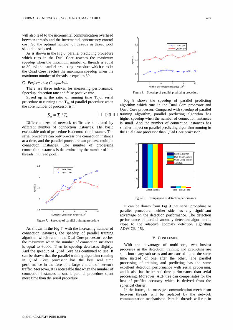
will also lead to the incremental communication overhead between threads and the incremental concurrency control cost. So the optimal number of threads in thread pool should be selected.

As is shown in the Fig 6, parallel predicting procedure which runs in the Dual Core reaches the maximum speedup when the maximum number of threads is equal to 30 and the parallel predicting procedure which runs in the Quad Core reaches the maximum speedup when the maximum number of threads is equal to 50.

C. Perfermance Comparison There are three indexes for measuring performance:

Speedup, detection rate and false positive rate. Speed up is the ratio of running time Tspof serial

procedure to running time Tpp of parallel procedure when the core number of processor is n:

nn TTS /1=

Different sizes of network traffic are simulated by different number of connection instances. The basic executable unit of procedure is a connection instance. The serial procedure can only process one connection instance at a time, and the parallel procedure can process multiple connection instances. The number of processing connection instances is determined by the number of idle threads in thread pool.

(4)

2 4 6 8 100.5

1

1.5

2

2.5

Number of Connection Instances(104)

Spe

edup

Dual CoreQuad Core

Figure 7. Speedup of parallel training procedure

As shown in the Fig 7, with the increasing number of connection instances, the speedup of parallel training algorithm which runs in the Dual Core processor reaches the maximum when the number of connection instances is equal to 60000. Then its speedup decreases slightly. And the speedup of Quad Core has continued to rise. It can be drawn that the parallel training algorithm running in Quad Core processor has the best real time performance in the face of a large amount of network traffic. Moreover, it is noticeable that when the number of connection instances is small, parallel procedure spent more time than the serial procedure.

2 4 6 8 101

1.5

2

2.5

3

3.5

4

Number of Connection Instances (104)

Spe

edup

Dual CoreQuad Core

Figure 8. Speedup of parallel predicting procedure

Fig 8 shows the speedup of parallel predicting algorithm which runs in the Dual Core processor and Quad Core processor. Compared with speedup of parallel training algorithm, parallel predicting algorithm has higher speedup when the number of connection instances is small. And the number of connection instances has smaller impact on parallel predicting algorithm running in the Dual Core processor than Quad Core processor.

Detection Rate False Positive Rate0

20

40

60

80

100

Serial AlgorithmDual Core(Parallel)Quad Core(Parallel)ADWICE

Figure 9. Comparison of detection performance

It can be drawn from Fig 9 that serial procedure or parallel procedure, neither side has any significant advantage on the detection performance. The detection performance of parallel anomaly detection algorithm is close to the adaptive anomaly detection algorithm ADWICE [15].

V. CONCLUSION

With the advantage of multi-core, two busiest processes in the detection: training and predicting are split into many sub tasks and are carried out at the same time instead of one after the other. The parallel processing of training and predicting has the same excellent detection performance with serial processing, and it also has better real time performance than serial processing. Moreover, ACF tree can compensates for the loss of profiles accuracy which is derived from the spherical cluster.

In the future, the message communication mechanism between threads will be replaced by the network communication mechanisms. Parallel threads will run in



different hosts. We will focus on a distributed anomaly detection algorithm.

ACKNOWLEDGMENT

This work was supported in part by the National High Technology Research and Development Program of China under Grant No. 2011AA010101, the National Natural Science Foundation of China under Grant No. 61103197 and 61073009, the Key Programs for Science and Technology Development of Jilin Province of China under Grant No. 2011ZDGG007, the Youth Foundation of Jilin Province of China under Grant No. 201101035.

REFERENCES

[1] Erbacher RF, Walker KL and Frincke DA, “Intrusion and misuse detection in large-scale systems,” IEEE Computer Graphics and Applications. vol: 22, pp: 38-47, January 2002.

[2] Depren O, Topallar M and Anarim E, “An intelligent intrusion detection system (IDS) for anomaly and misuse detection in computer networks,” Expert Systems with Applications. vol: 29 pp: 713-722, November 2005.

[3] Zhan Justin, Oommen B. John and Crisostomo Johanna, “Anomaly Detection in Dynamic Systems Using Weak Estimators,” ACM Transacctions on Internet Technology. vol: 11, July 2011.

[4] Khazai Safa, Homayouni Saeid and Safari Abdolreza, “Anomaly Detection in Hyperspectral Images Based on an Adaptive Support Vector Method,” IEEE Geoscience and Remote Sensing Letters. vol: 8 pp: 646-650, July 2011.

[5] Androulidakis Georgios and Papavassiliou Symeon, “Two-stage selective sampling for anomaly detection: analysis and evaluatio, ” Securiyt and Communiation Networks. vol: 4, pp: 608-621, June 2011.

[6] Patcha Animesh and Park Jung-Min, “An overview of anomaly detection techniques: Existing solutions and latest technological trends,” Computer Networks. vol: 51, pp: 3448-3470, August 2007.

[7] Thottan M and Ji C, “Anomaly detection in IP networks,” IEEE Transactions on Signal Processing. vol: 51 pp: 2191-2204, Aug 2003.

[8] Ester M. and Kriegel H.-p. “A density –based Algorithm for discovering clusters in large spatial databases with noise,” Proc. 2nd Int. Conf. on knowledge discovery and Data mining. Portland USA, pp 226-231, 1996.

[9] Derya. Briant and Alp. Kut. “ST-DBSCAN: An algorithm for clustering spatial-temporal data,”. Data & Knowledge Engineering. vol: 60, pp:208-221, January 2007.

[10] Tran Thanh N., Wehrens Ron and Buydens Lutgarde M. C, “KNN-kernel density-based clustering for high-dimensional multivariate data,” Computational Statistics & Data Analysis,” vol: 51, pp: 513-525, November 2006.

[11] Brecheisen S, Kriegel HP and Pfeifle M, “Multi-step density-based clustering,” Knowledge and Information Systems. vol: 9, pp: 284-308, March 2006.

[12] Karypis G, Han EH and Kumar V, “Chameleon: Hierarchical clustering using dynamic modeling,” Computer, vol: 32, pp: 68, August 1999.

[13] Tsekouras G, Sarimveis H and Kavakli E; “A hierarchical fuzzy-clustering approach to fuzzy modeling,” Fuzzy Sets and Systems. vol: 150, pp: 245-266, March 2005.

[14] Zhang T, Ramakrishnan R and Livny M. BIRCH: “an efferencient data clustering method for very large database,” SIGOD record 1996 ACM SIGMOD international conference on management of data, vol:25(2), pp104-114, 1996.

[15] Buibeck K and Simmin Nadim-Tehrani. “ADWICE-anomaly detection with fast incremental clustering,” In: Proceedings of the seventh international conference on security and cryptology, Springer Verlag, 2004.

[16] Murty R and Okunbor D, “Efficient parallel algorithms for molecular dynamics simulations,” Ararllel Computing. vol: 25 pp: 217-230, March 1999.

[17] Xu XW, Jager J and Kriegel HP, “A fast parallel clustering algorithm for large spatial databases,” Data Mining and Knowledge Discovery.” vol: 3, pp: 263-290, September 1999.

[18] Rajasekaran S, “Efficient parallel hierarchical clustering algorithms,” IEEE Transactions on Parallel and Distributed Systems. vol: 16, pp: 497-502, June 2005.

[19] Dursun Hikmet, Kunaseth Manaschai, “Hierarchical parallization and optimization of high-order stencil computations on multicore clusters.” Vol 62, pp:946-966, Nov 2012.

[20] Chan Siew yin, Ling Teck Chaw, Aubanel Eric, “The impact of heterogeneous multi-core clusters on graph partitioning: an empirical study.” Vol 15, pp:281-302, Sep 2012

[21] Huang Lei, Wang Jiabing and He Xing, “A graph clustering algorithm providing scalability,” Journal of Network, Vol 7, pp: 229-335, 2012.

[22] Chen Huimin, Bart Jr. and Henry L. and Huang Shuqing, “Integrated feature selection and clustering for taxonomic problems within fish species complexes,” Journal of Multimedia, Vol 3, pp: 10-17, July 2008.

[23] Zhang Qiaorong, Zheng Yafeng, Liu Haibo, Shen Jing and Gu Guochang, “Perceptual object extraction based on saliency and clustering,” Journal of Multimedia, Vol 5, pp: 393-400, 2010.

Wei-wu Ren studies in the College of Computer Science and Technology at Jilin University, and separately gained a bachelor's degree in 2007 and a master's degree in 2010. Now, he is a doctorate candidate in the same university. His research interests are information security, data mining and knowledge representation.

Liang Hu received his Ph.D. degree in Computer Software and Theory from Jilin University in 1999. He is currently a professor in the College of Computer Science and Technology, Jilin University. His research interest covers network security and distributed computing, including related theories, models, and algorithms of PKI/IBE, IDS/IPS, and grid

computing.



Kuo Zhao received the B.E degree in Computer Software in 2001 form Jilin University, followed by M.S degree in Computer Architecture in 2004 and Ph.D. in Computer Software and Theory from the same university in 2008. He is currently associate professor in the College of Computer Science and Technology, Jilin University. His research

interests are in operating systems, computer networks and information security. He is the corresponding author of this paper.

Jianfeng Chu ([email protected])

corresponding author

is currently an associate professor in the College of Computer Science and Technology, Jilin University. He received his Ph.D. degree from Jilin University. His research interests include network security, mobile security, cloud security and security of Internet of Things.



Improving K-means Clustering Method in Fault Diagnosis based on SOM Network

Anhua Chen

Hunan Provincial Key Laboratory of Health Maintenance for Mechanical Equipment, Hunan University of Science and Technology, Xiangtan, China

[email protected]

Yang Pan and Lingli Jiang Hunan Provincial Key Laboratory of Health Maintenance for Mechanical Equipment, Hunan University of Science

and Technology, Xiangtan, China [email protected], [email protected]

Abstract—According to the problem of K value and initial cluster centers selection difficult on K-means clustering algorithm, form essential characteristics of the complex network, the fault samples can be abstracted into network nodes, and the connection between samples can be abstracted into edge, and then the network model of fault data can be established .Failure data network model is divided into several regions self-organizing feature map (SOM) network. K value can be determined from the maximum value which is selected in different division result by the use of community modularity at the same time. Complex network node correlation degrees can be calculated to select important nodes as initial clustering center, then by means of K-means clustering realizing clustering diagnosis. This study is applied to rolling bearing clustering the diagnosis examples and has good effect of fault diagnosis. Index Terms—SOM network, Complex network, Community modularity, K-means clustering, Fault diagnosis

I. INTRODUCTION Rolling bearing as a kind of general connection and

transfer power parts in mechanical equipment plays an important role in almost any large equipment. When the equipment is running, Wear, fatigue, corrosion, overload and other reasons may cause the rolling bearing inner ring, outer ring and rolling elements damage. How to extract effective information in a number of fault information so that they could identify and distinguish state between normal and abnormal system (failure).because efficient troubleshooting is a problem which is very concerned by academia and industry. At present, the rotating machinery fault diagnosis research mostly take the method of neural network [1], Bayesian classification [2], support vector machine [3], the rough set theory [4], k-means clustering [5] and so on, all kinds of methods have different advantages and disadvantages. The final clustering results of K-means clustering algorithm, to some extent, depend on the choice of K value and initial cluster centers. While

selecting different K value and initial cluster centers, clustering effect is different. Due to fault types are often unknown in the process of actual fault diagnosis and fault data is going to be divided into the number of categories, which user is not known. Under the condition of the number of clusters unknown to people, they often need to combine other algorithm get clustering number. That is, the value of K. Therefore, the certainty of K value is especially important in k-means algorithm. K-means clustering algorithm is heavily dependent on the initial clustering center choice. The traditional methods of selecting initial center such as: experience choose representative point, calculation method of center of gravity [6], "Density" method, before using the K a sample point as a representative point [7], etc. Experience choose representative point is very easy to create the clustering result into local optimal solution and even lead to wrong clustering result, computing center of gravity method choose clustering center is slow, etc.

In view of these disadvantages, in order to more rapidly and accurately find K value and initial clustering center of K-means clustering algorithm, this paper proposes a method that Improving K-means clustering method based on SOM network. Firstly, extracts feature vector, calculated node connection matrix, and fault data network model can be established. Network is divided into several data areas by using SOM network [8, 9]. According to complex network community structure modularity judges type number of faults for K-means algorithm looking for the K value, then the use of complex network degree of the sample data selection clustering center, finally, finishing clustering analysis by using K-means clustering algorithm. Through the example analysis shows that, Complex network community structure modularity is able to accurate select K values in k-means clustering algorithm. Compared with traditional selecting initial cluster center of K-means clustering algorithm method, In this paper, the use of complex networks degrees select cluster centers intuitive, clear and has a higher fault recognition rate, at the same time avoid the shortcomings of traditional methods.



Improving K-means clustering method based on SOM network verify a new method for the selection of K value and initial cluster center.

II. IMPROVED K-MEANS CLUSTERING ALGORITHM

K-means clustering algorithm is an indirect clustering method based on the similarity of sample between measures, belonging to the unsupervised learning method. K as a parameter in the process of this algorithm, n data samples are divided into k classes, in order to make within the cluster have high similarity and the degree of similarity between clusters is relatively low. According to the Euclidean distance calculation between each sample degree similarity, firstly, this algorithm chooses k objects, and each object represents a clustering center of mass. According to the distance between the object and each clustering center, the rest objects are assigned to they most similar clustering separately, repeat the process, until the n objects are assigned to complete.

K value is set by the user in k-means clustering algorithm, and the K value is difficult to directly identify in practical application, especially when the data amount large, how to identify the value of K will be a very great problem. When the K value select is different, the clustering result is different, through test K value to obtain in many methods, and these methods not have an accurate judgment basis. Therefore, in order to get the correct clustering result, it is important to determine the value of K. Initial cluster center select improper is very easy to cause the clustering result to fall into a local optimal solution or even lead to error in the result of clustering. In this paper, the initial clustering center is determined by the application of complex network node correlation degree [10], each node correlation degree is calculated in the network model, and chooses K important nodes as the initial clustering centers, at the same time network can clearly reflect relationship between the nodes, avoiding the defect of traditional methods.

A. Establish Fault Data Network Model Complex network [11] is an abstraction and

description about complicated system, any complex system contains a large number of units, when the units were abstracted into nodes, the relationship between units were abstracted for edge, and they can be research as a complex network. According to the complex network properties, the node can represent anything, we can know the nodes' relationship by the node analysis, different mechanical fault types’ samples can be regarded as one complex network, and each sample is a node in the network. Through the analysis of the relationship between the complex networks’ nodes can achieve the sample classification and diagnosis. Along with the intensive study of complex network as well as experiment, people found the nodes in the network, and the connection relationship between these nodes are often not be out of order, but contains some rules, most networks have a common nature -- community structure [11]. Community structure includes module class, crowd,

group and other meanings, the nodes connection are more compact in internal community structure, but connection between the community structures are sparse. Community structure of complex network model [11] as shown in figure 1.

community structure 1



Figure 1. Complicated network community structure model

Through the field monitoring, we can collection dynamic fault information to extract the characteristic quantities of different fault types and component failure samples. Fault samples can be abstracted into network nodes, and the connection between samples can be abstracted into edge, so different fault types samples be seen as a network structure.

To collect the fault data composed of sample collection { }1 2, ......., nX x x x= , each sample has p

attribute, namely { }1 2, .......,i i i ipx x x x= , (i=1,2,…n). the relationship between ix and jx with similarity

ija A∈ representation, each data sample ix as "node"; the link between the data samples can be expressed as "relations", then the data structure can be expressed into a weighted undirected network[12] ( , )G X A .

Comparison of similarity of different modes can be transformed into comparing distance of the two vectors. Generally speaking, ija is the function that the distance between sample ix and jx . The principle of similarity function [12] design is that the network has good block structure (block inside as close as possible similarity, similarity degree between blocks is differences large). In this paper, it is defined as:

exp( 10 )ij ija d= − ∗ (1)

1 1 2 2( ) ( ) ( )ij i j i j ip jpd x x x x x x= − + − + − (2)

In the formula, ijd using Euclidean distance metric, and the smaller ijd , the bigger ija , this obviously shows that between ix and jx is similarity degree greater. Due to samples self-similarity has no meaning, this paper defined self-similarity to 0, that is to say, when i j= ,

0ija = .Due to the similarity between two nodes are equal, namely ija = jia , so A is a symmetric matrix. The network connection matrix of n nodes:



11 12 1

21 22 2

1 2

n

n

n n nn

a a aa a a

A

a a a

=

(3)

So far, we can get fault data network model ( , )G X A .

B. Community Division based on SOM Network

Community modularity [13] is that a measure of quality of the network partition metrics introduced by Newman. Fault data network is divided by SOM network C community.SOM network is that with self-learning function and it can simulate function of the human brain neural networks. SOM network is consisting of input layer and output layer. When SOM network accept outside input, input data will divided into different regions and each region has a different response characteristics of input mode, which different kinds of signal incentive is responded to different neurons that use the best way. This process is accomplished through unsupervised and adaptive. The purpose of clustering is that similar sample are classified as a class and not similar sample are separated, so we can realize pattern sample within the category of similar and inter-class separation. Because training sample of unsupervised learning do not contain expect output, so a sample input mode should belong to which category will not have any prior knowledge.

The SOM network structure [8] as shown in the Figure 2, which consists of input and output layers. Generally, the output layer is form of two-dimensional array, and input layer and output layer node are completed mutual connection.

x1 x2 xn

…

…

Output layer

Input layer

Figure 2. SOM network structure

SOM network algorithm is as follows: (1) Initialization

Each weight vector of SOM network output layer are endowed with smaller random number and normalized to obtain ˆ ( 1 ,2 ,jw j = )m . m is the number of output layer neuron. Then the initial outperformance neighborhood * (0)jN and learning rateη initial values are established. (2) Accept input

We are random take from an input mode and normalized in the training set, so can

get ˆ ( 1,2, )pX p n= , n is the number of input layer neuron. (3) Looking for winning node

We calculate dot product between ˆ pX and ˆ jw to find

the largest dot product winning node *j . If the input mode without normalization, we should make use of formula (4) calculating Euclidean distance to find out the minimal distance between winning node.

2

1

ˆˆˆ [ ]m

j j jj

d X W X W=

= − = −∑ (4)

(4) Define winning neighborhood We set *j as weight adjustment domain in the t time.

Generally, when initial neighborhood * (0)jN is larger, * ( )jN t is shorter with training time in the training

process. (5) Adjust weights

Weights of all nodes will be adjusted in the winning neighborhood * ( )jN t

( 1) ( ) ( , )[ ( )]pij ij i ijw t w t t N x w tα+ = + − (5)

*1, 2, ( )ji n j N t= ∈ In the formula, ( )ijw t is a weight of neuron i in the

j time. ( , )t Nα is function that between the j neurons and winning neuron *j topological distance N. (6) End judgment

When learning rate min( )tα α≤ , we will finish training. Otherwise, it will turn to step (2) continue training. The above this self-organizing clustering complete in independent and under condition of without supervision.

According to SOM network classification results, we make px and qx for get two subsets in the clustering obtain C set. The degree of similarity between two subsets is defined as pqe [11]:

, 1, 2, ,i p j q

i j

ijx X x X

pqij

x X x X

ae p q C

a∈ ∈

∈ ∈

= =∑ ∑

∑ ∑ (6)

When p q= , ppe is between subset within pX a similarity measure. When p q≠ , pqe is subset between

PX and qX similarity measure. We can define a symmetric matrix ( )ijE e= of k k× dimension. At the same time, we draw on the concept of complex network community modularity that it is defined as Q :

2

1 1 1( )

C C C

pp ppP p q

Q e e= = =

= −∑ ∑ ∑ (7)

In this formula, the1

c

pqp

e=∑ reflect community internal

node connection and 2

1 1( )

c c

pqp q

e= =∑ ∑ reflect between



community and community node connection. Obviously,

the bigger1

c

pqp

e=∑ , the smaller 2

1 1( )

c c

pqp q

e= =∑ ∑ , Q value

larger shows community structure more obvious. We can with fault data as complex network structure,

so that each community can be seen as each type of fault. It is used of Modularity Q value bigger show the community structure is more obvious, so as to determine community number, which the result can for k-means clustering algorithm provide for K value and solve the K value acquisition difficulties problem.

C. Degree of Complex Network The degree of complex network [14, 15] is a concept

about node. The correlation degree between two adjacent nodes is determined by their share of edge, the node degree of i with ik said, which defined as the number of branches of the side connected with node i. Visual point of view, the greater the degree of a node is, the more important it is in the k-means algorithm.

We use node degree selection method to select the cluster center in the k-means algorithm. This paper extract characteristic parameter for the normal, inner ring and outer fault three fault types and component fault samples set. Each sample can be abstracted into network nodes, and the connection between samples can be abstracted into edge. According to the definition of the judgment factor, we will be greater than or equal to the judgment factor as 1, showing that two nodes have connection, less than it to 0, showing that there has been no connection. Complex network structure can be abstracted into a diagram. In this diagram, we can calculate each node degree, and then find out the biggest k node degree. This is what we are looking for clustering center.

Thus, Improving K-means clustering diagnosis method based on SOM network described as follows: Step1: Collection of fault data, extraction feature

component failure sample set; Step2: Input fault data to construct the similarity

matrix A , fault data network model ( , )G X A is established;

Step3: Fault data network is divided into C community makes use of SOM network;

Step4: Calculation of network model community modularity for k-means clustering algorithm provides the K value;

Step5: Select appropriate judgment factor to calculate the degree of each node in the network model;

Step6: Find out K the maximum node degree as the initial cluster centers of K-means clustering algorithm;

Step7: K-means clustering to realize fault diagnosis.

III. ROLLING BEARING FAULT PATTERN RECOGNITION EXAMPLE

Take rolling bearing fault diagnosis for example, Spectra Quest Company (USA) machinery fault simulator table as rolling bearing experiment equipment, in order to verify the validity of this method above. As shown in figure 4, the rotor-bearing system is driven 3 HP frequency conversion motor. The right side with rolling bearings fault, the left side is the normal bearing in the same condition. We set rotation frequency of the shaft for 30Hz and sampling frequency for 12 KHz in the process of experiment, and using the Austrian Dewetron company DEWE-16 channel high-precision test system. The mechanical fault simulator experiment as shown in figure 4.

Feature extraction composition fault sample

establishing fault data network model

network is divided into several community

Calculation network community modularity to find K value

Select the appropriate judgment factor,calculation associated with each node of network

model degrees

Looking for K maximum node degrees for K - means algorithm

select cluster center

Output fault diagnosis result

Initialize weight vector,establish initial winning areas and

learning rate

Input normalized vector

Seeking winning node

Change superior field

Adjusting weight and change learning rate

t=T

t=t+1

N

Y

SOM network

Figure 3. The flow chart of improving K-means clustering diagnosis method based on SOM network



0 0.2 0.4 0.6 0.8 1 1.2 1.4 1.6 1.8 2-0.2

0

0.2

t/s

Am

plitu

de

Inner race fault signal

Figure 4. The machinery fault simulator

0 0.2 0.4 0.6 0.8 1 1.2 1.4 1.6 1.8 2-0.05

00.05

IMF

1

0 0.2 0.4 0.6 0.8 1 1.2 1.4 1.6 1.8 2-0.2

00.2

IMF

2

0 0.2 0.4 0.6 0.8 1 1.2 1.4 1.6 1.8 2-0.1

00.1

IMF

3

0 0.2 0.4 0.6 0.8 1 1.2 1.4 1.6 1.8 2-0.05

00.05

IMF

4

0 0.2 0.4 0.6 0.8 1 1.2 1.4 1.6 1.8 2-0.05

00.05

IMF

5

0 0.2 0.4 0.6 0.8 1 1.2 1.4 1.6 1.8 2-0.01

00.01

IMF

6

0 0.2 0.4 0.6 0.8 1 1.2 1.4 1.6 1.8 2-505

x 10-3

IMF

7

0 0.2 0.4 0.6 0.8 1 1.2 1.4 1.6 1.8 2-505

x 10-3

IMF

8

Figure 5. EMD results of Inner ring fault

We collect normal bearing, inner ring fault and outer ring failure vibration signal of three states in the same condition. Collected vibration signal are processed with empirical mode decomposition (EMD) [16, 17]. The inner ring fault signal by EMD as shown in the figure.

According to formula (8), (9) and (10), we can calculate the energy entropy value that EMD get intrinsic mode function of time sequence ( 1,2, )ix i n= .

2

1

n

ii

E x=

= ∑ (8)

1lg

n

EN emd emdi endii

H p p−=

= −∑ (9)

8

1/emdi emdi emdi

ip E E

=

= ∑ (10)

In this paper, we extract 50 samples from each fault type to form 150 x 1 sample set. Normal bearings, inner ring fault and outer ring fault samples be abstracted into a complex network, each sample as complex network a node, connection between sample and sample is abstract for edge, so complex network model ( , )G X A with 150 nodes. First, according to formula (1) and (2) ,we establish a connection matrix A that it is a symmetric matrix of 150x150, and all zeros are on the main diagonal, As is shown in table I.

Failure data network model is divided into several regions by SOM network. Its division results as shown in figure 6.

According to formula (6) and (7) , when k take different value, we can calculate the corresponding modularity value of Q. The results are shown in Figure7:

The figure7 shows that when divide three communities, modularity Q value is the maximum, and we think that the ideal community division should be clustered into three categories. So we can determine contain three kinds of fault types in the failure data network model. This result is consistent with the experiment. It proves that this paper proposed method can find K value for K-means clustering algorithm.

According to the K value offered above, randomly select K initial cluster centers to K-means clustering algorithm. Take 0-50 as normal bearing, 51-100 as inner ring fault and 101-150 as outer ring fault. The results are shown in figure 8.

It is known that the clustering results are poor in the figure 8. In the paper, we select initial cluster center by the complex networks degree. To calculate the size of the degree of each node in the network, setting a factorφ , when the connection matrix A value is larger thanφ , it is set to 1 and smaller thanφ is set to 0. Because factor φ has no definite standard, therefore, we begin to take

0.5φ = steps of 0.05 increasing. Through 10 times test, we conclude that when 0.75φ = , the size of each node degrees can be clearly distinguished. Greater than

0.75φ = is set to 1, less than 0.75φ = is set to 0.The size of degree of each sample is shown in figure 9:

TABLE I. PART IS CONNECTED WITH THE VALUES OF THE MATRIX A

a 1 2 3 4 5 6 7 8

1 0 0.56159 0.85255 0.13522 0.21491 0.98982 0.92687 0.99999

2 0.56159 0 0.87833 0.65122 0.79393 0.47669 0.79114 0.56425

3 0.85255 0.87833 0 0.35685 0.49334 0.77837 0.98478 0.85467

4 0.13522 0.65122 0.35685 0 0.97 0.10054 0.2733 0.13642

5 0.21491 0.79393 0.49334 0.97 0 0.16553 0.39452 0.21658

6 0.98982 0.47669 0.77837 0.10054 0.16553 0 0.8677 0.98919

7 0.92687 0.79114 0.98478 0.2733 0.39452 0.8677 0 0.92846

8 0.99999 0.56425 0.85467 0.13642 0.21658 0.98919 0.92846 0



1.6 1.8 2 2.2 2.4 2.6 2.8 31.6

1.8

2

2.2

2.4

2.6

2.8

3

1.6 1.8 2 2.2 2.4 2.6 2.8 31.6

1.8

2

2.2

2.4

2.6

2.8

3

k=6 k=5

1.6 1.8 2 2.2 2.4 2.6 2.8 31.6

1.8

2

2.2

2.4

2.6

2.8

3

1.6 1.8 2 2.2 2.4 2.6 2.8 31.6

1.8

2

2.2

2.4

2.6

2.8

3

1.6 1.8 2 2.2 2.4 2.6 2.8 31.6

1.8

2

2.2

2.4

2.6

2.8

3

K=4 k=3 k=2

Figure 6. SOM network partition fault data

0 1 2 3 4 5 6 70

0.02

0.04

0.06

0.08

0.1

0.12

0.14

k

Q

K community of corresponding modularity

Figure 7. The modularity of k community divided form network

0 50 100 1500

1

2

3

Samples

Pat

tern

reco

gniti

on re

sults

1 normal bearing 2 inner ring fault 3 outer ring fault

Figure 8. K-means clustering results

0 50 100 15010

20

30

40

50

60

70

80

90

100

110

node number

The

degr

ee o

f eac

h no

de

The degree of size distribution of each sample

Figure 9. The size of each sample degrees

0 50 100 1500

1

2

3

Samples

Patte

rn re

cogn

ition

resu

lts

1 normal bearing 2 inner ring fault 3 outer fault

Figure 10. Improving k-means clustering results As shown in Figure 9, we take the largest number of

nodes degrees respective for 29x , 83x , 135x , namely as



TABLE II. K-MEANS CLUSTERING, IMPROVED K-MEANS CLUSTERING COMPARISON

algorithm normal Inner ring fault outer ring fault Overall accuracy k-means clustering results 94% 88% 84% 87.7%

improved k-means clustering results 96% 88% 96% 96% the initial clustering center. Then K-means clustering, the cluster effect is shown in Figure 10.

Basically, all kinds of fault can be distinguished. This paper proposes that complex network degree can select the initial cluster centers for K-means clustering algorithm, and can be applied in rolling bearing pattern recognition. In this paper, we compute accuracy rate of improve K-means clustering method and K-means clustering methods, as shown in Table II: Table II shows that improving K-means clustering diagnosis method based on SOM network in normal, inner ring failure, outer ring failure, the overall accuracy rate are higher than the traditional K-means clustering algorithm. This study proves that the algorithm proposed in the paper has good fault diagnosis effect and it can be applied in the fault diagnosis.

V. CONCLUSION

According to the disadvantages of k-means clustering algorithm in selecting K value and initial clustering center, the paper expects to take advantage of the characteristics of complex network to abstract fault samples into the network nodes and the connection between samples is abstracted into edge, then the network model of fault data can be established. Failure data network model are divided into several regions by using SOM network, and then we can make use of complex network modularity to determine the corresponding classification results in different categories. When Q value the maximum, according to the classification result for K-means clustering algorithm determine K value. Complex network degree is used to calculate the size of the degree of each node, and select K clustering initial center. Compared with the traditional K- means clustering method applied to rolling bearing fault diagnosis examples, it proves that our method has higher accuracy rate. The improves K-means clustering method based on SOM network provides a new way for selecting K value and initial clustering center.

ACKNOWLEDGEMENTS

This work is supported by the national natural science foundation of China (51175169, 51105138), the national high technology research and development program items (2012AA041805), the Pre-research project (813040302), Hunan university of science and technology innovation fund project (S120015) and the aid program for science and technology innovative research team in higher educational institutions of Hunan province.

REFERENCES

[1] M. Tarek Habib, M. Rokonuzzaman. “Distinguishing Feature Selection for Fabric Defect Classification Using Neural Network”. Journal of Multimedia, vol 6, pp.

416-424, Oct 2011. [2] C H Yang, C G Zhu, X J Hu. “Complex system fault

diagnosis method based on Bayesian network”. China mechanical engineering, 2009, vol. 20-22,pp.2726-2732

[3] X J Li, D L Yang, J G Wu. “SVM Optimization based on BFA and its Application in AE Rotor Crack Fault Diagnosis”. Journal of Computers. 2011. vol. 6-10, pp. 2084-2091.

[4] Y Yang, M Kamel. “Clustering ensemble using swarm intelligence”. Proceedings of the 2003 IEEE Swarm Intelligence Symposium, 2003, pp. 65-71.

[5] Y P Guo, W J Yan. “Based on EMD and optimization of k-means clustering algorithm rolling bearing fault diagnosis”. Computer application research, 2012, vol.29-7, pp. 2555-2557.

[6] S Kang, J Ryu, J Lee, “Analysis of space time and adaptive processing performance using K-means clustering algorithm for normalization method in non-homogeneity detector process”. IET Signal Processing,2011, vol.5-2, pp. 113-120．

[7] J W Lee, R H Park, S Chang. “Local tone mapping using the K-means algorithm and automatic gamma setting”. IEEE Transactions on Consumer Electronics, 2011, vol. 57-1, pp. 209-217．

[8] K Xiao, S C Yuan, D Wang. “Application of SOM neural network in fault diagnosis of rotating machines”. Machinery Design and Manufacture, 2010, vol. 11, pp, 44-45.

[9] D Kumar, C.S. Rai, S Kumar. “Dimensionality Reduction using SOM based Technique for Face Recognition”. Journal of Multimedia, vol. 3, pp. 1-6, Mar 2008.

[10] H H Chen, A M Lin, “Complex Network Characteristics and Invulnerability Simulating Analysis of Supply Chain”. Journal of Networks, 2012, vol. 3, pp. 591-597.

[11] M E J Newman. “The structure and function of complex network”. SIAM Review, 2003, vol. 45-2, pp.167-256.

[12] H F Du, N Wang, J H Zhang. “Fault diagnosis strategy based on complex network”. Journal of Mechanical Engineering, 2010, vol. 46-3, pp.90-96.

[13] H F Du, Z S Yue, “Based on the modularity index of the dynamic network community structure detection methods”. System engineering theory and practice.2009, vol. 29-3, pp. 163-171.

[14] X F Wang, X Li, G R Chen, “Complex network theory and application”, Tsinghua University licensing agency, 2006.

[15] F F Zhang, J Liu, C L Zuo. “Evolution Modeling of Complex Network Dynamics” Journal of Networks, vol. 7, pp. 547-553, Oct 2008.

[16] L L Jiang, Y L Liu, X J Li. “EMD - fuzzy clustering method and the application of rolling bearing fault diagnosis. Mechanical strength, 2011, vol. 33-1.

[17] Y X Su,G P Liu,L Li,X Q Shen. “Ship Power Quality Detection based on Improved Hilbert-Huang Transform”. Journal of Computers, 2012, vol. 8, pp. 1990-1997.



Anhua Chen, male, born in May,1963, in Heng-yang city of Hunan province, received PHD in 1997 from Central South University, research fields are health maintenance and control mechanical fault dynamics.

He is currently a professor and vice-principal in the Hunan University of Science and Technology, China, mainly engaged in scientific research, teaching

and student management. His other works include “dynamics theory and method of vibration diagnosis” (Beijing, Mechanical Industry Press, December 2002), “Numerical investigations on dynamic transmission error and stability of a geared rotor-bearing system”, (Chinese, Journal of Mechanical Engineering, 2004), and so on. His research interests include mechanical dynamics, fault diagnose, dynamic test and signal process and equipment maintenance technology.

Prof. Chen is the Senior Member of the Chinese Mechanical Engineering Society and director of fault diagnosis branch of Chinese Vibration Engineering in recent years. He is presiding

more than 5 research projects and had published more than 80 academic papers. Yang Pan, male, born in 1986. He is a graduate student in Key Laboratory of Health Maintenance Equipment of Hunan Province, Hunan University of Science and Technology, Xiangtan, China. His main research direction is mechanical fault diagnosis and equipment health maintenance technology. Lingli Jiang, female, born in 1981. She received MSc from Hunan University of Science and Technology in 2007. She obtained her PHD degree from Central South University in 2010. She has been working at Hunan University of Science and Technology since 2010. Her research interest is mechanical equipment fault diagnosis and signal process. Her works include: “Degradation assessment and fault diagnosis for roller bearing based on AR model and fuzzy cluster analysis”. (Shock and Vibration, 2010), and so on.



Research on Web Information Retrieval based on Vector Space Model

Zhang Ji Bo Ning

College of Information Science and Technology, Hainan University, Hainan, Haikou 570228, China, Email: [email protected]

Abstract—Existing methods and technologies for Web services discovery mainly consist of two models: service matching based on grammar and based on semantics. With keywords service matching method, we introduce text information retrieval technology with vectors and concept lattice theory. Then a web service discovery algorithm using eigenvectors is put forward. It orders the Web services by correlation among the services in Web service subset. The services which have bigger correlation will get anterior places. According to this algorithm a Web service discovery system based on eigenvectors is designed. We give description to key modules of the system. At last the improved algorithm is compared to methods based on full-text retrieval and pure similarity retrieval. The results show it has better performance in accuracy and response. Index Terms—Web services, text information retrieval, eigenvectors, clustering, correlation

I. INTRODUCTION

Effective Web services discovery algorithm is very important for Web services performance. There are a lot of relevant researches referred in [1-6] have been carried out domestically and overseas. Based on the relied technological specification difference of service match, research techniques are divided into two categories: grammatically leveling service match and semantically leveling service match. The service match in grammar level is a kind of matching algorithm based on key words and this method is mainly on the basis of WSDL service to describe language. Besides, this matching algorithm adopts simple classification and key words match. For instance, the Web services matching algorithm adopted by Web services registration center: When Web services is registering in service registration center, relative information of service will be distributed to registration center. Service matching algorithm will be implemented accurate match based on some key words like service classification, service name, service symbols or service finite attributive value, etc. Then it tries to find out service corresponding to user requirement. The advantage of this algorithm is easy to implement and it has high query efficiency. But low precision ratio also exists. Domestic and overseas scholars have performed a lot of researching work and put forward a series of solution methods. Christian, etc, propose that vector space model can be applied to Web services discovery in [7-9]. Their idea is: Web services description information is

decomposed at first, then, vector space based on key words is constructed and Web services is sought according to space vector similarity. Wu Jian, etc, brought forward the similarity matching algorithm based on TF/IDF in [10]. These methods improved retrieval accuracy of Web services discovery. However, due to high complexity of constructing space vector and low quality of Web services query, as referred in [11-12], Web services precision ratio needs further improvement. Domestic scholars brought forward Web services discovery methods based on clustering in [13-16], using clustering algorithm to classify Web services on method-level and similarity value to search Web services. This kind of description which is based on method layer cannot describe Web services completely. At the same time, this discovery algorithm performs description classification on Web services at the method layer granularity. The same service tends to be divided into multi categories simultaneously, which enlarges service retrieval space. So the retrieval efficiency of Web services will be reduced to some extent.

To sum up, the development based on semantic Web services discovery is not mature enough. It cannot be put into commercial implementation in large-scale. The Web services discovery based on grammar has been broadly applied but its precision ratio is relatively low. This paper’s research purpose is: on the basis of research achievements based on grammatical service discovery, to perform currently technological improvement on Web services expression and Web services clustering match. We also try to improve the precision of Web services and to reduce response time of Web services search. With information retrieval technique of space vector, we will reduce the complexity of constructing special vector and give reasonable classification to Web service. It will help to improve the service precision and query efficiency of Web services.

II. WEB SERVICES SYSTEM STRUCTURE

Systematic structure of Web service mainly involves three main characters and three main operations. Three characters refer to service provider, service client and service registration center. Three main operations refers to service publish, service discovery and service binding. Service provider carries out registering towards service at service registration center, service registration center carries out registering management towards service,



Figure 1. System structure of Web service.

service client seeks needed service at service registration center and service will be carried out binding and invoking according to service description. The system structure of Web services is shown as the following figure:

As a kind of coarse-grained and loosely coupled service structure, [17] performs communication through simple and accurate definition interface without involving bottom program interface and communication model. The components in SOA systematic structure must have one or more characters from following three characters: Service provider, Service requester, Service broker. The operations among characters are: Publishing operation: Service provider can register

its function and access interface to Service broker; Finding operation: Service requester can search

specific kinds of service through Service broker ; Binding operation: Service requester can truly

make use of Service provider.

III. WEB SERVICES DISCOVERY TECHNOLOGY BASED ON EIGENVECTOR

A. Text Information Retrieval based on Vectors The text information retrieval technology based on

vector mainly adopts vector space model to express texts. It describes features of files with VSM and assigns weight to each feature item with TF/IDF formulas. Inverted files are used for indexing and cosine angle is used for correlation measurement. Recall and precision ratio are adopted to give evaluation on the performance of system.

VSM method [18] extracts a series of feature items in files to compose eigenvectors, and then some methods are given to assign weight. For example: If file D is expressed as 1 2( , ,..., )Nt t t , ti is feature item, [1, ]i N∈ . According to the importance of each item weight iw is assigned to each item.So file D can be expressed as

1 1 2 2( , ; , ;...; , )N Nt w t w t w .Assume the feature items are different form each other.Then 1 2( , ,..., )Nt t t is looked as N-dimension coordinate system and corresponding

1 2( , ,..., )Nw w w is vector in this space. 1 2( , ,..., )ND w w w is the VSP of D. When information of the feature items are not taken into account, a file can be expressed as an eigenvector and a file set can be expressed as a matrix.

Similarity [19] is an important concept to measure the correlation between two files. For example: 1 2( , )Sim D D

denotes the similarity between 1D and 2D .When both files are described with eigenvectors, we can calculate the correlation of files with distance formulas of vectors. It has two forms.

Inner-product distance:

1 2 1 21

( , ) *N

i ii

Sim D D w w=

= ∑ (1)

Cosine distance:

1 2

11 2

2 21 2

1 1

*( , ) cos

N

i ii

N N

i ii i

w wSim D D

w wθ =

= =

= =∑

∑ ∑ (2)

From above formulas, space vector model involves two basic questions: how to select feature items and how to calculate feature items weight. Feature items selection is mainly influenced by some factors like handling speed, precision and storage space. So selecting feature items should follow the below principles: Feature items contain much information and it has

strong expressing ability on document, that is, text content can be better reflected.

Feature items have regularity on text distribution, which is easy for statistics.

Feature items selection should be easy and feasible. It should consume less time and space complexity.

Feature items weight is mainly influenced by recall ratio and precision ratio. In order to ensure that retrieval system has higher recall and precision ratio, retrieval system should contain weight factors which can improve recall ratio and precision ratio. Weight factors include three parts: frequency factors, document set factors and standardization factors.

a. If one specific feature item appears with high frequency in the document, the weight of it should also be high. Retrieval system makes use of TF to assign weight on feature items and applies query words with high frequency to retrieval, which can improve the systematic recall ratio.

b. Only using term frequency cannot sufficiently guarantee the improvement of recall ratio and precision ratio. Thus, variables related to document set should be introduced to make more obvious discrimination among documents. If the percentage of feature items is low in document set, that is, it only appears a small part of document, the IDF which is Inverse Document Frequency in document set is very large. It is supposed that total number of document is N and document numbers including one feature item is n, the document set factor is

log( / )IDF N n= . c. If the document is very large, the matching

possibility between query expression and document is also large. Therefore, the probability that long document is sought out is higher than that in short document. In order to eliminate this effect, standardization factor is introduced. We set w as weight of feature item and the



definition of standardization factor is k

ww∑

or

2k

ww∑

.

B. Service Discovery Model based on Eigenvector (1)Web Services Vector

Web services can be expressed as 3-tuple [20]: WS= (WSB, WSF, QD).WSB is basic description of Web services and WSF is functional description of Web services. We adopt text expression retrieval technology in [21] to make use of space vector model to express Web services and to describe feature items of Web services from WSDL description document. We apply input/output information name and type to functionally describe these elements’ expressing Web services function, that is, the Web services functional vector WSF ( I,IT,O,OT,WSF ) ,I refers to input information, IT refers to input information type, O refers to output information and WSF refers to description information with service function. WSF refers to description information of service function. In WSDL document structure, its sub-element <input> defines input information and its input information type, <output> element defines output information and its output information type and <input>,<output> and <Port> commonly define and describe functions offered by Web services.

In addition to Web services function description, Web services description also contains Web services basic description which includes Web services names and text description. On WSDL document structure [22], <serviceName> element defines Web services names and <textDescription> element defines text description of Web services. Thus, basic description of Web services can describe these elements expression through Web services names and Web services text description, that is, WSB={SN,SD} with SN representing Web services names and SD representing text description of Web services.

Then, in service discovery models based on Eigenvectors, Web services are expressed as WS= {I, IT, O, OT, WSF, SN, SD}.They are called Web services feature items. Web services vector is:

1 2 3 4 5 6 7{ , , , , , , }k k k k k k k kWS w w w w w w w=

(3)

1 2 3 4 5 6 7, , , , , ,k k k k k k kw w w w w w w are corresponding weight to I,IT,O,OT,WSF,SN,SD and its value range belongs to [0,1]. (2) Correlation on Web Services

On the basis of text information and retrieval technique, 1 2( , )Sim D D is the similarity of file D, that is, the

correlation between 1D and 2D . When 1D and 2D are expressed by eigenvectors, file 1D is expressed as

11 12 1( , ,..., )Nw w w and document 2D is expressed as

21 22 2( , ,..., )Nw w w . Distance formula among vectors in [23] can be used to calculate documents similarity. Calculation formula of similarity is shown as formula 1.

In the discovery model based on eigenvectors, correlation measuring among Web services can adopt the method in text information retrieval. Assume given two Web service vectors 1 2{ , ,..., }i i i imWS w w w=

&

1 2{ , ,..., }j j j jmWS w w w=

.Then the correlation between

iWS

and jWS

can be expressed with cosine function of their corresponding vectors:

Re ( , )|| || || ||

i ji j

j j

WS WSl WS WS

WS WS=

(4)

This paper set the threshold τ to judge whether two Web services is correlated in advance, that is, while Re ( , )i jl WS WS τ≥ , we considers Web services WS and WS is correlated, otherwise, they are not. (3)Web Services Clustering

The purpose of Web services clustering is collecting Web services with certain correlation to further support fast retrieval of Web services and to improve precision ratio of Web services discovery, referred in [24]. We introduces concept lattice in [25] and applies aggregation theory in concept lattice to Web services discovery to further put forward the Web services aggregation algorithm.

Web services aggregation is to divide Web services in Web services set into many services sub sets. In order to realize the perfect service aggregation and to further improve precision ratio of Web services discovery, Web services aggregation should ensure that Web services in the same service sub set is correlated and Web services in different Web services sub set is uncorrelated. That is, the below conditions should be satisfied. Towards randomly given two Web services set P1 and P2, wsi and wsj are two random services in Web Service set P2.While wsk is another service in Web services set P2, which satisfies

e ( , ) e ( , )

e ( , ) e ( , )i j i k

i j j k

r l ws ws r l ws wsr l ws ws r l ws ws

(5)

When Web service is clustering, the relevant threshold should be set to guarantee Web services cluster results satisfying above conditions.

First we need to construct a web services subset 1P

and randomly select a service sw to put in 1P .Then select some service siw in the set and calculate correlation reli1 between siw and 1P .τ is the threshold related to Web service and its subset. If

1( , )sirel w P τ≥ ,add siw to subset 1P ; Otherwise, construct a second Web services subset 2P and add

siw to 2P . And so on, when calculating sjw , assume k subsets have been constructed. Calculate the correlation of sjw and k subsets respectively. Select the maximum correlation to find corresponding subset mP ; Otherwise, construct new Web services subset 1kP + and add sjw to

1kP + .Cycle the process until the last service is added to suitable subset.



C. Web Services Discovery Algorithm (1)Description Information Vectorization

Description information vectorization of Web services means that Web services description information is expressed as vectors. Its process is that Web services description information is decomposed into input/output information, information type of Web services, Web services names, Web services description and functional description of Web services. This information is seen as feature items of Web services and weight value of each feature item is acquired through the weight value formula TF/IDF calculation using vectors’ text information retrieval technology

log | |kj kj

j

Pw freqdfreq

== (6)

In this formula, kjfreq is the appearing frequency of feature item J in all WSDL documents’ corresponding description element, jdfreq is the totally appearing frequency of feature item J in all WSDL documents, |P| is service numbers in Web services set. After Web services vectorization, in order to calculate in the future easily, Web services vectorizaiton is carried out for standardization.

Usually, Web services request submitted by users is text description. This paper resorts to feature items selected from Web services’ requesting text description to reflect features of users’ needing services. In order to guarantee precision ratio, Web services name QN , Web services description QD, Web services output information QO, Web services output information and types QOT ,Web services input information type QIT , Web services input information QI , Web services functional information QF will be taken as feature items in Web services request information. In order to be easy to perform Web services discovery, Web services retrieval request is carried out vectorization in advance. In the service discovery model based on eigenvector, the method of vectorizaion applying information retrieval technology carried out vectorization on retrieval request and vectorization process is shown as the following:

It is supposed that Web services retrieval request is ir ,

jk is a feature item of ir described in text. The weight of jk can be acquired by following formula

1 | |( ) log2 max

ijij

i ij i

tf Prwtf n

= + (7)

In this formula, ijf refers to retrieval request of Web services. max i denotes the most frequency of feature items. |P| refers to totally containing service numbers in Web services set. in refers to Web services retrieval request number containing feature item jk .Similarly, request vectorization of Web services is performed standardization. (2)Web Services Match

In service discovery model based on eigenvector and in order to improve discovery performance of Web

services,This paper makes use of Web services clustering algorithms to classify, to reduce Web services retrieval numbers and then to carry out Web services match. The formalized language description of Web service cluster algorithm is shown as the following: WS Clustering() { Input WS, τ ; Output P; S=new WebService(WS);//Vector expression of Web services SC=new ServiceCincept(P);// Vector expression of subset P=null;//Initialization For (int k=1;k≤|WS|);k++)

{For (int j=2;j≤|WS|;j++) {if ( k jSC S τ≥ ) { ( 1) ) /k k jSC SC j S j= × − + ;

( )k jP Add WS= }

} }

Return kP }

Through Web services cluster algorithm, Web services set is divided into k Web services sub set. Through Web services vectorization, description information and request information of Web services is expressed as vector and sub set vector of Web services (each component’s averaging value of Web services vector in the set) is calculated. Correlation formula between Web services and Web services sub set can be applied to calculate the correlation value of Web services request Q and Web services sub set P. If Re ( , )l Q P ε> , Web services request Q is correlated to Web services sub set P. So the services contained in sub set of Web services are query Web services demanded by users.

The formal Languages of Web services matching are described as follows: WS Vector Match(){ Input Request;//Service request information Output WS;Web Services sequence satisfying users’ demand; R=new Request();//Vector expression for request S=new WebService();//Vector expression for Web service SC=new ServicesConcept();//Service subset vector WS=null;// Initialization of service output set j=0;//Counter For (int i=1;i≤|SC||;i++) { Re Re ( , );i il l R SC= If ( Re il ε≥ ) ( )iWS ADD SC= ;

j++; }

Return WS; For (int i=1;i≤j-1|;i++) {if ( 1Re Rei il l +< ) Swap ( iSC , 1iSC + );



Figure 2. Structure of Web service discovery system.

} For (int i=1;i≤j;i++)

{S=Convert( iSC ); WS=S;

} Return WS; } (3)Web service ordering

Through Web services matching algorithm, we can get the set made up of Web services sub set, which is called service result set. However, service result set’s containing Web services numbers is very large, we can use correlation between Web services is to rank Web services in Web services sub sets. First, the request vector of Web services and all Web services vector of Web services implement correlation calculation and the correlation value is ranked from high to low. The Web services ranking position will be more forward if it has larger correlation value.

IV. SYSTEMATIC MODEL OF WEB SERVICE DISCOVERY BASED ON EIGENVECTOR

A. Web Service Discovery Systematic Design The system is set up at the UDDI [26] registration

center, using UDDI registration center to be taken as storage media to store descriptive information of Web services and related information of Web services provider. This systematic kernel module is the Web services matching module to complete the match between Web services request information and Web services descriptive information.

The purpose of Web services discovery model designed in this paper is to find out the Web services satisfying Web services requesters’ requirement and filter out Web services which cannot satisfy users’ demand. According to layering patterns, Web services discovery system is divided into three layers: user interaction layer, intermediate logic layer and data layer. The structure of Web services discovery system based on eigenvector is shown as figure 2:

User interaction layer is used to receive query information of Web services requesters and Web services descriptive information of Web services providers and transmit confirmed effective information to intermediate logic layer.

Intermediate logic layer is the systematic core and it is the connecting link between interaction layer and data layer. Its functions contain performing vectorization on Web services requesting information as well as Web services description information, performing Web services match and ordering Web services query result. Besides, it also stores Web services descriptive information at the UDDI registration center to WSDL information storage base. Data layer contains UDDI registration center and WSDL information storage base, which is mainly functioned to provide Web services data information for intermediate logic layer.

B. Function Modules (1)User interaction module

This module mainly completes Web services registration and Web services query function. The Web services discovery should make efforts to maintain the consistence between Web service provider and the information provided by Web services requesters, like the information of I, IT, O, OT, WSF, SN, SD, etc. We applied the same one page to complete Web services query and Web services registration. (2)Information transformation module

This module mainly completes the mapping from Web services description document UDDI on WSDL. Element description in UDDI Model should correspond to definitions in WSDL and element description in UDDI business services should correspond to element Service in WSDL. <serviceName>, <input>, <output>, <textDescription> can be acquired through element description. (3)Web Services matching module

This module is the core of the whole Web services discovery system. Its function is to complete matching process between Web services request vector and Web services descriptive vector so as to find out satisfying users’ requirement of Web services.

Web services matching are to carry out query according to Web services request information on registered Web services. During query, the match will be performed simultaneously between SN, SD and I, IT, O, OT, WSF. Web Services matching process is shown as follows:

First, Web services vectorization module is invoked to implement vectorization expression on registered Web services and Web services clustering algorithm is applied to classify Web services to generate multi-Web services sub sets and Web services sub set vector.

When one piece of Web services request information is received, this module will invoke Web services vectorization module to select QN, QI, QIT, QO, QOT, QF, QD and perform vectorization on service request information to further generate Web services request vector.

Finally, the Web services request vector and the Web services sub set vector will implement matching to get request information and correlation values of each Web



services sub set. These correlation values will be transferred to ranking modules in the form of array and Web services sub set will be transferred to ranking module in the form of array. (4)Ordering module

Through Web services matching module, we can acquire a series of correlation values. Since Web services sub set contains a lot of Web services, this module will perform correlation value calculation on request vector of Web services and Web services in Web services sub set, the calculation results will be ranked from high to low to return to users.

B. Algorithm Implementation Web services match implemented by this paper adopts

the strategy of classification and match. First, Web services description information and Web services request information will be carried out vectorization. Then, Web services will be implemented classification according to Web services clustering algorithm and finally Web service match is completed.

Class QueryInfoVectorization is designed to complete vectorization of Web services request information. The method getValue() belongs to this class gets users’ input information which includes Web services basic description information and Web services functional description information. The method inputVectorization() is applied to input information vectorization and the vectorization information is stored in vector object. Besides, the designed DataBase class acquires published Web services description information from database, applies wsVectorization() in class QueryInfoVectorization to complete vectorization of Web services description information and stores vectorization information in vector objects.

Web services clustering is the key part of service match which classifies vectorized Web services. We design class WsCluster to complete service categorization. This class takes Web services vector in class QueryInfoVectorizaion as input parameter, applies Cluster() method in class wsCluster to divide into different Web services sub set and calculates Web services sub set vector of each and Neb services sub set.

Web services matching is to carry out match between service input information vectors in class QueryInfoVecotorizaion and Web services sub set vectors in class WsCluster class to finally achieve correlation value, which performs ranking from high to low. Besides, Web services sub set is stored to array. This paper makes use of match() method in class QueryInfoVectorization to complete match between service input information vector and Web services sub set vector to store match results to data array

The following displays partial key programming code in model design. Acquiring user’s information: getValue(DataStore d){ name=d.getName(); desc=d.getDesc(); functionDesc=d.getFunctionDesc();

inputlnfo=d.getInputInfor(); inputInfoType=d.getInputInfoType(); outputInfo=d.getOutputInfo(); outputlnfoType=d.getOutputlnfoType(); Service description vectorization: wsVectorization(){ wsName=db.name*log10(db.ws)/db.wsName wsDesc=db.desc* log10(db.ws)/db.wsDesc; wsFunctionDesc=db.functionDesc*1og10(db.ws)/db.wsFunctionDesc; …… double temp; temp=Math.sqrt(Math.pow(wsName,2)+Math.pow(wsDesc,2)+Math.pow(wsFunctionDesc.2)+Math.pow(wsInputInfo,2)+Math.pow(wsInputInfoType,2)+Math.pow(wsOutputInfo,2)+Math.pow(wsOutputInfoType,2)); wsName/=temp; wsDesc/=temp; … wsInputinfoType/=temp; wsInputinfo/=temp; wsOutputinfoType/=temp; wsOutpuinfo/=temp; wsVector.add(0,wsName); wsVector.add(1,wsDesc); … wsVector.add(6,wsFunctionDesc); } Web Services clustering and Matching Cluster(){ double rel=0; int k=0; while (k<800){ for (int j=1;j<800;j++){ for (int i=0;j<7;i++){ rel=rel+value[k][i]*value[j][i]; BigDecimal r=new BigDecimal(rel);

if (r.compare To(r9)>=0){ l1.add(j+1); } ... k++ } Match(DataBase.db,DataSeore d){ db.Data(); db.itemAmount(); db.converVector(d); while(j<800){ for (i=0;i<7;i++){ rel=rel+db.qValue[i]*db.value[j][i]; } System.out.println(rel) BigDecimal z=new BigDecimal(rel); Int r=z.compareTo(y);

If (r>0) { k=j+1; re[m]=k; m++;



Figure 3. Comparison of average accuracy.

0

200

400

600

800

1000

200 400 600 800

Web service vector retrieval

pure similarity retrieval

full-text retrieval

Figure 4. Response time of Web service discovery.

} j++;

rel=0; }

V. CASES AND ANALYSIS

Towards the evaluation standards for experimental results, we adopt indicators in information retrieval: precision ratio and query response time. Query response time refers to needing time from query instruction to query results and precision ratio refers to the ratio between service numbers of query results’ concentrated satisfying query requirement and the total service number of query result set.

Since there have not currently acknowledged standard platform and dataset which are used to measure Web services discovery, this paper takes Web services selected by Google search and XMethod, webxml website as test data from this experiment.The total Web services numbers in this paper are 200, 400, 600 and 800 and the query request information is input 20 times respectively under different Web services test data set. The precision ratio with different test Web services data set is shown in Table 1.

We analyzes precision ratio and query response time

under the condition of setting correlation closed value T with setting value of correlation closed value T is 0.6. Query information is input in different test sets, the measured query rate as well as query response time is performed calculation and the result is compared to full-text retrieval and pure similarity retrieval. The comparison results are shown in figure 3 and 4:

From these figures, it is discovered that service discovery algorithm of Web services vector based on eigenvector has kind of advantages with higher accurate precision ratio and less query response time.

VI. CONSLUSION

The space vector model and clustering algorithm provide solutions for mentioned problems. Using vector and clustering to classify Web services can effectively improve the precision of web service. At present, syntax-based Web service discovery has two shortcomings: independent classification and low precision. In this paper, we deeply study technologies of web service discovery at home and abroad. Firstly, we analyze Web Services description language, concept lattice theory and vector-based text information retrieval technology in-depth and introduce these theories into web service discovery. Then, on the basis of current web

service discovery, we propose eigenvector-based Web service discovery algorithm. The method takes the most information from Web service description as key feature items which accurately and effectively represent web service. We use Web Service clustering algorithm to classify Web services. Reducing the amount of retrieved web services, the way can improve the precision and recall. Besides, on the base of improved algorithm, we design an eigenvector-based Web service discovery system, and describe Web service library modules. In the end, the performance of the algorithm is proved by some cases.

REFERENCES

[1] M. Little, “Service-oriented computing".Transaetions and Web Services”, ACM, 2003, 46(10): 49-54.

[2] Liang Na, Zhang Xiaolin, “UDDI & Web service discovery”, Journal of Information, 2003, 17(3), pp. 20-26.

[3] Richard III, Golden G., “Service advertisement and discovery: Enabling universal device cooperation”. IEEE Internet Computing, 2000, 4(5), pp.18-26.

[4] LIU Zhen-peng, YI Kai, SONG Xiao-jing, “A Web Service Discovery Mechanism Based on Peer Group”, Microelectronics & Computer, vol. 37, No. 9, pp. 538- 542, 2006.

[5] Kindberg Tim, Barton John, “Web-based nomadic computing system”, Computer Networks, vol. 35, no. 4, pp. 443-456, 2001.

TABLE I. RELATION BETWEEN SERVICES AMOUNT AND AVERAGE ACCURACY

Amount of services

200 400 600 800

average accuracy

0.73 0.75 0.78 0.81



[6] Wenli Dong, “The research on web service based network management”, Journal of Networks, vol. 5, no. 7, pp. 849- 854, 2010.

[7] Christensen. F. Curbera, G. Meredith and S. Weerawarana, “Web Services Description Language WSDL1.1”, http://www.w3.org/TR/2001/NOTE-wsd1-20010315, 2001.

[8] Al-Canaan Amer, Khoumsi Ahmed, “Multimedia Web services performance: Analysis and quantification of binary data compression, Journal of Multimedia”, vol. 6, no. 5, pp. 447-457, 2011.

[9] ZHANG Jian-shuo, FANG Yu, “Web Service Discovery Method Based on Vector Space Model”, Computer Engineering, vol. 37, no. 3, pp. 36-38, 2011.

[10] WU Jian, WU Zhao, Hui LI Ying, “Web Service Discovery Based on Ontology and Similarity of Words”, Chinese Journal of Computers, vol. 20, no. 4, pp. 94-102, 2005.

[11] ZHANG Zheng, ZUO Chun, WANG Yu-guo, "Web service discovery method based on semantic expansion”, Journal on Communications, vol.18, no. 1, pp. 95-101, 2007.

[12] WU Kai-gui, WAN Hong-bo, ZHU Zheng-zhou, “A Computation Method of Conceptual Similarity in Ontology Based on Semantic Web”, Computer Science, vol. 35, no. 5, pp. 123-125, 2008.

[13] Zhou Juan, Li Shuyu, “Semantic web service discovery approach using service clustering”, Proceedings of ICIECS, 2009, pp. 1792-1796.

[14] Liu Xingwei, Yao Shuhuai, “A Dhcs-Based Discivery Mechanism of Semantic WEB Services”, Computer Applications and Software, vol. 10, no. 7, pp. 235-236, 2007.

[15] Sun Ping, Jiang Chang-Jun, “Using service clustering to facilitate process-oriented semantic web service discovery”, Jisuanji Xuebao/Chinese Journal of Computers, vol. 32, no. 8, pp. 1340-1353, 2008.

[16] ZHANG Jing-yu, YU Xue-li, FU Feng-ke, “Semantic Web service discovery with clustering”, Computer Engineering and Applications, vol. 45, no. 34, pp. 430-436, 2009.

[17] W. T. Tsai, Xiao Wei, Yinong Chen, “Data provenance in SOA: security, reliability, and integrity”, Service Oriented Computing and Applications, vol. 18, no. 4, pp. 223-247, 2007.

[18] Samatova Nagiza F., Potok Thomas E., Leuze Michael R, “Vector space model for the generalized parts grouping problem”, Robotics and Computer-Integrated Manufacturing, vol. 17, no. 1-2, pp.73-80,2001.

[19] Liu Shih-Hsi, Cao Yu, Li Ming, “A semantics and data-driven biomedical multimedia software system”, Journal of Mutimedia, vol. 5, no. 4, pp. 352-360, 2010.

[20] CHEN Jian-jie, YANG Shu-feng, LI Chang-jiang, “Implementation of spatial information web services based on ontology”, Journal of Zhejiang University(Engineering Science), vol. 28, no. 3, pp. 882-888, 2006.

[21] Zou Tao, Wang ji-cheng, Zhang Fu-yan, et al, “The survey of text information retrieval”, Computer Science, 1999. 26(9), pp. 72-75.

[22] ShiXuan, “Sharing service semantics using SOAP-based and REST Web services”, IT Professional, vol. 8, no. 2, pp. 18-24, 2006.

[23] He Yuanjiao, Zhang Guoying, “Semantic Simple Vector Distance Classification Based on Ontology”, Journal of Beijing Institute of Petro-Chemical Technology, vol. 24, no. 3, pp. 76-80, 2007.

[24] LIU Shuo, GAO Haining, LI Shuyu, “Optimizing Web Service Selection with QoS Assurances”, Microcomputer Applications, vol. 17, no. 9, pp. 330-334, 2011.

[25] Hu K.Y., Lu Y.C., Shi C.Y., “Advances in concept lattice and its application”, Qinghua Daxue Xuebao/Journal of Tsinghua University, vol. 40, no. 9, pp. 77-81, 2000.

[26] Shen Boqing, Yang Zongkai, “Foundation Stone of Web Service: UDDI”, Computer Engineering and Applications, vol. 4, no. 3, pp. 147-150, 2011.



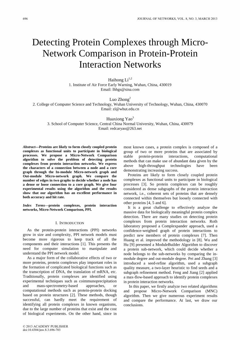
Detecting Protein Complexes through Micro-Network Comparison in Protein-Protein

Interaction Networks

Haihong Li1. Institute of Air Force Early Warning, Wuhan, China, 430019

1,2


Luo Zhong2. College of Computer Science and Technology, Wuhan University of Technology, Wuhan, China, 430070

2


Huaxiong Yao3. School of Computer Science, Central China Normal University, Wuhan, China, 430079

3


Abstract—Proteins are likely to form closely coupled protein complexes as functional units to participate in biological processes. We propose a Micro-Network Comparison algorithm to solve the problem of detecting protein complexes from protein interaction networks. We express the characters of a connection between a node and a core graph through the In-module Micro-network graph and Out-module Micro-network graph. We compare the number of edges in two graphs to decide whether a node has a dense or loose connection to a core graph. We give four experimental results using the algorithm and the results show that our algorithm has an excellent performance in both accuracy and hit rate. Index Terms—protein complexes, protein interaction networks, Micro-Network Comparison, PPI.

I. INTRODUCTION

As the protein-protein interactions (PPI) networks grow in size and complexity, PPI network models must become more rigorous to keep track of all the components and their interactions [1]. This presents the need for computer simulation to manipulate and understand the PPI network model.

As a major form of the collaborative effects of two or more proteins, protein complexes play important roles in the formation of complicated biological functions such as the transcription of DNA, the translation of mRNA, etc. Traditionally, protein complexes are identified using experimental techniques such as coimmunoprecipitation and mass-spectrometry-based approaches, or computational methods such as protein-protein docking based on protein structures [2]. These methods, though successful, can hardly meet the requirement of identifying all protein complexes in known organisms, due to the large number of proteins that exist and the cost of biological experiments. On the other hand, since in

most known cases, a protein complex is composed of a group of two or more proteins that are associated by stable protein-protein interactions, computational methods that can make use of abundant data given by the above high-throughput technologies have been demonstrating increasing success.

Proteins are likely to form closely coupled protein complexes as functional units to participate in biological processes [3]. So protein complexes can be roughly considered as dense subgraphs of the protein interaction network, i.e., coherent sets of proteins that are densely connected within themselves but loosely connected with other proteins [4, 5 and 6].

It is a great challenge to effectively analyze the massive data for biologically meaningful protein complex detection. There are many studies on detecting protein complexes from protein interaction networks. Roth laboratory proposed a Complexpander approach, used a confidence-weighted graph of protein interactions to predict new members of protein complexes [7]. Then Huang et al. improved the methodology in [8]. Wu and Hu [9] presented a ModuleBuilder Algorithm to discover a protein sub-network, which could decide whether a node belongs to the sub-networks by comparing the in-module degree and out-module degree. Pei and Zhang [3] introduced a seed-refine algorithm, used a subgraph quality measure, a two-layer heuristic to find seeds and a subgraph refinement method. Feng and Jiang [2] applied a max-flow-based approach to identify protein complexes in protein interaction networks.

In this paper, we firstly analyze two related algorithms and propose Micro-Network Comparison (MNC) algorithm. Then we give numerous experiment results and compare the performance. At last, we draw our conclusions.



II. PTOBLEM STATEMENT

We can consider a protein interaction network as a undirected graph G(V, E), where nodes V represents the set of proteins and edges E represents the set of interaction. Then a protein complex seems as a subgraph Gc(Vc, Ec

), and is a dense graph belonging to G(V, E). So the problem of detecting protein complexes from protein interaction networks is converted to how to find a dense network from a whole graph.

G

GcGo

seed

Fig 1. Procedure of finding a dense graph based on seed

Fig 1 shows the procedure of finding a dense graph

from a graph G based on a seed node. Firstly, based on the neighbor nodes of seed, the core graph Go(Vo, Eo) is to be found which has the most connections among themselves. Then whether other nodes are members of a complex graph Gc

A. Analysis of related algithms

is to be decided based on their connections to the core graph.

Pei and Zhang [3] presented a Seed-Refine (SR) algorithm to solve the problem of detecting protein complex using graph theories. SR decides whether a node belongs to a complex graph through adding or deleting a node to the core graph, and checking whether it improves the quality of the density of graph. But it only considers connections into the core graph, but ignores connections out of the core graph which might be their vital part.

Hu and Wu [9] proposed a ModuleBuilder (MB) algorithm to finding protein subnetworks. MB makes the decision through the comparison of the in-module degree (Kin) and out-module degree (Kout). As shown in Fig. 2, among all edges connected to node N1, solid lines represent edges between N1 and nodes in core graph Go, and dashed lines represent edges between N1 and nodes out of core graph Go. Kin is the number of solid lines, and Kout is the number of dashed lines. N1 belongs to the complex graph if Kin is bigger than Kout

Since protein complexes have the character of connecting densely within and loosely out of themselves as mentioned in the first paragraph of this section, we should decide whether a node in graph G has a dense connection or loose connection to core graph G

.

o. Through the detailed analysis to the numerous data of protein interaction networks, we find PPI networks are

characterized that some nodes have many connections as well as some have very few, even only one connection (we use rare connections to represent this kind of connection). MB directly compares Kin with Kout, in spite of Kout

could contain some rare connections which play an insignificant role in networks while contrarily lower the performance of networks.

Go(Vo, Eo)

seed

N1

Kin

Kout

Fig 2. Kin and Kout

in ModuleBuilder

Since protein complexes have the character of connecting densely within and loosely out of themselves as mentioned in the first paragraph of this section, we should decide whether a node in graph G has a dense connection or loose connection to core graph Go. Through the detailed analysis to the numerous data of protein interaction networks, we find PPI networks are characterized that some nodes have many connections as well as some have very few, even only one connection (we use rare connections to represent this kind of connection). MB directly compares Kin with Kout, in spite of Kout

We have downloaded eight species of PPI data from DIP [10] database, and counted the numbers of nodes which has only one connection in the PPI network. As seen in Table 1, we can find that there are considerable nodes have only one connection in the network and the proportion of this kind of nodes in the whole PPI network is from 20% to 70%. Accompanied with considerable rare connections, such kind of nodes will definitely affect the performance of networks.

could contain some rare connections which play an insignificant role in networks while contrarily lower the performance of networks.

TABLE 1.

STATISTICS OF NODES WITH ONLY ONE CONNECTION

Species Total nodes # of only 1 connection percent Saccharomyces cerevisiae

5078 1178 23.20%

Escherichia coli

2968 902 30.39%

Drosophila melanogaster

7565 2404 31.78%

Homo sapiens 3090 1634 52.88% Caenorhabditis elegans

2672 1565 58.57%

H. pylori 714 273 38.24% Rattus norvegicus

400 272 68.00%

Mus musculus 1204 760 63.12%



For example, in Fig.3, N1 has four adjacent nodes in the core graph Go(Vo, Eo), N2, N3, N4, N5, which are completely connected with each other. This means each two nodes have a connection. So we can think them as a dense connection. At the same time N1 has five adjacent nodes out of the core graph Go(Vo, Eo), N6, N7, N8, N9, N10, which have no connection with each other and can be seemed as a loose connection. But when judging by MB algorithm, Kin = 4 is smaller than Kout = 5, then MB algorithm will make a wrong decision that the node N1 which has a dense connection with the core graph doesn’t belong to the core graph. So we cannot simply decide whether a node belongs to the core graph or not through comparing the value of Kin with Kout

.

Go(Vo, Eo)

N1N2

N3

N4N5

N6

N7N8N9

N10

Fig 3. An example of comparison of Kin and Kout

B. Micro-Network Comparison Algorithm We propose Micro-Network Comparison (MNC)

algorithm in this section to detect protein complexes accurately from protein interaction networks. We define two concepts, In-module Micro-network Graph and out-module Micro-network Graph, and compare the number of edges inside the two graphs to decide whether a node has a dense or loose connection to the core graph.

In a protein interaction networks G(V, E), we assume that Go(Vo, Eo) represents the core graph based on assigned seed node S, where Vo is the set of core nodes chosen from all adjacent nodes of node S, and Eo

To a node N1 not in G

is the set of edges among these core nodes.

o, adjacent graph GADJ(VADJ, EADJ

( ){ } { }11,| NENuuVADJ ∪⊂∀=

) means a graph consists of all its neighbor nodes and itself, as showed in formula (1).

( ){ }ADJADJ VvuvuE ∈∀= ,|, (1) In-module Micro-network Graph GIM(VIM, EIM)

means a graph consists of its connected nodes to core graph Go

oADJIM VVV ∩=, as shown in formula (2).

( ){ }IMIM VvuvuE ∈∀= ,|, (2) Out-Module Micro-network Graph GOM(VOM, EOM)

means a graph consists of its connected nodes out of core graph Go

}{ 1NVVVV oADJADJOM −∩−=, as shown in formula (3).

( ){ }OMOM VvuvuE ∈∀= ,|, (3)

To better understand the meaning of these different graphs, we draw them in Fig 4. In the figure, the left horizontal oval is core graph Go(Vo, Eo), the right horizontal oval is adjacent graph GADJ(VADJ, EADJ), the left vertical oval is In-module Micro-network Graph GIM(VIM, EIM), and the right vertical oval is Out-module Micro-network Graph GOM(VOM, EOM

).

Go

seed

GADJ

GIM GOM

N1

Fig 4. Relevant Graph and Irrelevant Graph

Then we compare the number of edges in the two

graphs and use D to represent the relation of node N1 to core graph Go

OMIM EED −=, as shown in formula (4):

(4) If D > 0, it means node N1 densely connects to

core graph Go(Vo, Eo). Then node N1 can be included into the complex S. If D <= 0, it means node N1 loosely connects to Go(Vo, Eo

III. ALGORITHM

). Then node N1 cannot be included into the complex S.

Based on the comparison between the In-Module Micro-network graph and the Out-Module Micro-network graph, we propose the Micro-Network Comparison (MNC) algorithm to detecting protein complexes from PPI networks. MNC algorithm mainly includes two parts: identify core graph with a given seed node, and get protein complex through comparing the edge amount between In-Module Micro-network graph and Out-Module Micro-network graph.

We apply the same method to identify core graph as [8]. As the data flow shown in Fig.5, firstly, find all the adjacent nodes of seed node and compose these nodes and seed to adjacent graph GADJ(VADJ, EADJ). Then compute the in-module degree (Kin) for every node in the adjacent graph except seed, and get the minimal (Kmin) and the maximal (Kmax) value of Kin. Afterwards, delete the node with minimal Kin from GADJ, and repeat this action until Kmin equals to Kmax. Finally, compose rest nodes to a graph Go(Vo, Eo

Fig 6 is the dataflow of Micro-Network Comparison algorithm to detect the protein complex. After we get the core graph G

), which is the result for identifying core graph.

o(Vo, Eo), we find all adjacent nodes of each node in Go and compose them to adjacent graph GADJ(VADJ, EADJ). Then we generate the In-Module



Micro-network graph GIM(VIM, EIM) and Out-module Micro-network graph GOM(VOM, EOM) for each node in GADJ, and use variable D to represent the difference of edge amount in these two graphs. If the value of D is positive, add the corresponding node Ni into core graph Go, and repeat the anterior steps. If the value of D is negative, delete node Ni from adjacent nodes VADJ and compute the value D for other nodes in VADJ. We get the final result until the adjacent nodes set GADJ is empty and the final Go

is the protein complex set which our algorithm detects.

Find adjacent graph GADJ(VADJ, EADJ)of seed node

Compute Kin for all nodes in VADJ except seed

Kmin = Kmax ?

Return GO(VO, EO)

Y

Delete the node with Kmin from VADJ

N

Fig 5. Data flow of identifying core graph

GADJ(VADJ, EADJ): Get adjacent

nodes set of GO(VO, EO)

> 0 ?

?φ=ADJV

{ } ADJADJ VNiV →−

{ } oo VVNi →+

N

Y

N

Return GO(VO, EO)

Y

Get GIM(VIM, EIM) and GOM(VOM, EOM) of node Ni, Ni∈VADJ

N

OMIM EED −=

Fig 6. Data flow of Micro-network Comparison algorithm

IV. EXPERIMENTS

In this section, we apply the Micro-Network Comparison (MNC) algorithm to the yeast interaction

network. We download the Saccharomyces cerevisiae data set from DIP [10], which has 5078 proteins and 22418 interactions. For the convenience of comparison, we chose four same seed proteins as ModuleBuilder (MB) algorithm [9]: TAF6, NOT3, RFC2, and ARP3. Using the four proteins as seed, we find their corresponding sub-networks by MNC algorithm. The sub-networks are visualized by Cytoscape [11], which is an open source platform for complex network analysis and visualization. We search seed proteins’ related complexes from the complexes database CYC2008 [12], which is a comprehensive catalogue (like mips database) of manually curated 408 heteromeric protein complexes in Saccharomyces cerevisiae reliably backed by small-scale experiments from the literature. Following, we will list experiment results of four seed proteins. Then, we will compare the performance of our algorithm to MB algorithm.

A. TAF6 TAF6 is a Subunit of TFIID and SAGA complexes,

involved in transcription initiation of RNA polymerase II and in chromatin modification. Searching TAF6 related complexes from CYC2008, we find 2 results: SAGA complex [13], and TFIID complex [14]. SAGA complex includes 20 proteins, and TFIID complex includes 15 proteins.

Fig.7. TAF6 sub-network

TABLE 2. PROTEINS OF TAF6 SUB-NETWORKS

Unitprobkb Gene Description

Q02336 ADA2 Transcription coactivator s

P07248 ADR1 Carbon source-responsive zinc-

finger transcription factor

P28003 FUN19 Expression induced in response to

heat stress

P03069 GCN4

Basic leucine zipper (bZIP) transcriptional activator of amino

acid biosynthetic genes in response to amino acid starvation

Q03330 GCN5

Acetyltransferase, modifies N-terminal lysines on histones H2B

and H3 s

Q12060 HFI1

Adaptor protein required for structural integrity of the SAGA

complex s

P32494 NGG1 Transcriptional regulator involved s



in glucose repression of Gal4p-regulated genes

P25554 SGF29

Component of the HAT/Core module of the SAGA, SLIK, and

ADA complexes s

P53165 SGF73 SAGA complex subunit s

P13393 SPT15transcription initiation factor IID;

TATA-binding protein t

P50875 SPT20Subunit of the SAGA

transcriptional regulatory complex s

P06844 SPT3

Subunit of the SAGA and SAGA-like transcriptional regulatory

complexes s





P46677 TAF1 TFIID subunit t

Q12030 TAF10Subunit of TFIID and SAGA

complexes s,t

Q04226 TAF11 TFIID subunit t


complexes s,t





P38129 TAF5Subunit of TFIID and SAGA

complexes s,t

P53040 TAF6Subunit of TFIID and SAGA

complexes s,t




complexes s,t

P50102 UBP8Ubiquitin-specific protease that is

a component of the SAGA complex s

DIP-524N VP16 Transactivator VP16 s indicates that the protein belongs to SAGA complex t indicates that the protein belongs to TFIID complex

Using TAF6 as seed, TAF6 sub-network is detected

through the Micro-Network Comparison algorithm, as shown in Fig.7, which has 29 proteins and 110 interactions. As shown in Table 2, the sub-network detected by our algorithm contains 29 proteins, in which 25 proteins belong to TAF6 related complexes. Separately, the sub-network has 16 of 20 SAGA complex proteins, only missing CHD1, SGF11, SUS1 and TRA1; 14 of 15 TFIID complex proteins, only missing TAF14.

B. NOT 3 NOT3 is a Subunit of the CCR4-NOT complex, which

is a global transcriptional regulator with roles in transcription initiation and elongation and in mRNA degradation. Searching NOT3 related complexes from CYC2008, we find only 1 result: CCR4-NOT core complex [15], which includes 9 proteins.

Fig 8. NOT3 sub-network

Using NOT3 as seed, NOT3 sub-network is detected

through the Micro-Network Comparison algorithm, as shown in Fig.8, which has 7 proteins and 20 interactions. As shown in Table 3, the sub-network detected by our algorithm contains 7 proteins, which all belong to CCR4-NOT complex. Among 9 CCR4-NOT complex proteins, our algorithm misses 2 proteins: CCR4 and CDC36.

TABLE 3. PROTEINS OF NOT3 SUB-NETWORK

Uniprotkb Gene Description

P06102 NOT3* Subunit of the CCR4-NOT complex

Q12514 NOT5* Subunit of the CCR4-NOT complex

P34909 MOT2* Subunit of the CCR4-NOT complex

P25655 CDC39* Component of the CCR4-NOT complex

P39008 POP2* RNase of the DEDD superfamily

P53829 CAF40* Evolutionarily conserved subunit of the CCR4-NOT

complex

P53280 CAF130*

Part of the evolutionarily-conserved CCR4-NOT

transcriptional regulatory complex

* indicates that the protein belongs to CCR4-NOT complex

C. RFC2 RFC is a Subunit of heteropentameric Replication

factor C (RF-C), which is a DNA binding protein and ATPase that acts as a clamp loader of the proliferating cell nuclear antigen (PCNA) processivity factor for DNA polymerases delta and epsilon. Searching RFC2 related complexes from CYC2008, we find it belongs to DNA replication factor C (RFC) complex [16], which includes 5 proteins.

Using RFC2 as seed, RFC2 sub-network is detected through the Micro-Network Comparison algorithm, as shown in Fig.9, which has 10 proteins and 27 interactions. As shown in Table 4, the sub-network detected by our algorithm contains 10 proteins, which all belong to RFC2 related complexes. Separately, the sub-network has all 5



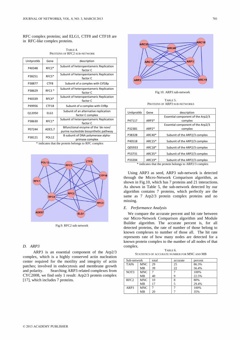
RFC complex proteins; and ELG1, CTF8 and CTF18 are in RFC-like complex proteins.

TABLE 4.

PROTEINS OF RFC2 SUB-NETWORK

Unitprotkb Gene description

P40348 RFC2* Subunit of heteropentameric Replication factor C


P38877 CTF8 Subunit of a complex with Ctf18p

P38629 RFC3 * Subunit of heteropentameric Replication factor C


P49956 CTF18 Subunit of a complex with Ctf8p

Q12050 ELG1 Subunit of an alternative replication factor C complex


P07244 ADE5,7 Bifunctional enzyme of the 'de novo' purine nucleotide biosynthetic pathway

P38121 POL12 B subunit of DNA polymerase alpha-primase complex

* indicates that the protein belongs to RFC complex

Fig.9. RFC2 sub network

D. ARP3 ARP3 is an essential component of the Arp2/3

complex, which is a highly conserved actin nucleation center required for the motility and integrity of actin patches; involved in endocytosis and membrane growth and polarity. Searching ARP3 related complexes from CYC2008, we find only 1 result: Arp2/3 protein complex [17], which includes 7 proteins.

Fig 10. ARP3 sub-network

TABLE 5. PROTEINS OF ARP3 SUB-NETWORKS

Unitprotkb Gene description

P47117 ARP3* Essential component of the Arp2/3

complex

P32381 ARP2* Essential component of the Arp2/3

complex

P38328 ARC40* Subunit of the ARP2/3 complex


Q05933 ARC18* Subunit of the ARP2/3 complex


P33204 ARC19* Subunit of the ARP2/3 complex * indicates that the protein belongs to ARP2/3 complex

Using ARP3 as seed, ARP3 sub-network is detected

through the Micro-Network Comparison algorithm, as shown in Fig.10, which has 7 proteins and 21 interactions. As shown in Table 5, the sub-network detected by our algorithm contains 7 proteins, which perfectly are the same as 7 Arp2/3 protein complex proteins and no missing.

E. Performance Analysis We compare the accurate percent and hit rate between

our Micro-Network Comparison algorithm and Module Builder algorithm. The accurate percent is, for all detected proteins, the rate of number of those belong to known complexes to number of those all. The hit rate represents rate of how many nodes are detected for a known protein complex to the number of all nodes of that complex.

TABLE 6. STATISTICS OF ACCURATE NUMBER FOR MNC AND MB

Sub-network total accurate percent TAF6 MNC 29 25 86.3%

MB 39 22 56.4% NOT3 MNC 7 7 100%

MB 40 9 22.5% RFC2 MNC 10 8 80%

MB 17 5 29.4% ARP3 MNC 7 7 100%

MB 20 7 35%



Fig. 11. Comparison of accurate percent between MNC and MB

We compare our results with those in [18]. From [18],

we only reference the raw detected sub-networks for every seed, but not use their statistics data, precision and recall, which correspond to accurate percent and hit rate. For seed TAF6, [18] considered nodes in SAGA complex and SRB complex as correct results, which is unreasonable because SRB complex [19] doesn’t contain TAF6 at all. The correct nodes should be in SAGA and TFIID complex according to the search for seed TAF6 from CYC2008. So we re-count the hit number and accurate number based on the raw detected sub-networks.

Table 6 is the statistics of accurate number for our MNC algorithm and MB algorithm. From the data, sub-networks detected by our algorithm MNC always have much less nodes than by MB algorithm. In TAF6 sub-network, MNC has 29 nodes while MB has 39; in NOT3, the number is 7 vs 40; in RFC2, 10 vs 17; in ARP3, 7 vs 20. Meanwhile, our algorithm MNC always has more accurate nodes than MB, except NOT3. That is because the CCR4-NOT complex has a low connectivity and the 2 missing nodes by MNC have too many neighbors. Both reasons drop the performance of MNC algorithm. The comparison of accurate percent between MNC and MB is shown in Fig 11. From the figure, we show that our algorithm MNC has a significant improvement to MB on accurate percent, and that MNC even has a completely accurate identification in small complexes while MB only has 30% around for it includes too many irrelevant nodes. Table 7 is the statistics of hit number of our algorithm MNC and MB. From the table, we can find that MNC and MB can identify most of complex nodes. Especially in some small complexes, they have detected all nodes, such as RFC complex, and ARP2/3 complex. Fig 12 compares their hit rate for different complexes. In big complexes such as TAF6 related, MNC performs better than MB, while worse in some small complexes such as CCR4-Not

TABLE 7. COMPARISON OF HIT NUMBER FOR DIFFERENT COMPLEXES

Seed Complex Total Hit (MNC)

Rate (MNC)

Hit (MB)

Rate (MB)

TAF6 SAGA 20 16 80% 14 70% TFIID 15 14 93.3% 13 86.7%

NOT3 CCR4-NOT

9 7 77.8% 9 100%

RFC2 RFC 5 5 100% 5 100% ARP3 ARP2/3 7 7 100% 7 100%

Fig 12. Comparison of hit rate between MNC and MB

complex. This is because it is easier for MB to hit an additional node in a much bigger detected sub-network than MNC.

V. CONCLUSION

In this paper, we discuss the character of protein complexes and problems of some detecting algorithm. Proteins are densely connected within their complexes, while loosely connected with other proteins. We use In-module Micro-Network graph and Out-module Micro-Network graph to represent the relation of connection between a node and a core graph. We compare the number of edges in two graphs to represent whether a node has a dense or loose connection with a core graph. A node is deemed to have a dense connection with a core graph if the difference is positive, which means the edges in In-module Micro-network graph are more than edges in the other graph. Then we propose the Micro-Network Comparison algorithm to detecting protein complexes from protein interaction networks. MNC algorithm decides whether a node belongs to a protein complex through comparison of the number between core graph and nodes out of core graph. Applying MNC algorithm to the yeast interaction network, we assign four seed proteins to detect related complexes. Experimental results show that our algorithm has an excellent performance in both accuracy and hit rate.

REFERENCES

[1] Faruck Morcos, Marcin Sikora, Mark S. Alber, Dale Kaiser, and Jesús A. Izaguirre, "Belief Propagation Estimation of Protein and Domain Interactions Using the Sum–Product Algorithm," IEEE TRANSACTIONS ON INFORMATION THEORY, VOL. 56, NO. 2, FEBRUARY 2010, pp. 742-755.

[2] Jianxing Feng, Rui Jiang, and Tao Jiang, "A Max-Flow-Based Approach to the Identification of Protein Complexes Using Protein Interaction and Microarray Data," IEEE/ACM TRANSACTIONS ON COMPUTATIONAL BIOLOGY AND BIOINFORMATICS, VOL. 8, NO. 3, MAY/JUNE 2011, pp. 621-634.

[3] Pengjun Pei and Aidong Zhang, "A “Seed-Refine” Algorithm for Detecting Protein Complexes From Protein Interaction Data," IEEE TRANSACTIONS ON NANOBIOSCIENCE, VOL. 6, NO. 1, MARCH 2007, pp. 43-50.

[4] Xiao Zou, Heng Wang, Qiuyu Zhang, “Hand Gesture Target Model Updating and Result Forecasting Algorithm



based on Mean Shift,” Journal of Multimedia, 2013 Feb, 8(1): 1-7.

[5] Ke Xu, Wen Cui, Jun Tie, Xinfang Zhang, “An Algorithm for Detecting Group in Mobile Social Network,” Journal of Networks, 2012 Oct, 7(10): 1584-1591.

[6] Jie Jiang, Long Bao Guo, Wei Mo, Feng Ke Fan, “Block-Based Parallel Intra Prediction Scheme for HEVC,” Journal of Multimedia, 2012 Aug, 7(4): 289-294.

[7] Asthana S, King OD, Gibbons FD, Roth FP, “Predicting Protein Complex Membership Using Probabilistic Network Reliability,” Genome Res. 2004, 14: 1170-1175.

[8] H Huang, LV Zhang, FP Roth & JS Bader, “Probabilistic paths in protein interaction networks,” Proceedings of the RECOMB Conferences on Systems Biology and Computational Proteomics (2007), pp:14-28.

[9] Xiaohua Hu and Daniel D. Wu, "Data Mining and Predictive Modeling of Biomolecular Network from Biomedical Literature Databases," IEEE/ACM TRANSACTIONS ON COMPUTATIONAL BIOLOGY AND BIOINFORMATICS, VOL. 4, NO. 2, APRIL-JUNE 2007, pp. 251-263.

[10] I. Xenarios et al., “Dip, the database of interacting proteins: a research tool for studying cellular networks of protein interactions,” Nucl. Acids Res., vol. 30, pp. 303–305, 2002.

[11] Michael Smoot, Keiichiro Ono, Johannes Ruscheinski, Peng-Liang Wang, Trey Ideker, “Cytoscape 2.8: new features for data integration and network visualization,” Bioinformatics. 2011 February 1; 27(3): 431–432.Published online 2010 December 12.

[12] Pu, S., Wong, J., Turner, B., Cho, E. & Wodak, S.J, “Up-to-date catalogues of yeast protein complexes,” Nucleic Acids Res., 2008 Dec 18.

[13] Brown CE, Lechner T, Howe L, Workman JL, "The many HATs of transcription coactivators," Trends Biochem Sci., 2000 Jan, 25(1):15-9.

[14] John Locker, Transcription Factors: Essential Data. John Wiley & Sons,June 27, 1996.

[15] Liu HY, Chiang YC, Pan J, Chen J, Salvadore C, Audino DC, Badarinarayana V, Palaniswamy V, Anderson B, Denis CL, "Characterization of CAF4 and CAF16 reveals a functional connection between the CCR4-NOT complex and a subset of SRB proteins of the RNA polymerase II holoenzyme," J Biol Chem., 2001 Mar 9, 276(10):7541-8.

[16] Kim J, MacNeill SA, "Genome stability: a new member of the RFC family," Curr Biol., 2003 Nov 11, 13(22):R873-5.

[17] Kovacs EM, Yap AS, "The web and the rock: cell adhesion and the ARP2/3 complex," Dev Cell., 2002 Dec, 3(6):760-1.

[18] D Wu, X Hu, “ Topological Analysis and Sub-Network Mining of Protein-Protein Interactions,” in Advances in Data Warehousing and Mining, David Taniar (Ed), Idea Group Publisher.

[19] Gustafsson CM, Samuelsson T, "Mediator--a universal complex in transcriptional regulation," Mol Microbiol. 2001 Jul, 41(1):1-8.

Haihong Li was born in PingLiang, Gansu Province, China on April 22, 1973. He received his Bachelor’s degree on radar engineering from Air Force Radar academy, Wuhan, China in 1996. He received the Master’s degree on microwave technology in Air Force Radar academy, Wuhan China, in 2003. He is a PHD candidate in the college of Computer Science and Technology, Wuhan University of Technology.

He works as an associate professor in the institute of Air Force Early Warning, Wuhan, China. He has published 28 papers and 8 books. He is mainly studying on the fields of bioinformatics and radar early warning. Luo Zhong was born in Wuhan, China in 1957. He received his bachelor’s degree in Wuhan University, Wuhan, China in 1982. He received his master’s and PHD’s degree in Wuhan University of Technology, Wuhan, China in 1991 and 1996. He is a professor and the chairman of the college of Computer Science and Technology in Wuhan University of Technology, Wuhan, China. His research areas include software engineering, intelligent monitoring and visualization research. Huaxiong Yao was born in Wuhan, China on Oct 27, 1979. He received his Bachelor’s and PHD’s degree on communication engineering in Huazhong University of Science and Technology, Wuhan China, in 2001 and 2007 respectively.

He works as an associate professor in the School of Computer Science, Central China Normal University, Wuhan, China. He has published 20 papers and 4 books. He is mainly studying on the fields of bioinformatics and fiber networks.



Stability of Impulsive Cellular Neural Networks with Time-varying Delays

Yuanqiang Chen

College, Guizhou Minzu University, Guiyang550025, China Email: [email protected]

Abstract—The problems of exponential stability and exponential convergence rate for a class of impulsive cellular neural networks with time-varying delays are studied. By means of the Lyapunov stability theory and discrete-time Halanay-type inequality technique, stability criteria for ensuring global exponential stability of no-impulsive discrete-time cellular neural networks and impulsive discrete-time cellular neural network with time-varying delays are derived respectively, and the estimated exponential convergence rate is provided as well. Finally, the validity of the obtained results is shown by two numerical examples. Index Terms—Cellular neural networks, Exponential stability, Discrete-time Halanay inequality

I. INTRODUCTION

In 1988, a novel class of information-processing systems called cellular neural networks (CNN) been proposed [1-3]. Their key features are asynchronous parallel processing and global interaction of network elements. In many evolutionary systems there are two common phenomena: delay effects and impulsive effects. In implementation of electronic networks, for example, delays frequently appear because of the finite switching speed of amplifiers. On the other hand, the state of electronic networks is often subject to instantaneous perturbations and experience abrupt change at certain instants which may be caused by switching phenomenon, frequency change or other sudden noise, that is, do exhibit impulsive effects. Even in biological neural networks, impulsive effects are likely to exist. For instance, when a stimulus from the body or the external environment is received by receptors the electrical impulses will be conveyed to the neural net and impulsive effects arise naturally in the net. Therefore, neural network model with delays and impulsive effects should be more accurate to describe the evolutionary process of the systems. Since delays and impulses can affect the dynamical behaviors of the system by creating oscillatory and unstable characteristics, it is necessary to investigate both delay and impulsive effects on the stability of neural networks. Cellular neural networks and delayed cellular neural networks (DCNN) have been applied to various fields such as linear and nonlinear programming, optimization, pattern recognition, associative memory and computer vision [4]. Therefore, the study of the

stability of CNN and DCNN is known to be an important problem in theory and applications. However, the state of electronic networks is often subject to instantaneous perturbations and experience abrupt changes at certain instants [5]. Since delays and impulses can affect the dynamical behaviors of the system, it is necessary to investigate both delay and impulsive effects on the stability of cellular neural networks. A large number of the criteria on the stability of DCNN without impulse has been derived (see [6-7]).Correspondingly, there is not much work dedicated to investigate the stability of impulsive discrete-time cellular neural networks. Recently, some mathematical models of impulsive cellular neural networks described by measure differential equations or general impulsive differential equations have been formulated ([1],[2],[8-25]). Some interesting results on the stability of impulsive discrete-time cellular neural networks without delay or with constant delays have been obtained. However, in practical evolutionary processes of the networks, absolute constant delay may be scarce and delays are frequently varied with time.

In this paper, we shall deal with a class of discrete-time cellular neural networks with time-varying delays subject to impulsive perturbations:

( ) ( ) ( )( )

( )( )( )( ) ( ) ( ) ( )( )

( ) ( )( ) ( ) ( ) ( )

1

1

1

, ,

1 ,

, 1 , 0 ,

, ,0 , 1, ,

n

i i i ij j jj

n

ij j j j kj

i i i i i

k

i i

x m c x m a f x m

b f x m m m N

x m x m x m P x m

m N m N k N

x m m m N i N n

τ

φ τ

=

=

+ = +

+ − ≠

∆ = + − =

= ∈ ∈

= ∈ − ∈

∑

∑ (1)

where ( )1 2, , , nnx x x x R= ∈ is the state of system,

continuous function :jf R R→ denote the output of the

j th unit and ( )0 0jf = ， , ,i ij ijc a b are constants, ic , 0 1ic≤ < , represents the rate with which the i th unit will reset its potential to the resting state in isolation when disconnected from the network and external inputs,

,ij ija b denote the strength of the j th unit on the i th unit

at time m and ( )jm mτ− respectively, ( )j mτ corresponds to the transmission delay along the axon of the j th unit and satisfies ( )0 j tτ τ≤ ≤ (τ is integer) and




m →∞ as ( )ijm mτ− → ∞ , integer ( ), 0kN k N∈ are the moments of impulsive perturbations and satisfy

0 10 N N< < < and k →∞ as kN →∞ , continuous

function ( )( ) :i i kP x N R R→ represents the abrupt

change of the state at the impulsive moment kN and

( )0 0iP = , :j R Rφ → is continuous function,

( ) { }, 1, 2,N k k k k= + + , ( ) { }, , 1, 2, ,N k l k k k l= + + . By utilizing the Lyapunov stability theory and discrete-time Halanay-type inequality, we shall obtain global exponential stability criteria and estimated exponential convergence rate for impulsive discrete-time cellular neural networks with time-varying delays. The rest of this paper is organized as follows. In Section II, impulsive cellular neural networks with time-varying delays are introduced and some preliminary lemmas are presented. In Section III, based on the Lyapunov stability theory and discrete-time Halanay-type inequality technique, global exponential stability criteria for ensuring global exponential stability of no-impulsive discrete-time cellular neural networks and impulsive discrete-time cellular neural network with time-varying delays are derived respectively. Moreover, two numerical examples are presented in Sections IV. Section V concludes the paper.

II. PRELIMINARIES

Let us introduce the following necessary definitions and lemmas.

Lemma 1: [26] (Discrete-time Halanay-type Inequality) Suppose that the real numbers sequence { }n n hα

≥−

satisfied ( ) ( ) ( ]1, , , , , 1 , 0,1n n n n n hg n n Nα εα α α α ε− −∆ = − + ∈ ∈ ,

if there exists a ( )0,δ ε∈ such that

( ){ } ( )

,max , 0n n ii N n h n

n Nα εα δ α∈ −

∆ ≤ − + ∀ ∈ .

Then, there exists a ( )0,1λ ∈ such that

( ){ } ( )

,0max , 0n

n ii N hn Nα λ α

∈ −∆ ≤ ∀ ∈ ,

Where ( ) 1: 0 hg N R R+× → , ( )1 0, , ,h hα α α− − + is the initial

condition, ( )0h N∈ is a constant and λ is the smallest root

in the interval ( )0,1 of the following equation,

( )1 1 0h hλ ε λ δ+ + − − = . Definition 1: For the impulsive discrete-time cellular

neural network (1), the trivial equilibrium point is exponentially stable if there exist positive constants

0K > and ( )0,1r∈ such that

( ) ( ), 1mx m Kr m N≤ ∀ ∈ , (2) Where r is called the exponential convergence rate. If (2) is satisfied for any initial condition ( ) nx m R∈ , ( ),0m N τ∈ − , the trivial equilibrium point is globally exponentially stable for the impulsive discrete-time cellular neural network (1).

Without loss of generality, we may assume system (1) satisfies the following assumptions.

Assumption A: The sequence { }kN of the impulsive time points satisfies

12k kN N ++ < . Assumption B: For the impulsive increment function

sequence ( )( )i i kP x N , there exists 0ikw > , such

that ( ) ( ), 0ix t t N∈ , the following condition is satisfied,

( ) ( )( ) ( ) ( ), 1,i i i ik ix t P x t w x t i N n+ ≤ ∈ . (3)

Assumption C: There exists a constant 0jl > , such

that ( )1 2, 0t t N∀ ∈ , the function ( )jf m in system (1) is bounded and satisfies the following Lipschitz condition,

( ) ( ) ( )1 2 1 2 , 1,j j jf t f t l t t j N n− ≤ − ∈ . (4)

III. MAIN RESULTS

In this section, we shall investigate the global exponential stability criteria and the estimated exponential convergence rate of impulsive discrete-time cellular neural networks. The following theorem presents the results on the global exponential stability of the no-impulsive system (1).

Consider a discrete-time neural network described by

( ) ( ) ( )( )

( )( )( ) ( )

( ) ( ) ( ) ( )

1

1

1

, 1 ,

, ,0 , 1, ,

n

i i i ij j jj

n

ij j j jj

i i

x m c x m a f x m

b f x m m m N

x m m m N i N n

τ

φ τ

=

=

+ = +

+ − ∈

= ∈ − ∈

∑

∑ (5)

The following theorem presents the results on the global exponential stability of the system (5).

Theorem 1: Suppose that Assumption C and the following inequality is satisfied, 1c l+ < , (6) Where

( )( )

1, 1max

n

j ij j iji N n jl l a u b

∈ =

= +

∑ ,

( ){ }

1,max ii N n

c c∈

= ,

( )( )

( ){ }{ },inf : maxj j j j jt N m m

u u x m u x tτ∈ −

= ≤ .

Then, the trivial equilibrium point of (5) is globally exponentially stable with the convergence rate λ , which is the smallest root in the interval ( )0,1 of the following equation

1 0c lτ τλ λ+ + − = . Proof: From the trajectory ( ){ } ( ), 1x m m N∈ of

system (5), we have

( ) ( ) ( )( )1

1

0 10

m nm m s

i i i i ij j js j

x m c x c a f x s−

− −

= =

= +∑ ∑

( )( )( )( ) ( )

11

0 1,

1 , 1, ,

m nm si ij j j j

s jc b f x s s

m N i N n

τ−

− −

= =

+ −

∈ ∈

∑ ∑

Then,



( ) ( ) ( )( )

( )( )( )

11

0 1

1

0 (

)

m nm m s

i i i i ij j js j

n

ij j j jj

x m c x c a f x s

b f x s sτ

−− −

= =

=

≤ +

+ −

∑ ∑

∑

( )( ) ( )( )( )( )( )

11

0 1

0

m nm s

i ij j j ij j j js j

mi i

c a f x s b f x s s

c x

τ−

− −

= =

≤ + −

+

∑ ∑

( ) ( )( )( )( )

11

0 1

0

m nm s

i j ij j ij j js j

mi i

c l a x s b x s s

c x

τ−

− −

= =

≤ + −

+

∑ ∑

( )( )

( ){ }( )

11

,0 1max

0

m nm s

i j ij j ij jt N s ss j

mi i

c l a u b x t

c x

τ

−− −

∈ −= =

≤ +

+

∑ ∑

( )( ){ }

( ) ( )( ){ }{ }

1,

11

, 1,0

max 0

max max .

mjj N n

mm s

jt N s s j N ns

c x

l c x tτ

∈

−− −

∈ − ∈=

≤

+ ∑

For any ( )m N τ∈ − , let

( )( ){ } ( )

( )( ){ }

( ) ( )( ){ }{ } ( )

1,

1,

11

, 1,0

max , ,0 ,

max 0

max max , 1 .

ii N n

mjj N nm

mm s

jt N s s j N ns

x m m N

c x

l c x t m Nτ

τ

ξ

∈

∈

−− −

∈ − ∈=

= ∈ −≤+ ∈∑

Clearly, ( ) ( ) ( ), 1, ,i mx m i N n m Nξ τ≤ ∈ ∀ ∈ − . (7)

Since 1m m mξ ξ ξ+∆ = −

( )( )

{ } ( ),

1 max , 1m tt N m mc l m N

τξ ξ

∈ −≤ − − + ∀ ∈ .

It follows from Lemma 1 that there exists a ( )0,1λ ∈ , such as

( ){ } ( )

,0max , 0m

m ti Nm N

τξ λ ξ

∈ −≤ ∀ ∈ .

Furthermore, by (7), we have ( )

( )( ){ } ( )

1,max ,i mi N n

x m x m m Nξ τ∞ ∈= ≤ ∀ ∈ − ,

Thus, ( )

( ){ } ( )

,0max , 0m

ti Nx m m N

τλ ξ

∞ ∈ −≤ ∀ ∈ .

Therefore, by virtue of Definition 1, the trivial equilibrium point of (5) is globally exponentially stable with the convergence rate λ , which is the smallest root in the interval ( )0,1 of the following equation,

1 0c lτ τλ λ+ + − = . This completes the proof.

For the following no-impulsive cellular neural network without delays, we have the following corollaries from Theorem 1.

( ) ( ) ( )( ) ( )

( ) ( )1

0

1 , 1 ,

0 , 1, ,

n

i i i ij j jj

i

x m c x m a f x m m N

x x i N n=

+ = + ∈

= ∈

∑

Corollary1. Suppose that Assumption C and the following inequality is satisfied,

1c l+ < , Where

( )1, 1max

n

j iji N n jl l a

∈ =

=

∑ ,

( ){ }

1,max ii N n

c c∈

= .

Then, the trivial equilibrium point of the no-impulsive cellular neural network without delays is globally exponentially stable with the convergence rate λ , which is the smallest root in the interval ( )0,1 of the following equation

1 0c lτ τλ λ+ + − = . We now give two criteria for global exponential

stability of impulsive discrete-time cellular neural network with time-varying delays.

Theorem 2: Suppose that Assumption A, Assumption B, Assumption C and the following conditions are satisfied,

i) ( ) ( )0ln 1 ln 0, 0

k

jj

w k c k N=

− + ≤ ∈∑ , (8)

ii) 1c l+ < , (9) Where

( )( )

1, 1max

n

j ij j iji N n jl l a u b

∈ =

= +

∑ ,

( )( )

( ){ }{ },inf : maxj j j j jt N m m

u u x m u x tτ∈ −

= ≤ ,

( ){ }

1,max ii N n

c c∈

= , ( )

{ }1,

maxk iki N nw w

∈= .

Then, the trivial equilibrium point of (1) is globally exponentially stable with the convergence rate λ , which is the smallest root in the interval ( )0,1 of the following equation,

1 0c lτ τλ λ+ + − = . Proof: For any ( ]1,k km N N +∈ , we have

( ) ( )

( ) ( )( ){ }{ }

1

11

, 1,1

1

max max

k

k

m Ni i i k

mm s

i jt N s s j N ns N

x m c x N

c l x tτ

− −

−− −

∈ − ∈= +

≤ +

+ ∑

( )( ){ }1

1,maxkm N

i ik j kj N nc w x N− −

∈≤

( ) ( )( ){ }{ }1

1

, 1,1max max .

k

mm s

i jt N s s j N ns Nl c x t

τ

−− −

∈ − ∈= +

+ ∑ (10)

Thus, ( )

( )( ){ }1 1

1 1,maxk kN N

i k i k j kj N nx N c w x N+ − −

+ ∈≤

( ) ( )( ){ }{ }1

11

1

, 1,1max max

Kk

k

NN s


τ

++

−− −

∈ − ∈= +

+ ∑ .

By induction, we obtain that



( )

( )( ){ }

( ) ( )( ){ }{ }

0

11

0

1

01,0

11

, 1,11

max

max max

kk

N N ki k i j jj N nj

NkN k s

j i jt N s s j N ns Nj

x N c w x N

l w c x tτ

−− −

∈=

−−− −

∈ − ∈= +=

≤

+

∏

∑∏

( ) ( )( ){ }{ }2

1

111

, 1,12

max maxkNk

N k sj i jt N s s j N ns Nj

l w c x tτ

−−− − +

∈ − ∈= +=

+ +∑∏

( ) ( )( ){ }{ }1

2

12

1 , 1,1max max

kk

k

NN s

k i jt N s s j N ns Nlw c x t

τ

−

−

−− −

− ∈ − ∈= +

+ ∑

( ) ( )( ){ }{ }

1

11

, 1,1max max

kk

k

NN s


τ−

−− −

∈ − ∈= +

+ ∑ .

Since ( )

( )( ){ }0

0 1,max 0N

i i jj N nx N c x

∈≤

( ) ( )( ){ }{ }0

01

1

, 1,0max max

NN s

i jt N s s j N nsl c x t

τ

−− −

∈ − ∈=

+ ∑ .

We have

( )( )

( ){ }

( ) ( )( ){ }{ }0

1

1,0

111

, 1,00

max 0

max max

k

k

kN k

i k i j jj N nj

NkN k s

j i jt N s s j N nsj

x N c w x

l w c x tτ

−−

∈=

−−− − −

∈ − ∈==

≤

+

∏

∑∏

( ) ( )( ){ }{ }1

1

0

11

, 1,11

max maxNk


l w c x tτ

−−− −

∈ − ∈= +=

+ ∑∏

( ) ( )( ){ }{ }2

1

111

, 1,12

max maxkNk


l w c x tτ

−−− − +

∈ − ∈= +=

+ +∑∏

( ) ( )( ){ }{ }1

2

12

1 , 1,1max max

kk

k

NN s

k i jt N s s j N ns Nlw c x t

τ

−

−

−− −

− ∈ − ∈= +

+ ∑

( ) ( )( ){ }{ }

1

11

, 1,1max max

kk

k

NN s


τ−

−− −

∈ − ∈= +

+ ∑ . (11)

Thus, it follows from (8), (10) and (11) that ( )

( )( ){ }

1,max 0m

i jj N nx m c x

∈≤

( ) ( )( ){ }

0 11

, 1,0max { max }

Nm s

jt N s s j N nsl c x t

τ

−− −

∈ − ∈=

+ ∑

( ) ( )( ){ }

1

0

11

, 1,1max { max }

Nm s

jt N s s j N ns Nl c x t

τ

−− −

∈ − ∈= +

+ +∑

( ) ( )( ){ }

1

11

, 1,1max { max }

k

k

Nm s


τ−

−− −

∈ − ∈= +

+ ∑

( ) ( )( ){ }

( ) ( )

11

, 1,1max { max }

, 1, , 1 .k

mm s

jt N s s j N ns N

m

l c x t

i N n m N

τ

η

−− −

∈ − ∈= +

+

= ∀ ∈ ∈

∑

Let

( )( ){ } ( )

( )1,

max , ,0 ,

, 1 .

ii N nm

m

x m m N

m N

τξ

η∈

∈ −= ∈

Then, the rest of the proof follows readily from similar arguments as those given for the proof of Theorem 1. This completes the proof.

For the following impulsive cellular neural network without delays, we have the following corollaries from Theorem 2.

( ) ( ) ( )( )

( ) ( ) ( ) ( )( )( ) ( )

( ) ( )

1

0

1 , ,

1 ,

, 1 , 0 ,

0 , 1, ,

n

i i i ij j j kj

i i i i i

k

i

x m c x m a f x m m N

x m x m x m P x m

m N m N k N

x x i N n

=

+ = + ≠

∆ = + − =

= ∈ ∈

= ∈

∑

Corollary2. Suppose that Assumption A, Assumption B, Assumption C and the following conditions are satisfied,

i) ( ) ( )0ln 1 ln 0, 0

k

jj

w k c k N=

− + ≤ ∈∑ ,

ii) 1c l+ < , Where

( )1, 1max

n

j iji N n jl l a

∈ =

=

∑ ,

( ){ }

1,max ii N n

c c∈

= , ( )

{ }1,

maxk iki N nw w

∈= .

Then, the trivial equilibrium point of the impulsive cellular neural network without delays is globally exponentially stable with the convergence rate λ , which is the smallest root in the interval ( )0,1 of the following equation,

1 0c lτ τλ λ+ + − = . Now, we give the other stability criteria for ensuring

global exponential stability of impulsive discrete-time cellular neural network with time-varying delays.

Theorem 3: Suppose that Assumption A, Assumption B, Assumption C and the following conditions are satisfied,

i) ( ) ( )0ln 1 ln 0, 0

k

jj

w k c k N=

− + ≤ ∈∑ , (12)

ii) 1c l+ < , (13) Where

( )1, 1max

n

i ij ji N n jc c a l

∈ =

= +

∑ ,

( )1, 1max

n

j iji N n jl l b

∈ =

=

∑ ,

( ){ }

1,maxk iki N n

w w∈

= .

Then, the trivial equilibrium point of (1) is globally exponentially stable with the convergence rate λ , which is the smallest root in the interval ( )0,1 of the following equation,

1 0c lτ τλ λ+ + − = . Proof: For any ( ]1,k km N N +∈ , we have

( ) ( ) ( )

( )( )1

1

1 1

1 1

n

i i i ij j jj

n

ij j j jj

x m c x m a l x m

b l x m mτ

=

=

≤ − + −

+ − − −

∑

∑

( )( ){ }

( )( ){ }

1,1

1 , 11

( ) max 1

max

n

i ij j jj N nj

n

ij j jt N m mj

c a l x m

b l x tτ

∈=

∈ − − −=

≤ + −

+

∑

∑



( )( ){ }

( ) ( )( ){ }{ }1, 1 , 1 1,

max 1 max maxj jj N n t N m m j N nc x m l x t

τ∈ ∈ − − − ∈≤ − + .

By induction, we obtain that ( )

( )( ){ }

( ) ( )( ){ }{ }

1

1,

11

, 1,1

max 1

max max

k

k

m Ni j kj N n

mm s

jt N s s j N ns N

x m c x N

l c x tτ

− −

∈

−− −

∈ − ∈= +

≤ +

+ ∑

( )( ){ }

( ) ( )( ){ }{ }

1

1,

11

, 1,1

max

max max .

k

k

m Nk j kj N n

mm s

jt N s s j N ns N

c w x N

l c x tτ

− −

∈

−− −

∈ − ∈= +

≤

+ ∑

Thus,

( )

( )( ){ }

( ) ( )( ){ }{ }

1

11

11 1,

11

, 1,1

max

max max .

k k

Kk

k

N Ni k k j kj N n

NN s

jt N s s j N ns N

x N c w x N

l c x tτ

+

++

− −+ ∈

−− −

∈ − ∈= +

≤

+ ∑

By induction, we have

( )( )

( ){ }

( ) ( )( ){ }{ }

0

11

0

1

01,0

11

, 1,11

max

max max

k

kN N k

i k j jj N nj

NkN k s

j jt N s s j N ns Nj

x N c w x N

l w c x tτ

−− −

∈=

−−− −

∈ − ∈= +=

≤

+

∏

∑∏

( ) ( )( ){ }{ }2

1

111

, 1,12

max maxk

NkN k s


l w c x tτ

−−− − +

∈ − ∈= +=

+ +∑∏

( ) ( )( ){ }{ }1

2

12

1 , 1,1max max

kk

k

NN s

k jt N s s j N ns Nlw c x t

τ

−

−

−− −

− ∈ − ∈= +

+ ∑

( ) ( )( ){ }{ }

1

11

, 1,1max max

kk

k

NN s


τ−

−− −

∈ − ∈= +

+ ∑ .

Since ( )

( )( ){ }

( ) ( )( ){ }{ }

0

00

0 1,

11

, 1,0

max 0

max max .

Ni jj N n

NN s

jt N s s j N ns

x N c x

l c x tτ

∈

−− −

∈ − ∈=

≤

+ ∑

The following inequality holds,

( )( )

( ){ }

( ) ( )( ){ }{ }0

1

1,0

111

, 1,00

max 0

max max

k

k

kN k

i k j jj N nj

NkN k s

j jt N s s j N nsj

x N c w x

l w c x tτ

−−

∈=

−−− − −

∈ − ∈==

≤

+

∏

∑∏

( ) ( )( ){ }{ }1

1

0

11

, 1,11

max maxNk

N k sj jt N s s j N ns Nj

l w c x tτ

−−− −

∈ − ∈= +=

+ ∑∏

( ) ( )( ){ }{ }2

1

111

, 1,12

max maxk

NkN k s


l w c x tτ

−−− − +

∈ − ∈= +=

+ +∑∏

( ) ( )( ){ }{ }1

2

12

1 , 1,1max max

kk

k

NN s

k jt N s s j N ns Nlw c x t

τ

−

−

−− −

− ∈ − ∈= +

+ ∑

( ) ( )( ){ }{ }

1

11

, 1,1max max

kk

k

NN s


τ−

−− −

∈ − ∈= +

+ ∑ . (14)

Thus, it follows from (14) that ( )

( )( ){ }

1,max 0m

i jj N nx m c x

∈≤

( ) ( )( ){ }

0 11

, 1,0max { max }

Nm s

jt N s s j N nsl c x t

τ

−− −

∈ − ∈=

+ ∑

( ) ( )( ){ }

1

0

11

, 1,1max { max }

Nm s


τ

−− −

∈ − ∈= +

+ +∑

( ) ( )( ){ }

1

11

, 1,1max { max }

k

k

Nm s


τ−

−− −

∈ − ∈= +

+ ∑

( ) ( )( ){ }

( ) ( )

11

, 1,1max { max } ,

1, , 1 .k

mm s

j mt N s s j N ns Nl c x t

i N n m N

τη

−− −

∈ − ∈= +

+ =

∀ ∈ ∈

∑

Let

( )( ){ } ( )

( )1,

max , ,0 ,

, 1 .

ii N nm

m

x m m N

m N

τξ

η∈

∈ −= ∈

Clearly,

( ) ( ) ( ), 1, ,i mx m i N n m Nξ τ≤ ∈ ∀ ∈ − . (15) Since

1m m mξ ξ ξ+∆ = −

( )( )

{ } ( ),

1 max , 1m tt N m mc l m N

τξ ξ

∈ −≤ − − + ∀ ∈ .

It follows from Lemma 1 that there exists a ( )0,1λ ∈ , such as

( ){ } ( )

,0max , 0m

m tt Nm N

τξ λ ξ

∈ −≤ ∀ ∈ .

Furthermore, by (15), we have ( )

( ){ }

( )( ){ } ( )

,0

,0

max

max , 1 .

mtt N

m

t N

x m

x t m N

τ

τ

λ ξ

λ

∞ ∈ −

∞∈ −

≤

= ∀ ∈

Therefore, by virtue of Definition 1, the trivial equilibrium point of (1) is globally exponentially stable with the convergence rate λ , which is the smallest root in the interval ( )0,1 of the following equation,

1 0c lτ τλ λ+ + − = . This completes the proof. From Theorem 3, we have the following corollaries. Corollary3. Suppose that Assumption A, Assumption

B, Assumption C and the following conditions are satisfied,

i) ( ) ( )0ln 1 ln 0, 0

k

jj

w k c k N=

− + ≤ ∈∑ ,

ii) 1c < , Where

( )1, 1max

n


∈ =

= +

∑ ,

( ){ }

1,maxk iki N n

w w∈

= .

Then, the trivial equilibrium point of the impulsive cellular neural network without delays is globally exponentially stable with the convergence rate λ , which is the smallest root in the interval ( )0,1 of the following equation,

1 0c lτ τλ λ+ + − = .

Ⅳ. NUMERICAL EXAMPLE



In this section, two numerical examples are presented to verify and illustrate the usefulness of our main results. We consider a two-neuron discrete-time cellular neural network with time delays

Example1. In this example, we consider a two-neuron discrete-time cellular neural network with time delays.

For ( )1m N∈ ,

( ) ( ) ( )( ) ( )( )

( )( ) ( )( )

( ) ( ) ( )( ) ( )( )

( )( ) ( )( )

1 1 1 1 2 2

1 1 2 2

2 2 1 1 2 2

1 1 2 2

1 1 1124 8 4

1 12 1 ,8 4

1 1 1113 3 8

1 12 1 ,3 8

x m x m f x m f x m

f x m f x m

x m x m f x m f x m

f x m f x m

−+ = + −

+ − − −

+ = + +

+ − + −

(16)

And for ( )2,0m N∈ − ,

( ) ( ) ( ) ( )1 1 2 2, .x m m x m mφ φ= =

Where

( )1 sinf t t= , ( )2f t t= , ( ) ( )21 1t tφ = − , ( ) ( )3

2 2t tφ = − + .

It is easy to verify that

( ) ( )1 1 , ,f s f t s t s t R− ≤ − ∀ ∈ ,

( ) ( )2 2 , ,f s f t s t s t R− ≤ − ∀ ∈ .

( ){ }

( )

2

1,2 1,2 1max max (

1 1 3 11max , max , 0.9936.24 13 4 12

i j ij j iji N i N jc l a u b

∈ ∈ =

+ +

≤ + =

∑

Thus, all the conditions of Theorem 1 are satisfied. Therefore, the trivial equilibrium point of (5) is globally exponentially stable with the convergence rate 0.8814λ = . The time sequence chart for systems with time-varying delays is shown in figure 1 below.

Example2. For 4m k≠ ,

( ) ( ) ( )( ) ( )( )

( )( ) ( )( )

( ) ( ) ( )( ) ( )( )

( )( ) ( )( )

1 1 1 1 2 2

1 1 2 2

2 2 1 1 2 2

1 1 2 2

1 1 1112 4 4

1 11 2 ,12 12

1 1 1112 3 3

1 11 2 ,12 12

x m x m f x m f x m

f x m f x m

x m x m f x m f x m

f x m f x m

−+ = + −

+ − − −

+ = − +

− − + −

(17)

And for ( ) ( )4 , 1 , 1m k m N k N= ∈ ∈ ,

( ) ( )( ) ( )

1 1

2 2

,

,

x m x m

x m x m

δ

δ

∆ =

∆ =

( ) ( )( ) ( )

1 1

2 2

,

,

x m m

x m m

φ

φ

=

= ( )1,0m N∈ − ,

Where

( )1 sinf t t= , ( )2 sinf t t= , ( ) ( )21 1t tφ = − , ( ) ( )3

2 2t tφ = − + .

Clearly,

( )1, 1

9max12

n


∈ =

= + =

∑ ,

( )1, 1

2max12

n

j iji N n jl l b

∈ =

= =

∑ ,

( ){ }

1,max 1k iki N n

w w δ∈

= = + .

Thus, all the conditions of Theorem 3 are satisfied

when 21 112 4

δ− −< ≤ . Therefore, the equilibrium point of

(1) is globally exponentially stable with the convergence

rate 0.18λ = . The time sequence chart for no-impulsive

systems with and time-varying delays is shown in figure

2 below. The time sequence chart for impulsive systems

with time-varying delays when 0.5δ = − is shown in

figure 3 below.

5 10 15 20 25 30-8

-6

-4

-2

0

2

4

x(1)x(2)

Fig.1. The time sequence chart of systems (16) with time-varying delays.

2 4 6 8 10 12 14 16 18 20-8

-6

-4

-2

0

2

4

6

8

10

x(1)x(2)

Fig.2. The time sequence chart of the no-impulsive systems (17) with

time-varying delays.



0 2 4 6 8 10 12 14 16 18 20-8

-6

-4

-2

0

2

4

6

8

10

n

x

x(1)x(2)

Fig.3. The time sequence chart of the impulsive systems (17) with time-

varying delays when 0.5δ = − .

V. CONCLUSION

We have developed global exponential stability criteria for ensuring global exponential stability of no-impulsive discrete-time cellular neural networks and impulsive discrete-time cellular neural network with time-varying delays are derived based on the Lyapunov stability theory and discrete-time Halanay-type inequality technique respectively. Finally, two numerical examples were given to show the effectiveness of our results.

ACKNOWLEDGMENT

This work was partially supported by the National Natural Science Foundation of China under Grant 11171079, and the Natural Science Foundation of Guizhou Province under Grant LKM[2011]03, and the Construction Projects of Key Laboratory about Pattern Recognition & Intelligent Systems of Guizhou Provinc under Grant [2009]4002, and the Graduate Education Innovation Bases about Information Processing & Pattern Recognition of Guizhou Provinc.

REFERENCES

[1] X. Liu, K. L. Teo, B. Xu, “Exponential stability of impulsive high-order Hopfield-type neural networks with time-varying delays”, IEEE Trans. Neural Networks, vol. 16, pp. 1329–1339, 2005.

[2] Z. Yang, D. Xu, “Stability analysis of delay neural networks with impulsive effects”, IEEE Trans. Circuits Syst.II , vol. 52, pp. 517–521, 2005.

[3] L. O. Chua, L. Yang, “Cellular neural networks: Theory”, IEEE Trans. Circuits Syst. CAS , vol. 35, pp.1257–1272, 1988.

[4] P. P. Civalleri, M. Gilli, “A set of stability criteria for delayed cellular neural networks”, IEEE Trans. Circuits Syst. I, vol. 48, pp.494–498, 2001.

[5] I. M. Stamova, G. T. Stamov, “Lyapunov–Razumikhin method for impulsive functional differential equations and applications to the population dynamics”, J. Comput. Appl. Math, vol. 130, pp.163–171, 2001.

[6] S. Arik, V. Tavsanoglu, “On the global asymptotic stability of delayed cellular neural networks”, IEEE Trans. Circuits Syst, vol. 47, pp. 571–574,2000.

[7] H. Huang, J. Cao, “On global asymptotic stability of recurrent neural networks with time-varying delays”, Appl. Math. Comput, vol. 142, pp. 143–154, 2003.

[8] H. Akca, R. Alassar, V. Covachev, Z. Covacheva, E. Al-Zahrani, “Continuous-time additive Hopfield-type neural networks with impulses”, J. Math. Anal. Appl , vol. 290, pp. 436–451, 2004.

[9] D. G. Yang, C. Y. Hu, “Global Asymptotic Stability Criteria of Bam Neural Networks with Time Delays”, International Journal of Advancements in Computing Technology, vol.4, pp.9-16, 2012.

[10] Y. Q. Zhang, C. X. Liu, “H∞ Control of Fuzzy Impulsive Systems with Quantized Feedback”, Journal of Software, vol.4, pp.444-451, 2009.

[11] X. F. Wu, C. Xu, J. Feng, “Mean synchronization of pinning complex networks with linearly and nonlinearly time-delay coupling,” International Journal of Digital Content Technology and its Applications, vol. 5, pp. 33–46, 2011.

[12] X. Liu, G. Ballinger, “Uniform asymptotic stability of impulsive delay differential equations”, Computer and Mathematics with Applications, vol. 41, pp. 903-915, 2001.

[13] Y. Q. Jin, J. w. Lei, Y. Liang, “

[14]

Tracking of Super Chaotic System with Static Uncertain Functions and Unknown Parameters”, Journal of Computers, Vol. 7, pp. 2853-2860, 2012. W. Li, J. Cao, D. Wu, “

[15]

Multi-feature Fusion Tracking Based on A New Particle Filter”, Journal of Computers, Vol. 7, pp. 2939-2947, 2012. J. Wu, Y. G. Wang, J. Huang, H. Y. Zhou, “

[16]

Nonlinear Internal Model Control Using Echo State Network for Pneumatic Muscle System”, Journal of Computers, Vol. 7, pp. 3060-3067, 2012. J. J. Du, C. Y. Song, “

[17] B. Whitehead, C. H. Lung, P. Rabinovitch, “Tracking Per-Flow State – Binned Duration Flow Tracking”,

Multi-PI Control for Block-structured Nonlinear Systems”, Journal of Computers, Vol. 7, pp. 3044-3051, 2012.

Journal of Networks, Vol. 7, pp. 37-46, 2012.

[18] X. Wu, “A Distributed Trust Evaluation Model for Mobile P2P Systems”, Journal of Networks, Vol. 7, pp. 157-165, 2012.

[19] Y. Gao, M. Wu, W. F. Du, “Performance Research of Modulation for Optical Wireless Communication System”, Journal of Networks, Vol. 6, pp. 1099-1108, 2011.

[20] X. Wu, P. H. Lou, D. B. Tang, “Multi-objective Genetic Algorithm for System Identification and Controller Optimization of Automated Guided Vehicle”, Journal of Networks, Vol. 6, pp. 982-991, 2011.

[21] H. Li, Y. H.Shen, K. Xu, “Neural Network with Momentum for Dynamic Source Separation and its Convergence Analysis”, Journal of Networks, Vol. 6, pp. 791-799, 2011.

[22] A. W. Zheng, Y. H. Gao, Y. P. Ma, J. P. Zhou, “

[23]

Software Design and Development of Chang’E-1 Fault Diagnosis System”, Journal of Software, Vol. 7, pp. 2687-2694, 2012. S. b. Hu, H. Shu, T. c. Lin, “Analysis on Stability of a Network Based on RED Scheme”, Journal of Networks, Vol. 6, pp. 654-661, 2011.

[24] J. Shao, Z. Jia, Z. P. Li, F. Q. Liu, J. W. Zhao, P. Y. Peng,

[25]

“A Closed-loop Background Subtraction Approach for Multiple Models based Multiple Objects Tracking”, Journal of Multimedia, Vol. 6, pp. 33-38, 2011. T. Gao, P. Wang, C. S. Wang, Z. J. Yao, “Feature Particles Tracking for Moving Objects”, Journal of Multimedia, Vol. 7, pp. 408-414, 2012.



http://www.journaldatabase.org/journal/issn1796-2056�








[26] E. Liz, J. B. Ferreiro, “A note on the global stability of generalized difference equations”, Appl. Math. Lett., vol. 15, pp. 655-659, 2002.

Yuanqiang Chen born in 1976, an Associate Professor with the College of Guizhou Minzu University, China. He is a senior member of the Guizhou Provinc Institute of Systems Engineering. He received the B.S.degree in Mathematics and Applied Mathematics from Guizhou Minzu University, China in 1999, the M.S.degree in Operations research and Control theory from Guizhou University,

China, in 2007. He current research fields focus on complex dynamical systems, smart power systems, nonlinear impulsive control and neural networks. He has over 20 papers published in international peer reviewed journals and presided five research projects.



Spectrum Allocation Based on Game Theory in Cognitive Radio Networks

Qiufen Ni 1, Rongbo Zhu*, 1, 2, Zhenguo Wu 1, Yongli Sun 1, Lingyun Zhou 1, Bin Zhou 1

1. College of Computer Science, South-Central University for Nationalities, 708 nyuan Road, Wuhan 430074, China

2. Hubei Key Laboratory of Intelligent Wireless Communications, South-Central University for Nationalities, 708 Minyuan Road, Wuhan 430074, China

email:[email protected], [email protected], [email protected] *Corresponding author: [email protected]

Abstract—As a kind of intelligent communication technology, the characteristic of dynamic spectrum allocation of cognitive radio provides feasible scheme for sharing with the spectrum resources among the primary user and secondary users, which solves the current spectrum resource scarcity problem. In this paper, we comprehensively explored the cognitive radio spectrum allocation models based on game theory from cooperative game and non-cooperative game, which provide detailed overview and analysis on the state of the art of spectrum allocation based on game theory. In order to provide flexible and efficient spectrum allocation in wireless networks, this paper also provides the general framework model based on game theory for cognitive radio spectrum allocation.

Index Terms—Cognitive radio; Spectrum allocation; Game theory

I. INTRODUCTION

In recent years, with the development of wireless communication technology [1], wireless spectrum resource gradually decrease. And the main reason of spectrum scarcity is the reasonable of the spectrum allocation. Wireless spectrum resource is allocated to different wireless communication system by the spectrum authorities of each country in a fixed spectrum allocation way [2, 3], and were authorized to obtain wireless spectrum communication system, which will be used to maintain the communication in a large-scale region for a long time, even if the authorized user in a certain place and a certain time without using its authorized spectrum, other unauthorized users can't use the frequency spectrum resource, which lead to the waste of time and space, the low spectrum utilization rate. The situation doesn't adapt to the rapid development of wireless communication [4].

In order to solve the deficient problem of spectrum resources, people put forward the concept of Cognitive

Radio (Cognitive Radio, CR). Cognitive radio is an intelligent wireless communication system. It realizes spectrum sharing and dynamic spectrum allocation by the spectrum sensing and intelligent learning ability of the system. It is visible that spectrum allocation is an important content in the cognitive radio. Spectrum allocation refers to allocate spectrum to one or more given nodes based on the node number which needs to access system and its service requirements. The choice of spectrum allocation strategy directly determines the system capacity, spectrum utilization rate and whether it will meet users' continuous changing needs because of different business. The current spectrum allocation technologies are classified as below (as shown in Figure 1):

In the cognitive radio, spectrum allocation algorithm design choose spectrum allocation strategies that adapt to the time change characteristics of the wireless environment, which based on detecting available spectrums and controlling the transmit power, therefore, the cognitive radio spectrum allocation focuses on dynamic spectrum allocation [1]. At present, the cognitive radio spectrum allocation model mainly has six kinds: graph theory, the interference temperature, price auction, Partially Observable Markov Decision Process (POMDP), and the game theory.

Game theory logic spreads over the whole economics, and is widely used in politics, science, psychology, evolutionary biology and other social and behavioral sciences. Hence using the game theory to analyze the cognitive radio is a good method. Reference [2] analyzed the convergence of various kinds of game models in cognitive radio network, which combined with interference control and spectrum allocation. Reference [3] used game theory to analysis the power control of the cognitive radio, interference avoidance and Call Admission Control (CAC) and so on.



Figure 1. Classification of spectrum allocation schemes

Reference [4] applied the game framework to analysis the cognitive radio users' behavior in distributed adaptive spectrum allocation, and put forward a kind of adaptive spectrum allocation algorithm, and to minimize the interference to the authorized users. Cognitive users made decisions according to their respective interference benefit function and adaptively choose the minimum interference channel. Reference [5] proposed a kind of non-convex game, and used the optimization theory to study it, which comprehensively analysis the existence and uniqueness of a standard Nash equilibrium. The proposed algorithm is suitable for cooperative or noncooperative cognitive radio scene. Reference [6] used game theory model to solve the security problems in cognitive radio network, and discussed the attacking problems of different protocol layers.

Although cognitive radio can provide feasible scheme for sharing with the spectrum resources among the primary user and secondary users, we still are lack of comprehensive understanding on current spectrum resource scarcity problem. In this paper, we explored the cognitive radio spectrum allocation models based on game theory from cooperative game and noncooperative game, which provide detailed overview and analysis on the state of the art of spectrum allocation based on game theory. In order to provide flexible and efficient spectrum allocation in wireless networks, this paper provides the general framework model based on game theory for cognitive radio spectrum allocationalso proposes a cognitive radio spectrum allocation framework model based on game theory.

The remainder of this paper is organized as follows. Section II introduces Spectrum Allocation general Models. Section III explores the Spectrum Allocation Special Models in details. At last, section 6 draws the conclusion.

II. SPECTRUM ALLOCATION GENERAL MODELS

The spectrum allocation problems in cognitive radio include the secondary user game process, the primary user game process and the primary and the secondary users united game process. In the game of the secondary user system, cognitive radio users are game participants, their action strategy is to select the demand spectrum, decision making process is that secondary users select

primary users' spectrum for communication and determine the number of required spectrums. During the process of the primary user game, the primary user with spectrum authorization is the participants in the game. Their action strategy is to choose the number of loan spectrums, the decision-making process is that the primary user chooses how much spectrums to loan to the secondary user for communication. And in the primary and secondary users united game, the primary and the secondary users are participants, primary users' strategy is the amount that they what to loan, secondary users' action is to choose the spectrum demand. Decision making process is the primary user determines the number of the loan spectrums. Secondary users decide the spectrum demand.

Reference [7] considered the problem that a primary user and multiple cognitive users share with spectrums. The paper considered the problem as a oligarchic market competition. Spectrum allocation between secondary users was the cooperation game. Firstly the author made a static game. All of the secondary users had the current adopted strategies and the mutual payment information, and then the secondary user gradually adjusted their strategies iteratively according to the last stage they observed. Reference [8] analyzed the problem of wireless spectrum allocation problem that multiple primary users sold spectrum opportunities to multiple cognitive users. Multiple primary users' competition could be decomposed into the problem of every two primary users' competition. This paper considered the wireless spectrum allocation model of two primary users and multiple ( N = 100) cognitive users. Two primary users had two independent spectrum shared pool: H and L. Primary users had the right to decide which part of the channel of the spectrum shared pool to rent. The channel quality of the spectrum shared pool H and L also had certain differences, each cognitive user had different preference in using the channel. Secondary users adjusted their spectrum purchasing behavior through the observation of the quality and price which provided by primary users. Primary users adjusted their behavior to achieve the highest utility when they sold spectrum opportunities to secondary users; the utility of the target was the maximum of the channel utilization. Reference [9] analyzed the scene of the oligopoly market that multiple



primary users competed each other for providing spectrums for a secondary user in the cognitive radio network. Through the use of a balanced pricing scheme, each primary user's first goal was to maximize its profits under the condition that the quality of service (QoS) was limited. The decline of the primary user's quality of service was the cost that providing the spectrum access opportunities to secondary users. Through establishing collusion between primary users to lead the primary user could obtain higher utility than that of the Nash equilibrium. Reference [10] considered the scene that multiple secondary users and a primary user disturb each other. Firstly, constructing a potential game model to allocate power and spectrum at the same time. Then, forming the Stackelberg Game model based on this structure. They analyzed how the authorized users allocated spectrums to cognitive users for communication under the condition that their QoS were satisfied. The simulation results showed that the designed model had good convergence.

The general model based on game theory of the spectrum allocation problem in the cognitive radio is as below:

1, 1,{ , , ; , }N NG N S S u u= (1) The expression (1) indicates that there are N game

participants. 1{ , , }NS S is the strategy space or strategy set of all participants. For any one of the game participants i, iS is its strategy space. Any of a particular strategy uses is to express, and i is S∈ . 1,{ , }s sΝ is a strategy combination which is constituted by the strategy every participant choose one,

iu indicates the revenue function of the game participant i, 1{ , , }i Nu s s is the revenue of the game participant i when he chooses the strategy 1,{ , }s sΝ .

The System model that considers all the secondary users as a whole can be shown like the following:

Figure 2. SYSTEM MODEL

The performance of the spectrum allocation algorithm

based on game theory in cognitive radio largely depends on the selection of the utility function. Cognitive radio network under different application situations would select utility function based on different targets, such as setting the goal to maximize the system throughput, or to maximize spectrum utilization rate, to minimize system

interference level, to ensure users fairness and so on.

III. SPECTRUM ALLOCATION SPECIAL MODELS

Game theory can be divided into the cooperative game and the non-cooperative game according to the method of cooperative. The difference between cooperative game and non-cooperative game is whether the behavior among participants have a binding agreement. If any, it is the cooperative game, else it is a cooperative game.

A. Cooperative Game The definition of cooperative game is given in the form

of characteristic function ， like ( , )N v . We make {1, 2,3 , }N n= …… indicates the set of participants. N is

an integer. It shows the number of participants. S is a subset of N. It shows the coalition among participants, S N⊆ .Given a limited set of participants. The characteristic of cooperative game is ordered pair ( , )N v . Thereinto eigenfunction v is the mapping from 2 { / }N S S N= ⊆ to the set of real numbers NR , namely : 2N Nv R→ , and ( ) 0v ϕ = . v is the corresponding eigenfunction with every coalition S in N . ( )V s is the utility that participants in a coalition S cooperate with each other. There have been a lot of researches which using the cooperative game theory to analyze the resource allocation problem in cognitive radio. Reference [11] described the problem of spectrum allocation process with the cooperative game theory in cognitive radio, the procedure is as follows:

They signed a spectrum use agreement before cognitive users accessing spectrums. The agreement ensured that the user could get more revenues through the cooperation than that of acting alone. The core could be used to test whether the cooperation was stable. When considering the principle of average and fairness, we can use shapely value to allocate cooperative income of cognitive users. When considering maximizing the minimum fair principle, we can use the kernel to allocate the benefit of cooperation of cognitive users. The spectrum allocation problem of the cognitive radio combined auction theory with cooperative game theory is analyzed in [12]. In the cognitive radio secondary users (SUs) cooperatively sensed spectrums to identify and obtain free spectrums and share them. The sensing and sharing scene of spectrum is modeled as a transferable utility (TU) cooperative game in the paper. They used Vickrey-Clarke-Groves (VCG) auction mechanism to allocate spectrum resources for each secondary user fairly. The secondary users formed alliances to sense spectrum together. Each secondary user’s value could be calculated according to the activity information of the primary user which was obtained from spectrum sensing in the joint. The resulting game was balance and super additive. Every secondary user got a sum of income according to their value in the league. According to the secondary users’ demand of spectrum, they used the income to bid for free spectrums through the VCG auction. VCG auction mechanism made secondary users bid honestly according



to their needs. Reference [13] considered that the resource allocation

network always cooperated and coexisted in cognitive network. They used the cooperation game theory to analyze the resource allocation problem in cognitive radio network. In the real cases, partners only had part of information related or didn't have to make a decision in advance. However, current game theory models always think partners have enough information in the cognitive radio network. In this paper, they considered incomplete information and put forward a algorithm based on the cooperative game theory was considered to allocate resources. Simulation results show that, with the traditional algorithm, the algorithm could improve resource allocation efficiency of the cognitive radio network. Reference [14] constructed an Asymmetric Nash Bargain Solution Based (ANBS) utility function based on OFDM cognitive radio environment, which achieved a new spectrum sharing algorithm through two users' bargaining based on sensing contribution weighted proportional fairness. The simulation results showed that using the cooperative game theory, the method in this paper not only realized the fairness and validity of spectrum resources allocation, but also helped to maximize the spectrum sensing.

Matching Game (Matching Game) is a kind of cooperation game which is widely researched and used. In the matching game models of spectrum allocation, the user and channel match as bilateral market. Cognitive users obtain the available channel information through spectrum sensing in cognitive radio network and send the channel information to the base station. Base station calculates the preference of the available channel according to channel information and allocates channels to the cognitive users according to the matching game algorithm.

There are also related researches of cognitive radio spectrum allocation with match game model. In order to manage spectrums in cognitive radio system effectively, reference [15] used reinforcement learning method based on POMDP (Partially Observable Markov Decision Processes) model to analyze time-varying characteristics of secondary users and channel states and puts forward Matching Game model (Matching Game) of spectrum allocation. Cognitive users adjusted their matching strategies through observing payoffs of maximum system of history information statistics. The simulation results showed that this method could realize efficient allocation of spectrum resources.

Primary users rent spectrums to secondary users to get some rewards, so there is a competitive relationship among primary users. Whereas it's competitive relationship is among secondary users for leasing spectrums. Therefore, it's generally selfish noncooperation to obtain the greatest utility among primary users and secondary users respectively. So it is a very effective method if we use non-cooperative game to study spectrum allocation in cognitive radio network.

B. Non- cooperative Game The main non-cooperative game models are: cournot

game model, bertrand game model, stackelberg games model, repeated games model, supermodular game model, potential game model, evolutionary game model, auction game model.

(1) Cournot Games Model Cournot game model belongs to the complete

information static game, game participants compete for output. Reference [16] used this model to study selfish noncooperative spectrum allocation behavior among primary users. The price of spectrum of the primary user was the same, but the sale quantity was not identical. The primary user always knew other primary users' spectrum history strategies and determined the current strategy according to the historical information. The number of spectrum which was sold by primary user achieves stable equilibrium state after many games. Therefore, the purpose of the cournot game model was to maximize spectrum number which was sold by primary users system, the method was to maximize the utility function of primary users. Reference [17] studied cognitive radio dynamic spectrum allocation based on the game theory, considering the difference of spectrums; this paper used a cournot game model and added the spectrum similarity matrix to original pricing function. They put forward a new utility function to make the spectrum allocation closer to the real network environment. The simulation analysis showed that the allocation algorithm was more diversified than the original algorithm in considering the differences of spectrums. It was applicable to the actual network allocation. Reference [18] used game theory to analyse primary users' leasing spectrum behavior in the cognitive radio. First of all, the system model of spectrum allocation was established. Secondly, the cournot algorithm was designed based on the system model. Finally, the simulation completed the situation that the total number and the price of the lending spectrum vary with the increasing of the number of the primary users. The simulation results showed that the lease spectrum quantity increased a lot. Compared with static spectrum allocation algorithm, using cournot algorithm reduced the price of the spectrum.

(2) Bertrand Game Model Bertrand game model also belongs to the category of

complete information static game, game participants compete for the price. Reference [9] used bertrand game model to study the selfish noncooperative spectrum allocation behavior among primary between users. The primary user always knew other primary users' history sale price of the spectrum, and determined their own current price according to this historical information. After many games, the primary user sell spectrum price to reach the Nash equilibrium state. Therefore, the purpose of bertrand game model was to optimize the sale price of the primary user' system. The method was to make to maximize the utility function of the primary user. Reference [19] constructed the behavior of the primary user in spectrum allocation as bertrand game model. This paper put forward a oligopoly pricing framework for dynamic spectrum allocation. In this model, the primary



user sold excessive spectrums to secondary users to get rewards. The paper put forward strict constraint and QoS punishment two kinds of methods to simulate the primary user whose ability was limited in the actual situation. In the oligopoly model which had strict constraints, the author proposed a low complexity searching method to get Nash equilibrium and proves its uniqueness. When reducing to a duopoly game, the analysis showed interesting gap in the leadership-subordinate pricing strategy. In the QoS punishment based on oligopoly model, this paper proposed a novel variable transformation method and deduced the unique Nash equilibrium. When the market information was limited, this paper provided three short-sighted optimal algorithm "StrictBEST", "StrictBR" and "QoSBEST", to make the price adjust principles based on the best response function (BRF) and bounded rationality (BR) for duopoly primary users.Numerical results demonstrated the validity of the analysis and proved that the "StrictBEST" and "QoSBEST" converged to the Nash equilibrium. "StrictBR" algorithm revealed the chaotic behavior of the dynamic price adaptation in response to the learning rate.

(3) Stackelberg Game Model Stackelberg game model belongs to the category of

complete information dynamic game. Game participants compete for production. This model was used to study the primary user's selfish noncooperative spectrum allocation behavior in reference [20]. The price of the spectrum which were lended by primary users was the same, but the number of every primary user' sale spectrum each was not identical. Different from the game process of cournot game model, primary users didn't take the strategy at the same time during the game.

Part of the primary users took strategies first, and the other part took strategies later. The primary user who took the strategy later knew the sale spectrum strategy information which took the strategy first, and determined their own current strategies according to this information. After many game, the rental spectrum number of authorized user achieved stable equilibrium state. The goal of stackelberg game model was to maximize the amount of the spectrum rented by the primary user system. The method was to maximize the primary users and secondary users' utility function.

In order to understand the interaction between the secondary user and the primary user, Reference [21] first constructed a game of union form to study secondary users' subband assignment problem, and then combined joint form game with layered structure based on stackelberg game. This paper put forward a simple distributed algorithm in order that secondary user would find optimal bandwidth, which proved that the transmission power and the secondary user's subband allocation and the price of the primary user were associated through the price function of the primary user. This made the joint optimization possible. The paper also proved that if the primary user's pricing coefficient has a certain linear relationship, the secondary user's subband allocation would be very stable. Stackelberg game

equilibrium of stratified game architecture was unique and optimal.

Reference [22] used the stackelberg game model to analyze the primary user allocated spectrum resources to the secondary user's problem in the cognitive radio technology. The primary user was the seller and the secondary user was the buyer in this spectrum sale game. Modeling the spectrum users is selfish, rational players. Considering that the primary user always knew more about the information of "the market" and the market price should always be purchased in advance. This paper used stackelberg game to analysis the spectrum pricing and allocation process under the condition of the asymmetric information, and which introduces parameter I to measure the negative effect from the secondary user to the primary user. If given a predefined value I, you could find a feasible pricing area to guarantee primary service. At last, it put forward a contract between the primary user and the secondary user as a asymmetric information matching, Having observed the increase of the secondary user's utility when the contract is effective.

The primary user and secondary user's utility function of stackelberg game model and the transmission system modulation model the same with the cournot game model. The first-mover advantages of stackelberg game model in spectrum allocation algorithm were also presented. The number that the primary user who adopt the strategy first sell spectrum number stable state is greater than those who adopt the strategy after. According to the process of the game, it is known that stackelberg game model is more suitable for authorized user to take strategies in sequential, and the cournot game model is suitable for the scene that authorized users take strategies at the same time.

(4) Repeated Game Model

Repeated game model belongs to the category of the dynamic game. It can be the complete information dynamic game, and also can be the incomplete information dynamic game. Repeated game is composed of multiple game phases, the game form of each phase is the same. It's different from one game that cooperative behavior would appear in the repeated game.

Reference [23] showed that players would estimate their future values of iu . After many repeated game phases, they modified the original objective functions by discounting the expected returns in future stages by δ , where 0 1δ< < ,so the anticipated value player i in stage k is as below:

, ( ) ( )ki k a iu u aδ= (2)

Reference [24] showed that when there is no

communication between the players, memory of past events, or speculation of future events, the repeated game is called the myopic game .There are two convergence dynamics possible in a myopic game. They are the best response dynamic and the better response dynamic. The paper also gave the definition of the two dynamics:

Best response dynamic:



At every stage, one player i N∈ is permitted to deviate from ia to some randomly selected action

i ib A∈ if ( , ) ( , )i i i i i i i i iu b a u c a c b A− −≥ ∀ ≠ ∈ and ( , ) ( )i i i iu b a u a− > Better response dynamic: At every stage, one player i N∈ is permitted to deviate

from ia to some randomly selected action i ib A∈ ,

if ( , ) ( , )i i i i i iu b a u a a− −≥ Repeated game has been fully applied. Reference [25]

put forward a utility function based on the primary user free probability which used the game theory model in the distributed cognitive radio network which had multiple primary users and a secondary user. The primary users could realize Nash equilibrium through adjusting learning rate with the repeated game. Simulation showed that this method makes the primary user's free probability bigger and the system utility higher. The system had the largest utility when the spectrum provided by the primary user was completely free. In addition, the Nash equilibrium was invalid when the total profit of the primary user's didn't reach the maximization. At last, the cooperation optimal solutions could obtain the highest system profit. Reference [26] researched the spectrum sharing problem that multiple systems coexisted and interfered mutually in a unauthorized band. They put forward the spectrum allocation algorithm based on repeated game theory to maximize the system throughput in non-cooperative scene. In the repeated game, the game participants may be active in establishing a "good" reputation to sacrifice immediate interests for long-term benefits.

(5) Supermodular Game Model

To all i N∈ , the supermodular game restricts { }ju like the following expressions [27]:

2 ( )

0i

i j

u aj i N

a a

∂≥ ∀ ≠ ∈

∂ ∂ (3)

2 ( )0i

i j

u aj i N

a a

∂≤ ∀ ≠ ∈

∂ ∂ (4)

When meets expression (3), the game is said to be supermodular; when expression (4) is satisfied, the game is said to be submodular.

Reference [28] mentioned that the supermodular game has weak FIP property, such as, it started from the initial action vector, there are a series of "selfish" strategy to change the way to make the game converges to the Nash equilibrium. In particular, in the supermodular game a best response sequence could also make a game process converges to the Nash equilibrium [28]. By the Topkis fixed point theorem [29], it is known that all supermodular games exist one Nash equilibrium at least. Furthermore, if radio only produces limit errors, or the radio makes the best response according to the average weight of the past behavior of their own observation. The entire process will be convergence [28] [30]. Reference [31] used the method of the supermodular game theory to study the spectrum sharing in the cognitive radio

network. In this paper, they considered a bertrand competition game model, the main service providers competed for selling their free spectrums to maximize their profits. Then proving that bertrand competition was a smooth supermodular game, and using the method of the cyclic optimization to obtain the optimal price solutions. The simulation results verified the algorithm approximately converged to an equilibrium point, and analyzed the influence of equilibrium point of external variables.In the reference [32], Nie Nie etc. proposed a spectrum allocation algorithm based on exact potential game, and at the same time, in order to make up for the deficiency of the algorithm, they put forward a kind of spectrum allocation algorithm of no regret learning. Reference [33] analyzed the convergence of all kinds of game models in the cognitive radio. The paper also separately discussed the spectrum allocation problem of the supermodular game, exact potential game and other special game model in detail, and gave the corresponding spectrum allocation algorithm.

(6) Potential Game

To the potential game, meeting the condition of exact potential game in

' ', ,( ) ( , ) ( ) ( , )i i i i i ii i i iU s s U s s P s s P s s− −− −− = − that P get to

the points of maximum are all the Nash equilibrium point of potential game, potential game has FIP attribute, so when the node take the selection of selfish strategy, it will converge to a Nash equilibrium.

Reference [32] used potential game theory framework to the analysis distributed adaptive channel allocation behavior of cognitive radio. The allocation model was set like this: in a cognitive radio network, N sending and receiving couples of cognitive users distributed in the scene equably, they were viewed as stationary, or slow moving. There were K available spectrums in the scene, satisfying K < N. The paper also defined two different objective functions for spectrum sharing game, it respectively captured the utility of the selfish users and cooperation users. In this paper, they proved that the channel allocation problem of the utility definition of the cooperation user could be constructed as a potential game, so it converged to a Nash equilibrium point of deterministic channel allocation. The utility function proposed by reference [32] can be proved with the

expression 2 2( ) ( ) , , ,i i

i j j i

u a u ai j N a A

a a a a

∂ ∂= ∀ ∈ ∈∂ ∂ ∂ ∂

that the

utility function has a exact potential function P, meeting ' '

, ,( ) ( , ) ( ) ( , )i i i i i ii i i iU s s U s s P s s P s s− −− −− = − . Reference [33] would be a reference about the solution

of the Nash equilibrium. Assuming that every player could clearly know the strategy information of their rivals. Game participants made the goal that maximizing the utility function of the next game process. Through observing the strategy of the opponent to determine their optimal strategies, and achieving Nash equilibrium ultimately through continuous repeated game process.

Reference [34] proposed a non-cooperative game theory framework to allocate powers and spectrums for



cognitive users of the cognitive radio network together. The proposed game was proved to be a exact potential game. The game converged to Nash equilibrium ultimately by following the best response dynamics. The paper also put forward the certain optimal response strategy based on the opponent of observation of each cognitive radio. From the simulation results，we could see that the resources are shared fairly in all the cognitive users.

Reference [35] analyzed the cognitive radio model based on the game theory: a potential game and no regret learning game. And putting forward a mathematical model based on dynamic spectrum allocation algorithm of the potential game. Finally, the simulations of these algorithm proved that advanced dynamic spectrum allocation algorithm based on potential game theory that had the best capacity performance. However, how to reduce the allocation cost is also a very big problem in the process of spectrum allocation.

(7) Evolutionary Game

The evolutionary game theory is the new development of game theory in recent years. The basic thought of it is the evolution and genetic theories [36]. The evolutionary game theory assumes that the behavior subjects have "limited rationality", knowing the local information and need to adapt to environmental changes gradually through the test, the imitation and study and other dynamic adjustment process, and this is more close to the real life.

Reference [37] put forward a kind of spectrum allocation algorithm based on evolutionary game in the cognitive radio network. The primary users leased their free spectrums to secondary users. In the process of the evolutionary game, the secondary users in different groups competed for the limited spectrums resource. At the same time they also needed to complete their own evolutionary adjustment of spectrum selection strategy. i.e., if a user observed and found the current frequency band that it selected to access in the period was lower than the average incomes of all the users of the group, the user would have their own strategy adjustment (i.e., select to access to other usable frequency band), and tried to increase their incomes in the next period through imitating other users' good spectrum selecting strategy of the group. At the same time, the strategy equilibrium among the cognitive users was the result of learning adjustment of repeated game. When the spectrum selection process of the users reached to evolutionary equilibrium state, each user of the group would get the same benefits. At the same time they could realize the equilibrium stable spectrum choice under the evolutionary stable strategy. The primary users got their best utility through mutual competitive price. The simulation showed that the proposed algorithm was better than the equilibrium price and utility of the primary user. Reference [38] considered a dynamic spectrum leased problem of the spectrum secondary market of the cognitive radio network that the secondary service provider leased spectrum from the spectrum

brokers and then provided services to the secondary users. The optimal decision of the secondary providers and the secondary users decided dynamically under the competition. Since the secondary users could adapt to the service selection strategy according to the received service qualities and prices. Modeling the dynamic service selection to a evolutionary game in a lower level. Applying the replicator dynamics to simulate service choice adaption and evolutionary balance, using dynamic service choice, competitive secondary providers could dynamically lease spectrums to provide services to secondary users. In a higher layer making a spectrum leased differential game to simulate the competition. The evolutionary game service chose distributed to describe the state of differential game. Open loop and closed loop Nash equilibrium both had solutions as differential dynamic control game. Numerical comparison showed that it was better than the static control in the profit and convergence speed. Reference [39] used the method of the evolutionary game theory to study cooperative spectrum allocation problem in the cognitive radio. This paper pointed out that the cooperative spectrum sharing among primary users (PU) and multiple secondary users (SUs) helped to improve the whole system's throughput. They proposed a kind of two-tier game in the sharing of spectrum in which secondary users decided whether to cooperate under replicator dynamics and the primary user adjusted its strategy to allocate time slots for the cooperative secondary users' transmission. In addition, the author also designed a distributed algorithm to describe the secondary user's learning process, proved that the dynamics could effectively converge to the evolutionary stable strategy (ESS), this was also the optimal strategy of the primary and the secondary users. The simulation results showed that the proposed mechanism converged to the ESS automatically, at this time all the secondary users would keep their strategies. In addition, it showed that the mechanism could help secondary users to share information and obtained higher transmission rate than that in fully cooperative or non-cooperative scene.

(8) Auction Game

In cognitive radio network, secondary users requests the primary user to rent spectrums, the primary user received the request from the secondary users and to loan the free spectrums to the secondary users in appropriate prices. Because the secondary users can hire multiple primary users' spectrums, different primary users bid mutually in order to attract secondary users. They also have to consider their own benefits at the same time, so as to form the game process that multiple primary users bid. Through the auction game, the primary users get the additional utility; the secondary users can also use the transmission information of spectrum of the primary users. It realizes the spectrum sharing and improves the spectrum utilization.

Reference [40] studied the multimedia flow problems of the cognitive radio network. There were a primary user and N secondary users in the network. This paper looked the spectrum allocation problem as a auction game and put forward three spectrum allocation scheme based



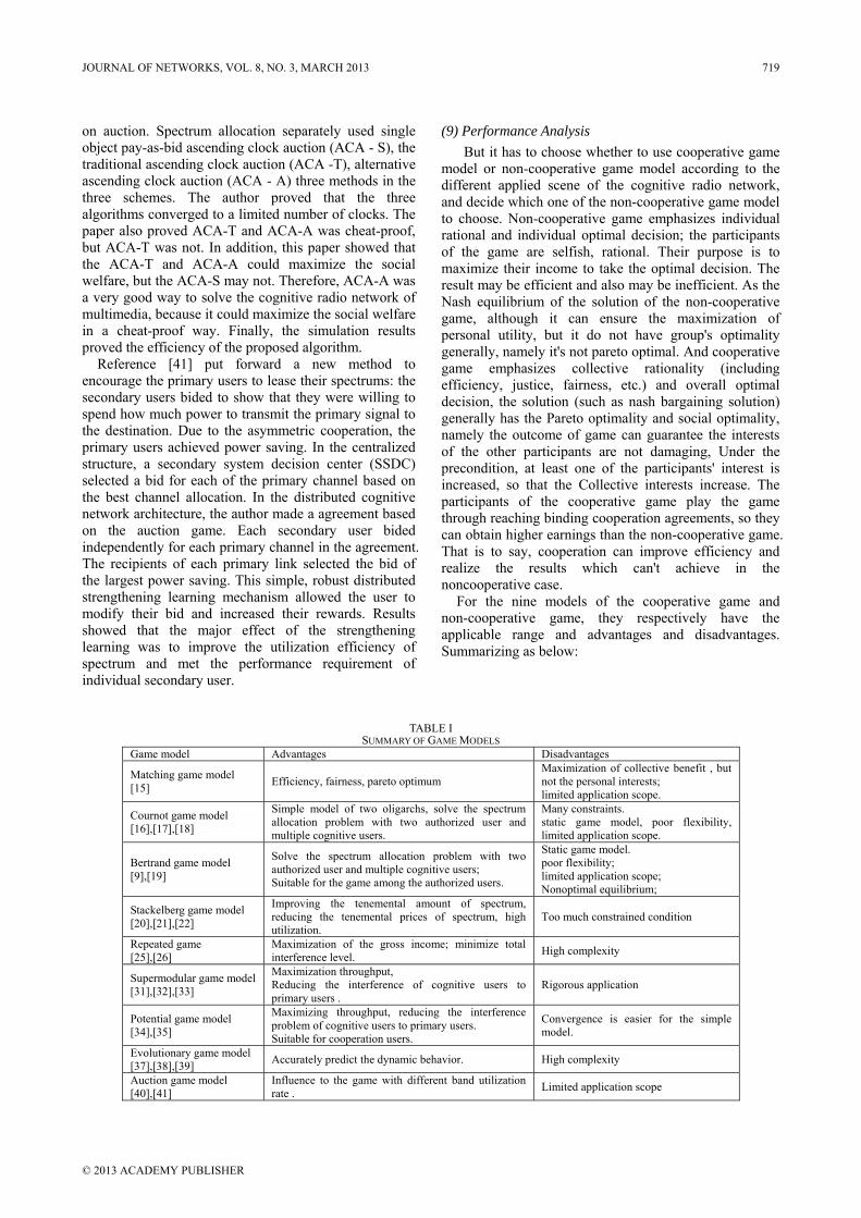
on auction. Spectrum allocation separately used single object pay-as-bid ascending clock auction (ACA - S), the traditional ascending clock auction (ACA -T), alternative ascending clock auction (ACA - A) three methods in the three schemes. The author proved that the three algorithms converged to a limited number of clocks. The paper also proved ACA-T and ACA-A was cheat-proof, but ACA-T was not. In addition, this paper showed that the ACA-T and ACA-A could maximize the social welfare, but the ACA-S may not. Therefore, ACA-A was a very good way to solve the cognitive radio network of multimedia, because it could maximize the social welfare in a cheat-proof way. Finally, the simulation results proved the efficiency of the proposed algorithm.

Reference [41] put forward a new method to encourage the primary users to lease their spectrums: the secondary users bided to show that they were willing to spend how much power to transmit the primary signal to the destination. Due to the asymmetric cooperation, the primary users achieved power saving. In the centralized structure, a secondary system decision center (SSDC) selected a bid for each of the primary channel based on the best channel allocation. In the distributed cognitive network architecture, the author made a agreement based on the auction game. Each secondary user bided independently for each primary channel in the agreement. The recipients of each primary link selected the bid of the largest power saving. This simple, robust distributed strengthening learning mechanism allowed the user to modify their bid and increased their rewards. Results showed that the major effect of the strengthening learning was to improve the utilization efficiency of spectrum and met the performance requirement of individual secondary user.

(9) Performance Analysis

But it has to choose whether to use cooperative game model or non-cooperative game model according to the different applied scene of the cognitive radio network, and decide which one of the non-cooperative game model to choose. Non-cooperative game emphasizes individual rational and individual optimal decision; the participants of the game are selfish, rational. Their purpose is to maximize their income to take the optimal decision. The result may be efficient and also may be inefficient. As the Nash equilibrium of the solution of the non-cooperative game, although it can ensure the maximization of personal utility, but it do not have group's optimality generally, namely it's not pareto optimal. And cooperative game emphasizes collective rationality (including efficiency, justice, fairness, etc.) and overall optimal decision, the solution (such as nash bargaining solution) generally has the Pareto optimality and social optimality, namely the outcome of game can guarantee the interests of the other participants are not damaging, Under the precondition, at least one of the participants' interest is increased, so that the Collective interests increase. The participants of the cooperative game play the game through reaching binding cooperation agreements, so they can obtain higher earnings than the non-cooperative game. That is to say, cooperation can improve efficiency and realize the results which can't achieve in the noncooperative case.

For the nine models of the cooperative game and non-cooperative game, they respectively have the applicable range and advantages and disadvantages. Summarizing as below:

TABLE I

SUMMARY OF GAME MODELS Game model Advantages Disadvantages

Matching game model [15] Efficiency, fairness, pareto optimum

Maximization of collective benefit , but not the personal interests; limited application scope.

Cournot game model [16],[17],[18]

Simple model of two oligarchs, solve the spectrum allocation problem with two authorized user and multiple cognitive users.

Many constraints. static game model, poor flexibility, limited application scope.

Bertrand game model [9],[19]

Solve the spectrum allocation problem with two authorized user and multiple cognitive users; Suitable for the game among the authorized users.

Static game model. poor flexibility; limited application scope; Nonoptimal equilibrium;

Stackelberg game model [20],[21],[22]

Improving the tenemental amount of spectrum, reducing the tenemental prices of spectrum, high utilization.

Too much constrained condition

Repeated game [25],[26]

Maximization of the gross income; minimize total interference level. High complexity

Supermodular game model[31],[32],[33]

Maximization throughput, Reducing the interference of cognitive users to primary users .

Rigorous application

Potential game model [34],[35]

Maximizing throughput, reducing the interference problem of cognitive users to primary users. Suitable for cooperation users.

Convergence is easier for the simple model.

Evolutionary game model [37],[38],[39] Accurately predict the dynamic behavior. High complexity

Auction game model [40],[41]

Influence to the game with different band utilization rate . Limited application scope



IV. CONCLUSION

This paper illustrates that introducing the game theory into spectrum allocation of the cognitive radio and describes the analytical scheme of game theory of spectrum allocation in cognitive radio. The paper divided the spectrum allocation models based on game theory into cooperative game model and non-cooperative game model. And making related investigative summary and description about the matching game model of the cooperative game model of and eight kinds of non-cooperative game models: the cournot game model, the bertrand game model, the stackelberg game model, the repeated game, the supermodular game model, the potential game model, the evolutionary game model, the auction game model. And the problems that each model is suitable for researching are different. We should choose the right model according to of the problem you analysis. Game theory provides a good theoretical tool for the research of spectrum allocation in cognitive radio, but this method is still in its beginning stage and doesn't form a complete theoretical system, and also the game models which can apply is limited and the conditions are very strict. The spectrum allocation based on the game theory in the cognitive radio network still has a lot of problems to be solved. The future work will focus on optimized spectrum allocation algorithm based on game theory to achieve better performance and spectrum utilization.

ACKNOWLEDGMENT

This research was supported by the National Natural Science Foundation of China (No.60902053, 61272497), the Hubei Key Laboratory of Intelligent Wireless Communications (IWC2012008), and “the Fundamental Research Funds for the Central Universities”, South-Central University for Nationalities (Grant Number: CZY12009).

REFERENCES

[1] Kloeck. C, Jaekel. H, Jondral. F. K. Dynamic and local combined pricing, allocation and billing system with cognitive radios. The First IEEE International Symposium on New Frontiers in Dynamic Spectrum Access Networks (DySPAN), pp. 73 – 81, (2005).

[2] J. Neel, J. H. Reed, R. P. Gilles. The Role of Game Theory in the Analysis of Software Radio Networks. SDR Forum Technical Conference November, 2002.

[3] J. Neel, J. H. Reed, R. P. Gilles. Convergence of Cognitive Radio Networks. Wireless Communications and Networking Conference, 2004.

[4] N. Nie, C. Comanieiu, “Adaptive channel allocation spectrum etiquette for cognitive radio networks”, IEEE New Frontier in Dynamic Spectrum Access Networks 2005, 2005: 267-278.

[5] Gesualdo Scutari, Jong-Shi Pang. Joint Sensing and Power Allocation in Nonconvex Cognitive Radio Games: Nash Equilibria and Distributed Algorithms IEEE Transactions on Information Theory. August 8, 2012, page(s): 1

[6] Saed Alrabaee, Anjali Agarwal, Devesh Anand, Mahmoud Khasawneh. Game Theory for Security in Cognitive Radio Networks. International Conference on Advances in

Mobile Network, Communication and Its Applications. 2012, page(s):60-63

[7] Niyato D, Hossain E. Competitive spectrum sharing in cognitive radio networks: a dynamic game approach. IEEE Transactions on Wireless Communications, 2008, 7(7):2651-2660.

[8] Niyato D, Hossain E, HAN Z. Dynamics of multiple-seller and multiple-buyer spectrum trading in cognitive radio networks:A game-theoretic modeling approach. IEEE Transactions Mobile Computing, 2009, 8(8).

[9] Dusit Niyato, Ekram Hossain, Competitive Pricing for Spectrum Sharing in Cognitive Radio Networks: Dynamic Game, Inefficiency of Nash Equilibrium, and Collusion. IEEE journal on selected areas in communications, vol. 26, no.1, January 2008, page(s): 192- 202

[10] Michael Bloem, Tansu Alpcan, Tamer Basar. A Stackelberg Game for Power Control and Channel Allocation in Cognitive Radio Networks. 2nd international conference on Performance evaluation methodologies and tools, 2007.

[11] Ekram Hossain, Vijay Bhargava. Cognitive Wireless Communication Networks. Springer Science Business Media, LLC2007: 231-267.

[12] Rajasekharan, J., Eriksson, J., Koivunen, V. Cooperative game theory and auctioning for spectrum allocation in cognitive radios. 2nd International Symposium on Personal Indoor and Mobile Radio Communications (PIMRC), IEEE 2. 2011, Page(s): 656 - 660

[13] Zehui Qu, Zhiguang Qin, Jiaohao Wang, Lan Luo, Zhengyao Wei .A cooperative game theory approach to resource allocation in cognitive radio networks. The 2nd IEEE International Conference on Information Management and Engineering (ICIME), 2010. Page(s): 90 - 93

[14] Tian Feng, Yang Zhen. A new algorithm for weighted proportional fairness based spectrum allocation of cognitive radios. International Conference on Software Engineering, Artificial Intelligence, Networking and Parallel Distributed Computing, 2007, 1:531-536.

[15] An Chengquan, Liu Yang. A Matching Game Algorithm for Spectrum Allocation Based on POMDP Model. 7th International Conference on Wireless Communications, Networking and Mobile Computing (WiCOM), 2011:1-3.

[16] Dusit Niyato, Ekram Hossain. A game-theoretic approach to competitive spectrum sharing in cognitive radio networks. Wireless Communications and Networking Conference (WCNC), 2007:16-20.

[17] Xin-chun Zhang, Shi-biao He; Jiang Sun. A game algorithm of dynamic spectrum allocation based on spectrum difference. 19th Annual Wireless and Optical Communications Conference (WOCC), 2010 , Page(s): 1- 4

[18] Yunxiao ZU, Peng LI. Study on Spectrum Allocation of Primary Users for Cognitive Radio Based on Game Theory. 6th International Conference on Wireless Communications Networking and Mobile Computing (WiCOM), 2010, Page(s): 1 - 4

[19] Yuedong Xu, John C. S. Lui, Dah-Ming Chiu. On oligopoly spectrum allocation game in cognitive radio networks with capacity constraints. Computer Networks, Volume 54, Issue 6, 29 April 2010, Page(s): 925-943

[20] Dusit Niyato, Ekram Hossain. Optimal Price Competition for Spectrum Sharing in Cognitive Radio: A Dynamic Game-Theoretic Approach. Global Telecommunications Conference, IEEE. 2007, page(s): 4625-4629



[21] Yong Xiao, Guoan Bi, Dusit Niyato, Luiz A. DaSilva, A Hierarchical Game Theoretic Framework for Cognitive Radio Networks. IEEE journal on selected areas in communications, vol. 30, no.10, November 2012, page(s): 2053-2069

[22] Yun Li; Xinbing Wang; Guizani, M. Resource Pricing with Primary Service Guarantees in Cognitive Radio Networks: A Stackelberg Game Approach. Global Telecommunications Conference, GLOBECOM, IEEE, 2009. Page(s): 1 - 5

[23] Goodman, David and Narayan Mandayam, “Network Assisted Power Control for Wireless Data,” Vehicular Technology Conference, Spring 2001 pp. 1022-1026.

[24] J. Friedman and C. Mezzetti, “Learning in Games by Random Sampling” Journal of Economic Theory, vol. 98, May 2001, pp. 55-84.

[25] Shuai Liu; Yutao Liu; Xuezhi Tan. Competitive spectrum allocation in cognitive radio based on idle probability of primary users. Youth Conference on Information, Computing and Telecommunication, IEEE, 2009.Page(s): 178 - 181

[26] Raul Etkin, Abhay Parekh, David Tse. Spectrum sharing for unlicensed bands. IEEE Journal on Selected Areas in Communications, 2007, 25(3):517-528.

[27] James Neel. How Does Game Theory Apply to Radio Resource Management. //www.mprg.org/people /gametheory/files/jn_qual.pdf?

[28] Friedman, James W. and Claudi Mezzetti. Learning in Games by Random Sampling. Journal of Economic Theory vol. 98, pp. 55-84, 2001.

[29] Topkis, Donald M. Supermodularity and Complementarity. Princeton University Press, Princeton, New Jersey, 1998.

[30] Milgrom, Paul and John Roberts. Rationalizability, Learning and Equilibrium in Games with Strategic Complementarities. Econometrica, Vol. 58, Issue 6 (Nov 1990), pp. 1255-1277.

[31] Huili Cheng, Qinghai Yang, Fenglin Fu, Kyung Sup Kwak. Spectrum Sharing with Smooth Supermodular Game in Cognitive Radio Networks. The 11th International Symposium on Communications & Information Technologies (ISCIT) IEEE, 2011, page(s): 543-547

[32] Nie Nie, Cristina Comaniciu. Adaptive channel allocation spectrum etiquette for cognitive radio networks. First IEEE International Symposium on New Frontiers in Dynamic Spectrum Access Networks, 2005:269-278.

[33] James O. Neel ,Jeffrey H. Reed, Robert P. Gilles. Convergence of cognitive radio networks. Wireless Communications and Networking Conference, 2004, 4: 2250-2255.

[34] Nguyen Duy Duong; Madhukumar, A. S; Premkumar, A. B. A game theoretic approach for power control and spectrum allocation for cognitive radio networks. 54th International Midwest Symposium on Circuits and Systems (MWSCAS) IEEE, 2011. Page(s): 1-4

[35] Zhang Hongshun; Yan Xiao. Advanced Dynamic Spectrum Allocation Algorithm Based on Potential Game for Cognitive Radio. 2nd International Symposium on Information Engineering and Electronic Commerce (IEEC), 2010. Page(s): 1-3

[36] T. L. Vincent and J.S.Brown, Evolutionary Game Theory, Natural Selection, and Darwinian Dynamics. Cambridge Univ. Press, July 2005

[37] Qingyang Song,Jianhua Zhuang; Lincong Zhang. Evolution Game Based Spectrum Allocation in Cognitive Radio Networks. Wireless Communications, 7th International Conference on Networking and Mobile Computing (WiCOM). 2011, Page(s): 1-4

[38] Kun Zhu, Dusit Niyato, Ping Wang, ZhuHan. Dynamic Spectrum Leasing and Service Selection in Spectrum Secondary Market of Cognitive Radio Networks. IEEE transactions on wireless communication, vol. 11, no. 3, March 2012, page(s): 1136-1145

[39] Zhengwei Wu, Peng Cheng. Xinbing Wang, Xiaoying Gan, Hui Yu, Hailong Wang. Cooperative Spectrum Allocation for Cognitive Radio Network: An Evolutionary Approach. International Conference on Communications (ICC), IEEE, 2011, Page(s): 1-5

[40] Yan Chen, Yongle Wu, Beibei Wang, Liu, K. J. R. Spectrum Auction Games for Multimedia Streaming Over Cognitive Radio Networks. IEEE Transactions on Communications. 2010, Page(s): 2381-2390

[41] Sudharman K. Jayaweera, Mario Bkassiny. Asymmetric Cooperative Communications Based Spectrum Leasing via Auctions in Cognitive Radio Networks. IEEE transactions on wireless communications, vol. 10, no. 8, August 2011, page(s): 2716 -2724

Qiufen Ni received the Bachelor of Engineering degree in electronic information engineering from Hubei University of Technology, China, in 2011. She is a graduate in College of Computer Science of South-Central University for Nationalities. Her research interests include cognitive radio networks and wireless communications.

Rongbo Zhu received the B.S. and M.S. degrees in Electronic and Information Engineering from Wuhan University of Technology, China, in 2000 and 2003, respectively; and Ph. D degree in communication and information systems from Shanghai Jiao Tong University, China, in 2006. He is currently an Associate Professor in College of Computer Science of South-Central University for Nationalities.

He is the Editor-In-Chief of International Journal of Satellite Communications Policy and Management, Associate Editor of International Journal of Radio Frequency Identification Technology and Applications. He serves as a guest editor for several journals, such as, Future Generation Computer Systems, Telecommunication Systems, and as a reviewer for numerous referred journals such as IEEE Systems Journal etc. He has been actively involved in around 10 international conferences. Dr. Zhu is a member of the ACM and IEEE.

Zhenguo Wu received the Bachelor of Engineering degree in Computer Science and Technology from Fuyang Teachers College, An Hui, China, in 2012. He is a graduate in College of Computer Science of South-Central University for Nationalities. His research interests include cognitive radio networks.



Yongli Sun received the Bachelor of Engineering degree in information engineering from Fuyang Teachers College, An Hui, China, in 2012. He is a graduate in College of Computer Science of South-Central University for Nationalities. His research interests include cognitive radio networks.

Lingyun Zhou is a Lecture of College of Computer Science of South-Central University for Nationalities. Her main research interests include Web mining and mobile computing.

Bin Zhou received the B.S. and M.S. degrees in School of Computer Science and Technology at National University of Defense Technology (NUDT), China, in 1994 and 2002, respectively. He is a PH.D Candidate in the College of Computer at Huazhong University of Science and Technology (HUST), China. He is currently an Associate Professor in College of Computer Science of South-Central University for Nationalities. His main research interest is in massive data management.



A Workflow-based RBAC Model for Web Services in Multiple Autonomous Domains

Zhenwu WANG

School of Mechanical and Information Engineering, China University of Mining and Technology, Beijing, China Email: [email protected]

Xuejun ZHAO1, Benting WAN2, Jun XIE3, Pengfei BAI1

1School of Mechanical and Information Engineering, China University of Mining and Technology, Beijing, China 2Software and Communication Engineering institute, Jiangxi University of Finance and Economics, Nanchang, China

3

Information Engineering institute, Capital Normal University, Beijing, China

Abstract—A workflow-based RBAC model for web services (WFRBAC4WS) has been proposed in this paper. The model organizes web services in different autonomous domains through workflow mechanism, and maps RBAC model to tasks of workflow model. The paper details the authorization procedure of WFRBAC4WS model, the lifetime management, the extension of authorization constraint and the formal descriptions of the proposed model. Compared with other RBAC models for web services, this model not only combines RBAC model to workflow, but also describes the interactions between workflow mechanism and RABC model in web services environment, the authorization work of this model is dynamically and comprehensively. Index Terms—workflow, RBAC, web services, autonomous domains

I. INTRODUCTION

(1) Cross-domain

Service-oriented architecture (SOA) is a framework for distributed systems, which is platform-independence and is constructed by components. Web service becomes the most popular implementation of SOA, and it has many advantages, such as high development efficiency, fast response ability, good reusability, and so on. The service requesters and providers both have the high dynamic because of the heterogeneity of environment and the variousness of operation methods, it is necessary that access control methods of web services need adapt the variety dynamically. The access control of web services must face the following problems [1, 2].

The traditional access control models base on single autonomous domain, the providers and requesters are both in the same domain, and they can “recognize” each other. But web services generally are deployed in different domains and the service requesters and providers cannot “recognize” each other, this problem is called the access control issue among “strangers” [3, 4].

(2) Dynamic authorization The traditional access control models generally assign

permissions to subjects according to certain rules, and

This work was supported by National “863” High Technology Research and Development Program of China (No.2012AA12A308).

then save these assignment relations, this procedure is called static authorization. But in web services environment, web services are distributed in multiple autonomous domains and the authorization activities are dynamic. The subjects which make the requests and the objects which provide service resources both have high dynamic characters, the dynamic traits of subjects are caused by the variety of operations and the heterogeneous environment, the dynamic characters of web services represent that the web services composition is dynamic, so we need a dynamic authorization mechanism.

(3) Loose coupling Web services are deployed in different autonomous

domains, the coupling relationships among web services are decided by the workflow of composite web services. The coupling relationships are different in contexts of different composite services because these components can be reused in many applications.

Owing to the above traits, we cannot directly adopt the traditional access control models which usually are used to web services in single domain, and the security problem of web services is the obstruction of web services popularization. Many scholars discussed the security problem of web services in various aspects [5-9]. Literature [5] proposed an attribute-based access control (ABAC) model based on XACML in Web Service, literature [6] designed a cross-domain trust-based access control model for Web service, which based on XACML and WS-Security, and literature [7] discussed the security technologies based on SOAP, which adopted methods of encryption, digital signature and authorization. Recently, some literatures discussed the access control problem of composite web services in multiple domains, literature [8] detailed a dynamic multiple domains access control model based on RBAC and gave a role mining algorithm to find the role set with minimized permissions, literature [9] proposed an UCON enhanced business process dynamic access control model, which unbounded the coupling relationship of organization model and the process model. Business process access control mechanism is a difficult problem in Web services composition application [9], literature [8][9] analyzed the permissions which are needed by services execution according to the procedures of composite web services,



but they only use a little idea of workflow and don’t detail how to map roles and web services to the tasks of workflow, which represent the business process. In this paper, we use workflow mechanism to describe the business processes, and allocate role instances to the tasks of workflow instead of the static role in run-time environment, this method adds flexibility and dynamic to the permission allocation strategy.

The rest of the papers are organized as follows. Section II provides an overview of the theory of NIST RBAC model and the review of workflow mechanism; Section III details the principle and formal descriptions of the proposed model, an example illustrates the model’s application in section IV and at last section V concludes this paper.

II. THE RELATED WORK

A. The NIST RBAC Model The RBAC model is the research hotspot in access

control domain, and it appeared a series of models, for example, RBAC96, ARBAC97 (Administrative RBAC97), ARBAC99, ARBAC02 and NIST RBAC (National Institute of Standards and Technology RBAC), these models have gradually been perfected. The RBAC model uncouples users and permissions through roles, which provide a bridge between them, it is characterized by the notion that permissions are assigned to roles, and not directly to users. Users are assigned appropriate roles according to their job functions, and hence indirectly acquire the permissions associated with those roles, and it is widely used to many information systems.

The NIST RBAC model has four components, they are Core RBAC, Hierarchal RBAC, and two units of Constraint RBAC. The Core RBAC is the smallest element set which can build an access control system, it includes the following conceptions.

(1) Users= {u1,u2,…,um(2) Roles={r

},it is the set of all the users. 1,r2,…,rn

(3) Ops={op},it is the set of all the roles.

1,op2,…,opk

(4) Objects={ob

},it describes the set of all the operations.

1,ob2,…,obl

(5) Session={s

},it is the set of all the access objects.

1,s2,…,sp

(6)

}, it represents the set of all the sessions.

ObjectsOpsPerms ×= 2 ,it is the set of all the permissions.

(7) RolesUsersUA ×⊆ ,it describes a many-to-many relation from user set to role set, and represents that users are given to roles.

(8) RolesPermsPA ×⊆ , it describes a many-to-many relation from permission set to role set, and represents that roles are given to permissions

(9) UsersRolesrusersassigned 2):(:_ → , return the user set which are given to role r.

}),({)(_ UAruUsersurusersassigned ∈∈= .

(10) PermsRolesrpermsassigned 2):(:_ → , return the permission set which are given to role r.

}),({)(_ PArpPermsprpermsassigned ∈∈= .

(11) RolesUsersurolesassigned 2):(:_ → , return the role set which are given to user u.

}),({)(_ UAruRolesrurolesassigned ∈∈= . (12) OpsPermspop →):( , return the operations

which are associated with certain permission p, }),({)( pobjopObjectsobjOpsoppop =∩∈∃∈= .

(13) ObjectsPermspob →):( , return the objects which are associated with certain permission p,

}),({)( pobjopOpsopObjectsobpob =∩∈∃∈= .

(14) SessionsUsersusessionuser 2)(_ →∈ , return the sessions which are associated with certain user u.

(15) Rolessessionssrolessession 2):(_ → , return the roles which are associated with certain session s, that is

})),(_({)(_ UArsuserssessionRolesrsrolessession ∈∈⊆ .

(16) Permssessionsspermssession 2):(_ → , return the permissions which are associated with certain session s, that is

)(_)(_)(_

suserssessionrrpermsassignedspermssession

∈∪= .

Many literatures [10-13] improved the NIST RBAC model from different aspects and discussed its discrete form in different application domains. In literature [10], we introduced visual data muster into RBAC model and proposed a three-dimensional space RBAC model, which constrained permissions from three dimensions and enhanced the ability of access control. Literature [11] gave a generalized temporal and spatial RBAC model, which is applied to mobile service applications; Literature [12] implemented the RBAC model in healthcare ad hoc network, literature [13] gave a united access control model for systems in collaborative commerce, which combined the advantages of RBAC, task-based authentication control (TBAC), attribute-based access control (ABAC) and automated trust negotiation (ATN).

Some scholars [16-20] discussed RBAC model in distributed environment. WANG Hao[16] made all of the nodes manage the user’s right and adopts different encryption policy according to the ability of the device object to realize high level of control and low consumption of calculation, LANG Bo[17] defined the semantics properties elements of trust in the context of access control in distributed systems, Wang Jun[18] designed a distributed secure access control system, HANG Shuai[19] proposed a role mining algorithm according to the process structure, and ZHAO Jun[20]

Some literatures[21-23] applied RBAC model to web services, which are the new software model of distributed systems.R.Wonoboesodo [21] introduced RBAC model

studied the application of distributed multi-channel MAC protocols in wireless sensor network(WSN).



to web services and assigned roles to web services through classifying them into single web service and composite web services, literature [22] proposed a role and task-based access control model (RTBAC),which bases on the traditional RBAC,TBAC and security workflow model, literature [23] presented a new dynamic hierarchical RBAC model for web services in order to enhance the flexibility and expansion. All the above papers extended RBAC model from different aspects, but they cannot depict the distributed characters of web services security mechanism. This paper combines RBAC model to workflow in order to describe the security problem more comprehensively.

B. The Workflow Mechanism Workflow is the automation of a business process in

whole or part, and the workflow idea has been used to various domains [14,15]

Although the above papers used workflow ideas to extend their access control models, they did not describe how to control the workflow and who control them, and they did not discuss the detailed interactions of workflow mechanism and RABC model in web services environment. This paper would detail the configurations of RBAC model in workflow modeling component, the model running theory in workflow executing component and the formal descriptions of the whole model. The workflow-based RBAC model discussed in this paper is based on my paper [27], in that paper, we describe workflow as a groupware of subtasks and actions, and the detailed theory of workflow system can refer literature [27].

.For software development of service-oriented architecture(SOA), the workflow idea provides a promising solution for organizations to achieve their business goals by interactions and collaborations between web services. Some scholars [24-26] introduced workflow mechanism to extend the access control mechanisms, literature [24] formalized web services and workflow processes, and proposed a type system to ensure that the specified TBAC policy is respected during system reductions, literature [25] introduced two notions of services and authorization transfer to describe dynamic service-oriented architecture and proposed a workflow–based and services-oriented role-based access control(WSRBAC)model, literature [26] also gave a access control model which has some workflow concepts to protect web services in business process, literature[16] presented a dynamic hierarchical role-based access control model for web services, which improved the flexibility and independence and expansion of access control for web services.

III. THE WORKFLOW-BASED RBAC MODEL FOR COMPOSITE WEB SERVICES

A. The Principle of WFRBAC4WS Generally, the workflow management system includes

two parts, they are workflow modeling component and workflow executing component. The workflow modeling component provides a build-time environment for

workflow constructors, and can be used to define, analyze and manage workflow model, the executing component provides a run-time environment to workflow execution. The paper will discuss the procedure of permission definition and allocation during the two parts.

1. Basic conceptions In order to describe the workflow-based RBAC model

for composite web services (WFRBAC4WS), we define the following conceptions.

(1) Role instance: Compared with role which is the key notion in RBAC model, role instance represents an instance of role, and it has the lifetime, that is to say, it is a dynamic conception which is generated when role is activated by users.

(2) FlowStep: FlowStep is a segment of workflow, and it is composed by a series of FlowSubTasks and FlowActions.

(3) FlowSubTask: FlowSubTask represents a functional operation, it describes the necessary executing task in workflow process, and it also can contain other FlowSubTask. FlowSubTask can map to one web service, or a series of web services, it relies on the function granularity.

(4) FlowAction: FlowAction describes the moving conditions of FlowSubTasks, it controls when the workflow is triggered to the next segment.

(5) Global web service: Global web service (gws) is the web services which can assign permissions to other web services and configure the whole workflow. Compared with common web services, this type web services control the permissions configuration and distribution in the entire distributed environment, and generally, global web service can be bound to FlowAction.

(6) Main Domain: Main Domain is the domain which runs Global Web Service, and it is in charge of the execution of WFRBAC4WS model.

2. The principle of WFRBAC4WS model The principle of WFRBAC4WS model can be

described as figure 1, the authorization work can be divided two parts which are corresponding to workflow definition component and executing component.

(1) authorization definition Authorization definition runs in workflow definition

step and system manager can do this work. This procedure can be describe by the full line part of figure 1.users obtain roles ,and roles can be assigned to FlowStep, then FlowSubTask and FlowAction can be distributed to FlowStep, at last web services are bound to FlowSubTask and global web services are bound to FlowAction.

(2) authorization activation In workflow executing step, system will automatically

generate a role instance according to certain role which is associated to certain user, and the role instance are bound to FlowSubTask and FlowAction, which are mapped to web services and global web services separately, that is to say, when a web service return computed results to system, the role instance which connected with this web service will be released because the role instance has lifetime.



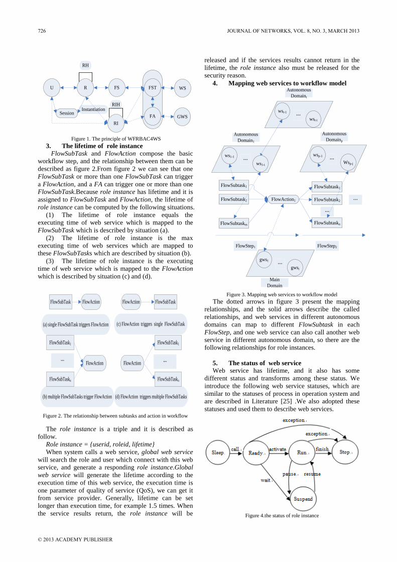
U R

RH

Session

RI

FST

RIH

WS

FA GWS

FS

Instantiation

Figure 1. The principle of WFRBAC4WS 3. The lifetime of role instance FlowSubTask and FlowAction compose the basic

workflow step, and the relationship between them can be described as figure 2.From figure 2 we can see that one FlowSubTask or more than one FlowSubTask can trigger a FlowAction, and a FA can trigger one or more than one FlowSubTask.Because role instance has lifetime and it is assigned to FlowSubTask and FlowAction, the lifetime of role instance can be computed by the following situations.

(1) The lifetime of role instance equals the executing time of web service which is mapped to the FlowSubTask which is described by situation (a).

(2) The lifetime of role instance is the max executing time of web services which are mapped to these FlowSubTasks which are described by situation (b).

(3) The lifetime of role instance is the executing time of web service which is mapped to the FlowAction which is described by situation (c) and (d).

FlowSubTask FlowAction

(a) single FlowSubTask triggers FlowAction

FlowSubTask1

FlowAction

(b) multiple FlowSubTasks trigger FlowAction

FlowSubTaskn

…

FlowSubTaskFlowAction

(c) FlowAction triggers single FlowSubTask

FlowSubTask1

FlowAction

(d) FlowAction triggers multiple FlowSubTasks

FlowSubTaskn

…

Figure 2. The relationship between subtasks and action in workflow

The role instance is a triple and it is described as

follow. Role instance = {userid, roleid, lifetime} When system calls a web service, global web service

will search the role and user which connect with this web service, and generate a responding role instance.Global web service will generate the lifetime according to the execution time of this web service, the execution time is one parameter of quality of service (QoS), we can get it from service provider. Generally, lifetime can be set longer than execution time, for example 1.5 times. When the service results return, the role instance will be

released and if the services results cannot return in the lifetime, the role instance also must be released for the security reason.

4. Mapping web services to workflow model

FlowSubtask1

FlowSubtask2

FlowSubtaskm

FlowAction1

FlowSubtask1

FlowSubtask2

FlowSubtaskn

…

…

FlowStep1 FlowStep2

Autonomous Domain1

ws1-1

ws1-i

Autonomous Domainp

wsp-1

Wsp-j… …

Autonomous Domaint

wst-1

wst-i…

Main Domain

gws1

gwsi…

Figure 3. Mapping web services to workflow model The dotted arrows in figure 3 present the mapping

relationships, and the solid arrows describe the called relationships, and web services in different autonomous domains can map to different FlowSubtask in each FlowStep, and one web service can also call another web service in different autonomous domain, so there are the following relationships for role instances.

5. The status of web service Web service has lifetime, and it also has some

different status and transforms among these status. We introduce the following web service statuses, which are similar to the statuses of process in operation system and are described in Literature [25] .We also adopted these statuses and used them to describe web services.

Figure 4.the status of role instance



Web service has five statuses, they are sleep, ready, run, suspend, and stop.

(1) Sleep status: it represents that one web service is the inactivated status.

(2) Ready status: it represents that the web service has completed the current preparatory work and the running condition has been satisfied.

(3) Run status: it represents that one web service has been activated successfully and is running.

(4) Suspend status: it represents that one web service has been paused to execute for some reasons.

(5) Stop status: it represents that one web service has been terminated, or finish its task.

The status transformation among the above statuses can be described by figure 4, and from it we can see that web services can be called when certain user accesses web services. When one user calls a web service, the system will judge whether user is legal or not according to its role instance.

From figure 3 we can see that web services are mapped to FlowSubTasks and FlowActions, so we need discuss the relations among them.

We can describe the relationship among FlowSubTasks as follows.

(1) Synchronized relationship. It shows that one FlowAction is triggered only if all the web services associated with FlowSubTasks complete their work.

(2) Asynchronous relationship. It shows that one FlowAction is triggered when one web service which is associated with FlowSubTask completes its work.

(3) Mutual exclusion relationship. It shows that two web services which are mapped to FlowSubTasks cannot execute at the same time.

The relationship between FlowSubTask and FlowActions or between two FlowActions can be described by dependency relation.

(4) Dependency relationship. a web service which is mapped to FlowAction is triggered only when FlowSubTasks complete their work, The FlowActions in workflow also satisfy the dependency relationship.

B. The Formal Description and Traits of WFRBAC4WS 1. The formal definition (1) },..,,{ 21 mfsfsfsFS = ,it is the set of all the

FlowSteps. (2) },..,,{ 21 nfstfstfstFST = , it is the set of all the

FlowSubTasks. (3) },..,,{ 21 lfafafaFA = ,it is the set of all the

FlowActions. (4) },..,,{ 21 lwswswsWS = ,it is the set of all the

common web services. (5) },..,,{ 21 pgwsgwsgwsGWS = ,it is the set of all

the global web services. (6) },..,,{ 21 kriririRI = ,it is the set of all the role

instances.

(7) RIUsersUIA ×⊆ , it describes a many-to-many relation from user set to role instance set, and represents users are assigned to role instances.

(8) RolesFSFSA ×⊆ , it is a many-to-many relation from FS to Roles, and it shows the FlowStep set which are assigned to Roles.

(9) RIFSTFSTA ×⊆ , it describes a many-to-many relation from FST to RI, and it represents the fst set which are assigned to RI.

(10) RIFAFAA ×⊆ , it describes a many-to-many relation from FA to role set, and it represents the fs set which are assigned to RI.

(11) mifafstfstfstfs ini ≤≤= 1},,,..,,{ 21 ,it describes that a FlowStep includes more than one FlowSubTask and one FlowAction.

(12) FSRolesrFSassigned 2):(_ → , return the FlowStep set which are assigned to role r, and }),({)(_ FSArfsFSfsrFSassigned ∈∈= .

(13) RIRolesrrisgenerated 2):(:_ → , return the role instance set which are generated by role r.

(14) FSTRIriFSTassigned 2):(_ → , return the FlowSubTask set which are assigned to role instance ri.and

}),({)(_ FSTArifstFSTfstriFSTassigned ∈∈=

(15) FARIriFAassigned 2):(_ → , return the FlowAction set which are assigned to role instance ri,and

}),({)(_ FAArifaFAfariFAassigned ∈∈= . (16) WSFSTfstws →∈ )( , return the web services

which associated to FlowSubTask fst. (17) GWSFAfagws →∈ )( , return the global web

services which are associated to FlowAction fa. (18) FSTFSfstFSfafst →∈∩∈ )( , return the

FlowSubTask set which are connected with FlowAciton fa.

(19) RIRIRIH ×⊆ , it represents a partially-ordered set on RI, and is marked as .

)(_)(_)(_)(_

21

1221

rusersauthorizedriusersauthorizedriFSTauthorizedriFSTauthorizedriri

⊆∩⊆⇒

)(_)(_)(_)(_

21

1221

rusersauthorizedriusersauthorizedriFAauthorizedriFAauthorizedriri

⊆∩⊆⇒

UsersRIriusersauthorized 2)(_ →∈ , and it can conclude the following formula.

}),(,{

)(_''' UIAriuririRIriUsersu

riusersauthorized

∈∩≥∈∃∈

=

FSTRIrifstsauthorized 2)(_ →∈ , and it can conclude the following formula.



}),(,{

)(_''' FSTArifstririRIriFSTfst

rifstsauthorized

∈∩≥∈∃∈

=

FARIrifasauthorized 2)(_ →∈ , and it can conclude the following formula.

}),(,{

)(_''' FAArifaririRIriFAfst

rifasauthorized

∈∩≥∈∃∈

=

2. The extension of authorization constraint Although the NIST RBAC model has the ability of

authorization constraint, it only concerns the conflict when multiple roles assigned to users. This paper extends authorization constraint based on first order logic. We introduce the following set to extend authorization constraint.

(20) Uncertain Function OE and AO

)}({)(:,)(:

XOEXXAOAllOtherXxxXOEOneElement ii

−=∈=

We further introduce the following sets. RIcrcricricriCRI is ⊆= },,...,{ 21 , CRI is the set of

conflicted role instances. FSTcfstcfstcfstcfstCFST iq ⊆= },,...,{ 21 , CFST

describes the set of conflicted FlowSubTasks. FAcfacfacfacfaCFA io ⊆= },,...,{ 21 ,CFA is the set of

conflicted FlowActions FScfscfscfscfsCFS it ⊆= },,...,{ 21 ,CFS is the set of

conflicted FlowSteps. The descriptions of first order logic are as follows.

1)(_:, ≤∩∈∀∈∀ crirrisgeneratedCRIcriRolesr

1)(_:, ≤∩∈∀∈∀ cfstriFSTassignedCFSTcfstRIri

1)(_:, ≤∩∈∀∈∀ cfariFAassignedCFAcfaRIri

1)(_:, ≤∩∈∀∈∀ cfsrFSassignedCFScfsRolesr 2. The characters of WFRBAC4WS model Compared with the traditional RBAC model, the

WFRBAC4WS model has the following characters. (1) To refine and depict the workflow control

information through introducing the conceptions of FlowStep and FlowAction.Web services provided by different providers cannot understand the whole workflow steps and it is necessary to configure and run these control information by certain global services. We use FlowStep to map common web services provided by different providers, and use FlowAction to map the global services which are in charge of workflow shift.

(2) To configure and control the access control of distributed web services through introducing the conception of global service. It is unrealistic that each web service can control the workflow shift, because different providers only provide the web services which are like “blackboxes” and have standard interfaces, and they have not duty to do these “extra work”. So the workflow control work must be done by a global service which can configure and run all the steps of workflow shift

(3) To manage roles dynamically through introducing the conception of role instance. Compared

with role, role instance is dynamical and has lifetime. When web services are called, the corresponding role instance will start and control the access permissions.

IV. EXAMPLE ILLUSTRATION

We will use an example to demonstrate how the WFRBAC4WS model works. In this example, there are three autonomous domains, and the domain 1 is the Main Domain, and it defines the workflow processes. Each FlowSubtask in workflow processes can be mapped to certain web service which is provided by different domains. In authorization definition step, Global web services will allocate roles to FlowSubtasks, and when system calls the concrete web services, the authorization task will be activated, and system will generate role instances which associate to roles, the dotted arrowheads in figure 5 represent that Global web services assign role instances to the concrete web services and manage them in their lifetimes.

Domain 1

Domain 2

Domain 3

Global web services

Check the weather

Book the travel itinerary

Book the air tickets

Book the air hotels

S2-1 S2-2

S3-1

S3-2

Book the travel itinerary Book the air tickets Book the air hotelsCheck the weather

FlowSubTask: Common Web service : Global web service:

Workflow processes

Figure5. The illustrated example

V. CONCLUSION

With the rapid development of service-oriented architecture, web services bring high productiveness and low cost for software development, but the security problem is the obstruction of web services popularization. Recently, the access control of web services becomes the hot research issue and scholars discussed this problem in various aspects according to protocol stack of web services. This paper proposed a workflow-based RBAC model for composite web services, the model configures permissions according to the workflow steps which include FlowSubTask and FlowAction, and manage the authorization task dynamically in multiple autonomous domains, so this method not only can satisfy the authorization requirement in distributed environment, but also can take back the permissions dynamically.

REFERENCES

[1] ZHANG Y, JOSHI J, "A request-driven secure interoperation framework in loosely-coupled multi-domain



environments employing RBAC policies[C]"//IEEE International Conference on Collaborative Computing:Networking,Applications and Worksharing,pp25-32,2007.

[2] HU Jin-wei,LI Rui-xuan,LU Zheng-ding, "Establishing RBAC-based secure interoperability in decentralized multi-domain environments[C]"//Proceedings of the 10th international conference on Information security and cryptology,pp 49-63,2007.

[3] O’Neill M,Allam-Baker P,Cann S M,et al, "Web services Security[M]",McGraw-Hill,2003.

[4] Yuan E,Tong J, "Attributed-based Access Control(ABAC) for Web Services[C]"//IEEE International Conference on Web Services,pp 561-569,2005.

[5] SHEN Hai-bo,HONG Fan, "ABAC model based on XACML in Web Service",Computer Applications,v25,n12,pp 2765-2768,2005.

[6] MA Xiao-ning,FENG Zhi-yong,XU Chao, "Cross-domain trust-based access control of Web services",Application Research of Computers,v26,n12,pp 4751-4754,2009.

[7] LIU Zhi-du,JIA Song-hao,ZHANG Shi-hua, "Research and Application of SOAP Security",Computer Engineering,v34,n5,pp142-144,2008.

[8] ZHANG Shuai,SUN Jian-ling,XU Bin,et al,"RBAC based access control model for services compositions cross multiple enterprises", Journal of Zhejiang University(Engineering Science),v46,n11,pp2035-2043,2012.

[9] SHANG Chaowang,LIU Qingtang,ZHAO Chengling,et al. "A Research on UCON Enhanced Dynamic Access Control Model for the Business Process of Composite Web Services”, Journal of Wuhan University(Nature and Science Edition) ,v57,n5,pp408-412,2011.

[10] CHEN Ming,WANG Zhen-wu, "Three-dimensional Space Access Control Model Based on Role",Computer Engineering,v34,n9,pp.157-159,2008

[11] Hsing-Chung Chen, Shiuh-Jeng Wang, Jyh-Horng Wen, Yung-Fa Huang, Chung-Wei Chen, "A Generalized Temporal and Spatial Role-Based Access Control Model",Journal of Network ,vol 5, no 8,pp.912-920,2010.

[12] Memon, Qurban A., "Implementing role based access in healthcare ad hoc networks",Journal of Networks, v 4, n 3, pp. 192-199,2009.

[13] Ruo-Fei, Han, Hou-Xiang, Wang, Qian, Xiao, Xiao-Pei, Jing, Hui, Li, "A united access control model for systems in collaborative commerce",Journal of Networks, v4, n4, p p.279-289,2009.

[14] Badii, Atta, Fuschi, David, Zhu, Meng, "Migrating from process automation to process management support: A holistic approach to software engineering applied to media production",Journal of Multimedia, v5, n5, pp. 404-416,2010.

[15] Pastorello Jr., Gilberto Zonta, Daltio, Jaudete, Medeiros, Claudia Bauzer, "A mechanism for propagation of semantic annotations of multimedia content”, Journal of Multimedia, v5, n 4, pp.332-342, 2010

[16] WANG Hao,WU Bo,GE Jin Wen,and WANG Ping, "Distributed Access Control Scheme Based on Controlled Object in the Internet of Things",Journal of University of Electronic Science and Technology of China,v141, ,n6,pp.893-898,2012

[17] LANG Bo, "Access control oriented quantified trust degree representation model for distributed systems",Journal on Communication,v31,n12,pp.45-54,2010

[18] Wang Jun,Jia Lianxing,Yao Haichao,and He Jianping, "Research on a File Level Distributed Secure Access

Control System Based on RBAC",Journal of Computer Research and Development,v41,n1,pp.24-29,2011

[19] ZHANG Shuai,SUN Jian-ling,XU Bin,HUANG Chao,and KAVS Aleksander J., "RBAC based access control model for services compositions cross multiple enterprises",Journal of Zhejiang University(Engineering Science),v46,n11,pp.2035-2043,2011

[20] ZHAO Jun,CHEN Xiang-guang,LIU Chun-tao,YU Xiang-ming,YUE Bin, "Study on Application of Distributed Multi-channel MAC Protocols in WSN",ACTA ARMAMENTARII,v33,n6,pp.695-702,2012

[21] Roosdiana Wonoboesodo,Zahir Tari, "A Role based Access Control for Web Services"//Proceedings of the 2004 IEEE International Conference on Services Computing,2004.

[22] Yu, Dingguo, "Role and task-based access control model for web service integration", Journal of Computational Information Systems, v8, n7, pp2681-2689, 2012.

[23] ZHU Yi-qun,LI Jian-hua,ZHANG Quan-hai, "A New Dynamic Hierarchical RBAC Model for Web Services",Journal of Shanghai Jiaotong University,v41,n5,pp 783-787,pp 686-693,2007.

[24] Yahui Lu,Li Zhang, "Type for Workflow Access Control in Web Service Context",Congress on Services,pp 621-628,2009.

[25] XU Feng,LAI Hai-Guang,HUANG Hao,XIE Li, "Service-Oriented Role-Based Access Control",Chinese Journal of Computers,v28,n4,2005.

[26] Peng Liu,Zhong Chen,"An Extended RBAC Model for Web Services in Business Process[c]"//Proceedings of the IEEE International Conference on E-Commerce Technology for Dynamic E-Business,2004.

[27] WANG Zhen-wu,CHEN Ming, "Workflow management system model based on subtask and action",Computer Engineering and applications,v43,n23,pp48-50,2007.

Zhenwu WANG was born in 1978, Qingdao, Shandong province, China.His main research interests include web services selection and composition, network security, and intelligent optimization algorithm. He received his M.S.and Ph.D. degrees from China University of Petroleum, Beijing, China in 2005 and 2008 respectively. He has authored/coauthored more than 20 scientific papers, and he is a fellow of Chinese Computer Federation (CCF), and Association for Computing Machinery (ACM). Xuejun ZHAO was born in 1962,Beijing,China.Her main research interests include network security, graphics and image processing, and remote sensing technology. She received her M.S. degree from China University of Mining and Technology, Beijing, China in 1990.Now she is an associate professor in China University of Mining and Technology, she presides a number of national fund projects, and is a fellow of Chinese Computer Federation (CCF), and Association for Computing Machinery (ACM). Benting WAN was born in 1976, Nanchang, Jiangxi province, China. His main research interests include mobile computing, parallel and distributed computing and Internet of things technology. He received his M.S. and Ph.D degrees from China University of Petroleum, Beijing, China in 2003 and 2006 respectively. Now he is an associate professor in Jiangxi University of Finance and Economics, Nanchang, China. He is in charge of more than five fund projects of Jiangxi province, and he is a fellow of Chinese Computer Federation (CCF), and Association for Computing Machinery (ACM).



Jun XIE was born in 1982, Ji’an, Jiangxi province, China.His main research interests include parallel and distributed computing and Internet of things technology. He received his M.S degree from Jilin University, Jilin, China in 2006, and received his Ph.D degree from China University of Petroleum, Beijing, China in 2009.Now he is an associate professor in Capital Normal University, Beijing, China, he is a fellow of

Chinese Computer Federation (CCF), and Association for Computing Machinery (ACM). Pengfei BAI was born in 1991, his main research interests include Role-based Access Control (RBAC) model and now he is a student in China University of Mining and Technology, Beijing, China.



Blocking DoS Attack Traffic in Network with Locator/Identifier Separation

Jianqiang Tang, Ying Liu, Ming Wan, Hongke Zhang

Beijing Jiaotong University/School of Electronic and Information Engineering, Beijing, China Email: {tangjianqiang, yliu, 07111021, hkzhang}@bjtu.edu.cn

Abstract—DoS attacks remain a most serious threat to the Internet currently, how to mitigate DoS attack is still an open issue. Besides, the current Internet faces serious scaling problems, and locator/identifier separation is widely recognized as a most promising solution for the future Internet. To block DoS attack traffic in network with locator/identifier separation, we propose a network layer defense system called BlockDoS. BlockDoS expands the mapping entries of the mapping system to store the block information, and enables any DoS attack victim to actively request the network to block unwanted traffic at tunnel routers. We implement a prototype of BlockDoS. The analysis and experiment results show that BlockDoS can block multi-million attackers’ traffic within tens of minutes, and the computing and storage costs added by BlockDoS won’t affect the performance of the mapping servers and tunnel routers. Index Terms—locator/identifier separation, DoS attack, DoS defense, mapping system, network security

I. INTRODUCTION

The Internet achieves great success and growth in the past few years for its openness. Openness is also one of the reasons for that the Internet is vulnerable to various security threats. The free-access model of Internet enables that a sender can send anything to anyone at anytime only if it knows the address, regardless the receiver wants or not. Even worse, attackers can launch denial of service (DoS) attacks with the free-access model of Internet easily and not be tracked. DoS attacks are one of the most significant threats on the current Internet, and also in the future [20]. DoS attacks aim to disrupt legitimate users access to services by flooding limited resource on the Internet. The attacking targets include the network bottlenecks such as bandwidth of access links, the computing and memory resource on servers, clients, router, and firewalls et al.

It’s easy for attackers to launch large-scale DoS attacks with botnets which consist of thousands of compromised hosts. Any DoS attack from botnets with enough compromised hosts can take down anyone on the Internet. And DoS attacks never stop, in Mary 2011, Wordpress suffered connectivity issues for the reason of DoS attacks with the attack data transfer speed up to Gbps level [4]. In June 2011, the owners of TDL-4 have created an ‘indestructible’ botnet, which has 4.5 million infected computers and it is still increasing [3]. If each

infected host sends one full-sized packet per second (1500 bytes), the aggregated attack traffic from TDL-4 botnet would exceed 54 Gbps. It is fatal for anyone on the Internet suffering this attack.

Besides, the current Internet routing and addressing architecture is facing serious challenges in scalability, multihoming, mobility and inter-domain traffic engineering [19]. Locator/identifier separation is widely recognized as one of the most promising solutions for the future Internet [11, 13]. And there already has a LISP beta network [1] to research the real-word behavior of the LISP protocol [8]. Locator/identifier separation uses two independent namespaces, identifier and locator, to decouple identity and location embodied by Internet Protocol (IP) addresses. Identifier represents the identity role of end host while locator represents the location role of IP address. Identifiers and locators are mapped onto each other at tunnel routers (TRs), and a mapping system is needed to resolve the mapping between identifiers and locators. While there have been many mapping systems proposed in the literature [9, 16].

Locator/identifier separation can enhance the network with routing scalability and routing security. However, network security is still a serious issue in the future Internet. Hosts will not be absolutely secure, and attackers are very sly. Attackers would launch DoS attacks with botnets which consist of thousands of compromised hosts in the future Internet just like that in the current Internet.

Locator/identifier separation creates a level of indirection between end hosts and locations, it enables the development of new security mechanism. In this paper, we propose a network layer defense system (BlockDoS) to block large-scale DoS attacks in locator/identifier separation network without changing the free-access attribute of the Internet. BlockDoS enables any DoS victim to notify the network to block unwanted traffic. It is an attempt to introduce a native security support of an efficient DoS defense mechanism at the beginning design of the future Internet architecture. In particular, we make the following contributions.

First, we propose to utilize the indirection character between identifiers and locators to block DoS attack traffic at TRs. When a host is considered as malicious, the TR will not map its identifier and locator onto each other but drop its packets.



Second, we incorporate the BlockDoS into the design of a mapping system. BlockDoS expands the mapping system to store the block information. It also uses the mapping system to resolve the locators of attackers and transfer block-requests to the corresponding TRs.

Third, in order not to affect the mapping system performance, we propose an efficient method to store the block information in mapping servers (MSs) and mapping cache in TRs.

Finally, we implement a prototype on Linux. Our experiments and analysis show that BlockDoS can block multi-million attackers’ traffic within tens of minutes, and the computing and storage costs added by BlockDoS won’t largely affect the performance of MSs and TRs.

The rest of the paper is organized as follows. In Section II we outline related work, focusing on DoS defense and locator/identifier separation. In Section III, we present the network model and our assumptions. In Section IV and V, we describe the proposed approach and its protection measures, respectively. We present the prototype in Section VI and the analysis and experiment results in Section VII. We conclude the paper in Section VIII.

II. RELATED WORK

A. DoS Defense Early work to mitigate DoS attacks tries to identify the

unwanted traffic source and filter the spoofing traffic at the ingress/egress routers. DoS attacks are evolving and ingress/egress filtering is no longer sufficient in dealing with large-scale DoS attacks. The study shows that source spoofing is no longer commonly employed in DoS attacks because the attacker control a large number of bot and source–spoofed packets can be easily filtered out [17].

The recent DoS defense work is mainly two approaches: capability-based approach [5, 15, 24] and filter-based approach [7, 14]. Capability-based approach enables the receiver to decide whether to receive the packets from the sender or not. The sender must request a capability and attach it to the subsequent packets, otherwise, the intermediate routers will consider the packets are invalid and drop or rates limit them. A capability is an unforgivable digital consent granted by the routers on the path and the receiver. Capability-based approach is an effective solution to defense DoS attacks but it changes the free-access mode of the Internet. In addition, Capability-based approach faces a new attack of denial-of-capability [6].

Filter-based approach allows receivers to request the router which is as close as possible to the attack source to stop unwanted traffic by install flow-level packets filters. AITF [7] uses three-way handshake between victim’s network and the network hosting attack source to install the filters. The filters may not be installed if the handshake packets are dropped on the link that is being flooded. StopIt [14] creates an overlay network consists of dedicated servers to forward the filter requests. However, the filters are installed in routers close to the

attack sources, and the routers should maintain a large number of filter rules.

BlockDoS will not change the free-access attribute of the Internet, and it adopts the idea of the filter-based approach to blocks attack traffic at TRs close to the attack source. BlockDoS does not need to maintain large number of filter rules, it judges unwanted traffic with the block information added into mapping cache in TRs.

B. Locator/Identifier Separation In locator/identifier separation, identifier, also called

endpoint identifier (EID), is used in the application and transport layers to identify a connection endpoint. And EID is not changed during the lifetime of a host. Locator (Loc) is used in the network layer to represent a node attachment point in the internet topology, and it will change when a host roams.

To solve the routing scalability, a number of new Internet routing architectures based on locator/identifier separation have been proposed [8, 18, 22, 25]. Generally, all the architectures can be divided into two categories: core-edge separation and core-edge elimination [11]. In core-edge separation category, routing in edge network and transit core is separated from each other. On the other hand, in core-edge elimination category, routing architecture is not changed per se. For core-edge separation category would significantly benefit both routing scalability and routing securities, we assume that routing in edge network and transit core is separated in network with locator/identifier separation and that packets are routed by global routable locators in transit core networks and by local locators [18] or identifiers [8] in edge networks.

Identifiers and locators are mapped onto each other at TRs. TRs exchange the EID and Loc of the packet header in Ivip [22] and GLI-Split [18], and TRs encapsulate an outer header to packets in LISP [8]. A mapping system is used to resolve the mapping between identifiers and locators.

The mapping system is the most critical challenge part of locator/identifier separation, for it should be fast, scalable, reliable and secure. There have been many mapping systems proposed in the literature, including LISP-ALT [9], SSM [16]. Each of the approaches has advantage and disadvantages, and only LISP-ALT has been developed for testing the LISP beta network [1]. These mapping systems generally response to map-requests for specific identifiers with appropriate locators, and each TR maintains a mapping cache to store the recently used mapping information to reduce the mapping resolve time. For ease of presentation, we use EID-to-Loc present the mapping entry stored in the mapping system in this paper.

III. NETWOKR MODEL AND ASSUMPTIONS

Before we describe the details of the BlockDoS, we first describe the network model with locator/identifier separation. We also make some assumptions here.



Figure 1. The network model with locator/identifier separation.

A. Network Model The network with locator/identifier separation we

consider is as Figure 1. The edge networks are separate from transit core. Edge networks are generally customer networks (CNs), while transit core network is Internet transit networks including Internet service providers (ISPs). CNs connect with the ISPs networks through TRs located at the edge of either ISPs networks or CNs. We assume that packets are routed by Locs in transit core and by EIDs in edge networks. We do not assume the structures of Loc or EID. Because IPv4 address is lacking, we assume the EID is 128 bits which would compatible with IPv6.

The mapping system is maintained by ISPs or some other commercial mapping service provider, it stores the whole EID-to-Loc mapping information of the network with many MSs. MSs respond to map-requests for specific identifiers with map-replies contain appropriate Locs. For simplicity, we assume that there is a MS in each ISP and each MS stores the mapping information of CNs that connected to local ISP.

Packets from a CN to another CN are generally tunneled from one TR to another TR. Each TR maintains a mapping cache that stores some recently used EID-to-Loc mapping entries. Each mapping entry stores in a TR’s mapping cache have a time-to-live (TTL) value that is originally set to an entry timeout. If a mapping entry is used before its TTL value, the TTL for the mapping entry is reset to be the given entry timeout; otherwise, the mapping entry is removed from the cache.

We illustrate two hosts’ packets forwarding through an example shown in Figure 1. The dashed circle represents the mapping system. Assume host A with EIDA wants to access the host B with EIDB. Denote the locator of TR1 and TR2 by Loc1 and Loc2

Step 1: Host A first sends a packet to the TR respectively.

1, EIDA and EIDB

Step 2: When TR

are the source and destination respectively as illustrated in Figure 1.

1 receives the packet from the host A, it looks up a locator in its mapping cache for EIDB

Step 3: TR

, as illustrated by (2) in Figure 1. If the cache hits, go to Step 5; otherwise, go to Step 3.

1 sends a map-request to MS1 in order to resolve a locator (or a set of locators) for EIDB

Step 4: MS

, as illustrated by (3) in Figure 1.

1 finds the locator of EIDB, we omit the map resolve process in the mapping system here. MS1 sends the map-reply contains EIDB-to-Loc2 to TR1

Step 5: When TR


1 receives the map-reply, it stores EIDB-to-Loc2 into its mapping cache. TR1 encapsulates the received packet with an outer header whose destination is Loc2 and source is Loc1. TR1 then sends the encapsulated packet, and it will be forwarded to TR2

Step 6: When TR


2 receives the encapsulated packet, it strips the outer header, sends the packet to its destination host B, as illustrated by (6) in Figure 1. Besides, it stores the EIDA-to-Loc1

B. Assumptions

gleaned from the packet into its mapping cache for the subsequent packets.

We also make a few assumptions about the underlying network conditions in this work. These assumptions allow us to limit the scope of this work.

• TRs can’t spoof source address of other CNs: We assume that TRs are more secure than hosts, and that they can’t spoof other CNs’ source addresses. In addition, each CN is responsible to the source address spoofing packets from it. An CN may prevent source address spoofing within its network using any anti-spoofing method such as ingress filtering or SAVA [23].

• Robust and secure mapping system. We assume that the mapping system is feasible, robust and secure. In addition, there has some methods to verify the messages in the mapping system, and the messages between MSs and TRs won’t be changed or spoofed.

• DoS traffic identification: We assume that there is a mechanism for an end system to identify DoS attack traffic. End system can observe the bad behavior of the senders. There are some existing technologies identifies attack flows [2, 21]. So we believe this is not an over-optimistic assumption.

• Flooding attacks: An attacker may compromise multi-million machines and control them to send traffic at the same time in network with locator/identifier separation, and then a DoS attack is launched. This large scale DoS attack could disrupt the destination’s communications, or congest narrow links.

IV. BLOCKDOS DESIGN

In this section, we describe the basic design of BlockDoS. We initially assume that the hosts in network are honest and well behaved. We will show how to secure BlockDoS in the next section.

A. Basic idea The basic idea of BlockDoS is to block unwanted

traffic with the indirection character between identifier and locator. The mapping system is the infrastructure of BlockDoS.



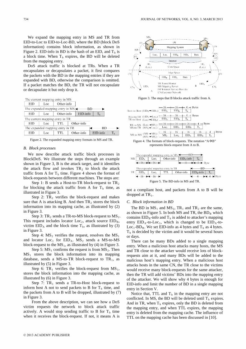
Figure 2. The expanded mapping entry formats in MS and TR.

Figure 3. The steps that B blocks attack traffic from A.

Figure 4. The formats of block-requests. The notation “AB”

represents block-request from A to B.

Figure 5. The BD-info in MS and TR.

We expand the mapping entry in MS and TR from EID-to-Loc to EID-to-Loc-BD, where the BD (block DoS information) contains block information, as shown in Figure 2. EID-info in BD is the hash of an EID, and Tb is a block time. When Tb

DoS attack traffic is blocked at TRs. When a TR encapsulates or decapsulates a packet, it first compares the packets with the BD in the mapping entries if they are expanded with BD, otherwise the comparison is omitted. If a packet matches the BD, the TR will not encapsulate or decapsulate it but only drop it.

expires, the BD will be deleted from the mapping entry.

B. Block processes We now describe attack traffic block processes in

BlockDoS. We illustrate the steps through an example shown in Figure 3, B is the attack target, and it identifies the attack flow and invokes TR2 to block the attack traffic from A for Tb

Step 1: B sends a Host-to-TR block-request to TR

time. Figure 4 shows the format of block-requests between different machines. The steps are:

2 for blocking the attack traffic from A for Tb

Step 2: TR

time, as illustrated in Figure 3.

2 verifies the block-request and makes sure that A is attacking B. And then TR2

Step 3: TR

stores the block information into its mapping cache, as illustrated by (2) in Figure 3.

2 sends a TR-to-MS block-request to MS2. This request includes locator Loc2, attack source EIDB, victim EIDA and the block time Tb

Step 4: MS


2 verifies the request, resolves the MS1 and locator Loc1 for EIDA. MS2 sends a MS-to-MS block-request to the MS1

Step 5: MS, as illustrated by (4) in Figure 3.

1 confirms the request is from MS2. Then MS1 stores the block information into its mapping database, sends a MS-to-TR block-request to TR1

Step 6: TR


1 verifies the block-request from MS1

Step 7: TR

, stores the block information into the mapping cache, as illustrated by (6) in Figure 3.

1 sends a TR-to-Host block-request to inform host A not to send packets to B for Tb

From the above description, we can see how a DoS victim requests the network to block attack traffic actively. A would stop sending traffic to B for T

time, and the packets from A to B will be dropped, illustrated by (7) in Figure 3.

b time when it receives the block-request. If not, it means A is

not a compliant host, and packets from A to B will be dropped at TR1

C. Block information in BD

.

The BD in MS1 and MS2, TR1 and TR2 are the same, as shown in Figure 5. In both MS and TR, the BDB which contains EIDB-info and Tb is added to attacker’s mapping entry EIDA-to-Loc1, which is changed to be EIDA-to-Loc1-BDB. We set EID-info as 4 bytes and Tb as 4 bytes. Tb

There can be many BDs added to a single mapping entry. When a malicious host attacks many hosts, the MS and TR close to the attacker would receive lots of block-requests aim at it, and many BDs will be added to the malicious host’s mapping entry. When a malicious host attacks hosts in the same CN, the TR close to the victims would receive many block-requests for the same attacker, then the TR will add victims’ BDs into the mapping entry of the attacker. We will show why 4 bytes is enough for EID-info and limit the number of BD in a single mapping entry in Section V.

is decided by the victim and it would be several hours or days.

Notice that, TTL and Tb in the mapping entry are not conflicted. In MS, the BD will be deleted until Tb expires. And in TR, when Tb

10

expires, only the BD is deleted from the mapping entry, and when TTL expires, the mapping entry is deleted from the mapping cache. The influence of TTL on the mapping cache has been discussed in [ ].



V. MAKE BLOCKDOS SECURE

BlockDoS could be abused or be the attack target. BlockDoS faces some threats, the threats include:

• Block-request spoofing attacks: Malicious hosts may spoof source address or use other method to send spoofing block-request to block other legitimate hosts’ communication.

• Malicious block-request attacks: Malicious hosts may abuse block-requests to disturb legitimate hosts’ traffic.

• Mapping cache or database exhaustion: Attacker may flood block-request to TR or MS and overflow the mapping cache or mapping database. It would take down BlockDoS, or TR or even the mapping system.

In this section, we describe how BlockDoS copes with these various threats.

A. Verify the block-requests The block-requests would be spoofed, and BlockDoS

should verify the block-requests. We now describe how to authenticate each type of block-requests.

1) Verify the block-requests between TR and Host BlockDoS does not detect source address spoofing. It

is easy to prevent address spoofing in a CN if the network administrator wants to, using method such as SAVA [23]. Hash-based message authentication code (HMAC) [12] can also be used in BlockDoS to authenticate block-requests between TRs and hosts. A pair of keys between a TR and a host can be obtained by IKEv2 when the host accesses to a CN. TRs will take further actions until they verify the block-requests from hosts.

2) Verify the block-requests in mapping system As is assumed in Section III, the mapping system

should provide a message authentication method. So here we consider that the block-requests between TRs and MSs, and that between MSs can’t be changed or spoofed. If there does not have a message authentication method in the mapping system, public/private key pair encryption algorithm can be used to authenticate the block-requests.

B. Confirm attacks Malicious hosts could abuse block-requests, and

botnets also may be used to send malicious block-requests to disrupt legitimate hosts’ communication. To prevent malicious block-requests attack, TRs should first confirm that the hosts whose packets are requested to be blocked are sending unwanted traffic.

1) Confirm attacks at the TR near the victim In BlockDoS, a host should not send block-requests if

it’s not being attacked. When receives a block-request from host B for blocking A’s attack traffic, TR2 should first verify it. And then, TR2 checks whether EIDA-to-Loc1 is in its mapping cache. If not, it means that A has not sent a packet to EIDB for at least TTL time and TR2 will not add the block information into the mapping cache. Otherwise, TR2 expands A’s mapping entry to be EIDA-to-Loc1-BDB

BlockDoS adopts the idea of StopIt [

, and sends Host-to-Host block-requests to A, as shown in Figure 4.

14] to confirm attacks, TR2 forges and sends Host-to-Host block-requests to check whether A is misbehaving. TR2 sends three Host-to-Host block-requests directly to A. The Host-to-Host block-request which uses EIDB as its source address is forged by TR2. If A does not comply with the block-requests and still sends unwanted packets to B, the packets will match the BDB in EIDA-to-Loc1-BDB. Then TR2 will treat A as malicious, and send a block-request to MS2. To save memory space, TR2 will delete the corresponding BDB in EIDA-to-Loc1-BDB after sending the block-request to MS2

Notice that, the three Host-to-Host block-requests could be dropped on network links and A may not receive them for link congestion or some other reasons. BlockDoS does not care this situation, and TR

.

2 sends block-request to MS2

2) Confirm attacks at the TR near attackers

as soon as it receives a packet from A to B again. However, a legitimate host won’t be treated as a malicious one if it stop sending unwanted traffic when receives block-request from the TR close to it.

When TR1 near the requested blocking host receives a block-request from MS1, it first verifies the request. After that, TR1 adds the block information into mapping entry EIDA-to-Loc1, and sends three block-requests to A. A compliant host receives the block-request will not send unwanted traffic for Tb time. A will be treated as a malicious host if it still sends unwanted traffic. And TR1

C. Control resource consumption

will not encapsulate or forward all packets from A until it is repaired.

The block information added to mapping cache in TR or mapping database in MS may be very large, and there may not have enough space to store all block information. In addition, attackers may launch attacks to overflow the mapping cache or mapping database in mapping system. We describe three knobs to control resource consumption added by BlockDoS.

1) Limit the rate of block-requests To avoid a TR’s resource being exhausted or

monopolized by a single victim, a TR should grant per-host a Host-to-TR block-request rate (RB). It is the maximum rate of block-request a host could send. If a host’s block-request rate exceed RB

2) Manage block information near the victim

, its requests are dropped.

The TRs near the victims will deal with all the block-requests, add all block information into mapping cache, and also send lots of block-requests to MS. The block information added into mapping cache may be very large, but the memory space is limited. To save memory space, when TR2 sends a block-request to MS2

If there are many hosts in a CN requesting to block the same attacker, the TR near the victims will add into the many BD into the attacker’s mapping entry. In BlockDoS, we limit the number of BDs added into a single mapping entry to N

, it removes the BD in the corresponding mapping entry.

s in TR near the victim. If the number of BD in an attacker’s mapping entry reaches Ns, TR will block all the traffic from the attacker to all hosts in the CN.



Figure 7. Tunnel Router Prototype

Figure 6. The network topology of our experiments

3) Manage block information near attackers MS1 and TR1 need to store all the received block

information into the corresponding mapping entries. MS1 stores the block information to ensure the attack traffic will be blocked for Tb time if the attacker’s mapping entry in TR1 is removed for the TTL expires. While TR1 stores all block information to ensure unwanted traffic will not be encapsulated and forwarded. There also may many BDs add into a single mapping entry in TR1 if many block-requests aim to the same attacker. We also limit the number of BDs in a single mapping entry in TR1 near the attacker. Nm is the granted maximum number of block-requests aim at a host per hour. If it exceeds Nm, TR1

D. Non-cooperating TRs close to attackers

informs the network administrator that the host is misbehaving and drops all the packets from it until it is repaired.

It is possible that TR1 receives block-requests will not add the block information into the mapping entries and unwanted packets won’t be blocked. To deal with this situation in BlockDoS, the victim B can use a radical punitive measure, requests TR2 to block all traffic from TR1 to B for a while. Other legitimate hosts’ traffic in the same CN1 is blocked either, so B should gingerly block all traffic from a non-cooperation TR1

However, non-cooperating TRs in BlockDoS don’t bring other attacks to the network. If BlockDoS does not work, the network security won’t be worse. We can also use other method to punish the non-cooperating TRs, for example, limiting the traffic rate from non-cooperating TRs at TRs near the victim.

.

E. Attack sources Multihoming consideration If the attacker A is multihoming, there are a set of

locators map onto EIDA in the mapping system. When receives block-requests, MS1

VI. IMPLEMENTATION

will send each locator (TR) a block-request.

We develop a prototype on Linux and build a laboratory environment as shown in Figure 7. All the machines are running Linux Fedora core 8 with Intel Celeron(R) 2.8 GHz CPU and 1 GB memory. All the machines configure with IPv6 addresses as EIDs or Locs.

For simple and quick prototyping, we implement the Locator/Identifier separation based on the Linux kernel netfilter framework by exchanging Locs and EIDs in the header of packets but not encapsulating packets with outer headers. And we also implement BlockDoS protocol on top of UDP. As shown in Figure 7, tunnel routers get and release packets from PRE_ROUTING and POST_ROUTING hook of netfilter respectively. We expand the mapping table with BlockDoS field in kernel space, the mapping information and block information are installed into linux kernel space via netlink.

We test whether BlockDoS can block unwanted traffic that grows proportionally with the number of attackers, and we further test the time needs to block unwanted traffic in the laboratory environment as shown in Figure 6.

The block-request rate between TR and host is RB, here we set the RB as 10000 block-requests per second. The time need to block NA attackers’ unwanted traffic is about NA/RB

VI. FEASIBILITY AND EFFICIENCY ANALYSIS

. In our experiment environment, Host A emulates 1 to 10 million attackers by repeatedly sending packets at 20kpps to B. When the host receive the TR-to-Host block-request, it will not send unwanted traffic with that source any more. Figure 8 shows our analysis and experiment results that the time for BlockDoS to block an attack with various numbers of attackers. Each attack repeats 10 times, and the error bars show the deviation from the average block time. As shown in Figure 8, BlockDoS can block all the unwanted traffic, and it takes about 20 minutes to block 10 million attackers’ traffic.

We analyze the feasibility and efficiency of BlockDoS in this section. BlockDoS will add some burden to mapping system, but here we argue that the burden is not heavy.

A. EID-info EID-info is a 32 bits hash of an EID. The 32 bits EID-

info hash code can distinguish hosts. It’s not possible that hosts communicate with a host at the same time. So 32 bits is enough to distinguish the attackers’ identifiers from legitimate hosts’. If there are 10 million attackers and we do not consider the collision probability



0 1 2 3 4 5 6 7 8 9 10 11

x 106

0

200

400

600

800

1000

1200

Number of Attackers

Sec

onds

ExprimentAnalysis

Figure 8. The time to block various number of attackers

of hash function, the false probability of a legitimate identifier to be treated as a malicious one is 2.33‰. This is acceptable, and a malicious host’s identifier will never be treated as a legitimate one.

B. Memory cost Each mapping entry in TR contains EID (16 bytes),

Loc (16 bytes), TTL (4 bytes) and other-info (assume 14 bytes), so that its size is about 50 bytes. While the BD is 8 bytes, which is about 16% of the mapping entry size.

The requested memory in TR2 is dynamic. Let us consider the worst situation, every attacker does not sends unwanted traffic when receives the Host-to-Host block-request, and the BDs in the mapping cache will be removed until TTL or Tb expires. In this case, it needs about another 16% of the attackers’ mapping entries size in mapping cache for the BDs. If there are 1 million attackers’ mapping entries in TR2 and it will add 1 million BDs into its mapping cache, the needed memory for 1 million mapping entries is about 50M, while for BDs is about 8M (8×1 million bytes). It’s not too large for TR2

The requested memory in TR, and usually this situation won’t happen.

1 and MS1 is almost the same. In MS1 a BD will be removed until Tb expires, while in TR1 a BD will be removed when TTL expires or Tb expires. Generally, Tb is longer than TTL, Tb will not affect the number of mapping entries in mapping cache. Because MS1 and TR1 will add all the block information into the mapping entry, the number of received block-requests by MS1 and TR1 decides the memory size for BDs. If Nr is the number of received block-requests, it needs Nr×8 bytes for BDs in MS1 and TR1. On the other hand, Nm

C. Bandwidth consumption

would limit the size of the BDs.

The block-request contains two EIDs (32 bytes) and Tb (4 bytes), its size is about 36 bytes. Adding the IPv6 header 40 bytes and other control information 24 bytes, a block-request would be about 100 bytes. The block-request rate between TR and host is RB, so the maximum Host-to-TR block-request rate is RB

D. Computation added by BlockDoS

×800 bps, it’s also the maximum rate of TR-to-MS block-request. If a victim sends 10000 block-requests per second to a TR, the rate would be 8Mbps. It’s not a heavy burden for a TR or a MS comparing with the large rate of attack traffic.

Two aspects of computation are added by BlockDoS: hash operation and block information comparison. The cost of hash operation is neglectable, we only consider block information comparison here.

In TR2, only the packets which are from host A, need to be compared with the BDB in EIDA-to-Loc1-BDB. Other packets’ encapsulation and forwarding won’t be affected. In TR1, only the packets which are from A, need to compare with the BDB in EIDA-to-Loc1-BDB

We test the packets transfer delay added by BD in the laboratory environment. We compare 10000 ICMP packets transfer delay between A and B when there is no BDs in TR and when there is a BD in TR. The average delay of per ICMP request and reply is about 0.631 ms and 0.633 ms respectively. The hash operation and block information comparison delay added by BlockDoS is about 2 us per packet. It’s acceptable for that not all the packets need to compare with the BD in mapping cache but only the attackers packets.

. The comparison delay is related with the number of BDs in a single mapping entry. However, it will be more efficiency than filter. Because in filter-based approach all packets must compare with the filter rules, but in BlockDoS only the packets from specific hosts need to compare with the BDs.

VII. CONCLUSION

We have presented a network-layer DoS defense system, BlockDoS, in network with locator/identifier separation. BlockDoS needs not to maintain large number of filter rules, it stores block information in mapping entries and uses the mapping system to transfer block-requests. Victims are able to actively request the network to block unwanted traffic with BlockDoS. We also design some mechanisms to protect BlockDoS to be abused or attacked. We implement a prototype and build a laboratory environment. We have showed that: (1) 32 bits EID-info is enough to denote a 128 bits EID, the false probability is about 2.33‰. (2) The requested memory in TR close to the victim is about 16% of the attackers’ mapping size and the requested memory in TR and MS close to the attacker grows proportionally with the received block-requests. (3) Our results show that a victim can block 10 million attackers’ unwanted traffic in about 20 minutes, and the bandwidth consumption and computation added by BlockDoS is acceptable. From this study, we conclude that it is feasible to introduce native security support at the beginning design of the future internet architecture. Our future work is to make the DoS defense system more efficiently and test it on a large-scale network topology.

ACKNOWLEDGMENT

This work is supported in part by the National High-Tech Research and Development Program of China (863) under Grant No. 2011AA010701, and in part by National Nature Science Foundation of China (No. 61202428 and



No. 60903150), and in part by the Fundamental Research Funds for the Central University (No. 2012YJS019).

REFERENCES

[1] Beta-Network Locator/ID Separation Protocol, [Online] Available: http://www.lisp4.net/, 2012.

[2] Peakflow X. [Online] Available: http://www.arbornetworks.com/peakflow-x-enterprise-network-security.html, July.2011.

[3] TDL4-Top Bot. [Online] Available: http://www.securelist. com/en/analysis/204792180/TDL4_Top_Bot, June. 2011.

[4] "WordPress.com Suffers Largest DDoS Attack In Its History," [Online] Available: http://news.cnet.com/ 8301-1 0 0 9 _ 3 - 2 0 0 3 8 8 7 4 - 8 3 . h t m l . M a r . 2 0 1 2 .

[5] T. Anderson, T. Roscoe, and D. Wetherall, "Preventing Internet denial-of-service with capabilities," SIGCOMM Comput. Commun. Rev., vol. 34, pp. 39-44, 2004.

[6] K. Argyraki and D. Cheriton, "Network Capabilities: The Good, the Bad and the Ugly," in Fourth Workshop on Hot Topics in Networks, 2005.

[7] K. Argyraki and D. R. Cheriton, "Scalable network-layer defense against internet bandwidth-flooding attacks," IEEE/ACM Trans. Netw., vol. 17, pp. 1284-1297, 2009.

[8] D. Farinacci, V. Fuller, D. Meyer, et al. "Locator/ID Separation Protocol (LISP)", IETF Internet draft, draft-ietf-lisp-23.txt, May 4, 2012.

[9] V. Fuller, D. Farinacci, D. Meyer, et al. "LISP Alternative Topology (LISP+ALT)", IETF Internet draft, draft-ietf-lisp-alt-10.txt, December 6, 2011.

[10] L. Iannone and O. Bonaventure, "On the cost of caching locator/ID mappings," in Proceedings of the 2007 ACM CoNEXT conference, New York, New York, 2007.

[11] D. Jen, M. Meisel, H. Yan, et al., "Towards A New Internet Routing Architecture: Arguments for Separating Edges from Transit Core," presented at the ACM HotNets-VII, Calgary, 2008.

[12] H. Krawczyk, M. Bellare, and R. Canetti. "HMAC: Keyed-Hashing for Message Authentication", IETF Internet Standard, RFC 2104, Feb. 1997.

[13] T. Li. "Design Goals for Scalable Internet Routing", IETF Internet Standard, RFC 6227, May 2011.

[14] X. Liu, X. Yang, and Y. Lu, "To filter or to authorize: network-layer DoS defense against multimillion-node botnets," in Proceedings of the ACM SIGCOMM 2008, Seattle, WA, USA, 2008.

[15] X. Liu, X. Yang, and Y. Xia, "NetFence: preventing internet denial of service from inside out," in Proceedings of the ACM SIGCOMM 2010, New Delhi, India, 2010.

[16] H. Luo, H. Zhang, M. Zukerman, "Decoupling the design of identifier-to-locator mapping services from identifiers," Computer Networks, vol. 55, pp. 959-974, 2011.

[17] Z.M. Mao, V. Sekar, O. Spatscheck, et al., "Analyzing large ddos attacks using multiple data sources," in ACM SIGCOMM Workshop on Large-Scale attack Defense(LSAD), 2006.

[18] M. Menth, M. Hartmann, and D. Klein, "Global Locator, Local Locator, and Identifier Split (GLI-Split)," [Online] Available:www3.informatik.uni-wuerzburg.de/staff/menth/ Publications/papers/Menth08-GLI-Split.pdf. April 2009

[19] D. Meyer, L. Zhang, and K. Fall. "Report from the IAB Workshop on Routing and Addressing", IETF Internet Standard, RFC 4984, Sep.2007.

[20] Arbor Networks, "Worldwide Infrastructure Security Report, Volume VI," 2011.

[21] H. Rahmani, N. Sahli, and F. Kamoun, "Distributed denial-of-service attack detection scheme-based joint-entropy," Security and Communication Networks, pp. n/a-n/a, 2011.

[22] R. Whittle. "Ivip (Internet Vastly Improved Plumbing) Architecture", IETF Internet draft, draft-whittle-ivip-arch-04.txt, Mar.2010.

[23] J. Wu, J. Bi, X. Li, et al. "A Source Address Validation Architecture (SAVA) Testbed and Deployment Experience", IETF Internet Standard, RFC 5210, June 2008.

[24] X. Yang, D. Wetherall, and T. Anderson, "TVA: a DoS-limiting network architecture," IEEE/ACM Trans. Netw., vol. 16, pp. 1267-1280, 2008.

[25] P. Dong, Y. Qin, and H. Zhang, " Research on Universal Network Supporting Pervasive Services", ACTA ELETRONICA SINICA, vol. 35, pp. 599-606, 2007.

Jianqiang Tang received the B.S. degree in the School of Electronics and Information Engineering from Beijing Jiaotong University, China in 2009. From September 2009 to now, he is a Ph.D candidate in National Engineering Laboratory for Next Generation Internet Interconnection Devices of Beijing Jiaotong University. His research focuses

on future Internet architecture, routing, and network security. Email: [email protected].

Ying Liu received the B.S. and M.S. degrees from Beijing Jiaotong University in 2000 and 2003, respectively. She is currently working toward the PhD degree in communication and information systems at Beijing Jiaotong University, where she is a lecturer with the School of Electronic and Information Engineering. Her research interests include Internet routing, network

monitoring and network security. Email: [email protected] Ming Wan received the B.S. degree in information and communication engineering from Beijing Jiaotong University in July 2007. From September 2007 to now, he is a Ph.D candidate at Beijing Jiaotong University. His research interests include the areas of architecture of future Internet, network and information security. Email: [email protected].

Hongke Zhang received his Ph.D. degree in Electrical and Communication Systems from the University of Electronic Science and Technology of China in 1992.He is the director of the National Engineering Laboratory for Next Generation Internet Interconnection Devices. He has published more than 100 research papers in the areas

of communications, computer networks and information theory. He is now the chief scientist of the projects "a universal network architecture for supporting pervasive services" founded by the National Basic Research Program of China ("973 Program"). Email: [email protected]



Optimality and Duality for Minimax Fractional Semi-Infinite Programming

Xiaoyan Gao

School of Science, Xi’an University of Science and Technology, Xi’an, China Corresponding author,


Abstract—The purpose of this paper is to consider a class of nonsmooth minimax fractional semi-infinite programming problem. Based on the concept of H − tangent derivative, a new generalization of convexity, namely generalized uniform ( , )HB ρ − invexity, is defined for this problem. For such semi-infinite programming problem, several sufficient optimality conditions are established and proved by utilizing the above defined new classes of functions. The results extend and improve the corresponding results in the literature. Subsequently, these optimality conditions are utilized as a basis for formulating dual problems. Weak, strong and reverse duality theorems are also derived for dual programs, using generalized invexity on the functions involved. Some previous duality results for differentiable minimax fractional programming problems turn out to be special cases for the results described in the paper Index Terms— H − tangent derivative, generalized convexity, minimax fractional semi-infinite programming, optimality conditions, duality

I. INTRODUCTION

In recent years, the concept of convexity and generalized convexity is well known in optimization theory and plays a central role in mathematical economics, management science, and optimization theory. Therefore, the research on convexity and generalized convexity is one of the most important aspects in mathematics programming. To relax convexity assumptions imposed on theorems on optimality conditions for generalized mathematical programming problems, various generalized convexity notations have been introduced. In particular, the concept of generalized ( , )F ρ − convexity, introduced by Preda [1] is in turn an extension of the convexity and was used by several authors to obtain relevant results. In [2, 3], the concept of V ρ− − invexity and ( , , , )F dα ρ − convexity were introduced, respectively. Other classes of generalized type I functions have been discussed in [4, 5].

On the other hand, a large literature was developed around generalized convexity and its applications in mathematical programming. Many authors investigated the optimality conditions and duality results for min-max programming problems under the conditions of generalized convexity. In particular, Aparna Mehra [6] employed various optimality conditions and duality

results under arcwise connectedness and generalized arcwise connectedness assumptions for a static minimax programming problem. Lin [7] and Wu [8] derived the sufficient optimality conditions for the generalized min-max fractional programming in the framework of ( , )F ρ − convex functions and invex functions. In [9], the Karush-Kuhn-Tucker-type sufficient optimality conditions and duality theorems for a nondifferentiable minimax fractional programming problem under the assumptions of alpha-univex and related functions were derived. Hang-Chin Lai [10] established the necessary and sufficient optimality conditions of nondifferentiable minimax fractional programming problem with complex variables under generalized convexities. Lai and Liu [11] employed the elementary method and technique to prove the necessary and sufficient optimality conditions for nondifferentiable minimax fractional programming problem involving convexity. In [12], a unified higher-order dual for a nondifferentiable minimax programming problem was formulated involving generalized higher-order (F, α, ρ, d)-Type I functions.

Semi-infinite programming have been a subject of wide interest since they play a key role in a particular physical or social science situation, i.e., control of robots, mechanical stress of materials, and air pollution abatement etc. Recently, Qingxiang zhang [13] obtained the necessary and sufficient optimality conditions for the nondifferentiable nonlinear semi-infinite programming involving B-arcwise connected functions. In [14, 15, 16, 17], the optimality conditions under various constraints qualification for semi-infinite programming problems were established.

In this paper, motivated by the above work, we first define a kind of generalize convexity about the H-tangent derivative. Then, the sufficient optimality conditions are obtained for a class of min-max fractional semi-infinite programming problem involving the new generalized convexity. Further, we develop duality theory. Several duality results are established for the optimization problem.

II. DEFINITIONS AND PRELIMINARIES

Let nX R⊂ be a nonempty set, 0 , nx X d R∈ ∈ and : { }f X R→ +∞ be a function, 0 0( , ( ))H

epifT x f x+

be



H − tangent cone of epif+ with respect to 0 0( , ( ))x f x . We say that 0( ; )Hf x d is H − tangent derivative of f at

0x along the direction d , where 0

0 0( ; ) inf{ ( , ) ( , ( ))}H Hepiff x d d T x f xη η

+= ∈

To define a class of new functions, we suppose that X is nonempty open subset of nR , real valued function

:f X R→ is H − tangent derivable at 0 ,x X Rρ∈ ∈ , 0 0

0: [0,1] , lim ( , ; ) ( , ), :b X X R b x x b x x R R

λλ ϕ

++→

× × → = →

, :η , :n nX X R X X Rθ× → × → , where η and θ are vectori- al application.

Definition2.1. f is said to be generalized uniform ( , )HB ρ − invex function at 0x X∈ , if for any x X∈ , there exists , , , b andϕ η θ ρ , such that

20 0 0 0 0( , ) [ ( ) ( )] ( , ( , )) ( , )Hb x x f x f x f x x x x xϕ η ρ θ− ≥ +

Definition2.2. f is said to be strictly generalized uniform ( , )HB ρ − invex function at 0x X∈ , if for any x X∈ and 0x x≠ , there exists , , , b andϕ η θ ρ , such that

20 0 0 0 0( , ) [ ( ) ( )] ( , ( , )) ( , )Hb x x f x f x f x x x x xϕ η ρ θ− > + Definition2.3. f is said to be generalized uniform

( , )HB ρ − pseudoinvex function at 0x X∈ , if for any x X∈ , there exists , , , and b ϕ η θ ρ , such that

0 0

20 0 0

( , ) [ ( ) ( )] 0

( , ( , )) ( , ) 0H

b x x f x f x

f x x x x x

ϕ

η ρ θ

− <

⇒ + <

Definition2.4. f is said to be strictly generalized uniform ( , )HB ρ − pseudoinvex function at 0x X∈ , if for any x X∈ and 0x x≠ , there exists , , , b andϕ η θ ρ , such that

0 0

20 0 0

( , ) [ ( ) ( )] 0

( , ( , )) ( , ) 0H

b x x f x f x

f x x x x x

ϕ

η ρ θ

− ≤

⇒ + <

Definition2.5. f is said to be generalized uniform ( , )HB ρ − quasiinvex function at 0x X∈ , if for any x X∈ , there exists , , , and b ϕ η θ ρ , such that

0 0

20 0 0

( , ) [ ( ) ( )] 0

( , ( , )) ( , ) 0H

b x x f x f x

f x x x x x

ϕ

η ρ θ

− ≤

⇒ + ≤

Definition2.6. f is said to be weakly generalized uniform ( , )HB ρ − quasiinvex function at 0x X∈ , if for any x X∈ , there exists , , , b andϕ η θ ρ , such that

0 0

20 0 0

( , ) [ ( ) ( )] 0

( , ( , )) ( , ) 0H

b x x f x f x

f x x x x x

ϕ

η ρ θ

− <

⇒ + ≤

III. SUFFICIENT OPTIMALITY CONDITIONS

In this section, we consider the following minimax fractional semi-infinite programming problem:

( )SIFP ( , )minimize ( ) sup( , )y Y

f x yF xh x y∈

= ,

subject to ( , ) 0g x u ≤ , , u U x X∈ ∈ , where X is a nonempty open subset of nR , Y is compact subset of mR ;

( , ) :f X Y R⋅ ⋅ × → , ( , ) :h ⋅ ⋅ X Y R× → , ( , ), ( , )f x h x⋅ ⋅ are continuous on Y for

every x X∈ ; : rg X U R× → and rU R⊂ is an infinite index set; ( , ) 0f x y ≥ and ( , ) 0h x y > for each ( , )x y ∈ X Y× . We assume that ( , ), ( , )f x h x⋅ ⋅ and ( , )g u⋅ are H − tangent derivable at x X∈ . We put 0 { ( , )X x g x u=

0, }u U≤ ∈ for the feasible set of problem (SIFP). For each 0x X∈ , we define

0 0 0

*

{ ( , ) 0, , },

( ) { ( , ) 0, , },

{ ( , ) 0, , },

{ 0, }

j j

j j

j j

j j

j g x u x X u U

J x j g x u x X u U

U u U g x u x X j

jµ µ

∆ = ≤ ∈ ∈

= = ∈ ∈

= ∈ ≤ ∈ ∈∆

Λ = ≥ ∈∆

Where *U is a countable subset of U , in the set Λ , every 0jµ ≥ , for all j∈∆ , and only finitely many are strictly positive.

{ }( , ) ( , )( )( , ) ( , )sup

z Y

f x y f x zY x y Yh x y h x z∈

= ∈ <

1 2{( , , ) 1 1, ( , , , ) s ms ssQ s y N R R s n Rλ λ λ λ λ+ += ∈ × × ≤ ≤ + = ∈

1 21

with 1,and ( , , , ) with ( ), 1, , }s

i s ii

y y y y y Y x i sλ=

= = ∈ =∑

In view of the continuity of ( , )f x ⋅ and ( , )h x ⋅ on Y

and compactness of Y , it is clear that ( )Y x is nonempty compact subset of Y for each x X∈ , and for any

0( )iy Y x∈ , we let 0

*0

( , )( , )

i

i

f x yqh x y

= , which is always a

constant. Definition3.1. For the problem (SIFP), a

point 0 0x X∈ is said to be an optimal solution, if for any 0x X∈ such that

0

0

( , ) ( , )( , ) ( , )sup sup

y Y y Y

f x y f x yh x y h x y∈ ∈

≤

Definition3.2. It is said that *x satisfies the Kuhn-Tuker constraint qualification for (SIFP), if there exists

* * * * * *0, 0,1 , , , ( ),1ii js i s j y Y x i sλ µ> ≥ ≤ ≤ ∈Λ ∈∆ ∈ ≤ ≤

and *q R∈ , such that



*

* *

* * * *

1* * * *

* * * *

* *

* * *

1 1

( ) ( , ; ( , ))

( , ; ( , )) 0,

( , ) ( , ) 0, 1, ,

( , ) 0,

0, 1

sH

ii xi

H j jj x

j

i ij

j

s s

i j ii j i

f q h x y x x

g x u x x u U

f x y q h x y i sg x u j

λ η

µ η

µ

λ µ λ

=

∈∆

= ∈∆ =

− +

≥ ∀ ∈

− = =

= ∈∆

+ ≠ =

∑

∑

∑ ∑ ∑

(1)

Theorem3.1. Let * 0x X∈ and for any 0x X∈ , we assume that there exists * * * *( , , ) , , js y Q q Rλ µ+∈ ∈ ∈Λ ,

j∈∆ and ** * ( )

0 0 1 1, , , , , , ,sb b R Rφ φ η θ ρ τ ∆∈ ∈ , such that

(i)For any * * *( ), 1, , , ( )( , )i iy Y x i s f q h y∈ = − ⋅ is genralized uniform *( , )H iB ρ − invex at *x with respect to

0b and 0φ ; (ii) For any * *, ( ), ( , )j ju U j J x g u∈ ∈ ⋅ is generalized

uniform *( , )H jB τ − invex at *x with respect to 1b and 1φ ;

(iii)*

* * * *

1

( ) ( , ; ( , ))s

Hii x

if q h x y x xλ η

=

−∑

* * * *( , ; ( , )) 0, , ;H j jj x

jg x u x x u U jµ η

∈∆

+ ≥ ∀ ∈ ∈∆∑

(iv) * * *( , ) 0, ,j jj

jg x u u U jµ

∈∆

= ∀ ∈ ∈∆∑ ;

(v) * * * *( , ) ( , ) 0, 1, ,i if x y q h x y i s− = = ; (vi) 0 0 10 ( ) 0 and (0) 0, 0 ( ) 0,a a a aφ φ φ< ⇒ < = ≤ ⇒ ≤

* *0 1( , ) 0, ( , ) 0 ;b x x b x x> ≥

(vii) *

* * * *

1

0s

i i j ji jλ ρ µ τ

= ∈∆

+ ≥∑ ∑ .

Then *x is an optimal solution of (SITP). Proof: Suppose that *x is not an optimal solution of

(SITP). Then there exists 0x X∈ , such that *

*

( , ) ( , )( , )( , )

sup supy Y y Y

f x y f x yh x yh x y∈ ∈

<

Also **

* * ** *

( , )( , ) , ( ), 1, ,( , ) ( , )

sup ii

y Y i

f x yf x y q y Y x i sh x y h x y∈

= = ∀ ∈ =

Further

( , ) ( , )( , ) ( , )

supi

y Yi

f x y f x yh x y h x y∈

≤

Thus, we have

( , ) * *, 1, , .( , )

i

i

f x y q i sh x y

≤ =

That is * *( , ) ( , ) 0, 1, ,i if x y q h x y i s− < =

By (v), we obtain

* * * *

*

( , ) ( , ) 0 ( , ) ( , ),

1, ,i i i if x y q h x y f x y q h x y

i s− < = −

=

From (vi), we get * *

0 0

* * *

( , ) [( ( , ) ( , ))

( ( , ) ( , ))] 0i i

i i

b x x f x y q h x y

f x y q h x y

φ −

− − <

Then from (i), we have 2

* * * * *( ) ( , ; ( , )) ( , ) 0Hix if q h x y x x x xη ρ θ− + <

Since * 0iλ ≥ and*

*

1

1s

iiλ

=

=∑ , we have

*

*

* * * *

1

2* * *

1

( ) ( , ; ( , ))

( , ) 0

sH

ii xi

s

i ii

f q h x y x x

x x

λ η

λ ρ θ

=

=

−

+ <

∑

∑

Now from (iii) and (vii), we get 2

* * * * * *( , ; ( , )) ( , ) 0H jj x j j

j jg x u x x x xµ η µ τ θ

∈∆ ∈∆

+ >∑ ∑

By (iv), we know that as * *\ ( ), 0, jj J x µ∈∆ = always

holds for any *ju U∈ . Hence, as *( ), j J x∈ we also have

*

*

* * *

( )

2* * *

( )

( , ; ( , ))

( , ) 0

H jj x

j J x

j jj J x

g x u x x

x x

µ η

µ τ θ

∈

∈

+ >

∑

∑ (2)

But as *( ),j J x∈ we know * *( , ) 0 ( , ),j j jg x u g x u u U≤ = ∈

From (vi), we get * * *

1 1( , ) [( ( , ) ( , )] 0,j j jb x x g x u g x u u Uφ − ≤ ∀ ∈

By (ii), we have 2

* * * *

* *

( , ; ( , )) ( , ) 0,

, ( )

H jx j

j

g x u x x x x

u U j J x

η τ θ+ ≤

∀ ∈ ∈

Since * *, ( )j j J xµ ∈Λ ∈ , we get

*

*

* * *

( )

2* * * *

( )

( , ; ( , ))

( , ) 0,

H jj x

j J x

jj j

j J x

g x u x x

x x u U

µ η

µ τ θ

∈

∈

+ ≤ ∀ ∈

∑

∑

Finally, we have a contradiction. Thus the theorem is proved and *x is an optimal solution of (SITP).

Theorem3.2. Let * 0x X∈ and for any 0x X∈ , we assume that there exists * * * *( , , ) , , ,js y Q q Rλ µ+∈ ∈ ∈Λ

j∈∆ , and** * ( )




(i) For any * * *( ), 1, , , ( )( , )i iy Y x i s f q h y∈ = − ⋅ is generalized uniform *( , )H iB ρ − pseudoinvex at *x with respect to 0b and 0φ ;

(ii) For any * *, ( ), ( , )j ju U j J x g u∈ ∈ ⋅ is generalized uniform *( , )H jB τ − quasiinvex at *x with respect to 1b and

1φ ;

(iii)*

* * * *

1

( ) ( , ; ( , ))s

Hii x

if q h x y x xλ η

=

− +∑

* * * *( , ; ( , )) 0, , ;H j jj x


∈∆

≥ ∀ ∈ ∈∆∑

(iv) * * *( , ) 0, ,j jj

jg x u u U jµ

∈∆

= ∀ ∈ ∈∆∑ ;

(v) * * * *( , ) ( , ) 0, 1, ,i if x y q h x y i s− = = ; (vi) 0 10 ( ) 0 , 0 ( ) 0,a a a aφ φ< ⇒ < ≤ ⇒ ≤

*0 ( , ) 0b x x > , *

1( , ) 0;b x x ≥

(vii)*

* * * *

1

0s


= ∈∆

+ ≥∑ ∑ .

Then *x is an optimal solution of (SIFP). Proof: Suppose that *x is not an optimal solution of

(SIFP). Then there exists 0x X∈ , such that *

*

( , ) ( , )( , )( , )

sup supy Y y Y

f x y f x yh x yh x y∈ ∈

<

Also **

* * ** *

( , )( , ) , ( ), 1, , .( , ) ( , )

sup ii

y Y i

f x yf x y q y Y x i sh x y h x y∈

= = ∀ ∈ =

Further

( , ) ( , )( , ) ( , )

supi

y Yi

f x y f x yh x y h x y∈

≤

Thus, we have

* *( , ) , 1, , .( , )

i

i

f x y q i sh x y

≤ =

Which is equivalent to * *( , ) ( , ) 0, 1, ,i if x y q h x y i s− < =

By (v), we get * * * *

*

( , ) ( , ) 0 ( , ) ( , ),

1, ,i i i if x y q h x y f x y q h x y

i s− < = −

=

From (vi), we get * *

0 0

* * *

( , ) [( ( , ) ( , ))

( ( , ) ( , ))] 0i i

i i

b x x f x y q h x y

f x y q h x y

φ −

− − <

Then by (i), we have 2

* * * * *( ) ( , ; ( , )) ( , ) 0Hix if q h x y x x x xη ρ θ− + <

Since * 0iλ ≥ and*

*

1

1s

iiλ

=

=∑ , we get

*

*

* * * *

1

2* * *

1

( ) ( , ; ( , ))

( , ) 0

sH

ii xi

s

i ii

f q h x y x x

x x

λ η

λ ρ θ

=

=

−

+ <

∑

∑ (3)

Also, as *( ), j J x∈ we have * *( , ) 0 ( , ),j j jg x u g x u u U≤ = ∀ ∈

Then using (vi), we obtain * * * *

1 1( , ) [( ( , ) ( , )] 0, , ( )j j jb x x g x u g x u u U j J xφ − ≤ ∀ ∈ ∈ Now by (ii), we have

2* * * *( , ; ( , )) ( , ) 0H j

x jg x u x x x xη τ θ+ ≤

Since * *, ( )j j J xµ ∈Λ ∈ , it follows that

* *

2* * * * * *

( ) ( )

( , ; ( , )) ( , ) 0H jj x j j

j J x j J x

g x u x x x xµ η µ τ θ∈ ∈

+ ≤∑ ∑

Also by (iv), as *\ ( ),j J x∈∆ we have * 0jµ = . So

2* * * * * *( , ; ( , )) ( , ) 0H jj x j j

j jg x u x x x xµ η µ τ θ

∈∆ ∈∆

+ ≤∑ ∑ (4)

Now, adding (3) and (4), then from (vii), we have *

*

* * * *

1

* * *

2* * * * * *

1

( ) ( , ; ( , ))

( , ; ( , ))

( ) ( , ) 0,

sH

ii xi

H jj x

j

sj

i i j ji j

f q h x y x x

g x u x x

x x u U

λ η

µ η

λ ρ µ τ θ

=

∈∆

= ∈∆

−

+

< − + ≤ ∀ ∈

∑

∑

∑ ∑

Finally, we have a contradiction. Hence *x is an optimal solution of (SIFP).

Theorem3.3. Let * 0x X∈ and for any 0x X∈ , we assume that there exists * * * *( , , ) , , js y Q q Rλ µ+∈ ∈ ∈Λ ,

j∈∆ and** * ( )


(i) For any * * *( ), 1, , , ( )( , )i iy Y x i s f q h y∈ = − ⋅ is strictly generalized uniform *( , )H iB ρ − invex at *x with respect to 0b and 0φ ;

(ii) For any * *, ( ), ( , )j ju U j J x g u∈ ∈ ⋅ is strictly generalized uniform *( , )H jB τ − invex at *x with respect to

1b and 1φ ;

(iii)*

* * * *

1

( ) ( , ; ( , ))s

Hii x

if q h x y x xλ η

=

−∑

* * * *( , ; ( , )) 0, ,H j jj x


∈∆

+ ≥ ∀ ∈ ∈∆∑ ;

(iv) * * *( , ) 0, ,j jj

jg x u u U jµ

∈∆

= ∀ ∈ ∈∆∑ ;


* *0 1( , ) 0, ( , ) 0b x x b x x> ≥ ;



(vii)*

* * * *

1

0s


= ∈∆

+ ≥∑ ∑ .

Then *x is an optimal solution of (SIFP). Theorem3.4. Let * 0x X∈ and for any 0x X∈ , we

assume that there exists * * * *( , , ) , , js y Q q Rλ µ+∈ ∈ ∈Λ ,

j∈∆ and** * ( )


(i) For any * * *( ), 1, , , ( )( , )i iy Y x i s f q h y∈ = − ⋅ is strictly generalized uniform *( , )H iB ρ − pseudoinvex at

*x with respect to 0b and 0φ ; (ii) For any * *, ( ), ( , )j ju U j J x g u∈ ∈ ⋅ is generalized

uniform *( , )H jB τ − quasiinvex at *x with respect to 1b and 1φ ;

(iii)*

* * * *

1

( ) ( , ; ( , ))s

Hii x

if q h x y x xλ η

=

−∑

* * * *( , ; ( , )) 0, ,H j jj x


∈∆

+ ≥ ∀ ∈ ∈∆∑ ;

(iv) * * *( , ) 0, ,j jj

jg x u u U jµ

∈∆

= ∀ ∈ ∈∆∑ ;


* *0 1( , ) 0, ( , ) 0b x x b x x≥ ≥ ;

(vii)*

* * * *

1

0s


= ∈∆

+ ≥∑ ∑ .

Then *x is an optimal solution of (SIFP).

IV. DUALITY THEOREMS

In this section, we formulate a dual problem to the minmax problem (SIVP).

(SIFD)

*

( , , ) ( , , ) ( , , )

1*

*

max sup

( ) ( , ; ( , ))

( , ; ( , )) 0, , ;

( , ) ( , ) 0, 1,2, , ;

( , ) 0, , ;

( , , ) .

s y Q s q D s y

sH

ii xi

H j jj x

j

i ij j

j

q

f qh z y x z

g z u x z u U j

f z y q hz y i sg z u u U j

s y Q

λ λ λ

λ η

µ η

µ

λ

∈ ∈

=

∈∆

−

+ ≥ ∀ ∈ ∈∆

− ≥ =

≥ ∀ ∈ ∈∆

∈

∑

∑

(5)

Where ( , , )D s yλ denotes the set of all ( , , )z qµ ∈ nR R+×Λ × to satisfy relations (5).

If for a triplet ( , , )s y Qλ ∈ , the set ( , , )D s yλ = Φ , then

we define the supremum over ( , , )D s yλ to be −∞ . Theorem4.1. (Weak duality) Let x be a feasible

solution of (SIFP) and ( , , , , , )z q s yµ λ be a feasible solution of (SIFD). For 0, 1,2, ,i i sλ ≥ = with

1

1,s

i jiλ µ

=

= ∈Λ∑ , and j q R+∈∆ ∈ , assume there exists

0 0 1 1, , , , , , sb b Rφ φ η θ ρ ∈ and ( )Rτ ∆∈ , such that

(i)For all , 1, , , ( )( , )i iy i s f qh y= − ⋅ is generalized uniform ( , )H iB ρ − invex with respect to 0b and 0φ at z ;

(ii) For all *, ( ), ( , )j ju U j J z g u∈ ∈ ⋅ is generalized uniform ( , )H jB τ − invex with respect to 1b and 1φ at z ;

(iii) 0 10 ( ) 0 ; 0 ( ) 0,a a a aφ φ< ⇒ < ≤ ⇒ ≤

0 1( , ) 0, ( , ) 0b x z b x z> ≥

(iv) 1

0s


= ∈∆

+ ≥∑ ∑ .

Then ( , )( , )sup

y Y

f x y qh x y∈

≥

Proof: Suppose contrary that ( , )( , )sup

y Y

f x y qh x y∈

<

Then, we have ( , ) ( , ) 0,f x y q hx y y Y− < ∀ ∈

Using the constraint condition (5), it follows that for all , 1, ,iy i s= , we get

( , ) ( , ) 0 ( , ) ( , )i i i if x y qh x y f z y qh z y− < ≤ −

By (iii), we get

0 0( , ) [( ( , ) ( , ))

( ( , ) ( , ))] 0i i

i i

b x z f x y q hx y

f z y q hz y

φ − −

− <

Then (i) yields

2

( ) ( , ; ( , )) ( , ) 0Hix if q h z y x z x zη ρ θ− + <

Since 0iλ ≥ and1

1s

iiλ

=

=∑ , it follows that

2

1 1

( ) ( , ; ( , )) ( , ) 0s s

Hii x i i

i if q h z y x z x zλ η λ ρ θ

= =

− + <∑ ∑

Hence by the constraint condition (5) and (iv), we get 2

( , ; ( , )) ( , ) 0H jj x j j

j jg z u x z x zµ η µ τ θ

∈∆ ∈∆

+ >∑ ∑

For ( )j J z∈ , using the constraint condition (5), then we get

*( , ) 0 ( , ),j j jg x u g z u u U≤ ≤ ∀ ∈

From (iii), we get *

1 1( , ) [( ( , ) ( , )] 0, , ( )j j jb x z g x u g z u u U j J zφ − ≤ ∀ ∈ ∈ By (ii), we have

2( , ; ( , )) ( , ) 0H j

x jg z u x z x zη τ θ+ ≤

Since , ( )j j J zµ ∈Λ ∈ , it follows that 2

( ) ( )

( , ; ( , )) ( , ) 0H jj x j j

j J z j J zg z u x z x zµ η µ τ θ

∈ ∈

+ ≤∑ ∑



According to the constraint condition (5), for all *ju U∈ , we let 0jµ = , as \ ( )j J z∈∆ .

Thus, we have 2

( , ; ( , )) ( , ) 0H jj x j j


∈∆ ∈∆

+ ≤∑ ∑

We have a contradiction. Therefore, we conclude

that ( , )( , )sup

y Y

f x y qh x y∈

≥ . Hence, the proof of the theorem is

complete. Theorem4.2. (Weak duality) Let x be a feasible


1

1,s

i jiλ µ

=



(i)For all , 1, , , ( )( , )i iy i s f qh y= − ⋅ is generalized uniform ( , )H iB ρ − pseudoinvex with respect to 0b and 0φ at z ;

(ii) For all *, ( ), ( , )j ju U j J z g u∈ ∈ ⋅ is generalized uniform ( , )H jB τ − quasiinvex with respect to 1b and 1φ at z ;

(iii) 0 10 ( ) 0 ; 0 ( ) 0,a a a aφ φ< ⇒ < ≤ ⇒ ≤

0 1( , ) 0, ( , ) 0b x z b x z> ≥

(iv) 1

0s


= ∈∆

+ ≥∑ ∑ .

Then ( , )( , )sup

y Y

f x y qh x y∈

≥

Proof: Suppose contrary that ( , )( , )sup

y Y

f x y qh x y∈

<

Then, we have ( , ) ( , ) 0,f x y q hx y y Y− < ∀ ∈

Using the constraint condition (5), it follows that for all , 1, ,iy i s= , we get

( , ) ( , ) 0 ( , ) ( , )i i i if x y qh x y f z y qh z y− < ≤ −

By (iii), we get

0 0( , ) [( ( , ) ( , ))

( ( , ) ( , ))] 0i i

i i

b x z f x y q hx y

f z y q hz y

φ − −

− <

Then (i) yields

2

( ) ( , ; ( , )) ( , ) 0Hix if q h z y x z x zη ρ θ− + <

Since 0iλ ≥ and1

1s

iiλ

=

=∑ , it follows that

2

1 1

( ) ( , ; ( , )) ( , ) 0s s

Hii x i i

i if q h z y x z x zλ η λ ρ θ

= =

− + <∑ ∑

(6) Hence by the constraint condition (5) and (iv), we get

2( , ; ( , )) ( , ) 0H j

j x j jj j

g z u x z x zµ η µ τ θ∈∆ ∈∆

+ >∑ ∑

For ( )j J z∈ , using the constraint condition (5), then we get

*( , ) 0 ( , ),j j jg x u g z u u U≤ ≤ ∀ ∈

From (iii), we get

*1 1( , ) [( ( , ) ( , )] 0, , ( )j j jb x z g x u g z u u U j J zφ − ≤ ∀ ∈ ∈

By (ii), we have 2

( , ; ( , )) ( , ) 0H jx jg z u x z x zη τ θ+ ≤

Since , ( )j j J zµ ∈Λ ∈ , it follows that

2

( ) ( )

( , ; ( , )) ( , ) 0H jj x j j

j J z j J zg z u x z x zµ η µ τ θ

∈ ∈

+ ≤∑ ∑

According to the constraint condition (5), for all *ju U∈ , we let 0jµ = , as \ ( )j J z∈∆ .

Thus, we have

2

( , ; ( , )) ( , ) 0H jj x j j


∈∆ ∈∆

+ ≤∑ ∑ (7)

Adding (6) and (7), then from (iv), we obtain

1

2

1

( ) ( , ; ( , )) ( , ; ( , ))

( ) ( , ) 0

sH H j

ii x j xi j

s

i i j ji j

f q h z y x z g z u x z

x z

λ η µ η

λ ρ µ τ θ

= ∈∆

= ∈∆

− +

< − + ≤

∑ ∑

∑ ∑

We have a contradiction. Hence, the proof of the theorem is complete.

Similarly, we can derive the following theorems. Theorem4.3. (Weak duality) Let x be a feasible


1

1,s

i jiλ µ

=



(i) For all , 1, , , ( )( , )i iy i s f qh y= − ⋅ is generalized uniform ( , )H iB ρ − quasiinvex with respect to 0b and 0φ at z ;

(ii) For all *, ( ), ( , )j ju U j J z g u∈ ∈ ⋅ is strictly generalized uniform ( , )H jB τ − pseudoinvex with respect to 1b and 1φ at z ;

(iii) 0 10 ( ) 0 ; 0 ( ) 0,a a a aφ φ< ⇒ < ≤ ⇒ ≤

0 1( , ) 0, ( , ) 0b x z b x z≥ ≥

(iv) 1

0s


= ∈∆

+ ≥∑ ∑ .

Then



( , )( , )sup

y Y

f x y qh x y∈

≥

Theorem4.4. (Strong duality) Let *x be an optimal solution of problem (SIFP). Assume that *x satisfies K T− constraint qualification for (SIFP). Then there exists

** *( , , )s y Qλ ∈ and ** * * * *( , , ) ( , , )x q D s yµ λ∈ ,

such that ** * * * *( , , , , , )x q s yµ λ is a feasible solution of

(SIFD). If the hypothesis of theorem 4.1 is also satisfied,

then ** * * * *( , , , , , )x q s yµ λ is an optimal of (SIFD),

furthermore, the two problems (SIFP) and (SIFD) have the same optimal value.

Proof: Since *x is an optimal solution of problem (SIFP), and *x satisfies K T− constraint qualification

for (SIFP), then there exists ** *( , , )s y Qλ ∈ , *q R+∈ and

*jµ ∈Λ , j∈∆ , such that the relations (3.1)- (3.4) hold.

Therefore, ** * * * *( , , , , , )x q s yµ λ is a feasible solution of

(SIFD), and we have **

***

( , )

( , )

f x yqh x y

=

The optimality of this feasible solution for (SIFD) follows from theorem 4.1. It is clear that the two problems have the same optimal values.

Remark 4.1. the result of strong duality under the hypothesis of theorem 4.2 (or 4.3) follows with the same lines as the argument given in theorem 4.1.

Theorem 4.5. (Strict reverse duality) Let *x and ( , , , , , )z q s yµ λ be an optimal solution of problem (SIFP) and (SIFD), respectively. Assume that *x satisfies K T−

constraint qualification for (SIFP). And for 1

1s

iiλ

=

=∑ ,

iµ ∈Λ , j∈∆ and q R+∈ , there exists 0 0 1 1, , , , ,b bφ φ η θ , ( ),sR Rρ τ ∆∈ ∈ , the following conditions are fulfilled:

(i)For all , ( , ) )( , )y f y qh y e⋅ − ⋅ is strictly generalized

uniform ( , )iHB ρ − invex with respect to 0b and 0φ at z ; (ii) For all *, ( ), ( , )j ju U j J z g u∈ ∈ ⋅ is strictly

generalized uniform ( , )jHB τ − invex with respect to 1b

and 1φ at z ; (iii) 0 10 ( ) 0 ; 0 ( ) 0,a a a aφ φ≤ ⇒ ≤ ≤ ⇒ ≤

* *0 1( , ) 0, ( , ) 0b x z b x z> ≥

(iv) 1

0s

i ji ji jλ ρ µ τ

= ∈∆

+ ≥∑ ∑ .

Then, *x z= ; that is, z is also an optimal solution of

(SIFP) and ( , )sup( , )y Y

f z yqh z y∈

= .

Proof: Suppose on the contrary that *x z≠ . From

Theorem 4.4, we know that there exists** *( , , )s y Qλ ∈

and ** * * * *( , , ) ( , , )x q D s yµ λ∈ , such that * * * *( , , , ,x q sµ

**, )yλ is an optimal solution of (SIFD) with the optimal value.

**

*

( , )sup( , )y Y

f x yqh x y∈

=

Now using the conditions (i)- (iv) and like the proof of theorem 4.1 (by replacing x by *x and ( , , , , , )z q s yµ λ by

( , , , , , )z q s yµ λ ), we arrive at the strict inequality. *

*

( , )sup( , )y Y

f x y qh x y∈

>

This contradicts the fact *

**

( , )sup( , )y Y

f x y q qh x y∈

= =

Therefore, we conclude that *x z= . Hence, the proof of the theorem is complete.

V. CONCLUSION

Throughout this paper, we have defined a new generalized convex function, extending many well- known classes of generalized convex functions. Furthermore, we have achieved some sufficient optimality conditions for a class of multiobjective semi-infinite programming problem. Finally, we have formulated the multiobjective dual problem and proved the results concerning weak and strong duality between the primal (SIVP) and the dual (SIVD), there should be further opportunities for exploiting this structure of the semi-infinite programming problem.

ACKNOWLEDGMENT

This work is supported by Scientific Research Program Funded by Shaanxi Provincial Education Department (Program No. 08JK237).

REFERENCES

[1] V. Preda, “On efficiency and duality for multiobjective programs”, J. Math. Anal. Appl., vol. 42, no. 3, pp. 234-240, 1992.

[2] Kuk, H., Lee, G.M., Kim, D.S., Nonsmooth multiobjective programs with�-invexity, Ind. J. Pure. Appl. Math., vol. 29, no. 2, pp. 405-412, 1998.

[3] Liang Z.A., Huang H.X., Pardalos P.M., “Optimality conditions and duality for a class of nonlinear fractional programming problems”, J. Optim. Theory Appl., vol. 110, no. 1, pp. 611-619, 2001.

[4] Hanson M.A., Pini R., Singh C., “Multiobjective programming under generalized type I invexity”, J. Math. Anal. Appl., vol. 261, no. 2, pp. 562-577, 2002.

[5] Suneja S.K., Srivastava M.K., “Optimality and duality in nondifferentiable multiobjective optimization involving d-type I and related functions”, J. Math. Anal. Appl., vol. 206, no. 2, pp. 465-479, 1997.



[6] Aparna Mehra, Davinder Bhatia, “Optimality and duality for minimax problems involving arcwise connected and generalized arcwise connected functions”, J. Math. Anal. Appl., vol. 231, no. 2, pp. 425-445, 1999.

[7] J.C. Liu, C.S. Wu, “On minimax fractional optimality conditions with�convex”, J. Math. Anal. Appl., vol. 219, no. 3, pp. 36-51, 1998.

[8] J.C. Liu, C.S. Wu, “On minimax fractional optimality conditions with invexity”, J. Math. Anal. Appl., vol. 219, no. 3, pp. 21-35, 1998.

[9] Mishra S.K., Pant R.P., Rautela J.S., “Generalized alpha-univexity and duality for nondifferentiable minimax fractional programming”, Nonlinear analysis theory method and applications, vol. 70, no. 1, pp. 144-158, 2009.

[10] Lai Hangchen, Huang Toneyau, “Optimality conditions for nondifferentiable minimax fractional programming with complex variables”, J. Math. Anal. Appl., vol. 359, no. 1, pp. 229-239, 2009.

[11] Lai Hangchin, Liu Jenchwan, “A new characterization on optimality and duality for nondifferentiable minimax fractional programming problems”, J. Math. Anal. Appl., vol. 12, no. 3, pp. 69-80, 2011.

[12] Ahmal L., Husain Z., Sharma S., “Higher-order duality in nondifferentiable minimax programming with generalized type I functios”, J. Optim. Theory Appl., vol. 141, no. 1, pp. 1-12, 2009.

[13] Qingxiang Zhang, “Optimality conditions and duality for semi-infinite programming involving B-arcwise connected

functions”, J. Glob. Optim., vol. 45, no. 4, pp. 615-629, 2009.

[14] N. Kanzi, S. Nobakhtian, “Nonsmooth semi-infinite programming problems with mixed constraints”, J. Math. Anal. Appl., vol. 351, no. 1, pp. 170-181, 2009.

[15] N. Kanzi, S. Nobakhtian, “Optimality conditions for non-smooth semi-infinite programming”, Optimization, vol. 59, no. 5, pp. 717-727, 2010.

[16] Shapiro A., “Semi-infinite programming duality discre- tization and optimality condition”, Optimization, vol. 58, no. 2, pp. 133-161, 2009.

[17] N. Kanzi, “Necessary optimality conditions for nonsmooth semi-infinite programming problems”, J. Glob. Optim., vol. 49, no. 1, pp. 713-725, 2011.

Xiaoyan Gao, female, was born in shanxi Province, China on August 28, 1979. She received her master’s degree in optimization theory and applications from Yan’an University, China in 2005. Now she is a lecturer of School of Science, Xi’an University of Science and Technology, Xi’an, China. Her main research fields include the generalized convexity, the optimization theory and applications for semi-infinite and multiobjective programming, etc.



Call for Papers and Special Issues

Aims and Scope. Journal of Networks (JNW, ISSN 1796-2056) is a scholarly peer-reviewed international scientific journal published monthly, focusing on theories,

methods, and applications in networks. It provide a high profile, leading edge forum for academic researchers, industrial professionals, engineers, consultants, managers, educators and policy makers working in the field to contribute and disseminate innovative new work on networks.

The Journal of Networks reflects the multidisciplinary nature of communications networks. It is committed to the timely publication of high-

quality papers that advance the state-of-the-art and practical applications of communication networks. Both theoretical research contributions (presenting new techniques, concepts, or analyses) and applied contributions (reporting on experiences and experiments with actual systems) and tutorial expositions of permanent reference value are published. The topics covered by this journal include, but not limited to, the following topics:

• Network Technologies, Services and Applications, Network Operations and Management, Network Architecture and Design • Next Generation Networks, Next Generation Mobile Networks • Communication Protocols and Theory, Signal Processing for Communications, Formal Methods in Communication Protocols • Multimedia Communications, Communications QoS • Information, Communications and Network Security, Reliability and Performance Modeling • Network Access, Error Recovery, Routing, Congestion, and Flow Control • BAN, PAN, LAN, MAN, WAN, Internet, Network Interconnections, Broadband and Very High Rate Networks, • Wireless Communications & Networking, Bluetooth, IrDA, RFID, WLAN, WMAX, 3G, Wireless Ad Hoc and Sensor Networks • Data Networks and Telephone Networks, Optical Systems and Networks, Satellite and Space Communications

Special Issue Guidelines Special issues feature specifically aimed and targeted topics of interest contributed by authors responding to a particular Call for Papers or by

invitation, edited by guest editor(s). We encourage you to submit proposals for creating special issues in areas that are of interest to the Journal. Preference will be given to proposals that cover some unique aspect of the technology and ones that include subjects that are timely and useful to the readers of the Journal. A Special Issue is typically made of 10 to 15 papers, with each paper 8 to 12 pages of length.

The following information should be included as part of the proposal: • Proposed title for the Special Issue • Description of the topic area to be focused upon and justification • Review process for the selection and rejection of papers. • Name, contact, position, affiliation, and biography of the Guest Editor(s) • List of potential reviewers • Potential authors to the issue • Tentative time-table for the call for papers and reviews If a proposal is accepted, the guest editor will be responsible for: • Preparing the “Call for Papers” to be included on the Journal’s Web site. • Distribution of the Call for Papers broadly to various mailing lists and sites. • Getting submissions, arranging review process, making decisions, and carrying out all correspondence with the authors. Authors should be

informed the Instructions for Authors. • Providing us the completed and approved final versions of the papers formatted in the Journal’s style, together with all authors’ contact

information. • Writing a one- or two-page introductory editorial to be published in the Special Issue.

Special Issue for a Conference/Workshop A special issue for a Conference/Workshop is usually released in association with the committee members of the Conference/Workshop like

general chairs and/or program chairs who are appointed as the Guest Editors of the Special Issue. Special Issue for a Conference/Workshop is typically made of 10 to 15 papers, with each paper 8 to 12 pages of length.

Guest Editors are involved in the following steps in guest-editing a Special Issue based on a Conference/Workshop: • Selecting a Title for the Special Issue, e.g. “Special Issue: Selected Best Papers of XYZ Conference”. • Sending us a formal “Letter of Intent” for the Special Issue. • Creating a “Call for Papers” for the Special Issue, posting it on the conference web site, and publicizing it to the conference attendees.

Information about the Journal and Academy Publisher can be included in the Call for Papers. • Establishing criteria for paper selection/rejections. The papers can be nominated based on multiple criteria, e.g. rank in review process plus

the evaluation from the Session Chairs and the feedback from the Conference attendees. • Selecting and inviting submissions, arranging review process, making decisions, and carrying out all correspondence with the authors.

Authors should be informed the Author Instructions. Usually, the Proceedings manuscripts should be expanded and enhanced. • Providing us the completed and approved final versions of the papers formatted in the Journal’s style, together with all authors’ contact

information. • Writing a one- or two-page introductory editorial to be published in the Special Issue. More information is available on the web site at http://www.academypublisher.com/jnw/.

(Contents Continued from Back Cover)

A Leakage-Based Beamforming Algorithm for Cognitive MIMO Systems via Game Theory Feng Zhao, Xuezhi Lv, and Hongbin Chen A SNR-based Multi-channel Multicast Scheme for Popular Video in Wireless Networks Ting T. Liu, Wei Yang, Chang L. Xu, and Young-Il Kim A Novel Multi-layered Immune Network Intrusion Detection Defense Model: MINID Xufei Zheng, Yonghui Fang, Yanhui Zhou, and Jing Zhang Enhancing Node Cooperation in Mobile Ad Hoc Network S. Kami Makki and Keenan B. Bonds Design of Three-dimensional Interchange Network Based on IPv4/IPv6 Network Yange Chen, Zhili Zhang, and Qingfang Cui Wireless Position Scheme based on ZigBee Network in the Freeway ETC System Baishun Su and Baoding Zhang Multiple Antennas Spectrum Sensing for Cognitive Radio Networks Yang Ou and Yi-Ming Wang An Efficient Parallel Anomaly Detection Algorithm Based on Hierarchical Clustering Ren Wei-wu, Hu Liang, Zhao Kuo, and Chu Jianfeng Improving K-means Clustering Method in Fault Diagnosis based on SOM Network Anhua Chen, Yang Pan, and Lingli Jiang Research on Web Information Retrieval based on Vector Space Model Zhang Ji Bo Ning Detecting Protein Complexes through Micro-Network Comparison in Protein-Protein Interaction Networks Haihong Li, Luo Zhong, and Huaxiong Yao Stability of Impulsive Cellular Neural Networks with Time-varying Delays Yuanqiang Chen Spectrum Allocation Based on Game Theory in Cognitive Radio Networks Qiufen Ni, Rongbo Zhu, Zhenguo Wu, Yongli Sun, Lingyun Zhou, and Bin Zhou A Workflow-based RBAC Model for Web Services in Multiple Autonomous Domains Zhenwu WANG, Xuejun ZHAO, Benting WAN, Jun XIE, and Pengfei BAI Blocking DoS Attack Traffic in Network with Locator/Identifier Separation Jianqiang Tang, Ying Liu, Ming Wan, and Hongke Zhang Optimality and Duality for Minimax Fractional Semi-Infinite Programming Xiaoyan Gao

623

628

636

645

650

658

665

672

680

688

696

704

712

723

731

739

Journal of Networks - CiteSeerX

Documents

Transcript of Journal of Networks - CiteSeerX