A study on the usage of computer and communication technologies for telecommuting
Upload
davidpublishingCategory
view
0download
0
Volume 10, Number 8, August 2013 (Serial Number 105)
Journal of
Communication and Computer
David Publishing Company
www.davidpublishing.com
PublishingDavid

Publication Information: Journal of Communication and Computer is published monthly in hard copy (ISSN 1548-7709) and online (ISSN 1930-1553) by David Publishing Company located at 3592 Rosemead Blvd #220, Rosemead, CA 91770, USA. Aims and Scope: Journal of Communication and Computer, a monthly professional academic journal, covers all sorts of researches on Theoretical Computer Science, Network and Information Technology, Communication and Information Processing, Electronic Engineering as well as other issues. Contributing Editors: YANG Chun-lai, male, Ph.D. of Boston College (1998), Senior System Analyst of Technology Division, Chicago Mercantile Exchange. DUAN Xiao-xia, female, Master of Information and Communications of Tokyo Metropolitan University, Chairman of Phonamic Technology Ltd. (Chengdu, China). Editors: Cecily Z., Lily L., Ken S., Gavin D., Jim Q., Jimmy W., Hiller H., Martina M., Susan H., Jane C., Betty Z., Gloria G., Stella H., Clio Y., Grace P., Caroline L., Alina Y.. Manuscripts and correspondence are invited for publication. You can submit your papers via Web Submission, or E-mail to [email protected]. Submission guidelines and Web Submission system are available at http://www.davidpublishing.org, www.davidpublishing.com. Editorial Office: 3592 Rosemead Blvd #220, Rosemead, CA 91770, USA Tel:1-323-984-7526, Fax: 1-323-984-7374 E-mail: [email protected]; [email protected] Copyright©2013 by David Publishing Company and individual contributors. All rights reserved. David Publishing Company holds the exclusive copyright of all the contents of this journal. In accordance with the international convention, no part of this journal may be reproduced or transmitted by any media or publishing organs (including various websites) without the written permission of the copyright holder. Otherwise, any conduct would be considered as the violation of the copyright. The contents of this journal are available for any citation. However, all the citations should be clearly indicated with the title of this journal, serial number and the name of the author. Abstracted / Indexed in: Database of EBSCO, Massachusetts, USA Chinese Database of CEPS, Airiti Inc. & OCLC Chinese Scientific Journals Database, VIP Corporation, Chongqing, P.R.China CSA Technology Research Database Ulrich’s Periodicals Directory Summon Serials Solutions Subscription Information: Price (per year): Print $520; Online $360; Print and Online $680 David Publishing Company 3592 Rosemead Blvd #220, Rosemead, CA 91770, USA Tel:1-323-984-7526, Fax: 1-323-984-7374 E-mail: [email protected]
David Publishing Company
www.davidpublishing.com
DAVID PUBLISHING
D

Journal of Communication and Computer
Volume 10, Number 8, August 2013 (Serial Number 105)
Contents Computer Theory and Computational Science
1019 Research in the Development of Finite Element Software for Creep Damage Analysis
Dezheng Liu, Qiang Xu, Zhongyu Lu and Donglai Xu
1031 The Global Crisis and Academic Communication: The Challenge of Social Networks in Research
Sandra Martorell and Fernando Canet
1042 Can You Explain This? Personality and Willingness to Commit Various Acts of Academic Misconduct
Yovav Eshet, Yehuda Peled, Keren Grinautski and Casimir Barczyk
Network and Information Technology
1047 Data Security Model for Cloud Computing
Eman M. Mohamed, Hatem S. Abdelkader and Sherif El-Etriby
1063 The Retraining Churn Data Mining Model in DMAIC Phases
Andrej Trnka
1070 Codebook Subsampling and Rearrangement Method for Large Scale MIMO Systems
Xin Su, Tianxiao Zhang, Jie Zeng, Limin Xiao, Xibin Xu and Jingyu Li
1076 A High-Precision Time Handling Library
Irina Fedotova, Eduard Siemens and Hao Hu
1087 New Hybrid Access Method for Femtocell through Adjusting QoS
Mansour Zuair, Abdul Malik Bacheer Rahhal and Mohamad Mahmoud Alrahhal
Communications and Electronic Engineering
1092 Design of an Information Connection Model Using Rule-Based Connection Platform
Heeseok Choi and Jaesoo Kim

1099 Communication Methods: Instructors’ Positions at Istanbul Aydin University Distance Education Institute
Kubilay Kaptan and Onur Yilmaz
1105 Coordination in Competitive Environments
Salvador Ibarra-Martinez, Jose A. Castan-Rocha and Julio Laria-Menchaca
1114 Logistics Customer Segmentation Modeling on Attribute Reduction and K-Means Clustering
Youquan He and Qianqian Zhen
1120 UHF Propagation Parameters to Support Wireless Sensor Networks for Onboard Trains
B. Nkakanou, G.Y. Delisle, N. Hakem and Y. Coulibaly
1131 A Novel Matlab-Based Underwater Acoustic Channel Simulator
Zarnescu George
1139 Normalized Efficient Routing Protocol for WSN
Rushdi Hamamreh and Mahmoud I Arda

Journal of Communication and Computer 10 (2013) 1019-1030
Research in the Development of Finite Element Software
for Creep Damage Analysis
Dezheng Liu1, Qiang Xu
2, Zhongyu Lu
2 and Donglai Xu
1
1. School of Science and Engineering, Teesside University, Middlesbrough TS1 3BA, UK
2. School of Computing and Engineering, University of Huddersfield, Huddersfield HD1 3DA, UK
Received: July 29, 2013 / Accepted: August 20, 2013 / Published: August 31, 2013.
Abstract: This paper reports the development of finite element software for creep damage analysis. Creep damage deformation and
failure of high temperature structure is a serious problem for power generation and it is even more technically demanding under the
current increasing demand of power and economic and sustainability pressure. This paper primarily consists of three parts: (1) the need
and the justification of the development of in-house software; (2) the techniques in developing such software for creep damage analysis;
(3) the validation of the finite element software conducted under plane stress, plane strain, axisymmetric, and 3 dimensional cases. This
paper contributes to the computational creep damage mechanics in general.
Key words: Finite element software, creep damage, CDM, axisymmetric, validation.
1. Introduction
Creep damage mechanics has been developed and
applied to analyze creep deformation and the
simulation for the creep damage evolution and rupture
of high temperature components [1].
The computational capability can only be obtained
by either the development and the application of
special material subroutine in junction with standard
commercial software (such as ABAQUS or ANSYS)
or the development and application of dedicated
in-house software.
The needs of such computational capability and the
justification for developing in-house software were
reported in the early stage of this research [2, 3].
Essentially, the creep damage problem is of time
dependent, non-linear material behavior, and
multi-material zones. Becker et al. [4] and Hayhurst
and Krzeczkowski [5] have reported the development
and the use of their in-house software for creep damage
Corresponding author: De Zheng Liu, Ph.D. student,
research fields: mechanical engineering, finite element method. E-mail: [email protected].
analysis; furthermore, Ling et al. [6] have presented a
detailed discussion and the use of Runge-Kutta type
integration algorithm. On the other hand, it was noted
that Xu [7] revealed the deficiency of KRH
(Kachanov-Rabatnov-Hayhurst) formulation and
proposed a new formulation for the multi-axial
generalization in the development of creep damage
constitutive equations. The new creep damage
constitutive equations for low Cr-Mo steel and for high
Cr-Mo steel are under development in this research
group [8, 9].
The purpose of this paper is to present the finite
element method based on CDM (continuum damage
mechanics) to develop FE software for creep damage
mechanics. More specifically, it summarizes the
current state of how to obtain such computational
capability then it concludes with a preference of
in-house software; secondly, it reports the development
of such software including the development of finite
element algorithms based on CDM for creep damage
analysis, and a flow diagram of the structure of new
finite element software has been completed to be

Research in the Development of Finite Element Software for Creep Damage Analysis
1020
guided in developing in-house FE software, and the use
of some standard subroutines in programming; thirdly,
the development and the validation of the finite
element software conducted so far include plane stress,
plane strain, axisymmetric case, and 3D case.
2. Current Finite Element Software for
Creep Damage Analysis
2.1 The Industrial Standard FE Package
The current industrial standard FE packages are
listed and commented in Table 1. The standard FE
package is not able to provide the creep damage
analysis capability and it can be expanded with the
development and use of special subroutine.
2.2 The In-house Finite Element Software
The in-house finite element softwares developed and
used for creep damage analysis are listed and
commented in Table 2.
2.3 Why the In-house Computational Software.
FE standard packages can only obtain the capability
for creep damage analysis by developing material user
subroutine for investigating creep damage problems,
which is very complex and not accurate [21].
Computational capability such as CDM for creep
damage analysis is not readily available in the
industrial standard FE packages. FE standard packages
such as ABAQUS does not currently permit the failure
of and the removal of the failed element from the
boundary-value problems during the solution process
[11]. Thus, there still have advantages in developing
and using in-house finite element software.
3. The Development of the New Finite
Element Software
3.1 The General Structure of the Finite Element
Software
The structure of developing in-house finite element
Table 1 The main industrial standard FE package.
Industrial standard FE
package Samples of application Observation and comment
ABAQUS
Numerical investigation on the creep damage induced by void growth in
heat affected zone of weldments [10] Benchmarks for finite element analysis of creep continuum damage mechanics [4]
The developer must develop a user-subroutine in junction with ABAQUS commercial FE code such as ABAQUS-UMAT damage code to analysis the creep CDM numerical problem [4]. It can access to a wide range of element types, material models and other facilities such as efficient equation solvers, not normally available in in-house FE codes. It does not currently permit the removal of failed elements from the
boundary-value problem during the solution process [11].
ANSYS
Development of a creep-damage model for non-isothermal long-term strength analysis of high-temperature components operating in a wide stress range [12]
Numerical benchmarks for creep-damage modelling [13]
ANSYS uses full Newton-Raphson scheme for global solution to achieve better convergence rate [13]. The material matrix must be consistent with the material constitutive integration scheme for the better convergence rate of the overall Newton-Raphson scheme. To ensure the overall numerical stability, the user should ensure that the integration scheme implemented in subroutine is stable.
Developing the user-subroutine for analyzing creep damage problems is very complex and inefficient [14].
MSC.Marc software Numerical modelling of GFRP laminates with MSC.Marc system and experimental validation [15]
Marc is a powerful, general-purpose, nonlinear finite element analysis solution to accurately simulate the response of your products under static, dynamic and multi-physics loading scenarios. Developing the user-subroutine for analyzing creep damage problems is very complex and inefficient [14].
RFPA2D-Creep Research on the closure and creep mechanism of circular tunnels [16]
RFPA2D-Creep introduces the degeneration equation on the mechanical characteristics of micro-element based on the meso-damage model in order to reveal the relationship between the damage accumulation, deformation localization and integral accelerated creep. The failed element can not be removed and the accuracy should be improved [11].

Research in the Development of Finite Element Software for Creep Damage Analysis
1021
Table 2 The main in-house finite element software.
FE software & author Characterization Observation and comment
FE-DAMAGE T.H. Hyde et al.
FE-DAMAGE is written in FORTRAN and developed at University of Nottingham [4]. Facilities for creep continuum damage analysis are included in which a single damage parameter constitutive equation is adopted. The failed elements from the boundary-value problem can be removed during the solution process.
The OOP (object oriented programming)
approach is not used in programming this software [4]. The OOP (object oriented programming) approach could be used in future.
DAMAGE XX D.R. Hayhurst et al.
DAMAGE XX is 2-D CDM-based FE solver, which has been developed over three decades by a number of researchers [17].
The failed elements from the boundary-value problem can be removed during the solution process. The running speed of the computer code has been increased by vectorization and parallel processing on the Cray X-MP/416.
The inability to solve problems with large numbers of elements and degrees of freedom [18]. An inefficiency numerical equation solver occupies a large proportion of the computer resource. Fourth order integration scheme was used in program, but the details have published might be incorrect according to Ling et al.
[6].
DAMAGE XXX R.J. Hayhurst M.T. Wang
DAMAGE XXX is developed to model high-temperature creep damage initiation, evolution and crack growth in 3-D engineering components [19]. The failed elements from the boundary-value problem can be removed during the solution process. It is running on parallel computer parallel architectures. The
tetrahedral elements are used in the DAMAGE XXX [17].
An inefficiency numerical equation solver occupies a large proportion of the computer resource. Fourth order integration scheme was used in program, but the details have published might be incorrect according to Ling et al
[6].
DNA (damage non-linear analysis) G.Z. Voyiadjis et al.
DNA stands for damage nonlinear analysis. It was at Louisiana State University in Baton Rouge. It includes the elastic, plastic and creep damage analysis of materials incorporating damage effects [20]. Both linear and nonlinear analysis options are available in DNA. The failed elements from the boundary-value problem can not be removed during the solution process.
Number of nodes in a problem must not exceed 3,000, the number of elements in a problem must not exceed 400 [20]. It is a 32-bit DOS executable file which can only run undue the Windows 96/98/NT operating system.
software for creep damage analysis is listed in Fig. 1.
The steps for the development of finite element
software can be summarized in:
(1) Input the definition of a specific FE model
including nodes, element, material property, boundary
condition, as well as the computational control
parameters;
(2) Calculate the initial elastic stress and strain;
(3) Integrate the constitutive equation and update the
field variables such as creep strain, damage, stress; the
time step is controlled;
(4) Remove the failed element [17] and update the
stiffness matrix;
(5) Stop execution and output results.
3.2 The Equilibrium Equations
Assume that the total strain ε can be partitioned into
the elastic and creep strains, thus the total strain
increment can be expressed as:
Δε = Δεe + Δε
c (1)
where Δε, Δεe and Δε
c are increments in total, elastic
and creep strain components, respectively [22].
The stress increment is related to the elastic and
creep strain increments by:
Δσ = D(Δε – Δεc) (2)
where D is the stress-strain matrix and it contains the
elastic constants.
The stress increments are related to the incremental
displacement vector Δu by:
Δσ = D(BΔu – Δεc) (3)
where B is strain matrix. The equilibrium equation to
be satisfied any time can be expressed by:
∫vBTΔσ dv = ΔR (4)
where ΔR is the vector of the equivalent nodal
mechanical load and v is the element volume.
Combining Eqs. (3) and (4):
∫vBTD(BΔu – Δε
c)dv = ΔR (5)
3.3 Sample Creep Damage Constitutive Equations
The creep damage constitutive equations are

Research in the Development of Finite Element Software for Creep Damage Analysis
1022
Fig. 1 The structure of developing new FE software.
proposed to depict the behaviors of material during
creep damage (deformation and rupture) process,
especially for predicting the lifetime of material. One
example is KRH constitutive equations which is
popular and is introduced here [23].
Uni-axial form
𝜀 = 𝐴 𝑠𝑖𝑛ℎ(
𝐵𝜎 1−𝐻
1−𝜑 1−𝜔 ) (6.1)
𝐻 =ℎ
𝜎 1 −
𝐻
𝐻∗ 𝜀 (6.2)
𝜑 =𝐾𝐶
3 1 − 𝜑 4 (6.3)
𝜔 = 𝐶𝜀 ∗ 6.4
(6)

Research in the Development of Finite Element Software for Creep Damage Analysis
1023
where A, B, C, h, H* and Kc are material parameters. H
(0 < H < H*) indicates strain hardening during primary
creep, φ (0< φ < 1) describes the evolution of spacing
of the carbide precipitates [23].
Multi-axial form
𝜀𝑖𝑗 =
3𝑆𝑖𝑗
2𝜎𝑒𝐴𝑠𝑖𝑛ℎ(
𝐵𝜎𝑒(1−𝐻)
(1−𝜑)(1−𝜔)) (7.1)
𝐻 =ℎ
𝜎𝑒 1 −
𝐻
𝐻∗ 𝜀 (7.2)
𝜑 =𝐾𝐶
3 1 −𝜑 4 (7.3)
𝜔 = 𝐶𝜀𝑒 𝜎1
𝜎𝑒 𝜈 7.4
(7)
where 𝜎𝑒 is the Von Mises stress, 𝜎1 is the maximum
principal stress and 𝜈 is the stress state index defining
the multi-axial stress rupture criterion [23].
The intergranular cavitation damage varies from
zero, for the material in the virgin state, to 1/3, when all
of the grain boundaries normal to the applied stress
have completely cavitated, at which time the material is
considered to have failed [24]. Thus, the critical value
of creep damage is set to 0.3333333 in the current
program. Once the creep damage reaches the critical
value, the program will stop execution and the results
will be output automatically. Other type of creep
damage constitutive equations will be incorporated in
the FE software in future.
3.4 The Integration Scheme
The FEA solution critically depends on the selection
of the size of time steps associated with an appropriate
integration method. Some integration methods have
been reviewed in previous work [3]. In the current
version, Euler forward integration subroutine,
developed by colleagues [25], was adopted here for
simplicity.
𝜀𝑛+1 = 𝜀𝑛 + 𝜀 ∗ ∆𝑡 (8.1)
𝐻𝑛+1 = 𝐻𝑛 + 𝐻 ∗ ∆𝑡 (8.2)𝜑𝑛+1 = 𝜑𝑛 + 𝜑 ∗ ∆𝑡 (8.3)
𝜔𝑛+1 = 𝜔𝑛 + 𝜔 ∗ ∆𝑡 8.4
𝑡𝑛+1 = 𝑡𝑛 + ∆𝑡 8.5
(8)
It is noted that D02BHF (NAG) [26] integrates a
system of first-order ordinary differential equations
solution using Runge-Kutta-Merson method. This
subroutine can be adopted in the FEA software of creep
damage analysis development, and a detailed
instruction on how to use it was published by the
company [26]. A more sophisticated Runge-Kutta type
integration scheme will be adopted and explored in
future.
3.5 The Finite Element Algorithm for Updating Stress
The Absolute Method [27] has been given for the
solution of the structural creep damage problems. The
principle of virtual work applied to the boundary value
problem is given:
Pload = [Kv] × TOTD – Pc (9)
where Pload is applied force vector, and [Kv] is the
global stiffness matrix, which is assembled by the
element stiffness matrices [Km]; TOTD is the global
vector of the nodal displacements and Pc is the global
creep force vector.
[Km] = ∫∫[B]T[D][B]dxdy (10)
The [B] and [D] represent the strain-displacement
and stress-strain matrices, respectively.
TOTD = [Kv]–1
× (Pload + Pc) (11)
The initial Pc is zero and the Choleski Method [27] is
used for the inverse of the global stiffness matrix [Kv].
By giving the Pload, the elastic strain εek and the elastic
stress σek for each element can be obtained:
εek = [B] × ELD (12)
σek = [D] × ε (13)
The element node displacement ELD can be found
from the global displacement vector and the creep
strain rate εckrate for each element can be obtained by
substituting the element elastic stress into the creep
damage constitutive equations. The creep strain can be
calculated as:
εck(t + △t) = εcK(t) + εcKrate × △t (14)
The node creep force vectors for each element are
given by:
Pck = [B]T[D] × εcK (15)
The node creep force vector Pck can be assembled
into the global creep force vector Pc and the Pc is used

Research in the Development of Finite Element Software for Creep Damage Analysis
1024
to up-date Eq. (9). Thus, the elastic strain can be
updated:
εtotk= [B] × ELD = εek + εck (16)
εek= [B] × ELD – εck (17)
where the εtotk and εck represent the total strain and
creep strain for each element, respectively; and the
elastic strain εek is used to up-date Eq. (13).
3.6 The Standard FE Library and Subroutines
In the development of this software, the existing FE
library and subroutines such as Smith’s [27] were used
in programming. The subroutines can perform the tasks
of finite element meshing, assemble element matrices
into system matrices and carry out appropriate
equilibrium, eigenvalue or propagation calculations.
Some subroutines used in programming are reviewed
in Table 3.
4. Preliminary Validation and Discussion
4.1 The Validation of Plane Stress Problem
The validation of new software for plane stress was
performed and it was conducted via a two-dimensional
tension model in Fig. 2. The length of a side is set to 1
m. The Young’s modulus E and Poisson’s ratio υ are
set to 1,000 MPa and 0.3, respectively. A uniformly
distributed linear load 40 kN/m was applied on the top
line of this uni-axial tension model.
The theoretical stress in Y direction is 40 kN/m2.
The stress in X direction should be zero. These stress
values should remain the same throughout the creep
test up to failure.
Samples of the stress obtained from FE software
with the stress updating invoked due to creep
deformation are shown in Fig. 3 and Fig. 4.
Using the theoretical stress value into the uni-axial
version of creep constitutive equations and a 0.1 h time
step with Euler forward integration method, the
theoretical rupture time, creep strain rate, creep strain
and damage can be obtained by a excel program [28]
and some of them are shown in Table 4.
Using the uni-axial version of creep constitutive
equations and a 0.1 h time step with Euler forward
integration method, the rupture time, creep strain rate,
creep strain and damage obtained from FE software at
failure were obtained and are shown in Table 5.
Table 3 The existing FE library and subroutines.
The standard subroutine Function
Subroutine geometry_3tx To form the coordinates and node vector for a rectangular mesh of uniform three-node triangles
Subroutine formkb and Subroutine formkv To assemble the individual element matrices to form the global matrices
Subroutine sparin and Subroutine spabac To solve the sets of linear algebraic equations based on the Cholesky direct solution method
Fig. 2 2D plane stress tension mode.
Fig. 3 The stress distribution in Y direction at rupture
time.

Research in the Development of Finite Element Software for Creep Damage Analysis
1025
Fig. 4 The stress distribution in X direction at rupture
time.
Table 4 The results obtained from excel program.
Rupture time Creep strain Creep damage
104,062 0.179934333 0.33333335
The percentage errors of FE results against
theoretical results are shown in Table 6.
A comparison of the results shown in Table 4 and
Table 5 and an examination of the percentage errors
shown in Table 6 clearly show that the results obtained
from the FE software do agree with the expected
theoretical values and the percentage errors are
negligible.
In the current version, Euler forward integration
subroutine, developed by colleagues [25], was adopted
here. Rupture time, strain rate, creep strain and damage
obtained from FE software have revealed that the FE
results have a good agreement with the theoretical
values.
4.2 The Validation of Plane Strain Problem
The validation of this software for plane stress was
performed and it was conducted via a uni-axial tension
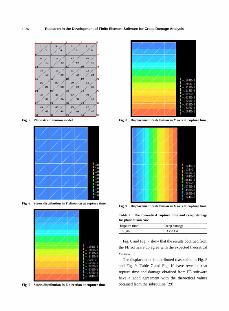
model in Fig. 5. The width of this model is set to 5 m.
The Young’s modulus E and Poisson’s ratio υ are set to
1,000 MPa and 0.3, respectively. A uniformly linear
distributed load 10 kN/m was applied on the top line of
this model.
The theoretical stress in Y direction can be shown as:
𝜎𝑦 =𝑃
𝐴=
50
5.0= 10 kN/m2
The theoretical stress in Z direction can be shown as:
𝜎𝑧 = 𝐸 × 𝜖𝑧 = 𝐸 × 𝜐 × 𝜖𝑦 = 𝐸 × 𝜐 ×𝜎𝑦𝐸
= 3kN/m2
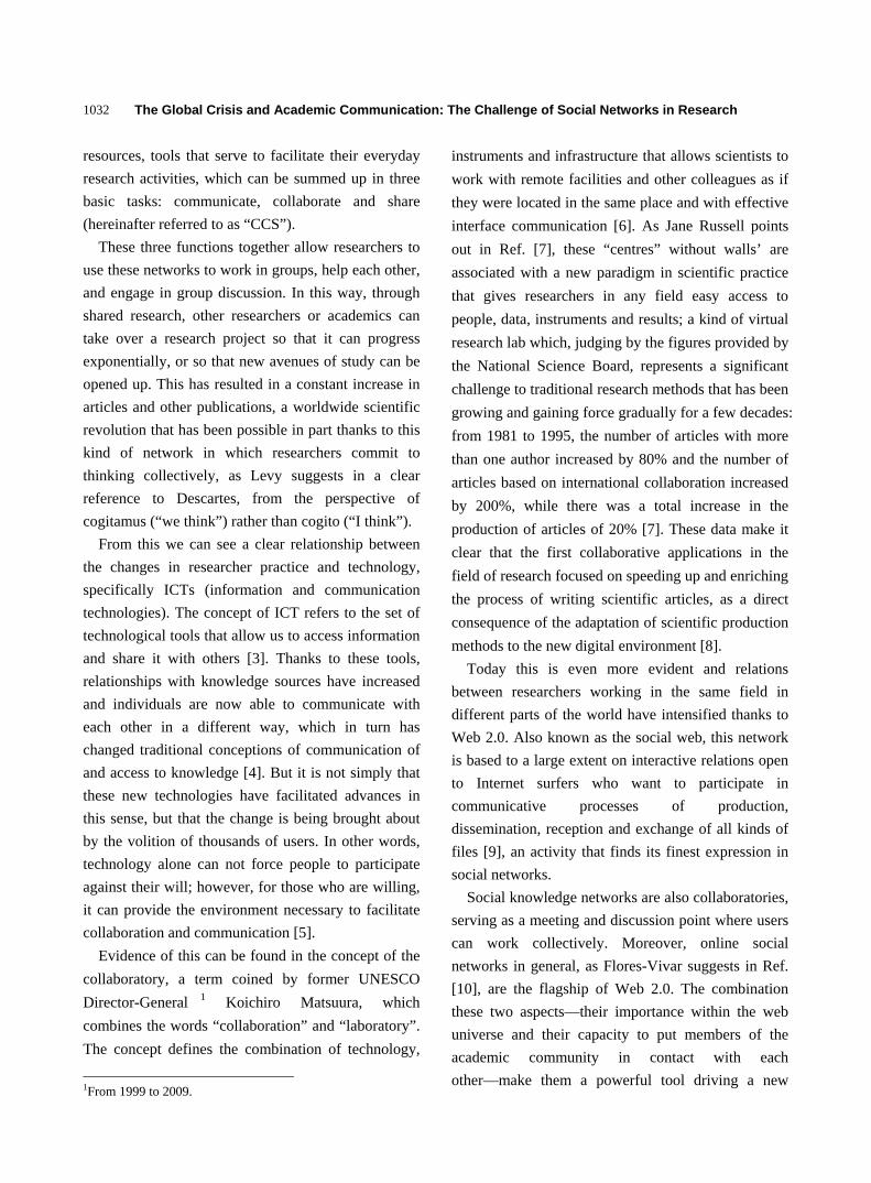
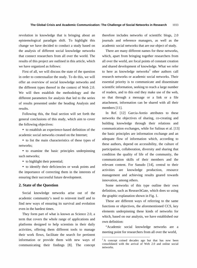
The stress and displacement obtained from FE
software with the stress updating invoked due to creep
deformation are shown in Fig. 6 and Fig. 7. The
displacements in x and y direction is shown in Fig. 8
and Fig. 9, respectively.
Using the theoretical stress value into the multi-axial
version of creep constitutive equations, the theoretical
rupture time and damage can be obtained without stress
update by a testified subroutine [25] and the results
obtained without stress update are shown in Table 7.
Table 5 The results obtained from FE software for plane stress problem.
Element number Rupture time Strain rate Creep strain Creep damage
Element No. 1 0.1040E+06 0.6540E-04 0.1798E+00 0.3334E+00
Element No. 2 0.1040E+06 0.6540E-04 0.1798E+00 0.3334E+00
Element No. 3 0.1040E+06 0.6540E-04 0.1798E+00 0.3334E+00
Element No. 4 0.1040E+06 0.6540E-04 0.1798E+00 0.3334E+00
Element No. 5 0.1040E+06 0.6540E-04 0.1798E+00 0.3334E+00
Element No. 6 0.1040E+06 0.6540E-04 0.1798E+00 0.3334E+00
Element No. 7 0.1040E+06 0.6540E-04 0.1798E+00 0.3334E+00
Element No. 8 0.1040E+06 0.6540E-04 0.1798E+00 0.3334E+00
Table 6 The percentage errors.
Rupture time percentage error = 104,000 − 104,062
104,062 × 100 = 0.0596%
Creep strain percentage error = 0.1798 − 0.179934333
0.179934333 × 100 = 0.0747%
Damage percentage error = 0.3334 − 0.33333335
0.33333335 × 100 = 0.02%
Research in the Development of Finite Element Software for Creep Damage Analysis
1026
Fig. 5 Plane strain tension model.
Fig. 6 Stress distribution in Y direction at rupture time.
Fig. 7 Stress distribution in Z direction at rupture time.
Fig. 8 Displacement distribution in Y axis at rupture time.
Fig. 9 Displacement distribution in X axis at rupture time.
Table 7 The theoretical rupture time and creep damage
for plane strain case.
Rupture time Creep damage
180,460 0.3333334
Fig. 6 and Fig. 7 show that the results obtained from
the FE software do agree with the expected theoretical
values.
The displacement is distributed reasonable in Fig. 8
and Fig. 9. Table 7 and Fig. 10 have revealed that
rupture time and damage obtained from FE software
have a good agreement with the theoretical values
obtained from the subroutine [29].

Research in the Development of Finite Element Software for Creep Damage Analysis
1027
4.3 The Validation of Axisymmetric Problem
The validation of new software for the axisymmetric
problem was performed and it was conducted via a
uni-axial tension model in Fig. 11. A uniformly
distributed tensile force 0.375 kN/m2 was applied on
the top line of this uni-axial tension model.
Using the theoretical stress value into the multi-axial
version of creep constitutive equations and a 0.1 h time
step with Euler forward integration method, the
theoretical rupture time and damage can be obtained by
a subroutine [29] and the results are shown in Table 8.
The stress and displacement obtained from FE
software with the stress updating invoked due to creep
deformation are shown in Fig. 12 and Fig. 13.
The stress has been uniformly distributed in Fig. 14
and do agree with the theoretical values.
Other results are shown in Table 8 and Fig. 15.
Rupture time and damage obtained from FE software
have been revealed that have a good agreement with
the theoretical values obtained from the subroutine [29].
4.4 The Validation of 3D Problem
A preliminary validation of such software was
performed and it was conducted via a three-
dimensional uni-axial tension model in Fig. 16. The
length of a side is set to 1 m and a uniformly distributed
load 5 kN was applied on the top surface of this
uni-axial tension model.
The theoretical stress in Z direction is 5 kN/m2. The
stress in X and Y direction should be zero and these
stress values should remain the same throughout the
creep test up to failure. The stress obtained from FE
software with the stress update program is shown in
Table 9 at a 0.1 h time step with Euler forward
integration method.
Table 9 shows that the results obtained from the FE
software do agree with the expected theoretical values.
The stress involving creep deformation and stress
updating confirmed the uniform distribution of stresses,
and the values of stress in Z direction obtained from FE
software are correct, and the stress in X and Y direction
Fig. 10 The damage distribution on 180,230 h.
Fig. 11 The axisymmetric FE model.
Table 8 The theoretical rupture time and creep damage
for axisymmetric case.
Rupture time Creep damage
146,080 0.3333334
Fig. 12 Displacement distribution in Z axis.
Fig. 13 The displacement distribution in r axis.

Research in the Development of Finite Element Software for Creep Damage Analysis
1028
Fig. 14 Stress distribution in Z direction.
Fig. 15 Damage distribution on 143,060 h.
Fig. 16 The three-dimensional uni-axial tension model.
Table 9 The stress obtained from FE software with the
stress update program.
Integration point 𝜎𝑥 𝜎𝑦 𝜎𝑧
No. 1 0.1545E-05 0.1377E-06 0.5000E+01
No. 2 0.4970E-06 0.7690E-06 0.5000E+01
No. 3 0.1068E-05 0.2017E-07 0.5000E+01
No. 4 0.5675E-06 0.1478E-06 0.5000E+01
No. 5 0.1760E-05 0.3392E-06 0.5000E+01
No. 6 0.1212E-05 0.8395E-06 0.5000E+01
No. 7 0.6717E-07 0.8630E-06 0.5000E+01
No. 8 0.6380E-06 0.1648E-06 0.5000E+01
Table 10 The theoretical values and FE results.
The results Theoretical value FE results
Rupture time 98,046 93,540
Strain rate 0.000065438 0.000067522
Creep strain 0.179934333 0.182658312
Damage 0.33333337 0.33333334
is negligible.
The lifetime and creep strain at failure, and other
field variable can be obtained for the simple tensile
case illustrated above. They have been obtained by
direct integration of the uni-axial version of
constitutive equation for a given stress [30]. They have
also been produced by the FE software. Table 10 is a
summary and comparison of them.
Table 10 reveals that real values have a good
agreement with the theoretical values obtained from
the subroutine [30]. Work in this area is ongoing and
will be reported in future.
5. Conclusion
This paper is to present the finite element method
based on CDM to design FE software for creep damage
mechanics. More specifically, it summarizes the
current state of how to obtain such computational
capability then it concludes with a preference of
in-house software; secondly, it reports the development
of such software including the development of finite
element algorithms based on CDM for creep damage
analysis, and a flow diagram of the structure of new
finite element software has been completed to be
guided in developing in-house FE software, and the use
of some standard subroutines in programming; thirdly,
the development and the validation of the finite
element software conducted so far include plane stress,
plane strain, axisymmetric case, and 3D case were
reported.
Work in this area is ongoing and future development
work includes: (1) development and incorporation of
the new constitutive equation subroutines; (2)
intelligent and practical control of the time steps; (3)
removal of failed element and update stiffness matrix;
and (4) further validation. Further real case study to be
conducted and reported.
References
[1] J. Lemaitre, J.L. Chaboche, Mechanics of Solid Materials,
1st ed., Cambridge University Press, Cambridge, 1994.
[2] D. Liu, Q. Xu, Z. Lu, D. Xu, The review of computational

Research in the Development of Finite Element Software for Creep Damage Analysis
1029
FE software for creep damage mechanics, Advanced
Materials Research 510 (2012) 495-499.
[3] D. Liu, Q. Xu, D. Xu, Z. Lu, F. Tan, The validation of
computational FE software for creep damage mechanics,
Advanced Materials Research 744 (2013) 205-210.
[4] A.A. Becker, T.H. Hyde, W. Sun, P. Andersson,
Benchmarks for finite element analysis of creep
continuum damage mechanics, Computational Materials
Science 25 (2002) 34-41.
[5] D.R. Hayhurst, A.J. Krzeczkowski, Numerical solution of
creep problems, Comput. Methods App. Mech. Eng 20
(1979) 151-171.
[6] X. Ling, S.T. Tu, J.M. Gong, Application of
Runge-Kutta-Merson algorithm for creep damage analysis,
International Journal of Pressure Vessels and Piping 77
(2000) 243-248.
[7] Q. Xu, Creep damage constitutive equations for
multi-axial states of stress for 0.5Cr0.5Mo0.25V ferritic
steel at 590 °C, Theoretical and Applied Fracture
Mechanics 36 (2001) 99-107.
[8] L. An, Q. Xu, D. Xu, Z. Lu, Review on the current state of
developing of advanced creep damage constitutive
equations for high chromium alloy, Advanced Materials
Research 510 (2012) 776-780.
[9] Q.H. Xu, Q. Xu, Y.X. Pan, M. Short, Current state of
developing creep damage constitutive equation for
0.5Cr0.5Mo0.25V ferritic steel, Advanced Materials
Research 510 (2012) 812-816.
[10] Y. Tao, Y. Masataka, H.J. Shi, Numerical investigation on
the creep damage induced by void growth in heat affected
zone of weldments, International Journal of Pressure
Vessels and Piping 86(2009) 578-584.
[11] R. Mustata, R.J. Hayhurst, D.R. Hayhurst, F.
Vakili-Tahami, CDM predictions of creep damage
initiation and growth in ferritic steel weldments in a
medium-bore branched pipe under constant pressure at
590 °C using a four-material weld model, Arch Appl
Mech 75 (2006) 475-495.
[12] M.S. Herrn, G. Yevgen, Development of a creep-damage
model for non-isothermal long-term strength analysis of
high-temperature components operating in a wide stress
range, 1st ed., ULB Sachsen-Anhalt, Kharkiv, 2008.
[13] H. Altenbach, N. Konstantin, G. Yevgen, Numerical
benchmarks for creep-damage modelling, in: Proceeding
in Applied Mathematics and Mechanics, Bremen, May 22,
2008.
[14] H. Altenbach, G. Kolarow, O.K. Morachkovsky, K.
Naumenko, On the accuracy of creep-damage predictions
in thinwalled structures using the finite element method,
Computational Mechanics 25(2000) 87-98.
[15] M. Klasztorny, A. Bondyra, P. Szurgott, D. Nycz,
Numerical modelling of GFRP laminates with MSC. Marc
system and experimental validation, Computational
Materials Science 64 (2012) 151-156.
[16] H.C. Li, C.A. Tang, T.H. Ma, X.D. Zhao, Research on the
closure and creep mechanism of circular tunnels, Journal
of Coal Science and Engineering 14 (2008) 195-199.
[17] M.T. Wong, Three-dimensional finite element analysis of
creep continuum damage growth and failure in weldments,
Ph.D. Thesis, University of Manchester, UK, 1999.
[18] D.R. Hayhurst, R.J. Hayhurst, F. Vakili-Tahami,
Continuum damage mechanics predictions of creep
damage initiation and growth in ferritic steel weldments in
a medium-bore branched pipe under constant pressure at
590 °C using a five-material weld model, Proc. R. Soc. A
461 (2005) 2303-2326.
[19] R.J. Hayhurst, F.Vakili-Tahami, D.R. Hayhurst,
Verification of 3-D parallel CDM software for the analysis
of creep failure in the HAZ region of Cr-Mo-V crosswelds,
International Journal of Pressure Vessels and Piping 86
(2009) 475-485.
[20] K. Naumenko, H. Altenbach, Modeling of Creep for
Structural Analysis, Springer Berlin Heidelberg, New
York, 2004.
[21] F. Dunne, J. Lin, D.R. Hayhurst, J. Makin, Modelling
creep, ratchetting and failure in structural components
subjected to thermo-mechanical loading, Journal of
Theoretical and Applied Mechanics 44 (2006) 87-98.
[22] F.A. Leckie, D.R. Hayhurst, Constitutive equations for
creep rupture, Acta Metallurgical 25 (1977) 1059-1070.
[23] D.R. Hayhurst, P.R. Dimmer, G.J. Morrison,
Development of continuum damage in the creep rupture of
notched bars, Trans R Soc London A 311 (1984) 103-129.
[24] I.J. Perrin, D.R. Hayhurst, Creep constitutive equations for
a 0.5Cr-0.5Mo-0.25V ferritic steel in the temperature
range 600-675 °C, J. Strain Anal. Eng 31 (1996) 299-314.
[25] F. Tan, Q. Xu, Z. Lu, D. Xu, The preliminary development
of computational software system for creep damage
analysis in weldment, in: Proceedings of the 18th
International Conference on Automation & Computing,
Loughborough, Sep. 7-8, 2012.
[26] M. Dewar, Embedding a general-purpose numerical
library in an interactive environment, Journal of
Numerical Analysis 3 (2008) 17-26.
[27] I.M. Smith, D.V. Griffiths, Programming the Finite
Element Method, 4th ed., John Wiley & Sons Ltd., Sussex,
2004.
[28] Q. Xu, M. Wright, Q.H. Xu, The development and
validation of multi-axial creep damage constitutive
equations for P91, in: ICAC'11: The 17th International
Conference on Automation and Computing, Huddersfield,
Sep. 10, 2011.
[29] F. Tan, Q. Xu., Z. Lu, D. Xu, D. Liu, Practical guidance on
the application of R-K-integration method in finite

Research in the Development of Finite Element Software for Creep Damage Analysis
1030
element analysis of creep damage problem, in: The 2013
World Congress in Computer Science, Computer
Engineering, and Applied Computing, Nevada, July.
22-25, 2013.
[30] D. Liu, Q. Xu, Z. Lu, D. Xu, Q.H. Xu, The techniques in
developing finite element software for creep damage
analysis, Advanced Materials Research 744 (2013)
199-204.

Journal of Communication and Computer 10 (2013) 1031-1041
The Global Crisis and Academic Communication: The
Challenge of Social Networks in Research
Sandra Martorell and Fernando Canet
Department of Media Communication, Information System and Art History, Polytechnic University of Valencia, Valencia 46022,
Spain
Received: June 21, 2013 / Accepted: July 30, 2013 / Published: August 31, 2013.
Abstract: The global economic crisis is seriously affecting academic research. The situation is provoking some big changes and an urgent need to seek alternatives to traditional models. It is as if the academic community was reinventing itself; and this reinvention is happening online. Faced with a lack of funding, researchers have determined to help each other develop their projects and they are doing so on social knowledge networks that they have created for this mission. The purpose of this paper is to analyze different social networks designed for academic online research. To this end, we have made a selection of these networks and established the parameters for their study in order to determine what they consist of, what tools they make use of, what advantages they offer and the degree to which they are bringing about a revolution in how research is carried out. This analysis is conducted from both a qualitative and a quantitative perspective, allowing us to identify the percentage of these networks that approach what would be the ideal social knowledge network. As we will be able to confirm, the closer they are to this ideal, the more effective they will be and the better future they will have, which will also depend on the commitment of users to participation and the quality of their contributions. Key words: Academic social networks, Web 2.0, research, participatory knowledge.
1. Introduction
“It is a change of epoch, a change of era. Many
things are changing, both in public life and in private
life. The mentalities of the people are changing too. I
believe that it is a change similar to what Europe went
through in the shift from the Middle Ages to the
Renaissance, except that then it took a century and
now we are going through it in just two or three
decades. We are experiencing a change of coordinates,
of mentality and of sensibility.” These are the words
of Professor Emeritus in Sociology Amando de
Miguel Rodriguez [1] in reference to the economic
crisis that we have been experiencing since the
collapse of Lehman Brothers Holdings in 2008.
Many countries, especially in Europe, are facing a
Corresponding author: Sandra Martorell, Ph.D. candidate,
research field: media communication, E-mail: [email protected].
period of huge changes, brought about largely by the
economic cutbacks that they have been subjected to.
One sector affected by the devastation arising from
the current crisis is the scientific and academic
community. This has been made clear by scientists
themselves in texts such as the open letter signed by
42 Nobel Prize and Fields Medal winners to the heads
of state and government of the European Union,
expressing the idea that science is fundamental for
progress [2]. In the face of the crisis, while continuing
to call for greater investment, many scientists have
diligently gone on pursuing their work by all means
available, one such means being the Internet, where
they have begun working in groups through social
networks. These are not general social networks like
Facebook or Twitter, but social networks created by
and for researchers where they can exchange
knowledge. This gives them, in addition to the usual
The Global Crisis and Academic Communication: The Challenge of Social Networks in Research
1032
resources, tools that serve to facilitate their everyday
research activities, which can be summed up in three
basic tasks: communicate, collaborate and share
(hereinafter referred to as “CCS”).
These three functions together allow researchers to
use these networks to work in groups, help each other,
and engage in group discussion. In this way, through
shared research, other researchers or academics can
take over a research project so that it can progress
exponentially, or so that new avenues of study can be
opened up. This has resulted in a constant increase in
articles and other publications, a worldwide scientific
revolution that has been possible in part thanks to this
kind of network in which researchers commit to
thinking collectively, as Levy suggests in a clear
reference to Descartes, from the perspective of
cogitamus (“we think”) rather than cogito (“I think”).
From this we can see a clear relationship between
the changes in researcher practice and technology,
specifically ICTs (information and communication
technologies). The concept of ICT refers to the set of
technological tools that allow us to access information
and share it with others [3]. Thanks to these tools,
relationships with knowledge sources have increased
and individuals are now able to communicate with
each other in a different way, which in turn has
changed traditional conceptions of communication of
and access to knowledge [4]. But it is not simply that
these new technologies have facilitated advances in
this sense, but that the change is being brought about
by the volition of thousands of users. In other words,
technology alone can not force people to participate
against their will; however, for those who are willing,
it can provide the environment necessary to facilitate
collaboration and communication [5].
Evidence of this can be found in the concept of the
collaboratory, a term coined by former UNESCO
Director-General 1 Koichiro Matsuura, which
combines the words “collaboration” and “laboratory”.
The concept defines the combination of technology,
1From 1999 to 2009.
instruments and infrastructure that allows scientists to
work with remote facilities and other colleagues as if
they were located in the same place and with effective
interface communication [6]. As Jane Russell points
out in Ref. [7], these “centres” without walls’ are
associated with a new paradigm in scientific practice
that gives researchers in any field easy access to
people, data, instruments and results; a kind of virtual
research lab which, judging by the figures provided by
the National Science Board, represents a significant
challenge to traditional research methods that has been
growing and gaining force gradually for a few decades:
from 1981 to 1995, the number of articles with more
than one author increased by 80% and the number of
articles based on international collaboration increased
by 200%, while there was a total increase in the
production of articles of 20% [7]. These data make it
clear that the first collaborative applications in the
field of research focused on speeding up and enriching
the process of writing scientific articles, as a direct
consequence of the adaptation of scientific production
methods to the new digital environment [8].
Today this is even more evident and relations
between researchers working in the same field in
different parts of the world have intensified thanks to
Web 2.0. Also known as the social web, this network
is based to a large extent on interactive relations open
to Internet surfers who want to participate in
communicative processes of production,
dissemination, reception and exchange of all kinds of
files [9], an activity that finds its finest expression in
social networks.
Social knowledge networks are also collaboratories,
serving as a meeting and discussion point where users
can work collectively. Moreover, online social
networks in general, as Flores-Vivar suggests in Ref.
[10], are the flagship of Web 2.0. The combination
these two aspects—their importance within the web
universe and their capacity to put members of the
academic community in contact with each
other—make them a powerful tool driving a new
The Global Crisis and Academic Communication: The Challenge of Social Networks in Research
1033
revolution in knowledge that is bringing about an
epistemological paradigm shift. To highlight this
change we have decided to conduct a study based on
the analysis of different social knowledge networks
that connect researchers from all over the world. The
results of this project are outlined in this article, which
we have organized as follows:
First of all, we will discuss the state of the question
in order to contextualize the study. To do this, we will
offer an overview of social knowledge networks and
the different types thereof in the context of Web 2.0.
We will then establish the methodology and the
different parameters for analysis that led to the series
of results presented under the heading Analysis and
results.
Following this, the final section will set forth the
general conclusions of this study, which aim to cover
the following objectives:
to establish an experience-based definition of the
academic social networks created on the Internet;
to list the main characteristics of these types of
networks;
to examine the basic principles underpinning
such networks;
to highlight their potential;
to identify their deficiencies or weak points and
the importance of correcting them in the interests of
ensuring their successful future development.
2. State of the Question
Social knowledge networks arise out of the
academic community’s need to reinvent itself and to
find new ways of ensuring its survival and evolution
even in the hardest times.
They form part of what is known as Science 2.0, a
term that covers the whole range of applications and
platforms designed to help scientists in their daily
activities, offering them different tools to manage
their work flows, facilitate the search for pertinent
information or provide them with new ways of
communicating their findings [8]. The concept
therefore includes networks of scientific blogs, 2.0
journals and reference managers, as well as the
academic social networks that are our object of study.
There are many different names for these networks,
which, apart from bringing together researchers from
all over the world, are focal points of constant creation
and shared development of knowledge. What we refer
to here as knowledge networks2 other authors call
research networks or academic social networks. Their
essential priority is to communicate and disseminate
scientific information, seeking to reach a large number
of readers, and to this end they make use of the web,
so that through a message or a link or a file
attachment, information can be shared with all their
members [11].
In Ref. [12] Garcia-Aretio attributes to these
networks the objectives of sharing, co-creating and
building knowledge through their relations and
communication exchanges, while for Salinas et al. [13]
the basic principles are information exchange and an
adequate flow of information which, according to
these authors, depend on accessibility, the culture of
participation, collaboration, diversity and sharing that
condition the quality of life of the community, the
communication skills of their members and the
relevant content. For Sanudo [14], central to their
activities are knowledge production, resource
management and achieving results geared towards
innovation, among others.
Some networks of this type outline their own
definition, such as ResearchGate, which does so using
the graphic explanation shown in Fig. 1.
These are different ways of referring to the same
functions or objectives, the aforementioned CCS, key
elements underpinning these kinds of networks for
which, based on our analysis, we have established our
own definition:
“Academic social knowledge networks are a
meeting point for researchers from all over the world, 2 A concept coined decades ago but that has now been consolidated with the arrival of Web 2.0 and online social networks.

The Global Crisis and Academic Communication: The Challenge of Social Networks in Research
1034
Fig. 1 Diagram of the three pillars that define ResearchGate.
who join forces in an effort to advance their studies on
the basis of three basic principles: communication,
collaboration and sharing their knowledge in a
democratic virtual environment that is optimal for
dissemination provided there is a commitment to
participation and a faithfulness to academic rigour.”
These networks have two different types of
idiosyncrasies: the first relates to the topic they
address, and the second to their operating policy. With
regard to the first, two basic types can be identified:
general networks and specialist networks. General
networks cover a more diverse range of disciplines,
allowing for interdisciplinary exchange on a single
platform, thereby fostering transversality of
knowledge.
Specialist networks, as their name suggests, focus
on specific fields, although the degree of specificity
may vary (ranging from fields as broad as the social
sciences to others limited to the study of history or
even further to the history of a particular discipline,
movement or period).
In terms of operating policy, we are particularly
interested in addressing the question of whether the
networks are free or require payment of a subscription
fee to gain access.
In this regard we have aimed to take samples of
both categories, although we have considered
dedicating special attention to free or open access
networks, which are based on a philosophy that is
becoming increasingly predominant, fostered to a
great extent by those voices calling for the publication
of raw data compiled in publicly funded research [8].
Open access is a movement that advocates free
access to scientific or academic online resources,
which should not be restricted by any impositions
other than technological limitations or the Internet
connection of the user [15]. The resources may
therefore be downloaded, read, distributed and
otherwise used in accordance with the licence, which
includes what is normally referred to as Creative
Commons, one of the more common systems for open
access publication, encompassing diverse categories
depending on the restrictions applicable, such as
author acknowledgement, non-commercial use or a
prohibition on modifications to the work.
Open access is a philosophy whose basic principles,
according to Tapscott [16], are collaboration,
transparency, sharing and empowerment. It has now
become a viable option endorsed in international
declarations that seek to define the concept, such as
the Budapest Open Access Initiative signed in 2002,
the Bethesda Statement on Open Access Publishing in
June 2003, or the Berlin Declaration on Open Access
to Knowledge in the Sciences and Humanities in
October 2003.
These declarations and others that have followed
them uphold the need to promote the principle of open
access, based on the idea that if we can make the best

The Global Crisis and Academic Communication: The Challenge of Social Networks in Research
1035
use of information technologies we will be able to
expand distribution capacity while reducing costs in
order to provide wider and easier access to research
results, thanks to the advantages offered [17], which
are:
The cost is low and the results can have a big
impact in a short period of time, facilitated to a large
extent by the viral nature of the Internet, as well as the
reduction of time needed for the evaluation and
publication process compared to the time needed to
produce a print publication;
The results obtained can be compared with other
previously published results, or the data can be reused
for further research without the need for a new
investment, which constitutes a vital advantage for
small research groups with limited resources.
Added to the above is the fact that all scholars in a
discipline will have equal access to the information
provided they have internet access without censorship
or government restrictions, thereby liberating research
from the constraints of intellectual inbreeding to open
it up to the world in the interests of development
fostered by the “collective intelligence”, meaning
simply “a form of universally distributed intelligence,
constantly enhanced, coordinated in real time, and
resulting in the effective mobilization of skills” whose
basis and objective is the “mutual recognition and
enrichment of individuals rather than the cult of
fetishized communities in hypostasis” [18].
In this regard, we could also cite Bailon-Moreno et
al. (quoted in Ref. [8]) in relation to the Ortega
hypothesis, according to which scientific progress is
based on the minimal contributions of a multitude of
scientists. Because, as will be shown below, these
types of networks can only function positively with
the commitment of users, who collectively form what
Surowiecki analysed in The Wisdom of Crowds [19]
or Rheingold in Smart Mobs [20] and to which Cobo
Romaní and Pardo Kuklinski refer in Ref. [21] as a
form of knowledge that is more valuable when
multiplied because, according to the authors, shared or
distributed knowledge is on average much more
effective and accurate than the knowledge that may be
produced by the most acclaimed or accomplished
expert.
3. Materials and Methods
We apply a methodological system based, on the
one hand, on the theories proposed by the authors
mentioned above, and on the other, on a qualitative
study for which a series of analysis criteria have been
established through the comparison of different
platforms of the same kind.
To conduct this study, we have first made a
selection of the knowledge networks to be analysed.
The basic premise has been that they need to be
networks whose mission is to bring the academic
community together, and that have a marked social
character3, i.e., they allow dialogue by connecting
users to each other. In addition to this, we have had to
distinguish between two types of networks of this kind:
general networks on one hand and, on the other,
networks focused on a specific field.
For general networks, the selection has been made
taking into account the number of users registered and
the quantity of documents stored, and considering
Metcalfe’s Law, according to which the value of a
network increases in proportion with the square of the
number of system users (n2), which Foglia [22] shows
using the graph in Fig. 2.
Fig. 2 Metcalfe’s law.
3Taking advantage of the resources offered by Web 2.0.

The Global Crisis and Academic Communication: The Challenge of Social Networks in Research
1036
We therefore chose three basic networks:
ResearchGate (2.2 million users and 35 million
documents), Academia.edu (2,201,270 users and
1,661,926 documents as of February 6, 2013) and
Mendeley (2,153,818 users and 351,357,178
documents as of February 8, 2013). The supremacy of
these networks is also reflected by their media
exposure and the interest that investors have taken in
them, as well as awards received. Evidence of this is
the space dedicated to Mendeley on the blogs of the
Wall Street Journal, Tech Europe, and The Guardian,
which rated it at number 6 among the “Top 100 Tech
Media Companies” [23], and awards such as
“European Start-up of the Year 2009” [24] and “Best
Social Innovation Which Benefits Society 2009” [25].
In terms of the interest that these kinds of networks
arouse outside the academic community, it is worth
noting that ResearchGate benefits from powerful
investors such as Founders Fund, and from
collaborations with Benchmark Capital, Accel
Partners and others such as Michael Birch and David
O. Sacks, who trust in the network’s potential, as
clearly expressed by Luke Nosek, Founders Fund
coordinator and partner [26]: “We have a genuine
appreciation for the considerable success that the team
at ResearchGate has demonstrated since the company
was founded. We truly believe that the network has
the potential to disrupt a much-outdated system”.
For specialist networks, the selection criteria have
been different. There are networks of this kind
associated with a wide range of disciplines, with some
of the most prolific fields being those related to the
natural sciences. These include the networks Biomed
Experts, Epernicus, Scilife and Nature Work, and
many other networks with large numbers of users that
have been the subject of numerous studies. There are
others, however, which to date have not had so much
visibility, such as those associated with the social
sciences, which are the very networks we have
determined to focus our attention on given their
increasing proliferation and the lack of articles
studying and analysing them, despite the fact they
constitute a substantial change in terms of the
knowledge models used in their different research
areas.
Of these we have selected five for their affinity with
our field of study, which is essentially the field of
communication. We have therefore focused on the
following networks: Social Science Research Network
(hereinafter SSRN), H-net, ECREA, NECS and Portal
de la Communication.
We have thus made a selection of eight (three
general and five specialist) networks for study using a
qualitative analysis, for which we have established a
series of variables (a total of 70) grouped into five
categories, which in turn are broken down into more
specific subcategories, allowing us to extract the
characteristics not only of the networks but also of the
users who participate and their content, and to
determine their nature, what they offer and how they
contribute to communication and exchange, among
other aspects. These five categories are outlined
below:
(1) General parameters: This section offers a
general idea of the network, both with regard to its
size and to the basic characteristics that define it, such
as the type of users it targets, the geographical regions
it covers and its objectives (plus eleven other
parameters).
(2) User data: This section is made up of
twenty-two items consisting of the fields to be filled
in every time a new registration is completed. This
allows us to determine the type of information that
this kind of network considers relevant for the
creation of user profiles.
(3) Services and resources: This is a list of 28
actions and resources that determine the possibilities
that network users have, ranging from conducting
searches to the option of contributing files or creating
work groups. Many of these features originate from
conventional social networks, such as the use of a wall
or chat function, but there are also others that are

The Global Crisis and Academic Communication: The Challenge of Social Networks in Research
1037
highly useful to academics, such as repositories for
storing users’ documents and consulting the
documents of other users, bookmarking, and the
facility to create quotes or links to scientific or
academic databases. This section also determines the
involvement of the network and its tools and resources
in the achievement of CCS, which are the
fundamental pillars for this kind of network.
(4) Content: This section allows us to analyse the
kind of files stored on the network and the nature of
their organization or access (whether you need to be a
registered user to view them, whether they can be
downloaded or whether all or only a part of the
information stored is accessible).
(5) Miscellaneous: Here we include other types of
data that did not fit into previous sections but that are
of relevance.
Upon completion of the qualitative analysis based
on the parameters encompassed by each category, we
have sought to extract a numeric representation of the
data through the use of percentages. Our aim is to
confirm, on the basis of a figure, the extent to which
each network conforms to our concept of knowledge
networks, irrespective of whether they are general or
specialist networks.
We have not been able to determine this from the
initial parameters, as among the seventy that we have
established there are many that have no special
relevance or are descriptive in nature and therefore not
applicable for this purpose. Thus, based on our ideal
conception of knowledge platforms, we have made a
selection of the 25 most important aspects that define
them, as shown in Table 1, giving each one a value of
four points4, i.e., 4% of the total.
4. Analysis and Results
Based on the 25 parameters established and after
conducting the quantitative analysis, we obtained the
results summarised in Table 2, regarding the degree to
which the networks studied conform to the ideal for
425 parameters with a value of 4% each = 100% of the total.
participatory knowledge networks developed on the
Internet by collectives of researchers and
academics:
The figures show that the general networks
conform more closely to the idea that we have of a
knowledge network than the specialist networks, with
ResearchGate (which is also the most popular)
standing out above the rest. This may be due to the
fact that because it has the largest number of users and
the highest user participation, it is able to monitor
actual user needs more dynamically and adapt the
network accordingly. Another determining factor is a
network’s international character; we therefore
especially take into account the languages in which it
is established, which as a general rule is English. The
one exception is Portal de la Communication, which
has opted for Spanish and Portuguese, which thus,
despite not operating in English like the others, also
expands its potential by reaching beyond national
borders. As can be seen, this platform is located at the
halfway point towards the ideal and is designed more
as a portal than a network as such, although we have
decided to include it because of its uniqueness, the
work it performs, and its marked social character,
which bring it closer to our idea of a knowledge
platform.
In terms of user fees, as noted above we have
sought a mixture of options. The three general
networks studied offer free access, unlike some of the
specialist networks such as ECREA and NECS, both
of which finished in last place, below those without
user fees. This makes it clear that the option of open
access is viable, and that there is no reason that the
quality of the platform will be lower if payment is not
required, but rather that free networks can be just as
sustainable. Moreover, the platforms analysed (both
general and specialist) that do not charge user fees
have more users (while NECS has around 1,100 users
and ECREA has 3,500, Social Science Research
Network reports more than 1.3 million and H-net
more than 100,000).

The Global Crisis and Academic Communication: The Challenge of Social Networks in Research
1038
Table 1 Important aspects for defining a knowledge platform.
Participation on social networks
Communication with users
Communication between users
Global character Follow/be followed
Free to users Search engine Subscription to topics of interest
Upload files Download files
Invite contacts Citation Creation of work groups Share links Wall
Chat Forum User recommendation Sending updates Repository
Calendar of events Job offers Statistics News Bookmarking
Table 2 Percentage of conformity to ideal for online knowledge networks.
General networks
ResearchGate 84%
Academia.edu 75%
Mendeley 75%
Specialist networks
SSRN 61%
H-net 52%
Portal de la Communication 49%
ECREA 39%
NECS 33%
In this respect, several aspects should be considered:
On the one hand, the wider the network’s field of
study, the more users will join, which in itself places
NECS and ECREA at a disadvantage due to their very
narrow focus (the first is the European Network for
Cinema and Media Studies and the second is the
European Communication Research and Education
Association), something that may be favorable for
certain researchers not seeking transversality between
disciplines but instead wishing to focus on a specific
field. On this basis, it is clear that they have fewer
users, while others like SSRN with many more users
cover the wide range of all the social sciences.
On the other hand, it is true that many of the users
registered on these networks are not willing to pay,
either because initially they will only be exploring and
getting to know the platform and refuse to pay for
something that they are not certain they will benefit
from, or because they are in favour of the philosophy
of open access, or perhaps even because they are
reluctant to pay for certain services online. In this
sense, we find that often the number of users is not
representative of the use of the network, since many
users registered on a network do not engage in any
activity on it. This tends to occur more often on the
networks with no user fees, where many register to try
it out but soon stop using it. On networks with user
fees, however, people may think it over more
carefully but if they ultimately decide to register it is
because they are truly convinced or at least have the
intention to use the network. As a result we find that
although they may have fewer users, the users they
have may participate more than users on free access
networks.
Indeed, low participation is one of the issues that
most severely afflict these types of networks in
general, constituting one of their most common weak
points. Thousands of registered users do not
participate, or if they do, they often abandon the
network to a certain degree once they have covered
their information needs and make no new
contributions. We can affirm that only a portion of
registered users participate actively and with a certain
degree of regularity in the achievement of CCS.
However, for the network to function properly
participation is essential, because to truly build
knowledge in virtual environments, according to No
Sanchez [27], the conditions of active commitment,
participation, frequent interaction and connection with
the real world need to be met, a point also underlined
by Arriaga Mendez et al. [11], who argue that the
meaning and objectives of a network will only be
made a reality through the work of the participants.
We therefore need to ask what the low participation
of certain groups of users could be due to. There may
be various reasons for the reluctance of researchers to
participate in these networks [8]. One factor may be

The Global Crisis and Academic Communication: The Challenge of Social Networks in Research
1039
the highly competitive nature of scientific work,
which fosters a certain degree of discretion in the
dissemination of results until those results are
published by conventional means. Another factor may
be the age of the researchers, i.e., the fact that the
more established researchers do not tend to be so
familiar with the Internet and the new possibilities it
offers, and prefer traditional methods, a situation that
nevertheless is changing thanks to the up-and-coming
generations of academics who have grown up with
ICTs and who apply them in practically all spheres of
action, both personal and professional.
Another aspect is the fact that there are knowledge
networks where there is total freedom to post content,
without the need for that content to undergo any type
of review process, the most common type being peer
review. While it is true that there are networks that do
include a review requirement, such as H-net and
SSRN, on others there is no filter whatsoever; this,
rather than favouring collective progress, is actually
harmful to it, given the hazard to scientific rigour
constituted by the possible inclusion of erroneous
information. Also this in a way keeps researchers
from publishing freely [28], as any contribution not
submitted to the scrutiny of their peers is always
under suspicion. Moreover, any unreviewed
publication would most probably not be taken into
account in the evaluation processes to which
researchers are submitted.
Of course, the review process does not guarantee
total accuracy of information, as we have seen in
cases such as that of Woo Suk Hwang, who published
a fraudulent scientific finding in the journal Science in
2005, and which the publication subsequently
withdrew, or Alan Sokal and Jean Bricmont’s book
Fashionable Nonsense [29], in which, to expose the
cultural relativism and confusing and pretentious use
of scientific terms by some intellectuals, the authors
revealed that they succeeded in publishing a farcical
article in the journal Social Text [30]. This
demonstrates the fact that reviews, and thus the filters
established to ensure maximum reliability, sometimes
fail, but at present they are the forms of legitimation
that are most widespread and commonly considered to
be the most reliable, and we therefore can not sidestep
them, either for journals or for the knowledge
networks that concern us here, which they endow with
scientific rigour, trustworthiness and prestige.
5. Conclusions
A Spanish newspaper has asserted that “things are
as bad now as in the worst moments of Spanish
history” [31]. Nevertheless, crisis and change always
go hand in hand. The current crisis is no exception,
and while it affects many sectors of the population,
those sectors will try to survive it however they can.
This is true of the academic community, which is
gradually embracing the idea that together we can
move forward.
To this end, academics are making use of the
resources available, including new tools that enable
them to publish and share their knowledge with a
great advantage over the conventional tools used in
the past [32].
Most of these tools are available on the Internet,
such as the social knowledge networks designed for
the academic community. These networks have been
developing for years but now more than ever have the
potential to become a fundamental resource for
research, not only at the national level but globally,
given that the current crisis is not only affecting Spain
but the whole world.
These networks did not appear with the crisis, but
they can help to make the crisis more bearable as they
offer a multitude of possibilities for communication
and exchange of knowledge.
To this end, they offer a series of resources and
services that have been developed through the
application of the advantages of Web 2.0 to the field
of research, such as work and collaboration online, the
creation of interest groups, communication via chats
or other types of messaging, and the possibility of

The Global Crisis and Academic Communication: The Challenge of Social Networks in Research
1040
document sharing.
In this way, these knowledge platforms or networks
have the virtue of offering two basic benefits,
especially those that are open access:
They benefit participants individually, as we
must not forget that sharing research data publicly can
have a positive effect on citation [33], thereby
contributing to an increase in productivity and in
impact;
They benefit society in general, given that,
according to the theories of Avalos [34] and Aguilera
[35], research and education constitute the
cornerstones of the economic policy of developed
nations. Toffler suggests something similar in arguing
that knowledge is the central element of our society
today. In this context the search for knowledge guides
our actions, is the source for the production of goods
and services, and the means that allows us to pursue
greater development [36].
We see the potential of these networks as lying in
the fact that they allow academics to develop
professionally while also pursuing the good of the
public in general, both inside and outside the
academic world.
To this end, the agents who participate in these
networks are at once apprentices and masters,
contributing their own experience and benefiting from
the experience of others, so that traditional
hierarchical structures give way to collaborative work,
shared leadership, participation and coordination [37].
It should be noted, however, that all these synergies
are based on an ideal conception of these networks.
We conceive of a dynamic and constant exchange
between all members of information that is checked,
analysed in depth, in a reliable and thorough manner,
which is not always the case.
In view of the above, we can conclude that this new
research model is currently in an incipient phase and
still needs to develop and mature, especially in terms
of the quality and indexing of content, as well as the
raising of awareness of the importance of advancing
together, because only in this way, united in practice,
can we ensure the dynamic and stable development of
research, without barriers and as a collective.
Acknowledgments
The research for this article was enabled with the
support of the Research Project “Study and analysis
for development of Research Network on Film
Studies through Web 2.0 platforms”, financed by the
National R + D + i Plan of the Spanish Ministry of
Economy and Competitivity (code HAR2010-18648).
References
[1] D. Zamora [Online], http://www.lne.es/sociedad-cultura/2012/09/11/vivimos-crisis-cambio-apenas-decadas/129365.html (accessed Apr. 21, 2013).
[2] D. Ahlstrom [Online], http://www.irishtimes.com/newspaper/ireland/2012/1023/1224325578288.html (accessed Apr.05, 2013).
[3] A. Solano [Online], http://www.slideshare.net/ppitufo/tic-y-web-20 (accessed Apr. 08, 2013).
[4] J.E. Reyes Iriarte, Conocimiento y tecnología; una relación esencial en la reinvención humana (Knowledge and technology, an essential link in the human reinvention), Akademeia 5 (2010) 32-37.
[5] National Science Board, Science and Engineering Indicators, US Government Printing Office, 1998.
[6] P. Glasner, From community to “collaborator”? The human genome project and the changing culture of science, Science and Public Policy 23 (1996) 109-116.
[7] J.M. Russell, Scientific communication at the beginning of the 21st century, International Social Science Journal 168 (2001) 271-282.
[8] A. Cabezas-Clavijo, D. Torres-Salinas, E. Delgado-Lopez-Cozar, Ciencia 2.0: Catálogo de herramientas e implicaciones para la actividad investigadora (Science 2.0: Catalog of tools and implications for research activity), El profesional de la información (The Information Professional) 18 (2009) 72-79.
[9] M. Cebrián Herreros, La Web 2.0 como red social de comunicación e información (Web 2.0 as a social network of communication and information), Estudios sobre el Mensaje Periodístico (Post Journalism Studies) 14 (2008) 345-361.
[10] J.M. Flores-Vivar, Nuevos modelos de comunicación, perfiles y tendencias en las redes socials (New

The Global Crisis and Academic Communication: The Challenge of Social Networks in Research
1041
communication patterns, profiles and trends in social networks), Comunicar 33 (2009) 73-81.
[11] J.A. Méndez, M.G.M. Jiménez, M.L.P. Cervantes, Retos y desafíos de las redes de investigación (Challenges of research network), Revista Iberoamericana Sobre Calidad, Eficacia y Cambio en Educación (Iberoamerican Journal on Quality, Efficiency and Change in Education) 10 (2012) 178-183.
[12] L. García-Aretio, Redes y comunidades (Networks and communities), Comunicación y Pedagogía (Communication and Education) 223 (2007) 28-33
[13] J. Salinas, A. Pérez, B. de Benito, Metodologías Centradas en el Alumno para el aprendizaje en Red (Learner-centered Methodologies for Networked Learning), Síntesis, 2008.
[14] L. Sañudo, El papel de las redes profesionales de investigación e un mundo globalizado (The role of research professional networking in a globalized world), Revista Iberoamericana sobre Calidad, Eficacia y Cambio en Educación (Revista Iberoamericana on Quality , Efficiency and Education)10 (2012) 136-143
[15] P. Suber, An Introduction to Open Access [Online], http://bibliotecavirtual.clacso.org.ar/ar/libros/secret/babini/Peter%20Suber.pdf (accessed May 27, 2013).
[16] D. Tapscott, Four principles for the open world [Online], http://www.ted.com/talks/don_tapscott_four_principles_for_the_open_world_1.html (accessed Feb. 1, 2013).
[17] J. Alonso, I. Subirats, M.L. Martínez Conde, Informe APEI sobre acceso abierto (AOSIS on Open Access), Asociación profesional de especialistas en información (Professional Association of Information Specialists), 2008.
[18] P. Levy, Collective Intelligence: Mankind’s Emerging World in Cyberspace, Basic Books, 1999.
[19] J. Surowiecki, The Wisdom of Crowds, Anchor Books, 2004.
[20] H. Rheingold, Smart Mobs, Editorial Gedisa, S.A, 2004 [21] C.C. Romaní, H.P. Kuklinski, Planeta Web 2.0,
Inteligencia colectiva o medios fast food (Planet Web 2.0. Collective Intelligence or Means Fast Food), Grup de Recerca d'Interaccions Digitals Universitat de Vic (Digital Interactions Research Group UVic), 2007.
[22] G. Foglia, [Online], http://www.iprofesional.com/notas/87619-Como-se-comportan-las-redes-sociales-segun-las-leyes-de-Moore-y-Metcalfe.html (accessed May 11, 2013).
[23] The top 100 tech media companies, [Online], http://www.guardian.co.uk/tech-media-invest-100/top-100 (accessed Feb. 14, 2013).
[24] R. Wauters, [Online], http://plugg.eu/media/blog/p/detail/winners-for-plugg-star
t-ups-rally-2009-announced (accessed May 22, 2013). [25] M. Butcher, The europas: The winners and finalists,
[Online], techcrunch.com/2009/07/09/the-europas-the-winners-and-finalists/ (accessed Jan. 22, 2013).
[26] ResearchGate: Founders Fund invests in science-network, [Online], http://www.eu-startups.com/2012/02/researchgate-founders-fund-invests-in-science-network/ (accessed Jan. 22, 2013).
[27] J.N. Sánchez, Comunicación y construcción del conocimiento en el nuevo espacio tecnológico (Communication and knowledge construction in the new technology space), Revista de universidad y sociedad del conocimiento (Journal of College and the knowledge society) 5 (2008) 2-3.
[28] D. Torres-Salinas, El paradigma 2.0 en las grandes revistas científicas (The paradigm 2.0 in major scientific journals), in: 3rd International LIS-EPI Meeting, Valencia, 2008.
[29] A. Sokal, J. Bricmont, Fashionable Nonsense: Postmodern Intellectuals’ Abuse of Science, Picador, New York, 1998.
[30] T. Delclòs, Scientific journals and reliability [Online], http://elpais.com/elpais/2013/03/02/opinion/1362219068_768198.html (accessed Mar. 03, 2013).
[31] E. Capurro, The current economic crisis reached the worst levels of the recession of the 90 [Online], http://www.abc.es/20120608/economia/abci-fedea-crisis-comparacion-201206071755.html (accessed Nov. 30, 2012).
[32] S. Biro, Miradas Desde Afuera: Investigacion Sobre Divulgacion, Universidad Nacional Autónoma de México, 2007.
[33] H.A. Piwowar, R.S. Day, D.B. Fridsma, Sharing detailed research data is associated with increased citation rate, PLoS One 2 (2007) 308.
[34] I. Avalos, La investigación universitaria en tiempos de la sociedad del conocimiento, Revista Venezolana de Economía y Ciencias Sociales 11 (2005) 89-105.
[35] M. Aguilera, La Investigación Universitaria: indispensable en los nuevos tiempos, Universitas 29 (2000) 11-12.
[36] J.G. Dominguez, R.D. Monaco, L.G. Garcia, et al., La investigación universitaria como eje de la transferencia social del conocimiento (University research as the center of social transfer of knowledge), Publicaciones en Ciencia y Tecnología (Publications in Science and Technology) 6 (2012) 41-51.
[37] J. Gairín, Las comunidades virtuales de aprendizaje, Educar 37 (2006) 41-51.

Journal of Communication and Computer 10 (2013) 1042-1046
Can You Explain This? Personality and Willingness to
Commit Various Acts of Academic Misconduct
Yovav Eshet1, Yehuda Peled2, Keren Grinautski1 and Casimir Barczyk3
1. School of Management, University of Haifa, Haifa 3190501, Israel
2. Department of Education, Western Galilee College, Akko 24121, Israel
3. School of Management, Purdue University Calumet, Hammond IN 46323, United States
Received: June 09, 2013 / Accepted: July 12, 2013 / Published: August 31, 2013.
Abstract: The rapid development of IT has created a problematic situation in higher education by providing individuals with a greater opportunity to engage in academic dishonesty especially in online courses, in contrast to traditional classroom courses. There are various factors that were used in research to explain the phenomenon of academic dishonesty. Among them are personality traits that were found to be effective in explaining unethical behaviors. Therefore, this study explores students’ personality traits as predictors of academic dishonesty in the context of traditional and distance-learning courses in higher education. Data from 1,365 students enrolled in academic institutes in the U.S.A and Israel were surveyed to assess their personality and their willingness to commit various acts of academic misconduct. The findings indicate that in both countries dishonest behaviors are greater in face-to-face than in online courses. In addition, both American and Israeli students identified with the personality trait of agreeableness showed a negative correlation with academic dishonesty. Furthermore, Israeli students identified with the personality traits of conscientiousness and emotional stability demonstrated a negative correlation with academic dishonesty. In contrast, the personality trait of extraversion among American students was positively correlated with academic misconduct. Implications for further research are discussed.
Key words: Academic dishonesty, personality traits, OCEAN, online courses.
1. Introduction
The concept of academic dishonesty is frequently
addressed in research along with various factors that
serve to explain the phenomenon. For instance, the
rapid development of IT has created a problematic
situation because the lessening of personal contact
between students and faculty provides individuals
with a greater opportunity to engage in academic
dishonesty [1, 2]. Therefore, online courses, in
contrast to traditional classroom courses, may
contribute to a higher incidence of academic
dishonesty among students by making them feel
“distant” from others [3-6]. In addition, scholars
suggest that students’ perception of what constitutes
Corresponding Author: Yovav Eshet, Ph.D., research fields: academic dishonesty and on-line education. E-mail: [email protected].
cheating has changed. For instance, working together
on a “take home” exam is considered “postmodern
learning”, and text-messaging answers is not
considered cheating by some students [7]. Another
important factor that might influence students’
tendency to engage in academic misconduct is related
to various personality traits.
This paper investigates the ubiquitous and
somewhat universal concept of academic dishonesty.
While the precise definition of the term has not yet
crystallized, we choose to define it as “forms of
cheating and plagiarism that involve students giving
or receiving unauthorized assistance in an academic
exercise or receiving credit for work that is not their
own” [8]. This definition is sufficiently broad to
include behaviors such as numerous forms of cheating,
intentional and non-intentional plagiarism,
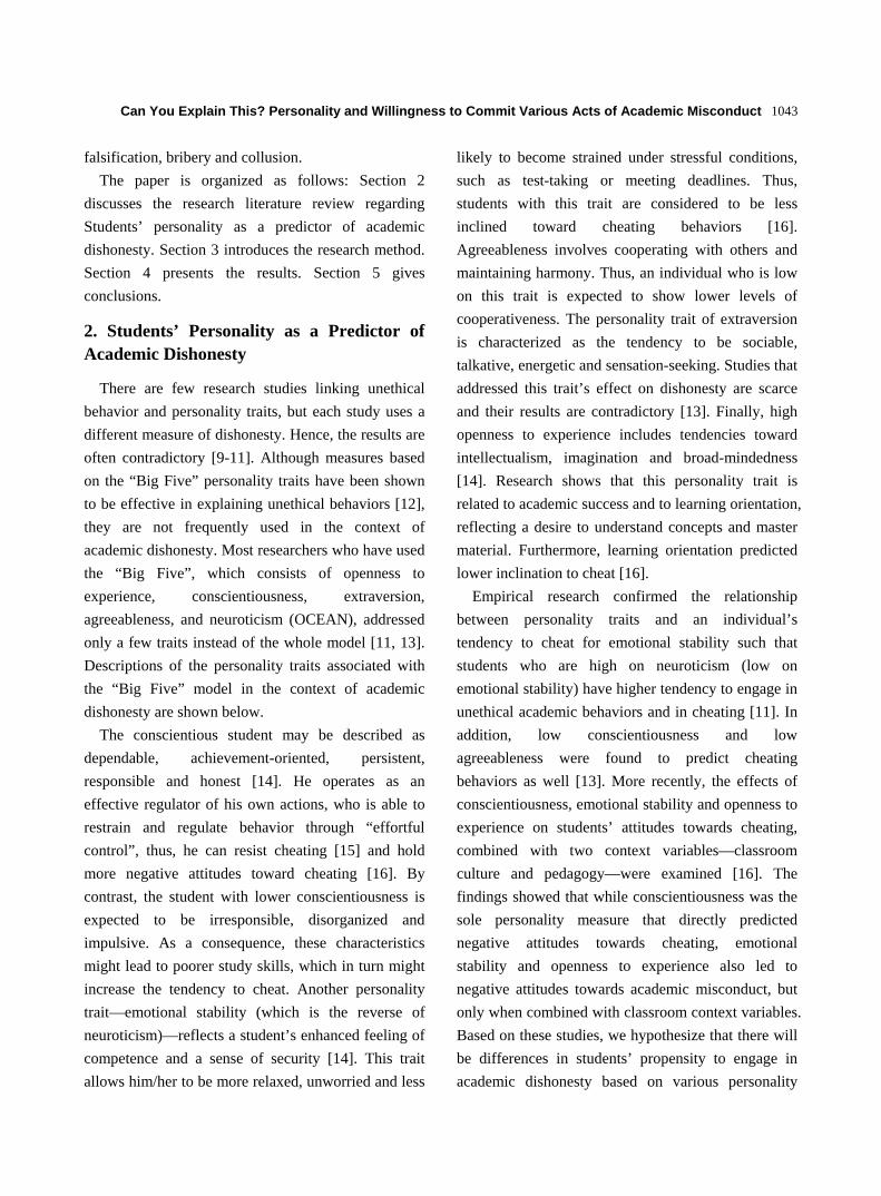
Can You Explain This? Personality and Willingness to Commit Various Acts of Academic Misconduct
1043
falsification, bribery and collusion.
The paper is organized as follows: Section 2
discusses the research literature review regarding
Students’ personality as a predictor of academic
dishonesty. Section 3 introduces the research method.
Section 4 presents the results. Section 5 gives
conclusions.
2. Students’ Personality as a Predictor of Academic Dishonesty
There are few research studies linking unethical
behavior and personality traits, but each study uses a
different measure of dishonesty. Hence, the results are
often contradictory [9-11]. Although measures based
on the “Big Five” personality traits have been shown
to be effective in explaining unethical behaviors [12],
they are not frequently used in the context of
academic dishonesty. Most researchers who have used
the “Big Five”, which consists of openness to
experience, conscientiousness, extraversion,
agreeableness, and neuroticism (OCEAN), addressed
only a few traits instead of the whole model [11, 13].
Descriptions of the personality traits associated with
the “Big Five” model in the context of academic
dishonesty are shown below.
The conscientious student may be described as
dependable, achievement-oriented, persistent,
responsible and honest [14]. He operates as an
effective regulator of his own actions, who is able to
restrain and regulate behavior through “effortful
control”, thus, he can resist cheating [15] and hold
more negative attitudes toward cheating [16]. By
contrast, the student with lower conscientiousness is
expected to be irresponsible, disorganized and
impulsive. As a consequence, these characteristics
might lead to poorer study skills, which in turn might
increase the tendency to cheat. Another personality
trait—emotional stability (which is the reverse of
neuroticism)—reflects a student’s enhanced feeling of
competence and a sense of security [14]. This trait
allows him/her to be more relaxed, unworried and less
likely to become strained under stressful conditions,
such as test-taking or meeting deadlines. Thus,
students with this trait are considered to be less
inclined toward cheating behaviors [16].
Agreeableness involves cooperating with others and
maintaining harmony. Thus, an individual who is low
on this trait is expected to show lower levels of
cooperativeness. The personality trait of extraversion
is characterized as the tendency to be sociable,
talkative, energetic and sensation-seeking. Studies that
addressed this trait’s effect on dishonesty are scarce
and their results are contradictory [13]. Finally, high
openness to experience includes tendencies toward
intellectualism, imagination and broad-mindedness
[14]. Research shows that this personality trait is
related to academic success and to learning orientation,
reflecting a desire to understand concepts and master
material. Furthermore, learning orientation predicted
lower inclination to cheat [16].
Empirical research confirmed the relationship
between personality traits and an individual’s
tendency to cheat for emotional stability such that
students who are high on neuroticism (low on
emotional stability) have higher tendency to engage in
unethical academic behaviors and in cheating [11]. In
addition, low conscientiousness and low
agreeableness were found to predict cheating
behaviors as well [13]. More recently, the effects of
conscientiousness, emotional stability and openness to
experience on students’ attitudes towards cheating,
combined with two context variables—classroom
culture and pedagogy—were examined [16]. The
findings showed that while conscientiousness was the
sole personality measure that directly predicted
negative attitudes towards cheating, emotional
stability and openness to experience also led to
negative attitudes towards academic misconduct, but
only when combined with classroom context variables.
Based on these studies, we hypothesize that there will
be differences in students’ propensity to engage in
academic dishonesty based on various personality

Can You Explain This? Personality and Willingness to Commit Various Acts of Academic Misconduct
1044
traits and whether they are face-to-face or
e-learners.
3. Method
3.1 Participants
The sample consisted of 1,574 participants with 803
from two American universities and 771 from four
Israeli academic institutes. 65% of the participants
were women and 35% were men. Their age ranged
from 17 to 59 (the mean was 26.4 years). 26% of the
participants were freshmen, 32%—sophomores,
20%—juniors, 19%—seniors and 3%—graduate
students. 46% were Christians, 38% were Jews, and
16% were Muslims. 13% of the participants were
excluded from the analysis because their surveys were
incomplete or carelessly completed. Therefore, the
final data set consisted of 1,365 participants.
3.2 Survey Instrument
A three part survey instrument was used in the
current study. Part 1 included the TIPI scale, which
consisted 10 items assessing the participants’
personality traits [17]. The reliability of this
questionnaire, measured by Cronbach’s alpha, was
0.72. Part 2 consisted of questions that examined
academic integrity using the Academic Integrity
Inventory [18]. These questions investigated the
students’ likelihood to engage in various forms of
academic misconduct. The instrument was validated
and reliability of this questionnaire, measured by
Cronbach’s alpha, was 0.75 [18]. Part 3 presented a
series of socio-demographic questions.
3.3 Procedure
In order to encourage the participants to think in the
frame of a specific type of course, we administered a
printed version of the survey instrument in the
traditional face-to-face courses and an on-line version
of the survey instrument in the e-learning courses. The
survey instruments were coded and grouped according
to the location of the participants’ university or
college (USA or Israel). The questionnaires were
distributed at the end of the courses.
4. Results
Table 1 summarizes the results of independent
sample t-test analyses, which indicate that there were
statistically significant differences in students’
likelihood to engage in academic dishonesty based on
the type of course in which they were enrolled.
Specifically, it was found that students in face-to-face
courses were more likely to engage in acts of
academic dishonesty than their counterparts in
e-learning courses.
Based on a MANOVA (multiple analysis of
variance) we found significant 2-way interaction
effect between country (Israel vs. United States) and
course type (on-line vs. face-to-face) [F (1, 1361) = 57.16,
p < 0.001].
Table 2 shows that there is a significant negative
correlation between the personality trait of
agreeableness and academic dishonesty indicating that
the more the students are cooperative with others, the
less are they to be academically dishonest in both
countries—Israel and USA. In addition, among Israeli
students that are identified with higher
conscientiousness and emotional stability
demonstrated a significant negative correlation with
academic dishonesty. General Linear Model revealed
that there is a significant 2-way interaction effect
among Israeli students between course type (on-line
vs. face-to-face) and the personality trait of
conscientiousness [F = 2.058, p < 0.05] and between
course type and the personality trait of emotional
stability [F = 2.047, p < 0.05]. Interestingly, the
personality trait of extraversion among American
students was found to be positively correlated with
academic dishonesty, indicating that the tendency to
be sociable is correlated with a higher inclination to
cheat.

Can You Explain This? Personality and Willingness to Commit Various Acts of Academic Misconduct
1045
Table 1 Differences in academic dishonesty by course type and country.
Country Course type N Mean S.D. T-Test F
USA E-learning 287 1.61 0.52
12.70***
57.16*** Face-to-Face 470 2.16 0.66
Israel E-learning 293 1.78 0.60
5.33*** Face-to-Face 315 2.52 0.65
***P < 0.001, **P < 0.01, *P < 0.05.
Table 2 Correlation between personality and academic dishonesty by course type and country.
Course type 1 2 3 4 5
Israel E-learning -.038 -.149* -.125* -.246** -.068
Face-to-Face -.090 -.131 -.237** -.151** -.063
USA E-learning -.100 -.090 -.057 -.121* -.038
Face-to-Face -.016 -.040 -.031 -.114* .105*
***P < 0.001, **P < 0.01, *P < 0.05 Israel (N = 608) USA (N = 757). Note: 1 = Openness to Experiences, 2 = Emotional Stability, 3 = Consciousness, 4 = Agreeableness, 5 = Extraversion.
5. Conclusions
Our research found that there is less overall
cheating in the virtual than in the traditional classroom
setting. These findings are similar to those found by
other researchers [19, 20], who explained this
phenomenon by the notion that students in virtual or
online courses may have a higher motivation to learn
or are able to learn without being dependent on the
typical structure of traditional classroom settings.
Our research also indicates that the personality
traits of emotional stability, agreeableness and
conscientiousness are negatively related to academic
dishonesty. These results are similar to the findings
reported by other researchers [11, 13, 16]. One of the
explanations for the notion that personality trait of
conscientiousness predicts academic dishonesty is that
conscientious students have less need to cheat since
they tend to be better prepared academically [21].
Conscientious students are able to resist cheating
since they are achievement-oriented, but at the same
time responsible and honest [14] and are able to
regulate their behavior [15]. The personality trait of
emotional stability also can help students to avoid
unethical academic behaviors, since students that are
high on this trait have sense of security [14], which
allows them to be less influenced by stressful
conditions [16].
The findings of this study revealed that the effects
of conscientiousness and emotional stability on
academic dishonesty that appeared among Israeli
students were not observed among their American
counterparts. This might be explained by the cultural
differences, as several studies that compared US
students with students in Lebanon [22], China [23]
and non-Western countries [24] indicated that
Americans tend to show less acceptance for cheating
and to possess higher standards with regard to
honesty.
Classroom contextual effects, such as those
presented in another study [16], may be worth
investigating in further research, since they seem to
contribute to the literature linking the effects of
personality traits to attitudes toward cheating. The
main practical implication of this research is its
contribution to our knowledge on the process of
student profiling, since we found that students who
use cheating practices are less emotionally stable, less
conscientious and less agreeable. Further research
should focus on how to amplify cooperative tasks in
online courses in order to reduce academic dishonesty.
References
[1] C. Robinson-Zanartu, E.D. Pena, V. Cook-Morales, A.M. Pena, R. Afshani, L. Nguyen, Academic crime and punishment: Faculty members’ perceptions of and

Can You Explain This? Personality and Willingness to Commit Various Acts of Academic Misconduct
1046
responses to plagiarism, School Psychology Quarterly 20 (2005) 318-337.
[2] J. Walker, Measuring plagiarism: Researching what students do, not what they say they do, Studies in Higher Education 35 (2010) 41-59.
[3] K. Kelley, K. Bonner, Distance education and academic dishonesty: Faculty and administrator perception and responses, Journal of Asynchronous Learning Network 9 (2005) 43-52.
[4] J. Burgoon, M. Stoner, J. Bonita, N. Dunbar, Trust and Deception in Mediated Communication, in: 36th Hawaii International Conference on Systems Sciences, Big Island, Jan. 7-9, 2003.
[5] N. Rowe, Cheating in online student assessment: Beyond plagiarism, Online Journal of Distance Learning 7 (2004).
[6] M. Heberling, Maintaining academic integrity in online education, Online Journal of Distance Learning Administration 5 (2004).
[7] I. Anitsal, M. Anitsal, R. Elmore, Academic dishonesty and intention to cheat: A model on active versus passive academic dishonesty as perceived by business students, Academy of Educational Leadership Journal 13 (2009) 17-26.
[8] W. Kibler, Academic dishonesty: A student development dilemma, National Association of Student Personnel Administrators. NASPA Journal 30 (1993) 252-267.
[9] D.E. Allmon, D. Page, R. Roberts, Determinants of perceptions of cheating: Ethical orientation, personality and demographics, Journal of Business Ethics 23 (2000) 411-422.
[10] S. Etter, J. Cramer, S. Finn, Origins of academic dishonesty: Ethical orientations and personality factors associated with attitudes about cheating with information technology, Journal of Research on Technology in Education 39 (2006) 133-155.
[11] C.J. Jackson, S.Z. Levine, A. Furnham, N. Burr, Predictors of cheating behavior at a university: A lesson from the psychology of work, Journal of Applied Social Psychology 32 (2002) 1031-1046.
[12] P.R. Sackett, J. E Wanek, New developments in the use of measures of honesty, integrity, conscientiousness, dependability, trustworthiness, and reliability for personnel selection. Personnel Psychology 42 (1996) 787- 829.
[13] K.M. Williams, C. Nathanson, D.L. Paulhus, Identifying
and profiling scholastic cheaters: Their personality, cognitive ability and motivation, Journal of Experimental Psychology 16 (2010) 293-307.
[14] M.R. Barrick, M.K. Mount, The big five personality dimensions and job performance: A meta-analysis. Personnel Psychology 44 (1991) 1-26.
[15] L.A., Jensen-Campbell, W.G. Graziano, The two faces of temptation: Differing motives for self-control, Merrill-Palmer Quarterly 51 (2005) 287–314.
[16] N.E. Day, D. Hudson, P.R. Dobies, R. Waris, Student or situation? Personality and classroom context as predictors of attitudes about business school cheating, Social Psychology of Education 14 (2001) 261-282.
[17] S.D. Gosling, P.J. Rentfrow, W.B. Swann Jr., A very brief measure of the big five personality domains, Journal of Research in Personality 37 (2003) 504-528.
[18] J.L. Kisamore, T.H. Stone, I.M. Jawahar, Academic integrity: The relationship between individual and situational factors on misconduct contemplations, Journal of Business Ethics, 75 (2007) 381-394.
[19] D. Stuber-McEwen, P. Wiseley, S. Hoggatt, Point, click, and cheat: Frequency and type of academic dishonesty in the virtual classroom, Online Journal of Distance Learning Administration 7 (2009).
[20] Y. Peled, C. Barczyk, Y. Eshet, K. Grinautski, Learning motivation and student academic dishonesty—A comparison between face-to-face and online courses, In P. Resta (Ed.), in: Proceedings of Society for Information Technology & Teacher Education International Conference, Chesapeake, Mar. 5-9, 2012, 752-759, VA: AACE.
[21] J. Hogan, R. Hogan, How to measure employee reliability, Journal of Applied Psychology 74 (1989) 273-279.
[22] D.L. McCabe, T. Feghali, H. Abdallah, Academic dishonesty in the Middle East: Individual and contextual factors, Research in Higher Education 49 (2008) 451-467.
[23] M. Rawwas, J. Al-Khatib, S. Vitell, Academic dishonesty: A cross-cultural comparison of U.S. and Chinese marketing students, Journal of Marketing Education 26 (2004) 89-100.
[24] P.W. Grimes, Dishonesty in academics and business: A cross-cultural evaluation of student attitudes, Journal of Business Ethics 49 (2004) 273-290.

Journal of Communication and Computer 10 (2013) 1047-1062
Data Security Model for Cloud Computing
Eman M. Mohamed, Hatem S. Abdelkader and Sherif El-Etriby
Department of Computer Science, Faculty of Computers and Information, Menofia University, Menofia 32511, Egypt
Received: May 16, 2013 / Accepted: June 09, 2013 / Published: August 31, 2013.
Abstract: From the perspective of data security, which has always been an important aspect of quality of service, cloud computing focuses a new challenging security threats. Therefore, a data security model must solve the most challenges of cloud computing security. The proposed data security model provides a single default gateway as a platform. It used to secure sensitive user data across multiple public and private cloud applications, including Salesforce, Chatter, Gmail, and Amazon Web Services, without influencing functionality or performance. Default gateway platform encrypts sensitive data automatically in a real time before sending to the cloud storage without breaking cloud application. It did not effect on user functionality and visibility. If an unauthorized person gets data from cloud storage, he only sees encrypted data. If authorized person accesses successfully in his cloud, the data is decrypted in real time for your use. The default gateway platform must contain strong and fast encryption algorithm, file integrity, malware detection, firewall, tokenization and more. This paper interested about authentication, stronger and faster encryption algorithm, and file integrity. Key words: Cloud computing, data security model in cloud computing, randomness testing, cryptography for cloud computing, OTP (one time password).
1. Introduction
In the traditional model of computing, both data and
software are fully contained on the user’s computer; in
cloud computing, the user’s computer may contain
almost no software or data (perhaps a minimal
operating system and web browser, display terminal
for processes occurring on a network).
Cloud computing is based on five attributes:
multi-tenancy (shared resources), massive scalability,
elasticity, pay as you go, and self-provisioning of
resources, it makes new improvements in processors,
Virtualization technology, disk storage, broadband
Internet connection, and combined fast, inexpensive
servers to make the cloud to be a more compelling
solution.
The main attributes of cloud computing are
illustrated as follows [1]:
Multi-tenancy (shared resources): Cloud computing
Corresponding author: Eman Meslhy Mohamed Elsdody, M.Sc., Lecturer, research fields: cloud computing and information security. E-mail: [email protected].
is based on a business model in which resources are
shared (i.e., multiple users use the same resource) at
the network level, host level and application level;
Massive scalability: Cloud computing provides the
ability to scale to tens of thousands of systems, as well
as the ability to massively scale bandwidth and
storage space;
Elasticity: Users can rapidly increase and decrease
their computing resources as needed;
Pay as you used: Users to pay for only the resources
they actually use and for only the time they require
them;
Self-provisioning of resources: Users’
self-provision resources, such as additional systems
(processing capability, software, storage) and network
resources.
Cloud computing can be confused with distributed
system, grid computing, utility computing, service
oriented architecture, web application, web 2.0,
broadband network, browser as a platform,
Virtualization and free/open software [2].
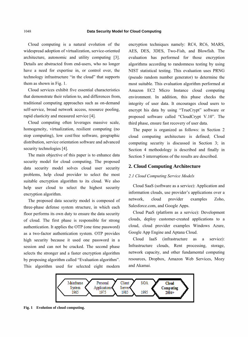
Data Security Model for Cloud Computing
1048
Cloud computing is a natural evolution of the
widespread adoption of virtualization, service-oriented
architecture, autonomic and utility computing [3].
Details are abstracted from end-users, who no longer
have a need for expertise in, or control over, the
technology infrastructure “in the cloud” that supports
them as shown in Fig. 1.
Cloud services exhibit five essential characteristics
that demonstrate their relation to, and differences from,
traditional computing approaches such as on-demand
self-service, broad network access, resource pooling,
rapid elasticity and measured service [4].
Cloud computing often leverages massive scale,
homogeneity, virtualization, resilient computing (no
stop computing), low cost/free software, geographic
distribution, service orientation software and advanced
security technologies [4].
The main objective of this paper is to enhance data
security model for cloud computing. The proposed
data security model solves cloud user security
problems, help cloud provider to select the most
suitable encryption algorithm to its cloud. We also
help user cloud to select the highest security
encryption algorithm.
The proposed data security model is composed of
three-phase defense system structure, in which each
floor performs its own duty to ensure the data security
of cloud. The first phase is responsible for strong
authentication. It applies the OTP (one time password)
as a two-factor authentication system. OTP provides
high security because it used one password in a
session and can not be cracked. The second phase
selects the stronger and a faster encryption algorithm
by proposing algorithm called “Evaluation algorithm”.
This algorithm used for selected eight modern
encryption techniques namely: RC4, RC6, MARS,
AES, DES, 3DES, Two-Fish, and Blowfish. The
evaluation has performed for those encryption
algorithms according to randomness testing by using
NIST statistical testing. This evaluation uses PRNG
(pseudo random number generator) to determine the
most suitable. This evaluation algorithm performed at
Amazon EC2 Micro Instance cloud computing
environment. In addition, this phase checks the
integrity of user data. It encourages cloud users to
encrypt his data by using “TrueCrypt” software or
proposed software called “CloudCrypt V.10”. The
third phase, ensure fast recovery of user data.
The paper is organized as follows: in Section 2
cloud computing architecture is defined; Cloud
computing security is discussed in Section 3; in
Section 4 methodology is described and finally in
Section 5 interruptions of the results are described.
2. Cloud Computing Architecture
2.1 Cloud Computing Service Models
Cloud SaaS (software as a service): Application and
information clouds, use provider’s applications over a
network, cloud provider examples Zoho,
Salesforce.com, and Google Apps.
Cloud PaaS (platform as a service): Development
clouds, deploy customer-created applications to a
cloud, cloud provider examples Windows Azure,
Google App Engine and Aptana Cloud.
Cloud IaaS (infrastructure as a service):
Infrastructure clouds, Rent processing, storage,
network capacity, and other fundamental computing
resources, Dropbox, Amazon Web Services, Mozy
and Akamai.
Fig. 1 Evolution of cloud computing.

Data Security Model for Cloud Computing
1049
2.2 Cloud Computing Deployment Models
Private cloud : Enterprise owned or leased;
Community cloud: Shared infrastructure for
specific community;
Public cloud: Sold to the public, mega-scale
infrastructure;
Hybrid cloud: Composition of two or more clouds.
2.3 Cloud Computing Sub-services Models
IaaS: DBaaS (database-as-a-service): DBaaS allows
the access and use of a database management system
as a service.
PaaS: STaaS (storage-as-a-service): STaaS involves
the delivery of data storage as a service, including
database-like services, often billed on a utility
computing basis, e.g., per gigabyte per month.
SaaS: CaaS (communications-as-a-service): CaaS is
the delivery of an enterprise communications solution,
such as Voice over IP, instant messaging, and video
conferencing applications as a service.
SaaS: SECaaS (security-as-a-service): SECaaS is
the security of business networks and mobile networks
through the Internet for events, database, application,
transaction, and system incidents.
SaaS: MaaS (monitoring-as-a-service): MaaS refers
to the delivery of second-tier infrastructure
components, such as log management and asset
tracking, as a service.
PaaS: DTaaS (desktop-as-a-service): DTaaS is the
decoupling of a user’s physical machine from the
desktop and software he or she uses to work.
IaaS: CCaaS (compute capacity-as-a-service):
CCaaS is the provision of “raw” computing resource,
typically used in the execution of mathematically
complex models from either a single “supercomputer”
resource or a large number of distributed computing
resources where the task performs well [5].
2.4 Cloud Computing Benefits
Lower computer costs, improved performance,
reduced software costs, instant software updates,
improved document format compatibility, unlimited
storage capacity, device independence, and increased
data reliability
2.5 Cloud Computing Drawbacks
Requires a constant Internet connection, does not
work well with low-speed connections, can be slow,
features might be limited, stored data might not be
secure, and stored data can be lost.
2.6 Cloud Computing Providers
AWS (amazon web services)—include Amazon S3,
Amazon EC2, Amazon Simple-DB, Amazon SQS,
Amazon FPS, and others. Salesforce.com—Delivers
businesses over the internet using the software as a
service model. Google Apps—Software-as-a-service
for business email, information sharing and security.
And others providers such as Microsoft Azure
Services Platform, Proof-point, Sun Open Cloud
Platform, Workday, etc..
3. Cloud Computing Security
With cloud computing, all your data is stored on the
cloud. So cloud users ask some questions like: How
secure is the cloud? Can unauthorized users gain
access to your confidential data?
Cloud computing companies say that data is secure,
but it is too early to be completely sure of that. Only
time will tell if your data is secure in the cloud. Cloud
security concerns arising which both customer data
and program are residing in provider premises.
Security is always a major concern in Open System
Architectures as shown in Fig. 2.
While cost and ease of use are two great benefits of
cloud computing, there are significant security
concerns that need to be addressed when considering
moving critical applications and sensitive data to
public and shared cloud environments. To address
these concerns, the cloud provider must develop
sufficient controls to provide the same or a greater
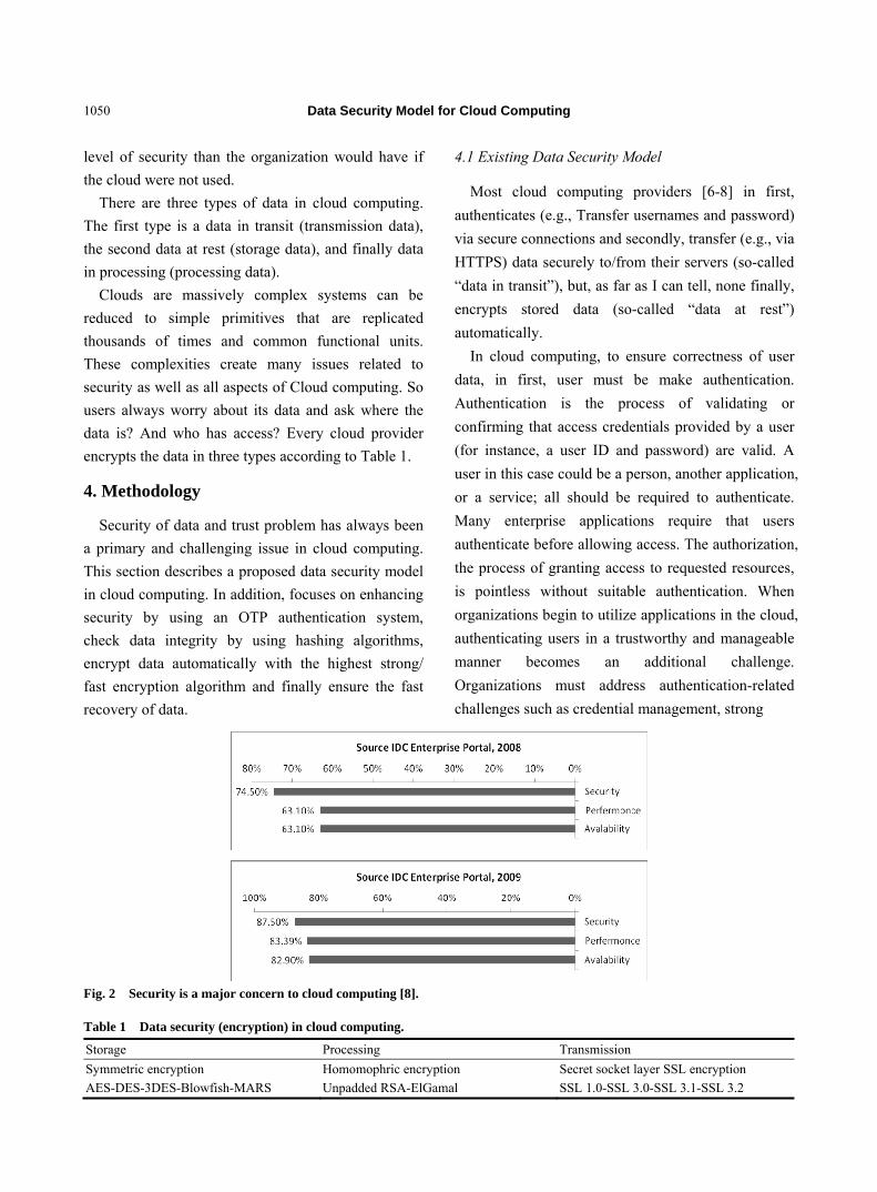
Data Security Model for Cloud Computing
1050
level of security than the organization would have if
the cloud were not used.
There are three types of data in cloud computing.
The first type is a data in transit (transmission data),
the second data at rest (storage data), and finally data
in processing (processing data).
Clouds are massively complex systems can be
reduced to simple primitives that are replicated
thousands of times and common functional units.
These complexities create many issues related to
security as well as all aspects of Cloud computing. So
users always worry about its data and ask where the
data is? And who has access? Every cloud provider
encrypts the data in three types according to Table 1.
4. Methodology
Security of data and trust problem has always been
a primary and challenging issue in cloud computing.
This section describes a proposed data security model
in cloud computing. In addition, focuses on enhancing
security by using an OTP authentication system,
check data integrity by using hashing algorithms,
encrypt data automatically with the highest strong/
fast encryption algorithm and finally ensure the fast
recovery of data.
4.1 Existing Data Security Model
Most cloud computing providers [6-8] in first,
authenticates (e.g., Transfer usernames and password)
via secure connections and secondly, transfer (e.g., via
HTTPS) data securely to/from their servers (so-called
“data in transit”), but, as far as I can tell, none finally,
encrypts stored data (so-called “data at rest”)
automatically.
In cloud computing, to ensure correctness of user
data, in first, user must be make authentication.
Authentication is the process of validating or
confirming that access credentials provided by a user
(for instance, a user ID and password) are valid. A
user in this case could be a person, another application,
or a service; all should be required to authenticate.
Many enterprise applications require that users
authenticate before allowing access. The authorization,
the process of granting access to requested resources,
is pointless without suitable authentication. When
organizations begin to utilize applications in the cloud,
authenticating users in a trustworthy and manageable
manner becomes an additional challenge.
Organizations must address authentication-related
challenges such as credential management, strong
Fig. 2 Security is a major concern to cloud computing [8].
Table 1 Data security (encryption) in cloud computing.
Storage Processing Transmission
Symmetric encryption Homomophric encryption Secret socket layer SSL encryption
AES-DES-3DES-Blowfish-MARS Unpadded RSA-ElGamal SSL 1.0-SSL 3.0-SSL 3.1-SSL 3.2

Data Security Model for Cloud Computing
1051
authentication, delegated authentication, and trust
across all types of cloud delivery models (SPI).
Two-factor authentication became solution for any
cloud application.
After authentication, cloud user can access data that
stored on servers at a remote location, and can access
it from any device/ anywhere.
So if you want your data to be secure in the cloud,
then consider encrypting the stored data. In addition,
do not store your encryption keys on the same server.
It is unclear whether a cloud computing provider
could be compelled by law enforcement agencies to
decrypt data that (1) it has encrypted or that (2) users
have encrypted, but if the provider has the keys,
decryption is at least possible.
4.2 Problems in Existing Data Security Model
The cloud users ask your cloud providers about
some problems:
Are files stored on cloud servers encrypted
automatically?
Can other users boot my machine?
Have unauthorized users of my machine
detected?
Is my data accessed solely by my virtual
machine?
Is the system should own my key?
Is my data retrieving fast?
Therefore, a data security model must solve the
previous problems. DSM (data security model) must:
ensure that data must be encrypted automatically;
use a strong encryption algorithm;
use the strong encryption algorithm that must be
fast to retrieve data faster;
use strong authentication;
ensure file integrity;
be kept not in cloud system; most of these
problems appear in previous data security model [9].
Clouds typically have a single security architecture.
This section provides a detailed overview of the
existing data security model, as well as explains the
data security model for Amazon web services as
shown in Table 2.
Amazon web services encourage user’s to encrypt
sensitive data by using TrueCrypt software, this free
encryption product provides the following:
Creates a virtual encrypted disk within a file and
mounts it as a real disk;
Encrypts an entire partition or storage device
such as USB flash drive or hard drive;
Encrypts a partition or drive where Windows is
installed;
Encryption is automatic, real-time (on-the-fly)
and transparent;
Provides two levels of plausible deniability, in
case an adversary forces you to reveal the password:
Hidden volume (steganography). No TrueCrypt
volume can be identified (volumes cannot be
distinguished from random data);
Encryption algorithms: AES, Serpent, and
Twofish.
Finally mode of operation is XTS.
TrueCrypt is an outstanding encryption solution for
anyone familiar with managing volumes and a slight
knowledge of encryption technology. For the rest, it
can be a bit daunting. Any organization planning to
deploy TrueCrypt as a cloud-data protection solution
must consider the cost and logistics of training and
supporting users, managing versions, and recovering
damages.
TrueCrypt is a computer software program whose
primary purposes are to: Secure data by encrypting it
before it is written to a disk. Decrypt encrypted data
after it is read from the disk. However, TrueCrypt uses
only three methods (AES, Serpent and Twofish) to
encrypt data as shown in Fig. 3.
4.3 Proposed Data at Rest Security Model
The proposed data security model used three-level
defense system structure, in which each floor performs
its own duty to ensure that the data security of cloud
as shown in Fig. 4.
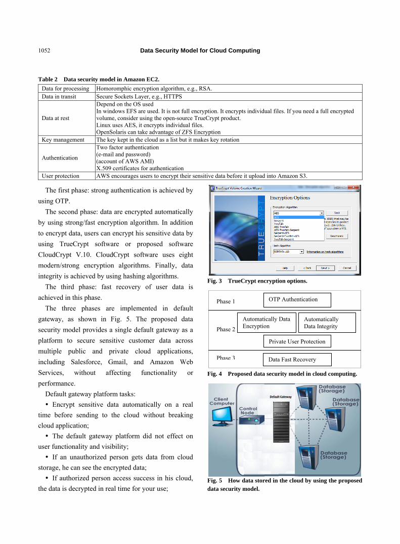
Data Security Model for Cloud Computing
1052
Table 2 Data security model in Amazon EC2.
Homoromphic encryption algorithm, e.g., RSA. Data for processing Secure Sockets Layer, e.g., HTTPS Data in transit Depend on the OS used In windows EFS are used. It is not full encryption. It encrypts individual files. If you need a full encrypted volume, consider using the open-source TrueCrypt product. Linux uses AES, it encrypts individual files. OpenSolaris can take advantage of ZFS Encryption
Data at rest
The key kept in the cloud as a list but it makes key rotation Key management Two factor authentication (e-mail and password) (account of AWS AMI) X.509 certificates for authentication
Authentication
AWS encourages users to encrypt their sensitive data before it upload into Amazon S3. User protection
The first phase: strong authentication is achieved by
using OTP.
The second phase: data are encrypted automatically
by using strong/fast encryption algorithm. In addition
to encrypt data, users can encrypt his sensitive data by
using TrueCrypt software or proposed software
CloudCrypt V.10. CloudCrypt software uses eight
modern/strong encryption algorithms. Finally, data
integrity is achieved by using hashing algorithms.
The third phase: fast recovery of user data is
achieved in this phase.
The three phases are implemented in default
gateway, as shown in Fig. 5. The proposed data
security model provides a single default gateway as a
platform to secure sensitive customer data across
multiple public and private cloud applications,
including Salesforce, Gmail, and Amazon Web
Services, without affecting functionality or
performance.
Default gateway platform tasks:
Encrypt sensitive data automatically on a real
time before sending to the cloud without breaking
cloud application;
The default gateway platform did not effect on
user functionality and visibility;
If an unauthorized person gets data from cloud
storage, he can see the encrypted data;
If authorized person access success in his cloud,
the data is decrypted in real time for your use;
Fig. 3 TrueCrypt encryption options.
Fig. 4 Proposed data security model in cloud computing.
Fig. 5 How data stored in the cloud by using the proposed data security model.
Phase 1 Phase 2
Phase 3
Automatically Data Encryption
Automatically Data Integrity
Data Fast Recovery
OTP Authentication
Private User Protection

Data Security Model for Cloud Computing
1053
The default gateway platform must contain
Strong/Fast Encryption Algorithm by using one or
more of encryption algorithms namely RC4, RC6,
MARS, AES, DES, 3DES, Two-Fish, and Blowfish
[10-16];
The default gateway platform must contain File
integrity;
The default gateway platform must contain
Malware detection, Firewall, Tokenization and more.
Proposed data security model implemented and
applied to cloudsim 3.0 by using HDFS architecture
and Amazon web services (S3 and EC2).
In this paper, automatically encryption, integrity,
fast recovery and private user encryption all are
achieved in the proposed data security model.
4.4 Implementation Details
4.4.1 First Phase, Authentication
The cloud user select company, then create an
account;
Cloud provider upload user information in DB in
cloud storage;
Cloud Provider confirms user with his username
and password;
Cloud user request login page;
The cloud provider displays login screen;
Cloud user login with username and password;
A cloud provider check is valid username and
password by searching in DB in cloud storage. If user
information not valid display error message else
display reserve a PC page;
Cloud user reserves your PC.
4.4.2 OTP Authentication Steps
Cloud user enters passphrase, challenge and
sequence number for OTP authentication;
Cloud user generates an OTP;
The cloud provider generates the OTP temporary
DB based on user information;
Cloud user login with OTP;
A cloud provider check is valid OTP by searching
in temporary DB for OTP in cloud storage. If OTP not
valid display error message else display user PC page.
4.4.3 In Second Phase, Private User Protection
Before adding data, cloud user can encrypt data by
using TrueCrypt or CloudCrypt software’s;
In second phase, Automatic data encryption;
Cloud user adds data;
Cloud server encrypt data automatically by using
fast/strong encryption algorithm that selected based on
an evaluation algorithm for the cloud company.
4.4.4 Second Phase, Automatic Check Data
Integrity
The cloud server generates file hash value;
Cloud server store data with its hash value;
When a cloud user requests his data, cloud server
decrypt data automatically, check integrity by check
the hash value.
4.4.5 Third Phase, Fast Recovery of Data
Finally, cloud server retrieves data with message of
file integrity.
4.5 Proposed Evaluation Algorithm
We use NIST statistical tests to get the highest
security encryption algorithm from eight algorithms
namely RC4, RC6, MARS, AES, DES, 3DES,
Two-Fish, and Blowfish as shown in Fig. 6. NIST
Developed to test the randomness of binary sequences
produced by either hardware or software based
cryptographic random or pseudorandom number
generators.
NIST statistical tests has 16 tests, namely: The
Frequency (Mon-obit) Test, Frequency Test within a
Fig. 6 Steps to select the highest encryption algorithm.

Data Security Model for Cloud Computing
1054
Block, The Runs Test, Tests for the
Longest-Run-of-Ones in a Block, The Binary Matrix
Rank Test, The Discrete Fourier Transform (Spectral)
Test, The Non-overlapping Template Matching Test,
The Overlapping Template Matching Test, Maurer’s
“Universal Statistical” Test, The Linear Complexity
Test, The Serial Test, The Approximate Entropy Test,
The Cumulative Sums (Cusums) Test, The Random
Excursions Test, and The Random Excursions Variant
Test.
We also compare between eight encryption
algorithms based on speed of encryption to achieve
faster recovery.
We use Amazon EC2 as a case study of our
software. Amazon EC2 Load your image onto S3 and
register it. Boot your image from the Web Service.
Open up the required ports for your image. Connect to
your image through SSH. And finally execute your
application.
For our experiment in a cloud computing
environment, we use Micro Instances of this Amazon
EC2 family, provide a small amount of consistent
CPU resources, they are well suited for lower
throughput applications, 613 MB memory, up to 2
EC2 Compute Units (for short periodic bursts), EBS
(elastic block store) storage only from 1 GB to 1 TB,
64-bit platform, low I/O Performance, t1.micro API
name, We use Ubuntu Linux to run NIST Statistical
test package [17-19].
4.6 Selection the Highest Encryption Algorithm Steps
Sign up for Amazon web service to create an
account. Lunch Micro instance Windows (64 bit)
Amazon EC2. Connect to Amazon EC2 [20-22]
Windows Micro Instance. Generate 128 plain stream
sequences as PRNG, each sequence is 7,929,856 bits
in length (991,232 bytes in length) and key stream
(length of key 128 bits). Apply cryptography
algorithms to get ciphers text. Lunch Micro instance
Amazon EC2 Ubuntu Linux Connect to Amazon EC2
Ubuntu Linux Micro instance Run NIST statistical
tests for each sequence to eight encryption algorithms
to get P-value Compare P-value to 0.01, if P-value
less than 0.01 then reject the sequence.
We compare between eight encryption methods
based on P-value, Rejection rate and finally based on
time consuming for each method.
We have 128 sequences (128-cipher text) for each
eight-encryption algorithm.
Each sequence has 7,929,856 bits in length
(991,232 bytes in length). Additionally, the P-values
reported in the tables can find in the results.txt files
for each of the individual test—not in the
finalAnalysisReport.txt file in NIST package.
The P-value represents the probability of observing
the value of the test statistic which is more extreme in
the direction of non-randomness. P-value measures
the support for the randomness hypothesis on the basis
of a particular test Rejection Rate number of rejected
sequences (P-value less than significance level α may
be equal 0.01 or 0.1 or 0.05). The higher P-value the
better and vice versa with rejection rate, the lower the
better [17].
For each statistical test, a set of P-values
(corresponding to the set of sequences) is produced.
For a fixed significance level α, a certain percentage
of P-values are expected to indicate failure. For
example, if the significance level is chosen to be
0.01 (i.e., α ≥ 0.01), then about 1% of the sequences
are expected to fail. A sequence passes a statistical
test whenever the P-value ≥ α and fails
otherwise.
We produce P-value, which small P-value(less than
0.01) support non-randomness. For example, if the
sample consists of 128 sequences, the rejection rate
should not exceed 4.657, or simply expressed 4
sequences with α = 0.01. The maximum number of
rejections was computed using the formula [17]:
)1(
3= # rateRejection
ss
(1)
where s is the sample size and α is the significance
level is chosen to be 0.01.

Data Security Model for Cloud Computing
1055
5. Simulation Results
In this section, we show and describe the simulation
results of the proposed data security model.
5.1 OTP Authentication
OTP [23] System steps as shown in Fig. 7.
The users connect to the cloud provider. Then the
user gets the username (e-mail), password and finally
account password.
Users login to the cloud provider website by getting
username (e-mail), password and account password.
Cloud node controller verifies user info. If user info
is true, controller-node send that login authentication
success and require OTP.
OTP generation software used to generate OTP as
shown in Fig. 8.
Users generate OTP by using MD5 hash function
and sequence number based on user name, password
and account password.
Then users login to cloud website with OTP as
shown in Fig. 9.
The cloud controller node generates 1000 OTP
based on user info by using the MD5 hash function.
Then the cloud controller saves 1000 OTP in the
temporary OTP database.
The cloud controller verifies user OTP from the
temporary OTP database.
If OTP is true, send OTP login success.
Password Space is a function of the size of the
alphabet and the number of characters from that
alphabet that are used to create passwords. To
determine the minimum size of the password space
needed to satisfy the security requirements for an
operational environment. In the text-based password, a
password space is computed as [23] :
S = A·M (2)
Password length and alphabet size are factors in
computing the maximum password space
requirements. Eq. 2 expresses the relationship between
S, A, and M where:
S = password space;
A = number of alphabet symbols;
M = password length.
To illustrate: If passwords consisting of 4 digits
using an alphabet of 10 digits (e.g., 0-9) are to be
generated: S = 104
That is, 10,000 unique 4-digit passwords could be
generated. Likewise, to generate random 6-character
passwords from an alphabet of 26 characters (e.g.,
A-Z): S = 266
Password entropy is usually used to measure the
security of a generated password which mean how
hard to blindly guess out the password.
Entropy = M × log2(A). (3)
Fig. 7 OTP authentication in PDSM.

Data Security Model for Cloud Computing
1056
Fig. 8 Proposed software for OTP generation.
Fig. 9 Proposed OTP login screen.
In other word, entropy tries to measure the
probabilities that the attacker obtains the correct
password based on random guessing. For example,
text message with 6 characters length with capital and
small alphabets then the number of entropy bits = 6 ×
log2(52) = 34.32 [23].
We have compared password space with different
password schemas we can identify the most secure
approaches with respect to brute force attack as shown
in Table 3. This table demonstrates the comparison of
the password space and password length for popular
user authentication schemas for cloud computing. It
shows that the approach presented by us is both more
secured and the easiest to remember. At the same time,
it is relatively fast to produce during an authentication
procedure as shown in Figs. 10 and 11.
Table 3 Password space comparison.
Authentication system Alphabet Password length Password space size Entropy bits
Static password 82 12 92.4 × 10²¹ 22.96
PIN number 10 12 1 × 10¹² 12
OTP 40 30 1.15 × 1048 48.06
Fig. 10 Security strength comparison based on entropy bits.
Fig. 11 Security strength comparison based on password space size.
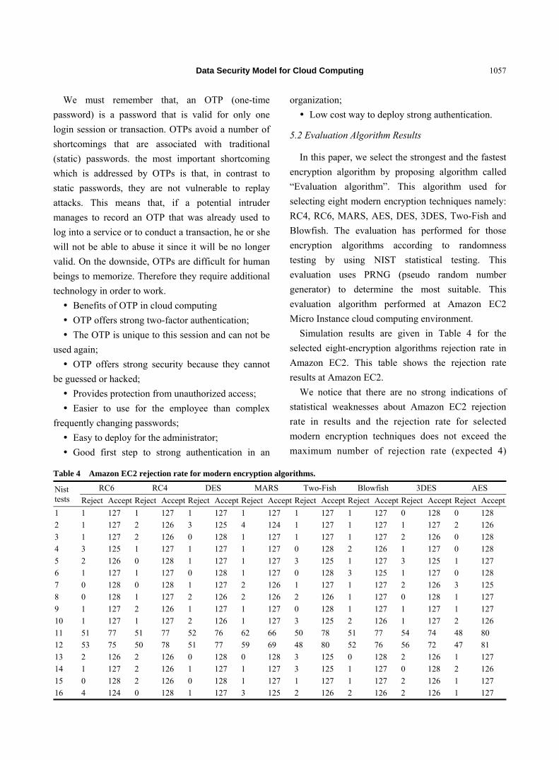
Data Security Model for Cloud Computing
1057
We must remember that, an OTP (one-time
password) is a password that is valid for only one
login session or transaction. OTPs avoid a number of
shortcomings that are associated with traditional
(static) passwords. the most important shortcoming
which is addressed by OTPs is that, in contrast to
static passwords, they are not vulnerable to replay
attacks. This means that, if a potential intruder
manages to record an OTP that was already used to
log into a service or to conduct a transaction, he or she
will not be able to abuse it since it will be no longer
valid. On the downside, OTPs are difficult for human
beings to memorize. Therefore they require additional
technology in order to work.
Benefits of OTP in cloud computing
OTP offers strong two-factor authentication;
The OTP is unique to this session and can not be
used again;
OTP offers strong security because they cannot
be guessed or hacked;
Provides protection from unauthorized access;
Easier to use for the employee than complex
frequently changing passwords;
Easy to deploy for the administrator;
Good first step to strong authentication in an
organization;
Low cost way to deploy strong authentication.
5.2 Evaluation Algorithm Results
In this paper, we select the strongest and the fastest
encryption algorithm by proposing algorithm called
“Evaluation algorithm”. This algorithm used for
selecting eight modern encryption techniques namely:
RC4, RC6, MARS, AES, DES, 3DES, Two-Fish and
Blowfish. The evaluation has performed for those
encryption algorithms according to randomness
testing by using NIST statistical testing. This
evaluation uses PRNG (pseudo random number
generator) to determine the most suitable. This
evaluation algorithm performed at Amazon EC2
Micro Instance cloud computing environment.
Simulation results are given in Table 4 for the
selected eight-encryption algorithms rejection rate in
Amazon EC2. This table shows the rejection rate
results at Amazon EC2.
We notice that there are no strong indications of
statistical weaknesses about Amazon EC2 rejection
rate in results and the rejection rate for selected
modern encryption techniques does not exceed the
maximum number of rejection rate (expected 4)
Table 4 Amazon EC2 rejection rate for modern encryption algorithms.
AES 3DES Blowfish Two-Fish MARS DES RC4 RC6 Nist tests AcceptRejectAccept Reject Accept RejectAcceptRejectAcceptRejectAcceptReject Accept Reject Accept Reject
128 0 128 0 127 1 127 1 127 1 127 1 127 1 127 1 1
126 2 127 1 127 1 127 1 124 4 125 3 126 2 127 1 2
128 0 126 2 127 1 127 1 127 1 128 0 126 2 127 1 3
128 0 127 1 126 2 128 0 127 1 127 1 127 1 125 3 4
127 1 125 3 127 1 125 3 127 1 127 1 128 0 126 2 5
128 0 127 1 125 3 128 0 127 1 128 0 127 1 127 1 6
125 3 126 2 127 1 127 1 126 2 127 1 128 0 128 0 7
127 1 128 0 127 1 126 2 126 2 126 2 127 1 128 0 8
127 1 127 1 127 1 128 0 127 1 127 1 126 2 127 1 9
126 2 127 1 126 2 125 3 127 1 126 2 127 1 127 1 10
80 48 74 54 77 51 78 50 66 62 76 52 77 51 77 51 11
81 47 72 56 76 52 80 48 69 59 77 51 78 50 75 53 12
127 1 126 2 128 0 125 3 128 0 128 0 126 2 126 2 13
126 2 128 0 127 1 125 3 127 1 127 1 126 2 127 1 14
127 1 126 2 127 1 127 1 127 1 128 0 126 2 128 0 15
127 1 126 2 126 2 126 2 125 3 127 1 128 0 124 4 16
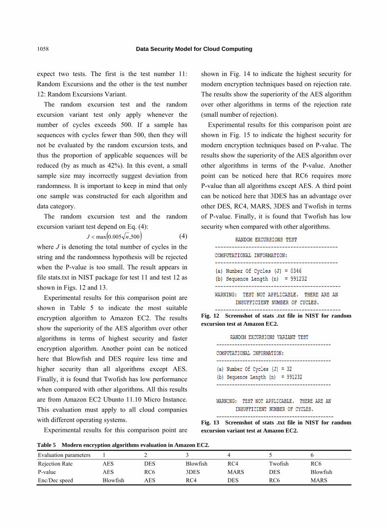
Data Security Model for Cloud Computing
1058
expect two tests. The first is the test number 11:
Random Excursions and the other is the test number
12: Random Excursions Variant.
The random excursion test and the random
excursion variant test only apply whenever the
number of cycles exceeds 500. If a sample has
sequences with cycles fewer than 500, then they will
not be evaluated by the random excursion tests, and
thus the proportion of applicable sequences will be
reduced (by as much as 42%). In this event, a small
sample size may incorrectly suggest deviation from
randomness. It is important to keep in mind that only
one sample was constructed for each algorithm and
data category.
The random excursion test and the random
excursion variant test depend on Eq. (4):
500,005.0max nJ (4)
where J is denoting the total number of cycles in the
string and the randomness hypothesis will be rejected
when the P-value is too small. The result appears in
file stats.txt in NIST package for test 11 and test 12 as
shown in Figs. 12 and 13.
Experimental results for this comparison point are
shown in Table 5 to indicate the most suitable
encryption algorithm to Amazon EC2. The results
show the superiority of the AES algorithm over other
algorithms in terms of highest security and faster
encryption algorithm. Another point can be noticed
here that Blowfish and DES require less time and
higher security than all algorithms except AES.
Finally, it is found that Twofish has low performance
when compared with other algorithms. All this results
are from Amazon EC2 Ubunto 11.10 Micro Instance.
This evaluation must apply to all cloud companies
with different operating systems.
Experimental results for this comparison point are
shown in Fig. 14 to indicate the highest security for
modern encryption techniques based on rejection rate.
The results show the superiority of the AES algorithm
over other algorithms in terms of the rejection rate
(small number of rejection).
Experimental results for this comparison point are
shown in Fig. 15 to indicate the highest security for
modern encryption techniques based on P-value. The
results show the superiority of the AES algorithm over
other algorithms in terms of the P-value. Another
point can be noticed here that RC6 requires more
P-value than all algorithms except AES. A third point
can be noticed here that 3DES has an advantage over
other DES, RC4, MARS, 3DES and Twofish in terms
of P-value. Finally, it is found that Twofish has low
security when compared with other algorithms.
Fig. 12 Screenshot of stats .txt file in NIST for random excursion test at Amazon EC2.
Fig. 13 Screenshot of stats .txt file in NIST for random excursion variant test at Amazon EC2.
Table 5 Modern encryption algorithms evaluation in Amazon EC2.
Evaluation parameters 1 2 3 4 5 6
Rejection Rate AES DES Blowfish RC4 Twofish RC6
P-value AES RC6 3DES MARS DES Blowfish
Enc/Dec speed Blowfish AES RC4 DES RC6 MARS

Data Security Model for Cloud Computing
1059
Fig. 14 Amazon EC2 average rejection rate for eight modern encryption algorithms.
Fig. 15 Amazon EC2 Average P-value for eight modern encryption algorithms based on 16 NIST test.
Experimental results for this comparison point are
shown in Fig. 16 to indicate the speed of
encryption/decryption. The results show the
superiority of the Blowfish algorithm over other
algorithms in terms of the processing time. Another
point can be noticed here that AES requires less time
than all algorithms except Blowfish. A third point can
be noticed here that RC4 has an advantage over other
DES, RC6, MARS, 3DES and Twofish in terms of
time consumption. A fourth point can be noticed here
that 3DES has low performance in terms of power
consumption when compared with DES. It always
requires more time than DES because of its triple
phase encryption characteristics. Finally, it is found
that Twofish has low performance when compared
with other algorithms.
5.3 Security Desktop vs. Cloud
We notice from results that, the Desktop rejection
Fig. 16 Encryption/decryption comparison with different size in Amazon EC2.
rate more than Amazon EC2 rejection rates. In
addition, Desktop P-value is less than Amazon EC2
P-value. That is because cloud computing has
advanced security technologies than Desktop. The
number of P-value in cloud computing (that is less
than 0.1 thresholds) is less than number of P-value in
desktop (that is less than 0.1 thresholds). This
conclusion ensures that the security in cloud
computing is higher than security in traditional
desktop as shown in Fig. 17.
5.4 Private User Protection
Amazon web services encourage users to encrypt
sensitive data by using TrueCrypt software. A new
computer software program is implemented to encrypt
data before storing in cloud storage devices. This
software enables users to choose from eight
encryption techniques namely: AES, DES, 3DES,
RC4, RC6, Twofish, Blowfish, and MARS as shown
in Fig. 18.
5.5 Ensuring Integrity
This is an extra concern for customers that now
they have to worry about how to keep data hidden
from auditors. The actual problem of “trust” remains
the same. In order to avoid third party auditors in this
chain, this paper propose that the integrity check of
data stored in the cloud can be checked on customer’s
side. This integrity check can be done by using
cryptographic hash functions.
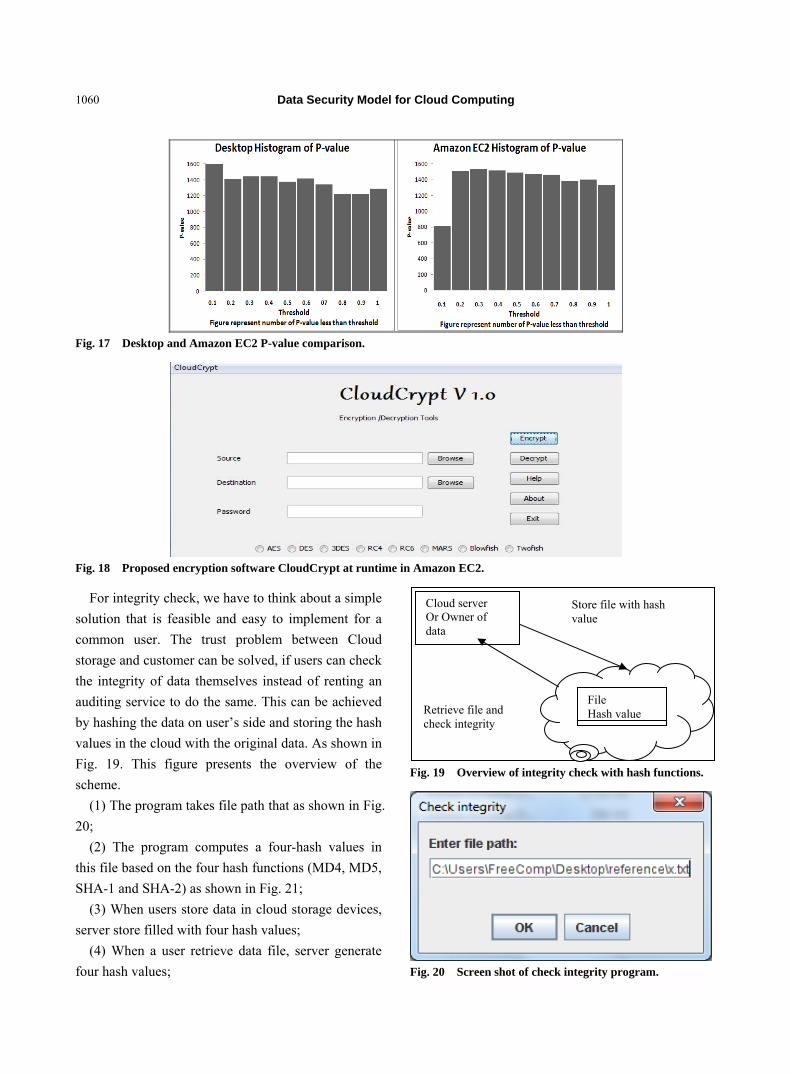
Data Security Model for Cloud Computing
1060
Fig. 17 Desktop and Amazon EC2 P-value comparison.
Fig. 18 Proposed encryption software CloudCrypt at runtime in Amazon EC2.
For integrity check, we have to think about a simple
solution that is feasible and easy to implement for a
common user. The trust problem between Cloud
storage and customer can be solved, if users can check
the integrity of data themselves instead of renting an
auditing service to do the same. This can be achieved
by hashing the data on user’s side and storing the hash
values in the cloud with the original data. As shown in
Fig. 19. This figure presents the overview of the
scheme.
(1) The program takes file path that as shown in Fig.
20;
(2) The program computes a four-hash values in
this file based on the four hash functions (MD4, MD5,
SHA-1 and SHA-2) as shown in Fig. 21;
(3) When users store data in cloud storage devices,
server store filled with four hash values;
(4) When a user retrieve data file, server generate
four hash values;
Fig. 19 Overview of integrity check with hash functions.
Fig. 20 Screen shot of check integrity program.
Retrieve file and check integrity
Store file with hash value
Cloud server Or Owner of data
File Hash value

Data Security Model for Cloud Computing
1061
Fig. 21 Check integrity program calculating hash values.
Table 6 Summarized results of the proposed data security model in cloud computing.
Features Description
Authentication OTP Authentication System (mathematical generation).
Provider encryption Software implemented to select the highest security and faster encryption algorithm based on NIST statistical tests. This software select AES algorithm to Micro Instance ubunto Amazon EC2 with Amazon S3.
Private user encryption TrueCrypt system or proposed software CloudCrypt v.10.
Data integrity Hashing-MD5-MD4-SHA-1-SHA-2.
Data fast recovery Based on decryption algorithm speed.
Key management User keys not stored in provider control domain.
(5) Server check integrity by comparing new four
hash values with stored four hash values.
The following are the advantages of using the
utility:
Not much implementation effort required.
Cost effective and more secured.
Do not require much time to compute the hash
values.
Flexible enough to change the security level as
required.
Not much space required to store the hash values.
6. Conclusions
According to the simulation results, in the
authentication phase in the proposed data security
model, OTP is used as two-factor authentication
software. OTP archived more password strength
security than other authentication systems (BIN and
static password). This appears by comparing between
OTP, BIN, and static password authentication systems
based on the space time size and entropy bits.
From the simulation results of the second phase in
the proposed data security model, test the proposed
system in Ubunto Amazon Micro Instance EC2, and
from randomness and performance evaluation to eight
modern encryption algorithms AES is the best
encryption algorithm in Ubunto Amazon Micro
Instance EC2. In addition to the randomness and
performance evaluation, data integrity must be
ensured. Moreover, the proposed data security model
encourages users to use true-crypt to encrypt his/her
sensitive data.
From the comparison and performance evaluation,
fast recovery of data achieved to the user. These
appear in the proposed data security model third
phase.
From the comparison and performance evaluation,
cloud computing depend on some condition, however
it has advanced security technologies rather than
traditional desktop. The summarized results of
proposed data security model are shown in
Table 6.
References
[1] Information Security Briefing Cloud Computing, Vol.1,
Center of The Protection of National Infrastructure CPNI
by Deloitte, 2010, p. 71.
[2] L. Foster, Y. Zhao, I. Raicu, S.Y. Lu, Cloud computing
and grid computing 360-degree compared, in: Grid
Computing Environments Workshop, GCE’08, Austin,
TX, Nov. 12-16, 2008, pp. 1-10.
[3] The NIST Definition of Cloud Computing, National
Institute of Science and Technology, p.7. Retrieved July
24 2011.

Data Security Model for Cloud Computing
1062
[4] J.W. Rittinghouse, J.F. Ransome, Cloud Computing Implementation, Management, and Security, CRC Press, Boca Raton, 2009.
[5] Security Guidance for Critical Areas of Focus in Cloud Computing V1.0 [Online], Apr. 2009, Cloud Security Alliance Guidance, www.cloudsecurityalliance.org/guidance/csaguide.v1.0.pdf.
[6] M.A. Vouk, Cloud computing-issues, research and
implementations, Journal of Computing and Information
Technology 16 (2008) 235-246
[7] Security Guidance for Critical Areas of Focus in Cloud Computing V2.1 [Online], Dec. 2009, Cloud Security Alliance Guidance.
[8] Security Guidance for Critical Areas of Focus in Cloud Computing V3.0 [Online], Cloud Security Alliance Guidance.
[9] Y.F. Dai, B. Wu, Y.Q. Gu, Q. Zhang, C.J Tang, Data security model for cloud computing, in: Proceedings of The 2009 International Workshop on Information Security and Application IWISA 2009, Qingdao, China, Nov. 21-22, 2009.
[10] C. Burwick, D. Coppersmith, The MARS Encryption Algorithm, Aug. 27, 1999
[11] E. Dawson, H. Gustafson, M. Henricksen, B. Millan, Evaluation of RC4 Stream Cipher, Information Security Research Centre Queensland University of Technology, Jul. 31, 2002
[12] W. Stallings, Cryptography and Network Security, 4th ed., Prentice Hall, N.J, 2005, pp. 58-309.
[13] D. Coppersmith, The Data Encryption Standard (DES) and Its Strength Against Attacks, IBM Journal of Research and Development 38 (1994) 243-250.
[14] J. Daemen, V. Rijmen, Rijndael: The advanced encryption standard, D r. Dobb's Journal 26 (2001)
137-139. [15] B. Schneier, The Blowfish Encryption Algorithm
[Online], http://www.schneier.com/blowfish.html (accessed: Oct. 25, 2008).
[16] B. Schneier, J. Kelseyy, D. Whitingz, D. Wagnerx, C. Hall, N. Ferguson, Twofish: A 128-bit block cipher, Jun. 15, 1998.
[17] J. Soto, Randomness Testing of the Advanced Encryption Standard Candidate Algorithms, U.S. Dept. of Commerce, Technology Administration, National Institute of Standards and Technology, 1999.
[18] R. Buyya, C.S. Yeo, S. Venugopal, Market-oriented
cloud computing: Vision, hype, and reality for delivering
IT services as computing utilities, in: 9th IEEE/ACM
International Symposium on Cluster Computing and the
Grid, CCGRID’09, Shanghai, May 18-21, 2009.
[19] A. Rukhin, J. Soto, J. Nechvatal, M. Smid, A Statistical Test Suite for Random and Pseudorandom Number Generators for Cryptographic Applications, NIST Special Publication, Apr. 2010.
[20] Amazon EC2 API, Amazon Elastic Compute Cloud Developer Guide [Online], Oct. 2006, http://docs.amazonwebservices.com/AWSEC2/2006-10-01/DeveloperGuide/.
[21] Amazon Web Services, Amazon Simple Storage Service Developer Guide [Online], Mar. 2006.
[22] Amazon Web Services, Overview of Security Processes [Online], Sep. 2009 http://aws.typepad.com/aws/2009/08/introducing-amazon-virtual-private-cloud-vpc.html.
[23] V. Prakash, A. Infant, J. Shobana, Eliminating vulnerable attacks using One-Time Password and PassText—Analytical study of blended schema, Universal Journal of Computer Science and Engineering Technology 1 (2010) 133-140.

Journal of Communication and Computer 10 (2013) 1063-1069
The Retraining Churn Data Mining Model in DMAIC
Phases
Andrej Trnka
Department of Mass Media Communication, Faculty of Mass Media Communication, University of SS. Cyril and Methodius, Trnava
917 01, Slovak Republic
Received: May 30, 2013 / Accepted: July 01, 2013 / Published: August 31, 2013.
Abstract: Six Sigma is a rigorous, focused, and highly effective implementation of proven quality principles and techniques. A company’s performance is measured by the sigma level of their business processes. Traditionally companies accepted three or four sigma performance levels as the norm. The Six Sigma standard of 3.4 problems-per-million opportunities is a response to the increasing expectations of customers. DMAIC is an acronym for five phases of Six Sigma methodology: Define, Measure, Analyze, Improve, Control. This paper describes possibility of using Bayesian Network for retraining data mining model. Concrete application of this proposal is in the field of the churn. Churn is a derivation from change and turn. It can be defined as a discontinuation of a contract. Data mining methods and algorithms can predict behavior of customers. We can get better results using Six Sigma methodology. The goal of this paper is proposal of implementation churn (with Bayesian network) to the phases of Six Sigma methodology.
Key words: Bayesian network, data mining, DMAIC, Churn, Six Sigma.
1. Introduction
Six Sigma methodology and its phases (Fig. 1) have
been widely adopted by industries and non-profit
organizations throughout the world. Six Sigma
methodology was first espoused by Motorola in the
mid-1980s. The successful implementation of the Six
Sigma program in Motorola led to huge benefits.
Motorola recorded a reduction in defects and
manufacturing time, and also began to reap financial
rewards. The Six Sigma has become the most
prominent trend in quality management not only for
manufacturing and service industries, but also for
non-profit organizations and government institutes
[1-5].
The main target of Six Sigma is to minimize
variation because it is somehow impossible to
Corresponding author: Andrej Trnka, Ph.D., research
fields: data mining, Six Sigma, statistical process control. E-mail: [email protected].
eliminate it totally. Sigma (σ) in the statistical field is
a metric used to represent the distance in standard
deviation units from the mean to a specific limit. Six
Sigma is a representation of six standard deviations
from the distribution mean. If a process is described as
within Six Sigma, the term quantitatively means that
the process produces fewer than 3.4 DPMO (defects
per million opportunities). Table 1 shows how
exponential the sigma scale is between levels 1 and 6
[6].
We can talk about Lean Six Sigma, too. Lean Six
Sigma for services is a business improvement
methodology that maximizes shareholder value by
achieving the fastest rate of improvement in customer
satisfaction, cost, quality, process speed, and invested
capital [7]. But for our research, we can ignore the fast,
so using the Six Methodology is proper.
In our previous research we implemented selected
data mining methods and algorithms to the DMAIC
phases of Six Sigma Methodology. The main area of

The Retraining Churn Data Mining Model in DMAIC Phases
1064
Fig. 1 Representation of Six Sigma methodology by BPMN.
Table 1 Six Sigma scale.
Sigma DPMO Efficiency (%)
1 691,462 30.9
2 308,538 69.1
3 66,807 93.3
4 6,210 99.4
5 233 99.98
6 3.4 99.9999966
Source: Ref. [6].
the implementation was manufacturing processes. But
Six Sigma methodology can be used in customer
services, too.
Some authors have used data mining algorithms in
manufacturing processes, but without Six Sigma
methodology [8-11].
Data mining is the process of discovering
interesting patterns and knowledge from large
amounts of data. The data sources can include
databases, data warehouses, the Web, other
information repositories, or data that are streamed into
the system dynamically [12]. One of the data mining
task is to predict the customer’s churn.
2. Churn
Mobile phone providers fight churn by detecting
patterns of behavior that could benefit from new
services, and then advertise such services to retain
their customer base. Incentives provided specifically
to retain existing customers can be expensive, and
successful data mining allows them to be precisely
targeted to those customers who are likely to yield
maximum benefit [13]. Churn is defined as a
discontinuation of a contract. Reducing churn is
important because acquiring new customers is more
expensive than retaining existing customers. In order
to manage customer churn to increase profitability,
companies need to predict churn behavior,
however, this problem not yet well understood
[14, 15].
Churning customers can be divided into two main
groups, voluntary and non-voluntary churners.
Non-voluntary churners are the easiest to identify, as
these are the customers who have had their service
withdrawn by the company. There are several reasons
why a company could revoke a customer’s service,
including abuse of service and non-payment of service.
Voluntary churn is more difficult to determine,
because this type of churn occurs when a customer
makes a conscious decision to terminate his/her
service with the provider. Voluntary churn can be

The Retraining Churn Data Mining Model in DMAIC Phases
1065
sub-divided into two main categories, incidental churn
and deliberate churn.
Incidental churn happens when changes in
circumstances prevent the customer from further
requiring the provided service. Examples of incidental
churn include changes in the customer’s financial
circumstances, so that the customer can no longer
afford the service, or a move to a different
geographical location where the company’s service is
unavailable. Incidental churn usually only explains a
small percentage of a company’s voluntary churn.
Deliberate churn is the problems that most churn
management solutions try to battle. This type of churn
occurs when a customer decides to move his/her
custom to a competing company. Reasons that could
lead to a customer’s deliberate churn include
technology-based reasons, when a customer discovers
that a competitor is offering the latest products, while
their existing supplier can not provide them.
Economic reasons include finding the product at a
better price from a competing company. Examples of
other reasons for deliberate churn include quality
factors such as poor coverage, or possibly bad
experiences with call centers [16-17].
3. Data Mining Model
For our research we used IBM SPSS Modeler 14.
Telecommunications provider is concerned about the
number of customers it is losing to competitors.
Historic customer data can be used to predict which
customers are more likely to churn in the future.
These customers can be targeted with offers to
discourage them from transferring to another service
provider.
This model focuses on using an existing churn data
to predict which customers may be likely to churn in
the future and then adding the following data to refine
and retrain the model [18].
Fig. 2 shows the built model in IBM SPSS Modeler,
which contains the historical data.
In analysis we used two data sets. These data sets
had identical structure of variables. First data set
contained 412 rows (records) and the second data set
contained 451 rows.
Fig. 2 Summary model for churn.
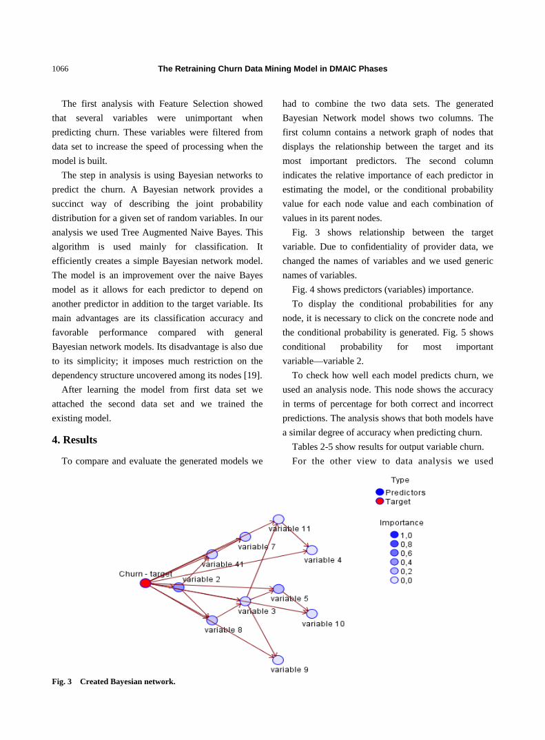
The Retraining Churn Data Mining Model in DMAIC Phases
1066
The first analysis with Feature Selection showed
that several variables were unimportant when
predicting churn. These variables were filtered from
data set to increase the speed of processing when the
model is built.
The step in analysis is using Bayesian networks to
predict the churn. A Bayesian network provides a
succinct way of describing the joint probability
distribution for a given set of random variables. In our
analysis we used Tree Augmented Naive Bayes. This
algorithm is used mainly for classification. It
efficiently creates a simple Bayesian network model.
The model is an improvement over the naive Bayes
model as it allows for each predictor to depend on
another predictor in addition to the target variable. Its
main advantages are its classification accuracy and
favorable performance compared with general
Bayesian network models. Its disadvantage is also due
to its simplicity; it imposes much restriction on the
dependency structure uncovered among its nodes [19].
After learning the model from first data set we
attached the second data set and we trained the
existing model.
4. Results
To compare and evaluate the generated models we
had to combine the two data sets. The generated
Bayesian Network model shows two columns. The
first column contains a network graph of nodes that
displays the relationship between the target and its
most important predictors. The second column
indicates the relative importance of each predictor in
estimating the model, or the conditional probability
value for each node value and each combination of
values in its parent nodes.
Fig. 3 shows relationship between the target
variable. Due to confidentiality of provider data, we
changed the names of variables and we used generic
names of variables.
Fig. 4 shows predictors (variables) importance.
To display the conditional probabilities for any
node, it is necessary to click on the concrete node and
the conditional probability is generated. Fig. 5 shows
conditional probability for most important
variable—variable 2.
To check how well each model predicts churn, we
used an analysis node. This node shows the accuracy
in terms of percentage for both correct and incorrect
predictions. The analysis shows that both models have
a similar degree of accuracy when predicting churn.
Tables 2-5 show results for output variable churn.
For the other view to data analysis we used
Fig. 3 Created Bayesian network.

The Retraining Churn Data Mining Model in DMAIC Phases
1067
Fig. 4 Predictors importance.
Fig. 5 Conditional probability of variable 2.
Table 2 Comparing churn_1 with churn.
Total 863
Correct 654 75.78%
Wrong 209 24.22%
Table 3 Comparing churn_2 with churn.
Total 863
Correct 655 75.9%
Wrong 208 24.1%
Table 4 Agreement between churn_1 and churn_2.
Total 863
Correct 682 79.03%
Wrong 181 20.97%
Table 5 Comparing agreement with churn.
Total 682
Correct 565 82.84%
Wrong 117 17.16%
evaluation graph to compare the model’s predicted
accuracy by building a gains chart. Fig. 6 shows
evaluating model accuracy.
The graph shows that each model type produces
similar results. However, the retrained model
(churn_2) using both data sets is slightly better
because it has a higher level of confidence in its
predictions. Therefore, we used another algorithm of
Bayesian network—Markov Blanket.
The Markov Blanket [19] for the target variable
node in a Bayesian network is the set of nodes
containing target’s parents, its children, and its
children’s parents. Markov blanket identifies all the
Fig. 6 Evaluation graph of analysis (TAN Bayes Network).
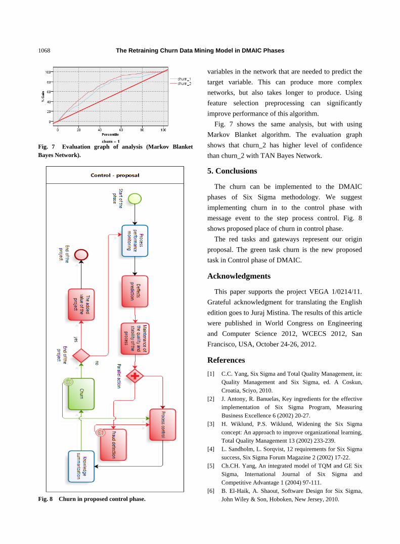
The Retraining Churn Data Mining Model in DMAIC Phases
1068
Fig. 7 Evaluation graph of analysis (Markov Blanket Bayes Network).
Fig. 8 Churn in proposed control phase.
variables in the network that are needed to predict the
target variable. This can produce more complex
networks, but also takes longer to produce. Using
feature selection preprocessing can significantly
improve performance of this algorithm.
Fig. 7 shows the same analysis, but with using
Markov Blanket algorithm. The evaluation graph
shows that churn_2 has higher level of confidence
than churn_2 with TAN Bayes Network.
5. Conclusions
The churn can be implemented to the DMAIC
phases of Six Sigma methodology. We suggest
implementing churn in to the control phase with
message event to the step process control. Fig. 8
shows proposed place of churn in control phase.
The red tasks and gateways represent our origin
proposal. The green task churn is the new proposed
task in Control phase of DMAIC.
Acknowledgments
This paper supports the project VEGA 1/0214/11.
Grateful acknowledgment for translating the English
edition goes to Juraj Mistina. The results of this article
were published in World Congress on Engineering
and Computer Science 2012, WCECS 2012, San
Francisco, USA, October 24-26, 2012.
References
[1] C.C. Yang, Six Sigma and Total Quality Management, in: Quality Management and Six Sigma, ed. A Coskun, Croatia, Sciyo, 2010.
[2] J. Antony, R. Banuelas, Key ingredients for the effective implementation of Six Sigma Program, Measuring Business Excellence 6 (2002) 20-27.
[3] H. Wiklund, P.S. Wiklund, Widening the Six Sigma concept: An approach to improve organizational learning, Total Quality Management 13 (2002) 233-239.
[4] L. Sandholm, L. Sorqvist, 12 requirements for Six Sigma success, Six Sigma Forum Magazine 2 (2002) 17-22.
[5] Ch.CH. Yang, An integrated model of TQM and GE Six Sigma, International Journal of Six Sigma and Competitive Advantage 1 (2004) 97-111.
[6] B. El-Haik, A. Shaout, Software Design for Six Sigma, John Wiley & Son, Hoboken, New Jersey, 2010.

The Retraining Churn Data Mining Model in DMAIC Phases
1069
[7] W. Bentley, P.T. Davis, Lean Six Sigma Secrets for the CIO, CRC Press, Boca Raton, Florida, 2010.
[8] M. Kebisek, P. Schreiber, I. Halenar, Knowledge discovery in databases and its application in manufacturing, in: Proceedings of the International Workshop “Innovation Information Technologies: Theory and Practice”, Dresden, Sep. 6-20, 2010, pp. 204-207.
[9] R. Halenar, Matlab possibilities for real time ETL method, Acta Technica Corviniensis: Bulletin of Engineering 5 (2012) 51-53.
[10] P. Vazan, P. Tanuska, M. Kebisek, The data mining usage in production system management, World Academy of Science, Engineering and Technology 7 (2011) 1304-1308.
[11] M. Kudla, M. Stremy, Alternatívne metódy ukladania pološtruktúrovaných dát (Alternative methods for storing semi-structured data,), in: Applied Natural Sciences 2007, International Conference on Applied Natural Sciences, Trnava, Slovak Republic, Nov. 7-9, 2007, pp. 404-409.
[12] J. Han, M. Kamber, J. Pei, Data Mining Concepts and Techniques, Elsevier, Waltham, Massachusets, 2012.
[13] I. Witten, E. Frank, M. Hall, Data Mining Practical Machine Learning Tools and Techniques, Elsevier, Burlington, Massachusets, 2012.
[14] J. Ahn, S. Han, Y. Lee, Customer churn analysis: Churn determinants and mediation effects of partial defection in the Korean mobile telecommunications service industry, Telecommunications Policy 30 (2006) 552-568.
[15] K.Ch. Lee, N.Y. Jo, Bayesian network approach to predict mobile churn motivations: Emphasis on general Bayesian network, Markov blanket, and what-if simulation, in: Second International Conference, FGIT 2010, Jeju Island, Korea, Dec. 13-15, 2010.
[16] H. Kim, C. Yoon, Determinants of subscriber churn and customer loyalty in the Korean mobile telephony market, Telecommunications Policy 28 (2004) 751-765.
[17] J. Hadden, A. Tiwari, R. Rajkumar, D. Ruta, Churn prediction: Does technology matter?, International Journal of Electrical and Computer Engineering 1 (2006) 397-403.
[18] IBM SPSS Modeler 14.2 Applications Guide, IBM, 2011.
[19] IBM SPSS Modeler 14.2 Algorithms Guide, IBM, 2011.

Journal of Communication and Computer 10 (2013) 1070-1075
Codebook Subsampling and Rearrangement Method for
Large Scale MIMO Systems
Xin Su1, Tianxiao Zhang2, Jie Zeng1, Limin Xiao1, Xibin Xu1 and Jingyu Li1
1. Tsinghua National Laboratory for Information Science and Technology, Research Institute of Information Technology, Tsinghua
University, Beijing 100000, China
2. School of Advanced Engineering, Beihang University, Beijing 100000, China
Received: April 28, 2013 / Accepted: June 01, 2013 / Published: August 31, 2013.
Abstract: In large scale MIMO (multiple-input multiple-output) systems, the size of codebook increases greatly when transmitters and receivers are equipped with more antennas. Thus, there are demands to select subsets of the codebook for usage to reduce the huge feedback overhead. In this paper, we propose a novel codebook subsampling method using chordal distance of different codewords and deleting them to affordable payload of PUCCH (physical uplink control channel). Besides, we design a related codebook rearrangement algorithm to mitigate the system performance loss when there are bit errors in the feedback channel.
Key words: Large scale MIMO, codebook subsampling, codebook rearrangement, PMI feedback.
1. Introduction
The explosive growth of wireless data service calls
for new spectrum resource. Meanwhile, the available
spectrum for further wireless communication systems
is very limited and expensive. Since the capacity of a
MIMO (multiple-input multiple-output) system
greatly increases with the minimum number of
antennas at the transmitter and receiver sides under
rich scattering environments [1], the large scale
MIMO [2] shown in Fig. 1 is one of the most
important techniques to address the issue of
exponential increasing in wireless data service by
using spatial multiplexing and interference mitigating.
For the consideration of practical application, the
number of antennas on the terminal side is restricted,
and thus the number of multiplexing layers is limited
though the number of antennas on the BS (base station)
could be very large. As a result, we should explore the
Corresponding author: Jie Zeng, M.Sc., engineer, research
fields: broadband wireless access, software defined radio, 4G/B4G technology and standardization. E-mail: [email protected].
large scale MIMO system potentials by utilizing
beamforming technologies. The performance of
beamforming relies on the accuracy of precoding.
However, the size of codebook can be very large
when antennas are increased, considering that the
payload capacity of PUCCH (physical uplink control
channel) is limited to 11 bits [3]. To decrease the
overhead in CSI (channel state information) feedback,
the choice of codebook subsampling for transmission
is necessary [4, 5].
Fig. 1 The close-loop MIMO system model.
Codebook Subsampling and Rearrangement Method for Large Scale MIMO Systems
1071
Several subsampling methods have been proposed
in Rel-10 in 2, 4, 8 Tx scenario. The subset selection
in this case naturally corresponds to the reduction of
granularity in direction and/or phase offset [6], such
as uniform subsampling or staggered subsampling
which keeps better granularity. However, the
codebook design for large scale MIMO system may
not be based on direction for each polarization and
phase offset between polarizations; hence the
application above for large scale MIMO is restricted.
In this case, we propose a novel codebook
subsampling method which applies to all kinds of
codebook design, in which we select the subset of
codebook using chordal distance of different
codewords and delete them to affordable payload of
PUCCH. In addition, to further optimize the
performance of PMI (precoding matrix indication)
when errors occur, we propose the codebook
rearrangement method to decrease the impact of
mismatch between PMI and the channel.
This paper is organized as follows: Section 2
introduces the model of the precoding system. Section
3 presents the codebook subsampling method and the
codebook rearrangement method. Section 4 shows the
simulation results. And finally, Section 5 concludes
the paper.
2. System Model
2.1 System Model
In this paper, we discuss about a close-loop MIMO
system withtN transmit antennas and
rN receive
antennas depicted in Fig. 1. For massive MIMO
system tN
could be very large.
Firstly, the data vector S in the system is
de-multiplexed into L streams. L is limited
by 1 min( , )t rL N N . When L = 1 we call the
transmission beamforming, while L > 1 we call it
multiplexing. After the data vector s is preprocessed
by an Nt × L precoding matrix Wi, we get a Nt × 1
signal vector x for the tN
antennas to transmit:
x Ws (1)
Thus, after x passing the channel and being added
the noise, we will get the received signal y, which can
be expressed as:
iy HW s v (2)
where, H ( r tN NH C ) denotes the fading channel matrix
with its entry ijH
denoting the channel response
from the thj transmit antenna to the thi receive
antenna, and v denotes the white complex Gaussian
noise vector with covariance matrix 0 rNN I .
The precoding matrix is selected from the
predesigned codebook which is known to the
transmitter and the receiver. Taking the downlink as
an example, when UEs have received the pilots from
the BS, the receiver can choose the optimal codeword
after the channel estimation. Then the receiver reports
the PMI with limited bits to BS [7] through the uplink
channel. If the feedback is limited to B bits, the size of
codebook satisfies BN 2 . Thus the transmitter can
retrieve the precoding matrix and perform the
precoding.
2.2 Kerdock Codebook
The basic idea of the Kerdock codebook design is
utilizing the feature of MUB (mutually unbiased bases)
to construct precoding matrices. The main
characteristic of the Kerdock codebook is that all the
elements of the matrix are ±1 or ±j. Hence, the
Kerdock codebook has some advantages, such as low
requirement for storage, low computational
complexity for codeword search, and the simple
systematic construction.
The MUB property is described as follows:
1{ ,..., }tNS s s ,
1{ ,..., }tNU u u are two orthonormal
bases with sizet tN N . If the column vectors drawn
from S and U satisfy , 1 /i j ts u N , we can say
that they have the mutually unbiased property [8].
An MUB is the set 1{ ,..., }
tNS s s satisfying the
mutually unbiased property. The Kerdock codebook
has several construction methods such as

Codebook Subsampling and Rearrangement Method for Large Scale MIMO Systems
1072
Sylvester–Hadamard construction and power
construction. In this paper, we use the
Sylvester–Hadamard construction:
First, we construct the generating matrices Dn
(t tN N
diagonal matrices with ±1, ±j elements) for n
= 0, 1, 2…Nt–1 according to Ref. [9].
Then we construct the corresponding orthonormal
matrix: 1 ˆ , 0,1,..., 1
tn n N t
t
W D H n NN
(3)
where, ˆtNH is the
t tN N Sylvester–Hadamard
matrix:
2 2ˆ ˆ ˆ ....
tNH H H
(4)
where 2
1 1ˆ1 1
H
For the beamforming, we can construct the
codebook by selecting each column of all the bases as
the precoding vector: { }{1} {2}
1 0 2 0 1{ , ,..., }t
t
N
N NC f W f W f W (5)
And for an L-layer spatial multiplexing codebook,
the largest codebook is derived by taking all L-column
combinations from each nW .
2.3 Codeword Search
We can choose the optimal main codeword from
1 2{ , ,..., }NK K K through the estimate of the channel.
The codebook is shared by the transmitter and
receiver.
Codeword selection criteria: for 1-layer
beamforming, the beamformer that minimizes the
probability of symbol error for maximum ratio
combining receiver is expressed as [10]: 2
2ˆ[ ] arg max [ ]
f Cf i H i f
(6)
where, f denotes a 1tN matrix. For spatial
multiplexing with a zero forcing receiver, the
minimum singular value selection criterion is
expressed as:
minˆ[ ] arg max { [ ] }
K CF i H i K
(7)
where, min
denotes the minimum singular value of
the argument. This selection criterion approximately
maximizes the minimum sub-stream SNR
(signal-to-noise ratio).
3. The Novel Codebook Subsampling and Rearrangement Method
3.1 Codebook Subsampling
To pursue the maximum SNR, we select the
codeword with the smallest chordal distance from the
transmission channel. The basic idea of the codebook
subsampling method is to delete one codeword of the
codeword pairs which have the smallest chordal
distance. The chordal distance between two precoding
vector is represented by 2
( , ) 1,
chord i j
i j
i j
d f ff f
f f
(8)
with ||.|| being the norm of the vector. If the chord
distance between two codewords is the smallest
among the codewords pool, we may reserve only one
of them and delete another. Therefore, we could
decrease the overhead as well as remain the
performance of precoding at the utmost.
The process of subsampling is shown as follows:
(1) Suppose the codebook includes K codewords.
Divide the codewords into g groups.
(1-1) Compute the chordal distance between any
two codewords ( , )i jd f f . Choose if and
jf as
reference codewords if their distance is the largest.
(1-2) Compute the chordal distance between the rest
( (0, ], ! & & ! )Lf L K L i L j and reference
codeword. If ( , ) ( , )i L L jd f f d f f , put Lf in if ’s
group. Otherwise put Lf in jf ’s group.
(1-3) Repeat the procedure until the number of
groups is g.
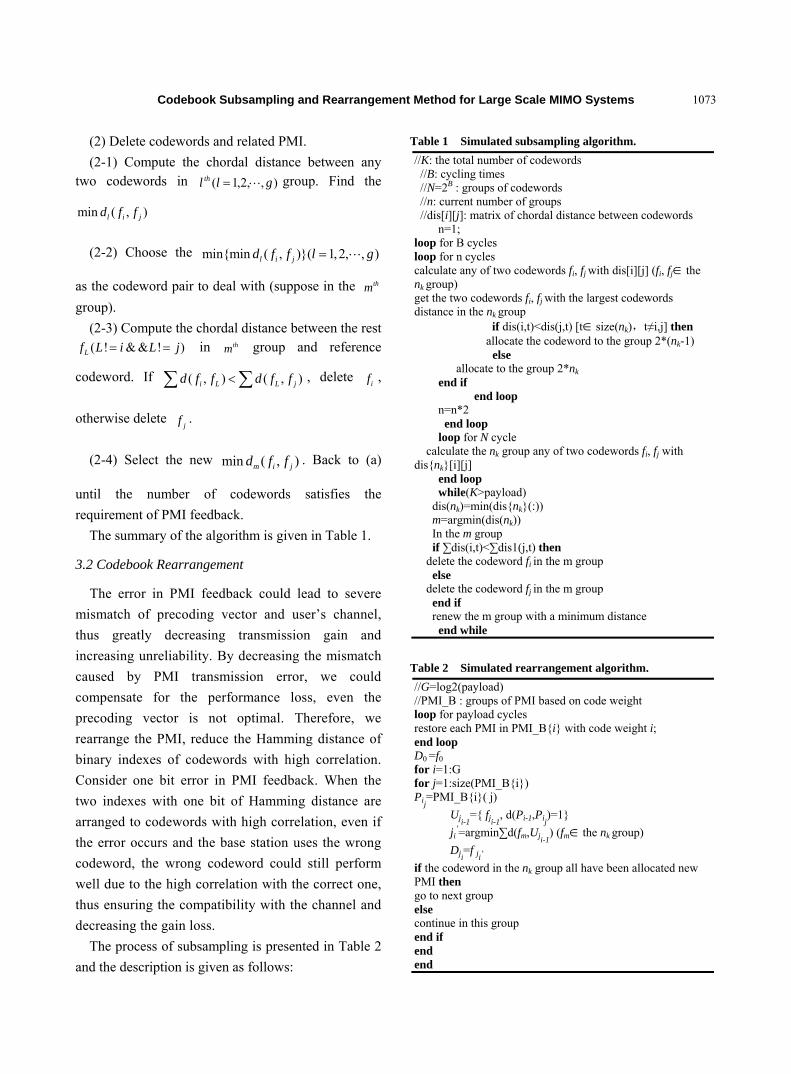
Codebook Subsampling and Rearrangement Method for Large Scale MIMO Systems
1073
(2) Delete codewords and related PMI.
(2-1) Compute the chordal distance between any two codewords in ),,2,1( gll th group. Find the
min ( , )l i jd f f
(2-2) Choose the min{min ( , )}( 1,2, , )l i jd f f l g
as the codeword pair to deal with (suppose in the thm
group).
(2-3) Compute the chordal distance between the rest ( ! & & ! )Lf L i L j in thm group and reference
codeword. If ( , ) ( , )i L L jd f f d f f , delete if ,
otherwise delete jf .
(2-4) Select the new min ( , )m i jd f f . Back to (a)
until the number of codewords satisfies the
requirement of PMI feedback.
The summary of the algorithm is given in Table 1.
3.2 Codebook Rearrangement
The error in PMI feedback could lead to severe
mismatch of precoding vector and user’s channel,
thus greatly decreasing transmission gain and
increasing unreliability. By decreasing the mismatch
caused by PMI transmission error, we could
compensate for the performance loss, even the
precoding vector is not optimal. Therefore, we
rearrange the PMI, reduce the Hamming distance of
binary indexes of codewords with high correlation.
Consider one bit error in PMI feedback. When the
two indexes with one bit of Hamming distance are
arranged to codewords with high correlation, even if
the error occurs and the base station uses the wrong
codeword, the wrong codeword could still perform
well due to the high correlation with the correct one,
thus ensuring the compatibility with the channel and
decreasing the gain loss.
The process of subsampling is presented in Table 2
and the description is given as follows:
Table 1 Simulated subsampling algorithm.
//K: the total number of codewords //B: cycling times //N=2B : groups of codewords //n: current number of groups //dis[i][j]: matrix of chordal distance between codewords n=1; loop for B cycles loop for n cycles calculate any of two codewords fi, fj with dis[i][j] (fi, fj the nk group) get the two codewords fi, fj with the largest codewords distance in the nk group if dis(i,t)<dis(j,t) [tsize(nk),t≠i,j] then allocate the codeword to the group 2*(nk-1) else allocate to the group 2*nk
end if end loop n=n*2 end loop loop for N cycle calculate the nk group any of two codewords fi, fj with dis{nk}[i][j] end loop while(K>payload) dis(nk)=min(dis{nk}(:)) m=argmin(dis(nk)) In the m group if ∑dis(i,t)<∑dis1(j,t) then delete the codeword fi in the m group else delete the codeword fj in the m group end if renew the m group with a minimum distance end while
Table 2 Simulated rearrangement algorithm.
//G=log2(payload) //PMI_B : groups of PMI based on code weight loop for payload cycles restore each PMI in PMI_B{i} with code weight i; end loop D0 =f0 for i=1:G for j=1:size(PMI_B{i}) Pij
=PMI_B{i}( j)
Uji-1={ fji-1
, d(Pi-1,Pij)=1}
ji’=argmin∑d(fm,Uji-1
) (fm the nk group)
Dji=f ji’
if the codeword in the nk group all have been allocated new PMI then go to next group else continue in this group end if end end
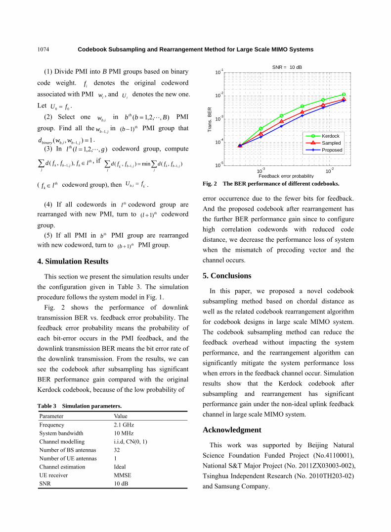
Codebook Subsampling and Rearrangement Method for Large Scale MIMO Systems
1074
(1) Divide PMI into B PMI groups based on binary
code weight. if denotes the original codeword
associated with PMI iw , and
iU denotes the new one.
Let 0 0U f .
(2) Select one ibw ,
in ),,2,1( Bbbth PMI
group. Find all thejbw ,1in thb )1( PMI group that
1),( ,1, jbibbinary wwd . (3) In ),,2,1( gll th codeword group, compute
1,( , ), thk b j k
j
d f f f l , if ' 1, 1,( , ) min ( , )b j k b jk
j j
d f f d f f
( thkf l codeword group), then ',b i k
U f .
(4) If all codewords in thl codeword group are
rearranged with new PMI, turn to thl )1( codeword
group.
(5) If all PMI in thb PMI group are rearranged
with new codeword, turn to thb )1( PMI group.
4. Simulation Results
This section we present the simulation results under
the configuration given in Table 3. The simulation
procedure follows the system model in Fig. 1.
Fig. 2 shows the performance of downlink
transmission BER vs. feedback error probability. The
feedback error probability means the probability of
each bit-error occurs in the PMI feedback, and the
downlink transmission BER means the bit error rate of
the downlink transmission. From the results, we can
see the codebook after subsampling has significant
BER performance gain compared with the original
Kerdock codebook, because of the low probability of
Table 3 Simulation parameters.
Parameter Value
Frequency 2.1 GHz
System bandwidth 10 MHz
Channel modelling i.i.d, CN(0, 1)
Number of BS antennas 32
Number of UE antennas 1
Channel estimation Ideal
UE receiver MMSE
SNR 10 dB
10-3
10-2
10-5
10-4
10-3
10-2
10-1
SNR = 10 dB
Feedback error probability
Tra
ns.
BE
R
Kerdock
Sampled
Proposed
Fig. 2 The BER performance of different codebooks.
error occurrence due to the fewer bits for feedback.
And the proposed codebook after rearrangement has
the further BER performance gain since to configure
high correlation codewords with reduced code
distance, we decrease the performance loss of system
when the mismatch of precoding vector and the
channel occurs.
5. Conclusions
In this paper, we proposed a novel codebook
subsampling method based on chordal distance as
well as the related codebook rearrangement algorithm
for codebook designs in large scale MIMO system.
The codebook subsampling method can reduce the
feedback overhead without impacting the system
performance, and the rearrangement algorithm can
significantly mitigate the system performance loss
when errors in the feedback channel occur. Simulation
results show that the Kerdock codebook after
subsampling and rearrangement has significant
performance gain under the non-ideal uplink feedback
channel in large scale MIMO system.
Acknowledgment
This work was supported by Beijing Natural
Science Foundation Funded Project (No.4110001),
National S&T Major Project (No. 2011ZX03003-002),
Tsinghua Independent Research (No. 2010TH203-02)
and Samsung Company.

Codebook Subsampling and Rearrangement Method for Large Scale MIMO Systems
1075
References
[1] E. Telatar, Capacity of multi-antenna gaussian channels, European Transactions on Telecommunications 10 (1999) 585-595.
[2] F. Rusek, D. Persson, B.K. Lau, E.G. Larsson, T.L.
Marzetta, O. Edfors, et al., Scaling up MIMO:
opportunities and challenges with very large arrays, IEEE
Signal Processing Magazine 30 (2012) 40-60.
[3] 3GPP TS 36.213: Evolved universal terrestrial radio
access (E-UTRA), Physical layer procedures,
pp. 56-64.
[4] R1-104164 Way forward on 8Tx codebook for Rel.10 DL
MIMO, CATT, Ericsson, LG Electronics, Mitsubishi
Electric, Nokia, Nokia Siemens Networks, NTT DoCoMo,
Panasonic, Sharp, ST-Ericsson, Texas Instruments,
RAN1 #61bis, June 2010, Dresden, Germany.
[5] R1-104259 Way Forward on CSI Feedback for Rel.10 DL MIMO Alcatel-Lucent, Alcatel-Lucent Shanghai Bell,
CATT, Ericsson, Huawei, Marvell, Mitsubishi Electric, NEC, Nokia, Nokia Siemens Networks, NTT DoCoMo, Panasonic, Samsung, Sharp, ST-Ericsson, Texas Instruments, ZTE, RAN1 #61bis, June 2010, Dresden, Germany.
[6] R1-104901 8Tx Codebook Subsampling, Panasonic, August 2010, Madrid, Spain.
[7] 3GPP TS 36.211: Evolved Universal Terrestrial Radio Access (E-UTRA), Physical channels and modulation, pp. 17-20.
[8] A. Klappenecker, M. Roetteler, Constructions of mutually unbi-ased bases, Finite Fields Appl. 2948 (2004) 137-144.
[9] R.W. Heath Jr., T. Strohmer, A.J. Paulraj, On quasi-orthogonal signatures for CDMA systems, IEEE Trans. Inf. Theory 52 (2006) 1217-1226.
[10] D.J. Love, R.W. Heath Jr., Limited feedback unitary precoding for spatial multiplexing systems, IEEE Trans. Inf. Theory 51 (2005) 2967-2976.

Journal of Communication and Computer 10 (2013) 1076-1086
A High-Precision Time Handling Library
Irina Fedotova1, Eduard Siemens2 and Hao Hu2
1 Faculty of Information Science and Computer Engineering, Siberian State University of Telecommunication and Information
Sciences, Novosibirsk 630102, Russia
2 Faculty of Electrical, Mechanical and Industrial Engineering, Anhalt University of Applied Sciences, Koethen 06366, Germany
Received: April 28, 2013 / Accepted: June 01, 2013 / Published: August 31, 2013.
Abstract: An appropriate assessment of end-to-end network performance presumes highly efficient time tracking and measurement with precise time control of the stopping and resuming of program operation. In this paper, a novel approach to solving the problems of highly efficient and precise time measurements on PC-platforms and on ARM-architectures is proposed. A new unified High Performance Timer and a corresponding software library offer a unified interface to the known time counters and automatically identify the fastest and most reliable time source, available in the user space of a computing system. The research is focused on developing an approach of unified time acquisition from the PC hardware and accordingly substituting the common way of getting the time value through Linux system calls. The presented approach provides a much faster means of obtaining the time values with a nanosecond precision than by using conventional means. Moreover, it is capable of handling the sequential time value, precise sleep functions and process resuming. This ability means the reduction of wasting computer resources during the execution of a sleeping process from 100% (busy-wait) to 1-1.5%, whereas the benefits of very accurate process resuming times on long waits are maintained.
Key words: High-performance computing, network measurement, timestamp precision, time-keeping, wall clock.
1. Introduction
Estimation of the achieved quality of the network
performance requires high-resolution, low CPU-cost
time interval measurements along with an efficient
handling of process delays and sleeps [1, 2]. The
importance on controlling these parameters can be
shown on the example of a transport layer protocol. Its
implementation may need up to 10 time fetches and
time operations per transmitted and received data
packet. However, performing accurate time interval
measurements, even on high-end computing systems,
faces significant challenges.
Even though Linux (and in general UNIX timing
subsystems) uses auto-identification of the available
hardware time source and provides nanosecond
resolution, these interfaces are always accessed from
Corresponding author: Fedotova Irina, M.Eng., research
fields: hard real-time system, for OS Linux. E-mail: [email protected].
user space applications through system calls. Thus it
costs extra time in the range of up to a few
microseconds—even on contemporary high-end PCs
[3]. Therefore, direct interaction with the timing
hardware from the user space can help to reduce time
fetching overhead from the user space and to increase
timing precision. The Linux kernel can use different
hardware sources, whereby time acquisition
capabilities depend on the actual hardware
environment and kernel boot parameterization. While
the time acquisition of some time sources costs up to 2
microseconds, others need about 20 nanoseconds. In
the course of this work, a new High Performance
Timer and a corresponding library HighPerTimer have
been developed. They provide a unified user-space
interface to time counters available in the system and
automatically identify the fastest and the most reliable
time source (e.g., TSC (time stamp counter) [4, 5] or
HPET (high-performance event counter) [6, 7]). In the

A High-Precision Time Handling Library
1077
context of this paper, the expression time source
means one of the available time hardware or
alternatively the native timer of the operating system,
usually provided by the standard C library.
Linux (as well as other UNIX operating systems)
faces a significant problem of inaccurate sleep time,
which is known for many years, especially in older
kernel versions, when Linux has provided a process
sleep time resolution of 10 m. This leads to a
minimum sleep time of about 20 ms [8]. Even
nowadays, when Linux kernels usually reduce this
resolution down to 1 m, waking up from sleeps can
take up to 1-2 m. With kernel 2.6 the timer handling
under Linux has been changed significantly. This
change has reduced the wakeup misses of sleep calls
to 51 µs on average and to 200-300 µs in peaks.
However, for many soft-real-time and
high-performance applications, this reduction is not
sufficient. Presented High Performance Timer not
only significantly improves the time fetching accuracy,
but also addresses the problem of those imprecise
wakeups from sleep calls under Linux.
These precision issues lead to the fact that, for
high-precision timing within state machines and
communication protocols, busy-waiting loops are
currently commonly used for waits, preventing other
threads from using the given CPU. The approach of
the High Performance Timer library aims at reducing
the CPU load down to an average of 1-1.5% within
the sleep calls of the library and at raising the wakeup
precision to 70-160 ns. Reaching these values enables
users of this library to implement many protocols and
state machines with soft real-time requirements in
user space.
The remainder of the paper is organized as follows.
In Section 2, related work is described. Section 3
shows the specific details of each time source within
the suggested single unified High-Performance Timer
class interface. In Section 4, we briefly describe the
implemented library interface. Some experimental
results of identifying appropriate timer source along
with their performance characteristics are shown in
Section 5. In Section 6, precise process sleeping
aspects are shown. Finally, Section 7 describes next
steps and future work in our effort to develop a tool
for highly efficient high-performance network
measurements.
2. Related Work
Since the problem of inefficient time keeping in
Linux operating system implementation has become
apparent, several research projects have suggested to
access the timing hardware directly from user space [1,
9-10]. However, most of this research considers
handling of a single time hardware source only,
predominantly the Time Stamp Counter [1, 9, 11].
Other solutions provide just wrappers around
timer-related system calls and so inherit their
disadvantages such as the high time overhead [12, 13].
In other proposals, the entire time capturing process is
integrated into dedicated hardware devices [14, 15].
Most of this research focuses only on a subset of the
problems, addressed in this work. Our work with the
HighPerTimer library improves timing support by
eliminating the system call overhead and also by
application of more precise process sleep techniques.
3. Unified Time Source of the HighPerTimer Library
While most of the current software solutions on
Linux and Unix use the timing interface by issuing
clock_gettime() or gettimeofday() system calls,
HighPerTimer tries to invoke the most reliable time
source directly from the user space. Towards the user,
the library provides a unified timing interface for time
period computation methods along with sleep and
wakeup interfaces, independently from the used
underlying time hardware. So, the user sees a “unified
time source” that accesses the best possible on the
underlying hardware, and that generally avoids system
call overheads. The HighPerTimer interface supports
access the mostly used time counters: TSC, HPET and,
A High-Precision Time Handling Library
1078
as the last alternative, the native timer of the operating
system, through one of the said Unix system calls.
The latter time source we call the OS Timer.
Using the Time Stamp Counter is the fastest way of
getting CPU time. It has the lowest CPU overhead and
provides the highest possible time resolution,
available for the particular processor. Therefore, in the
context of our library, the TSC is the most preferable
time source. In newer PC systems, the TSC may
support an enhancement, referred to as an Invariant
TSC feature. Invariant TSC is not tightly bound to a
particular processor core and has, in contrary to many
older processor families, a guaranteed constant
frequency [16]. The presence of the Invariant TSC
feature in the system can be tested by the Invariant
TSC flag, indicated by the cpuid processor instruction.
For most cases, the presence of this Invariant TSC
flag is essential in order to accept it as a
HighPerTimer source.
Formerly referred by Intel as a Multimedia Timer
[7], the High Precision Event Timer is another
hardware timer used in personal computers. The
HPET circuit is integrated into the south bridge chip
and consists of a 64-bit or 32-bit main counter register
counting at a given constant frequency between 10
MHz and 25 MHz. Difficulties are faced when the
HPET main counter register is running in 32-bit mode
because overflows of the main counter arise at least
every 7.16 min. With a frequency of 25 MHz, register
overflows would occur even within less than 3 min.
So, time periods longer than 3 min can not reliably
measured in 32 bit mode. So, in the HighPerTimer
library, we decided to generally avoid using the HPET
time source in case of a 32-bit main counter.
For systems, on which neither TSC nor HPET are
accessible or TSC is unreliable, an alternative option
of using the OS Timer is envisaged. This alternative is
a wrapper issuing the system call clock_gettime().
This source is safely accessible on any platform.
However, it has the lowest priority because it issues
system calls, with their time costs of up to 2
microseconds in worst case [17, 18]. Depending on
the particular computer architecture and used OS,
these costs can be less due to the support of the
so-called virtual system calls. These calls provide
faster access to time hardware and avoid expensive
context switches between user and kernel modes [19].
Nevertheless, invocation of clock_gettime() through a
virtual system call is still slower than the acquisition
time value from current time hardware directly. The
difference between getting the time value using virtual
system calls and getting the time values directly from
the hardware is about 3 to 17 ns, as measurement
results, discussed in Section 5, show.
4. The HighPerTimer Interface
The common guidelines on designing any interfaces
cover efficiency, encapsulation, maintainability and
extensibility. Accordingly, the implementation of the
HighPerTimer library pays particular attention to
these aspects. Using the new C++11 programming
language standard [20], the library achieves high
efficiency and easy code maintainability. Furthermore,
regarding the platform-specific aspects, HighPerTimer
runs on different 64-bit and 32-bit processors of Intel,
AMD, VIA and ARM, and considers their general
features along with specialties of time keeping.
However, some attention must be paid to obtaining
a clean encapsulation of hardware access when using
C++. For this encapsulation, the HighPerTimer library
comprises two header files and two implementation
files called HighPerTimer and TimeHardware. Each
of them contains three classes. HighPerTimer files
contain HighPerTimer, HPTimerInitAndClear and
AccessTimeHardware classes, as described below. In
TimeHardware files, the classes TSCTimer,
HPETTimer and OSTimer corresponding to the
respective time sources TSC, HPET and the OS
source have been implemented. Through an assembly
code within the C++ methods, they provide direct
access to the timer hardware, initialize the respective
timer source, retrieve their time value and are at only

A High-Precision Time Handling Library
1079
HighPerTimer class’s disposal. Dependencies
between the classes are presented in Fig. 1.
TSCTimer, HPETTimer and OSTimer classes have
a “friend” relationship with the HighPerTimer class,
which means that HighPerTimer places their private
and protected methods and members at friend classes’
disposal. For safety and security reasons, we protect
the hardware access from use by application users
directly and permit access only from special classes.
An AccessTimeHardware class provides a limited
read-only access to some information on CPU and
specific time hardware features, obtained in a
protected interface. For example, some advanced
users can find out failure reasons of the initialization
routine of the HPET device and get a corresponding
error message:
std::cout <<
AccessTimeHardware::HpetFailReason();
However, all the routines of time handling along
with access to the actual timer attributes such as clock
frequency are accessed by the library users via the
HighPerTimer class. For interfacing with other time
formats, HighPerTimer class provides a set of
constructors that sets its object to the given time
provided in seconds, nanoseconds or in the native
clock ticks of the used time source. Via specific
constructor, a time value in a Unix-specific time
format [21] can also be assigned to a HighPerTimer
object. The current time value is retrieved using the
following piece of code:
// declare HighPerTimer objects
HighPerTimer timer1, timer2;
HighPerTimer::Now (timer1);
// measured operation
HighPerTimer::Now (timer2);
Comparison operators allow effective comparison
to be performed using the main counter values. Some
of these methods are declared as follows:
bool operator >= (const HighPerTimer & timer)
const;
bool operator<= (const HighPerTimer& timer)
const;
bool operator!= (const HighPerTimer& timer)
const;
Fig. 1 Simplified class diagram of HighPerTimer library.

A High-Precision Time Handling Library
1080
The user can also set the value of a timer object
explicitly to zero and add or subtract the time values
in terms of timer objects, tics, nanoseconds or seconds.
Since the main “time” capability of a timer object is
kept in the main counter only, the comparison
operations between timer objects, as well as
arithmetical operations on them, are nearly as fast as
comparisons and elementary arithmetical operations
on two int 64 variables. Recalculations between tics,
seconds, microseconds and nanoseconds are only
done in the “late initialization” fashion when string
representations of the timer object or seconds,
microseconds or nanoseconds of the object are
explicitly requested via the class interface:
// subtract from timer object
HighPerTimer & SecSub (const uint64_t Seconds);
HighPerTimer & USecSub (const uint64_t
USeconds);
HighPerTimer & NSecSub (const uint64_t
NSeconds);
HighPerTimer & TicSub (const uint64_t Tics);
// add to timer object
HighPerTimer & SecAdd (const uint64_t Seconds);
HighPerTimer & USecAdd (const uint64_t
USeconds);
HighPerTimer & NSecAdd (const uint64_t
NSeconds);
HighPerTimer & TicAdd (const uint64_t Tics);
Assignment operators allow a HighPerTimer object
to be set from the Unix-format of time values -
timeval or timespec structs [21]. Both of these
structures represent time, elapsed since 00:00:00 UTC
on 01.01.1970. They consist of two elements: the
number of seconds and the rest of the elapsed time
represented either in microseconds (in case of timeval)
or in nanoseconds (in case of timespec):
struct timeval {
long tv_sec; /* seconds */
long tv_usec; /* microseconds */
}
struct timespec {
long tv_sec; /* seconds */
long tv_nsec; /* nanoseconds */
};
Assignment to these structures is also possible with
HighPerTimer objects through copying or moving:
const HighPerTimer & operator= (const struct
timeval & TV);
const HighPerTimer & operator= (const struct
timespec & TS);
const HighPerTimer & operator= (const
HighPerTimer & Timer);
HighPerTimer & operator= (HighPerTimer &&
Timer);
This way, the HighPerTimer library provides a fast
and efficient way to handle time values by operating
main counter value and seconds and nanoseconds
values only on demand. It also relieves users from the
manual handling of specific two-value structures such
as timeval or timespec.
However, for the whole routine of handling time
values, some central parameterization of the library
must be performed at the initialization time of the
library. Primarily, this is the initialization of the
HighPerTimer source, which is accomplished on the
basis of the appropriate method calls from the
TimeHardware file. Especially, InitHPTimeSource()
calls InitTSCTimer() and InitHPETTimer() methods,
which attempt to initialize respective time hardware
and return true on success or false on failure ( Fig. 1).
Before using any timer object, the following global
parameters must be measured and set: the frequency
of the main counter as a double precision floating
point value and as a number of ticks of the main
counter within one microsecond, the value of the shift
of the main timer counter against Unix Epoch, the
maximum and minimum values of HighPerTimer for
the given hardware-specific main counter frequency,
and the specified HZ frequency of the kernel. The
value of HZ is defined as the system timer interrupt
rate and varies across kernel versions and hardware
platforms. In the context of the library, the value of

A High-Precision Time Handling Library
1081
HZ is used for the implementation of an accurate sleep
mechanism, see Section 6. The strict sequence of the
initialization process is determined within an
additional HPTimerInitAndClean service class (Fig. 1)
by invoking corresponding HighPerTimer
initialization methods through their “friend”
relationship. A strict order of initialization of the
given global variables must be assured, which is
somewhat tricky since all the variables must be
declared static and must be initialized before entering
the main routine of the application.
Despite the advantage of automatic detection of
the appropriate time source, situations sometimes
arise when an application programmer prefers to use a
different time source than the one automatically
chosen at library initialization time. To account for
this, a special ability to change the default timer is
provided. This change causes a recalculation process
for most of the timer attributes:
// create variable for a new value of time source
TimeSource MySource;
MySource = TimeSource::HPET;
HighPerTimer::SetTimerSource (MySource);
However, since this change leads to invalidation of
all the already existing timer objects within the
executed program, this feature should be used with
caution and only at the system initialization time, and
definitely before instantiation of the first
HighPerTimer object.
5. Time Fetching Performance Results
Table 1 shows the performance results when getting
the time values using the HighPerTimer library as
measured on different processor families. The mean
and standard deviation values of the costs of setting a
HighPerTimer object are shown. For this investigation,
time was fetched in a loop of 100 million consecutive
runs and set to a HighPerTimer object. Since we are
interested here in measuring the time interval between
two consecutive time fetches only, without any
interruption in between, we filter out all outlying
peaks. These peaks are most probably caused by
process interruption by the scheduler or by an
interrupt service routine. Thus, filtering out such
outliers allows us to get rid of the bias caused by
physical phenomena, which are outside the scope of
this investigation.
The following two examples demonstrate the
behavior of HighPerTimer sources in more detail and
allow a comparison of their reliability and costs
depending on the particular processor conditions.
Although Table 1 shows the results for all three
processors, later investigations are shown only for less
powerful systems. It makes sense to examine in more
depth those systems, where for example, TSC is
unstable or does not possess Invariant TSC flag
(Section 3).
In the first case, processor VIA Nano X2 has TSC
as a current time source. Costs of time fetching here
are about 38 ns. Since TSC source has the highest
priority and has been initialized successfully, the
HPET device check is not necessary and so omitted
here. Moreover, on this processor, the Linux kernel is
also using TSC as its time source and so, within the
clock_gettime() call, the kernel is also fetching the
TSC register of the CPU. Fig. 2 shows the relation
between the TSC, OS and HPET timers on this
processor. Similarity between TSC and OS costs are
seen very clearly. As seen in Table 2, the difference
between the mean value of time fetching between OS
Timer and TSC Timer is 64 ns. Each system call with
a context switch would last at least ten times longer,
Table 1 Costs of setting timer on different processors.
Processor (CPU) Time source Mean, ns St. deviation, ns
Intel ® Core ™ i7-2600, 1600 MHz TSC 16.941 0.1231
VIA Nano X2 U4025, 1067 MHz TSC 38.203 0.3134
Athlon ™ X2 Dual Core BE-2350, 1,000 MHz HPET 1,063.3 207.92

A High-Precision Time Handling Library
1082
Fig. 2 Measurements of TSC, HPET and OS Timer costs on the VIA Nano X2 processor.
Table 2 Mean and standard deviation values of HPET, TSC and OS Timer costs on the VIA Nano X2 processor.
Timer source Mean, ns. Standard deviation, ns.
TSC Timer 38.23 0.3134
HPET Timer 598.72 76.015
OS Timer 102.20 0.5253
thus we can conclude that, on this system, a virtual
system call is issued by clock_gettime() instead of a
real system call with a context switch. HPET source
for the library can be set by the static method
HighPerTimer::SetTimerSrouce. However, we would
expect here much slower time operations, as seen in
Table 2.
The next example illustrates another case of a
dependence on the OS Timer from the current time
source. For the processor AMD Athlon X2 Dual Core,
the TSC initialization routine fails because TSC is
unstable here. However, since the HPET device is
accessible, there are two more options for the time
source for HighPerTimer–HPET or OS Timers - and it
is necessary to check the mean costs of getting the
ticks of both timers.
Although the mean value of time fetching for TSC
can be significantly lower than for HPET, the
HighPerTimer library considers the TSC to be a
non-stable, unreliable time source since the Invariant
TSC flag (Section 3 above) is not available and the
TSC constancy is not identified by additional library
checks. So, it must be assumed that TSC frequency
changes from time to time due to power saving or
other techniques of the CPU manufacturers. In the
next step, HPET and OS Timer characteristics must be
considered. The difference between the mean values
of HPET and OS Timer is about 54.1 ns, which is not
enough for a system call with a context switch. Thus
we conclude that clock_gettime() also uses the HPET
timer and passes it to the user via a virtual system call.
However, to provide an appropriate level of reliability,
we also evaluate numbers through their deviation
values. For this evaluation, a threshold for the
difference of mean values was chosen. When the
difference of the mean values of HPET and OS Timer
is no more than 25%, we also take into account
standard deviation values of time fetching and so
check the temporal stability of the considered time
source. Consequently, when the mean time fetching
value of the two time sources is similar, the
HighPerTimer library would give precedence to the
time source with a less standard deviation of the time
fetching costs.
Table 3 Mean and standard deviation values of HPET, TSC and OS Timer costs on the AMD Athlon processor.
Timer source Mean, µs Standard deviation, µs
TSC Timer 0.0251 0.0015
HPET Timer 1.0633 0.2079
OS Timer 1.1174 0.3743

A High-Precision Time Handling Library
1083
Fig. 3 Measurements of TSC, HPET and OS Timer costs on the AMD Athlon processor.
6. Precise Process Sleeping Aspects
For process sleeping or suspension, Linux provides
the sleep function (implemented in the standard C
library). Dependent on the sleep duration, the function
either suspends from the CPU or waits in the
busy-waiting mode (sometimes also called spinning
wait). However, measurements performed in this work
revealed that the sleep function of the standard C
library misses the target wake-up time by more than
50 ms on average. Such an imprecision however is
unacceptable for high-accuracy program sleeps. By
comparison, pure busy wait implementations within
an application miss the target return time by about 100
ns, but keep the CPU busy throughout the wait time.
Unlike the C library’s sleep call, the sleep of the
HighPerTimer library combines these two ways of
sleeping. It has very short miss times on waking up
with a minimum CPU utilization at the same time.
This improvement provides a big competitive
advantage over the predecessor solutions.
HighPerTimer provides a wide range of functions
for making a process sleep. For example, the user can
define the specific sleep time, given purely in seconds,
in microseconds or nanoseconds. A process
suspension with a nanosecond resolution can be done
as follows:
HighPerTimer timer1;
uint32_t SleepTimeNs(14500);
// sleep in nanoseconds
timer1.NSecSleep(SleepTimeNs);
Alternatively, the time value of a HighPerTimer
object can be set to a specific time value at which the
process shall wake up. On the call of SleepToThis(),
the process will then be suspended till the system time
has reached the value of that object :
//declare timer object equaled to 10 s, 500 ns
HighPerTimer timer2 (10, 500);
timer2.SleepToThis();
Table 4 shows the precision of sleeps and
busy-waits using different methods. Miss values are
here the respective differences between the targeted
wakeup time and real times of wakeups measured in
our tests. However, the miss values of sleep times
heavily depend on the fact, whether target sleep
interval was shorter or longer, than time between
Table 4 The comparison of miss values of different methods of sleeping, performed with TSC on the Intel Core –i7 processor.
Sleep time >= 1/HZ Sleep time < 1/HZ
Mean miss, µs Mean miss, µs
System sleep 61.985 50.879
Busy-waiting loop 0.160 0.070
HighPerTimer sleep 0.258 0.095

A High-Precision Time Handling Library
1084
Fig. 4 Dependency of miss on the target time from sleep time, performed with TSC on the Intel Core –i7 processor, HZ = 1,000.
two timer interrupts. So, Table 4 consists of two
parts—one where sleep time is longer than 1/HZ, and
one where it is less than 1/HZ. Thus, the left column
shows results for waits lasting longer than a period of
two kernel timer interrupts. The right column shows
the results for the scenario, in which the sleep call
lasts less than the interval between two kernel timer
interrupts. These measurements have been performed
on the Intel Core–i7 processor. Other than in
measurements from Section V, in this case it makes
sense to show results on a more stable and powerful
system. Moreover, it was expected that the accuracy
of sleeps would be higher on the newer Linux kernel
versions where time handling has been changed
significantly. However, as the measurements below
show, these kernel changes are still not sufficient.
In this test scenario, we have issued the respective
sleep method within a loop of 100000 sleeps with
different sleep times between 0.25 s and 1 µs, and
then the mean value of the sleep duration miss has
been calculated.
The above experiment took about 830 min, so the
upper limit of the range for sleep time value was
reduced to 0.25 s. The chart in Fig. 4 demonstrates
more detailed results of this experiment and shows the
dependency of miss against the target sleep time in
dependence from sleep duration. To track this
dependency more deeply, here the range of sleep time
value was increased and is taken between 10 s and 1
µs
In the next step, we measured the CPU
consumption of the respective sleep routine. In the
busy-waiting loop, the total CPU consumption during
the test achieves, as expected, almost 100%. For the
sleep function of the standard C library, it tends to
zero. In the case of sleeping using the HighPerTimer
library, the overall CPU consumption during the test
was 1.89%, which can be considered as a good
tradeoff between precision of waking up time and
CPU consumption during the sleep.
7. Conclusion and Future Work
In accordance with the requirements of advanced
high-speed data networks, we showed an approach for
the unified high performance timer library that
successfully solves two significant problems. Firstly,
A High-Precision Time Handling Library
1085
HighPerTimer allows identification of the most
efficient and reliable way for time acquisition on a
system and for avoiding system calls invocation on
time acquisition. Secondly, it solves the problem of
precise sleeping aspects and provides new advanced
sleeping and resuming methods.
The HighPerTimer library has the potential to
become widely used in estimation network packet
dynamics, particularly when conducting
high-accuracy and high-precision measurements of
network performance. At this stage, the integration of
the suggested solution into the appropriate tool for
distributed network performance measurement [22] is
in progress. Moreover, to the next steps, the better
support of the ARM processor will be addressed.
Since the ARM processor possesses neither HPET nor
TSC, the only way to support ARM at this stage is to
select OS Timer. Presumably, an invocation of the
initial ARM system timer can afford to save several
additional microseconds and improve the timer
accuracy.
References
[1] R. Takano, T. Kudoh, Y. Kodama, F. Okazaki, High-resolution timer-based packet pacing mechanism on the linux operating system, IEICE Transactions on Communication E94-B (2011) 2199-2207.
[2] J. Micheel, S. Donnelly, I. Graham, Precision time stamping of network packets, in: Proc. of the 1st ACM SIGCOMM Workshop on Internet Measurement, San Francisco, CA, USA, Nov.1-2, 2001, pp. 273-277.
[3] H. Hu, Untersuchung und prototypische implementierung von Methoden zur hochperformanten Zeitmessung unter Linux, Bachelor Thesis, Anhalt University of Applied Sciences, Koethen, Germany, Nov., 2011.
[4] Performance monitoring with the RDTSC instruction [Online], http://www.ccsl.carleton.ca/~jamuir/rdtscpm1.pdf (accessed: Jan., 2013).
[5] E. Corell, P. Saxholm, D. Veitch, A user friendly TSC clock, in: Proc. PAM, Adelaide, Australia, Mar. 30-31, 2006, pp. 141-150.
[6] S. Siddha, V. Pallipadi, D. Ven, Getting maximum mileage out of tickles, in: Proc. of the 2007 Linux Symposium, Ottawa, Jun. 27-30 2007, pp. 201-208.
[7] Intel IA-PC HPET (High Precision Event Timers)
Specification [Online], http://www.intel.com/content/dam/ www/public/us/en/documents/technical-specifications/software-developers-hpet-spec-1-0a.pdf (accessed: Jan., 2013).
[8] D. Kang, W. Lee, C. Park, Kernel Thread Scheduling in Real-Time Linux for Wearable Computers [Online], DOI: 10.4218/etrij.07.0506.0019 ETRI Journal 29 (2007) 270-280.
[9] P. Orosz, T.Skopko, Performance evaluation of a high precision software-based timestamping solution, International Journal on Advances in Software 4 (2011) 181-188.
[10] T. Gleixner, D. Niehaus, Hrtimers and beyond: transforming the Linux time subsystems, The Linux Symposium, Ottawa, Canada, Jul. 19-22, 2006, pp. 333-346.
[11] D. Kachan, E. Siemens, H. Hu, Tools for the high-accuracy time measurement in computer systems, in: 6th Industrial Scientific Conference, “Information Society Technologies”, Moscow, Russia, 2012, pp.22-25.
[12] Intel Trace Collector Reference Guide [Online], p. 5.2.5. http://software.intel.com/sites/products/documentation/hpc/ics/itac/81/ITC_Reference_Guide/ITC_Reference_Guide.pdf (accessed: Jan., 2013).
[13] D. Grove, P. Coddington, Precise MPI Performance Measurement Using MPIBench, in: Proc. of HPC Asia, Gold Coast, Australia, Sep. 24-28, 2001, pp. 1-14.
[14] The Dag project [Online], http://www.endace.com, (accessed: Jan., 2013).
[15] Pasztor, D. Veitch, PC based precision timing without GPS, in: The 2002 ACM SIGMETRICS International Conference on Measurement and Modeling of Systems, Marina Del Rey California, USA, 30 (2002) 1-10, DOI: 10.1145/511334.511336.
[16] Intel 64 and IA-32 Architectures, Software Developer‘s Manual [Online], vol. 3B 17-36, http://download.intel.com/ products/processor/manual/253669.pdf, (accessed: Jan., 2013).
[17] J. Dike, A user-mode port of the Linux kernel, USENIX Association Berkeley, California, USA, 2000, pp. 63-72,.
[18] K. Jain, R. Sekar, User-Level Infrastructure for System Call Interposition: A Platform for Intrusion Detection and Confinement, in: Proc. of the ISOC Symposium on Network and Distributed System Security, Feb. 3-4, 2000 pp. 19-34.
[19] J. Corbet, On vsyscalls and the vDSO, Kernel development news, Linux news site LWN [Online], http://lwn.net/Articles/446125/ (accessed: Jan., 2013).
[20] Online C++11 standard library reference, URL: cppreference.com (accessed: Jan., 2013).

A High-Precision Time Handling Library
1086
[21] GNU Operating System Manual, “Elapsed Time” [Online], http://www.gnu.org/software/libc/manual/html_node/Elapsed-Time.html (accessed: Jan., 2013).
[22] E.Siemens, S.Piger, C. Grimm, M. Fromme, LTest–A
Tool for Distributed Network Performance Measurement, in: Consumer Communications and Networking Conference, Las Vegas, NV, USA, Jan. 11-14, 2004, pp. 234-244, DOI: 10.1109/CCNC.2004. 1286865.

Journal of Com
New H
Adjust
Mansour Zu
Department of
Arabia
Received: May
Abstract: Theunderground lattracting consgiven cellular essential perfolimitations of scheme that camaximizing thadjusting QoS Key words: F
1. Introdu
Femtocell
capacity an
transmission
macrocell lo
and small c
femtocell is
maximum c
basic structu
The most
future wirel
(quality of
promising te
huge increa
various wir
network [4,
Femtocell
CorresponM.Sc., [email protected].
mmunication an
Hybrid A
ting Qo
uair, Abdul M
f Computer Eng
y 09, 2013 / Ac
e increasing numlocations; one osiderable attent
and to enhancormance promowireless comman manage the he system utilizS of the connect
Femtocell, hybri
uction
l provides in
nd provides
n of wireless
oad balancing
apacity base
between 13-2
overage is ab
ure of femtoce
t important p
less commun
service) an
echnologies
ase in wirele
reless applic
5].
l base station
nding author: arch field: .sa.
nd Computer 10
Access
oS
Malik Bacheer
gineering, Colle
ccepted: June 08
mber of mobileof suggestion sion in mobile cce user’s capac
otion issue. Devmunication are c
femocell resouzations, we provted users.
id access metho
ndoor, small
s high qua
communicat
[1]. Femtoce
station. The
20 dBm, in th
bout 15 to 50
ell access [2,
arameters for
nications are
nd cost. On
is to meet th
ess capacity
cations of th
n is installed i Abdul Malikcomputer n
0 (2013) 1087-1
s Meth
r Rahhal and M
ege of Compute
8, 2013 / Publis
e users raises isssolution to accocommunicationscity. Call admiveloping methocapacity and ranurces between svide a mechanis
od, QoS.
office cover
ality and h
tions services
ell is a low-po
e power rang
he same floor
0 m. Fig. 1 is
3].
r the current
e data rate, Q
ne of the m
he demand of
requirement
he femtocell
in homes as m
k Bacheer Ranetworks. E-m
1091
hod for
Mohamad M
er and Informat
shed: August 31
sues about coveommodate this s, it is a small bission control ads for femtocelnge. The main subscriber (femsm that leads to
rage,
high
s for
ower
ge of
r, the
s the
and
QoS
most
f the
t by
lular
mall
ahhal, mail:
priv
part
fem
own
call
F
con
hyb
In
serv
e-H
Fig.
Femto
Mahmoud Alra
tion Sciences, K
1, 2013.
erage extensiongrowing of mobase station thaand resource alll utilization is contribution of
mtocell user) ando serve more us
vate station
ticular subsc
mtocell may al
ner to use it,
led a hybrid a
From access
nfigured to be
brid access [6
n the past
vices increas
Health, online
. 1 The basic
ocell th
ahhal
King Saud Univ
n in some areas obile user is femat install to imprllocation infemvery comparatif our paper is dd non-subscribesers by admittin
which is ow
cribers can
llow users wh
for cell cove
access mode.
methods view
e either open
].
few years, t
sed (e.g., d
gaming, etc.
structure of fe
hrough
versity, Riyadh 1
such as rural zomtocell. Femtorove the indoor
mtocell’s hybridive nowadays. T
developing resouer (macrocell u
ng more subscri
wned by use
access it. H
ho are not of t
erage optimiz
wpoint femto
n access, clos
the demand
data, voice,
). 66% of voi
emtocell access
h
11543, Saudi
ones, indoor or cell have been r coverage of a d mode are an The two major urce allocation
user in order to ibers basing on
er. Therefore
However, the
this femtocell
zation, this is
ocells can be
sed access or
of wireless
multimedia,
ice and 90%
s.
e
e
l
s
e
r
s
,

New Hybrid Access Method for Femtocell through Adjusting QoS
1088
of data traffic occurs indoors [7], and due to high
penetration losses, macrocells are not very efficient
when delivering indoor coverage, providing such
coverage has become a challenge for operators this is
showing why the use of FAPs (femtocell access points)
seems a promising approach for coping with this
coverage problem.
Main goal of proposed scheme in Ref. [8] is to
transfer macrocell calls to femtocellular networks as
many as possible. They divide the proposed model into
three parts. The first one for the new originating calls,
the second one for the calls that are originally
connected with the macrocellular BS, and the last one
for the calls that are originally connected with the FAPs.
They offered the bandwidth degradation policy of the
QoS adaptive multimedia traffic to accommodate more
number of macrocell-to-macrocell and
femtocell-to-macrocell handover calls [8, 9].
One model has been proposed in Ref. [10] is based
on guard channel which is a mechanism to reserve
some portion of resources in advance for important
event. The propped model assumed that there are two
kinds of event, call for CSG (closed subscriber group)
members and call for non-CSG members. The call
will be new call in the cell or handover call from other
cells.
The remainder of this paper is organized as follows:
Section 2 explains access method; Section 3 talks
about our proposed model; Section 4 presents the
simulation results; Section 5 gives conclusions.
2. Access Method
Femtocells can be configured to be either open
access or closed access [6, 7]. Open access allows an
arbitrary nearby cellular user to use the femtocell,
whereas closed access restricts the use of the femtocell
to users explicitly approved by the owner. Seemingly,
the network operator would prefer an open access
deployment since this provides an inexpensive way to
expand their network capabilities, whereas the
femtocell owner would prefer closed access, in order to
keep the femtocell’s capacity and backhaul to himself.
These access methods (open, closed) suffer from
advantages and drawbacks. In order to overcome those
drawbacks, a hybrid access method reach can be used
to compromise between the impact on the performance
of subscribers and the level of access granted to
nonsubscribers. Therefore, the sharing of femtocell
resources between subscribers and nonsubscribers
needs to be tuned. Otherwise, subscribers might feel
that they are paying for a service that is to be exploited
by others. On the other hand, the impact on subscribers
must be minimized in terms of performance or via
economic advantages (e.g., reduced costs) [7].
The advantage and disadvantages of each access
method can be summarized as follows:
Open access: although open access method increases
the throughput and improve QoS but it also increases
number of handoff due to movement of outdoor users,
security issue, reduce the performance for femtocell
owner due to the sharing of femtocell resources with
nonsubscriber [6, 7, 11].
Closed access: in this case it is not allowed for
nonsubscriber to access to the femtocell even if
femtocell signal is stronger than that of macrocell,
which would cause strong cross tier interference but
also it increases the security, in addition to increasing
co-tier interference between neighboring femtocell in
dense deployment [6, 7].
Hybrid access: It needs to be analyzed carefully,
otherwise subscribers might feel that they are paying
for a service to be exploited by others.
3. Proposed Model
In this system there is one femtocell with capacity up
to M = 10 channels, time is slotted, arrivals are Poisson,
average service time is equal to slot time, probability to
transmit is P, and there is finite number of user equal to
20 users (10 subscribers and 10 nonsubscribers) with
no queuing. We can consider this work as extension of
our previous work [12]. The proposed model has these
enhancements: (1) subscriber users can use any
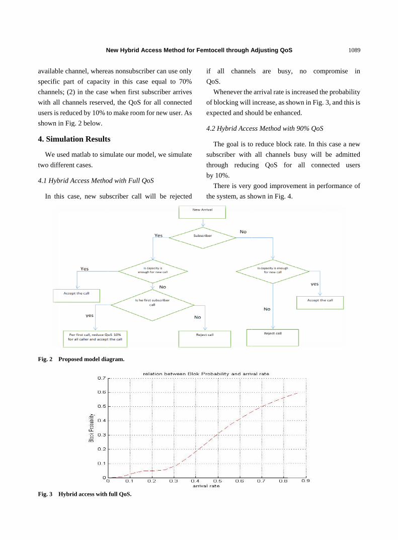
available ch
specific par
channels; (2
with all cha
users is redu
shown in Fig
4. Simulat
We used m
two differen
4.1 Hybrid A
In this ca
Fig. 2 Propo
Fig. 3 Hybr
N
annel, where
rt of capacity
2) in the case
annels reserve
uced by 10% t
g. 2 below.
tion Results
matlab to sim
nt cases.
Access Metho
ase, new sub
osed model dia
rid access with
New Hybrid A
as nonsubscr
y in this cas
when first s
ed, the QoS f
to make room
s
mulate our mo
od with Full Q
bscriber call
agram.
full QoS.
Access Metho
riber can use o
se equal to 7
subscriber arr
for all conne
m for new user
odel, we simu
QoS
will be reje
od for Femtoc
only
70%
rives
ected
r. As
ulate
ected
if
QoS
W
of b
exp
4.2
T
sub
thro
by
T
the
cell through A
all channel
S.
Whenever the
blocking will
pected and sho
Hybrid Acce
The goal is to
scriber with
ough reduci
10%.
There is very
system, as sh
Adjusting Qo
ls are busy
e arrival rate is
increase, as s
ould be enhan
ess Method wi
o reduce bloc
all channel
ng QoS fo
good improv
hown in Fig. 4
oS
y, no com
s increased th
shown in Fig.
nced.
ith 90% QoS
ck rate. In thi
s busy will
or all conn
vement in per
4.
1089
mpromise in
he probability
3, and this is
is case a new
be admitted
nected users
rformance of
9
n
y
s
w
d
s
f

New Hybrid Access Method for Femtocell through Adjusting QoS
1090
Fig. 4 Hybrid access with 0.9 QoS.
5. Conclusions
Femtocells have been attracting considerable
attention in mobile communications [13] which cover a
cell area of several tens of meters. Femtocells use
common cellular air access technologies [14].
Femtocells have the potential to provide high quality
network access to indoor users at low cost, while
reducing the load on the macrocells. Call admission
control in hybrid mode femtocell is an essential
performance promotion issue. In this paper, the
authors developed a mechanism for improving the
utilization of femtocell capacity and reducing rejection
rate of call through slight customization QoS.
Acknowledgment
This work was supported by the research center of
college of computer and information system, King
Saud University, Riyadh, Kingdom of Saudi Arabia.
The authors are grateful for this support.
References
[1] D. Lopez-Perez, A. Valcarce, Guillaume De La Roche, E. Liu, J. Zhang, Access methods to WiMAX femtocells: A downlink system-level case study, in: 11th IEEE Singapore International Conference on Communication System, Guangzhou, Nov. 19-21, 2008.
[2] D.N. Knisely, F. Favichia, Standardization of femtocells in 3GPP2, IEEE Com. Mag. 47 (2009) 76-82.
[3] S.J. Wu, A new handover strategy between femtocell and
macrocell for lte-based network, in: 4th International Conference on Ubi-Media Computing, Sao Paulo, Jul. 3-4, 2011.
[4] R.Y. Kim, J.S. Kwak, K. Etemad, WiMAX femtocell: requirements, challenges, and solutions, IEEE Communication Magazine 47 (2009) 84-91.
[5] M.Z. Chowdhury, Y.M. Jang, Z.J. Haas, Cost-effective frequency planning for capacity enhancement of femtocellular networks, Wireless Personal Communications 60 (2011) 83-104.
[6] J. Zhang, Guillaume de la Roche, Femtocell: Technologies and Deployment, John Wiley & Sons Ltd., UK, 2010.
[7] T. Chiba, H. Yokota, Efficient route optimization methods for femtocell-based all IP networks, in: IEEE International Conference on Wireless and Mobile Computing Networking and Communications WIMOB, Marrakech, Oct. 12-14, 2009.
[8] M.Z. Chowdhury, Y.M. Jang, Call admission control and traffic modeling for integrated macrocell/femtocell networks, in: 2012 4th International Conference on Ubiquitous and Future Networks (ICUFN), Phuket, Jul. 4-6, 2012.
[9] F.A. Cruz-Perez, L. Ortigoza-Guerrero, Flexible resource allocation strategies for class-based QoS provisioning in mobile networks, IEEE Transaction on Vehicular Technology 53 (2004) 805-819.
[10] S.Q. Lee, R.B. Han, N.H. Park, Call admission control for hybrid access mode femtocell system, in: 2011 IEEE 7th International Conference on Wireless and Mobile Computing, Networking and Communications (WiMob), Oct. 10-12, 2011.
[11] G. de la Roche, A. Valcarce, D. Lopez-Perez, J. Zhang, Access control mechanisms for femtocells, Communications Magazine IEEE 48 (2010) 33-39.

New Hybrid Access Method for Femtocell through Adjusting QoS
1091
[12] M. Zuair, Development of an access mechanism for femtocell networks, JATIT Journal 51 (2013) 434-441.
[13] S. FarazHasan, N.H. Siddique, S. Chakraborty, Femtocell versus WiFi-A survey and comparison of architecture and performance, in: 1st Internet Conference on Wireless Communication, Vehicular Technology, Information
Theory and Aerospace & Electronics Systems Technology Wireless VITAE, Aalborg, May 17-20, 2009.
[14] D. Lopez-Perez, A. Valcarce, G. de la Roche, J. Zhang, OFDMA femtocells: A Roadmap on Interference Avoidance, Communications Magazine IEEE 47 (2009) 41-48.
Journal of Communication and Computer 10 (2013) 1092-1098
Design of an Information Connection Model Using
Rule-Based Connection Platform
Heeseok Choi and Jaesoo Kim
National Science & Technology Information Service Center, Korea Institute of Science and Technology Information, Daejeon
306-806, Korea
Received: August 06, 2013 / Accepted: August 18, 2013 / Published: August 31, 2013.
Abstract: NTIS (National Science & Technology Information Service) collects national R&D information through the connection system in real time with specialized institutions under government ministries for R&D information service. However, because the information connection between the research management systems in each ministry (institution) and the NTIS is different, it is not easy to operate the connection system, and immediate data collection is thus not ensured. This study aims to propose an information connection model to be applied on the NTIS-like systems. To do this, we examine methods or styles of information connection and compare strength and weakness of connection methods. In this paper we also understand issues or characteristics of the methods through analyzing current information connection methods applied on the NTIS. Therefore, we design a rule-based information connection platform to minimize the information connection issues. Based on the platform, we also propose an information connection model.
Key words: Information connection, information sharing, rule-based connection.
1. Introduction
NTIS (National Science & Technology Information
Service) was developed for improving efficient
research and development throughout the cycle from
planning R&D to using the outcome thereof [1]. For
this purpose, each representative institution under the
government ministries and agencies comprehensively
manages its R&D information for connection with the
NTIS for the purpose of real-time collection of
national R&D information (periodical update when
collecting and changing the information at the time of
project agreement). The NTIS has currently built a
real-time connection system with representative
institutions under government ministries and agencies
[2].
However, since the connection criteria of each
Corresponding author: Heeseok Choi, Ph.D., KISTI senior
Researcher, research fields: information integration, information management, big data and data mining. E-mail: [email protected].
institution with external systems are different, the
NTIS is connected with the research management
system of each institution in various manners, to
collect R&D information. Accordingly, immediate
data collection is not ensured, and various manners of
connection contribute to inefficient
operation/maintenance.
This study aims to propose an information
connection model to be applied on the NTIS-like
systems. To do this, we examine methods or styles of
information connection and compare strength and
weakness of connection methods. In this paper we
also understand issues or characteristics of the
methods through analyzing current information
connection methods applied on the NTIS. Therefore,
we design a rule-based information connection
platform to minimize the information connection
issues. Based on the platform, we also propose an
information connection model to be applied on the
NTIS-like systems.

Design of an Information Connection Model Using Rule-Based Connection Platform
1093
The paper is organized as follows: Section 2
examines methods or styles of information connection
and compares strength and weakness of connection
methods. Section 3 contains issues or characteristics
of the methods through analyzing current information
connection methods applied on the NTIS. Section 4
presents our approach to design of an information
connection model using rule-based connection
platform. Section 5 gives conclusions.
2. Related Works
2.1 Technologies of Information Connection
For information connection between systems, P2P,
EAI, ESB or combinations thereof are currently
applied [3]. Features and characteristics of each
method are described below.
P2P: 1:1 connection between individual systems,
can not extended or reused. However, because
connection between individual systems is simple, a
connection system is easily built in conformity with
features of each system.
EAI: Individual applications are connected to the
central hub by means of an adapter, and are connected
to other applications through the central hub. This
significantly improves typical complex connections.
However, this method uses vender-dependent
technology and adapter costs should be paid for each
connected application.
ESB: This method was developed to avoid
weakness of non-standard EAI (Hub & Spoke) and
SPOF (single point of failure). However, because the
current ESB solution market is controlled by the EAI
solution providers, the tendency is that the previous
EAI solutions are supplemented and developed. In
general, this method is used for service connection.
Table 1 describes the strength and weakness of each
technology in terms of complexity, extensibility,
flexibility, and integration cost, etc..
2.2 Styles of Data Provision (Collection)
When systems of other organizations are connected,
independency of system operation and system/data
security of the organizations can be also an important
issue. Therefore, the subject of data provision
(collection) can be considered as an important factor
in building and operating a connection system.
Connection depending on the subject of data provision
(collection) is divided into the push method and the
polling method [4].
Push method: an information source (information
provider) that owns and manages original information
pushes data into information targets (information
consumers) in a given cycle according to the
information provision policy. Therefore, information
connection in this method is by a subject of
information provision who leads information
connection. This method is in favor of operation and
security of data and institution systems for
information providers, but does not ensure immediate
information collection for information providers.
Polling method: this is to access information
providers (systems for information sources) when an
information collector requires the information to bring
required information. Therefore, this is a method of
Table 1 Comparison of connection technologies.
Strength Weakness
P2P -Easy application to simple interworking between systems in a non-complex environment.
-As the number of systems to be connected increases, the cost for maintenance may sharply increase. -Low extension capability and flexibility.
EAI -Easy extension in introducing new applications. -Increased productivity and convenience for development and maintenance.
-High cost of establishment and maintenance. -Central hub failure affects the entire system. (Single Point of Failure)
ESB
-Reduced integration cost because standard technology is used and service units can be reused. -Loose connection in a bus type contributes to high extension capability and flexibility.
-High cost of initial establishment.

Design of an Information Connection Model Using Rule-Based Connection Platform
1094
connection in which the subject of information
collection leads information connection. This method
ensures immediate information collection, but is not
preferred by information providers in terms of
operation independency and security of internal
systems because information sources are directly
accessed from external systems.
Table 2 describes the strength and weakness of
provision styles in terms of security, maintenance,
performance, and dependency, etc..
3. Analysis of the NTIS Connection System
We analyzed the case of NTIS. The NTIS
established an information connection system with
research management systems of representative
institutions under government ministries and agencies
in order to connect and collect national R&D
information. In this case, the push method is applied
as a connection method to enable each representative
institution to have the right of providing data
appropriate for the connection policy and system
environment thereof with external systems, and to
have the ownership of the data owned by each
representative institution. That is, data are provided by
means of DB connection according to a given cycle
for data items defined in the national R&D
information standard. However, the principle of
providing data on a daily basis if data are created is
not ensured by adding an approval procedure for data
provision to the automatic connection process in
actually operating the connection system. Also,
although data are provided in the push method, the
DB link method and the unidirectional EAI method
are applied to each institution depending on each
institution environment. More details are shown in
Table 3 to show implemented connection systems in
various types. The reason of application is because the
method of data provision is determined and
implemented in various types according to the
preference of each institution (for tasks or system
environment) when the push method is applied. This
results in no assurance of immediate data provision,
and also makes monitoring and operation of the
connection system difficult.
Table 2 Comparison of data provision styles. Strength Weakness
Push
-High security in system connection between systems of institutions. -Independent connection with external systems in system operation. -Information providers lead connection.
-Because information providers lead information connection, integrated management of systems to be connected is not easy. -Information connection varies with institution by institution, maintenance is not easy.
Polling
-Because information collectors lead information connection, integrated management is easily implemented according to information collection policies. -Immediate data collection is ensured.
-Security is vulnerable in system connection. -Because performance may be affected by connection with external systems in system operation, information providers do not like this method.
Table 3 Information connection styles in the NTIS.
Method Type Description
DB link
View Direct connection to a DB in a connection server of an institution. The procedure Inquiry/Send is used.
Snapshot The copy of institution DB table refreshes the connection server DB in a given cycle.
DB trigger Trigger is established to reflect relevant changes on the connection server DB in updating the institution DB.
DB trigger + JDBC Trigger is established to reflect relevant changes on the connection server DB in updating the institution DB (based on Java, etc.).
DB script Uses script to send data from an institution DB to the connection server in a given cycle.
Procedures Transmits data from an institution to the connection server DB table by means of the procedure.
EAI Program Transmits data by means of the EAI program of each ministry (institution) (unidirectional).

Design of an Information Connection Model Using Rule-Based Connection Platform
1095
4. Design of an Information Connection Model Using Rule-Based Connection Platform
The current NTIS information connection system
has been established in the P2P style through the DB
link or the unidirectional EAI method as described in
the Section 3. However, it is necessary to improve the
connection system in a standardized method for
immediate provision, integrity, efficient connection
system monitoring and operation of data connection.
It is also important to design the method based on
easily managable rules. In this study, parts which can
be functionally standardized in information
connection between the NTIS and specialized
institutions under ministries and agencies are
identified to design them as a major functional module
of the connection platform. We design a rule-based
information connection platform to be applied on the
NTIS-like information connection systems. Based on
the platform, we also propose an information
connection model.
4.1 Rule-Based Connection Platform
Rule-based connection platform should be basically
designed on standardization for information
connection among heterogeneous systems. The
sections from which data are first acquired in
connection with each institution are divided into
variation areas for the purpose of information
connection based on standardization, and the next
phases are identified as standard functional areas. That
is, as shown in Fig. 1, the R&D information is first
transferred to the connection DB from the institution’s
system DB. This section is defined as a variation area.
Subsequent data processing in the connection DB and
data transmission to the integration DB is defined as a
major function of a common area which can be
standardized.
Therefore, it is necessary to build the connection
platform as a function to overcome variability of each
institution in the variation areas and to process the
functions in the common area. To this end, the
connection platform includes functions of connection
rule processing, mapping, connection error processing,
and creation of update information and monitoring
information. Fig. 2 shows system architecture of a
connection platform which includes the
aforementioned functions.
Fig. 2 shows the connection platform which is
composed of rule processing (preActors), connection
processing (Workers), and parallel task processing
control (Controllers), and which performs connection
of the common areas according to the rule predefined
in the Rule File.
Schema mapping (Mapper): This is carried out
between an institution DB schema and the NTIS
standard collection schema according to the schema
mapping rule defined in the Rule File for the data
transferred from the institution. Code mapping is also
carried out from the code value in the institution DB
to the code value in the NTIS integration DB
according to the code mapping rule defined in the
Rule File.
Comparison of data (Comparer, I/U/D Handler):
This is to compare the data transferred from an
institution with the data transferred in the previous
cycle to decide whether to update the data. On the
basis of comparison result, the system in the
connection institution system displays I (Insert), U
(Update), or D (Delete) to indicate that the relevant
data is new, updated or deleted data.
Connection error processing (Error Checker,
Error Handler): This is to check errors in connection,
for example, key errors, errors in essential connection
Fig. 1 Basic steps of information connection.

Design of an Information Connection Model Using Rule-Based Connection Platform
1096
Fig. 2 Rule-based connection platform.
items, code conversion errors, data conversion errors,
data format errors, data length errors, etc.. Details of
the checked connection errors are created to be an
error DB. Normal data are then stored as an OrgDB to
be transmitted to the NTIS integration DB.
Connection monitoring information creation
(Monitor): Information is created about whether
connection normally operates, for example, the
number of connection data, details of updated data,
execution of the connection module according to the
schedule, or how much new data have been provided.
Rule Parser: This enhances data mapping through
rule based processing. The Rule Parser interprets the
Rule File which specifies schema mapping, code
mapping and rules that should be observed when data
are provided from an institution to the NTIS.
Scheduler: Information connection is performed
periodically or in real time depending on information
type. Therefore, the function to control the
information connection execution cycle is provided.
Three types of execution scheduling is provided,
including manual execution (immediate execution) by
an operator, periodical execution and execution after
standby for a given period of time in consideration of
the features of NTIS connection.
Data Cacher: Information frequently used, for
example, schema information and code mapping
tables, is internally cached to improve connection
capability. Data are deleted after a given period of
time.
Operation environment (Controllers): This
controls listing tasks to be processed for optimized
resource management and function processing by
means of multi threads, and to carry out the tasks
according to the processing sequence. Controllers also
provide access to storages to store the connection
result in the DB or a file.
The connection platform designed as such can
improve data processing speed through internal data
caching. It can enhance data mapping through
rule-based data processing, and can operate and
maintain the connection system by
producing/changing rules. It sorts data sources from
targets to manage data history, and systematically
checks data errors. It can address difficulty in
connection monitoring due to different connection
methods between institutions, and processes data
update information.
4.2 Information Connection Model Using Rule-Based
Connection Platform
On the basis of the rule-based connection platform
designed in Section 4.1, information connections in
the push method, and in the EAI method or the polling
method by agents can be implemented. Therefore, two
types of information connection models were
designed and the two types of connection models were
compared with respect to the important issues
considered in information connection by the NTIS
with the representative specialized institutions.
(1) P2P & Push method using the connection
platform:
For standardized information connection, the
connection platform was defined, which processes the
information connection rule, performs encryption, and
creates connection error and monitoring information.
The connection standard platform contributes to
addressing limitations by different information
connection methods of each institution. That is,
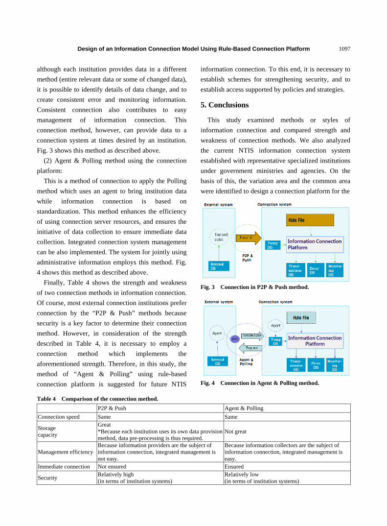
Design of an Information Connection Model Using Rule-Based Connection Platform
1097
although each institution provides data in a different
method (entire relevant data or some of changed data),
it is possible to identify details of data change, and to
create consistent error and monitoring information.
Consistent connection also contributes to easy
management of information connection. This
connection method, however, can provide data to a
connection system at times desired by an institution.
Fig. 3 shows this method as described above.
(2) Agent & Polling method using the connection
platform:
This is a method of connection to apply the Polling
method which uses an agent to bring institution data
while information connection is based on
standardization. This method enhances the efficiency
of using connection server resources, and ensures the
initiative of data collection to ensure immediate data
collection. Integrated connection system management
can be also implemented. The system for jointly using
administrative information employs this method. Fig.
4 shows this method as described above.
Finally, Table 4 shows the strength and weakness
of two connection methods in information connection.
Of course, most external connection institutions prefer
connection by the “P2P & Push” methods because
security is a key factor to determine their connection
method. However, in consideration of the strength
described in Table 4, it is necessary to employ a
connection method which implements the
aforementioned strength. Therefore, in this study, the
method of “Agent & Polling” using rule-based
connection platform is suggested for future NTIS
information connection. To this end, it is necessary to
establish schemes for strengthening security, and to
establish access supported by policies and strategies.
5. Conclusions
This study examined methods or styles of
information connection and compared strength and
weakness of connection methods. We also analyzed
the current NTIS information connection system
established with representative specialized institutions
under government ministries and agencies. On the
basis of this, the variation area and the common area
were identified to design a connection platform for the
Fig. 3 Connection in P2P & Push method.
Fig. 4 Connection in Agent & Polling method.
Table 4 Comparison of the connection method.
P2P & Push Agent & Polling
Connection speed Same Same
Storage capacity
Great *Because each institution uses its own data provision method, data pre-processing is thus required.
Not great
Management efficiency Because information providers are the subject of information connection, integrated management is not easy.
Because information collectors are the subject of information connection, integrated management is easy.
Immediate connection Not ensured Ensured
Security Relatively high (in terms of institution systems)
Relatively low (in terms of institution systems)

Design of an Information Connection Model Using Rule-Based Connection Platform
1098
functions of the common area. We also examined the
methods. In this paper we also understand issues or
characteristics of the methods through analyzing
current information connection methods applied on
the NTIS. Therefore, we designed a rule-based
information connection platform to be applied on the
NTIS-like information connection systems. Based on
the platform, we also proposed an information
connection model.
It is necessary to expand rule-based connection
platform to establish a flexible and extensible
connection system. In addition, it is necessary to
develop a connection guideline for standardizing
information connection.
References
[1] NTIS (National Science and Technology Information Service) Home Page, www.ntis.go.kr.
[2] H. Choi, etc., A study on real-time integration system extension of national R&D information, in: Korea Computer Congress, 2010.
[3] Y. Nah, ESB-based Data Service Connection [Online], 2010, www.dator.co.kr.
[4] H. Choi, etc., Technology Trends on Information Connection, Technical reports, Korea Institute of Science and Technology Information, Korea, 2012.

Journal of Communication and Computer 10 (2013) 1099-1104
Communication Methods: Instructors’ Positions at
Istanbul Aydin University Distance Education Institute
Kubilay Kaptan and Onur Yilmaz
Disaster Education, Application and Research Center, Istanbul Aydin University, Kucukcekmece 34290, Turkey
Received: June 19, 2013 / Accepted: July 30, 2013 / Published: August 31, 2013.
Abstract: In the world of higher education, several issues are converging: (1) advances in computer technology; (2) rapidly growing enrollments; (3) changing student demographics; and (4) continued cost containment requirements. Work based research involves action plan for the improvement of Distance Education Institute that requires a change based on quality mission of Istanbul Aydin University and EUA norms. This research is part of learning process in Doctorate of Professional Studies that has significant contributions on online pedagogy and teaching process for online tutors in enhancing their professional growth. The work based research aims to explore the importance of communication process within the work setting and to investigate roles of tutors in facilitating communication to overcome social barriers in constructing knowledge during online learning-teaching process. The research has qualitative and inductive nature that action research approach is chosen to change professional practices through collaborative activities. Therefore, focus group, trainings, in-depth interviews, self-reports and researcher diary are used as data collection techniques for each action. This proposal is part of ongoing research project that process is aimed to be shared with academic community.
Key words: Communication, online pedagogy, roles, work based project.
1. Introduction
Work based project is one of the achievements of
workers as researchers for their work settings and
their developments. It is part of lifelong learning
process that learning and reflection are incorporated to
propose a change and innovation regarding to the
vision and missions of work settings. In this respect,
researcher as worker play a great role to evaluate
environment of work and facilitate proposed actions
for the development of working practices.
Work based learning is a type of experiential
learning, in the sense that work based learning is
gained mostly through what people do at work. It
focuses on individuals’ work practices and on
experience gained from their work roles, cumulatively
throughout their careers. In essence it requires
Corresponding author: Kubilay Kaptan, Ph.D., lecturer,
research fields: disaster management and online education. E-mail: [email protected].
questioning and reflecting upon what researcher have
learnt about and from their own work based learning.
Work based research project provides researchers to
reflect concrete experiences and develop concepts, be
in active experimentation. It is about becoming a good
practitioner, about choosing the best option for better
working practice. It is about respecting humanity for
supporting others’ through researchers’ experiences
and actions. It provides to focus on being the
researcher as worker seeking to improve aspects of
own and colleagues’ practices [1].
1.1 Focus of Work Based Research Project and Its
Significance
In constructing continuous quality improvements in
higher education, there is intensified need to turn
attention in having innovative strategies in order to
gain competitive advantage. With this respect,
strategic plans regarding collective vision, culture,

Communication Methods: Instructors’ Positions At Istanbul Aydin University Distance Education Institute
1100
climate of the organizations and higher education
practices need to meet distance education practices as
part of innovation in order to gain differentiation and
competitive advantage [2]. In addition, higher
education institutions can gain competitive advantage
by having service differentiation which distance
education could be the most effective service and
strategy for improving institutional performance and
reputation in line with global standards in competitive
environment. The study of Thomas [3] put initial
perspective that distance education practices for the
universities which have dual mode, are the innovative
strategy for quality. According to Kamauin [4],
universities can have dual mode model of Mugridge
[5] which have both distance education and traditional
applications in their organizational structure. In other
words, universities use distance education that has
gained popularity as an alternative mode of delivery
because of its ability to address issues of equity to
people who did not go on with their education for one
reason or other. It enables higher institutions to train
staff, upgrade peoples’ academic and professional
qualifications and impart new skills without
withdrawing them from their duties. Its flexibility has
made it a feasible alternative since it utilizes available
physical, human and material resources. In order to
sustain quality in standards for higher education,
distance education practices need to be developed in
its both pedagogical and organizational aspects. In this
respect, communicative practices become crucial
element within the higher education institutions that
this unit of the institution need to expand its
connection with internal and external environments
and develop new pedagogy by considering changing
roles of the tutors based on change and development
activities regarding strategic action plans. Academic
staff who teach courses in distance education
programmes are invited to be aware on changing roles
and new pedagogy in online context by putting
emphasis on impact of social presence, collaborative
learning on students’ learning and satisfaction.
The study of Srikanthan and Dalrymple [6]
provided in-depth insights on the features of quality
management in education based on the approaches
spelt out in four well-articulated methodologies for
the practice of quality in higher education. The study
reflected the necessity of the quality improvements
and performance assessment in the higher education
by using various activities and quality action plans.
Additionally, Frahm and Brown [7] explored the
understanding on change and development of the
practices by the impact of communication roles and
the collaboration. Parka et al. [8] supported the idea
that communication and the collaboration are the
critical factors to implement change and development
within the organisations for the quality improvements.
Furthermore, this study put forward to the nature of
interaction among teachers and how that collegial
interaction influenced teachers’ professional
development.
Pallof and Pratt [9] defined quality as practicing
learner focused online education. In this respect,
online tutors need to be facilitator encourage online
learner to take their own learning process toward
acquisition of the knowledge without loosing the
facilitation of collaborative learning and social
interaction. Hubbard and Power [10] provided a
ground that online education practices could be
changed and developed through action research
approach based on collaboration and facilitation in the
process. In this respect, Saito et al. [11] underlined the
action research approach as tool to do reform in
educational practices. Gilbert [12] suggested criteria
of being effective online tutors who are designing
their courses specific for distance learning rather than
in-class courses, planning activities carefully by
letting students to know agenda in advance, being
comfortable with technology and seeing it as a tool,
guide students about technology and the structure of
the system. Online tutors need to consider interaction
which is the critical element for the lifelong learning.
Berge [13] listed the roles and functions of the

Communication Methods: Instructors’ Positions At Istanbul Aydin University Distance Education Institute
1101
online tutors and simply stated these roles in various
types as direct human-human communication;
transaction router; storage and retrieval functions.
Berge [13] pointed out that most important role of the
tutors is the responsibility of keeping discourse,
contributing special knowledge and insights, weaving
together various discussion threads and course
components; maintaining group harmony. In addition,
Berge [13] categorized four roles of successful online
tutoring which are pedagogical (intellectual, task);
social (social presence to overcome social barrier);
managerial (organizational, administrative); technical
(technology transparent). Coppola et al. [14] provided
insights on pedagogical roles and changing roles of
the tutors within online learning and teaching process.
Lim and Cheah [15] provided positive insights to the
Berge [13] study on the roles of the tutors and
explored these roles in online discussion within a
Singapore case. Lim and Cheah [15] categorized roles
of the tutors as managerial, facilitating and
pedagogical roles. The study examined the
pre-discussion, during the discussion and the
post-discussion evaluations on the role of the tutors by
focus groups and discussion record analysis.
Significantly, Maor [16] provided a framework for
the participatory action research process in relation to
research focus where focus on dialogue, instructor
c-learning and the joint construction of knowledge.
The simple metaphor of the “four hats” of pedagogical,
social, managerial and technical actions is used as a
framework to discuss the roles of the tutors and the
construction of knowledge based on the convergence
of social presence and interaction.
In respect to worthwhile reality on the status of
distance education institutes, proposing
change-oriented actions for the development of
working practice is crucial [10]. Research focus
covers the changing roles of the tutors, building and
maintaining the awareness on the necessity of new
pedagogy in online context differing from traditional
context, creating awareness on the importance of
social presence and communication to help student
construct knowledge within the institute’s online
courses and applications.
1.2 Aim of the Research
The proposed project aims to investigate the impact
of communication practices within organizational
change and development. In respect to this broader
aim of the project, the research is taken place at
distance education institute at Istanbul Aydin
University which is the innovative and strategic unit
of higher education to reach out quality and global
standards. In relation to that worthwhile reality,
current roles of the online tutors and changes on the
roles after the training based on participatory action
research is examined.
Additionally, the impact of social presence and
facilitation role of the tutor in the construction of
knowledge is explored within the study. Thereby, the
selected case provides to develop working practice
and academic agenda could gain insights from
proposed action plan and process in order to improve
their performances.
The main aim of our project is to create an action
plan for the development of Distance Education
Institute based on European University Association
Standards by focusing on the roles of tutors in
facilitating communication to overcome social barriers
in constructing knowledge. The research is significant
with its action plan by aiming to reach out the
following objectives:
(1) To provide in gaining awareness on the
relevance of communication, organizational climate in
Distance Education Institute and online learning and
teaching in order to focus on social interaction;
(2) To provide trainings on the roles of tutors and
create a consciousness on their roles in online learning
and teaching process;
(3) To enhance online socialization of students by
overcoming social barriers;
(4) To create an organizational culture to Distance

Communication Methods: Instructors’ Positions At Istanbul Aydin University Distance Education Institute
1102
Education Institute by focusing on communication
practices between tutors and among students.
2. Method
2.1 Research Design and Approach
Research relies on inductive process that
experiences, meanings of participant are constructed
from social context within a qualitative research
nature [17]. Action research approach was chosen for
this work based project as it allows the researcher to
use as a method in setting where a problem involving
people, tasks and procedures cries out for solution, or
where some change of feature results in more
desirable outcome [18]. Action research can be used
as an evaluative tool, which can assist in
self-evaluation for an individual or an institution. It
was thought that action research approach would
make an environment of improving the rationality and
justice of professional practices within self-reflective
self-critical context that relies on improving practice.
2.2 Data Collection Techniques and Analysis
Qualitative research covers participatory action
research that researcher attempts to use series of
action to change and develop institute’s performance
on new pedagogy based on the collaboration of the
members. During the participatory action research,
focus groups, in-depth interviews, self-report and
researcher diary are used as data collection techniques.
Firstly, focus group is used as a milestone data
collection technique to create awareness on
communication for change and development and gain
the initial perceptions of the members. In addition,
there is intensified need to examine that what the
extent the online tutors have awareness on their roles
in online learning-teaching process differing from
traditional context, online tutors perform facilitation
roles within online learning and teaching process.
Therefore, in depth interview is used to gain in-depth
insights from understandings and experiences of the
online tutors. Training process is done for the online
tutors to make them trained and developed awareness
on contemporary tutoring roles in distance education
practices. Self-reports of the online tutors and students
help to understand the online learning and teaching
process in relation to realize changes on roles of tutors.
Keeping diary about the actions within the research
process verifies the accuracy of findings. In managing
data and increasing the credibility of findings,
collected data are triangulated and content analysis is
used.
2.3 Ethics
Qualities that make a successful qualitative
researcher are revealed through sensitivity to the
ethical issues. The researcher’s role within research
process became essential that researcher enters into
the lives of participants and share participants’
experiences. Therefore, stressing researcher’s role by
technical and interpersonal considerations enhances
the degree of trust, access in the research. Having time
to focus issues, considering resources are not enough
to be qualitative researcher that qualitative researcher
needs to be active, patient, thoughtful listener, have
emphatic understanding and respect (Hubbard, Power,
1993).
In this respect, ethics in work based project is
crucial that there is an intensified need to concentrate
on conditions and guarantees proffered for school
based research project. In this project, the principles
which are remaining anonymous, treating with the
strictest confidentiality, verifying statements when the
research draft form, submitting final copy of final
report, benefiting report to school were the initial
considerations before making research into practice
[18]. Feedback was guaranteed by researchers in order
to increase confidentiality and building trust between
researchers and participants.
3. Results
At the end of the research project, the following
outcomes are expected to have:

Communication Methods: Instructors’ Positions At Istanbul Aydin University Distance Education Institute
1103
(1) Different tutors from different departments and
backgrounds will gain pedagogical knowledge and
reflection about online education;
(2) Having consciousness on the roles of online
tutors and students through training for their personal
and professional development;
(3) Collaboration and negotiation can be created
among online tutors in order to develop their
collegiality and critical friendship for organizational
knowledge and development;
(4) Strong communication can be created within
Distance Education Institute to create an
organizational climate and culture;
(5) Enhancing quality mission of the Istanbul Aydin
University regarding the Distance Education Institute
practices based European University Association;
(6) Enhancing the reputation of Distance Education
Institute within and outside of the university;
(7) Providing a handbook for online program and
courses of Distance Education Institute at Istanbul
Aydin University;
(8) Being beneficial to our institution and other
departments within the university.
4. Discussion
4.1 Self-evaluation on Research Process
Work based study is the reflective process which
requires practitioners engage with those we work with
and the way we see the world. In other words, it is the
engagement with problem where researcher act for the
solution, attempt to create difference, critically
understand the context and learn within the research
process.
Learning and the reflection are the critical factors
which bring practitioner to the success. In this respect,
reflecting on actions and learning are the significant
part of the research process. In order to implement
research, researcher needs to be secure on subject
knowledge, expertise, and choice of approach and data
collection techniques. Therefore, engaging various
events, negotiation with others, working hard on
writing up crucial chapters of project, preparing
research package and process guideline were the
evidences to justify that researcher has struggled with
challenges and gained confident to implement
process.
Having a worthwhile research topic and its
significance to the work context is the influential
factor to be succeeded. Investigation on literature
underlined the gap in relation to research focus. In line
with the literature analysis, EUA report on distance
education practices justified the necessity of work
based project in relation to new roles of the tutors in
online education for sustainable change and
development within work setting. In this respect,
having consciousness and confidence on worthwhile
topic provided destination to implement practical
project.
Educational background and positive relationship
within work environment draw attention to be
confident for implementing research process by
minimizing challenges of access and the specialization.
Because, access and being highly expertise on the
subject field and process may create challenge to
implement research process. Knowing more about
context, subject field helped overcome these
challenges.
In addition, creating a voluntarism to be part of the
research and increasing the sensitivity on ethics are
also milestones of successful process. Therefore,
preparing research package which consisted of aim,
importance of research, role of the researcher, process
with approach and data collection techniques, consent
forms provided significant evidence to justify that
researcher has rationale to create awareness about
research in order to increase participation for change
and innovation based on ethical understanding.
Also, preparing research process guideline which
gives detailed information on trainings, data collection
techniques is the justification of the research questions
and process which proposed to implement. Reviewing
guideline by experts and piloting increased the

Communication Methods: Instructors’ Positions At Istanbul Aydin University Distance Education Institute
1104
credibility of the process and created confidence for
the researcher.
As the reflection is central essence of the work
based learning, having high level of responsibility on
pre-planned actions provided confidence for the
researcher and reflection, negotiation on these
activities increased the learning.
5. Conclusions
It is work based project which requires
collaboration of the colleagues to propose change for
better working practice. Reflections and learning
experiences of researcher from research process are
aimed to share with academic community.
High risks and questionable rewards are the reality
for most complex organizations experiencing rapid
change. Work, even in higher education, is shifting
toward greater interdependence among individuals to
create collective and synergistic products and services
using advanced technology. As the boundaries
between traditional positions blur, role clarification
becomes increasingly important. In this learning
environment, the role of the ODL instructor requires
the merging of multiple roles. The convergence of
advances in computer technology, rapidly growing
enrollment needs, and cost cutting measures for higher
education suggest that innovative solutions are
required. The findings of this study illustrate the
complexity of the role of the online instructor through
a unique perspective in which two types of roles were
examined in great detail.
References
[1] Middlesex University Module Guide Handbook, (2008). [2] T.V. Eilertsen, N. Gustafson, P. Salo, Action research and
micropolitics in schools, Educational Action Research 16 (2008) 295-309.
[3] H. Thomas, An analysis of the environment and competitive dynamics of management education, Journal
of Management Development 26 (2007) 9-21. [4] J. Kamau, Challenges of course development and
implementation in a dual mode institution in Botswana, in: Pan Commonwealth Forum on Open Learning: Empowerment through Knowledge and Technology, Darussalam, Brunei, Mar. 1-5, 1999.
[5] I. Mugridge, Response to Greville Rumble’s article “The competitive vulnerability of distance teaching universities”, Open Learning 7 (1992) 59-62.
[6] G. Srikanthan, J. Dalrymple, A Synthesis of a quality management model for education in universities, International Journal of Educational Management 18 (2004) 266-279.
[7] J. Frahm, Developing communicative competencies for a learning organization, Journal of Management Development 25 (2006) 201-212.
[8] S. Parka, S.T. Oliverb, T.S. Johnsonc, P. Grahamd, N.K.
Oppongb, Colleagues’ roles in the professional
development of teachers: Results from a research study of
National Board certification, Teaching and Teacher
Education 23 (2007) 368-389.
[9] R.M. Pallof, K. Pratt, The Virtual Student, John Wiley &
Sons, San Francisco, 2003.
[10] R.S. Hubbard, B.M. Power, The Art of Classroom
Inquiry, Heinemann, USA, 1993.
[11] E. Saito, P. Hawe, S. Hadiprawiroc, S. Empedhe,
Initiating education reform through lesson study at a
university in Indonesia, Educational Action Research 16
(2008) 391-407.
[12] S.D. Gilbert, How to be a Successful Online Student,
McGraw-Hill, San Francisco, 2001.
[13] Z. Berge, The role of the online instructor/facilitator,
Educational Technology 35 (1995) 22-30.
[14] N.W. Coppola, S.R. Hiltz, N.G. Rotter, Becoming a
virtual professor: Pedagogical roles and asynchronous
learning networks, Journal of Management Information
Systems 18 (2002) 169-189.
[15] P.C. Lim, P.T. Cheah, The role of tutor in asynchronous discussion boards: A case study of a pre-service teacher course, Education Media International 40 (2003) 33-47.
[16] D. Maor, The teachers’ role in developing interaction and
reflection in an online learning community, Education
Media International 40 (2003) 127-137.
[17] D. Silverman, Doing qualitative research, SAGE, London, 2000.
[18] H. Altrichter, P. Posch, B. Somekh, Teachers Investigate Their Work, Routledge, London, 1993.

Journal of Communication and Computer 10 (2013) 1105-1113
Coordination in Competitive Environments
Salvador Ibarra-Martinez, Jose A. Castan-Rocha and Julio Laria-Menchaca
The Engineering School, Autonomous University of Tamaulipas, Victoria 87000, Mexico
Received: August 02, 2013 / Accepted: August 19, 2013 / Published: August 31, 2013.
Abstract: Despite several researches in autonomous agents important theoretical aspects of multi-agent coordination have been largely untreatable. Multiple cooperating situated agents support the promise of improved performance and increase the task allocation problems in cooperative environments. We present a general structure for coordinating heterogeneous situated agents that allows both autonomy of each agent as well as explicit coordination of them. Such situated agents are embodied for taking into account their situation to solve any action. Indeed, organizational features have been used as metaphor to achieve highest levels of interactions in an agent system. Then, a decision algorithm has been developed to perform a match between the situated agent knowledge and the requirements of an action. Finally, this paper presents preliminary results in a simulated robot soccer scenario showing an improvement of around 92% between the worst and the best cases. Key words: Multi-agent coordination, e-institutions, interactive norms, soccer robotics.
1. Introduction
Coordination depends on how autonomous agents
make collective decisions to work jointly in real
cooperative environments [1]. Nowadays, several
researchers have proposed that autonomous agent
systems are computational systems in which two or
more agents work together to perform some set of
tasks or satisfy some set of goals. Research in
multi-agent systems is then based on the assumption
that multiples agents are able to solve problems more
efficiently than a single agent does [2]. Special
attention has been given to MAS developed to operate
in dynamic environments, where uncertainty and
unforeseen changes can happen due to presence of
other physical representation (i.e., agents) and other
environmental representations that directly affect the
agents’ decisions. Such coordination allows agents to
reach high levels of interaction and increase their
successful decisions, improving the performance of
complex tasks. Agents must therefore work in some
Corresponding author: Salvador Ibarra-Martinez, doctor,
research fields: intelligent systems, autonomous robots and coordination algorithms. E-mail: [email protected].
way and under a wide-range of conditions or
constraints. In fact, an agent system will have to be
handled with a great level of awareness because the
failure of a single agent may cause a total degradation
of the system performance. For thus, this paper aims
to introduce a decision algorithm based on the e-I
(electronic Institution) features [3], which it represents
the rules needed to support an agent society.
Specifically, such algorithm uses knowledge of the
agent situation regards to three perspectives:
interaction with social information and other relevant
details to entrust in other agents or humans; awareness
representing the knowledge of the physical body
reflecting in the body’s skills; and world including
information perceived directly from the environment.
But each type of agent reacts to its perception of the
environment in different ways, modifying the overall
system performance. In particular, a match function
has been formulated to reach a suitability rate based
on the situated agents’ capabilities and the actions’
requirements. In fact, agents can select those actions
for which they are the best qualified. The
effectiveness of this work is illustrated by developing
several examples that analyze cooperative agents’
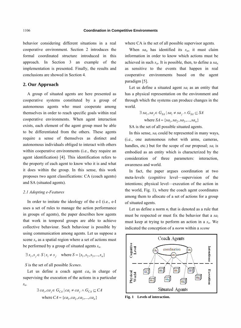
Coordination in Competitive Environments
1106
behavior considering different situations in a real
cooperative environment. Section 2 introduces the
formal coordinated structure introduced in this
approach. In Section 3 an example of the
implementation is presented. Finally, the results and
conclusions are showed in Section 4.
2. Our Approach
A group of situated agents are here presented as
cooperative systems constituted by a group of
autonomous agents who must cooperate among
themselves in order to reach specific goals within real
cooperative environments. When agent interaction
exists, each element of the agent group must be able
to be differentiated from the others. These agents
require a sense of themselves as distinct and
autonomous individuals obliged to interact with others
within cooperative environments (i.e., they require an
agent identification) [4]. This identification refers to
the property of each agent to know who it is and what
it does within the group. In this sense, this work
proposes two agent classifications: CA (coach agents)
and SA (situated agents).
2.1 Adopting e-Features
In order to imitate the ideology of the e-I (i.e., e-I
uses a set of rules to manage the action performance
in groups of agents), the paper describes how agents
that work in temporal groups are able to achieve
collective behaviour. Such behaviour is possible by
using communication among agents. Let us suppose a
scene sα as a spatial region where a set of actions must
be performed by a group of situated agents sα.
},...,,,{where|, 321 njiji ssssSssSss
S is the set of all possible Scenes.
Let us define a coach agent caα in charge of
supervising the execution of the actions in a particular
sα.
CAGcacaGcaca CAjiCAji |,
},...,,,{where 321 ncacacacaCA
where CA is the set of all possible supervisor agents.
When saα has identified its s, it must claim
information in order to know which actions must be
achieved in such s. It is possible, then, to define a saα
as sensitive to the events that happen in real
cooperative environments based on the agent
paradigm [5].
Let us define a situated agent sai as an entity that
has a physical representation on the environment and
through which the systems can produce changes in the
world.
SAGsasaGsasa SAjiSAji |,
},...,,,{where 321 nsasasasaSA
SA is the set of all possible situated agents.
In this sense, sai could be represented in many ways,
(i.e., one autonomous robot with arms, cameras,
handles, etc.) but for the scope of our proposal; sai is
embodied as an entity which is characterized by the
consideration of three parameters: interaction,
awareness and world.
In fact, the paper argues coordination at two
meta-levels (cognitive level—supervision of the
intentions; physical level—execution of the action in
the world, Fig. 1), where the coach agent coordinates
among them to allocate of a set of actions for a group
of situated agents.
Let us define a norm ni that is denoted as a rule that
must be respected or must fix the behavior that a sai
must keep at trying to perform an action in a sα. We
indicated the conception of a norm within a scene
Fig. 1 Levels of interaction.

Coordination in Competitive Environments
1107
following a set of rules such that:
if (ni) do/dont {action}
NsNnnsNnn jiji )(|)(,
},...,,,{)(where 321 annnnsN
Let us define an obligation obl as the imposition
given to some sai to perform some action, which it is
established following a set of rules. In order to denote
the notion of obligation obl the predicate [3] is present
as follows:
),,( spaobl i
where a sai is obligated to do in sα.
2.2 Cooperative Actions
Studies about which actions are involved in
determine scene are needed to perceive knowledge
that make possible the organization of any determined
scene. Once a coach knows in which scene it will
develop its function, it must identify the goals to be
accomplished in such spatial region, indicate the tasks
that must be performed to achieve these goals, and
what roles are necessary for the task achievement.
Then, a coach is defined in its knowledge base
KB(caα) by the consideration of a set of goals G, a set
of tasks T and a set of roles R.
)()()()( sRsTsGcaKB
where )( saKB is the information of all the issues
regarding to a specific scene sα, such that: )( sG is
the set of goals, )( sT is a set of all tasks, and )( sR
is the set of all roles involved in determined scene sα.
Indeed, it is necessary to propose a priority index pi
that represents the importance of every action. A saα
will know both the order in which the goals and the
tasks must be performed and the order of the role
allocation process regarding its supervised sα. Such
priority index will be established according to system
requirements (i.e., timeline) in order to achieve the saα
aims.
Goals then embody the overall system purpose;
however, a caα could achieve a particular goal without
the necessity of performing another goal at the same
sα.
GsGggsGgg jiji )(|)(,
},...,,,{)(where 321 oggggsG
1)(0|)()( )( isGii gpPgpsGg
where G is the set of all possible Goals and )( sG is
gβ involved in sα.
Let us to define a set of tasks T which represent the
issues that must be performed to achieve a specific gβ.
Goal then could be achieved without the implicit
necessity of performing all its involved tasks.
Therefore, the tasks selected are independent, but their
development could affect in a positive or negative
way the development of other tasks.
TsTgTttgTtt jiji )()(|)(,
},...,,,{)(where 321 pttttgT
1)(0|)()( )( igTii tpPtpgTt
where T is the set of all possible Tasks.
Let us define a set of roles R which represent the
actions that a pai must fulfil to perform a tγ within a sα.
RsRtRrrtRrr jiji )()(|)(,
},...,,,{)(where 321 qrrrrtR
1)(0|)()( )( itRii rpPrptRr
where R is the set of all possible Roles.
In order to illustrate how this process is performed,
let us suppose a scene s1 which is supervised by the
coach ca1 performing a decision process to define
which goal must be attended firstly (Fig. 2).
2.3 Embodying Situated Agents
Supposing that a situated agent lives in a real
environment, therefore, it has the ability to consider
Fig. 2 The coach ca1 defines which goal must be performed first.

Coordination in Competitive Environments
1108
its physical representation in such world. Although
these characteristics could supposedly take a lot of
“things” regarding the environment our proposal takes
three kinds of knowledge that seek to reference all the
information that characterize the perception of
particular sai.
2.3.1 Interaction
Interaction I refers to the certainty that an agent
wants to interact with other agents to assume a
specific behavior with successful and high reliability
to achieve any action proposed within any determined
scene. Such information is useful in the interaction
process of the agents because they can trust in other
agents based on the result of their previous
interactions. Obviously, if a sai has a positive
performance of its actions, its interaction level
increases; but if the outcome of the action is negative,
its interaction level decreases. Such knowledge is
obtained when a sai has a direct relationship with a
caα.
)()(, iisrSAi saIsaIGsa
where )(, isr saI
is the interaction level of a sai to
perform rγ in the sα. 2.3.2 Awareness
Awareness A refers to the set of physical
self-knowledge that a physical agent has represented
about its skills and physical characteristics to execute
any proposed action. Such physical representation is
considered as the embodiment of the physical features
that constitute all the information that physical agents
can include in their decision-making.
Physical agents could be any physical objects
“handled” by an intelligent agent (i.e., an autonomous
robot, a machine or an electric device). Such pai has
features that consider their physical body properties
(i.e., their dynamic, their physical structure) usually
when they commit to perform some task or to assume
a specific behaviour within a cooperative environment.
This fact represents the skill of the physical agents to
know that actions will be performed based on the
knowledge of the physical agents’ bodies, which is
achieved through representation of them on a
capabilities basis.
)()(, iisti paApaAPApa
where )(, ist paA
is the Awareness of pai to perform
t in the sα. 2.3.3 World
World W refers to the set of environmental
knowledge that physical agents have to perform the
proposed set of actions. Such domain representation is
considered as the embodiment of the environment
knowledge that represents all the physical information
that has influence in the physical agents’ reasoning
process.
Let us define a set of world conditions that
represent information about empirical knowledge of
the environmental state, such that:
)()(, iisti paWpaWPApa
where )pa(W is,t is the environmental condition of
pai to perform t in a sα; saα uses the above
information to know the physical situation of each pai. All knowledge of a particular pai )pa(KB i is then
constituted by the information provided for the three
modules, such that:
)]()()([)( iiiii paWpaApaIpaKBpa
In particular, all knowledge related to a specific tγ
in sα is given such that:
)]()()([)( ,,,, istististsti paWpaApaIpaKB
2.4 Communication Process
The humans have a communication process that
allows transmit information or ideas in a common
language to make sure and reliable commitments
between us. Likewise, artificial intelligence has
several approaches showing the same process [5-6] to
exploit the advantages of expressing communication.
To accomplish an action, a group of agents must
establish communication (to coordinate them). On
such coordination agents must “converse” among
them to agree who is who within the group (Fig. 3).
Then, a communication with three simple dialogues
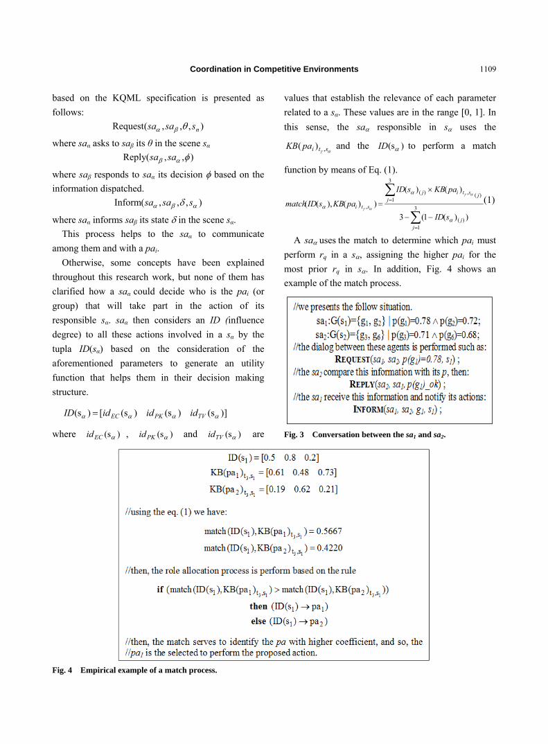
Coordination in Competitive Environments
1109
based on the KQML specification is presented as
follows:
),,,(Request nssasa
where saα asks to saβ its θ in the scene sα
),,(Reply sasa
where saβ responds to saα its decision based on the
information dispatched.
),,,(Inform ssasa
where saα informs saβ its state in the scene sα.
This process helps to the saα to communicate
among them and with a pai.
Otherwise, some concepts have been explained
throughout this research work, but none of them has
clarified how a saα could decide who is the pai (or
group) that will take part in the action of its
responsible sα. saα then considers an ID (influence
degree) to all these actions involved in a sα by the
tupla ID(sα) based on the consideration of the
aforementioned parameters to generate an utility
function that helps them in their decision making
structure.
)]s()s()s([)s( TVPKEC idididID
where )s( ECid , )s( PKid and )s( TVid are
values that establish the relevance of each parameter
related to a sα. These values are in the range [0, 1]. In
this sense, the sa responsible in s uses the
stipaKB ,)( and the )s( ID to perform a match
function by means of Eq. (1).
))(1(3
)()(
))(),((3
1)(
3
1)(,)(
,
jj
jjstij
sti
sID
paKBsID
paKBsIDmatch
(1)
A sa uses the match to determine which pai must
perform rq in a s, assigning the higher pai for the
most prior rq in s. In addition, Fig. 4 shows an
example of the match process.
Fig. 3 Conversation between the sa1 and sa2.
Fig. 4 Empirical example of a match process.

Coordination in Competitive Environments
1110
2.5 Decision Algorithm
An important criterion for the development of
collective actions within real cooperative
environments is the traffic of the information available
from the perception of the intentions to the execution
of them. We have therefore determined a particular
decision algorithm of four simple stages.
Stage 1. Refers to the property of a saα to perceive
which sα must manage, therefore, a saα then knows its
goals, tasks, roles (the priority of every item is also
perceived) and ID involved in its sα. Hence, the
knowledge base of each saα could be achieved.
Stage 2. All the sa (of the entire SA) must organize
them to define which will be the order in that they
could begin the recruitment of pa to perform the
actions within its sα. For thus, the sa must converse
among them using the developed dialog.
Stage 3. Based on the order obtained above, a saα is
approved to start the communication with the entire
PA to determine that pai will be the selected to
perform every action. For thus, a saα must obtain the
physical knowledge of each pai by means of directly
communication with them; the environment
conditions and trust value of each pai are obtained
when the saα uses the modules aforementioned
(respectively for each parameter). Once a saα completes the )pa(KB i of the entire PA,
it takes such information to perform the match using
the Eq. (1), considering the priority index of all the
roles. Then, saα has a list detailed (form higher to
lowest coefficient) of the entire PA. After, saα knows
that pai must perform that role; therefore, it is able to
obligate a determined pai to perform a role which
represents that action must be performed.
Hence, the best pai (of the entire PA) will choose
the prior role to perform and then others successively,
until all the roles finish in such sα. Such process
guaranty allocates us a suitable role because the rq
always allocated to the best pai. Indeed, a saα knows
how many PA needs because it needs the same
amount of PA, such as R(sα). Suppose that the system
has enough amount of PA to take all the defined roles.
To know, every saα is able to exclude a pai that
presents a lowest action capability.
Stage 4. Show-time. A pai knows the rq that must
perform. This involves physical changes in the
environment. Now, the environment has been
modified. So, a new consensus among the SA could be
performed to adjust it to the current changes in the
environment.
3. Implementation
In our implementation, each physical agent has a
different movement controller which differentiates
from others. Then, we have segmented the scenario
into three spatial regions (Fig. 5) to represent each sα.
For sake of simplicity, we only have defined one
goal per scene G(s1) = g1; G(s2) = g2 and G(s3) = g3.
The consensus to define the execution order of the
scenes is derived as as shown in Fig. 6.
The cbp is the current ball position on the
environment. So, the spatial regions are limited
according to the simulator dimensions (axis x: [0 220];
Fig. 5 Geographic segmentation of the experimental environment.
Fig. 6 Supervisor agent consensus.

Coordination in Competitive Environments
1111
axis y: [0 180]). Moreover, specific tasks are defined
in order to accomplish each gi such that:
},{)( },{)(},{ 653432211 ttg Tttg Ttt)T(g
where t1 is make-pass, t2 is shooting, t3 is player-on, t4
is kick-ball, t5 is protect-ball and t6 is covering a
position.
Following the rule presented for the goals, the tasks
also use the cbp as a reference to determine its
execution order.
Then, using the ranges above, a saα may decide the
task to perform at any time. But, to attempt to achieve
such tasks a saα must define which roles it must
perform and the priority order of such roles. Therefore,
by means of human analysis we have proposed four
roles that could be used to perform any task such that:
},,,)(t 4321 rrrrR
where, r1 goes to the ball, r2 kicks the ball, r3 covers a
zone and r4 takes a position to be used in each t.
In addition, we have performed a combination with
the information involved in the environment-based
knowledge. Such combination is used by saα to
perform the match process considering the
aforementioned parameters. Then, a binary
combination lets us generate eight influence degrees
(Table 1). We present a review to show how we have
implemented these parameters in the robot soccer
testbed.
Interaction here called Trust TV represents the
social relationship among agents taking into account
the result of past interactions of a sa with a pai. Eq.
(2) shows the trust calculation if the aim is reached.
Otherwise, using Eq. (3) shows the trust calculation if
the aim is not reached.
)2(),()()( ,, sApatvpatv istist
)3(),()()( ,, sPpatvpatv istist
where the ]1,0[)(, ist patv
and higher )(, ist patv
represents the best pai to perform t in s, ),( sA
and ),s(P are the awards and punishments given
in s respectively and is from 1 to )( sQ and ω is
from 1 to )(' sQ ; that are the number of awards and
punishments in s.
Awareness here called Physical Knowledge, PK
represents the knowledge of the agents about their
physical capabilities to perform any proposed task. In
particular, the introspection process is performed by
using neural networks taking into account the
knowledge that a pai has related to perform t in sα.
Consider that a high ]1,0[)(, ist paPK
by
representing a suitable pai.
World here called Environmental Conditions, EC is
a value related to the distance between the current
location of a pai and the location of the ball. Eq. (4)
shows the calculation: ,
,
( ) (1 ( , ( , ))
/ max(( )) ( ) [0,1]
y a
y a i
t s i i y a
a t s
ec pa d pa r t s
d s ec pa
(4)
where )(, ist paec
is the value of a pai to perform a
tγ in s; )),(,( strpad i is the distance between the
pai with ),( str and )max( sd is the maximal
distance of all pa in s. Then, Eq. (5) shows the )smax(d calculation where m is the total number of
pa in IAS. max( ) max( (1, ),..., ( , )) max [0, 1]a a ad s d s d m s d
(5) In order to show how our approach performs the
role allocation process we present a possible situation
(Fig. 7) where the ball is within the s2 and we use all
Table 1 Influence degree consideration (0: is not considered; 1: is considered).
Influence degree TV PK EC
ID0 0 0 0
ID1 0 0 1
ID2 0 1 0
ID3 0 1 1
ID4 1 0 0
ID5 1 0 1
ID6 1 1 0
ID7 1 1 1
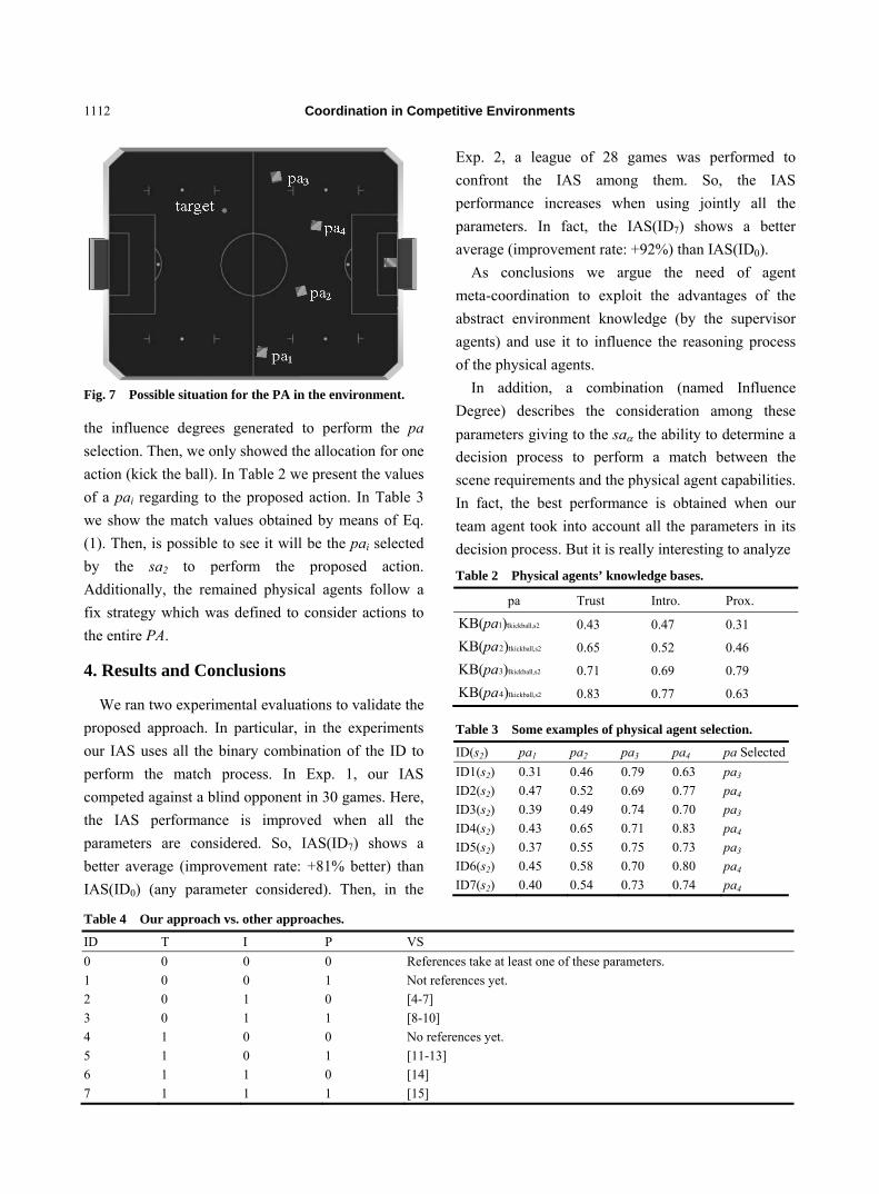
Coordination in Competitive Environments
1112
Fig. 7 Possible situation for the PA in the environment.
the influence degrees generated to perform the pa
selection. Then, we only showed the allocation for one
action (kick the ball). In Table 2 we present the values
of a pai regarding to the proposed action. In Table 3
we show the match values obtained by means of Eq.
(1). Then, is possible to see it will be the pai selected
by the sa2 to perform the proposed action.
Additionally, the remained physical agents follow a
fix strategy which was defined to consider actions to
the entire PA.
4. Results and Conclusions
We ran two experimental evaluations to validate the
proposed approach. In particular, in the experiments
our IAS uses all the binary combination of the ID to
perform the match process. In Exp. 1, our IAS
competed against a blind opponent in 30 games. Here,
the IAS performance is improved when all the
parameters are considered. So, IAS(ID7) shows a
better average (improvement rate: +81% better) than
IAS(ID0) (any parameter considered). Then, in the
Exp. 2, a league of 28 games was performed to
confront the IAS among them. So, the IAS
performance increases when using jointly all the
parameters. In fact, the IAS(ID7) shows a better
average (improvement rate: +92%) than IAS(ID0).
As conclusions we argue the need of agent
meta-coordination to exploit the advantages of the
abstract environment knowledge (by the supervisor
agents) and use it to influence the reasoning process
of the physical agents.
In addition, a combination (named Influence
Degree) describes the consideration among these
parameters giving to the sa the ability to determine a
decision process to perform a match between the
scene requirements and the physical agent capabilities.
In fact, the best performance is obtained when our
team agent took into account all the parameters in its
decision process. But it is really interesting to analyze
Table 2 Physical agents’ knowledge bases.
pa Trust Intro. Prox.
kickball,s21 tKB( )pa 0.43 0.47 0.31
kickball,s22 tKB( )pa 0.65 0.52 0.46
kickball,s23 tKB( )pa 0.71 0.69 0.79
kickball,s24 tKB( )pa 0.83 0.77 0.63
Table 3 Some examples of physical agent selection.
ID(s2) pa1 pa2 pa3 pa4 pa Selected
ID1(s2) 0.31 0.46 0.79 0.63 pa3
ID2(s2) 0.47 0.52 0.69 0.77 pa4
ID3(s2) 0.39 0.49 0.74 0.70 pa3
ID4(s2) 0.43 0.65 0.71 0.83 pa4
ID5(s2) 0.37 0.55 0.75 0.73 pa3
ID6(s2) 0.45 0.58 0.70 0.80 pa4
ID7(s2) 0.40 0.54 0.73 0.74 pa4
Table 4 Our approach vs. other approaches.
ID T I P VS
0 0 0 0 References take at least one of these parameters.
1 0 0 1 Not references yet.
2 0 1 0 [4-7]
3 0 1 1 [8-10]
4 1 0 0 No references yet.
5 1 0 1 [11-13]
6 1 1 0 [14]
7 1 1 1 [15]

Coordination in Competitive Environments
1113
how the cooperative IAS performance increases when
the system takes the parameters into consideration. In
conclusion, the situation matching approach is a
promising method to be used as utility function
between task requirements and physical agent
capabilities in MAS.
In Table 4 we show some approaches regarding
architecture for multi-agent cooperation. In particular,
these architectures express behavior by implementing
different kinds of knowledge, which can be related to
our approach.
References
[1] S. Ibarra, C. Quintero, J. A.Ramon, J. Ll de la Rosa, J. Castan, PAULA: Multi-agent Architecture for coordination to intelligent agent systems, in: Proc. of European Control Conference (ECC’07), Kos, Greece, July 2-5, 2007.
[2] D. Jung, A. Zelinsky, An architecture for distributed cooperative-planning in a behaviour-based multi-robot system, Journal of Robotics & Autonomous Systems (RA&S) 26 (1999) 149-174.
[3] M. Esteva, J.A. Rodriguez, C. Sierra, J.L. Arcos, On the formal specification of electronic institutions, Agent Mediated Electronic Commerce Lecture Notes in Computer Science 1991 (2001) 126-147.
[4] B. Duffy, Robots social embodiment in autonomous mobile robotics, Int. J. of Advanced Robotic Systems 1 (2004) 155-170.
[5] S. Russell, P. Norving, Artificial Intelligence: A Modern Approach, 3rd ed., Ed. Prentice Hall, London, Dec. 2009, p. 1152.
[6] M. Luck, P. McBurney, O. Shehory, S. Willmott, Agent Technology: Computing as Interaction (A Roadmap for Agent Based Computing), AgentLink, 2005.
[7] A. Oller, DPA2: Architecture for co-operative dynamical
physical agents, Doctoral Thesis, Universitat Rovira I Virgil.
[8] C.G. Quintero, J. Ll. de la Rosa, J. Vehi, Self-knowledge based on the atomic capabilities concept—A perspective to achieve sure commitments among physical agents, in: 2nd International Conference on Informatics in Control Automation and Robotics, Barcelona, Spain, Sep. 14-17, 2005.
[9] L. Pat, An adaptative architecture for physical agents, in:
IEEE /WIC/ACM International Conference on Intelligent
Agent Technology, Sep. 19-22, 2005 pp. 18-25.
[10] D. Busquets, R. Lopez de Mantaras, C. Sierra, T.G.
Dietterich, A multi-agent architecture integrating learning
and fuzzy techniques for landmark-based robot
navigation, Lecture Notes in Comp. Science 2504 (2002)
269-281.
[11] C.G. Quinero, J. Zubelzu, J.A. Ramon, J. Ll. de la Rosa,
Improving the decision making structure about
commitments among physical intelligent agents in a
collaborative world, in: In. Proc. of V Workshop on
Physical Agents, Girona, Spain, Mar. 25-27, 2004, pp.
219-223.
[12] R.S. Aylett, D.P. Barnes, A Multi-robot architecture for
planetary rovers, in: 5th ESA Workshop on Advanced
Space Technologies for Robotics and Automation,
ESTEC, Noordwijk, The Netherlands, Dec. 1-3, 1998.
[13] R. Simmons, T. Smith, M. Bernardine, D. Goldberg, D.
Hershberger, A. Stentz, et al., A layered architecture for
coordination of mobile robots, in: Multi-robot Systems:
From Swarms to Intelligent Automata, May, 2002.
[14] C.G. Quintero, J.L. de la Rosa, J. Vehi, Physical Intelligent Agents’ Capabilities Management for Sure Commitments in a Collaborative World, Frontier in Artificial Intelligence and Applications, IOS Press, 2004, pp. 251-258.
[15] S. Ibarra, C. Quintero, J. Ramon, J.L. De la Rosa, J. Castan, Studies about multi-agent teamwork coordination in the robot soccer environment, in: Proc. of 11th Fira Robot World Congress 2006, 2006, pp. 63-67.
Journal of Communication and Computer 10 (2013) 1114-1119
Logistics Customer Segmentation Modeling on Attribute
Reduction and K-Means Clustering
Youquan He and Qianqian Zhen
Department of Information Science & Engineering, Chongqing Jiaotong University, Chongqing 400074, China
Received: June 27, 2013 / Accepted: July 30, 2013 / Published: August 31, 2013.
Abstract: To develop logistics customers’ potential demands for logistics services, and raise the level of logistics enterprise services, the research for customer segmentation has become a primitive work of logistics enterprises in order to run a differentiated customers’ marketing. Through the use of clustering algorithm, this paper presented a segmentation modeling for differentiating customers in logistics industry. Firstly, based on attribute reduction, redundant properties were simplified in the complex data mining under variable parameters in order to improve the quality and efficiency of the modeling, and then the customer segmentation model was constructed through unsupervised clustering K-Means algorithm. It was verified that the logistics users have the obvious differentiation of characteristics by using the cluster model. And a logistics enterprise achieved significant benefits with application of the model in the differentiated data service marketing.
Key words: Customer segmentation, PCA, rough set, K-Means, logistics enterprise.
1. Introduction
Customers are one of the most important resources
of an enterprise, customer retention and satisfaction
drive enterprise profits. With the development of the
internet, the market competition intensifies, customers
become more and more diversified. To better identify
customers, allocate limited enterprise resources and
improve core competitiveness, it is important to do
customer segmentation. Customer segmentation is the
key to successful customer retention. After years of
development, the theory and methods of customer
segmentation are constantly improved. It also has
been used in differentiated marketing in various
industries, such as banking business [1],
telecommunications industry [2], retail business [3],
securities business [4], aviation industry [5] and some
other data-intensive industries. However, it is less
used in logistics industry.
Corresponding author: Youquan He, Ph.D., professor,
research fields: information processing and data mining. E-mail: [email protected].
With the development of logistics informatization,
many logistics enterprises have a lot of information
systems, and also accumulated a large amount of data.
Traditional methods of customer segmentation are not
strong enough to deal with increased enterprise data
and more complicated customer segmentation. The
appearance and development of the data mining
technology makes it possible to find new solutions for
big data based and complicated customer
segmentation cases. Clustering algorithm is one of the
most important data mining algorithms [6].Therefore,
this paper presented a segmentation modeling for
differentiating customers in logistics industry through
the use of clustering algorithm.
2. Problem Description and Analysis
2.1 Problem Description
Customer segmentation is the basis of differentiated
management and improving the level of logistics
service for logistics enterprises. The problem
descriptions of customer segmentation like this:
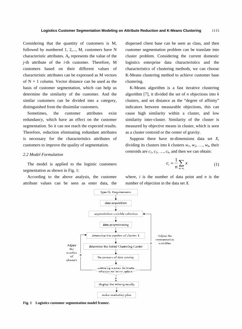
Logistics Customer Segmentation Modeling on Attribute Reduction and K-Means Clustering
1115
Considering that the quantity of customers is M,
followed by numbered 1, 2,..., M, customers have N
characteristic attributes. Aij represents the value of the
j-th attribute of the i-th customer. Therefore, M
customers based on their different values of
characteristic attributes can be expressed as M vectors
of N × 1 column. Vector distance can be used as the
basis of customer segmentation, which can help us
determine the similarity of the customer. And the
similar customers can be divided into a category,
distinguished from the dissimilar customers.
Sometimes, the customer attributes exist
redundancy, which have an effect on the customer
segmentation. So it can not reach the expected results.
Therefore, reduction eliminating redundant attributes
is necessary for the characteristics attributes of
customers to improve the quality of segmentation.
2.2 Model Formulation
The model is applied to the logistic customers
segmentation as shown in Fig. 1:
According to the above analysis, the customer
attribute values can be seen as enter data, the
dispersed client base can be seen as class, and then
customer segmentation problem can be translate into
cluster problem. Considering the current domestic
logistics enterprise data characteristics and the
characteristics of clustering methods, we can choose
K-Means clustering method to achieve customer base
clustering.
K-Means algorithm is a fast iterative clustering
algorithm [7], it divided the set of n objections into k
clusters, and set distance as the “degree of affinity”
indicators between measurable objections, this can
cause high similarity within a cluster, and low
similarity inter-cluster. Similarity of the cluster is
measured by objective means in cluster, which is seen
as a cluster centroid or the center of gravity.
Suppose there have m-dimensions data set X,
dividing its clusters into k clusters w1, w2, …, wk, their
centroids are c1, c2, …, ck, and then we can obtain:
1
i
ix w
c xn
(1)
where, i is the number of data point and n is the
number of objection in the data set X.
Fig. 1 Logistics customer segmentation model framer.

Logistics Customer Segmentation Modeling on Attribute Reduction and K-Means Clustering
1116
Attribute reduction is one of core contents in the
rough set theory [8]. It is the transformation of
high-dimensional data into a meaningful
representation of reduced dimensionality that
corresponds to the intrinsic dimensionality of the data
[9]. There have two basic conceptions in attribute
reduction: reduct and core.
Suppose RS is the gens relation of equivalence, R
∈ RS, If ind(RS) = ind(RS – {R}), then we can say R
is unnecessary in RS; conversely, we can say R is
necessary in RS. If every R ∈ RS are necessary in R
∈ RS, then we call Rs is independent; or they are
dependent, and can make reduction. If PS and Qs are
independent, and ind(QS) = ind(PS), then we can say
QS is one of reductions of PS. The set of all necessary
relationship in PS are being called the core of PS,
which is signed as core(PS).
3. Solution Algorithm
3.1 Attribute Reduction Used for Raw Data
Suppose U is the whole data field, Ui is the i-th
element in U, i ∈ 1, 2, 3, …, M; Aj is the j-th
attribute in U, j ∈ 1, 2, 3, …, N; Sij is the attribute
value corresponds to the i-th element, j-th attribute.
According to a specific problem, the importance of
each attribute is not the same, and also different in the
decision making. Therefore, this paper achieves
attribute reduction through calculating the importance
of the attribute. As shown below, it is the calculation
steps of attribute importance.
Algorithm: calculation of attribute importance;
Input: the attributes used for calculation of attribute
importance, and information systems;
Output: the scores of each attribute importance in
information systems;
Begin
(1) calculating core(RS) , RsR , calculating
Rs RR s Rs RR s R
R s R s
DR s R s1
R s
C ard Posr rSig
r C ard Pos D
,
all of the Sig attribute value which is greater than zero
constitute core(Rs), it may be ¢;
(2) Red(Rs) ← Core(Rs);
(3) Estimating whether ind(Red(Rs)) is equal to
ind(Rs). If they are equal, go to step 6; otherwise go to
step 4; (4) Calculating all of the SigRed(Rs)(R) value , R ∈
Rs – Red(RS), R1 accords with:
1 maxRED Rs RED RR Rs RED Rs
Sig R Sig R
(2)
(5) Red(RS) ← Red(RS)∪{R1}, go to step 3.
(6) Output minimum reduction Red(RS).
End
3.2 To Achieve K-Means Clustering Algorithm
The target of K-Means clustering: the data set is
divided into k clusters according to the specified
parameter k. Its core steps are as follows:
(1) Specified the cluster number k and the initial
clustering center;
(2) Cluster according to the principle of the closest;
(3) Redefining k classes centers.
Support i = i + 1, recalculate k classes centers using
Eq. (1), preparing for further iterations.
(4) Determine whether the clustering termination
condition is satisfied.
Calculating 2
i
k
ii p c
E p c
, if 1E i E i is
satisfied, K-Means algorithm is ended, otherwise go
to step 2, operation will continue.
The flow of K-Means algorithm as follows:
Algorithm: K-Means (S, k), S = {x1, x2,…,xn}
Input: n data object collection xi
Output: k cluster centers Zj, and k cluster data object
collection Cj
Begin
m = 1
initial k prototype Zj, j ∈ [1, k]
repeat
for i = 1 to n do
computer D(xi, zj) = ︱xi – zj︱
if D(xi, zj) = min{D(xi, zj)} then xi ∈ Cj
end
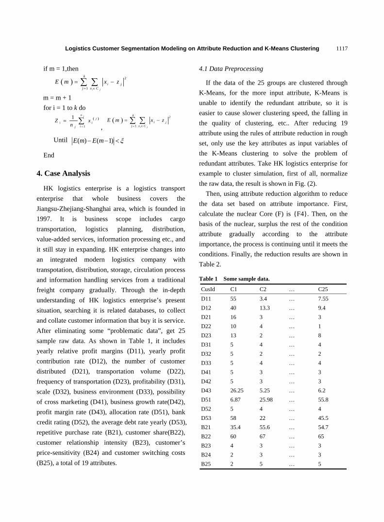
Logistics Customer Segmentation Modeling on Attribute Reduction and K-Means Clustering
1117
if m = 1,then
2
1 i j
k
i jj x C
E m x z
m = m + 1
for i = 1 to k do
1
1 jnj
i iij
Z xn
,
2
1 i j
k
i jj x C
E m x z
Until ( ) ( 1)E m E m
End
4. Case Analysis
HK logistics enterprise is a logistics transport
enterprise that whole business covers the
Jiangsu-Zhejiang-Shanghai area, which is founded in
1997. It is business scope includes cargo
transportation, logistics planning, distribution,
value-added services, information processing etc., and
it still stay in expanding. HK enterprise changes into
an integrated modern logistics company with
transpotation, distribution, storage, circulation process
and information handling services from a traditional
freight company gradually. Through the in-depth
understanding of HK logistics enterprise’s present
situation, searching it is related databases, to collect
and collate customer information that buy it is service.
After eliminating some “problematic data”, get 25
sample raw data. As shown in Table 1, it includes
yearly relative profit margins (D11), yearly profit
contribution rate (D12), the number of customer
distributed (D21), transportation volume (D22),
frequency of transportation (D23), profitability (D31),
scale (D32), business environment (D33), possibility
of cross marketing (D41), business growth rate(D42),
profit margin rate (D43), allocation rate (D51), bank
credit rating (D52), the average debt rate yearly (D53),
repetitive purchase rate (B21), customer share(B22),
customer relationship intensity (B23), customer’s
price-sensitivity (B24) and customer switching costs
(B25), a total of 19 attributes.
4.1 Data Preprocessing
If the data of the 25 groups are clustered through
K-Means, for the more input attribute, K-Means is
unable to identify the redundant attribute, so it is
easier to cause slower clustering speed, the falling in
the quality of clustering, etc.. After reducing 19
attribute using the rules of attribute reduction in rough
set, only use the key attributes as input variables of
the K-Means clustering to solve the problem of
redundant attributes. Take HK logistics enterprise for
example to cluster simulation, first of all, normalize
the raw data, the result is shown in Fig. (2).
Then, using attribute reduction algorithm to reduce
the data set based on attribute importance. First,
calculate the nuclear Core (F) is {F4}. Then, on the
basis of the nuclear, surplus the rest of the condition
attribute gradually according to the attribute
importance, the process is continuing until it meets the
conditions. Finally, the reduction results are shown in
Table 2.
Table 1 Some sample data.
CusId C1 C2 … C25
D11 55 3.4 … 7.55
D12 40 13.3 … 9.4
D21 16 3 … 3
D22 10 4 … 1
D23 13 2 … 8
D31 5 4 … 4
D32 5 2 … 2
D33 5 4 … 4
D41 5 3 … 3
D42 5 3 … 3
D43 26.25 5.25 … 6.2
D51 6.87 25.98 … 55.8
D52 5 4 … 4
D53 58 22 … 45.5
B21 35.4 55.6 … 54.7
B22 60 67 … 65
B23 4 3 … 3
B24 2 3 … 3
B25 2 5 … 5

Logistics Customer Segmentation Modeling on Attribute Reduction and K-Means Clustering
1118
Fig. 2 Discretization of data set.
Table 2 Data reduction.
X1 X2 X3
C1 0.70985 0.62773 -1.47345
C2 0.12587 0.07789 0.99645
C3 0.62016 -1.62654 0.52526
C4 1.34267 0.64071 -0.3608
C5 0.10486 1.32636 -1.09793
C6 -0.79073 -0.6545 1.77739
C7 -0.70061 0.91469 0.4336
C8 -0.96809 -1.07615 -0.50857
C9 -1.83022 0.21416 -0.459
C10 0.05782 -0.78809 -1.17345
C11 -1.48158 -0.07978 -0.09249
C12 0.04591 0.32934 0.81276
C13 -0.8961 -0.2026 -1.16839
C14 -1.04842 -1.41836 -0.7961
C15 1.63087 0.26136 -0.30325
C16 -0.44634 1.06685 0.39702
C17 0.2321 -1.69705 1.27427
C18 -1.20336 1.40651 -1.40786
C19 0.30905 -1.38533 -0.07175
C20 0.00047 0.04238 1.28661
C21 1.48548 -0.90059 -0.78134
C22 1.72006 1.23757 0.98059
C23 1.4249 -0.24336 -1.17173
C24 -0.3348 1.76434 1.37100
C25 -0.10979 0.16244 1.01117
4.2 The Results of Cluster Analysis
Calculate the data on Table 3 by K-Means
clustering computing, the experiment results are
obtained as shown in Table 3.
Table 3 shows the clustering result of each
customer. Compared with HK logistics enterprise’s
customer segmentation results gained from the ABC
classification method, we can find some changes of
the following:
For example, the customer C22, it is placed on the
second category in the original subdivision which is
placed on the first category. C4 and C18 are placed on
the worst category in the original subdivision which
are placed on the third and the second. C1 and C12 are
placed on the first category in the original subdivision
which are placed on the third and fourth. There is a
big difference between the company only measure
each customer in accordance with the customer’s
current value and the method used in this paper. The
former method only considered the customer’s current
value, but customer’s development potential and
relationships are not been considered. This method is

Logistics Customer Segmentation Modeling on Attribute Reduction and K-Means Clustering
1119
Table 3 Customer segmentation results.
Category Customer ID
1 C1、C4、C15、C21、C23
2 C8、C9、C10、C11、C13、C14
3 C22
4 C5、C7、C16、C18、C24
5 C2、C3、C6、C12、C17、C19、C20、C25
Table 4 Comparison of result.
The number of attribute
The total error rate (%)
K-Means 19 12.09
RS-K-Means 3 5.24
easy to cause enterprises are unable to identify
valuable customers. We can solve this problem
through the latter method. In customer segmentation
issues, the latter method is more reasonable than the
previous method.
As shown in Table 4, after attribute reduction
processed data the results are even better. This proves
that the proposed methods and models for HK
enterprises are feasible and effective.
5. Conclusions
Many indicators, redundant attributes are the
characteristics of the logistics enterprise data.
Attribute reduction based clustering method
mentioned in this paper could eliminate redundant
attributes, improve the quality of clustering.
Instantiated with HK logistics enterprises have proved
the effectiveness of the method. Customers fine
classification is based on the customer attributes
classified feature class. This method is conducive to
the logistics enterprises to change the business model,
extensive change management as differentiated
marketing, improve competitiveness; manage
customers based on customer demand, and allocate
service resources reasonable.
References
[1] X. Li. Establishment and application of commercial bank customer segmentation model, Statistics and Decision 9
(2008) 144-146.
[2] H. Ahn, J.J. Ahn, K.J. Oh, D.H. Kim, Facilitating
cross-selling in a mobile telecom market to develop
customer classification model based on hybrid data
mining techniques, Expert Systems with Applications 38
(2011) 5005-5012.
[3] V.L. Migueis, A.S. Camanho, J.F. Cunha, Customer data
mining for lifestyle segmentation, Expert Systems with
Applications 39 (2012) 9359-9366.
[4] Y. Wang, The securities industry customer segmentation
model building and empirical research, ShangHai
Management Science 34 (2012) 30-35.
[5] J.J.H. Liou, G.H. Tzeng, A dominance-based rough set
approach to customer behavior in the airline market,
Information Science 180 (2010) 2230-2238.
[6] M. Bottcher, M. Spott, D. Nauck, R. Kruse, Mining
changing customer segments in dynamic markets, Expert
Systems with Applications 36 (2009) 155-164.
[7] J.W. Han, M. Kamber, Data Mining Concepts and Techniques, Mechanical Industry Press, Beijing, Mar. 2005, pp. 253-273.
[8] S.S. Hu, Y.Q. He, The Theory and Application of Rough Decision, Beijing University of Aeronautics and Astronautics Press, Beijing, Apr. 2006, pp. 1-12.
[9] R. Dash, R. Dash, D. Mishra, A hybridized rough-PCA approach of attribute reduction for high dimensional data set, European Journal of Scientific Research 44 (2010) 29-38.

Journal of Communication and Computer 10 (2013) 1120-1130
UHF Propagation Parameters to Support Wireless
Sensor Networks for Onboard Trains
B. Nkakanou1, 2, G.Y. Delisle1, 2, N. Hakem1 and Y. Coulibaly1
1. LRTCS-UQAT, Val d’Or, Qc G1V 0A6, Canada
2. Dept. of Electrical Engineering and Computer Engineering, Laval University, Québec G1V 0A6, Canada
Received: July16, 2013 / Accepted: August 7, 2013 / Published: August 31, 2013.
Abstract: This paper reports numerical results for the characterization of the propagation channel in a train. Since the availability of a train to carry out measurements is not always easy, particularly when many changes must be done, a simulation tool provides a useful and reliable mean for the evaluation of the propagation characteristics of this complex and highly fluctuating channel. In order to benefit from previous results, the various existing softwares for complex electromagnetic fields environments simulations were fully searched and one that seems best suited has been retained for these computations. The results presented here are original, preliminaries and our approach provides a basis for study the propagation of waves in a very complex environment consisting of different electromagnetic fields like a train.
Key words: Train, channel propagation, wireless communication, electromagnetic fields, interference.
1. Introduction
Railway transportation has always been one of the
most effective means of transporting passengers and
goods and this being amplified in the last few years.
The passenger numbers has increased progressively
while the volume of goods and equipment increased
significantly. With the passengers and goods
transportation in a modern telecommunication world,
new challenges arise, notably the transmission of
passenger data, sensors data, etc., both for
communications and security purposes.
Wired communications have many drawbacks for
train communication systems (locomotives and
wagons), particularly when a large number of sensors
are in use in many locations. Indeed, most of the
system components must still be connected by cables.
Wireless communications systems in the railway
industry would represent an attractive alternative to
Corresponding author: Nadir Hakem, Ph.D., prof.,
research fields: wireless communications, confined areas, RF characterization and modeling. E-mail: [email protected].
wired and optical fiber communication system but the
reliability of the transmitted and received data must be
secured. Wireless communications systems in train
would allow acquiring information on various physical
parameters of the locomotives (fuel, position, dynamic
load, speed, axle load, wheel flat, etc.), transferring
data to the fixed points of acquisitions (wayside),
warning train drivers of impending dangers,
controlling different wagons and giving the exact
position of the train to the signalers.
Locomotives, wagons and special cars are
constructed mostly of metallic materials such as steel,
copper, aluminum or various alloys that severely
impact signal propagation. Radio waves propagating in
such environments dissipate some of their energy
within the structures and the induced currents generate
EM fields that are reradiated and they therefore alter
the propagation characteristics of the original RF signal.
Wireless communication is generally severely affected
by electromagnetic interferences [1-4].
For a comprehensive evaluation and understanding

UHF Propagation Parameters to Support Wireless Sensor Networks for Onboard Trains
1121
of the main implications of installing wireless
communication system onboard trains, the RF signal’s
propagation characteristics must thoroughly be
analyzed [5-13].
It would be very helpful to characterize the
propagation of electromagnetic fields to ensure the
quality of communications systems, quantify these
electromagnetic fields and then evaluate the most
penalizing electromagnetic noise [1-9].
The fact that our work focuses on the propagation in
an environment where the electromagnetic field
undergoes a lot of variations; the precise
characterization of this environment is crucial [5-13].
One of the aspects that must be considered is also the
communications among different sensors placed at
different locations in the locomotive and cars
[14-19].
Sensing devices must be located very close to the
monitored event sources (such as wheels, brakes,
boxcar doors, refrigerator units, etc.) without impeding
the signal path with obstacles, low ground clearance
and other impairments [14-16].
The objectives of this paper are to present how a
simulation and characterization of the propagation
channel in a train can be handled. The detail of the
procedures and measurement setup used to collect the
data against which simulation results shall be validated
will be reported and discussed in full details as soon as
completed. The strategy and the correct way to process
the acquired data are also explained. Finally, the
relating results to the signal quality, small-scale effects,
large-scale path-loss exponents and time dispersion
parameters are discussed. With the parameters of time
dispersion in particular RMS (root mean square) delay
spread, the coherence bandwidth can thus be
determined.
The paper is organized as follows: in Section 2, the
software environment and simulation setup are
presented. In Section 3, some relevant parameters of
the propagation channel, based on simulation, are
presented. Section 4 presents the conclusions.
2. Setup
For the wave propagation, a 3D ray-tracing tool
based on the UTD (uniform theory of diffraction) and
the theory of GO (geometrical optics) has been used.
The model includes modified Fresnel reflection
coefficients for the reflection and the diffraction, based
on the UTD. One of the major advantages of a 3D
ray-tracing tool is the wideband analysis of the channel.
Also, the frequency selectivity (delay spread) and time
variance (Doppler spread) of the channel can be easily
determined.
2.1 Software and Overview of XGtD
The first step of this study is the simulation of the
radio propagation channel and, for that purpose; a
rigorous simulation is conducted using XGtd®, of
Remcom Inc., a specialized package for EM-Field
simulations [20].
XGtd® is a ray-based electromagnetic analysis tool
for assessing the effects of a vehicle on antenna
radiation, estimating RCS (radar cross section) and
predicting coupling between antennas. This software
also allows us to evaluate the interaction between
electronic circuits and radio waves. Basically, it
simulates the interaction and interrelation between EM
fields and structures, based on classical techniques
such as GO (geometric optics), the UTD (uniform
theory of diffraction), PO (physical optics) and the
MEC (method of equivalent currents).
Performance and memory requirements are less
dependent on the electrical size of objects than full
wave methods. XGtd includes a number of features that
extend the capabilities of ray tracing. These
capabilities provide data suitable for various
applications namely far zone antenna radiation
diagrams for surface-mounted antennas, monostatic or
bistatic RCS, creeping waves diffraction, high-fidelity
field prediction in shadow zones, Doppler for moving
transmitters and receivers, coupling between antennas
and wide range of outputs for predicted EM fields and
channel characteristics [20]. To obtain results that are

UHF Propagation Parameters to Support Wireless Sensor Networks for Onboard Trains
1122
the closest possible to the reality, the available 3D
software environment has been fully exploited in
conjunction with 3D objects. Material properties have
been assigned to each individual component to fully
represent the 3D objects and their properties.
Assigning these properties is critical to the entire
simulation and evaluation process.
2.2 3D Train
In order to simulate with real train data, the Siemens
Velaro platform [21] which is one of the fastest
currently operating high-speed train in the world has
been chosen. High-speed trains of this kind are already
reliably operating in several countries around the world
including Germany, Spain and China. The technical
characteristics of this train are supplied in Table 1 [21].
In our simulations, the data for the train (train
Germany) shown in Fig. 1 has been purchased from
3DcadBrowser [22]. It’s composed of 11,940 polygons,
7,660 vertices, 430 sub-objects and 11 materials with a
length of 24 m.
The 3D model is imported in the simulation software.
This import was made very extensive due to the large
number of materials and polygons of the model. Due to
the difficulty to import the 3D train model, the number
of materials and polygons were reduced. Therefore, in
the simulation process, a maximum of six reflections
on the different faces of the train, two transmissions
and zero diffraction were considered. Due to the large
computation time required in simulation process, the
addition of one single diffraction increases the
computation time by about 18 h. Dipoles antennas at
990 MHz with a bandwidth of 20 MHz and several
transmitters were located within the train. The
receptors were located within and outside of the train.
In our scenarios, the green points represent
transmitters while the red ones are receivers. The
transmission power has been fixed to 0 dBm.
Table 1 Technical characteristics of the train.
Technical data
Maximum speed 320 km/h
Length of train 200 m
Length of end car body 25,535 mm
Length of intermediate car body 24,175 mm
Distance between bogie centers 17,375 mm
Width of cars 2,950 mm
Height of cars 3,890 mm
Track gauge 1,435 mm
Empty weight 439 t
Voltage system 15 / 25 kV AC and 1.5 / 3 kV DC–maximum
Traction power 8,000 kW
Gear ratio 2,62
Starting tractive effort 283 kN
Brake systems Regenerative, eddy-current brake, pneumatic
Number of axles 32 (16 driven)
Wheel arrangement Bo’Bo‘+2‘2‘+Bo’Bo‘+2‘2‘+2‘2‘+Bo’Bo‘+2‘2‘+Bo’Bo‘
Number of bogies 16
Axle load < 17 metric tons
Acceleration 0–320 km/h 380 s
Braking distance 320–0 km/h 3,900 m
Number of cars / train 8
Number of seats 485 / 99 / 386 (total / 1st / 2nd Class)
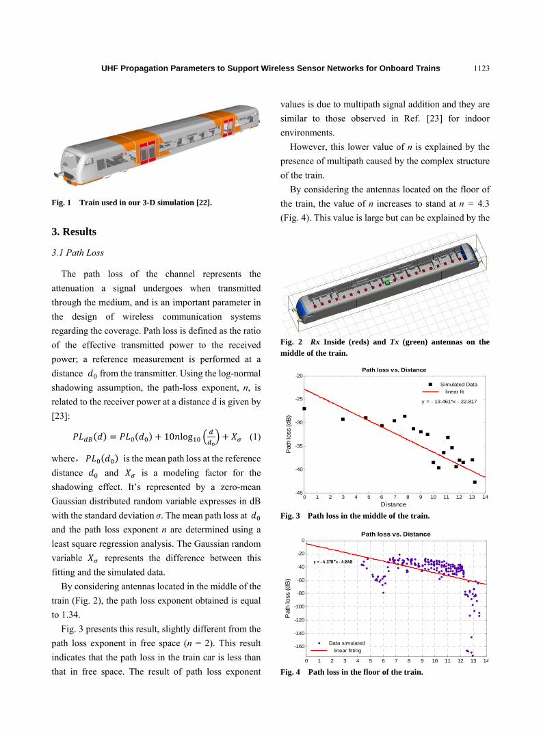
UHF Propagation Parameters to Support Wireless Sensor Networks for Onboard Trains
1123
Fig. 1 Train used in our 3-D simulation [22].
3. Results
3.1 Path Loss
The path loss of the channel represents the
attenuation a signal undergoes when transmitted
through the medium, and is an important parameter in
the design of wireless communication systems
regarding the coverage. Path loss is defined as the ratio
of the effective transmitted power to the received
power; a reference measurement is performed at a
distance from the transmitter. Using the log-normal
shadowing assumption, the path-loss exponent, n, is
related to the receiver power at a distance d is given by
[23]:
10 log (1)
where, is the mean path loss at the reference
distance and is a modeling factor for the
shadowing effect. It’s represented by a zero-mean
Gaussian distributed random variable expresses in dB
with the standard deviation σ. The mean path loss at
and the path loss exponent n are determined using a
least square regression analysis. The Gaussian random
variable represents the difference between this
fitting and the simulated data.
By considering antennas located in the middle of the
train (Fig. 2), the path loss exponent obtained is equal
to 1.34.
Fig. 3 presents this result, slightly different from the
path loss exponent in free space (n = 2). This result
indicates that the path loss in the train car is less than
that in free space. The result of path loss exponent
values is due to multipath signal addition and they are
similar to those observed in Ref. [23] for indoor
environments.
However, this lower value of n is explained by the
presence of multipath caused by the complex structure
of the train.
By considering the antennas located on the floor of
the train, the value of n increases to stand at n = 4.3
(Fig. 4). This value is large but can be explained by the
Fig. 2 Rx Inside (reds) and Tx (green) antennas on the middle of the train.
Fig. 3 Path loss in the middle of the train.
Fig. 4 Path loss in the floor of the train.
0 1 2 3 4 5 6 7 8 9 10 11 12 13 14-45
-40
-35
-30
-25
-20
Distance
Path
loss
(dB
)
Path loss vs. Distance
y = - 13.461*x - 22.817
Simulated Data
linear fit
0 1 2 3 4 5 6 7 8 9 10 11 12 13 14
-160
-140
-120
-100
-80
-60
-40
-20
0
Path
loss
(dB
)
Path loss vs. Distance
y = - 4.376*x - 4.848
Data simulated
linear fitting

UHF Propagation Parameters to Support Wireless Sensor Networks for Onboard Trains
1124
presence of surface waves which introduces
interference.
After obtaining the path loss for a transmitter located
in the middle of the wagon, the impact of this shift on
the transmitter power loss has been evaluated. The
transmitting antenna is placed on the roof of the wagon
in different places (middle and two extremities) as in
Fig. 5 and the data associated therewith has been
recorded.
These have allowed us to trace the path loss as
shown in Fig. 6.
The path loss exponents for receivers located on the
ground are 5.34 and 6.59 for transmitting antennas
located in the middle and at one extremity of the wagon,
respectively.
The position of the sensor is thereby important
because it may have an impact on radio wave
propagation and degrade received signal power in the
wagon. Comparing the path loss exponent of power
loss for transmitters situated in the middle of the wagon,
the losses in the wagon are greater at ground level than
on the edges. In addition, when the transmitting
antennas are located on the roof, these losses are even
more pronounced. Thus, the losses are stronger when
the data from the sensors are collected on the ground
with antennas located on the roof.
3.2 Impulse Response
The impulse response of a system is a useful
characterization of the system. A radio propagation
channel can be completely characterized by its impulse
Fig. 5 Rx Ground (reds) antennas on the ground and Tx roof (green) antennas on the roof of the train.
(a) middle
(b) extremity
Fig. 6 Path loss on the floor of the train.
response. The impulse response of a multipath channel
can be modeled as:
∑ (2)
where, N is the number of multipath components, ,
and are the random amplitude, arrival time and
phase of the kth path, respectively, and δ is the delta
function. The phases are assumed to be statically
independent uniform random variables distributed [23]
over [0, 2π].
The impulses responses are plotted at 21 m (Fig. 7)
then at 10 m (Fig. 8) with Tx roof antenna.
3.3 RMS Delay Spread
The time dispersive properties of broadband
multipath channels are most commonly quantified by
RMS delay spread. RMS Delay spread parameters
highlight the temporal distribution of power relative to
the first components. Delay spreads restrict the
transmitted data rates and could limit the capacity of the
0 2 4 6 8 10 12-120
-100
-80
-60
-40
-20
0
y = - 5.34*x - 9.24
Simulated data
linear fitting
0 2 4 6 8 10 12 14-120
-100
-80
-60
-40
-20
0
y = - 6.593*x - 18.11
Simulated data
Linear fit

UHF Propagation Parameters to Support Wireless Sensor Networks for Onboard Trains
1125
Fig. 7 Impulse response at 21 m.
Fig. 8 Impulse response at 10 m.
system when multi-user systems are considered. The
number of multipath in a train is important due to the
reflection and scattering from the surface, ceiling, side
walls and electromagnetics noises. The best parameter
that allows us to measure multipath is the root mean
square delay spread. This parameter determines the
frequency selectivity of channel, which degrades the
performance of digital communication systems over
radio channels. The RMS delay spread also limits the
maximum data transmission rate that can be transmitted
by the channel. Without using diversity or equalization,
the RMS delay spread is inversely proportional to the
maximum usable data rate of the channel.
The formulation of time dispersion parameters is
given in Ref. [23] by
(3)
where, and are the Mean excess delay and the
second moment of the PDP respectively. The mean
excess delay can be computed as:
∑
∑ (4)
∑
∑ (5)
where, and are the power and delay of the
thk path respectively. It is measured relative to the
first detectable signal arriving at the receiver at 0
Delay spreads over distance was computed and Fig. 9
shows the computed results.
The maximum is obtained at a distance of 15 m
within the wagon and is equal to approximately 14 ns.
In light of this result, it can be concluded that there is no
relation between delay spread and distance as in many
complex environments.
The CDFs of delay spread with transmitter in the
middle of wagon obtained are shown in Fig. 10.
Fig. 11 compares the CDF of the delay spread for the
receiving antennas on the ground and inside the car. On
the ground, the distributtion of delay spread is
completely different from that on the edges or inside the
wagon.
In order to measure impact of the position of
transmitting antennas on signal propagation and also to
know the impact of positioning of the receiving
1 2 3 4 5 6 7 8 9 10 11 12 13 14 15 16 17 18 19 20 21
4
6
8
10
12
14
16
Distance (m)
De
lay
spre
ad
(ns)
Delay spread vs. Distance
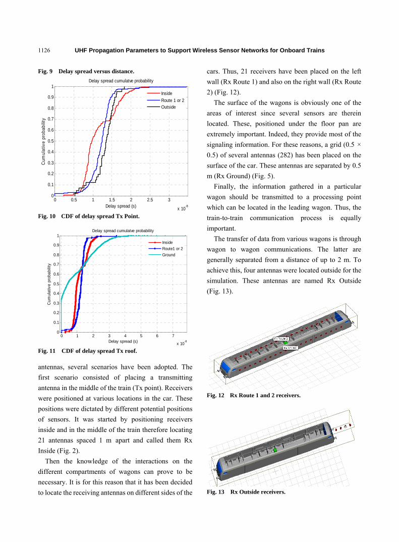
UHF Propagation Parameters to Support Wireless Sensor Networks for Onboard Trains
1126
Fig. 9 Delay spread versus distance.
Fig. 10 CDF of delay spread Tx Point.
Fig. 11 CDF of delay spread Tx roof.
antennas, several scenarios have been adopted. The
first scenario consisted of placing a transmitting
antenna in the middle of the train (Tx point). Receivers
were positioned at various locations in the car. These
positions were dictated by different potential positions
of sensors. It was started by positioning receivers
inside and in the middle of the train therefore locating
21 antennas spaced 1 m apart and called them Rx
Inside (Fig. 2).
Then the knowledge of the interactions on the
different compartments of wagons can prove to be
necessary. It is for this reason that it has been decided
to locate the receiving antennas on different sides of the
cars. Thus, 21 receivers have been placed on the left
wall (Rx Route 1) and also on the right wall (Rx Route
2) (Fig. 12).
The surface of the wagons is obviously one of the
areas of interest since several sensors are therein
located. These, positioned under the floor pan are
extremely important. Indeed, they provide most of the
signaling information. For these reasons, a grid (0.5 ×
0.5) of several antennas (282) has been placed on the
surface of the car. These antennas are separated by 0.5
m (Rx Ground) (Fig. 5).
Finally, the information gathered in a particular
wagon should be transmitted to a processing point
which can be located in the leading wagon. Thus, the
train-to-train communication process is equally
important.
The transfer of data from various wagons is through
wagon to wagon communications. The latter are
generally separated from a distance of up to 2 m. To
achieve this, four antennas were located outside for the
simulation. These antennas are named Rx Outside
(Fig. 13).
Fig. 12 Rx Route 1 and 2 receivers.
Fig. 13 Rx Outside receivers.
0 0.5 1 1.5 2 2.5 3
x 10-8
0
0.1
0.2
0.3
0.4
0.5
0.6
0.7
0.8
0.9
1
Delay spread (s)
Cum
ulat
ive
prob
abili
ty
Delay spread cumulatve probability
Inside
Route 1 or 2Outside
0 1 2 3 4 5 6 7
x 10-8
0
0.1
0.2
0.3
0.4
0.5
0.6
0.7
0.8
0.9
1
Delay spread (s)
Cum
ulat
ive
prob
abili
ty
Delay spread cumulatve probability
Inside
Route1 or 2
Ground
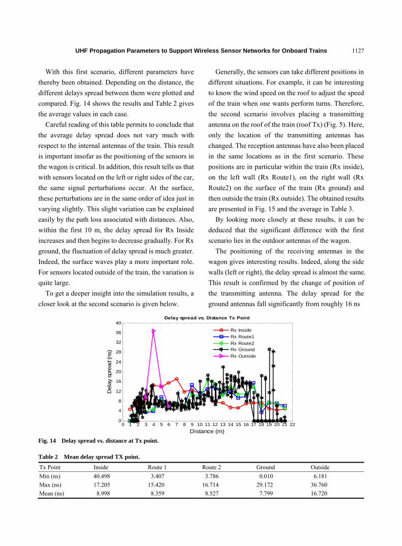
UHF Propagation Parameters to Support Wireless Sensor Networks for Onboard Trains
1127
With this first scenario, different parameters have
thereby been obtained. Depending on the distance, the
different delays spread between them were plotted and
compared. Fig. 14 shows the results and Table 2 gives
the average values in each case.
Careful reading of this table permits to conclude that
the average delay spread does not vary much with
respect to the internal antennas of the train. This result
is important insofar as the positioning of the sensors in
the wagon is critical. In addition, this result tells us that
with sensors located on the left or right sides of the car,
the same signal perturbations occur. At the surface,
these perturbations are in the same order of idea just in
varying slightly. This slight variation can be explained
easily by the path loss associated with distances. Also,
within the first 10 m, the delay spread for Rx Inside
increases and then begins to decrease gradually. For Rx
ground, the fluctuation of delay spread is much greater.
Indeed, the surface waves play a more important role.
For sensors located outside of the train, the variation is
quite large.
To get a deeper insight into the simulation results, a
closer look at the second scenario is given below.
Generally, the sensors can take different positions in
different situations. For example, it can be interesting
to know the wind speed on the roof to adjust the speed
of the train when one wants perform turns. Therefore,
the second scenario involves placing a transmitting
antenna on the roof of the train (roof Tx) (Fig. 5). Here,
only the location of the transmitting antennas has
changed. The reception antennas have also been placed
in the same locations as in the first scenario. These
positions are in particular within the train (Rx inside),
on the left wall (Rx Route1), on the right wall (Rx
Route2) on the surface of the train (Rx ground) and
then outside the train (Rx outside). The obtained results
are presented in Fig. 15 and the average in Table 3.
By looking more closely at these results, it can be
deduced that the significant difference with the first
scenario lies in the outdoor antennas of the wagon.
The positioning of the receiving antennas in the
wagon gives interesting results. Indeed, along the side
walls (left or right), the delay spread is almost the same.
This result is confirmed by the change of position of
the transmitting antenna. The delay spread for the
ground antennas fall significantly from roughly 16 ns
Fig. 14 Delay spread vs. distance at Tx point.
Table 2 Mean delay spread TX point.
Tx Point Inside Route 1 Route 2 Ground Outside
Min (ns) 40.498 3.407 3.786 0.010 6.181
Max (ns) 17.205 15.420 16.714 29.172 36.760
Mean (ns) 8.998 8.359 8.527 7.799 16.720
0 1 2 3 4 5 6 7 8 9 10 11 12 13 14 15 16 17 18 19 20 21 220
4
8
12
16
20
24
28
32
36
40
Distance (m)
Dela
y sp
read (ns)
Delay spread vs. Distance Tx Point
Rx Inside
Rx Route1
Rx Route2Rx Ground
Rx Outside

UHF Propagation Parameters to Support Wireless Sensor Networks for Onboard Trains
1128
Fig. 15 Delay spread vs. distance at Tx roof.
Table 3 Mean delay spread TX roof.
Tx Point Inside Route 1 Route 2 Ground Outside
Min (ns) 2.963 0.036 0.583 0.01 2.311
Max (ns) 17.941 11.868 11.564 33.707 4.595
Mean (ns) 8.275 6.51 6.672 7.108 3.244
to 3 ns. Contrary to the first scenario where the delay
spread increased over the first 10 m Rx inside, it
remains fairly constant here and begins to increase
after the first 10 m. Similarly for side’s antennas, the
delay spread is experiencing growth over a few meters
and then begins to decrease. For ground antennas, the
variation is in the same direction as in the first scenario.
3.4 Coherence Bandwidth
Multipath fading has an important impact on
performance of wireless communications system.
Multipath fading channels are globally classified as flat
fading and frequency-selective fading according to their
coherence bandwidth relative to the bandwidth of
transmitted signal. Coherence bandwidth is defined as
the range of frequencies over which two frequency
components retains a strong amplitude correlation. It is
defined as the range of frequencies over which the
channel can be considered flat. The analytic issue of
coherence bandwidth was first studied by many authors;
they concluded that the coherence bandwidth of a
wireless channel is inversely proportional to its RMS
delay spread. It can be easily computed. The coherence
bandwidth is defined by Ref. [23]:
90%
50% (6)
where, τ denotes the rms delay spread.
These results may allow us to determine the
maximum bandwidth that can be used for
communications in a wagon.
Fig. 16 and Fig. 17 respectively present coherence
bandwidth over distance with Tx point and Tx roof
respectively.
By inspecting these results it is found that when the
transmitting antenna is located on the roof of the car,
Fig. 16 Coherence bandwidth vs. distance at Tx point.
0 1 2 3 4 5 6 7 8 9 10 11 12 13 14 15 16 17 18 19 20 21 22 230
4
8
12
16
20
24
28
32
36
40
Distance (m)
Dela
y sp
read (ns)
Delay spread vs. Distance Tx Toit
Rx InsideRx Route1Rx Route2Rx GroundRx Outside
0 1 2 3 4 5 6 7 8 9 10 1112 13 1415 16 1718 19 2010
15
20
25
30
35
Distance (m)
Coh
enre
nce
Ban
dwid
th (
MH
z)
Inside RxOutside RxRx Route1Rx Route2
Delay spread vs. TxRoof

UHF Propagation Parameters to Support Wireless Sensor Networks for Onboard Trains
1129
Fig. 17 Coherence bandwidth vs. distance at Tx roof.
the coherence bandwidth is relatively constant over the
first 15 m for the receiving antennas situated in the
middle, on the edges of the wagon. The average value
of the coherence bandwidth here is 18.47 MHz. For the
transmitter in the middle of the wagon, the results are
different. The coherence bandwidth varies according to
the distance and fluctuates greatly. With receptors
located in the middle of the wagon, the coherence
bandwidth varies from about 10 MHz to 24 MHz at 1
meter to 4 m. It then drops to 19 MHz to 6 m and rising
to 33 MHz at 9 m. This fluctuation is also observed for
edges antennas. The coherence bandwidth for
train-to-train communications is also determined over
a distance of about 3 m and is plotted in Fig 16 and Fig.
17. Therefore, the location of the sensors inside a
wagon is crucial and knowledge of the proper position
is an important factor not to be neglected in any system
design.
4. Conclusions
A train environment was simulated in order to find
the important propagation parameters and unique
results were found. These results could help to deploy
wireless technologies onboard train for various needs
and especially environmental physical parameters
monitoring.
The path loss exponent is smaller than that in the free
space when the receiving antennas are located at a
convenient distance from the ground. On the contrary,
bringing them the floor, the path loss becomes
significant and this will render it more difficult to
acquire data from sensors located on or under the floor.
The delay spread varies slightly depending on the
distance of the first meters. The delay spread is almost
the same for sensors located along the side walls. These
delays spread allowed us to determine the coherence
bandwidth. The coherence bandwidth which is an
important parameter of a propagation channel was
determined and we noticed that it varies greatly
depending on the position of the receiving antennas.
This would determine the ideal locations for the
receivers.
The positioning of sensors is crucial in data
acquisition and that depends on the needed information.
Acquiring the characteristics of the propagation channel
in a train allows us to find the optimal positions for the
sensors.
For future work, these results obtained will be
compared with physical measurements of the
propagation parameters using actual trains. The
measurement campaign to obtain experimental results
is currently underway. Moreover, the simulation case
of a locomotive, where interference plays a major role,
is another step in the study of signal propagation in a
train. This step is part of the work to be developed in
the future.
Acknowledgments
The authors are deeply indebted to M. Denis Roy of
RDG2, Bromont, Qc, Canada for his special
contribution in our understanding of the behavior and
importance of many sensors onboard trains.
References
[1] H. Sharif, M. Hempel, Study of RF Propagation Characteristics for Wireless Sensor Networks in Railroad Environments [Online], June 2010, A Report on Research, http://matc.unl.edu/assets/documents/finalreports/Sharif_PropagationCharacteristicsWirelessSensorNetworks.pdf.
[2] L. Taehyung, C. Hongsik, K. Seogwon, K. Kihwan, Measurement and analysis of consumption energy for Korean high-speed trains, in: 2012 IEEE PES Innovative Smart Grid Technologies (ISGT), Washington, Jan. 16-20,
0 2 4 6 8 10 12 14 16 18 200
20
40
60
80
100
Distance (m)
Coh
eren
ce b
andw
idth
(M
Hz)
Inside RxOutside RxRx Route1Rx Route2

UHF Propagation Parameters to Support Wireless Sensor Networks for Onboard Trains
1130
2012, pp. 1-5. [3] C. R. Garcia, A. Lehner, T. Strang, K. Frank, Channel
Model for Train to Train Communication Using the 400 MHz Band, in Vehicular Technology Conference, 2008. VTC Spring 2008, Sigapore, May 11-14, 2008, pp. 3082-3086.
[4] L. Chang-Myung, V.N. Goverdovskiy, A.N. Trofymov, V.V. Babenkov, High-speed train and environment: A system concept of multi-stage vibration isolation, in: 2010 International Forum on Strategic Technology (IFOST), Ulsan, Oct. 13-15, 2010, pp. 299-305.
[5] T. Ito, N. Kita, W. Yamada, T. Ming-Chien, Y. Sagawa, M. Ogasawara, Study of propagation model and fading characteristics for wireless relay system between long-haul train cars, in: Proceedings of the 5th European Conference on Antennas and Propagation (EUCAP), Rome, April 11-15, 2011, pp. 2047-2051.
[6] N. Kita, T. Ito, W. Yamada, T. Ming-Chien, Y. Sagawa, M. Ogasawara, Experimental study of path loss characteristics in high-speed train cars, in: Antennas and Propagation Society International Symposium 2009, APSURSI '09, Charleston, June 1-5, 2009, pp. 1-4.
[7] B. Nkakanou, G.Y. Delisle, N. Hakem, Y. Coulibaly, Acquisition of EM propagation parameters onboard trains at UHF frequencies, in: 2013 7th European Conference on Antennas and Propagation (EuCAP), Gothenburg, April 8-12, 2013, pp. 1493-1496.
[8] Q. Jiahui, T. Cheng, L. Liu, T. Zhenhui, Broadband Channel Measurement for the High-Speed Railway Based on WCDMA, in: 2012 IEEE 75th Vehicular Technology Conference (VTC Spring), Yokohama, May 6-9, 2012, pp. 1-5.
[9] S. Knorzer, M.A. Baldauf, T. Fugen, W. Wiesbeck, Channel Characterisation for an OFDM-MISO Train Communications System, in: Proceedings of 2006 6th International Conference on ITS Telecommunications, 2006, pp. 382-385.
[10] D. Weihui, L. Guangyi, Y. Li, D. Haiyu, Z. Jianhua, Channel Properties of indoor part for high-speed train based on wideband channel measurement, in: 2010 5th International ICST Conference on Communications and Networking in China (CHINACOM), Beijing, August 25-27, 2010, pp. 1-4.
[11] Ghazal, W. Cheng-Xiang, H. Haas, M. Beach, L. Xiaofeng, Y. Dongfeng, A Non-Stationary MIMO Channel Model for High-Speed Train Communication Systems, in: 2012 IEEE 75th Vehicular Technology
Conference (VTC Spring), Yokohama, May 6-9, 2012, pp. 1-5.
[12] S. Knorzer, M. A. Baldauf, T. Fugen, W. Wiesbeck, Channel Analysis for an OFDM-MISO Train Communications System Using Different Antennas, in: 2007 IEEE 66th Vehicular Technology Conference: VTC-2007 Fall, Baltimore, Sep. 30-Oct.3 2007, pp. 809-813.
[13] Y. Lihua, R. Guangliang, Y. Bingke, Q. Zhiliang, Fast Time-Varying Channel Estimation Technique for LTE Uplink in HST Environment, IEEE Transactions on Vehicular Technology 61 (2012) 4009-4019.
[14] M. L. Filograno, P. Corredera Guillen, A. Rodriguez-Barrios, S. Martin-Lopez, M. Rodriguez-Plaza, A. Andres-Alguacil, Real-time monitoring of railway traffic using fiber bragg grating sensors, Sensors Journal, IEEE 12 (2012) 85-92.
[15] T. Alade, H. Osman, M. Ndula, In-Building DAS for
High Data Rate Indoor Mobile Communication, in: 2012
IEEE 75th Vehicular Technology Conference (VTC Spring), Yokohama, May 6-9, 2012, pp. 1-5.
[16] S. Dhahbi, A. Abbas-turki, S. Hayat, A. El-Moudni, Study of the high-speed trains positioning system: European signaling system ERTMS / ETCS, in: 2011 4th International Conference on Logistics (LOGISTIQUA), Hammamet, May 31-June3, 2011, pp. 468-473.
[17] Y. Lihua, R. Guangliang, Y. Bingke, Q. Zhiliang, Fast time-varying channel estimation technique for LTE uplink in HST environment, IEEE Transactions on Vehicular Technology, 61 (2012) 4009-4019.
[18] R. Lo Forti, G. Bellaveglia, A. Colasante, E. Shabirow, M. Greenspan, Mobile Communications: High-Speed train Antennas from Ku to Ka, in: Proceedings of the 5th European Conference on Antennas and Propagation (EUCAP), Rome, April 11-15, 2011, pp. 2354-2357.
[19] Y.Q. Zhou, Z.G. Pan, J.L.Hu, L.L. Shi, X.W. Mo, Broadband wireless communications on high speed trains, in: 2011 20th Annual Wireless and Optical Communications Conference (WOCC), Newark, April 14-15, 2011, pp. 1-6.
[20] Remcom Home Page, http://www.remcom.com/xgtd. [21] http://www.mobility.siemens.com/mobility/global/en/inte
rurbanmobility/rail-solutions/high-speed-and-intercity-trains/velaro/Pages/velaro.aspx.
[22] http://www.3dcadbrowser.com/preview.aspx?modelcode=11784
[23] T.S. Rappaport, Wireless Communications Principles and Practice, Prentice-Hall, New Jersey, 2002.

Journal of Communication and Computer 10 (2013) 1131-1138
A Novel Matlab-Based Underwater Acoustic Channel
Simulator
Zarnescu George
Department of Electrical Engineering and Telecommunications, Faculty of Electromechanics, Maritime University of Constanta,
Constanta 900663, Romania
Received: July 30, 2013 / Accepted: August 15, 2013 / Published: August 31, 2013.
Abstract: An accurate modeling of the UAC (underwater acoustic channel) can facilitate the development of an efficient architecture for an UAM (underwater acoustic modem). The performance comparison of different architectures can be performed rapidly and at a low cost in a simulation environment, compared to testing the modems in sea water. This article presents the development and utilization of an underwater acoustic channel simulator. The simulator can be used by a communications engineer in characterizing the time variability of the physical channel’s parameters or by a hardware engineer in designing an underwater acoustic modem. This tool is programmed in Matlab and is based on the algorithms Bounce and Bellhop. The input parameters of these algorithms must be saved in text files after a specific template and are cumbersome to process manually. To streamline the modeling of an UAC and the simulation of various communication algorithms the simulator automatically creates the input files based on key parameters entered by the user, hiding the algorithmic dependent ones and allows a quick visualization of the simulation results with a few routines specially created. The use of this simulator is emphasized with results obtained from the design of a low-power UAM for long-term monitoring activities.
Key words: Underwater acoustic channel simulator, underwater acoustic channel, underwater acoustic modem.
1. Introduction
When a hardware engineer wants to design a new
architecture for an underwater communications
system he must take into account the variability of the
UAC in the location where the modem is intended to
be placed. Testing the new system in a real
environment is performed at a high cost because a lot
of sophisticated equipment is needed. On the other
hand, the observation period is usually quite short
while the parameters of the underwater acoustic
environment might be constant. Thus the behavior of
the new system must be observed when different
parameters of the environment are changing. In
conclusion the testing must be done in different
periods of the year and this will raise the total cost of
Corresponding author: Zarnescu George, license, teaching
assistant, research fields: underwater acoustics, digital logic circuits. E-mail: [email protected].
the designing process.
To overcome these shortcomings an UAS must be
used to design and test the new architecture. An
accurate modeling of the variation of the parameters
of the underwater acoustic communication channel
can facilitate the development of efficient system
architecture. In Ref. [1] and Ref. [2] it was shown that
the simulated impulse responses obtained after
modeling the parameters of the underwater
environment with real measurements were very close
to those obtained from the ocean or seawater. The
simulated results were obtained with the algorithms
Bounce and Bellhop [3, 4]. It must be emphasized that
these routines represent the core of the simulation tool
described in this article. The input parameters of the
algorithms must be saved in text files after a specific
template and are cumbersome to process manually. To
streamline the modeling of the UAC and the
A Novel Matlab-Based Underwater Acoustic Channel Simulator
1132
simulation of various communication algorithms the
simulator, which is programmed in Matlab,
automatically creates the simulation files based on key
parameters entered by the user and hide the
algorithmic dependent ones. The values of the
dependent features were chosen so that high quality
simulation results can be obtained. The key input
parameters like the acoustical and geophysical
parameters, the location of the emitter and receiver or
the transmission frequency can be easily introduced in
an xlsx file by the user. Afterwards the simulator
processes this file, runs the algorithms and allows the
visualization of the results.
This tool came from the need to simulate the
operation of an underwater communications system at
the physical level in a synthetic environment that can
imitate the real one. The simulator was designed to
enable the rapid configuration of the underwater
environment and the modem’s parameters and this
was possible using Excel and Matlab.
In Ref. [1] the authors propose a simple underwater
acoustic channel simulator which can predict the
quality of a transmission for future field trials. The
channel estimates are obtained in AcTUP (Acoustic
Toolbox User interface and Post processor) [2, 3],
which is a guide user interface written by Amos
Maggi and Alec Duncan and can facilitates the
application of different acoustic propagation codes.
The signal processing scheme attempts to characterize
the operation of an existing commercial modem and is
presented as a block diagram. The authors emphasize
the processing results and provide a brief description
about the simulator’s modules. There are several other
free underwater simulators with which the operation
of a system at the networking layer can be
characterized [4-6].
The article is organized in the following manner.
Section 2 presents the organization of the simulator
emphasizing how the input data are introduced and
how they are processed. Section 3 highlights the
results obtained from the design of a low-power UAM
for long-term monitoring activities. Section 4 presents
the conclusions of this article and how the simulator
can be improved.
2. The Organization of the Underwater Acoustic Channel Simulator
Fig. 1 highlights the modular organization of the
underwater acoustic channel simulator. The simulator
is based on two routines, written in Fortran by
Michael Porter, called Bounce and Bellhop [7] and are
often used to simulation the propagation of
high-frequency sound underwater because they
produce very accurate results [8-10]. These routines
accept text files with the input data.
A text input file, when is created, requires detailed
knowledge of its structure and each parameter. An
input file must be created for each particular scenario
and for each transmission frequency making the file
management process to become cumbersome. These
inconveniences were eliminated by automating the
process of creating the input files. Therefore, the
important input data are entered into an xlsx file and
the specific parameters of the algorithms were hidden
from the user, but carefully chosen in order to obtain
simulation results at a good resolution without hinder
the running time of the algorithms. Two routines have
been developed to characterize the bathymetric profile
and the organization of the sedimentary layer and also
for the sea surface there are two routines to
characterize the surface profile and the reflection loss
at the surface.
Bounce and Bellhop algorithms will process the
input files and will create amplitude-delay profiles
that can be post processed with the communications
module or can be plotted using the plotting module.
Next the detailed structure and functionality of each
module from Fig. 1 is presented.
2.1 The Scientific Databases
The characterization of a certain area in terms of the
propagation of sound underwater requires the knowledge

A Novel Matlab-Based Underwater Acoustic Channel Simulator
1133
Fig. 1 The organization of the underwater acoustic channel simulator.
of the acoustical and geophysical parameters. They can
be found in the databases GEBCO [11], NGDC [12]
and NOAA [13]. If the data are complete and have the
necessary resolution, automating the process of
obtaining them is natural [14].
The data on the databases highlighted above were
recorded during scientific expeditions and were useful
in various research projects. Depending on the
purpose of the project there have been recorded only
certain parameters. In some cases the recorded data
are incomplete or do not have the resolution to
characterize in detail the transmission of sound
underwater. In other cases the data are nonexistent. In
conclusion automating the process of obtaining the
scientific data from the above databases is very
difficult to perform and is therefore better that the data
is processed by the user with a few routines.
The steps that define the data collection process are
as follows. The first step is to obtain, for a certain area,
the csv files in which the user can find information
about the parameters. The second step is to import and
process the csv files in Matlab using the routines from
the Scientific Data Preprocessing Module.
Following the above steps the user obtains the
location on the globe, the year, the month, the day and
the time of the day the data were recorded and
information about temperature, salinity and depth. In
case the information about the wind speed and
sedimentary composition do not exist, the user can
choose general values or a thorough documentation in
the scientific literature is required.
2.2 The CTD Processing Routine
The salinity, temperature and depth data, also called
CTD data, are processed with the program named
underwater_sound_speed.m. This routine provides the
sound velocity profile and is based on the underwater
sound speed equation [15], which is highlighted in
Relation 1
3422 109.2105.56.42.1449 TTTc
zST 22 106.1)35)(1034.1( (1)

A Novel Matlab-Based Underwater Acoustic Channel Simulator
1134
Relation 1 is an empirical equation that is valid for
CT 350 , 450 S and 000,10 z
m.
The sound velocity profile can be further processed
to obtain velocity averages depending on the season,
the mouth or the day. Afterwards the underwater
sound speed and the data about the wind speed and the
composition of the sedimentary layer can be
introduced by the user in an xlsx file. This file will be
used to automatically create the input text files for the
Bounce-Bellhop algorithms.
2.3 The Xlsx Input File
To allow the user a quick and easy configuration
and modification of the acoustical and geophysical
parameters, these input data will be entered in an xlsx
file. The structure of this file is shown in Fig. 2. The
user can enter in the first sheet a sound profile or a
collection of sound profiles. In the second sheet the
user can introduce the geophysical properties of each
sedimentary layer. It must be emphasized that the
organization of the first two sheets is approximately
identical to the structure of the main input text files
for the Bounce and Bellhop algorithms. Therefore, the
user will enter in the xlsx file only the important
parameters. The algorithm specific parameters were
masked from the user. It must be pointed out that in
case there were entered several sound speed profiles,
they will be processed individually and not as a 2D
surface, where consecutive profiles are considered for
particular locations on the transmission distance
between the transmitter and receiver.
In the third sheet the user can configure the way the
transmission frequencies will be interpreted. If the
user wants to simulate the transmission of the
underwater sound at a single frequency or for a range
of frequencies, defined as maxmin :: fff , can enter
the value 1.
This mode is used when there is a need to know the
Fig. 2 The organization of the xlsx input file.
optimal transmission frequency. If the user wants to
simulate the transmission for a few random
frequencies can enter the value 0. This mode is used
when there is the need to characterize the transmission
for each season or month of the year. For this mode
the number of frequencies must be equal to the
number of sound speed profiles. If the underwater
sound speed is measured at intervals of a few minutes
or hours during several days, the user can enter an

A Novel Matlab-Based Underwater Acoustic Channel Simulator
1135
array with the exact moments when the data were
recorded. This mode is used when there is a need to
characterize the transmission during the day and night.
Therefore the must define two transmission
frequencies. It is known that the mean sound speed
profile is different for the two periods of the day
which means that there will be two optimal
transmission frequencies.
In the fourth sheet the wind speed can be
introduced as an average value or as an array of values
for certain moments of time. In the fifth sheet the user
can configured the transmission distance, the depth of
the transmitter and receiver and the values of the
transmission frequencies according to the parameter
set in third sheet.
2.4 The Input Text Files
At this moment the program run_bellhop.m is run
in Matlab, having as input parameter the xlsx file.
This routine imports and processes the data from the
xlsx file and calls the routines that are intended to
create the input text files for the Bounce and Bellhop
algorithms. The routine create_bellhop_file.m
constructs the main input text file for the Bellhop
algorithm.
The program create_ati.m produces a file in which
the surface profile is defined as a sinusoid. The
routine has two input parameters, the wind speed and
the maximum depth, and computes the root mean
square height and the wavelength of the sea surface
with the following relations
g
vhrms
214784.0 (2)
g
vgdv 877.0
2 (3)
In the above relations v is the wind speed in m/s
measured at an altitude of 19.5 m, g is the
gravitational acceleration in 2sm , d is the
maximum depth of the water column in m, rmsh is
the root mean square height and v is the
wavelength of the sea waves both in m. The above
equations are based on the Pierson and Moskowitz
spectrum [16].
The program create_trc.m creates a text file in
which the reflection coefficient at the surface is
defined. This routine has three input parameters: the
transmission frequency, f, measured in Hz, the wind
speed, v, in m/s and the grazing angle, θ, measured in
degrees and is based on the relation 4, which is
describe in detail in Ref. [17] 2422106.8 vfRL (4)
The routine create_brc.m and the Bounce algorithm
create a text file in which the reflection coefficient for
the sedimentary layer is defined. The routine
create_bty.m creates a text file with a flat bathymetric
profile.
At this moment the main text file and the auxiliary
files described above are processed by Bellhop which
will generate output files with the amplitude-delay
profiles for each transmission frequency and for each
sound profile, for the defined transmission distance
and transmission-receiver depth.
2.5 The Post Processing Module
The user can use the routines of this module to
process the amplitude-delay profiles and to obtain
detailed information about the optimal transmission
frequency, the attenuation in the underwater
communication channel and the noise level.
2.6 The Plotting Module
The routines of this module can be used to plot the
amplitude-delay profiles, the frequency response or
the interactions of the sound waves with the sea
surface and the seafloor.
2.7 The Communications Module
With the use of the routines of this module the user
can simulate the transmission of digital signals in the
underwater acoustic communication channel. The
amplitude of the transmitted signals is computed using
a specific amplification value and the transmitting

A Novel Matlab-Based Underwater Acoustic Channel Simulator
1136
voltage response of a particular transducer. Then these
signals are BFSK, MFSK, BPSK, QPSK modulated
and are convolved with the amplitude-delay profiles.
Afterwards over the convolved signals is added white
Gaussian noise with a standard deviation that depends
on the wind speed. The resulted signals are passband
processed and the signal-to-noise ratio is computed.
3. The Simulation Results
This section presents the way in which the
underwater acoustic channel simulator was used in
designing a low-power underwater acoustic modem
for long-term monitoring activities in the
north-western part of the Black Sea.
The acoustical data were imported from NOAA
database for the region of interest and were processed
using the routines from the first module from Fig. 1.
The CTD data were processed using the routines from
the second module and the sound speed profiles were
obtained. Afterwards the profiles were averaged
depending on the season and the time of day and are
shown in Fig. 3.
The diurnal sound speed profiles are represented
with blue and the nocturnal sound speed profiles are
shown in red. The geophysical data were
characterized using the information from [18]. The
wind speed was chosen 10 m/s, the transmission
distance was chosen 500 m, the transmitter and
receiver were placed at 0.5 m above the sea floor and
the simulations were done in the range 1-99.9 kHz.
An xlsx file was created using the above data then
the routine run_bellhop.m was run in Matlab to obtain
the simulation results. The routines from the fourth
module were used to process the simulation results.
The programs from the sixth module can be used to
plot the results of the simulations. Thus Fig. 4 shows a
sample impulse response and in Fig. 5 a sample
transmission loss profile (frequency response) could
be seen. Posts processing the simulation results the
optimal transmission frequencies were obtained and
are shown in Fig. 6.
Afterwards using the optimal transmission
frequencies from Fig. 6, a series of data collected in
the region of interest at intervals of three hours, during
several days, for a few months were processed and a
series of amplitude-delay profiles were obtained. A
Fig. 3 Sound speed profiles organized by season and time of day.
Fig. 4 A sample amplitude-delay profile.

A Novel Matlab-Based Underwater Acoustic Channel Simulator
1137
Fig. 5 A sample transmission loss profile.
Fig. 6 Optimal transmission frequency organized by season and time of day. Season: Winter (1), Spring (2), Summer (3) and Autumn (4).
sample of these series of profiles is displayed in Fig. 7
using the routines from the sixth module. These series
were post processed with the routines from the fifth
move and a sample bit error rate analysis is shown in
Fig. 8.
4. Conclusions and Future work
This paper presents the organization of a novel
Matlab-based underwater acoustic channel simulator
and the way it was used in designing a low-power
underwater acoustic modem for long-term monitoring
activities in the north-western part of the Black Sea. It
was attempted, by creating this simulator, to fix the
shortcomings of the current simulators and to allow
the user a quick and easy configuration and
modification of the synthetic underwater environment
and the modem’s parameters.
The simulator is based on two routines named
Bounce and Bellhop. This tool allows the user to
introduce only the important parameters and hides
Fig. 7 A series amplitude-delay profile sample.
Fig. 8 Bit error rate analysis for the amplitude-delay profiles from Fig. 7 for BPSK and QPSK modulation schemes.
those that are algorithmic dependent. Using CTD data
from the world’s databases, wind speed values and
geophysical information the user can thoroughly
synthesize an underwater environment similar to the
real one. The CTD data are used to characterize the
variability of the sound speed profile. The wind speed
values are used to create a surface profile and to
compute the reflection loss at the surface and the noise
level. The geophysical information is used to create a
bathymetric profile and to compute the bottom
reflection loss.
The user could characterize the underwater acoustic
communication channel in terms of the
amplitude-delay profile, the frequency response and
the optimal transmission frequency. This simulator
has a communications module which other simulators
do not have, with which the user can compute the bit
error rate for BPSK, QPSK, BFSK, MFSK digital

A Novel Matlab-Based Underwater Acoustic Channel Simulator
1138
modulation techniques. The plotting module allows a
rapid visualization of the simulation results.
Currently the simulator implements only a flat
seafloor, but in the future the user will be able to
select from multiple choices. In addition the user will
be able to choose the surface reflection loss scheme
and to use the OFDM technique of transmitting digital
signals, which will be implemented in the
communications module.
References
[1] G. Pusey, A. Duncan, Development of a simple underwater acoustic channel simulator for analysis and prediction of horizontal data telemetry, in: Proceedings of ACOUSTICS 2009, Australia, Nov. 23-25, 2009.
[2] A. J. Duncan, A. L. Maggi, A consistent, user friendly interface for running a variety of underwater acoustic propagation codes, in: Proceedings of ACOUSTICS 2006, New Zealand, 2006, pp. 471-477.
[3] A.J. Duncan, A. L. Maggi, Underwater acoustic propagation modeling software–AcTUP v2.2l [Online], http://cmst.curtin.edu.au/products/actoolbox.cfm.
[4] F. Guerra, P. Casari, M. Zorzi, World ocean simulation system (woss): A simulation tool for underwater networks with realistic propagation modeling, in: Proceedings of the Fourth ACM International Workshop on UnderWater Networks, ser. WUWNet’09, Berkeley, California, USA, Nov. 3, 2009, pp. 1–8.
[5] A.F. Harris III , Michele Zorzi, Modeling the underwater acoustic channel in ns2, in: NSTools'07, Nantes, France, Oct. 22, 2007.
[6] I.A. Sehgal, J. Schonwalder, Aquatools: An underwater acoustic networking simulation toolkit, in: IEEE, Oceans, Sydney, Australia, May 24-27, 2010.
[7] M. B. Porter, The Bellhop manual and user’s guide
[Online], http://oalib.hlsresearch.com. [8] M. Badiey, S. Forsythe, M. Porter, Ocean variability
effects on high-frequency acoustic propagation in the Kauai Experiment, in: High Frequency Ocean Acoustics, New York, 2004, pp. 322-335.
[9] M. Badiey, A. Song, D. Rouseff, H-C. Song, W. S. Hodgkiss, M. B. Porter, High-frequency acoustic propagation in the presence of ocean variability in KauaiEx, in: Proceedings of OCEANS’07, Aberdeen England, Jun. 18-21, 2007.
[10] A. Song, M. Badiey, H.C. Song, W. S. Hodgkiss, M. B. Porter, and the KauaiEx Group, Impact of ocean variability on coherent underwater acoustic communications during the Kauai experiment (KauaiEx), JASA 123 (2008) 856–865.
[11] General Bathymetric Chart of the Oceans [Online], http://www.gebco.net.
[12] National geophysical data center, seafloor surficial sediment descriptions [Online], http://www.ngdc.noaa.gov.
[13] National Oceanic and Atmospheric Administration, NOOA, http://www.noaa.gov.
[14] J. Llor, M. Stojanovic, M. P. Malumbres, An integrated simulation framework for underwater acoustic networks, 2010.
[15] L.M. Brekhovskikh, Fundamentals of ocean acoustics, 3rd ed., Springer, New York, 2003.
[16] W.J. Pierson, L. Moskowitz, A proposed spectral form for fully developed wind seas based on the similarity theory of S. A. Kitaigorodskii, J. Geophys. Res. 69 (1964) 5181-5190.
[17] A.D. Jones, J.Sendt, A.J. Duncan, P.A. Clarke, A.Maggi, Modelling the acoustic reflection loss at the rough ocean surface, in: Proceedings of ACOUSTICS 2009, Adelaide, Australia, Nov. 23-25, 2009.
[18] G. Oaie, D. Secrieru, Black Sea basin: Sediment types and distribution, sedimentation processes, in: Proceedings of Euro-EcoGeoCentre, Ireland, May 10-13, 2004.

Journal of Communication and Computer 10 (2013) 1139-1146
Normalized Efficient Routing Protocol for WSN
Rushdi Hamamreh and Mahmoud I Arda
Computer Engineering Department, Al-Quds University, Jerusalem, Palestine
Received: July 19, 2013 / Accepted: August 19, 2013 / Published: August 31, 2013.
Abstract: WSNs (wireless sensor networks) consist of thousands of tiny nodes having the capability of sensing, computation, and wireless communications. Unfortunately these devices are limited energy devices, that is means we must save energy as much as possible, to increase network life time as long as possible. In this paper we introduce NEER—normalized energy efficient routing protocol that increases network life time through switching between AODV protocol that depends on request-reply routing, and MRPC that depends on residual battery in routing. Key words: WSN, energy-aware routing, routing protocols, meta-data, negotiation, network lifetime, energy threshold.
1. Introduction
A WSN (wireless sensor network) [1, 2] in its
simplest form could be defined as a network of
(possibly low-size and low-complex) devices denoted
as nodes that can sense the environment and
communicate the information gathered from the
monitored field through wireless links; the data is
forwarded, possibly via multiple hops relaying, to a
sink that can use it locally, or is connected to other
networks (e.g., the Internet) through a gateway [1].
Each node has five components shown in Fig. 1:
(1) Communication unit.
(2) Controller unit.
(3) Actuator unit
(4) Memory unit.
(5) Power supply.
The node senses the data from the environment, then,
processes it and sends it to the base station.
These nodes can either route the data to the BS (base
station) or to other sensor nodes such that the data
eventually reaches the base station as shown in Fig. 2.
In most applications, sensor nodes suffer from limited
energy supply and communication bandwidth. These
Corresponding author: Rushdi Hamamreh, Ph.D., lecturer,
research fields: routing protocols, networks security and distributed systems. E-mail: [email protected].
nodes are powered by irreplaceable batteries and hence
network lifetime depends on the battery consumption.
Innovative techniques are developed to efficiently use
the limited energy and bandwidth resource to
maximize the lifetime of the network. These
techniques work by careful design and management at
all layers of the networking protocol. For example, at
the network layer, it is highly desirable to find methods
for energy efficient route discovery and relaying of
data from the sensor nodes to the base station.
The route of each message destined to the base
station is really crucial in terms network lifetime. On
the other hand there are many factors that affect the
network life time such as topology of the network, the
transmission rate, transmission range and routing
protocol.
The simplest forwarding rule is to flood [3] the
network: send an incoming packet to all neighbors. As
long as source and destination node are in the same
connected component of the network, the packet is sure
to arrive at the destination. To avoid packets circulating
endlessly, a node should only forward packets which
have not yet been seen (necessitating, for example,
unique source identifier and sequence numbers in the
packet). Also, packets usually carry some form of
expiration date (time to live and maximum number
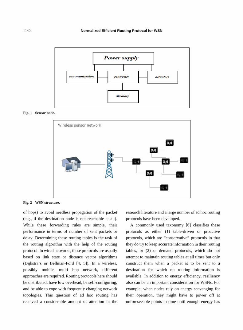
Normalized Efficient Routing Protocol for WSN
1140
Fig. 1 Sensor node.
Fig. 2 WSN structure.
of hops) to avoid needless propagation of the packet
(e.g., if the destination node is not reachable at all).
While these forwarding rules are simple, their
performance in terms of number of sent packets or
delay. Determining these routing tables is the task of
the routing algorithm with the help of the routing
protocol. In wired networks, these protocols are usually
based on link state or distance vector algorithms
(Dijkstra’s or Bellman-Ford [4, 5]). In a wireless,
possibly mobile, multi hop network, different
approaches are required. Routing protocols here should
be distributed, have low overhead, be self-configuring,
and be able to cope with frequently changing network
topologies. This question of ad hoc routing has
received a considerable amount of attention in the
research literature and a large number of ad hoc routing
protocols have been developed.
A commonly used taxonomy [6] classifies these
protocols as either (1) table-driven or proactive
protocols, which are “conservative” protocols in that
they do try to keep accurate information in their routing
tables, or (2) on-demand protocols, which do not
attempt to maintain routing tables at all times but only
construct them when a packet is to be sent to a
destination for which no routing information is
available. In addition to energy efficiency, resiliency
also can be an important consideration for WSNs. For
example, when nodes rely on energy scavenging for
their operation, they might have to power off at
unforeseeable points in time until enough energy has

Normalized Efficient Routing Protocol for WSN
1141
been harvested again. Consequently, it may be
desirable to use not only a single path between a sender
and receiver but to at least explore multiple paths. Such
multiple paths provide not only redundancy in the path
selection but can also be used for load balancing, for
example, to evenly spread the energy consumption
required for forwarding.
2. Motivation
In WSN, the route of each message destined to the
base station is really crucial in terms network lifetime.
If we always select the shortest route towards the base
station, that will causes the intermediate nodes deplete
faster and decreased network lifetime. We need to
increase WSN life time as long as possible.
3. Related work
In this section, we would study some routing
protocols that are important to get an overview about
routing in wireless sensor network. We would get a
view if ad-hoc on demand distance vector routing
AODV, SPIN, power aware routing protocols and
MRPC.
3.1 AODV
AODV [7] is the widely used algorithm for both
wired and wireless network. Ad-hoc On-demand
Distance Vector is known as one of the most efficient
routing protocols in terms of using the shortest path
and lowest power consumption. AODV is a reactive
protocol that builds routes between nodes on-demand
i.e. only as needed. Messages to other nodes in the
network do not depend on network-wide periodic
advertisements of identification messages to other
nodes in the network.
It broadcasts “HELLO” messages to the neighboring
nodes. It then uses these neighbors in routing.
Whenever any node (Source) wants to send a message
to another node (Destination) that is not its neighbor,
the source node initiates a Path Discovery in which the
source would send a RREQ (route request) message to
its neighbors. Nodes that received the Route Request
could update their information about the sending node.
The RREQ should contain the IP address of source
node. On the other hand, the RREQ contains broadcast
ID that necessary to identify that RREQ. The RREQ
has to have a current sequence number that determines
the freshness of the message. Finally, the RREQ should
keep track of the number of nodes that visited through
path discovery in a variable of Hop Count. When a
node receives a RREQ, it would check whether it has
received the same RREQ earlier (using IP, ID, and
Sequence number), if so, it would discard it. On the
other hand, if the recipient of the RREQ was an
intermediate node that does not have any information
about the path to the final destination, the node
increases the hop count and rebroadcasts the RREQ to
its neighbors. If the node that received the RREQ was
the final destination or an intermediate node that knows
the path to the final destination, it sends back the Route
Reply (RREP). This RREP should keep track of
traverse path of the RREQ but from destination to
source. As shown in Fig. 3, when the source node
receives the RREP, it should then start sending data.
We should take into consideration another control
message; that is it, RERR is used if a node detect that
there is a link break on the next hop of an active route,
or if it gets a data packet destined to a node which does
not have an active route without repairing. Finally if a
node receives a RERR from a neighbor for one or more
active routes it sends a RERR message.
Fig. 3 (a) Timing diagram; (b) Hello packet.

Normalized Efficient Routing Protocol for WSN
1142
3.2 SPIN Protocols
Heinzelman et al. [8] has proposed a family of
adaptive protocols called SPIN (sensor protocols for
information via negotiation) that passes all the
information at each node to every node in the network
assuming that all nodes in the network to be a potential
BS (base-stations). In this algorithm the user has the
ability to query any node and get the required
information or data immediately. These algorithms
make assumes that nodes in close proximity have
similar data, and hence there is a need to only distribute
the data that other nodes do not posses. The SPIN
family of protocols uses data negotiation and
resource-adaptive algorithms. Nodes running SPIN
assign a high-level name to completely describe their
collected data (called meta-data or meta content). Meta
data in its simplest definitions is describes as data of
data. That is it, meta data should provide data about
one or more aspects of the original data, for example
meta data aspects may be the mean of creation of that
data, purpose of the data, time and date of creation,
Creator or author of data, and location on a computer
network where the data was created) and perform
meta-data negotiations before any data (we means here
original data) is transmitted. Its importance arises from
the fact that we have used to make sure that there is no
redundant data sent throughout the network. That is it
to reduce the overhead on the network and to save
power. The semantics of the meta-data format is
application-specific and is not specified in SPIN. For
example, when sensors want to send meta-data for an
event in certain area, it would use its ID. On the other
hand, SPIN algorithm has the ability to access to the
energy level of the node and monitor the protocol
running according to how much energy it remaining in
a certain node. These protocols are known as a
time-driven fashion and broadcast the information all
over the wireless sensor network, despite the fact that
the user does not request any data at that moment.
SPIN’s meta-data negotiation approach solved the
traditional problems of flooding, and thus achieving a
lot of energy efficiency because you send meta-data,
not all data as used to in flooding. In SPIN, there are
three stages in which sensor nodes use three different
types of messages ADV (advertise) REQ (request) and
DATA to communicate with other nodes. ADV is used
to advertise new data, REQ to request data by the node
or sink or user itself and DATA is the actual message
itself. The protocol starts when a node gets new data
that it is willing to share with other nodes, after that it
broadcasts an ADV message containing meta-data. If
any nodes that receive ADV were interested in that data,
it sends a REQ message for the DATA and the DATA
is sent to this neighbor node. The neighbor sensor node
then repeats this process with its neighbors. As a result,
the entire sensor area will receive a copy of the data.
3.3 Power Aware Routing
Several algorithms had been developed for routing
in wireless sensor network, some of these algorithms
and protocols are energy based algorithms. In these
algorithms we take the network graph, assign to each
link a cost value that reflects the energy consumption
across this link, and pick any algorithm that computes
least-cost paths in a graph. An early paper along these
lines is Ref. [9], which modified Dijkstra’s shortest
path algorithm to obtain routes with minimal total
transmission power.
One of the most important algorithms used is known
as minimum energy per packet or per bit. The most
straightforward formulation is to look at the total
energy required to transport a packet over a multi hop
path from source to destination (including all
overheads). The goal is then to minimize, for each
packet, this total amount of energy by selecting a good
route. Minimizing the hop count will typically do not
achieve this goal as routes with few hops might include
hops with large transmission power to cover large
distances—but be aware of distance-independent,
constant offsets in the energy-consumption model.
Nonetheless, this cost metric can be easily included in
standard routing algorithms. It can lead to widely
differing energy consumption on different nodes [10].

Normalized Efficient Routing Protocol for WSN
1143
Some researches went to routing considering
available battery energy, as the finite energy supply in
nodes’ batteries is the limiting factor to network
lifetime, it stands to reason to use information about
battery status in routing decisions. Some of the
possibilities are maximum total available battery
capacity choose that route where the sum of the
available battery capacity is maximized, without taking
needless detours (called, slightly incorrectly,
“maximum available power” in Ref. [11]). Minimum
battery cost routing instead of looking directly at the
sum of available battery capacities along a given path;
MBCR instead looks at the “reluctance” of a node to
route traffic [10, 12]. This reluctance increases as its
battery is drained; for example, reluctance or routing
cost can be measured as the reciprocal of the battery
capacity. Then, the cost of a path is the sum of this
reciprocals and the rule is to pick that path with the
smallest cost. Since the reciprocal function assigns
high costs to nodes with low battery capacity, this will
automatically shift traffic away from routes with nodes
about to run out of energy. MMBCR (min-max battery
cost routing), this scheme [10, 12] follows a similar
intention, to protect nodes with low energy battery
resources. Instead of using the sum of reciprocal
battery levels, simply the largest reciprocal level of all
nodes along a path is used as the cost for this path.
Then, again the path with the smallest cost is used. In
this sense, the optimal path is chosen by minimizing
over a maximum. The same effect is achieved by using
the smallest battery level along a path and then
maximizing over these path values [11]. This is then a
maximum/minimum formulation of the problem.
Minimize variance in power levels to ensure a long
network lifetime, one strategy is to use up all the
batteries uniformly to avoid some nodes prematurely
running out of energy and disrupting the network.
Hence, routes should be chosen such that the variance
in battery levels between different routes is reduced.
MTPR (minimum total transmission power routing)
without actually considering routing as such, Bambos
[13] looked at the situation of several nodes
transmitting directly to their destination, mutually
causing interference with each other. A given
transmission is successful if its SINR exceeds a given
threshold. The goal is to find an assignment of
transmission power values for each transmitter (given
the channel attenuation metric) such that all
transmissions are successful and that the sum of all
power values is minimized. MTPR is of course also
applicable to multi hop networks.
3.4 MRPC
Misra and Banerjee [14] used to maximize network
lifetime for reliable routing in wireless environments
(MRPC), they depended on the fact that selecting the
path with the least transmission energy for reliable
communication may not always maximize the lifetime
of the ad-hoc network. On the other hand since the
actual drain on a node’s battery power will depend on
the number of packets forwarded by that node, it is
difficult to predict the optimal routing path unless the
total size of the packet stream is known during
path-setup. MRPC works on selecting a path, given the
current battery power levels at the constituent nodes,
that maximizes the total number of packets that may be
ideally transmitted over that path, assuming that all
other flows sharing that path do not transmit any
further traffic.
4. NEER Algorithm
MRPC algorithm has a problem in which it uses a
path that consumes much power. Simulation results [14]
showed that the transmission power per packet was
higher than that of minimum energy algorithm. Fig. 4
below shows that MRPC algorithm would take path P1
(A-C-F-H) because it would send 3 packets from to
while it would send only 2 packets through P2
(A-B-E-H) despite the fact that sending a packet
through P1 (6 units) consumes much more power than
P2 (only 3 units). We proposed a new algorithm called
NEER (normalized energy efficient routing).

Normalized Efficient Routing Protocol for WSN
1144
Fig. 4 Graph G and its components.
Our algorithm could be summarized as following:
Let G represent sensor network graph;
u, v represents nodes;
Edge (u, v) is the link between u and v;
ce (u) :residual battery of node u;
w(u, v) is the weighted cost of edge(u, v);
c(u, v) is the total number of packets that could be
sent from u to v. this value is defined as ce(u)/w(u, v).
Step 1: Initialize
Eliminate from G every edge (u, v) for which ce(u) <
w(u, v) this condition is used to ensure we could send at
least one packet through this path.
For every remaining edge (u, v) let
, / , (1)
Let L be the list of distinct c(u, v) values.
Step 2: Binary Search
Do a binary search in L to find the maximum value
max for which there is a path P from source to
destination that uses no edge with:
, (2)
For this, when testing a value q from L, we perform a
depth- or breadth-first search beginning at the source.
The search is not permitted to use edges with
, (3)
Let P be the source-to-destination path with lifetime
max. Simultaneously we should find minimum energy
path using Dijkstra’s algorithm as following:
∑ w u, v w u, v P (4)
Step 3: Wrap Up
If no path is found in Step 2, the route is not possible.
Otherwise, use P for the route.
Also find min(x), x P.
We need to derive a hybrid algorithm that takes the
advantages of both. Here we use the following steps:
We have to add a new condition that represents
threshold value Z in which we check battery level at all
nodes, if one of them was less than threshold value,
then NEER algorithm would switch to run MRPC.
Unless, NEER would continue to run AODV protocol.
In this case we took two factors in consideration.
The total power consumed through that path and the
residual battery in all nodes of that path. But we should
note that we use weight in our new algorithm. The
higher weight is for minimum energy factor. In such
case we guarantee that we use minimum energy
algorithm as long as possible but not to power off these
nodes.
In Fig. 5, we could summarize NEER functionality,
first of all, AODV would work until the first node
becomes about one fifth of its initial energy. In this
case, NEER would switch route algorithm. In this case,
MRPC algorithm would work. NEER would test if
there is any node
Fig. 5 NEER flow chart.

Normalized Efficient Routing Protocol for WSN
1145
We should also note that if we used threshold value
of the first condition to be (0) then NEER would
behave as AODV protocol. While if we choose
threshold value to be (1) then NEER protocol would be
full MRPC.
5. Analysis
There are some parameters used in simulation. Table
1 below summarize that parameters used in simulation.
We used NS-3.16 installed on Ubuntu as simulator,
after that we used wire shark network analysis to
analyze data gotten from NS-3. Here we would study
the behavior of NEER algorithm in comparison with
MRPC and Min-Energy Protocol in three fields. First
factor is the total number of dead nodes according to
time. In this factor nodes are dying slowly at the
beginning of running for NEER algorithm and would
die suddenly at the end of execution, since it takes the
features of both of (MRPC and Min-Energy). The
behavior of NEER algorithm is shown in Fig. 6.
If we want to compare between these algorithms
according to total sent packets by the network nodes,
our algorithm would send packets more than
Min-Energy and less than MRPC as shown in Fig. 7.
The horizontal axis represents time in seconds, while
the vertical one represents number of dead nodes.
Finally we would study energy per packet; here we
also expect that energy per packet would be also between
MRPC and Min-Energy, more than Min-Energy, less
than MRPC. Fig. 8 explains the idea.
6. Conclusion
In this paper we aim to introduce a new hybrid
algorithm that could increase network life time as long
as possible using minimum energy and residual battery
concepts. In this paper our algorithm depends mainly
on power consumption algorithms that are used in
WSN. This algorithm is based in the fact that most
power is consumed during data transmission not during
computations. This algorithm in fact takes advantages
of two important protocols. It takes the advantage of
consuming least power through minimum energy
protocol. On the other hand the presence of MRPC
protocol would increase network life time as long as
possible. In this way, NEER algorithm would use
minimum energy protocol as long as the residual power
is over a known threshold.
Table 1 Simulation parameters.
Parameter Description
Channel type Wireless channel
Mac protocol Mac/802_11
Number of nodes 40
Routing protocol Proposed Algorithm, MRPC, ME
Grid size 800 × 800
Packet size 64
Simulation time To die
Topology Random , Flat
Initial energy 3 joules
Source node 1
Destination node 1
Fig. 6 Expiration sequence.
Fig. 7 Number of sent packets.
0
10
20
30
40
50
20 40 60 80 100 120 140 160
Time
Expiration time (number of dead nodes)
MRPC Min‐ Energy NEER
0
5000
10000
15000
20000
MRPC Min ‐ Energy NEER
Number of sent packets

Normalized Efficient Routing Protocol for WSN
1146
Fig. 8 Energy per packet.
References
[1] G. Rodriguez-Navas, M.A. Ribot, B. Alorda, Understanding the role of transmission power in component-based architectures for adaptive WSN, in: Proceedings of the 2012 IEEE 36th Annual Computer Software and Applications Conference Workshops, Izmir, Jul. 16-20, 2012.
[2] F.C. Jiang, D.C. Huang, C.T. Yang, F.Y. Leu, Lifetime elongation for wireless sensor network using queue-based approaches, The Journal of Supercomputing 59 (2012) 1312-1335.
[3] I. Stojmenovic, X. Lin, Loop-free hybrid single-path/flooding routing algorithms with guaranteed delivery for wireless networks, IEEE Transactions on Parallel and Distributed Systems 12 (2001) 1023-1032.
[4] X. Chen, J. Wu, The Handbook of Ad Hoc Wireless Networks, CRC Press, USA, 2003. pp. 2–1-2–16.
[5] J.E. Wieselthier, G.D. Nguyen, A. Ephremides, On the construction of energy-efficient broadcast and multicast trees in wireless networks, in: Proceedings of IEEE Infocom, Tel-Aviv, Israel, March, 2000.
[6] E.M. Royer, C.K. Toh, A review of current routing
protocols for ad-hoc mobile wireless networks, IEEE Prersonal Communications 6 (1999) 46-55.
[7] W. Heinzelman, A. Chandrakasan, H. Balakrishnan, Energy-efficient communication protocol for wireless mi-crosensor networks, in: Proceedings of the 33rd Hawaii International Conference on System Sciences (HICSS '00), Hawaii, Jan. 4-7, 2000.
[8] W. Heinzelman, J. Kulik, H. Balakrishnan, Adaptive protocols for information dissemination in wireless sensor networks, in: Proceedings of the 5th Annual ACM/IEEE International Conference on Mobile Computing and Networking (MobiCom99), Seattle, WA, Aug. 15-19, 1999.
[9] K. Scott, N. Bambos, Routing and channel assignment for low power transmission in PCS, in: Proceedings International Conference on Universal Personal Communications, Cambridge, MA, Sep. 29-Oct. 2, 1996, pp. 469-502.
[10] C.K. Toh, Maximum battery life routing to support ubiquitous mobile computing in wireless ad hoc networks, IEEE Communications Magazine 39 (2001) 138-147.
[11] I.F. Akyildiz, W. Su, Y. Sankasubramaniam, E. Cayirci, Wireless sensor networks: A survey, Computer Networks 38 (2002) 393-422.
[12] S. Singh, M. Woo, C.S. Raghavendra, Power-aware routing in mobile ad hoc networks, in: Proceedings of the 4th ACM/IEEE International Conference on Mobile Computing and Networking (MOBICOM’98), Dallas, TX, Oct. 25-30, 1998.
[13] N. Bambos, Toward power-sensitive network architectures in wireless communications: Concepts, issues, and design aspects, IEEE Personal Communications 5 (1998) 50-59.
[14] A. Misra, S. Banerjee, MRPC: Maximizing network lifetime for reliable routing in wireless environments, in: 2002 IEEE Wireless Communications and Networking Conference, Orlando, Mar. 17-21, 2002.
0
2
4
6
8
10
MRPC Min‐Energy NEER
Energy per packet
Copyright © 2022 FDOKUMEN