
Journal of Communication and Computer(Issue 6,2013)
150
Volume 10, Number 6, June 2013 (Serial Number 103) Journal of Communication and Computer David Publishing Company www.davidpublishing.com Publishing David
-
Upload
davidpublishing -
Category
Documents
-
view
4 -
download
0
Transcript of Journal of Communication and Computer(Issue 6,2013)

Volume 10, Number 6, June 2013 (Serial Number 103)
Journal of
Communication and Computer
David Publishing Company
www.davidpublishing.com
PublishingDavid

Publication Information: Journal of Communication and Computer is published monthly in hard copy (ISSN 1548-7709) and online (ISSN 1930-1553) by David Publishing Company located at 3592 Rosemead Blvd #220, Rosemead, CA 91770, USA. Aims and Scope: Journal of Communication and Computer, a monthly professional academic journal, covers all sorts of researches on Theoretical Computer Science, Network and Information Technology, Communication and Information Processing, Electronic Engineering as well as other issues. Contributing Editors: YANG Chun-lai, male, Ph.D. of Boston College (1998), Senior System Analyst of Technology Division, Chicago Mercantile Exchange. DUAN Xiao-xia, female, Master of Information and Communications of Tokyo Metropolitan University, Chairman of Phonamic Technology Ltd. (Chengdu, China). Editors: Cecily Z., Lily L., Ken S., Gavin D., Jim Q., Jimmy W., Hiller H., Martina M., Susan H., Jane C., Betty Z., Gloria G., Stella H., Clio Y., Grace P., Caroline L., Alina Y.. Manuscripts and correspondence are invited for publication. You can submit your papers via Web Submission, or E-mail to [email protected]. Submission guidelines and Web Submission system are available at http://www.davidpublishing.org, www.davidpublishing.com. Editorial Office: 3592 Rosemead Blvd #220, Rosemead, CA 91770, USA Tel:1-323-984-7526, Fax: 1-323-984-7374 E-mail: [email protected]; [email protected] Copyright©2013 by David Publishing Company and individual contributors. All rights reserved. David Publishing Company holds the exclusive copyright of all the contents of this journal. In accordance with the international convention, no part of this journal may be reproduced or transmitted by any media or publishing organs (including various websites) without the written permission of the copyright holder. Otherwise, any conduct would be considered as the violation of the copyright. The contents of this journal are available for any citation. However, all the citations should be clearly indicated with the title of this journal, serial number and the name of the author. Abstracted / Indexed in: Database of EBSCO, Massachusetts, USA Chinese Database of CEPS, Airiti Inc. & OCLC Chinese Scientific Journals Database, VIP Corporation, Chongqing, P.R.China CSA Technology Research Database Ulrich’s Periodicals Directory Summon Serials Solutions Subscription Information: Price (per year): Print $520; Online $360; Print and Online $680 David Publishing Company 3592 Rosemead Blvd #220, Rosemead, CA 91770, USA Tel:1-323-984-7526, Fax: 1-323-984-7374 E-mail: [email protected]
David Publishing Company
www.davidpublishing.com
DAVID PUBLISHING
D

Journal of Communication and Computer
Volume 10, Number 6, June 2013 (Serial Number 103)
Contents Computer Theory and Computational Science
731 Proposal for an Optimal Job Allocation Method Based on Multiple Costs Balancing in Hybrid Cloud
Yumiko Kasae and Masato Oguchi
743 Probabilistic Health-Informatics and Bioterrorism
Ramalingam Shanmugam
748 A Hybrid Method to Improve Forecasting Accuracy—An Application to the Canned Cooked Rice and the Aseptic Packaged Rice
Hiromasa Takeyasu, Daisuke Takeyasu and Kazuhiro Takeyasu
759 System Reconstruction in the Field-Specific Methodology of Economic Subjects
Katarina Krpalkova Krelova and Pavel Krpalek
769 The Research of Wind Turbine Fault Diagnoses Based on Data Mining
Yu Song and Jianmei Zhang
Network and Information Technology
772 A Recommendation System Keeping Both Precision and Recall by Extraction of Uninteresting Information
Tsukasa Kondo, Fumiko Harada and Hiromitsu Shimakawa
783 Comparison of Contemporary Solutions for High Speed Data Transport on WAN 10 Gbit/s Connections
Dmitry Kachan, Eduard Siemens and Vyacheslav Shuvalov
796 Awaken the Cyber Dragon: China’s Cyber Strategy and its Impact on ASEAN
Miguel Alberto N. Gomez
806 Inter-MAC Green Path Selection for Heterogeneous Networks
Olivier Bouchet, Abdesselem Kortebi and Mathieu Boucher

815 Web Block Extraction System Based on Client-Side Imaging for Clickable Image Map
Hiroyuki Sano, Shun Shiramatsu, Tadachika Ozono and Toramatsu Shintani
Communications and Electronic Engineering
823 Multiple Chaos Generator by Neural-Network-Differential-Equation for Intelligent Fish-Catching
Mamoru Minami, Akira Yanou, Yuya Ito and Takashi Tomono
832 An Efficient Algorithm for the Evaluate of the Electromagnetic Field near Several Radio Base Stations
Algenti Lala, Sanije Cela and Bexhet Kamo
844 Composing Specific Domains for Large Scale Systems
Asmaa Baya and Bouchra EL Asri
857 Mobile Station Speed Estimation with Multi-bit Quantizer in Adaptive Power Control
Hyeon-Cheol Lee
863 On the Comparison Analysis of Two 4G-WiMAX Base Stations in an Urban Sub-Saharan African Environment
Eric Tutu Tchao, Kwasi Diawuo1 and Willie Ofosu
873 Error Analysis for the Three-Dimensional Detection and Reconstruction of the Road Surface
Youquan He and Jian Wang

Journal of Communication and Computer 10 (2013) 731-742
Proposal for an Optimal Job Allocation Method Based
on Multiple Costs Balancing in Hybrid Cloud
Yumiko Kasae and Masato Oguchi
Department of Information Sciences, Ochanomizu University, Tokyo 112-8610, Japan
Received: February 07, 2013 / Accepted: March 13, 2013 / Published: June 30, 2013.
Abstract: Due to the explosive increase in the amount of information in computer systems, we need a system that can process large amounts of data efficiently. Cloud computing system is an effective means to achieve this capacity and has spread throughout the world. In our research, we focus on hybrid cloud environments, and we propose a method for efficiently processing large amounts of data while responding flexibly to needs related to performance and costs. We have developed this method as middleware. For data-intensive jobs using this system, we have created a benchmark that can determine the saturation of the system resources deterministically. Using this benchmark, we can determine the parameters in this middleware. This middleware can provide Pareto optimal cost load balancing based on the needs of the user. The results of the evaluation indicate the success of the system. Key words: Hybrid cloud, load balancing, data processing, performance, cost balance.
1. Introduction
In recent years, large amounts of data, referred to as
big data, have become more common with the
development of information and communications,
creating the need for efficient data processing. As a
platform for processing these data, hybrid cloud
environments have become a focus of attention. In
hybrid cloud environments, users can access public
clouds and private clouds; private clouds are secure
clouds built using the secure resources of the user
company, and public clouds can provide scalable
resources if the user pays metered rates. Combining
these clouds can address shortcomings related to
safety and scalability. For data-intensive jobs, hybrid
clouds are appropriate. For increasing amounts of data,
hybrid clouds can provide secure and scalable
processing.
However, performance and costs must be balanced.
When we want to process large amounts of data more
rapidly, using many resources that are provided by
Corresponding author: Yumiko Kasae, master, research
field: information science. E-mail: [email protected].
public clouds, in addition to those provided by private
clouds, will increase speed, but the metered cost will
also be greater. In contrast, if these jobs are processed
using private cloud resources almost exclusively,
users will not have to pay metered rates, but the job
execution time will be longer. Thus, we need a system
that can determine optimal job placement based on
cost limitations and necessary performance to ensure
efficient processing in hybrid cloud environments.
Therefore, in this research, we proposed a method
for providing optimal job placement in hybrid cloud
environments in terms of monetary costs and
performance. We have developed this system as
middleware. In addition, the middleware provides
optimal job placement for both CPU-intensive
applications and data-intensive applications. In
general, unlike in CPU-intensive applications, which
can accurately determine the load using the CPU
usage, efficient resource use in data-intensive
applications is difficult to determine. In the proposed
method, we created a benchmark that can be used to
change the extent of the load of CPU processing and

Proposal for an Optimal Job Allocation Method Based on Multiple Costs Balancing in Hybrid Cloud
732
I/O processing, and measured the performance of
hybrid clouds as an execution environment using this
benchmark. Based on the results obtained using this
benchmark, we propose a method of determining job
execution status based on the status of the I/O
resources.
In this paper, we will describe the details of the
middleware that can be used to implement the method
proposed in this study. We have evaluated the balance
of performance and costs by using this middleware
with data-intensive applications. We examine the
evaluation axis for performance and monetary costs
and show that this middleware can provide optimal
job placement for efficient job processing. The
monetary cost is the sum of the power consumption
cost for private clouds and the metered costs
associated with public clouds.
The remainder of this paper is organized as follows:
Section 2 introduces cloud computing; Section 3
describes the proposed method of determining the
load; Section 4 describes the middleware that can be
used for optimal job allocation; Section 5 introduces
the evaluation results for their middleware; Section 6
comments on related research studies; and Section 7
presents concluding remarks and suggestions for
future work.
2. Cloud Computing
2.1 Overview of Cloud Computing and Classification
Cloud computing is a service through which users
can use necessary software and hardware resources
from servers through networks. If a user uses cloud
computing services, without having the physical
computer resources, the user can receive various
services.
The types of services include SaaS (software as a
service), PaaS (platform as a service) and IaaS
(infrastructure as a service).
Recently, because of the diversity of services that
can be provided, these services have been collectively
called XaaS (X as a service).
This study will consider IaaS. The types of
platforms for IaaS are private clouds and public
clouds. Public clouds can be used through the Internet,
and users can use cloud services scalable if they pay
metered rates to the cloud provider. However, in
public clouds, it is necessary to leave the data with the
cloud provider (albeit temporarily) during processing
jobs, which generates some security concerns.
Using private clouds can solve these problems.
A private cloud is a cloud that is built using
resources that users already have. The user can
construct the cloud taking security into account.
However, private clouds lack scalability relative to
public clouds.
Hybrid clouds can address the shortcoming of each
of the cloud types. These clouds can be both secure
and scalable. In this research, which is focused on
hybrid cloud environments, we proposed a method for
ensuring efficient processing.
2.2 The Trade-off between Cost of the Evaluation Axis
for Hybrid Clouds
When people use hybrid cloud environments, there
will be a trade-off relationship between performance
and necessary costs. When we want to process a large
amount of data more rapidly, using many resources
that are provided by the public cloud, in addition to
the resources of the private cloud, and the associated
metered cost will make the job more expensive. In
contrast, if these jobs are processed using private
cloud resources with little or no use of public cloud
resources, users will not have to pay metered costs,
but the job execution time will be longer. Thus, we
need a system that can determine optimal job
placement based on the equilibrium between
necessary cost and performance to ensure efficient
processing in a hybrid cloud environment.
This research proposes a method of providing
optimal job placement in hybrid cloud environments
in terms of monetary costs and performance. This
method has been operationalized as middleware. This

Proposal for an Optimal Job Allocation Method Based on Multiple Costs Balancing in Hybrid Cloud
733
middleware will consider job processing time and
monetary costs. Monetary cost is the sum of the
charge for power consumption in private clouds and
the metered costs associated with public clouds. The
recent environmentalism in global affairs makes it
especially important to reduce power consumption
when processing large amounts of data. It is important
that we not waste power. In addition, the monetary
cost of private clouds may include fixed costs
associated with the system installation. However, such
amounts are difficult to define categorically. Thus, we
assume that the equipment has already been
depreciated, and the fixed costs were evaluated as
zero.
The monetary cost does not include the fee for the
power consumption associated with the public cloud.
This is because it is difficult for the user to know
the price of the power consumption by each resource
in the public cloud. For the public cloud, the power
consumption charges are assumed to be included in
the metered costs.
2.3 Eucalyptus
Eucalyptus [1] is open source software that can
create cloud infrastructure. Eucalyptus is compatible
with the Amazon EC2 API [2]; the Amazon EC2
(Amazon elastic compute cloud) is a cloud service
that is provided by the U.S. company Amazon.com.
Using a cloud built in Eucalyptus, you can port a
service on this cloud as if the service was on Amazon
EC2. Fig. 1 shows the architecture of Eucalyptus.
Eucalyptus is composed of three components. It is
treated as a public network to the upper layers of the
CLC (cloud controller) from the CLC (cluster
controller), and it is treated as a private network to the
lower layers of the NC (node controller).
CLC (cloud controller)
manages the information in the entire cloud. Equipped
with compatible interfaces for Amazon EC2; a web
management screen provides an API for the user.
CC (cluster controller)
manages the node controller, the state of instances
(virtual machines) and the virtual network for the
instances.
NC (node controller)
controls the instance. When the program needs to run
multiple instances, the virtualization software runs on
the node controller.
2.4 Building a Hybrid Cloud Environment
In this paper, we have used the Eucalyptus to build
two cloud systems. By connecting with Dummynet to
generate an artificial delay between them, we have
built an emulated hybrid cloud environment in their
laboratory. In the configuration of server in
Eucalyptus, it is possible to run CC and CLC in a
single server. In this study, in each cloud, CC and
CLC operated in a single server as Frontend Server.
Number of node server running in NC, as shown in
Fig. 2, was four in each cloud.
Servers that constitute this hybrid cloud are shown
in Tables 1-4.
Fig. 1 Architecture of Eucalyptus.
Fig. 2 Hybrid cloud environment.

Proposal for an Optimal Job Allocation Method Based on Multiple Costs Balancing in Hybrid Cloud
734
Table 1 Private cloud frontend.
OS Linux 2.6.38 / / Debian GNU / Linux 6.0
CPU Intel® Xeon® CPU @ 3.60GHz 1 core
Memory 4 GByte
Table 2 Private cloud node.
OS Linux 2.6.32-xen-amd 64 and xen-4.0-amd64 / / Debian GNU / Linux 6.0
CPU Intel® Xeon® CPU @ 2.66GHz 1 core
Memory 8 GByte
Table 3 Public cloud frontend.
OS Linux 2.6.38 / / Debian GNU / Linux 6.0
CPU Intel® Xeon® CPU @ 2.40GHz 1 core
Memory 1 GByte
Table 4 Public cloud node.
OS Linux 2.6.32-xen-amd 64 and xen-4.0-amd64 / / Debian GNU / Linux 6.0
CPU Intel® Xeon® CPU @ 3.60GHz 1 core
Memory 4 GByte
3. Proposed Method for Determining the Load
The proposed middleware in this paper processes
not only CPU-intensive applications but also
data-intensive applications. In both these jobs in a
hybrid cloud environment, to obtain high-speed and
low-cost processing after all of the resources have
been used in the private cloud, the next tasks should
be processed using in the public cloud. In addition, in
the public cloud, after the borrowed resources have all
been used, new resources will be needed. Therefore,
even when it is important to utilize resources without
waste, it is also important to properly determine the
load, and all of each resource should be used.
Therefore, when used for CPU processing and disk
processing, this middleware determines when the
resource has been saturated. Based on this information,
this middleware will determine the resource load. The
methods of determining the load for each type of
processing are as follows.
3.1 Method for Determining the Load of CPU
Processing
Load balancing for CPU-intensive jobs has been
investigated in many past studies. In this research,
CPU usage is the focus. This proposed middleware
also determines the load based on CPU usage. This
method is same as that used in other studies; if the
usage reaches 100%, the resource has been saturated,
and the middleware does the load balancing. The
method of optimally balancing CPU-intensive jobs is
not a feature of this proposal because it does not
fundamentally change the techniques used in other
studies.
3.2 Method for Determining the Disk Processing Load
3.2.1 Disk Performance Measurement
Unlike in CPU intensive-jobs, it is difficult to make
a definitive decision about whether the disk load has
reached the saturation point during data-intensive jobs.
For data-intensive jobs, because the system is often
waiting for I/O processing, it is difficult to determine
the CPU load. Thus, in the proposed method, we use
each cloud resources /proc/disk stats file to obtain the
length of the queue for the current disk. Then, we
estimate the number of jobs that are running in these
disks. Therefore, in this method, it is also necessary to
know the length of the queue, which indicates the
saturation of the disk resources.
Therefore, we have created benchmarks that can
change the balance of I/O and CPU processing.
By using the benchmark Disk Bench, which
performs read-only processing, we measured disk
performance using the execution environment of the
middleware.
In Fig. 3, as an example of a job by Disk Bench,
people can see a state of transition for the CPU load
and the number of disk accesses. Disk Bench is a
simple benchmark that performs read processing for
the disks in the instance. This figure shows that Disk
Bench processing is not performed when there is little
CPU processing and will become I/O bound if many
jobs are processed at the same time.
Using Disk Bench, we have measured the
performance of the disk. We have made this performance

Proposal for an Optimal Job Allocation Method Based on Multiple Costs Balancing in Hybrid Cloud
735
Fig. 3 One example of the load transition of Disk Bench.
measurement for the instances of performance in
Table 5 for the hybrid cloud. In this measurement
process, we measured the execution time for the jobs
and the queue that is accumulated for the disk during
the processing of multiple simultaneous jobs using
Disk Bench. We then compare the processing time
when these jobs are processed sequentially and the
processing time using this measurement.
In general, if there are sufficient disk resources,
simultaneously processing the jobs can be more rapid
than sequentially processing them. However, when we
increase the number of jobs to be processed
simultaneously, there is a point at which processing
time will be slow as a result. This method determines
when there are no more disk resources, and the length
of the queue that has accumulated for the disk at that
time is defined as the “conditions in which the disk
resources have run out”.
Furthermore, in Disk Bench, there are two
parameters. One of parameters specifies the amount of
reading at a particular time, and the other specifies the
number of times this reading has been repeated. In this
performance measurement process, we create a job
that we intended to access a variety of patterns using
the disk; these parameters were varied. We have
measured performance changing these parameters.
Figs. 4 and 5 show examples of the comparison
results for processing times and the length of the
queue at the time of this performance measurement
experiments.
First, in this performance measurement process, we
compare the processing time for simultaneous
processing and sequential processing. In Fig. 4, the
vertical axis represents a ratio that indicates the
Table 5 Instance.
OS Linux 2.6.27-21-0.1-xen / x86_64 GNU / CentOS 5.3
CPU Intel® Xeon® CPU @ 3.60 GHz 1 core
Memory 1 Gbyte
Disk 20 Gbyte
Fig. 4 One example of comparison of processing times (block size: 512 Kbytes, repetition rate: 1,024 times).
Fig. 5 One example of the length of the queue (block size: 512 Kbytes, repetition rate: 1,024 times).
comparison results for the processing time. This ratio
was obtained by dividing the sequential processing
time into the simultaneous processing time. The
vertical axis at the value of 1 is indicated by a red
dashed line. If the value is below the dashed line, then
simultaneous processing is faster than sequential
processing. If the value is above the dashed line, then
sequential processing is faster than simultaneous
processing. In other words, the disk resource has been
exhausted. Thus, in Fig. 4, people can see that in job
number 4, the disk resource was exhausted.
Fig. 5 shows the transitions in the length of the
queue for each number of concurrent jobs at this
measurement. As shown in Fig. 5, if the number of
concurrent jobs is increased, the length of the queue is
increased. For this state, people can use the following
queuing model: The disk access requests from
multiple jobs arrive at random, the processing time for
the job is nearly constant, block size is constant and
the window for each disk is one. Therefore, the degree

Proposal for an Optimal Job Allocation Method Based on Multiple Costs Balancing in Hybrid Cloud
736
of congestion of I/O requests from the job, that is, the
length of the queue, accurately reflects the degree of
saturation of the input and output.
By analyzing the relative processing time and the
length of the queue with some parameter setting, in
this experimental environment, we found that the
lengths of the queues are between 2,000 and 2,700
when the disk resources run out. However, clearly,
this is a range of values. If we analyze the physical
disk in detail, these values may be uniquely
determined. However, in general, the accuracy of the
actual job will not be exact. Therefore, in this method,
we determine this range as the saturated disk load.
We discuss their preliminary experiments in the
next section.
3.2.2 Preliminary Experiments: Experiment in
Controlling Load Balancing
In our preliminary experiments, we process
data-intensive jobs using Disk Bench in this hybrid
cloud environment. In this experiment, as their
threshold for load balancing, we use the length of the
queue for the disk resource. Using this threshold, by
choosing a value in the range of values determined in
the performance measurements, we have examined the
evaluation of performance and cost.
In this experiment, we received Disk Bench jobs
every 2 seconds 100 times. These experiments were
load balancing experiments intended to determine
where to place jobs: whether in private clouds or
public clouds. For this experiment in hybrid cloud
environments, we ran eight instances with
performance as indicated in Table 5: four instances for
each cloud. In addition, this range of values for the
length of the queue (which was determined by
measuring performance) depends on the physical
machine. However, because all of the physical servers
built as hybrid cloud environments had the same
performance, this range is unified at the
above-mentioned value.
First, jobs are placed in one instance in a private
cloud. If the length of the queue for that instance is
equal to or greater than the threshold value, the next
jobs will be distributed under the conditions that the
length of the queue is less than this threshold or that
has not been used within the private cloud. If all of the
queue lengths in a private cloud are equal to or greater
than the threshold value, the public cloud begins to be
used. Then, the next jobs are similarly distributed until
the queue length is greater than or equal to the
threshold.
In this experiment, as the threshold for load
balancing, we varied this value from a small value to
large value from 500 to 12,500. By using a value
within the range of values obtained in the performance
measurement process, we verified whether this load
distribution could provide an optimal balance between
monetary costs and performance as described in
Section 2.2. During this experiment, we measured the
processing time for the jobs, the power consumption
rate for the private cloud and the metered rates for the
public cloud. To measure power consumption in this
environment, we have used a watt-hour meter
SHW3A [3], which is a high-precision power meter
produced by the System Artware Company in Japan.
After one plugs an electric product into the SHW3A,
the power consumption is instantly measured and
displayed. In this study, we measure only the private
cloud’s node power consumption.
Fig. 6 shows the evaluation results for the
experiment.
The horizontal axis is the processing time cost, and
the vertical axis is the monetary cost. Monetary costs
are calculated using the following equation:
Monetary cost: TR · NR · CR + PL · CL
Fig. 6 Evaluation results for experiment in controlling load balancing.
Proposal for an Optimal Job Allocation Method Based on Multiple Costs Balancing in Hybrid Cloud
737
TR: execution time for public cloud (h);
NR: number of instances of use of public cloud;
CR: charges for public cloud use ($/hour);
PL: power consumption in a private cloud (kWh);
CL: charges for power consumption in a private
cloud ($/kWh).
In this evaluation, the metered unit price is $0.5
based on the price of Amazon EC2 and the unit price
of power consumption is set at $0.24 based on the
price charged by the Tokyo electric power company.
As shown in Fig. 6, there is no configuration that
optimally balances both time costs and monetary costs.
However, in selecting a threshold for load balancing,
if we choose a value from 2,000 to 2,700 based on the
performance measurement that indicates the saturation
of the disk resource, we find that load balancing can
be provided based on a Pareto optimal cost balance. In
other words, if we set the threshold near 2,000,
although efficiency will be ensured and the load
balancing will occur quickly, the monetary costs will
increase slightly. In contrast, if we set the threshold
near 2,700, while efficiency will be ensured, it will
take a little time to perform load balancing and ensure
a low monetary cost. The balance of time costs and
monetary costs should be based on the needs of the
user.
Thus, in these preliminary experiments, we could
not find a point that best balances time cost and
monetary cost because there is a range in which the
disk resource is exhausted. However, by setting a
threshold value in response to a user request within
this range, we found that a processing cost balance
can be obtained without wasting resources.
3.2.3 Method of Controlling the Load Distribution
in Disk Processing
Based on the discussion in Sections 3.2.1 and 3.2.2,
in the proposed method of load determination for disk
processing, first, by measuring the performance of the
disk, we determine the range for queue length that
indicates disk saturation. This phase is regarded as a
learning phase. The threshold for load balancing in
middleware is the length of the queue for the disk
resource, and the user can select a threshold within
that range, which is determined by the performance
measurement process. This middleware can be used to
control the Pareto optimal cost balance load
distribution without wasting resources.
4. The Pareto Optimal Job Allocation Middleware
4.1 The Structure of the Middleware
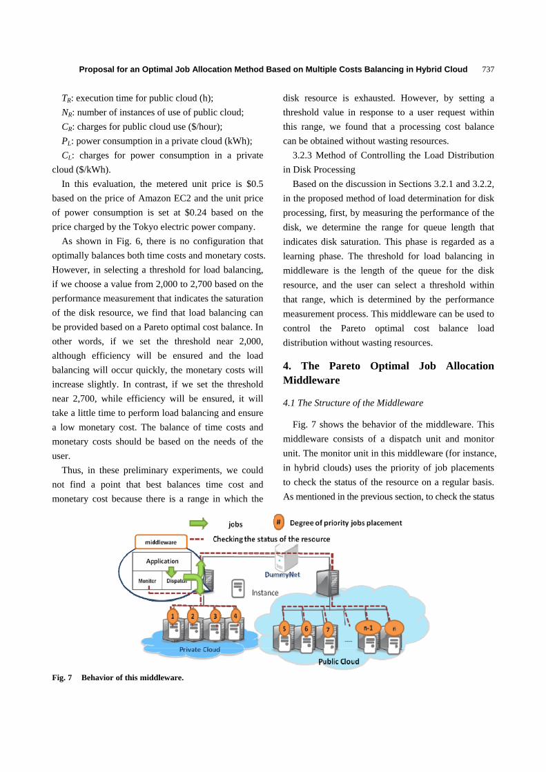
Fig. 7 shows the behavior of the middleware. This
middleware consists of a dispatch unit and monitor
unit. The monitor unit in this middleware (for instance,
in hybrid clouds) uses the priority of job placements
to check the status of the resource on a regular basis.
As mentioned in the previous section, to check the status
Fig. 7 Behavior of this middleware.

Proposal for an Optimal Job Allocation Method Based on Multiple Costs Balancing in Hybrid Cloud
738
of the resources requires measuring CPU utilization
for CPU processing and the length of the queue for
disk processing. In addition, the middleware evaluates
the load status of these resources, determining CPU
utilization and disk processing at the same time, and if
the processing becomes saturated, the middleware
determines that. The dispatch unit receives and
distributes jobs based on the information from the
monitor unit.
4.2 An Algorithm for Middleware
This middleware algorithm is as follows.
Additionally, when running this middleware in a
hybrid environment cloud for the first time, as
mentioned in Section 3.2.3, you must determine the
range of the queue length to identify disk resource
saturation.
(1) Based on the range of threshold values
determined in the learning phase, the user sets the
threshold for load balancing, which can be used to
obtain the desired cost balance, and runs the
middleware;
(2) Middleware receives the submitted job;
(3) In order of placement priority in private cloud
in-stances, check the load state of the resource to
determine whether it is greater than or equal to the
threshold. If the resource is at a value that is less than
the threshold value, execute the job using that instance,
and then return to (2). If the load states of all
resources in the private cloud are equal to or greater
than the threshold value, go to (4);
(4) In order of placement priority for public cloud
in-stances, check the load states of the resources to
determine whether they are greater than or equal to the
threshold. If the load state is less than the threshold
value, execute the job using that in-stance; then return
to (2). If all of the resource load states are equal to or
greater than the thresh-old value at that time, proceed
to (5);
(5) In the public cloud, select a new instance and
execute the submitted job using that instance; then
return to (2).
5. Experiments Using This Middleware
In this chapter, we describe examples of the results
of evaluations conducted using this middleware.
Conducting load balancing experiments using this
middleware for CPU-intensive applications in hybrid
cloud environments is not fundamentally different
from the process used in earlier studies of load
balancing. Therefore, in these examples, we consider
the evaluation results obtained for data-intensive
applications using this middleware.
5.1 Overview of Experiments
As shown in Figs. 2 and 7, as the experimental
environment for this middleware, we have built a
hybrid cloud environment. The node servers that
constitute each cloud are single-core CPUs, and all
servers have the same performance. For this reason,
we will generate one instance of performance from the
Table 5 for each node server. There are four instances
in the private cloud. If all instances are saturated, we
conduct load balancing using the public cloud
resources.
The experiment procedures are as follows:
First, in a learning phase, we measured the
performance of the disk. However, this experimental
environment is the environment in which the
performance measurement was carried out in Section
3.2. Therefore, for all instances in this hybrid cloud,
the queue length range that indicates disk saturation is
between 2,000 and 2,700. Next, based on this range,
we execute this middleware by varying the value of
the threshold for load balancing. During these
experiments, we measured the processing time for the
jobs, the cost of power consumption when the private
cloud was used and the metered rates for the public
cloud.
In this experiment, we evaluated these three types
of costs by varying the threshold for load balancing.
In particular, setting the threshold in the range

Proposal for an Optimal Job Allocation Method Based on Multiple Costs Balancing in Hybrid Cloud
739
determined by the performance measurement process,
we evaluated whether Pareto optimal load balancing is
possible without wasting resources.
5.2 Data-Intensive Applications That Were Used in
the Experiment
In these two experiments, we have evaluated
middleware used with two different data-intensive
applications.
As the first, we used pgbench, which is the
PostgreSQL benchmark. Pgbench is a simple tool
benchmark that is bundled with PostgreSQL. Tatsuo
Ishii created the first version, published in 1999 by the
PostgreSQL mailing list in Japan. Pgbench was
created based on the TPC-B, which mimics the online
transaction process and can measure the number of
transactions that can be processed per unit of time. We
received pgbench’s jobs every two seconds 200 times;
the middleware processed these jobs.
For the second, we used queries from DBT-3.
DBT-3 is a simplified version of the TPC-H and
performs complex select statement queries in large
databases. The TPC-H and DBT-3 are decision
support benchmarks and consist of ad-hoc queries and
concurrent data modifications. In the DBT-3, there are
22 search queries. However, because the processing
time may be long because of the number of queries, in
this experiment, we select 11 queries for shorter
processing times. Then, we submitted these queries
repeatedly for a total of 110 jobs, and the middleware
processed the jobs. The DBT-3 database was built
using MySQL.
The major difference between these two types of
data intensive applications is the difference in the
CPU processing load. In executing pgbench jobs, we
confirmed that CPU processing is generally not
performed. In contrast, the search queries for DBT-3
were processed to some extent with the CPU.
However, all the search queries were mainly
executed using disk processing; thus, these are
data-intensive applications. For each of these two
data-intensive applications, using this proposed
method, we show that the method does not depend on
the nature and type of application.
5.3 Data Placement in Experiments
In a cloud environment, especially for
data-intensive jobs, considering data placement is
very important. For data placement in a hybrid
environment cloud, we can consider using the block
storage associated with each cloud or using remote
access to local storage from the public cloud. In these
experiments, it is assumed that due to remote backup,
the necessary data are already located in some
instances. In Ref. [4], using middleware, remote
access to the local storage is attained using iSCSI
from a public cloud. We wish to consider this method
of data placement in the future.
5.4 Evaluation of the Results Obtained Using
Middleware
5.4.1 An Example of the Use of Pgbench
Fig. 8 shows the results of the cost evaluation
obtained using the middleware, which processed
pgbench’s jobs.
As people can see from this figure, if we set the
correct threshold at the relevant queue length based on
the performance measurement process (i.e., between
2,000 and 2,700), this middleware provides a
Pareto-optimal cost balance and uses resources
efficiently. Conversely, some points are on a
Pareto-optimal curve even though they are out of the
range of values determined by the performance
measurement process.
These points are examples that indicate when the
load balance is too focused on processing performance
and too many resources are used or when a
tremendous burden has been placed on the available
resources so as not to raise the monetary cost. For
points that are not listed on the Pareto optimal curve
and that for values other than the threshold value, it is
possible that a better cost balance exists.

Proposal for an Optimal Job Allocation Method Based on Multiple Costs Balancing in Hybrid Cloud
740
Fig. 8 Cost evaluation of processing pgbench jobs.
Fig. 9 Cost evaluation of processing DBT-3 queries.
Based on the above, we found that it is a necessary
condition for the point on the Pareto optimal curve to
set the threshold for load balancing based on the
saturation of the disk resource.
5.4.2 Example Using Search Queries of DBT-3
Fig. 9 shows the results of the cost evaluations
obtained using the middleware with DBT-3
processing queries.
In Fig. 9, as in Section 3.2.2, the vertical axis shows
the monetary cost, and the horizontal axis shows the
time cost. From this figure, as well as the DBT-3
processing queries, people can see that if we set the
correct threshold at the queue length determined by
the performance measurement process (i.e., from
2,000 from 2,700), this middleware provides a
Pareto-optimal cost balance in which resources are
used efficiently. Additionally, in other respects,
results similar to the ones found using pgbench are
obtained.
5.4.3 Observations from These Experiments
Based on the evaluation results for the processing
search queries for DBT-3 and pgbench as examples of
data-intensive applications, people can conclude that
this middleware provides a Pareto-optimal cost
balance while using resources efficiently when we set
the threshold to the queue length determined by the
performance measurement process.
In these experiments, we deliberately added a delay
of 20 msec by using Dummy net between the clouds.
However, because only certain jobs are transferred to
the remote cloud in this middleware, some of the
evaluations were barely influenced by the differences
in the delay time. In addition, because the unit price of
the metered cost for public cloud use was large, the
influence of the differences in power consumption in
the private cloud was limited. However, for technical
and social reasons, these monetary costs may vary
significantly. Even when the proposed method is used,
when the charge for power consumption is more
significant, this factor must be kept in mind during
load balancing. However, we can make this
modification by simply changing the cost calculation
expression.
6. Related Works
Previous researchers have discussed load balancing
in cloud computing [5, 6]. In these papers, however,
CPU-intensive applications were used as the targets of
load balancing jobs rather than data-intensive
applications. In computing-centric applications,
similarly to some scientific calculations, it is possible
to perform appropriate load balancing based on the
CPU load of each node. In this research, however, we
have used a data-intensive application for the jobs. In
such cases, because the CPU is often in the I/O
waiting state, load balancing is almost impossible
based on CPU load. In this research, we have used the
disk I/O as a load indicator. In data-intensive
applications, load balancing middleware has also been
developed that uses the amount of disk access for load
decisions [4]. This middleware based on disk access
provided dynamic load balancing between public
clouds and a local cluster and ensured optimal job

Proposal for an Optimal Job Allocation Method Based on Multiple Costs Balancing in Hybrid Cloud
741
placement. Because we have further developed
middleware by introducing user-specified parameters,
it will be possible to reduce the monetary costs of load
balancing, including the cost of power consumption.
Power saving in cloud computing has also been
actively investigated. Unlike in this study, researchers
have discussed an approach to power saving that
involves the use of CPU-intensive applications in a
cloud [7]. Other studies examined power saving
efforts for a cloud datacenter [8, 9]. Our study aims to
save power in all clouds, including private clouds.
Researchers [10] proposed a scheduling algorithm that
could be used to evaluate power consumption and job
execution time. However, these studies differ from
their study, especially because we have focused on
total costs in hybrid clouds, including job execution
time, public cloud charges at a metered rate, and
power consumption charges for private clouds. In
addition, we have used data-intensive applications as
the target jobs.
7. Conclusions
We proposed a method of determining the load
based on the required cost and performance to ensure
efficient processing load balancing in a hybrid
environment cloud. We have implemented this
procedure using middleware. This middleware uses
information about CPU processing and disk
processing to provide efficient load balancing if the
resources needed to perform a job are scarce. In
particular, in the proposed method, we determine the
load from CPU usage and the length of the queue for
disk processing. First, in a learning phase, by
measuring the performance of the disk, we determine
the range of queue lengths that indicate disk
saturation.
The user can select a threshold within that range,
which is determined by the performance measurement
process. Using this middleware, tone can control the
Pareto optimal cost balance load distribution without
wasting resources.
Future research should be focused on improving
data placement. In the experiments in this paper, data
placement was the task of interest. This data
placement is not realistic as a model for real situations.
A realistic model might aggregate local and remote
storage and synchronize these forms of storage.
Therefore, we are considering introducing network
storage. In their system, iSCSI has already been
introduced, and we plan to carry out an experiment
using iSCSI in the future. In addition, in the current
implementation, based on the values obtained in the
learning phase, the threshold should be set for load
balancing before running the middleware. In the
future, we would like to develop an automating
learning phase as a part of this middleware.
Acknowledgments
This work is partly supported by the Ministry of
Education, Culture, Sports, Science and Technology,
under Grant 22,240,005 of Grant-in-Aid for Scientific
Research. We would like to thank to Drs. Atsuko
Takefusa, Hidemoto Nakada, Ryousei Takano,
Tomohiro Kudoh at the National Institute of AIST
(Advanced Industrial Science and Technology),
Project Associate Professor Miyuki Nakano, Assistant
Professor Daisaku Yokoyama, Senior Researcher
Norifumi Nishikawa at the Institute of Industrial
Science, the University of Tokyo, and Associate
Professor Saneyasu Yamaguchi at Kogakuin
University for the conscientious advice and help with
this work.
References
[1] Eucalyptus, http://www.eucalyptus.com/. [2] Amazon EC2, http://aws.amazon.com/jp/ec2/. [3] SHW3A, http://www.system-artware.co.jp/shw3a.html. [4] S. Toyoshima, S. Yamaguchi, M. Oguchi, Middleware
for load distribution among cloud computing resource and local cluster used in the execution of data-intensive application, Journal of the Database Society of Japan 10 (2011) 31-36.
[5] G. Jung, K.R. Joshi, M.A. Hiltunen, R.D. Schlichting, C. Pu, Generating adaptation policies for multi-tier applications in consolidated server environments, in: Proc.

Proposal for an Optimal Job Allocation Method Based on Multiple Costs Balancing in Hybrid Cloud
742
5th IEEE International Conference on Autonomic Computing (ICAC2008), US, 2008.
[6] E. Kalyvianaki, T. Charalambous, S. Hand, Self-adaptive and self-configured CPU resource provisioning for virtualized servers using Kalman filters, in: Proc. 6th International Conference on Autonomic Computing and Communications (ICAC2009), Barcelona, Spain, 2009.
[7] C.Y. Tu, W.C. Kuo, W.H. Teng, Y.T. Wang, S. Shiau, A power-aware cloud architecture with smart metering, in: Proc. Parallel Processing Workshops (ICPPW), 2010 39th International Conference, San Diego, 2010.
[8] C. Peoples, G. Parr, S. McClean, Energy-aware data
centre management, in: Proc. Communications (NCC), 2011 National Conference, Bangalore, India, 2011.
[9] J. Baliga, R.W.A. Ayre, K. Hinton, R.S. Tucker, Green cloud computing: Balancing energy in processing, storage and transport, in: Proceedings of the IEEE, China, 2011.
[10] L.M. Zhang, K. Li, Y.Q. Zhang, Green task scheduling algorithms with speeds optimization on heterogeneous cloud servers, in: Proc. Green Computing and Communications (GreenCom), 2010 IEEE/ACM Int’l Conference on and Int’l Conference on Cyber, Physical and Social Computing (CPSCom), San Diego, California, 2010.

Journal of Communication and Computer 10 (2013) 743-747
Probabilistic Health-Informatics and Bioterrorism
Ramalingam Shanmugam
School of Health Administration, Texas State University, San Marcos, TX 78666, USA
Received: April 22, 2013 / Accepted: May 07, 2013 / Published: June 30, 2013.
Abstract: In this article, new probabilistic health-informatics indices connecting probabilities: P r( ), P r( ), P r( )A B A B
and
P r( )A B are discovered, where A and B denote respectively the “ability of a hospital to treat anthrax patients” and “whether
a hospital drilled to be prepared to deal with an adverse bioterrorism”. These probabilistic informatics are not seen in any textbooks or journal articles and yet, they are too valuable to be unnoticed to comprehend the hospitals’ preparedness to treat anthrax patients in an outbreak of bioterrorism. A demonstration of this new probabilistic informatics is made in this article with the data in the U.S. Government’s General Accounting Office’s report GAO-03-924. Via this example, this article advocates the importance of the above mentioned probabilistic-informatics for health professionals to understand and act swiftly to deal with public health emergencies. Key words: Conditional, marginal, total probability, hospital’s drilling, inequalities.
1. Motivation
Historically, probability tools are used to
understand the regularity in the uncertain environment.
Probability is a foundation on which informatics about
the uncertainty could be built to address the cyber
security, the importance of the electronic health
records, the efficacy of the medical drugs, the
designing of biomedical engineering devices, and the
decision making in public health crises among others.
Many notable heroes in the humanity like the famous
astronomer Christian Huygens utilized probability
informatics in his quest for securing the physical laws
of the universe. See de Finetti [1] and Jaynes [2] for
the history and basics of probability information. Yet,
some important probability informatics does not
appear in any textbooks or journal articles. These
probability informatics inequalities are too important
to be unnoticed. They are first derived in this article
and then are applied to comprehend the hospital’s
Corresponding author: Ramalingam Shanmugam, Ph.D.,
research fields: informatics, modeling infectious diseases, diagnostic methodology and modeling. E-mail: [email protected].
preparedness to treat anthrax in an outbreak of
terrorism in USA.
In Section 2, three new probability based
informatics inequalities are derived; the new
inequalities are illustrated in Section 3 with the data
about the U.S. Hospitals’ preparedness to treat anthrax
patients in an event of bioterrorism; In Section 4, a
few final thoughts are given. In the demonstration, the
preparedness of US hospitals in 34 states to a survey
conducted by the CDC (center for the disease control)
in Report GAO-03-924 by the federal Government
Accounting Office are analyzed and interpreted. The
remaining sixteen states in the USA did not respond to
the CDC’s survey; in the end, some conclusive
thoughts for future research work probability
informatics are included.
2. Probability-Informatics Inequalities
In this section, we first derive three new probability
informatics inequalities and use them later in Section
3 to comprehend how prepared are the states in the
USA to treat anthrax patients who might flock into a
hospital in an outbreak of a bioterrorism. To begin

Probabilistic Health-Informatics and Bioterrorism
744
with, let us introduce the following notations:
_ _ _A hospitals Can treat anthrax
_ _B hospital drilled bioterrorism
_ _ _B hospital not drilled bioterrorism
Among other illnesses, an infliction of anthrax
spores could turn out fatal, if it is not treated quickly
and it might happen in an outbreak of bioterrorism.
The public health agencies need to have worked out
the “informatics” early on before the occurrence of the
bioterrorism. There are uncertainties about the
hospitals’ readiness in a state. Had the hospitals
“drilled” on their emergency plans, it would help to
quickly treat anthrax patients. Since the terrorism on
September 11, 2001 in the New York City, several
hospitals in the USA and elsewhere are worried about
the likelihood of treating massive influx of anthrax
patients who might arrive for treatment in an event of
bioterrorism. Many hospitals, if not all the hospitals,
do drill and practice with preparedness plan to deal
bioterrorism including the treating effectively the
anthrax patients. In this regard, let Pr( )A be the
probability that a hospital is prepared to treat the
anthrax patients, whether or not the hospital has
drilled to deal any bioterror event. Realize that the
event A can happen with or without an associated
event B . Suppose that Pr( )B be the probability
that the hospital has drilled to deal bioterrorism.
Consequently, Pr( ) Pr( )
Pr( ) Pr( ) [1 Pr( )] Pr( )
A ABUAB
B A B B A B
.
The above statement can be rearranged as: Pr( ) Pr( ) Pr( )
Pr( )1 Pr( )
A B A BA B
B
(1)
The Eq. (1) means that the conditional probability
P r( )A B for a hospital to treat anthrax patients even
without a drilling experience is comparable to the
conditional probability P r( )A B for a hospital to
treat anthrax patients with a drilling experience. In this
comparison, the impact of drilling on the hospital’s
ability to treat anthrax patients can be felt and it is
brought out in our demonstrations. However, there
could be three possibilities in the scenario to capture
the impact of drilling and they are be felt and it is
brought out in our demonstrations. Now, let us discuss
one after another possibility.
The first possibility is that the cure of anthrax
patients could be certain because of the drilling and it
is echoed by the conditional probability P r( ) 1A B .
In this Scenario 1, by substituting P r( ) 1A B in
Eq. (1), the Eq. (1) transforms to Eq. (2) below:
Pr( ) [Pr( ) Pr( )] /[1 Pr( )]A B A B B (2)
Notice that Pr( ) Pr( )0 1
1 Pr( )
A B
B
, because the
probability P r( )A B has to obey an axiom
0 P r( ) 1A B of the probability. Consequently,
the probability informatics in Eq. (3) exists.
0 Pr( ) Pr( ) 1B A (3)
The second possibility is that the cure of anthrax
patients is unlikely in spite of the drilling and it is
indicated by the conditional probability
Pr( ) 0A B . In this Scenario 2, with the substitution
of Pr( ) 0A B in Eq. (1), the Eq. (1) transforms to
Eq. (4) below:
P r( ) P r( ) /[1 P r( )]A B A B (4)
Consequently, another probability informatics in Eq.
(5) is noticed.
0 Pr( ) Pr( ) 1B A (5)
The third possibility is that the cure of an anthrax
patient is likely but not surely or unlikely and it is
indicated by the conditional probability statement
0 Pr( ) 1A B . It is so because the drilling helps
but does not necessarily guaranty the successful

Probabilistic Health-Informatics and Bioterrorism
745
treatment of anthrax patients. In this Scenario 3, the
Eq. (1) implies a probability informatics in Eq. (6). P r ( ) P r ( ) P r ( )
1 P r( ) [1 P r( ) ]
B A B A
B A B
(6)
The probability for any hospital in a US state to be
prepared to treat anthrax patients is indicated by one
of the mutually exclusive probability informatics Eqs.
(3), (5) and (6) depending on the prevailing scenario
in the state’s hospitals. However, there is way to
visualize the probability informatics Eqs. (3), (5) and
(6) in a cubic box.
For this purpose, we sketch probability informatics:
Eqs. (3), (5) and (6) with the coordinate Pr( )x A ,
P r( )y B and P r( )z A B . The unit volume is
partitioned into mutually exclusive scenarios as seen
in the Fig. 1. Each state’s in the USA would fall in
only one scenario depending on its x, y and z
coordinates. Lastly, the importance of drilling to treat
anthrax patients can be captured by plotting
P r( )A B in terms of P r( )A B depending on
whether the Scenario 3, Scenario 2 or Scenario 1
prevails. The correlation between Pr( )A B and
P r( )A B portray a relationship between the presence
and absence of the drilling to treat anthrax patients.
Next, all these probability informatics are illustrated.
3. Preparedness for Anthrax Patients
In this section, the results of the Section 2 are
illustrated using 34 states’ data in the report
GAO-03-924 by the US General Accounting Office.
Fig. 1 Compartments in the unit cube due to probability informatics Eqs. (3), (5) and (6).
Fig. 2 (a) Eastern zone.

Probabilistic Health-Informatics and Bioterrorism
746
Fig. 2 (b) Central zone.
Fig. 2 (c) Mountain zone.
Fig. 2 (d) Pacific zone.

Probabilistic Health-Informatics and Bioterrorism
747
Table 1 The correlation between Pr( )A B and Pr( )A B in four time zones.
_Tim e Z one
C orr
Eastern zone Central zone Mountain zone Pacific zone
[Pr( ), Pr( )]Corr A B A B 0.43 0.12 -0.86 -0.98
The remaining sixteen states in the USA did not
respond to the survey which was conducted by the
CDC. For the sake of comparisons on how the states
perform, the thirty four states are grouped according
to their time zones. The rationale for grouping is that
the states are homogeneous within a time zone but not
across the time zones. The preparedness and drilling
data for the fifteen states in the Eastern Time zone, the
thirteen states in the Central Time zone, the three
states in the Mountain Time zone and the three states
in the Pacific Time zone are calculated and compared
using Pr( ),Pr( ),Pr( )A B A B and Pr( )A B as in
Figs. 2a-2d below. The correlation between Pr( )A B
and Pr( )A B are calculated and displayed in the
Table 1. The correlation captures the intricate balance
between the presence and absence of the drilling on
the ability to treat anthrax patients.
4. Conclusions
The states in the Eastern and Central time zones are
smaller in size in comparison to the states in the
Mountain or Pacific Time zones. Consequently, the
number of states is lesser in the Mountain and Pacific
Time zones. However, the pattern in the Eastern time
zone is different from the pattern in the Central time
zone and it is noticed by comparing the Fig. 2a with
the Fig. 2b. Likewise, the pattern in the Mountain
Time zone is different from the pattern in the Pacific
Time zone and it is realized by comparing the Fig. 2c
with the Fig. 2d. The preparedness in the Pacific states
is more collinear (see Fig. 2d). The preparedness in
the Mountain states is not collinear (see Fig. 2c). The
preparedness in the Central Time zone (see Fig. 2b) is
more diversified in comparison to the preparedness in
the Eastern Time zone (see Fig. 2a). Furthermore,
their correlation between Pr( )A B and Pr( )A B
reveals interesting similarities and differences among
the 34 states in the four time zones of USA (see Table
1). The correlation between Pr( )A B and Pr( )A B
is highest in the Eastern states, gradually decreasing
as one moves westward, and becomes the lowest in
the Pacific states. Surprisingly, the correlation
between Pr( )A B and Pr( )A B is negative only in
the Mountain and Pacific states. More research
investigations for the non-trivial reasons of such
remarkable differences among these time zones ought
to be done in a future project. The findings will be
valuable to the public health administrators. This new
informatics knowledge is made possible with the help
of new probability informatics in Eqs. (3), (5) and (6)
which involve the marginal, complementary and
conditional probabilities.
References
[1] B.D Finetti, Logical foundations and measurement of
subjective probability, Acta Psychologica 34 (1970)
129-145.
[2] E.T. Jaynes, Probability Theory: The Logic of Science,
Cambridge University Press, UK, 2003.
[3] Hospital Preparedness: Most Urban Hospitals Have
Emergency Plans but Lack Certain Capacities for
Bioterrorism Response Report GAO-03-924, Government
Accounting Office, Federal Government Press,
Washington, 2003.

Journal of Communication and Computer 10 (2013) 748-758
A Hybrid Method to Improve Forecasting Accuracy—An
Application to the Canned Cooked Rice and the Aseptic
Packaged Rice
Hiromasa Takeyasu1, Daisuke Takeyasu2 and Kazuhiro Takeyasu3
1. Faculty of Life and Culture, Kagawa Junior College, Kagawa 769-0201, Japan
2. Graduate School of Culture and Science, The Open University of Japan, Chiba City 261-8586, Japan
3. College of Business Administration, Tokoha University, Fuji City 417-0801, Japan
Received: March 24, 2013 / Accepted: April 17, 2013 / Published: June 30, 2013.
Abstract: In industries, how to improve forecasting accuracy, such as sales, shipping, is an important issue. In this paper, a hybrid method is introduced and plural methods are compared. Focusing that the equation of ESM (exponential smoothing method) is equivalent to (1, 1) order ARMA Model (autoregressive moving average model) equation, new method of estimation of smoothing constant in exponential smoothing method is proposed before by us which satisfies minimum variance of forecasting error. Trend removing by the combination of linear and 2nd order non-linear function and 3rd order non-linear function is executed to the original production data of two kinds of cooked rice (canned rice and aseptic packaged rice). Genetic algorithm is utilized to search the optimal weight for the weighting parameters of linear and non-linear function. For the comparison, monthly trend is removed after that. The new method shows that it is useful for the time series that has various trend characteristics and has rather strong seasonal trend.
Key words: Minimum variance, exponential smoothing method, forecasting, trend, bread.
1. Introduction
Many methods for time series analysis have been
presented such as AR Model (autoregressive model),
ARMA Model (autoregressive moving average model)
and ESM (exponential smoothing method) [1-4].
Among these, ESM is said to be a practical simple
method.
For this method, various improving methods, such
as adding compensating item for time lag, coping with
the time series with trend [5], utilizing Kalman Filter
[6], Bayes Forecasting [7], adaptive ESM [8],
exponentially weighted moving averages with
irregular updating periods [9], making averages of
forecasts using plural method [10], are presented. For
Corresponding Author: Hiromasa Takeyasu, professor, research field: time series analysis. E-mail: [email protected].
example, Maeda [6] calculated smoothing constant in
relationship with S/N ratio under the assumption that
the observation noise was added to the system. But he
had to calculate under supposed noise because he
could not grasp observation noise. It can be said that it
does not pursue optimum solution from the very data
themselves which should be derived by those
estimation. Ishii [11] pointed out that the optimal
smoothing constant was the solution of infinite order
equation, but he did not show analytical solution.
Based on these facts, we proposed a new method of
estimation of smoothing constant in ESM before [12].
Focusing that the equation of ESM is equivalent to
(1, 1) order ARMA model equation, a new method of
estimation of smoothing constant in ESM was
derived.
In this paper, utilizing above stated method, a

A Hybrid Method to Improve Forecasting Accuracy—An Application to the Canned Cooked Rice and the Aseptic Packaged Rice
749
revised forecasting method is proposed. In making
forecast such as production data, trend removing
method is devised. Trend removing by the
combination of linear and 2nd order non-linear
function and 3rd order non-linear function is executed
to the original production data of two kinds of cooked
rice (canned rice and aseptic packaged rice). Genetic
algorithm is utilized to search the optimal weight for
the weighting parameters of linear and non-linear
function. For the comparison, monthly trend is
removed after that. Theoretical solution of smoothing
constant of ESM is calculated for both of the monthly
trend removing data and the non-monthly trend
removing data. Then forecasting is executed on these
data. This is a revised forecasting method. Variance of
forecasting error of this newly proposed method is
assumed to be less than those of previously proposed
method.
The rest of the paper is organized as follows: In
Section 2, ESM is stated by ARMA model and
estimation method of smoothing constant is derived
using ARMA model identification; The combination
of linear and non-linear function is introduced for
trend removing in Section 3; The Monthly ratio is
referred in Section 4; Forecasting is executed in
Section 5, and estimation accuracy is examined.
2. Description of ESM Using ARMA Model
In ESM, forecasting at time t + 1 is stated in the
following equation:
tttt xxxx ˆˆˆ 1 (1)
tt xx ˆ1 (2)
Here,
:ˆ 1tx forecasting at 1t ;
:tx realized value at t ;
: smoothing constant 10 ;
Eq. (2) is re-stated as:
ltl
lt xx
01 1ˆ (3)
By the way, we consider the following (1, 1) order
ARMA model:
11 tttt eexx (4)
Generally, qp, order ARMA model is stated
as:
jt
q
jjtit
p
iit ebexax
11
(5)
Here,
:tx Sample process of Stationary Ergodic
Gaussian Process tx ,,,2,1 Nt ;
te : Gaussian White Noise with 0 mean 2e
variance; MA process in Eq. (5) is supposed to satisfy
convertibility condition. Utilizing the relation that
0,, 21 ttt eeeE
We get the following equation from Eq. (4):
11ˆ ttt exx (6)
Operating this scheme on t + 1, we finally get:
ttt
ttt
xxx
exx
ˆ1ˆ
1ˆˆ 1
(7)
If we set 1 , the above equation is the same
with Eq. (1), i.e., equation of ESM is equivalent to (1,
1) order ARMA model, or is said to be (0, 1, 1) order
ARIMA model, because 1st order AR parameter is
1 . Compared with Eqs. (4) and (5), we obtain
1
1 1
b
a
From Eqs. (1)-(7), 1
Therefore, we get:
1
1
1
1
b
a (8)
From above, we can get estimation of smoothing
constant after we identify the parameter of MA part of
ARMA model. But, generally MA part of ARMA
model becomes non-linear equations which are
described below.
Let Eq. (5) be:
it
p
iitt xaxx
1
~ (9)

A Hybrid Method to Improve Forecasting Accuracy—An Application to the Canned Cooked Rice and the Aseptic Packaged Rice
750
jt
q
jjtt ebex
1
~ (10)
We express the autocorrelation function of tx~ as
r k~
and from Eqs. (9) and (10), we get the following non-linear equations which are well known.
q
jje
jk
kq
jjek
br
qk
qkbbr
0
220
0
2
~
)1(0
)(~
(11)
For these equations, recursive algorithm has been
developed. In this paper, parameter to be estimated is
only b1 , so it can be solved in the following way.
From Eqs. (4), (5), (8) and (11), we get:
2
11
2210
1
1
~1~
1
1
1
e
e
br
br
b
a
q
(12)
If we set
0~
~
r
rkk (13)
the following equation is derived:
21
11 1 b
b
(14)
We can get b1 as follows:
1
21
1 2
411
b (15)
In order to have real roots, 1 must satisfy:
2
11 (16)
From invertibility condition, 1b must satisfy:
11 b
From Eq. (14), using the next relation:
01
012
1
21
b
b
Eq. (16) always holds.
As
11 b
1b is within the range of
01 1 b
Finally we get:
1
211
1
21
1
2
4121
2
411
b
(17)
which satisfied above conditions. Thus we can obtain
a theoretical solution by a simple way. Focusing on
the idea that the equation of ESM is equivalent to (1,
1) order ARMA model equation, we can estimate
smoothing constant after estimating ARMA model
parameter. It can be estimated only by calculating 0th
and 1st order autocorrelation function.
3. Trend Removal Method
As trend removal method, we describe the
combination of linear and non-linear function.
(1) Linear function
We set
11 bxay (18)
as a linear function.
(2) Non-linear function
We set
222
2 cxbxay (19)
332
33
3 dxcxbxay (20)
as a 2nd and a 3rd order non-linear function. ),,( 222 cba and ),,,( 3333 dcba are also parameters
for a 2nd and a 3rd order non-linear functions which
are estimated by using least square method.
(3) The combination of linear and non-linear
function.
We set
33
23
333
222
22111
dxcxbxa
cxbxabxay
(21)
1,10,10,10 321321 (22)
as the combination linear and 2nd order non-linear
and 3rd order non-linear function. Trend is removed
by dividing the original data by Eq. (21). The optimal

A Hybrid Method to Improve Forecasting Accuracy—An Application to the Canned Cooked Rice and the Aseptic Packaged Rice
751
weighting parameter 321 ,, are determined by
utilizing GA. GA method is precisely described in
Section 6.
4. Monthly Ratio
For example, if there is the monthly data of L years
as stated bellow:
12,,1,,1 jLixij where, Rxij ,
in which j means month and i
means year and ijx is a production data of i -th year,
j -th month. Then, monthly ratio jx~ 12,,1j is
calculated as follows:
L
i jij
L
iij
j
xL
xL
x
1
12
1
1
1211
1
~ (23)
Monthly trend is removed by dividing the data by
Eq. (23). Numerical examples both of monthly trend
removal case and non-removal case are discussed in
Section 7.
5. Forecasting Accuracy
Forecasting accuracy is measured by calculating the
variance of the forecasting error. Variance of
forecasting error is calculated by:
N
iiN 1
22
1
1 (24)
where, forecasting error is expressed as:
iii xx ˆ (25)
N
iiN 1
1 (26)
6. Searching Optimal Weights Utilizing GA
6.1 Definition of the Problem
We search 321 ,, of Eq. (21) which minimizes
Eq. (24) by utilizing GA. By Eq. (22), we only have to
determine 1 and 2 . 2 (Eq. (24)) is a function
of 1 and 2 , therefore we express them as
),( 212 . Now, we pursue the following:
Minimize: ),( 212
subject to: 1,10,10 2121 (27)
We do not necessarily have to utilize GA for this
problem which has small member of variables.
Considering the possibility that variables increase
when we use logistics curve, etc., in the near future,
we want to ascertain the effectiveness of GA.
6.2 The Structure of the Gene
Gene is expressed by the binary system using 0, 1
bit. Domain of variable is [0, 1] from Eq. (22). We
suppose that variables take down to the second
decimal place. As the length of domain of variable is
1 – 0 = 1, seven bits are required to express variables.
The binary bit strings (bit 6, ~, bit 0) is decoded to
the [0, 1] domain real number by the following
procedure [13].
Procedure 1: Convert the binary number to the
binary-coded decimal:
X
bit
bitbitbitbitbitbitbit
i
ii
10
6
0
20123456
2
,,,,,,
(28)
Procedure 2: Convert the binary-coded decimal to
the real number:
The real number = (Left hand starting point of the
domain) + 'X ((Right hand ending point of the
domain)/( 127 )) (29) The decimal number, the binary number and the
corresponding real number in the case of 7 bits are
expressed in Table 1.
1 variable is expressed by 7 bits, therefore 2
variables needs 14 bits. The gene structure is
exhibited in Table 2.
6.3 The Flow of Algorithm
The flow of algorithm is exhibited in Fig. 1.
6.3.1 Initial Population
Generate M initial population. Here, 100M .
Generate each individual so as to satisfy Eq. (22).

A Hybrid Method to Improve Forecasting Accuracy—An Application to the Canned Cooked Rice and the Aseptic Packaged Rice
752
Table 1 Corresponding table of the decimal number, the binary number and the real number.
The decimal number
The binary number
The Corresponding real number Position of the bit
6 5 4 3 2 1 0
0 0 0 0 0 0 0 0 0.00
1 0 0 0 0 0 0 1 0.01
2 0 0 0 0 0 1 0 0.02
3 0 0 0 0 0 1 1 0.02
4 0 0 0 0 1 0 0 0.03
5 0 0 0 0 1 0 1 0.04
6 0 0 0 0 1 1 0 0.05
7 0 0 0 0 1 1 1 0.06
8 0 0 0 1 0 0 0 0.06
… …
126 1 1 1 1 1 1 0 0.99
127 1 1 1 1 1 1 1 1.00
Table 2 The gene structure.
1 2
Position of the bit
13 12 11 10 9 8 7 6 5 4 3 2 1 0
0-1 0-1 0-1 0-1 0-1 0-1 0-1 0-1 0-1 0-1 0-1 0-1 0-1 0-1
Fig. 1 The flow of algorithm.
6.3.2 Calculation of Fitness
First of all, calculate forecasting value. There are 36
monthly data for each case. We use 24 data (1st to
24th) and remove trend by the method stated in
Section 3. Then we calculate monthly ratio by the
method stated in Section 4. After removing monthly
trend, the method stated in Section 2 is applied and
exponential smoothing constant with minimum
variance of forecasting error is estimated. Then the 1st
step forecast is executed. Thus, data is shifted to 2nd
to 25th and the forecast for 26th data is executed
consecutively, which finally reaches forecast of 36th
data. To examine the accuracy of forecasting, variance
of forecasting error is calculated for the data of 25th to
36th data. Final forecasting data is obtained by
multiplying monthly ratio and trend. Variance of
forecasting error is calculated by Eq. (24). Calculation
of fitness is exhibited in Fig. 2.
Scaling [14] is executed such that fitness becomes
large when the variance of forecasting error becomes
small. Fitness is defined as follows:
),(),( 212
21 Uf (30)
where U is the maximum of ),( 212 during the
past W generation. Here, W is set to be 5.
6.3.3 Selection
Selection is executed by the combination of the

A Hybrid Method to Improve Forecasting Accuracy—An Application to the Canned Cooked Rice and the Aseptic Packaged Rice
753
Fig. 2 The flow of calculation of fitness.
general elitist selection and the tournament selection.
Elitism is executed until the number of new elites
reaches the predetermined number. After that,
tournament selection is executed and selected.
6.3.4 Crossover
Crossover is executed by the uniform crossover.
Crossover rate is set as follows:
7.0cP (31)
6.3.5 Mutation
Mutation rate is set as follows:
05.0mP (32)
Mutation is executed to each bit at the
probability mP , therefore all mutated bits in the
population M becomes 14 MPm .
7. Numerical Example
7.1 Application to the Original Production Data of
Processed Cooked Rice
The original production data of processed cooked
rice for two cases (data of canned rice and those of
aseptic packaged rice: Annual Report of Statistical
Research, Ministry of Agriculture, Forestry and
Fisheries, Japan) from January 2008 to December
2010 are analyzed. Furthermore, GA results are
compared with the calculation results of all
considerable cases in order to confirm the
effectiveness of GA approach. First of all, graphical
charts of these time series data are exhibited in Figs. 3
and 4.
7.2 Execution Results
GA execution condition is exhibited in Table 3. GA
convergence process is exhibited in Figs. 5-8.
We made 10 times repetition and the maximum,
average, minimum of the variance of forecasting error
and the average of convergence generation are
exhibited in Table 4 and 5.
The case that monthly ratio is not used is smaller
than the case that monthly ratio is used concerning the
variance of forecasting error for canned rice. It may be
because canned rice does not have definite seasonal
trend towards the data for 2008.
The minimum variance of forecasting error of GA
coincides with those of the calculation of all
considerable cases and it shows the theoretical
solution. Although it is a rather simple problem for
GA, we can confirm the effectiveness of GA approach.
Further study for complex problems should be
examined hereafter.
Next, optimal weights and their genes are exhibited
in Tables 6 and 7.
In the case that monthly ratio is not used, the linear
function model is best in both cases. In the case that
monthly ratio is used, the linear function model is best
in both cases. Parameter estimation results for the

A Hybrid Method to Improve Forecasting Accuracy—An Application to the Canned Cooked Rice and the Aseptic Packaged Rice
754
Canned Cooked Rice
0
50
100
150
200
250
1 2 3 4 5 6 7 8 9 101112 1 2 3 4 5 6 7 8 9 101112 1 2 3 4 5 6 7 8 9 101112
2006 2007 2008
Fig. 3 Data of canned cooked rice.
Aseptic Packaged Cooked Rice
0
1000
2000
3000
4000
5000
6000
7000
8000
9000
10000
1 2 3 4 5 6 7 8 9 101112 1 2 3 4 5 6 7 8 9 101112 1 2 3 4 5 6 7 8 9 101112
2006 2007 2008
Fig. 4 Data of aseptic packaged cooked rice.
Table 3 GA execution condition.
GA Execution Condition
Population 100
Maximum generation 50
Crossover rate 0.7
Mutation ratio 0.05
Scaling window size 5
The number of elites to retain 2
Tournament size 2
Table 4 GA execution results (monthly ratio is not used).
Food The variance of forecasting error
Average of convergence generation Maximum Average Minimum
Canned cooked rice 4048.947313 3233.943529 3139.748713 9.4
Aseptic packaged cooked rice 815965.2277 684614.796 668794.6832 14.3
Table 5 GA execution results (monthly ratio is used).
Food The variance of forecasting error
Average of convergence generation Maximum Average Minimum
Canned cooked rice 5278.497079 3418.722411 3174.249743 13.2
Aseptic packaged cooked rice 323388.4005 214841.1023 206470.6901 9.7
A Hybrid Method to Improve Forecasting Accuracy—An Application to the Canned Cooked Rice and the Aseptic Packaged Rice
755
Canned Cooked Rice
Minimum Variance
3110
3120
3130
3140
3150
3160
3170
3180
3190
3200
1 3 5 7 9 11 13 15 17 19 21 23 25 27 29 31 33 35 37 39 41 43 45 47 49
Fig. 5 Convergence process in the case of canned cooked rice (monthly ratio is not used).
Canned Cooked Rice
Minimum Variance
3000
3100
3200
3300
3400
3500
3600
1 3 5 7 9 11 13 15 17 19 21 23 25 27 29 31 33 35 37 39 41 43 45 47 49
Fig. 6 Convergence process in the case of canned cooked rice (monthly ratio is used).
Aseptic Packaged Cooked Rice
Minimum Variance
667000
667500
668000
668500
669000
669500
670000
670500
671000
671500
672000
672500
1 3 5 7 9 11 13 15 17 19 21 23 25 27 29 31 33 35 37 39 41 43 45 47 49
Fig. 7 Convergence process in the case of aseptic packaged cooked rice (monthly ratio is not used).
Aseptic Packaged Cooked Rice
Minimum Variance
205500
206000
206500
207000
207500
208000
208500
1 3 5 7 9 11 13 15 17 19 21 23 25 27 29 31 33 35 37 39 41 43 45 47 49
Fig. 8 Convergence process in the case of aseptic packaged cooked rice (monthly ratio is used).

A Hybrid Method to Improve Forecasting Accuracy—An Application to the Canned Cooked Rice and the Aseptic Packaged Rice
756
Table 6 Optimal weights and their genes (monthly ratio is not used).
Data 1 2
Position of the Bit
13 12 11 10 9 8 7 6 5 4 3 2 1 0
Canned cooked rice 1 0 1 1 1 1 1 1 1 0 0 0 0 0 0 0
Aseptic packaged cooked rice 1 0 1 1 1 1 1 1 1 0 0 0 0 0 0 0
Table 7 Optimal weights and their genes (monthly ratio is used).
Data 1 2
Position of the Bit
13 12 11 10 9 8 7 6 5 4 3 2 1 0
Canned cooked rice 1 0 1 1 1 1 1 1 1 0 0 0 0 0 0 0
Aseptic packaged cooked rice 1 0 1 1 1 1 1 1 1 0 0 0 0 0 0 0
Table 8 Parameter estimation results for the trend of Eq. (21).
Data 1a 1b 2a
2b 2c 3a
3b 3c
3d
Canned cooked rice -0.38 130.17 0.24 -6.4 156.27 -0.004 0.39 -7.9 159.69
Aseptic packaged cooked rice 43.8 7410.01 0.69 26.45 7485.17 0.57 -20.85 246.28 6981.12
Fig. 9 Trend of canned cooked rice.
Fig. 10 Trend of aseptic packaged cooked rice.
Table 9 Parameter estimation result of monthly ratio.
Data 1 2 3 4 5 6 7 8 9 10 11 12
Canned cooked rice 1.38 1.39 1.43 0.98 0.69 0.68 0.43 0.87 0.6 0.98 1.23 1.3
Aseptic packaged cooked rice 0.89 0.94 1.1 1.06 0.92 0.98 1.01 1.0 0.98 1.04 1.0 1.07

A Hybrid Method to Improve Forecasting Accuracy—An Application to the Canned Cooked Rice and the Aseptic Packaged Rice
757
Table 10 Smoothing constant of minimum variance of Eq. (17) (monthly ratio is not used). Data ρ1 α
Canned cooked rice -0.280995 0.692422
Aseptic packaged cooked rice -0.206225 0.784169
Table 11 Smoothing constant of minimum variance of Eq. (17) (monthly ratio is used).
Data ρ1 α
Canned cooked rice -0.475263 0.274765
Aseptic packaged cooked rice -0.302345 0.663399
Fig. 11 Forecasting result of canned cooked rice.
Fig. 12 Forecasting result of frozen cooked rice.
trend of Eq. (21) using least square method are
exhibited in Table 8 for the case of 1st to 24th data.
Trend curves are exhibited in Figs. 9 and 10.
Calculation results of monthly ratio for 1st to 24th
data are exhibited in Table 9.
Estimation results of the smoothing constant of
minimum variance for the 1st to 24th data are
exhibited in Tables 10 and 11.
Forecasting results are exhibited in Tables 10 and 11,
Figs. 11 and 12.
7.3 Remarks
In the case of canned rice, that monthly ratio was
not used had a better forecasting accuracy. On the
other hand, aseptic packaged rice had a better
forecasting accuracy in the case that monthly ratio
was used. Both cases had a good result in the
combination of linear and non-linear function model.
The minimum variance of forecasting error of GA
coincides with those of the calculation of all
considerable cases and it shows the theoretical

A Hybrid Method to Improve Forecasting Accuracy—An Application to the Canned Cooked Rice and the Aseptic Packaged Rice
758
solution. Although it is a rather simple problem for
GA, we can confirm the effectiveness of GA approach.
Further study for complex problems should be
examined hereafter.
8. Conclusions
Focusing on the idea that the equation of ESM was
equivalent to (1, 1) order ARMA model equation, a
new method of estimation of smoothing constant in
exponential smoothing method was proposed before
by us which satisfied minimum variance of
forecasting error. Generally, smoothing constant was
selected arbitrary. But in this paper, we utilized above
stated theoretical solution. Firstly, we made estimation
of ARMA model parameter and then estimated
smoothing constants. Thus theoretical solution was
derived in a simple way and it might be utilized in
various fields.
Furthermore, combining the trend removal method
with this method, we aimed to improve forecasting
accuracy. An approach to this method was executed in
the following method. Trend removal by a linear
function was applied to the original production data of
two kinds of cooked rice (canned rice and aseptic
packaged rice). The combination of linear and
non-linear function was also introduced in trend
removal. Genetic algorithm was utilized to search the
optimal weight for the weighting parameters of linear
and non-linear function. For the comparison, monthly
trend was removed after that. Theoretical solution of
smoothing constant of ESM was calculated for both of
the monthly trend removing data and the non-monthly
trend removing data. Then forecasting was executed
on these data. The new method shows that it is useful
for the time series that has various trend
characteristics. The effectiveness of this method
should be examined in various cases.
References
[1] B. Jenkins, Time Series Analysis, 3rd ed., Prentice Hall, US, 1994.
[2] R.G. Brown, Smoothing, Forecasting and Prediction of Discrete–Time Series, Prentice Hall, US, 1963.
[3] H. Tokumaru, Analysis and Measurement–Theory and Application of Random data Handling, Baifukan Publishing, Tokyo, Japan, 1982.
[4] K. Kobayashi, Sales Forecasting for Budgeting, Chuokeizai–Sha Publishing, Japan, 1992.
[5] P.R. Winters, Forecasting sales by exponentially weighted moving averages, Management Science 6 (1984) 324-343.
[6] K. Maeda, Smoothing constant of exponential smoothing method, Seikei University Report Faculty of Engineering 38 (1984) 2477-2484.
[7] M. West, P.J. Harrison, Baysian Forecasting and Dynamic Models, Springer-Verlag, Germany, 1989.
[8] S. Ekern, Adaptive exponential smoothing revisited, Journal of the Operational Research Society 32 (1982) 775-782.
[9] F.R. Johnston, Exponentially weighted moving average (EWMA) with irregular updating periods, Journal of the Operational Research Society 44 (1993) 711-716.
[10] S. Makridakis, R.L. Winkler, Averages of forecasts;
some empirical results, Management Science 29 (1983) 987-996.
[11] N. Ishii, Bilateral exponential smoothing of time series, Int. J. System Sci. 12 (1991) 997-988.
[12] K.Takeyasu, K. Nagao, Estimation of smoothing constant of minimum variance and its application to industrial data, Industrial Engineering and Management Systems 7 (2008) 44-50.
[13] M. Sakawa, M. Tanaka, Genetic Algorithm, Asakura Publishing Co., Ltd., Japan, 1995.
[14] H. Iba, Genetic Algorithm, Igaku Publishing, Japan, 2002.

Journal of Communication and Computer 10 (2013) 759-768
System Reconstruction in the Field-Specific
Methodology of Economic Subjects
Katarina Krpalkova Krelova1 and Pavel Krpalek2
1. Department of Economic Teaching Methodology, University of Economics in Prague, Prague 130 67, Czech
2. Department of Finance and Accounting, University of Business, Prague 130 67, Czech
Received: May 19, 2013 / Accepted: June 09, 2013 / Published: June 30, 2013.
Abstract: The proposal is focused on reconsideration and total reconstruction of recent economic education on the basis of different teaching styles, real competence-based learning, education for entrepreneurship and other trends in life-long education. These qualities are closely and mainly linked to target competencies which are the results of education and are reconditioned by these qualities. A modernized taxonomy of teaching methods and styles and instructions for their application in a diverse form will be proposed. The project applicants believe that the conceptual changes should be addressed by basic research as an innovation of methodological support in the form of teaching aids stratification. Teachers of economic subjects must be able to create their own teaching aids independently. They should be field methodology innovators, too. The new proposed taxonomy should be reflected in the training of teachers so that they avail of the new paradigm. This article is provided as one of the outputs of the research project of the Faculty of Finance and Accounting, which is realized in the framework of institutional support University of Economics IP100040.
Key words: Field-specific methodology, economic education, competences, curriculum, teacher training.
1. Introduction
In the modern, information- and knowledge-based
society, according to Vasutova [1], the entire human
life is the time to learn and each area of knowledge
penetrates and enriches all the other areas. Therefore,
the perception of education as a preparation for life is
replaced by the concept of education as a concomitant
life phenomenon. Thus, learning is acquiring
experience, shaping and molding an individual
throughout his lifetime. And, according to Prucha et al.
[2] and other authors, the learned is the opposite of the
inborn. Moreover, Prucha [3] also points out that the
archetype of human learning is acquiring
preconditions for successful adaptation, active
adjustment to the natural and social environment. In
Corresponding author: Katarina Krpalkova Krelova, Ing.,
Ph.D., Ing.-Paed, research fields: methodology of education, education of vocational subjects. E-mail: [email protected].
this perspective the education is seen as a process in
which an individual within the system of education
masters a certain sum of information and activities
which he subsequently through an internal
process-learning transforms into knowledge, through
application in practice into skills and through repeated
activities into habits.
Later on there were doubts about whether the
formal educational systems matched the current
requirements and whether there would be a possibility
to adjust them. They seem to suffer from a lack of
flexibility, especially with respect to the acquisition of
competences that would be useful in the future.
Cognitive skills, work skills, the art of living together
with others and life skills, the so-called “four pillars of
education” create four closely interrelated aspects of
the same reality. The idea of multidimensional
education through a person’s life, i.e., the idea that
follows from the legacy of outstanding pedagogical

System Reconstruction in the Field-Specific Methodology of Economic Subjects
760
thinkers of various cultures of the past, was now,
according to Vasutova [1], readopted and there are
efforts being exerted to implement it in the
educational systems since it appears to be ever more
necessary to bring the multidimensional education
in the pedagogical practice. Formal education has
traditionally focused primarily on teaching
of knowledge rather than on learning how to act. The
remaining two pillars of education were mostly left to
chance or considered to be a natural outcome of the
first two pillars. But, according to Vasutova [1], equal
attention shall be paid to all the four “pillars of
education” as long as the education is seen as a
comprehensive experience, obtained all through one’s
life, as an experience related to both the knowledge
and skills and the ability to apply them and at the
same time to the personality of an individual and
his/her inclusion in society.
In February 2001 the Government of the Czech
Republic adopted the National Programme for the
Development of Education in the Czech Republic,
often referred to as the “White Paper” [4]. In line with
the EU developmental trends in education it offers a
basic system vision of education in the Czech
Republic. It defines the main starting points, general
objectives and developmental programs crucial for the
mid-term development of the educational system.
Apart from other things the document declares “the
transformation of the traditional school”, with the
main aim being to build firm foundations for lifelong
learning. Learners should acquire abilities and
motivation to autonomously learn and work with
information.
This shift in the recent paradigm is all-embracing,
covering the area of objectives and content of
education, but particularly the modern methods, forms
and styles of education and other teaching aids, the
school climate and environment which should be
based on openness, partnership and mutual respect.
An important aspect is also the stress put on
professionalism and responsibility of teaching staff
who, apart from their expertise, are expected to be
able to motivate, diagnose and efficiently manage the
learning processes of students.
At present, the final stage of curricular reform,
conceived in the Czech Republic as an internal
transformation of schools, is under way. It resulted in
the school educational programs which have been
developed by schools based on the framework
educational programs. The school educational
programs in secondary vocational education put an
emphasis particularly on the following aspects:
(1) preparedness of young people for lifelong
learning (provision of tools for effective work with
information, motivation, active involvement,
creativity, positive value orientation);
(2) employability of graduates throughout their life
and promotion of entrepreneurial mindsets;
(3) broad general and basic vocational educational;
(4) target competencies (key and vocational
competencies) [5].
Such a concept of education does not build on rote
learning (memorizing) of the largest possible quantity
of facts. The role of the school should be the provision
of a systematic structure of elementary concepts and
relationships of each taught discipline as a basis for
creation and development of the cognitive systems of
students. Mutual links between the objectives, the
content of education and target competences should be
enhanced. The presence of practical activities in
instruction should be substantially increased,
interdisciplinary bonds, teaching in integrated units
and new forms of instruction facilitating internal
differentiation and individualization of education
should be developed. It comprises especially the
project teaching, based on active involvement and
autonomy of students by which they are given an
opportunity to get a deeper insight in the covered
subject matter. It is essential to prepare the teacher
methodologically for the new concept of curriculum
and for the introduction of corresponding teaching
aids.
System Reconstruction in the Field-Specific Methodology of Economic Subjects
761
The above referred to principles support the
research conducted under Comenius 2.1. project
focusing on taking the responsibility for one’s own
learning by the learner [6]. The learner will
understand the importance of learning for his
professional development, will participate in his
education, will be motivated and mobilized. The
system behind the concept relies on the strengthening
of importance of learning process in the traditional
teaching scheme: teacher—subject matter
(knowledge)—student (learner). The learning
sub-system in the system of instruction assumes
pivotal role. The teacher moves from the position of a
mentor to the position of a facilitator who supports the
learner in his work with information, when the
information is received, mastered, integrated in the
knowledge system, used and interpreted. The learner
acquires information skills, under the teacher’s
guidance and masters the principles of rational work
with information. The teacher monitors and facilitates
the transformation of information into knowledge. The
direct teaching undergoes fairly dramatic changes,
especially with regard to teaching methods and forms
that are more open to students, and methods and forms
which are activity oriented and have stronger elements
of problem teaching. The focus of the above
mentioned principles is analogous to the integrated
forms of teaching of economic subjects. Also, the
work in practice firms, student companies and practice
offices reckons with the autonomy of students, their
independent processing of information and decision
making without any direct involvement of the teacher.
Activity teaching methods and teaching integration
help the learners get much better prepared for the
period when they will have to receive and process the
information on their own. In the course of direct
teaching activities the team work, cooperative
techniques and the project method, which is based on
communication between learners and their
autonomous work, are employed [7]. Where the
referred to principles are properly employed in
educational practice and under favorable conditions,
the competences of learners to work autonomously
with information, their ability to make decisions and
to act independently, their ability to deal with
problems and be flexible in new situations should
grow because the key competences are developed by
doing activities and students gain knowledge, skills
and experience not only by memorizing. The
following structure of competences was established
for the field of studies of M category (secondary
education with the GCE-school leaving examination):
competences for learning; competences for problem
solving; communication competences; personal and
social competences; civic competences and cultural
awareness; competences for employment and the
conduct of business; competences in mathematics;
competences to use information and communication
technologies and to work with information [8].
An important complement to key competences is
information literacy and education for
entrepreneurship. Preparation for life in the
information society requires the integration of the
foundations of information science in the education
system. School graduates should be able to define and
satisfy their information needs and demands made on
them by information- and knowledge-based society.
Apart from vocational and key competences they
should also achieve information literacy. That
presupposes an acquisition of a range of information
skills. Available information resources offer multiple
classifications and interpretations of information skills.
One of the most accurate concepts for the support of
information literacy in education is “The Big Six”
concept which understands information skills to be
information literacy curriculum, the process of
information problem solving based on work with
information. The strategy of six fundamental
information skills is applicable to numerous situations,
when students get the assignment with incomplete
information and have to find the “hidden” information
by themselves. Education for entrepreneurship is seen

System Reconstruction in the Field-Specific Methodology of Economic Subjects
762
as a purposeful effort of educators to shape the
attitudes learners towards entrepreneurship and to
create abilities which would help them successfully
join the business community, i.e., especially creativity,
independent critical thinking, responsibility, and
willingness and ability to take reasonable risks. The
referred to qualities are closely linked to key
competences which are to be obtained in the education
process
2. Structure of the Project, Its Objectives, Method of Research, Timetable and Stages of Research
The main objective of the proposed project is a
major paradigmatical innovation in the field of
methodology of teaching, development and
finalization of new taxonomy of teaching methods and
other means, adequate to the current curricular theory
in the Czech Republic, based on the target vocational
and key competencies. This new taxonomy should be
reflected in undergraduate and postgraduate training
of teachers of vocational subjects so that they avail of
the teachers’ portfolio.
The teachers portfolio is seen as a set of teaching
aids available to teachers who can combine the
individual methods, forms, styles, conception and
material teaching aids in real life instruction to make it
activity oriented and to ensure the integral and
harmonious development of all target competences of
students. The above referred to problems and ideas
concerning the desired changes have been discussed
for quite some time, but any projections into practice
are lacking. The issues of activity methods and
integration of subject matter was investigated by
numerous international research projects. Now it is
necessary to build on them and to reflect this concept
in training of teachers of vocational subjects and to
identify an appropriate manner of their
implementation in teaching practice. The educational
approaches of teachers are strongly affected by
methodological stereotypes, the teachers often give
preference to frontal teaching dominated by
whole-class presentation and do not integrate the
subject matter. If the activities of students are
managed and guided in this way, problems emerge in
the application of teaching methods based on
autonomous work of students with information.
Therefore, for methodological training of vocational
subject teachers the following recommendations are
made:
(1) To strengthen the comprehensive training in the
field of definition and implementation of pedagogical
and educational objectives targeted at competences, to
innovate the styles of teachers’ work with
instructional content and the development of
up-to-date classroom management projects (specific
and integrated models);
(2) to put stress on creative drafting and use of
curricular documents;
(3) to enhance the skills necessary for the use of
computers, the Internet and high tech educational
technology;
(4) the teaching aids of teachers portfolio—its
permanent creation and application in different
teaching units;
(5) as concerns the organizational forms of teaching
to devote special attention to problem teaching and
integrated forms of teaching;
(6) to improve the facilitation skills—to support
autonomous work of the learner with information
sources and to promote work with information
sources;
(7) to work with cross-cutting topics: man and the
world of work, citizen in a democratic society, man
and environment, information and communication
technologies;
(8) methodology of conducting and analyzing
evaluation activities and educometry.
The submitted project is an inter-university project
and relies on many years of experience of the
applicant and co-applicants with the training of
vocational subject teachers. In terms of transfer of

System Reconstruction in the Field-Specific Methodology of Economic Subjects
763
experience, extremely important for the research of
the proposed project is the participation of higher
education teachers of the University of Economics,
Prague and Mr. Rotport, the Associate Professor at the
Metropolitan University Prague, the founder of the
concept of practice firms in the Czech Republic. This
concept has undoubtedly helped improve the training
of future economists. In this field the economic
education has had a long tradition. In terms of transfer
of experience, extremely important for the research of
the proposed project is the participation of higher
education teachers of the University College of
Business in Prague, the Metropolitan University in
Prague, the University of Hradec Kralove and the
Institute of Hospitality Management in Prague. The
cooperation of all universities will undoubtedly help
improve the training of future economists. At the
Department of Economic Teaching Methodology of
the Faculty of Finance and Accounting of the
University of Economics, Prague, where the economic
education has had a long tradition, the teacher training
successfully incorporates integrated forms of
instruction, particularly the practice firms, student
companies (junior achievement), practice offices,
practicums, all sorts of practical training in industry
and project teaching. That can become a valuable
source of inspiration for the transfer of experience into
the innovated methodology of teaching of vocational
subjects.
First, a detailed description of the baseline situation
will be given, i.e., hypotheses will be formulated and
verified by conducting quantitative research.
Researchers shall focus on which teaching methods
are used, and in what structure they are used in
teaching practice, and to what extent they correspond
to the curriculum and the objectives of education. This
step will be followed by a thorough science based
projection of the innovated structure of teaching
methods for the purpose of teacher training and
development of the field-specific methodology
(didactics) as a scientific discipline. The innovated
taxonomy of teaching aids shall be subsequently
elaborated in terms of strategy of their application by
teachers of vocational subjects (to ensure that that are
able to use them in a qualified manner in their
teaching practice). Teachers of vocational subjects
should avail of methodological competences, directed
not only at expertise, but also at the development of
key competencies, information skills, creativity,
autonomy and entrepreneurial mindset of students.
The teaching styles should be differentiated, the
methodological stereotypes prevailing in teaching
units dominated by teacher-led monologue should be
overcome, and the students should be active and
should learn to autonomously work with information
under an indirect guidance of the teacher (preparation
for lifelong learning process).
The project’s output will be the innovation of
curriculum of field-specific methodologies at the
workplaces of the applicants achieved through the
addition of a new teachers portfolio, a scientific
monograph, which synthesizes the achieved results
and gives recommendations for pedagogical practice,
an international scientific conference for the sake of
dissemination of research outcomes and further
development of scientific and research cooperation.
Table 1 shows the three basic stages of research and
an indicative of the project:
(1) Preparatory stage—theoretical and
methodological preparation (setting up of an expert
group, situation analysis in the field of taxonomy and
application of teaching methods, forms, styles and
material means)—output: publications in professional
periodicals and on the occasion of conferences,
preparatory of surveys tools: 2014;
(2) Implementation (conceptual) stage—surveys,
analysis of the surveys outputs, and development of
teachers’ portfolio: 2014-2015;
(3) Finalization and validation stage—integration of
methodological approaches in a field-specific
methodology, a monograph, an international scientific
conference: 2016.
System Reconstruction in the Field-Specific Methodology of Economic Subjects
764
Table 1 Timetable of research activity.
Period Activity
February 2014-September 2014
Theoretical and methodological preparation, development of research strategy.
October 2014-September 2015
Questionnaire and qualitative survey, evaluation, modification, final survey, data collection.
October 2015-
July 2016 Evaluation, data interpretation, synthesis and dissemination.
September 2016-December 2016
Optimization of vocational subject teacher training and final international dissemination.
Timetable of conceptual steps of the project (within
the three year period):
3. Justification of the Need and Necessity to Do Research Concerning the Issues in the Given Time Frame
The methodology used in the pedagogical practice
of secondary technical and vocational schools fails to
reflect the achieved level of knowledge in
field-specific methodologies (didactics), while the
theory of instruction not always addresses the issues
essential for the pedagogical practice. There is a
number of perpetuating problems cutting across the
entire system of education. The Czech education has
been repeatedly criticized for overloading the students
with too many facts and forced memorizing of the
subject matter. The students are introduced to an
excessive sum of information, in a pre-processed form,
and the schools seek to imbue the students with a solid
system of knowledge which in the rapidly changing
society (learning society) has rather a negative effect.
The school education thus ironically contributes to the
fact that the school graduates lack the elementary key
competencies. They leave the school equipped with a
solid base of factual knowledge, but lacking the ability
of critical analysis, having a poorer ability of
independent decision making and expressing their
own opinions, lacking in sufficient predisposition for
team work and missing the ingrained urge for
continuous self-education.
The pedagogical practice continues to be dominated
by the teaching style relying on one-way
communication from the teacher to students and on an
external management that supports passive reception of
presented knowledge. It is not an exception that
teachers resort to frontal teaching comprising only a
whole-class presentation and dictation of notes to
students (the so-called “note taking in exercise books
style of teaching”) which subsequently serve the
students in their preparation, in which they do not use
the technical textbooks, let alone any other sources of
information. It has also been proven by surveys and
evaluations carried out at training facilities providing
the vocational subject teachers with pedagogical
competencies [9]. This situation was brought about by
the past educational policy.
A long-term priority of the Czech system of
education in the field of secondary vocational
education has been a one-sided training for future
career, emphasizing the educational content, whereas
throughout the world ever more preference was given
to the highest possible degree of autonomy of students
in the acquisition of information, to group work,
higher attractiveness of instruction, support for
creativity, own opinions of students and
individualization of instruction bearing in mind the
interests and needs of students. Majority of the current
trends in education highlights learning or teaching
based on activities of learners, on mutual
communication and activities. Learning by doing is
deemed to be the most effective way of acquiring and
using knowledge. The findings of educational
psychology explicitly prove the need to increase the
autonomy in learning, the need of the shift from
external management to self-regulation and
self-construction.
Educational research underlines the need of a
teaching dialogue and a broader use of activity and
cooperation based methods, i.e., methods enabling the
student to create his own knowledge by means of his
active involvement and communication, not only to
receive the knowledge in a passive manner. It is also

System Reconstruction in the Field-Specific Methodology of Economic Subjects
765
important in the course of education to create
conditions for the development of students’ abilities to
communicate, cooperate and learn. There have been
clear signs of a shift from behavioral models of
authoritarian education to cognitive models of
education, building on discovery, cooperative or
collaborative learning. Elements of constructivism
shall be integrated into the subsystem of learning,
learning shall be more quickly and efficiently induced
by doing and project oriented methods in the form of
cross-curricular projects shall be exploited. This is the
direction we wish to follow in the development and
implementation of the teacher's portfolio.
4. Description of the Proposed Conceptual and Methodological Procedures Necessary for the Research Conducted within the Project and for Achieving the Expected Results, and Their Analysis
The above referred to requirements will be
examined by means of triangulation of research
methods, with the use of methodological analysis of
basic curricular documents, research of approaches
taken abroad, questionnaire surveys and controlled
interviews with vocational subject teachers at
secondary schools, statistical evaluation and synthesis
of ascertained findings, proposals of system solutions,
development of a scientific monograph, organizing of
an international scientific conference and
dissemination of knowledge.
An overview of individual conceptual steps:
(1) theoretical and methodological preparation
(setting up of an expert group, research in the field of
taxonomy and application of teaching
methods)—outputs: six publications in professional
periodicals and on the occasion of conferences;
(2) development of a research strategy—output:
research techniques (the educational content analysis,
a concrete concept of a questionnaire survey, the
content and structure of controlled interviews and
definition of target group);
(3) research survey, evaluation, modifications, data
collection—output: data;
(4) evaluation, data interpretation, synthesis and
dissemination—outputs: scientific monograph;
(5) optimization of the model of teacher training
and final international dissemination—outputs: six
publications in professional periodicals and in
conference proceedings, modification of the
curriculum of teaching studies programs, organization
of an international scientific conference.
5. Cooperation of the Applicant with International Scientific Institutions
The proposed project is designed as an
inter-university project. It is based on the cooperation
between the Department of Economic Teaching
Methodology, the Faculty of Finance and Accounting
of the University of Economics in Prague and the
University College of Business in Prague, the
Metropolitan University in Prague, the University of
Hradec Kralove and the Institute of Hospitality
Management in Prague.
In 2008-2010 the applicant solved in the field of
research of education for entrepreneurship with the
Faculty of Material Sciences and Technology, Slovak
University of Technology in Trnava on the MoE SR
KEGA 3/62116/08 grant project addressing the
introduction of the “Encouraging the spirit of
enterprise” subject into the “Teaching studies of
vocational subjects” study program. Another
prominent foreign partner with whom the applicant
has many years of successful cooperation is the
Department of Pedagogy of the Faculty of National
Economy of the University of Economics in
Bratislava. Apart from other scientific and research
activities, they have been consistently endeavoring for
the integration of vocational subject teaching,
especially the practice firms. It is a sophisticated
integrated form of instruction, implicitly developing
the area of key competencies, which can be a source
of inspiration and experience for the research of the

System Reconstruction in the Field-Specific Methodology of Economic Subjects
766
submitted proposal of a grant project.
6. Information on Readiness of the Applicant, Co-applicants and Their Workplaces, Equipment of the Relevant Workplaces to be used in the Course of Research
The primary mission of the applicant is the training
of teachers for secondary and post-secondary
economic vocational schools in order to acquire the
pedagogical competence of a vocational subject
teacher. The teaching practice is done by trainee
teachers at laboratory schools. At present, the
applicant’s workplace collaborates with many
secondary and post-secondary vocational schools in
the Czech Republic serving as clinical schools. This
network of schools can be utilized for the conduct of
field surveys and experimental validation of proposed
approaches.
The co-applicant Mr. Rotport as the founder and top
methodologist of practice firms in the Czech Republic
is in contact with the headquarters of practice firms
and schools where this form of instruction is
successfully implemented. The co-applicants
workplace is equipped with quality multimedia
educational technology and information technologies,
including statistical software and know-how for the
research of the given area. Therefore, there is no need
of any capital investment, only limited material costs
are envisaged for the purchase of small pieces of
equipment. Communication and cooperation between
participating workplaces, including the foreign
partners, has already been under way. It is of benefit
across the full scope of conducted activities, including
exchange study stays and participation in the
organized international conferences.
7. Introducing Co-applicants and Partners; Specification of Their Involvement in the Research
The project will involve four major universities in
the Czech Republic. Top professionals who deal with
the issues discussed in the research were selected to
represent each participating university.
University of Economics, Prague
Applicant: Katarina Krpalkova Krelova, Ph.D.,
Ing.-Paed.—she will coordinate and guarantee all
team work under the project, she is methodologist of
vocational subjects, in the field of research she
focuses on the pedagogy, pedagogical practice and
information and communication technologies in the
education, under this project she will guarantee the
methodological aspects of the investigated area and
the field of educational goals;
Team of partners:
Jiri Dvoracek, CSc.—educator with many years of
experience, 17 years with the Faculty of Education of
the Charles University in Prague, later on as Associate
Professor at the ETMD FFA UOE, he has been
involved in international projects, focusing on general
and comparative pedagogy;
Alena Kralova, Ph.D.—methodologist of vocational
subjects, as a researcher she concentrates on
state-of-the-art teaching methods and their application
in the referred to subjects, she will be involved in the
concept of the research, creation of research tools and
interpretation of results;
Katerina Berkova, Ph.D.—methodologist of
economic subjects, as a researcher she concentrates on
accounting methodology, IFRS and its application in
the pedagogical practice, she will be involved in the
statistical support of the research and interpretation of
results;
Libor Klvana—methodologist of vocational
subjects, Ph.D. student, under this project he will
participate on creation of research tools and data
collection.
University College of Business, Prague
Co-applicant: Pavel Krpalek, CSc.—field
methodologist focusing on economic subjects, he will
be the guarantor of work progress in individual stages
of the project and the coordinator of project
CSc. is the older equivalent of Ph.D. in the Czech Republic.

System Reconstruction in the Field-Specific Methodology of Economic Subjects
767
cooperation with co-applicants;
Team of partners:
Karel Bruna, Ph.D.—Vice-Rector for Research, is
an university teacher of economics and tourism,
researcher focusing on the effectiveness and efficiency
of travel business and marketing activities. He has
successfully organized international scientific
conferences on economics and tourism. He will
participate in the preparation and conducting of the
quantitative research;
Pavel Neset, Ph.D.—Vice-Rector for Academic
Affairs, majored in economics, researcher focusing on
the applications of economics in higher education and
related social competences. For this reason he will be
an extremely useful participant in the research
conducted under the project;
Antonin Kulhanek, CSc.—for many years he has
concentrated on the finance in business and banking
(didactics), he is an expert in the financial aspects of
project activities, he will get involved in the research
financial aspects and evaluation processes.
Metropolitan University, Prague
Co-applicant: Miloslav Rotport,
CSc.—methodologist of vocational subjects focusing
on accounting, well known founder of practice firms
in the Czech Republic, author of the concept of
integrated forms of instruction and their incorporation
in curriculum, he will guarantee the transfer of
experience with the integration of subject matter and
mobilization of students into the concept of
methodology portfolio field methodologist focusing
on economic subjects, he will be the guarantor of
work progress in individual stages of the project and
the coordinator of project cooperation;
Partner:
Radek Maxa—university teacher with experience in
secondary education and higher education, he will
participate in the field of methodology, he will involve
in the concept of research and data collection, too.
Institute of Hospitality Management in Prague
Co-applicant: Jan Chromy, Ph.D.—university
teacher and researcher focusing on media
communications, technical, didactic, psychological,
social and other aspects of the use of media, and on
auditoriology;
Partner:
Donna Dvorak—senior lecturer, teaching English
language and leading the Institute of Hospitality
Management team in the international WelDest
project, she will be responsible of translation and
international communication.
University of Hradec Kralove
Co-applicant: Rene Drtina, Ph.D.—Associate
Professor at the Department of Technical Subjects in
the Faculty of Education at the University of Hradec
Kralove, he is focusing on auditoriology, especially
classroom acoustics, audiovisual equipment
installations and development in power electronics.
8. Conclusions
We recognize the need to change and prepare total
reconstruction of recent economic education on the
basis of different teaching styles, real
competence-based learning, education for
entrepreneurship and others trends in life-long
education. The currently used model is outdated. The
main objective is conceptual innovation in the
field-methodology of economic education: goals
revision, development of teaching aids incl.
Educational contents, adequate to the current
curricular needs. This new taxonomy should be
reflected in the teacher training so that they avail of
the new paradigm.
References
[1] J. Vasutova, Transformation of the educational context and competence of teachers on study program in training, Study Texts for Pilots Project (2005) 22.
[2] J. Prucha, E. Walterova, J. Mares, Pedagogical dictionary, Portal. Prague (2013) 400.
[3] J. Prucha, Modern education, Portal, Prague (2002) 495. [4] National Programme for the Development of Education
in the Czech Republic, Institute for Information on Education, Prague, (2001)98.

System Reconstruction in the Field-Specific Methodology of Economic Subjects
768
[5] P. Krpalek, K.K. Krelova, Methodology of economic subjects, Oeconomica: University of Economics (2012) 184.
[6] M. Vidal, Self-responsible learning, Comenius 2.1. Project Enabling the Learner to be Responsible for his own Learning, Pedagogical guide, Enter, Centre Experimantation Pedagogique of Florac, France, 2005.
[7] A. Kralova, Increasing the competencies of teachers in the subject of economics teaching in secondary schools, Analysis of Competencies of Vocational Subject
Teachers, Oeconomica, VSE, Praha, 2007. [8] K.K. Krelova, P. Krpalek, J. Chromy, M. Sobek,
Research in area of students entrepreneurship at middle and university schools: Recent advances in educational methods, in: 10th WSEAS International Conference on Engineering Education, WSEAS Press, Cambridge, 2013.
[9] P. Krpalek, Selected findings from the field of development of information skills, [Online], Media4u Magazine, 2010, pp. 34-37, http://www.media4u.cz/.
Contact:
K. Krpalkova Krelova is from the University of Economics, Prague, W. Churchilla 4, 130 67, Prague 3, Czech (corresponding
author to provide phone: +420 737930200; e-mail: [email protected]).
She is a member of International Society for Engineering Education (IGIP) in Graz, International Association for Continuing
Engineering Education, Atlanta, USA, TTnet Slovakia and Society for Information Science and Research (Slovakia).
P. Krpalek is from the University of Economics, Prague, W. Churchilla 4, 130 67, Prague 3, Czech (e-mail: [email protected]). He
is a teacher and guarantor of the Methodology of economic subjects and Economy of Enterprise. He is also a member of the board for
the defense of dissertations and a trainer in doctoral study programs, namely not only at the University of Economics, Prague, but
also at the Constantine the Philosopher University in Nitra (Slovakia).

Journal of Communication and Computer 10 (2013) 769-771
The Research of Wind Turbine Fault Diagnoses Based
on Data Mining
Yu Song and Jianmei Zhang
School of Control and Computer Engineering, North China Electric Power University, Baoding 071003, China
Received: June 10, 2013 / Accepted: June 20, 2013 / Published: June 30, 2013.
Abstract: Wind turbine is the key equipments of the wind farm, the distribution area is wide, and the working condition is poor, in the event of failure, caused by the loss and consequences are incalculable. Therefore, in order to ensure the safe and stable operation, it is necessary to research the fault diagnosis for the wind turbine. As the wind turbine produces vast amounts of data in the daily monitoring process, these data imply a large number of potential rules, and meet the necessary conditions for data mining. So the authors can use data mining technology to diagnose potential faults. This paper introduces methods and process of data mining and the rough set technology in wind turbine fault diagnosis applications, finally an example is analyzed to verify. Key words: Data mining, rough set, wind turbine.
1. Introduction
Wind power is recognized as the closest
commercialization of renewable energy technologies
in the word [1]. In the past 10 years, wind power has
become the fastest growing renewable energy [2].
With the rapid development, and because of many
units are installed in remote areas, resulting in load
instability and other factors, most of wind turbines
have experienced operational failure, which directly
affect the safety of wind power and economy.
Therefore, it is particularly important to study fault
diagnosis of wind turbines. It is the key to ensure
long-term operation of the unit and safety generation.
In recent years, the rise of the data mining
technology can solve the problem of automatic
acquisition of knowledge. Data mining dig out hidden
information that has important reference value for
people to make decision from a large, incomplete,
noisy, fuzzy, random data, so that it can overcome the
bottleneck of knowledge acquisition effectively.
Corresponding author: Jianmei Zhang, postgraduate,
research field: database and management information system. E-mail: [email protected].
Applying data mining techniques to wind power
equipment fault diagnosis system, the authors can
transform volumes of raw data into valuable
knowledge, discover useful information and predict
the evolution of trends in mechanical equipment
failures, providing decision support information [3].
2. Data Mining
Data mining is a process that use of artificial
intelligence methods to analyze data in the database in
order to gain knowledge. Data mining is usually
extracted knowledge can be expressed as the concept,
rules, regularity, patterns and other forms that can be
used for information management, query optimization,
decision support and process control as well as the
maintenance of the data itself [4]. In recent years,
research and application of data mining technology is
developing rapidly, and a variety of data mining
algorithm emerge.
Rough set approach is a new mathematical analysis
tools that can deal with uncertain, imprecise,
incomplete and inconsistent information. Its basic
methods is to first use the approximation method of

The Research of Wind Turbine Fault Diagnoses Based On Data Mining
770
Rough Set to discrete attribute value in the
information system (relationship); then divide each
attribute into equivalence class, and then reduce the
information system (relationship) by equivalence
relation of set; final the authors will get a minimal
decision relationship, thereby facilitate access rules.
The main advantage is that rough set does not require
any initial or additional information about the data.
Rough set theory is founded on the basis of
classification mechanism that links knowledge
description with classification of things together. A
knowledge representation system can be expressed as:
S = (U, C, D, V, F).
where U represents universe, C ∩ D = A is a set of
attributes, subset C is called condition attributes set
and subset D is called decision attribute set. V =
aAaV
is a set of attribute values, Va represents the
range of attribute a A; f: U × A → V is an
information function, which specifies attribute values
of object x, x U. In this way, knowledge
representation system can be used to express as the
two-dimensional form, this form is called a decision
table [5].
A data mining system based on rough set theory is
generally composed of data preprocessing, data
reduction which is based on rough set theory or
extended, decision algorithms and other components.
Rough set deal with the data does not need to
understanding of the data, which no longer require a
priori information on the data.
3. Data Mining Application in Fault Diagnosis
The diagnosis of wind turbines should be found
potential rule from a lot of fan operation monitoring
information, to extract useful knowledge, intelligently
judge current fan operation state, and found that the
implicit or existing fault. Fault diagnosis is mainly
divided into four steps: signal acquisition, feature
extraction, pattern recognition and diagnosis decisions.
For equipment fault diagnosis, the most important and
the most difficult problem is the failure feature
information extraction.
In order to fundamentally solve the key problem of
feature extraction, people mainly get more
information from the depth of the signal processing.
As the measured data increasing, in order to be more
effective and more convenient to obtain fault
information, the authors need a newer perspective to
observe the huge amounts of data, which is an
important way to research and develop the method of
fault feature extraction based data mining.
Data mining is a process of repeated treatment, it
can be used to appropriate diagnostic algorithm
gradually dig real failure mechanism and diagnostic
rules. Its implementation process is: first, the original
data is arranged into mining theme-related
information; then, according to the theme as well as
the characteristics of a variety of learning algorithms
to design data mining algorithm, and knowledge of
specific data sets are extracted. Checking the mining
results are consistent, reasonable, and compare it with
the expected target. If the results with the expected
target deviation greater, you should return algorithm
design stage, adjust or redesign mining algorithms; if
the deviation is small, adjust the mining algorithm; if
satisfactory, you should return data phase, expand
data sets and restart a mining process. Repeat the
above steps until you reach the ultimate goal [6].
4. Experiment
As an example, Table 1 shows some analysis data
of the wind turbine gearbox fault.
In Table 1, I1, I2, I3… I7 and Fi represents peak,
kurtosis, margin, skewness, spectral, frequency
variance, harmonic factor and fault number,
respectively.
First of all, adopting fuzzy clustering method
discrete continuous attributes, and obtain discrete
diagnosis decision table; then take advantage of the
improved rough set theory and the maximum
clustering principle to attributes reduction; and select

The Research of Wind Turbine Fault Diagnoses Based On Data Mining
771
Table 1 Gearbox fault sample table.
I1 I2 I3 I4 I5 I6 I7 Fi
0.1302 0.1111 0.1275 0.2127 0.6449 0.925 0.298 F1
1 0.6 0.7761 0.5778 0.5735 0.9215 0.139 F2
0.4472 0.2873 0.3812 0.3871 0.6415 0.9269 0.1677 F2
0.62 0.2922 0.4557 0.321 0.4617 0.9842 0 F3
0.1725 0.126 0.1452 0.2190 0.5379 0.9987 0.1593 F4
0.5221 0.26 0.4122 0.3433 0.5489 0.9952 0.1874 F5
0.9574 1 1 1 0.7344 0.792 0 F6
Table 2 Gearbox fault diagnosis rule set.
R Rule Description
R1 If x4 ≤ 0.3422 and x5 > 0.71, then normal
R2 If x4 ≤ 0.3422 and x5 ≤ 0.585, then bearing cage is broken
R3 If 0.3422 ≤ x4 ≤ 0.7351 and x1 > 0.765, then gear outer peeling
R4 If x4 > 0.7426, then gear tooth collapse
the best reduction set; finally, construct diagnostic
decision tree, get diagnosis rules. The results are
shown in Table 2.
5. Conclusions
For wind turbine equipment, rough set theory
provides a new way of fault diagnosis; promote
research and application of data mining technology in
this area. However, there are many problems and
challenges to be solved, such as not properly handle
redundant information and noise data mining results
invalidity and so on. Rough set theory in the
application of data mining is becoming a hot research
topic in information science, and its broad
development space.
References
[1] H.X. Xu, Energy utilization in China and countermeasures, Sino-Global Energy 15 (2010) 3-6.
[2] P.Y. Zhou, The fault diagnosis of gear box for wind urbine generator system, Thesis, Xinjiang University, Urumqi, 2010.
[3] J. Hou, Application investigation of data mining on fault diagnosis for rotary machinery, Master Thesis, Dalian University of Technology, 2007.
[4] X. Li, Q.W. Gong, Q.Y. Yang, Fault information management and analysis system based on data mining technology for relay protection devices, Electric Power Automation Equipment 31 (2011) 88-91.
[5] J.L. Chu, B.Y. Chen, The research of machinery fault diagnoses based on data mining, Microcomputer Information 23 (2007) 208-209.
[6] H. Li, Vibration condition monitoring system development of large-scale wind turbine, Thesis, North China Electric Power University, Beijing, 2009.

Journal of Communication and Computer 10 (2013) 772-782
A Recommendation System Keeping Both Precision and
Recall by Extraction of Uninteresting Information
Tsukasa Kondo1, Fumiko Harada
2 and Hiromitsu Shimakawa
2
1. Data Engineering Laboratory, Graduate School of Science and Engineering, Ritsumeikan University, Shiga 525-8577, Japan
2. Department of Information Science and Engineering, Ritsumeikan University, Shiga 525-8577, Japan
Received: March 21, 2013 / Accepted: April 17, 2013 / Published: June 30, 2013.
Abstract: A recommendation system which recommends interesting information to the target user must guarantee high precision and
recall. However, there is trade-off between precision and recall. In this paper, we propose a web page recommendation method
balancing both of them by take advantage of uninteresting information. The proposed method extracts the interest and uninterest
indicators from not only historical interesting web pages but also uninteresting ones in a target genre. The historical interesting and
uninteresting information is derived based on the browsing time and bookmarking. The proposed method can keep precision and
recall by excluding the uninteresting information from the recommended ones based on the interest and uninterest indicators. The
experimental result proved that the proposed method can improve the precision and recall than an existing method.
Key words: Recommendation system, uninterest indicator, precision, recall, trade-off.
1. Introduction
Huge numbers of web pages exist in resent WWW
(world wide web). Since it is difficult for users to pick
up his interesting web pages, web information
recommendation systems have been developed to
support a user to find individual interesting web pages
based on estimated user interest. Many such existing
recommendation systems find the web pages that are
interesting for a target user based on his interest
estimated from his WWW browsing history. For
example, a system derives the historical web pages
which may have been interesting for him from its
browsing time [1] or mouse operations [2]. Detecting
interesting historical web pages, the recommendation
system extracts the indicator, which enables the
system to determine whether a novel web page will be
interesting for the user or not by calculating the match
between the page and indicator. The recommendation
Corresponding author: Fumiko Harada, lecturer, research
fields: data engineering and real-time embedded systems. E-mail: [email protected].
system decides each of the
recommendation—candidate (target) web pages will
be interesting for him or not with the extracted
indicator. The target web pages which are decided to
match the indicator are recommended to the target
user.
The performance of such recommendation system
is measured by precision and recall. Though both of
them are important for accurate recommendation,
there is trade-off between them in general. Thus, this
paper focuses on the additional indicator which
indicates whether a web page is uninteresting for the
user or not. Moreover, this paper proposes a
recommendation method to keep both of precision and
recall based on interest and uninterest indicators.
The rest of this paper is organized as follows:
Section 2 explains needs for uninterest indicator from
the viewpoint of balancing precision and recall;
Section 3 proposes the recommendation method based
on interest and uninterest indicators. The experimental
result of verifying the validity of the proposed method

A Recommendation System Keeping Both Precision and Recall by Extraction of Uninteresting Information
773
is given in Section 4; Section 5 concludes this paper.
2. Need for Uninterest Indicator
2.1 Trade-off between Precision and Recall
Though recommendation systems must guarantee
high precision and recall, there is trade-off between
them [3]. An example of considering them in web
page recommendation is shown in Fig. 1. Suppose that
the historical interesting web page has the content
―Keisuke Honda scored the goal in the international
game‖. From the viewpoint of the included words or
content meaning, the word ―Keisuke Honda‖, that is
the name of a famous Japanese football player, can be
derived as the interest indicator (Indicator 1 in Fig. 1).
This means that a web page whose content matches
―Keisuke Honda‖ may be interesting for the user.
However, only ―Keisuke Honda‖ as the interest
indicator is a weak constraint. Here, suppose also 5
target web pages A-E to be the candidate of the
recommendation (Fig. 1). We assume that the pages A,
B and C will be interesting for the target user while
the pages D and E will be uninteresting because they
are not related to any excitement of the target user.
Though all of the web pages A-E are recommended
since they all match the interest indicator ―Keisuke
Honda‖, Web pages D and E are out of the target
user’s preference. This example implies that the
information matching the indicator is not always
interesting for him. This phenomenon decreases the
precision of recommendation. On the other hand, we
can consider extracting stricter indicator in order to
guarantee high precision by not recommending
uninteresting web pages. Suppose the indicator
―Keisuke Honda scored the goal‖ and ―Keisuke
Honda, a member of the national team‖ as a strict
indicator (Indicator 2 in Fig. 1). With Indicator 2, the
recommendation system excludes the web pages D
and E in the recommendation. However, it also
excludes the web page C. This is because the
historical web page does not enable extracting the
indicator matching the Web page C. This phenomenon
decreases the recall of the recommendation. In this
way, using strict interest indicator, any
recommendation system can not recommend all
target web pages that will be interesting for the target
user.
Fig. 1 Recommendation example that can not keep the precision and recall.
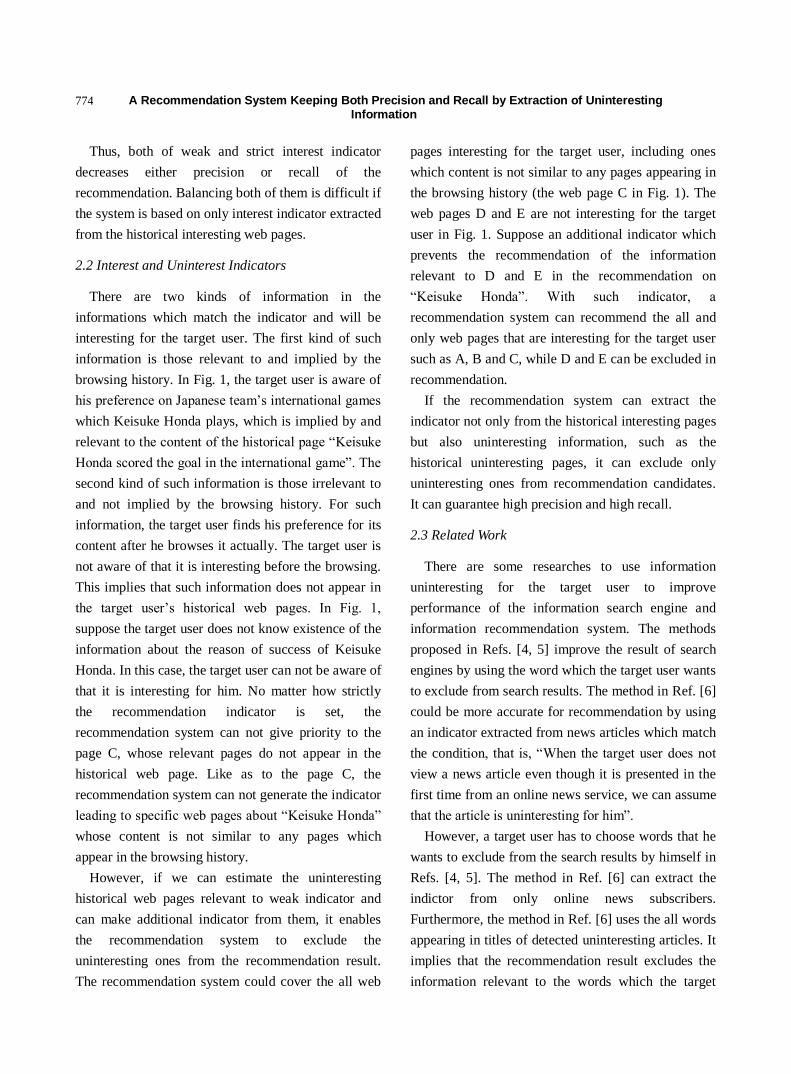
A Recommendation System Keeping Both Precision and Recall by Extraction of Uninteresting Information
774
Thus, both of weak and strict interest indicator
decreases either precision or recall of the
recommendation. Balancing both of them is difficult if
the system is based on only interest indicator extracted
from the historical interesting web pages.
2.2 Interest and Uninterest Indicators
There are two kinds of information in the
informations which match the indicator and will be
interesting for the target user. The first kind of such
information is those relevant to and implied by the
browsing history. In Fig. 1, the target user is aware of
his preference on Japanese team’s international games
which Keisuke Honda plays, which is implied by and
relevant to the content of the historical page ―Keisuke
Honda scored the goal in the international game‖. The
second kind of such information is those irrelevant to
and not implied by the browsing history. For such
information, the target user finds his preference for its
content after he browses it actually. The target user is
not aware of that it is interesting before the browsing.
This implies that such information does not appear in
the target user’s historical web pages. In Fig. 1,
suppose the target user does not know existence of the
information about the reason of success of Keisuke
Honda. In this case, the target user can not be aware of
that it is interesting for him. No matter how strictly
the recommendation indicator is set, the
recommendation system can not give priority to the
page C, whose relevant pages do not appear in the
historical web page. Like as to the page C, the
recommendation system can not generate the indicator
leading to specific web pages about ―Keisuke Honda‖
whose content is not similar to any pages which
appear in the browsing history.
However, if we can estimate the uninteresting
historical web pages relevant to weak indicator and
can make additional indicator from them, it enables
the recommendation system to exclude the
uninteresting ones from the recommendation result.
The recommendation system could cover the all web
pages interesting for the target user, including ones
which content is not similar to any pages appearing in
the browsing history (the web page C in Fig. 1). The
web pages D and E are not interesting for the target
user in Fig. 1. Suppose an additional indicator which
prevents the recommendation of the information
relevant to D and E in the recommendation on
―Keisuke Honda‖. With such indicator, a
recommendation system can recommend the all and
only web pages that are interesting for the target user
such as A, B and C, while D and E can be excluded in
recommendation.
If the recommendation system can extract the
indicator not only from the historical interesting pages
but also uninteresting information, such as the
historical uninteresting pages, it can exclude only
uninteresting ones from recommendation candidates.
It can guarantee high precision and high recall.
2.3 Related Work
There are some researches to use information
uninteresting for the target user to improve
performance of the information search engine and
information recommendation system. The methods
proposed in Refs. [4, 5] improve the result of search
engines by using the word which the target user wants
to exclude from search results. The method in Ref. [6]
could be more accurate for recommendation by using
an indicator extracted from news articles which match
the condition, that is, ―When the target user does not
view a news article even though it is presented in the
first time from an online news service, we can assume
that the article is uninteresting for him‖.
However, a target user has to choose words that he
wants to exclude from the search results by himself in
Refs. [4, 5]. The method in Ref. [6] can extract the
indictor from only online news subscribers.
Furthermore, the method in Ref. [6] uses the all words
appearing in titles of detected uninteresting articles. It
implies that the recommendation result excludes the
information relevant to the words which the target

A Recommendation System Keeping Both Precision and Recall by Extraction of Uninteresting Information
775
user are interested in. Actually, a part of words in an
uninteresting article can be inessential for his
uninterest and are rather than essential for his interest.
If we aim to use the uninteresting information as an
indicator for recommendation, we not only have to
extract the words essential to uninterestingness for the
target user as long as we should automate the
extraction of indicator corresponding to the
uninterestingness word.
3. Recommendation Method to Keep
Precision and Recall
3.1 Method Overview
We propose a recommendation system based on
interest and uninterest indicators to keep high
precision and recall. The proposed method
automatically extracts interest and uninterest
indicators. It gives positive weights to the target web
pages matching the interest indicator while it does
negative weights to the target web pages matching the
uninterest indicator. The target web pages are ranked
towards recommendation based on their total weights.
Fig. 2 shows the flow of the proposed method
consisting of the following 4 steps. Their details are
discussed in Subsections 3.2-3.5, respectively.
Step 1: The target user chooses a word for
recommendation. Then it extracts the historical web
pages whose contents are relevant to the chosen word
from the target user’s browsing history. The extracted
historical web page is called as historical related web
page;
Step 2: The method derives the interest indicator,
which is the indicator to decide whether a web page is
interesting for the target user or not. It is based on the
browsing time and bookmarking of each of the
historical related web pages;
Step 3: The method also extracts the uninterest
indicator by the similar way. The uninterest indicator
is for decision whether a web page is uninteresting or
not;
Step 4: The method determines the target web
pages to be recommended to the target user based on
interest and uninterest indicators.
3.2 Finding Historical Related Webpages
The target user chooses a word, which is called as a
related word, for recommendation. The method
recommends the web pages which have contents
relevant to the related word. It extracts the historical
related web pages from target user browsing history.
Fig. 2 Method overview.

A Recommendation System Keeping Both Precision and Recall by Extraction of Uninteresting Information
776
The historical web pages whose titles or body texts
include the related word are supposed to be historical
related pages.
3.3 Extraction of Interest Indicator
The historical interesting web pages are picked up
from the historical related web pages. If a historical
related web page satisfies either of the following
conditions, the proposed method picks it up as a
historical interesting one.
Condition 1: The web page is browsed for more
than 1 seconds, where 1
is a threshold.
Condition 2: The web page is bookmarked.
Condition 1 comes from that an article interested by
the target user is browsed for long period of time [1].
For Condition 2, it is reasonable to assume that
bookmarking a web page is the target user’s
declaration to revisit the web page in the future
because its content is interesting for the target user.
The interest indicator X is generated from the
historical interesting web pages as a set of words
according to the following idea. The target user judges
whether a web page is interesting or not based on its
content. Interest indicator has to be set as
characteristic words that can represent the contents of
the historical interesting web pages. Therefore, the
proposed method extracts the characteristic words of
the historical interesting web pages based on TFIDF.
We can suppose that characteristic words of an
historical interesting web page have high TFIDF
values with high probability. In the proposed method,
the words with the 5 highest TFIDF values are
extracted for each historical interesting web page. The
extracted words for all historical interesting web pages
are included in the interest indicator X. The
related word chosen in Step 1 is also included
into the interest indicator X regardless of its TFIDF
value.
3.4 Extraction of Uninterest Indicator
The historical uninteresting web pages are picked
up from the historical related web pages. If a historical
related web page satisfies both of the following
conditions, the proposed method derives it as an
historical uninteresting web page.
Condition 3: The web page is browsed for less than
2 seconds, where 2
is a threshold;
Condition 4: The web page is not bookmarked.
For Condition 3, a person stops browsing a web
page at the moment when he finds its
uninterestingness [1]. Thus, a historical uninteresting
web page may have a relatively short browsing time.
The limitation of the browsing time is represented by
Condition 3. For Condition 4, any bookmarked web
page should be out of the candidate of uninteresting
ones even if its browsing time is short.
The uninterest indicator Y is extracted as follows.
We consider that an uninteresting web page have
characteristic words which do not appear in the
interesting web pages, which are the factors of
uninterest. Thus, the characteristic words included in
the historical uninteresting web pages but the
historical interesting web pages can be extracted as
the uninterest indicator. Note that, however, a person
stops browsing a web page immediately when he finds
its uninterestingness. Even if he looked a partial
content of a web page and stopped browsing because
of its uninterestingness, the following content could
be interesting in fact. Thus, we consider extracting
characteristic words from only the browsed area in
each uninteresting web page. The browsed area of a
historical uninteresting web page Wi is determined
from the estimated number of read letters m (Wi). It is
given by the following equation:
)( )( ii WtRRWm (1)
where RR and t(Wi) are the reading rate and the
browsing time of Wi. The proposed method firstly
finds the words in the browsed areas with the 5
highest TFIDF values among the historical
uninteresting web pages. Secondly, the proposed
method extracts the words which do not appear in all
historical interesting web pages but in the browsed

A Recommendation System Keeping Both Precision and Recall by Extraction of Uninteresting Information
777
area of a historical uninteresting web page. The set of
such extracted words are the uninterest indicator Y.
3.5 Recommendation of Target Web Pages
The proposed method decides the target web pages
to be recommended based on their scores. Denoted by
W, M and N are a target web page which the target
user has not browsed, the number of words included
in both of the interest indicator X and the page W, and
the number of words included in both of the uninterest
indicator Y and the page W, respectively. The score
S(W) for each W is defined by Eq. (2).
M
m
N
n
muniWS11
)()1()()( (2)
Note that is a given parameter and 10 .
In Eq. (2), the word score of the k-th word included in
both of X and W is represented with )1)(( Nkki .
The word score of the l-th word included in Y is
represented with )1)(( Mllu . The Parameter
is constant to control the weights for the interest
indicator X and the uninterest indicator Y. The word
score of a word is given by its IDF value for the page
W. Eq. (2) estimates the interest on W for the target
user. If W includes a word in the interest indicator X,
the score S(W) increases by the IDF value of the word.
If W includes a word in the uninterest indicator Y,
S(W) decreases by the IDF value of the word. In this
way, the more words in the interest indicator W has,
the larger S(W) is. Similarly, the more words in the
uninterest indicator W has, the less S(W) is. The
proposed method do not use TFIDF value but the IDF
value as the word score because the possible range of
TFIDF value varies according to the length of the
body text of W. TFIDF value cannot fairly evaluate
the target web pages with different lengths of the body
texts.
Finally, the proposed method recommends the
target web pages according to their ranking in the
descending order of S(W).
4. Experimental Evaluation
4.1 Verification Contents
We verified the validity of the proposed method
through an experiment. We conducted two kinds of
verifications.
Verification 1: Thresholds decision and accuracy
The proposed method detects the historical
interesting and uninteresting web pages with
Conditions 1 and 3 in Subsections 3.3 and 3.4, which
evaluate the browsing time of web pages. These
conditions work under setting appropriate values of
the thresholds 1 and 2
.
Therefore, we investigated the browsing times of
interesting and uninteresting web pages to decide
appropriate values of the thresholds 1 and 2
. We
also investigated the detection accuracy for the
decided 1 and 2
.
Verification 2: Precision and recall improvement
The proposed method aims to keep both precision
and recall in recommendation by introducing
uninterest indicator.
We investigated whether the proposed method can
achieve balancing precision and recall than an existing
method or not. We also investigated the variation of
precision and recall with respect to the parameter ,
which determines the weight of uninterest indicator
relative to interest indicator.
4.2 Data Collection for Verification
We collected the data for verification through the
following steps. The examinees, called Examinees
A-L, were 12 university students in an IT department.
Step 1: Each examinee chose a related word. We
searched for the web pages whose titles or body texts
include the related word on the Hatena Bookmark [7].
We selected from 81 to 199 pages from the search
result and presented them to him;
Step 2: Each examinee browsed every presented
web page. He was not required to browse a presented
web page completely, where he could finish the

A Recommendation System Keeping Both Precision and Recall by Extraction of Uninteresting Information
778
browsing of uninteresting web page at any time
according to his interest. The browsing time of every
presented page was also measured;
Step 3: Each examinee evaluated every presented
web page through the following evaluation items:
Item A: ―Are there any interesting or useful
information in the presented web page?‖
It refers whether the web page is interesting or not.
The answer is by the following 4-grade evaluation: ―4:
It is very interesting web page.‖, ―3: It is interesting
web page.‖, ―2: It is uninteresting web page.‖, or ―1: I
hate this web page.‖
Item B: ―Do you want to bookmark the presented
web page?‖
It refers whether the web page is worth
bookmarking for him or not. The answer is binary,
that is, ―1: Yes, I want to bookmark it.‖ or ―0: No, I
do not bookmark it.‖
Steps 1–3 generate the pair of each presented web
page and its evaluation (interestingness and worth of
bookmarking) for each examinee.
We call the generated data as the verification data.
In the verification data, we call a presented web page
evaluated as 4 or 3 for Item A as an interesting web
page. We also do that evaluated 2 or 1 for Item A as
an uninteresting web page. Similarly, we do that
evaluated as 1 for Item B as a bookmarking
page.
4.3 Verification 1: Thresholds Decision and Accuracy
4.3.1 Thresholds Decision
Table 1 shows the average browsing times of the
interesting, uninteresting and all presented web pages
for each examinee. The interesting web pages are
browsed for longer times than all pages in every
examinee. The uninteresting web pages are done for
shorter time than all pages in every examinee. Since
the browsing times differ significantly among the
examinees, same values of thresholds 1 and 2
may not be applied to all examinees. We decided 1
and 2 for each examinee individually.
We firstly normalized each browsing time as the
standard score among all browsing times of the
corresponding examinee. It normalizes the browsing
times such that the mean and standard deviation are
changed to 50 and 10, respectively. We call the
standard score of each browsing time as the
normalized browsing time in below. Table 2 shows
the mean and the variance of the normalized browsing
times of the interesting web pages and the
uninteresting web pages among all examinees. The
normalized browsing times have a little variance in
the interesting web pages while the variance is almost
zero in the uninteresting ones. The reason of such
variance in the interesting web pages may be the
length of the body text. An examinee consumed
longer time to browse an interesting web page as its
body text was longer because he tended to browse
interesting web pages completely. Different lengths of
the body texts of the interesting web pages may bring
a little variance of the normalized browsing times. On
the other hand, because an examinee stopped
browsing a web page immediately after he found that
it was uninteresting, the variance may be almost zero
in the browsing times of the uninteresting web pages.
Table 1 Average browsing times (unit: s).
Examinee Interesting Uninteresting All
A 113 31 113
B 80 28 84
C 118 41 188
D 32 21 23
E 51 29 -
F 41 15 56
G 128 48 126
H 88 43 78
I 112 77 112
J 31 17 38
K 49 9 84
L 43 23 24
Table 2 The mean and variance of normalized browsing
times.
Interesting Uninteresting
Mean 54.91 45.84
Variance 5.72 0.8

A Recommendation System Keeping Both Precision and Recall by Extraction of Uninteresting Information
779
We decided the values of the thresholds 1 and
2 for each examinee such that the normalized
browsing times corresponding to 1 and 2
are the
mean of the normalized browsing times in the
interesting and uninteresting web pages, respectively.
ABAD
10
5091.541 (2)
ABAD
10
5084.452 (3)
Denoted by AD and AB are the standard deviation
and the mean of the browsing times of the presented
web pages for the examinee.
4.3.2 Verification of Thresholds Accuracy
We verified the validity of the values of 1 and
2 decided as mentioned in 4.3.1. We detected the
interesting and uninteresting web pages through
Conditions 1-4 in Subsections 3.3 and 3.4 by using the
decided values of 1 and 2
. Detection of
interesting web pages was conducted by 3 ways: only
Condition 1 (the condition on browsing times), only
Condition 2 (the condition on bookmarking), and both
Conditions 1 and 2. we call a detected web page as an
interesting and uninteresting one as detected
interesting and detected uninteresting web pages,
respectively. If the set of the interesting/uninteresting
web pages is the same of that of the detected ones, the
values of 1 and 2
are appropriate.
Table 3 shows the precision and recall of detection
of interesting web pages and uninteresting ones. The
result for interesting ones by only Condition 2 in
Examinee E is empty because no bookmarking page
for him existed. Table 3 shows that the deviation
between precisions of the interesting web pages is
smaller than that of the uninteresting web pages. It
may be caused by difference of browsing behavior for
interesting and uninteresting web pages.
There were four types of browsing behavior.
Generally, a person firstly looks the exordium of a
web page and determines to continue browsing or not
to do according to his interest. Examinees A, C, H, J
and L determined to continue browsing if they found
any little interesting content in the exordiums of a
presented web page. They saw that the web page was
uninteresting after the end of its browsing. It leads that
the browsing times of the uninteresting web pages are
longer and that the precisions for uninteresting web
pages are poor. Examinees B, D, F, G and K
determined to continue browsing or not definitely
when they browsed the exordiums. The browsing
times of the uninteresting web pages are short because
they stopped browsing a web page immediately after
they detect uninterestingness from the exordium. For
them, the precisions of detecting uninterest web pages
Table 3 Detection accuracies of interesting and uninteresting web pages (unit:%, P: Precision, R: Recall).
Exam.
Interesting web pages Uninteresting web pages
Only Cond. 1 Only Cond. 2 Cond. 1 & 2
P R P R P R P R
A 87 44 94 36 88 67 95 65
B 78 46 100 11 79 50 95 68
C 100 38 100 23 100 48 62 72
D 76 29 98 56 88 76 84 53
E 68 27 - - 68 27 76 63
F 83 52 100 15 84 58 93 71
G 76 41 67 4 73 41 91 68
H 80 29 100 44 90 63 88 57
I 69 32 88 83 79 86 80 48
J 91 33 75 3 89 35 69 68
K 96 56 100 22 96 56 97 61
L 94 28 75 6 90 33 52 55
Ave. 83 38 91 28 85 53 82 62

A Recommendation System Keeping Both Precision and Recall by Extraction of Uninteresting Information
780
tend to be higher than other examinees. Examinees E
and I browsed the web pages by remarkable ways,
which lowered the detection accuracy. Examinee E
did not browse an interesting web page carefully. He
browsed the web page roughly, searched for a
significantly interesting part, and browsed carefully
only found significantly-interesting parts with mouse
dragging. The browsing time depends on the length of
the body text because he searches for
significantly—interesting parts from the body text.
Examinee I browsed a web page completely even after
he found it is uninteresting from the exordium. The
browsing time depends on the length of the body text
even for the uninteresting web pages. Note that,
however, the average browsing time of the
uninteresting web pages is relatively shorter than that
of the interesting ones because he browsed the
uninteresting web page roughly. The proposed method
assumes that the browsing times of uninteresting web
pages are short while those of interesting ones are
long. It could not detect interesting and uninteresting
web pages accurately for the users such as Examinees
E and I, whose browsing times are determined with
dependent of the lengths of the body texts.
Table 3 shows that the precision and recall of
detecting interesting web pages by using Conditions 1
and 2 are 85% and 53%, respectively. Those for
uninteresting web pages are 82% and 62%,
respectively. In the proposed method, high precisions
for detection of interesting and interesting web pages
are required because invalid inclusion of words in
interest and uninterest indicators gives negative effect
to recommendation. The precisions exceed 80% in the
experimental result. Moreover, the recalls exceed 50%,
which means more than half of the interesting and
uninteresting web pages are detected validly.
Eventually, Verification 1 proves that decided values
of the thresholds 1 and 2
achieve valid and
exhaustive detection of the historical interesting and
uninteresting web pages.
4.5 Verification 2: Precision and Recall Improvement
4.5.1 Verification Purpose
The proposed method gives ranks to target web
pages from the descending order of their scores
derived by Eq. (2). General recommendation methods
do not recommend all target web pages but certain
numbers of them with the highest ranks. If a
recommendation method generates a ranking such that
many interesting web pages are at higher ranks while
uninteresting ones are at lower ranks, it achieves high
precision and recall toward good recommendation.
Verification 2 compares goodness of the rankings
between the proposed method and an existing one. If
the ranking of the proposed method is better than that
of the existing one, it can be proved that the proposed
method keeps both of precision and recall better.
4.5.2 Evaluation Method
We set the case where = 1.0 in Eq. (2) as an
existing method, which does not consider uninterest
indicator at all. The proposed method is the cases
where is each of 0.1, 0.2… 0.8, 0.9.
We firstly generated the training and test data for
each examinee. We applied the proposed method to
the verification data and detected the historical
interesting and uninteresting web pages. The detection
used the thresholds 1 and 2
set according to
Verification 1. We generated the training data by
randomly selecting 15 detected historical interesting
and 15 detected historical uninteresting web pages
from the verification data. The rest of the verification
data was set as the test data.
We secondly extracted the interest and uninterest
indicators from the training data for each examinee.
The reading rate RR in Eq. (1) was set to 8.
We thirdly applied the interest and uninterest
indicators to the test data by the proposed method
with each . We derived the ranking L of the test
data in the descending order of the score S(W). The
ranking K by the existing method was also generated
similarly.
A Recommendation System Keeping Both Precision and Recall by Extraction of Uninteresting Information
781
Fig. 3 RS improvement with respect to alpha.
We compared goodness of the rankings L and K for
each examinee by Rankscore [8]. The Rankscore RS
for L is calculated by Eqs. (5, 6) in below. is a
given parameter. I(L) is the set of interest web pages
in L. )( iWr is the rank of each interesting web page
Wi. idx(Wi) is the rank of each interesting web page
iW in an ideal ranking where all interesting web
pages are placed at the highest ranks.
)(1)(
)(1)(
2
1,
2
1
LIi
WWidxm
LIi
WWrp
iiRSRS
(5)
m
p
RS
RSRS (6)
RSp means the entire highness of the ranks of the
interesting web pages in L. It increases as more
interesting pages place in higher rank. RSm does that
in the ideal ranking. RSp/RSm measures how L is close
to the ideal ranking. We used 5 as the value of .
The Rankscore of the ranking K is calculated
similarly.
4.5.3 Verification Result
Fig. 3 shows the Rankscore improvement of the
proposed method compared with the existing one. It is
the value of RS for = 1.0 (the existing method)
subtracted from RS for each in 0.1, 0.2… 0.8, 0.9
with respect to . The positive value means the
proposed method improves RS than the existing one.
The average RS among all examinees improves as
decreases and it takes the highest value at =
0.3. However, it decreases for smaller . This is
because the uninterest indicator includes noisy words.
If the proposed method extracts the uninterest
indicator perfectly, the proposed method should
obtain the highest RS in the case = 1.0. However,
synonym words of the words in the interest indicator
and general words were included in the uninterest
indicator when the proposed method extracted the
uninterest indicator. Because of this fact, the weight
for uninterest indicator is too strong when the
proposed method works with = 1.0.
We can see the optimal value of is 0.3. A
one-tailed t-test finds statistical significance with the
significance level less than 5% (p = 0.0446) in the
difference of RSs between the proposed method with
= 0.3 and the existing method. This result shows
the utility of the proposed method. It also shows that
the proposed method can achieves balancing both of
the precision and recall by = 0.3.
6. Conclusions
This paper proposed a method to recommend web
pages under balancing both precision and recall based
on interest and uninterest indicators. The proposed
method extracts the interesting web pages and
uninteresting web pages automatically to determine
the interest indicator and uninterest indicator.
We have compared the goodness of rankings by
existing method and the proposed method. The
proposed method under = 0.3 improves the
Rankscore significantly compared with an existing

A Recommendation System Keeping Both Precision and Recall by Extraction of Uninteresting Information
782
method, where 1 is the relative weight of
uninterest indicator with respect to interest indicator.
This proves that the proposed method can recommend
interesting web pages with higher precision and recall.
Future work aims to improve extraction accuracy of
uninterest indicator. By considering the actual
browsed area of web pages and user’s individual
browsing behavior, the accuracy will improves.
References
[1] M. Morita, Y. Shinoda, Information filtering based on
user behavior analysis and best match text retrieval, in:
Proceedings 17th Annual international ACM-SiGiR
Conference on Research and Development in Information
Retrieval, Dublin, 1994.
[2] H. Sakagami, T. Kamba, Learning personal
preferenceson online newspaper articles from user
behaviors, in: Proceedings of the Sixth International
World Wide Web Conference, In Computer Networks
and ISDN Systems, Santa Clara, CA, 1997.
[3] M. Buckland, F. Gey, The relationship between recall and
precision, Journal of the American Society for
Information Science 45 (1994) 12-19.
[4] Google Home Page, https://www.google.co.jp/.
[5] T. Yamamoto, S. Nakamura, K. Tanaka, Rerank
everything: A reranking interface for exploring search
results, in: Proceedings of the 20th ACM Conference on
Information and Knowledge Management, Glasgow,
2011.
[6] K. Otsuki, G. Hattori, H. Haruno, K. Matsumoto, F.
Sugaya, A preference cluster management method based
on user access/non-viewed logs for online news delivery
toward portable terminals, DBSJ Letters 6 (2007) 37-40.
[7] Hatena Bookmark, http://b.hatena.ne.jp
[8] J.S. Breese, D. Heckerman, C. Kadie, Empirical analysis
of predictive algorithms for collaborative filtering, in:
Proceedings of the Fourteenth Annual Conference on
Uncertainly in Artificial Intelligence, Madison, 1998.

Journal of Communication and Computer 10 (2013) 783-795
Comparison of Contemporary Solutions for High Speed
Data Transport on WAN 10 Gbit/s Connections
Dmitry Kachan1, Eduard Siemens1 and Vyacheslav Shuvalov2
1 Department of Electrical, Mechanical and Industrial Engineering, Anhalt University of Applied Sciences, Kothen 06366, Germany
2 Department of Transmission of Discrete Data and Metrology, Siberian State University of Telecommunications and Information
Sciences, Novosibirsk 630102, Russia
Received: April 22, 2013 / Accepted: May 07, 2013 / Published: June 30, 2013.
Abstract: This work compares commercial fast data transport approaches through 10 Gbit/s WAN (wide area network). Common
solutions, such as FTP (file transport protocol) based on TCP/IP stack, are being increasingly replaced by modern protocols based on
more efficient stacks. To assess the capabilities of current applications for fast data transport, the following commercial solutions
were investigated: Velocity—a data transport application of Bit Speed LLC; TIXstream—a data transport application of Tixel
GmbH; FileCatalyst Direct—a data transport application of Unlimi-Tech Software Inc; Catapult Server—a data transport application
of XDT PTY LTD; ExpeDat—a commercial data transport solution of Data Expedition, Inc. The goal of this work is to test solutions
under equal network conditions and thus compare transmission performance of recent proprietary alternatives for FTP/TCP within
10 Gigabit/s networks where there are high latencies and packet loss in WANs. This research focuses on a comparison of approaches
using intuitive parameters such as data rate and duration of transmission. The comparison has revealed that of all investigated
solutions TIXstream achieves maximum link utilization in presence of lightweight impairments. The most stable results were
achieved using FC Direct. ExpeDat shows the most accurate output.
Key words: High-speed data transport, transport protocol, WAN acceleration, managed file transport.
1. Introduction
The growing demand for the fast exchange of huge
amounts of data between distant locations has led to
the emergence of many new commercial data
transport solutions that promise to transport huge
amounts of data many times faster than conventional
FTP/TCP solutions. Currently, most common
solutions for reliable data transport in IP networks
are based on the TCP protocol, which was developed
in 1970s. A number of papers describe how TCP,
with some tuning, can perform reasonably on LAN
(local area networks) with a high available
bandwidth [1]. However, it is well known that TCP
has a very limited performance when used in long
Corresponding author: Dmitry Kachan, MEng., research
fields: high speed data transport, IP networks. E-mail: [email protected].
distance networks with a high bandwidth—called
―LFN (long fat pipe network)‖ [2]. For example, a
test with Iperf using the topology described in Fig. 1
on an end-to-end 10 Gbit/slink with a 50 ms RTT
(round trip time) delay and in the presence of at least
0.1% packet loss rate shows a data rate of about 40
Mbit/s. Even after increasing socket buffers and
windows sizes to 128 MiBytes, the performance of
TCP and, accordingly, of most of solutions based on
it (SCP, Rsync, FTP), does not reach more than 60
Mbit/s. Comparable measurements of TCP over 10
Gbit/s were also performed by Wu et al. [1]. In their
work, the authors obtained a data rate of less than 1
Gbit/s even in the presence of a loss rate of 0.001%
and an RTT of 120 ms. They show a significantly
decreasing trend in a data rate with growing packet
loss rate. Another example of TCP weaknesses over
Comparison of Contemporary Solutions for High Speed Data Transport on WAN 10 Gbit/s Connections
784
long distances is described by Armbrust et al. in Ref.
[3], where the transmission of 10 TBytes of data
from Berkeley, California to Seattle, Washington via
a common TCP connection takes about 45 days,
whereas transmission of 10 TBytes hard drive takes
less than one day. A similar solution is described by
Armbrust et al. in Ref. [4]. Nevertheless, many
scenarios of remote collaboration (e.g, cloud
computing) demand data transport with maximum
synchronization times for huge data sets from a few
minutes to hours. As a result, many large companies,
for which the exchange of huge amounts of data is
often critical, avoid using legacy TCP-based
transport solutions and either prefer commercial high
speed approaches based on both TCP and UDP
transport protocols [5, 6] or develop their own
solutions based on an open source fast protocol
stacks such as UDT [7] and RBUDP [8].
Sections 2 and 3 contain brief overview of related
work and the motivation to this work; Section 4
describes the testbed that has been used for
experiments; Section 5 contains short information
about each solution under test and results of the tests;
Sections 6 and 7 are dedicated to comparison of
results, summary and conclusion of the work.
2. Related Work
The main goal of our work is to assess the
capabilities of transport solutions in a 10 Gbit/s
network. Of interest is the maximal possible
end-to-end application data rate on such networks in
the presence of impairments such as packet losses and
high round-trip times. Currently, there are a few
different performance measurements that have been
used to assess these impairments in open source and
freeware solutions. For example, Grossman et al. [9]
present the performance evaluation of UDT [7]
through a 10 Gbit/s network. The article shows how
using UDT and in the presence of 116 ms of RTT, this
network has a maximum throughput of 4.5 Gbit/s
within a single data stream. Two parallel streams
achieve together about 5 Gbit/s and within 8 parallel
streams about 6.6 Gbit/s are achieved. Further, a
performance result for data transmission using
RBUDP was presented at the Cine Grid 3rd Annual
International Workshop [10]. While the disk access
speed limited the data transport speed to 3.5 Gbit/s, on
the link from Amsterdam to San Diego only 1.2 Gbit/s
was reached. The distance of that path is about 10,000
km through optic fiber, which corresponds to about
100 ms of RTT.
Most other data transport performance results are
presented for 1 Gbit/s networks e.g. three rate based
transport protocols have been evaluated by Wu et al.
in Ref. [11]: RBUDP, SABUL and GTP. The overall
data rate of applications based on these protocols was
compared for all three protocols and for ―standard
unturned TCP‖. The experiment was performed on a
real network in the presence of 58 ms of RTT and a
loss rate of less than 0.1%. The results showed that all
solutions utilize the 1 Gbit/s link approximately 90%.
These test results show that for open source data
transfer solutions, even those using parallel streams, it
is quite hard to achieve full, or even close to full,
utilization of 10 Gbit/s links.
For commercial closed source solutions, the
situation differs significantly. There are several
published performance results of commercially
available solutions, provided by the manufacturers
themselves: Velocity [12], TIXstream [13], FC Direct
[14] and Catapult Server [15]—all of whom report
perfect results. However these results are mainly
providing commercial information to attract potential
customers and the investigative conditions vary. To
overcome this deficit, the main idea behind the
auhtors’ work is to place all investigated
solutions under equal conditions within the same
environment.
3. Background
For IP networks, packet loss behavior depends on
many factors such as quality of transmission media,

Comparison of Contemporary Solutions for High Speed Data Transport on WAN 10 Gbit/s Connections
785
CPU performance of intermediate network devices,
presence of cross traffic etc.. It is therefore
impossible to use one universal value of packet
losses for all cases. The best way to assess the
approximate values of packet losses is through
empirical measurements. In Ref. [16], Paxson
discusses the heterogeneity of packet losses and
shows that, even in 1994, the value of packet loss
rate in experiments between 35 sites in 9 countries
was about 2.7%. He also shows that, within one year,
the value of packet losses increased up to 5%.
Probably, such packet loss values are not relevant to
the current Internet; however the author pointed out
that distribution of packet losses is not uniform. Thus,
for some connections, ACK packet loss was not
observed at all. Nevertheless, relative values of all
lost IP packets in both directions for all experiments
were approximately equal. Recent views on the
packet loss ratio are presented by Wang et al. in Ref.
[17]. In this research, tests were made across 6
continents between 147 countries, involving about
10,000 different paths. The authors show that across
all continents for more than 70% of continental
connections, packet loss rate is less than 1%, in
Europe and North America this value is even on
about 90% of connections. The authors also
highlighted that for intercontinental connections,
packet loss value in general is lower than for
intra-continental—across the entire world, packet
loss rate is lower than 1% for about 75% of the
connections.
In Ref. [18], Settlemyer et al. use a hardware
emulator to emulate 10 Gbit/s paths, and they
compare throughput measurement results of the
emulated paths with real ones. The maximal RTT of a
real link used in the research is 171 ms. The authors
have shown that differences between profiles of both
kinds of paths—emulated and real ones—are not
significant, and they conclude that using emulated
infrastructure is a much less expensive way to
generate robust physical throughput.
4. Testbed Topology Description
In this work, the following solutions have been
investigated: Velocity, TIXstream, FileCatalyst Direct,
Catapult Server, ExpeDat. Manufactures of all these
solutions claim that their transport solutions are able
to handle data transmission via WAN in the most
efficient way.
Since all these solutions are commercial and closed
source, it was necessary to get in touch with the
support team of each manufacturer for both obtaining
trial licenses of their products and consulting them
about achieved results. Unfortunately, not all
manufactures were interested in such investigations.
Thus, for example, it would have been interesting to
test Aspera’s solution for fast data transport. However
the authors received no answer from this vendor.
To avoid unexpected inaccuracies, the scheme of
test topology is kept simple. Fig. 1 presents the
typology. The core of the test environment was the
WAN emulator Apposite Netropy 10G [19], which
allows the emulation of WANs under various
conditions such as packet delay, packet loss rate and
jitter in different variations, with an accuracy of about
20 ns. By comparison, software emulators, such as
Net Em, provide an accuracy of about tens of
milliseconds and this value is greatly dependent on the
hardware and operating system [20]. Moreover,
software emulators are very limited in their maximum
achievable data rates. Apposite 10G, for example,
enables a transmission through Ethernet traffic with
an overall throughput of up to 21 Gbit/s on both
copper and fiber optic links.
The testbed topology used here contains two
servers, connected via the 10 Gbit/s Ethernet switch
Extreme Networks Summit x650 and via the WAN
Emulator.
Fig. 1 Logical view of topology.
Internet
Host 1 Host 2
RTT up to 200 Packet loss up to 1%

Comparison of Contemporary Solutions for High Speed Data Transport on WAN 10 Gbit/s Connections
786
The typology was implemented by means of fiber
optics with a 10 Gbit/s bandwidth in Fig. 2.
There is no background traffic on the path since this
investigation focuses on the pure applications’
performance, not on the fairness aspects of the
protocols. The setup corresponds to the case when a
L2-VPN is used for big data transmission and another
application’s traffic is isolated by means of QoS.
Each server is equipped as follows:
(1) CPU: Intel Xeon X5690 @3.47GHz;
(2) RAM: 42 GiBytes (speed 3,466 MHz);
(3) OS: Linux CentOS 6.3;
(4) NIC: Chelsio Communications Inc T420-CR, 10
Gbit/s.
Operating system socket buffers were extended up
to:
(1) /proc/sys/core/net/wmem_max—64MiBytes
(2) /proc/sys/core/net/rmem_max—64MiBytes
The MTU size of all network devices along the path
was set to 8,900 Bytes.
For sending and receiving data with a rate of 10
Gbit/s, it is necessary to have a storage device that can
read on the sender side and write on the receiver side
with a sustained rate not less than 1,250 MByte/s
(corresponding to 10 Gbit/s). Off-the-shelf hard drives
provide read and write rates of up to 100 MByte/s, so
in the investigated case, data transfer rate would have
been limited by the hard drives. To circumvent this
limitation, storage systems such as RAID arrays with
write/read rates not less than the expected transport
rate must be used.
In the presented experiments, both storage write
and read bottlenecks and inefficient file access
implementations were avoided by using a RAM-based
Fig. 2 Technical view of topology.
file system on both servers. In comparison to common
hard drives, the read rate of RAM disk, as obtained in
several test runs during these investigations, was not
less than 4,500 MiBytes/s; the write rate of RAM disk
was not less than 3,000 MiBytes/s. Therefore, the
servers used for tests were equipped with 42 GiBytes
of RAM onboard, but due to the operating system’s
RAM requirements, it was only possible to use 30
GiBytes of space on RAM disk for test purposes.
Under ideal conditions, a transmission of 30
GiBytes through the network with a bandwidth of 10
Gbit/s without impairments, as explained in Eq. (1),
should take about 26 seconds.
sRi
ST 76.25
1010
10/81024303
63
(1)
where, T—time of transmission; s–size of data,
iR —ideal data rate.
However, this calculation disregards L2-L4 headers
along with some proprietary protocol headers and the
overhead for connection management and
retransmissions.
So, under real conditions, for some packet overhead
and retransmission handling, each solution needs a
certain amount of time for connection initialization
and the releasing of the network path. Besides this, in
high-performance implementations, initialization of
the protocol stacks and the internal buffers often takes
a significant amount of time, which is also
investigated during this research.
5. Experimental Results
The experiment on each data transport solution
under consideration consists of 25 consecutive tests.
Each test comprises the transfer of a 30 GiBytes file
from one server to another through the network
emulator. The RTT latency range is varied from 0 to
200 ms in steps of 50 ms and the packet loss rate takes
the values 0, 0.1%, 0.3%, 0.5% and 1%. Since 1 km of
fiber optics delays the signal by about 5 µs, the
maximum RTT in this test corresponds to 20,000 km
of fiber channel in both the forward and the backward
directions. The RTT is configured symmetrically
Server 1 Server 2Extreme Networks
Summit x650
Apposite

Comparison of Contemporary Solutions for High Speed Data Transport on WAN 10 Gbit/s Connections
787
across the forward and backward paths of the
emulator; thus 200 ms of RTT would delay data by
100 ms and acknowledgments or other control
information in the backward direction by another 100
ms. The packet losses are randomly injected according
to a normal distribution, whereby the set loss ratio is
applied to both forward and backward direction. Such
packet loss behavior is easier to reproduce, and it is
more complicated for protocols to handle than typical
packet loss behavior on the Internet [16]. An attempt
was made to configure each solution so that the
maximum possible data rate and the minimum
possible overall transmission time were achieved. The
tuning of the operating system and the configuring of
parameters are described below for each solution. All
the tests were repeated 4 times to avoid inaccuracies,
and the best result of each series is presented on the
plots.
The results of each test contain two parameters:
data rate and transfer duration. The first parameter is
average data rate, i.e. the average speed of data
transportation shown by the application during the
experiment. The second parameter is independent of
the solution output and represents the time interval.
This time interval was collected by means of the
operating system and shows the period of time
between the launching of the send command and the
time of completion of this command. This time
interval contains not only the time of actual data
transmission but also the time for service and
retransmission overhead.
5.1 Velocity
This solution was developed in the USA. It is a
TCP-based file transfer application, and according to
the vendor’s web site, it allows the available path
capacity to be fully utilized. Velocity ASC is also
available with on-the-fly data encryption of up to 24
Gbit/s and AES encryption of up to 1,600 Mbit/s. The
supported platforms are Windows, Mac OSX, Linux
and Solaris. According to the user manual, this
solution automatically adapts its parameters to
network conditions and chooses the optimal
parameters for data transmission. Fig. 3 shows the
behavior of the transport rate. The results of tests in
the presence of delays of more than 0.1% are not
shown since the data rate here was lower than 100
Mbit/s.
Increasing latencies do not significantly affect
Velocity’s data rate behavior, slowing it down to only
8 Gbit/s. The solution performs reasonably in the
presence of small packet loss rates without any
emulated delay (back-to-back RTT latency in the
testbed is about 0.15 ms). Thus it achieves a data rate
of 9 Gbit/s in the presence of 0.1% of packet loss, and
this value decreases down to 500 Mbit/s with a packet
loss of 1%. However, this configuration does not
correspond to the situation in Wide Area Networks. In
the presence of 0.1% packet loss and at least 50 ms
RTT, the data rate is reduced to 250 Mbit/s.
Multi-streaming TCP is using by default velocity. It
opens 7 TCP sockets on every single test on each side.
When the number of streams is manually set to 1, the
data rate in presence of 200 ms RTT without packet
loss is about 2.2 Gbit/s. The transfer durations of the
solution are shown in Fig. 4. The numbers on the plot
are obtained for two cases: without latency and with a
latency of 200 ms. A result worth noting was obtained
at a loss rate of 0.1% and an RTT of 0 ms. Under
these conditions, the data rate in the presence of losses
is, with 800 Mbits/s, less than the value without loss
Fig. 3 Behavior of data rate of velocity.

Comparison of Contemporary Solutions for High Speed Data Transport on WAN 10 Gbit/s Connections
788
Fig. 4 Data transfer duration of velocity.
rate. However, the transfer duration in the latter case
is higher by only 0.1 ms. This behavior was observed
in several experiments.
5.2 TIXstream
This transfer engine has been developed by
TixelGmbH, Germany, which spun off from
Technicolor Corporate Research in 2010. The core of
TIXstream is Tixel’s proprietary RWTP (reliable
WAN transfer protocol) [21], which provides
high-performance data transmission between two
hosts in the network using only one UDP-socket on
each host. The application works under Linux OS.
TIXstream 3.0 (the latest version) provides up to 20
Gbit/s end-to-end performance. It has a
platform—independent web-based user interface for
the management of data transmission between remote
SAN- and NAS systems. TIXstream also provides
on-the-fly AES-256 encryption of data without any
effect on data rate [22]. TIXstream has a peer-to-peer
architecture and uses one TCP socket for control
communication and one UDP socket for data
transmission connection on both sides.
Parameters of application:
(1) RWTP Buffer size—4,362,076,160 Bytes (4
GiBytes);
(2) MSS = 8,800 Bytes;
(3) Receiver buffer size (on both sides) =
1,073,741,824 Bytes (1 GiByte);
(4) Sender buffer size (on both sides) =
1,073,741,824 Bytes (1 GiByte).
The behavior of TIXstream’s data rate as a function
of network impairments is shown in Fig. 5.
There is no visibly decreasing effect on data rate
behavior till 100 ms RTT and till 0.3% of packet loss.
The solution achieves not less than 9.7 Gbit/s (97% of
capacity) with these impairments. With higher delays
in the presence of heavy packet losses, the figure
shows decreasing data rates down to 3,750 Mbit/s, as
on a path with 200ms of RTT and 1% of packet losses.
However, with modest impairments that correspond to
fairly normal WAN links, for example RTT 150 ms
and packet loss rate 0.1%,TIXstream achieves a data
rate of about 8,700 Mbit/s; an 87% utilization of a 10
Gbit/s link. It is worth noting that in the presence of
50 ms of latency, TIXstream performs better than
without any latency for all values of loss rate. This
behavior was found in several experiments.
Fig. 6 shows that the transfer duration quite
accurately corresponds to the behavior of the data
rates. However, the theoretically minimum time of
transmission calculated in Section 0, with a data rate
of 8,700 Mbit/s, is 29.62s versus the 37.25 s that was
measured in the experiment. These 7.63 s were spent
on connection initialization, and the establishing and
releasing of the control channel. Since no packet loss
Fig. 5 Behavior of data rate of TIXstream.
Fig. 6 Data transfer duration of TIXstream.

Comparison of Contemporary Solutions for High Speed Data Transport on WAN 10 Gbit/s Connections
789
shall occur on this link, time for packet retransmission
shall be neglected.
5.3 FileCatalyst Direct
FileCalatyst Direct was developed by Unlimi-Tech
Software Inc., a Canadian based company. Like
TIXstream, it transmits data via UDP and implements
packet loss management, rate and congestion control
in the user layer. The application obeys a client-server
architecture and the solution operates under Windows,
Mac OSX, Linux and Solaris operating systems. The
data sheet on the vendor’s website shows that this
solution provides data rates of up to 10 Gbit/s [23] and
that there is an option to use AES encryption for
secure transmission. FC Direct provides both,
graphical and command line user interfaces for server
and client applications.
Parameters of application:
(1) Start rate = 9,000,000 (9 Gbit/s);
(2) MSS = 8,800 Bytes;
(3) Buffers = 3,840,000,000 Bytes (3,58 GiBytes);
(4) Number of send sockets = 10;
(5) Number of receiver sockets = 4.
As shown on Fig. 7, FC Direct achieves 90% to
94% link utilization, even under high network
impairments. Data rate behavior is fairly immune to
growing latency and packet loss ratio. The data rate of
FC Direct shows values between 9 Gbit/s and 9.4
Gbit/s for all the tests. During the tests, the Linux
system monitor reveals that each data transmission
opens 10 UDP sockets on the sender side and 4 UDP
sockets on the receiver side and 1 TCP socket on each
side. In this mode, maximal data rates can be achieved.
Data packets from ten sender sockets are not
uniformly distributed over all four receiver sockets,
but according to a special proprietary distribution rule.
The vendor does not call it multi-streaming but ―more
intelligent resource management‖. However, with this
behavior, significant firewall transversal issues are to
be expected.
The distribution of session time durations showed
on Fig. 8 has slightly monotonically increasing
behavior with rising latencies.
5.4 Catapult Server
The Catapult Server is TCP-based and was
developed by XDT PTY LTD, Australia. This
solution follows a client-server architecture and,
according to the vendor’s web site, provides up to 8
Gbit/s on the 10 Gbit/s link. The solution functions
under the Windows, MAC OSX and Linux operating
systems. The vendor positions the solution as a high
data rate transmitting tool for networks with a high
level of latency but without any packet losses. To
prepare the operating system for high speed
transmissions, the vendor suggests using a shell script
to change network parameters. By default, this script
extends the TCP buffers to 32 Mbytes. However, for
the authors’ tests, the 64 Mbytes setting was chosen
since better performance had been reached with this
setting.
The script changes are:
(1) tcp_congestion_control = htcp;
(2) net.ipv4.tcp_rmem = 40,968,738,067,108,864;
Fig. 7 Behavior of send rate of FC direct.
Fig. 8 Data transfer duration of FC direct.

Comparison of Contemporary Solutions for High Speed Data Transport on WAN 10 Gbit/s Connections
790
(3) net.ipv4.tcp_wmem = 40,966,553,667,108,864;
(4) net.ipv4.tcp_no_metrics_save = 1;
(5) net.core.netdev_max_backlog = 250,000;
(6) net.core.rmem_max = 67,108,864;
(7) net.core.wmem_max = 67,108,864.
To improve the behavior of this solution in the
presence of packet losses, the manufacturer’s support
team also suggested applying the following
configurations:
(1) net.ipv4.tcp_timestamps = 1;
(2) net.ipv4.tcp_sack = 1.
Note that the command line client of XDT-sling
shot copy, which was used for the tests, shows the
data rate as GB/s, probably it means GiByte/s.
Furthermore the value 1.1 GB/s immediately follows
the value 1.0 GB/s, without any intermediate values.
However, the solution shows a transfer duration with an
accuracy of up to milliseconds. Therefore, the data rate
was calculated as shown on Eq. (2):
,T
S
0
XDTR (2)
Where by RXDT—is the data rate of XDT, which is
used for result presentation; S—data size (30 GiByte),
T0—transfer duration from the output of client
application.
Fig. 9 represents the data rate of Catapult Server
dependent on network impairments. The presence of
packet losses on the link makes the transmission
ineffective, so the data rate is reduced to less than 100
Mbit/s. However, in the presence of 150 ms RTT
without packet loss, transmission is about 8,300
Mbit/s
Fig. 10 shows the transfer durations for Catapult
technology.
5.5 ExpeDat
ExpeDat is a UDP-based data transport solution
developed by Data Expedition Inc., USA. The core of
this application comprises the MTP (multipurpose
transaction protocol) [24], developed by the founder
of Data Expedition. ExpeDat supports Windows, Mac
OSX, Linux / Solaris, NetBSD / FreeBSD, AIX and
HP-UX platforms. According to the company’s web
site, ExpeDat allows transmission of data with 100%
utilization of allocated bandwidth and in the presence
of on-the-fly AES encryption [25]. It implements the
transport protocol logics on a UDP channel, and uses
a single UDP socket on each side of the connection
for both data transmission and control information.
Though the product web site [25] claims that the
solution has ―zero-config installation‖, the significant
increase of data rate, namely from 2 Gbit/s up to 9
Gbit/s, even without impairments (RTT = 0 ms,
packet loss = 0%), was obtained only after application
of configuration changes as follows:
MSS—8,192 Bytes;
Environment variable MTP_NOCHECKSUM = 1.
With high values of packet loss on the channel, the
higher results were achieved using the following
option on the command line:
N 25.
Fig. 9 Behavior of data rate of XDT catapult.
Fig. 10 Data transfer duration of XDT catapult.

Comparison of Contemporary Solutions for High Speed Data Transport on WAN 10 Gbit/s Connections
791
The use of this option shows that heavy packet loss
rate is introduced in a channel.
In Fig. 11, the data rate values of ExpeDat tests are
presented. The plot shows that network latencies lead
to a much higher reduction of the transmission rate
than packet loss.
The distribution of transfer times is presented in
Fig. 12.
6. Comparison of the Solutions
Since not all of the investigated solutions perform
well in the presence of heavy packet losses, the
comparison of data rates was split into two stages. The
first stage is dedicated to a comparison of all
presented solutions on the networks with different
packet latencies and without any packet loss. In the
second stage, the solutions are compared under harder
conditions for terrestrial networks—with packet loss
of 1% and the whole range of investigated RTT. Only
solutions that show a data rate higher than 1% from
maximal channel capacity (100 Mbit/s) have been
considered in the second stage.
A comparison between the distribution of transfer
duration without packet losses and the ideal value
shows which solution spends more time on service
needs such as the initialization and releasing of a
channel.
A further comparison shows the discrepancy
between the actual time of transmission and the
calculated time from the output of all solutions. This
analysis is also split into two stages as described
above and shows how the values from the output of
the particular solution correspond to reality.
Fig. 13 shows a consolidated diagram of
transmission data rates of all tested solutions in the
presence of increasing latency and without any packet
loss on the path. The first set of bars shows how fast a
large set of data can be transmitted in a back-to-back
connection. For this case, the highest result was
achieved by Velocity. However all solutions showed
results of not less than 9.3 Gbit/s. With increased
latencies, Velocity performs worse, and of all the
remaining cases, TIXstream shows the best
performance with up to 9.8 Gbit/s (98% channel
utilization) without any significant decrease at higher
RTTs. FC Direct also shows very stable results. For
all presented impairments, its data rate lies between
9.2 Gbit/s and 9.3 Gbit/s. All other solutions show
decreasing data rates on increasing round-trip-times.
TCP-based solutions obviously can not cope
efficiently with the presence of packet losses on the
path. Although for all solutions except Velocity, the
Fig. 11 Behavior of data rate of ExpeDat.
Fig. 12 Data transfer duration of ExpeDat.
Fig. 13 Comparison of data rates of investigated solutions;
packet loss = 0.

Comparison of Contemporary Solutions for High Speed Data Transport on WAN 10 Gbit/s Connections
792
support teams of the respective manufacturers were
involved, those solutions did not provide adequate
results in the presence of packet loss. Fig. 14
represents the behavior of solutions of stage two in the
presence of 1% of packet loss.
With an RTT of 0 and 50 ms, TIXstream shows the
best results. However, starting at 100 ms, throughput
is decreased whereas FC Direct shows nearly constant
data rates. The ExpeDat data rate abruptly decreases
down to 5.7 Gbit/s on zero-delay links, and with
increasing latencies ExpeDat’s results are lower than 1
Gbit/s.
As pointed out in Section 0, the theoretical
minimum transfer duration for the transport of 30
GiBytes of data via a 10 Gbit/s WAN is 25.76 s. Fig.
15 compares, for each solution, the ideal value with
the lowest transfer durations obtained during the
experiments.
The minimum transfer duration was achieved by
XDT Catapult server. The time is only 1.4 s longer
than the theoretical minimum. This means that XDT
Catapult initializes the software stack along with
protocol buffers, and establishes and closes the
connection within less than 1.4 s. The time overhead
of Velocity, TIXstream and ExpeDat is slightly higher
but still less than 2 seconds. The worst result was
obtained when using FC Direct: it needed about 3.8 s.
for ramping-up and finishing the application.
Also of interest is the accuracy of the performance
outputs of the transport solutions. During the
experiment, the actual data rate was obtained from the
output of the running application, and program run
time was also measured by means of the operating
system. Transfer durations with a transmission of 30
GiByte with a data rate from output are calculated as
shown on Eq. (3).
][,R
[ B i t s ] S, t
0 sBits
T (3)
where Tt—is the calculated transfer duration; R0—data rate from output; S—data size (30 GiByte).
The differences between calculated transfer
durations and real program run time for the tests
performed without packet loses are presented in Fig.
16. The discrepancy of the values generally has an
increasing trend at higher latencies. Velocity showed
the lowest value of discrepancy along the tests without
Fig. 14 Comparison of data rate of tested solutions;
packet loss = 1%.
Fig. 15 Comparison of transfer durations with theoretical
minimum.
Fig. 16 Difference between calculated and actual transfer
durations; packet loss = 0.
Fig. 17 Difference between calculated and actual transfer
durations; packet loss = 1.

Comparison of Contemporary Solutions for High Speed Data Transport on WAN 10 Gbit/s Connections
793
packet loss. The second TCP-based
solution—XDTCatapult shows good results on RTTs
below 200 ms. However, with 200 msRTT, this
solution shows the worst of all results. ExpeDat
almost always has the lowest discrepancy values for
all cases. In the presence of RTTs of 100 ms and 150
ms without loss rate, the solution showed negative
result, meaning that the actual transfer duration was
lower than the calculated one. It is evident that the
output of some solutions show the average achieved
data rate including service processes such as
connecting, initializing and releasing the link, and
some of the solutions show the average data rate of
the transmission process only.
Similar to Fig. 16 but with a packet loss of 1%, Fig.
17 shows the differences of calculated transfer
durations and real program run time. A comparison of
these two figures shows that FC Direct has almost the
same discrepancies for all RTT cases except for the
200 ms and 150 cases, where the discrepancy is higher
in the presence of packet loss than without it. The
results of TIXstream have a decreasing trend and
ExpeDat shows again the lowest values—the actual
times of transmission are almost equal to the
calculated ones.
7. Conclusions
This work compares the state of the art of
commercial solutions for reliable fast data transport
via 10 Gbit/s WAN IP networks in the presence of
high delays and varying packet loss rates. The main
problem of such research is that the vendor companies
usually hide the technology used for the accelerated
data transport. The protocol used in ExpeDat solution
—MTP—is covered by some US patents. However
this does not mean that ExpeDat does not use any
algorithms besides the ones described in those patents.
The only independent method to assess these
commercial solutions is to externally observe the
solutions during tests under well-defined conditions.
All investigated solutions position themselves as
reliable high-speed transfer applications designed to
provide alternatives to FTP/TCP and overcoming the
pure TCP performance on 10 Gbit/s-WAN
connections by orders of magnitude. Two of them,
Velocity and XDT Catapult, exploit the TCP stack of
the Linux OS and the rest-FC Direct, TIXstream and
ExpeDat use UDP sockets and implement the protocol
logics in the user-level.
The results obtained show that solutions based on
TCP inherit its native problems on 10 Gbit/s links—a
significant decrease of data rate down to 1% of the
link capacity in the presence of packet loss on the path.
The commercial solutions achieve a higher speed by
increasing TCP window size or by establishing
multiple parallel TCP streams. However, the
experiments show that this solution only works on
links without any packet loss. However, even the
known STCP [26] on WAN networks with a low loss
rate show a reasonable result of about 5 Gbit/s [1].
Although in that paper, the authors tested pure
protocol performance, their results show that it is
possible to achieve good results by only tuning the
TCP on such networks.
UDP-based solutions show a good utilization of a
10 Gbit/s path even under bad network conditions
such as a loss rate of 1% in the presence of RTTs of
up to 200 ms. The best link utilization at the highest
impairment value was achieved by FileCatalyst
Direct—the values were never lower than 93% for all
performed tests. For the loss ratio up to 0.3% and RTT
up to 100 ms, TIXstream shows a better utilization of
about 97 %.
Transmission duration measurements were
primarily intended to prove that the solutions show
accurate data transport numbers in their outputs. The
comparison showed that the lowest transfer duration
of each solution is fairly close to the ideal one and that
the discrepancy of the obtained output values are close
to reality for all solutions.
Each solution uses some time for the allocation of
system resources and the initialization of network

Comparison of Contemporary Solutions for High Speed Data Transport on WAN 10 Gbit/s Connections
794
resources. This time can not be neglected, at least not
in sessions with up to 30 GiBytes data transport. The
comparison presented in Fig. 15 attempts to assess
this service time. Probably, the time overhead is also
due to the solutions not fully utilizing the bandwidth.
It was found that the data rate of FC Direct is not the
lowest one, but the transfer duration is higher than for
all other solutions under test conditions. This result is
possibly due to known java performance bottlenecks,
because FC Direct is the only solution written purely
in java.
When the solutions work under very light network
impairment conditions (for example back-to-back) and
the data rate achieves maximal value, the CPU usage
is fairly high. For example, the maximum achieved
data rate of ExpeDat seems to be due to CPU
limitations. The system monitor showed 99% CPU
usage in the ExpeDat process, and it also showed that
one core of twelve is used in 99%. Other solutions, e.g.
TIXstream, showed a CPU usage of about 150%, the
usage of two used cores was about 70% and 80%
respectively on the sender side, and on the receiver
side 3 cores were used with a usage of 40%, 90%,
30%. This solution distributes the performance among
several cores to maximally use the available
bandwidth when possible.
One more significant point of resources
management is the socket use. As shown in Section 0,
FC Direct uses different numbers of sockets on the
sender and receiver sides. This use causes no
problems for corporate LANs or simple back-to-back
connections. However, for data transport using more
complex structures, like real Internet connections, this
use could cause problems on such devices such as
firewalls. Such problems are well known even in
simple multi streaming cases. This is an even worse
situation in which each sender socket is sending data
to different destination ports, so at least M × N port
pairs must be tunneled in the firewall. It is very likely
that intrusion detection systems can consider such
behavior as violent traffic.
The analyzed solutions were tested on their abilities
in the presence of high values of latency and packet
losses. However, delay jitter is also a common
network impairment and measurements using
different values and different jitter patterns would also
be of interest.
The present research shows the behavior of the
solutions in an empty path such as VPN. Further
investigations could be made into the behavior of the
solutions in the presence of back-ground traffic.
The testbed topology was simplified to get a first
representation of the presented solutions. An
extension of the experimental topology makes sense
for in-depth investigations.
During the experiments, only the performance of
data transfer for commercial applications was
investigated. To get a deeper understanding of only
the telecommunication part, it would be of interest to
make tests with the technology cores (e.g. protocol
stacks without any wraps such as file system).
The questions of system resource consumptions
were addressed very briefly here. It would also be
interesting to research this topic more extensively.
References
[1] Y. Wu, S. Kumar, S.J. Park, Measurement and
performance issues of transport protocols over 10 Gbps
high-speed optical networks, Computer Networks 54
(2010) 475-488.
[2] H. Kamezawa, M. Nakamura, M. Nakamura, Inter-layer
coordination for parallel TCP streams on long fat pipe
networks, in: Proc. of the 2004 ACM/IEEE conference on
Supercomputing, Pittsburg, PA, USA, 2004.
[3] M. Armbrust, A. Fox, R. Griffith, A.D. Joseph, R.H. Katz,
A. Konwinski, Above the clouds: A berkeley view of
cloud computing, Tec. Rep. UDB/EECS 28 (2009) 19-25.
[4] M. Armbrust, A. Fox, R. Griffith, A.D. Joseph, R.H. Katz,
A. Konwinski, et al., A view of cloud computing,
Communications of the ACM 53 (2010) 50-58.
[5] S. Hohlig, Optimierter dateitranfer über 100 Gigabit/s, in:
100 Gigabit/s Workshop of the DFN, Mannheim, 2011.
[6] Aspera, Custumer Deluxe Digital Studios, [Online],
http://asperasoft.com/customers/customer/view/Customer
/show/deluxe-digital-studios/ (accesseed: Nov., 2012).
[7] Y. Gu, R.L. Grossman, UDP-Based datatransfer for
high-speed wide area networks, Computer Networks 51

Comparison of Contemporary Solutions for High Speed Data Transport on WAN 10 Gbit/s Connections
795
(2007) 1465-1480.
[8] E. He, J. Leigh, O. Yu, T.A. DeFanti, Reliable blast UDP :
Predictable high performance bulk data transfer, in: Proc.
of IEEE Cluster Computing, Chicago, USA, 2002.
[9] R.L. Grossman, Y. Gu, X. Hong, A. Antony, J. Blom, F.
Dijkstra,Teraflows over Gigabit WANs with UDT,
Journal of Future Computer Systems 21 (2005)
501-513.
[10] L. Herr, M. Kresek, Building a New User Community for
Very High Quality Media Applications on Very High
Speed Networks, [Online], CineGrid,
http://czechlight.cesnet.cz/documents/publications/networ
k-architecture/2008/krsek-cinegrid.pdf. (accessed: Feb.,
2013).
[11] X. Wu, A.A. Chien, Evaluation of rate-based transport
protocols for lambda-grids, in: Proc. of 13th IEEE
International Symposiumon High Performance
Distributed Computing, Honolulu, Hawaii, USA, Jun. 4-6,
2004.
[12] Bitspeed LLC, From Here to There-Much Faster,
Whitepaper,[Online]
http://www.bitspeed.com/wp-content/uploads/2011/10/Bi
tSpeed-White-Paper-From-Here-to-There-Much-Faster.p
df (accessed: Oct., 2012).
[13] Tixel GmbH, Tixstream: Overview, [Online],
http://www.tixeltec.com/ps_tixstream_en.html (accessed:
Oct., 2012).
[14] File Catalyst, Accelerating File Transfers, Whitepaper,
[Online],
http://www.filecatalyst.com/collateral/Accelerating_File_
Transfers.pdf (accessed: Oct., 2012).
[15] XDT PTY LTD, High-Speed WAN and LAN data
transfers, XDT, [Online],
http://www.xdt.com.au/Products/CatapultServer/Features
(accessed: Oct., 2012).
[16] V. Paxson, End-to-End internet packet dynamics,
networking, IEEE/ACM Transactions 7 (1999) 277-292.
[17] Y.A. Wang, C. Huang, J. Li, K.W. Ross, Queen:
Estimating packet loss rate between arbitrary internet
hosts, in: Proc. of the 10th International Conference on
Passive and Active Network Measurement, Seoul, Korea,
2009.
[18] B.W. Settlemyer, N.S.V. Rao, S.W. Poole, S.W. Hodson,
S.E. Hick, P.M. Newman, Experimental analysis of 10
Gbps transfers over physical and emulated dedicated
connections, in: Proc. of Computing, Networking and
Communications (ICNC), Maui, Hawaii, USA, 2012.
[19] Apposite Technologies, [Online],
http://www.apposite-tech.com/index.html (accessed: Oct.,
2012).
[20] A. Jurgelionis, J.P. Laulajainen, M.I. Hirvonen, A.I.
Wang, An Empirical Study of NetEm Network Emulation
Functionalities, ICCCN (2011) 1-6.
[21] Tixel GmbH, White Papers and Reports, Tixel, [Online],
http://www.tixeltec.com/papers_en.html (accessed: Nov.,
2012).
[22] Tixel GmbH, Tixel news. tixel.com, [Online],
http://www.tixeltec.com/news_en.html (accessed: Oct.,
2012).
[23] FileCatalyst, Direct, [Online],
http://www.filecatalyst.com/collateral/FileCatalyst_Direc
t.pdf (accessed: Oct., 2012).
[24] Data Expedition, Difference, [Online],
http://www.dataexpedition.com/downloads/DEI-WP.pdf
(accessed: Oct., 2012).
[25] Data Expedition, [Online],
http://www.dataexpedition.com/expedat/ (accessed: Oct.,
2012).
[26] R. Stewart, Q. Xie, Motorola, K. Morneault, C. Sharp,
Cisco, Stream Control Transmission Protocol, IETF, RFC
2960, [Online], http://www.ietf.org/rfc/rfc2960.txt
(accessed: Jan., 2013).

Journal of Communication and Computer 10 (2013) 796-805
Awaken the Cyber Dragon: China’s Cyber Strategy and
its Impact on ASEAN
Miguel Alberto N. Gomez
Center for Networking and Information Security, College of Computer Studies, De La Salle University, Manila 1004, Philippin
Received: April 22, 2013 / Accepted: May 07, 2013 / Published: June 30, 2013.
Abstract: The increase in cyber attacks launched against the ASEAN (Association of South East Asian Nations) regional bloc that have been attributed to the PRC (People’s Republic of China) sets a precedent for the future of low impact cyber conflicts. Conflicting interests between members and the nature of the ASEAN principles suggests that any eventual cyber defense policies can only be framed within the context of individual state interests. This paves the way for low impact cyber attacks that may enable the aggressor to influence the different instruments of national power within the region and serves as a viable tool to project power and influence with minimal risk of escalation. This study aims to discuss how the PRC has adopted this strategy in response to recent disputes with members within ASEAN. The study highlights the low impact approach that the PRC has chosen as a means of exerting its influence within the region. The study discusses the underlying factors that allow the PRC to operate freely by taking advantage of the fundamental weaknesses of ASEAN as a platform for establishing a cyber defense mechanisms within the region and goes on to caution as to such long term repercussions .
Key words: Cyber defense, cyber warfare, cyber strategy, security informatics.
1. Introduction1
The appearance of several high-profile cyber
security incidents the past year has brought the
possibility of cyber war into mainstream
consciousness. Incidents such as last year’s Stuxnet
outbreak and related malware Duqu and Flame, as
well as the recent compromise of the oil firm Saudi
Aramco has prompted commentary regarding the
implications these threats have on global security. So
that in October 2012, United States Defense Secretary
Leon F. Panetta has been quoted saying that the
United States faces an impending cyber-Pearl Harbor
that would be capable of crippling the nation’s critical
infrastructure [1]. While discourse such as this is not
novel, the frequency with which doomsday scenarios
have been proposed is increasing. The question that
faces policy makers, military leaders, and security
1Corresponding author: Miguel Alberto Gomez, lecture, research fields: security informatics, machine learning. E-mail: [email protected].
professionals alike is whether or not these events
signal a future trend in warfare. While acknowledging
the possibility of significant damage caused by attacks
against existing and future cyber infrastructure, a
study of current cyber conflicts demonstrate that the
impact of most have been imperceptible or
significantly milder than what has previously been
claimed; influencing public perception and national
policy rather than causing damage to key
infrastructure. To validate this argument, the study
uses the case of the PRC (People’s Republic of
China)—whose cyber capabilities have been
acknowledged by analysts in the field—and its recent
territorial conflicts with members of the ASEAN
regional bloc, namely the PHL (Republic of the
Philippines).
To support these claims, the study is divided into 4
sections. The first provides a distinction between
cyber war and cyber conflict. The distinguishing
factors between the two serve as a fundamental point

Awaken the Cyber Dragon: China’S Cyber Strategy and its Impact on Asean
797
to explain the PRC’s current approach. The second
and third section explores how cyber conflicts, and
LICC (low impact cyber conflicts) in particular,
contribute to the PRC’s cyber strategy and foreign
policy. Finally, the last section covers ASEAN’s how
inherent weaknesses are exploited when the PRC’s
cyber strategy is put to bear as a means to support
on-going policies and disputes. All discussions within
this study are viewed from the perspective of the
activities that take place between the PRC and
ASEAN. This, however, does not mean that
conclusions derived from this study are not applicable
to other regions or situations. So long as the initial
conditions that lead to LICCs are present, the
proponent believes that the thesis should hold true.
For the succeeding sections of this paper, the term
cyber conflict is used in place of cyber warfare. This
distinction is crucial, as the proponent of this study
does not believe that events that have occurred and
continue to transpire in cyber space are true forms of
warfare as per the definition used by Clausewitz.
Further discussion regarding this distinction is made
in the second section of this study.
2. Cyber War vs. Cyber Conflict
Existing literature and popular media have labeled
recent cyber attacks as being instances of cyber war.
While parallels have been drawn between kinetic
warfare and that of cyber warfare, these two can not
be taken or viewed on equal footing due to inherent
differences between them. This point is emphasized if
one were to take the definition of war as established
by Clausewitz wherein he provides three
characteristics that must first exist, these are its:
violent character, instrumental character, and political
nature. The first refers to the violent characteristics of
warfare, which is crucial as this is viewed to be
present in all forms of conflict that have been labeled
as war and not merely in the metaphorical sense of the
word. Second, war is said to be instrumental, as it
must serve as a means to an end. While war is violent,
this merely acts as a vehicle to reach the goals set by
the aggressor—which is typically to force the other
party to concede to the aggressor’s will or to act in a
manner which it would otherwise avoid. Lastly, all
conflict deemed to be war is political in nature. “War
is a mere continuation of politics by other means”, as
Clausewitz is most often quoted as saying clearly
illustrates this point. While the violence displayed in
war is clear, it is never a single act. Rather, these
actions all serve to further political interests of the
aggressor that would otherwise be unattainable
through other means. While events in cyberspace have
exhibited these traits, none of these have, at present,
been shown to demonstrate all three simultaneously.
Consequently, the claim that cyber warfare is simply
warfare moved to cyber space can not easily be made
as past events that, branded as cyber warfare, have
only displayed two of the three characteristics
highlighted above [2, 3].
If the assumption that cyber warfare is simply
warfare transplanted to cyberspace is maintained,
additional distinction may be made with regards to
whether or not such actions are visible to the general
populace. Two classifications are available in this
regard; that cyber warfare may either be subrosa or
non-subrosa with the former indicating that actions
are, for the most part unknown, while the later is
highly visible. While most incidents discussed in
existing literature are documented or at least known to
the general public, a compelling case exist for discrete
forms of cyber warfare. This being the threat of
retaliation against an aggressor and subsequent
escalation should their identity revealed. It should be
noted that despite the advantages gained in actions
conducted within cyberspace, a level of deterrence
exists between involved parties. Take the hypothetical
case of a disruptive attack launched against a nation’s
power grid. Should a rival launch a cyber attack
against it, and knowledge of such an attack is revealed
to the general public; the threat of escalation may
increase with calls for the affected party to retaliate in

Awaken the Cyber Dragon: China’S Cyber Strategy and its Impact on Asean
798
kind. Inversely, should knowledge of the attack be
kept or at least attributed to a more begin cause, the
respective governments of the rival parties are given
the opportunity to arrange for a de-escalation of the
hostilities without further escalation. In theory, this
gives the aggressor the ability to launch attacks with a
reduced fear of escalation—assuming that the parties
involved react as expected [4].
The ability to control information, particularly
regarding disruptive events that affect a significant
portion of the population, is difficult at best. In line
with this, revealing crucial information after-the-fact
affects a government’s credibility and would move
them towards full disclosure instead of re-attribution
or deception. Disclosure, while risking escalation, is
perhaps the best option as it provides the affected
party with more liberty to respond with or without
retaliation (legal action, diplomacy, etc.) [4]. While
this sounds counter-intuitive or even reckless, a recent
study of past cyber attacks launched between states
has shown these to be innocuous in nature. From this
it can be assumed that such attacks may actually form
the status-quo in terms of cyber relations between
states. Consequently, so long as an attack does not
lead to massive loss of life or significant damage, the
threat of escalation is minimal and the actions are
tolerated to a certain degree [2].
With these points in mind, the study posits that
cyber warfare does not exist primarily in light of the
fact that parties can not or are not willing to commit to
the first characteristic of warfare, violence, as it risks
escalation and mitigates advantages obtained by
operating in cyberspace to begin with. In its place, the
term cyber conflict is suggested as a means to label
conflicts that regularly exists between states within
cyber space. From this, two further subcategories are
established: LICC and HICC (high-impact cyber
conflicts). The former refers to cases of cyber
conflicts that are aimed towards influencing or
shaping public opinion within the target state while
the later refers to attacks that cause damage to specific
cyber infrastructure of the target state. However, due
to the risk of going beyond the established threshold
of cyber relations, the proponent believes that HICCs
are unlikely increase the likelihood of escalation as
these. Consequently, it can be postulated that current
and future incidents are likely to be in the form of
LICCs.
3. China’s Cyber Strategy
As the previous section has established, incidents
that have taken place in cyber space are not true forms
of warfare but rather instances of what the study has
termed as low-impact cyber conflicts. With this in
mind, the feasibility of such needs to be established
beyond the realm of intellectual discourse and must be
analyzed against the backdrop of current events. To
achieve this, the study takes note of the recent
conflicts between the PRC and ASEAN members
such as Vietnam and the Republic of the Philippines
as a means to demonstrate the existence of low-impact
cyber conflicts as part of a continuing conflict. Prior
to discussing this point further, the concept of cyber
strategy as it relates to the PRC must first be
established. From there, the process of low-impact
cyber conflict may then be presented.
Cyber strategy is defined as “the development and
employment of strategic capabilities to operate in
cyber space, integrated and operated with other
operational domains, to achieve or support the
achievement of objectives across the elements of
national power in support of national security
strategy” [5]. From this it can be deduced that cyber
strategy can be utilized to support different
instruments of power aside from military power. Most
notable amongst these is economic power that can be
gained through the theft of proprietary information
from rivals (not necessarily between states) [6]. In the
case of the PRC, strategy is defined as, “the analytical
judgment of such factors as international conditions,
hostilities in bilateral politics, military economics,
science and technology, and geography as they apply

Awaken the Cyber Dragon: China’S Cyber Strategy and its Impact on Asean
799
to the preparation and direction of the overall
military/war plan” [5]. Complementary to this, China
views cyber strategy as, “the use of information, a
crucial component of cyber processes, to influence or
control the direction of an opponent’s decision
making activities”.
From these definitions, two crucial points in the
PRC’s cyber strategy may be established. The first is
its willingness to utilize multiple instruments of
national power as a means to determine the most
appropriate military option—if one should be used at
all. Second is the end goal of influencing an
adversary’s decision making activities rather than
confronting them in direct action. To quote the
Chinese strategist Li Bingyan, “How do you get a cat
to eat a hot pepper? You can stuff down his throat.
You can put the pepper in cheese and make him
swallow it. Or you can ground the pepper up and
spread it on his back, which makes the cat lick himself
and receive the satisfaction of cleaning up the pepper”.
From these statements, it can be posited that the
PRC’s cyber strategy aims to influence an adversary’s
decision as a means to minimize escalation while
achieving its desired result. Niu, Li and Xu [7]
emphasize this point when they cited several
stratagems that the PRC may utilize to achieve
information supremacy and to seize the initiative in
the event of conflict. From these, four can be linked to
establish the study’s view of the PRC’s cyber strategy.
These are: thought directing, intimidation through
momentum-building, information-based capability
demonstration, and releasing viruses to muddy the
flow [5].
Thought directing functions by manipulating the
cognitive processes of an adversary such that an
incorrect decision, from their part, is reached. This
may be achieved by releasing factious information
that an adversary may mistake as true. Consequently
disguising the true intention of its initiator.
Intimidation through momentum building is the
process of generating psychological pressure directed
towards an adversary through intimidation.
Information-based capability is another form of
intimidation, though this is achieved through the
perceived unintentional demonstration of one’s
capabilities. These two differ in terms of the perceived
attempt on the part of the initiator. For the former, the
initiator would intentionally perform actions or release
information to cause discord and distress on the part
of the adversary. The latter is performed under the
guise of a routine action that is not intentionally meant
to intimidate but would do so nonetheless. Lastly,
releasing viruses as a means to muddy the flow
pertains to the corruption of information, thus denying
an adversary access to resources to assist in their
decision-making processes. This process would
perhaps be the most straightforward and intrusive of
those previously discussed as it attempts to
intentionally cause the corruption of an adversary’s
information resources [2, 5].
Taken collectively, the evidence that points to the
PRC’s cyber strategy supports the concept of
low-impact cyber conflicts. This is achieved by its
calls for an “influenced-based” approach rather than
that of a direct violent conflict. While the stratagems
provided by Niu, Li and Xu [7] also entertain the
possibility of more violent and damaging actions
recent actions on the part of the PRC and its foreign
policy demonstrates otherwise.
4. China Threat Theory and Cyber Conflict
Recent articles discussing the impending cyber
threat that the global community faces have often
cited the PRC’s liberal use of such tools to further its
political aims. While there is no disputing that
evidence collected in the aftermath of recent incidents
has highlighted the possibility of the PRC’s
involvement, the question is whether or not claims of
the PRC’s cyber capabilities and their intention to use
these pose an actual threat. This requires objective Attribution of cyber attacks does not provide certainty due to the nature of cyberspace.

Awaken the Cyber Dragon: China’S Cyber Strategy and its Impact on Asean
800
analysis of their foreign policy through the lens of
their cyber strategy that was discussed in the previous
section.
While it would not be possible to divine the PRC’s
true intentions, the perceived threat posed can be
traced to the China Threat Theory. Through this,
claims of the PRC’s hegemonic ambitions are used as
a basis to justify the impending threat posed by an
emerging China in the form of economic, military,
and ideological/political aggression and expansion.
This theory, while appealing in light of its current
events, may be drawn into question on the grounds
that it stands on two fundamental and simplistic
assumptions: (1) the PRC has ambitions to dominate
the region or the world and (2) it has the capacity to
develop capabilities that will allow it to challenge the
United State’s hegemony [7, 8]. While a substantial
amount of literature has been formulated to discuss
the validity of this perspective, little to no consensus
has been made in this regard. So as to be balanced in
terms of providing an explanation on the situation,
defining the PRC as either a status quo or revisionist
power is highly dependent on the environment in
which it exists.
Taking into consideration Chinese history, the shift
between status quo and revisionist has been driven by
external political, economic, and ideological factors.
Focusing on its contemporary history, during its
“opening up” period between 1970’s and early 2000’s,
China has found it necessary to shift its focus from
military, political, and territorial security issues into
that of a more “cooperative” and comprehensive
approach that emphasized the need to maintain
stability and participation in the global political
economy [7]. This need to adhere to the status quo is,
however, dependent on the relatively benign global
conditions that were present during the PRC’s rise to
power. Presently, with the global economic crisis in
both the United States and the European Union and
the PRC’s dependence on the stability of this system
forces it to reassess and act in order to maintain and/or
expand its position both regionally and globally.
Consequently, it can be said that the PRC is
revisionist in this sense, but not to the extent and
capabilities ascribed to it by proponents of the China
Threat Theory. Its peaceful rise is possible, but it only
through careful consideration of its actions [7].
Within the context of this cautious approach, the
existence of LICCs lends themselves well to further
the PRC’s attempts to consolidate its
power—specifically within South East Asia—through
the use of the traditional instruments of power:
political, informational, military, and economic [9].
This is due in part to the pervasiveness of ICT
(information and communication technologies) that
not only comes to support these but have also been a
cornerstone of development within the region [10].
Corollary to this, the nature of low-impact cyber
conflicts minimizes the possibility of escalation if
used as an instrument of power or as a supportive tool.
To further the point, Buzan has mentioned that
China’s rise within the region is dependent on its
ability to assume a benign posture towards its
neighbors. The ambiguity provided by LICCs and the
minimal damaged caused by these would dissuade or
limit retaliatory action against the PRC for fear of
escalation brought about by rash or incorrect action
[6]. Consequently, this places it in an advantageous
position to push for its interests with little fear of
damaging the benign image it continually attempts to
present to the international community.
5. ASEAN Vulnerability to Low-Impact Cyber Conflicts
While instances of the PRC’s cyber capabilities
have been suggested to occur at a global scale,
analysis of its use within the ASEAN regional bloc is
of particular interest as it has coincided with the
on-going territorial dispute in the South China Sea.
Specifically, the cyber attacks launched against the
Philippines are of particular interest.
For the Philippines, cyber attacks were initiated by

Awaken the Cyber Dragon: China’S Cyber Strategy and its Impact on Asean
801
suspected PRC nationals in April 20, 2012 with the
defacement of the University of the Philippines
website. A day later, on April 21, 2012, Filipino
hackers associate with Anonymous Philippines
retaliated with the defacement of PRC websites. In
response to rising tensions, the Philippine government
calls for a cessation of aggression between the
different parties involved. Despite these public calls
on multiple media, neither side yielded to the call;
suggesting that, at least from the Philippines, the
attacks were not state sponsored. Despite such calls,
cyber attacks between suspected PRC hackers and the
Philippines continued until May 11, 2012. The attacks
launched against the Philippines included DDoS
(distributed denial-of-service) attacks against public
and private organizations as well as the disclosure of
sensitive information [11].
It is important to point out that none of the activities
that have transpired during this period could be
dubbed as cyber warfare as was established in earlier
sections. That is to say, potential targets such as
critical infrastructure which cyber warfare advocates
often cite as crucial targets were not at all affected.
The act of defacing websites (in particular government
websites), denying access to them, and releasing
sensitive information to the public are, for the most
part, a demonstration of capacity and intimidation
rather than outright destruction—this was identified in
previous sections as a component of the PRC’s cyber
strategy. While it would be easy to dismiss this as a
result of a lack of “suitable targets”, it should be
pointed out that ICT serves as a crucial component of
the Philippine’s economic development [12].
A recent report has indicated that the Philippines’
BPO (business process outsourcing) industry—one
that is heavily reliant on ICT—grows annually at a
rate of 20% with its projected value to be 25B PHP by
2016 [13]. This figure does not, as of yet, include the
dependency of MSMEs on ICT to support their
operations—these include retail, financial services,
and telecommunications, etc.. Corollary to this, a
recent survey by the Economist Corporate Network
has shown that 35% of its respondents have indicated
that the Philippines is an attractive service provider
for IT-BPO services [14]. If direct damage to the
Philippines was the desired goal, there would have
been no shortage of targets. With the Philippines still
identified as an emerging economy, it remains to be
highly dependent on the presence and revenue
generated from these investments. Attacks against
these would impact economic activities within the
country and would, in the long run, reduce confidence
in the Philippine’s ability to protect foreign
investments.
While it would be convenient to categorize this
exchange as an isolated case for the Philippines,
similar cyber attacks have been observed against
Vietnam that followed the same form. Interestingly
enough, the triggering factor that initiated cyber
attacks in that case were also territorial disputes
concerning the South China Sea [15]. Besides these, a
study conducted by Dell Secure Works has shown an
increase in the number of cyber attacks that may be
categorized as LICCs within the ASEAN bloc (Vietna,
Brunei and Myanmar). The question though is what
makes ASEAN particularly vulnerable to this form of
cyber attack?
By analyzing the different historical, political and
social conditions within the ASEAN bloc, its
particular vulnerability may be explained through the
Socio-Political Cohesion framework provided by
Buzan as a means to analyze how nation states view
threats to their security relative to their current
socio-economic and military power (refer to Table 1)
[16]. While a through analysis of Buzan’s model
would prove interesting, this is beyond the goals of
this study. To briefly explain the proposed framework,
nation states are categorized based on their
socio-political cohesion and power, which in this case
refers to power. From this, four categories may be
established: Weak P/Weak SP, Weak P/Strong SP,
Strong P/Weak SP, and Strong P/Strong SP. Nation

Awaken the Cyber Dragon: China’S Cyber Strategy and its Impact on Asean
802
Table 1 Vulnerabilities and types of states Ref. [16].
Socio-Political (SP) Cohesion
Weak Strong
Power (P) Weak Highly vulnerable to most types of threats Particularly vulnerable to military threats
Strong Particularly vulnerable to political threats Relatively invulnerable to most types of threats
Table 2 Mapping to cyber threats Ref. [17].
Socio-Political (SP) Cohesion
Weak Strong
Power (P) Weak
De-stabilizing political actions in cyberspace, attacks on Internet infrastructure, criminal activities
DDoS and other major attacks on critical infra- structure
Strong De-stabilizing political actions in cyberspace Criminal activities in cyberspace
states for each category would view threats in a
significantly different manner from each other. For
example, a state that is viewed as Weak P/String
SP—which is characteristic of the tigers of ASEAN
such as Malaysia—lacks significant military power
but boasts a formidable economy. These would view
direct military action as threats to its security. States
that are identified as being Strong P/Weak SP, such as
the authoritarian regime of Myanmar, would be
viewed as a threat with internal destabilizing factors.
According to an earlier study conducted by Buzan,
most of ASEAN (with the exception of Singapore)
may be labeled as weak. While significant political
and economic developments have been made since,
none of the ASEAN members have reached the 4th
quadrant. This situation leads to a disjointed view of
threats within the region [17].
Table 2 illustrates how the framework may be
mapped to threats presented in cyberspace relative to
the type of state based on the factors explained earlier.
With the 1st and 2nd quadrants being the best
representations for the Philippines and Vietnam,
the attacks that were assumed to have been
initiated by the PRC match those predicted by the
framework.
A second and related factor that contributes to
ASEAN’s vulnerability is the ASEAN Way. This
originates from the region’s collective experience as
colonies of the major powers during the late 19th
century to the mid 20th century. This regional set of
values espouse, among others, non-interference in
internal affairs and consensus-based decision making.
While ideal, these two traits of the regional bloc have
historically proved themselves to be limiting when
addressing security threats within the region [18, 19].
From the perspective of cyber attacks and analyzing
these through the lens of the framework provided
earlier, the ASEAN Way is a major hindrance in
developing a feasible mechanism to collectively
address these threats-regardless of its origin. First, the
need for a consensus-ased decision prior to passing
any resolution is flawed. Given that the region is
composed of members with varying levels of
economic and military power, the heterogeneous
nature of the region would not permit any form of
consensus on security matters. This has been shown at
different points of ASEAN’s history [20].
Second, actions on the part of members that suggest
interference with internal affairs may limit the
efficacy of attempts to determine the true nature of a
cyber attack. The appeal of using cyberspace as
political tool or for criminal activities is the inherent
anonymity that it provides. Part of this anonymity is
achieved through the use of proxies2 to redirect the
source of the attack; consequently disguising the
actual source from the intended target. To mitigate
this, those wishing to identify the origin of the attack
would typically require the cooperation of the proxies
2This is not used in its technical sense rather simply as a reference to mediators of a particular act.

Awaken the Cyber Dragon: China’S Cyber Strategy and its Impact on Asean
803
involved. For this study, the authors can view these as
simply the states through which the cyber attack
passed through prior to reaching its final target. This
situation is unavoidable due to the interconnected
nature of cyberspace and its most popular
manifestation, the Internet. Unwillingness on the part
of the proxies to cooperate would limit the amount of
information gathered regarding the attack and would
in turn severely limit the decisions to be made due to
lack of information.
A hypothetical scenario that may be used to
illustrate this challenge would be a case in which a
cyber attack from the PRC passes through Cambodia
prior to reaching Vietnam. While the proponent is not
aware of any such case, the current political climate in
which Cambodia appears to be favoring Beijing’s
policies [21] can introduce difficulties in obtaining
their cooperation if such an event were to take place.
A similar issue that has occurred—though outside the
region in this study—attacks against Estonia in 2007.
A postmortem of the events identified the initial
source of attack as being a computer located within
Russia. But without further cooperation from Russia,
and the presumed source of the attacks, the allegations
remained as such—allegations of possible Russian
involvement with the incident [22].
Taken together, the unbalanced power distribution
within South East Asia and the inherent limitations of
the ASEAN regional bloc in the form of
non-interference and consensus-based decision
making restricts the possibility of a unified defense
against cyber attacks aimed at individual member
states or the region as a whole. From the perspective
of the PRC’s assumed cyber strategy, it allows actions
in cyber space—particularly low-impact cyber
attacks—to go unanswered. Considering the changing
political alliances within the region, it is also possible
that such attacks may be tolerated to maintain stability
within the region while at the same time allowing the
PRC to extend its influence through the cyber domain
unchallenged.
6. Conclusions
While this study presents a cross-section of the
current developments within cyberspace concerning
both ASEAN and the PRC, it does not attempt to
predict the future cyber conflict within the region with
completely certain. The conflicts based on the form
and nature of cyber attributed to the PRC that has
taken place within the region, the likelihood of a
“cyber Perl Harbor”, at least within ASEAN, remains
highly unlikely. Even though the analysis presented
has shown the PRC to be a revisionist power at this
point in time, its dependence on international
structures and their stability minimizes the likelihood
of any form of conflict with grave destabilizing
capabilities. On the other hand, activities that limit
damage and demonstrate or imply the capabilities of
the PRC have been observed, as in the case of the
Philippines and Vietnam, to be commonplace. These
forms of low-impact cyber conflicts, while not at the
scale and ferocity that most have claimed, are capable
to extending the PRC’s influence towards issues that
occur outside cyberspace while at the same time
limiting the threat of escalation and retaliation.
For ASEAN, the varying level of socio-economic
and military power between members continues to
challenge attempts at establishing a unified view of
security threats to the region. Rather, threats to
regional security and stability are addressed at a
national level or, at best, through bilateral agreements
among member states with similar socio-economic
and military characteristics. This situation is further
aggravated by the fact that the ASEAN Way may
limit the amount and quality of information gathered
from each other on the basis that this might be
perceived as interference.
It is widely known that ASEAN is developing into
a global economic focal point that is highly dependent
on ICT for its operations. This is best illustrated with
the establishment of the ASEAN ICT Master plan that
lays the groundwork that aims to further enhance the
use and adoption of ICT within the region [10]. At the
Awaken the Cyber Dragon: China’S Cyber Strategy and its Impact on Asean
804
same time, the PRC has, in the last three decades,
established itself as a formidable entity that is willing
to project and expand its power and influence through
non-traditional mediums such as cyberspace. The
vulnerability of ASEAN as a whole marks itself as the
perfect platform on which the PRC can demonstrate
and practice with efficiency its current cyber strategy.
To mitigate this threat, while taking into consideration
the constraining factors, the best solution would be for
individual states, at present to strengthen or develop
their respective cyber defense policies and practices as
a means to limit the impact of attacks that are
currently being attributed to the PRC.
While this is strictly a stopgap solution, it would
minimize the impact of certain forms of LICCs.
Programs such as strengthening existing cyber crime
legislation, information security awareness, and
private-public partnerships to assist in securing
government assets are all viable ways to lessen the
impact of these forms of conflict. These, however,
would only serve to rebuff attacks rather than provide
a constant deterrence that may only be achieved if a
more open and cooperative environment were to exist
within the region when it comes to addressing cyber
conflicts. As a first step, the respective members of
the ASEAN bloc, particularly those with
underdeveloped or nonexistent cyber legislation,
should take proactive steps to develop the necessary
laws to curb these threats at the home front. Initially,
this would require close collaboration between the
public sector and the private sector which posses a
significant amount of expertise in addressing cyber
threats. For its part, the public sector has the
manpower and resources required to apply this
expertise at a national level [17, 23]. As an example of
this form of cooperation, consultation may be
conducted between national governments, respective
national CERT (computer emergency response teams),
and the telecommunications industry. Once this has
been achieved, steps can then be taken to improve
information exchange and assistance programs
between member states when it comes to cyber attacks
[23-24]. The need for this has already been established
in the ASEAN ICT Masterplan. Unless these
measures, or some form of them are taken, it is the
proponent’s belief that the form of aggression which
is assumed to originate from the PRC will continue so
long as the factors that render it an attractive option
continues to persist within South East Asia.
References
[1] E. Bumiller, T. Shanker, Panetta warns of dire threat of cyberattack on U.S. [Online], 2012, http://www.nytimes.com/2012/10/12/world/panetta-warns-of-dire-threat-of-cyberattack.html?pagewanted=all &_r=0.
[2] B. Valeriano, R. Maness, Cyberwar and rivalry: The dynamic of cyber conflict between antagonists [Online], 2001-2011, http://tigger.uic.edu/~bvaler/Cyberwar%20and%20Rivalry%20Dyanamics%20of%20Cyber%20Conflict%20JPR.pdf.
[3] T. Rid, Cyber war will not take place, Journal of Strategic Studies 35 (2012) 5-32.
[4] M.C. Libicki, Sub rosa cyber war, in: Proceedings 2009 CCDCOE Conference on Cyber Warfare, Estonia, 2009.
[5] T.L. Thomas, Nation-State Cyber Strategies: Examples from China and Russia, Cyberpower and National Security, Potomac Books Inc., Washington, D.C., 2009.
[6] M. Hjortdal, China’s use of cyber warfare: Espionage meets strategic deterrence, Journal of Strategic Security 4 (2011) 1-24.
[7] O. Kwok, China’s foreign policy: Harmonious world, Is it a Mere Strategem, or an Abiding Policy the World can Trust, The Defence Academy Yearbook 2011: A Selection of Commended Essays, Defence Academy of the United Kingdom (2011) 116-138.
[8] K.E.A. Rodhan, A critique of the China threat theory: A systematic analysis, Asian Perspective 31 (2007) 41-66.
[9] D. Tuthill, Reimagining waltz in a digital world: Neorealism in the analysis of cyber security threats and policy, Dissertation, University of Kent, Brussels, 2012.
[10] ASEAN: ASEAN ICT Masterplan 2015, Association of South East Asian Nations (ASEAN), Proposal, ASEAN 2011.
[11] P. Passeri, Philippines and China, on the Edge of a New Cyber Conflict? [Online], 2011, http://hackmageddon.com/2012/05/01/philippines-and-china-on-the-edge-of-a-new-cyber-conflict/.
[12] CICT: The Philippine Digital Strategy Transformation 2.0, Digitally Empowered Nation, Proposal, Republic of

Awaken the Cyber Dragon: China’S Cyber Strategy and its Impact on Asean
805
the Philippines, Commission on Information and Communication Technology, 2011.
[13] T. Noda, IT-BPO sector eyes $25B target in 2016 [Online], 2012, http://www.philstar.com/breaking-news/795644/it-bpo-sector-eyes-25b-target-2016.
[14] M. Hamlin, Economist: Philippines is Number One [Online], 2012, http://www.mb.com.ph/articles/360743/economist-philippines-is-number-one#.UMROV5NetH8.
[15] Vietnam and China hackers escalate Spratly Islands row [Online], 2011, http://www.bbc.co.uk/news/world-asia-pacific-13707921.
[16] B. Buzan, People, States and Fear: An Agenda for International Security Studies in the Post-Cold War Era, European Consortium for Political Research Press, 2008.
[17] D. Kuehl, From Cyberspace to Cyberpower: Defining the Problem, Cyberpower and National Security, Potomac Books, Inc., Washington D.C., 2009.
[18] R. Sokolsky, A. Rabasa, R. Neu, The Role of Southeast
Asia in U.S. Strategy Towards China, Technical Report, RAND Corporation, 2001.
[19] A. Floristella, Building Security in the South East Asian Region: The Role of ASEAN, Technical Report, The European Consortium for Political Research, 2010.
[20] K. Jong, ASEAN way and its implications and challenges for regional integration in Southeast Asia, Journal of Southeast Asian Studies 12 (2010).
[21] S. Strangio, Cambodia as divide and rule pawn [Online], 2012, http://www.atimes.com/atimes/Southeast_Asia/NG18Ae03.html.
[22] N. Anderson, Massive DDoS attacks target Estonia; Russia accused [Online], 2007, http://arstechnica.com/security/2007/05/massive-ddos-attacks-target-estonia-russia-accused/.
[23] E. Tikk, Ten rules for cyber security, Survival 53(2011)119-132.
[24] Cyber Storm II Final Report, U.S. Department of Homeland Security, Technical Report, 2009.

Journal of Communication and Computer 10 (2013) 806-814
Inter-MAC Green Path Selection for Heterogeneous
Networks
Olivier Bouchet1, Abdesselem Kortebi2 and Mathieu Boucher3
1. WIDE, WASA, RESA, Orange Labs, France Telecom, Rennes 35510, France
2. MAG, ANA, RESA, Orange Labs, France Telecom, Lannion 22307, France
3. Neo-Soft, Lannion 22307, France
Received: April 25, 2013 / Accepted: May 31, 2013 / Published: June 30, 2013.
Abstract: Gigabit home networks represent a key technology to make the Future Internet success a reality. Consumers will require networks to be simple to install, without the need of any new wire and with green consideration. To make this network ubiquitous, seamless and robust, a technology independent MAC layer will ensure its global control and provide connectivities to any number of devices the user wishes to connect to it in any room. In order to make this vision comes true, substantial progress is required in the fields of protocol design and in systems architectures. For this goal, we introduce a new convergence layer denoted inter-MAC, which provides a common infrastructure to the home network. Among the inter-MAC functionalities, we focused the interest on the path selection mechanism including the green aspect. To improve quality of service, reduce energy consumption and radiofrequency devices number, we define a new path selection protocol based on several metrics. We present some preliminary results obtained on an experimental test bed.
Key words: Heterogeneous network, convergence layer, quality of service, green path selection, energy and radiofrequency device minimization.
1. Introduction
Home networks are becoming more attractive for
the researchers as the customers are becoming more
demanding, especially concerning the green aspects.
Nowadays, users are interested in services and content
such as HDTV streaming, gaming and high-quality
video conferencing that require high data rates and
high quality of services with a technology
transparency for the user.
To satisfy users’ demands, there was a
technology-independent layer called inter-MAC, from
Omega project [1, 2] which is a convergence layer
located above the different technologies MAC layer.
The inter-MAC realizes the convergence of the
different wired and wireless technologies and permits
Corresponding author: Olivier Bouchet, M.Sc. & MBA, research fields: hybrid network, optical wireless communication. E-mail: [email protected].
a high throughput within the home with high quality
of services requirements, while maintaining a single
IP sub network.
One of the main functionalities of the inter-MAC
layer is the path selection mechanism. This protocol is
capable of forwarding frames from a source A to a
destination B according to the flow identifier, and we
have added some parameters and modified the patch
selection algorithm to reduce energy consumption and
radiofrequency devices number. To do so, we define
several metrics per link which optimizes the patch
selection requested and chose the best outgoing
interfaces.
This paper is organized as follows: Section 2
proposes an overview on existing standards in this
area. Section 3 presents the design and the inter-MAC
architecture. Section 4 presents the metrics and the
green path selection mechanism. Finally, before
DAVID PUBLISHING
D

Inter-MAC Green Path selection for Heterogeneous Networks
807
conclusion, Section 5 presents some objectives and
preliminary results about the implementation process
and the green path selection mechanism use cases.
2. The Current Standardization Initiatives
Various network standards and industry forum’s
specifications could be used to build a local
heterogeneous network.
2.1 IEEE 802
IEEE 802 has many groups for interworking and
convergence. Group 802.1 is managing LAN/MAN
architecture and interworking between 802
technologies. Regarding “routing” protocols, they are
either very simple to manage star topology with single
links, either complex with manual configuration and
resources provisioning. Group 802.21 provides tools
to facilitate seamless handover between a terminal and
different access networks (mobile, WiMax, WiFi).
Finally, the 802.11s is defined for wireless mesh
networks with the path selection based on two
protocols: RM-AODV (radio metric ad hoc on
demand distance vector) and RAOLSR (radio-aware
optimized link state routing). The HWMP (hybrid
wireless mesh protocol) is a hybrid approach. These
protocols use MAC addresses (layer 2 routing) and
also used a radio-aware routing metric for the
calculation of paths. But PLC and MoCA are out of
the scope.
2.2 IEEE P1905
The IEEE P1905.1 [3] working group was created
in November 2010, thanks to both the results obtained
during the OMEGA project [2] and the interest of
manufacturers in “layer 2.5 convergence” or
inter-MAC concepts. The aim of P1905.1 is to
facilitate the usage of new services everywhere in the
home, by defining a unified framework for
multi-interface or multi-technologies devices.
A first version of the IEEE P1905.1 draft standard
is completed in spring 2012. Further enhancements of
this standard could be proposed (P1905.2).
2.3 HGI (Home Gateway Initiative)
The HGI [4] was founded by major BSPs
(broadband service providers) in 2004. It publishes
requirements for digital home building blocks. This
includes home gateways and home network devices.
HGI projects are triggered by the service-oriented
vision of the BSP members and built on the technical
collaboration of all the HGI participants.
At the end of 2011, the main on-going activities in
the HGI are related to the definition of key
performance indicators for evaluating the performance
of home networking technologies. This includes the
definition of requirements for energy saving in home
network infrastructure devices.
2.4 IETF/TRILL
TRILL is a layer 2 solution designed by IETF to
provide redundant/multi-path topology in data centers.
The main goal is to replace the spanning tree
architecture and to bring “link state” routing
intelligence at layer 2. The base protocol specification
was published in July 2011 as RFC6325 and
commercial products are available in 2011 by Cisco
(branded as FabricPath), Broadcom, Blade Networks
(IBM), etc.. A software solution is available in Solaris
Express where the implementation is done in kernel
space. Today, there is no Linux implementation
available.
Technologies supported by TRILL are PPP
(Point-to-Point Protocol) and Ethernet. If Wi-Fi and
PLC need to be supported, they are hidden by an
Ethernet port bridged to this technology. The path
selection protocol used for the control plane is IS-IS
(intermediate system to intermediate system) Protocol
with extra TLVs (Type-Length-Values) to carry
TRILL information (defined in RFC 6326).
3. Inter-MAC Convergence Layer
The OMEGA project [1] has developed the “2.5
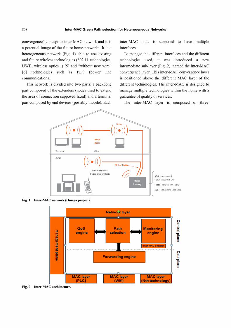
Inter-MAC Green Path selection for Heterogeneous Networks
808
convergence” concept or inter-MAC network and it is
a potential image of the future home networks. It is a
heterogeneous network (Fig. 1) able to use existing
and future wireless technologies (802.11 technologies,
UWB, wireless optics...) [5] and “without new wire”
[6] technologies such as PLC (power line
communications).
This network is divided into two parts: a backbone
part composed of the extenders (nodes used to extend
the area of connection supposed fixed) and a terminal
part composed by end devices (possibly mobile). Each
inter-MAC node is supposed to have multiple
interfaces.
To manage the different interfaces and the different
technologies used, it was introduced a new
intermediate sub-layer (Fig. 2), named the inter-MAC
convergence layer. This inter-MAC convergence layer
is positioned above the different MAC layer of the
different technologies. The inter-MAC is designed to
manage multiple technologies within the home with a
guarantee of quality of services.
The inter-MAC layer is composed of three
Fig. 1 Inter-MAC network (Omega project).
Fig. 2 Inter-MAC architecture.
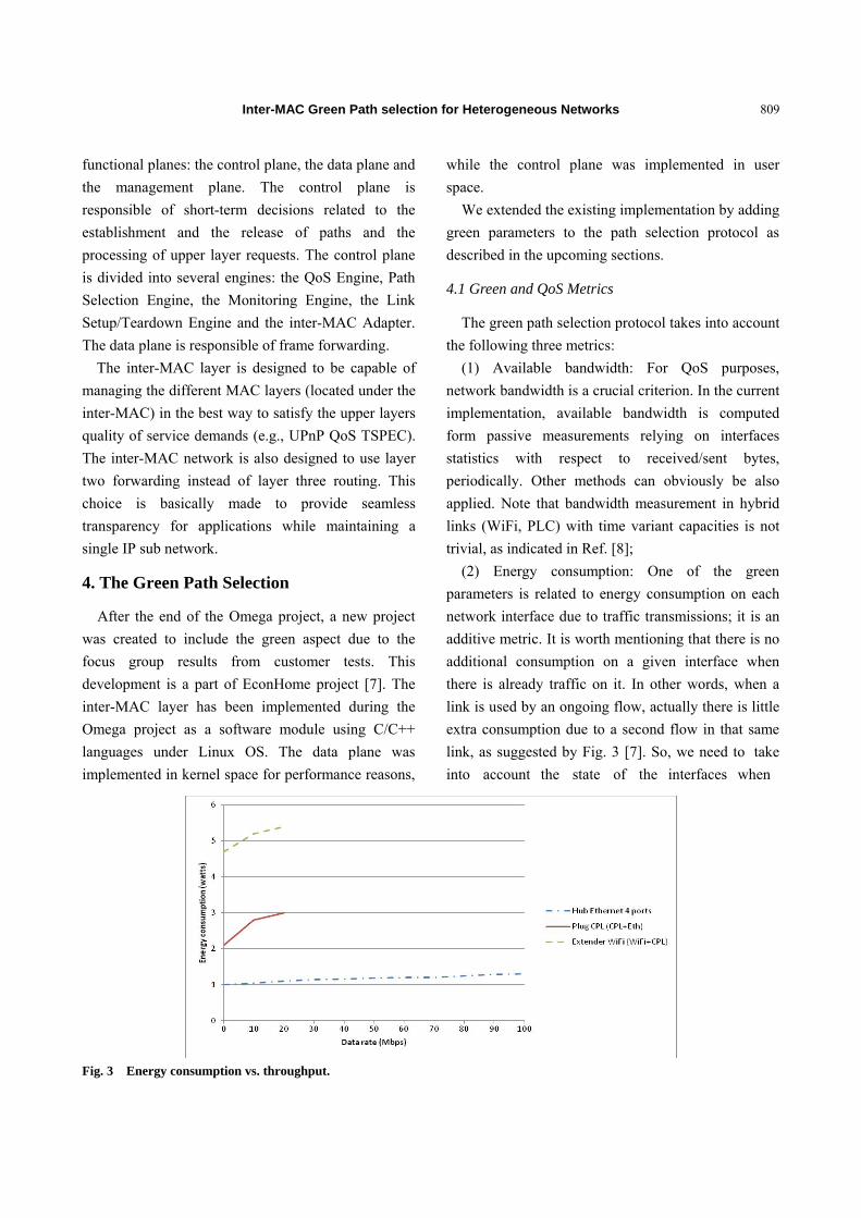
Inter-MAC Green Path selection for Heterogeneous Networks
809
functional planes: the control plane, the data plane and
the management plane. The control plane is
responsible of short-term decisions related to the
establishment and the release of paths and the
processing of upper layer requests. The control plane
is divided into several engines: the QoS Engine, Path
Selection Engine, the Monitoring Engine, the Link
Setup/Teardown Engine and the inter-MAC Adapter.
The data plane is responsible of frame forwarding.
The inter-MAC layer is designed to be capable of
managing the different MAC layers (located under the
inter-MAC) in the best way to satisfy the upper layers
quality of service demands (e.g., UPnP QoS TSPEC).
The inter-MAC network is also designed to use layer
two forwarding instead of layer three routing. This
choice is basically made to provide seamless
transparency for applications while maintaining a
single IP sub network.
4. The Green Path Selection
After the end of the Omega project, a new project
was created to include the green aspect due to the
focus group results from customer tests. This
development is a part of EconHome project [7]. The
inter-MAC layer has been implemented during the
Omega project as a software module using C/C++
languages under Linux OS. The data plane was
implemented in kernel space for performance reasons,
while the control plane was implemented in user
space.
We extended the existing implementation by adding
green parameters to the path selection protocol as
described in the upcoming sections.
4.1 Green and QoS Metrics
The green path selection protocol takes into account
the following three metrics:
(1) Available bandwidth: For QoS purposes,
network bandwidth is a crucial criterion. In the current
implementation, available bandwidth is computed
form passive measurements relying on interfaces
statistics with respect to received/sent bytes,
periodically. Other methods can obviously be also
applied. Note that bandwidth measurement in hybrid
links (WiFi, PLC) with time variant capacities is not
trivial, as indicated in Ref. [8];
(2) Energy consumption: One of the green
parameters is related to energy consumption on each
network interface due to traffic transmissions; it is an
additive metric. It is worth mentioning that there is no
additional consumption on a given interface when
there is already traffic on it. In other words, when a
link is used by an ongoing flow, actually there is little
extra consumption due to a second flow in that same
link, as suggested by Fig. 3 [7]. So, we need to take into account the state of the interfaces when
Fig. 3 Energy consumption vs. throughput.

Inter-MAC Green Path selection for Heterogeneous Networks
810
choosing a path to minimize energy consumption. In
order to minimize the global energy consumption of
the home network, we propose to compute the
difference between energy consumption in “idle” (the
interface is ON, but there is no significant data traffic
on it) and “ON” states. For interface i, we have:
If interface i is idle
ΔEi = Ei(ON) – Ei(idle)
Else
ΔEi = 0
Then, for a path k which is a succession of n
interfaces, we have:
Epath = ∑i = 1, n ΔEi
We assume that MAC layers take into account point
to multi point links, where energy consumption should
include a multiplicative factor depending on the
number of concerned nodes. Indeed, for shared media
such as WiFi and PLC, there are multiple receivers,
even when there is a single MAC destination.
Currently, as it is impossible to obtain dynamic values
in real time, we use static values for energy
consumption according to the interface type (with
watt-hours unit), as indicated in Table 1. These values
were obtained through a series of tests and
measurements conducted in EconHome project [7]. In
the future, it could be more interesting to rely on real
time indications provided by the physical and MAC
layers in order to have more accurate values;
(3) Radio frequency: the second green parameter is
related to electromagnetic pollution in the home. The
idea is to minimize radio frequency emissions due to
wireless and power line interfaces use in the network.
It is not an additive metric since radio values depend
on the considered frequency band (e.g. WiFi at 2.4
Ghz, WiFi at 5 Ghz, etc.). Thus, we propose to
associate a radio frequency cost to each interface,
which is a function of the transmission power,
frequency band and the potential impact on human
body. Then, the cost of the path is the sum of crossed
interfaces radio frequency costs. The definition of the
cost function is beyond the scope of this paper. Note
that, currently, even in the idle state, wireless
interfaces do emission of radio frequency. However,
we assume that future products will be able to enter
sleep mode (without radio frequency emissions) when
needed.
For sake of simplicity, in this paper, we propose to
use the binary values as indicated in Table 1 in our
testbed. Note that PLC radio frequency is much lower
than radio wireless interfaces, so we apply 0 instead of
1. When there is a radio wireless interface in “idle”
state in the considered path, we increment the metric
of radio frequency of the considered path which is
equal to the total number of active wireless interfaces
of the path.
Finally, in addition to these metrics, it is possible to
use the flows service class (based on DSCP marking,
for instance) to decide which criteria to apply for path
selection.
4.2 The Green Path Selection Protocol
The path selection protocol is based on a reactive
approach, where a path is calculated when a new flow
arrives. In fact, when there is no entry in the
forwarding table for an incoming packet, the path
calculation is triggered. Moreover, a new path is
established when there is a link failure or when there
is a better path to the destination. The process is based
on the following 7 control messages:
(1) Route request: it permits to compute a new (or
Table 1 Green metrics and statics values.
Interface type/Metric Energy consumption (W.h), ON state Energy consumption (W.h), Idle state Radio frequency cost
WiFi at 2.4 Ghz 3 1.7 1
PLC 3.2 2.4 0
GigaEthernet 0.6 0.5 0
FastEthernet 0.3 0.2 0

Inter-MAC Green Path selection for Heterogeneous Networks
811
better) path. It is sent by the source on all its interfaces
towards the destination. When the packets cross the
intermediate nodes, the metrics information (available
bandwidth, energy consumption and radio frequency)
are updated. These values are added into the route
request message;
(2) Route reply: it is sent by the destination on all
its interfaces in response to a route request message.
The route reply message contains the end to end path
from the source to the destination (including
intermediate nodes). The source stores the obtained
response, in order to choose an appropriate path after
receiving the different answers;
(3) Route activate: it is sent by the source to the
destination, after selecting the appropriate path. The
forwarding tables of the intermediate nodes are then
updated accordingly;
(4) Route activate confirm: it is sent by the
destination when it receives the route activate message
to indicate that the path is computed successfully.
Then, the flow can be transmitted on the
corresponding interface in the source node;
(5) Route delete: it is flooded in the network after a
link failure event. The corresponding entries in the
forwarding tables are erased. When the source of a
flow, which is impacted by the failure, receives this
message, it starts the computation of a new path;
(6) Route check: it is sent periodically by the source
to the destination in order to update the metrics values
(available bandwidth, energy consumption and radio
frequency). At the same time, to be able to detect all
possible paths, a route request message is sent (with a
specific flag). Since the metrics values are updated, a
better path than the initial one might be selected for a
given flow;
(7) Route check reply: it is sent by the destination
in response to a route check message. It contains the
information about the end to end path with the
updated metrics values.
The path selection algorithm applies iteratively the
following criteria to choose the best path for a given
flow. The intent is to choose a path that meets QoS
requirements and ensures minimum energy and radio
frequency consumption:
Among all possible paths between a source and a
destination, we select those that provide an available
bandwidth higher that the required one (we assume
that for some flows such as IPTV, the required rate is
known; otherwise we use a threshold value)
Among the remaining paths, we select the two that
offer lower energy consumption (we assume that there
are at least two possible paths, otherwise, the choice is
limited to the only remaining path).
Among the last 2 paths, we select the one that has
the minimum number of radio interfaces.
It is rather a simple algorithm which can be
implemented easily. Obviously, it is possible to apply
a different combination of these metrics depending on
which criteria we choose to prioritize. In fact, we want
to avoid complex NP hard optimization based
algorithms that could be more “intelligent”, but that
are too complex to implement in home network
environment where cost is a major issue, especially
for infrastructure equipments.
5. Objectives and Preliminary Results
The implementation of the green path selection
protocol on an experimental testbed is undergoing. In
this section, we discuss the objective of the testbed
and present some preliminary results.
5.1 Objectives
Fig. 4 represents a heterogeneous home network
configuration with Ethernet, PLC and WiFi links. The
testbed contains 4 mini PCs which play the role of
extenders, they implement the green path selection
protocol. The end devices (including a PC, NAS, TV,
tablet and mobile phone) are connected to these
extenders. The Home Gateway connects the home
network to the Internet. The idea is to highlight energy
consumption reduction while maintaining satisfactory
QoS for different flows, thanks to the green path

Inter-MAC Green Path selection for Heterogeneous Networks
812
Fig. 4 Testbed example.
Fig. 5 Graphical interface.
selection protocol described in section IV.
5.2 Preliminary Results
In this section, we present through an example
some typical results that we can obtain on the test bed.
Fig. 5 shows a graphical interface obtained on the
manager node in a test bed with 3 mini PCs referred
as Omega1, Omega2 and Omega3 nodes. It indicates
the devices where the path selection protocol is
running and their interconnection. We have a Fast
Ethernet link between Omega1 and Omega2, a WiFi
link between Omega1 and Omega3 and a PLC link
between Omega2 and Omega3. Currently, the
graphical interface does not distinguish the types of
the links.
We implemented a wirehark module to decode
inter-MAC frames and analyze them. Fig. 6 shows a
wireshark capture obtained on interface eth0 of
Omega1 when there is a flow from Omega1 to
Omega3. It indicates the path selection protocol
messages described in Section 4.2
Fig. 7 presents a wireshark capture, obtained on
Omega1 eth0 interface, of the route reply message
sent from Omega3 to Omega1. As people can see,

Inter-MAC Green Path selection for Heterogeneous Networks
813
Fig. 6 Wireshark capture of control messages.
Fig. 7 Wireshark capture of route reply messages.
the message contains the energy consumption metric
that we implemented (highlighted with a circle), in
addition to available bandwidth on transmitting and
receiving interfaces. The values correspond to the 2
hops path (O1-O2-O3) including Ethernet and PLC
links respectively. Note that available bandwidth on
PLC link is computed based on the maximum 200
Mbps physical capacity, as an example, which is

Inter-MAC Green Path selection for Heterogeneous Networks
814
higher than the actual IP throughput. It is possible to
modify this value as explained in Section 4.1 using an
appropriate measurement method. Assuming that both
paths offer sufficient bandwidth and that initially all
interfaces are in idle state, the selected path is the 2
hops one (O1-O2-O3) because is ensures lower
energy consumption (0.9 w.h vs. 1.3 w.h, as delta
energy values ((0.3 – 0.2) + (3.2 – 2.4)) vs. (3 – 1.7)).
This final part of the implementation is close to the
end. Indeed, if we compare the total energy
consumption in the network using the possible paths,
we have:
Direct Path (O1-O3): E = 11.2 w.h (= 2 × 3 (WiFi
ON) + 2 × 0.2 (Eth idle) + 2 × 2.4 (PLC idle));
Two hops path (O1-O2-O3): E = 10.4 w.h (= 2 ×
1.7 (WiFi idle) + 2 × 0.3 (Eth ON) + 2 × 3.2 (PLC
ON)).
6. Conclusions
The inter-MAC network was a good initiative to
reach gigabit throughput and high quality of service
with multi-technologies transparency (Omega project).
The green path selection protocol that we defined (part
of EconHome project) aims to ensure a high quality of
service with energy and radiofrequency minimization.
The preliminary results foreshadow positively the
demonstrator for heterogeneous home network
configuration with Ethernet, PLC and WiFi links.
Acknowledgments
The research leading to these results has received
funding from the French competitivity cluster FUI
project also referred as ECONHOME.
References
[1] ICT OMEGA Project Website, http://www.ict-omega.eu.
[2] V. Suraci, Convergence in Home Gigabit Networks:
Implementation of the inter-MAC layer as a pluggable
kernel module, PIMRC 2010.
[3] IEEE P1905.1, http://grouper.ieee.org/groups/1905/1/.
[4] HGI Website, http://www.homegatewayinitiative.org/.
[5] IEEE P802.11n/D9.0, Draft standard, Wireless LAN
Medium Access Control (MAC) and Physical Layer
(PHY) Specifications, Amendment 5: Enhancements for
Higher Throughput, Mar. 2009.
[6] HomePlug AV Specification, Version 1.1, May 2007
[7] J.P. Javaudin, Orange vision for green home networks, in:
IEEE WCNC 2012, Workshop on Future Green
Communications, Paris, 2012.
[8] O.O. Irigoyen, A. Kortebi, L. Toutain, D. Ros, Available
bandwidth probing in hybrid home networks, in: The 7th
IEEE International Workshop on Heterogeneous,
Multi-Hop, Wireless and Mobile Networks, 2012

Journal of Communication and Computer 10 (2013) 815-822
Web Block Extraction System Based on Client-Side
Imaging for Clickable Image Map
Hiroyuki Sano, Shun Shiramatsu, Tadachika Ozono and Toramatsu Shintani
Department of Computer Science and Engineering, Graduate School of Engineering, Nagoya Institute of Technology, Aichi
466-8555, Japan
Received: February 07, 2013 / Accepted: March 13, 2013 / Published: June 30, 2013.
Abstract: We propose a new Web information extraction system. The outline of the system and the algorithm to extract information
are explained in this paper. A typical Web page consists of multiple elements with different functionalities, such as main content,
navigation panels, copyright and privacy notices and advertisements. Visitors to Web pages need only a little of the pages. A system to
extract a piece of Web pages is needed. our system enables users to extract Web blocks only by setting clipping areas with their mouse.
Web blocks are clickable image maps. Imaging and detecting hyperlink areas on client-side are used to generate image maps. The
specialty of our system is that Web blocks perfect layouts and hyperlinks on the original Web pages. Users can access and manage their
Web blocks via Evernote, which is a cloud storage system. And HTML snippets for Web blocks enable users to easily reuse Web
contents on their own Web site.
Key words: Web information extraction, web service, HTML5.
1. Introduction
We have implemented a system that enables users
to extract specific contents from Web pages. The
extracted content is called “Web block” in this
research. Of course, there are several different systems
already in place to extract only selected areas from
Web pages, but the specialties of our system is that
Web blocks perfect layouts and hyperlinks on the
original Web pages. Users can access and manage
their Web blocks via Evernote, which is a cloud
storage system. In this paper, we propose the outline
of the system and the algorithm to extract Web blocks
are explained.
A typical Web page consists of multiple elements
with different functionalities, such as main content,
navigation panels, copyright and privacy notices, and
advertisements. Fig. 1 shows a screenshot of a page
Corresponding author: Toramatsu Shintani, professor,
research fields: decision support systems and web intelligence. E-mail: [email protected].
from Reuters.com [1], a news site that brings viewers
the latest news from around the world. This Web page
includes many contents. For example, the content
enclosed by a blue line is a header for the news site,
enclosed by a green line is a news article, enclosed by
an orange line is a navigation panel that contains
many hyperlinks for most popular news in
Reuters.com, and enclosed by a red line is a footer for
the news site. The page is very long, so visitors must
scroll the page down on the screen to seek an intended
content through the page. When printing out the
content, printing the whole page wastes much paper
and ink cartridge for the printer. A system to extract a
piece of Web pages is needed.
The rest of the paper is organized as follows:
Section 2 reviews related works and systems in the
area of Web information extraction; In Section 3, we
propose a Web block extraction system based on
client-side imaging and detecting hyperlink areas for
image maps; experiments and their results are
DAVID PUBLISHING
D

Web Block Extraction System Based on Client-Side Imaging for Clickable Image Map
816
Fig. 1 A page from Reuters.com that contains many contents.
in Section 4; Finally, we conclude the paper in
Section 5.
2. Related Works and Systems
There are several different Web information
extraction approaches already in place.
Most of existing algorithms for Web information
extraction are based on DOM (document object model)
structure of HTML or machine learning [2, 3], for
example, Web wrappers are well known tools for
information extraction from Web pages [4, 5]. They
focus on only main content and extract the main

Web Block Extraction System Based on Client-Side Imaging for Clickable Image Map
817
content from a Web page. In Fig. 1, we will extract the
news article. But the main contents for the visitors who
want to know most popular news list is that the part
enclosed by an orange line. So, a system is needed that
enables users to set clipping areas and can extract only
selected areas from Web pages.
FireShot [6], which is a Firefox extension, captures
screenshots of Web pages in Web browsers. Users can
capture an entire page or a selected part, add
annotations, and save the images by using the
extension. Users can save the images not only as image
file formats (JPEG, GIF, PNG and BMP) but also as
PDF by using the extension. But the extension does not
have a function to extract hyperlinks information from
the original Web pages, so PDFs generated by the
extension do not contain hyperlinks.
Evernote Web Clipper [7] also enables to crop Web
pages and can contain hyperlinks in cropped parts. But
users can only specify the cropped area based on DOM
structure of HTML, so they can not specify the area
freely. For example, consider the Web page layout in
Fig. 2. In this example, a user wants to extract the part
“2” in Fig. 2a. But the user can extract the part marked
“1” in Fig. 2a, the part “A” and “C” in addition to the
part “2”, by the Clipper. This is because the part “B”
and “D” are separately placed in DOM showed in
Fig. 2b.
Kwout [8] clears up the problems of FireShot and
Evernote Web Clipper. Kwout enables users to quote a
part of a Web page as an image with hyperlinks. Users
can set clipping areas freely by drag and drop with
mouse. Kwout provides server side imaging processing.
Kwout must query the Web server to collect the
resource of original Web pages via HTTP protocols,
Fig. 2 An example that Evernote Web Clipper can not
crop.
render the web pages to get screenshots of the entire
pages, and finally crop and generate an image map in
the rectangle specified by the user. The cropped parts
layout may be different from the displayed layout on
users Web browser. This is because Web rendering
engines may be different in user’s side and server side.
In addition, server side imaging will be unsuccessful
when users extract from Web application results.
Kwout already returns a screenshot of the Web
application’s initial state.
In this paper, we propose a system based on
client-side imaging and detecting hyperlink areas for
image maps to attack the problems described above.
Client-side processing can perfect layout and
hyperlinks of original web pages and enables users to
extract contents from Web application results.
3. Web Block Extraction System
3.1 Outline of the System
Fig. 3 shows the outline of the system. The system is
based on client-server model. The client system is
written in JavaScript and packaged as an extension for
Google Chrome. The extension has modules for
imaging Web pages, cropping the image, and getting
hyperlink areas in the rectangle specified by users.
A user starts up the extension after loading a Web
page and the extension enable the user to set a clipping
area by drag and drop using mouse. The imaging
module in the extension generates the screenshot of the
entire Web page by using Chrome Extensions API [9],
and the specified area by the user in the Web page is
cropped from the entire image. HTML5 canvas API is
used for cropping. The detail of an imaging process is
described in Section 3.2. The hyperlink analysis
module analyzes the HTML of the Web page in order
to get a list of coordinates of hyperlinks placed in the
cropped area. The detail of generating clickable image
maps is described in Section 3.3.
In Ref. [10], Kondo et al. proposed a system that
converts Web pages for personal computers into Flash
lite programs for mobile phones. The system
A<table>
A B C D
<td> <td> <td> <td>
<tr> <tr>
(a)Web Page Layout
B
C D
1 12
2 2
(b)DOM Tree

Web Block Extraction System Based on Client-Side Imaging for Clickable Image Map
818
Fig. 3 The system implemented in this study.
Fig. 4 A Web block as a clickable image map by using the system.
generates a screenshot of a Web page and gets a list of
coordinates of hyperlinks, and finally combines the
screenshot with the list into a Flash lite program. In this
study, we combine them into a clickable image map. A
clickable image map is a static map image that can be
clicked and linked with other HTML sources.
Clickable image maps generated by our system are
called as “Web blocks” in this paper. Fig. 4 shows an
example of a Web block generated by our system. The
cropped image and the list of hyperlinks are sent to the
server, and the combine module makes a clickable
image map by the image and the list of hyperlinks.
The system saves the HTML of the generated Web
blocks in Web server. So all Web blocks have URLs
and other systems can access the blocks via HTTP
protocol. And the server adds the generated Web block
to Evernote, which is a cloud storage system, as a new
note. Users can access and manage their Web blocks
via Evernote. Fig. 5 shows a screenshot of Evernote to
which several Web blocks are added. Fig. 5(1) is the
list of Web blocks user extracted from Web pages. The
selected Web block from the left list is displayed in a
large way in Fig. 5(2). And Fig. 5(3) is the HTML
snippet of the selected Web block. Users can easily
reuse and mashup Web blocks by using their snippets
on users’ own Web site.
Fig. 6 shows an example of Web block mashups. We
generate a new Web page by mashuping three Web
blocks. Fig. 6(1) is the Web block that shows the latest
headlines extracted from Reuters.com. Fig. 6(2) is a
news article block about Boeing 787 trouble in Japan
extracted from BBC News. And Fig. 6(3) is a block for
Web Server
User
stored
(URL is publised)
Evernote
・ Image
・ Hyperlinks
set a clipping area
Client S ide Server S ide
generate a
clickable map
Web
pageWWW
Google Chrome
URL
referenceXMLHttpRequest
add as
a new note

Web Block Extraction System Based on Client-Side Imaging for Clickable Image Map
819
top three search results extracted from Google, for
which the search query is “Web intelligence”. To
generate such a Web page showed in Fig. 6, a Web
page creator only copies and pastes the HTML snippets
of the Web blocks into a HTML source code of a new
Web page.
3.2 Client-Side Imaging
The method is captureVisibleTab. The method
returns an image of whole the Web page that is
displayed on a current selected tab. The image must be
cropped in the next step by the rectangle that the user
specified.
The Canvas API in HTML5 is used for cropping.
Canvas API is an API for drawing graphics via
JavaScript in Web browsers. The graphic context of
canvas has drawImage (image, sx, sy, sw, sh, dx, dy, dw,
dh) method to draw an image onto the canvas. The
Fig. 5 The system adds the Web blocks into Evernote and users can access and manage their blocks via Evernote.
Fig. 6 This figure shows an example of Web block mashup. In this example, three Web blocks from different Web pages
are reused.
(1) Web block list
(2) selected block from the left list
(3) HTML snippet for the block
(1) (2)
(3)

Web Block Extraction System Based on Client-Side Imaging for Clickable Image Map
820
Fig. 7 An algorithm for link analysis.
image parameter is the image to draw. The sx and sy
parameters determine from where in the source image
to start copying a rectangle of the image onto the
canvas. The sw and sh parameters determine the width
and height of the rectangle. The dx and dy parameters
determine where on the canvas the image is drawn. The
dw and dh parameters determine the width and height
to scale the image to when drawing it.
In the implementation of the system, the image
parameter is set to the image object obtained from
captureVisibleTab method. The sx and sy are set to x
and y coordinates of the upper-left corner of the
rectangle that the user specified. The sw and sh are set
to the width and height of the rectangle that the user
specified. The dx and dy are always set to zero, and the
dw and dh are set to the width and height of the
rectangle that the user specified. These parameters
make the method render only the image within the
clipping area that the user set in the canvas.
The system gets base64 data of the cropped image to
send the image to the server. The toDataURL method is
that canvas returns a dataURL of an image drawn in the
canvas. DataURL scheme is used for embedding some
binary data in text format data such as HTML or
JavaScript. The binary data is encoded by base64
format in dataURL scheme. In the proposed system,
the base64 data obtained from toDataURL method is
posted to the server by using XMLHttpRequest and the
server decodes the data into a PNG format image.
Table 1 The processing time for imaging (t1), getting image
maps (t2) and adding to Evernote (t3).
t1 (msec) t2 (msec) t3 (msec)
255.2 33.7 3,362.8
243.4 12.1 2,533.7
268.1 14.3 2,679.0
253.9 13.7 2,642.3
217.0 11.9 2,580.1
185.7 12.1 2,606.7
235.1 15.5 2,531.3
239.1 10.5 2,644.4
262.8 15.6 2,625.5

Web Block Extraction System Based on Client-Side Imaging for Clickable Image Map
821
3.3 Link Analysis in the Rectangle
The advantage of imaging is perfectly keeping up
layout and presentation of the Web pages. But the
disadvantage of imaging is losing the hyperlinks in the
rectangle. The Web blocks provided by the system are
generated as clickable image map to add hyperlinks for
the images.
The JavaScript program was run on the user’s Web
browser to get maps for hyperlinks. Fig. 7 shows the
link analysis algorithm.
First, all <A> nodes are collected and assigned to an
array A in line 1. The coordinates of all <A> nodes are
absolute coordinates, and they are transformed to
relative coordinates in lines 2 to 5. The base point of
the relative coordinates is the left-upper side of the
rectangle that the user specified. Next, in lines 6 to 10,
the <A> nodes that do not meet to the specified
rectangle are deleted from the array A. And in lines 11
to 18, the hyperlinks areas protruded outside the
rectangle are cut off.
4. Experimental Results
We measured the processing time to extract Web
blocks from several Web pages. The processing time
for imaging, link analysis and adding to Evernote were
measured. The Web pages that were used in the
experiment were newest 10 news pages that were
delivered on Yahoo! News in Japan at 0 a.m., on
February 3rd, 2013. We extracted 10 Web blocks
randomly from each Web page by using our proposed
system, and we measured the average processing
time.
The experiment was performed on the iMac (Mid
2010) that has Core i3 3.2GHz CPU and 8GB DDR3
SDRAM (PC3-8500). The operating system running
on the machine was Mac OS X 10.6.8 and the Web
browser was Google Chrome 24.0.1312.52.
Table 1 shows the processing time for imaging,
getting image maps, and adding to Evernote as new
notes. Thus, the experiment shows that the proposed
method can get screenshots and image maps very
quickly, and that the method has potential for practical
use, although the overheads of communication and
Evernote’s WebAPI-call are high.
5. Conclusions
We have implemented a system that enables users to
extract Web blocks from Web pages, and proposed the
outline of the system, and the algorithm to extract Web
blocks are explained in this paper. Imaging and
detecting hyperlink areas on client-side are used to
generate image maps. The specialty of our system is
that Web blocks perfect layouts and hyperlinks on the
original Web pages. Users can access and manage our
Web blocks via Evernote, which is a cloud storage
system. And HTML snippets for Web blocks enable
users to easily reuse Web contents on their own Web
site.
We conducted an experiment to show the
processing speed of the proposed method. The results
showed that the method can extracts Web blocks very
quickly, and that the method has potential for practical
use.
Acknowledgments
This work was supported by KAKENHI (22500128)
and the Hori Sciences & Arts Foundation in Japan.
References
[1] Business & Financial News, Breaking US & International
News, Reuters.com, http://www.reuters.com/.
[2] J. Pastenack, D. Roth, Extracting article text from the Web
with maximum subsequence segmentation, in:
Proceedings of the 18th International Conference on
World Wide Web (WWW’09), New York, 2009, pp.
971-980.
[3] S. Sarawagi, Information extraction, found, Trends
Databases 1 (2008) 261-377.
[4] Y. Yamada, D. Ikeda, H. Sakamoto, H. Arimura, An
information extraction from the Web: Automatic
generation of web wrappers, Journal of Japanese Society
for Artificial Intelligence 19 (2004) 302-310.
[5] Y .Kusumura, Y. Hijikata, S. Nishida, Unsupervised
information extraction by crossover and structure analysis,
The Transactions of the Institute of Electronics,
Information and Communication Engineers D 90 (2007)
2495-2509.

Web Block Extraction System Based on Client-Side Imaging for Clickable Image Map
822
[6] Webpage screenshot in firefox: Add-ons for firefox,
https://www.addons.mozilla.org/ja/firefox/addon/fireshot/.
[7] Evernote Web Clipper Lets you save webpage text, Links
and images with a single click, Evernote,
http://www.evernote.com/webclipper/.
[8] Kwout Home Page, http://www.kwout.com/.
[9] Google, Hello There! Google Chrome,
http://www.developer.chrome.com/extensions/docs.html.
[10] K. Kondo, S. Asami, T. Ozono, T. Shintani, On a Web
Contents Browsing Support Environment for Mobile
Devices and its Applications, IPSJ SIG technical report,
2008.

Journal of Communication and Computer 10 (2013) 823-831
Multiple Chaos Generator by
Neural-Network-Differential-Equation for Intelligent
Fish-Catching
Mamoru Minami, Akira Yanou, Yuya Ito and Takashi Tomono
Graduate School of Natural Science and Technology, Okayama University, Okayama 7008530, Japan
Received: June 18, 2012/ Accepted: July 21, 2012 / Published: June 30, 2013.
Abstract: Continuous catching and releasing experiment of several fishes make the fishes find some escaping strategies such as
staying stationary at corner of the pool. To make fish-catching robot intelligent more than fishes’ adapting and escaping abilities from
chasing net attached at robot’s hand, we thought something that goes beyond the fishes’ adapting intelligence will be required. Here
we propose a chaos-generator comprising NNDE (neural-network-differential-equation) and an evolving mechanism to have the
NNDE generate chaotic trajectories as many as possible. We believe that the fish could not be adaptive enough to escape from
chasing net with chaos motions that have much different chaos, since unpredictable chaotic motions of net may go beyond the fishes’
adapting abilities to the net motions. In this report we introduce the chaos generating system by NNDE, which can produce many
kinds of chaos theoretically, and then analyze the chaos with Lyapunov number, Poincare return map and initial value sensitivity.
Key words: Chaos, neural network, genetic algorithm.
1. Introduction
In recent years, visual tracking and servoing in
which visual information is used to direct the
end-effector of a manipulator toward a target object
has been studied in some researches [1, 2]. A new
trend of machine intelligence [3] that differs from the
classical AI has been applied intensively to the field of
robotics and other research areas like intelligent
control system. Typically, the animal world has been
used conceptually by robotics as a source of
inspiration for machine intelligence. For the purpose
of studying animal behavior and intelligence, the
model of interaction between animals and machines is
proposed in researches like Ref. [4]. In their previous
research, the fish emotional behavior has also been
examined and the robot with adaptive ability to react
to the fish status has been conceived. Another crucial
Corresponding author: Mamoru Minami, Ph.D., professor,
research fields: visual servoing, intelligent robot, mobile manipulator. E-mail: [email protected].
characteristic of machine intelligence is that the robot
should be able to use input information from sensor to
know how to behave in a changing environment and
furthermore can learn from the environment for safety
like avoiding obstacle. As known universally that the
robot intelligence has reached a relatively high level,
still the word “intelligence” is an abstract term, so the
measurement of the intelligence level of a robot has
become necessary. A practical and systematic strategy
for measuring MIQ (machine intelligence quotient) of
human-machine cooperative systems is proposed in
Ref. [5]. In our approach to pursue intelligent robot,
we will evaluate the intelligence degree between
fishes and the robot by Fish-Catching operation. we
think that the system combined with chaos is smarter
than the fish when the robot can beat the fish by
catching it successfully even after the fish finds out
some reached a relatively high level, still the word
“intelligence” is an abstract term, so the measurement
of the intelligence level of a robot has become

Multiple Chaos Generator by Neural-Network-Differential-Equation for Intelligent Fish-Catching
824
Fig. 1 Fish catching system PA10.
necessary. A practical and systematic strategy for
measuring MIQ (machine intelligence quotient) of
human-machine cooperative systems is proposed in
Ref. [5]. In their approach to pursue intelligent robot,
we will evaluate the intelligence degree between
fishes and the robot by Fish-Catching operation. We
think that the system combined with chaos is smarter
than the fish when the robot can beat the fish by
catching it successfully even after the fish finds out
some escaping strategy. As we did not find the
research about the intelligence comparison between
animal and robot, we mainly dedicate ourselves to
constructing a smart system that is more intelligent
than the fish. We consider that the competitive
relation can be very meaningful as one way to discuss
robotic intelligence. So we not only employ the
inspiration of animal’s behavior for robot
intellectualization, we can also conceive a robot that
can exceed the animal intelligence. By evolutionary
algorithms [6], Visual Servoing and Object
Recognizing based on the input image from a CCD
camera mounted on the manipulator has been studied
in their laboratory (Fig. 1) [7], and we succeeded in
catching a fish by a net attached at the hand of the
manipulator based on the real-time visual tracking
under the method of Gazing GA [8] to enhance the
real-time searching ability.
We have learned that it is not effective for fish
catching to simply pursue the current fish position by
visual servoing with velocity feedback control.
Actually, the consistent tracking is sometimes
impossible because the fish can alter motion pattern
suddenly maybe under some emotional reasons of fear.
Those behaviors are thought to be caused by
emotional factors and they can also be treated as a
kind of innate fish intelligence, even though not in a
high level.
While observing the fishes’ adapting behavior to
escape in the competitive relations with the robot, that
is continuous catching/releasing experiments, We
found that we can define a “FIQ” (fish’s intelligent
quotient) [9] representing decreasing velocity of fish
number caught by the net through continuous
catching/releasing operation. Through this measure we
can compare the innate intelligence of the fish and the
artificial intelligence of the robot.
It has been well known that many chaotic signals
exist in our body, for example, in nerves, in motions
of eye-balls and in heart-beating periods [10, 11].
Therefore we thought that imitating such animal’s
internal dynamics and putting chaos into robots have
something meaningfulness to address fishes’
intelligence. We embed chaos into the robot dynamics
in order to supplement the deficiency of their
Fish-Catching system [12].
Therefore what we have to pay attention to the
fishes’ nature that the fish does conceive always
escaping strategy against new stressing situation. This
means that robot’s intelligence to override the fishes’
thinking ability needs infinite source of idea of
catching motions. To generate such catching motion,
we propose in this report NNDE
(neural-network-differential-equation) that can
produce neural chaos and inherently have a possibility
to be able to generate infinite varieties of chaos,
derived from the neural network’s ability to
approximate any nonlinear function as accurate as
with desirable precision [13-15].
This paper is organized as follows: Section 2
discusses the fish tracking and catching; Section 3
introduces the problem of fish-catching; Section 4
defines fish intelligent quotient; Section 5 verifies the
validity of chaos; Section 6 shows
neural-network-differential-equation; Section 7

Multiple Chaos Generator by Neural-Network-Differential-Equation for Intelligent Fish-Catching
825
explains chaos verification methods; Section 8
proposes the chaos generate system; Section 9 gives
the verification results of chaos; Section 10 discusses
sensitivity of neuron’s weight; Section 11 concludes
this paper.
2. Fish Tracking and Catching
The problem of recognition of a fish and detection
of its position/orientation is converted to a searching
problem of Ttytxt )](),([)( r in order to maximize
))(( tF r , where ))(( tF r represents correlation
function of images and fish-shaped matching model.
))(( tF r is used as a fitness function of GA [8]. To
recognize a target in a dynamic image input by video
rate, 33 [fps], the recognition system must have
real-time nature, that is, the searching model must
converge to the fish in the successively input raw
images. An evolutionary recognition process for
dynamic images have been realized by such method
whose model-based matching by evolving process in
GA is applied at least only one time to one raw image
input successively by video rate. We named it as
“1-Step GA” [7]. When the converging speed of the
model to the target in the dynamic images should be
faster than the swimming speed of the fish in the
dynamic images, then the position indicated by the
highest genes represent the fish’s position in the
successively input images in real-time. We have
confirmed that the above time-variant optimization
problem to solve )(tr maximizing ))(( tF r could
be solved by “1-Step GA”. Ttytxt )](),([)( r
represents the fish’s position in Camera Frame whose
center is set at the center of catching net, then )(tr
means position deviation from net to fish, means
)()( tt rr . The desired hand velocity at the i-th
control period di
r is calculated as
)( 1 ii
V
i
Pdi
rrΚrKr (1)
where, ir denotes the servoing position error
detected by 1-Step GA [7]. PΚ and VΚ given are
positive definite matrix to determine PD gain. Now
we add chaos items to Eq. (1) above, and we also need
to redefine the meaning of di
r .
The simple PD servo control method given by
Eq. (1) is modulated to combine a visual servoing and
chaos net motion into the controller as follows
chaosi
fishii kk rrr
21 (2)
Here Tfish
ifish
ifish
i yx ],[ r , is the tracking error of
fish from the center of camera frame, and T
chaosi
chaosi
chaosi yx ],[ r denotes a chaotic oscillation
in yx plane around the center camera frame.
Therefore the hand motion pattern can be determined
by the switch value 1k and 2k . 01k and 02k
indicate visual servoing, and 01k and 12k
indicate the net will track chaotic trajectory made by
NNDE being explained later in this report. The
desired joint variable dq is determined by inverse
kinematics from dr by using the Jacobian matrix
)(qJ and is expressed by equation
ddq rJq )( (3)
where, )(qJ is the pseudo inverse matrix of )(qJ .
The robot used in this experimental system is a 7-Link
manipulator, Mitsubishi Heavy Industries PA-10
robot.
3. Problem of Fish-Catching
In order to check the system reliability in tracking
and catching process, we kept a procedure to catch a
fish and release it immediately continuously for 30
min. We released 5 fishes (length is about 40 mm) in
the pool in advance, and once the fish got caught, it
would be released to the same pool at once. The result of this experiment is shown in Fig. 2, in which
vertical axis represents the number of fishes caught in
successive 5 min and horizontal axis represents the
catching time. We had expected that the capturing
operation would become smoother as time passing on
consideration that the fish may get tired. But to their
astonishment, the number of fishes caught decreased
gradually.
The reason of decreased catching number may lie in
the fish learning ability. For example, the fish can
learn how to run away around the net as shown in

Multiple Chaos Generator by Neural-Network-Differential-Equation for Intelligent Fish-Catching
826
Fig. 2 Result of fish catching.
Fig. 3 Fish motion.
Fig. 3a by circular swimming motion with about
constant velocity, having made a steady state position
error that the net can not reach to the chasing fish. Or
the fish can stay in the opposite corner against the net
in the pool shown in Fig. 3b. And also, the fish can
keep staying within the clearance between the edge of
the pool and the net shown in Fig. 3c where the net is
inhibited to enter.
To solve these problems, and to achieve more
intelligent fish catching systems, we thought chaos
behavior of the net with many chaotic varieties can be
a possible method to overcome those fishes’ escaping
intelligence, since huge variety of chaos trajectories
seems to be unpredictable for the fish to adapt them.
This strategy to overcome fishes’ adaptive intelligence
is based on a hypothesis that unpredictability of the
motion of the chasing net produced by plural chaos
can made the fishes’ learning logic confuse, getting
the fish catching robot have made intelligence than the
fishes’. Then we propose Neural-Network-Differential
-Equation to generate chaos as many as possible.
4. Fish Intelligence Quotient
To evaluate numerically how fast the fish can learn
to escape the net, we adapted Linear Least-Square
approximation to the fish-catching decreasing
tendency, resulting in 7.20486.0 ty as shown
in Fig. 2. The decreasing coefficient −0.486 represents
adapting or learning velocity of the fishes as a group
when the fishes’ intelligence is compared with robotic
catching. We named the coefficient as “FIQ” (Fish’s
Intelligence Quotient), since learning velocity has
been thought as one of components of the Intelligence
Quotient. The larger minus value means high
intelligence quotient of the fish, zero does equal and
plus does less intelligent than robot’s. To overcome
the fishes’ intelligence, more intelligent robotic
system needs to track and catch the fish effectively, in
other words it comes to the problem on how to use the
item ichaosr chaos in Eq. (2) effectively to exceed the
fish intelligence.
5. Validity of Chaos
In 1982, some experiments revealed that mollusk
neuron cells and plant cells have irregular excitement
and show chaotic nature if gave them periodic current
stimulation. In addition, also chaotic response for
periodic current stimulation had been clarified in the
axon of the cuttlefish in 1984. From these studies, it
became clear that the chaos is associated with biology.
In the late 1980s, the relationship between chaos and
function of the nervous system has been discussed.
Mpitosos and colleagues examined the pattern of
rhythmic firing of motor neurons of sea cucumber and

Multiple Chaos Generator by Neural-Network-Differential-Equation for Intelligent Fish-Catching
827
showed that frequency variation of continuous
discharge relates to the rhythm of the movement with
chaotic behavior. Thus, chaos exists in biological
behavior. It is decided whether the nerve cell of the
organism is excited by a stimulation signal, and this is
because it follows the theory of the chaos. Therefore,
animal behavior and strategies can be estimated from
point of chaos, and maybe apply to catch fish. There
has been presented chaoses with a simplified model of
H-H (hodgkin-huxley) model or BVP (bonhoeffer-van
der pol) model. Using one chaos model to produce
unpredictable motion add to catching-net behaviors
seems to be effective, however we thought single
chaos model is not adequate to overcome fishes’
escaping idea since the fishes change their behavior
continuously.
6. Neural-Network-Differential-Equation
Lorenz and Rossler models renowned as chaos
generation comprise three differential equations,
producing three-dimensional chaotic trajectory in
phase space. Since a N.N. (neural-network) has been
proven to have an ability to approximate any
non-linear functions with arbitrarily high accuracy, we
thought it is straightforward to make a differential
equation including N.N. so that it can generate plural
chaoses by changing N.N.’s coefficients. We define
next nonlinear differential equation including N.N.
function ))(( tpf as
)).(()( tt pfp (4)
Ttptptpt )](),(),([)( 321p is state variable. The
nonlinear function of ))(( tpf in Eq. (4) is constituted
by N.N.’s connections, which is exhibited in left part
of Fig. 4 where the N.N. and integral function of
outputs of N.N. and the feedback of the integrated
value to the inputs of N.N. constitute nonlinear
dynamical Eq. (4). We call it as
Neural-Network-Differential-Equation.
7. Chaos Verification Methods
Since there have been no simple criterion to
determine whether irregular oscillation should be a
chaos or not, we have to apply plural evaluations over
the irregularities of trajectories produced by NNDE.
The followings are criteria being used for judging the
chaotic characters.
7.1 Lyapunov Exponent
As one of criteria to evaluate a chaos’ character of
expansion in time domain, Lyapunov exponent
expressed by the following equation is well known,
1
0
)(log1
limN
i
i
N
xfN
(5)
where, positive value can represent that the irregular
oscillation diverts from a standard trajectory, which
expands like a function of ate (a > 0).
7.2 Poincare Section
The trajectories of the motion made by
Neural-Network-Differential-Equation (4) is
examined by using the Poincare section to verify
further whether the resulted trajectories can be
identified as chaos. Next, the Poincare section is
explained. First of all, we examine a simple closed
curve in three dimensions as shown in Fig. 5. The
plane “A” that intersects with this closed trajectory
pointed by “P” is defined as the Poincare section.
The intersecting points are named as
,,,, 21 nnn PPP and corresponding x-axis position on A
are ,,,, 21 nnn xxx which are all pointed to the
Poincare Return Map as ,, 1nn xx as shown in Fig. 6.
With the Poincare return map of Fig. 6 representing a
Fig. 4 Block diagram of chaos generation.

Multiple Chaos Generator by Neural-Network-Differential-Equation for Intelligent Fish-Catching
828
Fig. 5 Poincare section.
Fig. 6 Poincare return map.
shape of “Λ”, the closed curve has the structure of
stretching and folding. This structure is a basic
character of chaos. Looking at the left half of Fig. 6,
we can see the inclination coefficient 1/1 nn dxdx
and right half has 1/1 nn dxdx , representing that left
half has expansion and the other does contraction.
8. Chaos Generate System
Fig. 4 represents the block diagram to find chaos by
using GA and Lyapunov number. This GA is not
1-Step GA, described in Section 2 but used as a
normal GA’s procedure that evolves genes
representing neural network coefficient’s volume. The
trajectory )(tp in time domain obtained from
Neural-Network-Differential-Equation is used for the
calculation of Lyapunov number. Here, T],,[ 321 L
is a Lyapunov number. Using this L for the
evolution of GA, fitness function is defined as
follows,
332211 kkkg (6)
This fitness function incorporated the chaotic
property of the Lyapunov spectrum, which is one of
factors to be essential for generating chaos trajectory.
Here, because we discuss three-dimensional chaotic
attractor in phase space, there are 3 Lyapunov
exponents. The relationship between positive and
negative Lyapunov spectrum is (+, 0, −), which means
resulted time trajectory of Eq. (4) may be thought to
be chaos. Parentheses indicate the sign of the
Lyapunov spectrum. In other words, 1 is positive,
2 is also positive or negative small values, 3 is
negative case, the fitness function of Eq. (6) appears
to have relatively large positive value when
0,0,0 321 . In addition, 21,kk , and 3k
are positive coefficients. The gene of GA is defined as
shown in Fig. 7, with connection weights of N.N.
being T
nqqq ],,,[ 21 q . In this report we adopted a
network of 3 × 6 × 3 as shown in Fig. 4, then the line
number of connections and coefficient are 48, i.e., n =
48. The bit length of q is 16 bits. Because the gene
is expressed in binary, converted to decimal and
normalized into a range from 0 to 1. Then, generating
a trajectory )(tp based on a given gene having been
determined by GA at one previous generation and
calculating Lyapunov number, and evolving new
generation of gene are repeated. This GA’s evolution
can find q to have a highest value of g defined by
Eq. (6), which means possible chaos trajectory.
9. Verification Results of Chaos
So far we have found four chaos patterns with
different neural coefficients explore by GA mentioned
in the previous section. We named them with a serial
number as chaos 01∼chaos 04. The followings are
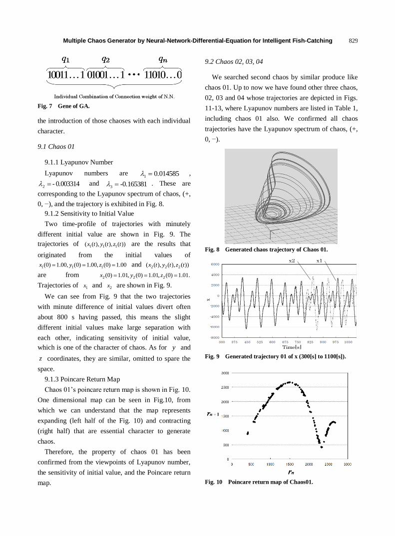
Multiple Chaos Generator by Neural-Network-Differential-Equation for Intelligent Fish-Catching
829
Fig. 7 Gene of GA.
the introduction of those chaoses with each individual
character.
9.1 Chaos 01
9.1.1 Lyapunov Number
Lyapunov numbers are 0.0145851 ,
0.003314- 2 and -0.1653813 . These are
corresponding to the Lyapunov spectrum of chaos, (+,
0, −), and the trajectory is exhibited in Fig. 8.
9.1.2 Sensitivity to Initial Value
Two time-profile of trajectories with minutely
different initial value are shown in Fig. 9. The
trajectories of ))(),(),(( 111 tztytx are the results that
originated from the initial values of
00.1)0(,00.1)0(,00.1)0( 111 zyx and ))(),(),(( 222 tztytx
are from .01.1)0(,01.1)0(,01.1)0( 222 zyx
Trajectories of 1x and 2x are shown in Fig. 9.
We can see from Fig. 9 that the two trajectories
with minute difference of initial values divert often
about 800 s having passed, this means the slight
different initial values make large separation with
each other, indicating sensitivity of initial value,
which is one of the character of chaos. As for y and
z coordinates, they are similar, omitted to spare the
space.
9.1.3 Poincare Return Map
Chaos 01’s poincare return map is shown in Fig. 10.
One dimensional map can be seen in Fig.10, from
which we can understand that the map represents
expanding (left half of the Fig. 10) and contracting
(right half) that are essential character to generate
chaos.
Therefore, the property of chaos 01 has been
confirmed from the viewpoints of Lyapunov number,
the sensitivity of initial value, and the Poincare return
map.
9.2 Chaos 02, 03, 04
We searched second chaos by similar produce like
chaos 01. Up to now we have found other three chaos,
02, 03 and 04 whose trajectories are depicted in Figs.
11-13, where Lyapunov numbers are listed in Table 1,
including chaos 01 also. We confirmed all chaos
trajectories have the Lyapunov spectrum of chaos, (+,
0, −).
Fig. 8 Generated chaos trajectory of Chaos 01.
Fig. 9 Generated trajectory 01 of x (300[s] to 1100[s]).
Fig. 10 Poincare return map of Chaos01.

Multiple Chaos Generator by Neural-Network-Differential-Equation for Intelligent Fish-Catching
830
Fig. 11 Generated chaos trajectory 02.
Fig. 12 Generated chaos trajectory 03.
Fig. 13 Generated chaos trajectory 04.
10. Sensitivity of Neuron’s Weight
We have noticed weight coefficient of N.N. that
generated chaos 03 is almost similar to chaos 04’s.
That is, only one weight coefficient is different, that is
“ 1q ” in Fig. 14. We think “ 1q ” is related to the
generation of chaos. So we increased the weight
slightly from “-1” and compare their trajectories. The
range of 1q is 0.10.1 1 q and
1q is increased
from -1.0 by 0.1. In the case of
,4.00.1 1 q 2.01.0 1 q and ,0.18.0 1 q we can
not be considered that the trajectories are
semi-periodic trajectories as shown in Figs. 15-17.
They indicate that the trajectories are expanded to
infinity as shown in the three figures. On the other
hand, the range of 0.03.0 1 q and 7.03.0 1 q
made chaos trajectories as shown in Figs. 18 and 19.
This result indicates that continuous changing of 1q
can make various chaos, stemming from continuity of
real variables. The Lyapunov number of each
trajectory is shown in Table 2.
Table 1 Lyapunov number.
chaos01 chaos02 chaos03 chaos04
1 0.014585 0.01919 0.015934 0.01208
2 -0.003314 0.00733 -0.002172 -0.00143
3 -0.165381 -0.10379 -0.123026 -0.075448
Fig. 14 Neural network for nonlinear function generation.
Fig. 15 Weight = -0.7.
Fig. 16 Weight = 0.2.

Multiple Chaos Generator by Neural-Network-Differential-Equation for Intelligent Fish-Catching
831
Fig. 17 Weight = 0.9.
Fig.18 Weight = 0.0.
Fig. 19 Weight = 0.7.
Table 2 Lyapunov number.
-0.7 0.0 0.2 0.7 0.9
1 0.007314 0.016477 0.008571 0.004668 0.003386
2 -0.004319 0.002719 -0.038939 0.011399 -0.046857
3 -0.30184 -0.106123 -0.061084 -0.136963 -0.048269
11. Conclusions
This paper proposed chaos generating system
composed of Neural Network and GA’s evolving
ability to change the Neural-Network-Differential-
Equation to be able to generate chaos. This chaos
generating system has exploited the neural network’s
nature of approximation of any nonlinear function
with any desired accuracy. We will utilize this chaos
motion for overcoming fishes’ escaping ability from
chasing net for now.
References
[1] R. Kelly, Robust asymptotically stable visual servoing of
planar robots, IEEE Trans. Robot. Automat. 12 (1996)
759-766.
[2] P.Y. Oh, P.K. Allen, Visual servoing by partitioning
degrees of freedom, IEEE Trans. Robot. Automat. 17
(2001) 1-17.
[3] T. Fukuda, K. Shimojima, Intelligent Control for
Robotics, Computational Intelligence (1995) 202-215.
[4] M. Bohlen, A robot in a cage-exploring interactions
between animals and robots, in: Proc. of Computational
Intelligence in Robot. Automat. (CIRA), 1999.
[5] H.J. Park, B.K. Kim, K.Y. Lim, measuring the MIQ
(machine intelligence quotient) of human-machine
cooperative systems, IEEE Trans. 31 (2001) 89-96.
[6] M. Minami, H. Suzuki, J. Agbanhan, T. Asakura, Visual
servoing to fish and catching using global/local GA
search, in: Int. Conf. on Advanced Intelligent
Mechatronics Proc., Como, Italy, 2001.
[7] M. Minami, J. Agubanhan, T. Asakura, Manipulator
visual servoing and tracking of fish using genetic
algorithm, Int. J. of Industrial Robot 29 (1999) 278-289.
[8] H. Suzuki, M. Minami, J. Agbanhan, Fish catching by
robot using gazing GA visual servoing, Transaction of the
Japan Society of Mechanical Engineers C-68-668 (2002)
1198-1206.
[9] J. Hirao, M. Minami, Intelligence comparison between
fish and robot using chaos and random, in: International
Conference on Advanced Intelligent Mechatronics, China,
2008.
[10] K. Aihara, Chaos in Neural System, Tokyo Denki
University Press, Tokyo, 1993.
[11] R. FitzHugh, Impulses and physiological states in
theoretical models of nerve membrane, Biophy. J. 1
(1961) 445-466.
[12] M. Minami, J. Hirao, Intelligence comparison between
fish and robot using chaos and random, in: Int. Conf. on
Advanced Intelligent Mechatronics Proc., China, 2008.
[13] C.T. Lin, C.S. Lee, Neural Fuzzy Systems, Englewood
Cliffs, Prentice Hall PTR, NJ, 1996.
[14] L.M. Peng, P.Y. Woo, Neural-fuzzy control system for
robotic manipulators, IEEE Control Systems Magazine
22 (2002) 53-63.
R. Endo, J. Hirao, M. Minami, Intelligent chaos
fish-catching based on
neural-network-differential-equation, in: SICE Annual
Conference,Taiwan, 2010.
1q

Journal of Communication and Computer 10 (2013) 832-843
An Efficient Algorithm for the Evaluate of the
Electromagnetic Field near Several Radio Base Stations
Algenti Lala, Sanije Cela and Bexhet Kamo
Faculty of Information Technology, Polytechnic University, Tirana 10000, Albania
Received: May 08, 2013 / Accepted: June 04, 2013 / Published: June 30, 2013.
Abstract: This paper is motivated by the increased presence of the radio base stations, and the need to calculate the electromagnetic
field near them. The debate on the effects of the electromagnetic field exposure, in line with the increased success and presence of the
mobile telephony, has attracted the public interest and it has become a concern for the community. The standard procedures in place
for estimation of the electromagnetic field require prior knowledge of the criteria for the field evaluation, be it near field, far field,
presence of one or several base stations, the operating frequencies bands and their combinations. Aiming to have a practical method
for the evaluation, the authors will try to do develop a theoretic model, on which base the authors will simulate the antenna of the
base station and prepare the numeric method that will provide the baseline for the application. They will than compare the
calculations for real situations for which all know the geometrical features, with the ones calculated based on a known theoretical
method also knows as method of the moments MoM, simulated with NEC-2 (numerical electromagnetic code), and further more with
the values measured in the field under the same conditions as the ones for the simulated environments. The results are interpreted in
order to define the efficiency of the proposed method as well as to have an idea on the simplicity, accuracy and computing capacities.
Key words: Evaluation, base stations, far field, FDTD method, algorithm.
1. Introduction
The task to be accomplished in this paper are the
theoretical calculations of the electric and magnetic
field, the density of power caused by the antennas of
the radio base stations, considering that this is caused
by joint presence of several base stations at a given
place. The proposed calculation method is based on
the below requirements:
The need for a simple, and practical method, to
evaluate the field nearby the radio base stations.
The need to define the security zones Iso-Curves
(spaces inside which the values of the electromagnetic
field are higher than the standard recommended ones)
The need for quick evaluations—be it time—wise
as well as space—wise: In Albania are operating 4
cellular operators AMC, VODAFONE, EAGLE and
Corresponding author: Algenti Lala, M.Sc., research fields:
systems in radiofrequency, antennas and measurement in radio frequency. E-mail: [email protected].
PLUS. These operators are obliged to monitor the
levels of the field in the vicinity of the radio base
stations, and to assure that the levels are within the
reference values of safety, this in the framework of the
client care. By monitoring it means the constant
measurement of the levels of electromagnetic field
near the stations. This is translated in relatively high
costs due to man work travel and density of the
measurements in time.
The presence of several operators in the same space
causes the levels of the electromagnetic field to
increase, independently that each individual antenna
contribution is within the allowed limits. Under these
circumstances it is required that the regulatory body
checks frequently the levels in the public spaces and
for the safety of the public. The state authorities are
trying to protect the population and at the same time
they must promote the cellular companies and
encourage new emerging services.

An Efficient Algorithm for the Evaluate of the Electromagnetic Field near Several Radio Base Stations
833
The literature [1-5] offered many models and
numerical methods for the calculation of the
electromagnetic field near the radio base stations.
The basis of these methods is the conversion of the
integral equations in a linear system, which can be
further computed in a computer. The simulations in
software environments provide accurate results but
they require a lot of processing power and they require
a lot of time to be processed.
In this paper the authors have selected a theoretical
model which implementation is based on the
numerical method FDTD (finite-difference
time-domain) by using the formula of the far field.
They are presenting the theoretical calculations in
real life scenarios in which the geometry of the
antennas in a group of radio base stations is known,
and the results are compared with the values acquired
by the simulator NEC-2 (numerical electromagnetic
code) and further compared to the measured values
acquired in the field by using the NARDA SRM 3000
equipment, for the same conditions of the radio base
stations simulated via the two methods.
The paper is organized as follows: Section 2
describes the proposed theoretical model for the
evaluation of the far field; Section 3 describes the
numerical method and the respective proposals;
Section 4 presents the proposed algorithm; Section 5
presents results and discussions; Section 6 gives
conclusions.
2. The Proposed Theoretical Model for the
Far Field
Modeling of the electromagnetic field near the radio
base stations is a way to evaluate and define the
excluded zones near these stations. The selection of an
appropriate model is important in order to have a good
estimation of the levels of the radiation.
In the literature [1-5] can be found many models for
the definition of the zones of the near field as well as
the far field. Attention must be paid to the fact that in
the zones of the near field, the levels of the radiation
depends not only on the distance from the antenna but
also one the movement along the vertical axis,
whereas in the case of the far field the levels depend
only on the distance not on the movement along the
vertical axes. The models of the far field aim towards
a simple formulation and based on them can be
applied numerical methods which make possible the
estimation of the electromagnetic field in a short time
and with modest computer processing power.
The proposed model is based on the model
―Far-field Gain-based‖ [6] as Eq. (1). This model
provides a simple and efficient method for the
evaluation of the levels of the electromagnetic field
radiated by the antennas of the radio base stations
with uniform groups of cells in the zone of the near
field and the ones of far field. The above is achieved
in two steps:
The first step, electrical intensity of the antenna is
calculated by combining the radiation of the far field
of the antenna elements, and the group factors, by
accepting that the antennas of the radio base stations
are an uniform group of cells. (Fig. 1):
3,),(
),(30),,(
1
)
due
d
GPdE
N
i
ii
j
i
iieini (1)
Second step as Eq. (2):
N
DDGG HeVeM
iie
)()(),(
(2)
i
i
di
2)1( (3)
where, N number of radiating cells, (di, θi, φi)
spherical coordinates of the i-th element up to the N-th
one, Pin total radiated power by a given group, Ge (θi,
φi) amplification of the radiating element, di distance
from the i-th element, u (θi, φi) unit vector of the i-th
element, λ wave length ,GM maximal gain of the
antenna, DVe(θ), DHe (φ) the models of the radiating
element in the vertical and horizontal plan and Φi the
differences of the phases between the coefficients of
the radiating element.
In this paper reference is made to Kathrein antennas
specifically to the models, 80010670, 80010671 and

An Efficient Algorithm for the Evaluate of the Electromagnetic Field near Several Radio Base Stations
834
Fig. 1 Modeling the antenna with N source cells.
80010672. The Kathrein model 80010671 [7] is used
for the spectrums 900/1800/2100 MHZ. The intensity
of the electric field calculated for each of the elements
(cells) of the antenna is vectorial and it can be
projected according to the axis x, y, z, and obtain the
respective components for each of the axes. The
electric and magnetic fields in the Cartesian
coordinates are composed of each of the three
components Ex, Ey and Ez for each and every
frequency the same is valid for the magnetic field with
respective Hx, Hy and Hz components [8] as Eq. (4):
222
tanRe ( zyxtezul EEEE (4)
The authors propose for the modeling of the base
antennas the below:
(1) The use of the ―Far-field Gain-based‖ model ins
which the intensity of the electric field is calculated by
the Eq. (1) with the approximation that
),( ii
jue i
=1. This approximation influences the
accuracy of the model ―Far-field Gain-based‖ for the
near fields up to 15 λ. This falls within the safety
distances as defined by the standards.
The acquired equation is as Eq. (5):
N
i i
iiein
d
GPdE
1
) ),(30),,(
(5)
(2) The statistical study considered is ―the worst
case scenario the vectors Ex1 Ex2… Exn in the same
phase as the Ey and Ez‖ This definition will lead to and
overestimation of the electromagnetic field on the
given point. The intensity of the electrical field in a
given point (weight per frequency) near the antenna of
a radio base station when the antenna is Three-Band
(900/1800/2100) and by considering the ―vectors Ex1
Ex2… Exn in the same phase as the Ey and Ez‖ is as per
the Eq. (6).
ERfrekuence-i-th—the electromagnetic field radiated by
the antenna for the i-th frequency on the calculated
point [9] .
2
1
2
1
2
1
(
N
z
N
y
N
xthiRfrekuence EEEE (6)
The intensity of the electrical field in a given point
(weight for the three frequencies) near the antenna of
a radio base station when the antenna is Three-Band
(900/1800/2100) is as Eq. (7).
ERTotale Frekuence —The electromagnetic field radiated
for the three frequencies on the calculated point [9]
23
2
2
2
1( FrekuencaFrekuencaFrekuencakuenceRTotaleFre EEEE (7)

An Efficient Algorithm for the Evaluate of the Electromagnetic Field near Several Radio Base Stations
835
In the majority of the real situations are
encountered antennas which operate in different
systems that cover the same fields or have their
radiating diagrams overwritten in their main lobbies.
It comes as a natural need to evaluate the generated
electric field by considering at the same time the
radiation of each and every antenna. By the
assumption that the signal sources are not correlated,
the contribution of the field is added in quadrature
therefore the electrical field in a given point will be as
Eq. (8). [9]
2
1
(
n
iEE (8)
where n is the total number of the antennas which
generate the field and Ei is the contribution from the
i-th antenna.
Eq. (5) is the formula proposed for the far field in
the vicinity of a radio base station. The overall
electromagnetic field is calculated by overlapping the
electrical intensity of the electromagnetic field
calculated for each of the contributing antenna as
Eq. (9):
n
j
N
i i
iiein
Rnd
GPdE
1
2
1
) ),(30),,(
(9)
The approximation of the far field can result in and
overestimation of the measured electromagnetic field.
The intensity of the electrical field in a given point
(weight per frequency) near some radio base stations
where the antennas are three-band (900/1800/2100) as
Eq. (10):
2
111 11 1
2(
N
z
nn N
y
n N
XRn EEEEthiFrekuence
(10)
The intensity of the electrical field in a given point
(the weight for the three frequencies) near some radio
base stations where the antennas are three-band
(900/1800/2100) as Eq. (11):
232
22
1( FrekuencaFrekuencaFrekuencakuenceRTotaleFre EEEE (11)
3. The Proposed Numerical Method
The FDTD (finite-difference time-domain) method
is a numerical one suitable for solving the
electromagnetic problems. The space in this method is
divided in tiny rectangular cells. Modeling the
dielectric materials or the antenna structures in the
stations is very simple by the use of this method [9].
As the result the FDTD is an appropriate nomination
for the evaluation of the electromagnetic radiation
near the radio base stations. As it is now known the
simulation of the full waves requires more and more
computing power and time. In order to increase the
efficiency a simple geometry for the antenna is
proposed, by using an optimization algorithm to meet
the required specifications for the antenna.
The proposal is based on the numerical method of
the finite differences in the time domain FDTD with
the below changes:
(1) discretization of the antenna of the radio base
stations, defining the elementary cell (the cell size
meets the criteria ∆ < λ/10);
(2) the space from the radio base station to the
given point is considered as free space;
(3) discretization of the Maxwell’s equations in the
time domain, explaining scheme as per the proposed
theoretical model;
(4) solving of the discretized equation and the
selection of the transitional step (time step ∆t must
meet the CFL criteria);
(5) interpreting the results.
The antenna model used in this study is presented
schematically (Fig. 2). The physical dimensions of the
antenna (height and width) 2,000 mm × 240 mm. The
cells in the cubical form size is Δx (= Δy = Δz) = 10
mm. The accuracy of the model ―cylindrical-wave‖ is
reduced when the distance from the antenna is
increased. At the same time the model
―spherical-wave‖ accuracy is increased.
The selection of the numerical method FDTD with
the respective proposal (discretizing only the antenna
of the radio base stations and the space from the
antenna to the observation point as free space)
influents by decreasing the execution time as compared

An Efficient Algorithm for the Evaluate of the Electromagnetic Field near Several Radio Base Stations
836
Fig. 2 Modeling the antenna according to FDTD.
with the NEC-2 simulation for the same machine.
The proposed model leads to an overestimation of
the electromagnetic field. This should not be
interpreted as a weakness of the model because the
goal is calculation of the field and comparison of the
calculated values with the reference ones. Therefore
the overestimation contributes to the understanding
that the real value is somewhat percent less than the
calculated one.
4. The Proposed Algorithm
This algorithm allows a simple and fast estimation
of the electromagnetic environment starting from the
antenna model. The essence of this method is the
calculation in the so called ―free space‖ of the
electromagnetic field, based on the same model used
for the far field. The 2D model is rebuilt by the
criteria of the projection placed in the algorithm. The
applicability of this method is based on the
assumption that the field radiates independently from
the direction of the observation.
Eq. (5) is the proposed theoretical model for the
antenna of a radio base station.
Eq. (9) is the theoretical model proposed for the
estimation of the electromagnetic field near some
radio base stations. The total field is achieved through
overlapping of electrical intensity of the respective
electrical intensity of the electromagnetic field
calculated for each and every antenna. The
approximation of the far field can result in an
overestimation of the electromagnetic field due to the
fact that the statistical study used on this case does
scalar sum.
Eq. (10) is valid for the electromagnetic field
created by the contribution of n antennas at a given
point for the i-the frequency.
Eq. (11) gives the total field from the n antennas at
the given point for the three frequencies
900/1800/2100MHz. By using the open source code
[10] for the calculation of the intensity of the electric
field for the far field scenario, the proposed algorithm
solves numerically as per the proposed FDTD the Eqs.
(9)-(11).
Afterwards by using the worst case criteria for the
projection of the surfaces in the plans Oxy, Oxz and
Oyz the authors build the iso-curves with the values of
the electric intensity E > 41V/m and define the safety
distances near these radio base stations.
The total value of the intensity of the electric field
for a frequency will be calculated as result of the
quadratic sum of the contribution from each and every
antenna in the particular frequency. On the other hand
the total value of the entire frequency spectrum for the
intensity of the electric field will be evaluated based
on the same procedure.
The proposed algorithm enables the calculation of
the electromagnetic field for up to 12 radio base
stations. For each antenna of the radio base stations is
required prior knowledge of some characteristics
which are presented as the inputs for antennas:
(1) Label of the antenna (not required for
calculation, it is the label in the final graphic);
(2) antenna gain (dBi);
(3) antenna mechanical down tilt (+/-): The
electrical down tilt should be included in the radiation
pattern of the antenna;
(4) horizontal plane rotation angle of the antenna
main beam (with reference to a fixed coordinate
system);
(5) antenna centre X-position;

An Efficient Algorithm for the Evaluate of the Electromagnetic Field near Several Radio Base Stations
837
(6) antenna centre Y-position;
(7) antenna centre Z-position;
(8) name of the file containing the horizontal plane
radiation pattern;
(9) name of the file containing the vertical plane
radiation pattern;
(10) input power to the antenna (W).
At the end of the file a routine can require the
punctual calculation of the EM field in some points
identified by their Cartesian coordinates this routine
produces the calculated EM field values to be printed
in the output window.
The program output is represented by the following
data, for each iso-curve level introduced in the input
file:
(1) Iso-curve safety zone on the x-y plane (graphic
window), representing the total contribution of the
antennas and the single safety zone of each antenna;
(2) Iso-curve safety zone on the y-z plane (graphic
window), representing the total contribution of the
antennas and the single safety zone of each antenna;
(3) Iso-curve safety zone on the x-z plane (graphic
window), representing the total contribution of the
antennas and the single safety zone of each antenna;
(4) safety distances.
Errors in the input file are indicated by a warning
message, and this leads to the termination of the
program.
5. Results and Discussion
To judge the algorithm for evaluating the intensity
of the electric field radiated by the antenna of the
radio base stations what is proposed is related in the
following three steps:
(1) Through the proposed model and the application
of the FDTD numerical method, the values of the
intensity of the electrical field are defined, depending
on the distance along the axis X, Y, Z and this is
presented in a graphical form;
(2) The simulations are performed for the same
given points along the X, Y and Z axis using the
NEC-2 program implementation of MoM [11];
(3) The intensity of the electrical field is measured
by using the NARDA SRM 3000 [12] in the same
points as the simulated and calculated ones, and the
results are presented graphically in the same graph
with the ones of the above steps.
Through the proposed method the authors are
capable to have a quick evaluation be it for the near
zones, as well as for the far ones, and the calculations
complexity is significantly reduced. The cases the
authors have considered consist in a situation in which
there are three cellular operators; each operator has
three antennas in the GSM 900, GSM 1800 and GSM
2100 (in total 9 antennas, 3 for each band). Reference
is made to Kathrein antennas specifically to the
models 80010670, 80010671 and 80010672.
Fig. 3 shows the three cellular operators (three
antennas each) in cartesian coordinates space for the
middle point values antenna 1(5, 5 ,5), antenna 2(2,8,6)
antenna 3(-4 ,-3 ,7).The distances are in meters m.
The calculations are performed for the three
frequencies 900/1800/2100MHz jointly for the below
cases:
Intensity of the electrical field in the X axis (Y = 0
and Z = 0)
Intensity of the electrical field in the Y axis (X = 0
and Z = 0)
Intensity of the electrical field in the Z axis (X = 0
and Y = 0)
In the case according to the X axis the values are
for points between negative value -4 m to 11 m (30
samples).
Fig. 4 shows the intensity of the electrical field,
magnetic field and the power density for two
calculating methods the NEC-2 (MoM method) and
Emf calculation Alg, as well as the measured values in
the site.
In the case according to Y axis the values are for
points between the negative -6 m up to 10 m (30
samples). The graphs below present the intensity of
the electrical field, magnetic field and the density of
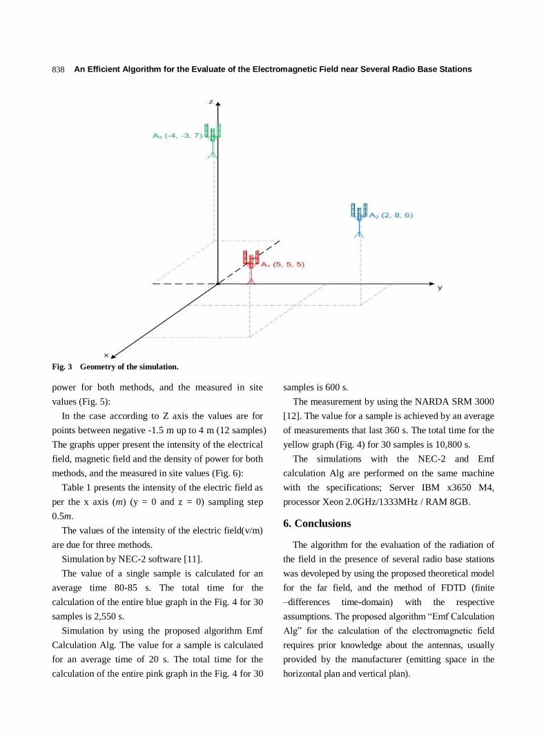
An Efficient Algorithm for the Evaluate of the Electromagnetic Field near Several Radio Base Stations
838
Fig. 3 Geometry of the simulation.
power for both methods, and the measured in site
values (Fig. 5):
In the case according to Z axis the values are for
points between negative -1.5 m up to 4 m (12 samples)
The graphs upper present the intensity of the electrical
field, magnetic field and the density of power for both
methods, and the measured in site values (Fig. 6):
Table 1 presents the intensity of the electric field as
per the x axis (m) (y = 0 and z = 0) sampling step
0.5m.
The values of the intensity of the electric field(v/m)
are due for three methods.
Simulation by NEC-2 software [11].
The value of a single sample is calculated for an
average time 80-85 s. The total time for the
calculation of the entire blue graph in the Fig. 4 for 30
samples is 2,550 s.
Simulation by using the proposed algorithm Emf
Calculation Alg. The value for a sample is calculated
for an average time of 20 s. The total time for the
calculation of the entire pink graph in the Fig. 4 for 30
samples is 600 s.
The measurement by using the NARDA SRM 3000
[12]. The value for a sample is achieved by an average
of measurements that last 360 s. The total time for the
yellow graph (Fig. 4) for 30 samples is 10,800 s.
The simulations with the NEC-2 and Emf
calculation Alg are performed on the same machine
with the specifications; Server IBM x3650 M4,
processor Xeon 2.0GHz/1333MHz / RAM 8GB.
6. Conclusions
The algorithm for the evaluation of the radiation of
the field in the presence of several radio base stations
was devoleped by using the proposed theoretical model
for the far field, and the method of FDTD (finite
–differences time-domain) with the respective
assumptions. The proposed algorithm ―Emf Calculation
Alg‖ for the calculation of the electromagnetic field
requires prior knowledge about the antennas, usually
provided by the manufacturer (emitting space in the
horizontal plan and vertical plan).

An Efficient Algorithm for the Evaluate of the Electromagnetic Field near Several Radio Base Stations
839
,
Fig. 4 Dependence of E, H and S in x axis (m) (y = 0 and z = 0).

An Efficient Algorithm for the Evaluate of the Electromagnetic Field near Several Radio Base Stations
840
Fig. 5 Dependence of E, H and S in y axis (m) (x = 0 and z = 0)

An Efficient Algorithm for the Evaluate of the Electromagnetic Field near Several Radio Base Stations
841
Fig. 6 Dependence of E, H and S in z axis (m) (x = 0 and y = 0).

An Efficient Algorithm for the Evaluate of the Electromagnetic Field near Several Radio Base Stations
842
Table 1 Comparative result.
Coordinates Values Values Values measured
Samples (X.Y.Z) NEC-2 Emf NARDA
Calculation Alg SRM3000
1 -4.0.0 0.30200514 0.2749 0.258406
3 -3. 0. 0 0.36012108 0.3278 0.308132
5 -2. 0. 0 0.50579544 0.4604 0.432776
7 -1. 0. 0 1.14880602 1.0457 0.982958
9 0 .0 .0 1.3853346 1.261 1.18534
11 1. 0. 0 1.1321073 1.0305 0.96867
13 2. 0. 0 0.74199444 0.6754 0.634876
15 3. 0. 0 0.91304646 0.8311 0.972387
17 4. 0. 0 1.93309656 1.7596 1.654024
19 5. 0. 0 2.043587 2.2457 2.110958
21 6. 0. 0 3.31821144 3.0204 2.839176
23 7. 0. 0 3.18835692 2.9022 2.728068
25 8. 0. 0 3.0563052 2.782 2.61508
27 8. 0. 0 3.0563052 2.782 2.61508
29 9. 0. 0 3.98989548 3.6318 3.413892
31 10. 0. 0 3.27196038 2.9783 2.799602
Analysis and comparison between the calculated
values and the measured ones concludes that the
proposed algorithm provides accurate results for the
field close and far from the radio base stations (up to
12 BTS antennas) in a given urban area. The error
between calculated and measured values is less than
10%.
Analysis and comparison between the values
calculated with the proposed algorithm and the ones
simulated with the NEC-2 software, concludes in
values that converge, thus confirming the accuracy of
the proposed algorithm.
Analysis and comparison between the time required
for running the proposed algorithm, and the NEC-2
simulation confirms the speed of calculations for the
authors’ algorithm, making it suitable for low
computing capacity machines.
For the reviewed radio base stations which operate
at the same time in the frequencies band
900/1800/2100MHz the algorithm ―Emf caclultion
Alg‖ calculates the safety zones in the Iso-kurves (the
space where the E ≥ 41 V/m) in the plans x-y, x-z and
y-z.
In an environment in the presence of several radio
base stations can be calculated the intensity of the
electrical field, magnetic field and the density of
power for different distances from the antenna in a
short period of time providing confident and accurate
results.
References
[1]. M. Barbiroli, C. Carciofi, V.D. Esposti, G. Faciasecca,
Evaluation of exposure levels generated by cellular
systems: methodology and results, IEEE Transactions on
Vehicular Technology 51 (2009) 1322-1329.
[2]. M. Martínez, A.F. Pascual, E. Reyes, V.V. Loock,
Practical procedure for verification of compliance of
digital mobile radio base stations to limitations of
exposure of the general public to electromagnetic fields,
IEEE Proceedings Microwaves, Antennas and
Propagation 149 (2009) 218-228.
[3]. Z. Altman, B. Begasse, C. Dale, A. Karwowski, J. Wiart,
M.F. Wong, et al., Efficient models for base station
antennas for human exposure assessment, IEEE
Transactions on Electromagnetic Compatibility 44 (2002)
588-592.
[4]. L. Correia, C. Fernandes, G. Carpinteiro, C.Oliveira, A
Procedure for Estimation And Measurement of
Electromagnetic Radiation in the Presence of Multiple Base
Stations, Instituto Superior Técnico, Lisbon, Portugal, 2002.
[5]. C. Oliveira, C. Fernandes, C. Reis, G. Carpinteiro, L.
Ferreira, Definition of Exclusion Zones around Typical
Installations of Base Station Antennas, Instituto Superior

An Efficient Algorithm for the Evaluate of the Electromagnetic Field near Several Radio Base Stations
843
Técnico, Lisbon, Portugal, 2005.
[6]. M. Bizzi, P Gianola, Electromagnetic fields radiated by
GSM antennas, IEEE Transactions on Electromagnetic
Compatibility, Electronic Letters 35 (1999) 855-857.
[7]. K.W. Kg, Technical Information and New Products 790
-2500 MHz Base Station Antennas for Mobile
Communications, Catalogue Issue, 2004.
[8]. A.W. Scott, Radio Frequency Measurements for Cellular
Phones and Wireless Data Systems, A John Wiley&Sons,
New York, 2008.
[9]. V. Prasad, Engineering Electromagnetic Compatibility
Principles, Measurements, Technologies and Computer
Model, A John Wiley & Sons, New York, 2008.
[10]. I. Laakso, T. Uusitupa, S. Ilvonen, Comparison of SAR
calculation algorithms for finite-difference time-domain
method, Physics in Medicine and Biology 55 (2010)
421-431.
[11]. Numerical Electromagnetics Code NEC2 Unofficial
Home Page, http:// www.nec2.org.
[12]. Available at http://www.narda-sts.de/en/products/emc/.

Journal of Communication and Computer 10 (2013) 844-856
Composing Specific Domains for Large Scale Systems
Asmaa Baya and Bouchra EL Asri
Models and Systems Engineering team, Mobile and Embedded Information Systems Laboratory, ENSIAS, Mohammed V Souissi
University, Rabat 10000, Morocco
Received: April 26, 2013 / Accepted: May 31, 2013 / Published: June 30, 2013.
Abstract: DSM (domain-specific modeling) offers many advantages over general purpose modeling, but this type of modeling is
effective just in narrow domains. The recent MDE (model driven engineering) approaches seek to provide a technology to compose
different specific domains in order to cover large scale systems. In this context, this article proposes a new approach for composing
specific domain models. First, we analyze some related works. On the basis of the key findings and conclusions drawn from the
analysis, we propose a multidimensional approach based on the composition of crosscutting concerns contained in the source domain
models. The approach is illustrated by a composition of service domains.
Key words: Composition, specific domain, separation of concerns, large scale systems, modularization.
1. Introduction
System development process becomes more
complex and time-consuming, because systems are no
more restricted to one specific domain, but describe a
set of related domains. So, it is impracticable to
describe the whole system by one model. To resolve
this problem, designer must combine models coming
from different specific domains. This, however, leads
to resolve model composition issues, which was and
remains one of the mean problem of the model driven
engineering.
In this paper, we are interested in domain model
composition as a practical solution to get the
maximum benefit from domains that have been
already developed and tested. This field of research
was intensified through a wide range of research in
order to extend the use of specific domains (e.g., Ref.
[1-3]). Indeed, the trend is to build libraries of
subdomains meta models that are reusable. These
basic domains (like interconnection of modules,
specialization, finite state machines, Petri networks,
Corresponding author: Asmaa Baya, Ph.D., student,
research fields: MDE, specific domains. E-mail: [email protected].
etc.) are used in the construction of most domains.
Thus, modeler can construct new domains just by
extending and defining rules of composition between
these basic subdomains. This basis arises the need to
define a new domain composition approach which
provides clear and practical mechanisms to extend and
compose domains.
In this paper, we treat domain composition issues.
The paper is structured as follows: Section 2 delimits
the context of work; Section 3 presents some model
composition methods; Section 4 presents some
examples of composition approaches; Section 5
presents our approach to compose specific domains.
We begin this section by presenting the process of the
approach, and then present its different phases. To
illustrate the approach, we present in the last section a
case study when we compose riche service and service
registry domains.
2. Context of Work
Model composition is a very wide field of research.
Especially, if we look for generative solution fit all
contexts, the number of constraints to consider
becomes infinite. That is why we must delimit our
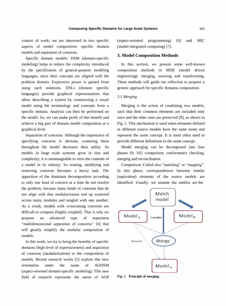
Composing Specific Domains for Large Scale Systems
845
context of work; we are interested in two specific
aspects of model composition: specific domain
models and separation of concerns.
Specific domain models: DSM (domain-specific
modeling) helps to reduce the complexity introduced
by the specification of general-purpose modeling
languages, since their concepts are aligned with the
problem domain. Expressive power is gained from
using such notations. DSLs (domain specific
languages) provide graphical representations that
allow describing a system by constructing a visual
model using the terminology and concepts from a
specific domain. Analysis can then be performed on
the model. So, we can make profit of this benefit and
achieve a big part of domain model composition at a
graphical level.
Separation of concerns: Although the importance of
specifying concerns is obvious, scattering them
throughout the model decreases their utility. As
models in large scale systems grow in size and
complexity, it is unmanageable to view the contents of
a model in its entirety. So reusing, modifying and
removing concerns becomes a heavy task. The
apparition of the dominant decomposition according
to only one kind of concern at a time do not resolve
the problem, because many kinds of concerns that do
not align with that modularization end up scattered
across many modules and tangled with one another.
As a result, models with crosscutting concerns are
difficult to compose (highly coupled). That is why we
propose an advanced type of separation
“multidimensional separation of concerns” [4] that
will greatly simplify the modular composition of
models.
In this work, we try to bring the benefits of specific
domains (high level of expressiveness) and separation
of concerns (modularization) to the composition of
models. Recent research works [5] explore this new
orientation under the name of AODSM
(aspect-oriented domain-specific modeling). This new
field of research represents the union of AOP
(aspect-oriented programming) [6] and MIC
(model-integrated computing) [7].
3. Model Composition Methods
In this section, we present some well-known
composition methods in MDE (model driven
engineering): merging, weaving and transforming.
These methods will guide our reflection to propose a
generic approach for specific domains composition.
3.1 Merging
Merging is the action of combining two models,
such that their common elements are included only
once and the other ones are preserved [8], as shown in
Fig. 1. This mechanism is used when elements defined
in different source models have the same name and
represent the same concept. It is most often used to
provide different definitions to the same concept.
Model merging can be decomposed into four
phases [9, 10]: comparison, conformance checking,
merging and reconciliation.
Comparison: Called also “matching” or “mapping”.
In this phase, correspondences between similar
(equivalent) elements of the source models are
identified. Usually, we assume tha entities are the
Fig. 1 Principle of merging.

Composing Specific Domains for Large Scale Systems
846
same when they have the same name or id, or when
they support the use of an explicit ontology, or a
thesaurus.
Conformance checking: The matching elements
identified in the previous phase are checked in this
phase. The purpose of this phase is to identify
potential conflicts that would render merging
infeasible.
Merging: The output of merging phase is a model
that retains all non-duplicated information in source
models; it collapses information that match model
declares redundant.
Reconciliation and restructuring: The target model
of merging phase may contain inconsistencies that
need fixing like violation of meta-model-specific
constraint. So, the purpose of this phase is to provide a
consistent merged model.
The main approach of model composition that uses
the merging method is “package merge” [11]. This
approach proposes a directed relationship between
two packages that indicates that the contents of the
two packages are to be combined. Other approaches
were developed in order to propose a more
deterministic process of merging [8, 10]. The
approach “Kompose” [12] is a merging approach that
proposes to merge models by comparing the
signatures of their element. The approach proposed in
Ref. [10] presents a specific algorithm that resolves
merge problem. This approach focuses on resolving
conflicts before and after merging.
3.2 Weaving
A weaving involves two actors: an aspect and a
base model. The aspect is made of two parts, a “point
cut”, which is the pattern to match in the base model,
and an “advice”, which represents the modification
made to the base model during the weaving. The parts
of the base model that match the point cut are called
“join points” (join points are, for example, methods or
variable assignments). During the weaving, each join
point is replaced by the advice [8] (Fig. 2).
Fig. 2 Principle of weaving.
Models and aspects can be woven in two ways [13]:
static and dynamic.
Static weaving: Modify source code of model
entities in order to insert aspect-specific statements at
join points. The mean advantage of this type of
weaving is the optimization of code. However, the
aspect-specific statements introduced become difficult
to identify later.
Dynamic weaving: This type of weaving solves the
problem of aspect identification in woven model. In
fact, it allows the explicit identification of aspects
both at weave-time and at runtime. Therefore, aspects
can be added, removed or updated during runtime.
A lot of approaches (e.g., Ref. [13-15]) adopt
weaving method in order to solve composition issues.
For example, the work in Ref. [14] proposes a
weaving process that exhibit composition properties to
allow multiple aspect weavings. Weaving model is
proposed in Ref. [15]. This model captures the
fine-grained relationships between elements of models
to compose. Other works propose an implemented
solution to weaving process. For example, the
approach “PROSE” (programmable extensions of
services) [16], offers a platform that allows aspects to
be woven, unwoven, and replaced at runtime.

Composing Specific Domains for Large Scale Systems
847
3.3 Transforming
“Transformation is the automatic generation of a
target model from a source model, according to a
transformation definition” [17].
A transformation definition is a set of
transformation rules (Fig. 3) that together describe
how a model in the source language can be
transformed into a model in the target language.
A transformation rule is a description of how one or
more constructs in the source language can be
transformed into one or more constructs in the target
language.
Composition can be seen as a particular case of
transformation, although a lot of works [18] studied
the relation between model composition and model
transformation. Transformation can also be a step in a
compositional process and can be supported by other
methods like weaving and merging. In this case,
transforming step ensures automatic generation of
target model, unlike weaving and matching that need
human intervention.
Model transformation has been used in many
compositional approaches [19]. AMW [20] is a model
composition framework that uses model weaving and
Fig. 3 Principle of transforming.
model transformations to produce and execute
composition operations. In fact, a weaving model
captures the links between the input model elements,
and then this weaving model is used to automatically
generate a transformation. So, the transformation
takes two input models and produces the composed
model as output. EML (epsilon merging language) [21]
is also a meta model agnostic language for expressing
model compositions. It includes a model comparison
and model transformation steps.
4. Composition Approaches for Specific
Domains: The State of Art
In this section, we analyze some current
composition approaches for specific domains, as we
draw up a summary of the criteria that guide our
contribution.
4.1 Current Domain Composition Approaches
Several research studies focused on the problem of
composition for specific domains. This contributed to
the emergence of several orientations. In what follows,
each paragraph presents a specific orientation.
Conceptual composition: The approach of Vega [1]
proposes to compose domains at the conceptual level
rather than components infrastructure, an additional
level is inserted between the two levels in order to
ensure their synchronization. The first step of this
approach is to materialize the concepts of the
composite domain by classes of meta model. The
meta model of the composite domain becomes an
extension of the source domain meta models.
Transformation to pivot language: “Multi-modeling
views” approach offers a solution to the composition
of heterogeneous models (called high-level models)
by transforming both high-level models into low level
models that conform to the same existing meta model,
or conform to an extension of it [2]. A correspondence
model (CM high-level) is used to align high-level
models by describing the relationships of
correspondence between the composing elements.
Then high-level models specified in different domain

Composing Specific Domains for Large Scale Systems
848
specific languages submit a sequence of
transformation steps in order to translate them into a
common low level language. A CM high-level needs
also to be propagated through the complete
transformation chains in order to automatically derive
CM low-level (correspondence model of low level
models). Finally, this approach proposes to make a
homogeneous model composition.
Composition by adopting template: “Template
instantiation” is a meta model composition approach
[3]. This approach is based on the reuse of common
meta modeling patterns in a single composite meta
model. Those patterns are saved as abstract meta
model templates and will be instantiated in
domain-specific meta models. This approach of
composition does not bring any changes to the source
meta models; however, it automatically creates new
relationships between the pre-existing entity types in a
target meta model to make them play roles in a
common meta modeling pattern.
Extending languages: Many approaches propose to
extend language in order to support domain
composition [22, 23]. For example, the approach of
Ledeczi [23] proposes to extend UML (unified
modeling language) with new operators in order to
combine source meta models. Another approach
proposes to extend the UML meta model with
behavior describing symmetric, signature-based
composition of UML model elements [22].
Coordination: The composition by coordination
was adopted in Ref. [24]. This approach proposes
architecture of coordination where every participant
preserves its autonomy, and the coordinator organizes
the collaboration of all participants. Another work
proposes to compose an inter domain specific
languages coordination [25]. This work introduces an
inter-model traceability and navigation environment
based on the complementary use of mega-modeling
and model weaving.
Graphical composition: Some works solve the
problem of composition at the graphical level. In
Ref. [26], researchers define a layer for graphical
syntax composition. This work provides formally
defined operators to specify what happens to graphical
mappings when their respective meta models are
composed.
4.2 Review of Domain Composition Approaches
The proposed approaches are non-exhaustive. MDE
contains a lot more approaches. However, we choose
these methods because each one illustrates a particular
orientation. The approaches above have several
advantages and disadvantages that we present in what
follows.
In Vega’s approach, the conceptual stage before the
composition of meta models aims at conceptualizing
the concepts of composite domain. Thus, the
composition is expressed at a high level abstraction.
The disadvantage is that the approach remains
complex as long as this high level abstraction is not
supported by simple and practical methods.
The approach “Multi-modeling views composition”
is based on a simple principle which is the
transformation of a high-level language to a low-level
language. However, it follows a long process and goes
through several transformations and intermediate
models before getting the final model. This increases
the complexity of this approach and its margin of
error.
“Template instantiation” approach ensures a
high-level abstraction through the use of abstract meta
model templates. However, these templates have
several limitations such as validity, adaptation and
instantiation, which greatly minimize their context of
use.
Extending languages maximizes reuse and makes
profit of existing languages. However, this orientation
is not generative because of its limitation to specific
languages.
The composition by coordination presents a lot of
advantages like the independence of source domains
and a high level of abstraction. However, it proposes

Composing Specific Domains for Large Scale Systems
849
usually many languages and techniques which are not
easy to use by domain experts.
A graphical composition is a limited orientation,
because it solves the problem of composition at the
syntactical level only.
Based on these results, we can conclude that
high-level abstraction approaches often provide a high
level reuse and a good operating range. However, this
advantage is often accompanied by a high level of
complexity. Thus, the challenge to overcome is to
ensure a high level of abstraction while avoiding both
introduction of complex mechanisms and limitation of
the context of use.
5. XCOMP approach
In this section, we present a compositional
approach for specific domain models. The challenge
to overcome is to present a generative approach that
resolves the main composition issues in large scale
systems.
In such context, applying one method is not enough
to resolve the whole composition problems that
designer can meet in a standard context. So we
propose a new approach that combines all presented
methods in previous section: merge, weave and
transforming. This combination allows benefiting
from advantages of these methods. In addition, these
methods are simple to use and familiar for designers.
This new approach is supported with additional
methods that simplify the manipulation of concerns
contained in domain models, as it allows also the
re-modularization on demand; because every designer
organizes the source models according to his point of
view.
5.1 Process of Composition
“XCOMP” (X-Composition) is a composition
approach for specific domains. This approach
proposes to compose the models of source domains.
The output is a new model called “model of
composition”. This model references source models or
its elements as it can contain some emergent
constraints of the composed domains.
To obtain the final model, XCOMP propose to
follow the process presented in Fig. 4.
This process proposes organizational and
transforming steps.
Organizational steps propose to reorganize models in
order to increase design flexibility and allow
obtaining modular models. However, transforming
steps allow the introduction of composition rules and
constraints. The rest of this section explains each step
in the XCOMP process.
5.2 Decomposition
This approach of composition is dedicated to
models that describe large scale systems. So the
models to compose are so diversified and complex
that the navigation through such models, and their
composition is extremely difficult and time
consuming. To compose large scale models, we
propose to reorganize them in order to obtain
simplified models that we can manipulate easily
without losing the necessary information needed for
composition.
For this, we thought to divide the domains to
compose into dimensions. This notion of dimensions
was introduced in the “multidimensional separation of
concerns” [4]. In this context, dimension is a set of
concerns gathered in order to form independent unit of
sense. To identify dimensions, designer can choice
one of the several proposed policies in the domain of
multidimensional separation of concerns, or can just
try to make intuitive separation. In spite of the
followed decomposition policy, defined dimensions
must be weakly coupled. This characterization implies
that changes to one dimension have a limited or no
effect on other dimensions, which allow having a big
flexibility while composing domain models.
Fig. 5 presents a proposition to define dimensions that
will simplify composition later. This figure presents
examples of concerns in every type of dimensions.

Composing Specific Domains for Large Scale Systems
850
Fig. 4 XCOMP process.
Fig. 5 Decomposition policy.
The first dimension to define in a domain model is
a business dimension “functional dimension”. It
contains concerns that provide the main functionalities
of systems and deal directly with problem domains.
Defining this part of each systems allows to simplify
the accumulation of the principle functionalities in
composed domain model.
The rest of concerns will be organized in
“non-functional dimensions”. However, we propose to
separate them according to their dependence on
context changes or not. So, non-functional concerns
that will be parameterized depending on environment
of execution are gathered in “context dimensions”.
Once we have defined the dimensions, we
decompose the source domain models following these
dimensions. Each dimension must be represented by a
part of the model (called block). To keep the
consistency of the model, we must trace the
relationships between the blocks.
So, the resulted models from the step of
decomposition, named “model of composition”, will
conform to meta model shown in Fig. 6. Each model
is composed of blocks relied between them, and every
block contains a set of entities and relationships.
5.3 Merging
In this phase, dimensions that have been identified
in previous step are examined for conformance with
each other. The purpose of his phase is to identify
potential conflicts and repetitions in the model of
composition. Fig. 7 presents the process of this step.
This process is repeated for each dimension of the
first domain model.
The first activity of this phase is to compare one
dimension (presented by block) of the first source
model with dimensions of the second model. If this
dimension conforms to dimension in the second
model, we merge blocks that represent these
dimensions. To check conformance, we compare all
entities contained in each block, particularly, their
names, ids and attributes.
To merge blocks, we delete the block from one
model and keep it in the second model. Relations
between the deleted block and the rest of the blocks
will be inserted to the same block of the second, so
those relations will henceforth rely blocks from
different source models.
Fig. 6 Model of composition metamodel.

Composing Specific Domains for Large Scale Systems
851
Fig. 7 Merging process.
If this dimension does not conform to any
dimension of the second model, then we move to the
second level which is checking dimension entities. So,
we compare each entity of the block that represents
this dimension with entities of the second model. If
entities conform totally, we merge entities by the
same way that we merge dimensions. If entities
conform partially, we merge entities by adding
attributes and relations that not exist in the first entity
to the second entity, then delete the first entity.
It should be noted that a good decomposition policy
will reduce the number of entities merging, because
repeated elements will appear in the same dimensions.
So, merging dimensions will be sufficient to eliminate
overlaps between source domain models.
5.4 Weaving
The main purpose of composing existing domains
is to obtain new domain that contains all
functionalities of source domains. However, resulting
domain will need additional concepts and
functionalities, directly linked to the new problem
domain, but do not exist in composed domains. To
add these emergent concepts, we propose to weave
concerns with model of composition.
Once we have defined concern to weave, all must
identify the block when the new concern will be
inserted, then identify the join points and point cuts.
5.5 Transforming
After the weaving phase, the model of composition
may contain inconsistencies that need fixing. In the
final step of the process, such inconsistencies are
removed and the model is polished to acquire its final
form.
The composed domain will reuse artifacts of source
domains. That is why source domains must remain
intact. All composition constraints and methods are
inserted in the model of composition. This model
ensures the collaboration of source models and the
introduction of emergent concepts. To achieve this,
we propose to represent new entities and relations
(that exist in resulting model and do not exist in
source models) in additional dimensions instead of
dispersing them throughout the model.
To define which transformations must be made to
obtain a consistent model of composition, we define
model of composition and source model matrices as
shown in Figs. 8 and 9.
Matrices are defined as follows:
(1) Each column and line represents a dimension in
a domain model;
(2) Bi is a block which represent a dimension Di;
(3) Ri,j is a relation between the block “i” and the
block “ j”.
In the same way, we define the matrix of model of
composition (Fig 10). The diagonal of model of
composition matrix contains blocks which represent
all dimensions contained in source models. The Ri, j
represent the relationships between blocks from the
same model. The part X and X’ of this matrix varies
according to composition mechanisms.
The transformations to make is to delete the part X
and X’ of the matrix. New entities inserted while the
composition must be gathered in new dimensions that
reference the existing dimensions. Relations of X and

Composing Specific Domains for Large Scale Systems
852
Fig. 8 Matrix of the first domain model.
Fig. 9 Matrix of the second domain model.
Fig. 10 Matrix of the model of composition.
X’ must appear in new dimensions in order to keep the
consistence of the resulting model.
Our approach stop at this level, since all proposals
to homogenize blocks must specify the target
language. However, our goals are to propose a
generative approach applicable to any type of
language. Indeed, to adapt the composite domain
model, there are other alternatives such as keeping
models heterogeneous and proceeding directly to the
code generation, or applying one of the transformation
methods from language to another in order to unify
the language used in the model [27].
6. Case Study
To illustrate what we explain above, we present an
example of composition of rich service domain and
service registry domain. Fig. 11 shows the model of
rich service domain and Fig. 12 shows the model of
service registry domain.
The first step is to identify dimensions, blocks and
relations of domain models. The model of rich service
domain can be organized in five dimensions of
concerns: service (B11), infrastructure (B12), routing
(B13), communication (B14) and application (B15).
Each dimension is represented by a block. Fig. 13
shows the blocks and relations contained in the model
of rich service domain.
The model of service registry domain can be
organized in three dimensions: storage (B21), registry
(B22) and service definition (B23). Blocks and
relations of this model domain are shown in Fig. 14.
The second step is to apply the merging process
(Fig. 7). As we can see through the domain models,
we have no repeated dimensions. However, the entity
“service” appears in B11 and B23. So, we have to
merge the entities “service”. We remove this entity
from the block B11 and link the block B11 with the
entity service of the block B23.
To simplify, we suppose that we have no emergent
concepts. So, we go on the transforming step. We
begin by defining the matrices of source domain
models based on the separation of concerns made in
the decomposition step (Figs. 13 and 14).
The Fig. 15 shows the operation of composing rich
service domain model matrix and service registry
domain model matrix. The resulted matrix of this
composition is shown in Fig. 16.
The part X and X’ (presented in Fig. 10) contain in
this case one relation R1, 2. This relation represents

Composing Specific Domains for Large Scale Systems
853
Fig. 11 Rich service domain model.
Fig. 12 Service registry domain model.

Composing Specific Domains for Large Scale Systems
854
Fig. 13 Separation of concerns in rich service domain model.
Fig. 14 Separation of concerns in service registry domain model.
Fig. 15 Composition of rich service and service registry domain model matrices.

Composing Specific Domains for Large Scale Systems
855
Fig. 16 Resulted matrix of composition.
the inheritance between “rich service” entity and
“service” entity of the block (B11). After removing
“service” entity, this inheritance became between
“rich service” entity of the block (B11) and “service”
entity of the block (B23). So, a new dimension must
be inserted. This new dimension must reference the
blocks (B11) and (B23).
7. Conclusions
The main motivation behind this proposal is to
promote the composition of crosscutting concerns,
and to allow the insertion of new concerns throughout
the domains life cycle. However, this approach uses
several theoretical basis that must be implemented in
order to have a practical approach.
To build this approach, we used the basic principle
of the multidimensional separation of concerns. This
multidimensional separation has several advantages.
The separation is done according to multiple concerns,
which deal with the problem of the dominant
decomposition according to only one kind of concern
at a time. In addition, it allows on-demand
remodularization. Indeed, it is possible to add or omit
concerns throughout the life cycle without having to
change the entire model.
This domain composition approach begins first with
a multidimensional decomposition of concerns, and
then merges dimensions and entities that overlap.
After that, new aspect specific to composed domain
must be weaved to resulting model. Finally, it
proposes to insert new dimensions in order to ensure
the consistence of the composed domain.
References
[1] G. Vega, Développement d'applications à grande echelle
par composition de méta-modèles, Ph.D. thesis,
University Joseph Fourier, 2005.
[2] A. Yie, R. Casallas, D. Deridder, D. Wagelaar, A
practical approach to multi-modeling views composition,
in: Proceedings of the 3rd International Workshop on
Multi-Paradigm Modeling, Denver, Colorado, USA,
2009.
[3] M. Emerson, J. Sztipanovits, Techniques for metamodel
composition, in: OOPSLA—6th Workshop on Domain
Specific Modeling, Portland, 2006.
[4] H. Ossher, P. Tarr, Multi-dimensional separation of
concerns in hyperspace, in: ECOOP’99 Corkshop on
Aspect-Oriented Programming, Lisbon, 1999.
[5] J. Gray, T. Bapty, S. Neema, J. Tuck, Handling
crosscutting constraints in domain-specific modeling,
Communications of the ACM 44 (20) 87-93.
[6] Annual Aspect-Oriented Software Development

Composing Specific Domains for Large Scale Systems
856
Conference Home Page, http://www.aosd.net.
[7] J. Sztipanovits, G. Karsai, Model-Integrated Computing,
IEEE Computer 30 (1997) 10-12.
[8] J. Marchand, B. Combemale, B. Baudry, A categorical
model of model merging and weaving, in: MiSe 2012—
4th International Workshop on Modeling in Software
Engineering, Zurich, Switzerland, 2012.
[9] D. Kolovos, R. Paige, F. Polack, Merging Models with
the Epsilon Merging Language (EML), in: MoDELS,
Genova, Italy, Oct. 1-6, 2006.
[10] R. Pottinger, P. Bernstein, Merging models based on
given correspondences, in: Proceedings of 29th
International Conference on Very Large Data Bases
(VLDB’03), Berlin, Germany, 2003.
[11] OMG 2003, UML 2.0 Superstructure Final Adopted
specification, Document-ptc/03- 08-02.
[12] R. France, F. Fleurey, R. Reddy, B. Baudry, S. Ghosh,
Providing support for model composition in meta models,
in: Proceedings of the 11th IEEE International Enterprise
Distributed Object Computing Conference, Washington,
DC, USA, 2007.
[13] K. Bollert, On weaving aspects, in: International
Workshop on Aspect-Oriented Programming, ECOOP99,
Portugal, 1999.
[14] J.M. Jézéquel, Modeling and aspect weaving, in: Methods
for Modeling Software Systems (MMOSS), Germany, 2007.
[15] M.D.D. Fabro, J. Bezivin, F. Jouault, E. Breton, G.
Gueltas, AMW: A generic model weaver, in: IDM-
Ingénierie des Modèles, 1ères Journées sur l'Ingénierie
Dirigée par les Modèles, Paris, 2005.
[16] A. Popovici, T. Gross, G. Alonso, Dynamic weaving for
aspect-oriented programming, in: Proceedings of the 1st
International Conference on Aspect-Oriented Software
Development, Enschede, The Netherlands, Apr., 2002.
[17] A. Kleppe, J. Warmer, W. Bast, MDA Explained, The
Model-Driven Architecture: Practice and Promise,
Addison Wesley Longman Publishing, Boston, 2003.
[18] B. Baudry, F. Fleurey, R. France, R. Reddy, Exploring
the relationship between model composition and model
transformation, in: Proceedings of Aspect Oriented
Modeling Workshop, in conjunction with MoDELS’05,
Montego Bay, Jamaica, 2005.
[19] J. Bezivin, S. Bouzitouna, M.D.D. Fabro, M.P. Gervais, F.
Jouault, D. Kolovos, et al., A canonical scheme for model
composition, in: Proceedings of the 2nd European
Conference on Model Driven Architecture—Foundations
and Applications, Bilbao, Spain, Jul. 10-13, 2006.
[20] Atlas Model Weaver Project Web Page, 2005,
http://www.eclipse.org/gmt/amw/.
[21] D.S. Kolovos, Epsilon Project Page,
http://www.cs.york.ac.uk/~dkolovos.
[22] F. Fleurey, R. Reddy, B. Baudry, S. Ghosh, Providing
support for model composition in meta models,
in: Proceedings of EDOC 2007, Annapolis, MD, USA,
2007.
[23] A. Ledeczi, G. Nordstrom, G. Karsai, P. Volgyesi, M.
Maroti, On metamodel composition, in: Proceedings of
the 2001 IEEE International Conference, Mexico, 2001.
[24] T.L. Anh, Fédération: une architecture logicielle pour la
construction d’applications dirigée par les modèles, Ph.D.
thesis, University Joseph Fourier, 2004.
[25] F. Jouault, B. Vanhooff, H. Bruneliere, G. Doux, Y.
Berbers, J. Bezivin, Inter-DSL coordination support by
combining megamodeling and model weaving, in:
Proceedings of the 2010 ACM Symposium on
Applied Computing, Suisse Sierre, 2010.
[26] L. Pedro, M. Risoldi, D. Buchs, B. Barroca, V. Amaral,
Composing visual syntax for domain specific languages,
in: 13th International Conference, HCI International 2009,
USA, 2009, pp. 889-898.
[27] M. Brambilla, P. Fraternali, M. Tisi, A transformation
framework to bridge domain specific languages to MDA,
in: Models in Software Engineering: Workshops and
Symposia at MODELS 2008, Toulouse, France, 2008.

Journal of Communication and Computer 10 (2013) 857-862
Mobile Station Speed Estimation with Multi-bit Quantizer
in Adaptive Power Control
Hyeon-Cheol Lee
Satellite Technology Research Laboratory, Korea Aerospace Research Institute, Daejeon 305-806, Rep. of Korea
Received: May 10, 2013 / Accepted: June 09, 2013 / Published: June 30, 2013.
Abstract: The adaptive power control with multi-bit quantizer of CDMA (code division multiple access) systems for communications between multiple MSs (mobile stations) with a link-budget based SIR (signal-to-interference ratio) estimate is applied to four inner loop power control algorithms. The speed estimation performances of these algorithms with their consecutive TPC (transmit-power-control) ratios are compared to each inner loop power control algorithm, and the speed shows full linearity with the consecutive TPC ratio information of CS-CLPC (consecutive TPC ratio step-size closed loop power control), FSPC (fixed step-size power control), and KS-CLPC (Kalman gain step-size closed loop power control). These algorithms show more linearity with increased bit quantization. The result however, indicates consecutive TPC ratio of AS-CLPC (adaptive step-size closed loop power control) is independent of target speed. It is concluded that the speed can be estimated with the consecutive TPC ratio with CS-CLPC, FSPC and KS-CLPC. Key words: Speed estimation, adaptive power control, link-budget, SIR, multi-bit quantizer.
1. Introduction
The communication system of multiple MSs
(mobile stations) requires a mobile wireless network
to share data between MSs. One communication
network protocol that may be used is CDMA (code
division multiple access). CDMA differs from both
FDMA (frequency division multiple access) and
TDMA (time division multiple access) in that it uses
the same frequency for multiple users.
Since all users utilize a single frequency, the signal
from each MS may interfere with other MSs’
receivers [1]. This is referred to as the near-far effect.
To eliminate the near-far effect in CDMA systems, the
transmission signal power from every MS must be the
same as the signal power at the receiver. This
technique of controlling the magnitude of the
transmission power according to the distance between
the MS and the BS (base station) is officially termed
Corresponding author: Hyeon-Cheol Lee, Ph. D., principal researcher, research fields: wireless communications and SAR. E-mail: [email protected].
power control. It equalizes the received power and
eliminates the near-far effect, though it is subject to
such complications as path loss, shadowing,
multi-path fading, etc..
This power control technique is differentiated into
open loop power control and closed loop power
control. The closed loop power control is further
divided into inner loop power control and outer loop
power control. The inner loop power control is
responsible for adjusting the power transmitted to
maintain the received SIR (signal-to-interference ratio)
at the BS at a level equal to that at the SIRtarget. The
outer loop power control is responsible for setting the
SIRtarget based on the BER (bit error rate) or service
requirement.
Conventional SIR estimates [2, 3] consider only the
transmission power and the link-gain, but this paper
takes into account the link-budget, which has more
realistic parameters including distance information
than the link-gain. Using the SIR estimate that reflects
the link-budget, speed estimation [4] is introduced
DAVID PUBLISHING
D
Mobile Station Speed Estimation with Multi-bit Quantizer in Adaptive Power Control
858
based on a CTR (consecutive transmit-power-control
ratio). The proposed speed estimation method is
applied to four algorithms with one, two and three-bit
level quantizers, and the results are compared.
This paper is organized as follows: The literature
related to this work is surveyed in Section 2; the inner
loop power control is described in Section 3; the
concept of the link-budget based SIR estimate is
introduced in Section 4; followed by description of
simulation environments in Section 5; Section 6 gives
details of the speed estimation. The simulation results
are analyzed in Section 7; finally, conclusions are
drawn in Section 8.
2. Related Work
Kim et al. introduced in Ref. [5] the AS-CLPC
(adaptive step-size closed loop power control)
algorithm for a narrowband CDMA system. This
algorithm adapts its power control step-size based on
the optimal factors determined with the mean fade
duration which is inversely proportional to the
maximum Doppler frequency. Nourizadeh et al. [6]
proposed the BA-CLPC (blind adaptive closed loop
power control) in which the power control step-size is
adjusted to cope with the user mobility. Taaghol [7]
introduced the SA-CLPC (speed adaptive closed loop
power control) algorithm in which the power control
step-size is selected based on the user speed
estimation categorized by speed ranges. Lee and Cho
[8] proposed the M-ACLPC (mobility based adaptive
closed loop power control) algorithm in which the
power control step-size is adjusted depending on the
combination of the cumulative information of the
three power control commands and speed estimation.
Patachaianand and Sandrasegaran [3] compared
performances of the AS-CLPC, BA-CLPC, SA-CLPC,
and M-ACLPC in terms of PCE (power control error)
under the same simulation environment. In their
comparisons, the AS-CLPC showed the best
performance when the target speed was lower than 25
km/h, while the SA-CLPC was the best when the
speed was greater than 25 km/h.
Patachaianand and Sandrasegaran [3] presented the
CS-CLPC (CTR step-size closed loop power control)
algorithm whose power control step-size is
determined based on a parameter called CTR. They
measured the moving target speed by CTR, then,
calculated the PCE as the RMS (root mean square) of
the difference between the received SIR and the
SIRtarget. They also suggested in Ref. [4] the mapping
equation and mapping table which can yield accurate
speed estimation using CTR.
3. Inner Loop Power Control
In CDMA, the process of inner loop power control
occurs as follows: In the reverse link direction (from
the MS to the BS), the transmission power
information goes to the BS. At the BS, the SIRtarget
and the received SIR are calculated from the
transmission power, the link-gain and the noise power.
Based on these factors, the BS sends a TPC
(transmit-power-control) command to each MS at rate
of 1,500 Hz (= 0.667 ms) in the forward link direction
(from the BS to the MS). This power equalization
increases the maximum communication number
between MSs and consequently eliminates the near-far
effect. These procedures [2, 3] are represented in Eqs.
(1) and (3).
)()()()1( tiTPCtitiPtiP (1)
where Pi(t) is the transmission power, δi(t) is the
power control step-size, and TPCi(t) is the TPC
command for the ith MS at time t. )()()( ,arg tSIRtSIRtx iietti (2)
Where, SIRtarget,i(t) (= SIRtarget(t) here) is the target SIR
and SIRi(t) is the received SIR for the ith MS at time t.
Non-uniform quantizer [9] used in voice coding is
introduced that (m + 1)-bit TPC is adopted TPCi(t) =
C0 C1···Cm where C0 is the sign bit.
)12()1(
)/))(1log((
))(()(
mi
ii
Rptx
txsigntTPC
(3)
where δ = 2(m+1) – 1 and RP is dynamic range of power
adjustment in Table 1.
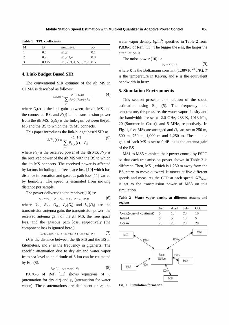
Mobile Station Speed Estimation with Multi-bit Quantizer in Adaptive Power Control
859
Table 1 TPC coefficients.
M D multilevel RP
1 0.5 ±1,2 0.1
2 0.25 ±1,2,3,4 0.3
3 0.125 ±1, 2, 3, 4, 5, 6, 7, 8 0.5
4. Link-Budget Based SIR
The conventional SIR estimate of the ith MS in
CDMA is described as follows:
ij
Njij
iii
PtGtP
tGtPtSIR
)()(
)()()(
(4)
where Gi(t) is the link-gain between the ith MS and
the connected BS, and Pi(t) is the transmission power
from the ith MS. Gji(t) is the link-gain between the jth
MS and the BS to which the ith MS connects.
This paper introduces the link-budget based SIR as
ijNjiR
iRi PtP
tPtSIR
)(
)()(
,
, (5)
where PR,i is the received power of the ith MS. PR,ji is
the received power of the jth MS with the BS to which
the ith MS connects. The received power is affected
by factors including the free space loss [10] which has
distance information and gaseous path loss [11] varied
by humidity. The speed is estimated from moving
distance per sample.
The power delivered to the receiver [10] is: ))()(/()( ,,,, iGiFiRiTiTiR DLDLGPGP (6)
where GT,i, PT,I, GR,i, LF(Di) and LG(Di) are the
transmission antenna gain, the transmission power, the
received antenna gain of the ith MS, the free space
loss, and the gaseous path loss, respectively (the
component loss is ignored here.). )(log20)(log204.92))(( 1010 iiF DFdBDL (7)
Di is the distance between the ith MS and the BS in
kilometers, and F is the frequency in gigahertz. The
specific attenuation due to dry air and water vapor
from sea level to an altitude of 5 km can be estimated
by Eq. (8).
iWOiG DDL )()( (8)
P.676-5 of Ref. [11] shows equations of γo
(attenuation for dry air) and γw (attenuation for water
vapor). These attenuations are dependent on σ, the
water vapor density (g/m3) specified in Table 2 from
P.836-3 of Ref. [11]. The bigger the σ is, the larger the
attenuation is.
The noise power [10] is: BTKPN (9)
where K is the Boltzmann constant (1.38×10⁻²³ J/K), T
is the temperature in Kelvin, and B is the equivalent
bandwidth in hertz.
5. Simulation Environments
This section presents a simulation of the speed
estimation using Eq. (5). The frequency, the
temperature, the pressure, the water vapor density and
the bandwidth are set to 2.0 GHz, 288 K, 1013 hPa,
20 (Summer in Coast), and 5 MHz, respectively. In
Fig. 1, five MSs are arranged and Dis are set to 250 m,
500 m, 750 m, 1,000 m and 1,250 m. The antenna
gain of each MS is set to 0 dB, as is the antenna gain
of the BS.
MS1 to MS5 complete their power control by FSPC
so that each transmission power shown in Table 3 is
different. Then, MS1, which is 1,250 m away from the
BS, starts to move outward. It moves at five different
speeds and measures the CTR at each speed. SIRtarget
is set to the transmission power of MS3 on this
simulation.
Table 2 Water vapor density at different seasons and regions.
Jan. April July Oct.
Coast(edge of continent) 5 10 20 10
Inland 5 5 10 5
Ocean 20 20 20 20
Fig. 1 Simulation formation.

Mobile Station Speed Estimation with Multi-bit Quantizer in Adaptive Power Control
860
Table 3 Initial condition of MS1 to MS5.
PT(dB) GT(dB) GR(dB) Di(m)
MS1 +8.048 0.0 0.0 1250
MS2 +4.1314 0.0 0.0 1000
MS3 +0.0000 0.0 0.0 750
MS4 -5.229 0.0 0.0 500
MS5 -13.979 0.0 0.0 250
Table 4 MS1 moving distance for 28.0 s (42,000 × 0.667 ms).
Speed (km/h) Speed (m/s) Moving distance (m)
100 27.7778 777.78
200 55.5556 1555.56
300 83.3333 2333.33
400 111.111 3111.11
500 138.8889 3888.89
600 166.6667 4666.67
6. Speed Estimation
There are several algorithms addressing inner loop
power control, including CS-CLPC [3], AS-CLPC [5],
FSPC and Kalman gain Step-size Closed Loop Power
Control, etc..
This section investigates changes in transmission
power for the above four algorithms with the
link-budget based SIR. MS1 moves outward for
42,000 × 0.667 ms (the number of the sample =
42,000) at the six different speeds listed in Table 4;
100 km/h, 200 km/h, 300 km/h, 400 km/h, 500 km/h,
and 600 km/h. As MS1 moves away, the four inner
loop power control algorithms alter the transmission
power to compensate for the distance between BS
and MS1. Eq. (10) [3] measures the CTR as
follows:
t
mtnm
nTPCnTPCdtCTR
1
)1()()( (10)
where d is a scale factor (see Table 1), m = t if t < w,
and m = w if t ≥ w. w is the maximum size of the
window average.
6.1 CS-CLPC
Patachaianand et al. [3] introduced the CS-CLPC
algorithm, where the step-size is adjusted as shown in
Eq. (11).
),(min1)(
maxCTRtCTRt
(11)
where α, β and CTRmax are constants.
6.2 AS-CLPC
Kim et al. [5] suggested the AS-CLPC algorithm.
This algorithm adapts its step-size based on TPC
history. The step-size is given by Eq. (12).
..,/)(
)1()(,)()(
WOLt
tTPCtTPCKtt
(12)
where K and L are positive real constants with ranges
of 1 < K and 1 < L < 2.
6.3 FSPC
In this simulation, the algorithm uses a fixed
step-size.
6.4 KS-CLPC
The well-known Kalman algorithm [12] for
adaptive step-size is used in this simulation.
)()()1()(
)()1()(
tRtHtPtH
tHtPt
Te
Te
K
(13)
)1())()(()( tPtHtItP eKe (14)
where δK(t) is a Kalman gain vector, H(t) is the an
observation matrix, and Pe(t) is an error covariance
matrix at time of t.
7. Simulation Results
Six different speeds are measured with CTR, and
the relationships are shown in Fig. 2 to Fig. 7
according to two window sizes and three quantizers.
The CS-CLPC, FSPC and KS-CLPC algorithms
show a linear relationship between speed and CTR,
in addition they show more linearity and can
estimate higher speed as quantizing bits are increased.
Therefore, the target speed can be measured
by mapping the CTR with the 3 algorithms. But, the
AS-CLPC algorithm deviates from linearity.
All the results are same with different window
sizes.

Mobile Station Speed Estimation with Multi-bit Quantizer in Adaptive Power Control
861
Fig. 2 CTR vs. MS1 speed at 1-bit Quantizer, window size 3 (Summer, Coast).
Fig. 3 CTR vs. MS1 speed at 1-bit Quantizer, window size 12 (Summer, Coast).
Fig. 4 CTR vs. MS1 speed at 2-bit Quantizer, window size 3 (Summer, Coast).
Fig. 5 CTR vs. MS1 speed at 2-bit Quantizer, window size 12 (Summer, Coast).
Fig. 6 CTR vs. MS1 speed at 3-bit Quantizer, window size 3 (Summer, Coast).
Fig. 7 CTR vs. MS1 speed at 3-bit Quantizer, window size 12 (Summer, Coast).

Mobile Station Speed Estimation with Multi-bit Quantizer in Adaptive Power Control
862
8. Conclusions
This paper introduced a speed estimation of four
different inner loop power control with consecutive
TPC ratios which use the link-budget based SIR in the
CDMA communication systems between MSs. It was
concluded that linear relationship exists between
speed and Consecutive TPC Ratios, and that MS
speed can be estimated using the Consecutive TPC
Ratios of the CS-CLPC, FSPC and KS-CLPC
algorithms.
References
[1] J.P. Romero, O. Sallent, R. Agusti, M.A.D. Guerra, Radio Resource Management Strategies in UMTS, John Wiley & Sons, New York, 2005.
[2] R. Patachaian, K. Sandrasegaran, Performance Comparison of Adaptive Power Control in UMTS, in: Int. Conf. Wireless Broadband and Ultra Wideband Commun. (AusWireless 2007), Sydney, Australia, 2007.
[3] R. Patachaian, K. Sandrasegaran, Consecutive transmit power control ratio aided adaptive power control for UMTS, Electronics Letters 43 (2007) 55-56.
[4] R. Patachaian, K. Sandrasegaran, User speed estimation
techniques for UMTS, Electronics Letters 43 (2007)
1036-1037.
[5] J.H. Kim, S.J. Lee, Y.W. Kim, Performance of single-bit
adaptive step-size closed-loop power control scheme in
DS-CDMA system, IEICE Trans. Commun. E81-B (1998)
1548-1552.
[6] S. Nourizadeh, P. Taaghol, R. Tafazolli, A Novel
Closed-loop Power Control for UMTS, in: Int. Conf. 3G
Mobile Commun. Technologies (3G 2000), London,
England, 2000.
[7] P. Taaghol, Speed-adaptive power control for CDMA
systems, Bechtel Telecommunications Technical Journal,
2 (2004).
[8] H. Lee, D.H. Cho, A new user mobility based adaptive
power control in CDMA systems, IEICE Trans. Commun.
E86-B (2003) 1702-1705.
[9] W. Li, V.K. Dubey, C.L. Law, A new generic multistep
power control algorithm for the LEO satellite channel
with high dynamics, IEEE Commun. Lett. 5 (2001)
399-401.
[10] D. Roddy, Satellite Communications, Prentice Hall, New
Jersey, 1989.
[11] ITU Recommendations 2004, 2004.
[12] R.G. Brown, P.Y.C. Hwang, Introduction to Random
Signals and Applied Kalman Filtering, John Wiley &
Sons, New York, 1997.

Journal of Communication and Computer 10 (2013) 863-872
On the Comparison Analysis of Two 4G-WiMAX Base
Stations in an Urban Sub-Saharan African Environment
Eric Tutu Tchao1, Kwasi Diawuo1 and Willie Ofosu2
1. Department of Electrical/Electronic Engineering, Kwame Nkrumah University of Science and Technology, Kumasi, Ghana
2. Department of Electrical Engineering Technology, Penn State Wilkes-Barre, USA
Received: June 04, 2013 / Accepted: June 15, 2013 / Published: June 30, 2013.
Abstract: A growth in the demand for WBA (wireless broadband access) technology has been seen in Ghana in the last few years.. The reason for this growth can be attributed to the emergence of the use of multimedia applications, demands for ubiquitous
high-speed Internet connectivity, the massive growth in the wireless and mobile communications sector and the deregulation in the
telecommunications industry. WiMAX, which is a WBA technology, is currently being deployed in the 2,500-2,690 MHz band to help serve the ever increasing needs of broadband internet subscribers in the country. This paper presents simulation results and field trial measurements for two BS (base stations) in a newly deployed 4G-WiMAX network in a typical dense urban Sub-Saharan African environment. We have used a model which uses the interference to noise ratio (n) parameter to obtain the coverage range of these two BS under evaluation. The simulated cell range for site 1 is 4.90 km and that for site 2 is 3.19 km. The final coverage simulation and the field measurements results have also been presented. Key words: Wireless broadband access, WiMAX, field measurements, interference modeling, Sub-Saharan African environment.
1. Introduction
WiMAX is a wireless digital communications
system which is intended for wireless metropolitan
area networks. WiMAX can provide BWA
(broadband wireless access) up to 30 miles (50 km)
for fixed stations, and 3-10 miles (5-15 km) for
mobile stations [1]. WiMAX allows for more efficient
bandwidth use and is intended to offer higher data
rates over longer distances [2]. Because WiMAX
operates in both licensed and non-licensed frequency
bands, it provides a viable economic model for
wireless carriers which make it a BWA technology of
choice for deployment in many developing
countries [3].
Deployment of WiMAX networks has currently
started in many sub-Saharan African countries. In
Ghana, the 2,500-2,690 MHz band, sometimes
Corresponding author: Eric Tchao, Ph.D., student, research
fields: wireless networks. E-mail: [email protected].
referred to as 2.6 GHz band, which is one of the
various bands defined by the ITU (International
Telecommunication Union), has been auctioned for
WiMAX deployment [4].
Pilot deployments are well underway in several
parts of Accra and Tema. The first successful pilot
deployment which covers 55 km2 in the urban centers
of Accra and Tema has about 535 fixed and mobile
CPE (customer premise equipment). Eleven WiMAX
base stations have been used to provide coverage to
the CPEs in the network using an adaptive 4T4R (four
transmit four receive) MIMO (multi input multi output)
antenna configuration. The final distribution of the
antenna sites in the deployment area is shown in
Fig. 1.
In order to deploy this high grade pilot WiMAX
network, engineering tools and techniques that
allowed rapid system design were used to achieve the
main objective of planning the new network to give
ubiquitous coverage to the user terminals in the

On the Comparison Analysis of Two 4G-WiMAX Base Stations in an Urban Sub-Saharan African Environment
864
Fig. 1 Final distribution of base stations in pilot network.
service area. This paper explores the techniques and
the accuracy of network plan which was used to
successful deploy two WiMAX base stations.
These techniques which we will discuss in this
paper were later extended to the deployment of the
extensive and high grade pilot WiMAX network.
2. Propagation Environment and Interference Modeling
In order to estimate signal parameters accurately in
wireless communication systems, it is necessary to
estimate signal propagation characteristics in different
terrain environments, such as free space, urban,
suburb, country and indoor. To some extent, the
communication quality is influenced mainly by
applied terrain environment [5]. Propagation analysis
provides a good initial estimate of the signal
characteristics.
There are two general types of propagation
modeling: site-specific and site general. Site-specific
modeling requires detailed information on building
layout, furniture, and transceiver locations. It is
performed using ray-tracing methods. For large-scale
static environments, this approach may be viable. For
most Sub-Saharan environments however, the
knowledge of the building layout and materials is
limited and the environment itself can change. Thus,
the site-specific technique is not commonly employed.
Site general models provide gross statistical
predictions of path loss for link design and are useful
tools for performing initial design and layout of
wireless systems especially under Sub-Saharan
African conditions.
The Hata-Okumura model which is best suited for
large cell coverage can be used to model the
propagation environment for this WiMAX network.
Because of its simplicity, it is a widely used model for
most of the signal strength predictions in
macro-cellular environment [6, 7], even though its
frequency band is outside the band of WiMAX.
In order to estimate the coverage range of the two
base stations, mapping of the CPEs which will be
served by the two bases stations was done and the
distribution is as shown in Fig. 2.
The propagation environment can be modeled using
the distribution of CPEs as shown in Fig. 2. It consists
of a fixed station F00 (site 1) and a mobile station M00
attempting to establish a radio link in the presence of
n additional fixed stations niFi 1 . Each fixed
station communicates with additional mobile stations.
Mi is the total number of mobile stations
communicating with the CPE Mij at a power Fij on the
downlink channel. Different propagation models are

On the Comparison Analysis of Two 4G-WiMAX Base Stations in an Urban Sub-Saharan African Environment
865
Fig. 2 Distribution of CPE covered by two base stations.
required for different environments. The simplest
model is the single slope path loss model [8]:
oo
tr ddd
dPP
,
(1)
where Pr is the power received at a distance d (relative
to the reference distance) from a transmitter radiating
at a power Pt. The parameter γ is the path loss
exponent (in free space) and κ is the free space path
loss between the transmission antenna and the
reference distance do: 2
r 4
ot dGG
(2)
where Gt and Gr are the antenna gains of the
transmitter and receiver respectively and λ is the
wavelength of the transmission. The single slope path
loss model is used to describe the mean path loss in
large area environments [9, 10]. Fig. 2 however shows
propagation at close ranges in an urban environment.
Propagation at close ranges however behaves more
like the plane earth model and a dual slope path loss
model is more appropriate [9, 11]:
(3)
where b is the breakpoint distance, γ1 is the path loss
exponent before the breakpoint and γ2 is the path loss
exponent after the breakpoint. The breakpoint is
related to the height above plane earth of the
transmitter antenna ht and receiver antenna hr and is
approximately given by [11]:
rthh
b4
(4)
Eq. (4) gives one theoretical expression for the
breakpoint in the plane earth model, however, the
breakpoint is not well defined due to the oscillatory
nature of the signal envelope in the plane earth
model, and different definitions of where the
breakpoint occurs give slightly different expressions
[12, 13]. Over a region of tens of wavelengths, a
received signal will exhibit variation about the mean
power predicted by the path loss models of Eqs. (1)
and (3). Measurements have consistently indicated
these power variations exhibit lognormal statistics [8,
14]. This phenomenon is called lognormal
shadowing and can be incorporated into either path
loss model as a multiplicative factor to the path loss
PL:
1010
Lr PP (5)
where ζ is a normally distributed dB variable with
dbb
d
d
dkP
bddd
dkP
P
ot
oo
t
r21
1
On the Comparison Analysis of Two 4G-WiMAX Base Stations in an Urban Sub-Saharan African Environment
866
zero mean, and a standard deviation σ typically
between 6 and 12 dB in macrocell systems [8]. From
Eq. (5) it can be seen that shadowing models both
signal attenuation due to obstructions and signal
amplification due to waveguide effects. At a receiver,
a link will be considered successful if the signal to
noise plus interference ratio 1N
S is greater than
or equal to the system protection ratio Z, otherwise an
outage is deemed to occur. The region in which this
threshold is maintained is the region in which radio
communication is considered successful and is called
the “cell”. The extent of the cell is thus a function of
the radio signal and interference statistics [15].
Examining Fig. 1, assuming M00 is communicating
with Fo in the presence of a single interferer Fi which
spills a power Pu into the wanted uplink and Pd into
the wanted downlink. A spatial analysis of link outage
in the presence of an interferer but in the absence of
receiver noise was presented by Cook [16] using the
single slope path loss model. When the effect of
receiver noise is incorporated (assuming that the same
protection ratio applies to noise and interference),
M00’s uplink outage contour is a family of circles
centred on the fixed station F0, but the downlink
outage contour is a higher plane curve [17]. By
introducing a parameter called the interference to
noise ratio (n) the equations for both outage contours
can be written in a simple form. n is the total
interference power at a receiver divided by the
receiver noise power. For a single interferer under the
single slope path loss model, n at the fixed station F0
is given by [17]:
N
rPn iu
u
0, (6)
whiles the DL n at the CPE Moo is given by:
N
rPn id
d
0, (7)
Using this parameter, it can be shown that the
equation for the uplink outage contour can be written
[17]:
1
1
1,,uu
uooiuuooo nn
nrKr (8)
and the DL outage contour equation can be written:
1
1
1,,dd
dooiddooo nn
nrKr (9)
where ZNKPt and the parameter is given by
[14]:
tt
sirtt
WZP
LWGGPK (10)
where Ls is a system loss factor, Pi is the interference
power, and Wi and Wt are the bandwidths of the
interfering and wanted signals respectively.
As the receiver S = [N + I] threshold must be
exceeded on both the uplink and downlink in order for
the duplex link to be successful, the range of the
mobile terminal from in any direction is the minimum
of ru and rd. Thus, the range described by Eq. (8)
represents the cell radius regardless of the downlink
conditions.
3. Coverage Simulation
The coverage prediction for the deployed network
is based on the simulation parameters in Table 1 and a
realistic distribution of BS and CPEs in the network.
Genex-Unet has been used to simulate the average
throughput per sector and the final radio network plan.
The CPE antenna configuration used for the
coverage and capacity simulation was 1T2R.
The capacity simulation results in Table 2 and Fig.
3 show better performance by 4 × 4 Antenna
configuration. The minimum simulated cell edge
uplink rate using a DL/UL ratio of 35:12 which was
used for the final network plan shown in Fig. 4 is 256
Kbps. This value was obtained at 4.90 km and 3.19
km for sites 1 and 2 respectively as shown in Fig. 5.
4. Measurement
The measurements were done at several locations
within the network in Accra which are dense urban
and urban environments. The selection of these

On the Comparison Analysis of Two 4G-WiMAX Base Stations in an Urban Sub-Saharan African Environment
867
Table 1 Simulation parameters.
Parameter Site 1 Site 2
Resource frequency 2.5-2.53 GHz
Channel bandwidth 10 MHz
Average users per sector 10
Fast Fourier Transform (FFT) Size 1,024
Subcarrier spacing 10.93 kHz
Useful symbol time 91.4 μs
Guard time 11.4 μs
OFDMA symbol time 102.8 μs
Modulation QPSK, 16-QAM, 64-QAM
Antenna frequency range 2.3-2.7GHz
VSWR ≤ 1.5
Input impedance 50 Ω
Gain 18 dBi
Horizontal beamwidth (3 dB) 60°
Vertical beamwidth (3 dB) 7°
Electrical downtilt 2°
CPE antenna configuration 1T2R
Maximum power (dBm) 43 43
Antenna height 42 m 38 m
Table 2 Capacity simulation results.
Permutation TDD split ratio
WiMAX carrier average throughput per sector
Minimum simulated cell edge throughput per sector
4T4R adaptive MIMO(Mbps) 4T4R adaptive MIMO
DL UL DL (Mbps) UL (Kbps)
PUSC with all SC 1 × 3 × 3 26:21 11.23 5.18 1.21 104
PUSC with all SC 1 × 3 × 3 29:18 13.00 4.32 1.52 108
PUSC with all SC 1 × 3 × 3 31:15 14.18 3.46 1.76 128
PUSC with all SC 1 × 3 × 3 35:12 16.55 2.59 2.24 256
Fig. 3 SINR simulation for the MIMO antenna configurations.

On the Comparison Analysis of Two 4G-WiMAX Base Stations in an Urban Sub-Saharan African Environment
868
Fig. 4 Final radio simulation of the 2 BS.
Fig. 5 Coverage range of the 2 BS.
locations was based on various criteria, where distance,
elevation and line of sight capabilities were the main
factors. The field trial measurement setup comprised:
(1) GPS antenna;
(2) RF cable;
(3) Dongle XCAL-X;
(4) Laptop with XCAL-X software;
(5) WiMAX PCMCIA CARD.
The measurements were divided into physical
measurements and throughput measurements. The
physical measurements collected RSSI (received
signal strength indication) values in about 10,260 and
7,210 locations in sites 1 and 2, respectively. The
overview of the measurement areas around the base
station and the summary of the measured RSSI values
have been summarized in Figs. (6), (7), (8), and (9).
Throughput measurements were performed by
downloading and later uploading FTP file size of 10
MB form and to a remote server as the subscriber
moves away from the base station until the connection
was dropped. The results of the throughput
measurement have been discussed in the next section.
5. Discussion of Results
From the RSSI measurements taken from the
102,060 locations in sites 1, about 86.55% of the
measured RSSI values were greater than –80 dbm.
From the site 2 measurements taken from 7,210

On the Comparison Analysis of Two 4G-WiMAX Base Stations in an Urban Sub-Saharan African Environment
869
Fig. 6 Summary of RSSI results for site 1.
Fig. 7 RSSI measurement areas for site 1.
Fig. 8 RSSI summary results for site 2.

On the Comparison Analysis of Two 4G-WiMAX Base Stations in an Urban Sub-Saharan African Environment
870
Fig. 9 RSSI measurement areas for site 2.
locations within the cell, 79.39% of the measured
RSSI values were greater than –80 dbm. For site 1,
99.45% of the measured values obtained from up to a
of about 5.30 km away from the base station were
greater than or equal to the simulated cell edge RSSI
value of –90 dBm. For site 2 on the other hand,
95.81% of the measured RSSI values obtained from
up to about 3.5 km away from the base station were
greater than or equal to the simulated cell edge RSSI
value. The results of the throughput measurements
have been summarized in Table 3 and Fig. 10.
The maximum measured throughputs for sites 1 and
2 are 8.62 Mbps and 7.20 Mbps, respectively.
Comparing the field results with the Federal
Communications Commission’s broadband
applications support speed guide [18], the least
measured throughput of 108 kbps and 203 Kpbs for
sites 1 and 2 respectively is enough to support
applications like online job searching, navigating
websites, streaming radio, voice over IP calls and
standard video streaming.
Field measurement trials for the overall pilot
network which have been presented in Ref. [19]
showed that the maximum measured throughput
during the entire pilot network trial measurement was
9.62 Mbps as compared to the simulated throughput
per sector of 16.55 Mbps. The measured throughputs
of 8.62 Mbps and 7.20Mbps for sites 1 and 2 show the
two base stations overall network performance have
been very impressive when compared with results in
Ref. [19]. The two sites will undoubtedly give
ubiquitous network coverage to its CPEs given the
obtained 99.45% and 95.81% RSSI values of -90 dBm
measured for sites 1 and 2 respectively. The
propagation models used for the coverage and
capacity simulation were developed for areas where
the harshness of the Sub-Saharan African terrain has
not been considered explicitly. Analysis of field
measurement results in Ref. [20] supports the
assumption that the correction factor for
Hata-Okumara model which have not been specified
for the Sub-Saharan African environment could have
contributed to the differences between the simulated
throughput per sector and the measured values.
Table 3 Summary of throughput measurements.
Site Measured throughput (DL) Measured throughput (DL)
Maximum (Mbps) Distance (m) Minimum (Kbps) Distance (m)
Site 1 8.62 500 108 5,200
Site 2 7.20 420 203 3,500
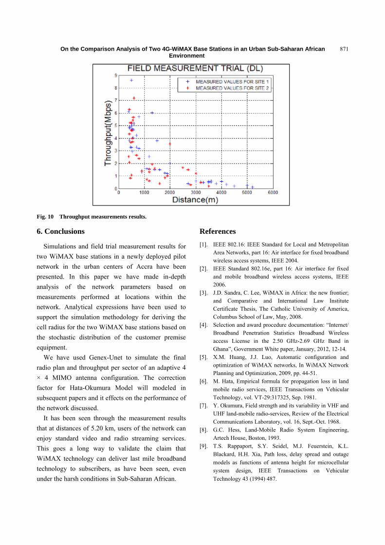
On the Comparison Analysis of Two 4G-WiMAX Base Stations in an Urban Sub-Saharan African Environment
871
Fig. 10 Throughput measurements results.
6. Conclusions
Simulations and field trial measurement results for
two WiMAX base stations in a newly deployed pilot
network in the urban centers of Accra have been
presented. In this paper we have made in-depth
analysis of the network parameters based on
measurements performed at locations within the
network. Analytical expressions have been used to
support the simulation methodology for deriving the
cell radius for the two WiMAX base stations based on
the stochastic distribution of the customer premise
equipment.
We have used Genex-Unet to simulate the final
radio plan and throughput per sector of an adaptive 4
× 4 MIMO antenna configuration. The correction
factor for Hata-Okumura Model will modeled in
subsequent papers and it effects on the performance of
the network discussed.
It has been seen through the measurement results
that at distances of 5.20 km, users of the network can
enjoy standard video and radio streaming services.
This goes a long way to validate the claim that
WiMAX technology can deliver last mile broadband
technology to subscribers, as have been seen, even
under the harsh conditions in Sub-Saharan African.
References
[1]. IEEE 802.16: IEEE Standard for Local and Metropolitan Area Networks, part 16: Air interface for fixed broadband wireless access systems, IEEE 2004.
[2]. IEEE Standard 802.16e, part 16: Air interface for fixed and mobile broadband wireless access systems, IEEE 2006.
[3]. J.D. Sandra, C. Lee, WiMAX in Africa: the new frontier; and Comparative and International Law Institute Certificate Thesis, The Catholic University of America, Columbus School of Law, May, 2008.
[4]. Selection and award procedure documentation: “Internet/ Broadband Penetration Statistics Broadband Wireless access License in the 2.50 GHz-2.69 GHz Band in Ghana”, Government White paper, January, 2012, 12-14.
[5]. X.M. Huang, J.J. Luo, Automatic configuration and optimization of WiMAX networks, In WiMAX Network Planning and Optimization, 2009, pp. 44-51.
[6]. M. Hata, Empirical formula for propagation loss in land
mobile radio services, IEEE Transactions on Vehicular
Technology, vol. VT-29:317325, Sep. 1981.
[7]. Y. Okumura, Field strength and its variability in VHF and
UHF land-mobile radio-services, Review of the Electrical
Communications Laboratory, vol. 16, Sept.-Oct. 1968.
[8]. G.C. Hess, Land-Mobile Radio System Engineering,
Artech House, Boston, 1993.
[9]. T.S. Rappaport, S.Y. Seidel, M.J. Feuerstein, K.L.
Blackard, H.H. Xia, Path loss, delay spread and outage
models as functions of antenna height for microcellular
system design, IEEE Transactions on Vehicular
Technology 43 (1994) 487.

On the Comparison Analysis of Two 4G-WiMAX Base Stations in an Urban Sub-Saharan African Environment
872
[10]. L.R. Maciel, A. Lindsay-Stewart, H.H. Xia, H.L. Bertoni,
R. Rowe, Microcellular propagation characteristics for
personal communications in urban and suburban
environments, IEEE Transactions on Vehicular
Technology 43 (1994) 743.
[11]. L.R. Maciel, A. Lindsay-Stewart, H.H. Xia, H.L. Bertoni,
R. Rowe, Radio propagation characteristics for line-of-
sight and personal communications, IEEE Transactions
on Antennas and Propagation 41 (1993) 1439.
[12]. M. Taylor, D. Li, V. Erceg, S. Ghassemzadeh, D.L.
Schilling, Urban/suburban out-of-sight propagation
modeling, IEEE Communications Magazine 30 (1992)
56.
[13]. E. Green, Radio link design for microcellular systems,
British Telecom Technology Journal 8 (1990) 85.
[14]. W.C. Jakes, Microwave Mobile Communications, IEEE
Press, New York, 1974.
[15]. B.C. Jones, D.J. Skellern, An integrated
propagation-mobility interference model for microcell
network coverage prediction, Wireless Personal
Communications 5 (1997) 223-258.
[16]. C.E. Cook, Modeling interference effects for land mobile
and air mobile communications, IEEE Transactions on
Communications 35 (1987) 151-165.
[17]. B.C. Jones, D.J. Skellern, Interference modeling and
outage contours in cellular and microcellular networks, in:
2nd MCRC International Conference on Mobile and
Personal Communications Systems, Adelaide, Australia,
Apr. 10-11,1995.
[18]. Broadband Speed Guide, http://www.fcc.gov. (Accessed
Jan. 7, 2013)
[19]. E.T. Tchao, W.K. Ofosu, K. Diawuo, Radio planning and field trial measurement for a 4G-WiMAX network in a Sub-Saharan Africa environment, in: IEEE Wireless Telecommunications Symposium, Phoenix, Arizona, Apr. 17-19, 2013.
[20]. L. Nissirat, M.A. Nisirat, M. Ismail, S. Al-Khawaldeh, A terrain roughness correction factor for hata path loss model at 900 MHz, Progress in Electromagnetics Research C 22 (2011) 11-22.

Journal of Communication and Computer 10 (2013) 873-876
Error Analysis for the Three-Dimensional Detection and
Reconstruction of the Road Surface
Youquan He and Jian Wang
Information Science & Engineering Department, Chongqing Jiaotong University, Chongqing 400074, China
Received: December 05, 2012/ Accepted: January 11, 2013 / Published: June 30, 2013.
Abstract: Aiming at the series of errors processing and analyzing produced in three-dimensional testing and reconstruction of the highway pavements, this paper conducts a detailed analysis and computation of these process errors, including calibration of signalized points, centerline calculation of light stripe, accumulated system error, etc.. After the contrast experiment and analysis, it finally introduces gravity method to calculate the camera’s internal parameters, and gray centroid algorithm to extract light stripes’ center. Result shows the system deviation is stabilized at 2 mm, which can better meet the needs of engineering practice. Key words: Road surface detection, three-dimensional transform, error analysis, calibration of signalized points.
1. Introduction
Three-dimensional information collecting of the
road surface is the significant application of computer
vision technology in transportation area. After
establishing the relationship between
two-dimensional images (image side) and
three-dimensional road space (object side) which is
quickly obtained by CCD imaging sensor, we can
work out three-dimensional information of the road
surface. As detection methods, algorithm and other
reasons could cause lots of errors in the whole process,
which directly affect precision of the system, it is
essential to make thorough qualitative and
quantitative analysis of the errors to reduce the
diviation and improve the accuracy of the system [1].
Taking binocular imaging based on three-dimensional
damage detection system for example, this paper
analyzes source and type of errors and discusses
how to improve the accuracy of the detection
system.
Corresponding author: Youquan He, Ph.D., professor, research fields: information processing, data mining. E-mail: [email protected].
2. System Components and Measuring Principle
As shown in Fig. 1, the system uses a LED linear
light as an auxiliary light and makes it ray on road
surface vertically. Then, it uses two CCD sensors, one
is on the left and the other is on the right, to access
pavement image. Especially, their central axis should
be set in 30 to 60 degree angle, not parallel with the
light. As we all know, LED line light could only form
a very narrow light stripe when it rays on road surface.
So, if we take no consideration of camera distortion,
the imaging light from any angle should be a straight
line when the road surface has no damage defects. But,
if pit damage exists, luminous stripe’s shape will
change at the defect. That is to say, every point of
light stripe would in different depth in the pothole.
According to the principle of 3-D projection
transformation, these different depth points would
image a deformation slit of light. Therefore, we can
calculate the actual coordinate value of each point
through transformation between object side and image
side coordinate system, and finally reconstruct the real
cross-section accurately [2, 3].

Error Analysis for the Three-Dimensional Detection and Reconstruction of the Road Surface
874
3. Calibration of the Inside and Outside Camera Parameters
Calibrating camera’s inside and outside parameters
is the first step of binocular vision based camera
calibration. Its major purpose is to establish the
relationship between three-dimensional world
coordinates of tested object and two-dimensional
image coordinates of the computer. This paper employs
RAC two-step method for calibration.
During the calibration, we need to make acquisition
and measurement of several points which are marked in
object plane. Generally, camera plane is not parallel
with object plane, which makes the actual standard
circles distorted in the image plane, such as an ellipse.
In order to work out image side coordinates of the
standard samples’ center, we should resort to the
distortion images. Here, we compared the
performances between value points intersection
method and gravity method.
3.1 Value Points Intersection Method
Taking the top left corner of image plane as the
origin of Cartesian coordinates, horizontal as X-axis,
vertical as Y-axis and pixels as the unit, we could obtain
coordinates of every curve’s point in image plane in
Fig. 2.
After figuring out the biggest X value point A and
minimum point C, we link them into a line, so does the
line between biggest Y value point B and minimum
point D. And then the two lines segments intersect at
point O. Given that: A(x2, y3), B(x3, y2), C(x1, y4),
D(x4, y1), then
(1)
According to the two equation of straight line AC
and BD, we could figure out the coordinate of point O
Fig. 1 Component diagram of the system.
Fig. 2 Location of the image center.
(x, y), which is also the center point of the image and
sample circle. Suppose that the minimum value x has
multiple corresponding values y, which means a
vertical cantlet in the leftmost pixel image, then we
take the means of these values as the point Y
coordinate, so does the situation of multiple
corresponding values x [4].
Finally, we obtained the center coordinates of the
right target, which are shown in the following Table 1.
3.2 Gravity Method
The method takes the image’s barycenter as target’s
center in image plane. We introduce integral to
calculate image’s center. After taking a unit—a pixel as

Error Analysis for the Three-Dimensional Detection and Reconstruction of the Road Surface
875
Table1 Center coordinates of the right target.
Circle number (x1, y1) (x2, y2) (x3, y3) (x4, y4) Center coordinates
A 162, 69 227, 272 185, 258 189, 299.67 180.614, 278.225
B 166, 388 225, 374.1 182, 357.1 187.8, 400.96 181.194, 383.099
C 159, 628.7 230.98, 630 178.8, 600.4 182.3, 652.65 176.071, 628.647
E 387, 307 428.17, 308 416, 288 422.8, 330.7 419.771, 306.132
D 381.46, 616 430.9, 611.9 411.07, 591.88 427.8, 637 418.822, 614.562
, we could obtain the area of the image, which is
also the number of pixels. Then we get the formula for
image center’s calculation:
, (2)
Eventually, we figure out coordinates of the five
target circles’ center in Table 2. Table 3 is results
comparison of the two methods. Value points
intersection method would cause a serious deviation.
Therefore, considering their efficiency, accuracy and
easy realization, this paper uses gravity method to
compute centers of the target points.
4. Error Analysis of Light Stripes’ Extraction
As we known, optical information could reflect
objects’ surface geometric information when LED line
light emits structure light on their surface. LED line
light source is of certain width, but only the points in
center line are really needed in measurement, so the
extraction accuracy of line structured light centerline
directly affects precision of the measurement. Because
of the random error, such as uneven light intensity,
different surface properties of the tested object and
noise produced by CCD camera, etc., it is quite
difficult to improve the precision of extraction. There
are some major algorithms to extract the center of a
light stripe, such as threshold method, gray level
barycenter method, Gauss fitting, etc. [5, 6].
Considering their measurement precision, this system
uses gray barycenter method and Gaussian distributed
curve fitting algorithm and makes a contrast between
their results.
The whole comparative trial is conducted on basis of
the detecting system. Firstly, we collect the light
stripe’s images under the detecting conditions in Fig.3;
then intercept the light stripe part of the image; lastly,
obtain the gray level distribution of the stripe’s section.
As it is show in Fig. 4.
This paper introduces two methods to extract the
light stripes’ center. Each time it selects 50 light stripe
sections, as light stripes center is a straight line when
structured light is projected onto the smooth surface,
we could get the maximum deviation and standard
deviation of the center by making least square linear
fitting to the extracted section [7].
Apparently, the standard deviation could reflect the
discrete degrees of the points. The comparison result
shows that gray barycenter method has better
performance in extracting, and its maximum deviation
and discrete degree are comparatively small. Table 4
gives partial analysis results of numerous extraction
experiments.
Table 2 Coordinates computed by gravity method.
Circle number Center coordinates
A 179.5134, 278.158
B 180.083, 382.029
C 175.072, 627.508
E 418.532, 305.823
D 417.898, 613.376
Table 3 Results comparison of the two methods.
Circle number
Coordinates computed by intersection method
Coordinates computed by gravity method
A 180.614, 278.225 179.5134, 278.158
B 181.194, 383.099 180.083, 382.029
C 176.071, 628.647 175.072, 627.508
E 419.771, 306.132 418.532, 305.823
D 418.822, 614.562 417.898, 613.376
dA
A
xdA
xA
A
ydA
yA
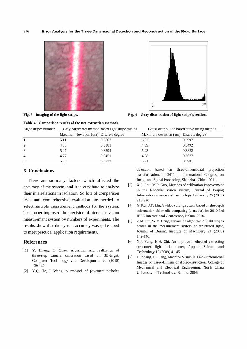
Error Analysis for the Three-Dimensional Detection and Reconstruction of the Road Surface
876
Fig. 3 Imaging of the light stripe.
Fig. 4 Gray distribution of light stripe’s section.
Table 4 Comparison results of the two extraction methods.
Light stripes number Gray barycenter method based light stripe thining Gauss distribution based curve fitting method
Maximum deviation (um) Discrete degree Maximum deviation (um) Discrete degree
1 5.11 0.3667 6.02 0.3997
2 4.58 0.3381 4.69 0.3492
3 5.07 0.3594 5.23 0.3822
4 4.77 0.3451 4.98 0.3677
5 5.53 0.3733 5.71 0.3981
5. Conclusions
There are so many factors which affected the
accuracy of the system, and it is very hard to analyze
their interrelations in isolation. So lots of comparison
tests and comprehensive evaluation are needed to
select suitable measurement methods for the system.
This paper improved the precision of binocular vision
measurement system by numbers of experiments. The
results show that the system accuracy was quite good
to meet practical application requirements.
References
[1] Y. Huang, Y. Zhao, Algorithm and realization of three-step camera calibration based on 3D-target, Computer Technology and Development 20 (2010) 139-142.
[2] Y.Q. He, J. Wang, A research of pavement potholes
detection based on three-dimensional projection transformation, in: 2011 4th International Congress on Image and Signal Processing, Shanghai, China, 2011.
[3] X.P. Lou, M.P. Guo, Methods of calibration improvement in the binocular vision system, Journal of Beijing Information Science and Technology University 25 (2010) 316-320.
[4] Y. Rui, J.T. Liu, A video editing system based on the depth information ubi-media computing (u-media), in: 2010 3rd IEEE International Conference, Jinhua, 2010.
[5] Z.M. Liu, W.Y. Deng, Extraction algorithm of light stripes center in the measurement system of structured light, Journal of Beijing Institute of Machinery 24 (2009) 142-146.
[6] X.J. Yang, H.H. Chi, An improve method of extracting structured light strip center, Applied Science and Technology 12 (2009) 41-45.
[7] H. Zhang, J.J. Fang, Machine Vision in Two-Dimensional Images of Three-Dimensional Reconstruction, College of Mechanical and Electrical Engineering, North China University of Technology, Beijing, 2006.