Institute of Computer ScienceAcademy of Sciences of the Czech Republic

A Model of an AmorphousComputer and its CommunicationProtocol

Lukas Petru and Jirı Wiedermann

Technical report No. 970

August 2006

Pod Vodarenskou vezı 2, 182 07 Prague 8, phone: +4202 6605 3520, fax: (+4202) 86 585 789,e-mail:jiri.wiedermann@cs.cas.cz

Institute of Computer ScienceAcademy of Sciences of the Czech Republic

A Model of an AmorphousComputer and its CommunicationProtocol1

Lukas Petru2 and Jirı Wiedermann3

Technical report No. 970

August 2006

Abstract:

We design a formal model of an amorphous computer suitable for theoretical investigation of its compu-tational properties. The model consists of a finite set of nodes created by RAMs with restricted memory,which are dispersed uniformly in a given area. Within a limited radius the nodes can communicate with theirneighbors via a single-channel radio. The assumptions on low-level communication abilities are among theweakest possible: the nodes work asynchronously, there is no broadcasting collision detection mechanismand no network addresses. For the underlying network we design a randomized communication protocoland analyze its efficiency. The subsequent experiments and combinatorial analysis of random networksshow that the expectations under which our protocol was designed are met by the vast majority of theinstances of our amorphous computer model.

Keywords:amorphous computing; networks; communication protocols; random graphs; complexity;

1This research was carried out within the institutional research plan AV0Z10300504 and partially supported by theGA CR grant No. 1ET100300419 and GD201/05/H014.

2Faculty of Mathematics and Physics, Charles University, Malostranske namestı 25, 118 00 Prague 1, Czech Republic,email:lukas.petru@st.cuni.cz

3Institute of Computer Science, Academy of Sciences of the Czech Republic, Pod Vodarenskou vezı 2, 182 07 Prague8, Czech Republic

1 Introduction

Thanks to recent developments in micro-electro-mechanical (MEMS) systems, wireless communica-tions and digital electronics, a mass production of extremely small-scale, low-power, low cost sensordevices is in sight. They integrate sensing, data processing and wireless communication capabilities.They are utilized in building sensor, mobile, and ad-hoc wireless networks, and also more exotic sys-tems, such as smart dust (cf. [11], [13]), or amorphous computers (cf. [1], [2], [4]). In these devices,the limitations of available memory space in individual processors given by their size and limitedcommunication range implied by a limited energy resource seem to impose severe restrictions to theclass of computations allowable by such devices. The design of the respective algorithms presents achallenge unmatched by the development in related areas such as in the theory of distributed systemsor ad-hoc networks. According to Nikoletseas [11] the specific limitations in such networks (e.g., inthe case of smart dust) call for a design of distributed communication protocols which are extremelyscalable (i.e., operating in a wide range of network sizes), time and energy efficient, and fault tolerant.

It seems that so far the respective research has mainly concentrated on the concrete algorithmicissues neglecting almost completely the computational complexity aspects in that kind of computing(cf. [12]). Very often the designers of such algorithms pay little attention to the underlying computa-tional model and, e.g., they take for granted the synchronicity of time in all processors, the existenceof unique node identifiers and that of communication primitives allowing efficient message delivery.

In our paper we concentrate on a computational model of a wireless communication network wheresuch functionalities are not available. This is a typical case with the “exotic” computational devicesmentioned earlier. Our model, called amorphous computer works under very week assumptions: ba-sically, it is a random graph which emerges by distributing the nodes randomly in the boundedplanar area. The graph’s nodes are processors (limited memory RAMs with random number gen-erators) without unique identifiers (“addresses”). The graph’s edges exist only among nodes withinthe bounded reach of each node’s radio. The nodes operate asynchronously, either broadcasting orlistening, hearing a message only if it is sent exactly by one of its neighbors. That is, there is nomechanism distinguishing the case of a multiple broadcast from the case of no broadcast.

Due to its weak (and thus, general) underlying assumptions which correspond well to the case ofamorphous computing as described in the literature, we believe that our model presents a basic modelof amorphous computing (cf. [1], [2], or an overview in [4]). Within the theory of computation amodel of an amorphous computer, as given by our definition, represents an interesting object of studyby itself since it contains elements of randomness built–in into both the computer’s “set–up process”and its operations.

Under the above mentioned mild assumptions concerning the communication among the nodes ofan amorphous computer and under reasonable statistical assumptions on the underlying graph wedesign a scalable randomized auto-configuration protocol enabling message delivery from a sourcenode to all other nodes. For networks whose underlying communication graph has N nodes, diameterD and node degree Q, the complexity of our algorithm is O(DQ log(N/ε)) with probability ε > 0 offailure.

For the synchronous case, the problem of message delivery similar to ours has been studied in theseminal paper by Ben-Yehuda, Goldreich and Itai in 1993 [3]. Under the same notation as above,the algorithm of Ben-Yehuda et al. runs in time O((D + log(N/ε)) log N). This algorithm is fasterthan ours, but the assumption of synchronicity (allowing that all nodes can start a required actionsimultaneously) is a crucial one for its correctness. However, synchronization is exactly the featureexcluded by the very definition of amorphous computing.

A formal model of amorphous computer is described in Section 2. The main result of the paper—an asynchronous communication protocol —is presented in Section 3. Due to the “amorphousness”of the underlying model of computations the functionality, the performance and fault tolerance of theprevious protocol heavily depend on the properties of large communication networks with a randomtopology. These properties are studied in Section 4 using both experiments and combinatorics. Section5 is devoted to conclusions.

1

2 Model

Various descriptions of amorphous computers can be found in the literature (e.g. [1], [2], [4] and[5]). Unfortunately, these “definitions” differ in details and can hardly be seen as complete and self-contained definitions of an amorphous computer. As a rule, the definitions in the above mentionedreferences only explicitly state the features of an amorphous computer distinguishing it from othersimilar computational systems. Often, the vital details like the assumptions on the underlying com-munication system are only present in amorphous computer emulators (if at all) which are written bythe authors and which are not described in the papers.

This is to be compared to the standards in the complexity theory where all computational models(Turing machines, RAMs, etc.) are described by formal definitions accepted by the entire community.In order to get a model of an amorphous computer (AC) amenable to computability and complexityanalysis we will define an AC as follows.

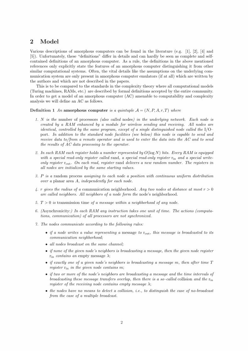
Definition 1 An amorphous computer is a quintuple A = (N, P,A, r, T ) where

1. N is the number of processors (also called nodes) in the underlying network. Each node iscreated by a RAM enhanced by a module for wireless sending and receiving. All nodes areidentical, controlled by the same program, except of a single distinguished node called the I/O–port. In addition to the standard node facilities (see below) this node is capable to send andreceive data to/from a remote operator and is used to enter the data into the AC and to sendthe results of AC data processing to the operator.

2. In each RAM each register holds a number represented by O(log N) bits. Every RAM is equippedwith a special read-only register called rand, a special read-only register rin and a special write-only register rout. On each read, register rand delivers a new random number. The registers inall nodes are initialized by the same starting values.

3. P is a random process assigning to each node a position with continuous uniform distributionover a planar area A, independently for each node.

4. r gives the radius of a communication neighborhood. Any two nodes at distance at most r > 0are called neighbors. All neighbors of a node form the node’s neighborhood.

5. T > 0 is transmission time of a message within a neighborhood of any node.

6. (Asynchronicity:) In each RAM any instruction takes one unit of time. The actions (computa-tions, communication) of all processors are not synchronized.

7. The nodes communicate according to the following rules:

• if a node writes a value representing a message to rout, this message is broadcasted to itscommunication neighborhood;

• all nodes broadcast on the same channel;

• if none of the given node’s neighbors is broadcasting a message, then the given node registerrin contains an empty message λ;

• if exactly one of a given node’s neighbors is broadcasting a message m, then after time Tregister rin in the given node contains m;

• if two or more of the node’s neighbors are broadcasting a message and the time intervals ofbroadcasting these message transfers overlap, then there is a so–called collision and the rinregister of the receiving node contains empty message λ;

• the nodes have no means to detect a collision, i.e., to distinguish the case of no-broadcastfrom the case of a multiple broadcast.

2

Note that since the register size of each RAM is bounded (as it is always the case in practice) eachRAM can be seen as a finite automaton. However, we have still chosen to see it as a “little RAM”since such a view corresponds more to practice. Consequently, increasingly more nodes must take partin a computation using asymptotically more than a constant amount of memory.

The communication model by the above given definition models a multi-hop radio network usingone shared channel without collision detection. This is the most general model considered in theliterature. We have chosen this model in order to capture the low–level details of communication inan AC. This model also seems to best characterize the capabilities of a communication system thatare envisaged for use in a real hardware implementation.

An AC operates as follows. The input data enter the AC via its input port. ¿From there, thedata (which might also represent a program for the processors) spread to all nodes accessible viabroadcasting. In a “real” AC additional data might also enter into individual processors via theirsensors which, however, are not captured in our model since they do not influent our results. Thenthe data processing within processors and data exchange among processors begins. The results aredelivered to the operator again via the output port. Obviously, an AC can work in the standard“Turing machine” mode as well as in an interactive mode.

3 Asynchronous Communication Protocol

In order to enable communication among all (or at least: a majority of) available processors theunderlying communication graph of our AC must have certain desirable properties. The propertieswhich are of importance in this case are: graph connectivity, graph diameter and the maximal degreeof its nodes. Obviously, a good connectivity is a necessary condition in order to be able to harnessa majority of all processors. Graph diameter bounds the length of the longest communication path.Finally, the node degree (i.e., the neighborhood size) determines the collision probability on thecommunication channel.

Assuming that all nodes of an AC should participate in its computation there must exist a mecha-nism of node–to–node communication used by the nodes to coordinate their actions. Such a mechanismwill consist of two levels. The lower level is given by a basic randomized broadcasting protocol en-abling each node to broadcast a message to its neighborhood. Making use of this protocol we extendit, on the next level, to a broadcasting algorithm that can be used to broadcast a message from agiven node to all other network nodes.

Protocol Send: A node is to send a message m with a given probability ε > 0 of failure. Theprotocol must work correctly under the assumption that all nodes are concurrently, asynchronously,in a non-coordinated way, using the same protocol, possibly interfering thus one with each other’sbroadcast.

The idea is for each node to broadcast sporadically, minimizing thus a communication collisionprobability in one node’s neighborhood. This is realized as follows. Each node has a timer measuringtimeslots (intervals) of length 2T (T is time to transfer a message). During its own timeslot, eachnode is allowed either listen, or to send a message at the very beginning of its timeslot (and then listentill the end of this timeslot). Making use of its random number generator, a node keeps sending m ateach start of the timeslot with probability p for k subsequent slots. The values of p and k are givenin the proof of the following theorem. After performing the above algorithm each node waits for 2kTsteps (so–called safe delay) before it can perform the next round of the protocol.

Theorem 1 (Sending a message) Let A be an amorphous computer, let the underlying computa-tional graph be connected with maximal neighborhood size bounded by Q. Let 1 > ε > 0 be an priorigiven allowable probability of failure. Assume that all nodes send their messages asynchronously ac-cording to the Protocol Send. Let X be a node sending message m and Y be any of X’s neighbors.Then the Protocol Send delivers m to Y in time O(Q log(1/ε)) with probability at least 1− ε.

Sketch of the proof: Thanks to our choice of the length of the timeslots, for each timeslot of a givennode X there is exactly one corresponding timeslot of some other node Y such that if both nodes

3

send asynchronously in their timeslots, only a single collision will occur. This is so because if X hasstarted its sending at the beginning of its timeslot, X’s and Y ’s sendings overlap if and only if Y hadstarted a sending in a timeslot that was shifted w.r.t. the beginning of X’s timeslot by less than Ttime units in either time direction. The timeslots of length shorter than 2T could cause more than asingle broadcast collision between the arbitrary pairs of nodes, whereas longer timeslots would delaythe communication.

We will treat message sendings as independent random events. Message m is correctly received byY in one timeslot if X is transmitting m (the probability of such event is p) and none of Y ’s neighborsis transmitting (the corresponding probability is (1 − p)Q), giving the joint probability p(1 − p)Q.The value of p(1− p)Q is maximized for p = 1/(Q + 1). The probability of a failure after k timeslotsis [1 − p(1 − p)Q]k = ε. Hence, k = ln ε/ln[1− p(1− p)Q]. The denominator in the latter expressionequals −∑∞

i=1[p(1 − p)Q]i/i ≤ −p(1 − p)Q = −1/(Q + 1)(1 + 1/Q)−Q ≤ −e−1/(Q + 1) leading tok = O(Q log(1/ε). 2

In order to send a message to any node of an AC we use flooding, i.e, broadcasting the messageto all nodes of the network.

Algorithm Broadcast. A node is to broadcast message m to be received by all other nodes. Thenode sends m using ProtocolSend. Upon receiving this message, any other node also starts sendingm using ProtocolSend. Within the duration of a safe delay, a node remembers the last sent messagein order to ignore it when receiving it repeatedly.

Theorem 2 (Broadcasting) Let the communication graph of A be connected, with Q,N and ε asabove. Assume a node X starts broadcasting a message m in the network using Broadcast Algorithm,making use of Protocol Send with error probability ε/N . Then m will be delivered to each node intime O(DQ log(N/ε)) where D denotes the diameter of the communication graph. The probability thatthere is a node in the network not receiving m is less than ε.

Sketch of the proof: Message m spreads through the network in waves, as a breadth-first searchalgorithm of the communication graph starting in X would do it. All nodes of the current wave sendm to their neighbors using ProtocolSend with error ε/N , which takes time O(Q log(N/ε). After atmost D waves, m has reached all nodes. The algorithm takes time O(DQ log(N/ε)). For one nodethe failure probability is ε/N and for the whole network this probability will rise to ε. The safe delayensures that a second message cannot outrun the first one if the same node sends two messages oneafter the other. 2

4 Properties of random networks

Note that the definition of an AC makes no assumptions about the underlying communications graphwhereas the statements of both Theorems 1 and 2 have referred to the underlying communicationgraphs. This has been so since only some graphs are “good” for our purposes while the otherscannot support any interesting computations. In the previous theorems the appropriateness of theunderlying graphs has been ensured in theorems’ assumptions. However, by the definition of an AC,its communication network is shaped by process P as a result of the node placement (cf. Definition 1,item 3), which means that the resulting network has a random structure. Now we will be interestedunder what conditions a randomly emerging network will have the properties assumed in the previoustheorems. As we have seen, for the basic protocol to work we needed connected networks. Moreover,in order to estimate the efficiency of the protocol we made use of the diameter and of the maximumneighborhood size of the respective networks. Therefore we will focus onto the latter mentionedproperties of random networks.

For an amorphous computer A = (N,P, A, r, T ) its node density d is defined as d = Nπr2/a (adenotes the size of area A). In the rest of the paper we assume that the nodes constituting a networkare distributed uniformly randomly (by process P ) over a square area A with a given density.Connectivity A connected component of a graph comprises all nodes among which a multi-hopcommunication is possible.

4

The existence of an edge between two nodes is a random event depending on the random positionsof the nodes. The probability of edge presence is higher with larger communication radius r and islower when the nodes are spread over a larger area A.

Node density d gives the average number of nodes in the communication area of one node. Depend-ing on the node density we expect to observe different topology of the node connections graph. Forlow densities, the majority of the nodes will be isolated with high probability. For medium densitiesconnected components of fixed average size (not depending on the total number of nodes) will beformed with high probability. For very high densities there is a critical density (co–called percolationthreshold) above which one huge component containing nearly all nodes will be formed with high prob-ability. This behavior has been studied by so–called percolation theory (cf. [8]) but, unfortunately,the available analytical results concern the case of nodes placed on a rectangular grid and hence donot cover the case we are after (cf. [14]). In [7], the critical density of around 4.5 has been found bysimulations in the continuum percolation model.

A percolation threshold also exists in our random network scenario. We were interested how thesize of the largest component in a random graph depends on the node density. To this end we haveexecuted experiments for several node counts. For each node count the experiment consisted of 400runs. In each run we created one random graph and observed the size of its largest component. Thenwe computed the component size such that it was not achieved only in 2 % of the experimental runs(i.e., we estimate the 2nd percentile). The results are shown in Fig. 1. All experiments were carriedout with density d = 6 which is the value chosen in order to get reasonably large components.

The interpretation of the results is following. Let’s take the case N = 100. The obtained value0.48 means that a random realization of a graph with N nodes will have a component with morethan 0.48N nodes with probability 98 %. As can be seen from our figure, for larger node counts thefraction tends to rise.

Thus, whenever an AC with at least 100 connected nodes is needed, we should actually createan AC with 100/0.48 = 210 nodes. The expected AC will then have a component containing 100connected nodes with 98 % probability. The penalty of this scenario is that a constant factor of nodesgets wasted which may be acceptable for cheap devices. This is in contrast with, e.g., the ad-hocnetworks scenario using expensive devices, where full connectivity is sought and the node densitymust rise as Ω(log N) (cf. [9]).Diameter The diameter of a graph is the maximum length of a shortest path between any two verticesof that graph.

Analytically, the size of a random graph diameter has been derived, e.g., in [6]. It shows that thediameter is about O(D/r), where D is the diameter of a circle circumscribing the area containing thenodes. But we cannot directly apply this result to our AC. First, the result has been proved only forthe asymptotic case when number N of nodes goes to infinity. Second, the referred result holds onlywhen the node density is above the connectivity threshold (which is Ω(log N)). In our scenario, wehave used constant node density that is above the percolation threshold but below the connectivitythreshold.

In [10] an experiment was carried out measuring the diameter size while varying both the numberof nodes and the transmission range. However, we are interested in the behavior of the graph diameterwhen the node density remains fixed. Therefore we performed 400 test runs with various numbersof nodes with density d = 6 and measured the 98th percentile of a graph diameter. The results areshown in Fig. 2.

5

0

0.1

0.2

0.3

0.4

0.5

0.6

0.7

0.8

0.9

100 300 500 700 900 1100

Fig. 1: The value of the 2ndpercentile of the size of the largest

component vs. node count in arandom graph

0

10

20

30

40

50

60

70

80

90

100

100 225 400 625 900 1225

Fig. 2: The 98th percentile ofgraph diameter vs. node count in a

random graph

Our experiments show that the graph diameter follows the asymptotic expression derived in [6]also below the connectivity threshold. When the node density d is fixed, then O(D/r) = O(

√N/d).

In Fig. 2, the node count increases quadratically and it can be easily seen that the graph diameterrises roughly linearly with

√N . We see that an upper bound in the form diameter = 2.7

√N holds.

We expect that at most in 2 % of random realizations the graph diameter will be larger than thisvalue.

Maximum neighborhood size can be estimated by applying the techniques known from the solu-tions of the classical occupancy problem.

Theorem 3 Let A = (N,P, A, r, T ) be an AC with N nodes randomly uniformly dispersed by procesP with density d over a square area A, let Q = d8 log N/ log log Ne. Then for a sufficiently large N,the probability that there are more than 12Q nodes in any communication neighborhood of a node isless than 4/(dN).4

Proof: We start by exactly covering A of size a by H = h × h squares, with h ∈ N; the size of eachsquare is chosen so that its size is maximal, but note greater than the area πr2 of a communicationneighborhood. Then (h− 1)2πr2 < a ≤ h2πr2 and since a = Nπr2/d, we get N/H ≤ d and for h ≥ 4,H/N < 2/d.

We estimate the probability p=k that in a randomly selected square there will be exactly k nodesfor k “not too small” (see in the sequel). Let us consider all sequences of length N over 1, 2, . . . ,H ofnode “throws” into H squares numbered by 1, 2, . . . H. There are HN of such sequences, each of thembeing equally probable. Consider any i, 1 ≤ i ≤ H. There are (H − 1)N−k

(Nk

)sequences containing

exactly k occurrences of i. Then p=k =(Nk

) (H−1)N−k

HN =(Nk

)1

Hk

(1− 1

H

)N−k and the probability that

there are at least k nodes in a square is p≥k =∑N

j=k p=j =∑N

j=k

(Nj

) (1H

)j (1− 1

H

)N−j. Using

Stirling’s approximation(Nj

) ≤ (eN/j)j and upper-bounding the last factor in the last expression by

1 we get p≥k ≤∑N

j=k

(eNjH

)j

≤ ∑Nj=k

(edj

)j

≤ (edk

)k ∑∞j=0

(edj

)j

≤ (edk

)k ∑∞j=0

(edk

)j. The latter

infinite series converges to 1/(1 − ed/k) providing ed < k. Consider k such that ed < k/2; then thesum of the series is at most 2 and for k ≥ (ed)2, p≥k ≤ 2

(edk

)k ≤ 2.2−1/2k log k.

For k = Q we get p≥k ≤ 2.2−12

8 log Nlog log N (3+log log N−log log log N) ≤ 2/N2 (taking into account that for

a sufficiently large N, 3 + log log N − log log log N ≥ 12 log log N). It follows that the probability that

in any of the H squares there will be at least Q nodes is 2H/N2 < 4/(dN).Finally, note that for h ≥ 2 the size of a square is s > ((h− 1)/h)2πr2 ≥ 1/4πr2. Hence, the area

of a communication neighborhood is smaller than the area of four squares. After realizing that thenodes from at most 12 squares can enter a circular neighborhood of area πr2 the claim of the theoremfollows. 2

4All logarithms are to the base 2.

6

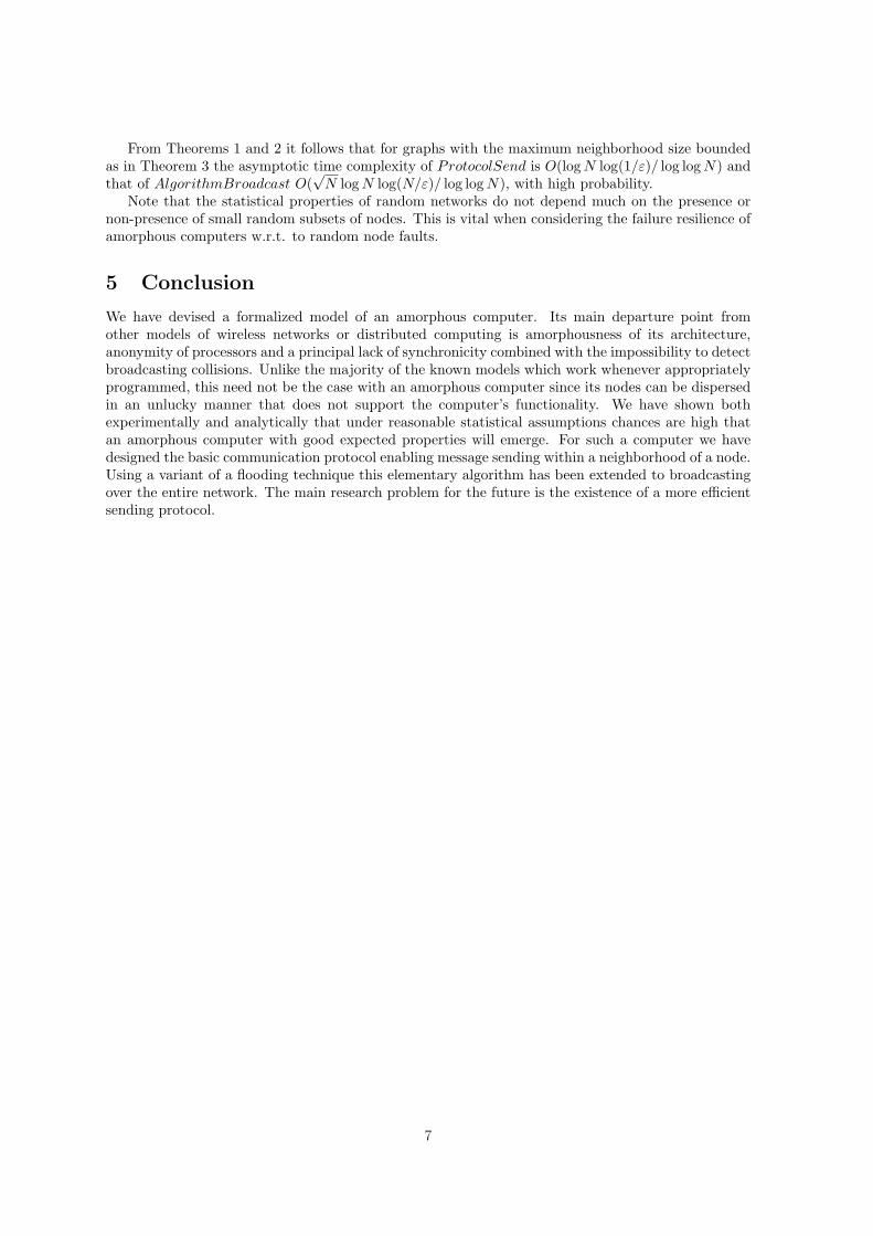
From Theorems 1 and 2 it follows that for graphs with the maximum neighborhood size boundedas in Theorem 3 the asymptotic time complexity of ProtocolSend is O(log N log(1/ε)/ log log N) andthat of AlgorithmBroadcast O(

√N log N log(N/ε)/ log log N), with high probability.

Note that the statistical properties of random networks do not depend much on the presence ornon-presence of small random subsets of nodes. This is vital when considering the failure resilience ofamorphous computers w.r.t. to random node faults.

5 Conclusion

We have devised a formalized model of an amorphous computer. Its main departure point fromother models of wireless networks or distributed computing is amorphousness of its architecture,anonymity of processors and a principal lack of synchronicity combined with the impossibility to detectbroadcasting collisions. Unlike the majority of the known models which work whenever appropriatelyprogrammed, this need not be the case with an amorphous computer since its nodes can be dispersedin an unlucky manner that does not support the computer’s functionality. We have shown bothexperimentally and analytically that under reasonable statistical assumptions chances are high thatan amorphous computer with good expected properties will emerge. For such a computer we havedesigned the basic communication protocol enabling message sending within a neighborhood of a node.Using a variant of a flooding technique this elementary algorithm has been extended to broadcastingover the entire network. The main research problem for the future is the existence of a more efficientsending protocol.

7

Bibliography

[1] H. Abelson, et al.: Amorphous Computing. Communications of the ACM, Volume 43, No. 5, pp.74–82, May 2000

[2] H. Abelson, et al.: Amorphous Computing. MIT Artificial Intelligence Laboratory Memo No.1665, Aug. 1999

[3] R. Bar-Yehuda, O. Goldreich, A. Itai: On the Time-Complexity of Broadcast in Multi-hop RadioNetworks: An Exponential Gap Between Determinism and Randomization. J. Comput. Syst. Sci.Vol. 45, No. 1, pp. 104-126, 1992

[4] D. Coore: Introduction to Amorphous Computing. Unconventional Programming Paradigms:International Workshop 2004, LNCS Volume 3566, pp. 99–109, Aug. 2005

[5] E. D’Hondt: Exploring the Amorphous Computing Paradigm. Master’s Thesis, Vrije University,2000

[6] R. B. Ellis, et al.: Random Geometric Graph Diameter in the Unit Disk with `p Metric. GraphDrawing: 12th International Symposium, GD 2004, LNCS Volume 3383, pp. 167–172, Jan. 2005

[7] I. Glauche, et al.: Continuum percolation of wireless ad hoc communication networks. PhysicaA, Volume 325, pp. 577–600, 2003

[8] G. Grimmett: Percolation. 2nd ed., Springer, 1999

[9] P. Gupta, P. R. Kumar: Critical power for asymptotic connectivity in wireless networks, inStochastic Analysis, Control, Optimization and Applications, pp. 547–566, Birkhauser, 1998.

[10] Keqin Li: Topological Characteristics of Random Multihop Wireless Networks. Cluster Comput-ing, Volume 8, Issue 2–3, pp. 119–126, July 2005

[11] Nikoletseas, S.: Models and Algortihms for Wireless Sensor Networks (Smart Dust). In: SOFSEM2006: Theory and Practice of Computer Science, Proceedings. Eds.: J. Wiedermann et al., LNCSVol. 38312, Springer, pp. 65–83, 2006

[12] P. G. Spirakis: Algorithmic and Foundational Aspects of Sensor Systems: (Invited Talk). In:ALGOSENSORS 2004, Lecture Notes in Computer Science, 3121, 2004, pp. 3-8

[13] B. Warneke, et al.: Smart dust: communicating with a cubic-millimeter computer. Computer,Volume 34, No. 1, pp. 44–51, Jan. 2001

[14] E. W. Weisstein: Percolation Threshold. From MathWorld — A Wolfram Web Resource.http://mathworld.wolfram.com/PercolationThreshold.html

8