Joint 3D-Wind Retrievals with Stereoscopic Views from ... - MDPI

remote sensing

Article

Joint 3D-Wind Retrievals with Stereoscopic Viewsfrom MODIS and GOES

James L. Carr 1,*, Dong L. Wu 2, Robert E. Wolfe 2, Houria Madani 1, Guoqing (Gary) Lin 2,3

and Bin Tan 2,3

1 Carr Astronautics, 6404 Ivy Lane, Suite 333, Greenbelt, MD 20770, USA2 NASA Goddard Space Flight Center, Greenbelt, MD 20770, USA3 Science Systems and Applications, Inc., 10210 Greenbelt Road, Suite 600, Lanham, MD 20706, USA* Correspondence: [email protected]; Tel.: +1-301-220-7350

Received: 31 July 2019; Accepted: 3 September 2019; Published: 9 September 2019��

Abstract: Atmospheric motion vectors (AMVs), derived by tracking patterns, represent the windsin a layer characteristic of the pattern. AMV height (or pressure), important for applications inatmospheric research and operational meteorology, is usually assigned using observed IR brightnesstemperatures with a modeled atmosphere and can be inaccurate. Stereoscopic tracking provides adirect geometric height measurement of the pattern that an AMV represents. We extend our previouswork with multi-angle imaging spectro–radiometer (MISR) and GOES to moderate resolution imagingspectroradiometer (MODIS) and the GOES-R series advanced baseline imager (ABI). MISR is aunique satellite instrument for stereoscopy with nine angular views along track, but its images havea narrow (380 km) swath and no thermal IR channels. MODIS provides a much wider (2330 km)swath and eight thermal IR channels that pair well with all but two ABI channels, offering a rich setof potential applications. Given the similarities between MODIS and VIIRS, our methods should alsoyield similar performance with VIIRS. Our methods, as enabled by advanced sensors like MODISand ABI, require high-accuracy geographic registration in both systems but no synchronization ofobservations. AMVs are retrieved jointly with their heights from the disparities between tripletsof ABI scenes and the paired MODIS granule. We validate our retrievals against MISR-GOESretrievals, operational GOES wind products, and by tracking clear-sky terrain. We demonstrate thatthe 3D-wind algorithm can produce high-quality AMV and height measurements for applicationsfrom the planetary boundary layer (PBL) to the upper troposphere, including cold-air outbreaks,wildfire smoke plumes, and hurricanes.

Keywords: 3D-winds; atmospheric motion vectors (AMVs); MODIS; GOES-R; ABI; planetaryboundary layer (PBL); stereo imaging; parallax

1. Introduction

Height assignment using infrared (IR) methods is arguably the largest source of uncertainty inatmospheric motion vectors (AMVs) derived by tracking cloud and water vapor features in satelliteimagery. Despite their wide coverage and good sensitivity to motion, the AMV height assignmenterror (i.e., assigning winds to a wrong height) has been a major obstacle for AMVs to realize their fullpotential in data assimilation, weather prediction, and atmospheric process studies.

To infer the height of a feature pattern, a conventional AMV height assignment relies oncollocated thermal IR radiances in the same images and requires knowledge of an a priori atmosphericthermodynamic profile (e.g., temperature lapse rate) [1]. Such IR-based height assignment methodshave at least three fundamental limitations. First, when AMVs are derived from visible imageryand heights are assigned using IR imagery, each spectral band may have different sensitivities to

Remote Sens. 2019, 11, 2100; doi:10.3390/rs11182100 www.mdpi.com/journal/remotesensing

http://www.mdpi.com/journal/remotesensing

http://www.mdpi.com

http://www.mdpi.com/2072-4292/11/18/2100?type=check_update&version=1

http://dx.doi.org/10.3390/rs11182100

http://www.mdpi.com/journal/remotesensing

Remote Sens. 2019, 11, 2100 2 of 35

cloud layers. This cross-spectral-band height assignment becomes problematic particularly in the casewhere semi-transparent multi-layer clouds are present [2]. Second, The IR method would fail in anatmosphere that has a small or reversed vertical temperature gradient. The reversed temperaturelapse rate can occur in the atmospheric planetary boundary layer (PBL) for low clouds [3] or nearthe tropopause [4]. Third, the height that characterizes an AMV feature is not necessarily that of thebrightest or coldest pixel. Rather, it is determined by a collection of dark and bright (cold and warm)pixels, and the contrast of these pixels relative to the background. These limitations have led to severalmodifications in IR-based algorithms in which one works better than another depending on the type ofcloud scene [5].

The IR-based height assignment is perhaps the best solution if only a single platform is availablefrom space. Simultaneous or near-simultaneous observations from multiple platforms have been rarewith sufficiently high-quality geo-registration accuracy. Recently, advanced sensors on low-Earthorbit (LEO) and geostationary Earth orbit (GEO) satellites have achieved superb pointing accuracy toproduce high quality imagery with fine spatial resolution. For example, the image navigation andregistration (INR) of the GOES-R series advanced baseline imager (ABI) has achieved geo-registrationaccuracy of a few tenths of a pixel [6,7]. In addition, the moderate resolution imaging spectroradiometer(MODIS) from LEO produces imagery with a similar geolocation accuracy [8]. These advances in GEOand LEO navigation and geo-registration now provide a new life to stereoscopic remote sensing ofAMVs from multiple spaceborne platforms.

We shall use the term “3D-winds” in this paper to generically describe our stereo methods sincea wind vector is solved for simultaneously with its three-dimensional (3D) position within the aircolumn. This is not to be confused with the sense of the term in wind profiling, which resolves themotion of air parcels at multiple heights along a single column of atmosphere. Stereo methods enable asingle wind to be retrieved along with its 3D position for each sight line but has the advantage of beingable to cover large swaths using a single pair of platforms. Our previous study has shown that jointAMV retrievals using stereo observations from two platforms can significantly improve the quality ofAMV wind and height measurements [9]. This study featured the multi-angle imaging capability ofthe multi-angle imaging spectro–radiometer (MISR), which can provide stereo-height determinationsfrom a single platform. Although MISR’s nine angular views can independently determine the heightand the cross-track component of wind, the along-track wind and height are coupled and difficult toseparate accurately. By adding GOES-16 ABI imagery, we demonstrated that the joint AMV retrievalsuncouple the along-track wind and height to enable improved wind and height products.

The 3D-wind algorithm developed for MISR-GOES is applicable in general to GEO-GEO, LEO-GEO,and LEO-LEO combinations. It requires no synchronization between images acquired by two differentplatforms. Because of the rapid refresh rate provided by a sensor in GEO (for ABI typically: 10 min.Full Disk, 5 min. CONUS, 1 min. MESO), AMV wind velocity is highly constrained by the GEOimage sequence. A snapshot from LEO will provide an additional key constraint on AMV height.The 3D-wind parallax solver takes into account wind-induced apparent parallaxes even if the LEOimage is not synchronized with the GEO images. This flexibility allows a single GEO system to pairwith neighboring GEOs and many LEOs that fly under its coverage, greatly enhancing the value ofeach individual platform.

In this paper, we extend the technique demonstrated with MISR and GOES to MODIS and GOESABI. The extension provides several benefits to global AMV observations with jointly retrieved stereoheights. First, using MODIS will produce a much wider swath relative to MISR for wind and heightmeasurements. The improved coverage provides for more frequent revisits to targets of interest,such as hurricanes and wildfires. Second, MODIS and ABI share several thermal-IR channels, includinga water-vapor channel, which allows stereo measurements in daytime and nighttime. Nighttimestereo techniques for AMV winds and heights is relatively new and requires validation from otherindependent observations. Third, the extended LEO-GEO algorithm will provide the stereo retrievalsof AMV winds and heights in the regions where the GEO-GEO stereo is not available because of a

Remote Sens. 2019, 11, 2100 3 of 35

lack of overlapping coverage. With the successful demonstration of MODIS-GOES 3D-winds, it is notdifficult to imagine that the technique can be successful with other LEO instruments such as the visibleinfrared imaging radiometer suite (VIIRS).

Our materials and methods are fully described in Section 2 of this paper. Section 3 presents ourresults and discussion. It includes validation and several application cases where vertical resolutionis critical to the study of atmospheric dynamics, including the PBL structure during a cold airoutbreak, vertically resolved atmospheric dynamics during Hurricane Michael with deep convention,and wildfire smoke plumes. The wildfire case shows the flexibility of stereo methods to study advectionof aerosols as well as clouds. These application cases demonstrate the value of using MODIS andGOES together to jointly retrieve AMVs and stereo heights. MODIS-GOES 3D-winds capability will bea useful new tool for atmospheric research to complement existing AMV methods with conventionalIR height assignments.

2. Materials and Methods

We have implemented our methods in MATLAB, first for MISR and GOES ABI and now forMODIS and ABI as is fully described in Section 2.1 below. Accurate joint AMV and stereo-heightretrievals are enabled by the highly accurate geolocation and geo-registration of the MODIS and ABIproducts, which are our materials, as is explained in Section 2.2.

2.1. Stereo 3D-Winds Method Using MODIS and GOES

MODIS spectral channels pair well with those of ABI in accordance with Table 1. Only ABI bands8 and 13 are not well paired with MODIS. In principle, any of these pairings can be used for jointMODIS-GOES AMV-height retrievals.

Table 1. Moderate resolution imaging spectroradiometer (MODIS) offers many close spectral matcheswith the advanced baseline imager (ABI) channels.

ABI Band Wavelength(µm)

SpatialResolution (m) MODIS Band Wavelength

(µm)Spatial

Resolution (m)

1 0.45–0.49 1000 3 0.459–0.479 500

2 0.59–0.69 500 1 0.620–0.670 250

3 0.846–0.885 1000 216

0.841–0.8760.862–0.877

2501000

4 1.371–1.386 1000 26 1.360–1.390 1000

5 1.58–1.64 1000 6 1.628–1.652 500

6 2.225–2.275 2000 7 2.105–2.155 500

7 3.80–4.0 2000 21,22 3.929–3.989 1000

8 5.77–6.6 2000 - - -

9 6.75–7.15 2000 27 6.535–6.895 1000

10 7.24–7.44 2000 28 7.175–7.475 1000

11 8.3–8.7 2000 29 8.4–8.7 1000

12 9.42–9.8 2000 30 9.58–9.88 1000

13 10.1–10.6 2000 - - -

14 10.8–11.6 2000 31 10.780–11.280 1000

15 11.8–12.8 2000 32 11.770–12.270 1000

16 13.0–13.6 2000 33 13.185–13.485 1000

Remote Sens. 2019, 11, 2100 4 of 35

2.1.1. Process Flow

The MODIS-GOES 3D-winds process flow is shown in Figure 1. The first step is to bring theimagery from both satellites into a common frame of reference. We have chosen the fixed grid of theGOES-R series ABI into which individual MODIS granules will be remapped. The ABI fixed grid is anidealized representation of the Earth-satellite imaging geometry from geostationary orbit for whichall pixels are constructed at standard fixed-grid sites for each GOES satellite reference longitude [10].GOES ABI product imagery is registered to the ellipsoid (effectively WGS 84) so that the line-of-sight toeach pixel is traced from an idealized satellite along that line-of-sight to a pierce-point on the ellipsoid.On the other hand, MODIS L1b products are navigated to the terrain surface and are not resampled tostandard fixed sites [11].

Remote Sens. 2019, 11, x FOR PEER REVIEW 4 of 36

2.1.1. Process Flow

The MODIS-GOES 3D-winds process flow is shown in Figure 1. The first step is to bring the imagery from both satellites into a common frame of reference. We have chosen the fixed grid of the GOES-R series ABI into which individual MODIS granules will be remapped. The ABI fixed grid is an idealized representation of the Earth-satellite imaging geometry from geostationary orbit for which all pixels are constructed at standard fixed-grid sites for each GOES satellite reference longitude [10]. GOES ABI product imagery is registered to the ellipsoid (effectively WGS 84) so that the line-of-sight to each pixel is traced from an idealized satellite along that line-of-sight to a pierce-point on the ellipsoid. On the other hand, MODIS L1b products are navigated to the terrain surface and are not resampled to standard fixed sites [11].

Figure 1. Creation of a 3D-winds dataset is a three-step process. Step 1 remaps a moderate resolution imaging spectroradiometer (MODIS) L1b granule into the fixed-grid projection of the advanced baseline imager (ABI). Step 2 matches features common to a triplet of GOES cloud and moisture imagery (CMI) or radiances and the remapped MODIS granule to measure disparities between apparent geographical positions, which are affected by both atmospheric motion and parallax. Step 3 interprets the observed disparities as atmospheric motion vectors (AMVs) with vertical height assignments.

In this paper, we use the nomenclature “MOD” to indicate MODIS on Terra and “MYD” to indicate MODIS on Aqua. MODIS granules contain 5 minutes of imagery labeled by the year, day of year, hour, minute, and collection; e.g., MOD2018196.1700.061 is Terra, day 196 of 2018 (July 15th), beginning at 17:00, from Collection 6.1. This nomenclature is stylistically similar to the MODIS granule file names. The MODIS geolocation data granules (“MOD03” files for the Terra satellite and “MYD03” files for the Aqua satellite) provide the geographic coordinates for MODIS pixels at a nominal 1 km nadir resolution. These coordinates are triplets of geodetic latitude, longitude, and terrain height above mean sea level (i.e., the geoid). In the case of a clear-sky pixel, these coordinates would truly represent the geodetic location of the pixel; if an atmospheric feature, such as a cloud, they would instead represent the point at which the line-of-sight from MODIS through the pixel’s assigned coordinates pierces the terrain surface. The difference would depend on the off-nadir scan angle and the height of the feature above the terrain. To

Figure 1. Creation of a 3D-winds dataset is a three-step process. Step 1 remaps a moderate resolutionimaging spectroradiometer (MODIS) L1b granule into the fixed-grid projection of the advanced baselineimager (ABI). Step 2 matches features common to a triplet of GOES cloud and moisture imagery (CMI)or radiances and the remapped MODIS granule to measure disparities between apparent geographicalpositions, which are affected by both atmospheric motion and parallax. Step 3 interprets the observeddisparities as atmospheric motion vectors (AMVs) with vertical height assignments.

In this paper, we use the nomenclature “MOD” to indicate MODIS on Terra and “MYD” to indicateMODIS on Aqua. MODIS granules contain 5 minutes of imagery labeled by the year, day of year, hour,minute, and collection; e.g., MOD2018196.1700.061 is Terra, day 196 of 2018 (July 15th), beginning at17:00, from Collection 6.1. This nomenclature is stylistically similar to the MODIS granule file names.The MODIS geolocation data granules (“MOD03” files for the Terra satellite and “MYD03” files for theAqua satellite) provide the geographic coordinates for MODIS pixels at a nominal 1 km nadir resolution.These coordinates are triplets of geodetic latitude, longitude, and terrain height above mean sea level(i.e., the geoid). In the case of a clear-sky pixel, these coordinates would truly represent the geodeticlocation of the pixel; if an atmospheric feature, such as a cloud, they would instead represent the pointat which the line-of-sight from MODIS through the pixel’s assigned coordinates pierces the terrainsurface. The difference would depend on the off-nadir scan angle and the height of the feature abovethe terrain. To work in the same frame of reference as ABI, we extend the line-of-sight from MODIS

Remote Sens. 2019, 11, 2100 5 of 35

to the WGS-84 ellipsoid and recalculate the geographic coordinates to represent the pierce-point onthe ellipsoid, as illustrated in Figure 2. Each MODIS scan is remapped on its own and placed intoa fixed-grid mosaic. In general, there is overlap between the coverage of successive swaths as theswath height grows away from nadir (“bowtie” effect) and there can also be gaps in the coverage nearnadir. Only the first duplicated pixel is retained in the mosaic and the coverage gaps are filled usingspatial interpolation.


work in the same frame of reference as ABI, we extend the line-of-sight from MODIS to the WGS-84 ellipsoid and recalculate the geographic coordinates to represent the pierce-point on the ellipsoid, as illustrated in Figure 2. Each MODIS scan is remapped on its own and placed into a fixed-grid mosaic. In general, there is overlap between the coverage of successive swaths as the swath height grows away from nadir (“bowtie” effect) and there can also be gaps in the coverage near nadir. Only the first duplicated pixel is retained in the mosaic and the coverage gaps are filled using spatial interpolation.

Figure 2. MODIS pixel geographic coordinates represent the geodetic location where the line-of-sight pierces the terrain surface. We recalculate the geographic coordinates to represent where the line-of-sight pierces the WGS-84 ellipsoid considering the terrain height above the geoid (i.e., mean sea level) and the height of the geoid above the ellipsoid (gravity model).

Accurate time tagging of pixels is essential for the 3D-winds application. The center time of each MODIS swath is recorded in atomic time relative to the universal-time epoch of midnight 1 January 1993 (TAI93). We use swath-center times and knowledge of the MODIS scan rate to assign a time tag to each pixel before it is remapped. These time tags are remapped along with the radiances to provide time tags for the MODIS mosaic in the ABI fixed grid. It is a little more difficult to estimate the time tags for the ABI pixels. The ABI scans the Earth in 22 swaths for a full-disk (FD) scene, six swaths for a continental U.S. (CONUS) scene, and two swaths for a mesoscale (MESO) scene of 1000 km × 1000 km (nominal sub-satellite point distances). The scan pattern is defined in a “timeline” for instrument activities that is commanded to the satellite. The timeline will determine the times for pixels up to an uncertainty near the stitching line between swaths. We accept this ambiguity as unavoidable and model the times according to the swath to which each pixel is most likely to belong and the timeline definition. Quality screening later in the processing will eliminate those few cases where the time tag has been incorrectly assigned. Figure 3 shows an ABI CONUS scene, a MODIS granule remapped into the ABI fixed grid, and their respective modeled time tags. The six swaths of the ABI CONUS scene are clearly seen. With the mode 3 and 6 timelines, each swath follows its predecessor by 30 seconds and time advances ~6 seconds from the west to the east. MODIS times advance along the ground track and are also organized in swaths, but they are only ~10km tall, much smaller than the ABI swaths, and therefore not readily apparent. MODIS times also advance west to east on the descending pass, but only by ~1 second.

Figure 2. MODIS pixel geographic coordinates represent the geodetic location where the line-of-sightpierces the terrain surface. We recalculate the geographic coordinates to represent where the line-of-sightpierces the WGS-84 ellipsoid considering the terrain height above the geoid (i.e., mean sea level) andthe height of the geoid above the ellipsoid (gravity model).

Accurate time tagging of pixels is essential for the 3D-winds application. The center time of eachMODIS swath is recorded in atomic time relative to the universal-time epoch of midnight 1 January1993 (TAI93). We use swath-center times and knowledge of the MODIS scan rate to assign a time tag toeach pixel before it is remapped. These time tags are remapped along with the radiances to providetime tags for the MODIS mosaic in the ABI fixed grid. It is a little more difficult to estimate the timetags for the ABI pixels. The ABI scans the Earth in 22 swaths for a full-disk (FD) scene, six swaths for acontinental U.S. (CONUS) scene, and two swaths for a mesoscale (MESO) scene of 1000 km × 1000 km(nominal sub-satellite point distances). The scan pattern is defined in a “timeline” for instrumentactivities that is commanded to the satellite. The timeline will determine the times for pixels up toan uncertainty near the stitching line between swaths. We accept this ambiguity as unavoidable andmodel the times according to the swath to which each pixel is most likely to belong and the timelinedefinition. Quality screening later in the processing will eliminate those few cases where the time taghas been incorrectly assigned. Figure 3 shows an ABI CONUS scene, a MODIS granule remapped intothe ABI fixed grid, and their respective modeled time tags. The six swaths of the ABI CONUS sceneare clearly seen. With the mode 3 and 6 timelines, each swath follows its predecessor by 30 secondsand time advances ~6 seconds from the west to the east. MODIS times advance along the ground trackand are also organized in swaths, but they are only ~10 km tall, much smaller than the ABI swaths,and therefore not readily apparent. MODIS times also advance west to east on the descending pass,but only by ~1 second.

Remote Sens. 2019, 11, 2100 6 of 35Remote Sens. 2019, 11, x FOR PEER REVIEW 6 of 36

Figure 3. MODIS radiances are remapped along with their time tags to form fixed-grid mosaics in the same geometry as GOES ABI. An ABI scan model provides the time tags for the ABI pixels in each scene. At the upper left (a) is the B02 GOES-16 cloud and moisture imagery (CMI) for the CONUS scene and at the upper right (b) is the matching MODIS granule remapped to the ABI fixed grid. Their respective time models are shown on the bottom row (c) and (d). A common time epoch is used, which is the time of the first center-of-scan in the MODIS granule (about one second after the granule’s product time in this case). The case shown is MODIS granule MOD2018196.1700.061 (MODIS Band 1) paired with GOES-16 CONUS ABI Band 2.

The ABI repetitively follows its commanded timeline and will usually acquire a FD scene every 10 minutes, a CONUS scene every five minutes, and either one or two distinct MESO scenes every 30 seconds (if one MESO) or 60 seconds (if two distinct MESOs). We work with triplets of a given scene type and select the middle scene (time: T0) so that it is most simultaneous with the MODIS granule being processed. Our second step matches templates taken from the GOES ABI scene T0 to locate the feature represented in each template in the other two ABI scenes (T0 − ∆t and T0 + ∆t, where ∆t is the refresh time between timelines) and matches the template against the MODIS mosaic as well. The apparent shift of the template relative to its nominal location is determined to subpixel accuracy through normalized cross correlation (NCC) with interpolation on the NCC correlation surface [12]. These shifts are the disparities (illustrated in Figure 4) that represent a combination of motion and parallax between the two satellite vantage points. We also perform an autocorrelation of the template with the ABI scene T0, from where the template is drawn, to eliminate templates that are too spatially uniform to provide adequate feature matches.

Figure 3. MODIS radiances are remapped along with their time tags to form fixed-grid mosaics in thesame geometry as GOES ABI. An ABI scan model provides the time tags for the ABI pixels in each scene.At the upper left (a) is the B02 GOES-16 cloud and moisture imagery (CMI) for the CONUS scene andat the upper right (b) is the matching MODIS granule remapped to the ABI fixed grid. Their respectivetime models are shown on the bottom row (c,d). A common time epoch is used, which is the time ofthe first center-of-scan in the MODIS granule (about one second after the granule’s product time in thiscase). The case shown is MODIS granule MOD2018196.1700.061 (MODIS Band 1) paired with GOES-16CONUS ABI Band 2.

The ABI repetitively follows its commanded timeline and will usually acquire a FD scene every10 minutes, a CONUS scene every five minutes, and either one or two distinct MESO scenes every30 seconds (if one MESO) or 60 seconds (if two distinct MESOs). We work with triplets of a given scenetype and select the middle scene (time: T0) so that it is most simultaneous with the MODIS granulebeing processed. Our second step matches templates taken from the GOES ABI scene T0 to locatethe feature represented in each template in the other two ABI scenes (T0 − ∆t and T0 + ∆t, where ∆tis the refresh time between timelines) and matches the template against the MODIS mosaic as well.The apparent shift of the template relative to its nominal location is determined to subpixel accuracythrough normalized cross correlation (NCC) with interpolation on the NCC correlation surface [12].These shifts are the disparities (illustrated in Figure 4) that represent a combination of motion andparallax between the two satellite vantage points. We also perform an autocorrelation of the templatewith the ABI scene T0, from where the template is drawn, to eliminate templates that are too spatiallyuniform to provide adequate feature matches.

Remote Sens. 2019, 11, 2100 7 of 35

1

Y in

AB

I B02

Pix

els

Figure 4. Disparities between matched features in GOES ABI scene T0 and the other images measure acombination of motion and parallax. Disparities are measured along the fixed grid axes (+X − east,+Y − north) in units of ABI B02 pixels. The legend identifies the match from GOES ABI T0 to T0 − ∆t(“GOES−”), T0 + ∆t (“GOES+”), MODIS, and to itself (“Self”). The characteristic wing pattern seen inthe MODIS disparities with respect to the central image of the GOES triplet is due to the large MODISscan angle at either end of its swath. The self matches (or autocorrelations) are tightly clustered atthe origin. The case shown is MODIS granule MOD2018196.1700.061 (MODIS Band 1) paired withGOES-16 CONUS ABI Band 2.

The last step is the interpretation of the disparities as 3D-winds model states. Each template site

is assigned a three-dimensional vector→

δ =→

δ 0 +→v · (t− t0), represented in Figure 5, to lift it off the

template’s assigned place on the WGS-84 ellipsoid as a function of time relative to the assigned time

tag t0 for the template. The initial vector displacement→

δ 0 plus the two components of the horizontalwind field

→v are the five model states per site. The model requires satellite position vectors for Terra or

Aqua and the GOES satellite. The former is included in the MODIS geolocation data granule fromwhich we interpolate to the time assigned to the template and the latter is taken from a GOES satellitemission-life ephemeris (courtesy of Marco A. Concha and the NASA GOES-R Program). The modelused is identical to the MISR-GOES 3D-winds model without bundle adjustment that is fully derivedin the Appendix of Carr, Wu, Kelly, and Gong [9]. It can also be used for GEO–GEO and LEO–LEO3D-winds and is therefore a generic multi-satellite model.


Figure 5. The MISR-GOES 3D-winds retrieval model is reused for MODIS and GOES. The n = 0 reference image provides a template for the feature 𝒪𝒪 with nominal location 𝑟𝑟0(𝒪𝒪) where it projects onto the ellipsoid as seen from camera look n = 0. The ellipsoid location of the matched feature 𝑟𝑟𝑛𝑛(𝒪𝒪) in n ≠ 0 is determined from the measured disparity between n ≠ 0 and n = 0. The model minimizes the weighted sum of the squares across all looks of the calculated differences 𝜖𝜖𝑛𝑛. Each 𝜖𝜖𝑛𝑛 measures the difference in the tangent plane for n ≠ 0 between where the model places the feature and where it was actually found. The minimization uses five model states for each retrieval and the problem is solved by iterative refinement of the states until converged because the problem is slightly nonlinear. Three position states

0δ

describe

the displacement of the template from its nominal location on the ellipsoid 𝑟𝑟0(𝒪𝒪) at the assigned time tag

0t for the template. The vertical component of 0δ

is the height assignment. Two more states describe the

motion of the template (wind) so that its instanteous displacement is ( )0 0v t tδ δ= + ⋅ −

, where v is an

AMV describing horizontal motion.

The retrieval model will generally leave residuals that are a fraction of one ABI pixel. Figure 6 shows an example where each residual displacement is resolved along the U (+East) and V (+north) directions in the tangent plane. The U-V notation is adopted for the rest of the paper to designate vector components in the cardinal directions that are either displacements or velocities. Figure 7 shows an example of the retrieved 3D-winds states. Sites for which the model does not explain the disparities are presumed anomalous and are screened out using a statistical plausibility test on the residuals.

Figure 5. The MISR-GOES 3D-winds retrieval model is reused for MODIS and GOES. The n = 0reference image provides a template for the feature Owith nominal location

→r 0(O) where it projects

onto the ellipsoid as seen from camera look n = 0. The ellipsoid location of the matched feature→r n(O)

in n , 0 is determined from the measured disparity between n , 0 and n = 0. The model minimizesthe weighted sum of the squares across all looks of the calculated differences

→ε n. Each

→ε n measures

the difference in the tangent plane for n , 0 between where the model places the feature and whereit was actually found. The minimization uses five model states for each retrieval and the problem issolved by iterative refinement of the states until converged because the problem is slightly nonlinear.

Three position states→

δ 0 describe the displacement of the template from its nominal location on the

ellipsoid→r 0(O) at the assigned time tag t0 for the template. The vertical component of

→

δ 0 is theheight assignment. Two more states describe the motion of the template (wind) so that its instanteous

displacement is→

δ =→

δ 0 +→v · (t− t0), where

→v is an AMV describing horizontal motion.

The retrieval model will generally leave residuals that are a fraction of one ABI pixel. Figure 6shows an example where each residual displacement is resolved along the U (+East) and V (+north)directions in the tangent plane. The U-V notation is adopted for the rest of the paper to designatevector components in the cardinal directions that are either displacements or velocities. Figure 7 showsan example of the retrieved 3D-winds states. Sites for which the model does not explain the disparitiesare presumed anomalous and are screened out using a statistical plausibility test on the residuals.


Figure 6. Residual disparities after applying the 3D-winds retrieval model in the tangent plane are plotted by image column in (a) and (c) or row in (b) and (d). The legend identifies the matches used in the retrievals: i.e., from GOES ABI T0 to T0 − ∆t (“GOES−“), T0 + ∆t (“GOES+“), and MODIS. Residuals are less than 0.5 ABI B02 pixel, which is 500 m at the subsatellite point. The case shown is MODIS granule MOD2018196.1700.061 (MODIS Band 1) paired with GOES-16 CONUS ABI Band 2.

Figure 7. Retrieved 3D-winds states describe the horizontal wind velocities and their pattern heights. Vector lengths in the righthand panel (b) are scaled in proportion to wind speed (length scale shows a 2 m/s wind speed) and color-coded according to assigned height (color bar shows height scale). The MODIS true-color composite is shown in the left-hand panel (a) for context. Sun glint is apparent in the MODIS composite, which is not found in the GOES imagery because of the difference in viewing geometry between low Earth orbit (LEO) and geostationary Earth orbit (GEO) satellites. The algorithm is

Figure 6. Residual disparities after applying the 3D-winds retrieval model in the tangent plane areplotted by image column in (a,c) or row in (b,d). The legend identifies the matches used in the retrievals:i.e., from GOES ABI T0 to T0 − ∆t (“GOES−”), T0 + ∆t (“GOES+”), and MODIS. Residuals are lessthan 0.5 ABI B02 pixel, which is 500 m at the subsatellite point. The case shown is MODIS granuleMOD2018196.1700.061 (MODIS Band 1) paired with GOES-16 CONUS ABI Band 2.


Figure 6. Residual disparities after applying the 3D-winds retrieval model in the tangent plane are plotted by image column in (a) and (c) or row in (b) and (d). The legend identifies the matches used in the retrievals: i.e., from GOES ABI T0 to T0 − ∆t (“GOES−“), T0 + ∆t (“GOES+“), and MODIS. Residuals are less than 0.5 ABI B02 pixel, which is 500 m at the subsatellite point. The case shown is MODIS granule MOD2018196.1700.061 (MODIS Band 1) paired with GOES-16 CONUS ABI Band 2.

Figure 7. Retrieved 3D-winds states describe the horizontal wind velocities and their pattern heights. Vector lengths in the righthand panel (b) are scaled in proportion to wind speed (length scale shows a 2 m/s wind speed) and color-coded according to assigned height (color bar shows height scale). The MODIS true-color composite is shown in the left-hand panel (a) for context. Sun glint is apparent in the MODIS composite, which is not found in the GOES imagery because of the difference in viewing geometry between low Earth orbit (LEO) and geostationary Earth orbit (GEO) satellites. The algorithm is

Figure 7. Retrieved 3D-winds states describe the horizontal wind velocities and their pattern heights.Vector lengths in the righthand panel (b) are scaled in proportion to wind speed (length scale showsa 2 m/s wind speed) and color-coded according to assigned height (color bar shows height scale).The MODIS true-color composite is shown in the left-hand panel (a) for context. Sun glint is apparentin the MODIS composite, which is not found in the GOES imagery because of the difference in viewinggeometry between low Earth orbit (LEO) and geostationary Earth orbit (GEO) satellites. The algorithmis unsuccessful in finding matches in the glint region. Any anomalous retrievals (typically << 1%)may be filtered out in a post-processing step or an assimilation quality control test. The case shown isMODIS granule MOD2018196.1700.061 (MODIS band 1) paired with GOES-16 CONUS ABI Band 2.(Note: retrieval sites are thinned 2:1 in each direction for clarity.).

Remote Sens. 2019, 11, 2100 10 of 35

2.1.2. Band-to-Band Adjustments

Using the full range of paired MODIS-ABI channels requires that the MODIS geolocation granulevalues be corrected for known band-to-band registration (BBR) offsets in the along-scan and along-track(cross-scan) directions. The BBR offsets are defined with respect to MODIS Band 1 and are availablefor the pre-launch phase and on-orbit operations using the on-board spectro–radiometric calibrationassembly (SRCA) [13,14]. The values for year 2017 are provided in Table 2 for Terra and Aqua for theMODIS bands [15] that have a matching GOES ABI Band as shown in Table 1.

Table 2. MODIS band-to-band registration (BBR) offsets in kilometers with respect to MODIS band 1for 2017.

MODIS BandAqua Along-Scan

(km)Aqua Along-Track

(km)Terra Along-Scan

(km)Terra Along-Track

(km)

2 −0.0033 −0.0075 −0.0033 −0.00833 0.0279 −0.0184 0.0264 0.02266 −0.2084 0.2725 −0.0577 −0.05627 −0.2007 0.4058 −0.0141 −0.040922 −0.2317 0.2186 −0.0473 −0.113126 −0.2043 0.3278 0.0749 −0.064327 −0.1766 0.2928 −0.1103 0.003828 −0.1946 0.3136 −0.0765 0.016329 −0.2034 0.3253 −0.0443 0.026730 −0.2310 0.3466 −0.0484 0.050631 −0.2467 0.1923 0.0137 −0.040632 −0.1805 0.2103 0.1238 −0.042533 −0.2770 0.3527 −0.0208 0.0432

If the BBR offsets are uncorrected, the retrieval model cannot fit the disparities, leaving theresiduals highly structured and indicative of a systematic error (e.g., Figure 8). The structure disappearsonce the correction is applied (Figure 9) when remapping into the ABI fixed grid.


Figure 8. Residual disparities in the tangent plane after applying the 3D-winds retrieval model without correcting for band-to-band registration (BBR) offsets. The case shown is MODIS granule MYD2019057.2000.061 (Band 31) paired with GOES-16 CONUS ABI band 14.

Figure 9. Residual disparities in the tangent plane after applying the 3D-winds retrieval model after correcting for the BBR offsets. The case shown is MODIS granule MYD2019057.2000.061 (band 31) paired

Figure 8. Residual disparities in the tangent plane after retrievals without correcting for band-to-bandregistration (BBR) offsets (versus longitude (a,c) and latitude (b,d)). The case shown is MODIS granuleMYD2019057.2000.061 (Band 31) paired with GOES-16 CONUS ABI band 14.


Figure 8. Residual disparities in the tangeS-16 CONUS ABI band 14.

Figure 9. Residual disparities in the tangent plane after applying the 3D-winds retrieval model after correcting for the BBR offsets. The case shown is MODIS granule MYD2019057.2000.061 (band 31) paired

Figure 9. Residual disparities in the tangent plane after retrievals after correcting for the BBR offsets(versus longitude (a,c) and latitude (b,d)). The case shown is MODIS granule MYD2019057.2000.061(band 31) paired with GOES-16 CONUS ABI band 14. For context, the ground footprint of an ABI band14 pixel is 2 km at the subsatellite point

Remote Sens. 2019, 11, 2100 12 of 35

2.1.3. Singular Geometry

The retrieval process provides a means to estimate the uncertainty of the retrieved modelparameters through a five-dimensional covariance matrix at each site. This covariance matrixrepresents the uncertainty statistics for the retrieved parameters (two velocity and three positionvector components resolved in a local tangent plane) assuming errors in measuring the disparitiesare Gaussian and independent. We generally assume that the disparity measurement errors are onthe order of one-half the nominal ground sample distance for the ABI channel being used. In theexample shown in Figure 7, the MODIS granule is centered at around 92.5◦ W longitude and 35◦ Nlatitude. This is a favorable geometry. The covariance matrix is symmetric and positive-definite andthe square root of each of its eigenvalues describes a principal axis for a one-sigma uncertainty volume.The square roots of the diagonal elements of the covariance matrix describe the one-sigma standarderror for each state. Figure 10 shows the state-space volume uncertainty and the standard errors for theretrieved height and wind vector components for this case. The small range of values for the velocitystates and the large range for the height is indicative of the fact that the GEO triplet provides mostof the information about the wind velocity states and the LEO and GEO sensors working togetherprovide the information about the height. The uncertainty of the height retrievals is quite sensitive tothe MODIS scan angle.


with GOES-16 CONUS ABI band 14. For context, the ground footprint of an ABI band 14 pixel is 2 km at the subsatellite point.

2.1.3. Singular Geometry

The retrieval process provides a means to estimate the uncertainty of the retrieved model parameters through a five-dimensional covariance matrix at each site. This covariance matrix represents the uncertainty statistics for the retrieved parameters (two velocity and three position vector components resolved in a local tangent plane) assuming errors in measuring the disparities are Gaussian and independent. We generally assume that the disparity measurement errors are on the order of one-half the nominal ground sample distance for the ABI channel being used. In the example shown in Figure 7, the MODIS granule is centered at around 92.5°W longitude and 35°N latitude. This is a favorable geometry. The covariance matrix is symmetric and positive-definite and the square root of each of its eigenvalues describes a principal axis for a one-sigma uncertainty volume. The square roots of the diagonal elements of the covariance matrix describe the one-sigma standard error for each state. Figure 10 shows the state-space volume uncertainty and the standard errors for the retrieved height and wind vector components for this case. The small range of values for the velocity states and the large range for the height is indicative of the fact that the GEO triplet provides most of the information about the wind velocity states and the LEO and GEO sensors working together provide the information about the height. The uncertainty of the height retrievals is quite sensitive to the MODIS scan angle.

Figure 10. The state-space uncertainty volume (a) and state standard errors (b) and (c) are estimated from the covariance matrix from the retrieval performed at each site. The case shown is MODIS granule MOD2018196.1700.061 (MODIS Band 1) paired with GOES-16 CONUS ABI Band 2. Some out-of-family covariances are calculated when the retrieved parallax corrections to site locations place a retrieved site at an inappropriate location. These retrievals are generally filtered out in later quality screening.

Less favorable geometries will exhibit larger error estimates and there exists a singular geometry where the line of sight for MODIS will be exactly parallel with that of ABI and the covariance matrix will have at least one infinite eigenvalue in the singular geometry, expressing the fact that height cannot be retrieved from parallax in this configuration. This will generally occur when MODIS crosses the equator near the subsatellite point for the GOES satellite, which can occur in a Full Disk scene. In the neighborhood of the singular geometry, the uncertainty for the retrieved height will be large and the retrieved height will be subject to large errors. Figure 11 shows the uncertainties when MODIS passes over Ecuador, which is near the GOES-16 subsatellite point. The height uncertainty suffers the most. We can use the standard error estimates to determine the quality of the retrieval and those with standard error on the height assignment greater than 1 km should not be trusted. Figure 12 shows the geographic distribution of height uncertainties for this case.

Figure 10. The state-space uncertainty volume (a) and state standard errors (b,c) are estimated fromthe covariance matrix from the retrieval performed at each site. The case shown is MODIS granuleMOD2018196.1700.061 (MODIS Band 1) paired with GOES-16 CONUS ABI Band 2. Some out-of-familycovariances are calculated when the retrieved parallax corrections to site locations place a retrieved siteat an inappropriate location. These retrievals are generally filtered out in later quality screening.

Less favorable geometries will exhibit larger error estimates and there exists a singular geometrywhere the line of sight for MODIS will be exactly parallel with that of ABI and the covariance matrixwill have at least one infinite eigenvalue in the singular geometry, expressing the fact that heightcannot be retrieved from parallax in this configuration. This will generally occur when MODIS crossesthe equator near the subsatellite point for the GOES satellite, which can occur in a Full Disk scene.In the neighborhood of the singular geometry, the uncertainty for the retrieved height will be large andthe retrieved height will be subject to large errors. Figure 11 shows the uncertainties when MODISpasses over Ecuador, which is near the GOES-16 subsatellite point. The height uncertainty suffers themost. We can use the standard error estimates to determine the quality of the retrieval and those withstandard error on the height assignment greater than 1 km should not be trusted. Figure 12 shows thegeographic distribution of height uncertainties for this case.


Figure 11. The state-space uncertainty volume (a) and state standard errors (b) and (c) depend on the geometry of the LEO satellite with respect to the GEO satellite. The state-space uncertainty volume and standard error for the retrieved height become infinite in the singular geometry. The case shown is MOD2019057.1510.061 (MODIS Band 31) paired with GOES-16 Full Disk Band 14. The height uncertainties are larger than those with MODIS Band 1 paired with ABI Band 2 to begin with due to the larger pixel footprint of the IR channels (four times larger in comparison to the finest resolution) and asymptotically approach infinity as the singular geometry is approached. The longer refresh time for a Full Disk scene compared to a CONUS scene will reduce the velocity uncertainties; but real-world features can change shape over longer periods of time, which is an error not represented here.

Figure 12. The geographic distribution of retrieved height uncertainty becomes very large when crossing the equator near the GOES subsatellite point, which is where the MODIS scan can be exactly parallel to that of GOES and height becomes unobservable. The case shown is MOD2019057.1510.061 (MODIS Band 31) paired with GOES-16 Full Disk Band 14.

2.2. Geometric Quality

Image geometric quality is critical for joint 3D-wind retrievals, both in terms of the accurate assignment of geographic coordinates to pixels (“navigation”) and their stability between successive frames of the same scene (“registration”) in the case of the GOES-R series ABI. Accurate 3D-wind retrievals are enabled by the outstanding geometric accuracy of observations from both the MODIS and

Figure 11. The state-space uncertainty volume (a) and state standard errors (b,c) depend on thegeometry of the LEO satellite with respect to the GEO satellite. The state-space uncertainty volumeand standard error for the retrieved height become infinite in the singular geometry. The case shownis MOD2019057.1510.061 (MODIS Band 31) paired with GOES-16 Full Disk Band 14. The heightuncertainties are larger than those with MODIS Band 1 paired with ABI Band 2 to begin with due to thelarger pixel footprint of the IR channels (four times larger in comparison to the finest resolution) andasymptotically approach infinity as the singular geometry is approached. The longer refresh time fora Full Disk scene compared to a CONUS scene will reduce the velocity uncertainties; but real-worldfeatures can change shape over longer periods of time, which is an error not represented here.


Figure 11. The state-space uncertainty volume (a) and state standard errors (b) and (c) depend on the geometry of the LEO satellite with respect to the GEO satellite. The state-space uncertainty volume and standard error for the retrieved height become infinite in the singular geometry. The case shown is MOD2019057.1510.061 (MODIS Band 31) paired with GOES-16 Full Disk Band 14. The height uncertainties are larger than those with MODIS Band 1 paired with ABI Band 2 to begin with due to the larger pixel footprint of the IR channels (four times larger in comparison to the finest resolution) and asymptotically approach infinity as the singular geometry is approached. The longer refresh time for a Full Disk scene compared to a CONUS scene will reduce the velocity uncertainties; but real-world features can change shape over longer periods of time, which is an error not represented here.

Figure 12. The geographic distribution of retrieved height uncertainty becomes very large when crossing the equator near the GOES subsatellite point, which is where the MODIS scan can be exactly parallel to that of GOES and height becomes unobservable. The case shown is MOD2019057.1510.061 (MODIS Band 31) paired with GOES-16 Full Disk Band 14.


Image geometric quality is critical for joint 3D-wind retrievals, both in terms of the accurate assignment of geographic coordinates to pixels (“navigation”) and their stability between successive frames of the same scene (“registration”) in the case of the GOES-R series ABI. Accurate 3D-wind retrievals are enabled by the outstanding geometric accuracy of observations from both the MODIS and

Figure 12. The geographic distribution of retrieved height uncertainty becomes very large whencrossing the equator near the GOES subsatellite point, which is where the MODIS scan can be exactlyparallel to that of GOES and height becomes unobservable. The case shown is MOD2019057.1510.061(MODIS Band 31) paired with GOES-16 Full Disk Band 14.


Image geometric quality is critical for joint 3D-wind retrievals, both in terms of the accurateassignment of geographic coordinates to pixels (“navigation”) and their stability between successiveframes of the same scene (“registration”) in the case of the GOES-R series ABI. Accurate 3D-windretrievals are enabled by the outstanding geometric accuracy of observations from both the MODIS andABI instruments, which has been achieved as a result of many years of development and investmenton the parts of the MODIS and GOES-R programs.

Remote Sens. 2019, 11, 2100 14 of 35

2.2.1. MODIS

MODIS geometric accuracy had been driven by the needs of the terrestrial research community,and a goal since well before the first MODIS was launched on Terra in 1999. During the designand prelaunch testing of the MODIS instruments and the Terra and Aqua spacecraft, including thedevelopment of the attitude control systems and the approach to satellite tracking, careful attention waspaid to the requirements for position and pointing knowledge accuracy with the goal to minimize anyerrors that could not be corrected after launch. Before launch, a global set of accurate finer-resolutionLandsat-based ground control points were collected to enable early post-launch bias correction,anomaly detection, and removal of any long-term trends. In addition, a detailed global terrain modelwas developed prelaunch for accurate terrain correction. Careful analysis has been and continues to beperformed to monitor and correct for long-term trends in pointing biases and improve the quality ofeach collection. This includes extrapolation of within-orbit and annual trends for forward processingand deriving the best available trends for reprocessing.

The MODIS instruments on the Terra and Aqua platforms were launched in 1999 and 2002,respectively. Their radiometric L1B and geolocation data products have gone through a few roundsof improvements through reprocessing for each new collection. L1 data products are availablenow in Collection 6.1. Geolocation errors are detected through ground control point matching andtime-dependent biases are corrected [16]. Currently, the mission-wise geolocation biases are within5 meters and root-mean-square errors (RMSEs) are within 55 meters in both the along-track directionand along-scan directions [17]. These geolocation accuracy values are for MODIS Band 1. Figure 13shows time series of the measured geolocation errors across the entire Collection 6.1 for both satellites.For other bands, there are band-to-band registration offsets as shown in Table 2 in this paper that areapplied to achieve similar accuracy. MODIS observations are expected to last into middle of the nextdecade, or around 2025, before Terra and Aqua are finally retired.


Figure 13. MODIS band 1 measured geolocation error is remarkably stable across all of collection 6.1 for both Terra (a) and Aqua (b). Each point plotted is the sample mean with one-sigma error bars for a 16-day sample of geolocation errors measured using ground control points. The geolocation error has been adjusted to a subsatellite-point equivalent distance and only the daylight portion of the orbit for each satellite is used since MODIS band 1 is a reflective channel.

The VIIRS instrument shares similar spectral bands with MODIS [18] and has similar geolocation accuracy [19,20]. VIIRS flies on the Suomi National Polar-orbiting Partnership (S-NPP) and the first Join Polar Satellite System (JPSS-1) platforms that were launched in 2011 and 2017, respectively. Three more copies of VIIRS will be launched onboard JPSS-2/3/4. VIIRS observations are expected to last to 2040, along with those of ABI. Therefore, the usefulness of the 3D-winds retrieval method described in this paper extends several decades into the future.

2.2.2. GOES

GOES-R series geometric accuracy has been driven by meteorological requirements, particularly the need for stable imagery for satellite winds applications in which the Earth can be said to stand still and only the clouds move. The INR technology to achieve this objective has been the subject of consistent

Figure 13. MODIS band 1 measured geolocation error is remarkably stable across all of collection 6.1for both Terra (a) and Aqua (b). Each point plotted is the sample mean with one-sigma error bars for a16-day sample of geolocation errors measured using ground control points. The geolocation error hasbeen adjusted to a subsatellite-point equivalent distance and only the daylight portion of the orbit foreach satellite is used since MODIS band 1 is a reflective channel.

The VIIRS instrument shares similar spectral bands with MODIS [18] and has similar geolocationaccuracy [19,20]. VIIRS flies on the Suomi National Polar-orbiting Partnership (S-NPP) and the first JoinPolar Satellite System (JPSS-1) platforms that were launched in 2011 and 2017, respectively. Three morecopies of VIIRS will be launched onboard JPSS-2/3/4. VIIRS observations are expected to last to 2040,along with those of ABI. Therefore, the usefulness of the 3D-winds retrieval method described in thispaper extends several decades into the future.

2.2.2. GOES

GOES-R series geometric accuracy has been driven by meteorological requirements, particularlythe need for stable imagery for satellite winds applications in which the Earth can be said to standstill and only the clouds move. The INR technology to achieve this objective has been the subject ofconsistent improvement efforts over the course of the previous GOES series, culminating with theGOES-R series (GOES-16 and -17). GOES is an operational system and unlike MODIS, ABI imagery isnot reprocessed into new collections. The INR performance at the present time will solely determinethe geometric quality of an image.

Remote Sens. 2019, 11, 2100 16 of 35

GOES-R series ABI image quality is evaluated with the INR performance assessment tool set(IPATS) [7]. ABI navigation accuracy is assessed by matching ABI imagery with small Landsat 8template images, called chips, that have been remapped into the ABI fixed-grid projection at a muchfiner resolution than that of ABI. Table 3 shows the best spectral pairings between the Landsat 8 andGOES ABI channels. The geolocation accuracy of Landsat 8 images is within 15 meters, which issufficiently accurate to be considered as “true geolocation data” for assessing the geo-registrationaccuracy (or “navigation”) of GOES ABI images. The INR for ABI improved through the post-launchtuning process for GOES-16. The misregistration improved from more than 3 km, at the beginning ofthe mission, to less than 70 m, after the latest major INR tuning in April 2018 (Figure 14). It should benoted that the linear distance is nadir-equivalent distance converted from the angular space of thefixed-grid projection.

Table 3. ABI channels and the corresponding Landsat channels utilized for Navigation (NAV)measurements. The ABI non-window IR channels are excluded from the NAV measurements (andnot included in this table) because they cannot see the ground and so cannot be compared withLandsat chips

ABI ChannelABI

Wavelength(µm)

ABI NadirResolution

(km)

Landsat 8Band

Landsat 8Wavelength

(µm)

Landsat 8Spatial

Resolution (m)

1 0.45–0.49 1 2 0.45–0.51 30

2 0.59–0.69 0.5 4 0.64–0.67 30

3 0.846–0.885 1 5 0.85–0.88 30

5 1.58–1.64 1 6 1.57–1.65 30

6 2.225–2.275 2 7 2.11–2.29 30

7 3.80–4.00 2

10 10.60–11.19 10011 8.3–8.7 2

13 10.1–10.6 2

14 10.8–11.6 2

15 11.8–12.8 211 11.50–12.51 100

16 13.0–13.6 2


improvement efforts over the course of the previous GOES series, culminating with the GOES-R series (GOES-16 and -17). GOES is an operational system and unlike MODIS, ABI imagery is not reprocessed into new collections. The INR performance at the present time will solely determine the geometric quality of an image.

GOES-R series ABI image quality is evaluated with the INR performance assessment tool set (IPATS) [7]. ABI navigation accuracy is assessed by matching ABI imagery with small Landsat 8 template images, called chips, that have been remapped into the ABI fixed-grid projection at a much finer resolution than that of ABI. Table 3 shows the best spectral pairings between the Landsat 8 and GOES ABI channels. The geolocation accuracy of Landsat 8 images is within 15 meters, which is sufficiently accurate to be considered as “true geolocation data” for assessing the geo-registration accuracy (or “navigation”) of GOES ABI images. The INR for ABI improved through the post-launch tuning process for GOES-16. The misregistration improved from more than 3 km, at the beginning of the mission, to less than 70 m, after the latest major INR tuning in April 2018 (Figure 14). It should be noted that the linear distance is nadir-equivalent distance converted from the angular space of the fixed-grid projection.

Table 3. ABI channels and the corresponding Landsat channels utilized for Navigation (NAV) measurements. The ABI non-window IR channels are excluded from the NAV measurements (and not included in this table) because they cannot see the ground and so cannot be compared with Landsat chips

ABI Channel

ABI Wavelength

(µm)

ABI Nadir Resolution

(km)

Landsat 8 Band

Landsat 8 Wavelength

(µm)

Landsat 8 Spatial Resolution (m)

1 0.45–0.49 1 2 0.45–0.51 30 2 0.59–0.69 0.5 4 0.64–0.67 30 3 0.846–0.885 1 5 0.85–0.88 30 5 1.58–1.64 1 6 1.57–1.65 30 6 2.225–2.275 2 7 2.11–2.29 30 7 3.80–4.00 2

10

10.60–11.19

100

11 8.3–8.7 2 13 10.1–10.6 2 14 10.8–11.6 2 15 11.8–12.8 2

11 11.50–12.51 100 16 13.0–13.6 2

Figure 14. The mean (a) and 3 times standard deviation (b) of navigation error of a 24-hour period (June 1st 18:00 UTC to June 2nd 17:59 UTC 2019) for GOES-16. The misregistration is converted to nadir equivalent distance from the angular space of the fixed grid projection. .

Figure 14. The mean (a) and 3 times standard deviation (b) of navigation error of a 24-hour period(June 1st 18:00 UTC to June 2nd 17:59 UTC 2019) for GOES-16. The misregistration is converted to nadirequivalent distance from the angular space of the fixed grid projection.

Remote Sens. 2019, 11, 2100 17 of 35

The frame-to-frame registration error is assessed by direct matching between successive ABIimages in the same spectral channel. There are more than 1000 evaluation locations over the ABI fulldisk where subset images are extracted from one image and used as templates for matching with theother. The average misregistration of the good-quality, clear-sky matches in a scene is considered tobe the misregistration of the scene pair. The most recent ABI frame-to-frame registration accuracy iswithin 25 meters at nadir except non-window IR channels (Figure 15), which cannot be accuratelyassessed in this manner.


The frame-to-frame registration error is assessed by direct matching between successive ABI images in the same spectral channel. There are more than 1000 evaluation locations over the ABI full disk where subset images are extracted from one image and used as templates for matching with the other. The average misregistration of the good-quality, clear-sky matches in a scene is considered to be the misregistration of the scene pair. The most recent ABI frame-to-frame registration accuracy is within 25 meters at nadir except non-window IR channels (Figure 15), which cannot be accurately assessed in this manner.

Figure 15. The mean (a) and three times standard deviation (b) of frame-to-frame error of a 24-hour period (June 1st 18:00 UTC to June 2nd 17:59 UTC 2019) for GOES-16. The misregistration is converted to nadir equivalent distance from the angular space of the fixed grid projection. .

The results presented above are typical of GOES-16 INR performance. GOES-17 INR performance has similar characteristics. Both satellites satisfy their mission INR requirements for navigation (28 µrad or 1 km at the subsatellite point, 3-sigma) and frame-to-frame registration (21 µrad or 0.75 km at the subsatellite point, three-sigma, for channels with <2 km resolution and 28 µrad or 1 km for the others) with substantial margins. INR performance is subject to continuous monitoring and improvement through the efforts of the GOES-R program.

2.2.3. Remapped MODIS Granules

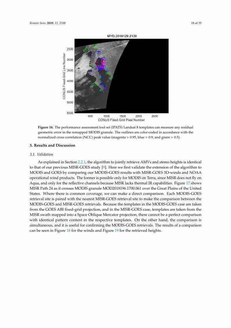
The IPATS technology can also be used to validate the geometric accuracy of the MODIS granules after they have been remapped into the GOES fixed-grid projection, verifying both the quality of the navigation of the MODIS pixels and the correctness of the remapping process. Any residual systematic errors can be measured by matching with Landsat 8 chips, exactly as just described. Any systematic residual error that can be measured can also be compensated by making an adjustment to the remapping and redoing it. Figure 16 shows an example of a remapped Aqua granule with the outlines of the Landsat 8 chips used in the verification. The error statistics of good quality matches (peak correlation coefficient >0.9) in this case are means of −0.06 pixels (EW) and −0.03 pixels (NS), and standard deviations of 0.09 pixels in both directions. The same statistics for the ABI B02 CONUS scene most simultaneous with this granule are means of −0.14 pixels (EW) and −0.03 pixels (NS), and standard deviations of 0.06 pixels in both directions.

Figure 15. The mean (a) and three times standard deviation (b) of frame-to-frame error of a 24-hourperiod (June 1st 18:00 UTC to June 2nd 17:59 UTC 2019) for GOES-16. The misregistration is convertedto nadir equivalent distance from the angular space of the fixed grid projection.

The results presented above are typical of GOES-16 INR performance. GOES-17 INR performancehas similar characteristics. Both satellites satisfy their mission INR requirements for navigation (28 µrador 1 km at the subsatellite point, 3-sigma) and frame-to-frame registration (21 µrad or 0.75 km at thesubsatellite point, three-sigma, for channels with <2 km resolution and 28 µrad or 1 km for the others)with substantial margins. INR performance is subject to continuous monitoring and improvementthrough the efforts of the GOES-R program.

2.2.3. Remapped MODIS Granules

The IPATS technology can also be used to validate the geometric accuracy of the MODIS granulesafter they have been remapped into the GOES fixed-grid projection, verifying both the quality of thenavigation of the MODIS pixels and the correctness of the remapping process. Any residual systematicerrors can be measured by matching with Landsat 8 chips, exactly as just described. Any systematicresidual error that can be measured can also be compensated by making an adjustment to the remappingand redoing it. Figure 16 shows an example of a remapped Aqua granule with the outlines of theLandsat 8 chips used in the verification. The error statistics of good quality matches (peak correlationcoefficient >0.9) in this case are means of −0.06 pixels (EW) and −0.03 pixels (NS), and standarddeviations of 0.09 pixels in both directions. The same statistics for the ABI B02 CONUS scene mostsimultaneous with this granule are means of −0.14 pixels (EW) and −0.03 pixels (NS), and standarddeviations of 0.06 pixels in both directions.

Remote Sens. 2019, 11, 2100 18 of 35

1

Y in

AB

I B02

Pix

els

Figure 16. The performance assessment tool set (IPATS) Landsat 8 templates can measure any residualgeometric error in the remapped MODIS granule. The outlines are color-coded in accordance with thenormalized cross correlation (NCC) peak value (magenta > 0.95, blue > 0.9, and green > 0.5).

3. Results and Discussion

3.1. Validation

As explained in Section 2.2.1, the algorithm to jointly retrieve AMVs and stereo heights is identicalto that of our previous MISR-GOES study [9]. Here we first validate the extension of the algorithm toMODIS and GOES by comparing our MODIS-GOES results with MISR-GOES 3D-winds and NOAAoperational wind products. The former is possible only for MODIS on Terra, since MISR does not fly onAqua, and only for the reflective channels because MISR lacks thermal IR capabilities. Figure 17 showsMISR Path 24 as it crosses MODIS granule MOD2018196.1700.061 over the Great Plains of the UnitedStates. Where there is common coverage, we can make a direct comparison. Each MODIS-GOESretrieval site is paired with the nearest MISR-GOES retrieval site to make the comparison between theMODIS-GOES and MISR-GOES retrievals. Because the templates in the MODIS-GOES case are takenfrom the GOES ABI fixed-grid projection, and in the MISR-GOES case, templates are taken from theMISR swath mapped into a Space Oblique Mercator projection, there cannot be a perfect comparisonwith identical pattern content in the respective templates. On the other hand, the comparison issimultaneous, and it is useful for confirming the MODIS-GOES retrievals. The results of a comparisoncan be seen in Figure 18 for the winds and Figure 19 for the retrieved heights.


Figure 17. A MODIS granule that has been remapped into the GOES ABI fixed-grid projection is overlaid with red boxes at the left (a) showing the blocks in the MISR path intersecting the granule. The MISR-GOES 3D-wind product is shown at the right (b). The MODIS granule is MOD2018196.1700.061 (MODIS Band 1) and is simultaneous with MISR Path 24, Orbit 98797. (Note: retrieval sites are thinned 4:1 in each direction for clarity.).

Figure 18. Retrieved winds from MODIS and GOES are compared to retrievals from MISR and GOES in the U (+East) and V (+North) directions on the tangent plane to the WGS84 ellipsoid in (a) and (b) respectively. The diagonal line is the perfect match, and robust statistics (mean µ and standard deviation σ, over sample size N) are computed over the retrieval differences. The Median Absolute Difference (MAD) filter technique is used with a six-sigma threshold to edit out spurious pairings then the regular mean and standard deviation are computed over the remaining population. The MODIS granule is MOD2018196.1700.061 (MODIS Band 1) and is simultaneous with MISR Path 24, Orbit 98797.

Figure 17. A MODIS granule that has been remapped into the GOES ABI fixed-grid projectionis overlaid with red boxes at the left (a) showing the blocks in the MISR path intersecting thegranule. The MISR-GOES 3D-wind product is shown at the right (b). The MODIS granule isMOD2018196.1700.061 (MODIS Band 1) and is simultaneous with MISR Path 24, Orbit 98797. (Note:retrieval sites are thinned 4:1 in each direction for clarity).


Figure 17. A MODIS granule that has been remapped into the GOES ABI fixed-grid projection is overlaid with red boxes at the left (a) showing the blocks in the MISR path intersecting the granule. The MISR-GOES 3D-wind product is shown at the right (b). The MODIS granule is MOD2018196.1700.061 (MODIS Band 1) and is simultaneous with MISR Path 24, Orbit 98797. (Note: retrieval sites are thinned 4:1 in each direction for clarity.).

Figure 18. Retrieved winds from MODIS and GOES are compared to retrievals from MISR and GOES in the U (+East) and V (+North) directions on the tangent plane to the WGS84 ellipsoid in (a) and (b) respectively. The diagonal line is the perfect match, and robust statistics (mean µ and standard deviation σ, over sample size N) are computed over the retrieval differences. The Median Absolute Difference (MAD) filter technique is used with a six-sigma threshold to edit out spurious pairings then the regular mean and standard deviation are computed over the remaining population. The MODIS granule is MOD2018196.1700.061 (MODIS Band 1) and is simultaneous with MISR Path 24, Orbit 98797.

Figure 18. Retrieved winds from MODIS and GOES are compared to retrievals from MISR and GOESin the U (+East) and V (+North) directions on the tangent plane to the WGS84 ellipsoid in (a) and(b) respectively. The diagonal line is the perfect match, and robust statistics (mean µ and standarddeviation σ, over sample size N) are computed over the retrieval differences. The Median AbsoluteDifference (MAD) filter technique is used with a six-sigma threshold to edit out spurious pairings thenthe regular mean and standard deviation are computed over the remaining population. The MODISgranule is MOD2018196.1700.061 (MODIS Band 1) and is simultaneous with MISR Path 24, Orbit 98797.


Figure 19. Jointly retrieved wind heights are compared between the MODIS-GOES and MISR-GOES cases with robust statistic on their differences (mean µ and standard deviation σ, over sample size N). The heights are with respect to the WGS84 ellipsoid. The MODIS granule is MOD2018196.1700.061 and is simultaneous with MISR Path 24, Orbit 98797.

The comparison between the wind velocities shows small biases and standard deviations that are in accord with an estimated wind accuracy of <0.5 m/s for the MISR-GOES product [9]. This is supported by a comparison between the MODIS-GOES winds and the NOAA operational derived motion wind (DMW) product for the same time as shown on Figure 20. This should not be surprising since the same GOES-16 CONUS scenes are used for both. There are fewer samples in the DMW comparison because the NOAA operational winds are generally less densely sampled. Paired sites that are too far away (>2.2 km) are not considered coincident and therefore not part of the comparison.

Figure 20. Retrieved MODIS-GOES winds are compared with the NOAA operational derived motion wind (DMW) product along the U axis (a) and V axis (b). The diagonal line is the perfect match, and the

Figure 19. Jointly retrieved wind heights are compared between the MODIS-GOES and MISR-GOEScases with robust statistic on their differences (mean µ and standard deviation σ, over sample size N).The heights are with respect to the WGS84 ellipsoid. The MODIS granule is MOD2018196.1700.061 andis simultaneous with MISR Path 24, Orbit 98797.

The comparison between the wind velocities shows small biases and standard deviations thatare in accord with an estimated wind accuracy of <0.5 m/s for the MISR-GOES product [9]. This issupported by a comparison between the MODIS-GOES winds and the NOAA operational derivedmotion wind (DMW) product for the same time as shown on Figure 20. This should not be surprisingsince the same GOES-16 CONUS scenes are used for both. There are fewer samples in the DMWcomparison because the NOAA operational winds are generally less densely sampled. Paired sitesthat are too far away (>2.2 km) are not considered coincident and therefore not part of the comparison.


Figure 19. Jointly retrieved wind heights are compared between the MODIS-GOES and MISR-GOES cases with robust statistic on their differences (mean µ and standard deviation σ, over sample size N). The heights are with respect to the WGS84 ellipsoid. The MODIS granule is MOD2018196.1700.061 and is simultaneous with MISR Path 24, Orbit 98797.

The comparison between the wind velocities shows small biases and standard deviations that are in accord with an estimated wind accuracy of <0.5 m/s for the MISR-GOES product [9]. This is supported by a comparison between the MODIS-GOES winds and the NOAA operational derived motion wind (DMW) product for the same time as shown on Figure 20. This should not be surprising since the same GOES-16 CONUS scenes are used for both. There are fewer samples in the DMW comparison because the NOAA operational winds are generally less densely sampled. Paired sites that are too far away (>2.2 km) are not considered coincident and therefore not part of the comparison.

Figure 20. Retrieved MODIS-GOES winds are compared with the NOAA operational derived motion wind (DMW) product along the U axis (a) and V axis (b). The diagonal line is the perfect match, and the

Figure 20. Retrieved MODIS-GOES winds are compared with the NOAA operational derived motionwind (DMW) product along the U axis (a) and V axis (b). The diagonal line is the perfect match, and thestatistics are computed over the retrieval differences (mean µ and standard deviation σ, over samplesize N). The MODIS granule is MOD2018196.1700.061 and the DMW product is for ABI band 2 and theCONUS scene with product time 2018/196 17:02.

Remote Sens. 2019, 11, 2100 21 of 35

A similar comparison between MODIS-GOES 3D-wind retrievals and the operational DMWs isshown in Figure 21 for ABI Band 14. The IR spatial resolution is four times coarser than that of ABIBand 2.


statistics are computed over the retrieval differences (mean µ and standard deviation σ, over sample size N). The MODIS granule is MOD2018196.1700.061 and the DMW product is for ABI band 2 and the CONUS scene with product time 2018/196 17:02.

A similar comparison between MODIS-GOES 3D-wind retrievals and the operational DMWs is shown in Figure 21 for ABI Band 14. The IR spatial resolution is four times coarser than that of ABI Band 2.

Figure 21. Retrieved MODIS-GOES winds are compared with the NOAA operational DMW product for an IR case along the U axis (a) and V axis (b). The diagonal line is the perfect match, and the statistics are computed over the retrieval differences (mean µ and standard deviation σ, over sample size N). The MODIS granule is MOD2019057.2000.061 and the DMW product is for ABI band 14 and the CONUS scene with product time 2019/057 20:02.

The operational NOAA DMW wind vectors are assigned pressure levels. As noted in [9], when converted to an equivalent height in atmosphere, the differences between the MISR-GOES 3D-wind height assignments and the DMW height assignments can be as large as 1 km. A more accurate validation of the MODIS-GOES height assignments is made by looking at the clear-sky retrievals from the MODIS-GOES 3D-winds. This is a method that has been pioneered with MISR [21]. It is true that the ground retrievals are not cloud tracks and therefore not winds; however, the range of terrain heights above the ellipsoid can be several km, a good range for low clouds, and the fact that the ground is known to be static also offers a means to obtain an estimate of the velocity uncertainty for zero-speed objects. Figure 22 is an example of ground-point retrievals from MODIS-GOES 3D-winds. The clear-sky ground retrievals are classified by whether the retrieval site is over land, apparently close to the ground (< 300 m), and stationary (within 0.3 m/s of zero in both U and V axes) and the height error is the difference between the retrieved height and the known terrain height. For the purposes of calculating the velocity errors, the velocity limit is relaxed to 2 m/s to admit possibly larger errors. In the case shown, there is a small height bias of 18 m. The equivalent ground-point height bias for the MISR-GOES ground-point retrievals (case shown in Figure 17) is −47 m with a 162 m standard deviation. Therefore, the relative height bias is 65 m, which is smaller but still comparable with the mean difference seen in Figure 19. The small bases may be due to small residual geolocation errors in the three systems. The error statistics in Figure 22 are also comparable with the uncertainties from the state covariance matrix that are shown in

Figure 21. Retrieved MODIS-GOES winds are compared with the NOAA operational DMW productfor an IR case along the U axis (a) and V axis (b). The diagonal line is the perfect match, and thestatistics are computed over the retrieval differences (mean µ and standard deviation σ, over samplesize N). The MODIS granule is MOD2019057.2000.061 and the DMW product is for ABI band 14 andthe CONUS scene with product time 2019/057 20:02.

The operational NOAA DMW wind vectors are assigned pressure levels. As noted in [9],when converted to an equivalent height in atmosphere, the differences between the MISR-GOES3D-wind height assignments and the DMW height assignments can be as large as 1 km. A moreaccurate validation of the MODIS-GOES height assignments is made by looking at the clear-skyretrievals from the MODIS-GOES 3D-winds. This is a method that has been pioneered with MISR [21].It is true that the ground retrievals are not cloud tracks and therefore not winds; however, the range ofterrain heights above the ellipsoid can be several km, a good range for low clouds, and the fact that theground is known to be static also offers a means to obtain an estimate of the velocity uncertainty forzero-speed objects. Figure 22 is an example of ground-point retrievals from MODIS-GOES 3D-winds.The clear-sky ground retrievals are classified by whether the retrieval site is over land, apparently closeto the ground (<300 m), and stationary (within 0.3 m/s of zero in both U and V axes) and the heighterror is the difference between the retrieved height and the known terrain height. For the purposesof calculating the velocity errors, the velocity limit is relaxed to 2 m/s to admit possibly larger errors.In the case shown, there is a small height bias of 18 m. The equivalent ground-point height bias forthe MISR-GOES ground-point retrievals (case shown in Figure 17) is −47 m with a 162 m standarddeviation. Therefore, the relative height bias is 65 m, which is smaller but still comparable with themean difference seen in Figure 19. The small bases may be due to small residual geolocation errors inthe three systems. The error statistics in Figure 22 are also comparable with the uncertainties fromthe state covariance matrix that are shown in Figure 10 for the same case. The height retrieval errorswill depend on the LEO-GEO relative viewing geometry and will become large near the singulargeometry as described in Section 2.1.3. The uncertainty from the covariance is an effective guide toretrieval quality.

Remote Sens. 2019, 11, 2100 22 of 35


Figure 10 for the same case. The height retrieval errors will depend on the LEO-GEO relative viewing geometry and will become large near the singular geometry as described in Section 2.3. The uncertainty from the covariance is an effective guide to retrieval quality.

Figure 22. Clear-sky ground retrievals from the MODIS-GOES 3D-winds show the accuracies of retrieved heights (a) and velocities (c) and (d). The mean µ and standard deviation σ over sample size N are computed for each histogram and the regression parameters (b) for retrieved height versus terrain height are reported for the ground-point class (“Low and static”). The MODIS granule is MOD2018196.1700.061 (MODIS band 1).

Thermal-IR ground point measurements can sometimes be obtained for a granule (Figure 23). In the thermal IR, the pixel size is four times (2 km versus 0.5 km) that of the previous example, which results in larger errors in the height assignment and static-target velocity error.

Figure 22. Clear-sky ground retrievals from the MODIS-GOES 3D-winds show the accuracies ofretrieved heights (a) and velocities (c,d). The mean µ and standard deviation σ over sample sizeN are computed for each histogram and the regression parameters (b) for retrieved height versusterrain height are reported for the ground-point class (“Low and static”). The MODIS granule isMOD2018196.1700.061 (MODIS band 1).

Thermal-IR ground point measurements can sometimes be obtained for a granule (Figure 23).In the thermal IR, the pixel size is four times (2 km versus 0.5 km) that of the previous example, whichresults in larger errors in the height assignment and static-target velocity error.


Figure 23. Clear-sky ground retrievals from the MODIS-GOES 3D-winds show the accuracies of retrieved heights (a) and velocities (c) and (d) for an infrared (IR) case. The mean µ and standard deviation σ over sample size N are computed for each histogram and the regression parameters (b) for retrieved height versus terrain height are reported for the ground-point class (“Low and static”). The MODIS granule is MOD2019057.2000.061 paired with ABI Band 14, CONUS scene time 2019/057 20:02.

In summary, we compare MODIS-GOES retrievals to simultaneous collocated MISR-GOES retrievals using the same 3D-winds retrieval algorithm. In our previous work [9], we compared MISR-GOES retrievals to NOAA operational DMWs and extensively analyzed ground-point retrievals to validate the application of the new algorithm with MISR and GOES datasets. We concluded that MISR-GOES retrieval height errors were <200 m and AMV errors <0.5 m/s. The MODIS-GOES to MISR-GOES comparison above (Figures 18 and 19) shows an agreement to within these error bounds. Our previous work also compared the MISR-GOES retrievals to NOAA operational DMWs that use IR methods for height assignments. The two often differed by ~1 km. Therefore, we expect that both the MISR-GOES and MODIS-GOES retrievals (except near the singular geometry) should improve the state of the art in AMV height assignments if not necessarily the AMVs alone. However, since wind speed can vary significantly with altitude, a better height assignment can also mean better correlation between the AMV and the in situ wind. Ground-point retrievals are another powerful method for validation. The results presented

Figure 23. Clear-sky ground retrievals from the MODIS-GOES 3D-winds show the accuracies ofretrieved heights (a) and velocities (c,d) for an infrared (IR) case. The mean µ and standard deviation σ

over sample size N are computed for each histogram and the regression parameters (b) for retrievedheight versus terrain height are reported for the ground-point class (“Low and static”). The MODISgranule is MOD2019057.2000.061 paired with ABI Band 14, CONUS scene time 2019/057 20:02.

In summary, we compare MODIS-GOES retrievals to simultaneous collocated MISR-GOESretrievals using the same 3D-winds retrieval algorithm. In our previous work [9], we comparedMISR-GOES retrievals to NOAA operational DMWs and extensively analyzed ground-point retrievalsto validate the application of the new algorithm with MISR and GOES datasets. We concluded thatMISR-GOES retrieval height errors were <200 m and AMV errors <0.5 m/s. The MODIS-GOES toMISR-GOES comparison above (Figures 18 and 19) shows an agreement to within these error bounds.Our previous work also compared the MISR-GOES retrievals to NOAA operational DMWs that use IRmethods for height assignments. The two often differed by ~1 km. Therefore, we expect that both theMISR-GOES and MODIS-GOES retrievals (except near the singular geometry) should improve thestate of the art in AMV height assignments if not necessarily the AMVs alone. However, since windspeed can vary significantly with altitude, a better height assignment can also mean better correlationbetween the AMV and the in situ wind. Ground-point retrievals are another powerful method forvalidation. The results presented above (Figure 22) are consistent with those from the MODIS-GOES toMISR-GOES comparison. The processing of a ground pattern is identical to that of a cloud pattern anda range of heights can be sampled according to the natural variation of the terrain. The fact that groundpoints are static could be a limitation, but comparisons with other AMV products seems perfectly

Remote Sens. 2019, 11, 2100 24 of 35

adequate to validate retrieved AMVs alone. The true height assignment for an AMV is, of course,more nuanced as a tracked pattern is not necessarily confined to a single plane. Using the same patternused for AMV determination to measure directly the pattern height through parallax is a more directmethod of assigning a height than IR methods, but certainly additional validations using in situ windmeasurements would be beneficial to quantify the relative benefits of the new methods.

3.2. Applications

The MODIS-GOES algorithm greatly enlarges the spatiotemporal coverage of the stereo techniqueusing LEO-GEO pairs, compared with the MISR-GOES algorithm developed in our earlier study [9].Vector winds are essentially retrieved from a triplet/doublet of rapidly refreshed GEO images withthe stereo height being observable thanks to the snapshot provided by the LEO satellite at a differentview angle and interposed in the GEO image sequence. The newly extended algorithm requires nosynchronization between the LEO-GEO pair, only the ability to time tag pixels, because the parallaxsolver can account for feature motion effects if the LEO image is not taken in synchronization with theGEO images.

The wider spatial coverage from MODIS-like imagers and frequency of LEO-GEO pairings allow ahost of science applications that require accurate knowledge of AMVs and their heights, including PBLprocesses, overshooting convective clouds, and dispersion of wildfire smoke plumes. Following thesuccessful development of the MODIS-GOES 3D-wind algorithm, we demonstrate here its capabilitieswith several applications, to illustrate the future research that the stereo-AMV technique will enable.

3.2.1. Quasi-3D Representation of Mesoscale Dynamics (January 2019)

The MODIS-GOES algorithm can retrieve an AMV field with ~4 km horizontal resolution and<300 m vertical accuracy. Since AMVs are derived from cloud-top features, each AMV represents avector at a height characteristic of the cloud tops. In a scene of broken clouds with tops at differentaltitudes, a densely sampled, high-resolution AMV field can effectively sample multiple layers.Figure 24a illustrates a benefit of high-resolution (<4 km) AMV retrievals for representing mesoscaledynamics. Without thinning the AMV field from different vertical levels (as often practiced byNWP data assimilation), these AMVs can provide a quasi-3D view of mesoscale dynamics over asynoptic domain.

Figure 24b is a case on January 31, 2019, when cold Arctic air descended into CONUS, creatinga severe weather event with heavy snow and record cold in many Midwest states. The coldesttemperature recorded by a ground station was −49 ◦C in Cotton, Minnesota, while it reached −35 ◦C inRockford, Illinois, breaking its −32 ◦C record set in January 1982. The AMV pattern retrieved fromthe MODIS-GOES algorithm over CONUS represents the classic cold air outbreak (CAO) case wherea strong upper-level trough descends into mid-latitudes while low-level warm air collides with thetrough, generating complex 3D dynamics.


Figure 24. (a) Illustration of the improvement from high-resolution (<4 km) AMVs in representing a quasi-3D synoptic flow. Compared to conventional AMV retrievals at a coarser resolution, the high-resolution algorithm provides more vertical levels of AMVs that can be assimilated in the NWP system. (b) AMVs at 2 km horizontal resolution from the MODIS-GOES retrieval on January 31, 2019 when a cold Arctic system dipped down to CONUS and created severe winter storms in most of the northern states (c). The height of wind vectors is color coded and shows a range of AMV heights from the surface to ~11 km. The blue lines indicate the borders of MODIS image granule in this case (as shown in the embedded image).

3.2.2. PBL Dynamics (January-February 2019)

The primary motivation for developing the MODIS-GOES 3D-wind algorithm is to provide a better height assignment for AMVs. PBL AMVs are one of the challenging cases for height assignments, primarily because traditional IR methods have difficulty with the PBL thermodynamic structure, which may include inversions. The stereo approach as implemented in the MODIS-GOES algorithm does not require any knowledge about atmospheric thermal structures. Therefore, AMV retrievals in the PBL provide a good test for the new algorithm.

In Figure 24, the PBL AMVs and their structure are hardly seen due to the color scale used to include the high-level winds. To highlight the PBL winds, Figure 25 shows the same case with a different color scale for the region over Lakes Superior and Michigan where the CAO event produced a very dynamic PBL cloud field. As the cold air blows over open water, convective activity in the marine PBL produces cloud streets that can often stretch hundreds of kilometers [22]. These organized cloud patterns occur more than 50% of the time over the North Atlantic during winter, and most of them last less than 2 days [23]. These clouds can also occur over an extensive lake surface, such as in the Great Lakes (Figure 25).

On January 31, 2019, most of Lake Superior and Lake Michigan still had open water except near the shore where lake ice might have formed. The rising PBL top is readily seen in the AMV height retrievals, with the colored wind vectors in Figure 25 showing that the PBL height increases steadily from ~400 m on the western shore to ~1100 m on the eastern shore of Lake Michigan. The CAO event over Lake Michigan was dominated by the zonal wind, which was approximately constant at ~8 m/s for these PBL heights. The rise in PBL height is caused by growth of a stably stratified boundary layer, downstream from the land/ice edge, which progresses slowly by advection of continental air over the water (Figure 26). As detailed by Garratt [24], the depth of the PBL layer is a function of distance and wind speed. PBL clouds from CAO events have an important implication for Earth’s weather and climate systems, because they can cause heavy snowfall and modulate shortwave (SW) solar radiation.

The 3D-wind algorithm provides an additional method for cloud detection during day and night. Radiometric methods for cloud detection would encounter a great difficulty for the low clouds over a

Figure 24. (a) Illustration of the improvement from high-resolution (<4 km) AMVs in representinga quasi-3D synoptic flow. Compared to conventional AMV retrievals at a coarser resolution,the high-resolution algorithm provides more vertical levels of AMVs that can be assimilated inthe NWP system. (b) AMVs at 2 km horizontal resolution from the MODIS-GOES retrieval on January31, 2019 when a cold Arctic system dipped down to CONUS and created severe winter storms in mostof the northern states (c). The height of wind vectors is color coded and shows a range of AMV heightsfrom the surface to ~11 km. The blue lines indicate the borders of MODIS image granule in this case (asshown in the embedded image).

3.2.2. PBL Dynamics (January-February 2019)

The primary motivation for developing the MODIS-GOES 3D-wind algorithm is to provide abetter height assignment for AMVs. PBL AMVs are one of the challenging cases for height assignments,primarily because traditional IR methods have difficulty with the PBL thermodynamic structure, whichmay include inversions. The stereo approach as implemented in the MODIS-GOES algorithm does notrequire any knowledge about atmospheric thermal structures. Therefore, AMV retrievals in the PBLprovide a good test for the new algorithm.

In Figure 24, the PBL AMVs and their structure are hardly seen due to the color scale used toinclude the high-level winds. To highlight the PBL winds, Figure 25 shows the same case with adifferent color scale for the region over Lakes Superior and Michigan where the CAO event produced avery dynamic PBL cloud field. As the cold air blows over open water, convective activity in the marinePBL produces cloud streets that can often stretch hundreds of kilometers [22]. These organized cloudpatterns occur more than 50% of the time over the North Atlantic during winter, and most of them lastless than 2 days [23]. These clouds can also occur over an extensive lake surface, such as in the GreatLakes (Figure 25).

On January 31, 2019, most of Lake Superior and Lake Michigan still had open water except nearthe shore where lake ice might have formed. The rising PBL top is readily seen in the AMV heightretrievals, with the colored wind vectors in Figure 25 showing that the PBL height increases steadilyfrom ~400 m on the western shore to ~1100 m on the eastern shore of Lake Michigan. The CAO eventover Lake Michigan was dominated by the zonal wind, which was approximately constant at ~8 m/sfor these PBL heights. The rise in PBL height is caused by growth of a stably stratified boundary layer,downstream from the land/ice edge, which progresses slowly by advection of continental air over thewater (Figure 26). As detailed by Garratt [24], the depth of the PBL layer is a function of distance andwind speed. PBL clouds from CAO events have an important implication for Earth’s weather andclimate systems, because they can cause heavy snowfall and modulate shortwave (SW) solar radiation.

The 3D-wind algorithm provides an additional method for cloud detection during day and night.Radiometric methods for cloud detection would encounter a great difficulty for the low clouds over awhite snowy/icy background such as in Figure 25. With the stereo AMV product, we can provide moreconfidence for cloud detection by classifying the surface retrievals as low-wind-speed (<0.5 m/s) and

Remote Sens. 2019, 11, 2100 26 of 35

low height (<300 m) features. This has a clear benefit for those applications (e.g., snow and ice cover)that require a robust cloud mask.

The wind direction retrieved from the 3D-wind algorithm represents an instantaneous directionfor a wind vector. Although the cloud streets from the CAO event are generally in line with thewind vectors, their patterns reflect a history of wind transport. Evolution of PBL height can causethe clouds streets not to align with the instantaneous wind direction. This has an implication for thesemi-autonomous tool (MISR INteractive eXplorer, or MINX) used for MISR-only PBL AMV retrievals.The MINX retrievals require a priori information about the wind direction in order to mitigate thealiasing problem between along-track motion and height parallax. The MINX operators usually usethe cloud streets as a guess for the wind direction. As revealed in the MODIS-GOES 3D-wind AMVs inFigure 25, the cloud streets are not necessarily same as the instantaneous wind direction in this scene.


white snowy/icy background such as in Figure 25. With the stereo AMV product, we can provide more confidence for cloud detection by classifying the surface retrievals as low-wind-speed (<0.5 m/s) and low height (<300 m) features. This has a clear benefit for those applications (e.g., snow and ice cover) that require a robust cloud mask.

The wind direction retrieved from the 3D-wind algorithm represents an instantaneous direction for a wind vector. Although the cloud streets from the CAO event are generally in line with the wind vectors, their patterns reflect a history of wind transport. Evolution of PBL height can cause the clouds streets not to align with the instantaneous wind direction. This has an implication for the semi-autonomous tool (MISR INteractive eXplorer, or MINX) used for MISR-only PBL AMV retrievals. The MINX retrievals require a priori information about the wind direction in order to mitigate the aliasing problem between along-track motion and height parallax. The MINX operators usually use the cloud streets as a guess for the wind direction. As revealed in the MODIS-GOES 3D-wind AMVs in Figure 25, the cloud streets are not necessarily same as the instantaneous wind direction in this scene.

Figure 25. PBL cloud streets are readily seen from the cold air outbreak (CAO) event (a) over Lakes Superior and Michigan (shown at larger scale in Figure 24). The bottom-right panel (c) is a cross-section of the full set of retrievals at 43°N latitude where terrain height is in orange and the stereo height is in black, showing PBL clouds rising in height from 400 m to 1100 m over Lake Michigan, as cold air blows over the relatively warmer water. Heavy snow often occurs downstream from the lake, as a result of the so-called ‘lake effect’.

Figure 25. PBL cloud streets are readily seen from the cold air outbreak (CAO) event (a) over LakesSuperior and Michigan (shown at larger scale in Figure 24). The bottom-right panel (c) is a cross-sectionof the full set of retrievals (b) at 43◦ N latitude where terrain height is in orange and the stereo height isin black, showing PBL clouds rising in height from 400 m to 1100 m over Lake Michigan, as cold airblows over the relatively warmer water. Heavy snow often occurs downstream from the lake, as aresult of the so-called ‘lake effect’.


Figure 26. A schematic diagram to illustrate interactions between cold air and warmer water in producing a rising boundary-layer top over open water during the CAO event.

The direction of PBL AMVs can change in a short period of time. On February 1, 2019, the PBL AMVs veered northward in a narrow band over Lake Michigan (Figure 27). There was a less variation in the AMV height, as compared to the January 31, 2019 situation. Clouds and snowy/icy surfaces cannot be readily classified in the MODIS visible image but can with the stereo height map. It is evident that lake ice had grown along the shore during January 28–February 1, as the cold air froze more lake surface. The open water area plays an important role in forming the PBL clouds. In a recent study [25], we found using MISR that the PBL cloud amount increased significantly over the Arctic Ocean as a result of there being more open water from the summertime warming.

Figure 27. As in Figure 25 but for Feb.1, 2019 when the winds over Lake Michigan changed their direction drastically and the PBL clouds were aloft at the approximately same altitude.

3.2.3. Hurricane Michael (October 2018)

The MODIS-GOES 3D-wind algorithm is applied to Hurricane Michael on October 9, 2018 to evaluate its AMV and stereo height retrievals from different spectral bands. As seen in Figure 28, shortly before the hurricane reached its peak intensity, MODIS on Terra flew over the eye at 16:25Z with full coverage across the span of the cyclone in the Gulf of Mexico. Hurricane Michael was a deadly Category

Figure 26. A schematic diagram to illustrate interactions between cold air and warmer water inproducing a rising boundary-layer top over open water during the CAO event.

The direction of PBL AMVs can change in a short period of time. On February 1, 2019, the PBLAMVs veered northward in a narrow band over Lake Michigan (Figure 27). There was a less variationin the AMV height, as compared to the January 31, 2019 situation. Clouds and snowy/icy surfacescannot be readily classified in the MODIS visible image but can with the stereo height map. It is evidentthat lake ice had grown along the shore during January 28–February 1, as the cold air froze more lakesurface. The open water area plays an important role in forming the PBL clouds. In a recent study [25],we found using MISR that the PBL cloud amount increased significantly over the Arctic Ocean as aresult of there being more open water from the summertime warming.


Figure 26. A schematic diagram to illustrate interactions between cold air and warmer water in producing a rising boundary-layer top over open water during the CAO event.

The direction of PBL AMVs can change in a short period of time. On February 1, 2019, the PBL AMVs veered northward in a narrow band over Lake Michigan (Figure 27). There was a less variation in the AMV height, as compared to the January 31, 2019 situation. Clouds and snowy/icy surfaces cannot be readily classified in the MODIS visible image but can with the stereo height map. It is evident that lake ice had grown along the shore during January 28–February 1, as the cold air froze more lake surface. The open water area plays an important role in forming the PBL clouds. In a recent study [25], we found using MISR that the PBL cloud amount increased significantly over the Arctic Ocean as a result of there being more open water from the summertime warming.

Figure 27. As in Figure 25 but for Feb.1, 2019 when the winds over Lake Michigan changed their direction drastically and the PBL clouds were aloft at the approximately same altitude.


The MODIS-GOES 3D-wind algorithm is applied to Hurricane Michael on October 9, 2018 to evaluate its AMV and stereo height retrievals from different spectral bands. As seen in Figure 28, shortly before the hurricane reached its peak intensity, MODIS on Terra flew over the eye at 16:25Z with full coverage across the span of the cyclone in the Gulf of Mexico. Hurricane Michael was a deadly Category

Figure 27. As in Figure 25 but for Feb.1, 2019 when the winds over Lake Michigan (a) changed theirdirection drastically and the PBL clouds were aloft at the approximately same altitude (b).


The MODIS-GOES 3D-wind algorithm is applied to Hurricane Michael on October 9, 2018 toevaluate its AMV and stereo height retrievals from different spectral bands. As seen in Figure 28,shortly before the hurricane reached its peak intensity, MODIS on Terra flew over the eye at 16:25Z withfull coverage across the span of the cyclone in the Gulf of Mexico. Hurricane Michael was a deadlyCategory 5 hurricane, known for its rapid intensification from category 2 on October 8 to category 5 onOctober 9 before its landfall on October 10.


Figure 28. (a) MODIS image of Hurricane Michael on October 9, 2018 with the circles indicating deep convective zones and the arrows for wind direction. (b) Retrieved AMVs from ABI band 2 with height in color. The circles highlight small AMV wind speeds at high altitudes.

In addition to the chip size sensitivity, spectral bands can have different sensitivities to AMVs, because cloud features seen by each band can vary significantly. Band 2 (visible) is less sensitive to thin cirrus than band 14 (thermal IR). In the case of multi-layer clouds covered by thin cirrus, band 2 tends to see through the cirrus and finds the feature pattern below, whereas band 14 tends to find the cirrus for pattern matching. This is clearly evident in Figure 29 where there are more low-level clouds in the Band 2 AMVs than in band 14. This type of multi-layer clouds is mostly seen on the eastern side of the cyclone, and an advantage with both band 2 and 14 AMVs is to provide two distinct vertical levels of mesoscale dynamics at the same location. On the other hand, band 4 (1.37 µm) is known as the “cirrus” band, which uses water vapor absorption to screen out low-level clouds and surface features. As seen in Figure 29, the majority of its retrievals are high-level AMVs, some of which are higher than those from bands 2 and 14 near the hurricane center, but not many low-level AMVs are found except where the atmosphere is dry and clear. Band 7 (mid-wave IR) is a channel that has about same amount of radiance from the reflected sunlight as from the terrestrial emissions. It has been used for fire/hot-spot, daytime snow/ice detection, and low-level AMVs. In this hurricane case, its yield for AMVs is not as great as bands 2 and 14, but it has a balanced sampling in the multi-layer cloud scenes.

Different AMV sensitivities by the spectral bands is further illustrated by the vertical distribution of height measurements. Along the meridian of 87.5°W longitude (Figure 30a), bands 4 and 14 produce a peak stereo height as high as 17.8 and 17.4 km, respectively, compared with 16.3 km from Band 2. Again, the higher peaks are consistent with the better cirrus sensitivity from bands 4 and 14. Since these high-level cirrus clouds are clearly above the tropopause, it is impossible for the conventional IR techniques to provide accurate height assignment. Also noticeable in Figure 30a is the smoothness of band 2 and band 14 height measurements. Because these bands are spectral windows, cloud features are less attenuated by atmospheric emissions (e.g., CO2 and H2O) and have better contrast for pattern recognition.

Figure 30b summarizes the vertical distribution of AMV height retrievals from the four spectral bands, all revealing a trimodal distribution except band 4. The trimodal height distribution, a unique tropical cloud property, consists of PBL clouds, congestus, and cirrus outflows. As expected for its low-cloud screening, band 4 observes only the two high-level modes. The observation of the trimodal cloud distribution reflects one of the stereo technique strengths, compared to other passive remote sensing methods for cloud height assignment. Wu et al. [26] evaluated several passive techniques for cloud height

Figure 28. (a) MODIS image of Hurricane Michael on October 9, 2018 with the circles indicating deepconvective zones and the arrows for wind direction. (b) Retrieved AMVs from ABI band 2 with heightin color. The circles highlight small AMV wind speeds at high altitudes.

Retrieval experiments were conducted with different configuration parameters to evaluate thetrade-off between AMV quality and spatial resolution in the Hurricane Michael case where Terra/MODISare matched to GOES-16 CONUS images. A higher spatial resolution is always desired for mesoscaledynamics such as hurricanes and other severe weather phenomena, which requires a smaller chip size(i.e., size of an image template for pattern matching). On the other hand, since clouds are non-rigidfeatures and can change (grow or decay) in time, a smaller chip size may lead to a noisier product,due to less robust pattern recognition. In this study we tested three chip sizes (8 × 8, 16 × 16 and32 × 32 km) for four spectral bands, namely, ABI bands 2 (visible), 4 (near IR), 7 (mid-wave IR), and 14(thermal IR) as shown in Table 4. For each test, the sampling interval is a half of the chip size, so moreretrievals are being made at the higher resolutions as well and consuming more computer resources.Figure 28 shows the high-resolution (4 × 4 km sampled) AMV retrievals from band 2 with a chip size of8 × 8 km. In the band 2 pairing, GOES-16 has a pixel resolution (500 m), 4× better than bands 4, 7 and14, to match MODIS 250-m pixel resolution, which allows pattern matching to produce good results atthe highest resolution among all MODIS-GOES spectral band pairs. To evaluate AMV retrieval quality,

we compare each wind vector (⇀U) with the background wind (

⇀Ub) in a 40 × 40 km domain centered at

this AMV. The norm ‖⇀U −

⇀Ub‖ < 0.2 m/s is used as a “consistency” flag, and Table 4 summarizes the

percentage of consistent AMV retrievals from each band for different chip sizes. For the hurricane case,ABI band 2 can still produce useful AMVs at 8 km resolution, whereas bands 4, 7 and 14 AMVs canonly go down to 16 km resolution mainly because their pixel resolution is 4x coarser than Band 2.

Table 4. AMV Quality (i.e., consistency) for the hurricane Michael retrievals.

Chip Size (km) Band 2 Band 4 Band 7 Band 14

8 × 8 93% 22% 21% 22%16 × 16 97% 95% 92% 95%32 × 32 99% 99% 99% 99%

The high-resolution AMV and height retrievals provide extraordinary insights into severe weathersystems such as Hurricane Michael. Divergence of the wind fields at the top of cyclone deck,as highlighted by the circles in Figure 28, is indicative of strong deep convection zones in the arms thatwere strengthening the cyclone. The highlighted high-level AMVs are associated with a low windspeed as expected for deep convection reaching a neutral buoyancy level in the upper tropopause.

Remote Sens. 2019, 11, 2100 29 of 35

Outside the deep convective zone, the upper-level AMVs must flow away from the updraft region, as aresult of the mass conservation law. Such deep convection may occur in other parts of the cyclone’sarms, but is obscured by the cirrus outflows aloft.

In addition to the chip size sensitivity, spectral bands can have different sensitivities to AMVs,because cloud features seen by each band can vary significantly. Band 2 (visible) is less sensitive to thincirrus than band 14 (thermal IR). In the case of multi-layer clouds covered by thin cirrus, band 2 tendsto see through the cirrus and finds the feature pattern below, whereas band 14 tends to find the cirrusfor pattern matching. This is clearly evident in Figure 29 where there are more low-level clouds in theBand 2 AMVs than in band 14. This type of multi-layer clouds is mostly seen on the eastern side of thecyclone, and an advantage with both band 2 and 14 AMVs is to provide two distinct vertical levels ofmesoscale dynamics at the same location. On the other hand, band 4 (1.37 µm) is known as the “cirrus”band, which uses water vapor absorption to screen out low-level clouds and surface features. As seenin Figure 29, the majority of its retrievals are high-level AMVs, some of which are higher than thosefrom bands 2 and 14 near the hurricane center, but not many low-level AMVs are found except wherethe atmosphere is dry and clear. Band 7 (mid-wave IR) is a channel that has about same amount ofradiance from the reflected sunlight as from the terrestrial emissions. It has been used for fire/hot-spot,daytime snow/ice detection, and low-level AMVs. In this hurricane case, its yield for AMVs is not asgreat as bands 2 and 14, but it has a balanced sampling in the multi-layer cloud scenes.


measurements by comparing them against active sensor data, and found that only stereo technique was able to clearly detect the trimodal height distribution. In their study, the IR height-assignment method tended to often mix up low- and middle-level clouds with its height assignment, whereas the UV method suffers from the similar problem in addition to its poor sensitivity to high clouds.

Finally, retrieving stereo heights from IR images is particularly important for nighttime observations, despite a finer pixel resolution with the visible band. Both bands 7 and 14 are able to produce stereo heights in the absence of sunlight while band 7 may have a better sensitivity to low clouds over land (not shown). Among the thermal IR bands listed in Figure 29, our test results show that their coverage and sensitivity are all similar to band 14, but not significantly better than band 14.

Figure 29. Distributions of the AMV height retrieval (chip size 32 × 32 km) for the four spectral bands. The vertical line is 87.5°W longitude.

Figure 29. Distributions of the AMV height retrieval (chip size 32 × 32 km) for the four spectral bands(ABI bands 2, 4, 7, and 14 in panels (a–d) respectively). The vertical line is 87.5◦ W longitude.

Different AMV sensitivities by the spectral bands is further illustrated by the vertical distributionof height measurements. Along the meridian of 87.5◦ W longitude (Figure 30a), bands 4 and 14produce a peak stereo height as high as 17.8 and 17.4 km, respectively, compared with 16.3 km fromBand 2. Again, the higher peaks are consistent with the better cirrus sensitivity from bands 4 and

Remote Sens. 2019, 11, 2100 30 of 35

14. Since these high-level cirrus clouds are clearly above the tropopause, it is impossible for theconventional IR techniques to provide accurate height assignment. Also noticeable in Figure 30a is thesmoothness of band 2 and band 14 height measurements. Because these bands are spectral windows,cloud features are less attenuated by atmospheric emissions (e.g., CO2 and H2O) and have bettercontrast for pattern recognition.Remote Sens. 2019, 11, x FOR PEER REVIEW 31 of 36

Figure 30. (a) Stereo height retrievals along 87.5°W longitude for the four spectral bands. The surface height is in orange. (b) Vertical distributions of the AMV stereo heights derived from the four spectral bands for the entire granule. All height retrievals are from chip size 32 × 32 km.

3.2.4. California Camp Fire (November 2018)

Several California wildfires broke out in November 2018, including the Camp Fire in Northern California and the Woolsey Fire in the south, as revealed in the MODIS images on November 9–10 (Figure 31, Figure 32). In particular, the Camp Fire was one of the deadliest wildfires in California history, causing fatalities of 85, property damage over $16B, and evacuation of 52,000 people in 13 counties. It started on November 8th, and quickly spread to 20,000 acres on November 9th and 100,000 acres by November 10th with only 20% containment. It lasted till November 25th before it was 100% contained.

On November 9th, the fire entered the town of Paradise. Figure 31 captured a moment of rapid development of Camp Fire at 18:55 UTC (11:55 Local Time), showing ~5 m/s northwesterly winds at the top of the plume. The leading edge of plume, along the slice west-to-east, has a higher altitude than the trailing edge, decreasing steadily from 4 km to 2 km. The elevated fire plume (~4 km) suggests intense burning and heating on the ground. In the case of very intensified burning, strong fires can send a pyroculonimubus cloud up to ~12 km [27]. In the Paradise case, wind speeds of 22 m/s were reported at the ground on November 9th, allowing the fire to grow rapidly. Because of such rapid development, many residents in Paradise were unable to evacuate before the fire arrived, and firefighters were unable to prevent the flames from spreading.

Figure 32 shows a scene of the northern California wildfires at 21:15 UTC on November 10th where Aqua/MODIS and GOES-16 made a joint stereo retrieval of the AMV and height from the fire plumes. At this time, the wildfire near Dos Rios was more than 50% contained, but the Camp fire continued to spread its damage. As seen in the MODIS image, the plumes from the Camp Fire were dense with heights topped at 1–1.5 km above the surface. The plumes near the fire sources are slightly higher than those in the downstream, with a northwesterly wind speed of ~5 m/s. By combining the stereo height and wind measurements with MODIS fire intensity data, 3D-wind products can help to improve the wildfire emission and dispersion models used for public health and air quality prediction [28].

Over the coastal ocean, the height of plumes transported by the winds on previous days appears to decrease with distance from the coastline, as expected with aerosol scavenging processes (i.e., wet and dry deposition) [29]. Northern California and its coast region had little cloud coverage (except for smoke

Figure 30. (a) Stereo height retrievals along 87.5◦ W longitude for the four spectral bands. The surfaceheight is in orange. (b) Vertical distributions of the AMV stereo heights derived from the four spectralbands for the entire granule. All height retrievals are from chip size 32 × 32 km.

Figure 30b summarizes the vertical distribution of AMV height retrievals from the four spectralbands, all revealing a trimodal distribution except band 4. The trimodal height distribution, a uniquetropical cloud property, consists of PBL clouds, congestus, and cirrus outflows. As expected for itslow-cloud screening, band 4 observes only the two high-level modes. The observation of the trimodalcloud distribution reflects one of the stereo technique strengths, compared to other passive remotesensing methods for cloud height assignment. Wu et al. [26] evaluated several passive techniquesfor cloud height measurements by comparing them against active sensor data, and found that onlystereo technique was able to clearly detect the trimodal height distribution. In their study, the IRheight-assignment method tended to often mix up low- and middle-level clouds with its heightassignment, whereas the UV method suffers from the similar problem in addition to its poor sensitivityto high clouds.

Finally, retrieving stereo heights from IR images is particularly important for nighttimeobservations, despite a finer pixel resolution with the visible band. Both bands 7 and 14 are able toproduce stereo heights in the absence of sunlight while band 7 may have a better sensitivity to lowclouds over land (not shown). Among the thermal IR bands listed in Figure 29, our test results showthat their coverage and sensitivity are all similar to band 14, but not significantly better than band 14.

Remote Sens. 2019, 11, 2100 31 of 35

3.2.4. California Camp Fire (November 2018)

Several California wildfires broke out in November 2018, including the Camp Fire in NorthernCalifornia and the Woolsey Fire in the south, as revealed in the MODIS images on November 9–10(Figures 31 and 32). In particular, the Camp Fire was one of the deadliest wildfires in California history,causing fatalities of 85, property damage over $16B, and evacuation of 52,000 people in 13 counties.It started on November 8th, and quickly spread to 20,000 acres on November 9th and 100,000 acres byNovember 10th with only 20% containment. It lasted till November 25th before it was 100% contained.

On November 9th, the fire entered the town of Paradise. Figure 31 captured a moment of rapiddevelopment of Camp Fire at 18:55 UTC (11:55 Local Time), showing ~5 m/s northwesterly winds at thetop of the plume. The leading edge of plume, along the slice west-to-east, has a higher altitude than thetrailing edge, decreasing steadily from 4 km to 2 km. The elevated fire plume (~4 km) suggests intenseburning and heating on the ground. In the case of very intensified burning, strong fires can send apyroculonimubus cloud up to ~12 km [27]. In the Paradise case, wind speeds of 22 m/s were reportedat the ground on November 9th, allowing the fire to grow rapidly. Because of such rapid development,many residents in Paradise were unable to evacuate before the fire arrived, and firefighters were unableto prevent the flames from spreading.


plumes) during November 8–10, and therefore the dry deposition was likely the dominant process in removing large particulate matter (PM) in the fire plume. The observed decrease of plume height is indicative of dry deposition of large PMs that determines the plume aerosol optical depth (AOD) and visibility/contrast in the visible bands.

Dense fire plumes on November 9–10 also severely impacted the visibility at San Francisco International Airport (SFO). Hundreds of flights scheduled to depart or land at SFO were either delayed or canceled on these days due to poor visibility and air quality conditions caused by the camp fire. On November 10th (Figure 32), the Bay Area is covered by smoke from the Camp Fire with a top of ~1.2 km above the surface. This unhealthy air was mixed within the PBL, causing poor air quality and reduced visibility on these two days.

The stereo height retrieval can track the terrain height quite well in the regions where neither clouds nor smoke are present. These regions are usually associated with a near-zero wind speed. In the 37.8°N cross section in Figure 32, the terrain height riseereo height retrieval.

Figure 31. (a) California camp fire and Woolsey fire as seen by Aqua/MODIS on November 9th. (b) The MODIS-GOES AMV and height retrievals over the northern California, and the cross-section (c) at a latitude of 39.6°N. The AMV vectors in the map are colored by their height above terrain. In the 39.6°N cross section, the terrain height is in orange whereas the 3D-wind stereo height is in black.

Figure 31. (a) California camp fire and Woolsey fire as seen by Aqua/MODIS on November 9th. (b) TheMODIS-GOES AMV and height retrievals over the northern California, and the cross-section (c) at alatitude of 39.6◦ N. The AMV vectors in the map are colored by their height above terrain. In the 39.6◦

N cross section, the terrain height is in orange whereas the 3D-wind stereo height is in black.

Figure 32 shows a scene of the northern California wildfires at 21:15 UTC on November 10thwhere Aqua/MODIS and GOES-16 made a joint stereo retrieval of the AMV and height from the fireplumes. At this time, the wildfire near Dos Rios was more than 50% contained, but the Camp firecontinued to spread its damage. As seen in the MODIS image, the plumes from the Camp Fire were

Remote Sens. 2019, 11, 2100 32 of 35

dense with heights topped at 1–1.5 km above the surface. The plumes near the fire sources are slightlyhigher than those in the downstream, with a northwesterly wind speed of ~5 m/s. By combiningthe stereo height and wind measurements with MODIS fire intensity data, 3D-wind products canhelp to improve the wildfire emission and dispersion models used for public health and air qualityprediction [28].

Over the coastal ocean, the height of plumes transported by the winds on previous days appears todecrease with distance from the coastline, as expected with aerosol scavenging processes (i.e., wet anddry deposition) [29]. Northern California and its coast region had little cloud coverage (except forsmoke plumes) during November 8–10, and therefore the dry deposition was likely the dominantprocess in removing large particulate matter (PM) in the fire plume. The observed decrease of plumeheight is indicative of dry deposition of large PMs that determines the plume aerosol optical depth(AOD) and visibility/contrast in the visible bands.

Dense fire plumes on November 9–10 also severely impacted the visibility at San FranciscoInternational Airport (SFO). Hundreds of flights scheduled to depart or land at SFO were either delayedor canceled on these days due to poor visibility and air quality conditions caused by the camp fire.On November 10th (Figure 32), the Bay Area is covered by smoke from the Camp Fire with a top of~1.2 km above the surface. This unhealthy air was mixed within the PBL, causing poor air quality andreduced visibility on these two days.

The stereo height retrieval can track the terrain height quite well in the regions where neitherclouds nor smoke are present. These regions are usually associated with a near-zero wind speed. In the37.8◦ N cross section in Figure 32, the terrain height rises sharply to ~3000 m towards the Sierra NevadaMountains. Although the 3D-wind algorithm does not retrieve every highly varying mountain peakwith 8 km spatial resolution, it shows that the height retrievals can track smoothed mountain heightswithin ~200 m, which provides further validation on the quality of the stereo height retrieval.Remote Sens. 2019, 11, x FOR PEER REVIEW 33 of 36

Figure 32. California camp fire and Woolsey fires (a) are shown as in Figure 31 but for November 10th. The cross-section (c) is at the latitude of SFO (37.8°N).

4. Conclusions

Our work demonstrates that high-accuracy AMVs can be jointly retrieved from contemporaneous MODIS and GOES-R series ABI imagery along with the geometric height of each AMV using stereo methods. This is an extension of our prior work with MISR and GOES [9]. The advantages of using MODIS with GOES for this application are that MODIS offers a wider swath (2330 km versus 380 km) and eight thermal IR bands that pair well with those of ABI. AMVs and heights are jointly retrieved from measurements of the disparities between features seen in one image and the matches to those features in the others. In general, disparities represent a mixture of motion (wind information) and parallax (height information). The 3D-winds retrieval model is identical to that used in our previous MISR-GOES work (without bundle adjustment) and is universally applicable to LEO–GEO, GEO–GEO, and LEO–LEO pairings. The model accounts for the non-simultaneity between observations by using pixel time-tagging models and therefore no synchronization is needed between the observations of heterogeneous platforms. Our methods are enabled by the very accurate geolocation provided by both MODIS and ABI. In each of their highest resolution visible channels, the verified mean plus three-times standard deviation geolocation error is ~0.5 pixels.

We have validated our methods by comparing MODIS-GOES 3D-wind retrievals against MISR-GOES retrievals and NOAA operational wind products, and through clear-sky terrain retrievals. The validation shows consistency in the retrieved winds between the various methods. We show a collection of clear-sky terrain retrievals using the highest resolution bands of MODIS and GOES that have small height biases (<20 m) and ~120 m random errors. Its retrieved winds are essentially unbiased (<0.03 m/s) and have ~0.2 m/s random errors in wind velocity. More cases would be of course necessary to establish

Figure 32. California camp fire and Woolsey fires (a) are shown as in Figure 31 but for November 10th.The cross-section (c) of the full set of retrievals (b) is at the latitude of SFO (37.8◦ N).

Remote Sens. 2019, 11, 2100 33 of 35

4. Conclusions

Our work demonstrates that high-accuracy AMVs can be jointly retrieved from contemporaneousMODIS and GOES-R series ABI imagery along with the geometric height of each AMV using stereomethods. This is an extension of our prior work with MISR and GOES [9]. The advantages of usingMODIS with GOES for this application are that MODIS offers a wider swath (2330 km versus 380 km)and eight thermal IR bands that pair well with those of ABI. AMVs and heights are jointly retrievedfrom measurements of the disparities between features seen in one image and the matches to thosefeatures in the others. In general, disparities represent a mixture of motion (wind information) andparallax (height information). The 3D-winds retrieval model is identical to that used in our previousMISR-GOES work (without bundle adjustment) and is universally applicable to LEO–GEO, GEO–GEO,and LEO–LEO pairings. The model accounts for the non-simultaneity between observations by usingpixel time-tagging models and therefore no synchronization is needed between the observations ofheterogeneous platforms. Our methods are enabled by the very accurate geolocation provided by bothMODIS and ABI. In each of their highest resolution visible channels, the verified mean plus three-timesstandard deviation geolocation error is ~0.5 pixels.

We have validated our methods by comparing MODIS-GOES 3D-wind retrievals againstMISR-GOES retrievals and NOAA operational wind products, and through clear-sky terrain retrievals.The validation shows consistency in the retrieved winds between the various methods. We showa collection of clear-sky terrain retrievals using the highest resolution bands of MODIS and GOESthat have small height biases (<20 m) and ~120 m random errors. Its retrieved winds are essentiallyunbiased (<0.03 m/s) and have ~0.2 m/s random errors in wind velocity. More cases would be of coursenecessary to establish accuracy bounds over a broader population of cases. The retrieval accuracy alsodepends on spectral band pairings and their spatial resolutions. Thermal-IR channels where the ABIresolution is 2 km instead of 0.5 km should be less accurate in general. It is also especially important tonote that retrieval accuracy is sensitive to the relative geometry between MODIS and GOES. There isa singular geometry in which the lines of sight from each system to the feature are parallel and it isimpossible to retrieve the AMV height in this situation. The retrieval uncertainty becomes infinitein the singular geometry and large in its neighborhood. The retrieval model provides a covarianceestimate of the uncertainty of the retrieved model states (two velocities and three positions) that can beused to estimate jointly retrieved AMV and height uncertainties. Highly uncertain retrievals such asthose near the singular geometry should be suppressed.

This new method offers many exciting possibilities for applications in atmospheric research andoperational meteorology where accurate vertical resolution of atmospheric dynamics is important.The wide swath, many spectral channels, and multiplicity of MODIS and MODIS-like (e.g., VIIRS)sensors in orbit are greatly beneficial for the spatiotemporal coverage of 3D-winds enabled by ourtechniques. We showcased several examples of science applications, including probing the structureand dynamics of the PBL during a cold air utbreak over the Great Lakes of the United States, studyingthe vertically resolved dynamics of Hurricane Michael including deep convection using four spectralbands, and a study of wildfire smoke plumes. In all the cases, the horizontal and vertical resolutionsprovided by our methods are enabling of finely detailed descriptions of the phenomena under study.There is no doubt many more applications exist in addition to the examples that we have provided,and we welcome other investigators to explore them.

Author Contributions: Conceptualization, J.L.C., D.L.W.; methodology, J.L.C., D.L.W., R.E.W., G.L., B.T.; software,J.L.C., H.M., B.T.; validation, B.T., H.M., J.L.C.; formal analysis, J.L.C., D.L.W.; investigation, J.L.C., D.L.W.;resources, D.L.W., R.E.W.; data curation, J.L.C., H.M.; writing—original draft preparation, J.L.C., D.L.W., H.M.,G.L., B.T., R.E.W.; writing—J.L.C., D.L.W., H.M., G.L., B.T., R.E.W.; visualization, J.L.C., D.L.W., H.M.; supervision,D.L.W., R.E.W.; project administration, D.L.W., R.E.W.; funding acquisition, D.L.W., R.E.W.

Remote Sens. 2019, 11, 2100 34 of 35

Funding: Carr Astronautics was supported through a task on the Support for Atmospheres, Modeling, and DataAssimilation (SAMDA) contract at NASA Goddard Space Flight Center (NNG17HP01C), prime contractor, ScienceSystems and Applications, Inc. (SSAI). Gary Lin and Bin Tan were supported through a task on the Hydrosphericand Biospheric Science (HBS) Support Services contract at NASA Goddard Space Flight Center (NNG15HG01C),managed by Science Systems and Applications, Inc. (SSAI). The work of Dong Wu and Robert Wolfe wassupported by NASA’s Terra project.

Acknowledgments: Thanks to Marco Concha of the NASA GOES-R program for providing a mission-lifeephemeris for both GOES-R satellites. Thanks also to Diego Principe, NASA/GSFC summer intern, for runningseveral of the cases presented here. Special thanks to Stacey Williamson at Carr Astronautics who assisted withthe bibliography and final production of the manuscript.

Conflicts of Interest: The authors declare no conflict of interest.

References

1. Menzel, W.P.; Smith, W.L.; Stewart, T.R. Improved cloud motion wind vector and altitude assignment usingVAS. J. Clim. Appl. Meteorol. 1983, 22, 377–384. [CrossRef]

2. Roebeling, R.; Baum, B.; Bennartz, R.; Hamann, U.; Heidinger, A.; Thoss, A.; Walther, A. Evaluating andimproving cloud parameter retrievals. Bull. Am. Meteorol. Soc. 2013, 94, ES41–ES44. [CrossRef]

3. Holz, R.E.; Ackerman, S.A.; Nagle, F.W.; Frey, R.; Dutcher, S.; Kuehn, R.E.; Vaughan, M.A.; Baum, B.Global Moderate Resolution Imaging Spectroradiometer (MODIS) cloud detection and height evaluationusing CALIOP. J. Geophys. Res. Atmos. 2008, 113. [CrossRef]

4. Bedka, K.; Brunner, J.; Dworak, R.; Feltz, W.; Otkin, J.; Greenwald, T. Objective satellite-based detectionof overshooting tops using infrared window channel brightness temperature gradients. J. Appl. Meteorol.Climatol. 2010, 49, 181–202. [CrossRef]

5. Nieman, S.J.; Schmetz, J.; Menzel, W.P. A comparison of several techniques to assign heights to cloud tracers.J. Appl. Meteorol. 1993, 32, 1559–1568. [CrossRef]

6. Chapel, J.; Stancliffe, D.; Bevacqua, T.; Winkler, S.; Clapp, B.; Rood, T.; Gaylor, D.; Freesland, D.;Krimchansky, A. Guidance, navigation, and control performance for the GOES-R spacecraft. CEAS Space J.2015, 7, 87–104. [CrossRef]

7. Tan, B.; Dellomo, J.; Wolfe, R.; Reth, A. GOES-16 ABI navigation assessment. In Earth Observing SystemsXXIII; SPIE: Bellingham, DC, USA, 2018; Volume 10764. [CrossRef]

8. Wolfe, R.E.; Nishihama, M.; Fleig, A.J.; Kuyper, J.A.; Roy, D.P.; Storey, J.C.; Patt, F.S. Achieving sub-pixelgeolocation accuracy in support of MODIS land science. Remote Sens. Environ. 2002, 83, 31–49. [CrossRef]

9. Carr, J.L.; Wu, D.L.; Kelly, M.A.; Gong, J. MISR-GOES 3D Winds: Implications for future LEO-GEO andLEO-LEO winds. Remote Sens. 2018, 10, 1885. [CrossRef]

10. Carlomusto, M. GOES R Series Product Definition and Users’ Guide (PUG): Volume 1; Main. 2018. Availableonline: https://www.goes-r.gov/users/docs/PUG-main-vol1.pdf (accessed on 20 July 2019).

11. MODIS Characterization Support Team. MODIS Level 1B Product User’s Guide. Availableonline: https://mcst.gsfc.nasa.gov/sites/default/files/file_attachments/M1054E_PUG_2017_0901_V6.2.2_Terra_V6.2.1_Aqua.pdf (accessed on 24 July 2019).

12. Carr, J.L. Georegistration of meteorological images. In Image Registration for Remote Sensing; Le Moigne, J.,Netanyahu, N.S., Eastman, R.D., Eds.; Cambridge University Press: Cambridge, UK, 2011; pp. 339–354.[CrossRef]

13. Xiong, X.; Che, N.; Barnes, W. Terra MODIS on-orbit spatial characterization and performance. IEEE Trans.Geosci. Remote Sens. 2005, 43, 355–365. [CrossRef]

14. Xiong, X.; Che, N.; Barnes, W.; Xie, Y.; Wang, L.; Qu, J. Status of Aqua MODIS spatial characterizationand performance. In Sensors, Systems, and Next-Generation Satellites X; SPIE: Bellingham, DC, USA, 2006;Volume 6361.

15. Xiong, X.; MODIS Characterization Support Team (MCST). MODIS Instrument Operations Status.In Proceedings of the October 2018 MODIS Science Team Meeting, Silver Spring, MD, USA, 15–19 October2018; Available online: https://modis.gsfc.nasa.gov/sci_team/meetings/201810/calibration.php (accessed on30 July 2019).

http://dx.doi.org/10.1175/1520-0450(1983)022<0377:ICMWVA>2.0.CO;2

http://dx.doi.org/10.1175/BAMS-D-12-00041.1

http://dx.doi.org/10.1029/2008JD009837

http://dx.doi.org/10.1175/2009JAMC2286.1

http://dx.doi.org/10.1175/1520-0450(1993)032<1559:ACOSTT>2.0.CO;2

http://dx.doi.org/10.1007/s12567-015-0077-1

http://dx.doi.org/10.1117/12.2321170

http://dx.doi.org/10.1016/S0034-4257(02)00085-8

http://dx.doi.org/10.3390/rs10121885

https://www.goes-r.gov/users/docs/PUG-main-vol1.pdf

https://mcst.gsfc.nasa.gov/sites/default/files/file_attachments/M1054E_PUG_2017_0901_V6.2.2_Terra_V6.2.1_Aqua.pdf

https://mcst.gsfc.nasa.gov/sites/default/files/file_attachments/M1054E_PUG_2017_0901_V6.2.2_Terra_V6.2.1_Aqua.pdf

http://dx.doi.org/10.1017/CBO9780511777684.022

http://dx.doi.org/10.1109/TGRS.2004.840643

https://modis.gsfc.nasa.gov/sci_team/meetings/201810/calibration.php

Remote Sens. 2019, 11, 2100 35 of 35

16. Wolfe, R.E.; Nishihama, M. Accurate MODIS global geolocation through automated ground control imagematching. In Image Registration for Remote Sensing; Le Moigne, J., Netanyahu, N.S., Eastman, R.D., Eds.;Cambridge University Press: Cambridge, UK, 2011; pp. 437–455.

17. Lin, G.; Wolfe, R.E.; Tilton, J.C.; Zhang, P.; Dellomo, J.J.; Tan, B. (Terra, Aqua) MODIS Geolocation Status.In Proceedings of the October 2018 MODIS Science Team Meeting, Silver Spring, MD, USA, 15–19 October2018. Available online: https://modis.gsfc.nasa.gov/sci_team/meetings/201810/calibration.php (accessed on4 September 2019).

18. Cao, C.; Luccia, F.J.D.; Xiong, X.; Wolfe, R.; Weng, F. Early on-orbit performance of the visible infrared imagingradiometer suite onboard the Suomi National Polar-Orbiting Partnership (S-NPP) satellite. IEEE Trans.Geosci. Remote Sens. 2014, 52, 1142–1156. [CrossRef]

19. Wolfe, R.E.; Lin, G.; Nishihama, M.; Tewari, K.P.; Tilton, J.C.; Isaacman, A.R. Suomi NPP VIIRS prelaunchand on-orbit geometric calibration and characterization. J. Geophys. Res. Atmos. 2013, 118, 11508–11521.[CrossRef]

20. Lin, G.; Wolfe, R.E.; Tilton, J.C.; Zhang, P.; Dellomo, J.J.; Tan, B. JPSS-1/NOAA-20 VIIRS early on-orbitgeometric performance. In Earth Observing Systems XXIII; SPIE: Bellingham, DC, USA, 2018; Volume 10764.

21. Moroney, C.; Horvath, A.; Davies, R. Use of stereo-matching to coregister multiangle data from MISR.IEEE Trans. Geosci. Remote Sens. 2002, 40, 1541–1546. [CrossRef]

22. Young, G.S.; Kristovich, D.A.; Hjelmfelt, M.R.; Foster, R.C. Rolls, streets, waves, and more: A review ofquasi-two-dimensional structures in the atmospheric boundary layer. Bull. Am. Meteorol. Soc. 2002, 83,997–1002. [CrossRef]

23. Brümmer, B.; Pohlmann, S. Wintertime roll and cell convection over Greenland and Barents Sea regions:A climatology. J. Geophys. Res. Atmos. 2000, 105, 15559–15566. [CrossRef]

24. Garratt, J.R. The internal boundary layer—A review. Bound. Layer Meteorol. 1990, 50, 171–203. [CrossRef]25. Wu, D.L.; Lee, J.N. Arctic low cloud changes as observed by MISR and CALIOP: Implication for the enhanced

autumnal warming and sea ice loss. J. Geophys. Res. Atmos. 2012, 117. [CrossRef]26. Wu, D.L.; Ackerman, S.A.; Davies, R.; Diner, D.J.; Garay, M.J.; Kahn, B.H.; Maddux, B.C.; Moroney, C.M.;

Stephens, G.L.; Veefkind, J.P.; et al. Vertical distributions and relationships of cloud occurrence frequency asobserved by MISR, AIRS, MODIS, OMI, CALIPSO, and CloudSat. Geophys. Res. Lett. 2009, 36. [CrossRef]

27. Fromm, M.; Lindsey, D.T.; Servranckx, R.; Yue, G.; Trickl, T.; Sica, R.; Doucet, P.; Godin-Beekmann, S.The untold story of pyrocumulonimbus. Bull. Am. Meteorol. Soc. 2010, 91, 1193–1210. [CrossRef]

28. Goodrick, S.L.; Achtemeier, G.L.; Larkin, N.K.; Liu, Y.; Strand, T.M. Modelling smoke transport from wildlandfires: A review. Int. J. Wildland Fire 2013, 22, 83–94. [CrossRef]

29. Urbanski, S.P.; Hao, W.M.; Baker, S. Chapter 4 chemical composition of wildland fire emissions.In Developments in Environmental Science; Bytnerowicz, A., Arbaugh, M.J., Riebau, A.R., Andersen, C., Eds.;Elsevier: Amsterdam, The Netherlands, 2008; Volume 8, pp. 79–107.

© 2019 by the authors. Licensee MDPI, Basel, Switzerland. This article is an open accessarticle distributed under the terms and conditions of the Creative Commons Attribution(CC BY) license (http://creativecommons.org/licenses/by/4.0/).

https://modis.gsfc.nasa.gov/sci_team/meetings/201810/calibration.php


http://dx.doi.org/10.1002/jgrd.50873


http://dx.doi.org/10.1175/1520-0477(2002)0832.3.Co;2

http://dx.doi.org/10.1029/1999JD900841

http://dx.doi.org/10.1007/BF00120524

http://dx.doi.org/10.1029/2011JD017050

http://dx.doi.org/10.1029/2009GL037464

http://dx.doi.org/10.1175/2010BAMS3004.1

http://dx.doi.org/10.1071/WF11116

http://creativecommons.org/

http://creativecommons.org/licenses/by/4.0/.

Joint 3D-Wind Retrievals with Stereoscopic Views from ... - MDPI

Documents

Transcript of Joint 3D-Wind Retrievals with Stereoscopic Views from ... - MDPI